55

- CHAPTER 3 -

3. IMPEDANCE POLE-SLIP PROTECTION

“Things should be made as simple as possible, but

not any simpler.’

Albert Einstein

3.1 INTRODUCTION

Pole-slip protection is commonly used in generator protection relays world wide. Some of the companies

that developed pole-slip protection relays are listed below:

• ABB

• AREVA (ALSTOM)

• BASLER ELECTRIC

• BECKWITH ELECTRIC

• GENERAL ELECTRIC

• SEL

• SIEMENS

All pole-slip protection relays currently on the market use the impedance pole-slip protection method to

determine when a generator could pole-slip. No relay can accurately predict when the generator is about

to experience a damaging pole-slip. All the relays on the market will only trip the generator after it has

pole-slipped once, which might be too late to prevent mechanical damage on the shaft.

3.2 DIFFERENCE BETWEEN “POLE SLIPPING” AND “OUT-OF-STEP” OPERATION

It is important to clarify the difference between “Pole Slipping” and “Out-of-Step” operation, since the

term is generally used interchangeably in literature. In this thesis, “Pole slipping” is referred to as the

occurrence when a synchronous machine rotor magnetic field slips with respect to the stator rotating

magnetic field.

“Out-of-step” operation is referred to as the occurrence when a synchronous generator is out-of-

synchronism with the rest of the network, but the generator rotor and stator magnetic fields may still be

in synchronism with each other.

56

A generator can therefore fall “out-of-step” with the rest of the network without pole-slipping. A network

with generators can become unstable without any generator pole-slipping. It must be emphasized that

the terms “pole-slip” and “out-of-step” are often used interchangeably in text books and in the industry,

while it is technically not the same.

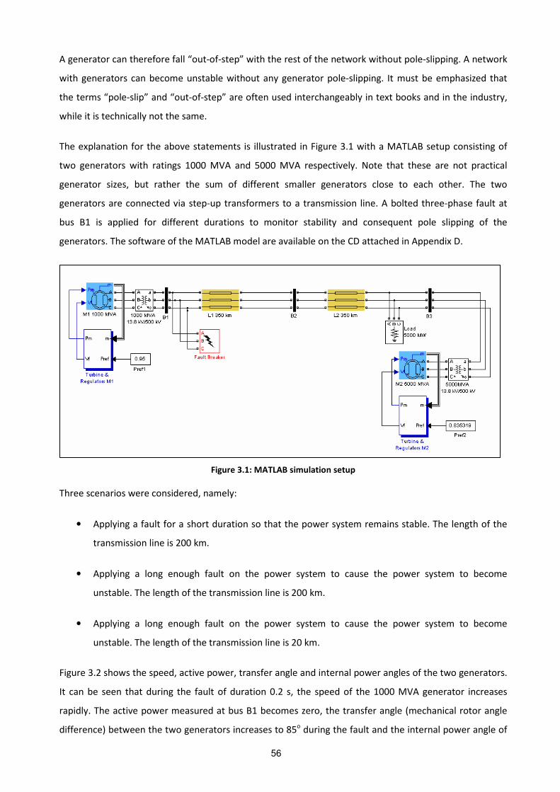
The explanation for the above statements is illustrated in Figure 3.1 with a MATLAB setup consisting of

two generators with ratings 1000 MVA and 5000 MVA respectively. Note that these are not practical

generator sizes, but rather the sum of different smaller generators close to each other. The two

generators are connected via step-up transformers to a transmission line. A bolted three-phase fault at

bus B1 is applied for different durations to monitor stability and consequent pole slipping of the

generators. The software of the MATLAB model are available on the CD attached in Appendix D.

Figure 3.1: MATLAB simulation setup

Three scenarios were considered, namely:

• Applying a fault for a short duration so that the power system remains stable. The length of the

transmission line is 200 km.

• Applying a long enough fault on the power system to cause the power system to become

unstable. The length of the transmission line is 200 km.

• Applying a long enough fault on the power system to cause the power system to become

unstable. The length of the transmission line is 20 km.

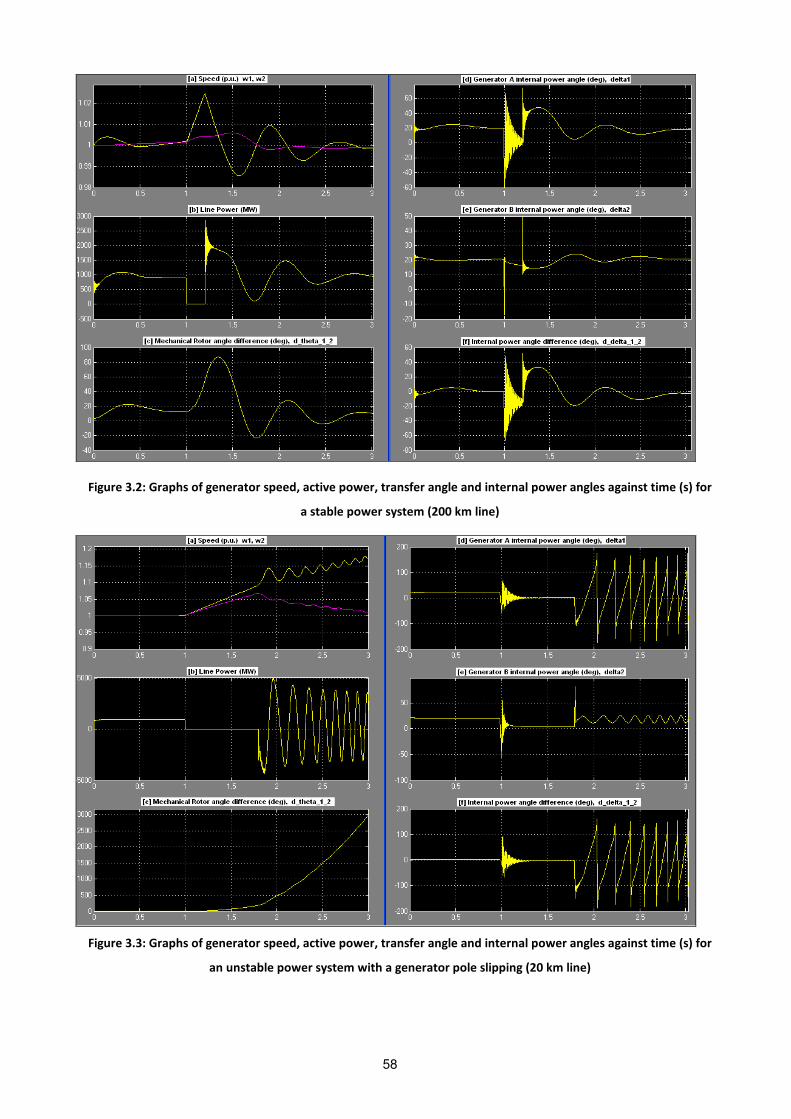
Figure 3.2 shows the speed, active power, transfer angle and internal power angles of the two generators.

It can be seen that during the fault of duration 0.2 s, the speed of the 1000 MVA generator increases

rapidly. The active power measured at bus B1 becomes zero, the transfer angle (mechanical rotor angle

difference) between the two generators increases to 85o during the fault and the internal power angle of

57

the 1000 MVA generator becomes as high as 60o. After the fault all the quantities return to normal and

the power system remains stable.

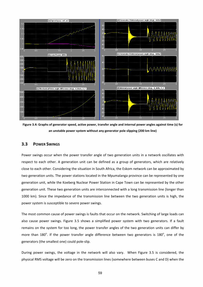
Figure 3.3 shows the speed, active power, transfer angle and internal power angles of the two generators

with a 20 km transmission line. It can be seen that during the fault of duration 0.8 s, the speed of the both

generators increases. The active power measured at bus B1 becomes zero and the transfer angle between

the two generators increases rapidly during the fault. The internal power angle of the 1000 MVA

generator becomes zero during the fault after the initial transient occurrence. The reason why the power

angle is close to zero during the fault, can be explained by the following equation:

1 2

12

sin⋅

≈ δV V

PX

(3.1)

where P is the active power transfer

V1 and V2 are the voltages at bus 1 and bus 2 in a network

X12 is the reactance between bus 1 and bus 2 in the network

δ is the transfer angle between bus 1 and bus 2

When the active power is zero, it means that the transfer angle δ will also be zero. However, when the

fault is cleared, the active electrical power on the 1000 MVA generator returns and since the generator

has sped up during the fault, the generator EMF is now out-of-synchronism with the terminal voltage. This

condition causes the generator to pole-slip once the fault is cleared. It can be seen that the internal power

angle (delta 1) oscillates between 180o and -180

o rapidly, which indicates pole slipping. The

5000 MVA generator is not pole-slipping.

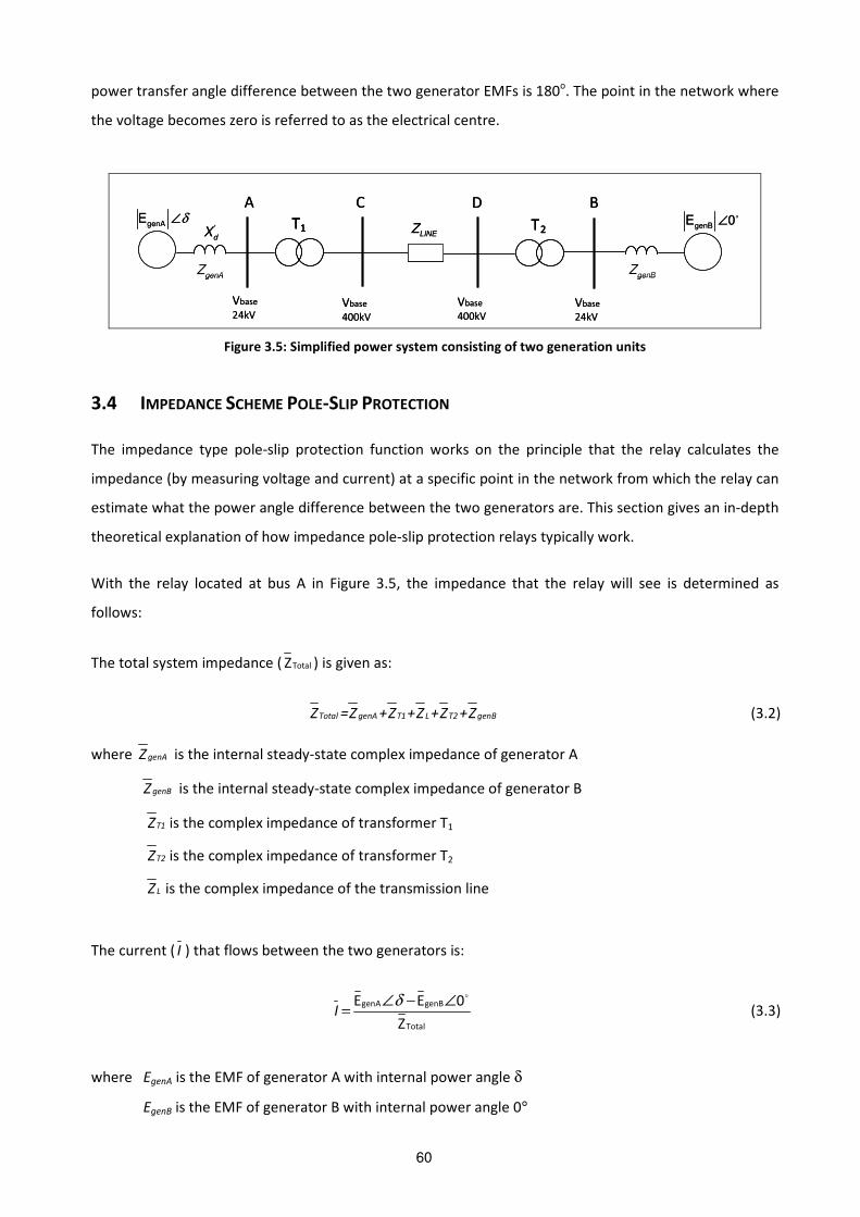
Figure 3.4 shows the speed, active power, transfer angle and internal power angles of the two generators

with a 200 km transmission line. It can be seen that during the 0.8 s fault, the speed of both the

generators increases. The active power measured at bus B1 becomes zero and the transfer angle between

the two generators increases rapidly during the fault. After the fault is cleared, the internal power angle of

both generators oscillate, but none of the power angles reach 180o, which means that the generators are

not pole slipping. It can therefore be stated that, although the power system is unstable, the generators

are not pole slipping due to the relatively high impedance of the transmission line connecting them.

58

Figure 3.2: Graphs of generator speed, active power, transfer angle and internal power angles against time (s) for

a stable power system (200 km line)

Figure 3.3: Graphs of generator speed, active power, transfer angle and internal power angles against time (s) for

an unstable power system with a generator pole slipping (20 km line)

59

Figure 3.4: Graphs of generator speed, active power, transfer angle and internal power angles against time (s) for

an unstable power system without any generator pole slipping (200 km line)

3.3 POWER SWINGS

Power swings occur when the power transfer angle of two generation units in a network oscillates with

respect to each other. A generation unit can be defined as a group of generators, which are relatively

close to each other. Considering the situation in South Africa, the Eskom network can be approximated by

two generation units. The power stations located in the Mpumalanga province can be represented by one

generation unit, while the Koeberg Nuclear Power Station in Cape Town can be represented by the other

generation unit. These two generation units are interconnected with a long transmission line (longer than

1000 km). Since the impedance of the transmission line between the two generation units is high, the

power system is susceptible to severe power swings.

The most common cause of power swings is faults that occur on the network. Switching of large loads can

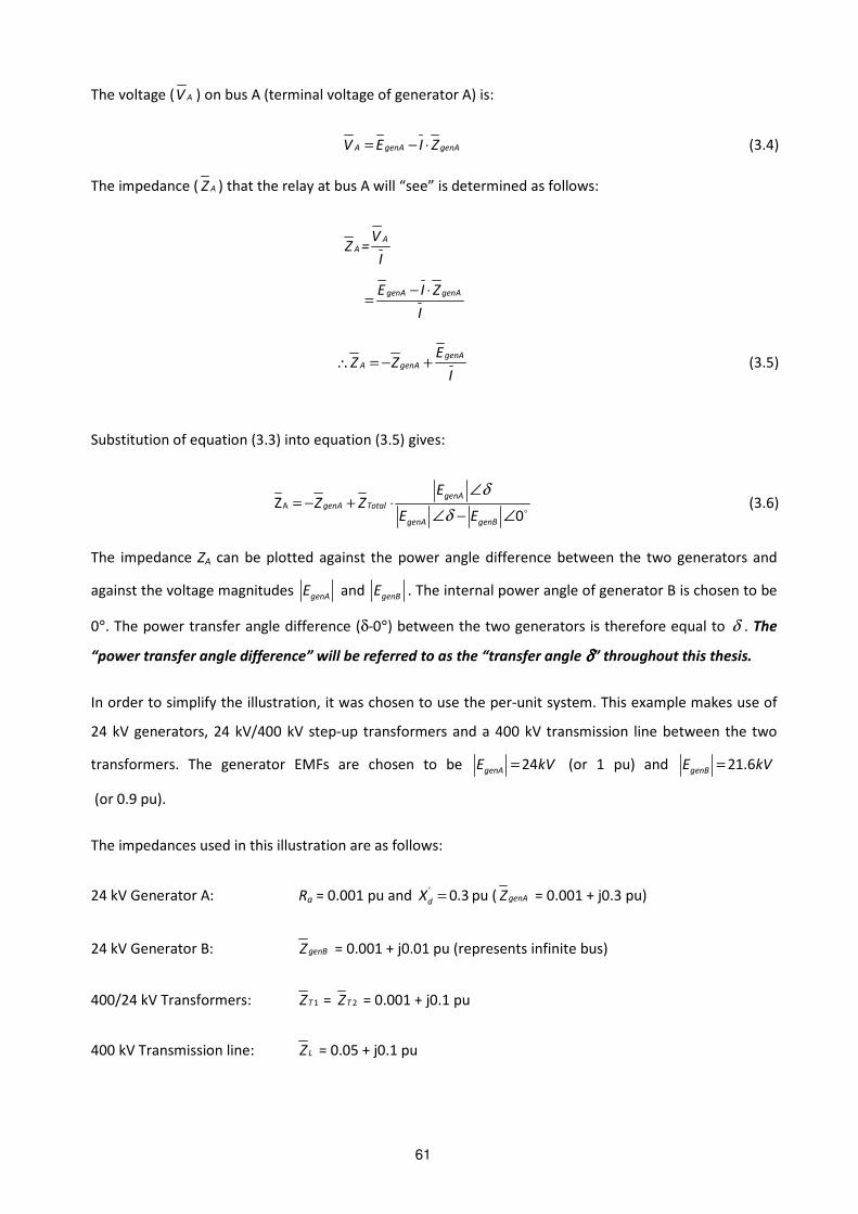
also cause power swings. Figure 3.5 shows a simplified power system with two generators. If a fault

remains on the system for too long, the power transfer angles of the two generation units can differ by

more than 180o. If the power transfer angle difference between two generators is 180

o, one of the

generators (the smallest one) could pole-slip.

During power swings, the voltage in the network will also vary. When Figure 3.5 is considered, the

physical RMS voltage will be zero on the transmission lines (somewhere between buses C and D) when the

60

power transfer angle difference between the two generator EMFs is 180o. The point in the network where

the voltage becomes zero is referred to as the electrical centre.

genAE δ∠'

dXgenBE 0∠

LINEZ

A C D B

T1 T2

genBZgenAZ

Vbase

24kVVbase

24kV

Vbase

400kV

Vbase

400kV

genAE δ∠'

dXgenBE 0∠

LINEZ

A C D B

T1T1 T2T2

genBZgenAZ

Vbase

24kVVbase

24kV

Vbase

400kV

Vbase

400kV

Figure 3.5: Simplified power system consisting of two generation units

3.4 IMPEDANCE SCHEME POLE-SLIP PROTECTION

The impedance type pole-slip protection function works on the principle that the relay calculates the

impedance (by measuring voltage and current) at a specific point in the network from which the relay can

estimate what the power angle difference between the two generators are. This section gives an in-depth

theoretical explanation of how impedance pole-slip protection relays typically work.

With the relay located at bus A in Figure 3.5, the impedance that the relay will see is determined as

follows:

The total system impedance ( TotalZ ) is given as:

Total genA T1 L T2 genBZ =Z +Z +Z +Z +Z (3.2)

where genAZ is the internal steady-state complex impedance of generator A

genBZ is the internal steady-state complex impedance of generator B

T1Z is the complex impedance of transformer T1

T2Z is the complex impedance of transformer T2

LZ is the complex impedance of the transmission line

The current ( I ) that flows between the two generators is:

genA genB

Total

E E 0

Z

∠ − ∠=

δI (3.3)

where EgenA is the EMF of generator A with internal power angle δ

EgenB is the EMF of generator B with internal power angle 0°

61

The voltage ( AV ) on bus A (terminal voltage of generator A) is:

A genA genAV E I Z= − ⋅ (3.4)

The impedance ( AZ ) that the relay at bus A will “see” is determined as follows:

AA

VZ =

I

genA genAE I Z

I

− ⋅=

genA

A genA

EZ Z

I∴ = − + (3.5)

Substitution of equation (3.3) into equation (3.5) gives:

AZ0

∠= − + ⋅

∠ − ∠

δ

δ

genAgenA Total

genA genB

EZ Z

E E (3.6)

The impedance ZA can be plotted against the power angle difference between the two generators and

against the voltage magnitudes genAE and genBE . The internal power angle of generator B is chosen to be

0°. The power transfer angle difference (δ-0°) between the two generators is therefore equal to δ . The

“power transfer angle difference” will be referred to as the “transfer angle δδδδ” throughout this thesis.

In order to simplify the illustration, it was chosen to use the per-unit system. This example makes use of

24 kV generators, 24 kV/400 kV step-up transformers and a 400 kV transmission line between the two

transformers. The generator EMFs are chosen to be 24=genAE kV (or 1 pu) and 21.6=genBE kV

(or 0.9 pu).

The impedances used in this illustration are as follows:

24 kV Generator A: Ra = 0.001 pu and ' 0.3=dX pu ( genAZ = 0.001 + j0.3 pu)

24 kV Generator B: genBZ = 0.001 + j0.01 pu (represents infinite bus)

400/24 kV Transformers: 1TZ = 2TZ = 0.001 + j0.1 pu

400 kV Transmission line: LZ = 0.05 + j0.1 pu

62

The above impedances were chosen arbitrarily to illustrate the theoretical principle of operation of the

impedance pole-slip protection relays, but can be considered as typical power system impedances. Sbase is

chosen as 100 MVA and 2

= basebase

base

VZ

S for each section of the power system with a different voltage base.

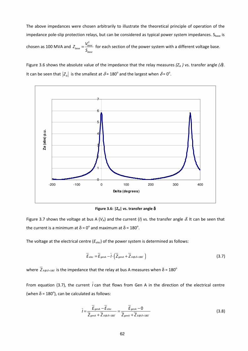
Figure 3.6 shows the absolute value of the impedance that the relay measures (ZA ) vs. transfer angle (δ).

It can be seen that AZ is the smallest at δ = 180o and the largest when δ = 0

o.

0

1

2

3

4

5

6

7

-200 -100 0 100 200 300 400

Delta (degrees)

Za (

ab

s)

p.u

.

Figure 3.6: |ZA| vs. transfer angle δδδδ

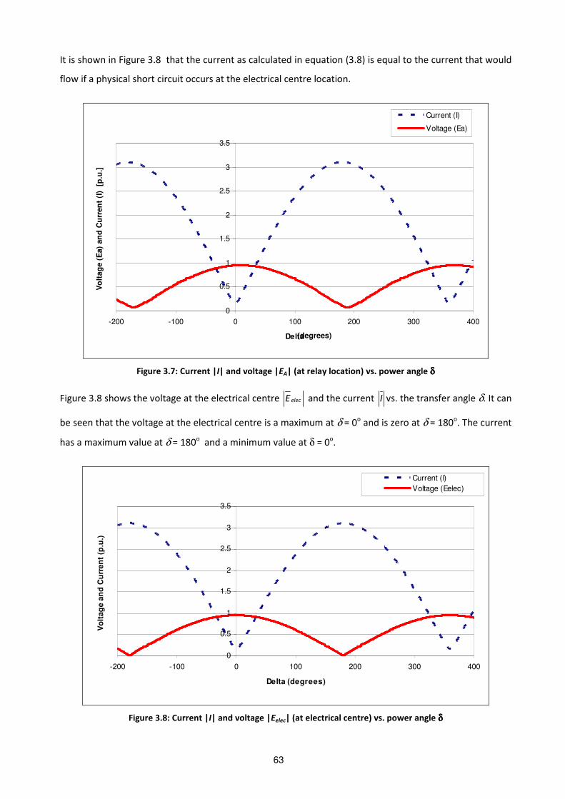
Figure 3.7 shows the voltage at bus A (VA) and the current (I) vs. the transfer angle δ. It can be seen that

the current is a minimum at δ = 0o and maximum at δ = 180

o.

The voltage at the electrical centre (Eelec) of the power system is determined as follows:

( )@ 180elec genA genA AE E I Z Z δ == − ⋅ + (3.7)

where @ 180= δAZ is the impedance that the relay at bus A measures when δ = 180o

From equation (3.7), the current I can that flows from Gen A in the direction of the electrical centre

(when δ = 180o), can be calculated as follows:

@ 180 @ 180

0genA elec genA

genA A genA A

E E EI

Z Z Z Zδ δ= =

− −= =

+ +

(3.8)

63

It is shown in Figure 3.8 that the current as calculated in equation (3.8) is equal to the current that would

flow if a physical short circuit occurs at the electrical centre location.

0

0.5

1

1.5

2

2.5

3

3.5

-200 -100 0 100 200 300 400

Delta

Vo

ltag

e (

Ea)

an

d C

urr

en

t (I

) [

p.u

.]

Current (I)

Voltage (Ea)

Figure 3.7: Current |I| and voltage |EA| (at relay location) vs. power angle δδδδ

Figure 3.8 shows the voltage at the electrical centre elecE and the current I vs. the transfer angle δ. It can

be seen that the voltage at the electrical centre is a maximum at δ = 0o and is zero at δ = 180

o. The current

has a maximum value at δ = 180o and a minimum value at δ = 0

o.

0

0.5

1

1.5

2

2.5

3

3.5

-200 -100 0 100 200 300 400

Delta (degrees)

Vo

ltag

e a

nd

Cu

rren

t (p

.u.)

Current (I)

Voltage (Eelec)

Figure 3.8: Current |I| and voltage |Eelec| (at electrical centre) vs. power angle δδδδ

(degrees)

64

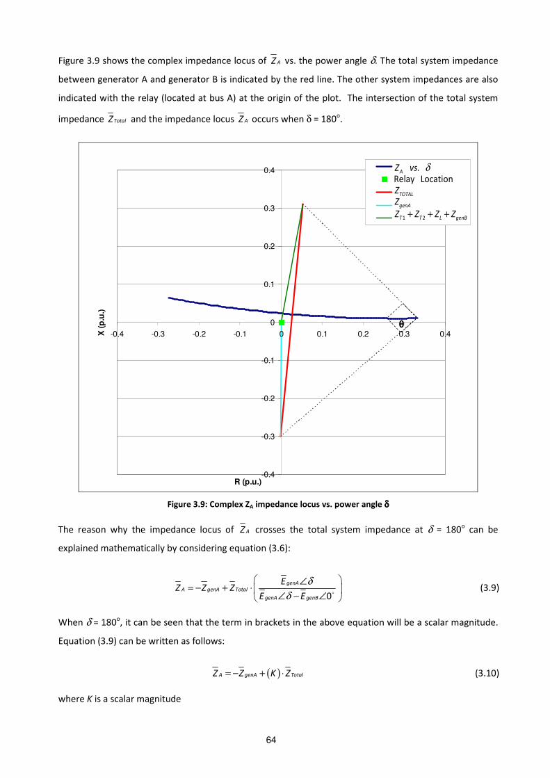
Figure 3.9 shows the complex impedance locus of AZ vs. the power angle δ. The total system impedance

between generator A and generator B is indicated by the red line. The other system impedances are also

indicated with the relay (located at bus A) at the origin of the plot. The intersection of the total system

impedance TotalZ and the impedance locus AZ occurs when δ = 180o.

-0.4

-0.3

-0.2

-0.1

0

0.1

0.2

0.3

0.4

-0.4 -0.3 -0.2 -0.1 0 0.1 0.2 0.3 0.4

R (p.u.)

X (

p.u

.)

Za locus (vs delta)

Relay Location

Total Impedance (Zt)

ZgenA

Zt1+Zl+Zt2+ZgenB

θ

1 2

.Relay Location

A

TOTAL

genA

T T L genB

Z vs

ZZ

Z Z Z Z

δ

+ + +

Figure 3.9: Complex ZA impedance locus vs. power angle δδδδ

The reason why the impedance locus of AZ crosses the total system impedance at δ = 180o can be

explained mathematically by considering equation (3.6):

0

∠= − + ⋅

∠ − ∠

δ

δ

genAA genA Total

genA genB

EZ Z Z

E E (3.9)

When δ = 180o, it can be seen that the term in brackets in the above equation will be a scalar magnitude.

Equation (3.9) can be written as follows:

( )= − + ⋅A genA TotalZ Z K Z (3.10)

where K is a scalar magnitude

65

The vector TotalZ is not drawn from the origin, since the relay is located at the origin. From equation (3.10)

it can be seen that AZ is proportional to TotalZ minus the impedance genAZ . AZ as described by

equation (3.10) is proportional to what defines the total impedance vector TotalZ in Figure 3.9. The AZ

impedance locus will therefore fall on the impedance vector TotalZ when δ = 180o.

The point on the AZ impedance locus (in Figure 3.9), where δ = 90o, is connected with dotted lines to both

ends of the TotalZ vector. It can be seen from Figure 3.9 that the angle θ that the dotted lines make at the

AZ impedance locus is also 90o. The angle θ is therefore equal to the power transfer angle δ. Impedance

pole-slip relays use θ to initiate tripping after the generator has pole-slipped once. When θ = 180o, the AZ

impedance locus will intersect the vector TotalZ . Alternatively, δ will be 180o when the AZ impedance

locus crosses the vector TotalZ .

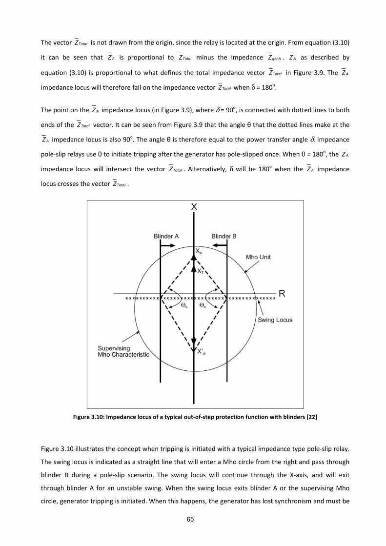
Figure 3.10: Impedance locus of a typical out-of-step protection function with blinders [22]

Figure 3.10 illustrates the concept when tripping is initiated with a typical impedance type pole-slip relay.

The swing locus is indicated as a straight line that will enter a Mho circle from the right and pass through

blinder B during a pole-slip scenario. The swing locus will continue through the X-axis, and will exit

through blinder A for an unstable swing. When the swing locus exits blinder A or the supervising Mho

circle, generator tripping is initiated. When this happens, the generator has lost synchronism and must be

66

separated from the system [22]. For a stable power swing, the impedance locus will enter blinder B and

will exit via blinder B again. Tripping will be blocked for a stable power swing.

3.5 IMPEDANCE RELAY PRINCIPLE OF OPERATION

This section explains the method of transfer angle calculation by the impedance scheme as described in

section 3.4. The steady state transfer angle calculation will form part of the new pole-slip protection

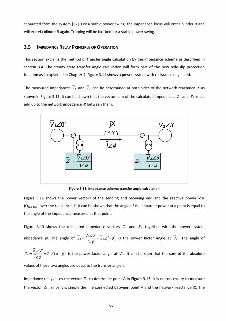
function as is explained in Chapter 4. Figure 3.11 shows a power system with resistance neglected.

The measured impedances 1Z and 2Z can be determined at both sides of the network reactance jX as

shown in Figure 3.11. It can be shown that the vector sum of the calculated impedances 1Z and 2Z must

add up to the network impedance jX between them.

jX1 0V ∠ 2V δ∠

11

0VZ

I φ

∠=

∠

2

2V

ZI

δ

φ

∠=

∠

I φ∠

jX1 0V ∠ 2V δ∠

11

0VZ

I φ

∠=

∠

1

10V

ZI φ

∠=

∠

2

2V

ZI

δ

φ

∠=

∠

I φ∠

Figure 3.11: Impedance scheme transfer angle calculation

Figure 3.12 shows the power vectors of the sending and receiving end and the reactive power loss

(Qline_loss) over the reactance jX. It can be shown that the angle of the apparent power at a point is equal to

the angle of the impedance measured at that point.

Figure 3.13 shows the calculated impedance vectors 1Z and 2Z together with the power system

impedance jX. The angle of ( )1

1 1

0∠= = ∠ −

∠

φφ

VZ Z

I is the power factor angle at 1V . The angle of

( )2

2 1

∠= = ∠ −

∠

δδ φ

φ

VZ Z

I is the power factor angle at 2V . It can be seen that the sum of the absolute

values of these two angles are equal to the transfer angle δ.

Impedance relays uses the vector 1Z to determine point A in Figure 3.13. It is not necessary to measure

the vector 2Z , since it is simply the line connected between point A and the network reactance jX. The

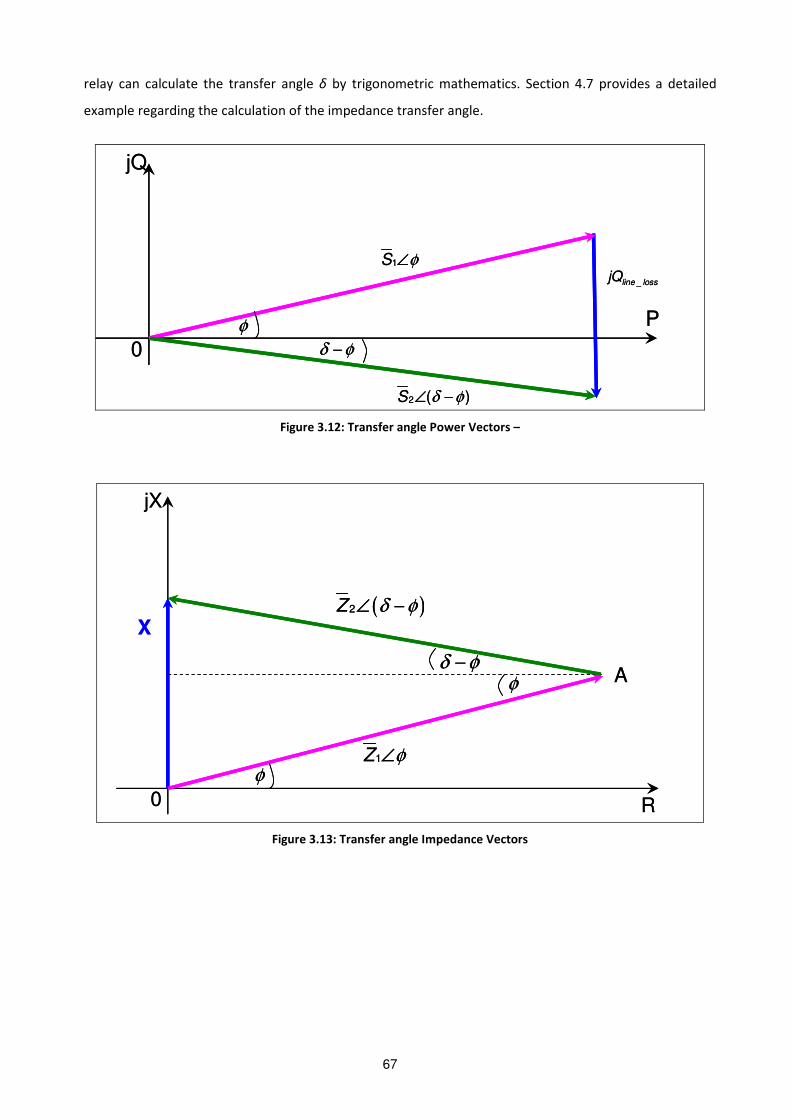
67

relay can calculate the transfer angle δ by trigonometric mathematics. Section 4.7 provides a detailed

example regarding the calculation of the impedance transfer angle.

P

2 ( )S δ φ∠ −

0

jQ

1S φ∠

φ

δ φ−

_line lossjQ

P

2 ( )S δ φ∠ −

0

jQ

1S φ∠

φ

δ φ−

_line lossjQ

Figure 3.12: Transfer angle Power Vectors –

A

0

X

R

jX

( )2Z δ φ∠ −

δ φ−φ

1Z φ∠φ

A

0

X

R

jX

( )2Z δ φ∠ −

δ φ−φ

1Z φ∠φ

Figure 3.13: Transfer angle Impedance Vectors

68

0 R

X

txjX

'

djX

lineZ

( ),l lR X

totalZ

relayZ

( ),r rR X

φ

φα

0 R

X

txjX

'

djX

lineZ

( ),l lR X

totalZ

relayZ

( ),r rR X

φ

φα

Figure 3.14: Impedance scheme vectors with relay on transformer HV side

Figure 3.14 explains how the network transfer angle is determined by the impedance principle. The

following impedances are drawn in the R-X complex impedance plane:

• Generator transient direct-axis reactance: '

djX

• Step-up transformer reactance: txjX

• Network impedance (transmission lines up to the infinite bus): line l lZ R jX= +

• Total system impedance (including generator and transformer): totalZ

• The impedance as measured by the impedance relay: relay r rZ R jX= +

• Calculated Impedance angle φ (also the power factor angle)

• Transmission line power angle: ( )Tlineδ φ α= +

69

The impedance measured by the relay is calculated as follows:

a

r

a

VZ

I= (3.11)

where aV is the generator terminal voltage (line to neutral)

aI is the generator line current

Also,

r r rZ R jX= + (3.12)

Therefore:

( )

( )

cos

sin

r r

r r

R Z

X Z

φ

φ

= ⋅

= ⋅ (3.13)

where φ is the power factor angle

The measured impedance angle φ is also the power factor angle:

1tan r

r

X

Rφ −

=

(3.14)

The angle φ can be positive or negative depending on the signs of Xr and Rr. The calculation of the

transfer angle as shown in Figure 3.13 is only valid for scenarios where no shunt loads are present close to

the generator. Section 3.6 describes the modifications required to include the effect of shunt loads in the

transfer angle calculation algorithm.

3.6 THE EFFECT OF SHUNT LOADS ON IMPEDANCE RELAYS

3.6.1 INTRODUCTION

The pre-fault transfer angle between the generator EMF and the infinite bus as calculated by an

impedance relay depends on the network impedance. The transfer angle over the transmission line will

increase for each generator in parallel that generates active power than what an impedance relay would

calculate without considering generators in parallel. On the other hand, the transfer angle over the

transmission line will be smaller for every shunt load that consumes active power close to the generator

terminals than what an impedance relay would calculate without considering shunt loads.

Transmission line feeders are referred to as feeders that connect the power station under consideration to

other power stations via transmission lines. Shunt load feeders are referred to as feeders that feed loads

like large factories or municipalities nearby the power station under consideration.

70

3.6.2 THEORETICAL ANALYSIS

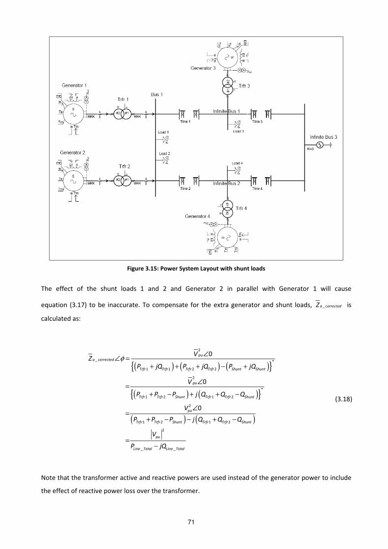
Figure 3.15 shows a power system with four generators and three “infinite buses” and shunt loads. By

definition, an infinite bus can be regarded as a section in the network where the voltage at that bus is

behind a zero (or very small) impedance.

The pole-slip relay will use Infinite Bus 1 and 2 as the reference to determine the transfer angle of

generators 1 and 2 respectively. The transfer angle is the angle between the generator EMF and the

infinite bus.

The Loads 3 and 4 will not have a considerable influence on the transfer angle calculation if the paralleled

impedance of transmission lines Tline3 and Tline4 is less than 5% of the paralleled impedance of Tline1 and

Tline2. However, the shunt loads (Load 1 and 2 in Figure 3.15) will cause the transfer angle calculation to be

inaccurate if the shunt loads are ignored in the transfer angle calculation. If the amount of active power

supplied by Generator 2 is equal to the active power consumed by shunt loads 1 and 2, the transfer angle

over the transmission lines will be calculated correctly by a conventional impedance relay.

From equation (3.11) in per-unit notation, the generator current is calculated as follows:

a

aa

VI

Z= (3.15)

*

*

2

*

0

⋅=

∠=

a a

a

a

a

a

V VS

Z

V

Z

(3.16)

2

*

aa

a

VZ

S∴ = (3.17)

where * denotes the complex conjugate

aS is the generator apparent power

71

Figure 3.15: Power System Layout with shunt loads

The effect of the shunt loads 1 and 2 and Generator 2 in parallel with Generator 1 will cause

equation (3.17) to be inaccurate. To compensate for the extra generator and shunt loads, _a correctedZ is

calculated as:

( ) ( ) ( )

( ) ( )

( ) ( )

2

_*

1 1 2 2

2

*

1 2 1 2

2

1 2 1 2

2

_ _

0

0

0

pua corrected

Trfr Trfr Trfr Trfr Shunt Shunt

pu

Trfr Trfr Shunt Trfr Trfr Shunt

pu

Trfr Trfr Shunt Trfr Trfr Shunt

pu

Line Total Line Total

VZ

P jQ P jQ P jQ

V

P P P j Q Q Q

V

P P P j Q Q Q

V

P jQ

φ∠

∠ =+ + + − +

∠=

+ − + + −

∠=

+ − − + −

=−

(3.18)

Note that the transformer active and reactive powers are used instead of the generator power to include

the effect of reactive power loss over the transformer.

72

From equation (3.18), the angle of _a correctedZ is calculated as:

_1

_

t n−

=

φ Line Total

corrected

Line Total

Qa

P (3.19)

( ) ( )

2

_2 2

_ _

=

−

pu

a corrected

Line Total Line Total

VZ

P Q

(3.20)

From Figure 3.14, the angle α is calculated as:

_ _ sin( )= ⋅ φa corrected a corrected correctedX Z (3.21)

_ _ cos( )= ⋅ φa corrected a corrected correctedR Z (3.22)

_1

_

tan−

−=

−α Tline a corrected

a corrected Tline

X X

R R (3.23)

The power angle over the transmission line is calculated from Figure 3.14 as:

= +δ α φTline corrected (3.24)

Section 4.7.1 provides more information on transfer angle calculation (angle between generator EMF and

infinite bus).

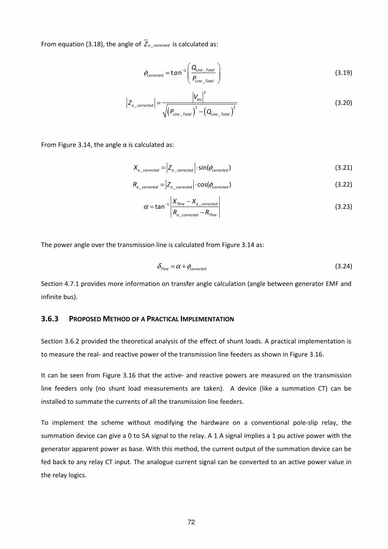
3.6.3 PROPOSED METHOD OF A PRACTICAL IMPLEMENTATION

Section 3.6.2 provided the theoretical analysis of the effect of shunt loads. A practical implementation is

to measure the real- and reactive power of the transmission line feeders as shown in Figure 3.16.

It can be seen from Figure 3.16 that the active- and reactive powers are measured on the transmission

line feeders only (no shunt load measurements are taken). A device (like a summation CT) can be

installed to summate the currents of all the transmission line feeders.

To implement the scheme without modifying the hardware on a conventional pole-slip relay, the

summation device can give a 0 to 5A signal to the relay. A 1 A signal implies a 1 pu active power with the

generator apparent power as base. With this method, the current output of the summation device can be

fed back to any relay CT input. The analogue current signal can be converted to an active power value in

the relay logics.

73

Alternatively, a 4-20 mA signal or LAN / LON / Profibus communication can be used to transmit the

transmission line current magnitudes to the pole-slip relays.

Figure 3.16: Power System Layout with shunt loads

3.7 TRANSMISSION LINE IMPEDANCE

This section describes how transmission line impedances will be used in the new pole-slip protection

function. Transmission line per-unit impedances as obtained from transmission line manufacturer’s data,

can be processed to obtain a typical per-unit impedance range for transmission lines, which can be used

to test the new pole-slip protection function.

For example, let the transmission line parameters be:

( )22

628

275

275120.42

628

=

=

= = = Ω

base

base

basebase

base

S MVA

V kV

kVVZ

S MVA

(3.25)

74

For a “Twin-Bear”-transmission line, the 275 kV line impedance is (shunt admittance neglected) [56]:

( ) 0.059 0.304 /Ω = + ΩlineZ j km (3.26)

The maximum MVA rating of the “Twin Bear’ transmission line used above is 628 MVA [56]. Typical

transmission line tables indicate that when a Twin Bear transmission line is loaded at 628 MVA, the

maximum length that Twin-Bear transmission line can be is 61 km [56]. If the transmission line is longer

than 61 km at 628 MVA, stability across the line can be lost.

The per-unit impedance value of 61 km transmission line is:

( )( . .)

4 3

2 1

0.059 0.304 /

120.42

4.899 10 2.524 10 . . /

2.989 10 1.540 10 . .

Ω

− −

− −

+ Ω= =

Ω

= +

= +

lineline p u

base

j kmZZ

Z

x j x p u km

x j x p u

(3.27)

A generator step-up transformer has an impedance of typically 0.1 pu to 0.15 pu. The 61 km Twin-Bear

transmission line reactance (as calculated above) is 0.154 pu. The generator transient reactance is

typically Xd’ = 0.3 pu. This means that the largest portion of the transfer angle will typically be across the

generator/transformer combination. In other words, the electrical centre is likely to be in the

generator / transformer combination.

If a transmission line longer than 61 km is needed at 628 MVA, two Twin-Bear transmission lines can be

used in parallel. Alternatively, a larger transmission line conductor like Zebra or Twin-Zebra can be used.

The generator sizes of Eskom (South Africa) are typically 600 MW each. In some power stations (like

Koeberg nuclear power station) larger generators are used.

When larger generators are used, the MVA base will be chosen as the generator MVA rating, which means

the transmission line per-unit impedance will become larger. Due to the higher MVA demand, a larger

transmission line conductor must be used (or lines in parallel).

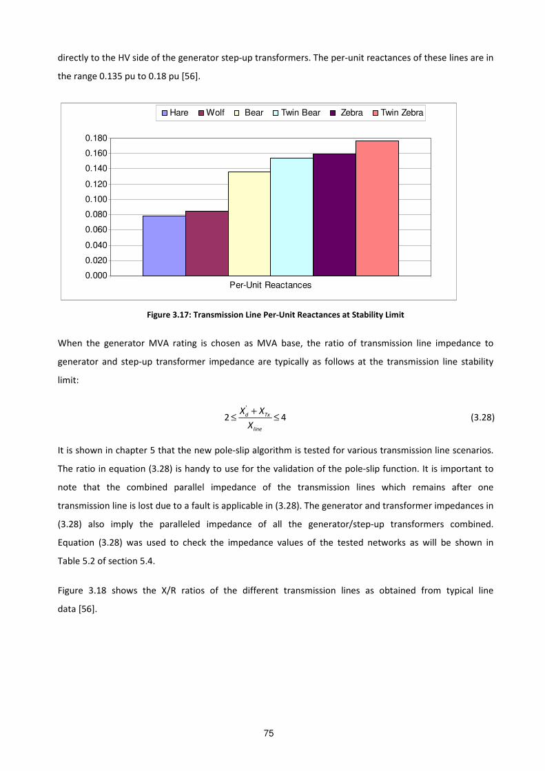
A “rule-of-thumb” ratio between generator impedance and maximum transmission line impedance can be

obtained. Figure 3.17 shows the per-unit reactances of different transmission lines at the stability limit. In

other words, the reactances are calculated on the transmission line rated MVA base and at the maximum

transmission line length (km) at the rated MVA.

It can be noted from Figure 3.17 that the transmission line reactances are in the range 0.08 pu to 0.175

pu. “Wolf” and “Hare” transmission lines are typically not connected directly to power stations, due to the

small MVA capacity of these lines. The other lines (“Bear” and “Zebra”) will typically be used to connect

75

directly to the HV side of the generator step-up transformers. The per-unit reactances of these lines are in

the range 0.135 pu to 0.18 pu [56].

0.000

0.020

0.040

0.060

0.080

0.100

0.120

0.140

0.160

0.180

Per-Unit Reactances

Hare Wolf Bear Twin Bear Zebra Twin Zebra

Figure 3.17: Transmission Line Per-Unit Reactances at Stability Limit

When the generator MVA rating is chosen as MVA base, the ratio of transmission line impedance to

generator and step-up transformer impedance are typically as follows at the transmission line stability

limit:

'

2 4d Tx

line

X X

X

+≤ ≤ (3.28)

It is shown in chapter 5 that the new pole-slip algorithm is tested for various transmission line scenarios.

The ratio in equation (3.28) is handy to use for the validation of the pole-slip function. It is important to

note that the combined parallel impedance of the transmission lines which remains after one

transmission line is lost due to a fault is applicable in (3.28). The generator and transformer impedances in

(3.28) also imply the paralleled impedance of all the generator/step-up transformers combined.

Equation (3.28) was used to check the impedance values of the tested networks as will be shown in

Table 5.2 of section 5.4.

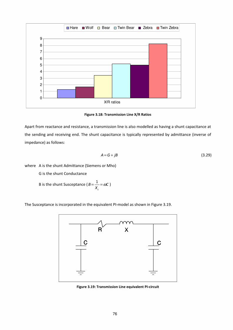
Figure 3.18 shows the X/R ratios of the different transmission lines as obtained from typical line

data [56].

76

0

1

2

3

4

5

6

7

8

9

X/R ratios

Hare Wolf Bear Twin Bear Zebra Twin Zebra

Figure 3.18: Transmission Line X/R Ratios

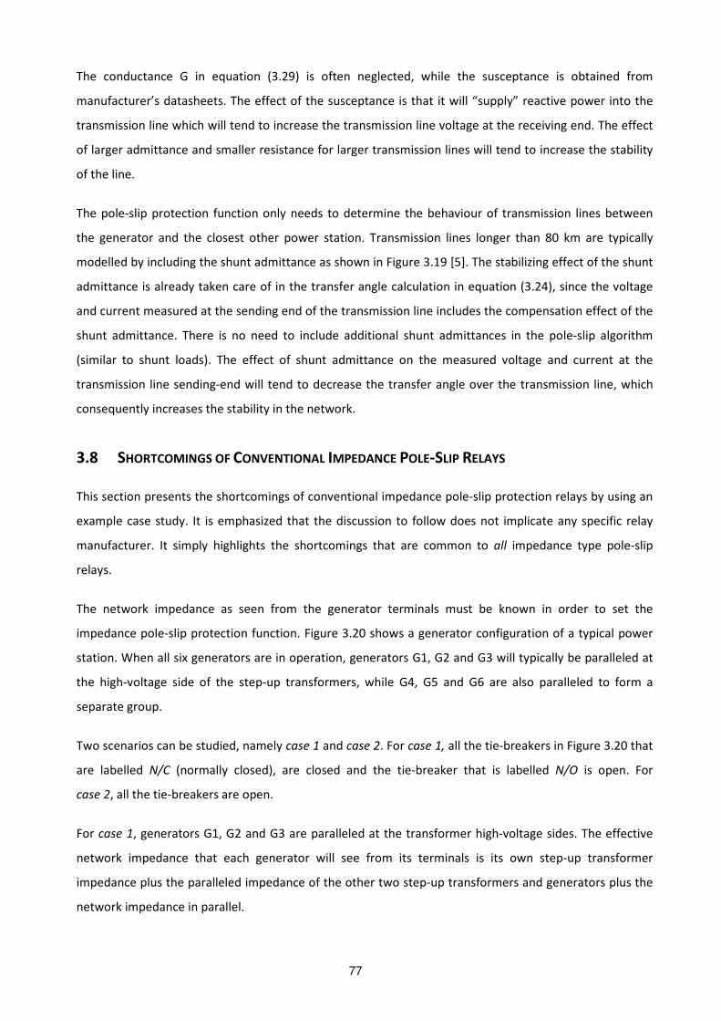
Apart from reactance and resistance, a transmission line is also modelled as having a shunt capacitance at

the sending and receiving end. The shunt capacitance is typically represented by admittance (inverse of

impedance) as follows:

= +A G jB (3.29)

where A is the shunt Admittance (Siemens or Mho)

G is the shunt Conductance

B is the shunt Susceptance (1

= = ωc

B CX

)

The Susceptance is incorporated in the equivalent PI-model as shown in Figure 3.19.

R

C

X

C

R

C

X

C

R

C

X

C

Figure 3.19: Transmission Line equivalent PI-circuit

77

The conductance G in equation (3.29) is often neglected, while the susceptance is obtained from

manufacturer’s datasheets. The effect of the susceptance is that it will “supply” reactive power into the

transmission line which will tend to increase the transmission line voltage at the receiving end. The effect

of larger admittance and smaller resistance for larger transmission lines will tend to increase the stability

of the line.

The pole-slip protection function only needs to determine the behaviour of transmission lines between

the generator and the closest other power station. Transmission lines longer than 80 km are typically

modelled by including the shunt admittance as shown in Figure 3.19 [5]. The stabilizing effect of the shunt

admittance is already taken care of in the transfer angle calculation in equation (3.24), since the voltage

and current measured at the sending end of the transmission line includes the compensation effect of the

shunt admittance. There is no need to include additional shunt admittances in the pole-slip algorithm

(similar to shunt loads). The effect of shunt admittance on the measured voltage and current at the

transmission line sending-end will tend to decrease the transfer angle over the transmission line, which

consequently increases the stability in the network.

3.8 SHORTCOMINGS OF CONVENTIONAL IMPEDANCE POLE-SLIP RELAYS

This section presents the shortcomings of conventional impedance pole-slip protection relays by using an

example case study. It is emphasized that the discussion to follow does not implicate any specific relay

manufacturer. It simply highlights the shortcomings that are common to all impedance type pole-slip

relays.

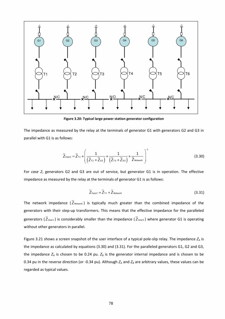
The network impedance as seen from the generator terminals must be known in order to set the

impedance pole-slip protection function. Figure 3.20 shows a generator configuration of a typical power

station. When all six generators are in operation, generators G1, G2 and G3 will typically be paralleled at

the high-voltage side of the step-up transformers, while G4, G5 and G6 are also paralleled to form a

separate group.

Two scenarios can be studied, namely case 1 and case 2. For case 1, all the tie-breakers in Figure 3.20 that

are labelled N/C (normally closed), are closed and the tie-breaker that is labelled N/O is open. For

case 2, all the tie-breakers are open.

For case 1, generators G1, G2 and G3 are paralleled at the transformer high-voltage sides. The effective

network impedance that each generator will see from its terminals is its own step-up transformer

impedance plus the paralleled impedance of the other two step-up transformers and generators plus the

network impedance in parallel.

78

Figure 3.20: Typical large power station generator configuration

The impedance as measured by the relay at the terminals of generator G1 with generators G2 and G3 in

parallel with G1 is as follows:

( ) ( )

1

1 1

2 2 3 3

1 1 1Case T

NetworkT G T G

Z ZZZ Z Z Z

− = + + + + +

(3.30)

For case 2, generators G2 and G3 are out of service, but generator G1 is in operation. The effective

impedance as measured by the relay at the terminals of generator G1 is as follows:

2 1Case T NetworkZ Z Z= + (3.31)

The network impedance ( NetworkZ ) is typically much greater than the combined impedance of the

generators with their step-up transformers. This means that the effective impedance for the paralleled

generators ( 1CaseZ ) is considerably smaller than the impedance ( 2CaseZ ) where generator G1 is operating

without other generators in parallel.

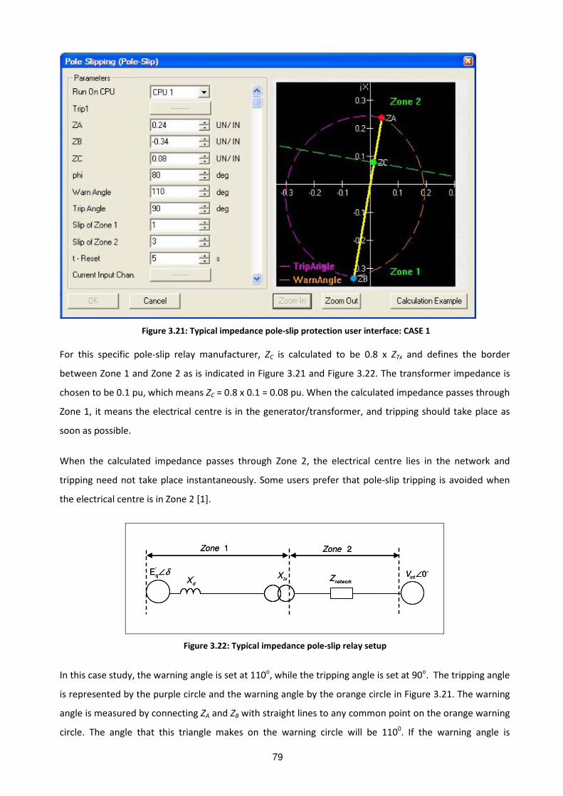
Figure 3.21 shows a screen snapshot of the user interface of a typical pole-slip relay. The impedance ZA is

the impedance as calculated by equations (3.30) and (3.31). For the paralleled generators G1, G2 and G3,

the impedance ZA is chosen to be 0.24 pu. ZB is the generator internal impedance and is chosen to be

0.34 pu in the reverse direction (or -0.34 pu). Although ZA and ZB are arbitrary values, these values can be

regarded as typical values.

G1 G2 G3

N/C N/C

G4 G5 G6

N/C N/C N/O

T1 T2 T3 T4 T5 T6

79

Figure 3.21: Typical impedance pole-slip protection user interface: CASE 1

For this specific pole-slip relay manufacturer, ZC is calculated to be 0.8 x ZTx and defines the border

between Zone 1 and Zone 2 as is indicated in Figure 3.21 and Figure 3.22. The transformer impedance is

chosen to be 0.1 pu, which means ZC = 0.8 x 0.1 = 0.08 pu. When the calculated impedance passes through

Zone 1, it means the electrical centre is in the generator/transformer, and tripping should take place as

soon as possible.

When the calculated impedance passes through Zone 2, the electrical centre lies in the network and

tripping need not take place instantaneously. Some users prefer that pole-slip tripping is avoided when

the electrical centre is in Zone 2 [1].

δ∠'

qE'

dX∠

inf 0VnetworkZtxX

1Zone 2Zone

δ∠'

qE'

dX∠

inf 0VnetworkZtxX

1Zone 2Zone

Figure 3.22: Typical impedance pole-slip relay setup

In this case study, the warning angle is set at 110o, while the tripping angle is set at 90

o. The tripping angle

is represented by the purple circle and the warning angle by the orange circle in Figure 3.21. The warning

angle is measured by connecting ZA and ZB with straight lines to any common point on the orange warning

circle. The angle that this triangle makes on the warning circle will be 1100. If the warning angle is

80

increased to say, 1200, the orange circle will get smaller to allow for the greater angle. The tripping angle

works on a similar principle.

The impedance will typically be in the top-right quadrant of the R-X plane during normal operation. During

a power swing, the impedance will approach the warning circle from the right. When the impedance

enters the warning circle, the relay will give a pole-slip warning. When the impedance crosses the ZA – ZB

line, an out-of-step condition is detected. If the impedance swing continues to the left of the R-X plane

and exits the trip-angle circle, the relay will issue a pole-slip trip, provided that the power swing frequency

is between 0.2 Hz to 8 Hz. The trip angle is normally set at 90o to minimize the current breaking stress on

the generator circuit breaker.

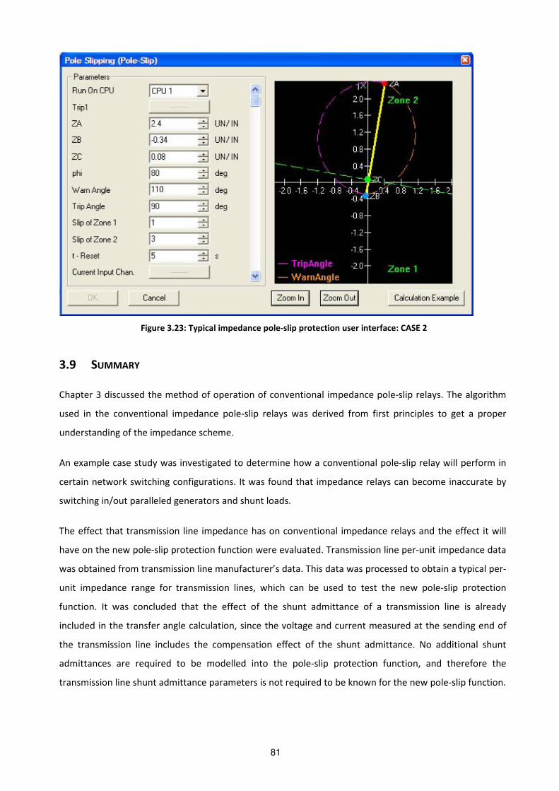
If ZA in the relay is set for normal operation (case 1), and generators G2 and G3 are out of operation, the

pole-slip function will not detect slips in Zone 2 that have an impedance greater than the preset ZA value.

When generator G1 is operated alone (case 2), the network impedance ZA can be as great as 10 times the

value that is preset to be ZA. Figure 3.23 shows the impedance line for ZA = 2.4 pu. The impedance locus

can cross the ZA – ZB line anywhere during power swings. With a ZA value set at 0.24 pu, the relay will not

detect power swings (or out-of-step operation) if the impedance locus crosses the ZA – ZB line at 0.25 80°∠ ,

for example. At this impedance, the out-of-step condition can cause serious mechanical stress and

damage on the generator without detecting the out-of-step condition.

By setting the relay at ZA = 2.4 pu for case 2, the tripping and warning angles will not be accurate if the

generators are operated in normal configuration (i.e. three generators in parallel). A tripping angle that is

set at 90o, will issue a trip once the angle has reached approximately 20

o. This could possibly cause the

breaker to experience damage if it is only rated to break the current at an angle of 90o. A network

impedance ZA can be chosen to be an average for the different switching scenarios, but the accuracy of

the impedance pole-slip protection function cannot be guaranteed throughout different switching

configurations.

When set up correctly, the impedance pole-slip scheme could eventually trip a machine that fell out-of-

step, but it cannot trip a machine before it falls out-of-step. It is important to note that if the tie-breaker

status changes to an configuration that is not normal, the impedance pole-slip protection relay will not

work accurately anymore.

81

Figure 3.23: Typical impedance pole-slip protection user interface: CASE 2

3.9 SUMMARY

Chapter 3 discussed the method of operation of conventional impedance pole-slip relays. The algorithm

used in the conventional impedance pole-slip relays was derived from first principles to get a proper

understanding of the impedance scheme.

An example case study was investigated to determine how a conventional pole-slip relay will perform in

certain network switching configurations. It was found that impedance relays can become inaccurate by

switching in/out paralleled generators and shunt loads.

The effect that transmission line impedance has on conventional impedance relays and the effect it will

have on the new pole-slip protection function were evaluated. Transmission line per-unit impedance data

was obtained from transmission line manufacturer’s data. This data was processed to obtain a typical per-

unit impedance range for transmission lines, which can be used to test the new pole-slip protection

function. It was concluded that the effect of the shunt admittance of a transmission line is already

included in the transfer angle calculation, since the voltage and current measured at the sending end of

the transmission line includes the compensation effect of the shunt admittance. No additional shunt

admittances are required to be modelled into the pole-slip protection function, and therefore the

transmission line shunt admittance parameters is not required to be known for the new pole-slip function.

82

The shortcomings of impedance relays, such as network switching configurations and operation with

shunt loads were investigated. Recommendations on how to incorporate shunt loads in impedance pole-

slip relays were also made. It was suggested to measure the active and reactive power of the transmission

line feeders, as well as the active and reactive power of the shunt load feeders. Transmission line feeders

were defined as feeders that connect to other power stations via transmission lines. Shunt load feeders

were defined as feeders that feed loads like large factories or municipalities and power station internal

loads etc. By measuring transmission line feeder currents, it can be determined which transmission lines

are in operation. The shunt load feeders were treated as loads that will cause the transfer angle between

the generator EMF and the infinite bus to decrease. By measuring the power on the shunt load feeders

and the transmission line feeders, the transfer angle can be adjusted accordingly in the new pole-slip

protection function.