Continuous pole placement for delay equations

Automatica 38 (2002) 747–761www.elsevier.com/locate/automatica

Continuous pole placement for delay equations1

W. Michiels ∗, K. Engelborghs, P. Vansevenant, D. RooseDepartment of Computer Science, Katholieke Universiteit Leuven, Celestijnenlaan 200A, B-3001 Leuven, Belgium

Received 6 October 2000; received in revised form 6 July 2001; accepted 15 October 2001

Abstract

In this paper, we describe a stabilization method for linear time-delay systems which extends the classical pole placement methodfor ordinary di7erential equations. Unlike methods based on :nite spectrum assignment, our method does not render the closedloop system, :nite dimensional but consists of controlling the rightmost eigenvalues. Because these are moved to the left halfplane in a (quasi-)continuous way, we refer to our method as continuous pole placement. We explain the method by means of thestabilization of a linear :nite dimensional system in the presence of an input delay and illustrate its applicability to more generalstabilization problems. ? 2002 Elsevier Science Ltd. All rights reserved.

Keywords: Delay equations; Feedback stabilization; Pole assignment

1. Introduction

The stabilization of linear time-delay systems has beenstudied extensively in the literature. Existing stabilizationmethods include those based on :nite spectrum assign-ment (Breth@e & Loiseau, 1998; Manitius & Olbrot, 1979;Olbrot, 1978; Wang, Lee, & Tan, 1999), methods usingan algebraic Riccati approach (where stability conditionsare expressed by the solvability of a Riccati equation orby the feasibility of a linear matrix inequality, see Dion,Dugard, and Fliess (1998) and the references therein)and variants of the Smith predictor (see Palmor (1996),Chap. 10 for an overview).In this paper we develop a numerical stabilization

method which is related to the classical pole-placementmethod for ordinary di7erential equations (Ackermann,1972). The approach, which starts from the state spacedescription of a linear time-delay system, is mixedanalytical=numerical and makes use of a recently de-veloped method (Engelborghs & Roose, 1999) for thedetermination of the rightmost eigenvalues of a lineartime-delay system.

� This paper was not presented at any IFAC meeting. This paperwas recommended for publication in revised form by Associate EditorIrene Lasiecka under the direction of Editor Roberto Tempo.

∗ Corresponding author.E-mail address: [email protected] (W. Michiels).

As an illustration of our method, we study the stabi-lization of the system

x = Ax + Bu(t − �); A∈Rn×n; B∈Rn×1; (1)

where x∈Rn is the state, u∈R is the input and �¿ 0represents an input delay. We use a linear static statefeedback controller,

u= KTx; K ∈Rn×1: (2)

The control law (2) is not only motivated by the fact thatit reveals the link between our stabilization method andthe classical pole placement method, and allows to ob-tain some nice theoretical results. We will also show thatfor system (1), a static state feedback controller leads tostabilizability properties which are comparable to thoseof methods based on :nite spectrum assignment, whensmall perturbations are taken into account. Furthermore,the extension to the output feedback case is straightfor-ward.The structure of the paper is as follows. First, we study

theoretical stabilizability properties of system (1)–(2)and motivate the use of control law (2), thereby ex-plaining the ideas behind the continuous pole placementmethod. Then we study the stabilization method in detailand apply it to a (numerical) example. After a discussionof the output-feedback case, we end with some numericalexamples illustrating the applicability of our method tomore general types of delay equations involving delays inboth state and control variables, and multiple feedbacks.

0005-1098/02/$ - see front matter ? 2002 Elsevier Science Ltd. All rights reserved.PII: S 0005-1098(01)00257-6

748 W. Michiels et al. / Automatica 38 (2002) 747–761

2. Preliminaries

The state of the delay equation

x = Ax + Adx(t − �); x∈Rn; A; Ad ∈Rn×n; (3)

at time t is given by a function segment xt ∈C([− �; 0]; Rn) de:ned as

xt( ) = x(t + ); ∈ [− �; 0]:

Here C([ − �; 0];Rn) is the Banach space of continuousfunctions mapping the delay-interval [ − �; 0] into Rnand equipped with the supremum-norm ‖:‖s. A solutionis uniquely de:ned by specifying as initial condition afunction segment x0 ∈C([−�; 0];Rn). Note that the delayequation can be considered as an evolution equation overthis space. Therefore, delay equations belong to the verybroad class of functional di7erential equations (Hale &Verduyn Lunel, 1993; Kolmanovskii & Myshkis, 1999;Kolmanovskii & Nosov, 1986).Stability de:nitions for (3) are analogous to the ODE

case (Dugard & Verriest, 1998; Kolmanovskii & Nosov,1986). The zero solution of (3) is asymptotically stablewhen

∀�¿ 0; ∃�¿ 0: ‖x0‖s6 �→ ‖xt‖s6 �; ∀t¿ 0

and

limt→∞ x(t) = 0; ∀x0 ∈C([− �; 0];Rn):

This is equivalent with the fact that all eigenvalues, i.e.the roots of the characteristic equation,

det(�I − A− Ade−��) = 0; (4)

are in the open left half plane. Condition (4) is equivalentto requiring the existence of a nonzero vector v∈Cn×1

such that (�I − A− Ade−��)v= 0. The function segmentve� ; ∈ [−�; 0] is the eigenfunction corresponding to theeigenvalue �. Eq. (4) is transcendental and has in:nitelymany solutions. However, the number of eigenvalues tothe right of any vertical line, R(�)¿ r, with r ∈R, is :-nite, and hence−∞ is the only accumulation point for thereal parts of the eigenvalues (Dugard & Verriest, 1998;Hale & Verduyn Lunel, 1993).In the rest of paper we make the following assumption:

Assumption 2.1. The pair (A; B) in (1) is controllable.

This allows to bring the closed loop system (1)–(2),after a similarity transformation z = Tx, into the controlcanonical form:

z = Acz + BcKTc z(t − �) (5)

or

z=

0 10 1

. . . . . .

0 1−a1 −a2 : : : −an

z(t)

+

0...0−1

[k1 k2 : : : kn]z(t − �): (6)

Hence the eigenvalues of (1)–(2) satisfy,

H (�), �n + (an + kne−��)�n−1 + · · ·+(a2 + k2e−��)�+ (a1 + k1e−��) = 0: (7)

3. Motivation

The problem of the stabilization of system (1) with afeedback controller of form (2) is hard because its designinvolves the determination of only n parameters, whilethe closed loop system has an in:nite number of eigen-values. On the other hand the proposed controller struc-ture is very simple and easy to implement. Furthermore,recent research (Engelborghs, Dambrine, & Roose, 2001;Van Assche, Dambrine, Lafay, & Richard, 1999) showsthat more sophisticated controllers, which are based onprediction and yield only a :nite number of closed loopeigenvalues, may be sensitive to arbitrary small imple-mentation errors and su7er from the same limitationsas controller (2) from a practical point of view. Thiswill be illustrated with a one-dimensional example inSection 3.3.

3.1. A 2nite-dimensional controller for anin2nite-dimensional problem

The classical pole placement algorithm (Ackermann,1972) cannot be applied directly to the time-delay casebecause the characteristic equation (7) has in:nitelymany solutions while the number of degrees of freedomin the controller is n. A direct placement of n eigenval-ues is always possible. This follows from the linearity ofthe characteristic equation (7) w.r.t. the components ofKc. Indeed Eq. (7) can be rewritten as

[1 � �2 : : : �n−1][k1 k2 : : : kn]T =− Mp(�)e��;

where Mp(�)=∑n

i=1 ai�i−1 +�n. When forcing n di7erent

eigenvalues �1; : : : ; �n to satisfy this equation, a linear

W. Michiels et al. / Automatica 38 (2002) 747–761 749

system of equations with unknown Kc and a regu-lar Jacobian matrix (a Vandermonde matrix) is ob-tained. However, by placing n eigenvalues, whichdetermines the complete spectral picture, control is lostover the position of the other ones, and these may causeinstability.Our method is based on the fact that, unlike for neu-

tral equations (Michiels, Engelborghs, Roose, &Dochain,1998), the number of unstable eigenvalues is always :-nite (Hale & Verduyn Lunel, 1993, Lemma I:4:1), and onthe availability of a software tool to calculate the right-most eigenvalues (Engelborghs, 2000). Once we havedetected unstable eigenvalues, our strategy consists ofmoving them to the left half plane by applying smallchanges to the controller gain K , and meanwhile moni-toring the other eigenvalues with large real part. Becausethe eigenvalues move continuously w.r.t. changes in thefeedback gain, see Theorem 8 in the appendix, we referto our method as the continuous pole placement method.Before describing the method in more detail in the nextsection, we introduce some theorems concerning the lim-itations and diNculties of linear state feedback control inthe presence of input delays.When the uncontrolled system (1) has eigenvalues in

the closed RHP, the destabilizing e7ect of a time delayis illustrated with the fact that no :xed feedback-gain Kis able to achieve stabilization for all values of the timedelay �, a consequence of the following theorem fromin ’t Hout (1994). By �(·) we denote the spectrum andby r�(·) the spectral radius.

Theorem 1. Delay-independent stability:

x(t) = Ax(t)+Adx(t−�) asymptotically stable for all�¿0

⇓R(�(A))¡0 and sup

!∈Rr�((j!I − A)−1Ad)61:

We can strengthen this result: when A has eigenvaluesin the open right half plane, even semi-global stabilizationin the delay is not possible.

Theorem 2. When A has eigenvalues in the open RHP;the system x=Ax+Bu(t − �) cannot be asymptoticallystabilized semi-globally in the delay using state feedbacku= Kx; i.e.

∃ M�¡∞ such that

∀K ∈Rn; ∃�6 M�: x = Ax + BKTx(t − �) is notasymptotically stable:

Proof. Suppose that the theorem does not hold; i.e. thereexist sequences {Kn}n¿1 and {�n}n¿1 with limn→∞ �n=∞such that the feedback u= Knx asymptotically stabilizesthe system for 06 �6 �n. We show that this always

leads to a contradiction. We make distinction betweentwo cases.Case 1: the sequence {‖Kn‖}n¿1 is bounded. Because

all elements of {Kn}n¿1 belong to a compact region in Rn,there exists a converging subsequence with limit K . De-note by �0 an eigenvalue of A in the open right half planeand de:ne the disc D= {�: |�− �0|6R(�0)=2}. The se-quence of analytic functions {f(�; �n)}n¿1 = {det(�I −A−BKTe−��n)}n¿1 converges uniformly on the disc D tothe function f(�)=det(�I −A). We can apply Lemma 7of the appendix, which states that for large n, the numberof zeros of f(�; �n) and f(�) in D are equal. As a conse-quence, the system x= Ax+ BKTx(t − �n) has an eigen-value in the open RHP for large values of n. Hence, thereexists an integer n such that x=Ax+BKx(t− �n) has aneigenvalue in the open RHP, whereas x=Ax+BKnx(t−�n) is asymptotically stable for large n, since {Kn}n¿1

asymptotically stabilizes the system for �∈ [0; �n]. Be-cause {Kn}n¿1 has a subsequence converging to K , thisimplies that an arbitrarily small change of the feedbackgainK stabilizes the (unstable) systemwhen �=�n and wehave a contradiction because the eigenvalues move con-tinuously w.r.t. parameter changes, see Theorem 8 in theappendix.Case 2: the sequence {‖Kn‖}n¿1 is unbounded. First

note that with an arbitrary feedback gain K and for any!¿r�(A), the system x = Ax + BKTx(t − �) has eigen-values at ±j! i7

det(I − ( j!I − A)−1BKTe−j!�) = 0;

meaning that the matrix ( j!I − A)−1BKTe−j!� hasan eigenvalue 1. Since this is a rank-1 matrix, withits only possible nonzero eigenvalue equal to �nz =KT( j!I−A)−1Be−j!�, this is equivalent with |�nz|=1 andI(�nz) = 0. Consequently, when |KT( j!I − A)−1B|= 1,we have eigenvalues at ±j! for a value of the delay� satisfying �6 2&=!. We will also use the fact thatlim!→∞ KT( j!I − A)−1B= 0.There exists a converging subsequence {Fn}n¿1 of

{Kn=‖Kn‖}n¿1 and let its limit be F . Consider the param-etrized curve in the complex plane, !∈ (r�(A);∞) →FT( j!I − A)−1B. It is impossible that this curve lies atzero for all !¿r�(A). Indeed when !¿r�(A), we canexpand ( j!I − A)−1 = 1

j!

∑∞k=0 (A=j!)

k . Hence

0 = FT( j!I − A)−1B

=1j!

[FTB+

1j!FTAB+

1( j!)2

FTA2B : : :]

∀!¿r�(A)

would imply that FTAkB=0; k ∈N, and thus FT[B AB : : :An−1B] = 0. Because the pair (A; B) is controllable, itfollows that F = 0 and we have a contradiction since‖F‖= 1.


As a consequence, ∃(¿ 0 and ∃ M!¿r�(A) such that|FT( j M!I − A)−1B| = (. Because Fn → F there existsan integer N such that for n¿N , 3

2(¿ |FTn ( j M!I −

A)−1B|¿ (=2. With a feedback gain kFn; k ¿ 0; n¿N ,there are eigenvalues on the imaginary axis whenk¿ 2=( for a delay �6 2&= M!, because then the curve!∈ (r�(A);∞) → kFT

n ( j!I − A)−1B intersects the unitcircle, and hence |kFT

n ( j!I − A)−1B| = 1, for some!¿ M!.

As a result, there is a subsequence of {Kn}n¿0

which cannot asymptotically stabilize the system indelay intervals larger than [0; 2&= M!] and we have acontradiction.

The next theorem illustrates an inherent di7erence be-tween the ODE and the DDE case. When � �=0, the setof all stabilizing feedback gains is bounded, hence it isimpossible to apply a high-gain approach and move theeigenvalues as far away as desired into the left half planeby increasing the controller gain.

Theorem 3. Suppose that a feedback u=KTx asymptot-ically stabilizes the system x=Ax+Bu(t−�) for �∈ [0; r]with r¿ 0. Then there exist constants *; �¿ 0 indepen-dent of K; such that ‖K‖6 * and; for each �∈ [0; r];infK supR(�)¿− �.

Proof. Denote by B the unit ball in Rn and de-:ne M! = max(2&=r; 2r�(A)). For K ∈B; we havesup!¿ M! |KT( j!I − A)−1B|¿ 0; because of the control-lability of (A; B); see the proof of Theorem 2. From thecompactness of B it follows that;

(, infK∈B

sup!¿ M!

|KT( j!I − A)−1B|¿ 0:

Therefore;when the feedback gain K satis:es ‖K‖¿ 1=(;there will be eigenvalues on the imaginary axis forvalues of the delay smaller than 2&= M!6 r; as fol-lows from the arguments spelled out in the proof ofTheorem 2. Hence; the family of all asymptoticallystabilizing controls for the delay interval [0; r] canbe embedded in the set {K : ‖K‖6 1=( , *}; whichproves the :rst part of the theorem. The second state-ment follows from the fact that supR(�) is continu-ous w.r.t. the components of K; see Theorem 8 in theappendix; and all stabilizing feedback gains belong toa compact set.

Remark 4. When r → 0; we have *; � → +∞; whichlinks the DDE to the ODE situation.

3.2. Methods based on prediction

Existing methods based on :nite spectrum assignment(Manitius & Olbrot, 1979; Olbrot, 1978; Smith, 1957;Wang et al., 1999) avoid at :rst sight the conRict be-tween the :nite-dimensional controller parameter space

and the in:nite-dimensional closed loop system. They usean in:nite-dimensional controller making the closed loopsystem :nite dimensional. This can be done by counter-acting the e7ect of the delay using a prediction of thestate over a delay interval: for system (1), let x(t1; t2) bethe prediction of x at time t2 based on its values for t6 t1.With the control law

u(t) =KTx(t; t + �) = KTeA�x(t)

+KT∫ �

0eA(�− )Bu(t + − �) d ; (8)

the characteristic equation of the closed loop system isgiven by

det(�I − A− BKT) = 0

and under the controllability assumption of the pair (A; B),the n closed loop eigenvalues can be assigned arbitrar-ily. However, in order to apply the control law (8), theintegral term needs to be calculated on-line and in re-cent papers (Van Assche et al., 1999; Engelborghs etal., 2001) it is shown that the stability of closed loopsystem (1)–(8) might not be robust w.r.t. arbitrarilysmall implementation errors. The underlying reason isthat the approximation error of the integral in (8), e.g.caused by an approximation with a :nite sum, may forma noncompact perturbation of the semi-group associatedwith Eqs. (1)–(8). In the next subsection, we will showthat for a one-dimensional example, the practical stabi-lizability properties with a control law of form (8) arequalitatively the same as with the simple state feedbacku= KTx.

3.3. The two approaches applied to a theoreticalexample

We investigate the stabilization of the system,

x = ax + u(t − �); x∈R: (9)

Using the control law u = kx we obtain the closed loopsystem

x = ax + kx(t − �); (10)

which is also analyzed in Cooke and Grossman (1982),Dugard and Verriest (1998) and Kolmanovskii andMyshkis (1999). Fig. 1 shows the stability regions inthe parameter space (a; k). The boundary of these re-gions can be calculated by substituting � = j!; !∈Rin the characteristic equation � − a − ke−�� = 0. Thesystem is asymptotically stable for all values of thedelay when a¡ 0 and −|a|6 k ¡ |a|. Note that whenthe uncontrolled system is unstable (a¿ 0), delay in-dependent stability is not possible (Theorem 1). Whenonly asymptotic stability for all delays �6 r is required,the stability region extends to the curve through the


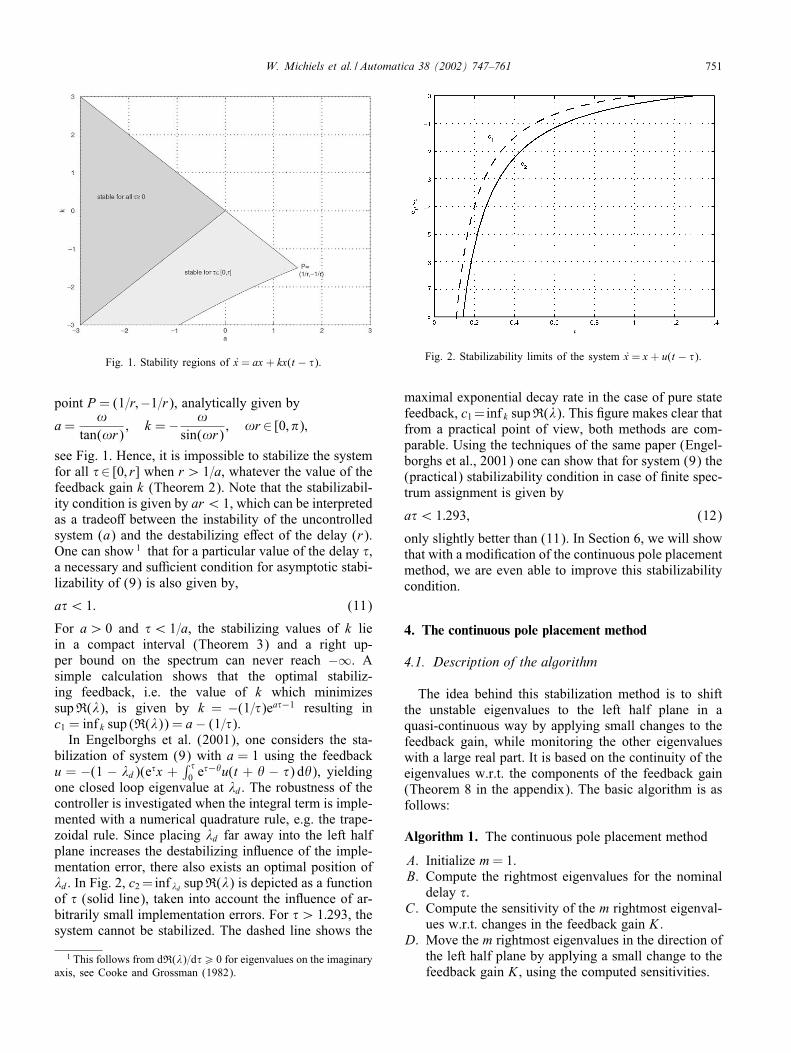
Fig. 1. Stability regions of x = ax + kx(t − �).

point P = (1=r;−1=r), analytically given by

a=!

tan(!r); k =− !

sin(!r); !r ∈ [0; &);

see Fig. 1. Hence, it is impossible to stabilize the systemfor all �∈ [0; r] when r¿ 1=a, whatever the value of thefeedback gain k (Theorem 2). Note that the stabilizabil-ity condition is given by ar¡ 1, which can be interpretedas a tradeo7 between the instability of the uncontrolledsystem (a) and the destabilizing e7ect of the delay (r).One can show 1 that for a particular value of the delay �,a necessary and suNcient condition for asymptotic stabi-lizability of (9) is also given by,

a�¡ 1: (11)

For a¿ 0 and �¡ 1=a, the stabilizing values of k liein a compact interval (Theorem 3) and a right up-per bound on the spectrum can never reach −∞. Asimple calculation shows that the optimal stabiliz-ing feedback, i.e. the value of k which minimizessupR(�), is given by k = −(1=�)ea�−1 resulting inc1 = inf k sup (R(�)) = a− (1=�).

In Engelborghs et al. (2001), one considers the sta-bilization of system (9) with a = 1 using the feedbacku = −(1 − �d)(e�x +

∫ �0 e

�− u(t + − �) d ), yieldingone closed loop eigenvalue at �d. The robustness of thecontroller is investigated when the integral term is imple-mented with a numerical quadrature rule, e.g. the trape-zoidal rule. Since placing �d far away into the left halfplane increases the destabilizing inRuence of the imple-mentation error, there also exists an optimal position of�d. In Fig. 2, c2 = inf �d supR(�) is depicted as a functionof � (solid line), taken into account the inRuence of ar-bitrarily small implementation errors. For �¿ 1:293, thesystem cannot be stabilized. The dashed line shows the

1 This follows from dR(�)=d�¿ 0 for eigenvalues on the imaginaryaxis, see Cooke and Grossman (1982).

Fig. 2. Stabilizability limits of the system x = x + u(t − �).

maximal exponential decay rate in the case of pure statefeedback, c1=inf k supR(�). This :gure makes clear thatfrom a practical point of view, both methods are com-parable. Using the techniques of the same paper (Engel-borghs et al., 2001) one can show that for system (9) the(practical) stabilizability condition in case of :nite spec-trum assignment is given by

a�¡ 1:293; (12)

only slightly better than (11). In Section 6, we will showthat with a modi:cation of the continuous pole placementmethod, we are even able to improve this stabilizabilitycondition.

4. The continuous pole placement method

4.1. Description of the algorithm

The idea behind this stabilization method is to shiftthe unstable eigenvalues to the left half plane in aquasi-continuous way by applying small changes to thefeedback gain, while monitoring the other eigenvalueswith a large real part. It is based on the continuity of theeigenvalues w.r.t. the components of the feedback gain(Theorem 8 in the appendix). The basic algorithm is asfollows:

Algorithm 1. The continuous pole placement method

A. Initialize m= 1.B. Compute the rightmost eigenvalues for the nominal

delay �.C. Compute the sensitivity of the m rightmost eigenval-

ues w.r.t. changes in the feedback gain K .D. Move the m rightmost eigenvalues in the direction of

the left half plane by applying a small change to thefeedback gain K; using the computed sensitivities.


E. Monitor the rightmost uncontrolled eigenvalues.If necessary; increase the number of controlledeigenvalues; m. Stop when stability is reached orwhen the available degrees of freedom in the con-troller do not allow to further reduce supR(�). Inthe other case; go to step B.

We will now describe the di7erent steps of the algo-rithm in more detail.

4.1.1. Computation of the rightmost eigenvaluesIn Engelborghs and Roose (1999) a method is

proposed which automatically computes the rightmosteigenvalues of the characteristic equation. First, a dis-cretization is obtained of the time integration operator ofthe linear or linearized system of DDEs, whose eigen-values are exponential transforms of the roots of thecharacteristic equation. Then, selected eigenvalues of theresulting large matrix are computed. The e7ect of dis-cretization on stability using linear multi-step methodsis well understood, see, e.g. Hong-Jiong and Jiao-Xun(1996) and Hu, Hu, and Liu (1997). A steplength heuris-tic is used to ensure that all eigenvalues of interest areaccurately approximated by the discretization. Accuracycan be increased by employing a Newton iteration on thecharacteristic equation using the approximate eigenval-ues as starting values. This method has been implementedin the Matlab package DDE-BIFTOOL (Engelborghs,2000).

4.1.2. Sensitivity of eigenvalues with respect to thefeedback gain KWhen �i is a solution of the characteristic equation and

vie� ; ∈ [ − �; 0], its corresponding eigenfunction, wehave

(�iI − A− BKTe−�i�)vi = 0;

n(vi) = 0;(13)

where n(vi) is a normalizing condition. Di7erentiatingthis equation w.r.t. a component kj of K , we obtain alinear system of equations in the unknowns @�i=@kj and@vi=@kj:�iI − A− BKTe−�i� (I + BKT�e−�i�)vi

dndvi

T

0

@vi@kj@�i@kj

=

[BvTi eje

−�i�

0

](14)

with ej ∈Rn×1 the jth unity vector.

When the system is in the control canonical form (5),one can compute directly from (7),

@�i@kj

=−e−�i��j−1i

dH=d�i: (15)

This result is useful for the derivation of theoretical prop-erties of the method, but our implementation is based on(13), since Eq. (7) is not practical from a numerical pointof view.

4.1.3. Continuation of eigenvalues as a function of thefeedback gain KAssume that m6 n eigenvalues �1; : : : ; �m are con-

trolled. When the ‘sensitivity’ matrix Sm, de:ned by

Sm = [si; j]∈Rm×n where si; j =@�i@kj; (16)

is of rank m and the desired (small) displacement of thecontrolled eigenvalues is given byV2dm=[V�d1 : : :V�

dm]

T,one can compute a change VK for K such that

SmVK =V2dm: (17)

When m¡n this equation has in:nitely many solutions.One possibility to determine a unique solution consistsof controlling the m eigenvalues using only m selectedcomponents of K and hence taking n − m componentsof VK equal to zero. Another possibility, which we willmotivate later, consists of taking the solution with ‖VK‖minimal. This solution is given by

VK = S†mV2dm; (18)

where S†m is the Moore–Penrose inverse of Sm, seeBen-Israel and Greville (1974, Chap. 3).A physical constraint on the feedback gain is imposed

by the fact that its components must be real, but this isassured by taking the components of V2dm in complexconjugate pairs.With the new feedback gain K+VK , the displacement

of the controlled eigenvalues will generically not be equaltoV2dm, since Eq. (17) is based on linearization, and somecorrection is needed. However, since the eigenvalues andeigenfunctions are continuous w.r.t. parameter changes,with for instance the predictor

�(p)i = �i +V�di ; v(p)i =n∑j=1

@vi@kj

Vkj; i = 1; m

only a few Newton iterations on Eq. (13) are neededwhen VKm is suNciently small. Since it is also desirableto have the eigenvalues for the new feedback gain closeto their predictions, (18) is generally a good choice forthe solution of (17).The n components of the controller gain allow to

control both real and imaginary parts of at most n eigen-values, as illustrated by (17), or, when stabilization


Fig. 3. Two typical situations where it is necessary to extend the number of controlled eigenvalues for a further reduction of supR(�).

is of main concern, only the real part of possibly morethan n eigenvalues. For instance, with n = 2 degrees offreedom in the controller, one can control either two realeigenvalues, or one real eigenvalue and the real part of acomplex pair, or the real parts of two complex pairs. Forthe latter case, note that

@R(�i)@kj

= R

(@�i@kj

):

This approach is applied to all examples of the paper,combined with an adaptation of all controller parametersin an iteration step, as in (18). This leads to the modi:edadaptation formula for the feedback gain,

VK = (R(Sm))†VR(2dm); (19)

where VR(2dm) is the desired displacement of the realparts of the controlled eigenvalues.

4.1.4. Increasing the number of controlled eigenvaluesIn the examples of the paper, where the focus lies on

stabilization, we only control the real parts of the eigen-values. We start by shifting the dominant real eigenvalueor by reducing the real part of the dominant complex pair.In this way control is lost over the other eigenvalues andwhenever an interaction occurs, the number of controlledeigenvalues, m, generally needs to be increased to furtherreduce supR(�). This will now be illustrated.

In Fig. 3, we display two typical situations, where thereal part of only the rightmost eigenvalue is controlledand the number of controlled eigenvalues must be in-creased when it interacts with other eigenvalues. In theupper part the situation is shown where two real eigen-values interact. When only the dominant eigenvalue iscontrolled, no further reduction of supR(�) is possibleafter the interaction (left): when the two eigenvalues co-incide, they :rst transform to a complex conjugate pairwhich does not move to the left in the complex plane bythe next parameter change (we control only its real part),but immediately splits up again into two real eigenvalues,and then the whole process repeats itself. By controllingthe two real eigenvalues from iteration number 150 on,a further reduction of supR(�) is possible (right). In thelower part of Fig. 3, a real eigenvalue interacts with acomplex pair of eigenvalues. A decrease of the real eigen-value leads to an increase of the real part of the complexpair and vice versa (left). This problem can be avoidedby controlling both the real eigenvalue and the real partof the complex pair (right).As will be illustrated with the numerical examples in

the paper, a special situation also occurs when a complexpair, whose real part is controlled, splits up into two realeigenvalues. This is possible because its imaginary part isnot controlled and may tend to zero during the stabiliza-tion procedure. After the splitting both real eigenvaluesneed to be controlled.


In the current version of the algorithm, the number ofcontrolled eigenvalues is manually increased, wheneverstagnation of supR(�) or a splitting of a complex pairoccurs. The method breaks down when no further reduc-tion of supR(�) is possible, i.e. when the available de-grees of freedom in the controller (n) is not suNcient tocontrol the real parts of all dominant eigenvalues. Thiscan happen when n+1 real parts need to be controlled toreduce supR(�) or when the matrix R(Sm) in (19) has arank strictly smaller than m.

4.2. Theoretical properties

In each step of the continuous pole placement algo-rithm, the sensitivity matrix Sm must be of rank m, if fullcontrol over the changes of the m eigenvalues is desired.The next theorem states that when both real and imag-inary parts of n eigenvalues of multiplicity 1 are con-trolled, the sensitivity matrix Sn is always regular.

Theorem 5. If �1; : : : ; �n are single eigenvalues; then thesensitivity matrix Sn is regular.

Proof. Since the pair (A; B) is controllable; the sys-tem can be transformed into the control canonical form(5)–(7). Using (15); we obtain the following sensitivitymatrix:

Sn =

e−�1�

dH=d�1. . .

e−�n�

dH=d�n

1 �1 : : : �n−11

1 �2 : : : �n−12

...... : : :

...

1 �n : : : �n−1n

:

(20)

This matrix is regular if no eigenvalues coincide; sincedH=d�i �=0 and the Vandermonde matrix is regular.

When two eigenvalues are close to each other, the sen-sitivity w.r.t. changes in the feedback gain is large, asshown in the next theorem. This result is related to thefact that large qualitative changes in the spectral picturecan occur when eigenvalues coincide.

Theorem 6. When two eigenvalues are brought together;the norm of the sensitivity matrix Sn becomes arbi-trarily large.

Proof. Start from (20) and consider the asymptotic casewhere �j → �i while the other eigenvalues are kept :xed.With the explicit expression for the determinant of aVandermonde matrix; we have

lim�j→�i

det(Sn) = e−2�i�n∏

k=1; k �=i; k �=j

(e−�k�

dH=d�k

)

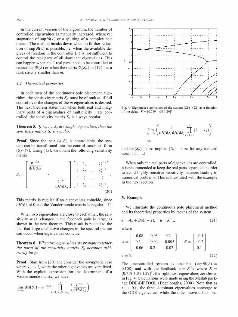
Fig. 4. Rightmost eigenvalues of the system (21)–(22) as a functionof the delay, K = [0:719 1:04 1:29]T.

lim�j→�i

(1

dH=d�i dH=d�j

n∏l¿k=1

(�l − �k))

=∞and det(Sn) → ∞ implies ‖Sn‖ → ∞ for any inducednorm ‖:‖.

When only the real parts of eigenvalues are controlled,it is recommended to keep the real parts separated in orderto avoid highly sensitive sensitivity matrices leading tonumerical problems. This is illustrated with the examplein the next section.

5. Example

We illustrate the continuous pole placement methodand its theoretical properties by means of the system

x = Ax + Bu(t − �); u= KTx; (21)

where

A=

−0:08 −0:03 0:20:2 −0:04 −0:005

−0:06 0:2 −0:07

; B=

−0:1−0:20:1

;

�= 5: (22)

The uncontrolled system is unstable (supR(�) =0:108) and with the feedback u = KTx where K =[0:719 1:04 1:29]T, the rightmost eigenvalues are shownin Fig. 4. Calculations were made using the Matlab pack-age DDE-BIFTOOL (Engelborghs, 2000). Note that as� → 0+, the three dominant eigenvalues converge tothe ODE eigenvalues while the other move o7 to −∞.


Fig. 5. Real parts of the the rightmost eigenvalues of (21)–(22)with � = 5 as a function of the iterations of the continuous poleplacement algorithm. For values of the feedback gain at iterations 37,110 (indicated by the dashed lines), and its value in the optimum,the rightmost eigenvalues are continued as a function of the delay inFig. 7.

Fig. 6. Feedback gain K = [k1 k2 k3]T as a function of the iterationsof the continuous pole placement algorithm applied to (21)–(22).

Although the particular control law achieves stability for�=0, the system is unstable for the nominal delay �=5and we now describe its stabilization with the continuouspole placement method.In Fig. 5, the rightmost eigenvalues are shown as a

function of the number of iterations taken in Algorithm1. The corresponding values of the feedback gain K =[k1 k2 k3]

T are displayed in Fig. 6. First we only reducethe real part of the dominant pair of complex conjugateeigenvalues, which is already suNcient to achieve stabi-lization. Meanwhile the real part of an uncontrolled pairgrows, and after 50 iterations we reduce the real part of the

two complex pairs of eigenvalues. In this way, we loosecontrol over the imaginary parts and because we wantto avoid coinciding eigenvalues, which cause numericalproblems (Theorem 6), we keep the real parts separated.However, around iteration 58, the eigenvalues are closeand the e7ect of a high sensitivity w.r.t. changes in thefeedback gain is visible. At iteration 158, a complex pairsplits into two real eigenvalues and all components of thefeedback gain K are used to reduce these real eigenval-ues and the real part of the dominant pair. From iteration176 on, where also this pair splits, we only control thethree dominant real eigenvalues and around iteration 190the method breaks down. At this point we are close to theminimum of supR(�) characterized by four coincidingrightmost eigenvalues at �=−0:150. The correspondingfeedback gain is given by K = [0:471 0:504 0:602]T.In Fig. 7 the rightmost eigenvalues are displayed as a

function of the delay at iterations 37, 110, and in the opti-mum. This :gure illustrates how the real parts of the dom-inant eigenvalues evolve towards the minimum for thenominal delay, characterized by coinciding eigenvaluesand the resulting high sensitivity w.r.t. parameter changes(including the delay). This high sensitivity around theoptimum is a property of the system. Our experience in-dicates that for this type of control problems, coincidingeigenvalues are a general characteristic of the global op-timum. Another illustration can be found in Michiels andRoose (2001), where all possible con:gurations of therightmost eigenvalues in the global minimum of supR(�)were given for 2D systems. These were all characterizedby (some) eigenvalues with multiplicity larger than one.In our example the high sensitivity w.r.t. delay changesfor the :nal feedback gain is caused by the fact that weexecuted Algorithm 1 until we reached the minimum.However, from a practical point of view, where also therobustness aspect is important, this is not needed. Forinstance, the feedback gain obtained at iteration number37, see Fig. 7, already achieves stability. The exponentialdecay rate of the closed loop solution is smaller than forthe optimum, yet less sensitive to delay changes.

6. Observer based controller

We now assume that not the full state x, but only anoutput y = CTx∈R, is available for measurement, with(C; A) observable. Note that in this case the system canbe equivalently described by the transfer function

G�(s) =G(s)e−s�; (23)

with G(s) = CT(sI − A)−1B, and that any system of theform

x = Ax + Bu(t − �1); y = CTx(t − �2); �1 + �2 = �;

(24)


Fig. 7. Rightmost eigenvalues of (21)–(22) as a function of the delay, for values of K at iteration 37 (upper left), iteration 110 (upperright) and in the optimum (below). The corresponding values of the feedback gain are K = [0:712 1:075 0:831]T, K = [0:559 0:770 0:694]T andK = [0:471 0:504 0:602]T.

is a realization of (23). In order to apply the continu-ous pole placement method, we construct an observerfor (24),

˙x = Ax + Bu(t − �1) + L(CTx(t − �2)− y);

with L∈Rn×1 the observer gain, and apply the feedbacku=KTx(t). With e= x− x the observer error, we obtain

x = Ax + BKTx(t − �1)− BKTe(t − �1);e= Ae+ LCTe(t − �2):

(25)

Since in the characteristic equation of the closed loopsystem (25),

det

(�I −

[A 00 A

]−[BKT −BKT

0 0

]e−��1

−[0 0

0 LCT

]e−��2

)= 0;

all matrices are block-triangular, the separation princi-ple is valid and the closed loop eigenvalues consist of

the solutions of det(�I − A − BKTe−��1) = 0, i.e. thecontroller eigenvalues, and of det(�I − A− LCTe−��2) =det(�I − AT − CLTe−��2) = 0, i.e. the observer eigen-values. Hence to achieve stability we apply the contin-uous pole placement twice, to the systems (A; B; �1) and(AT; C; �2).In the construction of realization (24), we are free to

distribute the delay over input and output. This additionaldegree of freedom can be used to obtain better perfor-mance of plant and observer. It also allows to extend theclass of systems which can be stabilized with the con-tinuous pole placement method. To see this, reconsidersystem (9) with output y = x. Although the full stateis available for feedback, it will be useful to constructan observer. The transfer function is given by G�(s) =e−s�=s − a and we construct an observer based on therealization,

x = ax + u(t − �1); y = x(t − �2); �1 + �2 = �:

With the observer ˙x = ax + u(t − �1) + l(x(t − �2) − y)and the controller u = kx, the closed loop eigenvaluescoincide with the eigenvalues of the systems,

x = ax + kx(t − �1); e= ae+ le(t − �2): (26)


Fig. 8. Rightmost eigenvalues of (28) (left) and components of the feedback gain K = [k1 k2 k3 k4]T (right) as a function of the iterations ofthe continuous pole placement algorithm.

Since these equations are of form (10), the optimal sta-bilizing controller (i.e. values of k and l which minimizesupR(�)) results in,

supR(�) = max(a− 1

�1; a− 1

�2

);

and the best stabilizability results are obtained when dis-tributing the delay equally over input and output. Henceasymptotic stability can be achieved i7

a�¡ 2; (27)

which is twice as good as (11), valid for pure state feed-back, and better than (12), the ‘practical’ condition incase of :nite spectrum assignment.

7. Extension

The continuous pole placement method can be consid-ered as a natural generalization of the classical pole place-ment algorithm to the input delay case. Since it is based onthe continuous dependence of the rightmost eigenvalueson the controller parameters and because the algorithmsdescribed in Section 4.1.1 can also deal with equationswith several discrete delays , it can easily be extendedto more general types of linear delay equations involvingdelays in both state and control variables, and multiplefeedbacks. Although theoretical stabilizability propertiesand convergence results, such as Theorem 5, are gener-ally not valid and depend on the structure of the systemunder consideration, we will brieRy illustrate with someexamples the e7ectiveness of the method in solving morecomplicated stabilization problems.As a :rst example consider the following system,

x=A1x+A2x(t−�1)+B1u(t−�2)+B2u(t−�3);u= KTx;

(28)

where

A1 =

0:1 −0:5 −0:3 0:30 0 0:2 −0:20 0 −0:1 00 0:4 0:3 −0:4

;

A2 =

−0:2 0:3 0:2 −0:50 −0:2 −0:2 0:2

−0:1 0:1 0:1 0:10:1 −0:6 −0:6 0

;

B1 =

0−0:100:1

; B2 =

−0:3000

;

�1 = 2; �2 = 1; �3 = 3;

(29)

and a stabilizing feedback gain K=[k1 k2 k3 k4]T needs

to be determined. In Fig. 8, the rightmost eigenvalues of(28) are shown as a function of the iterations of the con-tinuous pole placement algorithm, as well as the com-ponents of the feedback gain. The initial value of thefeedback gain is [0 0 0 0]T. We have four control pa-rameters and the method converges towards an optimumcharacterized by :ve coinciding real eigenvalues (in thelast iteration step we already have a good approximationwhen taking into account the high sensitivity around theoptimum).Now consider the case where the two inputs in (28)

are independent,

x=A1x+A2x(t−�1)+B1u1(t−�2)+B2u2(u−�3);u1 = KT

1 x; u2 = KT2 x;

(30)

with the system parameters given by (29). In Fig. 9, it-erations of the continuous pole placement algorithm are


Fig. 9. Rightmost eigenvalues of (30) (left) and components of the feedback gains K1 = [k1 k2 k3 k4]T and K2 = [k5 k6 k7 k8]T (right) as afunction of the iterations of the continuous pole placement algorithm.

shown. Compared to system (28) a further reduction ofthe real parts of the dominant eigenvalues is possible,which is expected from the independent choice of bothfeedback gains. The algorithm also converges towards anoptimum (w.r.t. all controller parameters), characterizedby :ve coinciding real eigenvalues and hence, althoughthere are eight controller parameters, it is not possible tofurther reduce supR(�) by trying to control the real partsof more than four eigenvalues. This limitation is imposedby the structure of the controlled system, not by our al-gorithm. In this context we would like to emphasize :rstthe danger of an ‘over-parametrization’ of the controller:having more degrees of freedom in the controller doesnot generally imply that more eigenvalues can be con-trolled or better stability results can be obtained. This isclearly illustrated in Michiels and Roose (2001), where astabilization problem with four controller parameters wasstudied, which could analytically be reduced to three ef-fective controller parameters. Second, although the con-tinuous pole placement algorithm uses a local strategyin each iteration step and in the beginning only a feweigenvalues are controlled, generically all controller pa-rameters are adapted in an iteration step when using for-mula (19), see, e.g. Fig. 9, and therefore the search spaceof the underlying optimization procedure (i.e. :nding aminimum of supR(�)) is generally not limited to a sub-space of the parameter space where, e.g. some controllerparameters are not used and remain zero.As a second example we consider,

x=A1x+A2x(t−�1)+∫ t

t− �1A3x(s) ds+Bu(t−�2);

u= KTx;(31)

where

A1 =

0:1 0 00:2 0 −0:20:3 0:1 −0:2

; A2 =

−0:2 0 0−0:4 −0:2 0:4−0:4 −0:1 0:2

;

Fig. 10. Rightmost eigenvalues of the system (31)–(33) for u=0 as afunction of the delay �1. The solid lines correspond to the eigenvaluesof (31). Eq. (33) has in addition a triple eigenvalue at zero (dashedline).

A3 =

0:1 −0:2 00 0:1 0:1

−0:1 0 0:1

; B=

0:100

;

�1 = 6; �2 = 1: (32)

We can deal with the distributed delay term because dif-ferentiation of (31) leads to the following equation withonly discrete delays,

z=

[0 IA3 A1

]z +

[0 0

−A3 A2

]z(t − �1)

+

[0

BKT

]z(t − �2); (33)


Fig. 11. Rightmost eigenvalues of (31)–(33) and components of the feedback gains K = [k1 k2 k3]T (right) as a function of the iterations ofthe continuous pole placement algorithm.

Fig. 12. Rightmost eigenvalues of (31) for K =0 (above) and for the :nal value of the feedback gain (Iteration 89; K = [− 5:19 0:491 4:06]T)(below) on two di7erent scales.

where z = [ xx ]. It is easy to show that the transformationfrom (31) to (33) introduces n additional zero eigenval-ues in the spectrum, with n the dimension of the sys-tem. However, the continuous pole placement method cancope with this problem because the zero eigenvalues cansimply be removed after applying step B of Algorithm 1to (33). In Fig. 10, the eigenvalues of the uncontrolledsystem (31)–(33) are shown as a function of the delay�1. For the nominal delay �1 = 6, there are three eigen-

values in the open right half plane. Iterations of the con-tinuous pole placement algorithm are shown in Fig. 11.In Fig. 12, we depict the spectrum of (31) for K =0 andfor the :nal value of the feedback gain. The continuouspole placement algorithm converges to an optimum char-acterized by :ve rightmost eigenvalues, a complex pairwith multiplicity 2 and a real eigenvalue. Such a situationalso occurred in the three-parameter problem discussedin Michiels and Roose (2001).


8. Concluding remarks

In this paper, we have shown that the classical poleplacement method for ODEs can be adapted to time-delaysystems where the closed loop system is in:nite dimen-sional and the number of degrees of freedom of the con-troller is :nite. The method consists of controlling onlythe rightmost eigenvalues, which is possible because analgorithm to compute the rightmost eigenvalues of a lin-ear time-delay system is available.Further research includes the re:nement of the contin-

uous pole placement method, more speci:cally the de-velopment of strategies to determine the trajectories ofthe controlled eigenvalues in the complex plane, takinginto account also robustness issues, and the study of theoptima reached when the method breaks down. Also thecomparison with methods based on :nite spectrum as-signment deserves further attention.

Acknowledgements

This research presents results of the Research ProjectOT 98=16 funded by the Research Council K.U. Leuven,of the Research Project G.0270.00 funded by the Fund forScienti:c Research—Flanders (Belgium) and of the Re-search Project IUAP P4=02 funded by the programme onInteruniversity Poles of Attraction, initiated by the Bel-gian State, Prime Minister’s ONce for Science, Technol-ogy and Culture. The scienti:c responsibility rests withits authors. K. Engelborghs is a Postdoctoral Fellow ofthe Fund for Scienti:c Research—Flanders (Belgium).

Appendix A. Continuity properties

In the proof of Theorem 2, we use the following result,Lemma A-1 of Michiels et al. (1998):

Lemma 7. Let f(�) and the sequence {fn(�)}n¿1 beanalytic functions on an (open) domain D ⊆ C. Sup-pose that {fn(�)}n¿1 converges uniformly to f(�) onthe disc D = {�: |� − �0|6R} ⊂ D for some R¿ 0and that on this disc �0 is the only zero of f(�); withmultiplicity k¿ 0 (k = 0 means no zeros in D). Thenthere exists a number N ∈N such that ∀n¿N; fn(�)has exactly k zeros �n;1; : : : ; �n;k in D and limn→∞ �n;j =�0; ∀j∈{1; : : : ; k}.

With this lemma, continuity properties of the spectrumw.r.t. the feedback gain K can easily be deduced:

Theorem 8. For the system x = Ax + BKTx(t − �); theindividual eigenvalues are continuous w.r.t. changes in

the feedback gain K.Moreover cK=sup{R(�): det(�I−A− BKTe−��) = 0} is continuous w.r.t. K.

Proof. For an arbitrary eigenvalue �0 of

x = Ax + BKTx(t − �) (A.1)

with multiplicity k; de:ne for some (small) R¿ 0the set D = {�∈C: |� − �0|6R}; containing no othereigenvalues. Further; consider an arbitrary sequence{Kn}n¿1 ∈R1×n with limit K . Since

det(�I − A− BKTn e

−��) → det(�I − A− BKTe−��)

uniformly on D as n→ ∞; we can apply Lemma 7 whichstates that the system

x = Ax + BKTn x(t − �) (A.2)

has exactly k eigenvalues arbitrarily close to �0 as n→ ∞;which proves continuity of the individual eigenvalues.The proof of the second statement is by contradiction.

Since there exist eigenvalues of (A.1) with real part arbi-trarily close to cK , which are continuous w.r.t. changes inK , supR(�) cannot ‘jump’ to the left by applying smallparameter changes, and therefore violation of the state-ment would imply: ∃�¿ 0; ∃{Kn}n¿1 → K; ∃{�n}n¿1,such that (A.2) has an eigenvalue �n with R(�n)¿cK +�. From det(�nI − A − BKT

n e−�n�) = 0 it follows that

|�n|6 ‖A‖+‖B‖Kmaxe−cK � with Kmax =supn¿1 ‖Kn‖. De-:ne the set

S = {�∈C: R(�)¿ cK + �; |�|6 ‖A‖+ ‖B‖Kmaxe−cK �}:When S is empty, we have a contradiction. In the othercase, clearly {�n}n¿1 ∈ S. Now de:ne a closed disc Dcontaining S and satisfying R(�)¿ cK + �=2 for �∈D.Since for n → ∞, the function det{�I − A − BKT

n e−��}

converges uniformly on D to det(�I − A − BKTe−��),which has no zeros in D, it follows from Lemma 7 that(A.2) cannot have eigenvalues in S for large n and wehave again a contradiction.

References

Ackermann, J. (1972). Der entwurf linearer regelungssysteme imzustandsraum. Regelungstechnik und prozessdatenverarbeitung, 7,297–300.

Ben-Israel, A., & Greville, T. N. E. (1974). Generalized inverses:theory and applications. Pure and applied mathematics. NewYork: Wiley.

Breth@e, D., & Loiseau, J. J. (1998). An e7ective algorithm for:nite spectrum assignment of singe-input systems with delays.Mathematics and Computers in Simulation, 45(3–4), 339–348.

Cooke, K. L., & Grossman, Z. (1982). Discrete delay, distributeddelay and stability switches. Journal of Mathematical Analysisand Applications, 86, 592–627.

Dion, J. M., Dugard, L., & Fliess, M. (Eds.). (1998). IFACInternational Workshop on Linear Time Delay Systems,Grenoble, France.


Dugard, L., & Verriest, E. I. (1998). Stability and control oftime-delay systems Lecture notes in control and informationsciences, vol. 228. Berlin: Springer.

Engelborghs, K. (2000). DDE-BIFTOOL: a Matlab packagefor bifurcation analysis of delay di@erential equations. TWReport 305, Department of Computer Science, KatholiekeUniversiteit Leuven, Belgium, March. Available fromhttp://www.cs.kuleuven.ac.be/∼koen/delay/ddebiftool.shtml.

Engelborghs, K., Dambrine, M., & Roose, D. (2001). Limitationsof a class of stabilization methods for delay equations. IEEETransactions on Automatic Control, 46(2), 336–339.

Engelborghs, K., & Roose, D. (1999). Numerical computation ofstability and detection of Hopf bifurcations of steady state solutionsof delay di7erential equations. Advances in ComputationalMathematics, 10(3–4), 271–289.

Hale, J. K., & Verduyn Lunel, S. M. (1993). Introduction tofunctional di@erential equations Applied mathematical sciences,vol. 99. Berlin: Springer.

Hong-Jiong, T., & Jiao-Xun, K. (1996). The numerical stability oflinear multistep methods for delay di7erential equations with manydelays. SIAM Journal on Numerical Analysis, 33(3), 883–889.

Hu, G. -D., Hu, G. -D., & Liu, M. -Z. (1997). Estimation ofnumerically stable step-size for neutral delay-di7erential equationsvia spectral radius. Journal on Computational and AppliedMathematics, 78, 311–316.

in ’t Hout, K. J. (1994). The stability of -methods for systems ofdelay di7erential equations. Annals of Numerical Mathematics,1, 323–334.

Kolmanovskii, V. B., & Myshkis, A. (1999). Introduction tothe theory and application of functional di7erential equations.Mathematics and its applications, vol. 463. Dordrecht: KluwerAcademic Publishers.

Kolmanovskii, V. B., & Nosov, V. R. (1986). Stability of functionaldi@erential equations Mathematics in science and engineering,vol. 180. New York: Academic Press.

Manitius, A., & Olbrot, A. (1979). Finite spectrum assignmentproblem for systems with delays. IEEE Transactions onAutomatic Control, 24(4), 541–553.

Michiels, W., Engelborghs, K., Roose, D., & Dochain, D. (1998).Sensitivity to in2nitesimal delays in neutral equations. TW Report286, Department of Computer Science, Katholieke UniversiteitLeuven, Belgium, December; SIAM Journal on Control andOptimization, Accepted for publication.

Michiels, W., & Roose, D. (2001). Limitations of delayed statefeedback: a numerical study. TW Report 323, Department ofComputer Science, Katholieke Universiteit Leuven, Belgium April;International Journal of Bifurcation and Chaos, Accepted forpublication.

Olbrot, A. (1978). Stabilizability, detectability and spectrum assi-gnment for linear autonomous systems with general time delays.IEEE Transactions on Automatic Control, 23(5), 605–618.

Palmor, Z. J. (1996). The control handbook. New York: CRC andIEEE Press, pp. 224–237.

Smith, O. J. (1957). Closer control of loops with dead time. ChemicalEngineering Progress, 53, 217–219.

Van Assche, V., Dambrine, M., Lafay, J.-F., & Richard, J.-P. (1999).Some problems arising in the implementation of distributed-delaycontrol law. In Proceedings 38th IEEE CDC, paper FRM08-1.

Wang, Q. G., Lee, T. H., & Tan, K. K. (1999). Finite spectrumassignment for time-delay systems. Lecture notes in control andinformation sciences, vol. 239. Berlin: Springer.

Wim V.A. Michiels was born in Mol,Belgium, on 9 January 1974. He ob-tained a M.S. degree in electrical engi-neering from the K.U. Leuven, Belgium,in 1997. Currently he is pursuing hisPh.D. at the Department of ComputerScience of the same university. Hisresearch interests include the stabiliza-tion and control of systems describedby functional di7erential equations,nonlinear dynamical (control) systemsand bifurcation analysis.

Koen Engelborghs was born on 2January 1973. He obtained an engi-neering degree in Computer Scienceand Applied Mathematics in 1996 anda Ph.D. in Applied Sciences in 2000both from the K.U. Leuven, Belgium.Currently he is a Postdoctoral Fellowof the Fund for Scienti:c Research—Flanders (Belgium). His research inter-ests include numerical algorithms andsoftware for bifurcation analysis andcontrol of partial di7erential equations

and di7erent types of delay di7erential equations. He is author of thesoftware package DDE-BIFTOOL for numerical bifurcation analysisof delay di7erential equations.

Patrick Vansevenant was born inOstend, Belgium, on 19 September1974. He obtained the degree of Com-plementary Studies in Applied Infor-matics from the K.U. Leuven, Belgium,in 1999. Currently he is researcher inthe division Numerical Analysis andApplied Mathematics of the departmentof Computer Science of the same uni-versity. His research interests includethe analysis and control of time-delaysystems.

Dirk Roose was born on 25 Decem-ber 1954. He obtained an engineeringdegree in computer science and appliedmathematics in 1978 and his Ph.D. inApplied Sciences in 1985, both from theK.U. Leuven, Belgium. From 1989 till1994 he has been assistant professor andsince 1994 he is full professor at theDepartment of Computer Science of thesame university, where he leads a re-search group on Scienti:c Computing.His research interests include nonlinear

dynamical systems and bifurcation problems, and algorithms andsoftware for scienti:c computing. He has co-authored over 100publications on these subjects. He is editor of the book series‘Lecture Notes on Computational Science and Engineering’, SpringerVerlag and of the international journal ‘Parallel ProcessingLetters’.

http://www.cs.kuleuven.ac.be/~koen/delay/ddebiftool.shtml

Continuous pole placement for delay equations

Documents

Transcript of Continuous pole placement for delay equations