Many-electron Electrochemical Processes

Many-electron Electrochemical Processes

Aleksandr A. AndriikoYuriy O. AndriykoGerhard E. Nauer

Reactions in Molten Salts, Room-Temperature Ionic Liquids and Ionic Solutions

Monographs in ElectrochemistrySeries Editor: F. Scholz

Many-electron Electrochemical Processes

For further volumes:http://www.springer.com/series/7386

Monographs in Electrochemistry

Surprisingly, a large number of important topics in electrochemistry is not covered

by up-to-date monographs and series on the market, some topics are even not

covered at all. The series Monographs in Electrochemistry fills this gap by publish-

ing indepth monographs written by experienced and distinguished electrochemists,

covering both theory and applications. The focus is set on existing as well as

emerging methods for researchers, engineers, and practitioners active in the many

and often interdisciplinary fields, where electrochemistry plays a key role. These

fields will range – among others – from analytical and environmental sciences to

sensors, materials sciences and biochemical research.

Information about published and forthcoming volumes is available at

http://www.springer.com/series/7386

Series Editor: Fritz Scholz, University of Greifswald, Germany

Aleksandr A. Andriiko • Yuriy O. Andriyko •Gerhard E. Nauer

Many-electronElectrochemical Processes

Reactions in Molten Salts,Room-Temperature Ionic Liquidsand Ionic Solutions

Aleksandr A. AndriikoKyiv Polytechnic InstituteChemical Technology DepartmentNational Technical University of UkraineKyivUkraine

Yuriy O. AndriykoCentre of Electrochemical SurfaceTechnology (CEST)Wiener NeustadtAustria

Gerhard E. NauerVienna UniversityInstitute of Physical ChemistryViennaAustria

ISSN 1865-1836 ISSN 1865-1844 (electronic)ISBN 978-3-642-35769-5 ISBN 978-3-642-35770-1 (eBook)DOI 10.1007/978-3-642-35770-1Springer Heidelberg New York Dordrecht London

Library of Congress Control Number: 2013932472

# Springer-Verlag Berlin Heidelberg 2013This work is subject to copyright. All rights are reserved by the Publisher, whether the whole or partof the material is concerned, specifically the rights of translation, reprinting, reuse of illustrations,recitation, broadcasting, reproduction on microfilms or in any other physical way, and transmission orinformation storage and retrieval, electronic adaptation, computer software, or by similar or dissimilarmethodology now known or hereafter developed. Exempted from this legal reservation are brief excerptsin connection with reviews or scholarly analysis or material supplied specifically for the purpose of beingentered and executed on a computer system, for exclusive use by the purchaser of the work. Duplicationof this publication or parts thereof is permitted only under the provisions of the Copyright Law of thePublisher’s location, in its current version, and permission for use must always be obtained fromSpringer. Permissions for use may be obtained through RightsLink at the Copyright Clearance Center.Violations are liable to prosecution under the respective Copyright Law.The use of general descriptive names, registered names, trademarks, service marks, etc. in thispublication does not imply, even in the absence of a specific statement, that such names are exemptfrom the relevant protective laws and regulations and therefore free for general use.While the advice and information in this book are believed to be true and accurate at the date ofpublication, neither the authors nor the editors nor the publisher can accept any legal responsibility forany errors or omissions that may be made. The publisher makes no warranty, express or implied, withrespect to the material contained herein.

Printed on acid-free paper

Springer is part of Springer Science+Business Media (www.springer.com)

Dedicated to the memory ofProfessor Yu. K. Delimarskiy

Preface of the Editor

Both in nature, e.g. in photosynthesis and respiration, and in industrial electrochem-

istry, multi-electron processes by far outnumber single-electron processes. Hence,

their significance is indisputable, but this is also true for their complexity with

respect to theory and experiments. The authors of this monograph have a strong

background in high-temperature molten salt electrochemistry, which concerns

especially the transition metals and their ions. These elements have a rich redox

chemistry and their electrochemical reactions can only be understood considering

rather complex multi-electron processes. The senior Ukrainian author Aleksander

Andriiko is a pupil of Juriy Konstantinovich Delimarskiy (1904–1990), the former

head of the Kiev school of (high-temperature) molten salt electrochemistry which

flourished over many decades. Unfortunately, the scientific treasures of wisdom

gathered during that period are badly accessible to Western scientists. Hence it is a

very lucky constellation that the senior author Aleksander Andriiko was joined by

the young Ukrainian electrochemist Yuriy Andriyko, by the way his son, and the

Austrian electrochemist Gerhard Nauer to compile this monograph. High-

temperature molten salt electrochemistry of transition metals and other polyvalent

metals offers a great amount of relevant information, especially for the room-

temperature ionic liquid electrochemistry which blossoms nowadays. Preserving

and disseminating the precious knowledge and experience of people who have

actively taken part in the development of molten salt electrochemistry are thus an

investment in the future of electrochemistry.

Greifswald, Germany Fritz Scholz

June 2012

vii

Preface of the Authors

“All things run, all things change” (Heraklit)

The main ideas of this book originate from Electrochemistry of Molten Salts.The two of us (AA and GN) belong to the generation of electrochemists who

worked in this branch of science in times of its blossoming and evidenced its

rapid degradation. Once powerful, this field of chemistry had fallen in a state of

deep decline till the mid-1990s.

How and why could it happen?

Alexander Andriiko, a former Soviet Union scientist who worked in this field

since the end of 1970s for about 25 years, knows that the Soviet Science had been

shaken in the mid-1980s. “Remember my word, fellows, this is not for good”—that

was the comment relating to the situation of science given at the beginning of

perestroika (1986) by his (i.e., Andriiko’s) Maitre, Academician Prof. Yu.

Delimarskiy. This prophecy became a reality very soon. A last nail in the coffin

of his science had been thrust after Cold War was over. Indeed, the streams from the

mighty river of Military Industries that fed this science—it is not a secret

anymore—dried out very soon after the collapse of SU.

Hardly ever he, the former Soviet scientist, regrets about this. Freedom is great

thing. However, everything must be paid in this world. The price was a severe loss

of science on 1/6 part of our world.

As for the Electrochemistry of Molten Salts, it was lost worldwide—not in the

FSU countries only. The diagram below gives an idea about the scale of this

catastrophe. It represents the structure of electrochemical researches in the world

through the publications in a representative international journal in 1995–1996, just

a few years after these events. As we can see, Molten Salts electrochemistry took

the last place among other various branches of electrochemistry. Nothing has been

changed since then.

Deplorable situation—especially taking into account leading positions of Mol-

ten Salt Electrochemistry some 20–25 years ago.

ix

All things change indeed. None of us is working in the field of pure Electro-

chemistry of Molten Salts anymore. A. Andriiko heads the Chair of General and

Inorganic Chemistry in National Technical University of Ukraine “Kyiv Polytech-

nic Institute”; Gerhard Nauer, a professor of Physical Chemistry, works in Vienna

State University; the youngest of us, Yuriy Andriyko, has recently received his PhD

degree from Vienna Technical University for the research in a newly emerging

field—electrochemistry of ionic liquids.

Lithium Batteries

Corrosion

Fuel Cells

Electroplating

Other Batteries

Theory

Organic Electrochemistry

Sensors

Photoelectrochemistry

Electrochromism

Electrocatalysis

IONIC MELTS

Capacitors

0 5 10 15 20 25 30

% of publications

Solid State Electrochemistry "Classical" fields

Why did we decide to abandon our routine work and spend our time for

preparation of this book?

There are two reasons:

First. Now we know that the ideas are of interest not only for the electrochemistry

of molten salts, but for other research fields as well. In particular, the recent

results in the Electrochemistry of Ionic Liquids fit perfectly well in the devel-

oped pattern. We believe that our nature is united; we ourselves divide it

conventionally for the reasons of analysis and simplification.

Second. Regretfully, our scientific knowledge is not only accumulated but can

dissipate under certain circumstances. Following curious example comes to

our mind. One of us (AA), being young researcher in the mid-70s and having

conducted his studies on thermodynamics of electrode–electrolyte interface,

came across a paper in worldwide known scientific journal announcing the

“discovery of new phenomenon, reversible heat effect at first kind–second

kind conductor interface, similar to the Peltier effect at a junction of two

different metals”. Digging deeper, he found with astonishment that this phenom-

enon was long ago described theoretically, verified experimentally with very

x Preface of the Authors

high precision and published in a series of papers in Zeitschrift furElektrochemie (Lange and others, 1930s).

Who knows how many such scientific treasures were buried—possibly for-

ever—in those bulky German “Zeitschriften” after Germany lost the War? It

seems that we shall never get an answer to this question. However, we can predict

for sure a vast cemetery of scientific ideas and results buried in papers published in

Russian language in scientific journals of the USSR, who also lost this (Cold) War.

Who would read them now, if they were not too wide cited even in those times of

communist empire, which is now vanished?

The present book contains two kinds of the results. The first, more numerous,

obtained mainly in Kiev in 1980s—the beginning of 1990s, belong to electrochem-

istry of “classic” high-temperature ionic melts. Being scattered in Russian language

papers, they are practically unknown to Western readers. The second are recent

results on the electrochemistry of polyvalent metals in ionic liquids, which, as we

shall see, are in very good agreement with the first.

This book is not for a popular chemical reading. Basic knowledge in modern

theoretical electrochemistry and some mathematical skills are expected from a

reader, though we tried not overloading the text by formulas and equations.

However, the equations are sometimes very useful for someone writing in a

language that is not native for him (as it is the case for each of us). As Poincare

once aptly said, they serve as crutches for a limping man, because using a foreign

language is like walking for a lame.

Thus, the book is addressed to anyone who is interested in general problems of

electrochemistry—but not only for him or her. Perhaps, the book will be of use for

future generation of researchers when Electrochemistry of Molten Salts revives

again. We have such hope, because we believe not only in the dictum of Ancient

Greeks with which we have started, but also in far more ancient wisdom of

Aecclesiastus: “Nothing is new under this Moon . . ., and everything turns back in

its common cyclic way”.

Kyiv, Ukraine Aleksandr A. Andriiko

Wiener Neustadt, Austria Yuriy O. Andriyko

Vienna, Austria Gerhard E. Nauer

Preface of the Authors xi

Introduction

Thus, bare facts cannot satisfy us; in other words, we needscience ordered, or, better to say, organized.

H. Poincare

This book deals with the processes in electrochemical systems containing

compounds of polyvalent elements. Most of the theoretical generalisations and

ideas are based on the experimental data relevant to molten high-temperature

systems containing complex fluorides. For a long period of time, such systems

were of significant practical interest for technology of nuclear materials, electro-

metallurgy of refractory and non-ferrous metals and other applications [1–3]. Thus,

the systems were investigated extensively throughout the world. As a result, a vast

amount of experimental data has been accumulated.

Analysis of these data gives the impression of chaos and disorder. The results

and conclusions of different authors are often controversial, and the data do not fit

any logical pattern (possibly, that is the reason why no comprehensive reviews or

monographs are available in this field). Some experimental phenomena did not

receive satisfactory theoretical explanations, such as, for example: the formation of

metal–salt cathode deposits, the breakdown of the industrial electrowinning of

Al–Si alloys and the anode effect.

The general feature of such systems is that the electrochemical processes are

many-electron ones since compounds of polyvalent elements are, typically, chang-

ing their oxidation states by more than one.

The first main idea of this work is to refuse the assumption of possible one-step

transfer of several (more than one) electrons in one elementary electrochemical act

and to consider any real many-electron process as a sequence of one-electron steps.

Although this idea is not new (it follows immediately from quantum theories of

electron transfer [4]), it is not followed consistently in research practice. The reason

is that a number of significant problems ought to be overcome in such an approach:

description of the accompanying intervalence chemical reactions, general scheme

of the mechanism, estimation of stability of low-valence intermediate species and

xiii

revision of some deeply rooted concepts inconsistent with the one-electron repre-

sentation of the overall process. The first 3 chapters of the book are devoted to these

problems.

To begin with, the basic concepts and definitions related to the model of stepwise

processes are introduced and rigorously formulated. This model presumes a series

of consecutive one-electron electrochemical reactions with conjugated chemical

intervalence reactions, every low valence intermediates taking part in these

reactions. The properties of a particular system, including the possibility to observe

the separate steps, follow logically from the stability of the intermediates that can

be characterised by either equilibrium or rate constants of the intervalence

reactions.

Provided the solubility of low-valence intermediates (LVI) is low, the stepwise

character of the process should result and often does result in the formation of three-

phase system “electrolyte-film of LVI-metal”; we call it “electrochemical film

system” (EFS). Such situation is very common in a long-term electrolytic process.

Thus, the second main aspect of the approach is to consider the film as an active

participant of the process rather than simply as a passivative layer. This point of

view is also defined and substantiated in the first chapter. As a starting point, some

ideas on the solid-phase electrochemical reduction mechanism were borrowed from

the electrochemistry of refractory metals in aqueous solutions [5].

It is shown that the Velikanov model [6] of polyfunctional conductor (PFC) is a

good approximation for the properties of the LVI film. The electrochemistry of PFC

had attracted considerable attention in the 1970s with regard to the practical

problem of electrochemical processing of chalcogenide (sulphide) compounds,

the components of natural polymetallic ores.

Since the properties of PFC are a key point for understanding the behaviour of

electrochemical film systems, this subject is reviewed in Chap. 4 with special

emphasis on the recent results related to the electrochemistry of ionic liquids.

The classification of electrode film systems is proposed based on the above

ideas, and main qualitative regularities of the electrolytic processes in the film

systems of different kind are envisaged in Chap. 4. In particular, the mechanism of

formation of cathode deposits is considered. It is shown that the deposition of

metal–salt “carrots” or compact metal layers depends on the properties of the

cathode film system (prevailing type and ratio of the electronic and ionic conduc-

tivity of the film). The nature of crisis phenomena at the electrodes is also analysed

(anode effect in fluoride melts, complications at the electrolytic production of Al–Si

alloys in industrial-scale electrolytic cells), the mechanisms are elaborated and the

means to escape the crises situations are developed.

From the standpoint of thermodynamics, the system electrolyte–film–electrode

is open and far from equilibrium state. In this study we use the theoretical approach

to the description of such systems created by H. Poincare and further developed

later by Andronov and others. This method is called bifurcation analysis or,

alternatively, theory of non-linear dynamic systems [7]. It has been applied to the

studies of macrokinetics (dynamics) of the processes in electrode film systems.

xiv Introduction

http://dx.doi.org/10.1007/978-3-642-35770-1_4

http://dx.doi.org/10.1007/978-3-642-35770-1_4

There, the mathematical model is represented by a system of non-linear differ-

ential equations based on the balances of extensive physical quantities like mass,

energy and charge. General rules for construction and analysis of such models are

given in Chap. 1, while their applications to the specific systems are discussed in

Chap. 5. In particular, a theory of anode refinement of a polyvalent metal in long-

term processes is considered. It explains the periodic changes of current efficiency

in the refinement of Nb and Ta along with the development of crisis phenomenon in

pilot-scale long-term refinement process for metallurgical silicon that did not

appear in short-term laboratory experiments. A theoretical model of the anode

process at carbon electrodes in the condition of anode effect is also considered.

This model allows for predictions of some interesting features of the process. For

example, it proves the “supercritical” regimes to be possible for the electrolysis at

current density of several orders higher than the initial critical value. This possibil-

ity is verified experimentally in KF–KBF4 molten salt mixtures. Finally, as an

additional example of the capabilities of the theoretical methods, Chap. 5 includes

the developed mathematical model of self-discharge of highly energy-intensive

lithium batteries. It predicts the situations when instability occurs developing

finally into thermal runaway and explosion of the cell during storage with no

apparent external reasons.

Hence, the purpose of this book is to provide a unified basis for a wide range of

problems relevant to the electrochemistry of many-electron processes in ionic melts

and in other media as well. Equilibria in many-electron systems, non-stationary

many-electron processes, electrochemical processes in mixed conductors, aspects

of the electrodeposition of polyvalence elements and anode processes are consid-

ered. No arbitrary assumptions like one-step many-electron transfers or “discrete”

discharge of complex species are involved—the consideration is based on a few

very general ideas.

Of course, the results presented are neither a final solution to all problems nor

a completed phenomenological theory of many-electron electrochemical pro-

cesses; rather, this is an attempt to make a few steps towards such theory. Since

the whole problem is challenging and complex, some results are not flawless; we

are quite aware of that. Especially this is true for the kinetics of many-electron

processes: the proposed mechanism is a sketch rather than a rigorous description.

Perhaps, some conclusions are disputable requiring further discussion and

elaboration.

Anyway, this book is an attempt to find order in the huge set of separated facts

accumulated by numerous works in the electrochemistry of many-electron pro-

cesses. Pursuing this aim, we were inspired by the ideas of [8]: science has to find

an order and simplicity under apparent disorder and complexity of the observed

facts. Further on, new complexity is hidden under this simplicity; it is already

looking out when we consider the systems far from equilibrium—to find new

simplicity under this new complexity is a task for future researchers. And so on,

ad infinitum.

Introduction xv

http://dx.doi.org/10.1007/978-3-642-35770-1_1

http://dx.doi.org/10.1007/978-3-642-35770-1_5

http://dx.doi.org/10.1007/978-3-642-35770-1_5

References

1. Delimarskii YuK, Markov BF (1960) Electrochemistry of molten salts.

Metallurgizdat, Moskow (in Russian).

2. Baimakov YuV, Vetiukov MM (1966) Electrolysis of molten salts.

Metellurgizdat, Moscow (in Russian).

3. Delimarskii YuK (1978) Electrochemistry of ionic melts. Metallurgia, Moscow

(in Russian).

4. Dogonadze RR, Kuznetsov AM (1978) Kinetics of heterogeneous chemical

reactions in solutions. In Kinetics and catalysis. VINITI, Moscow, pp 223–254

5. Vas’ko AT, Kovach SK (1983) Electrochemistry of refractory metals. Tekhnika,Kiev (in Russian).

6. Velikanov AA (1974) Electronic–ionic conductivity of non-metal melts. In Ionic

melts, vol 2. Naukova Dumka, Kiev, pp 146–155

7. Strogatz SH (1994) Nonlinear dynamics and chaos with applications to physics,

biology, and engineering. Cambridge, MA, Westview Press

8. Poincare H (1982) The foundations of science: science and hypothesis; the value

of science; science and method. UPA

xvi Introduction

Contents

1 Many-Electron Electrochemical Systems: Concepts and Definitions 1

1.1 Definition of a Stepwise Electrochemical Process . . . . . . . . . . . . 1

1.2 Stepwise Many-Electron Process: Problem of Kinetic Description . . . 4

1.3 Electrode Film Systems. Formation, General Properties,

Classification . . . . . . . . . . . . . . . . . . . . . . . . . . . . . . . . . . . . . . 6

1.4 Velikanov’s Polyfunctional Conductor . . . . . . . . . . . . . . . . . . . . 7

1.5 Classification of Film Systems. Processes in Chemical Film

Systems . . . . . . . . . . . . . . . . . . . . . . . . . . . . . . . . . . . . . . . . . . 8

1.5.1 Processes in Chemical Film Systems . . . . . . . . . . . . . . . 8

1.6 Macrokinetics of Processes in Film Systems: General Principles

of Theoretical Modelling . . . . . . . . . . . . . . . . . . . . . . . . . . . . . 12

1.6.1 Mathematical Models of Physico-chemical Processes

Using an Approach Based on the Bifurcation Theory . . . . 13

References . . . . . . . . . . . . . . . . . . . . . . . . . . . . . . . . . . . . . . . . . . . . 17

2 Many-Electron Systems at Equilibrium . . . . . . . . . . . . . . . . . . . . . 21

2.1 General Formulation . . . . . . . . . . . . . . . . . . . . . . . . . . . . . . . . . 21

2.2 Experimental Methods: Equilibrium Conditions . . . . . . . . . . . . . 24

2.2.1 Solubility of Metals in Molten Salt Media . . . . . . . . . . . . 24

2.2.2 Potentiometry . . . . . . . . . . . . . . . . . . . . . . . . . . . . . . . . 27

2.3 Experimental Methods: Nernstian Stationary Conditions . . . . . . . 31

2.3.1 General Notions and Validity Conditions . . . . . . . . . . . . 31

2.3.2 Stationary Potential . . . . . . . . . . . . . . . . . . . . . . . . . . . . 32

2.3.3 Voltammetry at Stationary Conditions (Polarography) . . . 35

2.4 Experimental Methods: Nonstationary Nernstian Conditions . . . . 39

2.4.1 Applicability . . . . . . . . . . . . . . . . . . . . . . . . . . . . . . . . . 39

2.4.2 Chronoamperometry . . . . . . . . . . . . . . . . . . . . . . . . . . . 39

2.4.3 Chronopotentiometry . . . . . . . . . . . . . . . . . . . . . . . . . . . 40

2.5 Instead of Conclusions: More About “System” and “Non-system”

Electrochemistry . . . . . . . . . . . . . . . . . . . . . . . . . . . . . . . . . . . 48

References . . . . . . . . . . . . . . . . . . . . . . . . . . . . . . . . . . . . . . . . . . . . 50

xvii

3 Phenomenology of Electrochemical Kinetics . . . . . . . . . . . . . . . . . . 51

3.1 Diagnostics of Intervalent Reactions . . . . . . . . . . . . . . . . . . . . . 51

3.2 Electrochemical Reduction of Germanium Compounds in Fluoride

Melts . . . . . . . . . . . . . . . . . . . . . . . . . . . . . . . . . . . . . . . . . . . . 54

3.3 Experimental Study of Many-Electron Kinetics: General Rules and

Recommendations . . . . . . . . . . . . . . . . . . . . . . . . . . . . . . . . . . 61

3.4 Some Data on the Electroreduction Mechanisms of Polyvalent

Species in Ionic Melts . . . . . . . . . . . . . . . . . . . . . . . . . . . . . . . . 63

3.5 Disputable Problems of Many-Electron Kinetics . . . . . . . . . . . . 66

References . . . . . . . . . . . . . . . . . . . . . . . . . . . . . . . . . . . . . . . . . . . . 68

4 Electrode Film Systems: Experimental Evidences . . . . . . . . . . . . . . 71

4.1 Ion–Metal Film Systems in Processes of Electrodeposition and

Electrorefinement of Polyvalent Metals . . . . . . . . . . . . . . . . . . . 71

4.2 Ion–Semiconductor Film Systems . . . . . . . . . . . . . . . . . . . . . . . 80

4.3 Dielectric Film Systems . . . . . . . . . . . . . . . . . . . . . . . . . . . . . . 81

References . . . . . . . . . . . . . . . . . . . . . . . . . . . . . . . . . . . . . . . . . . . . 87

5 Dynamics of a Non-equilibrium Electrochemical System . . . . . . . . 89

5.1 Coupling in Electrochemical Systems: Electrochemical

Decomposition of Mixed Conductor . . . . . . . . . . . . . . . . . . . . . 89

5.1.1 The Mathematical Model . . . . . . . . . . . . . . . . . . . . . . . . 90

5.1.2 Experiment and Its Analysis . . . . . . . . . . . . . . . . . . . . . . 91

5.2 Coupling in Electrochemical Systems: Electrorefining of

Polyvalent Metals in a Long-Term Continuous Process . . . . . . . . 97

5.2.1 Simplest Linear Model . . . . . . . . . . . . . . . . . . . . . . . . . . 99

5.2.2 Non-linear Mathematical Model . . . . . . . . . . . . . . . . . . . 100

5.3 Thermokinetic Models of Dynamics in Physico-Chemical Systems:

Thermal Self-destruction of Lithium Power Sources with High

Energy Density . . . . . . . . . . . . . . . . . . . . . . . . . . . . . . . . . . . . . 104

5.3.1 A Model of Chemical Power Source (CPS)

Self-Discharge . . . . . . . . . . . . . . . . . . . . . . . . . . . . . . . . 105

5.3.2 Conditions of CPS Stability During Storage . . . . . . . . . . 108

5.4 Thermokinetic Model of Electrolysis in the Conditions of Anode

Effect . . . . . . . . . . . . . . . . . . . . . . . . . . . . . . . . . . . . . . . . . . . 113

5.4.1 Theory . . . . . . . . . . . . . . . . . . . . . . . . . . . . . . . . . . . . . 113

5.4.2 Experimental Verification . . . . . . . . . . . . . . . . . . . . . . . 119

Appendix A. Derivation of the Differential Equations

(5.11) and (5.12) . . . . . . . . . . . . . . . . . . . . . . . . . . . . . . . . . . . . . . . . 122

Appendix B. Approximate Solution of the Non-linear Second-Order

Differential Equation by Small-Parameter (Krylov–BogoIiubov)

Method . . . . . . . . . . . . . . . . . . . . . . . . . . . . . . . . . . . . . . . . . . . . . . 124

References . . . . . . . . . . . . . . . . . . . . . . . . . . . . . . . . . . . . . . . . . . . . 125

6 Electrochemistry of Ti(IV) in Ionic Liquids . . . . . . . . . . . . . . . . . . 127

6.1 What Are Ionic Liquids? . . . . . . . . . . . . . . . . . . . . . . . . . . . . . . 127

6.2 Solutions of TiCl4 in 1-Butyl-2,3-Dimethyl Imidazolium Azide . . . 128

xviii Contents

6.3 Solutions of TiCl4 in 1-Butyl-2,3-Dimethyl Imidazolium

Tetrafluoroborate . . . . . . . . . . . . . . . . . . . . . . . . . . . . . . . . . . . 135

6.3.1 Diluted Solution (0.025 mol L–1 TiCl4 in BMMImBF4) . . . 135

6.3.2 “Medium” Concentration Range . . . . . . . . . . . . . . . . . . . 139

6.3.3 “Concentrated” Solutions . . . . . . . . . . . . . . . . . . . . . . . . 140

6.4 Solutions of TiF4 in 1-Butyl-2,3-Dimethylimidazolium

Tetrafluoroborate . . . . . . . . . . . . . . . . . . . . . . . . . . . . . . . . . . . 142

6.5 Conclusions . . . . . . . . . . . . . . . . . . . . . . . . . . . . . . . . . . . . . . . 156

References . . . . . . . . . . . . . . . . . . . . . . . . . . . . . . . . . . . . . . . . . . . . 157

Afterword . . . . . . . . . . . . . . . . . . . . . . . . . . . . . . . . . . . . . . . . . . . . . 159

About the Authors . . . . . . . . . . . . . . . . . . . . . . . . . . . . . . . . . . . . . . 161

About the Editor . . . . . . . . . . . . . . . . . . . . . . . . . . . . . . . . . . . . . . . . 163

Index . . . . . . . . . . . . . . . . . . . . . . . . . . . . . . . . . . . . . . . . . . . . . . . . . 165

Contents xix

Chapter 1

Many-Electron Electrochemical Systems:

Concepts and Definitions

Law < of Nature > is taken to be simple until the opposite isproven.

H. Poincare

1.1 Definition of a Stepwise Electrochemical Process

Hereby, an electrochemical process is defined as a many-electron one when the

oxidation states of a reagent and final product differ by more than 1, thus requiring

the transfer of more than one electron to transform, “electrochemically”, at a

defined current flow, the reagent into the product.

The stepwise description of such process necessarily follows from general

principles of chemical kinetics: a third order reaction is unlikely; a reaction of

higher order is improbable. If electrochemical reactions are considered, a direct

two-electron process should be thought of as a third order and, hence, as an unlikely

reaction.

Quantum theory of an elementary electron transfer act confirms this suggestion.

In the early 1970s, using Marcus’ idea on the fluctuations of solvent energy as a

driving force for electron transfer [1], Vorotyntsev and Kuznetsov [2] showed

theoretically that, for non-adiabatic reactions, the elementary two-electron step is

highly improbable, while Dogonadze and Kuznetsov proved that the steps with

more than two transferred electrons are practically impossible [3]. It is consistent

with the rules of chemical kinetics mentioned above: two-electron elementary step

can formally be presented as almost improbable reaction of third order, and three or

more electron steps as the impossible reactions of more than third order.

Lately, Karasevskii and Karnaukhov [4] considered the adiabatic many-electron

reactions. They showed that, at a certain (adiabatic) conditions, when the system is

far enough from equilibrium state, the energy minima corresponding to the

A.A. Andriiko et al., Many-electron Electrochemical Processes,Monographs in Electrochemistry, DOI 10.1007/978-3-642-35770-1_1,# Springer-Verlag Berlin Heidelberg 2013

1

intermediate oxidation states disappear; thus, several electrons can follow to the

final state from/onto the electrode practically simultaneously. Thus, for electro-

chemical states with wave functions strongly overlapping (adiabatic behaviour) the

possibility exists for apparent one-step transfer of at least two electrons. Perhaps,

this mechanism is similar to the synchronous “concerted” electron transfer pro-

posed for homogeneous redox systems [5]. Again, when the adiabatic many-

electron system is shifting nearer to equilibrium (by lowering the current density),

the intermediate energy minima reappear, thus transforming the apparent process to

a sequence of one-electron steps.

Unfortunately, the above theories of elementary electrochemical reactions cause

very little impact on the experimental research practice. It is still widely accepted

that a current–potential curve of a many-electron reaction, if not split into several

waves, can be evaluated assuming a one-stage many-electron transfer on the basis

of simple equations derived for a one-step, one-electron reaction. Usually, it looks

as follows. If only one electrochemical wave in the current–potential curve is found

corresponding to the overall n-electron process, then the conclusion is drawn that

the process proceeds through one n-electron step. The curve is analysed in terms of

one of the electrochemical equations derived for typical one-electron process, some

coefficient RT/αnaF is calculated, where α means the “transfer coefficient” of the

one-step reaction with na electrons being transferred together. When the value of αis close to 1, the process is considered as reversible (Nernstian), otherwise as

irreversible (or quasi-reversible) n-electron step. As an example, see [6, 7] and

references therein concerning the reduction of WO42– in molten halides.

The above situation is common in electrochemistry of molten salts, especially in

the description of processes related to the production of refractory metals. A large

number of reaction mechanisms were proposed including one or more one-stage

many-electron reaction: WðVIÞ þ 6e� ! W and MoðVIÞ þ 6e� ! Mo [6–8]; Ta

ðVÞ þ 5e� ! Ta [9]; NbðIVÞ þ 4e� ! Nb [10, 11]; UðIIIÞ þ 3e� ! Uð0Þ [12];

and many other similar schemes are currently in use. Obviously, such approach is

ambiguous, is sometimes meaningless (for example, what is the physical meaning

of the transfer coefficient α for a number of electrons more than 1?), and has a little

prediction capability. Why then such descriptions are so widespread? One of the

reasons is that almost each of electrochemical handbooks, both on molten salts [13]

and general [14], offers these “αna”—equations for irreversible electrochemical

reactions without even mentioning the fact that all such equations were derived for

a simple one-step one-electron reaction. To our knowledge, only the second edition

of Bard and Faulkner book [15] is an exception.1

1 Curious footnote on page 109 of [15] says:

“In the first edition and in much of the literature, one finds na used as the n value of the rate-

determining step. As a consequence na appears in many kinetic expressions. Since na is probablyalways 1, it is a redundant symbol and has been dropped in this edition. The current–potential

characteristic for a multistep process has often been expressed as <Butler–Volmer equation with

αna coefficient>. This is rarely, if ever, an accurate form of the i–E characteristic for multistep

mechanisms.”

At last!

2 1 Many-Electron Electrochemical Systems: Concepts and Definitions

The opposite approach considering a one-electron multistep mechanism can be

found in many research publications related to the electrochemistry of aqueous

solutions. It originates from early works of Vetter [16], where a many-electron

process is represented as a sequence of one-electron steps at the electrode surface.

Rather cumbersome equations were obtained for the stationary current–potential

curves, transforming into the known electrochemical equations in simplest limiting

cases [15–18]. The weakness of this model consists in representation of the

intermediate products as merely surface states which are unable to leave the

electrode in course of the process. The experience shows that such assumption is

physically unreal. Hence, the model is restricted only to some specific adsorption

processes.

In this book we will follow the concept of one-electron stepwise discharge that

differs from the Vetter’s one. It can be formulated in the following terms:

1. The assumption on the one-step many-electron transfer is not used. Any elemen-

tary electrochemical reaction of many-electron process is represented as a one-

electron step.

2. Every possible low valence intermediate (LVI) is formed in such a process.

3. Every LVI enters chemical redox interactions in the bulk. According to [19], we

define these interactions as intervalence reactions (IVR).4. The concept of IVR comprises all reactions of electron exchange between the

species of polyvalent element in every oxidation state. The disproportionation

reaction, when two identical species with equal oxidation state react, is a

particular case of IVR.

5. An elementary IVR is taken to be also one-electron. That is, two particles can

exchange no more than one electron in one elementary action. For example, the

reactions

2SiðIIÞ. SiðIIIÞ þ SiðIÞ (1.1)

or

SiðIVÞ þ SiðIÞ. SiðIIIÞ þ SiðIIÞ (1.2)

are elementary LVR, but

2SiðIIÞ. SiðIVÞ þ Sið0Þ (1.3)

should be considered only as a notion for an overall scheme of a complex

multistep process.

6. Stability of a LVI is an important parameter. It can be defined in either thermo-

dynamic or kinetic terms. Equilibrium constants of IVR determine the thermo-

dynamic stability, and rate constants determine the kinetic stability of LVI.

A fixed set of independent equilibria should be used for quantitative description

of thermodynamic stability. This will be discussed in the next chapter.

1.1 Definition of a Stepwise Electrochemical Process 3

7. The apparent character of many-electron processes, and thus the experimental

possibility to observe the one-electron electrochemical steps, depends on the

stabilities of the LVIs, either thermodynamically or kinetically defined.

A process should appear as one-stage many-electron one at low stabilities of

LVIs and will split into sequential reactions at higher stabilities. The intermedi-

ate region exists where the overall process is represented by one distorted

electrochemical wave in an electrochemical curve. Thus, the discussion on

one- or many-electron electrochemical steps is becoming of quantitative rather

than qualitative nature.

8. Low solubility of a LVI could invoke the formation of new solid phases at the

electrodes. The number of possible phases at the conditions not far from

equilibrium ones is determined by Gibbs’ rule. At constant temperature and

pressure, it states:

Smax þ 1 ¼ κ (1.4)

where Smax is a maximal number of separate phases of the compounds in all

oxidation states and κ is a number of components.

For a two-component system, for example, Pb/PbCl2, Smax ¼ 1, that is, in the

presence of the individual metal phase, the LVI cannot form a separate thermody-

namically stable phase. For a three-component system, e.g., Si/K2SiF6–KF, co-

existence of solid Si and one solid phase of an intermediate is possible; if SiO2 is

added to the melt, then two stable solid intermediate phases are thermodynamically

possible, etc.

No basic ideas other than mentioned above are used. Thus, the developed

approach is not used as a microscopic insight; in other words, it is a purely

phenomenological concept. Hence, it is rather general being not restricted by any

model assumptions.

1.2 Stepwise Many-Electron Process: Problem of Kinetic

Description

A rigorous description of the kinetics of a many-electron process should, in

principle, be based on the solution of the system of differential equations of reactive

diffusion written down for all soluble species including intermediate low valence

compounds (LVI):

@Yi@t

¼ Dr2Yi þWiðYÞ (1.5)

where Yi is the concentration of component Yi, D is the diffusion coefficient, and

r2 is the Laplace operator. The kinetic term Wi(Y) denotes the concentration


dependence of the rate of accompanying chemical reactions. It is determined by all

accompanying elementary IVRs that, according to clause 5 of the section above,

can be denoted as follows:

EðiÞ þ EðjÞ.Eði� 1Þ þ Eðj� 1Þ (1.6)

where oxidation states of the species are given in brackets; 0 � i, j � N, N being

the maximal possible oxidation number.

In the attempt to develop such description, two complications arise:

Firstly, the accompanying reactions (1.6) are of second order; thus, the kinetic

terms Wi(Y) are quadratic and a system of differential equations (1.5) becomes

non-linear.

Secondly, it is easy to show that, if the highest oxidation number is N, the total

number of the possible reaction of Eq. (1.6) type, including the reverse ones, is

equal to

q ¼ NðN � 1Þ: (1.7)

Evidently, it becomes practically impossible to take into account this large

number of reactions when N > 2 (for example, q ¼ 12 for four-electron process

like reduction of Ti(IV) to Ti metal).

Moreover, a superposition of other chemical reactions (like the dissociation of

components, interaction with supporting electrolytes, and others) is also possible in

a real electrochemical process.

Thus, a discouraging conclusion follows that an absolutely accurate description

is practically impossible and some simplifying assumptions are inevitable.

A simplified kinetic scheme of a many-electron process has been proposed

which takes into consideration not every but only those of the reactions (1.6)

where i ¼ j, that is, N – 1 disproportionation reactions of general kind [16, 20–22]

2EðiÞ.Eðiþ 1Þ þ Eði� 1Þ (1.8)

Then, for example, the general reaction scheme of four-electron process can be

written as follows:

E(IV) E(III) E(II) E(I) E(0)e e e

[E(III)]s [E(I)]s

[E(II)]s

e ð1:9Þ

1.2 Stepwise Many-Electron Process: Problem of Kinetic Description 5

Here the contour I denotes the reaction (1.8) where i ¼ 1, and the II and III are

for i ¼ 2 and 3 accordingly. Solid intermediate species are denoted by index s. The

arrows!e represent heterogeneous reactions of electron exchange between particles

and the electrode surface. The dashed arrows point to the possibility of deposition

of solid LVIs on the electrode, resulting in the formation of an electrode film system(see below).

Sometimes, other reactions [e.g., previous dissociation with formation of the

electroactive species E(IV)] have also to be considered.

Application of the approximate scheme (1.9) to the description and interpreta-

tion of the experimental studies of many-electron processes is given below in

Chap. 3.

1.3 Electrode Film Systems. Formation, General Properties,

Classification

Supposing the LVIs of a many-electron process have low solubility in the

supporting electrolyte, they can form a deposit on the electrode surface in course

of discharge [see the scheme (1.9) above] causing the formation of a three-phase

system electrolyte–film–metal. After Vas’ko [23], we shall call this structure an

electrode film system (EFS).

A central and most important idea of EFS is to consider the film not as a simple

passive layer but as an active participant of the process. Particularly, in a cathodic

process, it can be electrochemically reduced directly to the metal by solid-state

electrochemical mechanism.

Upon our knowledge, Gerischer and Kappel [20] were the first who mentioned

this possibility with regard to the electrochemical deposition of chromium from

aqueous electrolytes containing Cr(VI) compounds. It was then only a guess; the

EFS was first cast explicitly in works of Vas’ko [21, 23], who made the first attempt

to correlate the behaviour of the electrode system to electrophysical properties of

the film. Later on, similar ideas were also used by Gorodyskiy and co-workers in a

series of papers on the electrodeposition of some metals from fluoride-containing

aqueous electrolytes [see review [22] and references therein]. These authors use the

notation “bifunctional electrode system” in a sense that the film possesses a double

function, acting as an electrode with regard to the outer liquid electrolyte and as a

solid electrolyte relatively to inner metal electrode.

These ideas, which come from electrochemistry of aqueous solutions, have been

further developed and applied to the processes in molten salts media [24, 25]. It was

found that the properties of the intermediate film could be represented in terms of

the concept of a polyfunctional conductor (PFC), which was invented and described

by Velikanov [26]. This phenomenological concept is based on the theory of

amorphous [27] and liquid [28–30] semiconductors. Since it is important for our

purposes, it will be discussed in more detail below in Chap. 4. Here we should only

emphasise a few main features of the object:


http://dx.doi.org/10.1007/978-3-642-35770-1_3

http://dx.doi.org/10.1007/978-3-642-35770-1_4

– The PFC has electronic and ionic electric conductivity simultaneously.

– The electronic constituent can be of metallic or semiconductive nature.

– The PFC is considered to be amorphous, that is, in case of semiconductive nature

of electronic conductivity, it cannot be doped retaining its intrinsic conductivity.

Hence, our model of EFS is represented by consecutively connecting a conduc-

tor of 1st kind (electronic)—the PFC—and a conductor of second kind (ionic). The

description of the EFS is thus focused on the concept of polyfunctional conductors.

For this reason, we use the earlier introduced term “film system” as more appropri-

ate than the “bifunctional” one.

1.4 Velikanov’s Polyfunctional Conductor

The concept was elaborated as the expansion of the theory of liquid semiconductors

[30] applied to the problem of electrochemical decomposition of liquid chalcogen-

ide compounds [26, 31]. In particular, basic components of natural metal ores, non-

oxidised metal sulphides, exhibit the properties of PFC in the fused state. According

to Velikanov, the PFC is an idealised complex ion–electron conductor where

several electron transport mechanisms (ionic, semiconductor, metallic) of different

physical nature contribute to the overall conductivity, and each of these

contributions exhibits its own temperature dependency of the conductivity [26, 31].

Thus, the ionic contribution is weakly dependent on temperature increasing

approximately linearly as the temperature increases.

Remarkably, the known Arrhenius-type equation

σ ¼ σ0 � e�ΔE2kT (1.10)

derived for solid semiconductor remains valid for the semiconductor part of

conductivity of PFC; hence, this contribution increases exponentially with temper-

ature. As the semiconductor degenerates at higher temperatures, the electronic part

of conductivity becomes metallic. It decreases slowly as the temperature increases.

Then the analysis of the experimental temperature dependence (polynomial) of

conductivity allows determining the dominating charge transport mechanism and

calculating the separate contributions to the overall conductivity. From this, one can

derive the conditions for the electrochemical decomposition of the PFC, which is

possible when ionic contribution is large compared to the electronic one.2

2Within this approach, a number of research works were carried out in Kiev in 1960–1980s. The

ways to affect the nature of ionic-electronic transport were studied. As a result, direct electrolytic

methods were developed for production of some nonferrous metals based on the phenomenon of

suppressing electronic conductivity with some “heteropolar” additives like alkali metal sulphides,

chlorides, and some other compounds [32–36].

1.4 Velikanov’s Polyfunctional Conductor 7

The electrochemical behaviour of a PFC is of prime interest for our purposes.

When separating the total current into electronic and ionic parts, it is usually

assumed that the ratio of these particular currents is equal to the ratio of electronic

and ionic conductivities. We shall use this simple model of parallel connection of

electronic and ionic resistors for qualitative classification of EFSs (see below).

However, as it has been shown more recently, such model is only a rough

approximation—the ratio does not remain constant with change of the applied

current because of non-linear dependence of the partial conductivities on current

[37, 38]. This problem will be discussed in Chap. 4.

1.5 Classification of Film Systems. Processes in Chemical Film

Systems

The qualitative classification of film systems, both chemical and electrochemical,

was proposed in [25]. It is based on the prevailing type and magnitude of

conductivity of the film considering the film as a PFC as mentioned above. It is

as follows:

FILM SYSTEMS

CHEMICAL ELECTROCHEMICAL

STATIONARY NON-STATIONARY INSULATORY(dielectric)

ION-METALLIC

ION-SEMICONDUCTIVEsteady unsteady

ð1:11Þ

The electrolysis process is essentially different for each type of EFS. These

peculiarities will be considered in Chap. 4.

One can see that the classification scheme (1.11) points out the separate

group of chemical film systems where the process does not involve electric

current across the interface. Let us briefly overlook the main features of such

systems.

1.5.1 Processes in Chemical Film Systems

If a solid substance As reacts with a dissolved component U forming a poorly

soluble compound V, then the latter can precipitate at the surface forming the film.

This can be represented by the approximate scheme


http://dx.doi.org/10.1007/978-3-642-35770-1_4

http://dx.doi.org/10.1007/978-3-642-35770-1_4

As + U 1 V 2 S

Vl

3 ð1:12Þ

The product V of reaction 1 forms the surface deposit S (reaction 2) and partly is

transferred into the bulk of liquid by diffusion. The component V can be as well the

low soluble intermediate entering further into reaction 3 with components of the

solvent (melt) and forming more soluble substance Vl. Both of these cases result in

the formation of chemical film system.

A number of such systems were found experimentally in the reactions of ceramic

materials with ionic melts, for example, quarts with molten alkali [39], alumina

with molten borax [40], ceramic oxides (Al2O3, SiO2, ZrO2, porcelain) with

fluoride melts [41], germanium with oxyfluoride melts [24], and aluminium with

cryolite–alumina melts [42, 43].3

Figure 1.1 represents the schematic drawing of a chemical film system resulting

from the reactions (1.12).

Symbols λ and l in Fig. 1.1 correspond to the thickness of film S and solubility ofthe component V in the bulk, and dashed lines indicate the tentative non-stationary

distribution of concentrations of species V and U after the deposit is formed.

The stationary thickness of the film λst is expressed by the formula:

λst ¼ αδU0

l� 1

� �� D

k(1.13)

where δ is the thickness of diffusion layer in the liquid, U0 is the concentration of

the component U in the bulk, l is the solubility of the deposit (component V), D is

the diffusion coefficient, k is the rate constant of heterogeneous reaction 1 of the

scheme (1.12), and α is a parameter accounting for the permeability of the deposit S

for the diffusion flux of component U to the boundary (0 < α < 1).

Analysis of the relation (1.13) reveals three possible specific types of chemical

film systems:

1. If 0 < λst < L, where L is a characteristic dimension of the whole system (for

example, a distance from the sample to the wall of the experimental cell, or

diameter of the vessel), then a stationary system is finally formed with finite

thickness of the film (type 1). Intuitively, the stationary state seems to be stable,

although this problem was not studied theoretically.

3 The two last examples represent the FS intermediate between chemical and electrochemical ones,

because the interaction follows the mechanism of electrochemical corrosion: overall current is

zero, though partial currents flow with opposite sign, typical for corrosion situation. It seems that

this kind of systems comprises also the processes of metal oxidation which obey Wagner’s theory

(see Chap. 4).

1.5 Classification of Film Systems. Processes in Chemical Film Systems 9

http://dx.doi.org/10.1007/978-3-642-35770-1_4

2. If λst > L, which could happen at very low solubility l, the stationary state,

however being possible theoretically, becomes unattainable practically. The

behaviour of such non-stationary steady system is governed by the well-

known Tamman law for parabolic growth of the film (type 2).

3. Finally, if Eq. (1.13) gives λst < 0, it does not necessarily mean the absence of

the film in the system. The situation is also possible (e.g., very small α or k) whenthe film is formed; however, its positive stationary thickness is impossible.

These non-stationary unsteady systems can exist either at partial covering of

the surface or in the regime of periodic formation and dissolution of the film

(type 3). The behaviour of such systems is somewhat similar to the unsteady

electrochemical systems (see Chap. 5).

In general, a theoretical description of non-stationary (transient) processes in any

chemical FS (especially, of third type) is a very difficult mathematical problem. It

consists in solution of system of differential equations for diffusion of the

components in moving coordinate system shown in Fig. 1.1. These equations are

highly non-linear:

@V

@t¼ D

@2V

@x2þ _λ

@V

@x(1.14)

(similarly, for component U). Here, _λ ¼ dλ=dt is the rate of film’s grows that is

determined by the values of fluxes at the boundaries. Hence, the coefficient at the

first derivative with respect to the coordinate contains implicitly the boundary

conditions in terms of the first coordinate derivatives at the interfaces of the system.

Presently, this problem has defied solution. It could only be mentioned that, at

l � 0 and α 6¼ 0, the asymptotic solution is the Tamman’s parabolic law, as for the

case 2 above. Though, this result, reflecting the proportionality between the values

As S

U0

CU

CV

l

0- l x

Fig. 1.1 Schematic presentation of a chemical film system. Approximate concentration profiles

are shown of the reagent U and product V the solubility of which is l


http://dx.doi.org/10.1007/978-3-642-35770-1_5

of coordinate and square root of time, is trivial for diffusion problems that do not

include any data with the dimension of time or length in boundary conditions [44,

45] and, thus, is of not much interest. As a matter of fact, the behaviour of real

systems is much more complex and variable. For example, macroscopic oscillations

of the weight of sample mass have sometimes been observed. Figure 1.2 shows

some examples of such processes [24, 25] registered with the experimental method

of automatic balance described in [46].

These considerations point to the qualitatively unusual nature of film systems

comparatively with common subjects of electrochemistry. Even in the simplest

case not involving the current passed through the interface, we deal with systems

where traditional methods of chemical thermodynamics and kinetics are helpless.

Nevertheless, the development of mathematic models is sometimes possible to

account for main regularities of macrokinetics4 in such systems. The basic ideas

and methods of this modelling will be given below in the final section of this

chapter.

Fig. 1.2 Oscillations of weight in some non-stationary chemical film systems: (1) Alumina

sample in cryolite melt with SiO2 additives; (2) germanium metal in the molten mixture

KF–NaF–K2GeF6–GeO2; and (3) fresh cathode deposit of germanium in the melt as in the case 2

4Under this term we understand the regularities of the processes developing in the system in time

on long-term scale, from tens minutes to several days or more, which results in relatively slow

changes of macroscopic variables. A similar term is “dynamics”; it is used more often in physical

papers and will be used in this book as well.

1.5 Classification of Film Systems. Processes in Chemical Film Systems 11

1.6 Macrokinetics of Processes in Film Systems: General

Principles of Theoretical Modelling

From the thermodynamic point of view, the systems under consideration are open

and far from equilibrium state. Obviously, common physico-chemical methods of

research and theoretical description fail to be helpful in this case.

Up to date, significant progress in the development of theoretical methods for

such non-equilibrium systems has been achieved. Three main approaches can be

outlined as follows:

1. Theory of dissipative structures.

2. Statistic theory of macroscopic open systems.

3. Catastrophe theory.

Eventually, all of them are based on the methods of general qualitative theory of

differential equations developed by Poincare more than a century ago [47]. This

theory was essentially developed by Andronov in 1930s [48] and, finally, after

Hopf’s theorem on bifurcation appeared in 1942 [49]; it became a self-consistent

branch of mathematics. This subject is currently known under several names:

Poincare–Andronov’s general theory of dynamic systems; theory of non-linear

systems; theory of bifurcation in dynamic systems. Although the first notion is, in

our opinion, the most exact one, we will use the term “bifurcation theory”, or BT,

for the sake of brevity.

Theory of dissipative structures (or theory of self-organisation) was born as a

result of fusion of BT and ideas of irreversible thermodynamics developed mainly

by the “Brussels school” of physicists (Prigogine and co-workers) [50–52]. This

approach, like a masterpiece of art, reveals the harmony of Nature giving the unique

physical background for a widest range of phenomena, from hydrodynamics to life;

thus, its philosophic value is beyond any doubt. However, one can agree also with

Murrey [53] who suggests that the formalism of self-organisation theory provides

nothing new and useful for any specific problem, comparatively with pure methods

of BT. Really, it seems very likely that the theory of dissipative structures is a

presentation of the theory of dynamic systems in terms of irreversible thermody-

namic language rather than a self-contained theory.

Catastrophe theory is based, again, on the BT methods and Whitney’s theorem

on the singularities of smooth manifolds [54] related to such abstract science as

mathematics topology. Emerging in the 1960s [55], it had soon gained wide

popularity due to philosophic works of the founder, French mathematician Thom

[56, 57]. It was tried to be applied to almost any branch of knowledge, from

mechanics to economy and policy. However, some scientists consider this theory

as imperfect and speculative [55, 58]. Anyway, from the very beginning and by

virtue of its generality, the catastrophe theory was intended only for qualitative

understanding how the old structures (symmetries) are lost and new ones are born

[57]. Consequently, it is of little use for the development of quantitative (or even

semi-quantitative) models of physico-chemical systems.


Statistic theory of macroscopic open systems represents an attempt to combine

the dynamic (Poincare–Andronov) and statistic (originated from Boltzman)

approaches to open non-equilibrium systems [59]. This theory looks promising

since it gives rise for more complete description of the systems. In particular, it

could, in principle, predict the behaviour of the system near the bifurcation point

that mere BT is not able for. However, this modern sophisticated theory is still in a

state of development and far from been completed. In our opinion, it has a little

chance to be easily applied to physico-chemical systems at present.

Following conclusions can be drawn from the brief review given above.

The statistical theory of open systems is not yet developed enough to be applied

to physico-chemical problems. Both catastrophe and dissipative structure theories

are of more general philosophic rather than practical value. So, only the classic

Poincare–Andronov’s bifurcation theory gives real tools for the formulation and

investigation of the mathematical models of the processes developing in physical

and chemical systems far away from equilibrium. Some examples are presented in

Chap. 5 where these tools were successfully applied to electrochemical systems.

Main principles of such applications are given below.

1.6.1 Mathematical Models of Physico-chemical Processes Usingan Approach Based on the Bifurcation Theory

Before mathematical modelling, an appropriate physical pattern must be envisaged

on the basis of experimental data. Since the nature of real systems is complicated,

the choice of the physical model is ambiguous in most of the real situations. Several

possibilities exist that cannot be preferred beforehand. The adequacy of the physical

model has then to be estimated qualitatively. Preliminary it can be done considering

the character of feedbacks in each possible model.

Under the feedback in dynamic system we understand the effect of variables on

the rate of change of the variables. If the rate increases as a variable increases, the

feedback is defined as positive; otherwise it is negative. A feedback is intrinsicwhen a variable affects its own rate of change and crossed if one variable affects therate of other variable’s change.

The idea of stability is a central point of BT. Some qualitative information on the

stability of system’s stationary state often follows immediately from the character

(or direction in an above sense) of the feedbacks, before any mathematical model is

formulated.

In many cases the physical model can be reduced to two-dimensional dynamic

system, that is, with two independent variables. For instance, in a group of

thermokinetic models, the behaviour of system is governed by equations of energy

and material balances, and thus, content (concentration) of a component and

temperature could be the independent variables. Following rules are valid for

such kind of systems:

1.6 Macrokinetics of Processes in Film Systems: General Principles of. . . 13

http://dx.doi.org/10.1007/978-3-642-35770-1_5

If intrinsic feedbacks are negative and crossed ones are of different sign, all stationary

points of the system are stable. If all intrinsic feedbacks are positive, no stable stationary

state exists in such system. Both stable and unstable stationary states of the system are

possible at any other combination of the feedbacks.

The situation may occur when stationary state of the system sharply transforms

into another one if a value of certain parameter passes through some critical point.

The character of the new state after this event (which is called bifurcation) dependson the type of attractor in the phase space of the system in the vicinity of the old

steady state that lost its stability after the bifurcation. The idea of attractor plays an

important part in BT and means “attractive manifold” that pulls together all tracks

(locuses) of a system at infinite (in time) distance away from the initial state.

Two types of attractors were known since the times of Poincare: points or closed

curves (limit cycles). The third type was discovered in 1971 [60]. It is so-called

“strange attractor”, which can exist in three- and more-dimensional systems. In

accordance with these three known types of attractors, three different kind of

system’s behaviour are possible after bifurcation: (1) transition into a new stable

steady state; (2) undamped self-oscillations, and (3) chaotic regime (turbulence).

Bifurcations with self-oscillation scenario are most probable in the systems

where the pairs of both intrinsic and crossed feedbacks have opposite signs. If the

signs of the crossed feedbacks are the same, the oscillations are less probable.

After these preliminary qualitative physical considerations, the development of

mathematical models has to be the next step of the study.

Such a mathematical model of a non-equilibrium physico-chemical system is

represented in terms of a system of differential equations (as a rule, essentially non-

linear). These equations are derived from appropriate physical balances of

substances, energy, and charge. Following rules are useful in the process of

construction of the model:

– The balance differential equations are written in form of dependencies of the

rates of change (time derivatives) of system’s natural variables (like concentra-

tion, temperature, etc.) on the values of these variables.

– Then, by an appropriate choice of scaling for the variables, the differential

equation system is brought to a dimensionless form where time derivatives of

dimensionless variables are the functions of these new dimensionless variables

and dimensionless parameters.

– A probable order of magnitude is estimated for each dimensionless parameter.

Judging from these values, the parameters are chosen that could be neglected and

then all possible simplifications of the model are made.

As a result, a mathematical model is obtained in form of a system of differential

equations:_Xi ¼ fiðX; αkÞ (1.15)

where X are the variables, α the parameters, f the (non-linear) functions of the

variables and parameters, and index i ¼ 1, . . . , n, where n is the n-dimensionality

of the system.


Mathematical investigation of the model (1.15) includes the following steps:

1. Determination of stationary states (points of rest) of the system.

For this, the system of algebraic equations

fiðXst; αkÞ ¼ 0 (1.16)

has to be solved.

2. Analysis of stability of stationary states.

By Lyapunov, the solution of system is asymptotically stable if, for an arbitrary

however small value ε, such value of time τ exists that X � Xstj j < ε at t > τ.The solution of non-linear system (1.15) is stable if the solution of the linearised

system

δ _Xj ¼ Σ@fi@Xj

δXj (1.17)

where δXj ¼ Xj � Xjst denotes the deviation from equilibrium state, is also stable.

A partial derivative in Eq. (1.17) is a mathematical definition of the system’s

feedback (see above): the feedback is intrinsic if i ¼ j and crossed if i 6¼ j.Analysing the matrix of coefficients of the system (1.17)

A ¼ @fi@Xj

� �(1.18)

one can determine the stability of the stationary points of the system (1.15).

The condition of stability is the following:

SpðAÞ < 0; JðAÞ > 0 (1.19)

where Sp(A) is the sum of diagonal numbers, or “spur”, of the matrix A (that is,

the sum of derivatives @fi=@Xj at i ¼ j), and J(A) ¼ detA is the determinant of

matrix (1.17), or “Jacobian” of the system (1.17).

The inequalities (1.19) are the mathematical notation for qualitative statements

above. In particular, they are met immediately at all intrinsic feedbacks negative

and crossed ones of opposite sign; the stability may be lost once a positive

intrinsic feedback occurs.

3. Determination of bifurcation points.

A bifurcation (loss of stability of a stationary state) takes place as some critical

set of parameters αk of Eq. (1.15) is achieved when the inequalities (1.19)

become broken. Hence, the values of parameters αk at bifurcation points are

determined by the relations (1.19) written as the equations. Usually, the analysis

results in the construction of the plot (diagram) dividing the whole domain of

parameters into “stable” and “unstable” parts. Having known the orders of

values of the parameters of a real system, one can use such “bifurcation

1.6 Macrokinetics of Processes in Film Systems: General Principles of. . . 15

diagram” to judge about the possibility of bifurcation in the system. If the

bifurcation(s) is (are) possible, then the next step is:

4. Investigation of the system’s behaviour after the bifurcation.

If variation of some parameters (current, temperature, etc.) brings about the loss

of stability, following possibilities exist after the bifurcation:

(a) Jump into another stationary state. This new state could be physically unreal

(for example, the temperature rising up to infinity in some thermokinetic

models, the so-called “thermal runaway”). Then the behaviour of the system

would be really “catastrophic”; for instance, arc discharge at the electrode in

“anode effect” regime, or self-destruction of a chemical power source (see

Chap. 5).

(b) Origination of undamped self-oscillations. This version of the post-

bifurcation event (so-called Hopf’s bifurcation [49]) was studied most

widely, first, relatively to non-linear electric oscillations [48, 61], and,

later, to chemical [62, 63] and biological [53, 64, 65] oscillators.

A positive value of the Jacobian (1.19) in the bifurcation point is one of

the conditions for oscillatory regime. This is an equivalent of the assertion

that the self-oscillations are most probable in the systems where crossed

feedbacks have opposite signs. There are some other methods to identify the

self-oscillatory systems: direct application of Hopf theorem, analysis of type

of singular points, Bendixson criterion, reduction of the equation system to

Lienard equation, and others. One can find details, for example, in Chap. 4 of

[53], or elsewhere [65].

(c) Transition to the regime of dynamic chaos. This kind of behaviour is caused

by existence of “strange” attractors [60]. Rossler [66] first discovered this

regime in physico-chemical systems in 1976; presently, this problem is still

poorly studied.

Establishing the bifurcation point and finding out the post-bifurcation trends are

the main and most valuable results of the theoretical study of non-equilibrium

physico-chemical systems. After that, the investigation of mathematical model is

essentially completed. Sometimes, in simplest cases, one can derive an approximate

analytical solution for evolution of the system in time, or obtain the numerical

solution by computer simulations, and compare these with real experimental

dependencies. Though, such solutions could never be rigorous. Because of com-

plexity of real processes and unavoidable simplifications adopted in the model, they

would reflect only qualitative trends and, thus, could not be used for quantitative

calculations.

Above we have considered the general approaches and methods of non-linear

analysis that have been used for studies of macrokinetic models of film systems.

Some results are presented in Chap. 5.


http://dx.doi.org/10.1007/978-3-642-35770-1_5

http://dx.doi.org/10.1007/978-3-642-35770-1_4

http://dx.doi.org/10.1007/978-3-642-35770-1_5

References

1. Marcus R (1993) Nobel lectures “Electron transfer reactions in chemistry: theory and experi-

ment”. Angew Chem 32:8–22

2. Vorotyntsev SA, Kuznetsov AM (1970) Elektrokhimiya 6:208–211

3. Dogonadze RR, Kuznetsov AM (1978) Kinetics of heterogeneous chemical reactions in

solutions. In: Kinetics and catalysis. VINITI, Moscow, pp 223–254

4. Karasevskii AI, Karnaukhov IN (1993) J Electroanal Chem 348:49–54

5. Cannon RD (1980) Electron transfer reactions. Butterworth, London

6. Shapoval VI, Malyshev VV, Novoselova IA, Kushkhov KB, Solovjov VV (1994) Ukrainian

Chem J 60:483–487

7. Shapoval VI, Malyshev VV, Novoselova IA, Kushkhov KB (1995) Uspekhi Khimii

64:133–154

8. Baraboshkin AN, Buchin VP (1984) Elektrokhimiya 20:579–583

9. Taxil P, Mahene J (1987) J Appl Electrochem 17:261–265

10. Taxil P, Serano K, Chamelot P, Boiko O (1999) Electrocrystallisation of metals in molten

halides. In: Proceedings of the international George Papatheodorou symposium, Patras, 17–18

September, pp 43–47

11. Polyakova LP, Taxil P, Polyakov EG (2003) J Alloys Compd 359:244–250

12. Hamel C, Chamelot P, Laplace A, Walle E, Dugne O, Taxil P (2007) Electrochim Acta

52:3995–3999

13. Delimarskii YK, Tumanova NK, Shilina GV, Barchuk LP (1978) Polarography of ionic melts.

Naukova Dumka, Kiev (in Russian)

14. Galus Z (1994) Fundamentals of electrochemical analysis, 2nd edn. Wiley, New York, NY

15. Bard AA, Faulkner LR (2001) Electrochemical methods. Fundamentals and applications, 2nd

edn. Wiley, New York, NY

16. Vetter K (1961) Electrochemical kinetics. Springer, Berlin

17. Rotinian AA, Tikhonov KI, Shoshina IA (1981) Theoretical electrochemistry. Khimia,

Leningrad (in Russian)

18. Sukhotin AM (ed) (1981) Handbook on electrochemistry. Khimia, Leningrad (in Russian)

19. Baimakov YV, Vetiukov MM (1966) Electrolysis of molten salts. Metellurgizdat, Moscow (in

Russian)

20. Gerischer H, Kappel M (1956) Z Phys Chem 8:258–264

21. Vas’ko AT, Kovach SK (1983) Electrochemistry of refractory metals. Tekhnika, Kiev

22. Ivanova ND, Ivanov SV (1993) Russian Chem Rev 62:907–921

23. Vas’ko AT (1977) Electrochemistry of molybdenum and tungsten. Naukova Dumka, Kiev (in

Russian)

24. Andriiko AA, Tchernov RV (1983) Electrodeposition of powdered germanium from

oxide–fluoride melts. In Physical chemistry of ionic melts and solid electrolytes. Naukova

Dumka, Kiev, pp 46–60

25. Andriiko AA (1987) Film electrochemical systems in ionic melts. In: Ionic melts and solid

electrolytes, vol 2. Naukova Dumka, Kiev, pp 12–38

26. Velikanov AA (1974) Electronic-ionic conductivity of non-metal melts. In: Ionic melts, vol 2.

Naukova Dumka, Kiev, pp 146–154

27. Mott NF, Davis EA (1979) Electronic processes in non-crystalline materials. Clarendon,

Oxford

28. Ioffe AF (1957) Physics of semiconductors. USSR Academy of Sciences, Moscow-Leningrad

(in Russian)

29. Regel AP (1980) Physical properties of electronic melts. Nauka, Moscow (in Russian)

30. Glazov VM, Chizhevskaya SN, Glagoleva NN (1967) Liquid semiconductors. Nauka,

Moscow (in Russian)

References 17

31. Velikanov AA (1971) Electrochemical investigation of chalcogenide melts. Dr of Sciences

Thesis. Institute of General and Inorganic Chemistry, Kiev

32. Velikanov AA (1974) Electrochemistry and Melts (in Russian). Nauka, Moscow

33. Belous AN (1978) Studies on the electrode processes at the electrodeposition of thallium, lead

and tin from sulphide and sulphide–chloride melts. PhD (Kandidate) Thesis, Institute of

General and Inorganic Chemistry, Kiev

34. Lysin VI (1985) Studies on the nature of conductivity and electrochemical polarization in

Chalcogenide–halogenide melts. PhD (Kandidate) Thesis, Institute of General and Inorganic

Chemistry, Kiev

35. Zagorovskii GM (1979) Electrochemical investigations of molten systems based on antimony

sulphide. PhD (Kandidate) Thesis, Institute of General and Inorganic Chemistry, Kiev

36. Vlasenko GG (1979) Electrochemical investigations of sulphide–chloride melts. PhD

(Kandidate) Thesis, Institute of General and Inorganic Chemistry, Kiev

37. Mon’ko AP, Andriiko AA (1999) Ukrainian Chem J 65:111–118

38. Andriiko AA, Mon’ko AP, Lysin VI, Tkalenko AD, Panov EV (1999) Ukrainian Chem J

65:108–114

39. Orel VP (1982) Studies on the reactions of quartz and alkali silicates with hydroxide–salt

melts. PhD (Kandidate) Thesis, Institute of General and Inorganic Chemistry, Kiev

40. Dmitruk BF, Dubovoi PG, Zarubitskii OG (1983) Zhurnal Prikladnoi Khimii (USSR J Appl

Chem) 56:1634–1637

41. Andriiko AA, Delimarskii YK, Tchernov RV (1979) Poroshkovaya Metellurgiya (USSR

Journal “Powder Metall”) 5:8–14

42. Prutskov DV, Andriiko AA, Tchernov RV, Delimarskii YK, Khvalin AP (1983) Ukrainian

Chem J 49:845–852

43. Prutskov DV, Pirozhkova VP, Khvalin AP (1983) Ukrainian Chem J 49:1027–1032

44. Afanas’ev PB, Zel’dovich YB, Todes OM (1949) Zhurnal Fizicheskoi Khimii (USSR J Phys

Chem) 23:156–165

45. Zel’dovich YB, Todes OM (1949) Zhurnal Fizicheskoi Khimii (USSR J Phys Chem)

23:180–191

46. Delimarskii YK, Andriiko AA, Tchernov RV (1979) Ukrainian Chem J 45:1237–1242

47. Poincare H (1885) Acta Math 7:259–338

48. Andronov AA, Vitt AA, Khaikin SE (1959) Theory of oscillations. Fizmatgiz, Moscow

(English translation: Andronov AA, Vitt AA, Khaikin SE (1966) Theory of oscillators.

Pergamon, London)

49. Hopf E (1942) Ber Math-Phys Kl Sachs Akad Wiss Leipzig 94:3–22

50. Nikolis T, Prigogine I (1977) Self-organization in non-equilibrium systems. Wiley, New York,

NY

51. Prigogine I (1980) From being to becoming. Freeman, New York, NY

52. Prigogine I, Stengers I (1984) Order out of chaos. Bantam Books, New York, NY

53. Murrey JD (1983) Lectures on nonlinear differential equation models in biology. Mir, Moscow

54. Whitney H (1955) Ann Math 62:374–396

55. Arnold VI (1990) Catastrophe theory. Nauka, Moscow

56. Thom R (1969) Topological models in biology. Topology 8:313–352

57. Thom R (1975) Structural stability and morphogenesis. Benjamin WA, Reading, MA

58. Arnold VI, Varchenko AN, Gusein-Zade SM (1982) Singularities of differentiable mappings.

Nauka, Moscow (in Russian)

59. Klimontovich YuL (1990) Turbulent motion and chaos structure: a new approach to the theory

of open systems. Nauka, Moscow (English translation: Klimontovich YL (1991) Turbulence

motion and Chaos structure. Kluwer, Dordrecht)

60. Ruelle D, Takens F (1971) On the nature of turbulence. Commun Math Phys 20:167–185

61. Migulin VV (1988) Fundamentals of oscillation theory. Nauka, Moscow

62. Murrey JD (1983) Lectures on nonlinear differential equation models in biology. Mir, Moscow

63. Salnikov IE (1949) Zhurnal Fizicheskoi Khimii 23:258–276


64. Svirezhev YM (1987) Non-linear waves, dissipative structures and catastrophes in ecology.

Nauka, Moscow (in Russian)

65. Strogatz SH (2000) Nonlinear dynamics and Chaos: with application in physics, biology,

chemistry, and engineering (Studies in nonlinearity). Perseus Publishing, Cambridge, MA

66. Rossler OE (1976) Z Naturforsch 31a:1168–1187

References 19

Chapter 2

Many-Electron Systems at Equilibrium

Any data can be generalized in an infinite number of ways.From them, we must choose only one, namely, the simplestone.

H. Poincare

2.1 General Formulation

According to the ideas considered in Chap. 1, when electric current passes through

the electrolyte containing species of a polyvalent element in highest oxidation state

N, the N – 1 low valency intermediates (LVIs) are formed in all possible oxidation

states. Assuming the system is at equilibrium conditions, its properties have been

determined by thermodynamic stability of the intermediates.

Naturally, the mathematical description of the equilibrium N-electron system

does not require the all intervalence reactions (1.6) to be taken into consideration; a

fixed set of N – 1 equilibria will suffice for the purpose. These equilibria should be

independent; that is, no reaction could be obtained by any combinations of the other

ones.

The choice of the equilibrium reactions is not unique. Theoretically, several

possible equivalent ways exist. The optimal choice, in our opinion, should fulfil two

requirements: first, the mathematical description has to be most simple and, second,

the equilibrium constants should have clear physical meaning of a measure of

stability of LVIs.1 From this point of view, a set of equilibrium reactions

1No possible set of independent equilibria fulfils these conditions. For example, N – 1 elementary

disproportionation reactions of Eq. (1.8) type were used to describe the reversible polarographic

wave of N-electron process [1]; however, the mathematics is too cumbersome in this case.


21

http://dx.doi.org/10.1007/978-3-642-35770-1_1

1� i

N

� �Eð0Þ þ i

NEðNÞ ! EðiÞ (2.1)

accounting for the formation of each intermediate from initial E(0) and final E(N)oxidation states, is the most convenient2 [2].

The equilibrium constant of any reaction (2.1) becomes now a quantitative

measure of thermodynamic stability of an intermediate E(i) relatively to the stan-

dard states, initial and final ones. The activity of an LVI can then be expressed in

terms of the activities of the standard states and the equilibrium constants of

Eq. (2.1):

ai ¼ kia1�i=N0 a

i=NN (2.2)

and the anions of the supporting melt can contribute significantly if the species in

highest oxidation state N are strong oxidants (complex fluorides of Ni(IV) or Mn

(IV) [3] and other similar species could be the examples). In the Species in

oxidation state i can be associated, completely or partially, as, for example in

subcompounds Cd2Cl2 or Mg2Cl2. The activity of the appropriate associate

containing ni molecules (particles) can then be determined by the equation

a

1

ni

� �i ¼ kia

N � i

N

� �0 a

i

N

� �N (2.3)

In general case, the reactions with the molten salt solvent should also be taken

into consideration. One equilibrium or more, depending on the number of possible

products of reduction (or oxidation) reactions with the solvent, should be added to

the basic system (2.1).

In particular, the reactions particular case when halide melts are considered, the

equilibrium properties of the N-electron system can be described comprehensively

by including the equilibrium

1

NEðNÞ þ H1�!

1

NEð0Þ þ 1

2ðH1Þ2 (2.4)

Another case is sometimes of importance when the reactions with cations of the

solvent melt should be taken into account. For example, they impact considerably

in a number of processes related to electrodeposition of polyvalent metals from

molten salts media. The most appropriate notation for this equilibrium is proven [2]

to be

2 For example, three equilibria should be used for the description of the system where Ti metal is at

equilibrium with the melt containing Ti(IV) species: 3=4Tið0Þ þ 1=4TiðIVÞ !TiðIÞ, 1=2Tið0Þþ1=2TiðIVÞ !Ti ðIIÞ, and 1=4Tið0Þ þ 3=4TiðIVÞ !Ti ðIIIÞ.

22 2 Many-Electron Systems at Equilibrium

M � j

NEð0Þ þ BðMÞ!

M � j

NEðNÞ þ 1

mjBmjðjÞ (2.5)

where B is the cation of the supporting melt, M is its initial oxidation number, j isthe oxidation number of a subcompound formed, andmj is the number of atoms B in

oxidation state j if associates are also formed.

The activity of sub-ions bj can then be expressed by the equilibrium constant κjand the activity of the solvent bM as follows:

b

1

mj

� �

j ¼ κjbMa0aN

� �M � j

N(2.6)

If the sub-ions B(j) are capable of further association (forming, for example,

Me2+, where Me is an alkali metal atom [4]), then Eq. (2.6) becomes somewhat

more complicated:

bj ¼ κjbqjM

a0aN

� �mjðM � jÞN

(2.7)

where qj is the total number of atoms B in the associated subcompound of BmjðjÞ�

Bqj�mjðMÞ type (for example, Na+�Na0).

If the solvent is a mixture of alkali metal halides, as often happens, Eq. (2.7)

becomes more simple since j ¼ 0 and, likely, mj ¼ 1:

b0 ¼ κbqa0aN

� �1

N(2.8)

Thus defined, such set of independent equilibria in N-electron system allows

expressing the experimental data for many practically important cases in terms of a

polynomial function

Φ ¼ ΣN

0kiX

i (2.9)

or its logarithmic derivative

n ¼ d lnΦ

d lnX¼

ΣN

0ikiX

i

ΣN

0kiXi

(2.10)

where the variables Φ and X are calculated from experimental data.

2.1 General Formulation 23

Once such functions are obtained, they can be used for the calculation of

equilibrium constants of Eqs. (2.1), (2.4), and (2.5). As one can see, Eqs. (2.9)

and (2.10) are quite similar to the functions widely used in Bjerrum’s theory of

stepwise complex formation in solutions (Leden’s and Bjerrum’s functions accord-

ingly) [5,6]. Thus, the mathematical analysis and calculation of the constants

become well-elaborated routine. Some examples of such calculations are given

below.

2.2 Experimental Methods: Equilibrium Conditions

2.2.1 Solubility of Metals in Molten Salt Media

Two main versions of the method are commonly used:

1. Constant composition of salt phase; activity of a metal in an alloy varies.

2. Activity of the metal phase is kept constant; the composition of the salt phase

varies.

Taking into consideration an overall material balance of the reactions (2.1) and

(2.5), the concentration of a metal which passed into the melt (that is, the solubility

of metal E) can be written as follows:

S ¼ ΣN�10

1� i

N

� �½EðiÞ� þ Σ

M�j

0

m� j

N½BðjÞ� (2.11)

where [E(i)] and [B(j)] are the molar concentrations of intermediates of element Eand sub-cations of solvent B in the melt.

Since the solubilities of metals, and hence the concentrations of intermediates

are usually low, we can accept the constancy of activity coefficients and

proportionality of the concentrations [E(i)] and [B(j)] to the values of activities aiand bj. General formulas for these activities are given by Eqs. (2.3) and (2.6).

For the case (1), aN ¼ const and b ¼ const. Thus, we can write for the solubility S:

S ¼ ΣN�10

1� i

N

� �kia

nið1�iÞ=N0 þ Σ

m�10

κjamjðM�jÞ=N0 (2.12)

or more simple, if the alkali metal halide melt is used as a solvent:

S ¼ ΣN�10

1� i

N

� �kia

nið1�iÞ=N0 þ κa1=N0 (2.13)


where the formal equilibrium constants are accurate to a constant multiplier with

regard to the true values.

Consequently, the dependence of solubility on the activity of the metal

represented in terms of the dependency Sða1=NÞ takes the form of a polynomial

function (2.9). Mathematical treatment of this function (graphic method of succes-

sive extrapolations, numerical least square method, or others [6]) allows for calcu-

lation of oxidation numbers, relative stability, and relative content of LVI formed.

However, two complications must be pointed out.

First: Taking into account the possible formation of solvent’s sub-ions and

associates, the number of terms in the polynom Sða1=NÞ is of the order of

N + M or more. Thus, the number of experimental points in a series should be

essentially more than N + M if some reliable conclusions are envisaged. Mean-

while, most of experimental data reported (see, for example, review [4]) are

restricted to 3–5 points only.

Second: Strictly speaking, the unambiguous conclusions cannot be obtained princi-

pally if the version (1) alone is used. As follows from Eq. (2.12), the compounds

of different physical nature sometimes contribute equally to the function S. Forexample, in the particular system Mg(alloy)—MgCl2–KCl, the linear term (with

regard to a1=2Mg ) corresponds to MgCl as well as to K2Cl formation; hence, these

two processes are inseparable by means of the method considered. The same is

also true for the formation of physical atomic solution of metal magnesium and

subcompound Mg2Cl2, etc.

The version (2) of the solubility method implies that a0 ¼ 1 or constant. If the

equilibriums with the melt are neglected and the activity coefficients of the

intermediates are constant, we can obtain the following function of the activity aNof metal salt in the salt melt:

S ¼ ΣN�10

1� i

N

� �kia

nii=NN (2.14)

that is, again, the polynomial function of a1=NN . More complicated equation, with

negative exponent terms, accounts for the reactions with the melt [Eq. (2.5)]:

S ¼ ΣN�10

1� i

N

� �kia

nii=NN þ Σ

N�10

κjbqjMa

mjðj�MÞ=NN (2.15)

or, for the solution in a molten mixture of alkali metal halides,

S ¼ ΣN�10

1� i

N

� �kia

nii=NN þ κbqa�1=NN (2.16)

Again, the equations above show that this version of the experiment also gives

rise to an ambiguity in the interpretation of the results. For example, if ni 6¼ 1 (the

2.2 Experimental Methods: Equilibrium Conditions 25

associates form) and N > 2, the formation of dimers in oxidation state 1 and

monomers in oxidation state 2 cannot be separated. Hence, unambiguous

conclusions can be drawn only by use of both experimental versions together.

The requirements to the number of experimental points remain the same; besides,

reliable data on the activities (or on the excessive thermodynamic functions [7,8])

of the components are essential, both for metal and salt phases.

No experimental data for solubility of metals in molten salts were found in the

literature which would satisfy the above demands completely. As an example, we

shall consider the data of Bukun and Ukshe [9] on the solubility of magnesium in

the systems Mg/MgCl2–MCl obtained by second version of the experiment, that is,

variation of the content of MgCl2 in salt melt, the activity of Mg in metal phase

being kept constant [1]. The values of activities used were calculated from partial

excessive free energies given by Markov [7,8] and Grjotheim et al. [10].

Some results are summarised in Fig. 2.1 and Table 2.1.

The following conclusions can be made from these data. Dimer Mg2Cl2 is the

main product formed in MgCl2–CaCl2 and MgCl2–LiCl systems. The monomer

MgCl represents the basic state of LVI in MgCl2–KCl and MgCl2–KCl–NaCl

systems. Both the monomer and dimer coexist in comparable quantities in

MgCl2–NaCl system. Also, the calculated polynomial function (2.14) includes

zero-order term for each system (perhaps, except for MgCl2–KCl), which can be

attributed to the presence of metal magnesium in form of physical atomic solution.

It should be noted, however, that the same data could also be represented in

terms of the model where sub-ions of alkali metals are formed (Eq. 2.16), with no

term of zero order (see the Table 2.1). With given errors and number of the

experimental data (four points per series), neither of the schemes is preferable.

aMgCl2aMgCl2,

Fig. 2.1 Solubility of magnesium in molten mixtures MgCl2–CaCl2 (1), MgCl2–KCl (2), and

MgCl2–NaCl (3) as a function of activity (1) and square root of the activity (2, 3) of MgCl2


Possibly, combination of the two mechanisms could be suggested; however, some

additional measurements are necessary to prove this hypothesis.

2.2.2 Potentiometry

In the potentiometric method for study of intervalence equilibria, the potential of

the metal electrode in the melt, or else, the redox potential of the inert electrode in

the melt has to be measured.

Two essentially different modifications of the method are possible:

1. Measurements are taken when the electrode equilibrium is attained and no

diffusion flux passes in the system.

2. Stationary values of the potential are measured, the concentrations at the elec-

trode surface and in the bulk being not equal, and stationary diffusion fluxes of

electroactive species being available in the system. Since the species at the

surface are in equilibrium and the Nernst equation is still valid, we can denote

such conditions as Nernstian.

Let us first consider the case (1) related to totally equilibrated systems.

The following technique was proposed [11] for processing the experimental

data: The average oxidation number of low valence compounds, n, is first deter-mined from the concentration dependency of the potential by means of the equation

nF

RT¼ d lnC

dφ(2.17)

After that the equilibrium constants are calculated from the values of conven-

tional standard redox potentials.

In our opinion, this method has at least two significant drawbacks. Firstly, it does

not consider the possibility of the reactions with the supporting electrolyte and

formation of associates. Secondly, the existing methods for determining the

Table 2.1 Analysis of the data [9] on the solubility of magnesium in molten systems MgCl2–MCl

at 800 �C in terms of Eqs. (2.14) and (2.16); X ¼ a1=2MgCl2

; b ¼ aMCl

System

Approximating equations (S � 104 mol fraction) and calculated values of the

coefficients

a0 þ a1X þ a2X2 α0bX�1 þ α1X þ α2X2

a0 a1 a2 α0 α1 α2

MgCl2–CaCl2 16.5 � 0.5 – 44.7 � 1.2 – – –

MgCl2–LiCl 16 5 28.4 14 0 38

MgCl2–NaCl 6.1 � 1.4 10.2 � 8.8 29 � 11 1.5 18 30.3

MgCl2–KCl 2.3 � 0.3 44.3 � 0.9 – 0.4 48 0

MgCl2–NaCl–KCl 13.1 � 2.1 47.3 � 5.8 – – –


standard potentials for equilibria involving LVIs (inflections of titration curves or

concentration dependencies of the potential) are not reliable, especially if the

equilibrium concentration of LVI is small. That is why the method above could

give the correct results only in some simplest cases. A more precise approach is

considered below.

Redox potential of an equilibrium system is related to the activities of the

components by Nernst equations, which can be conveniently written here as

follows:

φ ¼ φ00=i þ

RT

iFlna1=nii

a0(2.18)

for the reaction involving species Ei and

φ ¼ φ0j=M þ

RT

ðM � jÞF lnbq=mj

M

b1=mj

j

(2.19)

for the electrodeequilibrium involving the sub-ions of solvent likeBmjðjÞ � Bq�mj

ðMÞ.By combining Eqs. (2.18) and (2.19) with the expressions for equilibrium

constants (2.3) and (2.6), we obtain formulae connecting the potential values to

the activities of intermediates and activity of one particular oxidation state chosen

for a standard one, for example, a0:

a1=nii ¼ kia0P

i (2.20)

bi=mj ¼ κbq=mj

M Pj�M (2.21)

where

P ¼ expF

RTðφ� φ0

0=NÞ� �

(2.22)

Also, the following relations remain true:

φ00=N � φ0

i=N ¼RT

iFln ki (2.23)

φ0j=M � φ0

0=N ¼RT

ðM � jÞF ln κi (2.24)

Then, if the equilibrium potential of the metal electrode is obtained as a function

of total molar concentration CE of all species of the metal E in a fairly diluted


solution in the supporting melt, this can be represented, at a0 ¼ 1, as a polynomial

function of P:

CE ¼ ΣN

0kiP

nii (2.25)

The parameters of each intervalence equilibrium can be determined from

Eq. (2.25), both qualitative and quantitative as well. However, it should not be

forgotten that the ambiguity still exists when the formation of associates is possible,

because more than one different intermediate could contribute with the same value

of nii.

Usually, the value ofφ00=N [see Eq. (2.18)] which is necessary for the calculations

is unknown. In this case, the arbitrary reference frame of potential can be chosen in

such a way that zero value of φ is fixed approximately in the middle of the whole

range of experimental potential values. Then, the calculated coefficients of the

polynomial would contain the arbitrary factor expð�φ0F=RTÞ , where φ0 is the

value of standard potential in the chosen reference system. This factor could be

calculated from the coefficient at PN since, by definition, kN ¼ 1 [Eq. (2.2)].

A version of the experiment is possible when the metal E(0) is brought into

contact with the melt containing only the highest oxidation state E(N) with defined

known concentration, and the measurements are performed after establishing all

equilibria in the system. In this case, Eq. (2.25) is no longer valid for the depen-

dency of potential on the initial concentration of E(N). A true equation can be

derived from the material balance of the equilibria (2.1) and (2.5):

NCinE þ Σ

M�10ðM � jÞ½BðjÞ� ¼ Σ

N

0i½EðiÞ� (2.26)

or, if the solvent is an alkali metal halide (M ¼ 1, j ¼ 0),

NCinE þ ½Bð0Þ� ¼ Σ

N

0i½EðiÞ� (2.27)

Taking into account Eqs. (2.20) and (2.21), we obtain from Eq. (2.27):

NCinE ¼ Σ

N

0ikiP

nii � κP�1 (2.28)

Multiplying both sides of Eq. (2.28) by P, we obtain the dependence ofCinPon Pin a form of polynomial function of the power N + 1 with negative zero power term.

It would mean that a notable reaction with solvent cations occurs.

Equation of (2.25) type turns out to be a good approximation for the data,

taken from the book [11], on potential of beryllium electrode in LiCl–KCl–BeCl2melt at 527 K (Fig. 2.2). The plot of CBeP

–1 on P is a straight line that does


not pass to the origin of the coordinate system, thus evidencing the formation

of a low valence chloride like BeCl. The equilibrium constant of the reaction

1=2Beþ 1=2BeCl2 !BeCl is equal to (4.5 � 0.7) � 10–2. The data do not allow

for any suggestion on the possible formation (or absence) of dimer Be2Cl2 because

this compound and BeCl2 contribute to the function (2.25) in the same way.

The potential of the uranium electrode in LiCl–KCl melt [12] can be

approximated by equation of (2.28) type. The data of Fig. 2.3 clearly show the

negative limit of CP dependency on P2 when P2 ! 0. This should be an evidence

for essential contribution of the reaction of uranium metal with alkali metal cations.

Quantitative calculations are hardly ever possible there, because the equilibrium

conditions of the experiments are not quite clear.

Fig. 2.2 Presentation of data [11] on the equilibrium potential of beryllium electrode in LiCl–KCl

melt in terms of Eq. (2.25):

1 2 3 4 5-0.2

0.0

0.2

0.4

0.6

0.8

1.0

1.2

CUP

P2

Fig. 2.3 Concentration dependence of the potential of uranium metal electrode in

LiCl–KCl–UCl3 melt [12] represented in terms of Eq. (2.28)


2.3 Experimental Methods: Nernstian Stationary Conditions

2.3.1 General Notions and Validity Conditions

Eventually, the investigations of the properties of equilibrium systems aim at the

determination of thermodynamic stability of LVIs by the calculation of equilibrium

constants of Eqs. (2.1) and (2.5) or Eq. (2.4); after that, one can calculate the

concentrations of all species in equilibrium.

Two groups of methods can be applied to this task: equilibrium, which have

already been considered above, and non-equilibrium ones. The latter, in turn, can be

divided into stationary and nonstationary methods. The non-equilibrium methods

can be applied only to Nernstian systems, which means that the electrode equilib-

rium is attained. Of course, the intervalence equilibria have also to be established.

The whole system, however, is non-equilibrium because of the presence of

diffusion fluxes of E(i) and B(j). These fluxes are constant at stationary conditions:

Ji ¼ βið½EðiÞ�s � ½EðiÞ�vÞ (2.29)

Jj ¼ βjð½BðjÞ�s � ½BðjÞ�vÞ (2.30)

where βi,j ¼ Di,j/δ, Di,j are the diffusion coefficients, δ is the thickness of diffusionlayer, and indices s and v are related to the electrode surface and bulk volume

accordingly.

The current of each component, the association being allowed, is equal to

Ii ¼ iniFJi (2.31)

We can express the concentrations at the electrode surface via the electrode

potential using equations in form of Eqs. (2.20)–(2.22). Then the equations of

stationary methods can be obtained from current balance

ΣN

1Ii þ Σ

M

1Ij ¼ I (2.32)

where the external current I, in a particular case, can be zero. If each component of

the system is soluble, then the sum of fluxes must be zero:

ΣN

0niJi ¼ Σ

M

0mjJj ¼ 0 (2.33)

Using the relationships (2.29)–(2.33) together with Eqs. (2.20) and (2.22) for

concentration dependencies of the potential, one can obtain the equations

representing the experimentally measured properties of an equilibrium many-

electron system via the equilibrium constants for any kind of stationary methods.

2.3 Experimental Methods: Nernstian Stationary Conditions 31

However, it should not be forgotten that the final expressions would be valid only if

the intervalence equilibria would have had time enough to ascertain. General

physical considerations that can be used to estimate the fulfilment of this condition

are as follows.

The characteristic value of a time constant for a transient process can be written

in the form

τeq � ðkeCeÞ�1 (2.34)

where ke is a rate constant of the slowest elementary intervalent reaction (1.6) and

Ce is the concentration of the species E in the melt. A similar time constant for

attaining the steady state of diffusion is approximately equal to

τd � δ2D�1; (2.35)

where δ is the thickness of diffusion layer.

Hence, a method is valid when the condition

τeq τd (2.36)

is satisfied.

Taking δ � 3 � 10–2 cm and D � 3 � 10–5 cm2 s–1, the value of τd is of order102 s. The value of ke, above the temperatures 500–600 �C, is perhaps not less than104–105 s–1 cm3 mol–1. This gives the order of value for τeq in a range of 1–10–1 at

common concentrations of dissolved species about 10–4 mol cm–3.

For example, ke ¼ 1.5 � 105 s–1 cm3 mol–1 for the reaction2GeðIIIÞ ! GeðIIÞ þGeðIVÞ in KF–NaF eutectic melt at 750 �C [13], and ke ¼ 2 � 106 s–1 cm3 mol–1

for 2SiðIIÞ ! SiðIIIÞ þ SiðIÞ in KF–KCl melt [14]. These result in the values of

τeq ¼ 7 � 10–2 s and τeq ¼ 5 � 10–3 s correspondingly at Ce ¼ 10–4 mol cm–3.

It seems likely that the condition (2.36) is true for most many-electron systems in

ionic melts.

2.3.2 Stationary Potential

Provided the concentration of E(N) in the bulk of melt is CN, and the supporting

melt is alkali metal halide(s), the equation

NCN ¼ ΣN

0ikiP

ini � κP�1 (2.37)

follows from the general equations (2.29)–(2.33) describing the concentration

dependencies of stationary potentials of a metal E electrode immersed into the


electrolyte containing the highest oxidation state E(N) only. Equation (2.37) is

similar to Eq. (2.28) for the dependency of equilibrium potential on the initial

concentration, the numerical values of formal equilibrium constants differing by the

multiplier Di/DN (it seems to be about 1).

If the reactions with solvent melt are neglected, the concentration dependence of

the stationary potential can be represented in form of the polynomial function

CN ¼ ΣN

0

i

NkiP

ini (2.38)

This formula is similar but not identical to Eq. (2.25) for the equilibrium

potential.

In particular, the logarithmic derivatives of functions (2.25), n, and (2.38), �n,which are determined as

n; �n ¼ d lnCN

d lnP¼ RT

F

d lnCN

dφ(2.39)

are not equal, being related by the equation

�n ¼ nþ d ln n

d lnP(2.40)

Since the n is a smooth ascending function, then �n > n everywhere.

It is commonly accepted [11] that the derivative (2.39), in case of the potential of

metal/metal ions pair, is equal to the average oxidation number of metal ions in the

electrolyte. Equation (2.40) shows that, if the potentials are measured at stationary

but non-equilibrium condition, the oxidation number calculated in such way would

be overstated. Also, it is easy to show that if the contribution from the reactions with

the supporting electrolyte is essential and Eq. (2.37) is true, the method of calcula-

tion of average oxidation number would give even larger values.

The above equations have been verified experimentally for the system silicon/

chloride–fluoride melts at 660 �C [2]. The initial open circuit voltage of the cell

Sis=KF;KCl...KF;KCl;K2SiF6=Sis (2.41)

has been measured. Hence, the experimental conditions corresponded to stationary

rather than to the equilibrium state.

The experimental values of OCV are plotted in Fig. 2.4 vs. the concentrations of

K2SiF6 in the melt. Calculating the derivative (2.39), one can obtain the average

value 2.25. From the commonly accepted approach, one might come to conclusion

that the species of bivalent silicon prevail in equilibrium with silicon metal.

However, as follows from the more exact equation (2.37), that is not the case.


Figure 2.5 represents the data as a function CSiP on P2. Good linear fit is

observed with the plot intersecting the negative part of ordinate axis. Hence

it follows that main species in equilibrium with silicon metal are potassium sub-

ions and Si(I). This conclusion consists with the data available on chemical

reactions of elementary silicon and nonstationary electroreduction of silicon (IV)

in chloride–fluoride melts [14].

The linear fit approximation of the data in Fig. 2.5 gives the value of equilibrium

constant κ ¼ (1.34 � 0.84) � 10–2 for the reaction Sis þ Kþ ! SiðIÞ þ Kwhere

the concentrations are molar fractions, error being calculated at confidence proba-

bility 0.95.

Fig. 2.4 Open circuit voltage of the cell (2.41) as a function of K2SiF6 concentration

Fig. 2.5 Concentration dependence of Fig. 2.4 plotted in terms of Eq. (2.37)


2.3.3 Voltammetry at Stationary Conditions (Polarography)

We shall consider now the version of stationary methods when I 6¼ 0 in current

balance equation (2.32). From Eqs. (2.29) to (2.32), together with Eqs. (2.20) and

(2.21), the general equation for current–potential dependency follows that is valid

for diluted solutions, the alkali metal halides being used as a solvent:

I ¼ βFXN1

ikiani0 P

ini � NCE � κP�1 !

(2.42)

where β ¼ DN/δ; CE is the concentration of element E species in the bulk in form of

higher valence compound E(N), and a0 is the activity of E(0) in zero or lowest

possible oxidation state.

As follows from Eq. (2.42), a stationary current–potential curve contains the

information on intervalence equilibria provided the validity condition (2.36) is

satisfied. In particular, when E(0) is insoluble, then a0 ¼ 1 and the formal equilib-

rium constants can be obtained directly from Eq. (2.42) applying appropriate

numerical processing of this function. Otherwise, if E(0) is a soluble product,

then a0 should be determined from Eq. (2.33), which in this case takes the form

XN0

kiani0 P

ini ¼ CE (2.43)

Thus, Eq. (2.42) at a0 ¼ 1 describes the process without depolarization, while

the system of Eqs. (2.42) and (2.43) describes the process with depolarization if the

method of stationary current–potential curves is applied to the sufficiently diluted

solutions of E(N) compounds.

One can see that, in the general case, the equations of voltammetric curves

cannot be reduced to the simple functions of (2.9) or (2.10) type. Also it is clear that,

if κ 6¼ 0, these dependencies are not the equations of electrochemical waves having

neither anode (P ! /) nor cathode (P ! 0) constant limit current. It should be

only noted that the curves represented by Eq. (2.42) or equation system (2.42) and

(2.43), at the values of κ not too large, show the inflection point gradually

transforming into the plateau of limit current while κ ! 0.

The equations for voltammetric curves become more simple when the associa-

tion and reactions with the supporting electrolyte can be neglected (ni ¼ 1, κ ¼ 0).

For instance, a polynomial function is valid for the process without depolarization

Id � I

Id¼ 1

NCE

XN0

ikiPi (2.44)


where

Id ¼ lim IP!0¼ �βFNCE (2.45)

is the cathode limiting current.

The equation for the process with a soluble product (with depolarization) can

then be presented in the form

Id � I

Id¼ 1

N

PN0

ikiPi

PN0

kiPi

(2.46)

Sometimes other equivalent notation of Eq. (2.46) is more convenient:

I

Id¼ 1

N

PN0

jkiP�j

PN0

kiP�j(2.47)

where the new sum index is j ¼ N – i.Hence, the equation of �n -function type (2.10) describes the polarographic

current–potential wave of a many-electron electrochemical process with depolari-

zation. For example, it was established [2] that this kind of equation provides good

approximation for the electrochemical wave of reduction of Si(IV) on a platinum

electrode in KCl–KF–K2SiF6 melt (Fig. 2.6).

Following method of calculations was used. The equation of the wave was

represented in form of Eq. (2.47):

I

Id¼ 1

N

PN0

jkiXj

PN0

kiXj

(2.48)

where X ¼ P�1 ¼ expð�φF=RTÞ , φ being the value of potential in an arbitrary

reference system. Then, taking into account the relation zN ¼ ðd lnΦ=d lnXÞ , anumerical integration was carried out in order to calculate the function

Φ ¼XN0

kiXj ¼ exp

NF

RT

Zφ

φ

Zdφ

264

375 (2.49)


where φ is the running value of the potential, and φa is the upper (anodic) limit

of the integral, which, being theoretically equal to +/, is practically chosen as

the potential value where the current is zero within the limits of experimental

error.

Thus obtained, the values of function Φ(X) were then fitted with a polynomial of

power N. Since the total number of electrons was unknown beforehand, the

calculations were performed for three numbers of N equal to 2, 3, and 4. Figure 2.7

shows the best fit obtained for N ¼ 3. This means that the reduction of Si(IV) to

Si(I) is the overall process corresponding to the curve in Fig. 2.6. The approxi-

mating polynomial function is calculated as

Φ ¼ 1þ k3λX þ k2λ2X2 þ λ3X3

where λ is a constant determined by the choice of zero point in the scale of potential;

see the discussion on usage of Eq. (2.25); k3 and k2 are the formation constants of

intermediates Si(III) and Si(II), the reference oxidation states being Si(IV) and Si(I).

The equilibrium constants k3 and k2 calculated from the polynomial fit, Fig. 2.7,

are equal to 1.72 � 0.16 and 0.23 � 0.35, where the error limits are taken at a

confidence level 0.95. From these data, one can see that the reduction of Si(IV)

results in the final product Si(I). Unexpectedly, the intermediate Si(III) turned to be

much more stable than Si(II).

Generally, this accords with the data available on the nonstationary process

[14]. Hence, the electrochemical reduction of silicon (IV) species in halide—

hexafluorosilicate melts is accompanied by formation of rather stable

Fig. 2.6 Experimental

polarogram of Si(IV)

reduction on Pt electrode in

KCl–KF–K2SiF6 at 660�C [2]


intermediates in oxidation states (III) and (I); the presence of Si metallic in the

system onsets the reaction with alkali metal cations (see Sect. 2.3.2). In other

words, the formation potential of Si metal seems to be “more negative” than the

discharge potential of the supporting electrolyte. Why then the silicon can be

obtained from these systems with a significant current efficiency? The concept

regarding the formation of a cathode film system gives an answer. It will be

discussed below in more details.

Analysis of the equations of stationary voltammetric curves (or polarographic

waves) allows for a new look at the old problem of one-step many-electron waves.

Following considerations should be taken in mind when evaluating the numerous

experimental data on the apparent one-stage many-electron reactions:

1. If a polarographic wave of an N-electron process in terms of

Heyrovsky–Ilkovich equation ðlnðI � Id=IÞ vs: φÞ has an average pre-logarithm

coefficient b > ðRT=NFÞ , it does not necessarily mean the electrochemically

irreversible direct N-electron transfer reaction with a transfer coefficient αsatisfying the relation b ¼ ðRT=αNFÞ . One can see that the average value of

b > ðRT=NFÞ is true for a reversible stepwise N-electron process as well.

2. Likewise, if the Kolthoff–Lingane equation φ ¼ ðRT=NFÞ lnðId � IÞ þ const

does not fit an experimental curve, it does not necessarily mean the depolariza-

tion due to the solubility of the final product E(0) in electrolyte or electrode

material, because the equation for N-electron process without depolarization hasthe more complex form (2.42) or (2.44).

3. Variation of shape of a many-electron wave (e.g., a half-wave potential) with

concentration of depolarizer is no longer a proof of electrochemical

irreversibility, since this is the case for a reversible many-electron process as

well, if the formation of associated intermediate species [see equation system

(2.42) and (2.43)] is taken into account.

Fig. 2.7 Experimental data

of Fig. 2.6 represented in

form of polynomial function

(2.49) (points), and fit by thirdorder polynomial equation

(line)


2.4 Experimental Methods: Nonstationary Nernstian

Conditions

2.4.1 Applicability

As far as the intervalent equilibria are concerned, the nonstationary methods are

less informative with respect to equilibrium than the stationary methods which we

have just considered. Stringent requirements to experimental conditions have to be

met in order to obtain the correct data. On the one hand, these requirements are

imposed by the conditions which are necessary to achieve the equilibrium for

intervalence reactions, and on the other hand, by the necessity to maintain the

regime of linear semi-infinite diffusion that only allows for a theoretical analysis.

The combinations of the necessary conditions can be rendered by the inequalities:

τeq < t < τc; τr (2.50)

where τeq is determined by Eq. (2.34); t is an operation time (for example, transition

time in chronopotentiometry); τc and τr denote the characteristic time values where

the effect of convection (τc) and non-linearity (cylindricity or sphericity) of

diffusion (τr) becomes essential.

Fixing the acceptable distortions (or errors) at a level 2 %, we can estimate the

upper transition time when the impact of convection is negligible, from the

relation [15]:

0:24ðDτcÞ2=3δ�3 < 0:02 (2.51)

Taking the order of magnitude for diffusion coefficientD � 10–5 cm2 s–1 and for

the thickness of diffusion layer δ � 3 � 10–2 cm, we have got the estimation

τc � 14 s.

Sometimes, for example in highly corrosive media like fluoride melts, it is

difficult to apply a plain surface working electrode. Thus, the common practice is

to use an immersed metal wire, that is, cylinder shape electrode. To estimate the

influence of non-linearity in such cases, the numerical values are useful that were

first tabulated in Evans and Price [16] and are also given elsewhere [15]. It follows

that the non-linearity (especially cylindricity), rather than convection, imposes the

upper limits of operation times in such experiments. In particular, for cylinder wire

of 0.5 mm diameter, the τr � 1.5 s.

2.4.2 Chronoamperometry

If the relation (2.50) is maintained, then a relatively simple equation for calculation

of the equilibrium constants can be derived for the method of chronoamperometry,

where the current–time response is analysed after the potential step is applied.

2.4 Experimental Methods: Nonstationary Nernstian Conditions 39

Similarly to Eq. (2.29) for a steady diffusion flux, the equation for the flux of

species E(i) can be written as follows [17]:

Ji ¼ffiffiffiffiD

πt

r½EðiÞ�s � ½EðiÞ�v� �

(2.52)

where the subscripts s and v mean, as usual, the electrode surface and the bulk

volume of the electrolyte.

Equations (2.31)–(2.33) also remain valid. Thus, to the constant multiplier, the

equations of voltamperic curves (2.42)–(2.46), should be used after substitution Iffiffiffiτp

instead of I.In particular, when the association of the species is negligible (ni ¼ 1), the final

product is insoluble (a0 ¼ 1), and only the highest oxidation state is present in the

bulk volume, the resulting equation takes the form

I

F

ffiffiffiffiπt

D

r¼XN1

ikiPi � NCN � κP�1 (2.53)

if the supporting electrolyte is based on alkali metal halides, and the reaction with

solvent cations is taken into consideration.

If reactions with the ions of the supporting electrolyte are ignored (κ ¼ 0), E(0)

is soluble, and other conditions being the same, we come to the equation similar to

Eq. (2.47) of a polarographic wave:

I

FCN

ffiffiffiffiπt

D

r¼P

jkiP�jP

kiP�j(2.54)

The chronoamperometry method has not yet been used for the study of

intervalence equilibria.

It should be noted that the theory accounting the formation of LVI is still very

poorly developed. Some results have been obtained with regard to the chronopo-

tentiometry method [18].

2.4.3 Chronopotentiometry

A two-electron process was theoretically considered in Andriiko and Tchernov [18]

X�!e�Y�!e

�Z (2.55)

with the reversible intervalent reaction


Xþ Z ! 2Y (2.56)

for two cases of insoluble and soluble final product Z.The equilibrium constant of Eq. (2.56) is taken to be a measure of stability of the

intermediate Y. It is equal to

K ¼ a2YaXaZ

(2.57)

for soluble Z, and

K ¼ a2Y=aX (2.58)

if aZ ¼ 1 (insoluble Z).

All reaction steps are regarded as reversible. Then the Nernst’s equation for both

first and second stage of the reaction (2.55) can be written as below:

φ ¼ φ0X=Y þ

RT

FlnasXasY¼ φ0

Y=Z þRT

FlnasYasZ

(2.59)

or

φ ¼ φ0X=Y þ

RT

FlnasXasY¼ φ0

Y=Z þRT

Fln asY (2.60)

for the reaction of deposition of solid Z on the inert electrode. Indices s referring to

the activities of species at the electrode surface will be further omitted for the sake

of brevity. Also, the concentrations instead of activities are used in the equations

below, which is a fair approximation for sufficiently low concentrations of the

depolarizer used in the method of chronopotentiometry.

General equation has been derived in Testa and Reinmuth [19], which relates the

values of surface concentrations of different depolarizers to the time variable in a

process of simultaneous discharge of several species. For our purpose, it takes a

form

2C0XD

1=2X �

2it1=2

π1=2F2CXD

1=2X þ CYD

1=2Y (2.61)

where t is the time from the beginning of the electrolysis and i is the current densityapplied.

If we denote


σ ¼ t

τ

1=2(2.62)

where

τ1=2 ¼ C0XFπ

1=2D1=2X i�1 (2.63)

and assume the diffusion coefficients of all species to be equal, then Eq. (2.61)

becomes more compact:

2C0Xð1� σÞ ¼ 2CX þ CY (2.64)

From Eqs. (2.57)–(2.60) and (2.64), the theoretical relationships can be obtained

for the time–potential dependencies.

Let us first consider the process without depolarization (aZ ¼ 1), for example,

the deposition of metal Z on an inert electrode surface.

Just after the current is switched on, the solid phase of product Z is not yet

formed and the equilibrium condition (2.58) does not hold. Thus, the whole process

proceeds in two stages—before and after the product Z appears on the electrode

surface. The first stage is described by simple equation of one-electron wave with

the transition time being equal to 0.25τ from Eq. (2.63):

ψ ¼ F

RTðφ� φ0

X=YÞ ¼ ln1� 2σ

2σ(2.65)

Following the appearance of Z, the equilibrium distribution of concentrations is

established according to the condition (2.58). Solving Eqs. (2.58), (2.60), and (2.64)

together, one can obtain the formula

ψ ¼ ln1

4

ffiffiffiffiffiffiffiffiffiffiffiffiffiffiffiffiffiffiffiffiffiffiffiffiffiffiffiffi1þ 4bð1� σÞ

p� 1

h i(2.66)

where

b ¼ 4C0X=K (2.67)

and K is the equilibrium constant (2.57).

The value of the parameter b defines the intersection point of Eqs. (2.66) and

(2.67) according to the equation:

σc ¼ ðffiffiffiffiffiffiffiffiffiffiffi1þ bp � 1Þ=b (2.68)

Thus, the total chronopotentiometric curve should be described by the system of

equations


ψ1 ¼ ln 1�2σ2σ ; σ σc

ψ2 ¼ ln 14

ffiffiffiffiffiffiffiffiffiffiffiffiffiffiffiffiffiffiffiffiffiffiffiffiffiffiffiffi1þ 4bð1� σÞp � 1

� �; σ � σc

(2.69)

Figure 2.8 shows the examples of chronopotentiograms calculated from

Eq. (2.69).

Several interesting conclusions follow from the brief analysis of the equations

above.

Evidently, the process looks as a sequence of two different electrochemical stepsif the curve Ψ 2 meets the concave part of the curve Ψ 1. The condition for this is

b ¼ 4C 0X=K < 3 (2.70)

The unity term under the sign of square root may be neglected if b � 1. Then

ψ2 � ln1

2

ffiffiffiffiffiffiffiffiffiffiffiffiffiffiffiffiffibð1� σÞ

p¼ constþ 1

2lnð1� σÞ (2.71)

which corresponds to a well-known equation for a two-electron wave for the

process Xþ 2e- ¼ Z without depolarization.

Other limiting case, b 1, gives the equation of a one-electron wave for the

second electrochemical step of the reaction (2.55):

ψ2 � lnb

2ð1� σÞ ¼ const þ lnð1� σÞ (2.72)

Fig. 2.8 Theoretical potential–time curves for two-electron process (2.55) and (2.56) with insolu-

ble final product at different values of the parameter b, Eq. (2.69). Sharp maxima can appear at the

intersection point σc because of the nucleation energy required for the formation of new phase


Hence, the general equations (2.69) describe an undistorted two-electron wave at

low stability of the intermediate (b � 1, practically, b � 103) and separate into a

sequence of two equations of one-electron waves at high stability of the intermedi-

ate (b 1, practically, b < 10–2). In the first case, the product Z first appears in the

time whenσc ¼ 1=ffiffiffibp

, that is, apparently at the start of electrolysis. At high stability

of the intermediate, σc � 0.5, that is, the final product begins to deposit at t ¼ τ/4.Between these extremes, in the intermediate region 10–2 < b < 103, a distorted

wave, like the intermediate one in Fig. 2.8, represents the two-electron process

without depolarization.

The theory of a reversible two-electron process with diffusion transport of the

product into the bulk electrolyte or electrode was first elaborated in Andriiko and

Tchernov [18]. Hereafter, we shall follow the analysis given in this paper.

The derivation is based on the equation [20]:

D1=2X CX þ D

1=2Y CY þ D

1=2Z CZ ¼ D

1=2X C0

X (2.73)

and Eqs. (2.57), (2.59), and (2.64); all diffusion coefficients are taken to be equal for

simplicity. The resulting equation takes the form

ψ ¼ F

RTðφ� φ0

X=YÞ ¼ ln1þ ffiffiffiffiffiffiffiffiffiffiffiffiffiffiffiffiffiffiffiffiffiffiffiffiffiffiffiffiffiffi

1� 4κσð1� σÞp4σ

� 1

2

" #(2.74)

where

κ ¼ ðK � 4Þ=K (2.75)

and K is determined by Eq. (2.57).

Figure 2.9 shows the potential–time curves calculated from Eq. (2.74) at differ-

ent values of the equilibrium constant K.Let us look at the behaviour of the general equation (2.74) on variation of the

value of equilibrium constant (2.57), and thus on changing the thermodynamic

stability of the intermediate Y.

Unstable intermediate, K 4. Then κ < 0, j4κσð1� σÞj � 1, the unity under

the square root can be neglected, and the two-electron wave equation follows after

the simple rearrangement:

ψ ¼ 1

2lnK þ 1

2ln1� σ

σ(2.76)

Gradually increasing the stability of the intermediate, we obtain a distortion of

the two-electron waves, as if the number of electrons would become <2.3 Remark-

ably, at K ¼ 4, the general equation (2.74) transforms exactly into the equation of

an undistorted one-electron wave:

3 It is worthwhile to remember the “non-system” electrochemistry operating with “αna-equations”which was mentioned in Chap. 1. Remaining in the framework this misconception, such situation

would be dealt with regarding the process as one-step two-electron irreversible one and introducing

“transfer coefficient” into the denominator of pre-logarithm coefficient of Eq. (2.76).


http://dx.doi.org/10.1007/978-3-642-35770-1_1

ψ ¼ � ln 2þ ln1� σ

σ(2.77)

Stable intermediate. Further increase of stability to K > 4 gives rise to the

inflection point at σ ¼ 0.5 (i.e. at t ¼ τ/4). This inflection becomes noticeable at

K > 102 and visualises as a distinct transition time of the first one-electron step

at K > 103.

General qualitative result of the analysis when K > 4 is as follows:

The initial part of the whole two-electron wave (the larger the higher is the K

value) corresponds to the first step X�!e�Y, and the final part represents the second

step Y�!e�Z, while the middle part is described by the general equation (2.74). The

wider is the distorted part, the lower is the stability of the intermediate.

The chronopotentiometric potential–time curves are often plotted and analysed

in terms of semi-logarithmic functions lnðτ1=2 � t1=2Þ=t1=2 ¼ f ðφÞ, or, in our

dimensionless notion, lnð1� σÞ=σ ¼ f ðΨÞ . Figure 2.10 shows a series of such

dependencies calculated from Eq. (2.74).

As follows from these data, the semi-logarithmic dependency at K 10–2

is a straight line with a “two-electron” slope; thus, no evidences of intermediate

Fig. 2.9 Potential–time

curves calculated from

Eq. (2.74) at different values

of equilibrium constant (2.57)


formation can be obtained in these conditions by the method of chronopoten-

tiometry.4 The dependencies become non-linear as the value of formation constant

grows, with a formal number of electrons being between 2 and 1, until the plot again

transforms into the straight line with “one-electron” slope at K ¼ 4. After K > 4,

the dependencies take typical S-shaped form with formal number of electrons from

the slope of middle part being <1 (Fig. 2.10).

In this case, the equilibrium formation constant of the intermediate can be

determined by plotting the data in “improved” semi-logarithmic coordinates ψ � ln

ð1� σ0Þ=σ0 , where σ0 ¼ 2σ ¼ ð2t1=2=τ1=2Þ for t < 0:25τ and σ0 ¼ 2σ � 1 fort > 0:25τ. It can be shown that the initial ðσ ! 0Þ and final ðσ ! 1Þ parts of thetotal curve may then be approximated by simple formulas ψ ¼ lnð1� σ0=σ0Þ andψ ¼ � lnK þ lnð1� σ0Þ=σ0 accordingly. Hence, the plot should contain linear

initial and final “one-electron” parts, which, being extrapolated to potential axis,

intercept with this axis at the distance Δφ ¼ ðRT=FÞ lnK . Figure 2.11 gives an

example of such plot, which was calculated theoretically.

Hence the shape of a chronopotentiometric wave of a Nernstian electrochemi-

cal process [Eq. (2.55)] with the reversible reaction of the intermediate formation

Fig. 2.10 Chronopotentiometric curves in semi-logarithmic coordinates at different stabilities of

the intermediate. Numbers near the curves are the formation constant values

4 Of course, it is correct for Nernstian reversible process, which is the only subject of this chapter.


[Eq. (2.56)] is determined solely by thermodynamic stability of intermediate

species, which, in turn, is expressed by the equilibrium formation constant (or,

alternatively, the disproportionation equilibrium constant) of the intermediate

valence compound.

For the two-electron process considered, the wave should have two distinct

transition times ifK > 103 (for a soluble product) orK=4C0x > 102 (for an insoluble

product). The curves should have characteristic distortions at 10�2 < K < 103

or 10�3 < K=4C0x < 102 accordingly. Only at lower constant values the process

should look as the undistorted single two-electron step. That means, at sufficiently

low thermodynamic stability of the intermediate and no kinetic limitation of

the reaction (2.56), the stepwise character of the process cannot be revealed

experimentally.

Thus, as we have already found out, the data of chronopotentiometric

experiments cannot be presented in simple form such as Eq. (2.9) or (2.10) to

calculate the equilibrium stability constants of LVIs by a standard routine. In our

opinion, this method is more appropriate for the studies of intervalence reaction

kinetics (see the next chapter) rather than equilibrium. However, some information

on the intervalence equilibria also can be obtained in certain cases. For example,

equilibrium disproportionation constant may be estimated from the shape of the

wave, as was pointed out above, if K > 4 and the plot in semi-logarithmic

coordinates is typically S-shaped as in Fig. 2.10.

Figure 2.12 gives an example of such calculations according to Delimarskii et al.

[13]. It represents an experimental curve of the reduction of Ge(IV) species in the

NaF–KF–K2GeF6 melt. The first transition time in this curve was established to

correspond to the type of process like Eqs. (2.55) and (2.56), where the species X,

Y, and Z are related to Ge(IV), Ge(III), and Ge(II). The values of Δφ were

determined at several current densities as shown in Fig. 2.12, and extrapolated to

zero current. Finally, the value of K ffi 20 was obtained for the equilibrium constant

of the reaction GeðIVÞ þ GeðIIÞ ! 2GeðIIIÞ at 750 �C.

-2 0 2 4 6

-2

-4

0

2

4

lnK

-ln(1-s’)/s’

-Y

Fig. 2.11 A

chronopotentiogram in

“improved” semi-logarithmic

coordinates at K ¼ 20


2.5 Instead of Conclusions: More About “System”

and “Non-system” Electrochemistry

Finally, we must outline the main qualitative result of this chapter. In terms of the

“system” approach outlined in Chap. 1, the following diagram can render this.

Stability of low valence intermediates

Sequence of visible one–electron steps

Apparent one-step many–electron

processDISTORTIONS

The diagram tells us that no traces of LVI in a particular experiment do not

evidence against the fundamental “one-electron” approach. A lower threshold of

thermodynamic stability exists where LVI cannot be registered experimentally. The

magnitude of this detection threshold depends on the method applied.

There is another characteristic value of the stability where the apparent process

splits into a series of sequential one-electron steps. Between these thresholds, a

rather wide range of stability lies where a process manifests itself as an electro-

chemical wave with specific distortions.

Facing this situation, there are two ways to deal with.

The first one is “non-system” approach. The process is considered as irreversible

one-step transfer of N electrons and the experimental curve is approximated by a

-2 0 2 4 6

-4

-2

0

2

4

lnK

-ln(1-s’)/s’

-Y

Fig. 2.12 Cathodic chronopotentiometric wave of reduction of Ge(IV) in molten

NaF–KF–K2GeF6 plotted in “improved” semi-logarithmic coordinates. Concentration of

Ge: 0.75 � 10–4 mol cm–3, current density 3 � 10–2 A cm–2, temperature 750 �C [13]


http://dx.doi.org/10.1007/978-3-642-35770-1_1

formal electrochemical equation with a fit parameter αN�N, the 0 < αN < 1 being

treated as the transfer coefficient of the N-electron elementary electrochemical step.

The other alternative is the “system” approach which we have adopted. Here, the

correct problem consists in the determination of LVI’s stability and their influence

on the apparently visible process, instead of the discussion whether or not they are

formed in a particular process.

What way is then really true? In the spirit of the philosophical ideas of Poincare,such question is not correct. The second approach is more useful allowing for

systematic explanation and prediction of much wider range of phenomena. In

other words, the “system” approach is much more efficient, because it gives the

uniform theoretical basis for wider range of phenomena which remain mysterious

in the framework of “non-system” approach.5

We shall see how it works in the next chapters. Concluding this one, we have a

few words to our Reader who was able to follow us through the conglomeration of

the algebraic constructions.

So far we have been stayed in a quiet harbour named “equilibrium” armed with

old reliable tools of classical thermodynamics. Everything was steady so far. The

conformity principle was unshaken, that is, the newly derived equations comprised

the former well-known relations as specific cases. Hereafter, we are going outwards

this peaceful place to “non-equilibrium” ocean, where these old tools will be of less

and less use.

In fact, we have already stepped on the deck—have you noticed the gentle

rocking when going from totally equilibrium (solubility of metal, equilibrium

potentiometry) to partly irreversible conditions (steady-state voltammetry,

chronopotentiometry)? The real troubles will begin later. So, keep firmly, we take

the anchor up.

5 In a way, both approaches are true, because nobody can propose an experimentum crusis to

distinguish which of them is right and which is wrong—such experiment is impossible in principle.Let us explain this statement. For example, experimental study of a process EðIVÞ þ 4e� ! Eð0Þby cyclic voltammetry gave following results: (1) only one wave was observed; (2) E(0) wasreliably identified as the final product. OK, says a “non-system” electrochemist, the process is one-

step four-electron one. We try to prove that he is wrong. For that, we carry out a second experiment

investigating the same process by some modern fast technique. We apply very short pulses of

current or potential and fix the intermediates by an appropriate spectral method in situ. Finally, weresolve each intermediate identifying it as short-lived compound which decomposes quickly by

disproportionation reactions. “You see—we could say to the colleague—you are wrong, the

process is stepwise, each step is one-electron, in accordance with our” system “concept, although

both thermodynamic and kinetic stability of intermediates are very low and that is why we did not

see it in the first experiment.” “You proved nothing”—might be the answer. “The process was the

one-step in the first experiment and became multistep in the conditions of the second experiment,

that is all”. But the nature of process cannot be dependent on the experimental conditions!—we

oppose. Stop! Here we come to the core. The statement in italics is not a fact that can, by any

means, be verified experimentally. It is pure convention. A fruitful convention, because it brings

many separated facts into one system. That is why our concept is neither true nor wrong—it is just

more convenient for any research purpose.

2.5 Instead of Conclusions: More About “System” and “Non-system” Electrochemistry 49

References

1. Boiko OI, Chernov RV (1983) Ukrainian Chem J 49:936–941

2. Andriiko AA, Boiko OI (1983) Ukrainian Chem J 53:1165–1172, 1279–1286

3. Dove MF, Court TL (1971) J Chem Soc D 14:726–735

4. Morachevskii AG, Demidov AI (1975) Reactions of metals with molten salts. In Rastvory,

Rasplavy (Solutions and melts), vol 2. VINITI, Moscow, pp 242–270

5. Beck M (1973) Equilibrium chemistry of complex formation reactions. Mir, Moscow

6. Rossotti F, Rossotti C (1961) Calculation of stability constants and other equilibrium constants

in solutions. McGraw-Hill, New York, NY

7. Markov BF (1974) Thermodynamics of molten salt mixtures. Naukova Dumka, Kiev (in

Russian)

8. Markov BF (ed) (1985) Thermodynamic properties of molten salt systems. Reference guide.

Naukova Dumka, Kiev

9. Bukun NG, Ukshe EA (1961) Zhurnal Neorganicheskoi Khimii (Soviet J Inorg Chem)

6:913–924

10. Grjotheim K, Holm JL, Malmo J (1970) Acta Chem Scand 24:77–84

11. Smirnov MV (1973) Electrode potentials in molten chlorides. Nauka, Moscow (in Russian)

12. Kisza A, Trzebiatovski W (1962) Bull Acad Polon Sci Ser Sci Chem 10:387–394


14. Boiko OI, Delimarskii YK, Chernov RV (1985) Ukrainian Chemical J 51:385–389

15. Zakharov MS, Bakanov VI, Pnev VV (1978) Chronopotentiometry. Chemistry. Khimiya,

Moscow

16. Evans DH, Price JE (1963) J Electroanal Chem 5:77–86

17. Damaskin BB, Petriy OA (1983) Introduction to electrochemical kinetics. Vysshaja Shkola,

Moskow (in Russian)

18. Andriiko AA, Tchernov RV (1980) Ukrainian Chem J 46:1257–1264

19. Testa AC, Reinmuth WH (1961) Anal Chem 33:1320–1328

20. Baraboshkin AN, Saltykova NA, Kosikhin LT (1966) Trudy Instituta Elektrokhimii UF AN

SSSR (Trans Ural Inst Electrochem USSR Acad Sci) 9:53–59


Chapter 3

Phenomenology of Electrochemical Kinetics

When studying the history of science, we observe twophenomena, which may be regarded as mutually opposite:either simplicity is hidden under the apparent complexity, or,vice versa, a visible simplicity contains extraordinarycomplexity in itself.

H. Poincare

3.1 Diagnostics of Intervalent Reactions

A general way of kinetic description of a many-electron process, based on the

simplified reaction mechanism (1.9), was pointed out in Chap. 1. Again, we must

admit that the situation still remains complicated and a general theory of application

of the experimental methods to the studies of many-electron kinetics is still poorly

developed.

However, some progress has been achieved, especially with regard to the

method of chronopotentiometry. The general criterion for diagnosis of the type of

associated chemical reactions is among the main results in this field [1–3]. The

adequate choice of the reaction mechanism is facilitated significantly by applying

this criterion. It can be explained as follows.

The information on the chemical reactions associated or conjugated with elec-

tron transfer is hidden in the term Wi of the reactive diffusion equations like (1.5).

This term is a function of component concentrations depending on the particular

mechanisms of chemical stages and their rates.

The values of transition times, rather than the shapes of potential–time curves,

contain essential kinetic information.

The well-known Sand’s equation represents a particular solution of differential

equation (1.5) at Wi ¼ 0, that is, for pure diffusion process. It relates the transition


51

http://dx.doi.org/10.1007/978-3-642-35770-1_1

time τ and current density i to the concentration Y0 of depolarizer in the bulk of

electrolyte:

iτ1=2 ¼ 1

2ðπDÞ1=2nFY0 ¼ AY0 (3.1)

Thus, the product iτ1/2 at constant values of Y0 is a constant independent on

current density.

At the onset of conjugated chemical reactions, when Wi 6¼ 0, the product

iτ1/2 becomes a function of the applied current density. The explicit functions

as a result of the exact solution of Eq. (1.5) are available only for a few

simplest cases when Wi is a linear function of the depolarizer concentration,

that is, only for accompanying chemical reactions of the first order.

An attempt has been made to elucidate the general effect of conjugated reactions

on the shape of iτ1/2(i) dependence [2]. Following considerations were used:1

1. If the conjugated reactions occur, then the parameter Y0 in Eq. (3.1) would

represent some average effective concentration of depolarizer dependent of the

current value:

iτ1=2 ¼ AYðiÞ (3.2)

2. The impact of chemical processes could be negligible at current values large

enough; that is, Y(i) ! Y0 when i ! /, Y0 being the bulk concentration of

electroactive form of depolarizer before the current is applied.

3. Evidently, Y(i) ¼ Y0 + ΔY(i) and hence Y(i) > Y0, if the conjugated reactions

replenish the electroactive form of depolarizer in course of the process.

4. It is also clear that Y(i) ¼ Y0 – ΔY(i), or Y(i) < Y0, when partial inactivation of

the depolarizer occurs due to the conjugated reactions.

These considerations are represented schematically in Fig. 3.1.

Although semi-intuitive, the above considerations can be summarized by the

following general rule:

Providing the diffusion is planar and semi-infinite, and double layer chargingeffect is negligible:

– The derivative dðiτ1 2= Þ=di > 0 if the conjugated reactions of depolarizer’sinactivation (auto-inhibiting) take place or the diffusion process is partiallyoverlapped with the discharge process of surface layer (slow adsorption).

– The derivative dðiτ1=2Þ=di < 0 if the depolarizer is partially replenished byantecedent or subsequent (auto-catalytic) chemical reactions.

1 Similar, though incomplete, ideas can be found in the more recent book [4].

52 3 Phenomenology of Electrochemical Kinetics

Of course, the heuristic considerations represented by Fig. 3.1 cannot prove the

rule rigorously. To obtain such proof, we can formulate the mathematical problem

to be solved as follows:

There is a differential equation in partial derivatives:

@Yðx; tÞ@t

¼ D@2Yðx; tÞ

@x2þWðYÞ (3.3)

with the initial condition

t ¼ 0; x � 0; Y ¼ Y0 (3.4)

and boundary conditions

t � 0; x ¼ 1; Y ¼ Y0 (3.5)

and

t � 0; x ¼ 0; D@Y

@x¼ I ¼ const: (3.6)

Following assertion has to be established:

Taken the value of variable t ¼ τ so that Y(0, τ) ¼ 0.

The derivative dðIτ1 2= Þ=dI > 0 if, at any x, t, the function W(Y) is negative.

The derivative dðIτ1 2= Þ=dI < 0 if the W(Y) is positive.

Since, physically, W(Y) means a rate of chemical reaction, the problem can be

discussed a little simpler—the function is an algebraic dependence on Y and, very

probably, can be represented in terms of a two-parameter expression:

WðYÞ ¼ �kYp (3.7)

Inactivation of depolarizer

Replenishment of depolarizerit1/2

i

Pure diffusion

Fig. 3.1 Graphical

presentation of diagnostic

criterion for the type of

conjugated chemical reaction

for the method of

chronopotentiometry

3.1 Diagnostics of Intervalent Reactions 53

where k is a constant dependent of rate constant values of chemical reactions, and

p is an apparent reaction order being commonly 0 � p � 2.

Upon our knowledge, this mathematical problem was neither solved nor even

stated before. It belongs to the mathematical physic’s theory of parabolic differen-

tial equations [5], and significant mathematical difficulties are anticipated to obtain

its solution. Thus, the enunciated rule on the impact of conjugated chemical

reactions on the sign of the slope of iτ1=2ðiÞ plot is not strictly proved yet.

Nevertheless, the available theoretical results on particular reaction schemes con-

firm its validity. The Table 3.1 represents the literature data on the slopes of iτ1=2ðiÞplots for different reaction mechanisms.

Thus, the sign of the derivative dðIτ1=2Þ=dI can be used as a diagnosis criterion

for the identification of chemical reactions conjugated with electrode process.

In form of the rule above, this conclusion has first been formulated in Delimarskii

et al. [2].

Similar rule is probably true for the method of linear sweep voltammetry, if the

function ipV�1=2ðV1=2Þ is taken instead of iτ1=2ðiÞ, ip and V being peak current and

the rate of potential sweep accordingly. This suggestion is based on the similarities

of the both methods, which were pointed out by Galus in his well-known book [21].

However, since the boundary problem of the theory of voltammetry is more

complicated, the exact proof for this method should be even more difficult to obtain.

The diagnostic criterion above can be usefully employed at the first stage of the

study to abridge the range of plausible reaction schemes. Further on, several

techniques could be used for the elaboration of the exact (or at least most probable)

reaction mechanism.

The examples below show how it works in particular experimental research

results.

3.2 Electrochemical Reduction of Germanium Compounds in

Fluoride Melts

The general mechanism of a many-electron process, which we consider in this

book, was first employed persistently in a series of experimental works on the

electrochemical behaviour of germanium species in the eutectic melt KF–NaF with

K2GeF6 and GeO2 additives [2, 3, 22]. The main kinetic results were obtained by

the method of chronopotentiometry.

A cylindrical immersion electrode (Pt wire of 0.5 mm diameter) was used as a

working electrode, because assembling of flat microelectrode proved to be very

hard in corrosive media such as fluoride melts. The upper limit of working transi-

tion times was then restricted by the effect of non-linear (cylindrical) diffusion. As

described in Sect. 2.4.1, it was calculated to be 1.5 s. As for the lower limit, it was

imposed by the effect of double layer charging. According to [23], it was evaluated


http://dx.doi.org/10.1007/978-3-642-35770-1_2#Sec000210_2

as τc > 2:5i�1 ms; then the relative error due to the impact of charging could not

exceed 2 %.

Hereby limited:

2:5� 10�3i�1 < τ < 1:5 ðsÞ (3.8)

Table 3.1 Reaction mechanism of total electrochemical process and qualitative behaviour of

iτ1=2ðiÞ plots

dðiτ1=2Þdi Type of process

Reaction

scheme

lim iτ1=2 Function for data

analysis Referencesi!1 i! 0

0 Pure diffusion Y��!e� R AYY0 AYY0 iτ1=2ðiÞ; [6]

τ1=2ði�1Þþ Non-kinetic problems:

Charging double

layer capacity

Y��!e� R – AYY0 iτðτ1=2Þ [7, 8]

Discharge of surface

layer (slow

adsorption, surface

film)

Y! YS

YS��!e� R

– 0 iτðτ1=2Þ [9, 10]

Inactivation of

depolarizer with

subsequent chemical

reaction (auto-

inhibition)

Y��!e� R

Rþ Y! Z

AYY0 0 iτ1=2

AYY0ðlgY0τÞ [11, 12]

– Non-kinetic problems:

(a) Non-planar diffusion

Y��!e� R AYY0 / iτ1=2ðτ1=2Þ [13]

(b) Finite diffusion

(effect of convection)

[14]

Generation or

regeneration of

depolarizer with

subsequent or

preceding chemical

reactions

Z$ Y��!e� R AYY0 AZZ0 iτ1=2ðiÞ;ðiτ1=2Þ�1ð1/τ1=2:Þ

[15, 16]

Y��!e� RRþ Z! Y

AYY0 AZZ0 iτ1=2ði2Þ [17]

Z! Xþ Y

Y��!e� X

AYY0 AZZ0 iτ1=2ði3 4= τ1 4= Þ [18]

Z! Xþ Y

Y��!e� R“ “ “ [18]

Z! 2Y

Y��!e� RAYY0 2AZZ0 iτ1=2ði1=3Þ [19]

Y��!e� R2R! Xþ Y

AYY0 2AYY0 iτ1=2ði2=3Þ [20]

3.2 Electrochemical Reduction of Germanium Compounds in Fluoride Melts 55

the chronopotentiometric curves expose several transition times with the values of

iτ1=2 dependent on current density applied (see [2], for more details). Figure 3.2

shows the typical plots for an oxygen-free (KF–NaF)eut – K2GeF6 melt at 750 �C.The transition times were determined by the position of inflection points (con-

cave down/up). Such method was shown [24] to be most reliable in case of

complicated reaction mechanisms.

Initial part of the curves includes a wave with two equal transition times of the

order of several milliseconds. For this initial doubled wave, the values of iffiffiffiτp

are

independent of the concentration of depolarizer and positively sloped (Fig. 3.2,

plot 3). As stated above, such behaviour can be determined by the effect of imposed

discharge of a surface layer.

Figure 3.3 confirms this hypothesis. The data are represented here in form of the

dependence iτ ¼ f ð ffiffiffiτp Þ. The plot shows iτ ¼ const evidencing for a pure, diffusion-

free, surface process [25]. The surface charge Qs ¼ iτ ¼ 1:6� 10�3 C cm�2 was

calculated and then the surface excess Γ ¼ Q=nF ¼ 8:3� 10�9 mol cm�2

was determined, taken n ¼ 2 because the initial process requires at least two

0.0 0.1 0.2 0.3 0.40.00

0.02

0.04

0.06

0.08

0.10

2a

1a

2b

1b

3

i, A cm -2

21

cm-2i t,As

Fig. 3.2 Analysis of chronopotentiometric transition times of Ge(IV) cathodic electroreduction in

KF–NaF–K2GeF6 melt [2]. Concentrations of Ge(IV) species: 0.752 � 10–4 (plots a) and

1.103 � 10–4 (plots b) mol cm–3, temperature 750 �C


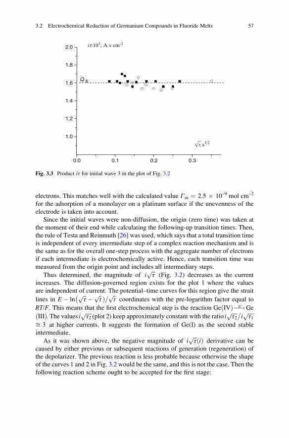
electrons. This matches well with the calculated value Γm ¼ 2.5 � 10–9 mol cm–2

for the adsorption of a monolayer on a platinum surface if the unevenness of the

electrode is taken into account.

Since the initial waves were non-diffusion, the origin (zero time) was taken at

the moment of their end while calculating the following-up transition times. Then,

the rule of Testa and Reinmuth [26] was used, which says that a total transition time

is independent of every intermediate step of a complex reaction mechanism and is

the same as for the overall one-step process with the aggregate number of electrons

if each intermediate is electrochemically active. Hence, each transition time was

measured from the origin point and includes all intermediary steps.

Thus determined, the magnitude of iffiffiffiτp

(Fig. 3.2) decreases as the current

increases. The diffusion-governed region exists for the plot 1 where the values

are independent of current. The potential–time curves for this region give the strait

lines in E� lnffiffiffiτp � ffiffi

tp Þ= ffiffi

tp�

coordinates with the pre-logarithm factor equal to

RT/F. This means that the first electrochemical step is the reaction GeðIVÞ��!e� Ge

ðIIIÞ. The values i ffiffiffiffiτ2p

(plot 2) keep approximately constant with the ratio iffiffiffiffiτ2p

iffiffiffiffiτ1p�

ffi 3 at higher currents. It suggests the formation of Ge(I) as the second stable

intermediate.

As it was shown above, the negative magnitude of iffiffiffiτp ðiÞ derivative can be

caused by either previous or subsequent reactions of generation (regeneration) of

the depolarizer. The previous reaction is less probable because otherwise the shape

of the curves 1 and 2 in Fig. 3.2 would be the same, and this is not the case. Then the

following reaction scheme ought to be accepted for the first stage:

0.0 0.1 0.2 0.3

1.0

1.2

1.4

1.6

1.8

2.0

Q s

it×103, A s cm-2

t, 1/2s

Fig. 3.3 Product iτ for initial wave 3 in the plot of Fig. 3.2


GeðIVÞ��!e� GeðIIIÞ; 2GeðIIIÞ��!k1 ��k2

GeðIVÞ þ GeðIIÞ (3.9)

Fischer and Dracka [20] have considered the theory of such reaction mechanism

and derived the equation for the case of a totally irreversible chemical reaction:

iτ1=2 ¼ C0Fπ1=2D

1=2

IV �3

16

� �1=3

π1=2

D�1=2II D

2=3III F

1=3k�1=31 i2=3 (3.10)

where k1 is the rate constant of Eq. (3.9) and DII, DIII and DIV are the diffusion

coefficients of related species.

Figure 3.4 represents the data of Fig. 3.2 in terms of Eq. (3.10). The larger

parts of these plots are linear, thus evidencing in favour of the chosen reaction

scheme (3.9). The rate constant k1 has been calculated from the slopes of these

lines. For the calculations, the simplification DIV DIII was used and the

value DIV 0.7 � 10–5 cm2 s–1 has been determined from the level parts of

the plots in Fig. 3.2. Eventually, the value of the rate constant was estimated

as k1 ¼ ð1:5� 0:2Þ � 105 mol�1 cm3 s�1 . The equilibrium constant has also

been calculated for this reaction (see Chap. 2, Fig. 2.12).

At the concentrations of Ge(IV) equal to or less than 0.75 � 10–4 mol cm–3, the

formation of Ge(II) intermediate brings about no separate transition time provided

the restriction (3.8) holds true. However, the chronopotentiometric curves of the

second stage of the process are typically S-shaped when being plotted as functions

of the time variable lnffiffiffiffiτ2p � ffiffiffi

t0p Þ= ffiffiffi

t0p�

where the current time is substituted byffiffiffit0p ¼ ffiffi

tp � ffiffiffiffi

τ1p

(see Sect. 2.4.3). This implies the formation of Ge(II) intermediate

with a disproportionation constant larger than 4. The kinetics of the Ge(II) decom-

position reaction manifests itself at higher concentrations (plot 2b in Fig. 3.2).

0.0 0.1 0.2 0.3 0.4 0.5 0.6

1

2

3

4

5

6

7

8

9

10

B

A

cm-2, As102×ti

32

21

22

3 2

3 4

cm,Ai

Fig. 3.4 Fischer–Dracka’s

[20] plots for the first

chronopotentiometric waves

of Ge(IV) cathodic reduction.

Curves A and B correspond to

the data 1a and 1b of Fig. 3.2.


http://dx.doi.org/10.1007/978-3-642-35770-1_2

http://dx.doi.org/10.1007/978-3-642-35770-1_2#Fig000212_2


Considering the data above, the conclusion can be drawn that the general

simplified scheme (1.9) approximates fairly well the mechanism of Ge(IV) dis-

charge in the pure fluoride melt KF–NaF–K2GeF6. The conjugated chemical

reactions other than intervalence ones do not manifest themselves in this case.

The visible pattern of the process changes when oxygen ions are added to the

melt with GeO2 (together with K2GeF6). If the atomic ratio of oxygen to germanium

in the melt is higher than 1.5, two diffusion-governed waves are observed which can

be related to the process GeðIVÞ��!e� GeðIIIÞ��!e� GeðIIÞ: The thermodynamic

stability of a Ge(III) intermediate increases as the relative content of oxygen ions

increases: the equilibrium constant of the reaction GeðIVÞ þ GeðIIÞ! 2GeðIIIÞ isequal to 0.2 � 10–2, 3.5 � 10–2 and 6 � 10–2 at O/Ge ratios 0, 1.55 and 2.0,

accordingly.

If the ratio O/Ge becomes lower than 1.5, the transition time for the first step can

be detected only at higher current values, and the product iffiffiffiτp

becomes current-

dependent with a positive magnitude of iffiffiffiτp ðiÞ derivative (Fig. 3.5). According to

the rule of Sect. 3.1, it could be accounted either for superposition of a surface

process or for inactivation of the depolarizer. The first cause is less probable—the

transition times are too large for a surface process, as, for instance, is in the case

shown in Fig. 3.2 (plot 3).

The process with the inactivation of a depolarizer can be represented by the

general scheme

X ��!el R;Xþ R! Z (3.11)

0.2 0.4 0.6 0.8

0.05

0.10

0.15

1

2

i, A/cm-2

21

cm-2As,ti

Fig. 3.5 Values iffiffiffiτp ðiÞ for the first (1) and second (2) waves of Ge(IV) reduction in

KF–NaF–K2GeF6 molten electrolyte at 750 �C [3]. Total content of Ge is 4.74 � 10–4 mol cm–3;

the ratio GeO2/Getotal ¼ 0.304


where el denotes the electrochemical step of the process. Of course, the mechanism

(3.11) is simplified because the reverse chemical reaction is neglected and the

reaction is not necessarily of the first order relative to X and R species, especially

when an intermediate rather than the initial form of the depolarizer is inactivated.

The mechanism (3.11) was theoretically considered by Dracka and Fischer [12]

for two cases: the surface and bulk inactivation. The problem had been

solved numerically and the results were represented in terms of plots

iffiffiffiτpð Þ i

ffiffiffiffiffiffiτ1p� �� ¼ f ðlgCτÞ where i ffiffiffiffiffiffi

τ1p ¼ lim

i!1i

ffiffiffiτp

and C is the volume concentra-

tion of the depolarizer. The solid lines in Fig. 3.6 show these theoretical

dependencies whereas points correspond to the experimental data of Fig. 3.5,

curve 2. One can see that the points are scattered around the upper theoretical

curve pointing to a heterogeneous reaction of inactivation. Obviously, this process

corresponds to the deposition of LVI, most probably Ge(III), to form the film

electrode system.

A direct experiment was carried out to check this conclusion [3, 22]. Figure 3.7

shows the stationary polarization curve of Ge(IV) reduction on a Ni electrode in

KF–NaF–GeO2–K2GeF6 molten electrolyte at 750 �C together with in situ weight

change of the working electrode taken simultaneously by the method of automatic

electrogravimetry developed in Delimarskii et al. [27].

In terms of Heyrovsky–Il’kovich function, the part OA of the polarization curve

(2), Fig. 3.7, becomes a straight line with “one-electron” slope suggesting the

discharge process GeðIVÞ��!e� GeðIIIÞ: Meanwhile the electrogravimetric curve

(1) comes down, which can be accounted for by “pushing up” the electrode under

applied current due to electromagnetic effect as well as the change of Archimedes

0.0 0.5 1.0 1.5

0.5

0.6

0.7

0.8

0.9

1.0

2

1

5+lgCt

tii t

¥

Fig. 3.6 Theoretical dependencies [12] for catalytic inactivation of the depolarizer at the elec-

trode surface (line 1) and in the bulk of electrolyte (line 2). Points mark the experimental data of

the plot 2 in Fig. 3.5


force. The descending part AB is very similar to a polaropraphic maximum of

fourth kind [28] resulting from a passivating effect of a non-metal phase deposited

onto the electrode surface. The curve (1) shows that the mass of the electrode grows

indeed. The Ohmic part BC points to the passivation of the electrode surface as

well.

Following scheme summarizes the mechanism of the electroreduction of germa-

nium species in molten fluorides:

Ge(IV) Ge(III) Ge(II) Ge(I) Ge(0)

[Ge(III)] solid

ð3:12Þ

where [Ge(III)]solid is the solid LVI that deposits onto the electrode and forms the

Cathode Film System. Dotted lines denote the last chemical and electrochemical

stages, which occur at very negative potentials close to the discharge of the

supporting electrolyte and thus may not appear in a working range of potentials.

3.3 Experimental Study of Many-Electron Kinetics: General

Rules and Recommendations

The study on the electrochemical behaviour of germanium compounds in (oxy)

fluoride melts had been conducted about 30 years ago [2, 3, 22]. Nevertheless,

it still remains the most comprehensive example of “system” research of

C

0.0 0.5 1.0 1.5

0.1

0.2

0.3

0.4

0.5

Dp, m

g

B

A

O2

1

t, min

I, A

-E, V

2 4 6 8 10 12 14 16

-100

-80

-60

-40

-20

0

Fig. 3.7 Polarization (2) and related electrogravimetric (1) curve for the first step of Ge(IV)

cathodic reduction in KF–NaF–GeO2–K2GeF6 melt at 750 �C [3]. Total germanium concentration

1.3 � 10–3 mol cm–3, K2GeF6/Getotal ¼ 0.206

3.3 Experimental Study of Many-Electron Kinetics: General Rules and Recommendations 61

many-electron kinetic mechanism. Further on, we shall consider more recent

examples. Before that, we should like to emphasize some general features and

steps involved in such researches. They are the following:

1. Before non-stationary studies, some information is desirable to be gained about

the intervalence equilibria in the many-electron system under consideration. The

methods discussed in Chap. 2 can be used.

2. Most of the theoretic evaluations for complex reaction mechanisms are devel-

oped for the method of chronopotentiometry. Hence, this method should be

recommended as a primary experimental technique. Of course, the other supple-

mentary methods would be useful.

3. Correct experimental conditions and preliminary evaluations of the data are of

vital importance. The effects of non-kinetic factors—charging of double layer,

non-planarity and finiteness of diffusion—have to be eliminated.

4. The preliminary processing of the experimental data involves the following

steps:

(a) Preliminary determination of transition times. In case of several times inside

each curve, they are measured from zero point of the curve and determined

by the positions of inflecting points (concave down/up) or the relevant

maxima in corresponding differential curves.

(b) Presentation of the data in terms of iffiffiffiτp ðiÞ functions. If the initial wave

happened to occur with a positive magnitude of the derivative, it could be

attributed to some non-diffusion process, slow adsorption or discharge of

surface layer. One can check this hypothesis plotting the data as a function of

iτð ffiffiffiτp Þ. If iτs ¼ const or a sloped straight line with positive intercept iτs on

Y-axis, this proves the surface process taking place and permits to calculate

its characteristics.

(c) In case of the surface process, the subsequent transition times have to be

recalculated by subtracting the initial time from the total time value. After

that, the graphs iffiffiffiτp

vs. (i) are plotted again with the corrected values of the

transition times.

5. After the data are preliminary handled, following routine is appropriate for

further analysis:

(a) The transition times are presented as functions of iffiffiffiτp

vs. (i), the diffusion-controlled regions where the functions keep constant are defined and the

number of electrons for each of such transition time are calculated from the

shapes of related potential–time curves.

(b) The diagnostic criterion discussed in Sect. 3.2 is applied to define a class of

kinetic problem and encompass all possible reaction mechanisms.

(c) An actual reaction mechanism is elaborated with the aid of appropriate theo-

retical scheme available in literature. Taking this way, one can establish the

type of reaction (previous or subsequent) accounting for the partial regenera-

tion of the depolarizer if dði ffiffiffiτp Þ di= ; < 0. Alternatively, if dði ffiffiffi

τp Þ di= > 0, the

surface or bulk inactivation of the depolarizer can be distinguished. It is


http://dx.doi.org/10.1007/978-3-642-35770-1_2

useful to calculate the ratios of limit values of iffiffiffiτp

at large and small

currents—they should be close to ratios of integer numbers for the

accompanying intervalence reactions.

6. After the general mechanism is elaborated as stated above, the final stage has to

be the determination of some quantitative parameters: rate and equilibrium

constants of satellite reactions, diffusion coefficients.

7. Experimental methods other than chronopotentiometry (cyclic voltammetry,

chronoamperometry, electrolysis, non-electrochemical techniques) could use-

fully add to the refinement of final reaction mechanism.

After the early example above, a few studies on the electrochemical behaviour of

polyvalent metals in ionic melts and ionic liquids followed this line. They are

reviewed in the next section and in the Chap. 6.

3.4 Some Data on the Electroreduction Mechanisms

of Polyvalent Species in Ionic Melts

Cathode reduction of Si(IV) species in chloride–fluoride melts was studied in [29].

The general mechanism turned out to be very similar to the case of Ge(IV)

electroreduction. The stepwise process was established with relatively stable Si

(III) and Si(I), and less stable Si(II) intermediates. However, some specialties were

found. In particular, the formation potentials of elementary silicon were unattain-

able being more negative than that for alkali metals of the supporting electrolyte.

Together with the data on the stationary potential of the silicon electrode and

stationary polarization curve (see Chap. 2), the results [29] on non-stationary

kinetics bring about the following general mechanism of cathode process in

KCl–KF–K2SiF6 melt at 700 �C:

[Si(I)]s (film)

Si(IV) Si(III) Si(II) Si(I) Si(0)+K+ K(0)

ð3:13ÞThe species of Si(I) form at the end of the non-stationary cathode reduction.

They deposit onto the electrode surface resulting in the formation of the film.

Elementary silicon can be obtained only at longer times when the electrode film

system with appropriate properties is finally settled down and the solid-phase

reduction mechanism enters its play (see Chaps. 1 and 5). If, by any chance, the

elementary silicon is available in the system, then the intervalence reaction occurs

with K+ ions taking an essential part.

3.4 Some Data on the Electroreduction Mechanisms of Polyvalent Species in. . . 63

http://dx.doi.org/10.1007/978-3-642-35770-1_6

http://dx.doi.org/10.1007/978-3-642-35770-1_2

http://dx.doi.org/10.1007/978-3-642-35770-1_1

http://dx.doi.org/10.1007/978-3-642-35770-1_5

Lately, the electrochemical behaviour of uranium(IV), hafnium(IV) and niobium(V) was investigated in chloride melts by chronopotentiometry and linear sweep

voltammetry (LSV) applying the general approach discussed above [30]. In the

pure chloride melts, the formation of intermediates is even more pronounced than in

fluoride-containing electrolytes, because fluoride ions stabilize the highest oxida-

tion states and thus destabilize the intermediates.

Hence, in KCl–NaCl–UCl4 system, the U(III) oxidation state compound turned

to be the most stable intermediate. Some U(I) species were proved to deposit onto

the electrode before metal formation.

Similar situation arose in the system of HfCl4–NaCl–KCl. Two steps were

recorded at higher concentrations of HfCl4. The plot of iffiffiffiτp ðiÞ had a positive

slope for the first step, and negative for the second step. Only at high current

densities (chronopotentiometry) and at high scan rates (LSV) did the plot indicate

an uncomplicated diffusion process. It was concluded that the adsorption of either

Hf(II) or Hf(I) species caused the inactivation of the intermediates.

In case of the Nb(V) electroreduction in KCI–NaCl–NbCl5 chloride melt at

650 �C, all one-electron steps were resolved and observed at definite conditions.

The deposition of solid intermediates was identified as well.

As follows from the examples given in this chapter, general reaction mechanism

(1.9), though simplified, remains very good approximation for many real processes,

from high-temperature molten salts to, as we can see in Chap. 6, low temperature

ionic melts (ionic liquids). We believe that, to some extent, this approach is also

applicable to the processes in aqueous media.2 However, there are obvious

restrictions due to rather narrow electrochemical window of aqueous systems and

solvatation effects, which would necessitate the consideration of reactions other

than intervalence ones only. Sometimes, the coupled chemical reactions do not

confine exclusively to the IVR even in molten salt systems. One of such examples,

the electroreduction of Si(IV) species in cryolite melts, is considered below.

The impact of slow pre-dissociation was found in the process of electroreduction

of Si(IV) species in Na3AlF6–AlF3–SiO2 melt at 900 �C [31, 32]. Three waves were

found at SiO2 concentrations below ~0.5 wt%, each being governed by

diffusion with iffiffiffiτp ¼ const. The first corresponds to a single two-electron reduction

step SiðIVÞ��!e� SiðIIIÞ��!e� SiðIIÞ with an equilibrium constant of SiðIVÞ þ SiðIIÞ! 2SiðIIIÞ <10–2; then, two resolved one-electron steps SiðIIÞ��!e� SiðIÞ��!e� Sið0Þfollow consecutively. At the experimental conditions applied, the kinetics of

intervalence reactions had no significant impact on the apparent process, thus

evidencing their high reaction rates. The measured magnitudes of Si(IV) diffusion

coefficient happened to decrease as the concentration of silica in the melt increases.

Physically, it could mean the presence of associated species or oligomers, which

decompose as the concentration decreases. Then, one might expect the conditions

where the pre-dissociation kinetics would be detectable. Indeed, this situation is

observed when the SiO2 concentrations become higher than 0.5 wt%.

2 In particular, it follows from early works of Kozin summarized in [35].


http://dx.doi.org/10.1007/978-3-642-35770-1_6

Figure 3.8 exemplifies the situation. Here, the product iffiffiffiτp

keeps constant for the

first two waves attributed to stepwise discharge of Si(IV) species; however, these

waves can be observed only over a narrow range of working currents. The product

iffiffiffiffiτ3p

(last wave) behaves tricky, first rising, then attending maximum and, finally,

descending. The analysis showed that the inactivation of the depolarizer due to the

deposition of Si(II) species is responsible for the ascending part of the graph. The

descending part is caused by slow dissociation of polymerized Si(IV) oxide species,

which proceeds reversibly and shows itself only in a concentration dependence of

the diffusion coefficient at lower concentrations. The scheme below summarizes

the results of these studies:

[SiO2]n Si(IV) ® {Si(III)} ® Si(II) ® Si(I) ® Si(0)

[Si(II)]s

ð3:14Þ

The intervalent reactions proceed reversibly and thus are not shown in the

scheme. Unlike for the case of KCl–KF–K2SiF6 molten system, the Si(III) interme-

diate is least stable in the cryolite-based electrolytes. The Si(II) compounds are

deposited onto the cathode surface to give rise to the complications for the indus-

trial process of electrowinning Al–Si alloys [33].

The pre-dissociation reaction proceeds reversibly at low SiO2 concentrations.

The increase in silica content causes the kinetic retardation of the process. The

overlapping of the both accompanying chemical reactions, pre-dissociation and

inactivation of Si(II), is seen clearly at silica concentration about 0.75 wt%,

Fig. 3.8 Transition times analysis for the process of Si(IV) reduction in cryolite-based melt at

900 �C with 0.75 wt% SiO2. Dashed lines show hypothetical plots for inactivation (deposition) of

Si(II) (A) and pre-dissociation (B) in the scheme (3.14)

3.4 Some Data on the Electroreduction Mechanisms of Polyvalent Species in. . . 65

Fig. 3.8, or higher. The Si(III) intermediates are not traced in the experiment

because of low thermodynamic stability in cryolite media.

A few examples above comprise almost all studies along the line of “system”

approach to the electrochemical kinetics of many-electron processes in the high-

temperature ionic melts. More recent data on the electrochemistry of Ti(IV) in ionic

liquids are considered in Chap. 6.

Anyway, some fundamental problems are still to be overcome for wider appli-

cation of these ideas. They are discussed below.

3.5 Disputable Problems of Many-Electron Kinetics

The transfer of only one electron in any elementary electrochemical step is the core

idea of the developed approach. Like any other fundamental idea, by no means it is

new. As it was said before, it was exploited consistently by Vetter in the 1950s of

the twentieth century [34]. He considered the intermediates of successive chain of

one-electron steps as surface states that neither leave the electrode to pass into the

bulk of electrolyte nor undergo any chemical transformations. Based on these

premises, the two-electron reaction mechanism

Mzþ ��!þ e� ��e� Mðz�1Þþ ��!þe� ��e� Mðz�2Þþ (3.15)

has been considered and general equation of stationary polarization curve has been

derived. These results, especially the particular cases when the rates of separate

reaction stages differ essentially, become classical appearing in any electrochemi-

cal handbook.

The disadvantages of this model are evident—it cannot account for the impact of

the intervalent reactions kinetics to the total electrochemical process. That this

impact is significant and cannot be ignored was substantiated earlier in the works of

Kozin and co-authors summarized in their book [35]. In order to allow for the

contribution of the intermediates, the so-called hetero-staged reaction mechanism

was proposed, in contrast to Vetter’s mechanism defined there as the homo-stagedone [34].

It works as follows. At least one intermediate is presupposed to appear in course

of the overall z-electron process, namely Mm+, where 0 < m < z. If this intermedi-

ate is formed by preceding m-electron electrochemical reaction, then the final

product Mz+ results from the subsequent disproportionation reaction:

M0��!k!; k

�� Mmþ þ me�; zMmþ��!k!1; k 1 �� mMzþ þ ðz� mÞM0 (3.16)


http://dx.doi.org/10.1007/978-3-642-35770-1_6

Alternatively, the mechanism is allowed when the intermediate is formed by a

preceding chemical reaction of reproportionation and then transforms into the final

product by the electrochemical oxidation:

ðz� mÞM0 þ mMzþ! zMmþ; Mmþ! Mzþ þ ðz� mÞe� (3.17)

However incorporating the accompanying reactions with intermediate

compounds, this hetero-staged mechanism is still uncertain, arbitrary and thus

unsatisfactory and “non-system” like. Hence, the next step is obvious—it is the

attempt to develop the systematic approach by synthesis of the two considered

mechanisms.

The first step in this direction has already been made. The results analysed in the

last chapters demonstrate the possibility of non-contradictory systematic descrip-

tion of many-electron systems incorporating the effect of intermediate species.

However, some problems still remain to be overcome on this way. First of all, the

fact of intimate coupling between electrode and intervalent reactions must be

deeply understood.

This coupling, for example, follows immediately from the fact that the potential

differences for separate electrochemical steps are strictly determined by

intervalence equilibrium constants values; see Eq. (2.23). If the whole process is

irreversible,3 then such coupling invokes uncertainty to the determination (even

definition) of the irreversible limiting step.

Let us consider, for example, a stationary non-Nernstian process. Following

qualitative conclusions stems from this consideration:

1. If the IVRs occur reversibly (that is, the equilibrium relationships of 2.2 or 2.3

type are obeyed), this results immediately in the fulfilment of the Nernst

equation for near-electrode space. Then, the irreversibility of an electrode

reaction is not detectable in this case. In other words, the kinetics of an electrode

reactions cannot show itself when the IVRs are reversible. Here lies the answer

on the question why the Vetter’s theory on the kinetics of stepwise electrochem-

ical process was developed for the situation of infinitesimal rates (or absence) of

coupled intervalent reactions. No chemical kinetics—no electrochemicalkinetics!

2. If heterogeneous electrochemical steps are reversible (that is, the Nernst equa-

tion obeyed), then the conditions of chemical equilibrium for any IVR are also

obeyed. Certainly, the IVRs could be irreversible as well. However, this would

not reveal itself in the shape of stationary voltage–current curves bringing about

only the distortions in concentration profiles of the diffusion layers near the

electrode. Then, conversely to the above, no electrochemical kinetics—nochemical kinetics should be true as well.4

3 The term “irreversibility” is used here in the narrow electrochemical sense meaning the deviation

of near-surface concentrations from the equilibrium values when the Nernst’ equation is no longer

valid.4 Naturally, this reasoning is valid for stationary conditions only; the chronopotentiometric

transition times, for example, depend on the rates of IVRs as discussed previously.

3.5 Disputable Problems of Many-Electron Kinetics 67

3. Thus, an electrochemical step could be seen as irreversible if at least one IR in

the system would also proceed irreversibly. On the other hand, however, the

necessary condition for electrochemical irreversibility is the irreversibility of the

chemical IVR; it does not explicitly manifest itself in the stationary response of

the system with irreversible electrochemical steps.

Hence, we came to some apparently paradoxical situation when the kinetics of

IVR in the bulk and electrochemical electron transfer reactions at the interface

happen to be inherently entangled. Then, could one disentangle a pure electrochem-

ical step from the impact of “chemical” electron transfer reaction and study it

separately? So far, this is the question with no clear answer.

References




4. Kisinger PT, Heineman WR (eds) (1996) Laboratory techniques in electroanalytical chemis-

try, Ch 4. Marcel Dekker, New York, NY

5. Friedman A (1968) Equations in partial derivatives of parabolic type. Mir, Moscow

(in Russian)

6. Sand HJS (1901) Philos Mag 1:45–57

7. De-Vries VT (1968) J Electroanal Chem 17:31–38

8. Rodgers RS, Meites L (1968) J Electroanal Chem 16:1–16

9. Herman HB, Tatwawadi SH, Bard AJ (1963) Anal Chem 35:2210–2216

10. Laitinen HA, Chambers LM (1964) Anal Chem 36:5–17

11. Shapoval VI, Reznik GV (1974) On the theory of non-stationary processes of electroreduction

of anions in molten salts (chronopotentiometry). In Ionic melts, vol 2. Naukova Dumka, Kiev,

pp 135–149

12. Dracka O, Fischer O (1974) Coll Czech Chem Commun 39:1970–1979

13. Mamomtov G, Delahay P (1954) J Am Chem Soc 76:5322–5332

14. Filinovskiy VY, Kirianov VA (1964) Doklady Akademii Nauk SSSR (Proc USSR Acad Sci)

156:1412–1416

15. Delahay P, Berzins T (1953) J Am Chem Soc 75:2486–2495

16. Reinmuth WH (1972) J Electroanal Chem 38:95–103

17. Delahay P, Mattax CC, Berzins T (1954) J Am Chem Soc 76:5319–5331

18. Fischer O, Dracka O, Fischerova E (1961) Coll Czech Chem Commun 26:1505–1512

19. Fischer O, Dracka O, Fischerova E (1960) Coll Czech Chem Commun 25:323–330

20. Fischer O, Dracka O (1959) Coll Czech Chem Commun 24:3046–3052

21. Galus Z (1994) Fundamentals of electrochemical analysis, 2nd edn. Wiley, New York, NY


oxyfluoride melts. In: Physical chemistry of ionic melts and solid electrolytes. Naukova

Dumka, Kiev

23. Bard A (1963) Anal Chem 35:340–349

24. Baraboshkin AN, Vinogradov-Zhabrov ON (1970) Trudy Instituta Elektrokhimii UF AN

SSSR (Trans Ural Inst Electrochem USSR Acad Sci) 15:126–130

25. Tatwawadi SA, Bard AJ (1964) Anal Chem 36:5–14

26. Testa AC, Reinmuth WH (1961) Anal Chem 33:1320–1328



28. Delimarskii YK, Tumanova NK, Shilina GV, Barchuk LP (1978) Polarography of ionic melts.

Naukova Dumka, Kiev (in Russian)

29. Boiko OI, Delimarskii YK, Chernov RV (1985) Ukrainian Chem J 51:385–390

30. Boiko O, Serrano K, Chamelot P, Taxil P (2000) High Temp Mater Process 4:441–450

31. Delimarskiy YK, Prutskov DV, Andriiko AA, Tchernov RV (1983) Ukrainian Chem

J 49:738–743

32. Prutskov DV, Andriiko AA, Delimarskiy YK, Tchernov RV (1986) Ukrainian Chem

J 51:826–833

33. Prutskov DV, Andriiko AA, Tchernov RV (1987) Tsvetnyje Metally (Non-Ferrous Metals)

2:39–42

34. Vetter K (1961) Electrochemical kinetics. Springer, Heidelberg

35. Kozin LF (1989) Electrodeposition and dissolution of polyvalent metals. Naukova

Dumka, Kiev

References 69

Chapter 4

Electrode Film Systems: Experimental

Evidences

What is a good experiment? This is the experiment whichgives us something more than a separate fact; this is theexperiment, which permits us to foresee; that is, the onewhich leads to generalisations.

H. Poincare

This chapter analyses some experimental examples, demonstrating qualitatively the

concept of electrode film system (EFS). The discussion is based on the classification

of EFS considered in Chap. 1.

4.1 Ion–Metal Film Systems in Processes of Electrodeposition

and Electrorefinement of Polyvalent Metals

The film system on metal electrodes in ionic melts often belongs to the ion–metal

type. This is consistent with the general model of polyvalent conductor, which

predicts the degeneration of semiconductor conductivity into metal one at higher

temperatures [1, 2].

Qualitatively, the mechanism of the processes when the current passes in the

cathode direction is depicted in Fig. 4.1.

The Faradaic process at the outer boundary corresponds to the partial reduction

of the species with higher oxidation state to the lower valence intermediates (LVI).

This process results in the deposition of a film and growth of the film with the rate

being proportional to the electronic part of the total current.

The ionic component of the conductivity brings about the Faradaic process at the

inner boundary of the film. It invokes further reduction of the film compounds—

actually, to the phase with pure electronic conductivity. The rate of this process is

proportional to the ionic current passing through the film.


71

http://dx.doi.org/10.1007/978-3-642-35770-1_1

The prevailing type of charge carriers in the film should affect considerably the

apparent character of the inner electrochemical process. Should these carriers be

alkali metal cations, their discharge at the inner boundary would be preferable.

Thus, the formation of alkali metal is expected to be the side process in such

systems resulting in the low current efficiency of the targeted process of the

reduction of a polyvalent metal species. Evidently, that accounts for higher current

efficiency of elementary silicon electrodeposition from potassium halide baths

relatively to the electrolytes based on sodium halides.

Presumably an anionic nature of ionic conductivity is favourable for the

electroreduction of a polyvalent metal species in a film system. If the movable

anions are liberated at the inner interface due to the Faradaic process there, this

process is to be the further reduction of the compounds forming the film—actually,

to the metallic phase with electronic conductivity—because the liberated anions

can leave the reaction zone with the ionic current passing across the film. This is the

main reason why fluoride-containing electrolytes are so widespread, especially in

e- e- e-E(N) E(N-1) ..... E(i)¾¾® ¾¾® ¾¾®

solidE(i) E(0)ie--++ ¾¾¾®

CATHODE FILM ELECTROLYTE

CATHODE

ELECTROLYTE

ELECTROLYTE

FILMCATHODE

ieliel

iion

iion

eM

Fig. 4.1 Film system at a cathode. The distribution of ionic and electronic current components is

shown schematically below

72 4 Electrode Film Systems: Experimental Evidences

molten salt electrochemistry—the small fluoride anions are good carriers for the

charge removing outside the surface film.

Figure 4.1 gives a formal idea about the system’s behaviour in such case. There

the rate of the inner electrochemical process is proportional to the ionic current.

This process results in metallization of the film. The dynamics of the overall process

depends, first of all, on the relative rates of the inner and outer processes. In turn,

these rates are the functions of the part of the electronic conductivity of the film.

When this part is large (near 1), then the compounds forming the film have to be the

only final product of the electrolysis. The examples can be the electrolysis of

oxide–fluoride melts containing Ti [3] or Nb [4] species, or electrodeposition of

tungsten bronzes from oxide melts [5].

If the ionic conductivity is low but no longer negligible (roughly, the part of

electronic conductivity is more than 0.5), the cathode deposit should consist of two

layers: a thick outer one including LVIs and a thin inner one including pure metal.

Such situation can be observed when some species are added to the bath increasing

the electronic conductivity of the film, as it happens when copper compounds are

added to the electrolyte for silicon deposition [6].

In principle, a system with several inner boundaries is possible enclosing the

layers with different oxidation states and, thus, with different electronic-to-ionic

conductivity ratios. This hypothetic possibility has been discussed by Vas’ko and

Kovach [7].

For such a “polysurface” system to exist, the drop in electronic conductivity at

each inner interface must be less than the drop at the neighbouring interface (closer

to the electrolyte). However, the calculations showed that such situation could not

be stable dynamically on sufficiently large timescales. We have so far no distinct

evidence for the formation of such deposits, neither in molten nor in aqueous

electrolytes.

The outlined pattern is especially important for molten fluoride systems where

the transport properties of the mobile F– ions determine the conductivity. Let us

consider some qualitative details of the dynamics in such systems.

If the part of ionic conductivity is more than i/N (i is the oxidation state of LVI inthe film and N is the oxidation state of initial species in the bulk of the electrolyte),

the behaviour of the electrochemical film system should not be stable, as it is in the

case of the non-stationary chemical systems considered in Chap. 1. In particular, it

could not grow steadily with layers separated by the interface, because the rate of

metallization should be higher than the rate of growth at the outer boundary. Then

the stages depicted in Fig. 4.1 should alternate: after the sufficient accumulation of

LVIs near the electrode, fast precipitation follows, the film thickness increases, and

then the metallization of the film goes on till the electronic conductive phase

“pricks” the film and enters the surface forming electronic contact to the electrode

base material. After that, the discharge to the LVI takes place again, the new portion

of the film precipitates, and so on.

The question arises whether these alternating stages can be synchronized in time

in the whole electrode surface. Certain experimental data show that they really can(see below). An “oscillatory” deposition occurs then: the macroscopic parameters,

4.1 Ion–Metal Film Systems in Processes of Electrodeposition and. . . 73

http://dx.doi.org/10.1007/978-3-642-35770-1_1

like current and/or potential and the mass of the deposit, are oscillating around

some averaged trend.

Other data demonstrate the dendritic (not smooth) movement of the inner

boundary during the metallization of the film. Thus, the needles of dendrites pierce

through the film before the metallization is completed, and then the deposit contains

some amount of a non-metal phase together with the crystals of the metal product.

After cooling down the deposit to the ambient temperature, the partly reduced

constituent of the deposit (that is, LVI) often can be disproportionate, giving very

fine metal powder dispersed between the larger primary crystals of the metal in the

final product.

The above-considered pattern provides satisfactory explanation for the mecha-

nism of formation of metal–salt cathode deposits, so-called “pears” in Russian or

“carrots” in Western literature. Such deposits are very common if the electrolysis is

carried out at temperatures below the melting point of a deposited metal. A number

of examples can be found in the processes of electrodeposition of refractory and

other polyvalent metals (Nb, Ta, Ti, Si, B and others) in fluoride-containing molten

salt electrolytes.

Such electrodeposition process had been widely investigated for

electroreduction of germanium species in molten KF–NaF–K2GeF6–GeO2 electro-

lyte [8]. One of the most interesting information has been obtained with the

automatic balance experimental technique permitting to record the weight of the

electrode in situ in course of the electrolysis [9].

Figure 4.2 shows typical electrogravimetric curves related to the kinetics of

germanium electrodeposition in galvanostatic conditions. These curves include the

initial section when the weight remains almost unchanged for a few minutes.

Obviously, this inductive time period is required for the accumulation of LVIs at

the near-electrode area. After that the weight begins to rise with the rate higher than

it is necessary for the deposition of pure germanium. This fact evidences for the co-

deposition of non-metal phase as it was considered above.

The initial period of the FS formation had also been detected when the electrogra-

vimetric and polarization curves were taken simultaneously (see Fig. 3.7). These

data show the onset of deposition only after the maximum current is achieved in the

polarization curve. The curve shows such maximum because of increasing ohmic

resistance due to the formation of the film on the electrode; that is the reason of the

decrease of the limiting current of the reduction process GeðIVÞ!e� GeðIIIÞ.The predicted oscillatory behaviour has been found for the potentiostatic regime

of the process. Figure 4.3 shows such example when the weight of the cathode,

rising in total, exhibits clearly distinct local oscillations.

Microscopic investigations of the germanium powder samples after washing out

the salt components from the cathode deposit reveal two different kinds of crystals:

large germaniumdendrites and very fine particles.According to the abovemechanism,

the first can be considered as a primary electrocrystallization product, while the second

is a product of a secondary disproportionation of film’s LVI.



Such “two-phase” composition was also found for silicon powder electrolyti-

cally produced by the method described in [10] from molten salt electrolyte

KF–KCl–K2SiF6 with addition of silica. It is clearly seen from the plot in Fig. 4.4

representing a histogram size distribution curve obtained from the mesh analysis of

a pilot-scale batch of electrolytically produced silicon.

Thus, the proposed mechanism of the processes in the ion–metal FS is in good

qualitative agreement with most essential experimental facts related to the cathodicdeposition of polyvalent metals. Let us consider now the behaviour of such system

in case of a reversed (anode) direction of the applied current. This problem is

important, in particular, for the electrolytic refinement of polyvalent metals in

molten electrolytes.

Fig. 4.2 Weight (including Archimedean force) of the cathode with the deposit vs. time in course

of germanium electrodeposition from KF–NaF–K2GeF6–GeO2 melts at 750 �C in galvanostatic

conditions. Dashed straight line corresponds to the deposition of pure germanium with 100 %

Faradaic efficiency [8]. The numbers indicate the ratio of GeO2 to K2GeF6 in the electrolyte


The anodic current in the ion–metal FS brings about the oxidation of the metal to

LVI at the inner boundary. These LVIs have to be oxidized at the outer boundary,

passing finally to the electrolyte in form of species with higher oxidation states.

This is the most general pattern for anodic dissolution of a polyvalent metal. Having

this in mind, following phenomena have to be expected in course of long-time

electrolysis.

If the ionic conductivity is low, the rate of film’s dissolution should be higher

than the rate of its formation. Thus, the film should eventually disappear and the

dissolution occurs with no complications.

Fig. 4.3 Kinetics of potentiostatic electrodeposition of germanium from the oxyfluoride melt

0.0 0.2 0.4 0.6

0.1

0.2

0.3

0.4

0.5

0.6

d, mm

mm-1,1m Dd

Dm

Fig. 4.4 Size distribution plot for the powder of electrolytically produced silicon,

KF–KCl–K2SiF6 (+SiO2) bath, 720�C


On the contrary, when the ionic conductivity is higher than the electronic one,

the film should grow continuously. Then, after sufficiently long time of electrolysis,

the complications are inevitable due to the accumulation of non-metal phases at the

anode.

That is, the expected behaviour of an anodic FS with low ionic (high electronic)

conductivity has to be similar to a cathodic FS with low electronic (high ionic)

conductivity. This consideration leads to a rather pessimistic conclusion: practical

employment of electrorefining process of a polyvalent metal in a long-time scale

should appear to be a hard task if the FS would possibly form both at the cathode

and at the anode.

In terms of the developed ideas, the possible complications are caused by the fact that

the conditions for successful cathode and appropriate anode processes are mutually

incompatible: high ionic conductivity is required for the efficient cathode deposition,

whereas high electronic conductivity is necessary for easy anode dissolution.1

Generally, we can apprehend certain peculiarities of continuous long-term

electrorefining process, which do not follow and cannot be predicted from the

short-term laboratory experiments. In other words, the success of such experiments

does not guarantee the success of the large-scale process.

That was true, for example, for the process of metallurgical silicon electrorefining

in aKCl–KF–K2SiF6melt at 750 �C. A number of short-term laboratory experiments

had been carried out, excellent results were obtained and a patent had been filed [11].

Nevertheless, an attempt to reproduce these results in a large-scale process (pilot

electrolyser with 500 A current load) was unsuccessful. The problems arose after

operation for approximately 24 h. They manifested themselves in increasing the cell

voltage, the electrolyte temperature and a drop in current efficiency. This ultimately

led to technological failure and termination of the process. The cause was established

to be the non-predicted slag accumulation in the anode area.

In contrast to the silicon process, durable electrorefining of Nb and Ta was more

successful. The processes were performed in the molten mixture KCl–NaCl–K2NbF7(K2TaF7) at 720 � 10 �C in course of 1 or 2 weeks. Two different types of

electrolysers were used, i.e., laboratory type and pilot plant cells, enabling operating

currents up to 50 and 300 A, respectively. The techniques, other conditions and results

of the experiments were described in detail in [12].

As followed from the available literature on the electrorefining of Nb and Ta, the

numerous data on current efficiency, purity and other parameters differed signifi-

cantly in the works of different authors. The reason was established to be very poor

reproducibility of the common short-term laboratory experiment results. Some

parameters of the process (e.g., current efficiency) varied significantly, especially

if the electrolyte was repeatedly used in several electrolyses.

1 The same reasoning will be valid when considering the operation of rechargeable electrode in a

battery. If the FS is formed at its surface, the film must have mostly ionic conductivity during the

“cathodic” part of its life (the discharge for a positive electrode and charge for a negative one),

while prevailing electronic conductivity is required to behave as anode at the reversed current.

Obviously, that is why numerous attempts to make a lithium metal electrode rechargeable failed.


That this irreproducibility is not a consequence of experimental errors but an effect

of the inner property of the system was discovered in course of long-term continuous

processes. Here, after some quantity of charge passed, each portion of the deposit was

quantitatively removed from the cathode and weighed. Such obtained yields of the

product per unit charge were also scattered significantly. However, this scattering was

found to obey an amazing order when plotted against total time of the electrolysis

(or total charge passed): the cathode current efficiency oscillated about a mean value.

Figure 4.5 shows this unusual regularity for pilot-scale process of Nb electro-

refining. Similar pattern is observed for continuous electrolysis in the laboratory cell

(Fig. 4.6). One can see that, though the amplitudes of the oscillations may differ

significantly, the period remains constant with good precision.

Some parameters of the electrorefining of Nb and Ta in long-term electrolyse

processes are presented in Table 4.1.

The theory of the observed phenomena was developed later. It is based on the

above-considered ideas upon electrochemical FS and bifurcation analysis. These

results will be further discussed in Chap. 5.

We are finishing now the consideration of ion–metal FS in molten electrolytes.

In conclusion, one important circumstance has to be borne in mind.

In some cases, e.g., at the electrochemical reduction of silicon species, the

potential of final stage (formation of a metal) turns out to be more negative than

the potential of the alkali metal formation (see Chap. 3). Similar situation seems to be

true for a number of other polyvalent metals. For example, the reaction of zirconium

metal with fluoride melts is known [13] where the potassium metal is a product.

In such kind of systems, the winning of a pure metal is only possible by means of

a solid-phase reduction mechanism, in a FS with a high ionic conductivity. More-

over, not just ionic but predominantly anionic conductivity is required. Otherwise,

the cations of the alkali metals would migrate through the film to the inner interface

Fig. 4.5 Yield of Nb cathode deposits in a pilot-scale cell [12]. Operating current 120 A


http://dx.doi.org/10.1007/978-3-642-35770-1_5

http://dx.doi.org/10.1007/978-3-642-35770-1_3

discharging there to form an alkali metal. Obviously, such situation took place in

the attempts to obtain elementary silicon from oxide melts—alkali metal was the

main product there [14].

As it was already mentioned before, high anionic conductivity can most easily be

achieved in fluoride-containing electrolytes, with mobile F– ions as current carriers.

This accounts for the widespread employment of fluoride-based electrolytes in

applied electrochemistry of polyvalent metals. However, sometimes the condition

of prevailing anionic conductivity is not satisfied even in fluoride-containing

systems. For example, current efficiency of silicon deposition drops considerably

if cations become to contribute to the ionic conductivity. It happens when sodium

Fig. 4.6 Periodic changes of charge efficiency in long-term laboratory electrorefining of Nb and

Ta at the constant current 20 A (Ta) and 29 A (Nb)

Table 4.1 Experimental parameters and results of long-term experiments on the electrorefining of

Nb and Ta in long-term continuous process, electrolyte KCl–NaCl–K2NbF7 (K2TaF7),

720 � 10 �C

Process

Current

Current density

(A cm–2)

ηav (%)a Me (wt%)b

Period T of the

oscillations TS/Vc

A Cathode Anode Ah h 103 s cm–1

Nb, Lab 29 � 1 0.60 0.95 32.3 36.0 258 � 11 8.9 1.48 � 0.11

Nb, Pilot 120 � 10 1.20 0.60 42.3 32.0 1,262 � 49 10.4 1.51 � 0.18

Ta, Lab 20 0.50 0.64 26.5 40.0 239 � 19 12.0 3.34 � 0.25aAverage current efficiency calculated for the process EðVÞ þ 5e� ! Eð0Þ from the total charge

passed for the whole run of the electrolysisbMean content of metal in the cathode depositcS is the mean geometric area of the electrodes (

ffiffiffiffiffiffiffiffiffiffiffiffiffiffiffiffiffiffiffiffiScathSanode

p), and V is the volume of the

electrolyte. This number relates to some fundamental properties of the dynamic system (see

Chap. 5)


http://dx.doi.org/10.1007/978-3-642-35770-1_5

or, especially, lithium salts are used as bath components. The liberation of alkali

metal is then the main side process.2

Alkali metal is a main product if the electrolysis is performed of the solutions of

silica in molten fluorides with no additives of complex silicon fluorides [15].

Though the solubility of silica in such melts is high enough, it seems that the film

with high anionic conductivity could form only in “acidic” melts, where the ratio

O/Si is much <2.

We have seen that the idea of an electrode film system is useful for electrochem-

istry of molten salts including low-temperature ionic liquids. It is not restricted,

however, to this field only. As an example, the protective layer on lithium metal in

aprotic organic electrolytes could be mentioned. This layer, so-called “solid elec-

trolyte interphase” (SEI), exhibits properties of a polyfunctional conductor with

high ionic conductivity (Li ions are the carriers) and low electronic conductivity of

semiconductive nature. Some peculiarities of film systems with semiconductive

character of electronic conductivity are considered below.

4.2 Ion–Semiconductor Film Systems

According to Velikanov [1], the exponential growth of conductivity with temperature

is the main feature of a semiconductive PFC. Taking the film system as a whole, we

can recognize two other distinctions.

Firstly, the polarization characteristics should depend not only on the properties

of the system, but also on the electrode material. This follows from the non-linearity

of the metal–semiconductor junction, which is dependent on the work function of

electrons, and thus, on the nature of the electrode material [16].

Secondly, the electrode FS should exhibit the rectifying effect caused by the

potential barrier of the forbidden energy band of the semiconductor. Qualitatively,

if this band is sufficiently wide, the electrons penetrating the film can reduce not

only the depolarizer near the Fermi level, but also compounds of the supporting

electrolyte. This is a typical situation in aqueous electrolytes where large amount of

charge is usually spent for the reduction of protons or protonated species with

generation of hydrogen.

It seems likely that such ion–semiconductor systems are rare in ionic melts due

to the degeneracy of the semiconductor at high temperatures. However, some data

evidence their formation at some peculiar conditions in course of Si metal deposi-

tion out of a KF–KCl–K2SiF6 melt. It was shown [17] that the initial parts of

polarization curves contained the non-diffusion waves similar to that observed for

germanium systems (see Chap. 3) on a platinum electrode. The same “surface”

waves were detected on Ag and Au electrodes as well, thus suggesting the reduction

2 This manifests itself in characteristic sparks and flames on the surface of the electrolyte when the

process is conducted in the ambient atmosphere or in intensive evolution of hydrogen when the

cooled cathode deposit is placed into water.


http://dx.doi.org/10.1007/978-3-642-35770-1_3

of chemisorbed layers of a depolarizer rather than a reaction of oxide layer of the

cathode material.

Additionally, these layers (or the products of its reduction) turned to acquire the

barrier effect. Their conductivity rose sharply at the potentials close to the discharge

potential of alkali metal (positive by 0.2–0.4 V). This results in “cut-off” of the

initial parts of discharge stepwise diffusion waves in polarization curves, e.g., at a

potential �1.5 V vs. quasi-reference Pt electrode in case of Au in KCl–KF–K2SiF6melt (Fig. 4.7).

In this case, the barrier properties of electrode–electrolyte interface together

with the effect of electrode material can be considered as evidence for the formation

of ion–semiconductor FS with low ionic conductivity.

4.3 Dielectric Film Systems

If the gap in the forbidden band of the semiconductor film is wide enough and

exceeds the decomposition voltage of the supporting electrolyte, the film substance

would behave as a pure ionic conductor—superionic conductor, if the ion conduc-

tivity were high.

The situation should then be favourable if the ion electric carriers would take

part in the Faradaic process at the inner boundary inside the film. The ions could

pass across the film discharging at the metal/film interface or, vice versa, liberating

in the Faradaic process at this interface, and passing through the film into the bulk of

the electrolyte. The processes at the negative electrode of a lithium battery (Li metal

or Li/C intercalate compound) could be an example of such situation.

Fig. 4.7 Voltammetric curves for Si(IV) discharge in a KCl–KF–K2SiF6 melt on platinum and

gold cathodes [17]

4.3 Dielectric Film Systems 81

Otherwise, if the ionic carriers are electrochemically inactive or the ionic conduc-

tivity is very small, the FS would acquire qualitatively new properties becoming a

dielectric, or insulating one. Some harmful phenomena, such as crisis (or blockade in

terms of [18]), are indicative for such systems. They manifest themselves in sharp rise

in voltage (galvanostatic regime) or drop in current (potentiostatic regime). That is, the

electric resistance of a system tends to increase sharply when the dielectric electrode

FS begins to develop. This brings typically the increase of temperature, spark, glow or

arc discharge at the electrode, deterioration of wettability of an electrode surface, etc.

Such phenomena result from blocking of a surface by a dielectric film where an

appreciable current can be achieved only in conditions of a dielectric breakdown.

The so-called “anode effect” on carbon electrodes in fluoride-containing melts is

probably the most vivid manifestation of a dielectric FS. This phenomenon was first

related to the industrial electrolysis of aluminium in Hall–Heroult cells and, thus, is

widely known for more than a 100 years. Nevertheless, a generally acknowledged

theory is not achieved yet. Several possible causes have been considered: non-

wettability of the electrode surface, electrostatic repulsion of the bubbles of the gas

evolved at the anode, hydrodynamic crisis of the gas evolution and, finally, the

formation of a fluorocarbon dielectric film [18–20]. This latter explanation had been

developed since then, mainly by Japanese researchers, relatively to the electrochemi-

cal production of fluorine [21]. A fluorocarbon film is now widely recognized as a

cause of the anode effect both in fluoride and inmixed fluoride-containing electrolytes.

In particular, the formation of a blocking film was found to be responsible for the

anode effect in mixed chloride–fluoride melts like MCl–MF–M2SiF6 [22]. The

kinetics of gas evolution at the anode and its quantitative composition have been

studied in [23]. In addition, the impact of natural hydrocarbon gas on the properties

of the electrode under the anode effect was investigated [24].

Relatively to a KCl–KF–K2SiF6 melt as an electrolyte, following basic facts

have been established.

Even a small content of oxides (<1 %) in the electrolyte results in formation of

carbon mono- and dioxide as main anode products. After the oxide ions are worked

out, the anode gas consists of chlorofluorocarbons of methane series (CF4, CF3Cl

and CF2Cl2) with small admixtures of ethane and ethylene derivatives. The evolu-

tion of chlorine gas was not observed in a wide range of melt composition and other

experimental conditions. Presumably, the current densities required for the chlorine

evolution are higher than the critical values for the onset of the anode effect and,

thus, cannot be attained.

The anode reactions include the stages of joint Cl– and F– discharge, formation

of a solid chlorofluorocarbon (CFxCly)s on the anode surface and decomposition of

this surface compound with liberation of gaseous chlorofluorocarbons:

Cþ xF� þ yCl� ! ðCFxClyÞs þ ðxþ yÞe�ðCFxClyÞs !k CFnClm " þC

(4.1)


The experimental results on the kinetics of the gas evolution supported this

mechanism [23]. According to the reactions (4.1), the theoretical time dependency

of the volume of the evolved gas can be written as

V ¼ EVI

Ft� EVI

kFð1� e�ktÞ (4.2)

where EV is the volumetric electrochemical equivalent, I is the current and k is therate constant of the chemical reaction (4.1). Taking the time t sufficiently long, we

can neglect the exponential term. This results in the equation of a straight line,

which does not pass through the origin of coordinate system:

V ¼ EVI

Ft� 1

k

� �(4.3)

Indeed, the experimental plots V(t) obey such regularity (see Fig. 4.8 as an

example). The lines intercept the values of t0 ¼ 1/k on the time axis, which are,

first, practically independent of current and, second, decay exponentially with

rising temperature (see Fig. 4.9). Such experimental findings are consistent with

the film formation mechanism.

The activation energy calculated from the plots like in Fig. 4.9, 66 kJ mol–1, is in

good agreement with reference data [25] on the activation energy of thermal

decomposition of fluorinated graphite, 44–61 kJ mol–1.

The stationary state in the accepted model is established in course of “normal”

electrolysis with the surface being partly free and partly occupied by the solid

carbon halides. The occupied part of the surface is proportional to the applied

Fig. 4.8 Initial parts of time dependencies for the volume of gas liberated on a graphite anode at

the electrolysis of a KCl–KF–K2SiF6 melt in galvanostatic conditions for two different current

values; temperature 700 �C [22]


current density. At some critical value of the current density, the solid film covers

the whole surface and the anode effect sets on.

A response of the blocking film upon the exposure to a natural hydrocarbon gas

was investigated in [24]. The diagram in Fig. 4.10 shows the changes in the total

resistance of the cell before (OA) and after (AB) the input of the hydrocarbon gas

on the electrode. The resistance is rising gradually as the anode effect is developing

in time and the gas is off. After the gas is on (point A), the resistance is quickly

diminishing and, after about an hour, normal conditions of the electrolysis are

recovered. As a result, the critical value of current density becomes essentially

higher and the anode is no longer consumed because of the oxidation of gaseous

hydrocarbons rather than anode material.

The products of this process have been identified by gas chromatography and IR-

spectroscopy. Most remarkably, only fluorinated derivatives were found among the

gaseous products. The chlorine was bound with hydrogen and evolved from the

melt in form of HCl gas.

Following reactions have been suggested for the anode oxidation of the gaseous

hydrocarbons in KCl–KF–K2SiF6 melt on the surface of a graphite anode:

CnH2nþ2 þ CðgraphiteÞ ! ðCxHyÞsolidðCxHyÞsolid þ mF� ! ðCxHy�mFmÞsolid þ mHþ þ 2me�

Hþ þ Cl� ! HCl�

ðCxHy�mFmÞsolid ! CnHy�mFm þ ðx� nÞC

ðchemosorptionÞðanode oxidationÞðneutralizationÞðdecompositionÞ

(4.4)

The behaviour of carbon anodes in molten salts media at the conditions of

“normal” electrolysis, being a subject of numerous research works, is understood

in general. As for the regime of developed anode effect, the mechanism and

dynamics of the processes are much less clear. Only a few works related to cryolite

103,K-1*1T

Fig. 4.9 Temperature dependenceof theparameter t0,min (Fig. 4.8) ofEq. (4.3) inArrhenius coordinates


melts can be mentioned.3 Some current–potential diagrams were obtained there

with sharp current oscillations and very poor reproducibility.

The first complex study of the anode effect dynamics appeared in 1990 [27]. The

ideas of dielectric FS and some mathematics of the bifurcation theory were used in

this work. We shall consider the results of this study in the next chapter. The end of

this section is devoted to some evidence for cathodic dielectric FS.One of the examples, the so-called “cathode effect” in Al electrolysis, has been

reported in 1966 [28]. This typical blockade phenomenon occurs at Al cathode at

very high current densities of about tens A cm–2. This effect shows itself in sharp

increase of ohmic resistance at the cathode followed by arc or glow discharge. The

early explanation suggested the formation of a layer of gaseous sodium. In our

opinion, formation of dielectric solid film accounts better for this phenomenon.

The formation of a FS with distinct dielectric properties have been found in a

system of liquid Al–cryolite melt with additions of silica. This system has been

investigated in a series of works [28–31]. Followingmechanism has been suggested:

Si(Al)Si(II)Si(IV))(SiO Al2SAl1s2 ¾¾ ®¾¾¾ ®¾®

4s[Si(II)]

3 ð4:5Þ

After the silica is dissolved in the melt, fast bulk reaction 1 occurs, where the initial Si

(IV) is reduced to the Si(II) intermediate species. The metal aluminium dissolved in the

melt4 acts there as a reductant. Further on, the heterogeneous reaction 2 s takes place at the

Fig. 4.10 Change in total resistance of the electrolysis cell [24]. The gas flow is on at the time

moment, which corresponds to the point A

3 See, for example, a relatively recent paper [26] and references therein.4 The nature of the dissolved aluminum is still a subject of discussion; intermediate Al(I) and

individual Al in form of so-called “metal fog” concepts are in use. Both hypotheses are equally

acceptable for the mechanism (4.5).


melt/liquid aluminium interface, resulting in the formation of a liquid Si–Al alloy. This

reaction is described in terms of the electrochemical corrosion theorywith two conjugated

processes: cathodic reduction of silicon (II) and anodic dissolution of aluminium. The rate

of cathode half-process is restricted by the limiting diffusion current of silicon species; at

900 �C it corresponds to the rate of silicon reduction [in g(Si) cm–2 h]W2 ¼ 3:0� 10�2

CSiO2, where CSiO2

is the concentration of silicon in the melt recalculated on wt% SiO2.

The solubility of the intermediate Si(II) is rather low, corresponding to about 0.6 wt%

SiO2. In normal course of the process, the stationary concentration of silicon in themelt is

lower than this value and is determined by the rate of supply of the silica to the bath.When

this rate would allow being higher than some critical value, the intermediate should

deposit onto the surface forming the blockingfilm.The process 2 thenwould be hampered

and silicon should have to pass into the aluminium through slow reaction 4 between solid

substance and liquid aluminium (W4 ¼ 0.76 � 10–2 g(Si) cm–2 h).

It is worthwhile to note that the developed mechanism became a basis for novel

process of Al–Si alloys production in industrial Al cells by controlled introduction

of silica into the electrolyte [32, 33]. This process was known since the 1930s of the

last century [34, 35]; however, numerous attempts of its practical implementation

were unsuccessful. Inevitably, the complications arose that accompanied with

growth of temperature, evaporation of the electrolyte and losses of fluorides from

the bath, slag accumulation. Ultimately, this situation, which was called the “hot

run” of the cell, led to the full disorder and termination of the process.

The above mechanism was able to explain easily the cause and give the means to

avoid this “hot run”. It is clear that silicon can be consumed by the liquid alloy with

the rate less than or equal to the rate of the reaction (4.2). This maximum possible

rate is equal to about 2 � 10–2 g cm–2 h. This number determines the upper possible

rate of silica input into the bath that must not be exceeded to avoid the “hot run”.

Also it is clear that the upper limit exists for the concentration of silicon in the

product alloy. For a particular cell, it can be estimated from the formula:

CmaxSi ¼ iSiESi

icEAl � iSiðEAl � ESiÞ (4.6)

where ESi ¼ 7; EAl ¼ 9 are the electrochemical equivalents of silicon and alumin-

ium; ic is the total cathode current density. According to the above, the maximum

current of silicon is iSi ffi 0.07–0.08 A cm–2. In most types of industrial cells the

total cathode current density is about ic ffi 0.5–0.7 A cm–2. This gives the estimation

for maximum concentration of electrochemical Al–Si alloy CmaxSi � 9� 12 wt% .

Such alloy can be obtained without technological complications using rigorous

monitoring of the flow of silica into the cell.

Before finishing this chapter, let us stop now and take a brief look back. There we

can see many complicated experimental phenomena that have got the classification

and explanation in the framework of the electrode FS ideas—alas, so far only

qualitatively! Remember that we are now very far from simple equilibrium situation;

everything is blurred and uncertain here; each phenomenon does not easily give up to

a quantitative theory. However, some hopes still remain—the bifurcation theory as a


method for investigation of the dynamic behaviour of non-equilibrium systems. We

shall try this approach in the final Chap. 5.

References

1. Velikanov AA (1974) Electronic-ionic conductivity of non-metal melts. In: Delimarskii

YuK (ed) Ionic melts, vol 2. Naukova Dumka, Kiev, pp 146–178

2. Mott NF, Davis EA (1979) Electronic processes in non-crystalline materials. Clarendon Press,

Oxford

3. Reznichenko VA, Ustinov VS, Kariazin NA, Khalimov FB (1983) Chemical technology of

titanium. Nauka, Moscow

4. Konstantinov VI (1977) Electrolytic production of tantalum, niobium and its alloys.

Metallurgia, Moscow

5. Spitsyn VN, Drobashova TM, Kazanskiy AN (1983) On the alkali tungsten bronzes obtained

by electrolysis of molten isopolytungstanates. In: Mokhosoev MV (ed) Chemistry of Mo(VI)

and W(VI) compounds. Nauka, Novosibirsk

6. Tchernov RV, Boiko OI, Diubova LD et al. (1983) Method for production of silicon. USSR

Patent 1085293, 29 March 1983.

7. Vas’ko AT, Kovach SK (1983) Electrochemistry of refractory metals. Tekhnika, Kiev


oxyfluoride melts. In: Delimarskii YuK (ed) Physical chemistry of ionic melts and solid

electrolytes. Naukova Dumka, Kiev, pp 6–60


10. Boiko OI, Andriiko AA, Yakovlev BV et al (1988) Method for production of silicon. USSR

Patent 1462847, 31 March 1988

11. Tchernov RV, Boiko OI, Andriiko AA et al. Method for purification of silicon. USSR Patent

1053530, 8 July 1983

12. Andriiko AA, Panov EV, Gorban´ VA, Parkhomenko NI (1991) Rasplavy (Russian Journal

“Melts”) 2:123–126

13. Mellors JW, Senderoff S (1966) J Electrochem Soc 113:60–64

14. Dodero M (1939) Bull Soc Chim France 6:309–311

15. Boiko OI, Delimarskiy YK, Tchernov RV (1982) Poroshkovaja Metallurgija (Powder Metall)

6:1–4

16. Gorbachev BV, Spitsyna LG (1982) Physics of semiconductors and metals. Metallurgia,

Moscow (in Russian)

17. Boiko OI, Delimarskii YK, Tchernov RV (1985) Ukrainian Chem J 51:385–388

18. Grjotheim K, Krohn C, Malinovsky M, Matiasovsky K, Thonstad J (1977) Aluminium

electrolysis: the chemistry of the Hall–Heroult process. Aluminium Verlag, Dusseldorf

19. Watanabe N, Fudjii Y, Yoshisawa S (1963) J Electrochem Soc Japan (Denki Kagaku)

31:131–135

20. Mashovets BP, Aleksandrov GN (1970) On the nature of anode effect. In: French–Soviet

symposium on the theory of aluminium electrolysis. Tsvetmetinformatsija, Moscow,

pp 138–149.

21. Nakayama T, Ogawa T, Watanabe N (1988) J Fluorine Chem 40:407–410

22. Andriiko AA, Boiko OI, Delimarskii YK, Tchernov RV (1982) Ukrainian Chem J 48:

1186–1191

23. Andriiko AA, Delimarskii YK, Tchernov RV (1984) Ukrainian Chem J 50:1174–1179

24. Delimarskii YK, Andriiko AA, Boiko OI, Bandur VA, Tchernov RV (1985) Ukrainian Chem J

51:52–56

25. Kamarchik P, Margrave JL (1977) J Thermal Anal Calorim 11:259–264

References 87

http://dx.doi.org/10.1007/978-3-642-35770-1_5

26. Haverkamp RG, Rolseth S, Thonstad J, Gudbrandsen H (2001) In: Light metals 2001,

Proceedings of the 130-th TMS annual meeting, New Orleans, 11–15 February 2001,

pp 81–488

27. Andriiko AA (1990) Rasplavy (Russian Journal “Melts”) 1:65–74

28. Piontelli R, Mazza B, Pedeferri P (1966) Electrochim Met 1:213, cited by [19]

29. Delimarskii YK, Prutskov DV, Andriiko AA, Tchernov RV (1983) Ukrainian Chem J 49:

738–742

30. Prutskov DV, Andriiko AA, Tchernov RV, Delimarskii YK, Khvalin AP (1983) Ukrainian

Chem J 49:845–849

31. Prutskov DV, Pirozhkova VP, Khvalin AP (1983) Ukrainian Chem J 49:1027–1031

32. Prutskov DV, Andriiko AA, Tchernov RV (1987) Tsvetnyje Metally (Russ J Non-Ferrous Met)

2:39–43

33. Prutskov DV, Filippenko AV, Artemenko SA et al (1989) Method for production of

aluminium–silicon alloys. USSR Patent 1505076, 1 May 1989; 1600392, 15 June 1990

34. Batashev KN, Zhurin AP (1933) Metallurgy 2:66–70

35. Beliayev AN (1944) Metallurgy of light metals. Metallurgizdat, Moscow (in Russian)


Chapter 5

Dynamics of a Non-equilibrium Electrochemical

System

Irreversible phenomena are much more stubborn. Howevereven they tend to enter the general order.

H. Poincare

5.1 Coupling in Electrochemical Systems: Electrochemical

Decomposition of Mixed Conductor

As was shown in Chap. 4, the behaviour of real electrochemical systems on long

timescales cannot often be predicted from short-term observations. In terms of the

approach considered in 1.6, this happens because of the onset of positive feedbacks

destabilising the stationary state of the system. Several possible reasons exist for this

event to take place. Among them, most significant, however very rarely considered, is

the coupling between the electrochemical processes at separate electrodes. To

understand how it works, we shall first consider the process of electrochemical

decomposition of an electrolyte with mixed ion–electron conductivity.

As follows from the previous chapters, a complex interfaceMetal/MIEC/Electrolyte

(MIEC ¼ mixed ion–electron conductor) appears in many processes related to the

electrochemistry of polyvalent metals. The model of MIEC in terms of the concept

of polyfunctional conductor (PFC) can be a useful approach to deal with the

mechanisms of the processes in such systems. The qualitative classification of

EFS has been given based on this approach. Further on, we are going to demonstrate

that this concept is useful for quantitative (or at least, semi-quantitative) modelling

of macrokinetics (dynamics) of the processes in highly non-equilibrium systems.

Before doing this, it is worthwhile to outline some basic ideas related to the MIEC.

These considerations will also show some restrictions and approximations that are

commonly applied in electrochemical practice and which are no longer valid in

such kind of systems.


89

http://dx.doi.org/10.1007/978-3-642-35770-1_4

The processes in ionic conductors and on the interface between ionic and

electronic conductors (metal, semiconductor) are a research subject of classic

electrochemistry. Over the past decades researchers paid some attention to the

nonclassic electrochemical object—the conductor with the mixed ionic–electronic

conductivity where charge is transferred both with electrons (and/or holes) and ions.

Electrolytical production of metals from chalcogenide (in particular, sulphide)

compounds was, in fact, the first problem where the researchers faced the essential

effect of mixed conductivity in electrochemical practice. Owing to the studies of

Velikanov and his team [1–7], we had got the term polyfunctional conductor (PFC)

and the main ideas about physico-chemical properties of this object. According to

his theory, the electronic conductance of PFC can undergo the semiconductor to

metal transformation (Mott transition), which can be detected from the conductivity–

temperature dependency. The possibility had been found for the enhancement of

ionic conductivity and, thus, for the improvement of electrochemical behaviour of

the melt. It was achieved by means of so-called “heteropolar” additives—

compounds with ionic chemical bond.

How the system metal/PFC/metal behaves when the direct current passes

across? To give the answer means to solve the basic problem of the electrochemis-

try of PFC. The first intuitive idea, of course, was to represent the system by two

constant resistances, for electronic and ionic currents, respectively, connected in

parallel. It was commonly applied in early studies of the electrolytic decomposition

of liquid PFC [1–3]. Unfortunately, the situation turned to be more complex. The

analysis given recently shows that the partial currents are the function of the value

of current applied [8–10].

The equations for the diffusion and charge transfer processes into the crystalline

ionic–electronic conductors were obtained by Wagner [11] and Yokota [12]. They

became the basis for study of transport properties of solid electrolytes, in particular,

for determination of the electronic conductivity value [13]. However, these theories

are no longer true if the Faradaic process of electrochemical decomposition of the

PFC occurs at the interfaces. The elementary theory for stationary process at such

conditions [8] and some experimental examples [9] are considered below.

5.1.1 The Mathematical Model

If the PFC is connected between two metallic electrodes, Eq. (5.1) for dependence

of the electrical current density on the voltage applied to the electrodes has been

obtained, in accordance with the Yokota’s diffusion theory of electrical conductiv-

ity [2]:

i1 ¼ i1 � 1� ez1Φ

1þ ez1Φ(5.1)

90 5 Dynamics of a Non-equilibrium Electrochemical System

where

i1 ¼ κ1δ� R � Tz1 � F (5.2)

is Wagner’s limiting electronic current density.

Equation (5.1) is not true if the Faradaic process of the PFC decomposition takes

place. The correct equations (5.3) and (5.4) have been derived [8] describing the

situation when both electronic i1 and ionic i2 current flows together:

i1 ¼ðφd � φÞ κ1

2δ

1þ ð1� e�z1 � Φd Þðez1 � Φd � ez1 � ΦÞz1ðΦd �ΦÞð1� ez1 � ΦÞ

(5.3)

i2 ¼ ðφd � φÞ κ22δ

(5.4)

where Φ ¼ ðFφ=RTÞ; � � �Φd ¼ ðFφd=RTÞ.These equations provide the basis for the mathematical analysis of the

polarisation curves. Such analysis was carried out to gain some important informa-

tion on the properties and the behaviour of sulphide melts: ionic and electronic

conductivities; the efficiency of electrolytic decomposition and its dependence on

electrolysis conditions; the values of the stationary voltage φc; and dissolution rate

of electrolysis products ic after the current cut-off.

5.1.2 Experiment and Its Analysis

The polarisation curves for the melts of the systems Tl2S–TlI and Ag2S–AgCl were

obtained by linear sweep voltammetry [14].

The cathodic polarisation curves of the melts Tl2S–TlI at 60 mol% of TlJ and at

three different temperatures are given in Fig. 5.1.

Linear fit of the initial parts of the curves in Fig. 5.1, which apparently corre-

spond to the electronic current prior to the beginning of electrochemical decompo-

sition, has been performed using Eq. (5.1) expressed in a linearised form

y ¼ ax (5.5)

where

y ¼ i1F

RT(5.6)

x ¼1� exp z1

FφRT

� �

1þ exp z1FφRT

� � (5.7)

5.1 Coupling in Electrochemical Systems: Electrochemical Decomposition of. . . 91

a ¼ κ1z1δ

(5.8)

Figure 5.2 shows the initial parts of Fig. 5.1 in terms of linear equation (5.5).

The values of limiting electronic current densities Eq. (5.2) were calculated from

the slopes of the straight lines plotted in Fig. 5.2.

The parameter δ which we can see in Eq. (5.2) can be interpreted as one-half ofthe effective thickness of the sample if the sample is solid and if the stationary

distribution of the charge carriers has already been established. In case of a melt

where convective mixing in the bulk occurs, the value δ should correspond to the

thickness of the diffusive layer where mixing is absent. The exact value of δ in

sulphide melts at free convection conditions was not a subject of experimental

investigations; the order of value about 10–2 cm can be estimated from hydrody-

namic considerations.1 That is why we are not able to extract the precise value of κ1from the data on limiting electron currents i1.

The second part of the polarisation curves in Fig. 5.1 consists of the sum of

current densities i1 Eq. (5.3) and i2 Eq. (5.4).From this part of the curves, the values of decomposition voltage and the ratio of

the ionic conductivity to the thickness of the diffusive layer have been obtained by

computer numerical calculations.

Figure 5.3 shows an example of such analysis applied to the experimental

polarisation curve of the melt Tl2S–TlI. The calculated curve Eq. (5.4) consists of

the partial current densities i1 and i2 (curves 2 and 3) described by the Eqs. (5.3) and(5.4); the points correspond to the experimental curve 2 of Fig. 5.1.

0.00 0.05 0.10 0.15 0.20 0.25 0.300

2

4

6

1 2 3, i×10- 3

Аm-2

-j, V

Fig. 5.1 The cathodic polarization curves of melts Tl2S–TlI at 60 mol% of TlJ and at three

temperatures: (1) 788 K, (2) 765 K, (3) 723 K; sweep rate 40 mV s–1. Pt wire was used as a (quasi)

reference electrode

1 Such estimation is not much reliable due to the lack of experimental data on the viscosity and

density of the melts at different temperatures. However, it is in agreement with the value (2�3)�10–2 cm which was obtained by direct optical measurements [15] for conditions of free convection

in the chloride melts.


Thus calculated, the values of κ1/δ, κ2/δ and the ionic conductivity part of the

melt are summarised in Table 5.1. The values of the ionic conductivity part and

the partial conductivities obtained by independent method are also shown. To the

extent of experimental error, the values for the part of ionic conductivity σ2 obtainedfrom the polarisation curves practically coincide with the data obtained earlier for

this system.

The thicknesses of the diffusion layers were calculated from the values κ1/δ andindependently measured κ1* values; they are also shown in Table 5.1. These data,

by order of magnitudes, correspond to the above estimations.

The efficiency of the electrochemical decomposition of Tl2S η (that is, current

efficiency) is determined by the ratio of the ionic current to the total, which, as we

can see, is not constant: after reaching the decomposition potential φd it tends to the

maximal value ηmax ¼ σ2 as the current increases. Thus calculated, the values of ηare plotted as functions of potential, Fig. 5.4, and current density, Fig. 5.5.

0 0.2 0.4 0.6 0.8 1.00

8

16

24

y×10- 3

1

3

2

x

Fig. 5.2 Initial parts of the curves of Fig. 5.1 (points) fitted by linear Eq. (5.5) (lines); (1) 788 K,

(2) 765 K, (3) 723 K

Table 5.1 The results of the analysis of polarisation curves for the system Tl2S–TlI at 60 mol%

of TlJ

T(K)

i1�10–3(A m–2)

κ1/δ�10–4(S m–2)

κ1*(S m–1)

κ2/δ�10–5(S m–2)

κ2*(S m–1)

δ�104(m) σ2 σ2*

–φc

(V)

ic�10–3(A m–2)

–φd

(V)

723 0.72 1.15 5.3 1.34 62.7 4.61 0.92 0.92 0.212 0.64 0.221

765 1.12 1.70 7.6 1.56 68.4 4.47 0.90 0.90 0.207 0.97 0.219

788 1.72 2.53 10.1 1.81 74.0 3.98 0.88 0.88 0.185 1.41 0.200


Similar analysis has been performed with regard to electrochemical decomposition

of Ag2S–AgCl molten mixture according to the overall reaction Ag2S ¼ 2Ag þ S.

The set of anodic polarisation curves like that shown in Fig. 5.6 was used for the

calculations. The results are represented in Table 5.2.

As follows from the obtained data, the contribution of ionic conductivity

decreases as the temperature increases. It seems that such regularity is common

for all similar systems. The effectiveness of the electrochemical decomposition (the

expected current efficiency) essentially depends on the current density of electroly-

sis and approaches the ionic conductivity part only asymptotically. The calculations

show that the current efficiency for the decomposition reaction should smoothly

increase with the current density increase. However, in many cases the current

density values could be too large to observe such behaviour. In particular, the

additional Joule’s heat at large current densities should result in the temperature

increase and, hence, the decrease in ionic conductivity part; that would result in a

current efficiency decrease. Hence, the dependence of the current efficiency on the

0 0.1 0.2 0.3

4

2

3

1

-j, V

і×10-

3 , А

m-2

2

4

6

Fig. 5.3 Stationary

current–potential

dependencies for the melt

Tl2S–TlI at 60 mol% of TlI

and T ¼ 788 K (points).(1) initial part described by

Eq. (5.1), (2) partial

electronic current density

Eq. (5.3), (3) partial ionic

current density Eq. (5.4) and

(4) total current density

0.2 0.25 0.3 0.35 0.40

0.2

0.4

0.6

0.8

h

1

23

-j, V

Fig. 5.4 Calculated current

efficiencies for the overall

reaction Tl2S ¼ 2Tl + S vs.

the potential for the melt

Tl2S–TlI at the temperatures:

(1) 723 K, (2) 765 K,

(3) 788 K


applied current density is expected to pass through a maximum if the current

density varies up to tens A cm–2. This conclusion proves to be true for many

cases of the electrolytic decomposition of sulphide melts [16].

0 1 2 3 4 50

0.2

0.4

0.6

0.8

12

3

.10 -4, m-2

hFig. 5.5 Current efficiencies

vs. total current for the same

melt at: (1) 723 K, (2) 765 K,

(3) 788 K

0.0 0.1 0.2 0.3 0.40

1

2

3

4

5

- i×10-4 , Аm-2

j, V

4 3

12

Fig. 5.6 The anodic

polarisation curves for the

molten Ag2S–AgCl systems

at different temperatures:

(1) 673 K, (2) 723 K,

(3) 773 K, (4) 823 K,

60 mol% AgCl

Table 5.2 The results of the polarisation curves analysis for the system Ag2S–AgCl

T(K)

–i1�10–4(A m–2)

κ1/δ�10–5(S m–2)

κ1*(S m–1)

κ2/δ�10–5(S m–2)

κ2*(S m–1)

δ�103(m) σ2 σ2*

φc

(V)

–ic�10–4(A m–2)

φd

(V)

673 0.75 1.30 300 4.03 700 2.3 0.76 0.70 0.229 0.61 0.259

723 1.53 2.46 458 4.46 632 1.9 0.62 0.58 0.223 1.10 0.272

773 3.72 5.76 840 4.62 660 1.5 0.44 0.44 0.188 2.11 0.279

823 6.10 9.44 – – – – – – – – –


The calculated data on the stationary voltages are given in Tables 5.1 and 5.2.

After external current is disconnected (i1 þ i2 ¼ 0), the electrolysis products begin

to dissolve with the rate |i1| ¼ |i2| ¼ ic at some stationary voltage φc. These impor-

tant parameters were also calculated from the experimental polarisation curves and

tabulated. One can see that the rates of dissolution, by the order of a magnitude,

correspond to the limiting electronic current, though being a little smaller.

Hence, the attainment of the decomposition voltage is a necessary condition for

the electrochemical decomposition of the PFC being possible. This condition is

satisfied if the current density i is higher than the limiting electronic current density i1.

In turn, the value of i1 depends on the effective diffusion layer thickness,

according to Eq. (5.2). Thus, with other conditions being equal, the decomposition

efficiency of a melt should be lower, for example, under forced convection of the

electrolyte. Alternatively, the limiting electronic current should be much lower and

the decomposition efficiency much higher if the convection is eliminated, for

example, by the electrolysis of a porous system filled with an inert matrix or a

heterogeneous system where the solid MIEC is distributed inside a liquid ionic

conductor. The available experimental data on electrochemical decomposition of

the solid suspensions of non-ferrous metals sulphides in molten chlorides [6, 17]

maintain this conclusion.

It is important to emphasise that the above theoretical approach for the electro-

chemical decomposition of PFC has been developed for the whole electrochemical

system without separating it into the cathode and anode sub-systems. Remembering

modern theoretical electrochemistry, we must admit that such approach is not

common. Really, the partial cathode and anode processes used to be studied

separately at different electrodes (except for corrosion studies). It is believed that

the adequate pattern can be obtained for the whole system by “mechanical joining”

the separate mechanisms together. Is it valid every time and everywhere? The

answer is no. We should consider it only as practically useful simplification and

remember that there are situations where it is no longer true.

In particular, that is the case for the system considered above. Here the theoreti-

cal analysis is hardly ever possible for separate electrode reactions. It becomes clear

immediately after we try to define the key parameter, electrode potential, for each

single electrode. How can we do it, phenomenologically? How could we determine

an electrode reference system and its equilibrium function? How could we define

the equilibrium state and how could we determine the deviation from this equilib-

rium? No way.

Turning back to the Electrochemical Film Systems (EFS), we shall see that a

similar situation occurs when the macrokinetics of the electrolysis is investigated.

No wonder, the EFS is, in fact, a one-half of the whole electrochemical system and

must be coupled with the opposite half-system in any real process. The correct

question is whether or not we can neglect the coupling effect. Given the electrore-

finement of polyvalent metal as an example, we cannot do this anymore.

Thus, there are cases when usual electrochemical approach of constructing the

whole systems from partial sub-systems gives away. There we step into the

uncertain and unexplored world of the “wild” systems governed by unique

mechanisms of their own. It seems to be the other step away from equilibrium.


5.2 Coupling in Electrochemical Systems: Electrorefining

of Polyvalent Metals in a Long-Term Continuous Process

The simplest model of coupled electrode system (ES) comes up if we connect two

electrodes to the bulk of the electrolyte with uniform composition via two adjacent

diffusion layers (DL) where the composition of the electrolyte varies:

ES1jDL1jElectrolytejDL2jES2 (5.9)

In that case, we can approximately estimate the timescale where coupling

phenomena could appear by a characteristic time constant τc:

τc � δd=D (5.10)

where δ is the thickness of the diffusion layers DL, D is the diffusion coefficient,

and d is a characteristic dimension of the system, which, most naturally, could be

taken as the ratio of the electrolyte volume to the area of the interface. Then, the

coupling phenomena can be neglected if the characteristic time Eq. (5.10) is much

larger than the timescale of the investigated problem. Otherwise, we could expect

for some effects which would not show themselves in short timescale experiments.

Such effects can be especially significant in many modern miniature electro-

chemical devices like sensors or batteries. For example, in a common Li battery, the

spirally wound thin electrodes of metal foil are separated by an electrolyte layer of

10–2 cm order of thickness. The diffusion coefficient of Li in the electrode material

is about 10–8 cm2 s–1, the path of diffusion being of about 10–3 cm. Then the

characteristic time is estimated as 103 s, that is, less than an hour. Since operation

time of a battery (charge or discharge) is several hours, one can suspect that the

coupling effects are important. Indeed, here we have the situation familiar to battery

researchers—the behaviour of the electroactive materials in standard electrochemi-

cal cells with large volume of the electrolyte and in a real battery surrounding is

often quite different. Thus, the reliable data on the properties of electroactive

battery materials can be obtained only in real batteries or mock-up cells with similar

dimensions. That was established empirically and became a common research

practice in the recent years.

Traditional electrochemical devices, electrolysis cells, have characteristic

dimension of d ~ 10 cm, diffusion layer of δ ~ 10–2 cm, and diffusion coefficient

about D ~ 10–5 cm2 s–1. That gives the characteristic time τc ~ 104 s, that is, of 10 h

order. Such timescale is important for pilot or industrial electrolysers operating

continuously. The dynamics of such long-term process can then be affected by

coupling feedbacks. The game of these feedbacks in case of long-term

electrorefining of a polyvalent metal is considered below [18].

5.2 Coupling in Electrochemical Systems: Electrorefining of Polyvalent Metals. . . 97

The qualitative model of long-term electrorefining process has been considered

before (see Sect. 4.1). In that case, the scheme Eq. (5.9) for coupling between

cathode and anode systems can be rendered by Fig. 5.7.

This draft represents a simplified model when an anodic film of low-solubility

intermediates is typical. The film conductivity is regarded to be both ionic and

metallic (see Sect. 4.1). The Faradaic process at the inner junction (that is, metal/

film interface) is bound up with the ionic current component giving rise to the film

growth. The metallic part of the conductivity causes oxidation of low-valence

intermediates at the outer junction (film/electrolyte), both transported from the

bulk by the flux Ja and the film’s constituents.

Concentration of the intermediate (Cx) in the bulk of the electrolyte and the film

thickness (or total amount of film substance) μ are independent variables in the

present model. Increasing Cx leads to an increased consumption rate of the inter-

mediate and thus to the increased rate of accumulation of the film deposit. These

are, accordingly, the negative and the positive feedback in a dynamic system under

consideration.

The quantity of the deposit (denotes here as μ) affects the rate of transport of theintermediate into the bulk of the electrolyte with cathodic flux Jc. The more film

deposited, the less is the total bulk concentration of polyvalent compound; the less

is the cathodic surface concentration of the intermediate, the lower is the flux Jcand, hence, the lower is the rate of volume accumulation of the intermediate. This

influence, therefore, is a negative feedback.

The effect of the amount of the deposit upon its accumulation rate occurs

because of the change in the ratio of the parts of conductivity of the film. The

most obvious reason for such an effect is an additional heat generation due to Joule

heating. This would cause the anode temperature to rise as the deposit is

accumulated. Since the temperature dependence of metallic electronic conductivity

is weak and ionic conductivity (the F– ion migration in the cases considered in

previous chapter) is of an activation nature, the temperature increase should give

rise to an increase in the ionic conductivity part and to an increase in the rate of

accumulation of the anodic deposit. Thus, the effect of the amount of deposit μ on

its accumulation rate is a positive feedback.

As mentioned in Chap. 1 (Sect. 1.6), such set of intrinsic and crossed feedbacks

may result in a variety of possible dynamic behaviours of the system—loss of

Diffusion layers

+ –

Anode Electrolyte CathodeFilm

Cx

Ja Jcm

d d

Fig. 5.7 Simplified scheme

of an electrorefining system.

Distribution of the low-

valence compound

concentration Cx and fluxes Jcand Ja are shown




http://dx.doi.org/10.1007/978-3-642-35770-1_1


stability of steady states, oscillations, and other peculiarities. The mathematical

analysis given below supports this conclusion.

5.2.1 Simplest Linear Model

The above considerations may be represented mathematically by the following set

of differential equations obtained from the material balances (see Appendix A):

dμ

dt¼ μ0 ¼ ðα � N � iÞ

i � ðN � iÞ � Fþ Sa � Dδ� Ci; (5.11)

VdCi

dt¼ V � Ci

0 ¼ ScD

δk � Ci=N

0 � 1� μi2

N2C0 � V� �

� SD

δCi (5.12)

where I is current, i oxidation number of low-valence intermediate, C concentra-

tion, N maximum oxidation number of the polyvalent compound in the electrolyte,

Sa, Sc, S surface areas of anode, cathode, and their sum, V volume of the electrolyte,

and α the part of ionic conductivity of the film.

The dimensionless form of Eqs. (5.11) and (5.12) are

dY

dτ¼ Y0 ¼ J þ a � X (5.13)

dX

dτ¼ X0 ¼ b� Y � X (5.14)

where

τ ¼ t � D � Sδ � V (5.15)

X ¼ Ci

k � Ci=N0

(5.16)

Y ¼ μ � i2 �ScN2 �C0 �V �S (5.17)

are the dimensionless variables: time, concentration, and quantity of the deposited

film compounds, respectively, and

J ¼ α� iN

� � � i�δ �Sc �IN �ðN � iÞ�C0 �S2 �D�F (5.18)


a ¼ ScSaS2

� i

N

� �2

� k � Cði�NÞ=N0 (5.19)

b ¼ Sc=S (5.20)

are the dimensionless parameters.

Equations (5.13) and (5.14) represent the simplest linear model of

electrorefining. This model, which does not take into account the above-mentioned

positive feedback (μ0 – μ), predicts three types of systems behaviour in a long-term

process:

1. Unlimited accumulation of the anodic deposit when J > 0 (or α > i/N).2. Absence of the anodic film when Jj j a > b= .3. Stable steady-state conditions with a limited film thickness when Jj j a < b= . The

transient process may be smooth when a < 1/4 or periodic when a > 1/4.

5.2.2 Non-linear Mathematical Model

The actual behaviour of the electrorefining system can be more complicated owing

to non-linear effects, which may manifest themselves in the dependencies of the

parameters on the variables of Eqs. (5.13) and (5.14). The influence of the positive

feedback between the amount of deposit and its accumulation rate is considered

below.

Let us suppose that the parameter J depends on the variable Y because of the

temperature dependence of the part of the ionic conductivity of the film, which can

be expressed in the form

α ¼ σiðθÞσe þ σiðθÞ (5.21)

The temperature dependence of the electronic conductivity σе is neglected, andthe dependence of the ionic conductivity is assumed to be exponential:

σi ¼ σ0 � e ER�T ¼ σT0 � e

ER�T0�θ (5.22)

The dimensionless temperature θ ¼ ΔT T= can be expressed as a function of the

variable Y from the heat balance with respect to the heat exchange taking place

under stationary conditions:

qe ¼ qt (5.23)


The heat evolution (Joule heating) is

qe ¼ I2 � v � μσ � S2a

(5.24)

where μ can be expressed in terms of Y from Eq. (5.17).

The heat transfer into the bulk is proportional to the temperature difference

qt ¼ Sa � β � ΔT ¼ Sa � β � T � θ � Sa � β � T0 � θ (5.25)

where β is the heat transfer coefficient.

Assuming that a steady-state solution of the Eqs. (5.13) and (5.14) exists (case 3

of the linear model), we can use new variables

y ¼ ðY � YsÞ � p; x ¼ ðX � XsÞ � p (5.26)

where

Xs ¼ � Jsa; Ys ¼ σ þ Js

a(5.27)

and, thus, bring Eqs. (5.13) and (5.14) to the normalised form

y0 ¼ γ � f ðyÞ ¼ a � x (5.28)

x0 ¼ �γ � x (5.29)

The f(y) is a non-linear function of y. Taking into account Eqs. (5.18) and

(5.21)–(5.26), it may be written in the form

f ðyÞ ¼ e2�y � 1

e2�y þ g(5.30)

The dimensionless parameters of Eqs. (5.26), (5.28), and (5.30) are

p ¼ N2 � C0 � V � v � S � I2 � E2 � i2 � Sc � S3a � σS � β � T2

0 � R(5.31)

γ ¼ N � δ � V � v � E � I32 � i � ðN � iÞ � S � S3a � σS � β � T2

0 � R � D � F (5.32)

g ¼ σe=σi;s (5.33)

The value of the parameter g does not differ significantly from 1. Thus, a

hyperbolic tangent can be a fair approximation for the function of Eq. (5.30).


Further, if the system is not far from a steady-state point, the approximate formula

for a hyperbolic tangent can be used:

f ðyÞ ¼ e2�y � 1

e2�y þ g� e2�y � 1

e2�y þ 1¼ thy � y� y3

3(5.34)

Using the simplifications in Eq. (5.34), the non-linear model Eqs. (5.28) and

(5.29) can be reduced to one second-order differential equation:

y00 � ðγ � 1Þ � γ � y2� � y0 þ γ

3� y3 þ ða� γÞ � y ¼ 0

or approximately:

y00 � ðγ � 1Þ � γ � y2� � y0 þ ða� γÞ � y ¼ 0 (5.35)

Equation (5.35) includes one additional parameter γ; Eq. (5.32). The dependenceof the system’s behaviour on this parameter is expressed by the bifurcation diagram

in Fig. 5.8.

This diagram includes four parts:

1. γ < 1; a < (γ þ 1)2/4—stable steady state; a smooth transient process.

2. γ < 1; a > (γ þ 1)2/4—stable steady state; damped oscillations in a transient

process.

3. γ > 1; a < (γ þ 1)2/4—unstable steady state; an unlimited accumulation of the

anodic deposit.

4. γ > 1; a > (γ þ 1)2/4—unstable steady state; undamped self-oscillations

(a limit cycle).

Thus, γ is the bifurcation parameter of the non-linear model. The Hopfs bifurca-

tion occurs at γ ¼ 1, stability of the steady state being lost and a limit cycle being

1

II

I

II

IV

I

1/4

1

0

a

g

Fig. 5.8 Bifurcation diagram

of the system (Eqs. 5.28 and

5.29). Region IV corresponds

to oscillatory behaviour


born. The system gains the regime of the undamped oscillations (region 4 in

Fig. 5.8). Equation (5.35) corresponds to Van der Pole’s equation in this case [19].

Its approximate periodic solution can be obtained by Krylov–Bogoliubov method

(see Appendix B) [20]. This solution is represented by the ellipse on the phase plane

(Fig. 5.9), where more precise numerical solutions of the system of Eqs. (5.28) and

(5.30) are also shown. These have the shape of distorted ellipses in the vicinity of

the rough harmonic solution. It confirms the validity of the simplifications of

Eq. (5.34).

The approximate formula for the period T of the oscillatory solution in a real

timescale is

T � 2 � π � δ � VD � ffiffiffiffiffiffiffiffiffiffiffiffi

Sc � Sap (5.36)

Comparing it with a characteristic time (Eq. 5.10) obtained from dimension

considerations, we can see that they differ by some constant coefficient close to 2π.Hence, our heuristic considerations as for the effect of coupling were good enough.

This important fact allows us for qualitative prediction of possible complicated

1.5 1 0.5 0 0.5 1 1.5 2

4

3

2

1

1

2

3 Y

X

2

34

1

Fig. 5.9 Oscillatory solutions (limit cycles) of the differential equations (Eqs. 5.28 and 5.29)

on the phase plane under the following approximations of the non-linear function f(y) accordingto Eqs. (5.34): (2) y – y3/3; (3) thy; (4) g ¼ 1.25 in general formula (5.34). The ellipse

(1) corresponds to an approximate harmonic solution by the small-parameter method

(see Appendix B); parameter values a ¼ 3; γ ¼ 2


dynamic situations even when a system is very complex and sophisticated mathe-

matical analysis is not possible.

We are now summarising the results of our theoretical considerations in form of

the following conclusions for the electrorefining systems in molten salt electrolytes:

1. As a result of the effects of a solid intermediate film at the anode, long-term

continuous processes of polyvalent element electrorefining have features which

cannot be predicted from data from short-term laboratory experiments.

2. Three main types of such systems are possible: (a) anodic dissolution without

anodic film formation, (b) unlimited accumulation of low-valence compounds at

the anode up to complete breakdown of the whole technological process, and (c)

the electrolytic process proceeding in the presence of an anodic film of a certain

stationary thickness.

3. The presence of additional non-linear effects may cause the loss of the stability

of the steady-state condition. There are two possibilities for this case: (a) a

change to the conditions of the unlimited accumulation of the anodic deposit,

and (b) bifurcation with the birth of a stable limit cycle, the system going over to

an undamped oscillation regime.

Turning back to the Chap. 4, we can see that these conclusions are in good

agreement with the experimental data available. In particular, the results on the

electrorefining of Nb and Ta can be interpreted in terms of the developed theoretical

approach as follows. The system under consideration must be related to the type 4

in bifurcation diagram (Fig. 5.8), with an unstable steady state and an oscillatory

behaviour. The order of magnitude of the experimental period is in a good agree-

ment with that theoretically predicted. Furthermore, the theory predicts indepen-

dence (or a very weak dependence) of the parameter TffiffiffiffiffiffiffiffiffiSaSc

p=V on the operating

current and cell design and its inverse proportionality to the diffusion coefficient

[see Eq. (5.36)]. This is borne out in practice (see the last column of Table 4.1), the

parameter values being (1.48 � 0.11) � 103 s cm–1 (laboratory cell) and

(1.51 � 0.18) � 103 s cm–1 (pilot plant cell) for Nb and about twice more,

(3.24 � 0.25) � 103 s cm–1 for Ta, whose diffusivity is less.

5.3 Thermokinetic Models of Dynamics in Physico-Chemical

Systems: Thermal Self-destruction of Lithium Power

Sources with High Energy Density

Previous example demonstrated the upraise of destabilising positive feedback in a

coupled electrochemical system due to comparatively week non-linear effect in the

governing differential equations (5.28) and (5.29), which resulted from thermal

variation in conductivity of the film (Eq. (5.21)). Such non-linearity can be much

more expressed in many dynamic systems related to chemical processes in non-

isothermal conditions. As will be shown below, a very strong positive feedback can


http://dx.doi.org/10.1007/978-3-642-35770-1_4

be borne in case of the impact of an exothermal chemical reaction, the rate of which

grows exponentially with temperature according to Arrhenius law. Theoretical

models considering this highly non-linear positive feedback in dynamic systems

can be defined as thermokinetic ones.To our knowledge, Sal’nikov [21] was the first who developed such type of

model and applied it to bifurcation analysis of chemical kinetics in oscillating

systems. Further on, the thermokinetic models were successfully applied to the

stability problems in the operation of chemical reactors [22]. Lately similar

approach was applied to investigation of electrochemical processes [23].

Strong thermokinetic feedback can be significant in many processes related to

physical and chemical kinetics. In the model above, this feedback acted implicitly,

through the effect of accumulated deposit on the ratio of electronic and ionic

conductivity due to the temperature increase. We are now to consider the models

where the thermokinetic feedback will act explicitly through the differential equa-

tion of heat balance. The temperature in such model acts as one of the independent

variables. First, we shall demonstrate the main principles of thermokinetic

modelling discussing a relatively simple example—analysis of thermal runaway

of highly energy-intensive chemical power sources.

Highly energy-intensive chemical power sources (CPSs), such as lithium

thionylchloride systems, are known to be subject to thermal destruction during

storage [24]. Thermodynamic causes of this phenomenon have been analysed in

[25]. Szpak et al. [26] have shown that the self-destruction can be initiated by an

external local heat source. Some cases are known, however, in which the self-

destruction proceeds without any external action, i.e. only due to internal causes.

These causes, which were analysed in [27], are considered below.

5.3.1 A Model of Chemical Power Source (CPS) Self-Discharge

It is assumed that CPS self-discharge during storage is not uniform in the whole

cell, but proceeds at local regions, where the film of lithium has defects which

provide access for an oxidiser. Such a region, together with a volume of

electrolyte—limited within the pores of the separator, and in the corresponding

regions of the cathode, anode, and current collectors—can be represented as a local

cell with emf Ed, connected in the circuit by its internal resistance r in parallel to themain source (Fig. 5.10).

Fig. 5.10 A circuit with a

local cell

5.3 Thermokinetic Models of Dynamics in Physico-Chemical Systems:. . . 105

At the point of the electrolyte contact, a chemical reaction proceeds with the

rate:

VdC

dt

� �chem

¼ �kSdC (5.37)

where C (mol cm–3) is the concentration of the oxidiser in the defect region, V (cm3)

the volume of electrolyte in the pore, Sd (cm2) the area of contact of the electrolyte

with lithium in the defect region, and k (cm s–1) the heterogeneous rate constant.

The rate constant is exponentially dependent on the temperature:

k ¼ koe�Ec=RT (5.38)

where Ec (~100 kJ) is the activation energy of the chemical reaction. The case

is possible, when the reaction rate depends on the diffusion of oxidiser. Then

kD ¼ D lD= is the diffusion constant, where D and lD are the diffusion coefficient

and length of diffusion path, respectively. As to the activation energy, it is smaller

by a factor of 3–4.

Due to this reaction, the local cell in the defect region becomes more discharged

in comparison with the main cell. A current I arises charging the defect region:

I ¼ ΔE=r ¼ ΔEκSS (5.39)

where ΔE ¼ E� Ed, κ (Ω–1 cm–2) is the conductivity, and S is the area of the defectsection which approximates to the section of the separator pore.

E.m.f. decreases due to a decrease in the oxidiser concentration in the pore:

ΔE ¼ RT

nFlnCo

C(5.40)

where Co is the concentration of oxidiser in the initially charged cell.

The rate of charge of the defect region:

VdC

dt

� �el¼ I

nFΔEκSS ¼ RTκSS

nFlnCo

C(5.41)

The sum of Eqs. (5.37) and (5.41) is a differential equation of the oxidiser massbalance with two variables—concentration and temperature. The conductivity of

the cell, κ, is also, in general, temperature-dependent, and this dependence should

be similar to Eq. (5.38) if the migration of ions through the film at the lithium

surface determines the cell resistance.

The second differential equation presents the heat balance of the local cell:

WH ¼ �WHT þWP þWJ þWC (5.42)


where WH is the heat for heating the local region, WP the latent heat of the reaction

(the Peltier heat), WJ is the Joule heat, WC is the chemical reaction heat, and WHT is

the heat transferred from the defect region.

The heat for heating the defect area WH can be expressed as

WH ¼ VcHρdT

dt(5.43)

where CH is the average heat capacity of the local cell and ρ the cell density.

The heat transferred from the defect region is assumed, as usual, to be propor-

tional to the difference in temperature:

WHT ¼ αSi T � Toð Þ (5.44)

where α is the effective coefficient of heat transfer, and Si is the area of heat transfer.The latent heat of the reaction may be conveniently written as

WP ¼ TΠ ¼ ΔEκSSΠ (5.45)

where

Π ¼ T@E

@T(5.46)

is the Peltier coefficient (V), and @E=@T is the temperature coefficient of the e.m.f.

of the cell. We assume Π > 0, if the heat is evolved during charge, which

corresponds to cells with @E=@T > 0;

the Joule heat:

WJ ¼ ðΔEÞ2κSS (5.47)

and the heat of the chemical reaction in the form:

WC ¼ ΔHVdC

dt

� �chem

(5.48)

Substituting Eqs. (5.43)–(5.48) into Eq. (5.42) and introducing dimensionless

variables—concentration (the degree of charge):

ξ ¼ C

C0

(5.49)

and temperature:

Θ ¼ T � T0T

� T � T0T0

(5.50)


we obtain the final model of CPS self-discharge through the defects in the form of a

set of non-linear differential equations:

τξ _ξ ¼ �ξeεcΘ � eεrΘK ln ξ ¼ Pðξ;ΘÞτΘ _Θ ¼ �Θ� ðp� d ln ξÞeεrΘ ln ξþ HξeεcΘ ¼ Qðξ;ΘÞ ð5:51Þ

where

τξ ¼ V

k0Sd(5.52)

and

τΘ ¼ VcHρ

RT0(5.53)

are constants with the dimensions of time;

εc ¼ Ec

RT0and εr ¼ Er

RT0(5.54)

are the dimensionless activation energies of chemical reaction Ec and conductivities

Er (or internal resistance) of the cell, respectively.

The dimensionless parameters of Eq. (5.51), depending on the system properties,

are expressed by the following formulas:

K ¼ RT0Sκ0n2F2SdC0k0

(5.55)

p ¼ RSΠκ0αSinF

(5.56)

d ¼ R2T0SκSn2F2αSi

(5.57)

H ¼ ΔHk0C0SdαSiT0

(5.58)

5.3.2 Conditions of CPS Stability During Storage

Estimation of possible limits of variation of the parameters of the Eqs. (5.51) using

data on the properties of the Li/SOCl2 system cells summarised in [27] gave the


following orders of magnitudes: TΞ ~ 102–105 s; TΘ ~ 0.01–1 s; k ~ 0.1–100;

p ~ d ~ 10–2–10–5; H ~ 10–2–10–4. Hence, TΞ � TΘ, i.e. the time constant for

variation of the oxidiser concentration is much less than that for temperature

variation. This allows the concentration to be considered as a “slow” variable,

and each of Eqs. (5.51) can be analysed separately. Thus, analysing the equation of

heat balance we can consider ξ to be constant at any moment of time, whereas the

heat exchange proceed under almost stationary conditions:

� Θ� ðp� d ln ξÞeεrΘ ln ξþ HξeεΘ ¼ Qðξ;ΘÞ ¼ 0 (5.59)

In this case, the analysis of the thermal stability of the local cell is similar to

that used in the theory of heat explosion [28] (Fig. 5.11). The stationary condition

at any moment of time, according to Eq. (5.59), follows from the condition of

equality of the rate of heat transfer, presented in Fig. 5.11 by the line W1 ¼ Θ, andheat evolution W2 which, in the model accepted, is equal to the sum of the two last

terms from Eq. (5.59). In the general case, the system has three stationary states, of

which only two are considered within the model accepted (due to the

simplification in determining the dimensionless temperature, Eq. (5.50), and the

third—high-temperature stationary state—disappears). The “low-temperature”

equilibrium state 1 (Fig. 5.11) is a stationary one, and, if it exists, the local “defect”

cell will be stable for an unlimited long period of time, provided that the degree of

charge remains constant. In the model accepted, the presence of such stable local

cells is the cause of the usual low self-discharge of a CPS during storage.

Combinations of parameters are possible, however, at which, during storage,

curve W2 will gradually shift upwards. The stationary states 1 and 2 will converge

and, at some critical value of dimensionless variable, ξτ will disappear. This

bifurcation will lead to the development of local heat source and to catastrophic

destruction of the cell. The condition of this is

Qðξτ;ΘcÞ 0 (5.60)

where Θc is determined from the equation:

@Q

@ΘðΘ¼ΘcÞ¼ 0 (5.61)

Fig. 5.11 Graphical

representation of the critical

situation under uncontrolled

self-acceleration of an

exothermal reaction [28]


The appearance of instability has been analysed for two limiting cases of

Eq. (5.51):

1. The internal resistance of the cell decreases with increasing temperature in

accordance with the same regularity as an increase in the rate of chemical

interaction, i.e. ε ¼ εr.2. The internal resistance of the cell is temperature-independent, εr ¼ 0. From

Eqs. (5.60) and (5.61) functions are found, whose sign determines the cell

stability for these two limiting cases:

F1 ¼ eεðHξ� ðp� d ln ξÞ ln ξÞ � 1 (5.62)

F2 ¼ ln eεξ� ðp� d ln ξÞ ln ξ (5.63)

At F < 0 the local defect is stable, whereas at F > 0 unstable.

It is obvious that in a freshly charged cell (ξ ¼ 1) the defect should be stable,

because otherwise it fails immediately after its production. This is possible under

the following condition:

eεH < 1 (5.64)

But even if Eq. (5.64) is satisfied, this does not guarantee stability of the cell

during a long storage.

The combination of parameters, at which the defect is stable (at some unchanged

stationary ξst value), is determined from the inequality FðξstÞ < 0, where the value

of ξst is determined from the set of equations Pðξst;ΘstÞ ¼ Qðξst;ΘstÞ ¼ 0 [see

Eqs. (5.51) and (5.61)]. For case (1), this inequality cannot be written in the explicit

form, because ξst should be found numerically from the transcendental equation

ξst þ blnξst ¼ 0. For case (2) it has the form

KH ln εH þ 1þ p� 1

εþ d

εKH< 0 (5.65)

As the analysis shows, the two parameters K, Eq. (5.55), and H, Eq. (5.58), exertthe greatest effect on the local cell stability. This can be represented by a rough

diagram, Fig. 5.12, where the line represents the left-hand side of Eq. (5.65), while

the last three terms are much less than 1 and, therefore, can be neglected.

The form of the curve in Fig. 5.12, as well as the position and height of

maximum depends, to a certain extent, on the value of p and d which display the

contribution of the latent heat of reaction and the Joule heat, but the qualitative form

of the diagram remains unchanged. The region of stationary stability is limited by

the curve and the x-axis, whereas the shaded part of this region corresponds to an

absolutely stable defect, where the condition of initial stability Eq. (5.64) holds


true. With all other combinations of parameters the defect is unstable and, with

time, can become a local heat source, capable of initiating thermal destruction of

the cell.

A possible development of the process is represented by Fig. 5.13, where

numerical solutions of a set of differential equation (5.51) are given at a combina-

tion of parameters which does not fall in the stability region (Fig. 5.12).

Calculations are presented for two limiting cases, corresponding to stability

Eqs. (5.62) and (5.63).

In both cases, the system behaviour has pronounced “catastrophic” character.

After a fairly long induction period (the unit of dimensionless time in Fig. 5.13

corresponds to hours or tens of hours of real time) an abrupt increase in the

temperature of the local cell proceeds. The “catastrophe” occurs firstly for case (1),

when the internal resistance decreases rapidly with increasing temperature.

This theoretical study gives rise to some practical conclusions. Firstly, to

produce a stable source, the condition of initial stability of Eq. (5.64) must be

achieved. Consequently, the parameter, determined from Eq. (5.58), should be as

small as possible. All parameters in Eq. (5.58), except for Sd, are rigidly prescribed

either by physico-chemical properties of the system or by standards for production

and operation conditions. As to the area of the defect, where the contact of the

oxidiser with lithium occurs (Sd), it depends, in the first place, on the presence of

impurities in lithium, including mechanical ones. Therefore, the more pure the

anode material is, the lesser is the probability of formation of the local source.

Secondly, if the condition of Eq. (5.64) is satisfied, then, to get in the stationary

stability region, Fig. 5.12, the K constant, determined from Eq. (5.55), should be as

large as possible. An increase in purity and the absence of mechanical impurities in

lithium also promote this. Besides, the conductivity of local elements, determined

as the product of κ and the area of the separator pore section, should be maximum.

Fig. 5.12 A diagram of mutual influence of K and H on the stability of the local cell


The probability of formation of the local heat source greatly increases if the

distribution of pore sizes in the material of the separator is highly nonuniform

and the local defect of the film at lithium falls in an anomalously narrow pore

(small S). This probability also highly increases in the case of nonuniform

electrolyte and the defect falls in a pore, where the concentration of the ionic

compound is decreased (small κ). Thus, the appearance of local heat sources,

capable of initiating CPS destruction during storage, is less probable; the smaller

the content of impurities (including mechanical ones) in lithium, the more uniform

the pore sizes in the separator material and the more uniform the distribution of

concentration of ionic compound (fluoroborate, lithium preparation, etc.) in the

bulk separator.

Thus, the thermokinetic models employ differential equations of material and

heat balances when electric current passes through the system. We have just

considered the model where the heat equilibrium is fast achieved and the rate of

the transient process related to the mass transport is rather slow. This allowed us to

simplify the mathematic problem and to extend the analysis as far as to obtain the

bifurcation diagram and estimate the time dependence of the variables.

Unfortunately, such simplifications are hardly ever possible in more complicated

cases. As an example, we shall consider below the model where only a steady-state

stability analysis is possible. Nevertheless, important information can be obtained

even in this situation.

Fig. 5.13 Variation of local temperature (curves a) and the degree of charge (curves b) of thedefect in the approximation of exponential decrease in the internal resistance with temperature

(curves 1) and without dependence on temperature (curves 2) as well as variation of stability,

Eqs. (5.62) and (5.63) in the critical region. The values of parameters: ε ¼ 40; H ¼ 0.003;

d ¼ p ¼ 0.02; K ¼ 0.4; the ratio of time constants τξ/τΘ ¼ 100; dimensionless time τ ¼ tffiffiffiffiffiffiffiffiffiτξτΘ

p�


5.4 Thermokinetic Model of Electrolysis in the Conditions

of Anode Effect

5.4.1 Theory

The qualitative mechanism of the anode effect in fluoride-containing melts has been

considered in Chap. 4. The onset of the anode effect gives birth to the surface

system of graphite—fluorocarbon film—electrolyte. The film of fluorinated carbon

in this system consists of polymer covalent compounds CFx (x � 1), where free

π-electrons of the original graphite structure are no more available. That is why the

conductivity of the film is very low, and the film has pronounced passivative

properties.

According to the developed classification (see Chap. 1), this film system belongs

to the category of the ion–semiconductor ones with very low total conductivity—

that is, to dielectric type of systems. Its low conductivity constitutes of electronic

(semiconductive) and ionic (migrative) parts. The electronic band theory prescribes

the exponential temperature dependence of the electronic conductivity. Then, the

electronic current can be written as

ie ¼ U

lσ0s e

�Es=RT (5.66)

where U (V) is the potential drop across the film, l (cm) is the film’s thickness, and

σ0s ðΩ�1 cm�1Þ is the pre-exponential coefficient for semiconductivity. The activa-

tion energy Es is determined by the width of forbidden gap, which is rather large for

such kind of substances. The electronic (semiconductive) current corresponds to the

Faradaic process at the outer surface of the film. This is the evolution of fluorine in

purely fluoride melts:

2F� ! F2 þ 2e� (5.67)

The ionic part of the film conductivity results from the migration of Frenckel’s

type defects (interstitial ions) in the electric field. It should depend similarly on the

temperature:

im ¼ U

lσ0me

�Em=RT (5.68)

where the activation energy Em is a barrier for an ion to become migratory [29]. The

ionic current Eq. (5.68) corresponds to electrochemical fluorination of carbon at the

inner surface of the film:

Cþ xF� ! CFx þ xe� (5.69)

5.4 Thermokinetic Model of Electrolysis in the Conditions of Anode Effect 113

http://dx.doi.org/10.1007/978-3-642-35770-1_4

http://dx.doi.org/10.1007/978-3-642-35770-1_1

The fluorocarbon surface film is unstable at elevated temperatures and

decomposes to form gaseous fluorocarbons:

CFx��!t 1� n

mx

� �Cþ x

mCnFm (5.70)

The rate of this process, in current units, is

iCh ¼ i0e�ECh=RT (5.71)

According to [30], the activation energy ECh varies from 44 to 61 kJ.

The dynamics of the whole process can be described by the set of differential

equations of material balance:

K _l ¼ im � iCh (5.72)

and heat balance:

cmðΔTÞ ¼ iU � αΔT (5.73)

together with the current balance equation:

i ¼ ie þ im (5.74)

where i is total current density; partial values of ie, im, and iCh are determined by

Eqs. (5.66), (5.68), and (5.71); c is heat capacity of the anode material; m the mass

of the electrode per surface unit; α the heat transfer coefficient for natural convec-

tion conditions; K the charge required to form the unit volume of surface substance

according to the reaction (5.70); and ΔT the temperature difference between

electrode surface and bulk of the electrolyte. The point above a variable denotes,

as usual, a time derivative.

In order the system Eqs. (5.72)–(5.74) to be closed, it requires one more

equation. This must be an equation of the outer source of electric power, which is

usually represented as the dependence of the potential difference on the connected

load (electric voltage) on the current passing. The exact form of such equation

depends on the particular type of the applied current source. Generally, we can use

the equation in the form

U ¼ U0 1� i

ish

� �(5.75)

whereU0 is the open circuit voltage (OCV) of the source, and ish is the current of theshort-circuited source related to the unit surface of the anode. The power source

(Eq. 5.75) transforms into a galvanostat if i ¼ ish, and a potentiostat when ish ! 1.

We shall further use the Eq. (5.75) having in mind that U0 should be corrected by


the e.m.f. value of the electrolysis cell and taking the potential drops in the

electrolyte and the current connectors negligibly small relatively to the potential

difference across the anodic film.

To simplify the mathematic problem, we assume the equality of the activation

energies of electronic Eq. (5.66) and ionic Eq. (5.68) currents (it means indepen-

dence of the ratio of electronic and ionic conductivities on temperature). Further on,

we represent the differential equations (5.72) and (5.73) in dimensionless form

using the formulas for particular currents Eqs. (5.66), (5.68), and (5.71) and

equation of external source Eq. (5.75):

τl _λ ¼ jveεΘΘþ1

veεΘΘþ1 þ jλ

� eεkΘΘþ1 ¼ Pðλ;ΘÞ (5.76)

τl _Θ ¼ j2v2λeεΘΘþ1

ðve εΘΘþ1 þ jλÞ2

� Θ ¼ Qðλ;ΘÞ (5.77)

where

λ ¼ li20e

ε�2εk

β2αT0σ(5.78)

and

Θ ¼ ΔTT0

(5.79)

are dimensionless variables corresponding to the film thickness and temperature

difference;

τl ¼ kαT0 β2σi�3

0 e3εk�ε (5.80)

and

τt ¼ cm

α(5.81)

are the constants with time units dimension;

ε ¼ Ee

RT0¼ Em

RT0(5.82)

and

εk ¼ ECh

RT0(5.83)


are the dimensionless activation energies of currents and chemical reactions;

v ¼ U0i0e�εk

αT0β(5.84)

and

j ¼ ishi0e�εk

(5.85)

are the dimensionless OCV and short circuit current of the external source; σ is totalconductivity at T0, and β ¼ σm

σ is the ionic contribution to conductivity.

Thus, we have derived the non-linear mathematic model of the electrochemical

process with low-conductive surface film that can decompose with an exponential

temperature-dependent rate. Essentially, this is an example of a thermokinetic

model.

The model is highly non-linear, and linearization is impossible without loss of

the main physical features of the phenomena. Thus, we shall try to analyse the

model Eqs. (5.76) and (5.77) as it is, with no simplifications. This is a not so simple

mathematic problem, because the model cannot be reduced to any known non-

linear differential equation that has already been studied [31].

What analysis is possible, then? First of all, it is the analysis of the stationary

solutions (steady states) and their stability, as it was described in Chap. 1.

The stationary values of the variables cannot be written down in terms of explicit

functions of the parameters. These have to be determined from the conditions

Pðλ;ΘÞ ¼ Qðλ;ΘÞ ¼ 0. The equations below are valid:

Θst ¼ v expεkΘst

Θst þ 1

� �1� j�1 exp

εkΘst

Θst þ 1

� �(5.86)

λst ¼ v expεΘst

Θst þ 1

� �exp

�εkΘst

Θst þ 1� j�1

� �¼ Θst exp

ðε� 2εkÞΘst

Θst þ 1(5.87)

Following useful equations can be derived from the formulas for stationary state

conditions.

First, in the anode effect conditions, the equation of the steady-state polarisation

curve can be written explicitly as

Ψ st ¼ 1

Jst

ln Jstεk � ln Jst

(5.88)

The dimensionless potential drop

Ψ ¼ U

U0

v (5.89)


http://dx.doi.org/10.1007/978-3-642-35770-1_1

and dimensionless current

J ¼ i

i0eεk (5.90)

are, in steady-state conditions, the functions of the steady-state temperature:

Jst ¼ expεkΘst

Θst þ 1(5.91)

and

Ψ st ¼ Θst exp�εkΘst

Θst þ 1(5.92)

The function Eq. (5.88) gives extremes if εk > 4. Taking the above estimations

for the activation energy of fluorocarbon decomposition, we obtain εk � 25–30

[see Eq. (5.82)]. Figure 5.14 represents qualitatively the polarisation curve for such

order of εk values.One can see the three different parts in the curve of Fig. 5.14: two ascending (OA

and BC) and descending (AB) lines. The ascending branch BC approaches asymp-

totically the critical current value ln Jc ¼ εk, which is the maximum possible in the

model under consideration. The temperature then increases infinitely.

The first ascending branch, OA, represents common conditions of the anode

effect, when high increase in the applied voltage results in a very small increase in

the critical current value. If the current–voltage dependency were taken in

Fig. 5.14 Theoretic stationary polarisation curve calculated from Eq. (5.88) and output

characteristics of an external power source: (I) potentiostat; (II) galvanostat, and (III) general

case Eq. (5.75)


potentiostatic conditions, the system would jump onto the high-temperature branch

BC. Temperature should then rise sharply bringing about spark-over the film and

glow discharge at the anode, which were observed in numerous experiments; see

Refs. in Sect. 4.3.

The most attractive electrolysis conditions belong to the descending branch AB

of the polarisation curve. The approximate estimations of currents and voltages in

extreme points of the curve in Fig. 5.14 predict possibility of tremendous enhance-

ment of the electrolysis. Since the minimum and maximum currents can differ by

10 and more orders of value, the conclusion follows about intense electrolysis with

current densities thousand times higher than initial critical values.

The attainment of such intensive conditions depends upon the shape of

polarisation curve φst – Jst. It is determined by the parameter εk—the higher it

is the lower and closer to the coordinate origin is the maximum in the curve. Hence,

the intensive conditions are the more probable the higher is the activation energy of

the chemical decomposition of film compounds. The type of the applied power

source is also of great importance. Figure 5.14 shows characteristics of OCV—

inner resistance type source (Eq. 5.75) along with its limiting cases: galvanostat

ði ¼ ish;U0 ! 1Þ and potentiostat ðish ! 1;U ¼ U0Þ.Hence, the system has 1 or 3 rest points (stationary states). The problem of their

stability is the primary task of the analysis.

Preliminary conclusions on the stability of stationary states can be drawn from

some qualitative physical considerations. They can be elucidated by means of the

plot in Fig. 5.15.

Figure 5.15 presents the temperature dependence of the power of heat generation

in the film [which is described by the right side of Eq. (5.86)] together with the

sloped straight line corresponding to the intensity of the heat flux into the bulk of

the electrolyte [left-hand side of Eq. (5.81)]. Naturally, interceptions of these lines

give stationary states (heat generation is equal to heat removal, points A, B, C).

Considerations similar to that used in the theory of heat explosion lead to

conclusions that the middle point B should be unstable, and the two others (A, C)

are stable.

Fig. 5.15 Qualitative plot of

heat evolution (curved) andheat removal (straight) vs.dimensionless temperature Θ



Rigorous analysis of stability was performed by means of Liapunov’s theorem,

which was written concisely as the inequalities Eq. (1.19). This analysis showed

that the initial and end points A and C are stable nodes while the middle B is usually

an instable saddle point. This saddle point can sometimes transform into an unstable

node or focus, thus allowing for birth of a limit cycle and self-oscillation behaviour.

Unexpectedly, the mathematic analysis showed also the possibility of a stable

intermediate state in some narrow region of parameters’ values (such that the

maximum in Fig. 5.15 is not very far from the straight line W ¼ Θ). This result

differs from the intuitive physical considerations above.

Now we can summarise the results of theoretical analysis of this non-linear

thermokinetic model as follows:

1. In the conditions of an anode effect, the dependency between current and

electrode temperature has almost exponential character (Eq. 5.91).

2. The combination of parameters exists where the stable electrolysis at fairly low

voltages is possible with current densities of many orders higher than the initial

critical values.

3. Apart from the system’s properties, the attainment of the intensive regimes

depends also on the external power source applied. A potentiostat, as well as

common current rectifier with constant voltage output, does not fit because of the

instability of “intensive” stationary state. Stability of practical galvanostatic

conditions depends on the sign of the derivative @U@I ; ideally, it should be infinite

(vertical line II in Fig. 5.14). In practice, it is equal to some large number, which

can be both positive and negative, depending on the particular type of power

source. If positive (@U=@I ! 1, which is possible in some electronic regulated

sources), the galvanostatic electrolysis should be absolutely unstable. Moreover,

galvanostatic devices could hardly ever allow passing over the initial barrier and

achieving the descending branch of the polarisation curve. Thus, we can con-

clude that the only suitable type of current supplier for intensive electrolysis in

the conditions of anode effect is the OCV—inner resistance power source with

regulated values of output voltage and short circuit current (for example,

battery–rheostat).

5.4.2 Experimental Verification

As follows from the model, high activation energy of the chemical reaction is an

important prerequisite for “intensive” regime of the electrolysis. Thus, the devel-

oped theoretical approach was checked in experiments on the electrolysis of

KF–KBF4 melts with graphite anode [32]. The ability of boron to increase the

activation energy of thermal destruction of carbon compounds was taken into

consideration when choosing the molten system.

Lead accumulator battery–rheostat was chosen as power supplier. The output

voltage and short circuit current were up to 60 V and 50 A accordingly.


The experimental cell was used, offering the possibility to take samples of anode gases

for chromatographic and chemical analysis by the method described in [33].

The anode was a graphite cylinder with a thermocouple positioned in a well inside

for measurement of temperature. Temperature differences weremeasured with differ-

ential thermocouple, with one junction being inside the anode and the other junction

in the bulk electrolyte. Other experimental details can be found elsewhere [32].

Long-term electrolysis of KF–KBF4 melt was performed at 670 C with small

initial additions (1–2 wt%) of anhydrous boron oxide B2O3.

The behaviour of the system in this process is represented in Fig. 5.16 as the

plots of operating current vs. cell voltage. Initially, when B2O3 is available in the

electrolyte, the parameters are fitted by straight line IV, which represents

the normal electrolysis with no anode effect complications. The boron oxide is

working out of the melt in this process due to evolution of carbon oxides. After it is

consumed to practically negligible concentration, the system comes into the

conditions of common anode effect jumping onto the line I along the line U0 � Ish,the slope of which depends on the adjusted parameters of the power source. After a

new portion of boron oxide is added to the melt, the normal electrolysis on the line IV

is recovered, then again the jump follows into the region of low currents (line I), etc.

Further on, the situation is developing in the following way. After 2–3 days of

such operation, delays occur in the intermediate region II while the system passes to

the conditions of “common” anode effect I. Upon a time, these delays become more

and more durable, and then oscillations appear in the region II, as shown in

Fig. 5.17. Oscillations vanish after another 3–5 h of the electrolysis, and then,

a few hours later, the system jumps into the conditions of “intensive” regime

represented by line III in Fig. 5.16. Finally, after 4–5 days operation, the anode

0 5 10 150

5

10

15

20

25

30

35

IV

III

II

I

U, V

I, A

Fig. 5.16 Voltage–current diagram for electrolysis of a KF–KBF4 melt with periodic small

additions of B2O3 [32]


prepared from electrode grade graphite is working stable in region III with no

addition of boron oxide to the electrolyte. Thus, stable electrolysis of pure fluoride

melt was achieved with 6–10 A current and 8–12 V cell voltage, while the initial

critical current at such voltage was less than 20 mA.

Figure 5.15 can explain the transformations of the system as follows.

Initially, the system has one stationary state on the lower dashed curve, which

corresponds to low-current region I in Fig. 5.16. Upon a time, the activation energy

of chemical decomposition of the surface fluorocarbon film increases due to

soaking of the graphite and doping it with boron compounds. The curve in

Fig. 5.15 is then shifting upward, which results in the birth of two other new

stationary points.

The transition to the situation of the anode effect occurs then as follows. In

normal electrolysis conditions (low straight line in Fig. 5.16), the temperature

difference between electrode surface and electrolyte bulk is practically zero.

After the anode effect takes place, the blocking surface film grows up bringing

about essential heat evolution at the electrode–electrolyte interface. The tempera-

ture increases, and it permits to achieve the middle equilibrium (steady state) point.

This point can be stable at a certain set of parameters, such that the maximum in the

heat evolution curve (Fig. 5.15) is not too high. This equilibrium point belongs to

the region II of Fig. 5.16. Further increase in the activation energy results in the

instability of the intermediate steady-state point; then an attractor of a limit cycle

type appeared and self-oscillations (Fig. 5.17) occur. Further on, the intermediate

region II (Fig. 5.16) becomes absolutely unstable and the system falls into the

region of “intensive” electrolysis III.

Other experimental results [32] are also in agreement with the considered model.

Thus, the chemical compositions of anode gases were established by means of

chromatography and chemical analysis, and free fluorine and fluorocarbons were

formed by the reactions (5.67) and (5.70). Noteworthy is the experimental depen-

dence between current and temperature inside the graphite anode that is given in

Fig. 5.18. One can see that it is almost exponential, as the Eq. (5.91) predicts.

Fig. 5.17 Examples of non-

linear self-oscillations in

region II of Fig. 5.16


Appendix A. Derivation of the Differential Equations (5.11)

and (5.12)

Because of the mixed conductivity of the anodic film, the Faradaic process at the anode

splits into two, i.e. at the inner junction (metal/film) and the outer one (film/electrolyte).

Let us denote the ionic current part as α. Then, at current I and in a lime interval

of dt the quantity of deposit

dμint ¼α � Ii � F dt (1a)

is formed at the inner junction.

At the outer junction, (1 – α)Idt Coulombs of electricity are consumed at the

same time to oxidise the portion of the film substance dμext, and the portion of the

intermediate transferred from the bulk by the flux Jc is

ð1� αÞ � I � dt ¼ �ðN � iÞ � F � dμext þ Sa � Ja � dt (2a)

To determine the flux, Nernst model of stationary diffusion with linear distribu-

tion of the concentration across the layers of the constant thickness is used, and the

concentration of the intermediate is assumed to be zero, i.e. the anode discharge

proceeds at limit current condition. Then

Ja ¼ D

δ� Ci (3a)

The differential equation (Eq. 5.11) is obtained by combination of the equation

for the material balance of the film substance

*102TTD

lnI

Fig. 5.18 Current–temperature plot for electrolysis of a KF–KBF4 melt in the anode effect

conditions


μ0 ¼ dμ

dt¼ dμint

dtþ dμext

dt(4a)

with Eqs. (1a)–(3a).

Equation (5.12) can be obtained from the balance of the intermediate in the

electrolyte, which is supported by the cathodic flux Jc to the bulk and the anodic

flux Ja from the bulk

V � Ci ¼ Sc � Jc � Sa � Ja (5a)

Apart from the above-mentioned Nernst diffusion, the following assumptions

and approximations were made in the derivation of Eq. (5.12).

Intervalent equilibrium between polyvalent species at the cathode surface

is assumed to establish. A convenient notation of this equilibrium, according

Chap. 2, is

1� i

N

� �� Eð0Þ þ i

N� EðNÞ ¼ EðiÞ; (6a)

where the symbols E(0), E(i), and E(N) correspond to polyvalent metal compounds,

oxidation numbers being zero, i, and N, respectively.The activity of E(0) is regarded to be 1 (solid pure metal). Further, the concen-

tration CN of the high-valence compound E(N) at the surface of the cathode and in

the bulk is assumed to be equal. This is acceptable for not very dilute solutions. We

can now express the cathodic surface concentration of the intermediate by

Ci;cath ¼ k � Ci=NN (7a)

Further, the charge balance equation in the form

NC0 ¼ N � CN þ i � Ci þ i � μV

(8a)

is used, where Co is the total initial concentration of the electrolyte. This means that

the electrolyte at the initial time condition contains only the high-valence com-

pound E(N) with a concentration of Co, and no additions of salts to the melt during

the process are made.

Now the cathodic concentration Ci,cath required for the determination of the flux

Jc ¼ D

δ� ðCi;cath � CiÞ (9a)

can be obtained by determining CN from Eq. (8a) and substituting it into Eq. (7a).

The obtained power function may be expanded into a series and, after neglecting

the second and higher order members, may be written in the form

Appendix A. Derivation of the Differential Equations (5.11) and (5.12) 123

http://dx.doi.org/10.1007/978-3-642-35770-1_2

Ci;cath ¼ k � Ci=N0 � 1� μ � i2

N2 � C0 � V� �

(10a)

This linearising simplification is sufficiently correct when the condition is

fulfilled

Ci <<μ

V<<

N

iC0 (11a)

Finally, Eq. (5.12) is obtained by substitution of Eqs. (3a), (9a), and (10a) into

Eq. (5a).

Appendix B. Approximate Solution of the Non-linear

Second-Order Differential Equation by Small-Parameter

(Krylov–BogoIiubov) Method [20]

If the non-linear term of the differential equation may be thought of as a small

disturbance, the above-mentioned method can then be applied to derive an approxi-

mate solution. Equation (5.35) is presented as follows:

y00 þ w2 � yþ γ � f ðy; y0Þ ¼ 0 (12a)

where

w2 ¼ a� γ (13a)

and non-linear function

f ðy; y0Þ ¼ �γ � y0 � γ � 1

γ� y2

� �(14a)

The solution is sought in the form

y ¼ rðτÞ cosφðτÞ (15a)

by a common technique described elsewhere [19, 20].

Finally, the approximate periodic solution of the limit cycle type is obtained in

the form

yL ¼ 2 �ffiffiffiffiffiffiffiffiffiffiffiγ � 1

γ

scosðw � τ þ φ0Þ (16a)


where the dimensionless frequency w is approximately equal toffiffiffiffiffiffiffiffiffiffiffia� γ

p. The

dimensionless period T ¼ 2π=w of the oscillation, then, is equal to 2πffiffiffiffiffiffiffiffiffiffiffia� γ

p�.

Therefore, the formula of Eq. (5.36) for the real timescale period is accurate to a

constant coefficient. This coefficient is of the order 1 and should increase as the

current I and concentration C0 increase. This is hard to verify experimentally

because of the very long duration of the tests.

References

1. Velikanov AA (1971) Electrochemical investigation of chalcogenide melts. Dr of Sciences

Thesis, Institute of General and Inorganic Chemistry, Kiev

2. Velikanov AA (1974) Electronic-ionic conductivity of non-metal melts. In: Ionic melts, vol 2.

Naukova Dumka, Kiev, p 146–154

3. Velikanov AA (1974) Electrochemistry and melts. Nauka, Moscow

4. Belous AN (1978) Studies on the electrode processes at the electrodeposition of thallium, lead

and tin from sulfide and sulfide–chloride melts. PhD (Kandidate) Thesis, Institute of General

and Inorganic Chemistry, Kiev

5. Zagorovskii GM (1979) Electrochemical investigations of molten systems based on antimony

sulfide. PhD (Kandidate) Thesis, Institute of General and Inorganic Chemistry, Kiev

6. Vlasenko GG (1979) Electrochemical investigations of sulfide–chloride melts. PhD

(Kandidate) Thesis, Institute of General and Inorganic Chemistry, Kiev

7. Lysin VI (1985) Studies on the nature of conductivity and electrochemical polarization in

Chalcogenide–halogenide melts. PhD (Kandidate) Thesis, Institute of General and Inorganic

Chemistry, Kiev

8. Mon’ko AP, Andriiko AA (1999) Ukrainian Chem J 65:111–118

9. Andriiko AA, Mon’ko AP, Lysin VI, Tkalenko AD, Panov EV (1999) Ukrainian Chem J 65:

108–114

10. Andriiko AA, Panov EV, Mon’ko AP, Lysin VI (2002) Visnyk Lvivskoho Universytetu

(Bulletin of Lviv University). Chemistry 42:109–113

11. Wagner C (1956) Z Elektrochem 60:4–12

12. Yokota I (1953) J Phys Soc Jpn 8:595–598

13. Hebb MH (1952) J Chem Phys 20:185–189

14. Zinchenko VF, Lisin VI, Il’chenko AI (1991) Ukrainian Chem J 57:389–393

15. Polyakov PV, Isaeva LI, Anokhina VS (1975) Izvestiya VUZov. Tsvetnye metally 6:73–76

16. Shevchuk PP, Velikanov AA, Malinovskii VV, Ivanova EI (1973) Elektrokhimiya 9:

1984–1988

17. Izgaryshev NA, Grigor’ev NK (1936) Zhurnal Obschei Khimii (Russ J Gen Chem) 6:

1676–1683

18. Andriiko AA, Panov EV, Mon’ko AP (1998) J Solid State Electrochem 2:198–203

19. Migulin VV (1986) Fundamentals of oscillation theory. Nauka, Moscow (in Russian)

20. Bogoliubov NN, Mitropol’skiy YA (1974) Asymptotic methods in theory of non-linear

oscillations. Nauka, Moscow (in Russian)

21. Sal’nikov IE (1949) Russ J Phys Chem 23:258–270

22. Vol’ter BV, Sal’nikov IE (1981) Stability of operation regimes of chemical reactors.

Khimija, Moscow (in Russian)

23. Engelgardt GR, Dikusar AI (1986) J Electroanal Chem 207:1–8

24. Godshall NA, Driscoll JR (1984) J Electroanal Chem 131:2291–2297

25. Kuz’minskii YV, Andriiko AA, Nyrkova LI (1993) J Power Sources 46:29–38

26. Szpak S, Gabriel CJ, Driscoll JR (1987) Electrochim Acta 32:239–246

References 125

27. Andriiko AA, Kuz’minskii YV (1993) J Power Sources 45:303–310

28. Semenov NN (1986) Chain reactions, Part I. Nauka, Moscow (in Russian)

29. Tchebotin VN (1982) Physical chemistry of solids. Khimija, Moscow (in Russian)

30. Kamarchik P, Margrave JL (1977) J Therm Anal Calorim 11:259–264

31. Reissig P, Sansone H, Conti P (1974) Qualitative theory of nonlinear differential equations.

Nauka, Moscow

32. Andriiko AA (1990) Rasplavy (Russian Journal “Melts”) 1:65–73

33. Andriiko AA, Delimarskii YK, Tchernov RV (1984) Ukrainian Chem J 50:1174–1179


Chapter 6

Electrochemistry of Ti(IV) in Ionic Liquids

Each generalization assumes, to some extent, the belief inunity and simplicity of Nature.

H. Poincare

Above we have considered the mechanisms of many-electron electrochemical pro-

cesses, which were developed with respect to the electrochemistry of molten salts.

In this chapter we will consider more recent data on the many-electron processes in

ionic liquids (ILs), newly developed electrolyte media which fit perfectly to the

developed patterns.

6.1 What Are Ionic Liquids?

Generally, an “Ionic Liquid” (IL) is any liquid media consisting of ions (salts above

the melting point). Thus, in a broad sense, the high-temperature ionic melts, which

were considered above, are also ILs. However, with the discovery of salts which melt

at temperatures below the boiling point of water, these were specified in the literature

[1] as Ionic Liquids. In this chapter we will use that definition.

In spite of the long history (some alkylammonium salts were found to be liquid in

the early years of the twentieth century [2]), they gained considerable attention as a

promising class of solvents for various applications including electrochemical ones,

only at the end of twentieth century.

Applications of the ILs in the electrochemistry of polyvalent metals are based on

their ability to dissolve the compounds of these metals and to be stable in a wide range

of applied voltages. Thus, the requirements are similar for both ILs and classical high-

temperature molten salt electrolytes.

Imidazolium-based Ionic Liquids are of considerable interest for electrochemical

applications. The hydrogen of the imidazolium group can be substituted easily and

therefore a variety of properties are achievable. Probably the most widely used

imidazolium-based ILs are the 1,3-alkyl substituted derivatives, due to their low

melting points, relatively low viscosity and high conductivities. Their physical and


127

some chemical properties have been studied [3, 4]. The relatively low cathodic

stability of the disubstituted imidazolium cation limits their application for electro-

chemical purposes [5, 6]. The cations undergo cathodic dimerisation and dialkylation

reactions occur involving the acidic proton in the two-position.

Due to the absence of an acidic proton in the two-position, 1,2,3-trialkylated

imidazolium cation-based ILs show superior electrochemical stability compared to

the 1,3-substituted ones [7]. Therefore, their use as electrolytes for the deposition of

metals is preferable to the disubstituted imidazolium-based ILs.

Electrochemical reduction of Ti(IV) species has been studied in two trisubstituted

imidazolium ILs [8–10], both based on the 1-butyl-2,3-dimethylimidazolium cation

with BF4– (BMMImBF4) and azide (BMMImN3) anions (Fig. 6.1). The solutions of

TiCl4 in both salts and TiF4 in BMMImBF4 were investigated.

Physico-chemical properties, such as conductivity, viscosity and density of

BMMImN3, BMMImBF4 and their mixtures, were reported in [11]. Both these salts

have similar conductivities and viscosities with the density of the azide IL being about

10 % lower, in the range of the temperatures higher than 65 �C. The electrochemical

windowof the azide IL is by 1.5V less than the fluoroborate IL due to the lower anodic

stability of the N3– anion, though the cathodic decomposition potentials of both ILs vs.

Ag/AgCl reference electrode are almost equal.

6.2 Solutions of TiCl4 in 1-Butyl-2,3-Dimethyl

Imidazolium Azide

It is known that the products of electrochemical decomposition of fluoroborate salts

contain fluorinated compounds [12], which are environmentally harmful. That is why

the azide compound, BMMImN3, is considered as a potentially environmental friend-

lier electrolyte. The electrochemical reduction of TiCl4 solutions in BMMImN3 IL at

65 �C which is about 20 �C higher than the melting point of the IL has been studied

in [8]. This salt was synthesised using the reaction of 1-butyl-2,3-dimethyl

imidazolium chloride with sodium azide in acetone:

BMMImClþ NaN3 ! BMMImN3 þ NaCl # (6.1)

NN BF4-

+

NN N3-+

a

b

Fig. 6.1 (a) Structure of

1-butyl-2,3-dimethyl

imidazolium tetrafluoroborate

(BMMImBF4) and

(b) 1-butyl-2,3-dimethyl

imidazolium azide

(BMMImN3)

128 6 Electrochemistry of Ti(IV) in Ionic Liquids

Linear sweep voltammograms of pure azide and fluoroborate salts are shown in

Fig. 6.2. Comparing the electrochemical behaviour of these two Ils, one can see that the

anodic stability of BMMImN3 is much lower, whereas the cathodic decomposition

potential remains the same. Itmeans that the cathodic limit for the azide salt is also defined

by the reduction of the imidazolium-based cation and the decomposition potentials of both

ILs are similar.

Itwas found thatTiCl4 has agood solubility in the ionic liquidBMMImN3.Solutions of

three different concentrations of TiCl4, i.e., 0.025, 0.05 and 0.12mol L–1, were studied by

CV and chronopotentiometry. Only one broad wave appears in the studied concentration

range (Figs. 6.3 and 6.4).

As seen from Fig. 6.2, the wave is much wider than described for a reversible

diffusion-controlled process [13].

This, and also a shift of the peak position towards the negative potentials with

increasing of the sweep rate, indicates the irreversibility of the reduction process. The

peak currents do not obey the Sevcik–Randles equation [13], and the dependence of

ðip=v1=2Þ on the sweep rate, Fig. 6.5, is slightly non-linear, resembling the curves for

irreversible process according to Matsuda–Ayabe theory [14].Figure 6.6 shows an example of a stationary polarization curve for a solution of

TiCl4 in BMMImN3. The limiting current value, which is attained at –1 V, is unsteady

because of gas evolution starting at a potential of�1.05Vwhich can be seen distinctly

at the electrode. Thus, one can conclude that the product generated by the reduction

Fig. 6.2 Voltammetry of the pure 1-butyl-2,3-dimethyl imidazolium ionic liquids with (1) azide

and (2) fluoroborate cations; potential sweep rate 100 mV s–1, temperature 65 �C, Pt workingelectrode, Ag/AgCl reference electrode

6.2 Solutions of TiCl4 in 1-Butyl-2,3-Dimethyl Imidazolium Azide 129

Fig. 6.3 Cyclic voltammograms of TiCl4 solutions in BMMImN3 at 65 �C: (a) with different

TiCl4 concentrations, potential sweep rate 0.4 V s–1

Fig. 6.4 Cyclic voltamograms of TiCl4 solutions in BMMImN3 at 65 �C at different potential

sweep rates; concentration of TiCl4 0.025 mol L–1 (potential range 0 to �1.9 V)


Fig. 6.5 Peak current analysis for cyclic voltammetry studies of different TiCl4 concentrations at

65 �C in BMMImN3

Fig. 6.6 Current–potential curve at a scan rate 1 mV s–1, temperature 65 �C, 0.05 mol L–1

concentration of TiCl4


reaction is not stable and gradually decomposes evolving volatile products, since the

pure BMMImN3 was found to be stable up to�1.8 V.Thus, as it follows from voltametric investigation, reduction of Ti(IV) in BMMImN3

electrolyte is a one-step irreversible process. Theproduct of this process, aTi(III) complex,

is not stable and decomposes slowly in the conditions of stationary polarization.

As CV, the potential–time chronopotentiometric curves also contain only one

reduction wave (cf. Fig. 6.7).

The shapeof the curves is typically non-Nernstian.TheplotEvs. lnð ffiffiffiτp � ffiffi

tp Þ is linear

(Fig. 6.8) in accordance with the theoretical equation for an irreversible process [13]:

E ¼ RT

αFln

2k�f

ðπDÞ1=2" #

þ RT

αFln½τ1=2 � t1=2� (6.2)

The analysis delivers a pre-logarithm coefficient ðRT=αnFÞ ffi 115 mV, which

obviously corresponds to a one-electron process.

Transition time analysis for different Ti(IV) concentrations is given in Fig. 6.9. The

iτ0.5 product is approximately constant and linearly depends on the concentration

(Fig. 6.10) in accordance with Sand equation:

iffiffiffiτp ¼ 1

2nFC

ffiffiffiffiffiffiffiπDp

(6.3)

Fig. 6.7 Potential response after applying constant current step 4.0–10.5 mA cm–2; BMMImN3

with 0.12 mol L–1; temperature 65 �C; Pt working electrode


Fig. 6.8 Semi-logarithmic plot of a potential–time curve; CTiCl4 ¼ 0:12 mol L�1 ; current step4.9 mA cm–2. Temperature 65 �C

Fig. 6.9 Analysis of the obtained transition times in terms of the Sand equation; BMMImN3 with

different TiCl4 concentrations; temperature 65 �C; Pt working electrode


where i is the applied current, τ is the transition time and n is the number of

electrons involved in the reaction.

Assuming n ¼ 1 in Eq. (6.3), from the data of Fig. 6.10, a value of the diffusion

coefficient for the Ti(IV) species (1.3 � 0.6) � 10–6 cm2 s–1 was calculated.

Comparison of chronopotentiometry and CV data validates the conclusion that

the reduction is a one-electron process. As follows from the theory, the ratios of

ðipv�1=2=iτ1=2Þ at the same conditions must be equal to

ipv�1=2

iτ1=2¼ 0:284

ffiffiffiffiffiffinF

RT

r¼ 1:67

ffiffiffinp

at 65 �C (6.4)

for a diffusion-controlled reversible process and

ipv�1=2

iτ1=2¼ 0:317

ffiffiffiffiffiffiffiffiαnF

RT

r¼ 1:86

ffiffiffiffiffiffiαnp

; also at 65 �C; (6.5)

if the process is totally irreversible.

The average ratio was calculated to be 1.23 � 0.09, which should correspond to

an irreversible process with n ¼ 1 and α ¼ 0.44.

Thus, the process in the azide electrolyte involves only one electron and is

kinetically hindered. As follows from the studies of FTIR spectra [8], the reason

Fig. 6.10 Dependence of iffiffiffiτp

on the concentration of TiCl4 at 65�C


for such behaviour is the formation of strong anion complex [Ti(N3)6]2–, which can

be reduced only to Ti(III) azide complex:

½TiðN3Þ6�2� þ e� ! ½TiðN3Þ6�3� (6.6)

The product of this process slowly decomposes with gas evolution.

Thus, the systemTiCl4–BMMImN3 cannot be used for deep reduction of Ti(IV) species.

6.3 Solutions of TiCl4 in 1-Butyl-2,3-Dimethyl Imidazolium

Tetrafluoroborate

The system TiCl4–BMMImBF4 was studied by CV and chronopotentiometry

techniques at 65 �C. The experimental details can be found in [9].

It was found that the pure IL is electrochemically stable in the range of �1.8 to

+2 V vs. Ag/AgCl reference electrode (Fig. 6.2). The cathodic limit, as in the case of

the azide salt, is caused by reduction of the imidazolium-based cation. In the anodic

direction, oxidation of tetrafluoroborate anion, with BF3 and fluorocarbon formation, is

limiting the electrochemical window [12, 15]. The anodic peak at +1.2 V is attributed

to the chloride anion oxidation. The impurity of Cl– results from the synthesis.

The observed pattern differs depending on the concentration. The CV of diluted

solutions (Fig. 6.11) shows a first cathodic peak within the range �0.36 to �0.38 V.

At concentrations higher than 0.02mol L–1, an additional cathodic peak appears at +0.03

to –0.05V.These twocathodic peaks graduallymergewith increasing concentration.Up

to a concentration of 0.1mol L–1, a third cathodic peak is observed at�0.9V (Fig. 6.12).

The dependence of the peak current density on the concentration for the first cathodic

peak (I) consists of two linear branches (Fig. 6.13). In addition, the peak at �0.9 V

vanishes and, instead, a broad irregular cathodic wave appears at approx. –1.25 V.

Thus, the preliminary study of TiCl4–BMMImBF4 system by cyclic voltammetry

revealed at least three concentration regions where the electrochemical behaviour of

dissolved TiCl4 is essentially different: (1) “diluted”, C < 0.03 mol L–1; (2)

“medium”, 0.03 < C < 0.14 mol L–1; and (3) “concentrated”, C > 0.14 mol L–1.

The reduction processes in these three concentration regionswere studiedwithCVand

chronopotentiometry methods.

6.3.1 Diluted Solution (0.025 mol L–1 TiCl4 in BMMImBF4)

Two cathodic waves are distinctly observed, both in CV and chronopotentiograms

(Fig. 6.14), in this concentration region.

The transition times related to the two observed CV peaks at low concentrations

are plotted in Fig. 6.15.

The first wave is typically S-shaped if plotted in terms of Karaoglanov equation:

E ¼ f lnffiffiffiτp � ffiffi

tp� � ffiffi

tp��

(Fig. 6.16).

6.3 Solutions of TiCl4 in 1-Butyl-2,3-Dimethyl Imidazolium Tetrafluoroborate 135

Fig. 6.11 Cyclic voltammograms of TiCl4 solutions in BMMImBF4 at concentrations

0–0.1 mol L–1 in concentration steps 0.02 mol L–1. Scan rate 0.1 V s–1

Fig. 6.12 Cyclic voltamograms of TiCl4 solutions in BMMImBF4 at concentrations

0.1–0.35 mol L–1 in concentration steps 0.05 mol L–1. Scan rate 0.1 V s–1


Fig. 6.13 Current of cathodic peak I (filled square) and peak III (open circle) vs. concentration

Fig. 6.14 Potential response to a current step �1.45 mA cm–2 (curve 1) and its first derivative

(curve 2)


Fig. 6.15 Chronopotentiometric transition time analysis for the waves obtained at 0.025 mol L–1

TiCl4 in the electrolyte

Fig. 6.16 Karaоglanov plot of the potential–time curve in potential range of peak II


As we have discussed it in Chap. 2, this is evidence of the formation of rather

thermodynamically stable intermediate when the reaction of its disproportionation is

at equilibrium. Hence the first wave should correspond to the two-electron process:

TiðIVÞ �e� !þe�TiðIIIÞ �e� !þe�TiðIIÞ; 2TiðIIIÞ! TiðIVÞ þ TiðIIÞ.The ratio of transition times for second and first waves suggests the formation of

Ti(I) as the product of this second process. The negative slope of iτ1=22 vs. (i) plot couldbe caused by its irreversible disproportionation according to the Fisher–Drackareaction mechanism [16]. To check this assumption, the data were plotted as the

function iffiffiffiτp ¼ i

ffiffiffiτp

2 � iffiffiffiffiτ1p� �

vs. i2/3 (Fig. 6.17). It is linear, which allows us

to suggest that the process for the second wave can be represented as TiðIIÞ�!e� TiðIÞ;2TiðIÞ ! TiðIÞ þ Tið0Þ.

Fitting the data in Fig. 6.17withEq. (3.10), the rate constant of the disproportionation

reaction was calculated to be kr ¼ (1.95 � 0.05) � 106 cm3 mol–1 s–1.

6.3.2 “Medium” Concentration Range

Three consecutive separated waves are observed in the “medium” concentration

range of TiCl4, up to 0.14mol L–1 (Fig. 6.11). The first wave (peak I) appears at more

positive potentials (~0V), corresponding to the formation of the first intermediate, Ti

(III), which becomes more stable as the concentration increases (the relative height

of the peak is growing). Figure 6.18 shows the potential response to a current step in

the electrolyte with 0.05 mol L–1 TiCl4.

Fig. 6.17 Transition times (Fig. 6.16) analysis in terms of Fischer–Dracka equation [16]


http://dx.doi.org/10.1007/978-3-642-35770-1_2

The independence of iτ1=2 of the current density is evidence of a diffusion-

controlled reaction (Fig. 6.19).

The iτ1=2 ratios in Fig. 6.19 are approximately equal to iτ1=21 : iτ1=22 : iτ1=23 ¼1 : 3 : 4, which could be attributed to the formation of Ti(III), Ti(I) and Ti(0)

reduction products at the end of each reduction step. A similar pattern is observed

at a concentration 0.1 mol L–1.

6.3.3 “Concentrated” Solutions

Further increase of the concentration results in a phase separation in themelt: small drops

of undissolved TiCl4 are clearly visible on the surface and in the bulk of the electrolyte.

Accordingly, the reduction pattern becomes much more complicated at

potentials more negative –1 V mol L–1. Series of poorly resolved waves appear in

potential region about �1 to �2 V in the CVs (Fig. 6.12) and up to five peaks are

observed in the derivative curve of the CP data (Fig. 6.20).

The CP transition times and CV peaks for concentrated solutions can be hardly

interpreted in terms of simple stepwise reduction mechanism. The reason of such

behaviour can be related to the phase separation, which is observed in “concentrated”

solutions. In fact, the electrochemical process takes place in heterogeneous system

containing two liquid phases—IL saturated with TiCl4 and vice versa. There are no

theoretical studies of this case in the literature yet.

Fig. 6.18 Potential response to a current step �0.97 mA cm–2 (curve 1) and its first derivative

(curve 2)


Fig. 6.19 Transition time analysis in terms of Sand equation for three consecutive cathodic

waves: (filled triangle) peak I at 0.03 V; (filled square) peak II at �0.4 V and (open circle) peakIII at �0.9 V

Fig. 6.20 Potential response to a current step (�3.0 mA cm–2) and its first derivative for

CTiCl4 ¼ 0:2 mol L�1


As follows from the results, the overall electrochemical reduction in the system

TiCl4–BMMImBF4 can be represented in terms of general schemeof stepwise reaction

mechanism (1.9), which, though simplified, remains very good approximation for the

processes in IL media.

In diluted solutions, the Ti(II) intermediate is more stable, and also the dispropor-

tionation kinetics of Ti(I) can be detected. Total four-electron reduction to Ti(0) is

observedwith the formation of Ti(III) and Ti(I) as the relatively stable intermediates.

6.4 Solutions of TiF4 in 1-Butyl-2,3-Dimethylimidazolium

Tetrafluoroborate

An attempt has been made [17] to summarize the results on the electrochemical

behaviour of TiCl4 in disubstituted imidazolium-based ionic liquids with bis

(trifluoromethylsulfonyl) imide (Tf2N) anion. The authors [17] came to very inter-

esting conclusion: the reduction of Ti(IV) to Ti metal is essentially impossible in the

presence of chloride ions because of the low solubility of the titanium chloride

intermediates, which deposit on the cathode in the form of non-stoichiometric

halides instead of elemental Ti. Thus, in fact, the electrochemical reduction process

of titanium (IV) in these ionic liquids was implicitly recognised to proceed in three-

phase system: electrolyte–film–metal.

Now we know that the film can be reduced to pure metal at the interface

film–electrode, following a solid state electrochemical reduction mechanism, as it was

described inChaps. 1 and 4. Let us remember that the preconditions for the deposition of

the pure metal in such system are the following ones: (1) predominant conductivity of

the filmmust be of ionic nature and (2) the anions rather than the cationsmust ensure the

charge transfer across the film. In that case, the solid film cations can be reduced to the

phase with metal type of conductivity. In this case, negative excess charge at the inner

boundary will be transported across the film into the electrolyte solution by anions.

Evidently, the bulky Cl– anions cannot be efficient charge carriers in the solid film.

The replacement with more mobile F– anions can bring the possibility of reducing the

film to Ti metal. In order to check this possibility, the electrochemical reduction of Ti

(IV) in TiF4–BMMImBF4 ionic liquids has been studied in [10]. As before, the main

electrochemical techniques were chosen to be CV and CP methods.

The mixtures of BMMImBF4 with TiF4 (range 2–35 mol%) were melted in an

inert atmosphere of argon (99.999%) in an oil bath with stirring until the transparent

liquids were formed. The homogenisation takes 15–20 min and the total dissolution

of TiF4was achieved at 80–85�C.After cooling, the ionic liquidswere liquid at room

temperatures. As the concentration of TiF4 reached 20mol% (approx. 1mol L–1), the

gas evolution was observed at the temperatures around 80 �C most probably due to

the chemical reaction in the IL. Some information about the nature of this reaction

was obtained by FTIR spectra measurements of the compositions.

As in the case of TiCl4, the observed CV patterns depend essentially on the

concentration of TiF4 in the electrolyte (Fig. 6.21).


http://dx.doi.org/10.1007/978-3-642-35770-1_1

http://dx.doi.org/10.1007/978-3-642-35770-1_4

Up to ~0.1 mol L–1, one can observe the typical sequence of two reduction waves

(at�0.3 to�0.4 and�0.9 to�1.1 V vs. Ag/AgCl), most probably, corresponding to

TiðIVÞ�!e� TiðIIIÞ�!e� TiðIIÞ stepwise reduction process. The current values for thefirst peak increase linearly as the concentration of TiF4 increases (area 1 in Fig. 6.22).

The CV response becomes more complicated with the further increase of the

TiF4 concentration. An additional reduction peak (III in Fig. 6.21) appears at about

�0.75 V; the values of the first peak currents are increasing up to 0.2 mol L–1 TiF4,

but at higher concentrations the peak current of the peak I decreases (Fig. 6.22).

Further on, as the concentration of TiF4 becomes higher than 0.2 mol L–1, two

more reduction waves appear at less negative potentials in the cathodic part of the

cyclic voltammograms (IV and V, Fig. 6.21).

In order to explain this complex reduction pattern observed at higher

concentrations of TiF4, chemical reactions between TiF4 and BMMImBF4 were

assumed, resulting in the appearance of additional species that can be reduced together

with the titanium (IV) compounds. In order to verify this assumption, FTIR spectra of

TiF4–BMMImBF4 at different concentrations of TiF4 were analysed [10].

The FTIR spectra of solid TiF4, pure BMMImBF4 and TiF4–BMMImBF4mixtures with different content of TiF4 are presented in Figs. 6.23 and 6.24.

In the FTIR spectrumofBMMImBF4, the absorptionbands at 1,028 and 1,045 cm–1

are assigned to the ν3 stretching vibrations and the band at 666 cm–1 to the ν4 stretchingvibration of BF4

– anions [18]. As follows from the data in Fig. 6.3, their intensities

gradually decrease as the content of TiF4 in the melt increases. Instead, the new bands

at 555, 579, 682, 717, 840 and 887 cm–1 appear in the spectra and their intensities rise

Fig. 6.21 Cyclic voltammograms of BMMImBF4–TiF4 liquid mixtures at various concentrations

of TiF4. Sweep rate 100 mV s–1, temperature 65 �C

6.4 Solutions of TiF4 in 1-Butyl-2,3-Dimethylimidazolium Tetrafluoroborate 143

Fig. 6.22 Current of peak I (at –360 mV, Fig. 6.21) vs. concentration of TiF4

Fig. 6.23 FTIR spectra of BMMImBF4 and the mixtures BMMImBF4–TiF4 at various

concentrations of TiF4 (2, 4, 6, 10, 15, 20 and 25 mol%), 20 �C


as the concentration of TiF4 increases. The comparison of the data obtained from the

FTIR spectra of TiF4 and K2TiF6, and also from the spectra of TiF4 and K2TiF6 in the

eutectic mixture NaF–KF, allows to identify the presence of TiF4 (717 cm–1, ν3 (F2))

[19] andTiF62– complexes (555 cm–1 and 579 cm–1 sh, ν3 (F1u)) in the system [20]. The

most pronounced band at 677 cm–1 is attributed to the formation of the hetero-nuclear

complexes between BF4– and TiF4, sharing a common edge, with formation of the

TiBF8– units.

The most plausible explanation for the observed FTIR spectra can be given in

terms of two chemical reactions:

2BF4� þ TiF4 ! TiF6

2� þ 2BF3 " (6.7)

BF4� þ TiF4 ! TiBF8

� (6.8)

The reaction (6.7) accompanied by BF3 gas evolution is intensified as the concen-

tration of TiF4 in the IL increases and with the temperature increase. That is confirmed

by the increase of the intensity of the band at 555 cm–1 assigned to the TiF62– anions.

Simultaneously, the intensity of the bands at 1,028 cm–1and 1,045 cm–1 of BF4– anions

decreases. That can be caused first of all by the gas evolution according to the reaction

(6.1) and the participation of BF4– in the formation of the complexes according to the

reaction (6.8). The gas evolution becomes distinctly visible in concentrated solutions

(25–35 mol%) at temperatures above 130 �C. Up to 15–20 mol% TiF4, the solutions

Fig. 6.24 The FTIR spectra of BMMImBF4 and the mixtures BMMImBF4–TiF4 (Fig. 6.23) inenlarged scale


are sufficiently stable if the temperature does not exceed ~130 �C. The reaction (6.8)does not manifest itself for low concentrated solutions (area 1 in Fig. 6.22) in the

temperature range up to 180 �C. Thus, the electrolytes with the content of TiF4 up to~0.1 mol L–1 can be considered as stable enough for electrochemical interpretation.

Further electrochemical studies were focused on the electrolytes with concentration of

TiF4 < 2 mol% (�0.1 mol L–1).

Only two reductionwaves are observed both inCV (Fig. 6.25) and inCP (Fig. 6.26)

curves at 0.05 mol L–1 (�1 mol%) TiF4 in the temperature range of 65–180 �C.As follows from the CV data (Fig. 6.25), the peak potential depends on the scan

rate, which indicates the irreversibility of the first reduction step. The irreversibility

also manifests itself in the width of the observed peak.

The first reduction wave is similar to that observed for the solutions of TiCl4 in the

azide melt (see Sect. 6.2). Analysis of the peak currents in terms of the ip – v1/2 plot(Fig. 6.27) is consistent with the theory of Matsuda and Ayabe [14]. We can observe

three regions: reversible process—scan rates lower than 0.1 V s–1 (area 1),

irreversible—scan rates higher than 0.5 V s–1 (area 2) and quasi-reversible—process

in between (area 3).

Thus, the first one-electron reduction step is not reversible. Another electron is

consumed at the second step, which follows from the ratio of the chronopotentiometric

transition times approximately equal to iτ1=22 =iτ1=21 ffi 2 (Fig. 6.28).

The product iτ1=22 corresponding to the second reduction wave becomes dependent

on the current value at the lowest temperature 65 �C (Fig. 6.29).

Fig. 6.25 Cyclic voltammograms of 0.05 mol L–1 TiF4 solution at different potential sweep rates

at 65 �C


Fig. 6.26 Typical chronopotentiometric curve (1) and its derivative (2), used for determination of

transition times: t ¼ 120 �C, CTiF4 ¼ 0.05 mol L–1, i ¼ 1.62 mA cm–2

Fig. 6.27 Dependence of the peak currents (for the peak 1, Fig. 6.25) on the square root of the

potential sweep rate


Fig. 6.28 Transition time analysis for CP data: t ¼ 120 �C, CTiF4 ¼ 0:05 mol L�1 (filled square,wave 1; open circle, wave 2 in Fig 6.26)

Fig. 6.29 Transition time analysis for two reduction waves of Ti(IV) in 0.05 mol L–1 TiF4solution at 65 �C


The plot of iτ1=22 vs. i has a negative slope. According to the general rule (see

Chap. 3), it gives an evidence of the replenishment of the depolarizer by subsequent

disproportionation of the product. Then, the reaction mechanism of the second step

should be considered as follows:

TiðIIIÞ�!e� TiðIIÞ; 2TiðIIÞ ! TiðIIIÞ þ TiðIÞ (6.9)

According to Eq. (6.9), the overall process at low current densities should corre-

spond to the formation of Ti(I) as a final product. Meanwhile, the chemical reaction

according to the scheme (6.9) can be neglected at high current densities, and thus,

Ti(II) should be the reduction product. That is, one can expect limi!0ðiτ1=22 =iτ1=21 Þ � 3

and limi!1ðiτ1=22 =iτ1=21 Þ � 2 . The data in Fig. 6.29 demonstrate consistency of the

suggestion.

Since the mechanism (6.9) was already theoretically analysed by Fischer and

Dracka [16], the data of Fig. 6.29 were represented in terms of their equation:

iτ1=2 ¼ C0Fπ1=2D

1=2A �

3

16

� �1=3

π1=2D�1=2A D2=3B F1=3k�1=3i2=3; (6.10)

where A and B are Ti(III) and Ti(II), respectively, and k is the rate constant of thechemical reaction. The plot of the data is shown in Fig. 6.30.

After linear fit of the data in Fig. 6.9, the rate constant was calculated from the

slope as k ¼ (8.7 � 3.8) � 105 cm3 mol–1 s–1. It is about a factor of two lower than

the disproportionation rate constant of Ti(II) for TiCl4 solutions in BMMImBF4(see above).

The comparison of the mechanism of TiF4 reduction to that one of TiCl4 in

BMMImBF4 (Sect. 6.3) demonstrates that the non-stationary reduction behaviour

of Ti(II) is qualitatively similar.

The values of the diffusion coefficients increase rapidly as the temperature

increases. Figure 6.31 presents the Arrhenius plot of the data in Table 6.1.

Activation energy of the diffusion transport calculated from the data of Fig. 6.10

is equal to 38.1 � 0.7 kJ, which is common for diffusion processes. This value,

however, seems to be not precise because of essential non-linearity of the plot—the

point at the lowest temperature deviates significantly from the expected position on

the linear fit line. That is why the activation energy of diffusion transport was

recalculated using the data on CV peak currents at different temperatures.

Arrhenius plot of the first peak current logarithm is shown in Fig. 6.32. Again,

the value at the lowest temperature deviates, but other points fit the straight line

perfectly well.


http://dx.doi.org/10.1007/978-3-642-35770-1_3

Fig. 6.30 Plot of the data for the second wave of Fig. 6.29 in terms of Eq. (6.10). The transition

time here is calculated as follows:ffiffiffiτp ¼ ffiffiffiffiffi

τ2p � ffiffiffiffiffi

τ1p

Fig. 6.31 Temperature dependence of DTi(IV) in TiF4–BMMImBF4 solutions according to

chronopotentiometric data CTiF4 ¼ 0:05 mol L�1


Provided Sevcik–Randles equation is valid for the first reduction peak, the

logarithmic expression, if sweep rate and concentration are constant, can be written

as

ln ip ¼ 1

2lnDþ const (6.11)

Hence, the slope of ln ip vs. the reverse temperature should be equal to � EA=2R,where EA is the activation energy of diffusion. The value of EA, calculated from the

data in Fig. 6.32, is equal to 40.2 � 0.4 kJ and is consistent with the activation

energies of viscous flow and conductivity of pure BMMImBF4 [11], indicating

similarity of the transport mechanisms.

Table 6.1 Diffusion coefficients of Ti(IV) species in the system calculated from chronopoten-

tiometric data by Sand equation

T (�C) DTi(IV) (cm2 s–1)

65 (0.80 � 0.03) � 10–8

120 (13.2 � 0.5) � 10–8

180 (51.2 � 0.7) � 10–8

Fig. 6.32 Arrhenius plot of the peak currents for peak I (�450 mV)


Thus, in the low concentration region (1 in Fig. 6.22) stepwise reduction of Ti(IV)

is observed with formation of the Ti(III) and Ti(II) intermediates. The latter is able to

form Ti(I) intermediate according to the disproportional reaction [scheme (6.9)].

This is consistent with general scheme of a many-electron reduction process (1.9).

In this case, the general mechanism (1.9) can be adjusted as follows:

FILM solid statereduction

Ti(IV) e Ti(III) e Ti(II) e Ti(I) Ti(0)ð6:12Þ

The contours in scheme (6.12) denote disproportionation reactions which could

proceed both at equilibrium and in kinetic conditions. The straight arrowed lines

show the possibility of titanium intermediate valency compounds to deposit at the

electrode surface and to form an electrochemicaly active film system. The experi-

mental proof of such a possibility follows from the analysis of stationary polariza-

tion curve shown in Fig. 6.33.

Fig. 6.33 Polarization curve at the potential sweep rate 0.5 mV s–1, CTiF4 ¼ 0:05 mol L�1 ,t ¼ 65 �C


As follows from the analysis given above (Fig. 6.27), the reduction process at the

potential sweep rate lower than 0.1 V s–1 is reversible. This means that the stationary

polarization curve should be described by the Heyrovsky–Ilkovich equation type for a

polarographic wave with a limiting current. However, Fig. 6.33 shows no common

limiting current plateau onLSV curves even at very low potential sweep rates. Instead,

the current descends after reaching the maximum value. Meanwhile the shape of

the curve looks at the first sight like a classical reversible polarographic wave.

The situation is quite similar to that described in Chap. 3 for the reduction of Ge(IV)

in oxyfluoride melts (see Fig. 3.7).

Indeed, the first wave, plotted in semi-logarithmic coordinates, is a straight line

(Fig. 6.34) in accordance with the Heyrovsky–Ilkovich equation for a reversible

polarographic curve:

E ¼ E1=2 þ RT

nFlnilim � i

i(6.13)

Fig. 6.34 Semi-logarithmic plot of the first reduction wave Fig. 6.13 in terms of Eq. (6.13)


http://dx.doi.org/10.1007/978-3-642-35770-1_3


The pre-logarithm coefficient calculated from the plot, Fig. 6.34, is equal to 32mV,

which is in quite a good agreementwith the theoretical value of 29mV for one-electron

process at 65 �C. Thus, the decrease of the current after going through a maximum

cannot be explained by non-stationary diffusion restrictions as in the case of common

LSV of Sevcik–Randles type. The reason for the current decrease is the increase of the

ohmic resistance due to a deposition of the reduction product on the electrode surface.

The formation of a certain deposit at the electrode can be visually seen as the

electrode surface becomes darker after themomentwhen current attains its maximum.

The second stationary wave exhibits similar maximum (Fig. 6.33). After that, at

more negative potentials than�1.2 V, the reduction is related (at least partly) to thesolid state process. Hence, there is a possibility of reducing the Ti(IV) to Ti metal in

this system by means of long-time electrolysis. This possibility was verified in DC

electrodeposition experiments, which were carried out for 3–8 h in galvanostatic

conditions at 180 �C.During the electrolysis, the cell voltage increases gradually in time, thus indicating

the accumulation of sparingly soluble intermediates on the electrode (Fig. 6.15).

After definite time (from 10 min up to several hours depending on the current,

composition and temperature), the process becomes unsteady which causes the non-

linear oscillations of voltage (Fig. 6.35). As we already know (see Chaps. 4 and 5),

such behaviour is often observed in electrochemical film systems with mixed

ion–electron conductivity of the film.

Fig. 6.35 Change of the cell voltage in time during the galvanostatic electrolysis of TiF4 solutions

in BMMImBF4


http://dx.doi.org/10.1007/978-3-642-35770-1_4

http://dx.doi.org/10.1007/978-3-642-35770-1_5

It was found that the product of electrolysis at concentrations of TiF4 > 0.1

mol L–1 consists mainly of a fine black powder which is very difficult to handle

because of the poor adhesion to the surface of the electrode and rapid oxidation in

the presence of the traces of oxygen. Thin (up to 2 μm) smooth coherent deposits

were obtained in the electrolytes at lower (up to 0.1 mol L–1) concentrations of TiF4at 180 �C (Fig. 6.36).

The EDX elemental analysis of the deposit surface (Fig. 6.37) showed Ti as the

main component.

The dark deposit (Figs. 6.36 and 6.37) becomeswhite in contact with ambient air due

to the oxidation of the electrolytically deposited, very fine grained Ti metal which has a

very high chemical activity. As it follows from the Raman spectrum (Fig. 6.38), the

surface of even freshly prepared and handled under argon Ti deposits is immediately

covered by the thin film of titanium dioxide during Raman spectrum acquisition under

ambient air.

Fig. 6.36 Optical microscope images of electrolytic deposits of titanium on Pt wire (left) and on

the Pt chip


6.5 Conclusions

Except for the azide IL where only shallow reduction of Ti(IV) is possible, the

non-stationary reduction mechanism of Ti(IV) in both a titanium chloride and fluo-

ride–1-butyl-2,3-dimethyl imidazolium tetrafluoroborate electrolyte is a sequence of

one-electron steps with the formation of the Ti(III), Ti(II) and Ti(I) low valence

Fig. 6.37 ESEM image of the of titanium deposit at �5,000 magnification in secondary electrons

mode (above) and the EDX analysis of the surface layer (below)


compounds, which are poorly soluble in the electrolyte. This fact is in agreement with

the general mechanism developed for the reduction of polyvalent method compounds

in high-temperature molten salt electrolytes.

At the conditions of long-term stationary electrolysis, the intermediate valency

titanium compounds are deposited at the electrode surface forming a three-phase

electrode/film/metal system, which is also very common in high-temperature melts.

Due to the presence ofmobile F– anion, the reduction of the film’s substances to Timetal

becomes possible in long-term electrolysis process in the system TiF4–BMMImBF4.

References

1. Wasserscheid P, Welton T (2004) Ionic liquids in synthesis. Wiley-VCH, Weinheim

2. Walden P (1914) Bull Acad Imper Sci (St Petersburg, 1800) 8:405

3. Bonhote P, Dias AP, Papageorgiou N, Kalyanasundaram K, Gratzel M (1996) Inorg Chem

35: 1168–1178

4. McEwen AB, Ngo HL, LeCompte K, Goldman JL (1999) J Electrochem Soc 146:1687–1695

5. Nishida T, Tashiro Y, Yamamoto M (2003) J Fluorine Chem 120:135–142

6. Ohno H (2005) Electrochemical aspects of ionic liquids. Wiley, New York, NY

7. Gifford PR, Palmisano JB (1987) J Electrochem Soc 134:610–614

8. Andriyko Y, Nauer GE (2007) Electrochim Acta 53:957

9. Andriyko Y, Fastner U, Kronberger H, Nauer GE (2007) Z Naturforsch 62a:529–538

10. Andriyko Y, Andriiko A, Babushkina OB, Nauer GE (2010) Electrochim Acta 55:1081–1089

11. Andriyko YO, Reischl W, Nauer GE (2009) J Chem Eng Data 54(3):855

Fig. 6.38 Raman spectra of the deposits (1) and TiO2 anatase from the database (2)

References 157

12. Xiao L, Johnson KE (2003) J Electrochem Soc 150(6):E307

13. Bard AJ, Faulkner LR (2001) Electrochemical methods: fundamentals and application,

2nd edn. Wiley, New York, NY

14. Matsuda H, Ayabe Y (1955) Z Elektrochem 59:494

15. Trulove P, Mantz RA (2003) In: Wasserscheid P, Welton T (eds) Ionic liquids in synthesis.

Wiley-VCH, Weinheim, p 103

16. Fischer O, Dracka O (1959) Collect Czhech Chem Commun 24:3046

17. Endres F, Zein El Abedin S, Saad AY, Moustafa EM, Borissenko N, Price WE, Wallace GG,

MacFarlane DR, Newman PJ, Bund A (2008) Phys Chem Chem Phys 10:2189

18. Goubeau J, Bues W (1952) Z Anorg Allg Chem 268:221

19. DeVore TC, Gallaher TN (1985) J Chem Phys 82:2512

20. Forest IW, Lane AP (1976) Inorg Chem 15:265


Afterword

Hereby we finish our narrative on the electrochemistry of many-electron electro-

chemical processes.

We tried to demonstrate the application of the stepwise mechanism of discharge

taking into consideration the intervalent reactions, which accounts for the formation

of electrode film systems, which are the active participants of the electrolysis

process.

We started from the solid thermodynamic background of equilibrium, then went

through and finally came to unsteady field of non-linear dynamics of electrochemi-

cal systems. The results in this field are scarce; apart from the above, only a few

works can be mentioned related to aqueous electrochemistry. This wild land is still

waiting for explorers.

A.A. Andriiko et al., Many-electron Electrochemical Processes,Monographs in Electrochemistry, DOI 10.1007/978-3-642-35770-1,# Springer-Verlag Berlin Heidelberg 2013

159

About the Authors

Aleksandr A. Andriiko (born 1951) has

been a professor and head of Chair of Gen-

eral and Inorganic Chemistry of the National

Technical University of Ukraine “Kyiv Poly-

technic Institute” (NTUU “KPI”) since 2003.

He obtained his diploma in Chemical Engi-

neering in 1974 and worked in the Institute

of General and Inorganic Chemistry (IGICH)

of the National Academy of Science of

Ukraine since then and till 2003. He recei-

ved his degrees of PhD (Kandidate) in 1981

and DSc in 1993 from IGICH for the

works in field of electrochemistry of molten

fluorides.

He worked as scientific advisor in Republic of Korea (1998) and as visiting

Professor at the Centre of Electrochemical Surface Technology (CEST) in Wiener-

Neuschtadt, Austria (Summer 2008).

He has carried out researches in various fields of inorganic chemistry (coordina-

tion chemistry of 3d-metals, high-temperature chemistry of molten fluorides),

physical chemistry (phase equilibria in molten salt systems), electrochemistry

(thermodynamics of metal–electrolyte interface, electrodeposition of refractory

and other metals from molten salts, lithium batteries and active materials for

them) and, more recently, nanochemistry of inorganic oxide materials.

The results of his research activities were published in more than 120 papers in

refereed journals. Also he is co-author of 24 inventions.


161

Yuriy Andriyko works now as a senior

researcher at the Centre of Electrochemical

Surface Technology in Austria.

In 2002 he got his bachelor’s degree

in Chemical Technology and Engineering at

the Technical University of Ukraine “Kyiv

Politechnical Institute”. At the same Univer-

sity in 2004, he acquired a Master of Science

degree in Electrochemistry by defending the

Diploma on the topic of “Electrochemical

properties of the thermal decomposition

products of lithium permanganate”. Further

on, he continued his studies at the Technical University of Vienna, and in the year

2007, he defended his PhD Thesis on the subject “Electrochemistry of Ti in ionic

liquids”.

Among his research interests are investigation of the cathode materials for the

lithium–ion batteries, physical–chemical properties of low-temperature ionic

liquids and electrochemistry of refractory metals in ionic liquids. Recently he has

been taking part in the research and optimization on the industrial scale of processes

of Zn, Zn–Fe and Zn–Ni alloy deposition.

Gerhard E. Nauer has studied chemistry, phys-

ics and classical archaeology at the University

of Vienna, Austria, and he specialised in physi-

cal chemistry and electrochemistry. Since 1975

he worked at the Institute of Physical Chemistry

at the University of Vienna. His research has

been focused on battery technology, in situ elec-

trochemical methods, surface technology and

corrosion. In 2000 he founded the “Kplus-Kompetenzzentrum ECHEM fur Angewandte

Elektrochemie” (a centre of competence in

applied electrochemistry), and he was its head

until 2008. He is consultant for various national

and international companies, especially in the area of “green surface technology”,

batteries and corrosion. Nauer has more than 150 publications in the field of applied

electrochemistry and is author or co-author of 12 patents. Currently he is president

of “IG Energieautarkie” (community of interest in energetic autarchy) and member

of the board of PFI (“platform innovation management”) in Austria.

162 About the Authors

About the Editor

Fritz Scholz is Professor at the University

of Greifswald, Germany. Following studies

of chemistry at Humboldt University, Berlin,

he obtained a Dr. rer. nat. and a Dr. sc. nat.

(habilitation) from that University. In 1987

and 1989 he worked with Alan Bond in

Australia. His main interest is in electrochemis-

try and electroanalysis. He has published more

than 280 scientific papers, and he is editor and

co-author of the book “Electroanalytical

Methods” (Springer, 2002, 2005, 2010, and

Russian Edition: BINOM, 2006), co-author of

the book “Electrochemistry of Immobilized

Particles and Droplets” (Springer 2005), co-

editor of the “Electrochemical Dictionary”

(Springer, 2008) and co-editor of volumes 7a

and 7b of the “Encyclopedia of Electrochemistry” (Wiley–VCH 2006). In 1997

he founded the Journal of Solid State Electrochemistry (Springer) and serves

as Editor-in-Chief since that time. He is the editor of the series “Monographs

in Electrochemistry” (Springer) in which modern topics of electrochemistry

are presented. Scholz introduced the technique ‘Voltammetry of Immobilized

Microparticles’ for studying the electrochemistry of solid compounds and materials;

he introduced three-phase electrodes to determine the Gibbs energies of ion transfer

between immiscible liquids, and currently he is studying the interaction of free

oxygen radicals with metal surfaces, as well as the interaction of liposomes with the

surface of mercury electrodes in order to assess membrane properties.


163

Index

A

Ag2S–AgCl, 95

Al–cryolite melt, silica, 85

Alkali metal halides, 23

Al–Si alloys, 86

Arc discharge, anode effect, 16

Attractor, 14

B

Beryllium electrode, LiCl–KCl melt, 30

Bifurcations, 12, 14, 15

Butyl-2,3-dimethyl imidazolium azide

(BMMImN3), 128

Butyl-2,3-dimethyl imidazolium

tetrafluoroborate (BMMImBF4), 135

C

Carbon electrodes, anode effect, 82

Catastrophe theory, 12

Cathode effect, 85

Cathodic deposition, polyvalent metals, 75

Ceramic oxides, 9

Chemical power sources (CPSs), 105

self-discharge, 105

stability, 108

Chlorofluorocarbons, 82

Chromium, 6

Chronoamperometry, 39

Chronopotentiometry, 40, 51

Conductors, polyfunctional, 7

Coupling, 89, 97

D

Depolarizers, 41

Diffusion layers, 97

Disproportionation, 3, 5

Dynamic chaos, 16

E

Electrode film systems (EFS), 6, 71, 96

Electrolysis, anode effect, thermokinetic

model, 113

Electrolytic cells, 97

Electron transfer, 1

Electrorefinement, polyvalent metals, 71, 97

Equilibrium, 21

constants, 22

F

Film systems, 7

chemical, 8

classification, 8

dielectric, 81

macrokinetics, 12

metal electrodes, ionic melts, 71

Fluorocarbon film, anode effect, 82

Four-electron processes, 5

G

Ge(IV), 47

Germanium compounds, electrochemical

reduction, fluoride melts, 54


165

Germanium electrodeposition, oxyfluoride

melt, 76

Graphite, fluorinated, 83

H

Hafnium(IV), 64

Halides, molten, 2, 22

Heteropolar additives, 90

Hetero-staged reaction mechanism, 66

Homo-staged reaction mechanism, 66

I

Imidazolium-based ionic liquids, 127

Intervalence reactions (IVR), 3

Intervalent reactions, diagnostics, 51

Ionic liquids, 127

Ionic melts, electroreduction, polyvalent

species, 63

Ion–metal film systems, 71

Ion–semiconductor film systems, 80

Irreversibility, 67

K

KF–KBF4 melts, 119

Kolthoff–Lingane equation, 38

L

Lead accumulator battery–rheostat, 119

Linear sweep voltammetry, 54

Lithium thionylchloride, thermal destruction,

105

Low valence intermediates (LVI), 3, 21

solubility, 4

stability, 3

M

Magnesium, solubility, Mg/MgCl2–MCl, 26

Many-electron processes, kinetics, 4

Metal/PFC/metal, 90

Metals, solubility, molten salt media, 24

Mixed conductor, electrochemical

decomposition, 89

Mott transition, 90

N

NaF–KF–K2GeF6 melt, 47, 56

Nernstian stationary conditions, 31

Niobium (V), 64

No chemical kinetics—no electrochemical

kinetics, 67

Non-equilibrium electrochemical systems, 89

Nonstationary Nernstian conditions, 39

O

One-electron multistep mechanism, 3

One-electron processes, 2

simple one-step, 2

One-electron stepwise discharge, 3

Open circuit voltage, 33

Oscillatory deposition, 73

Oxidation states, 5

P

Poincare–Andronov’s general theory of

dynamic systems, 12

Polarography, 35

Polyfunctional conductor (PFC), 6, 7, 89

Polysurface, 73

Potentiometry, intervalence equilibria, 27

Q

Quantum theory, 1

R

Redox systems, homogeneous, 1

S

Salts, molten, 2, 22

Sand’s equation, 51

Self-destruction, CPSs, 105

Self-oscillations, undamped, 16

Semiconductor conductivity, degeneration, 71,

80

Si(IV), cathode reduction, chloride–fluoride

melts, 63

Silicon, 34

Singularities of smooth manifolds, Whitney, 12

Solid electrolyte interphase (SEI), 80

Solvent energy, 1

Stationary potentials, 32

Stepwise many-electron process, 4

Strange attractor, 14

166 Index

T

Thermal runaway, 16

Third-order reactions, 1

TiCl4, 1-butyl-2,3-dimethyl imidazolium

azide, 128

1-butyl-2,3-dimethyl imidazolium

tetrafluoroborate, 135

Ti(IV), electrochemical reduction, 128

TiF4, 1-butyl-2,3-dimethyl imidazolium

tetrafluoroborate, 142

Transfer coefficient, 2

U

Uranium(IV), 64

Uranium electrode, LiCl–KCl melt, 30

V

Voltammetry, stationary conditions, 35

Y

Yokota’s diffusion theory, 90

Index 167

Many-electron Electrochemical Processes

Documents

Transcript of Many-electron Electrochemical Processes