Classical Detection and Estimation Theory
49
Classical Detection and Estimation Theory 2.1 INTRODUCTION In this chapter we develop in detail the basic ideas of classical detection and estimation theory. The first step is to define the various terms. The basic components of a simple decision-theory problem are shown in Fig. 2.1. The first is a Source that generates an output. In the simplest case this output is one of two choices. We refer to them as hypotheses and label them HO and H1 in the two-choice case. More generally, the output might be one of 44 hypotheses, which we label HO, HI, . . . , HM- 1. Some typical source mechanisms are the following: 1. A digital communication system transmits information by sending ones and zeros. When “ one” is sent, we call it HI, and when “zero” is sent, we call it Ho. 2. In a radar system we look at a particular range and azimuth and try Hl . Probabilistic Source transition - Ho > mechanism Decision rule v Decision Fig. 2.1 Components of a decision theory problem. 19 Detection, Estimation, and Modulation Theory, Part I: Detection, Estimation, and Linear Modulation Theory. Harry L. Van Trees Copyright 2001 John Wiley & Sons, Inc. ISBNs: 0-471-09517-6 (Paperback); 0-471-22108-2 (Electronic)
-
Upload
khangminh22 -
Category
Documents
-
view
3 -
download
0
Transcript of Classical Detection and Estimation Theory

Classical Detection and Estimation Theory
2.1 INTRODUCTION
In this chapter we develop in detail the basic ideas of classical detection and estimation theory. The first step is to define the various terms.
The basic components of a simple decision-theory problem are shown in Fig. 2.1. The first is a Source that generates an output. In the simplest case this output is one of two choices. We refer to them as hypotheses and label them HO and H1 in the two-choice case. More generally, the output might be one of 44 hypotheses, which we label HO, HI, . . . , HM- 1. Some typical source mechanisms are the following:
1. A digital communication system transmits information by sending ones and zeros. When “ one” is sent, we call it HI, and when “zero” is sent, we call it Ho.
2. In a radar system we look at a particular range and azimuth and try
Hl .
Probabilistic Source transition
- Ho > mechanism
Decision rule
v Decision
Fig. 2.1 Components of a decision theory problem.
19
Detection, Estimation, and Modulation Theory, Part I:Detection, Estimation, and Linear Modulation Theory. Harry L. Van Trees
Copyright 2001 John Wiley & Sons, Inc.ISBNs: 0-471-09517-6 (Paperback); 0-471-22108-2 (Electronic)

20 2 .I Introduction
to decide whether a target is present; H1 corresponds to the presence of a target and HO corresponds to no target.
3. In a medical diagnosis problem we examine an electrocardiogram. Here & could correspond to the patient having had a heart attack and HO to the absence of one.
4. In a speaker classification problem we know the speaker is German, British, or American and either male or female. There are six possible hypotheses.
In the cases of interest to us we do not know which hypothesis is true. The second component of the problem is a probabilistic iransition
mechanism; the third is an observation space. The transition mechanism
\- Transition Observation
mechanism space
Fig. 2.2 A simple decision problem: (a) model ; (b) probability densities.

Detection Theory Model 2X
can be viewed as a device that knows which hypothesis is true. Based on this knowledge, it generates a point in the observation space according to some probability law.
A simple example to illustrate these ideas is given in Fig. 2.2. When H1 is true, the source generates + 1. When Ho is true, the source generates - 1. An independent discrete random variable n whose probability density is shown in Fig. 2.2b is added to the source output. The sum of the source output and n is the observed variable
Und er th e two hypotheses we have r.
H1:r = 1 + n, H,:r = -1 +n.
The probability densities of r on the two hypotheses are 2.2b. The observation space is one-dimensional, for any
.otted on a A related
. . line. exam
shown in Fig. output can be
(1)
.ple is shown in Fig. 2.3~~ in which the source generates two numbers in sequence. A random variable nl is added to the first number and an independent random variable n2 is added to the second.
Thus Hl:rl = 1 + nl
r2 = 1 + n2,
Ho:rl = -1 + nl (2)
r2 = - 1 + n2.
The joint probability density of rl and r2 when HI is true is shown in Fig. 2.3b. The observation space is two-dimensional and any observation can be represented as a point in a plane.
In this chapter we confine our discussion to problems in which the observation space is finite-dimensional. In other words, the observations consist of a set of N numbers and can be represented as a point in an N-dimensional space. This is the class of problem that statisticians have treated for many years. For this reason we refer to it as the classical decision problem.
The fourth component of the detection problem is a decision rule. After observing the outcome in the observation space we shall guess which hypothesis was true, and to accomplish this we develop a decision rule that assigns each point to one of the hypotheses. Suitable choices for decision rules will depend on several factors which we discuss in detail later. Our study will demonstrate how these four components fit together to form the total decision (or hypothesis-testing) problem.
The classical estimation problem is closely related to the detection problem. We describe it in detail later.

22 2.1 Introduction
r1
r2
l-l
Fig. 2.3 A two-dimensional problem: (a) model; (b) probability density.
Organization. This chapter is organized in the following manner. In Section 2.2 we study the binary hypothesis testing problem. Then in Section 2.3 we extend the results to the case of M hypotheses. In Section 2.4 classical estimation theory is developed.
The problems that we encounter in Sections 2.2 and 2.3 are characterized by the property that each source output corresponds to a different hypoth- esis. In Section 2.5 we shall examine the composite hypothesis testing problem. Here a number of source outputs are lumped together to form a single hypothesis.
All of the developments through Section 2.5 deal with arbitrary prob- ability transition mechanisms. In Section 2.6 we consider in detail a special class of problems that will be useful in the sequel. We refer to it as the general Gaussian class.
In many cases of practical importance we can develop the “optimum” decision rule according to certain criteria but cannot evaluate how well the

Decision Criteria 23
test will work. In Section 2.7 we develop bounds and approximate expres- sions for the performance that will be necessary for some of the later chapters.
Finally, in Section 2.8 we summarize our results and indicate some of the topics that we have omitted.
2.2 SIMPLE BINARY HYPOTHESIS TESTS
As a starting point we consider the decision problem in which each of two source outputs corresponds to a hypothesis. Each hypothesis maps into a point in the observation space. We assume that the observation space corresponds to a set of N observations: rl, r2, r3, . . . , rN. Thus each set can be thought of as a point in an N-dimensional space and can be denoted by a vector r:
r1
rn r2 - [I . . .
rN
(3)
The probabilistic transition mechanism generates points in accord with the two known conditional probability densities prlH,(RIHI) and prIH,,(RIHo). The object is to use this information to develop a suitable decision rule. To do this we must look at various criteria for making decisions.
2.2.1 Decision Criteria
In the binary hypothesis problem we know that either HO or H1 is true. We shall confine our discussion to decision rules that are required to make a choice. (An alternative procedure would be to allow decision rules with three outputs (a) HO true, (b) H1 true, (c) don’t know.) Thus each time the experiment is conducted one of four things can happen:
1. HO true; choose HO. 2. HO true; choose H1. 3. H1 true; choose H1. 4. HI true; choose Ho.
The first and third alternatives correspond to correct choices. The second and fourth alternatives correspond to errors. The purpose of a decision criterion is to attach some relative importance to the four possible courses of action. It might be expected that the method of processing the received

24 2.2 Simple Binary Hypothesis Tests
data (r) would depend on the decision criterion we select. In this section we show that for the two criteria of most interest, the Bayes and the Neyman-Pearson, the operations on r are identical.
Bayes Criterion. A Bayes test is based on two assumptions. The first is that the source outputs are governed by probability assignments, which are denoted by p1 and PO, respectively, and called the a priori probabilities. These probabilities represent the observer’s information about the suurce before the experiment is conducted. The second assumption is that a cost is assigned to each possible course of action. We denote the cost for the four courses of action as COO, CIO, Cxl, CO1, respectively. The first subscript indicates the hypothesis chosen and the second, the hypothesis that was true. Each time the experiment is conducted a certain cost will be incurred. We should like ta design our decision rule so that on the average the cost will be as small as possible. To do this we first write an expression for the expected value of the cost. We see that there are two probabilities that we must average over; the a priori probability and the probability that a particular course of action will be taken. Denoting the expected value of the cost as the risk X, we have:
3L = COOP0 Pr (say HOI HO is true) + CloPo Pr (say HII Ho is true) + C& Pr (say HI 1 H1 is true) + COIP1 Pr (say HoIN, is true).
Because we have assumed that the decision rule must say either Hr. or HO, we can view it as a rule for dividing the total observation space 2 into two parts, ZO and Z1, as shown in Fig. 2.4. Whenever an observation falls in Zu we say Ho, and whenever an observation falls in Z1 we say HI.
Fig. 2.4 Decision regions,

Decision Criteria 25
We can now write probabilities and the
the expression for decision regions :
the risk in terms of the transition
+ CllP, s Pr,H1 (RI w dR Zl
+ COlPl s pr, Hl (RI 6) tat* ZO
(5)
For an N-dimensional observation space the integrals in (5) are N-fold integrals.
We shall assume throughout our work that the cost of a wrong decision is higher than the cost of a correct decision. In other words,
Go ’ coo, co1 ’ Cll- (6)
Now, to find the Bayes test we must choose the decision regions Z. and Z1 in such a manner that the risk will be minimized. Because we require that a decision be made, this means that we must assign each point R in the observation space 2 to Z. or Z1.
Thus 2 = z() + 21 a_ z,LJz,. (7)
Rewriting (5), we have
ZR = P&j s
p,,Ho(RIHo) dR + poem s
Pl.lH,(RIH,) dR ZO z-z0
+ &Co1 s pr,zQ(RI Hl) dR + PlCll s Pr,I+(RI H,m* @) ZO z-z0
Observing that
s Pr,H,(RIH,) dR = s pr,*#qK)dR = l, Z Z
(8) reduces to
x = P&o + P&l
+ s
wl(col - GlIPr,H#wlN ZO
- [POGO - C,,lpr,H,(RI ml} dR*
(9)
(10)
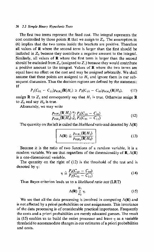
26 2.2 Simple Binary Hypothesis Tests
The first two terms represent the fixed cost. The integral represents the cost controlled by those points R that we assign to ZO. The assumption in (6) implies that the two terms inside the brackets are positive. Therefore all values of R where the second term is larger than the first should be included in Z0 because they contribute a negative amount to the integral. Similarly, all values of R where the first term is larger than the second should be excluded from Z0 (assigned to 2,) because they would contribute a positive amount to the integral. Values of R where the two terms are equal have no effect on the cost and may be assigned arbitrarily. We shall assume that these points are assigned to H1 and ignore them in our sub- sequent discussion. Thus the decision regions are defined by the statement: If
assign R to Z1 and consequently say that H1 is true. Otherwise assign R to Z. and say Ho is true.
Alternately, we may write
p,,,,(RIH,) ">'~OWlO - Gd
p,l~,(RlH,) H<o pl(col - cll)’
The quantity on the left is called the fikelihood ratio and denoted by A(R)
Because it is the ratio of two functions of a random variable, it is a random variable. We see that regardless of the dimensionality of R, A(R) is a one-dimensional variable.
The quantity on the right of (12) is the threshold of the test and is denoted by 7:
TA pow10 - Coo)
- p1(COl - Cd’ (14)
Thus Bayes criterion leads us to a likelihood ratio test (LRT)
We see that all the data processing is involved in computing A(R) and is not affected by a priori probabilities or cost assignments. This invariance of the data processing is of considerable practical importance. Frequently the costs and a priori probabilities are merely educated guesses. The result in (15) enables us to build the entire processor and leave 7 as a variable threshold to accommodate changes in our estimates of a priori probabilities and costs.

Likelihood Ratio Tests 27
Because the natural logarithm is a monotonic function, and both sides of (15) are positive, an equivalent test is
In A(R) $ In v. (16) Ho
Two forms of a processor to implement a likelihood ratio test are shown in Fig. 2.5.
Before proceeding to other criteria, we consider three simple examples.
Example I. We assume that under HI the source output is a constant voltage m. Under Ho the source output is zero. Before observation the voltage is corrupted by an additive noise. We sample the output waveform each second and obtain N samples. Each noise sample is a zero-mean Gaussian random variable n with variance 02. The noise samples at various instants are independent random variables and are indepen- dent of the source output. Looking at Fig. 2.6, we see that the observations under the two hypotheses are
and
Hl:rf=m+nr i=l,2 ,..., N, Ho:rl = ni i= I,2 ,..., N, (17)
1 X2 P@) = e exp -2a2 9
d2 7Tu ( ) (18)
because the noise samples are Gaussian. The probability density of rt under each hypothesis follows easily:
1 ptf IZ&IHI) = Pnr(& - m) = - exp
(R i- d2 -- 42
(19) na 2a”
and
prt ,H~UGIHO) = pn@V = -J+- exp ( -g2)e (20) 7ru
0 a
, Threshold
R Data In A (R) device Decision I
* processor -w----e, *
In A (R) 4 9lnV
Fig. 2.5 Likelihood ratio processors.

28 2.2 Simple Binary Hypothesis Tests
Source 7 N samples
Fig. 2.6 Model for Example 1.
Because the nf are statistically independent, the joint probability density of the Y( (or, equivalently, of the vector r) is simply the product of the individual probability densities. Thus
JJ~,~JRIH~) = fi +- =P (-(” 2;zm)2)9 (21) i=l 770
and
P~,HO(RIHO) = fi+ exP t=1 no
(-3
Substituting into (13), we have
A(R) =
N
I-I 1 - exp UC - mJ2 -
i=l 42 7Tu 2a2 N
I-I i=l
After canceling common terms and taking the logarithm, we have
In A(R) = 5 3 Rf - $$a f=l
Thus the likelihood ratio test is
a2 t-2 5 lnrl f=l 20 Ho
mN CR
Nm2 H1
(22)
(23)
(24)
(25)
or, equivalently,
% R,: a2 Nm -lnT+-+y.
i=l HO m (26)
We see that the processor simply adds the observations and compares them with a threshold.

Likelihood Ratio Tests 29
In this example the only way the data appear in the likelihood ratio test is in a sum. This is an example of a suficient statistic, which we denote by I(R) (or simply 1 when the argument is obvious). It is just a function of the received data which has the property that A(R) can be written as a function of 1. In other words, when making a decision, knowing the value of the sufficient statistic is just as good as knowing R. In Example 1, I is a linear function of the &. A case in which this is not true is illustrated in Example 2.
Example 2. Several different physical situations lead to the mathematical model of interest in this example. The observations consist of a set of N values: rl, y2, r3, . . ., rN*
Under both hypotheses, the Gaussian random variables.
ri are Under
independent, identically distributed, HI each rr has a variance a12. Under
zero-mean Ho each ri
has a variance o 02. Because the variables are independent, the joint density is simply the product of the individual densities. Therefore
and
Substituting (27) and (28) into (13) and taking the logarithm, we have
(2%
In this case the sufficient statistic is the sum of the squares of the observations
N
&W = 2 Ri2, i=l
(30)
and an equivalent test for aI2 > go2 is
For al2 < uo2 the inequality is reversed because we are multiplying by a negative number:
47’; (or2 < uo2). (32)
These two examples have emphasized Gaussian variables. In the next example we consider a different type of distribution.
Example 3. The Poisson distribution of events is encountered frequently as a model of shot noise and other diverse phenomena (e.g., [l] or [Z]). Each time the experiment is conducted a certain number of events occur. Our observation is just this number which ranges from 0 to 00 and obeys a Poisson distribution on both hypotheses; that is,
( 1 Pr (n events) = J$J e-*1, n = 0, 1,2 . . . , i = 0, 1, (33) .
where mr is the parameter that specifies the average number of events:
E(n) = mf. (34)

30 2.2 Simple Binary Hypothesis Tests
It is this parameter ttlt that is different in the two hypotheses. emphasize this point, we have for the two Poisson distributions
Rewriting (33) to
W,:Pr (n events) = !$eBrni, n = 0,1,2 ,..., (35) .
&:Pr (n events) = FeWrno, n = 0,1,2 ,.... (36) .
Then the likelihood ratio test is
A(n) = (37) Ho
or, equivalently,
nz Hl In 7 + ml - mo, ~~ In ml - In m.
if ml > mo,
(38) HO In q + ml - m.
n I$ ln ml - In m. ’ if m. > ml.
This example illustrates how the likelihood ratio test which we originally wrote in terms of probability densities can be simply adapted to accom- modate observations that are discrete random variables. We now return to our general discussion of Bayes tests.
There are several special kinds of Bayes test which are frequently used and which should be mentioned explicitly.
If we assume that COO and C,, are zero and CO1 = Cl0 = 1, the expres- sion for the risk in (8) reduces to
We see that (39) is just the total probability of making an error. There- fore for this cost assignment the Bayes test is minimizing the total probability of error. The test is
Hl lnA(R)2ln$=lnP,- -P& In (1
Ho 1
When the two hypotheses are equally likely, the threshold is zero. This assumption is normally true in digital communication systems. These processors are commonly referred to as minimum probability of error receivers.
A second special case of interest arises when the a priori probabilities are unknown. To investigate this case we look at (8) again. We observe that once the decision regions ZO and Z1 are chosen, the values of the integrals are determined. We denote these values in the following manner:

Likelihood Ratio Tests 31
PF = s pr,*,(RIH,) dR, 21
(41)
PM = s
p,,H,(RIH,) dR = 1 - & 20
We see that these quantities are conditional probabilities. The subscripts are mnemonic and chosen from the radar problem in which hypothesis HI corresponds to the presence of a target and hypothesis Ho corresponds to its absence. PF is the probability of a false alarm (i.e., we say the target is present when it is not); PD is the probability of detection (i.e., we say the target is present when it is); PM is the probability of a miss (we say the target is absent when it is present). Although we are interested in a much larger class of problems than this notation implies, we shall use it for convenience.
For any choice of decision regions the risk expression in (8) can be written in the notation of (41):
3t = P&o + &Cl1 + Pl(c,l - GlmLf - Po(C10 - Coo)(1 - pP)* (42)
Because PO = 1 - PI, (43-I
(42) becomes
Jw,) = Coo(l - PF) + Go& + Pl[(Cll - Co()) + (Co1 - Cll)hf - (Go - coovx (44)
Now, if all the costs and a priori probabilities are known, we can find a Bayes test. In Fig. 2.7a we plot the Bayes risk, X,(P,), as a function of PI. Observe that as PI changes the decision regions for the Bayes test change and therefore PF and PM change.
Now consider the situation in which a certain PI (say PI = Pf) is assumed and the corresponding Bayes test designed. We now fix the threshold and assume that PI is allowed to change. We denote the risk for this fixed threshold test as &(Pr, P,). Because the threshold is fixed, Pp and PM are fixed, and (44) is just a straight line. Because it is a Bayes test for PI = PF, it touches the X,(P,) curve at that point. Looking at (14), we see that the threshold changes continuously with PI. Therefore, when- ever PI # Pr, the threshold in the Bayes test will be different. Because the Bayes test minimizes the risk,
$(P?, P,) 2 Jh(P1).

32 2.2 Simple Binary Hypothesis Tests
!R
XF Cl1
<
XB
coo
0 1 Pl
Glo Cl1
h-0
Fig. 2.7 Risk curves: (n) fixed risk versus typical Bayes risk; (6) maximum value of X1 at PI = 0.
If A is a continuous random variable with a probability distribution function that is strictly monotonic, then changing ~r;l always changes the risk. xB(&) is strictly concave downward and the inequality in (45) is strict. This case, which is one of particular interest to us, is illustrated in Fig. 2.7a. We see that %F(PT, P,) is tangent to %#1) at P1 = PT. These curves demonstrate the effect of incorrect knowledge of the a priori probabilities.
An interesting problem is encountered if we assume that the a priori probabilities are chosen to make our performance as bad as possible. In other words, P1 is chosen to maximize our risk %F(Pr, PI). Three possible examples are given in Figs. 2.76, c, and d. In Fig. 2.76 the maximum of iIt, occurs at P1 = 0. To minimize the maximum risk we use a Bayes test designed assuming P1 = 0. In Fig. 2.7~ the maximum of XB(P1) occurs at P1 = 1. To minimize the maximum risk we use a Bayes test designed assuming P1 = 1. In Fig. 2.7d the maximum occurs inside the interval

Likelihood Ratio Tests 33
[O, 11, and we choose %, to be the horizontal line. This implies that the coefficient of P1 in (44) must be zero:
W 11 - Coo) + (Co1 - Cll)&l - (Go - COO)PF = 0. (46)
A Bayes test designed to minimize the maximum possible risk is called a minimax test. Equation 46 is referred to as the minimax equation and is useful whenever the maximum of XB(P1) is interior to the interval.
A special cost assignment that is frequently logical is
C 00 = Cl, = 0 (47)
(This guarantees the maximum is interior.) Denoting,
co1 = CM, C 10 = CF.
(48) the risk is,
and the minimax equation is
C,P, = CFpF.
Before continuing our discussion of likelihood ratio tests we shall discuss a second criterion and prove that it also leads to a likelihood ratio test.
Neyman-Pearson Tests. In many physical situations it is difficult to assign realistic costs or a priori probabilities. A simple procedure to by- pass this difficulty is to work with the conditional probabilities PF and P,. In general, we should like to make P, as small as possible and PD as large as possible. For most problems of practical importance these are con- flicting objectives. An obvious criterion is to constrain one of the prob- abilities and maximize (or minimize) the other. A specific statement of this criterion is the following:
Neyman-Pearson maximize PD (or
Criterion. Constrai n PF = a’ < a and design a test to minimize PM) under this constraint.
The solution is obtained easily by using Lagrange multipliers. We con- struct the function F,
F = PM + h[P, - a'], (50 or
F= s Pr,H,(RI w dR + h Pr,Ho(RIHo)~~ - a' I ' (52)
20
Clearly, if PF = a’, then minimizing F minimizes P,.

34 2.2 SimpIe Binary Hypothesis Tests
or
F = X(1 - a’) + s
[PrlH,(RIH,) - hp,l,,(RIH,)l at* (53) 20
Now observe that for any positive value of A an LRT will minimize F. (A negative value of h gives an LRT with the inequalities reversed.)
This follows directly, because to minimize F we assign a point R to Z0 only when the term in the bracket is negative. This is equivalent to the test
PrlH,@wl) < h
Pr,H,@lH,) ’ assign point to Z0 or say Ho.
The quantity on the left is just the likelihood ratio. Thus F is minimized by the likelihood ratio test
A(R)? A. Ho (59
To satisfy the constraint we choose h so that PF = a’. If we denote the density of A when Ho is true as paI H,(A 1 H()), then we require
PF = s
Am pA,H,(nlH,) dA = a’*
Solving (56) for A gives the threshold. The value of X given by (56) will be non-negative because pa 1 Ho (A I I&) is zero for negative values of h. Observe that decreasing h is equivalent to increasing Z1, the region where we say H1. Thus P, increases as h decreases. Therefore we decrease X until we obtain the largest possible a’ < CX. In most cases of interest to us PF is a continuous function of h and we have PF = a. We shall assume this con- tinuity in all subsequent discussions. Under this assumption the Neyman- Pearson criterion leads to a likelihood ratio test. On p. 41 we shall see the effect of the continuity assumption not being valid.
Summary. In this section we have developed two ideas of fundamental importance in hypothesis testing. The first result is the demonstration that for a Bayes or a Neyman-Pearson criterion the optimum test consists of processing the observation R to find the likelihood ratio A(R) and then comparing A(R) to a threshold in order to make a decision. Thus, regard- less of the dimensionality of the observation space, the decision space is one-dimensional.
The second idea is that of a sufficient statistic I(R). The idea of a sufficient statistic originated when we constructed the likelihood ratio and saw that it depended explicitly only on I(R). If we actually construct A(R) and then recognize I(R), the notion of a sufficient statistic is perhaps of secondary value. A more important case is when we can recognize I(R) directly. An easy way to do this is to examine the geometric interpretation of a sufEcient

Likelihood Ratio Tests 35
statistic. We considered the observations rl, t2, . . . , rN as a point r in an N-dimensional space, and one way to describe this point is to use these coordinates. When we choose a sufficient statistic, we are simply describing the point in a coordinate system that is more useful for the decision problem. We denote the first coordinate in this system by I, the sufficient statistic, and the remaining N - 1 coordinates which will not affect our decision by the (N - 1).dimensional vector y. Thus
Now the expression on the right can be written as
(57)
(58)
If I is a sufficient statistic, then A(R) must reduce to A(L). This implies that the second terms in the numerator and denominator must be equal. In other words,
py,l,Ho(YIL, H,) = PYIZ,HI(YlL HII (59
because the density of y cannot depend on which hypothesis is true. We see that choosing a sufficient statistic simply amounts to picking a co- ordinate system in which one coordinate contains all the information necessary to making a decision. The other coordinates contain no informa- tion and can be disregarded for the purpose of making a decision.
In Example 1 the new coordinate system could be obtained by a simple rotation. For example, when N = 2,
L = -&(Rl + R2)9
(60)
y = L (R, - R2). 42
In Example 2 the new coordinate system corresponded to changing to polar coordinates. For N = 2
L = RI2 + R22,
Notice that the vector y can be chosen in order to make the demonstra- tion of the condition in (59) as simple as possible. The only requirement is that the pair (I, y) must describe any point in the observation space. We should also observe that the condition

36 2.2 Simple Binary Hypothesis Tests
does not imply (59) unless I and y are independent under HI and HO. Frequently we will choose y to obtain this independence and then use (62) to verify that I is a sufficient statistic.
2.2.2 Performance : Receiver Operating Characteristic
To complete our discussion of the simple binary problem we must evaluate the performance of the likelihood ratio test. For a Neyman- Pearson test the values of pF and p0 completely specify the test perform- ance. Looking at (42) we see that the Bayes risk XB follows easily if P, and PD are known. Thus we can concentrate our efforts on calculating pF and P D*
We begin by considering Example 1 in Section 2.2.1.
Example I. From (25) we see that an equivalent test is
Fig. 2.8 Error probabilities: (a) PF calculation; (b) PD calculation.

Performance: Receiver Operating Characteristic 37
We have multiplied (25) by +Gm to normalize the next calculation. Under Ho, l is obtained by adding N independent zero-mean Gaussian variables with variance o2 and then dividing by 1/N Q. Therefore I is N(0, 1).
Under H,, I is N(1/N m/o, 1). The probability densities on the two hypotheses are sketched in Fig. 2.8a. The threshold is also shown. Now, PF is simply the integral of pl IHO(L] Ho) to the right of the threshold.
Thus 1
Y exp 42 n
W)
where d n dErn/o is the distance between the means of the two densities. The integral in (64) is tabulated in many references (e.g., [3] or [4]).
We generally denote
x erf, (X) L! s --aD
-!= exp (-g) dx, 42 n
where erf, is an abbreviation for the error function? and
erfc, (X) 4 f
* 1 - exp
x 1/27r
(65)
(66)
is its complement. In this notation
PF = erfc+ @+!z). (67)
Similarly, PD is the integral of pllH1 @IHI) to the right of the threshold, as shown in Fig. 2.8b:
PD= ao s
1 Y exp
(x - d)l (In n)/d + d/2 d2n
-- dx 2 1 al 1 d = s - exp 42
dy L! erfc, (2 - & (68) (In n)ld -d/2 37
In Fig. 2.9a we have plotted PD versus PF for various values of d with q as the varying parameter. For 7 = 0, In 7 = -00, and the processor always guesses HI. Thus PF = 1 and PD = 1. As 7 increases, PF and PD decrease. When r) = 00, the processor always guesses Ho and PF = PO = 0.
As we would expect from Fig. 2.8, the performance increases monotonically with d. In Fig. 2.96 we have replotted the results to give PD versus d with PF as a parameter on the curves. For a particular d we can obtain any point on the curve by choosing v appropriately (0 5 77 5 co).
The result in Fig. 2.9a is referred to as the receiver operating characteristic (ROC). It completely describes the performance of the test as a function of the parameter of interest.
A special case that will be important when we look at co mmunication the case in which we want to minimize the total probability of error
systems
Pr (E) a PoPF + PIPM. (694
t The function that is usually tabulated is erf (X) = 1/2/n jt exp ( -y2) dy, which is related to (65) in an obvious way.

38 2.2 Simple Binary Hypothesis Tests
0.8
t
0.6
PO
/ I I 1 I 1 I I I I
0.2 0.4 0.6 0.8
pF -
(4
Fig. 2.9 (a) Receiver operating characteristic: Gaussian variables with unequal means.
The threshold for this criterion was given in (40). For the special case in which PO = PI the threshold 7 equals one and
Pr (c) = +(PF + PM).
Using (67) and (68) in (69), we have
(694
Qo Pr (E) = 1
-& exp (-5) cik = erfc+ (+$ (70) + d/l 7T
It is obvious from (70) that we could also obtain the Pr (E) from the ROC. However, if this is the only threshold setting of interest, it is generally easier to calculate the Pr (E) directly.
Before calculating the performance of the other two examples, it is worthwhile to point out two simple bounds on erfc, (X). They will enable

Performance: Receiver Operating Characteristic 39
us to discuss its approximate behavior analytically. For X > 0
&X(1 - $) exp (-f) < erfc* (X) < *Xexp (-7). (71)
This can be derived by integrating by parts. (See Problem 2.2.15 or Feller [3O].) A second bound is
erfc, (X) < & exp x > 0, (72)
0.9999 t I I
0.999 -
0.99 -
0.98 -
0.8
0.7
Fig. 2.9 (6) detection probability versus da

40 2.2 Simple Binary Hypothesis Tests
which can also be derived easily (see Problem 2.2.16). The four curves are plotted in Fig. 2.10. We note that erfc, (X) decreases exponentially.
The receiver operating characteristics for the other two examtAes are also of interest.
1.0
0.5
0.3
0.1
0.01
0.00:
X---t
Fig. 2.10 Plot of erfc+ (X) and related functions.

Performance: Receiver Operating Characteristic 41
Example 2. In this case the test is
l(R) = 5 Hl 2tJ()%p
R,2 >< - i=l Ho 012 - ao2
ins - Nlnz = y, (a1 ) 4. (73)
The performance calculation for arbitrary N is somewhat tedious, so we defer it until Section 2.6. A particularly simple case appearing frequently in practice is N = 2. Under Ho the rl are independent zero-mean Gaussian variables with variances equal to ao2:
PF = Pr (I 2 ylHo) = Pr (r12 + ra2 >, yl Ho). (74)
To evaluate the expression on the right, we change to polar coordinates:
Then
rl = z cos 8, z = Al2 + r22 (75)
r2 = z sin 0, 8 = tan-1 2 r1
Pr (z2 2 ~1 Ho) = s s
2n de QD 2 k2 exp (-&) dZ. (76) 0 4
Integrating with respect to 8, we have
We observe that I, the sufficient statistic, equals z2. Changing variables, we have
PF = f
* 1 2 exP
Y 200
(Note that the probability density of the sufficient statistic is exponential.) Similarly,
PD=exp -+ ( )
(78)
(79)
To construct the ROC we can combine (78) and (79) to eliminate the threshold y. This gives
PO = (P*)Q02'"12. (80)
In terms of logarithms
In PO = f?! In PF. 012
(81)
As expected, the performance improves monotonically as the ratio u12/uo2 increases. We shall study this case and its generalizations in more detail in Section 2.6
The two Poisson distributions are the third example.
Example 3. From (38), the likelihood ratio test is
H1 In 7 + ml - m0 = n><
Ho h ml - h m. ” (ml ) mol. (82)
Because n takes on only integer values, it is more convenient to rewrite (82) as HI
n 2 YI, YI = 0,1,2 ,..., (83) Ho

42 2.2 Simple Binary Hypothesis Tests
where yI takes on only integer values. Using (39, q-1
pD = - e'"l 1 c ( 1 ml n
YI = 0,1,2 ,..., (84) and from (36)
n=O n!’
yl’ ’ (mo)n PF = 1 - ewmo 2 -9 n! Yx =0,1,2 ,.... (85)
n=O
The resulting ROC is plotted in Fig. 2.1 la for some representative values of m. and ml.
We see that it consists of a series of points and that PF goes from 1 to 1 - earn0 when the threshold is changed from 0 to 1. Now suppose we wanted PF to have an intermediate value, say 1 - +e -mo. To achieve this performance we proceed in the following manner. Denoting the LRT with ‘ye = 0 as LRT No. 0 and the’ LRT with YI = 1 as LRT No. 1, we have the following table:
LRT YI PF PD
1.0
0.8
0.6
Fil
0.4
0.2
0
0 1
0 1
1 1 1 - ewmo 1 - ewrni
6” -
‘;
“8
- 4”
05 -
/ /
/ /
/ /
/ /
/ /
0 ??a() = 2, ml = 4
/ 0 m() = 4, ml = 10
/ /
/
/ /
/ /
/ /
/
/ /
/ /
/ 1 I I I I I I I I 0.2 0.4 0.6 0.8
w---+
Fig. 2.11 (a) Receiver operating characteristic, Poisson problem.

Performance: Receiver Operating Characteristic 43
0.8
t
0.6
Fil
0.4
0.2
0
0 m0 = 2, ml = 4
/ om0=4, ml= 10
/ - /
/ / 1 I I I I I I 1 I
0.2 0.4 0.6 0.8 1.0
Fig. 2.11 (6) Receiver operating characteristic with randomized decision rule.
To get the desired value of PF we use LRT No. 0 with probability 3 and LRT No. 1 with probability 3. The test is
If n = 0, say HI with probability 3, say Ho with probability 3,
n>l say HI.
This procedure, in which we mix two likelihood ratio tests in some probabilistic manner, is called a randomized decision rule. The resulting PO is simply a weighted combination of detection probabilities for the two tests.
PO = 0.5(l) + 0.5(1 - ewrnl) = (1 - 0.5 e-ml). (86)
We see that the ROC for randomized tests consists of straight lines which connect the points in Fig. 2.11a, as shown in Fig. 2.1lb. The reason that we encounter a randomized test is that the observed random variables are discrete. Therefore A(R) is a discrete random variable and, using an ordinary likelihood ratio test, only certain values of PF are possible.
2.2 Simple Binary Hypothesis Tests
Looking at the expression we have
for PF in (56) and denoting the threshold by 7,
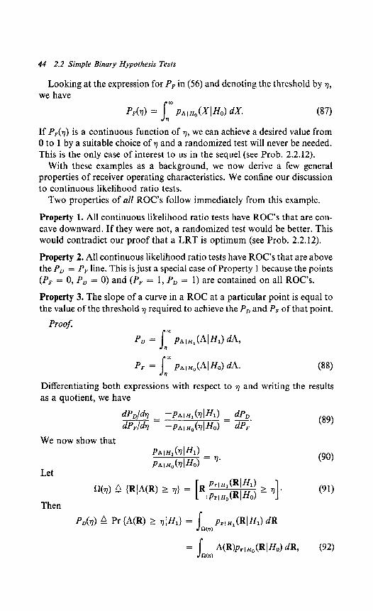
If P&) is a continuous function of q, we can achieve a desired value from 0 to 1 by a suitable choice of r) and a randomized test will never be needed. This is the only case of interest to us in the sequel (see Prob. 2.2.12).
With these examples as a background, we now derive a few general properties of receiver operating characteristics. We confine our discussion to continuous likelihood ratio tests.
Two properties of all ROC’s follow immediately from this example.
Property 1. All continuous likelihood ratio tests have ROC’s that are con- cave downward. If they were not, a randomized test would be better. This would contradict our proof that a LRT is optimum (see Prob. 2.2.12).
Property 2. All continuous likelihood ratio tests have ROC’s that are above the PD = PF line. This is just a special case of Property 1 because the points (P F = 0, PD =O)and(P, = 1,PD = 1) are contained on all ROC’s.
Property the value
3. The slope of a curve in a ROC at a particular point is equal to of the threshold r) required to achieve the PD and PF of that point.
Jtl
Differentiating both expressions with respect as a quotient, we have
dPDld7 -P*wJrlWd - = @F/h -PnIHJdHo)
We now show that PA,HJ?dm PA,I&lHO) = r)*
Let
to 7 and writing the results
dP D = -. dP F
(89)
= s A(R>Pr I Ho (RI Ho) m (92) ncfl>

Performance: Receiver Operating Characteristic 45
where the last equality follows from the definition of the likelihood ratio. Using the definition of Q(q), we can rewrite the last integral
Ml) = s WQPr I H() (RI Ho) aa =
s O” xP*,H()(xI~0) dX (93)
w?) tl Differentiating (93) with respect to 7, we obtain
Equating the expression for dP,(n)/dT in the numerator of (89) to the right side of (94) gives the desired result.
We see that this result is consistent with Example 1. In Fig. 2.9a, the curves for nonzero d have zero slope at PF = PD = 1 (7 = 0) and infinite slope at PF = PD = 0 (q- = co).
Property 4. Whenever the maximum value of the Bayes risk is interior to the interval (0, 1) on the PI axis, the minimax operating point is the intersection of the line
(C 11 - Coo) + (Co1 - GA1 - PD) - Go - coo)P, = 0 (95)
and the appropriate curve of the ROC (see 46). In Fig. 2.12 we show the special case defined by (50),
CFpF = &PM = CM(1 - PD),
0.4 0.6
‘F -
(96)
Determination of minimax operating point.

46 2.3 M Hypotheses
superimposed on the ROC of Example 1. We see that it starts at the point P F = 0, PD = 1, and intersects the Pp = 1 line at
This completes our discussion of the binary Several key ideas should be re-emphasized :
P c F= -2. 1 C iu (97)
hypothesis testing problem.
1. Using either a Bayes criterion or a Neyman-Pearson criterion, we find that the optimum test is a likelihood ratio test. Thus, regardless of the dimensionality of the observation space, the test consists of comparing a scalar variable A(R) with a threshold. (We assume p,(q) is continuous.)
2. In many cases construction of the LRT can be simplified if we can identify a sufficient statistic. Geometrically, this statistic is just that coordinate in a suitable coordinate system which describes the observation space that contains all the information necessary to make a decision.
3. A complete description of the LRT performance was obtained by plotting the conditional probabilities PO and pF as the threshold 7 was varied. The resulting ROC could be used to calculate the Bayes risk for any set of costs. In many cases only one value of the threshold is of interest and a complete ROC is not necessary.
A number of interesting binary tests are developed in the problems.
2.3 M HYPOTHESES
The next case of interest is one in which we must choose one of M hypotheses. In the simple binary hypothesis test there were two source outputs, each of which corresponded to a single hypothesis. In the simple M-ary test there are M source outputs, each of which corresponds to one of M hypotheses. As before, we assume that we are forced to make a decision. Thus there are M2 alternatives that may occur each time the experiment is conducted. The Bayes criterion assigns a cost to each of these alternatives, assumes a set of a priori probabilities PO, PI, . . . , PM - 1, and minimizes the risk. The generalization of the Neyman-Pearson criterion to M hypotheses is also possible. Because it is not widely used in practice, we shall discuss only the Bayes criterion in the text.
Bayes Criterion. To find a Bayes test we denote the cost of each course of action as Ci,. The first subscript signifies that the ith hypothesis is chosen. The second subscript signifies that the jth hypothesis is true. We denote the region of the observation space in which we choose Hr as Zt

Buyes Criterion 47
and the a priori probabilities are Pr. The model is shown in Fig. 2.13. The expression for the risk is
Jt = yg y-g w*, fi, PrlH,@IHj) cm* (98) = =
To find the optimum Bayes test we simply vary the Zr to minimize X. This is a straightforward extension of the technique used in the binary case. For simplicity of notation, we shall only consider the case in which M = 3 in the text.
Noting that Z. = Z - Z1 - Z2, because the regions are disjoint, we obtain
Jt = P&o I z-z, -22
Pr,H,(RIH,) dR + POGO s PrlHJRIHCJ dR
21
+ poc20 s
Pr,,,(RJH,) dR + PlCll 22 f
Pr,H,O dR z-20 -22
+ fwo1 s
Pr,H,(RlH,) dR + Plczl ZO s
Pr,,,(RIH,) dR z2
+ p2c22 s z-z0 ‘Zl
pl.,H,(RIH,) dR + p2co2 Pr,H,(RIH,) dR
+ p2c12 [ P rIH2CRlHd dR* JLl
This reduces to
+ s
[P2Wo2 - CzzlPrIHJ~ ZO + s [PO(clO - COOIPrlHJR Zl
Ho) + P&2 - C221PrIH2(R
+ J [POW20 - coo)prlHo(R~Ho) + p1(c21 - Cd’wdR
z2
As before, the first three terms represent the fixed cost and the Integrals represent the variable cost that depends on our choice of Zo, Z1, and Z2. Clearly, we assign each R to the region in which the value of the integrand is the smallest. Labeling these integrands IO(R), I,(R), and 12(R), we have the following rule :
if IO(R) < II(R) and 12(R), choose Ho, if II(R) c IO(R) and 12(R), choose HI, if I,(R) < lo(R) and I,(R), choose H2.
ww
(99)

48 2.3 M Hypotheses
PrlHi
Fig. 2.13 M hypothesis problem.
We can write these terms in terms of likelihood ratios by defining
Using (102) in (100) and (lOl), we have
HI or Hz
mco1 - cll) R,(R) 5 Po(Clo - coo) + p2(c12 - Co2)AdR) (lo3) Ho or Hz
Hz or HI
p2wo2 - c22) A,(R) >< Ho or HI
P&20 - Coo) + h(C21 - cod Al(R), (104)
Hz or Ho
P2G2 - c22) A,(R) 5 Po(C20 - Go) + p&21 - cu)AdR)- (lo% HI or HO
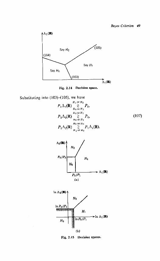
We see that the decision rules correspond to three lines in the AI, A, plane. It is easy to verify that these lines intersect at a common point and therefore uniquely define three decision regions, as shown in Fig. 2.14. The decision space is two-dimensional for the three-hypothesis problem. It is easy to verify that M hypotheses always lead to a decision space which has, at most, (M - 1) dimensions.
Several special cases will be useful in our later work. The first is defined by the assumptions
C 00 = Cl1 = c22 = 0, C if = 1, i# j.
These equations indicate that any error is of equal importance. Looking at (98), we see that this corresponds to minimizing the total probability of error.
Bayes Criterion 49
Fig. 2.14 Decision space.
Substituting into (103)-( 109, we have H1 or H2
f2uR) >< PO9 Ho or Hz
H2 or HI
&A,(R) >< PO9 Ho or HI
Hz or Ho
p2MR) z mLw* HI or Ho
(107)
04
Fig. 2.15 Decision spaces.

50 2.3 M Hypotheses
The decision regions in the &, &) plane are shown in Fig. 2.1%~. In this particular case, the transition to the (ln A,, In A,) plane is straight- forward (Fig. 2.1%). The equations are
HI or H2
In A,(R) z In $9 Ho or H2 1
HI or H2
In A,(R) 3 In $$ Ho or HI
ww 2
Ho or H2
ln A,(R) 3 Pl
Ho or HI In A,(R) + In p*
2
The expressions in (107) and (108) are adequate, but they obscure an important interpretation of the processor. The desired interpretation is obtained by a little manipulation.
Substituting (102) into (103-105) and multiplying both sides by PrI Ho(RI&), we have
HI or Hz
plib,H1(Ri~l) z P,h,Ho(RI&), Ho or Hz
Hz or H1
P2hI,2(RtH,) z pOp,, Ho(RIH,), Ho or HI
uw
Hz or Ho
p2PrlH2tR1H2) z pl~r,Hl(R~H,). H1 or Ho
Looking at (log), we see that an equivalent test is to compute the a posteriori probabilities Pr [HoI R], Pr [H, JR], and Pr [H,IR] and choose the largest. (Simply divide both sides of each equation by p,(R) and examine the resulting test.) For this reason the processor for the minimum probability of error criterion is frequently referred to as a maximum a posteriori probability computer. The generalization to M hypotheses is straightforward.
The next two topics deal with degenerate tests. Both results will be useful in later applications. A case of interest is a degenerate one in which we combine H1 and Hz. Then
c 12 = c21 = 0, (110)
and, for simplicity, we can let
c 01 = C 10 = C 20 = c 02 and
C oo= C 11= c 22= l 0
Then (103) and (104) both reduce to HI 0; Hz
PlAl(R> + P2A2W c PO Ho
and (105) becomes an identity.
(111)
(112)
(113)

Bayes Criterion 51
1 A2 CR)
PO
pz HI or H2 5 HO
PO
p1
Fig. 2.16 Decision spaces.
The decision regions are shown in Fig. 2.16. Because we have eliminated all of the cost effect of a decision between HI and Hz, we have reduced it to a binary problem.
We next consider the dummy hypothesis technique. A simple example illustrates the idea. The actual problem has two hypotheses, HI and Hz, but occasionally we can simplify the calculations by introducing a dummy hypothesis Ho which occurs with zero probability. We let
PO = 0, PI + Ps = 1, and (114)
c 12 = co29 c21 = COP
Substituting these values into (103-109, we find that (103) and (104) imply that we always choose HI or Hz and the test reduces to
P2G2 - C22) A,(R) 7 PdC21 - Gl) MW. (119 HI
Looking at (12) and recalling the definition of A,(R) and R,(R), we see that this result is exactly what we would expect. [Just divide both sides of (12) by ~~~ Ho(RI Ho).] On the surface this technique seems absurd, but it will turn out to be useful when the ratio
Pr, HstR1 H2)
is difficult to work with and the ratios A,(R) and A,(R) can be made simple by a proper choice of pFI Ho(RI Ho).
In this section we have developed the basic results needed for the M- hypothesis problem. We have not considered any specific examples

52 2.4 Estimation Theory
because the details involved in constructing the likelihood ratios are the same as those in the binary case. Typical examples are given in the problems. Several important points should be emphasized.
1. The minimum dimension of the decision space is no more than iv- 1. The boundaries of the decision regions are hyperplanes in the
(A . , AM - J plane. 21 *The optimum test is straightforward to find. We shall find however,
when we consider specific examples that the error probabilities are frequently difficult to compute.
3. A particular test of importance is the minimum total probability of error test. Here we compute the a posteriori probability of each hypothesis Pr (H,IR) and choose the largest.
These points will be appreciated more fully as we proceed through various applications.
These two sections complete our discussion of simple hypothesis tests. A case of importance that we have not yet discussed is the one in which several source outputs are combined to give a single hypothesis. To study this detection problem, we shall need some ideas from estimation theory. Therefore we defer the composite hypothesis testing problem until Section 2.5 and study the estimation problem next.
2.4 ESTIMATION THEORY
In the last two sections we have considered a problem in which one of several hypotheses occurred. As the result of a particular hypothesis, a vector random variable r was observed. Based on our observation, we shall try to choose the true hypothesis.
In this section we discuss the problem of parameter estimation. Before formulating the general problem, let us consider a simple example.
Example 1. We want to measure a voltage a at a single time instant. From physical considerations, we know that the voltage is between - V and + Vvolts. The measure- ment is corrupted by noise which may be modeled as an independent additive zero- mean Gaussian random variable n. The observed variable is Y. Thus
r =a+n. (116) The probability density governing the observation process is P~I~(RIA). In this case
1 prra(R(A) = p,(R - A) = v
d2 7T (Jn
(117)
The problem is to observe Y and estimate a.
This example illustrates the basic features of the estimation problem.

Model 53
A model of the general estimation problem is shown in Fig. 2.17. The model has the following four components:
Parameter Space. The output of the source is a parameter (or variable). We view this output as a point in a parameter space. For the single- parameter case, which we shall study first, this will correspond to segments of the line -oo < A < 00. In the example considered above the segment is
(- K 0
Probabilistic Mapping from Parameter Space to Observation Space. This is the probability law that governs the effect of a on the observation.
Observation Space. In the classical problem this is a finite-dimensional space. We denote a point in it by the vector R.
Estimation Rule. After observing R, we shall want to estimate the value of a. We denote this estimate as 6(R). This mapping of the observation space into an estimate is called the estimation rule. The purpose of this section is to investigate various estimation rules and their implementations.
The second and third components are familiar from the detection prob- lem. The new features are the parameter space and the estimation rule. When we try to describe the parameter space, we find that two cases arise. In the first, the parameter is a random variable whose behavior is governed by a probability density. In the second, the parameter is an unknown quantity but not a random variable. These two cases are analogous to the
observation space
Fig. 2.17 Estimation model.

54 2.4 Estimation Theory
source models we encountered in the hypothesis-testing problem. To corre- spond with each of these models of the parameter space, we shall develop suitable estimation rules. We start with the random parameter case.
2.4.1 Random Parameters: Bayes Estimation
In the Bayes detection problem we saw that the two quantities we had to specify were the set of costs Crr and the a priori probabilities Pi. The cost matrix assigned a cost to each possible course of action. Because there were M hypotheses and M possible decisions, there were M2 costs. In the estimation problem a and ci(R) are continuous variables. Thus we must assign a cost to all pairs [a, a(R)] over the range of interest. This is a function of two variables which we denote as C(a, ci). In many cases of interest it is realistic to assume that the cost depends only on the error of the estimate. We define this error as
a,(R) 4 B(R) - a. uw
The cost function C(a,) is a function of a single variable. Some typical cost functions are shown in Fig. 2.18. In Fig. 2.18a the cost function is simply the square of the error:
C(a,) = ac2. (119)
This cost is commonly referred to as the squared error cost function. We see that it accentuates the effects of large errors. In Fig. 2.18b the cost function is the absolute value of the error:
In Fig. 2.18~ we assign zero cost to all errors less than &A/2. In other words, an error less than A/2 in magnitude is as good as no error. If at, > A/2, we assign a uniform value:
C(a,) = 0, A
Ia,1 < 2’
A = 1, IQEI > -2’ (121)
In a given problem we choose a cost function to accomplish two objectives. First, we should like the cost function to measure user satis- faction adequately. Frequently it is difficult to assign an analytic measure to what basically may be a subjective quality.
Our goal is to find an estimate that minimizes the expected value of the cost. Thus our second objective in choosing a cost function is to assign one that results in a tractable problem. In practice, cost functions are usually some compromise between these two objectives. Fortunately, in many

Random Parameters: Bayes Estimation 55
Fig. 2.18 Typical cost functions: (a) mean-square error; (6) absolute error; (c) uniform cost function.
problems of interest the same estimate will be optimum for a large class of cost functions.
Corresponding to the a priori probabilities in the detection problem, we have an a priori probability density p,(A) in the random parameter estima- tion problem. In all of our discussions we assume that p,(A) is known. If p,(A) is not known, a procedure analogous to the minimax test may be used.
Once we have specified the cost function and the a priori probability, we may write an expression for the risk:
x n E{C[a, @)I} = Ia dA sm C[A, ci(R)]p,,,(A, R)dR. (122) --co --a0
The expectation is over the random variable a and the observed variables r. For costs that are functions of one variable only (122) becomes
zR = /IL) dA/:a CIA - @hz,r(A, R) dR. (123)

56 2.4 Estimation Theory
The Bayes estimate is the estimate that minimizes the risk. It is straight- forward to find the Bayes estimates for the cost functions in Fig. 2.18. For the cost function in Fig. 2.18a, the risk corresponds to mean-square error. We denote the risk for the mean-square error criterion as X,,. Substituting (119) into (123), we have
JLs = /yrn dA I:_ dR[A - 6(R)]2p,,,(~, R). (124)
The joint density can be rewritten as
p,,,(A, R) = pr(R)p,,.(AIR). Using (125) in (124), we have
(125)
iR ms = s
ao dRpr(R) -CO s
ao dA[A - ~(R)12p,,,(AIR). (126) -m
m Now the inner integral and .inimize S ‘ms by minimizing t
Pm are non-negative. Therefore we can he inn er i .ntegral. We denote this estimate
&m,(R). To find it we differentiate the inner integral with respect to 6(R) and set the result equal to zero:
d - fm WA - m12Pa,r(AIw A da --oo
s ao s * = -2 APa,r(AiR)dA + u(R) p,,,(AIR) dA. (127)
--oo -CO
Setting the result equal to zero and equals 1, we have
observing that the second integral
6ms(R) = s
O” d/i APa,r(A IN. w8) --Q)
This is a unique minimum, for the second derivative equals two. The term on the right side of (128) is familiar as the mean of the a posteriori density (or the conditional mean).
Looking at (126), we see that if d(R) is the conditional mean the inner integral is just the a posteriori variance (or the conditional variance). Therefore the minimum value of Xms is just the average of the conditional variance over all observations R.
To find the Bayes estimate for the absolute value criterion in Fig. 2.18b we write
x abs = ao dRp,(R) s
dA[lA - @)]l~cz,r(AIR). (129 --oo
To minimize the inner integral we write &RI
= s O” I(R) dA [6(R) - A]Pa,.(AIR) + s dA[A - B(R)]paI,(AIR).
-00 d(R) (130)

Random Parameters: Bayes Estimation 57
Differentiating with respect to 6(R) and setting the result equal to zero, we have
s &bs(R)
d/I PadAIR) = j- &f p&IIR). -CO has(R)
This is just the definition of the median of the a posteriori density. The third criterion is the uniform cost function in Fig. 2.18~. The risk
expression follows easily :
To minimize this equation we maximize the inner integral. Of particular interest to us is the case in which A is an arbitrarily small but nonzero number. A typical a posteriori density is shown in Fig. 2.19. We see that for small A the best choice for 6(R) is the value of A at which the a posteriori density has its maximum. We denote the estimate for this special case as dmap (R), the maximum a posteriori estimate. In the sequel
A we use amap (R) without further reference to the uniform cost function. To find brnap we must have the location of the maximum of p&4 IR).
Because the logarithm is a monotone function, we can find the location of the maximum of In palr(AIR) equally well. As we saw in the detection problem, this is frequently more convenient.
If the maximum is interior to the allowable range of A and In pa ,,(A IR) has a continuous first derivative then a necessary, but not sufficient, condition for am .aximum can be obtained by differentiating In pa1 .(A I R) with respect t oA and sett ing the result equal to zero:
a lnp,,r(AlR) = 8A
0. A = d(R)
(133)
Fig. 2.19 An a posteriori density.

58 2.4 Estimation Theory
We refer to (133) as the MAP equation. In each case we must check to see if the solution is the absolute maximum.
We may rewrite the expression for P,,,(A IR) to separate the role of the observed vector R and the a priori knowledge:
Pa,rwo = Pr , a(RI4Pd4 Pm l
Taking logarithms,
lnPa,r(AlR) = In Pr Ia(RIA) + In Pa(A) - In P,(R)- (13% For MAP estimation we are interested only in finding the value of A
where the left-hand side is maximum. Because the last term on the hand side is not a function of A, we can consider just the function
right-
44 4 lnPr,.(Rl4 + InPa( (136)
The first term gives the probabilistic dependence of R on A and the second describes a priori knowledge.
The MAP equation can be written as
mo = a ln Prla(Rl4 aA
= A = &RI i3A
+ a ln Pa(A) aA 0. WV
A = d(R) A = t%(R)
Our discussion in the remainder of the book emphasizes minimum mean- square error and maximum a posteriori estimates.
To study the implications of these two estimation procedures we consider several examples. Example 2. Let
ri = a + a, i= I,2 ,..., N. (138) We assume that a is Gaussian, N(0, ua), and that the nt are each independent
Gaussian variables N(0, o,,). Then
1 pr,a(RlA) = fir- =P (
(R, - Al2 -- f=l n =n
2an2 1
9
1 P,(A) = -
42 r exP ua ( A2
-37 a 1 l
(139)
To find d,,(R) we need to know pa &AIR). One approach is to find pF(R) and substitute it into (134), but this procedure is algebraically tedious. It is easier to observe that pa &AIR) is a probability density with respect to a for any R. Thus pr(R) just contributes to the constant needed to make
s a3 PaIdAIR) dA = 1. (140)
-CO
(In other words, pF(R) is simply a normalization constant.) Thus
PaIlJAIR) = [
(f!$~Z&] exp -JfZ>RiJ A)2 + $
i I\
. (141)

Random Parameters: Bayes Estimation 59
Rearranging the exponent, completing only on Rt2 into the constant, we have
the square, and absorbing terms depending
p&AIR) = k(R)exp (142)
where
(143)
is the a posteriori variance. We see that paIr(AIR) is just a Gaussian density. The estimate d,,(R) is just the
conditional mean
Because the a posteriori variance is not a function of R, the mean-square risk equals the a posteriori variance (see (126)).
Two observations are useful :
1. The Rt enter into the a posteriori density only through their sum. Thus
Z(R) = 2 Ri i=l
(145)
is a suficient statistic. This idea of a sufficient statistic is identical to that in the detection problem.
2. The estimation rule uses the information available in an intuitively logical manner. I f aa2 CC o,~/N, the a priori knowledge is much better than the observed data and the estimate is very close to the a priori mean. (In this case, the a priori mean is zero.) On the other hand, if aa >> an2/N, the a priori knowledge is of little value and the estimate uses primarily the received data. In the limit 8,, is just the arithmetic average of the Rt.
lim on2
d,,(R) = & 2 Ri. --0 i=l Noa
(146)
The MAP estimate for this case follows easily. Looking at (142), we see that because the density is Gaussian the maximum value of paIr(AIR) occurs at the conditional mean. Thus
4mwm = &SW (147)
Because the conditional median of a Gaussian density occurs at the conditional mean, we also have
hms(R) = cfms(W w-0
Fi Thus we see that for this particu lar example all three cost functions in g. 2.1 8 lead to the same estimate. This invariance to th .e choice of a cost
function is obviously a useful feature because of the subjective judgments that are frequently involved in choosing C(a,). Some conditions under which this invariance holds are developed in the next two pr0perties.t
t These properties are due to Sherman [20]. Our derivation is similar to that given by Viterbi [36].

60 2.4 Estimation Theory
Property 1. We assume that the cost function C(a,) is a symmetric, convex- upward function and that the a posteriori density pa ,,(A IR) is symmetric about its conditional mean; that is,
a%) = cc- a,) (symmetry), (149)
C(bx, + (1 - @x2) < bC(x,) + (1 - b) C(Xz) (convexity) (150)
for any b inside the range (0, 1) and for all x1 and x2. Equation 150 simply says that all chords lie above or on the cost function.
This condition is shown in Fig. 2.20a. If the inequality is strict whenever x1 # x2, we say the cost function is strictly convex (upward). Defining
da-8 - ms = a - E[aIR] Wl)
the symmetry of the a posteriori density implies
P,,r(ZIW = Pd-~IW~ (152)
The estimate 6 that minimizes any cost function in this class is identical to &ms (which is the conditional mean).
Fig. 2.20 Symmetric convex cost functions: (n) convex; (6) strictly convex.

Random Parameters: Bayes Estimation 61
proof. As before we can minimize the conditional risk [see (126)]. Define
X,(6IR) 12 E,[C@ - a)lR] = E,[C(a - d)lR], (153)
where the second equality follows from (149). We now write four equivalent expressions for S&Z (R) :
,a,(tiIR) = s
O” C(6 - dms - ZIP, ,r@ I w dz (154) --a0
[Use (151) in (153)]
= s O3 C(6 - bms + ~lP~,d~IJQ 0 (155) --CO
[( 152) implies this equality]
[( 149) implies this equality]
[( 152) implies this equality].
We now use the convexity condition (150) with the terms in (155) and (157):
X,(BIR) = W(W[z + @Ins - S)] + C[Z - (h,, - S)]}lR)
2 E{C[+(Z + (Cims - b)) + +(Z - (Cims - a))] [ R}
= E[C(Z)IR]. (158)
Equality will be achieved in (158) if dms = &. This completes the proof. If C(a,) is strictly convex, we will have the additional result that the minimizing estimate ci is unique and equals bms.
To include cost functions like the uniform cost functions which are not convex we need a second property.
Property 2. We assume that the cost function is a symmetric, nondecreasing function and that the a posteriori density pa,@ IR) is a symmetric (about the conditional mean), unimodal function that satisfies the condition
lim C(x)p,&lR) = 0. X-+00
The estimate & that minimizes any cost function in this class is identical to
4rlS~ The proof of this property is similar to the above proof [36].
2.4 Estimation Theory
The significance of these two properties should not be underemphasized. Throughout the book we consider only minimum mean-square and maxi- mum a posteriori probability estimators. Properties 1 and 2 ensure that whenever the a posteriori densities satisfy the assumptions given above the estimates that we obtain will be optimum for a large class of cost functions. Clearly, if the a posteriori density is Gaussian, it will satisfy the above assumptions.
We now consider two examples of a different type.
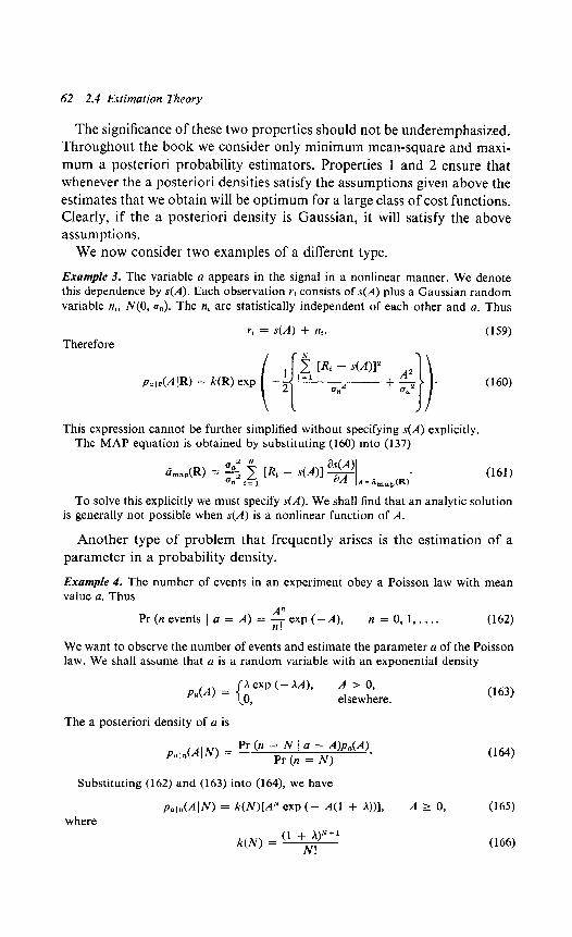
Example 3. The variable a appears in the signal in a nonlinear manner. We denote this dependence by s(A). Each observation rf consists of s(A) plus a Gaussian random variable ni, N(0, o,J. The ni are statistically independent of each other and a. Thus
ri = s(A) + nf. (159) Therefore
P~I~AIR) = k(R) ew (-!{ fk ‘“b- s(A)12 + $}I. (160)
This expression cannot be further simplified without specifying s(A) explicitly. The MAP equation is obtained by substituting (160) into (13 7)
2 N
&m, w aa wo =-
2 21 Ri - on is1 - s(A)1 aA A= ;,,+j’ (161)
To solve this explicitly we must specify s(A). We shall find that an analytic solution is generally not possible when s(A) is a nonlinear function of A.
Another type of problem that frequently arises is the estimation of a parameter in a probability density.
Example 4. The number of events in an experiment obey a Poisson law with mean value a. Thus
A” Pr (n events 1 a = A) = Texp (-A), n = 0, 1,. . . . (162) .
We want to observe the number of events and estimate the parameter a of the Poisson law. We shall assume that a is a random variable with an exponential density
Pa(A) = h exp (- AA), A > 0, 0
9 elsewhere. (163)
The a posteriori density of a is
(164)
Substituting (162) and (163) into (164), we have
where PaIn(AlN) = W)[AN exp (- 41 + 91, A r 0, (165)
k(N) (l + ‘IN+’ = N! (166)

Random Parameters: Bayes Estimation 63
in order for the density to integrate to 1. (As already pointed out, the constant is unimportant for MAP estimation but is needed if we find the MS estimate by integrating over the conditional density.)
The mean-square estimate is the conditional mean:
6 ms (N) (’ ’ ‘IN+’ = s
O” AN+l exp[ A(1 + A)] dA - N! o
(1 + /\)N+l = (1 + h)N+2 w + 1) = (167)
TO find 8m,, we take the logarithm of (165)
lnp,,,(AIN) = Nln A - A(1 + h) + In k(N). (168)
By differentiating with respect to A, setting the result equal to zero, and solving, we obtain
drntbp WI N =-.
l+A (169)
Observe that Cimap is not equal to cfms.
Other examples are developed in the problems. The principal results of this section are the following:
1. The minimum mean-square error estimate (MMSE) is always the mean of the a posteriori density (the conditional mean).
2. The maximum a posteriori estimate (MAP) is the value of A at which the a posteriori density has its maximum.
3. For a large class of cost functions the optimum estimate is the conditional mean whenever the a posteriori density is a unimodal function which is symmetric about the conditional mean.
These results are the basis of most of our estimation work. As we study more complicated problems, the only difficulty we shall encounter is the actual evaluation of the conditional mean or maximum. In many cases o f interest the MAP and MMSE estimates will turn out to be equal.
We now turn to the second class of estimation problems described in the introduction.
2.4.2 Real (Nonrandom) Parameter Estimation7
In many cases it is unrealistic to treat the unknown parameter as a random variable. The problem formulation on pp. 52-53 is still appro- priate. Now, however, the parameter is assumed to be nonrandom, and we want to design an estimation procedure that is good in some sense.
7 The beginnings of classical estimation theory can be attributed to Fisher [5, 6, 7, 81. Many discussions of the basic ideas are now available (e.g., Cramer [9]), Wilks [lo], or Kendall and Stuart [ll]).

2.4 Estimation Theory
A logical first approach is to try to modify the last section to eliminate the average over p&4). As mean-square error criterion,
X(A) n s
* km - 42Pr,a@I -CO
Bayes procedure in the an example, consider a
where the expectation is only over R, for it is the only random variable in the model. Minimizing X(A), we obtain
L&(R) = A. (171)
The answer is correct, but quantity that we are trying to
not of any value, for A is the find. Thus we see that this direct
is not fruitful. A more useful method in the nonrandom parameter case
unknown approach
is to examine other possible measures of quality of estimation procedures and then to see whether we can find estimates that are good in terms of these measures.
The first measure of quality to be considered is the expectation of the estimate
E[d(R)] 4 /+a WV Pr,.(RIA) dR* (172) --a0
The possible values of the expectation can be grouped into three classes
1. If E[b(R)] = A, for all values of A, we say that the estimate is UIZ- bimed. This statement means that the average value of the estimates equals the quantity we are trying to estimate.
2. If Q?(R)] = A + B, where B is not a function of A, we say that the estimate has a known bias. We can always obtain an unbiased estimate by subtracting B from 6(R).
3. If&?(R)] = A + B(A), we say that the estimate has an unknown bias. Because the bias depends on the unknown parameter, we cannot simply subtract it out.
Clearly, even an unbiased estimate may give a bad result on a particular trial. A simple example is shown in Fig. 2.21. The probability density of the estimate is centered around A, but the variance of this density is large enough that big errors are probable.
A second measure of quality is the variance of estimation error:
Var [b(R) - A] = E{[&(R) - A12} - B2(A). (173)
This provides a measure of the spread of the error. In general, we shall try to find unbiased estimates with small variances. There is no straight- forward minimization procedure that will lead us to the minimum variance unbiased estimate. Therefore we are forced to try an estimation procedure to see how well it works.

Maximum Likelihood Estimation 65
Fig. 2.21 Probability density for an estimate.
Maximum Likelihood Estimation. There are several ways to motivate the estimation procedure that we shall use. Consider the simple estimation problem outlined in Example 1. Recall that
r =A+n, (174)
prla(RjA) = (16&,)-~ exp [-$(R - A)2]. n
(175)
We choose as our estimate the value of A that most likely caused a given value of R to occur. In this simple additive case we see that this is the same as choosing the most probable value of the noise (N = 0) and subtracting it from R. We denote the value obtained by using this procedure as a maximum likelihood estimate.
6,,(R) = R. (176) In the general case we denote the function prla(RI A), viewed as a
function of A, as the likelihood function. Frequently we work with the logarithm, In Prla(RIA), and denote it as the log likelihood function. The maximum likelihood estimate 6,,(R) is that value of A at which the likeli- hood function is a maximum. If the maximum is interior to the range of A, and lnp,l.(RIA) has a continuous first derivative, then a necessary con- dition on d,,(R) is obtained by differentiating lnp,,JRIA) with respect to A and setting the result equal to zero:
a ln Pr,a(W aA
= . 0 A=d,z(R)
This equation is called the likelihood equation. Comparing (137) and (177), we see that the ML estimate corresponds mathematically to the limiting case of a MAP estimate in which the a priori knowledge approaches zero.
In order to see how effective the ML procedure is we can compute the bias and the variance. Frequently this is difficult to do. Rather than approach the problem directly, we shall first derive a lower bound on the variance on any unbiased estimate. Then we shall see how the variance of d,,(R) compares with this lower bound.

66 2.4 Estimation Theory
Cram&Rao Inequality: Nonrandom Parameters. We now want to con- sider the variance of any estimate b(R) of the real variable A. We shall prove the following statement.
Theorem. (a) If ci(R) is any unbiased estimate of A, then
Var [B(R)
or, equivalently,
Var [d(R) - A] >
(178)
where the following conditions are assumed to be satisfied:
0 C
exist and are absolutely integrable. The inequalities were first stated by Fisher [6] and proved by DuguC [31].
They were also derived by Cramer [9] and Rao [ 121 and are usually referred to as the Cramer-Rao bound. Any estimate that satisfies the bound with an equality is called an eficient estimate.
The proof is a simple application of the Schwarz inequality. Because B(R) is unbiased,
O” E[b(R) - A] n s
--ao Pr,a@lA)[w9 - AI dR = 0 . (1 80)
Differentiating both sides with respect to A, we have
d
-1
00
dA _ mPr,oo[6(R) - AI dR al a =
s -ao a {Pr,a(RIA)P(R) - 41 dR = 09 (181)
where condition (c) allows us to bring the differentiation inside the integral. Then
co pr,JRIA) dR + s
ap,i;yiA’ [B(R) - A] dR = 0. (182) --oo
The first integral is just + 1. Now observe that
ap,.,.oQo i3A =
a lnp,l,op aA ru
, (RI/J) . (183)

Cram&- Rao Inequality 67
Substituting (183) into (182), we have
s O” a lIv~,cz(Rl4 i3A
pr,.(RIA)[B(R) - A] dR = 1. --oo
Rewriting, we have
a0 s [
alnpr,.(RIA) 4 aA
prIa(RIA) dpl.,,(RIA) [d(R) - Al dR = 1, (18% -00 I[ I
and, using the Schwarz inequality, we have
alnhdRIA) 2p , @IA) dR aA I
ru
X [B(R) - A]2pr,a(RIA)dR >
> 1, (186)
where we recall from the derivation of the Schwarz inequality that equality holds if and only if
a ln Pq.(RIA) 8A
= [h(R) - A] k(A), (187)
for all R and A. We see that the two terms of the left side of (186) are the expectations in statement (a) of (178). Thus,
-l E{[&(R) - A12} 2 . (188)
To prove statement (b) we observe
s 00 -* P&q4 dR = 1. Differentiating with respect to A, we have
(18% a0 +r,dRIA) dR s O” =
aA alnb,dRIA)p , @IA)&
aA ra = 0. (190) -a, --Q)
Differentiating again with respect to A and applying (183), we obtain
s ao a21np,ldRIA)p , (R(A)& aA ra -CO
+ = 0 (191)
or E a2 In jh,.(RIA) aA ] = -E[alnp;&@‘A)]2, (192)
which together with (188) gives condition (b).