http://pih.sagepub.com/Medicine

Engineers, Part H: Journal of Engineering in Proceedings of the Institution of Mechanical

http://pih.sagepub.com/content/225/8/753The online version of this article can be found at:

 DOI: 10.1177/0954411911407669

originally published online 2 June 2011 2011 225: 753Proceedings of the Institution of Mechanical Engineers, Part H: Journal of Engineering in Medicine

A H Prins, B L Kaptein, B C Stoel, R G H H Nelissen, J H C Reiber and E R ValstarIntegrated contour detection and pose estimation for fluoroscopic analysis of knee implants

  

Published by:

http://www.sagepublications.com

On behalf of: 

  Institution of Mechanical Engineers

can be found at:Proceedings of the Institution of Mechanical Engineers, Part H: Journal of Engineering in MedicineAdditional services and information for

   

  http://pih.sagepub.com/cgi/alertsEmail Alerts:

 

http://pih.sagepub.com/subscriptionsSubscriptions:  

http://www.sagepub.com/journalsReprints.navReprints:  

http://www.sagepub.com/journalsPermissions.navPermissions:  

http://pih.sagepub.com/content/225/8/753.refs.htmlCitations:  

What is This? 

- Jun 2, 2011 OnlineFirst Version of Record 

- Jul 26, 2011Version of Record >>

at Bibliotheek TU Delft on October 3, 2012pih.sagepub.comDownloaded from

Integrated contour detection and pose estimation forfluoroscopic analysis of knee implantsA H Prins1, B L Kaptein1*, B C Stoel2, R G H H Nelissen1, J H C Reiber2, and E R Valstar1,3

1Biomechanics and Imaging Group, Department of Orthopaedics, Leiden University Medical Center, Leiden,

The Netherlands2Division of Image Processing, Department of Radiology, Leiden University Medical Center, Leiden, The Netherlands3Department of Biomechanical Engineering, Faculty of Mechanical, Maritime and Materials Engineering, Delft

University of Technology, Delft, The Netherlands

The manuscript was received on 19 November 2010 and was accepted after revision for publication on 30 March 2011.

DOI: 10.1177/0954411911407669

Abstract: With fluoroscopic analysis of knee implant kinematics the implant contour must bedetected in each image frame, followed by estimation of the implant pose. With a large num-ber of possibly low-quality images, the contour detection is a time-consuming bottleneck. Thepresent paper proposes an automated contour detection method, which is integrated in thepose estimation.

In a phantom experiment the automated method was compared with a standard method,which uses manual selection of correct contour parts. Both methods demonstrated compara-ble precision, with a minor difference in the Y-position (0.08 mm versus 0.06 mm). The preci-sion of each method was so small (below 0.2 mm and 0.3�) that both are sufficiently accuratefor clinical research purposes.

The efficiency of both methods was assessed on six clinical datasets. With the automatedmethod the observer spent 1.5 min per image, significantly less than 3.9 min with the standardmethod. A Bland–Altman analysis between the methods demonstrated no discernible trendsin the relative femoral poses.

The threefold increase in efficiency demonstrates that a pose estimation approach with inte-grated contour detection is more intuitive than a standard method. It eliminates most of themanual work in fluoroscopic analysis, with sufficient precision for clinical research purposes.

Keywords: fluoroscopic analysis, knee implant kinematics, contour detection, pose estimation

1 INTRODUCTION

Single-plane fluoroscopic analysis is an important

tool for the evaluation of knee implant kinematics.

Many methods have been described for the estima-

tion of the three-dimensional (3D) position and

orientation (pose) of the implant in each fluoro-

scopic image. Template-matching [1, 2] or model-

based 3D-to-2D registration [3, 4] are common

approaches. These methods have accuracies ranging

from 0.09 mm to 0.40 mm for the in-plane positions

and from 0.35� to 1.30� for the orientations [1, 2, 5–10].

These in-plane accuracies are sufficient for clinical

uses, whereas the out-of-plane position is consid-

ered not accurate enough for usage in many clinical

applications.

Many of these methods require that the contour

of the implant is detected in each image frame. The

implant pose is then estimated by minimizing

the difference between the contour and a virtual

projection of the model. Contour detection is often

a manual or semi-automatic task, which requires a

significant amount of user interaction: selecting the

relevant contour parts or discarding the erroneous

parts. Since fluoroscopic images have lower image

*Corresponding author: Biomechanics and Imaging Group,

Department of Orthopaedics, Leiden University Medical Center,

Albinusdreef 2, 2333 ZA Leiden, The Netherlands.

email: B.L.Kaptein@lumc.nl

753

Proc. IMechE Vol. 225 Part H: J. Engineering in Medicine

at Bibliotheek TU Delft on October 3, 2012pih.sagepub.comDownloaded from

contrast and resolution than standard X-rays and

the contour detection must be performed for each

single image in a dataset, this makes the analysis

cumbersome and time-consuming. In addition, the

accuracy of the detected contour is an important

factor in the final accuracy of the estimated pose [5,

11]. Because Mahfouz et al. [5] considered contour

detection too prone to errors, they suggested that

use of an a priori contour detection step should be

avoided and a direct model-to-image pose estima-

tion method should be used instead.

The goal of the present study was to validate a

new and automated model-based contour detection

method, which is integrated into a model-based

pose estimation method. If the automatic contour

detection turns out to be of sufficient accuracy and

reproducibility, the method will be much more

intuitive and efficient to use for the researcher. The

analysis of a complete fluoroscopic dataset can easi-

ly be automated by propagating the pose from one

image to the next [3].

Both phantom and clinical data were used to vali-

date the accuracy and precision of the clinically rele-

vant in-plane positions and orientations. The new

automated model was compared with a conventional

model-based pose estimation method [4] with semi-

automatic contour detection (the Canny edge detec-

tor [12]). The effects of image quality and the agree-

ment in pose were investigated with data from a

phantom experiment. Clinical data were used to

assess the agreement in pose and the improvements

in analysis time in order to demonstrate the feasibility

of the method on clinical data and to demonstrate a

more intuitive and efficient use for the flow of work.

2 METHOD

The main input of the automated model-based con-

tour detection method consists of a fluoroscopic

image, the relative X-ray focus position, and a 3D

surface model of the implant. Furthermore, an ini-

tial candidate pose is required.

The image is pre-processed by applying noise

reduction with a Gaussian filter. The integrated pose

estimation and contour detection consists of the fol-

lowing loop, updating the contour and pose in each

iteration.

For each iteration:

1. Detect model-based contour, based on the cur-

rent candidate pose.

2. Select contour points, automatically selecting 20

per cent of the (good-quality) contour parts.

3. Estimate robust pose with the selected contour

parts, giving a new candidate pose. end for each.

These three steps are described in more detail in

sections 2.1 to 2.3. A small number of iterations

(typically five) with the above three steps is often

sufficient for the method to converge to the desired

pose and contour. As a final post-processing step,

the same robust pose estimation as in iteration step

3 is applied to the final contour, but using all of the

good-quality contour parts. This makes pose esti-

mation slower, but also more accurate.

The initial pose for the method can be provided by

the user. For example, in the present application the

user can easily and intuitively manipulate the 3D sur-

face model and can get direct feedback of the implant

pose with respect to the image. A second possibility is

the propagation of the implant pose from the analysis

of an earlier image frame [3], and this allows for the

automatic analysis over all image frames.

2.1 Model-based contour detection

First, a virtual projection of the model onto the

image plane is calculated (Fig. 1(A)) [4]. This projec-

tion is a closed curve and represents the outer

boundary of the implant silhouette.

A region of the image around the virtual projec-

tion is then resampled along scan lines perpendicu-

lar to the virtual projection (counterclockwise and

from outside to inside). The resulting scan matrix

represents a straightened version of the image region

in a band around the virtual projection. Each line in

the matrix corresponds to a scan line starting at the

outside of the virtual projection and ending on the

inside of the virtual projection (Fig. 1(B)). The width

of this region can be adjusted by setting the length

of the scan lines; the pixel spacing is the same as in

the original image.

A derivative matrix is calculated with a convolution

operation ([1 0 –1] kernel) along each line in the

intensity matrix. This represents the derivative in the

image perpendicular to the virtual projection. With a

dark implant silhouette, the positive edges (from black

to white) will be assigned a high value, while negative

edges (from white to black) a low value (Fig. 1(C)).

A dynamic programming approach extracts an

optimal path, passing each scan line once, while max-

imizing the sum of edge values in the edge matrix

[13]. The resulting path follows decreasing edges

(from white to black) as close as possible (Fig. 1(C)).

This path is transformed back into the image domain

(Fig. 1(D)) and for each point the edge strength (deri-

vative edge value) is stored.

In the original image domain the result is a new

contour within the band around the virtual projec-

tion, with the edge strengths available for later use

by the pose estimation.

754 A H Prins, B L Kaptein, B C Stoel, R G H H Nelissen, J H C Reiber, and E R Valstar

Proc. IMechE Vol. 225 Part H: J. Engineering in Medicine

at Bibliotheek TU Delft on October 3, 2012pih.sagepub.comDownloaded from

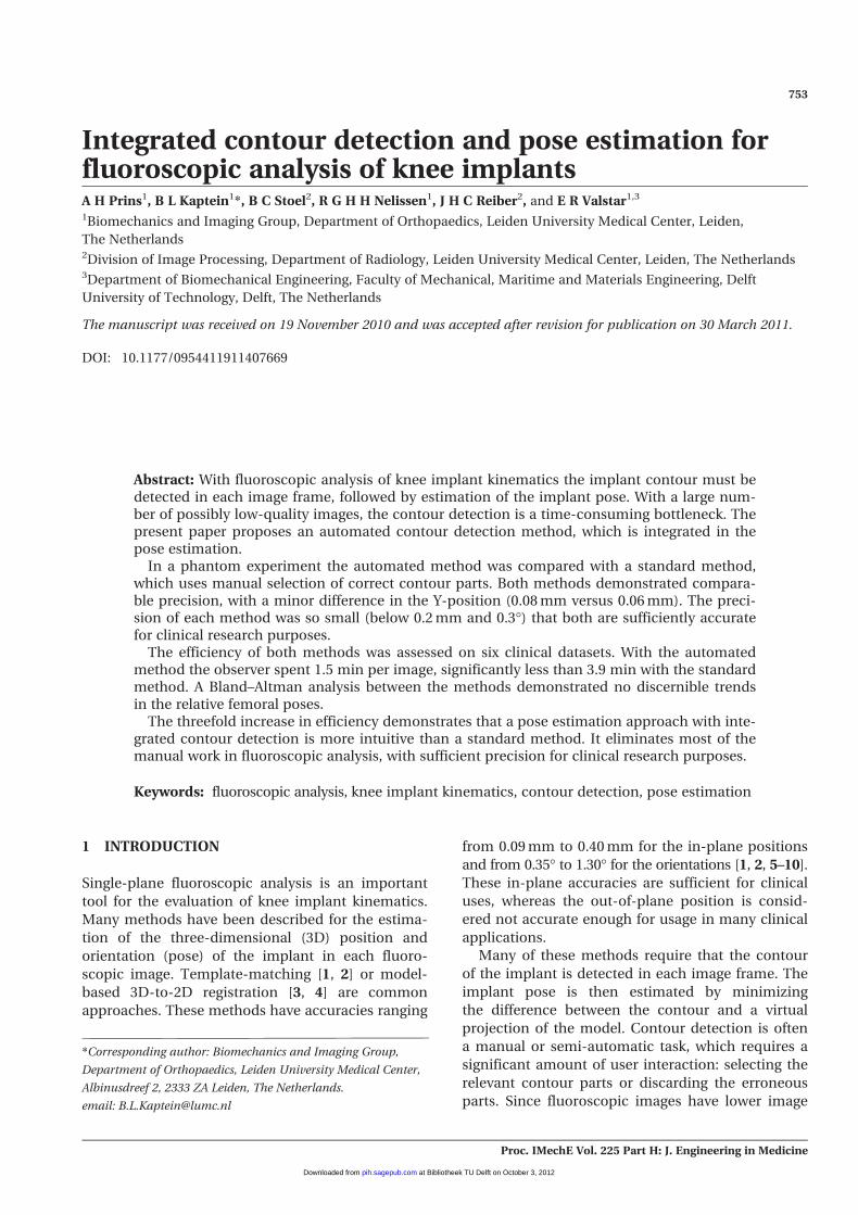
Fig. 1 (A) Contour detection starts with a virtual projection (in white). The image is resampled(counterclockwise as indicated by the arrow) with scan lines perpendicular to the projec-tion. (B) The resulting scan image represents a straightened version of the image regionaround the virtual projection (vertical dashed line) with the original corresponding scanlines indicated by the horizontal lines. Note also the distorted shape of the tibia compo-nent on the left side. (C) A convolution with a positive difference filter ([–1 0 1]) results inthe cost image. Minimal path extraction using dynamic programming then extracts a path(dashed curve). (D) After back-transforming this path, the result is a contour (right image)with associated edge strengths

Integrated contour detection and pose estimation for fluoroscopic analysis of knee implants 755

Proc. IMechE Vol. 225 Part H: J. Engineering in Medicine

at Bibliotheek TU Delft on October 3, 2012pih.sagepub.comDownloaded from

2.2 Contour points selection

The edge strengths are normalized over the entire

contour to a range from [0, 1]. Using a threshold in

the range of [0, 1], the user can specify how much of

the contour should be discarded. Contour points

with an edge strength below the threshold are then

discarded (a threshold of 0.25 was typically used).

From the remaining contour points (those with an

edge strength above the threshold), 20 per cent are

selected, uniformly sampled along the contour, in

order to reduce the computational cost.

2.3 Robust pose estimation

A global optimization method (downhill simplex

method [14] combined with simulated annealing

[15]) finds the pose for which the virtual projection

fits the selected contour points best. To this end, a

weighted distance measure is calculated between

the selected contour points and the virtual projec-

tion of the implant model. The distance measure is

the same as that described by Kaptein et al. [4], with

one addition: the edge strengths from the selected

contour points are used as weights.

3 VALIDATION

3.1 Experimental validation

3.1.1 Experimental set-up

Data were collected from a phantom experiment

using a bi-plane flat-panel fluoroscopic set-up

(Toshiba Infinix super digital fluoroscopy (SDF) sys-

tem; Toshiba Medical Systems Europe, Zoetermeer,

The Netherlands). The phantom study was per-

formed with a size 3 cruciate-substituting PFC-Sigma

prosthesis fixed in sawbones with a 5 mm thick insert

(DePuy Orthopedics, Warsaw, Indiana, USA). A 3D

implant model of the femoral component was

reverse engineered with an accuracy of 0.05 mm

(TNO Industry, Eindhoven, The Netherlands) for use

by the pose estimation methods.

The image intensifiers were positioned perpendi-

cular to each other and the sawbones were placed

such that one image intensifier had a medial–lateral

view, while the other had an anterior–posterior view.

The X-ray focus positions were calculated using a

calibration box [16].

Two motions of the femur were captured (15

frames/s). In the first motion, the femur moved

from full extension to 90� of flexion, followed by an

abduction of approximately 20�, back to 20� adduc-

tion, and finally back to full extension. In the second

motion, the femur started at 30� of flexion and

moved to full extension, after which some internal/

external rotation (roughly 20�) was performed.

A subset of the images (N = 58) was used for the

experiments, capturing a broad range of poses. A

standard model-based pose estimation method

(Model-Based RSA 3.21; Medis Specials, Leiden, The

Netherlands [4]) was applied to the images from

both image intensifiers and this was used as the ref-

erence measurement.

3.1.2 Image quality

The new method was validated on single-plane

fluoroscopic image data using the data from the

phantom experiment, but only from the image inten-

sifier with a medial–lateral view. These data were of

excellent quality; high resolution and high image

contrast. In routine clinical practice, the image quali-

ty is worse and can have an influence on the accu-

racy of contour detection and pose estimation. In

this validation experiment the effects of lower image

quality on the new method were investigated.

The image qualities were assessed as encountered

in ongoing clinical studies. Four quality levels were

defined: L0, L1, L2, and L3. Level L0 has no quality

reduction and serves as a baseline measurement.

Levels L1 to L3 represent good, moderate, and poor

quality, respectively. Each image was degraded

according to these levels with the following method.

1. A template image was created with Simplex

noise [17] which was used as a template for local

intensity reduction. This resulted in different

parts of the image having different intensity lev-

els and was used to crudely simulate different

contrasts, which can arise in clinical practice

due to soft tissue.

2. Locally varying Gaussian noise was introduced

and the overall sharpness of the image was

reduced with a Gaussian blur.

The parameters used, the example images, and

the corresponding clinical images are presented in

Fig. 2.

3.1.3 Estimation of pose and comparisonbetween methods

The new automated method was applied to all

images with an experienced user providing the ini-

tial pose of the model. For comparison, a standard

model-based pose estimation method (Model-Based

RSA 3.21, Medis Specials [4]) was also applied to the

images. In this standard method an experienced

756 A H Prins, B L Kaptein, B C Stoel, R G H H Nelissen, J H C Reiber, and E R Valstar

Proc. IMechE Vol. 225 Part H: J. Engineering in Medicine

at Bibliotheek TU Delft on October 3, 2012pih.sagepub.comDownloaded from

user was responsible for supervising the Canny edge

detection by selecting and cutting out contour parts

and for providing an initial pose. The pose was then

estimated with iterative inverse-perspective match-

ing [18] followed by a global optimization of the dis-

tance measure between the contour points and the

implant model [4].

For both the automated and the standard meth-

ods, the error in pose was calculated as the differ-

ence for each pose parameter with respect to the

pose obtained by the bi-plane reference measure-

ment. Student’s t-test was then used to compare the

mean errors between the standard and automated

method, and Levene’s test to compare the variance

of the differences.

3.2 Clinical validation

Six fluoroscopic datasets were collected from two

patients with a ROCC prosthesis (Biomet, Warsaw,

Indiana, USA) with a total of 266 images. These data

were part of a larger, currently ongoing, clinical

study and informed consent was obtained from the

patients. The datasets were acquired with single-

plane flat-panel fluoroscopy (15 frames/s) while

these patients were performing a step-up task. The

three datasets of one patient were considered of

moderate quality, while those of the other patient

were considered of good quality, comparable to L1

and L2 in Table 1.

An experienced user applied both the automated

and standard methods to each dataset and the total

analysis time was recorded for each method. The

tibial and femoral components were analysed and

the relative poses between the two components were

calculated for each method. To determine the agree-

ment between the two methods, a Bland–Altman

analysis was performed for each pose parameter.

4 RESULTS

4.1 Experimental

All errors in pose for both methods are presented in

Table 1. The mean errors and the standard devia-

tions for the highest and lowest image qualities

Fig. 2 Examples of reduced quality images of the phantom experiment in the first row and theirclinical counterparts on the second row. The intensity range on a scale of [0, 1] is present-ed for each image in the third row, together with the variance for the noise

Integrated contour detection and pose estimation for fluoroscopic analysis of knee implants 757

Proc. IMechE Vol. 225 Part H: J. Engineering in Medicine

at Bibliotheek TU Delft on October 3, 2012pih.sagepub.comDownloaded from

(L0 and L3) are presented in Fig. 3. The most promi-

nent differences are in the systematic errors

between the two methods. The automated method

demonstrates small, but statistically significant

worse systematic errors in the in-plane positions (X:

0.07 mm, Y: 0.08 mm), which is consistent over all

quality levels. The mean error in the less accurate

out-of-plane position increases up to 0.77 mm for

the automated method and is significantly larger

(P\0.001) than with the standard method for all

quality levels.

The standard deviations are highly comparable

between the two methods and, with values being

below 0.1 mm and 0.10�, sufficiently precise for

most clinical uses. For quality levels L1 to L3, the

standard deviation in the Y-position (0.06 mm) of

the standard method is slightly better (P\0.02)

than that of the automated method (0.07 mm on

Fig. 3 Standard deviations of the error in pose with respect to the reference pose measurementfor the automated and standard methods, and the best and the worst level of image quality

Table 1 Means and standard deviations of the errors in position and orientation for both automated and standard

methods on single-plane data, with respect to the reference method (from bi-plane data). The single-plane

data were reduced according to four quality levels

Quality Method

Position Orientation

X Y Z X Y Z

Mean SD Mean SD Mean SD Mean SD Mean SD Mean SD

L0 Standard 20.03* 0.07 20.02* 0.06 0.29* 0.35 0.02 0.09 20.02* 0.08 20.06 0.21Automated 0.07 0.08 0.08 0.07 0.54 0.34 0.03 0.08 20.08 0.07 20.06 0.24

L1 Standard 20.03* 0.08 20.02* 0.05 0.11* 0.44 0.03 0.09* 20.02* 0.07 20.05 0.22Automated 0.06 0.08 0.09 0.07 0.52 0.34 0.03 0.07 20.08 0.09 20.07 0.24

L2 Standard 20.03* 0.08 20.01* 0.05 0.15* 0.47 0.02 0.11 20.04* 0.07 20.06 0.23Automated 0.06 0.08 0.08 0.08 0.58 0.40 0.02 0.08 20.10 0.08 20.06 0.26

L3 Standard 20.03* 0.09 20.01* 0.06 0.20* 0.41 0.03 0.12 20.04* 0.07 20.07 0.23Automated 0.06 0.09 0.08 0.08 0.77 0.55 0.03 0.11 20.11 0.08 20.06 0.26

*Significant difference (P\0.05) between the automated and the standard methods on the same level of image quality.

758 A H Prins, B L Kaptein, B C Stoel, R G H H Nelissen, J H C Reiber, and E R Valstar

Proc. IMechE Vol. 225 Part H: J. Engineering in Medicine

at Bibliotheek TU Delft on October 3, 2012pih.sagepub.comDownloaded from

L0 up to 0.08 mm on L3). When considering the

magnitude of these standard deviations, the two

methods perform very similarly.

4.2 Clinical

On average, an experienced user spent 3.960.36 min

per image with the standard method, whereas the

automated required only 1.560.36 min per image.

This difference was highly significant (P\0.001).

The Bland–Altman plots of the relative pose with

respect to the tibia pose are presented in Fig. 4.

There were no strong trends discernible in the

Bland–Altman plots. The largest differences present-

ed themselves in the out-of-plane position with a

mean difference of 0.77 mm and large standard

deviation of 3.46 mm. A relatively large discrepancy

in the Y- and Z-orientations was found with stan-

dard deviations of 1.11� and 0.98�.

5 DISCUSSION

This study has demonstrated that the contour detec-

tion can be completely integrated within the pose

estimation. The integration of automatic contour

detection enables a more intuitive and thus faster

analysis procedure for the researcher, with only

minor consequences for the accuracy of the system.

Although the systematic errors of the automated

method are consistently higher than the errors of the

standard method, their values in the clinically rele-

vant parameters remain below 0.1 mm and 0.1�. In

addition, the systematic errors are less important

than the standard deviations when investigating

implant kinematics, where the relative motions of the

components are considered. With respect to the stan-

dard deviations, the two methods performed virtually

identically. The only significant difference (0.08 mm

versus 0.06 mm) was found in the Y-position. These

differences are, however, clinically irrelevant.

The systematic errors of both methods (up to

0.08 mm) in the in-plane positions are hard to

explain. On quality level L0, the images to which the

standard and automated methods were applied are

identical to the images used by the reference meth-

od. The standard and reference methods employ the

same technique, except that the reference method

has a second image available from the bi-plane set-

up. It may be that the contour detected in a single

image is slightly off with respect to the actual sil-

houette of the implant. With a pixel size of 0.39 mm,

a difference of e.g. half a pixel could already intro-

duce a systematic shift of 0.1 mm in the pose.

Whereas the bi-plane reference method can correct

for such discrepancies by using the data in the sec-

ond image, this is not possible with the single-plane

Fig. 4 Bland–Altman plots for the agreement in the pose measured by the standard method andthe automated method on the clinical data. The x axes represent the agreement in the poseparameters, calculated as the mean of the two methods. The y axes represent the differ-ence in pose parameter between the two methods. The colours represent the two patientsfrom which the data were obtained. The central dashed line represents the mean differ-ence over all measurements, while the two outer dashed lines the indicate limits of agree-ment for the differences (two standard deviations around the mean)

Integrated contour detection and pose estimation for fluoroscopic analysis of knee implants 759

Proc. IMechE Vol. 225 Part H: J. Engineering in Medicine

at Bibliotheek TU Delft on October 3, 2012pih.sagepub.comDownloaded from

standard and automated methods. The difference in

contour detection method between the standard

and automated methods may then cause the discre-

pancy in the systematic errors between the standard

and automated methods.

The results from the phantom experiment com-

pare well with the results published in the literature

and are more accurate than the literature. Earlier

studies on single-plane fluoroscopy have reported

precisions for estimating positions from 0.09 mm to

0.46 mm and precisions for estimating orientations

between 0.35� and 1.30� [1, 2, 5–7]. Fregly et al. [11]

have demonstrated the effects of X-ray attenuation

on the accuracy of the silhouette in the image and

how this could possibly account for most of mea-

surement bias. Mahfouz et al. [5] demonstrated how

manual segmentation can severely affect the accu-

racy of pose estimation and even recommended a

pose estimation process without ‘manual, a priori

segmentation’. The automated method has no such

‘manual, a priori segmentation’, but instead relies on

an automatic model-based segmentation method.

In the clinical experiments a threefold improve-

ment was found in analysis time with the automated

method, with the added advantage that no continu-

ous supervision by the researcher was required. With

a fluoroscopic dataset of 50 images, a researcher

would spend 75 min with the new automated meth-

od and 195 min with the standard method.

The lack of a good reference measurement in the

clinical data makes it difficult to determine the

accuracy of the two methods. The two methods

show differences within 1 mm and 1� for all orienta-

tions and positions, respectively, except for the out-

of-plane position where the differences can be as

high as 7 mm. These values are comparable with the

earlier mentioned ranges from the literature.

A difficult problem arose with the tibial orienta-

tion in three of the six datasets. For several images,

there was some ambiguity in the silhouette of the

tibial component. Its silhouette was such that both

pose estimation methods had to choose from two or

sometimes three pose candidates. In those cases it

could be that the standard and automated methods

picked different pose candidates, resulting in differ-

ences in measured orientations of a few degrees.

This is likely an issue with any pose estimation

method and could have caused the relatively large

differences in Y-orientation and Z-orientation.

When dealing with patient data, the motion

between two consecutive images can be large.

Extrapolation of the pose from one image to the

next [3] can then put the implant model too far

away from its new silhouette. This can cause the

automatic model-based contour detection to fail,

when the detection region on the image around the

virtual projection of the model is too small to cap-

ture enough parts of the new contour. To overcome

this problem, the detection region can be enlarged.

However, this adds the risk that another strong con-

tour instead of the implant contour is found, e.g. the

skin-to-air transition. In those cases it was easier for

the user to update the model pose interactively and

then continue the analysis.

A possible limitation of the present study is that

only two implants were assessed. Another potential

issue may be the lower accuracies in the clinical

data, compared with the phantom data. This will

make it less straightforward to generalize the results

to other implant types. Nevertheless, the main prin-

ciple of using the 3D surface model to guide contour

detection is independent of specific features of the

tested implants. Similar improvements in analysis

time can therefore be reasonably expected when

applying the method to other implant types, without

general loss of accuracy.

Overall, a pose estimation approach was demon-

strated with integrated contour detection, which

yielded precise poses in the clinically relevant

directions (below 0.2 mm and 0.3�). The easier

workflow, the omission of a semi-automatic con-

tour detection, eliminates most of the manual work

in fluoroscopic analysis. This makes the method

more objective and results in a threefold reduction

in analysis time.

ACKNOWLEDGEMENTS

This project was sponsored by the European

Community Project DeSSOS IST-2004-27252.

� Authors 2011

REFERENCES

1 Banks, S. and Hodge, W. Accurate measurementsof three-dimensional knee replacement kinematicsusing single-plane fluoroscopy. IEEE Trans.Biomed. Engng, 1996, 43(6), 638–649.

2 Hoff, W., Komistek, R., Dennis, D., Walker, S.,Northcut, E., and Spargo, K. Pose estimation ofartificial knee implants in fluoroscopy images usinga template matching technique. In Proceedings ofthe 3rd IEEE Workshop on Applications of compu-ter vision (WACV’6), 1996, pp. 181–186.

3 Zuffi, S., Leardini, A., Catani, F., Fantozzi, S., andCappello, A. A model-based method for the recon-struction of total knee replacement kinematics.IEEE Trans. Med. Imag., 1999, 18(10), 981–991.

4 Kaptein, B., Valstar, E., Stoel, B., Rozing, P., andReiber, J. A new model-based RSA method validated

760 A H Prins, B L Kaptein, B C Stoel, R G H H Nelissen, J H C Reiber, and E R Valstar

Proc. IMechE Vol. 225 Part H: J. Engineering in Medicine

at Bibliotheek TU Delft on October 3, 2012pih.sagepub.comDownloaded from

using CAD models and models from reversed engi-neering. J. Biomech., 2003, 36(6), 873–882.

5 Mahfouz, M., Hoff, W., Komistek, R., andDennis, D. Effect of segmentation errors on 3D-to-2D registration of implant models in X-ray images.J. Biomech., 2005, 38(2), 229–239.

6 Komistek, R., Dennis, D., and Mahfouz, M. In vivofluoroscopic analysis of the normal human knee:knee kinematics and total knee replacementdesign. Clin. Orthop. Relat. Res., 2003, (410), 69–81.

7 Kanisawa, I., Banks, A., Banks, S., Moriya, H., andTsuchiya, A. Weight-bearing knee kinematics insubjects with two types of anterior cruciate liga-ment reconstructions. Knee Surg. Sports Traumatol.Arthrosc., 2003, 11(1), 16–22.

8 Li, G., Wuerz, T. H., and DeFrate, L. E. Feasibilityof using orthogonal fluoroscopic images to mea-sure in vivo joint kinematics. J. Biomech. Engng,2004, 126(2), 313–318.

9 Garling, E., Kaptein, B., Geleijns, K., Nelissen, R.,and Valstar, E. Marker configuration model-basedroentgen fluoroscopic analysis. J. Biomech., 2005,38(4), 893–901.

10 Hanson, G. R., Suggs, J. F., Freiberg, A. A.,Durbhakula, S., and Li, G. Investigation of in vivo6DOF total knee arthroplasty kinematics using adual orthogonal fluoroscopic system. J. Orthop.Res., 2006, 24(5), 974–981.

11 Fregly, B., Rahman, H., and Banks, S. Theoreticalaccuracy of model-based shape matching for mea-suring natural knee kinematics with single-planefluoroscopy. Trans. ASME, 2005, 124(4), 692–699.

12 Canny, J. A computational approach to edge detec-tion. IEEE Trans. Pattern Anal. Machine Intell.,1986, 8(6), 679–698.

13 Bellman, R. E. and Dreyfus, S. E. Applied dynamicprogramming, 1962 (Princeton University Press,Princeton, New Jersey, USA).

14 Nelder, J. and Mead, R. A simplex method for func-tion minimization. Comput. J., 1965, 7(4), 308–313.

15 Kirkpatrick, S. Optimization by simulated anneal-ing: quantitative studies. J. Stat. Phys., 1984, 34(5),975–986.

16 Koning, O., Kaptein, B., Garling, E., Hinnen, J.,Hamming, J., Valstar, E., and van Bockel, J. Assess-ment of three-dimensional stent-graft dynamicsby using fluoroscopic roentgenographic stereopho-togrammetric analysis. J. Vasc. Surg., 2007, 46(4),773–779.

17 Perlin, K. Noise hardware. In Real-time shading(SIGGRAPH Course Notes) (Ed. M. Olano), 2001,ch. 2.

18 Wunsch, P. and Hirzinger, G. Registration of CAD-models to images by iterative inverse perspectivematching. In Proceedings of the 1996 InternationalConference on Pattern recognition, 1996, vol. 1, 78–83.

Integrated contour detection and pose estimation for fluoroscopic analysis of knee implants 761

Proc. IMechE Vol. 225 Part H: J. Engineering in Medicine

at Bibliotheek TU Delft on October 3, 2012pih.sagepub.comDownloaded from