Oscillations in SIRS model with distributed delays

arX

iv:0

912.

1250

v3 [

q-bi

o.PE

] 3

0 Se

p 20

10

Oscillations in SIRS model with distributed delays

Sebastian Goncalves1, G. Abramson2 and Marcelo F. C.

Gomes1

1Instituto de Fısica, Universidade Federal do Rio Grande do Sul,Caixa Postal 15051,

90501-970 Porto Alegre RS, Brazil2Centro Atomico Bariloche, CONICET and Instituto Balseiro, 8400 S. C. de

Bariloche, Argentina

E-mail: [email protected]



http://arxiv.org/abs/0912.1250v3

Oscillations in SIRS model with distributed delays 2

Abstract. The ubiquity of oscillations in epidemics presents a long standing

challenge for the formulation of epidemic models. Whether they are external and

seasonally driven, or arise from the intrinsic dynamics is an open problem. It is known

that fixed time delays destabilize the steady state solution of the standard SIRS model,

giving rise to stable oscillations for certain parameters values. In this contribution,

starting from the classical SIRS model, we make a general treatment of the recovery

and loss of immunity terms. We present oscillation diagrams (amplitude and period)

in terms of the parameters of the model, showing how oscillations can be destabilized

by the shape of the distributions of the two characteristic (infectious and immune)

times. The formulation is made in terms of delay equation which are both numerical

integrated and linearized. Results from simulation are included showing where they

support the linear analysis and explaining why not where they do not. Considerations

and comparison with real diseases are presented along.

PACS numbers: 87.19.X-, 87.23.Cc

1. Introduction

Many diseases that have affected and still affect humans come and go with time in a well

established way. Examples are plenty and fill the bulletins of world and national health

organizations. Measles, typhus and cholera epidemic waves, just to cite a few, are even

part of mathematical biology books [1, 2]. The common denominator of such diseases is

the cyclic natural history of them, in which a susceptible subject can go to infected, then

to removed, and finally back to the susceptible state. However, the mere cyclic nature of

the disease does not grant an oscillatory behavior of its epidemic, as can be exemplified

by gonorrhea [3, 4]. In 2009 a new variant of influenza A H1N1, dubbed swine flu,

appeared in the scene taking the media to discuss on the wave behavior of influenza.

In which way do these oscillations arise in a population, apparently synchronizing the

infective state of many individuals? Are they related to external driving causes, such as

the seasons? Or do they arise dynamically from the very natural history of the disease?

It is known that several causes can produce oscillations in model epidemic systems:

seasonal driving [5], stochastic dynamics [6, 7], a complex network of contacts [8], etc.

In every infectious disease several characteristic times clearly appear in the

dynamics. In a SIRS type disease (see figure 1) one has an infectious time (during

which the agent stays in category I, infected and infectious), and an immune time

(during which the agent stays in category R, recovered from infection, and immune to

re-infection until it returns to the susceptible class S). A standard SIRS model uses the

inverse of these characteristic times as rates in mass-action equations, showing damped

oscillations toward the endemic state in most typical situations. However, the standard

SIRS model does not exhibit sustained oscillations for any value of the parameters.

Would it be possible for a deterministic SIRS model to sustain oscillations, and if so

how do the characteristic times relate to the period of the epidemic? These are some of

the questions we address in this contribution.


As observed by Anderson and May [1] the mathematically convenient treatment of

the duration of the infection as a constant rate is rarely realistic. It is more common

that recovery from infection takes place after some rather well defined time. It would

seem a valid simplification to assume that recovery happens exactly at a given time,

instead of continuously at some rate. Both extremes are called Type B and Type A

recovery respectively by Anderson and May. Most infections belong to an intermediate

type between these two extremes (but closer to Type B). These intermediate types have

an infectious time distributed with a shape between that of an exponential (Type A)

and that of a delta distribution (Type B). An accurate model should implement the

distributions based on empirical data. And as suggested by Hoppenstaedt and others

[9], that could be done replacing the simple constant rate term by an integral, leading to

integro-differential equations. Similar considerations can be made about the transition

from recovered to susceptible term. It is almost thirty years ago that Hethcote et al [10]

showed precisely that the SIRS model with fixed delay in the recovered to susceptible

transition presents stable periodic solution for certain parameter values. On the other

side they demonstrated that fixed delay in the recovery from infection term does not

have the same effect when the other one is considered in the usual way. This implies

that the immunity time plays the most important role in the emerging oscillations as we

will show in detail. Recently, continuing with the work of Hethcote et al , Taylor and

Carr [11] studied in detail the dynamics of the SIRS model with temporary immunity,

but considering that a fraction of the population acquire permanent immunity. In other

words, that is equivalent to a distribution of immunity times made of two delta peaks

(at a finite time and at infinite). That makes the analysis of the oscillations much

more involved because of the extra parameter: the fraction of individuals who became

permanently removed.

Our contribution can be regarded as an extension of the work of Hethcote et al

with time delays, in which we use arbitrary distributions of both infectious and immune

times. While doing this we want to keep the problem as simple as possible in terms

of parameters, thus we avoid the use of vital dynamics. We start by considering the

most extreme case: fixed delay in both terms (delta distributions). This is the simplest

mathematical case in terms of delays, and it is close related with the first case studied

by Hethcote et al.[10]. Then, we consider a mono-parametric family of models in which

the times are described by continuous distributions —being possible to go continuously

from a Type B to a Type A model for example. In other words we go from the SIRS

model with deterministic delays to the classical constant rates SIRS, taking all the

intermediate situations in between. In this way, while we cover previous results, we can

go further considering the most general situation for a SIRS model.

For delayed models, we analyze the onset of sustained oscillations and characterize

them with the parameters of the system. Linear analysis, together with numerical

solutions of the nonlinear model, provide a clear characterization of the phenomenon.

Stochastic numerical simulations provide further support to our analysis. Moreover,

we show the effect of the shape of the distributed delays on the stabilization of the


oscillations. Besides, the oscillations period, which may play an important role in the

design of intervention policies, are shown to satisfy general rules in terms of the SIRS

parameters.

2. SIRS model with arbitrary recovery and loss of immunity dynamics

As mentioned above, the usual formulation of a SIRS model implies that recovery from

infection, I → R, proceeds at a rate which is independent of the moment of infection.

Also, the loss of immunity R → S is also just proportional to the current sub-population

and proceeds at its own rate. The mathematical formulation of such a model is usually

presented in terms of differential equations as follows:

ds(t)

dt= −β s(t) i(t) +

r(t)

τr, (1a)

di(t)

dt= β s(t) i(t) −

i(t)

τi, (1b)

dr(t)

dt=

i(t)

τi−

r(t)

τr, (1c)

where s(t), i(t) and r(t) stand for the corresponding fractions of susceptible, infectious

and recovered individuals in the population (s(t) + i(t) + r(t) = 1). The parameters

of the model are β, the contagion rate per individual, and τi and τr, the characteristic

infectious and immunity periods respectively‡

The analysis of more general systems —in which the recovery from infection and

loss of immunity processes obey more general and more realistic dynamics— is more

involved, leading to non-local integro-differential equations. Before proceeding to the

most general situation, we analyze the simplest case of fixed times.

2.1. SIRS with fixed infectious and immunity times

Let us assume that the disease is characterized by an infectious time τi as well as

an immunity time τr. That is, an individual that becomes infectious at time t will

deterministically recover at time t + τi, becoming immune, and will subsequently loose

its immunity at time t + τi + τr ≡ t + τ0, becoming susceptible again. The process is

schematically depicted in figure 1. This system can be represented by the following set

S I R S

contagionτI τ

Rtime

Figure 1. Timeline of an individual, showing the course of the disease after contagion.

‡ Note on nomenclature: the infectious time is frequently called as recovery time as well, because it

marks the passage from I to R which is the recovery from infection. While we prefer the first name,

in order to avoid ambiguities with labels we associate them to the classes, i.e.: τi is the time in the

infective class, τr is the time in the recovered class.


of equations for the fraction of susceptible and infectious sub-populations (bear in mind

that r(t) = 1 − s(t) − i(t), so that just two equations describe the dynamics):

ds(t)

dt= −β s(t) i(t) + β s(t − τ0) i(t − τ0), (2a)

di(t)

dt= β s(t) i(t) − β s(t − τi) i(t − τi). (2b)

Before proceeding with the detailed analysis of the above formulation of the SIRS

model we show in figure 2 a result in advance, comparing the time evolution of the

fraction of infectives in the two scenarios: the SIRS with two fixed time delays and the

standard SIRS. The last one produce the well know behavior of damped oscillations

toward the endemic state. Using the same parameters (β = 0.4, τi = 5, τr = 50) the

SIRS with two delays shows clearly the sustained peaked oscillation in the infective

fraction. The time delay in the removed to susceptible transition instead of the usual

continuous rate transition is the responsible for the oscillation as we will see in the

next sections. In general, delay equations applied to SIR like models have noticeable

effects on the dynamics, that is different forms of the infection time distribution yield

different dynamics for the infectives and susceptibles [12]. The example of figure 2 is a

remarkable case.

0 100 200 300 400time (arbitrary units)

0

0.1

0.2

0.3

frac

tion

of I

nfec

tives

SIRS standardSIRS with delay

Figure 2. Time evolution of the fraction of infected individuals for the SIRS model.

Comparison between the numerical solutions for the standard and the two fixed time

delays formulation. Parameters are β = 0.4, τi = 5, τr = 50.

In equations (2a-2b), the first terms represents the contagion of susceptible by

infectious ones, which occurs locally in time at a rate β. The second terms account

for loss of infectivity (2b) and loss of immunity (2a). Both terms correspond to the

individuals infected at some earlier time: t − τi and t − τ0 respectively, and who

have proceeded through the corresponding stage of the disease. These equations must

be supplemented with initial conditions, appropriate for interesting epidemiological

situations. A reasonable choice, which we use in the remaining of the paper, is an

introduction of infectious subjects into a completely susceptible population:

s(0) = 1 − i0, i(0) = i0, r(0) = 0. (3)


The system (2a-2b) has the drawback that any pair of constants (s0, i0) satisfies

them, apparently indicating that any pair of values are equilibria. The origin of this

problem lies in the fact that (2a-2b) together with (3) do not constitute a well-posed

differential problem. Due to the non-locality in time, extended initial conditions must

be provided. Mathematically, it is usual to provide arbitrary functions s(t) and i(t)

in the interval [−τ0, 0). From an epidemiological point of view, however, it is more

reasonable to provide just the initial conditions at t = 0, and complementary dynamics

in the intervals [0, τi): no loss of infectivity or immunity, just local contagion; and [τi, τ0):

transitions from I to R (the second term of (2a) being absent), and the functions s(t), i(t)

already obtained by the initial dynamics.

Indeed, this is the most reasonable choice for the numerical solution of the system,

and it is the one we have followed in the numerical results shown below. For the analysis

of equilibria, however, an integral representation of the system results into a better-posed

problem and the difficulties for the calculation of the equilibria disappear.

An integral equation equivalent to (2b) is:

i(t) = c1 + β∫ t

t−τi

s(u) i(u) du, (4)

the interpretation of which is immediate: the integral sums over all the individuals that

got infected since time t − τi up to time t. These are all the infectious at time t, since

those infected before have already recovered. The integration constant c1 is, in principle,

arbitrary, but it is easy to see that it must be zero since no other sources of infectious

exist beyond those taken into account by the integral term.

Complementing (4) it is convenient to write the equation for 1 − r = s + i, which

cancels out the first terms in (2a-2b):

s(t) + i(t) = c2 − β∫ t−τi

t−τ0

s(u) i(u) du, (5)

where, again, c2 is an integration constant. In this case we have c2 = 1 since no other

sources of R exist.

The system (4,5) can be solved for the equilibria of the dynamics, s∗ and i∗. One

obtains:

s∗ =1

βτi, i∗ =

βτi − 1

βτ0, (6)

which coincides with the equilibria found numerically by integrating (2a-2b), and also

corresponds to the same equilibria that can be found in a constant-rate SIRS model

(1a), where the rates of recovery and loss of immunity are 1/τi and 1/τr respectively.

2.2. SIRS with general distribution of infectious and immunity times

The idea behind the fixed-time delays can be generalized to describe more complex

dynamics. Let us start with the infected individuals, which is simpler. Consider a

probability distribution function G(t), representing the probability (per unit time) of

loosing infectivity at time t after having become infected at time 0. Observe that the


fixed-time dynamics is included in this description, when G(t) = δ(t − τi). G(t) can

be used as an integration kernel in a delayed equation for the infectious. Indeed, the

individuals that got infected at any time u < t and cease to be infectious at time t are:

β∫ t

0s(u)i(u) G(t − u)du,

so that the differential-delayed equation for i(t) is:

di(t)

dt= βs(t)i(t) − β

∫ t

0s(u)i(u) G(t − u)du, (7)

analogous to (2b).

A second kernel H(t) must be considered for the loss of immunity process. The

differential equation for susceptible can then be written as:

ds(t)

dt= −βs(t)i(t) + β

∫ t

0

[∫ v

0s(u)i(u) G(v − u)du

]

H(t − v)dv, (8)

where the second term corresponds to individuals that get infected at earlier times, then

loose their infectivity at intermediate times with probability G, and finally recover at

time t with probability H .

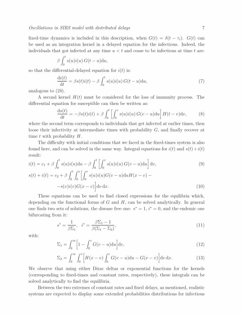
The difficulty with initial conditions that we faced in the fixed-times system is also

found here, and can be solved in the same way. Integral equations for i(t) and s(t)+ i(t)

result:

i(t) = c1 + β∫ t

0s(u)i(u)du − β

∫ t

0

[∫ v

0s(u)i(u) G(v − u)du

]

dv, (9)

s(t) + i(t) = c2 + β∫ t

0

∫ x

0

[∫ v

0s(u)i(u)G(v − u)duH(x − v) −

−s(v)i(v)G(x − v)]

dv dx. (10)

These equations can be used to find closed expressions for the equilibria which,

depending on the functional forms of G and H , can be solved analytically. In general

one finds two sets of solutions, the disease free one: s∗ = 1, i∗ = 0, and the endemic one

bifurcating from it:

s∗ =1

βΣ1

, i∗ =βΣ1 − 1

β(Σ1 − Σ2), (11)

with:

Σ1 =∫

∞

0

[

1 −

∫ v

0G(v − u)du

]

dv, (12)

Σ2 =∫

∞

0

∫ x

0

[

H(x − v)∫ v

0G(v − u)du − G(x − v)

]

dv dx. (13)

We observe that using either Dirac deltas or exponential functions for the kernels

(corresponding to fixed-times and constant rates, respectively), these integrals can be

solved analytically to find the equilibria.

Between the two extremes of constant rates and fixed delays, as mentioned, realistic

systems are expected to display some extended probabilities distributions for infectious


and immunity times. A convenient interpolation between the exponential and delta

distributions that characterize those regimes can be achieved by gamma distributions:

Gpi(t) =

ppi

i tpi−1e−pit/τi

τpi

i (pi − 1)!, (14a)

Hpr(t) =

ppr

r tpr−1e−prt/τr

τpr

r (pr − 1)!. (14b)

These distributions have mean τi and τr respectively, for any value of the parameter

pi,r. Besides, they interpolate between exponential (when pi,r = 1) and Dirac delta

distributions (when pi,r → ∞), with smooth bell-shaped functions for intermediate

values of pi,r. It can be shown that the equilibria (11) are identical to the classical ones

(6) for any pi,r.

3. Sustained oscillations in SIRS with delays

Standard SIRS systems, without delays (or equivalently, with G1(t) and H1(t) as delay

kernels) have either nodes or stable spirals as equilibria. That is, oscillations appear in

them as transient regimes damped towards the fixed points. SIRS systems with delays,

on the other hand, can exhibit sustained oscillations. These appear as a Hopf bifurcation

of the spiral points, controlled by the parameters τi, τr and β. A linear stability analysis

of the fixed-times case can exemplify how this happens.

Assuming that the system (2a-2b) is close to equilibrium, one sets s(t) = s∗ + x(t),

i(t) = i∗ + y(t), obtaining in linear approximation a linear delay-differential system for

the departures from equilibrium:

x(t)/β = −i∗x(t) − s∗y(t) + i∗x(t − τ0) + s∗y(t − τ0), (15a)

y(t)/β = i∗x(t) + s∗y(t) − i∗x(t − τi) − s∗y(t − τi). (15b)

From this system, proposing exponential solutions x(t) = c1eλt and y(t) = c2eλt, a

transcendental characteristic equation is obtained:

λ2 + λβ[

s∗(e−λτi − 1) − i∗(e−λτ 0 − 1)]

= 0. (16)

Equation (16) can be solved numerically for complex λ, obtaining from its real part

the bifurcation line from the stable spirals. This line is shown in figure 3 along with

the amplitude of oscillations represented by a colour (gray) map. The amplitude is

the result of the numerical integration of the full nonlinear system (2a-2b). Figure 3

condenses the bifurcation phenomenon as a function of the key parameters τr/τi and

R0. The black region represents the non oscillating endemic solution. It can be seen

that the linear analysis, represented by the line, defines almost exactly the transition.

3.1. Distributed delays: the general case

The fact that we have qualitatively different results regarding the nature of the endemic

state for a delta or an exponential distribution gives rise to a fundamental question. Is

the existence of an oscillatory endemic state particular to the delta distribution? Or is


0

0.1

0.2

0.3

0.4

2

4

6

8

10

0.5 1 1.5 2 2.5 3 3.5

R0

τr / τi

Figure 3. Bifurcation diagram of the SIRS model with fixed times in the space

defined by τr/τi and R0. The yellow(white) line shows the linear result. The squared

root amplitude of the infectives oscillations is shown as colour (gray) coded shades

above the transition line. The black region means zero amplitude, representing non-

oscillatory endemic states.

there a critical shape of the distributions G and H necessary for the emergence of the

oscillations? Using the Gamma functions defined in (14a) we can check the existence

of such solutions for different shapes by controlling the parameter pi,r. In this way, we

can verify if there is a critical shape pi,r = pc(β, τi, τr) beyond which the system has

sustained oscillations at the endemic state. Linearizing the general system (7,8) in the

same way presented in the previous section, one has the following integral characteristic

equation:

λ2 + λβi∗

[

1 −

∫ t

0

∫ t−v

0H(v)G(u)e−λ(u+v)dudv

]

− λβs∗

[∫ t

0G(u)e−λudu

]

= 0. (17)

Using the distributions (14a) in the equation above and taking the limit t → ∞ we get:

λ2 + λβi∗

1 −

(

1 +λτi

pi

)

−pi(

1 +λτr

pr

)

−pr

− λβs∗

1 −

(

1 +λτi

pi

)

−pi

= 0. (18)

As expected, for pi,r = 1 and pi,r → ∞ we recover the characteristic equations of

the constant rates and fixed delays models, respectively. Solving (18) numerically for

complex λ, one finds that for every set of parameters (provided that R0 = βτi > 1)

where pr > 1 there is always a critical shape pi = pc above which the endemic state

consists of sustained oscillations. Conversely, any value of pr > 1 can present sustained

oscillations in some region of parameter space. Instead, the constant rate model pr = 1

is a particular case where there is no such solution for any set of parameters, as was

demonstrated by Hethcote et al ([10]).

Figure 4 shows the real part of the solution of (18) as a function of the shape

(pi,r = p) of the two time distributions, and for fixed values of the parameters β, τi and

τr. In other words we can appreciate (for those β, τi, τr) the critical p value (pc) to have

oscillations in the SIRS dynamics, i.e. the value at which Re[λ] = 0.


0 1 2 3t

0

0.5

1

1.5

2

Gp(t

)

p=1p=3p=15

0 5 10 15 20p

-0.2

-0.1

0

0.1

Re{

λ}

β = 2 τi = 0.8 τ

r = 16

β = 1 τi = 5 τ

r = 10

Figure 4. Real part of the eigenvalue λ as a function of the shape parameter

pr = pi = p. Inset: examples of the distribution Gp with τi = 1.

The critical shape pc obtained by numerical calculation of (18) gives an accurate

prediction of the emergence of oscillations in the full nonlinear system (7,8), as can be

seen in figure 5. The meaning of the critical shape is simple: the time distributions have

to be narrower than the one represented by pc in order to have sustained oscillations.

10 15 20p

-0,02

0

0,02

Re{

λ}

2000 2020 2040 2060 2080 2100time (arbitrary units)

0,2

0,4

frac

tion

of in

fect

ives

p=12p=13p=14

Figure 5. Numerical integration of the SIRS general model with β = 1, τi = 5, τr = 10

near the critical shape pi,r = pc predicted by the linear analysis of the system (inset,

12 < pc < 13).

The distributions of infectious and immunity times used so far share a common

shape given by the value of p —that made the analysis, restricted to only one shape

parameter, simpler. In real situations, though, it is reasonable to expect that these

uncorrelated kernels have different shapes, not necessarily of the same relative width.

We explore this more general scenario, presenting an oscillation diagram in terms of pi

and pr in figure 6, for two sets of the SIRS parameters. Some interesting conclusion can

be extracted from such diagram:

• If the immunity time distribution is not sharp (pr < 5 for the parameters used in

figure 6) there is no oscillation independent of the type of infection time distribution.


• For a relatively narrow distribution of immunity times there is a critical infective

time width above which (i.e. a critical pi below which) no oscillations are obtained.

• The broader one of the time distribution is, the narrower the other one has to be

in order to have oscillations.

• Longer immunity times (in units of infectious time) makes the oscillatory region

wider in the pi, pr space.

1 5 10 15 20 25 30p

i

1

5

10

15

20

p r

β = 1 τi= 2 τ

r= 10

β = 1 τi= 2 τ

r= 20

non oscillatory region

Figure 6. Oscillation diagram in the pi, pr plane for two sets of parameters: β = 1,

τi = 2, τr = 10 (circles) and β = 1, τi = 2, τr = 20 (triangles).

In the case pi,r → ∞ there is a critical value of R0(τr/τi) above which the endemic

solution is always a stable cycle. The linear analysis also shows that for finite pi,r the

bifurcation is more involved. Figure 7 shows that the bifurcation line encloses a region

of oscillating solutions. Then, for a given value of τr/τi, there is a second critical R0,

larger then the previous one, where the endemic solution ceases to be cyclic. This

phenomenon is verified in the numerical solution of the nonlinear system. For any given

τr/τi, if one increases p the region of oscillation grows (as shown in figure 7), so that

in the limit pi,r → ∞ the upper critical R0 disappears. In such a situation, the only

way to break the oscillations is by decreasing R0. On the other hand, by decreasing

pi,r the oscillatory region shrinks, disappearing completely when pi,r = 1 (exponential

distributions, constant rates).

Yet, the interplay between the uncorrelated shapes pi and pr and the SIRS

parameters is very interesting. Again, in figure 7 we see for example that when

pi = pr = 5 (equal very broad shapes) the oscillation region is very small. But increasing

pi to 20 (narrow infective times distribution), keeping the other fixed, expands the region

considerably. Similarly, but in other part of the same diagram, when pi = pr = 20

(equal very narrow shapes), the region of sustained oscillations is relatively large. Now,

by letting the distribution of infective times to be broader (pi = 5) again with the

other distribution fixed, we see the oscillatory region to shrink significatively. So, while

it is true that the immunity times distribution must be necessarily different from an

exponential in order to have oscillations, in general both distributions are relevant to


define the actual parameter region of oscillations. The narrower one or the two are, the

wider the oscillatory region is.

0 5 10 15 20τ

r / τ

i

0

2

4

6

8

10

R0

p → ∞p = 20p = 12p = 5p

i= 20 p

r= 5

pi= 5 p

r= 20

non oscillatory region

Figure 7. Oscillation diagram in the τr/τi, R0 plane for the SIRS model with different

distribution for infectious and immunity times controlled by the pi,r-shape factor of the

Gamma distribution function. For each pair, pi, pr the oscillatory region is enclosed

by the corresponding line. The curves with only one p are for pi = pr = p.

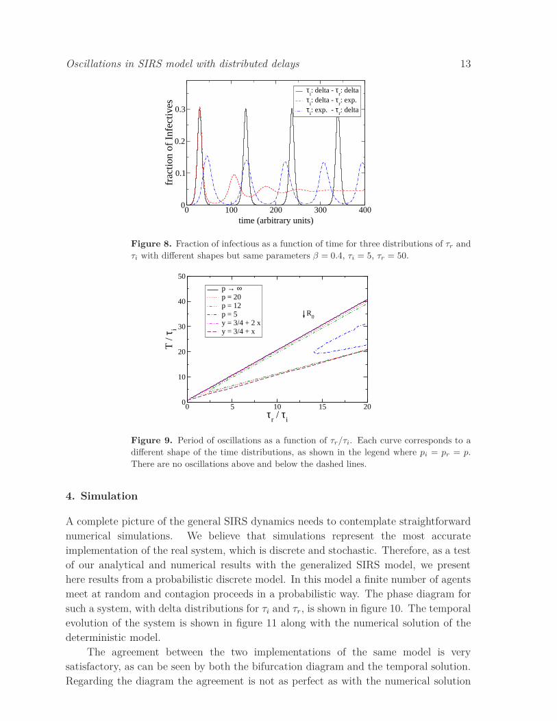
Three examples of dynamics of the SIRS with different shapes sets are displayed

in figure 8. The curves correspond to the numerical solution of systems with the same

epidemic parameters but three different shape sets: (pi = pr = ∞), (pi = 1, pr = ∞),

and (pi = ∞, pr = 1). The first two show the sustained oscillations because the SIRS

parameters are inside the oscillatory region, while in the last case we know that there is

no possible region of oscillation so we have the damped behavior. Besides, we see that

enlarging the τi distribution alone, while it shortens the period of the oscillation, it does

not destabilizes the oscillation. Remarkably it shows an enhancement of the number of

infected during the low part of the cycles. This behavior diminishes the probability of

extinction in a discrete population realization of the system, a problem that is common

in simulations as we will see in the next section.

From the imaginary part of (18) it is possible to obtain the period of oscillations in

the linear approximation. In figure 9 we show the result of this calculation for different

shapes of the distributions of infectious and immunity times. For finite pi,r, the period

of oscillation has a dependency on the parameters that approaches the one found for

pi,r → ∞ (delta distributions, fixed times) in the lower critical value of R0, given by

T = 3/4τi + 2τr. (19)

For a fixed value of τr/τi, this period decreases as R0 increases up to the upper limit

of oscillation, being bounded from below by 3/4τi + τr, as shown in figure 9. There

are no oscillations above and below these two straight lines, for any value of pi,r. This

remarkable lock of the period of disease oscillation is related to the one obtained by

Taylor and Carr ([11]) in the case of exponential distributed τi studied by them.


0 100 200 300 400time (arbitrary units)

0

0.1

0.2

0.3

frac

tion

of I

nfec

tives

τi: delta - τ

r: delta

τi: delta - τ

r: exp.

τi: exp. - τ

r: delta

Figure 8. Fraction of infectious as a function of time for three distributions of τr and

τi with different shapes but same parameters β = 0.4, τi = 5, τr = 50.

0 5 10 15 20τ

r / τ

i

0

10

20

30

40

50

T /

τ i

p → ∞p = 20p = 12p = 5y = 3/4 + 2 xy = 3/4 + x

R0

Figure 9. Period of oscillations as a function of τr/τi. Each curve corresponds to a

different shape of the time distributions, as shown in the legend where pi = pr = p.

There are no oscillations above and below the dashed lines.

4. Simulation

A complete picture of the general SIRS dynamics needs to contemplate straightforward

numerical simulations. We believe that simulations represent the most accurate

implementation of the real system, which is discrete and stochastic. Therefore, as a test

of our analytical and numerical results with the generalized SIRS model, we present

here results from a probabilistic discrete model. In this model a finite number of agents

meet at random and contagion proceeds in a probabilistic way. The phase diagram for

such a system, with delta distributions for τi and τr, is shown in figure 10. The temporal

evolution of the system is shown in figure 11 along with the numerical solution of the

deterministic model.

The agreement between the two implementations of the same model is very

satisfactory, as can be seen by both the bifurcation diagram and the temporal solution.

Regarding the diagram the agreement is not as perfect as with the numerical solution


0

0.1

0.2

0.3

0.4

1

2

3

4

5

2 4 6 8 10

R0

τr / τi

Figure 10. Diagram of the oscillation amplitude, in the τr/τi, R0 plane, obtained by

simulation with N = 1000 agents in the SIRS model with fixed times. Vertical axis is

R0 = βτi, horizontal axis is the ratio τr/τi, and the colour (gray) map represent the

squared root amplitude of the i(t) at the steady state. The black region means zero

amplitude, representing non-oscillatory endemic or non-epidemic states. Superimposed

is the critical line obtained by the linear analysis as in figure 3.

0 2 4 6 8time (years)

0

0.01

0.02

0.03

0.04

0.05

0.06

0.07

0.08

frac

tion

of I

nfec

tives

EquationsSimulations

Figure 11. Evolution of an epidemic with stochastic and deterministic models. Time

distributions are deltas at τi = 10days and τr = 180days, and β = .13perday. With

the time scale in years, the annual oscillation is clearly observed (T = 2τr + 3/4τi =

367days).

of the deterministic equations (figure 3) because of fluctuations that arise in simulation

due to finite size. These cause large amplitude oscillations which become extinct but

that contribute with a non-zero value for the amplitude. As for the temporal evolution,

eventually, as time goes by, a small drift develops in the simulation due to the stochastic

nature of its dynamics. Far from being disappointing this is a desirable feature, since in

real systems epidemic oscillations are not exactly periodic. Yet, the extinctions, that are

normally observed in the simulations, are related with the discreteness of them. Long

time ago discussed by Bartlett [13] and others it manifests here as being very sensitive

to the distance to the lower threshold in the bifurcation diagram, which relates to the


amplitude of the oscillation. Greater amplitudes drive the system closer to the absorbing

state at i = 0. To illustrate this effect we show in figure 12 three dynamics obtained by

simulation with N = 105 for three different values of β, close to the onset of epidemics

and oscillations. However we saw in the previous section (figure 8) that a distribution

of infectious times with finite width can increase the lower values of the infectives cycle,

which eventually may prevent the extinction in the simulation counterpart.

0 2 4 6 8 10time (years)

0

0.01

0.02

0.03

0.04

0.05

0.06

frac

tion

of I

nfec

tives

β = 0.11β = 0.12β = 0.13

Figure 12. Evolution of the epidemic in the stochastic model, showing extinctions of

the infected population. Time distributions are deltas at τi = 10 and τr = 180 days,

N = 105.

5. Conclusions

We have analyzed a general SIRS epidemic model, in which the infective state as well

as the immune state last prescribed times drawn from distributions. These distributed-

time transitions constitute a generalization of the standard SIRS model, in which the

transitions out of the infective and the immune states happen at a constant rate.

The generalization allows for situations in which these states last for certain fixed

times—which is more similar to many real diseases than the constant rate assumption.

Between the two extremes of constant rates and fixed times, we have also analyzed the

intermediate situations of broader or narrower distributions of the transition times.

The generalization runs along the proposals made by previous authors, by

implementing the differential equations of the model as non-local in time. For example

Hethcote etal. have shown that cyclic models have a transition to oscillatory behavior

when the immunity time is distributed [10].

Our contribution shows how the oscillating state arises as a function of all the

parameters of the model, completing a phase diagram that provides a thorough and

general view of the possible behaviors. We show, moreover, that the linear analysis, the

numerical integration of the model, and its stochastic implementation, all converge to

the same general picture, within the inherent limitations of each one.


For delta distributed delays (i.e., for fixed times spent in the infective and recovered

classes), the phase diagram of figure 3 shows that the region of oscillation is bounded

from below by the basic reproductive number R0 as a function of the scaled immunity

time τr/τi. We see that, as τr decreases toward zero, the minimum value of R0 diverges.

This result is in agreement with the fact that in the SIS model there are no sustained

oscillations. On the other hand, the amplitude of the oscillations grows both with R0

and τr/τi. This kind of behavior may be relevant in the analysis of real epidemics where

changes in the parameters are occurring due to interventions, advances in treatment or

natural causes. For example, let us imagine an epidemic in the endemic non-oscillating

region (shaded black in the diagram), for which, as a desirable consequence of the

treatment of the disease, there is an increase in the duration of the immune state,

at constant R0. As a result, the epidemic may start to oscillate. Such a transition

may manifest itself as an initial increase of the infectious fraction, due to the onset of

oscillation, which should be properly understood in the right context.

We have also shown that the transition to oscillations behaves as a critical

phenomenon depending on the width of the time distributions. Figure 4 shows

this behavior. The remarkable stabilization of the oscillations of pertussis after the

introduction of massive vaccination [1, section 6.4.2] may be related to a narrowing of

the immunity time distributions.

For distributed delays, corresponding in our model to values of the parameter

1 < pi,r < ∞, we have found a remarkable reentrance phenomenon in the phase diagram.

As exemplified by figure 7, this reentrance means that the region of oscillations is also

bounded from above by a curve of R0 vs τr/τi. One sees, also, that the region of

oscillation shrinks with lowering pi,r, until its disappearance at the critical value pc.

Only the case pi,r → ∞, corresponding to delta distributed times is unbounded. This

is at variance with the SIR case analyzed by [14] who claims that there is no significant

change between large values of pi,r = p (p = 10-20) and p → ∞. On the other hand our

model supports their result in that the region of oscillations is already large for p in this

range. An important general result that can be derived from this diagram is the fact

that, whenever τr ≫ τi, the minimum value of R0 is very close to 1, implying that such

systems—provided that pi,r is sufficiently large—are very prone to sustained oscillations.

This implies that oscillations due to the implementation of real time distribution into

the SIRS formalism are not a marginal or delicate effect as someone could think before.

Our analysis also shows the behavior of the period of oscillation and its dependence

on system parameters. Is interesting to discuss this aspect of our model in connection

with real infectious diseases. For example in the case of influenza, where the period of

oscillation is more or less a year and the infectious time is of the order of 10 days, our

model predicts oscillations for any R0 > R0min = 1.09. This minimum value is lower

than the usual estimate for this disease, which is around 1.4 [15]. Indeed, this value is

so close to R0 = 1 that one can conclude that there will always be oscillations for this

disease as long as it remains endemic. Besides we see that using a value of τr = 180

days for the loss of immunity, the region of oscillation lays between 1.22 < R0 < 2.4


for a rather wide distribution with pi,r = p = 10, and 1.16 < R0 < 3.4 for a narrower

distribution with p = 30. In the first case, the corresponding period of oscillation is

188 < T < 342 (in days), while on the second one it is 190 < T < 360. Therefore, one

needs a narrow distribution to satisfy the observed period of oscillation for influenza. In

any case, the predicted region of oscillation includes the observed values of R0. We want

to stress that, although an infection by a specific strain of the influenza virus confers

permanent immunity after the infection period, the mutation rate of the virus can be

thought of as an effective immunity period and therefore can also be modeled with the

SIRS dynamics.

In the case of other oscillating epidemics, such as syphilis and pertussis, our model

also fits the observed data rather well. For syphilis, in the pi,r → ∞ case, using the

period of 132 months measured in United States [3] and the usual value of τi = 6 months,

we have an R0min = 1.17 and τr ≈ 6 years. Greater values of R0 (which are expected

for syphilis in [3]), with fixed τi, predict even longer immune times (which is also the

case of syphilis). For pertussis, using the period of 4 years and τi = 1 − 2 months, we

find R0min = 1.06 − 1.15, which is smaller than the estimations obtained for mixing

models [15].

In the open field of oscillatory epidemics, we believe that there is a multiplicity of

causes that can concur to produce the observed phenomena. Our present contribution

does not intend to provide an exclusive and definitive answer to this matter. The

construction of valid theoretical models for real diseases should incorporate all the

relevant mechanisms, therefore a thorough theoretical investigation of any concurrent

possible cause deserves due attention. We hope our work has revealed one good

candidate.

Acknowledgments

This work was supported by a cooperative agreement between Brazilian Coordenacao de

Aperfeicoamento de Pessoal de Nıvel Superior and Argentinian Ministerio de Ciencia y

Tecnologia agencies (grant CAPES-MINCyT 151/08 - 017/07), and by Brazilian agency

Conselho Nacional de Desenvolvimento Cientıfico e Tecnologico (grant CNPq PROSUL-

490440/2007). S.G. and M.F.C.G acknowledge financial support from CNPq, Brasil.

G.A acknowledges support from Argentinian agencies Agencia Nacional de Promocion

Cientıfica y Tecnologica (PICT 04/943), Consejo Nacional de Investigaciones Cientıficas

y Tecnicas (PIP 112-200801-00076), and Universidad Nacional de Cuyo (06/C304).

References

[1] Anderson, R. M. and May, R. M. 1991 Infectious Diseases of Humans: Dynamics and Control,

Oxford University Press.

[2] Murray, J. D. 1993 Mathematical Biology, Springer.

[3] Grassly, N. C., Fraser, C. and Garnett, G. P. 2005 Nature 433, 417-421. doi:10.1038/nature03072

[4] Grenfell, B. and Bjørnstad, O. 2005 Nature 433, 366-367. doi:10.1038/433366a

http://dx.doi.org/10.1038/nature03072

http://dx.doi.org/10.1038/433366a


[5] Abramson, G. and Kenkre, V. M. 2002 Phys. Rev. E 66, 011912. doi:10.1103/PhysRevE.66.011912

[6] Risau-Gusman, S. and Abramson, G. 2007 Eur. Phys. Jour. B 60, 515-520.

doi:10.1140/epjb/e2008-00011-7

[7] Aparicio, J. P. and Solari, H. G. 2001 Math. Biosciences 169, 15.

doi:10.1016/S0025-5564(00)00050-X

[8] Kuperman, M. and Abramson, G. 2001 Phys. Rev. Lett. 86, 2909.

doi:10.1103/PhysRevLett.86.2909

[9] Hoppensteadt, F. C. 1975 Mathematical Theories of Populations: Demographics, Genetics and

Epidemics. In: Regional Conference Series on Applied Mathematics. Philadelphia: SIAM.

[10] Hethcote, H. W. Stech, H. W. and Van Den Driessche, P. 1981 SIAM J. Appl. Math. 40, 1-9.

[11] Taylor, M. L. and Carr T. W. 2009 J. Math. Biol. 59, 841-880.

[12] Gomes, M. F. C. and Goncalves, S. 2009 Physica A 388, 3133-3142 doi:10.1016/j.physa.2009.04.015

[13] Bartlett, M. S. 1957 Journal of the Royal Statistical Society, Series A 120, 48-70.

[14] Black, A. J. McKane, A. J., Nunes, A. and Parisi, A. 2009 Phys. Rev. E 80, 021922-1-9.

doi:10.1103/PhysRevE.80.021922

[15] Hethcote, H. W. 2000 SIAM Review 42, 599-653. doi:10.1137/S0036144500371907

http://dx.doi.org/10.1103/PhysRevE.66.011912

http://dx.doi.org/10.1140/epjb/e2008-00011-7

http://dx.doi.org/10.1016/S0025-5564(00)00050-X

http://dx.doi.org/10.1103/PhysRevLett.86.2909

http://dx.doi.org/10.1016/j.physa.2009.04.015

http://dx.doi.org/10.1103/PhysRevE.80.021922

http://dx.doi.org/10.1137/S0036144500371907

Oscillations in SIRS model with distributed delays

Documents

Transcript of Oscillations in SIRS model with distributed delays