SENSITIVITY TO INFINITESIMAL DELAYS IN NEUTRALEQUATIONSW. MICHIELS y, K. ENGELBORGHS y, D. ROOSE y, AND D. DOCHAIN zAbstract. The stability of a steady state solution of a neutral functional di�erential equationcan be sensitive to in�nitesimal changes in the delays. This phenomenon is caused by the behaviourof the essential spectrum and is determined by the roots of an exponential polynomial. Avellar andHale have considered the case of multiple �xed and nonzero delays. In the �rst part of this papertheir results are illustrated by means of spectral plots. In the second part we extend the theory ofAvellar and Hale to the limit case whereby some of the delays are brought to zero, which may lead tocharacteristic roots with arbitrary large real part. Necessary and su�cient conditions are provided.Using these results we show that the ratio of the delays plays a crucial role when several delays tendto zero simultaneously. As an illustration of the theory, we analyze the robustness of a boundarycontrolled PDE in the presence of a small feedback delay.Key words. neutral equation, sensitivity, characteristic rootsAMS subject classi�cations. 34K40,34K351. Introduction. In this paper we study the behaviour of the roots of the ex-ponential polynomialH(�) , 1�PNj=1 aje���j ; �j 2 R+0 ; aj 2 R; j = 1; : : : ; N(1.1)in the complex plane. H(�) = 0 is the characteristic equation of the functionaldi�erence equation x(t) =PNj=1 ajx(t� �j) which determines the essential spectrumof the solution operator of the neutral functional di�erential equation (NFDE),ddt 0@x(t)� NXj=1 ajx(t� �j)1A = b0x(t)� NXj=1 bjx(t� �j):(1.2)It is well known that the spectrum of equation (1.2) determines the stability of itszero solution since equations of this form satisfy the spectrum determined growthcondition, see [10, Corollary IX.3.1]. However the stability of the zero solution maybe sensitive to arbitrarily small changes in the delays �j . Since this sensitivity iscaused by the essential spectrum, which is determined by equation (1.1), see [9], weperform a detailed study of (1.1). In terms of the characteristic roots of (1.1), thissensitivity is caused by the occurrence of so-called in�nite root chains, sequences ofroots whose imaginary parts grow unbounded, yet whose real parts have a �nite limit.It was shown by Avellar & Hale [1] that, as a consequence, the smallest upper boundc = sup f<(�) : H(�) = 0g is not continuous w.r.t. the delays �j . Hence it is possiblethat arbitrarily small changes in the delays destabilise the NFDE system. This is ofimportance in control problems, since such critical delay changes can be caused by asmall delay in the application of the control action.NFDEs arise for example in models of distributed networks [13, 14], combustion[21] and the control of structures through delayed forcing depending on the accelera-tion [2].yKatholieke Universiteit Leuven, Department of Computer Science, Celestijnenlaan 200A, B-3001Leuven, Belgium, phone +32 16 327537, fax +32 16 327996,fWim.Michiels,Koen.Engelborghs,Dirk.Rooseg@cs.kuleuven.ac.bezUniversit�e Catholique de Louvain, Batiment Euler, 4 av. Georges Lema�tre, B-1348 Louvain-la-Neuve, Belgium, phone +32 10 472378, fax +32 10 472180,dochain@auto.ucl.ac.be1

2 W. Michiels et al.The lack of robustness w.r.t. small changes in the delays is also observed forboundary controlled (hyperbolic) partial di�erential equations [4, 5, 6, 7, 8, 9, 11, 16,20, 22] and feedback controlled descriptor systems [15]: a small delay in the applicationof the control action, which is inevitable in practice due to e.g. measurements or AD-DA conversion, can lead to instability of the stable undelayed system. Hence it isvery important to include all possible delays in the model.In the literature basically two approaches are used to analyse such problems. A�rst approach, which will be followed in this paper, studies directly the in uence ofdelay perturbations on the characteristic roots of equations of the form (1.1). In [1]Avellar & Hale consider equation (1.1) and show that the rational (in)dependencyof the delays plays a crucial role for the robustness properties of the given system.However, in [1] only perturbations of �xed, nonzero delays are considered. Theseresults do not safely apply to the case discussed in this paper, where zero delaysare perturbed to (small nonzero) delays. In the latter case, in�nite root chains occur,whose real part may tend to +1, a phenomenon which does not occur in the presenceof perturbations of (only) nonzero delays. As in [1] we allow a general dependencystructure on the delay perturbations and derive su�cient and necessary conditionsfor the occurrence of characteristic roots with large real part for vanishing delays.Furthermore, we discuss the occurrence of roots with large positive real but smallimaginary part. We prove that the occurrence of these phenomena is determined bywhat we call the 'small delay' part of the characteristic equation (except for somedegenerate cases).On the other hand, for the analysis of a small time-delay in feedback systems,another approach can be followed. In [16, 17] Logemann et al. rewrite the closedloop system as an input-output mapping H(s) with (delayed) unity feedback e��s,where � represents a small feedback delay, and formulate conditions for robustnessand non-robustness of stability against the small time-delay on the open loop transferfunction H(s). They show that, depending on the properties of H(s), a small time-delay may not only result in instability but may also cause characteristic roots witharbitrarily large imaginary and real part. While [17] assumes regularity of H(s),some extensions are made in [16] to the case where H(s) is non-well posed. In [18]Logemann and Townley use this approach to show that when a neutral functionaldi�erential equationddtDxt = Lxt +Bu(t); Dxt = x(t)�Xi Dix(t� hi)(1.3)with control input u(t) has an exponentially unstable di�erence operator D, anystabilising state feedback law is not robust against a small perturbation of the feedbackdelays. Since the essential spectrum is determined by the di�erence equation insidethe di�erentiation operator, such a feedback law should include velocity feedbacku = � ddt �Pj Fjx(t� kj)� ; kj > 0, which leads to a closed loop system with theessential spectrum determined by,det0@I �Xi Die��hi +Xj Fje��(kj+�)1A = 0;(1.4)where � represents a small perturbation in the feedback delays. Since there is onlyone perturbation � on the (�xed and nonzero) delays hi; kj in (1.4), the analysis of

Sensitivity to delays in neutral equations 3this robustness problem can be recasted in the framework of [17]. This procedure isnot possible for the broader class of delay perturbations considered in this paper.Note that for some problems both approaches described above can be used. Forinstance, in Section 6 we apply the theory developed throughout this paper to aboundary controlled wave equation, which was also analysed in [17].In x2 we repeat the main results of [1] and introduce necessary notation. In x3we visualise and interpret these results by means of plots of the characteristic roots,thereby explaining the nature of the instability mechanisms. We explain that thesensitivity of c to arbitrary small changes of the delays is necessarily caused by rootswith large imaginary part. In x4 we motivate with a simple example that the theory of[1, 18] is not su�cient to deal with vanishing delays. We prove under which conditionscharacteristic roots with large real part can occur and give a thorough discussion ofthese results. We conclude in x6 with two illustrative examples.2. Analysis with �xed delays. In this section we brie y describe the mainresults of [1], where the case of �xed and nonzero delays is considered.2.1. De�nitions and notation. Throughout this section we consider the rootsof exponential polynomials of the form,H(�) , 1� NXj=1 aje���j ;(2.1)where we assume that the delays �j are �xed and satisfy 0 < �1 < �2 < : : : < �N .De�ne the collection of the real parts of all the roots of (2.1) as Z,Z = f<(�) : H(�) = 0g ;and denote its closure by �Z. The smallest upper bound of �Z, which is important forstability considerations, is c = sup f<(�) : H(�) = 0g :Assume that the N delays �j , j = 1; : : : ; N , depend on M � N so called inde-pendent delays r1; : : : ; rM : �j = MXk=1 j;krk = j � r(2.2)whereby j = ( j;1; : : : ; j;M ) 2 NM are nonzero vectors with non-negative integercoe�cients and r 2 (0;1)M . Dependency of the kind (2.2) often appears in di�erenceequations arising from practical applications, as for example in (delayed) boundarycontrolled wave equations (see x6). The same holds when dealing with vector valueddi�erence equations. Indeed, the characteristic equation ofx(t) =PMk=1 Akx(t� rk); x(t) 2 Rn ; Ak 2 Rn�n ; l = 1; : : : ;M;is given by det I � MXk=1Ake��rk! = 0;which is seen, using an explicit formula for the determinant, to be an exponentialpolynomial with dependent delays.

4 W. Michiels et al.2.2. Rationally dependent and rationally independent delays. The num-bers r1; r2; : : : ; rM are rationally independent if and only if,MXk=1nkrk = 0; nk 2 Zimplies nk = 0; k = 1; : : : ;M . For example two numbers are rationally independentif their ratio is an irrational number. An important property of rationally independentnumbers which will be used throughout the paper is given by Kronecker's theorem[12, Theorem 444]:Theorem 2.1. Given r = (r1; r2; : : : ; rM ) with rationally independent compon-ents and � = (�1; : : : ; �M ) arbitrary. Then there exists a sequence of real numbersfdngn�1 such that limn!1 ei(dnrk��k) ! 1; k = 1; : : : ;M:We now provide a useful characterisations of �Z(r) and its dependence on r. First,consider the following de�nitions. For any two sets E and F � R and any � 2 R, letd(�;E) = inft2E j�� tj;�(E;F ) = sup�2E d(�; F ) andD(E;F ) = max f�(E;F ); �(F;E)g :The number D(E;F ) is called the Hausdor� distance between the sets E and F .We will illustrate with examples that �Z(r) is not continuous w.r.t. the delays r 2(0;1)M since arbitrarily small delay changes can change their rational (in)dependence.However the following weaker property holds: [1, Lemma 2.5]Theorem 2.2. �Z(r) is lower semicontinuous in r, that is, for each r0 2 (0;1)M ,limr!r0 �( �Z(r0); �Z(r)) = 0:When the delays r are rationally independent, we have [1, Theorem 2.2]Theorem 2.3. �Z(r) is continuous in the Hausdor� metric for rationally inde-pendent delays r.This result is important because it implies the continuity of the supremum c(r) of�Z(r) at rationally independent r. In this case the set �Z(r) is completely characterisedby: [1, Theorem 3.1 & Corollary 3.2]Theorem 2.4. If the components of r are rationally independent then the fol-lowing statements are equivalent: � 2 �Z(r)m9� = (�1; : : : ; �M ) with �k 2 [0; 2�], k = 1 : : :M , such that1�PNj=1 aje�� j �re�i j �� = 0Corollary 2.5. �Z is the union of a �nite number of intervals.The combination of Theorem 2.2 and Theorem 2.3 is very important for con-trol problems because the rightmost characteristic roots determine stability: supposefor example that r0 is given with rationally dependent components and denote themaximum of �Z(r0) by c(r0). On the other hand, consider a sequence of rationally

Sensitivity to delays in neutral equations 5independent delays frngn�1 with limit r0 and denote by c(rn) the maximum of �Z(rn).Then from Theorem 2.2 and Theorem 2.3 it follows thatc(r0) � limn!1 c(rn):(2.3)In other words, the supremum of �Z is always higher when one considers the givendelays as independent. In x3 it will be shown that inequality (2.3) can be strict. Thismeans that when the delays in the characteristic equation modelling a physical systemare results of independent phenomena (for example independent measurements) onehas always to consider the delays as rationally independent in order to obtain a reliableupper bound on the real parts of the spectrum. In x3 it will be explained what happenswith the individual characteristic roots when one deals with rationally independentdelays close to rationally dependent delays.2.3. Special cases.Fully independent delays. This corresponds to the case where M = N , j = ej ,the j-th unity vector in RN and the delays �1; �2; : : : ; �N are rationally independent.Theorem 2.4 can be rewritten as:Theorem 2.6. When the delays are rationally independent c = sup f<(�) : H(�) = 0gsatis�es 1� NXj=1 jaj je�c�j = 0:(2.4)The solution c of (2.4) also serves as a (non-strict) upper bound in the case ofrationally dependent delays.Commensurate delays. This is the case when M = 1. Thus delays �1; : : : ; �n arecommensurate if and only if there exists a real number r such that �j = njr withnj 2 N, j = 1; : : : ; N , i.e. all the delays are integer multiples of a same number. Inthis case equation (2.1) can be rewritten as a polynomial in e��r. As a consequence�Z(r) consists of a �nite numbers of points and the spectrum is vertically periodic withperiod 2�r i.3. Visualisation and interpretation. In the previous section the delays r wereconsidered �xed. When one approaches rationally dependent delays r0, the supremumof the real parts of the characteristic roots can have a discontinuity. First, we illustratehow this discontinuity is compatible with the continuous movement of individual rootsas r approaches r0. Secondly, we discuss the consequences for control applications.3.1. Non-uniform convergence. Consider, as an example, the characteristicequation H(�; h) , 1 + 1:1e�� + 0:2e��(2+h) = 0;(3.1)with delays 1 and 2 + h. When h is zero, (3.1) is a quadratic equation in e�� andthe roots are: � � �1:4704+ i(2l+ 1)�; l 2 Z, and � � �0:1391+ i(2l+ 1)�; l 2 Z.When h > 0 and irrational (and therefore the two delays rationally independent), thesupremum c(h) = supf<(�) jH(�) = 0g satis�es:1� 1:1e�c(h) � 0:2e�c(h)(2+h) = 0;(3.2)which yields limh!0 c(h) � 0:2302 > c(0) � �0:1391. Hence c(h), and the corres-ponding stability of the associated essential spectrum, changes discontinuously with

6 W. Michiels et al.

−2 −1 0 1

−300

−200

−100

0

100

200

300

ℑ(λ

)

ℜ (λ)−2 −1 0 1

−30

−20

−10

0

10

20

30

ℜ (λ)

ℑ(λ

)Fig. 3.1. Part of the spectrum of (3.1) on two di�erent scales for h = 0:01.respect to h. Individual (single) roots however move continuously with respect to thedelays. From 1 + 1:1e�� + 0:2e��(2+h) = 0;one derives d�dh = �0:2�e��(2+h)1:1e�� + 0:2(2 + h)e��(2+h) :But this 'sensitivity' of the individual roots increases to in�nity as their modulusj�j ! 1. Figure 3.1 shows part of the spectrum of (3.1) on two di�erent scaleswhen h = 0:01. When h is reduced to zero, the spectrum converges point-wise andnon-uniformly to the limit case h = 0, as shown in �gure 3.2.3.2. Unstable di�erence equations cannot be stabilised. Consider the fol-lowing control system with input u(t):ddt (x(t) + 2x(t� 1)) = ax(t) + bx(t� �) + u(t):(3.3)When u(t) � 0 the di�erence equationx(t) + 2x(t� 1) = 0(3.4)determines the essential spectrum of the semigroup associated with (3.3), see [10].The zero solution of (3.4) is clearly unstable: all eigenvalues have real part log(2). In[18] it is shown such an equation cannot be stabilised robustly in the presence of asmall time delay in the application of the feedback law.When applying the velocity feedback u(t) = 32 _x(t�1�h), the di�erence equationis modi�ed to x(t) + 2x(t� 1)� 32x(t� 1� h) = 0(3.5)

Sensitivity to delays in neutral equations 7

−2 −1 0 1

−1500

−1000

−500

0

500

1000

1500

ℜ (λ)

ℑ(λ

)

h=0.01

h=0.002

−1 −0.5 0 0.5 1−100

−80

−60

−40

−20

0

20

40

60

80

100

ℜ (λ)

ℑ(λ

)

h=0.01

h=0.01

h=0.002

h=0.002Fig. 3.2. Part of the spectrum of (3.1) for h = 0:01 and h = 0:002.

−1.5 −1 −0.5 0 0.5 1 1.5 2 2.5

−200

−100

0

100

200

300

ℜ (λ)

ℑ(λ

)

uncontrolled

controlled, h=1/100

Fig. 3.3. Part of the spectrum of the uncontrolled system (3.4) and the controlled system (3.5)for h = 0:01.where h models the estimation error of the delay. For h = 0 the di�erence equationis clearly stabilised: all roots have real part � log(2). However for irrational h thesupremum c(h) of the real parts of the spectrum can be calculated from1� 2e�c(h) � 32e�c(h)(1+h) = 0From which follows limh!0 c(h) = log(3:5) > log(2). Thus a practical feedbackdestabilizes the original system even more. This is shown in �gure 3.3.Because sensitivity to small changes of the delays is caused by roots of (2.1) withlarge modulus and because the set of the real parts of the roots of (2.1) is contained ina �nite number of intervals, such roots have large imaginary part. Thus sensitivity toin�nitesimal changes in the delays is caused by modes of very high frequency. This is

8 W. Michiels et al.

−2 −1.5 −1 −0.5 0 0.5 1

−250

−200

−150

−100

−50

0

50

100

150

200

250

h=1/100h=1/500

ℜ λ

h=0

ℑ (

λ)

Fig. 3.4. When h ! 0, the spectrum of (3.5) converges pointwise to the spectrum of x(t) +12x(t � 1) = 0.shown in �gure 3.4. Note, that the control of (3.3) works for low frequency modes whileit does not for high frequency modes (see �gure 3.3). We remark that the questionarises whether the model used is a valid description of the modelled reality for suchfrequencies. In reality one (usually) expects larger damping for larger frequencies.Whether this damping occurs strong and soon enough depends on the particularapplication. In section 4 we will see that our generalisation leads to situations wheresensitivity is not necessarily caused by high-frequency modes.4. Vanishing delays. The analysis in x2 is valid under the assumption thatall the delays are �xed, di�erent and nonzero. These assumptions can be relaxed tothe requirements that �rstly the smallest delays are not arbitrary close to zero andsecondly that the largest delays are not arbitrary close to each other. In this sectionwe explicitly deal with these limit cases. We show that vanishing delays can give riseto roots with unbounded positive real parts, and, that, in a similar way, coincidinglargest delays can give rise to roots with unbounded negative real part. Since thelatter is of less importance for applications we only brie y mention the occurrence ofthis phenomenon.4.1. Introductory example. We investigate the zeros of,H(�; h) = 1 + 2e��h � 12e��;(4.1)as h! 0+.If we set h to 0 in (4.1) all roots ofH(�; 0) are of the form � = � log(6)+i2�l, l 2 Zand the collection of real parts of the roots of H(�; 0) is �Z(0) = f� log(6)g. However,from the analysis of section 2, we know that for h and 1 rationally independent(i.e. h irrational), �Z(h) coincides with the �-components of all solutions (�; �1; �2) ofequation 1 + 2e��he�i�1 � 12e��e�i�2 = 0:(4.2)

Sensitivity to delays in neutral equations 9

−2 −1.5 −1 −0.5 0

−800

−600

−400

−200

0

200

400

600

800

ℜ (λ)

ℑ(λ

)

−50 0 50 100

−800

−600

−400

−200

0

200

400

600

800

ℜ (λ)

ℑ(λ

)

Fig. 4.1. Zeros of (4.1) for h = 0:01 in two di�erent regions of the complex plane.If h goes to 0 in (4.2) we are led to the conclusion thatlimh!0+ �Z(h) = [� log(6);� log(2)];(4.3)i.e., that, although the real part of each individual root of H(�; h) approaches� log(6)as h goes to zero, at the same time the collection of all the real parts of all rootsconverges to (4.3).Figure 4.1 (a) shows part of the roots of equation (4.1) for h = 0:01. At �rst sightthis con�rms the above conclusions. However, if we look at a larger region in thecomplex plane (see �gure 4.1 (b)) we see that there exist additional roots of H(�; h)with quite di�erent behaviour. When h is further reduced the real part of the rootsat <(�) � 69:3 move o� to +1, approximately as the solutions of1 + 2e��h = 0:(4.4)Indeed, if the real part of � is large we cannot set �h to zero. Rather we can neglect12e�� leading to (4.4) and� � 1h (log 2 + i(2l + 1)�) ; l 2 Z:(4.5)Formula (4.5) clearly illustrates that arbitrarily small delays (0 < h� 1) can lead toarbitrarily unstable characteristic roots (<(�) � 1).The situation can be summarised as follows. When h tends to zero the spectrumconsists partly of roots with bounded real part, which can be analysed along the linesof x2, and partly of 'diverging' roots whose real part grows without bound as thesolutions of the `small-delay part' (4.4) of equation (4.1). In the rest of this sectionthese properties will be generalized to the multiple delay case.4.2. Notation. The general form of the exponential polynomial studied withinthis section is, H(�; r; s) = 1�Xi2I aie���i �Xj2J bje���j ;(4.6)

10 W. Michiels et al.where 8i 2 I : �i = i � r; 8j 2 J : �j = j � r + �j � s:and where I = f1; 2; : : : ; N1g; J = fN1 + 1; N1 + 2; : : : ; N1 +N2gare used for notational convenience. The components of r 2 [0;+1)M and s 2[0;+1)L are the independent delays; i 2 NM , j 2 NM and �j 2 NL are vectorswith non-negative integer coe�cients. i and �j are nonzero vectors, that is both haveat least one nonzero element for all i and j. Splitting the independent delays intor and s opens the possibility to deal with a combination of 'normal' and arbitrarilysmall delays by letting r ! 0 combined with constant s > 0. We also extend thede�nition of the inner product '�' to the situation with i 2 NM and R 2 [0;+1]M .Then i � R = MXj=1 i;jRj ;has the usual meaning, except that i;j � (Rj = +1) is taken to be 0 when i;j = 0and +1 otherwise. The underlying rationale for this is that Rj = +1 will be theresult of some limit while the i;j are �xed.4.3. Arbitrarily unstable characteristic roots. The 'small-delay part' of(4.6) is 1�Xi2I aie���i :We now prove how its solutions determine when arbitrarily small delays can lead toarbitrarily unstable characteristic roots.Theorem 4.1. The following statements are equivalent:9� 2 [0; 2�]M ; 9R 2 [0;+1]M such that 1�Pi2I aie� i�Re�i i�� = 0m9 frngn�1 ; fcngn�1 ; fdngn�1with limn!1 cn =1; rn � 0 and limn!1 krnk = 0 and such thatlimn!1H(cn + idn; rn; s) = 0 for �xed s > 0:Proof of +. Consider a (re)ordered partition of R = (R1; : : : ; RK ; RK+1; : : : ; RM )such that R1; : : : ; RK are �nite and RK+1; : : : ; RM are in�nite. That is, let R =(R[1]; R[2]) with R[1] = (R1; R2; : : : ; RK) 2 RK and R[2] = (1;1; : : : ;1) =1M�K .Likewise, consider the corresponding partition for � and i: � = (�[1]; �[2]) and i =( [1]i ; [2]i ) with �[1] = (�1; �2; : : : ; �K) the �rstK components and �[2] = (�K+1; �K+2; : : : ; �M )the remaining M �K components of � and similar for [1]i and [2]i , i 2 I . De�ne theset of indices I1 � I whereby for i 2 I1 the last M �K components of i are zero,that is, where [2]i = 0M�K ; and set I2 = I n I1. Obviously1�Xi2I aie� i�Re�i i�� = 0

Sensitivity to delays in neutral equations 11can be written as: 1�Xi2I1 aie� [1]i �R[1]e�i [1]i ��[1] = 0:Because the components of R[1] may be rationally dependent, consider a sequencefu[1]n gn�1 that converges to R[1] but whereby the components of u[1]n 2 (0;+1)Kare rationally independent for each n. Choose a (strictly positive) sequence of realnumbers f�ngn�1 with limn!1 �n = 0, such thatku[1]n �R[1]k < �n:Because u[1]n has rationally independent coe�cients, due to Theorem 2.1, there exists,for each n, a sequence of real numbers fvn;mgm�1 such thatlimm!1 ei [1]i :(vn;mu[1]n ��[1]) = 1; 8i 2 I1;hence 9m�(n) such that jei [1]i �(vn;m�(n)u[1]n ��[1]) � 1j < �n, 8i 2 I1. Set vn = vn;m�(n).We have created nu[1]n on�1 and fvngn�1 withku[1]n �R[1]k < �n;jei [1]i �(vnu[1]n ��[1]) � 1j < �n; 8i 2 I1; andlimn!1 �n = 0:Choose further nu[2]n on�1 with u[2]n 2 (0;+1)M�K and with limn!1 u[2]n =1M�K ;and de�ne fungn�1 as un = (u[1]n ; u[2]n ) 2 (0;+1)M .We are now in a position to choose a sequence of real parts cn. Choose fcngn�1with cn 2 (0;+1) such that cn goes to in�nity faster than every component of un,that is, such that limn!1 cn = +1 and limn!1 1cnun = 0M . Secondly de�ne asequence of imaginary parts fdngn�1 as dn = cnvn, and a sequence of vanishingdelays, frngn�1 as rn = 1cnun.We now haveH(cn + idn; rn; s)= 1�Pi2I aie�cn i�rne�idn i�rn �Pj2J bje�cn( j �rn+�j �s)e�idn( j �rn+�j �s)= 1�Pi2I aie� i�une�i i�vnun �Pj2J bje�cn( j �rn+�j �s)e�idn( j �rn+�j �s):The second term can be split in �rstlyPi2I1 aie� i�une�i i�vnun whereby the lastM�K components of i are zero and thus i�un = [1]i �u[1]n and secondlyPi2I2 aie� i�une�i i�vnunwhereby limn!1 i � un = +1.Hence H(cn + idn; rn; s)= 1�Pi2I1 aie� [1]i �R[1]e�i [1]i ��[1]e� [1]i �(u[1]n �R[1])e�i [1]i �(vnu[1]n ��[1])�Pi2I2 aie� i�une�i i�vnun �Pj2J bje�cn( j �rn+�j �s)e�idn( j �rn+�j �s)= 1�Pi2I1 aie� [1]i �R[1]e�i [1]i ��[1] e� [1]i �(u[1]n �R[1])| {z }!1 e�i [1]i �(vnu[1]n ��[1])| {z }!1�Pi2I2 aie� !1z }| { i � une�i i�vn�un �Pj2J bje� !1z }| {cn 6=0z }| {�j � se�cn j �rne�idn( j �rn+�j �s)tends to zero as n approaches in�nity which completes this part of the proof.

12 W. Michiels et al.Proof of *. The limn!1H(cn + idn; rn; s) = 0 implieslimn!1 1�Xi2I aie� i�cnrne�i i�dnrn = 0(4.7)because the other term vanishes at in�nity.Consider the sequence fcnrngn�1 with elements cnrn = (cnrn;1; : : : ; cnrn;M ). Foreach sequence of the k-th component, fcnrn;kgn�1, there are two possibilities as ntends to in�nity: the sequence is unbounded (with or without limit), or the sequenceis bounded (with or without limit). Suppose that fcnrn;kgn�1 is unbounded. Thenthere exists a subsequence with limit in�nity. When, on the other hand, fcnrn;kgn�1is bounded, a subsequence with �nite limit exists.This way one can repeatedly construct subsequences to obtain an in�nite set ofindices S1 such that for each k 2 f1; 2 : : : ;Mg, limn!1;n2S1 cnrn;k exists in [0;+1].We still have, limn!1;n2S1 1�Xi2I aie� i�cnrne�i i�dnrn = 0;(4.8)and because each i is a vector of integer coe�cients, e�i i�dnrn equals e�i i�((dnrn)mod2�)and thus limn!1;n2S1 1�Xi2I aie� i�cnrne�i i�((dnrn)mod 2�) = 0:Consider the sequence of vectors f(dnrn)mod 2�gn�1;n2S1 which is bounded and thuscontained in a compact set (w.r.t. some norm). Consequently it must have a conver-ging subsequence, denoted by the indices S2 � S1. Finallylimn!1;n2S2 1�Xi2I aie� i�cnrne�i i�((dnrn)mod 2�) = 0;and we de�ne Rk = limn!1;n2S2 cnrn;k 2 [0;+1]; k = 1; 2; : : : ;M;and �k = limn!1;n2S2(dnrn;k)mod 2� 2 [0; 2�]; k = 1; 2; : : : ;M:Hence we have de�ned every component of R and � and by its construction it follows1�Xi2I aie� i�Re�i i�� = 0;which completes the proof. �We now strengthen the results of the previous theorem: we prove the existenceof a sequence of roots �n of H(�; rn; s) = 0 with real part tending to +1, in otherwords, that arbitrarily small delays cause roots with arbitrarily large real part.Theorem 4.2. Consider the statements:(a) 9� 2 [0; 2�]M ; 9R 2 [0;+1]M such that 1�Pi2I aie� i�Re�i i�� = 0,

Sensitivity to delays in neutral equations 13(b) 9i 2 I such that i � R 6= 0 and i �R 6= +1,(c) 9 frngn�1 ; f�n = en + ifngn�1 with limn!1 en = +1; rn � 0 andlimn!1 rn = 0M such that H(�; rn; s) = 0.Then the following holds:1. (a) and (b) ) (c)2. (c) ) (a)The special case where statement (a) holds but statement (b) is violated, is treatedseparately in subsection 4.5. This corresponds to a degenerate case where the 'smalldelay part' of the characteristic equation doesn't provide enough information aboutthe existence of roots with large real part for vanishing delays.Proof of 2. Trivial (theorem 4.1).Proof of 1. Following theorem 4.1 there exist sequences frngn�1, fcngn�1, fdngn�1with limn!1 cn = +1, rn � 0 and limn!1 rn = 0M such thatlimn!1H(cn + idn; rn; s) = 0and the proof provided us with a way to construct such sequences.Choose f�ngn�1, nu[1]n on�1 and fvngn�1 as in theorem 4.1 and such that�����1�Xi2I1 aie� [1]i �R[1]e�i [1]i ��[1]e� [1]i �(u[1]n �R[1])e�i [1]i �(vnu[1]n ��[1])����� < e�n:Further requirements on the decay-rate, which can be chosen arbitrarily fast, will begiven later in the proof (see formulae (4.9) and (4.10)). Choose fcngn�1 as cn =n, nu[2]n on�1 as u[2]n = pn(1; 1; : : : ; 1), fdngn�1 as dn = vncn, fungn�1 as un =(u[1]n ; u[2]n ), and frngn�1 as rn = 1cnun.Consider the functions �Hn(�) = cnH(�; rn; s). Using the particular choices aboveit is straightforward to show thatlimn!1 �Hn(cn + idn) = 0; limn!1 d �Hnd� (cn + idn) = Q;where Q = Xi2I1 ai [1]i � R[1]e� [1]i �R[1]e�i [1]i ��[1] 2 C ;and limn!1 dk �Hnd�k (cn + idn) = 0; k � 2:Around cn + idn the analytic function �Hn can be expanded as�Hn(�) = 1Xk=0 dk �Hnd�k ����cn+idn (� � (cn + idn))k;and when de�ning � = �� (cn + idn),�Hn(�) = 1Xk=0 dk �Hnd�k ����cn+idn �k;

14 W. Michiels et al.We will now show that �Hn(�) converges uniformly on j�j � 1 to the function �H(�) =Q� or equivalently that the functionDn(�) = �Hn(�)�Q�converges uniformly to zero in j�j � 1. In the appendix it is shown (lemma A.1) thatthis implies that �Hn(�) has a root near � = 0 for su�ciently large n when Q 6= 0. Oneshould emphasize that � is in fact a local coordinate depending on n: we compare thelocal behaviour of each function �Hn(�) near cn + idn with �H(�) = Q�.To construct an upper bound on jDn(�)j for j�j � 1, �rst de�ne strictly positivenumbers �i, �j , �i and integer P such that for n � P , j � rn � �j ; j 2 J; i � cnrn � [1]i �R[1] +�i; i 2 I1; i � rn � 1; i 2 I = I1 [ I2 and i � cnrn � �ipn; i 2 I2:Secondly the decay rate of f�ngn�1 should have been chosen in such a way thatfor n � P n �����1�Xi2I1 aie� i�cnrne�i i�dnrn����� � 1nXi2I1 jaij(4.9)and �����Xi2I1 ai i � cnrne� i�cnrne�i i�dnrn �Q����� � 1nXi2I1 jaij( [1]i �R[1] +�i):(4.10)In this way we can compute bounds for Dn(0) and its derivatives in � = 0, n � P .jDn(0)j � n ��1�Pi2I1 aie� i�cnrne�i i�dnrn��+ n ��Pi2I2 aie� i�cnrne�i i�dnrn��+nPj2J ��bje��j �scne� j �cnrne�i j �dnrn��� 1nPi2I1 jaij+Pi2I2 ne��ipnjaij+Pj2J ne�n�j �sjbj jand concerning the derivatives:jdDnd� (0)j � 1nPi2I1 jaij( [1]i �R +�i) +Pi2I2 ne��ipnjaij+Pj2J n(�j + �j � s)e�n�j �sjbj jand for k � 2,jdkDnd�k (0)j � 1nPi2I1 jaij( [1]i �R[1] +�i) +Pi2I2 ne��ipnjaij+Pj2J n(�j + �j � s)ke�n�j �sjbj j:Finally, for each � with j�j � 1,jDn(�)j � P1k=0 1k! jdkDd�k j� Pi2I1 1n jaij( [1]i � R[1] +�i)P1k=0 1k! +Pi2I2 ne��ipnP1k=0 jaij 1k!+Pj2J ne�n�j �sjbj jP1k=0 (�j+�j �s)kk!� Pi2I1 1n jaij( [1] � R[1] +�i)e+Pi2I2 ne��ipnjaije+Pj2J ne�n�j �sjbj je(�j+�j �s)

Sensitivity to delays in neutral equations 15can thus be bounded uniformly whereby the upper bound tends to zero as n!1.Because the series f �Hn(�)gn�1 converges uniformly to a function �H(�) = Q�,due to lemma A.1, there must be a number N 2 N such that for 8n � N , �Hn(�)has a root which converges to zero as n ! 1, whenever Q 6= 0. Returning tothe original problem, this means that cn + idn asymptotically coincides with a rooten + ifn of �Hn(�) which is of course a root of H(�; rn; s). Thus 8n � N; 9en + ifn :H(en + ifn; rn; s) = 0 and limn!1(cn � en) + i(dn � fn) = 0. By renumbering thesequences starting from n = N the proof is complete in the case Q 6= 0.We will now show that when Q = 0, there always exists an integer k suchthat Pi2I1 ai( [1]i � R[1])le� [1]i �R[1]e�i [1]i ��[1] = 0 for l < k and Q0 = Pi2I1 ai( [1]i �R[1])ke� [1]i �R[1]e�i [1]i ��[1] 6= 0. In this case cknH(�; rn; s) will converge locally toQ0(�� (cn + idn))k and the proof proceeds as in the case Q 6= 0.We prove that if Q0 does not exist, statement (b) is necessarily violated. Fornotational convenience, de�ne ai = aie� [1]i �R[1]e�i [1]i ��[1] . Given Pi2I1 ai = 1 andPi2I1( [1]i � R[1])ai = 0, Pi2I1( [1]i � R[1])2ai = 0; : : : (because Q0 does not exist),multiply the above equations with scalars and add them together to obtain:p(0) = Xi2I1 aip( [1]i �R[1])(4.11)for all polynomials p(�). In (4.11) it is possible that for some indices k; l 2 I1; [1]k �R[1] = [1]l � R[1] or [1]k � R[1] = 0. We group these factors:g0p(0) +X gjp( [1]j � R[1]) = 0:If we choose for p(�) an interpolating (complex) polynomial such that p(0) = �g0 andp( [1]j �R[1]) = �gj ; 8j, this leads tojg0j2 +X jgj j2 = 0) g0 = 0; gj = 0; 8j ) g0 +X gje [1]j �R[1] = 0or 1�Xi2I1 aie�i [1]i ��[1] = 0:This means that in 1�Pi2I aie� i�Re�i i�� = 0, for all i 2 I , i �R is zero or in�nity,which contradicts statement (b). �For control applications the following theorem is important. It provides su�cientand necessary conditions for equation (4.6) to have roots with arbitrarily large realpart but small imaginary part in the presence of vanishing delays.Theorem 4.3. Consider the statements:(a) 9R 2 [0;+1]M such that 1�Pi2I aie� i�R = 0,(b) 9i 2 I such that i � R 6= 0 and i �R 6= +1,(c) 9 frngn�1 ; f�ngn�1with �n 2 C ; limn!1<(�n) = +1; limn!1=(�n) =0; rn � 0 and limn!1 krnk = 0 and such that H(�n; rn; s) = 0:Then the following holds:1. (a) and (b) ) (c)2. (c) ) (a)The above result can easily be shown by following the lines of the proofs of theorem4.1 and 4.2. Note that the occurrence of arbitrarily large roots does not depend onthe fact whether the small delays are rationally (in)dependent.

16 W. Michiels et al.4.4. Interpretation and illustration. When the delays r in equation (4.6)approach zero, the real part of each characteristic root remains bounded or movesto +1. We call the set of these roots the �nite respectively the in�nite part of thespectrum.The supremum of the real parts of the �nite part of the spectrum, cf , can becalculated as the rightmost solution � of1�Xi2I aie�i i��1 �Xj2J bje���j �se�i( j ��1+�j ��2) = 0(4.12)which corresponds to applying theorem 2.4 and putting �r to zero. This last step isallowed because the delays r are arbitrarily small and � �nite.The in�nite part of the spectrum is empty if1�Xi2I aie� i�Re�i i�� = 0(4.13)has no solution with R 2 [0;+1]M . In the other case we can conclude that arbitrarilyunstable roots exist except in the degenerate case where all the solutions of (4.13) withR � 0 satisfy that i � R is zero or in�nite for all i 2 I . For this degenerate case, thesmall-delay part of the exponential polynomial does not provide enough informationabout the existence of the in�nite spectrum, as will be shown in section 4.5.We now illustrate how the solutions of (4.13) determine the structure of the in�nitepart of the spectrum and raise and partially answer an important open question whichnaturally arises from our analysis.In both theorems 4.2 and 4.3 we have allowed complete freedom in the way theindependent delays approach zero. In practical applications it may be of interest toknow whether additional dependencies (like e.g. r1 < r2 ! 0) between the delays canin uence the stability results. For this, consider the following example,1� 2e��(r1+r2) + 4e��8r2 � 12e��2 = 0;(4.14)which has, when r1 and r2 ! 0+, as small-delay part:1� 2e��(r1+r2) + 4e��8r2 = 0:(4.15)The supremum of the real parts of the �nite part of the spectrum is cf = � 12 log 2 < 0.The in�nite part of the spectrum is nonempty if and only if1� 2e�(R1+R2)e�i(�1+�2) + 4e�8R2e�i8�2 = 0;(4.16)has solutions with R1 and R2 2 [0;+1]. In �gure 4.2 the area between curves A, Band C is the projection on the (R1; R2)-plane of the solutions of (4.16). Using theorem4.3, equation (4.14) has roots with real part tending to +1 but small imaginary partif and only if (4.16) has a solution with R1 and R2 2 [0;+1] and �1 = �2 = 0. Thesesolutions form the curve C in �gure 4.2.Following theorem 4.2 the solutions of 1�Pi2I aie� i�Re�i i�� = 0 determine theexistence of roots with large real part.When the delays approach zero with a �xed ratio these solutions further providea complete characterisation of the structure of the diverging characteristic roots. This

Sensitivity to delays in neutral equations 17will be illustrated for the example discussed above. We will only consider the solu-tions of (4.15), since one can show that these solutions asymptotically coincide withsolutions of (4.14) as (r1; r2)! (0; 0) (proof similar to theorem 4.2).Suppose (4.16) has the following interval of solutions parametrised by �,(R1; R2) = �(R�1 ; R�2) 0 < �1 � � � �2whereby we assume at the moment that R�1 and R�2 are �nite and rationally inde-pendent. Then for each � we have1� 2e��kR�1+R�2k e�(�1+�2) + 4e�8�kR�2k e�8�2 = 0whereby �1 and �2 depend on �. Applying theorem 2.4 to this formula it is clear thatfor the vanishing delays (R1; R2) = (R�1k ; R�2k ); k ! 1, (4.15) has solutions with realpart arbitrarily close to k�; �1 � � � �2.This leads to the following conclusion: the intervals in �gure 4.2 which form theintersection of a line through the origin and the projected solution surface of (4.16)correspond to intervals of �Z which move to in�nity (k !1) when the delays approachzero in the ratio determined by the slope of the line. Secondly the number and lengthsof these intervals, when existing, depend on the way (ratio) the delays approach zero.Using the same kind of arguments, the intersection of a line through the originwith curve C in �gure 4.2 corresponds to a real root going to in�nity. As can beseen from the picture, the occurrence of this phenomenon depends on additionaldependencies between the delays such as �xing their ratio. Whether the same is truefor the occurrence of roots with large real part but arbitrary imaginary part remainsan open question.Note: when R�1R�2 would be rational, the delays are commensurate and �Z consistsof a number of points. However when the ratio is close� to an irrational number(due to the lower semi-continuity of �Z w.r.t. the delays) these points will �ll up theintervals (rationally independent case) quite well. Figure 4.3 shows some of the rootsof (4.15) for the delays (R1; R2) = ( 1k ; 8k ) which corresponds to line D in �gure 4.2.For computational convenience these delays are chosen rationally dependent but theresonance is relatively weak: the two intervals predicted by �gure 4.2 are alreadyvisible. The two real roots correspond to the intersection of curves D and C in �gure4.2. One can remark that when the delays approach zero, the imaginary parts of thenon real roots increase to in�nity. As already mentioned, when dealing with practicalcontrol problems, the question arises whether the damping at very high frequencies isunderestimated in the model (and the corresponding exponential polynomial) or not.In any case the large real roots are important. When one can estimate the ratio ofthe delays in the real system, one can predict whether such unstable behaviour occursusing diagrams like �gure 4.2.4.5. Degenerate case. We call the exponential polynomial (4.6) degenerate i�all solutions with R � 0 of 1�Xi2I aie� i�Re�i i�� = 0(4.17)�A (positive) rational number a is close to an irrational number i� a = N1N2 whereby N1 andN2 2 N are large and coprime.

18 W. Michiels et al.0 0.1 0.2 0.3 0.4 0.5 0.6 0.7 0.8 0.9 1

0

0.1

0.2

0.3

0.4

0.5

0.6

0.7

0.8

0.9

1

R1

R2

A

B

C

D

Fig. 4.2. Projection of solutions of (4.16)0 0.01 0.02 0.03 0.04 0.05 0.06 0.07 0.08

−3

−2

−1

0

1

2

3

ℜ (λ/k)

ℑ(λ

/k)

Fig. 4.3. Part of the spectrum of (4.15) for the delays (r1; r2) = ( 1k ; 8k ), corresponding to thedashed line D in �gure 4.2satisfy i � R = 0 or i �R = +1; 8i 2 I:For instance equation1� NXi=1 ai �e��:r�i �Xj2J bje��( jr+�j �s) = 0is degenerate i� the polynomial 1 � PNi=1 aixi has some roots on and all otherroots outside the unit circle. For N = 2, the equation 1 � a1e��r1 � a2e��r2 �Pj2J bje��( j �r+�j�s) = 0 is degenerate i� ja1j+ ja2j = 1.Note that we are now in the case where statement (b) is not satis�ed in Theorems4.2 and 4.3. By means of an example we show that in such a situation the large delay-part plays a role in the existence of arbitrarily large characteristic roots for vanishingdelays. Therefore, consider �rstlyH(�; h) , 1 + e�h� + e�2� � e�(2+h)� = 0;(4.18)whose 'small delay' part is degenerate. Withhn = 1n+ 12 ; dn = (n+ 12 )�;

Sensitivity to delays in neutral equations 19we have H(c+ idn; hn) = 0, e�chn = tanh(c);hence there are roots with arbitrarily large real part as n ! 1. However when onemodi�es equation (4.18) to1 + e�h� + e�2� + e�(2+h)� = 0;(4.19)degeneration is preserved while there are no roots with arbitrarily large real part since(4.19) can be factored in (1 + e�h�)(1 + e�2�).5. Largest delays coincide. In the previous section we showed that in thepresence of both normal and arbitrarily small delays there may exist roots with arbit-rarily large real part. An analogous phenomenon occurs when the largest delays arearbitrarily close together. Then roots may exist with real part moving to �1. Froma control point of view this phenomenon is less important (no stability problem) andtherefore we only give an illustrative example. Su�cient and necessary conditions canbe found in [19].In the characteristic equation,1 + e�� � 3e��2 + 2e��(2+h) = 0;(5.1)the largest delays 2 and 2 + h coincide as h! 0. Multiplying this equation with e�2yields e�2 + e� � 3 + 2e��h = 0and the roots of �3 + 2e��h,� = � log(3=2) + i2�lh ; l 2 N;approximate corresponding roots of (5:1) as h! 0+.6. Applications and examples. We illustrate the results obtained in this pa-per by means of two examples.6.1. Boundary controlled PDE. This example and the phenomena whichoccur are also described in [6, 17]. Considerwxx = wtt; 0 � t <1; 0 � x � 1;(6.1)subject to the boundary conditions� w(0; t) = 0wx(1; t) = �kwt(1; t� h)(6.2)where h � 0, k > 0. Formulae (6.1) and (6.2) describe the transversal movementof a beam clamped at one side and stabilised by applying a force at the other side.h represents a small delay in the velocity feedback. Substituting a solution of theform w(x; t) = e�tz(x) in (6.1) and taking the boundary conditions into account, thefollowing characteristic equation is obtained,e�h + k tanh(�) = 0;(6.3)

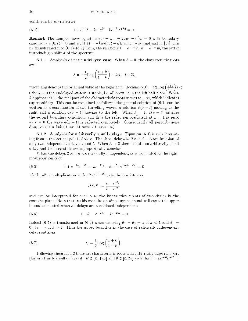
20 W. Michiels et al.which can be rewritten as1 + e��2 + ke��h � ke��(2+h) = 0:(6.4)Remark The damped wave equation �wtt � �wxx + 2a �wt + a2 �w = 0 with boundaryconditions �w(0; t) = 0 and �wx(1; t) = ��k �wt(1; t� h), which was analysed in [17], canbe transformed into (6.1){(6.2) using the relations �k = e�ahk; �w = e�atw, the latterintroducing a shift a of the spectrum.6.1.1. Analysis of the undelayed case. When h = 0, the characteristic rootsare � = �12Log�1 + k1� k�+ i�l; l 2 Z;where Log denotes the principal value of the logarithm. Because c(0) = <(Log� 1+k1�k�) <0 for k > 0 the undelayed system is stable, i.e. all roots lie in the left half plane. Whenk approaches 1, the real part of the characteristic roots moves to �1, which indicatessuperstability. This can be explained as follows: the general solution of (6.1) can bewritten as a combination of two travelling waves, a solution �(x � t) moving to theright and a solution (x + t) moving to the left. When k = 1, �(x � t) satis�esthe second boundary condition, and thus the re ection coe�cient at x = 1 is zero;at x = 0 the wave �(x + t) is re ected completely. Consequently all perturbationsdisappear in a �nite time (at most 2 time-units).6.1.2. Analysis for arbitrarily small delays. Equation (6.4) is very interest-ing from a theoretical point of view. The three delays h, 2 and 2 + h are function ofonly two independent delays, 2 and h. When h! 0 there is both an arbitrarily smalldelay and the largest delays asymptotically coincide.When the delays 2 and h are rationally independent, cf is calculated as the right-most solution � of 1 + e�2�e�i�1 + ke�i�2 � ke�2�e�i(�1+�2) = 0(6.5)which, after multiplication with e2�ei(�1+�2), can be rewritten ase2�ei�1 = k � ei�2k + ei�2and can be interpreted for each � as the intersection points of two circles in thecomplex plane. Note that in this case the obtained upper bound will equal the upperbound calculated when all delays are considered independent:j1� kj � e�2cf � ke�2cf = 0:(6.6)Indeed (6.5) is transformed in (6.6) when choosing �1 = �2 = � if k < 1 and �1 =0; �2 = � if k > 1. Thus the upper bound cf in the case of rationally independentdelays satis�es cf = 12Log�1 + k1� k� :(6.7)Following theorem 4.2 there are characteristic roots with arbitrarily large real part(for arbitrarily small delays) if 9R 2 (0;+1] and � 2 [0; 2�] such that 1+ke�Re�i� =

Sensitivity to delays in neutral equations 21

0 0.2 0.4 0.6 0.8 1 1.2 1.4 1.6 1.8 2−6

−4

−2

0

2

4

6

cfc

f

infinite spectrum

infinite spectrum

k

c f, c0

c0

c0

Fig. 6.1. Upper bounds on the spectrum of (6.1): c(0) = c0 is the real part of all characteristicroots in the undelayed case, cf the supremum of the �nite part of the spectrum for an arbitrarilysmall delay, h ! 0+.0. This is the case when k > 1. These roots have large imaginary part (no solutionwith � = 0). When k = 1 we have a degenerate case: equation (6.4) becomes (4.18)for which the existence of an in�nite spectrum is shown in subsection 4.5.One can prove that there are roots whose real part moves o� to �1 for vanishingh when k < 1 [19].The obtained results are summarised in �gure 6.1.6.2. Bifurcation diagram: parameter dependence. As a last example wediscuss the position of the roots of the characteristic equation1 + ae��h + be��2h(6.8)as a function of the parameters a and b. Note that (3.1) is a special case of (6.8).First we �x h. The delays h and 2h are clearly dependent and the roots of (6.8)can be calculated from: e��h = �a�pa2 � 4b2b(6.9)Hence, when a2 � 4b < 0 (> 0) the spectrum is situated on one (two) vertical linesin the complex plane. The position of these lines depend on the parameters. Fora2 � 4b > 0 one can show that such a line crosses the imaginary axis when a = b+ 1and when a = �b� 1, indicating a change of stability of the line under consideration.When a2 � 4b < 0 the single line crosses the imaginary axis when b = 1. Thecorresponding curves in two-parameter space (a; b) are shown in �gure 6.2.When h and 2h should be considered to be independent, i.e. when these delaysare perturbed in such a way that their rational dependency is lost, the upper boundc(h) can be calculated from1� jaje�c(h)h � jbje�2c(h)h = 0;

22 W. Michiels et al.

−2 −1.5 −1 −0.5 0 0.5 1 1.5 2 2.5 3−4

−3

−2

−1

0

1

2

3

4

b

a

S−U

S−U

U−U

U−U

S−S

S−S

S−U

S−U

S−S

S−S

S

S

U−U

U−U

U

U

S

S

Fig. 6.2. Stability areas of equation (6.8). When the delays are dependent, 'S' denotes a stablevertical line of characteristic roots in the complex plane and 'U' an unstable line. When the delaysare independent, the system is stable for parameter values inside the curve jaj+ jbj = 1and thus the system is stable when jaj+ jbj � 1. Comparing the dependent with theindependent case, one can see that the dangerous area in the parameter space, i.e. theparameter values for which small changes in the delays destroy stability, is enclosedby the triangles (0; 1); (1; 0); (1; 2) and (0;�1); (1; 0); (1;�2) (see �gure 6.2).Equation (6.8) corresponds to the small-delay part of1 + ae��h + be��2h + de�� = 0(6.10)as h! 0+. One can show that when the 3 delays are considered independent, (6.10)has roots with real part!1 for parameter values a en b outside the curve jaj+jbj = 1and that there are arbitrarily unstable roots with small imaginary part when b < a24if a � �2 and b < �a� 1 if a � �2. All roots of (6.10) are in the open left half planewhen jaj+ jbj < 1 and jdj < 1� jaj � jbj.7. Conclusions. Sensitivity of neutral functional di�erential equations to in�n-itesimal changes of the delays is caused by the behaviour of the essential spectrumwhich is determined by the roots of an exponential polynomial. A remarkable conclu-sion of the theory developed in [1, 9], concerning the roots of exponential polynomials,is that the supremum of the real parts of the spectrum can change discontinuouslyw.r.t. the delays whereas the individual roots move continuously. In a �rst part ofthis paper the underlying mechanisms are interpreted and explained by means ofspectral plots. For example, when rationally independent delays approach rationallydependent delays, this gives rise to a point-wise but non-uniform convergence of thespectrum, whereby the sensitivity of an individual root increases as its modulus in-creases. In a second part, we extend the theory developed in [1] to the case wheresome of the delays are arbitrarily small, which can result in characteristic roots witharbitrarily large real part. Su�cient and necessary conditions are provided. Therebywe also treat the special case of roots with large real part but small imaginary part.We further show that when the small delays are brought to zero in a �xed ratio, thestructure of the set of the roots with large real part depends strongly on this ratio.

Sensitivity to delays in neutral equations 23The paper ends with two illustrative examples.Appendix. We formulate a lemma which is used in the proof of theorem 4:2.The lemma is a modi�cation of Hurwitz's theorem, see e.g. [3].Lemma A.1. Let f(�) and the sequence ffn(�)gn�1 be analytic functions on an(open) domain D. Suppose that ffn(�)gn�1 converges uniformly to f(�) on the discf� : j�j � Rg � D for some R > 0 and that on this disc f(�) only has a zero in � = 0with multiplicity k. Then there exists a number N 2 N such that 8n � N , fn(�) hasexactly k zeros �n;1; : : : ; �n;k in j�j � R whereby limn!1 �n;j = 0; 8j 2 f1; : : : ; kg.Proof. Consider for some 0 < r � R the curve � : [0; 2�]! C : t! �(t) = reit.The function jf(�)j attains a minimumM on � wherebyM > 0. Because the sequenceof functions fn(�) is uniformly converging,9N such that 8n � N : jfn(�) � f(�)j < M � jf(�)j on �:Consequently j1� fn(�)f(�) j < 1on �.For each n � N the curve (t) = fn(reit)f(reit) ; t 2 [0; 2�] satis�esj1� n(t)j < 1and because it can be embedded in a closed disc not containing the origin the windingnumber of the curve w.r.t. the origin, n( n; 0), is zero:n( n; 0) = 12�i Z n d�� = 12�i Z 2�0 0n(t) n(t)dt = 0:Using the de�nition of n(t), 12�i R 2�0 0n(t) n(t)dt can be written as 12�i R� � f 0n(�)fn(�) � f 0(�)f(�) � d�.This integral is well de�ned because from the previous it follows that neither fn norf are zero in f� : r � �n < j�j < r + �ng for some �n 2 R+0 .But this implies 12�i Z� f 0f d� = 12�i Z� f 0nfn d�; 8n � N:Following the theorem of the principle of the argument (see for example [23]) , theseintegrals correspond to the zero-pole excess of f and fn (number of zeros-number ofpoles) inside � and in this case to the number of zeros. When taking r = R the �rststatement of the lemma is proven. The second statement follows from the fact that rcan be chosen arbitrary small.Acknowledgements. This paper presents research results of the Belgian pro-gramme on Interuniversity Poles of Attraction, initiated by the Belgian State, PrimeMinister's O�ce for Science, Technology and Culture (IUAP P4/02). Koen Engel-borghs is a Postdoctoral Fellow of the Fund for Scienti�c Research - Flanders (Bel-gium). The scienti�c responsibility rests with its authors.REFERENCES

24 W. Michiels et al.[1] C.E. Avellar and J.K. Hale. On the zeros of exponential polynomials. Mathematical analysisand applications, 73:434{452, 1980.[2] S. A. Campbell. Resonant codimension two bifurcation in a neutral functional di�erentialequation. Nonlinear Analysis, Theory, Methods & Applications, 30(7):4577{4584, 1997.Proc. 2nd World Congress of Nonlinear Analysts.[3] J.B. Conway. Functions of one complex variable. Springer New York, 1995.[4] R. Datko. An example of the e�ect of time delays in boundary feedback stabilization of waveequations. SIAM J. Control and Optimization, 36(1):697{713, 1986.[5] R. Datko. Not all feedback stabilized hyperbolic systems are robust with respect to small timedelays in their feedbacks. SIAM J. Control and Optimization, 26(3):697{713, 1988.[6] R. Datko. Two examples of ill-posedness with respect to time delays revisited. IEEE transac-tions on Automatic Control, 42(4):434{452, 1997.[7] R. Datko, J. Lagnese, and M.P. Polis. An example on the e�ect of time delays in boundaryfeedback stabilization of wave equations. SIAM Journal on Control and Optimization,24:152{156, 1986.[8] R. Datko and Y.C. You. Some second-order vibrating systems cannot tolerate small time delaysin their damping. Journal of Optimization Theory and Applications, 70:521{537, 1991.[9] J. K. Hale. E�ects of delays on dynamics. In A. Granas, M. Frigon, and G. Sabidussi, edit-ors, Topological methods in di�erential equations and inclusions, pages 191{238. KluwerAcademic Publishers, 1995.[10] J.K. Hale and S.M. Verduyn Lunel. Introduction to functional di�erential equations, volume 99of Applied mathematical sciences. Springer Verlag, 1993.[11] K.B. Hannsgen, Y. Renardy, and R.L. Wheeler. Efectiveness and robustness with respect totime delays of boundary feedback stabilization in one-dimensional viscoelasticity. SIAMJournal on Control and Optimization, 26:1200{1234, 1988.[12] G.H. Hardy and E.M. Wright. An introduction to the theory of numbers. Oxford UniversityPress, 1968.[13] V. B. Kolmanovskii and A. Myshkis. Introduction to the theory and application of functionaldi�erential equations, volume 463 of Mathematics and its applications. Kluwer AcademicPublishers, 1999.[14] V.B. Kolmanovskii and V.R. Nosov. Stability of functional di�erential equations, volume 180of Mathematics in Science and Engineering. Academic Press, 1986.[15] H. Logemann. Destabilizing e�ects of small time-delays on feedback-controlled descriptor sys-tems. Linear Algebra and its Applications, 272:131{153, 1998.[16] H. Logemann and R. Rebarber. The e�ect of small time-delays on the closed-loop stability ofboundary control systems. Math. Control Signals Systems, 9:123{151, 1996.[17] H. Logemann, R. Rebarber, and G. Weiss. Conditions for robustness and nonrobustness ofthe stability of feedback control systems with respect to small delays in the feedback loop.SIAM Journal on Control and Optimization, 34(2):572{600, 1996.[18] H. Logemann and S. Townley. The e�ect of small delays in the feedback loop on the stabilityof neutral systems. Systems & Control Letters, 27:267{274, 1996.[19] W. Michiels, K. Engelborghs, and D. Roose. Sensitivity to in�nitesimal delays in neutralequations. TW report 286, Department of Computer Science, Katholieke UniversiteitLeuven, Belgium, December 1998.[20] �O. Morg�ul. On the stabilization and stability robustness against small delays of some dampedwave equations. IEEE transaction on Automatic Control, 40(9):1626{1630, 1995.[21] R.M. Murray, C.A. Jacobson, R. Casas, A.I. Khibnik, C.R. Johnson Jr., R. Bitmead, A.A.Peracchio, and W.M. Proscia. System identi�cation for limit cycling systems: a case studyfor combustion instabilities. Technical Report cds97-012, Caltech, 1997.[22] R. Rebarber and S. Townley. Robustness with respect to delays for exponential stability ofdistributed parameter systems. SIAM Journal on Control and Optimization, 37(1):230{244, 1999.[23] W. Rudin. Functional analysis. McGraw-Hill Book Company, New York, 1973.