Toroidal magnetic confinement of non-neutral plasmas

NON-NEUTRAL PLASMA PHYSICS Princeton, New Jersey August 1999

EDITORS John J. Bollinger

National Institute of Standards and Technology

Ross L. Spencer Brigham Young University

Ronald C. Davidson Princeton Plasma Physics Laboratory

20000928 031 AIP CONFERENCE PROCEEDINGS 498 AIP

American Institute of Physics Melville, New York

Editors:

John J. Bollinger National Institute of Standards and Technology MS 847.10 325 Broadway Boulder, CO 80303 USA

E-mail: [email protected]

Ross L. Spencer Department of Physics and Astronomy Brigham Young University Provo, UT 84602 USA


Ronald C. Davidson Plasma Physics Laboratory Princeton University P.O. Box 451 Princeton, NJ 08543 USA


The article on pp. 353-366 was authored by U. S. Government employees and is not covered by the below mentioned copyright.

Authorization to photocopy items for internal or personal use, beyond the free copying permitted under the 1978 U.S. Copyright Law (see statement below), is granted by the American Institute of Physics for users registered with the Copyright Clearance Center (CCC) Transactional Reporting Service, provided that the base fee of $15.00 per copy is paid directly to CCC, 222 Rosewood Drive, Danvers, MA 01923. For those organizations that have been granted a photocopy license by CCC, a separate system of payment has been arranged. The fee code for users of the Transactional Reporting Service is: l-56396-913-0/99/$15.00.

© 1999 American Institute of Physics

Individual readers of this volume and nonprofit libraries, acting for them, are permitted to make fair use of the material in it, such as copying an article for use in teaching or research. Permission is granted to quote from this volume in scientific work with the customary acknowledgment of the source. To reprint a figure, table, or other excerpt requires the consent of one of the original authors and notification to AIP. Republication or systematic or multiple reproduction of any material in this volume is permitted only under license from AIP. Address inquiries to Office of Rights and Permissions, Suite 1N01, 2 Huntington Quadrangle, Melville, N.Y. 11747-4502; phone: 516-576-2268; fax: 516-576-2450; e-mail: [email protected].

L.C. Catalog Card No. 99-068554 ISBN 1-56396-913-0 ISSN 0094-243X Printed in the United States of America

CONTENTS

Foreword xi C. W. Roberson

Sponsors and Organizing Committee xv Group Photo xvii

SECTION 1: ANTIMATTER PLASMAS

Progress in Creating Low-Energy Positron Plasmas and Beams 3 C. M. Surko, S. J. Gilbert, and R. G. Greaves

Development and Testing of a Positron Accumulator for Antihydrogen Production 13

M. J. T. Collier, L. V. Jdrgensen, O. I. Meshkov, D. P. van der Werf, and M. Charlton

Technological Applications of Trapped Positrons 19 R. G. Greaves and C. M. Surko

Progress Toward Cold Antihydrogen 29 G. Gabrielse, J. Estrada, S. Peil, T. Roach, J. N. Tan, and P. Yesley

The ATHENA Antihydrogen Experiment 40 K. S. Fine (for the ATHENA Collaboration)

Trapping, Cooling and Extraction of Antiprotons, and the ASACUSA Project 48

Y. Yamazaki Multi-Ring Trap as a Reservoir of Cooled Antiprotons 59

T. Ichioka, H. Higaki, M. Hori, N. Oshima, K. Kuroki, A. Mohri, K. Komaki, and Y. Yamazaki

Self-Consistent Static Analysis of Using Nested-Well Plasma Traps for Achieving Antihydrogen Recombination 65

D. D. Dolliver and C. A. Ordonez Analysis of Time-Dependent Effects When Operating Nested-Well Plasma Traps for Achieving Antihydrogen Recombination 71

Y. Chang, D. D. Dolliver, and C. A. Ordonez Two-Component Nonequilibrium Nonneutral Plasma in Penning-Malmberg Trap 77

H. Totsuji, K. Tsuruta, C. Totsuji, K. Nakano, K. Kamon, and T. Kishimoto

SECTION 2: FLUID AND KINETIC STUDffiS

Characteristics of Two-Dimensional Turbulence That Self-Organizes into Vortex Crystals 85

D. Z. Jin and D. H. E. Dubin A Selection of Experiments Performed with the Photocathode Trap 93

D. Durkin, L. Zimmerman, and J. Fajans

2-D Interaction of Discrete Electron Vortices 99 Y. Kiwamoto, A. Mohri, K. Ito, A. Sanpci, and T. Yuyama

Vortex Motion Driven by a Background Vorticity Gradient 106 D. A. Schecter and D. H. E. Dubin

Inviscid Damping of Elliptical Perturbations on a 2D Vortex 115 D. A. Schecter, D. H. E. Dubin, A. C. Cass, C. F. Driscoll, I. M. Lansky, and T. M. O'Neil

Analytic Study of Two-Ring Patterns of Vortices in a Penning Trap 123 G. G. M. Coppa

Simulation of the Evolution of the Diocotron Instability 129 G. G. M. Coppa, A. D'Angola, and G. Lapenta

A 2D Vlasov Code for the Electron Dynamics in a Penning-Malmberg Trap 135

F. Califano, A. Mangeney, F. Pegoraro, R. Pozzoli, and M. Rome

Dynamics of Coherent Structures in a Penning-Malmberg Trap with 2D Vlasov Simulations 141

M. Rome, R. Pozzoli, F. Pegoraro, A. Mangeney, and F. Califano

The Modified Drift-Poisson Model: Analogies with Geophysical Flows and Rossby Waves 147

D. del-Castillo-Negrete, J. M. Finn, and D. C. Barnes

Equilibrium Particle Orbits in Nonneutral Plasmas 153 R. L. Spencer

SECTION 3: COLLECTIVE MODES

Steady-State Confinement of Non-Neutral Plasmas Using

Trivelpiece-Gould Modes Excited by a "Rotating Wall" 161 F. Anderegg, E. M. Hollmann, and C. F. Driscoll

Wave Angular Momentum in Nonneutral Plasmas 170 R. W. Gould

Autoresonant (Nonstationary) Excitation of the /f=l Diocotron Mode 176 J. Fajans, E. Gilson, and L. Friedland

Experimental Observations of Nonlinear Effects in Waves in a Nonneutral Plasma 182

G. W. Hart, R. L. Spencer, and B. G. Peterson

Numerical Investigations of Solitons in a Long Nonneutral Plasma 192 S. N. Rasband and R. L. Spencer

The m=l Diocotron Instability in Single Species Plasmas 198 J. M. Finn, D. del-Castillo-Negrete, and D. C. Barnes

End Shape Effects on the me—\ Diocotron Instability in Hollow Electron Columns 208

A. A. Kabantsev and C. F. Driscoll

Measurement of Plasma Mode Damping in Pure Electron Plasmas 214 J. R. Danielson and C. F. Driscoll

VI

SECTION 4: TRANSPORT

Measurement of Cross-Magnetic-Field Heat Transport due to Long Range Collisions 223

E. M. Hollmann, F. Anderegg, and C. F. Driscoll 2D Collisional Diffusion of Rods in a Magnetized Plasma Column with Finite ExB Shear 233

D. H. E. Dubin and D. Z. Jin Experimental Test of the Resonant Particle Theory of Asymmetry-Induced Transport 241

D. L. Eggleston Quadrupole Induced Resonant Particle Transport in a Pure Electron Plasma 250

E. Gilson and J. Fajans Two Experimental Regimes of Asymmetry-Induced Transport 256

J. M. Kriesel and C. F. Driscoll Experiments on Viscous Transport in Pure-Electron Plasmas 266

J. M. Kriesel and C. F. Driscoll Viscous Expansion of a Non-Neutral Plasma 272

P. Goswami, S. N. Bhattacharyya, A. Sen, and K. P. Maheshwari Effects of Background Gas Pressure on Pure Electron Plasma Dynamics in the Electron Diffusion Gauge Experiment 278

E. H. Chao, R. C. Davidson, S. F. Paul, and K. A. Morrison An Annular Penning Trap for Studies of Plasma Confinement 290

J. Kline, S. Robertson, and B. Walch Bifurcations in Elliptical, Asymmetric Non-Neutral Plasmas 299

J. Fajans, E. Gilson, and K. Backhaus

SECTION 5: CHARGED PARTICLE BEAMS

Intense Nonneutral Beam Propagation Through a Periodic Focusing Quadrupole Field I—A Compact Paul Trap Configuration to Simulate Beam Propagation Over Large Distances 309

R. C. Davidson, H. Qin, and G. Shvets Intense Nonneutral Beam Propagation Through a Periodic Focusing Quadrupole Field II—Hamiltonian Averaging Techniques in the Smooth-Focusing Approximation 320

R. C. Davidson, H. Qin, and G. Shvets Verification of Coulomb Order in a Storage Ring 329

R. W. Hasse Proton Beam-Electron Plasma Interactions 336

R. E. Pollock, J. Ellsworth, M. W. Muterspaugh, and D. S. Todd

The Cryston: An Induction Accelerator for the Production of Crystalline Beams 345

R. Bliimel

vn

SECTION 6: STRONGLY COUPLED PLASMAS

Crystalline Order in Strongly Coupled Ion Plasmas 353 T. B. Mitchell, J. J. Bollinger, X.-P. Huang, W. M. Itano, J. N. Tan, B. M. Jelenkovic, and D. J. Wineland

An Ultracold Neutral Plasma 367 S. Kulin, T. C. Killian, S. D. Bergeson, L. A. Orozco, C. Orzel, and S. L. Rolston

Collective Modes in Strongly Coupled Dusty Plasmas 376 M. S. Murillo

Experiments on Particle-Particle Interactions in Dusty Plasma Crystals 383 A. Melzer and A. Peil

Structures and Dynamics of Dusty Plasmas and Dusty Plasma Mixtures 389 H. Totsuji, C. Totsuji, K. Tsuruta, K. Kamon, T. Kishimoto, and T. Sasabe

SECTION 7: TOROIDAL DEVICES

Toroidal Magnetic Confinement of Non-Neutral Plasmas 397 Z. Yoshida, Y. Ogawa, J. Morikawa, H. Himura, S. Kondo, C. Nakashima, S. Kakuno, M. Iqbal, F. Volponi, N. Shibayama, and S. Tahara

Confinement of Nonneutral Plasmas in the Prototype Ring Trap Device 405

H. Himura, Z. Yoshida, C. Nakashima, J. Morikawa, H. Kakuno, S. Tahara, and N. Shibayama

Experiments on Pure Electron Plasmas Confined in a Toroidal Geometry 411

C. Nakashima, Z. Yoshida, J. Morikawa, H. Himura, H. Kakuno, S. Tahara, and N. Shibayama

Design of a Toroidal Plasma Confinement Device with a Levitated Super-Conducting Internal Coil 417

Y. Ogawa, H. Himura, S. Kondoh, J. Morikawa, Z. Yoshida, T. Mito, N. Yanagi, and N. Iwakuma

SECTION 8: SPECIAL TOPICS

The Penning Fusion Experiment—Ions 425 M. M. Schauer, K. R. Umstadter, and D. C. Barnes

Confinement of Pure Ion Plasma in a Cylindrical Current Sheet 435 S. F. Paul, E. H. Chao, R. C. Davidson, and C. K. Phillips

Magnetic Cusp and Electric Nested- or Single-Well Configurations for High Density Antihydrogen and Fusion Nonneutral Plasma Applications 445

C. A. Ordonez Virtual Cathode Formations in Nested-Well Configurations 451

K. F. Stephens, II, C. A. Ordonez, and R. E. Peterkin, Jr.

Vlll

Formation of a 7Be Plasma 457 B. G. Peterson and G. W. Hart

Self-Consistent Numerical Solution to Poisson's Equation in an Axisymmetric Malmberg-Penning Trap 461

E. H. Chao, R. C. Davidson, S. F. Paul, and K. S. Fine Ion-Electron Collisions in a Homogeneous Magnetic Field 469

G. Zwicknagel

Program 475 Author Index 485

FOREWORD

C. W. Roberson

Physical Science & Technology Division Office of Naval Research

Arlington, VA 22217

The Princeton workshop is the fifth in a series of workshops on Nonneutral Plasma Physics. Previous workshops were in Washington D.C. (1988), [1] Irvine, CA (1992), Berkeley, CA (1994), [2] and Boulder, CO (1997). This series of workshops started as a result of a five-year Accelerated Research Initiative by the Office of Naval Research. The Plasma Science Committee of the National Academy of Sciences was in the early stages of formation at that time. We coordinated this Initiative with the PSC activities by accepting an offer to hold the meeting at the Academy and inviting a number of sponsors from other funding agencies.

The first meeting had one day devoted to nonneutral plasmas in traps and the second day to radiation sources and accelerators. In addition to the proceedings, one of the participants expanded his paper into a book.[3] Questions and answers were tape recorded and published in the proceedings. This provides some interesting insights into the motivations of the research. The University of California at San Diego (UCSD) group is primarily interested in transport, and the group at the National Institute of Standards and Technology (NIST) in trapping and laser cooling ions for atomic clocks. The approach was quite different, but the two groups found common ground in single component plasmas. Everyone was interested in working on a system in which precise experiments and theory could be compared. These single-component plasmas in traps provided the simplicity from the plasma point of view and the complexity from the particle point of view to make them interesting to both communities.

The Berkeley workshop in 1994 focused on traps. Single component plasmas in traps are sometimes referred to as microplasmas, since the density and size are limited by space-charge (self field) effects. There has been steady progress in the technology- intensive areas of accelerators and coherent free electron radiation sources. However it is the developments in traps, laser cooling of ions and the unique transport properties of single component plasmas that have led to the remarkable results of recent years.

At the Berkeley meeting, all experiments funded after the first workshop were operational and many new efforts were emerging. The UCSD group had their ion trap with the Laser Induced Fluorescence measurements of density and temperature operating. They had invented the "rotating wall" and were confining ions for weeks. Some unique fluid dynamics experiments with electrons were in progress, including the discovery of "vortex crystals". Positron plasmas in traps were being used to carry out electron-positron beam plasma experiments and as well as experiments on the interactions of positrons with atoms and molecules.

xi

Highly deformed asymmetric equilibria were under investigation at U. C. Berkeley as well as a re-examination of Debye shielding. The Princeton Plasma Physics Laboratory (PPPL) was exploring the possibility of a pressure standard based on electron-neutral collisions in the Malmberg-Penning trap. They were also analyzing the dynamics of intense beams in a periodic focusing field. NIST had their new ion trap in operation. They were trapping 105 ions and looking for crystalline order with Bragg scattering.

A remarkable example of cross-fertilizations came out of this meeting. An outstanding problem on the path to a Penning trap ion clock was controlling the rotational motion of the ion cloud. The solution, which was suggested during the panel discussion, was UCSD's rotating wall. A number of other new directions emerged at this meeting. There was a Penning fusion experiment from Los Alamos presented, and a dusty plasma experiment from U. Colorado. The Pacific Northwest Laboratory was looking at space-charge effects in cyclotron mass spectrometry. A number of computer simulations were in progress. There was an increased emphasis on One-Component Plasma theory. A single-component plasma bibliography was included in the proceedings.

The Princeton workshop is best characterized by the word diversity. There were about 100 participants, half of which could be considered "young investigators". There was a much stronger representation from Japan and Europe than at previous workshops.

The first talk was on quantum computing with trapped ions. Quantum computing is a rapidly growing research area at the interface of physics and computing. The NIST group has been using laser-cooled trapped ions as an approach to this problem.

The activity in antimatter has increased dramatically since the Berkeley and Boulder workshops. There are now three groups (US, Europe and Japan) doing antiproton or anti-hydrogen experiments. There were reports from Harvard, CERN and the University of Tokyo on this work. Antihydrogen experiments require making positron traps, anti-proton traps, neutral plasma traps and traps for antihydrogen. This work involves particle physics, atomic physics and plasmas physics, and so is a kind of physics triple point with vastly different length scales. The next few years should be an exciting time for these experiments.

The positron plasma trap work has developed significantly, with ongoing work at UCSD, and Harvard. The 0.5 megavolt energy spread from radio active sources can be reduced to milliVolts by a combination of moderators and traps. New approaches to bright positron trap beam sources are being explored. A number of potential applications were discussed. NIST is exploring sympathetic cooling of positrons with laser cooled ions. This approach has the possibility of reaching positron temperatures of 10 milliKelvin.

The work on 3D ion crystals and 2D "vortex crystals" has matured and stimulated interest in the physics community. [4] Laser-cooled, phase-locked, real space imaging of trapped ions at NIST has led to some remarkable results. In addition to the cubic (bcc) lattice,[5] they can create an ordered rotating disk of ions.[6] Such disks offer a possible 2D alternative to quantum computing with linear arrays of trapped ions. Lawrence Livermore National Laboratory reported on an experiment which

Xll

demonstrated sympathetic laser cooling of Xe44-1" in a trap. These results open the possibility of crystalline arrays of highly charged ions.

The UCSD ion experiment was designed to carry out detailed experiments on collisional transport in plasmas using Laser Induced Fluorescence diagnostics. They have set a new standard when it comes to experiments on the fundamental processes of transport in plasmas. This work has been coupled with an active theory effort that has provided guidance and explanations of this and other work. [7] They reported on cross- magnetic-field heat transport, building on previous measurements of test particle transport and viscous transport. In all these experiments they find that the transport is dominated by long-range "guiding center" collisions. In the recent experiment the thermal diffusivity is independent of magnetic field strength and plasma density and more than 100 times greater than classical diffusivity.

A wide range of other trap experiments were reported at Princeton. Asymmetry- induced transport continues to be an active area of research, with the challenge to conventional wisdom coming from Occidental College. The nonneutral experiment at PPPL has shown that electron-neutral collisions affect the diocotron mode dynamics. They find the mode amplitude sensitive to gas pressure down to 5 x 10"10 Torr. Considerable theoretical and experimental effort (Cal Tech, UCSD) indicates the coupling of the "rotating wall" to the plasma is through the Trivelpiece-Gould modes. The U. C. Berkeley group did an interesting experiment on the autoresonant excitation of diocotron waves and is using a photocathode trap to study vortex merger. Brigham Young University is active in soliton-like nonlinear waves in traps and computer simulation of nonneutral plasmas in traps. Experiments at the University of Colorado are using an annular Malmberg-Penning trap to study transport when there are banana- like particle drift orbits.

In addition to the Penning Fusion Experiment from Los Alamos National Laboratory, an additional nonneutral plasma approach to fusion was presented at this workshop. The University of Tokyo is exploring approaches to high beta plasmas using an electron ring, in a concept similar to the Field Reversed Configuration. In accelerator related work there was a PPPL talk on the propagation of intense nonneutral beams in strong focusing fields. The halo formed by high current beams as they approach equilibrium is similar to the halo formed in traps as equilibrium is approached.

At the Boulder workshop we invited scientist from related fields to give presentations. For example, there was a talk from the Fermi National Accelerator Laboratory on using plasma wave echoes to diagnose ion storage rings. At this meeting there was a talk from the Jefferson Lab on a high average power free electron laser (FEL). Average power is important in industrial applications concerned with the cost per photon. Although high average power has been a strong motivation in the development of free electron lasers, no one had broken the "kilowatt barrier" at any wavelength until the Jefferson Lab results this year (1.7 kW at 5 microns). The potential of the FEL to be tunable and to operate at any wavelength from the microwave to x-rays is often limited by the mirrors, especially in the low-gain regime. There is a great deal of research activity at present to design and construct a fourth generation light source based on a single pass x-ray FEL. This FEL would operate in the exponential gain regime where the dispersion relation has the same form as the two-stream

xm

instability.[8] Although mirrors may not be a problem, the electron beam quality requirements are a challenge.

The workshop Chair and PPPL staff did an outstanding job of organizing the meeting, choosing an interesting setting and arranging for delightful weather.

Since the beginning of these workshops there has been a great deal of interest by the plasma physics community and appreciation of the high quality of the work. There have been 5 plenary session talks featuring nonneutral plasmas at the APS Plasma Physics Division meetings since the 1988 Washington meeting. Two of these talks were given by Maxwell prize recipients. This program was held up as a role model in the National Research Council's report on plasma science.[9]

The internal logic of the science drives much of the research, always working towards simplicity to achieve predictability. We have chosen single-component nonneutral plasmas in traps as a focus. The excellent confinement properties and the fact that the plasma does not recombine to form a neutral gas means that the free energy in the system can be minimized. In systems such as beams where the free energy is dominant, predictability can be achieved by limiting the number of particles. However technology requirements usually drive us in the opposite direction, towards more particles and more free energy. For intense beams, tailoring of the beam distribution function becomes critical for efficient transport. The enabling science that is coming out of this work is pointing the way to new applications and extending the frontiers of knowledge.

The rigidly rotating pure electron plasma in a Malmberg-Penning trap has become the "hydrogen atom" of plasma physics. However, the diversity of the meeting shows that nonneutral plasma physics is a truly multi-disciplinary field.

REFERENCES

1. C. W. Roberson and C. F. Driscoll Eds., Non-neutral Plasma Physics, AIP Conf. Proc. No. 175 (AIP, New York, 1988).

2. J. R. Fajans and D. E. Dubin, Eds., Non-neutral Plasma Physics II, AIP Conf. Proc. No. 331 (AIP, New York, 1995).

3. R. C. Davidson, Physics of Nonneutral Plasmas, (Addison-Wesley, Redwood City, CA, 1990). 4. T. M. O'Neil, Physics Today 52, NO.8, 24 (1999). 5. W. M. Itano, J. J. Bollinger, J. N. Tan, B. Jelenkovic, X-P Haung, and D. J. Wineland, Science 279,

686 (1998). 6. T. B. Mitchell, J. J. Bollinger, X-P. Haung, W. M. Itano, and R. H. Baughman, Science 282, 290

(1998). 7. D. H. E. Dubin and T. M. O'Neil, 1999, Trapped Nonneutral Plasmas, Liquids, and Crystals (the

thermal equilibrium states), Rev. Mod. Phys. 71, 87 (1999). 8. C. W. Roberson and P. Sprangle, A Review of Free Electron Lasers, Phys. Fluids B 1, 3 (1989). 9. Plasma Science: From Fundamental Research to Technological Applications, (National Academy

Press, Washington, D. C, 1995).

XIV

1999 Workshop on Non-Neutral Plasmas

August 2-5,1999 Princeton University

Princeton, New Jersey USA

Sponsored by US Office of Naval Research

US Department of Energy Princeton Plasma Physics Laboratory

Princeton University

Organizing Committee

Ronald Davidson, Chair Princeton Plasma Physics Laboratory

John Bollinger, Vice Chan- National Institute of Standards and Technology

Gerald Gabrielse, Vice Chan- Harvard University

Daniel Barnes Los Alamos National Laboratory

Patrick Colestock Fermi National Accelerator Laboratory

William Dove U. S. Department of Energy

C. Fred Driscoll University of California, San Diego

Joel Fajans University of California, Berkeley

John Goree University of Iowa

Alan Marshall National High Magnetic Field Laboratory

Thomas O'Neil University of California, San Diego

Charles Roberson Office of Naval Research

Scott Robertson University of Colorado, Boulder

John Schiffer Argonne National Laboratory

Ross Spencer Brigham Young University

Clifford Surko University of California, San Diego

xv

SECTION 1

ANTIMATTER PLASMAS

Progress in Creating Low-energy Positron Plasmas and Beams

C. M. Surko, S. J. Gilbert and R. G. Greaves*

Physics Department, University of California San Diego, LaJolla, CA 92093-0319

Abstract. A summary is presented of recent research to create positron plasmas in new regimes of density, temperature, and particle number. The operation of a new, compact positron accumulator is discussed. It has a number of improvements including enhanced vacuum capabilities and an easily modified electrode structure. Using a 90 mCi Na source and neon moderator, a plasma of 3 x 10s positrons, with a diameter of 6 mm (FWHM) and a density of 2 x 107cm"3, has been accumulated in 8 minutes. This is a factor of 50% more positrons and an order of magnitude increase in plasma density over the performance of the previous accumulator. Plans for a separate, high magnetic field (i.e., 5 Tesla), low-temperature (< 10 Kelvin) trap are described. This trap is expected to permit the creation and long-term storage of cryogenic plasmas with more than an order of magnitude larger particle number and more than two orders of magnitude in plasma density. A method is described that uses positron accumulation techniques to create a cold, bright positron beam (e.g., < 20 meV FWHM), tunable from ~ 0.1 eV upward. Results are described of studies of positron scattering from atoms and molecules in a new range of energies (e.g., < 1 eV) using this cold positron beam. Other applications of trapped cold positron plasmas and beams are briefly discussed.

INTRODUCTION

Once the province of high-energy physics, antiparticles such as the antiproton and the positron are now routinely used in a much wider range of applications. In the case of positrons, these uses include the study of atomic and molecular physics, antihydrogen formation, plasma physics, and the characterization of solids and solid surfaces [1,2]. Further progress in many of these areas hinges on the ability to manipulate and cool large collections of antiparticles, relying in large part on nonneutral plasma techniques.

One benchmark for handling antimatter is the lifetime of antiparticles in the presence of matter. This time is of the order of a few nanoseconds for either positrons or antiprotons in solids or gases at atmospheric pressure. This fact leads immediately to the conclusion that, if antimatter is to be confined, accumulated and cooled, it must be done in a vacuum environment. Over the past decade, we have developed methods to accumulate large numbers of positrons [2,3], by exploiting nonneutral plasma

CP498, Non-Neutral Plasma Physics III, edited by John J. Bollinger, et al. © 1999 American Institute of Physics l-56396-913-0/99/$15.00

techniques developed for electron plasmas [4]. Plasmas of greater than 108 particles and confinement times of many minutes to hours are now routine [2].

Using the positron accumulator, we have recently developed a new technique to create a state-of-the-art cold positron beam with an energy spread as small as 18 meV (FWHM), tunable from 0.1 eV upwards [5,6]. Recently, we used this technique to make the first measurements of the cross section for excitation of vibrational modes in a molecule (the asymmetric stretch mode in CF4, Ae = 0.16 eV, measured for positron energies from 0.2 to 1 eV) [7]. We also measured the differential cross section for elastic scattering of positrons from atoms in the range of energies between 0.4 and 2 eV [7]. These experiments are expected to provide important new information, such as understanding the role of virtual positronium states in positron interactions with matter and the mechanisms by which positrons bind to atoms and molecules.

In this paper, we review recent progress in positron accumulation and the development and use of the cold positron beam. We also discuss briefly other applications. For a discussion of the application of cold positron beams to condensed matter and surface physics and positron ionization mass spectrometry, the reader is referred to a complementary paper elsewhere in this volume by [8].

BUFFER-GAS TRAPPING AND A NEW ACCUMULATOR

The principle of the buffer-gas trapping scheme is illustrated schematically in Fig. 1. Inelastic collisions of positrons with N2 molecules are used to trap positrons in a specially designed Penning-Malmberg trap [2,3,9]. Positrons from the source are slowed to a few electron Volts using a neon rare-gas "moderator," which consists of solid neon condensed on a metal surface at 7 Kelvin. There is an applied magnetic field of ~ 0.1 - 0.15 T in the z direction. The positrons are injected into the accumulator at energies ~ 30 eV. The accumulator has three "stages," I, II, and III, each with successively lower gas pressure and electrostatic potential. Following a series of inelastic collisions ("A", "B," and "C" in Fig. 1), the positrons are trapped in stage III where the pressure is lowest. The positrons cool to room temperature by collisions with theN2 in ~ 1 s. The positron lifetime in the third stage is > 40 s, limited by annihilation on the N2 gas. Using this technique, we are able to accumulate > 108

e+ in a few minutes from a 90 mCi 2Na source. The lifetime of the plasma with the buffer gas removed ranges from tens of minutes to hours, depending upon the quality of the vacuum.

The design of the original positron accumulator (circa 1985) is shown in the upper part of Fig. 2. This design used a split magnet surrounding the accumulator electrodes to achieve the required differential pumping. One focus of our work in the last two years has been the completion of a new positron accumulator. A key feature of the new accumulator is elimination of the separate pumping port for the second stage.

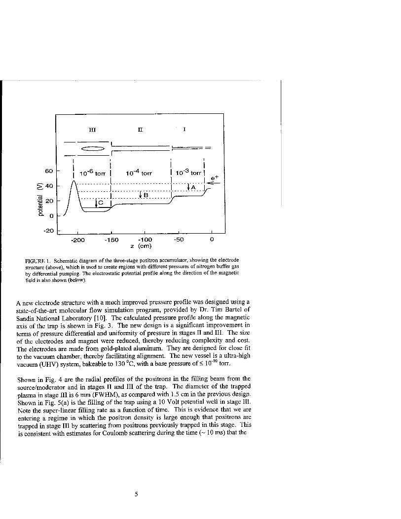
FIGURE 1. Schematic diagram of the three-stage positron accumulator, showing the electrode structure (above), which is used to create regions with different pressures of nitrogen buffer gas by differential pumping. The electrostatic potential profile along the direction of the magnetic field is also shown (below).

A new electrode structure with a much improved pressure profile was designed using a state-of-the-art molecular flow simulation program, provided by Dr. Tim Bartel of Sandia National Laboratory [10]. The calculated pressure profile along the magnetic axis of the trap is shown in Fig. 3. The new design is a significant improvement in terms of pressure differential and uniformity of pressure in stages II and III. The size of the electrodes and magnet were reduced, thereby reducing complexity and cost. The electrodes are made from gold-plated aluminum. They are designed for close fit to the vacuum chamber, thereby facilitating alignment. The new vessel is a ultra-high vacuum (UHV) system, bakeable to 130 °C, with a base pressure of < 10"10 torr.

Shown in Fig. 4 are the radial profiles of the positrons in the filling beam from the source/moderator and in stages II and III of the trap. The diameter of the trapped plasma in stage III is 6 mm (FWHM), as compared with 1.5 cm in the previous design. Shown in Fig. 5(a) is the filling of the trap using a 10 Volt potential well in stage III. Note the super-linear filling rate as a function of time. This is evidence that we are entering a regime in which the positron density is large enough that positrons are trapped in stage III by scattering from positrons previously trapped in this stage. This is consistent with estimates for Coulomb scattering during the time (~ 10 ms) that the

Magnetic Field Coils Electrode Structure

To Pump Positron Plasma To Pump

To Pump

FIGURE 2. Shown to scale are the designs of the original (above) and the new positron accumulator (below). The new design provides a true UHV-quality vacuum and the ability to easily modify the electrode structure.

1 III II I ] io-3

io-4

t! o b10,

CU

3

1 10" V

io-7

1 1

in-s i

z(m)

FIGURE 3. Calculated pressure profile as a function of distance along the magnetic axis in the new positron accumulator. This design improves the maximum pressure differential between each stage by an order of magnitude.

particles spend in stage II before becoming trapped in stage III. The maximum positron number in Fig. 5(a) is limited by the space charge of the positrons in stage III. Figure 5(b) shows data taken when the stage-Ill potential well was lowered from 10 to 15 Volts during filling. The maximum number trapped is just under 3 x 108. Note that the filling has not yet saturated for an 8 minute accumulation.

5 mm

FIGURE 4. Radial profiles of the positron filling beam (left); the plasma accumulated in stage II after a 0.5 ms fill (center); and the plasma in stage III after a 10 s fill.

200

o 150

c o

0) o a

100

50

(a) • •

0.95 million/s

y* 0.63 million/s

100 200 300

time (s)

400 200 400

time (s)

600

FIGURE 5. Positron filling of the accumulator: (a) filling with a 10 Volt potential well in stage III. The increase in filling rate appears to be due to scattering from positrons already in stage III; (b) filling curve taken when the well depth is lowered from 10 to 15 V during the fill.

A UHV environment is required for many applications, such as antihydrogen formation or studies of positron annihilation with test molecules. We have been able to accomplish this in the new buffer-gas trap by rapidly pumping out the gas after positron filling. As shown in Fig. 6, we are able to cycle stage III from an operating pressure of 3 x 10"7 torr to < 1 x 10"9 torr in a few seconds. This will also be useful in shuttling the positrons from positron accumulator into a separate UHV storage and experimentation trap (described below) through a fast pulsed valve.

Valve open

FIGURE 6. The pressure in the third stage of the new accumulator can be decreased by three orders of magnitude in 10 seconds.

A HIGH-FIELD LOW-TEMPERATURE TRAP [11]

The buffer-gas trap is attractive for a range of applications because of the high trapping efficiency. However, as mentioned above, many of these applications require an ultra-high vacuum (UHV) environment, and a limitation of the technique is that the positrons are initially in a background of nitrogen gas at a pressure > 10"7 torr. As shown in Fig. 6, we can create a good vacuum in the trap rapidly by pumping out the buffer gas (e.g., in ~ 10 s) and then conduct the specific experiment of interest. However, this will interrupt the fill cycle. Thus, it is advantageous to combine the ability to pump down the accumulator rapidly with the ability to "stack" positron plasmas efficiently in a UHV environment. For this purpose, we are building an isolated UHV stage into which the positrons from the accumulator can be shuttled repetitively through a fast pulsed valve. In this way, we can isolate the efficient buffer-gas trap from the UHV stage. The proposed apparatus is shown in Fig. 7.

UHV storage stage

E3 .. , ,M

positrons

positron trap

B = 5T

gas feed

-. f ■ L_ positron "~ beam

B = 0.15 T H

t

to pump to pump 2 m

to pump

FIGURE 7. The UHV storage trap in relation to the three-stage positron accumulator.

During positron accumulation, the UHV storage stage will be isolated from the positron trap by a fast valve. Then the buffer-gas feed will be switched off and the trap will be pumped rapidly to base pressure (i.e., -1x10" torr). The gate valve will then be opened for the brief time ( < 1 s) required to transfer the positrons to the storage trap and the cycle repeated. Long confinement times and low plasma temperatures will be achieved by applying a magnetic field of 5 T in this region. In the 5 T field, the cyclotron radiation time is ~ 0.2 sec. We plan to cool the walls to 10 Kelvin, and so the plasma will cool radiatively to approximately the wall temperature. The cold walls should provide excellent vacuum (e.g., pressures < 10"u torr or better). The trap will have a "rotating wall" electrode for control of plasma density and confinement time [12]. Using this technique, we are likely to be able to achieve an "infinite" confinement time, as has been done in the case of electron plasmas.

In Table I, the operation of the old positron accumulator is compared with that expected for the new accumulator and UHV storage trap. We assume a six- minute trapping cycle including one minute to pump out the buffer gas. Presently, the positron loading rates are ~ 3 xlO8 per cycle or 3 x 109 per hour. With modest improvements, we expect that it will be possible to increase the number of positrons by a factor of as much as five, to > 1 x 109 per cycle. These improvements include an increased source strength of 150 mCi and modest improvements in the source geometry, magnetic field, and vacuum system. With these modifications, positron accumulation rates of greater than 1 x 1010 positrons per hour are expected. With this filling rate and confinement times > 3 hours, the number of positrons accumulated will be limited by the space charge of the plasma. For example, an hour's accumulation of 1 x 1010 positrons in a plasma 1 mm in radius by 10 cm long corresponds to a plasma density of > 1 x 1010cm"3 and a 1 kV space potential.

TABLE I. Expected Performance of the UHV Storage Trap*

Parameter Old Positron New Accumulator Accumulator and UHV Storage Tran

Source strength (mCi) 70 95 Positrons per cycle 2 x10s ~3xl08

Cycles per hour n.a. 10 Positrons per hour n.a. ~3xl09

Density (cm"3) ~2xl06° >lxl01("' Base pressure (torr) 3 x IQ"10 < 1 x 10"" (cold)

on current new-trap performance " One cycle in a 0.1 T magnetic field. 4 One hour accumulation in a 5 T field.

A COLD POSITRON BEAM AND APPLICATION TO ATOMIC PHYSICS

While sources of cold electron beams are common, this is not true for positrons. Recently, we developed a method to create a state-of-the-art cold positron beam using trapped positron plasmas [6,7]. This technique can be used to increase the brightness of a positron or electron beam, and to create intense, short pulses of positrons with narrow energy spreads. The beam energy can be tuned over a wide range of energies, from -0.1 eV to tens of electron Volts.

i positrons

(a) V<z«

J_ axial position

(b)

1.6 1.7

bias voltage (V)

FIGURE 8. Schematic diagram of the arrangement used to create a cold positron beam (above), and the retarding-potential curve and energy distribution (below).

The experimental arrangement is illustrated in Fig. 8(a). Positrons are accumulated and cooled in a Penning-Malmberg trap. Then the potential of the bottom of the trap is raised, forcing the particles over a fixed-height potential barrier [energy Eo in Fig. 8(a)], and this sets the energy of the beam. The spread in parallel energies of the beam can be as low as, or lower than, the temperature of the plasma in the potential well. However, care must be taken not to empty the trap too quickly, or space-charge effects will increase the energy spread of the beam. Shown in Fig. 8(b) are data for the energy resolution of a positron beam created using this technique. We have been able to operate the beam in both continuous and pulsed modes; the latter was accomplished by reducing the depth of the confining potential well in small steps.

Two topics that could not be addressed previously due to the lack of suitable low- energy positron sources were study of the excitation of molecular vibrations by positrons and measurement of low-energy differential scattering cross sections. We

10

have now been able to do both [7]. The experiments were done exploiting the fact that the cold positron beam is in a magnetic field. This is in contrast to contemporary electron scattering experiments which are typically done using electrostatic beams.

The first measurements of the differential elastic scattering cross section for argon at 1 eV positron energy are shown in Fig. 9(a). Comparison with theoretical predictions of McEachran, et al. and Duzba, et al. (solid and dotted curves, respectively, with no fitted parameters) [13,14] indicate excellent agreement. In the future, we hope to study elastic scattering in the important regime, ka ~ 1, where k is the momentum of the positron and a is the scattering length (in atomic units). In this limit, both the sign and magnitude of the s-wave scattering length, a, can be measured, and these quantities provide important information about positron-atom and positron-molecule bound states.

0 20 40 60 80

angle (deg)

10

8

6

4

2

(b) X1/5

O

o o

° 8" Positrons

Electrons

0.0 0.2 0.4 0.6 0.8

energy (eV) 1.0

FIGURE 9. (a) differential elastic scattering cross section of positrons scattered from argon at 1.0 eV; (b) the cross section (in atomic units) as a function of positron energy for excitation of the asymmetric stretch mode in CF4, which corresponds to an energy of 0.16 eV. Also shown is the cross section for electrons, taken from electron-swarm data. (See Ref. 7 for details.)

We have also used the cold beam to make the first measurement of the vibrational excitation of a molecule (CF4) with positrons [7]. This was accomplished by locating the scattering event in a magnetic field of 1000 Gauss and analyzing the spectrum of parallel energies of the scattered beam in a smaller magnetic field. In this case, the (nominally parallel-energy) retarding-potential analyzer measures the total positron energy and therefore measures the energy loss due to scattering. Data for CF4 are shown in Fig. 9(b). The asymmetric stretch mode that is excited has an energy of 0.16 eV. This is an absolute measurement and extends down to positron beam energies of 0.2 eV, which is possible only because of the excellent energy resolution of the cold positron beam.

CONCLUDING REMARKS

We are continuing to advance the technology of accumulating and cooling positrons. The new UHV trap should provide capabilities for a range of experiments, furnishing a

11

reservoir of cold, dense positron plasma in a high-quality vacuum environment that can be used as required for the particular experiment at hand. It should be well suited, for example, as a positron source for antihydrogen production. These efforts have now been extended to the creation of a state-of-the-art bright, pulsed positron beam, tunable over a wide range in energies. The new UHV trap and cold walls should be well suited for the creation of a new generation of positron beams [e.g., having an energy spread as low as 1 meV (FWHM)].

Driven by advances in this technology, we continue to use these antimatter beams and plasmas to study a range of scientific problems ~ from the electron-beam positron- plasma instability and modeling of astrophysical processes to antihydrogen formation and the interaction of low energy positrons with atoms and molecules. In particular, the cold positron beam appears to be able to address many new problems in these areas.

ACKNOWLEDGMENTS

This work is supported by the Office of Naval Research, Grant No. N00014-96-10579, and the National Science Foundation, Grant No. PHY 96-00407. We wish to thank Gene Jerzewski for his expert technical assistance and James Sullivan for help with a number of aspects of this manuscript.

REFERENCES

* First Point Scientific, Inc., Agoura Hills, CA 91301

1. Schultz, P. J., and Lynn, K. G., Reviews of Modern Physics 60, 701 (1988). 2. Greaves, R.G., and Surko, C. M, Physics of Plasmas 4, 1528 (1997). 3. Murphy, T. J., and Surko, C. M., Physical Review A 46, 5696 (1992). 4. O'Neil, T. M., Physica Scripta T59, 341 (1995). 5. Gilbert, S. J., et al, Applied Physics Letters 70, 1944 (1997). 6. Kurz, C., et al., Nucl. Inst. and Meth. in Physics Research B143, 188 (1998). 7. Gilbert, S. J., Greaves, R. G., Surko, C. M., Phys. Rev. Lett. 82, 5032 (1999). 8. Greaves, R. G., and Surko, C. M., "Technological Applications of Trapped

Positrons," this volume. 9. Surko, C. M., et al, Phys. Rev. Letters 61, 1831 (1988). 10. Bartel, T. J., et al, "Icarus: A 2D Direct Simulation Monte Carlo (DSMC) Code

for Parallel Computers, Users Manual - V3.0", Sandia National Laboratories Report SAND96-0591, October 1996.

11. This scheme is proposed in Surko, C. M., Greaves R. G., and Charlton, M., Hyperfine Interactions 109, 181 (1997).

12. Anderegg, F., Hollmann, E., and Driscoll, C. F., Phys. Rev. Lett. 81, 4875 (1998). 13. McEachran, R. P., et al, J. Phys. B12, 1031 (1979). 14. Dzuba, V. A., et al, J. Phys. B29, 3151 (1996).

12

Development and Testing of a Positron Accumulator for Antihydrogen Production

M. J. T. Colliera, L. V. J0rgensen ■* O. I. Meshkovc, D. P. van der Werf '* and M. Charlton^

"Department of Physics and Astronomy, University College London, Gower Street, London WC1E6BT, United Kingdom

b Department of Physics, University of Wales Swansea, Singleton Park, Swansea SA2 8PP, United Kingdom

c Budker Institute of Nuclear Physics, 11 Lavrentiev Prospect, Novosibirsk 630090, Russian Federation

Abstract. A positron accumulator based on a modified Penning-Malmberg trap has been constructed and undergone preliminary testing prior to being shipped to CERN in Geneva where it will be a part of an experiment to synthesize low-energy antihydrogen. It utilises nitrogen buffer gas to cool and trap a continuous beam of positrons emanating from a Na radioactive source. A solid neon moderator slows the positrons from the source down to epithermal energies of a few eV before being injected into the trap. It is estimated that around 10 8 positrons can be trapped and cooled to ambient temperature within 5 minutes in this scheme using a 10 mCi source.

INTRODUCTION

In order to produce low energy antihydrogen via recombination it is necessary to have copious amounts of cold positrons available. To attain this a positron accumulator based on the design of the Surko Group at the University of California San Diego (1-3) has been constructed and undergone preliminary testing at University College London (UCL) before being shipped to CERN in Geneva to be a part of the ATHENA (AnTiHydrogEN Apparatus) experiment (4). The accumulator is an ideal source of positrons in this case as it is capable of supplying large quantities (>108) of positrons in short well defined bursts, with a short cycle time, in the order of 5 minutes.

POSITRON MODERATION

The continuous beam of slow positrons injected into the accumulator is generated by moderating ß+ particles from a radioactive source and guiding them into the trapping


13

9 mCi BNa source

77 K Thermal shield \ ^_2 cm_ Elkonite

FIGURE 1. The source-moderator setup with the copper cone and the thermal shield.

region using a magnetic field. The radioactive source used in our set-up is an encapsulated 9 mCi 22Na y3+-radioactive source from Dupont Pharma. The source is mounted on an Elkonite rod fitted to a APD Displex 204SLB cryogenic coldhead (Fig.l) capable of reaching 5.5 K. Elkonite is a Tungsten-Copper alloy that possesses a high thermal conductivity while also providing excellent shielding for the gamma radiation from the source. The rod itself is split into two sections separated by a sapphire disk allowing a potential to be applied to the source/moderator. On top of the source capsule there is a cone shaped copper extension. A gold plated copper thermal radiation shield, held at 77 K, encloses the entire coldfinger.

The source end is pumped out by a magnetically levitated turbomolecular pump, which is roughed out by a scroll pump. This maintains a base pressure of 1 x 10 ~9

mbar in the source end while also keeping the vacuum system oil free. This is important since positrons have been shown to readily attach themselves to large hydrocarbon molecules (5, 6) where they subsequently annihilate causing the storage time of the positrons in the trap to be much reduced. Finally the pumps allow for accurate control of the pressure in the source-end during deposition of the neon moderator. This is accomplished by letting in neon gas at a pressure of 5 x 10 ~* mbar for an hour or more depending on the desired thickness of the moderator.

The fast/?+ particles from the source are emitted over a continuous range of energies up to a cut-off energy of 545 keV. These are moderated using a layer of a condensed noble gas, in this case neon, condensed onto the source cone arrangement. This type of moderation can be far more efficient although more complex in operation, due to the cooling requirements, than more conventional metal foil moderators. However, the overall attainable efficiency of this type of moderator has been shown to depend on the geometry of the source-moderator system. Thus an increase of a factor of 5 in the moderation efficiencies have been reported for a conical geometry compared to a flat geometry (7). This is the reason for the copper cone on top of the source.

14

CO

i \

Pressure lO*mbar 10" mbar 107 mbar ■ i

IV V VI VII VIII

FIGURE 2. The trapping scheme showing the electrodes with the potentials and gas pressures in the different parts of the trap.

Due to the method of final slow down and emission from rare gas solid moderators the positrons emitted from them have a wider energy spread than that typical for traditional metal moderators. This broader energy spectrum has the effect of a subsequent reduction in the trapping efficiency of the final stage, where the trapping electrode voltages are tuned to trap certain positron energies more efficiently. Thus a reduction in the region of 25 % was noted by Greaves and Surko (8). However, this is more than compensated for by the order of magnitude improvement in the initial moderation step.

After moderation the positrons are transported through the source chamber by a series of 3 "pancake" coils. These coils maintain a field of around 250 Gauss and introduce a 2 cm kink in the positron path, raising the beamline to remove the source from being in a direct line of sight with the remainder of the apparatus. Upon exiting the source chamber the positrons are magnetically guided along a small diameter transfer tube by a small (300 Gauss) solenoid before entering the trapping and accumulation region. This transfer tube is necessary to ensure that the solid neon moderator remains unaffected by the presence of the buffer gas in the accumulation region.

TRAPPING

The second stage of the vacuum apparatus consists of a pair of pumping boxes connected together by a smooth bore cylindrical chamber. The two pumping boxes are each fitted with a 1200 1/s cryopump. These were chosen not only to obtain UHV

15

conditions, but also for their pumping speed, necessary for the rapid removal of nitrogen gas from the system. This is important both for minimising annihilation losses and for keeping the accumulation cycle time down to a minimum. Again, as mentioned earlier, the vacuum system is kept oil-free to avoid positrons being trapped at hydrocarbon molecules. The base pressure of the main trapping region is 1 x 10 ~10

mbar.

The smooth bore cylindrical chamber is situated within a 0.15 T magnet and contains an electrode array. This consists of a set of eight separate gold-plated aluminium electrodes with an appropriate potential applied will confine the positrons in the axial direction after the initial trapping (Fig.2). The 0.15 T axial magnetic field supplies the radial confinement and combined with the electric potentials this constitutes our Penning-Malmberg trap.

The physical dimensions of the electrodes are designed to allow a pressure gradient to be developed along their length. Nitrogen gas can be introduced midway along electrode II and is pumped out at either end or through a set of three vents located at the end of the same electrode. These vents can be manually adjusted by covering them to various degrees with a sleeve actuated by a linear drive. Thus the pressure along the array can be adjusted to obtain the optimal trapping of the positrons. Typically a pressure in the region of 10"3 mbar is sufficient within electrode II, falling to 10"7 mbar within the final stages. A steadily falling trapping potential is also applied along the array in order to accumulate the trapped positrons in the region of electrodes V and VI.

The positrons are trapped and cooled within the array via a buffer gas method. The nitrogen gas pressure is tuned such that on average, a positron entering from the source region will experience one inelastic collision with a nitrogen molecule whilst traversing electrode II. Now confined and unable to escape the array a second collision typically occurs within a millisecond further confining the positron to between electrodes III and VI, typically a third collision after some 10ms will then finally restrict the positron to electrodes V and VI.

As stated earlier the electrode potentials are critical to the effective performance of this trapping system. Positrons initially entering with some 31-35 eV of kinetic energy pass into the array over the gate electrode (I) which has a potential of approximately 30 V applied. The second electrode is then set to 24 V, corresponding to the positron having some 7-11 eV of kinetic energy. This range is chosen as it corresponds to the so-called "trapping gap" (1), between the first available nitrogen electronic transition at about 7 eV and 11 eV where positronium formation starts to become the dominant process. Similar considerations are taken with the voltage along the length of the array until the positron is eventually confined to the last stage. Here the gas pressure is much lower, reducing annihilation losses yet cooling the positrons to room temperature in less than 1 second by a mixture of excitation of nitrogen molecules and direct momentum transfer. The accumulation cycle continues until an equilibrium state is

16

50000

3 40000 CO

CD ■♦-» CO DC c 3 O Ü

30000

20000

10000

Positron Energy / eV

FIGURE 3. The first results for slow positron energy spread obtained by applying a retarding potential in front of a channeltron detector.

reached between further positron trapping and losses due to annihilations and plasma expansion. At this point we hope to have trapped in excess of 108 positrons, which have a lifetime of up to an hour after the buffer gas is pumped out. After the buffer gas is switched off, the base pressure of this part of the vacuum system should be reached in roughly 10 seconds due to the high pumping speed of the cryopumps.

PROGRESS

The positron accumulator is currently being reassembled at CERN following the transfer from its initial UCL development site. Prior to this, good progress was being made with the source end moderation where initial moderation/transport tests have been performed.

A preliminary study of moderator growth was conducted using a channeltron and a plastic scintillator detector in coincidence in order to ascertain the moderator efficiencies for different moderator thicknesses etc. These detectors were placed at the entrance to the main vacuum system. Using this method we have been able to detect more than 6 x 105 e+ s"\ giving a moderator efficiency of 0.18 % based on a source strength of 9 mCi at the time of the measurement. However, these were only the first preliminary measurements and there were strong indications that higher positron yields can be achieved. Once reconstructed further rigorous tests will be conducted to ascertain and maximise both the moderator and transport efficiency. A preliminary study of the energy spectrum of the slow positrons, has also been conducted (Fig.3),

17

showing at FWHM of -2.5 eV. Both this and the gross positron yield are of the same order of magnitude as seen in similar experiments.

The trapping and accumulation region was also assembled and vacuum tested. An attempt was then made to trap electrons in the system. During these test problems with the radial magnetic field of the main magnet was discovered which led to trapping times of only 10 s for electrons. These magnet problems have resulted in several months delay while the magnet was returned to the supplier for repairs. These repairs have now been completed and the magnet has been installed at CERN for further tests.

ACKNOWLEDGEMENTS

We would like to thank the EPSRC (grant number GR/L63266) for its support of this project, the TMR-network EUROTRAPS (contract number ERBFMRXCT970144) for its funding of a postdoctoral position. OIM would like to thank the Royal Society for the providing a visiting fellowship. Finally we would also like to thank Cliff Surko at the University of California San Diego, for many useful discussions and invaluable technical assistance.

REFERENCES

1. Murphy, T.J. and Surko, CM., Phys. Rev. A, 46, 5696-5709 (1992) 2. Greaves, R. G., Tinkle, M. D., and Surko, C. M., Phys. Plasmas 1, 1439 (1994) 3. Surko, C. M., Greaves, R. G., and Charlton, M., Hyperflne Interactions 109,181 (1997) 4. Holzscheiter, M. H. et al., Nucl. Phys. B 56A, 336-348 (1997) 5. Murphy, T. J. and Surko, C. M., Phys. Rev. Lett. 67, 2954-2957 (1991) 6. Surko, C. M., Passner, A., Leventhal, M., and Wysocki, F. J., Phys. Rev. Lett. 61,1831-1834 (1988) 7. Khatri, R., Charlton, M., Sferlazzo, P., Lynn, K. G., Mills, A. P. Jr., and Roellig, L. O., Appl. Phys. Lett. 57, 2374- (1990) 8. Greaves, R. G. and Surko, C. M., Can. J. Phys. 74,445-448 (1996)

Technological Applications of Trapped Positrons

R. G. Greaves* and C. M. SurW

'First Point Scientific, Inc., Agoura Hills CA 91301 t Physics Department, University of California, San Diego, La Jolla CA 92093

Abstract. Low-energy positron beams are extensively employed in various areas of science

and technology such as surface analysis, atomic physics, plasma physics and mass spectrometry. Recent advances in positron trapping and in manipulating nonneutral plasmas present the opportunity for creating a new generation of bright, ultracold positron beams with parameters that far exceed those currently available. Current applications of low-energy positron beams are described, and the potential for the development of advanced trap-based positron beams is discussed.

I INTRODUCTION

Over the past several decades, a variety of powerful analytical tools for materials and surface analysis based on positron beams have been developed [1]. These techniques are generally implemented using steady state and pulsed beams derived from radioactive sources. Recent developments in nonneutral plasma and positron trapping techniques have now created the opportunity for producing a new generation of positron beams based on the extraction of positrons accumulated in a Penning trap. These unique techniques have never before been applied to beam formation, and as described in this paper, they offer the potential to create bright, ultracold, pulsed positron beams with parameters that far exceed current positron beam technology.

This paper is organized as follows. In Sec. II, we describe low-energy positron beams and their current uses for surface analysis and other applications. In Sec. Ill, we briefly review a high-efficiency positron trapping technique and the formation of positron beams using traps. We also discuss important recent advances in techniques to manipulate nonneutral plasmas and describe how they might be applied to the creation of state-of-the-art cold, bright positron beams. Section IV summarizes the paper.


19

II LOW-ENERGY POSITRON TECHNOLOGY

A Low-energy positron beams

Positrons beams are typically derived from radioactive sources and moderated to low energies using single crystal or polycrystallinc metals or insulators [2]. Positron beams are produced from these sources by accelerating, guiding, bunching and focusing the positrons using various combinations of electric and magnetic fields. The resultant low-energy positron beams have been extensively applied to the analysis of solids and surfaces [1], and they have also been employed for several decades in basic atomic physics experiments [3].

B Brightness enhancement and microbeams

For many applications, positron beams with diameters ~ 1 micron or less (microbeams) are required. Such beams can be rastered across a sample under study to obtain spatially-resolved information. When combined with variable energy positron beams that can be implanted to varying depths, a three-dimensional scan of the sample can be obtained. Since radioactive positron sources are typically several mm in diameter, microbeams must be obtained by focusing using electrostatic or magnetic lenses [2].

A fundamental limitation on focusing is imposed by Liouville's theorem, which states that the phase space volume occupied by a swarm of particles moving in a conservative field cannot be reduced. For a particle beam, the phase space volume is represented by the product fi = d2AE±, where d is the beam diameter and Ex. is the perpendicular energy spread. The minimum diameter d of a focussed beam of initial diameter do accelerated to an energy E is given by d m d0/aJE±/E, where a is the convergence angle. For positron beams, typical parameters are a ~ 0.2, E± ~ 0.25 eV (from tungsten moderators) and E ~ 2.5 kV, giving d RJ d0/2Q. Since do ~ 3 mm for typical radioactive sources, the minimum size for a focussed positron beam would be ~ 150/xm, which is too large for many applications.

This limitation has been partially overcome by the technique of remodcration brightness enhancement [4]. Positrons are implanted into a moderator with a well- defined energy. They rapidly thermalize in the moderator and a fraction of them (~ 30%) are reemitted with a narrow energy spread, which allows them to be further focused in subsequent stages of remoderation. Typically reductions by about a factor of 10-20 in beam diameter are possible. This process is typically repeated 3 or 4 times to obtain microbeams. Unfortunately the 70% loss in each stage results in an overall reduction of about two orders of magnitude in beam strength. As described in Sec. Ill B, positron traps have the potential for achieving brightness enhancement using much more efficient processes.

20

C Surface analysis using positron beams

An important application of positron beams is the wide variety of techniques that have been developed for the analysis of solids and surfaces [1]. By varying the energy of the incident positrons over the range from a few kV to >100 kV, positrons can be used for depth profiling.

Positron reemission Microscopy (PRM)—Positrons implanted near the surface of a solid can thermalize and be reemitted and analyzed to yield types of contrast that are not available with conventional scanning electron microscopy. The technique can distinguish non-uniform film thickness, varying crystal orientations, differences in bulk defect density, concentrations of absorbed molecules, and con- taminant layers [5].

Positron annihilation induced Auger electron spectroscopy (PAES)— This technique is analogous to electron induced Auger electron spectroscopy (AES), except that the core hole, which leads to the ejection of the Auger electron, is created by positron annihilation rather than electron impact [6]. For this technique, positrons are injected at low energy into the surface to be analyzed. The ejected electrons are analyzed in the usual way, but the measurement is substantially simplified by the absence of background high-energy secondary electrons.

Low-Energy Positron Diffraction (LEPD)—A crystalline sample is bom- barded with low-energy (0-300 eV) monoenergetic positrons. Backscattered positrons diffract producing spots on a fluorescent screen. The positions of the spots are a measure of the sample's diffraction sites. This information can be used to determine the crystal structure of a substrate or to analyze adsorbed layers.

Positron Induced Ion Desorption Spectroscopy (PUDS)—Time-of-flight is used to measure the mass spectrum of ions desorbed from surfaces by the injection of positron pulses [7]. The ion desorption rate due to positron injection is much larger than that for photodesorption.

Positron Annihilation Lifetime Spectroscopy (PALS)—Positrons injected into surfaces can be trapped and subsequently annihilate in vacancy-type defects. Measurement of the positron lifetime yields information about the defects. This technique has been extensively applied to the study of bulk properties of solids [1]. Applications include characterizing the properties of semiconductors, such as ion-implanted silicon to study, for example, stress voiding and electromigration, and voids in polymers, which determine such properties as impact strength, gas permeability and aging characteristics. Another important topic is the development of low-fc dielectrics in microelectronic fabrication.

Variable Energy Positron Lifetime Spectroscopy (VEPLS)—The power of the PALS technique can be substantially enhanced using a variable energy beam which enables positrons to be implanted to varying depths so that a depth profile of void size and concentration can be obtained. When implemented using a scanning microbeam, three-dimensional information can be obtained. The technique requires pulse widths of the order of typical annihilation times in materials (~100 ps).

21

Positron Annihilation Spectroscopy (PAS)—This technique measures the Doppler-broadening of the 511 keV gamma-ray line resulting from the annihilation of positrons implanted into solids. The required information is contained in the gamma-ray lineshape. PAS can provide the same type of information about defects as PALS and VEPLS.

D Positron Ionization Mass Spectrometry

Positron beams have the potential for use in a novel ion source for mass spectrometry. The formation of positive ions by positron annihilation was first demonstrated by Passner et al. in a positron trap [8]. The experiment involved introducing sample gases into the trap during positron filling. The positive ions were trapped by the same potentials as the positrons, and mass spectra were obtained using a simple time-of-flight technique. They reported fragmentation patterns for hy- drocarbons that were similar to those obtained using electron impact ionization. Subsequently, Hulett and coworkers investigated ionization by positronium formation [9], which occurs for positrons with energies above the positronium formation threshold Eps = Ej — 6.8 eV, where Ei is the ionization energy of the molecule. They found that, for energies slightly above Eps, very little fragmentation of hydrocarbon molecule occurred, but as the positron energy is increased further, molecular fragmentation increased in a controlled manner.

This effect may be useful in the mass spectroscopic analysis of complex biomolecules of interest in biotechnology and molecular medicine, such as pep- tides. One possible configuration for implementing this technique using trap-based positron beams consists of a positron trap connected to an ion trap as shown in Fig. 1. By allowing positrons to pass through the ion trap, a recirculating positron beam with well-defined (and potentially very narrow) energy spread can be created in the ion trap. The positron energy in the ion trap can be tuned by varying the depth of the well. Because the beam recirculates, the positrons make multiple passes through the ion trap leading to efficient use of the positrons. Since the ions are confined in a Penning trap, precision mass spectroscopy can be implemented using ion cyclotron resonance.

E Other uses of positron beams

Positron beams are also used for a variety of basic research studies. These include atomic physics [3,10], plasma physics [11], and antihydrogen formation [12]. For many of these applications, the trap-based beams will provide a powerful tool which will provide new capabilities, such as the ability to explore important low-energy regimes and identify narrow-energy resonances that are presently inaccessible to experimental investigation.

22

positron trap ion trap

recirculating positrons

FIGURE 1. Possible configuration for implementing positron ionization mass spectrometry using a trap-based beam.

Ill POSITRON TRAPS AS BEAM SOURCES

Several research groups have been investigating the use of Penning traps for various aspects of beam formation and handling. Penning traps are currently employed to capture positron pulses from LIN ACS for pulse-stretching applications [13,14]. The capture and cooling of positrons from a radioactive source using laser-cooled ions in a Penning trap is being investigated for the production of an ultra-cold positron beam [15].

The trap-based beam sources described in this paper employ the high efficiency buffer gas trapping technique that we have developed as described in an accompa- nying paper in this volume [16]. That paper also describes how the trap can be used as a high quality positron beam source by releasing the positrons in a controlled manner. Beams with energy spreads as low as 18 meV have been created and these beams have recently been applied to the study of positron-atom and positron-molecule interactions in a low-energy regime that is not accessible by any other technique [10].

A unique feature of positron traps is their ability to supply ultra-cold positrons. Once trapped, the positrons cool to the ambient temperature by cyclotron cooling or by collisions. Positrons as cold as 4.5 K have been produced in this way [17] and techniques for producing even colder positrons by collisions with laser-cooled ions are being developed [15]. For the positron beam demonstrated by Gilbert et al, the positrons were cooled to 300 K (0.025 eV) by collisions with room temperature nitrogen at a pressure <lx 10-6 torr The technique could be extended to liquid nitrogen temperatures or even to liquid helium temperatures if hydrogen were used as a buffer gas, because hydrogen is a molecular gas with appreciable vapor pressure at low temperature.

23

c 0) o a. o

</> o

*-» a <o w

. (a) positrons

L beam energy

c 0) o D. O

u CD

distance along magnetic field

FIGURE 2. Axial potential profiles for creating pulsed beams quadratic potential dump.

distance along magnetic field

a) Conventional dump and (b)

A Pulsed beam formation using traps

Pulsed positron becims are required for a variety of applications such as VEPLS and time-of-flight PAES. Various techniques have been developed for producing pulsed positron beams in conventional beamlines [1], but these arc often complicated and inefficient. Trap-based beams sources have the potential for producing pulsed positron beams in a simple and efficient manner. The simplest technique is illustrated in Fig. 2(a). Positrons are released from the trap by reducing the depth of the potential well in a series of steps. This technique produces pulse widths that are determined by the transit time of positrons in the well. For example, for room temperature positrons in a 1-cm long well, the pulse width would be ~100 ns, which is suitable for many applications.

Pulses of significantly shorter duration are required for VEPELS and TOF-PAES, and these can be produced using the more sophisticated technique shown in Fig. 2(b). The positrons are dumped from the trap by applying a quadratic potential profile to the entire positron flight path, leading to spatial and temporal focusing at the target [2].

To first order, the pulse width is independent of the length of the positron cloud and is given approximately by:

'my/2 zoAtf1'2

(1)

where e and m are the charge and mass of the positron, respectively, Vo is the magnitude of the applied potential, AE is the energy spread of the positrons, and z0 is the length of the length of the buncher. In practice, one might have Vo = 500V, z0 = 0.1 m and AE — 0.025 eV, yielding At ~ 150 ps, which would be suitable

24

segmented plasma electode

confining electrodes'

FIGURE 3. Geometry for plasma compression by application of a rotating electric field.

for lifetime spectroscopy. To achieve this performance in a conventional beamline would require multiple stages of rf bunching.

B Brightness enhancement using traps

The capabilities of trap-based beam sources can be further enhanced by the use of recent breakthroughs in trapping technology. The most significant of these is development of a rotating electric field to compress nonneutral plasmas in traps. This has recently been demonstrated by Anderegg et al. for an electron plasma [18] and should be equally applicable to positrons. The maximum compression ratio reported was 4.5 in radius, without loss of particles. This would correspond to a brightness enhancement of 20 for a beam extracted from the plasma. Fur- thermore, it is likely that the technique has not been developed to its limit, so further improvements are possible. In addition, the rotating electric field can be combined with the technique of extracting positrons from the center of the plasma, as described below, to achieve even greater brightness enhancement.

The basic geometry for plasma compression and beam extraction is illustrated in Fig. 3. A cylindrical plasma is contained in a Penning-Malmberg trap. An azimuthally segmented electrode is located near one end of the plasma. A rotating electric field is created by applying suitably phased signals to the ring segments. Plasma compression is observed when the applied frequency coincides with one of the Trivelpiece-Gould modes. Compression is accompanied by plasma heating, so some cooling mechanism must be provided. In the experiments of Anderegg et al, the cooling was provided by cyclotron radiation in the strong magnetic field of a superconducting magnet, which provides a characteristic cooling time TC(S) ~ 4/[B(T)}2. For the 4 T field that they used, this gives a cooling time of 0.25 s. For many applications, it would be advantageous to replace the cyclotron cooling with buffer gas cooling and use a low-field conventional magnet to reduce

25

the overall cost of the system. For nitrogen gas, the cooling rate has been measured at 0.55 s/^Torr [19], so that

at a typical operating pressure of 1 x 10~6 torr, the cooling time would be about 0.5 s, which is similar to the cyclotron cooling time of the electron compression experiments. The annihilation time at this pressure is ~30 s. The plasma expansion time at these pressures is ~ 150 s, which is the slowest characteristic timescale in the system. The annihilation time therefore sets the time limit on which plasma compression and extraction must be achieved. Certain other gases are likely to serve as even better cooling agents than nitrogen. For example, for CO, the cooling rate at 10-6 torr is ~100 ms, while for CF4 and SF6, it is even faster. Since compression rates n/n of up to 0.6 s_1 were reported by Anderegg et al. using large-amplitude drives, it seems likely that significant compression can be achieved using gas cooling.

A second process that can lead to brightness enhancement using traps arises from the nature of the extraction process itself: because there is a radial potential profile within the plasma, particles at the center of the plasma are ejected from the trap before those at the edge. Thus, a beam extracted from a trap is narrower than the plasma, at least for those particles that are ejected initially. The plasma remaining in the trap will then have a hollow profile, which is unstable. The system will come into a stable equilibrium by particle transport. This fundamental property of trap-generated beams, in conjunction with plasma compression, provides a potential method of extending the capabilities for brightness enhancement beyond that obtainable by plasma compression alone.

The narrowest beam diameter, dm\n, that can be extracted from a plasma of diameter d is determined by the positron space charge, Vs, and the positron temperature Tp, and is roughly given by dmin ~ dJTp/Vs. Typical parameters might be Vs ~ 10 V, Tp = 2 meV (for cryogenic positrons), yielding dmm ~ d/70. If this can be achieved in practice, and combined with a factor of 25 in compression by the rotating electric field, a reduction of more than three orders of magnitude in beam diameter might be achieved in a single stage of brightness enhancement with an efficiency of up to 30%. Furthermore, these results can be achieved using high-efficiency neon moderators, which have too large an energy spread to be used in conventional remoderation brightness enhancement systems. Even if the actual performance is an order of magnitude below this value, the system would still represent the state-of-the-art in positron beams. Furthermore, the analysis presented above ignores the electrostatic focusing that could potentially produce an additional factor of 10 if the positrons are extracted from the magnetic field.

C Proposed Developments

First Point Scientific, Inc. (FPSI) is currently addressing the issue of trap-based beams by developing an advanced positron beam source (APBS) based on the accumulation of positrons from a radioactive source in a Penning trap [20]. The

26

magnet

magnetic field terminating

plate

e+ beam from source

pump

2 target

Stage 1 Stage 2

-czziczjcn—if

Focussing optics

Harmonic buncher

1 m

FIGURE 4. Layout of and the APBS showing the two stage trap, quadratic potential buncher,

and electrostatic extraction optics.

new source uses the trap to create short positron pulses, followed by extraction from the magnetic field into an electrostatic beam line (Fig. 4). The APBS will

include the following features:

• Simplified low-cost, two-stage, design.

• Integral quadratic potential buncher capable of producing subnanosecond

positron pulses.

• Electrostatic optics for extracting the beam from the magnetic field.

FPSI is also considering the development of a complementary system in the form of a positron trap beam source (PTBS) that will employ a conventional three-stage design. While the PTBS will not be as economical as the APBS, it will include the

following additional advanced features:

• Rotating electric field for plasma compression permitting high efficiency brightness enhancement.

• Controlled extraction of the positrons from the center of the plasma to further increase the brightness enhancement.

• Cryogenic electrodes to.produce ultra-cold positrons.

These two systems have the capability of providing state-of-the-art postron beams for a variety of technological applications such as those described in Sec. IIC.

27

IV SUMMARY

Current developments in the fields of nonneutral plasma science and positron trapping technology have introduced exciting opportunities for the creation of a new generation of positron beams in the form of trap-based beam sources. These novel beam sources are based on new techniques that have never before been applied to beam production. They offer the possibility of producing state-of-the art positron beams with performance parameters more than an order of magnitude better than current systems. When incorporated into surface analysis tools used by industry and research, they offer the potential for substantially improved performance at lower cost. For scientific users, they offer new capabilities and the potential to investigate regimes not presently accessible to experiments.

ACKNOWLEDGMENTS

The work at FPSI is supported by the National Science Foundation under SBIR Phase I award number 9861217. At UCSD, the continued development of positron trapping technology is supported by the Office of Naval Research and the research in positron atomic physics by National Science Foundation.

REFERENCES

1. P. J. Schultz and K. G. Lynn, Rev. Mod. Phys. 60, 701 (1988). 2. A. P. Mills, Jr., Exp. Methods in Phys. Sei. 29A, 39 (1995). 3. W. E. Kauppila and T. S. Stein, Adv. Atomic, Molec. Opt. Phys. 26, 1 (1990). 4. A. P. Mills Jr., Appl. Phys. 23, 189 (1980). 5. L. D. Hulett, Jr., Mat. Sei. Forum 175-178, 99 (1995). 6. A. Weiss et al, Phys. Rev. Lett. 61, 2245 (1988). 7. I. K. Kanazawa et al, Measurement Sei. Technol. 116, 129 (1997). 8. A. Passner et al., Phys. Rev. A 39, 3706 (1989). 9. L. D. Hulett, Jr. et al., Chem. Phys. Lett. 216, 236 (1993).

10. S. J. Gilbert, C. M. Surko, and R. G. Greaves, 82, 5032 Phys. Rev. Lett., (1999). 11. R. G. Greaves and C. M. Surko, Phys. Rev. Lett. 75, 3846 (1995). 12. R. G. Greaves and C. M. Surko, Phys. Plasmas 4, 1528 (1997). 13. F. Ebcl et al., Nucl. Instrum. Methods A274, 1 (1989). 14. D. Segers et al, Nucl. Instrum. Methods A337, 246 (1994). 15. D. J. Wineland, C. S. Weimer, and J. J. Bollinger, Hyperfine Interact. 76, 115 (1993). 16. C. M. Surko, S. J. Gilbert, and R. G. Greaves, "Progress in creating low-energy

positron plasmas and beams", This volume. 17. L. Haarsma, K. Abdullah, and G. Gabriclse, Phys. Rev. Lett. 75, 806 (1995). 18. F. Anderegg, E. M. Holmann, and C. F. Driscoll, Phys. Rev. Lett. 81, 4875 (1998). 19. T. J. Murphy and C. M. Surko, Phys. Rev. A 46, 5696 (1992). 20. R. G. Greaves, Advanced Positron Beam Source, NSF SBIR PHASE I Award Num-

ber 9861217, 1997.

28

Progress Toward Cold Antihydrogen

G. Gabrielse*, J. Estrada*, S. Peil*, T. Roach*, J.N. Tan* and P. Yesley*

'Harvard University1

Cambridge, MA 02138

Abstract. The production and study of cold antihydrogen will require the manipulation of dense and cold, single component plasmas of antiprotons and positrons. The undertaking will build upon the experience of the nonneutral plasma physics community. Annihilations of the antimatter particles in the plasmas can be imaged, offering unique diagnostic opportunities not available to this community when electrons and protons are used. The techniques developed by our TRAP collaboration to capture and cool antiprotons will certainly be used by our expanded ATRAP collaboration, and by the competing ATHENA Collaboration, both working at the nearly completed AD facility of CERN. We recently demonstrated a new techniques for accumulating cold positrons directly into a cryogenic vacuum system. The closest we have come to low energy antihydrogen so far is to confine cold positrons and cold antiprotons within the same trap structure and vacuum container. Finally, we mention that stored electrons have been cooled to 70 mK, the first time that elementary particles have been cooled below 4 K. In such an apparatus it should be possible to study highly magnetized plasmas of electrons or positrons at this new low temperature.

INTRODUCTION

The pursuit of cold antihydrogen began some time ago, long before a few antihydrogen atoms traveling at nearly the speed of light [1]. Unlike the extremely hot antihydrogen, antihydrogen that is cold enough to be confined in a magnetic trap for highly accurate laser spectroscopy offers the possibility of comparisons of antihydrogen and hydrogen at an interesting level of accuracy.

In my Erice lecture in 1986 [2], shortly after we had trapped antiprotons of the first time [3], I mentioned our aspirations to make cold antihydrogen

"For me, the most attractive way ... would be to capture the antihydrogen in a neutral particle trap ... The objective would be to then study the properties of a small number of [antihydrogen] atoms confined in the neutral trap for a long time."

sponsored by the ONR, NSF and AFOSR.


29

I was inspired by the attempts to confine neutrons and the recently successful trapping of atoms for the first time [4].

Later we compared the different mechanisms by which cold antihydrogen might be formed in a Penning trap [5]. We suggested that a "nested Penning trap", which we have since demonstrated [6], might provide the most useful environment. In addition to radiative recombination and laser assisted radiative recombination, we pointed out that the three body process whereby two positrons and one antiproton interact, would likely play an important role if positrons and antiprotons are merged directly. The instantaneous rate could be so high that this process could easily dominate. For laser assisted recombination we suggested that using a CO2 laser to stimulate recombination to n = 10 or a diode laser to stimulate to n = 3 were most attractive. We are pursuing the first option, but have found that the light from a laser diode array cannot be focused sufficiently in the configurations that seem most feasible. A titanium saphire laser now seems more attractive for stimulating to n = 3.

Subsequently, the accumulation of both cold antiprotons [7] and cold positrons [8] in extremely high vacuum has become common, as has the trapping of hydrogen atoms [9]. A substantial "Antiproton Decelerator" (AD) facility is now under construction at CERN to carry forward experiments with low energy antiprotons, and two large collaborations (ATRAP [10] and ATHENA [11]) have formed to produce and study cold antihydrogen.

We developed the techniques for accumulating low energy antiprotons to allow a precise comparison of the charge-to-mass ratios of the antiproton and proton, and to allow the production and study of cold antihydrogen. A comparison of q/m for the antiproton and proton to 9 parts in 10u was recently reported [12]. We will briefly review the steps required to accumulate cold antiprotons into an extremely high cryogenic vacuum, demonstrated to be better than 5 x 10~17 Torr using antiprotons as a vacuum gauge [7].

We discuss in more detail a new method for accumulating cold positrons directly into the extremely good cryogenic vacuum that is desirable for antihydrogen storage. Highly magnetized positronium in a high Rydberg state is formed, and then ionized within a Penning trap.

The production of cold antihydrogen requires that antiprotons and positrons be allowed to interact. We have demonstrated that such an interaction can take place within a nested Penning trap [6]. The closest approach to cold antihydrogen has just been reported [13], though space will not permit much review of this crucial step towards cold antihydrogen. Cold positrons and cold antiprotons were simultaneously confined. Finally, we mention the recently reported cooling of electrons to 70 mK [14], the first demonstration of an apparatus capable of cooling a single component plasma of elementary particles below 4 K.

30

COLD ANTIPROTONS

The Low Energy Antiproton Ring (LEAR) at the CERN Laboratory in Geneva was so named because the 6 MeV antiprotons it delivered to users were much lower in energy than antiprotons available anywhere else in the world. Over a decade, our TRAP collaboration developed the techniques to slow and cool these antiprotons to an energy which is 1010 times lower. Some of the antiprotons slow below 3 keV as they pass though a thin window [15], then are captured while within the electrodes of a Penning trap by a sudden application of a 3 kV trapping potential [3]. The trapped antiprotons, with energies up to 3 keV, are cooled via collisions with 4 K electrons that are preloaded into the trap [16]. As many p as will fit, limited by space charge to about 0.4 million, end up in a small inner, harmonic well with of order 107 cooling electrons. We trap up to 0.6 million antiprotons from a single LEAR pulse in our whole trap. The lighter electrons leave when the trapping potential is reduced to zero for a short time, leaving the much heavier antiprotons behind.

A NEW TECHNIQUE TO ACCUMULATE COLD POSITRONS DIRECTLY WITHIN A CRYOGENIC

VACUUM

A cold plasma of positrons, confined in a region free of gas atoms, offers exciting research opportunities. Losses could be precisely monitored, and even spatially imaged, using the photons from e+ annihilation. A sufficiently dense plasma, interacting with cold antiprotons, could lead to the production and precise laser spectroscopy of cold antihydrogen. It is well established that a fraction of the energetic e+ from a radioactive source, if sent into a crystal, will emerge with eV energies [17]. However, it is difficult to find an efficient physical mechanism which can slow even these low energy e+ rapidly enough to confine them in a nearly ideal vacuum. The challenge is that a charged particle by itself cannot travel into a trap and be captured. If it has enough energy to get into a region where conservative forces would confine it, it has enough energy to get out. Even a slow, 1 meV e+ travels 1 cm, the typical length of a trap, in only 0.5 ps. The required physical mechanism must remove sufficient kinetic energy on this time scale to allow the e+

to be trapped. In this section we demonstrate a new physical mechanism for capturing cold

positrons in a nearly ideal vacuum [18]. We form strongly magnetized Rydberg positronium (which may itself be useful for antihydrogen production) and ionize it using a weak electric field within a Penning trap. The accumulation rate is orders of magnitude higher than was attained by electronically damping positrons passing through the trap [19,8]. Positrons are accumulated directly into an exceptionally high vacuum, with the density of background gas atoms shown to be less than

31

100/cm3 in a similar apparatus [7]. This is a pressure more than 10 orders of magnitude lower than used to initially capture positrons via collisional damping [20], an approach not yet demonstrated to be compatible with the cryogenic vacuum. As a e+ accumulation method, the new approach is simple, efficient and robust. An early version allowed simultaneous confinement of the ingredients of cold antihydrogen in a cryogenic vacuum [13]. The new physical mechanism is also unusual and extremely interesting in its own right, especially since only the formation of low excited states of positronium (Ps) has been previously observed [17].

Fig. la shows the simplicity of the apparatus. A thin transmission moderator, a 2 ßm tungsten crystal W(100), is added to an open access Penning trap [21] at one end. A thick reflection moderator, a 2 mm tungsten crystal W(110), is added at the other. Positrons from a radioactive source (2.5 mCi22Na with a 2 mm diameter), traveling along field lines of a strong magnetic field (5.3 T), pass through the transmission moderator to enter the trap. They accumulate in the location shown.

transmission moderator crystal \ reflection moderator crystal x, positrons .,

20

0

40

0

-40

- (b) potential on axis /

__—.//\y J. ' vb \

-vt ~~~~~^s-^./

(c) electric field on axis

/ ■ ~\y\/

10 12 14 0 2 4 6 8 centimeters

FIGURE 1. The electrodes of an open access Penning trap (a) are biased to produce an electric potential (b) and field (c) along the central axis that confines e+ (solid curves) or e~ (dashed curves). A 5.3 T magnetic field parallel to this symmetry axis guides fast positrons entering from the left through the thin crystal and towards the thick crystal.

Both the thin transmission moderator crystal and the highly polished reflection moderator crystal were treated using standard techniques [22]. They were heated by an electron beam to 1200 C in 10"6 Torr of oxygen for 30 minutes and then held at 2000 C for 3 minutes in a vacuum better than 10"7 Torr. After 5 repetitions the moderators were slowly cooled to room temperature, exposed to 1 Torr of oxygen, then placed into our apparatus. Both moderators were exposed to air for at least 3 days before the apparatus was evacuated. The transmission moderator is suspended from four 70 /an tungsten wires to thermally isolate it.

The potentials and electric fields used to accumulate e+ (solid curves in Fig. lb- c) are produced by separately biasing the stack of coaxial, gold-plated, copper ring

32

electrodes. Electrons are accumulated at the same location when the potential in the trapping region is reversed in sign (dashed curves in Fig. lb-c). The trap is completely surrounded by an evacuated copper enclosure kept at 4.2 K via thermal contact to liquid helium. The energetic e+ from the source pass through a shutter which either blocks them or allows them to enter the enclosure through a 10 /zm Ti window. A 2 pA e+ current is measured on the transmission moderator.

A nondestructive measure of the number of accumulated e+ or e", equally efficient for both species, comes from the Johnson noise spectrum across an RLC circuit attached to the trap electrodes. For an empty trap, the measured frequency spectrum is a Lorentzian centered at the circuit's resonant frequency (e.g. central peak in Fig. 2a). The harmonic oscillation of trapped particles along the magnetic field direction shorts the Johnson noise at the resonant frequency of the particles. The single peak splits into two, with a frequency spacing (e.g. Fig. 2a) that grows with the number of trapped particles in a well understood way [23]. Fig. 2b shows the accumulation of more than a million positrons.

The new physical mechanism for accumulating positrons takes place one positron at a time; it does not depend upon the interaction of successive e+ from the source. The most direct evidence is that the number of accumulated e+ is proportional to the incident flux of e+ from the radioactive source. The radioactive source is pulled away from the trap, away from the homogeneous center of the superconducting solenoid, to vary this incident flux. The measured accumulation rate is a linear function of the directly measured e+ current on the reflection moderator.

-500 0 500 ~ frequency-28612 kHz

FIGURE 2. More than one million positrons, measured nondestructive^ using the Johnson noise detection described in the text (a), are accumulated in 17 hours (b).

The strong magnetic field is crucial to the new physical mechanism. It keeps the "guiding center" [24] of any slowed e+ or e~ that emerges from the transmission moderator on a magnetic field line as it passes through the trap. The tiny magnetic moment associated with a small radius cyclotron orbit about the guiding center has negligible effect on the trajectories. Such a moment is an adiabatic invariant. Since the magnetic field is homogeneous, the magnetic moment and the cyclotron energy to which it is proportional are essentially constant (except for radiation damping) and uncoupled from the axial motion. The electric fields of the trap (or from a partner particle of order 1 ^m away) will accelerate or decelerate a charged particles along its magnetic field line. These electric fields are not strong enough

33

allow E x B drift motion to move the particle appreciably off its one dimensional axial field line path during one pass through the trap.

The new physical mechanism for capturing positrons arises when a moderated positron leaves the transmission moderator followed by a secondary electron. (As mentioned, an e+ cannot travel into the trap by itself and be captured.) The strong magnetic field keeps the e+ and e~ on nearby field lines. Biasing the transmission moderator to potential Vt with respect to neighboring electrodes adds energy eVt to one species and removes eVt from the other. Optimizing Vt (Fig. 3a) thus reduces the axial spacing between e+ and e~ and improves their axial velocity matching as they approach the potential well of the trap. If their Coulomb attraction energy exceeds their kinetic energy in the center-of-mass frame they are bound in a highly magnetized state of Rydberg positronium. This positronium is polarized and then ionized by the electric field within the trapping well if this field is strong enough. If the kinetic energy of the e+ is sufficiently low it will be captured, while the e~ carries off the excess energy.

(b) • initial n G 1.0 J ' fQ A 2.3 J

\ 1 ° 4.0 J [nl o after

cycling'

-2 0 2

V, in Volts

-2 0 2

V, in Volts

FIGURE 3. (a) Accumulation rates, strikingly equal for positrons and electrons, depend upon

the potential of the transmission moderator, and hence upon the electric field at the moderator

surface, (b) Changes in positron accumulation rate when adsorbates on the transmission moder-

ator surfaces arc desorbed using laser pulses (100 ms of 818 nm with a 20% duty-cycle) with the

total energy indicated. The cycling is to 300 K then back to 4.2 K.

A distinct signature of this new physical mechanism is that the rates for accumulating e+ and e~ should be the same. Positrons are captured in the potential well represented by the solid curve in Fig. lb. Inverting only the well potential (dashed curve in Fig. lb) instead confines e~. The striking equality of the superimposed accumulation rates in Figs. 3a, 4a and 4b for positrons (filled circles) and electrons (open circles) provides the confirming evidence. The rates depend identically upon the trap potentials which are not inverted - the transmission moderator potential Vt (Fig. 3a), the reflection moderator potential Vr (Fig. 4a), and the barrier potential Vb (Fig. 4b).

As a further test that positronium enters the trap, we raise the potential between the transmission moderator and the trapping well by up to 6 V so that one of the charged species by itself could not enter the trap well at all. The potential changes

34

(c)

(d)

-500 0 500 1000 95 100 105 110 reflection moderator bias (Vr) barrier potential (Vb)

e+ (fast)

e+ (fast) >.

Ps —>

e+ (fast)

e+ (accelerated) e+ (slow)

Ps

transmission moderator reflection moderator

FIGURE 4. (a) Increasing the potential Vr of the reflection moderator opens a second channel for positron accumulation, (b) Increasing the potential barrier Vb above the potential Vr = 100 V potential of the reflection moderator, shuts off the positron accumulation due to the slow positrons from the reflection moderator, and reveals an average kinetic energy of 1.5 eV, with a 2.5 eV width. Two channels to positronium formation and positron accumulation are represented

in (c) and (d).

gradually enough as a function of position that the electric field does not increase significantly. If the loading mechanism does not involve neutral positronium this would essentially eliminate the accumulation. It does not.

The positronium that is ionized must be in a high Rydberg state, with positron and electron well separated, insofar as the weak electric field of the Penning trap (Fig. lc) is sufficient to accomplish the ionization. Fig. 5 shows the accumulation rate as a function of the magnitude of the maximum axial electric field within the Penning trap. The electric field Ez necessary to counter the attraction of the e+ and e~, spaced by r, is Ez = 14(/xm/r)2V/cm in the simplest linear model, neglecting the kinetic energies. In this model, most of the positronium ionized thus seems to have e+ and e~ spaced by 1 — 5 /mi. As the electric field in the trap well is increased further than shown in the figure, the accumulation rate begins to drop slightly, presumably because the electric field starts to influence the tuning of the relative velocity previously optimized by changing Vt and more field ionization takes place before the trapping well.

The formation of the ground state and lowest excited states of positronium at the surface of crystal moderators is well known [25], and becomes more efficient when the moderator is heated [26]. Stabilization of large-orbit positronium in a strong magnetic field is also predicted [27]. However, field-assisted formation of Rydberg positronium from a cold surface has yet to be theoretically investigated.

The magnetized Rydberg positronium that we have been discussing is formed via

35

two distinguishable channels that arc represented in Figs. 4c - 4d. The first channel (Fig. 4c) is most direct. An energetic positron from the radioactive source slows in the transmission moderator, from which it emerges accompanied by a secondary electron and is ionized as described above.

separation in urn (simple model)

2.0 1.0

accumulation rate

energy distribution (slope of above, arb. units)

0 10 20

maximum electric field magnitude in trap (V/cm) FIGURE 5. Measured dependence of accumulation rate upon the maximum electric field magnitude within the confines of the Penning trap (points), and deduced shape of the ionization energy of the Rydberg positronium (dotted curve).

The second channel (Fig. 4d) is more efficient, contributing twice as many accumulated e+ as the first, but is less direct. Most incident positrons emerge from the thin transmission moderator crystal with high enough energies to pass through the trap and strike the thick reflection moderator crystal. A fraction r)r ss 10~3 of these slow and diffuse near the entrance surface of this crystal, then emerge with energies of a few eV [17]. The second channel opens, as indicated by a substantial increase in the e+ and e~ accumulation rates in Fig. 4a, when a positive bias Vr on the reflection moderator gives these e+ sufficient energy to return to the transmission moderator. Fig. 4b gives direct evidence of these low energy e+ for Vr = 100 V. Varying the height of a potential barrier Vb placed in their path shows them to be moderated positrons, with an average kinetic energy of 1.5 eV and an energy width of 2.5 eV. Upon entering the transmission moderator some fraction of the backward traveling positrons are slowed in the transmission moderator and emerge accompanied by a secondary electron just as for the first channel. Above Vr = 400 V the accumulation rate gradually decreases, presumably because an accelerated e+ penetrates deeply enough into the transmission moderator to be less likely to diffuse near the crystal surface and emerge with a secondary electron.

The formation rate for Rydberg positronium depends upon the e+ and e~ work functions, which are modified by gas adsorbed on the surface of the transmission moderator. We gradually remove this layer with 100 ms pulses of up to 4 W of 818 nm radiation (with a 20% duty cycle) from a laser diode, while the trap remained at 4.2 K. Fig. 3b shows the resulting decrease in the e+ accumulation rate. The peak in the accumulation rate also shifts to a value of the transmission moderator potential Vt that is higher by 2 V. The adsorbed gas layer and higher accumulation rate are restored when the trap and its vacuum container are simply warmed to 300 K and then cooled back to 4.2 K. The restored accumulation rate is slightly larger

36

than initially observed. We observed similar changes in e+ efficiency when we used antiprotons and electron-beam heating to remove absorbed gas [13]. Nonetheless, over months of loading and repeated cycling of the apparatus between 300 K and 4 K, the peak loading rate remains stable as long as adsorbed gas is not deliberately removed from the surface of the transmission moderator crystal.

The peak loading rate we observed was 4 x 104e+/hr/mCi. This corresponds to 2 x 10-6 trapped e+ per high energy e+ incident on the transmission moderator. (This would be 0.2% of the number of slowed e+ leaving the moderators if rjt = T)r = 10~3 of the e+ from the source emerge after being thermalized.) Improved rates for the production of Rydberg positronium and the accumulation of cold e+ seem possible. The most straightforward increase would come with a larger radioactive source. For example, a 150 mCi 22Na source (the largest available commercially in a compatible size) should increase the rates by a factor of 60, so that a million e+ should be accumulated in 12 minutes. Increasing the efficiency r]r

for slowed positrons ejected from the reflection moderator, by covering the reflection moderator with neon [28], could improve the accumulation rate by more than an order of magnitude, provided that an insulating layer of neon would not be allowed on the trap electrodes.

In conclusion, highly magnetized Rydberg positronium is formed when fast positrons from a radioactive source slow and pick up electrons from tungsten crystals in the presence of a strong magnetic field. With the application of appropriate electric fields, the Rydberg positronium is ionized. Either the positrons or the electrons can be accumulated by choosing the sign of the potential well. Equal accumulation rates for positrons and electrons give evidence that their source is positronium, and only Rydberg states could be ionized with the weak electric field that is used. The dependence of the accumulation rates upon the applied electric fields are presented to stimulate the development of detailed production models. As a positron accumulation method, the new technique is efficient, robust and compatible with a cryogenic vacuum.

Many applications are envisioned. For antihydrogen production, the Rydberg positronium has a large cross-section [29] in collisions with antiprotons to form antihydrogen directly. Cold plasmas of pure positrons could be mixed with pure antiprotons to produce antihydrogen that is cold enough to be magnetically confined for precise spectroscopy measurements. The pure positron plasma in a cryogenic vacuum could also be used as a cooling fluid for highly stripped ions [8], just as electrons are used to cool energetic antiprotons [16], without fear of charge-exchange. Finally, a cold single-component plasma of positrons offers the unusual possibility to image losses spatially with a suitable annihilation detector.

CLOSER TO ANTIHYDROGEN THAN EVER BEFORE

Though space does not permit a review of the recently reported success we had in simultaneously confining the ingredients of cold antihydrogen [13], it seems like

37

a shame to pass over this significant step towards cold antihydrogen entirely. Fig. 6 shows the apparatus and the electrical signals from the simultaneously trapped antiprotons and positrons.

(a) cSjjrn M'

40 _C~ 30

§* 10 o? 0

O -10 -20

Q)

O Q.

-0.2 0.0 0.2 -800 0 800

v2 - 32.880883 (MHz) vz -1362366 (Hz)

FIGURE 6. (a) Electrode cross sections and the initial position of the simultaneously trapped p and e+. (b) Trap potential on the symmetry axis. Fits (solid curves) to the electrical signals from simultaneously trapped e+ (c) and p (d) establish the number of trapped particles.

EVEN COLDER PLASMAS

For some years single component plasmas of elementary particles have been studied at temperatures down to 4 K. We have now managed to cool stored electrons down to 70 mK and below. So far, only one trapped electron (at a time) has been studied in detail at this low temperature, though there is no reason to expect any difficulties with larger numbers.

Quantum jumps between Fock states of a one-electron oscillator reveal the quantum limit of a cyclotron [14]. With a surrounding cavity inhibiting synchrotron radiation 140-fold, the jumps show a 13 s Fock state lifetime, and a cyclotron in thermal equilibrium with 1.6 to 4.2 K blackbody photons. These disappear by 80 mK, a temperature 50 times lower than previously achieved with an isolated elementary particle. The cyclotron stays in its ground state until a resonant photon is injected. A quantum cyclotron offers a new route to measuring the electron magnetic moment and the fine structure constant.

38

REFERENCES

1. G. Baur, et al., Phys. Lett. B 368, 251 (1996). 2. G. Gabrielse, in Fundamental Symmetries, edited by P.Bloch, P. Paulopoulos, and

R. Klapisch (Plenum, New York, 1987), p. 59. 3. G. Gabrielse, X. Fei, K. Helmerson, S. Rolston, R. Tjoelker, T. Trainor, H. Kali-

nowsky, J. Haas, and W. Kells, Phys. Rev. Lett. 57, 2504 (1986). 4. A.J. Migdall, et al., Phys. Rev. Lett. 54, 2596 (1985). 5. G. Gabrielse, S. Rolston, L. Haarsma, and W. Kells, Phys. Lett. A129, 38 (1988). 6. D. Hall and G. Gabrielse, Phys. Rev. Lett. 77, 1962 (1996). 7. G. Gabrielse, X. Fei, L. Orozco, R. Tjoelker, J. Haas, H. Kalinowsky, T. Trainor,

and W. Kells, Phys. Rev. Lett. 65, 1317 (1990). 8. L. Haarsma, K. Abdullah, and G. Gabrielse, Phys. Rev. Lett. 75, 806 (1995). 9. C. Cesar, D. Fried, T. Killian, A. Polcyn, J. Sandberg, I. Yu, T. Greytak, D. Klepp-

ner, and J. Doyle, Phys. Rev. Lett. 77, 255 (1996). 10. ATRAP proposal to the CERN SPSLC, CERN SPSLC/P306 (25 March 1997). 11. Athena proposal to the CERN SPSLC, CERN SPSLC/P302 (20 Oct. 1992). 12. G. Gabrielse, A. Khabbaz, D. Hall, C. Heimann, H. Kalinowsky, and W. Jhe, Phys.

Rev. Lett. 82, 3189 (1999). 13. G. Gabrielse, D. Hall, T. Roach, P. Yesley, A. Khabbaz, J. Estrada, C. Heimann,

and H. Kalinowsky, Phys. Lett. B 455, 311 (1999). 14. S. Peil and G. Gabrielse, Phys. Rev. Lett. 83, 1287 (1999). 15. G. Gabrielse, X. Fei, L. Orozco, S. Rolston, R. Tjoelker, T. Trainor, J. Haas, H.

Kalinowsky, and W. Kells, Phys. Rev. A 40, 481 (1989). 16. G. Gabrielse, X. Fei, L. Orozco, R. Tjoelker, J. Haas, H. Kalinowsky, T. Trainor,

and W. Kells, Phys. Rev. Lett. 63, 1360 (1989). 17. P. Schultz and K. Lynn, Rev. Mod. Phys. 60, 701 (1988). 18. J. Estrada, T. Roach, J. Tan, P. Yesley, D. Hall, and G. Gabrielse, Field Ionization of

Strongly Magnetized Rydberg Positronium: A New Physical Mechanism for Positron Accumulation, (submitted to Phys. Rev. Lett.).

19. R.S. Van Dyck, Jr., P. Schwinberg, and H. Dehmelt, Phys. Rev. Lett. 59, 26 (1987). 20. C. Surko, R. Greaves, and M. Charlton, Hyper. Int. 109, 181 (1997). 21. G. Gabrielse, L. Haarsma, and S. Rolston, Intl. J. of Mass Spec, and Ion Phys. 88,

319 (1989), ibid. 93, 121 (1989). 22. RG. Musket and et al, Appl. of Sur. Sei. 10, 143 (1982). 23. D. Wineland and H. Dehmelt, J. Appl. Phys. 46, 919 (1975). 24. B. Lehnert, Dynamics of Charged Particles (Wiley, New York, 1964). 25. K. Canter, A.P. Mills, Jr. , and S. Berko, Phys. Rev. Lett. 34, 177 (1975). 26. K. Lynn, Phys. Rev. Lett. 44, 1330 (1980). 27. J. Ackermann, J. Shartzer, and P. Schmalcher, Phys. Rev. Lett. 78, 199 (1997). 28. A. Mills and E. Gullikson, Appl. Phys. Lett. 49, 1121 (1986). 29. M. Charlton, Phys. Lett. A143, 143 (1990).

39

The ATHENA Antihydrogen Experiment

K.S. Fine (for the ATHENA Collaboration*)

CERN-CH, Division EP, 1211 Geneva 23, Switzerland

Abstract. The ATHENA experiment is being built at CERN to produce and trap neutral antihydrogen. Here we give an overview of the plans to produce antihydrogen. The experiment must 1) trap the antiprotons produced by the CERN accelerators, 2) produce and trap positrons, 3) combine the two charge species into antihydrogen, and finally 4) detect the presence of the antihydrogen. In this paper we discuss how we intend to accomplish each of these steps.

INTRODUCTION

The ATHENA experiment is being constructed at CERN with the goal of producing neutral antihydrogen (H) for precise laser spectroscopy. A second experiment at CERN with a similar goal is being built by the ATRAP collaboration (1). The most important scientific goals are to test CPT invariance and to measure the gravitational charge of antimatter (2). This paper focuses on the plans for the production of antihydrogen.

Producing H involves several steps: 1) trap and cool p's made by the CERN

accelerators, 2) produce and trap an e+ plasma and 3) combine the two to form H. Finally, the presence of H must be detected. Figure 1 shows an overview of the ATHENA apparatus, designed to accomplish these goals. Antiprotons delivered by the Antiproton Decelerator (AD) arrive from the left. They enter into a superconducting magnet with a 3 Tesla field, where they are trapped in a Malmberg-Penning trap with a hyperbolic trap in the center. There they are cooled by collisions with a cold electron cloud. The electrons are cooled by emitting cyclotron radiation to the environment.

The positrons arrive from the right, generated by a 22Na source. They are accumulated in a positron accumulator over a period of several minutes, then transferred to the superconducting magnet where they are also cooled by cyclotron radiation. At this point the electrons can be ejected, and then the antiprotons brought

Amsler C, Bollen G., Cantone A., Carlberg C.B., Cesar C.L., Charlton M., Collier M.J.T., Doser M., Eades J., Ekloew N.A., Fedele R., Fine K.S., Fontana A., Fritioff T., Gemme G., Gorini G, Hängst J.S., Hayano R., Hermes E., Holzscheiter M.H., J0rgensen L.V., Kleppner D., Lagomarsino V., Landua R., Lewis R.A., Lodi-Rizzini E., Macri M., Manuzio G, Marchesotti M., Merrison J.P., Pruys R, Regenfus C, Riedler P., Rotondi A., Rouleau G., Salvini P., Schuch R.H., Smith G.A., Testera G, Torelli G, Uggerhoj E., Van der Werf D. P., Venturelli L., Yamazaki T., Yamazaki Y., Zanello D., Zwahlen M.

CP498, Non-Neutral Plasma Physics III, edited by John J. Bollinger, et al. © 1999 American Institute of Physics 1-56396-913-0/99/S15.00

40

p>=>

p and Recomb traps

(3 Tesla)

Transfer section

e+ accumulator (0.15 Tesla)

22Na source

<=) e+

3 Tesla

0.15 Tesla

1 2 z (meters)

FIGURE 1: Overview of the ATHENA apparatus. Drawing is to scale; dimensions are shown on the plot of axial magnetic field at the bottom.

into contact with the positrons, where they will recombine by either two-body or three- body processes. An imaging detector surrounding the recombination trap detects the annihilations of the antihydrogen. In the following sections we will elaborate on these steps.

PRODUCTION OF ANTIPROTONS IN THE AD

Antiprotons are produced and accumulated in the Antiproton Decelerator (AD) at CERN. The antiprotons are created by colliding a 26 GeV/c proton beam with an iridium target, and then separated from other particles using a mass spectrometer. The antiprotons are then steered into the AD storage ring where they are decelerated and cooled by stochastic and electron cooling. The AD ring is capable of delivering one bunch of about 107 p 's at a kinetic energy of 5 MeV every 2 minutes.

The AD ring is approximately 60 meters in diameter, and the antiproton experiments are installed inside this ring. There are three experiments: ASACUSA, designed to study various aspects of antiproton physics, including the spectroscopy of antiprotonic helium the ATRAP experiment, which has already been mentioned, and the ATHENA experiment discussed in this paper. Each p bunch will be delivered to

one experiment at a time.

41

Commissioning of the AD ring is currently foreseen to finish in November 1999. Since the CERN accelerator complex is closed during the months from December to April, the beginning of physics in the AD is expected to be in May 2000.

TRAPPING OF ANTIPROTONS

Figure 2 shows the scheme to be used to degrade and capture the antiprotons. The p bunch from the AD beam line is shown arriving from the left, where the bunch exits the AD vacuum system through a thin titanium foil. The p's make a short journey in air, where a silicon counter will be placed. The counter will be useful to trigger the voltages that trap the p's. The p beam then enters the ATHENA vacuum system through another thin titanium foil. The beam next encounters a segmented silicon detector, as shown in Fig. 2. The segments will give information about the centering and radial profile of the bunch. Note that the vacuum system shown on the right side of Fig. 2 is the bore of the 3 Tesla superconducting magnet. As the bunch enters into the bore and traverses the second silicon detector, it is compressed by the 3 Tesla magnetic field.

Inside the bore of the superconducting magnet is a second vacuum system, called the "cold nose". This design was driven by the need to have two temperatures available: the particle traps should be at LHe temperature (4 K) to cool the particles as much as possible, while the H detector electronics operates better at LN2 temperature (77 K). The magnet bore will be connected to the magnet LN2 reservoir, and the detector will be thermally anchored to the bore. The cold nose will be inside the

Vacuum Windows 12nmTi

Degrader 120 um Al

SELAJ

Entrance Counter 6 |j.m Silicon

Beam Monitor 50 um Silicon

FIGURE 2: Path of the antiproton bunch into the ATHENA apparatus. The AD vacuum system is on the left, on the right is the bore of the ATHENA superconducting magnet at 10"6 Torr. Inside this bore is another vacuum system at 10'12 Torr. A very low pressure is necessary to reduce annihilation of the antiparticles by neutral atoms.

42

■*

FIGURE 3: Antiproton bunch (black) is captured by quickly ramping a -15 kV potential after the p bunch enters the trap. Electron cloud (grey) is cooled by radiating cyclotron radiation, and the cold electrons cool the antiprotons by collisions.

detector, and will be cooled by a separate external cryostat. The cold nose will contain the particle traps.

Finally, the p bunch will traverse an aluminum degrader. The thickness has been

chosen so that about half of the p's will annihilate, and those that emerge will be spread over the energy range from 0 to 500 keV. Those in the range from 0 to 15 keV will be trapped downstream from the degrader using the technique illustrated in Fig. 3. A cylindrical Malmberg-Penning trap will have the far end electrode at -15 kV, and will quickly ramp (-100 ns) the other end electrode to -15 kV after the p bunch enters, trapping all p's in this energy range. This will trap between 104 to 105 p's. The p cloud will then be cooled by collisions with an electron plasma trapped in a hyperbolic region of the larger trap. The electrons are cooled by cyclotron radiation (T~0.4 sec), unlike the p's which are too massive for significant radiative cooling. Once the particles are cooled, the end potentials can be reduced to voltages below 100 volts, and the electron cloud can be ejected by quickly lowering and raising an end electrode. The light electrons will be ejected before the heavier p's can escape the trap.

PRODUCTION AND ACCUMULATION OF POSITRONS

A separate paper in this volume describes the positron accumulation scheme (3), originally developed by Cliff Surko's group at UC San Diego (4). We use the radioactive decay of 22Na as an e+ source along with a neon moderator to reduce the energy of the positrons. The positrons then fall into a Malmberg-Penning trap by

43

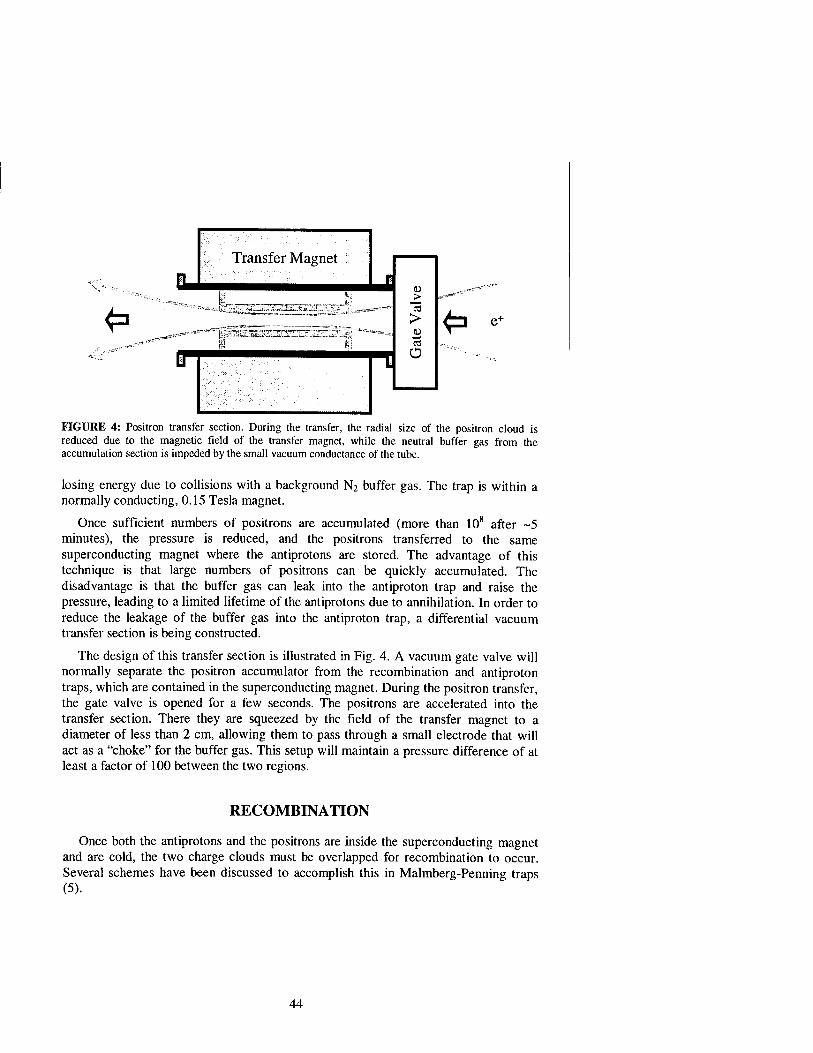
1 Transfer Magnet r

>

'S Ü

Ü Hl L

FIGURE 4: Positron transfer section. During the transfer, the radial size of the positron cloud is reduced due to the magnetic field of the transfer magnet, while the neutral buffer gas from the accumulation section is impeded by the small vacuum conductance of the tube.

losing energy due to collisions with a background N2 buffer gas. The trap is within a normally conducting, 0.15 Tesla magnet.

Once sufficient numbers of positrons are accumulated (more than 108 after ~5 minutes), the pressure is reduced, and the positrons transferred to the same superconducting magnet where the antiprotons are stored. The advantage of this technique is that large numbers of positrons can be quickly accumulated. The disadvantage is that the buffer gas can leak into the antiproton trap and raise the pressure, leading to a limited lifetime of the antiprotons due to annihilation. In order to reduce the leakage of the buffer gas into the antiproton trap, a differential vacuum transfer section is being constructed.

The design of this transfer section is illustrated in Fig. 4. A vacuum gate valve will normally separate the positron accumulator from the recombination and antiproton traps, which are contained in the superconducting magnet. During the positron transfer, the gate valve is opened for a few seconds. The positrons are accelerated into the transfer section. There they are squeezed by the field of the transfer magnet to a diameter of less than 2 cm, allowing them to pass through a small electrode that will act as a "choke" for the buffer gas. This setup will maintain a pressure difference of at least a factor of 100 between the two regions.

RECOMBINATION

Once both the antiprotons and the positrons are inside the superconducting magnet and are cold, the two charge clouds must be overlapped for recombination to occur. Several schemes have been discussed to accomplish this in Malmberg-Penning traps (5).

44

When the two charge species are in contact, they can recombine by two-body or three body collisions (6). (There are also ideas to induce recombination with resonant laser stimulation (7)). The recombination rate scales with positron temperature T and density n as

2-body: e++p=>H + /m R~n T^2

3-body: e++e++p=>H + e+ R~n2T-9'2.

In both cases a low positron temperature and a high positron density results in a higher recombination rate. It is certain to be advantageous for the positrons to be as cold and dense as possible. This means that the best recombination rates are achieved when the

positrons are in the plasma regime, i.e. when the Debye length X D = -y/T/47r ne2

becomes smaller than the size of the positron cloud (8).

The plasma temperature may be significantly higher than the electrode wall temperature (9), contrary to common belief. The electrostatic energy of a nonneutral plasma is large compared to its thermal energy, and any slow expansion of the plasma liberates electrostatic energy, which will be converted to thermal energy. Assuming collisions with neutrals can be neglected, the only cooling mechanism is cyclotron radiation. If the plasma has a radial expansion time given by xm, a cyclotron cooling time given by xc and the electric potential at the center of the plasma is <j)p, then in equilibrium

dT _ Ne(j)p NkT

dt xm xr = 0,

where N is the number of charges in the trap. Therefore, the plasma temperature will have a lower limit of kT/e « (xc/tm)<|)p. At the 3 Tesla field planned for ATHENA,

xc~0.4 seconds. If the potential of the positron cloud is 10 Volts, this requires expansion times >104 seconds to achieve temperatures as low as 4 K (0.0004 eV).

ANTIHYDROGEN DETECTOR

Once antihydrogen is formed in the trap, it will no longer be contained by the electric and magnetic fields, and will move in a straight line out of the system. Once it collides with the electrode wall or with a background gas atom, both the positron and the antiproton will annihilate almost simultaneously, within about 1 ns of each other.

The antihydrogen detector will surround the vacuum system of the recombination trap. The detector detects the products of both the antiproton and the positron annihilations. The annihilation of antihydrogen is distinguished from that of unbound antiprotons and positrons by the fact that with antihydrogen both the antiproton and the positron annihilate at the same point in time and space.

45

Silicon Strip Detectors

100 mm

FIGURE 5: Cross section of the antihydrogen detector and recombination trap. The charged particles are in the center; the inner black ring represents the electrode where annihilation occurs. The 511 keV gammas are detected by the Csl crystals and the pions by the silicon strip detectors. Drawing is to scale.

The annihilation of an antiproton on a nucleon produces on average 3 to 4 charged pions in the 50 to 900 MeV energy range. Si strip detectors, arranged in two layers around the recombination trap, measure two points of the trajectories. Each layer of strip detectors consists of 16 detector modules arranged around the circumference, with each module having 128 strips on one side (r-cp) and 128 pads (z) on the other side. The vertex of the antiproton annihilation is determined by the intersection of the lines extrapolated from the measured points on the strip detectors. The error on the vertex position is largely dominated by the unknown curvature of the pion tracks, leading to an average extrapolation error of about 1 mm.

The annihilation of a positron produces two 511 keV back-to-back gamma rays. They are detected in an array of 16 (r) x 12 (<p) Csl crystals with dimensions 17 (r) x 17.5 (cp) x 13 (z) mm, surrounding the Si strip detectors. If two crystals register energy deposits compatible with 511 keV gamma rays within about 1 microsecond of an antiproton annihilation, it is assumed that they originate from within a straight line between the two crystals. For antihydrogen annihilation, it is then required that the vertex position determined by charged pions lies within the errors in determining this line.

46

The figure of merit of the detector is the ability to pinpoint the vertex of these annihilations in space and time. This detector will locate the vertex of the pions to rjz ~ 5 mm, and ar(p ~ 1 mm. The vertex of the gamma rays is located to a tube of radius CTT

~ 7 mm. The time resolution of the device will be about 1 |j.Sec.

Many details have been left out of this simplified description. The evidence for the existence of H will be statistical, since there are several background sources. The main source of the 511 keV background is positrons annihilating in the material outside the detector. These positrons stem from pair creation by n0 decay gamma rays, which are emitted during the antiproton-nucleon annihilation.

REFERENCES

1. Gabrielse, G., et al., ATRAP Collaboration, "The Production and Study of Cold Antihydrogen", Proposal to the SPSC, CERN, SPSC 97-8/P306, March 1997. 2. For a recent review, see Holzscheiter, M.H. and Charlton, M., Rep. Prog. Phys. 62,1-60 (1999) and references therein. 3. Collier, M.J.T., J0rgensen, L.V., Meshkov, O.I., van der Werf, D.P. and Charlton, M., "Development and Testing of a Positron Accumulator for Antihydrogen Production," presented at the AIP Conference on Nonneutral Plasma Physics, Princeton, NJ, August 2-5,1999. 4. Greaves, R. G, Tinkle, M. D. and Surko, C. M., Phys. Plasmas 1, 1439 (1994). 5. Ordonez, C. A., Phys. Plasmas 4, 2313-5 (1997). 6. Müller, A. and Wolf, A., Hyperfine Interact. 109,233-67 (1997). 7. Wolf, A., Hyperfine Interact. 76 189-201 (1993). 8. Chen, F.F., Introduction to Plasma Physics and Controlled Fusion, New York: Plenum Press, 1984, ch. 1, p. 11. 9. Anderegg, F., Hollmann, E. M. and Driscoll, C. F., Phys. Rev. Lett. 81,4875-8 (1998).

47

Trapping, Cooling and Extraction of Antiprotons, and the ASACUSA Project

Yasunori Yamazaki

Institute of Physics, University of Tokyo, Komaba, Meguro, Tokyo, Japan 153-8902 &

Atomic Physics Laboratory, RIKEN, Wako, Saitama, Japan 351-0198

Abstract. Ultra slow mono-energetic antiproton beams are under preparation combining novel techniques to decelerate antiprotons with an RFQD (Radio Frequency Quadrupole Decelerator), to trap, cool, and compress in an electromagnetic trap, and finally to extract as an ultra slow monoenergetic beam. This unique beam will make it possible to study the ionization processes around adiabatic energy regions, channeling, stopping power, antiprotonic atom formation processes under single collision conditions, to prepare metastable antiprotonic atoms such as pp, pHe+, pHe++, pLi+ in vacuum, and to make high precision laser spectroscopy of them. This project

named ASACUSA (Atomic Spectroscopy And Collisions Using Slow Antiprotons) is expected to open a new physics regime in antimatter science under well controlled conditions.

INTRODUCTION

Before the termination of LEAR (Low Energy Antiproton Ring) at CERN in 1996, atomic collisions particularly charge asymmetry effects and high resolution laser spectroscopy of antiprotonic helium ( pHe+) were intensively studied. Recently, the second generation facility, AD (Antiproton Decelerator), devoted to atomic physics experiments had been approved at CERN, and is expected to start its operation before the end of 1999. Until now, three proposals have been approved, two of which are on the production and spectroscopy of antihydrogen (ATENA and ATRAP collaboration) aiming to investigate a violation of CPT. The third one is on atomic collisions and spectroscopy of antiprotonic atoms (ASACUSA collaboration), which is to be discussed in the present report (1).

When an antiproton approaches an atom, an outermost electron is repelled by the antiproton, which causes the binding energy of the outermost electron to be shallower. In such a case, even a very tiny "kick" is strong enough to liberate the electron from the atom. This is expected to be a universal scenario of ionization at the initial stage induced by slow negatively charged heavy particles, which is essentially different from those by positively charged heavy particles. It is noted however that such a scenario has never been tested simply because no such beam has been available. Until now, ionization processes with antiprotons were studied as low as a few tens keV (2). Theoretical predictions get conflicting with each other below this energy range, i.e., it is crucial to prepare antiproton beams with lower energies, which is the important subject of ASACUSA project beyond the foregoing projects in the LEAR era.

When the kinetic energy of the antiproton is less than the binding energy of the outermost electron, the particle is bound to the atom after the release of the electron,

CP498, Non-Neutral Plasma Physics III, edited by John J. Bollinger, et al. © 1999 American Institute of Physics 1-56396-913-0/99/$ 15.00

48

which is a naive picture of an "exotic atom" formation process. As is discussed later, the binding energy of the particle just after the formation is comparable to or even less than the binding energy of the released electron, i.e., the particle is in a high Rydberg state. Furthermore, a considerable fraction of them are in a high angular momentum state, which is expected to be metastable with cascading lifetimes of the order of usec or even longer, and a laser spectroscopy with a precision as high as ppb becomes in principle possible. However, in the real world, it is well-known that energetic hadrons with negative charge annihilate immediately in dense media through thermalization and antiprotonic atom formation. Inter- and Intra-Auger transitions and Stark mixing induced by neighboring atoms have been considered to be responsible to accelerate cascading processes and to shorten the lifetime. Because of this "common sense", it was a big surprise when metastable particle-He complexes were found and identified (3, 4). Particularly, in the case of antiproton, a considerable fraction of pHe+ has been found to survive more than ~usec even in liquid He. _This extreme metastability has allowed to determine the binding energies of pHe+ with ppm or even better precision, which provides the charge ratio and mass ratio between protons and antiprotons with an accuracy an order of magnitude better than before (5). Extensions of the pHe+ spectroscopy to higher resolution including a laser-microwave double resonance to measure hyperfine structure is the important subject of the ASACUSA project.

There have been vast progresses in catching and cooling antiprotons in an electromagnetic trap, which opens a way to develop ultra slow monoenergetic antiproton beams (6). Once developed, various antiprotonic atoms can be prepared in vacuum keeping their intrinsic metastability, which enables for the first time to make a high precision laser spectroscopy of various antiprotonic atoms such as protonium ( pp), the simplest pure hadronic atom, pHe^, pLi+, etc. (1) (7). Such an ultra slow antiproton beam will be prepared by the combination of AD (antiproton decelerator), RFQD (radio frequency quadrupole decelerator), and a Multi-Ring electrode trap (MRT) (8). By this way, the number of ultra slow antiprotons available will at least be two orders of magnitudes larger than ever achieved.

In the following sections, several research plans are discussed together with the procedure to prepare ultra slow antiprotons, which includes in itself various interesting research fields like accelerator physics, non-neutral antimatter plasma physics, etc.

PRODUCTION OF ULTRA SLOW ANTIPROTONS

Antiprotons had been discovered in 1955 for several GeV protons hitting a target (9), the reaction of which is given by

p + p-> P + P + P + P- 0)

Considering that the inner product of 4 dimensional momentum is invariant with respect to Lorentz transformation and four particles in the final states are all at rest in

49

p sroduetiortj 3. 5GeV/cp tareet fi /

pprod AD RFQD MRT

3.5GeV/c SMeV/i lOVpuls 1 pu!se/r

e nin

50keV/u SxlO6 /puls 1 pulse/mir

e > 10eV/u

2x10 /min

the center of mass frame (eq.l), the threshold energy of incident protons to produce antiprotons is evaluated to be about 5.6GeV in the target frame, i.e., the antiprotons so produced inevitably possess kinetic energies at least several hundreds MeV. In old days, the only way to get low energy antiprotons was to use a degrader foil followed by a momentum selector, which yield only weak and low quality antiprotons contaminated by 2 orders of magnitudes stronger pions and muons of the same momentum. In this respect, it was really a revolution when LEAR started to supply high intensity and high quality ~5MeV p, which reduces the kinetic energy by three digits. What is going to be discussed here is to reduce another five digits, i.e., a new regime in slow antiproton studies.

FIGURE 1. A schematic drawing of the proton synchrotron complex and AD at CERN

As is schematically shown in fig.l, the production of a high quality antiproton beam of-10 eV is going to be realized via

1 production of ~5xl07 p/pulse at around 3.5GeV/c with 26 GeV/c protons of 1.5x10,3/pulse supplied from theCERN PS (proton synchrotron)

2)Accumulation of the 3.5GeV/c p, cooling, and deceleration down to 100MeV/c (5.3MeV/u) in the AD (Antiproton Decelerator), which takes ~lmin for cooling and deceleration. (Because of this macroscopic cooling time, slow unstable particles such as u" or % are not available in this way.)

3)Extraction of -lxlO7 antiprotons per lmin. at 5.3MeV/u with the pulse width of ~250ns from the AD, and deceleration down to ~50keV by the RFQD (radio frequency quadrupole decelerator). (The electrodes of the RFQD can be biased by 50kV, i.e., the energy of p from the RFQD is in principle continuously tunable from 0 to lOOkeV)

4)Injection into a superconducting solenoid where the Multi-Ring electrode Trap (MRT) is installed.

5)Capture, cooling down below eV, radial compression, and finally extraction from the MRT, which is expected to provide ultra slow antiprotons with an efficiency of several tens %.

Transport features of the antiprotons from the RFQD to the trap have been simulated intensively by the RFQD group at CERN, which tells that the envelope (at

50

Antiprotons (50keV)

<r>

Degradation Foil (Biased)

5 standard deviations) of the antiproton trajectories is compressed down to ~2 mm in radius upon injection at the center of the solenoid (10) (11).

A schematic diagram of the antiproton cooling procedure is given in fig.2. In order to capture antiprotons with rather low trapping potential, a thin degrader foil will be inserted to reduce the antiproton energy below 10 keV. The foil can be positively biased, which effectively reduces the energy straggling of the degraded beam and eventually increases the trapping efficiency (12). The right end electrode of the trap (see fig.4) is negatively biased so that it reflects antiprotons. Before the reflected antiprotons reach the left end of the trap, the left end electrode is biased from 0 to <-10 kV, which results in trapping the antiprotons. In the trap, electrons are pre-loaded, which are cooled via synchrotron radiation with a time constant Trad. At 5T, xrad is about 0.1 sec (7). The cooled electrons then cool the injected antiprotons via the Coulomb interaction in the time range of | Solenoid Coil 10 sec. (6) (13). The MRT has been employed to store as many as ~5xl06 p and about 100 times more electrons in a prolate spheroid with a radius ~1 mm and its axial length ~50 mm with a rather low trapping potential. It is noted that the overall trapping efficiency of the present setup is designed to be about two orders of magnitudes higher than that obtained by a conventional trapping scheme, i.e., the combination of a degrader foil and an electro-magnetic trap. Recently, slow positrons of 0.1 eV to several tens eV with an energy width of about 18meV have been successfully prepared (14) employing a ~J 10' p method similar to what is discussed here, which supports the scheme described here.

Injection f ~^^

Capture

Cooling, Compression

Electron Ejection

Extraction

~^mf~

FIGURE 2. A schematic procedure to trap, cool, and extract antiprotons.

Figure 3 shows a drawing of the superconducting solenoid, which is designed so that (a)the bore is bakable while keeping the superconducting solenoid at liquid helium temperature, and (b)the bore where the MRT is installed is independently movable to align the MRT axis to the symmetry axis of the magnetic field, which is

51

essential to realize a successful extraction of slow charged particles. Further, the magnetic field is scannable at 5T/90sec, which allows us to vary the field strength depending on the operational stage, i.e., injection, cooling, or extraction. In order to simulate the whole procedure to prepare ultra slow p trapping, cooling, and extraction, experiments with p and H" are in progress (13).

As is well known, the rotation angular frequencies for electron and antiproton plasmas, coe and a> -, are given by

roc = (l/2)(cocc+-(öC£2-2 0,'2), (2)

<D-P = (m/2mp)(ü>ccMöce2-2(m/2m>pe2)1/2) , (3)

respectively, where coce is the cyclotron angular frequency of electron (=eB/me), K»pc is a plasma angular frequency of the electron, which is defined as ((Pe+Pp)e2/mce0)

1/2 ~ 5xl04 (p^cm3))"2

(sec"1). In the present condition (i.e., pc

» p - ), pc governs the Brillouin limit for antiprotons as well as that for electrons, which are 3xl09B(T)2/cm3 and 5xl012B(T)2/cm3, respectively. The solenoid is designed to yield 5T, which guarantees that the expected plasma density is well-below the Brillouin limit even for antiprotons. In this case, coe

+

and co -+ are approximately given by coce

and (me/m -) coce (= coc - ), respectively, andco„ and co -' are

co„

co-

~ (copc2/2 coce) (1+ cope

2/2co«2), (4)

~(cope2/2 cocc)(l+ m - copc

2/2me coce2),

(5) FIGURE 3. A drawing of the 5T superconducting solenoid,

respectively. Equations (4) and (5) tell that (a) co -" is proportional to pJB, i.e., the kinetic energies of antiprotons and electrons due to the rotation are higher for lower B, (b) for pe~5xl09/cm3 and B=5T, co-" is ~2% larger than co/, which causes the antiproton cloud to be extruded out from the electron cloud (15,16), and (c) co -" is ~107/sec, which corresponds to the p kinetic energy of-0.5 eV at the periphery of the plasma. This rotation could cause a serious problem if one wants to have very cold antiprotons in the laboratory frame although the antiproton temperature in the rotation frame could be as low as the environmental temperature, i.e., several K in

52

Catching Electrode Segmented Electrodes

Harmonic Part

Calchins Electrode

200mm FIGURE 4. A drawing of the MRT.

the present case. A drawing of the MRT is shown in fig.4, which consists of 14 cylindrical

electrodes of 40 mm in inner diameter and total length of -500 mm. Seven electrodes near the center are to form a harmonic potential to stably store and cool antiprotons (8). One of them is segmented into four so that a rotating field can be applied to the plasma to increase or decrease its rotation frequency (17) (18). As is seen from eqs. (4) and (5), the higher the frequency, the higher the density, i.e., the plasma is compressible by applying appropriate rotating fields. The plasma compression in the MRT has been successfully tested with electrons (13).

Cooled antiprotons will be extracted at ~keV as a continuous or a pulsed beam from the trap and transported to the target area, where the antiprotons are decelerated down to 10 eV range. Several differential pumping stages separated by small holes (~3 mm<|>) are necessary on the way from the trap to the target chamber, to keep the trap area at UHV and at the same time to use a gas cell of 10"3Torr in the target chamber.

ATOMIC PHYSICS WITH ANTIPROTONS

Ionization

One of the most fundamental process in atomic collisions is ionization. In particular, ionizing processes in p-H collisions provide the simplest and accordingly the ideal case to test our understanding of collision dynamics (2) (19). At high velocities (i.e., the projectile velocity is much higher than a typical velocity of the electron to be ionized), single ionization cross sections are known to be practically the same for p and p as the first Born approximation tells. When the projectile velocity gets lower, the polarization effects and then deflection effects start to play roles, which make the ionization cross section by p to be smaller and then higher than that by p.

Single ionization cross sections of D for p are summarized in fig.5 together with

53

several theoretical predictions (20) (21) (22). It is seen that the theoretical predictions agree more or less with one another for energies higher than ~ 50 keV as well as with the experimental results. At lower impact energies, although the scatter among different theoretical predictions is rather large, many theoretical results predict that the cross section becomes almost energy independent. Already in the late 40', Fermi and Teller (23) discussed that the binding energy of an outermost electron of the atom gets smaller when an antiproton approaches an atom, and at a certain distance, dcr, the binding energy vanishes (dcr is called the critical distance), i.e., the atom is ionized even when the collision evolves adiabatically as far as the distance of closest approach is smaller than dcr. It is noted that such a behavior is quite different from that of the ordinary ion-atom collisions, where the ionization cross section decreases as the projectile velocity decreases unless a resonant charge transfer process comes into play. According to this discussion, an expected ionization cross section is -1.3 a.u. (Fermi-Teller limit) considering dcrfor H is 0.63 a.u. It is noted that the experimental results are about three times bigger than the Fermi-Teller limit. It is predicted that "non- 2.5 adibatic effects in adiabatic collisions" play important roles 20

because the binding energy gets very shallow during the collision, i.e., the Massey criteria, 27taAE/hu » 1 (a is of the order of the impact parameter, AE the energy difference, h the Planck constant, and u the projectile velocity), is not necessarily satisfied for negatively charged 1 10 100 1000 particles even at low velocities. EncrfyiKcv

FIGURE 5. Single ionization cross section of D by antiprotons (see the text for details)

„r~ 1.5

1.0

0.5

TDSE Wells cl a] (96) » --- - CTMC Wells ct al (96) \ ** TDSK Krslic el al (96)

** * _... CDW-bIS Hainslein (94) CTMCKrmolaev(87)

— --- \ # *• OCAOCC Schiwiet* (95)

** -V ,'"\\ TCAOCC Toshima (93)

^^^^s-r^^^-e^, ■ PS194|95|

wk P+D *-~-~~^^ F. - T. Effective

/ TK% / 1 \Xfc / *ifc * "N^Ä —— _/ Fermi - Teller limit T*^.

The single ionization cross section of He shows a clear peak at ~70 keV in contrast to the D target case (2) (24). It is noted that the critical distance for He is "negative", i.e., the electronic binding energy stays negative finite even under unified atom limit, which is known as H". Ionizations of atoms and molecules with different critical distances are expected to be very important for comprehensive understanding of collision dynamics.

Kinematically complete ionization experiments of hydrogen and helium targets by antiprotons are under discussion employing a technique of Recoil-Ion Momentum Spectroscopy (25), which will be combined with a table top electrostatic storage ring (26). The double ionization process of helium by antiproton has been intensively studied, which revealed that a^ p) is about two times larger than ^(p) of the same velocity even for projectile energies as high as 10 MeV/u (2). It has been shown that the electron-electron correlation plays an essential role to reproduce the observations. In this direction, the study of double excitation process combined

54

with the kinematically complete experiment described above should be very interesting, because a collision system with (quasi-)bound states can be handled more accurately as compared with those involving two continua like in the case of double ionization, and could be more sensitive to details of the collision dynamics (27).

The stopping power of ~keV antiprotons, the channeling of -100 keV antiprotons through a single crystal target, etc. will also be studied with beams directly from the RFQD and the MRT. It is predicted that -lOOkeV antiprotons show a characteristic channeling pattern (28), which will be experimentally studied for the first time with antiproton beams from the RFQD.

Antiprotonic Atom Formation

When an antiproton with very low kinetic energy ionizes an atom, it can be trapped into an atomic orbital with a large principal quantum number n. Considering the energy conservation before and after the collision in the center of mass system, the binding energy of p,£-pA, is estimated to be

SpA(~(^iAH)(%/n2)) ~ Ee, K pA> (6)

14

cC 12

z o i- o UJ co w to O a: ü

8

pbar + H (protonium) pbar + H (ioni. + protonium) _

— pbar + H2 (protonium) — pbar + H2 (ioni. + protonium) -

where nAB is the reduced mass of particles A and B, ER is the Rydberg constant (-13.6 eV), EAB is the binding energy between A and B, KAB = (l/2)nAB uAB

2, and uAB is the relative velocity between A and B (7). Equation (6) tells that (a) the trapping cross section is finite if 0 < K -A < e^, and (b) n is a function of K -A, which varies from nmia (~(UpA

/me)(sR/e-pA )m ) to infinity as K-A

increases from 0 to e,^, i.e., the principal quantum number n is tunable. Because the momentum carried by the released electron is fairly small, the momentum of pA+ is practically that of the incident p. In other words, the pA+ so prepared could be used as a high quality beam maintaining the quality of the incident p beam.

20 40 60 80

ENERGY (eV)

100 120

FIGURE 6. Protonium formation cross section for H and H2 (see text for details).

The above qualitative arguments are more or less confirmed by a CTMC (Classical Trajectory Monte_ Carlo) method and an FMD (Fermion Molecular Dynamics) method to treat p-H and -H2 collisions in a low energy region (29)(30), the prediction of which is shown in fig. 6. The solid line and the dotted line shows protonium formation cross section, a -p, and total (formation and ionization) cross

55

section, CJ„ in p-H collisions, respectively. A clear threshold is seen at around 30eV for a pp, although a, varies smoothly. The same calculation predicts that the n distribution peaks at around 30, 38, and 60 for the antiproton energy of 2.7, 10.8, and 21.8eV, respectively, which is also consistent with eq.6. The / distribution peaks at around 25, 35, and 30 for the above antiproton energies (30). At very low energies, the polarization of the target atom becomes important, which makes the antiprotonic atom formation cross section to be inversely proportional to the antiproton velocity.

The prediction for H2 targets are also shown in fig.6, which indicates that initial internal motion of the molecule plays an important role in the antiprotonic atom formation process (29). Because of this, the antiprotonic atom formation cross section stays finite even beyond the threshold energy given in eq.6. The dash-dotted line and the dashed line in fig.6 show CT -p, and a, for p-H2 collisions, respectively. The internal motion also considerably broadens the angular distribution of pp. The role of the third body in determining the pA+ formation cross section above the threshold has also been predicted for multi-electron system like Ne (31). Further, molecular targets could provide an interesting chance to study a "dynamic Stark effect" because the antiprotonic atom evolves in the electric field of the spectator atom (ion) for a finite time. The electric field will increase the fraction of s-state components due to Stark mixing, and accordingly increase the annihilation rate, which may provide a new and sensitive measure of collision dynamics.

Various multielectron antiprotonic atoms are also expected to have intrinsic metastability, which can be realized only when they are produced in vacuum under single collision conditions. Like in the case of H, Li has a positive critical distance for antiproton (dcr=0.79 a.u) (32). As the antiproton replaces the 2s electron of Li, it is far outside of the residual two Is electrons, i.e., the Auger transition rates will be fairly small because the transition energies are large and the spatial overlap between the initial and the final orbits is small. It is further noted that the antiprotonic states with the same principal quantum number but with different orbital angular quantum numbers do not degenerate, i.e., pLi+ is strong against annihilation induced by Stark mixing(32,7,ll). In the same direction, pHe+ produced in collisions with He in metastable states(ls2s1,3S, ls2p3P, etc.) is also expected to be very stable. pHe+

eventually decays into pHe+ +, which is again metastable as far as it is in vacuum. Other examples of metastable antiprotonic are discussed in ref.(7) (11).

High Precision Spectroscopy of Antiprotonic Atoms

The discovery of meta-stable pHe+ has made it possible to study the nature of antiprotonic atoms with high precision laser spectroscopy (3) (33). This field has developed rapidly from the level of identification of the principal and angular momentum quantum numbers {i.e., n and I) to the level of determination of the transition energies with a fraction of ppm (5), which agrees with theoretical predictions taking into account relativistic and QED effects on the bound electron (34) (35) (36). The above finding tells that if the theoretical treatment of the Coulomb three-body system is correct, the mass and the charge difference between

56

nn c Detector

Laser

^

proton and antiproton is less than ppm, which is an order of magnitude more accurate than before. JI

In the ASACUSA \ Track Detector project, studies in this direction will further be pursued employing, e.g., laser and microwave double resonance, which enables to determine the magnetic moment of antiprotons with much higher accuracy than ever achieved.

£

(perpendicular or parallel to Lhc beam)

FIGURE 7. A possible experimental setup of lifetime measurements and laser spectroscopy of pp, pHe+, pHe^, etc.

Among various antiprotonic atoms to be available with the ultra slow p beams, protonium is particularly interesting because it is the simplest two body system consisting of a particle and an antiparticle with strong interaction. It is noted again that a monoenergetic pp is available only with an atomic hydrogen target, the density of which cannot be very high. In this respect, a possible alternative of a pure two body system is pHe**, the principal quantum number of which could be tunable not only with the incident energy of p but also with a He target in excited states. Such a two body system in a Yrast state can decay only via slow radiative transitions when the external electric field is negligible, and its lifetime can be much longer than lusec, i.e., a high resolution laser spectroscopy becomes applicable to protonium and/or pHe** for the first time. A sketch of a possible experimental setup to measure the formation cross section and to make high precision laser spectroscopy is drawn in fig.7. The formation cross section and the («,/) distribution of pp will be determined by measuring the time difference between the electron signal and the annihilation signal together with the position of annihilation. In the case of Laser spectroscopy, again the emitted electron triggers a Laser, which excites one of the formed states into a high n state with a much longer lifetime, i.e., a high precision spectroscopy of pp can be made via the lifetime measurements.

ACKNOWLEDGEMENTS

The author is deeply indebted to J. S. Cohen, K. Ohtsuki, H. Totsuji, G. Ya. Korenman, N. Kabachnik, A. Lombardi, and colleagues of the ASACUSA project, particularly the trap group members, T.Ichioka, RHigaki, K.Yoshiki Franzen, M.Hori, N.Ohshima, A.Mohri, and K.Komaki for their fruitful and vivid discussions. The work is supported by the Grant-in-Aid for Creative Basic Research (10NP0101),

57

Ministry of Education, Science, and Culture.

REFERENCES

1. ASACUSA collaboration proposal, 1997 CERN/SPSC 97-19, SPSC P-307 2. Knudsen,H., and Reading,J., Phys. Rep.212, 107(1992). 3. YamazakiJ., et al., Nature 361,238(1993), Morita, N., et al., Phys. Rev. Lett. 72,1180(1994), Hayano, R.S.,et al, Phys. Rev. A 55,1(1997). 4. Condo, G.T., Phys.Lett. 9, 65(1964). 5. Torii,H.A., et al., Phys. Rev. A 59, 223 (1999). 6. Feng,X., Holzscheiter,M.H., Charlton,M., HangstJ., King,N.S.P., Lewis,R.A., Rochet,!, and Yamazaki, Y, Hyperfme Interactions 109, 145(1997). 7. Yamazaki, Y, Nucl.Instrum.Methods B154(1999)174. 8. Mohri,A., et al., Jpn. J. Appl. Phys. 37, 664(1998), and Higaki, H., and Mohri, A., Jpn. J. Appl.Phys. 36(1997)5300. 9. Chamberlain, O., Segre, E., and Wiegand, C, Phys.Rev.100 (1955)947. 10. Lombardi,A., Private communication. 11. Yamazaki, Y, to be published in the Proceedings of 18,h International Conference on X-ray and Inner-Shell Processes. 12.Tschalaer, C, Nucl.Instrum.Methods 64(1968)237. 13. Ichioka, T., et al., this proceedings. 14. Gilbert, S.J., Greaves, R.G, and Surko CM., Phys.Rev.Lett. 84(1999)5032. 15. Larson, DJ., et al., Phys. Rev. Lett. 57, 70(1986). 16. Totsuji, H., et al., this proceedings 17. Huang,X.-R, et al., Phys. Rev. Lett. 78, 875(1997). 18. Anderegg, R, Hollmann, E.M., and Driscoll, C.F., Phys.Rev.Lett. 81(1998)4875. 19. Knudsen,H., et al., Phys. Rev. Lett. 74,4627(1995). 20. Toshima,N., Phys. Lett. A 175, 133(1993). 21. Krstic,P.S., Schultz,D.R.,and Janev, R.K., J. Phys. B 29, 1941(1996). 22. Wells,J.C, Schultz,D.R., Gravras.P., and Pindzola,M.S., Phys. Rev. A 54, 593(1996). 23. Fermi, E. and Teller, E., Phys. Rev. 72, 399(1947). 24. Andersen,L.H., et al., Phys. Rev. A 41, 6536(1990). 25. Ullrich,!, et al., Topical Review,! Phys. B 30, 2917(1997). 26. Schumidt-Boecking, H., et al., Abstract of International Workshop on Atomic Collisions an Atomic Spectroscopy with Slow Antiprotons, (Tsurumi, Japan, 1999), and Moller, S.P., Nucl.Instrum.Methods A394, 281(1997). 27. Morishita,T, et al., J. Phys. B 30, 2187(1997). 28. Kabachnik, N.M., Balashova, L.L., and Trikalinos, Ch., Abstract of International Workshop on Atomic Collisions an Atomic Spectroscopy with Slow Antiprotons, (Tsurumi, Japan, 1999), and private communications, E.Uggerhoj, Nucl.Instrum.Methods B135(1998)35 29. Cohen, J.S., Phys. Rev. A 56, 3583(1997), and private communication. 30. Cohen, J.S. and Padial, N.T., Phys. Rev. A 41, 3460(1990), Cohen, J.S., Phys. Rev. A 36, 2024 (1987) 31. Cohen, J.S., to be published in the Proceedings of the XXIth ICEAC (Sendai, 1999) 32. Ohtsuki, K., Abstract of International Workshop on Atomic Collisions an Atomic Spectroscopy with Slow Antiprotons, (Tsurumi, Japan, 1999), and private communication. 33. Widmann, E.,et al., Phys. Lett. B 404, 15(1997). 34. Korobov.V!., Phys. Rev. Lett, to be published. 35. Elander, N., and Yarevsky, E., Phys. Rev. A 56, 1855(1997). 36. Kino,Y, Kamimura, M.,and Kudo,H., Proc.XV. Int. Conf. Few-Body Problems in Physics, Groningen, 1997.

58

Multi-ring Trap as a Reservoir of Cooled Antiprotons

T.IchiokaA'C, H.HigakiA, M.HoriB, N.Oshimac, K.Kuroki0, A.Mohri0, K.KomakiA, Y.YamazakiA'C

A Institute of physics, University of Tokyo,

3-8-1 Komaba, Meguro-ku, Tokyo 153-8902, Japan B Department of Physics, University of Tokyo,

7-3-1 Hongo, Bunkyo-ku, Tokyo 113-0033, Japan 0Atomic Physics Laboratory, RIKEN,

2-1 Hirosawa, Wako-shi, Saitama 351-0198, Japan D National Research Institute of Police Science,

6-3-1 Kashiwanoha, Kashiwa-shi, Chiba 277-0882, Japan

Abstract. For the ASACUSA project, a new charged particle trap was designed and con-

structed. Like a Penning-Malmberg trap, static electric and static magnetic fields are used. Multi-ring electrode is exploited to generate a harmonic potential on the trap axis. It enables the confinement of a number of antiprotons and electrons for the electron cooling. Upon its design, plasma behavior of trapped particle clouds was taken into consideration.

As the first step, trap performances have been checked with electrons. Current status are presented.

INTRODUCTION

In ASACUSA project, experiments are planned to investigate initial formation processes of antiprotonic atoms, interaction between antimatter and matter etc., most of which require ultra-low energy antiproton beams [1-3]. At Antiproton Decelerator (AD ; at CERN), 107 antiprotons of 5 MeV will be at hand as a pulse of 250 ns with a repetition period of one minute. In our scheme, MeV- energy antiprotons from AD will have several tens of keV after passing through an RFQ, post decelerator. Those antiprotons enter a Multi-Ring Electrode(MRE) trap described in the following section. Then the well-known electron cooling technique will be applied. Dense cloud of antiprotons, together with electrons, are supposed to behave as a nonneutral plasma. Extraction method is being considered.

A MRE trap allows the utilization of axially long harmonic potential region. Advantages are :


59

(a) It ensures longer life times of plasmas than in the case of square potential [4].

(b) When the plasma radii are reduced, plasmas can freely accommodate themselves so that their axial lengths are longer, which can reduce a possibility of plasma heating up.

(c) It allows the plasma CM motion which can be used for diagnoses.

TRAP DETAILS

Design In designing the trap, following two points are especially considered :

1. Preparation of 106"7 antiprotons with sub-eV energy within one minute (the value of which comes from the pulse interval at AD).

2. Extraction of cooled antiprotons from the trap which is located in the strong magnetic field.

As low energy charged particles tend to follow the field line, it is essential to make the position of the particles as close to the axis as possible for their extraction as a beam. One solution is the application of a rotational electric field, known as a "rotating wall method". Such a field can exert a torque on the plasma so that the plasma shape can be changed [5,6]. This method is thought to be effective in our application and one of the electrodes is segmented for the radial compression of the plasma.

When the plasma composed of electrons and antiprotons is axially compressed in this way, it stretches in the harmonic region. It can be noted that the square potential does not allow such an axial expansion. To reduce the space potential while keeping the cooling power high enough, central harmonic region is elongated in the axial direction so that the density will be optimum. Multi-ring structure [7,8] is exploited to generate such a harmonic potential.

Supposing that an antiproton cloud (density np, temperature TP[K]) and an electron cloud (density ne, temperature Te[K]) are uniformly mixed at a time t = 0, simulations were done to estimate the time necessary for the electron cooling of antiprotons. Using cgs units, time evolution of Tp and Te were determined by following set of equations

^ = Vpe(Te-Tp) (1)

^ = uep(Tp - Te) - TeA (2)

where A ~ ,^|2 is a synchrotron radiation cooling rate found experimentally

[8]. Using Boltzmann constant(/c), electronic charge(e), electron mass(rae) and antiproton mass(mp), equilibration rates (i^pe, vep) are given by

60

8\/27re4

^DR 3fc5

8\/2^e4

T^e^pe' rnjimg

3fc5 Tin A»

mpTe + meTp) 2

nip mi

(3)

(4) ep (mpTe + merp) 2

In FIGURE 1 and 2, result are shown. Realistic experimental conditions are assumed : B = 5[T], T„(0) = 5.8 x 107[K](= 5000[eV]), Te(0) = 4[K] , Coulomb logarithm \ep = \pe ~ 30. For the calculation in FIGURE 1, np = 108[cm 3], ne = 108[cm-3] were inputted and in the FIGURE 2, np = 108[cm-3], ne = 109[cm 3] were used.

o 1

> (D

O) O

1

0

-1

-2

-3

20 30 40 SO 60

Time (sec)

10 20 30 40 50 60

Time (sec)

FIGURE 1. Simulation of electron cooling rate. ; np = 108[cm 3], ne = 108[cm

O)

„ 2 > S. 1 o.

-3

4 6

Time (sec)

4 6

Time (sec)

FIGURE 2. Simulation of electron cooling rate. ; np 108[c , ne = 109[cm-3]

It is seen that electrons initially warmed up by incoming hot antiprotons lose their energy via synchrotron radiation and both antiprotons and electrons will be cooled below 1 eV within one minute. We may note that the cooling time will be longer if consider the anisotropy on the space and the temperature. Cooling time is thought to be optimized by adjusting the densities of two species.

61

Experimental Setup In FIGURE 3, shown are electrode configuration and schematic trap-cool-dump procedure. The ratio of the axial extent of the harmonic region to the radius of electrodes is about 5 times larger than that of a traditional Penning trap.

OD = 38 mm ID = 2 mm

Segmented electrode

ectrons : 50 - 100 eV / ' \

cold electrons

Electron spheroidal plasma

FIGURE 3. Configuration of trap electrodes. Inner diameter of cylindrical electrodes is 40 mm.

All the electrodes are made of OFHC copper with the machining precision of 10 ^m and gold plated with the thickness enough to improve the surface property while the precision is tolerable. They are aligned on a base plate which is machined with the same precision. Insulation is done by pieces of A1N, which is known to be a good thermal conductor as well as an electric insulator.

For the application of rotational rf field, an electrode that is azimuthally segmented into four identical parts is located next to the one at the center. On one end of the trap there is a Faraday cup which serves as a detector for destructive diagnosis. It consists of two concentric parts as shown in FIGURE 3. In the future when the system is incorporated with the beam line, this part will be replaced by an grounded electrode. Two electrodes marked as HV are for the catching of energetic antiprotons.

All the system is installed in a superconducting solenoid. The uniformity of the magnetic field is better than ±0.5% within a region of 10 mm(D) x 1100 mm(L) and considered to be much better in the trapping region.

We also have a duoplasmatron ion source which can supply both proton and negative hydrogen ion beam. A negative hydrogen ion has a binding energy of 0.74 eV and can be used to simulate an antiproton in the low energy region. For tests like the injection of a high energy beam into the trap, protons will be used. A beam line which connects the ion source and the trap is already constructed and tested.

62

RESULTS

At first, electron trapping experiments were performed. A hot cathode located at the position 5cm off axis, in about 1 m from the center of the magnet (B-field strength ~ 100G) is used to generate electrons. They were injected into the trap as a pulse train. Typical incident energy was 95 eV. Two HV electrodes were not used for electron trapping. Instead, two electrodes next to them (F3 and B2) were utilized for the initial confinement.

Trapping potential except the one for the entrance wall was formed before- hand(F2 - B2) and, by raising the potential height on the entrance(F3), confinement was completed(shown as 1 in the FIGURE 3). After a trapping period, electrons were dumped by changing the potential(shown as 2) and detected at the Faraday cup. Magnetic field strength was kept at 1 T during all the measurements.

The life time of electron plasmas was measured to be around 200 sec under the base pressure of 5 x 10-9 Torr.

In FIGURE 4, the effect of rotating electric field is shown. Sweep rate was set to be 2 MHz/min. There was shot-by-shot fluctuation in the number of electrons(about 10 %), which is not shown in the graph.

(A) • total ♦ center

(B)

< o

-O 5 - E z

15

1 1 ' 1 ' 1 ' 1 ' 1 ' 1 '

-• • • • • • •

10

♦ -

♦ ♦

5

♦,

♦ 1 i

♦

1 i 1 i 1 , 1 ,

♦

1 ,

i ' r i ' i ' i

♦, i». i». i». i», i+, i». 0 10 20 30 40 50 60 70 I

Trapping time (sec); RF sweep : 1 to t/30 MHz

FIGURE 4. Effect of rotating electric field. (A) : with RF, (B) : without RF

10 20 30 40 50 60 70

Trapping time (sec)

It was shown that the rotational electric field can compress the plasma and up to 60 % of the constituent particles was confined in a region of 2 mm in diameter. In addition, the life time of the plasma became longer. It can also be seen that the application of too high frequency reduces the fraction of electrons compressed

63

radially. Since the effectiveness also depends on the sweep rate, optimization is still necessary. Generation of electrons by ionizing the residual gas was observed when the amplitude was too high.

Observation of radial and axial plasma modes by a spectrum analyzer has been also performed by picking signals up from the segmented electrode or one of the ring electrodes. When the rotational electric field was properly applied, (2,0) and (3,0) mode frequencies increased.

Injection of negative hydrogen beam was tried, though their plasma oscillations have not yet been observed. Electron cooling of them is in progress.

CONCLUSION

In a newly constructed Multi-Ring Electrode(MRE) trap, electrons were successfully trapped and electrostatic modes of plasmas are observed. The rotating wall method was applied and radial compression was achieved.

Simulation experiments are being performed with protons(~50keV) and H~ ions(~lkeV) from a duoplasmatron ion source.

ACKNOWLEDGEMENTS

The work reported here is supported by the Grant-in-Aid for Creative Basic Research (10NP0101), Ministry of Education, Science, and Culture.

REFERENCES

1. ASACUSA collaboration proposal, CERN/SPSC97-19, CERN/SPSCP-307 (1997). 2. Yamazaki Y., WMB154, 174 (1999). 3. Yamazaki Y., this volume (1999). 4. Mohri A., private communication. 5. Huang X.-P, Anderegg F., Hollmann E.M., Driscoll C.F. and O'Neil T.M., Phys. Rev.

Lett. 78, 875 (1997) 6. Anderegg F., Hollmann E.M., and Driscoll C.F., Phys. Rev. Lett. 78, 4875 (1998) 7. Higaki H., and Mohri A., Jpn. J. Appl. Phys. 36, 5300 (1997). 8. Mohri A., Higaki H., Tanaka H., Yamazawa Y., Aoyagi M., Yuyama T., Michishita

T., Jpn. J. Appl. Phys. 37, 664 (1998).

64

Self-Consistent Static Analysis of Using Nested-Well Plasma Traps for Achieving

Antihydrogen Recombination

D. D. Dolliver and C. A. Ordonez*

Department of Physics, University of North Texas, Denton, Texas 76203

Abstract. The use of a Malmberg-Penning type trap with nested electric potential wells to confine overlapping antiproton and positron plasmas for the purpose of producing low temperature antihydrogen is studied. Two approaches for confining antiproton and positron plasmas with a region of overlap are considered. In one approach the two components have a large temperature difference. In the other, one of the components is in a nonequilibrium "antishielding" plasma state.1'2 A finite differences algorithm is used to solve Poisson's equation based on a simultaneous overrelaxation numerical approach.3 Self-consistent numerical results for required trap potentials and possible particle density profiles are presented.

INTRODUCTION

The possibility of precise tests of CPT invariance and other fundamental symmetries using antimatter has increased interest in the production and confinement of cold antihydrogen. Various methods of confining antiproton and positron plasmas together to allow for recombination have been proposed [1]. One such proposal is to use a Malmberg-Penning trap with nested oppositely signed electric potential wells to simultaneously confine the antiprotons and positrons in the same spatial region [2].

Using a Malmberg-Penning trap, two confined plasma components with equal- magnitude oppositely signed charges can have a region of overlap through one of two scenarios [3]. An electrode configuration suitable for both scenarios is shown in Fig. 1. The difference in potential between the central electrode and the inner electrodes produces an electric potential well referred to as the inner well. The difference in potential between the central electrode and the outer electrodes produces an oppositely signed potential well, referred to as the outer well, which is nested

t) Electronic mail: [email protected] *> C. Hansen and J. Fajans, Phys. Rev. Lett. 74, 4209 (1995). 2> C. Hansen, A. B. Reimann, and J. Fajans, Phys. Plasmas 3, 1820 (1996). 3> R. L. Spencer, S. N. Rasband, and R. R. Vanfieet, Phys. Fluids B 5, 4267 (1993).


65

VQ m v2

t t * Central E I—-Ttifioi» THIo

Central Electrode

Inner Electrodes—1

Outer Electrodes

FIGURE 1. A nested electrode configuration.

about the inner well. In the first scenario for using a nested Malmberg-Penning trap for producing antihydrogen atoms, the two temperature approach, both the antiproton and positron plasma have a thermal (Maxwellian) velocity distribution. To allow for confinement with overlap, it is necessary for one plasma component to be significantly hotter than the other. The second scenario allows for the overlap to occur with two equal temperature components, provided one of the components is in a nonequilibrium plasma state.

TWO TEMPERATURE METHOD

If each plasma component is in a local thermal equilibrium, two simultaneous requirements exist. Considering antiprotons to be the inner well species, it is necessary for eA0m/T_ » 1 to have good confinement of the antiprotons along a magnetic field line, where e is the unit charge, A<f>m is the inner well depth along the field line and T_ is the antiproton temperature in energy units. For the positrons to overlap the inner well, eA<f>m/T+ < 1 is required, where T+ is the positron temperature. It is only possible to satisfy these requirements for T_ «T+. Because of this temperature difference, it will be necessary to have the outer well depth much larger than the inner well depth to provide similar confinement timescales for both species.

Because the outer well plasma component must be significantly hotter than the inner well component, and because it is necessary for the antiprotons to have a temperature of approximately 1 K to magnetically confine antihydrogen atoms which are produced [1], it would not be feasible to use a two temperature approach with positrons in the inner well and antiprotons in the outer well. Using a two temperature approach with positrons in the outer well may also present difficulties. A positron plasma with a high enough temperature to achieve overlap without too much Debye shielding of the inner well does not appear to provide a sufficient

66

recombination rate. The recombination rate decreases significantly as the positron temperature increases [1].

NONEQUILIBRIUM METHOD

Figure 2 shows the procedure for altering the applied potential to achieve an overlap of positron and antiproton plasmas with the antiproton plasma in a nonequilibrium state. Initially the two components are separated and held at the same potential as shown in Fig. 2(a). Then the shape of the external potential is al- tered to allow the antiprotons to flow into the nested well. After this occurs the antiprotons will be in a nonequilibrium "antishielding" state [4,5], and will have a maximum density within the inner well. Eventually the antiprotons will relax towards local thermal equilibrium and the two components will separate. Depend- ing upon the timescales for recombination and relaxation the process may need to be repeated. Initial calculations indicate that recombination will occur on a much more rapid timescale than relaxation and only one cycle will be needed to achieve recombination of a majority of the trapped antiprotons [6].

Positrons Antiprotons

(a) aaaa

(br

Inner Well

FIGURE 2. Time dependent procedure for establishing an antishielding antiproton distribution, (a) Initially the antiprotons are confined outside the nested well, (b) The electric potential barrier keeping them out of the nested well is removed, (c) The outer well asymmetry is removed such that the nested well profile is produced with the antiprotons trapped within the outer well. Initially the antiprotons will move through the end wells quickly so that their density there is smaller than in the inner well. Eventually the antiprotons will relax toward a Boltzmann density profile and

become trapped in the end wells.

The density profile of the antiprotons along a magnetic field line immediately after their introduction into the nested well is given by [7]

i_ = n0_ev'-erfc[Re(vAi/'-)] (1)

67

where n0_ is the density of the antiprotons on that field line at z = 0, the axial midplane, and ^»_ = e[(j>{z) - </>(0)]/T_ is the normalized potential energy of the antiprotons. This distribution is characterized by a maximum density at locations at which ^_ = 0. The density is actually lower within the two end-well regions, where the antiprotons would be most prevalent if they followed a Boltzmann density distribution.

The results for a two-dimensional self-consistent calculation of a trap with an antiproton plasma in the antishielding state is shown in Fig. 3. The trap dimensions are L0 = 14 cm, L\ = 1.5 cm, L2 = 1.5 cm and rw = 1 cm, where rw is the inner radius of an electrode. The voltages are V0 = 0, Vx = 4 V, and V2 = —6 V. The midplane radial profile used at z = 0 is h(r) = 1 - (2r/rw)a for 0 < r < rw/2, where a = — 2.3/ln(l - XD/^W) [3]. Plasma parameters used are n0+(r = 0) = 1013nT3, n0_(r = 0) = 109nr3, T+ = 0.1 eV, T_ = 0.0001 eV (« 1 K) where n0±(r = 0) is the density of the positrons/antiprotons at the geometric center of the trap. The high positron temperature is chosen for computational reasons only. As the temperature of the positrons decreases the Debye length decreases and the number of computational grid points required to do the calculation increases. However, the voltages used are large compared to the positron temperature, and the positron density will fall to zero at roughly the same axial and radial positions. These results are expected to be independent of the positron temperature for T+ <C A0m.

Figure 3(a) illustrates axial confinement of the positron plasma. For z > 7 cm, which is where the center electrode is not present, the positron plasma density becomes negligible. Figure 3(b) illustrates an antiproton plasma that follows the density profile described by Eq. (1). Because eA</>m » T_, the antiproton density in the inner well is much larger than in each end well. It should be noted that the resolution of the plot is insufficient to show a spike in the density that occurs at around z = 8.5 cm where the potential passes through a zero point. Figure 3(c) shows the electric potential profile. Along the inner surface of the electrodes (at 1" = ru>), the potential has a square nested-well appearance. This occurs because in the calculation the separations between electrodes are set equal to the grid spacing. Along the axis of the trap (at r = 0), the potential is much smoother as expected. Within the central electrode, the space-charge of the positron plasma raises the potential along the axis to about 1.36 V. The voltage V\ had to be chosen larger than the positron plasma potential so that A</>m was sufficient to confine the positrons. With Vx = 4 V, A(f>m = 1.59 V along the axis and A<pm = 2.6 V at r = rw/2.

In the antishielding state, the antiprotons can be considered to comprise two counter-streaming antiproton "beams" within the end wells. The average axial speed and density of antiprotons in an end well can be calculated using Eqs. (2) and (3) of Ref. [7]. The relative velocity between the beams is twice the average axial speed or,

Vrel = 7rßerfc (v^w)

68

"pos (m"3)

lxlO13

8xl012

-) 6xl012

4xl012

2xl012

lxlO9

8xl08

(M 6xl08

4x10s

2 x10s

.025 .050 .075 z(m)

.100 .025 .050 .075 .100 z(m)

«»(V)

(c)

-2

-4

-6

r=0

1=3 T

.025 .050 .075 300 z(m)

FIGURE 3. A plot of the self-consistently calculated density profiles along r = 0 for (a)

positrons and (b) antiprotons, as well as electric potential along r = 0, r = rw/2 and r = rw (c)

for a nested well plasma trap with positrons in the inner well, and antiprotons in an antishielding

distribution.

where tpm = eA<jf>m/TL is the normalized well depth, ß = m_/(2T!_), and m_ is the antiproton mass. The density for one beam is half the total density in the well or,

ribeam = -Tln-e^erfc Utp,

One thing that should be considered for a plasma in an antishielding state is the possible occurrence of the two-stream instability. The condition for the two-stream instability to occur is (c.f. Ref. [9])

L> ITVrei

( 2/3 . 2/3\ 3/2

where wpi and up2 are the angular plasma frequencies for each counter-streaming beam, respectively. For the antiprotons,

^pl — ^p2 — e nbe,

e0m_

In consideration of the above parameters, it is easy to find that the antiprotons in the end wells are not subject to the two-stream instability.

69

CONCLUDING REMARKS

An initial analysis of the problem of confining antiprotons and positrons in a nested well trap at parameters suitable for producing cold (sa 1 K) antihydrogen has been performed. The results indicate that a region of overlap between the two plasma components can be achieved by preparing the outer well plasma component in an "antishielding" state. After initially preparing the antihydrogen plasma in an antishielding state, the plasma will gradually relax to a Maxwell-Boltzmann phase- space distribution. If the positron plasma is not present, the temperature of the relaxed antiproton plasma would be Tfinal = (2/3)eA0m + Tinitial. However, with the presence of a positron plasma having a heat capacity much larger than that of the antiproton plasma, the positron temperature can be expected to remain roughly constant, and the final temperature of the antihydrogen plasma will approach the temperature of the positron plasma (with the two species separating). During the antiproton plasma relaxation, the antiproton plasma in the overlap region can be expected to remain in collisional thermal equilibrium with the positron plasma [6].

ACKNOWLEDGMENTS

This material is based upon work supported by the National Science Foundation under Grant No. PHY-9876921.

REFERENCES

1. Holzscheiter, M. H., and Charlton, M., Rep. Prog. Phys. 62, 1 (1999). 2. Gabrielse, G., Rolston, S. L., Haarsma, L., and Kells, W.,Phys. Lett. A 129, 38

(1988). 3. Ordonez, C. A., Phys. Plasmas 4, 2313 (1997). 4. Hansen, C, and Fajans, J., Phys. Rev. Lett. 74, 4209 (1995). 5. Hansen, C, Reimann, A. B., and Fajans, J., Phys. Plasmas 3, 1820 (1996). 6. Chang, Y., and Ordonez, C. A., "Analysis of Time Dependent Effects When Oper-

ating Nested-Well Plasma Traps for Achieving Antihydrogen Recombination", 1999 Workshop on Nonneutral Plasmas.

7. Ordonez, C. A., IEEE Trans, on Plasma Sei. 24, 1378 (1996). 8. Spencer, R. L., Rasband, S. N., and Vanfleet, R. R., Phys. Fluids B 5, 4267 (1993). 9. Goldston, R. J., and Rutherford, P. H., Introduction to Plasma Physics, Philadelphia:

Institute of Physics Publishing, 1995, ch. 23, pp. 402-404.

70

Analysis of Time-Dependent Effects When Operating Nested-Well Plasma

Traps for Achieving Antihydrogen Recombinat ion

Yongbin Chang, D. D. Dolliver, and C. A. Ordonez1'


Abstract. In the work reported, time-dependent effects are considered which affect the prospect of getting two oppositely signed plasmas to overlap the same region while trapped within a solenoidal magnetic field. Parameters that are relevant to future experimental attempts at producing cold antihydrogen atoms using nested-well plasma traps are considered. It is found that the timescale over which an overlap remains, without changing the electrode voltages, can be much larger than the timescale over which the overlap plasma recombines. Hence, it does not appear necessary to use time-dependent electrode voltages to maintain the overlap while antihydrogen atoms are being produced.

INTRODUCTION

Different field configurations can be used for confining nonneutral plasmas. Con- figurations that consist of a solenoidal magnetic field for providing radial plasma confinement and an electric field produced by cylindrical electrodes for providing axial confinement have been called Penning traps and, more recently, Malmberg- Penning or Penning-Malmberg traps. Malmberg-Penning traps are typically config- ured to produce a single electric potential well in order to provide axial confinement for a nonneutral plasma consisting of charged particles having the same sign [1]. In theory, such traps can also be used to confine oppositely signed plasmas within regions that overlap [2-4]. A suitable axial electric potential profile is illustrated in Fig. 1. The electric potential provides an "inner well" for confining positive plasma particles (e.g., positrons) and an "outer well" for confining negative plasma particles (e.g., antiprotons). (For convenience, the term "plasma" is used here regardless of whether each plasma species is capable of providing Debye shielding.) Under three scenarios, the negative plasma species extends through the inner well to overlap the positive plasma species [3]. In the first scenario, the oppositely

f Electronic mail: [email protected]


71

1, innei well ,i p ltty\l

Mm H

onii 1 1 I well t \-z

+ H*- outer well

L-ew

FIGURE 1. Illustration of an electric potential profile having a nested-well configuration.

signed plasma species are at widely different temperatures with the hotter plasma species confined by the outer well. The second scenario requires the positive plasma particles to have high charge states. In the third scenario, the plasma in the "end wells" is maintained in a nonequilibrium plasma state. The possibility of producing an overlap using the first scenario has been investigated experimentally [5]. With sympathetic cooling observed to occur between oppositely signed plasma species, the presence of an overlap region has been inferred [5]. In the study reported here, the third scenario is considered and associated timescale issues are identified. To guide the study, use of nested-well traps for producing antihydrogen atoms is considered. For the analysis, antiprotons are considered to be trapped within the outer well and to overlap a position plasma trapped within the inner well.

ONE-DIMENSIONAL DESCRIPTION OF ANTIPROTON PLASMA

In the present section, the problem is considered in one dimension and the number of antiprotons that overlap the inner well is assumed to be much larger than the number within the end wells. Suppose that with suitable choices for the applied electrode voltages, any of the three axial electric potential profiles illustrated in Fig. 2(a) can be produced by the end-well electrodes. Assume that the potential profile corresponding to curve 1 is initially produced and that a collisionless antiproton plasma having a Maxwellian velocity distribution with temperature T is stored within the trap. If the potential profile is suddenly switched to the nested-well configuration, curve 2, on a timescale short compared to the antiproton transit time across the end well, the axial antiproton density profile will be given by

= rio-e^erfc Re KM (1)

where n0_ = n_(z = 0), ip = e[(j>(z) — <p(0)]/(kBT) is the electric potential normalized to the plasma temperature, e is the unit charge, kB is Boltzmann's constant, erfc is the complementary error function and Re takes the real part of its argument. Equation (1) applies both inside and outside of the end well. It corresponds to Eq. (1) of Ref. [6] for ip > 0 and to the Boltzmann relation for ip < 0. The density profile described by Eq. (1), which is illustrated as curve 4 in Fig. 2(b), occurs

72

n- Ato

<*)

0>)

FIGURE 2. Illustrations of normalized electric potential profiles (a) and normalized antiproton density profiles (b). The conditions under which the density profiles occur are described in the

text.

when a collisionless Maxwellian plasma is allowed to flow into an initially empty potential well such that energy and momentum carry plasma particles through the well without becoming trapped within the well. Because the axial speed of the plasma particles is larger inside the well than outside of it, the density is smaller inside the well. Consequently, a nonneutral plasma that follows Eq. (1) and causes an increase in the well depth can be said to "antishield" the well [6]. Hereafter, the term "antishielding state" will be used to describe a nonequilibrium plasma state associated with a density profile that follows Eq. (1).

Now assume that the potential profile corresponding to curve 3 is initially produced and that an antiproton plasma is stored within the trap. This time if the potential profile is switched to the nested-well configuration (curve 2), the antiproton density within the end well will have a contribution associated with antiprotons that flow through the end well without becoming trapped plus a contribution from antiprotons that are trapped in the end well as the transition in the potential profile occurs. The antiproton density within the end well will be [6],

= n0_ (e^erfc Be(yfi\ +erf KeCfi) (2)

if the potential is switched during a time period short compared to the antiproton transit time across the end-well length, or, for a long time period [6],

n_ = n0_ (e^erfc Re (yfi\ +2Re yfi/ir (3)

where erf is the error function. Equations (2) and (3) are illustrated as curves 5 and 6, respectively, in Fig. 2(b). For curves 4 - 6 in Fig. 2(b), the density remains within a factor of 10 of the value at z = 0. In comparison, the density for an antiproton plasma that follows the Boltzmann relation [not shown in Fig. 2(b)], n_ = n0_e^, would reach a maximum value more than eight orders of magnitude larger than the value at z = 0. Also shown in Fig. 2(b), as curve 7, is the normalized density profile for a positron plasma that follows the Boltzmann relation: n+/n0+ = e~^.

73

The density profiles described by Eqs. (1) - (3) axe transient with collisions driving the antiproton plasma toward a Boltzmann distribution. To characterize this, consider a time scale, rc, defined as the time required for the antiproton density in an end well to increase by some fraction of the density at z = 0. Also consider a second time scale, rQ, defined as the antiproton transit time across the end well. In consideration of the experimental observations reported in Ref. [7] (e.g., an antishielding relaxation timescale that was considerably larger than the collision timescale associated with the plasma before the antishielded well was formed) and the calculations of rc and ra reported in Ref. [2], it is reasonable to consider TC » ra. On the basis of this difference in timescales, it is possible to develop a time dependent approach for confining two oppositely signed plasma species (e.g., antiprotons and equal temperature positrons) that overlap the same region. A three-step switching process has been analyzed in detail (see Ref. [2]) and schemes using moving potential barriers have been studied experimentally [8].

An important characteristic of an antiproton plasma that follows Eq. (1), (2) or (3) is that within the inner well, the antiproton plasma has a Maxwellian velocity distribution and can be in collisional equilibrium with a higher density (and higher heat capacity) positron plasma. Furthermore, the number of antiprotons that oc- cupy the end wells and are associated with a non-Maxwellian velocity distribution can be much smaller than the number associated with a Maxwellian velocity distribution. In addition, for an antiproton plasma that follows Eq. (1), the antiproton density within an end well can be much less than that within the inner well. For example, at a location in the end well where V = 30 the antiproton density is an order of magnitude less than that at tp = 0.

TIMESCALES FOR AN ANTIHYDROGEN PLASMA

In this section, various timescales are calculated for an antihydrogen plasma within the inner well of a nested-well trap. The following parameters are considered equal temperatures for each species, T = 1 K; a uniform magnetic field, ß = 5T a positron density, n+ = 5x 1013 m~3; an antiproton density, n_ = 5 x 1010 m~3

an end-well length, Lew = 1 cm; and an inner-well depth, A0m = 1.5 V. A significant overlap of equal-temperature positron and antiproton plasmas is

assumed with antiprotons in an antishielding state. A simple procedure that can be used to prepare the antiproton plasma in an antishielding state is described in Ref. [9]. An antishielding state will last a limited time because collisions will force a nonequilibrium state to relax to a thermal equilibrium state. The population of antiprotons will gradually move from the inner well to the end wells. Therefore, the timescale over which an effective overlap can remain with constant electrode potentials is of the same order as the relaxation timescale TC from the antishielding state to a thermal equilibrium state.

Another important timescale TT describes the recombination rate of antihydrogen. If TT « rc, then a single overlap with constant electrode potentials can

74

recombine most of the antiprotons. Two recombination reactions for forming antihydrogen from free antiprotons and positrons are spontaneous radiative recombination SRR and three-body recombination TBR. The SRR reaction rate coefficient aSRR for a i K antihydrogen plasma can be found in Ref. [10]. The associate timescale is T

SRR = l/(aSRRn+) — 102 s. The TBR reaction rate coefficient can

be expressed as [11], aTBR = 6 x 10-24(4.2/T)9/2n+. This recombination rate per- tains to zero magnetic field. For infinitely high fields, the rate will be an order of magnitude less [12]. So the TBR timescale TT = l/{aTBRn+) is estimated to be TT = 1CT7 — 10-6 s for T = 1 K. Although atoms produced by three-body recombination are in highly excited states, collisional de-excitation may occur sufficiently fast to avoid field ionization of the. atoms [13].

If there are no collisions, an antiproton of any velocity that goes into an end well will come back out to the inner well, and the antishielding state will last forever. However, collisions cause antiproton trapping in the end wells. Assuming the parallel energy loss is Aex for an antiproton during one cycle of motion through an end well, if the antiproton's parallel energy is below Aex traveling into the end well, the particle cannot return to the inner well, and it becomes trapped in the end well. The antishielding relaxation time is the timescale for a significant number of anitprotons to become trapped in the end wells. It is possible to calculate the average energy decrease (Aex) based on stopping power theory [2],

(A.) - L-'"- j£*i^]'h (l + f^f \ (4) 256e^ßT ^ e6ß2 [eV'-erfc (v^)] /

where ipm = eA^m/(ÄßT), m is the antiproton mass, and e0 is the permittivity of free space. For the parameters above, the average energy decrease is Aex = 10-30

J. This means that only those antipostrons in the inner well with parallel energy below Aex become trapped in an end well.

With the average energy decrease Aex, it is possible to calculate the relaxation time by assuming that the antiproton plasma in the inner well keeps a Maxwellian velocity distribution. So the inner well is like a plasma source which constantly emits antiprotons with a Maxwellian velocity distribution, at the edge between the inner well and an end well. The relaxation time is estimated by [2],

LewJirm/{2kBT)

2erf (^(Ae.) /(kBT))

For the above parameters, the relaxation time is rc = 0.2 s. This timescale assumes that the antiproton plasma in the overlap region relaxes to a Maxwellian velocity distribution faster than the rate at which the velocity distribution is deformed due to loss of antiprotons to the end wells. If not, then the rate at which the antiproton plasma relaxes to a Maxwellian velocity distribution in the inner well will determine the rate at which the antiprotons become trapped in the end wells.

75

An estimate of the rate at which the antiproton plasma relaxes to a Maxwellian velocity distribution in the overlap region is assumed to be the collision time for 90° scattering, which is 2 x 10~6 s for the above parameters. Consequently, the antiprotons will remain in a collisional thermal equilibrium with the positrons in the inner well.

CONCLUDING REMARK

With the above calculations, it is found that TT « TC. For the same parameters but considering the temperature to be 10 K, the antishielding relaxation timescale is TC = 0.1 s, while the recombination timescale, which is TT = 10~3 — 10-2 s, increases about 4 orders of magnitude. Nevertheless, the relation TT « TC still holds. Because of this, most of the antiprotons can recombine with positrons to form antihydrogen during the time the antiproton plasma relaxes from an antishielding density distribution given by Eq. (1). Hence, it does not appear necessary to maintain the overlap using time-dependent electrode voltages during the time the antiproton plasma relaxes.

ACKNOWLEDGMENTS


REFERENCES

1. D. H. E. Dubin and T. M. O'Neil, Rev. Mod. Phys. 71, 87 (1999). 2. C. A. Ordonez, IEEE Trans, on Plasma Sei. 24, 1378 (1996). 3. C. A. Ordonez, Phys. Plasmas 4, 2313 (1997). 4. D. D. Dolliver and C. A. Ordonez, Phys. Rev. E 59, 7121 (1999). 5. D. S. Hall and G. Gabrielse, Phys. Rev. Lett. 77, 1962 (1996). 6. C. Hansen, A. B. Reimann, and J. Fajans, Phys. Plasmas 3, 1820 (1996). 7. C. Hansen and J. Fajans, Phys. Rev. Lett. 74, 4209 (1995). 8. E. Gilson, A. B. Reimann, and J. Fajans, "Double Well Neutral Plasma Traps," 1997

Workshop on Nonneutral Plasmas, Boulder, Colorado, July 29 - August 1, 1997. 9. D. D. Dolliver and C. A. Ordonez, "Self-Consistent Static Analysis of Using Nested-

Well Plasma Traps for Achieving Antihydrogen Recombination," 1999 Workshop on Nonneutral Plasmas.

10. M. H. Holzscheiter and M. Charlton, Rep. Prog. Phys. 62, 1 (1999). 11. G. Gabrielse, S. L. Rolston, L. Haarsma, and W. Kells, Phys. Lett. A 129, 38 (1988). 12. M. E. Glinsky and T. M. O'Neil, Phys. Fluids B. 3, 1279 (1991). 13. P. O. Fedichev, Phys Lett. A 226, 289 (1997).

76

Two-Component Nonequilibrium Nonneutral Plasma in

Penning-Malmberg Trap

Hiroo Totsuji, Kenji Tsuruta, Chieko Totsuji, Koichi Nakano, Kenichi Kamon, and Tokunari Kishimoto

Faculty of Engineering, Okayama University Tsushimanaka 3-1-1, Okayama 700-8530, Japan

Abstract. The behavior of the two-component nonneutral plasma in the Penning- Malmberg trap is analyzed by simulations and theoretical approaches. The parameters expected in experiments of antiproton cooling by electrons are assumed. The relaxation of antiproton energy is followed by the rate equation with proper account taken into account for the slow transfer of energy between parallel and perpendicular components of strongly magnetized electrons. The equilibrium distribution of each species are obtained by molecular dynamics simulations for various values of parameters and the results are reproduced by theoretical calculations to a good accuracy. The condition for the centrifugal separation is obtained.

INTRODUCTION

Systems of charged particles in traps are one of typical and simple examples of strongly coupled nonneutral plasmas and clear observations of various properties of plasma have been made on classical one-component plasmas in the Penning- Malmberg or Paul traps [1]. The assembly of trapped charged particles can be also used to host other particles. The cooling of high energy particles by cryogenic plasmas in the trap is one of such applications [2,3]. Here the behavior of multi- component plasmas in the trap is of essential importance. In this paper, we analyze relaxation processes and the thermal equilibrium in multi-component plasmas in the Penning-Malmberg trap, assuming the case of electrons and antiprotons when necessary.

We consider the cylindrical Penning-Malmberg trap with the uniform magnetic field in the ^-direction B = Bz and denote the coordinates of particles r as (R, 6, z). In thermal equilibrium, trapped particles perform a solid rotation around the z-axis. The Hamiltonian in the coordinate frame rotating with u is given by H = H0-CJMZ,

where Mz is the z-component of total canonical angular momentum, and rewritten into the form H = H^ + \ £i fcjÄ?, where


77

I E kiRl = -\o> J2(liB + mr^Rl (1)

and H'0 has the same form as the Hamiltonian for particles in the rest frame [4]. The term (1) in H serves as a potential which confines particles around the z-axis.

When we have several species of charged particles in the same trap, the confining potential for the species a is given by \kaR

2, where

kQ — -u(qaB + maw). (2)

For electrons (suffix e) and antiprotons (suffix p), qa = -e < 0, and the Hamiltonian in the rotating frame is given by

H = H'Q + lu> £ (eB - meu)R* + L £ (eB - mpw)/2?. (3) electrons antiprotons

For confinement of both species, u> > 0, and it is also necessary to have io{eB rripUj) > 0.

PARAMETERS

Here we list typical values of parameters expected in experiments to cool antiprotons by cryogenic electrons trapped in the Penning-Malmberg trap.

magnetic field B 5T trap length 1 ~ 10 cm trap radius 0.1cm

electron density ne 109cm-3

antiproton density np 107 ~ 109cm-3

electron temperature Te 10K electron solid rotation U)e 105 ~ lOV1

electron Debye length electron mean distance

electron cyclotron radius

(e0kBTe/neezy<2

{3/4irney/3

2-irvth,e/{eB/me)

7-10-4cm 6 • 10-4cm 9 • 10_6cm

The Coulomb coupling constant for electrons is given by Te = e2/4.weoackBTe = 3 • 10_1. We have an inequality for length scales

electron cyclotron radius <C electron mean distance

<C antiproton mean distance <C antiproton cyclotron radius. (4)

78

RELAXATION PROCESSES

Let us now consider the relaxation of energy of antiproton beam parallel to the magnetic field introduced into cryogenic electrons. This relaxation occurs in three steps; from the antiproton beam (parallel component) to the parallel component of electrons, from parallel to perpendicular component of electrons, and from perpendicular component of electrons to cyclotron radiation.

When antiprotons are impinging cold electrons with the velocity vp\\, the loss rate of parallel energy is estimated by moving to the frame where the antiproton is at rest and the electron is coming with the velocity -vp\\ from z = oo. In the strong magnetic field, the drift approximation may be applied [6]. In this approximation, electrons within the impact parameter

e2/47re0(me/2)t;J11 (5)

are reflected and those with the impact parameter larger than the above make a drift motion around the antiproton and eventually move to z = -oo. The perpendicular energy E±_ is an adiabatic invariant.

Estimating the frequency of collisions with the impact parameter smaller than (5), we have

^„ = -1^,, I.^nJ/-)2-^^)172. (6) dt p" n p|" TI V47r£o/ TraJ/2£$| ^mey

We have performed simulations on the two-body problem in strong magnetic field and confirmed the validity of (5), obtaining a numerical factor of N(l) .

In strong magnetic field where cyclotron radius is smaller than the close collision radius, parallel and perpendicular components of energy of electrons relax separately to the Maxwell distributions with different temperatures: The relaxation between these components is a slow process limited by the many-body adiabatic invariance [7-9]. The relaxation time for the latter is written as

l^-icr«-™ I.,(5^)'(^),/V,. en where /(re) is a function of

eB 2e2 (kBTe^ 1/2

me4TT£0kBTe\\ \me/2 (8)

For ne = 109cm"3, Te„ ~ TeX ~ 10K, and B = 5T, re = 1.7 • 102 and r2 l - 10°s l.

The last process is the cyclotron radiation from electrons given by

^ = -^x ±—£& (Q)

79

This process is determined only by the magnetic field and r3 ~ 9.7s for B = 5T. For the values of parameters described above, the time development of the each

component of energy is followed numerically. Some examples are shown in Fig. 1. We observe that the input of the energy from the antiproton beam is shared equally by the all degrees of freedom and then cooled by radiation with a rather long time scale r3. The slow relaxation between the parallel and perpendicular components of electrons in strong magnetic fields leads to the overshooting of the parallel temperature before equipartition. The effect on the overall relaxation, however, is small and may be virtually negligible: The time scale r3 is too long to observe this effect in the final results. For smaller electron densities, the time scale for relaxation of antiproton energy naturally increases as indicated by the factor ne

in inverse relaxation time.

EQUILIBRIUM DISTRIBUTION

Let us now assume that electrons and antiprotons are in thermal equilibrium and look into their distributions. We have simulated our system by the constant temperature molecular dynamics and analyzed the results on the basis of our theoretical approach which has been successful for the case of single component.

Molecular Dynamics Simulation

The distribution in thermal equilibrium depends on the frequency of solid rotation u), the temperature expressed in terms of the coupling constant T, and the ratio of densities np/ne. For some examples of parameters, the distribution of each component is shown in Fig. 2. We observe that when the frequency of solid rotation is large and the temperature is low, there exists clearly separated shell of antiprotons. The position of the antiproton shell is plotted in Figs. 3a and 3b as a function of the solid rotation frequency together with the outer radius of electron distribution.

Theoretical Analyses

Without antiprotons, electrons form a cylinder composed of many concentric shells at low temperatures. When antiprotons are introduced, they will seek the minimum of the sum of the electrostatic potential due to electrons <pe, confining potential for antiprotons, and their mutual interaction. Regarding electrons as continuum, we have for <f>e

-e2^-—- + const (R<Re), -e2—^-In # +const (R>Re), (10) Z£Q 2 27T£o

80

104

MO2

lo"2

IO"4

IO4 i I i

" kBTe

1 1 1 1

i[eV] 1

IO2

_ *, \ 1

10° - \\« r

io-2 A

/.'it

v 1 til

in-4

IO"8 IO"6 IO-4 IO-2

t[s] 10° 10'8 IO"6 10"4 IO"2 10° IO"8 10"6 10"4 10"2 10°

t [s] t [s] FIGURE 1. Relaxation of energies. From left to right, parallel component of antiprotons, parallel, and perpendicular components of electrons.

left: Tlp/rie = 0.2

w/o.ce = l-10-5,re«2

np/ne = 0.2 wMe = l-10-4,re»20

right: Tlp/rie = 0.2

w/wce = 3-10-4,re«20

np/ne = 1.0 w/u;Ce = l-10-4,re<«0.5

FIGURE 2. Examples of equilibrium distribution of electrons (dots) and antiprotons (crosses) observed along the magnetic field.

0.25

s 1 0.15

-O-Rp (Theory) • Rp (Simulation) Re (Theory)

O Re (Simulation)

•3 0.1

: 0.05 Np/Ne = 0.2 (Np:Nc=200:1000)

0.25

ja 0.2

E

§ 0.15

1.0.05

-O-Rp (Theory) • Rp (Simulation) Re (Theory)

O Re (Simulation)

Theory: Position of outer shell in 2 shell structure

OS N/Nc=1.0

(N :Ne=600:600)

0.00001 <a/(0,..

0.0001 0 0.00001

CO/CO,, 0.0001

FIGURE 3. Position of antiproton shell and the radius of electron distribution. Simulation (symbols) and theory (lines).

81

where Ne is the line density of electrons and Re is the radius of electron distribution. Their mutual interaction may be calculated as a sum of the continuum limit and the two-dimensional correlation energy. Since, outside of electrons, the electrostatic potential of average electron distribution can be evaluated by collecting electrons to the axis, this is an extension of our previous results for one-component system with an central electrode [10].

The results of theoretical analyses are shown also in Figs. 3a and 3b. We observe that theoretical results almost reproduce simulations. In the case of np/ne = 1, all of antiprotons cannot be accommodated in the outer shell and some are mixed with electrons thus increasing the radius of electron distribution.

CONCLUSION

The two-component nonneutral plasmas in the Penning-Malmberg trap have been analyzed by molecular dynamics and theoretical approach. The energy equilibration process and the equilibrium distribution have been obtained and the conditions for the centrifugal separation are clarified. The equilibrium distribution is almost reproduced by theoretical approach.

This work has been partly supported by the Grants-in-Aid for Scientific Research (B)08458109 and (B) 11480110 from the Ministry of Education, Science, Sports, and Culture of Japan.

REFERENCES

1. For example, T. B. Mitcell, J. J. Bollinger, D. H. E. Dubin, X.-P. Huang, W. M. Itano, and R. H. Baughman, Science 282, 1290(1998).

2. G. Gabrielse, X. Fei, L. A. Orozco, R. L. Tjoelker, J. Haas, H. Kalinowski, T. A. Trainor, and W. Kells, Phys. Rev. Lett., 63, 1360(1989).

3. Atomic Spectroscopy and Collisions Using Slow Antiprotons (ASACUSA), CERN/SPSC 97-19, CERN/SPSC P-307.

4. L. D. Landau and E. M. Lifshitz, Mechanics, Third Edition (Pergamon, Oxford, 1976), §39.

5. J. H. Malmberg and T. M. O'Neil, Phys. Rev. Lett., 39, 1333(1977). 6. E. M. Lifshitz and L. P. Pitaevskii, Physical Kinetics (Pergamon, Oxford, 1981),

§60. 7. T. M. O'Neil, Phys. Fluids, 26, 2128(1983). 8. T. M. O'Neil and P. G. Hjorth, Phys. Fluids, 28, 3241(1985). 9. M. E. Glinsky, T. M. O'Neil, M. N. Rosenbluth, K. Tsuruta, and S. Ichimaru, Phys.

Fluids B, 4, 1156(1992). 10. H. Totsuji, Phys. Rev. E 47, 3784(1993).

82

SECTION 2

FLUID AND KINETIC STUDIES

Characteristics of Two-Dimensional Turbulence That

Self-Organizes into Vortex Crystals

Dezhe Z. Jin and Daniel H. E. Dubin

Physics Department, University of California at San Diego, La Jolla, CA 92093

Abstract. Experiments have found that freely relaxing turbulence in inviscid, incompressible

two-dimensional Euler flows can self-organize into ordered structures - vortex crystals, in which a number Nc ~ 2 - 20 of strong vortices form stable geometrical patterns in a low vorticity background. In this paper we show that Nc can be roughly predicted from the flows in the early stage of the turbulence relaxation.

Turbulence in inviscid, incompressible, two dimensional (2D) fluids is applicable to large scale geophysical and astrophysical flows. These fluids evolve according to the 2D Euler equations: dtw + v • Vu = 0, u> = z • V x v, where v(r, t) and w(r, t) are the velocity and vorticity fields of the flow, respectively, and z is the unit vector perpendicular to the plane of the flow. The velocity and the vorticity are related via the stream function i/j(r,t): v = V x ipi, V2ij) = -w.

Over the years, numerical simulations and experiments have found that, from a large variety of unstable initial conditions, 2D Euler flows quickly organize into large numbers of strong vortices (intense patches of vorticity) and a filamentary, low vorticity background. Subsequently, the turbulence is dominated by the chaotic mutual advection of the strong vortices and mergers of like sign strong vortices. The merger of the strong vortices occurs when two strong vortices come close to each other, and often goes on until only a single strong vortex or a pair of opposite signed strong vortices remains [1,2].

However, experiments with a magnetized pure electron column have discovered that 2-20 strong vortices can remain in the relaxed states of the 2D turbulence. Moreover, the vortices settle down to geometric equilibrium patterns in a low vorticity background, which last about 104 rotations of the flow, until the strong vortices are dissipated by non-ideal effects. These equilibrium states are called vortex crystals [3,4].

Experimentally, the formation of the vortex crystals depends on delicate control of the initial vorticity distribution of the flow. Slight variations of the initial con-


85

dition can result in vortex crystals with different numbers of strong vortices, and from some initial conditions, no vortex crystal forms.

In this paper we show that the formation of vortex crystal and the number Nc of the strong vortices remaining in them can be roughly predicted from the characteristics of the turbulent flows in their early stages of evolution. We will focus on flows with single sign of vorticity, subject to a free-slip circular boundary.

Our analysis relies on the following physical picture, supported by recent vortex- in-cell simulations [5]. Vortex crystals form because of the interaction between the strong vortices and the low vorticity background. While advecting chaotically and merging occasionally with each other, the strong vortices ergodically mix the background, causing the fluid entropy of the background to increase. The mixing of the background, in return, "cools" the chaotic motions of the strong vortices and leads to the formation of vortex crystal states. The physics of cooling, while quite complex, is similar in spirit to that of a marble rolling across the floor: the marble slows to a stop because the entropy of the floor is increased, implying an irreversible flow of energy from the marble to the floor.

This mechanism of vortex crystal formation is verified by the close agreement between the observed vortex crystal states and the predictions of regional maximum fluid entropy (RMFE) theory [6], which calculates the maximum fluid entropy states of the background. Given the conserved quantities of the flow and the number of the strong vortices as well as their vorticity profiles, the theory predicts the equilibrium patterns of the strong vortices and the coarse-grained vorticity distribution of the background. The predictions compare very well with the observed vortex crystals.

Quantitatively, this physical picture suggests that if the average time rm between merger events becomes longer than the average time rc for cooling the chaotic motions of the strong vortices, merger stops and a vortex crystal forms. Then, by estimating rm and rc from the turbulent flow, we are able to predict the formation of the vortex crystals and the number of the strong vortices in them.

We estimate rm from the time evolution N(t) of the number of the strong vortices in the early stage of the turbulent evolution. Numerical simulations [1] and experiments [2] have found that N(t) evolves according to a power law:

N(t) = N(to)(ty\ (!)

where £ > 0 is a constant. Other quantities associated with the strong vortices also evolve in time according to power laws. For example, the average circulation of the strong vortices, Ta(t), increases in time as

ra(t) = ra(t0)[£),'\ (2)

where rj > 0 is a constant. Although there are some heuristic arguments for the power law behavior of N(t) [8], this behavior remains as an empirical fact. The punctuated scaling theory, which is based on a merger model that conserves the

86

total energy and the maximum vorticity of the strong vortices, suggests that f = 0.70 ~ 0.75, and r? = 0.5 [7]. Although the theory is supported by some numerical calculations [9] and experiments done with a thin stratified layer of electrolyte [10], experiments that observed vortex crystals [3] have shown that these exponents can take different values in different flow evolutions. In this work, we take Eqs. (1) and (2) as empirical laws, and measure the exponents from experiments and simulations.

The time scale rm between mergers is given by the time required for the number of the strong vortices to decrease by one: AN = -1. For large N, AN/rm = -l/rm « dN(t)/dt = -?iV(to)(*/*o)"1-e/*o, where in the last step Eq.(l) is used. Therefore,

(-!)_ to '*^+e

,m~ f ~wo)D ' (3)

To estimate the cooling time scale rc, we recall that mixing of the background increases the fluid entropy of the background and drives the strong vortices towards equilibrium patterns. As the background is mixed and the strong vortices approach equilibrium positions, it becomes unlikely that a fluctuation will drive the two strong vortices sufficiently close together to merge. Therefore, we estimate rc as the time scale to mix the background.

The mixing in turbulent fluids is in general very complicated and hard to analyze. However, chaotic advection, or the chaotic motion of passive scalars in a prescribed flow that retains the essence of the turbulent flow, can often provide insights into the nature of the turbulent mixing [12]. In our case, since the strong vortices, which are intense in vorticity and small in radius, are the primary mixers of the background, we can study the chaotic advection of passive scalars in the fields of point vortices to understand the mixing of the background.

The velocity of a passive scalar in the flow field of N point vortices is given by dx/dt = dtpv{x,y,t)/dy, dy/dt = -dipv{x,y,t)/dx, where il>v{x,y,t) is the stream function due to the point vortices and depends on time due to the motion of the point vortices. Observe that ipv can be regarded as the Hamiltonian for a particle in one dimensional motion, with x(t) and y(t) being the generalized coordinate and momentum. Then the trajectory of the passive scalar is the phase space trajectory of the particle. The Hamiltonian structure for the motion of the passive scalar enables us to apply many results from the study of the dynamical systems to the chaotic advection problem [12].

If the point vortices are in equilibrium positions, tpv is time independent in the rotating frame of the equilibrium. Then, the trajectory of the passive scalar is integrable and non-chaotic. The trajectory can go around one of the point vortices, or a number of them, depending on the initial position. The initial positions for different types of trajectories are separated by separatrices. On the other hand, if the strong vortices are completely out of equilibrium, their motions are chaotic. Then the trajectory of the passive scalar is also chaotic starting from all of the initial positions except those very close to the strong vortices [13].

87

The trajectory of a passive scalar is chaotic if its Lyapunov exponent A is positive, non-chaotic otherwise. The Lyapunov exponent of a trajectory is defined in terms of the difference 6r(t) = Ti(t) — r2(i) of two infinitesimally close trajectories, Ti(t) and r2(t): A = lim^ln |<Jr(t)|/|Är(0)|/t.

A collection of passive scalars occupying a small region in the stochastic region will spread out over the whole chaotic region exponentially in time. The rate of this complete randomization is given by the average of the Lyapunov exponents of the passive scalars in the chaotic region, since the Lyapunov exponents are the rates of the exponential divergence of trajectories of passive scalars initially placed closely.

It is difficult to obtain an analytic value for the average Lyapunov exponent X in the stochastic region. However, when the point vortices have approximately equal circulations and their motions are chaotic in a region of area A, the main physical quantities that determine Ä is the average circulation Fa of the point vortices and the average distance D = \JA/N between the nearby point vortices. Dimensional analysis then gives

A * a& = QT' (4)

where a is a constant, and TT = JVTQ is the total circulation of the point vortices. To check the validity of Eq.(4), we have calculated Ä, with the method proposed

in Ref. [14], in the field of N point vortices with circulations Air. The point vortices are randomly placed initially in a circular region. We vary both N (5 ~ 50) and the radius of the circular region (0.2 ~ 0.8). The result confirms Eq.(4), with a ta 0.031.

With the estimation of the Lyapunov exponent for the passive scalars in the fields of the point vortices, the complete randomization time of the background can be estimated as

1

A aTi (5)

where A is now identified as the area occupied by of the background flow, and IV as the total circulation of the strong vortices.

To show that TC as given in Eq.(5) is indeed the time scale on which the mergers of the strong vortices tend to stop, we have performed several vortex-in-cell simulations, an example of which is shown in Fig.l. In the simulation, five identical point vortices with total circulation 0.5 are randomly distributed within a ring vorticity with inner radius 0.4 and width 0.05. The total circulation of the flow is 1. In Fig.l, we plot the flow evolution as well as the evolution of the minimum distance between the point vortices. For the flow, TC = 32.43 as evaluated by Eq.(5), with A = 0.427T. This value is indicated with an arrow in the figure. The figure shows after t = rc, the lower limit for the minimum distances steadily increases, and close encounters between the point vortices are prohibited.

> tu

t, o >

0.6

0.06 t=0

g0.2F ö

CO

Q

a a 3 go.i

t=31.4

10 100 time

t=798

:"l <iO ' ' 1 ""'I ' ' ^

o»° r O 2&$M

O jiil 1 = o o - oo <o^o JFJ - o J :■■! i • S T

s..l : 1000

FIGURE 1. A vortex-in-cell simulation in which five identical point vortices with total circulation 0.5 randomly distributed in a ring vorticity with inner radius 0.4 and width 0.05. The total circulation of the flow is 1. The flow evolution is display on the top rows. In the figure, the minimum distance between the point vortices is plotted against time. The arrow in the figure indicates the complete randomization time rc as evaluated by Eq.(5), with A = 0.4?ir.

The randomization time rc depends on the total circulation of the strong vortices, which decreases as the strong vortices merge. From Eqs.(l) and (2), we obtain TT(t) = N{t0)ra{t0){t/t0)rtS. Therefore, from Eq.(5) we obtain

aN{t0)Ta{t -(if*. (6)

Equation (6) shows that rc grows in time more slowly than rm since rj > 0 (cf. Eq.(3)). Therefore, starting from rm < rc, rm will eventually catch up with rc at t = tc, and mergers of the strong vortices stop. Here tc is found by setting rc « Tm, and from Eqs. (3) and (6) we arrive at

tc «to ^ ott0Ta(t0)

i+vt

(7)

89

0.07

t=38 t=1229

FIGURE 2. Flow evolution in a typical run of the simulation. Images: Vorticity distributions at three different times. Plot: The evolution of the number of the strong vortices.

Accordingly, the number of the strong vortices in the vortex crystals is obtained by setting t = tc in Eq.(l):

N^N(t0){^^ (8)

This equation shows that in order to form vortex crystals with many surviving strong vortices, initially the flow should have a large number of strong vortices with large average circulation, concentrated in a small area.

The prediction of Eq.(8) is checked with both experiments with pure electron columns [3] and vortex-in-cell simulations. The exponents £, rj, as well as quantities N, T„ and A are measured in the power law regime of the turbulent relaxation. Then each flow in this regime predicts Nc according to Eq.(8).

In the simulation, initial conditions are generated by randomly distributing in a circular region a large number of Gaussian vortices with a given radius and random

90

13

> u

o

- • ' . 1 . . . ' 1 ' ' , i , , . . , 1 . . . . , ..

ab

O /

20 — o ^ - L 0 / • J** ° **^

lb 0 v — - m / - o* 0 / -

10 - oo o 0 9y —

o <*>«*''

-

5 - O*

. , 1 , , . 1 . .

# simulation — O experiment

. . 1 . . . . 1 , . . . 1 ,- 10 15 (predicted)

20 25

FIGURE 3. Comparison of the predicted number Nc of the strong vortices in the vortex crystals with the Nc of the experiments and the simulations. Each data point represents a particular evolution of the turbulent flow. The value for the predicted Nc for each evolution is obtained by averaging the predictions at different times in the power law regime.

maximum vorticity. Within one rotation time of the flow, a large number of strong vortices and a low vorticity background form from this kind of initial distribution. Generally, the number of the strong vortices formed increases with the decrease of the radius of the Gaussian vortices. In Fig.2, we show a typical run of the simulation. The vorticity distributions at three times and the evolution of the number of the strong vortices are displayed. As expected from Eq.(8), a vortex crystal with a large number of strong vortices forms.

The prediction of Eq.(8) agrees reasonably well with the experiments and the simulations. This is shown in Fig.3, in which we plot the predicted JVC, averaged over the power law region of N(t), against the observed Nc for the experiments the simulations. The scattering of the data, however, is quite large. This might be expected, given that the process of vortex crystal formation is chaotic. Furthermore, our estimation of rc is not yet a detailed theory, and the assumptions that we made, i. e. the strong vortices have approximately the same size and the background can be treated as passive scalars, might not be well satisfied for some of the experiments and the simulations. Nevertheless, the prediction at least clearly distinguishes the characteristics of the flows that form vortex crystals with many strong vortices from that of the flows that form no vortex crystals.

Until now, vortex crystals have been only observed in the turbulent flows with a single sign of vorticity, subject to a circular, free-slip boundary condition. It is

91

interesting to know if vortex crystals can form in more general cases with both signs of vorticity and/or different boundary conditions. As we have shown in this paper, one requirement is that there are many strong vortices in the initial stages of the turbulent flow. Our theory also suggests that two conditions are crucial for vortex crystal formation. The first condition is that there should be stable RMFE states. Calculations similar to those we have done in Ref. [6] should be carried out to reveal that ordered, stable structures for the strong vortices can emerge by maximization of the fluid entropy of the low vorticity background. The second condition is that the mixing time scale TC of the background must be sufficiently fast. This can be investigated with the chaotic advection of the point vortices, as we have done in this paper. It is conceivable that the mixing time scale can be very different depending on the characteristics of the turbulent flow. For example, if there are approximately equal number of similar-sized positive and negative strong vortices, the mixing of the background may not be as efficient as the case we have studied in this paper, since the opposite signed strong vortices tend to form dipole pairs and hence at least partially cancel each other's mixing ability.

This work was supported by NSF grant PHY-9876999 and ONR grant N0.N00014-96-0239. We thank Dr. K. S. Fine for providing the experimental data.

REFERENCES

1. J. C. McWilliams, J. Fluid Mech., 146, 21 (1984); R. Benzi et. al, Europhys. Lett., 3, 811 (1987)

2. P. Tabeling et. al, Phys. Rev. Lett., 67, 3772 (1991); 3. K. S. Fine et al, "Relaxation of 2D turbulence to vortex crystals" Phys. Rev. Lett.,

75, 3277 (1995) 4. In these experiments, the electron density averaged along the magnetic field lines

evolves as a nearly inviscid, incompressible 2D Euler flow in a circular domain with free-slip boundary. An unusual characteristic of the experimental flow is that only a single sign of vorticity exists.

5. D. A. Schecter et. al., Phys. Fluids 11, 905 (1999) 6. D. Z. Jin and D. H. E. Dubin, Phys. Rev. Lett., 80, 4434 (1998) 7. G. F. Carnevale et. al, Phys. Rev. Lett., 66, 2735 (1991) 8. Y. Pomeau, J. Plasma Phys. 56, 407 (1996) 9. J. B. Weiss and J. C. McWilliams, Phys. Fluids A5, 608 (1993)

10. A. E. Hansen et. al, Phys. Rev. E, 58, 7261 (1998) 11. In this paper the physical quantities are normalized according to the following units:

length - rw, the radius of the free-slip circular boundary; vorticity - T/r^,, where T is the total circulation of the flow; time - r^/F.

12. H. Aref, J. Fluid Mech., 143, 1 (1984); J. M. Ottino, Annu. Rev. Fluid Mech., 22, 207 (1990)

13. A. Babiano et. al, Phys. Fluids, 6, 2465 (1994) 14. G. Benettin et al, Meccanica, 15, 21 (1980)

92

A Selection of Experiments Performed with The Photocathode Trap

D. Durkin1, L. Zimmerman, and J. Fajans2

Department of Physics University of California, Berkeley Berkeley, California, 94720-7300

Abstract. Electrons confined within a Malmberg-Penning trap are a valuable experimental tool with which to study two-dimensional (2D) fluid phenomena. We developed a cesium antimonide photocathode electron source that can generate more complicated initial distributions than the traditional thermionic sources. We present a selection of experiments performed with The Photocathode Trap illustrating its capabilities, hopefully thereby stimulating future collaborations.

Strongly magnetized electron columns are a valuable experimental tool with which to study two-dimensional (2D) fluid phenomena. "Real" 2D fluids are difficult to manipulate, difficult to diagnose, hindered by three-dimensional boundary effects, and are perturbed by viscosity; therefore, most 2D fluid "experiments" have been computational.

Under certain experimental conditions, the motion of a strongly magnetized electron column is bounce-averaged along the magnetic field and the column behaves two-dimensionally. A system of columns evolves by the interaction with its self- electric field (E x B drift), and is described by the 2D Drift-Poisson equations. Because these equations are identical to the 2D Euler equations describing an ideal 2D fluid, both systems evolve identically. The vorticity of the electron "fluid" is proportional to the electron density; hence, a strongly magnetized electron column is equivalent to a 2D fluid vortex [1].

The electrons are confined within a Malmberg-Penning trap using static magnetic and electric fields [2]. A simple trap, diagrammed in Fig. 1, consists of three coaxial, conducting cylinders contained within a high vacuum chamber. Radial confinement is provided by an axial magnetic field, about which the electrons gyrate. Axial confinement is provided by negatively biasing the end cylinders with respect to the central one, in which the electrons bounce back and forth. The electrons are destructively imaged by grounding one end cylinder, allowing them to stream along

*) [email protected] 2) [email protected]


93

PHOTOCATHODE PHOSPHOR

FIGURE 1. The Photocathode Trap.

the magnetic field and onto a phosphor screen, producing a light image. This image is then detected by a CCD camera.

We inject the electrons with a photocathode. To inject a desired 2D electron density distribution, we make a slide of the distribution using a printer with transparency film. The slide is illuminated with white light and projected onto the photocathode. Electrons are emitted only where there is light, so the initial distribution corresponds to the light image.

We selected cesium antimonide (Cs3Sb) as the photoemitter because of its fairly strong quantum yield in the visible (1 to 5 % for a semitransparent photocathode), its reputed ease of fabrication (involves only two chemicals), and its robustness (tolerates vacuums below 10~6 Torr) [3]. The fabrication of Cs3Sb consists of two steps: 1) A layer of antimony (Sb) is deposited onto a substrate; 2) The substrate is exposed to cesium (Cs) vapor while xmder vacuum and between 120 and 140 °C. Though the initial antimony layer can be exposed to atmosphere, Cs3Sb cannot; therefore, the release of cesium must occur in situ (see Fig. 1).

The photocathode can inject circular electron columns up to several Debye lengths in radius, with densities of 3 x 107cm~3 and temperatures of 3 eV, corresponding to Debye lengths of approximately 0.2 cm (these values depend on the light source's intensity, the cathode's volt-age, and the photocathode's quantum efficiency). Unlike thermionic sources, it cannot inject columns many Debye lengths in radius.

The photocathode's advantage over thermionic sources is its ability to inject more complicated electron distributions, as illustrated by the following selection of experiments [4-7]:

94

Advisor 0.01 ms 0.10 ms 1.00 ms

FIGURE 2. The Advisor Instability: Everyone can have an instability with the photocathode.

0.01 ms 0.10 ms 1.00 ms 10.00 ms

•

FIGURE 3. Equipotential Cathode Injections: The injected electron distribution versus the inject time for a -20 V equipotential cathode and a column radius of 0.50 cm, showing that electrons are being trapped during the injection phase. For 0.01 ms, the distribution is centrally peaked. For 0.10 ms, it is flat-topped. For 1.00 ms, it is slightly hollow and there is a m = 7 diocotron instability present. For 10.00 ms, it is very hollow with lots of structure. A hollow distribution is predicted for an equipotential cathode [8].

N = 7 10000

FIGURE 4. N Vortices Arranged in a Ring: An example of these patterns is shown for N = 7, and the experimental lifetimes demonstrate excellent agreement with Havelock's theory (dashed

line) [9].

95

V=1 y = 2 Y = 3

• • • • • • • • • • • »

» • • • • * . 0 • « • • • • • • • • » • •

FIGURE 5. N Vortices Arranged in a Ring with a Central Vortex: The strength of the central

vortex with respect to the ring vortices, 7, is controlled by varying its radius, as demonstrated here

for N = 10+ 1. The experimental lifetimes agree well with theory (dashed line) [10]. Experiments

have been performed for N = 3 + 1 to 10 + 1.

10,

FIGURE 6. Campbell and Ziff Patterns: Campbell and Ziff have generated a catalog of stable

2D vortex patterns for N = 1 to 30 and for certain N up to 217 [11]. Here are three of those

patterns; all are stable, as predicted.

7 = 1+6 19 = 1+6+12 37 = 1+6+12+18 61 =1+6+12+18+24

FIGURE 7. Triangular Numbers of Vortices: Patterns of triangular numbers of vortices,

N = 1 + 6(1 + 2 + 3 + ...), are interesting because an infinite number of vortices favors a

triangular lattice. The patterns presented here arc also found in Campbell and Ziff's catalog, and

experimentally they survive for over 100 bulk rotations.

96

(a)

•

1 • • • ^

y • #

• (I

(c)

© ©

©

© ©

©

(d)

© © ©

© ©

©

FIGURE 8. The Jin 6: This pattern emerged from a maximum entropy theory developed by Jin and Dubin to predict the evolution of stable vortex patterns from the turbulent decay of an electron system [12]. This research inspired Coppa to analytically study the stability of two sets of N vortices with strengths 71 and 72 arranged in two rings with radii ri and r2 in a boundary. If 7l = 72 and n = 0.66, then a stable pattern will also have r2 = 0.49 (from Coppa's formulas), as shown in (a); experimentally, it lives for over 800 bulk rotations. We also experimented with a smaller version: n = 0.25 and r2 = (0.49/0.66) (0.25) = 0.19. The initial state in (b) exhibits a curious breathing motion around the stable N = 6 hexagon. The patterns oscillate between near-triangular and near-hexagonal states, as shown in (b)-(e). One breath takes approximately 1.5 bulk rotations and they continue for over 1000 bulk rotations.

(a)

© © ©

FIGURE 9. 3 Vortices in a Line: The system in (a) is integrable and unstable: the three equilibria are 123, 213, and 132 [14]. (b) depicts the motion we observe in the reference frame rotating with the pattern: vortices 1 and 2 swap positions continually for 100 bulk rotations.

97

FIGURE 10. "Negative" Vorticity: In (a), we illustrate the possibility of simulating "negative" vorticity with just electrons by having a uniform background density, corresponding to a uniform bulk rotation; regions with twice the density (clumps) should behave like positive vorticity, whereas regions with no density (holes) should behave like negative vorticity. (b) shows an experimental image of 3 holes in a uniform background (the lighter region on the outside edge, from 2 to 7 o'clock, is a defect in the phosphor).

ACKNOWLEDGMENTS

This work was supported by the Office of Naval Research.

REFERENCES

1. C. F. Diiscoll and K. S. Fine, Phys. Fluids B 2, 1359 (1990). 2. J. H. Malmberg, C. F. Diiscoll, B. Beck, D. L. Egglcston, J. Fajans, K. Fine, X. P.

Huang, and A. W. Hyatt, in Nonneutral Plasma Physics, edited by C. Roberson and C. Diiscoll (American Institute of Physics, New York, 1988), Vol. AIP 175, p. 28.

3. A. H. Sommer, Photoemissive Materials (John Wiley & Sons, Inc., New York, 1968). 4. http://socrates.berkeley.edu/~durkin/. 5. D. Durkin, Ph.D. thesis, University of California, Berkeley, 1998. 6. D. Durkin and J. Fajans, A Photocathode Source for Studying Two-Dimensional

Fluid Phenomena with Magnetized Election Columns, submitted to Rev. Sei. In- strum.

7. D. Durkin and J. Fajans, Experiments on Two-Dimensional Vortex Patterns, submitted to Phys. Fluids.

8. C. F. Diiscoll and J. H. Malmberg, Phys. Fluids 19, 760 (1976). 9. T. Havelock, Philos. Mag. 11, 617 (1931).

10. G. Morikawa and E. Swenson, Phys. Fluids 14, 1058 (1971). 11. L. Campbell and R. Ziff, A Catalog of Two-Dimensional Vortex Patterns, Los Alamos

Scientific Laboratory Report No. LA-7384-MS, 1978. 12. D. Jin and D. Dubin, Phys. Rev. Lett. 80, 4434 (1998). 13. G. G. M. Coppa, Analytic Study of Two-Ring Patterns of Vortices in a Penning

Trap, in these proceedings. 14. H. Aref, Ann. Rev. Fluid Mech. 15, 345 (1983).

98

2-D Interaction of Discrete Electron Vortices

Y. Kiwamoto, A. Mohri, K. Ito, A. Sanpei and T. Yuyama

Department of Fundamental Sciences, Faculty of Integrated Human Studies, Kyoto University, Kyoto 606, Japan

Abstract We experimentally study 2-dimensional interaction among discrete vortices and broad voracity distribution. Here we report a few topics from our initial results. We observe long-lasting orbital motion of discrete vortices in vacuum, while a rapid re-organization occurs in the spatial distribution of vorticity when a discrete vortex is immersed in an extended distribution of the background vorticity.

INTRODUCTION

Nonneutral plasmas not only provide excellent means of studying 2-dimensional (2D) dynamics of Euler fluid which has been a subject of extensive studies over 100 years but also exhibit varieties of collisionless and collective processes that make the dynamics physically more colorful and rich. One interesting aspect is interaction among many vortex strings that is described by Hamiltonian equations in the limit of zero cross- section but leads to mutual merging and reorganization of spatial distribution in the other limit. Work in this field includes single vortex motion in vacuum (1) or with externally applied shear field (2), merging process between two vortices (3), and relaxation of spontaneously-generated many vortices to a quasi-steady crystallized state (4). One drawback with previous experiments is that the initial conditions are not sufficiently controllable for studying dynamics involving two vortices or more.

In this paper we describe a new scheme of vortex generation and report some new results, observed with this configuration, that include 2D dynamics of point vortices in vacuum compared with the Hamiltonian model and dynamics of a discrete vortex immersed in a background vorticity.

EXPERIMENTAL DEVICE

We have produced an ensemble of many point vortices of nonneutral electron plasma in a cylindrical trap. The core part is an array of cathodes, as shown in Fig.l, each of which consists of impregnated tungsten surface (1.1mm in diam) supported by cylindrical body with outer diameter of 3.1 mm. The body consists of double shells for thermal insulation, and the outer shell is mechanically supported in an array of holes drilled in a ceramics plate. The emitters are heated with insulated filaments. The array of the emitters faces with a 1 mm-apart anode plate with mesh-covered extraction holes


99

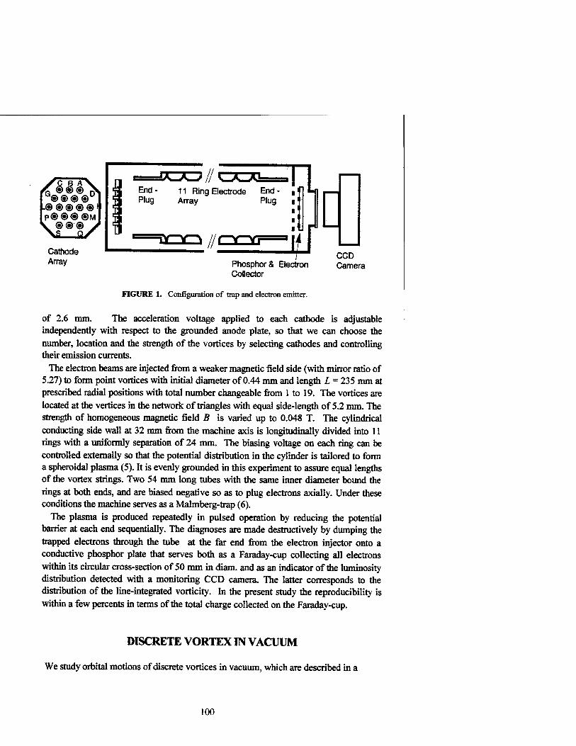
®®@® ,® ® ® ® ® I P®®@®M \®@® J

Cathode Array

"Wi^ // L^_A1= End- 11 RingHectrode End- Plug Array Plug

//coca

Pi .I ■

H Phosphors Electron Collector

CCD Camera

FIGURE 1. Configuration of trap and electron emitter.

of 2.6 mm. The acceleration voltage applied to each cathode is adjustable independently with respect to the grounded anode plate, so that we can choose the number, location and the strength of the vortices by selecting cathodes and controlling their emission currents.

The electron beams are injected from a weaker magnetic field side (with mirror ratio of 5.27) to form point vortices with initial diameter of 0.44 mm and length L = 235 mm at prescribed radial positions with total number changeable from 1 to 19. The vortices are located at the vertices in the network of triangles with equal side-length of 5.2 mm. The strength of homogeneous magnetic field B is varied up to 0.048 T. The cylindrical conducting side wall at 32 mm from the machine axis is longitudinally divided into 11 rings with a uniformly separation of 24 mm. The biasing voltage on each ring can be controlled externally so that the potential distribution in the cylinder is tailored to form a spheroidal plasma (5). It is evenly grounded in this experiment to assure equal lengths of the vortex strings. Two 54 mm long tubes with the same inner diameter bound the rings at both ends, and are biased negative so as to plug electrons axially. Under these conditions the machine serves as a Malmberg-trap (6).

The plasma is produced repeatedly in pulsed operation by reducing the potential barrier at each end sequentially. The diagnoses are made destructively by dumping the trapped electrons through the tube at the far end from the electron injector onto a conductive phosphor plate that serves both as a Faraday-cup collecting all electrons within its circular cross-section of 50 mm in diam. and as an indicator of the luminosity distribution detected with a monitoring CCD camera. The latter corresponds to the distribution of the line-integrated vorticity. In the present study the reproducibility is within a few percents in terms of the total charge collected on the Faraday-cup.

DISCRETE VORTEX IN VACUUM

We study orbital motions of discrete vortices in vacuum, which are described in a

100

Hamiltonian form. A concrete expression of the location (xa,ya) of a vortex a is given

in the complex plane by,

dt

dw(z) dz + Q(U)z«l.

where z* = xa + iya. The first term in the right hand side is described as,,

w\ w"?2

(1)

(2)

Here the first term stands for effects from other vortices, and the second from the image charges induced on the conductive wall at k\ = R. The circulation Kß of vortex ß is

related to the plasma density by the following relation, .en(x',y')

BQBL K ß ■ ffdx'dy'- e0B

. CTdx'dy'-£-~ (ol eNß

(3)

The integration is made over the cross-section of each vortex. The rotational drive forced by static radial electric field associated with confining potential at the ends is given by Qdz«|).

In the case of a single vortex put in vacuum, the first term in eq.(2) disappears, and only the interaction with its image and the external drive are present. From eq.(l) the vortex is known to show a circular orbit with the angular frequency of

K (O =• • + Q(r). (4)

2*(tf2-r2)

Figure 2 shows the rotation frequency of the vortex as a function of the total number of constituent electrons Nv that corresponds to the circulation of the vortex. Different symbols correspond to different plug potentials and different injection energies. The linear dependence of the rotation frequency is the manifestation of the contribution of the image charge.

The offset at JVV = 0 corresponds to Q(r) that is attributed to the radial electric field externally imposed at the end-plug cylinders.

1.4

1.3

£ 1-2

2 1.1 m O E 1-0 T0.9

0.8

0.7

1 1 1 1—1—1 1 1 1 1 1 1 1 1 1 1 1 1 1-

> (

,.l. l-L-i-

^^^g^l ^p^ jj^l j

" J^t^ 1 ■ f^ |||:

11

11

1 ti

-L.

2 4 6 8

Electron Number N (x107)

10

FIGURE 2. Rotation frequency of single vortex in vacuum.

101

It agrees quite well with the bounce-averaged ExB rotation velocity of electrons that is calculated for actual potential distribution in vacuum. Since eq. (1) shows a good agreement with the observations, it may be developed as a convenient method for experimental determination of the vacuum electric field.

Dynamics of two or more interacting vortices has been examined in the same way. The initial trajectory of each vortex agrees with the calculated results of eq.(l), though the discrepancies increase after a few rotation periods probably due to small differences in the initial conditions. Details of the examinations will be reported elsewhere. An important statement at this stage is that the discrete vortices interacting in the vacuum continue to orbit around without merging for a long period comparable to the coulomb collision time. However the trajectories of the vortices are observed quite different once the space among the vortices are filled with a continuous distribution of an electron plasma that forms a background vorticity as described below.

DISCRETE VORTEX IN BACKGROUND VORTICITY

We produce the background plasma by stacking electrons which are injected repeatedly from two cathodes, one on the machine axis and the other at the periphery (r = 10.4 mm). The stacking includes pulsed filling of electrons along the magnetic field lines and radial transport which are repeated up to a few hundreds times until the electrons form a moderate radial density distribution. We wait typically one more second for the distribution to become broad enough and axisymmetric before injection of discrete vortex under study.

Figures 3 shows the dynamics of a discrete vortex that is produced initially at different radial positions, r = 9, 8 and 5 mm with Nv = (2.6, 1.3, 2.4) x 107,

respectively. The electron number of the background plasma, Nb = (2.5 - 3.0) x 10 8, is one order of magnitude higher than Nv in the discrete vortex.

In each panel the radius ( distance from the center of background vortex, circle) and the angular velocity (square) of the discrete vortex are plotted as a function of time after the injection (t = 10 (is), and the corresponding quantities without the background plasma (open symbols) are plotted for comparison. While the vortex keeps a steady orbit in vacuum for more than 2 ms, the background vorticity increases the rotating velocity of the discrete vortex and attracts it toward the center. The discrete vortex either reaches the center of the background quickly to form a peaked distribution of vorticity or stagnates at a close distance to the center to be shortly dispersed into the background while rotating. In either case the identity of the discrete vortex is lost within a time of a few rotations around the center that is shorter than an orbiting period in vacuum.

102

CO

T3 CO

CC

E E, CO

"TJ ca

DC

E E, CO

T3 CO tr

o 12

-■•■-

—1—1 1 1- —T 1 T—1

? 5 0 6 "c > < ) < > 4 ; •• ' | ■

1

1 ■■■■ j '.

■ '. 009". 6 9 a 6

. . 1 . i 1 ■ 1 t J i_.i_.j_.ü_i—1—1—1—i—1—1—1—1—1—1—1—1—uJ

12

8 X s ><" o

03 Q. cS"

rr~rt' ■

i >• -> ■ 1 ■ i | - ? 7 m

l .-•r^ 1

■ ■ ■ • "

[ *•

i • « •

» ►

'■ I 3 1 1 1 1

6 .... i ... .

C 3 :

0 12

8 X S

o CJ1

s Q.

12

; :

l ■ ■

1 :

t a S«! 3 C 5 C ? i 5 D

\ • • i !■

'

0 □ ?••••* c ■.... I .... i .... i ... .

h ö 6 i 1 1 1 1 I 1 J i-i

8 X. s

o Ol

—^ 03 Q.

10 15 20 25 30 Time (JAS)

35

FIGURE 3. Orbit of a discrete vortex in a background vorticity. Distance from the background center and the rotation velocity is plotted as a function of lime. Vortex is produced at 10 /is.

DISCUSSION

The observation indicates that some collective interaction plays an essential role in the rapid merging. Excitation of waves, such as diocotron mode, in the background may enhance the interaction (7), though we do not have an adequate theoretical model applicable to the present experiment.

Very recently Schecter and Dubin have proposed a theoretical model of vortex

103

motion in a background vorticity gradient (8). For present analysis we start from eq.(6) of ref.8, neglecting the logarithmic factor of order 1. We approximate that the

density distribution of the background electrons as nb(r) « (A/^/J* L|exp(-r fb j,

and introduce characteristic time T0 - eQBLb jeNv. Employing normalized radius

p = r/b and time t - f/r0, we can write the equation for the location of the discrete

vortex as,

±.?4A*j.m . (5) dt nS(p) \ 2xy )

Here the gradient of the background vorticity is given by to " ~2pexp(-p UjcftQb,

and its shear by |A| - -S(p)/nYTo, where S(p)«(l + l/p jexpl-p l-l/p . The

contribution ofiVj, remains only in the time-dependent term as y =■ NvfNi,.

The equation can be solved only numerically. With experimental parameters such

that L = 0.235m, b •=> 0.01m and Nv - 2 x 107, therefore T0 - 3.1 //s, we calculate

the radial position of the discrete vortex as a function of time. Figure 4 shows the results for vortex starting at 5 mm and 10 mm from the center of the background that consists of different number of electrons such that y - 1/20» 1/10,1/5. The trajectory curve shifts upward as JV& decreases, namely the merging speed of the discrete vortex

increases as the vorticity of the background increases. We further notice that the calculated time scale is very close to die experimental one as evaluated from the data shown in FIG.3.

Though the main part of our new observation appears to be described well by the fairly simplified theoretical model, the bounced trajectory as shown in the middle of FIG.3 cannot be obtained from eq.(5). Since radial derivatives come in the original equation, a slight modification in the density profile of the background plasma may lead to the bouncing. More detailed density distribution in the background should be determined experimentally for full understanding of the process.

In the workshop we also have reported observation that two or more discrete vortices, which remain orbiting around separately for a sufficiently long time in vacuum, merge very rapidly or form a quasi-steady structure in the presence of the background vorticity. These observations strengthen the statement that the background vorticity plays an essential role in the evolution of a turbulent state which consists of strong vortices and weak vorticity distribution that is smoothed out in coarse-graining.

In summary we have reported experimental observation of 2-dimensional dynamics of discrete electron vortices both in vacuum and in background vorticity, demonstrating very strong influence of the background vorticity in the evolution of the spatial structure of the guiding-center fluid.

104

12

E E CO 3

TJ CO

EC

■I 1 ! . i i i i 1 i i i i i i i i I i i i—i— i i i i

m .

* ■

" Y=1/20\ ̂ /iO\ ̂ 7=1/5 "" ■

\ ^v i^Vt \ .

■—>■*— ' ■ i i '

10 15 20 25 Time (fis)

30 35

FIGURE 4. Calculated orbits of a discrete vortex in a background vorticity. Distance from the background center is plotted as a function of time for different level of the background Vortex starts at 10

ACKNOWLEDGMENTS

One of the authors (Y.K.) thanks D. A. Schecter for informing of his newest work, and Prof. Fred Driscoll, Prof. Tom OTsfeil, Prof. M. Kono for stimulating discussion. This work was supported by the Grant-in-Aid program of Ministry of Education, Science, Sports and Culture of Japan.

REFERENCES

1. Fine, K. S., Driscoll, C. D„ Mahnberg, J. H., and Mitchell, T. B., Phys. Rev. Lett. 67,588 (1991).

2. Eggleston, D. L., Phys. Plasmas 1,38S0 (1994). 3. Mitchell, T. B., Driscoll, C. D., and Fine, K. S., Phys. Rev. Lett. 71,1371 (1993). 4. Fine, K. S., Cass, A. C, Flynn, W. G., Driscoll, C. F., Phys. Rev. Lett. 75, 3277 (1995). 5. HigakLH. and Mohri, A., Jpn. J. Appl. Phys. 36,5300 (1997). 6. Mahnberg, J. H., and deGrassie, J. S„ Phys. Rev. Lett. 35,577 (1975). 7. Lansky, I. M., CNeil, T. M^ and Schecter, D. A., Phys. Rev. Lett 79,1479 (1997). 8. Schecter, D. A., and Dubin, H. E., Phys. Rev. Lett. 83,2191 (1999). Paper M-P19 in this workshop.

105

Vortex Motion Driven by a Background Vorticity Gradient l

David A. Schecter and Daniel H.E. Dubin

Physics Department University of California at San Diego, La Jolla, CA 92093

Abstract. The motion of self-trapped vortices on a background vorticity gradient is examined numerically and analytically. The vortices act to level the local background vorticity gradient. Conservation of momentum dictates that positive vortices ("clumps") and negative vortices ("holes") react oppositely: clumps move up the gradient whereas holes move down the gradient. A linear analysis gives the trajectory of small clumps and holes that rotate against the local shear. Prograde clumps and holes are always nonlinear, and move along the gradient at a slower rate. This rate vanishes when the background shear is sufficiently large.

Self-trapped vortices can be clumps (vorticity excesses) or holes (vorticity deficits). The interaction of clumps and holes with a background vorticity gradient often plays an important role in 2D hydrodynamics. For example, the decay of 2D turbulence can be controlled by the slow drift of holes down a vorticity gradient [1]. The motion of hurricanes on a rotating planet is influenced by the north-south gradient in the Coriolis parameter, which can be thought of as a (potential) vorticity gradient [2-7].

Here, we calculate the rate at which clumps and holes ascend or descend a background vorticity gradient under the conditions that (i) the vortices are point-like and (ii) the background flow has strong shear. While point-like vortices and strong background shear may be rare in geophysical settings, they are common in nonneutral plasmas [1,8] and may also be found on planets like Jupiter that have intense storms in strong zonal winds [9].

Clumps and holes can be classified as prograde or retrograde, depending on whether they rotate with or against the local background shear. We find that a linear analysis gives the motion of a retrograde vortex. Prograde vortices are always nonlinear and move at a slower rate that is given by a simple "mix-and- move" estimate.

We neglect viscosity and consider flows that are governed by the 2D Euler equations:

This article is scheduled to appear in the 13 September 1999 issue of Physical Review Letters.


106

dt + tf.VC = 0, v = zx\7ip, VV = C- (1)

Here, v(r,6,t) is the velocity field, C(»",0,t) = ■* • V x v is vorticity and ij){r,9,t) is a stream function. For analysis, the vorticity is decomposed into vortices («) and background (b): £ = C& + EC«- We focus on tne case where £6 is positive, cylindrically symmetric and monotonically decreasing at t = 0, making clumps retrograde and holes prograde.

Figure 1 shows that clumps ascend a background vorticity gradient whereas holes descend the gradient [2,3]. At t - 0, a clump and a hole are placed in an axisymmetric background. The system is evolved with a vortex-in-cell (VIC) simulation that numerically integrates Eq. (1) [10]. Eventually, the clump is driven to the peak in background vorticity, whereas the hole is driven toward the minimum. Such gradient-driven separation may help organize storms into bands of like-sign vortices on planets with strong zonal winds, with holes in vorticity troughs and clumps on vorticity peaks [9].

The opposite drifts of clumps and holes can be understood by momentum conservation. A similar argument has been used to explain the motion of phase-space density clumps and holes in plasma turbulence [11]. We focus on cylindrical geometry, where the flow conserves canonical angular momentum, P$ = J d?r £r2. The analysis carries over to planar geometry, where linear momentum replaces Pg.

When there is just one vortex, P$ consists of two parts, a background contribution and a vortex contribution: Pe = Tb {r2)b+rvr%. Here T6 > 0 is the total circulation of the background flow, Tv is the vortex circulation, rv is the radial position of the vortex and < r2 >b denotes the Cft-weighted spatial average of r2. As indicated in Figs. 1 and 2, both clumps and holes mix and flatten the (0-averaged) background vorticity. As the background is levelled, < r2 >b increases (since d^/dr < 0). To conserve Pe, a clump (r„ > 0) must climb the background gradient and decrease r„, whereas a hole (r„ < 0) must descend the gradient and increase r„.

We now determine the radial speed of the vortex. The vortex's dominant trans-

vorticity

FIGURE 1. Gradient-driven radial separation of a clump (black dot) and hole (white dot) in a

circular shear flow.

107

clump

rv>o

FIGURE 2. Local mixing of the background increases < r2 >(,. By conservation of Pg, clumps and holes react oppositely.

lational motion is rotation about the center of the background. We work in this rotating frame, so the vortex is nearly stationary, and we define a local (x, y) coordinate system centered at the vortex. In these coordinates, the initial velocity due to the background is v = Ayx near the vortex, where A is the shear, and the initial background vorticity gradient is £'0y (where y points in the local r-direction).

Figure 3 shows the initial stream-lines in the vicinity of a retrograde clump (a) and a prograde hole (b). The stagnation points in Fig. 3(a) are at a distance I above and below the clump, where

l\ y/\Tv/2TTA\. (2)

We treat the vortex and the disturbance that it generates as perturbations to the initial shear-flow, and suppose that the Euler equation for the evolution of Q, can be linearized,

9 A d •*a = -c ,r„ 2ir x2 + y2 (3)

Here, 5£& is the background vorticity perturbation, and we have used £, = Tv5(x). This assumes that the vortex is point-like and moves slowly compared to the evolution of the background. We have also neglected the velocity perturbation due to 6Cb, assuming that it is negligible compared to the vortex velocity field.

Equation (3) can be solved by the method of characteristics, yielding

öCb -r, v S,o

4TT Ay In

x2 + y2

(x-Ayt)2 + y2 (4)

The radial velocity (f„) of the vortex is the y-component of the velocity perturbation that develops at the origin. By summing the contributions to the velocity field from each vorticity element, we obtain the following integral expression for r„ (here, u = x/y) :

T C L

Tv ~ 4n2 A \

dy

y

oo

/ —oo

du- ll2 + 1

-In u2 + l

(u - At)2 + 1 (5)

108

A small scale (/) and a large scale (L) cut-off are introduced to escape infinities in the y-integral. The small scale cut-off describes the minimum distance from the vortex at which nonlinearities in the background flow can be ignored. Thus, we identify the small scale cut-off with I [Eq. (2)], the size of the shaded trapping region in Fig. 3(a). To determine the upper cut-off, we note that curvature in the unperturbed flow can not be ignored for \y\ Z rv, where rv is the radial position of the vortex. We therefore set L = c ■ rv, where c is presumably O(l).

The integrals in Eq. (5) yield

r.= ^^ln{Lll)-tan-'{Tl2)

= ± Co I2 In (c rv/l) tan'1 {T12), (6)

where T = \A\t and +/- is for clumps/holes. For T » 1, the inverse tangent is approximately 7r/2 and r„ is approximately constant. Equation (6) gives a reasonable scaling for the vortex speed: rv increases with Tv and Co, while it decreases as the local shear A intensifies.

However, the validity of Eq. (6) rests on the accuracy of Eq. (3), which neglects curvature in the unperturbed flow, the velocity perturbation due to S£b, motion of the vortex, and all nonlinear terms. We now test Eq. (6) against a VIC simulation that keeps all of these effects [10]. A linear simulation that incorporates the first three effects is used as an independent check.

We consider the specific case where the initial background vorticity distribution (Ct at t — 0) is given by

Ur) -{I 1.25 • r r<0.8 r > 0.8. (7)

The rotation frequency of this background is Q,0(r) = 0.5- 0.417 -r, for r < 0.8. We assume that the flow is bounded by a circular wall with radius Ru, — 1, and that

< (b)

FIGURE 3. Initial stream lines for a retrograde clump (a) and a prograde hole (b) in a shear

flow v = Ayx, A > 0.

109

there is free slip at the wall (tp = 0 at R^). The background chosen here represents a larger class, where the radial derivatives ££ and Q'0 vary slowly with r.

The linear simulation integrates the following set of equations. The vorticity perturbation is expanded as a Fourier series in the polar angle 6,

00

5C= £ Z(m\r,t)-Jm9. (8) m=—oo

The linear evolution of Z^ is given by

Z(m) = im^ [*[m) + #[m>] . (9) — + imQ0(r)

Here, \I>„ and $(, are Fourier coefficients of the vortex stream function and the stream function of <5£&- The vortex moves radially according to fv = — döip),/d6\fv r"

1, which can be written

e\ 00

rv = - £ m ■ Im Km) (r„, t)eim9»] . (10) rf tn=l

The angular velocity of the vortex is given by the unperturbed flow,

9V = Vo{rv). (11)

In the linear simulation, Poisson's equation is solved for ^^ to second order accuracy in the radial grid-point spacing (~ fi„,/2000). The vortex position rv

and the Fourier coefficients {Z(m)} are evolved with third-order Adams-Bashforth steps (~ 103 steps per background rotation). The number of (excited) Fourier components is made finite in the linear simulation by setting \lj£m) = 0 for m > y/e-rv(t)/l(t). This wave-number is the inverse of the horizontal width (in radians) of the trapping region (TR) that is shaded in Fig. 3(a). Neglecting larger m amounts to neglecting the contribution to rv from the TR, where the fluid is rapidly (T ^ 1) mixed by the vortex. Although the TR is defined only for a retrograde vortex, we try the same cut-off for a prograde vortex.

Figure 4 shows the linear (dashed line) and the VIC (solid line) computations of rv(t) for a retrograde clump and a prograde hole of initial strength l/rv = 0.12. The ratio l/rv is called the "vortex strength" because it is a dimensionless measure of the vortex intensity relative to the background shear A — — rvQ,'0(rv). The linear simulation of clump motion is in good agreement with the VIC simulation. In contrast, the hole moves much slower in the VIC simulation than in the linear simulation. The results for 6v{t) (not shown) give similar agreement for clumps and disagreement for holes.

Consider first the motion of the retrograde clump. It is apparent from Fig. 4 that the clump rapidly accelerates to a constant radial speed. Equation (6) offers a value for this speed, up to a factor c (of order 1) in the logarithm.

110

0.8

hole (prograde) \

Qlump (retrograde)

T 300

FIGURE 4. Radial position of vortex versus time T = rv{0>)\ti'o\t for linear (dashed) and VIC

(solid) simulations.

Rather than set c = 1 on physical grounds, we use a precise value for c that can be obtained by a standard (but lengthy) analysis of Eqs. (9-11). Unlike the previous derivation of Eq. (6), this analysis incorporates curvature of the unperturbed flow, and the velocity perturbation due to SCb- However, the calculation still makes use of an unperturbed orbit approximation: 6^, is evolved with the vortex fixed on a circular orbit [8V = Ct0(rv)t], and r„ is taken to be the radial velocity perturbation at the vortex center. Wave-numbers m > y/e • rv/l are neglected, as in the linear simulation. The analysis yields a time-asymptotic value for rv that converges to Eq. (6) in the limit of small l/rv. In general, the factor c depends on rv and the form of Co(0- In our example [Eq. (7)], the expression for r„ reduces to Eq. (6) for l/rv < 0.1, with c = 0.43 for rv < 0.7.

Figure 5 shows that the radial speed of the clump converges to linear theory [Eq. (6)] as the clump strength l/rv approaches zero. All clumps start at r„ = 0.4 and the background is always given by Eq. (7). We vary l/rv by changing Tv only. We obtain rv from a straight-line fit to r„ vs. t, as rv decreases from 0.375 to 0.35. In the plot, rv is normalized to Corl- Botn Cr« and tne clump strength l/rv are evaluated at rv = 0.363. The diamonds correspond to linear simulations and each 'X' corresponds to a VIC simulation. The solid curve is the T -r oo limit of Eq. (6), with c = 0.43. Both linear and VIC simulations converge to the solid curve as l/rv

tends to zero, indicating that the linear theory of Eq. (6) works well for retrograde vortices.

We now consider the motion of prograde holes. The failure of linear theory for holes can be understood by considering the stream lines in Fig. 3(b). Linear theory breaks down for times greater than the orbital period r of a fluid particle initially at x ~ I, the small length scale cut-off. The orbit of this particle is dashed. Since r ~ l2/Tv, r remains constant for holes as Tv approaches zero, while the time scale for the hole to move a distance of order I becomes infinite. Thus, the background perturbation around a small hole becomes nonlinear "instantaneously" for all practical considerations. For clumps [Fig. 3(a)], this problem does not arise, since fluid particles at x ^ I are not trapped around the vortex. Note that linear theory fails for holes not because the hole has negative vorticity, but because the hole is prograde with respect to the shear flow in our example [Eq. (7)].

Ill

10-' - ' ' ^. ' -

10-2

T 1> i

clumps ^gf***^ r (retrograde) *$T^ •' ]

>? ,-D holes

Ö5 10 X

• v-> 10"4

m-5

: Eq. (6) .< ^'d (prograde)-\

>/ ,'''Eq.(12) i :

10" 10' l/r «r' l

FIGURE 5. r„ versus l/rv for linear simulation (diamonds), VIC simulation (X's and O's) and experiment (square).

The following "mix-and-move" argument gives a good estimate for the hole velocity. A hole will attempt to mix a thin layer of background vorticity and move a distance Ar in response [Fig. 2(b)]. This mixing layer (ML) corresponds to the shaded region in Fig. 6, which shows the flow around a hole with l/rv — .05. The ML extends from 0 = —TT to -K and has an average radial width of ~ 21. Suppose that the hole levels the entire ML (d<^>g —> 0) and has a negligible effect on fluid outside the ML. Then, using conservation of Pe, it can be shown that r„ must increase by Ar ~ lC,'o/0!o. To obtain the hole velocity also requires an estimate of the time At required for the ML to flatten. The orbital speed of a trapped particle is on average dominated by the background shear, so A£ is approximately 47r/£|Q^|. The velocity of the hole is Ar/At, or equivalently

47T i2C (12)

In Fig. 5, we compare Eq. (12) to the late time hole velocities that are observed in the VIC simulations. As before, Co is given by Eq. (7) and the holes are located initially at r„ = 0.4. The plotted values of rv are from straight-line fits to rv vs. t, as r„ increases from 0.5 to 0.6. The ratio l/rv and the velocity normalization (J0rl are evaluated at rv = 0.55. The simulation velocities (denoted by O's) are between 0.6 and 1.1 times the estimate, indicating that Eq. (12) is a reasonably accurate approximation for the speed of prograde vortices.

The speed of a prograde hole down a vorticity gradient was recently measured in an experiment [1]. The speed (plotted in Fig. 5) is within a factor of 4 of Eq. (12), which is at the level of estimated error. The slower radial drift that is measured in the experiment may be due to the presence of multiple (2-3) holes, which changes the structure of the mixing layer. Simulations with multiple holes also give lower values of r„.

The "mix-and-move" estimate assumes that the hole continuously moves into new regions where the 0-averaged background vorticity has a slope d<fr

>e = C0-

112

r

r„ -*e—— O =~i2/-

0 -, 0 e *

FIGURE 6. Initial stream lines and mixing layer (shaded) for a prograde hole in a circular shear flow [Eq. (7)].

However, if the ML moves with the hole, d<f^f shortly becomes zero at rv, and the background and hole equilibrate in a phenomenon akin to the formation of a BGK mode in a nonlinear plasma wave [12]. This will occur if At « tu where tt is the time for r„ to increase by I and At is the mixing time. Using Eq. (12) for rv

then implies that an equilibrium forms when C,'J£t'0 «I [13]. For the simulation data in Fig. 5, £0IQ'0 = 3, so only a small fraction of the

ML moves with the hole [14]. However, by artificially increasing |fi'0| in the VIC simulation so that C/^o is less tnan *> one can examine hole motion when the "mix- and-move" model breaks down. For C,'JÜ'0 equal to 3/4 and 3/8 (and l/rv = 0.2), we find that the ML moves with the hole and an equilibrium is reached after a small radial displacement (;$ .lr„).

Several issues remain. First, undamped modes or quasi-modes can affect vortex motion if their phase velocities resonate with the vortex velocity. This is particularly important when the background has steps [15]. Also, when l/rv ^ 1, our linear treatment of retrograde vortex motion becomes invalid. Finally, our analysis indicates that there is a critical value of C,'JQ!0, of order 1 for a prograde vortex and smaller for a retrograde vortex, below which equilibria form and above which the vortex continues to move. This nonlinear behavior merits further study.

The authors thank W.G. Flynn for his work on the VIC simulation and C.F.Driscoll for help with interpreting the experiment. This research was supported by NSF grant PHY94-21318 and ONR grant N00014-96-1-0239.

REFERENCES

1. X.P. Huang, K.S. Fine and C.F. Driscoll, Phys. Rev. Lett. 74, 4424 (1995). 2. CG. Rossby, J. Marine Res. 7, 175 (1948). 3. C.H. Liu and Lu Ting, Comp. & Fluids 15, 77 (1987). 4. G.F. Carnevale et al, J. Fluid Mech. 233, 119 (1991). 5. G.M. Reznik, J. Fluid Mech. 240, 405 (1992). 6. R.K. Smith in Tropical Cyclone Disasters; Ed. Lighthill et al, Peking Univ. Press,

Beijing, 264 (1993).

113

7. G.G. Sutyrin and G.R. Flierl, J. Atmos. Sei. 51, 773 (1994). 8. K. S. Fine et al, Phys. Rev. Lett. 75, 3277 (1995). 9. For data, see Reta Beebe, Chaos 4, 113 (1994).

10. D.A. Schecter et al, Phys. Fluids 11, 905 (1999). Here, we use at most 1025 x 1025 grid-points and 3 x 106 particles.

11. T.H. Dupree, Phys. Fluids 26, 2460 (1983). 12. I.B. Bernstein, J.M. Greene and M.D. Kruskal, Phys. Rev. 108, 546 (1957). 13. Similarly, we estimate that an equilibrium forms for a retrograde clump if

27T y/ln(rv/l) Co/^'o << 1, a substantially more stringent requirement when I «rv. 14. In the experiment, C,'ol0!o ~ 2-7. 15. I.M. Lansky, T.M. O'Neil and D.A. Schecter, Phys. Rev. Lett. 79, 1479 (1997).

114

Inviscid Damping of Elliptical Perturbations on a 2D Vortex

D.A. Schecter, D.H.E. Dubin, A.C. Cass C.F. Driscoll, I.M. Lansky and T.M. O'Neil

Physics Department University of California at San Diego, La Jolla, CA 92093

Abstract. The inviscid damping of an elliptical perturbation on a 2D vortex is examined experimentally and theoretically. The perturbation is generated by an impulse at the wall. Initially, the quadrupole moment (ellipticity) of the perturbation decays exponentially. This result is significant, since arbitrary perturbations need not decay exponentially. The decay rate is given by a "Landau pole" of the equilibrium profile. When the Landau damping is weak, the vorticity perturbation, in addition to the quadrupole moment, behaves like an exponentially damped mode. This "quasi-mode" is actually a wave-packet of exceptional continuum modes that decays as the continuum modes disperse.

The inviscid relaxation of a 2D vortex after a weak external impulse is studied experimentally and theoretically. In the experiments, the 2D fluid is a strongly magnetized electron plasma in a cylindrical Penning trap, with wall radius Ru, [1,2]. These electron plasmas have negligible viscosity and are governed approximately by the 2D Euler equations:

dC/d* + tf-VC = 0, v = zxVtjj, and V2^ = C (1)

Here, v(r, 9, t) is the (E x B drift) velocity field in the plane perpendicular to the trap-axis, £{r,9,t) = z • V x vis the vorticity, and ip(r,d,t) is a stream function. The boundary condition is ip = 0 at B^.

EXPERIMENTS

Figure 1 shows two experiments that illustrate the process of "inviscid damping" [2-8]. In both experiments, we excite an elliptical (m = 2) perturbation on an initially circular vortex. The initial vorticity distribution £0(r) and the initial rotation frequency fio(0 are monotonically decreasing functions of radius, making the vortex stable [4]. In experiment (a), the impulse excites an undamped elliptical mode, with frequency w. The fluid rotation is resonant with this mode at a radius


115

T=0

(a) 0.45 4.5 45_ 450

vorticity (lo3 sec-1) vorticity (10 sec-1)

FIGURE 1. Experiments, a) An undamped mode is excited, with critical radius rc outside the vortex, b) Inviscid damping occurs when rc is inside the vortex. In both experiments, the unperturbed vorticity £„(r) decreases monotonically with r. Time is measured in central rotation periods: T = t ■ fio(0)/27r.

rc, defined by 2Q0(rc) = u/, and this critical radius lies outside the vortex. The vortex in (b) is similar to the vortex in (a), except that C0(r) extends past the critical radius rc. The excited mode is now damped by resonant mixing of vorticity at rc. This inviscid damping is analogous to collisionless Landau damping, where a compressional plasma wave decays due to its interaction with charged particles that travel at the same velocity as the wave [4].

Figure 2 shows the evolution of the quadrupole moment Q? of the perturbation in Fig. 1(b). We define the quadrupole moment by the equation

Q2= fRvdrr36<;W(r,t), Jo

(2)

where R„ is the vortex radius, and 8C,^ is the m = 2 Fourier component of the vorticity perturbation. The amplitude of Q2 is a measure of ellipticity. Also plotted in Fig. 2 is the theoretical linear response of the vortex to an externally applied 8(t) impulse. Initially, there is good agreement between linear theory and the experiment. However, after 5 rotations, the experiment diverges from linear theory, and the amplitude of Q2 begins to oscillate. These nonlinear oscillations are due to mixing of trapped vorticity at rc. Eventually, the amplitude saturates, and the vortex relaxes to a rotating "cat's eyes" equilibrium [Fig. 1(b), far right].

For the remainder of this paper, we focus on the initial linear decay, which properly describes the evolution for arbitrarily long times if the amplitude is sufficiently small [2]. Figure 2 indicates that the initial decay of Q2 is approximately exponential, i.e. |<52(0I ^ IQ2(0)\e"yt. This result is generic to the experiments, and is significant, since arbitrary linear perturbations need not decay exponentially. Of equal interest is that, when the damping is weak (7/w << 1), the actual vorticity perturbation behaves like an exponentially damped eigenmode: 5(,{r,t) « £(r)e-7'e-,ü't, for r ;$ rc. This perturbation is referred to as a "quasi-mode", since it is not an exact eigenmode of the Euler equations.

116

IQ, 1

0.1

0.01

r <§f-*T&:x trapping saturation 7 $f oscillations •

r \ de c ■.. 1.... 1...». 1.... 1.... 1.... 1 1.1..."

0 10 20 30 40 50 70

FIGURE 2. Typical evolution of the quadrupole moment, Qi. The X's give Q2 for the experiment in Fig. 1(b). The diamonds correspond to linear theory. The dashed line is an exponential fit to the initial decay.

LINEAR EIGENMODE THEORY

As pointed out by Case [9], a linear vorticity perturbation varying as e%™ can be viewed as a sum of discrete modes plus an integral of continuum modes (also called "shear-waves") [9-11]:

£CM) = £A(Wd)ar)e-^ + f <kjA(u>)Ur)t d J

,—iuit (3)

We will use the index k to refer to both discrete and continuum modes. These eigenmodes satisfy the following integral eigenvalue equation:

777 fRv mfio(r)&(r)--Ci(r)jf <WGm(r|r%(r') = wfc&(r), (4)

where Co is the radial derivative of the equilibrium vorticity. The Green's function 1

"2m ferhfe)2ra]-Here^>^<)isthe in Eq. (4) is given by Gm(r\r')

greater (smaller) of r and r'. The eigenmodes can be obtained numerically by discretizing Eq. (4) in r. This

leads to a standard matrix eigenvalue equation, £,• My&fa) = w^fo). If there are N radial grid-points between 0 and Ry, then a solution to the matrix equation gives N eigenmodes. Any linear initial value problem can be solved numerically with a superposition of these eigenmodes: 6((r,t) RS E^=I^(wfc)^(r)e_1Wtt. The solution generally breaks down for times greater than the minimum value of 27r/mQ'0Ar, where Ar is the radial grid-point spacing and Cl'0(r) is the radial derivative of the rotation frequency.

When there are no discrete modes, the perturbation consists entirely of continuum modes. It is common (but often misleading) to view this perturbation intuitively as a passive scalar in the equilibrium shear flow. However, a quasi-mode is a superposition of continuum modes that does not behave like a passive scalar.

117

\ •... Q

(a) 1

\ R r

v c

£, A discrete mode 0)=0.496

0

0.832 ^s

0.968

. 0.992

> 0.996

0.2 0.4 0.6

r/R 0.8

k Q

(b) fye) < 0 V

«1 'r

c

co=0.498

i r exceptional 0.509

il . 0.519 r A 0.557

0.990

0.995

0.2 0.4 0.6 0.8

FIGURE 3. Equilibrium profiles and (m = 2) radial eigenfunctions for a top-hat vortex with a discrete mode (a), and a top-hat vortex with a quasi-mode (b).

One goal of this paper is to clarify how the "phase-mixing" of continuum modes is consistent with the observed quasi-modes.

It is useful to compare a quasi-mode, which exists when Co(rc) < 0, to an undamped discrete mode, which exists when C0(

rc) = 0. Figure 3(a) shows the m — 2 eigenmodes of a "top-hat" vortex, similar to that studied by Kelvin [12]. This top- hat supports a single discrete mode, which has a critical radius rc> R„, and a set of continuum modes that have eigenfrequencies in the range 2Q0(RV) <wk < 2Qo(0). Figure 3(b) shows the eigenmodes of a similar vortex, with a skirt of vorticity that tapers past rc. The negative vorticity gradient at rc causes the discrete mode to be replaced by a wave-packet of continuum modes. The continuum modes in this wave-packet are labelled "exceptional" in Fig. 3(b), since they are approximately the same as the original discrete mode. The only noticeable difference is that each continuum mode has a singular spike near rc, where the fluid rotation is resonant with the mode. As we will soon see, the wave-packet that replaces the undamped discrete mode evolves as a quasi-mode, which decays exponentially (at early times) as the continuum modes disperse.

LINEAR RESPONSE TO AN IMPULSE

We now consider the response of the vortices in Fig. 3 to a brief external impulse, of strength e. The impulse is applied at the wall, and creates an instantaneous "external" stream function, tpext{r,0,t) = e6(t)(r/Rw)2ei26. A straight-forward

118

c

i 3 <

Qrc)=0 (a): ^^ discrete mode

continuum

FIGURE 4. The (m = 2) eigenmode amplitudes after an impulse is applied to a top-hat vortex with a discrete mode (a), and a top-hat vortex with a quasi-mode (b).

calculation shows that, for a monotonic vortex, the complex amplitude of each eigenmode (immediately) after the impulse is given by

A{ujk) = i 2e <&,<} 2e Cdrr%(r)

(R*)2 (6,6) (Rv)2 <£*>&> (5)

Here, {f,h) is short-hand for the inner-product /0fi" dr r2f*(r)h(r)/\C0(r)\. Equa-

tion (5) indicates that the excitation of an eigenmode is proportional to its (scaled) multipole moment (here the quadrupole moment, since m = 2). In this sense, the system exhibits reciprocity: the eigenmodes that produce the largest external fields are also the most sensitive to excitation by a brief external impulse.

Figure 4 shows the response of both vortices in Fig. 3 to an external impulse. In case (a), the discrete mode is excited about 100 times more strongly than any of the continuum modes. In case (b), a similar initial perturbation is excited, but it now decomposes into a sharply peaked distribution of continuum modes. The continuum modes in the peak region are exceptional, in that they are similar in form to the original discrete mode (see Fig. 3). Due to this similarity, and the sharply peaked distribution, the excitation will behave like an exponentially damped version of the original discrete mode. The decay rate 7 of this quasi-mode is proportional to the width of the peak in A(uk). Note that the simple mode- like behavior of the excitation breaks down near rc, where the continuum modes have singular spikes. Here, the perturbation forms filaments, like those seen in the experiments [Fig. 1(b)].

The evolution of the quadrupole moment of the excitation in case (b) is shown in Fig. 5. At early times, the amplitude of Q2 decays exponentially. The inset shows that, for r ;$ rc, the vorticity perturbation merely decays as a damped

119

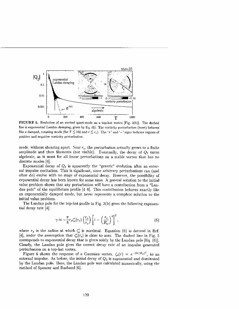
IQ, 0.1

0.01 -

0.001

y/co=.01

-C.16

600 rp 1000

FIGURE 5. Evolution of an excited quasi-mode on a top-hat vortex [Fig. 3(b)]. The dashed line is exponential Landau damping, given by Eq. (6). The vorticity perturbation (inset) behaves like a damped, rotating mode (for T < 100 and r < rc). The '+' and '-' signs indicate regions of positive and negative vorticity perturbation.

mode, without shearing apart. Near rc, the perturbation actually grows to a finite amplitude and then filaments (not visible). Eventually, the decay of Q2 turns algebraic, as it must for all linear perturbations on a stable vortex that has no discrete modes [4].

Exponential decay of Q2 is apparently the "generic" evolution after an external impulse excitation. This is significant, since arbitrary perturbations can (and often do) evolve with no stage of exponential decay. However, the possibility of exponential decay has been known for some time. A general solution to the initial value problem shows that any perturbation will have a contribution from a "Lan- dau pole" of the equilibrium profile [4-6]. This contribution behaves exactly like an exponentially damped mode, but never represents a complete solution to the initial value problem.

The Landau pole for the top-hat profile in Fig. 3(b) gives the following exponential decay rate [4]:

7: ■r*<i)H (6)

where r0 is the radius at which Q is maximal. Equation (6) is derived in Ref. [4], under the assumption that C,'0{rc) is close to zero. The dashed line in Fig. 5 corresponds to exponential decay that is given solely by the Landau pole [Eq. (6)]. Clearly, the Landau pole gives the correct decay rate of an impulse generated perturbation on a top-hat vortex.

Figure 6 shows the response of a Gaussian vortex, C,0{r) = e~(-5r^Rw^, to an external impulse. As before, the initial decay of Q2 is exponential and dominated by the Landau pole. Here, the Landau pole was calculated numerically, using the method of Spencer and Rasband [6].

120

y/ü)=.35

o 20 40 60 T 100

FIGURE 6. Decay of an impulse generated perturbation on a Gaussian vortex. The dashed

line corresponds to the exponential decay that is given by a Landau pole, which is calculated

numerically [6].

Although Q2 decays exponentially, the vorticity perturbation (inset) does not behave like an exponentially damped mode. This is due to the large decay rate 7/w = .35, compared to the previous case where 7/w = 0.01. Because 7 is large, the excitation has a broadly peaked distribution of continuum modes, with resonant radii (and singular spikes) spanning most of the vortex. The evolution of such perturbations is characterized by the "spiral wind-up" [13-15] that is observed here.

SUMMARY

In this paper, we examined the inviscid damping of elliptical perturbations on a 2D vortex. Specifically, we considered perturbations that were generated by an impulse, applied at the wall. It was shown that, in general, exponential Lan- dau damping properly describes the initial decay of the perturbation's quadrupole moment Q2, despite the fact that arbitrary perturbations need not decay exponentially. We also showed that when Landau damping is weak (7/w << 1), the vorticity perturbation 6( behaves like an exponentially damped mode (for r <rc). This quasi-mode was identified as a wave-packet of exceptional continuum modes that decays exponentially as the continuum modes disperse. When Landau damping is strong (7/w ~ 1), the vorticity perturbation exhibits spiral wind-up, and does not resemble a mode.

ACKNOWLEDGEMENT

This work was supported by the National Science Foundation (NSF PHY-9876999).

121

REFERENCES

1. C. F. Driscoll and K. S. Fine, Phys. Fluids B 2, 1359 (1990); 2. S. Pillai and R.W. Gould, Phys. Rev. Lett. 73, 2849 (1994). 3. M.V. Melander, J.C. McWilliams and N.J. Zabusky, J. Fluid Mech. 178, 137 (1987). 4. R. J. Briggs, J. D. Daugherty, and R. H. Levy, Phys. Fluids 13, 421 (1970). 5. N.R. Corngold, Phys. Plasmas 2, 620 (1995). 6. R.L. Spencer and S.N. Rasband, Phys. Plasmas 4, 53 (1997). 7. A.C. Cass, Ph.D. dissertation, University of California at San Diego (1998). 8. D.A. Bachman, Ph.D. dissertation, California Institute of Technology (1997). 9. K.M. Case, Phys. Fluids 3, 143 (1960).

10. G.G. Sutyrin, Sov. Phys. Dokl. 34, 104 (1989). 11. M.T. Montgomery and C. Lu, J. Atmos. Sei. 54, 1868 (1997). 12. Lord Kelvin, Phil. Mag. 10, 155 (1880). 13. A.J. Bernoff and J.F. Lingevitch, Phys. Fluids 6, 3717 (1994). 14. A.P. Bassom and A.D. Gilbert, J. Fluid. Mech. 371, 109 (1998). 15. P.B. Rhines and W.R. Young, J. Fluid Mech. 133, 133 (1983).

122

Analytic Study of Two-Ring Patterns of Vortices in a Penning Trap

Gianni G.M. Coppa Istituto Nazionale per la Fisica della Materia

Dipartimento di Energetica - Politecnico di Torino

Corso Duca degli Abruzzi, 24 - 10129 Torino, Italy

Abstract. The equilibrium configuration and the stability of vortex patterns made of point vortices equally distributed on two circumferences in a bounded system are studied. Such patterns appear worth studying from a theoretical point of view, as they have been observed experimentally in nonneutral plasmas confined by a Penning trap. The results presented in the paper prove that stable configurations of two rings of point vortices can exist.

INTRODUCTION

Experiments on nonneutral plasmas confined in a Penning trap [1] have shown the existence of stable configurations of vortex patterns, which can be classified into three categories: (1) vortices equally distributed on a circumference; (2) vortices equally distributed on a circumference with an additional central vortex; (3) two sets of vortices equally spaced on two circumferences having the same center but different radius (in fact, only one pattern of this kind has been observed, made of six vortices nearly placed in the vertices and in the middle of the edges of a triangle). While the study of the patterns of the first kind is a classic subject in the vortex theory, analytic results for the second category have been presented only recently [2]. For the third kind of pattern, theoretical work was performed by Aref [3] only for an infinite medium. The present work generalizes Aref's results when the domain of the physical system whose domain is a circle of radius Rc. An analytic condition is derived for the existence of a stationary configuration and the linear stability analysis is carried out. Finally, a non-linear analysis is performed for the m = 0 mode.

EQUILIBRIUM FOR TWO RINGS OF VORTICES

Due to the very high value of the bouncing frequency in axial direction with respect to the rotation frequency of the guiding center in transverse direction,


123

charged particles in a Penning trap can be regarded as straight lines of uniform charge, and the dynamics of the system becomes essentially a two-dimensional problem. Moreover, the linear charge density is here assumed to be nonvanishing only for a finite set of regions (vortices), each of them having a size much smaller than the radius Rc of the cross section of the trap. As the Larmor radius is usually small with respect to Rc, the velocity of each vortex in the (x, y) transverse plane is given by the E x B drift. By expressing the total electric field as the sum of the fields produced by each vortex, a set of differential equations governing the time evolution of the coordinates (xn, yn) of the vortices is obtained. The equations can be written in a compact form by making use of the complex variables (n — xn + iyn

and defining the strength of the n-th vortex as fn = —Qn/(2-KEoBz), being Qn the linear charge density of the vortex and Bz the axial magnetic field. In addition, when a stationary configuration rotating with angular velocity Q is investigated, a reference frame rotating with the same velocity can be usefully employed [2]. In this frame, the classic equations for the dynamics of point vortices [4] can be written as:

dt -"<;+£' ik

Cn-C* _ST" _Jk__

k Cn — Cfc

where ]Tfc stands for ^Zfc_^n, while £n = R%/Q represents the location of the n-th image charge in the complex plane.

In the following, the equilibrium condition is studied for a configuration of 2N vortices, equally distributed on two circumferences of radius i?i and i?2, where the vortices have the same strength, 71 and 72, respectively. The locations of the vortices are provided by two groups of N complex numbers, £,

(P = R, exp [i {tpn + $!)], C? = R-2 exp [i (<pn + $

(i) and (n , given by:

<. = 1,...,N (2)

being tpn = ^p; $1 and $2 are the phases for the two sets of vortices. By introducing

the expressions (2) for Q into Eq. (1) and supposing the pattern to be stationary, one obtains

fi = 7iw (Rx) + 72K (Ru R2, A$) and Ü = 72w (R2) + 7XK (R2, Ri, -A*) (3)

for the first and the second ring, respectively, being A<£ = <£2 — $1, while the quantities w {R{) and K (RI, R2, A<£>) are defined in terms of the function SN (z) = N/(l - zN) as:

u(Ri) = 1

— oN (1)] (4)

K(Ä1,Ä2,A*) = -^ ISJV

Ui ) -SN(

Rc iA$\ (5)

124

For a stationary configuration, expressions (3) must provide the same value of Q. This requires that the ratio 72/71 between the strengths of the vortices of the two rings must have a precise value, given by:

72 = /c(fla,.Ri,-A$)-h;(fli) (g)

7l K{RuR2,A$)-u{R2)

In addition, ti must be real. To meet this requirement, A<E> must be either 0 or TT/N

(this pattern is referred in the literature as "double alternating ring" [3]). Having fixed the value of A$, regions can be distinguished in the plane (Ri, R2) in which 72/71 has the same sign. For a plasma made of a single species of particles, the region where 72/71 is negative is forbidden. The curves, TT and rx, defined by

K {Ri, Ri, -A$) = u (Äi) and K (ä1} R2, A$) = u {R2) (7)

respectively, represent the boundary between permitted and forbidden regions. An explicit parametric equation for TT can be derived by using the new coordinates (9, P) in the {Ru R2) plane, such that Rx/R2 = tan 6 and (i?c/i?i)2JV = P; in fact, the first Eq. (7) becomes a second-order algebraic equation for P:

. 2„r 1 1 \ = N~1 x (*\ tan ^ll-trtan^G 1 - aP tan" 6 / 2N \-P K>

where a = 1 if A$ = 0 and cr = -1 if A$ = 7r/AT. After solving Eq. (8) with respect to P, Ri(Q) and R2{Q) are determined analytically. The curve T| is plotted simply by exchanging Ri with R2. In Figs. 1, the curves TT and ]?j. are plotted for double alternating rings for N = 2 -=- 5. In each figure, the forbidden region is indicated as a shaded area.

LINEAR STABILITY OF THE VORTEX PATTERN

The stability properties of a stationary vortex pattern can be determined by writing the coordinates of the two rings of vortices as [2]:

tf'2) (t) = (Äi.2 exp (i$li2) + «#'2> (t)) exp (»¥?„) (9)

where R\>2 and $ii2 represent the equilibrium configuration as determined in the previous Section. By substituting the expressions (9) into Eq. (1) and supposing

that 6Cn'2^ < I #1,21, a system of linear differential equations for £„ is obtained.

The fully-coupled system can be simplified by performing a Fourier analysis. In facts, by defining the Fourier amplitudes for the two rings as:

A£2) (t) = E exP H™<AO «tf-2) (*) (io)

125

0.2 0.4 0.6 0.8 0.2 0.4 0.6 0.8 R,/Fb

FIGURE 1. (Left) The curves Tj and T± are plotted for two alternating ring patterns of vortices with N = 2 (in the region where Ri > R2) and N = 3 (in the region where Ri < R2). The shaded area represents the region of the (R^,R.2) plane where vortices having strengths of different sign are required for the equilibrium. (Right) Same for N = 4 {R\ > R2) and N = 5 (Ri < R?).

the system is decoupled into 4x4 systems having the form

d_ dt

( A<£ \ A(1)

A(2)*

^ 771 -^771 &711 ■* T7t

(D_m)* (C_r)* (F_mr (£-«.)* _£,m --^m -Cm ~D'm

\{Fimy {E-_my (Dimy (c-_myj

( Af!> \ Am>

A(_t

being

-y,i?2

r>„ = *(. ^2l

1^1 ■Qm+Mx

\Zi\2

&)BW& Mi Zi

with

Mm(z) N

{ mzm^1 + (N -m)zN+m-\ m e [0, N]

(1 _ zNf A \ -mz*"-1 + (N + m)zN+m~\ m e [-JV, 0]

and

0m = ^{\m\-l)(\m\-N+l)

(11)

(12)

(13)

(14)

126

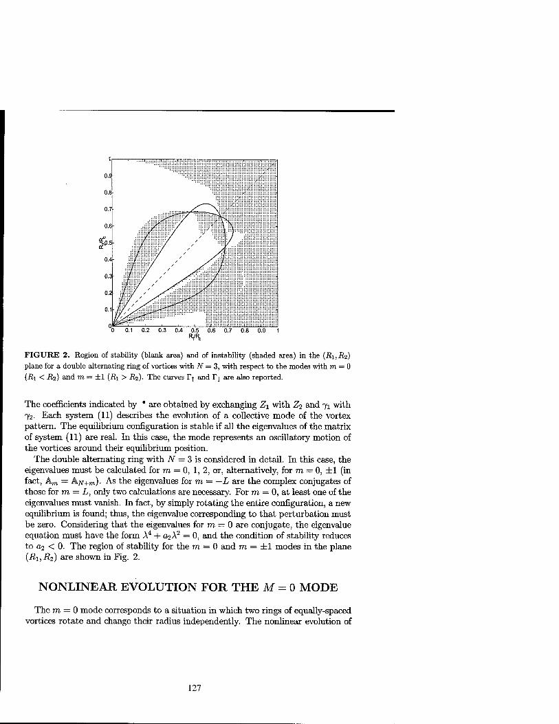
FIGURE 2. Region of stability (blank area) and of instability (shaded area) in the (A^ife) plane for a double alternating ring of vortices with N = 3, with respect to the modes with m = 0 (Ri < R2) and m = ±1 (i?i > R2). The curves Fj and Tj are also reported.

The coefficients indicated by " are obtained by exchanging Z\ with Z% and 71 with 72. Each system (11) describes the evolution of a collective mode of the vortex pattern. The equihbrium configuration is stable if all the eigenvalues of the matrix of system (11) are real. In this case, the mode represents an oscillatory motion of the vortices around their equihbrium position.

The double alternating ring with N = 3 is considered in detail. In this case, the eigenvalues must be calculated for TO = 0, 1, 2, or, alternatively, for m = 0, ±1 (in fact, Am = Ajv+m)- As the eigenvalues for m = — L are the complex conjugates of those for m — L, only two calculations are necessary. For m = 0, at least one of the eigenvalues must vanish. In fact, by simply rotating the entire configuration, a new equilibrium is found; thus, the eigenvalue corresponding to that perturbation must be zero. Considering that the eigenvalues for m = 0 are conjugate, the eigenvalue equation must have the form A4 + a2X

2 = 0, and the condition of stability reduces to a2 < 0. The region of stability for the m = 0 and m = ±1 modes in the plane (Ri, R2) are shown in Fig. 2.

NONLINEAR EVOLUTION FOR THE M = 0 MODE

The TO = 0 mode corresponds to a situation in which two rings of equally-spaced vortices rotate and change their radius independently. The nonlinear evolution of

127

the mode was studied by Arcf [3] for an unbound system, by introducing complex quantities, Z\(t) and Z2{t), such that:

&1,2)(*) = zh2{t) exp (iipn) = Pifi(t) exp (i$i,2(«)) CXP (*Vn) (15)

From Eq.(l), one obtains the equations governing the time evolution of Z\ and Z2, which can be cast into a complex Hamiltonian formulation, as:

. dz*a dm . dza dm tlair = dz:'nair = -dz;>a = 1>2 (16)

where the Hamiltonian of the problem is defined as

^{Zi,Z2,Z[, Z%) 2 ( I \Z \2N

J2 \ -"7a \Za\2 + (N-1) rt log \Za\ - ii log I 1 - i-^- (17)

+7i 72 log ^i - Z%\ - 7J 72 log m ' The basic properties of the motion can be determined by noticing that two constants of the motion exist: l)the Hamiltonian H; 2) the quantity L = 71/9? + ~i2p\, related to the angular momentum of the vortices. By writing pi and p2 in terms of L and of pz/pi, and considering that H is a function of pu p2 and A<J> = <E>2 - $1, one can conclude that the trajectory of the system in the (A$,p2/Pi) plane occurs on the curve

H L (L, ^ ,p2 (Y, gV A$| = Const (18)

Trajectories obtained from Eq. (18) confirm the linear analysis, for they show '0' and 'X' points for stable and unstable configurations, respectively.

Acknowledgements. The author thanks Prof. Roberto Pozzoli (University of Milan, Italy) for introducing him to the subject and Prof. Thomas O'Neil (UCSD) for encouragement.

REFERENCES

1. K.S. Fine, A.C. Cass, W.G. Flynn, C.F. Driscoll, Relaxation of 2D Turbulence to Vortex Crystals, Phys. Rev. Lett., 75, 3277, 1995.

2. I.M. Lansky, T.M. O'Neil, Stability Analysis of a Two-dimensional Vortex Pattern, Phys. Rev. E, 55, 7010, 1997.

3. H. Aref, Point Vortex Motions with a Center of Symmetry, Phys. Fluids, 25, 2183, 1982.

4. G.K. Batchelor, An Introduction to Fluid Dynamics, Cambridge University Press, 1967.

128

Simulation of the Evolution of the Diocotron Instability

Gianni G.M. Coppa, Antonio D'Angola, Giovanni Lapenta Istituto Nazionale per la Fisica della Materia

Dipartimento di Energetica - Politecnico di Torino

Corso Duca degli Abruzzi, 24 - 10129 Torino, Italy

Abstract. The diocotron instability in Penning traps is studied with a new simulation code based upon the point-vortex method. The equations of motion for the computational particles are solved by using the fourth-order Runge-Kutta method. Cylindrical coordinates are used in the solution of the Poisson's equation, allowing the boundary conditions for the electric potential to be applied exactly; moreover, an efficient algorithm based on the Fast Fourier Transform can be employed. The code has been validated by considering the linear evolution of the diocotron instability. Comparisons have shown excellent agreement between the simulation results and the ones obtained with the linear theory.

INTRODUCTION

The study of the time evolution of the particle distribution in a Penning trap is an important topic in the physics of nonneutral plasmas. The discovery that the electron distribution can evolve towards stable configurations of vortex crystals [1] has been recently reproduced successfully by Schecter et al. [2] with a simulation code solving the classic 2D drift-Poisson model. According to this physical model, the evolution of the electron density, n(r,9,t), is governed by the following set of equations [3]:

£ + v.Vn = 0 dt v = — ez x V$ (1)

-£>z V2$ = —

£o

where the velocity field, v(r, 6, t), is given by the E x B drift, and the electrostatic potential, $(r, 6, t), is calculated by solving the two-dimensional Poisson's equation. The conclusions of the work by Schecter et al. represent a very important result, for they prove that Eqs. (1) are an appropriate model for the study of vortex


129

evolution. In this framework, the Authors have developed a new Particle-in-Cell code in order to obtain high-accuracy results for the long-time evolution of the electron distribution. The new code presents some peculiarities, which are different from the normally-used codes and would allow highly accurate simulations, in the Authors' opinion. In order to test the precision of the code, the simulation of the diocotron instability has been considered. In fact, whenever a small perturbation is introduced, the evolution of the system can be calculated accurately by solving a set of linearized equations obtained from Eqs. (1). On the other hand, the simulation of such a situation represents an important benchmark for a PIC code, in which the numerical noise could in principle hide the phenomenon one would observe. The comparisons between the results of the PIC simulation and the solution of the linearized equations, which are presented in the last part of the paper, show the excellent performance of the new code and prove that the numerical noise does not alter the physical evolution of the system.

DESCRIPTION OF THE SIMULATION CODE

The numerical solution of Eqs. (1) has been performed by implementing a Particle-in-Cell code [4], in which computational particles are employed to represent a large number of real particles, which are described by the guiding-center approximation. The code is constituted by three parts: the Poisson solver, the particle-grid interpolation and the particle mover. The implementation of each part of the code has been performed by taking into account the peculiarities of the physical system to be simulated. Here follows a brief description of the techniques employed:

• Poisson solver

Due to the geometry of the physical system, cylindrical coordinates (r, 6) are the most appropriate ones in the solution of the Poisson's equation. In fact, they present two advantages: the former is the possibility to exactly impose the boundary condition for the potential, <f>(Rc, 0) = 0 (being Rc the radius of the cross section of the trap); the latter is that, by using cylindrical coordinates, the Pois- son's equation can be solved with an efficient algorithm based upon the Fast Fourier Transform. In fact, by taking the discrete Fourier Transform of the 0-discretized equation for $Q(r) = <&(r,2-Ka/Ne) :

19 (r^] + \^-llz + ^=e-^,a = Q,l,..,Ne-l (2) r dr \ dr ) r2 AÖ2 eo

a set of decoupled differential equations is obtained for the Fourier components of the potential, $k(r)'-

M 2

$fc = ^^, k = 0,l,...,Ng-l (3)

130

Once the Eqs. (3) are solved numerically, the potential distribution is reconstructed by using the inverse transform:

N„-l _

*0(r) = — J2 $^r) exp{2irika/N9), a = 0,1,..., Ng - 1 (4) 0 fc=0

• Particle-grid interpolation

The interpolations between grid and particles and vice versa are performed by means of the classic Cloud-in-Cell method [4]. According to this procedure, the electric charge of a particle P having coordinates (r>, 6P) is assigned to the four nearest grid points, by using an (r, #)-bilinear weighting. More precisely, if the coordinates of these four grid points, A, B, C, D are (R+Ar, 9), (R+Ar, 6+A9), (R,Q) and (R, 9 + A8), respectively, the fractions of charge assigned to each cell are

WA = WrWe, wB = Wr(l - We), , , wc = (l-Wr){l-We), wD = {l-Wr)We, ()

being

(rP + R+Ar){rP-R) ^-9 2rPAr Au

Slightly different expressions are used when a particle approaches the center or the boundary of the domain.

In order to provide a precise, noiseless representation of the initial electron density distribution, computational particles can have different charge. In practice, if a given cell contains initially M particles, each particle is assigned 1/M of the charge pertaining to that cell.

• Particle mover

The equations of motion for Np computational particles of coordinates {ri,r2, ...,rjvP} and constant charges {ft, #2, ■■-,qNP} can be written formally as a system of differential equations:

dv —?■ =Vp({ri,r2,...,rJvF},{<7i,g2,"-,<?Np}), P= 1,2,...,NP (7)

where the function vp contains the particle-grid interpolation, the solution of the Poisson's equation, the evaluation of the electric field on the grid, the interpolation grid-particle and the calculation of the E x B drift. The system (7) can be solved by using classic techniques of the numerical analysis. After a number of tests, the fourth-order Runge-Kutta method has been chosen, as the most effective in terms of CPU time.

131

SOLUTION OF THE LINEARIZED EQUATIONS

When perturbations of small amplitude are introduced in an equilibrium configuration, Eqs. (1) can be linearized, obtaining

( dnx -r- + vx • Vn0 + v0 • Vni = 0 dt

vi = — ez xV$,, V2$! = —i Bz e0

(8)

where the quantities labelled by 0 and 1 refer to the unperturbed configuration and to the perturbation, respectively. Equations (8) can be further simplified by considering the evolution of a single normal mode, in which every quantity depends on 9 as exp(ik0). A system of equations can be written for the amplitudes riitk(r, t) and $i,fc(r,i), as [3]

dnly ik (d<&0 _ dna ~

B,r \ dr ' dr = 0

dr

hi.

7*1,<

(9)

Equations (9) can be solved analytically when the unperturbed density profile no(r) is piecewise constant, as the problem presents a finite number of time eigenvalues [3], from which the growth rate of the instability can be immediately evaluated. For a continuous density profile, both discrete and continuous eigenvalues are present [5, 6]. In this case, a simple comparison with the simulation code can be obtained by solving numerically Eqs. (9). In fact, by considering n^k and $lfc only for a finite set of iVr radial positions ra = aRc/Nr, Eqs. (9) can be approximated as

dfii,* + ik (Ani /

di Lfc$iifc = nlife

,) 0 (10)

where A, B and Lfc are sparse matrices, which are obtained by discretizing the space operators appearing in Eqs. (9), while n^. and «J^^ are the unknown vectors for the density and the potential perturbations, respectively. Finally, a system of linear differential equations for $lfc

L, ' dt

ik (B - ALfc) $iifc (11)

is obtained. The system can be solved numerically with very high precision. In the rest of the work, the initial value for $!_*. will correspond to a density perturbation Siifc(r) proportional to the unperturbed density no(r).

132

RESULTS

The PIC code has been validated by comparing the simulations with the results provided by the linear theory. Two different categories of unperturbed density profiles have been considered: staircase and continuous profiles. Here follow the results for two different profiles, one for each category.

For the first category, a hollow-ring distribution has been considered, where n0(r) is constant for 0.5fic < r < 0.7RC and zero otherwise. Excellent agreement was found between the growth rates obtained from the results of the PIC code (using 45,000 particles) and the analytically-calculated values of the time eigenvalues u [3]. In fact, by exciting the k = 2 and k = 3 modes (the k = 1 mode is stable), Im(oj/u>D) has been evaluated from the PIC simulations as 0.1467 and 0.2550, respectively, to be compared with the exact values, 0.1466 and 0.2528.

As an example of continuous profiles, the following density distribution:

™2 / v*"

, \ I Const x — 1 - — I , r <b /10N n0(r) = { b2 \ b2J (u)

0 otherwise

with b = Rc/2, has been considered. The PIC code has been used with the initial conditions n{r,6,t = 0) = n0(r) + 10"3n0(r)cos(fcö), for k = 1,2,3. A space discretization with Nr = 995 and Ne = 256 was employed. One particle was placed initially in the center of each cell, with a charge that was proportional to the density in that cell. During simulation, the dimensionless mode amplitude, defined as

, „2 IoCMr,t) \\M2 = -r-z

Jo *o(r,0)

2 r dr

(13) 2 r dr

has been evaluated. The same quantity has been calculated by using a numerical code to solve the linear model, Eq. (11). The results of these calculations are presented in Fig.l. As can be observed, the results of the PIC code are again in excellent agreement with those of the linear theory and the growth of the instability is reproduced correctly for many orders of magnitude. As predicted by Rosenbluth and Smith [7], the k = 1 mode exhibits an algebraic instability. In order to show the effect of the space discretization, three different couples of values for (Nr,Ne) have been used in one case (k = 2).

These results, together with many others which are not presented here, lead to the conclusion that the new code provides a highly accurate solution for the equations governing the evolution of the charge density in a Penning trap.

Acknowledgements. Work performed in the framework of an Italian research project on nonneutral plasmas, coordinated by Prof. Roberto Pozzoli. The Authors wish to thank David Schecter for useful discussions.

133

1CT

10-'

10"°

io-7

Linear theory o PIC code

Linear theory o PIC code

200 400 0>D-t

k=1

0 200 400 600 800 (DD-t

k=3 600 800

10"

ri_

IO"7

Linear theory PIC N=995 Na=256

k=2 200 400

coD-t 600 800

FIGURE 1. Comparison between PIC calculations and linear theory. The evolution of the amplitude for the k = 1,2,3 modes is shown for a continuous density profile [ Eq. (12)j.

REFERENCES

1. K.S. Fine, A.C. Cass, W.G. Flynn, C.F. Driscoll, Relaxation of 2D Turbulence to Vortex Crystals, Phys. Rev. Lett., 75, 3277, 1995.

2. D.A. Schecter, D.H.E. Dubin, K.S. Fine, C.F. Driscoll, Vortex crystals from 2D Euler Flow: Experiment and Simulation, Phys. Fluids, 11, 905, 1999.

3. R. Davidson, An Introduction to the Physics of Nonneutral Plasmas, Addison-Wesley, Redwood City, 1990.

4. C.K. Birdsall, A.B. Langdon, Plasma Physics via Computer Simulation, Adam Hilger, Bristol, 1991.

5. K.M. Case, Stability of Inviscid Plane Couette Flow, Phys. Fluids, 3, 143, 1960. 6. R.J. Briggs, J.D. Daugherty, R.H. Levy, Role of Landau Damping in Crossed-Field

Electron Beams and Inviscid Shear Flow, Phys. Fluids, 13, 421, 1970. 7. R.A. Smith, M.N. Rosenbluth, Algebraic Instability of Hollow Electron Columns and

Cylindrical Vortices, Phys. Rev. Lett., 64, 649, 1990.

134

A 2D Vlasov code for the electron dynamics in a Penning-Malmb erg trap

F. Califano1, A. Mangeney2, F. Pegoraro1, R. Pozzoli3, M. Rome3

1 INFM, Sez. A, U.d.R. Pisa and Dipartimento di Fisica, Pisa, Italy

2 Departement de Recherche Spatiale, Observatoire de Paris-Meudon, France 3 INFM U.d.R. Milano Universitä and Dipartimento di Fisica, Milano, Italy

Abstract. A two-dimensional numerical code for the kinetic description of the electron dynamics in a Penning-Malmberg trap has been developed. The code solves the Vlasov equation for the electron distribution function in the guiding center approximation, coupled to the Poisson equation for the electrostatic potential. In the present version of the code, the drift velocity is given by the E x B-drift. The present code constitutes the first step of a numerical project for the solution of the gyrokinetic Vlasov-Poisson system of equations in a 3D cylindrical geometry.

In this paper we describe the two-dimensional numerical code that we have developed so far for the kinetic description of the electron dynamics in a Penning- Malmberg trap. In the present (bounce averaged) version of the code effects due to the finite axial length of the system are neglected, and the considered equations are isomorphic to the Euler equations which govern the flow of 2D inviscid incompressible fluids, with free-slip conditions at the boundary. The obtained results will then be suitable for comparison with the existing 2D vortex-in-cell simulations [1]. The long term aim of our project is to describe the 3D nonlinear dynamics of a nonneutral plasma, and in particular the influence of the axial electron motion on the 2D vortex dynamics for different values of the ratio between bounce and rotation frequencies (the so-called "rigidity" parameter).

In low density pure electron plasmas confined in Malmb erg-Penning traps [2] the characteristic plasma rotation frequency wr is much smaller than the plasma

frequency wp

^^«1 (1) up 2wc

where wc is the electron cyclotron frequency. In addition, the characteristic rotation velocity, vg — r wr is much smaller than the velocity of light c,

--^äJ-«1- (2) c 2cu>c la. uc


135

Here de — c/wp is the electron skin depth and r is the radius of the plasma column. In this regime we can adopt a purely electrostatic description of the plasma dynamics, with the electric field given by E = -V$, and describe the motion of the particle gyro-centers in terms of the particle drift equations

R 1 B i 1,. (d „ \ -j— \ VE + — b x — vE + vE • VvE Jcm [ wc \ot )

+ V* b + J\7 x b + —V x vE wc m I

v- lB V\\ 1 b + -^V x b + —V x vE

wc ui. m E - ( ^-vE + vE • Vvj -V5

TO

where vE = cE x B/B2 is the particle E x B-drift velocity and

TO ^b • V x b + —b • V x vE

represents the Jacobian of the transformation (r, v) —> (R, y., V\\,ip), <p being the gyro-angle, and E and B are the self-consistent electric and magnetic fields. To leading order in the ratio (wr/wc)

2, and assuming the externally imposed magnetic field to be spatially homogeneous, the gyrocenter motion is simply given by

R = vE + V»b, Vn = -2-E • b. (3)

Neglecting temperature effects in the perpendicular plane the gyroaveraged Vlasov equation reduces to the drift kinetic equation,

dF ■ dF -+K.VF+Vllwr0; Vz$ -47T/3, (4)

D -

P = 1- JdpdV\\F(R.,ii,Vn,t), (5)

where F = F(R,/x, Vj|,<) is the distribution function of the guiding centers and the conservation of the total number of guiding centers is expressed by / dfidV^dR. Jc F — const..

The ratio between the characteristic time of the parallel dynamics and the rotation period is measured by

Wfc (6)

where ut ~ vthe/2L is the bounce frequency of the electrons along the magnetic field lines, vthe is their thermal speed and L is the trap length. If the rigidity

136

parameter W(,/wr is large, electrons bounce back and forth many times before com- pleting an azimuthal rotation and the plasma response, on the rotation time scale, is determined by the bounce averaged kinetic equation. Then, Eq.(4) reduces to

^- + vE-Vxi? = 0 (7) dt

where all quantities are now bounce averaged, and depend on time and on the coordinates perpendicular to the magnetic field only. Integration of F, over p, reduces simply to the particle density n. In this equation the effects due to the dependence of the plasma length on r , which arise from the r, z dependence of the confining potential, as discussed in [3] , are neglected. In order to estimate a characteristic rotation frequency for inhomogeneous configurations, we define

< u,r >= r fR 9-^F dvdO I r [R Fr drdO . (8)

In the present version, the code solves the drift-kinetic equations in a two- dimensional cylindrical geometry for a uniform magnetic field at zeroth order in the guiding center approximation. Writing the E X B-drift velocity in terms of the electric potential $, and considering explicitly the case of the electron density ne, Eq.(7) together with Poisson's equation can be written as

(d c9$9 cWfl\ , ,

{ll^r^w)^9'^4-^6^ (10)

where polar coordinates (r, 9) are used. The boundary condition for the potential is given at the wall of a circular container. These equations are discretized on a bidimensional polar grid (rj.flj), with r{ = i • dr {i = 0,... ,nr; dr = l/nT) and 6 = 2ivj-d6 {j = 0,... ,nB; d6 = l/ne).

The Vlasov equation is solved by means of a finite volume technique, by advanc- ing in time the distribution function averaged over the grid cells

n£ij = -— I*' rdr [ ' ne{r,6)d9 i = l,...,nT ; j = 1,... ,ne. (11) Ti^i/2drdV ,/rj_i J«j_i

The time advancement is explicit and it is obtained by means of a Runge-Kutta scheme.

For the Poisson equation, fourth order finite differences are used. The equation is first (fast) Fourier transformed in the azimuthal angle 6 obtaining a system of ordinary differential equations in r

137

(A)

t = o, r S, 20, 25 '.

.b^V^\J^W^^^^

(B)

— = t — 0

1 .2 • — t — 25 ;

^~-, - OS \ :

O G -

0.4 -

0.2 -

0. 0 - ' : 0.0 0.2 0.4 o.e o.a 00 02 0.4 o e 0.8

FIGURE 1. The mean density radial profile at different times (normalized on wc/vi ) for two

stable configurations: (A) step-like profile, < wT >= 0.5, and (B) smoothed monotonic decreasing

profile, < u>r >= 0.47.

1 A A rn^ -y-r—$m(r)-—$m{r) = 4-Kene:m(r) m = 0.... ,[(n« - l)/2], (12) r ar ar r'

where 3>m(r) and ne>m are the amplitudes of the m-th Fourier component of potential and density, respectively. The solution is then obtained by an inverse (fast) Fourier transform. The nodal values of the distribution function required for the solution of the Poisson equation are obtained by means of a reconstruction algorithm based on the computation of the "primitive function" [4]

G(r,0) = I' r' dr' f dff ne{r',6'), Jo Jo

i i t = 0,.. ,nT j = 0,...,ng.

k=l 1=1

The nodal values are then obtained by 1 Q O

i = Q,...,nr 0, ,nB.

(13)

(14)

(15)

A standard FFT technique is used for the computation of the derivatives in the azimuthal angle, while for the radial derivatives a three-point combined compact difference scheme is employed [5]. The scheme computes both the first and the second derivative at the same time.

The main numerical problem of the present version of the 2D Vlasov-Poisson numerical code is the onset of a numerical instability when strong gradients (or discontinuities) are formed. This instability is responsible for the appearance of growing spurious oscillations which rapidly lead to a numerical divergence of the

138

';--■! (3)

ii~\ sW w

FIGURE 2. The evolution of the I = 2 mode in the case of the initial (smooth) density profile of Fig. 1, frame (B). The four snapshot are the shaded density fluctuations at (A) t=0, (B)

t=10, (C) t=40, {D) t=150, respectively. Here < uT >= 0.47.

distribution function. The onset of the numerical instability in the presence of "strong" density gradients is shown in Fig. 1 where we plot at different times (normalized on u>c/^p) the mean density radial profile in two different stable situations. The density is perturbed at t = 0 by a small amplitude (e = 0.01), I = 2 mode. In the case of an initial step-like density profile, frame {A), we see that numerical oscillations are generated close to the discontinuity and then propagate and accumulate at the origin. On the other hand, when the density gradient is resolved by the numerical mesh, frame {B), the density profile remains unchanged. The evolution of the corresponding density fluctuations up to t - 150 is shown in Fig. 2. We see that a filamentary structure of the mode is produced in correspondence

of the density gradient. In order to investigate the process of vortex formation by an initially unstable

configuration, we have used the following initial ring-like density profile, F, and

perturbation, SF, k=8

F{r) = e-90(r-°-5>2, Sf - e £ sin{k0) e

■90(r-0.5)2

(16) k=2

with e = 0.01. In Fig. 3 we show the evolution of the instability at four different times. At t = 35, frame (D), a number of vortices are generated. Unfortunately, after that time, the discontinuities formed between the larger vortices lead to a nu-

139

(D)

FIGURE 3. The evolution of an initially unstable ring-like density profile (see Eqs. 16). The four snapshot are the density isocontours at (A) t=0, (£) t=20, (C) t=25, (D) t=35, respectively. The resolution used in this simulation is NT — 150 and Ng = 256 and < wT >= 0.16.

merical divergence, as expected from what discussed above. A number of standard methods capable of correctly describing the formation and evolution of discontinuities are presently under investigation.

The extension of the code with the aim of describing the evolution of the system in a five-dimensional phase space (three spatial coordinates and two coordinates in velocity space) is also presently under development (in the electrostatic case, at first). The component of the velocity in the direction of the magnetic field, v\\, and the magnetic moment, /x, are the coordinates in velocity space in the general case. Since the derivative with respect to the magnetic moment does not appear in the Vlasov equation, the problem is in fact formally solved in a four dimensional phase space.

This work was supported by "ex 40%" MURST funds (Italian Ministry for Uni- versity and Scientific Research)

REFERENCES

1. D.A. Schecter, D.H.E. Dubin, K.S. Fine, C.F. Driscoll, Phys. Fluids, 11, 905 (1999) 2. C.F. Driscoll and K.S. Fine, Phys. Fluids B, 2, 1359 (1990) 3. D.H.E. Dubin and T.M. O'Neil, Phys. Plasmas, 5, 1305 (1998) 4. A. Harten,/. Comp. Phys., 131, 3 (1997) 5. P.C. Chu and C. Fan, J. Comp. Phys. 140, 370 (1998)

140

Dynamics of coherent structures in a Penning-Malmberg trap with 2D Vlasov simulations

M. Rome1, R. Pozzoli1, F. Pegoraro2, A. Mangeney3, F. Califano2

1 INFM U.d.R. Milano and Dipartimento di Fisica, Universitä di Milano, Milano, Italy

2 INFM Sez. A U.d.R. Pisa and Dipartimento di Fisica, Universitä di Pisa, Pisa, Italy 3 Departement de Recherche Spatiale, Observatoire de Paris-Meudon, France

Abstract. Preliminary results on the drift dynamics of electrons in a Penning- Malmberg trap, obtained by means of a two-dimensional electrostatic fluid code, are presented. The code solves the continuity equation for the electron density in the guiding center approximation, coupled to the Poisson equation for the electrostatic potential. The drift velocity is simply due to the E x B-drift.

INTRODUCTION

The results presented in this paper are relevant to the two-dimensional dynamics of a pure electron plasma. They have been obtained with the first, simplified, version of a more complex code for the solution of the drift-kinetic Vlasov-Poisson system of equations in a 3D cylindrical geometry [1]. This code will support the experimental activity presently under development at Milano University, based on a Penning-Malmberg trap for electron confinement, aimed at the study of coherent structures (using the methods developed in San Diego [2] [3]), and at the investigation of single particle regimes [4]. In its present version, the code solves the drift-kinetic equations for a uniform magnetic field at zeroth order in the guiding center approximation. At this level of approximation only the E x B-drift is taken into account. In the two-dimensional case, after integration of the Vlasov equation in velocity space, the resulting equations are equivalent to the description of the system in the cold-fluid guiding-center approximation with me ->• 0.

Writing the E x B-drift velocity in terms of the electric potential $, and considering explicitly the case of electrons, the equations are written as

id 10$ 0 10$ 9 1 m


141

(I d d 1 d2\ Ä, „ x

[räffr + ^W) $(r'M) = "e(r'*>')' (2)

where ne is the electron density, and polar coordinates (r,0) are used. Eqs. (1)- (2) are isomorphic to the Euler equations which govern the flow of 2D inviscid incompressible fluids with a single sign of the vorticity. The boundary condition for the potential is given at the wall of a circular conductor surrounding the plasma (this corresponds to a free-slip boundary condition in the fluid analogy), and at the wall of an internal circular conductor, when it is present. In Eqs. (l)-(2), the radial coordinate,?-, is normalized over the radius, R, of the outer circular conductor, the density, ne, over a characteristic density, ne, the potential, $, over 4weneR

2 and the time, t, over wc/w

2, being wc the electron gyro-frequency and u>p the electron plasma frequency (computed with the characteristic density nc.)

Our aim here is to test the capability of the code to properly describe typical situations that will be faced in the experiments. Therefore, we have considered different cases, suitable for comparison with analytical estimates. First, the development of azimuthal perturbations of an annular equilibrium density distribution, for the cases of sharp and soft plasma boundary. Then, two cases where boundary conditions of the potential are changed: the first refers to the influence of a central axial rod on stability, the second to the process of plasma deformation starting from a cylindrical shape, to a new equilibrium when static potential perturbations are applied to the external boundary. Finally, we have considered the more complex case of evolution of a perturbation in a hollow column. Deliberately, no spectral filter, nor artificial viscosity effects have been introduced in the code.

LINEAR THEORY

The newly developed code has been tested at first against the linear perturbation theory. The case of an annular step function has been considered, for which analytical results are known in the literature [5]. An initially perturbed density ne(r, 6,t = 0) = n [H(r2 - r) - H(ri - r)] [l + e cos(W)} has been considered, where H represents the Heaviside function. Fig. 1 refers to n = 0.4, r2 = 0.6, n = 1. e = 1 • 10-3 and / = 3, and shows the time evolution of the (averaged) spectrum of the potential, /J dr |$;(r,i)|2 (for / = 3), computed numerically (solid curve) compared with the result expected analytically (dotted curve).

The agreement of the numerically obtained growth rates with the analytical results is quite good within the time scale of the linear evolution.

However, the full evolution cannot be described correctly by the present code as it becomes unstable in the presence of "strong" density gradients [1]. The results become therefore unreliable after a certain time (in the specific case, after t ~ 60). The problems mentioned above are avoided if the evolution of a perturbed "smooth" profile is considered (see Fig. 2). An initial perturbed electron density of the form

(r,M = 0) = n [A + (r/rp)2} [1 - (r/rp)

2]2 H(rp - r) [1 + ecos(l6)} has been n,

142

FIGURE 1. Average square Fourier amplitude of the potential, for / = 3, versus time. The solid curve represents the numerically obtained result and the dotted line is the analytical result, exp(27i), respectively. For the parameters of the run, the theoretical growth rate 7 ~ 0.1223.

50 100

t

150 200

FIGURE 2. Average square Fourier amplitude of the potential, for I = 3, versus time.

143

0.0 0.5 1.0

t

1.5 2.0

FIGURE 3. Average square Fourier amplitude of the potential, for / = 3, versus time (initial evolution) for an annular plasma confined between two concentric circular conductors. The solid curve refers to $rod — +0.01 and the dotted curve to $rorf = -0.01, respectively.

considered, with the parameter A satisfying 0 < A < 1. Fig. 2 refers to A = 0, rp = 0.5, n = 27/4, e = 1 • 10~3 and / = 3; no numerical instability has occurred within the time of the run. These results coincide with those obtained with a simplified version of the code which solves the linearized Vlasov-Poisson system.

CENTRAL CONDUCTOR AND 2D PLASMA SHAPING

The code has also been used to treat the case in which a central conductor with radius rd is present (in this case the confinement region of the plasma becomes annular), and different boundary conditions are imposed on the conductors. Fig. 3 refers to the stabilizing effect of a negative potential cf>rod, applied to the central conductor, while the outer boundary is at zero potential. This figure shows the evolution at short time of the averaged squared perturbed potential for a positive 4>rod (growing perturbation) and for a negative (f>rod, with the same absolute value (stabilizing effect). An initially perturbed density profile of the form ne(r,6,t = 0) = n[l - ((r - rc)/rp)

2]4 [H(rc + r„ - r) - H{rc - rp - r)] [1 +ecos{W)] has been considered. The thickness of the annular plasma is 2rp. The results shown in Fig. 3 refer to rd = 0.1, rc = 0.55, rv = 0.15, n = 1, e = 10~3 and / = 3.

The 2D plasma deformation towards a new equilibrium when an azimuthally dependent potential is applied on the outer boundary is demonstrated in Fig. 4,

144

where the time evolution of the density contours starting from a purely radial distribution is shown. An initial density profile of the form ne(r,t = 0) = n[l - (r/rp)

2]4 H(rp - r) has been considered in this case, and the boundary condition for the potential has been chosen as <f>(r = 1,9) = -esm(W). The results shown in Fig. 4 refer to rp = 0.6, n = 1, e = 0.08 and / = 3. Note that the plasma tends to be "repelled" from the azimuthal positions where the applied potential on the conductor is positive, and vice versa [6].

INSTABILITY OF A HOLLOW COLUMN

The code has been used for the investigation of the time evolution of an initial perturbation with / = 1 in a hollow density distribution. The linear theory of this problem has been developed by Smith and Rosenbluth [7]. The time evolution of the average square amplitude of the / = 1 Fourier mode is shown in Fig. 5. The equilibrium density profile in the simulation is similar to that considered in [7]. The observed oscillations seem to agree with the linear solution reported in [7]. We observe also a linear growth of the amplitude squared up to t « 250.

-1.0 -0.5 0.0 0.5 1.0 -1.0 -0.5 0.0 0.5 1.0

-1.0 -0.5 0.0 0.5 1.0 -1.0 -0.5 0.0 0.5 1.0

FIGURE 4. Evolution of the density due to a static perturbation of the potential

145

CONCLUSIONS

The presented cases, seem to confirm the basic validity of the Vlasov-Poisson code in its 2D version. However, taking into account the caveat mentioned here and in [1], significant adjustments are required to make it suitable for the investigation of phenomena on very long time scales.

This work was supported by "ex 40%" MURST (Italian Ministry for University and Scientific Research) funds and INFM (Italian National Institute of Physics of Matter) Sect. A funds for Advanced Projects (PAIS)

0 50 100 150 200 250 300 350

t

FIGURE 5. Average square Fourier amplitude of the potential, for / = 1, versus time.

REFERENCES

1. F. Califano, A. Mangeney, F. Pegoraro, R. Pozzoli and M. Rome, A 2D Vlasov code for the electron dynamics in a Penning-Malmberg trap, these Proceeedings.

2. X.P. Huang, K.S. Fine, C.F. Driscoll, Phys. Rev. Lett. 74, 4424 (1995). 3. K.S. Fine, A.C. Cass, W.G. Flynn, C.F. Driscoll, Phys. Rev. Lett. 75, 3277 (1995). 4. R. Pozzoli, D. Ryutov, Electromagnetic Waves and Electronic Systems 3, 12 (1998). 5. R.C. Davidson, Physics of Nonneutral Plasmas, (Addison-Wesley Pub. Co., 1990). 6. J. Notte, A.J. Peurrung, J. Fajans, R. Chu, J.S. Wurtele, Phys. Rev. Lett. 69, 3056

(1992). 7. R.A. Smith, M.N. Rosenbluth, Phys. Rev. Lett. 64, 649 (1990).

146

The modified drift-Poisson model: analogies with geophysical flows

and Rossby waves

D. del-Castillo-Negrete*1, J. M. Finn* and D. C. Barnes*

'Theoretical Division and tApplied Theoretical and Computational Physics Division Los Alamos National Laboratory, Los Alamos, NM 87545

Abstract. We discuss an analogy between magnetically confined nonneutral plasmas and geo-

physical fluid dynamics. The analogy has its roots in the modified drift Poisson model, a recently proposed model that takes into account the plasma compression due to the variations of the plasma length [1]. The conservation of the line integrated density in the new model is analogous to the conservation of potential vorticity in the shallow water equations, and the variation of the plasma length is isomorphic to variations in the Coriolis parameter with latitude or to topography variations in the quasigeostrophic dynamics. We discuss a new class of linear and nonlinear waves that owe their existence to the variations of the plasma length. These modes are the analog of Rossby waves in geophysical flows.

There is a well-known analogy between nonneutral plasmas confined in a Penning-Malmberg trap and two-dimensional inviscid fluids. In this analogy the plasma electrostatic potential and density correspond to the fluid streamfunction and vorticity respectively [2]. This analogy has proved to be particularly useful in the experimental study of various fluid dynamics problems using nonneutral plasmas, e.g. Ref. [3]. The goal of this paper is to study a new analogy between nonneutral plasmas and geophysical fluid dynamics. This analogy is based on the modified drift-Poisson system, a recently proposed model that generalizes the usual drift-Poisson equations by taking into account the variations of the plasma length [1]. The modified drift-Poisson model consists of the conservation of the line-integrated density and the Poisson equation, in dimensionless variables

§-t(nL) = 0, V2<£ = n, (1)

where n{r,9,t), <j>(r,0,t), and L(r,6, t) are the density, potential and length of the plasma respectively, D/Dt — dt+u-V with u = z x V</> the E x B drift velocity,

^ e-mail: [email protected]


147

and V2 is the 2-dimensional (perpendicular to the magnetic field) Laplacian. As illustrated in Fig. l-(a), when the plasma length varies, due to the curvature of the sheaths at the ends, charge conservation of plasma columns aligned in the direction of the magnetic field implies a variation of the plasma density. The model (1) was originally proposed to resolve a controversy regarding the stability of the m = 1 diocotron mode, see Refs. [4,1,5].

For the present discussion we will assume L = Lo(r). A more general model for L, which incorporates free boundary effects on the plasma length, is discussed in [1]. For L = L0(r) the modified drift-Poisson model (1) becomes

^{***<}-(£) £*<='■ where the prime denotes derivative with respect to r, and {/, g} = 1/r (dTf dog — dTf dgg). Writing 4> = 4>o{r) + <j>{i\ 6, t), and neglecting nonlinear terms in <j> we get the linearized version of Eq. (1)

£0 + {^,} + {Av*}-(^)# = o. (3)

where no(r) = V2^o is the equilibrium density. The precise form of L0(r) depends on the numerical solution of the plasma equilibrium equations. However, as discussed in Ref. [1], Lo(r) can be parametrized as

L0(r) = L0(0) [l - Kr2] , (4)

where Lo(0) and the curvature K depend on the equilibrium parameters. Typically K>0.

ANALOGIES WITH GEOPHYSICAL FLOWS

When the variation of the plasma length L is taken into account the plasma density n is not conserved, and the analogy with the two-dimensional Euler equation breaks down. However, there remains a new and interesting analogy with geophysical fluid dynamics based on the conservation of the line-integrated density nL in Eq. (1). In addition to its intrinsic theoretical interest, this analogy is important from the perspective of modeling geophysical flows with nonneutral plasmas experiments in Penning-Malmberg traps.

To explain this analogy consider a uniform density, incompressible, rotating fluid, shown in Fig. l~(b), with free surface z = j](x,y,t), and bottom topography z = —H0\l — A(r)]. This system is commonly used in geophysical fluid dynamics as the starting point in the development of simple models of the oceans and the atmosphere [6]. An important parameter in rotating fluid dynamics is the Rossby

148

number defined as Ro = U/(2QL) where U is a horizontal velocity scale, L is a horizontal length scale, and ft is the rotation frequency.

The limit Ro <C 1 is of particular interest in geophysical flows. In this limit, because of the Taylor-Proudman theorem, the horizontal velocity u is to a good approximation independent of z. If in addition it is assumed that the scale of vertical motions is small compared to the scale of the horizontal motions, specifically if Ro(H0/L)2 <C 1, we get the shallow-water model which implies the conservation of the potential vorticity q in the co-rotating reference frame

Dq Dt

0, 9 = C + 2Q

H (5)

where £ is the vorticity and h = n + H0(l - A) is the fluid depth. In the non-rotating (inertial) frame Eq. (5) reduces to D[(/h)/Dt = 0 which is

analogous to the conservation of the line integrated density in Eq. (1) if we identify the plasma density n with the vorticity C, and the fluid depth h with the inverse plasma length 1/L.

Topography variations. Neglecting free surface effects (n — 0) and assuming A ~ C/2Q ~ Ro we get to first order in the Rossby number

C + 2ti _ 2ti Ho {I-A) "Y0

1 + 4 + AW + 0{Ro2) (6)

On the other hand, a small Rossby number expansion of the advective derivative in (5) gives D/Dt = dt + u • V + 0(Ro), where u = z x Vi/> is the geostrophic velocity, which is the analog of the E x B plasma drift velocity, iß is the streamfunction, and ( = V2V»- Accordingly, to first order in Ro the potential vorticity conservation law in (5) becomes the quasigeostrophic equation:

r\ r\ (a)

z = 0

z = -Ho

Y plane f=fo-yr'

z = -Ho(1-A)

FIGURE 1. Because of charge conservation, when the plasma column shown in (a) is displaced to a region of large L it experiences a transverse compression. This effect is analogous to the vortex stretching experienced by a fluid column due to topography variations in geophysical flows as illustrated in (b). At the same time, topography variations are equivalent to variations of the Coriolis parameter with latitude as illustrated in (c).

149

dVli> Ll ^ ,i (2?Ltt\ dii at {*-**H*r}% = <>- m

where the prime denotes derivative with respect to r. Writing ip — i/'o(r)+V;(r! ^> *)' we get the linearized version of Eq. (7)

dV2^ f _2 n c - _2 -, /2fiA'\ ö^

at + Kv^) + ^,VV,}-(^) ^ = 0. (8)

Note that Eq. (2) is different from Eq. (7), but the linearized drift-Poisson model (3) is identical to the linearized quasigeostrophic equation (8) if we make the identification 2QA'(r) «->■ L'0(r) n0(r)/L0(r). In particular, for L0 in (4) with K > 0, A(r) is maximum at r — 0 and decreases with r.

Coriolis parameter variation. When considering quasigeostrophic motion on an sphere, the variation of the Coriolis force with latitude has to be taken into account. In particular, the term 2Ü in Eq. (5) has to be replaced by the Coriolis parameter f — 2fi sin <p, where <p is the latitude angle. Let ipo denote a reference latitude angle and write ip = <po + 6(p. Then, neglecting free surface and topography effects (TJ = A = 0), we can expand the potential vorticity as

g=^«^[/o + C + /3r-7r2 + 0(<V3)] , (9)

where /o = 2Q sin cp0, ß and 7 are constants, and r = 5ip R with R the radius of the earth. As shown in Fig. l-(c), at mid-latitude cos <p0 ^ 0 and q « fo + C + ßr- This is the so-called /3-plane approximation [6]. However, near the poles cos<p0 « 0 and thus q ~ /o+C—7r2 which is known as the 7-plane approximation [7,8]. Comparing Eqs. (6) and (9) we have that the variations of the Coriolis parameter in the earth can be mimicked by topography variations if we identify A(r) ■H- ßr — 2jr2. This identification is the guiding principle in the modeling of geophysical flows with laboratory experiments. In the plasma physics case the analogy is based on the identification ß — 2^r -H- L'0(r) no(r)/Lo(r). In particular, for n0 = constant, and Lo(r) given in Eq. (4) we have, in the small curvature limit, ß = 0 and 7 = no K. It should be remarked that this analogy is different from the well- known analogy between the Hasegawa-Mima equation for plasma drift waves and the quasigeostrophic equation.

ROSSBY WAVES

According to the modified drift-Poisson model, Eq. (1), a nonconstant plasma length induces a variation of the plasma density. This density variation provides the restoring mechanism of a new class of plasma waves in nonneutral plasmas which are the analog of Rossby waves in geophysical fluid dynamics. As an example of this kind of waves consider traveling wave solutions of the form

150

<t> — fair) + fa (r, mO - ut) .

Substituting (10) into Eq. (2) we get

{0o -ur2/2m,L0V2fa} + {fa,L0V

2ci>0} + {<f>i,L0V2fa} = 0 .

In what follows we construct linear and nonlinear solutions of this equation. Linear solutions Let

0O = ft r-72, 4n = f{r)e*n9-*'>,

(10)

(11)

(12)

for r < rp < 1, where rp is the plasma radius, i.e. n0 = 20, for r < rp, and n0 - 0 for r > rp. Substituting (12) into Eq. (11) and neglecting the nonlinear term {fa,L0{r)V2fa} we get the following eigenvalue problem for /:

/" + -/' + r **)-£ 1 = 0, (13)

where we have defined D = ^imü/ (mtt - u) and \{r) = -L'0(r)/2rL0(r). Equa- tion (13) can be solved numerically. However, if A is constant this equation reduces to Bessel's equation. This can happen for L0(r) in Eq. (4) in the small curvature limit, or if L0(r) is gaussian. In the first case, fa = BJm{Dy/Kr) expi(m6 - ut), where Jm is the Bessel function of order m. On the other hand, the solution of the vacuum equation V2<f> = 0, is </> = C (r~m - rm) ^M-"*). Matching these two solutions using the "jump" conditions [fa = 0, and [r(tt - u/m)fa - n0(r)<f>] = 0, where [/] = f(rp + 0) - f(rp - 0) denotes the jump, we get the dispersion relation:

4K7-2

um - mQ, [ 1 ^JL

rrnn (14)

m=1 n=1 m=2 n=2

FIGURE 2. Rossby waves in nonneutral plasma. The figure shows contour plots of plasma density according to the traveling wave solution in Eqs. (10) and (12). The + (-) sign labels the regions where V20i > V20o (V2<£i < V2<£0)-

151

where pmn is determined from the solution of

2/trjj 1

1 / 1 - r2m

JmiPmn) = OLm pmnJ'm{prnn) , am = — [ — f— . (15) 77! V 1 + r^7"

The direction of propagation of these waves depends on the sign of K. For K > 0, which is the usual case, u>/m < fi. The same happens with Rossby waves whose direction of propagation depends on the sign of the topography or Coriolis parameter gradient. Figure 2 shows contour plots of this solution for rp — 1 and small K. According to the geophysical fluids analogy A(r) <-» - A'(r)/2r +* —ß/2r+ 7, and thus we have the Bessel's function solution when A is a quadratic function or in the 7-plane approximation.

The main difference between these Rossby modes and the modes of Ref. [9] is that the Rossby modes are z-independent compressional modes whereas the z- independent modes of Ref. [9] are incompressible. Also, the radial dependence of the Rossby modes introduces a radial wave number which has no spheroidal mode analogue.

Nonlinear solutions According to (13), fa in (12) satisfies

L0(r)V2fa = ^D2fa. (16) IT

For Lo(r) in (4), the right hand side of Eq. (16) is proportional to fa and (12)- (13) becomes an exact nonlinear solution because the term {fa, Lo(r)V2fa} in (11) vanishes. This nonlinear solution is a special case of solutions of the form

4> = sr2/2m + x(r, mB - st) , L0{r) [V2X + 2 s/m] = T(x) (17)

where s is a constant, and T is an arbitrary function of X- h* geophysical flows a nonlinear solution of the form (12)—(13) also exists in the 7-plane approximation or when A(r) is a quadratic function.

REFERENCES

1. Finn, J. M., del-Castillo-Negrete, D., and Barnes, D. C, Phys. Plasmas 6, 3744 (1999).

2. Briggs, R. J., Daugherty, R. J., and Levy R. H., Phys. Fluids 13, 421 (1970). 3. Driscoll, C. F., and Fine, K. S., Phys. Fluids B 2, 1359 (1990). 4. Driscoll, C. F., Phys. Rev. Lett. 64, 645 (1990). 5. Kabantsev, A. A., and Driscoll, C. F., these proceedings. 6. Salmon, R., Lectures on Geophysical Fluid Dynamics New York: Oxford University

Press, 1998. 7. Leblond, P. H., Tellus 4, 503 (1964). 8. Nof, D., Geophys. Astrophys. Fluid Dynamics 52, 71 (1990). 9. Dubin, D. H. E., Phys. Rev. E 53, 5268 (1996).

152

Equilibrium particle orbits in nonneutral plasmas

Ross L. Spencer

Department of Physics and Astronomy Brigham Young University

Provo, Utah 84602

Abstract. An approximate analytic expression for the unperturbed orbits in a nonneutral plasma is obtained The approximate orbits consist of a constant-velocity portion inside the plasma and a sinusoidal turn-around portion in the plasma end.

INTRODUCTION

To carry out kinetic theory in nonneutral plasmas a knowledge of the equilibrium (unperturbed) particle orbits is required [1]. An analysis of these orbits for nonneutral plasmas with small Debye lengths compared to plasma size will be presented here. In addition, it will be shown that a simple model does a good job of representing these orbits. This simple model, consisting of constant velocity in the plasma interior and harmonic motion in the end, should make it possible to make analytic progress on the problem of a kinetic theory for these plasmas.

PLASMA EQUILIBRIUM

Consider a nonneutral plasma with midplane radius rp, axial half-length zp. It is assumed to be cold enough that A0 -C rp, zp. It is also assumed to be in global thermal equilibrium so that the density distribution as a function of distance normal to the plasma edge is the same at every point on the edge [2]. Under these conditions the equation for the scaled electrostatic potential g — qcj)/kT as a function of the scaled axial coordinate ( = z/Ap on the axis (r = 0) is

9" = l-e-9 , (1)

with g fts 0 inside the plasma [2,3]. The solution of this equation satisfies g RJ 0 along the central axis of the plasma, but then g rises rather abruptly, on the scale of the Debye length, through the plasma sheath. This causes the density, which is proportional to e~9, to fall to zero, defining the plasma edge.


153

To solve this equation, first multiply it by g' and integrate to obtain

€f= y/2[g + exp(-g) - 1} => d( = dg . (2) J2[g + exp(-g)-l}

To integrate once more to get <?(() would appear to be difficult, but a simple approximate result makes further progress possible. The 5-integrand in this equation has a remarkable power series:

1 1 1 g2 g3 g4

/1 R 1 ncn 11 ncn ' 101 AAI\ ' '" V / V^(5 + exp(-5)-l) 9 6 1,080 12,960 181,440

All of the higher order terms have very large denominators so that over the range g e [0,4] an accuracy of about 1% is obtained from just the first two terms. Note that this is the expected physical range for g since the density is proportional to e~9. This approximation leads to a simple approximate relation between ( and g:

C = Mff/sb) + (s-$b)/6 , (4)

where gQ is the value of g at the place where we choose ( = 0. Since most of the interesting physics is at the edge of the plasma it is convenient to set g0 = In 2 so C = 0 where the density has half of its central value. But other choices are sometimes used, so g0 will be left as a parameter.

It is a little awkward to have ((g) instead of 17(C), but Eq. (4) is easy to solve numerically. A simple technique that works over most of the relevant values of ( is simple successive approximation with under-relaxation:

gn+r = (1 - u)gn + ug0 exp [( + (50 - <7„)/6] , (5)

with u = 1 for C < 0.5 and u = 2.5/(2 + ()] for ( > 0.5.

UNPERTURBED PARTICLE ORBITS

It is now possible to analyze the equilibrium motion of the particles. We will use the dimensionless variables ( = z/XD, v = v/vlh = v/^kT/m, and T = wpt, where wp is the local plasma frequency in the center of the plasma, and where AD is the Debye length there as well. Energy conservation at r — 0 is then simply

v20 = v2 + 2g(Q , (6)

where u0 is the scaled particle velocity when it is at the plasma midplane, and where we have taken g K, 0 in the center of the plasma. ( Note that this is an approximation rather than an arbitrary choice of the zero of potential. We have already determined the arbitrary additive constant in g by our choice of 50- We

154

may take g = 0 at the plasma midplane only because the Debye length is much less than the plasma length so that g « 0 for all values of ( well inside the plasma. ) The turning point occurs when g(() = gt, where

9t = vl/2 . (7)

The particle speed as a function of the scaled electrostatic potential g can now be expressed as

dC/dr = ±jvl - 2g . (8)

Using Eqs. (8), (2), and the approximate form of (3) gives

•äZij-Qtem« , (9) 4 V2 Jgc y/gt-g

where T is the time for one full cycle of the particle bounce motion and where the lower limit gc is the exponentially small, but non-zero, value of g in the plasma midplane. We can't set it to zero here because its non-zero value is what makes the integral include the time it takes for the particle to coast across the nearly constant-potential interior of the plasma. Performing the integral (neglecting gc

except in a logarithmic term) then gives

upT ^ UQ_ _ 1_ I gc_ . _ -„ 4 ~ 6 u0 \4gt) ADi/0

«O + IlnfM^.* 6 VQ \ g0 I &fo

(10)

where we have used z = zp at ( — 0 (where g = g0 by definition) and where we have also used Eq. (4) to obtain zp/XD RS In (gc/go) - 5o/6 . This formula has been tested against exact particle periods in numerically-computed nonneutral plasma equilibria, and has been found to be accurate to about 1% from very low velocities up to v ÄJ Avth (for particles at r = 0).

It is useful to break the particle motion up into two parts. The first is the nearly ballistic coasting of the particle across the plasma interior and the second is the turnaround at the plasma end. Numerical experimentation shows that the turnaround motion is well approximated (to better than 5%) by a half-period of simple harmonic motion. A good way to fit these two kinds of motion together to get an approximation to the real motion is to look at what happens in a quarter- period of the particle motion. The particle is first assumed to travel ballistically from z — 0 to z = L during time t — td — L/v. Then its motion is assumed to be described by z(t) = L + Asinojt(t - td) where I, A and u>t are still to be determined. The three conditions that determine these constants are (i) that the ballistic velocity match the initial velocity of the harmonic-motion portion:

ÄLÜt=V ; (11)

(ii) that the axial travel distance of the two parts of the motion equals the distance from the center of the plasma to the turning point:

155

L + A = zp + \DCt , (12)

where Q = C(gi) is the value of ( at the turning point; and (iii) that the ballistic travel time and the quarter-period of the harmonic turnaround must add up to the quarter period of the true motion:

T/4 = L/v + ir/(2ut) . (13)

Solving these equations gives a good approximation to the particle motion along the central axis of the plasma. At radii away from the axis they are modified because the particle enters the thermal region at an angle, experiencing weaker gradients. Because the density profile in the plasma edge is approximately invariant as a function of normal distance [2], and since the edge is thin compared to the plasma size, a particle at a radius where the angle between the z-axis and the normal in the edge is 9 approximately moves axially in the scaled potential function g((cos9). Repeating the period calculation in Eqs. (8) and (9) then shows that in the end the turn-around time is increased by a factor of cos 6. A careful analysis of this effect, leaving the drift time across the plasma interior unchanged and modifying the end dynamics, simply leaves the first term on the right side of Eq. (10) unchanged and divides the last three terms in square brackets by cos 9. Solving the equations taking this effect into account finally gives

^ = .(n-2)(v/vlh)coS9 s A = v/Uf f (14)

and

L = zp(r) + A D

41n2 + (u/ü(,,)2/6

(?r-4) v2 g0 4 In 2 COSÖ

In ^-~- + 2g0v*J (TT-2)l2v?h 6 (TT - 2)

(15)

where 9 is the angle between the normal to the plasma surface and the 2-axis. Note that u>t oc v, with a small non-linear correction, and that this turn-around frequency is on the order of the plasma frequency.

Figure 1 on the next page shows a. comparison of two typical sets of particle phase- space orbits from a numerical simulation using a computed thermal equilibrium with this approximation. As can be seen, the approximation works quite well, except at the larger velocities at r ^ 0 where the errors are on the order of 10%.

156

Theory vs. Simulation: 8» 0.0s

Theory vs. Simulation: 0=46.0

1.5

Figure 1: Orbits from a simulation (solid circles) and from the analytic model (crosses) are compared. The 0 = 0 case is at r = 0 and the other is at finite radius. The symbols mark time along the orbit and zp0 is zp at r = 0. The discrepancy in distance along the orbits between the circles and the crosses is due to the approximate orbit period not being quite right, and is worse for r ^ 0.

CONCLUSION

A simple approximate form for equilibrium particle orbits in nonneutral plasmas has been found. The time it takes for a particle to turn around in the end of the plasma is of order l/wp. For Penning trap plasmas of medium aspect ratio, for which the mode frequencies are typically comparable to uip, the physics of the end should be quite important. In long plasmas the mode frequencies are much less than wp, but even though the turnaround time is very short compared to the mode period for these plasmas, it is still possible that this small end effect could have a strong effect on the also-small damping rates. In any case, these orbits should be a valuable tool for doing kinetic theory in nonneutral plasmas.

REFERENCES

1. Ichimaru, S., Basic Principles of Plasma Physics Reading, Massachusetts, W. A. Benjamin, 1973, p. 46.

2. Prasad, S. A. and O'Neil, T. M., Phys. Fluids 22, 278 (1979). 3. Spencer, R. L., Rasband, S. N., and VanFleet, R. R., Phys. Fluids B 5, 4267 (1993).

157

SECTION 3

COLLECTIVE MODES

Steady-State Confinement of Non-Neutral Plasmas

Using Trivelpiece-Gould Modes Excited by a "Rotating Wall"

F. Anderegg, E.M. Hollmann, and C.F. Driscoll

Department of Physics and

Institute for Pure and Applied Physical Sciences University of California at San Diego, la Jolla, CA 92093-0319 USA

Abstract. A "rotating wall" voltage varying as exp(img9 + ikzz - Hit ft) can give steady-state

confinement of more than 109 charges in a Penning-Malmberg trap at 4 Tesla. For both pure ion plasmas and pure electron plasmas, the torque exerted on the plasma by the rotating wall exhibits peaks at the frequencies of kz ^ 0 Trivelpiece-Gould modes [1]. As expected, modes with / > mefR (i.e. propagating faster than the plasma rotation) give positive torque and cause plasma compression; and modes with / < mefR give adverse torque and cause plasma expansion. The rotating wall drive also causes plasma heating, but cyclotron radiation (in the electron case) and collisions with background residual neutral gas (in the ion case) keep the temperature low enough that background ionization is negligible. The rotating wall "slip" is typically greater for electrons than for ions, because / - m(/fi is proportional to the plasma frequency wp. This contrasts with the kz = 0 rotating wall perturbation which couples to crystallized ion plasmas with no slip [2]. By increasing the frequency of the rotating wall, we observed a plasma central density compression of about a factor of 20. These techniques may be useful for a variety of trapping experiments.

INTRODUCTION

Non-neutral electron or ion plasmas confined in Penning-Malmberg traps have inherent confinement times which are long, but finite. In practice, background neutral gas and small confinement field asymmetries exert a drag on the rotating plasma, causing slow radial expansion and eventual particle loss. Previous work [3] on small ion plasmas has demonstrated radial compression and steady-state confinement using laser techniques to apply a torque which counteracts the drag on the plasma. However, there is considerable interest in containment of elementary particles, including antimatter [4], where laser techniques are not applicable.


161

Recently, "rotating wall" electric fields applied to the end of a column of 109

Mg+ ions have been shown to give steady-state confinement and compression up to 20% of the Brillouin density limit nm [5]. The E x B rotation rate fE of the ions is observed to be somewhat less than the wall rotation frequency fw, with a "slip" frequency Af = fR- fw varying with ion temperature as A/ oc T1/2. Here the rotation frequency fR can be approximated by fR ~ fE when the diamagnetic and centrifugal drift terms are small. The rotating wall technique has also been applied to spheroidal ion plasmas in the strongly correlated or crystalline regimes [2]; here, the applied perturbation was axially uniform along the plasma (kz = 0), and the plasma rotation was generally observed to be phase-locked to the rotating field (i.e. A/ = 0).

Previously, modest density and angular momentum changes of electron columns were reported [6] when an applied dipolar perturbation excited a plasma mode; but strong plasma heating limited the technique at low magnetic fields. Other experiments [7] utilize this heating to replenish the electron plasma by ionization.

In this paper, we describe electron plasmas and magnesium ion plasmas confined by rotating dipole (me = 1) and quadrupole (mg = 2) electric fields applied at one end of the plasma column. We show that the rotating wall fields apply a torque which can be used to compress or expand the plasma, and the torque is shown to arise from Trivelpiece-Gould plasma modes. The rotating wall fields also cause plasma heating: for electron plasmas the cyclotron radiation cooling at B — 4T keeps the plasma temperature low; for ion plasmas, collisions with neutral gas or laser cooling keeps the ion temperature low.

APPARATUS

Figure 1 shows the "IV" Penning-Malmberg trap consisting of cylindrical electrodes in ultra-high vacuum (PRJ3X 10-9 Torr, 97% H2), in a uniform axial magnetic field (B — AT). This apparatus can contain Mg+ ions continuously diagnosed by laser-induced fluorescence [8], or contain only electrons and operate in a standard inject/hold/dump-and-measure cycle [9].

Electron injection from a thoriated tungsten filament gives JVtot «3x 109 electrons in a column of length Lp ss 35 cm and radius Rp « 0.27 cm, with central density n0 « 4 x 108 cm-3. The electron plasma density profile n(r) and an estimate of the thermal energy T are obtained by dumping the plasma axially and measuring the charge passing through a hole in a (rotatable) collimator plate [10]. Both measurements require shot-to-shot reproducibility of the injected plasma, and we typically obtain variability Sn/n < 1%.

For ion experiments, a metal vacuum vapor arc (MEVVA) source is used to create Ntot ~ 5 x 108 ions in a typical column length L„ ~ 14 cm and radius Rp ~ 0.5 cm with a central density n0 ~ 5 x 107 cm-3. The ion plasma is diagnosed by a CW laser (~ 280 nm) scanning through a 32S1/2 ->• 32P3/2 cyclic transition of Mg+ at each radial position. The Doppler-broadened and -shifted laser induced fluorescence

162

Collimator Plate

Faraday Cup

Figure 1. Schematic diagram of the cylindrical trap, with inset representing the rotating wall drive on sectored cylinder S8.

signal gives the ion velocity distribution f(v). From the measured ion distribution f(v,r,t), we obtain the local magnesium density n(r) and temperature T(r).

Figure 2 shows the radial electron density profile (I) for the initial plasma 5 sec after injection, and profiles after plasma expansion (E) or compression (C) as described below.

RESULTS

The rotating wall drive consists of sinusoidal voltages $wj = Aw cos(m9^-27r/si) applied to the eight sectors at 6j = 2irj/&. Here, fs is the signal generator frequency, and the wall perturbation effectively rotates at fw = fs/mg.

In practice, inherent "background" asymmetries in the magnetic or electric confinement fields [11] exert a weak drag on the rotating plasma, causing a decrease in angular momentum and a bulk expansion of the plasma. For electrons, measurements show that this "mobility" expansion rate scales roughly as ^-i = -(n0/"o)bkg ~ (6 x 10~4 sec_1)(n0/108 cm-3)2 for the electron columns described here (Lp - 35 cm, B - 4T). To maintain or compress the plasma, the rotating wall drive must supply a positive torque as large or larger than this drag; alternately, a reverse-rotating drive can substantially increase the background expansion rate.

We find that the applied drive couples to the plasma through discrete kz ^ 0 Trivelpiece-Gould (T-G) plasma mode resonances [12]. Figure 3 shows the mea-

163

10

CO ■

oo o

T i i—i—i—i—i—r

- Collimator Hole i—i

0 ■**■•* J—i—i i i_ I V^Ttn » ■ ■ -0.5 0

r [cm] 0.5

Figure 2. Electron radial density profile for injected plasma (/), a compressed plasma (C), and an expanded plasma (E).

sured peaks in the compression rate versus drive frequency when a strong drive of amplitude Aw = 0.4V is applied to the injected plasma profile. Here, an mg = 1 rotating drive at a chosen frequency is applied to the sectored electrode S8 for 5 sec, and the initial compression (or expansion) rate n0/n0 is measured. The measured background expansion rate of (h0/n0)hk& = -4 x 10"3 sec-1 (somewhat less than expected from the n2 scaling) has been subtracted from the data, so the plot indicates torque from the rotating drive alone. Two strong compression peaks and one broader compression region are observed; and two negative torque peaks are clearly visible in the reverse drive direction. Figure 3 also shows the rate of temperature change T, suggesting that the drive causes general heating as well as heating directly associated with T-G mode resonances. These temperature changes shift and broaden the T-G modes, making precise comparison with theory difficult.

For comparison to linear mode theory, we apply a weak mg — 1 rotating wall, with Aw — 0.025V. The resulting compression peaks are shown in Fig. 4. This small amplitude drive does not measurably heat the plasma, so the temperature remains low, with TKO.1- 0.2 eV. We observe many narrow T-G compression peaks, and these correspond closely with observed mode transmission peaks, i.e. 10-30dB enhancement in the wave signal received at S4. The observed mode transmission peaks, launched with S8 and detected with S4, correspond closely with numerical drift- kinetic predictions for T-G plasma modes varying as h(r, mr) exp(img9+imz zir/Lp) where h(r,mr) represents the radial eigenfunction with mr zeros (counting the one at r = 0). The six observed wave transmission and plasma compression peaks agree quantitatively with the (m2, mr) mode frequencies calculated numerically us-

164

fs [MHz] Figure 3. Electron density compression rate n0/n0 for a strong ms = 1 drive. The compression peaks are associated with shifted (mz, mT) modes. The open diamonds represent the associated heating rate T.

ing two "fit" parameters of iVtot = 2.7 x 109 and T = O.leV. These parameters are consistent with the measured JVtot = (3 ± 0.6) x 109 and T = 0.1 - 0.2eV. This correspondence has been further verified by varying the plasma length and by tailoring the antenna configuration to distinguish even and odd mz.

The T-G modes for long columns within a cylindrical wall are predicted to have a rotationally-shifted "acoustic" dispersion relation, with frequency / given approximately by

f - mgfR « -^ Rp -r—g{mT,T) . Z1T h„

(1)

The left hand side of Eq. (1) represents the frequency of the mode in the plasma rotating frame JR, which can be approximated by /« s=s fB when the diamagnetic and centrifugal drift terms are small. The shifted frequencies are proportional to Nljj2 through up = [Anne2/m]112 and Rp, are proportional to kz = irmz/Lp, and depend functionally on T and mT. In contrast, the radial density profile n(r) and absolute column size Rp have little effect on the mode frequencies except through

The magnesium ion analog of Fig. 4 showing compression peaks corresponding to T-G modes can be found in Ref. [13]. Also, Figure 4 of Ref. [5] shows ion compression with a strong drive; here, the peak due to T-G modes is so broad that only one bump can be seen for f$ > fR. This broadening due to large amplitude and heating effects hindered the identification of T-G mode coupling in the original data.

165

0.1

ü 0.05 o

~l 1 1 1 1 1 1 1 1 1 1 1 1 1 1 1 ! , , p

m0= 1 hAw = 25mV

0 £ ^•«V. n yf Observed modes Y ...

Calculated modes £? q> £ £- Q- £ (m , m ) ,_H" (vf ^ _? ^ ^

-. - '. i ■ , .---t- , y, s^ i >-< s-^. >—: . , , I

0 0.5 1 1.5 2 2.5

fs [MHz]

Figure 4. Electron density compression rate for a weak me = 1 drive, compared to the observed and calculated Trivelpiece-Gould (T-G) plasma mode frequencies for various (mz,mr).

The rotating wall technique enables practical plasma manipulation; for example, Fig. 5 demonstrates plasma compression (solid dots) by slowly ramping the drive frequency from 0.5 to 2.13 MHz in 1000 seconds. From 0.5 MHz to 0.65 MHz, the central density slowly decreases, indicating that there is no significant torque from the rotating wall drive and that no torque-balanced equilibrium is reached. From 0.65 MHz to 1.95 MHz, the torque provided by the rotating wall coupling through the (1,2) mode exactly balances the background drags, and the plasma is in equilibrium with the drive. Above 1.95 MHz, the background drags are larger than the rotating wall torque, and the plasma expands rapidly before reaching a new equilibrium with torque coupled through the (2,2) mode.

One should emphasize that quadrupole rotating perturbation (mg — 2) works as well, and that a central density compression of a factor of 20 has been reported [1]. It is also apparent that mB — 2 tends to heat electron plasmas less than mo — 1, perhaps because fw — fs/m,0 is smaller.

The nonlinear nature of the coupling to the (1,1) mode is shown in Fig. 6. The measured compression rate (dots) scales as h0/n0 oc Al

wx for the experimentally

accessible range of Aw > 0.025V. To understand this result, we measured the amplitude ATec of the received signal in a transmission experiment, and obtained scalings of Aiec oc A]^ for Aw < 0.02V and Arec oc A°w for Aw > 0.03V.

Simple perturbation theory suggests that the compression should scale as (n0/n0) a 6n ■ 6ip ■ cos(</>), where 5n is the plasma density perturbation (with On oc A-ec), Sip is the applied potential perturbation (with 8ip a ^4^,), and <j> is the

166

15

m

B 10

00 o

o

-i 1 r- -7—7—i i—i 1 1 1 1 . r

i me = l #/ AW = 0.4V

i

-j—i—1—i—i—i i—I i i i i 1 i_

> CD

H o

0 0.5 1 1.5 2 fs [MHz]

Figure 5. Electron central density n0 and temperature T during a ramped me = 1 drive.

phase shift between Sn and Sip (with measurements showing <f> w const). Since the density perturbation Sn is observed to be saturated for Aw > 0.03V, the observation that h0/n0 oc Al

w is consistent with this theory perspective.

A summary of the ion and electron density compression obtained by slowly ramping the frequency of the rotating wall is shown in Fig. 7. The ions reach a density n0 ~ O.lnßi; note that with shorter plasmas, densities up to no = 0.23 n^ were obtained [5]. The slip in the ion case is a lot smaller than in the electron case. This is expected, since Eq. (1) suggests that the slip is proportional to the plasma frequency, and wpe — 210 wpMg+- The ion temperature exhibits peaks that we identify asm» = 0 T-G mode due to a weak (undesired) me = 0 component of the rotating wall drive. For the electrons, no similar peaks were observed because the first me — 0 T-G mode is above 2 MHz.

We have interpreted the rotating wall coupling as a collective effect, in contrast with "side band cooling" which is interpreted as a single particle effect, i.e. the energy of a single particle transferred from the magnetron motion into damped axial or cyclotron motion.

A rotating wall technique has also been applied to spheroidal ion crystals [2] using an axially uniform rotating electric field. Here, the torque is applied to a solid object, and in this "rotating brick" case, the crystal rotation was generally observed to be phase locked with the rotating field [2]. For an electron plasma, finite slip is required to apply a torque on the fluid; the T-G modes rotate faster (or slower) than the plasma, and the angular momentum carried by the wave is transferred to the particles. However, further experiments will be needed to clarify the distinction between the finite-slip kz ^ 0 couplings described here and the zero

167

1 1—i—r—r"i"i"r| r

Electrons i "i i—i i 11

0.001

Aw [Volts]

Figure 6. Peak density compression rate n0/n0 and amplitude ATec of the received signal on S4 for the m0 = 1, (1,1) mode driven by S8.

i i i 1111 1—i—i i i 1111 -i—i i i 11 if

( Electrons ) ,

I- me=U

©rnfl = 2

r+

■SB ;/ Vi ' >

- 0.1 H

0.01 fw [MHz]

Figure 7. Central density n0 versus ramped rotating wall frequency /„, = fs/mg

for electrons and ions using mB — 1 and 2; and measured temperature T during ramp.

168

slip kz = 0 coupling obtained with spheroidal coulomb ion crystals. Further, the wave-particle interaction which generates the torque is not understood theoretically: if the interaction is essentially Landau damping, the measurements imply that this damping is not in the linear regime. Further experiments may clarify this issue.

We thank Drs. Thomas M. O'Neil, Daniel H.E. Dubin, Travis Mitchell, John J. Bollinger, Robert E. Pollock, and Mr. James Danielson for stimulating discussions, Dr. Ross Spencer for use of his drift kinetic computer code; and the late Mr. Robert Bongard for outstanding technical support. This work is supported by Office of Naval Research Grant No. N00014-96-1-0239 and National Science Foundation Grant PHY-9876999.

REFERENCES

1. Anderegg, F. et al., Phys. Rev. Lett. 81, 4875 (1998). 2. Huang, X-P. et al, Phys. Rev. Lett. 80, 73 (1998); Mitchell, T.B. et al, Science

282, 1290 (1988). 3. Heinzen, D.J., Bollinger, J.J., Moore, F.L., Itano, W.M. and Wineland, D.J., Phys.

Rev. Lett. 66, 2080 (1991). 4. Hall, D.S. and Gabrielse, G., Phys. Rev. Lett. 77, 1962 (1996); ATHENA Collabo-

ration, Hyperfine Interactions 109, 1 (1997). See also Gabrielse, G. et al. and Fine, K.S. et al. in this proceedings.

5. Huang, X.-P., Anderegg, F., Hollmann, E.M., Driscoll, C.F. and O'Neil, T.M., Phys. Rev. Lett. 78, 875 (1997).

6. Eggleston, D.L., O'Neil, T.M. and Malmberg, J.H., Phys. Rev. Lett. 53, 982 (1984); Mitchell, T.B., Ph.D. Thesis, UCSD (1993).

7. Pollock, R.E. and Anderegg, F., Non-Neutral Plasma Physics II, AIP Coinf. Proc. 331, edited by J. Fajans and D.H.E. Dubin (AIP, New York, 1994), p. 139. See also Pollock, R.E. et al. in this proceedings.

8. Anderegg, F., Huang, X.-P, Sarid, E. and Driscoll, C.F., Rev. Sei. Instrum. 68, 2367 (1997).

9. deGrassie, J.S. and Malmberg, J.H., Phys. Fluids 23, 63 (1980). 10. Beck, B.R., Fajans, J. and Malmberg, J.H., Phys. Pias. 3, 1250 (1996); Eggleston,

D.L., Driscoll, OF., Beck, B.R., Hyatt, A.W. and Malmberg, J.H., Phys. Fluids B 4, 2432 (1992).

11. Driscoll, OF., Fine, K.S. and Malmberg, J.H., Phys. Fluids 29, 2015 (1986). 12. Prasad, S.A. and O'Neil, T.M., Phys. Fluids 26, 665 (1983); Trivelpiece, A.W. and

Gould, R.W., J. Appl. Phys. 30, 1784 (1959). 13. Hollmann, E.M., Anderegg, F. and Driscoll, C.F., "Confinement and manipulation

of nonneutral plasma using T-G modes driven by rotating electric field," to be submitted to Physics of Plasmas.

169

Wave Angular Momentum in Nonneutral Plasmas*

Roy W. Gould

California Institute of Technology, Pasadena, CA 91125

Abstract. Angular momentum and energy are added (or removed) when exciting a mode, such as a diocotron, Trivelpiece-Gould, or Dubin mode, and we discuss rates at which mode angular momentum and energy are added by applied fields. Excitation of a plasma mode is an effective way to transfer angular momentum and energy to the plasma because it is a resonant process. We relate this to recent experiments on compression and expansion of plasmas using a "rotating wall" field. We also calculate the torque on a Coulomb crystal which is phase-locked to a "rotating wall" field and describe phase oscillations and the maximum rate of acceleration which can be achieved.

Early experiment^ 1) showed that asymmetric applied potentials can cause particle transport in nonneutral plasmas, and static field errors are thought to be responsible for the anomalous loss of particles from traps. Collective modes, either time dependent or static, can enhance the asymmetric fields responsible for this transport, and either inward or outward transport can occur. Recent "rotating-wall" field experiments(2) have brought some of these ideas into sharper focus by showing that nonneutral plasmas can be contained indefinitely with such fields and that the angular momentum transfer rates are much larger when the excitation frequency corresponds to one of the Trivelpiece-Gould(TG) mode frequencies.

Theoretical attempts to understand transport have generally focussed on the details of particle transport near resonant surfaces in the plasma(3). In this paper, we focus instead on the angular momentum and energy added when a mode is excited. The added angular momentum and energy is associated with a coherent wave perturbation in the plasma. If the mode damps, the added wave angular momentum and energy then become part of the equilibrium plasma. Dissipative processes are required for damping and the details of these processes are important in determining exactly where the momentum and energy is deposited within the plasma. However, it is useful to separate the process of transferring angular momentum to the wave from its redistribution within the plasma and to obtain transfer rates from properties of the

Research Sponsored by the U. S. Office of Naval Research.

CP498, Non-Neutral Plasma Physics III, edited by John J. Bollingcr, et al. © 1999 American Institute of Physics l-56396-913-0/99/$15.00

170

modes. It is not actually necessary for the applied field to be a "rotating-wall" field, so long as the mode excited has a rotating field. We obtain the transfer rates from a susceptiblity, x» which is the ratio of oscillating charge induced on the wall to the oscillating applied potential which excites the mode.

A spatially uniform cold electron plasma has a canonical angular momentum Pg = Nm(ur - wc/2) < r2 > , where N is the total number of electrons of mass m, ujr is the rotation frequency, independent of r for a spatially uniform plasma, and wc = eBo/m is the electron cyclotron frequency and < r2 > is the mean square radius of the plasma fluid. The first term represents the mechanical part of the canonical angular momentum and the second term represents the magnetic part. For plasmas obeying the drift approximation (wr < wc/2), the latter term is larger than the former, so that the canonical angular momentum is actually negative. Thus a positive torque, which increases the canonical angular momentum, decreases the magnitude of the angular momentum and therefore < r2 > , thereby compressing the plasma. However, when wr > u)cl2, Pe > 0 and a positive torque expands the plasma. While we discuss an electron plasma here, these ideas and results are applicable to ion plasmas with appropriate changes in sign of various quantities.

We can calculate the torque Ton the plasma either by integrating the moment of the electric force over the volume V of the plasma, or by integrating the stress tensor over a surface S (the negative of the torque on the wall charges) outside the plasma at the wall. We can also calculate P, the power input to the plasma, from the wall potential times the inward displacement current at the wall:

T = - JvrneEedV = e0JsETEebdS = iRe\imErmk<l>*mk]S

P = - e0 Js f^ dS = lRe[ÜjErmk<l>*mk}S.

where S = 2irbL is cylindrical surface at r = b, the wall and length L, so that k — kn = nn/L (periodic boundary conditions). The wave torque involves quadratic wave quantities, such as the field Ee times the perturbed ET of the wave, ~ exp[i(m9 + kz - ut). <j>mk and £rmfcare the complex amplitudes of the oscillating

wave potential and radial electric fields at the wall, respectively. Such fields travel with angular velocity w/m. We regard <j>mk as applied and Ermk as the response and define the response function, or susceptiblity, for a single wave with wave number pair (m, k) as

Xmfc(w) = - T-^\r=b

This allows us to write the torque and power input in terms of the applied potential as

171

T= - |fie[imxmfc(w)0mfc^Jt]S P = - \Re[iwxmk{u>)<f>mk<j>*mk]S.

It follows from these relations that P/T = u/m, the angular velocity of the rotating field. Both P and T are quadratic in the applied potential.

We anticipate that xmfc(w) wil1 have poles at the mode frequencies, with one pole for each radial eigenmode (whose number is denoted by /), and to be of the form,

Xmfc(w) = E {ul ,,fl'"?,w -, + 0ther terms

vimk, Rimk> and limk WQ me frequency, residue or coupling strength, and damping rate of the mode with radial, azimuthal, and axial mode numbers (l,m,k). These are measurable quantities. If we focus on just one mode, hence one term in this series, this is the classic case of an oscillator driven by a sine wave. For a dissipationless plasma, limk = °> and die susceptibility function will be purely real, with poles at the mode frequencies. Then there is continuous increase, or decrease, of angular momentum and energy of the mode only if the applied frequency is exactly equal to a mode frequency. With damping, the steady input rate at resonance is proportional to Rlmkhlmk.

The sign of Rlmk determines the direction of the transfer. When Rlmk is negative, transfer is to the plasma, and when Rlmk is positive, transfer is from the plasma. When limk - ° and at exact resonance, the oscillator is continuously excited until the pulse ends. Off resonance, there is transfer to and from the mode at the difference frequency with a net transfer to the plasma if Ä/mfc < 0 and from the plasma if Rlmk > 0. For an applied pulse whose length is short compared to the beat period there will be a momentum transfer to or from the plasma, depending on the sign of Rlmk, so long as the pulse has frequency components at one of the mode frequencies.

We note that the input admittance of a patch electrode can be written in the form

Y(u)= -ia;E|5mn|2XmnM,

run

where Smn is a "structure" factor for the patch with k = nn/L. This includes all of the modes and is a measureable quantity. In this connection we again note it is not necessary for the applied field to be rotating in order to excite a mode which rotates.

To obtain xmfc(u>) one must solve the potential equation within the plasma and surrounding vacuum regions for a sinusoidally varying potential applied to the wall electrode. xmfe(w) is simply the negative of the logarthmic derivative of $ at the wall. For this discussion, we consider a cold uniform plasma cylinder of radius a. The potential equation is V • e ■ V$ = 0, where e = e(u) is the linear dielectric tensor for

172

sinusoidally varying fields. The methods for solving this equation when $ = Oat the wall (r — b), and the for modes which result, have been discussed extensively in the literature(4,5). This model has ilmk = 0. It is straightforward to obtain the solution when there is an applied time-varying potential applied on the wall, and to obtain

Xmfc(^) r F(u)+Gi U3F(u)+G2

TarJm(Ta)- m [Jm(Ta) ■

kb Jm(<sc)iC(fca)--Km(fcc)4,(fca) ™ Km{kc)Im(ka)-Im{kc)Km(ka) '

kb fm(kc)K'm (ka)-KUkc)fm{ka.) m K,

m(kc)Im{ka)-fm(kc)Km(ka) ' , K'm(kc)Im.(ka)~fm(kc)Km(ka) KC Km(kc)Im(ka)-Im(kc)Km(ka)'

with T2 = - fc2e3(u;)/e1(w). Primes denote derivatives with respect to the argument. F(tü) contains all of the frequency dependent terms and properties of the plasma and G1, G2 and G3 depend only on the wave numbers m and k and the dimensions a and b. The components of the dielectric tensor are given in Ref. 5. The poles of Xkmi^) give the mode frequencies and are obtained from the solution of F(ui) + G2-0. F(w), and thusXfcmM' ^as alternating poles and zeros for real frequencies because of the Bessel functions. They are clustered about about u = mu>r for small ka, becoming very dense at this frequency. Since m and k = rnra/L are fixed, these various poles correspond to higher order radial modes, with increasing number of radial nodes, characterized by radial mode number I. There is also one isolated mode, the diocotron mode with u) = ojr[l - (a/b)2m] for ka = 0. Coupling to the latter is quite large.

It is straightforward to obtain the frequencies and residues for each of these poles numerically. Illustrative results are shown in Figures la and lb, respectively. Both are in units of ov, the rotation frequency. Only the lowest few T-G modes and the one

Co

CO,

FIGURE la. Mode Frequencies in units of wr versus ka for m = 2, b/a = 2, wp/ur = 10.

173

-0.05

CD

CO CD

0.05

0.15

FIGURE lb. Residues in units of ur versus ka for m = 2, b/a = 2, u>p/u>r = 10.

diocotron mode are shown. Higher modes have frequencies closer to mwr and even smaller residues. These fall in the shaded regions of the figures. Fast modes, those whose fields rotate faster than plasma rotation {u/m > cur) have negative residues, while slow modes (co/m < ur) have positive residues. Thus the excitation of a fast mode adds angular momentum so that a fast wave has positive angular momentum. Similarly, the excitation of a slow mode removes angular momentum so that a slow wave has negative angular momentum.

For b«l, the dispersion relation of the Z'th radial TG eigenmode is wlmn ~ mujr ± ka (u)p/pml), where pml is the l-thxoot of Jm(x) — 0. Similarly,

3 R, ■kmn c. Jm1 . (ka)6

A similar expression has been obtained for the susceptiblity of spheroidal plasmas, using the methods of Ref. 5. LeGendere functions replace the Bessel functions.

It has recently been shown the rotation of a Coulomb crystal can be phase-locked to a rotating wall field(6) and that this is a very useful technique. Here we calculate the torque on an ideal Coulomb crystal. The effective potential of the applied trap field is static in a frame rotating with the field and has the following form

$T = K,[22 + /3p2] + ^ PZWd) P™(0) cos(m<f>).

where V0 = muj2z/2e, with uz the single particle axial bounce frequency of the trap and

Vj the amplitude of the rotating multipole potential at the crystal boundary, £, = 6, £2 = 0. In equilibrium, the crystal adjusts its so as to produce a potential $p which just

174

cancels $T inside the crystal. This gives a spheroid(6), of radius a and half-length b, with a slight deformation of its surface arising from the second term. The deformation can be characterized by its surface charge,

• = n0ea6 Mg& ^Mcos[m(^> + A0)],

where 6 is the fractional distortion in the radius a, hi is the element of the metric tensor associated with £t. In equilibrium, A<^> = 0, and the torque on this surface charge vanishes. However, if this charge distribution is rotated (ahead) through an angle A<j> from the equilibrium position without significant change in shape, then the torque T = Jv pE^dq is non-zero and is

T = CmQ0Vi<5 sm(mA0) = - Tmax sin(mA<t>)

where Q0 is the total charge of the crystal, and c™ = (3m/4) /+1 [P™(0/P„ (0)]2d£ = 8/5 for m = 2. Vj is proportional to 6 so that the torque is quadratic in 6. This

torque acts to speed or slow the rotation, according to the sign of m A</> and keep the crystal rotating, on the average, with the applied field. However there may be small amplitude phase oscillations and there is a maximum torque Tmax which governs the maximum rate at which the crystal rotation can be accelerated. Both also depend on the moment of inertia of the crystal, and phase oscillations are probably damped by viscous effects: Phase oscillations might be excited by an abrupt change in phase of the rotating field, and a study of the response of the system may yield useful properties of the crystal, since the time required to come into a new equilibrium shape is not known. Again, it should not be necessary for the applied field to be a "rotating wall" because the rotating crystal will respond mainly to the rotating component of a standing wave field whose angular velocity is close to that of the crystal.

REFERENCES.

1. D. L. Eggleston, T. M. O'Neil.and J. H. Malmberg, Phys. Rev. Lett. 53 982 (1984).

2. F. Anderegg, E. M. Hollman, and C. F. Driscoll, Phys. Rev. Lett. 81 4875 (1998). X.-P. Huang, F. Anderegg, E. M. Hollman, C. F. Driscoll, and T. M. O'Neil, Phys.Rev. Lett. 78 875 (1997).

3. D. Eggelston and T. M. O'Neil, Phys. Plasmas, 6 2699 (1999).

4. A. W. Trivelpiece and R. W. Gould, J. App. Phys. 30 1784 (1959), S. A. Prasad and T. M. O'Neil, Phys. Fluids 26 665 (1983), R. C. Davidson, "Physics of Nonneutral Plasmas", Addison Wesley, Redwood City, CA 1990.

5. D.H.E. Dubin, Phys. Rev. Lett. 66 2076 (1991)

6. X.-P. Huang et a!., Phys. Rev. Lett. 80 73 (1998).

175

Autoresonant (nonstationary) excitation of the £ = 1 diocotron mode

J. Fajans,1 E. Gilson

Department, of Physics University of California, Berkeley Berkeley, California, 9J, 720- 7300

L. Friedland

Racah Institute of Physics, Hebrew University of Jerusalem 91904 Jerusalem Israel

Abstract. The autoresonant (nonlinear phase locking) manipulation of the diocotron mode

in a non-neutral plasma is investigated. Autoresonance is a very general phenomena in driven nonlinear oscillator and wave systems. By sweeping or chirping the drive frequency, autoresonance allows the amplitude of a nonlinear wave to be controlled without the use of feedback. The experimental results, including a novel scaling relation, are in excellent agreement with a simple theoretical model.

The oscillation frequency of a nonlinear, Duffing-like oscillator changes with amplitude. If you excite such an oscillator by driving it at its linear resonant frequency, the oscillator's amplitude will grow only marginally before its shifting frequency causes it to go out of phase with its drive, after which the oscillator's amplitude will beat back down to zero. By measuring the oscillator's instantaneous frequency and phase, you could use feedback to grow the oscillator's amplitude arbitrarily. But how can you grow the oscillator to high amplitude without feedback? A general property of weakly-driven, nonlinear oscillators is that, under certain conditions, they automatically stay in resonance with their drives even if the parameters of the system vary in time and/or space. This phenomenon is called autoresonance.

The autoresonance concept dates back to McMillan [1] and Veksler [2], and was further developed by Böhm and Foldy [3] for particle accelerators. The term "phase stability principle" was used to describe the phenomenon in these early studies. The synchrotron, synchrocyclotron [4], and other, later acceleration schemes [5,6] all are based on autoresonance. Recently, the effect has been studied theoretically

J) [email protected]


176

in atomic and molecular physics [7,8], nonlinear dynamics [9,10], nonlinear waves [11] and fluid dynamics [12].

Autoresonance also occurs for waves and modes. One system which can exhibit autoresonance is the £= 1 dioctotron mode, for which the mode frequency increases with mode amplitude. If the mode is driven by a sufficiently large drive is applied to an azimuthal sector, and if the drive frequency is chirped through the linear mode frequency, the mode will be excited until it crashes into the trap wall [13] (see Fig. 1) Once autoresonantly excited, chirping downwards will decrease the mode amplitude. Autoresonance can also occur when the mode is driven by a single frequency and the linear frequency of the mode decreases slowly due to plasma expansion (see Fig. 2).

>.00 0.01 0.02 0.03 0.04 0.05 Time (s)

FIGURE 1. Autoresonant response to a swept drive, (a) Mode amplitude (b) Drive frequency (solid line), measured linear resonant frequency (dashed line), and measured excitation frequencies (•). The driving frequency is swept from 20kHz (well below the linear resonant frequency) to 45 kHz (well above the linear resonant frequency) in 0.067 s and the drive amplitude is 0.5Vp-p. At first, the mode amplitude is small, and has frequency components at both the drive frequency and the linear diocotron mode frequency. After the drive frequency passes the linear resonant frequency, the amplitude grows autoresonantly, and only one frequency is present. Finally, the amplitude grows large enough to send the plasma into the wall, and the mode frequency drops precipitously.

Autoresonance will not occur when the drive frequency or system parameters are changed too quickly or when the drive amplitude is too small. For a fixed chirp rate A (the change in the drive frequency per second), there is a critical drive amplitude V& below which the maximum mode amplitude is relatively small and increases with the drive amplitude, and above which the mode amplitude follows

177

0.2 0.3 Time (s)

FIGURE 2. Response to a constant frequency drive. Autoresonance occurs because the system's linear resonant frequency drops as the plasma expands, (a) Mode amplitude (b) Drive frequency (solid line), measured linear resonant frequency (dashed line), and measured excitation frequencies (•). The drive frequency is 27.4 kHz and the drive amplitude is 0.04 Vp-p. The initial linear diocotron frequency is 28.4 kHz, but plasma expansion causes the linear diocotron frequency to drop [14] by about 14% in 0.5 seconds. (The background residual gas pressure was deliberately set high to increase the expansion rate.) Autoresonant growth occurs only after the linear mode frequency has dropped to the drive frequency, at t = 0.11 s.

the drive frequency to high amplitude and is independent of the drive amplitude. As shown in Fig. 3, the threshold is very sharp. Lower chirp rates have lower critical drive amplitudes. Theoretically,

Va oc A075, (1)

and is in excellent agreement with the data, as shown in Fig. 4. The threshold exists because the autoresonantly driven mode can be modeled as a

pseudoparticle oscillating in a slowly-varying pseudopotential. The slowly-varying Hamiltonian is:

#(<l,A) = SA2/2 + Vpseudo(i>),

where the pseudopotential is

VPseudo($) = -2e/01/2cos4>+^<i>,

and the slowly-varying inverse mass is

(2)

(3)

178

la 1.0

0.188 0.190 0.192 0.194 0.196/0.198

0.6 (b)

0.00 0.04 0.08 0.12 0.16 0.20 2.00

Drive Amplitude (Vp-p)

FIGURE 3. Autoresonant response near threshold, (a) Mode amplitude D/Rw as a function of time for drive amplitudes of 0.100, 0.190, 0.195, and 0.300 Vp-p. Note that the response to the 0.195 and 0.300 Vp-p drives is essentially identical, (b) Maximum mode amplitude as a function of drive amplitude. Near the drive threshold voltage 0.193 Vp-p, the response is bimodal; some shots stay low, while other shots go to high amplitude, (c) The fraction of shots near threshold that go to high amplitude. All data are taken at a chirp rate of A = 2 x 105 Hz/s.

S = Wo + 21,

■3/2' (4)

The potential, Vpseudo, looks like a tilted series of potential wells. Here $ is the phase of the pseudoparticle in the pseudopotential, A is the oscillation amplitude, e is the drive strength, a is the chirp rate, and Jo is the instanteous action.

Autoresonance will occur so long as the variations are slow and the pseudopotential has wells. The depth of the wells depends on the chirp rate and the drive amplitude, but also exhibits a minimum at an intermediate, but small value of the action. This minimum can be observed experimentally as a minimum in the frequency of oscillations of the action (see Fig. 5). If the chirp is too fast or the drive too small, the wells will disappear altogether, leading to the threshold condition

e> 37 (5)

179

103 104 105 106 107

Chirp Rate (Hz/s)

FIGURE 4. Critical amplitude Va vs. chirp rate A . Measured results (•), and theoretical prediction from Eq. (1) (solid line). The proportionality constant in Eq. (1) is fit to the data.

2000

1000

V?

Action

FIGURE 5. Action vs. pseudoparticle oscillation frequency. The dots are measured experimen-

tally, and the line plots /osc oc \lI0 S, where the position of the minimum and the frequency at the minimum are fit to the data. The drive amplitude was 0.15 Vp-p. The discrepancy between the experiment and theory at large action is due to the supralinear terms in the nonlinear frequency, which are not included in the weakly-nonlinear theory.

i.e. to Eq. 1. The experiments, theory and implications of this work is further described in two

180

publications, Ref. [13] and Ref. [15] The authors thank the Office of Naval Research and the Binational U.S.-Israel

Science Foundation for funding this project, and Prof. J. S. Wurtele for his helpful

comments.

REFERENCES

1. E. M. McMillan, Phys. Review 68, 143 (1945). 2. V. Veksler, J. Phys. USSR 9, 153 (1945). 3. D. Böhm and L. Foldy, Phys. Review 70, 249 (1946). 4. M. S. Livingston, High-energy particle accelerators (Interscience, New York, 1954). 5. K. S. Golovanivski, IEEE Trans. Plasma Sei. PS-11, 28 (1983). 6. L. Friedland, Phys. Plasmas 1, 421 (1994). 7. B. Meerson and L. Friedland, Phys. Rev. A 41, 5233 (1990). 8. W. K. Liu, B. Wu, and J. M. Yuan, Phys. Rev. Lett. 75, 1292 (1995). 9. B. Meerson and S. Yariv, Phys. Rev. A 44, 3570 (1991).

10. G. Cohen and B. Meerson, Phys. Rev. E 47, 967 (1993). 11. L. Friedland, Phys. Rev. E 58, 3865 (1998). 12. L. Friedland, Phys. Rev. E 59, 4106 (1999). 13. J. Fajans, E. Gilson, and L. Friedland, Phys. Rev. Lett. 82, 4444 (1999). 14. K. S. Fine and C. F. Driscoll, Phys. Plasmas 5, 601 (1998). 15. J. Fajans, E. Gilson, and L. Friedland, submitted to Phys. Plasmas.

181

Experimental Observations of Nonlinear Effects in Waves in a Nonneutral Plasma

Grant W. Hart, Ross L. Spencer and Bryan G. Peterson

Department of Physics and Astronomy Brigham Young University

Abstract. We have been making measurements of nonlinear effects that occur in the normal modes of electrostatic waves in a pure electron plasma. The two effects described here are (1) mode coupling between normal modes and (2) formation of solitons from the normal modes. The coupling between the modes in the plasma occurs because of the nonlinear terms in the continuity and momentum equations. We see the coupling between the n. = 1 and n, = 2 modes in our plasma, where nz is the number of half-wavelengths that fit into the plasma. These are the only two modes that have close enough frequency matching to couple significantly. The predicted amplitude and phase dependence of this coupling theory are verified in our data.

When normal modes are grown to large amplitudes, they can become solitons bouncing between the ends of the system. We have measured these solitons and have shown that they have the expected properties of solitons: when not interacting, they travel faster than the linear wave speed in the plasma and they also show the phase delay expected when they interact with each other. Because of the interaction between the height of the soliton and its speed, solitons can only be grown from normal modes in a limited amplitude range. Mode coupling can come into play with these solitons and even cause one to disappear.

INTRODUCTION

We have been studying electrostatic Trivelpiece-Gould modes in a nonncutral plasma confined in a Malmberg-Penning trap [1]. Our plasma is 60 cm long and about 2 cm in radius. The plasma temperature is about 1 cV [2]. The waves that we have been studying have had large enough amplitudes that nonlinear effects become important. There are two main nonlinear effects that we have observed: (1) Coupling between different modes and (2) Solitons.

MODE COUPLING

The mode coupling we observe occurs between the lowest frequency standing waves. Because of our long, thin geometry these are basically Trivelpiece-Gould


182

modes with close to an integral number of half-wavelengths in the plasma [3,4]. We identify these modes by their nz value, which can be defined as the number of half-wavelength in the plasma. The lowest frequency mode has 1/2 wavelength in the plasma, so it has an nz of 1. It has odd symmetry relative to the center of the plasma. The next higher mode has one full wavelength in the plasma, so it has an nz of 2. It has even symmetry relative to the center of the plasma.

Physical Mechanism of mode coupling

Product terms, such as V • (nv) in the continuity equation and v ■ Vv in the momentum equation can create a drive for other modes, because they involve the sum and difference frequencies. If the drive from these terms matches a mode's structure both spatially and temporally, then the driven mode can either grow or shrink, depending on the phase relationship between the mode and the drive.

For example, if we have mostly the nz = 2 mode with just a little bit of the nz = 1 mode present, this can cause the nz = 1 mode to grow to large amplitude.

Simple theory

Assume modes of the form

m — nw sin (u>it) sin (kiz) (1)

n2 — n20s'm(uj2t + 41) cos (k2z) (2)

the corresponding velocities are

Vi = cos (uiit) cos [k\z) (3) n0 fci

v2 = T~ cos(io2t + 4>)sm(k2z) (4) n0 k2

We put these into the continuity equation and find the terms that have the same spatial and temporal dependence as the rii and n2 modes. The result is that

dnw ni0n20 , . ^r = -2^WiCOS^ (5)

%» =-1^008*. (6) at 2n0

Note that if the phase is in the right range the first equation leads to initial exponential growth for the nz = 1 mode. If there is a small frequency mismatch between the two modes, we define SLO - u>2 - 2wi. We can model this by having a time dependent phase, <j> = cf>0 + 8wt in the above equations and it leads to alternate periods of growth and decay.

183

2.00

1.50

1.00

0.50

0.00

-—3=2 '—' nz=1 ^/

,-'

^' ^s -

"■*"■ *-^

IT/?

n S^

It/?. ,

-71

25 50

Time ([is)

75 100

FIGURE 1. Mode conversion for 1 Volt drive. The upper plot shows the amplitude of the two

modes as a function of time. The lower plot shows the relative phase between the two modes.

Experimental Measurements

We launch these modes by oscillating the confining potentials at the end of the plasma at the nz = 2 mode frequency. For these experiments we applied the same oscillating potential to both ends, matching the even symmetry of the mode.

We observe the modes by measuring the image charge induced on the wall rings. The amount of charge induced on an azimuthally symmetric ring is close to the total charge under the ring, so what we measure is approximately

i: n dz. (7)

Note that if a mode has a node centered under a ring, then we are insensitive to that mode on that ring.

We recorded our data on two rings centered at ±20 cm away from the center of the plasma, approximately 2/3 of the way from the center of the plasma to its end. The rings were 10 cm long. It should be noted that this configuration is insensitive to the nz = 3 mode because of the ring placement relative to the nodes of that mode. The signals for the nz=l and n-=2 modes can be separated by adding and subtracting these two signals because of the symmetry of the modes. We observe the image charge on these rings after the drive has stopped.

Figure 1 shows the amplitude of the two modes as a function of time when the driving voltage is one volt. Note that the amplitude of the n~=\ mode grows and the nz—2 mode goes to a smaller (but nonzero) value. The phase approaches — |. When the phase is ±|, the mode conversion will stop because of the cos^> dependence in

184

u

14 8* 2

0

/'\ .^.^ / N^ ^ *•'

— ~- X /. \^^ xn

0 20 40 60 80 100

& 0 u cö

OH -71

T -f. irf*>* -T— "^

^P^NI ^^^AT^- T r

^f^ 1 ■■

l\j/r —-*-..

0 20 40 60 80 100

Time (|is)

FIGURE 2. Mode conversion for 2 Volt drive. The upper plot shows the amplitude of the two

modes as a function of time. The lower plot shows the relative phase between the two modes.

The shaded regions show the times when the nz = 1 mode is shrinking and the nz = 2 mode is

growing.

equations 5 and 6. All of our one-volt data shows the phase eventually going to one of these values.

Figure 2 shows the amplitude of the two modes when the driving voltage is two volts. In this case we get conversion back and forth between the two modes as the relative phase varies due to the frequency mismatch. Equations 5 and 6 predict growth for the nz = 1 mode when cos 4> is in the range from —\ to f and damping when outside that range. The shaded areas on the lower curve in Figure 2 are the times when the phase should be outside of that range, based on the growth or damping of the modes. We can see that within the error bars this prediction is

correct. In order go beyond the qualitative result shown above, we need to verify that the

growth of the nz = 1 mode has the proper cos <f> dependence. The left hand plot of Figure 3 shows the growth rate of the nz = 1 mode with the n20 dependence divided out plotted versus cos <f>. This fits a linear curve very nicely, showing the predicted cos</> dependence. We can also take the same data and plot it versus the amplitude of the nz = 2 mode, since this should also be linear when the j> dependence is removed. The right hand plot of Figure 3 shows this plot, which is also linear. The slopes of these lines should depend only on n0 and wu but there appears to be some variation between shots of different drive amplitude that is not yet understood.

185

3.5

2.5

S. 1.5

4 ♦ *

1.4

1.2

.? 1 c

a 0.8 < s- ° 6

| 0.4

0.2

0

♦ /

S * > ^

S'' A • s^+ ♦

♦ y

_#_ < ♦

y '' ♦ ♦.

s' /* ♦

/ 0.2 0.4 0.6 0.8

Cos(<M

0.5 1 1.5 2 2.5 3 3.5 4

Amplitude (mV)

FIGURE 3. Phase and Amplitude dependence of mode growth. The figure on the left shows

that ~//A is proportional to cos0. The figure on the right shows that -,/cosO is proportional to A.

Energy transfer

The small signal energy density of these modes can be shown to be

u = CoEl ( 1 + -'

The connection between Ez and the voltage that we measure on the rings can be obtained by recognizing that the voltage is proportional to the charge under the rings, as in Equation 7. n can be obtained by recognizing that in this geometry the radial part of V2 dominates in Poisson's equation. This makes the electric potential proportional to n, independent, of the frequency for low frequency modes. Therefore, Ez is proportional to j or nu. Since both modes are integrated over an integer number of half-wavelengths, the total mode energy can be written as

/ u:2

Energy oc n2uj2 \\ -\—%r \ UJ2

Using this result to plot the energy transfered between the two modes in the two volt case shown above, we get Figure 4. We can see that the energy initially drops due to the damping of the nz — 2 mode. This levels out as energy gets stored in the n. — l mode, which has much less damping. When the system converts back to the nz = 2 mode, the energy again decays until the system ends up back in the nz — 1 state. The wiggles in the energy curve at about 25 and 40 /isec might correspond to energy being coupled into and out of the nz = 3 mode. The frequency of the wiggles roughly corresponds to the frequency mismatch between these modes, but we are unable to measure the nz = 3 mode directly because of the placement of the measuring rings.

186

5==^

0

^v.

V"~"

^T7^ -fr- - .. ^_— —~~

» ■ 1 "~ — ' s • __^- ~

~* - - _ __ _ - - 0 20 80 100 40 60

Time (microsec)

FIGURE 4. Energy in the two modes. The dotted curve is the energy in the nz = 1 mode, the dashed curve is the energy in the nz = 2 mode and the solid curve is the total energy in both

modes.

This simple model does not predict that the modes should end up in the final state that we see, with the phase near ±| and the nz = 1 mode large and the nz = 2 mode small. To predict how the phase should behave, we need more information.

A more complete model

We need to include the momentum equation to find how the phase should evolve (equivalent to finding the nonlinear frequency shifts). We convert the set of equations (one continuity and one momentum equation for each mode) to second order equations. From this we find a growth rate of

7 = 3\ n20

47 2n0

Uli cos <f> (8)

for the nz = 1 mode, which is 3/4 of the rate given by Eq. 5 in the earlier model. When we numerically integrate these coupled equations, we find that phase lock-

ing does not occur unless there is damping of the nz=2 mode. Without damping the modes just convert back and forth indefinitely. With damping, the phase locks

near that given by

tancp — 25u

72 (9)

where 72 is the damping rate of the nz—2 mode. Note that for a small 72 this will be near ±|, depending on the sign of 5u.

The amplitudes obey the relationship that

«20 constant (10)

187

where the constant depends on — and —. This final state represents a slow decay a.s energy is slowly fed into the n,=2

mode from the nz=\ mode. Since the amplitude of the nz=2 mode is small, the rate of energy loss is small and this state persists for a long time. Of course this model is also incomplete, as it is an infinite space model and ignores finite-length, image charge, and radial profile effects. It also ignores the damping of the n.=\ mode. It does, however, seem to capture the essential physics of what is going on in the experiment.

GROWTH OF SOLITONS FROM NORMAL MODES

A soliton is a wave in a dispersive medium that is large enough that nonlinear steepening effects just balance the dispersive spreading, causing it to propagate unchanged. Solitons occur in many physical situations [5].

The cold fluid equations for a plasma in a cylinder can be manipulated, making some assumptions, into the form of the first integral of the Korteweg-deVries equation [6]. This means that these solitons should have the properties of the well known solutions of that equation.

The relevant properties of Korteweg-deVries (KdV) solitons are

1. They tra.vel faster than the linear wave speed in the medium.

2. Two solitons pass through each other basically unaffected, except that their exit times are delayed relative to what you would expect from their initial speeds and entry times. If we just observe their entry time and exit time we would say that their average velocity is less while interacting.

3. The amplitude is linked to a specific speed and width. As the amplitude increases the speed also increases. As the amplitude increases the width decreases.

4. The soliton has the characteristic shape of sech2(.i/A) where A is the width of the soliton.

Solitons can be created in two ways. One is to put a large potential step on a confining ring [7,8]. This requires a relatively large voltage (tens to hundreds of volts.) Another way is to create them from normal modes [6]. Essentially you are repeatedly hitting the pulses at the right time with a small voltage. This second method is the one used to make the solitons in this paper.

The number of solitons created from a given normal mode is equal to nz and in numerical simulations they have the characteristic sech2 shape of KdV solitons [6]. Solitons can only be created in a small amplitude range with this method. For the soliton to to remain in phase with the drive, the average speed of the soliton must be equal to the linear wave speed. This requires a balance between the amplitude of the soliton (which affects its speed) and the nonlinear slowing during interactions.

0.80-

0.40-

js o.oo ■ o >

-0.40

-0.80

\ y

0.25 0.50 0.75 Fraction of cycle

0.60-

0.40

0.20 <D

2 0.00- o > -0.20 ■

-0.40

-0.60

"**'NJ ' / X -x V ■ >*v \ s ■ \ /

-<~>c

0.00 1.00 0.00 0.25 0.50 0.75 Fraction of cycle

1.00

FIGURE 5. Normal Modes and Solitons. The figure on the left shows waveforms on various

wall rings when the nz = 2 mode is in its linear state. The figure on the right shows the waveforms

when solitons are present in the system.

When the soliton is not interacting, its speed is greater than the linear wave speed, and so the speed can average to the linear wave speed.

Figure 5 shows the waveforms on different sections of the wall both with and without solitons. Without solitons, shown on the left, all the signals have different amplitudes, but the same time dependence. With solitons, as shown on the right, you can see the negative bump of the soliton moving under each ring in sequence. There are also other oscillations visible in this figure that we think are due to external resonances in our system. Assuming that the peaks in the figure occur when the peak of the soliton passes under the center of each ring and knowing where each ring is located allows us to compute the velocity of the soliton. The position as a function of time is shown in Figure 6. This shows that the speed is higher during the short time when the solitons are not interacting either with the ends or with each other.

If we observe these solitons 20 microseconds later, as shown in Figure 7, we see that one of the solitons has disappeared. This disappearance of the soliton is somewhat reminiscent of the mode coupling - the equivalent of the nz=2 mode has disappeared and been replaced by the equivalent of the nz=\ mode. When we observe during the time of disappearance, as shown in figure 8, we find that one of the solitons decreases in amplitude and slows down until it is overtaken and appears to be absorbed by the other. The details of how this happens are still unclear. It is possible that a small amount of the linear type nz = 2 normal mode oscillation occurs underneath the solitons. If this mode converts to the nz = 1 mode, one side will be enhanced and the other decreased by that mode. This would cause one side to be smaller and move more slowly. This hypothesis has not yet been investigated in detail, however.

The non-interacting velocity of the single soliton is too high for a cold fluid model of the soliton to explain, but is about what you would expect from a kinetic model [9]. The non-interacting velocity of the two solitons is somewhat higher than that

189

FIGURE 6. Position vs. Time for a soliton when two solitons are in the system.

0.00 0.25 0.50 0.75 Fraction of cycle

FIGURE 7. One Soliton Signals. The figure on the left shows the waveforms on various wall

rings after one of the solitons has disappeared. The cycle referred to on the x-axis label is now

twice as long as it is in Figure 5. The figure on the right shows the position vs. time of the one

soliton.

190

> E

FIGURE 8. Disappearance of One Soliton. One soliton becomes smaller and slower than the other. The arrows indicate the position of the soliton that will disappear.

of the one soliton and cannot yet be fully explained.

CONCLUSIONS

The nonlinear effects of mode coupling, phase locking and soliton formation have all been experimentally observed and most of their properties are as predicted. Some points have not yet been reconciled, including the amplitude dependence of mode coupling, the fact that the free soliton velocity is too high when two solitons exist in the system and the details of how one of the solitons disappears.

REFERENCES

1. deGrassie, J. S. and Malmberg, J. H., Phys. Rev. Lett. 39, 1077 (1972). 2. Hart, G. W. Phys. Fluids B, 3, 2987 (1991). 3. Prasad, S. A. and O'Neil, T. M., Phys. Fluids26, 665 (1983). 4. Jennings, J. K., Spencer, R. L., and Hansen, K. C., Phys. Plasmas2, 2630 (1995). 5. Ikezi, H., Barrett, P. J., White, R. B., and Wong, A. Y., Phys. Fluids 14, 1997 (1971)

and references contained therein. 6. Hansen, K. C., "The Linear and Nonlinear Stages of the Electrostatic Modes of a

Warm, Nonneutral Plasma", Master's Thesis, Brigham Young University (1995). 7. Moody, J. D., and Driscoll, C. F., Phys. Plasmas, 2 4482 (1995). 8. Neu, S. C. and Morales, G. J., Phys. Plasmas, 2 3033 (1995). 9. Rasband, S. N., "Numerical Investigations of Solitons and Holes in a Long Nonneutral

Plasma", These proceedings.

191

Numerical Investigations of Solitons in a Long Nonneutral Plasma

S. Neil Rasband and Ross L. Spencer

Department of Physics and Astronomy, Brigham Young University, Provo, Utah 84602

Abstract. For realistic density profiles we have obtained two-dimensional soliton solutions numerically for a cold-fluid (CF) model and as a BGK wave with finite temperature. The CF soliton profile agrees well with an earlier analytic approximation (K. C. Hansen, Master's Thesis, BYU, 1995), and for small temperatures(<0.1eV) the profiles for the CF soliton and the BGK soliton agree as well. The effects of temperature are evident in the propagation velocities and differences in the models are also evident for large amplitude solitons.

INTRODUCTION

Solitons in nonneutral plasmas have been studied using simulations by Neu and Morales [1] in slab geometry and by Hansen [2] in cylindrical geometry. Solitons have also been observed experimentally by Moody and Driscoll [3] and by Hart [4]. Solitons in nonneutral plasmas offer the potential for careful study of nonlinear waves and two-dimensional soliton type structures in a system where they live and interact for a substantial duration of time.

SOLITONS IN THE COLD-FLUID MODEL

The familiar equations for the fluid density n(x,<), velocity v(x, f), and electrostatic potential </>(x, t) are:

dn■ „ , W + V.(nv)=0,

^J-E + XvxB, at m mc

V2(f> = -Aixqn.

We make the following assumptions:


192

d vr = 0, — = 0, (no <f> dependence)

V = rw0(r)</> + vzz, B = B0z,

where B0 denotes a constant magnetic field. We then simplify to find

dn d , . ,,.

m + Tz^ = °' (1)

% + *'7T = --!P (2)

1 d d<j> d2<t> ,„, —£- (r-z- ) + — = -4Trqn. (3) r or or ozl

We now transfer focus to the moving frame of the soliton. Assume the soliton is moving to the right with a velocity u and let ( denote the coordinate in the moving frame along the direction of the magnetic field. Then

(,—z — ut, vz = vi + u, n(r,z,t) = n(r,((z,t)), similarly for v( and </>.

Equation (1) becomes

—(nv() = 0 =$■ nv£ = const (in ().

We assume the boundary conditions that vz = 0 when z (or £) —>■ 00 and that also that n(r,() -» "o(r) and <£(ri 0 "^ <M?"). Thus

n{r, Ovc(r, () = -un0{r). (4)

Equation (2) becomes

d A 2 , « äC(2^ £u»c + -# = °>

=* ^ca(r,C) + ^(r,C) = ^a + ^(r). (5)

We now solve for v^ and n(r, () to find

vc(r,C) = -ti(l-2^(r,C))» and (6)

n(r,C) = no(r)/(l-2^(r,C))', (7)

where V>(r, () = <l{4>{ri 0 — 4>o{r))/mu2. From Poisson's Equation (3) we then find

V2<Mr, C) = ^P- [l - (1 - 2^(r, C))-"] (8)

193

Approximate analytic solution to Eq. (8)

Following Hansen [2], assume |i/>| C 1 so that 1/y 1 - 2^> ~ 1 + «/> + |t/>2. Sub- stituting in Equation (8) find:

V^ = -^4% + U2)- (9)

Let tp(r,Q — R(r)f((), where we assume a knowledge of R(r); with boundary conditions R(0) = 1 and #(rwan) = 0. Substitute into Equation (9), multiply through by rR(r) and then integrate from 0 to rwa\\. We obtain the following equation:

g.^.öfiü,,»^, (10) at, ul I uL

where a, ß2, and if are defined below. Let ||sr||2 = /0rwa" rg2 dr. Then

P \\RWh dr[dr)K Mlfiir' { ' 11*11 = ^2(0)||ü||2 Jo

2- wwr^rR2dr> ™ °=^i^r^r)rR3dr- (i3)

Equation (10) we recognize as the first integral of the KdV equation and is readily verified to have the soliton solution:

/(C) = Asech2(|-), where (14)

*-^®W-^ (15)

Numerical solution to Eq. (8)

We assume a tensor product spline approximation for 0(r, £) = Yli,j V'iMV'jCO and take a Galerkin approximation to Eq. (8). We assume symmetry about £ = 0 and r = 0 and thus require di>/d((r, 0) = 0 and 9«/'/9r(0, () = 0. Furthermore we take V>(rwan, £) = 0 and ^>(r, (wail) = 0, where Cwan is arbitrary but taken large enough to approximate oo. The unperturbed radial density profile is taken to be of the form

194

n0{r) = n00exp [-(—)"]. rP

Due to the nonlinear nature of Eq. (8), the numerical solution is obtained via Picard iteration. Let superscripts denote the iteration index, then symbolically,

^(n+1)(r,C) = (V2)-1/(^(n))

where (V2)-1 represents the inverse of the matrix operator obtained in the Galerkin procedure to represent the Laplacian and /($'"') represents the right hand side of Eq. (8). An efficient algorithm is devised that converges rapidly without underre- laxation: compute ^("+1)(r, ^), then adjust u according to

u(n+l) = u(n) I I ^^(n+l) daj /(^(n))2 da,

The amplitude $(0,0) is fixed, 0 < $(0,0) < 0.5, and thus after finding u<n+1)_the coefficients are adjusted to satisfy this constraint which then give us a new f"l Then cycle again until convergence is achieved.

As an example we choose rwaJ] = 4.0cm and Call = 30.0cm. For the density profile we choose rp - 2.0cm, \i = 4.5, and n00 = 4.0 X 106cm ~3. We choose $(0,0) = 0.4 and then find the numerical solution to Eq. (8). Figure 1 shows the two-dimensional soliton function ip(r,() for ( > 0.

soliton equilibrim function +(r,£)

0.4

°.a ■&

0.2

0.1

°-0 (

■P^o )

^(e^ 30

FIGURE 1. Potential soliton for < > 0

Figure 2 compares the numerical solution to Eq. (8) to the approximate analytic solution as given in Eqs. (14)-(16) for r = 0.

Using Eqs. (11)-(13) with the function R(r) replaced by $(r, () and then choosing an average over (, we estimate a = 0.52, ß2 = 0.41, and rf = 0.68 for the soliton computed above. With these values Eq. (15) gives u/(rpoje(0)) = 0.74 whereas the numerical solution has u/(rpu>e(0)) — 0.80.

195

0.4

0.3

soliton equilibrim function + ot r=0 \ ■ ■ ■ 1 ■ ■ ■

• V ■ V

Vl

¥• V -

Ay ö 0.2

. . i

• *

■

0.1

n n

\ \ \\ Vs.

. . . . ^-i->=7?-_ .....

-

10 20 30 {(cm)

FIGURE 2. Comparison of numerical (solid), Eq. (8), and analytic(dashed), Eq. (14), solitons

for C > 0

BGK WAVE SOLITON

To find the appropriate nonlinear BGK wave we need the distribution function f(r,(iv) where

/oo

f(r,C,v) -oo

dv.

We obtain this distribution function by assuming that far away from the soliton, £ —>■ oo, the distribution function should be a Boltzmann distribution centered about — u, f ~ exp[— 2J2 ], where vr is the thermal velocity given by JkT/m

and t>oo(i>,C) is defined below. In other words, we inject a Boltzmann distribution toward the soliton from the right. This distribution function we get everywhere by noting that the distribution function is preserved along particle orbits and using conservation of energy, |mv2 + q</>(r, £) = ^mv^ + q(p0(r). Thus we find

f(r, C, v) oc exp 2vT

'u±[v2 + 2u24,(r,0}i)2

where the ± must be decided according to whether the particle at 00 has positive or negative velocity. This distribution function is normalized by demanding the n(r, () —> no(r) as ( —^ 00. The net result of this procedure is the following density distribution which then goes into Poisson's equation. The overbars on the velocities denotes that they have been scaled by u.

r,0 n0{r) 2

VT 2(l+erf(—T=))-erf

VT V2' 1 - vojr)

vTy/2 — erf

1 + üo(r)

vTy/2

-1

196

exp

r.C)

(l-[v2 + 2Tp(r,0}>)2]dv

+ r exp[^(l + [ö2 + 2^(r,C)]^)2]^ (17)

In this expression we use u0(r) = ^2^{r,0) and u0(r,C) = y^h/K^O) - i>{r,()\-

The right-hand side of Eq. (8) becomes then

"Ur) (l-n(r,C)/n„(r))

With the above right-hand side we solve Eq. (8) for the BGK solution. Under- relaxation is now required for convergence. As an example we choose ip(0,0) = 0.1 and T = l.OeV. Figure 3 compares this soliton with the analytic approximation. The corresponding soliton velocities are u/(rptoe(0)) = 0.67 for the analytic approximation, 0.68 for the CF numerical solution, and 0.80 for the BGK soliton.

soliton equilibrim function + at r=0 -l—r_

20 100 40 60 {(cm)

FIGURE 3. Comparison of a BGK numerical soliton(solid) and the analytic approximation

(dashed) for C > 0

REFERENCES

1. Neu, S. C. and Morales, G. J., Phys. Plasmas, 2, 3033 (1995). 2. Hansen, K. C., Masters Thesis, Brigham Young University, 1995. 3. Moody, J. D. and Driscoll, C. F., Phys. Plasmas, 2, 4482 (1995). 4. Hart, G. W., These Proceedings.

197

The m = 1 diocotron instability in single species plasmas

J. M. Finn*1, D. del-Castillo-Negrete* and D. C. Barnes*

'Theoretical Division and * Applied Theoretical and Computational Physics Division Los Alamos National Laboratory, Los Alamos, NM 87545

Abstract. According to conventional theory based on the drift-Poisson equations, the m = 1

diocotron mode is stable, even for hollow density profiles. However, experiments[C. F. Driscoll, Phys. Rev. Lett. 64, 645 (1990)] show instability for this mode. These results have remained unexplained since 1990. We have found two effects, related to compression parallel to the magnetic field, which lead to instability with growth rates and other properties in good agreement with the experiments. The first is due to curvature of the sheaths at the ends of the trap. The second is the free boundary effect due to the linearized perturbation of the plasma length. These effects are described in terms of the modified drift-Poisson model, which states the conservation of the line integrated density. The modified drift-Poisson equations derived are analogous to the shallow water equations of geophysical fluid dynamics (GFD), with the line integrated density corresponding to the potential vorticity. This is explained in more detail in [del- Castillo-Negrete et al., this volume]. More recent experimental results[A. A. Kabantsev and C. F. Driscoll, this volume] show agreement over a wider range of parameters than the original experiments. We study the m = 2 mode and show that curvature and free boundary effects can increase the growth rate, but it is still small compared to that of the m = 1 mode for realistic parameters, and the critical hollowness for stability is much greater. Results are also shown for m = 1 modes in the analogous GFD system. It is shown that topography variation in cylindrical geometry and free surface effects both lead to instability with properties similar to those in the plasma models.

According to the classical theory of diocotron modes in nonneutral plasmas [1,2], the m = 1 mode (where m is the azimuthal mode number, and the magnetic field is in the z direction) is stable even in the presence of a hollow density profile. However, experiments with such profiles in a Penning-Malmberg trap [3] have shown an instability [4], with an exponential growth rate a substantial fraction of the ExB rotation frequency. There have been several theoretical attempts [5-8] to explain this discrepancy, but the results showed either zero exponential growth rate or growth rate orders of magnitude less than found in the experiment.

V e-mail: [email protected]


198

The theory of low frequency behavior, such as that of diocotron modes, is based on the drift-Poisson model. This system consists of the continuity equation with velocity equal to the E x B drift Uj_ = z x V^/ßo (the magnetic field B = B0z is constant) and </> obtained from the Poisson equation, i.e.

-J! = 0 , V2j> = 47ren , (1)

where D/Dt = d/dt + u± ■ V, —e is the electron charge. Our goals here are (i) to review the modified drift-Poisson model, results of

Ref. [9] on the m = 1 diocotron instability, and the geophysical fluid dynamics (GFD) analogy, (ii) to outline an alternate derivation of the free boundary effect in Penning-Malmberg traps, (iii) to show new results with the modified drift-Poisson model for m = 2 modes, (iv) to investigate the destabilizing effects of topography and free surface on an analogous m = 1 mode in GFD.

THE MODIFIED DRIFT-POISSON MODEL

The drift-Poisson model is based on an assumption of strictly two-dimensional behavior of the plasma in the trap. However, equilibrium computations [9-12] show that in general there is curvature in the electrostatic sheaths at the ends of a plasma. Based on this observation, we have introduced a new model [9] in order to explain the discrepancy between theory and experiment. The equations of this model, which we call the modified drift-Poisson model, are derived by integrating the three dimensional continuity equation including parallel compression d(nuz)/dz in z over —L(r,0,t) < z < L(r,0,t). This treatment is consistent with the fact that the plasma is independent of z in the region —L<z<L (neglecting the width of the sheaths at the ends, which is of order the Debye length). This leads to Dn/Dt + n \uz(L) — uz(—L)] /L = 0. Using the kinematic relations uz(r, 0, L) = (D/Dt) L, uz(r, 0, -L) = -(D/Dt) L we find

§-t(nL) = 0. (2)

The quantity nL is the line integrated density, and Eq. (2) is the equation for conservation of charge in plasma columns aligned with B. In this approximation, all quantities are independent of z for — L < z < L (except uz ~ z). Therefore the Poisson equation takes the same form as in Eq. (1), and the velocity Uj_ = zx V<j>/Ba

is also unchanged. The plasma length is of the form L(r,0,t) = LQ(r)+A[(j)(r,0,t) — <£o(r)]> where (j>o(r) is the equilibrium potential, and A allows for the possibility of a moving boundary; A is in general a linear functional obtained by matching at z — L, z = —L to the vacuum region \z\ > L(r,0,t). Equation (2) can be written in dimensionless variables in the form

D „2 ± V10 Dt ±V L

Kdl,D_x r 80 Dt

- 0 , (3)

199

where D/Dt is as before the E x B convective derivative. We assume a conducting wall at r = rw = 1.

There is an analogy [9,14] between the modified drift-Poisson equations and the shallow water equations [13] of GFD, in which the line integrated density nL corresponds to the potential vorticity, and the first term (the curvature term) in the brackets in Eq. (3) is the analog of either topography variation or of latitude variation. Specifically, for a cylindrical tank with a sloping bottom at z = — H0[l—A(r)], the equation analogous to Eq. (2) states the conservation of potential vorticity q in a frame rotating at constant angular frequency £l0:

Dq _ C + 2Q0

Wt=0, *=—j— ■ (4)

Here, h(r, 6, t) = r](r, 6, t)-H0[l-A(r)\ includes the topography variation as well as the motion of the free surface at z = 77 and D/Dt is the convective derivative with the geostrophic flow ux-zx Wip. The streamfunction is given by ip = gri/(2ü0), g is the gravitational acceleration, and £ is the vorticity V2

±tp in the rotating frame. Expanding for Ro « 1, A(r) << 1 (Ro is the Rossby number) and ignoring the constant 2^o we obtain the approximation

where the term proportional to k\ = 4ttl/gH0 is due to the free surface, and k^1 is called the Rossby deformation radius. Expanding near some positive radius, A(r) contributes a term linear in r. This is called the /?-plane approximation. Expanding near r = 0 gives the 7-plane approximation [13], in which the leading order variation of A(r) is proportional to r2. We will explore this analogy further in the context of an m = 1 fluid instability in the 7-plane approximation. As discussed further in Ref. [14], this equation for kR = 0 is analogous to the modified drift-Poisson equations, specifically to Eq. (3) with Ä = 0, although there is no analogy in the latter system to the terms proportional to k2

R. The terms proportional to A'(r) and L'(r) in Eqs. (5) and (3) respectively are both related to z compression, but in the former the 3D compression is zero, duz/dz = -V± • Uj_. In the latter, V • Uj. — 0 and V ■ u = duz/dz.

MODEL

Equilibrium computations for Penning-Malmberg traps show that it is appropriate to parameterize the equilibrium length L0{r) of the plasma as

L0(r) = Lo(0) (l - Kr2) , (6)

with the curvature parameter K typically positive [9]. We consider density profiles of the form [15]

200

no(r) = no(0) [l - (r/rp)2f [l + (M + 2) (r/rp)

2] (7)

for 0 < r < rp and zero otherwise, where rp the plasma radius. The density profile is hollow if (JL> 0; in this case the E x B rotation profile fi(r) is also hollow.

LINEARIZATION AND FREE BOUNDARY PERTURBATION

Linearizing Eq. (3), we obtain

(w - mSl(r)) V*> + ^ I = JUma^l 4 _ no(w _ mSl(r)) k[$\/L0 , (8) v r rLo

where we have assumed the normal mode dependence $ ~ etm»-tut an(j w js ^e complex frequency. This equation reduces to the conventional Rayleigh equation if the terms on the right due to variation of L are zero.

The free surface linear perturbation k[$\ is computed by matching to the vacuum region. In Ref. [9] we showed that by requiring continuity of the normal as well as tangential components of the electric field E at z — Lo{r) + A[$\ one obtains the following equation for A:

n0(r)Ä-[l + L'0(r)2](9^)e , (9)

where the subscript e denotes the external region just to the right of z = L0(r). In order to show the equivalence of an alternate matching approach [16] with

ours, we rederive Eq. (9). Following this alternate approach, we first write the equilibrium density in the limit of zero Debye length as n{r, z) = n0(r)Q{L0(r) - z), where 6 is a step function. Then, n has a singular component due to axial motion ns = -kdzn(r, z) given by

n. = Rn0{r)6(z - L0{r)) . (10)

Thus, the perturbed density n has a surface charge contribution even though the full nonlinear density is bounded, consistent with continuity of the full nonlinear electric field E. Defining * = [z - L0(r)] /Jl + L'0{r)2, such that V* is the unit outward normal to the curved equilibrium plasma boundary at * = 0, we write ns

in terms of the distribution a of surface charge at z — L0(r) as

«, = **(*), 0= ~Ano{r) . (11)

Relating the jump in the normal derivative | V* • V^l to ö and requiring L J z=Lo(r)

continuity of the tangential derivative of 0, we obtain

201

NL =LoM \A + £'oM2 (12)

Using dz<f> = 0 in the plasma z < L0(r), we recover Eq. (9) from Eqs. (11) and (12), showing that this alternate formulation is identical to that discussed in Ref. [9].

To express (dz(p\ at z = L0(r) in terms of </> at z — L0{r) involves solving

Laplace's equation in the vacuum region L0(r) < z < Lo(0) + b, where b is the length of the end-cap, and with Neumann boundary conditions at z — L0(0) + 6, a reasonable approximation to open boundary conditions. In general, this can be done in terms of a Green's function. However, for b « rw = 1, assuming Lo(0) — L0(r) = 0(b), there is a differential approximation [9]:

(dz$)e = bf(r)Vl4>, (13)

where /(r) = 1 + [Lo(0) - L0(r)]/b. Substituting Eqs. (9),(13) into Eq. (8), using Eq. (6), and neglecting terms of order K

2, we find f(r) = 1 + Kr2jr\ and

m (1 + 77 + Kr2)[w - mft(r)]V;j> + —

2«x

1 — K,r' ;no <£ = 0, (14)

where r] = b/Lo(0). Note that we have assumed rj ~ K.

For Ä = 0 in Eq. (8), i.e. ignoring free surface effects, and using Eq. (6), we find

(w - mü) V]_4> + — r «-&)

n0 <t> = 0 . (15)

x10<9 Scaling near the ousel of «nobility (a)

ii r

Stability diagram ß)

RAYLEIGH / STABLE / STABLE

FIGURE 1. (a) Scaled growth rate y/ß2 as function of n/p, for fi = 0.05 (top), 0.10, 0.15, 0.20, and 0.25 (bottom) from Eq. (15). The overlap of the curves shows that for {K,H) -> 0, 7(/c,/i) converges to the self-similar form ß2T(K/ß) of Eq. (16). (b) Stability diagram p, K. The solid curve is the stability boundary computed numerically, and satisfies K//J. < 1.55 for ß, K « 1, with little variation for K,H ~ 1. The dashed line is the modified Rayleigh criterion [n0{r)L0(r)]' < 0 stability boundary, which for rp = 0.59 gives n/p. < 2.87.

202

Note that along with 77 = 0 the term nr2 in the factor multipling V2^ in Eq. (14) is dropped, because it is included there under the assumption 77 ~ K. The two significant parameters in Eq. (15) are the hollowness \i of Eq. (7) and K.

RESULTS WITH CURVATURE

For K > 0 and 77 = 0, i.e. using Eqs. (15) and (7) with \x > 0 (hollow), a mode with a positive growth rate 7 is found. For fixed n and K —> 0, 7 scales as re2/3

for K small, and u)r —> Q,max, the maximum of tt(r). The fractional power and threshold K = 0 are associated with a boundary layer near Qmax. We have found that u)T decreases slowly from Qmax as K is increased, giving two resonant radii (where Q(r) = wr). The perturbation decays rapidly outside the radius where Q(r) is maximum, showing the self-shielding property observed in the experiments [4]. For K < 0 the mode is stable (7 = 0) with a real frequency u>r that increases above &max as \K\ increases, i.e. the mode becomes nonresonant. More details are given in Ref. [9].

For ji, K —> 0, there are scaling properties due to the localization of the mode inside the radius rn where Q(r) is maximum. For fi, K small but K//J ~ 1, and using r ~ rn ~ fi1/2 we find the scaling [9]

7/M2 = T(K/II) . (16)

The scaled growth rate 7//J2 as function of K//J from Eq. (15) is shown in Fig. 1- (a) for five values of /a. The results are in agreement with the scaling of Eq. (16). From the scaling 7 ~ /c2/3 as K -> 0 and these results we conclude 7 ~ K

2/3///

3 for

K « ß. From Fig. l-(a) we observe further that the marginal stability point to the right satisfies K//I ~ 1.55. This marginal stability curve is shown in Fig. l-(b). Note that the marginal stability curve is nearly linear even for K, \I of order unity.

The linearized equation (15) for A = 0 has a modified Rayleigh criterion. The usual derivation [2] is easily generalized to give a sufficient condition for stability: the equilibrium is stable if the line integrated density n0{r)L0(r) is monotonic. This condition is satisfied for n sufficiently large since the length L0(r) [c.f. Eq. (6)] is a decreasing function or r. The sufficient condition from the modified Rayleigh criterion as well as the actual marginal stability curve n/ß = 1.55 are shown in Fig. l-(b).

Equilibrium computations show that K increases as the length decreases, and that values K ~ 1 can be obtained for short plasmas [9]. Thus, the linear results shown on Figs. 1 predict stability for short plasmas. This stabilization has been observed in experiments [17].

203

RESULTS WITH CURVATURE AND FREE BOUNDARY

In Figure 2-(a) we show the growth rate 7 obtained from Eq. (14) as a function of 77 for fi = 3 and eight equally spaced values of K between 0 and 0.35. For these values of 77 the differential approximation of Eq. (13) used in Eq. (14) is adequate. These values of j/u}r are in reasonable agreement with experiments [4]. We find that the behavior as a function of 77 is similar to the behavior as a function of K.

In particular, 7 ~ rf^ for K — 0, 77 > 0, and the mode is stable and nonresonant (with wr > £lmax) for K = 0,77 < 0.

It is easily seen that the linearized equation in the presence of curvature and free boundary effects in the differential approximation, Eq. (14), satisfies the same modified Rayleigh criterion as for 77 = 0, namely (n0Lo)' < 0. However, the observed stabilization for large 77 and K = 0 [9] is not predicted by the modified Rayleigh criterion. Note also that the modified Rayleigh criterion applies to all modes with m^O. We conclude that the usual diocotron modes with \m\ > 1 can in principle be stabilized by sufficiently large curvature. We return to this point in the next section.

RESULTS FOR M = 2 MODES

We have obtained results for m = 2 modes in the presence of curvature and free boundary, i.e. K and 77. First, we have studied the case 77 — 0, with rp = 0.50 and 0 < V < 0.06. (V = 1//Z is the hollowness parameter written as A in Ref. [15].) For K between 0 and 0.2, we found that the growth rate relative to that obtained

(b)

's**

*

Y/">1 \V\ \T1=0.1

M

- T1=0

0.0 OS 1.0 1.5 2.0 IS 3.0 12 3 4 5 D Il0-2

FIGURE 2. (a) Dependence of the growth rate 7 on 77 according to Eq. (14), for eight equally spaced values of K between 0 and 0.35 and ß - 3. (b) Growth rate 7 for the m = 2 mode, relative to the m = 1 diocotron frequency wi = ü(r = rw). Results are plotted for rw = 0.50, K - 0 as a function of the hollowness parameter V = l//x of Ref. [15] for five equally spaced values of the free boundary parameter 77 between 0 and 0.1.

204

in Ref. [15] changes by less than 0.1%, the real frequency changes by less than 1%, and the marginal stability point V w 0.05 does not change significantly. In Fig. 2-(b) we show the growth rate 7, scaled to the m = 1 stable diocotron mode frequency wi = ft(r = rw), as in Ref. [15] for n = 0, 0 < 77 < 0.1 and V in the above range. These results show that in this range of 77 the growth rate of m = 2 modes increases by about a factor of two and the relative change in the real frequency changes by a factor up to 10%, i.e. 6ur/wr ~ 77. The absolute changes 5j and 6wT are comparable. However, the marginal stability value of V increases by only a small amount. As described in Ref. [15], these modes are destabilized by a small population of resonant particles. Because of this local resonant nature their growth rates are very small {-y/wr ~ a few times 10~3 [15].) (However, it should be noted that a m = 2 mode of the drift-Poisson equations with a much larger growth rate has been recently found [18].) The results with K > 0, or the results with 77 > 0 of Fig. 2-(b), show that the conclusion of very small growth rates still holds. Moreover, these modes for 77 = K - 0 have a very large critical /x (small V) for instability, which does not change substantially for reasonable values of K and 77. Furthermore, the possible stabilization for large K is irrelevant for the m = 2 modes; they are unstable only for a large degree of hollowness V < 0.05 [15] (consistent with Fig. 2-(b)), i.e. \i > 20, so that an unrealistically large curvature K ~ \i would be required for the modified Rayleigh criterion to be satisfied. Such values of K, are not observed in equilibria [9]. Indeed, the representation (6) is invalid for K, > 1/r2,. It is anticipated that the m > 2 modes behave similarly to those for m = 2.

In conclusion, the m — 1 mode in the presence of curvature or free boundary has a much larger growth rate than the resonant m — 2 (and higher) modes. Furthermore, end effects, which can be further destabilizing, do not change this conclusion qualitatively. (However, the faster growing m — 2 mode of [18] can have a growth rate which is comparable to that of the m = 1 mode driven by end effects.) Also, the m = 1 mode has a small critical hollowness ßc for stabilization, unlike the resonant m — 2 and higher modes, and /xc goes to zero as K goes to zero.

M = 1 RESULTS IN ANALOGOUS FLUIDS

Based on the above results, showing instability for m - 1 modes in Penning- Malmberg traps with hollow density profiles, and the analogy with geophysical fluid dynamics, we have investigated the m = 1 stability properties of rotating fluids with topography variation, including free surface effects. As a concrete example, consider a rotating cylindrical tank with topography, i.e. a sloping bottom. Linearizing Eq. 5, we obtain

(w - mü(r)) (V2J - k2Ri>) + j [Ci(r) - rÜ(r)k2

R + Kr] $ = 0 . (17)

Here, Co(r) is the equilibrium vorticity and Q(r) = r^dipo^/dr is the equilibrium rotation velocity, both in the frame rotating at f20. We have taken the

205

relative topography A(r) = er2/rl, where e « 1 and rw is the radius of the tank, and defined v = 4eQ0/V£,. The relative topography A(r) includes the equilibrium parabolic deformation of the surface due to the rigid rotation to0, i-e. A(r) -> A(r)-r29,l/(2gH0). The free surface terms proportional to k2

R in Eq. (17) have no analog in the Penning trap.

If Fig. 3-(a) we show the growth rate 7 as a function of v for three values of kR. Note that instability occurs for v < 0. There is a zero threshold in v for kR = 0, with 7 ~ \v\2/3 for small \v\, and stabilization is observed for large \v\, similar to the plasma case. Again, there is a modified Rayleigh criterion for Eq. (17): a sufficient condition for stability is that (0(r) - kRip0(r) + 2QA(r) must be decreasing, or Q(r) - rU(r)k2

R + vr must be negative. In Fig. 3-(b) we show 7 as a function of kR for six values of v. The growth rate increases with kR and \u\. For v = 0, the curve is cut off for small kR because of the resolution required. As in the plasma case, the real frequency approaches timax from below as \v\ or kR

decreases, and for v > 0 the mode is stable with a real frequency uT > ümax. That is, for parameters for which there is instability there are two resonant radii, where u)r = fi(r), whereas when there is stability the mode is nonresonant. The mode structure has the self-shielding property of the plasma case: ■ip goes to zero rapidly just outside £2(r) = Clmax. Since the total height is h = H0[l - A(r)] for zero free boundary perturbation, we see that instability occurs when the total height is an increasing function of r, h'(r) = -H0A'(r). (Note that this suggests instability even for A' = 0, due to the equilibrium parabolic deformation, if the vorticity in the rotating frame is hollow.) The fluid and plasma have opposite stability criteria because the potential vorticity in the lab frame is, respectively, C,/h and nL. That is, advection into a region of increasing height (length) increases the vorticity in the fluid case but decreases the vorticity (i.e. n) in the plasma case.

FIGURE 3. (a) Growth rate for the m = 1 mode from Eq. 17 as a function of v for three equally spaced values of kR between 0 and 1.0. (b) Growth rate for the m = 1 mode from Eq. 17 as a function of kR for six equally spaced values of v between 0 and -0.1.

206

COMPARISON WITH EXPERIMENTS

As discussed, the theoretical results for the m = 1 diocotron mode are in good agreement with the earlier experiments [4]. Recent experiments [19] over a wider range of parameters show further agreement. Specifically, the agreement between theory and experiment includes: (i) the scaling 7 ~ K

2I

Z for small K; (ii) the sta-

bilization for short plasmas (large K); (iii) the decrease of the real frequency for increasing positive K; (iv) stability for K < 0 with real frequency that increases above Qmax with |re|; (v) the self-shielding property. There appears to be a discrepancy in 7 of about a factor of two, but it is possible that this may be resolved by a Green's function treatment not restricted to b/rw « 1. (The conditions for the validity of the differential approximation of Eq. (13) are only qualitatively satisfied in the experiments.) Also, Eqs. (14),(15) have the property that the perturbed density n = V\<f> should be zero where [no(r)L0(r)]' is zero. In the experiments [4], [19], \n\ does indeed have a minimum there, but its value appears to be positive. This possible discrepancy may also disappear in a Green's function treatment.

ACKNOWLEDGMENTS. We wish to thank R. C. Davidson, C. F. Driscoll, D. Dubin, A. A. Kabantsev, and T. M. O'Neil for stimulating and useful discussions.

REFERENCES

1. Levy, R. H., Phys. Fluids 8, 1288 (1965); 11, 920 (1968). 2. Davidson, R. C, Theory of Noneutral Plasmas (Benjamin, Reading, MA, 1974). 3. Malmberg, J. H. and deGrassie J. S., Phys. Rev. Lett. 35, 577 (1975). 4. Driscoll, C. F., Phys. Rev. Lett. 64, 645 (1990). 5. Smith, R. A. and Rosenbluth, M. N., Phys. Rev. Lett. 64, 649 (1990). 6. Smith, R. A., Phys. Fluids B 4, 287 (1992). 7. Rasband, S. N., Spencer, R. L., and Vanfleet R. R., Phys. Fluids B 5, 669 (1993). 8. Rasband, S. N., Phys. Plasmas 3, 94 (1996). 9. Finn, J. M., del-Castillo-Negrete, D., and Barnes D. C, to appear in Phys. Plasmas,

Oct. 1999. 10. Prasad,, S. A. and O'Neil, T. M., Phys. Fluids 22, 278 (1979). 11. Peurrung, A. J. and Fajans, J., Phys. Fluids B 2, 693 (1990). 12. Spencer, R. L., Rasband, S. N., and Vanfleet, R. R., Phys. Fluids B 5, 4267 (1993). 13. Salmon, R., Lectures on Geophysical Fluid Dynamics (Oxford University Press, NY,

1998). 14. del-Castillo-Negrete, D., Finn, J. M., and Barnes, D. C, this volume. 15. Davidson, R C. and Felice, G. M., Phys. Plasmas 5, 3497 (1998). 16. O'Neil, T. M. and Hilsabeck, T., personal communication(1999). 17. Driscoll, C. F., Malmberg, J. H., and Fine, K. S., Phys. Rev. Lett. 60, 1290 (1988). 18. Goswami, P., Bhattacharyya, S. N., Sen, A., and Maheshwari, K. P., Phys. Plasmas

6, 3442 (1999). 19. Kabantsev, A. A. and Driscoll, C. F., this volume.

207

End Shape Effects on the m0= 1 Diocotron Instability in Hollow Electron Columns

A.A.Kabantsev and C.F.Driscoll

Physics Department, University of California at San Diego La Jolla, California 92093

Abstract. Magnetically confined hollow columns of electrons exhibit a robust exponential me =1 diocotron instability, whereas standard 2-D fluid theory predicts at most algebraic growth. This discrepancy suggests that experimental subtleties such as finite axial length of the plasma column must be considered. Here, we present a systematic analysis of our experiments to determine the detailed influence of the plasma end curvature on the observed diocotron instability. Observed dependencies of unstable mode frequency, growth rate and spatial eigenfunction as a function of the plasma end curvature are in quantitative (factor-of-two) agreement with recent quasi-2D extension of the fluid theory.

INTRODUCTION

Ancient experiments by Driscoll (1) established that hollow electron columns exhibit a robust exponential niQ = 1 diocotron instability, whereas standard 2D fluid theory predicts at most algebraic growth (2). There have been several theoretical attempts to explain this instability. In Refs. (3, 4) it was shown that the effects of finite gyroradius lead to an exponentially growing instability, but with negligible growth rate for values characteristic of the experiments. Smith (5) has shown that shifts in the azimuthal rotation frequency due to finite plasma length can lead to exponential growth rates comparable to the experiments; but the shifts were ad hoc, making quantitative comparison with experiment difficult. Most recently, Finn et al. (6) have included the effect of plasma end curvature in this quasi-two dimensional analysis, making direct test of the theory possible. The instability mechanism involves compression of the plasma parallel to the magnetic field, with conservation of the line-integrated density.

Here, we present detailed experimental measurements of how the radial variation of the plasma length, i.e. curvature of the ends, affects the ntg = 1 diocotron instability of partially hollow electron columns. Direct tests of the theory are provided by changes of the plasma end curvature due to changes of the trap length Lc (normalized to the wall radius Rw) or of the plasma self-potential (j>0 (relative to the confining potential Vc). The measured dependencies of the unstable mode frequency, growth rate and spatial


208

eigenfunction as a function of the plasma end curvature are in quantitative (factor-of- two) agreement with this quasi-2D extension of the fluid theory.

EXPERIMENT

Figure 1 shows the experimental device with the imaging diagnostic. Electrons from a spiral tungsten filament are trapped in a series of grounded conducting cylinders (radius Rw = 3.5 cm) enclosed in a room-temperature vacuum chamber (P < 10"9 torr). The electrons are contained axially by negative voltage Vc (up to -300 V) on the end cylinders, and confined radially by a uniform axial magnetic field Bz = 4 kG, resulting in a confinement time of about 100 sec. The trapped electron column typically has density n < 107 cm-3, radius Rp~2 cm, and confinement length 3 < Lc < 90 cm. The electrons have average kinetic energy T ~ 1 eV and are effectively collisionless. The kinetic energy perpendicular to Bz is bound up in cyclotron orbits, which are fast (fc ~ 10 GHz) and small enough (rc = 5 (im) to be ignorable. The axial bounce frequency of an electron fb s v/2Lc is large compared to the ExB drift rotation frequency fExB, so the (r, 9) flow of the electrons can be described by the 2D drift- Poisson equations.

VP V,

phosphor screen

FIGURE 1. The cylindrical experimental apparatus with phosphor screen/CCD camera diagnostic.

The confined electrons are sensed and manipulated by antennas in the wall, and, at any desired time, the z-integrated electron density Q(r,8, t) is accurately measured (destructively) by dumping the column axially onto a phosphor screen biased to 15 kV, from which the luminescence is imaged by a low noise 512x512 pixel xl6 bit CCD camera. The shot-to-shot variations in the initial images are small, so the temporal dependence can be inferred from a sequence of shots with essentially identical initial conditions and different hold times, t.

For axisymmetric plasmas we used an (r, z) solution to Poisson's equation to determine the radial dependence of the equilibrium plasma length L0(r) and z-averaged

209

density KQ(T) = Q(r) I Lo(r). The z-dependence of plasma density, n(r, z), and self-

consistent space-charge potential, (fij, z), are routinely reconstructed from the measured z-integrated density Q{r), the measured electron temperature T(r), and the known boundary conditions at the walls, assuming only local thermal equilibrium along field lines. Following Ref. (6), we determine here the plasma end as equipotential surface, where <p(r, z) - (fir, 0) = Tie. From the plasma end shape we find the plasma end curvature x(r) = - L0"(r) I 2L0(0), where L0"(r) = (d2/dr2) L0(r). For

enough high confining potential, Vc » <f>0, the equilibrium plasma length L0{r) has

Lo"(r) < 0 (and thus Kir) > 0) for monotonic as well as hollow density profiles, except

for cases with very broad density profiles with rn -» Rw, where r„ is defined by the

maximum of g(r). In practice, we use parabolic approximation of L0(r) for r < r„, and determine the plasma end curvature as

if s {L0(0) - L0(rn)} IL0(0)(rn IRj*.

For the experiments described here, we apply a small nig = 1 "seed" perturbation to a stable, quiescent, monotonic and azimuthally symmetric density profile, then make the density profile partially hollow (by ejection from the center), and then observe and measure the time evolution of the resulting instability.

The initial stages of this evolution can be analyzed from the perspective of linear modes. We consider the mg= 1 component of the data, given by

Sn{r,t)= $d6n{r,6,t)eie . o

From the sequence experimental images, we observe that two frequency components characterize the data rather completely, and that these frequencies do not vary with radius. Thus, the rriQ = 1 data component can be computationally fitted by a sum of these two modes (q = 1,2), as

Mr,t) = EqSnq{r) e12^ ety.

The least-squares fit determines the mode frequencies /„, the growth rates yq, and the

radial eigenfunction dnq(x). As a rule, we fit to data at sixty radii and forty times.

Figure 2 shows the amplitude and phase of the radial eigenfunction for a typical unstable mode. The eigenfunction is approximately proportional to dQ/dr inside the radius rn, but, in contrast to the stable mode, the eigenfunction for r > rn is unrelated to

dQ/dr. This outer part of the eigenfunction is close to zero for small plasma end curvature, but increases with curvature. The calculated electric field arising from the mode shows the self-shielding property, going to zero rapidly just outside the radius rE

defined by the maximum of fE^(r).

210

n E

1 \z~ ' 1 / \. 612K ■

■ ///\ / \ \ •

■ \f f \ / \ \ . *\ \ r \ \ - ■ 1 \ i \ \f ■

i \ ^^BtB

,1 i / \PW \ -

' \ l<5",' .

1

0.8

0.6

0.4

0.2

0 0.5 1 1.5 2 2.5 3 R

r [cm]

FIGURE 2. Amplitude and phase of the measured unstable eigenfunction. Also shown are the initial hollow z-integrated density profile and the initial Exß drift rotation/£Xg(r).

Figures 3 and 4 show the normalized frequency and growth rate of the unstable mode as a function of K. This data all has hollowness "o(OVnmax ~ 0-77. The curvature

«•was varied by varying the confinement potential % < Vc < 300 V, and by changing the electrode lengths (b, Lc). Here, b is the length of the end (confining) cylinders, and

Lc is the confinement length. The mode frequency / slightly increases as K decreases,

and in the limit K—> 0 approaches the maximum value fmax =fExB(rE)> l-e-f-fmax.

0.95

0.9 f/f

max

0.85

0.8 -

0.75

D - b = 6.8 cm; L = 34.6 c

cm

3 o- b =13.8 cm; L =20.8 cm ■ •

-\ -

^V ■

-© DQ. -

o o ~°"-o--Q--o__

J..I....

' 0.5 1

K 1.5

Figure 3. Measured frequency of the instability as a function of the plasma end curvature K, for "o(0)/'W = 0.77.

211

0.5

0.4

0.3

y/f max 0.2

0.1

' '/

'. .14+.328KT// .08>^33K

3'2

~-^ 0-

•ßV\/U3+.317K3'2 \

W~m D - b = 6.8; Lc = 34.6 ;

W o- ■ ■

■ .1,.

b = 13.8;Lc

b = 13.8;LC

. c

= 20.8 = 17.2

0.5 1.5

FIGURE 4. Measured growth rate of the instability as function of the plasma end curvature K, for »oW/'W = 0.77.

The unstable mode growth rate /increases with ras x"2/3 for K"< 0.5, and the all curves have the same coefficient ß ~ 0.33 ± 0.01 in the least-square fit

y =cc+ßK2n. Also we observe that there is some offset in growth rate at K= 0, which depends on

confinement geometry. We attribute this to some contribution to the instability from a linear perturbation of the plasma length (6). For K > 1 the growth rate saturates and then decreases as K increases. This behavior is similar to the behavior of the growth rate versus the parameter A in Ref. (5), or versus the parameter K"in Ref. (6).

The equilibrium becomes stable in the experiments for K> Kcrit, where Kcrit depends on riQ(0)/nmax, and in the experiments with negative K. Unfortunately, the first case is achievable only for very short (Lc /Rw < 2) electron columns, making accurate measurements of the growth rate near the transition point difficult due to a lack of manipulating electrodes. The second case (negative curvature) is achievable for extremely long confinement length (Lc /Rw > 20), extremely high confining voltage

(Vc Wo - 1^)' anc* very broad hollow density profile (rn > 0.5RW). In particular, we observe the rriQ=\ mode to be stable on a hollow column with Lc = 88 cm, Vc ItpQ = 10, and rn = 0.5RW, with a calculated x(0) = -0.024.

CONCLUSIONS

We have studied experimentally the dependence of the m Q = 1 unstable mode eigenvalues (growth rate and real frequency) on three dimensionless plasma parameters: confinement length, Lc /Rw, the self-potential, <J>Q /VC, and the hollowness, riQ(ß)lnmax, describing the equilibrium of the electron column.

212

We have shown that there is a strong influence of the curvature of the ends of the electron column. This is not only modifies the relation between the finite axial length and the rotation frequency, but it also has important consequences with regard to the stability of the diocotron modes.

We have established the existence of a clear functional dependence between the plasma end curvature and the growth rate of the unstable mode, and we have also shown that there is some influence of axial confinement geometry on the instability. All of our experimental results, including the dependencies of unstable mode growth rate, frequency and spatial eigenfunction, are found to be in factor-of-two agreement over a wide range of plasma end curvature K with predictions based on the model of quasi-2D finite length correction of the eigenvalue equation (6). Specifically, in both the experiment and the model, the unstable mode has following features:

S for small K the growth rate scales as y<x K-2/3 ;

S for K > 1 the growth rate saturates and then decreases as K increases until the mode is stabilized for curvatures K > Kcrit(nmax/no(0));

■S for K> 0 the frequency/ decreases from fmax =fExB.(rE) as «"increases ;

•S for K< 0 the mode is stable with frequency/ >fmax ; S the unstable mode has a "self-shielded" eigenfunction, i.e. the perturbed

potential and density vanish outside the plasma radius. Despite these intriguing similarities, there are still a factor-of-two discrepancy in the

growth rate and some discrepancy in the eigenfunction between the experiments and the calculation of Ref. (6). From the experiments we have y= a+ ßK2ß with ß ~ 0.33 (for riQ(0)/nmax ~ 0.77), which is nearly independent from (b, Lc), while from the model

of Ref. (6) we can estimate it as ß ~ 0.16. In our experiments the eigenfunction of the unstable mode has a deep minimum, but it does not vanish totally inside the plasma radius; while in the model the density eigenfunction has sharp zero at that radius where

Q' s (9/9r)[L0(r)-n0(r)] = 0. The last problem may be resolved by considering a range of electron kinetic energies: different kinetic energies would give different effective plasma lengths L0 and therefore different radii where {LtfiQ)' = 0, so the eigenfunction would be expected to have a smeared minimum rather than a true zero.

ACKNOWLEDGMENTS

This work is supported by the National Science Foundation Grant PHY-9876999.

REFERENCES

1. Driscoll, C.F., Phys. Rev. Lett. 64, 645 (1990). 2. Smith, R.A., and Rosenbluth, M.N., Phys. Rev. Lett. 64, 649 (1990). 3. Rasband, S.N., Spencer, R.L., and Vanfleet, R.R., Phys. Fluids B 5, 669 (1993). 4. Rasband, S.N., Phys. Plasmas 3, 94 (1996). 5. Smith, R.A., Phys. Fluids B 4, 287 (1992). 6. Finn J.M., del-Castillo-Negrette, D., and Barnes, D.C., submitted to Phys. Plasmas 6 (1999).

213

Measurement of Plasma Mode Damping in Pure Electron Plasmas

J. R. Danielson and C. F. Driscoll

Physics Department, University of California at San Diego, La Jolla, CA 92093

Abstract. Measurements of nv=0 Trivelpiece-Gould modes in a finite length pure electron plasma show damping rates ylcj ~ JO"3 to 10"' with no correspondence to standard linear theory. The modes are excited by a short resonant burst; and the wave potential versus time is detected at the other end of the plasma. Measured mode frequencies w agree with calculations of finite kz Trivelpiece-Gould modes using the experimental density profile and plasma temperature. For low amplitude excitation, the measured wave potential damps exponentially in time (at rate y) independent of amplitude. However, measured damping rates show no correspondence with linear Landau damping, nor with dissipation due to compressionai viscosity, nor with recent estimates of "bounce-harmonic" damping.

INTRODUCTION

Theories of non-neutral plasma modes have been notoriously inaccurate in predicting the imaginary part of the mode frequency (i.e. damping or growth). This may be because the trapped particle velocity distribution is easily perturbed by the wave, or because realistic boundary conditions for finite length plasmas are difficult to describe analytically. For example, in the "Rotating Wall" compression of a plasma column, finite kz Trivelpiece-Gould resonances provide the coupling, but the mode is apparently nonlinear, and no connection has been made to theoretical damping rates [1,2]. In this, and other circumstances, theory correctly predicts the measured real part of the wave frequency but cannot explain the mode damping mechanism.

The current study investigates damping of plasma waves where the wavelength is comparable to the plasma size, and the waves are in the small amplitude linear regime. Most single species plasmas, being fundamentally finite in extent, cannot satisfy all of the theoretical assumptions for Landau damping [3]. It is hoped that these measurements will help in the discussion of how Landau damping is modified in finite systems and to investigate the form of collisionless damping in trapped non-neutral


214

plasmas. To that end, we present measurements of damped axially symmetric (me=0)

Trivelpiece-Gould modes in pure electron plasmas. The measured rates ylco are found to be independent of amplitude, independent of magnetic field, and to have a temperature dependence that does not correspond with linear Landau damping nor with dissipation due to compressional viscosity, nor with recent estimates of "bounce- harmonic" damping.

EXPERIMENT

We confine the plasmas in a Penning-Malmberg trap [4,5], shown schematically in Figure 1. Electrons from a tungsten filament are confined in a series of conducting cylinders of radius Rw = 1.27 cm, enclosed in a vacuum can at 4.2 K, with background pressure < 1013 torr. The electrons are confined axially by negative voltages (typically Vc = -200V) on cylinders LI, L2, and L6; radial confinement is provided by a uniform axial magnetic field, with 1< Bz < 4 Tesla. The trap is operated in an inject-hold-dump cycle. The plasma is dumped onto collector plates which gives a coarse density profile. The trapped plasma typically has central density 0.5 < no < 5xl09 cm"3, radius Rp ~ 0.05 cm, and length LP ~ 4 or 8 cm.

The plasma temperature is measured by slowly ramping the dump gate voltage while measuring the collected charge as a function of confinement voltage. Initially, particles with the highest energy escape, and these are fitted to the exponential tail of a Maxwellian to give an estimate to the plasma temperature. For plasmas with thermal energies T 2: 0.2eV this measurement is accurate to about 10% [4,6].

B -t> Dump Collectors

P3 U Pb P1

Wave Detection

Figure 1. Schematic of CV apparatus with mode excitation electronics.

215

The modes are excited by a short burst (5-20 cycles) at the wave resonant frequency applied to cylinder L4. The excited plasma wave is measured by detecting the image charges induced on cylinder LM, using either a low noise amplifier with Zin = 50Ü // 500pF or a high input impedance amplifier with Zm = 1 MÜ // 500pF; the choice of amplifier had no effect on the experimental results. This signal is fed into either a fast digital oscilloscope or into a RF spectrum analyzer. A second generator can be attached to cylinder L3 (for example) to externally heat the plasma to an elevated temperature [7].

RESULTS

A typical measurement of the wave dispersion is compared to theory in Figure 2. The measured real frequencies agree closely with numerical predictions of m9=0 Trivelpiece-Gould modes from a solution of the drift-kinetic equations using the experimental density profile and temperature [8].

Figure 3 shows the received wave amplitude versus time for different launched amplitudes; here the driving voltage for each curve is a factor of two bigger than the previous, starting with 10mV. It can be seen that the wave damps exponentially and the damping rate y is unchanged for the amplitude changing by more than a decade.

Figure 4 shows the measured scaled damping rates y/o» for modes m* = 1,2,3,4 as a function of plasma temperature. Two general trends are apparent: (1) for temperatures below about leV, y/co is less for the higher frequency (i.e. high nt)

N

60 , . . .

50

40

30

(2 20

10

0

■i i ■ i i ■ i r i i I i ■ i 1" t i1 'T

*

O Meas Res Freq + Calc Freq for T=0.2eV

'■■■' I...!

12 2 4 6 8 10

Axial Mode Number mz

Figure 2. Measured wave dispersion with drift kinetic predictions

216

3

-20 0 20 40 60 80 100 120 140 Time (usec )

Figure 3. Wave potential vs time for different excitation amplitudes

10"

10-2L

10

^ 10"

-3

10"" r

1<T

^ ! mm

BRHny :i_.--^ [_._._.-...

BRHny --"/ 1 : vu/wi

—^

/ ^

xf 1 wy^ m=2 *7\ -

: />7 \ = ■

A- mz=4 A— -r*f I

! | LD [

R ^=3

/ :

0.01 10 0.1 1 T [eV]

Figure 4. Measured y/co versus temperature, for modes mz=l,2,3,4

217

modes; (2) for temperatures above about leV, ylu> is approximately independent of mode frequency.

The independence of frequency would be expected for a process such as Landau damping that only depends on the phase velocity (VPh = co/k « constant).

There are several curves representing numerical calculations of Landau damping. The first curve, labeled LD, is the standard wave-particle resonance formula that only depends on the ratio of the wave phase velocity to the plasma thermal velocity. For low temperatures, the Landau damping rate increases exponentially with temperature. At high temperatures, this increase is moderated by the increase in mode frequency and phase velocity.

Some theory work for finite-length plasmas suggests that mode wavelengths are not strictly given by integer multiples of the plasma length [8,9]. Specifically, for long columns, Ref. 8 gives a formula for the "effective" plasma length Lar > Lp, with the mode wavenumber given by kz = xml Letr. An analysis of the mode potential in terms of the plasma length gives rise to a summation over all bounce harmonics of the electron motion. The curves labeled BRH estimate this "bounce-resonant-harmonic" damping enhancement for the mz=l and mz=2 modes [10]. Note that the bounce- resonant curves are always above the single wave resonant curve. Although the bounce-resonant curve BRH mz=l is within a factor of 10 of the measurements, the theoretical dependence on m* is opposite to the experimental data.

A theoretical estimate of damping from collision induced compressional viscosity has been derived using the second viscosity coefficient found in Ref. 5. The result is y/u)« 4 (kAo)2 vxt/ to, where k?. « TtmJLp, AD is the plasma Debye length, and VJ.II is the perpendicular to parallel equilibration rate [4]. For the experiments presented here, kzAx> ^ 10"2; thus y/co for compressional viscosity is of order 108. For the purpose of comparison only, we display vxl/o>i, where «i is the frequency of mode nk=l.

CONCLUSIONS

The damping of long wavelength axially symmetric Trivelpiece-Gould modes has been measured. The excited modes appear to be linear, and decay exponentially at a rate independent of amplitude. The damping rate y/a> has been measured over more than a decade in temperature and shows little agreement with the standard theory of linear Landau damping nor with viscous dissipation.

ACKNOWLEDGMENTS

The authors thank Drs. R.E. Pollock, R.L. Spencer, J.M. Kriesel, D.H.E. Dubin, E.M. Hollmann, and F. Anderegg for many interesting discussions. We also

218

thank Dr. Spencer for the use of his drift kinetic computer code. This work was supported by the National Science Foundation and the Office of Naval Research.

REFERENCES

1. F. Anderegg, E.M. Hollmann, and C.F. Driscoll, "Rotating field confinement of pure electron plasmas using Trivelpiece-Gould modes," Phys. Rev. Lett. 81, 4875 (1998).

2. E.M. Hollmann, Experimental Studies of Cross-Magnetic-Field Transport in Nonneutral Plasmas. Ph.D. Dissertation, UCSD (1999).

3. L.D. Landau, "On the Vibrations of the Electronic Plasma," J. Phys. U.S.S.R. 10, 25 (1946). 4. B.R. Beck, Measurement of the magnetic and Temperature Dependence of the Electron-Electron

Anisotropie Temperature Relaxation Rate. Ph.D. Dissertation, UCSD (1990). 5. B.P. Cluggish, Experiments on Asymmetry-Induced Particle Transport in Magnetized, Pure Electron

Plasma Columns. Ph.D. Dissertation, UCSD (1995). 6. D.L. Eggleston, C.F. Driscoll, B.R. Beck, A.W. Hyatt, and J.H. Malmberg, "Parallel energy

analyzer for pure electron plasma devices," Phys. Fluids B 4, 3432 (1992). 7. B.P. Cluggish, J.R. Danielson, and C.F. Driscoll, "Resonant particle heating of an electron plasma

by oscillating sheaths," Phys. Rev. Lett. 81, 353 (1998). 8. J.K. Jennings, R.L. Spencer, and K.C. Hansen, "Numerical calculations of axisymmetric

electrostatic modes for cold finite-length non-neutral plasmas," Phys. Plasmas 2, 2630 (1995) 9. S.A. Prasad and T.M. O'Neil, "Vlasov theory of electrostatic modes in a finite length electron

column," Phys. Fluids 27, 206 (1984). 10. R.L. Spencer, personal communication (1997).

219

SECTION 4

TRANSPORT

Measurement of Cross-Magnetic-Field Heat Transport due to Long Range

Collisions

E.M. Hollmann, F. Anderegg, and C.F. Driscoll

Department of Physics and

Institute for Pure and Applied Physical Sciences University of California at San Diego, la Jolla, CA 92093-0319 USA

Abstract. Cross-magnetic-field heat transport in a quiescent pure ion plasma is found to be diffusive and to be dominated by long-range "guiding center" collisions. In these long-range collisions, which occur in plasmas with AD > rc, particles with impact parameters rc < p < XD exchange parallel kinetic energy only. The resulting thermal diffusivity Xh is independent of plasma density n and magnetic field B. We measure a thermal diffusivity x which agrees within a factor of 2 with the long-range prediction XL — 0.49 nvb2\2

D over a range of 103 in temperature, 50 in density, and 4 in magnetic field. This thermal diffusivity is observed to be up to 100 times larger than the classical diffusivity. These long-range collisions are typically dominant in unneutralized plasmas, and may also contribute to electron heat transport in neutral plasmas.

INTRODUCTION

The study of cross-magnetic-field heat transport in plasmas is an area of active research relevant to magnetic fusion plasmas [1], astrophysical objects [2], plasma processing [3], and basic plasma physics [4]. Heat transport can be broadly catego- rized as collisional or turbulent. "Collisional" transport is driven by the fluctuating fields from thermal motions of individual particles, whereas "turbulent" transport is driven by non-thermal fluctuations such as unstable waves or broadband turbu-

lence. Collisional transport can occur as a result of direct (binary) Coulomb collisions

and as a result of wave-mediated (multiple-particle) collisions. Direct Coulomb collisions between particles can occur over distances up to a Debye shielding length AD, while wave-mediated collisions can occur over distances as large as the plasma dimensions. In a direct Coulomb collision, the character of the collision depends on the impact parameter p compared to the cyclotron radius rc; here, we distinguish between "short-range" collisions, with impact parameters p < rc and "long-range"


223

collisions, with impact parameters rc < p < XD. Short-range collisions occur in all plasmas, while long-range collisions occur only in plasmas with rc < Xo-

"Classical" transport theory analyzes short-range collisions with p < rc. These collisions cause scattering between the perpendicular and parallel velocities and thus drive the perpendicular and parallel velocity distributions toward a Maxwellian with a single temperature T. For ion-ion collisions, the (momentum transfer) collision rate [5] resulting from short-range collisions is

vn = —\pKnvb2 ln(-^) (1) 15 o

« (l.Os-^T-^nr [1 + 0.08 \n(T3/2B~1)} ,

where b = e2/T = (0.14 pm)T~x is the distance of closest approach. Here, the numerical values are appropriate to 24Mg+ ions, with density v7 = ??/10'cm~'\ magnetic field B in Tesla and temperature T in eV. Eq. (1) uses the form of the Coulomb logarithm appropriate for plasmas with rc < Xo [6], where »•,. = r/H, « (0.5mm)T1/2ß-1 and XD = [TlAnehi}1'2 tu (2.4mm)T1/2iv1/2 . These collisions cause a random cross-field step of the ion guiding centers by a distance of order rc, causing cross-field diffusion of particles, momentum, and heat. The resulting classical thermal diffusivity \c is given [7] by

Xc = vnr\ (2)

« (2.5 x lO^cmV1) T~1/2B~2n7 [I + 0.08 liifT^ß-1)] •

Long-range transport occurs as a result of collisions with impact parameters rc < p < AD- In these long-range collisions, the ions exchange parallel energies over radial distances p. The interaction time is long compared with the cyclotron motion of the particles, so the cyclotron action px. = mv2

±/2B of each particle is conserved and there is no significant change in the perpendicular velocities. There is also a small E X B drift due to these collisions; this produces negligible heat transport, but is important for particle and angular momentum transport [8].

The cross-field thermal diffusivity \L resulting from long-range collisions is calculated [9] to be

Xi = 0.49mU2AD (:i)

«(l.ixio-Ws-'jr1'2.

This long-range thermal diffusivity \L results from pairs of particles with small relative parallel velocity; particles with large relative velocities do not significantly exchange parallel energy in these 1-D collisions. Any given particle will interact with other particles with relative velocity Av K (b/Xp)v; and the effective density of these other particles is An ~ (b/XD)n, so the resulting thermal diffusivity is XL — AnAvX2

DX2

D ~ nvb2X2D. Comparing Eqs. (2) and (3) suggests that long-range

collisional heat transport will be larger than short-range collisional heat transport

224

in plasmas with XD > 7 rc. Single species plasmas are commonly in this regime clue to the Brillouin density limit [10], and the electrons in some neutral plasmas are in this regime, i.e. AD > 7rce.

Wave-mediated heat transport is predicted to occur as the result of the thermal emission and absorption of lightly damped plasma waves over distances p > \D- In collisionless plasmas, the resulting thermal diffusivity is expected to scale as [11]

Xw oc nvtfXoLr , (4)

where LT is the cross-magnetic-field scale length of the thermal gradient. The effect of wave-mediated heat transport is thus expected to become dominant in plasmas with very large thermal gradient length scales, i.e. LT > AD,rc. For collisionless plasmas, for example, it is estimated that the wave-mediated thermal diffusivity of Eq. (4) will become larger than the long-range collisional thermal diffusivity of Eq. (3) if LT^IOOAD [9].

Thus, we expect a cross-field heat flux Tq given by

T, - -\n (xiVT|| + XcVT) + TND , (5)

where the term TMD represents a possible heat flux due to non-diffusive effects such as waves or convection. In Eq. (5), we have separately identified T\\ to emphasize the unusual nature of XL, but for most of our experiments we have T± ~ Tj| = T.

Here, we measure collisional heat transport in a quiescent pure ion plasma [12]. These plasmas can be confined in a near-thermal equilibrium state where fluctuation levels are small and transport is dominated by collisions, rather than by turbulence. The measurements are made on uncorrelated magnesium-ion (Mg+) plasma columns with temperatures 5 x 10~4 < T < 0.5 eV, densities 0.2 < n7 < 10, and magnetic fields 1 < B < 4Tesla. The measurements show that the cross- magnetic-field heat flux in these plasmas is diffusive, i.e. TND — 0, with average thermal diffusivity x ~ 1-7 Xz. ^ Xc- These measurements are consistent with theory predictions to within the present accuracy of the data. It is not known whether the factor of 1.7 difference is significant. Here, the thermal diffusivity is expected to be dominated by long-range collisions, since fluctuation levels in these plasmas are very small and we typically have AD > rc. Wave-mediated heat transport is not predicted to be significant in the present experiments, since Ly < 100 AD.

EXPERIMENTAL SETUP

The experimental setup used is shown schematically in Fig. 1. Magnesium ions are created with a metal vacuum vapor arc (MEVVA) [13] and are trapped in a Penning-Malmberg trap with uniform axial magnetic field B and end-confinement potentials Vc — 200 V. Typically, Ntot «5x 108 ions form a plasma column of length Lp PS 14 cm and radius i?p ra 0.5 cm inside conducting cylinders with radius

225

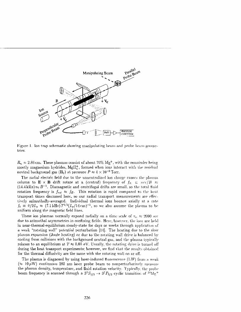
VA0®

Manipulating Beam

&&*■ «^V ^6^

Figure 1. Ion trap schematic showing manipulating beam and probe beam geometries.

Rw = 2.86 cm. These plasmas consist of about 70% Mg+, with the remainder being mostly magnesium hydrides, MgH+, formed when ions interact with the residual neutral background gas (H2) at pressure P K 4 x 10~9 Torr.

The radial electric field due to the unneutralized ion charge causes the plasma, column to E x B drift rotate at a (central) frequency of /E = nec/B ~ (14.4kHz)rnB~x. Diamagnetic and centrifugal drifts are small, so the total fluid rotation frequency is /ro< ~ /#. This rotation is rapid compared to the heat transport times discussed here, so our radial transport measurements are effectively azimuthally-averaged. Individual thermal ions bounce axially at a rate /;, = v/2Lp « (7.1kHz)T1/'2(Z/p/14cm)_1, so we also assume the plasma to be uniform along the magnetic field lines.

These ion plasmas normally expand radially on a time scale of rm ~ 2000 sec due to azimuthal asymmetries in confining fields. Here, however, the ions are held in near-thermal-equilibrium steady-state for days or weeks through application of a weak "rotating wall" potential perturbation [14]. The heating due to the slow plasma expansion (Joule heating) or due to the rotating wall drive is balanced by cooling from collisions with the background neutral gas, and the plasma typically relaxes to an equilibrium at T ~ 0.05 eV. Usually, the rotating drive is turned off during the heat transport experiments; however, we find that the results obtained for the thermal diffusivity are the same with the rotating wall on or off.

The plasma is diagnosed by using laser-induced fluorescence (LIF) from a weak (~ lO^W) continuous 280 nm laser probe beam to nonperturbatively measure the plasma density, temperature, and fluid rotation velocity. Typically, the probe beam frequency is scanned through a 32S\/2 ->• 32P3/2 cyclic transition of 24Mg+

226

-1.5 -1 -0.5 0 0.5

r [cm]

Figure 2. (a) Measured Mg+ density nMg, temperature T, and inferred total charge density n as a function of radius r. (b) Measured total fluid rotation vtot and calculated diamagnetic rotation velocity vaa.

at each radial position; from the measured ion distribution functions, f±(v±,,r,t) or /||(u||, r,t), we obtain the local magnesium density nus{r), temperatures T±(r,t) and T[\(r,t), and total fluid rotation velocity vtot(r). In the heat transport experiments, the rapid temperature evolution is generally obtained from just the velocity distribution peaks, that is, f\\(0,r,t) or fi.{vtoUr,t) , since the ion density is constant on the time scales of the measurements. As indicated in Fig. 1, the probe beam can be aligned parallel or perpendicular to the magnetic field, so that both T± and Tj| are measured; for the experiments presented here, however, we can approximate Tj_ ~ T|| = T to adequate accuracy. The total charge density n(r) is calculated as that required to give frot{r) - vtot{r)/2T:r. Typically, we find that "MgM/n(r) « 0.7 at all radii, so centrifugal mass separation [15] is negligible.

A typical equilibrium plasma is shown in Fig. 2. Here, we display UMS, T, and vtot measured as a function of radius for plasma that has been held in steady-state for 20 hours by a rotating wall drive [14]. Also shown is the total charge density n and diamagnetic velocity v<na calculated from the measured riMg(r), T(r), and vtot(r)- These steady-state plasmas are typically confined close to thermal equilibrium, i.e. n, T, and frot are relatively constant over the bulk of the plasma.

A temperature gradient is created in the plasma by locally heating or cooling with a strong (~ 1 mW) manipulating beam. This heating or cooling is obtained by detuning the parallel manipulating beam to the blue or red side of the cyclic

227

0.075

0.050 "> tu

- 0.025

0.000 -0.8

Figure 3. Measured thermal diffusion starting from locally (r = 0) cooled initial condition.

transition. The manipulating beam is aligned along the r = 0 axis of the plasma, thus creating an initial condition with a strong radial temperature gradient. The manipulating beam is chopped and the plasma temperature and density are measured using the probe beam during times when the manipulating beam is off.

RESULTS

Heat transport experiments are performed by creating steady-state plasmas with a strong temperature gradient, then blocking the manipulating beam and measuring the resulting temperature evolution. Figure 3 shows such an evolution. At t — 0, the cooling beam is turned off, and the central plasma temperature is observed to rise from T fa 3 x 10~3 eV at t = 0 toward the equilibrium temperature of T ~ .05 eV. For clarity, only t = 0, 0.1, and 1 sec and the approximate final equilibrium state t —>■ co are shown; actually, the temperature evolution is measured with 100 time steps over 0 < t < 4 sec for each radial position.

The temperature evolution of Fig. 3 results from a radial heat flux plus small external heating terms. The radial heat flux T, is obtained from the measured change in local energy density, q(r, t) = JU|rc(r) T(r, t)] as

Vq(r,t) = -- r r'dr'[q(r',t)-qcxt(r',t)} r Jo (6)

where the weak external heating or cooling term qext is known from independent measurements, as described below.

228

r-~i 4 , i | 1 »* 1 W - T = .01 -> .04 eV ■

M 1 - n - 5xl07 cm-3

O T y R \_ B = 4 T

o 3 . l\ y-K N o r = 0.1 x- > . X r = 0.15

o r = 0.2 °X/ t=0.1 sec ;

•* O 2 t=0.4 see V

y

"—' . x o

- C\2

1

/00 t=1.9 sec

-

U . 1 ^ , , , , 1 , , i

0.05 VT [eV/cm]

0.1

Figure 4. Measured normalized heat flux vs. temperature gradient for experiment shown in Fig. 3, demonstrating diffusive heat transport.

In Fig. 4, we plot the measured radial heat flux Tq as a function of the temperature gradient VT obtained from the data of Fig. 3. We plot the heat flux measured at radii r = 0.1, 0.15, and 0.2 cm, and at times t = 0.1 to 1.9 sec. These radii were chosen here because they have a strong gradient and a strong signal, i.e. q > qexi. It can be seen that the gradients and fluxes are largest at early times, and decrease as the temperature profile relaxes toward equilibrium. Since both classical and long-range transport predict Tq <x x^T <x T~1/2VT, the displayed Yq is divided by T~x>2 to better illustrate the proportionality with VT.

The error bars shown in Fig. 4 are estimates of the random error based on the level of scatter in the LIF signal; the error shown here is typical of all the data, points in Fig. 4. The dashed line in Fig. 4 is an unconstrained, error-weighted linear fit to the data; it can be seen that a straight-line fit is a reasonable description of the measurements. Also, from the intercept of the line, it can be seen that Y^D — 0 within the scatter in the data; thus Fig. 4 demonstrates diffusive heat conduction. In general, our measurements show no consistent signature of non-diffusive heat flux.

We calculate the local thermal diffusivity \ at any chosen radius and time as

X = - 5n VT ;7)

The diffusivity x depends on the local plasma density and temperature, as well as on the magnetic field. Values of x(n, S,T) were obtained for different equilibrium plasmas covering a range of 50 in density, 103 in temperature, and 4 in magnetic field. In Fig. 5, we plot the measured x as a function of temperature T. The

229

T [eV]

Figure 5. Measured cross-magnetic-field thermal diffusivity x plotted as a function of temperature T, demonstrating heat transport dominated by long-range collisions.

dashed curves in Fig. 5 show the predicted classical thermal diffusivities \£. for the 5 densities and magnetic fields used. The solid line shows the predicted long- range thermal diffusivity \L, which depends only on temperature. The data points of Fig. 5 labeled "small ST" correspond to plasmas which are slightly perturbed away from a known uniformly heated or cooled equilibrium plasma. These small perturbation measurements are taken at densities 0.5 < n- < 2.5 and magnetic fields 1 < B < 4 T.

The measured thermal diffusivities are up to 100 times larger than the classical prediction, and are independent of B and n. The T~ll2 scaling is observed over 3 decades in T, and extends into the low-temperature regime where rc m b. A fit to the data with x oc T~1/2 gives x = (1.93±1) x 10~3 cmV1 T~i!2 = (0M±Jj)>;\})

BACKGROUND HEATING TERMS

The small external heating correction, qexU used in Eq. (6) is obtained by measuring the temperature evolution of a plasma which has been uniformly heated or cooled by a wide manipulating beam. The measurements are qualitatively consistent with a model that includes the Joule heating expected from the slow radial plasma expansion, and the heating or cooling expected from ion-neutral collisions.

For the heat transport data presented here, the correction to \ due to the external heating terms is small, since qext/q ^ 0.1 in the regions with a large temperature gradient.

230

DISCUSSION

The cross-magnetic-field heat flux in a quiescent pure ion plasma is observed to be proportional to the thermal gradient VT, and dominated by long-range collisions with impact parameter up to a Debye length. These long-range collisions cause heat fluxes which are independent of magnetic field strength and plasma density: the observed thermal diffusivity scales as x oc n°B°T~lf2, whereas classical diffusivity is Xc oc nB~2T~1/2. At high magnetic field and low densities, the classical prediction is more than two orders of magnitude too small to explain the observed heat fluxes. This enhanced heat transport should occur in many nonneutral plasmas, where AD > rc is always satisfied, and may apply to the electron component of neutral plasmas which satisfy AD ~ 7rce.

Presumably, classical heat transport is also occuring in these systems; we do not observe this directly, however, since XL 3> Xc f°r most of our parameter range. Direct measurements of the equipartition rate i/j_\\ = \vu between perpendicular and parallel temperatures Tj. and Ty in these plasmas have been performed, however [16]; these measurements verify that short-range velocity-scattering collisions are occuring as expected, that is, we measure values of Vu in agreement with Eq. (1).

Wave-mediated heat transport is not believed to be significant here, since these plasmas are many, but not thousands, of Debye lengths across; the lowest- temperature data presented here (T~5x 10~4 eV), corresponds to plasmas about 100 Debye lengths across. Future experiments will attempt measure wave-mediated heat transport in these plasmas.

ACKNOWLEDGMENTS

The authors wish to thank Drs. T. M. O'Neil and D. H. E. Dubin for theory support and the late Mr. R. Bongard for outstanding technical assistance. This work is supported by the Office of Naval Research (ONR N00014-96-1-0239) and the National Science Foundation (NSF PHY-9876999).

REFERENCES

1. F. Wagner and U. Stroth, Plasma Phys. and Contr. Fusion 35, 1321 (1993). 2. S. M. Ichimaru, H. Iyetomi, and S. Tanaka, Phys. Rep. 149, 93 (1987);

B. D. G. Chadran and S. C. Cowley, Phys. Rev. Lett. 80, 3077 (1998). 3. M. Tuszewski, Phys. Plasmas 5, 1198 (1998). 4. A. T. Burke, J. E. Maggs, and G. J. Morales, Phys. Rev. Lett. 81, 3659 (1998);

D. D. Needleman and R. L. Stenzel, Phys. Rev. Lett. 58, 1426 (1987). 5. T. M. O'Neil and C. F. Driscoll, Phys. Fluids 22, 266 (1979). 6. D. Montgomery, G. Joyce, and L. Turner, Phys. Fluids 17, 2201 (1974). 7. M. N. Rosenbluth and A. N. Kaufmann, Phys. Rev. 109, 1 (1958). 8. D. H. Dubin, Phys. Plasmas 5, 1688 (1998).

231

9. D. H. E. Dubin and T. M. O'Neil, Phys. Rev. Lett. 78, 3868 (1997). 10. L. Brillouin, Phys. Rev. 67, 260 (1945); R. C. Davidson, Physics of Nonnriifrcil

Plasmas (Addison-Wesley, Redwood City, 1989) p. 42. 11. M. N. Rosenbluth and C. S. Liu, Phys. Fluids 19, 815 (1976). 12. E.M. Hollmann, F. Anderegg, and C.F. Driscoll, Phys. Rev. Lett. 82, 4839 (1999). 13. F. Anderegg, X. -P. Huang, E. Sarid, and C. F. Driscoll, Rev. Sei. lustrum. 68, 2367

(1997). 14. X. -P. Huang, F. Anderegg, E. M. Hollmann, C. F. Driscoll, and T. M. O'Neil, Phys.

Rev. Lett. 78, 875 (1997); F. Anderegg, E. M. Hollmann, and C. F. Driscoll, Phys. Rev. Lett. 81, 4875 (1998).

15. T. M. O'Neil, Phys. Plasmas 24, 1447 (1981). 16. F. Anderegg, X. -P. Huang, C. F. Driscoll, E. M. Hollmann, T. M. O'Neil, and

D. H. E. Dubin, Phys. Rev. Lett. 78, 2128 (1997); B. R. Beck, J. Fajans, and J. H. Malmberg, Phys. Rev. Lett. 68, 317 (1992).

232

2D Collisional Diffusion of Rods in a Magnetized Plasma Column

with Finite E x B Shear

Daniel H. E. Dubin and Dezhe Z. Jin

Physics Department, University of California San Diego, LaJolla, CA 92093-0319

Abstract. Cross-field collisional diffusion of test particles is discussed for a non-neutral plasma column in the 2D E x B regime, where the diffusion is due to the E x B drift of charged rods (bounced-averaged charges) in the random Coulomb fields of the other rods. If the overall flow has a finite E x B velocity shear the diffusion is found to be considerably smaller than previous calculations, which are shown to hold only for a nearly shear-free plasma. Preliminary simulations showing the effect of shear on the particle diffusion are in qualitative agreement with the theory .

INTRODUCTION

This paper considers cross-magnetic field diffusion of test particles in a non-neutral plasma confined in a Penning-Malmberg trap. The diffusion is evaluated for plasmas in the 2D E x B regime, where the axial bounce frequency of individual charges between the ends of the trap is large compared to both the collision frequency vc and the characteristic rate for cross-field dynamics. This characteristic rate is typically on the order of the shear rate r d(i)(r)/dr in the plasma's E x B rotation frequency (o(r). In this regime the axial dynamics can presumably be bounce-averaged, and the charges are then treated as 2D charged rods that E x B drift in the fields of the other rods.

Previous theory and experiments on test particle diffusion in non-neutral plasmas was carried out for plasmas that were not in the 2D E x B regime. For such 'floppy' plasmas axial dynamics is important and the diffusion coefficient D has the classical scaling, D ~ vc Yc, where rc is the cyclotron radius [1,2]. Note that this diffusion decreases with increasing magnetic field strength as MB .

Diffusion of 2D charged rods across a magnetic field has been considered previously by several authors. One reason for the early interest in this problem was that neutral plasma experiments often observed anomalously large diffusion coefficients with


233

Böhm scaling, D°^\l B, rather than the classical scaling D °= 1 / B2. The 2D model for cross-field diffusion was invoked as one possible explanation for this scaling, since one can easily show that 2D E x B drift dynamics implies that all time scales (including the diffusive timescale) increase linearly with magnetic field strength.

Taylor and McNamara [3] and Dawson and Okuda [4] considered collisional diffusion in a uniform homogeneous neutral plasma of charged rods as the simplest possible version of such 2D transport. Interestingly, the diffusion was thought to depend on whether the rods were distributed randomly or whether they were given time to equilibrate and Debye-shield one-another. For the case of random uncorrelated rod positions in a square box with periodic boundary conditions, the diffusion coefficient was calculated to be [3]

D™={\.9/TZ)mqcNmIB, (1)

where q is the charge per unit length on each rod, and TV is the number of rods. The result depends on the boundary conditions, since the diffusion is due to large scale 'Taylor vortices', which are E x B fluctuations with wavelengths on the order of the system size [4]. However, non-neutral plasmas in a Penning trap are not in periodic boundary conditions, and more importantly they often have large-scale equilibrium E x B shear flows. These flows might be expected to disrupt the Taylor vortices and thereby reduce the diffusion.

In this paper we show that the diffusion coefficient is in fact reduced when the plasma is sheared, and we also show that the level of shear required for Eq. (1) to be valid is quite small:

rdcoldr< a> I\[N. (2)

There has been considerable recent interest in the effect of large-scale E x B shear on the cross-field transport in neutral plasmas. Such plasmas are turbulent with fluctuation levels much larger than those considered here. Nevertheless, our results showing the reduction of collisional diffusion in the presence of shear might be thought of as the simplest possible paradigm for this phenomenon, just as the original shear-free case was put forward as a simplified model of homogeneous plasma turbulence.

2D E xB DIFFUSION OF RODS IN THE PRESENCE OF SHEAR

Consider a cylindrically-symmetric non-neutral plasma consisting of a collection of N+l identical charged rods of infinite length, with charge q per unit length, immersed in a uniform magnetic field. The plasma rotates due to the E x B drift of the rods, with a mean-field rotation frequency (a(r).

234

Consider a rod initially located at radial position r. The rod feels the fluctuating electric fields due to the other rods in the plasma and diffuses radially according to [5]

D = ]dt<Svr(t)Svr(0)>, (3) o

where the radial velocity fluctuation is given by the E x B drift as

8vr = c8Ee IB,

and the electric field is determined by the other m=l,2, ...,,/Vrods:

r dv m=I ;=_

Here, (j> / is the Greens function for the Coulomb potential, Fourier-transformed in the 8 coordinate.

The velocity correlation function is then evaluated using the standard method of integration along unperturbed orbits, in which each particle is assumed to merely rotate about the center of the plasma in the cylindrically-symmetric shear flow co( r):

rm(t) = ro= const, 0m W = 0O + ®W-

Then assuming that the initial conditions for the rods are uncorrelated the statistical average can be evaluated, yielding

ß=-(?TW0*J*2^-^ (4) ^ " ' o i.i r

where w20 is the 2D density of rods (in units of cm"2). The 60 integral implies that only / = -/ need be kept in the sum, and the time integral yields a 8 function:

D =^j Jr0dr0n^2n2L| ^{r,r0)I28[l((0(r)-0)(ro))].

The 8 function means that only resonant particles cause appreciable transport, since resonant particles interact for long times and take large drift steps. For a monotonic rotation frequency profile, the 8 function implies that r=r0 , and evaluation of the remaining r0 integral then yields

235

ßj \rd(0E/dr\ ,±L\1\

where we have assumed an unshielded Coulomb interaction between the rods and neglected image charges in the walls, so that <j>,(r,r) --Ml.

Note that Eq. (5) displays a logarithmic divergence at large wavenumbers, since close collisions between rods cause large E x B drifts. The divergence can be cut off by physical mechanisms that impose an effective maximum possible wavenumber in the sum, lmax. There are several possibilities: 1) Guiding center dynamics becomes invalid for length scales smaller than the cyclotron radius, implying lmca~r/rc. 2) Rods that are initially close to one another will orbit one-another rather than drift apart, provided that they are within a trapping distance of order -Jcq I (Brdoo I dr),

implying Zmax ~ ^J(Br3d(01 dr) I (cq) 3) In simulations of the diffusion to be presented later, the electric field is evaluated on a grid keeping wavenumbers only up to /max roughly of order 500 r/rwan.

To logarithmic accuracy the diffusion coefficient is then

D = 47t2(^-) "" n ln(/max). (6) KBJ \rdcoldr\ max

Note that as the shear rate increases, the diffusion coefficient decreases, as one would expect intuitively. However, Eq. (6) clearly breaks down when the shear is so small that the diffusion given by Eq. (6) is larger than the Taylor-McNamara result for a shear free plasma, Eq (1). Comparing Eq. (1) to Eq. (6), D™ < D when

VL9 BN]n VT9 Vnm'N,/2Qr,

which is equivalent to Eq. (2) aside from a numerical factor. When this inequality is satisfied, the plasma is effectively shear-free and the Taylor-McNamara result applies. However, for large TV the shear rate must be extremely small in order to satisfy this inequality. This can be easily understood: the shear in the equilibrium flow must be smaller than the shears created by fluctuations in order for the Taylor-McNamara result to apply, and the shears created by fluctuations arising from discreteness are of order a/N1'2.

236

SIMULATIONS

We have carried out particle in cell simulations of the diffusion of rods in a sheared non-neutral plasma column. In this preliminary work, N rods were placed randomly so as to produce an overall mean density profile of form

n2D(r) = Ar-^a+l> , 0.05 rwaIl < r < 0.4 rmiU. (7)

This profile was chosen so that

rdcol dr = const =

Ba 4nqc

(8)

The parameter a characterizes the amount of shear in the plasma: as a increases the shear decreases.

Simulations were performed on a 512 by 512 square grid, for JV varying from 5000 to 100,000 rods, and values of a varying from 0.1 to 100. In order to measure the diffusion coefficient, rods in the range 0.2 < r /rwaii < 0.3 were followed, and their change in radial position, Sr(t) = r(t) - r(0), was evaluated. Here t = 0 corresponds to an arbitary initial time, taken to be approximately one rotation period after the simulation was begun. An average over the rods was then carried out to obtain < Sr(t)2 >, the mean square change in radial position of the rods.

0.01 N= =100,000, oc=5 v^*

yj^

A-, ^ 0.005

n

y^2Dt

10 15 20 t in units of (B r^, /cQ)

FIGURE 1. Mean square change in position of rods in a non-neutral plasma simulation, measured in terms of rwa!i. The number of rods is N= 100,000 and the shear parameter is a=5.

237

For diffusive motion, this function should increase with time like 2Dt. A plot of <ör(tf >is shown in Fig. 1. As expected, after an autocorrelation time the mean square change in position does increase roughly linearly with time. It begins to saturate at late times because the rods start to explore the entire plasma (which has radius 0.4 rwan). The slope of the straight line portion of the curve is taken to be 2D.

In Fig. 2, the result for D is displayed from 4 simulations with a=l. Here D is meas-

ured in units of c Q/B where Q is the total charge per unit length in the plasma. In these units, Eq.'s (1) and (6) can be written as

~ cc. cQ D = 7f—ln(/ )—,

N B (9a)

D™= \i-9cQ (9b)

The N dependence of the 2 theories differs. Fig (2) displays Eq.s (9a) and (9b) as dashed and solid lines respectively. In Eq. (9a) have taken ln(/max) = 2.7, which gives the best fit to the data and is a not-unreasonable value given the 0(7) uncertainties inherent in the logarithmic approximation used to derive Eq. (9a) and in the precise value of /raax to be used in the theory. The scaling with N of the simulation results agrees well with Eq. (9a) and disagrees with Eq. (9b), showing that the diffusion is sharply reduced by the presence of shear, in agreement with our calculation.

€9 a o

o

c

C

lfj

10-

10 -4

a = l

~ ~__D™ -

: ^^JEg(9a)

>^

i

(

104 N 105

FIGURE 2. Measured diffusion coefficient (dots) versus number of rods in the simulation, for shear parameter a = 1. Also shown as the solid line is the Taylor-McNamara theory, Eq. (9b). Our theory with shear, Eq. (9a), is shown as the dashed line, taking In (/max) = 2.7.

238

In Fig. 3 we vary the shear parameter a for 2 values of N. Since the diffusion rate ap-

pears to depend inversely on N for Q fixed and a ~1, we plot N D to remove the N dependence. As expected from our calculation, the diffusion increases as the shear decreases until the Taylor-McNamara level is approached. Note that one would not necessarily expect the exact Taylor McNamara result in the limit of no shear (i.e. a -> °°), since Eq. (9b) was derived for periodic boundary conditions and the simulation was carried out for a cylindrical plasma. This may explain the discrepancy between Eq. (9b) and the simulation results in the small shear regime.

102

101

10°c

s s

4 s

69 o o

o CO

+->

c C

Q

DTMX

Eq. (9ak s ° < S 0

so

/

/ OS s

s

s s -

S o o

, oo o . o

•

• N=50000

o N=100,000 ,

0.1 10 100 a

FIGURE 3. As shear decreases (i.e. as a increases), the diffusion increases in agreement with Eq. (9a) (the dashed line), until the shear becomes small. Again we take ln(/max) = 2.7. The Taylor-McNamara theory (Eq. (9b)) for the 2 values of N shown is displayed as the solid lines.

CONCLUSIONS

We have evaluated the test particle diffusion coefficient for a collection of charged rods undergoing E x B drift dynamics in a cylindrically-symmetric shear flow. The theoretical calculation was compared to particle-in-cell simulations of the diffusion, showing reasonably good agreement with our theory . The diffusion was found to be greatly reduced by the presence of shear in the equilibrium plasma when compared to the Taylor-McNamara/Dawson-Okuda theory [3,4], which was shown to hold only for a nearly shear free plasma.

239

The theory should apply to a non-neutral plasma column confined in the 2D E xB regime, for which the bounce frequency is sufficiently large that the plasma particles can be bounce-averaged and treated as rods. Thus, the diffusion may be measured experimentally in the future, perhaps using the laser-tagging techniques employed in previous experiments [1] on pure ion plasmas.

The theory may also be thought of as a simplified model for the effect of shear on cross-field diffusion in a turbulent neutral plasma. As such, it may provide some useful intuition for the study anomalous transport in the presence of large E x B shear.

ACKNOWLEDGMENTS

This work is supported by the Office of Naval Research, Grant No. N00014-96-1- 0239, and the National Science Foundation, Grant No. PHY-9876999. The authors thank Prof. C. F. Driscoll for suggesting improvements to the manuscript.

REFERENCES

1. Anderegg, F., Huang, X.-P., Driscoll, C. F., Hollman, E. M., O'Neil, T.M. and Dubin, D. H. E., Phys. Rev. Lett. 78, 2128 (1997).

2. Dubin, D. H. E., Phys. Rev. Lett. 79, 2678 (1997). 3. Taylor, J. B. and McNamara, B., Phys Fluids 14, 1492 (1971). 4. Okuda, H. and Dawson, J. M, Phys. Fluids 16,408 (1973); Dawson. J. M., Okuda. H. and Carlile.

R. N., Phys. Rev. Lett. 27,491 (1971). 5. Reif, F., Fundamentals of Statistical and Thermal Physics, New York: McGraw-Hill. 1965, p 576.

240

Experimental Test of the Resonant Particle Theory of Asymmetry-Induced

Transport

D.L. Eggleston

Occidental College, Physics Department, Los Angeles, CA 90041

Abstract. While it is easy to experimentally demonstrate that applied field asymmetries produce radial transport, convincing comparisons of experiment and theory have yet to be made. A key prediction of the theory is that the transport will be dominated by particles that move in resonance with the asymmetry. For the general case of a time-varying asymmetry, the resonance condition is CJ — IL>R — kv = 0, where v is the axial velocity, UR is the E x B rotation frequency, and ui, I and k are the asymmetry frequency, azimuthal and axial wavenumbers, respectively. We present experiments on our low density trap in which w, WR, and k are varied and the resulting radial particle flux is measured. The experiments show a resonance in the flux similar to that predicted by theory. The peak frequency of this resonance increases with UR and k, but not in the way theory predicts. The peak magnitude of the measured transport is roughly forty times smaller than the theoretical prediction, and low-frequency asymmetries are especially ineffective at producing transport.

INTRODUCTION

Plasma traps of the Malmberg-Penning type have been found to be useful in a variety of fields including basic plasma physics, atomic spectroscopy, anti-matter physics, and mass spectroscopy. Early studies of the confinement time of such traps found good agreement between experiments [1] and a transport theory [2] based on collisions with neutrals. However, at the lowest neutral pressures the confinement time was much lower than expected [3] and decreased with machine length [4]. It was suggested that this anomalous transport was due to the presence of electric or magnetic fields that break the cylindrical symmetry of the trap. The presence of such asymmetries would produce a radial component to the E x B drift that would lead to particle loss. This notion was later supported by further confinement studies [5] as well as experiments with applied asymmetries [6-8].

These early papers also suggested that the asymmetry-induced transport might be described by a theoretical model developed in early studies of radial transport in tandem mirrors [9-13] where static asymmetric end cells produced radial grad-


241

B drifts that, largely determined the radial particle flux. A key prediction of the theory is that the resulting transport will be dominated by particles whose axial bounce motion and azimuthal drift motion causes them to move in resonance with the asymmetry. As these resonant particles repeatedly encounter the asymmetry they take radial steps in the same direction, thus allowing them to diffuse more quickly than non-resonant particles.

We have recently adapted this theory to Malmberg-Penning traps [14] and in this paper present our first attempts to test the theory using an experimental device specifically designed for the task. While the experiments provide evidence for the dominance of resonant particles they also contradict other predictions of the theory.

ASYMMETRY-INDUCED TRANSPORT THEORY

The geometry of the non-neutral experiments is cylindrical with an axial magnetic field B. The magnetic field is typically strong enough that the Larmor radius is much smaller than any other scale length in the plasma and all relevant frequencies are small compared to the cyclotron frequency. Asymmetric electric fields are applied by placing voltages on wall sectors. Under these conditions the basic equations for a non-neutral plasma are Poisson's equation, the drift kinetic equation with a collision operator, and the boundary conditions on the conducting walls. For simplicity we take as our model a plasma of length L with flat ends, thus ignoring end effects. This allows us to linearize the potential as <f>(r, 6, z, t) = (j>o(r) + <j>\{r, 6, z, t) where

0! (r, 0, z,t)=J2 4>mM ■ exp {if^-z + W- wt) J (1)

and similarly for the distribution function /. For an electron plasma (q — —e) Poisson's equation then becomes

ld_ d__l_ r dr dr r2

cl dfo nir e dfo

T) ^(r) -**ji.'»;+J->^) (2)

where UR is the azimuthal E x B rotation frequency of the plasma column, </>niw(r) is the Fourier amplitude of the asymmetry mode characterized by axial mode n, azimuthal mode I, and frequency w, and the integral is over the axial velocity v.

The form of the resulting radial particle flux depends on the relative size of an effective collision frequency vejf and the oscillation frequency uT of particles

trapped in the asymmetry potential, where v^ff « vee \*jf) and

2 Je /nn\2 cl dwn UT = \m\LJ ~7B~dT

4>nlw (3)

242

When veff » UJT, frequent collisions interrupt the trapped particle orbits and the basic radial step is the radial drift velocity times the time between collisions. Deviations from unperturbed orbits are small and a perturbation approach is appropriate. This is called the resonant plateau regime. When vejf <CüT, a trapped particle can complete at least one oscillation before a collision knocks it out of resonance. Now the basic radial step is the radial extent of the drift during a trapping oscillation and the orbits are fully nonlinear. A heuristic derivation of the resulting radial flux is often employed for this so-called banana regime. The resulting radial particle flux for the plateau regime is given by (See reference [14] for details)

-plateau- Z^/^2 1 n.Liv \\FMV

1

cl<f)nluJ

rB

2 r 1 dnn r-nKTWc J- + V2—-^a; no dr L Iv

(4)

and for the banana regime by

■ banana- E n.l.uf

n0 \717T /

,_\2

(£) W 1/2

2TT [\ - (lLY 1 du'R\ I \7i7r / rule dr j

1 dno f-mrrojc no dr L Iv (5)

For simplicity we have assumed here that the temperature T is constant with radius. The variable x is equal to vres/\/2v, where vTes = ^(u — IWR) is the resonant velocity for the asymmetry mode n,l,uj. The symbols v, u>c, and i/ee are the thermal velocity, the cyclotron frequency, and the electron-electron collision frequency, repectively.

It is worth noting several features of these solutions. Both plateau and banana regime fluxes involve a sum over all the asymmetry modes produced by the wall voltages. The square brackets contain a diffusive term ^^ and a generalized

mobility \p2?fr-^x (note that this latter term reduces to eE/kT for u = 0). The plateau regime flux is independent of the collision frequency and is proportional to the square of the asymmetry amplitude, whereas the banana regime flux depends linearly on vee and scales like $)•£. The dominance of the flux by resonant particles is reflected in the e~x2 factor which stems from evaluating the Maxwellian distribution function at the resonant velocity. Note that x can be positive or negative as CJ is greater than or less than WR. Thus, while static field asymmetries (u> = 0,x < 0) move electrons radially outward (r > 0), an appropriately chosen asymmetry (u > UJR, X > 0) can move particles radially inward as is observed in "rotating wall" experiments [6,8]. Here we use the convention that u > 0 corresponds to an asymmetry that rotates with the plasma column and w < 0 to one that rotates against the column.

The presence of a; in the variable x provides the experimentalist with an ideal way of testing the notion that resonant particles dominate the transport. By varying u> one can obtain any value of the resonant velocity vres and the resulting flux should exhibit a resonance as vres sweeps through the distribution function. However this

243

Eir=0)

io3

io*

10'

10°

IO"'

Efl(r=R) 10-2

10"3

IO"4

IO-5

IO"6

IO"7

T ■ I 1 | . 1 1 1 |—i—r t I-, r—■ ,..,-,111

. ,0.25 eV

- /v\ A A /io eV

:

^^\~L_L/^^^ 5.0 eV

- \ / n = IO7 cm-3

B = 300 G

6)R = 3 MHz

- k = je/75cm \ /

- 1= 1 V

-15 -10 10 15

Asymmetry Angular Frequency a (MHz)

FIGURE 1. Computed variations of the normalized Ee at the plama center versus asymmetry

frequency w. The three curves correspond to three plasma temperatures. The strong variations in

Eg are produced by plasma collective effects and make it difficult to observe the resonant particle

dominance of the radial transport.

approach is complicated by the strong w-dependence of the asymmetry potential 4>niu- Figure 1 shows numerical solutions of Equation (2) for typical plasma parameters [14]. We plot Eg = lcj)niu/r at the center of the plasma (normalized to its value at the wall) as a function of asymmetry frequency u. Note that Eg varies by many orders of magnitude as adjustments of to produce plasma phenomena ranging from standing waves (the peaks of the curves) to Debye shielding (the strong dip around ui = U>R) . These variations in Eg (and thus in the flux T) tend to dominate or mask those produced by resonant particle effects. This produces, for example, enhanced transport when the asymmetry is at a standing wave frequency of the plasma column [6]. Nonlinear collective processes are also possible [15]. These collective effects, although interesting, are not, in our view, essential to the transport physics. We note, then, that the variations in Eg are reduced as the temperature is increased and/or the density is reduced (see reference [14]).

These considerations led us to the modified trap design shown in Figure 2. The plasma is replaced by a biased wire running along the axis of the trap. Electrons injected into this device have the same dynamical motions as those in a normal nonneutral plasma (i.e. axial bounce and azimuthal drift motions), but the collective variations of 0n;w are eliminated since the lower density (105 cm~3) and higher temperature (4 eV) of the electrons give a Debye length larger than the trap radius. Despite these changes, the confinement time scaling with no applied asymmetries

244

Center Wire 40 Sectors for Applying Asymmetries

Phosphor Screen 7

Electron Gun x Injection Gote

<r 76.8 cm

Dump Gate

->

/

FIGURE 2. Schematic of the Occidental Trap. The plasma is replaced by a biased wire that maintains the basic dynamical motions of the injected electrons. Forty wall sectors allow for the application of asymmetries consisting of essentially one Fourier mode.

[16] shows the same {L/B)2 dependence found in higher density experiments [4], thus supporting the notion that the transport is a single particle effect.

For the current experiments, up to forty wall sectors are employed to produce an asymmetry consisting of a single Fourier mode, thus eliminating the sum over n, I, and w in the flux and making for a simpler comparison between theory and experiment. Electrons injected into the trap are quickly dispersed into an annular distribution [17]. At the end of an experimental cycle the electrons are dumped onto a phosphor screen and the resulting image is digitized. A radial cut through this image gives the density profile of the electrons. Profiles are taken both with the asymmetry on and off, and the change in density 6n(r) is either used directly to approximate dn/dt or integrated to give the radial particle flux T(r).

EXPERIMENTAL RESULTS

Our initial data addresses three aspects of the theory: 1) the scaling of transport with asymmetry amplitude, 2) the dominance of the transport by resonant particles and 3) the absolute magnitude of the transport flux. Figure 3 shows the scaling of dn/dt with the amplitude of the asymmetric potential applied to the wall. The scaling is consistent with plateau regime theory (i.e. <f>2) when the amplitude is small and falls off to roughly 04/3 at higher amplitudes. The banana regime scaling of <j)1/2 is not observed.

Figure 4 shows the radial flux vs. asymmetry frequency at three radial positions. The radial density profile is shown in the inset. The data is qualitatively consistent with resonant particle theory. When the density gradient is large, the flux should go like e~*2, a Gaussian curve centered where w =WR. This behavior is shown by the curves for r/R equal to 0.28 and 0.56 (note that u)R is set by the center wire bias and decreases with radius). At the top of the density profile the gradient is zero, so we expect an xe~x behavior, and this seems to match the r/R = 0.39 curve. Although not shown, we have verified that the curves shift horizontally in an appropriate way as the center wire bias (and thus UJR) is varied. Also, if the asymmetry is made to spin opposite the direction of LOR (corresponding to negative

245

1(T

dn/dt oc +u

r = 0.5 cm

10"* 10"' 10° 10'

Applied Perturbation Amplitude at Wall $ (V)

FIGURE 3. Log-log plot of the asymmetry-induced rate of density change dn/dt versus the asymmetry amplitude at the wall. The scaling is consistent with plateau-regime theory only for low amplitudes.

values of LJ), no resonances are observed in the flux. Figure 5 shows how the peak frequency of these flux resonances varies with

radius and axial mode number n, and it is here that, we get our first indication of discrepancy between theory and experiment. As noted above, the experimental peak frequency decreases with radius as expected (open symbols), but the decrease does not match that predicted by theory (filled symbols). Theory also predicts an increase of peak frequency with axial mode number n. We observe an increase, but it is not in accord with the theory.

We have also compared the amplitude of the experimentally measured flux resonances with the prediction of plateau regime theory. The result is shown in Figure 6. Although the curves are similar, several discrepancies are clear. As noted above the peaks (in this case the minima) of the resonances occur at slightly different frequencies. More importantly, the value of the experimental flux at, the peak is roughly forty times smaller than the theoretical prediction. Lastly, although the theoretical curve passes smoothly through u> = 0 with a significant positive flux, the experimental curve shows anomalously low transport near u = 0.

CONCLUSION

We have begun to test the resonant particle theory of asymmetry-induced transport under very simple conditions. Our initial results support the idea that reso-

246

1500

1000

500

-500

-1000 0.0 0.5 1.0 1.5

Asymmetry Frequency f (MHz)

FIGURE 4. Radial particle flux at three radii as a function of asymmetry frequency for center

wire bias (j>cw = -110V. The shape of the flux curves is qualitatively consistent with that expected

from theory.

3.0E+6 T 1 1-

Rotation Freq. fR

0 Exper. for n = 1

—#— Theory for n = 1

-B— Exper. for n = 3 —■— Theory for n = 3

0.0E00 0.0 0.2 0.4 0.6

Radius r (in.)

FIGURE 5. Variation of the flux resonance peak frequency with radius and axial mode number

n. The open symbols give the experimental values and the corresponding closed symbols give the

theory. For reference, the solid line gives the E x B rotation frequency fR.

247

3 cö

500

0

•S -500 - .2 •3

-1000

2E+4

-i 1—i—r- -i 1—i—|—i—i—i 1—|—i 1—r-

Experiment

-i i i i i i i i i i i i i i i _1 I I L-

^t*^1 ' ' 'The»;/ -l 1 1 r-

«3

Z3

• total

O mobility

A diffusion

E*- _

eö

cd OS

-3E+4 0.0 0.5 1.0 1.5 2.0

Asymmetry Frequency f (MHz)

FIGURE 6. Absolute comparison between experimental flux and the prediction of plateau regime theory for center wire bias </>cu, = -110 V and r/R = 0.28. The experimental flux is roughly forty times smaller than the theory predicts. The open symbols on the theory plot show the contributions of the diffusive and mobility-like terms in equation (4).

248

nant particles dominate the transport and we observe an amplitude scaling consistent with plateau regime theory. However, several discrepancies between theory and experiment are observed and it already seems clear that current theory does not give a complete description of this transport.

ACKNOWLEDGEMENTS

This work was supported by U.S. Department of Energy grant DE-FG03- 98ER54457.

REFERENCES

1. J. S. DeGrassie and J. H. Malmberg, Phys. Fluids 23, 63 (1980). 2. M. H. Douglas and T. M. O'Neil, Phys. Fluids 21, 920 (1978). 3. J. H. Malmberg and C. F. Driscoll, Phys. Rev. Lett. 44, 654 (1980). 4. C. F. Driscoll and J. H. Malmberg, Phys. Rev. Lett. 50, 167 (1983). 5. C. F. Driscoll, K. S. Fine, and J. H. Malmberg, Phys. Fluids 29, 2015 (1986). 6. D. L. Eggleston, T. M. O'Neil, and J. H. Malmberg, Phys. Rev. Lett. 53, 982 (1984). 7. J. Notte and J. Fajans, Phys. Plasmas 1, 1123 (1994). 8. X.-P. Huang et al, Phys. Rev. Lett. 78, 875 (1997). 9. D. Ryutov and G. Stupakov, JETP Lett. 26, 174 (1978).

10. D. Ryutov and G. Stupakov, Sov. J. Plasma Phys. 4, 278 (1978). 11. D. Ryutov and G. Stupakov, Sov. Phys. Dokl. 23, 412 (1978). 12. R. Cohen, Comments Plasma Phys. Cont. Fusion 4, 157 (1979). 13. R. Cohen, Nuclear Fusion 19, 1579 (1979). 14. D. L. Eggleston and T. M. O'Neil, Phys. Plasmas 6, 2699 (1999). 15. D. L. Eggleston and J. H. Malmberg, Phys. Rev. Lett. 59, 1675 (1987). 16. D. L. Eggleston, Phys. Plasmas 4, 1196 (1997). 17. D. L. Eggleston, Phys. Plasmas 1, 3850 (1994).

249

Quadrupole Induced Resonant Particle Transport in a Pure Electron Plasma

E. Gilson1 and J. Fajans2


Abstract. We have performed experiments that explore the effects of a magnetic quadrupole field on a pure electron plasma confined in a Malmbcrg-Penning trap. We have developed a model which describes the shape of the plasma and shows that a certain class of resonant electrons follows trajectories that take them out of the plasma. Even though the quadrupole field destroys the cylindrical symmetry of the system, the theory predicts that if the electrons are off resonance, the lifetime of the plasma is not greatly affected by the quadrupole field, but near resonance the lifetime diminishes sharply. Preliminary experimental results show that the shape of the plasma and the plasma lifetime agree with the model. We are investigating the lifetime scaling with various experimental parameters such as the plasma length, density, and strength of the quadrupole field. This resonant particle transport may be detrimental to experiments which plan to use magnetic: quadrupole neutral atom traps to confine anti-hydrogen created in double-well positron/anti-proton Malmberg-Peiming traps.3

Resonant particle transport has long been suspected as the primary cause of plasma loss in Malmberg-Pcnning traps, but there is no conclusive experimental evidence to support this claim [1-5]. We have found experimental evidence for resonant particle transport when we apply a quadrupole magnetic field to our system. We have also measured the equilibrium shape of plasmas when a magnetic quadrupole perturbation is present. The results of this research apply directly to anti-hydrogen creation experiments proposed by the ATHENA and ATRAP collaborations. Malmberg-Penning traps will be used to confine positrons and antiprotons, which should recombine into anti-hydrogen. Quadrupole fields will be used to confine the neutral anti-hydrogen.

With an axially invariant transverse magnetic quadrupole field, the total magnetic field becomes

3 = B0z + ßq(xx-yy), (1)

*' [email protected] 2) [email protected] 3> ATHENA and ATRAP Collaborations.


250

where B0z is the standard axial field. The self electric fields of the plasma cause it

5^—3 A ^^^~-~*

l^r* ^f } ?

FIGURE 1. Adding a small transverse quadrupole perturbation to a constant axial field pro-

duces the field lines shown in this figure.

to E x B drift around the trap axis. When this rotation is slow compared to the time it takes an electron to bounce back and forth across the length of the plasma, the electrons follow the magnetic field lines shown in Fig. 1. The plasma has a circular cross section in the middle and has elliptical cross sections at both ends. The ellipses are rotated 90° from one another. When the rotation is fast compared to the bounce time, the plasma smears out into a cylinder.

FIGURE 2. The equilibrium shape of a slowly rotating plasma. The lines with arrows (to be discussed later) show the trajectory followed by an outward moving resonant electron.

We measure the ellipticity e and orientation 6 of the plasma either by imaging the plasma or by measuring the image charge induced on the trap walls. When the plasma is rotating slowly, the quadrupole moment, as expected, is zero in the center of the plasma, has equal and opposite values at the ends of the plasma, and is proportional to ßq. When we image quickly and slowly rotating plasmas, we see the expected circular and elliptical shapes.

Theoretically, e - 1 should scale with ßq/B0, and is in rough agreement with the data shown in Fig. 5. We do not understand the step in the data at B0 ~ 400 G. The variation in angle is reminiscent of the drive/response phase shift of a damped driven simple harmonic oscillator as it passes through resonance.

If the rotation rate is such that an electron makes a quarter revolution each time it travels the length of the plasma, the electron can move ever outwards or inwards (see the lines with arrows in Fig. 2). For a constant density plasma, the resonance condition is,

B0=^. (2) ne0vz

Resonant and near-resonant electrons traveling outwards can leave the plasma very quickly. Diffusion due to this mechanism can be large. There are higher order

251

4(G/cm) FIGURE 3. Measurements of quadrupole moment along the plasma's length show the axial dependence and ßq proportionality that we expect.

(a) FIGURE 4. ßg/B0 = 0.004 cm-1, (a) B0 = 32.43 G so the plasma is rotating quickly. We measure e = 1.09 and 0 — 53.5°. (b) B0 = 500 G so the plasma is rotating slowly. We measure e = 1.26 and 0 = -37.5°.

resonances in which the electron makes N/A (N odd) revolutions as it travels across the plasma, but these are less important.

Above resonance, when the plasma is rotating slowly, the resonant velocity lies well within the electron distribution function f(v). There are many resonant electrons and the quadrupole field has a strong effect. Well below resonance, when the plasma is rotating quickly, the resonant velocity falls in the tail of f(v). Conse- quently, there are few resonant electrons and the quadrupole field has little effect.

This resonance effect can be seen in Fig. 6. Below resonance [Fig. 6 (a)], the application of the quadrupole field has no effect on the evolution of the central density as a function of time until the plasma expands enough so that the resonance condition is met. The plasma in Fig. 6 (b) begins above resonance so the quadrupole field has an immediate effect on the central density.

From a series of images taken at successive times, we measure the diffusion coefficient, D. The plasma images measure the z-averaged radial density profile 77,(7", t), from which we compute N(r, t) = /J" n(r', t)2itr' dr'.

We write the diffusion equation in polar coordinates, integrate once with respect to T and rearrange to yield

D(R) = dN/dt

2-KR dn/dr r=fi (3)

252

E-l 1 O fi/H,, - 0.001 cm"'

w fl/B„=0.0013cm'

Q a P/H.,- 0002 an'' c 0 ^»„=0.004 cm'

Cl) A ft<®„*= 0.006 cm'

B„(G) FIGURE 5. The scaled ellipticity and angle of the plasma as functions of B0 as measured from images such as those shown in Fig. 4.

2500

2000

1500

S 1000

500 U

1 I 1

X _ «=20G /* -0.0806/; lern

"V , «=40O Ä =0G

" H The plasma is - .^- ß=4()G«<"0.16Gffi;lcm-

M passing through v» T\ resonance. y^\

TJ / \\ - v/ \ \^ v*%^. \ ^^_^

- > • (bl V—T—^ T , i i i i i

0 10 12 3

Time (ms) FIGURE 6. By comparing the time evolution of the central density with the quadrupole field on and off, we can separate the effects of the quadrupole field from other plasma loss mechanisms.

All 9 variations have been neglected because the quadrupole field used in the diffusion experiments is typically small.

In Fig. 7 (a,b), we keep ßq/B0 fixed, as would be the case if the quadrupole field were due to imperfections in the main magnet coils. When ßq ^ 0, D is the sum of the diffusion due to both the quadrupole field and background processes. Below resonance, the quadrupole field has little effect, but above resonance it enhances diffusion. In Fig. 7 (c,d), we hold ßq fixed. For large B0, the diffusion due to the quadrupole field becomes small and background processes dominate the diffusion. The anomalous structure in the background (Dßq=0) data needs to be understood before further study can be completed.

By measuring the relative lifetimes using three different plasma lengths, we see that the location of the resonance moves in agreement with the change in the resonance condition. To find the plasma's lifetime, we measure the time it takes for the central density to drop to ~ 70% of its initial value. We do this both with the quadrupole field on and off, then compute the relative lifetime.

We model the results of our experiments by constructing a diffusion coefficient, D — AV/, where A is the average step size of a resonant electron, v is the fre-

253

: I I 1 I 1 I 1 III

■ o.

1 1 :

(c) : 10

1

- 8 O ■ : o ■

o ° o o ■

0 . 1 °

_

t ■ ß9 = 0.1Gcm 0 e ■

0.1 r O ß = 0 G cm ,,e^

100 Bo(G)

1000

^ 107

! I I I I I I | I III I I I I ||

in : o y " E 1 m -X.-'- 1

CJ

^ 10s

EQ • m y : C5 10« ^M Smm 1

1W * 1000 1000

Bo(G)

FIGURE 7. (a) D for ßq/B0 = 0,0.002 cur1. (1>) D due only to the quadrupole field. Above

B0 ~ 200 G, D scales roughly like B20. (c) D for ftq = 0,0.1 G cm-1, (d) Near resonance, D

due to the quadrupole field is enhanced. In (1>) and (d), the solid curve is D(n,kT,B0) from the

theory using the measured densities at each point and assuming kT — 1.5 eV.

quency of collisions that knock an electron oiit of resonance, and / is the fraction of electrons that satisfy the resonance condition. We must sum over the higher order resonances to obtain an expression for D. The result is D = Y,N Odd Av, where, for a constant density plasma,

?2„2Ö2

DN = m, '.(il

2wkT\BJ Ar5R2

L3

exp "th

(4)

This formula, suitably generalized for arbitrary n(r), is \ised in Fig. 7 (b,d). Clear evidence for resonant particle transport as the mechanism for plasma loss in

Malmberg-Penning traps has been lacking. When applying a magnetic quadrupole perturbation, we observe resonant behavior that could help to explain plasma loss in Malmberg-Penning traps. If operating in suitable parameter regime, experiments planned by the ATHENA and ATRAP collaborations may be able to use both Malmberg-Penning traps and quadrupole traps. For example, if ATRAP operates with B0 = 2 T, n = 108 cm"3, L = 1 cm, and T = 4 K [6], they will be near the resonant axial field of 0.7 T and plasma loss due to the quadrupole field may be too great to tolerate.

254

1.0 *——i___-'' ^^^ L —n

0.5 V L=26cm -

E 0.0 T, 10 .A

•• i, 0.5 • . • • L=l 0.5cm . >

3s o.o ——▼-

■ W L=5.4cm

0.5

no 10 100 1000

B(G) FIGURE 8. Graphs of the relative lifetime versus magnetic field show that when the resonance condition is met, particle loss is enhanced. The resonance location is length dependent.

ACKNOWLEDGMENTS

This work was supported by the Office of Naval Research and Los Alamos Na- tional Laboratory.

REFERENCES

1. D. L. Eggleston, T. M. O'Neil, and J. H. Malmberg, Phys. Rev. Lett. 53, 982 (1984). 2. D. L. Eggleston and J. H. Malmberg, Phys. Rev. Lett. 59, 1675 (1987). 3. D. L. Eggleston, Phys. Plasmas 4, 1196 (1997). 4. D. L. Eggleston, Bull. Am. Phys. Soc. 43, 1805 (1998). 5. J. M. Kriesel, Ph.D. thesis, University of California, San Diego, 1999. 6. G. Gabrielse, (private communication, 1999).

255

Two Experimental Regimes of Asymmetry-Induced Transport

Jason M. Kriesel and C. Fred Driscoll

Physics Dept, University of California, San Diego CA 92093-0319

Abstract. In a cylindrical trap, azimuthally asymmetric electric or magnetic fields (such as inherent trap asymmetries) cause the cross-magnetic-field transport of particles, leading to bulk radial expansion and eventually to particle loss at the trap walls. Experiments with applied electrostatic asymmetries identify two different transport regimes, "slightly-rigid" and "highly-rigid". Here the plasma rigidity, U = Tblfs, is the ratio of the axial bounce frequency to the azimuthal E x B rotation frequency. In the slightly-rigid regime (1 < H < 10), the transport scales as Va 1Z~2, where Va is the applied asymmetry strength. This TV2 ex L2 /B2 scaling has previously been observed for transport due to inherent trap asymmetries. The "Va TIT2" mechanism appears to "turn-off' as the rigidity is increased into the range 11 > 10. In the highly-rigid regime (TZ > 20), the transport scales as V211°.

INTRODUCTION

Non-neutral plasmas are readily confined in simple cylindrical traps for relatively long periods of time, allowing for many of the experimental studies described in these proceedings. Typically, confinement is limited by inherent trap asymmetries which cause particles to move radially and be lost at the trap walls. Despite more than 20 years of study, this asymmetry-induced transport is not well understood.

In this paper, we present a brief summary of recent measurements of asymmetry- induced transport in electron plasma columns [1]. We purposely break the azimuthal symmetry by applying static voltages of strength Va to sections of the trap wall (as shown in Figure 1), and measure the induced change in the plasma density profile. We find that the induced transport rates are well characterized by the "rigidity" Tl = //,//£, which is the ratio of the thermal axial bounce frequency to the azimuthal E x B drift frequency. Two different transport regimes are identified: "slightly-rigid" (1< K < 10) and "highly-rigid" (11 > 20).

In the slightly-rigid regime, the expansion rate increases linearly with the applied asymmetry strength, Va, and decreases with rigidity as TV2. The mechanism responsible for this so-called "V* Tl~2" transport appears to "turn-off' as the rigidity is increased into the range Tl — 10 - 20. In the highly-rigid regime, a different transport mechanism causes transport with radically different parameter scalings.


256

-Va r¥ '&

JL

B

A Vc

FIGURE 1. Simplified schematic of the experiment.

In this regime, the expansion rate increases with asymmetry strength as V2 and is roughly independent of the plasma rigidity.

The results presented in this paper lay an empirical framework from which theory can progress, and also ties together previous experimental studies. Many previous studies measured transport due to inherent trap asymmetries in the slightly-rigid regime. These studies found that the transport also scales roughly as TV2 on many different apparatuses [2-5]. The original studies [2,3] were conducted at nearly constant density and temperature, in which case the rigidity scaling just depends on the magnetic field B and plasma length L as K~2 oc L2/B2. This same L2/B2

scaling has also been observed for particle loss measurements in experiments on test-particles in which the particle density is too low to be considered a plasma [6].

Other experiments on applied asymmetries found that the transport rate increases as the square of the asymmetry strength and only weakly depends on the magnetic field [7]. These studies were conducted on plasmas primarily in the highly- rigid regime and most of the results can be understood in terms of the scalings reported in this paper. More recent experiments have found some evidence of enhanced transport due to bounce-resonant effects [8,9], but it is not certain exactly how these experiments relate to those presented here.

ANGULAR MOMENTUM & RADIAL TRANSPORT

In a Penning-Malmberg trap (shown schematically in Figure 1), particles are prevented from leaving along the trap axis simply by applying a sufficient confining voltage Vc to end electrodes. The primary loss is in the radial direction, across the magnetic field to the walls of the trap at radius R^. This radial transport is con- strained by the conservation of angular momentum, and confinement is guaranteed in an ideal cylindrically-symmetric trap. In reality, perfect cylindrical symmetry is never achieved, and confinement is degraded by inherent trap asymmetries.

For our electron plasmas, the mechanical part of the canonical angular momentum is negligible compared to the vector potential part. Thus, the angular momentum for Ntot electrons with charge -e can be written as

257

eB Co = ^Ntot{Rl - (r2)), (1)

where (r2) is the mean-square-radius of the plasma, and c is the speed of light. Conservation of angular momentum thus implies d(r2)/dt = 0, and the plasma is restricted from expanding. Conversely, by breaking the symmetry, one can change (r2) by torquing on the plasma. Static asymmetries, such as inherent trap asymmetries, drag on the rotating plasma and cause an increase in (r2), i.e. the plasma expands. On the other hand, the so-called "rotating wall" exerts a positive torque on the plasma and causes compression by rotating faster than the plasma [10].

In this paper, the primary experimental quantity is the global expansion rate,

_ 1 d(r2) 1 dCg

^ = (?rsr K " £ IT (2)

For the experiments presented here Ntot is conserved. Therefore, v^ is directly proportional to the rate of change of Co, and is unaffected by internal transport mechanisms which conserve Co, such as viscous transport [1,11].

EXPERIMENTAL MEASUREMENTS

Measurements were conducted on two different Penning-Malmberg traps known by the acronyms "CamV" and "EV". The traps are similar in construction with electrode radii of R», — 3.5 cm for CamV and R^, = 3.81 cm for EV. Both have an excellent density diagnostic, which is crucial in accurate studies of radial transport. The primary difference is that the magnetic field on CamV has a much larger range (B = 0.1 - 10 kG) compared to EV (B = 0.1 - 0.5 kG).

The radial density profile n(r) is measured by dumping the plasma out one end of the trap to a collection device. From the time evolution of the density profile we calculate local transport quantities, such as the radial flux of particles T(r), as well as global quantities, such as the expansion rate ^(r

2)- An example of the change in the density profile due to an applied asymmetry of

strength Va — 3 V is shown in Figure 2(a). The difference in hold times between density measurements is kept short enough that iVtot is conserved and the plasma density and temperature do not change substantially.

Examples of the time evolution of (r2) are shown in Figure 2(b) for 4 different applied voltage strengths, including Va = 0. Each point is this figure is calculated from a different density profile using the formula

(r2) = ^r- f * rdrn{r)r2. (3) i^tot JO

At the bottom of Figure 2(b), we display the time dependence of the applied asymmetry. After the perturbation is ramped on, the plasma expands at a rate, i/(r2)(va), that depends upon the asymmetry strength Va. With no applied voltage

258

6 o

o.is

CV2 £

A

V

0.11

(b) a

n a 3 V

a o

o o 2 V

9

D O

□ O X X

° X

g x + + +

: va

x x 1 V

+ + 0 V -

o_^ ! ■ >

0.1 0.2 0.3

t [see] 0.4

FIGURE 2. (a) Change in density due to applied asymmetry, (b) Time evolution of (r2) due to applied asymmetries of different strengths.

(i.e. Va = 0), the plasma expands due to the inherent trap asymmetries. We subtract off this "background" expansion rate, ^(o), to obtain the net expansion rate, Au^Va), due just to the applied asymmetry,

Al/(r2)(Va) = V(T2){Va) -V(T2)(0) (4)

We find that this expansion rate is well characterized by the plasma rigidity 11. In terms of the axial magnetic field B, the average plasma density n, length L, and temperature T, we approximate the rigidity for each plasma as

11 = fb/fs w 14-6 r B i LlkGj

r T i [levJ

1/2 n -l r L i .10 cm. Ll07cm-3J (5)

EXPERIMENTAL RESULTS

The voltage dependencies of the expansion rate are shown in Figure 3 for the two different transport regimes. For the slightly-rigid plasma (R. — 2.5) shown in Figure 3(a), the expansion rate increases linearly with applied voltage (i.e. Ai/^j oc V^) over two orders of magnitude in Va. This scaling is in direct contradiction to current theories of transport due to bounce-resonant particles, which predict either a Va

2 or Va1/2 dependence [9,12]. The arrows at the bottom of the figure

indicate the effective strength of inherent trap asymmetries for EV and CamV as well as published estimates for traps at Occidental College [6] and the University of California at Berkeley [7]. Figure 3(a) thus shows that the Va

l scaling occurs for

259

lO*

1 101

ü 0) CO

A 10° N

u V

^ < 10"1

10"

1(a) R = 2.5

ii i 1 1 1 1 1 \A I 1 1 1 _

V2 / ! v a /

/ - / — —

—r a / Jr

— * A

- $* yf/ mr /. ■ ■

^ ..-••••"v1/2 ~^ . - -'' a -

— W' / \ / ; / Occi dental Berkeley |

: / EV i I i I 1 i I 1 i i i

ICamV ■ 111111 i i i

10 -1 10L

Va [Volts] 10J

10L

1 lo-1

o CD W

A 10~2

N u V

^ < 10-3

10"

X-TT-TT 1 1 1 1 I I I

(b) R = 62

4 I t i 111 i i iiit

10 -1 _I I I I I I 11 I I l_

10l 10J

Va [Volts]

FIGURE 3. Net expansion rate vs asymmetry strength for (a) a slightly-rigid plasma (b) a highly-rigid plasma.

260

ü Cfl

10*

10^

10 -1

II a

> (Ö

A N

fn V

<

10 -2 _

10 -3

10

i i i 11 1 1—i—i i i i 11

.A V<r2> <* R

T 1 1 1—I I I I I -i 1—r-

-4 ' 11 I___I i i i i i i

B = 100-10,000 G T = 0.5-4 eV L = 4-30 cm n = 0.3-1.6 x 107cm~3

■ EV Data © CamV Data

a o kr = 0

10^ 101 10* ,1/2 R = fb/fE -BT1/2/nL

FIGURE 4. Net expansion rate at Va = 1 V vs the plasma rigidity.

A l/<r2> ^ R

i I I i ' L.

asymmetry strengths on the order of (and even less than) the inherent asymmetries in many typical Penning-Malmberg traps.

The voltage scaling is different for a highly-rigid plasma. The expansion rate for these plasmas increases as A^r2} a Fa

2 even for relatively large asymmetry strengths, as shown in Figure 3(b) for a plasma with 71 = 62.

In addition to the voltage dependence, we have measured asymmetry transport for a range of density, length, temperature, and magnetic field. The scaling of the expansion rate with these plasma parameters is condensed to a dependence on the rigidity, as shown in Figure 4. The points in this figure are obtained from measurements of A^(r2) vs Va for each set of initial conditions. The voltage dependence is scaled out by fitting each data set to a power-law; for a slightly-rigid plasma we fit to Va\ and for a highly-rigid plasma we fit to Va

2. We evaluate the data fits at Va = 1 V, and plot the results in Figure 4 as a function of the rigidity of the plasma. For example, fits to the data sets shown in Figure 3 yield values of 1.2 for 11 = 2.5 and 5.4 x 1(T4 for 11- 62.

In Figure 4, the expansion rate for slightly-rigid plasmas is shown to decrease with plasma rigidity approximately as Av^ oc TZ oc TB2 In this regime, the expansion rate is well approximated with the simple formula [1]

261

Af(r2) = 7 sec l Va IV.

-FT2 (slightly-rigid), (6)

where 7£ is approximated by Equation 5. As the plasma rigidity is increased, not only does the voltage dependence change

(as shown in Figure 3), but the dependence on plasma parameters changes also. The Vß TV2 mechanism appears to "turn-off' as the rigidity is increased into the range "R, > 10. This "turn-off' is not understood, but may be an indication of the bounce motion becoming a good adiabatic invariant at high rigidity.

For a highly-rigid plasma, the transport is independent of rigidity, as shown by the circular points on the bottom right of Figure 4. For this data, the rigidity was primarily varied by changing the magnetic field; therefore, the independence in rigidity is more accurately an independence in magnetic field (i.e. A^sj oc B°).

Cross-field transport that is independent of the magnetic field strength has been observed in other experiments which measured the damping of the m = 1 diocotron mode [13]. These measurements were found to agree very closely with so- called "Rotational-Pumping" theory [14]. A similar mechanism may be causing asymmetry-induced transport in the highly-rigid regime; however, calculations of Rotational-Pumping theory appropriate to the perturbations applied here have not yet been made.

In addition to the observed independence with magnetic field, the expansion rate in the highly-rigid regime has been found to be roughly independent of length and inversely proportional to both density and temperature. For this (somewhat preliminary) data, the transport rate is approximated with the formula [1]

\Ya] LivJ 2 r T i

lleV.

-l n [l07cm-3J

*V>~5xlO -4sec -£ — 3 (highly-rigid). (7)

DEPENDENCE ON AXIAL AND AZIMUTHAL VARIATIONS

In the remainder of this paper, we present results concerning the dependence of the measured transport on the axial and azimuthal variations of the applied asymmetry. We begin by considering the decomposition of an asymmetry applied at r — Ry, into Fourier vacuum fields of relative amplitude Am^. '■

$a(r,M = K £ 4»,*, (Vf eimfl e"fc=2/L> (8) m,kz

yH™J

where kz describes the axial dependence and m describes the azimuthal dependence. For all the data shown in Figures 3 and 4, a positive voltage +Va was applied

to a wall patch on one side of the plasma and a negative voltage —Va was applied to a patch on the opposite side (as shown in Figure 1). We label this an m = 1

262

asymmetry, in terms of its dominant azimuthal mode number. The wall patches are of fixed length of about 4 cm. In general, the plasma extends beyond the patches (as shown in Figure 1), which means the plasma "sees" an asymmetry with an axial variation. Properly considered, the asymmetry has many different kz Fourier modes, but we simply refer to this case as a kz ^ 0 asymmetry. The data in Figure 3 and all the solid points in Figure 4 are for kz # 0 asymmetries.

We find that the V* TC2 transport mechanism is not active if we apply the asymmetry over the entire axial extent of a short (L « 4 cm) plasma. In this case, kz = 0 and Equation 6 is not valid. Instead, the expansion rate follows a Ai/(r2) oc Vl dependence regardless of whether the plasma is slightly- or highly- rigid. Also, the magnitude of the expansion rate in the slightly-rigid regime is about a factor of 10 less for a kz = 0 compared to a kz £ 0 asymmetry of Va = 1 V. This latter result is shown in Figure 4, where the open points are for kz = 0. Therefore, it appears that the plasma must be slightly-rigid and the asymmetry must have some axial variation for the V* TV2 mechanism to be active.

In addition to measurements for m = 1 asymmetries, we have also measured transport due to nominal m = 2 and m = 4 asymmetries. We find that the global expansion rate Av^ does not depend strongly on the azimuthal variation in the asymmetry [1]; however, the radial dependence of local transport measurements are qualitatively different.

In Figure 5, we shown the effects on the density profile n(r) of a slightly-rigid plasma (11 = 2.5) due to the inherent trap asymmetries, and due to m = 1, m = 2, and m = 4 applied asymmetries. Here the asymmetry is kz ^ 0 applied near the axial middle of a long (L = 30 cm) plasma. In all four cases, the plasma has the same initial density profile (dashed curves), but the different asymmetries cause the plasma to evolve to different final density profiles (solid curves). The time between profiles is At = 0.033 sec, and we plot An(r)/At in the top portion of each figure.

The inherent asymmetries cause a relatively small amount of transport only at the radial edge of the plasma. In contrast, an m = 1 asymmetry causes transport across the the entire plasma. The m = 2 and m = 4 asymmetries cause a similar amount of transport near the edge of the plasma, but the density near the center of the plasma is not strongly affected. The contrast is particularly striking between the m — 1 and m = 4 asymmetries.

From the measured change in density, we calculate the local radial flux of particles for the different m number asymmetries as T(r) = -$ Jo dr'r'^£p-. The fluxes are shown in Figure 6 to vary as T(r) oc rm over the interior of the plasma. The dashed curve in the figure is the initial density profile, which is plotted to show that the flux goes to zero at the edge of the plasma (as expected).

In the slightly-rigid regime, not only does the global transport depend linearly on the applied voltage (i.e. Ai^ oc Va), but the local flux appears to vary linearly with the local vacuum field of the asymmetry (i.e. T(r) oc V;(r/i4)m). This is somewhat surprising, because one might have expected the asymmetry to be "shielded" from the center of the plasma, and the transport to occur just at the

263

> Ir- 'B

-. O-H'tHIHlu, # •^Mllll'l)!!

(a) Inherent

Va = 0

«*%?

J 1__1 I I L

J I I 1^.1 I L

(b) m = l

Av=lV + +

■HllllWHH

,/v- _1 I I I I I L

(c) f m = = 2 IV

+ +

h +

♦ + -

if,,,

i i i V i i i

"Sr

(d) m=4

•'MUM*!

■•¥■

_l I I I I I L

J I k_l l_L

R» o r [cm]

2 R„ o r [cm]

R„ o r [cm] r [cm]

FIGURE 5. Change in density profile for a slightly-rigid plasma (72. = 2.5) over a short duration

(At = 0.033s) due to (a) inherent trap asymmetries (b) applied m = 1 asymmetry (c) applied

m = 2 asymmetry (d) applied m = 4 asymmetry.

10'

i—, m6 10°

►? m5

—*

10°

10*

10°

■ + inherent «^Rä ■ m^l dfiP^ j(T TL

r- ♦m=2 : x m=4 s*s i/\ n

: ^ / // \ / A+ * - : / J+ | : ? ♦/ r * ■ ^ / * r+ I -

<*" / V^ ^ <s/ */+ 1

— / <./+ * - ■_ A 1 : \ / * :

1 1 1 1 1 1 1 i+ / i • Jj L 1 1 1 L_L-L 1 1 1 1+ 1

10" 10' 1-1 10u

- 10°

10°

10"

9

n 3

R. 10J

r [cm]

FIGURE 6. Radial dependence of the particle flux for different m-number asymmetries.

264

radial edge of the plasma. However, as was shown in Figure 5(b), transport can occur over the entire plasma with no apparent effects due to shielding.

SUMMARY

We measure transport caused by static azimuthally asymmetric voltages applied to wall patches on cylindrical traps. We identify two different transport regimes, slightly-rigid and highly-rigid, in which two different mechanisms dominate the transport. The parameter dependence in these two regimes are summarized in the table below. In terms of the applied asymmetry strength and rigidity, plasmas expand at a rate that scales as Ai/<r2> x K^~2 in the slightly-rigid regime. This mechanism is not active when the rigidity is too high, nor when the asymmetry is applied over the entire plasma. In the highly-rigid regime, plasma expansion scales as Ai/(r2) oc V2TZ°, which is independent of the magnetic field strength.

Regime Voltage Dependence Parameter Dependence

Slightly Rigid (1< 11 < 10) V1 "a /V OC j, £j2

Highly Rigid (ft > 20) V2 r a ^- (preliminary)

This work supported by ONR #N00014-96-l-0239 and NSF #PHY-9876999.

REFERENCES

1. Kriesel, J. M., PhD thesis, University of California at San Diego, (1999). 2. Driscoll, C. F. and Malmberg, J. H., Phys. Rev. Lett. 50, 167 (1983). 3. Driscoll, C. F., Fine, K. S., and Malmberg, J. H., Phys. Fluids 29, 2015 (1986). 4. Cluggish, B. P., PhD thesis, University of California at San Diego, (1995). 5. Cass, A. C, et. al, Bull. Am. Phys. Soc. 39, 1737 (1994). 6. Eggleston, D. L., Phys. Plasmas 4, 1196 (1997). 7. Notte, J., Fajans, J., Phys. Plasmas 1, 1123 (1994). 8. Gilson, E., Fajans, J., see article in these proceedings. 9. Eggleston, D. L., see article in these proceedings.

10. Anderegg, F., Hollmann, E. M., and Driscoll, C. F., see article in these proceedings. 11. Kriesel, J. M. and Driscoll, C. F., see separate article in these proceedings. 12. Eggleston, D. L. and O'Neil, T. M., Phys. Plasmas 6, 2699 (1999). 13. Cluggish, B. P. and Driscoll, C. F., Phys. Rev. Lett. 74, 4213 (1995). 14. Crooks, S. and O'Neil, T. M., Phys. Plasmas 2, 355 (1995).

265

Experiments on Viscous Transport in Pure-Electron Plasmas

Jason M. Kriesel and C. Fred Driscoll

Physics Dept., University of California, San Diego CA 92093-0319

Abstract. Viscous transport in pure-electron plasmas is a rearrangement of particles due to like-particle interactions, eventually leading to a confined global thermal equilibrium state. The measured transport is observed to be proportional to the shear in the total (E x B -f diamagnetic) fluid rotation of the plasma, for both hollow and monotonic rotation profiles. We determine the local kinematic viscosity, K, from measurements of the local flux of electrons. The measured viscosity is 50 -104 times larger than expected from classical transport due to short-range velocity-scattering collisions, but is within a factor of 10 of recent theories by O'Neil and Dubin of transport due to long-range drift collisions. The measured viscosity scales with magnetic field and plasma length roughly as K <X B/L. This scaling suggests a finite-length transport enhancement caused by particles interacting multiple times as they bounce axially between the ends of the plasma.

INTRODUCTION

Like-particle interactions cause a non-neutral plasma to evolve toward the global thermal equilibrium state of rigid rotation and essentially uniform density. This cross-field transport to thermal equilibrium was previously observed in 1988 by Driscoll et.al. using short hollow plasmas [1]. The global rate at which the plasma approached equilibrium was found to be orders of magnitude faster than classical theory predictions and to scale differently with magnetic field.

In this paper, we summarize recent detailed measurements of like-particle transport in electron plasma columns [2]. The radial flux of electrons is well described by a local model of viscosity, in which the transport is driven by local shears in the fluid velocity of the column. From measured density profiles we experimentally determine the local coefficient of viscosity and compare the results to theoretical predictions. We find that recent Long-Range theories, which consider interaction distances on the order of a Debye length, are in much better agreement with the measurements than Classical theory, which only considers interaction distances on the order of a cyclotron radius.


266

THEORIES OF VISCOUS TRANSPORT

Comparisons between measurements and theory are based on a standard model of viscous transport in a cylindrically-symmetric fluid [3]. Here, we are concerned with the radial transport due to shears in the azimuthal velocity. This transport is described by the (r, 6) component of the stress tensor,

PT6 = ~Vr dr (1)

where rj is the coefficient of viscosity and ujtot = uE + UD = ^ [^ ~ 7^(fr\ *s

the total (E x B + diamagnetic) rotation frequency in the azimuthal direction. The viscosity coefficient, in effect, describes angular momentum exchange be-

tween interacting particles. It has the form r\ - menveffö2, where veff is the

effective collision frequency of momentum exchange, and 5 is the distance over which the electrons interact. In this paper, we plot the kinematic viscosity /t, which is T] scaled by the electron density n and mass me,

_ V K —

men veff5

2. (2)

A simplified summary of theoretical predictions for K is displayed in the table below. Classical theory [4] describes transport due to velocity-scattering collisions be-

tween electrons separated by a distance on the order of the cyclotron radius (i.e. 5 ~ rc), as shown in Figure 1(a). These interactions occur at an effective rate on the order of the electron-electron collision frequency, i.e. ve!S ~ uee « vc In (rc/&), where vc = nv b2, v is the thermal velocity, and b is the distance of closest approach.

Long-Range theories by Dubin and O'Neil [5-7] describe transport due to E x B drift collisions, as shown in Figure 1(b). The "3-D" version of the theory [5] considers an infinite length plasma, so electrons effectively collide only once. The interaction distance is a Debye length, i.e. S ~ XD, and the effective collision frequency is vej; ~ vc ln(wp/i/ee), where LJP is the plasma frequency. In a non-neutral plasma, this Long-Range prediction gives a substantially larger viscosity coefficient than Classical theory, since A# S> rc.

Interaction

Distance 5

Effective Collision

Frequency uefj

Scaling of K with

JB-field & Length

Classical rc vc ln(rc/6) B-2L°

Long-

Range

3D \D i/c ln(wp/i/ee) B°L°

2D XDrcLJp l/L dL/dr T duJE/dr Vc Koll BlL~z

Empirical AD vc (1 + NcoU) B'L-1

267

(a)

B 0

(b)

0 A

SE

B 0

dE

Vs

G

FIGURE 1. Cartoon of electron-electron interactions as described by (a) Classical velocity-scattering theory (b) Long-Range E x B drift theory.

Enhancements to the Long-Range viscosity are predicted to occur when finite length effects are included in the theory; but these effects are not yet understood in detail^ As electrons bounce axially between the ends of the plasma (with thermal rate fb = v/2L), they "collide" NcoU = Tb/\rduE/dr\ times before being sheared apart. In the current "2-D" Long-Range theory [7], the bounce motion is averaged out and electrons are considered to interact as rods of charge. The interaction distance is listed in the table and the effective collision frequency is vefj ~ uc NcoU. This theory applies to plasmas with either monotonic or hollow rotation profiles, whereas a previous version [6] only applied to hollow plasmas.

In the table, we also list an empirical viscosity formula, which uses the interaction distance of the 3-D Long-Range theory (6 = XD) and an effective collision frequency similar to that of the 2-D Long-Range theory {vefl = vc (1 + iVco„)). We find that this simple empirical viscosity provides the best agreement with the measurements.

MEASURED VISCOSITY

We determine the radial particle transport from measurements of the density profile of the plasma n(r). The local radial flux of particles, T(r) = -i J0

r dr'r' ^p, is calculated from the change in density An(r) over a duration At, and the local experimental stress (or flux of angular momentum) is Px{r) = —\ födr'r'2 T(r'). Motivated by the viscous model, the kinematic viscosity is then calculated experimentally as the ratio of the measured stress to the shear in the plasma Mr) == -men(r)^a2tot(r)/3r' where Vtot(r) is determined from the measured density n(r) and temperature T.

Figure 2 shows the evolution of the radial density and rotation profile at three different times. Initially, the plasma has substantial density gradients and rotational shear. The plasma rearranges itself to eliminate the shears; as a consequence, some

268

a

s-,

H

1.0

0.5

0.0

Density- Rotation Frequency

L = 4.5 cm B = 95G T= 1.0 eV

l.o e

0.5 Cfl

O

0.0 3.0 2.0 1.0 0.0 1.0 2.0 3.0

r [cm] FIGURE 2. Example of density profile evolution due to viscous transport.

electrons move radially inward while others move outward. The angular momentum is conserved throughout the entire evolution shown in Figure 2, indicating the transport is due to like-particle (internal) interactions. In addition, the local flux of particles appears to be driven by the local shears in the total plasma rotation, in verification of the viscous model [2].

The local kinematic viscosity nx(r) is calculated for small values of At so that the plasma parameters do not vary substantially, e.g. between ti = 0.1 s and i2 = 0.3 s in Figure 2. We then average Kx(r) over the radial region near the density peak (where the signal to noise is best) to obtain a single number KX for any given set of initial conditions.

Measurements of the kinematic viscosity for relatively short plasmas are shown in Figure 3 as a function of the confining magnetic field. The measured viscosity is as much as 4 orders of magnitude larger than predictions from Classical theory and increases with magnetic field roughly as KX OC Bl. Predictions of the 3D Long-Range theory, while much closer than Classical theory, are smaller than the measured values and scale as K oc 5°. The 2D Long-Range theory prediction has the B1 scaling, but is about 10 times larger. An additional result is that we find no substantial difference between the measured viscosity for a hollow profile and that for a monotonic profile.

We have measured the viscosity for different length plasmas, and find the approximate scaling KX OC 1/L [2]. (Note: This scaling is in sharp contrast to the observed increase in (external) asymmetry-induced transport with plasma length for these "slightly-rigid" plasmas [2,8].) The viscosity coefficient also appears to depend upon the E x B shear in the plasma, as described by Ncou.

The entire parameter dependence is summarized by Figure 4, which displays the

269

10Ä

.» ml = 10

p 10"

10

10-

-2 _

E^

_2D

-., ■^^J^^^--I 1 1 1 r—:

3D Long-Range ~B° *

—

, , . 1

O Monotonie ; ■ Hollow-1988 \

L = 4.5 cm — T = 1eV \ n- 107cm"3 ;

1 1 L_i>U 1 1 1

10c

B [Gauss]

FIGURE 3. Kinematic viscosity, n, versus magnetic field, B.

10J

scaled kinematic viscosity K/VCX2

D as a function of the average number of collisions NcoH. The data roughly follows the simple empirical formula

K = (1 + iVco„) vc X2D. (3)

In terms of the rigidity % = 2TT fb/uiE, the plasmas used in this study were "slightly-rigid" with 1 < 11 < 10. The prediction from the 3D Long-Range theory is in agreement with the measured data for JVC0,( « 1, where the plasma is somewhat "floppy" (72. < 1) and the enhancement due to multiple collisions is weak. At larger values of JVco(,, the plasma is "slightly-rigid" and the measured viscosity is larger than the 3-D predictions by an amount that is approximately proportional to Ncoll. Further experiments are planned using "highly-rigid" plasmas (11 > 10) at larger magnetic fields (up to B = 104 G) to obtain the viscosity at even larger values of NcoH.

In other experiments, the 3-D Long-Range theory of like-particle interactions has successfully predicted coefficients for heat [9] and test-particle transport [10]. Both these studies were conducted on "floppy" ion plasmas, for which NcoU < 1. Experiments have not yet tested the 2-D Long-Range predictions [11] for these coefficients at higher values of NcoU.

270

100

M a

3D Long-Range .

0.5 10 ■ i i i—i i i

100 50

N coll fb / |r duE/dr\ * B/L

FIGURE 4. Scaled kinematic viscosity versus the average number of collisions, JVco;j.

SUMMARY We determine the effective viscosity in electron plasmas from measurements of

the local flux of particles. The measured viscosity disagrees strongly with Classical velocity-scattering theory, but agrees well with 3-D Long-Range E x B drift theory when the plasma is somewhat "floppy". At higher plasma rigidity, finite length effects appear to cause an enhancement to the viscosity which scales roughly as the average number of collisions NcoU oc B/L. A 2-D theory predicts such an enhancement, but gives viscosity coefficients about 10 times too large.

This work supported by ONR #N00014-96-1-0239 and NSF #PHY-9876999.

REFERENCES 1. Driscoll, C. F., Malmberg, J. H., and Fine, K. S., Phys. Rev. Lett. 60, 1290 (1988). 2. Kriesel, J. M., PhD thesis, University of California at San Diego, (1999). 3. Driscoll, C. F., Phys. Fluids 25, 97 (1982). 4. O'Neil, T. M. and Driscoll, C. F., Phys. Fluids 22, 266 (1979). 5. O'Neil, T. M., Phys. Rev. Lett. 55, 943 (1985). 6. Dubin, D. H. and O'Neil, T. M., Phys. Rev. Lett. 60, 1286 (1988). 7. Dubin, D. H. and O'Neil, T. M., Phys. Plasmas 5, 1305 (1998). 8. Kriesel, J.M. and Driscoll, C.F., see separate article in these proceedings. 9. Hollmann, E. M., Anderegg, F., and Driscoll, C. F., see article in these proceedings.

10. Anderegg, F., et. al, Phys. Rev. Lett. 78, 2128 (1997). 11. Dubin, D. H. and O'Neil, T. M., see article in these proceedings.

271

Viscous Expansion of a Non-neutral Plasma

Priyanka Goswami*, S.N. Bhattacharyya*, A. Sen* and K.P. Maheshwari+

* Institute for Plasma Research, Bhat, Gandhinagar 382428, India

+ Department of Physics, D.A. University, Khandwa Road, Indore 452001, India

Abstract. Viscous dissipation is shown to cause radial expansion of asymmetric non-neutral plasmas. Energy balance considerations are used to explain some of the features of the experimentally observed scaling law for the confinement time of azimuthally asymmetric nonneutral plasmas.

INTRODUCTION

Pure electron plasmas have been confined in the laboratory in azimuthally symmetric traps for hours (1). The long confinement time was explained theoretically using the conservation of canonical angular momentum (2). In the absence of azimuthal symmetry canonical angular momentum is not conserved and this theory would not apply. To test whether good confinement would still be obtained, experiments were carried out with deliberately applied large asymmetries (3). Surprisingly, long confinement times were observed even in the presence of applied asymmetries. From the experimental data a scaling law for the confinement time was derived (4). Theoretical models were provided for the equilibrium and stability of the asymmetric plasmas (5-7) but no theoretical explanation was provided for the scaling law for confinement time.

Recently Eggleston and O'Neil (8) have developed a theoretical model which explains some of the features of the scaling law. Starting from the drift kinetic equation the model computes the radial transport assuming it to be dominated by particles which move in resonance with the applied asymmetry. In the present study we suggest an alternative theoretical explanation based on a fluid model for the plasma. Ex- planation for the degradation in the confinement time due to asymmetry is based on a simple physical reasoning. Imposition of asymmetry causes deviation from a rigid rotor equilibrium, resulting in viscous dissipation. For a non-diamagnetic, low density non-neutral plasma this energy dissipated must come from the electrostatic energy of the plasma, consequently the plasma must expand radially. The expansion rate can be obtained from energy balance. This is used to explain some of the features of the Notte-Fajans scaling law (4).


272

ENERGY BALANCE IN THE PRESENCE OF VISCOSITY

We consider a cylindrical column of non-neutral plasma surrounded by a vacuum region, enclosed, in tarn, by a grounded conducting wall. The governing equations in the plasma, assuming a fluid model, are

— + V-(«v)=(), (1) dt v

0 = *iK-V9 + vxB)-V;,+ % + ^ + ^-, (2) 8x ay oz

V2cp = -^-H, (3)

where n, v, and p are the number density, fluid velocity, and pressure of the plasma, 0X, CTy, and az are the viscous stress vectors acting on planes normal to the x, y, and z directions, in a Cartesian coordinate system (xy^), cp and B are the electrostatic potential and the magnetic field, q is the charge on each particle of the plasma and 8o is the permittivity of free space. We have assumed that plasma inertia can be neglected. In the vacuum the electrostatic potential satisfies

V2cp = 0 . (4) Integrating the scalar product of equation (2) with v over the plasma volume, we obtain, after some algebra

■fe,<tjV'<tdV

-i /„ \ dv dv dv

plV-v)-ar a„ a. ^V ' x dx " dy z dz

dV, (5)

where P represents the plasma volume. In deriving equation (5) we have used equations (1) and (3) and it has been assumed that n goes smoothly to zero on the plasma boundary and no work is done by pressure and viscous stresses on the plasma boundary, which would be true for a stress free boundary. From equation (4) it readily follows that

-f£0cp-V2cprfF = 0, (6) f dt

where V represents the vacuum region. Adding equations (5) and (6), using the identity

,±Vf-v(f|vf)-i(I|vH using continuity of cp and its normal derivative at the plasma vacuum boundary and assuming cp = 0 on the conducting wall, we obtain

*L = -D-W. (7) dt

Here

273

U-- J^O|V<P!2 dV+jU0\Vq>\2dV,

is the electrostatic energy

W = -$p(V-\)dV, p

is the work done in compressing the plasma and

D= fodV, p

where

(8)

(9)

(10)

<1> = CT. 8v

— + o „ dx '

dv - + 0. (ID

dy 8z' which is called the dissipation function, represents the energy dissipated by viscosity in a unit volume. If we assume that the plasma compression term W can be neglected then equation (7) shows that the energy dissipated by viscosity comes from the electrostatic energy. By the first law of thermodynamics this is converted to internal energy of the plasma.

APPLICATION TO A NON-CIRCULAR PLASMA

We now compute the viscous dissipation for a plasma column of non-circular cross-section. We assume that the dissipation function has the same expression as for a Newtonian fluid. Then, in cylindrical coordinates (r,0,z), assuming v. =0,

d/dz = 0, we have (9)

<D = 2u dr J do

dvr 1 dva

r 1

+ — 2 dr

v,

r r do

dr ■ + —

r d& (12)

where u is the coefficient of viscosity. To evaluate O we need the velocity distribution, which we compute using an inviscid model. Including viscosity would lead to corrections of higher order in u. Therefore, the dissipation computed using the velocity distribution from an inviscid model would be correct to leading order in u. For simplicity we also neglect pressure. Then equation (2) reduces to

-Vcp + vxB = 0. (13) In the inviscid model there is no radial expansion and equation (1) reduces to V ■ (nv) = 0. Since we assume v2 = 0, d/dz = 0, we can write

«v = VxxeI. (14)

From the component of equation (13) parallel to v it follows that % = x(<p). Then from equations (3) and (13) it readily follows that

274

V2<p=F((p), (15)

where F(q>) = (qB0 /s0 )d%/dq>. To construct an equilibrium with a non-circular cross-

section we choose, for simplicity, F(cp) = C = const, and assume a plasma boundary

r = a[1 + s(cos2e-i)]> (16) where ic is a measure of ellipticity. We assume ic «1 and use it as an expansion parameter to solve perturbatively for the equilibrium. We obtain

(p = _£(^_r2)+^l_^r2cos2e + <9(-2); (17)

v = — |--Krcos2e|e9-—(icrsin2e)e,+ ö(K2). (18)

B0 \2 ) B0

From equations (9) and (18) it is readily seen that W = 0. Substituting from equation (18) in equation (12), we obtain

O = 4jo. Bo

Substituting in equation (10) the dissipation in unit length of the plasma column, correct to leading order in ic and (x, is

0 = 4^^-^, (19)

where X is the charge per unit length of the plasma. For computing the electrostatic energy of the plasma we neglect ellipticity.

Including ellipticity would lead to higher order corrections in ic. For a plasma column of uniform charge density and radius a surrounded by a grounded conducting wall of radius b the electrostatic energy per unit length is

[/ = _i^ + jLln*; (20) 16TC0 47is0 a

where X is again the charge per unit length. Substituting from equations (19) and (20) in equation (7), and using ^ = 0we

obtain

da2 _ 32uic2

dt " zX ' The confinement time of the plasma is defined as the time for the central density to fall by a certain amount (4), alternatively, for the radius to increase by a certain amount. Then from equation (21) it is readily seen that the confinement time scales as

BQ/\XK2 . Recent transport theories (10), supported by experimental observations, in-

dicate u ~ B0. The confinement time, therefore, scales as B0/K.2 . It can be readily

shown, as in (11), that ic is linearly related to a perturbing potential Vp applied on the wall to produce the ellipticity. Therefore, the confinement time is predicted to scale as

B0V~2 which is in fairly good agreement with B%65V~2 observed in experiments. Our

275

theoretical model, however, cannot explain the dependence of the confinement time on density and temperature, observed in experiments.

DISCUSSION

Pure electron plasmas in azimuthally symmetric traps have been observed to reach a state of global thermal equilibrium in which the plasma rotates as a rigid body (12). It has been recognized that non-rigid rotor equilibria would have viscous dissipation, which causes entropy generation, and, therefore, cannot represent a state of thermal equilibrium (13). For a non-circular cylindrical equilibrium, using energy balance considerations we have shown that viscous dissipation leads to radial expansion of the plasma. We have used this to explain some of the features of the scaling law for the confinement time of an electron plasma in a trap with applied asymmetry.

We now discuss some future areas of research relevant to the role of viscous dissipation in the relaxation of non-neutral plasma configurations. The expansion of an electron plasma due to collision with neutrals has been modelled by Davidson and Moore (14) using a fluid model. It would be relevant to carry out an analysis on the same lines to compute the evolving density profile of a non-neutral plasma expanding due to its own viscosity. However, the presence of derivatives of velocity in the viscous term, as opposed to the collision term in ref. (14), which is algebraic in the velocity, makes this task more difficult.

In non-neutral plasmas, besides azimuthally asymmetric equilibria, viscous dissipation could play a significant role in many other situations. For example, in toroidally confined non-neutral plasmas where again analytical studies indicate a non- rigid rotor equilibrium there would be viscous dissipation. To provide the energy for viscous dissipation the plasma would have to either expand in the minor radial direction or contract in the major radial direction. Since there are two degrees of freedom energy balance alone cannot predict the evolution. The viscous evolution of a toroidal non-neutral plasma could form the subject of a future study. Furthermore, in experiments an initial rapid expansion of the plasma has been observed (4) even in azimuthally symmetric traps. This again could be due to viscous dissipation in evolving from a non-rigid rotor equilibrium to a rigid rotor state. In symmetric traps, during the evolution to thermal equilibrium, an increase in the plasma temperature has been observed. This could be due to the energy dissipated by viscosity.

REFERENCES

1. Driscoll, C.¥., Fine, K.S., and Malmberg, J.H., Phys.Fluids 29,2015-2017 (1986). 2. 0'Nei\,TM., Phys.Fluids 23,2216-2218 (1980). 3. Notte, J., Peurrung, A.J., Fajans, J., Chu, R., and Wurtele, J.S., Phys.Rev.Lett. 69, 3056-3059

(1992). 4. Notte, J., and Fajans, J., Phys.Plasmas 1, 1123-1127 (1994). 5. Chu, R., Wurtele, J.S., Notte, J., Peurrung, A.J., and Fajans, J., Phys.Fluids B 5, 2378-2386 (1993). 6. Fajans, J., Backhaus, E.Yu., and McCarthy, J.E., Phys.Plasmas 6, 12-18 (1999).

276

7. Backhaus, E.Yu., Fajans, J., and Wurtele, J.S., Phys.Plasmas 6, 19-30 (1999). 8. Eggleston, D.L., and O'Neil, T.M., Phys.Plasmas 6, 2699-2704 (1999). 9. Yuan, S.W., Foundations of Fluid Mechanics, Englewood Cliffs, New Jersey: Prentice-Hall, 1967,

p. 121. 10. Dubin, D.H.E., Phys.Plasmas 5, 1688-1694 (1998). 11. Bhattacharyya, S.N., and Avinash, K., Phys.Lett. A 171, 367-372 (1992). 12. Driscoll, C.F., Malmberg, J.H., and Fine, K.S., Phys.Rev.Lett. 60, 1290-1293 (1988). 13. O'Neil, T.M., and Dubin, D.H.E., Phys.Plasmas 5,2163-2193 (1998). 14. Davidson, R.C., and Moore, D.A., Phys.Lett. A 209, 189-194 (1995); Phys.Plasmas 3, 218-225

(1996).

277

Effects of Background Gas Pressure on Pure Electron Plasma Dynamics in the Electron Diffusion Gauge Experiment

Edward H. Chao, Ronald C. Davidson, Stephen F. Paul, and Kyle A. Morrison

Plasma Physics Laboratory Princeton University, Princeton, New Jersey 08543

Abstract. A pure electron plasma is confined in a Malmberg-Penning trap and its confinement and stability properties are studied. Of particular interest are the effects that collisions between plasma electrons and background neutral gas atoms have on the plasma expansion and on the evolution of the m = 1 diocotron mode. Essential features of the m = 1 diocotron mode dynamics in the absence of electron-neutral collisions have been verified to behave as expected. The mode frequency, the resistive growth rates, and the frequency shift at nonlinearly large amplitudes are all in good agreement with predictions. When background neutral gas is injected, the evolution of the mode amplitude is found to be sensitive to the gas pressure down to pressures of 5 x 10~10 Torr, the lowest base pressure achieved in the EDG device. The evolution of the plasma density profile has also been monitored in order to examine the shape of the evolving density profile, and to measure the expansion rate. The density profile has been observed to expand radially while maintaining a thermal equilibrium profile shape, as has been predicted theoretically. The plasma expansion rate is affected by the background neutral gas pressure, but the measured expansion rate is generally faster than the expansion rate predicted by considering only electron-neutral collisions.

I INTRODUCTION

This paper summarizes recent experimental results [1] on the effects of background gas pressure on the expansion of the electron density profile and the dynamics of the m = 1 diocotron mode in the Electron Diffusion Gauge (EDG) experiment [2,3]. The EDG device [2,3] is a cylindrical Malmberg-Penning trap with the following characteristic operating parameters: wall radius Rw — 2.54 cm; end electrode potentials -145 V; axial magnetic field in the range 100 G < B < 600 G; field variation less than 0.2 %; and base pressures of 5 x 10~10 Torr. The source of electrons is thermionic emission from a thoriated tungsten filament (Rj = 1.27 cm), which produces a long column of electrons (Lp ~ 15 cm) confined axially between the end electrodes, with characteristic line density 107cm_1 < NL < 7 X 107cm-1,


278

and electron temperature T in the range of 0.8 eV. The trap is operated with repeated cycles of inject, hold, and dump phases. After a variable 'hold' time, the dump gate potential is pulsed to ground, and the electrons stream out axially along the magnetic field lines, permitting a measurement of the electron density profile by the collector assembly [2,3].

In this paper, we summarize recent experimental results on the effects of background neutral gas on the dynamics of the electron plasma in the EDG device, including results from the direct measurement of the density profile expansion (Sec. II), and the effects of background neutral pressure on the nonlinear dynamics of the m = 1 diocotron mode (Sec. III).

II PLASMA EXPANSION IN THE EDG DEVICE

In a recent calculation [4,5], assuming elastic collisions between the electrons and background neutral atoms with collision frequency ven, a macroscopic fluid model was used to describe the collisional relaxation of a strongly-magnetized (w2 -C LO ) pure electron plasma with isothermal electrons (T =const.), assuming a long, axisymmetric plasma column with d/dz = 0 = d/dO. It was shown [4] that the electron-neutral collisions cause the electron density profile n(r,z) to relax to a dynamically-expanding (thermal equilibrium) profile of the form

, , ., , {e4>(r,t) - e4>{t) r2 / NLe2\\ n. n^ = n^{ IT -J^){1 + 2w)) ■ (1)

In Eq. (1), c/>(r,z) is the electrostatic potential determined self-consistently from Poisson's equation, <j>(t) = <f>(r = 0,i) and h(t) = n{r = 0,t) are the on-axis potential and density, respectively, fcß is Boltzmann's constant, — e is the electron charge, NL = 2n J0

w drrn(r,t) = const, is the line density, and (r2) (t) =

NL~12n JQ w drr r2 n(r, t) is the mean-square radius of the plasma column. In addi-

tion, the mean-square radius (r2) (t) is predicted to increase due to electron-neutral collisions according to [4]

d , 2> 2NLe2 ven ( 2kBT\

at meujceojce \ NL& )

where ujce = eB/mec is the electron cyclotron frequency. The remarkably simple form of the classical predictions in Eqs. (1) and (2)

are amenable to direct experimental measurement. In recent experiments on the EDG device, carried out in a regime where the initial plasma density profile is not too irregular (e.g., hollow), it was found [2] that the experimental density profiles, measured in repeated hold-and-durnp cycles, fit remarkably well to the expanding thermal equilibrium shape in Eq. (1), using one adjustable parameter (the electron temperature) at fixed line density NL. There are two notable anomalies in the data

279

[2], however. First, the measured expansion rate [2], although increasing with background gas pressure, is anomalously fast in comparison with Eq. (2), due possibly (in part) to enhanced radial diffusion caused by field asymmetries [6]. Second, the best-fit values of the electron temperature (not measured directly) consistent with Eq. (1) and the measured profile shape for n(r,t) remain relatively constant [2] (between 0.7 eV and 0.9 eV). This is true even though the relatively large decrease [2] in electrostatic field energy (1-2 eV per particle) would be expected to result in a sizeable increase in electron temperature, if the electron-neutral collisions are elastic and the total plasma energy is conserved [5].

Using the detailed measurements [1] of the electron density profiles n(r, t) in the EDG device, the mean-square radius, (r2) (t), and electrostatic field energy per particle, W/(t), are calculated from

2TT fR™ <r2)W=^yo drrSn{r,t), (3)

97T pRw 1

(4)

where NL = 27r J* "' drrn(r,t) is the line density, and —e is the electron charge. Typical results are illustrated in Figs. 1 and 2, which show plots of (r2) (t) and Wj(t) versus time t at various background helium gas pressures. Although the experimental results in Fig. 1 are in qualitative agreement with Eq. (2) (the expansion is faster at higher background gas pressures), the absolute rate of expansion in Fig. 1 is much faster than that predicted by Eq. (2) (see also Fig. 3), likely due to radial transport induced by field asymmetries [6]. As the plasma expands, there is a correspondingly sizeable decrease in electrostatic field energy W/(t), as evident from Fig. 2. The plots in Fig. 2 correspond to the mean-square radius evolutions shown in Fig. 1, and the instantaneous radial density profiles shown in Fig. 2 of Ref. 2.

If the electron-neutral collisions are elastic and the total plasma energy is conserved, then the decrease in W/(t) in Fig. 2 would be compensated by a corresponding increase in the plasma kinetic energy (directed rotational energy and/or electron temperature T). For the plasma parameters in the EDG device, it is found [1] that the rotational kinetic energy per unit length is small in comparison with {3/2)NLkBT. From Fig. 2, setting kBAT = -(2/3)AW/ would give electron temperature increases approaching 0.9 eV. As noted earlier, this is inconsistent with the 'best-fit' temperatures [2] inferred from Eq. (1), and the experimentally-measured density profiles n(r,t). Indeed, the best-fit values of T show a slight decrease [2] in electron temperature as the plasma expands, which is also consistent with Eq. (2) and the (slight) downward concavity of the plots of (r2) (t) versus t in Fig. 1 [5]. A likely cause for energy loss from the plasma is through inelastic collisions with either the majority background helium atoms or other residual gas atoms present. The predicted loss of energy by electrons through collisions with the helium atoms is minimal, with a characteristic energy-loss time of 4(me/M)ven, where me is the

280

1.6

1.4

1.2

0.8

0.6

0.4

0.2

; 1— i ■ i_ _ *

; r ,*■''

■ W ...-«■"''

\

/A r '

ft"' . . .

--A--2xlO"BTorr ;

-■--♦—- 4x10""Torr - ;

; - D- -2xlO'9Torr -

0.2 0.4 0.6 0.8

Time (sec.) FIGURE 1. The plasma mean-square radius increases with time, with the rate of expansion

depending on the background neutral gas pressure as shown. The expansion rates also depend on

the magnetic field strength, which was 200 G for the data shown here.

c

; ' ' ' ' ' ' ' . .. C ~

~» --•--4x10'" Torr

- •^- - •»• • -8\ 10" Torr

. t^^^h-^ — ♦-- - 2x1 0" Torr

-— 4x1 0 ' Torr

\ r._-^";" — __"""' — """----. -

-_ —-■—__ : . - - * . - - " - - . - - " - 1 . . , . ■

0.2 0.4 0.6 0.8

Time (sec) FIGURE 2. The electrostatic field energy is calculated numerically using the measured radial

density profile. As the plasma expands, the electrostatic field energy decreases.

281

electron mass, M is the mass of a helium atom, and ven is the electron-helium collision frequency. At a pressure of 1 x 10~8 Torr, the predicted collision frequency ven is approximately 10 sec-1, and the characteristic energy transfer time would be greater than 102 seconds. Collisions with other trace neutral gas atoms present in the system, including polyatomic molecules such as H2, N2, CO, CO2, H2O, etc., are much less frequent than collisions with helium atoms, but the energy exchange can be far greater.

While earlier experiments [6,7] have measured the evolution of the central density and the total charge trapped over a wide range of background gas pressure P and magnetic field strength B, these experiments did not give a detailed characterization of the evolution of the density profile n(r,t) as has been done in the EDG device [1,2]. Using the experimentally-measured [1,2] density profiles to calculate (r2) (t) from Eq. (3), Figs. 3 and 4 show typical experimental results obtained in the EDG device in which the measured expansion rate, (d/dt) (r2), is plotted versus background helium gas pressure P (Fig. 3) and magnetic field strength B (Fig. 4).

In Fig. 3, beginning with a base pressure of approximately 3 x IO-10 Torr, purified helium gas is injected into the EDG device to increase the pressure in controlled amounts. The measurements in Fig. 3 are performed at a constant plasma line density NL = 4.0 x 107 cm-1, magnetic field B = 610 G, and temperature T = 1 eV. If the cause of the plasma expansion were primarily due to electron-neutral collisions, the expansion rate would be expected to scale linearly with pressure, and the data shown in Fig. 3 would exhibit a decade increase in expansion rate per decade increase in pressure. This is clearly not the case. Instead, the expansion rate reaches a saturation level at pressures below 10~8 Torr and does not continue to decrease at lower pressures. The cause of the saturation is likely due to asymmetry- induced radial transport [6], which is independent of background gas pressure.

The solid curves shown in Fig. 3 give the expansion rate predicted by Eq. (2), where a constant offset has been added to the prediction to account for transport caused by factors independent of background gas pressure (e.g. asymmetry-induced transport). The lower curve gives the predicted expansion rate with no adjustable parameters other than the constant offset. The upper curve is a best-fit line allowing an adjustable multiplying factor to the predicted expansion rate of Eq. (2). The best-fit multiplying factor of 4.2 could be explained by uncertainties in the measured background pressure, and the related uncertainties in the electron-neutral collision frequency ven.

The data in Fig. 3 are obtained at a constant magnetic field of 610 G. Varying the magnetic field will also change the expansion rates according to Eq. (2), with the expansion rate scaling as B~2. Again, this assumes that the expansion is caused by electron-neutral collisions. In Fig. 4, the expansion rate is plotted as a function of the magnetic field strength, for five different combinations of the background gas pressure and the plasma line density. The background gas pressure ranges from 5 x 10-9 to 5 x 10~8 Torr, and the line density ranges from 2 x 107 to 4 x 107 cm-1. The solid lines plotted are proportional to B'3?2. For this range of experimental parameters, the scaling of the expansion rates is closer to B~3/2, rather than the

282

1 ! !!!.!!! ! !!!!:.! ■ : '•'.';"■■ ' '',';"■-'■[■

♦

..;....;...; \ .%

: • i j!!'

4.2 XT

Rale +1

icotetiqa Dffset -

Expansioil

.... /». . /

MA Theoretical Expansion

0.1

- !....;...i.ii; i; -rT|L:jM

Rale. ■+ Offset

\ rftrHf i i i ; i i i i i i i i \,\, i i i i i iii ; ;

10'11 10* 10* If/7 10'"

Pressure (Torr)

FIGURE 3. The measured plasma expansion rates (d(r2)/dt) are plotted versus background

neutral helium pressure. The expansion rates predicted by Eq. (2) have also been plotted where

a constant offset in the expansion rates has been added.

B~2 scaling predicted by Eq. (2). This discrepancy in the scaling rate with magnetic field may be due to the same

anomalous factors that contribute to the plasma expansion rate. One possible factor mentioned previously is asymmetric errors in the confining fields. This effect has been studied [8] by applying a potential to an asymmetric patch in the trap wall. Since the trap asymmetry is large, it may be assumed to be the dominant cause of plasma expansion. Under these conditions, the plasma expansion rate is found [8] to scale as J3-0-65. A combination of asymmetric fields and electron-neutral collisions might lead to the scaling observed in EDG.

Ill DYNAMICS OF THE m = 1 DIOCOTRON MODE

The m = 1 diocotron mode [9-12] can be detected through the image charge induced in the trap walls. In the EDG device [1-3], one section of the colinear cylinders is divided axially into two half-cylinders. As the mode propagates azimuthally, the image charges also propagate azimuthally, causing an electron current to flow across the half-cylinders. In principal, any odd-numbered diocotron mode (m = 1,3,...) can be measured, but in the experiments described here, only the m = 1 mode has been observed. The image currents are measured by adding an impedance between the sector probe and ground [1], resulting in a measurable voltage.

283

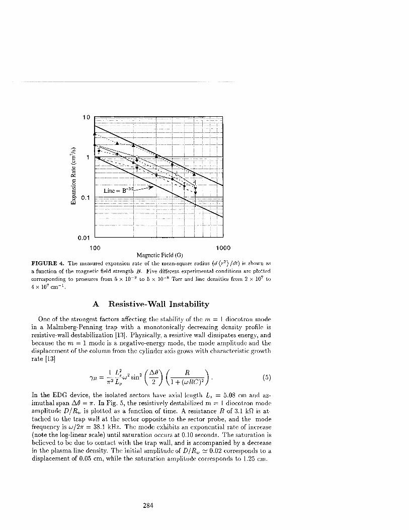
Di

B a a. x W

0.01

100 1000 Magnetic Field (G)

FIGURE 4. The measured expansion rate of the mean-square radius (rf(r2)/d/) is shown as a function of the magnetic field strength B. Five different experimental conditions are plotted corresponding to pressures from 5 x 10-9 to 5 x 10~8 Torr and line densities from 2 x 107 to 4x 107cm"1.

A Resistive-Wall Instability

One of the strongest factors affecting the stability of the m = 1 diocotron mode in a Malmberg-Penning trap with a monotonically decreasing density profile is resistive-wall destabilization [13]. Physically, a resistive wall dissipates energy, and because the m — 1 mode is a negative-energy mode, the mode amplitude and the displacement of the column from the cylinder axis grows with characteristic growth rate [13]

1 I2 1 Ls 2-2

1R = -77-w sin IT Lp

A0 ~2~

R 1 + {ujRcy (5)

In the EDG device, the isolated sectors have axial length Ls = 5.08 cm and azimuthal span AÖ = 7r. In Fig. 5, the resistively destabilized m = 1 diocotron mode amplitude D/Rw is plotted as a function of time. A resistance R of 3.1 kfi is attached to the trap wall at the sector opposite to the sector probe, and the mode frequency is w/27r = 38.1 kHz. The mode exhibits an exponential rate of increase (note the log-linear scale) until saturation occurs at 0.10 seconds. The saturation is believed to be due to contact with the trap wall, and is accompanied by a decrease in the plasma line density. The initial amplitude of D/Rw ~ 0.02 corresponds to a displacement of 0.05 cm, while the saturation amplitude corresponds to 1.25 cm.

284

1.00

Pt «4-1

<ü ~a 3

t <

c o .—t

o cd

0.10

0.01 0.00 0.05 0.10

Time (seconds) 0.15

FIGURE 5. The m = 1 diocotron mode amplitude D/Rw is plotted versus time on a log-linear scale. The mode is destabilized with a 3.1 kfi resistance, leading to an exponential increase in the mode amplitude. The mode saturates due to contact with the trap wall.

S

O

Ü

1000

100

10

0.1

:

1—i nun 1—TTTTTTT "■T'T'I Mill —r™r rriTrT —i rmm

■

: :

-

\ t

V - i ;

:

1 U.J.U! i i i < in —i i\inn

•

10° 10* 10a 1 04 1 o6

Resistance (Ohms) FIGURE 6. The measured growth rates due to resistive wall destabilization are plotted versus resistance R, together with the absolute predictions of Eq. (5) for a wide range of wall resistances.

285

The m = 1 diocotron mode growth rates have been measured for a wide range of resistances, and are shown in Fig. 6. These growth rates are measured while keeping a constant diocotron frequency u>/2ir = 38.0 kHz, plasma length Lp = 15.0 cm, and capacitance C — 200 pF (= 180 cm in cgs units). The theoretical growth rate given by Eq. (5) is also plotted in Fig. 6. For low resistances with u>RC <gi 1, Eq. (5) increases linearly with the resistance R. At uRC = 1 there is a roll-over in the predicted growth rates, and for u>RC 3> 1, Eq. (5) decreases as R~l.

It is clear from Fig. 6 that measured growth rates are in excellent agreement with the theoretical predictions for all resistances between 17 Q and 106 Q, representing 2.5 orders-of-magnitude in growth rate. These measurements not only reproduce previously published data [13], but extend the data to both a lower and a higher range of resistances, and to smaller growth rates. The same level of agreement between the experimental data and theoretical predictions is found over the range of 102 fi to 106 Q examined previously [13]. Beyond this range, the measured growth rates are somewhat larger than the predictions, especially at resistances greater than 106 $7. The cause of the discrepancy at large resistances is not known. Previous measurements using a potentiometer to vary the resistance resulted in even greater discrepancies, so non-ideal effects of the resistors are a possibility. For example, the resistors may have an inherent inductance.

B Effects of Background Neutral Pressure on the Nonlinear Evolution of the m = 1 Diocotron Mode

We now consider the effects of collisions with background gas atoms on the dynamics of the m — \ diocotron mode. A recent calculation [14] predicted that elastic collisions between electrons and background neutrals can induce an instability in the (negative energy) m = 1 diocotron mode, with characteristic linear growth rate In = VenWoz/bJce where i/en is the electron-neutral collision frequency, coce — eB/mec is the electron gyrofrequency, and ui^ = lecNijR2

WB is the diocotron frequency for an infinite-length plasma column. The calculation [14] assumed that the expansion of the plasma is sufficiently slow that the radial density profile can be regarded as stationary on the time scale of the instability. In the experiments on the EDG device, however, the expansion rate is observed to be faster than that expected due to electron-neutral collisions alone [2,3], and also faster than the predicted characteristic exponentiation time of the instability. Although providing initial motivation for the expansion measurements, this theoretical model [14] is not expected to predict correctly the behavior of the diocotron mode in the EDG device.

The effects of electron-neutral collisions on the m = 1 diocotron mode evolution are studied in the EDG device by injecting purified helium gas into the vacuum vessel while monitoring the evolution of the m = 1 diocotron mode. The amplitude evolution for 11 different background gas pressures is shown in Fig. 7, for a constant magnetic field strength of 612 G, and diocotron mode frequency of 55 kHz. The solid and dotted lines are used to distinguish between pressures, and at each

286

2.0 Pressure (Torr)

(a) 5.0E-10 (b) 6.0E-10 (c) 7. "IE-10 (d) 9.0E-10

(e) (f) (g) (h) (0 (]■)

(k)

1.2E-09 1.8E-09 3.1E-09 6.2E-09 1.2E-08 2.6E-08 5.2E-08

4 6 Time (seconds)

FIGURE 7. The amplitude evolution of the m = 1 diocotron mode is shown for 11 different background helium pressures, ranging from 5 x 10"10 to 5 x lO"8 Torr. The solid and dotted lines are used to distinguish between pressures. At each pressure, 5 measurements of the mode

evolution are shown.

E P 00 e

'S. E

u ... .. _ «v^^ t>

— "T..!"'..!"" !—'.!._!!' ■■-^j—"'■■ ■-'■-■■^■:^'\

■*\.^ * * ! Time to 1/10 j ' ; " Initial Amplitude !

Time tc "" " | Initial ^

1/2 ^\^ .mplitude" ■■■■;• a:*- : ...J.

IH " t __ : ■ !

1 ! H ■ ^ ■<' '

.. . : I : ■■;"■"'; ■;r:

j - „

t = 2.17x10 P

-c = 6.86xl04P

ill , i i 1 ! Il.i

■045

i<r 10s 10° io-7

Pressure (Torr) FIGURE 8. The time for the measured m = 1 diocotron mode amplitudes to decay to one-half of their initial amplitudes is plotted as a function of the background gas pressure. Also plotted is the time to decay to one-tenth of the initial amplitude. The vertical width of the bars are the maximum and minimum times for this to occur, as determined by the data shown in Fig. 7

287

pressure 5 measurements of the mode evolution are shown. The amplitudes plotted are normalized to the initial amplitude for clarity. The frequencies are constant as a function of time (to within 1%) even as the mode amplitude decays to zero, indicating that no charge is lost during the measured evolution.

From Fig. 7, a non-exponential damping of the m = 1 diocotron mode is observed, which becomes stronger as the background neutral pressure is increased. The solid lines labeled "a" show the amplitude evolution at the base pressure of 5 x 10~10 Torr. A slight increase in the mode amplitude is evident initially, possibly due to a small wall resistance, with an equivalent exponential growth rate of less than 0.1 sec""1. The "dotted" lines labeled "b" show the amplitude evolution after helium has been injected to increase the measured pressure to 6 x 10~10 Torr (N2 equivalent), a difference of only 1 x 10-10 Torr from the base pressure. At this pressure, the diocotron mode evolution is measurably different, with good rcproducibility, and with the amplitude decaying to nearly zero by 10 seconds. As the background gas pressure is increased further, the diocotron mode damping rate becomes greater.

The sensitivity of the diocotron mode evolution to changes in the background gas pressure of as little as 1 x 10~10 Torr is somewhat surprising in view of the expansion data in Sec. II, where it appears that for pressures lower than 1 x 10-8 Torr the plasma expansion rate is independent of pressure. However, the data in Fig. 3 required many hundreds of repeated plasma shots to obtain each data point, and variations in the experimental parameters over the long times necessary to obtain the data obscure the expansion rate dependence on the background gas pressure at very low pressures. By contrast, the evolution of the diocotron mode can be measured in a single plasma shot, and therefore, small changes in the background gas pressure can be more readily measured while keeping other experimental parameters constant.

To conveniently characterize the non-exponential damping shown in Fig. 7, the time T for the mode amplitude to decay to one-half of its initial amplitude is plotted as a function of the background gas pressure P in Fig. 8. Also shown is the time for the amplitude to decay to one-tenth of its initial amplitude. A power law fit is performed on both sets of data which indicates that the time r is approximately proportional to P-1/2. The non-exponential rate of damping and the P~ll2 scaling of r are not yet understood. The non-exponential rate of damping could be explained if the damping were due to plasma proximity with the trap walls. The amplitude evolution would then be expected to look similar to those in Fig. 7, with very little decay initially because the plasma is far from the trap walls, and more rapid decay later in time as the plasma expansion brings the plasma closer to the trap walls. However, since the plasma is expected to expand at a rate proportional to the background gas pressure P, the time for the mode to damp would be expected to be proportional to P-1. To investigate the cause of the mode damping further, more experiments are needed which measure the density profile evolution during the mode damping.

In any case, from Figs. 7 and 8, the strong sensitivity of the evolution of the m = 1 diocotron mode to the background neutral gas pressure has been clearly

demonstrated in the EDG device.

IV CONCLUSIONS

In this paper, we have described the effects of background neutral gas on the plasma dynamics in the EDG device. The results presented in Sec. II, based on direct measurements of the expanding density profile n(r,t), described how the plasma expansion rate scaled with background gas pressure P (Fig. 3) and magnetic field strength B (Fig. 4). In Sec. Ill, it was shown that the evolution of the m = 1 diocotron mode exhibits a strong sensitivity to the background gas pressure P (Fig. 7), and that the time scale for damping of the diocotron mode scales as P~1/2

(Fig. 8).

ACKNOWLED GMENTS

This research was supported by the Office of Naval Research.

REFERENCES

1. Chao, E.H., Ph.D. Thesis, Princeton University (1999). 2. Chao, E.H., Davidson, R.C., and Paul, S.F., J. Vac. Sei. Tech. A17, 2050 (1999). 3. Chao, E.H., Paul, S.F., and Davidson, R.C., J. Vac. Sei. Tech. A17, 2034 (1999). 4. Davidson, R.C., and Moore, D.A., Phys. Plasmas 3, 218 (1996). 5. Davidson, R.C., and Chao, E.H., Phys. Plasmas 3, 2615 (1996). 6. Malmberg, J.H., and Driscoll, C.F., Phys. Rev. Lett. 44, 654 (1980). 7. deGrassie, J.S., and Malmberg, J.H., Phys. Fluids 23, 63 (1980). 8. Notte, J., and Fajans, J., Phys. Plasmas 1, 1123 (1994). 9. Levy, R., Phys. Fluids 11, 920 (1968).

10. Fine, K.S., Ph.D. Thesis, University of California, San Diego (1988). 11. Driscoll, C.F., and Fine, K.S., Phys. Fluids B2, 1359 (1990). 12. Fine, K.S., and Driscoll, C.F., Phys. Plasmas 5, 601 (1998). 13. White, W.D., Malmberg, J.H., and Driscoll, C.F., Phys. Rev. Lett. 49, 1822 (1982). 14. Davidson, R.C., and Chao, E.H., Phys. Plasmas 3, 3279 (1996).

289

An Annular Penning Trap for Studies of Plasma Confinement

John Kline,* Scott Robertson1" and Bob Walch*

*Department of Physics, West Virginia University, Morgantown, WV 26506 1Department of Physics, University of Colorado, Boulder, CO 80309-0390

^Department of Physics, University of Northern Colorado, Greeley, CO 80639

Abstract An annular version of the Malmberg-Penning trap is described in which electrons are confined between concentric cylinders. The space within the inner cylinder contains conductors for adding an azimuthal magnetic field and a solenoid for inducing an azimuthal electric field. Experiments with potential differences from 0 to 90 volts applied to the cylinders show that the mobility transport may be varied or made smaller than the diffusive transport. The mobility transport is shown to be independent of the azimuthal magnetic field. The diffusive transport is shown to scale linearly with pressure and inversely as the square of the axial field. The azimuthal electric field made by changing the magnetic flux in the solenoid results in a radial displacement of the electrons such that they remain on surfaces enclosing constant flux.

INTRODUCTION

An annular Malmberg-Penning trap (1) is described in which a nonneutral plasma of electrons is confined between concentric cylinders. This geometry makes possible several new types of confinement experiments. First, the bias potentials on the inner and outer cylinders may be used to adjust the radial electric field, whereas in the standard trap the radial electric field is determined by the electron density. This feature allows the transport by mobility to be varied or to be made smaller than the transport from diffusion. Second, conductors may be placed within the inner cylinder to create an azimuthal magnetic field. The combined axial and azimuthal fields result in helical field lines and helical bounce orbits. There is an additional electric drift in the end regions which is radially outward at one end of the device and inward at the other. These drifts give the bounce orbits a finite width which is analogous to the banana width of orbits of the tokamak and the particle transport is analogous to the neoclassical transport of the tokamak (2). Third, a solenoid may be placed within the inner cylinder and the flux within it changed to create an azimuthal electric field. The resulting E x B drift results in a radial displacement of particles which may be studied or used to create initial plasma profiles which are separated from the wall.

CP498, Non-Neutral Plasma Physics HI, edited by John J. Bollinger, et al. © 1999 American Institute of Physics 1-56396-913-0/99/$ 15.00

290

THE APPARATUS

The device is shown schematically in Fig. 1. The confinement volume is the annular space between two concentric cylinders of equal length. An axial magnetic field is applied by Helmholtz coils. Annular grids at the ends of the cylinders are biased negatively for electrostatic confinement. Current in conductors along the axis creates an additional azimuthal field. The field lines are then helical and the flux surfaces are cylinders. The azimuthal field has a radial gradient and there are additional gradient and inertial drifts which are both axial and azimuthal. In the end regions where there is a strong axial electric field, there is a drift from Ez * Be which is radial. This drift is inward at one end of the device and outward at the other end because Ez changes sign at the midplane. The drift displacement is the same at each end thus the orbits have a finite width when projected onto either the r-z plane or the r-8 plane. These orbits are illustrated by the numerical simulations in Fig. 2.

Construction details of the trap have appeared previously (3) and are briefly summarized here. The device is contained in a standard 15 cm diameter pipe cross pumped by a turbomolecular pump to a base pressure of <10"7 Torr. Helium may be added by means of a leak valve. The inner and outer cylinders of the trap have diameters of 25.4 and 48 mm. Their ends are at z = ± 75 mm and the negatively biased grids are at ± 87 mm. An axial field of 0-18 mT is made by water-cooled Helmholtz coils and an azimuthal field of 0-15 mT is made by a set of six rectangular coils fabricated from solid copper rod. These pass within an inner vacuum wall which has a radius of 38 mm. A pulsed azimuthal electric field is created by a solenoid within the inner wall. This solenoid has 220 turns with a winding radius of 17 mm and a length of 25 cm. It is operated from a supply which generates rectangular pulses of 0-100 V and 0-100 A. The current rises to a relatively constant value in 0.5 ms which is the L/R time of the coil and the duration of the azimuthal electric field.

The density profile may be measured by dumping the electrons onto a set of five annular electrodes of equal width which are connected to integrators. Electrons are dumped by removing the bias potential from the grid at +87 mm. Electrostatic pickup from the gate pulse is reduced by having a grounded grid between the gated grid and the annuli. The remaining pickup is subtracted using signals recorded with no electrons in the trap. The inner and outer cylinders are connected to amplifiers which measure the collected current. Bias potentials are applied to the cylinders by means of batteries in series with the inputs of these amplifiers.

The trapped electrons are secondaries created by passing energetic electrons through the trap. The characteristic energy of secondary electrons from helium is 15 eV (4). The energetic electrons are from a heated tungsten filament which is biased to -150 V. The filling is stopped by removing the bias potential from the filament. There is an upper bound to the density determined by the depth of the potential well. Near the density limit, oscillatory signals are seen which may indicate the onset of diocotron modes (5). In the experiments reported below, the density is kept below this limit.

291

FIELD COILS

SOLENOID

ANNULI

GRIDS

OUTER CYLINDER

ORBIT

FILAMENT

FIGURE 1. Schematic diagram of the annular trap showing the concentric cylinders, end grids, a particle orbit projected onto the r-z plane, the annuli for collecting dumped electrons, the conductors near the axis for creating an azimuthal magnetic field, the solenoid for creating an azimuthal electric field, and the filament for creating trapped electrons by impact ionization of helium.

Perspective view r-z projection r-6 projection

FIGURE 2. Simulated particle trajectories in the annular trap. The plot is made in a frame rotating with the local E x B drift velocity. The orbit fails to close because of the azimuthal gradient and inertial drifts. The plot is for an energy of 6 eV (2 eV in each degree of freedom), an axial field of 2 mT and an azimuthal field of 2 mT The fields are artificially low to make the orbit scale lengths visible.

292

EXPERIMENTS

Mobility driven by an applied electric field

Mobility transport in the trap is most easily derived from conservation of the azimuthal canonical angular momentum,

Pe= r(q/4e + mve), (1)

where r is the radial coordinate, AQ = 14 Bz r is the vector potential for a uniform axial field Bz, and q and m are the charge and mass of an electron, respectively. Collisions with neutrals cause a loss of Pe at the average rate rvmve where v is the momentum transfer collision frequency and ve is the azimuthal drift speed E, /Bz. The electron Larmor radius is small in comparison with the radius of the device thus the mechanical angular momentum, rmve, is much smaller than the electromagnetic momentum rqAe. This implies that a loss of angular momentum must come from the electromagnetic part of Pe which results in a radial drift velocity,

vtl = dr/dt = vmEr/qBz2 = uEr, (2)

where v^ is the mobility drift velocity and \i - vm /qBz2 is the mobility coefficient. A

mobility confinement time, x^, may be defined as the half-width of the plasma annulus, a, divided by the mobility drift velocity,

Tn = aqBz2/vmEr. (3)

Thus we expect the confinement time to scale inversely with the applied electric field. The mobility transport was varied by grounding the inner cylinder, biasing the

end grids to -6 V and increasing the voltage on the outer cylinder in steps of 9 V from 27 V to 90 V. The decay in the current to the outer cylinder was recorded, Fig. 3a, after the filling was stopped. The axial field was 14 mT and the helium pressure was 5 x 10"5 Torr. The data were fit to an exponential curve and the e-folding times were found. The loss rates, Fig. 3b, show the expected linear scaling of the loss rate with electric field. Other data have shown that the e-folding times scale as the square of the magnetic field and scale inversely with the pressure (5).

The integrated current to the outer cylinder gives an initial charge of 145 pC. This divided by the volume of the trap gives a confined density of 1.2 x 106 cm"3. This density is about a factor of four below the density which would give a potential drop which matches the 36 V applied between the inner and outer cylinders.

293

Mobility with an azimuthal magnetic field

The azimuthal field adds to the absolute value of the field and one might expect that the mobility with the combined fields would be u = vm/q|B|2. The derivation of u. in the preceding section, however, shows that Be does not enter. The correct expression can be referred to as the neoclassical mobility because it applies to axisymmetric systems like the tokamak with drifts orthogonal to flux surfaces. In the experiment, the mobility was shown to be independent of the azimuthal field by recording the current to the outer cylinder with the axial field fixed at 5 mT and the azimuthal field increased in steps from 0 to 15 mT. The absolute value of the field was increased by more than a factor of three, but the decay rates. Fig. 4, are nearly indistinguishable, indicating that the mobility is independent of Be.

b)

20 40 60 80

Cylinder potential [V]

100

FIGURE 3. a) The current to the outer cylinder as a function of time for bias voltages of 27, 36, 45, 63 and 90 volts. The higher bias voltage results in the shortest decay time. For clarity, data sets at intermediate voltages were not plotted, b) The decay constant, 1/t, as a function of cylinder bias potential. The data show that the loss rate scales linearly with the potential difference applied to the cylinders. The line is a linear regression.

100

Time, ms

FIGURE 4. Four superimposed traces of current to the outer cylinder as a function of time with Bz = 5 mT and with Be = 0, 5, 10, and 15 mT. The decay is independent of the azimuthal field. The potential applied to the outer cylinder is 36 V and the helium pressure is 1 x 10*4 Torr.

294

Confinement limited by diffusion

Transport by mobility may be nearly eliminated by placing both cylinders at ground potential. There will remain some mobility transport driven by the space charge electric field but this can be kept negligible by limiting the density. The classical diffusion coefficient is D = V2 rL

2 v, where rL is the thermal Larmor radius. The confinement time determined by diffusion is approximately

xD = a2/D = a2q2Bz2/vmT, (4)

where T is the electron temperature in energy units. The ratio of the diffusive time scale to the mobility time scale is

TD/T^ 2qaEr/T = |q|U/T, (5)

where U = -2aEr is the potential difference between the cylinders. Thus if the potential difference is much smaller than the mean electron energy the transport is dominated by diffusion rather than mobility.

Diffusive transport was examined experimentally by placing both cylinders at ground potential and biasing the grids to -30 V. The decay in density was measured by dumping the electrons onto the annuli with delay times that were successively longer, Fig. 5. For this measurement, the charge deposited on two annuli near the center was used. The decay rates are plotted in Fig. 6a as a function of pressure at 18 mT. The data show the expected linear dependence upon collision frequency, however, the linear regression does not pass through the origin which indicates an additional loss mechanism. The decay time plotted as a function of the square of the magnetic field, Fig. 6b, shows the expected linear dependence.

FIGURE 5. Example of the diffusive mode of operation. Displayed is the output of an integrator connected to two annuli midway between the cylindrical walls. Ten traces are superposed and each is made with a longer hold time. The magnetic field is 14 mT and the pressure is 3 x 10"6 Torr. The vertical scale is the charge indicated by the peak of the signal.

295

5 10 15

R-essure [uTorr]

20 100 200

B,2 [mT2]

300 400

FIGURE 6. a) The decay rate, 1/x, plotted as a function of pressure shows that the diffusivity increases linearly with collision frequency, b) The decay time, T, plotted as a function of the square of the magnetic field shows the expected linear scaling. The pressure is 2 x 10~5 Torr.

The e-folding times calculated from equation (4) using the characteristic energy of secondaries, 15 eV, is approximately a factor of two longer than the measured value. This discrepancy maybe due to the electron distribution falling more slowly with energy than a Maxwellian distribution. The charge dumped onto the annuli corresponds to a density of approximately 3 x 105 cm3. This density gives a space charge potential of less than one volt thus transport by mobility is negligible.

Displacement by an azimuthal electric field

The drift rate caused by application of E0 may be found from conservation of canonical angular momentum. The magnetic vector potential may be divided into two parts, Aeo = Vi rB2 which arises from the uniform axial confining field Bz, and Aes = Vi (rs

2/r)Bs which arises from the field Bs within the solenoid. The solenoid has radius rs < r thus at the particle's location the solenoid current changes Ao and Bz changes negligibly. Angular momentum conservation requires that

Pe = r {mve + Vt q [r Bz + (rs2 /r) Bs ]} (6)

be constant. One may average over the rapid cyclotron motion of the particle in which case r becomes the guiding center location and ve becomes the azimuthal component of the guiding center velocity. The mechanical momentum rmvo is much smaller than the electromagnetic part of the momentum, rqAe, thus conservation of Pe is equivalent to rAe remaining constant at the particle's location. For axisymmetric systems, the flux, v|/(r), enclosed at a radius r is related to the vector potential through Ae = v|/(r) /27tr, thus conservation of rAe is equivalent to the particle guiding center

296

remaining on a surface enclosing a constant flux. Conservation of enclosed flux gives a displacement that satisfies

rf2 = ri2-AT/itBz (7)

where rf is the final radial position of the particle, r, is the initial position and A*F = 7irs

2Bs is the flux change. The displacement was measured by loading the trap, increasing the current in

the solenoid from zero to a fixed value, and then dumping the electrons onto the annuli. This was repeated with increasing values of the current. The polarity of the current was chosen to decrease the net flux which results in an outward displacement. The data in Fig. 7 show that the density profile is displaced to larger radii as the current is increased. The line in the figure shows the boundary calculated from equation (7). The boundary should pass the first annulus at 18 A and the last at 54 A. There is agreement between the expected and calculated values. Similar results are obtained when the polarity of the solenoid is reversed so that the outer boundary of the plasma is displaced inward.

Current [A]

FIGURE 7. The four pedestals indicate the charge in arbitrary units dumped onto four annuli spanning 30 mm to 48 mm in radius. The current is that in the solenoid at the time of the dump. The pedestals of zero height indicate that the plasma boundary has moved past that annulus. The inner annulus is in the foreground and the outer is in the background. The white line is the inner plasma boundary expected from conservation of enclosed flux.

297

SUMMARY AND CONCLUSION

A new version of the Malmberg-Penning trap has been constructed in which the plasma is contained between concentric cylinders. The potential difference between the cylinders has been varied to demonstrate scaling of mobility transport with electric field. The space interior to the inner cylinder contains conductors for creating an azimuthal magnetic field and a solenoid for changing the azimuthal vector potential without altering the magnetic field within the plasma volume. Experiments with the solenoid have shown that the drift from the induced azimuthal electric field results in a displacement such that the electrons remain on surfaces enclosing constant flux. The azimuthal magnetic field allows experimental tests of several aspects of neoclassical transport theory. The first such experiment has shown that the mobility is independent of the azimuthal field. Other experiments which should be possible include the demonstration of the Ware drift (6), neoclassical diffusion, and the transition from neoclassical to classical diffusion as the collision time is made shorter than the axial bounce time (2).

ACKNOWLEDGMENTS

The authors acknowledge valuable discussions with John Cary and Earl Scime. The technical assistance of Hikmet Andic, Qudsia Quraishi and Matt Triplett is appreciated.

REFERENCES

1. J. H. Malmberg, C. F. Driscoll, B. Beck, D. L. Eggleston. J. Fajans, K. Fine, X.-P. Huang and A. W. Hyatt, in Non-Neutral Plasma Physics, AIP Conf. Proc. Vol. 175, edited by C. W. Roberson and C. F. Driscoll, New York: American Institute of Physics, 1988 , p. 28. 2. F. L. Hinton and R. D. Hazeltine, Rev. Mod. Phys. 48, 239 (1976). 3. S. Robertson and B. Walch, Rev. Sei. Instrum. 70, 2993 (1999). 4. J. L. Pack, R. E. Voshall, A. V. Phelps and L. E. Kline, J. Appl. Phys. 71, 5363 (1992). 5. S. Robertson and B. Walch, submitted to Phys. Plasmas. 6. A. A. Ware, Phys. Rev. Lett. 25, 15 (1970).

298

Bifurcations in elliptical, asymmetric non-neutral plasmas

J. Fajans,1 E. Gilson and K. Backhaus


Abstract. Pure electron plasma deform into ellipses when subjected to stationary, £ = 2 potential perturbation on the trap wall. At first, the plasma's ellipticity is proportional to the strength of the potential perturbation. Once the perturbation is increased beyond a critical value, the plasma equilibrium bifurcates into two off-axis equilibria and a saddle. At the bifurcation point, the diocotron frequency dips to near zero. The diocotron orbits become very elliptical just below the bifurcation, and, after the bifurcation, split into three classes delimited by a separatrix: two classes surrounding the individual new equilibria, and one class surrounding both equilibria. The mode frequencies slow near the separatrix, and the trajectories themselves slow near the saddle at the origin. Interaction with the elliptical mode causes the diocotron mode to spontaneously and reversibly jump across the separatrix.

When a pure-electron plasma confined in a Malmberg-Penning trap is subjected to a V cos 20-like voltage perturbation along the trap wall, it deforms into an ellipse. The voltages are applied to electrically-isolated sectors in the trap wall. The plasma is stable, stationary in the lab frame and reasonably long-lived. Curiously, negative voltages attract the plasma, while positive voltages repel the plasma. Thus, in the above figure the plasma is squeezed away from the +17 V applied to the left and right sectors.

Some years ago, we studied the effects of small perturbations [1,2]. Recently we extended the analysis to highly deformed plasmas [3,4]. The analysis predicts that as the perturbation V is increased, the plasma will become more elliptical. When V exceeds a critical voltage, the plasma equilibrium will bifurcate, and the plasma will move off center. This classic pitchfork bifurcation [5] is illustrated in Fig. 3.

Trap construction asymmetries favor one of the post bifurcation equilibria over the other, but the effect of these asymmetries can be tuned out by applying a small voltage to the top or bottom sectors or by making the left and right sector voltages slightly different. We chose to tune by applying a voltage Vb = ßV to the bottom

x> [email protected]


299

+0.0V

+17.0V mm- +17.0V

-0.046V

FIGURE 1. Pure electron plasma deformed into an ellipse by the application of +17 V to the side sectors. The —0.046 V applied to the bottom sector is a balancing voltage, described later in the poster.

Filament,

Phosphor Screen

%

m

-V FIGURE 2. Schematic of the trap showing the electrically isolated sectors.

sector. Typically the balance proportionality \ß\ is less than 0.005. The tuning can be quite sharp; changing ß by less than 0.0015 will consistently send the plasma up or down. For example, in Fig. 3, changing ß from —0.0027 to -0.0031 changed the selected equilibrium. Over the course of a few days, however, the equilibrium ß can drift.

The plasma's center of charge is plotted as a function of the perturbation voltage in Fig. 4; the ellipticity is plotted in the succeeding figure. The theory curves in both graphs are derived from a second-moment Hamiltonian model given by Chu [2,4], with an added magnetron term. Unfortunately, Chu's equations are for flat-top, infinite-length plasmas, and the experimental plasmas are neither. Conse- quently we fit the critical voltage and the initial slope of the ellipticity curve to get the theory curves shown. The discrepancy in the ellipticity curve for large voltages is probably due to higher order moments. Such moments are increasingly important as the plasma approaches the wall, as is clearly visible for the V = 28.3 V plasmas in Fig. 3.

An important prediction of the theory is that the diocotron frequency goes to zero at the bifurcation. The £ = 1 diocotron mode is driven by the plasma image charge fields, but, at the bifurcation, these fields are canceled by the fields from

300

/

\

J X

FIGURE 3. Ellipse bifurcation.

301

10 15 20 25 30

Perturbation (V)

FIGURE 4. Measured (triangles) and predicted (line) center of charge (normalized by the wall radius) of the ellipse as a function of the perturbation voltage. The bifurcation occurs at 17.67 V.

5 10 15 20 25 30

Perturbation Voltage (V)

FIGURE 5. Measured (dots) and predicted (line) ellipticity as a function of the perturbation voltage.

the perturbation voltage. Consequently the diocotron stalls, small-amplitude diocotron frequency should be

/ = f0}Jl - V/Vc

= 2f0(V/Vcf2Jl vjv

V <vc

v>vc,

Theoretically, the

(1)

where /0 is the unperturbed diocotron frequency. As shown in Fig. 6, this prediction is well verified by our experiments. However, the experimental diocotron frequency does not go precisely to zero at the bifurcation, as it is predicted to by Eq. (1). The minimum frequency is a sharp function of the balance proportionality (see Fig. 7.) When detuned, nonlinearities dropped in the analysis leading to Eq. (1) keep the diocotron frequency finite (see Fig. 7). The effects of nonlinearities are magnified by the shape of the diocotron orbits near the bifurcation, which, as shown in Fig. 8, becomes extremely elliptical. Even low amplitude orbits sample the field nonlinearities found away from the origin.

As shown in Fig. 9, the post bifurcation diocotron orbits exhibit all the phase- space features associated with a 2-D bifurcation [6]:

Classically, the separatrix between the tear-drop and peanut orbits is inviolable. We find, however, that if we drive the diocotron mode too close to the separatrix,

302

0 5 10 15

Perturbation (V)

FIGURE 6. Diocotron frequency as a function of the perturbation voltage. The measured

values /o = 47.6 kHz and Vc = 17.67 V are used to calculate the theory line.

-0.10 -0.05 0.00 0.05 0.10

Balance Proportionality ß

FIGURE 7. Minimum diocotron frequency as a function of the balance proportionality ß. (The

best ß, +0.005, has drifted from the ß observed in Fig. 3).

+17.4V/ A

\J f + 17.4V

+0.0 IV FIGURE 8. Diocotron orbits just below bifurcation. Proceeding outwards, the orbit frequencies

are 4, 8, 16 and 16 kHz. The ellipticity of the 4 kHz orbit is almost 28.

the plasma can spontaneously jump between the three orbit groups. The jumps are not repeatable, and occur at random intervals. All the tear-drop orbits in the

303

+ 19V

+19V

FIGURE 9. Diocotron orbits above bifurcation showing tear-drop shaped orbits around the two

equilibria (marked by +'s) and peanut shaped orbits surrounding both equilibria. The signal on

the bottom sector, Vj,, is tuned to select the upper or lower equilibria. The origin is a saddle,

and the separatrix is somewhere between the 25 kHz and 16 kHz orbits. Note how the orbital

frequencies decrease near the separatrix. The circles denote 1 /xs intervals along the orbit. For

clarity, the hash marks are suppressed on the upper half of the 16 kHz orbit, the lower 25 kHz

orbit, and on both the 38 kHz orbits.

sequence have roughly the same frequency, implying that the tear-drop orbit amplitudes do not change. The peanut orbit frequencies are approximately half the tear-drop orbit frequencies. The jumps can continue for over fifty milliseconds,

Time (us) FIGURE 10. Signal induced on the upper sector by the plasma charge. The magnitude and sign

of the signal depends on the position of the plasma, with large negative-going signals indicating

that the plasma is close to the upper sector, and smaller positive-going signals indicating that the

plasma is far from the upper sector.

making many transitions therein, so dissipation does not seem to be the cause of this phenomenon. We suspect that the jumps are due to an exchange of energy between the diocotron mode and the elliptical mode; strictly speaking, the separatrix only exists for the two dimensional (xc, yc) system, not for the full (xc, yc, A, </>) system. Previous experiments on adiabatic invariants [7] two-vortex stability [8] and on autoresonance [9] have demonstrated that the diocotron mode is very well decoupled from the elliptical mode. Effectively irreversible interactions [10] have

304

been observed between the diocotron and elliptical modes, but this may be the first time that any reversible coupling has been observed.

We thank J.S. Wurtele for his help with this problem. This work was supported by the Office of Naval Research.

REFERENCES

1. J. Notte, A. J. Peurrung, J. Fajans, R. Chu, and J. Wurtele, Phys. Rev. Lett. 69, 3056 (1992).

2. R. Chu, J. S. Wurtele, J. Notte, A. J. Peurrung, and J. Fajans, Phys. Fluids B 5, 2378 (1993).

3. J. Fajans, E. Y. Backhaus, and J. McCarthy, Phys. Plasmas 6, 19 (1999). 4. E. Y. Backhaus, J. Fajans, and J. S. Wurtele, Phys. Plasmas 6, 19 (1999). 5. A movie showing the bifurcation can be downloaded from

http://socrates.berkeley.edu/"" fajans/EquilStab/EllipseBifurcation.avi. 6. An animation of the post-critical diocotron orbits can be downloaded from

http://socrates.berkeley.edu/~ fajans/EquilStab/EllipDiocOrbits.avi. 7. J. Notte, J. Fajans, R. Chu, and J. Wurtele, Phys. Rev. Lett. 70, 3900 (1993). 8. T. B. Mitchell, Ph.D. thesis, University of California, San Diego, 1993. 9. J. Fajans, E. Gilson, and L. Friedland, , submitted to Phys. Plasmas.

10. T. Mitchell, Phys. Fluids 8, 1 (1996).

305

SECTION 5

CHARGED PARTICLE BEAMS

Intense Nonneutral Beam Propagation Through a Periodic Focusing Quadrupole

Field I — A Compact Paul Trap Configuration to Simulate Beam

Propagation Over Large Distances

Ronald C. Davidson, Hong Qin, and Gennady Shvets


Abstract. This paper considers an intense nonneutral charged particle beam propagating in the z-direction through a periodic focusing quadrupole magnetic field with transverse focusing force, — Kq(s)[xex — yey], on the beam particles. Here, s = ßbd is the axial coordinate, (7t, - l)mbC2 is the directed axial kinetic energy of the beam particles, qt, and mt, are the charge and rest mass, respectively, of a beam particle, and the oscillatory lattice coefficient satisfies Kq(s + S) = Kq(s), where 5 is the axial periodicity length of the focusing field. The particle motion in the beam frame is assumed to be nonrelativistic, and the Vlasov-Maxwell equations are employed to describe the collisionless nonlinear evolution of the distribution function fb(x,y,x',y',s) and the (normalized) self-field potential ip{x,y,s) = qt,<j>{x,y,s)/7%mbßb

2c2 in the transverse laboratory-frame phase space (x,y,x',yl), assuming a thin beam with characteristic radius r;, <C S. It is shown that collective processes and the nonlinear transverse beam dynamics can be fully simulated in a compact Paul trap configuration in which a long nonneutral plasma column (L > rp) is confined axially by applied dc voltages V — const, on end cylinders at z = ±L, and transverse confinement in the x — y plane is provided by segmented cylindrical electrodes (at radius rw) with applied oscillatory voltages ±Vb(i) over 90° segments. Here, Vo(t + T) = Vb(i), where T — const, is the oscillation period, and the oscillatory quadrupole focusing force on a particle with charge q and mass m near the cylinder axis is — mKq(t)[xex — yey], where Kq{t) = 8qVo{t)/Trmr^. This configuration offers the possibility of simulating intense beam propagation over large distances in a compact configuration which is stationary in the laboratory frame.

I INTRODUCTION

Periodic focusing accelerators and transport systems [1-6] have a wide range of applications ranging from basic scientific research, to applications such as heavy ion fusion, spallation neutron sources, and nuclear waste treatment, to mention a


309

few examples. Of particular interest, at the high beam currents and charge densities of practical interest, are the combined effects of the applied focusing held and the intense self fields produced by the beam space charge and current on determining detailed equilibrium, stability, and transport properties [1]. Through analytical studies based on the nonlinear Vlasov-Maxwell equations, and numerical simulations using particle-in-cell models and nonlinear perturbative simulation techniques, considerable progress has been made in developing an improved understanding of the collective processes and nonlinear beam dynamics characteristic of high-intensity beam propagation [7-24] in periodic focusing and uniform focusing transport systems. Nonetheless, it remains important to develop an improved basic understanding of the nonlinear dynamics and collective processes in periodically-focused intense charged particle beams, with the goal of identifying operating regimes for stable (quiescent) beam propagation over large distances, including a minimum degradation of beam quality and luminosity.

In this paper, we present in Sec. II a brief summary of the nonlinear Vlasov- Maxwell equations describing the collective processes and nonlinear transverse dynamics of a thin (r(, <C S), intense charged particle beam propagating through a periodic focusing quadrupole magnetic field with axial periodicity length S = const. In Sec. Ill, a compact Paul trap configuration is described which fully simulates the equivalent collective processes and nonlinear transverse beam dynamics in a periodic focusing quadrupole transport system. Unlike a Malmberg-Penning trap [25-28], which provides transverse confinement of the plasma particles by an applied axial magnetic field Boez, a Paul trap configuration [29,30] provides transverse confinement in the x — y plane by oscillating voltages applied to electrodes external to the plasma. The idea of using a single-species trap to model periodically-focused beam propagation has previously been discussed by Okamoto and Tanaka [31]. The emphasis of their work is on solenoidal confinement [31], whereas the present analysis focuses on periodic quadrupole confinement. In addition, the present analysis treats the case of arbitrary (but periodic) time dependence of the focusing potential.

To briefly summarize, a long nonneutral plasma column (L S> rp) is confined axially by applied dc voltages V = const, on end cylinders at z = ±L, and transverse confinement in the x — y plane is provided by segmented cylindrical electrodes (at radius rw) with applied oscillatory voltages ±V0(t) over 90° segments. Here, Vo(t + T) = Vo(t), where T = const, is the oscillation period, and the oscillatory quadrupole focusing force on a particle with charge q and mass m near the cylinder axis is — m,Kq{t)\xex — yey], where Kq(t) = 8qVo(t)/'irrnr^. This configuration offers the possibility of simulating intense beam propagation over large distances in a compact configuration which is stationary in the laboratory frame.

This is the first of a two-paper sequence. The second paper [32] applies a recently- developed canonical transformation and Hamiltonian averaging formalism [23] to transform away the rapidly oscillating quadrupole focusing contributions to the laboratory-frame Hamiltonian H±(x,y,x,y,t). The analysis leads to a new Hamil-

tonian 1-L±(X,Y,X,Y,l) in the 'slow' transformed variables (X,Y,X,Y). The

310

transformed Hamiltonian has constant transverse focusing coefficient K/9 = const. (independent of £), and the corresponding transverse focusing force is isotropic in the X — Y plane. This leads to enormous simplification in the analysis of the non-

linear Vlasov-Poisson equations for the distribution function F(X,Y,X,Y,t) and self-field electrostatic potential </>a(X,Y,t) in the transformed variables.

II THEORETICAL MODEL FOR INTENSE BEAM PROPAGATION THROUGH A PERIODIC

FOCUSING QUADRUPOLE FIELD

We consider a thin, intense charged particle beam with characteristic radius n, and average axial momentum ^rribßbC propagating in the ^-direction through a periodic focusing quadrupole magnetic field with axial periodicity length S. Here, rb S> S is assumed, (76 — l)mt,c2 is the directed axial kinetic energy of the beam particles, 7t = (1 — ß2)-1^2 is the relativistic mass factor, V& = ß\,c is the average axial velocity, <#, and mj, are the particle charge and rest mass, respectively, and c is the speed of light in vacuo. In addition, the particle motion in the beam frame is assumed to be nonrelativistic. We introduce the scaled time variable s = ßbd, and the (dimensionless) transverse velocities x' = dx/ds and y' — dy/ds. Then, within the context of the assumptions summarized above, the collisionless nonlinear beam dynamics in the transverse, laboratory-frame phase space (x,y,x',y') is described self-consistently by the nonlinear Vlasov-Maxwell equations for the distribution function fb(x, y, x', y', s) and the normalized self-field potential ip(x,y,s) — qb(ß(x,y,s)/^mbßbC2, where <f>(x,y,s) is the electrostatic potential. For a thin beam (rb <C S), the transverse focusing force on a beam particle produced by the periodic quadrupole field can be approximated over the cross-section of the beam by

Fjoc = -Kq(s)[xex - yey] , (1)

where (x,y) is the transverse displacement of a particle from the beam axis, and the 5-dependent focusing coefficient Kq(s + S) = Kq{s) is defined by

K (s) = qbB'i^ (2) ' •ybmbßbC2

Here, the field gradient B'q(s) is defined by B'q(s) = (öB«/öj/)(0,o) = (dB*/dx)m. Note from Eq. (2) that Kq(s) has the dimensions of (length)- . In terms of the normalized self-field potential i/>(x,y,s) = qbcf>{x,y,s)/jb'mbßbC2 and the distribution function fb(x,y,x',y',s), the nonlinear beam dynamics and collective processes in the laboratory-frame transverse phase space (x,y,x',y') is described self- consistently by the Vlasov-Maxwell equations [1,23]

311

' d ,d ,d ( . , ÖV'\ ö -*u»+^)£}* = 0'<3> and

Here, ni,(x,y,s) = / dx'dy'fb is the number density of the beam particles. Moreover, the laboratory-frame Hamiltonian H±(x,y,x',y',s) for transverse single-particle motion consistent with Eqs. (3) and (4) is given (in dimensionless units) by

H±(x, y, x', y', s) = ~{x'2 + y'2) + -Kq(s)(x2 - y2) + i>(x, y, s) . (5)

The nonlinear Vlasov-Maxwell equations (3) and (4) are rich in physics content and are widely used to describe the stability and transport properties of an intense nonneutral beam propagating through a periodic focusing quadrupole field Kq(s + S) — Kq(s). While considerable progress has been made in analytical and numerical studies of Eqs. (3) and (4) [7-24], detailed calculations of the equilibrium and stability behavior are generally complex because the quadrupole focusing coefficient nq(s) is both s-dependent and oscillatory, with /0 dsnq(s) = 0 for a periodic focusing lattice. Indeed, as described in Ref. 23, only recently has a canonical transformation been developed that utilizes an expanded generating function that transforms away the rapidly oscillating terms in Eq. (5), leading to a Hamiltonian in the transformed variables, H{X,Y,X',Y', s) = {l/2){X'2 + Y'2) + (l/2)Kfq{X2 + Y2) + ip(X, Y,s), where Kfq — const, (independent of 5).

Ill COMPACT TRAP CONFIGURATION TO MODEL PERIODICALLY-FOCUSED INTENSE BEAM PROPAGATION OVER LARGE DISTANCES

In practical accelerator applications, if the spacing between quadrupole magnets corresponds (for example) to S = 2m, and the transverse nonlinear beam dynamics described by Eqs. (3)-(5) is to be followed in detail for 500 lattice periods, then the length of the transport system that is required is 1 km. The obvious question arises as to whether or not it is possible to model the nonlinear transverse beam dynamics described by Eqs. (3)-(5) in a compact laboratory configuration. The answer is yes, and the key is to recognize that the particle motion in the frame of the beam is nonrelativistic, and that the oscillatory quadrupole focusing terms in Eqs. (5) can be simulated in the laboratory frame by applying oscillatory voltages to cylindrical electrodes in a Paul trap configuration as illustrated in Fig. 1.

To model an axially continuous charged particle beam (or a very long charge bunch), we consider a long nonneutral plasma column [Fig. 1(a)] with length 21

312

and characteristic radius rp < L, confined axially by applied dc voltages V = const, on end cylinders at z = ±L. The particles making up the (nonrelativistic) nonneutral plasma in Fig. 1(a) have charge q and mass m. With regard to transverse confinement of the particles in the x - y plane, there is no applied axial magnetic field (B0 = B0ez = 0). Rather, segmented cylindrical electrodes (at radius rw) have applied oscillatory voltages ±V0{t) over 90° segments with the polarity illustrated in Fig. 1(b). Here, the applied voltage V0(t) is oscillatory with

V0(t + T) = Vo(t),

L T dtV0(t) = 0 , (6)

where T = const, is the period, and /0 = 1/T is the oscillation frequency. While different electrode shapes will result in an oscillatory quadrupole potential near the cylinder axis, the configuration shown in Fig. 1(b) is particularly simple and amenable to direct calculation. Neglecting end effects (d/dz = 0), and representing the applied electric field by Ea = -VL(f>a{x, y, t), where Vx • E, = 0 and V± x E, ~ 0, it is readily shown that the solution to V\<j)a(x,y,t) = 0 that satisfies the appropriate boundary conditions at r = rw in Fig. 1(b) is given by

, , . 4V0(t) ^ sin(l7r/2) (r\u m

for 0 < r < rw and 0 < 9 < 2TC. Near the cylinder axis (r < rw), Eq. (7) readily gives to lowest order

q<t>a(x, y, t) = -mKq(t)(x2 - y2) , (8)

where the oscillatory quadrupole focusing coefficient Kg(t) is defined by

N(«) = ^. (»)

From Eqs. (6) and (9), note that Kq(t + T) = Kq(t) and J0T dtKq(t) = 0. Moreover,

Kq(t) has dimensions of (time)-2. Most importantly, from Eq. (7), the leading- order correction to Eq. (8) is of order (l/3)(r/rw)4. Therefore, for example, if the characteristic radial dimension rp of the plasma column in Fig. 1 satisfies rp/rw ~ 0.1, then the corrections to the simple quadrupole potential in Eq. (7) are smaller than one part in 104 over the transverse region occupied by the plasma particles. That is, for sufficiently small rp/rw, Eq. (8) is a highly accurate representation of the applied quadrupole focusing potential </>a(x,y,t). Additional segmentation of the electrodes could in principle be used to cancel the residual octopole potential.

We now construct the Hamiltonian for the transverse particle motion, neglecting axial variations (d/dz = 0). Denoting the (dimensional) transverse particle

313

velocities by x = dx/dt and y = dy/dt, and the self-field electrostatic potential due to the plasma space charge by 4>s(x,y,t), it readily follows that the (dimensional) Hamiltonian Hji(x,y,x,y,t) describing the transverse particle motion is given by

HL(x,y,x,ij,t) = -m(x2 + y2) + -m,Kq(t){x2 - y2) + q<f>s(x,y,t) , (10)

where use has been made of Eq. (8). The striking feature of the transverse Hamil- tonian in Eq. (10) is that it is identical in functional form to the transverse Hamil- tonian defined in Eq. (5) provided we make the replacements

t -> s ,

(i,y)->(i',y') ,

—</>3{x,y,t)^n/>(x,y,s), (11)

«,(0[Eq. (9)] -+ «,(5)[Eq. (2)] ,

1

m HL{x,y,x,y,t) -> H±(x,y,x',y',s)

in Eq. (10). Therefore, the collective processes and nonlinear transverse dynamics described by Eq. (10) and the configuration in Fig. 1 are fully equivalent to the collective processes and nonlinear transverse dynamics described by Eq. (5) for an intense nonneutral beam propagating through a periodic focusing quadrupole magnetic field, provided we make the replacements in Eq. (11). For example, intense beam propagation through 500 quadrupole magnet lattice periods S is equivalent to studying the transverse dynamics of the compact nonneutral plasma configuration in Fig. 1 (which is axially stationary in the laboratory frame) for 500 oscillation periods T of the voltage V0{t).

For completeness, consistent with Eq. (10) and Fig. 1, we summarize here the nonlinear Vlasov-Poisson equations describing the self-consistent evolution of the distribution function /(.x, y, x, y, t) and self-field electrostatic potential <f>s{x, y, t) in the transverse phase space (x, y, x, y). Of course, the characteristics of the nonlinear Vlasov equation correspond to the single-particle orbit equations calculated from Eq. (10), with dxjdt = m^dHJdkj. and d±±/dt = -m~1dH±/dx±. It readily follows that the nonlinear Vlasov-Poisson equations for f(x, y, x, y, t) and <f>s(x, y, t) consistent with the Hamiltonian in Eq. (10) can be expressed as

it+ilx+4y- (*•<*>*+ ir**) Ix - {-«Mv+ily*) 1} A = °' (12)

and

314

+ v

4mm

±v0(t)

l2rp

+ v

Z = -L z = o Z = +L

FIGURE 1(a). Axial confinement of a long (L > rp) noneutral plasma column is provided by applied dc voltages V = const, on end cylinders at z = ±L.

+ v0(t) "V +Vo(0

-v0(t)

FIGURE 1(b). Transverse confinement of the noneutral plasma column is provided by cylindrical electrodes at r = rw with applied oscillatory voltages ±V0(t) over 90° segments with V0(t + T) = V0{t) and JQ

T ^V0(i) = 0.

315

(I^^)^-4**/^' (13)

where n(x,y,t) — f dxdyf is the particle number density. As expected, the collective processes and transverse plasma dynamics described by the nonlinear Vlasov- Poisson equations (12) and (13) for the nonneutral plasma configuration in Fig. 1 are identical to those described by Eqs. (3) and (4) for an intense beam propagating through a periodic focusing quadrupole magnetic field, provided we make the replacements in Eq. (11).

Typical oscillatory waveforms for the quadrupole focusing coefficient Kq(t) = (8q/nm)V0(t) defined in Eq. (9) are illustrated in Fig. 2. Here, Fig. 2(a) corresponds to a periodic step-function lattice with maximum amplitude kq and filling factor n, and Fig. 2(b) corresponds to a sinusoidal waveform with Kq(t) — kqs'm(2nt/T), where kq — const, and T = 1/fo is the oscillation period.

The oscillatory applied potential, (m/2)Kq(t)(x2 — y2), in Eq. (10) [or, equiva-

lently, {\/2)nq{s){x2—y2) in Eq. (5)] typically results in a nonneutral plasma column (or intense charged particle beam) that has a pulsating elliptical cross-section [23] with characteristic transverse dimensions a(t) and b(t) in the x — y plane (see also Ref. 32). In this regard, it is convenient to denote the on-axis (r = 0) plasma density by h and the corresponding plasma frequency by CJV = (4Trhq2/m)1^2. From Eq. (10), we further denote the characteristic (angular) oscillation frequency ujq

for the transverse motion of a single particle in the (maximum) focusing field by £jq = \kq\ll2 = |8c?Vo/7rmr^|1/'2, where Vo = |Vo(^)Uai is the maximum applied voltage. Transverse confinement [23] of the nonneutral plasma by the field requires <JJp/y/2 < u>q. On the other hand, validity of the Hamiltonian averaging technique [23] summarized in Ref. 32 requires that the oscillation frequency f0 of the applied voltage V0(l) be sufficiently large and that the maximum voltage V0 be sufficiently small that Cjq < 2irf0. Combining these inequalities gives

—=wp < w, < 2TT/0 , (14)

or equivalently,

1 (4nhq2\1/2 1

V227T V ml 2ir

8qV0

1/2

< /o • (15)

The inequalities in Eq. (15) assure robust transverse confinement of the plasma particles by the oscillating voltage V0(t) in Fig. 1. Equation (15) applies to either a single-species pure ion plasma or to a pure electron plasma. For a nonneutral electron plasma (q = —e and m = me), which is relatively simple to create and confine in a practical sense [26,27], Eq. (15) becomes

6.35 x lO3^)1/2 < 1.07 x 107^— < /o , (16)

316

/Cq(t) 0

1.5

+/c„

*o(t) q^ 0.0

—t

-1.5

—1

1 ' 1

77/2-

1 , ...l

H i

1

1 1 i 1 i 1 0.0 0.5 1.0

t/T 1.5 2.0

FIGURE 2. Illustrative oscillatory wave forms for the quadrupole focusing coefficient Kq(t) = (Sq/irm)Vo(t) corresponding to (a) the sinusoidal waveform Kg(t) = Kg s'm(2irt/T), where kq = const., and (b) a periodic step-function waveform with maximum amplitude Kq and filling factor rj.

317

where h, VQ, rw, and /o are expressed in units of cm~3, volts, cm, and s"1, respectively. As illustrative design parameters for a pure electron plasma, we take Vo = 100V and rw = 10cm. Equation (16) then gives the requirements /o = 10.7 MHz and n < 2.8 x 106cm-3, which are both tractable requirements from a practical standpoint [26,27]. For a pure ion plasma, the requirements on the oscillation frequency /o are less stringent. For example, for protons (m = mp, q — +e, and m^jra-p = 1/1836), assuming V0 = 100V and rw = 10cm, Eq. (14) gives f0 — 254 kHz and n < 2.8 x 106cm~3.

IV CONCLUSIONS

In summary, in this paper we presented in Sec. II a brief description of the nonlinear Vlasov-Maxwell equations describing the collective processes and nonlinear transverse dynamics of a thin (rj <C S), intense charged particle beam propagating through a periodic focusing quadrupole magnetic field with axial periodicity length S — const. In Sec. Ill, a compact Paul trap configuration was described, which fully simulates the equivalent collective processes and nonlinear transverse beam dynamics in a periodic focusing transport system. This configuration (Fig. 1) offers the possibility of simulating intense beam propagation over large distances in a compact configuration which is stationary in the laboratory frame.

ACKNOWLEDGMENTS

This research was supported by the Office of Naval Research and the Department of Energy.

The authors wish to thank Drs. H. Okamoto and H. Tanaka for providing them with a preprint of their paper [31] on this subject before it was published. One of the authors (G.S.) also acknowledges the benefit of useful discussions with Dr. A. Ogata on the analogy between the Paul trap and periodic quadrupole focusing.

REFERENCES

1. Davidson, R. C, Physics of Nonneutral Plasmas (Addison-Wesley Publishing Co., Reading MA, 1990), and references therein.

2. Chao, A. W., Physics of Collective Beam Instabilities in High Energy Accelerators (John Wiley and Sons, Inc., New York, 1993).

3. Edwards, D. A., and Syphers, M. J., An Introduction to the Physics of High-Energy Accelerators (John Wiley & Sons, Inc., New York, 1993).

4. Reiser, M., Theory and Design of Charged Particle Beams (John Wiley & Sons, Inc., New York, 1994).

5. Wangler, T. P., Principles of RF Linear Accelerators (John Wiley & Sons, Inc., New York, 1998).

318

6. Lawson, J. D., The Physics of Charged-Particle Beams (Oxford Science Publications, New York, 1988).

7. Kapchinskij, I., and Vladimirskij, V., in Proceedings of the International Conference on High Energy Accelerators and Instrumentation (CERN Scientific Information Ser- vice, Geneva, 1959), p. 274.

8. Gluckstern, R. L., in Proceedings of the 1970 Proton Linear Accelerator Conference, Batavia, IL, edited by M. R. Tracy (National Accelerator Laboratory, Batavia, IL, 1971), p. 811.

9. Wang, T. -S., and Smith, L., Particle Accelerators 12, 247 (1982). 10. Hofmann, I., Laslett, L. J., Smith, L., and Haber, I., Particle Accelerators 13, 145

(1983). 11. Hofmann, I., and Struckmeier, J., Particle Accelerators 21, 69 (1987). 12. Struckmeier, J., and Hofmann, I., Particle Accelerators 39, 219 (1992). 13. Brown, N., and Reiser, M., Phys. Plasmas 2, 969 (1995). 14. Davidson, R. C., and Chen, C, Particle Accelerators 59, 175 (1998). 15. Davidson, R. C, Lee, W. W., and Stoltz, P. H., Phys. Plasmas 5, 279 (1998). 16. Davidson, R. C, Physical Review Letters 81, 991 (1998). 17. Davidson, R. C, Physics of Plasmas 5, 3459 (1998). 18. Stoltz, R H., Davidson, R. C, and Lee, W. W., Phys. Plasmas 6, 298 (1999). 19. Lee, W. W., Qian, Q., and Davidson, R. C, Physics Letters A230, 347 (1997). 20. Qian, Q., Lee, W. W., and Davidson, R. C, Phys. Plasmas 4, 1915 (1997). 21. Friedman, A., and Grote, D. R, Phys. Fluids B4, 2203 (1992). 22. Friedman, A., Barnard, J. J., Grote, D. P., and Haber I., Nuclear Instruments and

Methods in Physics Research A415, 455 (1998). 23. Davidson, R. C, Qin, H., and Channell, P. J., Physical Review Special Topics in

Accelerators and Beams 2, 074401 (1999). 24. Channell, P. J., Physics of Plasmas 6, 982 (1999). 25. O'Neil, T. M., and Dubin, D. H. E., Phys. Plasmas 5, 2163 (1998). 26. Chao, E. H., Davidson, R. C, and Paul, S. F., Journal of Vacuum Science and

Technology A17, 2050 (1999). 27. Chao, E. H., Paul, S. F., and Davidson, R. C, Journal of Vacuum Science and

Technology A17, 2034 (1999). 28. Dubin, D. H. E., and O'Neil, T. M., Rev. Mod. Phys. 71, 87 (1999). 29. Paul, W., and Steinwedel, H., Z. Naturforschung A8, 448 (1953). 30. Wineland, D. J., Itano, W. M., and Vandyck, R. S., Jr., Adv. Atom. Mol. Phys. 19,

135 (1983). 31. Okamoto and Tanaka, H., "Proposed Experiments for the Study of Space-Charge

Dominated Beams," Nuclear Instruments and Methods in Physics Research A, submitted for publication (1999).

32. Davidson, R. C, Qin, H., and Shvets, G., "Intense Beam Propagation Through a Periodic Focusing Quadrupole Field II — Hamiltonian Averaging Techniques in the Smooth-Focusing Approximation," (Proceedings of the 1999 Workshop on Nonneu- tral Plasmas, Princeton University).

319

Intense Nonneutral Beam Propagation Through a Periodic Focusing Quadrupole

Field II — Hamiltonian Averaging Techniques in the Smooth-Focusing

Approximation

Ronald C. Davidson, Hong Qin, and Gennady Shvets


Abstract. This paper considers a compact Paul trap configuration to model the transverse nonlinear dynamics of an intense charged particle beam propagating through a periodic focusing quadrupole magnetic field in the collisionless regime. A long nonneutral plasma column (L 3> rp) is confined axially by applied dc voltages V = const. on end cylinders at z = ±L, and transverse confinement of the particles in the x — y plane is provided by segmented cylindrical electrodes (at radius rw) with applied oscillatory voltages ±Vo(i) over 90° segments. Here, Vo{t + T) = Vb(t), where T = const, is the oscillation period. Neglecting axial variations (d/dz = 0), the Hamiltonian describing the transverse motion (assumed nonrelativistic) of a particle with charge q and mass rn near the cylinder axis (rp <g rw) is given by H±(x,y,x,y,t) = (m/2)(x2 -\-yi) + (m/2)Kq(t)(x

2 -y2) + q<j>s{x,y,t), where <p,(x,y,t) is the self-field electrostatic potential, and nq(t) = %qVa[t)/irmr^ is the (oscillatory) quadrupole focusing coefficient due to the applied field. Using a third-order Hamil- tonian averaging technique [R. C. Davidson, H. Qin, and P. J. Channell, Physical Review Special Topics on Accelerators and Beams 2, 074401 (1999)], a canonical transformation is employed that utilizes an expanded generating function that transforms away the rapidly oscillating terms in the Hamiltonian Hi_(x, y,x,y,t). Formally, c = \fcq\T2 / (2ir)2 < 1 is treated as a small dimensionless parameter, where kq is the characteristic (maximum) amplitude of the applied quadrupole field, and the canonical transformation is carried out correct to order c3. This leads to a Hamiltonian,

-H±(X,Y,X,Y,t) = (m/2)(X +Y ) + {m/2)tf(X2 + Y2) + <j>s{X,Y,t), correct to

order e3 in the 'slow' transformed variables (X, Y ,X ,Y). Here, the transverse focusing coefficient in the transformed variables satisfies ui — const., leading to enormous sim-

plification in the analysis of the nonlinear Vlasov-Poisson equations for F(X ,Y, X, Y, t) and (j>s(X,Y,t).


320

I INTRODUCTION AND THEORETICAL MODEL

As discussed in a previous paper [1], a compact Paul trap can be employed to model the transverse nonlinear dynamics of an intense charged particle beam propagating through a periodic focusing quadrupole magnetic field in the collisionless regime. The basic configuration is illustrated in Fig. 1 of Ref. [1], where a long nonneutral plasma column (L ^> rp), consisting of a single charge species with charge q and mass m, is confined axially by applied dc voltages V = const, on end cylinders at z — ±L. Transverse confinement of the particles in the x — y plane is provided by segmented cylindrical electrodes (at radius rw) with applied oscillatory voltages ±Vo(t) over 90° segments as shown in Fig. 1. Here, V0(t + T) = Vo(t) and Jo dtVo(t) — 0, where T = const, is the oscillation period and /o = 1/T is the frequency. Near the axis of the cylinder (rp -C rw) the applied focusing potential (j>ap(x,y,t) can be approximated by [1]

q<f>ap(x,y,t) = -mKq(t)(x2 - y2) ,

rmrr^

over the radial extent of the plasma column. Here, the oscillatory quadruple focusing coefficient Kq(t + T) = ng(t) has dimensions of (time)- . We denote transverse particle velocities by x = dx/dt and y = dy/dt. Neglecting axial variations (d/dz = 0), the nonrelativistic Hamiltonian Hj_(x,y,x,y,t) describing the transverse particle motion in Fig. 1 is given by

H±(x,y,x,y,t) = -m(x2 + y2) + -mKq(t){x2 - y2) + q4>s(x,y,t) , (2)

where c/>s(x,y,t) is the self-field electrostatic potential due to the space-charge of the nonneutral plasma column.

The transverse equations of motion determined from Eq. (2) are the characteristics of the corresponding nonlinear Vlasov equation [2] for the distribution function /(x, y, x, y, t) in the transverse laboratory-frame phase space (x, y, x, y). Therefore, consistent with Eq. (2), the nonlinear Vlasov-Poisson equations for f(x,y,x,y,t) and (j)s(x,y,t) are given by [1]

m+Xd~x+ydy- {^t)x + m^'j di ' {-^t)y + rn^'j d~y\ f = ° ' (3)

( d2 d2\ f

321

where n(x,y,t) = f dxdyf is the particle number density. The nonlinear Vlasov-Poisson equations (3) and (4) are rich in physics content

and provide a complete nonlinear description of the transverse dynamics and collective processes for the nonneutral plasma configuration illustrated in Fig. 1 of Ref. [1]. However, detailed calculations of equilibrium and stability behavior based on Eqs. (3) and (4) are generally complex because the quadrupole focusing coefficient Kg(t) is both time-dependent and oscillatory. Therefore, in the present paper we employ a canonical transformation [3] that utilizes an expanded generating function [4,5] to transform away the rapidly oscillating quadrupole terms in the laboratory-frame Hamiltonian H±(x,y,x,y,t) defined in Eq. (2). This leads to

the transformed Hamiltonian H±(X, Y,X, Y,t) defined in Eq. (11) in the 'slow'

transformed variables (X,Y,X,Y). The striking feature of Eq. (11) is that the transverse focusing coefficient satisfies il>2 — Kfq = const, (independent of 2), and

the transverse focusing is isotropic in the X — Y plane. As a consequence, the corre-

sponding nonlinear Vlasov-Poisson equations for F(X,Y,X, Y, i) and <j>s(X,Y,t) are much more amenable to direct calculation than Eqs. (3) and (4).

The organization of this paper is the following. First, the canonical transforma-

tion to the 'slow' transformed variable (X,Y,X,Y) is summarized in Sec. II. In Sec. Ill, several properties of the nonlinear Vlasov-Poisson equations in the transformed variables are discussed, and the back-transformation to laboratory-frame variables (x,y,x, y) is employed to determine plasma properties such as the (oscillatory) density profile n(x,y,t).

II CANONICAL TRANSFORMATION TO SLOW VARIABLES

As noted in Sec. I, detailed calculations of equilibrium and stability behavior based on Eqs. (3) and (4) are generally complex because the quadrupole focusing coefficient Kq(t) is both time-dependent and oscillatory, with /0 dtKq(t) = 0. In a recent analysis, however, we have developed a canonical transformation [3] that utilizes an expanded generating function [4,5] to transform away the rapidly oscillating terms in Eq. (2). The present analysis introduces the dimensionless small parameter e defined by

.-'^<l, (5) (2TT

where |K9| is the characteristic maximum amplitude of the quadrupole focusing coefficient. The single-particle Hamiltonian for transverse particle motion defined in Eq. (2) is formally expressed as

H±{x,y,x,y,t) -m(x2 + y2) + -niKq(t)(x2 - y2) + q<j>s(x,y,t) (6)

322

where the small parameter t is proportional to the strength of the focusing field. We employ a near-identity canonical transformation [3] from laboratory-frame variables (x, y, x, y) to 'slow' variables (X, Y, X, Y) that is generated by the generating function

oo

S(x,y,X, Y,t) = xX + yY+Y, *nSn(x,y,X, Y,t) . (7)

Consequently, the transformed Hamiltonian Hi_(X, Y, X, Y, t) in the new variables is given by

00 B ■ ■ H± = Y,£nKn = HL + -^S(x,y,X,Y,t), (8)

n=l

and the corresponding coordinate transformation is given by

ßQ °° 3 . . * = -^ = * + £ tn^Sn(x,y,X, Y,t) ,

dX ~L dX

/5<? • °° 8 ■ ■ x = 7- = X + Y,tn

irSn(x,y,X,Y,t). (9) dx ^ dx

The equations for Y and y are similar in form, provided we make the replacements (X,i) -j. (Y,y) and (x,X) -+ (y, Y) in Eq. (9).

We choose, order by order, the generating function Sn in such a way that Hn

is independent of the fast time scale associated with the oscillations in nq(t). The coordinate transformation is then determined iteratively when Sn is known. We introduce the definitions

aq(t) = f dtKq{t) , ß,(t) = f dt[aq(t) - (a,)] , Jo Jo

(...) = I jTT <&(...), Sq(t) = a2q(t)-2Kq(t)ßt(t),

= KSq = (5q) - (a9)2 = I j* dt[al(t) - (aq)

2} , (10) *?

where nq(t + T) = Kq(t) is assumed to have zero average with /0 dtKq(t) = 0, and odd half-period symmetry with Kq(t - T/2) = -Kq[—(t - T/2)]. Paralleling the detailed analysis presented in Ref. 3, we obtain the transformed Hamiltonian in the slow variables correct to order e3. This gives

Ux(X,Y,X,Y,t) = ^m(x\Y) + ^mwql(X2+Y2) + qMX,Y,t), (11)

323

where we have set e = 1. Here, w2 = Kfq = const, is the constant focusing coefficient defined in Eq. (10), and we have introduced the (canonical) fiber transformation to shifted velocity coordinates defined by

X = X , X = X- (aq)X ,

Y = Y, Y = Y + (aq)Y. (12)

In addition, correct to order e3, we calculate the coordinate transformation, x = X + txx + c2x2 + e3x3, x = X + eij + £2i2 + c3x3, etc. Setting e = 1, this gives

x(X, Y, X, Y, t) = [l- ßq{t)]X + 2 (jf <W)) X ,

x{X, Y, X, Y, t) = [l + ßq(t)]X + { - MO ~ (a,)]

x[l+ß,(t)]-(£dt[5q(t)-(6t)]

y(x, y,x, Y,t) = [i + 0,(<)]y - 2 QT <*<&(<)) y ,

2/(X,y,i-,y,i) = [1 -ßq{t)]Y + l[aq(t) - (a,)]

x [1-&(*)]- (£<&&(')-<*,)]) }v-

[dtßS)}

X

and

öy x'-Y^A^ux,?^

oX dY m (14)

where aq(t), ßq(t), and <S„(t) are defined in Eq. (10). In addition, aq(t) and (aq) are of order e; /3,(f) is of order e2; and (aq)ßq{t), aq(t)ßq{t), (/„'*#,(*)), and (/o dt[Sq(t) — {5q}]) are of order c3. The inverse coordinate transformation [3] can be

readily obtained correct to order e3 by solving Eqs. (13) and (14) for (X,Y,X,Y) in terms of (a;, y, x, y).

The major simplification associated with transforming to the 'slow' variables (X,Y,X,Y) is immediately evident from Eq. (11). In particular, the focusing coefficient C?q = njq occurring in Eq. (11) is both constant (independent of t)

324

and Isotropie in the transverse X — Y plane. This should be contrasted with the expression for the laboratory-frame Hamiltonian Hj_(x, y, x\ y', t) defined in Eq. (2), where the focusing coefficient KQ(t) is a rapidly oscillating function of t. Making use of Eq. (11), the nonlinear Vlasov-Poisson equations for the distribution function

F(X,Y, X, Y, t) and self-field potential (t>s{X, Y,t) in the transformed variables are given by

dt dX dY \ " mdX^JQx V ™dY ) dY) (15)

dX )2 d2 \ r ~ ~ ^- + -^- )(f>s = -47TO / dXdYF , X2 dY2) J

(16)

where n(X,Y,t) = / dXdYF is the particle density in the transformed variables.

Ill PLASMA PROPERTIES IN THE TRANSFORMED VARIABLES AND BACK-TRANSFORMATION TO

THE LABORATORY FRAME

The enormously simple form of Eqs. (15) and (16) in the transformed variables, relative to Eqs. (3) and (4) in laboratory-frame variables, permits the detailed calculation of a wide range of equilibrium and stability properties that would otherwise be elusive. We briefly summarize here a few of these properties, and the reader is referred elsewhere [3,6] for a more complete discussion.

(a) Defining X = RcosQ and Y = fisinö, Eqs. (15) and (16) support a broad class of axisymmetric equilibrium solutions (d/dQ = 0 = d/dt) of the form

F°(X,Y,X,Y) = F°{n°x) ,

1 ;2 ;2 1 %l = m{x +Y) + -mtfR2 + qcf>0

s(R) . (17)

Here, R = (X2 + Y2)1!2 is the radial coordinate in the transformed variables, "H° is the single-particle Hamiltonian in the equilibrium field configuration, and the equilibrium space-charge potential <^>°(i?) is determined self-consistently from the (nonlinear) Poisson equation

iÄÄÄ#(^ = -4^n°(£) = -47TS / dXdYF\Ul) . (18) RoR oR J

325

(b) Examples of self-consistent Vlasov equilibria F°CH0X) range from the thermal

equilibrium [2,3,6-9] distribution F°{H°±) = ßexp(-M°JT), to the Kapchinskij- Vladimirskij distribution [3,6,10], to the so-called 'waterbag' distribution [3,6,11]. Denoting the on-axis equilibrium density by h = n°(R = 0), for the entire class of equilibrium distributions F°(H°L) the condition for transverse confinement [3] of the particles [n°(R —> oo) = 0] by the applied focusing field is given by

„, I., 14nhq2 , „. < > -^ S 2-J- ■ <19)

Equation (19) is simply a statement that applied focusing force must exceed the (defocusing) space-charge force in order for there to be transverse confinement of the particles.

(c) Of course the nonlinear Vlasov-Poisson equations (15) and (16) possess global conservation constraints [2,12,13] corresponding to the conservation of particles, generalized entropy, and total energy. These constraints can be used to show that a sufficient condition for linear and nonlinear stability is given by [12,13]

The stability theorem in Eq. (20) is a very powerful result, and is valid for arbitrary space-charge intensity consistent with Eq. (19). Whenever the equilibrium distribution F°(%° ) is a monotonically decreasing function of energy %° , there is no free energy available [12,13] for perturbations to grow, and therefore the system is stable.

(d) In general, once the distribution function F(X,Y,X,Y,t) in the slow variables is calculated from the nonlinear Vlasov-Poisson equations (15) and (16), it is straightforward to determine the corresponding distribution function f(x,y,x,y,t) in the laboratory frame [3]. Specifically, we make use of f(x,y,x,y,t)dxdydxdy =

F(X,Y,X,Y,i)dXdYdXdY and the fact that the Jacobian of the (canonical) transformation in Eqs. (13) and (14) is equal to unity correct to order e3. This gives

f{x,y,x,y,t) = F \X(x,y,x,y,t),Y(x,y,x,y,t),X{x,y,x,y,t),Y{x,y,x,y,t),t\ ,

(21)

where the inverse coordinate transformation X(x,y,x,y,t), X(x, y,x,y, t), ■ ■ •, can

be easily obtained [3] correct to order e3 by solving Eqs. (13) and (14) for X, X,-- in terms of x,x, ■ ■ ■.

326

(e) Equation (21) can be used to calculate a wide variety of properties of the (oscillatory) solutions in the laboratory frame. For example, consider the class of equilibria F°(7i°±) in the transformed variables, which have circular cross-section

and constant mean-square radius fl20 = (fi2)0 = N'1 f dXdYdXdYR2F°(Hli),

where N = / dXdYdXdYF°(H°L) is the number of particles per unit axial length. In the laboratory frame, however, it can be shown from Eqs. (17) and (21) that the mean-square transverse dimensions of the plasma column, (x2)(t) — JV-1 f dxdydxdyx2f{x,y,x,y,t) and {y2){t) = N'1 f dxdydxdyy2f(x,y,x,y,t), are oscillatory with

(x2)(t)=l-a2(t)=l-[l-ßq(t)}2Rlo,

{yi){t) = h2(t)^\ll + ßg(t)]2Koi (22)

correct to order e3. From Eq. (10) and Kq(t + T) = Kq(t), it follows that ßq(i + T) = ßq(t) oscillates with the same period T as the confining quadrupole field. Moreover, Eq. (22) gives

'^ + Ä = i , (23) a\t) b2(t)

where a(t + T) = a(t) and b(t + T) = b(t). Therefore, for the entire class of equilibria F°(-H^_), the cross-section of the plasma column in the laboratory frame corresponds to a pulsating ellipse with period T.

(f) Finally, for the entire class of equilibria F°(H°L) in the transformed variables, we denote the solution for the equilibrium density profile by n°(R/Rv0), where we have scaled the radial coordinate to the rms radius Rpo. Without presenting algebraic details, it can be shown [3] that the corresponding density profile n(x, y, t) in the laboratory frame is given by

p2 y2

+ y a*(t) b2{t)

l/2\

(24)

correct to order e3. That is, the contours of constant density in the laboratory frame are (pulsating) elliptical surfaces with x2/a2(t) + y2/b2(t) = const. From Eq. (22), note that R2

p0/a{t)b(t) = [1 - ß2^)}'1 ~ 1, because ßq(t) is of order e2.

IV CONCLUSIONS

The canonical transformation and Hamiltonian averaging technique summarized in Sec. II represents a powerful formalism [3] for transforming the laboratory-frame

327

Hamiltonian H±(x,y,i,y,t) [Eq. (2)], with rapid oscillations in the quadrupole

focusing coefficient Kq(t), to the Hamiltonian HL(X,Y,X, Y,t) [Eq. (11)] in the

'slow' transformed variables (X, Y,X,Y). Because the focusing coefficient satisfies &>g = Kjq — const, in the transformed variables, and the transverse focusing force,

-Kjq(Xex + Yey), is isotropic in the X — Y plane, the resulting nonlinear Vlasov-

Poisson equations (15) and (16) for F(X,Y,X,Y,t) and <f>s(X,Y,t) are readily amenable to direct calculation (Sec. III). Time-dependent plasma properties in the laboratory frame, such as the particle density n(x,y,t), are also readily determined by employing the back-transformation to laboratory-frame variables (x,y,x,y).

ACKNOWLEDGMENTS

This research was supported by the Department of Energy and the Office of Naval Research.

REFERENCES

1. Davidson, R. C, Qin, H., and Shvets, G., "Intense Nonneutral Beam Propagation Through a Periodic. Focusing Quadrupole Field I — A Compact Paul Trap Con- figuration to Simulate Beam Propagation Over Large Distances" (Proceedings of the 1999 Workshop on Nonneutral Plasmas, Princeton University), and references therein.

2. Davidson, R. O, Physics of Nonneutral Plasmas (Addison-Wesley, Reading, MA, 1990), Chapters 2 and 4.

3. Davidson, R. C, Qin, H., and Channell, P. J., Physical Review Special Topics in Accelerators and Beams 2, 074401 (1999).

4. Channel], P. J., Phys. Plasmas 6, 982 (1999). 5. Landau, L. D., and Lifshitz, E. M., Classical Mechanics (Pergamon, New York,

1991). 6. Davidson, R. C, and Chen, C, Particle Accelerators 59, 175 (1998). 7. Brown, N., and Reiser, M., Phys. Plasmas 2, 965 (1995). 8. O'Neil, T. M., and Dubin, D. H. E., Phys. Plasmas 5, 2163 (1998). 9. Dubin, D. H. E. and O'Neil, T. M., Rev. Mod. Phys. 71, 87 (1999).

10. Kapchinskij, I., and Vladimirskij, V., in Proceedings of the International Conference on High Energy Accelerators and Instrumentation (CERN Scientific Information Ser- vice, Geneva, 1959), p. 274.

11. Hoffmann, L, and Struckmeier, J., Particle Accelerators 21, 69 (1987). 12. Davidson, R. C, Phys. Rev. Lett. 81, 991 (1998). 13. Davidson, R. C, Phys. Plasmas 5, 279 (1998).

328

Verification of Coulomb Order in a Storage Ring

Rainer W. Hasse*

GSI Darmstadt, D-64291 Darmstadt, Germany

Abstract. We verify theoretically that the anomalous longitudinal temperature reduction of strongly electron cooled heavy ions in the ESR at very low density is explained by the fact that there is no intrabeam scattering and that the particles by their Coulomb repulsion cannot pass each other any more. At the achievable momentum spreads Coulomb order is reached at particle distances of the order of centimeters. It is also shown that under the given experimental conditions in the proton NAP-M experiment of 1980 intrabeam heating counteracts Coulomb order.

In 1996, Steck et al. [1] reported on measurements with very low density and extremely electron cooled heavy ions in the Experimental Storage Ring (ESR) of GSI. By Schottky noise measurements they found a sharp drop of the longitudinal momentum spread 5p/p by an order of magnitude from 5 x 10~6 down to 5 x 10"7

for particle numbers from 103 down to 3 in the ring of about 100 m circumference. Thus, arranged in linear chains the average distances between the ions would be between 10 cm and 33 m. Due to machine limitations 5p/p could not fall below this lower value. A typical example is shown in Fig. 1.

if

ft 5

£ » ID"6

10

:IIIIH lira HUM mm IIIJH

.•* J> "

; i . ■ 1 • " : s E

: u92+: :• « ':. >** :

1 ■!■■ 1 1 IHM nitiJ min -IJUM 1 II IB

number of stored ions

FIGURE 1. Experimental momentum spread vs. number of stored ions in the ESR for electron cooled U92+ ions at 240 MeV/u (after ref. [1])

*) email [email protected]


329

The beam radius for the heavy beams could be determined to about 30 /xin and by emittance measurements, the transverse temperature was limited to about 1.5 eV. This anomaly resembles a strong suppression of intrabeam scattering below a certain threshold. Since heating of the beam is caused by intrabeam scattering, also heating is strongly inhibited, thus reaching the very low öp/p « 5 x 1(T7.

It has been speculated that the final beam structures might be the storage ring analogues of Coulomb crystals as they were calculated in ref. [2] and as they were found in ion traps [3]. Here we confirm with the methods applied in ref [4] that indeed the beams resemble strings with particles which move slowly in the beam direction but, however, cannot pass at each other any more. This type of order of a liquid caused by the nearest neighbours only we call Coulomb order in contrast to a Coulomb crystal which is generated by long range Coulomb interaction over many neighbours.

In order to explain this effect we perform classical Monte-Carlo trajectory calculations of two charged particles heading at each other with constant focusing with the betatron frequency of the ESR and calculate the probability of these two particles being reflected at each other. It is sufficient to consider the interaction of two particles only since their mutual Coulomb repulsion acts only considerably at near distance of the order of tens of micrometers. To have a constant beam radius for all masses the experimental transverse temperature must obey the approximate relation Tlrans = 7.5 x A meV. This energy is distributed among the two transverse degrees of freedom according to a Boltzmann distribution in harmonic potentials with equal betatron frequencies wß = 2irQßc./L, where ßc is the beam velocity, Q=2.3 is the average tune, and L is the circumference of the ring. The longitudinal kinetic energy is obtained from M(cß öp/p)2/(8 In 2). where M is the mass, see ref. [1].

100 i f

E 80 ' etraM = 2xio /

. elon6 = 5xinJ /

•§60 p.

13 40 t 20

0 10" 10*

d/aws=A"

FIGURE 2. Calculated reflection probabilities vs. distance between particles for given temperatures

In order to systematize the calculations, three dimensionless parameters are introduced: The relative transverse, 0trans and longitudinal, 0iong, kinetic energies measured in units of the mutual Coulomb energy of two particles at a distance d,

330

ec = q2ry/d, where q is the charge and 7 is the relativistic parameter. These relative temperatures, thus, are the reciprocal gamma parameters in Wigner crystal theory; i.e. a one-component plasma is in the gaseous state for T <C 1, in the liquid state for 1 < T < 100, and in the crystalline state for T > 170. Note, however, that here T does not play a decisive role since distances involved are much larger than the Wigner-Seitz radius. Furthermore, the linear string density A = a-ws/d is

the axial number of particles within a Wigner-Seitz radius ows = (392/2Mwgj . Note that at zero temperature A = 0.709 is the limiting value for a Coulomb string turning into a zigzag and A « 4 would give a helix with a string at the center [2].

For typical experimental values of the kinetic energies a result is shown in Fig. 2. Within a factor of two in the distance, e.g. from 10 cm to 20 cm, the reflection probability rises sharply from 10% to 90%. On the other hand, Fig. 3 shows a contour plot of the reflection probability for fixed distance. Similarly, for given distance the reflection probability varies very slowly with 0trans, i-e. it goes from 10% to 90% about within a factor 100 in 0trans, but more rapidly, with a factor of 5 only, in Oiong- As a rule of the thumb 6i0ng6tYanS stays constant for given distance and fixed reflection probability. In the analysis of the experiments, hence, the results are little sensitive to the assumed transverse temperature of 7.5 x A meV.

10

s 2 ®10>

10

1111^ III«| iim^ iim^ 11111^ iiniq nn^ mill

90 50 10 %

A=0.00015 -■■■IBJ I^IBJ IIIIIJ intnJ mmJ 1 nmJ 1 ninJ mm

10° 101 102 103 104 105 106 107 108

FIGURE 3. Contour plot of the calculated reflection probabilities vs. relative transverse and longitudinal temperature at fixed density A = 0.00015

With the help of these tools the ESR experiments were analysed with the results shown in Fig. 4. In most cases the calculated reflection probability rises sharply in the vicinity of the last upper (open) data point thus indicating that for larger particle distances the ions cannot pass each other any more. In the last frame the reflection probability is also calculated for the first ultracold data point (left line). This is shifted to smaller distances by almost two orders of magnitude. It indicates that here the ions move so slowly in the beam direction that reflection would happen even for much smaller interparticle distances which, however, cannot be reached experimentally. However, this distance is still two orders of magnitude larger than the Wigner-Seitz radius (the typical Coulomb crystal string distance) which means

331

that, real Coulomb crystals instead of Coulomb order only cannot be produced in the ESR with the present electron cooling methods. The same argumentation applies to the two lines in the nickel frame where even multiple points were measured for the same distance. An exception from this systematic^ is the case of argon which suggests that the last upper data point should be somewhat smaller than 5p/p = 4 x 10~6. In the titanium data there is no drop in the momentum spread. The point used for evaluation evidently belongs already to the ultracold branch which can also be seen from the low longitudinal temperature of table I.

distance (cm) distance [cm] distance [cm] JO'1 10~* ID-1 IO*1 10'' 10° 10* 101 ID1 10* IO'1 10~* IO"1 IP"' 10'' 10B 10* IQ1 IQ1 10* 10"' IO-* ity* IO* 10'' 10* 10* IP1 10* io*

a.

a.

Till : I - " - E ;

•-. 1 : - : i

: C6+ • I _I

um urn mm I.I*

-

s • • • • -_

! Ne,0+" • -_

•

• ••• -_

\ Ar18+ .'•

0 -

' »%m •

-_

so m •a ro a

50 W 40 O

w • - 20 sa

IIIIB

V _I

••, -. -f

: Ti22+ • >I

1° * -j

IUU

- s "••. *••.

S_

: NiM+ : ! -

1110 inm inn tin

IIIH III« TTfll

: - '•■>, —

"• . -_

: Kr36+

•; -_

\ 1 '•

: Xe"

Tmo m Tin« -rmii TTTDI

: •

-_

! Aura+ -_

KM 11«

* J0 + >. v-_

rnm ,_ u„. -mw

- J i H •• - : • 1 J -

! v»+ 1 -_ I I ^ **•' 1 «-

JL J.

20 S3

so n a 70 a

50 *"3 40 O

30 *

10

f 10"' IO*1 10** IP'1 10'' 10* IP1 10* io' 10* 10"' 10"* io"1 10"" 10"' IP* IP1 10* 10* 10* 10"* 10"* 10'* 10"' 10"' 10* 10' 10' 10' 10

distance [cm] distance [cm] distance [cm]

FIGURE 4. Experimental momentum spreads (points, left scale) and calculated reflection prob-

abilities (lines, right scale) vs. distance for the various ESR experiments [1]. The reflection

probabilities are calculated at the last upper or first lower (open) data point.

A summary of the data and of the results is shown in table I. The linear density A is about 5000 times smaller than the critical string density which shows again that the order reached is far from the one of Coulomb crystals. The average transverse rms displacement in the last column was calculated with [4] prms = di/4A30trans/3. As assumed, it settles around 30 /im for all elements as noted by the authors of ref. [1]. In the next to the last column is shown the ratio of collisional time to

332

transverse period of a particle, rcoii/rtrans = \/Ttrans/7iong x d/prms. As a result, thousands of betatron oscillations are performed during one binary collision, thus indicating that intrabeam scattering is negligible.

TABLE I. Experimental data, momentum spread Sp/p, distance d, Wigner-Seitz radius aws, linear density X, longitudinal and transverse temperatures Tiong, Ttrans, reflection probability, rms radius pims , and ratio of collision time to transverse period. The italicized lines are predictions.

Ion E Sp/p d aws A Jlong [meV]

-L trails r.p. Arms Troll

[MeV/u] [10-] [cm] [urn] [meV] [%] [/im] Ttrans

ESR 12C(i+ 240 2 0.17 7.7 0.0046 1.5 90 68 30 450 ESR 20Ne10+ 240 2 0.25 9.1 0.0036 0.40 2000 80 30 700 ESR 40Ar18+ 360 4 4 8.9 0.00020 19 300 b 21 8500

ESR 48TJ22+ 240 2.5 0. 11.5 0.0026 9 370 100 30 950 ESR 58N;28+ 205 4 8 13.6 0.00016 26 440 24 33 1300 ESR scKr36+ 240 4 6 13.3 0.00022 39 640 25 30 8000 ESR 132Xe54+ 240 6 10 15.0 0.00015 120 1000 10 30 10000 ESR 107Au79+ 360 6 2 14.0 0.00070 290 1500 82 21 2200 ESR 238JJ92+ 360 5 10 14.6 0.00015 240 1800 99 21 13000 ESR 65 1 0.2 9.1 0.0045 0.01 7.5 50 70 1000 SIS 86jfr3G+ 11.4 15 0.5-10 50 0.004-0.01 40 90-200 50 60-90 100-4000

NAP-M P 65 1 2/zm 8.0 4.2 0.01 25 — 150 0.6

The two italicized lines are predictions for a proton experiment in the ESR storage ring with the energy of the NAP-M experiment [5] and for a future krypton experiment in the synchroton SIS at GSI at injection energy with the recently installed electron cooler, respectively. The proton prediction is very close to the existing carbon data. On the other hand, due to the stronger focusing forces in the SIS (the horizontal and vertical tunes are 4.3 and 3.3), respectively) the threshold of 50% reflection will be shifted to larger linear densities closer to the critical string density i.e. to smaller interparticle distances. Coulomb order can be reached with even larger momentum spreads of the order of 1CT5. Here the calculation of the reflection probability was carried out with anisotropic focusing, however with little change in the results as compared to isotropic focusing.

Finally we analyse the cooling experiment with protons in the then existing Novosibirsk NAP-M storage ring [5] which burned down afterwards. Here the authors suggested long ago that order has been reached. Their argumentation was based on the fact that if the proton current fell below 10 /xA the noise power dropped to unmeasurable levels and thereafter stayed constant. With the given data of circumference 47.25 m, average tune 1.29, energy 65 MeV, the number of particles in the ring for 10 pA current was N = 2.5 x 107 from the relation 7p = eN/rev, where /rev is the revolution frequency. An average transverse kinetic energy of 25 meV was derived from the measured beam radius of 100 /im and an average longitudinal kinetic energy of 10~4 eV was obtained from Schottky noise measurements. From this one gets the momentum spread of Fig. 5 with a critical Sp/p = 10~6.

According to the last row of table I the linear density is A « 4 indicating that the system is no longer in the linear regime and the average axiai distance is 2 /im,

333

to

10

\

\

1 ■ '—r-

NAP-M

\

—•-—. • .

2 5 10 2 5 10 2 5

distance [/im]

FIGURE 5. Momentum spread vs. longitudinal distance between protons of the NAP-M experiment (after ref. [5])

much smaller than the Wigner-Seitz radius of 8 ^m. The average spacial particle distance is about 40 /xm. According to table I, collision time and transverse period are about the same. Two particle calculations without taking into account other neighbours, hence, do not suffice to simulate this system. Therefore we performed full molecular dynamics calculations with periodic boundary conditions as in ref. [4] with 1000 particles under constant focusing and computed the Coulomb interaction with Ewald summation [2].

160 240 320 400

time [fisec]

FIGURE 6. Half transverse (upper curve) and increase of longitudinal kinetic energy (lower curves) due to intrabeam scattering up to thermal equilibrium (Tiong = ^Ttrans) with the input data of the NAP-M experiment. Shown is the average over 20 Monte-Carlo simulations. The long lower line is without cooling and the short one with cooling with e-folding time 400/iscc.

Fig. 6 shows the average over 20 simulations with random initial coordinates of the particles. With (short lower line) or without (long lower line) cooling, by intrabeam scattering after 200 betatron oscillations the longitudinalal kinetic en-

334

ergy already reaches one third of the value of the transverse kinetic energy. This yields an initial longitudinal heating rate of more than 50 eV/sec and after about 1000 betatron oscillations, i.e. about 400 /isec, without cooling thermal equilibrium (©long = 2©tra,ns) has been reached. Cooling with an e-folding time of 400^sec just has the effect that the longitudinal temperature reaches only half of the value of thermal equilibrium. This has to be compared with typical electron cooling times of a few milliseconds [6]. The authors' theory of collective interaction of the protons together with beam magnetization [7] may explain a possible suppression of intrabeam scattering in this case. Our predictions, on the other hand, cf. table I, would yield Coulomb order for an interparticle distance of 0.2 cm, i.e. proton currents below 10 pA.

In summary, our calculations of the reflection probabilities have shown that with the ESR experiments for the first time Coulomb order has been established in a heavy ion storage ring. This order is of liquid type where the particles still move slowly against each other but cannot pass any more.

The author likes to thank M. Steck for valuable discussions.

REFERENCES

1. M. Steck, K. Beckert, H. Eickhoff, B. Franzke, F. Nolden H. Reich, B. Schlitt, and T. Winkler, Phys. Rev. Lett. 77, 3803 (1996); M. Steck, K. Beckert, H. Eickhoff, B. Franzke, F. Nolden H. Reich, P. Spädtke, and T. Winkler, Hyperf. Int. 99, 245 (1996); M.Steck, Nucl. Phys. A 626, 473c (1997)

2. R.W. Hasse, and J.P. Schiffer, Ann. Phys. (NY) 203, 419 (1990) 3. M.G. Raizen, J.M. Gilligan, J.C. Bergquist, W.M. Itano, and DJ. Wineland, J. Mod.

Opt. 39, 233 (1992); I. Waki, S. Kassner, G. Birkl, and H. Walther, Phys. Rev. Lett. 68, 2007 (1992);

4. R.W. Hasse, Phys. Rev. A 46, 5189 (1992) 5. E.N. Dementev, N.S. Dikansky, A.S. Medvedko, V.V. Parkhomchuk, and D.V.

Pestrikov, Sov. Phys. Tech. Phys. 25, 1001 (1980); G.I. Budker, N.S. Dikansky, V.l. Kudelainen, I.N. Meshkov, V.V. Parkhomchuk, D.V. Pestrikov, A.N. Skrinsky, and B.N. Sukhina, Part. Ace. 7, 197 (1976)

6. V.V. Parkhomchuk, priv. comm. 1999 7. V.V. Parkhomchuk, Proc. ECOOL 1984, Karlsruhe 1984, ed. H. Poth, p. 71; N.S.

Dikansky and V.V. Parkhomchuk, ibid. p. 275

335

Proton Beam-Electron Plasma Interactions

R. E. Pollock, Jennifer Ellsworth, M. W. Muterspaugh, D. S. Todd

Indiana University Department of Physics and Cyclotron Facility (1UCF)

Milo B. Sampson Lane, Bloomington IN 47408-1398

Stored, cooled proton beams of 200 MeV with intensities up to 3 mA pass along the axis of a

Penning-Malmbcrg trap containing a nonneutral plasma of 1010 electrons. The plasma is

maintained in a warmed steady state by injecting energy and angular momentum; the elevated

temperature giving weak ionization to replenish lost electrons. Comparing charge density

wave velocity with diocotron mode frequency gives continual non-destructive monitoring of

plasma radius and density. The beam is observed to cause an increase in plasma radius

indicating a torquing mechanism not yet understood. The effect is weakly sensitive to shifts

in beam position or angle. Monitoring power input shows either "cooling" (increased electron

loss rate) or heating depending on regulation method. Extension of these studies to higher

containment fields will be described.

INTRODUCTION

Study of properties of long-lived nonneutral plasmas began at Indiana University five years ago. A warm electron plasma can be stabilized by controlled power input, permitting quite detailed examination of near-equilibrium properties. A full description of techniques developed for creating, controlling and monitoring this plasma target is beyond the scope of this brief paper, and will be published elsewhere (1). The next section provides an abbreviated summary of relevant system properties.

For the past three years, experimental study of the effect of particle beams of high velocity on a trapped electron plasma has been carried out by placing the plasma in the path of a stored proton beam in the IUCF Cooler. Initial observations were limited to energy transfer from beam to plasma at beam intesities below 0.2 mA, and showed evidence for two mechanisms: one present with coasting beam (no time structure); and the second with bunched beam (multiple harmonics of the 2 MHz orbit frequency). The magnitude of the heating by coasting beam was in excess of estimates based on single particle scattering by two or three orders of magnitude. Bunching the beam increased the heating with a term quadratic in beam current, apparently a collective mechanism

CP498, Non-Neutral Plasma Physics HI, edited by John J. Bollingcr, et al. © 1999 American Institute of Physics l-56396-913-0/99/$15.00

336

involving charge density wave excitation. By overlapping a beam orbit harmonic with a plasma standing charge density wave resonance (Gould-Trivelpiece mode (2)), the bunched heating could be enhanced more than one-hundred-fold. The bunched beam heating was strong enough off-resonance to limit beam currents to below 0.5 mA.

In the past few months, a new capability of non-destructive plasma radius monitoring with beam present, has shown that angular momentum transfer from beam to plasma is significant. In the same interval, a new injector for the storage ring has made intensities up to 2 -3 mA available. A sampling of observations of beam-induced plasma expansion, and the revisions to our understanding of the power transfer comprise the two beam interaction sections below.

This data must be understood as an interim report on work in progress. Some variability among beam exposures indicates the presence of uncontrolled parameters in the interaction process. At higher beam currents, the plasma appears sensitive to beam properties which are not visible to the present storage ring diagnostics. Further investigation may reveal ways to use the plasma response as an aid to optimization of storage ring behavior.

SYSTEM PROPERTIES

The electron plasma is contained by a modified form of Malmberg-Penning trap with B < 0.23 T, length 0.37 < L < 0.52 m, wall radius Rw = 0.051 m, and a vacuum in the range 0.3 < p < 2 nTorr. The plasma is formed at low density by off-axis injection from a tungsten filament, then heated by a broadband noise signal applied to a ring electrode so ionization of residual gas can be used to raise the density to any desired value below the confinement potential limit of 200 eV. The input power is then reduced to sub-nanoWatt level to allow the plasma temperature to fall to about 4 eV where a weak, continuing ionization can balance slow loss of particles to maintain a constant particle number. The containment lifetime for a plasma electron lies in the range from 1 to 10 minutes, improving with increasing magnetic field or with the application of an (uncalibrated) torque by means of the "motor", a rotating dipole or quadrupole electric field applied to eight sector electrodes near one end of the trap. The plasma itself can be maintained in the time-independent near-equilibrium state for days or weeks, allowing quite detailed examination of its properties.

Non-destructive diagnostics include an N' = N/L monitoring process, in which a transverse kick is applied every 3 s to induce tranverse displacement for measurement of the (diocotron + magnetron) revolution frequency of the displaced plasma column about the trap symmetry axis. Negative feedback returns the plasma to the trap axis between measurements. The "kicked frequency" FFT peak is stable in the range 12 < fk < 60 kHz at Bz = 0.144T, corresponding to 1 1010/m < N < 5 1010/m.

337

The plasma potential Vpi is measured by exciting one or more standing charge density wave resonances (axisymmetric Gould-Trivelpiece modes). To lowest approximation, the wave velocity vw is given simply by the plasma potential (vw/c)2 = qVpi/mc2. The calibration is verified by the destructive dump pulse technique (lowering potential of one endcap until loss of particles is seen). An effective length for the plasma is extracted which agrees with the electrostatic expectation to about 10%. The exponential leading edge of the dump pulse also gives a check on plasma temperature. However because the ionization rate is exponentially sensitive to temperature, the stabilized plasma is essentially a constant temperature system with kT about 4 eV.

The ratio of Vpi to line charge density qN7(47te0) gives the logarithmic factor [1 + In (Rw/Rpi)2] from which the plasma radius Rpi is extracted. The absolute value of Rpi is subject to systematic uncertainties from end effects and other corrections which are believed to be established at about the 20% level. The relative precision is much better, so that small changes in radius are readily observed as system properties are varied.

The G-T resonance gives a useful method for stabilizing the value of Vp|. An rf synthesizer supplies a sinusoidal signal to a ring electrode. The frequency is tuned just below the resonance peak. If the plasma density drifts downward, the peak overlaps the synthesizer signal more strongly and the resulting enhanced wave amplitude supplies power for ionization to restore the equilibrium. By measuring the transmitted wave amplitude excited by the line source, and the damping width of the resonance signal (weakly excited by a swept source or the broadband noise source), the absolute power input can be determined.

An independent check of the power input calibration is obtained by using additional power to slowly raise the number of electrons at a measurable rate and making use of the 20 eV chemical potential ((ionization energy + 3/2 kT): creating a pair of electrons from one energetic tail electron in a collision with H2 residual gas; then adding thermal energy to the new one). The two methods are in reasonable agreement (3).

In the absence of beam, as the particle number N is varied, power input required to maintain a plasma is found to increase nearly linearly with N2. This behavior is illustrated in Figure 1. To display the similarity of shape, the (+) vertical scale has been adjusted to obtain agreement at large density. One would expect terms linear in N', for example to maintain constant temperature in the presence of radiation cooling. This is a likely explanation for the curvature and offset at the lower left. It is tempting to ascribe the dominant (N')2 term to an electron loss mechanism of this form. However this is not consistent with loss rate observations when the heat source is removed.

An example of the use of the non-destructive plasma radius determination in the absence of beam is shown in Figure 2, a comparison of the volume density in equilibrium with the density observed when heat is removed and the plasma allowed to "free fall". The density is somewhat higher at higher magnetic confinement fields. The freefall and equilibrium shapes are similar, but with lower density in freefall.

338

1.6 T

1.4

,1.1.2

5 i.o i_ i>

I 0.8 4 Q.

1. 0.6 c

0.4

♦ t

\ •+••*••-;»•"

.,

,♦..+' 1 *v 0.2

0.0-1 r 1(10*2 !

~r~ 4 8 12

—T~ 16 20 24

FIGURE 1. Heat input (arbitrary units) versus equilibrium number of electrons per unit length N'

squared (N' in units of 10l0/m). The diamonds and crosses refer to broadband and monochromatic heat

input regulation methods respectively. The positive intercept of the ordinate is evidence for a small

contribution from terms linear in N'.

2.5

<

< 1.5

-: a: freefal

A freefal

; 0.232 T

; 0.144 T «

-- • equilibrium ;0.144 T X

--

*■■

,*•

* A&2A1

A A A A

'—*—i—r—1— —1—1—1—1— —1—I—i—1—- |—,_,—|—1_ —1—1—1—1—

■g 1

CD -a g 0.5

o > 0

0 12 3 4 5 N /LllCnOAn)

FIGURE 2. Plasma volume density n (electrons/m3) versus N/L (electrons/m). Three data sets show

"heated" equilibrium, and "freefall" unheated decline, the latter at two field levels. The plasma radius

adjusts itself as electrons are lost so the volume density falls about half as fast as N/L. While the freefall

density is lower than the equilibrium density for the same B field, the similarity of shape suggests that

the decline proceeds through a set of near-equilibrium states.

339

BEAM- PLASMA TORQUE

Using the non-destructive plasma radius measurement scheme described in the preceding section allows radius changes to be monitored in the course of exposure to a fast proton beam. The quantity (Rp)/Rw)2 gives the fraction of the trap cross-sectional area occupied by plasma. Well below the Brillouin limit, this is proportional to the

canonical angular momentum per particle. Observations indicate that the beam-plasma interaction involves a significant and unanticipated angular momentum transfer leading to radial growth of the plasma.

As shown in Figure 3, the plasma area can be doubled with a beam current of about 0.3 mA, overwhelming the limited compression torque of a rotating electric dipole field "motor". The motor amplitude is adjusted for each beam current to supply half the power required to maintain plasma equilibrium. Note that at zero beam current, the motor torque is sufficient to raise or lower the plasma area by 30%.

Arguing from angular momentum conservation, one would expect no torque in a system with axial symmetry. However attempts to reduce the observed radial expansion by changes in beam position and angle have been largely unsuccessful. Using storage ring localized parameter combinations, it is possible to carry out the four-dimensional search over a restricted range of beam offsets. Results in the horizontal plane are

0.46

0.42 -

0.38 -\ CM

3 0.34 a: ■v a. 0.3

0.26 -

0.22 -

0.18

«is *

j&tr

.#...*. +;

*»i

v * * * * *

Motor at +1.8 MHz * -Motor at -1.8 MHz +

0 0.5 0.1 0.2 0.3 0.4

Proton Beam Current (mA) ->

FIGURE 3. Comparison of beam torque with rotating field torque over a range of beam currents.

The motor's dipole field rotates at + 1.8 MHz or -1.8 MHz in the laboratory frame, giving compression

for the former. A beam of 0.1 mA causes a change in equilibrium radius comparable to that produced by

turning off the rotating field. Note reduced slope and reduced reproducibility at currents above 0.3 mA.

340

shown in Figure 4. Plasma expansion increases only slightly for large transverse beam displacements. The dependence on beam angle is stronger, but the scan could not be extended further to show either a decrease on the right side (if optimal alignment gives maximum torque) or a rise on the left (if optimal alignment gives minimum torque). To resolve this issue, stronger steering magnets sets could be added to the storage ring to span a wider range of beam angles.

• 0.27 - ...# ., ......:'....

• • •

. • • * ' ♦ 0.25- ♦ -...♦. .. . ..♦. . ♦ ♦

0.23- (Rpl/Rw)A2 +....*...+...*

; + 0.21 -

+ 0.19- *-•' : -

0.17-

0.15- <No Beam

Beam Offset (mm; 2*mrad)

-■ r -■ 1 >- i ■ - 6 10

FIGURE 4. Sensitivity of beam-caused expansion to misalignment of beam relative to plasma. Plot

bottom represents plasma in equilibrium with no beam. Beam position scan, spanning 16 mm at beam

currents of 0.27(4) and 0.58 mA (•), shows a weak enhancement for large displacements. The angle

scan, covering 3 mrad at 0.27 mA (+). appears to show that expansion is reduced when misaligned, but

if so, the inferred reduction on the right side was inaccessible.

Tests for sensitivity of the beam-caused expansion to other parameters show that beam bunching, changes in vacuum by turning off or firing pumps, operating with different motor settings, while causing changes in the equilibrium plasma area in the absence of beam, do not alter the tendency in all cases for the beam to cause a radius increase, with decreasing rate of increase at higher beam currents.

As an example, the question of how the magnetic field strength might affect the observed plasma expansion was addressed in one short run, where three fields extending up to the strength limit of the present trap were used. For this run the rotating dipole field was set at 0.48 MHz, where heating of the plasma by the motor field is weakened, with a fixed large amplitude. Data at the 0.144 T level is sparse because that field value was studied more extensively in other beam exposures. The general trend of a rise at low beam current with saturation at higher current was observed for all three fields, but the initial slope was steeper for higher fields, as was the equilibrium radius in the absence of beam. The data are presented in Figure 5.

341

0.26

0.24

0.22

CM <

a. a:

0.2

%_ 0.18 -

0.16 -

0.14 i

0.12

0.1

#

Ji.

• »"A* *

Mm.

■rf-

*

B = 0.144 T B = 0.188 T B = 0.232 T

-r i-

0.5

1

0 0.1 0.2 0.3 0.4

Proton Beam Current (mA) ->

FIGURE 5. Radial expansion vs beam current for three trap magnetic fields. The rotating dipole

amplitude was near maximum so the plasma radius was smaller than in Figure 3. Note that higher field

gives a larger plasma area, and that the slope with beam current is steeper for higher fields.

3.5

3

2.5

2

1.5

1

0.5

0

-u -i- 4-

Q Coasting beam, Vpl Constant * Bunched beam, Vpl Constant x Coasting beam, N' Constant + Bunched beam, H' Constant

■xflfc- -x*- x- - -.->$: - - -x- - - -x

-H---I

X

** _j , ,

0.1 0.2 0.3

Proton Beam Current CmA)

0.4

FIGURE 6. Heat input (nanoWatts) vs beam current with plasma potential fixed shows that more

power must be supplied as N' grows. For plasma N' = N/L held constant as beam current is varied, the

coasting beam heats the plasma very little up to 0.2 mA, while the bunched beam adds a quadratic term.

342

BEAM - PLASMA POWER

The transfer of energy from beam to plasma is seen as a drop in the power applied to maintain a time-independent state. However the power input to maintain the plasma depends markedly on the stabilization mechanism. An example is shown in Figure 6. If N' is held fixed, beam heating is indicated by the negative slope. However if plasma potential is regulated, a strong "cooling" is indicated by the positive slope.

If the plasma potential is held constant, increasing radius requires a higher line density N' = N/L with increasing beam. As shown in Figure 1, the power input grows with N' so this regulation method should exhibit a power demand increasing with beam current as though the beam were cooling the plasma. However the observed cooling is too strong for quantitative agreement with this explanation.

In contrast, if N' is held fixed, the strong "cooling" is eliminated, the power input from the coasting beam is near zero at currents below 0.2 mA, while the bunched beam adds a collective heating term, quadratic in beam current. For higher beam currents Figure 6 shows that even the coasting beam may be developing a collective enhancement above 0.2 mA. The plasma shows new features at beam currents above 0.5 mA which are not included in the above data sample, including a step drop in radius at a current between 0.5 and 1 mA, accompanied by fluctuations in plasma power demand (turbulence?) and sensitivity to details of storage ring setup. Plasma has been maintained with coasting beams up to 2.5 mA, with luminosity (beam particles/s X plasma electrons/cm2) above 1025 Cm-2 s-'. However the stability and controllability are less satisfactory than in the region beolw 0.5 mA.

FUTURE DIRECTIONS

The observed transfer of both energy and angular momentum from a fast beam to a trapped nonneutral electron plasma may be counteracted to some extent. An electron plasma may tolerate power input by operating at higher trap magnetic fields, where radiation cooling is faster. A superconducting solenoid trap of 1.75 T is being commissioned which will raise the cooling rate by a factor of fifty. Magnetic and UHV components are completed, and the electrode structure is being machined.

The torque input may be better tolerated by exploiting resonant enhancement of the torque associated with the launching of helical charge density waves (4). For study of waves of the form cos (me6-mz7rz/L) with m6, mz = 1, 2, a newly-constructed swept rotating signal source and frequency-agile phase sensitive detector are allowing a systematic exploration of the plasma response in transmission mode. Figure 6 shows a representative sweep in dipole mode. Control and calibration of torque input to the plasma from study of such modes is just beginning.

343

1 -

1 -

2-

Transmitted ln-phase Signal (V)

Motor Output Frequency (MHz)

—i— 2.5 1.5 3.5 4.5

FIGURE 7. A rotating electric field created by eight sector plates at one end of a long electron plasma

is swept in frequency from 1 to 5 MHz in 0.1 s. Near the other end of the plasma, two opposite plates

sense a dipole mode excitation in phase with the swept "motor" signal. Note the two narrow peaks at

2.3 and 4.8 MHz where the plasma transmits strongly (mz = 1, 2?). A strong mg = 0 mode at 4.2 MHz

is invisible. Overall signal gain in the "agile multiplier" chain is about +100 dB.

ACKNOWLEDGMENTS

This work supported by DOE under grant DE FG0297 ER 54433 AOOl and by NSF PHY 96-02872 and 94-23896. Contributions to this work from former students including especially Tim Dueck, Dennis Stoller, Angela Sarrazine and Marc Pelath and valuable technical assistance from Terry Sloan, Bob Palmer and the IUCF staff are gratefully acknowledged.

REFERENCES

1) Pollock, R. E., Stoller D.,Muterspaugh, M.,Sarrazine, A., to be submitted to Nucl. lnstrum.

Methods (1999)

2) Trivelpiece, A. W., Gould, R. W., 3. Appl. Phys 30 1784 (1959)

3) Pollock, R. E., Dueck, T.,Muterspaugh, M., Stoller D., Bull. Am. Phys. Soc. 43 1807 (1998)

4) Hollman, E.M., Anderegg, F., Driscoll, C.F., submitted to Phys. Plasmas (1999)

344

The Crystron: An Induction Accelerator for the Production of Crystalline Beams

R. Blümel

Department of Physics, Wesleyan University, Middletown, CT 06459-0155

Abstract. The crystron, a combination of a quadrupole ring trap and a betatron, is a cyclic accelerator for the production and acceleration of crystalline beams. Re- alistic molecular dynamics calculations with up to 12,000 24Mg+ ions show that the acceleration process in the crystron is stable. Suppression of synchrotron radiation of crystalline beams is discussed.

INTRODUCTION

In 1985 Schiffer and Kienle suggested to produce crystalline beams of charged particles [1]. Since then the production of crystalline beams has been persued both experimentally and theoretically at many laboratories (see, e.g., [2-6]). Strong experimental indications of ordered heavy ion chains have recently been reported by an experimental collaboration based at GSI in Darmstadt [6]. Based on molecular dynamics calculations Hasse was able to confirm that the ions in the GSI experiments are indeed longitudinally ordered, but may still be hot in the transverse direction [7]. Due to shear forces [8] it may be difficult to produce crystalline beams with nonzero width in the transverse direction (3D crystals) in existing particle accelerators and storage rings. The crystron, a combination of a quadrupole ring trap [9-11] and a betatron [12] avoids the problem with shear forces. Detailed molecular dynamics calculations of ion chains and some simple 3D crystals show [13] that the crystron is indeed able to produce fast crystalline beams. Crystalline beams are interesting for many reasons [2]. Among others they are the ultimate examples of high quality, high brilliance beams. Moreover, crystalline beams show interesting radiation characteristics, for instance a suppression effect [14,15] that may be of technical interest for the construction of smaller cyclic accelerators.

THE CRYSTRON

Figure 1 shows a schematic sketch of the crystron. It consists of a betatron (B) [12] and a quadrupole ring trap (T) [9-11]. The ring trap is a quadrupole mass


345

filter [16] bent into the shape of a torus. It is located in the gap G between the poles P and Q of a betatron magnet with induction coil C. The air gap A in the central post of the crystron may be used to satisfy the betatron condition [12]. Production and acceleration of a crystalline beam in the crystron proceeds according to the following four steps:

1. The betatron is switched off, i.e., the current in the coil C is zero. The quadrupole ring trap is switched on and loaded with charged particles. The particles accumulate in the ring trap and form a hot nonneutral plasma.

2. A cooling mechanism is now applied to the hot plasma in order to reduce its temperature and to crystallize the particles. The experimental feasibility of this step has already been demonstrated experimentally [9,10].

3. As soon as crystallization is achieved, the cooling devices arc switched off. This step does not destroy the crystal, since rf heating in the crystalline state vanishes [17].

4. The current in the coil C is now ramped up producing an induced azimuthally directed electric field that accelerates the Coulomb crystal in the trap T.

The above four steps have been carefully modelled numerically with detailed classical molecular dynamics calculations of up to 1,000 24Mg+ ions [13]. It was shown that the acceleration stage in the crystron is stable, not increasing the initial temperature of the crystal. Although the main focus of [13] was the acceleration of crystalline chains of ions, a few runs with more complicated 3D crystals (mainly zig-zags and helices) showed that the acceleration stage is also stable for 3D crystals. This is so, because there are no shear forces in a circular accelerator such as the crystron. Because the crystron is based on the principle of a circular induction accelerator, there is also no accelerator lattice to consider, which may heat and

m . T

• G

" 1

c*

FIGURE 1. Schematic sketch of the crystron.

346

shear the crystal. This explains the excellent performace of the crystron for accelerating Coulomb crystals. Recently, a run with 12,000 24Mg+ ions confirmed the results of the earlier 1,000 ion calculations. The 12,000-ion run already models a realistic situation, since for an ion spacing of ~ 30 /xm used in the calculations, the corresponding crystron has a diameter of 11.5 cm, the exact dimension of existing quadrupole ring traps [9-11].

SUPPRESSION OF SYNCHROTRON RADIATION

More than half a century ago Schiff [18] discussed the suppression of synchrotron radiation of crystalline beams for enhancing the performance of particle accelerators. In Schiff's time, no mechanism was known to produce and maintain crystalline beams. With the advent of powerful cooling schemes such as electron and laser cooling [2] this situation has changed dramatically. Thus it may be time to re-evaluate Schiff's proposal and perhaps apply it for the construction of more efficient particle accelerators.

Consider a point charge q in a circular orbit of radius r with angular frequency u and corresponding angular speed v = wr. The total emitted electromagnetic power of the point charge is given by [19]

Pd) = _£_££: (i) O7reo rz

where ß = v/c, 7 = l/\/l - ß2 and c is the velocity of light. Due to the periodicity of the motion, the charge radiates into modes with frequencies u)n = nu> with partial powers PW. Thus the total emitted power (1) can be written as a sum of the partial powers pW according to

00

p(i) = £P(i). (2) 71=1

An explicit expression for the partial powers is derived, e.g., in [20] and given by

p(D= ^ 27re07 r

ß^nJ^nß) - n2 f J^nfld* Jo

(3)

where Jn are the ordinary Bessel functions of the first kind [21]. Let us now consider the case of N charged particles in a circular orbit of radius r. If the particles are randomly distributed on the orbit, the total emitted power is

00

Ä™ = ATP« = AT £ P«, (4) n=l

as expected. If, however, the particles are equi-spaced along the circular orbit, i.e., if they form a crystalline chain, then the total emitted power of the N particles is given by [19]

00

m=l

347

If (asymptotically) P^ is a rapidly decaying function of n, as it actually turns out to be in both the relativistic and the nonrelativistic regimes, then the emitted electromagnetic radiation of the crystalline beam may be considerably suppressed with respect to the radiation of a disordered beam. We define

p(N)

« = #• (6) random

Enhancement of radiation corresponds to a > 1, suppression to a < 1. In order to get a feeling for the behavior of a, let us consider a model for P,W that reflects the actual behavior of (3) very well:

P™ = P0 exp(-An), (7)

where A is a real number. For this model we have

a = N2 £"=» P^N = iVexp[-A(7V - 1)]/ ~ ^"^ < Wexp[-A(^ - 1)]. NYZ^IPP ;jl-exp(-A7V) - VL <■ ;J

(8) The right hand side of (8) is is a simple expression that is known to be less than 1 from some N = N0(X) on. Therefore, for a chain of charged particles, suppression of synchrotron radiation always occurs if the length of the chain exceeds N0(X).

DISCUSSION

So far only an ideal version of the crystron was studied using realistic molecular dynamics simulations. In order to show that the crystron can successfully be built and operated as an actual machine in the laboratory, several problems have to be addressed. An actual machine, e.g., will not have the ideal homogeneous fields assumed in the molecular dynamics calculations [13]. Fortunately this problem can be studied in detail, again using molecular dynamics simulations, but this time introducing small field distortions. A more fundamental problem is the induction of azimuthal and eddy currents in the ring trap's electrodes while ramping up the magnetic field in the crystron. While the azimuthal current can be eliminated by a gap in the trap's electrodes, eddy currents remain a problem. Another problem con- cerns the emission of photons. Although the emission of electromagnetic radiation by the circulating crystal should be suppressed, some photons will still be emitted. This causes recoil momentum to be transferred to the particles of the crystalline beam and may heat the beam to the point where it melts or disrupts. Fortunately this process can be studied in detail, again using molecular dynamics calculations. Such calculations have been done before in a similar context [22]. Especially at low beam temperatures, quantum effects, too, may become important. This, however, is expected to be of relevance only for crystalline electron or positron beams.

348

SUMMARY AND CONCLUSIONS

Based on detailed microscopic molecular dynamics calculations of up to 12,000 24Mg+ ions it was shown that an ideal version of the crystron is capable of producing fast crystalline beams. Questions concerning performance and stability of possible laboratory implementations of the crystron are currently under active investigation. The crystron is an ideal testing ground for the investigation of the radiation characteristics of one- and three-dimensional crystalline beams. The crystron may also be a first step towards more efficient circular accelerators that make full use of the phenomenon of the suppression of synchrotron radiation of crystalline beams.

REFERENCES

1. Schiffer, J. P., and Kienle, P., Z. Phys. A 321, 181 (1985). 2. Habs, D., and Grimm, R., Annu. Rev. Nucl. Part. Sei. 45, 391 (1995). 3. Hängst, J. S., Kristensen, M., Nielsen, J. S., Poulsen, 0., Schiffer, J. P., Shi, P.,

Phys. Rev. Lett. 67, 1238 (1991). 4. Lauer, I., Eisenbarth, U., Grieser, M., Grimm, R., Lenisa, P., Luger, V., Schätz, T.,

Schramm, U., Schwalm, D., and Weidemüller, M., Phys. Rev. Lett 81, 2052 (1998). 5. Wei, J., Li, X.-R, and Sessler, A. M., Phys. Rev. Lett. 73, 3089 (1994). 6. Steck, M., Beckert, K., Eickhoff, H., Franzke, B., Nolden, F., Reich, H., Schlitt, B.,

and Winkler, T., Phys. Rev. Lett. 77, 3803 (1996). 7. Hasse, R. W., Theoretical Verification of Coulomb Order of Ions in a Storage Ring,

GSI-Preprint 99-23, July 1999. 8. Schiffer, J. P., and Rahman, A., Z. Phys. A 331, 71 (1988). 9. Waki, I., Kassner, S., Birkl, G., and Walther, H., Phys. Rev. Lett. 68, 2007 (1992).

10. Birkl, G., Kassner, S., and Walther, H., Nature 357, 310 (1992). 11. Schätz, T., Schramm, U., and Habs, D., Hyperf. Int. 115, 29 (1998). 12. Bryant, P. J., and Johnsen, K., The Principles of Circular Accelerators and Storage

Rings, Cambridge: Cambridge University Press, 1993. 13. Bliimel, R., and Smaldino, P. E., Phys. Lett. A, in press (1999). 14. Primack, H., and Bliimel, R, Eur. Phys. J. A 3, 299 (1998). 15. Primack, H., and Bliimel, R, Phys. Rev. E 60, 957 (1999). 16. Paul, W., and Steinwedel, H., Z. Naturforsch A 8, 448 (1953). 17. Primack, H., and Bliimel, R., Phys. Rev. E 58, 6578 (1998). 18. Schiff, L. I., Rev. Sei. Inst. 17, 6 (1946). 19. Jackson, J. D., Classical Electrodynamics, New York: John Wiley & Sons, 1975. 20. Landau, L. D., and Lifshitz, E. M., The classical theory of fields, Oxford: Pergamon

Press, 1971. 21. Gradshteyn, I. S., and Ryzhik, I. M., Table of Integrals, Seris, and Products, Boston:

Academic Press, 1994. 22. Blümel, R., Chen, J. M., Peik, E., Quint, W., Schleich, W., Shen, Y. R., and Walther,

H., Nature 334, 309 (1988).

349

SECTION 6

STRONGLY COUPLED PLASMAS

Crystalline Order in Strongly Coupled Ion Plasmas*

T. B. Mitchell, J. J. Bollinger, X.-P. Huang,1 W. M. Itano, J. N. Tan,* B. M. Jelenkovic,§ and D. J. Wineland

Time and Frequency Division, National Institute of Standards and Technology, Boulder, CO 80303

Abstract. Laser-cooled trapped ions can be strongly coupled and form crystalline states. This manuscript reviews experimental studies which measure the spatial correlations of Be+ ion crystals formed in Penning traps. Both Bragg scattering of the cooling-laser light and spatial imaging of the laser-induced ion fluorescence are used to measure these correlations. In spherical plasmas with more than 2 x 105 ions, body-centered-cubic (bcc) crystals, the predicted bulk structure, are the only type of crystals observed. The orientation of the ion crystals can be phase-locked to a rotating electric-field perturbation. With this "rotating wall" technique and stroboscopic detection, images of individual ions in a Penning trap are obtained. The rotating wall technique also provides a precise control of the time-dilation shift due to the plasma rotation, which is important for Penning trap frequency standards.

INTRODUCTION

This manuscript summarizes recent progress on the study of strongly coupled ion plasmas in Penning traps. It is similar to the review in the conference proceedings of Ref. [1] and contains more background material on Bragg-scattering results than Ref. [2], which focuses on results obtained from real images of the ion crystals.

Trapped ions are a good example of a one-component plasma (OCP). An OCP consists of a single charged species immersed in a neutralizing background [3]. In an ion trap, the trapping fields provide the neutralizing background [4]. Examples of OCPs include such diverse systems as the outer crust of neutron stars [5] and electrons on the surface of liquid helium [6]. The thermodynamic properties of the classical OCP of infinite spatial extent are determined by its Coulomb coupling constant [3]

*' Work of the U.S. Government. Not subject to U.S. copyright t) Present address: Colorado MEDtech - RELA, Inc., 6175 Longbow Dr., Boulder, CO 80301 *' Present address: Physics Dept., Harvard Univ., Cambridge, MA 02138 §' On leave from the Institute of Physics, University of Belgrade, Belgrade, Yugoslavia

CP498, Non-Neutral Plasma Physics III, edited by John J. Bollinger, et al. 1999 American Institute of Physics 1-56396-913-0

353

1 e2

which is a measure of the ratio of the Coulomb potential energy of nearest neighbor ions to the kinetic energy per ion. Here, e0 is the permittivity of the vacuum, e is the charge of an ion, kg is Boltzmann's constant, T is the temperature, and aWs is the Wigner-Seitz radius, defined by A-n(aWsfl'i = l/n0, where n0 is the ion density. For low temperature ions in a trap, n0 equals the equivalent neutralizing background density provided by the trapping fields. Plasmas with T > 1 are called strongly coupled. The onset of fluid-like behavior is predicted at T « 2 [3], and a phase transition to a body-centered-cubic (bcc) lattice is predicted at T « 170 [3,7]. From a theoretical perspective, the strongly coupled OCP has been used as a paradigm for condensed matter for decades. However, only recently has it been realized in the laboratory [8].

Experimentally, freezing of small numbers (N < 50) of laser-cooled atomic ions into Coulomb clusters was first observed in Paul traps [9-11]. With larger numbers of trapped ions, concentric shell structures were observed directly in Penning [12] and linear Paul [13,14] traps. The linear Paul traps provided strong confinement in the two dimensions perpendicular to the trap axis and very weak confinement along the trap axis. This resulted in cylindrically shaped plasmas whose axial lengths are large compared to their cylindrical diameters. Cylindrical-shell crystals which are periodic with distance along the trap axis were observed. The diameter of these crystals was limited to ~10 aWs in Ref. [13] and ~30 aWs in Ref. [14], presumably due to rf heating [15] which is produced by the time-dependent trapping fields and increases with the plasma diameter. These plasma diameters appear to be too small to observe the 3-D periodic crystals predicted for the infinite, strongly coupled OCP. Strong coupling and crystallization have also been observed with particles interacting through a screened Coulomb potential. Examples include dusty plasma crystals [16] and colloidal suspensions [17,18].

Because Penning traps use static fields to confine charged particles, there is no rf heating. This has enabled ion plasmas which are large in all three dimensions to be laser-cooled. For example, we have laser-cooled ~ 106 Be+ ions in an approximately spherical plasma with diameter ~ 200aws- With these large ion plasmas we have used Bragg scattering of the cooling laser light to detect the formation of bcc crystals [19,20], the predicted state for a bulk OCP with T > 170. In addition, we have studied the spatial correlations in planar, lens-shaped plasmas with axial thickness ;$ lOaws- These plasmas consist of extended, two dimensionally periodic lattice planes. The importance of the plasma boundary in this case results in different crystalline structures depending on the details of the plasma shape.

A potential drawback of the Penning trap versus the rf trap is that the ions rotate about the trap magnetic field, and this has previously prevented the imaging of the ion crystals as done in Paul traps. This is because the rotation, created by the E xB drift due to the radial electric and the trap magnetic fields is, in general, not stable. For example, fluctuations in the plasma density or shape produce fluctuations in

354

rotating quadrupole field (top-view)

++

compensation electrodes (6x60°)

FIGURE 1. Schematic view of the cylindrical trap with real space imaging optics for the

side-view camera and Bragg diffraction detection system for the axial cooling beam. The size

of the plasma is exaggerated. Cross section of the rotating quadrupole field (in the x-y plane) is

shown in the insert. From Ref. [21].

the ion space-charge fields which change the plasma rotation. However, we are able to phase-lock the rotation of the laser-cooled ion crystals to a rotating electric-field perturbation [21,22]. The success of this "rotating wall" technique enables us to strobe the cameras recording the ion fluorescence synchronously with the plasma rotation and obtain images of individual ions in the plasma crystals [23].

Figure 1 is a schematic of the cylindrical Penning trap we use to confine 9Be+

ions. The trap consists of a 127 mm long vertical stack of cylindrical electrodes with an inner diameter of 40.6 mm, enclosed in a room temperature, 10~8 Pa vacuum chamber. The uniform magnetic field B0 = 4.46 T is aligned parallel to the trap axis within 0.01° and produces a 9Be+ cyclotron frequency ft = 2ir x 7.61 MHz. A quadratic, axially symmetric potential (mtol/2e)[z2 — r2/2] is generated near the trap center by biasing the central electrodes to a negative voltage — V0. At V0 = 1 kV, the single-particle axial frequency uz = 2ir X 799 kHz and the magnetron E x B drift frequency wm — 27T x 42.2 kHz. The trapped Be+ ions are Doppler laser-cooled by two 313 nm laser beams. The principal cooling beam (waist diameter ~ 0.5 mm, power ~ 50 /^W) is directed parallel to B0. A second,

355

typically weaker cooling beam with a much smaller waist (~ 0.08 mm) is directed perpendicularly to BQ (not shown in Fig. 1). This beam can also be used to vary the plasma rotation frequency by applying a torque with radiation pressure. With this configuration, ion temperatures close to the 0.5 mK Doppler laser-cooling limit are presumably achieved. However, experimentally we have placed only a rough 10 mK upper bound on the ion temperature [24]. For a typical value of n0 — 4 x 108

cm-3, this implies V > 200. Two types of imaging detectors were used. One is a charge-coupled-device (CCD)

camera coupled to an electronically gateable image intensifier. The other is an imaging photomultiplier tube based on a microchannel-plate electron multiplier and a multielectrode resistive anode for position sensing. For each detected photon, the position coordinates are derived from the current pulses collected by the different electrodes attached to the resistive anode. This camera therefore provides the position and time of each detected photon. However, in order to avoid saturation, we placed up to 20 dB of attenuation in front of this camera to lower the detected photon counting rate to less than ~ 300 kHz.

In thermal equilibrium, the trapped ion plasma rotates without shear at a frequency wr, where uim < wr < fi — wm [25,26]. For the low temperature work described here, the ion density is constant and given by n0 = 2e0mu>r(Q — wr)/e2. With a quadratic trapping potential the plasma has the simple shape of a spheroid, z2jzl + r2/rl = 1, where the aspect ratio a = z0/r0 depends on wr [24,26]. This is because the radial binding force of the trap is determined by the Lorentz force due to the plasma's rotation through the magnetic field. Thus low wr results in a lenticular plasma (an oblate spheroid) with large radius. As wr increases, r0 shrinks and z0 grows, resulting in an increasing a. However, large u>r (wr > Q/2) produces a large centrifugal acceleration which opposes the Lorentz force, and lenticular plasmas are once again obtained for u)r ~ fi — um. In our work, torques from a laser or a rotating electric field control wr and therefore the plasma density and shape. The plasma shape is observed by imaging the ion fluorescence scattered perpendicularly to B0 with an f/5 objective. (See Fig. 1.) All possible values of wr from wm to ft — u>m have been accessed using both methods of applying a torque [22,27,28]. Azimuthally segmented compensation electrodes located between the main trap electrodes are used to apply the rotating electric-field perturbation. Both rotating quadrupole (see inset in Fig. 1) and dipole fields (not shown in Fig. 1) have been used to control usr. Below we explain how the rotating quadrupole field provides precise control of wr.

BRAGG SCATTERING

BCC Crystals

An infinite OCP with T j£ 170 is predicted to form a bec lattice. However, the bulk energies per ion of the face-centered-cubic (fee) and hexagonal-close-packed

356

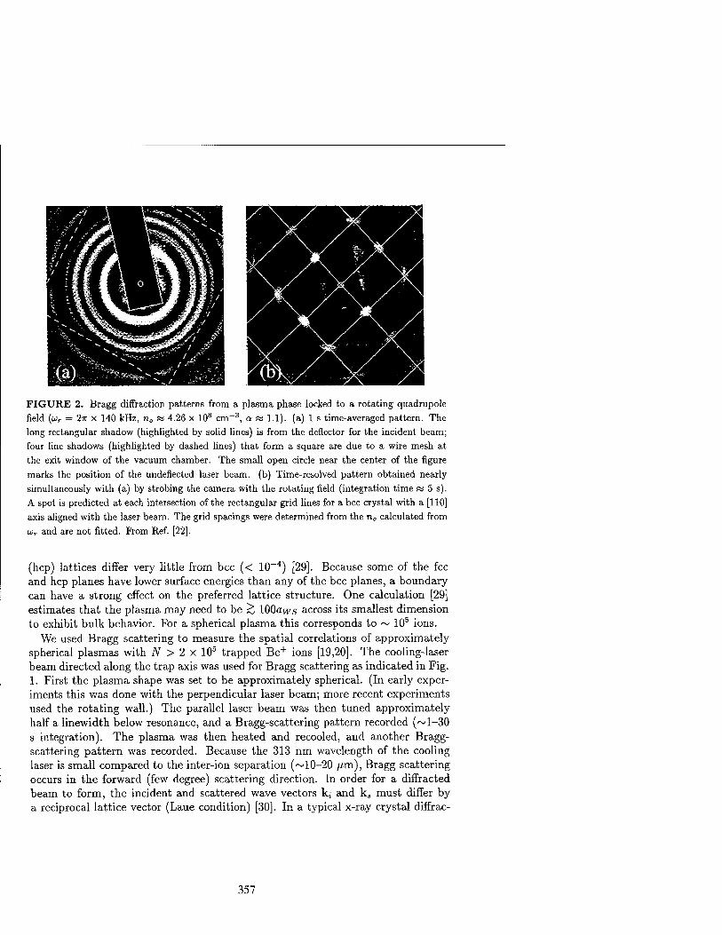
in FIGURE 2. Bragg diffraction patterns from a plasma phase locked to a rotating quadrupole field (wr = 2TT x 140 kHz, n0 « 4.26 x 10s cm-3, a fa 1.1). (a) 1 s time-averaged pattern. The long rectangular shadow (highlighted by solid lines) is from the deflector for the incident beam; four line shadows (highlighted by dashed lines) that form a square are due to a wire mesh at the exit window of the vacuum chamber. The small open circle near the center of the figure marks the position of the undeflected laser beam, (b) Time-resolved pattern obtained nearly simultaneously with (a) by strobing the camera with the rotating field (integration time sa 5 s). A spot is predicted at each intersection of the rectangular grid lines for a bcc crystal with a [110] axis aligned with the laser beam. The grid spacings were determined from the n0 calculated from ur and are not fitted. From Ref. [22].

(hep) lattices differ very little from bcc (< 10~4) [29]. Because some of the fee and hep planes have lower surface energies than any of the bcc planes, a boundary can have a strong effect on the preferred lattice structure. One calculation [29] estimates that the plasma may need to be <; lOOaws across its smallest dimension to exhibit bulk behavior. For a spherical plasma this corresponds to ~ 105 ions.

We used Bragg scattering to measure the spatial correlations of approximately spherical plasmas with N > 2 x 105 trapped Be+ ions [19,20]. The cooling-laser beam directed along the trap axis was used for Bragg scattering as indicated in Fig. 1. First the plasma shape was set to be approximately spherical. (In early experiments this was done with the perpendicular laser beam; more recent experiments used the rotating wall.) The parallel laser beam was then tuned approximately half a linewidth below resonance, and a Bragg-scattering pattern recorded (~l-30 s integration). The plasma was then heated and recooled, and another Bragg- scattering pattern was recorded. Because the 313 nm wavelength of the cooling laser is small compared to the inter-ion separation (~10-20 /im), Bragg scattering occurs in the forward (few degree) scattering direction. In order for a diffracted beam to form, the incident and scattered wave vectors k,- and ks must differ by a reciprocal lattice vector (Laue condition) [30]. In a typical x-ray crystal diffrac-

357

1 <2 VT 2 V5~ (/) 25 *" cfl Q. 20 C o c> 15 m

x> 10 o k.

5 E 3 C u M

10 12 14 16 q a ws

FIGURE 3. Histogram showing the numbers (not intensities) of peaks observed as a function of q ■ aws (defined in the text) for 30 time-averaged Bragg scattering patterns obtained on two different spherical plasmas with N > 2 x 105. The dotted lines show the expected peak positions for a bec crystal, normalized to the center of gravity of the peak at A (corresponding to Bragg reflections off {110} planes). From Ref. [20].

tion case, satisfying the Laue condition for many reciprocal lattice vectors requires that the incident radiation have a continuous range of wavelengths. Here the Laue condition is relaxed because of the small size of the crystal, so a crystalline Bragg diffraction pattern is frequently obtained even with monochromatic radiation.

Figure 2(a) shows a time-averaged diffraction pattern obtained on a spherical plasma with N ~ 7.5 x 105. The multiple concentric rings are due to Bragg scattering off different planes of a crystal. A concentric ring rather than a dot pattern is observed because the crystal was rotating about the laser beam. In general, many different patterns were observed, corresponding to Bragg scattering off crystals with different orientations. Figure 3 summarizes the analysis of approximately 30 time-averaged patterns obtained on two different spherical plasmas with N > 2 X 105. It shows the number of Bragg peaks as a function of the momentum transfer q=\ks — k; |= 2fc sm(9scatt/2) (~ k0scatt for 0scatt < 1), where k = 2-K/\ is the laser wave number and 6scatt is the scattering angle. The density dependence of the Bragg peak positions is removed by multiplying q by aws, which was determined from ujr. The positions of the peaks agree with those calculated for a bec lattice, within the 2.5% uncertainty of the angular calibration. They disagree by about 10% with the values calculated for an fee lattice. The ratios of the peak positions of the first five peaks agree within about 1% with the calculated ratios for a bec lattice. This provides strong evidence for the formation of bec crystals in spherical plasmas with N > 2 x 105 ions. This result is significant because it is the first evidence for bulk behavior in a strongly coupled OCP in the laboratory.

358

Rotating Wall

By strobing the camera recording the Bragg-scattering pattern synchronously with the plasma rotation, we should be able to recover a dot pattern from the time-averaged concentric ring pattern in Fig. 2(a). Initially we used the time dependence of the Bragg-scattered light to sense the phase of the plasma rotation [20,31]. More recently we used a rotating electric-field perturbation to phase-lock the ion plasma rotation [21,22].

Consider the rotating quadrupolar perturbation shown in the inset of Fig. 1. This ^-independent perturbation produces a small distortion in the shape of the spheroidal plasma. In particular, the plasma acquires a small elliptical cross section normal to the z-axis. (In our work the distortion created by the rotating quadrupole field was typically less than 1% of the plasma diameter.) The elliptical boundary rotates at the applied rotating wall frequency LOW. An ion near the plasma boundary experiences a torque due to this rotating boundary. If the ion is rotating slower than OJW, the torque will speed it up. If it is rotating faster than ww, the torque will slow it down. Through viscous effects, this torque is transmitted to the plasma interior. Therefore, if other external torques are small, the rotating wall perturbation will make wr equal UJW. Crystallized plasmas behave more like a solid than a liquid or gas. Because the viscosity is high, the whole plasma tends to rotate rigidly with its boundary. In particular, the orientation of the ion crystals can phase-lock to the rotating quadrupolar perturbation if the difference between wr and ww is small.

To check for phase-locked control of uv, we strobed the camera recording the Bragg-scattering pattern in Fig. 2(a) with the synthesizer used to generate the rotating wall signal. Specifically, once each 27r/w„, period, the rotating wall signal gated the camera on for a period < 0.02(2TT/U;,„). The resulting Laue dot pattern in Fig. 2(b) shows that the plasma rotation was phase-locked to the rotating electric- field perturbation. The dot pattern provides detailed information on the number and orientation of the crystals which contributed to the Bragg-scattering signal. For example, the pattern in Fig. 2(b) was due to a single bcc crystal with a [110] axis aligned along the laser beam. For phase-locked operation of the rotating wall, other external torques must be small. For example, a misalignment of the trap magnetic field with the trap-electrode symmetry axis of > 0.01° prevented phase- locked control of the plasma rotation. In our work, alignment to < 0.003° was obtained by minimizing the excitation of zero-frequency plasma modes [27,28].

In addition to the rotating quadrupole perturbation, phase-locked control was also achieved with a uniform rotating electric field (a "dipole" field). In fact under many circumstances a uniform oscillating field worked equally well. In these cases the co-rotating component of the oscillating field controlled the plasma rotation, while the perturbing effects due to the counter-rotating component were minimal. For further discussion, see Ref. [22].

359

lUiihi* »,< v«^^^^^,•'iv',,

1.2 mm 0.5 mm FIGURE 4. Real-space images of an N ~ 1.8 x 105 ion plasma phase-locked with an oscillating dipole field at u>r = 2ir x 120 kHz. (a) Time-averaged side-view image showing the overall plasma shape. The bright line of fluorescence through the plasma center is due to a laser beam directed perpendicularly to B0. The plasma shape is approximately spherical. The presence of heavier-mass ions, which centrifugally separate from the 9Be+ ions, produces the straight vertical boundaries in the image, (b) Strobed top-view image, obtained simultaneously with (a), showing the presence of a bcc crystal in the plasma center. The distance scales in (a) and (b) are different, as noted.

REAL-SPACE IMAGES

Bragg scattering measures the Fourier transform of the spatial correlations of the trapped ions. It provides a picture of these correlations in reciprocal-lattice space. With phase-locked control of Lor, real-space imaging of individual ions in a Penning trap becomes possible. To obtain real-space images with high resolution, we replaced the Bragg scattering optics (see Fig. 1) with imaging optics, starting with an f/2 objective, which formed a real, top-view image of the ion plasma. The combined resolution limit of the optics and camera was less than 5 /im near the optimal object plane of the f/2 objective. This is less than the ~10 /urn resolution limit required to resolve individual ions. However, the depth of field of an f/2 objective for 10 fim resolution is ~80 /im. For lenticular plasmas with 2z0 < 80 /im, all of the ions within the plasma were resolvable. For plasmas with 2z0 > 80 /im, the cooling-laser beam directed perpendicularly to B0 was used to illuminate a section of the plasma within the depth of field.

Figure 4 shows side-view and top-view images of an approximately spherical plasma with N ~ 1.8 X 105. The fluorescence from the perpendicular laser beam used to highlight a small region of the plasma is clearly visible. In the top-view

360

■, r *• • * * • t i i

* * ■■■ \ • S * * * «. k

* * * » ;: , v ^ > .^ *, .- * * „ * * f • i - ' I V". •> « r„.

** * ■ "* '

* * -. -* * ,. . * ." ( .• * "*. % V * ^* *. r a : *■.. <

• -.<*..»,».•

(b) ■UMfMfe^lJ*«» ■ *■*

"?*' !

FIGURE 5. Strobed top-view images of a small (JV ~ 300 Be+) ion plasma phase-locked with a rotating dipole field at (a) ur — 2n x 65.7 kHz and (b) 66.5 kHz. Below are unstrobed side-views showing the axial lattice planes. Heavier-mass ions are located outside the 9Be+ ions.

image a square grid of dots is observed near the plasma center. The measured spacing between nearest neighbor dots is 12.8 ± 0.3 yum, in good agreement with the 12.5 fim spacing expected for viewing along a [100] axis of a bcc crystal with density determined by the wr set by the rotating field. Real-space imaging provides direct information on the location and size of the crystals. In Fig. 4 the crystal was located in the radial center of the plasma and was at least 230 /mi across, or at least 1/4 of the plasma diameter.

For lenticular plasmas with 2z0 < 80 fim, all of the ions within the plasma are resolved without the use of the perpendicular laser beam. Lenticular plasmas are obtained with wr slightly greater than wm. For small plasmas (N ^ 2000 ions) we were able to use the rotating-dipole electric field to lower u>r and obtain a single plane while maintaining long-range order in the top-view images. Figure 5(a) shows top- and side-view images of such a plasma. Near the plasma center a 2-D hexagonal lattice is observed, the preferred lattice for a 2-D system. Here each dot is the image of an individual ion.

Starting with a single plane like that shown in Fig. 5(a), we studied the structural phase transitions that occur as wr is increased [23]. With increasing ur, the radial confining force of the Penning trap increases, which decreases r0. At a particular point, there is a structural phase transition near the plasma center from a single, hexagonal lattice plane to two lattice planes where the ions form a square grid in each plane, as shown in Fig. 5(b). Further increases in u>r increase the number of

361

ions per unit area of each plane as well as the spacing between the planes. During this process the square lattice planes smoothly change into rhombic lattice planes and eventually there is a sudden transition to hexagonal lattice planes. Further increases in u>r eventually produce a structural transition to three square lattice planes, and the basic pattern repeats.

The structure of the crystallized ions depends sensitively on the projected areal density a of the plasma. The side- and top-view images were analyzed to characterize the phase structure. Within a layer, the structural order is characterized by the primitive vectors ai and a2 (which are observed to be equal in magnitude) and the angle 6 (< 90°) between them. The interlayer order is characterized by the axial positions zn of the n lattice planes (measured by the side-view camera) and the interlayer displacement vector cn between layers 1 and n. Hence, the equilibrium positions in the (x,y) plane of ions in axial planes 1 and n are given by Ri = isn + ja2 and Rn = iai + ja2 + cn, where i,j are integers. Three different types of intralayer ordering are observed: hexagonal (0 = 60°), square (0 = 90°) and rhombic (90° > 0 > 65°). The observations were compared to the results from Dubin [23], who performed an analytic calculation of the energies of lattice planes which are infinite and homogeneous in the (x,y) direction but are confined in the axial direction by a harmonic external electrostatic confinement potential 4>e — l/2(m/e)w2z2. Since this potential is identical to the confinement potential of a Penning trap as seen in the rotating frame in the a —► 0 planar limit, the minimum-energy phase structures predicted by the theory should match the structures observed in the central regions of the oblate plasmas of the experiments.

Figure 6 displays the agreement between theory and experiment for the interlayer quantities, with measurements taken on different plasmas with N < 104. Lengths have been normalized by aws2n — (3e2/47re0n^^)1^3 = 10.7 /im, which is the Wigner-Seitz radius in the planar limit. As the central areal density is increased the lattice planes move further apart axially in order to match their average density to the neutralizing background. Eventually it becomes energetically favorable to form an additional lattice plane. The symbols indicate whether the lattices had an interlattice displacement vector c2 characteristic of the hexagonal phases (triangles) or the square and rhombic phases (squares).

Figure 7 displays the agreement between experiment and theory for the dependence of the angle 0 (between the primitive vectors) on central areal charge density a. The trend is that when a new lattice plane is formed, 0 changes discontinuously from « 60° to a higher value. As the central areal density of the crystal is further increased, 6 smoothly decreases to w 65° until there is a second discontinuous transition to a hexagonal structure. This latter transition has been predicted [32] to become continuous in liquid (T < 80) bilayer systems. The lines indicate the minimum energy structures predicted by the 2D theory.

362

-i |

3 c: n

Ü en () . Q.

1 CO X TO

0.5 1.0 1.5 2.0

a a s2D (central areal charge density)

FIGURE 6. Interlayer structure (plane axial positions and displacement vectors) as a function of normalized areal charge density. The lines are the predictions of theory, and the symbols are

experimental measurements.

90

1 1

7% ! *Df

In 85 . -b CD 05

#80

CD 1- -*1 D) 75 c c TO

a a* (central areal charge density)

FIGURE 7. Intralayer angle 8 structure as a function of normalized areal charge density. The lines are the predictions of theory, and the symbols are experimental measurements. Representa- tive error bars are included with some of the measurements.

363

DISCUSSION

With Bragg scattering and spatial imaging, we have measured the correlations in both spherical and highly oblate strongly coupled 9Be+ ion plasmas. The planar geometry permits a detailed comparison with theoretical calculations. We have measured the preferred lattice structures for up to five lattice planes in lenticular plasmas and obtain good agreement with theory. Ions in a trap have been proposed as a register for a quantum computer [33]. Work in this area has focussed on a string of a few ions in a linear Paul trap [34]. A single lattice plane of ions as in Fig. 5 could provide a 2-D geometry of trapped ions for studies of quantum computing or entangled quantum states.

In spherical plasmas with more than 2 x 105 ions, we have observed the formation of bec crystals, the predicted state for the infinite strongly coupled OCP. The crystals occupied the inner quarter of the plasma diameter. Outside the crystal there was a complicated transition to shell structure. In this system we have not observed the thermodynamic liquid-solid phase transition predicted for the bulk OCP. The phase transition may take place in the present system, but we have experimentally missed detecting it. Or, possibly larger crystals (for example, where the number of ions in the crystal is large compared to the number of ions in the shells) may be required in order for a sharp phase transition to be exhibited.

We have observed structures for which we do not have a good theoretical understanding. Figure 8(a) shows an approximate fivefold Bragg-scattering pattern that was observed a number of times under different experimental circumstances. A fivefold Bragg-scattering pattern is characteristic of a quasi-crystal. However, more sets of dots would be present in a true quasi-crystalline Bragg-scattering pattern. We now think that the fivefold Bragg-scattering pattern of Fig. 8(a) is due to a structure like that shown in Fig. 8(b). Figure 8(b) is a top-view image of a lenticular plasma which consisted of four horizontal planes. Even though it is difficult to distinguish individual ions in this figure, it is possible to see that there are five distinct regions where the ions resided in vertical planes. The planes from these different regions form a five-sided structure that would produce a Bragg scattering pattern like Fig. 8(a). Once formed, this fivefold structure was stable.

In addition to enhancing studies of Coulomb crystals, the phase-locked control of wr has improved the prospects of a microwave frequency standard based on a hyperfine-Zeeman transition of ions stored in a Penning trap. This is because the time-dilation shift due to the plasma rotation is one of the largest known systematic shifts in such a standard. Reference [35] discusses the potential frequency stability and accuracy of a microwave frequency standard based on 106 trapped ions. For ions such as 67Zn+ and 201Hg+, fractional frequency stabilities < 10_14/r1/2 with time-dilation shifts due to the plasma rotation of ~fewxlO~15 are possible. Here r is the measurement time in seconds. With phase-locked operation of the rotating wall, we think it should be possible to stabilize and evaluate the rotational time- dilation shift within 1%. Therefore the inaccuracy due to this shift would contribute a few parts in 10-17.

364

FIGURE 8. Fivefold Bragg scattering and real-space patterns obtained by strobing the intensi- fied CCD camera synchronously with the rotating electric field perturbation, (a) Bragg scattering pattern obtained on an JV ~ 1.2 x 105 ion plasma phase-locked with a rotating dipole field at wr = 2TT x 166.84 kHz. Here V0 - 500 V and a - 2.6. (b) Real-space image of a lenticular plasma consisting of 4 horizontal planes in the plasma center. The rotating dipole field was used to set

wr = 2TT x 74.35 kHz.

ACKNOWLEDGEMENTS

We gratefully acknowledge the support of the Office of Naval Research. We thank

S. L. Gilbert and R. J. Rafac for their comments on the manuscript.

REFERENCES

1. Bollinger, J. J., et al., in Trapped Charged Particles and Fundamental Physics, Dubin, D. H. E., and Schneider, D., ed. AIP, New York: 1999, pp. 295-304.

2. Mitchell, T. B., et al., Phys. Plasmas 6, 1751 (1999). 3. Ichimaru, S., Iyetomi, H., and Tanaka, S., Phys. Rep. 149, 91-205 (1987). 4. Malmberg, J. H., and O'Neil, T. M., Phys. Rev. Lett. 39, 1333-1336 (1977). 5. Horn, H. M. V., Science 252, 384-389 (1991). 6. Grimes, C. C., and Adams, G., Phys. Rev. Lett. 42, 795-798 (1979). 7. E. L. Pollock and J. P. Hansen, Phys. Rev. A 8, 3110-3122 (1973); W. L. Slattery,

G. D. Doolen, and H. E. DeWitt, ibid. 21, 2087-2095 (1980); W. L. Slattery, G. D. Doolen, and H. E. DeWitt, ibid. 26, 2255-2258 (1982); S. Ogata and S. Ichimaru, ibid. 36 5451-5454 (1987); G. S. Stringfellow and H. E. DeWitt, ibid. 41, 1105-1111 (1990); D. H. E. Dubin, ibid. 42, 4972-4982 (1990).

8. Schiffer, J. P., Science 279, 675 (1998). 9. Diedrich, F., et al., Phys. Rev. Lett. 59, 2931-2934 (1987).

365

10. Wineland, D. J., et al, Phys. Rev. Lett. 59, 2935-2938 (1987). 11. Strongly coupled clusters of highly charged, micrometer-sized aluminum particles

were previously observed in Paul traps. See R. F. Wuerker, H. Shelton, and R. V. Langmuir, J. Appl. Phys. 30, 342-349 (1959).

12. Gilbert, S. L., Bollinger, J. J., and Wineland, D. J., Phys. Rev. Lett. 2022-2025 (1988).

13. Birkl, G., Kassner, S., and Walther, H., Nature 357, 310-313 (1992). 14. Drewsen, M., et al, Phys. Rev. Lett. 81, 2878 (1998). 15. Walther, H., Adv. At. Opt. Phys. 31, 137-182 (1993). 16. Melzer, A., Homann, A., and Piel, A., Phys. Rev. E 53, 2757 (1996). 17. Murray, C. A., and Grier, D. G., American Scientist 83, 238-245 (1995). 18. Vos, W. L., Mehens, M., van Kats, C. M., and Bösecke, P., Langmuir 13, 6004-6008

(1997). 19. Tan, J. N., Bollinger, J. J., Jelenkovic, B., and Wineland, D. J., Phys. Rev. Lett. 75,

4198-4201 (1995). 20. Itano, W. M., et al, Science 279, 686-689 (1998). 21. Huang, X.-P., Bollinger, J. J., Mitchell, T. B., and Itano, W. M., Phys. Rev. Lett.

80, 73-76 (1998). 22. Huang, X.-P., Bollinger, J. J., Mitchell, T. B., and Itano, W. M., Phys. Plasmas 5,

1656-1663 (1998). 23. Mitchell, T. B., et al, Science 282, 1290 (1998). 24. Brewer, L. R., et al, Phys. Rev. A 38, 859-873 (1988). 25. Davidson, R. C., Physics of Nonneutral Plasmas Addison-Wesley Publishing: 1990,

pp. 39-75. 26. O'Neil, T. M., and Dubin, D. H. E., Phys. Plasmas 5, 2163-2193 (1998). 27. Heinzen, D. J., et al, Phys. Rev. Lett. 66, 2080-2083 (1991). 28. Bollinger, J. J., et al., Phys. Rev. A 48, 525-545 (1993). 29. Dubin, D. H. E., Phys. Rev. A 40, 1140-1143 (1989). 30. Ashcroft, N. W., and Mermin, N. D., Solid State Physics Saunders College: 1976,

pp. 95-110. 31. Tan, J. N., et al., in Proceedings of the International Conference on Physics of

Strongly Coupled Plasmas, Kraeft, W. D., and Schlanges, M., ed. World Scientific: 1996, pp. 387-396.

32. Valtchinov, V. I., Kaiman, G., and Blagoev, K. B., Phys. Rev. E 56, 4351-4355 (1997).

33. Cirac, J. I., and Zoller, P., Phys. Rev. Lett. 74, 4091-4094 (1995). 34. Wineland, D. J., et al., J. Res. Natl. Inst. Stand. Technol. 103, 259-328 (1998). 35. Tan, J. N., Bollinger, J. J., and Wineland, D. J., IEEE Trans. Instrum. Meas. 44,

144-147 (1995).

366

An Ultracold Neutral Plasma

Simone Kulin, Thomas C. Killian, Scott D. Bergeson*, Luis A. Orozco*, Chad Orzel, and Steven L. Rolston

National Institute of Standards and Technology, Gaithersburg, Maryland 20899-8424 t Department of Physics and Astronomy, Brigham Young University, Provo, Utah 84602-4 ,

'Department of Physics and Astronomy, State University of New York, Stony Brook, New York 11794-3800

Abstract. We present the first experiment to observe an ultracold neutral plasma. The plasma, which was created by photoionization of laser cooled atoms, has charge densities as high as 2 x 109cm-3, and the temperatures of electrons and ions are as low as 100mK and 10 /xK, respectively. The plasma has a lifetime of about 100 fj,s, much longer than predicted by recombination rates. When the laser that excites the atoms is tuned below the ionization limit we create a sample of very highly excited cold Rydberg atoms. At our highest densities and during a time of a few microseconds, in which the Rydberg atoms are essentially stationary, the ensemble evolves towards an unbound plasma-like state.

INTRODUCTION

Creating a neutral plasma at very low temperatures has for many years been an experimental challenge. By photoionizing a sample of laser cooled atoms we obtain a plasma that has electron temperatures as low as Te = 100 mK and ion temperatures as low as T,- = 10 /uK. The density of the ultracold plasma is as high as 2 x 109 cm-3. This new plasma is well suited to investigate and perhaps answer questions that are also important for nonneutral plasmas. The three-body recombination rate at low temperatures, for instance, is of great relevance for the success of the various antihydrogen projects underway [1]. Also, for both electrons and ions, the Coulomb interaction energy between nearest neighbours exceeds the the initial thermal energy of the particles.

This paper is organized as follows: In part I we introduce the atomic system and describe the experimental setup. We then discuss the temporal sequence of the experiment, and present the data. In section II, we develop a simple model that explains the experimental results and we discuss a numerical simulation that reproduces the data. The characteristics of the plasma are given in section III. The plasma opens the way to a number of interesting new experiments, some of which we shall briefly mention in section IV. We conclude by considering the possibility


367

of obtaining such a cold plasma during a phase transition from a dense sample of highly excited, cold Rydberg atoms. Preliminary experimental results are shown.

THE ATOMIC SYSTEM AND THE EXPERIMENTAL SETUP

The heart of our experiment is a sample of laser cooled metastable xenon atoms. The metastable 6s[3/2]2 state in xenon has an optical dipole transition at 882 nm to the 6p[5/2]3 state. The lifetime of this lower state is 43 s [2] and can therefore be treated as the ground state for laser cooling. The metastable atoms are produced in a gas discharge, and after deceleration using the Zeeman slowing technique, the atoms are collected in a magneto-optical trap. Further cooling by optical molasses reduces the temperature of the atoms to approximately 10 (iK. This slowing and trapping sequence is described in detail in [3]. The number of cold atoms and the size of the cloud can be determined by optical absorption imaging [4]. Typically we prepare samples of a few million atoms at a density of 2 x 10locm~3. The spatial distribution is Gaussian with a rms radius er ~ 200 /J,m.

To produce a plasma, a fraction of the cold atom sample is photoionized. The photoionization process requires two photons. The first photon at 882 nm is resonant with the cooling transition. From the 6p[5/2]3 state a green photon at 514nm excites the atoms to states at the ionization potential or above. In the experiment, the infrared light is provided by a Tirsapphire laser. The green light is supplied by a pulsed dye laser, that is pumped by a pulsed frequency tripled Nd:YAG laser. One laser pulse lasts approximately 10 ns and carries about 1 mJ of energy. We can ionize up to 10% of the cold atoms, which corresponds to an ion (and also an electron) density n = 2 x 109cm~3. The number of atoms photoionized increases linearly with the green laser intensity.

An externally applied electric field directs the electrons towards a single channel electron multiplier and the ions towards a microchannel plate. The neutral atoms fall free and are also recorded on the microchannel plates.

The temporal sequence of each experimental cycle is described below. First, the atoms are laser cooled and a small electric field of approximately 5mV/cm is applied. The atoms are then photoionized. Fig. 1 shows the recorded electron signal for four different green laser pulse energies. The photoionization occurs at time t = 0. A first pulse of electrons arrives at the detector after about 500 ns of time of flight. If the green laser pulse has enough energy, the first peak develops a tail and a second peak appears when the electric field is linearly increased a few microseconds later. During this time the ions are essentially stationary. They arrive and are detected on the microchannel plates about 300^s after photoionization.

368

II MODEL AND NUMERICAL SIMULATION

The experimental data presented in Fig.l are explained by a simple physical picture (see schematic in Fig. 2). Immediately after photoionization, the charge distribution is everywhere neutral but electrons and ions have acquired kinetic energy. This energy comes from the difference in energy AE between the energy of the green photon and the ionization potential. Because of the large mass ratio between ions and electrons (2.4 x 105) most of the energy AE is taken by the electrons in the form of kinetic energy. Therefore the electron cloud begins expanding, and a local charge imbalance builds up. The resulting internal electric field establishes a Coulomb potential energy well for electrons. The depth of this well is proportional to the number of electrons that have escaped. If the well never becomes deeper than their initial kinetic energy, all electrons escape. This is the case for the uppermost curve in Fig. 1. If many more atoms are photoionized, however, only an outer shell of electrons escapes and the well becomes deep enough to trap the rest. Inside the well, electrons will thermalize through collisions within 10 - 100 ns [6]. During this energy redistribution process, some particles acquire energies larger than the trap depth and will leave the well. This process of evaporation explains the tail of the first peak in the electron signal. As electrons continue to leave the trap, the depth of the potential well increases and eventually evaporation slows down. The remaining electrons stay in the well until an external electric field overcomes the trapping potential. They constitute the second peak that appears in Fig. 1.

According to the model described above, all electrons leave unless the potential well created by the positive ions exeeds the kinetic energy (~ AE) of the electrons.

0.15

4 Time [/is]

FIGURE 1. Electron time of flight signals. Photoionization occurs at t = 0. The initial kinetic energy of the electrons is AE/kß — 0.6 K. The uppermost curve corresponds to the lowest pulse energy of the green laser (charged particle density n « 105cm-3), and the bottom curve to the the highest pulse energy (n « 107cm~3). The data is averaged over 20 consecutive experimental cycles. Also shown is the magnitude of the applied electric field.

369

lo : li l2

M

C

i i i

A T r 'S

\ ! / /

0) \ i / I o

OH 1

e o t o

S3 <—3t—S

0 0 0 Position

FIGURE 2. Schematic of the potential energy seen by a test electron when enough atoms arc

photoionized to result in trapping of electrons. At t0 = 0 when photoionization occurs, the

sample is everywhere neutral. Because of their kinetic energy some electrons leave and the charge

imbalance yields a potential well. At <i « 10 ns the depth of the well equals the initial kinetic

energy, trapping the remaining electrons. Electrons in the well thermalize, evaporation occurs

and the well depth increases. By t2 « 1 fis evaporation essentially stops. The bottom of the

well is flat due to Debye screening. The dashed line indicates the average kinetic energy of the

electrons.

For a given AE this suggests a threshold number of photoions required to trap electrons. In the experiments, we can control the values of AE by varying the green laser frequency. We found that the number of ions required to trap electrons increases as the kinetic energy of the electrons increases. This threshold behaviour appears clearly in a plot of the fraction of electrons trapped versus the number of photoions created, and is shown in Fig. 3a.

The number N* of positive ions at the threshold can be readily estimated, considering that the spatial distribution of the charges is Gaussian. At threshold the well depth of the potential energy of a. cloud of A'* ions equals the kinetic energy of the electrons: N*U0 - AE. Here U0 is the depth of a potential well created by a Gaussian spatial distribution of total charge equal to the elementary charge e [5]. Over a large range of electron kinetic energies, this simple relation describes well the onset of trapping for the data shown in Fig. 3a. This behaviour becomes more evident when the number of photoions produced is scaled by N*. As shown in Fig. 3b all data fall on one curve, which is reproduced by a numerical integration of the equations of motion [7].

In the model we have so far included the Coulomb interaction between electrons and ions, and rethermalization of electrons in the well through collisions. The interaction between opposite charges explains the trapping of electrons by the positive ion cloud. Evaporation of electrons from the well suggests that the temperature of the electrons is Te < AE/kß, a result which is confirmed by the numerical simulation. We have neglected collisons which lead to equipartition of energy between

370

N N/N* FIGURE 3. (a) Fraction of electrons trapped versus number of photoions created. Each curve corresponds to a different green laser frequency, i.e. a different initial kinetic energy of the electrons, (b) Same as (a) but the number of photoions is scaled by JV*, the estimated threshold for trapping. The line is the result of a numerical simulation. There is a scale uncertainty of about 10% in determining the fraction of electrons trapped.

electrons and ions. For our experimental conditions, this process requires tens of ms [6], a time much longer than the duration of the experiment. Also, collisions between charged particles and neutral atoms may occur, but in the experiment we see no evidence of such interactions. The mean free path for atom-charged particle collisions is much larger than the size of the sample [8-10].

A complete model should also discuss the properties and the evolution of the positive ions. Their initial temperature is easily estimated. For excitation close to the ionization potential the energy imparted to the ions is negligible compared to the initial kinetic energy of the atoms. Therefore the minimal initial temperature is 10 fj,K. For large values of AE the temperature is given by 4 x 10~6 AE/kj3, which corresponds to 4mK for AE/kß = 1000 K. Also, after the untrapped fraction of electrons has escaped the charge imbalance leads to a Coulomb expansion of the cloud. The potential well depth decreases and formerly trapped electrons will be able to escape. This limits the time during which the electrons can be held in the trap. However, the electrons escape most easily from the outer edges of the spatial distribution', and for N > N* the center of the cloud is still neutral, a behaviour that also appears in the simulation. The presence of the electrons screens the Coulomb interaction between ions causing the expansion of the cloud to be slowed compared to that of a bare cloud of positive ions. For instance, a cloud of 5000 ions, initially with a = 200 jum reduces its well depth by a factor of two within a few microseconds. Experimentally, we observed that a cloud of 5000 photoions with only 10% charge imbalance holds half of the initially trapped electrons for

about 100 /us.

371

Ill THE ULTRACOLD PLASMA

Both the model and the simulation discussed above describe well the ionized gas that we obtain by photoionizing the laser cooled atoms. At this point one may ask whether this system is a plasma. Traditional plasmas are often defined in terms of the Debye screening length. An ionized gas is a plasma when the size of the sample is larger than the Debye length [11]. In our experiments the Debye length, which is

given by Ay = •v/c0/cgTc/e2n, can be as low as 500nm, while the size of the sample is about 200/im.

The threshold condition N = N* for electrons to be trapped is mathematically equivalent to Xp — a. If N > N* electrons are trapped by an internal electric field in the ion cloud. Equivalently if \D < a, any displacement of electrons from their equilibrium positions due to their thermal energy is counterbalanced by the local internal electric field; a plasma is formed. If jV < N*, the well depth of all the photoions is smaller than the kinetic energy of the electrons and they all leave. This condition is equivalent to \p > a, which means that the electrons are free to escape.

The low temperatures of the electrons and ions allow access to a new region of parameter space of neutral plasmas. The Coulomb interaction energy between nearest neighbours can be less than the thermal energy of the particles. This situation is characterized quantitatively by the Coulomb coupling parameters [12] re = (e2/(4ne0a))/(kBTe) for electrons and T, = e-^^F.TJT, for ions. Here a = (47rn/3)-1'3 is the Wigner-Seitz radius. The exponential factor in the expression of T, is due to the shielding of the ion-ion interaction by electrons. Plasmas that are in a state of thermal equilibrium and for which T > 1 are known as strongly coupled plasmas [12]. In our experiment, densities and temperatures can be such that the numerical values of the coupling parameters are Te = 10 and I\ = 1000. However, electrons and ions are not in thermal equilibrium, but they each have thermalized with themselves.

IV FUTURE EXPERIMENTS

The properties of traditional plasmas, in which the temperature spans a range from 1016K to 300K have been extensively studied [11]. At lower temperature the properties of a plasma, and in particular the recombination rates are expected to change. At high temperatures three-body recombination processes have a very strong temperature dependence (oc T~9//2) [13] and can exceed the radiative recombination rate (oc T-1/2) only at very high densities (> 1016cm-3) [14]. An extrapolation to the conditions in our experiment results in radiative recombination times of tens of seconds and three-body recombination times of nanoseconds (for Te = 1 K and n = 2 x 108cm-3). The long lifetimes we observed (ss 100/us) suggest that the theory, and also an extension to T m IK [15], is no longer valid.

372

Studies of the three-body recombination rate in the ultracold plasma are currently

under way.

With this new plasma a series of interesting experiments can be performed. Plasma oscillations, which have frequencies of up to 400 MHz can be used to determine the density distribution of the system. Magnetic confinement may be used to increase the lifetime of the plasma. Also thermalization and evaporative cooling of electrons need further study. In the current experimental setup, the lowest initial temperature of the electrons is 100 mK, and is limited by the bandwidth of the green laser (0.07cm-1). This temperature could be reduced to about 10mK by using a laser with a bandwidth equal to the Fourier transform of a 10 ns pulse.

Instead of photoionizing the cold atoms, one can tune the laser below the ionization potential and excite the atoms into very high lying Rydberg states. Such a dense cold gas of Rydberg atoms may undergo a phase transition to a plasma-like state [16]. We have performed preliminary experiments aimed to verify this prediction. The time sequence of these experiments is the same as the one described earlier for the plasma creation. The only difference is that the magnitude of the ramped electric field must be higher in order to be able to field-ionize the bound Rydberg states. Fig. 4a shows the electron signal recorded for two different densities of cold Rydberg atoms. At low density the large double peak in the signal is due to field-ionized Rydberg atoms. At higher densities an early peak of weakly

0.15-

o.oo

< 3

T 50

Arrival time (us) 100

1.0-

0.8-

0.6-

fc 0.2

Initial Rydberg atom density (cm" )

FIGURE 4. Excitation of laser cooled atoms into Rydberg states with principal quantum number 140. (a) Electron time of flight signals recorded for two different densities. At lower density, n = 5 x 106cm-3, the signal consists mainly of electrons from field-ionized Rydberg atoms (solid line). At high density, n = 5 x 107cm-3, the weakly bound electrons appear in an earlier peak (dotted line). Also shown is the applied electric field, (b) Fraction of electrons from field ionized Rydberg atoms (circles) and from weakly bound (plasma-like) states (triangles) as a function of initial density of Rydberg atoms.

373

bound electrons develops and the contribution of electrons from atoms is reduced. As the initial density of Rydberg atoms increases the fraction of electrons from field-ionized Rydberg atoms decreases, while the fraction of electrons in the early "plasma"-peak increases. This behaviour appears clearly in Fig. 4b. The onset of the transition is predicted to scale as the sixth power of the Rydberg principal quantum number and we are currently exploring this experimentally. The transition from the bound (Rydberg) states to an unbound plasma-like state is suggestive of insulator-conductor transitions, that are often referred to as Mott-transitions [17]. The cold and dense gas of Rydberg atoms is well suited for studying the insulator- conductor phase transition, since, unlike in solid state physics, we have control over parameters such as the temperature and density of the system.

CONCLUSION

We have created a new, ultracold, neutral plasma by photoionizing laser cooled atoms. The initial temperature of the ions T, ~ 10 /xK is essentially equal to that of the atoms, whereas the electron temperature depends on the laser frequency and can vary between Te — 0.1 - 1000 K. The densities of the ultracold plasma can be as high as n = 2 x 109 cm-3. The plasma is not confined and has a lifetime of about 100/is. This new system opens the way to a variety of studies, such as three-body recombination rates for temperatures less than 1 K and phase transitions between bound and unbound states. The technique is applicable to any atom that can be laser cooled.

S. Kulin acknowledges funding from the Alexander-von-Humboldt foundation, and T. C. Killian is supported by a NRC postdoctoral fellowship. This work was supported by ONR.

REFERENCES

1. Gabrielse G., Rolston S. L., Haarsma L., and Keils W., Phys. Lett. A 129, 38 (1988). 2. Walhout M., Witte A., and Rolston S. R., Phys. Rev. Lett. 72, 2843 (1994). 3. Walhout M., Mengens II. J. L., Witte A., and Rolston S. L., Phys. Rev. A 48, R879

(1993). 4. Walhout M., Sterr U., Orzel C-, Hoogerland M., and Rolston S. R., Phys. Rev. Lett.

74, 506 (1995). 5. The potential energy U0 is given by U0 = \Z2Jwe2/(4w(0(r). Here e0 designates the

electric permittivity of vacuum, e is the elementary charge, and a is the rms radius of the Gaussian spatial distribution. For a ~ 200/xK this yields U0/kß ^ 67 mK.

6. Spitzer L., Jr., Physics of Fully Ionized Gases, New York: John Wiley & Sons Inc., 1962.

7. In the simulation the initial velocity of the electrons v — \/2AE/m is assumed to be directed radially outward.

8. Haberland R., Fritsche L., and Noffke J., Phys. Rev. A 38, 2305 (1986).

374

9. Plenkiewicz B., Plenkiewicz P., Houee-Levin C, and Jay-Gerin P., Phys. Rev. A 38, 6120 (1988).

10. Mcllrath T. J., and Lucatorto T. B., Phys. Rev. Lett. 38, 1390 (1994). 11. Delcroix J.-L., and Bers A., Physique des plasmas, Paris: InterEditions/CNRS Edi-

tions, vol. 1 (1994). 12. Ichimaru S., Rev. Mod. Phys. 54, 1017 (1982). 13. Mansbach P., and Keck J., Phys. Rev. 181, 275 (1969). 14. Goldston R. J., and Rutherford P. H., Introduction to Plasma Physics, Bristol: In-

stitute of Physics Publishing (1995). 15. Hahn Y., Phys. Lett. A 231, 82 (1997). 16. Vitrant G., Raimond J. M., Gross M., and Haroche S., J. Phys. B: At. Mol. Phys.

15, L49 (1982). 17. Mott N., Proc. Phys. Soc. A62, 416 (1949).

375

Collective Modes in Strongly Coupled Dusty Plasmas 1

M. S. Murillo

MS BS59, Plasma Physics Applications Group Los Alamos National Laboratory

Los Alamos, N.M. 87545

Abstract. Dusty plasmas offer a new setting for exploring dynamical phenomena in the strong coupling regime. In contrast to nonneutral plasmas, screening occurs in the dusty plasma and the effective interaction is approximately of a Yukawa form; this leads to acoustic-like modes rather than Langmuir-like modes. Dust acoustic waves thus have a dispersion relation that exists for very low and very high frequencies and wavevectors. Here the interpolation ansatz method is used to construct a strong coupling theory that is valid over this range. In this method the correct hydrodynamic limit is recovered and the lowest-order sum rules are satisfied.

I INTRODUCTION

Laboratory dusty plasmas are multicomponent plasmas that contain large (~^m) grains that may have masses M as high as 1012 proton masses and have various shapes, compositions, and charges. In recent years such dusty plasmas are routinely created in the laboratory under controlled and increasingly well characterized conditions. The most common laboratory approach is to introduce spherical glass or plastic grains into a radio-frequency discharge plasma in which the electrode sheath acts as the trapping field. The grains are charged negatively, due to the higher electron mobility, and may have net charges as high as Q~—106 elementary charges. The neutral background acts to cool the grains to temperatures of order T~0.5eV\ Together, these two conditions of high charge and cool temperatures leads to large values of the Coulomb coupling parameter,

Q2

where a — (3/47rn)1/3 is half the mean intergrain spacing.

*) This research was supported by the Los Alamos National Laboratory Directed Research and Development (LDRD) program.

CP498, Non-Neutral Plasma Physics HI, edited by John J. Bollinger, et al. © 1999 American Institute of Physics 1-56396-913-0/99/S15.00

376

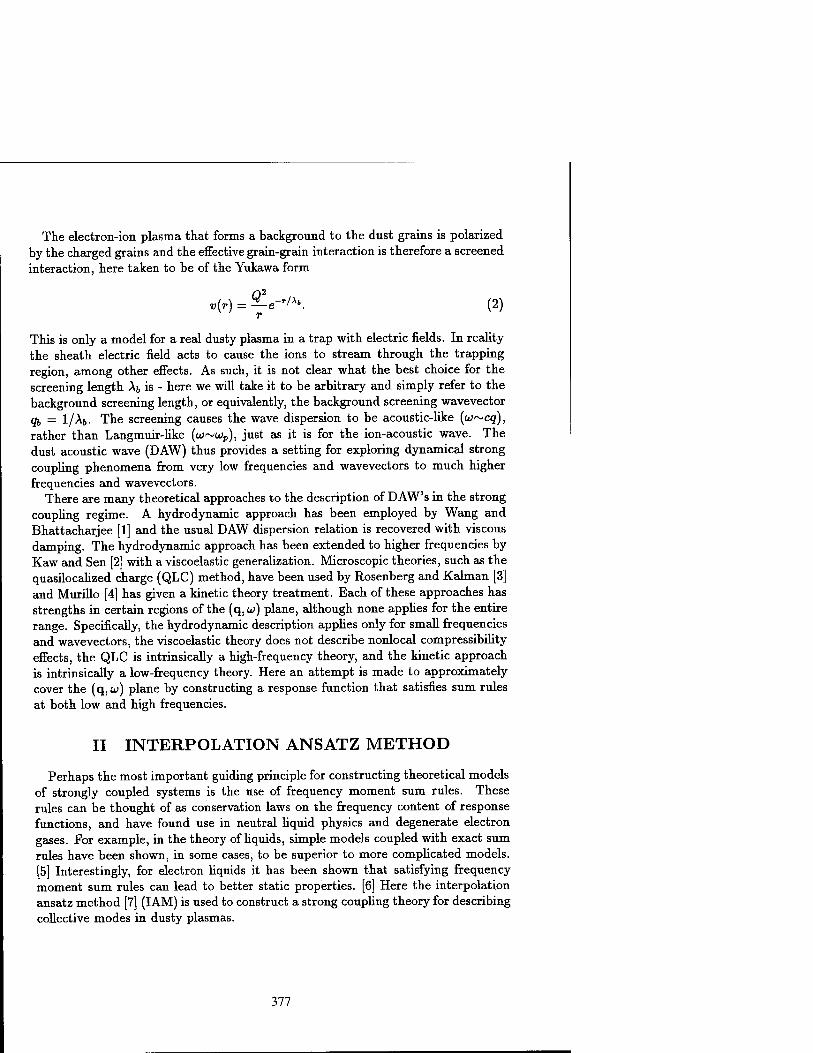
The electron-ion plasma that forms a background to the dust grains is polarized by the charged grains and the effective grain-grain interaction is therefore a screened interaction, here taken to be of the Yukawa form

v{r) = ^e-'/\ (2) r

This is only a model for a real dusty plasma in a trap with electric fields. In reality the sheath electric field acts to cause the ions to stream through the trapping region, among other effects. As such, it is not clear what the best choice for the screening length Aj, is - here we will take it to be arbitrary and simply refer to the background screening length, or equivalently, the background screening wavevector qb = 1/A&. The screening causes the wave dispersion to be acoustic-like (w~cq), rather than Langmuir-like (w~Wp), just as it is for the ion-acoustic wave. The dust acoustic wave (DAW) thus provides a setting for exploring dynamical strong coupling phenomena from very low frequencies and wavevectors to much higher frequencies and wavevectors.

There are many theoretical approaches to the description of D AW's in the strong coupling regime. A hydrodynamic approach has been employed by Wang and Bhattacharjee [1] and the usual DAW dispersion relation is recovered with viscous damping. The hydrodynamic approach has been extended to higher frequencies by Kaw and Sen [2] with a viscoelastic generalization. Microscopic theories, such as the quasilocalized charge (QLC) method, have been used by Rosenberg and Kaiman [3] and Murillo [4] has given a kinetic theory treatment. Each of these approaches has strengths in certain regions of the (q,w) plane, although none applies for the entire range. Specifically, the hydrodynamic description applies only for small frequencies and wavevectors, the viscoelastic theory does not describe nonlocal compressibility effects, the QLC is intrinsically a high-frequency theory, and the kinetic approach is intrinsically a low-frequency theory. Here an attempt is made to approximately cover the (q, a») plane by constructing a response function that satisfies sum rules at both low and high frequencies.

II INTERPOLATION ANSATZ METHOD

Perhaps the most important guiding principle for constructing theoretical models of strongly coupled systems is the use of frequency moment sum rules. These rules can be thought of as conservation laws on the frequency content of response functions, and have found use in neutral liquid physics and degenerate electron gases. For example, in the theory of liquids, simple models coupled with exact sum rules have been shown, in some cases, to be superior to more complicated models. [5] Interestingly, for electron liquids it has been shown that satisfying frequency moment sum rules can lead to better static properties. [6] Here the interpolation ansatz method [7] (IAM) is used to construct a strong coupling theory for describing collective modes in dusty plasmas.

377

The collective modes can be found from the poles of the response function x(q, w), defined by

%w) = x(q,«)^(q1«). (3)

This equation relates density fluctuations <Sn(q, w) to the strength of an external potential energy source [/e(q,w); clearly, the poles of x(q,w) correspond to finite density fluctuations for vanishingly small external perturbations. This equation is defined in terms of the wavevector q and the frequency w. The simplest starting point for calculating the response function is the ideal gas response function x'0)(q, w), again defined by

<^q,W)«X(°>(q,a;)[/e(q,u;). (4)

This can be improved by adding to the external potential a term that represents the interaction due to the other particles. That is, we can assume the dust grains are free particles that respond to an effective external potential of the form

£4(q,w) -» Ue((i,u)) + v(q)8n(ci,u). (5)

In terms of the definition (3), this gives a response function of the form

*n(q,«) = X(°)(q'j Ue(q,v) l-v(q)x^>(ci,w)

= Xm/(q,w)C/e(q,o;). (6)

This approximation is referred to as the "random phase approximation" or the "mean field approximation" (MFA) and, already with this approximation, we obtain collective modes of the form

w2 o2

- = 3^> (7) «5 g' + tf'

where the leading term in the large w expansion of X^°'(q, w) has been used. This is, of course, the usual (weak coupling) dispersion equation for DAW's.

Rather than using a relation such as (5), we can also view the MFA in terms of an excess inverse response, as in

= ~v{q), (8) Xm/(q,w) x(0)(q»w)

where the interaction plays the role of the excess inverse response function. By analogy with (8), and because we already have the MFA solution (7) in hand, we may define the exact excess inverse response by

1

x(q,<") Xm/(q,w) = -*(q,«), (9)

378

^^=l-*(qlW)Xm/(q,W)- (10)

Note that, in general, the excess response corresponds to a dynamical (wavevector and frequency dependent) interaction. Since the starting point (8) already leads to the the well known DAW dispersion (7) (with, e.g., Landau damping taken into account); all information beyond the MFA is contained within \P(q,w). The response $(q,w) is related to the dynamic local field correction G(q,bj) by *(q,u,) = -i;(g)G(q,u,).[8]

The problem is now to determine 9(q,w) in some manner. In the IAM a functional form for \P(q, w) is postulated that satisfies certain contraints. Typically these constraints are frequency moment sum rules that the full response function x(q,w) is known to satisfy exactly. For acoustic-like waves we require that both the low and high frequency limits of \P(q,w) are accurately treated and, hopefully, the transition region between the two limits is not too large. These asymptotic limits of %(q, w) can be obtain through the Kramers-Kronig relation

M X"(q,")

which yields

x(q>w = / ; ^r> (11)

Hmv(q,W)=^W2V(^)) (12)

m=0

and

(üT1)+«>-») + ■■■ (13)

oo /w2m+lV

Jlmx(q,-) = -EW (14) m=0 "^

(W) (c3) (15)

The frequency moments are defined by

r°° (L) («-) = r —wV'(q,«), (16)

./-oo 7T

and are purely structural (q-dependent) quantities. The equivalent ideal gas expansions that are needed are

limx(0)(q,a,) = ~... (17)

379

As a first example, consider the static limit %(q, w) —> xfai 0)- From the classical fluctuation-dissipation theorem,

we have immediately

IT S(q,w) = X"(q>W) (18)

-<<0 = ^(q). (19)

Here S(q, w) and 5(q) are the dynamic and static structure factors, respectively. Thus, by accurately calculating S'(q), we exactly satisfy the (w-1) sum rule provided we choose

*(q,o)= T

nv(q) [S(q) (20)

Similarly, the high-frequency sum rules (u) and (u3) can be obtained easily, and these are the most useful for constraining $(q, u>) - the other sum rules require knowledge of correlation functions beyond the pair correlation function. Some- times the so-called static local field correction approximation is assumed such that *(q,w) « *(q,0) for all w. [4]

At high frequencies we can combine (9), (11), and (17) to obtain

/ \ n92 — (w) =

. ,. 3nq4T n2q\, . , ,

Again, provided we accurately compute the sum rule (w3) and we choose a form for *(q,w) that has the high-frequency limit (21), we will satisfy the sum rules (u>) and (w3). Explicitly, we have

*(9,oo)= ^/d3r5(r)(l-cos(gx))^l. (22)

Given the exact forms for *(<?, 0) and \P(q, oo), a suitable form that interpolates between the limits is needed. One such form is

*(q,u,) = *(<7,0) + J^!^(*(g,oo) - *(g,0)), (23)

where r is some (unknown) characteristic timescale that separates low and high frequencies and ß is to be determined. Since the response function expansions are all in terms of even powers of w, we assume ß is even. It is important to note that the sum rules used so far only provide constraints on the real part of $(q, u),

380

which, may be, in general, a complex quantity that describes collisional damping. The imaginary part can be obtained by ensuring that collective modes based on \P(q,w) match the modes of the Navier-Stokes equation in the hydrodynamic limit. In that limit it has been shown that the damping results from the replacement [9]

-5->— —+ *goJiL7-i • (24)

Here rj is the shear viscosity, ( is the bulk viscosity, and 77* = na2Mud is a characteristic viscosity. Matching the collective modes of (10) to this form, it is revealed that

*"(q,u,H-^l^^ (25)

Damping of this sort is often generalized to higher frequencies with the replacement [2,9]

^ + <-^, (26) 6 1 — lU)Tve

where rve is the viscoelastic relaxation time that separates slow, viscous timescales from fast, elastic timescales. Clearly, at very high frequencies (above a collision frequency) and at large wavevectors (short length scales) we expect free particle rather than elastic behavior; thus, we assume that r(q) tends to zero for large wavevectors. Note that (26) makes (25) a complex quantity with a real part that scales like w2/(l + w27"2J, which suggests choosing ß = 2 and r = rve such that the ansatz (23) is consistent with the viscoelastic Navier-Stokes equation. Unfor- tunately, (26) does not suggest a method for extending into the finite wavevector regime. This can be partially accomplished by writing

**{**) = T^Q (27) and using the analytic property of \P(q,w) [8]

*(q,0)-*(q,oo)=7>r^^) (28) J-aa 7T W

to yield

*(q,«) = * 2 (*(q, 0) + o;2r2e$(q, 00) - io;r„e[*(q, 0) - *(q, 00)]) . (29)

1 ~\- W Tve

With this ansatz we have determined the dynamical response of a strongly coupled dusty plasma over the entire frequency range and have included collisional damping. The functional form for r(q) and the values of the viscosity for a Yukawa system are not known but may be obtained, in principle, by enforcing higher-order sum rules, but this requires unknown three-body correlation functions. Alternatively, it may be possible to determine r(q) by enforcing self-consistency between S'(q) and S(q,w). The viscosity may be obtained by a separate calculation based on, for example, molecular dynamics simulation.

381

Ill DISCUSSION

The IAM has been applied to strongly coupled dusty plasmas, which have been modeled as a Yukawa system. A response function *(q,w) has been given that satisfies the (w_1), (w), and (w3) sum rules and smoothly interpolates between low and high frequencies. The functional form for *(q,o>) is chosen to also match the response of the viscoelastic Navier-Stokes equation, which identifies the viscoelastic relaxation time as the characteristic scale separating low and high frequency regimes. This analysis has indicated the possibility of measuring the viscosity of a strongly coupled Yukawa system with DAW's.

REFERENCES

1. X. Wang and A. Bhattacharjee, Phys. Plasmas 4(11), 3759 (1997). 2. P. K. Kaw and A. Sen, Phys. Plasmas 5(10), 3552 (1998). 3. M. Rosenberg and G. Kaiman, Phys. Rev. E5, 1862 (1998). 4. M. S. Murillo, Phys. Plasmas 5(9), 3116 (1998). 5. K. N. Pathak and K. S. Singwi, Phys. Rev. A 2, 2427 (1970). 6. J. Hong and Y. Shim, J. Phys.: Condens. Matter 5, 3431 (1993). 7. D. Forster, "Hydrodynamic Fluctuations, Broken Symmetry, and Correlation Func-

tions", Frontiers in Physics Vol. 47, 92-94 (1975). 8. A. A. Kugler, J. of Statistical Phys. 12(1), 35 (1975). 9. M. S. Murillo, Phys. Plasmas, to appear.

382

Experiments on Particle-Particle Interactions in Dusty Plasma Crystals

A. Melzer, A. Piel

Institut für Experimentelle und Angewandte Phtjsik, Christian-Albrechts-Universität Kiel, 24098 Kiel, Germany

Abstract. The interaction forces between dust particles trapped in the space charge sheath of a plasma discharge is measured quantitatively. Dust particles in the same horizontal plane interact by means of a repulsive screened Coulomb interaction. Dust particles, however, at different vertical positions interact by net attractive forces, that are non-reciprocal as a consequence of the non-equilibrium sheath environment.

INTRODUCTION

Dusty plasmas are ideally suited as a model system for the study of strongly coupled systems. In typical experiments [1-4], monodisperse micron sized dust particles are trapped in the space charge sheath of plasma discharges, where strong inhomogeneous electric fields E(z) levitate the particles against gravity, i.e ZeE(z0) = mg, where m is the dust mass and g the gravitational acceleration. Since the monodisperse particles have the same mass they are trapped in a single horizontal plane at the height z0 in the sheath. The particles are charged by the continuous inflow of plasma electrons and ions to high (negative) charges of the order of Z = 104 elementary charges.

Due to this enormous charge the Coulomb coupling parameter Y = Z2e2/(4TTC0bkT) (with b denoting the interparticle distance and T the dust temperature) is much larger than unity even at room temperature, thus giving rise to the formation of Coulomb liquids or solids. The time scales and particle sizes in these dusty plasmas allow a direct observation of the particles' motion with CCD cameras.

From observations in dust crystal arrangements with more than one layer a number of peculiar observations have been made. The particles of different layers are typically found to be vertically aligned rather than close-packed [1,5]. Furthermore, these systems show self-excited horizontal oscillations about their vertical aligned lattice sites at reduced gas pressure in the discharge which finally leads to a drama- tic increase in dust temperature and a subsequent phase transition into a Coulomb liquid or gas [6,7].


383

Although a reasonable understanding of the properties of these dust systems in view of, e.g., the crystal structure [1,8], solid-liquid phase transitions [6,7], and wave propagation [9,10] has been achieved, the fundamental question of the particle- particle interaction in plasma crystals is still in need for experimental verification.

The difficulty involved with these systems is the non-neutral plasma environment with strong electric fields. Theoretical investigations attributed the vertically aligned structure to the ion streaming motion around the dust particles due to the prevailing electric field in the sheath and an attractive wake potential downstream the particles is formed by polarization of the plasma environment [11,12]. From a more complete analysis of the non-equilibrium sheath environment and of the dust-ion Coulomb collisions by means of Monte-Carlo simulations and analytical models [5,13] the ions are found to be deflected into a region downstream the dust particles. The ion cloud around the dust particle therefore forms a long tail downstream the dust particles. The interaction between this ion cloud and other dust particles is demonstrated to be not only attractive but also asymmetric or non- reciprocal in such a way that the upper particle can only mediate an attractive force on the particles downstream of the ion cloud [5,13]. The lower particle is not able to polarize the ion stream to yield a net attractive force on the upper particle. It is the attraction, that is responsible for the vertical aligned structure, and the asymmetry of the attraction is the reason for an instability leading to the observed oscillations and the phase transition of the plasma crystal [14].

Here, quantitative measurements on the dust particle interaction will be presented.

EXPERIMENTAL RESULTS AND DISCUSSION

The experiments are performed in a parallel plate rf discharge in helium (see Fig. 1). The lower electrode is powered at 13.56 MHz with discharge powers of the order of 10 W. The upper electrode as well as the entire discharge vessel is grounded. The dust particles are dropped into the discharge from a small container located above the upper electrode. In the experiments presented here, monodisperse plastic spheres of different radii a are used.

The dust particles are trapped in the sheath above the lower electrode at a position where the force balance of electric field force and gravity is established. The particles are illuminated by a fan of laser light (not shown in the figure) and the scattered light is viewed from top and from the side by CCD cameras.

The interaction between the dust particles in the horizontal plane is derived from the dispersion of longitudinal waves in the strongly coupled dust system. To simplify the experimental situation and the theoretical analysis, the dispersion in a linear (ID) particle arrangement is studied. The linear ordering is achieved by an elongated rectangular barrier on the electrode which confines the particles laterally (see Fig. 1 a). 10 particles of 9.47 /im diameter are trapped in a chain. The wave is excited by periodically modulating the beam of a laser diode (40 mW at 690 nm)

384

CCD-camera

■III grid electrode

aser diode

HeNe laser (illumination

laser)

—-—JPiL

powered electrode

lower electrode with parabolic trough

laser diode ■ (manipula-

RF voltage ,-ktion laser] generator >

FIGURE 1. Scheme of the experimental setup for (a) waves in a linear chain and (b) vertical

interactions.

that is focused onto the first particle in the chain. The radiation pressure of the laser sets the particle into motion, thus driving a longitudinal wave. For each particle

its time averaged position a;rjn) and its oscillatory motion x^> is determined. From

the phase shift between the particles the wavelength and from the spatial decrease of the amplitude the damping length is derived. These values correspond to the real (qr) and imaginary part (<?;) of the wave vector q — qr + iqi of the propagating wave x^ oc exp(iqx — icot). Since the wave is driven w has to be taken as real and

q as complex.

2.5

2.0 • qrb ■ --- q,b

.---' ^1.5 tr

■°1.0 IT

0.5

0.0

Z = 9000 K=0.9 ß= 6.3 s"1

0.0 0.5 1.0 1.5 2.0 2.5 3.0 3.5 4.0 4.5 frequency (Hz)

FIGURE 2. Dispersion relation of the linear chain.

The dispersion relation of an electrostatically coupled linear chain is [15,10]

w2 + i. *,-4 ££*>■(£' fan — Ancob3 exp(-rc«;)(2 + 2UK + nV) (1)

where ß describes the friction of the particles with the neutral gas. K = 6/AD is the screening strength (A^ denotes the Debye length). Here, the particle interaction

385

is assumed to be of Debye-Hiickel type. From the experiment, the complex wave vector as a function of excitation frequency is measured. The interparticle distance b = 600 /im is easily measured from the video images and ß is known from the gas pressure (10 Pa). The obtained dispersion can be compared to the theoretical one in order to derive the crucial parameters Z and n.

Figure 2 shows the measured dispersion relation along with the best fit of the theoretical dispersion (1). One can see that the real part of q increases linearly with frequency (acoustic dispersion), whereas g, stays almost constant up to 2 Hz and shows an increase at higher frequencies. From the best fit the dust charge is determined as Z = 9000 which is in good agreement with the value Z = 11000 obtained from the standard resonance technique [3,16] under the same conditions. The screening strength is measured as n = 0.9, which was also found under different conditions [10]. This value of the Debye length can be attributed to the shielding by the suprathermal ion flow in the sheath. Summarizing, the interaction between dust particles in the horizontal plane can be understood as a repulsive screened Coulomb interaction, where the screening length is close to the interparticle distance.

12 3 4 time (s)

23456789 time (s)

FIGURE 3. Behavior of the two particles at 61 Pa when (a) the upper and (b) the lower particle

is pushed by the laser. The upper particle is pushed with 30% and the lower particle is pushed

with 50% of the maximum laser force, respectively.

As mentioned above, the interaction for vertically separated particles is expected to be net attractive and asymmetric. In analytical models, the ion cloud is replaced by a positive point charge Q+ located at a distance d+ below the dust particle. The attraction of that cloud then acts on downstream particles, only. This non-reciprocity is an effect of reducing the many-body behavior and the directed motion of the ions to an effective dust-dust interaction. Nevertheless, this effective interaction mimics the real situation very accurately.

In order to measure the attractive force directly a system of only two single dust particles of different radii is immersed in the sheath (2a! = 3.47 /mi, mj = 3.31 ■ 10~14 kg, Zi = 2200 and 2a2 = 4.81 /mi, m2 = 8.82 • 10~14 kg, Z2 = 5860).

386

These two particles are then trapped at different heights in the sheath, but are free to move in the horizontal plane. They are pushed individually by a focused laser beam (see Fig. 1 b) and from the reaction of one particle to the motion of the other the attractive force is measured [17].

The motion of the two particles in the horizontal plane can be written as

.. , 0 ■ Q1Q2 , N

m2x2 + m2ß2x2

AiTCod3 (2)

X2), e=7T Q+l_ Q1S3 47re0oP

Here, d — 1110 ^m denotes the vertical distance between upper and lower particle. Coulomb repulsion is considered for the upper particle, whereas the lower particle experiences the repulsive force from the upper and the attraction from the ion cloud. The attractive force is measured in units of the repulsive force by the parameter e.

dust particle K)

ion cloud \~j"7 j

fatt dust particle

100 150 Ax (fim)

250

FIGURE 4. (a) Scheme of the forces acting on the lower particle. The ion density distribution

is replaced by a single positive point charge attracting the lower particle, only, (b) Measured

attractive force as a function of displacement of the lower particle. The horizontal dashed line

indicates the force necessary to separate upper and lower particle.

When the upper particle is hit by the focused laser beam (Fig. 3 a), both particles move as a pair. They stay vertically aligned during that motion, their horizontal position being identical. This observation gives immediate evidence that the lower particle feels an attractive force mediated from the upper particle. The force exerted by the laser is determined from the force balance with neutral drag rriißiii when the upper particle is moved by the laser. The laser force is determined as Fiaser = (17 ± 1) ■ 1(T15 N at full intensity.

When the lower particle is pushed it leaves its aligned position, and the upper particle does not follow the lower one. At a lower laser force (0.5Fiaser) the lower

387

particle is shifted by only 200 //m. At, higher laser forces the lower particle is completely separated from the upper one, but the upper does not follow the lower one. This definitely shows that the upper particle does not experience any attractive forces from the lower particle. Therefore, it is proven, that the interaction between upper and lower is indeed attractive and non-reciprocal, where only the lower one experiences a net attractive force by the upper one, but not vice versa.

When the lower particle is shifted by the laser, the net attractive force and the laser force balance each other, i.e. Fiaser = (e — l)QiQ2/(47re0d

3). Thus a variation of the laser force allows to directly probe the attractive well for the lower particle. The result of this measurement is shown in Fig. 4, where the horizontal deviation as a function of laser force is shown. From the gradient Fiascr/Ax = —4.63 • 10~n N/m the attractive force parameter is measured as e = 22.1.

In summary, in the horizontal plane the dust particles interact by means of a repulsive screened Coulomb potential with a screening length that is close to the interparticle distance. For particles located at different heights in the sheath, the interaction is much more complex. The upper particle only reacts to a repulsive force from the lower one, whereas the lower one experiences a much stronger attraction due to the ion cloud. This strong attraction leads to the observed vertical alignment.

We like to thank Irina and Vitaly Schwcigert for helpful discussions.

REFERENCES

1. Chu J. H. and I L. Phys. Rev. Lett. 72, 4009 (1994) 2. Thomas H. et al., Phys. Rev. Lett. 73, 652 (1994) 3. Melzer A., Trottenberg T. and Piel A. Phys. Lett. A 191, 301 (1994) 4. Hayashi Y. and Tachibana K. Jpn. J. Appl. Phys. 33, L804 (1994) 5. Melzer A. et al., Phys. Rev. E 54, 46 (1996) 6. Melzer A., Homann A. and Piel A. Phys. Rev. E 53, 2757 (1996) 7. Thomas H. and Morfill G. E. Nature 379, 806 (1996) 8. Quinn R. A. et al., Phys. Rev. E 53, 2049 (1996) 9. Pieper J. B. and Goree J. Phys. Rev. Lett. 77, 3137 (1996)

10. Homann A. et al., Phys. Rev. E 56, 7138 (1997) 11. Vladimirov S. V. and Nambn M. Phys. Rev. E 52, 2172 (1995) 12. Melands0 F. and Goree 3. Phys. Rev. E 52, 5312 (1995) 13. Schweigert V. A., Schweigert I. V., Melzer A., Homann A. and Piel A. Phys. Rev. E

54, 4155 (1996) 14. Schweigert V. A., Schweigert I. V., Melzer A., Homann A. and Piel A. Phys. Rev.

Lett. 80, 5345 (1998) 15. Melands0 F. Phys. Plasmas 3, 3890 (1996) 16. Homann A., Melzer A. and Piel A. Phys. Rev. £59, 3835 (1999) 17. Melzer A., Schweigert V. and Piel A. submitted to Phys. Rev. Lett.

388

Structures and Dynamics of Dusty Plasmas and Dusty Plasma Mixtures

Hiroo Totsuji, Chieko Totsuji, Kenji Tsuruta, Kenichi Kamon, Tokunari Kishimoto, and Takashi Sasabe

Faculty of Engineering, Okayama University, Tsushimanaka 3-1-1, Okayama 700-8530, Japan

Abstract. Dusty plasmas can be regarded as assemblies of Yukawa particles in a one- dimensional potential well. We extend the analyses on dusty plasmas in two directions: the two-dimensional Yukawa system and Yukawa mixtures. (1) Under appropriate conditions at low temperatures, dust particles sit in a plane which is perpendicular to the gravitational field. When they are also confined laterally by an electrode, we have a finite two-dimensional system of Yukawa particles. The low temperature structures are obtained by molecular dynamics simulations and the results are reproduced by theoretical analyses. Through these analyses we show that the correlation energy of the Yukawa system plays an essential role in structure formations. As for dynamics of this system, a crossover from the surface freezing of Coulomb system to surface melting of systems of short-ranged interactions is observed. (2) In the case of mixtures, we have an extra parameter characterizing the difference in the gravity on each species. We obtain the low temperature structures of this system and compare them with theoretical predictions based on the results for the case of one component.

INTRODUCTION

Physics of dusty plasmas, assemblies of macroscopic charged particles immersed in plasmas, is closely related both to important practical problems and to subjects of basic statistical physics. One of most exciting observations may be the formation of structures such as crystals and their transitions. We simplify the system as far as possible and try to find essential factors in the structure formation and transitions through numerical simulations and theoretical analyses.

We assume that our dusty plasma is formed above a wide horizontal plane electrode and dust particles are levitated by the electric field against the vertical gravitational field in the direction of -z. We adopt the ion matrix sheath model and further assume that the density of charges in the sheath (except for those of dust particles) ensh is constant, e being the elementary charge.

For a dust particle of mass m and charge -q, the total potential is given by mgz + 2irqenshz

2 in the domain z < 0, z = 0 being the boundary between the


389

plasma bulk and the sheath. Dust particles are thus in the potential well [1]:

<f>ext{z < 0) = mgz + 2ixqenshz2 = (pext{z0) + 2nqensh(z - zQ)

2, (1)

where z0 — — (g/A-n:ensh)(m/q) < 0. In the domain z > 0, we have only the gravitation <j>ext(z > 0) = mgz.

Regarding the interaction between dust particles as the isotropic repulsive Yukawa potential (q2/r)exp(-r/X), —q being the (negative) charge on a dust particle, we have obtained a phase diagram at low temperatures for the number of layers of dusty plasmas confined by a one-dimensional potential vext(z) = (l/2)kz2

such as (1), where k = 4irqensh) by molecular dynamics simulations. We have also theoretically shown that the correlation energy in the lattice plane is of essential importance in realizing such a phase diagram [2-7].

TWO-DIMENSIONAL YUKAWA SYSTEM

When we have strong enough confinement or weak enough repulsion between particles, only one layer is formed in the confined Yukawa system. We now consider the case where these dust particle in a plane are also confined laterally by an electrode surrounding dust particles. We denote the coordinates as r = (R, z), R being the xy components. The electrostatic potential of the surrounding electrode in the plane may be approximately expressed in the parabolic form

{1/2)KR2. (2)

We thus have a finite two-dimensional Yukawa system in a parabolic potential. At low temperatures, this system is characterized by a single dimensionless parameter

a = q2/KX3 (3)

in addition to the trivial one, the system size or the number of particles N.

Molecular Dynamics Simulation

We have performed molecular dynamics simulations at constant temperatures. Some results for the structures at low temperatures are shown in Fig. 1. For small systems, the global minimum is the ring structure for N < 5 and the star-like structure for N > 6, irrespective of the value of a. With the increase of the number of particles, these structures gradually change into triangular lattice in the central part and surrounding circular structures.

When we have relatively large number of particles, the distribution is described by the average surface number density p(R) plotted in Fig. 2. The number of local minima rapidly increases with the system size and it becomes almost impossible

390

to find the global minimum. We may expect, however, the function p(R) is not sensitive to whether our system is in one of local minima or in the global minimum.

In the case of unscreened Coulomb interaction, two-dimensional clusters have been simulated [8,9]. Structures of dust clusters have recently been observed ex- perimetally [10,11].

Theoretical Analyses

When the Yukawa particles are distributed uniformly on a plane z = 0 with the surface density p0, the interaction energy per unit area is calculated as irq2\pl. Neglecting the edge effect and adopting the local approximation, we may estimate the interaction energy of our finite Yukawa system Umt as

Uint = j dRnq2\p{R)2. (4)

Assuming that p{R) = 0 for R > Rm, we find p(R) and Rm which minimize the value of Uint + Uext where Uext = J dR{l/2)KR2p(R). The results are

wo-sb«-*». {¥="""■ (5)

When compared with results of simulations, this result underestimates the surface density, as shown in Fig. 2.

In the above calculation, the correlation (cohesive) energy between particles has been neglected. Since the correlation energy is negative, particles can be distributed more compactly when the correlation energy is taken into account. The correlation energy (per unit area) of the two-dimensional Yukawa lattice of the surface density pa is expressed by a function eco/l(l/ApJ/2) as q2pl/2ecoh{l/\pl/2) [6]. This expression provides us with approximate values of the cohesive energy of two-dimensional Yukawa system at low temperatures. When we take the cohesive energy between particles into account within the local approximation, we have finally the results also plotted in Fig. 2:

X2p(R) = const ■ 4na\2 (Rl - R2))

1/21 2

(6)

We observe that theoretical results for the density and the maximum radius are greatly improved and the results of simulations are almost reproduced when a > 1.

Melting in Two-Dimensional Finite Yukawa System

As one of most interesting dynamic behavior, we have observed the melting of the laterally confined two-dimensional Yukawa system by molecular dynamics simulations. Some results are shown in Fig. 3.

391

When the parameter a is large, the system melts from the surface as naturally expected from the fact that the bonding between surrounding particles are weak on the periphery. When a » 1, the system resembles that of short-ranged interaction and our result is consistent with that for, for example, the Lennard-Jones system.

When a is extremely small, it seems that the situation changes and the system melts from the center. Since the interaction between particles may be approximately considered to be Coulombic in this case, our result may be consistent with the known result of surface freezing for the finite Coulomb system [12]. The melting is sensitive to the existence of lattice defects and more extensive simulations may be necessary to establish this tendency of surface freezing for small values of a.

STRUCTURES OF CONFINED YUKAWA MIXTURES

When we have only one species of dust particles, the structure at low temperatures is completely determined by the relative strength of screening f and the relative strength of confinement 77 [5]. In the case where there are two or more species of dusts, we have to also take the dependence of z0 on species into account. We define a parameter «5 by [1]

6 = -zo/a = (g/4irensha)(m/q) (7)

to represent the separation in z-direction.

According to the values of 77 and 5, we have four cases. When 77 > 1 and 5 < 1, the Yukawa mixture forms a two-dimensional system or the two-dimensional Yukawa mixture, when 77 > 1 and 5 > 1, separate two-dimensional Yukawa systems, each being composed of one species, when 77 < 1 and 5 <C 1, a mixture of Yukawa particles with finite thickness, and when 77 < 1 and 6 > 1, two separate one-component Yukawa systems with finite thickness.

We have performed molecular dynamics simulations on dust mixtures with two components [1]. The parameters correspond to the case where both kinds of dust particles are of the same material and the ratio of radii is 2. We observe that when 77's for both species are sufficiently large, they are in the one-layer state and with the decrease of the parameters 77's, multiple layers are formed. The critical values of transitions have been compared with those for the one-component case and satisfactory consistency has been shown when appropriate interpretations are made. It is also noted that the low-lying heavier species can provide a support for the lighter species afloat in the domain of bulk plasma. This indicates that we may have dusty plasmas of light particles in the plasma bulk by intentionally adding heavy dust particles. In the bulk plasma, the ion flow is small and we may have a nearly ideal Yukawa system.

392

t 10.0 A

4 4 -4 1 -1 0 1 4 t

N=32 (a=1.0)

t 10.0A

1

„

t : 10.0 K ,

1 : 30.0A

N=256 (a=1.0) N=750 (a=1.0) N=256 (a=100.0) FIGURE 1. Low temperature structures of finite two-dimensional Yukawa system.

12

10

*<■£ 8

<2 6

A ■

2

0

1 1

a= N=

=1.0 =2000

i w

- Simulation theory-1 theory-2

i i

a=104

N=2000 -

- — simulation theory-1 theory-2

U ^^--^

■ i l i

6 RA.

40 60

FIGURE 2. Surface density vs. radial position. Molecular dynamics (thick lines), continuum theory (thin lines), and theory with correlation energy (medium lines).

_p_ _T_ ~~r*

- 0 < r < Rmax/5 - Rmax/5 < r < 2Rmaa/5

- - 2Rmax/5 < r < 3Rmax/5 - - 3Rmax/5 < r < 4Rmaxy5 - - 4Rmax/5 < r < Rmax

a=104

10 20 (timcJ/Cm/k)"2

5 l io°

10 20 (lime) /(m/k)"2

FIGURE 3. Orbits and mean square displacements at low but finite temperatures for a = 104 and 1(T8.

393

CONCLUDING REMARKS

We have extended our analyses on the simple model of dusty plasmas and observed the behavior of finite two-dimensional Yukawa systems and dusty plasma mixtures for a wide domain of characteristic parameters. These results can be compared with those in real experiments where those parameters are controlled. The critical parameters for transitions may be useful in determining the plasma parameters surrounding dust particles. The control of these structures may also applicable to structure formations related to plasma processing.

This work has been partly supported by the Grants-in-Aid for Scientific Research (B)08458109 and (B)11480110 from the Ministry of Education, Science, Sports, and Culture of Japan.

REFERENCES

1. H. Totsuji, T. Kishimoto, C. Totsuji, and T. Sasabe, Phys. Rev. E 58, 7831(1998). 2. H. Totsuji, T. Kishimoto, Y. Inoue, C. Totsuji, and S. Nara, Phys. Lett. A 221

215(1996). 3. T. Kishimoto, C. Totsuji, and H. Totsuji, Proc. 1996 Int. Conf. on Plasma Physics,

Nagoya, 1996 (Japan Society of Plasma Science and Nuclear Fusion Research, Nagoya, 1997) Vol. 2, p. 1974.

4. H. Totsuji, T. Kishimoto, and C. Totsuji, Advances in Dusty Plasmas, eds. P. K. Shukla, D. A. Mendis, and T. Desai (World Scientific, Singapore, 1997), p. 377.

5. H. Totsuji, T. Kishimoto, and C. Totsuji, Phys. Rev. Lett. 78, 3113(1997). 6. H. Totsuji, T. Kishimoto, and C. Totsuji, Jpn. J. Appl. Phys. 36, 4980(1997). 7. H. Totsuji, T. Kishimoto, and C. Totsuji, Strongly Coupled Coulomb Systems, eds.

G. J. Kaiman, K. Blagoev, and J. M. Rommel (Plenum, New York, 1998), p.193. 8. V. M. Bedanov and F. M. Peeters, Phys. Rev. B 49, 2667(1994). 9. V. A. Schweigert and F. M. Peeters, Phys. Rev. B 51, 7700(1995).

10. W-T. Juan, Z-H. Huang, J-W. Hsu, Y-J. Lai, and Lin I, Phys. Rev. E 58, R6947(1998).

11. J. Goree, R. A. Quinn, D. Samsonov, U. Konopska, G. Morfill, and H. M. Thomas, Abstract for 2nd International Conference on the Physics of Dusty Plasmas (ICPDP- 99), Hakone, 1999.

12. For example, H. Totsuji, J. Phys. C: Solid State Phys. 19, L573(1986).

394

SECTION 7

TOROIDAL DEVICES

Toroidal Magnetic Confinement of Non-Neutral Plasmas

Zensho Yoshida, Yuichi Ogawa, Junji Morikawa, Haruhiko Himura, Shigeo Kondo, Chihiro Nakashima, Shuichi Kakuno,

Muhamad Iqbal, Francesco Volponi, Norihisa Shibayama, Shigeru Tahara

University of Tokyo, Graduate School of Frontier Sciences, Tokyo 113-8656, Japan

university of Tokyo, Research Center for High-Temperature Plasmas, Tokyo 113-8656, Japan

Abstract. A new method of toroidal non-neutral plasma trap has been developed with applying the chaos-induced radial transport of particles near a magnetic null point. A pure electron plasma is produced by injecting an electron beam. The poloidal gyroradius of an electron at the energy of 1 keV is of order 10 mm, which determines the length scale of the chaotic region. Amongst various applications of toroidal non-neutral plasmas, a possibility of producing very high-/? plasma, which is suitable for advanced fusion, has been examined. The self-electric field of a non-neutral plasma can generate a strong shear flow. When the flow velocity is comparable to the Alfven speed (which is smaller than the ion sound speed, if ß > 1), a high-/? equilibrium can be produced in which the plasma pressure is primarily balanced by the dynamic pressure of the flow. This configuration is described by a generalized Bernoulli law.

I INTRODUCTION

Toroidal magnetic confinement of non-neutral plasmas will open a new regime of plasma physics; (1) the toroidal geometry enables us to confine a plasma without a longitudinal plugging electric field, and hence, multi-species with different charges can be trapped simultaneously, (2) a large internal electric field induces a strong flow (possibly sheared) in the plasma, adding various new phenomena which degenerate in neutral (or quasi-neutral) plasmas. Because of the conservation of the angular momentum, however, injection of charged particles across closed magnetic surfaces is not straightforward. It is required to develop an effective method to break the invariance of the angular momentum before particles come back to their source placed outside the confinement region. A connotation of such a process is the


397

Btcoil

Bvcoil

FIGURE 1. Proto-RT device: a toroidal non-neutral plasma confinement experiment. A dipole

magnetic field is produced by an internal ring conductor. A toroidal magnetic field yields a shear

of magnetic field lines.

collision-less particle transport across magnetic surfaces, which is one of the central problem of plasma physics.

To explore a new scheme of toroidal non-neutral plasma confinement and its rich physical properties, we have constructed a proto-type device "proto-RT" (Fig. 1) which can generate a variety of magnetic field configurations in combination of a poloidal field, a vertical field, and a toroidal field (Fig. 2). The dipole poloidal magnetic field is generated by an internal ring conductor (5 kA DC). A pair of external coils provides a vertical field to generate a separatrix. Through the axis of the cylindrical chamber, we can apply a longitudinal current (30 kA DC). The toroidal magnetic field yields a magnetic shear.

This system applies the chaos of electron orbits in a neighborhood of magnetic null points on a separatrix [1,2], which allows us to introduce a nonadiabatic effect that breaks the invariance of the angular momentum (Sec. II) resulting in collisionless diffusion of particles toward the confinement region. The collisionless diffusion induced by the chaos is associated with collisionless heating that is a diffusion process in the velocity space. Radio-frequency (RF) electron heating experiment has demonstrated effective collisionless power absorption (Sec. III). This effect can be applied for an advanced industrial plasma source [3-5].

In Sec. IV, we discuss a fusion application of a non-neutral plasma [6]. The

398

(a) (b)

1/■'■?■':

0.4

0.2

. \

li>( 0 Z(m) ((#))] i ;

\\v^v^::--N\ -0.2 ^yi

/ :

\ \ V\--.;C\\ -0.4 i 0 0.2 0.4 0. 6 3 0.2 0.4 0.6

R(m) R(m)

0.4

0.2

0 Z(m)

-0.2

-0.4

FIGURE 2. Two types of magnetic surfaces; (a) Separatrix generates an X-point on the outside of the internal conductor, (b) Magnetic null points are located on the center axis.

self-electric field of a non-neutral plasma can generate a strong shear flow. When the flow velocity is comparable to the Alfven speed (which is smaller than the ion sound speed, if ß > 1), a high-/? equilibrium can be produced in which the plasma pressure is primarily balanced by the dynamic pressure of the flow. This configuration is described by a system of Beltrami-Bernoulli laws [7]. The set of solutions contains field configurations which are qualitatively different from usual neutral plasma equilibria (which are naturally included in the set). The larger new set may help us to understand a variety of structures generated in plasmas. It also opens up the possibility of experimenting with altogether different configurations, and some of which may lead to a novel regime of high-/? plasma confinement.

II CONFINEMENT OF NON-NEUTRAL TOROIDAL PLASMA

Due to the conservation of the canonical angular momentum, charged particles cannot diffuse across closed magnetic surfaces of a toroidally symmetric magnetic field. When the adiabatic invariance of the magnetic moment holds, the guiding center orbit in an axisymmetric system is integrable, and hence, particles trace periodic orbits, resulting in short excursions from the source of the particles. Charged particles, however, can have long orbit lengths in an appropriately designed magnetic field [1]. The key is to create a null point in the magnetic field, which destroys the adiabatic constants of motion. Then, resultant increase in the degree of freedom brings about chaos of particle motion, and the particle travels a very long distance

399

350

300

£" 250

g1 200 I

!3 15° • g § ioo ^

50

0

-1 1 r—

Separatrix

01 23456789 10

Position Z (cm)

FIGURE 3. Radial distribution of the electrostatic potential in a pure electron plasma.

before it comes back to the particle source. This effect is applied to achieve high efficiency of charged particle trapping.

A pure electron plasma is produced by injecting an electron beam. The poloidal magnetic field is of order 10-2 T, and the corresponding poloidal gyro-radius of an electron at the energy of 1 keV is of order 10 mm, which determines the length scale of the chaotic region of electrons. An electron gun is placed near the magnetic null point. The calculated average connection length of chaotic orbits is of order 102 ~ 103 m. Once the electron is decelerated in the confinement region, possibly by collisions with neutral particles, it will be trapped by the closed magnetic field.

We demonstrated steady-state confinement of a pure electron plasma. The maximum electrostatic potential, achieved by injecting electrons with energy of 2 keV, was about 600 V. The corresponding E X B-drift velocity is of order 106 m/s. Figure 3 shows the radial distribution of the electrostatic potential. A steep gradient of the potential appears near the separatrix {z = 65 mm), implying that the separatrix determines the confinement region. Inside the separatrix, the potential has an almost parabolic distribution. The electron density is of order 1013 m~3.

By varying the probe potential, we measured the energy distribution of confined electrons. The bulk component has a temperature of ~ 60 eV. In some narrow regions insider the separatrix, the probe detects beam orbits, where the potential makes peaks and the energy distribution takes strongly irregular profiles.

400

III COLLISIONLESS HEATING AND DIFFUSION INDUCED BY CHAOS

The mixing effect of the chaos in a magnetic null region produces efficient collisionless heating of electrons, as well as the collisionless diffusion discussed in the preceding section. With applying a radio-frequency (RF) electric field, we obtain a large resistivity that represents the macroscopic entropy production. This "chaos- induced resistance" enables plasma production at a low gas pressure suitable for advanced industrial applications [3].

The collisionless motion of charged particles in an inhomogeneous magnetic field (length scale L) and an RF electric field (angular frequency u) becomes most nonlinear when the normalized electric field, defined by [2]

£ = ^g- {Bc = mw/e),

is order unity (m: electron mass, e: electron charge), and the resultant chaos of orbits yields a positive Lyapunov exponent of order 0.1 (implying that orbits decorrelate after about 10 cycles of the RF electric field). The "effective collision frequency" due to the chaos-induced randomization is of the order of the Lyapunov exponent [2]. The combination of the chaos effect due to the inhomogeneous magnetic field and an inelastic collision effect yields an enhanced resistance. Inelastic collisions open a sink of energy (entropy) in the high-energy region of the velocity space. This non-equilibrium system is characterized by the cascade process driven by the mixing effect. The energy dissipation is determined by the speed of the cascade, which is scaled by the Lyapunov exponent, and the energy removal rate in the sink region. The theory predicts that the effective resistance is larger than the classical collisional resistance by factor of 10 ~ 102 [2].

In the experiment, we launch an RF electric field (13.56 MHz) by a toroidal loop antenna. The electric field strength is of order 1 kV/m. These parameters are optimized to maximize the Lyapunov exponent of particle orbits in the magnetic null region. Figure III shows a photograph of the plasma light localized in the separatrix region. When we apply the same RF electric field without the magnetic field, we do not observe plasma production.

The RF modulation method also applies to yield collisionless diffusion of electrons. As a result of the chaotic modulation of the angular momentum, the electrons can move across magnetic surfaces. Numerical simulations show that the spatial inhomogeneity of RF electric field enhances the diffusion of particles [8].

IV HIGH-/? EQUILIBRIUM WITH PLASMA FLOW

Departure from the quasi-neutral condition allows us to apply significant two- fluid effects that impart a new freedom to designs of high-performance fusion plasmas. The self-electric field in a non-neutralized plasma induces a strong E x B-drift

401

FIGURE 4. RF production of a plasma using the chaos-induced collisionless power absorption. The plasma is produced in the magnetic null region and diffuses along the separatrix.

flow. A fast flow produces a large hydrodynamic pressure that can balance with the thermal pressure of the plasma.

A proper two-fluid treatment of the mutual interaction between the velocity and the magnetic fields leads to the delineation of qualitatively new phenomena in magnetofluids. In order to trace the origin of the coupling between the velocity and the magnetic fields, let us re-examine the standard formulation. Neglecting the small electron inertia, the electron equation of motion (under the Lorentz force and the electron pressure — Vpc) is

E + VexB + —VPe = 0, en (1)

where Ve is the electron flow velocity and n is the density (assumed to be constant). Denoting the ion velocity by V, the ion equation of motion reads

|V + (V.V)V = -l(£ + VKB)-ivP„ (2)

where M is the ion mass. We normalize the length by the ion skin depth (c/u>pi), time by the ion gyration time (l/wci), the magnetic field by its representative value (Bo), the velocity by the Alfven speed (VA = B0/\/(ioMn), and the pressures by the magnetic pressure (Bfi/fio)- Using E = —dA/dt — V<^ and j — ^V x B, we can rewrite (l)-(2) as

d7A = (V-V xB)xB-V (-<!> +Pc), (3)

dt d_

at (V + A) = V x(B + VxV)-V (y2/2 + pi + <t>). (4)

402

Taking the curl of (3) and (4), we can cast them in the standard form of vortex- dynamics equation:

^-Vx^xfi^O t/ = l,2) (5)

in terms of a pair of generalized vorticities and the corresponding flows

/ fix = B, / fi; \ U1 = V - V x B, \U

2 = B + VxV, 2 = V.

The simplest stationary solution to (5) is given by the "Beltrami conditions"

U^ßjSlj (j = l,2), (6)

implying the alignment of the vorticities with the corresponding flows [7]. Writing a = 1/Hi and 6 = 1/A*2> and assuming that a and b are constants, the Beltrami conditions (6) translate to the simultaneous linear equations

B = a(V-VxB), (7) B + V x V = bV, (8)

which have a simple and significant connotation; the electron flow (Ve = V — V X B) parallels the magnetic field B, while the ion flow V" follows the "generalized magnetic field" (B + V x V) which contains the Coriolis' force induced by the ion inertia effect on a circulating flow.

As a direct consequence of the Beltrami conditions (7)-(8) and equilibrium conditions for (l)-(2), we obtain a set of generalized "Bernoulli conditions"

V2/2 + pi + 4> = constant, (9)

pe — <f> = constant. (10)

We note that the constancy of the energy density (the sum of the potential and the kinetic energy) implied in (9)-(10) refers to the directions perpendicular, as well as parallel, to the streamlines of V and Ve. This is an essential difference from the conventional Bernoulli condition.

It might appear that the Beltrami-Bernoulli states are very special and may be generally inaccessible. These conditions, however, follow from the concept of relaxed states. Indeed, the Bernoulli conditions describe homogeneous distributions of the energy density.

Adding (9) and (10) yields

:U + Iy2= constant, (11) it &

where ß is the standard beta ratio. When the magnetic field and the flow have comparable magnitudes (in the Alfven normalized units), the equilibrium can have a large beta value. One possible method to generate such a large flow is to introduce an appreciable charge non-neutrality which drives the E x B drift spin.

403

V SUMMARY AND DISCUSSION

We have demonstrated the production of a toroidal non-neutral plasma and its stability in a sheared magnetic field. The experiment has been conducted on a proto-type device that uses insulated rods to support the internal conductor. The density (~ 1013 m~3) and the total charge (~ 10-8 Coulomb) of the trapped particles are in the same order of those obtained in standard open-field systems. The confinement time, however, is not evaluated yet, because of difficulty in applying diagnostics.

The device can be used as a charged particle trap to confine positrons, antiprotons and so on. The chaos-induced collisionless electron heating can be applied to produce plasmas at low gas pressure (< 10~2 Pa) for the use in ultra-fine etching of semiconductors [3]. Moreover, this effect may play an important role in high- temperature plasmas such as solar corona and neutral sheet. At magnetic null points, magnetic field lines can reconnect if there is a finite resistivity (magnetic diffusivity). In many different examples, the classical collisional resistivity is too small to account for the observed reconnection rates. The chaos-induced resistivity is one candidate to explain the anomalous resistivity.

After exploring characteristics of the non-neutral toroidal plasma, we will up- grade the device employing a levitated internal conductor, and will start experiments on high-/? plasmas. The principle of this confinement method is described by the generalized Bernoulli law. The plasma is primarily confined by the hydrodynamic pressure due to a strong shear flow which is produced by the radial self-electric field. Therefore, this scheme can be regarded as a new type of electric- field confinement.

ACKNOWLEDGMENTS

The authors are grateful to Professor Taijiro Uchida, Professor Nobuyuki Inoue, and Professor Swadesh M. Mahajan for their suggestions and discussions. This work was supported by grant-in-aid from the Japanese Ministry of Education, Science and Culture No. 09308011.

REFERENCES

1. Kondoh, S., Yoshida, Z., Nucl. Instrum. Methods Phys. Res. A 382, 561-566 (1996). 2. Yoshida, Z., et al, Phys. Rev. Lett. 81, 2458-2461 (1998). 3. Uchida, T., Jpn. J. Appl. Pkys. 33, L43-44 (1994). 4. Yoshida, Z., Uchida, T., Jpn. J. Appl. Phys. 34, 4213-4216 (1995). 5. Sakoda, T., et al., Jpn. J. Appl. Phys. 36, 6981-6985 (1997). 6. Yoshida, Z., et al Toroidal confinement of non-neutral plasma - a new approach to

high-ß equilibrium, Proc. of IAEA Conference on Fusion Research, Yokohama, 1998 (to be published).

7. Mahajan, S.M., Yoshida, Z., Phys. Rev. Lett. 81, 4863-4866 (1998). 8. Nakashima, C, Yoshida, Z., Nucl. lustrum. Methods Phys. Res. A 428, 284-291

(1999).

404

Confinement of Nonneutral Plasmas in the Prototype Ring Trap Device

Haruhiko Himura, Zensho Yoshida, Chihiro Nakashima, Junji Morikawa Hidekazu Kakuno,

Shigeru Tahara, and Norihisa Shibayama

University of Tokyo, Department of Advanced Energy, Graduate School of Frontier Sciences 7-3-1 Bongo, Bunkyo Ward, Tokyo 113-0033, Japan

Abstract. Recently, an internal-ring device named Proto-RT (Prototype Ring Trap) was constructed at University of Tokyo, and experiments on the device have been intensively conducted. The main goal of Proto-RT is to explore an innovative method to attain a plasma equilibrium with extremely high-/3 (ß > 1) in a toroidal geometry using non-neutral condition. At the first series of the experiments, pure electron plasmas (ne ~ 1013 m~3) have been successfully confined inside a separatrix. No disruption is so far observed. The confinement time of the electron plasmas is of order 0.1 ms for an X point configuration. The non-neutrality of An, ~ 1013 m~3 is already beyond the critical value which is required to produce an enough self-electric field E in non-neutral plasmas with n0 ~ 1019 m~3, causing a strong E x B flow thoroughly over the plasmas where the hydrodynamic pressure of the flow is predicted to balance with the thermal pressure of the plasmas.

I. INTRODUCTION AND SUMMARY

A possibility of high-/? equilibrium with strong flow has been theoretically pointed out [1], which is based on a double-curl Beltrami field. In fact, in our laboratory several high-/? solutions have been numerically found out in both cylindrical and toroidal geometries. The requirement to this high-/? equilibrium is to maintain two- fluid effects with the large velocity field whose magnitude should be comparable to

TABLE 1. Nominal plasma parameters required to

the high-/3 equilibrium for no ~ 1019 m-3.

Ane (m~3) central/? Ex B flow at plasma edge

l.4vA

3xlOn 0.5 4xlOn 1.0 lxlO12 3.5

CP498, Non-Neutral Plasma Physics IB, edited by John J. Bollinger, et al. © 1999 American Institute of Physics l-56396-913-0/99/$15.00

405

that of the magnetic field in plasmas. Another significant feature of this equilibrium is that the thermal pressure of plasmas is sustained by the hydrodynamic pressure of the strong flow, alleviating the strength of magnetic fields to confine the plasmas which offers attractive benefits including the lowest construction costs among toroidal fusion systems. Some central ß values expected from the double-curl Bel- trami condition are listed in Table 1 for cylindrical plasmas having the density n0

of ~ 1019 m~3. To obtain such a fast flow in plasmas, a nonneutral condition is proposed [2] which can actually produce a self-electric field E in plasmas, causing strong ExB shear flow if we apply an appropriate magnetic field B there. Then, the question is asked on how the nonneutral plasmas can be produced in laboratory experiments. Although several methods can be considered, we have proposed to inject quasi-neutral plasmas to pure electron plasmas. In order to explore this way, we have constructed an internal-ring device named Proto-RT (Prototype Ring Trap). The magnetic field B of Proto-RT is completely static so that experiments on the device can be performed in well-controlled laboratory settings. Moreover, the device has a great flexibility to produce various B configurations such as closed-field configurations with or without magnetic null (X point). Those properties allow us to investigate fundamental physics of (1) anomalous resistivity in magnetic null [3], (2) toroidal trapping of antimatters, as well as (3) magnetically confined plasmas.

Regarding to (3), the experiments to confine pure electron plasmas have been performed, and the electron density ne of ~ 1013 m-3 is attained inside the separatrix for the X point configuration that is shown in the companion paper (Fig. 2(a)) [4]. The electrons having the directed energy of 2 keV are launched from an electron gun which is placed by 4.5 cm inside the separatrix. In the experiments, no disruption of pure electron plasmas is observed. Both stronger poloidal fields Bp and a shear effect of magnetic fields result in higher ne inside the separatrix, while only few electrons can be confined by purely toroidal magnetic fields Bt- Such a shear effect can be recognized from Fig. 4 in Ref. [2] on which —$ inside the separatrix is about 50 V without Bt and, as Bt is applied, significantly increases up to ~ 500 V (Bt ~ 25 G). This result might be attributed to the suppression of microturbulence by the magnetic shear. Actually, a preliminary measurement of electrostatic fluctuations provided the frequency in range of 106 — 107 Hz with the magnitude of 10~3 of the ambient potential, and the value of $/$ seemed to decrease as Bt was applied up to 25 G. As for the particle confinement time TN of the electron plasmas, the value for the X point configuration is inferred to be the order of 0.1 ms which is evaluated from the decay signal of whole currents flowing into the chamber wall, while 1 ms for a Spherator like configuration (described also in Fig. 2 in Ref. [4]) where two X points are on the center stack of Proto-RT.

As already shown in Table 1, the non-neutrality of Ane ~ 1013 m~3 is already enough to attain extremely high-/? (> 1) at the central part of the plasmas. Thus, a project to inject high-pressure quasi-neutral plasmas to the pure electron plasmas is now being planned to explore the expected high-/? plasmas with flow.

In this paper, a description of the Proto-RT device and the diagnostics employed are explained in Sec. II. In Sec. Ill, the first data of pure electron plasmas, focusing

406

on the values of both ne and ExB flow, for an X point configuration are briefly explained and discussed. Other detail aspects of this experiment are shown in the following companion paper [5].

II. THE PROTO-RT DEVICE

Proto-RT, portraited in Fig. 1 of Ref. [4], was constructed in 1998 to investigate the fundamental physics of (1) non-neutral plasmas, (2) magnetic null, and (3) trapping of positrons or antiprotons in purely magnetic fields. The primary objective on Proto-RT is the study of toroidal confinement of pure electron plasmas inside a separatrix. The machine parameters are summarized in Table 2.

A 1.18 m inner diameter and 0.90 m long vacuum vessel, which is made of 1.0 cm thick stainless steel (SUS304), contains an internal-ring (30.0 cm major radius and 4.3 cm minor radius) and a center stack with 11.4 cm outside diameter. The internal-ring, 6 mm thick stainless steel, has one toroidal and four poloidal cuts which present to help smooth flux surfaces around the ring. Inside the ring, there is a 175 turn copper wire with 3.2 mm diameter to produce dipole fields (DF), and each of which is stiffen together with an epoxy. Two copper veneers are inserted into the coil as fins. Also, Freon is applied to cool the coil down. The Freon circulates in toroidal direction of the coil through a quarter-inch stainless tube that is attached to the fins. Furthermore, He2 gas is filled up inside the ring to promote the heat conduction there. Both the tube and the gas are introduced in the internal-ring through the same bus-bar. In fact, there are two bus-bars on the internal-ring. The another one is used to energize the coil. To hold the ring with the bus-bars, a set of eight stainless steel rods having 3 mm diameter is used to connect the ring with the center stack. A ceramic tube covers each rod.

The inner diameter of the center stack, 4.0 mm thick stainless steel, is 10.6 cm through which a set of six toroidal-field (TF) coils passes in order to carry poloidal currents, being linked with the vacuum vessel. Each TF coil has ten-turn which is made of copper boards (1 mm thick each), and is cooled down by water. A vertical-field (VF) is added to produce a magnetic separatrix. Proto-RT uses three DC power supplies, (1) TF: 50 V, 500 A, (2) DF: 60 V, 60 A, (3) VF: 60 V, 30 A x 2, to form a well-controlled static B. By properly programming these currents, we can flexibly create various B configurations as shown in Fig. 1. The vacuum vessel is pumped down to (3 — 4) x 10-7 Torr for the present experimental research. In Proto-RT, radio frequency of 13.56 MHz (up to 1 kW) is available to launch an electromagnetic wave to the plasmas through a toroidal loop antenna having 1.0 m diameter. An electron gun is installed at z = 0 to inject electrons which can be accelerated up to 2.0 kV. The head of the gun is movable in not only the radial direction but also the tangent plane perpendicular to the r — z plane.

Regarding to diagnostics of Proto-RT, two potential probes are now used to measure electrical potentials —$ of pure electron plasmas from which the value of electron density ne can be calculated. An array of probes having semiconductor

407

TABLE 2. Principal parameters of Proto-RT.

Vacuum vessel (SUS304)

Internal ring (SUS304)

A pair of vertical coil

Six toroidal coils

Center Stack (SUS304)

Inner diameter Height Thickness Major radius Minor radius Thickness Coil wire Wire diameter DC power supply Magnetic field strength Cooling method Diameter Coil wire Wire diameter DC power supply Magnetic field strength Cooling method Wide Height Coil board Board thickness DC power supply Magnetic field strength Cooling method Diameter

1.18 m 0.90 m 1.0 cm 30 cm 4.3 cm 6 mm

175 turn (copper) 3.2 mm

60 V, 60 A 10 - 100 G

Freon with Hc2 180 cm

175 turn in each (copper) 3.2 mm

60 V, 30 Ax2 45 G Air

111 cm 232 cm

10 turn in each (copper) 1 mm

50V, 500 A 120 G Water

11.4 cm

tips and electrodes are installed to determine static B and E simultaneously. A conventional Faraday cup is used to provide electron energy Ec. Also, a directional Faraday cup is now being designed to measure precise electron flow flux neyj inside the separatrix.

III. FIRST RESULTS AND DISCUSSION

Since the TF coils were completed, we have performed the first series of experiments to confine pure electrons inside the separatrix. In this experiment, electrons are injected by 4.5 cm inside the X point. Data in Fig. 1 is a typical radial profile of electrostatic potential $(r) measured at the midplane (z = 0). The value of —$ is about 500 V at r — 0.43 m, and decreases rapidly to 0 V at both r = 0.36 m and 0.54 m. These edges may be determined by the magnetic well produced by Bp

having diffusive region around the X point, although not proved rigourosly. One notes that several peaks can be recognized on the profile. Those are caused by beam components of injected electrons circulating inside the separatrix. In fact, they strongly hit the surface of the probe with faster directed velocity, resulting in larger particle flux on the probe.

408

- Measured * Curve fitting ■(tJe)M>

"B

o EL

3

FIGURE 1. Radial profile of electrostatic potential $ measured by a potential probe. Electron

density ne, being calculated from the dashed curve which fits to $, is also described.

Assuming there is no positive charges inside the separatrix, the value of ne can be numerically calculated from Poisson's equation: A$ = -ene/e0. The dashed curve, shown also in Fig. 1, is the radial density profile ne(r) for the same shot. Here, it should be noted that a polynomial function was used to fit the raw data and then differentiated twice to obtain ne(r) in order to avoid any numerical errors due to the spiky profile. As can be seen from the obtained profile, the value of ne is the order of 1013 m~3, being already beyond the critical value to produce strong ExB flow (as already described in Table 1). In fact, as can be seen in Fig. 2, the toroidal (shear) flow vt in Proto-RT is evaluated to be up to 9 x 106

m/s. Here, the values of B measued by three dimensional Hall probes are provided by another vacuum shot. Thus, if this non-neutrality is achieved in a nonneutral plasma (n0 ~ 1019 m-3) with excess electrons (Ane ~ 1013 m-3), such flow would be even faster, because B should be excluded away more from the plasma internal region by the ion diamagnetism, resulting in faster ExB flow.

Finally, since Proto-RT is not a linear machine but a torus device, the question should be asked on the confinement properties of the toroidal electron plasmas. We have tried several methods to measure TN of pure electron plasmas trapped inside the separatrix. However, no reliable data is so far obtained. As one of the methods, electron particle flux flowing into the chamber wall was directly measured, since once the electrons escaped from the separatrix, they were expected to rapidly draw into the chamber wall along magnetic field lines. The decay time of the flux was the order of 100 /xs, however, this was still insufficient to conclude TN < 1 ms. This is because the signal of the flux seemed to reflect only the beam components of electrons circulating inside the separatrix. Since the plasma volume is about

409

FIGURE 2. Toroidal flow velocity vt expected in Proto-RT when An, value of vA for n0 ~ 1019 m~3 is about 105 m/s in Proto-RT.

~ 10~2 m3, the total charge Q confined inside the separatrix is estimated to be 10~8

C. Suppose that Q flows out even in such a short confinement time (~ 100/xs), the expected current on the wall would be the order of 0.1 in A too small to be distinguished from the beam current which is about 7 mA. Thus, an electron particle detector is now considered to directly measure the number of electrons inside the separatrix.

ACKNOWLEDGMENTS

This work is supported in part by a Grant-in-Aid from the Ministry of Education, Science and Culture (Monbusho) in Japan, No. 11780343.

REFERENCES

1. Mahajan, S. M. and Yoshida, Z., Phys. Rev. Lett. 81 4863-4866 (1998). 2. Yoshida, Z, Ogawa, Y., Morikawa, J., Himura, H. et al., "Toroidal confinement of

non-neutral plasma" in Proceedings of 17th IAEA Fusion Energy Conference, IAEA- CN-69/ICP/10(R), Yokohama, Japan, October 1998 (to be published).

3. Yoshida, Z. et al, Phys. Rev. Lett. 81 2458-2461 (1998). 4. Yoshida, Z., Ogawa, Y., Morikawa, J., Himura, H. et al., "Toroidal magnetic confine-

ment of non-neutral plasmas" in this proceedings. 5. Nakashima, C, Yoshida, Z., Morikawa, J., Himura, H. et al., "Experiments of pure

electron plasmas confined in toroidal geometry" in this proceedings.

410

Experiments on Pure Electron Plasmas Confined in a Toroidal Geometry

Chihiro Nakashima, Zensho Yoshida, Junji Morikawa, Haruhiko Himura, Hidekazu Kakuno, Shigeru Tahara,

and Norihisa Shibayama

University of Tokyo, Graduate School of Frontier Sciences, Tokyo, Japan 113-0033

University of Tokyo, High-Temperature Plasma Center, Tokyo, Japan 113-8656

Abstract. The toroidal magnetic trap has an advantage in achieving long orbit lengths, which allows us to apply a slow process of energy reduction to the trapped particles. On Proto-RT (Prototype Ring Trap), we have demonstrated the confinement of a pure electron plasma without the help of external electric fields. We have injected electrons with the energy of 2 keV inside a separatrix. The electrostatic potential of the electron cloud is of order 100 V. The corresponding density of the electron plasma is calculated to be of order 1013 m~3. In order to modulate the kinetic energy of the electrons we are now planning RF assisted injection of electrons.

I INTRODUCTION

There are many applications of toroidal confinement of nonneutral plasmas. In the toroidal geometry, no external electric field is required to trap charged particles. Also, the connection length, which is a length between the source and the sink of the particle, is essentially much longer than in linear devices. Those properties allow us to confine high energy charged particles, such as antiparticles, with a slower method to decrease the kinetic energy of the particles. On the other hand, in the linear device, the orbit lengths of the particles are so short that we must rapidly reduce the kinetic energy of the particles below the external electrostatic plug potentials at both ends of the device.

The most critical difficulty in the toroidal trap is that the particles must propagate across the magnetic fields to be confined inside a separatrix. In order to cause such a cross-field inward diffusion, we have proposed to use the effective scattering at a magnetic null (B = 0) [1], on which adiabatic invariants are not conserved. The effects of the scattering in Proto-RT have been numerically studied [2,3], and in fact, the particles are trapped inside the separatrix; the connection length of


411

the particles significantly increases if the particles are injected so as to pass by the magnetic null. As an another application, the toroidal nonneutral plasma has been proposed as a high-/? plasma source [4,5], and the theoretical background of the concept is explained in the companion paper [6].

The aim of this paper is to show the advantage of the toroidal trap and to show the first experimental results of a pure electron plasma trapped in Proto-RT. The basic ideas of the toroidal trap and the numerical simulations for Proto-RT are described in Sec.II. In Sec.Ill, we show the first experimental results of pure electron plasmas on the device. Finally we discuss the results in Sec IV.

II APPLICATION OF CHAOS FOR PLASMA TRAP

Connection lengths of charged particles can be significantly long when the source of the particles is placed just on the separatrix in the toroidal trap [3]. The important point is to make a magnetic null, on which both the first and the second adiabatic invariants of the particles are not conserved. As a result, increase in the degree of freedom brings about chaos of particle motion, which enables a particle to have a very long orbit before it comes back to the particle source. The chaos yields an effective collision-less diffusion of charged particles from the particle source towards the confinement region. Once the particle is decelerated into the confinement region, it will be trapped by the closed magnetic field. Moreover, In a toroidal magnetic trap, due to the long orbit length, we can apply an RF electric field to impart non-adiabatic effects to the particles and induce a more enhanced collision-less diffusion of particles toward the confinement region (see Figure 1). In Fig. 1, we calculate the orbits of electrons, with energy of 1 keV, emitted from an electron gun that is placed outside the separatrix. Fig. 1 shows the projection, onto a poloidal cross section, of a typical orbit of an electron. Without the help of an RF electric field, particles escape along the open magnetic field outside the separatrix (Fig. 1(a)). If we apply a uniform toroidal RF electric field with amplitude of 100 V/m, the electron enters into the confinement region and stay there for a long time (Fig. 1(b)).

(a) Without RF electric field (b) With RF electric field (100 V/m, Uniform)

02 0.25 0.3 0.35 0.4 0.45 05 0.55 0. 02 025 0.3 0.35 0.4 0.45 0.5 055 0.6

R(m) R(m)

FIGURE 1. Calculated typical orbits (projection onto a poloidal cross section). The injected

electron can be trapped due to the non-adiabatic effect of RF electric field.

412

Ill EXPERIMENTS ON PURE ELECTRON PLASMA

We have conducted the experiments on the Proto-RT device shown in Fig. 2(a). The typical base pressure is about 5 x 10"7 Torr in the present experimental research. The principal parameters of Proto-RT are explained in detail in the companion paper [5]. On Proto-RT, several closed B configurations can be produced as described in Fig. 2 in [7], and we have examined the confinement properties on each B configuration. However, due to the page limit of this paper, we will show only the data on the X-point configuration. In the X-point configuration, we produce an X point outside the internal conductor as shown in Fig. 2(b). The typical strength of the magnetic field B is about 100 G inside the separatrix. The electron gun is placed on the midplane (z = 0) 4.5 cm inside the separatrix to inject electrons. The electrons can be accelerated up to 2.0 keV. The electrons are injected 45 degree against the midplane (and tangentially to the r-z plane) in this experiment. The beam current of the electron inside the separatrix is about 10 mA. We have measured the electrostatic potential $ profiles in both r and z directions in three different combinations of toroidal (B4) and poloidal (Bp) magnetic fields, that is, (1) purely Bt, (2) purely Bp, and (3) Bt + Bp. Data in Fig. 3(a) are typical radial profiles of <5(r) measured at the midplane.

In the case of (1), as can be seen the profile in Fig. 3, the value of-$ is almost 0 V, which indicates that electrons can not be confined by only Bt. This can be understood from the particle's orbit described in Fig. 4. In the case of (1), the injected electron moves upward along Z axis by V B drift.

In the case of (2), the value of -$ is about 50 V at r ~ 40 cm, and gradually decreases to 0 V at r ~ 50 cm. Here one notes that the separatrix is at r = 51 cm in this configuration. Thus, the edge of -$ is probably determined by the separatrix. On the other hand, at r ~ 36 cm the inner edge can be seen in the profile. This may be determined by the fact that the particles cannot approach there due to stronger B near the internal conductor placed at r = 34 cm.

In the case of (3), the value of -$ significantly increases up to -550 V at r = 43 cm. And the value of -$ drops to 0 V at both r = 36 cm and 54 cm. This improved result should be due to magnetic shear effects which actually seem to suppress <E> / $ in the recent experiments [5].

Figure 3(b) shows $(z) at r = 46 cm. Clearly, distinct sharp edges of $(z) can be recognized at both z = 4 cm and z = -5 cm on the separatrix, while not so sharp in $(r) profiles shown already in Fig. 3(a). The reason of this difference is unknown. However, it might be attributed to the existence of the X-point at z — 0 where particles are immediately diffused because of B = 0. In the case of (3), the inferred electron density is of order 1013 m~3. Finally, in both $(r) and $(z) for Bp

+ Bt case several spikes can be recognized. This is caused by the beam component of electrons as already experimented in [5].

413

Bt coil

Bv coil

(b)

Ring conductor

Potential probes

Chamber

Ring conductor

FIGURE 2. (a) Schematic view of Proto-RT (b) X-point configuration

Figure 4 shows the electron orbits on R-Z plane for the corresponding three cases of Fig 3. As already explained, in the case of (1), the electron causes V B drift along the z axis.

In the case of (2), the injected electron goes into the separatrix, but then escapes through the X point after reflecting at a magnetic mirror at (r,z) = (27,-6).

In the case of (3), the electron is almost completely trapped inside the separatrix.

(a) (b)

>

-600

-400

-200

"i i r

45 50 R(cm)

-600

-400

-200

0 Separatrix

J L

Bp + Bt

mWM*>Mw» "'

-4 0 4 Z (cm)

FIGURE 3. Electrostatic potential profiles in r and z directions.

414

20

10

lo N

-10

-20

~i 1 .•■. >>

' Bt only

im I'l --^w 1 Bp only

Internal Conductor Bp + Bt

20 30 40 50 R(cm)

60

FIGURE 4. Calculated electron orbits.

An electrostatic probe has been installed to measure electron temperature Te

and electron density ne inside the separatrix. Figure 5 shows the I-V characteristic taken from the probe at (r,z) = (46,5). As can be seen the profile, no ion saturation current is measured, probably due to no ions. The value of Te is estimated to be 62 eV, while 2 keV of the injected energy of the electrons. This suggests that the electrons are thermalized inside the separatrix by the expected non-adiabatic effects.

When the value of retarding potential is 0 V, the value of the probe current is about 1 /xA. From the equation of current I = enevS/i, where e is a charge of the electron, ne is the density, and v is the speed of the electron and S is the cross section of the probe, the value of the particle flux nev is calculated to be 1020

m"2^-1. If v is about 5 x 106 m/s (60 eV), then ne is about 2 x 1013 m-3, which is consistent with the $ measurements as already shown in Fig. 3.

(a)

8 12 Retarding voltage (x10 V) Retarding voltage (x10 V)

FIGURE 5. I-V characteristic of electrostatic probe measured in pure electron plasma on

Proto-RT at (r,z) (46,5) for X-point configuration.

415

IV SUMMARY

We have demonstrated the toroidal confinement of high energy electrons with initial energy of 2 keV by pure magnetic fields on Proto-RT. The electron plasma is essentially confined by Bp. B( can work only when Bp is applied to confine the electrons. The electrostatic potential of the electron plasma with Bp and B( is measured to be about 600 V for X-point configurations. The value of ne and Te

of the plasma are of order 1013 m-3 and about 60 eV, respectively. We are now planning the RF assisted injection of electrons.

ACKNOWLEDGMENTS

The authors are grateful to Professor Taijiro Uchida, Professor Nobuyuki Inoue, and Professor Yuichi Ogawa for their suggestions and discussions. This work is supported by Research Fellowships of the Japan Society for the Promotion of Science (JSPS) for Young Scientists as the first author is a JSPS research fellow.

REFERENCES

1. Yoshida, Z. et al, Phys. Rev. Lett. 81 2458-2461 (1998). 2. Nakashima, C, and Yoshida, Z., Nucl. Instr. and Meth. in Phys. Res. A 428, 284-291

(1999). 3. Kondoh, S., and Yoshida, Z., Nucl. Instr. and Meth. in Phys. Res. A 382, 561-566

(1996). 4. Yoshida, Z., et al, " Toroidal confinement of non-neutral plasma- a new approach to

high-/? equilibrium", in Proceedings of 17th IAEA Fusion Energy Conference, IAEA- CN-69/ICP/10(R), Yokohama, Japan, October 1998 (to be published).

5. Himura, H., et al, "Confinement of Nonneutral Plasmas in the Prototype Ring Trap Device", in this proceedings.

6. Mahajan, S.M., and Yoshida, Z., Phys. Rev. Lett. 81 4863-4866 (1998). 7. Yoshida, Z., et al, "Toroidal magnetic confinement of non-neutral plasmas", in this

proceedings.

416

Design of a toroidal plasma confinement device

with a levitated super-conducting internal coil

Y. Ogawa*, H. Himura$, S. Kondoh8, J. Morikawa* and Z. Yoshida5

* High Temperature Plasma Center and $ School of Frontier Science,

The University of Tokyo, Bunkyo-ku, Tokyo, 113-8656JAPAN

T. Mito and N. Yanagj National Institute for Fusion Sciecne, Toki, Gifu, 509-5292 JAPAN

N. Iwakuma Research Institute of Superconductivity, Kyushu University, Fukuoka, 812-8581 JAPAN

Abstract A toroidal device has been constructed and nonneutral plasma experiments have been intensively promoted, where an internal ring coil with a copper conductor has been employed. We are now designing a toroidal plasma trapping device with a levitated superconducting internal coil, so as to avoid plasma loss through current-lead and support structures of the internal coil. Typical machine parameters are as follows; the major radius of the internal ring coil is 40 cm and the coil current is 500 kA. Concerning to the levitated coil, the high- temperature (high-Tc) super-conducting coil is preferable for plasma experiments, because long pulse and/or high power heating experiments might be available due to the good property for the thermal stability and large heat capacity of the high-Tc super-conducting coil. Our primary candidate is Bi-2223 super-conducting cable. Since the maximum magnetic field strength is around 2 T in our device, the deterioration of the critical current is not so severe up to 40 K. We are now promoting a detailed design of the toroidal device with a high-Tc super-conducting internal coil.

Introduction

Nonneutral plasma trapping with a toroidal device has many advantages in comparison with conventional linear device, and a toroidal device with an internal ring has been proposed. ' A proto type device (call Proto-RT) has been constructed and experiments of nonneutral plasma trapping has been carried out.2

Electrons are injected into the toroidal device, and the buildup of the electric


417

potential up to a few hundreds volts has been observed.3 4 Since nonneutrality of plasma yields a radial electric field, strong toroidal rotation of nonneutral plasma is induced with the combination of the poloidal magnetic field. By introducing additional poloidal field with external poloidal coils and toroidal field, it is also possible to study trapping properties of nonneutral plasma for various configurations of magnetic surface.

Since the internal ring of the Proto-RT device is made of normal copper coil, the device should be equipped with the coil current feeder and the coil support rod, which intersect with the magnetic surface. Therefore, the life time of nonneutral plasmas might be limited by the interaction with these concrete obstacles. If the internal ring would be super-conducting levitating coil, we are free from these problems. In addition, relatively strong magnetic field might be available with the super-conducting coil, since the coil current density could be increased.

Here we have designed a toroidal device with a levitated super-conducting internal coil for the nonneutral plasma trapping experiments. From the viewpoints of plasma experiments and machine operation, high temperature (high- Tc) super-conducting coil seems to be very attractive. We have, therefore, paid much attention to the feasibility of the high-Tc super-conducting conductors as the levitated internal ring coil.

We have mainly two purposes with this internal ring coil device; one is nonneutral plasma trapping, and another is ultra high beta plasma confinement. The latter purpose is dominantly devoting to fusion plasma study. S.M. Mahajan and Z. Yoshida have found a new relaxed state under the strong plasma flow, and claim that the confinement of the extremely high beta plasma might be possible.5

This internal ring device is quite feasible to study this new relaxed state. Therefore, in designing the super-conducting coil device, we have taken high power plasma heating into account, as well.

OUTLINE OF THE DEVICE

Figure 1 shows a schematic view of the device, which is composed with levitated internal ring coil, several poloidal field coils and toroidal field coil. Various magnetic field configuration can be produced by the proper combinations of these coils. Some other coils such as feedback coil and charging coil system for the levitated coil are omitted in this picture.

The basic specification of the levitated internal ring coil is as follows; the major radius of the coil is 40 cm, and the coil current is 500 kAT The minor radius of the coil might be around 10 cm. The maximum magnetic field strength is estimated to be ~ 2T around the conductor. It is expected that the internal ring coil is levitating during a few hours or more. We have to carry out feedback control of this levitated coil, because there exists an unstable mode even for any levitation scenario. We should notice that there existed several levitated internal

418

coil devices in the 1970's for the fusion plasma study and position control within less than 0.1 mm has been achieved.6

FIGURE 1. Schematic view of a toroidal device with a levitated ring coil.

The internal ring coil produces the dipole magnetic field. By combining external poloidal field coils, several magnetic field configuration is available; for example, the plasma trapping configuration bounded with the magnetic separatrix located at the outer (or top/bottom) region of the torus can be produced. The toroidal field coil is equipped so as to introduce the magnetic shear. Some instabilities of nonneutral plasmas such as diocotron instability might be stabilized by the magnetic shear.

419

FEASIBILITY STUDY OF HIGH TEMPERATURE SUPER-CONDUCTING COIL FOR A LEVITATED RING COIL

There were, in the past, several experiences of construction and operation of levitated coils with a low temperature super-conducting cable,6 and a new large device is now under construction.7 If a high-Tc super-conducting cable could be employed as a levitated ring coil, it seems to be quite attractive from the viewpoints of plasma experiments and machine operation. Advantages of high-Tc superconducting coils are summarized as follows;

@ Large heat Capacity; i.e., specific heat capacity at 20-40 K is around 100 times as high as that at 4 K.

-^ High power and/or long pulse plasma heating experiments will be available.

-> Thermal stability of super-conducting coils will be improved, and thermal quench might be avoidable.

@ High Cooling Efficiency of refrigerators; i.e., the efficiency of refrigerators at 20-40 K is around 10 times as high as that at 4 K.)

-^ Easy maintenance and remarkable reduction of operation cost

At present, a Bi-2223 Ag-sheathed multifilamentary wire seems to be a most promising candidate for high magnetic field coil. For example, a 7T solenoid coil with an averaged major radius of 17.6 cm and 1.5 MAT has already been constructed8 and a large coil with the outer diameter of 120 cm is now fabricated.9

Bi-2223 is a thin tape (typically, 3.5mm X 0.24mm) and the critical current density strongly degradates as the magnetic field is increased at the relatively high temperature regime (e.g., T > 40 K). There exists a residual voltage of the high- Tc super-conducting coil, and n-value around the critical current density is relatively small. We should, therefore, pay attention to the coil current decay due to the residual voltage.

Operation temperature regime is set to be between 20K to 40K or less. During levitating operation for a few hours the heat input energy to the levitated internal ring coil should be compensated with the temperature increase of the structural materials of the coil. So as to increase the heat capacity of the coil itself, some heat reservoir with the large heat capacity should be equipped; e.g., lead, cooled helium and cooled nitrogen. Here we have roughly estimated the feasibility of the cooled nitrogen as a heat reservoir. The specific heat capacity of the nitrogen is p = 19.87 J/K/mol at 20 K. If the cooled nitrogen with 2 kg weight is introduced and the temperature increase from 20 K to 40 K is tolerable, the total heat capacity energy becomes 41.2 kJ. This large heat capacity might make it possible to carry out high power and/or long pulse plasma heating experiments.

Based on these considerations and fabrication experiences, a levitated coil has been designed with a high-Tc super-conducting cable. Basic parameters are

420

listed in Table 1.

TABLE 1. Design Parameters of High Temperature Super-conducting Coil

coil major radius:

rectangular cross section :

conductor with one tape

conductor size :

total turns :

total conductor length:

conductor current:

operation temperature:

stored energy of the coil:

coil inductance :

maximum magnetic field:

tension stress:

total resistance of coil:

-> flow loss :

-> current decay time :

R = 40.0 cm

axb= 10 cm x 10 cm

0.3mm x3.5 mm

250 x 25 = 6,250 turns

d = 15.7 km

lop = 80 A

T=30K

Wmag = 145 kJ

L = 45.4 H

Br,max = 1.68 T Bz,max = 2.23 T

a = 60 MPa

RQ=2.8 ufl

Qflow=17.9W

x = 4.5 hours

From these figures, we could conclude that the levitated internal ring coil might be designed with the high-Tc super-conducting cable.

ACKNOWLEDGMENTS

The authors thank engineers of Fuji Electric Corporation, Mitsubishi Electric Corporation, Sumitomo Electric Industries and Toshiba Corporation on designing high temperature superconducting coils. Especially Design parameters given in Table 1 are mainly analyzed by Toshiba Corporation.

REFERENCES

1. Yoshida, Z., et al., "Toroidal Confinement of non-neutral plasma," presented at the 17th IAEA Fusion Energy Conference, Yokohama, Japan, October 19-24, 1998, IAEA-CN-69/ICP/10(R). 2. Yoshida, Z. et al., "Toroidal magnetic confinement of nonneutral plasmas,"

421

presented at 1999 Workshop on Nonneutral Plasmas, Princeton, New Jersey, August 2-5, 1999. 3. Nakashima, C, et al, "Experiments of pure electron plasmas confined in toroidal geometry," presented at 1999 Workshop on Nonneutral Plasmas, Princeton, New Jersey, August 2-5, 1999. 4. Himura, H., et al, "Confinement of nonneutral plasmas in the prototype ring trap device (Proto-RT)," presented at 1999 Workshop on Nonneutral Plasmas, Princeton, New Jersey, August 2-5, 1999. 5. Mahajan, S.M. and Yoshida, Z., Phys. Rev. Lett., 81, 4863-4866 (1998). 6. Yoshikawa, S., Nuclear Fusion, 13, 433-449 (1973). 7. Schultz, J.H., et al., "The levitated dipole experiment (LDX) magnet system," presented at Applied Super Conductivity Conference '98, Palm Spring, California, 1998. 8. Kato, T., et al, "Development of High-Tc Superconducting Magnet using Ag- Sheathed Bi2223 Tapes," in Proceeding of ISS, 1997, 9. Ono, M, et al, "Development of high temperature superconducting magent for Si crystal growth -Design and fabrication of the model coil - & - Test results of the model coil -," in Proceedings of 60th Meeting on Cryogenics and Superconductivity (in Japanese), 1999, pp. 135-136.

422

SECTION 8

SPECIAL TOPICS

The Penning Fusion Experiment - Ions

M.M. Schauer, K.R. Umstadter, and D.C. Barnes

Los Alamos National Laboratory

Abstract. The Penning fusion experiment (PFX) studies the feasibility of using a Penning trap as a fusion confinement device. Such use would require spatial and/or temporal compression of the plasma to overcome the Brillouin density limit imposed by the nonneutrality of Penning trap plasmas. In an earlier experiment, we achieved enhanced plasma density at the center of a pure, electron plasma confined in a hyperbolic, Penning trap by inducing spherically convergent flow in a nonthermal plasma( 1,2,3). The goal of this work is to induce similar flow in a positive ion plasma confined in the virtual cathode provided by a spherical, uniform density electron plasma. This approach promises the greatest flexibility in operating with multi-species plasmas (e.g. DVT1") or implementing temporal compression schemes such as the Periodically Oscillating Plasma Sphere of Nebel and Barnes(4,5). Here, we report on our work to produce and diagnose the necessary electron plasma.

INTRODUCTION

A series of experiments is under way at Los Alamos National Laboratory to investigate the usefulness of Penning traps as fusion confinement devices. Such devices are attractive due to their excellent confinement times, with storage of charged particles stretching easily to hours. Unfortunately, due to the nonneutral nature of the plasmas the densities attainable are severely limited, the limiting value being the Brillouin limit. This would seem to restrict the usefulness of these systems for fusion confinement. However, this limitation is a global one, and it is therefore possible to exceed it over some limited spatial region while the average density remains well below the Brillouin limit. The goal of these experiments is to demonstrate such plasma compression.

Initial experiments concentrated on compression of a nonthermal, pure electron plasma in a traditional, hyperbolic Penning trap. Proper tuning of the trap electric and


425

magnetic fields assures that the periods of the radial and axial oscillations of the electrons are such that any orbit originating at the trap center will necessarily return to the trap center. A collection of zero or near-zero angular momentum electrons in such a trap will thus form a dense core plasma as their orbits converge on the trap center, thereby possibly exceeding the Brillouin limit. Note that unlike the fully thermalized case, where the space charge of the trapped plasma can at most cancel the vacuum fields, the center of a trap containing such a focused, electron plasma can actually be charged negatively thereby producing a virtual cathode. Such convergent flow and the resulting density focus were conclusively demonstrated by the Penning fusion experiment (PFX) which is described in detail elsewhere( 1,2,3).

Note that a plasma of particles undergoing such convergent flow is spherical in shape. That this is so can be seen by observing that, in a reference frame rotating at one-half the cyclotron frequency, electrons see an effective well which is spherical and purely radial. In this picture, the focusing is due to reflection at the spherical wall, hence producing a spherical plasma. Alternatively, it follows from the restriction placed on the periods of the axial and radial motions that, for equal energies, the radius of the motion in the radial plane is half the axial amplitude.

To be interesting as a fusion reactor, a storage device must have the flexibility to trap and compress multi-component plasmas, e.g. D+/T+, to high densities and must be able to do so at high energies. Use of convergent orbits produced by the vacuum trapping fields of a Penning trap is restricted to plasmas consisting of a single charge- to-mass ratio, since the frequencies of the radial and axial orbits depend differently on q/m. This precludes simultaneous focusing of charged species such as D+ and T+. The end result is that the Brillouin-limited density of the unfocused species will limit the reactivity.

However, it is possible to trap positively charged ions in the virtual cathode produced by converging electrons. The sphericity of the electron plasma assures that any trapped ions will be focused to the center of the virtual cathode regardless of q/m thus allowing for high ion density in a multi-species plasma. Alternatively, one could attempt to produce a spherically symmetric, uniform density electron plasma. This charge distribution would provide a harmonic well for ions allowing one to parametrically drive the ions by modulating the electron density. This system has been investigated theoretically by Barnes and Nebel(4,5), and the requirements on the electron distribution function are discussed later in this article. Demonstrating trapping of positive ions in a virtual cathode produced by an electron plasma is the goal of the present experiment, the Penning fusion experiment - ions or PFX-I. The remainder of the paper deals with this experiment

EXPERIMENTAL APPARATUS

As mentioned in the introduction, it is necessary to trap ions at high density and energy. This requires that, in addition to being spherical to a high order to produce the desired convergence, the electron space-charge field producing the virtual cathode be

426

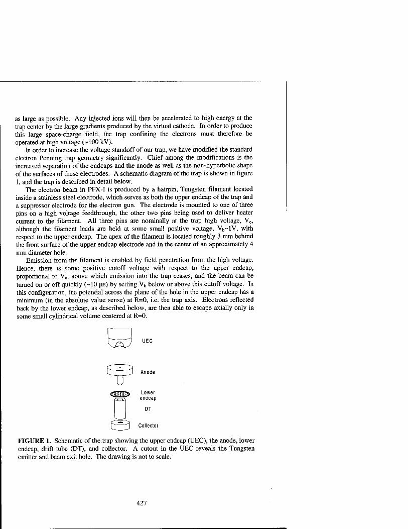
as large as possible. Any injected ions will then be accelerated to high energy at the trap center by the large gradients produced by the virtual cathode. In order to produce this large space-charge field, the trap confining the electrons must therefore be operated at high voltage (-100 kV).

In order to increase the voltage standoff of our trap, we have modified the standard electron Penning trap geometry significantly. Chief among the modifications is the increased separation of the endcaps and the anode as well as the non-hyperbolic shape of the surfaces of these electrodes. A schematic diagram of the trap is shown in figure 1, and the trap is described in detail below.

The electron beam in PFX-I is produced by a hairpin, Tungsten filament located inside a stainless steel electrode, which serves as both the upper endcap of the trap and a suppressor electrode for the electron gun. The electrode is mounted to one of three pins on a high voltage feedthrough, the other two pins being used to deliver heater current to the filament. All three pins are nominally at the trap high voltage, V0, although the filament leads are held at some small positive voltage, Vb~lV, with respect to the upper endcap. The apex of the filament is located roughly 3 mm behind the front surface of the upper endcap electrode and in the center of an approximately 4 mm diameter hole.

Emission from the filament is enabled by field penetration from the high voltage. Hence, there is some positive cutoff voltage with respect to the upper endcap, proportional to V0, above which emission into the trap ceases, and the beam can be turned on or off quickly (-10 u.s) by setting Vb below or above this cutoff voltage. In this configuration, the potential across the plane of the hole in the upper endcap has a minimum (in the absolute value sense) at R=0, i.e. the trap axis. Electrons reflected back by the lower endcap, as described below, are then able to escape axially only in some small cylindrical volume centered at R=0.

UEC

Anode

Lower endcap

DT

Collector

FIGURE 1. Schematic of the trap showing the upper endcap (UEC), the anode, lower endcap, drift tube (DT), and collector. A cutout in the UEC reveals the Tungsten emitter and beam exit hole. The drawing is not to scale.

427

Coll Scope

Figure 2. Electrical schematic of the trap apparatus.

For the initial tests described here, the anode consists of a stainless steel block roughly 18 mm thick with a 2 mm diameter hole through its center. The gap between the upper endcap and anode is 5.8 cm. The anode is maintained at ground potential, and electron current flowing to it can be monitored by means of an electrical lead exiting the vacuum system through a low voltage feedthrough. This enables us to monitor alignment of the trap axis with the magnetic field axis. Figure 2 contains an electrical schematic of the apparatus.

Approximately 3 cm below the lower surface of the anode is a 60% transparent grid which serves as the lower endcap or reflector. This electrode is maintained at sufficient negative voltage to reflect the electron beam and maintain axial confinement, but can be switched to ground potential with a variable time delay relative to the positive voltage ramp that halts electron emission from the filament. Trapped electrons then escape to the collector, which is monitored by an oscilloscope. The resulting pulse on the collector is the sum of two distinct signals. A background pulse arising from capacitive coupling of the lower endcap discharge pulse is summed with the electron arrival signal

Between the lower endcap and the collector is the drift tube. The drift tube is maintained at a fixed potential throughout the trap operation thereby decreasing the amplitude of the capacitive component of the collector signal. Nevertheless, before any electron data is taken a background pulse is attained by switching the lower endcap voltage with no electron beam in the trap. This background signal is subtracted from the full collector signal to retrieve the electron signal. Integration of the electron signal then gives the trap inventory.

The entire trap is contained within an ultrahigh vacuum system with operating pressure of roughly 3xl0"6 Pa maintained by a 50 1/s ion pump. The vacuum system then inserts into the room temperature bore of a superconducting magnet capable of

428

producing fields up to 7 T, although for the experiments reported here the fields used were less than 2 T.

The high voltage for the upper endcap and electron emitter is provided by a rack mounted 100 kV supply. This supply is used to float an instrument rack, which contains the filament current and bias supplies and various current monitoring devices, to high voltage. The rack is powered by an isolation transformer immersed in dielectric oil, and control of the instruments is via optical modems and fiber optic cable.

The experiments reported here were limited to low voltage (< 3 kV) as it was necessary to switch the lower endcap between ground and trapping voltage by means of a relay with limited voltage standoff. Additionally, the voltage was supplied to the lower endcap by means of a vacuum feedthrough with maximum voltage rating of 5 kV. In future experiments we envision grounding the lower endcap by means of a high resistance (10 GÜ.), high voltage resistor. The lower endcap will then charge to the same voltage as the upper endcap by means of the electron beam impinging on it.

RESULTS AND DISCUSSION

We have measured the trap inventory, N, as a function of trap voltage, V0, and have made initial measurements of inventory as a function of magnetic field. The inventory is measured immediately after the electron beam is switched off and is corrected for such systematic effects as the transmissivity of the lower endcap grid. In figure 3 one can see a linear dependence of the inventory on voltage.

The trap lifetime was determined by measuring the trap inventory as a function of

4.00E+008 -

0.00E+000 -

1000 1500

Voltage

FIGURE 3. Total trap inventory as a function of the trap voltage. The best fit to the data, shown by the solid line, is linear in trap voltage.

429

2.5E+08

2.0E+08 --

o 1.5E+08 c | l.OE+08

~ 5.0E+07 H

O.OE+00

0 200 400 600 800 1000

Time (msec)

Figure 4. Trap lifetime for various trap voltages and magnetic fields. The solid symbols are all for V0 = 400v, and open symbols are V0 = 200v. Magnetic fields are as follows: triangles B=1.14T, squares B=0.76T, and circles B=0.38T.

delay from the cessation of electron injection into the trap. Figure 4 shows the lifetime curves for different trap voltages and magnetic fields. We find a e"1 time of roughly 100 ms. The poor lifetime of the trap is undoubtedly due to misalignment of the trap and magnetic field axes and perhaps also to the unconventional trap geometry. Note that the data in figure 4 show a definite dependence of the trap inventory on magnetic field, but there is not sufficient data to conclusively determine the scaling. Also, it is not possible to determine the scaling of trap lifetime with magnetic field due to the paucity of data.

In general, the electron inventory is determined by a balance between injection rate, i.e. current into the trap, and loss rate. Thus, N = Ij x I e, where I( is the injection current, x the confinement time, and e the elementary charge. There are two modes of electron confinement, depending on electron space charge potential compared to applied voltage. Suppose first that space charge is small. Then Ij is determined by the source parameters, and x is determined by trap confinement. In the opposite limit, when space charge potential approaches the applied voltage V0, the voltage at the filament is decreased by the space charge potential of the electrons in the trap thereby decreasing Ij. In this limit, N is determined by the electrostatic solution which gives space charge potential equal to V0, and Ij adjusts to e N / x.

The scaling of electron inventory with magnetic field B, V0, and source parameters may be calculated in various operating regimes. The calculation is simplest in the space-charge dominated confinement regime. In this case, N <*= V0, and independent of X and, thus, B and source parameters. This rests on the assumption that the electron cloud will assume a density profile that has the same functional form (Gaussian, for example) across the entire radius of the trap regardless of B, so that the peak density,

430

and hence N, is proportional only to V0. In the low space-charge potential case, several scalings of both I; and x with the control parameters are possible. Ii may be emission limited, giving a scaling of N with heater current applied to the emitter. Alternatively, Ij may be limited by the space charge in the gap between the emitter and the UEC. In this case, Ii «= AVb3/2/d2, where AVb is the difference between the cutoff value (proportional to V0) and the bias voltage, Vb, applied to the emitter-UEC gap, and d is the effective gap distance.

Similarly, T may be determined by axial loss (in case electrons are collected near the UEC) or by radial loss (to the anode). Axial electron loss may be characterized by the number of recirculations, Nr, of a typical electron injected from the UEC system. This number will generally be large, because the acceptance aperture of the UEC for trapped electrons is typically small compared to the radial dimensions of the electron cloud. Thus, only some fraction of electrons travelling upward within the trap will be able to enter the UEC and be collected (if fr is this fraction, Nr = l/fr). If axial losses dominate confinement, x <* N/V0

1/2, since the axial bounce time is inversely proportional to the electron velocity. The velocity itself scales as the square root of the energy, which is in turn proportional to V0. Radial losses are believed to be dominated by misalignment errors in PFX-I. Previous studies of such transport(6) have shown a scaling x °= (B/L)2 in long, low-density electron traps, where L is the length of the plasma. In the case of PFX-I, L is fixed, so X °= B2 would be expected. Table 1 summarizes the expected scalings.

Based on the linearity of the trap inventory with voltage, it would seem that the trap is operating in the space-charge limited mode. In this case, according to the discussion above, we would expect to see no dependence of the inventory on the magnetic field, but as was pointed out previously, the data in figure 4 show a definite, if poorly characterized, dependence of N on B. This discrepancy is as yet not understood, but may be due to a deviation of the electron density profile from the universal one mentioned previously.

TABLE 1. Summary of inventory scaling.

Regime Inventory

Trap filled to space- charge limit

NocV0

Trap below space-charge limit

i^^^ÄÄs^^Bi^Älii Axial Loss Radial Loss

Emission limited source Heater/V0

1/2 Heater*B2

Space-charge limited source AVb

3/2/V01/2

Noc

AVb3/2-*B2

431

FUTURE PLANS

We are presently working on several modifications to the apparatus. We have completely redesigned the trap in order to provide better alignment of the trap electrodes, and we are working to improve the available diagnostics. We are also working to understand better the requirements on the electron distribution necessary to provide an axial ion well. In this section we discuss an optical diagnostic being installed on the trap and briefly summarize the electron distribution requirements.

Diagnostics

We are presently installing a nondestructive, optical diagnostic in addition to the existing destructive diagnostics. Hydrogen gas introduced into the trap volume will be dissociated, and the trapped electrons will excite the constituent atoms. In the presence of a significant electric field, a dipole potential term is added to the atomic Hamiltonian, resulting in a shift of the emission lines as described by the linear Stark effect. For Hydrogen atoms the shift is given by

f AE = n(n,-«2), (1)

15620

where F is the electric field strength in V/cm, n is the principal quantum number, and ni and TI2 are electric quantum numbers which result from separating the Schrodinger equation in parabolic coordinates(7). This leads to a splitting of the spectral lines that is linear with applied voltage, assuming the trap is filled to the space charge limit, and ranges from roughly 1 A for V0 = 10 kV to 10 A at 100 kV for the strongest K-

components of the Ha lines. Measurement of this splitting then can be used as an electron density diagnostic. Note that the Brillouin density limit for electrons in a 1 T field is much larger (xlOO) than the 100 kV space-charge limited density.

There are several effects that can produce a competing splitting or broadening, thereby masking the desired splitting. Chief among these is the Zeeman splitting due to the trap magnetic field, which ranges from 0.1 A to 0.2 Ä for fields ranging from 1 T to 2 T (8). Doppler broadening of the line could mask the Stark splitting, but the Doppler width is expected to be no greater than 0.5 A for atom temperatures up to an equivalent energy of 1 eV and less than 0.1 Ä at room temperature.

Electron Distribution Requirements

In order to produce an ion well depth with a usable fraction of V0, it is necessary that electrons have a nonthermal distribution. To ascertain this, suppose the contrary holds. Then, there is some electron temperature Te, and electron density is determined

432

as n0 exp[e <J> / Te], where O is the effective potential for electron confinement. <E> consists of an applied electrostatic part Oes and a magnetic part <£>A- 3>A vanishes along the magnetic axis of the system, where the range of <E> is at most the applied VG. For effective electron confinement then it is necessary that e V0 » Te. On the other hand, if Vj is the ion well depth, the condition that electron density vary little over the ion well region requires that e V; « Te. Thus, thermal electrons imply that V0 »» Vj, and very little of the applied voltage is available for ion confinement and heating. To maximize Vj, electrons should be nearly monoenergetic (possibly in a rotating frame). Then, electron confinement is assured for V0 just equal to this electron energy and density variation over the ion well region is only of order Vj/V0. A nearly monoenergetic distribution may be produced by adjusting electron confinement time to be much shorter than electron energy scattering time, and simultaneously collecting electrons at nearly their constant (source) energy, as was demonstrated in PFX(l).

In addition to a nearly monoenergetic energy distribution, an axial ion well will result only for a proper distribution of the electron canonical angular momentum about the trap symmetry axis, Pe. A theoretical study based on past and present work has identified three possible electron distributions:

1. Brillouin flow (Pe = 0 for all electrons) in which a beam distribution is maintained so that a third invariant besides e, the single particle energy, and Pe exists. An applied electrostatic field is optional. This is the EBIT approach(9).

2. Monoenergetic, rigid-rotor electrons [f ~ 8(£- QPe - £<>)] with magnetic shaping. Here Q is the plasma rotation frequency. No applied electrostatic field is required. This is the original PFX-I proposal(lO).

3. Spherically convergent flow in a spherical, harmonic trap such that f ~ 8(e)/L , where L is the total angular momentum. Note that there is no Pe dependence. An applied electrostatic field is required(ll).

PFX-I is currently focusing on 2 & 3 above, since the desired large electron recirculation makes maintaining a beam difficult. While most required features of 2 & 3 have been demonstrated in PFX,(1) the exact electron source, sink, and additional control are yet to be determined experimentally.

SUMMARY

PFX-I has demonstrated trapping of electrons in a modified Penning trap geometry. The trap electrodes have been spark conditioned to 75 kV, and the electron source has been operated in a 1 T field at trap voltages up to 50 kV. The trap inventory and lifetime have been measured at lower voltages as a function of trap voltage and magnetic field. This data is still under study. Ongoing work is concentrated on improving the trap lifetime and diagnostics and on theoretical understanding of the required electron distribution necessary to produce an axial ion well.

433

ACKNOWLEDGEMENTS

The authors would like to acknowledge the Office of Fusion Energy Sciences within the Department of Energy for generous financial support. We would also like to acknowledge Fred Ribe and Lou Schrank for many useful contributions to this experiment.

REFERENCES

1. Mitchell, T.B., Schauer, MM., and Barnes, D.C. Phys. Rev. Let. 78, 58 (1997). 2. Barnes, D.C, Mitchell, T.B., and Schauer, M.M. Phys. Plasmas 4, 1745 (1997). 3. Schauer, M.M. Mitchell, T.B., Holzscheiter, M.H., and Barnes, D.C. Rev. Sei. Inst. 68, 3340 (1997). 4. Nebel, R.A. and Barnes, D.C. Fusion Technology 38, 28 (1998). 5. Barnes, D.C. and Nebel, R.A. Physics of Plasmas 5, 2498 (1998). 6. Driscoll, C.F. and Malmberg, J.H. Phys. Rev. Let. 50, 167 (1982). 7. Bethe, H. A. and Salpeter, E.E. Quantum Mechanics of One- and Two-electron Atoms, New York: Springer-Verlag, 1957, pp. 228-232. 8. Goldman, S.P. in Atomic, Molecular, and Optical Physics, edited by G.W.F. Drake (AIP Press, Woodbury, NY, 1996) p. 177. 9. Levine, M.A., Marrs, R.E., Henderson, J.R., Knapp, D.A., and Schneider, M.B. Physica Scripta, T22, 157 (1988). 10. PFX-I proposal, available at http://ext.lanl.gov/projects/pfxi. 11. Barnes, D.C. to appear in Phys. of Plasmas (1999).

434

Confinement Of Pure Ion Plasma In A Cylindrical Current Sheet

Stephen F. Paul, Edward H. Chao, Ronald C. Davidson, Cynthia K. Phillips


Abstract. A novel method for containing a pure ion plasma at thermonuclear densities and temperatures has been modeled. The method combines the confinement principles of a Penning-Malmberg trap and a pulsed theta-pinch. A conventional Penning trap can confine a uniform-density plasma of about 5xl011cm-3 with a 30-Tesla magnetic field. However, if the axial field is ramped, a much higher local ion density can be obtained. Starting with a 107 cm-3 trapped deuterium plasma at the Brillouin limit (B = 0.6 Tesla), the field is ramped to 30 Tesla. Because the plasma is comprised of particles of only one sign of charge, transport losses are very low, i.e., the conductivity is high. As a result, the ramped field does not penetrate the plasma and a diamagnetic surface current is generated, with the ions being accelerated to relativistic velocities. To counteract the inward j x B forces from this induced current, additional ions are injected into the plasma along the axis to increase the density (and mutual electrostatic repulsion) of the target plasma. In the absence of the higher magnetic field in the center, the ions drift outward until a balance is established between the outward driving forces (centrifugal, electrostatic, pressure gradient) and the inward j x B force. An equilibrium calculation using a relativistic, 1-D, cold-fluid model shows that a plasma can be trapped in a hollow, 49-cm diameter, 0.2-cm thick cylinder with a density exceeding 4 x 1014 cm-3.

I INTRODUCTION

This paper presents a novel method for achieving a well-known goal: the confinement of non-neutral ion plasmas that are adequately dense for controlled thermonuclear fusion applications. This approach is a subset of a wider class of experiments known as Inertial Electrostatic Confinement experiments [1], but the question addressed here is quite specific: can the density of particles in a non-neutral plasma [2] be increased far beyond the density associated with the Brillouin limit?

A common device used to confine a non-neutral plasma is the cylindrical Malmberg-Penning trap [3]. Conventional magnetic fusion devices contain quasi- neutral plasmas in a toroidal or linear geometry, but generally the confinement is far


435

worse than that predicted classically. Though at first glance non-neutral plasmas would not appear good candidates for long confinement time applications (because of the strong, outward electrostatic forces associated with the space-charge potential), Malmberg-Penning traps have exhibited superb confinement capability. This is because the conservation of rotational angular momentum forces the mean square radius of a one-component plasma to remain constant in time. One-component plasmas also have two other benefits from a practical standpoint for fusion devices: the absence of both radiative losses and thermal wall loading because of the sharp radial fall-off in the density profile (typically on the order of several Debye lengths). This superior confinement capability has not been generally realized in controlled fusion devices, however, because conventional Malmberg-Penning traps can confine uniform-density plasmas of only about 5 x 10n cm-3, even with magnetic fields strengths in the tens of Tesla. This is expressed as the Brillouin limit,

oj2 B2

2-f < 1 or n<- -, (1)

where wp is the plasma frequency, y/Aime2/m, and wc is the cyclotron frequency, eB/mc. At the Brillouin limit, the plasma column is rotating at U>R, which is equal to wc/2. Equation (1) shows that higher density may be achieved only if the square of the magnetic field is increased proportionally. Even at these large field strengths, the Lawson criterion is satisfied, but with a required confinement time of nearly 1 hour.

Though most often viewed as a density limit, the Brillouin limit is a statement of the fact that the inward j x B force must balance the outward driving forces (centrifugal, electrostatic, pressure gradient). For plasmas that do not have a uniform density, force balance can be achieved even though local values of n far exceed the limit expressed in Eq. (1). In this paper, the simple geometry of the Penning trap is retained; the confinement device proposed provides radial confinement through an axial magnetic field, and longitudinal confinement electrostatically by end cylindrical electrodes kept at a potential higher than the plasma's space charge potential. The difference is that, unlike in a conventional Penning trap, the axial magnetic field is very non-uniform. In addition, the velocity shear in the device is very large and the density profile is not monotonically decreasing. These two factors could have serious consequences where the stability of the configuration is concerned.

II METHODOLOGY

A highly non-uniform field is created by initially producing a conventional, low- density Malmberg-Penning trap plasma, followed by ramping the axial field. For example, a uniform density, 107 cm-3 deuterium plasma might be generated at the Brillouin limit (here, at B — 0.6 Tesla), after which the field is slowly ramped to as high a value as is practical (here, 30 Tesla). Because the plasma is comprised

436

of particles of only one sign of charge, transport losses are very low, i.e., the conductivity is high. As a result, the ramped field does not penetrate the plasma as long as the ramping time is short compared to the magnetic diffusion time. A diamagnetic surface current is generated, and, in this example, the ions are accelerated to relativistic velocities, with the magnetic field outside the plasma 50 times stronger than inside. This method is distinguished from a theta-pinch approach, in which the inward j x B forces compress and heat the plasma. To counteract the inward j x B forces, ions are injected along the machine axis to increase the density (and mutual electrostatic repulsion) of the target plasma. With only the weak magnetic field present within the bulk of the plasma, the ion density inside the plasma column greatly exceeds the Brillouin limit and the ions drift outward. Ultimately, a balance is established between the outward driving forces (centrifugal, electrostatic, pressure gradient) and the inward j x B force, and the plasma is trapped in a thin current sheet between its own outward electrostatic repulsive forces and the confining magnetic field.

Ill EQUILIBRIUM MODELING

To determine the characteristics of such an equilibrium, a relativistic 1-D cold- fluid model was used to model the system. Starting with the radial force balance equation for a cold macroscopic fluid,

_m®L = e[Er + ßlBMh (2) where

operating on it with l/rd/dr[r...], and substituting in Ampere's law and Gauss' law leads to an equation for the derivative of ß{r) as a function of ß(r), Bz, and dBz/dr:

1 dB, 7?/3|

(3) dße 1 Bz dr dr 72/

where

1 + T/9^.(7V> + 2)

7(r) = V^T2

437

This first order ODE is solved using Mathematica with the boundary condition ß(r = 0+) = 0. Bz is specified as nearly a step function with penetration depth d0. The step is located at the surface (rc = 49cm) of the initial low density plasma:

B,(r) = ^ ( 1 + Tanh + r0){r - rc)

2dl (4)

Fusion power is maximized by increasing the ion density to the greatest extent possible. To that end, 30 Tesla is chosen for the ramped field to illustrate the potential of this approach. An equilibrium calculation using a relativistic 1-D cold- fluid model shows that the plasma can be trapped in a hollow, 49-cm diameter, 0.2-cm thick cylinder, whose density exceeds 4 x 1014 cm""3. The drawback, of course, is the very small thickness of the current sheet, resulting in a low plasma volume. For this simulation, the radius is maximized so that the resulting plasma volume is as large as possible without the local velocity exceeding the speed of light. The results indicate that 2 MW of fusion power could be produced in a 100-m long, 1-m diameter reactor. At 72 m3, the device would be only 4% of the volume of 1TER, while a device with the same volume as ITER would produce 55 MW. In the simulation, the thickness of the shell is set at 2 Larmor radii, i.e, the ramped B-field is assumed not to penetrate the highly conducting ion plasma at all. The other parameters are: Baz - 300 kG, r0 = 49.0, and da = 1.85 cm. The magnetic field in the region of the field transition given in Eq. (4) is shown in Fig. 1.

Given the magnetic field profile, the velocity profile is uniquely determined. In this case, the velocity is relativistic with ß about 0.85. The rotation frequency profile, uj(r) = cß/r is determined from the velocity and is shown in Fig. 2. Given the velocity profile, the density profile can be readily calculated from Ampere's law:

< ^ 1 dBz . n(r) = Ä^ß(r)-d7- (5)

The plasma forms a thin cylindrical shell in the region of the magnetic field transition, which is shown in Fig. 3. The current density is easily calculated from its definition:

j(r) = n(r)eß(r)c (6)

The very high current density (several MA/cm2, shown in Fig. 4.), confines the plasma through the inward radial j x B force. Given the density profile, the electric field is calculated from Gauss' law:

E(r) = 300 x 106 • 47re- j n(r') r' dr' (7)

The self electric field generated at the surface of the plasma as calculated from Eq. (7). is large (100's of MV/cm). However, there is little charge or field inside the plasma shell, as shown in Figs. 3 and 5.

438

B <

300

kG> Magnetic Field

/"

250 I

200 /

150 /

100 /

50 y 48 6 48.8 49 49.2 49.4

radius <cm>

FIGURE 1. The magnetic field in the region of the surface of the initial, low-density plasma.

,-l- freq <sec > Rotation

5-10£

radius <cm> 48.4 48.6 48.8 49 49.2 49.4 49.6

FIGURE 2. The rotation frequency profile in the region of the plasma shell.

439

<cir -J> Ion Density

4-1014

3-1014

2-1014

1-1014

48.6 48.8 49 49.2 49.4 radius <cm>

FIGURE 3. The density profile.

MAmps 1.75

„-2 cm Current Density

48.6 4 49 49.2 49.4 radius <cm>

FIGURE 4. A very high current density provides the confining forces.

440

MV cm !

140

120

100

80

60

40

20

Er

48.6 48.8 49 49.2 49.4 radius <cm>

FIGURE 5. The electric field in the region of the transition.

IV INCLUSION OF FINITE TEMPERATURE

To determine how the inclusion of finite temperature affects the characteristics of the cold fluid equilibrium, a relativistic pressure gradient term, 1/nVP, was added to the 1-D, cold-fluid model. A simplified model of pressure, with varying density but isotropic temperature is included in Eq. (2) by adding T/r d/dr(r/n dn/dr) to the right hand side. Similarly, operating on this equation with l/r d/dr [r ...] and substituting Ampere's law and Gauss' law as with Eq. (2) produces a second-order differential equation giving dB2/dr2 as a function of ß(r), dß(r)/dr, Bz, dBz/dr, dB2Jdr2, and d3Bz/dr3:

d2ße 1 (dß dr2 ße \dr

+

+

d2Bz

dr2

Bz + mc

1 dBz 9B,

T l ßa2 dr

2 dBz 83BZ

(OB, V dr

er

cPB. dr dr3 ßr2

^eßl + 2leße +

dBz

Ör

T ßemc2

dße dr (8)

441

At the temperatures considered here (T = 80 keV), the energy associated with the pressure gradient is only about 0.3% of the rotational energy of the ions or the electrostatic energy associated with the space charge. Consequently, the qualitative results of the simulation are nearly identical to the cold fluid case. The peak ion density confined with the same field strength is identical to the cold fluid case, but there is a small extension in the distribution of ion density towards the center of the configuration, as seen in Fig. 6. The rotation frequency profile is steeper at 48.7 cm than in the cold fluid case, and tapers off more sharply at r >49.0cm. The current density and the electric field remain identical to the cold fluid case.

cm -3 Ion Density

4-10

3-10

2-10

1-10'

48.6 4 49 49.2 49.4 radius <cm>

FIGURE 6. The ion density including finite temperature effects.

V A TEST CASE: PROPOSED EXPERIMENT FOR THE EDG

This concept can be easily tested in existing Malmberg-Penning traps. The cold fluid equations were solved for electrons as the plasma species and for parameters suited to the EDG device at Princeton [4,5]. For a very modest field of .01 Tesla and a plasma diameter of 1.8 cm, the rotation frequency is much higher than in the pure ion case because of the much lower mass of the electrons. Peak rotation frequencies of 8 GHz are modeled as shown in Fig. 7. This rotation corresponds to a beta of about 0.45. The electron density is concentrated at the edge, as expected, and the peak density is < 8.6 x 10u/cm3. The peak current density is about 1.6 kA/cm2. The main technical difficulty in performing an experiment in EDG is ensuring that the walls of the cylinder do not break down because of field emission.

442

The electric fields, even for this low density, peak at about 90 kV/cm, as shown in

Fig. 8.

GHz 8r

7

6

5

4

3

2

1

Rotation Frequency

-j radius <cm> 1.2 1.4 1.6 1.

FIGURE 7. The rotation frequencies in EDG.

kV cm lOOr

80

60

40

20

Er

1.2 1.4 1.6 1. _ radius <cm>

FIGURE 8. The electric field in EDG.

ACKNOWLEDGMENTS

This research was supported by the Office of Naval Research. The authors gratefully acknowledge Kyle Morrison for useful discussions and help in preparing this

manuscript.

443

REFERENCES

1. Barnes, D.C., Mitchell, T.B., Schauer, M.M., Phys. Plasmas 4, 1745 (1997). 2. Barnes, D.C., Nebel, R.A., Turner, L., Tiouririne, T.N., Plasma Phys. Controlled

Fusion 35, 929, (1993). 3. Davidson, R.C., Physics of Nonneutral Plasmas, Redwood City, California: Addison-

Wesley Publishing Company, 1990. 4. Chao, E.H., Davidson, R.C., and Paul, S.F., J. Vac. Sei. Tech. A17, 2050 (1999). 5. Chao, E.H., Paul, S.F., and Davidson, R.C., J. Vac. Sei. Tech. A17, 2034 (1999).

444

Magnetic Cusp and Electric Nested- or Single-Well Configurations for High Density Antihydrogen and Fusion Nonneutral Plasma Applications

C. A. Ordonez*


Abstract. Malmberg-Penning traps have had limited uses for applications that require high density nonneutral plasma confinement. For such traps, the density is severely limited because a magnetic field is used to provide a radially inward force to balance both self-electric and centrifugal radially outward forces. A possible way to confine higher density nonneutral plasmas is to use a magnetic cusp configuration. An annular nonneutral plasma would be confined in the radial magnetic field of a magnetic cusp such that radial confinement is provided by an externally produced electric potential well while axial confinement is provided by the magnetic field. In addition, a radial electric potential profile having a nested-well configuration can be used to simultaneously confine two oppositely signed plasma species (e.g., positrons and antiprotons) that overlap. In the work reported, various aspects of using magnetic cusp configurations and electric nested-well configurations are considered. Plasma confinement with these configurations may be useful for obtaining fast antihydrogen recombination and trapping rates and for achieving practical fusion power production.

INTRODUCTION

Experiments are now being planned for attempts to produce and trap cold antihydrogen atoms [1,2]. One approach being studied, which involves the use of nested electric potential wells, is described in recent review articles [3,4]. Antiprotons and positrons are confined to travel along the direction of an externally produced magnetic field. Externally produced nested electric potential wells along the magnetic field are used to provide simultaneous confinement of both particle species. Con- finement is achieved such that the antiprotons overlap the positrons, which form a higher density plasma. A fraction of the recombined antihydrogen atoms are produced in a low-magnetic-field-seeking state. Such atoms remain confined within the magnetic field, which has a local minimum in strength.

+) Electronic Mail: [email protected]


445

A question associated with the above approach is what configuration to use for the magnetic field. In the work presented here, a magnetic cusp is considered. The prospect of using a magnetic cusp is supported by a recent experimental demonstration of good confinement of a nonneutral plasma in a cusp [5]. A magnetic cusp is axisymmetric and, in an Andreoletti-Furth configuration [6], can provide a local magnetic minimum in the region where the antiprotons overlap the positrons. A magnetic minimum within the overlap region provides a means to initially trap newly recombined atoms in highly excited states and to subsequently de-excite the atoms by collisions with surrounding plasma particles.

MAGNETIC CUSP CONFIGURATION

Figure 1 illustrates a cross section of the coils, magnetic field lines, electrodes, and trapped nonneutral plasma for a magnetic cusp. Electrodes for producing single-well confinement of a nonneutral plasma are shown in Fig. 1(a) while electrodes for nested-well confinement are shown in Fig. 1(b). There is azimuthal symmetry about the z axis. The different appearance in each set of coils, one set located at z > 0 and one set at z < 0, is intended to show that each set carries a current in opposition to the other in order to produce a radial magnetic field between them. As drawn, the magnetic field lines show no axial component over the region where a positive nonneutral annular plasma is trapped. There are six disk shaped electrodes. The two electrodes to either side of the plasma have a negative applied potential with respect to the other four electrodes. The difference in potential between the electrodes produces an electric potential well suitable for radially confining the positive annular plasma. The externally produced potential well must counteract the self-electric force that tends to expand the plasma in the radial direction. For the magnetic field illustrated in Fig. 1(a), the configuration should have the interesting property of providing radial compression of a nonneutral plasma that is introduced along the axis. The compression would occur as a result of the radially outward magnetic moment force that acts on the plasma. For a magnetic field in an Andreoletti-Furth configuration, the nonneutral plasma can be located within a magnetic well such that magnetic and electric wells simultaneously provide radial confinement for the annular nonneutral plasma.

For the configuration illustrated in Fig. 1(a), the radial magnetic field serves to keep the plasma from expanding axially. Along the midplane (at z = 0), there is no axial electric force acting on the plasma because of left/right symmetry. Hence, there will be no azimuthal plasma rotation along the midplane. Away from the midplane an axial electric field does exist, which causes an azimuthal ExB rotation and an associated centrifugal force. Because the axial electric field strength increases with increasing distance from the midplane, the plasma must undergo a sheared azimuthal flow. Thus, global thermal equilibrium will not be possible.

A nonneutral plasma confined in the solenoidal magnetic field of a Malmberg- Penning trap necessarily produces a radial electric field. The crossed fields are

446

magnetic field lines I nonneutral

magnetic coils

II I I III I I I I

I I I I 111 III I I

(b)

FIGURE 1. Cross section of the coils and a trapped nonneutral plasma in a magnetic cusp for single-well electrodes (a) and nested-well electrodes (b).

responsible for an azimuthal ExB flow of the plasma. The resulting centrifugal force, as well as the radial electric force, must be balanced by a radially inward magnetic vxB force. Requiring force balance for a uniform density cylindrical plasma leads to the well known Brillouin density limit. For an annular plasma in a cusp magnetic field, the magnetic field only needs to provide an axially inward magnetic vxB force to balance an axially outward self-electric force, which approaches zero near the midplane.

A number of previous analyses have explored the possibility of using nonneutral plasmas for fusion applications [7,8]. An advantage of a nonneutral ion plasma is that there are no energy losses via electrons (e.g., by electron heat conduction, bremsstrahlung and cyclotron radiation). Approaches based on magnetically confining nonneutral fusion plasmas require the ion density to exceed the Brillouin limit in order to achieve a practical fusion power density. With a cusp magnetic field such as that illustrated in Fig. 1(a), it is conceivable to confine a thin washer-like annular nonneutral plasma at a density exceeding the Brillouin density limit.

ELECTRIC NESTED-WELL CONFIGURATION

Figure 1(b) shows a set of five nested electrodes that would be suitable for producing a nested electric potential well for trapping oppositely signed plasmas that

447

♦rot , . ♦«"

z=0 « \l \| II U W z z = 0

(a) (b)

FIGURE 2. Illustrations of one side of a multiply nested time-dependent potential profile at one instant in time. The potential has a sinusoidal time dependence at each axial position such that the potential profile looks like a wave packet with a phase velocity directed to the left and

no group velocity.

overlap. Use of a nested-well configuration for trapping oppositely signed plasmas that overlap is supported by both theory [9-11] and experiment [12]. First, the possibility of keeping a positron plasma (with as large a density as possible) overlapped by a lower density of antiprotons is considered. One way to maintain a constant overlap is to keep the antiproton plasma in a nonequilibrium plasma state referred to as an "antishielding" [13,14] state. Schemes using moving potential barriers have been studied experimentally [15]. Two examples of a moving-barrier approach are illustrated in Fig. 2. A way to visualize the time dependence is as a wave packet with zero group velocity and nonzero phase velocity. The phase velocity would be directed toward the plasma overlap region (toward z = 0). A simple animation with the computer program Mathematica is possible by entering f=Exp[-x2]Cos[27r(x-r-i/10)];Do[Plot[f,{xr2.5,2.5},PlotRange->{-l,l}],{i,10}] and animating the result. Figure 2(a) shows about ten positron barriers (positive <f> regions) and ten antiproton barriers (negative <f> regions). Hundreds of closely spaced electrodes would probably be needed to create such a profile. This may be possible for a thin washer-like positron plasma. Nevertheless, a moving-barrier approach that requires far fewer barriers (and electrodes) is also possible [15]. For the profile shown in Fig. 2(a), the positron and antiproton barriers move sequentially inward and each plasma species alternates extending past the other. For the profile shown in Fig. 2(b), the first group of barriers are positron barriers so that the positrons are always overlapped by the antiprotons. A nice feature of both profiles in Fig. 2 is that the voltage applied to each electrode only needs to change sinusoidally with time.

A possible problem with keeping a plasma in an antishielding state is that the plasma temperature can increase [15]. In Ref. [16], an analysis of keeping antiprotons at a density of 5 x 1010 m-3 and temperature of 1 K in an antishielding state is presented. The antiprotons are considered to overlap a positron plasma at a density of 5 x 1013 m~3 and temperature of 1 K. The time it would take for the

448

antiprotons to relax toward thermal equilibrium, which can be associated with the timescale for antiproton heating, is found to be much larger than the timescale for the antiprotons to approach a collisional thermal equilibrium with the positrons. Consequently, the antiproton temperature will remain about equal to that of the positrons. The timescale for the antiprotons to relax toward thermal equilibrium is found to be 0.2 s for the parameters considered. This is roughly the timescale for positrons in a 5 T field to cool by cyclotron radiation to thermal equilibrium with the surrounding structure (see Ref. [17] for a convenient formula). With a substantially larger number of positrons than antiprotons, the temperature of the positrons and antiprotons should remain relatively unaffected by the antiproton heating associated with maintaining the overlap.

The above considers the possibility of keeping a positron plasma overlapped by a lower density of antiprotons. It is possible for the nested-well configuration to be designed such that the plasma in the overlap region is neutral [9]. With a neutral overlap plasma, a self-electric field will not be produced, which may otherwise field ionize newly recombined atoms trapped in highly excited states. For a neutral density of 5 x 1010 m~3 and temperature of 1 K, the timescale for three-body recombination is 0.1 -1 s (see Ref. [16] for calculation details). Since this is close to the timescale for the antiprotons to relax toward thermal equilibrium, it is conceivable to use constant electrode potentials, as considered in Refs. [16] and [18]. It is interesting to note that als timescale for spontaneous radiative recombination would require the density to be about 1016 m-3.

CONCLUDING REMARKS

It may be possible to increase the reaction rate (e.g., recombination or fusion) for plasmas that are confined, in part, by an externally produced electric potential well. The electrode voltages can be oscillated such that an acoustic standing wave is driven. This should effectively enhance the reaction rate as a result of the higher density compressions that are produced, although the average plasma density is not increased. A somewhat similar enhancement is proposed for increasing the fusion reactivity in spherical fusion plasma systems based on the periodically oscillating plasma sphere (POPS) concept [19].

In summary, plasma confinement with magnetic cusp and electric nested- and single-well configurations have been considered. For single-well confinement of a nonneutral plasma in a magnetic cusp configuration, exceeding the Brillouin limit appears possible. Such a configuration may be useful as an approach to fusion energy production. For nested-well confinement of overlapping plasmas, a number of characteristics of the confinement may make the configuration useful as an approach to produce and trap antihydrogen atoms. In a purely radial magnetic field, self-compression of a thin positron plasma that is axially loaded along the axis may be possible. The high density positron plasma can then be radially confined in an electric potential well and the magnetic configuration can be modified to form a

449

magnetic well at the positron plasma. The nested-well configuration can be acti- vated and an overlapping antiproton plasma introduced. The high density positron plasma can provide for collisional de-excitation of antihydrogen atoms that are initially recombined and trapped in highly excited states. Overall, the combined magnetic cusp and electric nested-well configuration appears promising as a scheme for achieving fast antihydrogen recombination and trapping rates.

ACKNOWLEDGMENTS


REFERENCES

1. G. Gabrielse, "Progress in Antihydrogen Experiments," 1999 Workshop on Nonneu- tral Plasmas.

2. K. Fine, "The ATHENA Antihydrogen Experiment," 1999 Workshop on Nonneutral Plasmas.

3. M. H. Holzscheiter and M. Charlton, Rep. Prog. Phys. 62, 1 (1999). 4. J. Eades and F. J. Hartman, Rev. Mod. Phys. 71, 373 (1999). 5. A. Mohri, T. Yuyama, Y. Kiwamoto, Y. Yamazawa and T. Michishita, Jpn. J. Appl.

Phys. 37, L1553 (1998). 6. R. F. Post, Nucl. Fusion 27, 1579 (1987) [see page 1602]. 7. D. C. Barnes, T. B. Mitchell, and M. M. Schauer, Phys. Plasmas 4, 1745 (1997);

and references therein. 8. C. A. Ordonez, Fusion Technol. 22, 388 (1992). 9. C. A. Ordonez, Phys. Plasmas 4, 2313 (1997).

10. C. A. Ordonez, IEEE Trans, on Plasma Sei. 24, 1378 (1996). 11. D. D. Dolliver and C. A. Ordonez, Phys. Rev. E 59, 7121 (1999). 12. D. S. Hall and G. Gabrielse, Phys. Rev. Lett. 77, 1962 (1996). 13. C. Hansen and J. Fajans, Phys. Rev. Lett. 74, 4209 (1995). 14. C. Hansen, A. B. Reimann, and J. Fajans, Phys. Plasmas 3, 1820 (1996). 15. E. Gilson, A. B. Reimann, and J. Fajans, "Double Well Neutral Plasma Traps," 1997

Workshop on Nonneutral Plasmas, Boulder, Colorado, July 29 - August 1, 1997. 16. Yongbin Chang, D. D. Dolliver, and C. A. Ordonez, "Analysis of Time-Dependent

Effects When Operating Nested-Well Plasma Traps for Achieving Antihydrogen Re- combination," 1999 Workshop on Nonneutral Plasmas.

17. B. R. Beck, J. Fajans, and J. H. Malmberg, Phys. Rev. Lett. 68, 317 (1992). 18. D. D. Dolliver and C. A. Ordonez, "Self-Consistent Static Analysis of Using Nested-

Well Plasma Traps for Achieving Antihydrogen Recombination," 1999 Workshop on Nonneutral Plasmas.

19. R. A. Nebel and J. M. Finn, "Kinetic and Fluid Calculations for the Periodically Oscillating Plasma Sphere (POPS)," 1999 Workshop on Nonneutral Plasmas.

450

Virtual Cathode Formations in Nested-Well Configurations

K. F. Stephens II and C. A. Ordonez*

University of North Texas Department of Physics

Denton, TX 76203

R. E. Peterkin, Jr.

Air Force Research Laboratory Directed Energy Directorate

Kirtland AFB, NM 87117-5776

Abstract. Complete transmission of an electron beam through a cavity is not possible if the current exceeds the space-charge limited current. The formation of a virtual cathode reflects some of the beam electrons and reduces the current transmitted through the cavity. Transients in the injected current have been shown to lower the transmitted current below the value predicted by the electrostatic Child-Langmuir law.1 The present work considers the propagation of an electron beam through a nested-well configuration. Electrostatic particle-in-cell simulations are used to demonstrate that ions can be trapped in the electric potential depression of an electron beam. Furthermore, the trapped ions can prevent the formation of a virtual cathode for beam currents exceeding the space-charge limit.

INTRODUCTION

An understanding of electron transport that is space-charge limited (SCL) due to virtual cathode formation is important in a variety of fields, including sheath research [1,2] and high power microwave sources [3,4]. A virtual cathode is a time- dependent phenomenon that occurs when a current larger than the SCL current is passed through a region. If a current well below the space-charge limit is injected into a drift tube, for example, the axial velocity of the beam particles remains relatively constant. As the current increases, the greater space-charge density within

t) Electronic mail: [email protected] *) Luginsland, J., et al, "Virtual Cathode Formation Due to Electromagnetic Transients", IEEE Trans, on Plasma Science, 28(3), 901-904 (1998).


451

*(z) Inner Well

(a) / Outer Well K

(b) :m^"::iiK:::m<i:-i:i<-r:nr»i!':::w-':;■■:■:■■■.:

1 1 (c) i«

V

1 1

> (d) ?;:;

^- *~ " >

(e)

FIGURE 1. A nested-well profile (a) and some possible configurations that produce the inner well of a nested-well profile (b-e).

the drift tube decelerates those particles that are just entering the tube. Eventu- ally, there is sufficient space-charge within the tube that the decelerated particles come to rest and a virtual cathode is formed. As more particles are collected into the virtual cathode (i.e., the potential depression where the particles have zero axial velocity), the magnitude of the virtual cathode increases, ejecting many of the particles from within the potential depression of the virtual cathode. After this occurs, the magnitude of the virtual cathode decreases, allowing more particles to be transmited until the SCL current is again exceeded. The process is then repeated. Thus, the presence of a virtual cathode represents an instability in the beam flow, causing the magnitude of the beam current and potential depression to oscillate. This oscillation is one mechanism used in vircators to produce high power microwaves [3].

The present work investigates the transport of an electron beam through a nested electric potential well configuration. Nested-well configurations are being studied for use in Malmberg-Penning traps [5-8]. The electric potential profile for a nested- well configuration is qualitatively illustrated in Fig. 1(a). The increasing potential on the left side of the "outer" well accelerates electrons entering from the left. The outer well also decelerates the electrons before exiting through the right side. As shown in Fig. 1(a), the outer well is nested about the "inner" well. The inner well can be created by various methods and is the primary focus of the present study. Figure 1(b) illustrates the use of cylindrical electrodes to form the inner well. This method is typically employed to form the inner well in nested Malmberg-Penning traps [9].

There are alternative methods to produce the inner well. A drift tube with a

452

region of increased radius, as shown in Fig. 1(c), is one such configuration. Sim- ilar structures are used in backward-wave oscillators, travelling-wave tubes and vircators to produce high power microwaves [3]. The larger radius decreases the potential and retards the electron beam. With a sufficiently large radius, a virtual cathode can occur causing fractional transmission of the injected current. Another approach, shown in Fig. 1(d), is applying a spatially varying magnetic field (represented by the curved lines) that increases the beam density by constricting the beam. Figure 1(e) demonstrates another approach to creating a virtual cathode. It has recently been reported that including an inner coaxial electrode enhances the SCL current of a hollow beam compared to when the inner electrode is absent [10]. Thus, removing a section of the inner electrode from a coaxial drift tube can prompt the formation of a virtual cathode.

The present work investigates the effects of plasma pre-filling on the potential depression of an electron beam near the SCL current. The particular configuration considered is shown in Fig. 1(c). It will be shown that the plasma-filled device can accomodate a larger current than when the device is not plasma-filled. Fur- thermore, the plasma ions "fall" into the electric potential depression created by the beam and are effectively trapped within it. Although numerous experiments have demonstrated the benefits of plasma-filled microwave sources, only limited computer simulations exist [11,12].

METHOD

The 2 x/2 dimensional particle-in-cell (PIC) code OOPIC [13] is used to model the physical system shown qualitatively in Fig. 1(c). OOPIC is a fully relativistic code that can be run either electrostaticaly or electromagnetically. Only non-relativistic parameters are considered and all simulations were run in the electrostatic mode. The drift tube is formed from three cylindrically symmetric sections with perfectly conducting boundary conditions applied to each section. The narrow sections have a 10 mm radius and the wide section has a 20 mm radius. Each section is 50 mm long. A monoenergetic, 20 keV electron beam enters at z = 0 with a 9 mm radius, time-independent uniform current. An axial magnetic field of 3 T is applied to strongly inhibit radial and azimuthal motion.

The main parameters chosen for each run are the beam current, the plasma density and the plasma temperature. Before any plasma is added, a series of simulations are performed to determine a beam current slightly less than the space- charge limit. Using a current below this prevents the instability associated with the formation of a virtual cathode. For the complicated boundary of the drift tube, analytically predicting the SCL current is difficult. A rough estimate can be determined from the infinite-length approximation. The SCL current for a solid

453

electric potential [kVJ

FIGURE 2. Electrostatic potential for a 20 keV, 35 A electron beam entering the geometry shown in Fig. 1(c).

beam of radius r;, in a drift tube of radius rc is given approximately by [10]

3/2

'scl ^l + 21n(rc/r6)

Here, 75 = 1 + K/mc2 is the relativistic mass factor for beam electrons entering the drift tube with kinetic energy K and rest mass m. I A — 17 kA is the Alfven current. For a 20 keV electron beam with a radius of 9 mm, the SCL current in a 10 mm radius drift tube is 59 A and 27 A in a 20 mm radius tube. Although this demonstrates that increasing the radius of a drift tube reduces its SCL current, these values are only approximate for finite-length tubes and charge densities.

RESULTS

For the geometry shown in Fig. 1(c) and described above, injecting a 35 A electron beam produces an electric potential depression of approximately -13 keV, as shown in Fig. 2. The larger radius section of the drift tube more than doubled the space- charge potential of the beam over the value present in the narrow sections. The value of 35 A is close enough to the SCL current to significantly depress the potential in the wide section, but is low enough to avoid forming a virtual cathode. If a 50 A beam is injected, a virtual cathode forms which indicates that the SCL current of the wide section is less than 50 A. The phase-space plots (axial velocity vs. axial position) of the 35 and 50 A beams are shown in Fig. 3. The presence of a virtual cathode for the 50 A beam is evident. For comparison, an electromagnetic simulation of the 50 A beam was also performed. The phase-space plots showed no qualitative differences between the electrostatic and electromagnetic simulations.

If the device is prefilled with a neutral plasma, the maximum current can be increased without producing a virtual cathode. The plasma is composed of electrons

454

8.5

%*^A HS ..

>£ä 1 l£$.

b3

£ " '■•V'*-.- .^V:'":-'i"

V *."**" t•• %*/*■"■ ' ä

•S*'l■'.?'•'■}'. ■". •',"•" ■s S

-V/r" o z /cmy 15

8.S

i +

i.---:.v£v..». .:'.-»>'-:^>-;..*?Sp'-

^j«s»5saM»««w

Ü s S

-SS

••f,r*;.V':\,

0 Z /«Mi 15

FIGURE 3. Phase-space (axial velocity vs. axial position) comparison of 35 (left) and 50 A

(right) beams. The electrons decelerate as they enter the wide section. Each electron in the 35

A beam exits through the right boundary. However, the formation of a virtual cathode reflects a

fraction of the 50 A beam.

■5r<iS":*v*»'»,'-;S~:.

zlcmj

FIGURE 4. Axial phase-space for a 50 A, 20 keV electron beam (top) passing through the device with a plasma pre-fill and the remaining plasma ions (bottom).

and scaled-mass protons (40 x electron mass), and is loaded with a density of 5 x 1015

m-3 and temperature of 100 eV. The plasma extends the length of the device and to a radius of 10 mm. Injection of a 50 A beam (corresponding to a beam density of 1.5 x 1016 m-3) into the plasma-filled device no longer produces a virtual cathode, see Fig. 4. It should be noted from Fig. 4 that the plasma electrons are no longer present. As the beam begins travelling through the device, the plasma electrons are ejected axially due to the space-charge of the beam. As the space-charge of the plasma electrons decreases, the ions "fall" into the potential depression of the beam. With the ion space-charge reducing the space-charge of the beam, the device can operate with a larger beam current. However, it should be noted that this neutralization is not stationary. The ions gradually heat up and eventually "leak" out of the potential depression. Once sufficient neutralization is no longer available,

455

a virtual cathode will form when the beam current exceeds the SCL current.

CONCLUSION

An electrostatic particle-in-cell simulation has been performed which demonstrates ion trapping and space-charge reduction in the potential depression of an electron beam. With the ions partially neutralizing the space-charge of the beam, a current that exceeds the vacuum space-charge limit could be propagated. Various mechanisms that increase the electric potential depression of the beam were discussed which can form the "inner well" of a nested-well configuration. The effect of trapped ions on virtual cathode formation for a drift tube of varying radius, Fig. 1(c) was studied. Quantitative predictions for an increase in the space-charge limited current within a varying radius drift tube were reported.

ACKNOWLEDGMENTS

This material is based upon work supported by the Air Force Office of Scientific Research.

REFERENCES

1. Ordonez, C. A. and Peterkin, R. E., Jr., J. Appl. Phys. 79(5), 2270-2274 (1996). 2. Stephens, K. F., II and Ordonez, C. A., J. Appl. Phys. 85(5), 2522-2527 (1999). 3. Gold, S. H. and Nusinovich, G. S., Rev. Sei. Instrum. 68(11), 3945-3974 (1997). 4. Luginsland, J. W., McGee, S. and Lau, Y. Y., IEEE Trans. Plasma Science 28(3),

901-904 (1998). 5. Gabrielse, G, Rolston, S. L. Haarsma, L. and Keils, W., Phys. Lett. A 129(1), 38-42

(1988). 6. Ordonez, C. A., IEEE Trans, on Plasma Sei. 24(6), 1378-1382 (1996). 7. Ordonez, C. A., Phys. Plasmas 4(7), 2313-2315 (1997). 8. Dolliver, D. D. and Ordonez, C. A., Phys. Rev. £59(6), 7121-7127 (1999). 9. Hall, D. S. and Gabrielse, G., Phys. Rev. Lett. 77(10), 1962-1965 (1996).

10. Uhm, H. S., Phys. Plasmas 6(4), 1360-1362 (1999). 11. Goebel, D. ML, Carmel, Y. and Nusinovich, G. S., Phys. Plasmas 6(5), 2225-2232

(1999). 12. Nusinovich, G. S., Mitin, L. A., and Vlasov, A. N., Phys. Plasmas 4(12), 4394-4403

(1997). 13. Verboncoeur, J. R, Langdon, A. B. and Gladd, T., Comp. Phys. Comm. 87, 199-211

(1995).

456

Formation of a 7Be Plasma

Bryan G. Peterson and Grant W. Hart

Brigham Young University, Provo, Utah 84602

Abstract. 7Be is an isotope of beryllium that decays by electron capture to 7Li. Because the energy of decay is too small for electron-positron production, electrons must be present for 7Be to decay. It is possible to modify the rate of decay by changing the effective electron density in the region of the nucleus. As part of our effort to study the effect of ionization on the decay rate we will confine a uniformly-ionized non-neutral 7Be plasma for sufficiently long periods to determine the change in the decay rate as a function of ionization state. The 7Be is formed by proton bombardment of a B4C target containing 10B. In order to form the plasma the 7Be must be extracted from the B4C matrix, ionized, and inserted into the trapping region with as little boron, carbon, or lithium contamination in the final plasma as possible. We are currently investigating several possible techniques for forming a 7Be plasma. Some of the possibilities are evaporation followed by e-beam ionization, laser ablation, and electric discharge.

INTRODUCTION

7Be is a radioactive isotope with a half-life of 53.29 days which decays to 7Li through electron capture. The decay energy of 0.862 MeV is insufficient to produce a positron-electron pair so decay is only possible through electron capture. Of these decays 10.7% will produce a 477.6 keV gamma ray. The remainder will not produce any detectable products other than the 7Li daughter nucleus.

Because 7Be only decays by electron capture it is possible to modify the rate of decay by modifying the electron density in the vicinity of the nucleus. Several groups have recorded measurable changes in the rate of decay. The effects of chemical bonding show changes of up to 0.08% in BeF2 [1,2]. BeO at a pressure of 270 kbar exhibits a change of 0.59% in the decay rate [3]. Ionization of 7Be should also modify the rate of decay. It is estimated that removal of the 2s electrons will reduce the rate of decay by roughly 3% while removal of one of the Is electrons will reduce the rate by approximately 45%. A fully ionized 7Be atom should be stable as long as it can't capture an electron from a neighboring atom.


457

MEASURING THE EFFECT OF IONIZATION

The ideal device for measuring the effect of ionization on the decay rate of 7Be is an ion Malmberg-Penning trap. Such devices are now routinely used to confine ion plasmas for periods of weeks. These devices also allow the use of Fourier Transform Ion Cyclotron Mass Spectrometry (FT-ICR/MS) to measure the amount of 7Li that has been produced in the plasma as a function of time. This would require a mass resolution of greater than 8000 - a value that is commonly achievable in FT-ICR/MS systems. The alternative to FT-ICR/MS for detecting the decays would be to measure the rate at which 477.6 keV gamma rays are produced but the geometry of an ion trap will restrict the solid angle of detection to the point that it will be very difficult to achieve good statistics.

We are currently building a device that will confine about 109 ions in a 0.5 T magnetic field in a Malmberg-Penning configuration. This will result in a neutral decay rate of about 150/second with a rate of decay in a triply-ionized plasma of approximately 83/second. The sensitivity of FT-ICR/MS would be adequate to detect the presence of 7Li within a few seconds and to make accurate measurements within a few hours.

PRODUCTION OF 7BE 7Be is produced in the atmosphere by spallation reactions from the interaction of

cosmic rays with nitrogen and oxygen atoms. It is also produced in the core of the sun through a 3He+4He fusion reaction. For laboratory use 7Be is commercially available from several sources. However, this 7Be is contaminated with significant amounts of 7Li due to processing and shipping delays making detection of small changes in the decay rate more difficult. Removal of the trace 7Li is not possible because of the very small mass difference between the two isotopes. A more pure sample of 7Be can be produced in the laboratory by proton bombardment of 10B through the reaction

10B(p,a)7Be.

The rate for this reaction is significant for proton energies above about 250 keV. We are using a 400 keV van de Graaff accelerator to bombard a target of 10B-enriched B4C [4] and produce 7Be. Because of the presence of UB and 12C in this target there are four other possible reactions at this energy:

wB(p,i)nC^nB + ß+ + ve uB{p,a)8Be-> 2a

uB{p,2a)4He 12C(p,-y)13N -> 13C + ß+ + ue.

The cross-sections for these reactions are all significantly smaller than that for the production of 7Be. The two /?-decay reactions are relatively fast (half lives of 20.39

458

(x106) Be Deposition

0.0 1.0 Depth (m)

2-°s (x10"6)

FIGURE 1. The predicted rate of deposition of 7Be as a function of depth in the B4C target for 100 /xA of 300 keV protons.

minutes and 9.965 minutes respectively) and the two a-decay reactions are almost instantaneous. The resulting products of all four reactions will not be difficult to remove from the plasma during the formation and confinement phases. As can be seen in figure 1, the majority of the resulting 7Be will be deposited within about 1.5 /x of the surface of the target with about half of it within 0.35 ß of the surface. At a proton energy of 300 keV we also found that about 7% of the 7Be is ejected from the front of the target and deposited on the surrounding surfaces. This is about twice as much as we expected from the recoil of energetic 7Be atoms. It may be enhanced by local heating of the target by the proton beam causing some of the beryllium to evaporate.

EXTRACTION OF 7BE

Several methods of extracting the 7Be from the B4C target have been proposed, including thermal evaporation, e-beam evaporation, sputtering, electrical discharge, and laser ablation. The primary difficulty is that the beryllium constitutes an impurity in the target at a level of roughly 1 part in 108. At present we have only been able to test extraction using thermal evaporation. The B4C target was placed in a loop of tungsten wire and heated for about 30 minutes. The stainless steel plate that was placed above the target to catch any evaporated 7Be showed no trace of radioactivity when checked for 477 keV gamma rays but the activity of the target itself was decreased by about 25% indicating that some of the beryllium

459

was evaporated out of the target but it either did not come out of the target in the expected direction or it did not stick to the stainless steel plate. It is not known if the beryllium came out of the target slowly over the 30 minutes or if it all came out in a short period at the start.

CONCLUSION

It is clear that the production of 7Be is well understood. From our experience with thermal evaporation it appears that this method of extracting the 7Be is probably too inefficient and too slow to allow us to reliably form and confine a beryllium plasma. It is probable that e-beam evaporation and sputtering will suffer from the same difficulties as thermal evaporation. Laser ablation of the surface of the target appears at this point to offer the most promise in achieving a reliable plasma formation for the population of the ion trap.

REFERENCES

1. Leininger, R. F., Segre, E., and Wiegand, C, Phys. Rev., 76, 897-898 (1949). 2. Kraushaar, J. J., Wilson, E. D., and Bainbridge, K. T., Phys. Rev., 90, 610-614

(1953). 3. Hensley, W. K., Basse«, W. A., and Huizenga, J. R., Science, 181, 1164-1165 (1973). 4. The B4C was an engineering sample enriched to 80% 10B obtained from Eagle-Picher

Industries, Inc., Boron Department, P.O.Box 798, Quapaw, OK 74363.

460

Self-Consistent Numerical Solution to Poisson's Equation in an Axisymmetric

Malmberg-Penning Trap

Edward H. Chao, Ronald C. Davidson, and Stephen F. Paul


Kevin S. Fine

ATHENA Collaboration, CERN Geneva, Switzerland

Abstract. This paper summarizes a fast numerical technique for solving Poisson's equation in an axisymmetric Malmberg-Penning trap. The method assumes the charge density qn(r, z) and boundary potentials <j>(r = Rw,z) are specified, and solves for the electrostatic potential (j>{r, z) within the cylinder. The solution of Poisson's equation is often an important step in the numerical reconstruction of the nonneutral plasma density profile n(r, z) from the axially integrated measurements of the charge density profile, Q(r) = qAh J dz n(r, z), where q is the charge and Ah is the effective area of the collimator hole.

I INTRODUCTION

In nonneutral plasma experiments in a Malmberg-Penning trap [1-5], the density diagnostic typically measures an axially integrated charge density profile, Q(r) = qAh J dz n(r, z), where q is the charge (q = —e for a pure electron plasma), Ah. is the effective area of the collimator hole, and n(r, z) is the plasma density profile prior to dumping the plasma onto the collimating plate. From the measured profiles for Q(r), the density profile n(r, z) is reconstructed numerically by assuming that the plasma is in a state of local thermal equilibrium along magnetic field lines with density profile n(r, z) of the form

n(r, z) oc exp[-q4>(r, z)/kBT}. (1)

Here, 4>(r,z) is the electrostatic potential, kß is Boltzmann's constant, and T — const, is the plasma temperature. The process of reconstructing the density profile


461

R»

OL 0

Plasma

(-e)

-V — -V FIGURE 1. Trap geometry and illustrative boundary conditions for which Poisson's equation

is solved numerically.

n(r, z) from the measured profiles for Q(r) is iterative, and requires solving Poisson's equation

V2(jf)(r, z) = —ATcqn(r,z) (2)

for the electrostatic potential </>(r,z), given an initial input for the density profile n(r, z), and the boundary conditions satisfied by the potential. Using the calculated potential, a new approximation to the density profile is obtained that is closer to satisfying Eqs. (1) and (2) self-consistently. This process is repeated until a density profile is found which satisfies Eqs. (1) and (2) to some prescribed level of accuracy.

Because each step of the iterative process requires solving Poisson's equation (2) for a prescribed density profile n(r, z), a fast method of solving Poisson's equation is required. A direct method (as opposed to an iterative technique) of numerically solving Poisson's equation (2) in cylindrical (r, z) coordinates has previously been described [6]. However, that description [6] requires a prescription of the potential on axis (r = 0) and at some radius r — Rw. In the Electron Diffusion Gauge (EDG) device [1-3], the potential on-axis is not known a priori. In this paper, a direct method for solving Poisson's equation in cylindrical coordinates [1] is described, which extends previous work [6] to allow an unknown potential on-axis. The Poisson solver is then benchmarked against a few analytically-solvable cases.

II NUMERICAL SOLUTION TO POISSON'S EQUATION

The trap geometry and illustrative boundary conditions for which Poisson's equation is solved numerically is shown in Fig. 1. The region of interest is cylindrical, with wall radius Rw and total axial length L. The potential <j>(r, z) is assumed to

462

be specified at radius Rw, while at the axial boundaries (z = 0, L) the derivative is specified, with 84>/dz - 0. This axial boundary condition is equivalent to assuming that the system is axially periodic about z — 0 and z — L.

For a cylindrically symmetric trap (d/dO = 0), Poisson's equation (2) can be expressed as

av i9^ &<t> A tos or2 r or Oz*

where </>(r,2) is the electrostatic potential, and n(r,z) is the prescribed density profile. To solve this equation numerically, we consider the (r, z) plane to be covered by a uniform mesh with NR + 1 and Nz elements, and constant spacing Ar and A2

in the r- and z-directions, where

z = (t + -)-A„ t = 0, 1,...,NZ-1,

r = j-Ar, i = 0, l,...,iVR. (4)

Here, A2 = L/Nz and Ar = RW/NR, L is the axial length of the region of interest, and Rw is the wall radius, where the boundary potential <j>(r .= Rw,z) is assumed to be specified.

A cosine transform is applied by expressing <f>(r, z) as

^^) = J;E'^(r)cos(^fc)- (5)

Here, the 'prime' on the summation means that the k = 0 term has a coefficient of 1/2. Substituting into Poisson's equation (3) yields

Q + vt-hit)**-*-** (6)

where the density profile n(r,z) has been transformed similarly to Eq. (5). The cosine transform in Eq. (5) uses cosine functions only as a complete set of basis functions in the interval from 0 to L, and results in a potential that satisfies d<f>/dz = 0 at the axial boundaries (z = 0, L). These are reasonable boundary conditions for the application of interest here.

Next, Eq. (6) is expressed in a finite-difference form. For the region between the trap axis and the trap wall (l<j<NR- 1), Eq. (6) becomes

4>k,j+\ ~ 2<f>k,j + <t>k,j-i . 4>k,j+i ~ 4>k,j-i 2JA2

'nk\ Al \NZ)

1 /nk\' lk,j = -^qnk,j (1 < j < NR - 1).

(7)

463

Collecting terms, it is clear that the potential at each radial location j is related to the potential at neighboring points j ± 1 by the expression

°k,j 2 + ^(^2

A2 \Nz hj-i i1-^;)- &.i+i f1 + Yj ) = 4,r9Ar"*j- (8)

To simplify notation, the following quantities are introduced:

SkJ = 47rgA?ntii, A, = 2 + f|(^|)2, (9)

Equation (8) can then be expressed as

-u4>kj-i + *k4>k,j - ßj4>k,j+x = Sktj (i<j<NR- l) (10)

which corresponds to a set of NR — 1 equations relating the potential at each radial location to the neighboring potential. If the potential at the radial boundary <i>k,NR

is specified, there are NR unknown potential coefficients. An additional equation is thus needed to solve for the NR unknown potential

coefficients. This equation can be found by utilizing the assumed axisymmetry of the density and potential profiles, which leads to the result

<fo,+i = 4>k,-\- (11)

Equation (11) is equivalent to the axial boundary condition d(f>/dr\r=0 — 0. Nonetheless, Eq. (11) cannot be used until a finite-difference form of Poisson's equation is found which is valid for j = 0 (r = 0). We note that Eqs. (7) and (8) are not valid for j = 0 (r = 0). To find such an expression, Poisson's equation (6) is rewritten in the limit as r —» 0, i.e.,

!S5 \ft3- + r-fr - Äf \WZ) *" = -4nqnk) ■ (12)

Using L'Hospital's rule, the second term in this equation, which becomes indeter- minate at r = 0, can be expressed as

lim-/ = -4. 13 r->o r or or1 v '

Therefore, in the limit as r -$■ 0, the cosine-transformed Poisson's equation (12) becomes

B2Sk 1 /xlc^2

dr2 A2Z \NZ

— 1 <f>k = -Aitqnk, (14)

464

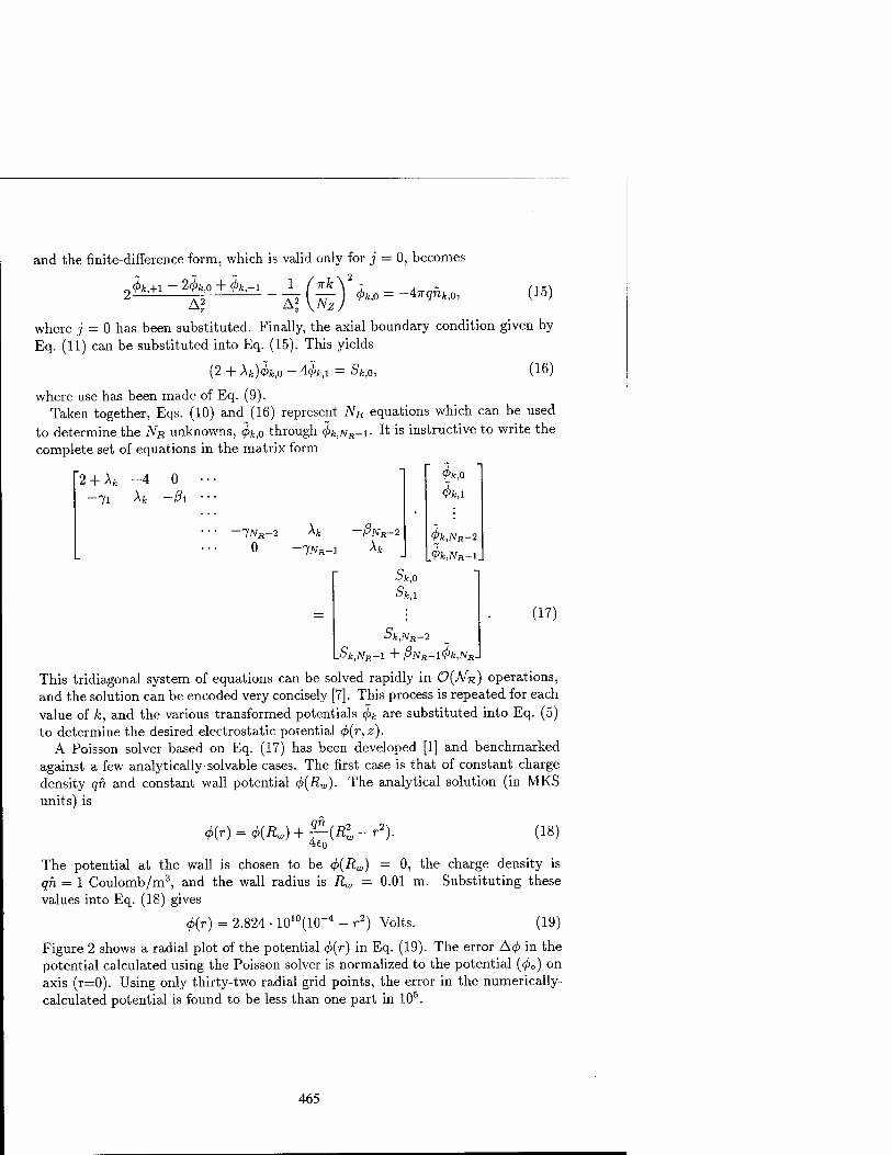
^4>k,+l — 2<^>fc,0 + 4>k,-l

A? (15)

and the finite-difference form, which is valid only for j = 0, becomes

h (£) k°=~4irqükfl' where j = 0 has been substituted. Finally, the axial boundary condition given by Eq. (11) can be substituted into Eq. (15). This yields

(2 + \k)fafl - Hk,i = Sk<o, (16)

where use has been made of Eq. (9). Taken together, Eqs. (10) and (16) represent NR equations which can be used

to determine the NR unknowns, <j>kfi through (j>k,NR-i- It is instructive to write the complete set of equations in the matrix form

2 + Afc

-7i

-4 0

-lNR-2 0 -INR-I

ONR-

9k,0

4>k,l

h,NR-2

t>k,NR-l_

Skfl

Sk.i

(17) Sk,NR-2

.Sk,NR-l + ßNR-l<f>k,NR.

This tridiagonal system of equations can be solved rapidly in ö(Mn) operations, and the solution can be encoded very concisely [7]. This process is repeated for each value of k, and the various transformed potentials ^ are substituted into Eq. (5) to determine the desired electrostatic potential <fi(r,z).

A Poisson solver based on Eq. (17) has been developed [1] and benchmarked against a few analytically-solvable cases. The first case is that of constant charge density qh and constant wall potential <j)(Rw). The analytical solution (in MKS units) is

(j>{r) = cj>{Rn +£(Ä--! (18)

The potential at the wall is chosen to be <f>(Rw) = 0, the charge density is qh = 1 Coulomb/m3, and the wall radius is Rw = 0.01 m. Substituting these values into Eq. (18) gives

<f>{r) = 2.824 • 1010(10"4 - r2) Volts. (19)

Figure 2 shows a radial plot of the potential <f>(r) in Eq. (19). The error A^ in the potential calculated using the Poisson solver is normalized to the potential (<f>0) on axis (r=0). Using only thirty-two radial grid points, the error in the numerically- calculated potential is found to be less than one part in 105.

465

3.0x10" - ' ' ' ' ' ' ' ' ' ' ' ' ' ' ' ' ' ' ' -

2.5xl06 P^^-\ \ 2.0xl06 I ^\ \

w -t->

| l.öxlO6 ' \. ; : N. "

1.0x10° :- \ -

5.0xl05 - \ -:

0 - . . . , ...,...,...,.. A 0.008 0.010 0.000 0.002 0.004 0.006

Radius (m) FIGURE 2. Plot showing the radial potential distribution for a uniform density column of

charged particles, used for benchmarking the numerical Poisson solver. The error in the potential

calculated using the Poisson solver, normalized to the potential (4>0) at r = 0), is found to be less

than one part in 105 using 32 radial gridpoints.

*( r,z)

1.0

0.5

Volts 0.0

-0.5

-1.0 0.2

Radius Axial distance

FIGURE 3. Plot of the vacuum potential profile <f>(r, z) within a cylinder with a sinusoidal wall

potential given by Vo COS(2JTZ/L). The length of the cylinder L is chosen to be four times the

cylinder radius Rw, and the amplitude of the sinusoidal wall potential is Vo = 1 V.

466

icr

10"

a B

10"' Kr 10-

1 10 100 1000

Radial Points FIGURE 4. The error in the computed potential is plotted as a function of the number of

radial grid points. Initially, the error decreases proportional to the square of the number of grid

points, as expected for errors due to the finite-difference approximation. Eventually, round-off

error becomes dominant, and the error increases with increasing numbers of grid points.

The second example is that of a vacuum potential (zero plasma charge density) with a sinusoidal wall potential Vocos(2nz/L). The analytical solution to Poisson's equation is given by

</>(r, z) Vo

I0(2TTRW/L) COS(2TT z/L)I0(2nr/L), (20)

where IQ(X) is the modified Bessel function of the first kind of order zero. Figure 3 shows a plot of the potential <f>(r, z) given by Eq. (20) for Vb = 1 V and axial length L = ARW. The difference between the analytical solution and the solution obtained with the Poisson solver using 32 radial x 32 axial grid points has been calculated. The maximum error in the numerically calculated potential is found to be approximately 8 x 10~5 V, whereas the actual potential variation is ±1 V.

The maximum error in the numerically-calculated potential 4>(r, z) is plotted as a function of the number of radial grid points in Fig. 4, assuming 32 axial grid points. This error is calculated using the vacuum potential test case. The error is observed to decrease initially as the square of the number of radial grid points used. This is likely due to the error involved in the finite-difference approximation of the derivatives, because the first- and second-derivatives both have errors that are dependent on the square of the grid spacing [8], i.e.,

467

/'(so) = 2x[/(*o + A) - /(*„ - A)] - ^/(3)(£),

/"(so) = ^[f(xo - A) - 2/(z0) + /(*„ + A)] - ^/(4)(0-

(21)

Eventually, at small enough grid spacing A, the error becomes dominated by round- off error, which becomes larger with an increasing number of grid points.

Ill CONCLUSIONS

In conclusion, a Poisson solver has been developed for an azimuthally symmetric cylindrical Malmberg-Penning trap. The solver computes the potential 4>{r,z), given the charge density distribution n(r,z), and the potential distribution on the radial boundary, 4>(Rw,z). The solver has been benchmarked against a few analytically-solvable cases, and good agreement has been obtained. For the Elec- tron Diffusion Gauge (EDG) experiment [1-3], this Poisson solver is an important tool in reconstructing the confined plasma density profile.

ACKNOWLEDGMENTS

This research was supported by the Office of Naval Research.

REFERENCES

1. Chao, E.H., Ph.D. Thesis, Princeton University (1999), and references therein. 2. Chao, E.H., Davidson, R.C., and Paul, S.F., J. Vac. Sei. Tech. A17, 2050 (1999). 3. Chao, E.H., Paul, S.F., and Davidson, R.C., J. Vac. Sei. Tech. A17, 2034 (1999). 4. Fine, K.S., Ph.D. Thesis, University of California, San Diego (1988). 5. Roberson, C.W., and Driscoll, C.F., (Eds.) Nonneutral Plasma Physics, American

Institute of Physics Conference Proceedings 175, (1988). 6. Hughes, M.H., Computer Physics Communications 2, 157 (1971). 7. Press, W.U., Teukolsky, S.A., Vetterlin, W.T., and Flannery, B.F., Numerical Recipes

in C (Cambridge University Press, 1992). 8. Burden, R.L., and Faires, J.D., Numerical Analysis (PWS Publishing Company,

Boston, MA 1993).

468

Ion-electron collisions in a homogeneous magnetic field

Günter Zwicknagel

Institut für Theoretische Physik, Universität Erlangen, Staudtstr. 7, D-91058 Erlangen, Germany

Abstract. As the basic ingredient for calculating the energy loss of ions in magnetized electron plasmas we investigate binary ion-electron collisions in a magnetic field by a classical trajectory Monte-Carlo type numerical treatment. We discuss results concerning mainly the nonlinear, strong coupling regime at low relative velocities and, in particular, the case of an ion motion transversal to the magnetic field lines.

INTRODUCTION

The transport properties of plasmas in an external magnetic field still raise many questions, as e.g. the energy loss of a heavy ion in a magnetized electron plasma which represents the basic process for electron cooling in heavy ion storage rings. Although electron cooling is now a well established method a lot of observations are not yet fully understood, basically because only approximative descriptions of ion stopping by magnetized electrons are available [1]. Such approximations are known to fail in a nonlinear regime occurring for highly charged, slow ions. For nonmag- netized electron plasmas the nonlinear stopping of heavy ions has been extensively investigated (see Ref. [2]) using numerical simulations as an essential tool. These studies verified particularly that the theoretical description of ion stopping can be extended into a moderate nonlinear regime by a specific combination of the linear response approach and the widely used binary collision model. The basic idea is to map the true ion-electron interaction which includes all the many-body effects responsible for dynamic screening and the excitation of plasma waves (wake field) into an effective, spherical symmetric interaction e.g. of the form

Vei(r) = -/^-exp(~). (1) 47re0 r A

Here the screening parameter X(V) may depend on the ion velocity V. It is determined from the linear response treatment which describes the dynamic target polarization in a moderate nonlinear regime still properly, although it fails to predict the stopping itself correctly, see [2] for details. Once the effective ion-electron


469

interaction (1) is given the needed transport cross section for binary collision can be calculated exactly, i.e. without any further approximations. This point is crucial for the success of the whole scheme. Here, we claim that this improved description should apply as well for magnetized electron targets which requires: (a) a determination of the effective interaction, i.e. A(V), from linear response including the magnetic field and a possible anisotropic velocity distribution of the electrons via the corresponding proper dielectric function; (b) a calculation of the energy and momentum transfer in binary ion-electron collisions in a homogeneous magnetic field. While work on the first topic is in progress we assume here that A and thus Vei(r) Eq. (1) are known and focus on the binary ion-electron collisions.

ION-ELECTRON COLLISIONS AT B = Be z

In the nonmagnetic case the transport cross section for the momentum transfer is a function only of the ion-electron relative velocity. With magnetic field additional dependencies show up like the strength of the magnetic field, the ratio of transversal and longitudinal velocities etc.. This makes even binary collisions a rather exhausting and challenging problem. While e.g. electron-electron collisions still separate in a centre-of-mass and a relative motion at B / 0, the centre-of-mass motion there couples to the relative motion for ion-electron collisions. To simplify the situation we restrict us to parameter regimes where an entirely classical treatment of the collision process is applicable and let the ion mass go to infinity after a transformation to centre-of-mass and relative (rr,vr) coordinates. The resulting classical equations of motion take then the form

A A ^r> = vr, -mvr = -Vr,Vd(|rr|) - e (vr x B) - e (V x B), (2)

where the ion or centre-of-mass velocity V has a given constant value and the reduced mass equals the electron mass m. Now, the homogeneous magnetic field B is chosen as B = Bez and the ion velocity as V = (Vx,0,Vz). Eqs. (2) can be put in a dimensionless form containing only the two parameters Z/\Z\ and B/B0

by scaling all lengths in units of the screening length A and all velocities in a characteristic velocity vc, where B0 and vc are defined through

mvc _ (\Z\m\1/2 ( \Z\# V'2

Here mv% equals the potential energy of the electron in the Coulomb field of the ion at a distance A. Strong coupling is expected for kinetic energies of the relative motion around TUVQ and smaller where the interaction dominates the collision process rather than the kinetic energy.

The geometry for the ion-electron motion before collision is sketched in Fig. 1 both in the lab-frame and the relative system where the initial velocity is vr(0) =

470

X lab-system

\M ill! 4 B

y© A z

relative-system

FIGURE 1. Collision geometry in the different frames

( v°x , v°y , v°z) = (y°± cos <p - Vx, v°x sin <p, vf\ - Vz). Here <p is the initial phase of

the spiral motion of the electron. The vector gr = (-14 ,0, v°rz) in Fig. 1 denotes the velocity of the guiding centre in the relative frame and allows to define an impact parameter b with respect to a plane perpendicular to gr and an incoming current density j — ne|gr| both needed to determine the stopping power from the energy loss per time. For example, the stopping power in direction of the ion motion results from the energy change AE in individual binary collisions by the averaging

F = F-v = ^ = ^/rfVK,<)|gr|/d2&/o2,rgA£;(vr,v1^). (4)

Here f(vpv°x) represents the velocity distribution of the electron plasma. For a deeper understanding of ion stopping by magnetized electrons it may be, however, more advantageous to study first the averaged relative changes of energy and momentum which can be expressed by the following partial transport cross sections (here scaled in 47rA2)

d2b f dip

m\v 0 12

aAEr,ll(*V°zX,T4)= ^Tp

j£?f%**^V~™ 4TTA2

d2b

J£fJ%****t"*-v«™ 4TTA2

d2b r dip

47rA2i 2n J^APM, >l,Vt,b,tp). (5)

The relative changes in the lab-frame of the transversal (_L B) energy -AEJ(mv2

c/2)

-AEr,||/(mv&/2)

[14 + v'rx]2 + v'ly - [v°±]2, the longitudinal relative energy

v'2z - [VrZ]2 and the longitudinal momentum -APz/mvc = [Vz + v'rz] - [Vz + v°TZ] = v'TZ - v°rz sum up to AE = AEL + AE^ + 2VZAPZ appearing in Eq. (4). Splitting the total energy change in these partial contributions provides, however, further insight in the complex collision process.

471

-(AEx) = -[v°±]2aAE±, v°=5

-(APz) = -v°zo&Pl, u° = 0.2

•-• B/B0 = 1 O-oB/B0 = 5 ■-•B/B0=10 O-O B/B0 = 50

-SSÄ^ -

- 5-ÖoöCKHiOOfiOöa^P-C^

1.0 10.0 100.0 1000.0

-(Aßj.) = -WU'*^, «i = 0.2

»-• BIB, = 1 o-DB/B0 = 5 ■-■B/B, = 10

-OO&OOtfoG

O-O B/B, = 50

10.0 100.0 1000.0

O-D B/B, = 5 B/B, = 10

O-O B/B, = 50 B/B, = 200

10.0

(v„)

100.0 1000.0

-(APz) = -v°.txAPz, v°_=5

100.0 1000.0

-(APz) = -«?2ffAP1, «1 = 5

-

T^V 1 D-D B/B, = 5 V\l ■-■B/B, = 10

VM O-O B/B, = 50 VK *-«B/B. = 200

\ 1^*»— ■

10.0

(O* FIGURE 2. Normalized averaged changes -(AE±) - -[v°±]

2a&E± (top) and -(AP-) = -■U°2CTAP2 (centre) for ion-electron collisions with parallel ion motion Vx = 0 and — (AE±), -(AP2) (bottom) for electron-electron collisions for different u^ and magnetic fields B/B0.

472

The changes of energy and momentum are calculated by a numerical integration of the electron trajectories through the interaction zone [3] for given initial conditions. The integration over the impact parameter b and the initial phase <p occurring in Eqs. (5) are performed by a Monte-Carlo method. The number of computed trajectories is adjusted by monitoring the convergence of the averaging procedure.

In the particular case of Vx = 0 the ion motion parallel to B can be completely transformed into vrz. Here energy conservation yields AE±_ = —AEri\\ and only the scaled values ~{AE±) = -[v0

±}2aABx and -(APZ) = -v°zaAPt are of interest.

They are shown in Fig. 2 as functions of [v°z]2 for different velocities of the cyclotron motion v°± and varying magnetic fields B/B0- Positive values of -(AE±) correspond to an increase of the energy in the cyclotron motion and a blowing up of the spirals during the collision in the average. This is observed for the low initial v°, = 0.2 which is always small compared to v°z (Fig. 2, left top). An oppositely

-(A£L) = - -K 2 *AE± , B/Bo = 6

0.0

-0.3 y

-0.6 -

-0.9 •—»v, = o n—n v, = 0.1

-1.2 ■—« V, = 0.3

O—OV, = 0.8

-1.5

10.0

(O2 100.0 1000.0

-<A£j.) = - -K 2 aAEj., B/B0 = 30

0.0

-0.3 ■

-0.6 • v, = o OV, = 0.1

-0.9 * V, = 0.3

O OV, = 0.8

-1.2

1.0 10.0 / 0.2 K)

100.0 1000.0

<APZ) = -v?. 'AP,, B/Bo = 6

0.35 ■

0.25

o—av, = 0.1

0.15 •—« V, = 0.3

O-OV, = 0.8

0.05

-0.05 J^ -

-<APz) = -u?2trAPl, B/Bo = 30

10.0

»ol ♦—»vr = 0

J5 R \\ °—° V, = 0.1

f°\ \v •—"v. = 0.3

\ \ \ o—ov, = 0.8

10.0

(v„Y

FIGURE 3. Normalized averaged changes -(AJSj.) = -[«5.]2 «TABJ. (top) and -(APZ) = -t,JzffAPi (bottom) for ion-electron collisions with varying transversal ion motion Vx at different

B/Bo and v°± = 6.

473

directed flow of energy related to a shrinking of the spirals occurs for the higher v°± = 5 when v% < v\ (right top). The same behaviour was also found for other v°±. In all cases, however, the absolute values of [UIJVAEL are strongly reduced with increasing magnetic field B. These features are recovered for the momentum change ~{APZ) — —VJ?0<7APZ (centre), where positive values indicate a deceleration of the electron motion parallel to B and negative ones an acceleration.

For comparison, results for repulsive electron-electron collisions are shown in the lower part of Fig. 2. Again, an increase of B yields a strong suppression of the energy transfer as it has been already documented e.g. in investigations on the equilibration of transversal and longitudinal temperatures in a magnetized electron plasma [4]. The momentum transfer (AP2) (right bottom) shows, however, a quite different behaviour than in the ion-electron case, mainly a weaker dependence on B and a convergence towards an always positive value for strong magnetic fields. This is certainly related to the repulsive force.

In the attractive case of ion-electron collisions again considerably different results are found for transversal ion motion Vx ^ 0. Here a net energy transfer, i.e. A£j_ ^ — AEVJI, results in a stopping power in transversal direction. In Fig. 3 we present the calculated averages (AEL), {APZ) for B/B0 = 6 and 30 and a initial transversal velocity u^ = 6. In the nonlinear regime which is reached for small [v°z]2 the results strongly depend on the transversal ion motion Vx. Here the energy transfer {AEx) can be much larger than for Vx = 0 and an interesting behaviour is observed for the change of transversal momentum — (APZ) (Fig. 3, bottom). There already a small Vx turns the average acceleration of electrons at low [wj?2]2

into a deceleration which initially increases with Vx, then reaches a maximum and decreases again at larger transversal ion motion. These results indicate that special attention has to be paid to the actual ion motion when calculating the energy loss related to electron cooling in storage rings where the low velocity regime is of particular importance. Similar observations on this role of the transversal ion motion in connection with stopping in magnetized electrons has already been made in PIC-simulations on this subject [5]. Work to investigate this in more detail is in progress.

REFERENCES

1. Meshkov I.N., Phys. Part. Nucl. 25, 631 (1994). 2. Zwicknagel G., Toepffer C, and Reinhard P.-G., Phys. Rep. 309, 117 (1999). 3. Spreiter Q., and Walter M., J. Comput. Phys. 152, 102 (1999). 4. Glinsky M.E., O'Neil T.M., Rosenbluth M.N., Tsuruta K., and Ichimaru S., Phys.

Fluids B 4 1156 (1992). 5. Walter M., Toepffer C. and Zwicknagel G., Hyperfine Interactions 115, 67 (1998).

474

PROGRAM

Monday, August 2

8:10 am - 3:15 pm Monday Oral Session

Morning Session Chair - John Bollinger, National Institute of Standards and Technology

8:10 am Opening Remarks

8:15 am - 8:50 am M-01 Quantum Computation with Trapped Ions, W. M. Itano, D. Kielpinski, B. E. King, C. Monroe, C. J. Myatt, C. A. Sackett, Q. A. Turchette, D. J. Wineland, NIST, Boulder

8:50 am - 9:25 am M-02 Progress in Antihydrogen Experiments, G. Gabrielse, Harvard University

9:25 am -10:00 am M-03 The ATHENA Antihydrogen Experiment, K. Fine and the ATHENA collaboration

10:00 am-10:20 am Break

10:20 am -10:55 am M-04 Trapping, Cooling and Extraction ofAntiprotons, and the ASACUSA Project, Y. Yamazaki, University of Tokyo

10:55 am - 11:30 am M-05 Next-generation Positron Accumulator and a Cold Positron Beam, C. M. Surko, U.C. San Diego

11:30 am - 12:05 pm M-06 Technological Applications of Trapped Positrons, R. G. Greaves, First Point Scientific, Inc.

12:05 pm - 1:30 pm Lunch (not provided)

Afternoon Session Chair - Scott Robertson, University of Colorado, Boulder

1:30 pm - 2:05 pm M-07 Autoresonant Excitation ofDiocotron Waves, J. Fajans, E. Gilson, U.C. Berkeley, L. Friedland, Hebrew University

2:05 pm - 2:40 pm M-08 Steady-State Confinement of Nonneutral Plasmas Using Trivelpiece-Gould Modes Excited by a "Rotating Wall", F. Anderegg, E. M. Hollmann, C. F. Driscoll, U. C. San Diego

2:40 pm - 3:15 pm M-09 Collisional Transport of Rods in a Magnetized Finite Length Plasma Column, D. H. E. Dubin, T. M. O'Neil, U.C. San Diego

475

3:15 pm - 5:30 pm Monday Poster Session

M-Pl Evolution of the m=l Diocotron Mode in the Electron Diffusion Gauge (EDG) Experiment, E. H. Chao, R. C. Davidson, S. F. Paul, K. A. Morrison, Princeton University

M-P2 Quadrupole Induced Resonant Particle Transport, E. Gilson, J. Fajans, U.C. Berkeley

M-P3 Two-Dimensional Fluid-Type Experiments Performed in a Malmberg-Penning Trap with a Photocathode, D. Durkin, J. Fajans, U.C. Berkeley

M-P4 Bifurcations in Elliptical, Asymmetric, Nonneutral Plasmas, J. Fajans, K. Backhaus, U.C. Berkeley

M-P5 Electron Confinement in an Annular Penning Trap, S. Robertson, University of Colorado, B. Walch, University of Northern Colorado

M-P6 Experiments of Pure Electron Plasmas Confined in Toroidal Geometry, C. Nakashima, Z. Yoshida, J. Morikawa, H. Himura, H. Kakuno, S. Tahara, N. Shibayama, University of Tokyo

M-P7 Confinement of Nonneutral Plasmas in the Prototype Ring Trap Device (Proto-RT), H. Himura, Z. Yoshida, C. Nakashima, J. Morikawa, H. Kakuno, S. Tahara, N. Shibayama, University of Tokyo

M-P8 Design of a Toroidal Plasma Confinement Device with a Levitated Super-Conducting Internal Coil, Y. Ogawa, H. Himura, S. Kondoh, J. Morikawa, Z. Yoshida, University of Tokyo, T. Mito, N. Yanagi, N. Iwakuma, Kyusyu University

M-P9 Two-Component Nonneutral Plasma in Penning-Malmberg Trap, H. Totsuji and Plasma Theory Group, Okayuma University

M-P10 Viscous Expansion of a Nonneutral Plasma, P. Goswami, S. N. Bhattacharyya, A. Sen, Institute for Plasma Research, K. P. Maheshwari, D. A. University, India

M-Pl 1 Excitation of Slow Solitary Perturbations in a Plasma Flow with Negative Ions, Cgo>

V. I. Maslov, Kharkov Institute

M-Pl 2 Simulation and Theory of Finite-Length Nonneutral Plasma Modes, R. L. Spencer, Brigham Young University

M-P13 Simulation and Theory of Finite-Length Nonneutral Plasma Modes, S. N. Rasband, R. L. Spencer, Brigham Young University

M-P14 Simulation of the Nonlinear Evolution of the Diocotron Instability, G. G. M. Coppa, A. D'Angola, G. Lapenta, Politecnico di Torino

476

M-P15 A 2D Vlasov Code for the Electron Dynamics in a Penning-Malmberg Trap, F. Califano, A. Mangeney, F. Pegoraro, R. Pozzoli, M. Rome, Universita di Pisa, Observatoire de Paris-Meudon, Universita di Milano

M-P16 Dynamics of Coherent Structures in a Penning-Malmberg Trap by 2D Vlasov Simulations, M. Rome, R. Pozzoli, F. Pegoraro, A. Mangeney, F. Califano, Universita di Milano, Universita di Pisa, Observatoire de Paris-Meudon

M-P17 Multiring Trap as a Reservoir of Cooled Antiprotons, T Ichioka, H. Higaki, N. Oshima, M Hori, A. Mohri, Y. Yamazaki, K. Komaki, K. Kuroki, University of Tokyo, RIKEN, National Research Institute of Police Science

M-Pl 8 Development and Testing of a Positron Accumulator for Antihydrogen Production, M. J. T. Collier, L. V. Jorgensen, O. L. Meshkov, D. P. van der Werf, M. Charlton, University College, London, Budker Institute of Nuclear Physics

M-P19 The Motion of Small Clumps and Holes on a Large Scale Vorticity Gradient, D. A. Schecter, D. H. E. Dubin, U.C. San Diego

477

Tuesday, August 3

8:15 am - 3:15 pm Tuesday Oral Session

Morning Session Chair - Cliff Surko, UC San Diego

8:15 am - 8:50 am T-01 Measurement of Collisional Cross-Magnetic-Field Heat Transport in a Pure Ion Plasma, E. M. Hollmann, F. Anderegg, C. F. Driscoll, U.C. San Diego

8:50 am - 9:25 am T-02 Experimental Observations of Nonlinear Effects in Waves in a Nonneutral Plasma, G. W. Hart, B. G. Peterson, R.L. Spencer, Brigham Young University

9:25 am - 10:00 am T-03 An Annular Malmberg-Penning Trap for Tests of Drift Kinetic Theory, S. Robertson, J. Kline, University of Colorado, B. Walch, University of Northern Colorado

10:00 am - 10:20 am Break

10:20 am - 10:55 pm T-04 Experimental Test of Resonant Particle Transport Theory, D. L. Eggleston, Occidental College

10:55 am - 11:30 am T-05 Characteristics of 2D Turbulent Flows that Self-Organize into Vortex Crystals, D. Z. Jin, D. H. E. Dubin, U.C. San Diego

11:30 am - 12:05 pm T-06 Two Experimental Regimes of Asymmetry-Induced Transport in Nonneutral Plasmas, J. M. Kriesel, C. F. Driscoll, U.C. San Diego


Afternoon Session Chair - Fred Driscoll, UC San Diego

1:30 pm - 2:05 pm T-07 Effect of Background Gas Pressure on Electron Plasma Dynamics in the Electron Diffusion Gauge (EDG) Experiment, E. H. Chao, R. C. Davidson, S. F. Paul, K. A. Morrison, Princeton University

2:05 pm - 2:40 pm T-08 Toroidal Magnetic Confinement of Nonneutral Plasmas, Z. Yoshida, Y. Ogawa, J. Morikawa, H. Himura, S. Kondo, C. Nakashima, H. Kakuno, M. Iqbal, F. Volponi, S. Tahara, N. Shibayama, University of Tokyo

2:40 pm - 3:15 pm T-09 Destabilization of the 1=1 Diocotron Mode in Nonneutral Plasmas, J. Finn, Diego del-Castillo-Negrete, D. C. Barnes, Los Alamos National Laboratory

478

3:15 pin - 5:30 pm Tuesday Poster Session

T-Pl Measurement of Plasma Mode Damping in Pure Electron Plasmas, J. R. Danielson, C. F. Driscoll, U.C. San Diego

T-P2 End Shape Effects on them-1 Diocotron Instability in Hollow Electron Columns, A. A. Kabantsev, C. F. Driscoll, U.C. San Diego

T-P3 Experiments on Viscous Transport in Pure-Electron Plasmas, J. M. Kriesel, C. F. Driscoll, U.C. San Diego

T-P4 Real-Space Imaging of Laser-Cooled Be+ Ion Crystals, J. J. Bollinger, T. B. Mitchell, L. B. King, W. M. Itano, NIST, Boulder

T-P5 Progress Toward a Sympathetically-Cooled Positron Plasma, B.J. Jelenkovic, J. J. Bollinger, A. S. Newbury, T. B. Mitchell, W. M. Itano, D. J. Wineland, NIST, Boulder

T-P6 Formation of a 'Be Plasma, B. G. Peterson, G. W. Hart, Brigham Young University

T-P7 Experiments on Particle-Particle Interactions in Dusty Plasma Crystals by Laser Manipulation, A. Melzer, Christian-Albrechts-Universitat Kiel

T-P8 Nonlinear Energy Loss of Ions in Magnetized Electrons, G. Zwicknagel, M. Walter, C. Toepffer, Universität Erlangen

T-P9 Consequences of Ion-Ion Interactions in Fourier Transform Ion Cyclotron Resonance Mass Spectrometry, C. L. Hendrickson, A. G. Marshall, National High Magnetic Field Laboratory

T-P10 Excitation of Solitary Perturbations from Normal Modes by Oscillating Field, V. I. Maslov, Kharkov Institute

T-Pl 1 Resonant Heating of Electron Sheath by Oscillations, V. I. Maslov, Kharkov Institute

T-P 12 Eigenmode Analysis of the Inviscid Growth and Decay of Small Perturbations on a Two-Dimensional Axisymmetric Vortex, D. A. Schecter, D. H. E. Dubin, I. M. Lansky, T. M. O'Neil, A. C. Cass, C. F. Driscoll, U.C. San Diego

T-P13 Analytic Study of Two-Ring Patterns of Vortices in a Penning Trap, G. G. M. Coppa, Politecnico di Torino

T-P 14 Formation of Vortex Crystals in Electron Plasmas, K. Avinash, R. Ganesh, Institute for Plasma Research

T-P 15 2-D Interaction of Discreet Electron Vortices, Y. Kiwamoto, A. Mohri, K. Ito, A. Sanpei, T. Yuyama, Kyoto University

479

T-P16 Structures and Dynamics of Dusty Plasmas and Dusty Plasma Mixtures, H. Totsuji and Plasma Physics Group, Okayama University

T-P 17 Positron Trap for Positron Injector ofLEPTA, S. Yakovenko, Dubna

T-P 18 A New Analogy Between Nonneutral Plasmas and Geophysical Fluid Dynamics, Diego del-Castillo-Negrete, John M. Finn, and Daniel C. Barnes, Los Alamos National Laboratory

7:00pm - 9:30 pm Banquet and Museum Tour

480

Wednesday, August 4

8:15 am - 3:15 pm Wednesday Oral Session

Morning Session Chair - Dan Dubin, UC San Diego

8:15 am - 8:50 am W-01 Wave Angular Momentum in Nonneutral Plasmas, R. Gould, Caltech

8:50 am - 9:25 am W-02 Modes, Crystalline Order and Antimatter Accumulation in Strongly Coupled Ion Plasmas, T. B. Mitchell, J. J. Bollinger, W. M. Itano, B. M. Jelenkovic, L. B. Kiftg, D. J. Wineland, NIST, Boulder

9:25 am -10:00 am W-03 Evidence of a Strongly-Coupled Highly-Charged Ion- Plasma, L. Gruber, J. P. Holder, J. Glassmann, J. Steiger, B. R. Beck, H. DeWitt, J. W. McDonald, D. A. Church, D. Schneider, Lawrence Livermore National Laboratory, Texas A&M University, University of Nevada Las Vegas

10:00 am-10:20 am Break

10:20 am -10:55 pm W-04 From Cold Neutral Atoms to Strongly Coupled Plasma, S. Kulin, NIST, Gaithersburg

10:55 am - 11:30 am W-05 Verification of Coulomb Order in a Storage Ring, R. Hasse, GSI Darmstadt

11:30 am-12:05 pm W-06 FEL Source Characteristics, S. Benson, Thomas Jefferson National Accelerator Facility


Afternoon Session Chair - Charles Roberson, Office of Naval Research

1:30 pm - 2:05 pm W-07 Hamiltonian Averaging Techniques for Intense Nonneutral Beam Propagation Through an Alternating- Gradient Quadrupole Field, R. C. Davidson, H. Qin, Princeton University, P. J. Channell, Los Alamos National Laboratory

2:05 pm - 2:40 pm W-08 Plasma-based Particle Accelerators, G. Shvets, Princeton University

2:40 pm-3:15 pm W-Q9 The Interaction of Intense Laser Pulses in Plasmas for Electron Acceleration and X-ray Generation, P. Sprangle, Naval Research Laboratory

481

3:15pm - 5:30 pm Wednesday Poster Session

W-Pl The Penning Fusion Experiment - Ions (PFX-1), M. M. Schauer, K. R. Umstadter, D. C. Barnes, Los Alamos National Laboratory

W-P2 Kinetic and Fluid Calculations for the Periodically Oscillating Plasma Sphere (POPS), R. A. Nebel, J. M. Finn, Los Alamos National Laboratory

W-P3 Confinement of Pure Ion Plasma in a Cylindrical Current Sheet, S. F. Paul, R. C. Davidson, C. K. Phillips, Princeton University

W-P4 Nuclear Fusion with Crystalline Beams, A. G. Ruggiero, Brookhaven National Laboratory, J. Machuzak, Massachusetts Institute of Technology

W-P5 Nuclear Fusion with Colliding Beams, A. G. Ruggiero, Brookhaven National Laboratory, J. Machuzak, Massachusetts Institute of Technology

W-P6 Initial Assessment of Nested- Well Plasma Traps for High Ion density Applications, C.A. Ordonez, University of North Texas

W-P7 Self-Consistent Static Analysis of Using Nested- Well Plasma Traps for Achieving Antihydrogen Recombination, D. D. Dolliver, C. A. Ordonez, University of North Texas

W-P8 Analysis of Time-Dependent Effects when Operating Nested- Well Plasma Traps for Achieving Antihydrogen Recombination, Y. Chang, D. D. Dolliver, K. F. Stephens, II, C. A. Ordonez, University of North Texas

W-P9 Virtual Cathode Formations in Nested-Well Plasma Traps, K. F. Stephens, II, C. A. Ordonez, University of North Texas, R. E. Peterkin, Jr., Air Force Research Laboratory

W-P10 Self-Consistent Trapping of Noncompensated Electron Beam in Homogeneous Magnetic Field, V. J. Maslov, I. K. Tarasov, Kharkov Institute

W-Pl 1 Solitary Electromagnetic Precursor in Electron Plasma, V. J. Maslov, Kharkov Institute

W-Pl2 Electromagnetically Induced Transparency and Pulse Propagation in Plasmas, B. Hafizi, P. Sprangle, R. F. Hubbard, J. R. Penano, Icarus Research, Naval Research Laboratory

W-P13 3D Multispecies Nonlinear Perturbative Particle Simulation of Intense Nonneutral Particle Beams, H. Qin, R. C. Davidson, W. Wei-li Lee, Princeton University

W-P14 Electron Cloud Effects in the Advanced Photon Source Storage Ring, K. C. Harkay, R. A. Rosenberg, Argonne National Laboratory, IL, P. Colestock, Fermi National Accelerator Laboratory, M. Furman, Lawrence Berkeley National Laboratory

482

W-P15 Production of Halo Particles by Collective Mode Excitations in High Intensity Beams, S. Strasburg, R. Davidson, Princeton University

W-P16 An Investigation of a Sheet Electron Beam Driven Backward Wave Oscillator, K. P. Maheshwari, Y. Choyal, K. C. Mittal, D. A. University, India

W-P17 Suppression of Synchrotron Radiation by Crystallized Beams, R. Blumel, Wesleyan University

W-P18 Series-Resonance Oscillations in Pure Electron Plasmas, K. L. Cartwright, P. J. Christenson, J. P. Verboncoeur, C. K. Birdsall, U. C. Berkeley

W-P19 Ultracold Rubidium Atoms Near the Ionization Threshold, A. V. Estrin, C. -H. Cheng, J. R. Ensher, P. L. Gould, E. E. Eyler, University of Connecticut

5:30 pm - 7:00 pm Tour of Princeton Plasma Physics Laboratory

483

Thursday, August 5

8:15 am - 3:15 pm Thursday Oral Session

Morning Session Chair - John Finn, Los Alamos National Laboratory

8:15 am - 8:50 am TH-01 Collective Modes in Strongly Coupled Dusty Plasmas, M. S. Murillo, Los Alamos National Laboratory

8:50 am - 9:25 am TH-02 Three-Dimensional Strongly-Coupled Plasma Crystal Under Gravity Conditions and New Results from Space Experiments, M. Zuzic, D. D. Goldbeck, J. A. Goree, U. Konopka, G. E. Morfill, H. Rothermel, R. Sutterlin, H. M. Thomas, Max-Planck-Institut, University of Iowa

9:25 am - 10:00 am TH-03 Electron Plasmas for Spherical Ion Focusing, D. C. Barnes, Los Alamos National Laboratory

10:00 am-10:20 am Break

10:20 am -10:55 pm TH-04 Proton Beam - Electron Plasma Interactions, R. E. Pollock, M. Muterspaugh, D. Todd, Indiana University

10:55 am - 11:30 am TH-05 New Description of Collisionless Relaxation in Beam- Plasma Systems, E. Y. Backhaus and J. S. Wurtele, U.C. Berkeley

11:30 am - 12:05 pm TH-06 Concepts of Temperature, Order, and Equilibrium Under Time-Dependent Confining Forces, J. Schiffer, Argonne National Laboratory

12:05 pm -1:00 pm Roundtable Discussion

484

AUTHOR INDEX

Anderegg, F., 161,223

B

Fajans, J., 93, 176, 250, 299 Fine, K. S., 40, 461 Finn, J. M, 147, 198 Friedland, L., 176

Backhaus, K., 299 Barnes, D. C, 147, 198, 425 Bergeson, S. D., 367 Bhattacharyya, S. N., 272 Blümel, R., 345 Bollinger, J. J., 353

Gabrielse, G., 29 Gilbert, S. J., 3 Gilson, E., 176, 250, 299 Goswami, P., 272 Gould, R. W., 170 Greaves, R. G., 3, 19

Califano, F., 135, 141 Cass, A. C, 115 Chang, Y., 71 Chao, E. H., 278, 435, 461 Charlton, M., 13 Collier, M. J. T., 13 Coppa, G G. M., 123, 129

D

H

Hart, G W., 182, 457 Hasse, R. W., 329 Higaki, H, 59 Himura, H, 397, 405, 411, 417 Hollmann, E. M, 161, 223 Hori, M., 59 Huang, X.-R, 353

D'Angola, A., 129 Danielson, J. R., 214 Davidson, R. C, 278,309, 320,435,461 del-Castillo-Negrete, D., 147, 198 Dolliver, D. D., 65, 71 Driscoll, C. F., 115, 161, 208, 214, 223,

256, 266 Dubin, D. H. E, 85, 106, 115, 233 Durkin, D., 93

I

Ichioka, T., 59 Iqbal, M., 397 Itano, W. M., 353 Ito, K., 99 Iwakuma, N., 417

E

Eggleston, D. L., 241 Ellsworth, J., 336 Estrada, J., 29

Jelenkovic, B. M., 353 Jin, D. Z., 85, 233 Jdrgensen, L. V., 13

485

K

Kabantsev, A. A., 208 Kakuno, H., 405, 411 Kakuno, S., 397 Kamon, K., 77, 389 Killian, T. C, 367 Kishimoto, T., 77, 389 Kiwamoto, Y., 99 Kline, J., 290 Komaki, K., 59 Kondo, S., 397 Kondoh, S., 417 Kriesel, J. M., 256, 266 Kulin, S., 367 Kuroki, K., 59

Orozco, L. A., 367 Orzel, C, 367 Oshima, N., 59

Paul, S. F., 278, 435, 461 Pegoraro, F., 135, 141 Peil, A., 383 Peil, S., 29 Peterkin, Jr., R. E., 451 Peterson, B. G., 182, 457 Phillips, C. K., 435 Pollock, R. E., 336 Pozzoli, R, 135, 141

Lansky, I. M., 115 Lapenta, G., 129

M

Qin, H., 309, 320

Maheshwari, K. P., 272 Mangeney, A., 135, 141 Melzer, A., 383 Meshkov, O. I., 13 Mitchell, T. B., 353 Mito, T., 417 Mohri, A., 59, 99 Morikawa, J., 397, 405, 411, 417 Morrison, K. A., 278 Murillo, M. S., 376 Muterspaugh, M. W., 336

R

Rasband, S. N., 192 Roach, T., 29 Roberson, C. W., xi Robertson, S., 290 Rolston, S. L., 367 Rome, M., 135, 141

N

Nakano, K., 77 Nakashima, C., 397, 405, 411

O

Ogawa, Y., 397, 417 O'Neil, T. M., 115 Ordonez, C. A., 65, 71, 445, 451

Sanpei, A., 99 Sasabe, T., 389 Schauer, M. M., 425 Schecter, D. A, 106, 115 Sen, A., 272 Shibayama, N., 397,405,411 Shvets, G, 309, 320 Spencer, R. L., 153, 182, 192 Stephens, II, K. F, 451 Surko, C. M., 3, 19

486

T W

Tahara, S., 397, 405, 411 Walch, B., 290 Tan, J. N., 29, 353 Wineland, D. J., 353 Todd, D. S., 336 Totsuji, C, 77, 389 Totsuji, H., 77, 389 Y Tsuruta, K., 77, 389

Yamazaki, Y., 48, 59 Yanagi, N., 417

U Yesley, P., 29 Yoshida, Z., 397, 405, 411, 417

Umstadter, K. R., 425 Yuyama, T., 99

van der Werf, D. P., 13 Zimmerman, L., 93 Volponi, F., 397 Zwicknagel, G., 469

487

Toroidal magnetic confinement of non-neutral plasmas

Documents

Transcript of Toroidal magnetic confinement of non-neutral plasmas