Confinement, screening and the center on S3× S1
23
arXiv:0711.0659v2 [hep-th] 15 Nov 2007 Preprint typeset in JHEP style - HYPER VERSION Confinement, Screening and the Center on S 3 × S 1 Carlos Hoyos 1 , Biagio Lucini 1 and Asad Naqvi 1,2 1. Department of Physics, Swansea University, Singleton Park, Swansea SA2 8PP, UK. 2. Lahore University of Management and Sciences, Lahore, Pakistan. E-mail: [email protected], [email protected], [email protected]. Abstract: We compute the one-loop effective potential for the Polyakov loop on S 3 × S 1 for an asymptotically free gauge theory of arbitrary group G and a generic matter content. We apply this result to study the phase structures of G 2 , SO(N ) and Sp(2N ) gauge theories which turn out to be in qualitative agreement with the results of lattice calculations. On S 3 × S 1 , at zero temperature, the Polyakov loop is zero for kinematical reasons. For small but non-zero temperature, the Polyakov loop is still zero if the gauge theory has an unbroken center, while it acquires a small vacuum expectation value for gauge theories whose center is trivial or explicitly broken by the presence of dynamical matter fields. At high temperatures, the saddle point structure of the effective potential is different from the low temperature case suggesting that the theory is in the deconfined phase. At finite N , the Polyakov loop is non-zero in the high temperature phase only in theories with no unbroken center symmetry, consistent with screening of the external charge introduced by the Polyakov loop and Gauss law on a compact space. Keywords: Yang-Mills Theories, Confinement, Finite Temperature.
-
Upload
independent -
Category
Documents
-
view
3 -
download
0
Transcript of Confinement, screening and the center on S3× S1

arX
iv0
711
0659
v2 [
hep-
th]
15
Nov
200
7
Preprint typeset in JHEP style - HYPER VERSION
Confinement Screening and the Center on S3 times S1
Carlos Hoyos1 Biagio Lucini1 and Asad Naqvi12
1 Department of Physics Swansea University Singleton Park Swansea SA2 8PP UK
2 Lahore University of Management and Sciences Lahore Pakistan
E-mail chbadayozswanseaacuk bluciniswanseaacuk
anaqviswanseaacuk
Abstract We compute the one-loop effective potential for the Polyakov loop on S3 timesS1
for an asymptotically free gauge theory of arbitrary group G and a generic matter content
We apply this result to study the phase structures of G2 SO(N) and Sp(2N) gauge theories
which turn out to be in qualitative agreement with the results of lattice calculations On
S3 times S1 at zero temperature the Polyakov loop is zero for kinematical reasons For
small but non-zero temperature the Polyakov loop is still zero if the gauge theory has
an unbroken center while it acquires a small vacuum expectation value for gauge theories
whose center is trivial or explicitly broken by the presence of dynamical matter fields At
high temperatures the saddle point structure of the effective potential is different from
the low temperature case suggesting that the theory is in the deconfined phase At finite
N the Polyakov loop is non-zero in the high temperature phase only in theories with no
unbroken center symmetry consistent with screening of the external charge introduced by
the Polyakov loop and Gauss law on a compact space
Keywords Yang-Mills Theories Confinement Finite Temperature
Contents
1 Introduction 1
2 Confinement on S3 for an arbitrary gauge theory 4
21 Large N phase transition 9
22 Some examples 10
3 The G2 case 12
4 Orthogonal and Symplectic Groups 15
5 Gauss law and Screening 17
6 Conclusions 18
1 Introduction
Quantum Chromodynamics (QCD) is a confining theory the elementary particles of the
theory quarks and gluons never appear as final states of strong interactions This property
holds for temperatures below a critical value Tc above which the system is deconfined and
quarks and gluons form a plasma Confinement is a property of both QCD and the pure
gauge theory without any matter To gain a better understanding of this phenomenon it
is useful to study confinement in pure Yang-Mills theory For pure SU(N) gauge theory
the existence of a deconfinement phase transition has been rigorously proved in [1]
The finite temperature theory is formulated on a four dimensional Euclidean space
with one compact dimension The length β of the compact dimension is the inverse of the
temperature T In the confined phase the free energy of an isolated static quark is infinite
The free energy F is related to the vacuum expectation value of the Polyakov loop
LR(~x) =1
dRtrR
(
eigR 1T0 A0(~xt)dt
)
(11)
where A0 is the vector potential in the compact direction (parameterized by the coordinate
t) g is the coupling of the theory dR is the dimension of the irreducible representation
under which the quark transforms1 and ~x is the position of the quark If we define the
vacuum expectation value (vev) of L (we drop the representation index from now on) as
〈L〉 =1
V
langint
L(~x)d3x
rang
(12)
1In QCD this is the fundamental representation it is useful however to study a more general case in
which the quark is in a generic representation of the gauge group
ndash 1 ndash
the relationship between L(~x) and the free energy of the quark is given by [2]
F = minusT log〈L〉 (13)
In SU(N) gauge theories the behavior of 〈L〉 across the deconfinement phase transition
can be explained in terms of a symmetry This is the symmetry of the system under the
ZN center of the group which leaves the Lagrangian unchanged Under a transformation
z isin ZN 〈L〉 rarr z〈L〉 In the deconfined phase F is finite ie 〈L〉 6= 0 This implies
that in the deconfined phase the center symmetry is broken Conversely in the confined
phase F is infinite 〈L〉 = 0 and the center symmetry is not broken This leads to the
natural interpretation that confinement reflects a change in the property of the vacuum
under the ZN center symmetry the vev of the Polyakov loop being the order parameter for
the transition This observation lead Svetitsky and Yaffe to the well-known conjecture [3]
that relates the deconfinement phase transition in a four dimensional SU(N) gauge theory
to the order-disorder transition in three dimensional ZN spin systems since the properties
of the deconfinement transition are determined by the underlying ZN symmetry the gauge
and the corresponding spin system are in the same universality class when both transitions
are second order
Since confinement is a non-perturbative phenomenon a fully non-perturbative ap-
proach such as putting the theory on a space-time lattice is mandatory for quantitative
studies For SU(N) gauge theory recently it has been shown in [4] that important in-
sights about the physics of color confinement and the phase structure of the theory can
be obtained by studying the system on a S3 times S1 manifold where the radius β of the S1
is connected to the temperature in the usual way (β = 1T ) and the radius R of the S3
provides the IR cutoff at which the running of the gauge coupling freezes When 1R is
much larger than the dynamical scale of the theory the coupling is small and perturba-
tive calculations are reliable It is then possible to compute an effective potential for the
Polyakov loop at one loop order in perturbation theory Evaluating the partition function
of the system for β ≪ R (high temperature regime) and β ≫ R (low temperature regime)
yields information about the phase structure of the theory In confining gauge theories
for a finite number of degrees of freedom a cross-over between the confined and deconfined
phase is observed with the two phases being characterized by a different structure of the
minima of the free energy (or using a more field theoretical terminology the effective po-
tential) In order to verify the existence of a real phase transition at some critical value of
the temperature an infinite number of degrees of freedom is needed In standard thermo-
dynamical calculations this is achieved by taking the infinite volume limit of the system
This limit is obviously not possible for S3timesS1 since the calculations rely on R being small
Instead the thermodynamic limit is achieved here in another way by sending to infinity
the number of elementary degrees of freedom of the theory (one example in SU(N) gauge
theory is to take the limit of infinite number of colors N with fixed g2N [5]) Thus the
existence of a phase transition can be rigorously proved only in some large N limit for
finite N or for exceptional groups weak coupling calculations on a S3 times S1 manifold can
only discover the existence of two regimes (confined and deconfined) but cannot establish
whether they are separated by a cross-over or a real phase transition in infinite volume
ndash 2 ndash
Weak coupling calculations on S3 times S1 have been used for determining the phase
structure of various supersymmetric and non-supersymmetric gauge theories [6ndash10] treat-
ing each case independently In this paper we shall show that a general expression can
be derived from the representation theory of the Lie Algebra of the gauge group that al-
lows one to compute the one-loop effective potential for a generic gauge theory containing
bosons and fermions in arbitrary representations Using our result it is straightforward to
work out the phase structure of non-Abelian gauge theories for any gauge group and given
matter content We shall show that our computation reproduces the previously known
results and we will use it to determine the phase structure of other gauge theories that
can help us to understand the physics of color confinement like G2 gauge theory with no
center and SO(N) gauge theory whose center is either trivial (N odd) or Z2 (N even) 2
While a priori it is not obvious that the small volume calculations reproduce features of
the thermodynamical limit comparisons with other techniques (such as the lattice as we
will show in this paper) provide evidence that this is indeed the case
Our calculation show that in general the minimum structure of the effective potential is
different at low and high temperatures This means that a cross-over (in the finite volume
case) or possibly a phase transition (which can arise only if the thermodynamical limit
can be taken eg by sending to infinity the number of elementary degrees of freedom of
the theory) separates those two regimes which are naturally identified respectively with
the confined and deconfined phase However in both regimes the details of the minimum
structure depend on the center symmetry A symmetry cannot be spontaneously broken
on finite volume so if there is a non-trivial center that is not broken explicitly by the
matter content of the theory the Polyakov loop cannot develop an expectation value at
any temperature Why the Polyakov loop vanishes in these theories differs in the low
temperature and the high temperature phase In the low temperature phase the effective
potential for the Polyakov loop will have only one saddle point in which the Polyakov
loop will be zero At high temperatures there are multiple saddle points of the effective
potential each related by the action of the center In each of the saddle points the
Polyakov loop is non-zero However since we are on finite volume these saddle points are
not superselection sectors and therefore we have to sum over all of them which yields a zero
value for the Polyakov loop It is plausible to assume that the existence of the saddle points
at high temperatures survives the infinite volume limit in which we can restrict ourselves
to one of the multiple saddle points thereby breaking the center symmetry and signaling
a confinementdeconfinment transition The situation is different when the theory has no
unbroken center subgroup In that case at both low and high temperatures there is one
global minimum of the effective potential In the low temperature phase the Polyakov loop
is small (O(eminusβR)) and is zero at zero temperature whereas in the high temperature phase
we find that it develops an O(1) non-zero expectation value This can be understood in
terms of screening the external charge introduced by the Polyakov loop For theories with
a non-trivial center the external charge cannot be screened by gluons and quarks popping
out of the vacuum However if there is no center symmetry any external charge can be
2In this paper we will exclusively study SO(N) groups and not their covering groups Spin(N)
ndash 3 ndash
screened by an appropriate number of gluons and quarks
The paper is organized as follows In Sect 2 we compute the effective potential for a
generic Lie group on a S3 times S1 manifold and derive the behavior of the Polyakov loop at
high and low temperature in terms of the root and weight vectors of the group and the
matter content of the theory emphasizing how our result reproduces previous calculations
and how it can be used to analyze other gauge theories In Sect 3 we specialize to the G2
case showing that the Polyakov loop is zero at sufficiently low temperature and different
from zero at high temperatures The same result is worked out for SO(N) gauge theories
in Sect 4 In Sect 5 we show that our results are compatible with the non-Abelian Gauss
law Finally Sect 6 sums up our findings and their implications for our understanding of
color confinement
2 Confinement on S3 for an arbitrary gauge theory
In the canonical ensemble the thermal partition function of a quantum field theory is
equal to the Euclidean path integral of the theory with a periodic time direction of period
β = 1T and anti-periodic boundary conditions for the fermions along the temporal circle
We will consider a gauge theory with a semi-simple group G with matter in arbitrary
representations on a spatial S3 In the following we will assume that the theories we want
to study are asymptotically free To understand the phase structure we need to calculate
the free energy which is just the log of the partition function Therefore we perform a
Euclidean path integral for the theory on S3R times S1
β
We take 1R to be large compared to the dynamical scale of the theory so the theory
is at weak coupling The S1 topology allows non-trivial flat connections Fmicroν = 0 that can
be parameterized in a gauge invariant way by the vev of the Polyakov loop The set of
flat connections are the lightest degrees of freedom of the theory and other excitations are
separated in energy by a gap proportional to 1R In fact the flat connection is a zero
mode of the theory in the sense that the quadratic part of the action does not depend on it
The low energy phase structure can be studied using a Wilsonian approach where heavier
degrees of freedom are integrated out to give an effective action for the flat connection In
the weak coupling regime we can perform a perturbative expansion in the coupling and the
one loop result provides a good approximation to the effective potential Our discussion
will generalize previous results [7 1112]
We can use time-dependent gauge transformations to fix A0 to be constant and in the
Cartan subalgebra
A0 =
rsum
a=1
HaCa [HaHb] = 0 foralla b (21)
where r is the rank of the group The vev of the Polyakov loop is
L = tr exp
(int
S1
A0
)
(22)
Notice that A0 is anti-Hermitian in this expression A coupling constant factor has been
absorbed in the field as well This means that in the classical Lagrangian the fields will
not be canonically normalized but there is a 1g2 overall factor
ndash 4 ndash
We will now consider adding matter fields to the gauge theory in arbitrary represen-
tations that can be obtained as tensor products of the fundamental (and anti-fundamental
in case it exists) The fundamental representation corresponds to a mapping of the group
to the (complex) general linear group acting on a vector space of dimension F So any
representation can be mapped to a tensor (we are ignoring the spinor representations of
SO(N) groups) The tensor can have covariant or contravariant indices and the adjoint
action can be defined as (summation understood)
Ad(A)X = Ak1i1Xj1middotmiddotmiddotjm
k1i2middotmiddotmiddotin+ middot middot middot +Akn
inXj1middotmiddotmiddotjm
i1middotmiddotmiddotknminusAj1
l1X l1middotmiddotmiddotjm
i1middotmiddotmiddotinminus middot middot middot minusAj1
lmX l1middotmiddotmiddotlm
i1middotmiddotmiddotin (23)
For SU(N) groups the Cartan subalgebra admits a diagonal form in terms of the funda-
mental weights ~νi i = 1 F where F is the dimension of the fundamental representa-
tion
Haij = νa
i δij (24)
The fundamental weights need not be linearly independent this will happen only if F = r
the rank of the group Real groups like SO(N) and Sp(N) cannot be diagonalized using
gauge transformations However once we have fixed the flat connection to be constant
we can do a global similarity transformation to diagonalize it Gauge invariant operators
remain unchanged so this transformation is allowed In the case of SO(N) this is done by
a U(N) transformation while in the case of Sp(N) it is a U(2N) transformation In the
diagonal basis the adjoint action simplifies to
Ad(A)X = ~C middot(
nsum
a=1
~νiaXj1middotmiddotmiddotjm
i1middotmiddotmiddotiamiddotmiddotmiddotinminus
msum
b=1
~νjbXj1middotmiddotmiddotjbmiddotmiddotmiddotjm
i1middotmiddotmiddotin
)
(25)
which is
Ad(A)X = ~C middot(
nsum
a=1
~νia minusmsum
b=1
~νjb
)
Xj1middotmiddotmiddotjm
i1middotmiddotmiddotin= (~C middot ~micromn)Xj1middotmiddotmiddotjm
i1middotmiddotmiddotin (26)
Here ~C ~ν and ~micromn are r dimensional vectors and the dot product is the standard
Euclidean product The weights of any representation are linear combinations of the fun-
damental weights so ~micromn = (sumn
a=1 ~νia minussummb=1 ~νjb
) is a weight of the tensor representation
with m covariant and n contra-variant indices
The covariant derivative acting on a field in the background field of the Polyakov loop
is
DmicroX = partmicroX minus δmicro0Ad(A)X (27)
To calculate the one-loop effective potential we expand the gauge field matter and the
ghosts in harmonics on S3timesS1 and keeping only the quadratic terms we integrate out the
various modes The one loop potential will be in general
V (C) = minus1
2
sum
R
(minus1)FRTrS3timesS1 log(
minusD20R minus ∆
)
(28)
where R denotes the gauge group representation of the different fields we have integrated
out FR is the fermionic number and the trace is over the physical degrees of freedom (zero
ndash 5 ndash
modes excluded) This can be written as
V (C) =sum
R
(minus1)FRsum
~microR
VR(~microR middot ~C) (29)
where ~microR are the weights of the representation and the potential VR can depend on the
Lorentz representation of the field In flat space (T n times Rd case) VR is just an universal
function times the number of physical polarizations (see [7] for instance) On S3 the
situation is different because the Kaluza-Klein decomposition depends on the spin of the
field The one-loop potential for several SU(N) theories on S3 times S1 has been computed
previously [4 8] We will generalize the computation to other groups and cast the results
in a simple form
In general
TrS3timesS1 log(
minusD20R minus ∆
)
=sum
~microR
sum
ℓ
sum
n
NR(ℓ) log
(
ε2ℓ +
(
2πn
β+ ~microR middot ~C
)2)
(210)
where NR is the number of physical polarizations of the field and εℓ is the energy of the
Kaluza-Klein mode ψl satisfying ∆ψl = minusε2ℓψl (∆ is the Laplacian on S3) NR and εℓdepend on the field type that is being integrated out in a way that we list below
(i) Scalars Scalar field can be conformally or minimally coupled The set of eigen-
vectors is the same in both cases However their eigenvalues are different For confor-
mally coupled scalars3 we have εℓ = Rminus1(ℓ + 1) whereas for minimally coupled scalars
εℓ = Rminus1radic
ℓ(ℓ+ 2) In both cases there is a degeneracy NR(ℓ) = (ℓ+ 1)2 with ℓ ge 0
(ii) Spinors For 2-component complex spinors we have εℓ = Rminus1(ℓ + 12) and
NR(ℓ) = 2ℓ(ℓ+ 12) with ℓ gt 0
(iii) Vectors A vector field Vi can be decomposed into the image and the kernel of
the covariant derivative Vi = nablaiχ + Bi with nablaiBi = 0 The eigenvectors for Bi have
εℓ = Rminus1(ℓ+ 1) and NR(ℓ) = 2ℓ(ℓ + 2) with ℓ gt 0 On the other hand the part nablaiχ has
εℓ = Rminus1radic
ℓ(ℓ+ 2) with degeneracy NR(ℓ) = (ℓ+ 1)2 but with ℓ gt 0 only
Notice that both spinors and vectors have no zero (ℓ = 0) modes on S3 This is why
in a pure gauge theory the only field with a zero mode is A0 which is a scalar on S3
It is a standard calculation using Poisson resummation to show that up to an infinite
additive constant
TrS3timesS1 log(
minusD20R minus ∆
)
=sum
~microR
infinsum
ℓ=0
NR(ℓ)
βεℓ minusinfinsum
n=1
1
neminusnβεℓ cos(nβ ~microR middot ~C)
(211)
The first term here involves the Casimir energy and since it is independent of ~C will play
no role in our analysis and we will subsequently drop it Ignoring this term the potential
VR is given by
VR(x) = 2sum
ℓ
NR(ℓ)
infinsum
n=1
eminusnβεℓ
sin2(
nβ2 x)
n (212)
3These have a mass term involving the Ricci scalar of the manifold in this case simply Rminus1
ndash 6 ndash
The sum on n can be done explicitly and the result is up to a constant
VR(x) =1
2
sum
ℓ
NR(ℓ) log
1 +sin2
(
βx2
)
sinh2(
βεℓ2
)
(213)
This is the contribution to the effective potential obtained by integrating out a particular
field The information about the type of field being integrated out (its Lorentz transfor-
mation properties etc) is encoded in NR(ℓ) and εℓ as explained above
In the remainder of this section we will restrict ourselves to a pure gauge theory with
no matter fields Then the basic degree of freedom is the non-Abelian gauge potential
Amicro which decomposes into a time component A0 which transforms as a minimally coupled
(massless) scalar on S3 and a vector Ai on S3 We can write Ai = nablaiC + Bi such that
nablaiBi = 0 Gauge fixing
(
nablaiAi +D0A0
)
= 0 by the usual Fadeev-Popov procedure leads
to the existence of ghosts
Then integrating out the A0 Bi C and ghost modes can be performed using the
following table
field S3 KK minus mode εℓ NR(ℓ)
Bi ℓ gt 0 (ℓ+ 1)R 2ℓ(ℓ+ 2) times (+1)
C ℓ gt 0radic
ℓ(ℓ+ 2)R (ℓ+ 1)2 times (+1)
ghosts ℓ ge 0radic
ℓ(ℓ+ 2)R (ℓ+ 1)2 times (minus2)
A0 ℓ ge 0radic
ℓ(ℓ+ 2)R (ℓ+ 1)2 times (+1)
Notice that for ℓ gt 0 the modes C ghost and A0 cancel and the only contributions is
from divergenceless modes Bi The constant ℓ = 0 modes for C ghosts and A0 give the
following contribution
V (x) sim minusinfinsum
n=1
cos(nx)
nsim log sin2
(x
2
)
(214)
This contribution is precisely the logarithm of the Jacobian that converts the integrals over~C into the invariant integral over the group element g = exp
(
i~microAd ~C)
yielding the correct
gauge invariant measure in the path integral dmicro(g) g isin G
Z ≃int
d~Cprod
microAd
sin
(
~microAd middot ~C2
)
middot middot middot ≃int
dmicro(g) middot middot middot (215)
The contribution from the divergenceless part of Ai which we have been denoting by Bi
can be easily written down using (213) and reading off the corresponding εℓ and NR(ℓ)
from the table above Then the total effective potential is
Vgauge( ~C) =sum
~microAd
V(~microAd middot ~C) (216)
where
V(x) = minus log∣
∣
∣sin(x
2
)∣
∣
∣+sum
lgt0
l(l + 2) log
1 +sin2
(
x2
)
sinh2(
β(l+1)2R
)
(217)
ndash 7 ndash
The two terms in the effective potential come with opposite signs the first term corresponds
to a log repulsion coming from the ℓ = 0 modes whereas the second term is an attractive
term It is the interplay between these two types of contributions that leads to an interesting
phase structure for the theory
In the low-temperature limit βR ≫ 1 the attractive contribution to the potential is
exponentially supressed
V(x) ≃ minus log∣
∣
∣sin(x
2
)∣
∣
∣+sum
lgt0
4l(l + 2) sin2(x
2
)
eminusβ(l+1)
R + (218)
In the high-temperature limit βR ≪ 1 the lower mode terms become stronger and cancel
the repulsive term except very close to the origin x sim βR
V(x) ≃ minus log∣
∣
∣sin(x
2
)∣
∣
∣+ 6 log
∣
∣
∣sin(x
2
)∣
∣
∣+ (219)
Therefore we expect a change of behavior with increasing temperature At low temper-
atures the expectation value of the Polyakov loop is zero up to exponentially supressed
contributions This can be seen from the fact that the repulsive term becomes the group
measure (215) and since the Polyakov loop corresponds to the character of the group
associated to the representation R
〈L〉 =1
Z
int
dmicro(g)χR(g) = 0 (220)
In the zero temperature limit this is a kinematical statement there cannot be unscreened
charges in a compact space Therefore confinement is just a kinematical fact The deriva-
tion of the Haar measure in S3 times S1 was known for unitary groups [4] but our discussion
is completely general and includes any semi-simple Lie group
It is interesting to notice that at higher temperatures the expectation value of the
Polyakov loop could be non-zero even in finite volume An intuitive explanation follows
from considering the Polyakov loop as the insertion of an external source in the system
At zero temperature pair production from the vacuum is completely frozen out so it will
cost an lsquoinfinite amount of energyrsquo to introduce a charge in finite volume However at
higher temperatures the system is in an excited state where the charges present in the
medium can screen the external source Whether this actually happens or not depends on
the details of the group and the type of source we introduce In gauge theories with unitary
groups this issue boils down to whether the center of the group is broken or not In pure
Yang-Mills the center is unbroken so the expectation value of the Polyakov loop should
be zero at any temperature On the other hand in a theory with quarks the center is
completely broken so the Polyakov loop can be nonzero at high temperatures In theories
with an unbroken center the Polyakov loop has to be zero due to kinematics However at
high temperatures the main contributions to the path integral will come from a sum over
saddle points corresponding to the minima of the potential For very large temperatures
the measure can be approximated by a sum of delta functions so the value of the Polyakov
loop is just the sum at the different minima At each of these points the Polyakov loop
ndash 8 ndash
has a nonzero value and it is plausible to assume that there is a map between them and
the possible vacua of the gauge theory in the deconfined phase in infinite volume where
kinematical constraints do not apply In this sense by restricting ourselves to only one
saddle point at high temperatures thereby getting a non-zero value of the Polyakov loop
we can interpret these results as a confinement-deconfinement phase transition at weak
coupling
Strictly speaking there is no transition at finite volume in the high temperature phase
we should sum over all the vacua so the average of the Polyakov loop will be still zero
or we would go smoothly from a zero to a non-zero value as we increase the temperature
However it is possible to show there is a sharp transition in the large N limit [4] Of course
this is not applicable to the exceptional groups but only to the classical groups
21 Large N phase transition
In the ensuing analysis it is convenient to write the potential in terms of the Polyakov loop
eigenvalues λi = ~νi middot ~C where νi are the fundamental weights This immediately follows
from the fact that the weights of any tensor representation are linear combinations of
the fundamental weights and the contributions from integrating out such representations
to the effective potential will depend on corresponding linear combinations of λi In the
N rarr infin limit for the classical groups we can approximate the discrete set of eigenvalues
by a continuous variable θ and substitute the sums over eigenvalues by integrals in θ
sum
λi
rarr N
int
dθρ(θ) (221)
with an eigenvalue density ρ(θ) ge 0 such that
int π
minusπdθρ(θ) = 1 (222)
The domain of integration is determined by the periodicity of the Polyakov loop eigenvalues
The potential becomes a functional of the eigenvalue distribution and the system is well
described by the saddle point that minimizes the potential When the parameters of the
theory change such as the ratio βR the dominating saddle point can change leading to
a phase transition
For pure U(N) Yang-Mills the potential is given by equation (217) with x = ~microadj ~C =
λi minus λj After converting the summation to the integral via the density of eigenvalues we
obtain
V [ρ] = N2
int π
minusπdθρ(θ)
int π
minusπdθprimeρ(θprime)
infinsum
k=1
1
k(1 minus zV (qk)) cos(k(θ minus θprime)) (223)
where q = eβR and zV is the partition function of divergenceless vector fields in S3
zV (q) =sum
lgt0
2l(l + 2)qminus(l+1) = 23 q minus 1
(q minus 1)3 (224)
ndash 9 ndash
We can expand the eigenvalue distribution in complex Fourier components ρn
ρ(θ) =1
2π+
infinsum
n=1
Re(ρn) cos(nθ) +
infinsum
n=1
Im(ρn) sin(nθ) (225)
and perform the integrals We are left with a quadratic potential for each Fourier compo-
nent
V = N2π2infinsum
n=1
(1 minus zV (qn))
n|ρn|2 (226)
For low enough temperatures zV (qn) lt 1 for all n and all the coefficients in the summation
are positive so the configuration of minimal energy is the uniform distribution ρ(θ) =
1(2π) In this case the expectation value of the Polyakov loop vanishes giving a weak
coupling version of the confining phase When we increase the temperature the coefficient
of the n = 1 component first becomes zero at a critical value qc = 2+radic
3 and then negative
beyond this point If we continue increasing the temperature eventually larger Fourier
components become unstable beyond the points q(n)c = q
1nc of marginal stability At the
critical value qc the eigenvalue distribution jumps to a qualitatively different saddle point
characterized by the appearance of a gap in the eigenvalue distribution ie there is a
range of values on θ over which that function ρ(θ) has no support At temperature just
above qc
ρ(θ) =1
2π(1 + cos(θ)) (227)
The expectation value of the Polyakov in this saddle point is no longer zero so this tran-
sition is a weak coupling analog of the confinementdeconfinement phase transition
22 Some examples
We would like to emphasize that the formulas derived in this section are completely general
on S3 times S1 for any semi-simple gauge group and for fields in any representation We can
cast the complete one-loop potential as a sum of different terms determined by the spin
of the field and the weight system of the group representation Possible examples are
pure gauge theories with unitary orthogonal symplectic or exceptional groups We will
comment some of them in the next sections
Here we give a small list of examples in terms of the eigenvalues of the Polyakov loop
λi = ~νi middot ~C for unitary groups The phase diagram of most of them has been analyzed
previously in the large-N limit [6 9] showing an interesting structure in terms of the
expectation values of the Polyakov loop All of them exhibit a deconfinement transition at
some critical temperature Tc We will use the potential generated by Weyl fermions
VF (x) =1
2
sum
lgt0
l(2l + 1) log
1 +sin2
(
x2
(
+π2
))
sinh2(
β(2l+1)4R
)
(228)
The π2 addition in the argument is for anti-periodic boundary conditions on fermions
Then we can write the following potentials
ndash 10 ndash
bull QCD SU(N) Yang-Mills with Nf massless flavors (or theories with fundamental
matter in general)
V (λ) =sum
i6=j
V (λi minus λj) minus 2Nf
Nsum
i=1
VF (λi)
At high temperatures the flavor contribution to the potential favors the λi = 0
minimum over other center-breaking minima At low temperatures the flavor po-
tential is exponentially supressed and only the repulsive term from the pure gauge
contribution is relevant
bull Supersymmetric theories N = 1 SU(N) (or theories with adjoint matter in general)
V (λ) =sum
i6=j
V (λi minus λj) minussum
i6=j
VF (λi minus λj)
Notice that when l rarr infin fermionic and bosonic contributions cancel at leading order
if we choose periodic boundary conditions for fermions At high temperatures all the
center-breaking minima become deeper so center symmetry is unbroken At large
N the system will sit at one of these center-breaking minima At low temperatures
the fermionic contribution is exponentially supressed
bull Orientifold theories [13] SU(N) gauge theories with a Dirac fermion in the anti-
symmetric (or symmetric) representation (or theories with two-index representations
in general)
V (λ) =sum
i6=j
V (λi minus λj) minussum
i6=j
VF (λi + λj) minus(
2Nsum
i=1
VF (λi)
)
The term inside the parentheses only appears in the symmetric representation in
the large-N limit its contribution is sub-leading At high temperatures there are two
possible situations depending on N being even or odd In the first case there are
two-minima that become deeper wrt other center minima If N is odd there is only
one minimum In general the vacuum corresponds to non-trivial center vacua [712]
At low temperatures we recover the pure gauge potential
bull Orbifold theories (cf [14]) for instance the Z2 case with SU(N) times SU(N) gauge
group and fermions in the bifundamental representation (or theories with several
gauge group factors in general)
V (λ(1) λ(2)) =sum
i6=j
V(
λ(1)i minus λ
(1)j
)
+sum
i6=j
V(
λ(2)i minus λ
(2)j
)
minus 2sum
ij
VF
(
λ(1)i minus λ
(2)j
)
In the limit l rarr infin and large N the diagonal sector λ(1) = λ(2) becomes supersym-
metric At high temperatures the minima are on λ(1)i = minusλ(2)
i [12] and in this sector
the potential is equivalent to the orientifold case
ndash 11 ndash
bull Theories with more exotic matter content etc For a SU(N) gauge theory whenever
we have a representation of non-trivial N -ality ηR the center vacua will be shifted at
high temperatures to a band with levels of ηR degeneracy and a splitting proportional
to ηRN [7] At low temperatures any contribution is exponentially supressed unless
conformally coupled scalars are included In that case there will be extra zero modes
that can modify the low-temperature regime
3 The G2 case
The results of section 2 can be applied to a gauge theory with exceptional group G2 We
briefly summarize its relevant group theoretic properties (we refer to [15] for a more in-depth
discussion of G2 gauge theory) G2 has rank 2 so the potential (216) is defined over a two-
dimensional plane The fundamental representation is 7 and the adjoint 14 dimensional
The group SU(3) is a subgroup of G2 The adjoint of G2 under this embedding splits into
an adjoint and the fundamental and anti-fundamental representations of SU(3) 14 rarr 8
oplus 3 oplus 3lowast Therefore the roots of G2 are the same as the roots and the weights of the
fundamental and anti-fundamental representation of SU(3)
The fundamental representation of G2 can be decomposed in terms of SU(3) represen-
tations as 7 rarr 1 oplus 3 oplus 3lowast Then the Polyakov loop of G2 can be written in terms of a
SU(3) matrix U
L = tr
1
U
U+
= 1 + 2Re trU (31)
As explained in section 2 we choose to work in the gauge where the SU(3) matrix for flat
connections is parameterized by the constant Cartan subalgebra of the group
U = diag(
ei~ν1middot ~C ei~ν
2middot ~C ei~ν3middot ~C)
(32)
where the weights of the fundamental representation of SU(3) ~νi are not linearly inde-
pendent but satisfy the following conditions
~νi middot ~νj = δij minus 1
3
3sum
i=1
~νi = 0 (33)
The physical region of the ~C plane is obtained quotienting by global periodic transfor-
mations that shift the phase of the eigenvalues of the Polyakov loop by multiples of 2π
~νi middot ~C rarr ~νi middot ~C + 2πni and by Weyl transformations that permute the eigenvalues of the
Polyakov loop In both cases the root lattice determines the structure of the Cartan torus
Periodic transformations can be seen as translations along the roots αij = νi minus νj while
Weyl transformations are seen as the reflections that move fundamental weights among
themselves The fixed lines of Weyl reflections lie along the roots As a basis for the
Cartan torus we can choose the simple roots αplusmn = (1radic
2plusmnradic
32) Since νi middot αplusmn = 0 1
the period is 2π If we consider other representations the group of Weyl reflections will be
ndash 12 ndash
different and the associated Weyl lines will show a different structure For a SU(3) theory
with fields in the adjoint representation we can also make Z3 center transformations that
shift the eigenvalues by multiples of 2π3 On the Cartan torus this is seen as translations
along the weights by 2π units In figures 1 2 we show some examples
2 3π
4πν
4πα
4πα
4πα
04πν4πα0
4πα
4πα
2π
4πν
4πν
Figure 1 The Cartan torus (with roots normalized to unit norm) for SU(3) for the adjoint
representation (on the left) and the fundamental representation (on the right) The Weyl lines are
indicated by dashed lines The global minima of the potential lie on the intersection of Weyl lines
For the fundamental representation we also mark by white circles the smooth critical points of
the potential The center symmetry corresponds to translations on the torus that move the global
minima of the adjoint representation among each other notice that it is not a symmetry of the
fundamental
0 2 4 6 8
-75
-5
-25
0
25
5
75
(a) (b)
Figure 2 The potential for G2 Yang-Mills at high temperatures There is a global minima located
at the origin of the Cartan torus and two local minima inside
The potential is then
V (~C) = 2
3sum
i=1
V(
~νi middot ~C)
+sum
i6=j
V(
(~νi minus ~νj) middot ~C)
(34)
In the SU(3) gauge theory the first term in (34) does not appear In that case the at-
tractive contribution of the potential has its minima located where the cosine is maximum
ndash 13 ndash
ie at
(~νi minus ~νj) middot ~C = 2πn n isin Z (35)
For the adjoint representation there are three minima located inside the physical region
In the pure Yang-Mills theory one can move from one minimum to the other using Z3
center transformations Therefore the localization around the minima at high tempera-
tures could be interpreted as the weak coupling analog of the breaking of the center in the
infinite volume theory When the temperature is very low the repulsive contribution of
the potential dominates so the minima become maxima and we expect the configurations
to be spread along the Cartan torus giving a vanishing expectation value to the Polyakov
loop When we consider matter in the fundamental representation of SU(3) or in the G2
pure gauge theory the center is no longer a symmetry In the one-loop potential (34) this
is reflected by the presence of the first term The minima of the attractive contribution
are located at
~νi middot ~C = 2πn n isin Z (36)
So there is only one minimum inside the physical region Then only one of the minima
of the SU(3) adjoint contribution is a global minimum while the other two can only be
local minima at most However the localization around the minimum still occurs when we
change the temperature
In figure 3 we have plotted the G2 potential for different temperatures We notice
that in the high temperature phase there is a single global minimum located at the corners
of the physical region This minimum corresponds to the trivial vacuum with trU = 1
There are also two local minima that in the pure SU(3) gauge theory will be the minima
corresponding to the Polyakov loop values trU = eplusmn2πi3 When we lower the temperature
the minima become repulsive points due to the logarithmic term in the potential The most
repulsive point is the trivial vacuum so the configurations will be distributed around the
center values
We can compute the expectation value of the Polyakov loop at different temperatures
In terms of the eigenvalues λi = ~νi middot ~C the zero temperature T = 0 path integral is
Z0 =
(
3prod
i=1
int π
minusπdλi
)
δ
(
3sum
i=1
λi
)
prod
iltj
sin2
(
λi minus λj
2
) 3prod
i=1
sin2
(
λi
2
)
equivint
dmicro(λ) (37)
The expectation value of the Polyakov loop is exactly zero
〈L〉T=0 =1
Z0
int
dmicro(λ)
(
1 + 2
3sum
i=1
cos(λi)
)
= 0 (38)
At non-zero temperature T = 1β the Kaluza-Klein modes on S3 give non-trivial contri-
butions
Zβ =
int
dmicro(λ)
infinprod
l=1
prod
iltj
1 +sin2
(
λiminusλj
2
)
sinh2(
β(l+1)2R
)
3prod
i=1
1 +sin2
(
λi2
)
sinh2(
β(l+1)2R
)
minus2l(l+2)
(39)
The expectation value becomes nonzero and for high temperatures the measure is peaked
around λi = 0 This qualitative picture agrees with recent lattice results [16]
ndash 14 ndash
0 2 4 6 8
-75
-5
-25
0
25
5
75
0 2 4 6 8
-75
-5
-25
0
25
5
75
0 2 4 6 8
-75
-5
-25
0
25
5
75
(a) (b) (c)
Figure 3 We show the G2 one-loop potential on the Cartan torus for (a) high temperatures
βR = 001 (b) intermediate temperatures βR = 125 and (c)low temperatures βR = 100
As we lower the temperature the initial single minimum A0 = 0 becomes a maximum and new
non-trivial symmetrically located minima appear being pushed apart The appearance of strong
repulsion lines along the symmetry axis is due to the logarithmic term These two features do not
appear in other topologies like the torus [7 17]
4 Orthogonal and Symplectic Groups
In this section we will consider the phase structure of SO(2N) and Sp(2N) gauge theories
The center of Sp(2N) is Z2 and that of SO(N) is Z2 timesZ2 or Z4 for N even and Z2 for N
odd However since we are not considering spinors only a Z2 subgroup of the center will
be relevant for our analysis for orthogonal groups for even N For odd N SO(N) groups
have a trivial center
The non-trivial roots of SO(2N) and Sp(2N) in terms of the fundamental weights ~ν
are given by plusmn~νi plusmn ~νj (for SO(2N) i 6= j whereas there is no such restriction for Sp(2N))
For SO(2N) using the gauge transformation the Polyakov loop can be brought in the
form
O =
cos θ1 sin θ1minus sin θ1 cos θ1
cos θ2 sin θ2minus sin θ2 cos θ2
cos θN sin θN
minus sin θN cos θN
(41)
Also by a gauge transformation we can flip the signs of θrsquos θi rarr minusθi The effective
potential for the θirsquos is given by
V (θi) =sum
i6=j
V(θi minus θj) + V(θi + θj) (42)
Introducing the density of eigenvalues ρ(θ) = 12π +
suminfinn=1 ρn cosnθ (where the Fourier
coefficient ρn is now real and ρ(θ) = ρ(minusθ)) and converting summations to integrals we
ndash 15 ndash
obtain
V [ρ] = N2
int π
minusπdθρ(θ)
int π
minusπdθprimeρ(θprime)
infinsum
n=1
1
n(1minuszV (qn))(cos(n(θminusθprime))+cos(n(θ+θprime))) (43)
Defining the Fourier components of ρ(θ) as in (225) the potential can be written as
V [ρn] = N2π2infinsum
n=1
(1 minus zV (qn))
nρ2
n (44)
For low temperatures ρn = 0 which implies a uniform distribution ρ(θ) = 12π and a
vanishing expectation value of the Polyakov loop At extremely high temperatures the
arguments of the cosine on the right hand side of (43) have to be minimized which
happens when the θprimei are the same and equal to 0 or π ie
ρ(θ) = δ(θ) or δ(θ minus π)
In the two saddle points the Polyakov loop trO = 2Nint
dθ ρ(θ) cos(θ) is
trO = +1 ρ(θ) = δ(θ)
trO = minus1 ρ(θ) = δ(θ minus π)
If we sum over the different saddle points we get a trivial value of the Polyakov loop
However in the large N limit we can choose one saddle point since large N provides a
thermodynamic limit In that case the Polyakov loop is non-zero and the center symmetry
is spontaneously broken
The situation is different for SO(2N + 1) The group SO(2N + 1) has no center The
roots in terms of the fundamental weights ~ν are given by plusmn~νiplusmn~νj and plusmn~νi The Polyakov
loop is now a (2N + 1) times (2N + 1) matrix similar to (41) with an extra row and column
having 1 along the diagonal and zeros everywhere else The effective potential for the θirsquos
is now given by
V (θi) =sum
i6=j
V(θi minus θj) + V(θi + θj) + 2sum
i
V(θi) (45)
As before we can introduce a density of eigenvalues and its Fourier components yielding
an effective potential (44) The effective potential then is
V [ρ] = N2infinsum
n=1
1
n(1 minus zV (qn))
(
int π
minusπdθρ(θ)
int π
minusπdθprimeρ(θprime)
(
cos(n(θ minus θprime)) + cos(n(θ + θprime)))
+1
N
int π
minusπdθρ(θ) cos(nθ)
)
(46)
Defining the Fourier components of ρ(θ) as in (225) the potential can be written as
V [ρn] = N2π2infinsum
n=1
(1 minus zV (qn))
n(ρ2
n +1
πNρn) (47)
ndash 16 ndash
This is minimized when ρn = minus 12πN This corresponds to an eigenvalue distribution ρ(θ) =
12π (1 + 1
2N ) minus 12N δ(θ) The Polyakov loop is given by
trO = 1 + 2N
int π
minusπdθρ(θ) cos θ = 1 + 2N
int π
minusπdθ( 1
2π(1 +
1
2N) minus 1
2Nδ(θ)
)
cos θ = 0 (48)
In the extreme high temperature phase because of the second line in (46) which picks
out the θ = 0 saddle point ρ(θ) = δ(θ) ie there is a unique saddle point in this case
giving a non-zero value of the Polyakov loop The linear term on ρn is similar to the one
present for SU(N) theories with fundamental matter In that case the potential becomes
V [ρn] = N2π2infinsum
n=1
(1 minus zV (qn))
nρ2
n +Nf
N
zF (qn)
nρn (49)
and is minimized at
ρn = minusNf
2N
zF (qn)
1 minus zV (qn) (410)
The value of the Fourier components is bounded to |ρn| le 1 because ρ(θ) ge 0 The
bound is saturated at a temperature below the Hagedorn temperature and the eigen-
value density changes to a gapped distribution in a continous way It can be shown that
the deconfinement transition becomes Gross-Witten like [18 19] However in the case of
SO(2N + 1) theories both the quadratic and the linear coefficient come from the adjoint
contribution and are the same Hence ρn = minus1(2πN) is fixed and therefore the transition
is Hagedorn-like
In the large N limit the behavior of the theory with gauge group Sp(2N) is identical
the the SO(2N) case
5 Gauss law and Screening
In the previous two sections we find that the Polyakov loop can be non-zero at high
temperature is theories with no surviving center symmetry even on finite volume We are
introducing a non-Abelian charge in finite volume and it does not cost infinite free energy
This is consistent with the non-Abelian Gauss law which we can write asint
S3
(
nablaiEai minus fabcAb
iEci
)
= Qa (51)
where Eai are the electric components of the non-Abelian field Aa
i is the magnetic potential
fabc are the group structure constants and Qa is the total external charge The first term
on the left hand side is a total derivative and vanish when integrated over a compact space
This is the only term that is present for Abelian fields and implies the known result that
we cannot introduce an Abelian charge on finite volume However for non-Abelian fields
the second term can be non-zero and Gauss law can be satisfied in the presence of a net
external charge
For a gauge theory with group G and an unbroken center C both the measure and the
action are invariant under center transformations This implies that there is a global center
ndash 17 ndash
symmetry which cannot be spontaneously broken in finite volume Then the expectation
value of any center-breaking operator should be zero The Polyakov loop in any representa-
tion charged under the center transforms non-trivially under the center (which can be seen
by performing large gauge transformations that are periodic up to an element of the cen-
ter) Therefore its expectation value should be zero which corresponds to the statement
that the free energy cost of introducing external particles that are charged under the center
is infinite When there is no center symmetry because the gauge group is centerless or the
representation of the matter fields explicitly breaks it there is no symmetry protecting the
expectation value of the Polyakov loop and indeed we observe that it is nonzero in general
In the zero temperature limit we find that the Polyakov loop is zero for any theory
We can also understand this in terms of Gauss law In this limit we can ignore the
Polyakov loop and the term coming from the non-Abelian nature of the group in Gauss
law This is because we are essentially working in the zero coupling limit The only non-
trivial interaction terms we have kept correspond to the interaction of the fields with the
background field α which is a zero mode of the theory 4 There is no α at zero temperature
and therefore no non-Abelian term in Gauss law In this case it costs infinite action to
introduce any external charge and the Polyakov loop expectation value is zero
This is consistent with the physical picture in terms of screening In the absence of a
surviving center symmetry an external particle in any representation can be screened by
an appropriate number of gluon or matter particles which allows us to introduce them at
finite free energy cost In theories with a center symmetry an external particle charged
under the center cannot be screened and therefore cannot have finite free energy in finite
volume
6 Conclusions
In this paper we have investigated confinement on S3 timesS1 for a gauge theory based on an
arbitrary semi-simple Lie group containing matter in generic representations Our analytic
calculation reproduces the behavior of the Polyakov loop computed by lattice simulations
for any theory for which lattice data exist [161720ndash22]
By using the general expression for the one-loop effective potential we have shown that
at zero temperature the Polyakov loop is exactly zero for any theory Since the Polyakov
loop is naturally related to the free energy of an isolated quark our result implies that on
a S3 times S1 manifold any gauge theory confines Although in this case confinement is due
to kinematics this finding is likely to be the weak coupling equivalent of confinement in
gauge theories For small but non-zero temperatures the Polyakov loop is still zero if the
theory has an unbroken center symmetry but acquire a non-zero (albeit exponentially small
O(eminusβR)) vacuum expectation value otherwise The very same features characterise the
high temperature phase although their explicit realisation differ from the low temperature
regime In the case in which the system is center symmetric this symmetry cannot be
broken on a finite volume hence the Polyakov loop will still be zero at high temperature
4In a normalization of fields that correspond to canonical kinetic terms in the action this corresponds
to taking the g rarr 0 limit after rescaling α rarr1gα
ndash 18 ndash
However this zero is due to a different phenomenon namely the emergence of center-
breaking minima of the effective potential over which we have to take an average when
we are not the in the thermodynamic limit In this limit one minimum is selected and
this gives a non-zero value to the Polyakov loop This is the case for SU(N) and SO(2N)
gauge theories For centerless theories like G2 and SO(2N+1) there seems to be only one
minimum for the effective potential in the high temperature phase On this saddle point
the Polyakov loop is different from zero
In this paper we have not considered Polyakov loop in the spinor representations
of SO(N) Since these Polyakov loops will be non-trivially charged under the center of
the gauge group they should exhibit a behavior similar to the fundamental Polyakov
loop in the SU(N) theory ie at finite N they should be zero at all temperatures In
the thermodynamic (large N) limit after restriction to one center-breaking minimum
we should find a non-zero value of the Polyakov loop We have also not studied the
Polyakov loop in the adjoint representation of SU(N) theories We expect to find that
all representations uncharged under the center would have a non-zero Polyakov loop at
non-zero temperature with a smooth cross over between the low temperature and the high
temperature regimes
The minima of the effective potential exhibit a different structure in the low and the
high temperature phase This is true independently of the existence of an unbroken center
group of the theory This means that with a finite number of degrees of freedom a cross
over between the confined phase and the deconfined phase should take place In the large
N limit this cross-over becomes a real phase transition For finite N or in the case of
exceptional groups whether there is a cross-over or a real phase transition cannot be
established by a computation on S3 times S1 Recent lattice calculations suggest that in pure
gauge theories the change of properties of the vacuum is always associated with a proper
phase transition [1720ndash22]
Another interesting question is whether calculations on a S3 times S1 manifold can shed
some light over the mechanism of color confinement For QCD with matter in the adjoint
representation an interesting development in this direction is reported in [23]
Acknowledgments
We would like to thank Guido Cossu and Prem Kumar for valuable discussions BL issupported by a Royal Society University Research Fellowship and AN is supported by aPPARC Advanced Fellowship
References
[1] C Borgs and E Seiler ldquoQuark deconfinement at high temperature A rigorous proofrdquo Nucl
Phys B215 (1983) 125ndash135
[2] L D McLerran and B Svetitsky ldquoQuark Liberation at High Temperature A Monte Carlo
Study of SU(2) Gauge Theoryrdquo Phys Rev D24 (1981) 450
[3] B Svetitsky and L G Yaffe ldquoCritical Behavior at Finite Temperature Confinement
Transitionsrdquo Nucl Phys B210 (1982) 423
ndash 19 ndash
[4] O Aharony J Marsano S Minwalla K Papadodimas and M Van Raamsdonk ldquoThe
Hagedorn deconfinement phase transition in weakly coupled large N gauge theoriesrdquo Adv
Theor Math Phys 8 (2004) 603ndash696 hep-th0310285
[5] G rsquot Hooft ldquoA planar diagram theory for strong interactionsrdquo Nucl Phys B72 (1974) 461
[6] O Aharony J Marsano S Minwalla K Papadodimas and M Van Raamsdonk ldquoA first
order deconfinement transition in large N Yang- Mills theory on a small S3rdquo Phys Rev D71
(2005) 125018 hep-th0502149
[7] J L F Barbon and C Hoyos ldquoDynamical Higgs potentials with a landscaperdquo Phys Rev
D73 (2006) 126002 hep-th0602285
[8] T Hollowood S P Kumar and A Naqvi ldquoInstabilities of the small black hole A view from
N = 4 SYMrdquo JHEP 01 (2007) 001 hep-th0607111
[9] M Unsal ldquoPhases of Nc = infin QCD-like gauge theories on S3 times S1 and nonperturbative
orbifold-orientifold equivalencesrdquo Phys Rev D76 (2007) 025015 hep-th0703025
[10] M Unsal ldquoAbelian duality confinement and chiral symmetry breaking in QCD(adj)rdquo
arXiv07081772 [hep-th]
[11] P van Baal ldquoQCD in a finite volumerdquo hep-ph0008206
[12] J L F Barbon and C Hoyos ldquoSmall volume expansion of almost supersymmetric large N
theoriesrdquo JHEP 01 (2006) 114 hep-th0507267
[13] A Armoni M Shifman and G Veneziano ldquoExact results in non-supersymmetric large N
orientifold field theoriesrdquo Nucl Phys B667 (2003) 170ndash182 hep-th0302163
[14] M Bershadsky and A Johansen ldquoLarge N limit of orbifold field theoriesrdquo Nucl Phys B536
(1998) 141ndash148 hep-th9803249
[15] K Holland P Minkowski M Pepe and U J Wiese ldquoExceptional confinement in G2 gauge
theoryrdquo Nucl Phys B668 (2003) 207ndash236 hep-lat0302023
[16] J Greensite K Langfeld S Olejnik H Reinhardt and T Tok ldquoColor screening Casimir
scaling and domain structure in G(2) and SU(N) gauge theoriesrdquo Phys Rev D75 (2007)
034501 hep-lat0609050
[17] M Pepe and U J Wiese ldquoExceptional deconfinement in G(2) gauge theoryrdquo Nucl Phys
B768 (2007) 21ndash37 hep-lat0610076
[18] H J Schnitzer ldquoConfinement deconfinement transition of large N gauge theories with Nf
fundamentals NfN finiterdquo Nucl Phys B695 (2004) 267ndash282 hep-th0402219
[19] B S Skagerstam ldquoOn the large Nc limit of the SU(Nc) color quark- gluon partition
functionrdquo Z Phys C24 (1984) 97
[20] G Cossu M DrsquoElia A Di Giacomo B Lucini and C Pica ldquoG2 gauge theory at finite
temperaturerdquo JHEP 10 (2007) 100 arXiv07090669 [hep-lat]
[21] A Barresi G Burgio and M Muller-Preussker ldquoUniversality vortices and confinement
Modified SO(3) lattice gauge theory at non-zero temperaturerdquo Phys Rev D69 (2004)
094503 hep-lat0309010
[22] K Holland M Pepe and U J Wiese ldquoThe deconfinement phase transition of Sp(2) and
Sp(3) Yang- Mills theories in 2+1 and 3+1 dimensionsrdquo Nucl Phys B694 (2004) 35ndash58
hep-lat0312022
ndash 20 ndash
[23] M Unsal ldquoMagnetic bion condensation A new mechanism of confinement and mass gap in
four dimensionsrdquo arXiv07093269 [hep-th]
ndash 21 ndash
-3 -2 -1 0 1 2 3
-3
-2
-1
0
1
2
3
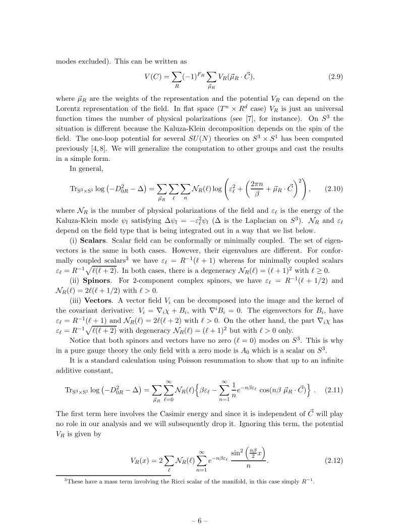

0 2 4 6 8
-75
-5
-25
0
25
5
75
0 2 4 6 8
-75
-5
-25
0
25
5
75
0 2 4 6 8
-75
-5
-25
0
25
5
75
(a) (b) (c)
Figure 3 We show the G2 one-loop potential on the Cartan torus for (a) high temperatures
βR = 001 (b) intermediate temperatures βR = 125 and (c)low temperatures βR = 100
As we lower the temperature the initial single minimum A0 = 0 becomes a maximum and new
non-trivial symmetrically located minima appear being pushed apart The appearance of strong
repulsion lines along the symmetry axis is due to the logarithmic term These two features do not
appear in other topologies like the torus [7 17]
4 Orthogonal and Symplectic Groups
In this section we will consider the phase structure of SO(2N) and Sp(2N) gauge theories
The center of Sp(2N) is Z2 and that of SO(N) is Z2 timesZ2 or Z4 for N even and Z2 for N
odd However since we are not considering spinors only a Z2 subgroup of the center will
be relevant for our analysis for orthogonal groups for even N For odd N SO(N) groups
have a trivial center
The non-trivial roots of SO(2N) and Sp(2N) in terms of the fundamental weights ~ν
are given by plusmn~νi plusmn ~νj (for SO(2N) i 6= j whereas there is no such restriction for Sp(2N))
For SO(2N) using the gauge transformation the Polyakov loop can be brought in the
form
O =
cos θ1 sin θ1minus sin θ1 cos θ1
cos θ2 sin θ2minus sin θ2 cos θ2
cos θN sin θN
minus sin θN cos θN
(41)
Also by a gauge transformation we can flip the signs of θrsquos θi rarr minusθi The effective
potential for the θirsquos is given by
V (θi) =sum
i6=j
V(θi minus θj) + V(θi + θj) (42)
Introducing the density of eigenvalues ρ(θ) = 12π +
suminfinn=1 ρn cosnθ (where the Fourier
coefficient ρn is now real and ρ(θ) = ρ(minusθ)) and converting summations to integrals we
ndash 15 ndash
obtain
V [ρ] = N2
int π
minusπdθρ(θ)
int π
minusπdθprimeρ(θprime)
infinsum
n=1
1
n(1minuszV (qn))(cos(n(θminusθprime))+cos(n(θ+θprime))) (43)
Defining the Fourier components of ρ(θ) as in (225) the potential can be written as
V [ρn] = N2π2infinsum
n=1
(1 minus zV (qn))
nρ2
n (44)
For low temperatures ρn = 0 which implies a uniform distribution ρ(θ) = 12π and a
vanishing expectation value of the Polyakov loop At extremely high temperatures the
arguments of the cosine on the right hand side of (43) have to be minimized which
happens when the θprimei are the same and equal to 0 or π ie
ρ(θ) = δ(θ) or δ(θ minus π)
In the two saddle points the Polyakov loop trO = 2Nint
dθ ρ(θ) cos(θ) is
trO = +1 ρ(θ) = δ(θ)
trO = minus1 ρ(θ) = δ(θ minus π)
If we sum over the different saddle points we get a trivial value of the Polyakov loop
However in the large N limit we can choose one saddle point since large N provides a
thermodynamic limit In that case the Polyakov loop is non-zero and the center symmetry
is spontaneously broken
The situation is different for SO(2N + 1) The group SO(2N + 1) has no center The
roots in terms of the fundamental weights ~ν are given by plusmn~νiplusmn~νj and plusmn~νi The Polyakov
loop is now a (2N + 1) times (2N + 1) matrix similar to (41) with an extra row and column
having 1 along the diagonal and zeros everywhere else The effective potential for the θirsquos
is now given by
V (θi) =sum
i6=j
V(θi minus θj) + V(θi + θj) + 2sum
i
V(θi) (45)
As before we can introduce a density of eigenvalues and its Fourier components yielding
an effective potential (44) The effective potential then is
V [ρ] = N2infinsum
n=1
1
n(1 minus zV (qn))
(
int π
minusπdθρ(θ)
int π
minusπdθprimeρ(θprime)
(
cos(n(θ minus θprime)) + cos(n(θ + θprime)))
+1
N
int π
minusπdθρ(θ) cos(nθ)
)
(46)
Defining the Fourier components of ρ(θ) as in (225) the potential can be written as
V [ρn] = N2π2infinsum
n=1
(1 minus zV (qn))
n(ρ2
n +1
πNρn) (47)
ndash 16 ndash
This is minimized when ρn = minus 12πN This corresponds to an eigenvalue distribution ρ(θ) =
12π (1 + 1
2N ) minus 12N δ(θ) The Polyakov loop is given by
trO = 1 + 2N
int π
minusπdθρ(θ) cos θ = 1 + 2N
int π
minusπdθ( 1
2π(1 +
1
2N) minus 1
2Nδ(θ)
)
cos θ = 0 (48)
In the extreme high temperature phase because of the second line in (46) which picks
out the θ = 0 saddle point ρ(θ) = δ(θ) ie there is a unique saddle point in this case
giving a non-zero value of the Polyakov loop The linear term on ρn is similar to the one
present for SU(N) theories with fundamental matter In that case the potential becomes
V [ρn] = N2π2infinsum
n=1
(1 minus zV (qn))
nρ2
n +Nf
N
zF (qn)
nρn (49)
and is minimized at
ρn = minusNf
2N
zF (qn)
1 minus zV (qn) (410)
The value of the Fourier components is bounded to |ρn| le 1 because ρ(θ) ge 0 The
bound is saturated at a temperature below the Hagedorn temperature and the eigen-
value density changes to a gapped distribution in a continous way It can be shown that
the deconfinement transition becomes Gross-Witten like [18 19] However in the case of
SO(2N + 1) theories both the quadratic and the linear coefficient come from the adjoint
contribution and are the same Hence ρn = minus1(2πN) is fixed and therefore the transition
is Hagedorn-like
In the large N limit the behavior of the theory with gauge group Sp(2N) is identical
the the SO(2N) case
5 Gauss law and Screening
In the previous two sections we find that the Polyakov loop can be non-zero at high
temperature is theories with no surviving center symmetry even on finite volume We are
introducing a non-Abelian charge in finite volume and it does not cost infinite free energy
This is consistent with the non-Abelian Gauss law which we can write asint
S3
(
nablaiEai minus fabcAb
iEci
)
= Qa (51)
where Eai are the electric components of the non-Abelian field Aa
i is the magnetic potential
fabc are the group structure constants and Qa is the total external charge The first term
on the left hand side is a total derivative and vanish when integrated over a compact space
This is the only term that is present for Abelian fields and implies the known result that
we cannot introduce an Abelian charge on finite volume However for non-Abelian fields
the second term can be non-zero and Gauss law can be satisfied in the presence of a net
external charge
For a gauge theory with group G and an unbroken center C both the measure and the
action are invariant under center transformations This implies that there is a global center
ndash 17 ndash
symmetry which cannot be spontaneously broken in finite volume Then the expectation
value of any center-breaking operator should be zero The Polyakov loop in any representa-
tion charged under the center transforms non-trivially under the center (which can be seen
by performing large gauge transformations that are periodic up to an element of the cen-
ter) Therefore its expectation value should be zero which corresponds to the statement
that the free energy cost of introducing external particles that are charged under the center
is infinite When there is no center symmetry because the gauge group is centerless or the
representation of the matter fields explicitly breaks it there is no symmetry protecting the
expectation value of the Polyakov loop and indeed we observe that it is nonzero in general
In the zero temperature limit we find that the Polyakov loop is zero for any theory
We can also understand this in terms of Gauss law In this limit we can ignore the
Polyakov loop and the term coming from the non-Abelian nature of the group in Gauss
law This is because we are essentially working in the zero coupling limit The only non-
trivial interaction terms we have kept correspond to the interaction of the fields with the
background field α which is a zero mode of the theory 4 There is no α at zero temperature
and therefore no non-Abelian term in Gauss law In this case it costs infinite action to
introduce any external charge and the Polyakov loop expectation value is zero
This is consistent with the physical picture in terms of screening In the absence of a
surviving center symmetry an external particle in any representation can be screened by
an appropriate number of gluon or matter particles which allows us to introduce them at
finite free energy cost In theories with a center symmetry an external particle charged
under the center cannot be screened and therefore cannot have finite free energy in finite
volume
6 Conclusions
In this paper we have investigated confinement on S3 timesS1 for a gauge theory based on an
arbitrary semi-simple Lie group containing matter in generic representations Our analytic
calculation reproduces the behavior of the Polyakov loop computed by lattice simulations
for any theory for which lattice data exist [161720ndash22]
By using the general expression for the one-loop effective potential we have shown that
at zero temperature the Polyakov loop is exactly zero for any theory Since the Polyakov
loop is naturally related to the free energy of an isolated quark our result implies that on
a S3 times S1 manifold any gauge theory confines Although in this case confinement is due
to kinematics this finding is likely to be the weak coupling equivalent of confinement in
gauge theories For small but non-zero temperatures the Polyakov loop is still zero if the
theory has an unbroken center symmetry but acquire a non-zero (albeit exponentially small
O(eminusβR)) vacuum expectation value otherwise The very same features characterise the
high temperature phase although their explicit realisation differ from the low temperature
regime In the case in which the system is center symmetric this symmetry cannot be
broken on a finite volume hence the Polyakov loop will still be zero at high temperature
4In a normalization of fields that correspond to canonical kinetic terms in the action this corresponds
to taking the g rarr 0 limit after rescaling α rarr1gα
ndash 18 ndash
However this zero is due to a different phenomenon namely the emergence of center-
breaking minima of the effective potential over which we have to take an average when
we are not the in the thermodynamic limit In this limit one minimum is selected and
this gives a non-zero value to the Polyakov loop This is the case for SU(N) and SO(2N)
gauge theories For centerless theories like G2 and SO(2N+1) there seems to be only one
minimum for the effective potential in the high temperature phase On this saddle point
the Polyakov loop is different from zero
In this paper we have not considered Polyakov loop in the spinor representations
of SO(N) Since these Polyakov loops will be non-trivially charged under the center of
the gauge group they should exhibit a behavior similar to the fundamental Polyakov
loop in the SU(N) theory ie at finite N they should be zero at all temperatures In
the thermodynamic (large N) limit after restriction to one center-breaking minimum
we should find a non-zero value of the Polyakov loop We have also not studied the
Polyakov loop in the adjoint representation of SU(N) theories We expect to find that
all representations uncharged under the center would have a non-zero Polyakov loop at
non-zero temperature with a smooth cross over between the low temperature and the high
temperature regimes
The minima of the effective potential exhibit a different structure in the low and the
high temperature phase This is true independently of the existence of an unbroken center
group of the theory This means that with a finite number of degrees of freedom a cross
over between the confined phase and the deconfined phase should take place In the large
N limit this cross-over becomes a real phase transition For finite N or in the case of
exceptional groups whether there is a cross-over or a real phase transition cannot be
established by a computation on S3 times S1 Recent lattice calculations suggest that in pure
gauge theories the change of properties of the vacuum is always associated with a proper
phase transition [1720ndash22]
Another interesting question is whether calculations on a S3 times S1 manifold can shed
some light over the mechanism of color confinement For QCD with matter in the adjoint
representation an interesting development in this direction is reported in [23]
Acknowledgments
We would like to thank Guido Cossu and Prem Kumar for valuable discussions BL issupported by a Royal Society University Research Fellowship and AN is supported by aPPARC Advanced Fellowship
References
[1] C Borgs and E Seiler ldquoQuark deconfinement at high temperature A rigorous proofrdquo Nucl
Phys B215 (1983) 125ndash135
[2] L D McLerran and B Svetitsky ldquoQuark Liberation at High Temperature A Monte Carlo
Study of SU(2) Gauge Theoryrdquo Phys Rev D24 (1981) 450
[3] B Svetitsky and L G Yaffe ldquoCritical Behavior at Finite Temperature Confinement
Transitionsrdquo Nucl Phys B210 (1982) 423
ndash 19 ndash
[4] O Aharony J Marsano S Minwalla K Papadodimas and M Van Raamsdonk ldquoThe
Hagedorn deconfinement phase transition in weakly coupled large N gauge theoriesrdquo Adv
Theor Math Phys 8 (2004) 603ndash696 hep-th0310285
[5] G rsquot Hooft ldquoA planar diagram theory for strong interactionsrdquo Nucl Phys B72 (1974) 461
[6] O Aharony J Marsano S Minwalla K Papadodimas and M Van Raamsdonk ldquoA first
order deconfinement transition in large N Yang- Mills theory on a small S3rdquo Phys Rev D71
(2005) 125018 hep-th0502149
[7] J L F Barbon and C Hoyos ldquoDynamical Higgs potentials with a landscaperdquo Phys Rev
D73 (2006) 126002 hep-th0602285
[8] T Hollowood S P Kumar and A Naqvi ldquoInstabilities of the small black hole A view from
N = 4 SYMrdquo JHEP 01 (2007) 001 hep-th0607111
[9] M Unsal ldquoPhases of Nc = infin QCD-like gauge theories on S3 times S1 and nonperturbative
orbifold-orientifold equivalencesrdquo Phys Rev D76 (2007) 025015 hep-th0703025
[10] M Unsal ldquoAbelian duality confinement and chiral symmetry breaking in QCD(adj)rdquo
arXiv07081772 [hep-th]
[11] P van Baal ldquoQCD in a finite volumerdquo hep-ph0008206
[12] J L F Barbon and C Hoyos ldquoSmall volume expansion of almost supersymmetric large N
theoriesrdquo JHEP 01 (2006) 114 hep-th0507267
[13] A Armoni M Shifman and G Veneziano ldquoExact results in non-supersymmetric large N
orientifold field theoriesrdquo Nucl Phys B667 (2003) 170ndash182 hep-th0302163
[14] M Bershadsky and A Johansen ldquoLarge N limit of orbifold field theoriesrdquo Nucl Phys B536
(1998) 141ndash148 hep-th9803249
[15] K Holland P Minkowski M Pepe and U J Wiese ldquoExceptional confinement in G2 gauge
theoryrdquo Nucl Phys B668 (2003) 207ndash236 hep-lat0302023
[16] J Greensite K Langfeld S Olejnik H Reinhardt and T Tok ldquoColor screening Casimir
scaling and domain structure in G(2) and SU(N) gauge theoriesrdquo Phys Rev D75 (2007)
034501 hep-lat0609050
[17] M Pepe and U J Wiese ldquoExceptional deconfinement in G(2) gauge theoryrdquo Nucl Phys
B768 (2007) 21ndash37 hep-lat0610076
[18] H J Schnitzer ldquoConfinement deconfinement transition of large N gauge theories with Nf
fundamentals NfN finiterdquo Nucl Phys B695 (2004) 267ndash282 hep-th0402219
[19] B S Skagerstam ldquoOn the large Nc limit of the SU(Nc) color quark- gluon partition
functionrdquo Z Phys C24 (1984) 97
[20] G Cossu M DrsquoElia A Di Giacomo B Lucini and C Pica ldquoG2 gauge theory at finite
temperaturerdquo JHEP 10 (2007) 100 arXiv07090669 [hep-lat]
[21] A Barresi G Burgio and M Muller-Preussker ldquoUniversality vortices and confinement
Modified SO(3) lattice gauge theory at non-zero temperaturerdquo Phys Rev D69 (2004)
094503 hep-lat0309010
[22] K Holland M Pepe and U J Wiese ldquoThe deconfinement phase transition of Sp(2) and
Sp(3) Yang- Mills theories in 2+1 and 3+1 dimensionsrdquo Nucl Phys B694 (2004) 35ndash58
hep-lat0312022
ndash 20 ndash
[23] M Unsal ldquoMagnetic bion condensation A new mechanism of confinement and mass gap in
four dimensionsrdquo arXiv07093269 [hep-th]
ndash 21 ndash
-3 -2 -1 0 1 2 3
-3
-2
-1
0
1
2
3
[23] M Unsal ldquoMagnetic bion condensation A new mechanism of confinement and mass gap in
four dimensionsrdquo arXiv07093269 [hep-th]
ndash 21 ndash
-3 -2 -1 0 1 2 3
-3
-2
-1
0
1
2
3
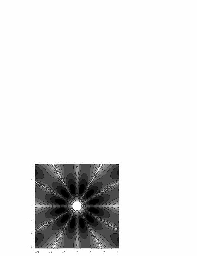
-3 -2 -1 0 1 2 3
-3
-2
-1
0
1
2
3