Keilwagen et al 2014 srep05231-s1
15
1 Supplementary Information 1 2 Separating the Wheat from the Chaff – a strategy to utilize 3 Plant Genetic Resources from ex situ genebanks 4 5 Jens Keilwagen 1,2 , Benjamin Kilian 3,11, *, Hakan Özkan 4 , Steve Babben 5 , Dragan 6 Perovic 5 , Klaus F. X. Mayer 6 , Alexander Walther 7 , C. Hart Poskar 8 , Frank Ordon 5 , 7 Kellye Eversole 9 , Andreas Börner 3 , Martin Ganal 10 , Helmut Knüpffer 3 , Andreas Graner 3 , 8 Swetlana Friedel 1 9 10 11 1 Molecular Genetics, Leibniz Institute of Plant Genetics and Crop Plant Research 12 (IPK), D-06466 Seeland OT Gatersleben, Germany 13 2 Institute for Biosafety in Plant Biotechnology, Julius Kühn-Institut (JKI) - Federal 14 Research Centre for Cultivated Plants, D-06484 Quedlinburg, Germany 15 3 Genebank, Leibniz Institute of Plant Genetics and Crop Plant Research (IPK), D- 16 06466 Seeland OT Gatersleben, Germany 17 4 University of Çukurova, Faculty of Agriculture, Department of Field Crops, 01330 18 Adana, Turkey 19 5 Institute for Resistance Research and Stress Tolerance, Julius Kühn-Institut (JKI) - 20 Federal Research Centre for Cultivated Plants, D-06484 Quedlinburg, Germany 21 6 MIPS/Institute for Bioinformatics and Systems Biology, Helmholtz Center Munich, 22 D-85764 Neuherberg, Germany 23 7 University of Gothenburg, Department of Earth Sciences, SE-405 30 Göteborg, 24 Sweden. 25 8 Physiology and Cell Biology, Leibniz Institute of Plant Genetics and Crop Plant 26 Research (IPK), D-06466 Seeland OT Gatersleben, Germany 27 9 International Wheat Genome Sequencing Consortium, Eversole Associates, MD 28 20816 Bethesda, USA 29 10 TraitGenetics GmbH, Am Schwabeplan 1b, D-06466 Seeland OT Gatersleben, 30 Germany 31 11 Current address: Bayer CropScience NV, Innovation Center, BCS R&D, Trait 32 Research, Technologiepark 38, 9052 Zwijnaarde (Gent), Belgium 33 34 *Communicating Author: E-mail: [email protected] 35 Tel: (+49) 39482 5-571 36 Fax: (+49) 39482 5-500 37 38
-
Upload
independent -
Category
Documents
-
view
0 -
download
0
Transcript of Keilwagen et al 2014 srep05231-s1

1
Supplementary Information 1
2
Separating the Wheat from the Chaff – a strategy to utilize 3
Plant Genetic Resources from ex situ genebanks 4
5
Jens Keilwagen1,2, Benjamin Kilian3,11,*, Hakan Özkan4, Steve Babben5, Dragan 6 Perovic5, Klaus F. X. Mayer6, Alexander Walther7, C. Hart Poskar8, Frank Ordon5, 7 Kellye Eversole9, Andreas Börner3, Martin Ganal10, Helmut Knüpffer3, Andreas Graner3, 8 Swetlana Friedel1 9 10
11
1 Molecular Genetics, Leibniz Institute of Plant Genetics and Crop Plant Research 12 (IPK), D-06466 Seeland OT Gatersleben, Germany 13
2 Institute for Biosafety in Plant Biotechnology, Julius Kühn-Institut (JKI) - Federal 14 Research Centre for Cultivated Plants, D-06484 Quedlinburg, Germany 15
3 Genebank, Leibniz Institute of Plant Genetics and Crop Plant Research (IPK), D-16 06466 Seeland OT Gatersleben, Germany 17
4 University of Çukurova, Faculty of Agriculture, Department of Field Crops, 01330 18 Adana, Turkey 19
5 Institute for Resistance Research and Stress Tolerance, Julius Kühn-Institut (JKI) - 20 Federal Research Centre for Cultivated Plants, D-06484 Quedlinburg, Germany 21
6 MIPS/Institute for Bioinformatics and Systems Biology, Helmholtz Center Munich, 22 D-85764 Neuherberg, Germany 23
7 University of Gothenburg, Department of Earth Sciences, SE-405 30 Göteborg, 24 Sweden. 25
8 Physiology and Cell Biology, Leibniz Institute of Plant Genetics and Crop Plant 26 Research (IPK), D-06466 Seeland OT Gatersleben, Germany 27
9 International Wheat Genome Sequencing Consortium, Eversole Associates, MD 28 20816 Bethesda, USA 29
10 TraitGenetics GmbH, Am Schwabeplan 1b, D-06466 Seeland OT Gatersleben, 30 Germany 31
11Current address: Bayer CropScience NV, Innovation Center, BCS R&D, Trait 32
Research, Technologiepark 38, 9052 Zwijnaarde (Gent), Belgium 33
34
*Communicating Author: E-mail: [email protected] 35 Tel: (+49) 39482 5-571 36 Fax: (+49) 39482 5-500 37
38
●
●
●
●
●
●
●
●
●
●
●
●
●
● ●
●
●
●
●
●
●
●
●
●
●●
●
●
●
●
●
●
●
●
●
●
● ●
●
●●
●
●
●
●
●
●
●
●
●
●
● ●
●
●
●
●
Average spring temperature in Gatersleben
Year
Ave
rage
tem
pera
ture
of M
arch
, Apr
il an
d M
ay in
°C
1953
1954
1955
1956
1957
1958
1959
1960
1961
1962
1963
1964
1965
1966
1967
1968
1969
1970
1971
1972
1973
1974
1975
1976
1977
1978
1979
1980
1981
1982
1983
1984
1985
1986
1987
1988
1989
1990
1991
1992
1993
1994
1995
1996
1997
1998
1999
2000
2001
2002
2003
2004
2005
2006
2007
2008
2009
6
7
8
9
10
y = 0.033x −57
R² = 0.2394
●
●
●
●
●
●●
●
●
●
●
●
●
●
●
●
●
●
●
●
●
●
●
●
●
●
●
●
●
●
●●●
●●
●
●
●
●
●
●
●●
●
●
●
●
●
●
●
●
●
●
●●
●
●
●
●
●
●
●
●●
●
●
●●
●●
●
●
●
●
●
●
Hanover (1)
1936
1955
1974
1992
2011
6
7
8
9
10
11
●●
●
●
●
●●
●
●
●
●
●
●
●●
●
●
●
●
●
●
●
●
●
●
●
●
●
●
●●
●●
●
●
●
●
●
●
●●●
●
●
●
●
●
●
●●
●
●
●
●
●
●
●
●
●
●
●
●
●
●
●
●
●
●
●
●
●
●
●●
●
●
●●
●
●
●
●
●
●
●
●
●
●●
●
●
●
●
●
●●
●
●
●
●
●
●●
●
●
●
●
●●
●
●
●●
●
●
●
●
●
●
●
●
Hamburg (2)
1891
1921
1951
1981
2011
6
7
8
9
10
●
●
●
●
●●
●
●
●●
●
●
●
●
●
●
●
●
●
●
●
●
●
●
●
●
●
●
●
●
●
●
●
●
●
●●
●
●
● ●
●
●
●
●
●
●
●
●
Berlin−Tegel (3)
1963
1975
1987
1999
2011
7
8
9
10
11
12
●
●
● ●
●
●
●
●
●
● ●
●
●
●●
●
●
●●
●●
● ●
●
●●
●
●
●
●
●
●●
●
●
●
●
●
●
●
●●
●
●
●
●
●
●
●
●
●
●
●
●
Cologne−Bonn (4)
1957
1970
1984
1998
2011
7
8
9
10
11
12
●
●
●●
●
●
●
●
●
●
●
●
●
●
●
●
●
●
●
●●
●
●
●
●
●
●
●
●
●
●●
●
●
●
●
●
●
●
●
●
●
●●
●
●
●
●
●
●
●
●●
●
●
●●
●●
●
●
●
●
●
●
Magdeburg (5)19
47
1963
1979
1995
2011
6
7
8
9
10
11
●
●
●
●
●
●
●
● ●
●
●
●●
●
●
●
●
●
●
●
●
●
●
●
●
●
●
●
● ●
●●
●
● ●
●
●
●
●
●
●●
●
●
●
●
●
●
●
● ●
●
● ●
●
●
●
●
●
●
●
●
●
Frankfurt/Main (6)
1949
1964
1980
1996
2011
8
9
10
11
12
● ●
●
●
●
●
●
●
●
●
●●
●
●
●
●
●
●
●●
●
●
●●
●
●
●
●
●
●
●
●●
●
●
●●
●
●
●
●
●
●
●
●
Dresden (7)
1967
1978
1989
2000
2011
7
8
9
10
11
●
●
●
●
●
●
●
●
●
●
●
●
●
●
●
●
●
●
●●
●
●
● ●
●
● ●
●
●
●
●
●
●●
●
●
●●
●
●
●●
●
●
●
●●
●
●
●
●
●
●
●
●
●
●
●
●
Stuttgart (8)
1953
1968
1982
1996
2011
7
8
9
10
11
●
●
●
●
●
●
●
●
●
●
●
●
●
●
●
●
●
●
●
●
●
●
●
●
●●
●
●
●
●
●
●
●
●
●
●
●
●
●
●
●
●
● ●
●
●
●
●
●
●
●
● ●
●
●●
●
●●
●
●
●
●
●
●
Regensburg (9)
1947
1963
1979
1995
2011
6
7
8
9
10
11
●
●
●
●
● ● ●
●
●
●
●
●
●●
●
●
● ●
●
●
●
●
●
●
●
●
●
●
●
●
●
●●
●
●
●
●
●
●
Leipzig−Halle (10)
1972
1982
1992
2001
2011
7
8
9
10
11
● 1
● 2
● 3
● 4
● 5
● 6
● 7
● 8● 9
● 10Gatersleben
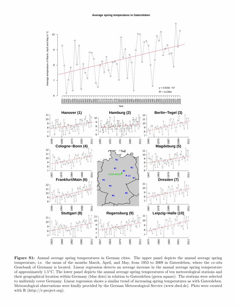
Figure S1: Annual average spring temperatures in German cities. The upper panel depicts the annual average springtemperature, i.e. the mean of the months March, April, and May, from 1953 to 2009 in Gatersleben, where the ex-situ
Genebank of Germany is located. Linear regression detects an average increase in the annual average spring temperatureof approximately 1.5◦C. The lower panel depicts the annual average spring temperatures of ten meteorological stations andtheir geographical location within Germany (blue dots) in relation to Gatersleben (green square). The stations were selectedto uniformly cover Germany. Linear regression shows a similar trend of increasing spring temperatures as with Gatersleben.Meteorological observations were kindly provided by the German Meteorological Service (www.dwd.de). Plots were createdwith R (http://r-project.org).

Wintertypes
Barley
1950 1960 1970 1980 1990 2000 2010
120
140
160
180
Year
FT
i [da
y of
yea
r]
●
●
●
●●●
●
●
●
●
●●●●●●●●●●●●●
●●
●●
●
●●
●●●
●
●●●●
●
●
●●
●●●●●●●●
●●●
●●●●●●●●●●●●●●●
●
●●●
●
●●●●
●
●●●
●
●●
●●●●
●●●
●
●●
●
●
●●
●●●
●
●
●
●
●
●●●●●●●
●
●
●
●
●
●
●
●
●● ●●●●●
●●
●●●
●●●●●
●
● ●
●
● ●
●
●●
●●
●
●●●
●
67.
79.
311
●
●
●
●
●
●
●
●
●
●
●
●
●
● ●
●
●
●
●
●
●
●
●
●
● ●●
●
●
●
●
●
●
●
●
●
● ●
●
● ●
●
●
●
●
●
●
●
●
●
●
● ●
●
●
●
●
●
Ave
rage
spr
ing
tem
pera
ture
120 140 160 180 200 220
0.0
0.2
0.4
0.6
0.8
1.0
FTi [day of year]
cum
. dis
trib
utio
n
[1946, 1955][1956, 1965][1966, 1975][1976, 1985][1986, 1995][1996, 2005]
Wheat
1950 1960 1970 1980 1990 2000 2010
140
160
180
200
Year
FT
i [da
y of
yea
r] ●
●
●
●
●
●
●●
●
●
●
●
●
●
●●●
●
●
●
●
●
●●
●
●●
●
●
●●●●●
●
●
●
●
●
●●
●
●
●
●
●●●
●
●
●
●
●●
●
●●●
●
●
●
●
●●
●●
●
●
●●●●
●●●●●
●
●
●
●
●
●●
●
●
●
●
●
●
●
●●●
●
●
67.
79.
311
●
●
●
●
●
●
●
●
●
●
●
●
●
● ●
●
●
●
●
●
●
●
●
●
●●
●
●
●
●
●
●
●
●
●
●
● ●
●
●●
●
●
●
●
●
●
●
●
●
●
● ●
●
●
●
●
●
Ave
rage
spr
ing
tem
pera
ture
120 140 160 180 200 220
0.0
0.2
0.4
0.6
0.8
1.0
FTi [day of year]
cum
. dis
trib
utio
n
[1946, 1955][1956, 1965][1966, 1975][1976, 1985][1986, 1995][1996, 2005]
Springtypes
Barley
1950 1960 1970 1980 1990 2000 2010
140
160
180
200
Year
FT
i [da
y of
yea
r]
●●●●●
●●●
●
●●●●
●
●
●●●
●
●●●
●●●●●●●
●
●
●
●
●●
●
●
●
●●●●●●●●●●
●
●
●●●●●●
●●
●●●
●
●●●●
●
●●
●●●●
●
●
●
●
●●●●●●●●
●
●●
●
●●
●●
●●
●
●
●
●
●
●
●
●●●
●
●●●●
●●●
●
●●
●●
●●
●
●
●●
●
●
●●●●●
●●
●
●
●●●●●●
●
●
●
●
●
●
●●●●●●●●●●●●●●●●●●●
●
●●●
●●
●
●●
●●●
●●
●
●●
●
●
●
●
●
●
●●●
●●●
●
●
●●●
●●
●
●
●
●
●
●
●
●
●
●
●●
●
●
●
●
●●●
●
●●
●●●●●●●●●
●
●
●
●●●
●
●●●●
●●
●●
●
●
●
●●●●●
●
●
●●
●●
●●
●●
●
●
●
●
●
●●
●●
●
●
●●
●
●
●●●●
●
●
●
66.
77.
48.
18.
99.
610
11
●
●
●
●
●
●
●
●
●
●
●
●
●
● ●
●
●
●
●
●
●
●
●
●
●●
●
●
●
●
●
●
●
●
●
●
● ●
●
●●
●
●
●
●
●
●
●
●
●
●
● ●
●
●
●
●
●
Ave
rage
spr
ing
tem
pera
ture
120 140 160 180 200 220
0.0
0.2
0.4
0.6
0.8
1.0
FTi [day of year]
cum
. dis
trib
utio
n
[1946, 1955][1956, 1965][1966, 1975][1976, 1985][1986, 1995][1996, 2005]
Wheat
1950 1960 1970 1980 1990 2000 2010
140
160
180
200
220
Year
FT
i [da
y of
yea
r]
●
●
●
●●
●
●
●●
●
●●
●
●●●●●●
●
●
●
●●●
●
●
●●●
●●●
●
●
●●●●●●
●
●●●●●●
●●●
●
●●●●●●●●●●●●●●●●
●
●●●●
●
●●●●●●●●●●
●
●●
●●
●●●
●●
●●
●●●●●●●●
●
●●
●●●●●●●
●
●
●
●
●●
●
●
●
●
●
●
●
●●
●
●
●
●●
●●
●
●●●●●
●
●
●●●●●●●●●●●
●
●●●●●●●●●●●●●
●●●●●
●
●●●
●
●●
●●●●●
●
●●●●
●
●●●
●
●
●
●●●●●●●●
●
●●
●
●●
●
●
●●
●
●
●
●●●
●
●
●
●
●●●
●
●
●
●
●
●
●
●●
●●
●
●
●
●
●●●●●
●
●
●
●
●
●
●●
●
●●●
●
●●
●
●●
●
●
●
●
●●●
●
●
●●●●●●●●●●●●●
●●●●
●
●
●
●
●●
●
●●●●●●●●●
●
●
●
●
●●
●●
●●●●
●●
●
●●●●
●●●
●
●
●●
●●
●●●
●
●●●●
●
●●
●
●
●●●
●
●●●●
●
●●●●●●●●●●
●
●●
●
●●●●●●●●●●●●●●●●●●●●●●●●
●
●
●●●
●●
●
●
●
●
●●●
●
●●
●
●
●●●●
●●
●
●
●
●●●●●●●●
●
●
●
●
●
●●●●●●●●
●
●●●●
●●●●●
●●●●●
●●
●
●
●●●●●●●●●●
●●
●
●●
●●●●
●
●
●
●●
●
●
●
●
●
●
●●●
●●●
●●●●
●
●
●
●
●
●●●●●
●●●●●●
●
●
●
●●
●
●
●
67.
28.
59.
811
●
●
●
●
●
●
●
●
●
●
●
●
●
● ●
●
●
●
●
●
●
●
●
●
●●
●
●
●
●
●
●
●
●
●
●
● ●
●
●●
●
●
●
●
●
●
●
●
●
●
● ●
●
●
●
●
●
Ave
rage
spr
ing
tem
pera
ture
120 140 160 180 200 220
0.0
0.2
0.4
0.6
0.8
1.0
FTi [day of year]
cum
. dis
trib
utio
n
[1946, 1955][1956, 1965][1966, 1975][1976, 1985][1986, 1995][1996, 2005]
Winter types Spring typesCorrelation p-value Correlation p-value
Barley -0.72 1.3E-9 -0.67 2.9E-8Wheat -0.83 1.8E-15 -0.67 1.4E-8
Figure S2: Relationship between flowering time and average spring temperature for barley and wheat for each species andeach annuality. In the left panel, flowering time is plotted in boxplots in black, whereas the red curve plots the average springtemperature. Analyzing the trend in flowering time, the cumulative distribution of flowering time (FTi) for each decade isillustrated in the right panel. Comparing the median flowering time of the decades (dashed line in right plots), a shift ofup to 20 days earlier flowering time was observed (red curves in right panel). The table below summarizes the correlationbetween flowering time and average spring temperature for each species and each annuality. A negative correlation betweenflowering time and spring temperature was found, which is associated with the shift of the flowering time in recent years.Plots were created with R (http://r-project.org).

< = >
FTi: Meana < Meanb & NRPa > NRPb
FTia ~ FTib
050
000
1000
0015
0000
2000
0025
0000
3000
0035
0000
Figure S3: Validation of the mean and NRP for flowering time of winter wheat. All pairs (a, b) of winter wheat accessionswere considered that were cultivated together at least in two years. In addition, mean and NRP yield contradicting ranks,i.e., the mean of a was smaller than the mean of b and the NRP of a was bigger than the NRP of b. Based on the repeatedcommon cultivation, the real flowering time was evaluated indicating that the NRP is less biases than the mean. The plotwas created with R (http://r-project.org).

(A)
0.0 0.2 0.4 0.6 0.8 1.00.0
0.2
0.4
0.6
0.8
1.0
0.00.2
0.40.6
0.81.0
NRP TGW
NR
P F
Ti
NR
P P
H
●
●
●
●
●
●
●
●
●
●
●
●
●
●
●
●
●
●
●
●
●
●
●
●
●
●
●
●
●
●
●
●
●
●
●
●
●
●
●
●
●
●
●
●
●
●
●
●
●
●
●
●
●
●
●
●
●
●●
●
●
●
●
●
●
●
●
●
●
●
●
●
●
●
●
●
●
●
●
●●
●
●
●
●
●
●
●
●
●
●
●
●
●
●
●
●
●
●
●●
●
●
●
●
●
●
●
●
●
●
●
●
●
●
●
●
●
●
●
●
●
●
●
●
●
●
●
●
●
●
●
●
●
●
●
●
●
●
●
●
●
●
●
●
●
●
●
●●
●●
●
●
●
●
●
●
●
●
●
●
●
●
●
●
●
●
●
●
●
●
●
●
●
●
●●
●
●
●
●
●
●
●
●
●
●
●
●
●
●
●
●
●
●
●
●
●
●
●
●
●
●
●
●
●
●
●
●
●
●
●
●
●
●●
●
●
●
●
●
●●
●
●
●
●
●
●
●
●
●
● ●
●
●
●
●
●
●
●
●●
●
●
●
●
●
●
●
●
●
●
●
●
●
●
●
●
●
●
●
●●
●
●
●
●
●
●
●
●
●
●
●
●
●
●
●●
●
●
●
● ●
●
●
●
●
●
●
●
●
●
●
●
●
●
●
●
●
●
●
●
●
●
●
●
● ●
●
●
●
●
●
●
●
●
●
●
●
●
●
●
●
● ●
●
●
●
●
●
●
●
●
●
●
●
●
●
●
●
●
●
●
●
●
●
●
●
●
●
●
●
● ●
●
●
●
●
●
●
●
●
●
●
●
●
●
●
●
●
●
●
●
●
●
●
● ●●
●
●●
●
●
●
●
●
●
●
●
●
●
●
●
●
●
●
●
●
●
●
●
●
●
●
●
●
●
●
●
●
●
●
●
●
●
●●
●
●
●
●
●
●
●
●●
●
●
●
●
●
●
●
●
●
●
●
●
●
●
●●
●
●
●
●
●
●
●
●
●
●
●
●
●
●
●
●
●
●
●
●
●
●
●
●
●
●
●
●
●
●
●
●
●
●
●
●
●
●
●
●
●
●
●
●
●
●
●
● ●
●
●
●
●
●
●
●
●
●
●
●
●
●
●
●
●
●
●
●
●
●
●●
●
●
●
●
●
●
●
●
●
●
●
●
●
●
●
●
●
●
●
●
●
●
●
●
●
●
●
● ●
●
●
●
●
●
●
●
●
●
●
●
●
●
●
●
●
●
●
●
●
●
●
●
●
●
●
●
●
●
●
●
●●
●
●
●
●
●
●
●
●
●●
●
●
●
●
●
●
●
●
●
●
●
●
●
●
●
●
●
●
●
●
●
●
●
●
●
●
●
●
●
●
●
●
●
●
●
●
●
●
●
●
●
●
●
●
●
●
●
●
●
●
●
●
●
●
●
●
●
● ●
●●
●
●
●
●
●
●
●
●●
●
●
●
●
●
●
●
●
●
●
●
●
●
●
●●
●
●
●
●
●
●
●
●
●
●
●
●
●
●
●
●
●
●
●
●
●
●
●
●
●
●
●
●
●
●
●
●
●
●
●
●
●
●
●
●
●
●
●
●
●
●
●
●
●
●
●
●
●
●
●
●
●
●
●
●
●
●
●
●
●
●
●
●
●
●
●
●
●
●
●
●
●
●
●
●
●
●
●
●
●
●
●
●
●
●
●
●
●
●
●
●
●
●
●
●
●
●
●
●
●
●●
●
●
●
●
●
●
●
●
●
●
●
●
●
●
●
●
●
●
●
●
● ●
●
●
●
●
●
●
●
●
●
●●
●
●
●
●
●
●
●
●
●
●
●
●
●
●
●
●
●
●
●
●
●
●
●
●
●
●
●
●
●
●
●
●
●
●
●
●
●
●●
●
●
●
●
●
●
●
●
●
●
●
●
●
●
●
●
●
●
●
●
●
●
●
●
●
●
●
●
●
●
●
●●
●
●
●
●
●
●
●
●
●
●
●
●
●●
●
●
●
●
●
●
●
●
●
●
●
●
●
●
●
●
●
●●
●
●
●
●
●
●
●
●
●
●
●
●
●
●
●
●
●
●
●
●
●
●
●●
●
●
●
●
●
●
●
●
●
●
●
●
●
● ●
●
●
●
●
●
●
●
●
●
●
●
●
●
●
●
●
●
●
●
●
●
●
●
●
●
●
●
●●
●
●
●
●
●
●
●
●
●
●
●
●●
●
●
●
●
●
●
●
●
●
●
●
●
●●
●
●
●
●
●
●
●
●
●
●
●
●
●
●
●
●
●
●
●
●
●
●
●
●
●
●
●
●
●
●
●●
●
●
●
●
●
●
●
●
●
●
●
●
●
●
●
●
●
●
●
●
●
●
●
●
●
●
●
●
●
●
●
●
●
●
●
● ●
●
●
●
●
●
●
●
●
●
●
●
●●
●
●
●
●
●
●
●
●
●
●
●
●
●
●
●
●
●
●
●
●
●
●
●
●
●
●
●
●
●
●
●
●
●
●
●
●
●
●
●
●
●
●
●
●
●
●
●
●
●
●
●
●
●
●
●
●
●
●
●
●
●
●
●
●
●
●
●
●
●
●
●
●
●
●
●
●
●
●
●
●
●
●
●
●
●
●
●
●
●
●
●
●
●
●
●
●
●
●
●
●
●
●
●
●
●
●
●
●
●●
●
●
●
●
●
●
●
●
●
●
●
●
●
●
●
●
●
●
●
●
●
●
●
●
●
●
●
●
●
●
●
●
●
●
●
●
●
●
●
●
●
●
●
●
●
●
●
●
●
●
●●
●
●●
●●●
●
●
●
●
●
●
●
●
●
●
●
●
●
●
●
●
●
●
●
●
●
●
●
● ●
●
●
●
●
●
●
●
●
●
●
●
●
●
●
●
●
●
●
●
●
●
●
●
●
●
●
●
●
●
●
●
●
●
●
●
●
●
●
●
●
●
●
●
●
●
●
●
●
●
●
●
●
●
●
●●
● ●
●
●
●
●
●
●
●
●
●
●
●
●●
●
●
●
●
●
●
●
●
●
● ●
●
●
●
●
●
●
●
●
●
●
●
●
●
●
●
●
●
●
●
●
●
●
●●
●
●
●
●
●
●
●
●
●
●
●
●
●
●●
●
●
●
●
●
●
●
●
●
●
●
●
●
●
●
●
●
●
●
●
●
●
●
●
●
●
●
●●
●
●
●
●
●
●
●
●
●
●
●
●
●
●
●
●
●
●
●
●
●
●
●
●
●
●●
●
●
●
●
●●
●
●
●
●
●
●
●
●
●
●
●
●
●
●
●
●
●
●
●
●
●
●
●
●
●
●
●
● ●
●
●
●
●
●
●
●
●
●
●
●
●
●
●
●
●
●
●
●
●
●
●
●
●
●
●●
●●
●
●
●
●●
●
●
●
●
●
●
●
●
●
●
●
●
●
●
●
●
●
●
●
●
●
●
●
●
●
●
●
●
●
●
●
●
●
●
●
●
●
●
●
●
●
●
●
●
●
●
●
●
●
●
●
●
●
●
●
●
●
●
●
●
●
●
●
●
●
●
●
●
●
●
●
●
●
●
●
●
●
●
●
●
●
● ●
●●
●
●
●
●
●
●
●●
●
●
●●
●
●
●
●
●
●
●
●
●
●
●
●
●●
●
●
●
●
●
●
●
●
●
●
●
●
●
●
●
●
●
●
●
●
●
●
●
●
●
●
●
●
●
●
●
●
●
●
●
●
●
●
●
●
●
●
●
●
●
●
●
●
●
●
●
●
●
●
●
●
●
●
●
●
●
●
●
●
●
●
●
●
●
●
●
●
●
●
●
●
●
●
●
●
● ●
●●
●
●
●
●
●
●
●
●
●
●
●
●
●
●
●
●
●
●
●
●
●
●
●
●
●
●
●
●
●
●
●
●
●
●
●
●
●
●
●
●
●
●
●
●
●
●
●
●
●●
●
●
●
●
●
●
●
●
●●
●
●
●
●
●
●
●
●
●
●
●
●
●
●
●
●
●
●
●
●
●
●
●
●
●
●
●
●
●
●
●
●
●
●
●
●
●
●
●
●
●
●
●
●
●
●
●
●
●
●
●
●
●
●
●
●
●
●
●
●
●
●
●
●
●
●
●
●
●●
●
●●
●
●
●
●
●
●
●
●
●
●
●
●
●
●
●
●
●
●
●
●
●
●
●
●
●
●
●
●
●
●
●
●
●
●
●
●
●
●
●
●
●
●
●
●
●
●
●
●
●
●
●
●
●
●
●
●
●
●
●
●
●
●
●
●
●
●
●
●
●
●
●
●
●
●
●
●
●
●
●
●
●
●
●●
●
●
●
●
●
●
●
●
●
●
●
●
●
●
●
●
●
●
●
●
●
●
●
●
●
●
●
●
●
●
●
●
●
●
●
●
●
●
●
●
●
●
● ●
●
●
●
●
●
●
●
●
●
●
●
●
●
●
●
●
●
●
●
●
●
●
●
●
●
●
●
●
●
●
●
●
●
●
●
●
●
●
●
●
●
●
●
●
●
●
●
●
●
●
●
●
●
●
●
●
●
●
●
●
●
●
●
●
●
●
●
●
●
●
●
●
●
●
●●
●
●
●
●●
●
●
●
●
●
●
●
●
●
●
●
●
●
●
●
●
●
●
●
●
●
●
●
●
●
●●
●
●
●●
●
●●
●
●
●
●
●
●
●
●
●
●●
●
●
●
●
●
●
●
●
●
●
●
●
●
●
●
●
●
●
●
●
●
●
●
●
●
●
●●
●
●
●
●
●
● ●
●
●
●
●
●
●
●
●
●
●
●
●
●
●
●
●
●
●
●
●
●
●
●
●
●
●
●
●
●
●
●
●
●
●
●
●
●
●
●
●
●
●
●
●
●
●●
●
●
●
●
●
●
● ● ●
●
●
●
●
●
●
●
●
●
●
●
●
●
●
●
●
●
●
●
●
●
●
●
●
●
●●
●
●
●
●
●
●
●
●
●
●
●
●
●
●
●
●
●
●
●
●
●
●
●
●
●
●
●
●
●
●●
●
●
●
●
●
●
●
●
●
●
●
●
●
●
●
●
●
●
●
●●
●
●
●
●
●
●
●
●
●
●
●
●
●
●
●
●
●
●
●
●
●●
●
●
●●
●
●
●
●
●
●
●
●
●
●
●
●
●
●
●
●
●
●●
●
● ●
●
●
●
●
●
●
●
●
●
●
●
●
●
●
●
●
●
●
●
●
●
●
●
●
●
●
●
●
●
●
●●
●
●
●
●
●●
●
●
●
●
●
●
●
●
●
●
●
●
●
●
●●
●
●
●
●
●
●
●
●
●
●●
●
●
●
●
●
●
●
●
●
●●
●
●
●
●
●
●
●
●
●
●
●
●
●
●
●
●
●
●
●
●
●
●
●●
●
●
●
●●
●
●
●
●
●
●
●
●
●
●
●
●
●
●
●
●
●
●
●
●
●
●
●
●
●
●
●
●
●
●
●
●
●
●
●
●
●
●
●
●
●
●
●
●
●
●
●
●
●
●
●
●
●
●
●
●
●
●
●
●
●
●
●
●
●
●
●
●
●
●
●
●
●
●
●
●
●
●
●
●
●
●
●
●
●
●●
●
●
●
●
●
●
●
●
●
●
●
●●
●
●
●
●
●
●
●●
●
●
●
●
●
●●
●
●
●●
●
●
●●
●
●
●
●
●
●
●●
●
●
●
●
●
●
●
●
●
●
●●
●
●
●
●
●
●
●
● ●
●
●
●●
●
●
●●
● ●
●
●
●
●
●
●
●
●
●
●
●
●
●
●
●
●
●
●
●
●
●
●
●
●
●
●
●
●
●
●
●
●
●
●
● ●
●
●
●
●
●
●
●
●
●
●
●
●
●
●
●
●
●
●
●
●●
●
●
●
●
●
●
●
●
●
●
●
●
●
●
●
●
●
●
●
●●
●
●
●
●
●
●
●
●
●
●
●
●
●
●
●
●
●
●
●
●
●
●
●
●
●
●
●
●
●
●
●
●
●
●
●
●
●
●
●
●
●
●
●
●
●
●
●
●
●
●
●
●
●
●
●
●
●
●
●
●
●
●
●
●
●
●
●
●
●
●
●
●
●
●
●●
●
●●
●
●
●
●
●
●
●
●
●
●
●
●
●
●
●
●●
●
●
●
●
●
●
●
●
●
●
●
●●
●
●
●
●
●
●
●
●
●
●
●
●
●●
●
●
●
●
●
●
●
●
●
●
●
●
●
●
●
●
●
●
●
●
●
●
●
●
●
●●
●
●
●
●
●
●
●
●
●
●
●
●
●
●
●
●
●
●
●
●
●
●
●
●
●
●
●
●
●
●
●
●
●
●●
●
●
●
●
●
●
●
●
●
●
●
●
●
●
●
●
●
●
●
●●
●
●
●
●
●
●
●
● ●
●
●
●
●
●
●
●
●
●
●
●
●
●
●
●
●
●
●
●
●●
●
●
●
●
●●
●
●
●
●
●
●
●
●
●
●
●
●
●
●
●
●
●
●
●
●
●
●
●
●
●
●
●
●
●
●
●
●
●●
●
●
●
●
●
●
●
●
●
●
●
●
●
●
●
●
●
●
●
●●
●
●
●
●
●
●
●
●
●
● ●
●
●
●
●
●
●
●
●
●
●
●
●
●
●
●
●
●
●
●
●
●
●
●
●
●
●
●
●
●
●
●
●●
●
●
●
●
●
●
●
●
●
●
●
●
●
●
●
●●
●
● ●
●
●
●
●●
●
●
●
●
●
●
●
●
● ●
●
●
●
●
●
●
●
●●
●
●
●
●
●
●
●
●
●
●
●
●
●
●
●
●
●
●
●
●
●●
●●
●
●
●
●
●
●
●
●
●
●
●
●
●
●
●
●
●
●
●
●
●
●
●
●
●
●
●●
●
●
●
●
●
●
●
●
●
●
●
●
●
●
●
●
●
●
●
●
●●
●
●
●
●
●
●
●
●
●
●
●
●
●
●
● ●
●
●
●
●
●
●
●
●
●
●
●●
●
●●
●
●
●
●
●
●
●
●
●
●
●
●
●
●
●
●
●
●
●
●
●
●
●
●
●
●
●
●
●●
●
●
●
●
●
●
●
●
●
●
●
●
●
●
●
●
●
●
●
●
●
●
●
●●
●
●
●
●
●
●
●
●
●
●
●
●
●
●
●
●
●
●
●
●
●
● ●
●
●
●
●
●
●
●
●
●
●
●
●
●
●
●
●
● ●
●
●
●
●
●
●
●
●
●
●
●
●
●●
●
● ●
●
●
●
●
●
●
●●
●
●●
●
●
●
●
●
●
●
●●
●
●
●
●
●
●
●
●
●
●
●
●
●
●
●
●
●
●
●
●
●
●
●
●
●
●
●
● ●
●
●
●
●
●
●
●
●
●
● ●
●
●
●
●
●
●
●
●●●
●
●
●
●
●
●
●
●
●
●
●
●
●
●
●
●●
●
●
●
●
●
●●
●●
●
●
●
●
●
●
●
●
● ●
●
●
●
●
●
●
●
●
●
●
●
●
●
●
●
●
●
●
●
●
●
●
●
●
●
●
●
●
●
●
●
●
●
●
●
●
●
●
●
●
●
●
●
●
●
●
●
●
●
●
●
●
●
●●
●
●
●
●
●
●
●
●
●●
●
●
●
●
●
● ●
●
●
●
●
●
●
●
●
●
●
●
●
●
●
●
●●
●
●
●
●
●
●
●●
●
●
●
●
●●
●
●
●
●
●
●
●
●
●●
●
●
●
●
●●
●
●
●
●
●
●
●
●
●
●
●
●
●
●
●
●
●
●
●
●
●
●
●
●
●●
●
●
●
●
●
●
●
●
●
●
●
●
●
●
●
●
●
●
●
●
●
●●
●
●
●
●
●
●
●
●
●
●
●
●
●
●
●
●
●
●
●
●
●
●
●
●
●
●
●
●
●
●●
●
●
●
●
●
●
●
●
●
●
● ●
●
●
●
●
●
●
●
●
●
●
●
●
●
●
●
●
●
●
●
●
●
●
●
●
●
●
●●
●●
●
●
●
●
●
●
●
●
●
●
●
●
●
●
●
●
●
●
●
●
●
●
●
●
●
●
●
●
●
●
●
●
●
●
●
●
●
●
●
●
●
●
●
●
●
●
●
● ●
●
●
●
●
●
●●
●
●
●
●
●
●
●
●
●
●
●●
●
●
●
●
●
●
●
●
●
●
●
●
●
●
●
●
●
●
●
●
●
●●
●
●
●
●●
●
●
●
●
●
●
●
●
●
●
●
●
●
●●
●
●
●
●
●
●
●
●
●
●
●
●
●
●
●
●
●
●
●
●
●
●
●
●●
●● ●
●●
●
●
●
●
●
●
●
●●
●
●
●
●
●
●
●
●
●
●
●
●
●
●
●
●
●
●
●
●
●
●
●
●
●
●
●
●
●
●
●
●
●
●
●
●
●
●
●
●
●
●
●
●
●
●
●
●
●
●
●
●
●
●
●
●
●
●
●
●
●●
●●
●
●
●
●
●
●
●
●
●
●
●
●
●
●
●
●
●
●
●
●
●
●
●
●
●
●
● ●
●
●
●
●
●
●
●
●
●
●
●
●
●
●
●
●
●
●
●
●
●
●
●
●
● ●
●
●
●
●
●
●
●
●
●
●
●
●
●●
●
●
●
●
●
●
●
●
●
●
●
●
●
●
●
●
●
●
●
●
●
●
●
●
●
●
● ●
●
●
●
●
●
●
●
●
●
●
●
●
●
●
●
●
●
●
●
●
●
●●
●
●
●
●
●
●
●
●
●
●
●
●
●
●
●
●
●
●●
●
●
●
●
●
●
●
●
●
●
●
●
●
●
●
●
●
●
●
●
●
●
●
●
●
●
●
●
●
●
●
●
●
●
●
●
●
●
●
●
●●
●
●
●
●
●
●
●●
●
●
●
●
●
●
●
●
●
●
●
●
●
●
●
●
●
●
●
●
●
●
●
●
●
●
●
●
●
●●
●
●
●
●
●
●
●
●
●
●
●
●
●
●
●
●
●
●
●
●
●
●
●
●
● ●
●
●
●
●
●
●
●
●
●
●
●
●
●
●
●
●
●
●
●
●
●
●
●
●
●
●
●
●
●●
●●
●
●
●
●●
●
●
●
●
●
●
●
●
●
●
●
●
●
●
●
●
●
●
●
●●
●
●●
●
●
●
●●
●
●
●
●
●
●
●
●
●
●
●
●
●
●
●
●
●
●
●
●
●
●
●
●
●
●
●
●
●
●
●
●
●
●
●
●
●
●
●
●
●
●
●
●
●
●
●
●
●
●
●
●
●
●
●
●
●
●
●●
●
●
●
●
●
●
●
●
●
●
●
●
●
●
●
●
●
●
● ●
●
●
●
●
●
●
●
●
●
●
●
●
● ●
●
●
●
●
●●
●
●
●
●
●
●
●
●
●
●●
●
●
●
●
●
●●
●
●
●●
●
●
●
●
●
●
●
●●
●
●
●
●
●
●
●
●
●
●
●
●
●
●
●
●
●
●
●
●
●
●
●
●
●
●
●
●
●
●
●
●
●●
●
●
●
●
●
●
●
●
●
●●
●
●
●
●
●
●
●
●
●
●
●●
● ●
●●
●
●
●
●
●
●
●
●
●
●
●
●
●
●●
●
●
●
●
●
●●
●
●●
●
●
●
●
●
●
●
●
●
●
●
●
●
●
●
●
●
●●
●
●
●
●
●
●
●
●
●
●
●
●
●●
●●
●
●
●●
●
●
●
●●
●
●
●
●
●
●
●
●
●
●
●●
●
●●
●
●
●
●
●
●
●
●●
●
●●
●
●
●
●
●
●
●
●
●
●
●●
●
●
●
●
●
●
●
●
●
●
●
●
●
●
●
●●
●
●
●
●
●
●
●
●
●
●
●
●
●
●
●
●
●
●
●
●
●
●
●
●
●
●
●
●
●
●●
●
●
●
●
●
●● ●
●
●
●
●
●
●
●
●
●
●
●
●
●
●
●
●
●
●
●
●
●
●
●
●
●
●
●
●
●
●
●
●
●
●
●
●
●
●
●
●
●●
●
●
●
●
●●
●● ●
●
●●
●
●
●
●
●
●
●
●
●
●
●●
●
●
●
●
●
●
●
●
●
●
●
●●
●●
●
●
●
●
●
●●●
(B) 1950 1951 1953 1956 1958 1963 1969 1970 1976 1994
FT
iP
HT
GW
(C) 1951 1953 1956 1959 1964 1965 1970 1971 1973 1978
FT
iP
HT
GW
Figure S4: (A) MTO for a large winter wheat collection based on the normalized traits of flowering time (NRP FTi),plant height (NRP PH) and thousand grain weight (NRP TGW). Two accessions with contrasting phenotypes have beenselected as indicated by the red and the green star. The red star is an early flowering short accession with high thousandgrain weight, while the green star is a late flowering tall accession with low thousand grain weight. (B) and (C) visualizethe recorded pre-normalized trait values of each year of multiplication by a histogram and display the ranks for the twoselected accessions by red and green lines respectively. Missing histograms indicate missing phenotypic observations. Plotswere created with R (http://r-project.org).

Winter types Spring typesBarley Wheat Barley Wheat
FTi vs. PH
0 0.2 0.4 0.6 0.8 1
0
0.2
0.4
0.6
0.8
1
NRP FTi
NR
P P
H
CC = 0.4 (p−value = 5.3e−50)
1
2
3
4
5
6
7
8
Counts
0 0.2 0.4 0.6 0.8 1
0
0.2
0.4
0.6
0.8
1
NRP FTi
NR
P P
H
CC = 0.42 (p−value = 1.4e−222)
1245781011121415171820212324
Counts
0 0.2 0.4 0.6 0.8 1
0
0.2
0.4
0.6
0.8
1
NRP FTi
NR
P P
H
CC = 0.48 (p−value = 0)
1246781012131416181920222425
Counts
0 0.2 0.4 0.6 0.8 1
0
0.2
0.4
0.6
0.8
1
NRP FTi
NR
P P
H
CC = 0.47 (p−value = 0)
1346791012141517182021232426
Counts
PH vs. TGW
0 0.2 0.4 0.6 0.8 1
0
0.2
0.4
0.6
0.8
1
NRP PH
NR
P T
GW
CC = 0.12 (p−value = 4.8e−05)
1
2
3
4
5
6
Counts
0 0.2 0.4 0.6 0.8 1
0
0.2
0.4
0.6
0.8
1
NRP PH
NR
P T
GW
CC = 0.19 (p−value = 4.5e−39)
12345678910111213141516
Counts
0 0.2 0.4 0.6 0.8 1
0
0.2
0.4
0.6
0.8
1
NRP PH
NR
P T
GW
CC = 0.23 (p−value = 1.6e−65)
1346891112141617192022242527
Counts
0 0.2 0.4 0.6 0.8 1
0
0.2
0.4
0.6
0.8
1
NRP PH
NR
P T
GW
CC = 0.066 (p−value = 1.2e−06)
1234567891011121314151617
Counts
FTi vs. TGW
0 0.2 0.4 0.6 0.8 1
0
0.2
0.4
0.6
0.8
1
NRP FTi
NR
P T
GW
CC = 0.12 (p−value = 6.5e−05)
1
2
3
4
5
6
7
8
9
Counts
0 0.2 0.4 0.6 0.8 1
0
0.2
0.4
0.6
0.8
1
NRP FTi
NR
P T
GW
CC = −0.0042 (p−value = 0.78)
1
2
3
4
5
6
7
8
9
10
11
12
13
14
Counts
0 0.2 0.4 0.6 0.8 1
0
0.2
0.4
0.6
0.8
1
NRP FTi
NR
P T
GW
CC = −0.08 (p−value = 2.4e−09)
12346789101112131416171819
Counts
0 0.2 0.4 0.6 0.8 1
0
0.2
0.4
0.6
0.8
1
NRP FTi
NR
P T
GW
CC = −0.13 (p−value = 4e−24)
124568911121315161819202223
Counts
Figure S5: Visual representation of the correlations between NRPs of agronomically important traits. For each species and annuality the figure depicts the pair-wisecorrelation coefficients (CC) between NRPs (NRP) of the traits: flowering time (FTi), plant height (PH), and thousand grain weight (TGW). For each hexagonal bin thenumber of plant samples assigned to this bin is represented by the color. The color of the bins ranges from light green, which represents a low number of samples, to violet,representing a high number. A significant positive correlation was found between flowering time and plant height as well as between plant height and thousand grain weight.However, no common trend is apparent for flowering time and thousand grain weight. Plots were created with R (http://r-project.org).

●
●
●
●
●
●
● ●
●
●
●●
●
●
●
●
●
●
●
●
●
●
●
●
●
●
●
●
●
●
●
●
●
●
●
●
●
●●
● ●
●
●
●
●
●
●
●●
●
●●
●
●
●
●
●
●
●
●
●
●
●
●
●
●
●
●
●
●
●
●
●
●
●
●
●
●
●
●
●
●
●
●
●
●
●
●
●
●
●
●
●
●
●
●
●
●
●
●
●
●
●
●
●
●
●●
●
●
●
●
●
●
●
●
●
●
●
●
●
●
●
●
●
●
●
●
●
●
●
●
●
●
●
●
●
●
●
●
●
●
●
●
●
●
●
●
●
●
●●
●
●
●
●
●●
●
●
●●
● ●
●
●
●
●
●
●
●
●
●
●
●
●
●
● ●
●
●
●
●
●
●
●
●
●
●
●
●
●
●
●
●
●
●
●
●
●
●●
●
● ●
●
●
●
●
●
●
●●
●
●
●
●
●
●
●
●
●
●
●
●
●
●
●
●
●
●
●
●
●
●
●
●
●
●
●
●
●
●
●●
●
●
●●
●
●
●
●
●
●
●
●
●
●
●
●
●
●
●
●
●
●
●
●
●
●
●
●
●
●
●
●
●
●●
●
●
●
●
●
●
●
●
●
●
●
●
●
●
●
●
●●
●
●
● ●
●
●●
●
●
●
●
●
●
●
●
●
●
●
●
●
●
●
●
●
●
●
●
●
0.0 0.2 0.4 0.6 0.8 1.0
0.0
0.2
0.4
0.6
0.8
1.0
NRP FTi
NR
P P
H
North America
●
●
●
●
●
●
●
●
●
●
●●
●
●
●
●
●
●
●
●
●
●●
●
●
●
●
●
●
●
●
●
●
●
●
●
●
●
●
●
●
●
●
●
●
●
●
●
●
●
●
●
●
●
●
●
●
●●
●
●
●
●
●
●
●
●
●
●
●
●
●
●
●●
●
●
●
●
●
●
●
●●
●
●
●
●
●●
●
●
●●
●
●
●
●
●
●
●
●
●
● ●
●
●
●
●●
●
●●
●
●
●●
●
●
●
●
●
●
●
●●
●
●●
●
●
●
●
●
●
●
●
●
●●
●
●
●
●
●
●
●
●
●●
●
●
●
●
●
●
●●
●
●
●
●
●
●
●
●
●
●●
●
●
●
●
●
● ●
●
●
●
●
●●
●
●
●
●
●
●
●
●
●
●
●
●
●
●
●
●
●
●
●
●
●●
●
● ●
●
●
●
●
●●
●
●
●
●
●●
●
●
●
●
●
●
●
●
●●
●●
●
●
●
●
●
●
●
●
●●
●
●
●
●
●
●
●
●
●●
●
●
●
●
●
●
●
●
●
●
●
●
●●
●
●
●
●
●
● ●
●
●
●
●
●●
●●
●
●
●
●
●
●
●
●
●
●
●
●
●
●
●
●
●
●
●
●
●
●
●
●
●
●
●
●
●
●
●
●
●
●
●●
●
●
●
●
●
●
●
●
●
●● ●
●
●●
●
●●
●
●
●
●●
●
●
●
●
●●
●
●
●
●
●
●
●
●●●
●
●
●
● ●
●
●
●
●
●
● ●●
●
●
●
●
●
●
●
●
●
●
●
●
●
●
●
●
●
●
●
●
●
●
●
●
●
●
●
●
●
●
●
●
●
●
●
●
●
●
●
●●
●
●
●
●
●
●
●
●●
●
●●
●
●
●
● ●
●
●
●
●
●
●
●
●
●
●
●
●
●
●●
●
●●
●
●
●●●
●
●
●
●
●
●
●
●
●
●●
●
●
●
●
●
●
●
●
●
●
●
●
●
●
●
●
●
●
●
●
●
●
●
●
●●
●
●
●
●
●
●
●
●
●
●
●
●
●
●
●●
●
●
●
●
●
●
●
●
●
● ●
●
●
●
●
●
●
●
● ●
●
●
●
●
●
●
●
●
●
●
● ●
●
●●
●
●
●
●
●
●
●
●
●
●
●
●
●
●
●
●
●
●
●
●
●●
●
●
●
●
●
●
●
●
●
●
●
●
●
●
●●
●
●
●
●
●
●
●
●
●
●
●
●
●
●
●
●
●
●
●
●
●●
●
●
●
●
●
●
●
●
●
●
●
●
●
●
● ●
●
●
●
●
●
●
●
●
●
●
●
●
●
●●
●
●
●
●
●
●
●●
●
●
●
●
●
●
●
●
●
●●
●
●●
●
●
●●
●
●
●
●
●
●●
●
●
●
●
●
●
●
●
●
●
●
●
●
●
●
●
●
●
●●
●
●
●
●
●
●
●
●
●
●
●
●
●
●
●
●●
●
●
●
●
●●
●
●
●
●
●
●
●
●
●
●
●
●
●
●
●
●
●
●
●
●
●
●
●
●
●
●
●
●
●
●
●
●
●
●
●
●
●
●●
●
●
●
●
●
●
●
●
●
●
●
●
●
●
●
●
●
●
●
●
●
●
●
●●
●
●
●●
●
●
●
●
●
●
●
●
●●
●
●
●
●
●
●
●
●
●
●
●
●
●
●
●
●
●
●
●
●●
●
●
●
●
●
●
●
●
●
●
●
●
●
●
●●
●
●
●●
●
●
●
●
● ●
●
●
●
●
●
●
●
●
●
●
●
●
●
●
●
●
●
●
●●
●
●
●
●
●
●
●
●
●
●
●
●
●
●●
●
●
●
●
●
●
●●
●
●
●●
●●
●
●
●
●
●
●
●
●
●
●
●
●
●
●
●
●
●
●
●
●
●
●
●
●
●●
●
●
●●●
●
●●
●●
●
●
● ●●
●
●
●
●
●
●
●
●
●
●
●
●●
●
●
●
●●
●
●
●
●
●
●
●
●
●
●
●
●
●
●
●
●
●
●
●
●
●
●
●
●
●
●
●
●
●
●
●
●
●
●
●●
●
●
●
●
●
●
●
●
●
●
●●
●
●
●
●●
●
●●
●
●
●
●
●
●
●
●
●
●
●
●
● ●
●
●●
●
●
●
●
●
●●
●
●
●
●●
●
●
●
●
●
●
●
●
●
●
●
●
●
●
●
●
●
●
●●
●
●
●
●
● ●
●
●
●
●
●
●
●
●
●
●
●
●
●
●
●
●
●
●
●
●
●●
●
●●
●
●
●
●
●
●
●
●
●●
●
●
●
●
●
●
●
●
●
●
●
●
●
●
●
●●
●
●
●
●
●
●
●
●
●
●
●
●
●
●●
●
●
●
●
●
●
●
●
●
●
●
●
●
●
●
●
●
●
●
●●
●
●
●
●
●
●
●●
●
●
●
●
●
●
●
●
●●
● ●
●
●
●
●●
●
●
●
●
●
●
●
●●
●
●
●
●
●
●
●
● ●
●
●
●
● ●●
●
●●
● ●
●
●●
●
●
●
●
●
●
●●
●
●
●
●
●
●
●
●
●
●
●
●
●
●
●
●
●
●
●
●
●
●
●
●
●
●
●
●
●
●
●
●
●
●
●
●
●●
●
●
●
●
●
●
●
●
●
●
● ●
●
●
●
●
●
●
●
●
●
●
●
●
●
●
●
●
●
●
●●
●
●
●
●
●
●
●
●
●
● ●
●●
●
●
●
●
●
●
●
●
●
●
●
●
●
●
●
●●
●
●●
●●
●
●●
●
●
●
●●
●
●
●●●
●
●
●
●
●
●
●
●
●
●●
●
●
●
●
●
●
●
●
●●
●
●
●
●
●●
●
●●
●
●
●
●
●
●
● ●
●
●
●
●
●●
●
●
●
●
●
●●
●
●
●
●
●
●
●
●
●
●
●
●
●
●
●
●
●
●●
●●
●
●
●
●
●
●
●
●
●
●
●
●
●
●
●
●
●
●
●
●
●
●
●
●●
●
●
●
●
●
●
●
●
●
●
●
●
●
●
●●
●
●
●
●
●
●
●
●
●
●
●
●
●
●
●
●
●
●
●
●
●
●
●
●
●●
●
●
●●
●●
●
●
●
●
●
●
● ●●
●
●
●
●
●
●
●
●
●
●
●
●
●
●
●●
●
●●
●
●
●
●
●
●
●
●
●
●
●
●
●● ●
●
●
●
●
●●
●
●
●
●
●
●
●
●
●
●
●
●
●
●
●
●
●
●
●
●
●
●
●
●
●
●
●
●
●
●
●
●
●
●
●
●●
●
●
●
●
●●
●
●
●
●
●
●
●
●
●
●
●
●
●●
●
●
●
●
●●
●
●
●
●
●
●
●
●
●
●
●
●
●
●
●
●
●
●
●
●
●
●
●
●●
●
●
●
●
●
●
●
●
●
●●
●
●●
●
●
●●●
●
●
●
●
●
●
●
●
●
●●
●
●
●
●
●
●
●
●
●
●
●
●
●
●
●
●
●
●
●●
●
●
●
●
● ●
●
●
●
●
●
●
●
●
●
●
●
●
●
●
●
●
●
●
●
●
●●
●
● ●
●
●
●
●
●
●
●
●
●
●
●
●
●
●
●
●
●
●
●
●
●
●
●●
●
●●
●
●
●
●
●
●
●
●
●
●
●
●
●
●
●
●●
●
●●
●●
●
●
●
●●
●
●●
●
●
●
●
●
●
●
●
●
●
●
●●
●
●
●
●
●
●
●●
●
●
●
●
●
●
●
●
●
●
●
●
●
●●
●●
●●
●
●
●
●
●
●
●
●
●●
●
●
●
●
●
●
●
●
●
●
●
●
●
●
●
●
●
●
●
●
●
●
●
●
●
●
●
●
●
●
●
●
●
●
●
●
●
●
●
●●
●
●
●
●
●
●
●
● ●
●
●
●
●
●
●
●
●
●
●
●
●
●
●
●●
●
●
●
●
●
●
●
●
●
●
●
● ●●
●
●
●
●●
●
●
●
●
●
●
●●
●
●
●
●
●
●
●
●
●
●
●
●
●
●
●
●
●
●
●
●
●
●
●
●
●
●
●
●
●
●
●●
●
●
●
●
●
●
●
●
●
●
●
●
●
●●
●
●
●
●
●
●
●
●
●
●
●
●
●
●
●
●
●
●
●●
●
●
●
●
●
●
●
●
●
●
●
●
●
●
●
● ●
●
●●
●
●
●
●
●
● ●
●
●
●
●
●
●●
●
●
●
●
●
●
●
●
●
●
●
●
●
●
●
●
●
●●
●
●
●
●
●
●
●●
●
●
●
●
●
●
●
●
●
●
●
●
●
●
●
●
●
●
●
●
●
●●
●
●
●●
●
●
●
●●
●
●
●
●
●
●
●
●
●
●
●
●
●
●
●
●●
●
●
●
●
●
●
●
●●
●
●
●
●●
●
●
●
●
●
●
●
●
●
● ●
●
●
●
●
●
●
●●
●
●
●
●
●
●
●
●
●
●
●
●
●
●
●
●
●
●
●
●
●
●
● ●
●
●
●
●
●
●
●
●
●
●
●
●
●
●
●
●
●
●●●
●●
●
●
●
●
●
●
●●
●
●
●
●
●
●●
●
●
●
●
●
●
●
●
●
●
●
●
●
●
●
●
●●
●
●●
●
●●
●
●
●
●
●
●
● ●
●●
●
●
●
●
●
●
●
●
●
●
●
●
● ●
●
●
●
●
●●
●
●
●
●
●
●
●
●
●
●●
●
●
●
●
●
●
●
●
●
●
●●
●
●
●
●
●
● ●
●●
●
●
●
●
●
●●
●●
●
●
●
●
●
●
●
●
●
●
●
●
●
●
●
●
●
●
●
●
●
●
● ●
●
●
●●
●
●
●
●
●
●●
●
●
●●
●
●●
●
●
●
●
●
●
●
●
●
●
●
●
●
●
●
● ●
●
●
●
●
●
●
●
●
●
●
●
●
●●
●
●
●
●●
●
●
●
●
●
●
●●
●
●
●●
●
●
●
●
●
●
●
●
●
0.0 0.2 0.4 0.6 0.8 1.00.
00.
20.
40.
60.
81.
0NRP FTi
NR
P P
H
Europe
●
●
●
●
●
●
●
●
●
●●
●
●
●
●
●
●
●●
●
●
● ●
●
● ●
●●
●
●●
●●
●
●
●
●
●
●
●
●
●
●
●
●
●
●
●
●
●●
●
●
●
●
●
●
●
●
●
●
●
●
●
●
●
●
●
●●
●
●
●●
●
●
●
●
●
●
●
●
●
●
●
●
●
●
●
●
●
●
●
●
●
●
●
●
●●
●
●
●
●
●●
●
●
●
●●
●
●
●
●
●
●
●
●
●
●
●
●
●
●
●
●
●
●
●
●
●
●
●
●
●
●
●
●
●
●
●
●●
●
●
●
●
●
●
●
●
●
●
●●
●
●
●
●
●
●
●●
●
●
●
●
●
●●
●
●
●
●●
●
●
●
●
●
●
●
●
●
●
●
●
●●
●
●
●
●
●
●
●
●
●
●
●
●
●
●
●
●
●
●
● ●
●
●
●
●
●
●
●
●
●
●
●
●
●
●
●
●
●
●
● ●
●
●●
●
●
●
●
●
●
●
●
●
●
●
●
●
●
●
●
●
● ●
●
●●
●
●
●
●
●●
●
●●
●
●
●
●
●
●
●
●
●
●●
●
●
●
●
●
●
●
●
●
●
●
●
●
●
●
●
●●
●
●
●
●
●
●
●
●
●
●
●
●●
●
●●
● ●
●
●
●
●
●
●
●
●●
●
●
●
0.0 0.2 0.4 0.6 0.8 1.0
0.0
0.2
0.4
0.6
0.8
1.0
NRP FTi
NR
P P
H
North/Central Asia
●●
●
●
●●
●
●
●
●
●
●●
●
●●
●
●
●●
●
●
●●
●
●
●
●●
●●●●
●
●
●
●●
●
●● ●
●
●
●
●
●
●
●
●
●
●
●
●
●
●
●
●
●
●
●
●●
●
●
●
●
●
●●
●
●
●
●
●
●
●
●
●
●
●
●●●
●
●●
●
●
●
●
●
●
●
●
●
●
●
●●
●
●
●
●
●
●●
●●
●
●
●
●
●
●
●●
●
● ●
●
●
●
●●
●
●
●●
●
●
●●
●
●
●
●
●
●
●
●
●
●
●●
● ●
●
●●
●
●
●
●
●
●
●
● ●●
●
●
●
●
●
●
●
●
●
●
●●●
●
●●
●
●
●
●
●●
● ●
●
●
●
●
●
●
●
●
●
●●
●
●
●
●
●
●
●
●●
●
●●
●
●
●
●
●
● ●
●
●
●
●
●
●
●
●
●
●
●
●
●
●
●
●●
●
●●
●
●
●
●
● ●
●
●
●
●
●
●
●
●
●
●
●
●
●
●
●
●
●
●
●
●●
●●
●
●
●
●
●
●
●
●
●
●●
●
●
●
●
●
●
●
●
●
●
●
●
●
●
●
●
●
●
●●●
●
●
●
●
●●
●
●●●
●
●●
●
●● ●
●
●
●
●
●
●
●
●
●
●
●
●
●
●
●
●
●
●
●
●
●
●
●
●
●
●
●
●
●
●
●
●●
●
●●
●
●
●
●
●
●
●
●
●
●
●
●
●
●
●
●
●
●
●
●
●
●
●
●
●
●
●
●
●
●
●
●●
●
●
●
●
●
●
●
●
●
●
●
●
●
●●
●
●
●
●
●
●
●
●
●
●
●●
●
●
●
●
●
●
●
●
●●●
●
●
●
●
●
●
●
●
●
●
●
●
●
●
●
●
●
●
●
●
●
●
●
●
●
●
●
●
●
●
●
●
●
●
●
●
●●
●
●
●
●
●
●
●
●
●
●●
●
●
●
●
●
●●
●
●
●
●
●
●
●
●
●
●
●
●
●
●
●
●
●
● ●
●
●
●
●
●●
●
●
●
●
●
●
●
●
●
●
●
●
●
●
●
●
●
●
●
●●
●
●
●
●●
●
●
●
●
●
●
●●
●
●
●
●
●
●
●
●
●
●
●
●
●
●
●
●
●
● ●
●
●●● ●●●
●
●●
●
●●
● ●●
●
●
●●
● ●
● ●
●
●
●
●
●
● ●
●
●
●
●
●
●
●●
●
●
●
●
●
●
●
●
●
●
●
●
●●●
●
●
●
●
●●
●
●
●
●
●●●
●
●●
●
●
●
●
●
●
●
●
●
●
●
●
●
●
●
●
●●
●
●●
●
●●●
●
●
●
●
●
●●
●●
●
0.0 0.2 0.4 0.6 0.8 1.0
0.0
0.2
0.4
0.6
0.8
1.0
NRP FTi
NR
P P
H
Mediterranean Basin
●●
●
●
●
●
●
●
●
●
●●
●●
●●
●
●
●
●
●
●
●
●
●
●
●
●
●
●
●
●
●
●
● ●
●
●
●
●
●
●
●●
●●
●
●
●
●●
●
●●
●
●
●
●
●
●
●
●
●
●
●
●
●
●
●
●
●
●
●
●
●
●
●
●
●
●
●
●
●
●
●
●
●
● ●●
●
●
●
●
●
●
●
●
●
●
● ●●
●
●
●
●
●
●
●●
●
●
●
●
●
●
●
●●
●
●
●
●●
●
●
●
●
●
●
●
●
●
●
●
●
●
●
●
●
●●
●
●
●
●
●
●
●
●
●●
●
●
●
●
●
● ●
●
●
●
●
●
●●
●
●
●
●●
●●
●
●
●
●
●
●
●
●
●●
●
●
●
●
●
●
●
● ●
●
●
●
●
●
●●
●●
●
●
●
●
●
●
●
●
●
●
●
●●
●
●
●
●●
●
●
●
●
●
●
●
●●
●
●
●
●
●
● ●
●● ●
●● ●
●
●
●●
●
●
●
●
●
●
●
●●
●
●
●●
●
●
●
●
●
●
●●
●
●
●
●
●
●
●●
●
●
●
●
●
●
●
●
●●
●
●
●
●
●
●
●
●
●
●
●●
●
●
●
●
●
●
●●
●
● ●●
●
●
●
●
●
●
●
●
●
●
●
●
●
●●
●
●●
●
●
●
●
●
●
●
●
●
●
●
●
●
●
●●
●
●
●
●
●
●
●
●
●●●
●●
●
●
●
●
●●
●● ●
●
●
●
●
●
●
●
●●
●
●
●
●●
●
●
●
●
●
●
●●
●
● ●
●
●
●
●
●●
●
●
●
●
●
●
●
●
●
●
●
● ●
●
●
●
●
●
●
●●
●
●
●
●●
●
0.0 0.2 0.4 0.6 0.8 1.0
0.0
0.2
0.4
0.6
0.8
1.0
NRP FTi
NR
P P
H
Western Asia
●
●●
●
●●●
●
●
● ●
●
●
●
●
●●
●
●
●
●
●
●
●
●
●
●
●
●
●
● ●
●
●●
●
●
●
●
●●
●
●
●
●
●●
●●
●
●
●
●
●●
●
●
●
●
● ●
●
●●
●
●
●
●
●
●
●
●
●
●
●
●
●
●
●●
●●
●
●
●
●
●
●
●
●
●
●
●●
●
●
●
●●
●
●
●
●
●
●
●
●
●
●
●
●
●
●
●●
●
●
●
●
●
●
●
●
●
●
●
●
●
●
●
●
●
● ●●
●
●
●
●
●
●
●
● ●
●
●
●
● ●
●
●
●
●
●
●
●
● ●●
●
●
●
●
●
●
●
● ●
●●
●
●
●
●
●
●
●
●
●
●
●
●
●
●
●
●
●
●
●
●
●
●
●
●
● ●
●
●
●
●
●
●
●
●
●●
●
●
●
●
●
●
●
●●
●
●
●
●
●
●
●
●●
●
●
●
●
●
●
●
● ●
●●
●
●
●
●
●
●
●
●
●
●
●
●
●
●
●
●
●
●
●
●
●
●
●
●●
●
●
●
●
●
●●
●
●●
●
●
●
●●
●
●
●
●●
●
●
●
●
●
●
●
●●
●●
●
●
●
●
●
●
●●
●
●
●
●
●
●
●
●
●
●
●
●
●
●
●
●
●●
●
●
●
●
●
●
●
●
●
●
●
●
●
●
●
●
●
●
●
●
●
●
●
●
●
●
●
●
●
●
●
●●
●
●
●
●
● ●
●
●
●
●
●
●
●
●
●
●
●
●
●●
●
●
●
●●
●● ●
●
●
●
●
●
●
●
●
●
●
●
●
●
●
●
●
●●
●
●
●
●
● ●
●
●
●
●
●
●●
●● ●
●●
●
●
●
●
●
●
●●
●
●
●● ●
●
●
●
●
●
●
●●
●
●
●●
●
●●
●●
● ●
●
●
●
●
●
●
●
●
●
●
●●
●
●
●
●
●
●
●
●
●
●
●
●
●
●
●
●
●
●
●
●
●
●●
●
●●
●
●
●
●
●
●
●
●
●
●
●
●
●
●
●
●
●
●
●
●
●
●
●
●
●
●
●
●
●●
●
●
●
●
●
●
●
●
●
●
●
●
●
●
●
●
●
●
●
●
●
●
●
●
●
●
●
●
●
●
●
●
●
●
●
●
●
●
●
●
●
●
●
●
●
●
●
●
●
●●
● ●
● ●
●●
●
●
●
●
●
●
●●●
●
●
●
●●
●
●
●●●●
●
●
●
●
●
●
●
●●
●
●
●
●
●
●
●
●
● ●
●
●
●
● ●
●
●
●
●
●
●
●
●
●
●
0.0 0.2 0.4 0.6 0.8 1.0
0.0
0.2
0.4
0.6
0.8
1.0
NRP FTiN
RP
PH
South/East Asia
FTi PHFigure S6: Regional differences of the traits flowering time and plant height for winter wheat. The countries are colored according to their assignment to regions: blue forNorth America, gray for Europe, green for the Mediterranean Basin, red for North and Central Asia, orange for West Asia, and black for South and East Asia. Regions withmore than 50 accessions grown at least three times have been taken into account. Countries that are not shown or not colored do not contribute to those regions. Regionallyfiltered scatter plots using the same color code as in the world map are shown below. The histograms for the NRPs of flowering time (NRP FTi) and plant height (NRPPH) are shown respectively on the top and right of each scatter plot. The histograms differ considerably between regions indicating a strong connection of trait distributionspecific to a given region. Plots and the map were created with R (http://r-project.org).

(A) Flowering timeD
ays
to fl
ower
ing
130
135
140
145
150
155
160
165
170
175
180
185
190
195
historical 2010/2011 2011/2012
(B) Plant height
cm
20
40
60
80
100
120
140
160
180
historical 2010/2011 2011/2012
Figure S7: Comparison of phenotyping results (minimum, mean and maximum of pre-normalized values) of the historicalphenotypic data (1946-2009), the field experiment in 2010/2011 and in 2011/2012 for 28 selected winter wheat accessions.Plots were created with R (http://r-project.org).

Deletion
TE
AT
→−−
C→
T
5pDeletion
G→
A
T→
C
1
2
3
4
5
6
7
8
9
Pair PrimerChromosomal locationvia NT lines
1DQ885766 s4450DQ885766 as5712
2DQ885766 s5677DQ885766 as6299
3DQ885766 s6277DQ885766 as7002
4DQ885766 s6939DQ885766 as8033
5DQ885766 s8011Ppd-D1exon8 R1
6Ppd-D1 FPpd-D1 R2
Beales et al. 2007
Pair PrimerChromosomal locationvia NT lines
7DQ885766 s3601DQ885766 as4689
8DQ885766 s5766DQ885766 as6535
9DQ885766 s8771DQ885766 as9720
Figure S8: Gene structure and resequencing at Ppd-D1. Amplified and sequenced fragments are shown in the upper part- where exons are depicted by grey boxes. Sequence differences in comparison to the reference genotype Chinese Spring(DQ885766) are indicated in red color. Nulli-tetrasomic wheat lines indicate the chromosomal location of each PCR fragment(lower part). Plots were created with LATEX(http://www.latex-project.org).

SI Table legends
Tab. S1 (see spread sheet attached)
Accession numbers, their origin, the year of initial cultivation in Gatersleben, the mean and the NRP for flowering time and plant height of the complete winter wheat collection of the Federal Genebank of Germany (6,737 accessions considered after preprocessing).
Tab. S2 (see spread sheet attached)
Summary of passport data, historical phenotypic data, their NRP and phenotypic data from the field experiment 2010/2011 for all 60 accessions selected by MTO.
Tab. S3 (see spread sheet attached)
Summary of genetic markers used for genotyping at major photoperiod response and vernalization loci in wheat.
Tab. S4 (a-c) (see spread sheet attached)
Summary of primers and experimental conditions used for resequencing the major photoperiod response locus Ppd-D1 in wheat.
Tab. S5 (see spread sheet attached)
Haplotypes and alleles of Ppd-D1 detected in this study. Polymorphic positions defining haplotypes/alleles in comparison to the reference sequence from Chinese spring are shown. Haplotype/allele designations followed10,11. Novel haplotypes and alleles are highlighted in orange. The heterozygoute state is highlighted in grey. Among 96 individual plants representing 60 contrasting accessions, 67 individuals belonging to 44 accessions provided high quality sequence information.
Tab. S6
Summary of C & E data for spring and winter types of the barley and wheat collections maintained by the Federal Genebank of Germany. The table presents the number of plant accessions and their observations before and after outlier detection. We denote all phenotypic records of an accession within one year as one observation. The numbers in the last two columns are based on the outlier detection performed on flowering time, plant height, and thousand grain weight.

Dataset: multiple sequence alignment containing sequence information from 67 individuals belonging to 44 accessions.
Species Annuality Original After data preprocessing
#accessions #observations #accessions #observations
Barley Spring 10,739 64,546 10,571 51,525
Winter 3,140 14,027 2,963 10,065
Wheat Spring 10,565 58,377 10,339 55,515
Winter 6,959 39,348 6,737 35,853
Total 31,403 176,298 30,610 152,958

2
Supplementary Text A: Dependencies among phenotypic traits 39
Based on the NRP applied to phenotypic and passport data from the Federal Genebank of 40
Germany, the data was investigated for dependencies that would hinder a simple 41
selection of promising plant samples. 42
The relations between the three important agricultural traits, flowering time, plant height 43
and thousand grain weight, were investigated. Initially, the pair-wise relation between 44
their normalized values were visualized and the �-value was computed using Spearman's 45
rank correlation1 (Fig. S5). 46
Investigating these pair-wise correlations, two global trends were found in comparing the 47
results for barley and wheat as well as winter and spring types. On the one hand, 48
flowering time has a significant positive correlation with plant height indicating that 49
plants with early flowering time have a tendency to be shorter than plants with a later 50
flowering time, which has been reported previously for small collections2,3. One plausible 51
explanation is that barley and wheat plants stop their stem elongation at growth stage 52
Z714 which may explain why early flowering plants tend to be shorter. 53
On the other hand, plant height has a significant positive correlation with thousand grain 54
weight, indicating that short plants tend to have a lower thousand grain weight than taller 55
plants. The positive correlation between plant height and grain yield in wheat has been 56
known for many years5, where the authors concluded that tall cereal plants would tend to 57
have a greater biomass than shorter plants and that the amount of biomass might be 58
correlated with the productive potential and final grain yields. In physiological terms tall 59
wheat plants would tend to provide a greater `source'. With the introduction of the 60
gibberellic acid insensitive semi-dwarfing genes in the 1970s it became clear that the 61
reduced plant height is pleiotropically linked with a reduced thousand grain weight6,7. 62
Comparing the absolute values of the correlations, a much stronger correlation was 63
observed between flowering time and plant height than between plant height and 64
thousand grain weight. 65
The case of flowering time and thousand grain weight is a completely different situation. 66
This correlation is close to zero and not significant for winter wheat. The weak but 67
significant negative correlation for spring types might be explained by the observation 68
that early flowering accessions can start to fill their seeds earlier and hence might utilize 69
available water more efficiently before drought. In contrast, winter types flower earlier in 70
the year than spring types (Fig. S2) and they start to fill their seeds earlier. For this 71
reason, drought is more critical for spring-sown types than for autumn-sown types. In 72
addition, wheat typically flowers later than barley and therefore it is more likely to be 73
exposed to drought irrespective of spring or winter type. These observations indicate that 74
drought affects the yield (thousand grain weight) of spring types in Germany which 75
emphasizes the need for well-adapted crop cultivars even in temperate zones. 76
77

3
Supplementary Text B: Dependencies of phenotypic and passport data 78
Dependencies between the selected traits and passport data were found in the collection 79
of the IPK Genebank. First the samples were grouped according to their country of origin 80
as maintained in the passport data. From there, the focus was placed on larger regions 81
gathering all accessions from countries of a given region into one set. Regions were 82
chosen to be represented by at least 50 accessions recorded in at least three years. 83
Dependencies between the normalized trait distributions within each of these regions 84
were investigated, under the environmental conditions of Gatersleben. Fig. S6, presents a 85
scatter plot of the NRPs of flowering time and plant height. 86
At first glance, large differences were found among the distribution of traits for different 87
regions. The most striking differences are the late flowering time of accessions from 88
Europe in comparison to the remaining regions and the short plant height for accessions 89
from West, South and East Asia. Remarkable differences were also found between 90
neighboring regions, for instance, between Europe and the Mediterranean Basin. 91
To confirm these observations, the Kolmogorov-Smirnov test was used, with a 92
significance level of 0.01, for the pair-wise comparison of the equality of the distributions 93
of NRPs for flowering time and plant height. For flowering, we found that the regional 94
distributions differ significantly, with the exception of the comparison of North America 95
and the Mediterranean Basin. Likewise for plant height, we found that the distributions of 96
the regions differ significantly, with exceptions for North and Central Asia and Europe as 97
well as North and Central Asia and North America. 98
These observations indicate that the accessions have been selected and adapted to the 99
environmental conditions of their country of origin. This adaptation leads to considerably 100
different phenotypes even under the environmental condition of the ex situ seed bank 101
location. Based on the substantial differences among the regions of origin, we found no 102
evidence that the few years of cultivation in Gatersleben have caused considerable 103
adaptation towards the local environmental conditions of the ex situ seed bank. 104
The fact that these regional differences are still detectable is due to the inbreeding 105
character of barley and wheat. In case of landraces (Landraces are traditional 106
domesticated populations of locally adapted genotypes.) that originally represent mainly 107
mixtures of genotypes, the splitting of phenotypically and phenologically heterogeneous 108
populations in more homogeneous subpopulations represents an essential constituent of 109
the conservation procedure of the Gatersleben seed bank. In this way selection effects can 110
be efficiently minimized8. 111
Summarizing these findings, there is an inherent and intrinsic structure in the C & E data. 112
Independent of the rationale behind them, we conclude that this will hamper manual 113
selection of plant samples to completely explore the collection. Hence, computer-assisted 114
methods for trait-based selection of accessions will gain great importance. 115

4
Supplementary Text C: Polymorphisms at the Ppd-D1 locus 116
Previously, five polymorphisms at Ppd-D1 were identified by partially or completely 117
resequencing the locus in wheat: ‘Chinese Spring’ (DQ885766), ‘Mercia’ (DQ885768), 118
‘Norstar’ (DQ885770), ‘Ciano 67’ (DQ885767), and the wheat wild D genome donor 119
Aegilops tauschii (DQ885771)9. Recently, genotyping 492 wheat varieties and 55 120
samples of Ae. tauschii revealed 5 polymorphic positions defining four haplotypes for 121
bread wheat and two haplotypes for Ae. tauschii10 (Tab. S5). 122
In our study, targeted resequencing at Ppd-D1 in a much small number of selected 123
genebank accessions revealed seven polymorphisms – which defined seven haplotypes (I, 124
II, III, IV, VII, VIII, IX) or seven alleles (Ppd-D1a, Ppd-D1b, Ppd-D1c, Ppd-D1d, Ppd-125
D1e, Ppd-D1f). 126
Among them, alleles previously known were I) the reference allele Ppd-D1b 127
(DQ885766); II) Ppd-D1a - harboring a 2kb deletion in the promoter region 128
(DQ885767); III) Ppd-D1c - harboring an insertion of a transposable element in intron 1 129
(DQ885768), and IV) Ppd-D1d - harboring a 5bp deletion in exon 7 (DQ885770)9,10. In 130
addition, one SNP [G/A] in exon 7 was found9. All resequenced samples harbored the 131
nucleotide A in contrast to ‘Chinese Spring’ (DQ885766) (Tab. S5). The remaining three 132
alleles found in our study are novel and include SNPs as well as one deletion. In exon 5, a 133
deletion of AT was observed in plants of accession 44 (TRI11658, collected in Pakistan, 134
Tab. S2) defining the allele Ppd-D1g (Tab. S5). This deletion affected the first two bases 135
of the codon ATA and led to a frame-shift and a premature stop codon 10 bases 136
downstream. In exon 6, a SNP [C/T] was observed in plants of accession 39 (TRI11693, 137
collected in Pakistan) leading to a mutation from the codon CGA to the stop codon TGA 138
(Ppd-D1f) In analogy to the known 5bp deletion in exon 7, both polymorphisms leading 139
to premature stop codons were located upstream of the CCT domain. In addition, a SNP 140
[T/C] was found in the 3’-UTR of accession 20 (Ppd-D1e) (Tab. S5). In summary, seven 141
haplotypes/ alleles were found in the collection of 60 accessions. In total, eleven plants 142
were heterozygote and harbored haplotype combinations I/II (9 individuals) or II/III (2). 143
It is interesting to note, that three allelic states were discovered for photoperiod-144
insensitive materials: haplotype I (Ppd-D1a), haplotype II (Ppd-D1b) and heterozygous 145
I/II ( Ppd-D1a/ Ppd-D1b). 146
147
148

5
References 149
150 1. Spearman, C. The Proof and Measurement of Association between Two Things. The American 151
Journal of Psychology 15, 72-101 (1904). 152 2. Pasam, R.K. et al. Genome-wide association studies for agronomical traits in a world wide spring 153
barley collection. BMC Plant Biol 12, 16 (2012). 154 3. Tavella, C.M. Date of Heading and Plant Height of Wheat-Varieties, as Related to Septoria Leaf 155
Blotch Damage. Euphytica 27, 577-580 (1978). 156 4. Zadoks, J.C., Chang, T.T. & Konzak, C.F. Decimal Code for Growth Stages of Cereals. Weed 157
Research 14, 415-421 (1974). 158 5. Law, C.N., Snape, J.W. & Worland, A.J. Genetic Relationship between Height and Yield in 159
Wheat. Heredity 40, 133-151 (1978). 160 6. Gale, M.D., Youssefian, S. & Russell, G. Dwarfing genes in wheat. Progress in plant breeding-1, 161
1-35 (1985). 162 7. Yediay, F.E. et al. The allelic state at the major semi-dwarfing genes in a panel of Turkish bread 163
wheat cultivars and landraces. Plant Genetic Resources-Characterization and Utilization 9, 423-164 429 (2011). 165
8. Lehmann, C.O. & Mansfeld, R. Zur Technik der Sortimentserhaltung. Genetic Resources and 166 Crop Evolution 5, 108-138 (1957). 167
9. Beales, J., Turner, A., Griffiths, S., Snape, J.W. & Laurie, D.A. A pseudo-response regulator is 168 misexpressed in the photoperiod insensitive Ppd-D1a mutant of wheat (Triticum aestivum L.). 169 Theoretical and Applied Genetics 115, 721-733 (2007). 170
10. Guo, Z.A., Song, Y.X., Zhou, R.H., Ren, Z.L. & Jia, J.Z. Discovery, evaluation and distribution of 171 haplotypes of the wheat Ppd-D1 gene. New Phytologist 185, 841-851 (2010). 172
11. Cane, K. et al. Ppd-B1 and Ppd-D1 and their effects in southern Australian wheat. Crop and 173 Pasture Science 64, 100-114 (2013). 174
175