S1-ln5616706-1570301650-1939656818Hwf1824382083Id V-11449873945616706PDF HI0001

For Peer Review

DATA EXPLORATION ON STANDARD ASPHALT MIX

ANALYSES

Journal: Journal of Chemometrics

Manuscript ID: CEM-08-0052.R2

Wiley - Manuscript type: Research Article

Keyword: asphalt, asphalt mix design, counterpropagation, bitumen, PLS

http://mc.manuscriptcentral.com/cem

Journal of Chemometrics

For Peer Review

Data exploration on standard asphalt mix analyses

Page 1/17

DATA EXPLORATION ON STANDARD ASPHALT MIX ANALYSES

Marjan Tušar*, Marjana Novič

National Institute of Chemistry

Hajdrihova 19, P.O.B. 660

SI-1001 LJUBLJANA

SLOVENIA

E-mail: [email protected], [email protected]

Summary

The purpose of our study was the evaluation of the most important factors that

affect the volumetric and conventional mechanical properties of produced asphalt

mix and the volumetric properties of built-in asphalt layer. Asphalt mix design

follows the standard procedure (Marshall procedure). We were interested not only

in the quantity of bitumen specified by the Marshall procedure, but also in the

quantity of stone aggregate fractions, temperatures of production and properties of

bitumen that is used. The influence of these factors was investigated with several

models.

For the building of models we used 444 asphalt samples, analysed by one

laboratory. To select the most important factors, several Multiple Linear

Regression (MLR) models, Partial Least-Squares (PLS) regression models, and

counterpropagation neural network models were made. Obtained models were

tested with Leave-One-Out and leave-10%-out Cross-Validation procedures. The

results of MLR and PLS models show that the independent variables are closely

related. Among 21 variables there is only one found as less important. MLR and

PLS models show better predictive ability than counterpropagation neural network

Page 1 of 34



123456789101112131415161718192021222324252627282930313233343536373839404142434445464748495051525354555657585960

mailto:[email protected]

For Peer Review


Page 2/17

models. The best MLR models will be employed for the preparation of the asphalt

mix design (recipe) with some unknown material.

Key words: asphalt, bitumen, asphalt mix design, counterpropagation, PLS

1. Introduction

Asphalt is a complex mix of stone aggregate, bitumen and air. In production process

several fractions of stone aggregates must be prepared. Warmed and dried fractions are mixed

in a mixer with hot bitumen. The produced asphalt mix must be transported warm to the

construction site. With asphalt laying machine, hot asphalt mix is built-in and after that asphalt

layer is additionally compacted with compaction machines (rollers).

Built-in asphalt layer consists of bitumen, stone aggregates and air voids; only mastic

asphalt type is without voids. It can be seen in Figure 1a that the stone aggregate takes majority

of the volume in the asphalt layer. Bitumen takes 10% and air 6% of volume in built-in asphalt

layer on average. Depending on traffic, asphalt can be built-in one or more layers.

Properties of input materials, produced asphalt mix, and at built-in asphalt layers are

prescribed with standards and other technical regulations (technical approvals,

recommendations, demands of customer, etc.). Standards and other technical regulations

contain the limiting values defining the allowed range of every property that is why asphalt mix

design (recipe) must be within certain limits.

Asphalt mix design is determined with standard Marshall procedure in most European

countries.1 The purpose of Marshall method is to determine the optimum bitumen content for

particular blend of aggregate. According to this procedure, the first stone aggregate sieving

curve is produced from the stone aggregate fractions. Five different contents of bitumen are

added to predetermined stone aggregate. All five asphalt mixtures are compacted with Marshall

Page 2 of 34



123456789101112131415161718192021222324252627282930313233343536373839404142434445464748495051525354555657585960

For Peer Review


Page 3/17

compactor. On compacted specimen first volumetric properties are measured (quantity of voids

and voids in stone aggregate, filled with bitumen) and then Marshall stability and flow are

determined. Marshall stability is defined as the maximum load carried by a compacted

specimen tested at 600C at a loading rate of 50 mm per minute. The flow is defined in the same

time as the vertical deformation of the specimen while being loaded. It is determined as

deformation from the beginnig of loading to the maximum of load. With common regression

curves (most of them quadratic), the proper content of bitumen is determined to gain the

optimal quantity of voids, voids in stone aggregate, filled with bitumen, the optimal stability

and flow. At the described Marshall procedure we only have one independent variable, which is

the quantity of bitumen.

More advanced UPROJ procedure takes two independent variables into account: quantity

of bitumen and quantity of filler. 2 Filler is the smallest fraction of stone aggregate with grain

size up to 0.09 mm (in new European standards 0.063 mm). The upgrade of this procedure is

RAMPEIN procedure, which takes an additional independent variable, absorption of bitumen in

stone aggregate into account.3

SUPERPAVE procedure, developed in the nineties in the USA, is focused on the

performance tests of the bituminous binder. Ageing of bitumen has a high importance in this

procedure.4,5,6 SUPERPAVE volumetric asphalt mix design procedure is a performance

prediction model, based on the results of performance based experiments. Due to the fact that

the performance based experiments were not standardised in Europe before year 2008,

SUPERPAVE volumetric asphalt mix design can not be directly implemented to national

asphalt mix design specifications. European countries had their national standards for testing

the asphalt mix before year 2008. The new European standards allow laboratories to perform

two types of tests on asphalt mix: empirical or fundamental.

Old national standards for testing building materials, used in in most European countries,

were more oriented to quality control and were not directly connected to asphalt properties.

Page 3 of 34



123456789101112131415161718192021222324252627282930313233343536373839404142434445464748495051525354555657585960

For Peer Review


Page 4/17

New European fundamental standards for asphalt are oriented to performance and allow us to

directly predict the properties of asphalt layers from test results. It is an obligation of every EU

member to the use new specification standards from serial EN 13108 and material testing

standards from serial EN 12697 from year 2008 forward.

The problems of most European countries are that there is a lot of test data and

knowledge about the relation between the results of testing according to the old national

standards and performance of pavement, but only few data about the relation between the

results of testing according to the new fundamental European standards and performance of

pavement. In BiTVal project we tried to find all available data about relations between the

results of testing according to new European standards and performance of pavement. 7 But the

standards still do not contain anything about the procedure for preparing an optimal asphalt mix

design (recipe). All European test methods for the determination of input material properties,

asphalt mix design procedures and pavement design methods were validated.8 All of them

provided insufficient information.

Here we present the evaluation of influential variables that affect the volumetric and

conventional mechanical properties of produced asphalt mix and the volumetric properties of

built-in asphalt layer. The data driven models were built using 444 asphalt samples, analysed by

one laboratory.

The analyses in the study follow standards, which are almost identical to the empirical

tests. When produced asphalt mix is tested according to the empirical standards for testing the

asphalt mix, the whole composition of asphalt mix is determined. The target volumetric and

conventional mechanical properties of produced asphalt mix were measured and compared to

values, specified in the requirements. The information about the temperature of production and

type of input bitumen was also available. We tried to use all of the available information to

construct predictive models, based on MLR, PLS, and counterpropagation neural network

modelling methods in our work.

Page 4 of 34



123456789101112131415161718192021222324252627282930313233343536373839404142434445464748495051525354555657585960

For Peer Review


Page 5/17

2. Experimental

For a long time the tests according to the empirical standards were performed in the

asphalt laboratory. Asphalt mix has always been sampled from the construction sites and the

following tests were regularly done:

• determination of bitumen quantity from produced asphalt mix. Quantity of bitumen in

asphalt mix is from 2.9 weight percent to 7.weight percent. It is usually determined

with hot extraction of bitumen soluble in trichloroethylene from asphalt mix.

• determination of stone aggregate quantity on sieves 0.09 mm, 0.25 mm, 0.71 mm, 2

mm, 4 mm, 8 mm, 11.2 mm, 16 mm, 22.4 mm, 32 mm from produced asphalt mix

(Figure 1b). When bitumen is removed, the remaining dried stone aggregate is sieved

through the standardised sieves.

• measurement of density of asphalt mix (maximal density of asphalt mix) with

pyknometer. Weighted amount of asphalt mix is put in pyknometer and the rest of

volume is filled with de-aired water.

• determination of bulk density of asphalt mix, that is the density of specimen,

containing air voids; from maximal density and bulk density the air void content is

calculated. To determine the of bulk density from produced asphalt mix, cylindrical

specimens are compacted with impact compactor. Ratio between weight and volume

of these specimens is bulk density.

• determination of mechanical properties of cylindrical specimen. Cylindrical

specimens from produced asphalt mix are compacted with impact compactor. Stability

is determined by the force, needed to break the asphalt specimen, and the flow is

determined by the shift of press, needed to break the asphalt specimen (Figure 2).

Page 5 of 34



123456789101112131415161718192021222324252627282930313233343536373839404142434445464748495051525354555657585960

For Peer Review


Page 6/17

• determination of bulk density and air void content of cylindrical specimens of asphalt

layer which were drilled at asphalt mix sampling site and do not have uniform

thickness as specimens prepared in laboratory (Figure 3);

Asphalt analyses data were first separated to independent and dependent variables. It was

clear that the quantity of bitumen and sieving curve of stone aggregate are the independent

variables. Additional independent variables which are important for stone aggregates are the

quantity of rounded stone and the quantity of silica. Three tests are always done on the

bitumen, extracted from the asphalt: softening point, penetration at 250C, and low temperature

Fraass breaking point. We always know if the input bitumen contains additional polymer

(mostly styrene-butadiene-styrene) and the class of hardness. Class of bitumen hardness is

designated according to its penetration. Bitumen with 45 mm/10, 60 mm/10 and 90 mm/10

penetrations is most common. For additional independent variables we selected temperature of

asphalt at construction site, thickness of asphalt layer, temperature of asphalt when asphalt mix

is compacted in laboratory, and finally maximal density of asphalt mix. The dependent

variables represent the properties of asphalt mix we would like to predict, such as air void

content and mechanical properties. We end up with 21 independent variables and 6 dependent

variables given in Table I.

In the first training set there were 444 analyses of asphalt. Regarding to sieving curve

there were three types of asphalt mix. 108 analyses were made on Stone Mastic Asphalts

(SMA), which is used for wearing course on highways; 109 analyses were made on Asphalt

Concretes (AC), used for wearing course on other roads; and 227 analyses were made on

Asphalt Concretes (AC), used for binder and base course. Typical values (mean values) of

independent and dependent variables for all three types of asphalt mixes are collected in Table

I.

Another set with 38 analyses of asphalt consists of four analyses of porous asphalt (PA),

which contains enormous content of air voids, two analyses with special asphalts mixes, used

Page 6 of 34



123456789101112131415161718192021222324252627282930313233343536373839404142434445464748495051525354555657585960

For Peer Review


Page 7/17

only at special trials, and 32 analyses of mastic asphalt (MA) without air voids. Analyses of

MA do not contain data about stability and flow, due to experimental circumstances. These are

the missing values of the second data set, consequently only counterpropagation neural network

could be directly used for modelling. The advantage of the counterpropagation neural network

method is in its straightforward applicability for data with missing values without any

assumption about the distribution of data.

Analysed asphalt mixes were collected from 10 asphalt plants. They were produced

according to the 80 different mix designs. Eight different bitumen types and several different

types of stone were used in the analysed asphalts. Before further handling, all data were pre-

processed (standardized).

Our first intention was to find out which are the most important independent variables

influencing the model for prediction of selected dependent variables. The main goal was to

make a universal model for all types of asphalts. With such universal model we would be able

to determine asphalt mix design (recipe) also for new innovative types of asphalt.

We knew for the two hidden independent variables in advance that we were not able to

control. It is known from practice that the main hidden independent variables are the source of

bitumen and the use of baghouse fines as filler. It is hard to get information about the source of

bitumen from the asphalt plants. The second hidden variable, the baghouse fines are dust

particles that are captured from the exhaust gases of asphalt mixing plants. Secondary

collection equipment called baghouses is commonly used to capture these very fine sized

materials. However, it is not advisable to use it in asphalt mix due to unsuitable angularity of

grains. Producers of asphalt should dump their baghouse fines, but to avoid problems with

waste materials, they mix it in asphalt as filler. It is hard to detect such filler, so the producers

of asphalt often claim that they do not use it.

Page 7 of 34



123456789101112131415161718192021222324252627282930313233343536373839404142434445464748495051525354555657585960

For Peer Review


Page 8/17

3. Methods

3.1. Multiple Linear Regression

We started the search of important independent variables for the construction of Multiple

Linear Regression model. We began with the dependence of single dependent variables on

single independent variables (type of equation is y= x1b1+b0), than continued with linear

combinations of two independent variables (type of equation is y= x1b1+ x2b2+b0), linear

combinations of all independent variables (type of equation is y= x1b1+ x2b2+…+ x21b21+b0)

and ended with linear combinations of all independent variable , including mixed terms (type of

equation is y= x1b1+ x2b2+…+ x21b21+…+x1x2b1_2+…+x20x21b20_21+b0). We used the program

Matlab to perform MLR for all 6 dependent variables. We determined several equations for

each dependent variable: 21 linear equations for separate independent variables, 210

combinations of 2 independent variables and 210 combinations of 2 independent variables with

interaction term. Due to rapidly increasing number of combinations we skipped linear equations

with 3 or more independent variables. For all 6 dependent variables we calculated equations

containing 21 independent variables and all 210 interaction terms. The data was standardized

before we did any calculations.

3.2. Partial Least Squares

Our strategy was to precede with a more sophisticated modelling method i.e. Partial

Least Squares method PLS.9,10 PLS is used to find the fundamental relations between

independent and dependent variables. Variables are transformed to the latent space and PLS

model determines the multidimensional direction in the space of independent variables that

explains the maximum multidimensional variance direction in the space of independent

variables. Partial least squares method is particularly suited when the matrix of predictors has

more variables than observations. Standard regression (MLR) fails in these cases.

Page 8 of 34



123456789101112131415161718192021222324252627282930313233343536373839404142434445464748495051525354555657585960

For Peer Review


Page 9/17

We wanted to find the most important independent variables. Evaluation of model

improvement with increasing number of components was also done with PLS. All PLS

calculations data were standardized first. For some results we used Excel module for PLS, but

from the results, obtained with Excel module, we were not able to obtain VIP (Variable

Importance for the projection) parameters. 10 Program SIMCA-P+ 12.0 was mostly used to

perform PLS modelling. We explored only the PLS1 option.

3.3. Counterpropagation neural network

Counter-propagation neural network is based on two-steps learning procedure, which is

unsupervised in the first step11. The first step corresponds to the mapping of objects in the input

layer (also called Kohonen layer). This part is identical to the Kohonen learning procedure. The

second step of the learning is supervised, which means that the response or target value is

required for each input for the learning procedure. The network is thus trained with a set of

input-target pairs {Xs, Ts}, where Xs represents the samples (independent variables) and Ts

represents the dependent variable(s).

The training of the counter-propagation neural network means adjusting the weights of

the nodes in such a way that the network would respond with the output Outs identical to the

target Ts for each input sample Xs from the training set. Once the position (central or winning

node - neuron c) of the input vector is defined, the weights of the input and output layer of the

counter-propagation neural network are corrected accordingly. The corrections in the output

layer are defined as follows:

• the winning node: Out(t+1) = Out(t) + η (T – Out(t))

• the neighbourhood nodes: Out(t+1) = Out(t) + η N(t,r) (T – Out(t))

Again η is the learning rate and N(t,r) is a neighbourhood function, see the details above. The

training is repeated until the network stabilizes.

Page 9 of 34



123456789101112131415161718192021222324252627282930313233343536373839404142434445464748495051525354555657585960

For Peer Review


Page 10/17

Basically the counter-propagation neural network model acts as a pointer device; there

are as many predictions available as there are units in the output layer (equal to the number of

nodes (neurons)). The advantage of counterpropagation model is that it can deal with missing

values without any assumption about the distribution of the data. PLS can also be performed

with missing values, but it is assumed that data is normally distributed with zero mean.12,13

3.4. Model assessment

Data were standardized before all calculations. We made several Multiple Linear

Regression models, PLS and counterpropagation models. For each model the Modelling and the

Predictive abilities (r2 and r2loo) were calculated for evaluation. Predictive ability (r2

loo) shows

the Leave-One-Out (LOO) Cross-Validation prediction results. The K-fold Cross-Validation

was used for most promising MLR and counterpropagation models, because Leave-One-Out

Cross-Validation is the variant of Cross-Validation that is most susceptible to over-fitting. On

the basis of LOO results as most promising MLR model linear combination of all independent

variables (type of equation is y= x1b1+ x2b2+…+ x21b21+b0) was selected. Counterpropagation

model the net with dimension 12X12 and number of epochs 200 was selected as the most

promising. Leave-10-percent-out Cross-Validation data was implemented for these two models.

More general Monte Carlo Cross-Validation that has been recently introduced in chemometrics

seems to give better validation.14,15,16 Because training of counterpropagation models is time

consuming, only leave-10-percent-out Cross-Validation was used. Leave-20-percent-out Cross-

Validation was additionally used for PLS models.

With Kennard&Stone algorithm we selected 70% of data for training set and left other

30% for test set.17 With selected training set we made PLS model and 12 X 12

counterpropagation model, then we tested them with test set.

Page 10 of 34



123456789101112131415161718192021222324252627282930313233343536373839404142434445464748495051525354555657585960

For Peer Review


Page 11/17

4. Results and discussion

4.1. Multiple Linear Regression

We started the search of important independent variables for the construction of Multiple

Linear Regression model. We began with the dependence of single dependent variables on

single independent variables (type of equation is y= x1b1+b0). Modelling and Predictive

abilities (r2 and r2

loo) were calculated to evaluate the model. Predictive ability (r2loo) shows the

Leave-One-Out (LOO) Cross-Validation prediction results. Four independent variables with the

highest correlation coefficient for each dependent variable are listed in Table II. The best

correlation for this type of equation between the observed and the predicted values of bulk

density of cylindrical sample, prepared in laboratory (y1), is in Figure 4a.

We found the most important pairs of independent variables with the linear combinations

of two independent variables (type of equation is y= x1b1+ x2b2+b0). Pairs of independent

variables with the highest correlation coefficient for each dependent variable are listed in Table

II. The best correlation for this type of equation between the observed and the predicted values

of bulk density of cylindrical sample, prepared in laboratory (y1), is in Figure 4b.

We made linear combinations of all independent variables (type of equation is y= x1b1+

x2b2+…+ x21b21+b0) and linear combinations of all independent variables, including mixed

terms (type of equation is y= x1b1+ x2b2+…+ x21b21+…+x1x2b1_2+…+x20x21b20_21+b0). The

Modelling and Predictive abilities are presented in Table III. The results of LOO Cross-

Validation were better for linear combinations of all independent variables, so leave-10-

percent-out Cross-Validation were implemented only on linear combinations of all independent

variables. Results of Leave-10-percent-out Cross-Validation in Table IV are similar to LOO

results. We concluded that the MLR model with linear combinations of all independent

variables is the best of MLR models tested in this study.

Page 11 of 34



123456789101112131415161718192021222324252627282930313233343536373839404142434445464748495051525354555657585960

For Peer Review


Page 12/17

That was the upper limit of our trial with linear equations, due to the fact that the number

of terms of polynomials is becoming too big. We assume that with the increasing complexity

the model would have a tendency of overfitting.

All Modelling and Predictive abilities (r2 and r2loo) are presented in Table III. Leave-10-

percent-out Cross-Validation results are presented in Table IV.

4.2. Partial Least Squares

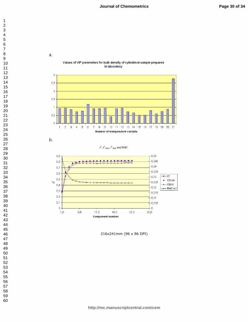
In Figure 5.a there are VIP (Variable Importance for the projection) parameters for bulk

density of cylindrical sample, prepared in laboratory. It can be seen from Figure 5.a that

independent variable x21 (the maximal density of asphalt mix) was more important than others.

Variable x6 (quantity of stone aggregate passing 8 mm sieve) is the second most important with

VIP value more than 1. The only less important variable is x10 (quantity of rounded stone

aggregate), importance of all other variables is in the grey zone with VIP values between 0.5

and 1. For the other dependent variables the maximal density of asphalt mix was not so

important, but x10 was almost always unimportant (Table II).

We can see the increasing modelling ability of PLS models with increasing number of

components (r2) in Figure 5.b. With only 6 components we can see that the model fits the

experimental data enough. A similar situation is found in the correlations, regarding all other

dependent variables. It can also be seen from Figure 5.b that modelling ability of PLS models

(r2train) for training set containing 70% of data set, selected with Kennard&Stone algorithm, was

similar to r2. Also, the values for test set were nearly as good as for modelling ability (r2test).

We can see the difference between the increasing modelling ability and the predictive

ability of PLS models with the increasing number of components in Figure 6. Modelling ability

(r2) is compared to the Leave-One-Out (r2loo), leave-10%-out Cross-Validation (r2

l10%o), leave-

20%-out Cross-Validation (r2l20%o) and Cross-Validation parameter obtained from SIMCA

Page 12 of 34



123456789101112131415161718192021222324252627282930313233343536373839404142434445464748495051525354555657585960

For Peer Review


Page 13/17

program (q2). All three r squares seem parallel from 10 to 21 components, but the leave-20%-

out Cross-Validation has a slight maximum at 15 components. Cross-Validation q2, obtained

from SIMCA, has a clear maximum at 5 components.

PLS was also applied to the data set, containing independent variables with mixed terms.

The independent variables with mixed terms can be seen from Figure 7.b, where the bulk

density of cylindrical sample, prepared in laboratory, is showing the increasing modelling

ability of PLS models with increasing number of components, but the Root Mean Square of

errors (RMS) is increasing after 70 components. Cross-Validation q2, obtained from SIMCA,

has clear maximum at 7 components.

4.3. Counterpropagation

We trained the counterpropagation neural network with two data sets: with a set of 444

samples and additionally with extended data set of 444+38 samples. Several

counterpropagation networks were tested, differing in the dimension of the Kohonen map. We

first trained neural networks (NN) with 100 epochs. With increasing dimension the fit of the

model was increasing t, but the Cross-Validation showed (Supplementary Material -Table S1)

that the 10X10 NN dimension was optimal (Regression plot is in Figure 4).

Later we trained NN with 200 epochs. At 200 epochs the Cross-Validation showed

(Supplementary Material -Table S1) the best values for the 12X12 NN dimension. It can be

concluded that the NN learning parameters are correlated and there is no simple rule for

determination of the optimal NN learning parameters. The training and test set, obtained with

Kennard Stone, were used to validate 12X12 network (Supplementary Material -Table S1). We

did not get any conflict node regarding the type of asphalt mix with the test set. There was a

clear separation between the 3 different types of asphalt mix in the topmap. We selected the NN

dimension 12X12 for further modelling

Page 13 of 34



123456789101112131415161718192021222324252627282930313233343536373839404142434445464748495051525354555657585960

For Peer Review


Page 14/17

With the NN dimension 20X20, the Cross-Validation showed slight improvement at 300

epochs, compared to the selected NN architecture, but there was no improvement in the

separation between the 3 different types of asphalt mix.

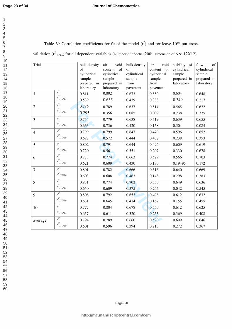
We can see from Figure 4, Tables III, IV and V and Supplementary Material (Table S1)

that the correlation coefficients (r2) for counterpropagation NN are bigger than those for MLR

models, but the Cross-Validation (r2loo and r

2l10%o) shows, that the MLR models are better. With

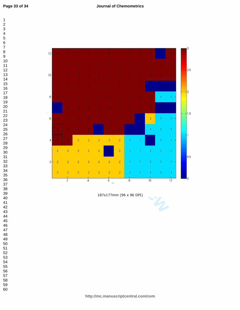
the counterpropagation NN we can visualize the position of classes of asphalt. The final topmap

of the counterpropagation model (dimension 12X12, after 200 epochs) can be seen in Figure 8.

Stone Mastic Asphalts (SMA) are labelled with number 1, Asphalt Concretes (AC) used for

wearing course are labelled with number 2 and Asphalt Concretes (AC) used for binder and

base course with number 3. The only conflicting nodes are in the first column, row 4 and 5.

We also made a counterpropagation model for classification purposes with asphalt

analyses, without removing the samples with missing data. In Figure 9 we can see that the

Mastic asphalts (MA), labelled with number 4, and the Porous asphalts (PA), labelled with

number 6, are clearly separated from the other asphalts. Special purpose asphalts, labelled with

number 1, are similar to the Stone Mastic Asphalts and they are classified between them in the

counterpropagation model.

5. Conclusion

We implemented a pure chemometrics approach on the extensive asphalt data collected

during the past ten years. To our best knowledge, such a research has not yet been published.

The study was performed without any predetermined assumptions, commonly considered in

previous studies. We were able to collect some information, usually not contained in the test

reports (i.e. temperature of asphalt on the building site, quality of recovered bitumen,

Page 14 of 34



123456789101112131415161718192021222324252627282930313233343536373839404142434445464748495051525354555657585960

For Peer Review


Page 15/17

percentage of rounded stone fractions). Exploration of these additional data enabled us to

extract useful information about the factors, influencing the quality of asphalt layers.

The results of MLR and PLS models show that all independent variables are important.

The lowest importance was ascribed to the quantity of rounded stone aggregate.

The best modelling and predictive abilities were obtained with MLR model, containing

the linear combinations of all independent variables. Counterpropagation models have good

modelling abilities, but predictive abilities are lower then those, obtained with MLR.

Nevertheless, there are two advantages of counterpropagation models. First, it can be used also

for classification and visualization of different types of asphalt, and second, the model can cope

with the missing data without any statistical pre-treatment.

The MLR models will be useful for the preparation of asphalt mix design (recipe) with

some unknown material. It may also be employed to correct mix design if some property of

input material is changed during production process, as for example the change of bitumen type

or sieving curve.

6. Acknowledgment

The authors thank of the Ministry of Higher Education, Science and Technology of the

Republic of Slovenia for the financial support through the Project P1-017: Modeling of

relationship between chemical structure and properties - QSAR –QSPR.

Page 15 of 34



123456789101112131415161718192021222324252627282930313233343536373839404142434445464748495051525354555657585960

For Peer Review


Page 16/17

7. References

1. Lavin P.; Asphalt Pavements: A Practical Guide to Design, Production and

Maintenance for Engineers and Architects, Taylor & Francis, 2003, ISBN

0415247330.

2. Ramljak Z. Bitumen Content Calculation in Designed Asphalt Mixture, proceedings

of 2nd Euroasphalt $Eurobitume Congress, Barcelona, 2000, 704.

3. Ramljak Z. Funkcionalna ovisnost optimalnog udjela bitumena u asfaltnoj mješavini

o uvjetima projektiranja te o gustoči ingredijenta, Zbornik referatov 7. kolokvija o

bitumnih, Gozd Martuljek, 2002, 44-54.

4. Cominsky R J, Huber G A, Kennedy T W, Anderson M. The Superpave mix design

manual for new construction and overlay, SHRP-A-407, National Research Council

Washington, DC, 1994.

5. Anderson R M. Superpave level 1 mixture design example, A first look at volumetric

mix design in Superpave system, Asphalt Institute Research Centre, Lexington, KY,

1993.

6. Kandhal P S, Cooley L A Jr. NCHRP report 464; The Restricted Zone in the

Superpave Aggregate Gradation Specification, National Academy Press,

Washington DC, 2001

7. Bitval final report (http://bitval.fehrl.org/index.php?id=14&no_cache=1)

8. COST 333 Final Report, 1999, 375 pp. - 17.5 x 25.0 cm, ISBN 92-828-6796-X -

EUR 18906

Page 16 of 34



123456789101112131415161718192021222324252627282930313233343536373839404142434445464748495051525354555657585960

For Peer Review


Page 17/17

9. Wold S, Martens S, Wold H. The multivariate calibration problem in chemistry

solved by the PLS method. In: Ruhe A, Kagstrom B(Eds.), Lecture Notes in

Mathematics. Proceedings of the Conference on Matrix Pencils, 1983, 286-293.

10. Brereton R G. Chemometrics: Data Analysis for Laboratory and Chemical Plant,

Wiley, 2003, ISBN 0-471-48978-6

11. Hecht-Nielsen R. Counterpropagation networks. Appl. Opt. 1987; 26: 4979-4984.

12. Zupan J, Novič M, Ruisanchez I. Kohonen and counter-propagation artificial neural

networks in analytical chemistry. Chemom. Intell. Lab. Syst. 1997; 38: 1-23

13. Nelson PRC, MacGregor JF, Taylor PA. The impact of missing measurements on

PCA and PLS prediction and monitoring applications. Chemometrics Intell. Lab.

Syst. 2006; 80: 1-12

14. Xu QS, Liang YZ. Monte Carlo cross validation. Chemometrics Intell. Lab. Syst.

2001; 56: 1-11.

15. Gourvénec S, Fernández Pierna JA, Massart DL, Rutledge DN. An evaluation of the

PoLiSh smoothed regression and the Monte Carlo cross-validation for the

determination of the complexity of a PLS model. Chemometrics Intell. Lab. Syst.

2003; 68: 41-51.

16. Xu QS, Liang YZ, Du YP. Monte Carlo cross-validation for selecting a model and

estimating the prediction error in multivariate calibration. J. Chemometrics 2004;

18: 112-120.

17. Kennard RW, Stone LA. Computer Aided Desing of Experiments. Technometrics,

1969, 11, 137–148.

Page 17 of 34



123456789101112131415161718192021222324252627282930313233343536373839404142434445464748495051525354555657585960

For Peer Review

Page 1/6

Tables:

Table I: Mean values for independent and dependent variables for three types of asphalt

mixes

Abbreviation Independent variables Stone

mastic

asphalt

SMA

Asphalt

concrete

(AC) for

wearing

course

Asphalt

concrete

(AC) for

binder and

base

course

x1 quantity of stone aggregate passing

0.09 mm sieve (range from 4.6 wt %

to 13.2 wt %), 10.8 9.9 6.9



to 18.0 wt %), 13.0 14.2 9.9



to 29.4 wt %) 16.3 23.1 15.6

x4 quantity of stone aggregate passing 2

mm sieve (range from 19.1 wt % to

58.9 wt %), 25.6 45.5 29.3



73.1 wt %), 35.0 61.7 40.7



99.8 wt %), 86.6 89.8 57.8



to 100 wt %), 99.3 99.4 68.9


16 mm sieve (range from 54.5 wt %

to 100 wt %), 100 100 80.9



to 100 wt %), 100 100 93.6

x10 quantity of rounded stone aggregate

(range from 0.0 wt % to 19.9 wt %), 0.000 0.005 0.643

x11 quantity of silica type stone aggregate

(range from 0.0 wt % to 88.7 wt %), 76.49 43.78 0.65

x12 quantity of bitumen (range from 2.9

wt % to 7.5 wt %), 6.3 5.5 3.8

x13 penetration of bitumen extracted from

asphalt mix (range from 18 mm/10 to

68 mm/10), 35.2 39.3 30.8

x14 softening point of bitumen extracted

from asphalt mix (range from 47.5 0C

to 860C), 70.4 59.0 63.2

Page 18 of 34



123456789101112131415161718192021222324252627282930313233343536373839404142434445464748495051525354555657585960

For Peer Review

Page 2/6

Abbreviation Independent variables Stone

mastic

asphalt

SMA

Asphalt

concrete

(AC) for

wearing

course

Asphalt

concrete

(AC) for

binder and

base

course

x15 Fraass breaking point of bitumen

extracted from asphalt mix (range

from -23 0C to -2.3

0C ), -13.3 -12.0 -10.3

x16 temperature of asphalt at construction

site (range from 130 0C to 195

0C), 171 162 163

x17 type of input bitumen (with or

without polymer) (for Polymer

modified and 0 for neat bitumen), 0.963 0.046 0.004

x18 hardness of input bitumen (according

to penetration) (1 soft, 2 middle, 3

hard), 1.6 1.3 2.1

x19 temperature of asphalt when asphalt

mix is compacted in laboratory(range

from 138 0C to 180

0C), 170 154 158

x20 thickness of asphalt layer(range from

1.65 cm. to 13 cm), 3.3 3.8 7.5

x21 maximal density of asphalt mix

(range from 2.355 g/cm3 to 2.707

g/cm3), 2.558 2.550 2.570

Abbreviation Selected dependent variables are: Stone

mastic

asphalt

SMA

Asphalt

concrete

(AC) for

wearing

course

Asphalt

concrete

(AC) for

binder and

base

course

y1 bulk density of cylindrical sample

prepared in laboratory (range from

2.204 g/cm3 to 2.556 g/cm

3), 2.446 2.444 2.404

y2 air void content of cylindrical sample


1.2 % (v/v) to 10.5 % (v/v)), 4.4 4.1 6.4

y3 bulk density of sample drilled from

pavement (range from 2.204 g/cm3 to

2.574 g/cm3), 2.439 2.406 2.407

y4 air void content of sample drilled

from pavement (range from 2.4 %

(v/v) to 8.7 % (v/v)), 4.65 5.626 6.367

y5 stability of cylindrical sample


4.2 kN to 15.3 kN) 9.16 9.86 10.66

y6 flow of cylindrical sample prepared

in laboratory(range from 2.4 mm to

8.7 mm) 5.4 4.5 4.1

Page 19 of 34



123456789101112131415161718192021222324252627282930313233343536373839404142434445464748495051525354555657585960

For Peer Review

Page 3/6

Table II: The most important independent variables, obtained with MLR and PLS

Type of model y1 y2 y3 y4 y5 y6

MLR 4 best x

(y=x1b1+b0)

x21, x8, x7,

x1

x2, x1, x8,

x12

x21, x13, x2,

x11

x12, x1, x11,

x7

x13, x12, x15,

x11

x17, x11, x12,

x1

MLR best pair

(y=x1b1+ x2b2+b0)

x21, x2 x2, x13 x21, x12 x12, x6 x13, x5 x17, x2

PLS VIP value over 1 x21, x6 x2, x1, x6,

x3, x8, x12,

x13, x20, x9

x21, x17, x19,

x11, x14

x12, x13, x6,

x17, x20, x2,

x11, x15, x1,

x21

x13, x15, x12,

x3, x2, x5,

x11

x17, x11, x12,

x1, x7, x20,

x8, x19, x14,

x6, x2

PLS VIP value less

than 0.5

x10 x19, x16 x18, x15, x10 x10 x21, x10

Page 20 of 34



123456789101112131415161718192021222324252627282930313233343536373839404142434445464748495051525354555657585960

For Peer Review

Page 4/6

Table III: Correlation coefficients for fit of the model (r2) and for leave-one-out cross-

validation (r2loo) for all dependent variables

Type of linear equation bulk

density of

cylindrical

sample

prepared in

laboratory

air void

content of

cylindrical

sample

prepared in

laboratory

bulk

density of

cylindrical

sample

from

pavement

air void

content of

cylindrical

sample

from

pavement

stability of

cylindrical

sample

prepared in

laboratory

flow of

cylindrical

sample

prepared in

laboratory

The best:

y= x1b1+b0

r2

r2

loo

0.303

0.297

0.558

0.554

0.390

0.385

0.176

0.168

0.182

0.179

0.317

0.317

The best:

y= x1b1+ x2b2+b0

r2

r2

loo

0.661

0.656

0.593

0.589

0.489

0.482

0.248

0.238

0.247

0.237

0.360

0.349

y= x1b1+ x2b2+…+

x21b21+b0

r2

r2

loo

0. 813

0.793

0. 760

0.734

0. 607

0.563

0. 365

0.297

0. 449

0.393

0. 414

0.352

y= x1b1+ x2b2+…+

x21b21+…+x1x2b1_2+…

+x20x21b20_21+b0

r2

r2

loo

0.933

0,239

0. 913

0,197

0. 827

0,206

0. 722

0,089

0. 781

0,107

0. 755

0,112

Page 21 of 34



123456789101112131415161718192021222324252627282930313233343536373839404142434445464748495051525354555657585960

For Peer Review

Page 5/6

Table IV: Correlation coefficients for fit of the model (r2) and for leave-10%-out-cross-

validation (r2l10%o) for all dependent variables (Type of linear equation: y= x1b1+ x2b2+…+

x21b21+b0)

Trial

bulk density

of

cylindrical

sample

prepared in

laboratory

air void

content of

cylindrical

sample

prepared in

laboratory

bulk density

of

cylindrical

sample

from

pavement

air void

content of

cylindrical

sample

from

pavement

stability of

cylindrical

sample

prepared in

laboratory

flow of

cylindrical

sample

prepared in

laboratory

1 r2

r2l10%o

0,821

0,772 0,762 0,749

0,607 0,660

0,371 0,423

0,440 0,506

0,420 0,341

2 r2

r2l10%o

0,824 0,674

0,773 0,622

0,630 0,229

0,401 0,030

0,459 0,324

0,430 0,222

3 r2

r2l10%o

0,805

0,869

0,754

0,786

0,597

0,664

0,362

0,362

0,476

0,257

0,429

0,203

4 r2

r2l10%o

0,818

0,747

0,765

0,675

0,615

0,483

0,357

0,387

0,445

0,459

0,415

0,362

5 r2

r2l10%o

0,809

0,828

0,759

0,712

0,612

0,551

0,371

0,295

0,446

0,478

0,410

0,382

6 r2

r2l10%o

0,810

0,829

0,762

0,735

0,600

0,632

0,372

0,271

0,446

0,429

0,419

0,351

7 r2

r2l10%o

0,813

0,798

0,761

0,734

0,609

0,566

0,377

0,201

0,462

0,280

0,427

0,276

8 r2

r2l10%o

0,819

0,733

0,757

0,799

0,605

0,589

0,350

0,467

0,471

0,141

0,402

0,524

9 r2

r2l10%o

0,810

0,827

0,760

0,749

0,601

0,631

0,377

0,220

0,430

0,574

0,414

0,386

10 r2

r2l10%o

0,813

0,808

0,762

0,738

0,621

0,431

0,367

0,298

0,439

0,533

0,408

0,444

average r2

r2l10%o

0,814

0,788

0,761

0,730

0,610

0,544

0,370

0,295

0,452

0,398

0,417

0,349

Page 22 of 34



123456789101112131415161718192021222324252627282930313233343536373839404142434445464748495051525354555657585960

For Peer Review

Page 6/6

Table V: Correlation coefficients for fit of the model (r2) and for leave-10%-out cross-

validation (r2l10%o) for all dependent variables (Number of epochs: 200; Dimension of NN: 12X12)

Trial

bulk density

of

cylindrical

sample

prepared in

laboratory

air void

content of

cylindrical

sample

prepared in

laboratory

bulk density

of

cylindrical

sample

from

pavement

air void

content of

cylindrical

sample

from

pavement

stability of

cylindrical

sample

prepared in

laboratory

flow of

cylindrical

sample

prepared in

laboratory

1 r2

r2l10%o

0.811

0.539

0.802

0.655

0.673

0.439

0.550

0.383

0.604

0.349

0.648

0.217

2 r2

r2l10%o

0.786

0.295

0.789

0.356

0.637

0.085

0.514

0.009

0.565

0.238

0.622

0.375

3 r2

r2l10%o

0.754

0.663

0.779

0.736

0.638

0.420

0.519

0.158

0.639

0.504

0.655

0.084

4 r2

r2l10%o

0.799

0.627

0.799

0.572

0.647

0.444

0.479

0.438

0.596

0.238

0.652

0.353

5 r2

r2l10%o

0.802

0.720

0.791

0.561

0.644

0.551

0.496

0.207

0.609

0.330

0.619

0.678

6 r2

r2l10%o

0.773

0.621

0.774

0.609

0.663

0.430

0.529

0.130

0.566

0.19495

0.703

0.172

7 r2

r2l10%o

0.801

0.603

0.782

0.608

0.666

0.463

0.516

0.143

0.640

0.298

0.669

0.383

8 r2

r2l10%o

0.831

0.650

0.774

0.609

0.702

0.375

0.550

0.245

0.649

0.042

0.636

0.545

9 r2

r2l10%o

0.808

0.631

0.792

0.645

0.653

0.414

0.498

0.167

0.612

0.155

0.632

0.455

10 r2

r2l10%o

0.777

0.657

0.804

0.611

0.678

0.320

0.550

0.253

0.612

0.369

0.625

0.408

average r2

r2l10%o

0.794

0.601

0.789

0.596

0.660

0.394

0.520

0.213

0.609

0.272

0.646

0.367

Page 23 of 34



123456789101112131415161718192021222324252627282930313233343536373839404142434445464748495051525354555657585960

For Peer Review

Page 1/2

Figure captions:

Figure 1: Cut through built in binder asphalt layer (a);

The lines represent the upper and lower limits of sieving curve for stone aggregate in asphalt

concrete with maximal grain size 22 mm (b) prescribed by the national standard;

Figure 2: Mechanical testing of cylindrical asphalt specimen

Figure 3: Cylindrical samples of asphalt layers from the Ring around Ljubljana (b);

Figure 4: Regression plots of the experimental versus predicted Bulk density for three

linear models (a-c) and counter-propagation neural model (d). Statistical parameters of

training (r2, Root Mean Square-RMStraining) and LOO validation of the models (r

2loo, Root

Mean Square-RMStesting) are presented.

Figure 5: VIP (Variable Importance for the projection) parameters for bulk density of the

cylindrical sample, prepared in a laboratory. (a);

Fit of PLS model with increasing number of component (independent variables) for bulk

density of cylindrical sample, prepared in a laboratory (b). Modelling ability (r2) is increasing

and RMS is decreasing with increasing number of components. Modelling ability of PLS

models (r2train) for training set, containing 70% of data set, selected with Kennard&Stone

algorithm, is similar and values for test set are nearly as good as for modelling ability (r2

test).

Page 24 of 34



123456789101112131415161718192021222324252627282930313233343536373839404142434445464748495051525354555657585960

For Peer Review

Page 2/2

Figure 6: Fit of PLS model with increasing number of component (independent variables) for

bulk density of cylindrical sample, prepared in a laboratory. Modelling ability (r2) is compared

to leave one out (r2loo), leave-10%-out cross-validation (r

2l10%o), leave-20%-out cross -validation

(r2

l20%o) and cross–validation parameter (q2), obtained from SIMCA program.

Figure 7: Regression coefficients of independent variables and mixed terms for bulk density of

the cylindrical sample, prepared in a laboratory (a);

Fit of PLS model with increasing number of component (independent variables and mixed

terms) for bulk density of cylindrical sample prepared in laboratory (b). Modelling ability (r2) is

increasing with increasing number of components, but RMS is decreasing after 70 components.

Figure 8: Final topmap of counterpropagation model for 444 asphalts. Stone Mastic Asphalts

are designated with number 1, Asphalt Concretes, used for wearing course, are designated with

number 2 and Asphalt Concretes, used for binder and base course, with number 3.

Figure 9: Final topmap of counterpropagation model for 482 asphalts. Stone Mastic Asphalts

are designated with number 1, Asphalt Concretes, used for wearing course, are designated with

number 2 and Asphalt Concretes, used for binder and base course, with number 3, Mastic

asphalts with number 4, special purpose asphalt with number 5 and Porous asphalts with

number 6.

Page 25 of 34



123456789101112131415161718192021222324252627282930313233343536373839404142434445464748495051525354555657585960

For Peer Review

146x142mm (111 x 111 DPI)

Page 26 of 34



123456789101112131415161718192021222324252627282930313233343536373839404142434445464748495051525354555657585960

For Peer Review

185x138mm (96 x 96 DPI)

Page 27 of 34



123456789101112131415161718192021222324252627282930313233343536373839404142434445464748495051525354555657585960

For Peer Review

216x197mm (96 x 96 DPI)

Page 28 of 34



123456789101112131415161718192021222324252627282930313233343536373839404142434445464748495051525354555657585960

For Peer Review

271x242mm (96 x 96 DPI)

Page 29 of 34



123456789101112131415161718192021222324252627282930313233343536373839404142434445464748495051525354555657585960

For Peer Review

216x241mm (96 x 96 DPI)

Page 30 of 34



123456789101112131415161718192021222324252627282930313233343536373839404142434445464748495051525354555657585960

For Peer Review

216x197mm (96 x 96 DPI)

Page 31 of 34



123456789101112131415161718192021222324252627282930313233343536373839404142434445464748495051525354555657585960

For Peer Review

216x241mm (96 x 96 DPI)

Page 32 of 34



123456789101112131415161718192021222324252627282930313233343536373839404142434445464748495051525354555657585960

For Peer Review

187x177mm (96 x 96 DPI)

Page 33 of 34



123456789101112131415161718192021222324252627282930313233343536373839404142434445464748495051525354555657585960

For Peer Review

184x173mm (96 x 96 DPI)

Page 34 of 34



123456789101112131415161718192021222324252627282930313233343536373839404142434445464748495051525354555657585960

S1-ln5616706-1570301650-1939656818Hwf1824382083Id V-11449873945616706PDF HI0001

Documents

Transcript of S1-ln5616706-1570301650-1939656818Hwf1824382083Id V-11449873945616706PDF HI0001