MEASUREMENT OF NEUTRAL CURRENT ELECTRON ...
262
MEASUREMENT OF NEUTRAL CURRENT ELECTRON-PROTON CROSS SECTIONS WITH LONGITUDINALLY POLARISED ELECTRONS USING THE ZEUS DETECTOR SYED UMER NOOR A DISSERTATION SUBMITTED TO THE FACULTY OFGRADUATE STUDIES IN PARTIAL FULFILMENT OF THE REQUIREMENTS FOR THE DEGREE OF DOCTOR OF PHILOSOPHY GRADUATE PROGRAM IN PHYSICS AND ASTRONOMY YORK UNIVERSITY TORONTO, ONTARIO DECEMBER 2007
-
Upload
khangminh22 -
Category
Documents
-
view
5 -
download
0
Transcript of MEASUREMENT OF NEUTRAL CURRENT ELECTRON ...

MEASUREMENT OF NEUTRAL CURRENT ELECTRON-PROTONCROSS SECTIONS WITH LONGITUDINALLY POLARISED
ELECTRONS USING THE ZEUS DETECTOR
SYED UMER NOOR
A DISSERTATION SUBMITTED TO THE FACULTY OF GRADUATESTUDIES
IN PARTIAL FULFILMENT OF THE REQUIREMENTSFOR THE DEGREE OF
DOCTOR OF PHILOSOPHY
GRADUATE PROGRAM IN PHYSICS AND ASTRONOMYYORK UNIVERSITY
TORONTO, ONTARIODECEMBER 2007

MEASUREMENT OF NEUTRAL CURRENTELECTRON-PROTON CROSS SECTIONSWITH LONGITUDINALLY POLARISED
ELECTRONS USING THE ZEUS DETECTOR
by Syed Umer Noor
a dissertation submitted to the Faculty of Graduate Stud-ies of York University in partial fulfilment of the require-ments for the degree of
DOCTOR OF PHILOSOPHYc© 2008
Permission has been granted to: a) YORK UNIVER-SITY LIBRARIES to lend or sell copies of this disserta-tion in paper, microform or electronic formats, and b) LI-BRARY AND ARCHIVES CANADA to reproduce, lend,distribute, or sell copies of this dissertation anywhere inthe world in microform, paper or electronic formats andto authorise or procure the reproduction, loan, distribu-tion or sale of copies of this dissertation anywhere in theworld in microform, paper or electronic formats.
The author reserves other publication rights, and nei-ther the dissertation nor extensive extracts for it maybe printed or otherwise reproduced without the author’swritten permission.

MEASUREMENT OF NEUTRAL CURRENT ELECTRON-PROTONCROSS SECTIONS WITH LONGITUDINALLY POLARISED
ELECTRONS USING THE ZEUS DETECTOR
by Syed Umer Noor
By virtue of submitting this document electronically, the author certifies that thisis a true electronic equivalent of the copy of the dissertation approved by YorkUniversity for the award of the degree. No alteration of the content has occurredand if there are any minor variations in formatting, they are as a result of theconversion to Adobe Acrobat format (or similar software application).
Examination Committee Members:
1. A. Kumarakrishnan
2. S. Menary
3. W. Taylor
4. P. Taylor
5. I. McDade
6. D. Bailey
Abstract
Neutral current (NC) electron-proton deep inelastic scattering (DIS) cross sections
with negatively and positively longitudinally polarised electrons are measured at
high momentum transfer squared (Q2 > 185 GeV2) using the ZEUS detector at
HERA. The HERA accelerator provides e±p collisions at a centre-of-mass energy
of 318 GeV, allowing high Q2 interactions which are sensitive to the weak force
contribution to the NC process. The e−p scattering data analysed corresponds to
an integrated luminosity of 177.2 pb−1, and is the largest amount of e−p data ever
recorded at ZEUS. Single-differential cross sections and reduced double-differential
cross sections are measured and agree well with the predictions of the Standard
Model. The two major results of this thesis are the first observation of parity
violation in NC e−p DIS at distances down to 10−18 m, and the measurement of the
structure functions xF3 and xF γZ3 , which are proportional to the proton valence
quark distribution, with the best precision to date.
iv

Dedicated to my mother and the memory of my father
v

Acknowledgements
This PhD has been one of the most fruitful endeavours I have ever undertaken, and
there are a number of people who have helped me along the way.
Firstly, I thank my supervisor Sampa for her support and guidance. I have
been very lucky to work with such a kind-hearted supervisor. I thank the NC e−p
analysis team; Yongdok who performed an enormous amount of excellent work in
tandem with my analysis and Kunihiro who has expertly guided us both. It has
been a pleasure to work closely with such delightful people. I thank everyone in the
High Q2 group, especially Enrico, Alex, James, Catherine, Katherine, and Micha l
for all their help. I express my gratitude to Richard who patiently taught me how
to perform my first analysis. I also thank all the Trigger group members, especially
Alessandro and Yuji, for their advice.
The Canadian group at DESY has been very supportive, and I thank the re-
search associates Mara, Serguei, and Roberval for their endless help, and professors
Scott, John, and Francois for their guidance. I thank the Canadian students, in
vi

particular Jerome, Ying, Jeff, Trevor, Chuanlei, and Jason, for all the good times.
Life at DESY was made much richer by the impromptu games of football/baseball
and outings for lunch. Many thanks to John, Tom, Billy, Dan, Avraam, Elıas,
Alessandro, Matt, and Tim for great laughs. I especially thank Jerome and John
for being such great friends. In addition to living in Hamburg, I also had the
pleasure of living in Tsukuba for 6 weeks to work on the NC analysis side-by-side
with Yongdok. I am grateful to all the members of the ZEUS KEK group for their
hospitality and I especially thank Katsuo for being a kind host.
I have shared an office with many friendly people at York, including George,
Brian, Steve, and Slavic. I thank Scott, Marko, and Wendy for their guidance at
York, and I thank Brad for his help with my lab. TAs. Whilst living in Hamburg
and Toronto, I have generated lots of paperwork and needed help with living ar-
rangements, so I especially thank Marlene and Lauren at York, and Susan and the
international office at DESY for their huge efforts.
I would not have made it this far without the love from my mother and late
father, the constant encouragement from my brother and sister, and the warm-
hearted support from my mother-in-law and brother-in-law. Finally, I cannot thank
my wife enough for sticking by me through the ups and downs of the PhD. She is
my true treasure and I am deeply grateful for her love.
vii
Contributions to the ZEUS experiment
I have been a member of the Canadian group of the ZEUS collaboration since
autumn 2003. During this time, I have had the privilege of being part of an inter-
national collaboration of approximately 400 physicists, and the opportunity to be
involved in the running of a large and exciting experiment. The ZEUS experiment
is located in Hamburg, Germany, and I have worked on site for almost two years,
between 2003-2006, and undertaken regular 8-hour shifts at the experiment.
From January 2005 to June 2006 I was part of the team responsible for the
Third Level Trigger (TLT). My duties included maintaining the filter code, verifying
code updates submitted by various physics groups, and migrating the TLT online
histograms to a widely used website.
I became a member of the High Q2 physics group in 2005 and joined the group
of volunteers that monitored data quality histograms. From October 2005 to June
2006 I was the trigger representative for the High Q2 physics group. My duties
entailed implementing changes to the trigger slots maintained by our group and
viii
investigating problems raised by either my physics group or the trigger experts.
The analysis presented in this thesis began in January 2005 and is based on
electron-proton data recorded between 2005-2006. The NC analysis is important
for the ZEUS collaboration as a whole, as there are many events with which to
study the performance of the detector. I joined the luminosity working group in
2005 and presented evidence that the luminosity monitor was performing well. I
worked closely with other High Q2 members to devise a new method of correcting
the effect of hadronic particles scattering off detector components (the backsplash
effect).
The NC DIS analysis is a springboard for other analyses such as the QCD fits
which provide parton density functions. I provided the QCD fitters at ZEUS with
the latest NC DIS cross sections and uncertainties. I was also part of the ZEUS
and H1 working group that combined results between the two collider experiments
at HERA for the best statistical impact. I contributed to the first ever public
ZEUS and H1 combined result of the structure function xF γZ3 and the polarisation
asymmetry A±, both presented at the 33rd International Conference on High Energy
Physics.
The main result of my thesis is the first observation of parity violation in NC e−p
DIS at distances down to 10−18 m through a measurement of the polarisation asym-
metry A−, and also the most precise measurement of the structure functions xF3
ix
and xF γZ3 , which are sensitive to the proton valence quark momentum distribution.
I have presented my work on behalf of the ZEUS collaboration at the 14th
International Workshop on Deep Inelastic Scattering (DIS 2006) in Japan and the
conference Rencontres de Moriond: QCD and Hadronic Interactions (Moriond QCD
2007) in Italy. I also submitted a contribution to the proceedings of the 33rd
International Conference on High Energy Physics (ICHEP 2006) in Russia. After
close collaboration between myself, Yongdok Ri, Kunihiro Nagano, and Sampa
Bhadra, a paper based on the HERA II NC e−p DIS analysis has been submitted
to the management at ZEUS for review.
x

Contents
Abstract iv
Acknowledgements vi
Contributions to the ZEUS experiment viii
Table of Contents xi
List of Tables xvii
List of Figures xxii
1 Introduction 1
2 Theory 5
2.1 The Standard Model . . . . . . . . . . . . . . . . . . . . . . . . . . 5
2.1.1 Matter . . . . . . . . . . . . . . . . . . . . . . . . . . . . . . 6
2.1.2 Forces . . . . . . . . . . . . . . . . . . . . . . . . . . . . . . 7
xi

2.2 The structure of the proton . . . . . . . . . . . . . . . . . . . . . . 8
2.2.1 Quark-parton model . . . . . . . . . . . . . . . . . . . . . . 8
2.2.2 Quantum chromodynamics . . . . . . . . . . . . . . . . . . . 15
2.2.3 QCD improved parton model . . . . . . . . . . . . . . . . . 17
2.2.4 Parton Density Functions . . . . . . . . . . . . . . . . . . . 19
2.3 The electromagnetic and weak interactions . . . . . . . . . . . . . . 22
2.4 The neutral current cross section . . . . . . . . . . . . . . . . . . . 27
3 HERA and the ZEUS detector 36
3.1 HERA collider . . . . . . . . . . . . . . . . . . . . . . . . . . . . . . 36
3.1.1 Proton and electron beams . . . . . . . . . . . . . . . . . . . 40
3.1.2 Spin rotators and polarimetry . . . . . . . . . . . . . . . . . 41
3.2 ZEUS detector . . . . . . . . . . . . . . . . . . . . . . . . . . . . . 43
3.2.1 Uranium Calorimeter . . . . . . . . . . . . . . . . . . . . . . 45
3.2.2 Central Tracking Detector . . . . . . . . . . . . . . . . . . . 48
3.2.3 Luminosity detector . . . . . . . . . . . . . . . . . . . . . . 50
3.2.4 Background rejection . . . . . . . . . . . . . . . . . . . . . . 50
3.2.5 Trigger and data acquisition . . . . . . . . . . . . . . . . . . 51
4 Monte Carlo Simulation 55
4.1 DIS Monte Carlo . . . . . . . . . . . . . . . . . . . . . . . . . . . . 55
xii
4.2 Photoproduction Monte Carlo . . . . . . . . . . . . . . . . . . . . . 58
4.3 Detector simulation and software environment . . . . . . . . . . . . 60
4.4 Monte Carlo samples . . . . . . . . . . . . . . . . . . . . . . . . . . 62
5 Reconstruction of Kinematic Variables 65
5.1 Electron reconstruction method . . . . . . . . . . . . . . . . . . . . 70
5.2 Jacquet-Blondel reconstruction method . . . . . . . . . . . . . . . . 71
5.3 Double Angle reconstruction method . . . . . . . . . . . . . . . . . 71
5.4 Bias and resolutions of reconstruction methods . . . . . . . . . . . . 72
6 Event Reconstruction 77
6.1 Track and vertex reconstruction . . . . . . . . . . . . . . . . . . . . 77
6.2 Longitudinal vertex reweighting . . . . . . . . . . . . . . . . . . . . 78
6.3 Electron identification . . . . . . . . . . . . . . . . . . . . . . . . . 79
6.4 Electron energy . . . . . . . . . . . . . . . . . . . . . . . . . . . . . 80
6.4.1 RCAL electron energy . . . . . . . . . . . . . . . . . . . . . 82
6.4.2 BCAL electron energy . . . . . . . . . . . . . . . . . . . . . 83
6.4.3 FCAL electron energy . . . . . . . . . . . . . . . . . . . . . 84
6.5 Calorimeter alignment . . . . . . . . . . . . . . . . . . . . . . . . . 84
6.6 Hadronic final state reconstruction . . . . . . . . . . . . . . . . . . 85
6.6.1 Hadronic energy scale . . . . . . . . . . . . . . . . . . . . . 86
xiii
6.6.2 Jet reconstruction . . . . . . . . . . . . . . . . . . . . . . . . 88
6.6.3 Investigation into the hadronic angle . . . . . . . . . . . . . 89
7 Backsplash in the Hadronic Final State 93
7.1 Updating the backsplash correction . . . . . . . . . . . . . . . . . . 95
7.2 New jet-based approach . . . . . . . . . . . . . . . . . . . . . . . . 96
7.3 Results using new jet-based approach . . . . . . . . . . . . . . . . . 100
8 Event Selection 109
8.1 Event characteristics . . . . . . . . . . . . . . . . . . . . . . . . . . 109
8.2 Background characteristics . . . . . . . . . . . . . . . . . . . . . . . 115
8.2.1 Photoproduction . . . . . . . . . . . . . . . . . . . . . . . . 115
8.2.2 Beam-gas . . . . . . . . . . . . . . . . . . . . . . . . . . . . 116
8.2.3 Halo and cosmic muons . . . . . . . . . . . . . . . . . . . . . 116
8.2.4 Elastic QED Compton . . . . . . . . . . . . . . . . . . . . . 117
8.3 Data preselection . . . . . . . . . . . . . . . . . . . . . . . . . . . . 117
8.3.1 First Level Trigger . . . . . . . . . . . . . . . . . . . . . . . 118
8.3.2 Second Level Trigger . . . . . . . . . . . . . . . . . . . . . . 119
8.3.3 Third Level Trigger . . . . . . . . . . . . . . . . . . . . . . . 120
8.3.4 Data quality . . . . . . . . . . . . . . . . . . . . . . . . . . . 121
8.4 Data sample . . . . . . . . . . . . . . . . . . . . . . . . . . . . . . . 121
xiv
8.5 Offline event selection . . . . . . . . . . . . . . . . . . . . . . . . . . 123
9 Cross section extraction and uncertainties 131
9.1 Cross section calculation and bin selection . . . . . . . . . . . . . . 131
9.2 Statistical uncertainties . . . . . . . . . . . . . . . . . . . . . . . . . 137
9.3 Systematic uncertainties . . . . . . . . . . . . . . . . . . . . . . . . 139
9.3.1 Background rejection . . . . . . . . . . . . . . . . . . . . . . 140
9.3.2 Electron purity and hadronic final state . . . . . . . . . . . . 141
9.3.3 Calorimeter energy and alignment . . . . . . . . . . . . . . . 143
10 Results and discussion 150
10.1 Single-differential cross sections . . . . . . . . . . . . . . . . . . . . 150
10.2 Reduced cross sections . . . . . . . . . . . . . . . . . . . . . . . . . 161
10.3 The structure functions xF3 and xF γZ3 . . . . . . . . . . . . . . . . 166
11 Summary and outlook 172
A Acronyms 176
B Trigger slots 178
B.1 First Level Trigger . . . . . . . . . . . . . . . . . . . . . . . . . . . 178
B.2 Second Level Trigger . . . . . . . . . . . . . . . . . . . . . . . . . . 181
xv
C Comparisons between electron finders 183
D Extracting cross sections using the Electron method 186
E Tables of Results 190
Bibliography 224
xvi
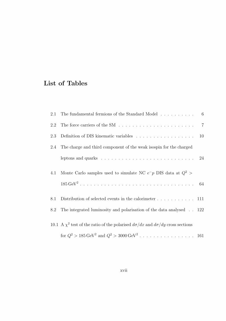
List of Tables
2.1 The fundamental fermions of the Standard Model . . . . . . . . . . 6
2.2 The force carriers of the SM . . . . . . . . . . . . . . . . . . . . . . 7
2.3 Definition of DIS kinematic variables . . . . . . . . . . . . . . . . . 10
2.4 The charge and third component of the weak isospin for the charged
leptons and quarks . . . . . . . . . . . . . . . . . . . . . . . . . . . 24
4.1 Monte Carlo samples used to simulate NC e−p DIS data at Q2 >
185 GeV2 . . . . . . . . . . . . . . . . . . . . . . . . . . . . . . . . . 64
8.1 Distribution of selected events in the calorimeter . . . . . . . . . . . 111
8.2 The integrated luminosity and polarisation of the data analysed . . 122
10.1 A χ2 test of the ratio of the polarised dσ/dx and dσ/dy cross sections
for Q2 > 185 GeV2 and Q2 > 3000 GeV2 . . . . . . . . . . . . . . . . 161
xvii

E.1 The single differential cross section dσ/dx for Q2 > 185 GeV2 mea-
sured using the combined 05-06 e−p data set (L = 177.2 pb−1, Pe =
−0.04) . . . . . . . . . . . . . . . . . . . . . . . . . . . . . . . . . . 191
E.2 The single differential cross section dσ/dx for Q2 > 185 GeV2 mea-
sured using the negatively polarised 05-06 e−p data set (L = 105.4 pb−1, Pe =
−0.27) . . . . . . . . . . . . . . . . . . . . . . . . . . . . . . . . . . 192
E.3 The single differential cross section dσ/dx for Q2 > 185 GeV2 mea-
sured using the positively polarised 05-06 e−p data set (L = 71.8 pb−1, Pe =
+0.30) . . . . . . . . . . . . . . . . . . . . . . . . . . . . . . . . . . 193
E.4 The single differential cross section dσ/dx for Q2 > 3000 GeV2 mea-
sured using the combined 05-06 e−p data set (L = 177.2 pb−1, Pe =
−0.04) . . . . . . . . . . . . . . . . . . . . . . . . . . . . . . . . . . 194
E.5 The single differential cross section dσ/dx for Q2 > 3000 GeV2 mea-
sured using the negatively polarised 05-06 e−p data set (L = 105.4 pb−1, Pe =
−0.27) . . . . . . . . . . . . . . . . . . . . . . . . . . . . . . . . . . 195
E.6 The single differential cross section dσ/dx for Q2 > 3000 GeV2 mea-
sured using the positively polarised 05-06 e−p data set (L = 71.8 pb−1, Pe =
+0.30) . . . . . . . . . . . . . . . . . . . . . . . . . . . . . . . . . . 196
xviii
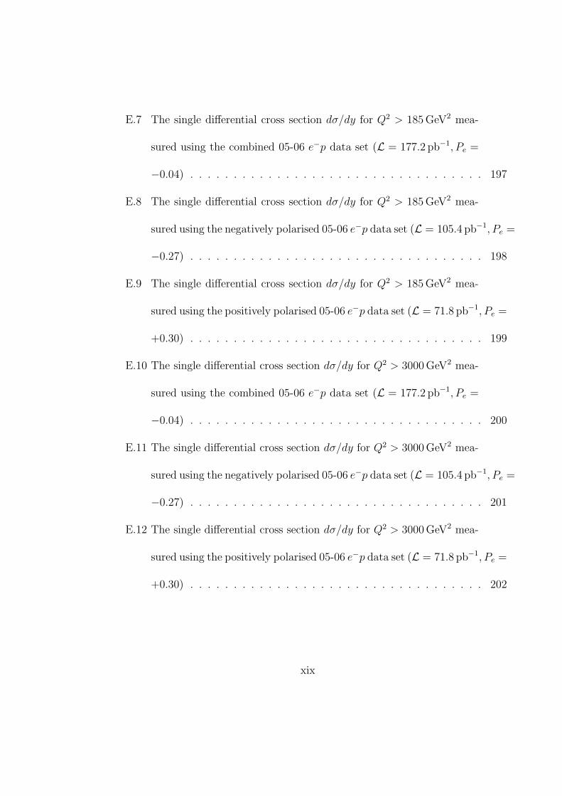
E.7 The single differential cross section dσ/dy for Q2 > 185 GeV2 mea-
sured using the combined 05-06 e−p data set (L = 177.2 pb−1, Pe =
−0.04) . . . . . . . . . . . . . . . . . . . . . . . . . . . . . . . . . . 197
E.8 The single differential cross section dσ/dy for Q2 > 185 GeV2 mea-
sured using the negatively polarised 05-06 e−p data set (L = 105.4 pb−1, Pe =
−0.27) . . . . . . . . . . . . . . . . . . . . . . . . . . . . . . . . . . 198
E.9 The single differential cross section dσ/dy for Q2 > 185 GeV2 mea-
sured using the positively polarised 05-06 e−p data set (L = 71.8 pb−1, Pe =
+0.30) . . . . . . . . . . . . . . . . . . . . . . . . . . . . . . . . . . 199
E.10 The single differential cross section dσ/dy for Q2 > 3000 GeV2 mea-
sured using the combined 05-06 e−p data set (L = 177.2 pb−1, Pe =
−0.04) . . . . . . . . . . . . . . . . . . . . . . . . . . . . . . . . . . 200
E.11 The single differential cross section dσ/dy for Q2 > 3000 GeV2 mea-
sured using the negatively polarised 05-06 e−p data set (L = 105.4 pb−1, Pe =
−0.27) . . . . . . . . . . . . . . . . . . . . . . . . . . . . . . . . . . 201
E.12 The single differential cross section dσ/dy for Q2 > 3000 GeV2 mea-
sured using the positively polarised 05-06 e−p data set (L = 71.8 pb−1, Pe =
+0.30) . . . . . . . . . . . . . . . . . . . . . . . . . . . . . . . . . . 202
xix
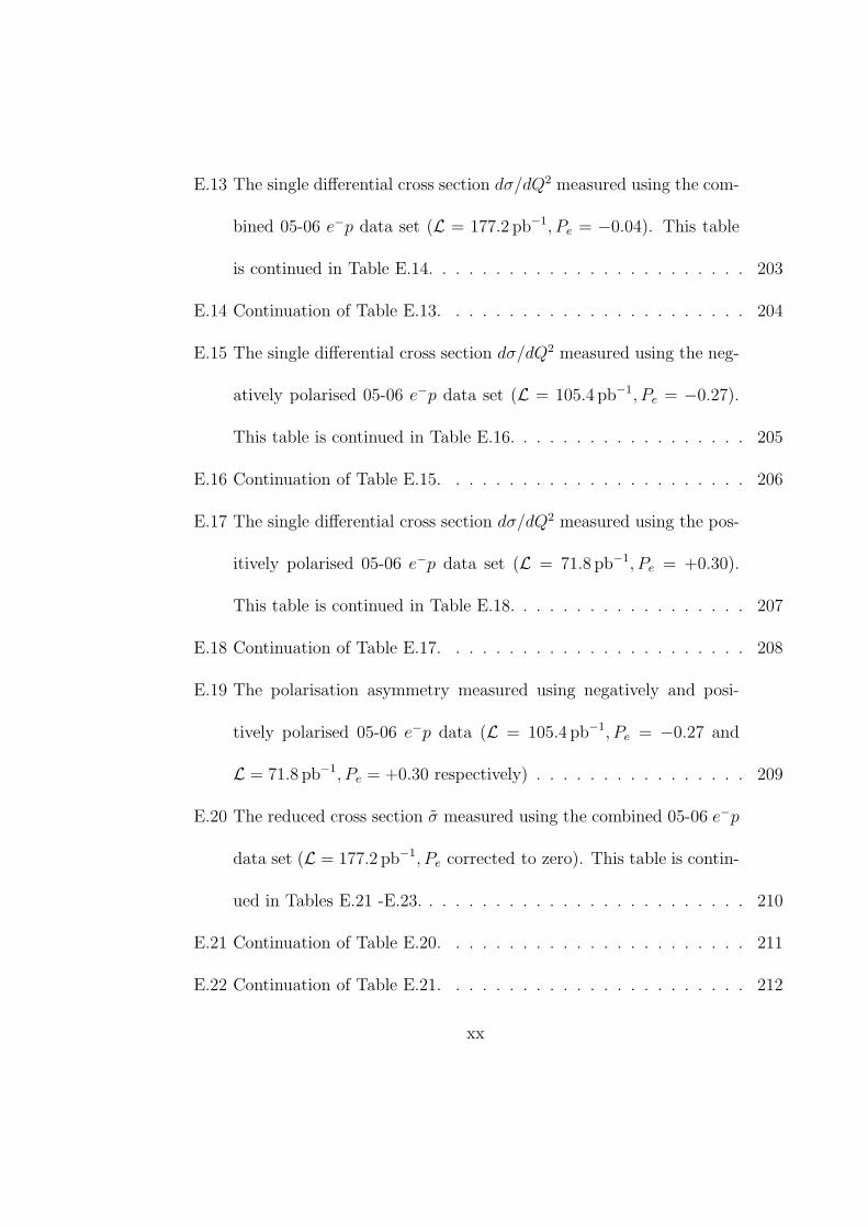
E.13 The single differential cross section dσ/dQ2 measured using the com-
bined 05-06 e−p data set (L = 177.2 pb−1, Pe = −0.04). This table
is continued in Table E.14. . . . . . . . . . . . . . . . . . . . . . . . 203
E.14 Continuation of Table E.13. . . . . . . . . . . . . . . . . . . . . . . 204
E.15 The single differential cross section dσ/dQ2 measured using the neg-
atively polarised 05-06 e−p data set (L = 105.4 pb−1, Pe = −0.27).
This table is continued in Table E.16. . . . . . . . . . . . . . . . . . 205
E.16 Continuation of Table E.15. . . . . . . . . . . . . . . . . . . . . . . 206
E.17 The single differential cross section dσ/dQ2 measured using the pos-
itively polarised 05-06 e−p data set (L = 71.8 pb−1, Pe = +0.30).
This table is continued in Table E.18. . . . . . . . . . . . . . . . . . 207
E.18 Continuation of Table E.17. . . . . . . . . . . . . . . . . . . . . . . 208
E.19 The polarisation asymmetry measured using negatively and posi-
tively polarised 05-06 e−p data (L = 105.4 pb−1, Pe = −0.27 and
L = 71.8 pb−1, Pe = +0.30 respectively) . . . . . . . . . . . . . . . . 209
E.20 The reduced cross section σ measured using the combined 05-06 e−p
data set (L = 177.2 pb−1, Pe corrected to zero). This table is contin-
ued in Tables E.21 -E.23. . . . . . . . . . . . . . . . . . . . . . . . . 210
E.21 Continuation of Table E.20. . . . . . . . . . . . . . . . . . . . . . . 211
E.22 Continuation of Table E.21. . . . . . . . . . . . . . . . . . . . . . . 212
xx

E.23 Continuation of Table E.22. . . . . . . . . . . . . . . . . . . . . . . 213
E.24 The reduced cross section σ measured using the negatively polarised
05-06 e−p data set (L = 105.4 pb−1, Pe = −0.27). This table is
continued in Tables E.25 -E.27. . . . . . . . . . . . . . . . . . . . . 214
E.25 Continuation of Table E.24. . . . . . . . . . . . . . . . . . . . . . . 215
E.26 Continuation of Table E.25. . . . . . . . . . . . . . . . . . . . . . . 216
E.27 Continuation of Table E.26. . . . . . . . . . . . . . . . . . . . . . . 217
E.28 The reduced cross section σ measured using the positively polarised
05-06 e−p data set (L = 71.8 pb−1, Pe = +0.30). This table is con-
tinued in Tables E.29 -E.31. . . . . . . . . . . . . . . . . . . . . . . 218
E.29 Continuation of Table E.28. . . . . . . . . . . . . . . . . . . . . . . 219
E.30 Continuation of Table E.29. . . . . . . . . . . . . . . . . . . . . . . 220
E.31 Continuation of Table E.30. . . . . . . . . . . . . . . . . . . . . . . 221
E.32 The structure function xF3 extracted using the combined 05-06 e−p
data set (L = 177.2 pb−1, Pe corrected to zero) and previously pub-
lished NC e+p DIS results (L = 63.2 pb−1, Pe = 0) . . . . . . . . . . 222
E.33 The interference structure function xF γZ3 at Q2 = 5000 GeV2 . . . . 223
xxi

List of Figures
2.1 Inelastic e − proton collision approximated as an incoherent sum of
e − parton scatters . . . . . . . . . . . . . . . . . . . . . . . . . . . 9
2.2 The structure function νW2 determined at SLAC . . . . . . . . . . 13
2.3 The electromagnetic and strong coupling strengths . . . . . . . . . 16
2.4 Leading order QCD additions to the quark-parton model . . . . . . 17
2.5 The evolution of the proton structure with increasing resolution . . 18
2.6 A sketch of F2 versus x and F2 versus Q2 . . . . . . . . . . . . . . . 18
2.7 The structure function F ep2 as a function of Q2 at different values of x 19
2.8 The proton valence quarks, sea quarks, and gluon parton density
functions . . . . . . . . . . . . . . . . . . . . . . . . . . . . . . . . . 22
2.9 The mixture of weak isospin and hypercharge carriers that forms the
observable photon and Z boson . . . . . . . . . . . . . . . . . . . . 25
2.10 Measurement of dσ/dQ2 versus Q2 in NC e±p scattering at HERA . 26
2.11 Feynman diagrams contributing to the Born-level NC cross section . 28
xxii

2.12 Contributions of the terms including F2, xF3 and FL to the reduced
cross section as predicted by the SM . . . . . . . . . . . . . . . . . 31
2.13 The σ(e−p) distribution versus Q2 at different polarisation values as
predicted by the SM . . . . . . . . . . . . . . . . . . . . . . . . . . 32
2.14 The σ(e±p) distributions versus Q2 as predicted by the SM . . . . . 34
2.15 The contribution of the xF γZ3 and xF Z
3 terms to structure function
xF3 versus x at fixed Q2 values as predicted by the SM . . . . . . . 35
3.1 A schematic view of the HERA collider and pre-accelerator rings . . 37
3.2 The integrated luminosity delivered by HERA, and the integrated
luminosity recorded by ZEUS during the HERA-II data taking period 39
3.3 Kinematic region accessible at ZEUS and other DIS experiments . . 40
3.4 A sketch of the HERA ring showing the spin rotators, polarimeters
and experiments . . . . . . . . . . . . . . . . . . . . . . . . . . . . . 43
3.5 Overview of the ZEUS detector cut along the beam-pipe . . . . . . 44
3.6 The ZEUS coordinate system . . . . . . . . . . . . . . . . . . . . . 45
3.7 The showering of different types of particles in the CAL . . . . . . . 46
3.8 Sketch of the CAL sections in the x − z plane . . . . . . . . . . . . 46
3.9 An octant of the CTD divided into superlayers. . . . . . . . . . . . 49
3.10 Sketch of the ZEUS trigger chain . . . . . . . . . . . . . . . . . . . 54
xxiii
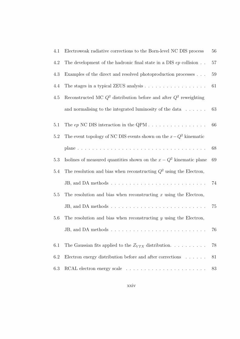
4.1 Electroweak radiative corrections to the Born-level NC DIS process 56
4.2 The development of the hadronic final state in a DIS ep collision . . 57
4.3 Examples of the direct and resolved photoproduction processes . . . 59
4.4 The stages in a typical ZEUS analysis . . . . . . . . . . . . . . . . . 61
4.5 Reconstructed MC Q2 distribution before and after Q2 reweighting
and normalising to the integrated luminosity of the data . . . . . . 63
5.1 The ep NC DIS interaction in the QPM . . . . . . . . . . . . . . . . 66
5.2 The event topology of NC DIS events shown on the x−Q2 kinematic
plane . . . . . . . . . . . . . . . . . . . . . . . . . . . . . . . . . . . 68
5.3 Isolines of measured quantities shown on the x − Q2 kinematic plane 69
5.4 The resolution and bias when reconstructing Q2 using the Electron,
JB, and DA methods . . . . . . . . . . . . . . . . . . . . . . . . . . 74
5.5 The resolution and bias when reconstructing x using the Electron,
JB, and DA methods . . . . . . . . . . . . . . . . . . . . . . . . . . 75
5.6 The resolution and bias when reconstructing y using the Electron,
JB, and DA methods . . . . . . . . . . . . . . . . . . . . . . . . . . 76
6.1 The Gaussian fits applied to the ZV TX distribution. . . . . . . . . . 78
6.2 Electron energy distribution before and after corrections . . . . . . 81
6.3 RCAL electron energy scale . . . . . . . . . . . . . . . . . . . . . . 83
xxiv
6.4 Hadronic energy scale determined from pT,h/pT,DA versus γh and θe 87
6.5 Control plots (Data/MC) of variables related to the hadronic energy
after applying a MC hadronic energy scales . . . . . . . . . . . . . . 88
6.6 The prediction of γh using the Electron method . . . . . . . . . . . 91
6.7 The prediction of γh using jets . . . . . . . . . . . . . . . . . . . . . 92
7.1 Original approach (HERA I method) to identify a non-backsplash
control sample using MC events . . . . . . . . . . . . . . . . . . . . 94
7.2 Hadronic angle description due to the backsplash correction . . . . 95
7.3 New approach to identifying a non-backsplash control sample using
jets . . . . . . . . . . . . . . . . . . . . . . . . . . . . . . . . . . . . 98
7.4 Measuring γmax using the control sample . . . . . . . . . . . . . . . 99
7.5 The mean of Gaussian fits applied to γmax in bins of γh . . . . . . . 102
7.6 Distributions of γh using the original and new backsplash corrections 103
7.7 The bias ∆γh = γrec − γtrue versus ytrue in bins of x for the old and
new backsplash corrections and with no backsplash correction . . . 106
7.8 The resolution in ∆γh = γrec − γtrue versus ytrue in bins of x for the
old and new backsplash corrections and with no backsplash correction107
7.9 The γh distribution when using the backsplash correction only for
forward events such that γh < 90 . . . . . . . . . . . . . . . . . . . 108
7.10 Energy removed by backsplash cut in bins of γh . . . . . . . . . . . 108
xxv
8.1 Event display of a typical NC DIS event . . . . . . . . . . . . . . . 110
8.2 Data to MC comparison of variables used in the event selection . . 112
8.3 Data to MC comparison of variables used in the event selection and
the kinematic variables . . . . . . . . . . . . . . . . . . . . . . . . . 113
8.4 The integrated luminosity of the data used in the NC e−p DIS anal-
ysis as a function of electron longitudinal polarisation . . . . . . . . 122
8.5 The run-by-run event yield for the data used in the NC e−p DIS
analysis . . . . . . . . . . . . . . . . . . . . . . . . . . . . . . . . . 123
8.6 Data events displayed on the x − Q2 plane after the full NC DIS
selection . . . . . . . . . . . . . . . . . . . . . . . . . . . . . . . . . 130
9.1 The generated kinematic variables for high x and high y MC events
compared with the measured MC events . . . . . . . . . . . . . . . 135
9.2 Efficiency, purity and acceptance in bins of dσ/dx, dσ/dy, and dσ/dQ2136
9.3 Efficiency and purity in the reduced cross section bins . . . . . . . . 137
9.4 Statistical error in the reduced cross section bins . . . . . . . . . . . 139
9.5 Systematic uncertainties in dσ/dQ2 . . . . . . . . . . . . . . . . . . 145
9.6 Systematic uncertainties in dσ/dx . . . . . . . . . . . . . . . . . . . 146
9.7 Systematic uncertainties in dσ/dy . . . . . . . . . . . . . . . . . . . 147
9.8 Individual systematic uncertainties in σ shown on the kinematic plane148
9.9 Individual systematic uncertainties in σ shown in terms of bin number149
xxvi
10.1 Measurements of dσ/dQ2, dσ/dx, and dσ/dy using the entire 2005-06
e−p data set. . . . . . . . . . . . . . . . . . . . . . . . . . . . . . . 151
10.2 Data/SM for dσ/dQ2 . . . . . . . . . . . . . . . . . . . . . . . . . . 153
10.3 Data/SM for dσ/dx and dσ/dy . . . . . . . . . . . . . . . . . . . . 154
10.4 Measurement of dσ/dQ2 versus Q2 for positively and negatively lon-
gitudinally polarised electrons . . . . . . . . . . . . . . . . . . . . . 155
10.5 Measurement of the polarisation asymmetry (A−) versus Q2 . . . . 157
10.6 A χ2 test of the polarisation asymmetry measurement . . . . . . . . 158
10.7 Measurement of dσ/dx versus x for positively and negatively longi-
tudinally polarised electrons . . . . . . . . . . . . . . . . . . . . . . 159
10.8 Measurement of dσ/dy versus y for positively and negatively longi-
tudinally polarised electrons . . . . . . . . . . . . . . . . . . . . . . 160
10.9 Reduced cross sections versus x for positively and negatively po-
larised electrons in fixed bins of Q2 . . . . . . . . . . . . . . . . . . 163
10.10Reduced cross sections versus x for the total e−p data set compared
with previously measured e+p from 1999 . . . . . . . . . . . . . . . 164
10.11Data/SM for the reduced cross sections . . . . . . . . . . . . . . . . 165
10.12The structure function xF3 versus x in fixed bins of Q2 . . . . . . . 167
10.13Previous measurements of xF γZ3 (also known as xG3) made by the
ZEUS and BCDMS collaborations. . . . . . . . . . . . . . . . . . . 168
xxvii
10.14The interference structure function xF γZ3 versus x in fixed bins of Q2 169
10.15The interference structure function xF γZ3 versus x extrapolated to
Q2 = 5000 GeV2 . . . . . . . . . . . . . . . . . . . . . . . . . . . . . 171
11.1 Fractional uncertainty of ZEUS-JETS PDFs and ZEUS-Pol PDFs . 174
11.2 Measurement of the polarisation asymmetry (A±) by the ZEUS and
H1 collaborations . . . . . . . . . . . . . . . . . . . . . . . . . . . . 175
B.1 A sketch of the energy sums used at the CFLT . . . . . . . . . . . . 180
C.1 Data/MC distributions for certain variables involved in the event se-
lection of NC DIS events, compared between the EM and SINISTRA
electron finders . . . . . . . . . . . . . . . . . . . . . . . . . . . . . 184
C.2 Percentage amount of PHP events in the single differential cross sec-
tions and reduced cross section, compared between the EM and SIN-
ISTRA electron finders . . . . . . . . . . . . . . . . . . . . . . . . . 185
D.1 Data/SM for dσ/dQ2 reconstructed using the Electron method . . . 187
D.2 Data/SM for dσ/dx and dσ/dy reconstructed using the Electron
method . . . . . . . . . . . . . . . . . . . . . . . . . . . . . . . . . 188
D.3 Data/SM for reduced cross sections reconstructed using the Electron
method . . . . . . . . . . . . . . . . . . . . . . . . . . . . . . . . . 189
xxviii

1 Introduction
Leptons and quarks are the fundamental particles that are normally associated with
matter. However, only the leptons are seen bare, as the quarks are confined into
bound states called hadrons. The HERA1 accelerator collides electrons or positrons
with protons (collision denoted as ep) at a centre-of-mass energy of 318 GeV, pro-
viding high-momentum probes with a spatial resolution small enough to reveal the
quarks inside the proton. Such highly energetic interactions also allow the exchange
of the massive force carriers of the weak force. The behaviour of the weak inter-
action and the structure of the proton is being studied at HERA using the ZEUS
detector.
Interactions with a large momentum transfer squared (Q2) between the electron
and proton are studied in this thesis. The wavelength (λ) of the exchanged force
carrier, for example a photon, is related to the momentum transfer by λ ∝ 1/√
Q2.
Therefore, higher Q2 interactions probe the proton to a higher resolution, revealing
1The frequently used acronyms are listed in Appendix A.
1

the dynamic structure of the proton. This process is called deep inelastic scattering
(DIS), as the force carrier probes ‘deep’ inside the proton and the momentum
transfer is large enough to break the proton apart (an inelastic collision). The
DIS interaction can be studied in neutral current (NC) exchanges. Neutral current
interactions are mediated by electrically neutral particles, the photon (γ) and the
Z boson. The massless γ exchange dominates the low momentum transfer squared
region, where Q2 is much smaller than the mass of the Z boson squared (M2Z ∼
(91 GeV)2). The Z boson, which is one of the weak force carriers, contributes
significantly to the NC interaction probability at Q2 & M2Z .
The weak force does not conserve parity, which is the operation of reversing the
signs of the coordinate axes. This means that the weak force couples to a particle
with a different strength if the momentum of the particle is reversed (and the in-
trinsic spin direction of the particle remains the same). This relates directly to the
helicity of a particle, which is the projection of the particle’s spin onto its direction
of motion. This is particularly relevant, as HERA has delivered negatively and pos-
itively longitudinally polarised electron beams (electron spin aligned approximately
parallel to electron momentum) to ZEUS for the first time. The helicity dependence
of the NC e−p DIS cross section (related to the probability of two particles interact-
ing) becomes significant at high Q2, so the observation of interactions at the highest
accessible Q2 is important. The cross section asymmetry due to polarisation can
2
be measured from the single differential cross section dσ/dQ2 using negatively and
positively longitudinally polarised electron beams. Parity violation can be mea-
sured at extremely small distances due to the large centre-of-mass energy provided
by HERA, which leads to an accessible spatial resolution of λ ∝ 1/√
Q2 ∼ 10−18 m.
The weak force couples with a different strength in unpolarised e−p and e+p
collisions due to parity violation. This so-called charge asymmetry can be explored
by comparing NC e−p DIS cross sections with published ZEUS measurements of
e+p cross sections. The NC cross section contains proton structure functions which
parameterise the complicated make-up of the proton. The parity violating terms
due to charge asymmetry are absorbed into the structure function xF3. The struc-
ture function xF3 can be measured by taking the difference of the e−p and e+p
cross sections. The structure function xF3 contains terms for pure Z boson ex-
change (xF Z3 ) and γ − Z interference (xF γZ
3 ). The interference structure function
xF γZ3 can be calculated from xF3, and is proportional to the difference of quark and
anti-quark momentum densities inside the proton. By assuming the virtual quark
sea inside the proton provides as many quarks as anti-quarks, xF γZ3 gives the shape
and magnitude of the proton valence quark momentum distribution. The integral
of xF γZ3 can be compared to a sum rule related to the number of valence quarks
inside the proton.
The goal of this thesis is to use the ZEUS detector to measure parity violation
3

in NC e−p DIS for the first time at distances down to ∼ 10−18 m, and also to gain
information on the proton valence quark momentum distribution. This has been
achieved using the largest amount of e−p scattering data ever recorded at ZEUS.
The cross section measurements are the most precise to date and can be used to
test the Standard Model of particle physics.
This thesis is organised into 10 chapters. The theory relevant to this analysis is
outlined in Chapter 2. The HERA collider and the ZEUS detector are introduced
in Chapter 3. The simulation of NC ep DIS, the methods used to reconstruct
kinematic variables such as Q2, and the techniques used to reconstruct events from
detector signals are described in Chapters 4 − 7. The selection criteria used to
obtain a NC data sample is outlined in Chapter 8. The cross section binning and
the determination of uncertainties in the cross sections is discussed in Chapter 9.
The main results and conclusions are presented in Chapters 10 − 11.
4

2 Theory
The fundamental particles and forces that embody the Standard Model of particle
physics are introduced in this chapter. The role that particle colliders perform and
the importance of the cross section measurements that will be presented in this
thesis will also be discussed.
2.1 The Standard Model
The known fundamental particles and forces (except gravity) are described by the
Standard Model (SM), a framework of calculational rules that have been proven to
describe the quantum world to great accuracy. Elementary particles can be grouped
according to their intrinsic spin. Matter contains spin 1/2 particles called fermions
(half-integer spin particles). The particles that govern the electromagnetic, weak
and strong forces contain spin 1 and are called bosons (integer spin particles).
5
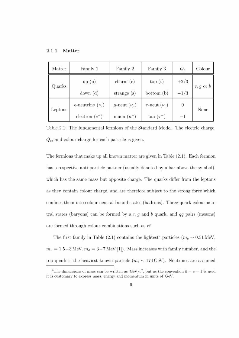
2.1.1 Matter
Matter Family 1 Family 2 Family 3 Qe Colour
Quarksup (u)
down (d)
charm (c)
strange (s)
top (t)
bottom (b)
+2/3
−1/3
r, g or b
Leptonse-neutrino (νe)
electron (e−)
µ-neut.(νµ)
muon (µ−)
τ -neut.(ντ )
tau (τ−)
0
−1
None
Table 2.1: The fundamental fermions of the Standard Model. The electric charge,
Qe, and colour charge for each particle is given.
The fermions that make up all known matter are given in Table (2.1). Each fermion
has a respective anti-particle partner (usually denoted by a bar above the symbol),
which has the same mass but opposite charge. The quarks differ from the leptons
as they contain colour charge, and are therefore subject to the strong force which
confines them into colour neutral bound states (hadrons). Three-quark colour neu-
tral states (baryons) can be formed by a r, g and b quark, and qq pairs (mesons)
are formed through colour combinations such as rr.
The first family in Table (2.1) contains the lightest2 particles (me ∼ 0.51 MeV,
mu = 1.5−3 MeV, md = 3−7 MeV [1]). Mass increases with family number, and the
top quark is the heaviest known particle (mt ∼ 174 GeV). Neutrinos are assumed
2The dimensions of mass can be written as GeV/c2, but as the convention ~ = c = 1 is usedit is customary to express mass, energy and momentum in units of GeV.
6
to be massless in the SM, though experiments have proved they have a very small
mass [1].
2.1.2 Forces
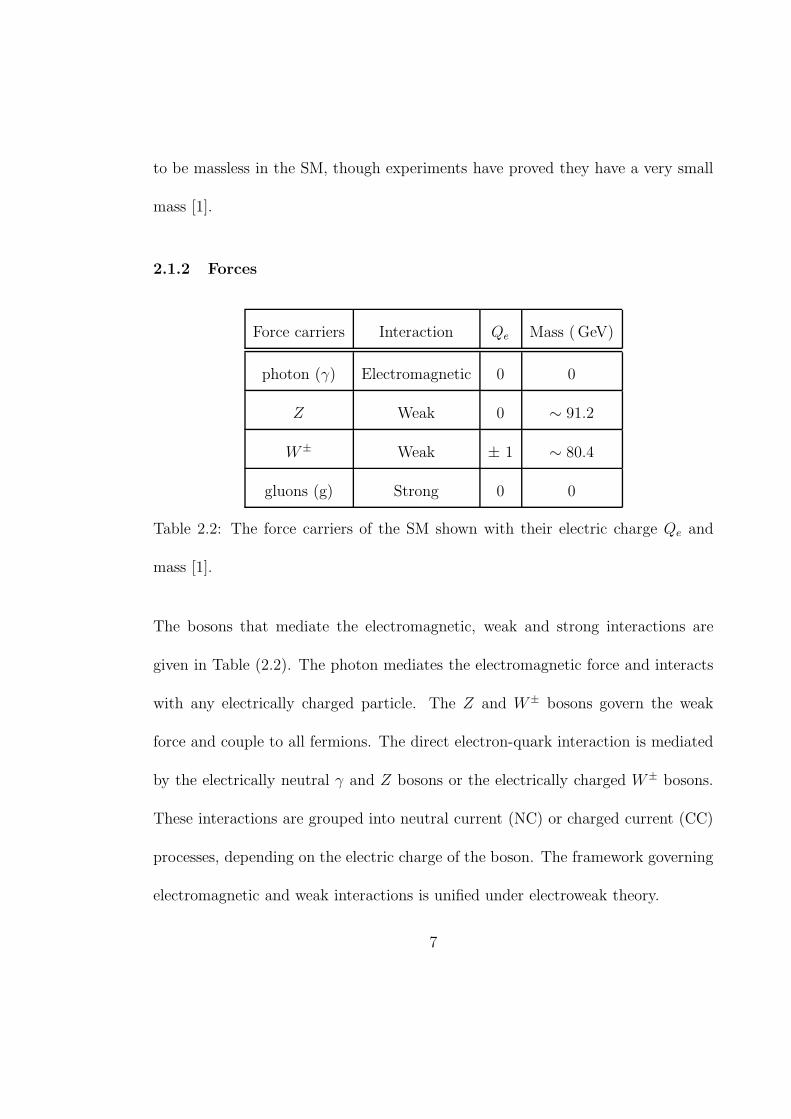
Force carriers Interaction Qe Mass ( GeV)
photon (γ) Electromagnetic 0 0
Z Weak 0 ∼ 91.2
W± Weak ± 1 ∼ 80.4
gluons (g) Strong 0 0
Table 2.2: The force carriers of the SM shown with their electric charge Qe and
mass [1].
The bosons that mediate the electromagnetic, weak and strong interactions are
given in Table (2.2). The photon mediates the electromagnetic force and interacts
with any electrically charged particle. The Z and W± bosons govern the weak
force and couple to all fermions. The direct electron-quark interaction is mediated
by the electrically neutral γ and Z bosons or the electrically charged W± bosons.
These interactions are grouped into neutral current (NC) or charged current (CC)
processes, depending on the electric charge of the boson. The framework governing
electromagnetic and weak interactions is unified under electroweak theory.
7
The gluons mediate the strong force and carry colour charge. They only couple
to other coloured particles, namely gluons and quarks. The theory of the strong
force is described by quantum chromodynamics (QCD).
2.2 The structure of the proton
A knowledge of the proton structure is needed to understand ep DIS. The first
successful model describing the proton structure was the quark-parton model, which
describes the proton as a collection of free point-like particles. This model was
improved by the introduction of QCD, which describes the confinement of quarks
inside the proton due to gluon exchange.
2.2.1 Quark-parton model
The quark-parton model (QPM) states that the nucleon is made up of free point-like
particles, referred to as partons. Therefore, the inelastic electron-proton collision
can be approximated as an incoherent sum of elastic electron-parton scatters. This
is illustrated in Fig. (2.1) using Feynman diagrams (a visual tool used to calcu-
late the cross section for a particular process). The inelastic cross section is then
constructed by combining the point-like elastic cross sections with proton struc-
ture functions which parameterise the dynamic proton composition, denoted by a
hashed circle in Fig. (2.1).
8

Kinematic variables used to characterise DIS are described in Table (2.3), and
are derived from the four-momenta denoted in Fig. (2.1). The most relevant kine-
matic variables for this thesis are Q2, which determines the spatial resolution of
the mediated force carrier, and x which is the fraction of the proton momentum
carried by the struck parton. Only these two variables are needed to characterise a
DIS event fully, as the kinematic variables are related by the centre-of-mass energy
squared provided by the collider, s = Q2/xy. The variable y is the fractional en-
ergy transferred by the electron in the proton’s rest frame, and is also related to the
electron scattering angle in the centre-of-mass frame (θ∗) via 1−y = (1+cos θ∗)/2.
γ(q) or Z(q)
proton (p)
e−(k) e−(k′)
=∑
i
[ γ(q) or Z(q)
partoni (xp)
proton (p)
e−(k) e−(k′)
]
Figure 2.1: The approximation of the NC inelastic e − proton collision (left) as an
incoherent sum of e − parton scatters (right). The four-momenta of the particles
are shown in brackets.
9

Kinematic variable Description
s = (k + p)2 ≈ 4EeEp Centre-of-mass energy (√
s), where Ee andEp
are the initial electron and proton energies.
Q2 = −q2 = −(k − k′)2 Resolving power of the exchanged boson,
0≤Q2≤s related to its wavelength by λ ∝ 1/Q.
x = Q2
2p·q Fraction of the proton momentum carried
0≤x≤1 by the struck parton.
y = p·qp·k = Q2
sxFractional energy transferred by the electron
0≤y≤1 in the rest frame of the proton.
Table 2.3: Definition of DIS kinematic variables using Fig. (2.1). Note that at the
HERA accelerator, Ee and Ep are fixed.
The probability of an interaction between particles is expressed through cross
sections. The general form of the ep DIS cross section is given by
dσ ∼ LeαβW αβ, (2.1)
where Leαβ and W αβ are the leptonic and hadronic tensors, respectively. If the low
Q2 region is considered (Q2 ≪ M2Z), such that the parity-violating weak force can
be ignored, the hadronic tensor can be written as [2]
W αβ = W1(q2, ν)(−gαβ +qαqβ
q2) +
W2(q2, ν)
M2(pα − p · q
q2qα)(pβ − p · q
q2qβ), (2.2)
10
where W1 and W2 are structure functions, gαβ is the metric tensor, p and q are
the four-momenta of the incoming proton and exchanged photon (as shown in
Fig. (2.1)), M is the proton mass, and ν = p · q/M .
The leptonic tensor can be written as
Leαβ = 2(k′
αkβ + k′βkα − k′ · kgαβ), (2.3)
where k and k′ are the four-momenta of the incoming and outgoing electron. By
contracting the leptonic and hadronic tensors in the laboratory frame one can write
the following [2]:
d2σ(ep → eX)
dΩdE ′ =4α2E ′2
Q4(2W1(Q2, ν) sin2 θ
2+ W2(Q
2, ν) cos2 θ
2), (2.4)
where ep → eX signifies the DIS process (the proton breaks up), E ′ is the energy
of the scattered electron, α is the QED coupling constant (giving the strength of
the electromagnetic force), dΩ is an element of solid angle and θ is the electron
scattering angle in the laboratory frame.
The foundation of the QPM is that the incoherent sum of elastic electron-parton
scattering can describe the inelastic electron-proton scattering process. Therefore,
to understand ep → eX scattering one can consider the point-like elastic scattering
cross section eµ → eµ [2]:
d2σ(eµ → eµ)
dΩdE ′ =4α2E ′2
Q4
(
cos2 θ
2+
Q2
2m2µ
sin2 θ
2
)
δ
(
ν − Q2
2mµ
)
, (2.5)
11
where mµ is the mass of the muon. By comparing Eqns. (2.4) and (2.5), the
structure functions can be expressed as
2mW1(ν, Q2) =
Q2
2mνδ
(
1 − Q2
2mν
)
, νW2(ν, Q2) = δ
(
1 − Q2
2mν
)
, (2.6)
where m is the parton mass. This signifies that the structure functions do not
depend on Q2 or ν separately but rather on a dimensionless quantity Q2
2mν. In this
case the following substitutions can be made [2]:
MW1(ν, Q2) → F1(x), (2.7)
νW2(ν, Q2) → F2(x), (2.8)
where x = Q2/2Mν is the fraction of the proton’s momentum as described in
Table (2.3). This agrees with the measurements of νW2 from ep DIS experiments
at the Stanford Linear Accelerator (SLAC) published in 1972 [3], shown in Fig. (2.2)
at a fixed value of x = 0.25 versus Q2. The SLAC measurements showed that in a
limited region in x, the structure functions do not depend on Q2. This means that
an increase in the spatial resolution of the photon (or in other words hitting the
objects harder) does not reveal further structure inside the proton, as the probe is
effectively interacting with free point-like partons. This phenomenon is known as
scaling.
12

Figure 2.2: The structure function νW2 determined by ep DIS at SLAC [4]. The
icons represent separate electron scattering angles. The structure function is seen
to be independent of the momentum transfer squared (q2 = Q2 in this plot) within
errors for x = 1ω
= 0.25.
The structure functions contain the sum of the momenta of the partons inside
the proton:
F2(x) =∑
i
e2i xfi(x), (2.9)
F1 =1
2xF2(x), (2.10)
where ei is the electric charge of parton i, and fi(x)dx is the probability of finding
a parton with proton momentum fraction x → x + dx, the so-called parton density
function (PDF). All the momentum fractions add up to unity:
∑
i
∫ 1
0
xfi(x)dx = 1, (2.11)
13
where the sum runs over all the partons, including the electrically neutral ones
which do not interact with the photon.
If the partons are assumed to be quarks, the proton can be considered as three
valence quarks (uud) and a sea of virtual qq pairs. The valence quarks provide
the proton with quantum numbers and the sea quarks (u, u, d, d, s, s, etc.) provide
higher mass quarks and anti-quarks. If the contribution to the proton content from
the heaviest quarks is neglected, the proton structure function F ep2 can be written
explicitly in terms of the three lightest quarks (u, d and s):
F ep2 (x) =
(
2
3
)2
x[u(x) + u(x)] +
(
−1
3
)2
x[d(x) + d(x) + s(x) + s(x)]. (2.12)
Each sea quark can be assigned a momentum probability distribution S(x) such
that F ep2 (x) can be expressed as
F ep2 (x) =
4
9xuv(x) +
1
9xdv(x) +
4
3xS(x), (2.13)
where uv and dv are the probability distributions of the proton valence quarks.
Measurements of F ep2 and F en
2 [2] showed that the quarks and anti-quarks con-
tributed to approximately half of the momentum of the nucleons. The other half
of the momentum of the nucleon is attributed to electrically neutral partons that
do not interact with the photon. These partons, unaccounted for by the QPM, are
called gluons, the force carriers of the strong force which is described by quantum
chromodynamics.
14

2.2.2 Quantum chromodynamics
Quantum chromodynamics (QCD) describes the strong interaction between quarks
and gluons. The charge of QCD is colour (r, g, b, r, g and b) and the strong force is
mediated through the exchange of massless, coloured gluons. The gluons can cou-
ple to themselves, which leads to the strong force behaving very differently to the
electromagnetic force as shown in Fig. (2.3). The strong coupling constant (αs),
which determines the strength of the strong interaction, increases as a coloured
charge moves further from another coloured charge. This phenomenon is known as
confinement, and is in stark contrast to the quantum electrodynamic (QED) cou-
pling constant (α), which tends to the asymptotic limit of 1/137 at large distances.
As more work is put into separating quarks, the energy contained in the strong field
becomes large enough to promote a quark-antiquark pair from the vacuum sea into
reality. This effectively lowers the potential energy of the system and acts to bind
quarks into neutral colour states (for example, rr or rbg). The proton is broken up
in ep DIS, but the quarks inside the proton cannot emerge as free particles. The
bare quarks fragment into ‘jets’ of colourless bound states (such as mesons), which
are collimated along the direction of the original partons.
Figure (2.3) shows that at small distances (high energies), αs becomes small.
High energy interactions take place in a shorter time scale than the inter-quark
15
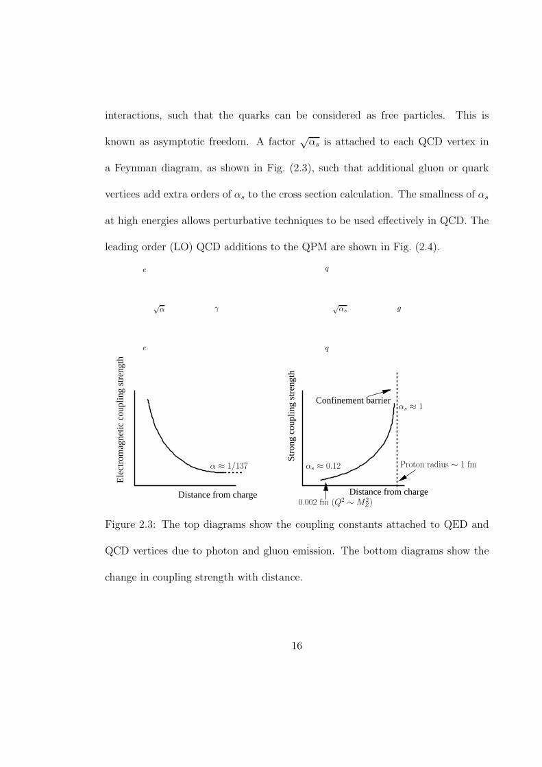
interactions, such that the quarks can be considered as free particles. This is
known as asymptotic freedom. A factor√
αs is attached to each QCD vertex in
a Feynman diagram, as shown in Fig. (2.3), such that additional gluon or quark
vertices add extra orders of αs to the cross section calculation. The smallness of αs
at high energies allows perturbative techniques to be used effectively in QCD. The
leading order (LO) QCD additions to the QPM are shown in Fig. (2.4).
e
e
γ√
α q
q
g√
αs
Stro
ng c
oupl
ing
stre
ngth
Distance from charge
Confinement barrier
Ele
ctro
mag
netic
cou
plin
g st
reng
th
Distance from charge
α ≈ 1/137 Proton radius ∼ 1 fmαs ≈ 0.12
αs ≈ 1
0.002 fm (Q2 ∼ M 2Z)
Figure 2.3: The top diagrams show the coupling constants attached to QED and
QCD vertices due to photon and gluon emission. The bottom diagrams show the
change in coupling strength with distance.
16
proton
ee
(c)(b)(a)√
αs√
αs
√α
√α
√α
√α
√α
√α
Figure 2.4: The QPM (a) and leading order QCD additions (b,c). The QED and
QCD coupling constants α and αs are shown.
2.2.3 QCD improved parton model
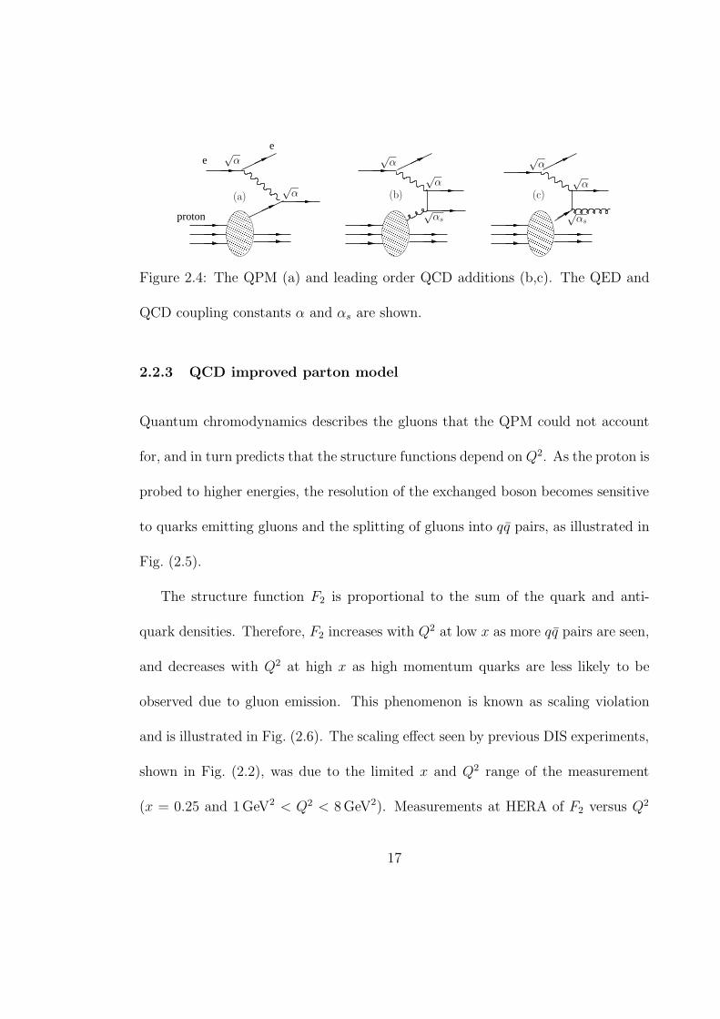
Quantum chromodynamics describes the gluons that the QPM could not account
for, and in turn predicts that the structure functions depend on Q2. As the proton is
probed to higher energies, the resolution of the exchanged boson becomes sensitive
to quarks emitting gluons and the splitting of gluons into qq pairs, as illustrated in
Fig. (2.5).
The structure function F2 is proportional to the sum of the quark and anti-
quark densities. Therefore, F2 increases with Q2 at low x as more qq pairs are seen,
and decreases with Q2 at high x as high momentum quarks are less likely to be
observed due to gluon emission. This phenomenon is known as scaling violation
and is illustrated in Fig. (2.6). The scaling effect seen by previous DIS experiments,
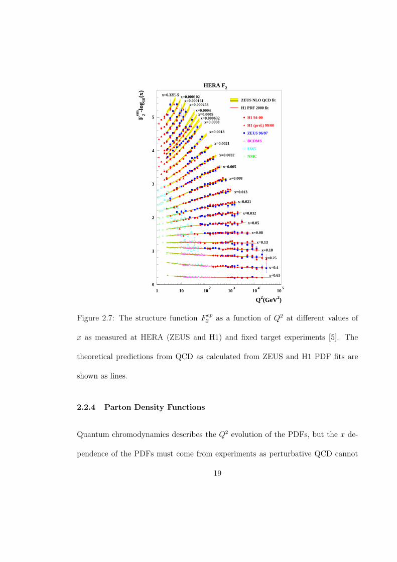
shown in Fig. (2.2), was due to the limited x and Q2 range of the measurement
(x = 0.25 and 1 GeV2 < Q2 < 8 GeV2). Measurements at HERA of F2 versus Q2
17

at fixed x values are shown in Fig. (2.7). The increase and decrease of F2 with Q2
in the approximate region of x < 0.1 and x > 0.1 overwhelmingly confirms scaling
violation. The theoretical predictions of QCD are able to describe the measurements
of F2 over four orders of magnitude in Q2 and over three orders of magnitude in x.
Proton
Proton
Proton
(a)
(b)
(c)
Three valence quarks
Bound quarks
Qua
rk d
ensi
ty
x
Qua
rk d
ensi
ty
xsea
valence
Bound quarks + splittingwavelength A
wavelength B
1/3
Qua
rk d
ensi
ty
x
Figure 2.5: The evolution of the proton structure with increasing resolution from
(a) to (c). Note that in picture (c), a higher Q2 probe (wavelength B) is required
to see the low x behaviour of a gluon splitting into quarks.
high Q2
low Q2
Q2
low x
high x
scaling violation
scaling violation
scaling
F2 F2
x ∼ 0.1
x
Figure 2.6: A sketch of F2 versus x (left) and F2 versus Q2 (right).
18
HERA F2
0
1
2
3
4
5
1 10 102
103
104
105
F2 em
-log
10(x
)
Q2(GeV2)
ZEUS NLO QCD fit
H1 PDF 2000 fit
H1 94-00
H1 (prel.) 99/00
ZEUS 96/97
BCDMS
E665
NMC
x=6.32E-5 x=0.000102x=0.000161
x=0.000253
x=0.0004x=0.0005
x=0.000632x=0.0008
x=0.0013
x=0.0021
x=0.0032
x=0.005
x=0.008
x=0.013
x=0.021
x=0.032
x=0.05
x=0.08
x=0.13
x=0.18
x=0.25
x=0.4
x=0.65
Figure 2.7: The structure function F ep2 as a function of Q2 at different values of
x as measured at HERA (ZEUS and H1) and fixed target experiments [5]. The
theoretical predictions from QCD as calculated from ZEUS and H1 PDF fits are
shown as lines.
2.2.4 Parton Density Functions
Quantum chromodynamics describes the Q2 evolution of the PDFs, but the x de-
pendence of the PDFs must come from experiments as perturbative QCD cannot
19
be solved at long distances (∼ 1 fm) where αs becomes large. Experimental data
can be fitted at certain initial Q2 values to obtain the proton PDF, which then can
be evolved to other values of Q2 using the DGLAP equations [6–8].
The PDFs used in this thesis are those produced by the ZEUS collaboration
(ZEUS-JETS [9]) and the CTEQ theory group [10]. The ZEUS-JETS PDFs for the
valence quarks, quark sea, and gluons are parameterised at Q20 = 7 GeV2 using the
following functional form:
xf(x) = p1xp2(1 − x)p3(1 + p4x), (2.14)
where p1,2,3,4 are fit parameters constrained by factors such as momentum sum rules
(for example, Eqn. (2.11)). The ZEUS-JETS fit relies entirely on ZEUS measure-
ments of structure functions and jet production. Neutral current measurements
at low x (x . 0.01) provide information on the sea and gluon distributions, while
sensitivity to the valence quarks are provided by high Q2 (Q2 & 200 GeV2) NC and
CC data. Jet production rates are used to gain information on the gluon, as the
rate of jet production depends directly on the gluon PDF through diagrams such
as Fig. (2.4b). The CTEQ PDFs are generally parameterised in the same form
as Eqn. (2.14) and use data from many different experiments. The measurements
include fixed target data (muon and neutrino scattering off a fixed nuclear target)
to gain information on the valence quarks and jet cross sections from pp collisions
to gain information on gluon densities.
20
The advantage of using only ZEUS data for the ZEUS-JETS PDF is that there
is generally a better understanding of the experimental systematic uncertainties as
only one experiment is considered. However, this also limits the statistical precision
of the data. The ZEUS-JETS PDFs for the valence quarks, sea quarks and gluons
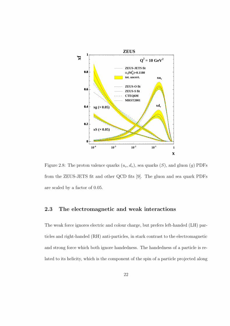
are shown in Fig. (2.8). The PDFs show that the valence quarks are populated in
the high-x region and the uv density is twice as large as the dv density because the
proton is a uud bound state. Note the similarities between the PDFs and the quark
density shown in Fig. (2.5c), as the gluons and sea quarks dominate the low x region
(the gluon and sea quark PDFs are scaled by a factor of 0.05 in Fig. (2.8)). The
PDF uncertainties stem from model and experimental uncertainties. The inclusion
of cross section measurements presented in this thesis will impact the valence quark
PDF uncertainties by improving the statistical precision of the data set. The con-
straint of the proton PDF uncertainties is of great importance, especially for the
Large Hadron Collider (LHC), which is planning to deliver proton-proton collisions
at a centre-of-mass energy of 14 TeV in 2008.
21
0
0.2
0.4
0.6
0.8
1
-410 -310 -210 -110 1
0
0.2
0.4
0.6
0.8
1
ZEUS-JETS fit)=0.11802
Z(Msα tot. uncert.
ZEUS-O fit
ZEUS-S fit
CTEQ6M MRST2001
x
xf
ZEUS
2 = 10 GeV2Q
vxu
vxd
0.05)×xS (
0.05)×xg (
0
0.2
0.4
0.6
0.8
1
Figure 2.8: The proton valence quarks (uv, dv), sea quarks (S), and gluon (g) PDFs
from the ZEUS-JETS fit and other QCD fits [9]. The gluon and sea quark PDFs
are scaled by a factor of 0.05.
2.3 The electromagnetic and weak interactions
The weak force ignores electric and colour charge, but prefers left-handed (LH) par-
ticles and right-handed (RH) anti-particles, in stark contrast to the electromagnetic
and strong force which both ignore handedness. The handedness of a particle is re-
lated to its helicity, which is the component of the spin of a particle projected along
22
its direction of motion. If the spin vector is aligned with or against the direction
of motion, the particle is called right-handed or left-handed, respectively. There-
fore, the weak interaction does not remain invariant under parity transformations
(reversing the signs of the coordinate axes).
The electroweak model groups the electron-type leptons, for example, into two
sets [11]:
le =
νe
e−
L
, e−R. (2.15)
As the neutrino is assumed to be massless in the SM, it is predicted to be only
left-handed. A quantum number known as weak isospin (T ) is introduced, such
that it is conserved in the left-handed and right-handed groups. The neutrino is
electrically neutral but the electron is charged, therefore a further quantum number
called hypercharge (Y ) is introduced such that the electric charge difference can
stem from weak isospin values. The electric charge for a fermion f is defined by
ef = e(T 3f + Yf/2), (2.16)
where e is the positron charge, and T 3 is the third component of the weak isospin.
The values of T 3 and the electric charge for the charged leptons and quarks are
shown in Table (2.3).
23
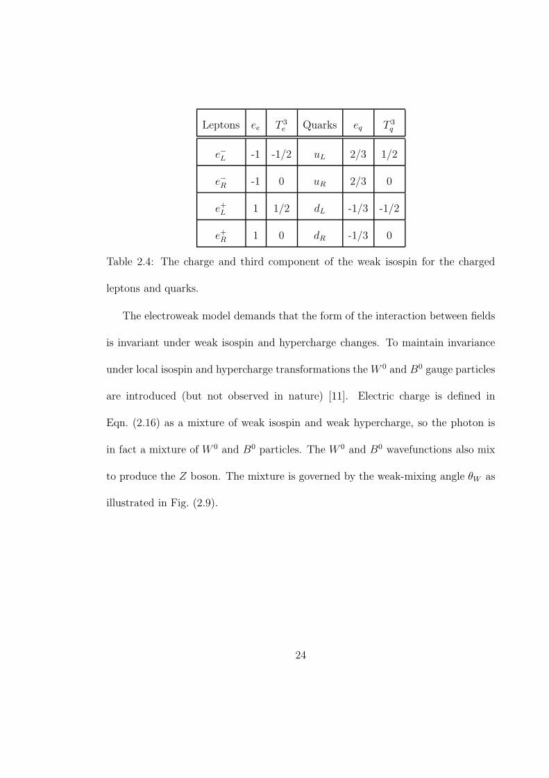
Leptons ee T 3e Quarks eq T 3
q
e−L -1 -1/2 uL 2/3 1/2
e−R -1 0 uR 2/3 0
e+L 1 1/2 dL -1/3 -1/2
e+R 1 0 dR -1/3 0
Table 2.4: The charge and third component of the weak isospin for the charged
leptons and quarks.
The electroweak model demands that the form of the interaction between fields
is invariant under weak isospin and hypercharge changes. To maintain invariance
under local isospin and hypercharge transformations the W 0 and B0 gauge particles
are introduced (but not observed in nature) [11]. Electric charge is defined in
Eqn. (2.16) as a mixture of weak isospin and weak hypercharge, so the photon is
in fact a mixture of W 0 and B0 particles. The W 0 and B0 wavefunctions also mix
to produce the Z boson. The mixture is governed by the weak-mixing angle θW as
illustrated in Fig. (2.9).
24
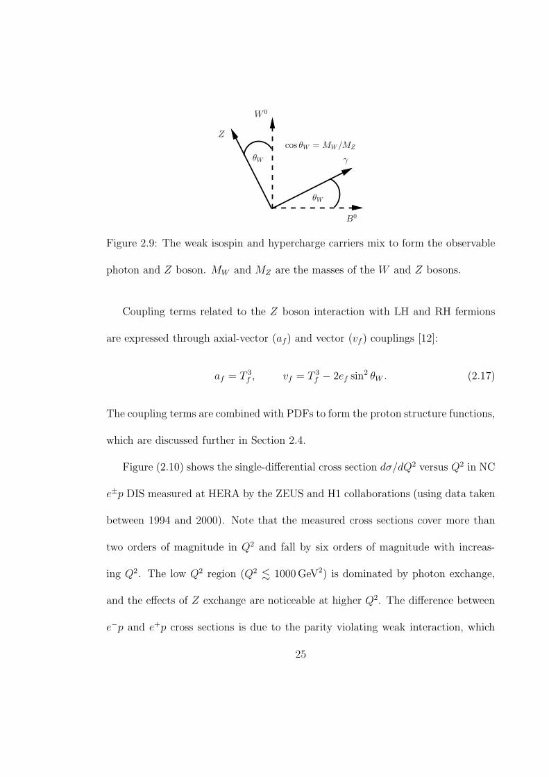
θW
B0
θW γ
W 0
cos θW = MW/MZ
Z
Figure 2.9: The weak isospin and hypercharge carriers mix to form the observable
photon and Z boson. MW and MZ are the masses of the W and Z bosons.
Coupling terms related to the Z boson interaction with LH and RH fermions
are expressed through axial-vector (af) and vector (vf ) couplings [12]:
af = T 3f , vf = T 3
f − 2ef sin2 θW . (2.17)
The coupling terms are combined with PDFs to form the proton structure functions,
which are discussed further in Section 2.4.
Figure (2.10) shows the single-differential cross section dσ/dQ2 versus Q2 in NC
e±p DIS measured at HERA by the ZEUS and H1 collaborations (using data taken
between 1994 and 2000). Note that the measured cross sections cover more than
two orders of magnitude in Q2 and fall by six orders of magnitude with increas-
ing Q2. The low Q2 region (Q2 . 1000 GeV2) is dominated by photon exchange,
and the effects of Z exchange are noticeable at higher Q2. The difference between
e−p and e+p cross sections is due to the parity violating weak interaction, which
25
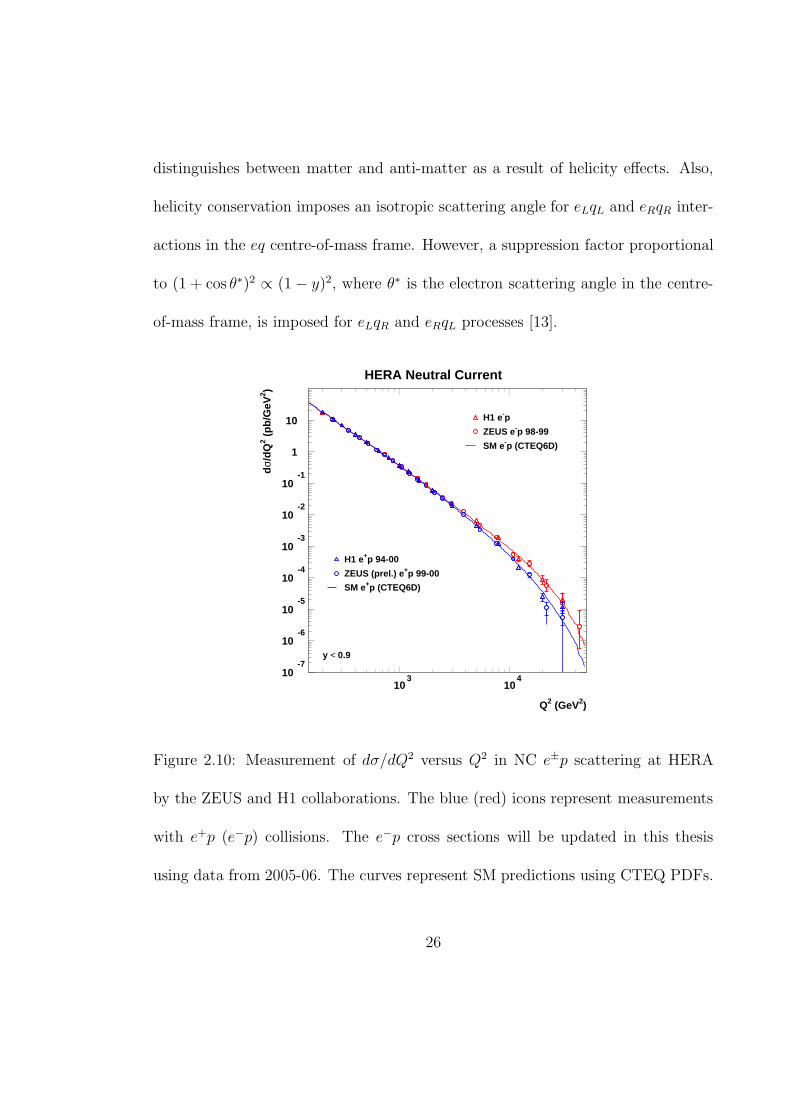
distinguishes between matter and anti-matter as a result of helicity effects. Also,
helicity conservation imposes an isotropic scattering angle for eLqL and eRqR inter-
actions in the eq centre-of-mass frame. However, a suppression factor proportional
to (1 + cos θ∗)2 ∝ (1 − y)2, where θ∗ is the electron scattering angle in the centre-
of-mass frame, is imposed for eLqR and eRqL processes [13].
10-7
10-6
10-5
10-4
10-3
10-2
10-1
1
10
103
104
HERA Neutral Current
H1 e+p 94-00
ZEUS (prel.) e+p 99-00
SM e+p (CTEQ6D)
H1 e-p
ZEUS e-p 98-99
SM e-p (CTEQ6D)
y < 0.9
Q2 (GeV2)
dσ/
dQ
2 (p
b/G
eV2 )
Figure 2.10: Measurement of dσ/dQ2 versus Q2 in NC e±p scattering at HERA
by the ZEUS and H1 collaborations. The blue (red) icons represent measurements
with e+p (e−p) collisions. The e−p cross sections will be updated in this thesis
using data from 2005-06. The curves represent SM predictions using CTEQ PDFs.
26
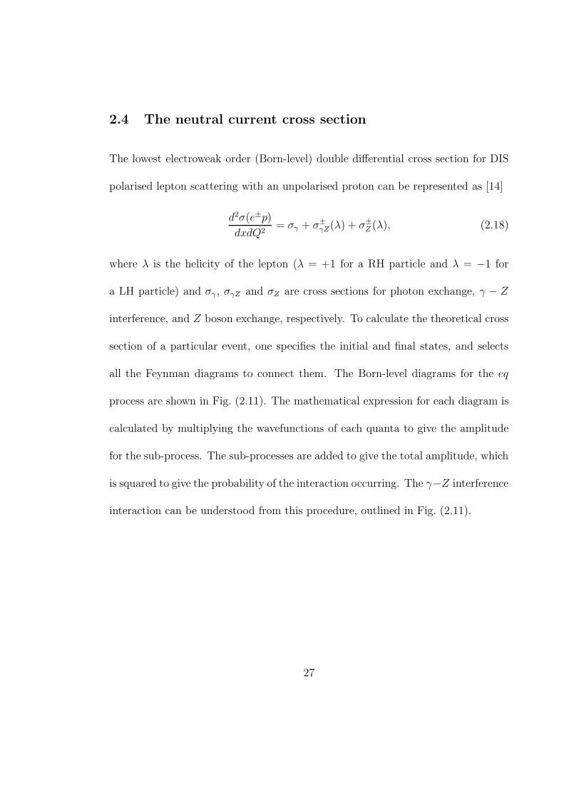
2.4 The neutral current cross section
The lowest electroweak order (Born-level) double differential cross section for DIS
polarised lepton scattering with an unpolarised proton can be represented as [14]
d2σ(e±p)
dxdQ2= σγ + σ±
γZ(λ) + σ±Z (λ), (2.18)
where λ is the helicity of the lepton (λ = +1 for a RH particle and λ = −1 for
a LH particle) and σγ , σγZ and σZ are cross sections for photon exchange, γ − Z
interference, and Z boson exchange, respectively. To calculate the theoretical cross
section of a particular event, one specifies the initial and final states, and selects
all the Feynman diagrams to connect them. The Born-level diagrams for the eq
process are shown in Fig. (2.11). The mathematical expression for each diagram is
calculated by multiplying the wavefunctions of each quanta to give the amplitude
for the sub-process. The sub-processes are added to give the total amplitude, which
is squared to give the probability of the interaction occurring. The γ−Z interference
interaction can be understood from this procedure, outlined in Fig. (2.11).
27

NC cross section ∝γ
q
e−
q
e−
eq
ee
+(ve, ae)
(vq, aq)
Z
q
e−
q
e−
2
Figure 2.11: Feynman diagrams contributing to the Born-level NC cross section.
The coupling constants e, v, and a refer to the electric charge, vector coupling, and
axial-vector coupling, respectively.
The cross section can be written explicitly in terms of the structure functions
F2, xF3 , and FL = F2 − 2xF1 [15]:
d2σ(e±p)
dxdQ2=
2πα2
xQ4[Y+F2(x, Q2) ∓ Y−xF3(x, Q2) − y2FL(x, Q2)], (2.19)
where α is the QED coupling constant and Y± ≡ 1 ± (1 − y)2.
The xF3 structure function contains terms only relating to Z exchange and
γ−Z interference and describes the parity violating part of the cross section due to
charge asymmetry. The difference between e+p and e−p unpolarised cross sections
is totally contained within xF3. This is reflected by the ∓ sign attached to the xF3
term in Eqn. (2.19), which depends on the charge of the lepton. The xF3 structure
function is proportional to the difference of quarks and anti-quarks in the proton.
By assuming that the quark and the anti-quark densities from the sea quarks cancel
(a LO QCD assumption), the xF3 structure function is proportional to the valence
28

quark momentum density.
The FL structure function is related to the absorption cross section of longitudi-
nally polarised photons. In the QPM, FL = F2−2xF1 = 0 (as shown in Eqn. (2.10))
as fermions cannot absorb longitudinally polarised photons without violating he-
licity conservation. However, QCD allows the interaction through gluon emission.
Therefore, FL describes the gluon distribution inside the proton.
The F2 structure function contains terms related to γ, γ − Z, and Z exchange,
and dominates the cross section at low Q2 due to the photon being massless. The
structure function F2 is proportional to the sum of the quark and the anti-quark
PDFs.
The structure functions are written in terms of contributions from γ and Z
exchange and γ − Z interference at LO QCD as [14]
[
F γ2 , F γZ
2 , F Z2
]
= x∑
q
[e2q , 2eqvq, v
2q + a2
q ](q(x, Q2) + q(x, Q2)), (2.20)
[
xF γZ3 , xF Z
3
]
= 2x∑
q
[eqaq, vqaq](q(x, Q2) − q(x, Q2)) ∝ qvalence, (2.21)
FL(x, Q2) ∝ g(x, Q2), (2.22)
where vq and aq are the vector and axial-vector couplings of a quark flavour q, and
eq is the quark’s electric charge and g(x, Q2) is the gluon density.
The double differential cross section can be divided by kinematic terms to define
29

the reduced cross section
σe±p =xQ4
2πα2
1
Y+
d2σ(e±p)
dxdQ2= F2(x, Q2) ∓ Y−
Y+
xF3(x, Q2) − y2
Y+
FL(x, Q2), (2.23)
where the structure functions F2 and xF3 are described in more detail in Eqns. (2.24
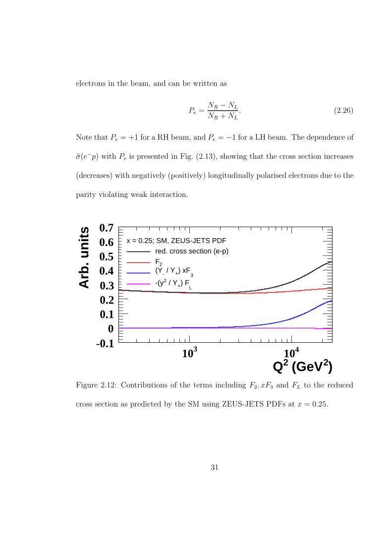
- 2.25). Figure (2.12) shows the theoretical prediction of σe−p and the magnitude
of each term on the right-hand side of Eqn. (2.23). Note that the term y2
Y+FL
contributes less than one percent to the reduced cross section in the Q2 and x
region considered.
The structure functions F2 and xF3 depend on the lepton charge, the lepton
beam longitudinal polarisation (Pe), the mass of the Z and W bosons (MZ and
MW ), and the weak-mixing angle (θW ), to give the following [14]:
F±2 = F γ
2 + k(−ve ∓ Peae)FγZ2 + k2(v2
e + a2e ± 2Peveae)F
Z2 , (2.24)
xF±3 = k(−ae ∓ Peve)xF γZ
3 + k2(2veae ± Pe(v2e + a2
e))xF Z3 , (2.25)
where the structure functions for γ, γ−Z and Z exchange are detailed in Eqns. (2.20
- 2.21) and k = 1
4 sin2 θW cos2 θW
Q2
Q2+M2Z
is proportional to the ratio of the Z and photon
propagators (expressions used to describe the propagation of virtual particles). The
SM values of the vector and axial-vector coupling of the electron to the Z boson are
ve = −1/2 + 2 sin2 θW and ae = −1/2. The longitudinal polarisation of the electron
beam (Pe) is defined using the number of left-handed (NL) and right-handed (NR)
30
electrons in the beam, and can be written as
Pe =NR − NL
NR + NL. (2.26)
Note that Pe = +1 for a RH beam, and Pe = −1 for a LH beam. The dependence of
σ(e−p) with Pe is presented in Fig. (2.13), showing that the cross section increases
(decreases) with negatively (positively) longitudinally polarised electrons due to the
parity violating weak interaction.
)2 (GeV2Q310 410
Arb
. un
its
-0.10
0.10.20.30.40.50.60.7
x = 0.25; SM, ZEUS-JETS PDF
red. cross section (e-p)
2F
3) xF+ / Y
-(Y
L) F+ / Y2-(y
Figure 2.12: Contributions of the terms including F2, xF3 and FL to the reduced
cross section as predicted by the SM using ZEUS-JETS PDFs at x = 0.25.
31
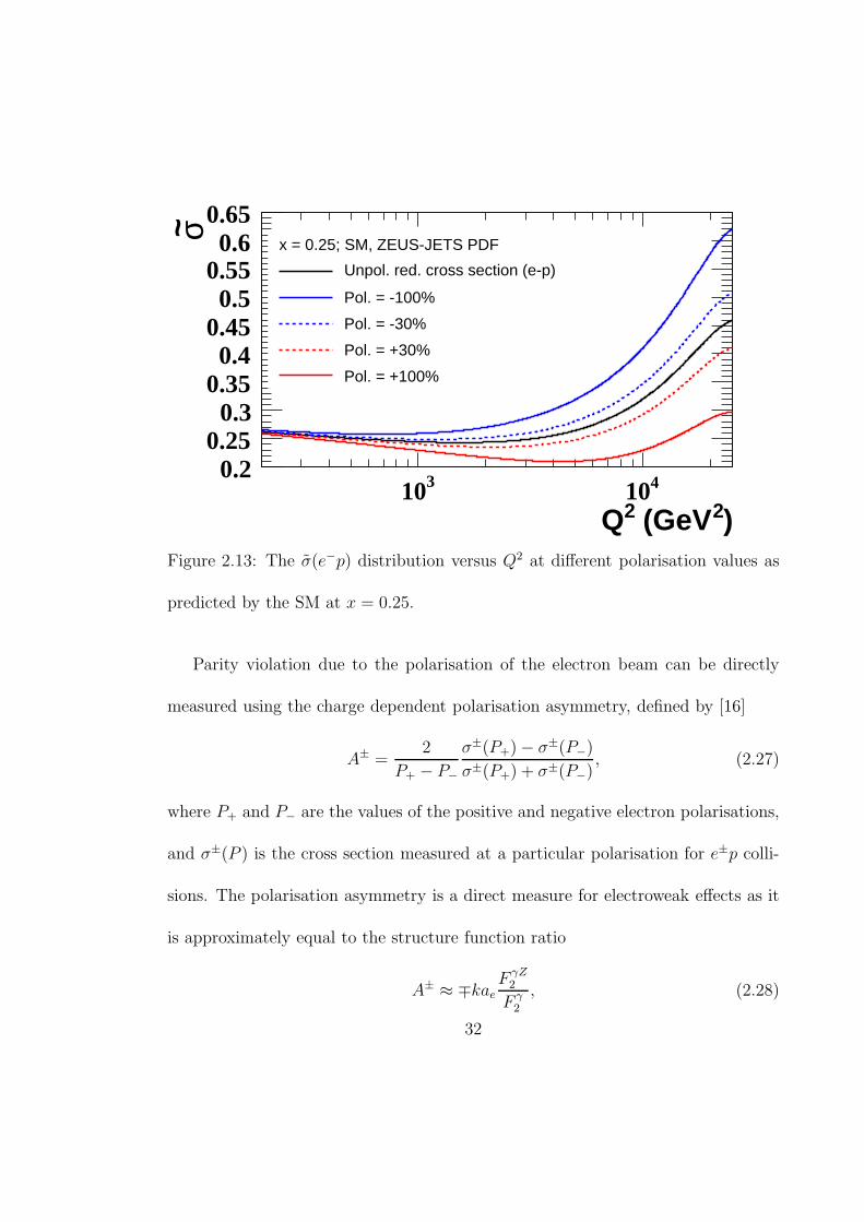
)2 (GeV2Q310 410
0.20.25
0.30.350.4
0.450.5
0.550.6
0.65 x = 0.25; SM, ZEUS-JETS PDF
Unpol. red. cross section (e-p)
Pol. = -100%
Pol. = -30%
Pol. = +30%
Pol. = +100%
~ σ
Figure 2.13: The σ(e−p) distribution versus Q2 at different polarisation values as
predicted by the SM at x = 0.25.
Parity violation due to the polarisation of the electron beam can be directly
measured using the charge dependent polarisation asymmetry, defined by [16]
A± =2
P+ − P−
σ±(P+) − σ±(P−)
σ±(P+) + σ±(P−), (2.27)
where P+ and P− are the values of the positive and negative electron polarisations,
and σ±(P ) is the cross section measured at a particular polarisation for e±p colli-
sions. The polarisation asymmetry is a direct measure for electroweak effects as it
is approximately equal to the structure function ratio
A± ≈ ∓kaeF γZ
2
F γ2
, (2.28)
32

which is proportional to coupling combinations aevq. The weak force contributes
a greater effect to the NC cross section at high Q2, so the polarisation asymmetry
will grow in magnitude with Q2. The measurement of the polarisation asymmetry
in e−p scattering (A−) is one of the goals of this thesis.
The other major goal for this thesis is to extract the structure function xF3
from the e±p unpolarised reduced cross sections (using Eqn. (2.23)):
xF3(x, Q2) =Y+
2Y−(σe−p − σe+p). (2.29)
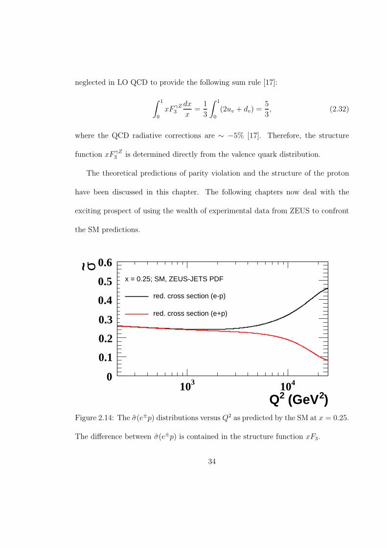
The difference between the e±p reduced cross sections grows with Q2 as shown in
Fig. (2.14). This highlights the motivation to measure events at high Q2 to be
sensitive to the xF3 contribution to the cross section. The structure function xF3
can be written as
xF3 = −aekxF γZ3 + 2veaek
2xF Z3 , (2.30)
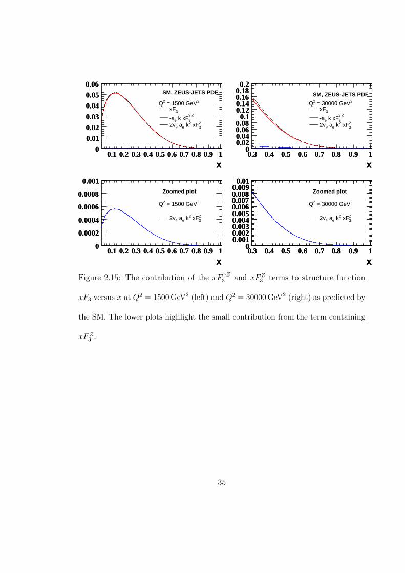
using Eqn. (2.25) and Pe = 0. The theoretical prediction of xF3 versus x at fixed
Q2 values and the magnitude of the terms on the right of Eqn. (2.30) is plotted in
Fig. (2.15), clearly showing that the xF γZ3 term dominates xF3. By inserting the
charge and axial-vector coupling into Eqn. (2.21), one can write the interference
structure function as
xF γZ3 =
x
3(2uv + dv + 2∆u + ∆d), (2.31)
where ∆u = (usea − u + c − c) and ∆d = (dsea − d + s − s). The ∆ terms can be
33
neglected in LO QCD to provide the following sum rule [17]:
∫ 1
0
xF γZ3
dx
x=
1
3
∫ 1
0
(2uv + dv) =5
3, (2.32)
where the QCD radiative corrections are ∼ −5% [17]. Therefore, the structure
function xF γZ3 is determined directly from the valence quark distribution.
The theoretical predictions of parity violation and the structure of the proton
have been discussed in this chapter. The following chapters now deal with the
exciting prospect of using the wealth of experimental data from ZEUS to confront
the SM predictions.
)2 (GeV2Q310 410
0
0.1
0.2
0.3
0.4
0.5
0.6 x = 0.25; SM, ZEUS-JETS PDF
red. cross section (e-p)
red. cross section (e+p)
~ σ
Figure 2.14: The σ(e±p) distributions versus Q2 as predicted by the SM at x = 0.25.
The difference between σ(e±p) is contained in the structure function xF3.
34
x0.1 0.2 0.3 0.4 0.5 0.6 0.7 0.8 0.9 1
0
0.010.020.03
0.040.050.06
2 = 1500 GeV2Q3xF
3 Zγ
k xFe-a
3Z xF2 ke ae2v
SM, ZEUS-JETS PDF
x0.1 0.2 0.3 0.4 0.5 0.6 0.7 0.8 0.9 1
0
0.010.020.03
0.040.050.06
x0.3 0.4 0.5 0.6 0.7 0.8 0.9 1
00.020.040.060.08
0.10.120.140.160.18
0.2
2 = 30000 GeV2Q3xF
3 Zγ
k xFe-a
3Z xF2 ke ae2v
SM, ZEUS-JETS PDF
x0.3 0.4 0.5 0.6 0.7 0.8 0.9 1
00.020.040.060.08
0.10.120.140.160.18
0.2
x0.1 0.2 0.3 0.4 0.5 0.6 0.7 0.8 0.9 1
0
0.0002
0.0004
0.0006
0.0008
0.001
2 = 1500 GeV2Q
3Z xF2 ke ae2v
Zoomed plot
x0.1 0.2 0.3 0.4 0.5 0.6 0.7 0.8 0.9 1
0
0.0002
0.0004
0.0006
0.0008
0.001
x0.3 0.4 0.5 0.6 0.7 0.8 0.9 1
00.0010.0020.0030.0040.0050.0060.0070.0080.009
0.01
2 = 30000 GeV2Q
3Z xF2 ke ae2v
Zoomed plot
x0.3 0.4 0.5 0.6 0.7 0.8 0.9 1
00.0010.0020.0030.0040.0050.0060.0070.0080.009
0.01
x0.3 0.4 0.5 0.6 0.7 0.8 0.9 1
00.0010.0020.0030.0040.0050.0060.0070.0080.009
0.01
Figure 2.15: The contribution of the xF γZ3 and xF Z
3 terms to structure function
xF3 versus x at Q2 = 1500 GeV2 (left) and Q2 = 30000 GeV2 (right) as predicted by
the SM. The lower plots highlight the small contribution from the term containing
xF Z3 .
35
3 HERA and the ZEUS detector
This chapter outlines the HERA accelerator, some key ZEUS detector components,
and the process of recording data.
3.1 HERA collider
The Hadron Elektron Ring Anlage (HERA) accelerator [18] collides protons with
electrons or positrons3 at high energies, and is the only such collider in the world. It
is located at the Deutsches Electronen Synchrotron (DESY) laboratory in Germany.
The HERA collider is located approximately 20 m underground inside a tunnel
with a circumference of 6.3 km in which protons and electrons are accelerated inde-
pendently in opposite directions. A schematic view of HERA and the experimental
halls can be seen in Fig. (3.1). The two beams are brought together to create colli-
sions in the South and North experimental halls, where the ZEUS [19] and H1 [20]
detectors are located. In the East hall, the HERMES experiment [21] uses only the
3The term ‘electrons’ will be generally used to denote both electrons and positrons for thischapter.
36

electron beam and inserts their own polarised gas target. The West hall was used
by the HERA-B experiment [22], which inserted a wire target in the proton ring.
The beams are collided by guiding magnets that deflect the proton beam into
the same vacuum pipe as the electron beam. The proton beam is deflected back into
its own ring after the interaction region, with 96 ns between each bunch crossing.
The proton and electron beam energies delivered for the data analysed in this
thesis are 920 GeV and 27.5 GeV, respectively, resulting in a centre-of-mass energy
of 318 GeV.
360m R=7
97m
360m
920 GeV
Protons
Hall West
Hall North
Hall East
Hall South
PETRA
HERA 40 GeV Protons
14 GeV Electrons
p e
e p
H1
ZEUS
HERMES
HERA B
27.5 GeV
electrons
Figure 3.1: A schematic view of the HERA collider and pre-accelerator rings. The
proton and electron beams are brought together at the centre of the ZEUS and H1
experiments in the South and North halls.
37
A key component for the effectiveness of a colliding-beam machine is the collision
rate in the interaction region. The reaction rate is given by
R = σL, (3.1)
where σ is the interaction cross section and L is the instantaneous luminosity. The
instantaneous luminosity can be expressed as [12]
L = fnN1N2
A, (3.2)
where N1 and N2 are the number of particles in each bunch, n is the number of
bunches in either beam around the ring, f is the revolution frequency, and A is the
effective cross-sectional area of the beam overlap. The units of L are effectively the
number of collisions per unit area per unit time.
Regular data taking for the collider experiments began in 1992. During a three
year shutdown period starting in 2000, a major luminosity upgrade was achieved at
HERA mainly through a reduction in the cross-sectional area of the beams. Also
during this period, spin rotators were installed in the collider ring to deliver posi-
tively and negatively longitudinally polarised electron beams. The pre-upgrade and
post-upgrade phases are known as HERA-I and HERA-II. The integrated luminos-
ity (L =∫
Ldt) delivered for these two periods is shown in Fig. (3.2). The data
presented in this thesis is based on e−p data from HERA-II. The massive increase
in luminosity is of direct relevance to this thesis, as it has allowed an improved
38
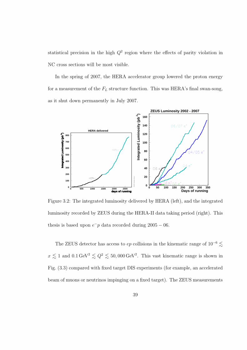
statistical precision in the high Q2 region where the effects of parity violation in
NC cross sections will be most visible.
In the spring of 2007, the HERA accelerator group lowered the proton energy
for a measurement of the FL structure function. This was HERA’s final swan-song,
as it shut down permanently in July 2007.
HERA delivered
0
100
200
300
400
500
600
700
800
0 500 1000 1500 2000 2500days of running
Inte
gra
ted
Lu
min
osi
ty (
pb
-1)
days of running
Inte
gra
ted
Lu
min
osi
ty (
pb
-1)
days of running
Inte
gra
ted
Lu
min
osi
ty (
pb
-1)
days of running
Inte
gra
ted
Lu
min
osi
ty (
pb
-1)
ZEUS Luminosity 2002 - 2007
0
20
40
60
80
100
120
140
160
0 50 100 150 200 250 300 350Days of running
Inte
gra
ted
Lu
min
osi
ty (
pb
-1)
Figure 3.2: The integrated luminosity delivered by HERA (left), and the integrated
luminosity recorded by ZEUS during the HERA-II data taking period (right). This
thesis is based upon e−p data recorded during 2005 − 06.
The ZEUS detector has access to ep collisions in the kinematic range of 10−6 .
x . 1 and 0.1 GeV2 . Q2 . 50, 000 GeV2. This vast kinematic range is shown in
Fig. (3.3) compared with fixed target DIS experiments (for example, an accelerated
beam of muons or neutrinos impinging on a fixed target). The ZEUS measurements
39

reach several orders of magnitude higher in Q2 than the fixed target experiments,
leading to extensive QCD and electroweak studies.
y=1 (
HERA √s=32
0 GeV
)
x
Q2 (
GeV
2 )
E665, SLAC
CCFR, NMC, BCDMS,
Fixed Target Experiments:
ZEUS
H1
10-1
1
10
10 2
10 3
10 4
10 5
10-6
10-5
10-4
10-3
10-2
10-1
1
Figure 3.3: Kinematic region accessible at the HERA collider experiments, ZEUS
and H1, compared with other fixed target DIS experiments [23].
3.1.1 Proton and electron beams
The proton beam begins its life as H− ions. These ions are accelerated to 7.5 GeV
and then the electrons are stripped off the ions. The protons are then accelerated
to 40 GeV in a pre-accelerator ring and then finally injected into HERA. Supercon-
ducting dipole and quadrupole magnets guide the protons around the ring, and the
40
beam is accelerated to 920 GeV using radio frequency cavities.
The electrons are collected by heating a filament, and are accelerated to 14 GeV
in the pre-accelerator ring and then finally to 27.5 GeV in the HERA ring. Syn-
chrotron radiation is emitted as charged particles are contained within the accel-
erator ring. Synchrotron radiation is inversely proportional to the mass of the
accelerated particle, and as the electron is approximately 1800 times lighter than
the proton, the electron beam is much more susceptible to energy loss due to syn-
chrotron radiation (e → eγ). Therefore, the maximum energy of the electron beam
possible at HERA is much lower than the proton beam energy.
3.1.2 Spin rotators and polarimetry
Electrons in a storage ring can become polarised antiparallel to the guiding mag-
netic field due to the emission of synchrotron radiation [24]. The projection of the
electron’s spin onto the vertical axis may flip direction, and a small difference in
the probability of the spin flipping from up-to-down and down-to-up causes a po-
larisation effect. This phenomenon is known as the Sokolov-Ternov effect [25], and
causes a transverse polarisation in the electron beam that builds up over time (t)
through the relation [26]
P (t) = PST (1 − e−t/τST ), (3.3)
41
where PST is the asymptotic polarisation (0.92) and τST is the polarisation rise
time constant (37 minutes at HERA). The maximum polarisation is not realised at
HERA due to effects such as de-focused beams.
However, longitudinally polarised electron beams are of interest, as the projec-
tion of the spin of a particle in the direction of its motion defines its helicity. Lon-
gitudinally polarised electron beams are achieved at HERA via spin rotators [26],
which consist of interleaved horizontal and vertical bending magnets.
The polarisation of the electron beam (Pe) is measured by two independent
polarimeters, the Transverse polarimeter (TPOL) [24, 27] and the Longitudinal
polarimeter (LPOL) [28]. The uncertainty on the polarisation measurement using
either the TPOL or LPOL is ∼ 4% [29]. Figure (3.4) illustrates the position of the
spin rotators and polarimeters at the HERA ring with respect to the experiments.
42
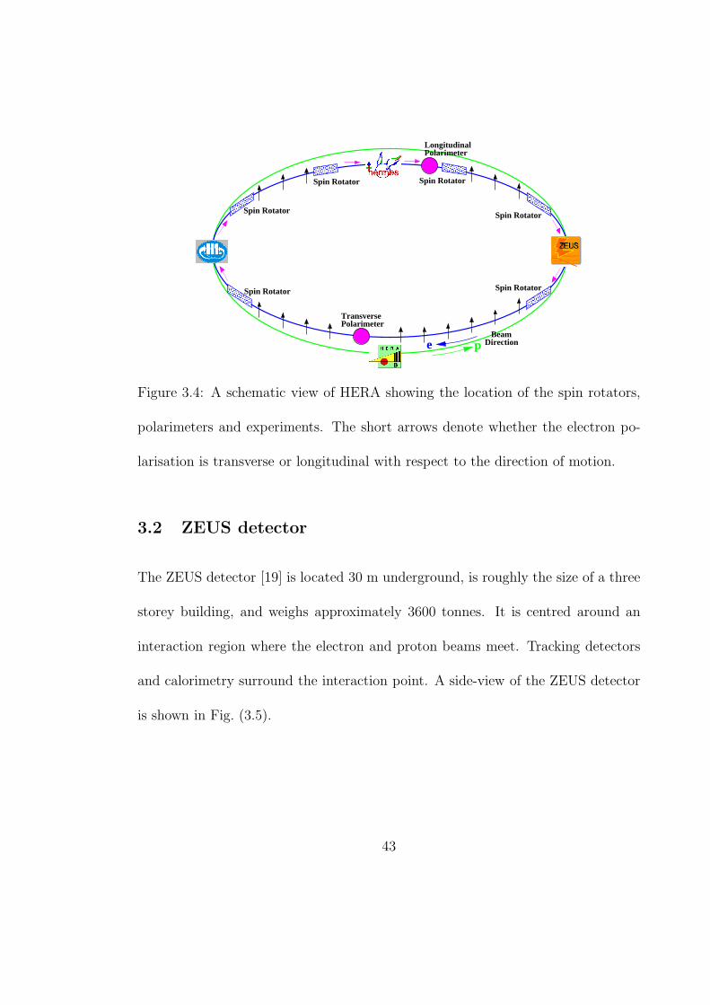
BeamDirection
Polarimeter
TransversePolarimeter
Spin Rotator
Spin Rotator
pe
Spin RotatorSpin Rotator
Spin Rotator
Spin Rotator
Longitudinal
Figure 3.4: A schematic view of HERA showing the location of the spin rotators,
polarimeters and experiments. The short arrows denote whether the electron po-
larisation is transverse or longitudinal with respect to the direction of motion.
3.2 ZEUS detector
The ZEUS detector [19] is located 30 m underground, is roughly the size of a three
storey building, and weighs approximately 3600 tonnes. It is centred around an
interaction region where the electron and proton beams meet. Tracking detectors
and calorimetry surround the interaction point. A side-view of the ZEUS detector
is shown in Fig. (3.5).
43

Figure 3.5: Overview of the ZEUS detector cut along the beam-pipe. The electron
beam enters the detector from the left and the proton beam enters from the right.
Detector parts are labelled by acronyms, with the most relevant components for
this thesis described in the text.
All angles and directions are made with respect to the ZEUS reference frame,
as illustrated in Fig. (3.6). The z axis points along the proton beam line, x points
towards the centre of HERA, and y points upwards, perpendicular to the beam.
The proton and electron beam directions are referred to as the forward and rear
directions, respectively. The angles θ and φ represent the polar and azimuthal
angles. The polar angle can be transformed into a Lorentz additive variable called
44
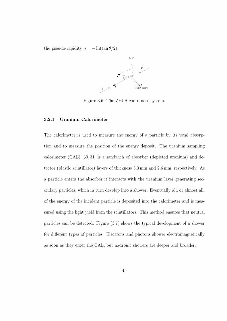
the pseudo-rapidity η = − ln(tan θ/2).
y
xHERA centre
z
r
e
p
Figure 3.6: The ZEUS coordinate system.
3.2.1 Uranium Calorimeter
The calorimeter is used to measure the energy of a particle by its total absorp-
tion and to measure the position of the energy deposit. The uranium sampling
calorimeter (CAL) [30, 31] is a sandwich of absorber (depleted uranium) and de-
tector (plastic scintillator) layers of thickness 3.3 mm and 2.6 mm, respectively. As
a particle enters the absorber it interacts with the uranium layer generating sec-
ondary particles, which in turn develop into a shower. Eventually all, or almost all,
of the energy of the incident particle is deposited into the calorimeter and is mea-
sured using the light yield from the scintillators. This method ensures that neutral
particles can be detected. Figure (3.7) shows the typical development of a shower
for different types of particles. Electrons and photons shower electromagnetically
as soon as they enter the CAL, but hadronic showers are deeper and broader.
45
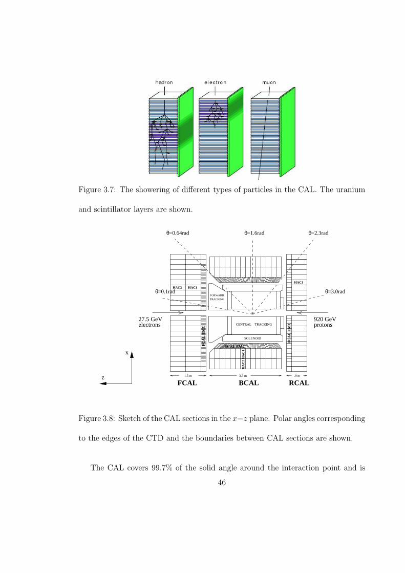
Figure 3.7: The showering of different types of particles in the CAL. The uranium
and scintillator layers are shown.
x
z
HAC1
CENTRAL TRACKING
FORWARD
TRACKING
SOLENOID
HAC1HAC2
1.5 m .9 m
RC
AL
EM
C
HA
C1
HA
C2
FC
AL
EM
C
BCAL EMC
3.3 m
θ=1.6rad
27.5 GeVelectrons
920 GeVprotons
θ=0.1rad
θ=0.64rad θ
θ=3.0rad
=2.3rad
BCAL RCALFCAL
Figure 3.8: Sketch of the CAL sections in the x−z plane. Polar angles corresponding
to the edges of the CTD and the boundaries between CAL sections are shown.
The CAL covers 99.7% of the solid angle around the interaction point and is
46

divided into three sections; the forward (FCAL), barrel (BCAL) and rear (RCAL)
calorimeters as shown in Fig. (3.8). Each section contains electromagnetic (EMC)
and hadronic (HAC) parts, with the EMC closest to the interaction point. Each
CAL section is divided transversely into towers, and longitudinally into an EMC
section, and either one HAC section in the RCAL or two HAC sections in the FCAL
and BCAL. This asymmetry is due to the large boost of the proton beam direction.
The light generated in the scintillator is collected by photomultiplier tubes (PMTs),
light guides, and wavelength shifters on both sides of the towers. The position of
an energy deposit is measured using the imbalance between these two signals.
The CAL energy resolutions as measured under test beam conditions are
σ(E)/E = 0.18/√
E( GeV) for purely electromagnetic deposits and σ(E)/E =
0.35/√
E( GeV) for hadrons. The angular resolution is 0.1 mrad and the time res-
olution is 1 ns for energy deposits larger than 4.5 GeV.
3.2.1.1 Presampler
Particles must traverse detector material as they travel from the interaction point
to the CAL. This intervening material, such as cables and magnets, are collectively
known as dead material. The energy loss due to interactions with dead material
is related to the number of particles (multiplicity) measured at the CAL. The
presampler [32] measures the multiplicity of particles entering the FCAL and RCAL,
47
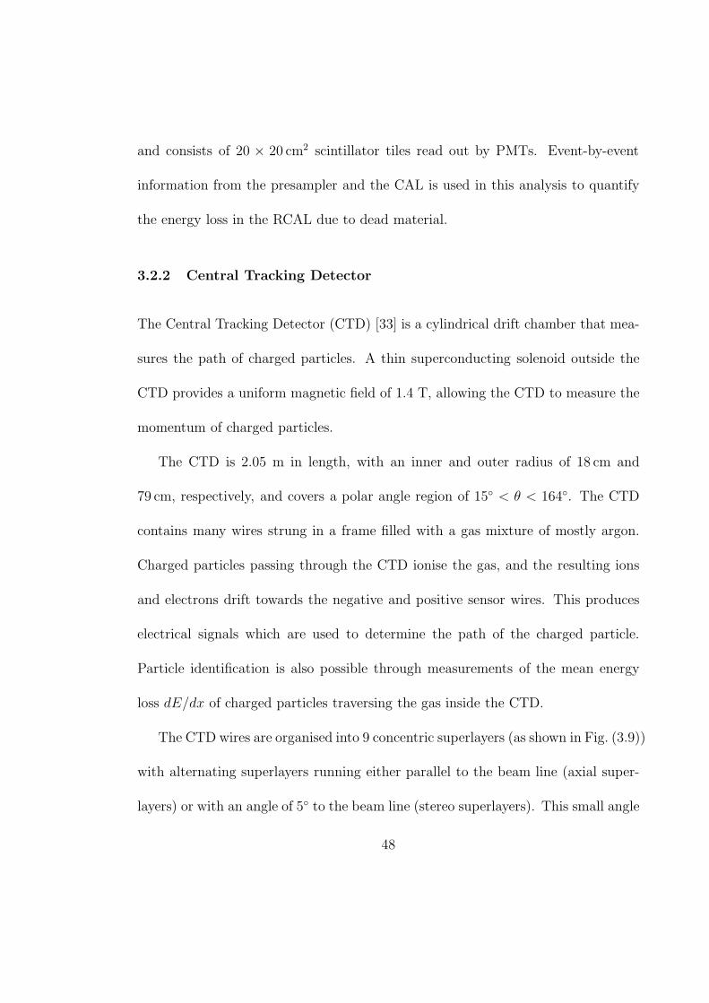
and consists of 20 × 20 cm2 scintillator tiles read out by PMTs. Event-by-event
information from the presampler and the CAL is used in this analysis to quantify
the energy loss in the RCAL due to dead material.
3.2.2 Central Tracking Detector
The Central Tracking Detector (CTD) [33] is a cylindrical drift chamber that mea-
sures the path of charged particles. A thin superconducting solenoid outside the
CTD provides a uniform magnetic field of 1.4 T, allowing the CTD to measure the
momentum of charged particles.
The CTD is 2.05 m in length, with an inner and outer radius of 18 cm and
79 cm, respectively, and covers a polar angle region of 15 < θ < 164. The CTD
contains many wires strung in a frame filled with a gas mixture of mostly argon.
Charged particles passing through the CTD ionise the gas, and the resulting ions
and electrons drift towards the negative and positive sensor wires. This produces
electrical signals which are used to determine the path of the charged particle.
Particle identification is also possible through measurements of the mean energy
loss dE/dx of charged particles traversing the gas inside the CTD.
The CTD wires are organised into 9 concentric superlayers (as shown in Fig. (3.9))
with alternating superlayers running either parallel to the beam line (axial super-
layers) or with an angle of 5 to the beam line (stereo superlayers). This small angle
48

allows measurements in r − φ and z with a resolution of ∼ 200 µm and ∼ 2 mm.
The momentum resolution of tracks that traverse through all CTD layers is
σ(pT )/pT = 0.0058pT ⊕0.0065⊕0.0014/pT (pT in GeV). The first term is related to
the resolution of the CTD hits and the second and third terms are due to multiple
scattering.
x
y
z
O
u
t
e
re
l
e
c
t
r
o
s
t
a
t
i
cs
c
r
e
e
n
S u p e r l
a
y
e
r
n
u
m
b
e
r
S
t
e
r
e
o
a
n
g
l
e
I
n
n
e
re
l
e
c
t
r
o
s
t
a
t
i
cs
c
r
e
e
n
1
2
45
89
3
67
+ 0
.
0
0+ 4
.
9
8
- 5 .
5
3
+ 5
.
6
2
- 5 .
5
1
+ 0
.
0
0
+ 0
.
0
0
+ 0
.
0
0
+ 0
.
0
0
Figure 3.9: An octant of the CTD divided into superlayers, with stereo angles
shown.
3.2.2.1 Microvertex Detector
The Microvertex Detector (MVD) [34] is a semiconductor (silicon) tracking detector
positioned close to the interaction point, between the CTD and the beam-pipe,
covering a polar angle of 7 < θ < 170. The MVD measurements are used in
49
combination with CTD information in this thesis to reconstruct a more precise
measurement of the event vertex position.
3.2.3 Luminosity detector
The luminosity is measured by studying photons produced in ep bremsstrahlung
(ep → eγp), the so called Bethe-Heitler process. This is a QED process that is well
understood so the theoretical cross section can be used to obtain a measurement of
the instantaneous luminosity (L) using
L = Rep/σobsB−H , (3.4)
where Rep is the observed rate for Bethe-Heitler events and σobsB−H is the theo-
retical cross section corrected for detector acceptance. The Photon Calorimeter
(PCAL) [35] is used in this analysis to measure the ep bremsstrahlung rate and
determine the integrated luminosity (L =∫
Ldt). The fractional uncertainty on
the integrated luminosity measurement is 3.5%.
3.2.4 Background rejection
There are certain background processes that need to be controlled at ZEUS:
• Beam-gas: These interactions arise mainly between the proton beam and
residual gas in the beam-pipe, causing hadronic energy deposits in the CAL
50
• Halo muons: The interaction between the proton beam and beam-gas or the
beam-pipe itself can produce charged pions which decay into muons that
travel parallel to the proton beam
• Cosmic muons: Interactions between cosmic rays and the upper atmosphere
of the earth produce muons that pass through the detector
Detector components used to reduce background events are outlined below.
The Veto Wall [19] consists of scintillators supported by an iron wall and is
positioned at z = −7.5 m. Its main purpose is to block proton halo muons from
entering the detector and take measurements which can be used to reject halo muon
events. The C5 counter [36] is a scintillator located at z = −1.2 m. It takes timing
measurements of the electron and proton beam which are used to veto events that
do not occur at the correct time. Muon chambers and a backing calorimeter [19]
surround the uranium calorimeter and can be used reject proton halo muons and
cosmic muons.
3.2.5 Trigger and data acquisition
The ZEUS detector delivers an enormous event rate of 10 MHz, a large percent-
age of which are background events such as beam-gas interactions. Therefore, the
events recorded by ZEUS are filtered using triggers. The trigger system [37] is de-
51
signed to reduce the event rate to a maximum of 10 Hz of interesting ep events. The
trigger is based on three levels which are illustrated in Fig. (3.10) and are described
below.
First Level Trigger (FLT)
The main purpose of the FLT is to reduce the event rate by rejecting background
events such as beam-gas interactions. The time between bunch crossings is 96 ns,
which is too fast to make a trigger decision, so the information is stored in a 5 µs
long pipeline until a decision is made. Each detector component involved at the
FLT contains dedicated hardware used to compute triggering information. This in-
formation is sent to the Global First Level Trigger (GFLT) which decides whether
to pass the event onto the second level trigger.
Second Level Trigger (SLT)
The second-level processors have more time (3 − 4 ms) for processing than the
first level processors (∼ 2 µs), and the available data is more complete. Therefore,
the SLT components can process data more accurately through measurements such
as the vertex position. Each detector component at the SLT calculates triggering
information locally and sends processed information to the Global Second Level
Trigger (GSLT) which includes filters designed to accept certain physics processes.
52

The complete event information is then passed on to the Event Builder (EVB)
which formats the data and passes it on to the third level trigger.
Third Level Trigger (TLT)
The TLT consists of a computer farm able to reconstruct the event fully and use
sophisticated algorithms such as electron-finders to categorise events and calculate
kinematic variables such as Q2, x and y. These filters are software based and can be
changed to suit the needs of the physics groups or tightened to reduce rates when
background conditions are high. The accepted events are written to a mass storage
tape for re-processing with complete detector calibrations and full reconstruction
software.
53

CTD
CTDFLT
Global
Accept/Reject
OtherComponents
Front End
5µS
Pip
elin
eCTDSLT
Accept/Reject
Eve
nt B
uffe
r
CTD ...
Event Builder
Third Level Trigger
cpu cpu cpu cpu cpu cpu
Offline Tape
CAL
CALFLT
Front End
CALSLT
Eve
nt B
uffe
r
CAL ...
First LevelTrigger
Global
OtherComponents
Second LevelTrigger
Rate107 Hz
200 Hz
35 Hz
5 Hz
5µS
Pip
elin
e
Fast ClearAccept/Abort
Figure 3.10: A sketch of the ZEUS trigger chain, with the approximate event rate
shown on the left. Note that in 2006 the CTD-SLT was phased out in favour of the
Global Tracking Trigger.
54
4 Monte Carlo Simulation
A measurement of the cross section requires a thorough understanding of the de-
tector efficiency, the acceptance of events and the resolution of measured variables.
Monte Carlo (MC) simulations are used to determine these factors, so that the
detector measurements can be used to extract cross sections. The generation of the
final state particles for the NC ep DIS process and the simulation of the detector
is outlined in this chapter.
4.1 DIS Monte Carlo
The generation of final state particles in an ep DIS process requires theoretical
descriptions of the processes involved or approximations through phenomenological
models. The QED radiative corrections to the simplest NC DIS process (Born-
level) are shown in Fig. (4.1). These diagrams contain a photon radiated before
and after the ep interaction, known as initial state radiation (ISR) and final state
radiation (FSR), and also virtual loops.
55

The development of the hadronic final state (HFS) in an ep DIS interaction is
shown in Fig. (4.2). The ep interaction occurs at time t = 0, before which the
interacting quark may radiate gluons. After the γq interaction, particles are pro-
duced (parton cascade) as the strong force grows large enough to pull virtual qq
pairs from the vacuum sea. Following this, the coloured partons are confined into
bound states of colourless hadrons in a process called hadronisation or fragmenta-
tion. These hadrons are the objects seen in the detector and are collimated into
jets of particles emanating from the direction of the original particles inside the
proton.
(a) (b) (c) (d)
γ, Z0
proton
e−
e−
Figure 4.1: Electroweak radiative corrections to the Born-level NC DIS process.
Figures (a) and (b) show final and initial state radiation. Figures (c) and (d) show
vertex and self-energy corrections.
56

protonat rest
t → – ∞ t → + ∞t = t0 t = 0
boost
initial state radiation
final state radiation
Q02 Q2
partoncascade
hadronisation
"jet"hadrons
"beam"hadrons
proton remnant
γ
Figure 4.2: The development of the hadronic final state in a DIS ep collision [38].
The shaded ovals at t → ∞ represent the hadrons seen in the detector.
The event generator DJANGOH 1.3 [39] was used to generate NC events in DIS
including both QED and QCD radiative effects, and CTEQ5D PDFs [10] were used
to parameterise the proton structure. The HERACLES generator [40] is used in
DJANGOH to describe the electroweak radiative corrections shown in Fig. (4.1).
The DJANGOH generator is also an interface to the ARIADNE [41] program
that describes the initial development of the hadronic final state called the parton
cascade. This cannot be described completely by perturbative QCD, so a phe-
nomenological model is used as a suitable approximation. ARIADNE uses the
57
Colour Dipole Method (CDM), which treats the struck quark and proton remnant
as a colour dipole. The energy contained in the dipole radiates more coloured ob-
jects creating more dipoles until a minimum energy is reached. At this point a
set of coloured quarks and gluons are generated. The final step is to simulate the
hadronisation process to generate all the final state hadrons. This is done using
the Lund string model in JETSET [42]. This model incorporates the strong force
in terms of strings that connect quarks. As a quark moves further away from other
quarks, the potential energy contained within the strings increases until the strings
snap and a new qq pair is created. This process is repeated until the available
energy is fully contained within the hadrons created.
4.2 Photoproduction Monte Carlo
A major source of background to the NC ep DIS cross section measurement is
photoproduction (PHP), which is the process mediated by a quasi-real photon. In
these events the electron scatters off the proton at very low angles and is usually
lost undetected through the rear beam-pipe.
However, a PHP event may be classified as DIS if a photon is falsely identified as
an electron. This may occur if, for example, a high energy photon is detected in the
calorimeter with a misidentified track pointing towards the energy deposit. A PHP
event is much more likely to be observed than a DIS event, as the NC differential
58
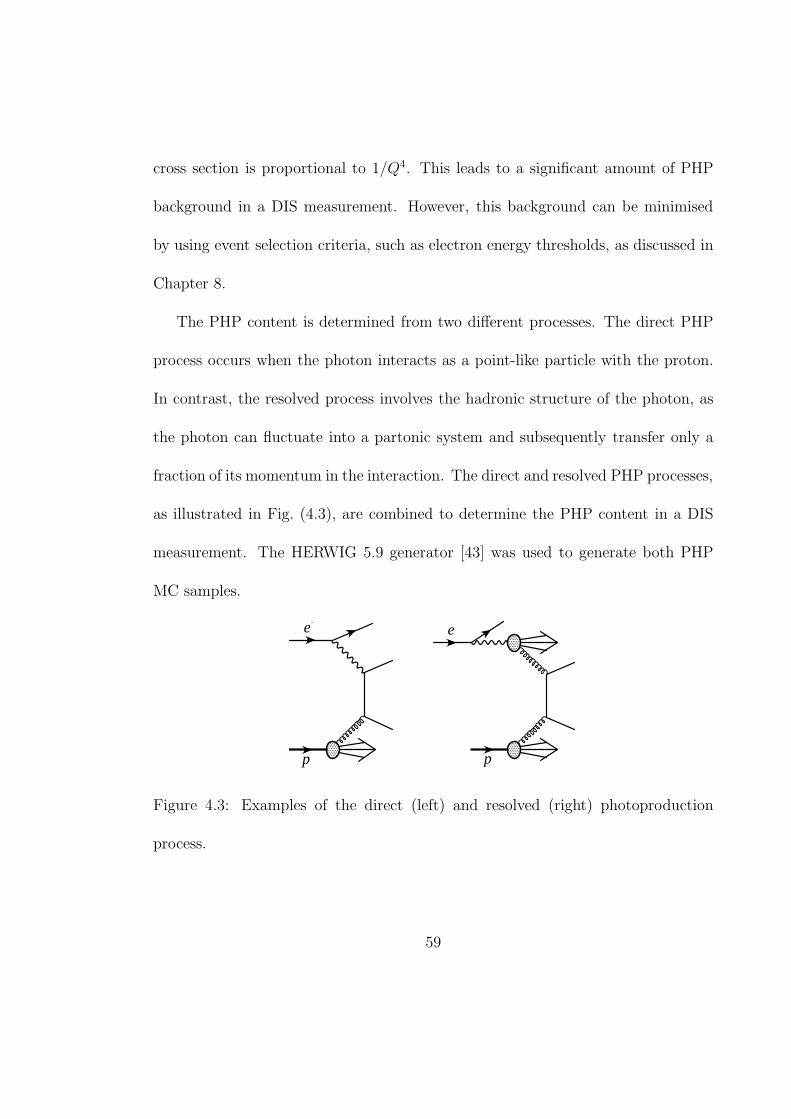
cross section is proportional to 1/Q4. This leads to a significant amount of PHP
background in a DIS measurement. However, this background can be minimised
by using event selection criteria, such as electron energy thresholds, as discussed in
Chapter 8.
The PHP content is determined from two different processes. The direct PHP
process occurs when the photon interacts as a point-like particle with the proton.
In contrast, the resolved process involves the hadronic structure of the photon, as
the photon can fluctuate into a partonic system and subsequently transfer only a
fraction of its momentum in the interaction. The direct and resolved PHP processes,
as illustrated in Fig. (4.3), are combined to determine the PHP content in a DIS
measurement. The HERWIG 5.9 generator [43] was used to generate both PHP
MC samples.
p
e
p
e -
Figure 4.3: Examples of the direct (left) and resolved (right) photoproduction
process.
59
4.3 Detector simulation and software environment
After the final state particles have been generated, the detector response is sim-
ulated. The first stage is to simulate the interaction of the particles with the
detector. This is done using a program called MOZART [44], based on the sim-
ulation program GEANT [45], that provides the shape, material, and position of
detector components. Also, the propagation of particles through the whole detector
is simulated, taking into account energy loss, multiple scattering, and the effect of
the magnetic field. After the detector response is simulated, the three trigger levels
are simulated (using a package called CZAR) and then finally a full reconstruction
of the event is performed (using software called ZEPHYR) such that the simulated
events can be directly compared with data.
The process of passing generated events through the detector simulation, trigger
simulation, and event reconstruction is done using the FUNNEL facility [46], which
produces MC events using computing power across the world. The MC production
capacity has been increased since 2004 using a Grid-enabled extension of FUNNEL
which exploits the large number of computing Grid sites designed for the Large
Hadron Collider (LHC). At the time of writing, the Grid simulates approximately
20 million ZEUS events per week [47], roughly four times the FUNNEL production
capacity.
60

The stages in a typical ZEUS analysis are shown in Fig. (4.4), starting from
raw detector signals and the physics event generators, and ending with an offline
event analysis. The analysis framework used in this analysis is ORANGE [48], a
software library that executes standard ZEUS analysis routines, such as electron
finders and calorimeter energy corrections. ORANGE version 2006a.3 was used in
this analysis.
(ZEPHYR)
(ORANGE)
Trigger Chain
FLT
SLT
TLT
Event Reconstruction
Offline Event Analysis
(AMADEUS)
Physics Event Generation
(MOZART)
Detector Simulation
Trigger Simulation
(CZAR)
Figure 4.4: The stages in a typical ZEUS analysis, adapted from [49]. On the left
side are the simulated events and on the right are the measured data events. The
software packages are shown in brackets.
61
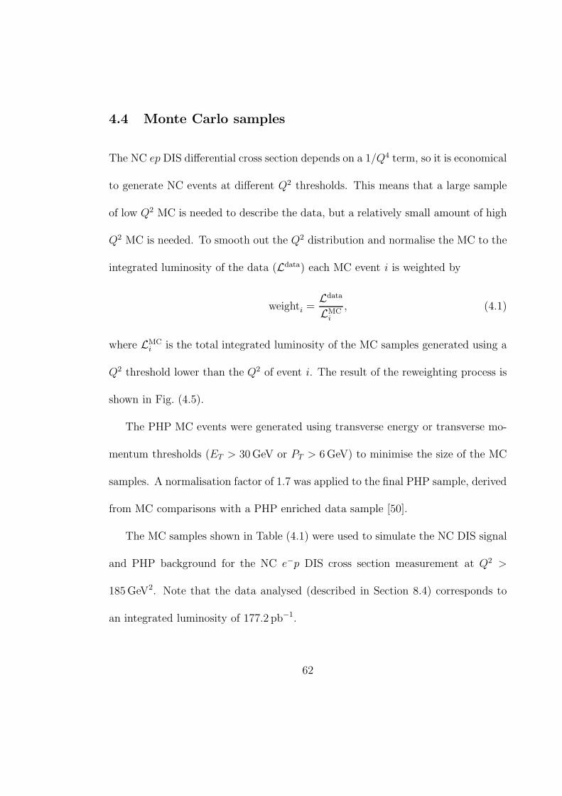
4.4 Monte Carlo samples
The NC ep DIS differential cross section depends on a 1/Q4 term, so it is economical
to generate NC events at different Q2 thresholds. This means that a large sample
of low Q2 MC is needed to describe the data, but a relatively small amount of high
Q2 MC is needed. To smooth out the Q2 distribution and normalise the MC to the
integrated luminosity of the data (Ldata) each MC event i is weighted by
weighti =Ldata
LMCi
, (4.1)
where LMCi is the total integrated luminosity of the MC samples generated using a
Q2 threshold lower than the Q2 of event i. The result of the reweighting process is
shown in Fig. (4.5).
The PHP MC events were generated using transverse energy or transverse mo-
mentum thresholds (ET > 30 GeV or PT > 6 GeV) to minimise the size of the MC
samples. A normalisation factor of 1.7 was applied to the final PHP sample, derived
from MC comparisons with a PHP enriched data sample [50].
The MC samples shown in Table (4.1) were used to simulate the NC DIS signal
and PHP background for the NC e−p DIS cross section measurement at Q2 >
185 GeV2. Note that the data analysed (described in Section 8.4) corresponds to
an integrated luminosity of 177.2 pb−1.
62
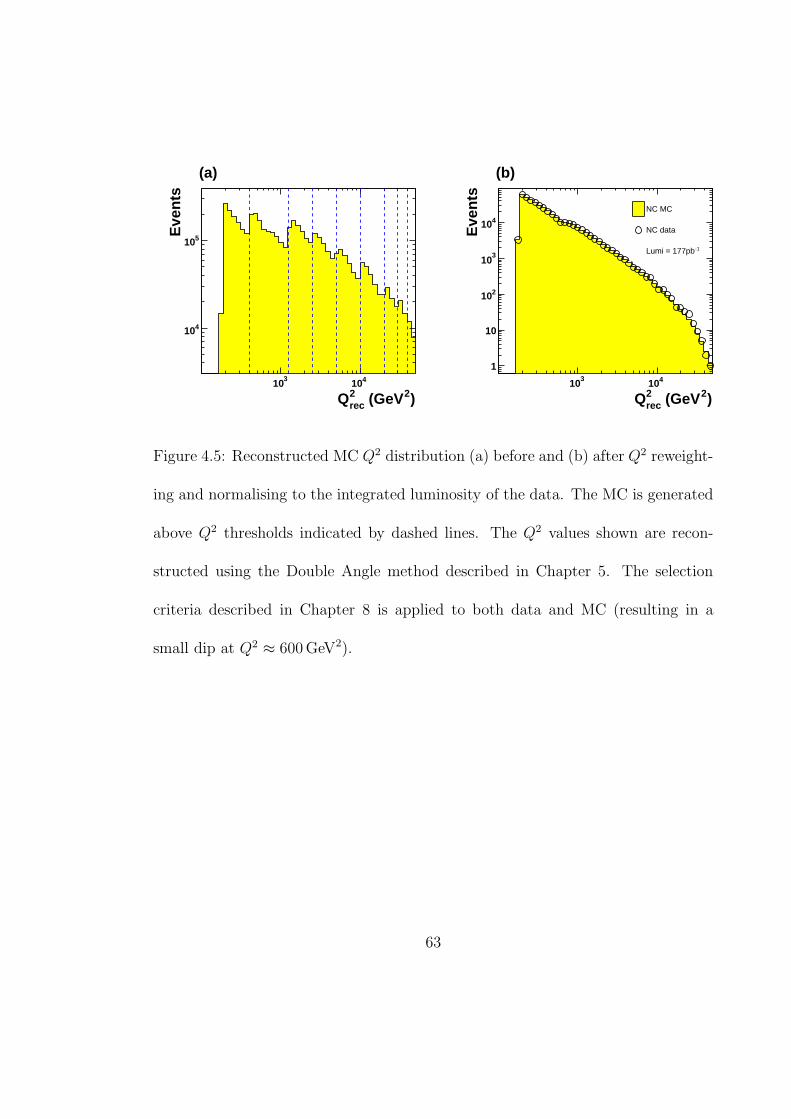
)2 (GeVrec2Q
310 410
Eve
nts
410
510
(a)
)2 (GeVrec2Q
310 410
Eve
nts
1
10
210
310
410
NC MC
NC data
-1Lumi = 177pb
(b)
Figure 4.5: Reconstructed MC Q2 distribution (a) before and (b) after Q2 reweight-
ing and normalising to the integrated luminosity of the data. The MC is generated
above Q2 thresholds indicated by dashed lines. The Q2 values shown are recon-
structed using the Double Angle method described in Chapter 5. The selection
criteria described in Chapter 8 is applied to both data and MC (resulting in a
small dip at Q2 ≈ 600 GeV2).
63

Process Cuts σ (pb) L ( pb−1) Events
NC DIS Q2had > 100 GeV2 8161 9.78 × 10² 8 × 10⁶
> 400 1197 1.59 × 10³ 2 × 10⁶
> 1250 217.3 5.56 × 10³ 1 × 10⁶
> 2500 71.87 6.96 × 10³ 5 × 10⁵
> 5000 21.73 2.30 × 10⁴ 5 × 10⁵
> 10000 5.383 4.82 × 10⁴ 3 × 10⁵
> 20000 0.8518 1.17 × 10⁵ 1 × 10⁵
> 30000 0.1867 3.21 × 10⁵ 6 × 10⁴
> 40000 0.04311 4.17 × 10⁵ 2 × 10⁴
> 50000 0.009312 2.09 × 10⁶ 2 × 10⁴
Direct PHP PT > 6 GeV or 2830 200.6 6 × 10⁵
ET > 30 GeV
Resolved PHP PT > 6 GeV or 11900 197.8 2 × 10⁶
ET > 30 GeV
Table 4.1: The NC DIS and PHP Monte Carlo samples used to simulate NC e−p
DIS data at Q2 > 185 GeV2 with an integrated luminosity of 177.2 pb−1. The cross
section (σ), integrated luminosity (L) and approximate amount of events are shown.
The generated Q2had values are calculated from the scattered electron and hadronic
final state.
64
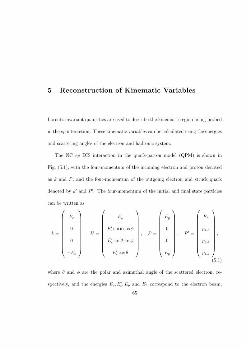
5 Reconstruction of Kinematic Variables
Lorentz invariant quantities are used to describe the kinematic region being probed
in the ep interaction. These kinematic variables can be calculated using the energies
and scattering angles of the electron and hadronic system.
The NC ep DIS interaction in the quark-parton model (QPM) is shown in
Fig. (5.1), with the four-momentum of the incoming electron and proton denoted
as k and P , and the four-momentum of the outgoing electron and struck quark
denoted by k′ and P ′. The four-momentum of the initial and final state particles
can be written as
k =
Ee
0
0
−Ee
, k′ =
E ′e
E ′e sin θ cos φ
E ′e sin θ sin φ
E ′e cos θ
, P =
Ep
0
0
Ep
, P ′ =
Eh
px,h
py,h
pz,h
,
(5.1)
where θ and φ are the polar and azimuthal angle of the scattered electron, re-
spectively, and the energies Ee, E′e, Ep and Eh correspond to the electron beam,
65

scattered electron, proton beam, and struck quark, respectively.
γ, Z0(q)
quark (xP )
struck quark (P ′)
proton (P )
e−(k) e−(k′)
Figure 5.1: The ep NC DIS interaction in the QPM.
By taking the QPM approximation, the four-momentum of the struck quark
(P ′) can be measured by adding the four-momenta of all the hadronic particles
not associated with the proton remnant (as shown in Fig. (4.2)). An obstacle to
this process is the loss of particles through the forward beam-pipe. This can be
minimised by using quantities such as the hadronic transverse momentum (pT,h)
and the difference between the energy and longitudinal momentum of the hadronic
final state (δh), which are defined by
p2T,h = p2
x,h + p2y,h = (
h∑
i
Ei sin θi cos φi)2 + (
h∑
i
Ei sin θi sin φi)2, (5.2)
δh = (E − pz)h =h
∑
i
(Ei − pz,i) =h
∑
i
Ei(1 − cos θi), (5.3)
66
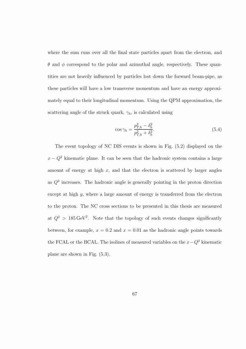
where the sum runs over all the final state particles apart from the electron, and
θ and φ correspond to the polar and azimuthal angle, respectively. These quan-
tities are not heavily influenced by particles lost down the forward beam-pipe, as
these particles will have a low transverse momentum and have an energy approxi-
mately equal to their longitudinal momentum. Using the QPM approximation, the
scattering angle of the struck quark, γh, is calculated using
cos γh =p2
T,h − δ2h
p2T,h + δ2
h
. (5.4)
The event topology of NC DIS events is shown in Fig. (5.2) displayed on the
x − Q2 kinematic plane. It can be seen that the hadronic system contains a large
amount of energy at high x, and that the electron is scattered by larger angles
as Q2 increases. The hadronic angle is generally pointing in the proton direction
except at high y, where a large amount of energy is transferred from the electron
to the proton. The NC cross sections to be presented in this thesis are measured
at Q2 > 185 GeV2. Note that the topology of such events changes significantly
between, for example, x = 0.2 and x = 0.01 as the hadronic angle points towards
the FCAL or the BCAL. The isolines of measured variables on the x−Q2 kinematic
plane are shown in Fig. (5.3).
67
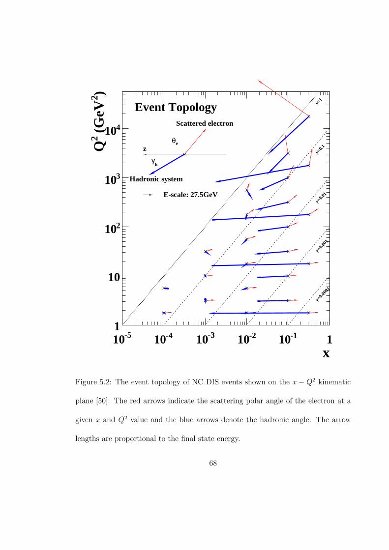
x-510 -410 -310 -210 -110 1
)2 (
GeV
2Q
1
10
210
310
410
y=1
y=0.1
y=0.0
1
y=0.0
01
y=0.0
001
Event TopologyScattered electron
Hadronic system
zeθ
hγ
E-scale: 27.5GeV
Figure 5.2: The event topology of NC DIS events shown on the x − Q2 kinematic
plane [50]. The red arrows indicate the scattering polar angle of the electron at a
given x and Q2 value and the blue arrows denote the hadronic angle. The arrow
lengths are proportional to the final state energy.
68

x-410 -310 -210 -110 1
)2 (
GeV
2Q
1
10
210
310
410
510
y=1
y=0.1
y=0.0
1
y=0.0
01
step)°
isolines (20eθ
°175
°35
x-410 -310 -210 -110 1
)2 (
GeV
2Q
1
10
210
310
410
510
y=1
y=0.1
y=0.0
1
y=0.0
01
isolines (5GeV step)e’
E
27.5
GeV
22.5
GeV
32.5 GeV
x-410 -310 -210 -110 1
)2 (
GeV
2Q
1
10
210
310
410
510
y=1
y=0.1
y=0.0
1
y=0.0
01
isolines (4GeV step)T,hP
4 GeV
40 GeV
x-410 -310 -210 -110 1
)2 (
GeV
2Q
1
10
210
310
410
510
y=1
y=0.1
y=0.0
1
y=0.0
01
2 step)× isolines (hδ
0.5 G
eV
x-410 -310 -210 -110 1
)2 (
GeV
2Q
1
10
210
310
410
510
y=1
y=0.1
y=0.0
1
y=0.0
01
step)°
isolines (20h
γ
°10
°17
0
x-410 -310 -210 -110 1
)2 (
GeV
2Q
1
10
210
310
410
510
y=1
y=0.1
y=0.0
1
y=0.0
01
2 step)× isolines (hE
27.5
GeV
6.87
5 G
eV
440
GeV
Figure 5.3: Isolines of measured quantities shown on the x−Q2 kinematic plane [50].
The scattered electron angle θe, energy of the scattered electron E ′e, transverse mo-
mentum of the hadronic system PT,h, hadronic energy minus the hadronic longitu-
dinal momentum δh, hadronic angle γh and the hadronic energy Eh are shown.
69
The energies E ′e, Eh and angles θ, γh are used to reconstruct the Lorentz invari-
ant kinematic variables that characterise the interaction. The kinematic variables
can be calculated using information only from the scattered electron, exclusively
from the hadronic final state, or a combination of the two. Three different methods
to reconstruct the kinematic variables are introduced below.
5.1 Electron reconstruction method
The Electron method [51] only uses information from the scattered electron to
reconstruct the kinematic variables:
Q2el = 2EeE
′e(1 + cos θ) = 4EeE
′e cos2 θ
2, (5.5)
yel = 1 − E ′e
2Ee(1 − cos θ) = 1 − E ′
e
Eesin2 θ
2, (5.6)
xel =Q2
syel
=E ′
e cos2 θ2
Ep(1 − E′e
Eesin2 θ
2). (5.7)
It can be seen from Fig. (5.3) that when the scattered electron has an energy close to
the beam energy (27.5 GeV), the event becomes independent of Q2 at fixed x. This
area of phase space is known as the ‘kinematic peak’ region, and leads to a poor
resolution of the electron method as a small variation in the energy measurement
leads to a significant change in the kinematic variables.
70
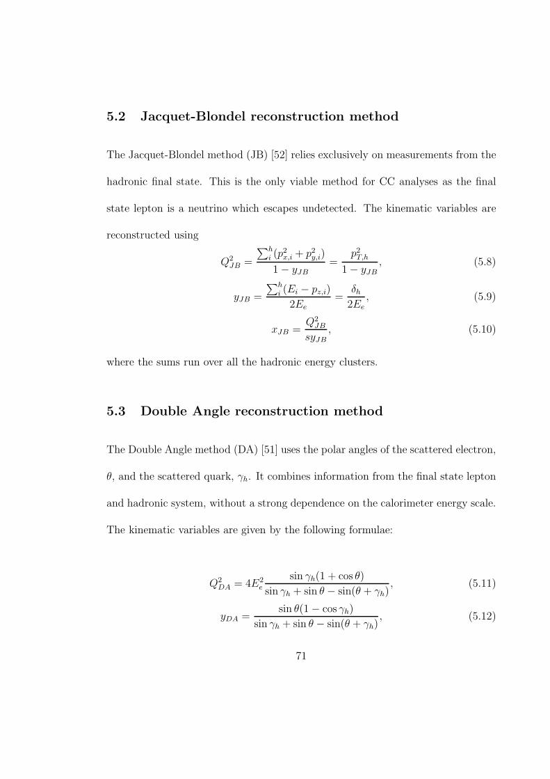
5.2 Jacquet-Blondel reconstruction method
The Jacquet-Blondel method (JB) [52] relies exclusively on measurements from the
hadronic final state. This is the only viable method for CC analyses as the final
state lepton is a neutrino which escapes undetected. The kinematic variables are
reconstructed using
Q2JB =
∑hi (p2
x,i + p2y,i)
1 − yJB=
p2T,h
1 − yJB, (5.8)
yJB =
∑hi (Ei − pz,i)
2Ee=
δh
2Ee, (5.9)
xJB =Q2
JB
syJB
, (5.10)
where the sums run over all the hadronic energy clusters.
5.3 Double Angle reconstruction method
The Double Angle method (DA) [51] uses the polar angles of the scattered electron,
θ, and the scattered quark, γh. It combines information from the final state lepton
and hadronic system, without a strong dependence on the calorimeter energy scale.
The kinematic variables are given by the following formulae:
Q2DA = 4E2
e
sin γh(1 + cos θ)
sin γh + sin θ − sin(θ + γh), (5.11)
yDA =sin θ(1 − cos γh)
sin γh + sin θ − sin(θ + γh), (5.12)
71
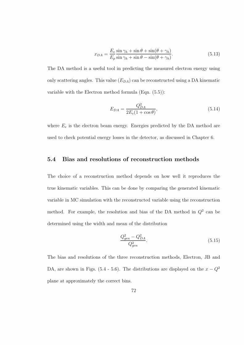
xDA =Ee
Ep
sin γh + sin θ + sin(θ + γh)
sin γh + sin θ − sin(θ + γh). (5.13)
The DA method is a useful tool in predicting the measured electron energy using
only scattering angles. This value (EDA) can be reconstructed using a DA kinematic
variable with the Electron method formula (Eqn. (5.5)):
EDA =Q2
DA
2Ee(1 + cos θ), (5.14)
where Ee is the electron beam energy. Energies predicted by the DA method are
used to check potential energy losses in the detector, as discussed in Chapter 6.
5.4 Bias and resolutions of reconstruction methods
The choice of a reconstruction method depends on how well it reproduces the
true kinematic variables. This can be done by comparing the generated kinematic
variable in MC simulation with the reconstructed variable using the reconstruction
method. For example, the resolution and bias of the DA method in Q2 can be
determined using the width and mean of the distribution
Q2gen − Q2
DA
Q2gen
. (5.15)
The bias and resolutions of the three reconstruction methods, Electron, JB and
DA, are shown in Figs. (5.4 - 5.6). The distributions are displayed on the x − Q2
plane at approximately the correct bins.
72
The DA method generally performs better than the other two methods when
reconstructing Q2, x and y over most of the kinematic plane. The Electron method
performs well at high y when reconstructing Q2, x and y, but introduces a large bias
and resolution at low y as a small change in the electron energy can severely bias
the reconstructed variable. The JB method is competitive at high x in x and y but
a large bias and resolution is seen in other kinematic regions and in Q2. Therefore,
the DA method is chosen to calculate NC ep DIS cross sections.
73

x
-210 -110 1
)2 (
GeV
2Q
310
410
510 bias2Q
Electron Method
JB Method
DA Method
generated
2 ) / Qreconstructed2 - Q
generated
2( Q
-0.4 -0.2 0 0.2 0.4
< 3002100 < Q0.001 < x < 0.004
-0.4 -0.2 0 0.2 0.4
< 3002100 < Q0.004 < x < 0.016
-0.4 -0.2 0 0.2 0.4
< 3002100 < Q0.016 < x < 0.064
-0.4 -0.2 0 0.2 0.4
< 3002100 < Q0.064 < x < 0.25
-0.4 -0.2 0 0.2 0.4
< 8002300 < Q0.004 < x < 0.016
-0.4 -0.2 0 0.2 0.4
< 8002300 < Q0.016 < x < 0.064
-0.4 -0.2 0 0.2 0.4
< 8002300 < Q0.064 < x < 0.25
-0.4 -0.2 0 0.2 0.4
< 8002300 < Q0.25 < x < 1.0
-0.4 -0.2 0 0.2 0.4
< 22002800 < Q0.004 < x < 0.016
-0.4 -0.2 0 0.2 0.4
< 22002800 < Q0.016 < x < 0.064
-0.4 -0.2 0 0.2 0.4
< 22002800 < Q0.064 < x < 0.25
-0.4 -0.2 0 0.2 0.4
< 22002800 < Q0.25 < x < 1.0
-0.4 -0.2 0 0.2 0.4
< 630022200 < Q0.016 < x < 0.064
-0.4 -0.2 0 0.2 0.4
< 630022200 < Q0.064 < x < 0.25
-0.4 -0.2 0 0.2 0.4
< 630022200 < Q0.25 < x < 1.0
-0.4 -0.2 0 0.2 0.4
< 1800026300 < Q0.064 < x < 0.25
-0.4 -0.2 0 0.2 0.4
< 1800026300 < Q0.25 < x < 1.0
-0.4 -0.2 0 0.2 0.4
< 50000218000 < Q0.25 < x < 1.0
Figure 5.4: The resolution and bias in Q2 using the Electron, JB, and DA methods.
The distributions are displayed on the x − Q2 plane at the approximate bins.
74
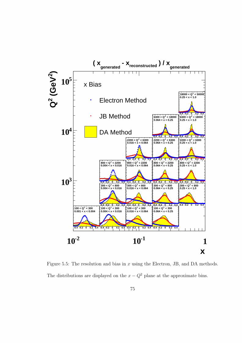
x
-210 -110 1
)2 (
GeV
2Q
310
410
510 x Bias
Electron Method
JB Method
DA Method
generated ) / xreconstructed - x
generated( x
-0.4 -0.2 0 0.2 0.4
< 3002100 < Q0.001 < x < 0.004
-0.4 -0.2 0 0.2 0.4
< 3002100 < Q0.004 < x < 0.016
-0.4 -0.2 0 0.2 0.4
< 3002100 < Q0.016 < x < 0.064
-0.4 -0.2 0 0.2 0.4
< 3002100 < Q0.064 < x < 0.25
-0.4 -0.2 0 0.2 0.4
< 8002300 < Q0.004 < x < 0.016
-0.4 -0.2 0 0.2 0.4
< 8002300 < Q0.016 < x < 0.064
-0.4 -0.2 0 0.2 0.4
< 8002300 < Q0.064 < x < 0.25
-0.4 -0.2 0 0.2 0.4
< 8002300 < Q0.25 < x < 1.0
-0.4 -0.2 0 0.2 0.4
< 22002800 < Q0.004 < x < 0.016
-0.4 -0.2 0 0.2 0.4
< 22002800 < Q0.016 < x < 0.064
-0.4 -0.2 0 0.2 0.4
< 22002800 < Q0.064 < x < 0.25
-0.4 -0.2 0 0.2 0.4
< 22002800 < Q0.25 < x < 1.0
-0.4 -0.2 0 0.2 0.4
< 630022200 < Q0.016 < x < 0.064
-0.4 -0.2 0 0.2 0.4
< 630022200 < Q0.064 < x < 0.25
-0.4 -0.2 0 0.2 0.4
< 630022200 < Q0.25 < x < 1.0
-0.4 -0.2 0 0.2 0.4
< 1800026300 < Q0.064 < x < 0.25
-0.4 -0.2 0 0.2 0.4
< 1800026300 < Q0.25 < x < 1.0
-0.4 -0.2 0 0.2 0.4
< 50000218000 < Q0.25 < x < 1.0
Figure 5.5: The resolution and bias in x using the Electron, JB, and DA methods.
The distributions are displayed on the x − Q2 plane at the approximate bins.
75
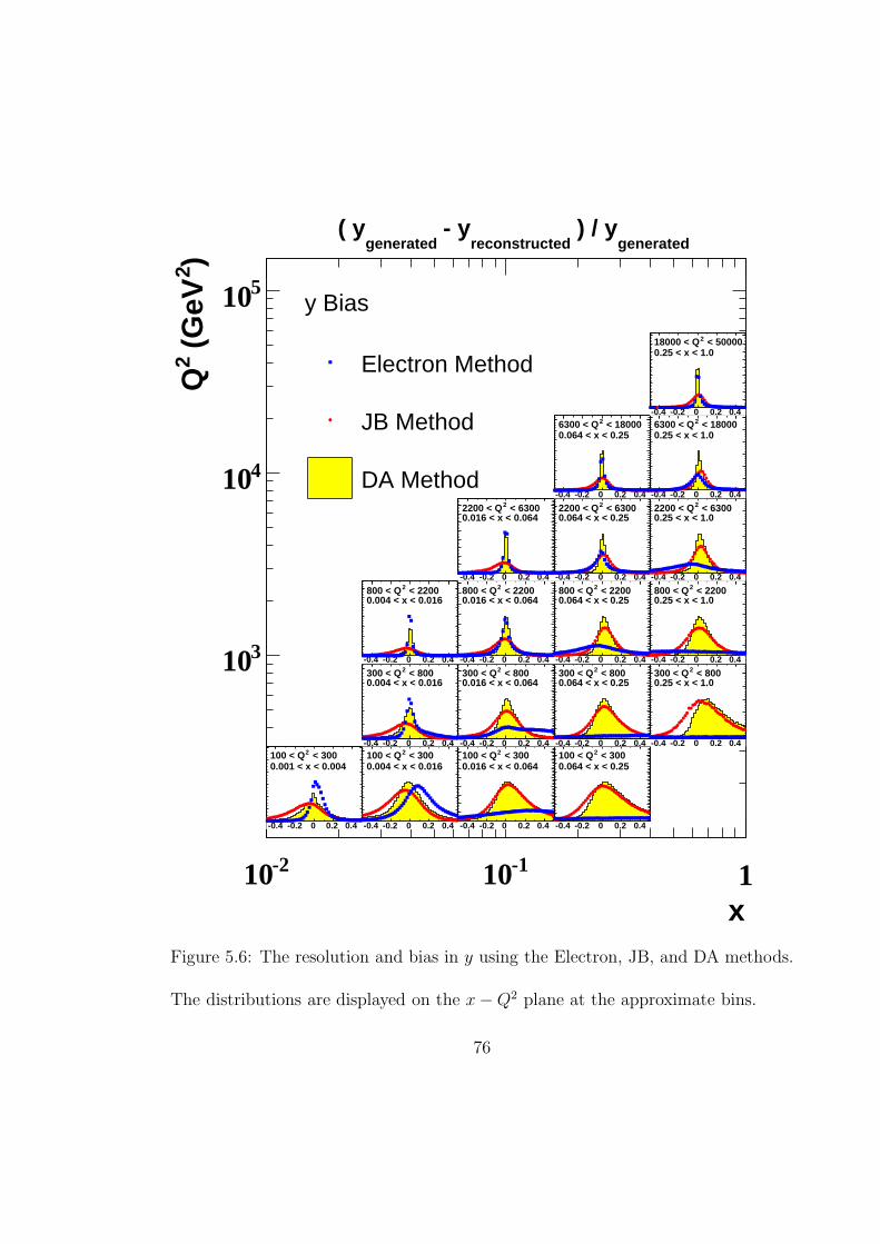
x
-210 -110 1
)2 (
GeV
2Q
310
410
510 y Bias
Electron Method
JB Method
DA Method
generated ) / y
reconstructed - y
generated( y
-0.4 -0.2 0 0.2 0.4
< 3002100 < Q0.001 < x < 0.004
-0.4 -0.2 0 0.2 0.4
< 3002100 < Q0.004 < x < 0.016
-0.4 -0.2 0 0.2 0.4
< 3002100 < Q0.016 < x < 0.064
-0.4 -0.2 0 0.2 0.4
< 3002100 < Q0.064 < x < 0.25
-0.4 -0.2 0 0.2 0.4
< 8002300 < Q0.004 < x < 0.016
-0.4 -0.2 0 0.2 0.4
< 8002300 < Q0.016 < x < 0.064
-0.4 -0.2 0 0.2 0.4
< 8002300 < Q0.064 < x < 0.25
-0.4 -0.2 0 0.2 0.4
< 8002300 < Q0.25 < x < 1.0
-0.4 -0.2 0 0.2 0.4
< 22002800 < Q0.004 < x < 0.016
-0.4 -0.2 0 0.2 0.4
< 22002800 < Q0.016 < x < 0.064
-0.4 -0.2 0 0.2 0.4
< 22002800 < Q0.064 < x < 0.25
-0.4 -0.2 0 0.2 0.4
< 22002800 < Q0.25 < x < 1.0
-0.4 -0.2 0 0.2 0.4
< 630022200 < Q0.016 < x < 0.064
-0.4 -0.2 0 0.2 0.4
< 630022200 < Q0.064 < x < 0.25
-0.4 -0.2 0 0.2 0.4
< 630022200 < Q0.25 < x < 1.0
-0.4 -0.2 0 0.2 0.4
< 1800026300 < Q0.064 < x < 0.25
-0.4 -0.2 0 0.2 0.4
< 1800026300 < Q0.25 < x < 1.0
-0.4 -0.2 0 0.2 0.4
< 50000218000 < Q0.25 < x < 1.0
Figure 5.6: The resolution and bias in y using the Electron, JB, and DA methods.
The distributions are displayed on the x − Q2 plane at the approximate bins.
76

6 Event Reconstruction
The signals recorded by the various detector components need to be interpreted
and combined to reconstruct the measured event. This chapter outlines some of
the corrections and algorithms used to reconstruct a NC DIS event.
6.1 Track and vertex reconstruction
Track reconstruction begins with a pattern recognition algorithm [53], which exam-
ines all the CTD hits (digitised signals in each CTD wire) to determine a track seed
formed from three hits in the outermost CTD superlayer. The pattern recognition
then proceeds inwards in the x−y plane towards the interaction point. The output
from the CTD is used as an input to a Kalman filter for the MVD [54]. This works
inwards, towards the interaction point, adding MVD hits to the CTD information
and accounting for effects such as material in the MVD and the beam-pipe. As
the track seed is extrapolated inwards, more hits are attributed to the track, which
improves the precision of the fit. Finally, the position of the event vertex is assigned.
77
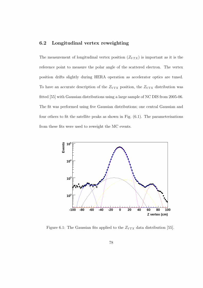
6.2 Longitudinal vertex reweighting
The measurement of longitudinal vertex position (ZV TX) is important as it is the
reference point to measure the polar angle of the scattered electron. The vertex
position drifts slightly during HERA operation as accelerator optics are tuned.
To have an accurate description of the ZV TX position, the ZV TX distribution was
fitted [55] with Gaussian distributions using a large sample of NC DIS from 2005-06.
The fit was performed using five Gaussian distributions; one central Gaussian and
four others to fit the satellite peaks as shown in Fig. (6.1). The parameterisations
from these fits were used to reweight the MC events.
Z vertex (cm)-100 -80 -60 -40 -20 0 20 40 60 80 100
Eve
nts
210
310
410
510
Figure 6.1: The Gaussian fits applied to the ZV TX data distribution [55].
78

6.3 Electron identification
An electron finder algorithm is used to identify electron candidates. The main
task of an electron finder is to distinguish electromagnetic and hadronic energy
clusters measured in the EMC and HAC cells [56]. The main electron finder for
this analysis, called EM, has been designed particularly for the high Q2 region,
where the electron is scattered by a large angle and is found in the BCAL or
FCAL sections (see Fig. (3.8) for a sketch of the CAL). Another electron finder
named SINISTRA, tuned especially for lower Q2 events (electrons scattered into
the RCAL), was used as a systematic check.
The EM electron finder [57] combines CAL and CTD information to identify
and reconstruct the scattered electron, whilst rejecting other final state particles
that may mimic the signature of an electron. At first, CAL ‘clusters’ are formed by
grouping CAL cells [58]. The cluster angle is then determined by taking the polar
angle between the cluster centre and the event vertex. A matching track is also
required if the cluster is within the CTD acceptance. A matched track is assigned if
the distance of closest approach between the extrapolated track and cluster centre
is within 10 cm. Several variables are then used to evaluate whether a CAL cluster
is a scattered electron candidate, including the difference in θ and φ between the
track and cluster, the fraction of the cluster energy measured in the HAC layers,
79

and parameters related to the width of the electron shower. Each of the variables
is transformed into a sub-probability with a large sub-probability related to a likely
electron candidate. An EM grand probability is assigned by taking the product of
all the sub-probabilities. The electron candidate is accepted if the grand probability
is above a certain threshold determined from MC studies.
The SINISTRA electron finder [59] is based on a neural network using CAL
information, and is tuned especially for electrons with a small scattering angle (low
Q2) penetrating the RCAL. This electron finder identifies the scattered electron
based on the shape of the shower it produces in the CAL. The inputs to the neural
net are the CAL cell energies and the output is the probability for each cluster to
be electromagnetic.
6.4 Electron energy
The CAL measurement of the electron energy is altered by some effects. As the
electron passes from the interaction point to the CAL, it must traverse detector
material such as magnets. This material reduces the true energy of the particle,
due to energy lost in interactions. Also the CAL surface is not uniform as there
are gaps between modules and towers. The corrections for these effects [50] are
discussed in the following sections. The electron energy distribution before and
after all corrections is shown in Fig. (6.2).
80

(GeV)e’
E0 10 20 30 40 50
Eve
nts
10000
20000
30000
40000
Whole CALUncorrected
(GeV)e’
E0 10 20 30 40 50
Eve
nts
10000
20000
30000
40000
Whole CALCorrected
(GeV)e’
E0 10 20 30
Eve
nts
10000
20000DataNC + PHP MCPHP MC
RCAL
(GeV)e’
E0 10 20 30
Eve
nts
10000
20000 RCAL
(GeV)e’
E0 20 40 60
Eve
nts
2000
4000BCAL
(GeV)e’
E0 20 40 60
Eve
nts
2000
4000 BCAL
(GeV)e’
E0 100 200 300
Eve
nts
50
100
150FCAL
(GeV)e’
E0 100 200 300
Eve
nts
50
100
150
FCAL
Figure 6.2: Electron energy distribution before (left) and after (right) corrections.
The dots represent data, the blue histogram represents PHP MC, and the yellow
histogram represents NC + PHP MC. From top to bottom is shown the energy
measured in the entire CAL, the RCAL, the BCAL, and the FCAL. The dashed
line indicates the cut of E ′e > 10 GeV applied in the final event selection.
81

6.4.1 RCAL electron energy
The energy loss due to dead-material is proportional to the particle multiplicity
due to these extra interactions. The rear presampler (PRES) can be used to mea-
sure the particle multiplicity from the deposited energy and so correct the electron
energy event-by-event. The energy loss can be quantified using the electron energy
predicted by the DA method (EDA). This reference energy is convenient as it is
calculated using the electron angle and hadronic angle, so is relatively insensitive
to the energy scale of the CAL sections.
The presampler correction [50] is parameterised by fitting a linear function to
the electron energy loss, E ′e −EDA, versus the energy deposited in the PRES inde-
pendently for data and MC. However, there are events in which the PRES energy
measurements are not valid. In these cases a dead-material map of the detector is
used, which simulates the location and type of dead-material inside the detector.
The energy loss through non-uniformity effects were also applied [60].
After these corrections are made the scale and resolution of the electron energy
was determined from the ratio E ′e/EDA as a function of EDA or the electron position
at the RCAL surface. The RCAL energy scale uncertainty was determined to be
2% by considering the data to MC comparison in Fig. (6.3) and an energy smearing
factor of 3.4% was determined for the MC events [50].
82
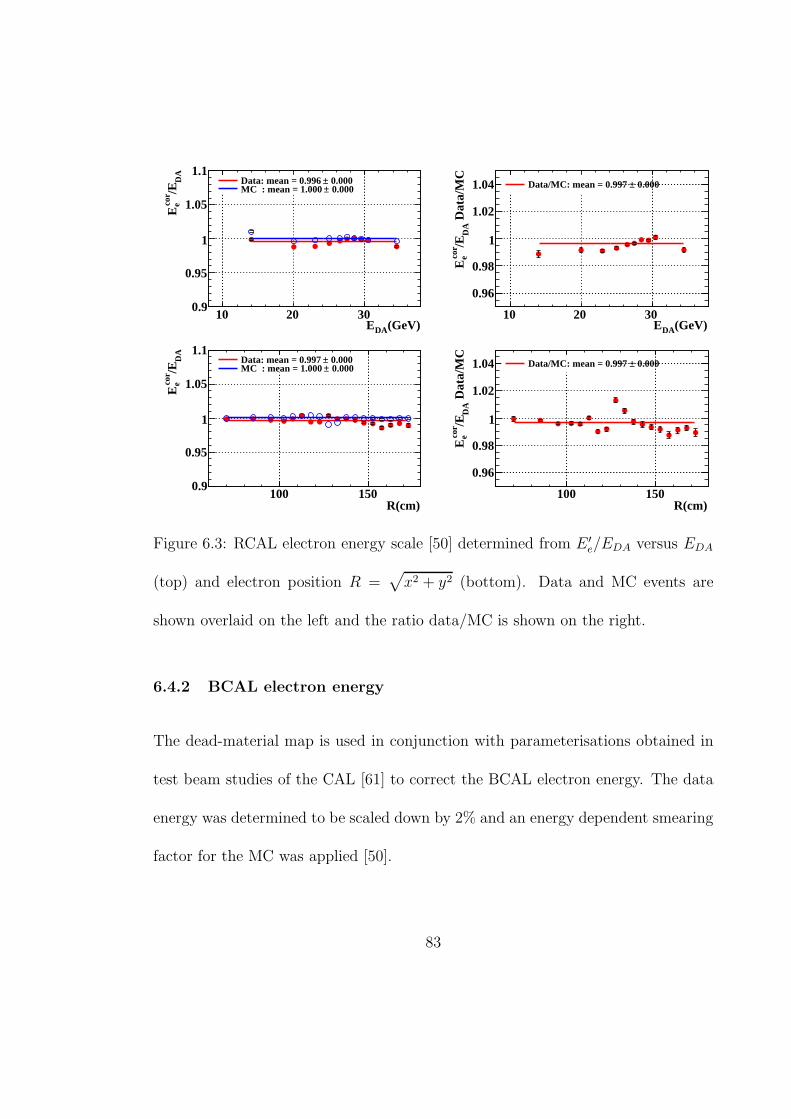
(GeV)DAE10 20 30
DA
/Eeco
rE
0.9
0.95
1
1.05
1.1 0.000±Data: mean = 0.996 0.000±MC : mean = 1.000
(GeV)DAE10 20 30
Dat
a/M
CD
A/E
ecor
E
0.96
0.98
1
1.02
1.04 0.000±Data/MC: mean = 0.997
R(cm)100 150
DA
/Eeco
rE
0.9
0.95
1
1.05
1.1 0.000±Data: mean = 0.997 0.000±MC : mean = 1.000
R(cm)100 150
Dat
a/M
CD
A/E
ecor
E0.96
0.98
1
1.02
1.04 0.000±Data/MC: mean = 0.997
Figure 6.3: RCAL electron energy scale [50] determined from E ′e/EDA versus EDA
(top) and electron position R =√
x2 + y2 (bottom). Data and MC events are
shown overlaid on the left and the ratio data/MC is shown on the right.
6.4.2 BCAL electron energy
The dead-material map is used in conjunction with parameterisations obtained in
test beam studies of the CAL [61] to correct the BCAL electron energy. The data
energy was determined to be scaled down by 2% and an energy dependent smearing
factor for the MC was applied [50].
83
6.4.3 FCAL electron energy
The dead-material map and non-uniformity corrections were used for events with
an electron scattered into the FCAL. The scale and smearing factors were derived
from a Gaussian fit to the ratio Ecorrectede /EDA. The data energy was shown to
require a 2% scale increase and a 3.7% smear was determined for MC events [50].
6.5 Calorimeter alignment
The polar angle of the scattered electron (θe) is reconstructed using CAL energy
deposit positions (if the electron is outside the acceptance of the CTD) or combined
with CAL and tracking information to achieve a better reconstruction. Therefore,
an accurate measurement of the CAL position with respect to the ZEUS reference
frame (set by the CTD) is of great importance as θe is used to reconstruct kinematic
variables. The CAL is opened and closed during detector shutdown periods, so the
CAL-CTD alignment can change slightly over time.
The alignment study [50] was done separately for the RCAL, BCAL and FCAL,
as these CAL sections are physically separate. The study was done in the RCAL and
FCAL using the difference between the CAL energy position and the extrapolated
CTD track position of the scattered electron. The alignment study in the BCAL
was performed by measuring the z position of the CAL module boundaries through
84

calculations of E ′e/EDA as a function of the z position.
The RCAL was shown to be aligned within 2 mm in x, y, and z [50]. The BCAL
was shown to be aligned within 1 mm in the z direction [50]. A 4 mm shift in y in the
FCAL was seen in data [50] and is corrected in the final analysis. After correcting
this shift in y, the position uncertainty at the FCAL is conservatively taken as
2 mm. All alignment factors are incorporated into the systematic uncertainties of
the final analysis by varying the θe measurement in the MC by ±1 mrad.
6.6 Hadronic final state reconstruction
The scattering angle of the struck quark, as approximated by the QPM, is calculated
from the distribution of particles associated with the hadronic final state (HFS). The
software package CorAndCut [62] is used to reconstruct the HFS in this analysis.
The CorAndCut package corrects the HFS for energy losses due to interactions with
dead material, energy losses in the boundaries between the BCAL and F/RCAL
(the so-called super-cracks) and energy overestimations for low energy deposits.
The energy losses were studied using distributions of the reconstructed and
generated MC hadronic energy. The dead material effect is treated using a fit of
the energy loss with respect to the amount of inactive material traversed. The
super-crack energy losses were parameterised using distributions of the energy loss
versus the hadronic angle.
85
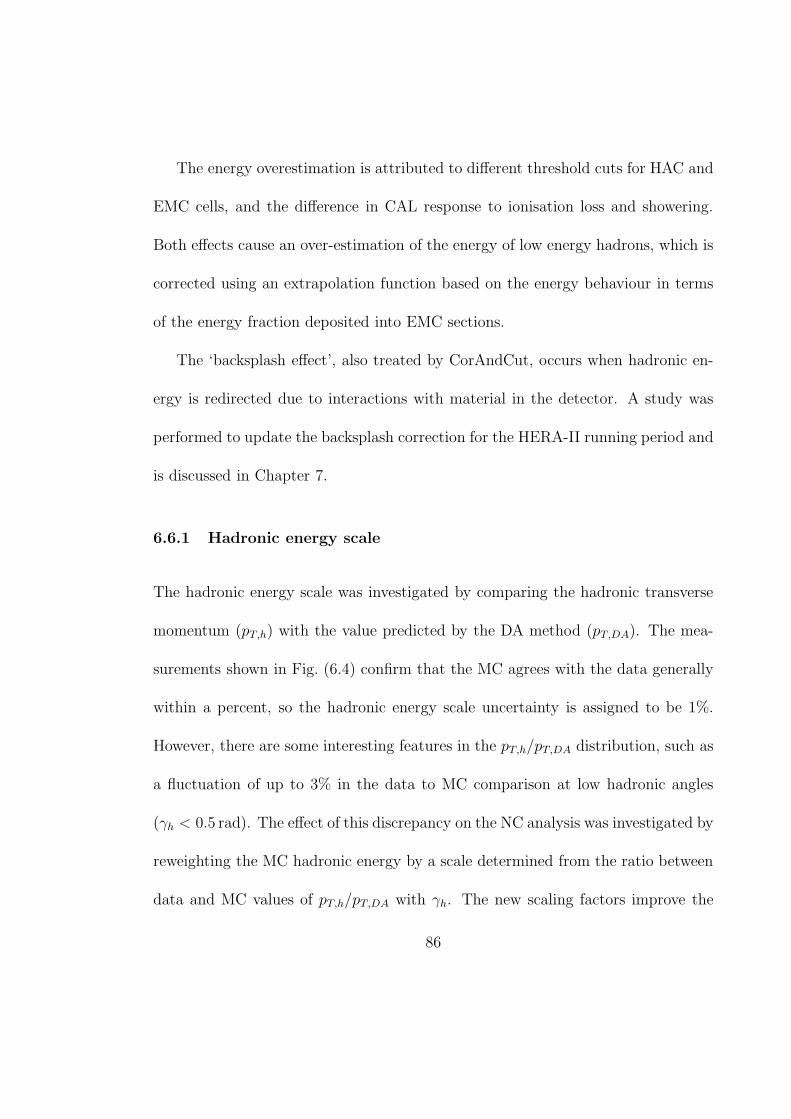
The energy overestimation is attributed to different threshold cuts for HAC and
EMC cells, and the difference in CAL response to ionisation loss and showering.
Both effects cause an over-estimation of the energy of low energy hadrons, which is
corrected using an extrapolation function based on the energy behaviour in terms
of the energy fraction deposited into EMC sections.
The ‘backsplash effect’, also treated by CorAndCut, occurs when hadronic en-
ergy is redirected due to interactions with material in the detector. A study was
performed to update the backsplash correction for the HERA-II running period and
is discussed in Chapter 7.
6.6.1 Hadronic energy scale
The hadronic energy scale was investigated by comparing the hadronic transverse
momentum (pT,h) with the value predicted by the DA method (pT,DA). The mea-
surements shown in Fig. (6.4) confirm that the MC agrees with the data generally
within a percent, so the hadronic energy scale uncertainty is assigned to be 1%.
However, there are some interesting features in the pT,h/pT,DA distribution, such as
a fluctuation of up to 3% in the data to MC comparison at low hadronic angles
(γh < 0.5 rad). The effect of this discrepancy on the NC analysis was investigated by
reweighting the MC hadronic energy by a scale determined from the ratio between
data and MC values of pT,h/pT,DA with γh. The new scaling factors improve the
86
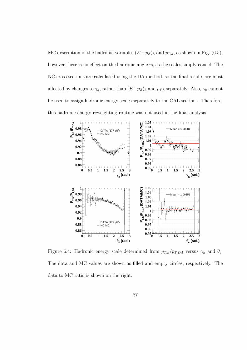
MC description of the hadronic variables (E−pZ)h and pT,h, as shown in Fig. (6.5),
however there is no effect on the hadronic angle γh as the scales simply cancel. The
NC cross sections are calculated using the DA method, so the final results are most
affected by changes to γh, rather than (E−pZ)h and pT,h separately. Also, γh cannot
be used to assign hadronic energy scales separately to the CAL sections. Therefore,
this hadronic energy reweighting routine was not used in the final analysis.
(rad.)h
γ0 0.5 1 1.5 2 2.5 3
T,D
A /P
T,h
P
0.86
0.88
0.9
0.92
0.94
0.96
0.98
1
)-1DATA (177 pbNC MC
(rad.)h
γ0 0.5 1 1.5 2 2.5 3
(D
AT
A/M
C)
T,D
A /P
T,h
P
0.950.960.970.980.99
11.011.021.031.041.05
Mean = 1.00381
(rad.)eθ0 0.5 1 1.5 2 2.5 3
T,D
A /P
T,h
P
0.86
0.88
0.9
0.92
0.94
0.96
0.98
1
)-1DATA (177 pbNC MC
(rad.)eθ0 0.5 1 1.5 2 2.5 3
(D
AT
A/M
C)
T,D
A /P
T,h
P
0.950.960.970.980.99
11.011.021.031.041.05
Mean = 1.00351
Figure 6.4: Hadronic energy scale determined from pT,h/pT,DA versus γh and θe.
The data and MC values are shown as filled and empty circles, respectively. The
data to MC ratio is shown on the right.
87
(rad.)h
γ0 0.5 1 1.5 2 2.5 3
T,D
A /P
T,h
P
0.86
0.88
0.9
0.92
0.94
0.96
0.98
1
)-1DATA (177 pbNC MC
Figure 6.5: The pT,h/pT,DA measurement versus γh after applying MC hadronic
energy reweighting scales is shown on the left. The middle and right plots show
the data/MC distributions of variables related to the hadronic energy. The black
and red dots correspond to the values before and after applying the MC hadronic
energy reweighting scales.
6.6.2 Jet reconstruction
A jet-finder can be used to cluster hadronic particles into collimated jets and is an
alternate approach to using all the hadronic deposits in the CAL to characterise
the HFS. The jet-finder used for systematic studies in this thesis is called the
‘longitudinally invariant kT clustering algorithm’ [63]. The energies (E) and angles
(θ and φ) of the input particles to the jet-finder are combined to make the quantities
ET = E sin θ and pseudo-rapidity η = − ln(tan θ/2). The pseudo-rapidity is used
as it is the longitudinally invariant polar angle, as a Lorentz boost along the z axis
changes this quantity by an additive constant.
88
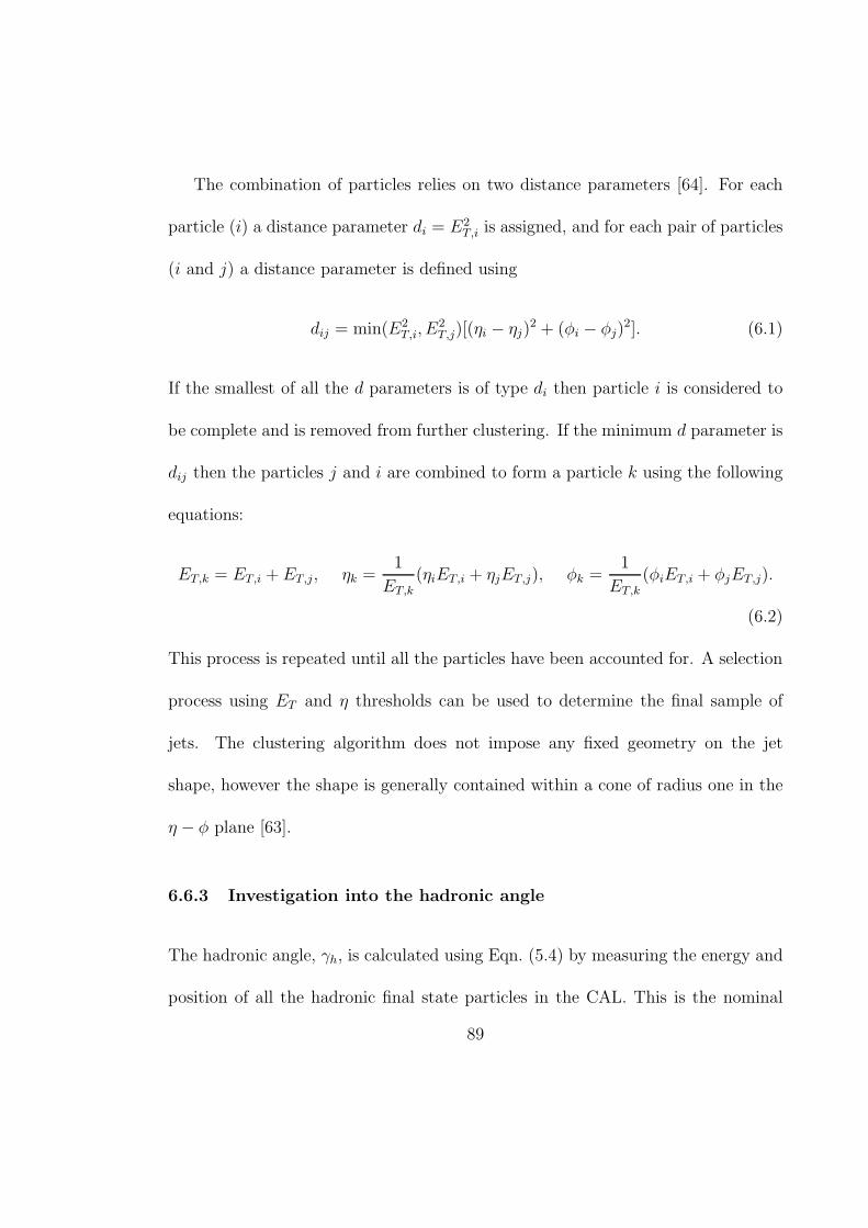
The combination of particles relies on two distance parameters [64]. For each
particle (i) a distance parameter di = E2T,i is assigned, and for each pair of particles
(i and j) a distance parameter is defined using
dij = min(E2T,i, E
2T,j)[(ηi − ηj)
2 + (φi − φj)2]. (6.1)
If the smallest of all the d parameters is of type di then particle i is considered to
be complete and is removed from further clustering. If the minimum d parameter is
dij then the particles j and i are combined to form a particle k using the following
equations:
ET,k = ET,i + ET,j, ηk =1
ET,k(ηiET,i + ηjET,j), φk =
1
ET,k(φiET,i + φjET,j).
(6.2)
This process is repeated until all the particles have been accounted for. A selection
process using ET and η thresholds can be used to determine the final sample of
jets. The clustering algorithm does not impose any fixed geometry on the jet
shape, however the shape is generally contained within a cone of radius one in the
η − φ plane [63].
6.6.3 Investigation into the hadronic angle
The hadronic angle, γh, is calculated using Eqn. (5.4) by measuring the energy and
position of all the hadronic final state particles in the CAL. This is the nominal
89
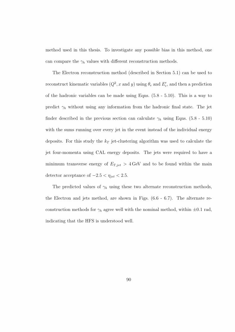
method used in this thesis. To investigate any possible bias in this method, one
can compare the γh values with different reconstruction methods.
The Electron reconstruction method (described in Section 5.1) can be used to
reconstruct kinematic variables (Q2, x and y) using θe and E ′e, and then a prediction
of the hadronic variables can be made using Eqns. (5.8 - 5.10). This is a way to
predict γh without using any information from the hadronic final state. The jet
finder described in the previous section can calculate γh using Eqns. (5.8 - 5.10)
with the sums running over every jet in the event instead of the individual energy
deposits. For this study the kT jet-clustering algorithm was used to calculate the
jet four-momenta using CAL energy deposits. The jets were required to have a
minimum transverse energy of ET,jet > 4 GeV and to be found within the main
detector acceptance of −2.5 < ηjet < 2.5.
The predicted values of γh using these two alternate reconstruction methods,
the Electron and jets method, are shown in Figs. (6.6 - 6.7). The alternate re-
construction methods for γh agree well with the nominal method, within ±0.1 rad,
indicating that the HFS is understood well.
90
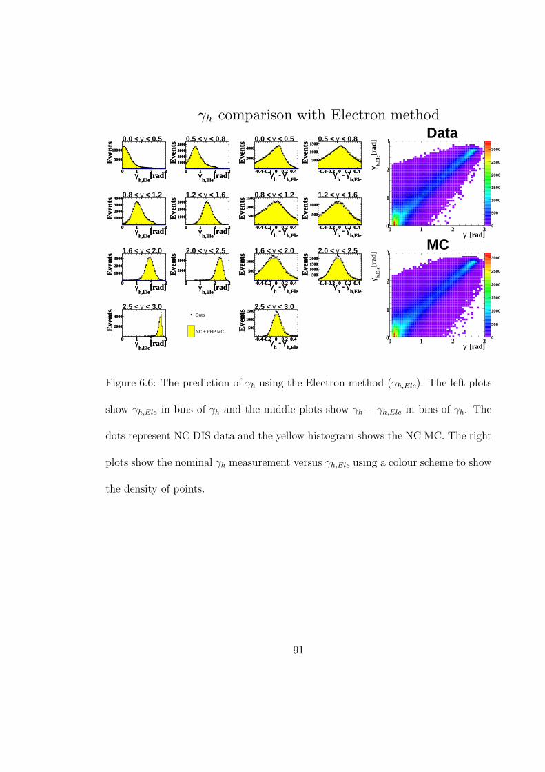
γh comparison with Electron method
[rad]h,Ele
γ0 1 2 3
Eve
nts
5000
10000
[rad]h,Ele
γ0 1 2 3
Eve
nts
5000
10000
< 0.5γ0.0 <
[rad]h,Ele
γ0 1 2 3E
vent
s
10002000
30004000
[rad]h,Ele
γ0 1 2 3E
vent
s
10002000
30004000
< 0.8γ0.5 <
[rad]h,Ele
γ0 1 2 3
Eve
nts
1000
2000
3000
4000
[rad]h,Ele
γ0 1 2 3
Eve
nts
1000
2000
3000
4000 < 1.2γ0.8 <
[rad]h,Ele
γ0 1 2 3
Eve
nts
1000
2000
3000
[rad]h,Ele
γ0 1 2 3
Eve
nts
1000
2000
3000
< 1.6γ1.2 <
[rad]h,Ele
γ0 1 2 3
Eve
nts
1000
2000
3000
[rad]h,Ele
γ0 1 2 3
Eve
nts
1000
2000
3000
< 2.0γ1.6 <
[rad]h,Ele
γ0 1 2 3
Eve
nts
2000
4000
[rad]h,Ele
γ0 1 2 3
Eve
nts
2000
4000
< 2.5γ2.0 <
[rad]h,Ele
γ0 1 2 3
Eve
nts
2000
4000
[rad]h,Ele
γ0 1 2 3
Eve
nts
2000
4000
< 3.0γ2.5 < Data
NC + PHP MC
h,Eleγ -
hγ-0.4-0.2 0 0.2 0.4
Eve
nts
2000
4000
h,Eleγ -
hγ-0.4-0.2 0 0.2 0.4
Eve
nts
2000
4000
< 0.5γ0.0 <
h,Eleγ -
hγ-0.4-0.2 0 0.2 0.4
Eve
nts
500
1000
1500
h,Eleγ -
hγ-0.4-0.2 0 0.2 0.4
Eve
nts
500
1000
1500 < 0.8γ0.5 <
h,Eleγ -
hγ-0.4-0.2 0 0.2 0.4
Eve
nts
500
1000
1500
h,Eleγ -
hγ-0.4-0.2 0 0.2 0.4
Eve
nts
500
1000
1500 < 1.2γ0.8 <
h,Eleγ -
hγ-0.4-0.2 0 0.2 0.4
Eve
nts
500
1000
h,Eleγ -
hγ-0.4-0.2 0 0.2 0.4
Eve
nts
500
1000
< 1.6γ1.2 <
h,Eleγ -
hγ-0.4-0.2 0 0.2 0.4
Eve
nts
500
1000
h,Eleγ -
hγ-0.4-0.2 0 0.2 0.4
Eve
nts
500
1000
< 2.0γ1.6 <
h,Eleγ -
hγ-0.4-0.2 0 0.2 0.4
Eve
nts
500100015002000
h,Eleγ -
hγ-0.4-0.2 0 0.2 0.4
Eve
nts
500100015002000
< 2.5γ2.0 <
h,Eleγ -
hγ-0.4-0.2 0 0.2 0.4
Eve
nts
500
1000
1500
h,Eleγ -
hγ-0.4-0.2 0 0.2 0.4
Eve
nts
500
1000
1500 < 3.0γ2.5 <
0
500
1000
1500
2000
2500
3000
[rad]γ0 1 2 3
[rad
]h,
Ele
γ
0
1
2
3Data
0
500
1000
1500
2000
2500
3000
[rad]γ0 1 2 3
[rad
]h,
Ele
γ
0
1
2
3MC
Figure 6.6: The prediction of γh using the Electron method (γh,Ele). The left plots
show γh,Ele in bins of γh and the middle plots show γh − γh,Ele in bins of γh. The
dots represent NC DIS data and the yellow histogram shows the NC MC. The right
plots show the nominal γh measurement versus γh,Ele using a colour scheme to show
the density of points.
91

γh comparison with jets method
[rad]h,Jet
γ0 1 2 3
Eve
nts
5000
10000
15000
20000
[rad]h,Jet
γ0 1 2 3
Eve
nts
5000
10000
15000
20000 < 0.5γ0.0 <
[rad]h,Jet
γ0 1 2 3E
vent
s
5000
10000
[rad]h,Jet
γ0 1 2 3E
vent
s
5000
10000
< 0.8γ0.5 <
[rad]h,Jet
γ0 1 2 3
Eve
nts
2000
4000
6000
[rad]h,Jet
γ0 1 2 3
Eve
nts
2000
4000
6000
< 1.2γ0.8 <
[rad]h,Jet
γ0 1 2 3
Eve
nts
2000
4000
[rad]h,Jet
γ0 1 2 3
Eve
nts
2000
4000
< 1.6γ1.2 <
[rad]h,Jet
γ0 1 2 3
Eve
nts
1000
2000
3000
4000
[rad]h,Jet
γ0 1 2 3
Eve
nts
1000
2000
3000
4000 < 2.0γ1.6 <
[rad]h,Jet
γ0 1 2 3
Eve
nts
1000
20003000
4000
[rad]h,Jet
γ0 1 2 3
Eve
nts
1000
20003000
4000 < 2.5γ2.0 <
[rad]h,Jet
γ0 1 2 3
Eve
nts
1000
2000
[rad]h,Jet
γ0 1 2 3
Eve
nts
1000
2000
< 3.0γ2.5 < Data
NC + PHP MC
h,Jetγ -
hγ-0.4-0.2 0 0.2 0.4
Eve
nts
5000
10000
15000
h,Jetγ -
hγ-0.4-0.2 0 0.2 0.4
Eve
nts
5000
10000
15000 < 0.5γ0.0 <
h,Jetγ -
hγ-0.4-0.2 0 0.2 0.4
Eve
nts
2000
4000
6000
h,Jetγ -
hγ-0.4-0.2 0 0.2 0.4
Eve
nts
2000
4000
6000 < 0.8γ0.5 <
h,Jetγ -
hγ-0.4-0.2 0 0.2 0.4
Eve
nts
1000
2000
3000
h,Jetγ -
hγ-0.4-0.2 0 0.2 0.4
Eve
nts
1000
2000
3000
< 1.2γ0.8 <
h,Jetγ -
hγ-0.4-0.2 0 0.2 0.4
Eve
nts
500100015002000
h,Jetγ -
hγ-0.4-0.2 0 0.2 0.4
Eve
nts
500100015002000
< 1.6γ1.2 <
h,Jetγ -
hγ-0.4-0.2 0 0.2 0.4
Eve
nts
500
1000
1500
h,Jetγ -
hγ-0.4-0.2 0 0.2 0.4
Eve
nts
500
1000
1500
< 2.0γ1.6 <
h,Jetγ -
hγ-0.4-0.2 0 0.2 0.4
Eve
nts
500100015002000
h,Jetγ -
hγ-0.4-0.2 0 0.2 0.4
Eve
nts
500100015002000
< 2.5γ2.0 <
h,Jetγ -
hγ-0.4-0.2 0 0.2 0.4
Eve
nts
500
1000
h,Jetγ -
hγ-0.4-0.2 0 0.2 0.4
Eve
nts
500
1000 < 3.0γ2.5 <
0
1000
2000
3000
4000
5000
6000
7000
8000
[rad]γ0 1 2 3
[rad
]h,
Jet
γ
0
1
2
3Data
0
1000
2000
3000
4000
5000
6000
[rad]γ0 1 2 3
[rad
]h,
Jet
γ
0
1
2
3MC
Figure 6.7: The prediction of γh using jets (γh,Jet). The left plots show γh,Jet in bins
of γh and the middle plots show γh − γh,Jet in bins of γh. The dots represent NC
DIS data and the yellow histogram shows the NC MC. The right plots show the
nominal γh measurement versus γh,Jet using a colour scheme to show the density of
points.
92

7 Backsplash in the Hadronic Final State
The kinematic variables Q2, x and y are used for cross section calculations and are
reconstructed from the energies and scattering angles of the final state particles
found in the detector. An accurate measurement of the hadronic final state is
crucial to correctly reconstruct the kinematic variables. The backsplash effect is
one process that can bias the HFS measurements.
Backsplash occurs whenever particles scatter off detector material and leave
energy deposits in other parts of the calorimeter. A sketch of this process is shown
in Fig. (7.1). As the HFS is usually concentrated in the forward direction (the
proton beam direction), the overall effect of backsplash deposits is an increase in
the hadronic angle of the event (γh). The γh distribution reconstructed before and
after the backsplash correction designed for HERA I is shown in Fig. (7.2). The
backsplash effect noticeably biases the measurement, smearing the low γh peak. An
update to the backsplash correction for HERA II data is presented in this chapter.
93

True
pointentry True
pointentry
BCAL
FCAL RCAL
electron proton
Hadronic particle Scatter
DISTANCE D
Scatter
(1) Run over each final state particle in MC (2) Cone island created for each particle separately
(3) Extrapolate true entry point at CAL afterscatterings
(4) Use distance D to define a control sampleD < 40 cm
Island detected
Island detected
Island detected
Figure 7.1: Original approach (HERA I method) to identify a non-backsplash con-
trol sample using MC events. The sketch shows the CAL cut along the beam-pipe
with a single particle track overlayed.
94
Figure 7.2: The hadronic angle description using the original backsplash correction
in CorAndCut is shown on the left and without any correction is shown on the
right. The dots are data, and the yellow histogram is NC MC.
7.1 Updating the backsplash correction
The CorAndCut software package used to reconstruct the HFS includes a back-
splash correction derived using HERA I MC [62]. Since the HERA II upgrade,
detector material has been added to ZEUS such as tracking detectors in the for-
ward direction. The object of this study was to update the backsplash correction
for HERA II data. The original method for identifying backsplash energy deposits
relied on parameters derived from the MC simulation, so there was an interest in
developing a new method that could also use data to tune the backsplash correction.
This would avoid a dependence on the MC simulation of the backsplash effect.
The backsplash correction is derived from a control sample of events which are
judged to contain a minimal amount of backsplashed energy. The determination of
95
the control sample is the key step in the entire method, as parameters are tuned
from this sample of events (described in the next section).
The original backsplash method identified a control sample by using the distance
from the true entry position of a particle at the CAL surface to the position of the
energy deposit, as illustrated in Fig. (7.1). The true entry position is determined by
extrapolating the track of a particle, from the point where a scatter occurs, to the
CAL surface. This position is then compared with the location of the energy deposit
(grouped into an object called a cone island) of the same particle in the CAL. The
distance (D) between these two positions can then be used to identify a control
sample of events which are judged to contain no backsplashed energy (D < 40 cm).
This method can only be developed using MC events as these detailed trajectories
are not known for data.
7.2 New jet-based approach
The new method developed in this study is based on grouping the HFS into jets
of collimated particles. The kT clustering algorithm does not impose a shape upon
the jets, but the jet shape is generally contained within a cone of radius one in
the η − φ plane. This is the foundation of the new method to identify a control
sample, as islands which are found far behind the jet axis (away from the proton
beam direction) are possible backsplash candidates. An arbitrarily large cone size
96
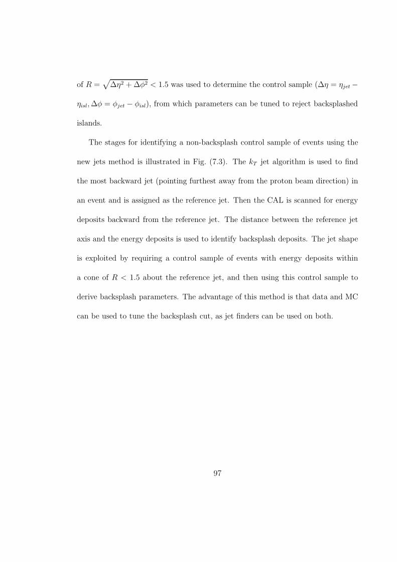
of R =√
∆η2 + ∆φ2 < 1.5 was used to determine the control sample (∆η = ηjet −
ηisl, ∆φ = φjet − φisl), from which parameters can be tuned to reject backsplashed
islands.
The stages for identifying a non-backsplash control sample of events using the
new jets method is illustrated in Fig. (7.3). The kT jet algorithm is used to find
the most backward jet (pointing furthest away from the proton beam direction) in
an event and is assigned as the reference jet. Then the CAL is scanned for energy
deposits backward from the reference jet. The distance between the reference jet
axis and the energy deposits is used to identify backsplash deposits. The jet shape
is exploited by requiring a control sample of events with energy deposits within
a cone of R < 1.5 about the reference jet, and then using this control sample to
derive backsplash parameters. The advantage of this method is that data and MC
can be used to tune the backsplash cut, as jet finders can be used on both.
97
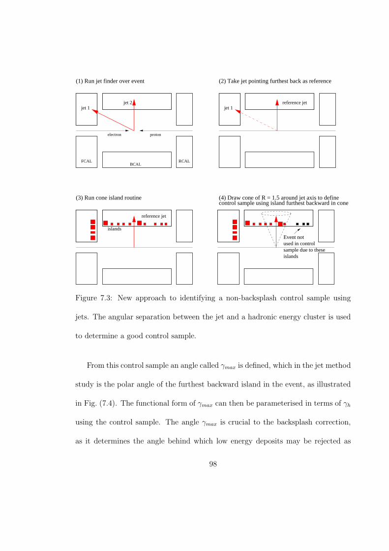
Event not
islands
used in controlsample due to these
(1) Run jet finder over event (2) Take jet pointing furthest back as reference
(3) Run cone island routine (4) Draw cone of R = 1.5 around jet axis to definecontrol sample using island furthest backward in cone
reference jet
BCAL
electron
FCAL RCAL
jet 1jet 1jet 2
proton
reference jet
islands
Figure 7.3: New approach to identifying a non-backsplash control sample using
jets. The angular separation between the jet and a hadronic energy cluster is used
to determine a good control sample.
From this control sample an angle called γmax is defined, which in the jet method
study is the polar angle of the furthest backward island in the event, as illustrated
in Fig. (7.4). The functional form of γmax can then be parameterised in terms of γh
using the control sample. The angle γmax is crucial to the backsplash correction,
as it determines the angle behind which low energy deposits may be rejected as
98

backsplash energy (away from the proton beam direction). Note that only the
islands behind the main hadronic activity are rejected, to avoid the complicated
coloured region between jets.
γmaxγh
Once control sample defined, measure hadronic angleand γmax event-by-event
Figure 7.4: Measuring γmax using the control sample. The polar angle of the most
backward island (away from the proton direction) in the control sample is identified
as γmax.
Once the γmax function in terms of γh has been determined, the backsplash cut
is then performed in the following manner,
1. Calculate the hadronic angle, γh, from all islands in the CAL
2. γmax is determined from γh (using the functional form derived from the control
sample)
3. Remove low energy islands with Eisl < 3 GeV and θisl > γmax
99

4. Repeat from step one until the difference between two successive γh values is
less than 1%
The cut of Eisl < 3 GeV was derived in the original backsplash study [62] from the
energy distribution of backsplashed islands.
7.3 Results using new jet-based approach
The new jets-based approach uses the following selection to define a control sample,
which is then used to determine the functional form of γmax.
• Jet selection: The kT clustering algorithm is used to select jets with ET,jet >
4 GeV. The jets are limited to those away from the beam-pipe holes such
that −2.5 < ηjet < 2.5. The jet with the smallest η, in other words pointing
furthest backward, is selected as the reference jet.
• Control sample selection: The angular difference in η and φ between the
reference jet and a particular island is used to determine whether the event be-
longs to the control sample. This sample is defined by ∆R =√
∆η2 + ∆φ2 <
1.5.
The γmax function for HERA II was parameterised using NC data collected from
2005 with an integrated luminosity of 122 pb−1, selected using the criteria detailed
in Chapter 8. The NC DIS MC detailed in Chapter 4 was also used to parameterise
100

γmax. Therefore two separate γmax functions can be determined for HERA II based
on data and MC simulation. Gaussian fits were made to the γmax distribution in
bins of γh to determine the functional form of γmax. The mean and spread of these
Gaussian fits were used to create the γmax vs γh plots shown in Figs. (7.5). The
data and MC show very similar distributions. The curve downwards to zero at low
γh is due to η approaching large values at small polar angles. As γh decreases, a
cone in the η−φ plane corresponds to a tighter cone in θ−φ plane. The jets method
generally predicts smaller γmax values than the original method. This indicates the
jets method predicts the hadronic particles are contained within a smaller angular
region.
To evaluate the effectiveness of the new γmax parameters, the hadronic angle
was studied when using the original or new backsplash correction, as shown in
Fig. (7.6). The MC describes the data well, though the MC slightly overshoots the
data (∼ 5%) at γh ∼ 0.5 rad.
101
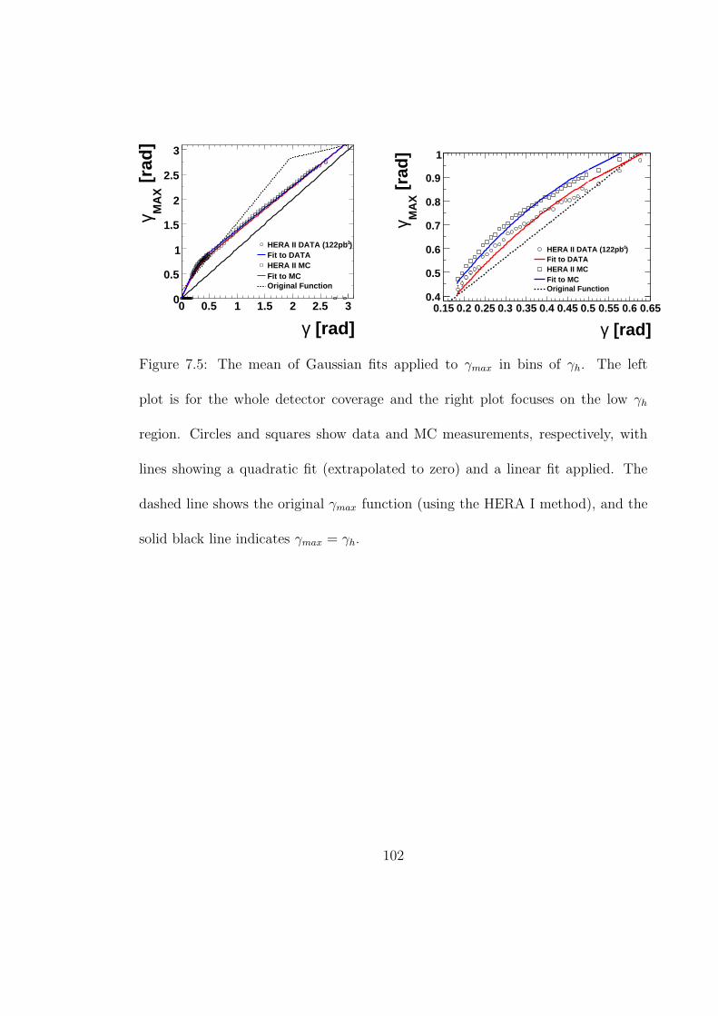
[rad]γ0 0.5 1 1.5 2 2.5 3
[ra
d]
MA
Xγ
0
0.5
1
1.5
2
2.5
3
)-1HERA II DATA (122pbFit to DATAHERA II MCFit to MCOriginal Function
[rad]γ0.15 0.2 0.25 0.3 0.35 0.4 0.45 0.5 0.55 0.6 0.65
[ra
d]
MA
Xγ
0.4
0.5
0.6
0.7
0.8
0.9
1
)-1HERA II DATA (122pbFit to DATAHERA II MCFit to MCOriginal Function
Figure 7.5: The mean of Gaussian fits applied to γmax in bins of γh. The left
plot is for the whole detector coverage and the right plot focuses on the low γh
region. Circles and squares show data and MC measurements, respectively, with
lines showing a quadratic fit (extrapolated to zero) and a linear fit applied. The
dashed line shows the original γmax function (using the HERA I method), and the
solid black line indicates γmax = γh.
102
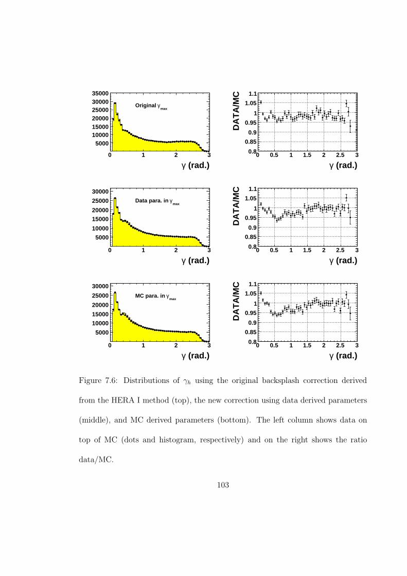
(rad.)γ0 1 2 3
5000100001500020000250003000035000
maxγOriginal
(rad.)γ0 0.5 1 1.5 2 2.5 3
DA
TA
/MC
0.8
0.85
0.9
0.95
1
1.05
1.1
(rad.)γ0 1 2 3
5000
10000
1500020000
25000
30000
maxγData para. in
(rad.)γ0 0.5 1 1.5 2 2.5 3
DA
TA
/MC
0.8
0.85
0.9
0.95
1
1.05
1.1
(rad.)γ0 1 2 3
5000
10000
15000
20000
25000
30000
maxγMC para. in
(rad.)γ0 0.5 1 1.5 2 2.5 3
DA
TA
/MC
0.8
0.85
0.9
0.95
1
1.05
1.1
Figure 7.6: Distributions of γh using the original backsplash correction derived
from the HERA I method (top), the new correction using data derived parameters
(middle), and MC derived parameters (bottom). The left column shows data on
top of MC (dots and histogram, respectively) and on the right shows the ratio
data/MC.
103

The bias and resolution of the hadronic angle is calculated using the recon-
structed and generated (true) MC variables. Figures (7.7 - 7.8) show the bias
and resolution using ∆γh = γrec − γtrue versus ytrue in fixed bins of x. Values are
compared between the old and new backsplash parameters and when using no back-
splash correction. The results show the importance of the backsplash correction,
as the bias is corrected from 0.15 rad to 0.03 rad at low y and high x. The new
γmax parameters perform similarly to the original γmax function, however the new
parameters slightly over-correct γh by ∼ 0.03 rad in the highest y bins (y > 0.9) or
very low x. This over-correction occurs as the new γmax function enforces a tighter
cut at high γh than the original parameters (see Fig. (7.5)).
A remedy for this over-correction at high y was to limit the backsplash cut to
events with γh < 90. It is the forward region that is particularly important for the
backsplash cut, as most of the hadronic material travels forward due to the high
proton beam energy. This constraint successfully fixed the over-correction problem,
however a significant drop in the γh distribution was seen at 90, corresponding
to the boundary at which the backsplash correction was switched off. This is
shown clearly in Fig. (7.9). A significant change in the shape of γh would cause
complications in calculating kinematic variables, so it was decided to close this
avenue and continue with using the backsplash correction over the entire γh region.
104
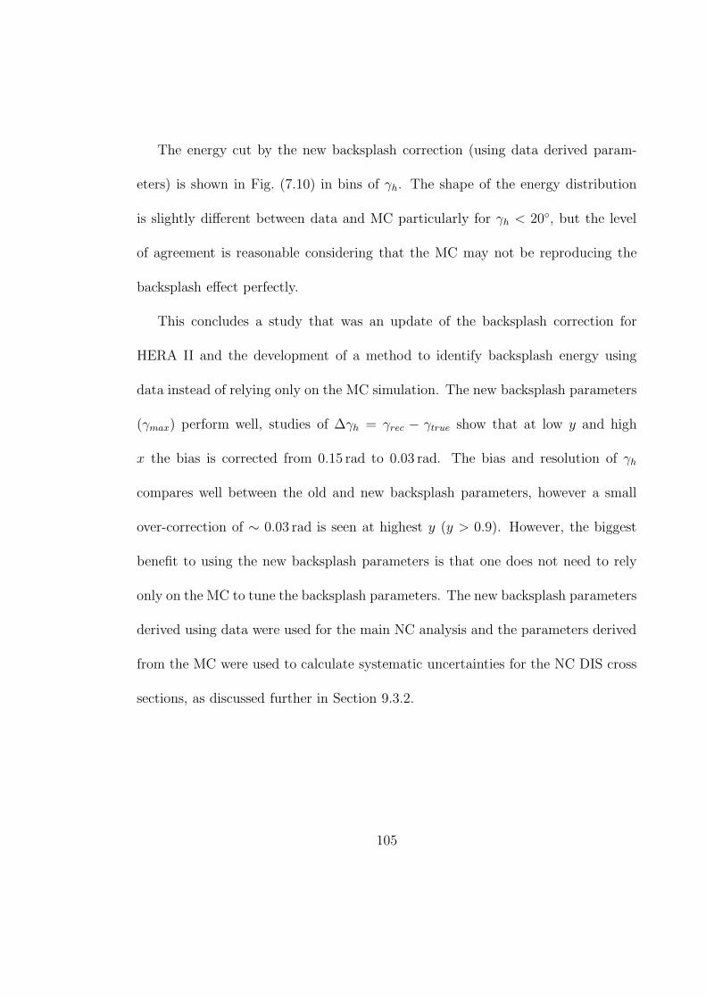
The energy cut by the new backsplash correction (using data derived param-
eters) is shown in Fig. (7.10) in bins of γh. The shape of the energy distribution
is slightly different between data and MC particularly for γh < 20, but the level
of agreement is reasonable considering that the MC may not be reproducing the
backsplash effect perfectly.
This concludes a study that was an update of the backsplash correction for
HERA II and the development of a method to identify backsplash energy using
data instead of relying only on the MC simulation. The new backsplash parameters
(γmax) perform well, studies of ∆γh = γrec − γtrue show that at low y and high
x the bias is corrected from 0.15 rad to 0.03 rad. The bias and resolution of γh
compares well between the old and new backsplash parameters, however a small
over-correction of ∼ 0.03 rad is seen at highest y (y > 0.9). However, the biggest
benefit to using the new backsplash parameters is that one does not need to rely
only on the MC to tune the backsplash parameters. The new backsplash parameters
derived using data were used for the main NC analysis and the parameters derived
from the MC were used to calculate systematic uncertainties for the NC DIS cross
sections, as discussed further in Section 9.3.2.
105
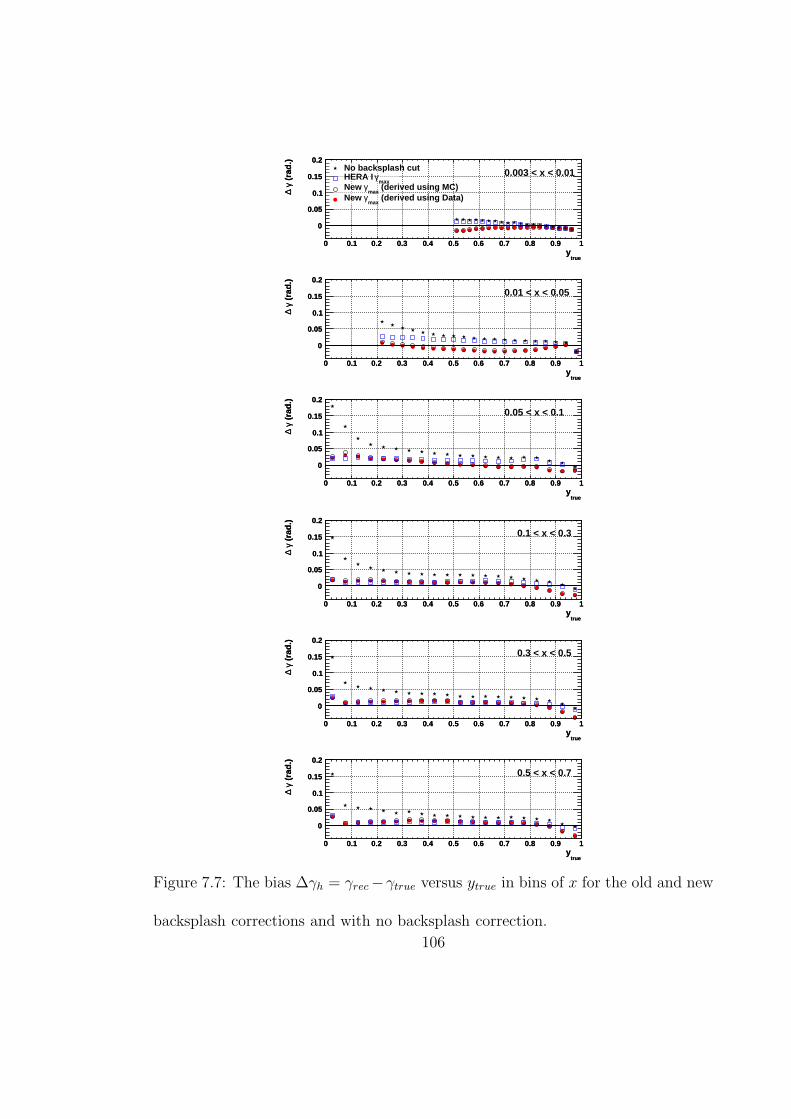
truey
0 0.1 0.2 0.3 0.4 0.5 0.6 0.7 0.8 0.9 1
(ra
d.)
γ ∆
0
0.05
0.1
0.15
0.2
0.003 < x < 0.01No backsplash cut
maxγHERA I (derived using MC)
maxγNew
(derived using Data)max
γNew
truey
0 0.1 0.2 0.3 0.4 0.5 0.6 0.7 0.8 0.9 1
(ra
d.)
γ ∆
0
0.05
0.1
0.15
0.2
truey
0 0.1 0.2 0.3 0.4 0.5 0.6 0.7 0.8 0.9 1
(ra
d.)
γ ∆
0
0.05
0.1
0.15
0.2
0.01 < x < 0.05
truey
0 0.1 0.2 0.3 0.4 0.5 0.6 0.7 0.8 0.9 1
(ra
d.)
γ ∆
0
0.05
0.1
0.15
0.2
truey
0 0.1 0.2 0.3 0.4 0.5 0.6 0.7 0.8 0.9 1
(ra
d.)
γ ∆
0
0.05
0.1
0.15
0.2
0.05 < x < 0.1
truey
0 0.1 0.2 0.3 0.4 0.5 0.6 0.7 0.8 0.9 1
(ra
d.)
γ ∆
0
0.05
0.1
0.15
0.2
truey
0 0.1 0.2 0.3 0.4 0.5 0.6 0.7 0.8 0.9 1
(ra
d.)
γ ∆
0
0.05
0.1
0.15
0.2
0.1 < x < 0.3
truey
0 0.1 0.2 0.3 0.4 0.5 0.6 0.7 0.8 0.9 1
(ra
d.)
γ ∆
0
0.05
0.1
0.15
0.2
truey
0 0.1 0.2 0.3 0.4 0.5 0.6 0.7 0.8 0.9 1
(ra
d.)
γ ∆
0
0.05
0.1
0.15
0.2
0.3 < x < 0.5
truey
0 0.1 0.2 0.3 0.4 0.5 0.6 0.7 0.8 0.9 1
(ra
d.)
γ ∆
0
0.05
0.1
0.15
0.2
truey
0 0.1 0.2 0.3 0.4 0.5 0.6 0.7 0.8 0.9 1
(ra
d.)
γ ∆
0
0.05
0.1
0.15
0.2
0.5 < x < 0.7
truey
0 0.1 0.2 0.3 0.4 0.5 0.6 0.7 0.8 0.9 1
(ra
d.)
γ ∆
0
0.05
0.1
0.15
0.2
Figure 7.7: The bias ∆γh = γrec −γtrue versus ytrue in bins of x for the old and new
backsplash corrections and with no backsplash correction.
106
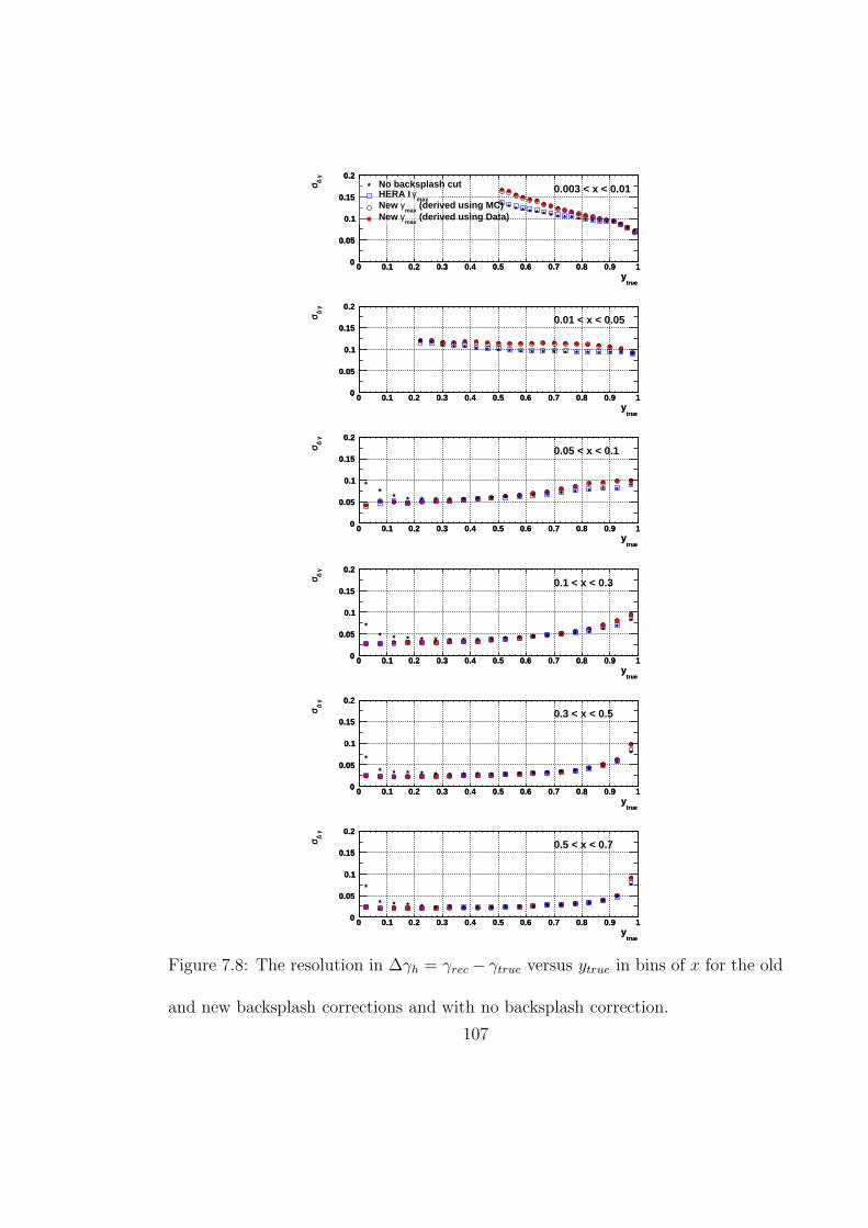
truey
0 0.1 0.2 0.3 0.4 0.5 0.6 0.7 0.8 0.9 1
γ ∆σ
0
0.05
0.1
0.15
0.2No backsplash cut
maxγHERA I (derived using MC)
maxγNew
(derived using Data)max
γNew
0.003 < x < 0.01
truey
0 0.1 0.2 0.3 0.4 0.5 0.6 0.7 0.8 0.9 1
γ ∆σ
0
0.05
0.1
0.15
0.2
truey
0 0.1 0.2 0.3 0.4 0.5 0.6 0.7 0.8 0.9 1
γ ∆σ
0
0.05
0.1
0.15
0.2
0.01 < x < 0.05
truey
0 0.1 0.2 0.3 0.4 0.5 0.6 0.7 0.8 0.9 1
γ ∆σ
0
0.05
0.1
0.15
0.2
truey
0 0.1 0.2 0.3 0.4 0.5 0.6 0.7 0.8 0.9 1
γ ∆σ
0
0.05
0.1
0.15
0.2
0.05 < x < 0.1
truey
0 0.1 0.2 0.3 0.4 0.5 0.6 0.7 0.8 0.9 1
γ ∆σ
0
0.05
0.1
0.15
0.2
truey
0 0.1 0.2 0.3 0.4 0.5 0.6 0.7 0.8 0.9 1
γ ∆σ
0
0.05
0.1
0.15
0.2
0.1 < x < 0.3
truey
0 0.1 0.2 0.3 0.4 0.5 0.6 0.7 0.8 0.9 1
γ ∆σ
0
0.05
0.1
0.15
0.2
truey
0 0.1 0.2 0.3 0.4 0.5 0.6 0.7 0.8 0.9 1
γ ∆σ
0
0.05
0.1
0.15
0.2
0.3 < x < 0.5
truey
0 0.1 0.2 0.3 0.4 0.5 0.6 0.7 0.8 0.9 1
γ ∆σ
0
0.05
0.1
0.15
0.2
truey
0 0.1 0.2 0.3 0.4 0.5 0.6 0.7 0.8 0.9 1
γ ∆σ
0
0.05
0.1
0.15
0.2
0.5 < x < 0.7
truey
0 0.1 0.2 0.3 0.4 0.5 0.6 0.7 0.8 0.9 1
γ ∆σ
0
0.05
0.1
0.15
0.2
Figure 7.8: The resolution in ∆γh = γrec − γtrue versus ytrue in bins of x for the old
and new backsplash corrections and with no backsplash correction.
107
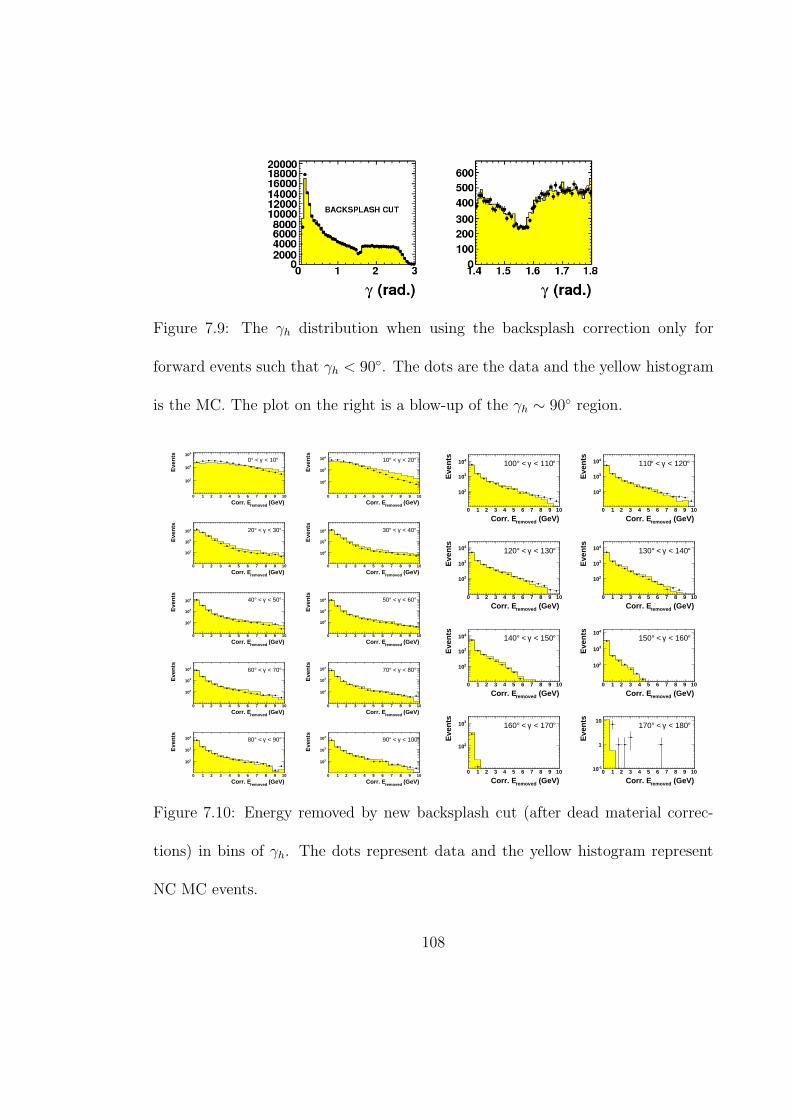
Figure 7.9: The γh distribution when using the backsplash correction only for
forward events such that γh < 90. The dots are the data and the yellow histogram
is the MC. The plot on the right is a blow-up of the γh ∼ 90 region.
(GeV)removedCorr. E0 1 2 3 4 5 6 7 8 9 10
Eve
nts
210
310
410° < 10γ < ° 0
(GeV)removedCorr. E0 1 2 3 4 5 6 7 8 9 10
Eve
nts
210
310
410 ° < 20γ < ° 10
(GeV)removedCorr. E0 1 2 3 4 5 6 7 8 9 10
Eve
nts
210
310
410 ° < 30γ < ° 20
(GeV)removedCorr. E0 1 2 3 4 5 6 7 8 9 10
Eve
nts
210
310
410 ° < 40γ < ° 30
(GeV)removedCorr. E0 1 2 3 4 5 6 7 8 9 10
Eve
nts
210
310
410 ° < 50γ < ° 40
(GeV)removedCorr. E0 1 2 3 4 5 6 7 8 9 10
Eve
nts
210
310
410 ° < 60γ < ° 50
(GeV)removedCorr. E0 1 2 3 4 5 6 7 8 9 10
Eve
nts
210
310
410 ° < 70γ < ° 60
(GeV)removedCorr. E0 1 2 3 4 5 6 7 8 9 10
Eve
nts
210
310
410 ° < 80γ < ° 70
(GeV)removedCorr. E0 1 2 3 4 5 6 7 8 9 10
Eve
nts
210
310
410 ° < 90γ < ° 80
(GeV)removedCorr. E0 1 2 3 4 5 6 7 8 9 10
Eve
nts
210
310
410 ° < 100γ < ° 90
(GeV)removedCorr. E0 1 2 3 4 5 6 7 8 9 10
Eve
nts
210
310
410 ° < 110γ < ° 100
(GeV)removedCorr. E0 1 2 3 4 5 6 7 8 9 10
Eve
nts
210
310
410 ° < 120γ < ° 110
(GeV)removedCorr. E0 1 2 3 4 5 6 7 8 9 10
Eve
nts
210
310
410 ° < 130γ < ° 120
(GeV)removedCorr. E0 1 2 3 4 5 6 7 8 9 10
Eve
nts
210
310
410 ° < 140γ < ° 130
(GeV)removedCorr. E0 1 2 3 4 5 6 7 8 9 10
Eve
nts
210
310
410 ° < 150γ < ° 140
(GeV)removedCorr. E0 1 2 3 4 5 6 7 8 9 10
Eve
nts
210
310
410° < 160γ < ° 150
(GeV)removedCorr. E0 1 2 3 4 5 6 7 8 9 10
Eve
nts
210
310 ° < 170γ < ° 160
(GeV)removedCorr. E0 1 2 3 4 5 6 7 8 9 10
Eve
nts
-110
1
10° < 180γ < ° 170
Figure 7.10: Energy removed by new backsplash cut (after dead material correc-
tions) in bins of γh. The dots represent data and the yellow histogram represent
NC MC events.
108
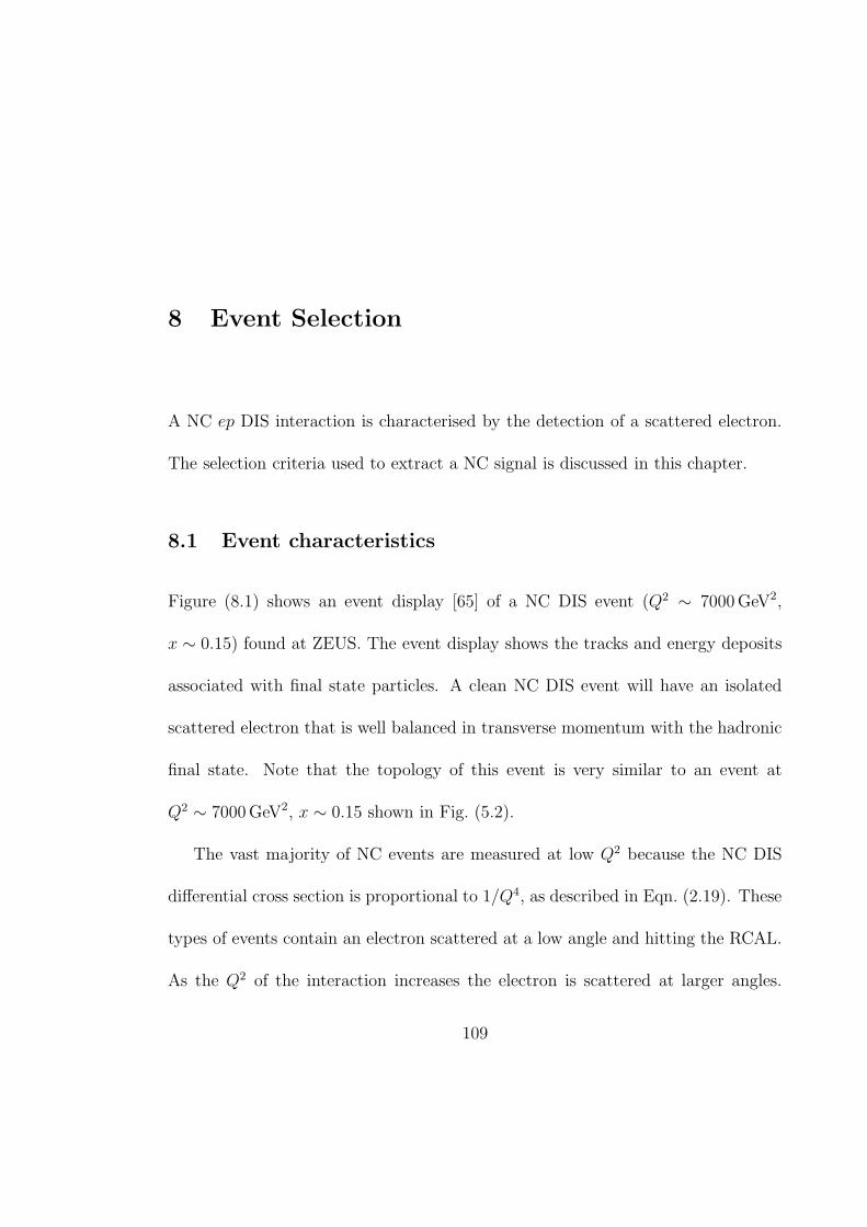
8 Event Selection
A NC ep DIS interaction is characterised by the detection of a scattered electron.
The selection criteria used to extract a NC signal is discussed in this chapter.
8.1 Event characteristics
Figure (8.1) shows an event display [65] of a NC DIS event (Q2 ∼ 7000 GeV2,
x ∼ 0.15) found at ZEUS. The event display shows the tracks and energy deposits
associated with final state particles. A clean NC DIS event will have an isolated
scattered electron that is well balanced in transverse momentum with the hadronic
final state. Note that the topology of this event is very similar to an event at
Q2 ∼ 7000 GeV2, x ∼ 0.15 shown in Fig. (5.2).
The vast majority of NC events are measured at low Q2 because the NC DIS
differential cross section is proportional to 1/Q4, as described in Eqn. (2.19). These
types of events contain an electron scattered at a low angle and hitting the RCAL.
As the Q2 of the interaction increases the electron is scattered at larger angles.
109

The higher Q2 events (Q2 & 500 GeV2) typically contain an electron found in the
BCAL. The very highest Q2 events contain an electron scattered into the FCAL.
The percentage of events selected in this analysis with a scattered electron in the
RCAL, BCAL or FCAL is shown in Table (8.1).
(a) (b)
Figure 8.1: Event display of a typical NC DIS event (Q2 ∼ 7000 GeV2, x ∼ 0.15).
Display (a) shows the x − y plane, looking through the beam-pipe, and figure (b)
shows the z − y plane with the electron (proton) coming in from the left (right).
The CAL is shown in blue and surrounds the tracking detectors, with the CTD
shown in light brown. The purple lines represent the measured particle tracks, the
blue lines are the tracks extrapolated to the CAL, and the area of the red rectangles
are proportional to the magnitude of the energy deposits measured by the CAL.
110

CAL section of Polar angle of Percentage of total
electron energy deposit scattered electron (rad.) NC DIS events
RCAL θe > 2.3 71.9%
BCAL 0.6 < θe < 2.3 27.9%
FCAL θe < 0.6 0.2%
Table 8.1: Distribution of selected events in the calorimeter. Note that a cut of
Q2 > 185 GeV2 is used to define the kinematic region of the data sample.
Events with an electron scattered into the FCAL are rare, corresponding to only
0.2% of the total NC DIS events selected in this thesis. However, these scarce events
are important to test the weak force, as the massive Z boson exchange contribution
to the NC cross section becomes significant at high Q2.
The variables used for event selection are shown in Figs. (8.2 - 8.3) and will be
described in detail throughout this chapter.
111
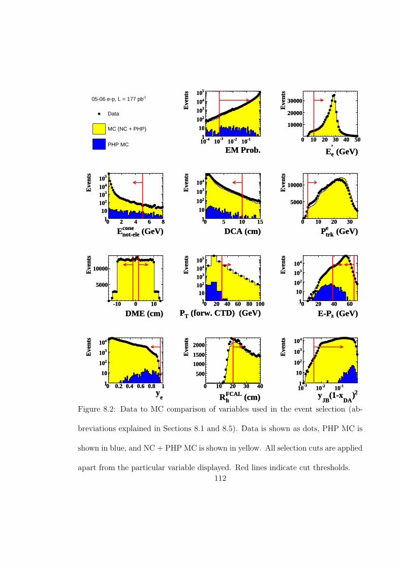
-105-06 e-p, L = 177 pb
Data
MC (NC + PHP)
PHP MCEM Prob.
-410-3
10 -210 -110
Eve
nts
1
10
210
310
410
510
EM Prob.
-410-3
10 -210 -110
Eve
nts
1
10
210
310
410
510
(GeV)e’
E
0 10 20 30 40 50
Eve
nts
10000
20000
30000
(GeV)e’
E
0 10 20 30 40 50
Eve
nts
10000
20000
30000
(GeV)not-eleconeE
0 2 4 6 8
Eve
nts
110
210
310
410
510
(GeV)not-eleconeE
0 2 4 6 8
Eve
nts
110
210
310
410
510
DCA (cm)0 5 10 15
Eve
nts
1
10
210
310
410
DCA (cm)0 5 10 15
Eve
nts
1
10
210
310
410
(GeV)trkeP
0 10 20 30
Eve
nts
5000
10000
(GeV)trkeP
0 10 20 30
Eve
nts
5000
10000
DME (cm)-10 0 10
Eve
nts
5000
10000
DME (cm)-10 0 10
Eve
nts
5000
10000
(forw. CTD) (GeV)TP0 20 40 60 80 100
Eve
nts
110
210
310
410
510
(forw. CTD) (GeV)TP0 20 40 60 80 100
Eve
nts
110
210
310
410
510
(GeV)zE-P0 20 40 60
Eve
nts
1
10
210
310
410
(GeV)zE-P0 20 40 60
Eve
nts
1
10
210
310
410
ey
0 0.2 0.4 0.6 0.8 1
Eve
nts
1
10
210
310
410
ey
0 0.2 0.4 0.6 0.8 1
Eve
nts
1
10
210
310
410
(cm)hFCALR
0 10 20 30 40
Eve
nts
500
1000
1500
2000
(cm)hFCALR
0 10 20 30 40
Eve
nts
500
1000
1500
2000
2)DA
(1-xJB
y-3
10 -210 -110
Eve
nts
1
10
210
310
410
2)DA
(1-xJB
y-3
10 -210 -110
Eve
nts
1
10
210
310
410
Figure 8.2: Data to MC comparison of variables used in the event selection (ab-
breviations explained in Sections 8.1 and 8.5). Data is shown as dots, PHP MC is
shown in blue, and NC + PHP MC is shown in yellow. All selection cuts are applied
apart from the particular variable displayed. Red lines indicate cut thresholds.
112
0
100
200
300
400
500
600
x (cm)-200 -100 0 100 200
y(cm
)
-200
-100
0
100
200
Data
0
100
200
300
400
500
600
x (cm)-200 -100 0 100 200
y (c
m)
-200
-100
0
100
200
MC
-105-06 e-p, L = 177 pb
Data
MC (NC + PHP)
PHP MC
0
1000
2000
3000
40005000
6000
7000
80009000
(GeV)TE0 20 40 60
(G
eV)
TP
0
20
40
60
Data
0
1000
2000
3000
4000
5000
6000
7000
8000
(GeV)TE0 20 40 60
(G
eV)
TP
0
20
40
60
MC
(cm)VTXZ-100 -50 0 50 100
Eve
nts
1
10
210
310
410
(cm)VTXZ-100 -50 0 50 100
Eve
nts
1
10
210
310
410
(rad)eθ0 1 2 3
Eve
nts
1
10
210
310
410
(rad)eθ0 1 2 3
Eve
nts
1
10
210
310
410
(rad)h
γ0 1 2 3
Eve
nts
10000
20000
(rad)h
γ0 1 2 3
Eve
nts
10000
20000
)2 (GeVDA2Q
310 410
Eve
nts
1
10
210
310
410
)2 (GeVDA2Q
310 410
Eve
nts
1
10
210
310
410
DAy
0 0.2 0.4 0.6 0.8 1
Eve
nts
10000
20000
30000
40000
DAy
0 0.2 0.4 0.6 0.8 1
Eve
nts
10000
20000
30000
40000
DAx-3
10 -210 -110
Eve
nts
1
10
210
310
410
DAx-3
10 -210 -110
Eve
nts
1
10
210
310
410
Figure 8.3: Data to MC comparison of variables used in the event selection (abbre-
viations explained in Sections 8.1 and 8.5). The 2D histograms are colour coded
to show the density of events. The 1D histograms show data as dots, PHP MC in
blue, and NC + PHP MC in yellow. Red lines indicate cut thresholds.
113
A useful quantity for event selection is the difference between the energy and
longitudinal momentum of all final state particles, given by
δ = (E − pz) =∑
i
(Ei − pz,i) =∑
i
Ei(1 − cos θi), (8.1)
where the sum runs over all energy deposits. The advantage of such a quantity
is that it is insensitive to objects lost down the forward beam-pipe, such as the
proton remnant. Undetected particles that escape through the forward beam-pipe
contribute little δ as the difference between the energy and longitudinal momentum
approximately cancel.
Another important quantity is the net transverse energy and momentum defined
by
ET =∑
i
Ei sin θi, (8.2)
p2T = p2
x + p2y = (
∑
i
Ei sin θi cos φi)2 + (
∑
i
Ei sin θi sin φi)2, (8.3)
where the sum runs over all energy deposits. A clean NC event should be mea-
sured with ET and pT close to zero due to energy and momentum conservation.
These quantities can be used to reject background events such as cosmic muons
penetrating the detector.
114

8.2 Background characteristics
Background events must be limited to enhance the high Q2 NC DIS signal. The
relevant types of background for this analysis are discussed in the following sections.
8.2.1 Photoproduction
Photoproduction, as discussed in Section 4.2, is defined by events with a quasi-
real photon exchanged. In a PHP event the electron is typically lost undetected
down the rear beam-pipe resulting in a δ measurement close to zero. However, in
a perfectly measured NC DIS event, where the detector covers all angular regions,
δ is equal to
E − pz ≈ Ee − (−Ee) + Ep − Ep = 2Ee = 55 GeV, (8.4)
where Ee and Ep are the initial beam energies of the electron and proton, respec-
tively. A minimum cut on δ is therefore useful for rejecting PHP events.
The PHP cross section is much larger than the high Q2 DIS signal, so a small
number of PHP events will manage to pass the NC DIS event selection. To account
for this, PHP MC events are used to estimate the number of PHP events still
remaining in the sample. This contamination is subtracted from the final number
of NC DIS data events for each cross section measurement. The PHP content is at
most 2% in the highest y bin of dσ/dy.
115
8.2.2 Beam-gas
The beam-pipe is maintained under a vacuum pressure of 0.1 nTorr (≈ 1×10⁻⁸Pa)
[66], but residual gas atoms, called beam-gas, remain in the vacuum chamber.
Beam-gas interactions with the proton or electron beam which occur before the
beams have reached the detector can be effectively rejected by the Veto Wall and
timing constraints on the calorimeter energy deposits. However due to the high
rate of beam-gas interactions, beam-gas events can occur in coincidence with an
interesting physics event. This is known as an overlaid event and usually contributes
a large E − pz. These background events can also be controlled using ET and pT
measurements, as these quantities are typically much larger than zero.
8.2.3 Halo and cosmic muons
Beam halo muons are mainly created from the decay of charged pions (π− → µνµ),
which are produced through interactions between the proton beam and material
around the beam-pipe. Cosmic muons originate from interactions between cos-
mic rays and the earth’s upper atmosphere, creating muons that penetrate mostly
through the top of the detector. Both types of background can be rejected by tim-
ing constraints on the calorimeter deposits, as these muons will not hit the opposite
ends of the detector simultaneously and are not likely to coincide (within ∼ 10 ns)
116

with a bunch crossing. These background events can also be rejected using the
imbalance in ET and pT .
8.2.4 Elastic QED Compton
QED Compton scattering refers to the process where the initial or final state elec-
tron radiates a photon (ISR and FSR, respectively). The inelastic QED Compton
scattering process, where the proton breaks up, is included in the MC simulation
and has been shown to be well understood [67]. However, it is preferable to reject
the elastic QED Compton process, ep → eγp, as it has a clean topology. The mea-
sured energy comes almost entirely from the electron and photon, and these two
objects are well balanced in φ and ET .
8.3 Data preselection
The first opportunity to select events is during actual data taking, referred to as
online event selection. A cocktail of triggers selected from the three levels are
chosen to reject background events, and enhance the NC DIS signal. Data quality
monitoring is also used to reject events recorded while problems occurred in any of
the critical detector components.
117

8.3.1 First Level Trigger
Information from the CAL (CFLT) and the CTD (CTD-FLT) are used to trigger
on interesting events. The event requirements concentrate on the summed CFLT
quantities, isolated deposits in the EMC sections, and good tracks found at the
CTD-FLT. Several vetoes are also used to reject background events. A general list
of the requirements used is shown below, with full details of the trigger slots in
Appendix B.1.
• Require one of the following energy sums, with a looser cut applied if a good
track is found at the CTD-FLT. Energy sums are defined in Fig. (B.1)
– Transverse energy (ET ) ≥ 20 GeV
– EMC energy ≥ 30 GeV
– Barrel EMC energy (BEMC) ≥ 4.8 GeV or Rear EMC energy (REMC)
≥ 3.4 GeV if a good track is found in the CTD
– Isolated EMC deposit in RCAL (> 4 GeV) or BCAL (> 3 GeV)
• Vetoes
– Timing information from components such as the Veto Wall and C5
counters should be consistent with the ep bunch crossing
118

– Beam-gas rejection by checking for tracks not emerging from the event
vertex
8.3.2 Second Level Trigger
The physics selection at the SLT is based on accepting events that appear to be
DIS with a good scattered electron candidate. High transverse energy slots are used
in parallel to accept the highest Q2 events. Timing measurements at the CAL are
used to veto background events. A general list of the requirements are listed below
with a full account of the trigger slots in Appendix B.2.
• Physics selection based on one of the following requirements
– An electron candidate with energy greater than 5 GeV, E−pz > 29 GeV
and energy deposits above 10 GeV or 2.5 GeV in the forward calorimetry
or the B/RCAL EMC sections, respectively
– A transverse energy above 35 GeV
• Vetoes
– To avoid cosmic muons, the event is rejected if the energy deposit in the
top half of the BCAL arrives more than 10 ns earlier than measurements
in the bottom BCAL half
119
– The event is vetoed due to beam-gas or halo muons if the time difference
between energy deposits in the FCAL and RCAL exceeds 8 ns, or if either
measurement is not within 8 ns of the planned ep bunch crossing
– Reject any events with a CAL spark from a faulty PMT or if the total
energy is close to zero (. 0.5 GeV)
8.3.3 Third Level Trigger
The TLT is the final step in the trigger chain and as a result has more time to
make decisions. A tracking package is implemented to give a more precise ZV TX
position, which leads to a better E − pz measurement. Electron finder algorithms
are employed to identify NC DIS events and ensure a good electron candidate is
available. Muon chambers are also used in combination with the CAL and CTD to
reject cosmic and halo muon events.
The physics selection was based upon the following requirements (slot TLT
DIS03):
• DIS FLT and SLT slots: Certain FLT and SLT slots were required to begin
a full DIS trigger chain. The FLT slots require a minimum CAL energy, an
isolated EMC deposit, or high ET . The SLT slots reinforce these requirements
and adds a minimum E − pz cut
120
• (E − pz) + 2 × ELumi−γ > 30 GeV, where ELumi−γ is the energy of a radiated
photon detected in the luminosity monitor
• E − pz < 100 GeV to reject overlaid events
• Ee > 4 GeV using either of the two electron finder algorithms available for
this slot
8.3.4 Data quality
To ensure the data was recorded reliably a logical bit called EVTAKE was used
to indicate the essential detector components were working well. This includes the
CTD, the luminosity monitor, and the CAL. Similar variables called MVDTAKE
and POLTAKE were also used to ensure that the MVD and the polarimeters were
in full working order during data taking.
8.4 Data sample
The data analysed was collected in 2005-06 and corresponds to an integrated lumi-
nosity of 177.2 pb−1. This is split between positively and negatively polarised data
as shown in Table. (8.2).
121

Data set Integrated luminosity Luminosity weighted polarisation
Total 177.2 pb−1 Pe = −0.04
Positively polarised 71.8 pb−1 Pe = +0.30
Negatively polarised 105.4 pb−1 Pe = −0.27
Table 8.2: The integrated luminosity and polarisation of the data analysed.
The integrated luminosity as a function of electron beam polarisation is dis-
played in Fig. (8.4). The run-by-run event yield is shown in Fig. (8.5), showing the
number of NC events measured divided by the luminosity. The yield is stable and
does not indicate any problems during data taking.
eP-0.6 -0.4 -0.2 0 0.2 0.4 0.6
)-1
Lu
min
osi
ty (
pb
0
2
4
6
8
10 -1Total Lumi. = 177.2 pb-1 = -0.27, Lumi. = 105.4 pbeLH data: P-1 = +0.30, Lumi. = 71.8 pbeRH data: P
Figure 8.4: The integrated luminosity of the data used in the NC e−p DIS analysis
as a function of electron longitudinal polarisation (Pe).
122
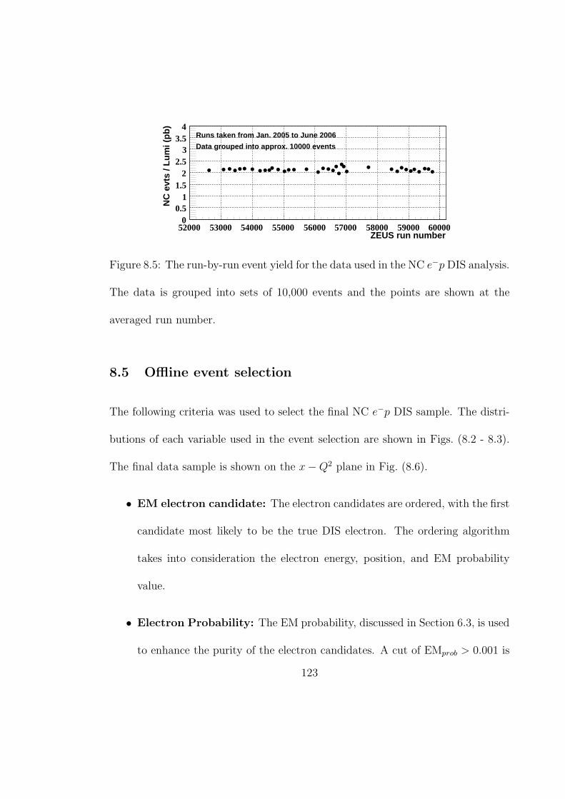
ZEUS run number52000 53000 54000 55000 56000 57000 58000 59000 60000
NC
evt
s / L
um
i (p
b)
00.5
11.5
22.5
33.5
4Runs taken from Jan. 2005 to June 2006
Data grouped into approx. 10000 events
Figure 8.5: The run-by-run event yield for the data used in the NC e−p DIS analysis.
The data is grouped into sets of 10,000 events and the points are shown at the
averaged run number.
8.5 Offline event selection
The following criteria was used to select the final NC e−p DIS sample. The distri-
butions of each variable used in the event selection are shown in Figs. (8.2 - 8.3).
The final data sample is shown on the x − Q2 plane in Fig. (8.6).
• EM electron candidate: The electron candidates are ordered, with the first
candidate most likely to be the true DIS electron. The ordering algorithm
takes into consideration the electron energy, position, and EM probability
value.
• Electron Probability: The EM probability, discussed in Section 6.3, is used
to enhance the purity of the electron candidates. A cut of EMprob > 0.001 is
123
used.
• Isolated electron: If the scattered electron is measured close to a hadronic
shower in the CAL it is difficult to determine which energy deposits belong
to the electron. This can be evaluated by checking the amount of energy
deposited close to the electron candidate, but not associated with the elec-
tron. The area close to the electron position is determined using a cone
of radius Rcone =√
(∆φ)2 + (∆η)2 = 0.8, where η is the pseudo-rapidity,
η = − ln(tan θ2). The electron is considered to be isolated if Econe
not−ele < 5 GeV.
• Electron energy: Low energy neutral pions in PHP events can decay into
photons, ‘faking’ an electron signal in the CAL. The PHP background can
be controlled by imposing a lower threshold on the electron energy (E ′e) of
10 GeV.
• Electron track inside the acceptance region of the CTD: The electron
is considered to be within the acceptance region of the CTD if the CTD
exit radius of the track is greater than 45 cm. This implies that the electron
reached at least CTD superlayer 4, ensuring a good polar angle measurement.
The following cuts were made when the electron is inside the acceptance of
the CTD,
– Track matching: The distance of closest approach (DCA) between the
124
calorimeter cluster and the endpoint of the extrapolated CTD track is
required to be less than 10 cm. This rejects events where a photon is
wrongly associated with a track in the CTD.
– Electron track momentum: A cut of ptrke > 3 GeV increases the
probability that the track belongs to the scattered electron, and not to
a low energy charged particle.
– Distance to module edge (DME): The calorimeter is divided into
modules, and energy measurements close to the module edges can be
unreliable. Therefore, events are rejected if the electron track is extrap-
olated to be within 1.5 cm of a calorimeter module edge.
• Electron forward of the acceptance region of the CTD: In this region
the CTD tracking information is not reliable, so one cannot easily distinguish
a photon from an electron. Therefore, the electron candidate transverse mo-
mentum (pT,e) is required to be above 30 GeV.
• Super-cracks: The term ’super-cracks’ refers to the edges of the BCAL next
to the RCAL and FCAL. Energy measurements are biased in these areas due
to large amounts of dead-material such as structural supports. Therefore,
the event is rejected if the scattered electron is found in the super-cracks,
corresponding to the regions -98.5 cm < ze < -104 cm and 164 cm < ze <
125
174 cm.
• Pipes in front of the RCAL: A small region of the RCAL is masked by
pipes that carry helium to and from the superconducting solenoid. This area
can be avoided by rejecting events in the RCAL where the energy cluster of
the electron candidate or the extrapolated track endpoint falls in the region
|xe| < 10 cm and ye > 10 cm.
• Radius of electron position at RCAL: Measurements from the outer
regions of the RCAL are not simulated well, as it is partially overlapped by
the BCAL. Therefore, events are rejected when the electron has been found
in the RCAL with a position radius of RRCALe =
√
x2e + y2
e > 175 cm.
• Longitudinal event vertex: Most ep collisions occur at ZV TX ≈ 0 cm, but
satellite peaks are observed in the distribution approximately 50 cm either
side of the central region. Therefore, the ZV TX distribution is restricted to a
central region of |ZV TX | < 50 cm.
• E - pz: As discussed in Section 8.2.1, a perfectly measured NC DIS event
would be measured with E−pz = 55 GeV, however PHP events are populated
at low E−pz values. Therefore, a cut of E−pz > 38 GeV is used to reject PHP
events. An upper cut of E − pz < 65 GeV is used to remove overlaid events
where the NC ep DIS interaction occurs in coincidence with a background
126
process, such as proton beam-gas interactions.
• Kinematic variable ye: When the electron candidate is detected in the
FCAL region, such that tracking is unavailable, a photon could be misiden-
tified as the scattered electron. In this case the measured energy and polar
angle would be low. This can be exploited using the kinematic variable y
reconstructed using the Electron method (ye), given by
ye = 1 − E ′e
Ee(1 − cos θ), (8.5)
which becomes large for such events. Therefore, a cut of ye < 0.95 is used to
reduce the PHP background.
• Transverse momentum balance: The transverse momentum (pT ) of a
perfectly measured NC event would be zero, but the resolution on the pT
measurement is approximately√
ET . A cut of pT√ET
< 4 GeV1/2 rejects events
with a significant imbalance in pT , usually arising from cosmic muons or beam-
gas events. At low ET , the pT√ET
quantity enters an unphysical region where
pT is larger than ET . This is accounted for by adding a cut of of pT
ET< 0.7.
• Projection of γh on to the FCAL (RFCALh ): At very low values of γh, the
energy deposits in the FCAL are usually a fraction of the actual energy of
the current jet, as much of the HFS is lost down the forward beam-hole. To
avoid this situation, events are rejected when the forward projection of the
127
hadronic angle falls within a radius of 20 cm from the centre of the forward
beam-hole.
• MC validity: The MC is not valid at very low y and high x due to missing
higher order QED corrections [68]. This kinematic region is avoided using the
cut yJB(1−xDA)2 > 0.004. The JB and DA reconstruction methods are used
as they are suitable for low y and high x events, respectively, as discussed in
Chapter 5.
• Elastic QED Compton rejection: These events are identified by finding an
electron and photon candidate in opposite regions in φ, and the two candidates
contain almost all the energy in the event, as detailed below [50]:
– |φe − φγ| > 3 rad
– 0.8 < peT /pγ
T < 1.2
– (ETotalCAL − Ee
CAL − EγCAL) < 3 GeV
where the notation e and γ refer to the electron and photon candidate.
• Kinematic region: The kinematic region is constrained using variables re-
constructed using the Double Angle method. The events are restricted to the
high Q2 region using Q2DA > 185 GeV2. A yDA < 0.9 cut is imposed to avoid
extrapolating to the full y range, otherwise correction factors of up to 10%
128
are needed due to the ye < 0.95 selection cut.
The distributions of all the variables used in the event selection is shown in
Figs. (8.2 - 8.3) for data and MC events. The MC is able to describe the data well,
which is important for the cross section extraction procedure. The calculated cross
sections are most sensitive to the variables used in the DA reconstruction method,
namely θe and γh, which are well reproduced by the MC. The small dips in the θe
distribution at approximately 2.2 rad and 0.6 rad are due to the super-crack cuts at
the BCAL boundaries with the RCAL and FCAL. These dips are propagated into
the Q2DA distribution.
The final data sample is shown on the x − Q2 plane in Fig. (8.6). The data is
mostly populated at the Q2 threshold and in the middle x region of approximately
0.01, however an impressive reach in Q2 and x is accessed. The largest momentum
transfer event selected in this analysis is Q2 ≈ 48000 GeV2 corresponding to a
spatial resolution of ∼ 9 × 10⁻¹⁹ m. An arc is noticeable on the kinematic plane
across the x range in the region Q2 . 600 GeV2 due to the super-crack cut.
129

0
20
40
60
80
100
120
140
160
180
x-310 -210 -110
)2 (
GeV
2Q
310
410
2 > 185 GeV2Qy < 0.9
> 20 cmFCALγ
R > 0.0042y(1-x)
> 10 GeVeE
2005/06 NC e-p data
Figure 8.6: Data events displayed on the x−Q2 plane after the full NC DIS selection.
The lines represent selection cuts which limit the kinematic region.
130

9 Cross section extraction and uncertainties
Experimental measurements are compared directly with theoretical predictions us-
ing cross sections. The process of calculating cross sections and the statistical and
systematic uncertainties of the final results are described in this chapter.
9.1 Cross section calculation and bin selection
A cross section bin is the interval in a particular variable in which events can be
counted. The definition of the cross section in a particular bin is given by
σ =N
L , (9.1)
where N is the number of events measured and L is the integrated luminosity of
the sample. However there are a number of corrections to be made:
1. Only a sub-sample of the total number of events can be measured due to the
geometry of detector and the selection criteria used to obtain the sample. The
acceptance correction is determined using the number of MC events generated
and measured (reconstructed) in a given bin via NgenMC/N rec
MC.
131

2. The total cross section for data and MC events includes QED radiative correc-
tions. To obtain the Born-level cross section one applies a radiative correction
σBornint /σrad
int , where the theoretical cross sections are integrated over the bin
width.
3. To measure the Born-level cross section at a particular bin-centre one applies
a bin-centring correction σBornbin−centre/σ
Bornint .
Using these corrections and the relation NgenMC/L = σrad
int , one can measure the Born-
level cross section dσ/dQ2, for example, using
(
dσ
dQ2
)measured
=Ndata − Nbg
N recMC
(
dσ
dQ2
)Born
bin-centre
, (9.2)
where Ndata, Nbg, and N recMC are the number of events measured in a certain bin
using data, background PHP MC, and NC MC, respectively.
Monte Carlo events generated (before simulating the detector response) and
reconstructed (after simulating the passage of generated events through the detec-
tor) in a given bin were used to determine whether the bin was appropriate for a
cross section measurement. Figures (9.1 (a)) and (9.1 (b)) show that the high x
and high y MC events are reconstructed (measured) at larger Q2 values than the
generated Q2 values. This is due to the selection cuts on the electron energy (E ′e),
the projection of γh on to the FCAL (RFCALh ), and the quantity y(1 − x)2. This
discrepancy between generated and measured MC events was addressed by raising
132
the measured Q2 > 185 GeV2 requirement to Q2 > 3000 GeV2 for the highest x and
y bins for the extraction of dσ/dx and dσ/dy. This ensured that the MC events
were generated and measured at comparable Q2 values.
The binning was chosen to be be proportionate to the resolutions of the kine-
matic variables [50], and to reflect the data statistical uncertainties. The bins in
σ were also chosen to be compatible with a previous NC e+p DIS measurement at
ZEUS [69] such that an extraction of the structure function xF3 was possible with-
out bin extrapolation. The suitability of the bins was investigated using variables
called efficiency, purity and acceptance defined as
Efficiency in bin i =Ngen∩rec
i
Ngeni
,
Purity in bin i =Ngen∩rec
i
N reci
,
Acceptance in bin i =Efficiency
Purity=
Ngeni
N reci
, (9.3)
where Ngen and N rec are the number of generated and reconstructed MC events in
bin i. The purity indicates the amount of migration over bin boundaries due to the
smearing of generated event variables after reconstruction. As bin widths decrease
so does the purity, as it is more likely for a generated event to be reconstructed in
a neighbouring bin. The efficiency is the fraction of events that are measured in
their true kinematic bin, and measures the suitability of the selection criteria for a
given bin. Finally, the acceptance quantifies effects such as detector geometry and
133

selection criteria, which limit the kinematic range in which cross sections can be
measured.
The efficiency, purity and acceptance for dσ/dQ2, dσ/dx, and dσ/dy are shown
in Fig. (9.2). Note that for dσ/dx and dσ/dy, the efficiency, purity and acceptance
are shown for Q2 > 185 GeV2 and Q2 > 3000 GeV2. Any bins with a very low
efficiency or purity would indicate that the binning is not suitable for a particular
kinematic region or the bin width is too small. However, the binning is shown
to be reasonable, with the purity typically above 50%, and the efficiency above
40%, dropping lower at very high x or y. The efficiency drops when the electron
is found near the boundaries between the BCAL and F/RCAL, as these events are
generated but rejected during the selection process (through the super-crack cut).
Events measured with a very low γh are rejected using the cut on the projection
of γh onto the face of the FCAL (RFCALh > 20 cm), which causes the efficiency to
drop at high x. The efficiency also drops at high y as the electron energy becomes
lower, so events are more likely to be rejected via the E ′e > 10 GeV cut.
134
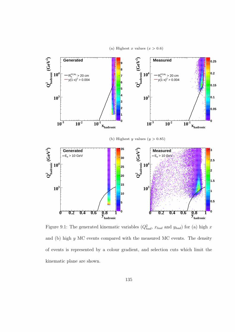
(a) Highest x values (x > 0.6)
0
1
2
3
4
5
6
7
8
9
hadronicx-310 -210 -110
)2 (
GeV
2 hadr
onic
Q
310
410 > 20 cmhFCALR
> 0.0042y(1-x)
Generated
0
0.05
0.1
0.15
0.2
0.25
hadronicx-310 -210 -110
)2 (
GeV
2 hadr
onic
Q
310
410 > 20 cmhFCALR
> 0.0042y(1-x)
Measured
(b) Highest y values (y > 0.85)
0
5
10
15
20
25
30
35
hadronicy0 0.2 0.4 0.6 0.8 1
)2 (
GeV
2 hadr
onic
Q
310
410
> 10 GeVeE
Generated
0
0.5
1
1.5
2
2.5
3
hadronicy0 0.2 0.4 0.6 0.8 1
)2 (
GeV
2 hadr
onic
Q
310
410
> 10 GeVeE
Measured
Figure 9.1: The generated kinematic variables (Q2had, xhad and yhad) for (a) high x
and (b) high y MC events compared with the measured MC events. The density
of events is represented by a colour gradient, and selection cuts which limit the
kinematic plane are shown.
135
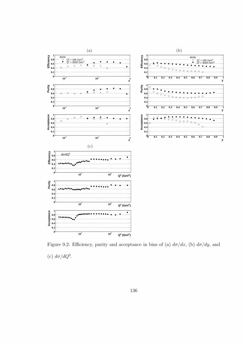
(a) (b)
x-210 -110 1
Eff
icie
ncy
0
0.2
0.4
0.6
0.8
1/dxσd
2 > 185 GeV2Q2 > 3000 GeV2Q
x-210 -110 1
Pu
rity
0
0.2
0.4
0.6
0.8
1
x-210 -110 1
Acc
epta
nce
0
0.2
0.4
0.6
0.8
1
y0 0.1 0.2 0.3 0.4 0.5 0.6 0.7 0.8 0.9 1
Eff
icie
ncy
0
0.2
0.4
0.6
0.8
1/dyσd
2 > 185 GeV2Q2 > 3000 GeV2Q
y0 0.1 0.2 0.3 0.4 0.5 0.6 0.7 0.8 0.9 1
Pu
rity
0
0.2
0.4
0.6
0.8
1
y0 0.1 0.2 0.3 0.4 0.5 0.6 0.7 0.8 0.9 1
Acc
epta
nce
0
0.2
0.4
0.6
0.8
1
(c)
)2 (GeV2Q310 410
Eff
icie
ncy
0
0.2
0.4
0.6
0.8
12/dQσd
)2 (GeV2Q310 410
Pu
rity
0
0.2
0.4
0.6
0.8
1
)2 (GeV2Q310 410
Acc
epta
nce
0
0.2
0.4
0.6
0.8
1
Figure 9.2: Efficiency, purity and acceptance in bins of (a) dσ/dx, (b) dσ/dy, and
(c) dσ/dQ2.
136
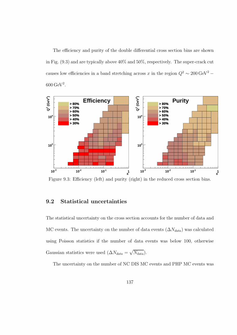
The efficiency and purity of the double differential cross section bins are shown
in Fig. (9.3) and are typically above 40% and 50%, respectively. The super-crack cut
causes low efficiencies in a band stretching across x in the region Q2 ∼ 200 GeV2 −
600 GeV2.
x-310 -210 -110 1
)2 (
GeV
2Q
310
410
Efficiency > 80% > 70% > 60% > 50% > 40% > 30%
> 80% > 70% > 60% > 50% > 40% > 30%
x-310 -210 -110 1
)2 (
GeV
2Q
310
410
Purity > 80% > 70% > 60% > 50% > 40% > 30%
> 80% > 70% > 60% > 50% > 40% > 30%
Figure 9.3: Efficiency (left) and purity (right) in the reduced cross section bins.
9.2 Statistical uncertainties
The statistical uncertainty on the cross section accounts for the number of data and
MC events. The uncertainty on the number of data events (∆Ndata) was calculated
using Poisson statistics if the number of data events was below 100, otherwise
Gaussian statistics were used (∆Ndata =√
Ndata).
The uncertainty on the number of NC DIS MC events and PHP MC events was
137

determined from the weights applied to each MC event (wi) for the normalisation
to the data integrated luminosity and the longitudinal vertex reweighting using
∆NMC =√
∑
i w2i . The uncertainty on the number of MC events was generally
insignificant.
The total statistical uncertainty (∆σstat) in a certain bin was then calculated
using
(
∆σstat
σ
)2
=
√
∆N2data + ∆N2
bg
Ndata − Nbg
2
+
(
∆N recMC
N recMC
)2
. (9.4)
The uncertainty on the number of data events for the reduced cross section bins
is shown in Fig.( 9.4). The statistical error is ∼ 1% (∼ 10, 000 events) in the lowest
Q2 bins, and grows to at most 15% (∼ 50 events) in the very high x and high Q2
bins.
138
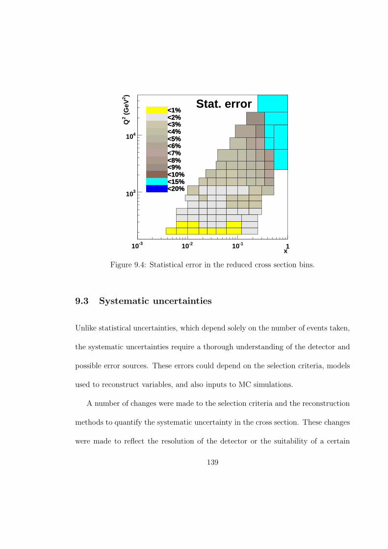
x-310 -210 -110 1
)2 (
GeV
2Q
310
410
Stat. error<1%<2%<3%<4%<5%<6%<7%<8%<9%<10%<15%<20%
<1%<2%<3%<4%<5%<6%<7%<8%<9%<10%<15%<20%
Figure 9.4: Statistical error in the reduced cross section bins.
9.3 Systematic uncertainties
Unlike statistical uncertainties, which depend solely on the number of events taken,
the systematic uncertainties require a thorough understanding of the detector and
possible error sources. These errors could depend on the selection criteria, models
used to reconstruct variables, and also inputs to MC simulations.
A number of changes were made to the selection criteria and the reconstruction
methods to quantify the systematic uncertainty in the cross section. These changes
were made to reflect the resolution of the detector or the suitability of a certain
139
reconstruction procedure (for example, an alternative parameterisation to reject
backsplash from the HFS). The particular variation to an individual selection cut
was determined from studies based on the resolution and effectiveness of the cut.
For example, the resolution on the projection of the hadronic angle onto the FCAL
is approximately 3 cm, so the RFCALh cut is varied by ±3 cm. Also, the changes
in the ye cut (ye < 0.95 to 0.9) and E − pz cut interval (varied by ±4 GeV) are
expected to alter the background contamination by approximately 10% [70].
The change in the cross section due to these individual alterations are added
in quadrature separately for the positive and negative deviations from the nom-
inal cross section value to obtain the total systematic uncertainty. Systematic
uncertainties which involve just one change, such as switching to a different elec-
tron finder algorithm, are symmetrised such that they contribute a positive and
negative deviation to the nominal cross section. The systematic uncertainties in
the single-differential cross sections and the reduced cross sections are shown in
Figs. (9.5 - 9.9) and are described in the following sections.
9.3.1 Background rejection
• Varying the E − Pz cut:
The cut interval 38 GeV < E−PZ < 65 GeV is changed by ±4 GeV to vary the
level of background contamination. This systematic error is typically within
140

1% growing to at most 3% in the highest Q2 bin in σ.
• Varying the PT /√
ET cut:
The cut PT/√
ET < 4 GeV is altered by ±1 GeV and contributes negligibly
to the systematic uncertainty.
• Varying the ye cut:
The high ye region contains PHP background events, so this cut is tightened
from ye < 0.95 to ye < 0.9 to improve the purity of DIS events. The uncer-
tainty on the cross sections is small apart from the highest y bin in dσ/dy,
where it reaches 5%.
• Varying the normalisation of the background PHP MC:
A normalisation factor of ±40% is applied to the PHP MC, determined from
MC comparisons with a PHP enriched data sample [50]. This causes at most
a 2% effect in dσ/dy at the highest y bin.
9.3.2 Electron purity and hadronic final state
• Varying the distance of closest approach cut:
The reliability of track matching is increased by tightening this cut from
DCA < 10 cm to 8 cm. The systematic uncertainty is typically within a
percent over the entire kinematic region considered.
141
• Varying the electron track momentum cut:
The cut P etrk > 3 GeV is varied by ±1 GeV, and typically changes the cross
sections by less than 1% over the whole kinematic region.
• Varying the electron isolation cut:
The isolation of the scattered electron is investigated by varying the cut
Econenot electron < 5 GeV by ±2 GeV. This systematic error is small in all kine-
matic regions except at high Q2 in dσ/dQ2 where it grows to at most 9%. The
reason for this uncertainty being large at very high Q2 is that in this kine-
matic region the electron is scattered in the forward direction (in the proton
direction) and so will be found close to the HFS.
• Varying the γh projection onto the FCAL cut:
The cut RFCALh > 20 cm is varied by ±3 cm. This variation is most relevant
to high x events where the current jet is very forward and detected close to
the FCAL beam-pipe. This leads to uncertainties growing at high x, reaching
5% in the highest x bin in dσ/dx. The reduced cross sections also show
uncertainties reaching 9% in the high x bins.
• Backsplash γmax parameter:
As discussed in Chapter 7, the γmax backsplash parameter derived using MC
events is used to determine the systematic uncertainty. The backsplash cut
142

is most sensitive to events at low γh, where the HFS is very forward, so this
systematic is largest at high x in dσ/dx and σ, reaching 5%.
• Changing electron finders (EM → SINISTRA):
The SINISTRA electron finder, described in Section 6.3, is used as an alter-
native to the EM electron finder. This systematic is generally the dominant
uncertainty in most kinematic regions, particularly at high y in dσ/dy grow-
ing to almost 20%. The SINISTRA electron finder tends to increase the
cross section value. Variables such as electron energy and electron scattering
angle are generally described well when using either EM or SINISTRA, so
this large systematic error is presently not well understood. An investigation
into the differences between the two electron finder algorithms is shown in
Appendix C.
9.3.3 Calorimeter energy and alignment
• Varying the hadronic energy scale:
The MC hadronic energy (Eh) is varied by ±1%. This variation in the
hadronic energy scale was determined from measurements of pT,h/pT,DA shown
in Fig. (6.4), and typically contributes less than one percent to the systematic
uncertainty.
143

• Varying the electron energy scale:
The MC electron energy (E ′e) is varied by ±3%, as determined from measure-
ments of E ′e/EDA [50]. The high y region is populated with events with an
electron energy close to the 10 GeV cut threshold, so a change in the elec-
tron energy scale generally effects only the high y region. It is the dominant
systematic error in dσ/dy (Q2 > 185 GeV2) at high y, growing to at most 6%.
• Varying the electron energy resolution:
The MC electron energy resolution is changed by ±3% and contributes a
negligible uncertainty over the entire kinematic region.
• Varying the electron polar angle:
The electron polar angle (θe) is varied by ±1 mrad to reflect the uncertainty
in the spatial alignment of the CAL [50]. This causes a negligible effect on
the cross sections.
144
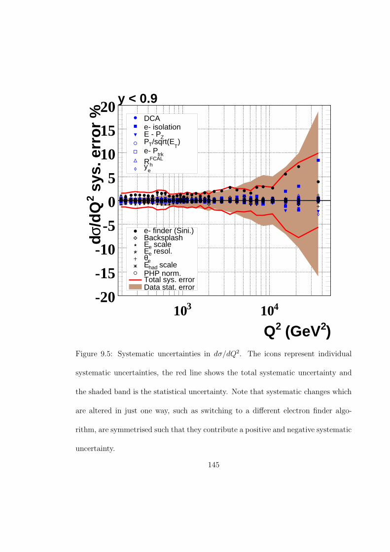
)2 (GeV2Q
310 410
sys
. err
or
%2
/dQ
σd
-20
-15
-10
-5
0
5
10
15
20DCAe- isolation
ZE - P)
T/sqrt(ETP
trke- P
hFCALR
ey
e- finder (Sini.)Backsplash
scaleeE resol.eE
eθ scalehadE
PHP norm.Total sys. errorData stat. error
y < 0.9
Figure 9.5: Systematic uncertainties in dσ/dQ2. The icons represent individual
systematic uncertainties, the red line shows the total systematic uncertainty and
the shaded band is the statistical uncertainty. Note that systematic changes which
are altered in just one way, such as switching to a different electron finder algo-
rithm, are symmetrised such that they contribute a positive and negative systematic
uncertainty.
145
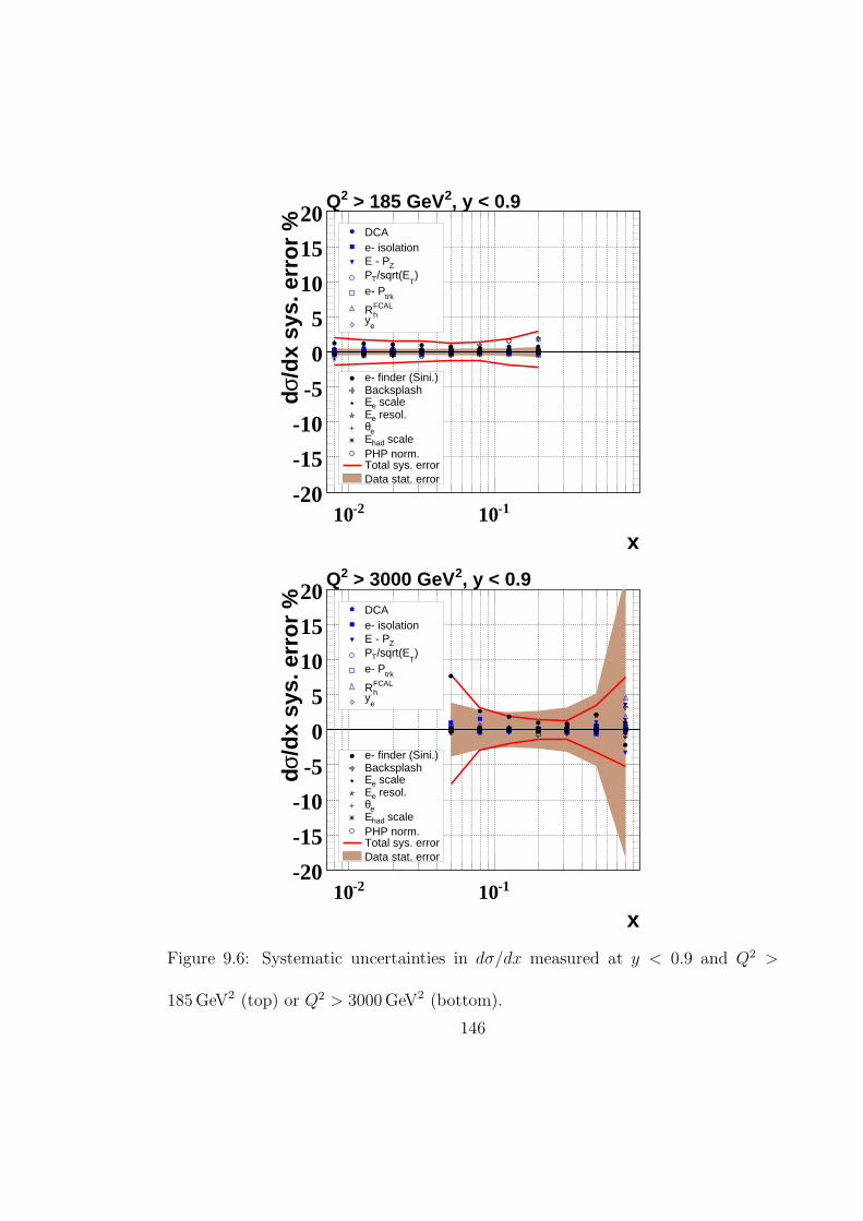
x
-210 -110
/dx
sys.
err
or
%σd
-20
-15
-10
-5
0
5
10
15
20DCAe- isolation
ZE - P)
T/sqrt(ETP
trke- P
hFCALR
ey
e- finder (Sini.)Backsplash
scaleeE resol.eE
eθ scalehadE
PHP norm.Total sys. errorData stat. error
, y < 0.92 > 185 GeV2Q
x
-210 -110
/dx
sys.
err
or
%σd
-20
-15
-10
-5
0
5
10
15
20DCAe- isolation
ZE - P)
T/sqrt(ETP
trke- P
hFCALR
ey
e- finder (Sini.)Backsplash
scaleeE resol.eE
eθ scalehadE
PHP norm.Total sys. errorData stat. error
, y < 0.92 > 3000 GeV2Q
Figure 9.6: Systematic uncertainties in dσ/dx measured at y < 0.9 and Q2 >
185 GeV2 (top) or Q2 > 3000 GeV2 (bottom).
146
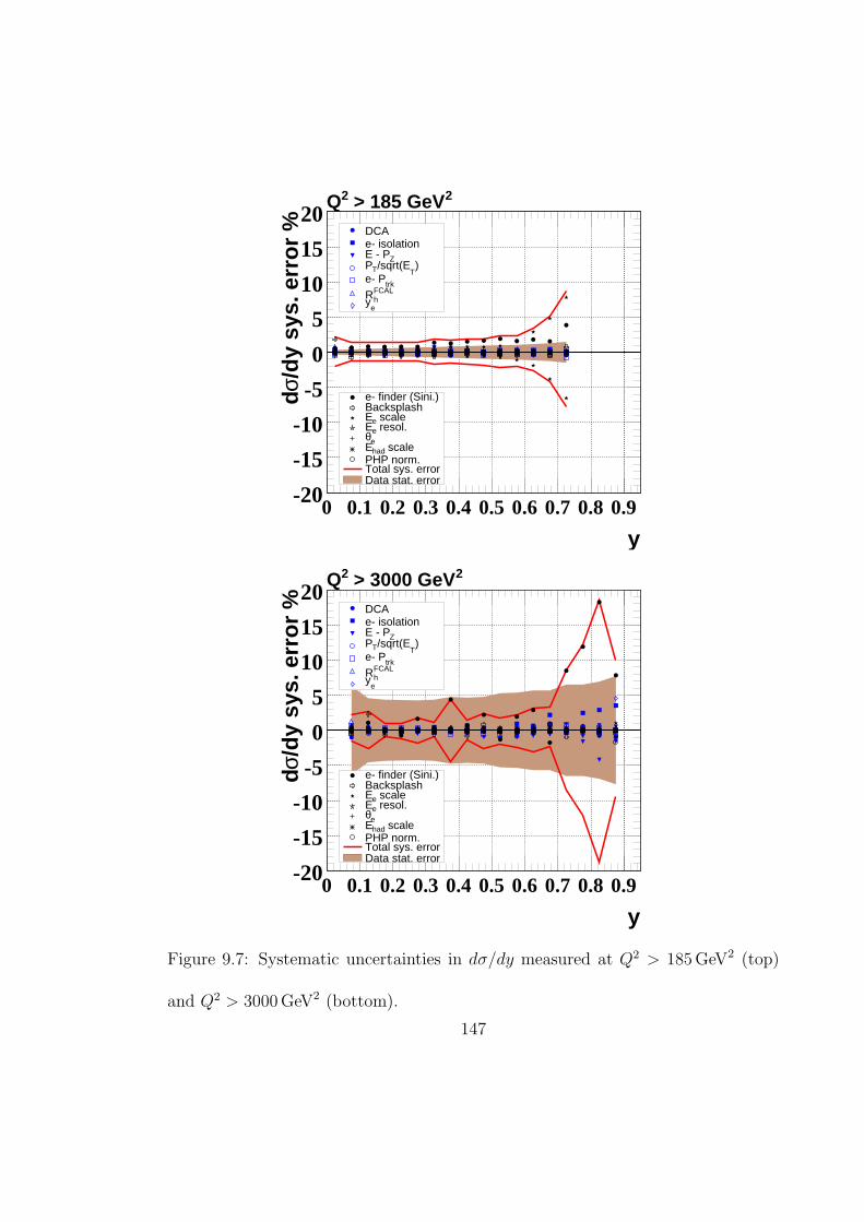
y0 0.1 0.2 0.3 0.4 0.5 0.6 0.7 0.8 0.9
/dy
sys.
err
or
%σd
-20
-15
-10
-5
0
5
10
15
20DCAe- isolation
ZE - P)
T/sqrt(ETP
trke- P
hFCALR
ey
e- finder (Sini.)Backsplash
scaleeE resol.eE
eθ scalehadE
PHP norm.Total sys. errorData stat. error
2 > 185 GeV2Q
y0 0.1 0.2 0.3 0.4 0.5 0.6 0.7 0.8 0.9
/dy
sys.
err
or
%σd
-20
-15
-10
-5
0
5
10
15
20DCAe- isolation
ZE - P)
T/sqrt(ETP
trke- P
hFCALR
ey
e- finder (Sini.)Backsplash
scaleeE resol.eE
eθ scalehadE
PHP norm.Total sys. errorData stat. error
2 > 3000 GeV2Q
Figure 9.7: Systematic uncertainties in dσ/dy measured at Q2 > 185 GeV2 (top)
and Q2 > 3000 GeV2 (bottom).
147
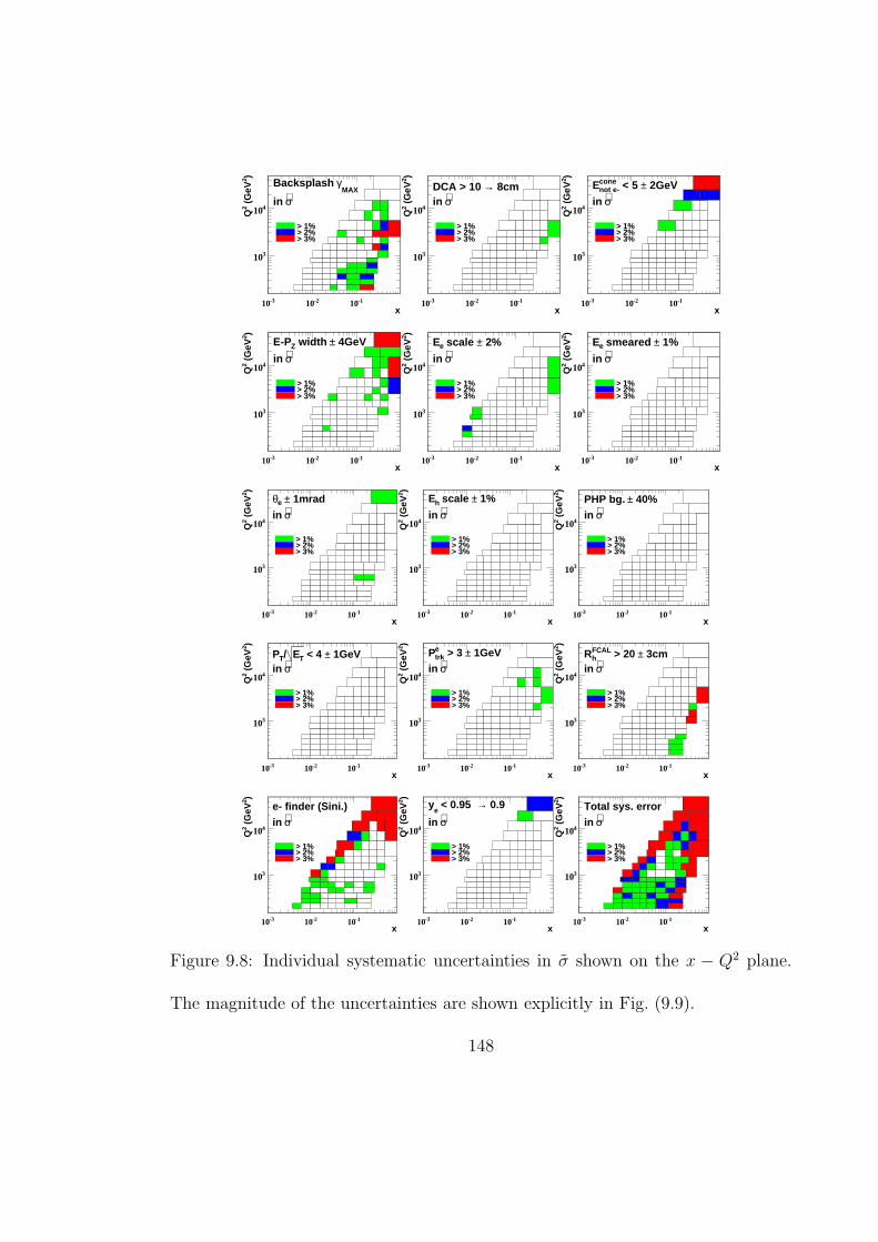
x-310 -210 -110
)2 (
GeV
2Q
310
410
> 1% > 2% > 3%
MAXγBacksplash
σ∼in
x-310 -210 -110
)2 (
GeV
2Q
310
410
> 1% > 2% > 3%
8cm→DCA > 10 σ∼in
x-310 -210 -110
)2 (
GeV
2Q
310
410
> 1% > 2% > 3%
2GeV± < 5 not e-coneEσ∼in
x-310 -210 -110
)2 (
GeV
2Q
310
410
> 1% > 2% > 3%
4GeV± width ZE-P
σ∼in
x-310 -210 -110
)2 (
GeV
2Q
310
410
> 1% > 2% > 3%
2%± scale eE
σ∼in
x-310 -210 -110
)2 (
GeV
2Q
310
410
> 1% > 2% > 3%
1%± smeared eE
σ∼in
x-310 -210 -110
)2 (
GeV
2Q
310
410
> 1% > 2% > 3%
1mrad± eθσ∼in
x-310 -210 -110
)2 (
GeV
2Q
310
410
> 1% > 2% > 3%
1%± scale hE
σ∼in
x-310 -210 -110
)2 (
GeV
2Q
310
410
> 1% > 2% > 3%
40%±PHP bg. σ∼in
x-310 -210 -110
)2 (
GeV
2Q
310
410
> 1% > 2% > 3%
1GeV± < 4 TE/TPσ∼in
x-310 -210 -110
)2 (
GeV
2Q
310
410
> 1% > 2% > 3%
1GeV± > 3 trkePσ∼in
x-310 -210 -110
)2 (
GeV
2Q
310
410
> 1% > 2% > 3%
3cm± > 20 hFCALRσ∼in
x-310 -210 -110
)2 (
GeV
2Q
310
410
> 1% > 2% > 3%
e- finder (Sini.)σ∼in
x-310 -210 -110
)2 (
GeV
2Q
310
410
> 1% > 2% > 3%
0.9→ < 0.95 e
y
σ∼in
x-310 -210 -110
)2 (
GeV
2Q
310
410
> 1% > 2% > 3%
Total sys. errorσ∼in
Figure 9.8: Individual systematic uncertainties in σ shown on the x − Q2 plane.
The magnitude of the uncertainties are shown explicitly in Fig. (9.9).
148

bin number2x-Q0 10 20 30 40 50 60 70 80 90
syst
emat
ic e
rro
r (%
)
-20
-15
-10
-5
0
5
10
15
20~ σ
DCAe- isolation
ZE-P)
T/sqrt(ETP
trke- P
hFCALR
ey
e- finder (Sini.)Backsplash
scaleeE resol.eE
eθ scalehadE
PHP norm.
Total sys. error
Data stat. error
x-310 -210 -110
)2 (
GeV
2Q
310
410
bin number scheme2x-Q
1 2 3 4 5 6 7 89 10 11 12 13 14 1516 17 18 19 20 21 2223 24 25 26 27 28 29 30
31 32 33 34 35 36 3738 39 40 41 42 43 4445 46 47 48 49 50 51 52
53 54 55 56 57 58 59 6061 62 63 64 65 66 67
68 69 70 71 72 73
75 76 77 78 79
80 81 82 83
85 86 87
88 89
90
74
84
Figure 9.9: The upper plot shows the systematic uncertainties in σ in terms of
x − Q2 bin number. The icons represent individual systematic uncertainties, and
the dashed lines show Q2 bin boundaries. The bottom plot shows the x − Q2 bin
numbering scheme (numbers 1-8 correspond to the horizontal band at lowest Q2).
Note that spikes occur in the highest x bins due to the statistical uncertainty.
149

10 Results and discussion
The main results are presented in this chapter (tabulated in Appendix E), and are
compared with the SM prediction obtained using the ZEUS-JETS PDFs. The SM
prediction is produced by extrapolating the PDFs in Q2 and combining them with
the appropriate electroweak couplings, kinematic factors, and polarisation values.
The ZEUS-JETS PDFs and the NC DIS cross section are discussed in Sections 2.2.4
and 2.4, and the details of obtaining the SM prediction can be found in [9].
10.1 Single-differential cross sections
The measurements of the single differential cross sections dσ/dQ2, dσ/dx, and
dσ/dy using the entire 2005-06 e−p data set with a residual polarisation Pe = −0.04
are shown in Fig. (10.1). The measurement of dσ/dQ2 is beautifully described by
the SM as it falls by six orders of magnitude. The precision of this measurement is
apparent by comparing with the previous results from HERA shown in Fig. (2.10).
The measurements of dσ/dx and dσ/dy are also well described by the SM, and span
150

the kinematic range of 0.00794 < x < 0.794 and 0.075 < y < 0.875.
ZEUS
)2 (GeV2Q
310 410
)2
(p
b/G
eV2
/dQ
σd
-610
-510
-410
-310
-210
-1101
10 , y < 0.92 > 185 GeV2Q
)-1p (177.2 pb-05-06 e
SM (ZEUS-JETS)
= -0.04eP
x-210 -110
/dx
(pb
)σd
310
410
510
y0.1 0.2 0.3 0.4 0.5 0.6 0.7 0.8
/dy
(pb
)σd
310
410
x-110
/dx
(pb
)σd
0
50
100
150
200
250
300
350
2 > 3000 GeV2Q
y0.1 0.2 0.3 0.4 0.5 0.6 0.7 0.8 0.9
/dy
(pb
)σd
0
20
40
60
80
2 > 3000 GeV2Q
Figure 10.1: Measurements of dσ/dQ2, dσ/dx, and dσ/dy using the entire 2005-06
e−p data set overlayed with the SM prediction calculated using ZEUS-JETS PDFs.
The inner error bars show the statistical uncertainty, while the outer bars show the
statistical and systematic uncertainties added in quadrature.
151

The ratio of the measured single differential cross sections to the SM predic-
tions are shown in Figs. (10.2) and (10.3) for the entire data set, and the neg-
atively/positively polarised data separately. The uncertainty in the SM predic-
tion is typically 1 − 2% in the kinematic region probed, and is shown in detail in
Fig. (10.11). The SM agrees with the dσ/dQ2, dσ/dx and dσ/dy measurements
typically within 5%. The fluctuations in dσ/dQ2 are generally within statistical
and systematic uncertainties, whereas the discrepancies in dσ/dx and dσ/dy at
Q2 > 185 GeV2 suggest a certain trend. The dσ/dx measurement at Q2 > 185 GeV2
tends to dip below the SM prediction by 5% in the middle x region (x ∼ 0.03),
which is also seen in the low y region in dσ/dy measured at Q2 > 185 GeV2. The
cross sections are extracted using the Double Angle (DA) method described in
Chapter 5, so the cross sections are most sensitive to the angles of the electron
and hadronic system (θe and γh). To test whether the discrepancy between the
measurements and the SM prediction is due to a bias in reconstruction of γh, the
cross sections were re-calculated using only information from the electron via the
Electron reconstruction method. The results are presented in Appendix D, and
show that the differences between the measured cross sections and the SM predic-
tion using the Electron method are of a similar shape and magnitude to the DA
method.
152
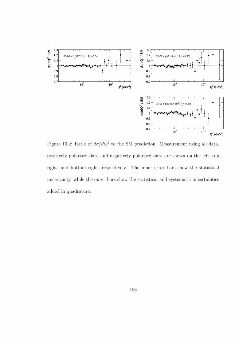
)2 (GeV2Q310 410
/ S
M2
/dQ
σd
0.7
0.8
0.9
1
1.1
1.2
1.3
=-0.04)e
, P-1p (177.2 pb-05-06 e
)2 (GeV2Q310 410
/ S
M2
/dQ
σd
0.7
0.8
0.9
1
1.1
1.2
1.3
=+0.30)e
, P-1p (71.8 pb-05-06 e
)2 (GeV2Q310 410
/ S
M2
/dQ
σd
0.7
0.8
0.9
1
1.1
1.2
1.3
=-0.27)e
, P-1p (105.4 pb-05-06 e
Figure 10.2: Ratio of dσ/dQ2 to the SM prediction. Measurement using all data,
positively polarised data and negatively polarised data are shown on the left, top
right, and bottom right, respectively. The inner error bars show the statistical
uncertainty, while the outer bars show the statistical and systematic uncertainties
added in quadrature.
153
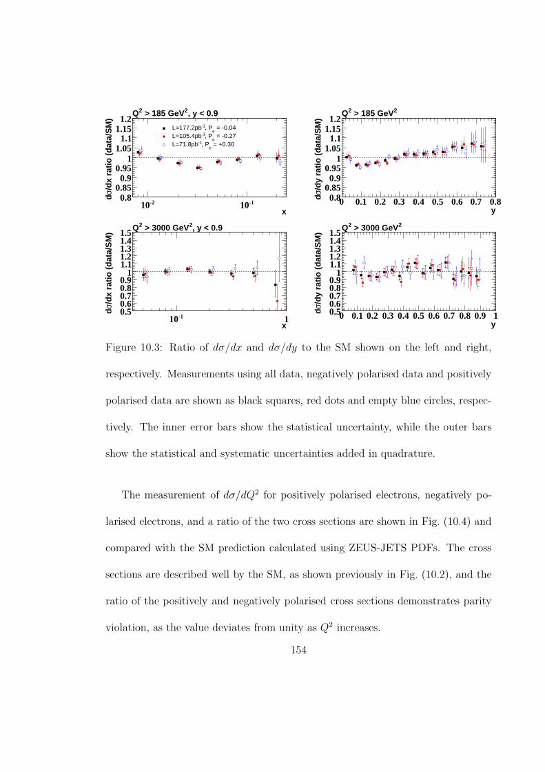
x-210 -110
/dx
rati
o (
dat
a/S
M)
σd 0.80.850.9
0.951
1.051.1
1.151.2
, y < 0.92 > 185 GeV2Q
= -0.04e
, P-1L=177.2pb = -0.27
e, P-1L=105.4pb
= +0.30e
, P-1L=71.8pb
y0 0.1 0.2 0.3 0.4 0.5 0.6 0.7 0.8
/dy
rati
o (
dat
a/S
M)
σd 0.80.850.9
0.951
1.051.1
1.151.2
2 > 185 GeV2Q
x-110 1
/dx
rati
o (
dat
a/S
M)
σd 0.50.60.70.80.9
11.11.21.31.41.5
, y < 0.92 > 3000 GeV2Q
y0 0.1 0.2 0.3 0.4 0.5 0.6 0.7 0.8 0.9 1
/dy
rati
o (
dat
a/S
M)
σd 0.50.60.70.80.9
11.11.21.31.41.5
2 > 3000 GeV2Q
Figure 10.3: Ratio of dσ/dx and dσ/dy to the SM shown on the left and right,
respectively. Measurements using all data, negatively polarised data and positively
polarised data are shown as black squares, red dots and empty blue circles, respec-
tively. The inner error bars show the statistical uncertainty, while the outer bars
show the statistical and systematic uncertainties added in quadrature.
The measurement of dσ/dQ2 for positively polarised electrons, negatively po-
larised electrons, and a ratio of the two cross sections are shown in Fig. (10.4) and
compared with the SM prediction calculated using ZEUS-JETS PDFs. The cross
sections are described well by the SM, as shown previously in Fig. (10.2), and the
ratio of the positively and negatively polarised cross sections demonstrates parity
violation, as the value deviates from unity as Q2 increases.
154
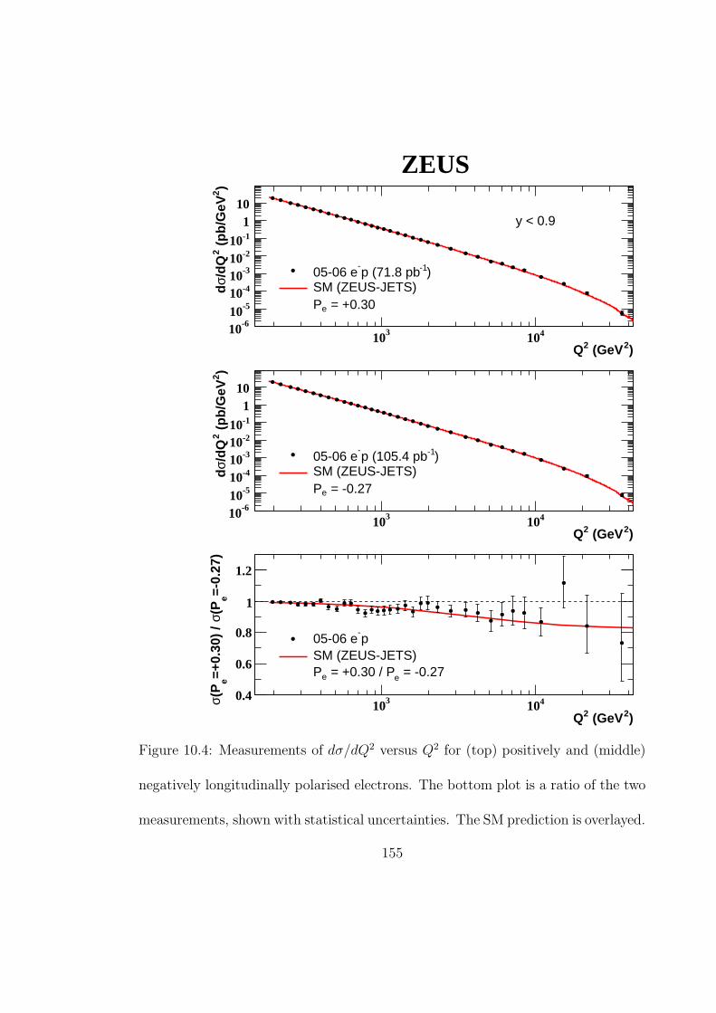
ZEUS
)2 (GeV2Q310 410
)2
(p
b/G
eV2
/dQ
σd
-610
-510
-410
-310
-210
-110
110
y < 0.9
)-1p (71.8 pb-
05-06 eSM (ZEUS-JETS)
= +0.30eP
)2 (GeV2Q310 410
)2 (
pb
/GeV
2/d
Qσ
d
-610
-510
-410
-310
-210
-110
110
)-1p (105.4 pb-
05-06 eSM (ZEUS-JETS)
= -0.27eP
)2 (GeV2Q310 410
=-0.
27)
e(Pσ
=+0.
30)
/ e
(Pσ 0.4
0.6
0.8
1
1.2
p-
05-06 eSM (ZEUS-JETS)
= -0.27e = +0.30 / PeP
Figure 10.4: Measurements of dσ/dQ2 versus Q2 for (top) positively and (middle)
negatively longitudinally polarised electrons. The bottom plot is a ratio of the two
measurements, shown with statistical uncertainties. The SM prediction is overlayed.
155

Parity violation is also clearly observed in the polarisation asymmetry (A−)
measurement shown in Fig. (10.5), where the asymmetry is defined by inserting the
appropriate dσ/dQ2 measurements into Eqn. (2.27). Note that the Q2 bin widths
were increased to lower the statistical uncertainties on each measured point. The
level of agreement between A− and the predicted value can be quantified via a χ2
test, defined using [71]
χ2 =∑
bins
(
measured value − expected value
uncertainty on measurement
)2
. (10.1)
The expected values for the asymmetry measurement were chosen to be either the
SM prediction or zero (in the case of no parity violation). The χ2 value divided
by the number of degrees of freedom (ndf) is shown in Fig. (10.6) versus the Q2
threshold. At Q2 > 1000 GeV2, χ2/ndf = 4.2 for the asymmetry = 0 case, and
χ2/ndf = 1.1 when using the SM prediction. The expected value of χ2 is the
ndf , so the measurements support the SM prediction of parity violation. This is
quantified further by using the probability of the χ2 distribution [71]
Pndf(χ2 > c), (10.2)
where the probability Pndf is for χ2 to be above a certain value (c) for a given ndf .
This probability is shown in Fig. (10.6) versus the Q2 threshold. The probability
for the asymmetry = 0 case at Q2 > 1000 GeV2 is 2 × 10⁻⁴, which supports the
evidence of parity violation.
156
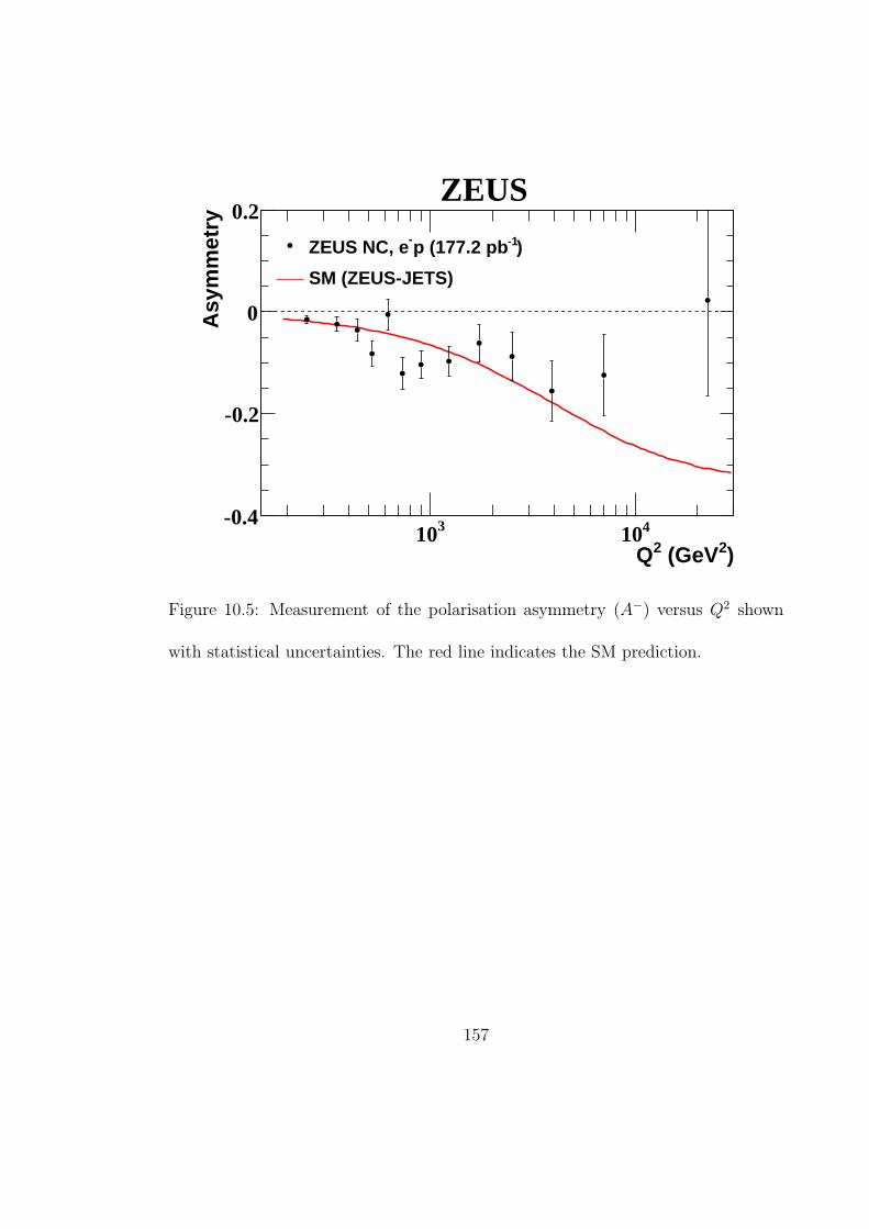
ZEUS
)2 (GeV2Q310 410
Asy
mm
etry
-0.4
-0.2
0
0.2
)-1p (177.2 pb-ZEUS NC, e
SM (ZEUS-JETS)
Figure 10.5: Measurement of the polarisation asymmetry (A−) versus Q2 shown
with statistical uncertainties. The red line indicates the SM prediction.
157
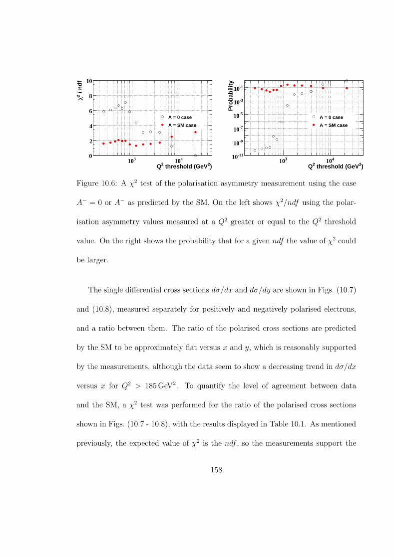
)2 threshold (GeV2Q310 410
/ n
df
2 χ
0
2
4
6
8
10
A = 0 case
A = SM case
)2 threshold (GeV2Q310 410
Pro
bab
ility
-1110
-910
-710
-510
-310
-110
A = 0 case
A = SM case
Figure 10.6: A χ2 test of the polarisation asymmetry measurement using the case
A− = 0 or A− as predicted by the SM. On the left shows χ2/ndf using the polar-
isation asymmetry values measured at a Q2 greater or equal to the Q2 threshold
value. On the right shows the probability that for a given ndf the value of χ2 could
be larger.
The single differential cross sections dσ/dx and dσ/dy are shown in Figs. (10.7)
and (10.8), measured separately for positively and negatively polarised electrons,
and a ratio between them. The ratio of the polarised cross sections are predicted
by the SM to be approximately flat versus x and y, which is reasonably supported
by the measurements, although the data seem to show a decreasing trend in dσ/dx
versus x for Q2 > 185 GeV2. To quantify the level of agreement between data
and the SM, a χ2 test was performed for the ratio of the polarised cross sections
shown in Figs. (10.7 - 10.8), with the results displayed in Table 10.1. As mentioned
previously, the expected value of χ2 is the ndf , so the measurements support the
158
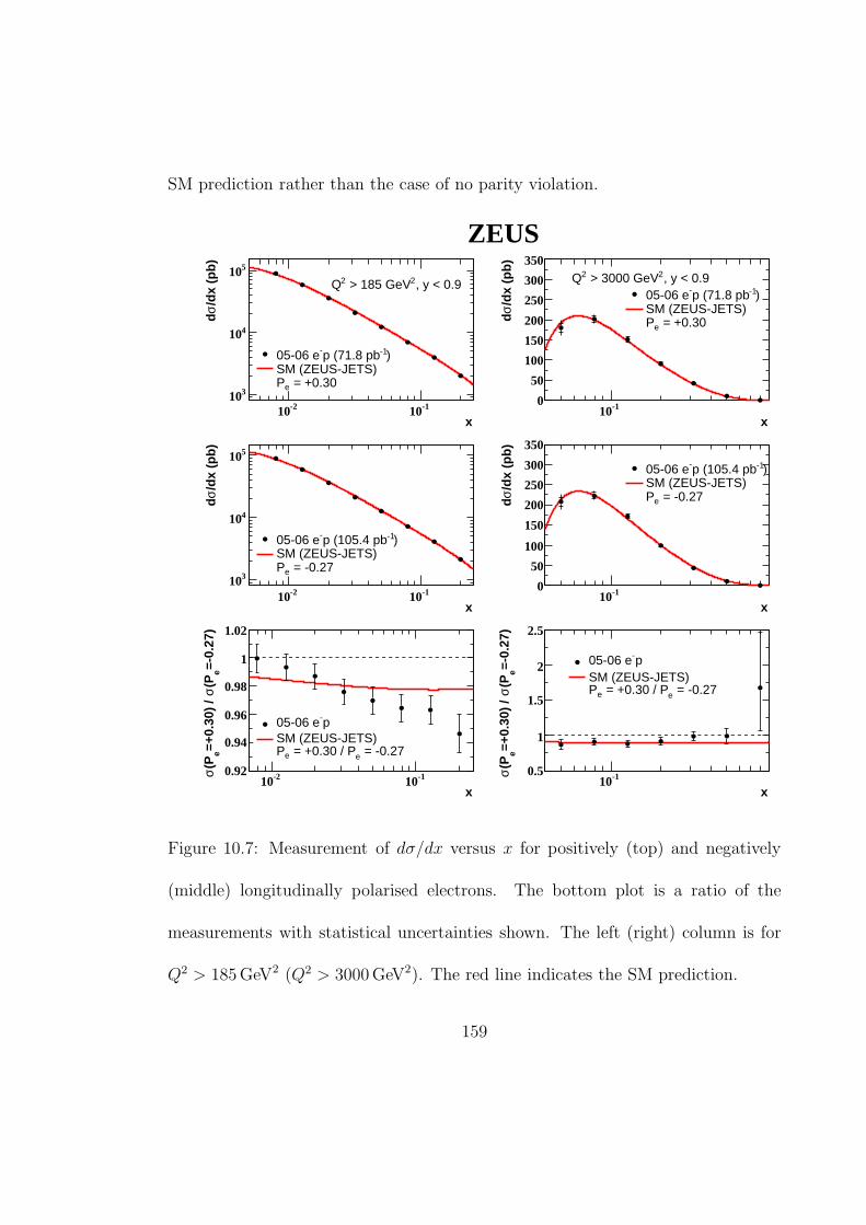
SM prediction rather than the case of no parity violation.
ZEUS
x-210 -110
/dx
(pb
)σd
310
410
510, y < 0.92 > 185 GeV2Q
)-1p (71.8 pb-05-06 eSM (ZEUS-JETS)
= +0.30eP
x-110
/dx
(pb
)σd
0
50
100
150
200
250
300
350, y < 0.92 > 3000 GeV2Q
)-1p (71.8 pb-05-06 eSM (ZEUS-JETS)
= +0.30eP
x-210 -110
/dx
(pb
)σd
310
410
510
)-1p (105.4 pb-05-06 eSM (ZEUS-JETS)
= -0.27eP
x-110
/dx
(pb
)σd
0
50
100
150
200
250
300
350
)-1p (105.4 pb-05-06 eSM (ZEUS-JETS)
= -0.27eP
x-210 -110
=-0.
27)
e(P
σ=+
0.30
) /
e(P
σ 0.92
0.94
0.96
0.98
1
1.02
p-05-06 eSM (ZEUS-JETS)
= -0.27e = +0.30 / PeP
x-110
=-0.
27)
e(P
σ=+
0.30
) /
e(P
σ 0.5
1
1.5
2
2.5
p-05-06 eSM (ZEUS-JETS)
= -0.27e = +0.30 / PeP
Figure 10.7: Measurement of dσ/dx versus x for positively (top) and negatively
(middle) longitudinally polarised electrons. The bottom plot is a ratio of the
measurements with statistical uncertainties shown. The left (right) column is for
Q2 > 185 GeV2 (Q2 > 3000 GeV2). The red line indicates the SM prediction.
159

ZEUS
y0.1 0.2 0.3 0.4 0.5 0.6 0.7 0.8
/dy
(pb
)σd
310
4102 > 185 GeV2Q
)-1p (71.8 pb-05-06 eSM (ZEUS-JETS)
= +0.30eP
y0.1 0.2 0.3 0.4 0.5 0.6 0.7 0.8 0.9
/dy
(pb
)σd
0
20
40
60
80
2 > 3000 GeV2Q
)-1p (71.8 pb-05-06 eSM (ZEUS-JETS)
= +0.30eP
y0.1 0.2 0.3 0.4 0.5 0.6 0.7 0.8
/dy
(pb
)σd
310
410 )-1p (105.4 pb-05-06 eSM (ZEUS-JETS)
= -0.27eP
y0.1 0.2 0.3 0.4 0.5 0.6 0.7 0.8 0.9
/dy
(pb
)σd
0
20
40
60
80
)-1p (105.4 pb-05-06 eSM (ZEUS-JETS)
= -0.27eP
y0.1 0.2 0.3 0.4 0.5 0.6 0.7 0.8
=-0.
27)
e(P
σ=+
0.30
) /
e(P
σ 0.85
0.9
0.95
1
1.05
p-05-06 eSM (ZEUS-JETS)
= -0.27e = +0.30 / PeP
y0.1 0.2 0.3 0.4 0.5 0.6 0.7 0.8 0.9
=-0.
27)
e(P
σ=+
0.30
) /
e(P
σ 0.6
0.8
1
1.2
1.4 p-05-06 eSM (ZEUS-JETS)
= -0.27e = +0.30 / PeP
Figure 10.8: Measurement of dσ/dy versus y for positively (top) and negatively
(middle) longitudinally polarised electrons. The bottom plot is a ratio of the
measurements with statistical uncertainties shown. The left (right) column is for
Q2 > 185 GeV2 (Q2 > 3000 GeV2). The red line indicates the SM prediction.
160
Measurement Q2 cut χ2/number of degrees of freedom
(ratio of polarised cross sections) ( GeV2) SM prediction Unity
dσ/dx 185 13.5 / 8 61.7 / 8
3000 5.1 / 7 17.2 / 7
dσ/dy 185 26.3 / 15 62.9 / 15
3000 14.2 / 17 30.5 / 17
Table 10.1: A χ2 test of the ratio of the polarised dσ/dx and dσ/dy cross sections
for Q2 > 185 GeV2 and Q2 > 3000 GeV2 (lower plots in Figs. (10.7 - 10.8)). The
expected value was taken as the SM prediction or unity (in the case of no parity
violation).
10.2 Reduced cross sections
The reduced cross section is defined as the double differential cross section with
respect to Q2 and x divided by kinematic terms, as shown in Eqn. (2.23), such that
the contributions of the structure functions is apparent:
σe±p = F2(x, Q2) ∓ Y−
Y+
xF3(x, Q2) − y2
Y+
FL(x, Q2). (10.3)
The reduced cross section measured using negatively and positively polarised elec-
tron data is shown in Fig. (10.9) versus x in fixed bins of Q2. The measurements are
161
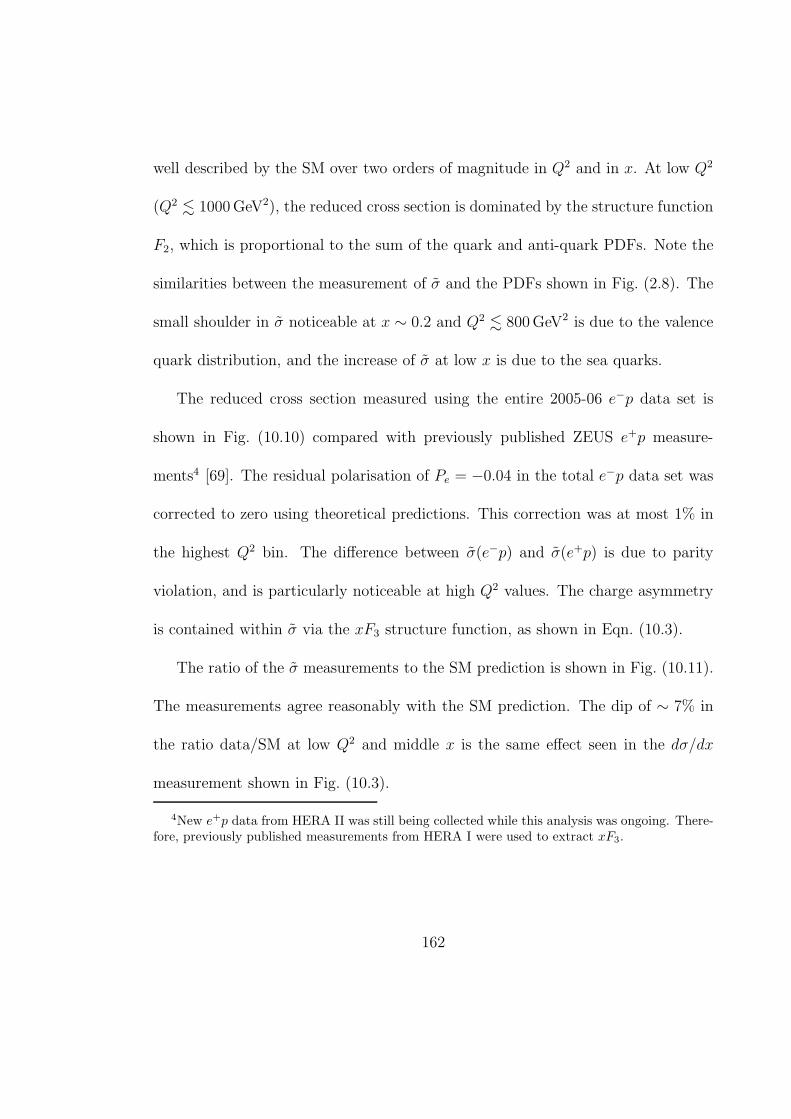
well described by the SM over two orders of magnitude in Q2 and in x. At low Q2
(Q2 . 1000 GeV2), the reduced cross section is dominated by the structure function
F2, which is proportional to the sum of the quark and anti-quark PDFs. Note the
similarities between the measurement of σ and the PDFs shown in Fig. (2.8). The
small shoulder in σ noticeable at x ∼ 0.2 and Q2 . 800 GeV2 is due to the valence
quark distribution, and the increase of σ at low x is due to the sea quarks.
The reduced cross section measured using the entire 2005-06 e−p data set is
shown in Fig. (10.10) compared with previously published ZEUS e+p measure-
ments4 [69]. The residual polarisation of Pe = −0.04 in the total e−p data set was
corrected to zero using theoretical predictions. This correction was at most 1% in
the highest Q2 bin. The difference between σ(e−p) and σ(e+p) is due to parity
violation, and is particularly noticeable at high Q2 values. The charge asymmetry
is contained within σ via the xF3 structure function, as shown in Eqn. (10.3).
The ratio of the σ measurements to the SM prediction is shown in Fig. (10.11).
The measurements agree reasonably with the SM prediction. The dip of ∼ 7% in
the ratio data/SM at low Q2 and middle x is the same effect seen in the dσ/dx
measurement shown in Fig. (10.3).
4New e+p data from HERA II was still being collected while this analysis was ongoing. There-fore, previously published measurements from HERA I were used to extract xF3.
162
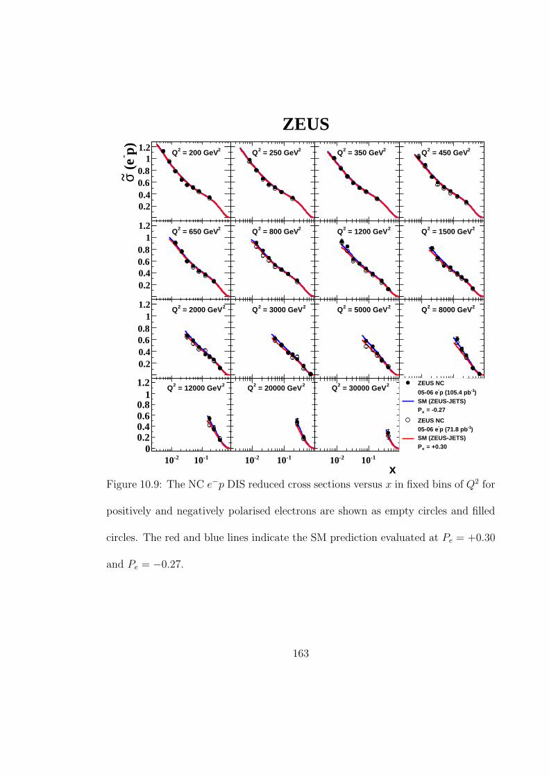
ZEUS
0.20.40.60.8
11.2 2 = 200 GeV2Q
0.20.40.60.8
11.2 2 = 650 GeV2Q
0.20.40.60.8
11.2 2 = 2000 GeV2Q
-210 -1100
0.20.40.60.8
11.2 2 = 12000 GeV2Q
2 = 250 GeV2Q
2 = 800 GeV2Q
2 = 3000 GeV2Q
-210 -110
2 = 20000 GeV2Q
2 = 350 GeV2Q
2 = 1200 GeV2Q
2 = 5000 GeV2Q
-210 -110
2 = 30000 GeV2Q
x
2 = 450 GeV2Q
2 = 1500 GeV2Q
2 = 8000 GeV2Q
ZEUS NC
)-1p (105.4 pb- 05-06 e SM (ZEUS-JETS)
= -0.27e P
ZEUS NC)-1p (71.8 pb- 05-06 e
SM (ZEUS-JETS) = +0.30e P
p)- (
eσ~
Figure 10.9: The NC e−p DIS reduced cross sections versus x in fixed bins of Q2 for
positively and negatively polarised electrons are shown as empty circles and filled
circles. The red and blue lines indicate the SM prediction evaluated at Pe = +0.30
and Pe = −0.27.
163
ZEUS
0.20.40.60.8
11.2 2 = 200 GeV2Q
0.20.40.60.8
11.2 2 = 650 GeV2Q
0.20.40.60.8
11.2 2 = 2000 GeV2Q
-210 -1100
0.20.40.60.8
11.2 2 = 12000 GeV2Q
2 = 250 GeV2Q
2 = 800 GeV2Q
2 = 3000 GeV2Q
-210 -110
2 = 20000 GeV2Q
2 = 350 GeV2Q
2 = 1200 GeV2Q
2 = 5000 GeV2Q
-210 -110
2 = 30000 GeV2Q
x
2 = 450 GeV2Q
2 = 1500 GeV2Q
2 = 8000 GeV2Q
ZEUS NC
)-1p (177.2 pb- 05-06 e SM (ZEUS-JETS)
= 0e P
ZEUS NC)-1p (63.2 pb+ 99-00 e
SM (ZEUS-JETS) = 0e P
p)± (
eσ~
Figure 10.10: The unpolarised NC e±p DIS reduced cross sections versus x in
fixed bins of Q2 for the total e−p data set (filled circles) compared with previously
published NC e+p cross sections (empty circles). The red and blue lines indicate
the SM prediction for e+p and e−p scattering.
164

0.8
1
1.2
1.4 2 = 200 GeV2Q
p) /
SM-
(e
σ~ 0.8
1
1.2
1.4
0.8
1
1.2
1.4 2 = 650 GeV2Q
0.8
1
1.2
1.4
0.6
0.8
1
1.2
1.4 2 = 2000 GeV2Q
0.6
0.8
1
1.2
1.4
-210 -1100.6
0.8
1
1.2
1.4 2 = 12000 GeV2Q
-210 -1100.6
0.8
1
1.2
1.4
2 = 250 GeV2Q
2 = 800 GeV2Q
2 = 3000 GeV2Q
-210 -110
2 = 20000 GeV2Q
-210 -110
2 = 350 GeV2Q
2 = 1200 GeV2Q
2 = 5000 GeV2Q
-210 -110
2 = 30000 GeV2Q
x-210 -110
2 = 450 GeV2Q
2 = 1500 GeV2Q
2 = 8000 GeV2Q
)-1p (177.2 pb- 05-06 e
= 0e P
)-1p (105.4 pb- 05-06 e
= -0.27e P
)-1p (71.8 pb- 05-06 e
= +0.30e P
SM uncertainty
Figure 10.11: Reduced cross sections divided by the SM prediction as a function
of x in fixed bins of Q2. Measurements using all data, negatively polarised data
and positively polarised data are shown as black squares, red dots and empty blue
circles, respectively. The shaded band corresponds to the uncertainty on the SM
prediction generated using ZEUS-JETS PDFs.
165
10.3 The structure functions xF3 and xF γZ3
The structure function xF3 is extracted by taking the difference of the σ(e−p) and
σ(e+p) measurements, as shown in Eqn. (2.29):
xF3(x, Q2) =Y+
2Y−(σe−p − σe+p).
Approximately 10 times more e−p integrated luminosity is available for this mea-
surement compared with the previous xF3 measurement at ZEUS [72], making this
the most precise measurement of xF3 in e−p DIS to date.
The structure function xF3 is shown in Fig. (10.12) versus x in fixed bins of Q2
and compared with the SM prediction. The xF3 structure function is proportional
to the valence quark content of the proton and grows with Q2 at fixed x. The
valence quark density versus x is expected to peak at x ∼ 0.2 and tend to zero at
low and high x. The data and SM prediction agree reasonably well.
166
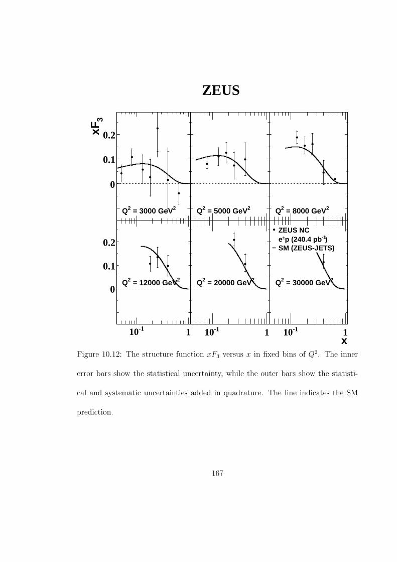
ZEUS 3
xF
-0.1
0
0.1
0.2
2 = 3000 GeV2Q
-110 1
-0.1
0
0.1
0.2
2 = 12000 GeV2Q
2 = 5000 GeV2Q
-110 1
2 = 20000 GeV2Q
2 = 8000 GeV2Q
-110 1
2 = 30000 GeV2Q
ZEUS NC)-1p (240.4 pb± e
SM (ZEUS-JETS)
xFigure 10.12: The structure function xF3 versus x in fixed bins of Q2. The inner
error bars show the statistical uncertainty, while the outer bars show the statisti-
cal and systematic uncertainties added in quadrature. The line indicates the SM
prediction.
167
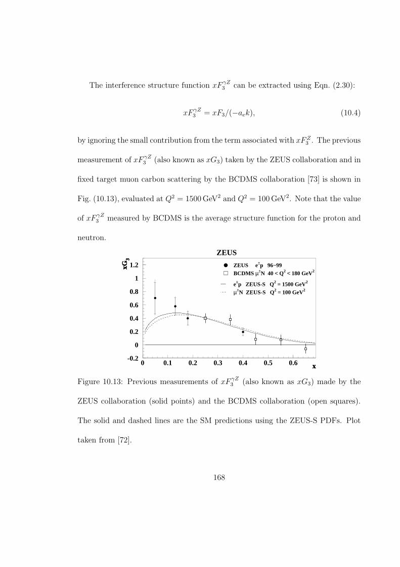
The interference structure function xF γZ3 can be extracted using Eqn. (2.30):
xF γZ3 = xF3/(−aek), (10.4)
by ignoring the small contribution from the term associated with xF Z3 . The previous
measurement of xF γZ3 (also known as xG3) taken by the ZEUS collaboration and in
fixed target muon carbon scattering by the BCDMS collaboration [73] is shown in
Fig. (10.13), evaluated at Q2 = 1500 GeV2 and Q2 = 100 GeV2. Note that the value
of xF γZ3 measured by BCDMS is the average structure function for the proton and
neutron.
-0.2
0
0.2
0.4
0.6
0.8
1
1.2
0 0.1 0.2 0.3 0.4 0.5 0.6 x
xG3
x
xG3
x
xG3
ZEUS
ZEUS e±p 96−99BCDMS µ±N 40 < Q2 < 180 GeV2
e±p ZEUS-S Q2 = 1500 GeV2
µ±N ZEUS-S Q2 = 100 GeV2
Figure 10.13: Previous measurements of xF γZ3 (also known as xG3) made by the
ZEUS collaboration (solid points) and the BCDMS collaboration (open squares).
The solid and dashed lines are the SM predictions using the ZEUS-S PDFs. Plot
taken from [72].
168
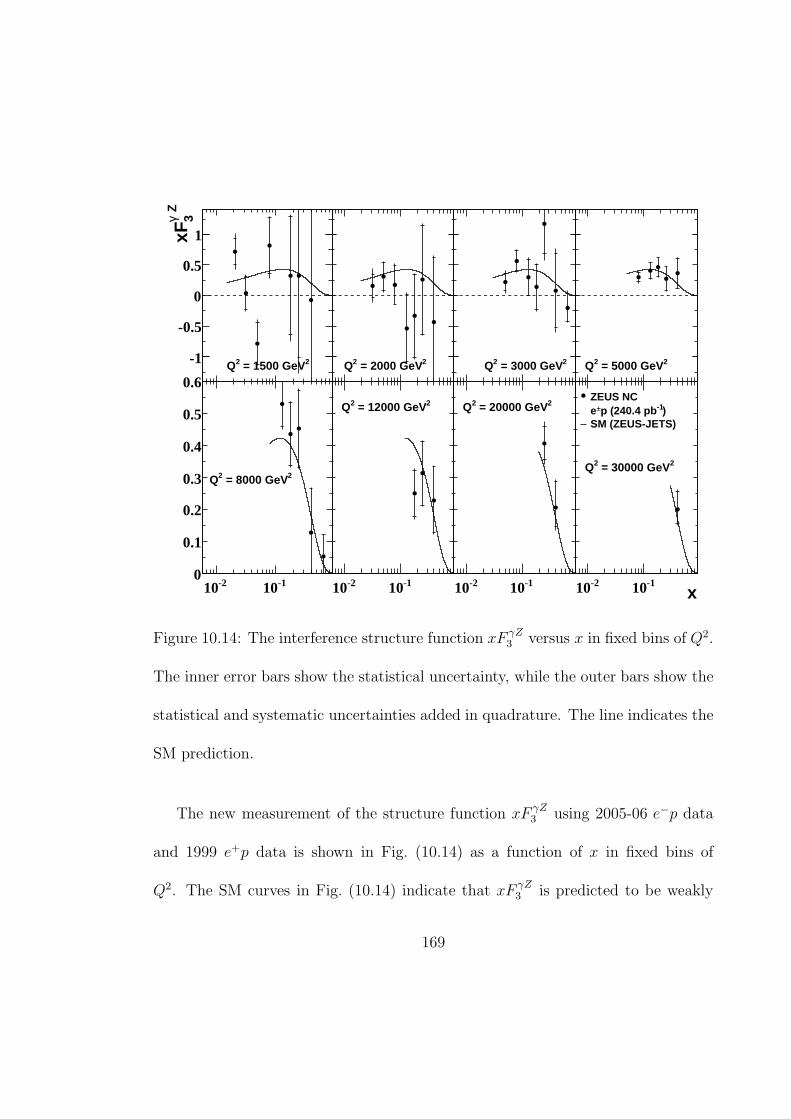
-1
-0.5
0
0.5
1
2 = 1500 GeV2Q
Zγ 3xF
-210 -1100
0.1
0.2
0.3
0.4
0.5
0.6
2 = 8000 GeV2Q
2 = 2000 GeV2Q
-210 -110
2 = 12000 GeV2Q
2 = 3000 GeV2Q
-210 -110
2 = 20000 GeV2Q
2 = 5000 GeV2Q
-210 -110
2 = 30000 GeV2Q
ZEUS NC)-1p (240.4 pb± e
SM (ZEUS-JETS)
x
Figure 10.14: The interference structure function xF γZ3 versus x in fixed bins of Q2.
The inner error bars show the statistical uncertainty, while the outer bars show the
statistical and systematic uncertainties added in quadrature. The line indicates the
SM prediction.
The new measurement of the structure function xF γZ3 using 2005-06 e−p data
and 1999 e+p data is shown in Fig. (10.14) as a function of x in fixed bins of
Q2. The SM curves in Fig. (10.14) indicate that xF γZ3 is predicted to be weakly
169

dependent on Q2 (note the change of scale on the axes). Therefore, the measure-
ments can be safely extrapolated to a single bin in Q2 using theoretical predictions,
and then averaged in x. This procedure was used to present xF γZ3 with the best
possible statistical precision. The data shown in Fig. (10.14) was extrapolated to
Q2 = 5000 GeV2, using factors generally within 5%, and is shown in Fig. (10.15).
The value of Q2 = 5000 GeV2 was chosen as it minimised the amount of Q2 extrap-
olation. The structure function xF γZ3 describes the valence quark distribution, and
can be directly compared with the valence quark PDFs shown in Fig. (2.8). The
statistical precision of this measurement is unprecedented, and can be compared
with previous measurements of xF γZ3 taken by the ZEUS and BCDMS collabora-
tion shown in Fig. (10.13). The new measurement of xF γZ3 extends the range of x
values down to 0.021. At the time of writing, new HERA II e+p data with an in-
tegrated luminosity of ∼ 120 pb−1 had been collected, but not fully analysed. This
additional data is projected to reduce the statistical error in the xF γZ3 measurement
presented by ∼ 8% at lowest x.
The sum rule shown in Eqn. (2.32) predicts∫ 1
0dxx
xF γZ3 = 5
3, by counting the
number of valence quarks inside the proton. However, the measurement of xF γZ3
is limited in the x range due to the acceptance of the detector. The integral of the
xF γZ3 measurement was obtained as
∫ 0.65
0.021
dx
xxF γZ
3 = 1.2 ± 0.1(stat) ± 0.1(sys), (10.5)
170
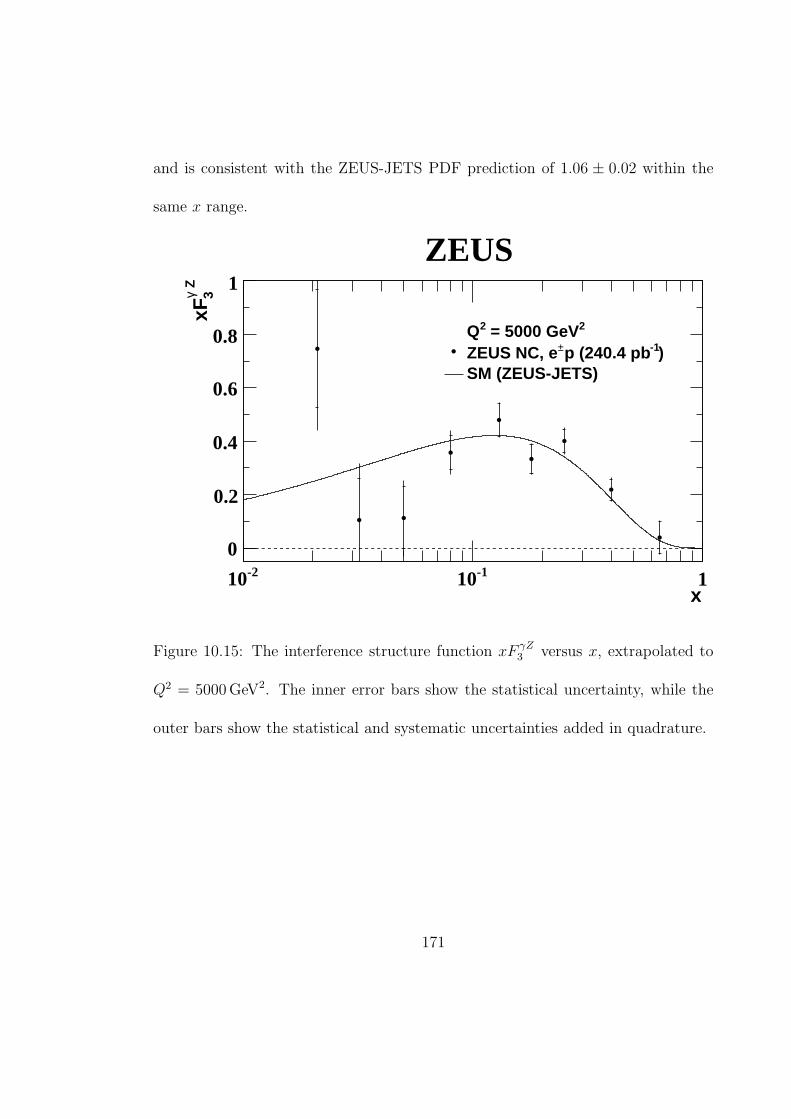
and is consistent with the ZEUS-JETS PDF prediction of 1.06 ± 0.02 within the
same x range.
ZEUS
x-210 -110 1
Zγ 3xF
0
0.2
0.4
0.6
0.8
1
2 = 5000 GeV2Q)-1p (240.4 pb±ZEUS NC, e
SM (ZEUS-JETS)
Figure 10.15: The interference structure function xF γZ3 versus x, extrapolated to
Q2 = 5000 GeV2. The inner error bars show the statistical uncertainty, while the
outer bars show the statistical and systematic uncertainties added in quadrature.
171
11 Summary and outlook
Neutral current e−p DIS cross sections measured at the ZEUS detector have been
presented. The HERA collider has provided an electron beam energy of 27.5 GeV
and a proton beam energy of 920 GeV yielding a centre-of-mass energy of√
s =
318 GeV. The data analysed was collected from 2005-06 and corresponds to an
integrated luminosity of 177.2 pb−1. The data set was split between negatively
polarised electrons (L = 105.4 pb−1, Pe = −0.27) and positively polarised electrons
(L = 71.8 pb−1, Pe = +0.30).
The single differential cross sections dσ/dx, dσ/dy, and dσ/dQ2 have been mea-
sured at y < 0.9 and Q2 > 185 GeV2 (and also Q2 > 3000 GeV2) and are well
described by the SM. The measurement of dσ/dQ2 in bin-centres ranging between
195 GeV2 < Q2 < 36, 200 GeV2 using negatively and positively polarised data has
been used to calculate the polarisation asymmetry (A−). This measurement is the
first observation of parity violation in NC e−p DIS at distances down to 10−18 m.
The e−p reduced cross section has been measured in the bin-centre ranges of
172

200 GeV2 < Q2 < 30, 000 GeV2 and 0.005 < x < 0.65. These measurements have
been compared with previously published e+p reduced cross sections to extract the
proton structure function xF3, which contains the parity violating part of the re-
duced cross section. The interference structure function xF γZ3 , which describes the
valence quark distribution inside the proton, has been extracted. The integral of
the measured xF γZ3 distribution versus x is consistent with the SM. The measure-
ments of the structure functions xF3 and xF γZ3 presented in this thesis are the most
precise to date.
The cross section measurements presented in this thesis will have a direct impact
on PDF fits. The ZEUS collaboration has released PDF uncertainties using the
preliminary results from this thesis and from HERA II e−p CC data, shown in
Fig. (11.1). The addition of these new measurements has improved the precision of
the high x PDF distributions, particularly for the u valence quark. The constraint
of the PDF uncertainties is of great importance, as a precise knowledge of the PDFs
provided by HERA will be essential for future studies at the Large Hadron Collider.
Efforts have begun to combine measurements from both the ZEUS and H1
detectors for a greater statistical impact. Figure (11.2) shows a combined polarisa-
tion asymmetry measurement (A±) from the H1 and ZEUS collaborations, which
includes preliminary measurements of A− from this thesis. This combined measure-
ment is based on an integrated luminosity of ∼ 290 pb−1 between the experiments,
173

and the shape and magnitude of A± as a function of Q2 is well described by the
SM. The ZEUS and H1 experiments have now collected a total of ∼ 900 pb−1 of
positively and negatively polarised e±p data. The analysis of this total data set
will yield the final word on electroweak measurements at HERA.
-1
-0.5
0
0.5
1vxu
0 0.2 0.4 0.6 0.8 1
0 0.2 0.4 0.6 0.8 1
2 = 10000 GeV2Q
-1
-0.5
0
0.5
1
-2
-1.5
-1
-0.5
0
0.5
1
1.5
2vxd
0 0.2 0.4 0.6 0.8 1
0 0.2 0.4 0.6 0.8 1
-2
-1.5
-1
-0.5
0
0.5
1
1.5
2
-1
-0.5
0
0.5
1xS
-410 -310 -210 -110
-410 -310 -210 -110
ZEUS-JETS
-1
-0.5
0
0.5
1
-1
-0.5
0
0.5
1xg
-410 -310 -210 -110
-410 -310 -210 -110
ZEUS-pol (prel.)
-1
-0.5
0
0.5
1
ZEUS
x
frac
tion
al u
ncer
tain
ty
Figure 11.1: Fractional uncertainty of the ZEUS-JETS PDFs compared with the
ZEUS-Pol PDFs [74] (which include preliminary measurements from this thesis).
The uncertainties at Q2 = 10, 000 GeV2 are shown, with an improvement seen at
high x, particularly for the u valence quark.
174
Figure 11.2: Measurements of the polarisation asymmetry A± by the ZEUS and
H1 collaborations combined to achieve the greatest statistical impact [16]. Data
collected with an integrated luminosity of ∼ 290 pb−1 has been used.
175

A Acronyms
BCAL - Barrel Calorimeter
CAL - Calorimeter
CC - Charged Current
CFLT - Calorimeter First Level Trigger
CTD - Central Tracking Detector
CTEQ - Coordinated Theoretical-Experimental Project on QCD
DESY - Deutsches Elektronen Synchrotron (a research centre)
DIS - Deep Inelastic Scattering
EMC - Electromagnetic Calorimeter
FCAL - Forward Calorimeter
FLT - First Level Trigger
FSR - Final State Radiation
H1 - A general purpose particle detector at HERA
HAC - Hadronic Calorimeter
176

HERA - Hadron Elektron Ring Anlage (an e±p accelerator)
HFS - Hadronic Final State
ISR - Initial State Radiation
LHC - Large Hadron Collider
LO - Leading Order
MC - Monte Carlo
MVD - Micro-vertex Detector
NC - Neutral Current
PDF - Parton Density Function
PHP - Photoproduction
PMT - Photomultiplier Tube
QED - Quantum Electrodynamics
QCD - Quantum Chromodynamics
QPM - Quark-Parton Model
RCAL - Rear Calorimeter
SLT - Second Level Trigger
SM - Standard Model
TLT - Third Level Trigger
ZEUS - A general purpose particle detector at HERA
177

B Trigger slots
B.1 First Level Trigger
The energy sums of importance to this analysis are detailed in Fig. B.1. Further
variables are listed below:
• EREMC,th: Energy deposited in the entire RCAL EMC, only including cells
with an energy above 625 MeV
• ET,all: Total transverse energy including all towers
• R/B/FIsoE: An isolated EMC deposit (IsoE) in the RCAL, BCAL, or FCAL,
respectively
• RIsoE - 3q: An isolated REMC deposit found, excluding the third quadrant.
The RCAL is made up of 4 quadrants defined by the sign of the coordinates
in the x − y plane; (+x, +y), (+x,−y), (−x, +y), and (−x,−y). The third
quadrant (−x, +y) suffers from background events arising from low energy
electrons in the incoming beam that are deflected into the RCAL surface.
178
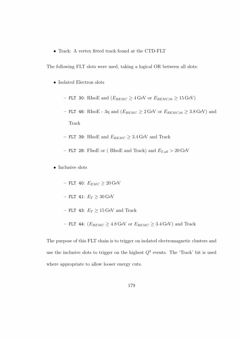
• Track: A vertex fitted track found at the CTD-FLT
The following FLT slots were used, taking a logical OR between all slots:
• Isolated Electron slots
– FLT 30: RIsoE and (EREMC ≥ 4 GeV or EREMC,th ≥ 15 GeV)
– FLT 46: RIsoE - 3q and (EREMC ≥ 2 GeV or EREMC,th ≥ 3.8 GeV) and
Track
– FLT 39: BIsoE and EBEMC ≥ 3.4 GeV and Track
– FLT 28: FIsoE or ( BIsoE and Track) and ET,all > 20 GeV
• Inclusive slots
– FLT 40: EEMC ≥ 20 GeV
– FLT 41: ET ≥ 30 GeV
– FLT 43: ET ≥ 15 GeV and Track
– FLT 44: (EBEMC ≥ 4.8 GeV or EREMC ≥ 3.4 GeV) and Track
The purpose of this FLT chain is to trigger on isolated electromagnetic clusters and
use the inclusive slots to trigger on the highest Q2 events. The ‘Track’ bit is used
where appropriate to allow looser energy cuts.
179

FCAL BCAL RCAL
e p
(b) CFLT: EMC
(c) CFLT: BEMC (d) CFLT: REMC
(a) CFLT: ET
3 rings
1 ring
1 ring
1 ring
Figure B.1: A sketch of the energy sums used at the CFLT, showing the CAL
centred around the beam-pipe (denoted by a dashed line). The yellow areas corre-
spond to the CAL regions used in the energy sums of (a) ET , the total transverse
energy, (b) EMC, the CAL sections used for electromagnetic deposits, (c) BEMC,
the barrel EMC, and (d) REMC, the rear EMC. Inner rings of CAL towers at the
FCAL or RCAL are excluded from the energy sums to avoid the proton remnant
or beam-gas interactions.
180

B.2 Second Level Trigger
The following slots were used at the SLT, taking a logical OR between all slots:
• DIS slot with good electron candidate
– SLT DIS07
∗ (EREMC or EBEMC > 2.5 GeV) or (EFEMC or EFHAC > 10 GeV),
where FHAC refers to the forward HAC section
∗ At least one FLT slot indicating a DIS event
∗ (E −Pz) + 2×ELumi−γ > 29 GeV, where ELumi−γ is the energy of a
radiated photon detected in the luminosity monitor
∗ An electron candidate with an energy above 5 GeV
• High transverse energy slots
– SLT EXO1
∗ ET > 35 GeV
– SLT EXO2
∗ (ET > 15 GeV and FLT 28) OR
∗ (ET > 25 GeV and E − PZ > 15 GeV)
– SLT EXO3
181

∗ ET > 16 GeV and E − PZ > 34 GeV
The purpose of this combination of triggers was to use the DIS slot for the main
bulk of the NC DIS events, and to use the high ET slots for the highest Q2 events.
Note that the ET sum avoids most of the proton remnant by excluding the FCAL
inner ring of towers.
182

C Comparisons between electron finders
The EM electron finder is the default algorithm used in this thesis, and the SINIS-
TRA electron finder is used to determine a contribution to the systematic uncer-
tainty in the cross sections. This systematic error generally dominates the other
uncertainties discussed in Section 9.3.2, as shown in Figs. (9.5-9.9).
To investigate the cause of this large systematic uncertainty, a number of data
to MC comparisons were made for the variables used in the event selection. A few
of these checks are shown in Fig. (C.1). The electron polar angle (θe) and electron
energy (E ′e) are consistent between the two electron finders, but a noticeable dif-
ference was seen in the distributions of the electron track momentum (P trke ) and
distance of closest approach (DCA) between the energy cluster and endpoint of
the extrapolated track. However, these discrepancies do not affect the measured
cross sections significantly (below 1%), as the differences occur away from the cut
thresholds (P trke > 3 GeV and DCA < 10 cm).
A further check of the electron finders involved determining the amount of
183

PHP contamination in each cross section bin. The percentage amount of PHP
events in the NC e−p DIS single differential cross sections and reduced cross section
(corresponding to the measurements shown in Fig. (10.1) for Q2 > 185 GeV2 and
Fig. (10.10)) is shown in Fig. (C.2). Both electron finders let through approximately
equal amounts of PHP events, with differences of up to 1.5% at high Q2 where the
statistical error is large.
Figure C.1: Data/MC distributions for certain variables involved in the event selec-
tion of NC DIS events, compared between the EM and SINISTRA electron finders
(black and red dots, respectively). The distributions of the electron energy (E ′e),
electron polar angle (θe), electron track momentum (P trke ), and distance of closest
approach (DCA) are shown. An account of these variables is given in Section 8.5.
184
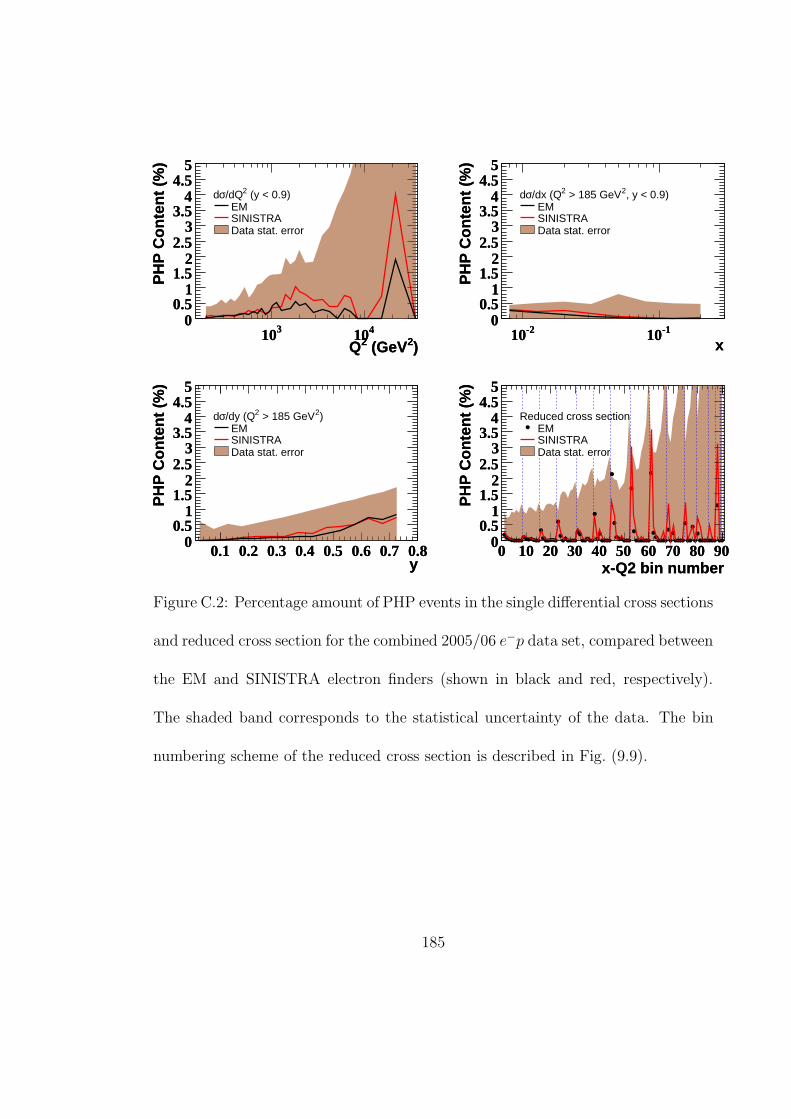
)2 (GeV2Q310 410
PH
P C
on
ten
t (%
)
00.5
11.5
22.5
33.5
44.5
5
(y < 0.9)2/dQσdEMSINISTRAData stat. error
)2 (GeV2Q310 410
PH
P C
on
ten
t (%
)
00.5
11.5
22.5
33.5
44.5
5
x-210 -110
PH
P C
on
ten
t (%
)
00.5
11.5
22.5
33.5
44.5
5
, y < 0.9)2 > 185 GeV2/dx (QσdEMSINISTRAData stat. error
x-210 -110
PH
P C
on
ten
t (%
)
00.5
11.5
22.5
33.5
44.5
5
y0.1 0.2 0.3 0.4 0.5 0.6 0.7 0.8
PH
P C
on
ten
t (%
)
00.5
11.5
22.5
33.5
44.5
5
)2 > 185 GeV2/dy (QσdEMSINISTRAData stat. error
y0.1 0.2 0.3 0.4 0.5 0.6 0.7 0.8
PH
P C
on
ten
t (%
)
00.5
11.5
22.5
33.5
44.5
5
x-Q2 bin number0 10 20 30 40 50 60 70 80 90
PH
P C
on
ten
t (%
)
00.5
11.5
22.5
33.5
44.5
5
Reduced cross sectionEMSINISTRAData stat. error
x-Q2 bin number0 10 20 30 40 50 60 70 80 90
PH
P C
on
ten
t (%
)
00.5
11.5
22.5
33.5
44.5
5
Figure C.2: Percentage amount of PHP events in the single differential cross sections
and reduced cross section for the combined 2005/06 e−p data set, compared between
the EM and SINISTRA electron finders (shown in black and red, respectively).
The shaded band corresponds to the statistical uncertainty of the data. The bin
numbering scheme of the reduced cross section is described in Fig. (9.9).
185

D Extracting cross sections using the Electron
method
The Double Angle (DA) reconstruction method was chosen to calculate cross sec-
tions, as discussed in Chapter 5. Therefore, the cross section binning relies on
the angles of the electron and hadronic system. A comparison with the Electron
reconstruction method is useful as it relies entirely on measurements of the scat-
tered electron. The single differential cross sections and the reduced cross section
measured using the Electron method divided by the SM prediction are shown in
Figs. (D.1 - D.3). The differences between the measurements and the SM prediction
are of a similar shape and magnitude to the nominal cross sections calculated using
the DA method (shown in Chapter 10).
186
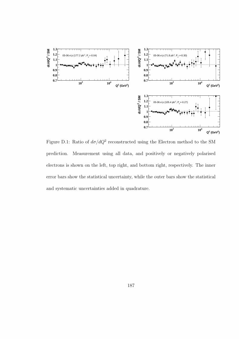
)2 (GeV2Q310 410
/ S
M2
/dQ
σd
0.7
0.8
0.9
1
1.1
1.2
1.3
=-0.04)e
, P-1p (177.2 pb-05-06 e
)2 (GeV2Q310 410
/ S
M2
/dQ
σd
0.7
0.8
0.9
1
1.1
1.2
1.3
=+0.30)e
, P-1p (71.8 pb-05-06 e
)2 (GeV2Q310 410
/ S
M2
/dQ
σd
0.7
0.8
0.9
1
1.1
1.2
1.3
=-0.27)e
, P-1p (105.4 pb-05-06 e
Figure D.1: Ratio of dσ/dQ2 reconstructed using the Electron method to the SM
prediction. Measurement using all data, and positively or negatively polarised
electrons is shown on the left, top right, and bottom right, respectively. The inner
error bars show the statistical uncertainty, while the outer bars show the statistical
and systematic uncertainties added in quadrature.
187
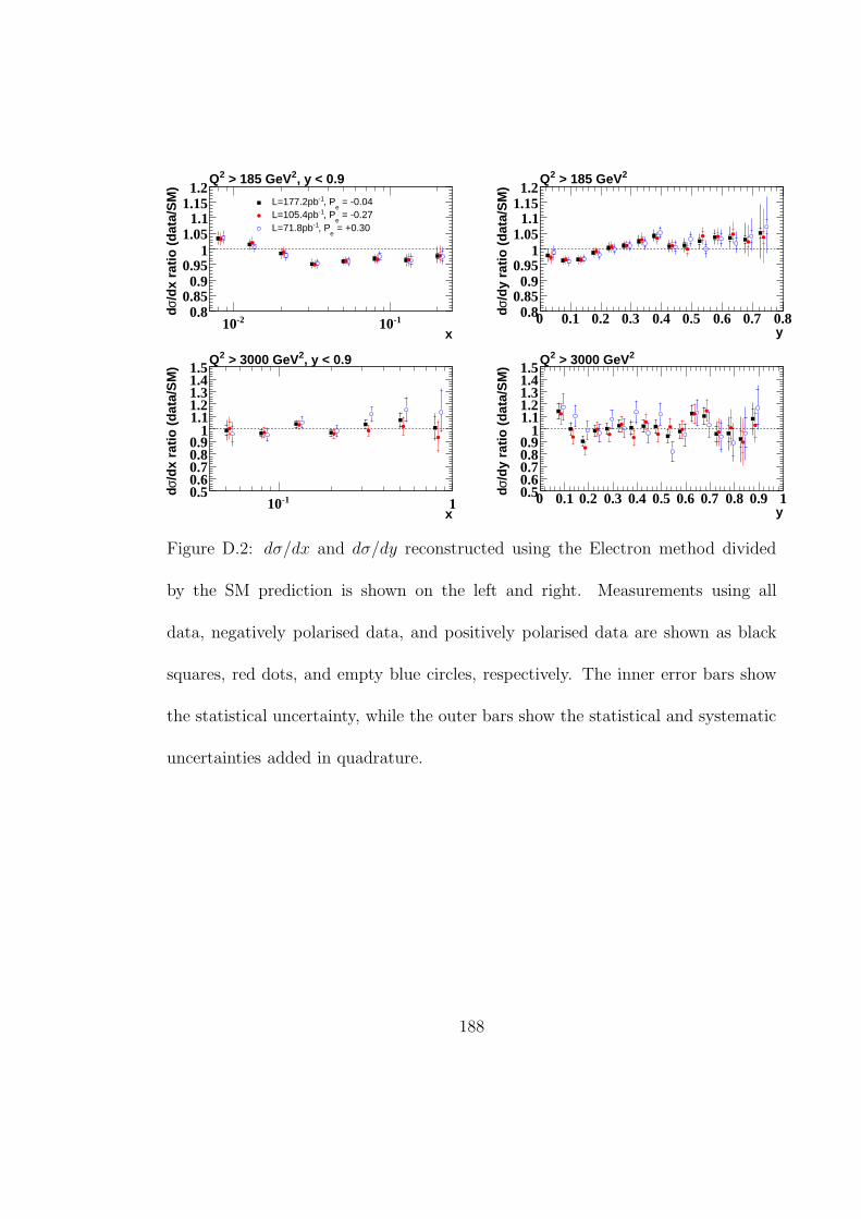
x-210 -110
/dx
rati
o (
dat
a/S
M)
σd 0.80.850.9
0.951
1.051.1
1.151.2
, y < 0.92 > 185 GeV2Q
= -0.04e
, P-1L=177.2pb = -0.27
e, P-1L=105.4pb
= +0.30e
, P-1L=71.8pb
y0 0.1 0.2 0.3 0.4 0.5 0.6 0.7 0.8
/dy
rati
o (
dat
a/S
M)
σd 0.80.850.9
0.951
1.051.1
1.151.2
2 > 185 GeV2Q
x-110 1
/dx
rati
o (
dat
a/S
M)
σd 0.50.60.70.80.9
11.11.21.31.41.5
, y < 0.92 > 3000 GeV2Q
y0 0.1 0.2 0.3 0.4 0.5 0.6 0.7 0.8 0.9 1
/dy
rati
o (
dat
a/S
M)
σd 0.50.60.70.80.9
11.11.21.31.41.5
2 > 3000 GeV2Q
Figure D.2: dσ/dx and dσ/dy reconstructed using the Electron method divided
by the SM prediction is shown on the left and right. Measurements using all
data, negatively polarised data, and positively polarised data are shown as black
squares, red dots, and empty blue circles, respectively. The inner error bars show
the statistical uncertainty, while the outer bars show the statistical and systematic
uncertainties added in quadrature.
188
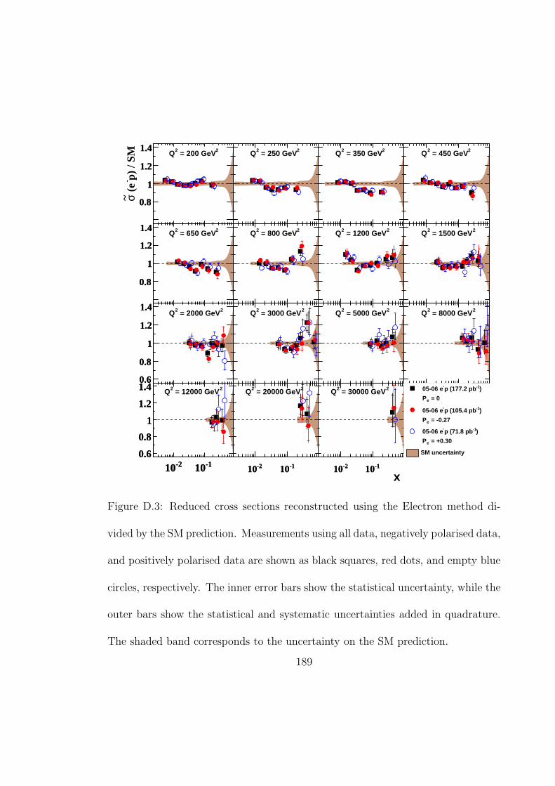
0.8
1
1.2
1.4 2 = 200 GeV2Q
p) /
SM-
(e
σ~ 0.8
1
1.2
1.4
0.8
1
1.2
1.4 2 = 650 GeV2Q
0.8
1
1.2
1.4
0.6
0.8
1
1.2
1.4 2 = 2000 GeV2Q
0.6
0.8
1
1.2
1.4
-210 -1100.6
0.8
1
1.2
1.4 2 = 12000 GeV2Q
-210 -1100.6
0.8
1
1.2
1.4
2 = 250 GeV2Q
2 = 800 GeV2Q
2 = 3000 GeV2Q
-210 -110
2 = 20000 GeV2Q
-210 -110
2 = 350 GeV2Q
2 = 1200 GeV2Q
2 = 5000 GeV2Q
-210 -110
2 = 30000 GeV2Q
x-210 -110
2 = 450 GeV2Q
2 = 1500 GeV2Q
2 = 8000 GeV2Q
)-1p (177.2 pb- 05-06 e
= 0e P
)-1p (105.4 pb- 05-06 e
= -0.27e P
)-1p (71.8 pb- 05-06 e
= +0.30e P
SM uncertainty
Figure D.3: Reduced cross sections reconstructed using the Electron method di-
vided by the SM prediction. Measurements using all data, negatively polarised data,
and positively polarised data are shown as black squares, red dots, and empty blue
circles, respectively. The inner error bars show the statistical uncertainty, while the
outer bars show the statistical and systematic uncertainties added in quadrature.
The shaded band corresponds to the uncertainty on the SM prediction.
189

E Tables of Results
The single-differential cross sections, polarisation asymmetry, reduced cross sec-
tions, and structure functions are tabulated in the following pages.
190

x range xc dσ/dx ( pb) Ndata NMC Nbg
Measured SM
0.0063 - 0.01 0.00794 (8.94 ± 0.04 +0.18−0.16 )·104 8.70 ·104 42010 42018 110
0.01 - 0.016 0.0126 (5.90 ± 0.03 +0.10−0.10 )·104 5.92 ·104 51117 51458 103
0.016 - 0.025 0.02 (3.59 ± 0.02 +0.06−0.05 )·104 3.69 ·104 51564 52920 77
0.025 - 0.04 0.0316 (2.09 ± 0.01 +0.03−0.03 )·104 2.21 ·104 52723 55383 46
0.04 - 0.063 0.0501 (1.25 ± 0.01 +0.02−0.01 )·104 1.27 ·104 43641 44588 15
0.063 - 0.1 0.0794 (7.11 ± 0.04 +0.10−0.09 )·103 7.18 ·103 39572 40216 7
0.1 - 0.16 0.126 (4.00 ± 0.02 +0.08−0.08 )·103 3.96 ·103 36022 35746 2
0.16 - 0.25 0.2 (2.07 ± 0.01 +0.06−0.05 )·103 2.07 ·103 20020 19903 2
Table E.1: The single differential cross section dσ/dx for for Q2 > 185 GeV2 measured using the combined 05-06e−p data set (L = 177.2 pb−1, Pe = −0.04). The first (second) error on the measured cross section refers tothe statistical (systematic) uncertainties. The cross sections as predicted by the SM using ZEUS-JETS PDFsare given. The number of observed data, MC and PHP background events are given as Ndata, NMC and Nbg
respectively. The subscript c indicates the bin centre.
191
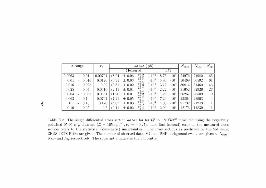
x range xc dσ/dx ( pb) Ndata NMC Nbg
Measured SM
0.0063 - 0.01 0.00794 (8.94 ± 0.06 +0.18−0.16 )·104 8.75 ·104 24976 24980 65
0.01 - 0.016 0.0126 (5.91 ± 0.03 +0.10−0.10 )·104 5.96 ·104 30469 30592 61
0.016 - 0.025 0.02 (3.61 ± 0.02 +0.06−0.05 )·104 3.72 ·104 30814 31460 46
0.025 - 0.04 0.0316 (2.11 ± 0.01 +0.03−0.03 )·104 2.22 ·104 31652 32926 27
0.04 - 0.063 0.0501 (1.26 ± 0.01 +0.02−0.01 )·104 1.28 ·104 26267 26509 9
0.063 - 0.1 0.0794 (7.21 ± 0.05 +0.10−0.09 )·103 7.24 ·103 23864 23903 4
0.1 - 0.16 0.126 (4.07 ± 0.03 +0.08−0.08 )·103 4.00 ·103 21732 21243 1
0.16 - 0.25 0.2 (2.11 ± 0.02 +0.06−0.05 )·103 2.09 ·103 12173 11839 1
Table E.2: The single differential cross section dσ/dx for for Q2 > 185 GeV2 measured using the negativelypolarised 05-06 e−p data set (L = 105.4 pb−1, Pe = −0.27). The first (second) error on the measured crosssection refers to the statistical (systematic) uncertainties. The cross sections as predicted by the SM usingZEUS-JETS PDFs are given. The number of observed data, MC and PHP background events are given as Ndata,NMC and Nbg respectively. The subscript c indicates the bin centre.
192

x range xc dσ/dx ( pb) Ndata NMC Nbg
Measured SM
0.0063 - 0.01 0.00794 (8.93 ± 0.07 +0.18−0.16 )·104 8.62 ·104 17034 17042 45
0.01 - 0.016 0.0126 (5.87 ± 0.04 +0.10−0.10 )·104 5.86 ·104 20648 20870 42
0.016 - 0.025 0.02 (3.56 ± 0.02 +0.06−0.05 )·104 3.65 ·104 20750 21464 31
0.025 - 0.04 0.0316 (2.06 ± 0.01 +0.03−0.03 )·104 2.18 ·104 21071 22461 19
0.04 - 0.063 0.0501 (1.22 ± 0.01 +0.02−0.01 )·104 1.26 ·104 17374 18082 6
0.063 - 0.1 0.0794 (6.96 ± 0.06 +0.09−0.09 )·103 7.08 ·103 15708 16315 3
0.1 - 0.16 0.126 (3.92 ± 0.03 +0.07−0.07 )·103 3.91 ·103 14290 14504 1
0.16 - 0.25 0.2 (2.00 ± 0.02 +0.06−0.04 )·103 2.04 ·103 7847 8067 1
Table E.3: The single differential cross section dσ/dx for for Q2 > 185 GeV2 measured using the positivelypolarised 05-06 e−p data set (L = 71.8 pb−1, Pe = +0.30). The first (second) error on the measured cross sectionrefers to the statistical (systematic) uncertainties. The cross sections as predicted by the SM using ZEUS-JETSPDFs are given. The number of observed data, MC and PHP background events are given as Ndata, NMC andNbg respectively. The subscript c indicates the bin centre.
193
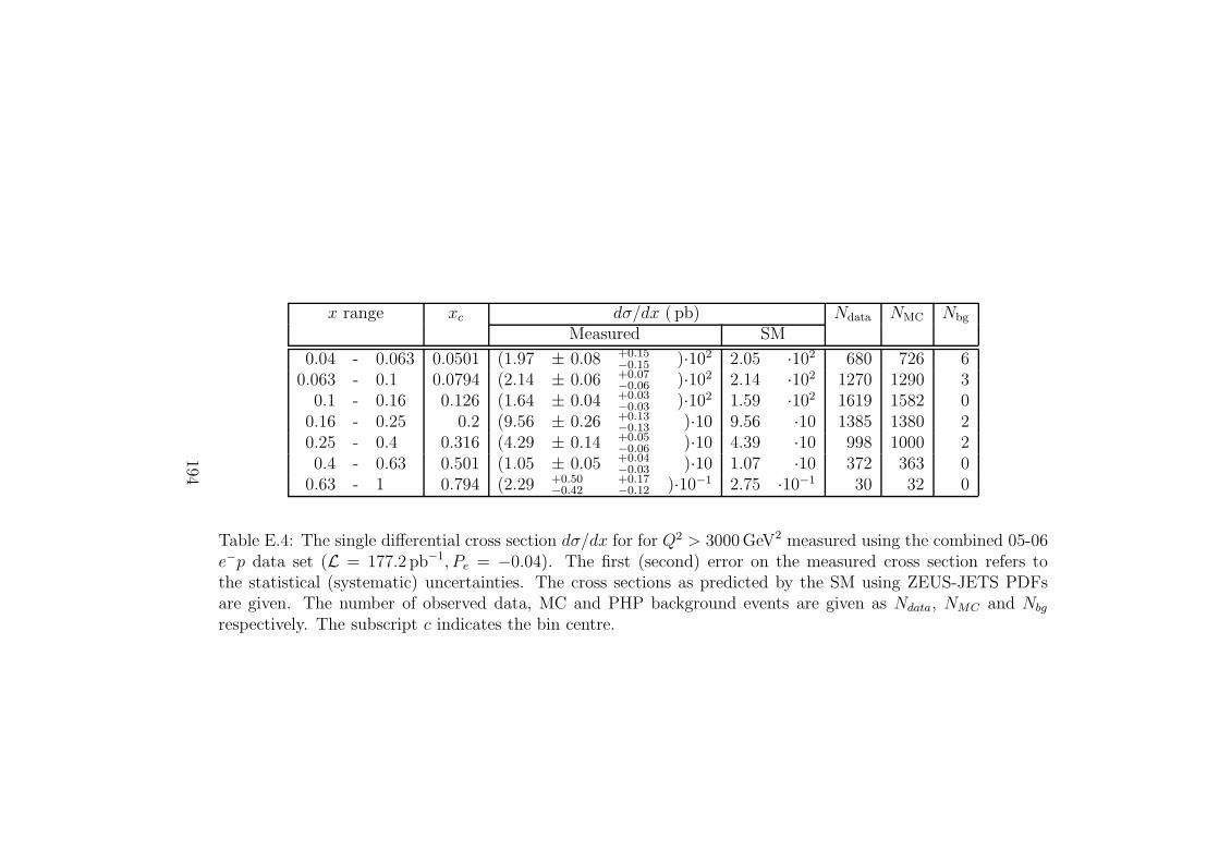
x range xc dσ/dx ( pb) Ndata NMC Nbg
Measured SM
0.04 - 0.063 0.0501 (1.97 ± 0.08 +0.15−0.15 )·102 2.05 ·102 680 726 6
0.063 - 0.1 0.0794 (2.14 ± 0.06 +0.07−0.06 )·102 2.14 ·102 1270 1290 3
0.1 - 0.16 0.126 (1.64 ± 0.04 +0.03−0.03 )·102 1.59 ·102 1619 1582 0
0.16 - 0.25 0.2 (9.56 ± 0.26 +0.13−0.13 )·10 9.56 ·10 1385 1380 2
0.25 - 0.4 0.316 (4.29 ± 0.14 +0.05−0.06 )·10 4.39 ·10 998 1000 2
0.4 - 0.63 0.501 (1.05 ± 0.05 +0.04−0.03 )·10 1.07 ·10 372 363 0
0.63 - 1 0.794 (2.29 +0.50−0.42
+0.17−0.12 )·10−1 2.75 ·10−1 30 32 0
Table E.4: The single differential cross section dσ/dx for for Q2 > 3000 GeV2 measured using the combined 05-06e−p data set (L = 177.2 pb−1, Pe = −0.04). The first (second) error on the measured cross section refers tothe statistical (systematic) uncertainties. The cross sections as predicted by the SM using ZEUS-JETS PDFsare given. The number of observed data, MC and PHP background events are given as Ndata, NMC and Nbg
respectively. The subscript c indicates the bin centre.
194
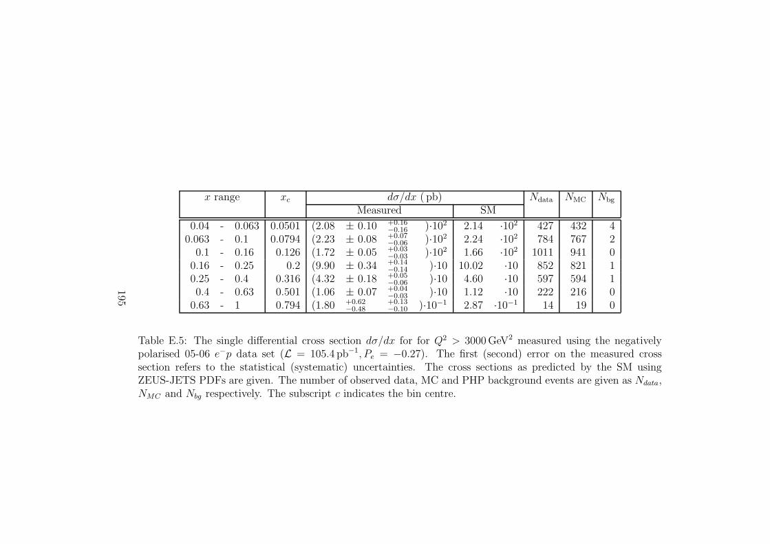
x range xc dσ/dx ( pb) Ndata NMC Nbg
Measured SM
0.04 - 0.063 0.0501 (2.08 ± 0.10 +0.16−0.16 )·102 2.14 ·102 427 432 4
0.063 - 0.1 0.0794 (2.23 ± 0.08 +0.07−0.06 )·102 2.24 ·102 784 767 2
0.1 - 0.16 0.126 (1.72 ± 0.05 +0.03−0.03 )·102 1.66 ·102 1011 941 0
0.16 - 0.25 0.2 (9.90 ± 0.34 +0.14−0.14 )·10 10.02 ·10 852 821 1
0.25 - 0.4 0.316 (4.32 ± 0.18 +0.05−0.06 )·10 4.60 ·10 597 594 1
0.4 - 0.63 0.501 (1.06 ± 0.07 +0.04−0.03 )·10 1.12 ·10 222 216 0
0.63 - 1 0.794 (1.80 +0.62−0.48
+0.13−0.10 )·10−1 2.87 ·10−1 14 19 0
Table E.5: The single differential cross section dσ/dx for for Q2 > 3000 GeV2 measured using the negativelypolarised 05-06 e−p data set (L = 105.4 pb−1, Pe = −0.27). The first (second) error on the measured crosssection refers to the statistical (systematic) uncertainties. The cross sections as predicted by the SM usingZEUS-JETS PDFs are given. The number of observed data, MC and PHP background events are given as Ndata,NMC and Nbg respectively. The subscript c indicates the bin centre.
195

x range xc dσ/dx ( pb) Ndata NMC Nbg
Measured SM
0.04 - 0.063 0.0501 (1.80 ± 0.11 +0.14−0.14 )·102 1.92 ·102 253 294 2
0.063 - 0.1 0.0794 (2.02 ± 0.09 +0.06−0.06 )·102 2.00 ·102 486 523 1
0.1 - 0.16 0.126 (1.51 ± 0.06 +0.03−0.03 )·102 1.48 ·102 608 642 0
0.16 - 0.25 0.2 (9.08 ± 0.39 +0.12−0.12 )·10 8.90 ·10 533 560 1
0.25 - 0.4 0.316 (4.25 ± 0.21 +0.05−0.06 )·10 4.09 ·10 401 405 1
0.4 - 0.63 0.501 (1.05 ± 0.09 +0.04−0.03 )·10 1.00 ·10 150 147 0
0.63 - 1 0.794 (3.01 +0.95−0.74
+0.22−0.16 )·10−1 2.57 ·10−1 16 13 0
Table E.6: The single differential cross section dσ/dx for for Q2 > 3000 GeV2 measured using the positivelypolarised 05-06 e−p data set (L = 71.8 pb−1, Pe = +0.30). The first (second) error on the measured cross sectionrefers to the statistical (systematic) uncertainties. The cross sections as predicted by the SM using ZEUS-JETSPDFs are given. The number of observed data, MC and PHP background events are given as Ndata, NMC andNbg respectively. The subscript c indicates the bin centre.
196
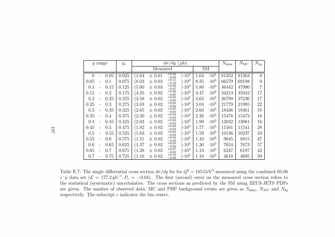
y range yc dσ/dy ( pb) Ndata NMC Nbg
Measured SM
0 - 0.05 0.025 (1.64 ± 0.01 +0.04−0.03 )·104 1.64 ·104 81352 81263 0
0.05 - 0.1 0.075 (8.03 ± 0.03 +0.11−0.10 )·103 8.35 ·103 66579 69198 9
0.1 - 0.15 0.125 (5.60 ± 0.03 +0.08−0.07 )·103 5.80 ·103 46442 47990 7
0.15 - 0.2 0.175 (4.35 ± 0.02 +0.06−0.05 )·103 4.47 ·103 34213 35042 17
0.2 - 0.25 0.225 (3.58 ± 0.02 +0.05−0.05 )·103 3.63 ·103 26799 27236 17
0.25 - 0.3 0.275 (3.03 ± 0.02 +0.04−0.04 )·103 3.04 ·103 21779 21995 22
0.3 - 0.35 0.325 (2.65 ± 0.02 +0.05−0.05 )·103 2.60 ·103 18436 18361 18
0.35 - 0.4 0.375 (2.30 ± 0.02 +0.04−0.04 )·103 2.26 ·103 15478 15473 18
0.4 - 0.45 0.425 (2.03 ± 0.02 +0.04−0.04 )·103 1.99 ·103 13032 13061 16
0.45 - 0.5 0.475 (1.82 ± 0.02 +0.03−0.03 )·103 1.77 ·103 11501 11541 28
0.5 - 0.55 0.525 (1.63 ± 0.02 +0.04−0.04 )·103 1.59 ·103 10136 10237 33
0.55 - 0.6 0.575 (1.51 ± 0.02 +0.04−0.03 )·103 1.43 ·103 9045 8915 47
0.6 - 0.65 0.625 (1.37 ± 0.02 +0.05−0.04 )·103 1.30 ·103 7654 7673 57
0.65 - 0.7 0.675 (1.28 ± 0.02 +0.07−0.05 )·103 1.19 ·103 6247 6197 42
0.7 - 0.75 0.725 (1.16 ± 0.02 +0.10−0.09 )·103 1.10 ·103 4618 4695 39
Table E.7: The single differential cross section dσ/dy for for Q2 > 185 GeV2 measured using the combined 05-06e−p data set (L = 177.2 pb−1, Pe = −0.04). The first (second) error on the measured cross section refers tothe statistical (systematic) uncertainties. The cross sections as predicted by the SM using ZEUS-JETS PDFsare given. The number of observed data, MC and PHP background events are given as Ndata, NMC and Nbg
respectively. The subscript c indicates the bin centre.
197
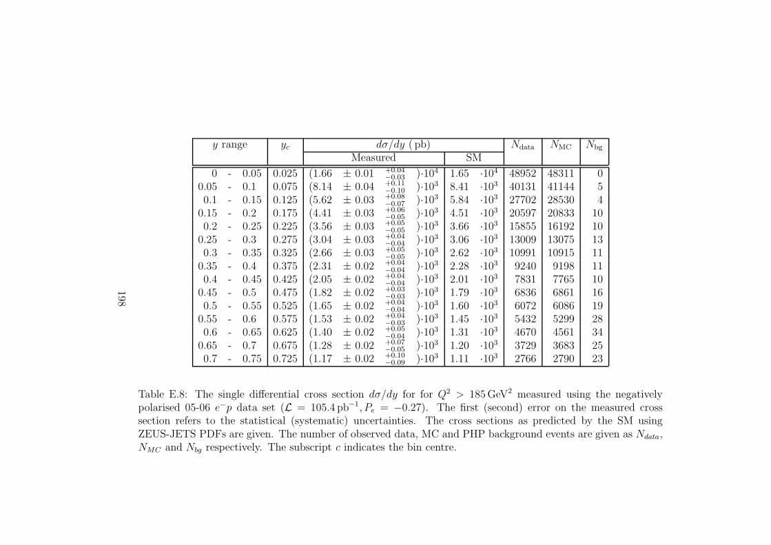
y range yc dσ/dy ( pb) Ndata NMC Nbg
Measured SM
0 - 0.05 0.025 (1.66 ± 0.01 +0.04−0.03 )·104 1.65 ·104 48952 48311 0
0.05 - 0.1 0.075 (8.14 ± 0.04 +0.11−0.10 )·103 8.41 ·103 40131 41144 5
0.1 - 0.15 0.125 (5.62 ± 0.03 +0.08−0.07 )·103 5.84 ·103 27702 28530 4
0.15 - 0.2 0.175 (4.41 ± 0.03 +0.06−0.05 )·103 4.51 ·103 20597 20833 10
0.2 - 0.25 0.225 (3.56 ± 0.03 +0.05−0.05 )·103 3.66 ·103 15855 16192 10
0.25 - 0.3 0.275 (3.04 ± 0.03 +0.04−0.04 )·103 3.06 ·103 13009 13075 13
0.3 - 0.35 0.325 (2.66 ± 0.03 +0.05−0.05 )·103 2.62 ·103 10991 10915 11
0.35 - 0.4 0.375 (2.31 ± 0.02 +0.04−0.04 )·103 2.28 ·103 9240 9198 11
0.4 - 0.45 0.425 (2.05 ± 0.02 +0.04−0.04 )·103 2.01 ·103 7831 7765 10
0.45 - 0.5 0.475 (1.82 ± 0.02 +0.03−0.03 )·103 1.79 ·103 6836 6861 16
0.5 - 0.55 0.525 (1.65 ± 0.02 +0.04−0.04 )·103 1.60 ·103 6072 6086 19
0.55 - 0.6 0.575 (1.53 ± 0.02 +0.04−0.03 )·103 1.45 ·103 5432 5299 28
0.6 - 0.65 0.625 (1.40 ± 0.02 +0.05−0.04 )·103 1.31 ·103 4670 4561 34
0.65 - 0.7 0.675 (1.28 ± 0.02 +0.07−0.05 )·103 1.20 ·103 3729 3683 25
0.7 - 0.75 0.725 (1.17 ± 0.02 +0.10−0.09 )·103 1.11 ·103 2766 2790 23
Table E.8: The single differential cross section dσ/dy for for Q2 > 185 GeV2 measured using the negativelypolarised 05-06 e−p data set (L = 105.4 pb−1, Pe = −0.27). The first (second) error on the measured crosssection refers to the statistical (systematic) uncertainties. The cross sections as predicted by the SM usingZEUS-JETS PDFs are given. The number of observed data, MC and PHP background events are given as Ndata,NMC and Nbg respectively. The subscript c indicates the bin centre.
198
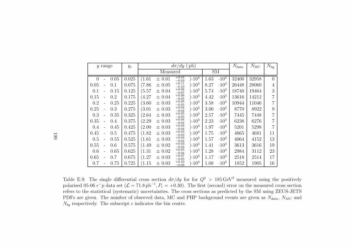
y range yc dσ/dy ( pb) Ndata NMC Nbg
Measured SM
0 - 0.05 0.025 (1.61 ± 0.01 +0.04−0.03 )·104 1.63 ·104 32400 32958 0
0.05 - 0.1 0.075 (7.86 ± 0.05 +0.11−0.10 )·103 8.27 ·103 26448 28060 4
0.1 - 0.15 0.125 (5.57 ± 0.04 +0.08−0.07 )·103 5.74 ·103 18740 19464 3
0.15 - 0.2 0.175 (4.27 ± 0.04 +0.06−0.05 )·103 4.42 ·103 13616 14212 7
0.2 - 0.25 0.225 (3.60 ± 0.03 +0.05−0.05 )·103 3.58 ·103 10944 11046 7
0.25 - 0.3 0.275 (3.01 ± 0.03 +0.04−0.04 )·103 3.00 ·103 8770 8922 9
0.3 - 0.35 0.325 (2.64 ± 0.03 +0.05−0.05 )·103 2.57 ·103 7445 7448 7
0.35 - 0.4 0.375 (2.29 ± 0.03 +0.04−0.04 )·103 2.23 ·103 6238 6276 7
0.4 - 0.45 0.425 (2.00 ± 0.03 +0.04−0.04 )·103 1.97 ·103 5201 5298 7
0.45 - 0.5 0.475 (1.82 ± 0.03 +0.03−0.03 )·103 1.75 ·103 4665 4681 11
0.5 - 0.55 0.525 (1.61 ± 0.03 +0.04−0.04 )·103 1.57 ·103 4064 4152 13
0.55 - 0.6 0.575 (1.49 ± 0.02 +0.03−0.03 )·103 1.41 ·103 3613 3616 19
0.6 - 0.65 0.625 (1.31 ± 0.02 +0.05−0.04 )·103 1.28 ·103 2984 3112 23
0.65 - 0.7 0.675 (1.27 ± 0.03 +0.07−0.05 )·103 1.17 ·103 2518 2514 17
0.7 - 0.75 0.725 (1.15 ± 0.03 +0.10−0.09 )·103 1.08 ·103 1852 1905 16
Table E.9: The single differential cross section dσ/dy for for Q2 > 185 GeV2 measured using the positivelypolarised 05-06 e−p data set (L = 71.8 pb−1, Pe = +0.30). The first (second) error on the measured cross sectionrefers to the statistical (systematic) uncertainties. The cross sections as predicted by the SM using ZEUS-JETSPDFs are given. The number of observed data, MC and PHP background events are given as Ndata, NMC andNbg respectively. The subscript c indicates the bin centre.
199

y range yc dσ/dy ( pb) Ndata NMC Nbg
Measured SM
0.05 - 0.1 0.075 (3.47 ± 0.22 +0.07−0.05 )·10 3.40 ·10 255 240 0
0.1 - 0.15 0.125 (6.19 ± 0.28 +0.17−0.16 )·10 6.48 ·10 481 490 2
0.15 - 0.2 0.175 (6.67 ± 0.29 +0.06−0.06 )·10 7.06 ·10 528 552 0
0.2 - 0.25 0.225 (6.40 ± 0.28 +0.06−0.08 )·10 6.85 ·10 539 571 0
0.25 - 0.3 0.275 (6.39 ± 0.27 +0.11−0.11 )·10 6.42 ·10 552 552 0
0.3 - 0.35 0.325 (6.10 ± 0.27 +0.06−0.06 )·10 5.95 ·10 525 512 0
0.35 - 0.4 0.375 (5.20 ± 0.25 +0.23−0.23 )·10 5.50 ·10 443 470 0
0.4 - 0.45 0.425 (5.38 ± 0.25 +0.08−0.07 )·10 5.09 ·10 464 439 0
0.45 - 0.5 0.475 (5.24 ± 0.25 +0.13−0.14 )·10 4.72 ·10 442 400 0
0.5 - 0.55 0.525 (4.31 ± 0.23 +0.08−0.08 )·10 4.39 ·10 359 369 0
0.55 - 0.6 0.575 (4.29 ± 0.23 +0.10−0.10 )·10 4.09 ·10 347 336 0
0.6 - 0.65 0.625 (3.90 ± 0.22 +0.12−0.12 )·10 3.83 ·10 312 310 0
0.65 - 0.7 0.675 (4.01 ± 0.23 +0.13−0.09 )·10 3.59 ·10 313 285 1
0.7 - 0.75 0.725 (3.08 ± 0.20 +0.27−0.26 )·10 3.39 ·10 235 265 0
0.75 - 0.8 0.775 (3.22 ± 0.21 +0.39−0.39 )·10 3.20 ·10 236 242 0
0.8 - 0.85 0.825 (3.00 ± 0.21 +0.56−0.56 )·10 3.04 ·10 212 221 2
0.85 - 0.9 0.875 (2.73 ± 0.21 +0.27−0.26 )·10 2.89 ·10 183 194 7
Table E.10: The single differential cross section dσ/dy for for Q2 > 3000 GeV2 measured using the combined05-06 e−p data set (L = 177.2 pb−1, Pe = −0.04). The first (second) error on the measured cross section refersto the statistical (systematic) uncertainties. The cross sections as predicted by the SM using ZEUS-JETS PDFsare given. The number of observed data, MC and PHP background events are given as Ndata, NMC and Nbg
respectively. The subscript c indicates the bin centre.
200

y range yc dσ/dy ( pb) Ndata NMC Nbg
Measured SM
0.05 - 0.1 0.075 (3.73 ± 0.29 +0.08−0.06 )·10 3.51 ·10 163 142 0
0.1 - 0.15 0.125 (5.78 ± 0.35 +0.16−0.15 )·10 6.72 ·10 267 291 1
0.15 - 0.2 0.175 (6.92 ± 0.38 +0.06−0.06 )·10 7.35 ·10 326 328 0
0.2 - 0.25 0.225 (6.67 ± 0.37 +0.06−0.08 )·10 7.14 ·10 334 340 0
0.25 - 0.3 0.275 (6.68 ± 0.36 +0.11−0.12 )·10 6.71 ·10 343 328 0
0.3 - 0.35 0.325 (6.25 ± 0.35 +0.07−0.06 )·10 6.22 ·10 320 304 0
0.35 - 0.4 0.375 (5.02 ± 0.31 +0.22−0.22 )·10 5.76 ·10 254 279 0
0.4 - 0.45 0.425 (5.87 ± 0.34 +0.08−0.08 )·10 5.33 ·10 301 261 0
0.45 - 0.5 0.475 (5.46 ± 0.33 +0.13−0.14 )·10 4.95 ·10 274 238 0
0.5 - 0.55 0.525 (4.48 ± 0.30 +0.08−0.09 )·10 4.60 ·10 222 220 0
0.55 - 0.6 0.575 (4.64 ± 0.31 +0.10−0.11 )·10 4.29 ·10 223 200 0
0.6 - 0.65 0.625 (4.10 ± 0.29 +0.13−0.13 )·10 4.02 ·10 195 184 0
0.65 - 0.7 0.675 (4.22 ± 0.30 +0.14−0.10 )·10 3.77 ·10 196 169 1
0.7 - 0.75 0.725 (3.17 ± 0.26 +0.27−0.27 )·10 3.56 ·10 144 157 0
0.75 - 0.8 0.775 (3.49 ± 0.28 +0.42−0.42 )·10 3.36 ·10 152 144 0
0.8 - 0.85 0.825 (3.05 ± 0.27 +0.56−0.57 )·10 3.19 ·10 128 131 1
0.85 - 0.9 0.875 (2.73 ± 0.27 +0.27−0.26 )·10 3.04 ·10 109 115 4
Table E.11: The single differential cross section dσ/dy for for Q2 > 3000 GeV2 measured using the negativelypolarised 05-06 e−p data set (L = 105.4 pb−1, Pe = −0.27). The first (second) error on the measured cross sectionrefers to the statistical (systematic) uncertainties. The cross sections as predicted by the SM using ZEUS-JETSPDFs are given. The number of observed data, MC and PHP background events are given as Ndata, NMC andNbg respectively. The subscript c indicates the bin centre.
201

y range yc dσ/dy ( pb) Ndata NMC Nbg
Measured SM
0.05 - 0.1 0.075 (3.08 +0.36−0.32
+0.07−0.05 )·10 3.23 ·10 92 97 0
0.1 - 0.15 0.125 (6.79 ± 0.47 +0.19−0.18 )·10 6.11 ·10 214 199 1
0.15 - 0.2 0.175 (6.29 ± 0.44 +0.06−0.06 )·10 6.64 ·10 202 224 0
0.2 - 0.25 0.225 (6.01 ± 0.42 +0.06−0.07 )·10 6.42 ·10 205 232 0
0.25 - 0.3 0.275 (5.96 ± 0.41 +0.10−0.11 )·10 6.00 ·10 209 224 0
0.3 - 0.35 0.325 (5.87 ± 0.41 +0.06−0.05 )·10 5.55 ·10 205 207 0
0.35 - 0.4 0.375 (5.47 ± 0.40 +0.24−0.24 )·10 5.12 ·10 189 191 0
0.4 - 0.45 0.425 (4.66 ± 0.37 +0.07−0.06 )·10 4.73 ·10 163 178 0
0.45 - 0.5 0.475 (4.91 ± 0.38 +0.12−0.13 )·10 4.38 ·10 168 162 0
0.5 - 0.55 0.525 (4.05 ± 0.35 +0.07−0.08 )·10 4.07 ·10 137 150 0
0.55 - 0.6 0.575 (3.78 ± 0.34 +0.09−0.09 )·10 3.79 ·10 124 136 0
0.6 - 0.65 0.625 (3.60 ± 0.33 +0.11−0.11 )·10 3.55 ·10 117 126 0
0.65 - 0.7 0.675 (3.69 ± 0.34 +0.12−0.08 )·10 3.33 ·10 117 116 1
0.7 - 0.75 0.725 (2.94 +0.34−0.31
+0.25−0.25 )·10 3.13 ·10 91 107 0
0.75 - 0.8 0.775 (2.82 +0.34−0.31
+0.34−0.34 )·10 2.96 ·10 84 98 0
0.8 - 0.85 0.825 (2.93 +0.36−0.32
+0.54−0.55 )·10 2.81 ·10 84 90 1
0.85 - 0.9 0.875 (2.72 +0.37−0.33
+0.27−0.26 )·10 2.67 ·10 74 79 3
Table E.12: The single differential cross section dσ/dy for for Q2 > 3000 GeV2 measured using the positivelypolarised 05-06 e−p data set (L = 71.8 pb−1, Pe = +0.30). The first (second) error on the measured cross sectionrefers to the statistical (systematic) uncertainties. The cross sections as predicted by the SM using ZEUS-JETSPDFs are given. The number of observed data, MC and PHP background events are given as Ndata, NMC andNbg respectively. The subscript c indicates the bin centre.
202
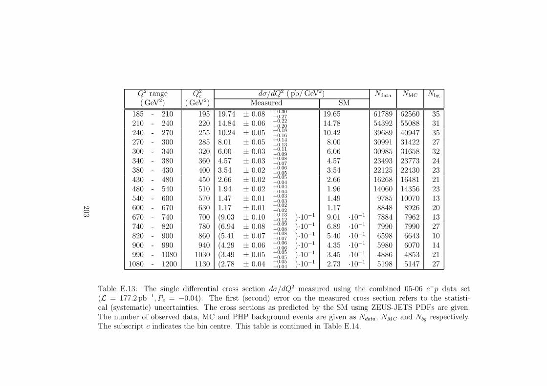
Q2 range Q2c dσ/dQ2 ( pb/ GeV2) Ndata NMC Nbg
( GeV2) ( GeV2) Measured SM
185 - 210 195 19.74 ± 0.08 +0.30−0.27 19.65 61789 62560 35
210 - 240 220 14.84 ± 0.06 +0.22−0.20 14.78 54392 55088 31
240 - 270 255 10.24 ± 0.05 +0.18−0.16 10.42 39689 40947 35
270 - 300 285 8.01 ± 0.05 +0.14−0.13 8.00 30991 31422 27
300 - 340 320 6.00 ± 0.03 +0.11−0.09 6.06 30985 31658 32
340 - 380 360 4.57 ± 0.03 +0.08−0.07 4.57 23493 23773 24
380 - 430 400 3.54 ± 0.02 +0.06−0.05 3.54 22125 22430 23
430 - 480 450 2.66 ± 0.02 +0.05−0.04 2.66 16268 16481 21
480 - 540 510 1.94 ± 0.02 +0.04−0.04 1.96 14060 14356 23
540 - 600 570 1.47 ± 0.01 +0.03−0.03 1.49 9785 10070 13
600 - 670 630 1.17 ± 0.01 +0.02−0.02 1.17 8848 8926 20
670 - 740 700 (9.03 ± 0.10 +0.13−0.12 )·10−1 9.01 ·10−1 7884 7962 13
740 - 820 780 (6.94 ± 0.08 +0.09−0.08 )·10−1 6.89 ·10−1 7990 7990 27
820 - 900 860 (5.41 ± 0.07 +0.08−0.07 )·10−1 5.40 ·10−1 6598 6643 10
900 - 990 940 (4.29 ± 0.06 +0.06−0.06 )·10−1 4.35 ·10−1 5980 6070 14
990 - 1080 1030 (3.49 ± 0.05 +0.05−0.05 )·10−1 3.45 ·10−1 4886 4853 21
1080 - 1200 1130 (2.78 ± 0.04 +0.05−0.04 )·10−1 2.73 ·10−1 5198 5147 27
Table E.13: The single differential cross section dσ/dQ2 measured using the combined 05-06 e−p data set(L = 177.2 pb−1, Pe = −0.04). The first (second) error on the measured cross section refers to the statisti-cal (systematic) uncertainties. The cross sections as predicted by the SM using ZEUS-JETS PDFs are given.The number of observed data, MC and PHP background events are given as Ndata, NMC and Nbg respectively.The subscript c indicates the bin centre. This table is continued in Table E.14.
203
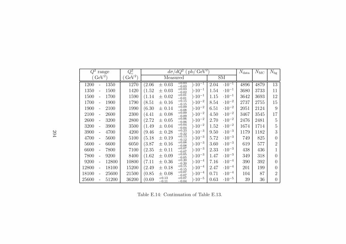
Q2 range Q2c dσ/dQ2 ( pb/ GeV2) Ndata NMC Nbg
( GeV2) ( GeV2) Measured SM
1200 - 1350 1270 (2.06 ± 0.03 +0.03−0.03 )·10−1 2.04 ·10−1 4896 4879 13
1350 - 1500 1420 (1.52 ± 0.03 +0.03−0.02 )·10−1 1.54 ·10−1 3680 3733 11
1500 - 1700 1590 (1.14 ± 0.02 +0.01−0.01 )·10−1 1.15 ·10−1 3642 3693 12
1700 - 1900 1790 (8.51 ± 0.16 +0.15−0.15 )·10−2 8.54 ·10−2 2737 2755 15
1900 - 2100 1990 (6.30 ± 0.14 +0.09−0.08 )·10−2 6.51 ·10−2 2051 2124 9
2100 - 2600 2300 (4.41 ± 0.08 +0.09−0.09 )·10−2 4.50 ·10−2 3467 3545 17
2600 - 3200 2800 (2.72 ± 0.05 +0.06−0.06 )·10−2 2.70 ·10−2 2476 2481 5
3200 - 3900 3500 (1.49 ± 0.04 +0.04−0.04 )·10−2 1.52 ·10−2 1674 1714 5
3900 - 4700 4200 (9.46 ± 0.28 +0.23−0.22 )·10−3 9.50 ·10−3 1179 1182 3
4700 - 5600 5100 (5.18 ± 0.19 +0.13−0.12 )·10−3 5.72 ·10−3 749 825 0
5600 - 6600 6050 (3.87 ± 0.16 +0.08−0.08 )·10−3 3.60 ·10−3 619 577 2
6600 - 7800 7100 (2.35 ± 0.11 +0.07−0.07 )·10−3 2.33 ·10−3 438 436 1
7800 - 9200 8400 (1.62 ± 0.09 +0.05−0.05 )·10−3 1.47 ·10−3 349 318 0
9200 - 12800 10800 (7.11 ± 0.36 +0.20−0.20 )·10−4 7.16 ·10−4 390 392 0
12800 - 18100 15200 (2.49 ± 0.18 +0.15−0.15 )·10−4 2.47 ·10−4 201 199 0
18100 - 25600 21500 (0.85 ± 0.08 +0.07−0.07 )·10−4 0.71 ·10−4 104 87 2
25600 - 51200 36200 (0.69 +0.13−0.11
+0.07−0.04 )·10−5 0.63 ·10−5 39 36 0
Table E.14: Continuation of Table E.13.
204

Q2 range Q2c dσ/dQ2 ( pb/ GeV2) Ndata NMC Nbg
( GeV2) ( GeV2) Measured SM
185 - 210 195 19.77 ± 0.10 +0.30−0.27 19.71 36795 37196 21
210 - 240 220 14.87 ± 0.08 +0.22−0.20 14.84 32417 32756 19
240 - 270 255 10.28 ± 0.07 +0.18−0.16 10.47 23682 24344 21
270 - 300 285 8.07 ± 0.06 +0.15−0.14 8.03 18582 18683 16
300 - 340 320 6.05 ± 0.04 +0.11−0.10 6.09 18560 18821 19
340 - 380 360 4.61 ± 0.04 +0.08−0.07 4.59 14076 14133 14
380 - 430 400 3.53 ± 0.03 +0.06−0.05 3.56 13127 13337 14
430 - 480 450 2.70 ± 0.03 +0.05−0.04 2.68 9813 9800 12
480 - 540 510 1.98 ± 0.02 +0.04−0.04 1.98 8534 8538 13
540 - 600 570 1.47 ± 0.02 +0.03−0.03 1.51 5852 5991 8
600 - 670 630 1.18 ± 0.02 +0.02−0.02 1.18 5285 5305 12
670 - 740 700 (9.23 ± 0.13 +0.13−0.12 )·10−1 9.11 ·10−1 4781 4723 8
740 - 820 780 (7.16 ± 0.10 +0.09−0.08 )·10−1 6.97 ·10−1 4894 4741 16
820 - 900 860 (5.53 ± 0.09 +0.08−0.07 )·10−1 5.47 ·10−1 4008 3946 6
900 - 990 940 (4.41 ± 0.07 +0.07−0.06 )·10−1 4.41 ·10−1 3647 3608 8
990 - 1080 1030 (3.57 ± 0.07 +0.05−0.05 )·10−1 3.50 ·10−1 2974 2885 12
1080 - 1200 1130 (2.84 ± 0.05 +0.05−0.04 )·10−1 2.78 ·10−1 3159 3060 16
Table E.15: The single differential cross section dσ/dQ2 measured using the negatively polarised 05-06 e−p dataset (L = 105.4 pb−1, Pe = −0.27). The first (second) error on the measured cross section refers to the statistical(systematic) uncertainties. The cross sections as predicted by the SM using ZEUS-JETS PDFs are given. Thenumber of observed data, MC and PHP background events are given as Ndata, NMC and Nbg respectively. Thesubscript c indicates the bin centre. This table is continued in Table E.16.
205

Q2 range Q2c dσ/dQ2 ( pb/ GeV2) Ndata NMC Nbg
( GeV2) ( GeV2) Measured SM
1200 - 1350 1270 (2.10 ± 0.04 +0.03−0.03 )·10−1 2.08 ·10−1 2969 2901 8
1350 - 1500 1420 (1.54 ± 0.03 +0.03−0.02 )·10−1 1.57 ·10−1 2211 2220 6
1500 - 1700 1590 (1.17 ± 0.02 +0.01−0.01 )·10−1 1.18 ·10−1 2225 2196 7
1700 - 1900 1790 (8.55 ± 0.21 +0.15−0.15 )·10−2 8.74 ·10−2 1636 1638 9
1900 - 2100 1990 (6.32 ± 0.18 +0.09−0.08 )·10−2 6.68 ·10−2 1224 1263 5
2100 - 2600 2300 (4.47 ± 0.10 +0.09−0.09 )·10−2 4.63 ·10−2 2093 2108 10
2600 - 3200 2800 (2.79 ± 0.07 +0.06−0.06 )·10−2 2.79 ·10−2 1510 1475 3
3200 - 3900 3500 (1.52 ± 0.05 +0.04−0.04 )·10−2 1.58 ·10−2 1018 1019 3
3900 - 4700 4200 (9.76 ± 0.36 +0.24−0.22 )·10−3 9.90 ·10−3 723 703 2
4700 - 5600 5100 (5.45 ± 0.25 +0.13−0.13 )·10−3 5.99 ·10−3 469 491 0
5600 - 6600 6050 (4.00 ± 0.21 +0.08−0.09 )·10−3 3.78 ·10−3 381 343 1
6600 - 7800 7100 (2.41 ± 0.15 +0.07−0.07 )·10−3 2.46 ·10−3 267 259 1
7800 - 9200 8400 (1.67 ± 0.11 +0.05−0.05 )·10−3 1.55 ·10−3 214 189 0
9200 - 12800 10800 (7.51 ± 0.48 +0.21−0.21 )·10−4 7.60 ·10−4 245 233 0
12800 - 18100 15200 (2.38 ± 0.22 +0.14−0.15 )·10−4 2.64 ·10−4 114 118 0
18100 - 25600 21500 (0.91 +0.13−0.11
+0.07−0.07 )·10−4 0.76 ·10−4 66 51 1
25600 - 51200 36200 (0.77 +0.18−0.15
+0.08−0.04 )·10−5 0.67 ·10−5 26 22 0
Table E.16: Continuation of Table E.15.
206

Q2 range Q2c dσ/dQ2 ( pb/ GeV2) Ndata NMC Nbg
( GeV2) ( GeV2) Measured SM
185 - 210 195 19.69 ± 0.12 +0.30−0.27 19.55 24994 25369 14
210 - 240 220 14.78 ± 0.10 +0.22−0.20 14.70 21975 22337 13
240 - 270 255 10.18 ± 0.08 +0.18−0.16 10.35 16007 16606 14
270 - 300 285 7.90 ± 0.07 +0.14−0.13 7.94 12409 12742 11
300 - 340 320 5.94 ± 0.05 +0.11−0.09 6.01 12425 12840 13
340 - 380 360 4.52 ± 0.05 +0.08−0.07 4.53 9417 9643 10
380 - 430 400 3.55 ± 0.04 +0.06−0.05 3.51 8998 9096 9
430 - 480 450 2.60 ± 0.03 +0.05−0.04 2.63 6455 6683 8
480 - 540 510 1.88 ± 0.03 +0.04−0.04 1.94 5526 5820 9
540 - 600 570 1.45 ± 0.02 +0.03−0.03 1.47 3933 4080 5
600 - 670 630 1.16 ± 0.02 +0.02−0.02 1.15 3563 3622 8
670 - 740 700 (8.73 ± 0.16 +0.12−0.11 )·10−1 8.86 ·10−1 3103 3238 5
740 - 820 780 (6.61 ± 0.12 +0.09−0.07 )·10−1 6.77 ·10−1 3096 3248 11
820 - 900 860 (5.23 ± 0.10 +0.08−0.07 )·10−1 5.29 ·10−1 2590 2697 4
900 - 990 940 (4.13 ± 0.09 +0.06−0.06 )·10−1 4.25 ·10−1 2333 2463 6
990 - 1080 1030 (3.36 ± 0.08 +0.05−0.04 )·10−1 3.37 ·10−1 1912 1969 8
1080 - 1200 1130 (2.68 ± 0.06 +0.05−0.04 )·10−1 2.67 ·10−1 2039 2088 11
Table E.17: The single differential cross section dσ/dQ2 measured using the positively polarised 05-06 e−p dataset (L = 71.8 pb−1, Pe = +0.30). The first (second) error on the measured cross section refers to the statistical(systematic) uncertainties. The cross sections as predicted by the SM using ZEUS-JETS PDFs are given. Thenumber of observed data, MC and PHP background events are given as Ndata, NMC and Nbg respectively. Thesubscript c indicates the bin centre. This table is continued in Table E.18.
207

Q2 range Q2c dσ/dQ2 ( pb/ GeV2) Ndata NMC Nbg
( GeV2) ( GeV2) Measured SM
1200 - 1350 1270 (2.00 ± 0.05 +0.03−0.03 )·10−1 1.98 ·10−1 1927 1979 6
1350 - 1500 1420 (1.50 ± 0.04 +0.02−0.02 )·10−1 1.49 ·10−1 1469 1514 4
1500 - 1700 1590 (1.10 ± 0.03 +0.01−0.01 )·10−1 1.12 ·10−1 1417 1497 5
1700 - 1900 1790 (8.44 ± 0.26 +0.15−0.15 )·10−2 8.23 ·10−2 1101 1117 6
1900 - 2100 1990 (6.26 ± 0.22 +0.09−0.08 )·10−2 6.26 ·10−2 827 862 4
2100 - 2600 2300 (4.31 ± 0.12 +0.09−0.09 )·10−2 4.31 ·10−2 1374 1438 7
2600 - 3200 2800 (2.61 ± 0.08 +0.06−0.06 )·10−2 2.57 ·10−2 966 1006 2
3200 - 3900 3500 (1.44 ± 0.06 +0.04−0.04 )·10−2 1.44 ·10−2 656 695 2
3900 - 4700 4200 (9.02 ± 0.42 +0.22−0.21 )·10−3 8.91 ·10−3 456 479 1
4700 - 5600 5100 (4.77 ± 0.29 +0.12−0.11 )·10−3 5.33 ·10−3 280 335 0
5600 - 6600 6050 (3.67 ± 0.24 +0.08−0.08 )·10−3 3.34 ·10−3 238 234 1
6600 - 7800 7100 (2.26 ± 0.17 +0.07−0.07 )·10−3 2.15 ·10−3 171 177 1
7800 - 9200 8400 (1.54 ± 0.13 +0.05−0.05 )·10−3 1.34 ·10−3 135 129 0
9200 - 12800 10800 (6.51 ± 0.54 +0.18−0.18 )·10−4 6.50 ·10−4 145 159 0
12800 - 18100 15200 (2.66 +0.32−0.28
+0.16−0.16 )·10−4 2.23 ·10−4 87 81 0
18100 - 25600 21500 (0.77 +0.15−0.13
+0.06−0.06 )·10−4 0.64 ·10−4 38 35 1
25600 - 51200 36200 (0.56 +0.20−0.15
+0.06−0.03 )·10−5 0.55 ·10−5 13 15 0
Table E.18: Continuation of Table E.17.
208

Q2 range Q2c Polarisation asymmetry
( GeV2) ( GeV2) Measured SM
185 - 300 250 (-1.49 ± 0.83 )·10−2 -1.84 ·10−2
300 - 400 350 (-2.46 ± 1.41 )·10−2 -2.53 ·10−2
400 - 475.7 440 (-3.60 ± 2.16 )·10−2 -3.14 ·10−2
475.7 - 565.7 520 (-8.22 ± 2.54 )·10−2 -3.66 ·10−2
565.7 - 672.7 620 (-0.52 ± 2.99 )·10−2 -4.30 ·10−2
672.7 - 800 730 (-12.09 ± 3.07 )·10−2 -4.98 ·10−2
800 - 1050 900 (-10.36 ± 2.68 )·10−2 -5.99 ·10−2
1050 - 1460 1230 (-9.71 ± 2.99 )·10−2 -7.83 ·10−2
1460 - 2080 1730 (-6.16 ± 3.75 )·10−2 -10.33 ·10−2
2080 - 3120 2500 (-8.78 ± 4.69 )·10−2 -13.55 ·10−2
3120 - 5220 3900 (-1.55 ± 0.60 )·10−1 -1.78 ·10−1
5220 - 12500 7000 (-1.24 ± 0.79 )·10−1 -2.34 ·10−1
12500 - 51200 22400 (0.23 ± 1.87 )·10−1 -3.08 ·10−1
Table E.19: The polarisation asymmetry measured using negatively and positively polarised 05-06 e−p data(L = 105.4 pb−1, Pe = −0.27 and L = 71.8 pb−1, Pe = +0.30 respectively). The total error on the measurementcorresponds to the statistical uncertainties. The asymmetry predicted by the SM using ZEUS-JETS PDFs isgiven. The subscript c indicates the bin centre.
209
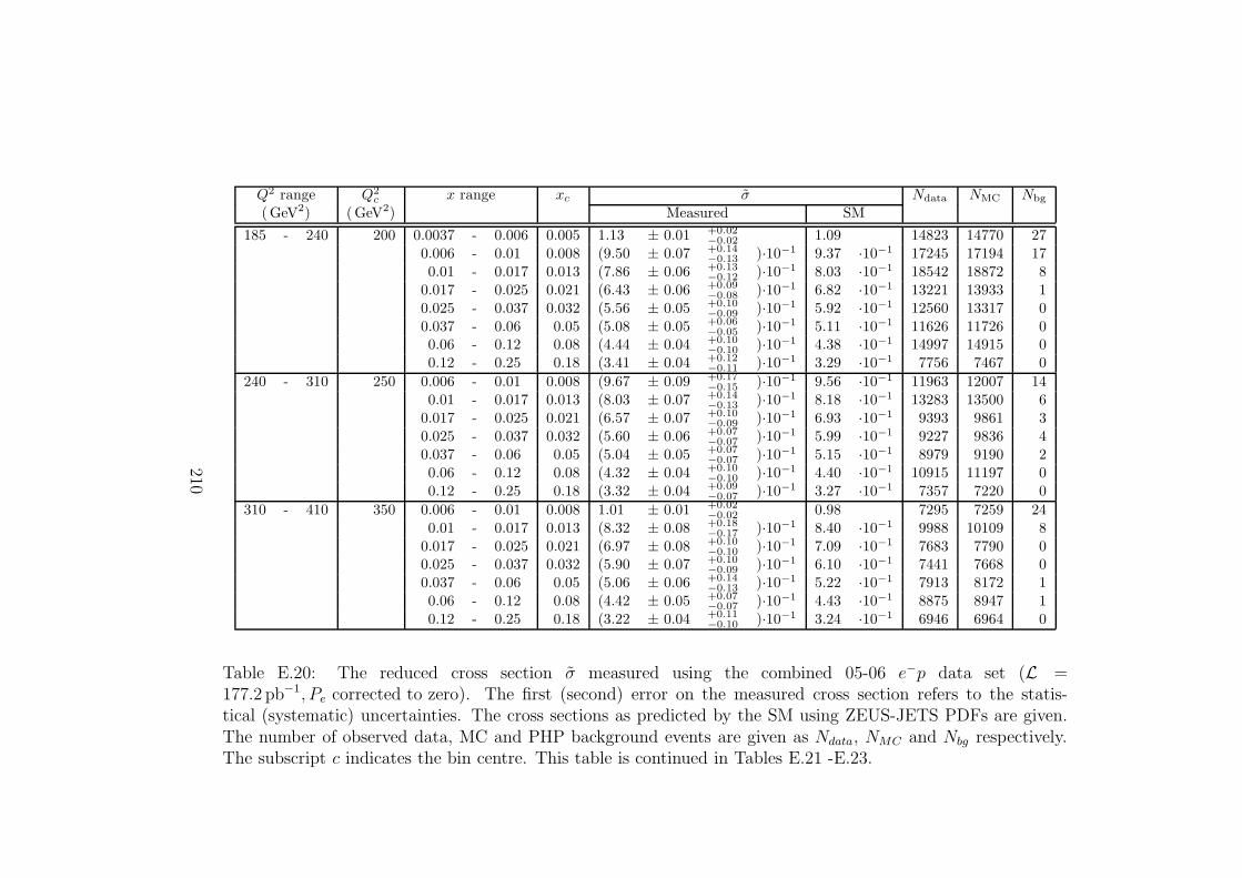
Q2 range Q2c x range xc σ Ndata NMC Nbg
(GeV2) (GeV2) Measured SM
185 - 240 200 0.0037 - 0.006 0.005 1.13 ± 0.01 +0.02−0.02 1.09 14823 14770 27
0.006 - 0.01 0.008 (9.50 ± 0.07 +0.14−0.13 )·10−1 9.37 ·10−1 17245 17194 17
0.01 - 0.017 0.013 (7.86 ± 0.06 +0.13−0.12 )·10−1 8.03 ·10−1 18542 18872 8
0.017 - 0.025 0.021 (6.43 ± 0.06 +0.09−0.08 )·10−1 6.82 ·10−1 13221 13933 1
0.025 - 0.037 0.032 (5.56 ± 0.05 +0.10−0.09 )·10−1 5.92 ·10−1 12560 13317 0
0.037 - 0.06 0.05 (5.08 ± 0.05 +0.06−0.05 )·10−1 5.11 ·10−1 11626 11726 0
0.06 - 0.12 0.08 (4.44 ± 0.04 +0.10−0.10 )·10−1 4.38 ·10−1 14997 14915 0
0.12 - 0.25 0.18 (3.41 ± 0.04 +0.12−0.11 )·10−1 3.29 ·10−1 7756 7467 0
240 - 310 250 0.006 - 0.01 0.008 (9.67 ± 0.09 +0.17−0.15 )·10−1 9.56 ·10−1 11963 12007 14
0.01 - 0.017 0.013 (8.03 ± 0.07 +0.14−0.13 )·10−1 8.18 ·10−1 13283 13500 6
0.017 - 0.025 0.021 (6.57 ± 0.07 +0.10−0.09 )·10−1 6.93 ·10−1 9393 9861 3
0.025 - 0.037 0.032 (5.60 ± 0.06 +0.07−0.07 )·10−1 5.99 ·10−1 9227 9836 4
0.037 - 0.06 0.05 (5.04 ± 0.05 +0.07−0.07 )·10−1 5.15 ·10−1 8979 9190 2
0.06 - 0.12 0.08 (4.32 ± 0.04 +0.10−0.10 )·10−1 4.40 ·10−1 10915 11197 0
0.12 - 0.25 0.18 (3.32 ± 0.04 +0.09−0.07 )·10−1 3.27 ·10−1 7357 7220 0
310 - 410 350 0.006 - 0.01 0.008 1.01 ± 0.01 +0.02−0.02 0.98 7295 7259 24
0.01 - 0.017 0.013 (8.32 ± 0.08 +0.18−0.17 )·10−1 8.40 ·10−1 9988 10109 8
0.017 - 0.025 0.021 (6.97 ± 0.08 +0.10−0.10 )·10−1 7.09 ·10−1 7683 7790 0
0.025 - 0.037 0.032 (5.90 ± 0.07 +0.10−0.09 )·10−1 6.10 ·10−1 7441 7668 0
0.037 - 0.06 0.05 (5.06 ± 0.06 +0.14−0.13 )·10−1 5.22 ·10−1 7913 8172 1
0.06 - 0.12 0.08 (4.42 ± 0.05 +0.07−0.07 )·10−1 4.43 ·10−1 8875 8947 1
0.12 - 0.25 0.18 (3.22 ± 0.04 +0.11−0.10 )·10−1 3.24 ·10−1 6946 6964 0
Table E.20: The reduced cross section σ measured using the combined 05-06 e−p data set (L =177.2 pb−1, Pe corrected to zero). The first (second) error on the measured cross section refers to the statis-tical (systematic) uncertainties. The cross sections as predicted by the SM using ZEUS-JETS PDFs are given.The number of observed data, MC and PHP background events are given as Ndata, NMC and Nbg respectively.The subscript c indicates the bin centre. This table is continued in Tables E.21 -E.23.
210

Q2 range Q2c x range xc σ Ndata NMC Nbg
(GeV2) (GeV2) Measured SM
410 - 530 450 0.006 - 0.01 0.008 1.03 ± 0.01 +0.03−0.03 0.99 5614 5625 34
0.01 - 0.017 0.013 (8.82 ± 0.13 +0.12−0.13 )·10−1 8.54 ·10−1 4967 4846 8
0.017 - 0.025 0.021 (6.92 ± 0.11 +0.12−0.10 )·10−1 7.20 ·10−1 3859 4012 0
0.025 - 0.037 0.032 (5.81 ± 0.09 +0.11−0.11 )·10−1 6.18 ·10−1 4383 4645 3
0.037 - 0.06 0.05 (5.10 ± 0.07 +0.10−0.10 )·10−1 5.27 ·10−1 5489 5674 0
0.06 - 0.1 0.08 (4.37 ± 0.07 +0.07−0.06 )·10−1 4.45 ·10−1 4455 4562 0
0.1 - 0.17 0.13 (3.62 ± 0.06 +0.08−0.07 )·10−1 3.72 ·10−1 3917 4039 0
0.17 - 0.3 0.25 (2.63 ± 0.05 +0.08−0.08 )·10−1 2.62 ·10−1 2960 2912 0
530 - 710 650 0.01 - 0.017 0.013 (9.06 ± 0.12 +0.18−0.16 )·10−1 8.70 ·10−1 5635 5529 15
0.017 - 0.025 0.021 (7.58 ± 0.12 +0.12−0.12 )·10−1 7.36 ·10−1 3745 3645 7
0.025 - 0.037 0.032 (5.95 ± 0.11 +0.10−0.08 )·10−1 6.30 ·10−1 2883 3053 0
0.037 - 0.06 0.05 (5.08 ± 0.09 +0.05−0.04 )·10−1 5.34 ·10−1 3057 3221 0
0.06 - 0.1 0.08 (4.25 ± 0.08 +0.10−0.10 )·10−1 4.48 ·10−1 2539 2685 1
0.1 - 0.17 0.13 (3.64 ± 0.08 +0.06−0.06 )·10−1 3.72 ·10−1 2331 2382 0
0.17 - 0.3 0.25 (2.55 ± 0.06 +0.07−0.07 )·10−1 2.58 ·10−1 1997 1993 0
710 - 900 800 0.009 - 0.017 0.013 (8.82 ± 0.15 +0.22−0.20 )·10−1 8.75 ·10−1 3517 3604 30
0.017 - 0.025 0.021 (7.40 ± 0.15 +0.16−0.14 )·10−1 7.45 ·10−1 2475 2514 1
0.025 - 0.037 0.032 (6.33 ± 0.12 +0.07−0.06 )·10−1 6.38 ·10−1 2602 2615 6
0.037 - 0.06 0.05 (5.16 ± 0.10 +0.07−0.07 )·10−1 5.39 ·10−1 2831 2963 0
0.06 - 0.1 0.08 (4.54 ± 0.09 +0.05−0.05 )·10−1 4.51 ·10−1 2449 2441 0
0.1 - 0.17 0.13 (3.81 ± 0.09 +0.04−0.04 )·10−1 3.72 ·10−1 1992 1946 0
0.17 - 0.3 0.25 (2.59 ± 0.07 +0.07−0.06 )·10−1 2.57 ·10−1 1475 1441 0
Table E.21: Continuation of Table E.20.
211

Q2 range Q2c x range xc σ Ndata NMC Nbg
(GeV2) (GeV2) Measured SM
900 - 1300 1200 0.01 - 0.017 0.014 (9.18 ± 0.19 +0.42−0.41 )·10−1 8.47 ·10−1 2317 2275 50
0.017 - 0.025 0.021 (8.11 ± 0.16 +0.17−0.16 )·10−1 7.63 ·10−1 2693 2580 15
0.025 - 0.037 0.032 (6.15 ± 0.12 +0.09−0.08 )·10−1 6.57 ·10−1 2612 2793 3
0.037 - 0.06 0.05 (5.51 ± 0.09 +0.05−0.05 )·10−1 5.53 ·10−1 3382 3388 1
0.06 - 0.1 0.08 (4.57 ± 0.08 +0.04−0.03 )·10−1 4.59 ·10−1 3192 3208 1
0.1 - 0.17 0.13 (3.76 ± 0.07 +0.03−0.02 )·10−1 3.75 ·10−1 2578 2563 0
0.17 - 0.3 0.25 (2.52 ± 0.06 +0.03−0.03 )·10−1 2.54 ·10−1 1988 1971 0
0.3 - 0.53 0.4 (1.25 ± 0.05 +0.10−0.03 )·10−1 1.36 ·10−1 675 704 0
1300 - 1800 1500 0.017 - 0.025 0.021 (8.11 ± 0.23 +0.25−0.25 )·10−1 7.67 ·10−1 1339 1302 22
0.025 - 0.037 0.032 (6.42 ± 0.17 +0.15−0.14 )·10−1 6.66 ·10−1 1477 1545 4
0.037 - 0.06 0.05 (5.26 ± 0.12 +0.06−0.05 )·10−1 5.61 ·10−1 1848 1977 0
0.06 - 0.1 0.08 (4.72 ± 0.11 +0.05−0.05 )·10−1 4.63 ·10−1 1985 1955 0
0.1 - 0.15 0.13 (3.83 ± 0.11 +0.05−0.04 )·10−1 3.77 ·10−1 1271 1249 0
0.15 - 0.23 0.18 (3.16 ± 0.10 +0.04−0.03 )·10−1 3.20 ·10−1 1080 1084 0
0.23 - 0.35 0.25 (2.65 ± 0.10 +0.09−0.08 )·10−1 2.53 ·10−1 766 720 0
0.35 - 0.53 0.4 (1.32 ± 0.07 +0.12−0.07 )·10−1 1.34 ·10−1 339 332 0
1800 - 2500 2000 0.023 - 0.037 0.032 (6.56 ± 0.21 +0.40−0.39 )·10−1 6.83 ·10−1 1037 1083 23
0.037 - 0.06 0.05 (5.62 ± 0.16 +0.12−0.11 )·10−1 5.77 ·10−1 1281 1321 3
0.06 - 0.1 0.08 (4.58 ± 0.13 +0.03−0.03 )·10−1 4.75 ·10−1 1305 1357 1
0.1 - 0.15 0.13 (3.75 ± 0.12 +0.05−0.05 )·10−1 3.83 ·10−1 927 946 0
0.15 - 0.23 0.18 (3.11 ± 0.11 +0.04−0.06 )·10−1 3.23 ·10−1 753 775 0
0.23 - 0.35 0.25 (2.51 ± 0.11 +0.03−0.02 )·10−1 2.54 ·10−1 524 522 0
0.35 - 0.53 0.4 (1.21 ± 0.08 +0.03−0.04 )·10−1 1.33 ·10−1 250 265 0
Table E.22: Continuation of Table E.21.
212

Q2 range Q2c x range xc σ Ndata NMC Nbg
(GeV2) (GeV2) Measured SM
2500 - 3500 3000 0.037 - 0.06 0.05 (6.04 ± 0.21 +0.33−0.32 )·10−1 6.12 ·10−1 821 847 3
0.06 - 0.1 0.08 (5.06 ± 0.16 +0.04−0.04 )·10−1 5.01 ·10−1 947 946 0
0.1 - 0.15 0.13 (3.79 ± 0.15 +0.05−0.05 )·10−1 3.99 ·10−1 656 689 2
0.15 - 0.23 0.18 (3.26 ± 0.14 +0.02−0.03 )·10−1 3.32 ·10−1 558 565 0
0.23 - 0.35 0.25 (2.86 ± 0.14 +0.14−0.13 )·10−1 2.58 ·10−1 441 392 0
0.35 - 0.53 0.4 (1.38 ± 0.10 +0.08−0.08 )·10−1 1.32 ·10−1 198 184 0
0.53 - 1 0.65 (1.66 +0.23−0.20
+0.11−0.10 )·10−2 2.08 ·10−2 65 76 0
3500 - 5600 5000 0.04 - 0.1 0.08 (5.37 ± 0.17 +0.27−0.26 )·10−1 5.65 ·10−1 1051 1121 6
0.1 - 0.15 0.13 (4.59 ± 0.18 +0.06−0.06 )·10−1 4.42 ·10−1 640 619 0
0.15 - 0.23 0.18 (3.49 ± 0.15 +0.04−0.02 )·10−1 3.60 ·10−1 535 550 0
0.23 - 0.35 0.25 (2.49 ± 0.14 +0.05−0.05 )·10−1 2.74 ·10−1 339 366 2
0.35 - 0.53 0.4 (1.38 ± 0.10 +0.04−0.03 )·10−1 1.36 ·10−1 184 175 0
5600 - 9000 8000 0.07 - 0.15 0.13 (5.82 ± 0.23 +0.17−0.19 )·10−1 5.16 ·10−1 625 559 1
0.15 - 0.23 0.18 (4.35 ± 0.23 +0.10−0.11 )·10−1 4.12 ·10−1 363 344 0
0.23 - 0.35 0.25 (3.17 ± 0.20 +0.03−0.05 )·10−1 3.04 ·10−1 250 237 0
0.35 - 0.53 0.4 (1.16 +0.13−0.12
+0.02−0.03 )·10−1 1.45 ·10−1 93 112 0
0.53 - 1 0.65 (1.76 +0.35−0.30
+0.10−0.09 )·10−2 2.08 ·10−2 35 39 0
9000 - 15000 12000 0.09 - 0.23 0.18 (4.89 ± 0.28 +0.20−0.19 )·10−1 4.85 ·10−1 298 298 0
0.23 - 0.35 0.25 (3.51 ± 0.28 +0.07−0.08 )·10−1 3.50 ·10−1 154 153 0
0.35 - 0.53 0.4 (1.56 +0.20−0.18
+0.07−0.07 )·10−1 1.59 ·10−1 75 74 0
15000 - 25000 20000 0.15 - 0.35 0.25 (4.69 ± 0.41 +0.40−0.41 )·10−1 4.32 ·10−1 132 121 2
0.35 - 1 0.4 (1.88 +0.30−0.26
+0.20−0.20 )·10−1 1.89 ·10−1 51 50 0
25000 - 50000 30000 0.25 - 1 0.4 (2.52 +0.43−0.37
+0.24−0.14 )·10−1 2.22 ·10−1 46 40 0
Table E.23: Continuation of Table E.22.
213

Q2 range Q2c x range xc σ Ndata NMC Nbg
(GeV2) (GeV2) Measured SM
185 - 240 200 0.0037 - 0.006 0.005 1.13 ± 0.01 +0.03−0.05 1.09 8814 8782 16
0.006 - 0.01 0.008 (9.45 ± 0.09 +0.23−0.30 )·10−1 9.41 ·10−1 10192 10223 10
0.01 - 0.017 0.013 (7.86 ± 0.07 +0.15−0.22 )·10−1 8.06 ·10−1 11013 11221 5
0.017 - 0.025 0.021 (6.39 ± 0.07 +0.23−0.20 )·10−1 6.85 ·10−1 7800 8284 1
0.025 - 0.037 0.032 (5.59 ± 0.06 +0.12−0.14 )·10−1 5.94 ·10−1 7506 7919 0
0.037 - 0.06 0.05 (5.09 ± 0.06 +0.08−0.11 )·10−1 5.13 ·10−1 6930 6972 0
0.06 - 0.12 0.08 (4.50 ± 0.05 +0.13−0.14 )·10−1 4.40 ·10−1 9017 8865 0
0.12 - 0.25 0.18 (3.48 ± 0.05 +0.07−0.07 )·10−1 3.30 ·10−1 4707 4443 0
240 - 310 250 0.006 - 0.01 0.008 (9.81 ± 0.12 +0.48−0.54 )·10−1 9.61 ·10−1 7210 7140 8
0.01 - 0.017 0.013 (8.08 ± 0.09 +0.12−0.29 )·10−1 8.22 ·10−1 7935 8026 4
0.017 - 0.025 0.021 (6.61 ± 0.09 +0.09−0.16 )·10−1 6.96 ·10−1 5618 5863 2
0.025 - 0.037 0.032 (5.65 ± 0.08 +0.04−0.07 )·10−1 6.02 ·10−1 5532 5847 3
0.037 - 0.06 0.05 (5.15 ± 0.07 +0.02−0.07 )·10−1 5.18 ·10−1 5452 5466 1
0.06 - 0.12 0.08 (4.32 ± 0.05 +0.03−0.04 )·10−1 4.42 ·10−1 6479 6654 0
0.12 - 0.25 0.18 (3.38 ± 0.05 +0.04−0.05 )·10−1 3.28 ·10−1 4445 4293 0
310 - 410 350 0.006 - 0.01 0.008 1.01 ± 0.02 +0.04−0.05 0.99 4346 4317 14
0.01 - 0.017 0.013 (8.29 ± 0.11 +0.42−0.44 )·10−1 8.46 ·10−1 5915 6011 4
0.017 - 0.025 0.021 (7.00 ± 0.10 +0.23−0.26 )·10−1 7.14 ·10−1 4584 4631 0
0.025 - 0.037 0.032 (5.94 ± 0.09 +0.06−0.09 )·10−1 6.15 ·10−1 4451 4559 0
0.037 - 0.06 0.05 (5.10 ± 0.07 +0.04−0.07 )·10−1 5.25 ·10−1 4736 4859 1
0.06 - 0.12 0.08 (4.44 ± 0.06 +0.03−0.08 )·10−1 4.46 ·10−1 5299 5317 1
0.12 - 0.25 0.18 (3.28 ± 0.05 +0.05−0.06 )·10−1 3.26 ·10−1 4200 4141 0
Table E.24: The reduced cross section σ measured using the negatively polarised 05-06 e−p data set (L =105.4 pb−1, Pe = −0.27). The first (second) error on the measured cross section refers to the statistical (system-atic) uncertainties. The cross sections as predicted by the SM using ZEUS-JETS PDFs are given. The numberof observed data, MC and PHP background events are given as Ndata, NMC and Nbg respectively. The subscriptc indicates the bin centre. This table is continued in Tables E.25 -E.27.
214

Q2 range Q2c x range xc σ Ndata NMC Nbg
(GeV2) (GeV2) Measured SM
410 - 530 450 0.006 - 0.01 0.008 1.02 ± 0.02 +0.05−0.06 1.00 3305 3341 20
0.01 - 0.017 0.013 (8.93 ± 0.16 +0.13−0.17 )·10−1 8.62 ·10−1 2985 2879 5
0.017 - 0.025 0.021 (6.95 ± 0.14 +0.16−0.14 )·10−1 7.27 ·10−1 2305 2390 0
0.025 - 0.037 0.032 (5.96 ± 0.12 +0.04−0.06 )·10−1 6.24 ·10−1 2671 2764 2
0.037 - 0.06 0.05 (5.21 ± 0.09 +0.06−0.06 )·10−1 5.31 ·10−1 3333 3375 0
0.06 - 0.1 0.08 (4.51 ± 0.09 +0.02−0.02 )·10−1 4.48 ·10−1 2733 2713 0
0.1 - 0.17 0.13 (3.64 ± 0.08 +0.04−0.05 )·10−1 3.75 ·10−1 2344 2401 0
0.17 - 0.3 0.25 (2.71 ± 0.06 +0.04−0.04 )·10−1 2.64 ·10−1 1813 1732 0
530 - 710 650 0.01 - 0.017 0.013 (9.10 ± 0.16 +0.42−0.46 )·10−1 8.82 ·10−1 3357 3284 9
0.017 - 0.025 0.021 (7.58 ± 0.16 +0.03−0.18 )·10−1 7.46 ·10−1 2215 2161 4
0.025 - 0.037 0.032 (5.98 ± 0.14 +0.07−0.11 )·10−1 6.38 ·10−1 1716 1811 0
0.037 - 0.06 0.05 (5.19 ± 0.12 +0.13−0.14 )·10−1 5.41 ·10−1 1855 1915 0
0.06 - 0.1 0.08 (4.31 ± 0.11 +0.03−0.03 )·10−1 4.53 ·10−1 1530 1599 1
0.1 - 0.17 0.13 (3.73 ± 0.10 +0.03−0.03 )·10−1 3.76 ·10−1 1419 1419 0
0.17 - 0.3 0.25 (2.56 ± 0.07 +0.01−0.02 )·10−1 2.61 ·10−1 1194 1187 0
710 - 900 800 0.009 - 0.017 0.013 (9.07 ± 0.20 +0.18−0.27 )·10−1 8.88 ·10−1 2151 2143 18
0.017 - 0.025 0.021 (7.76 ± 0.20 +0.03−0.17 )·10−1 7.57 ·10−1 1539 1494 1
0.025 - 0.037 0.032 (6.52 ± 0.16 +0.18−0.18 )·10−1 6.48 ·10−1 1588 1554 3
0.037 - 0.06 0.05 (5.32 ± 0.13 +0.14−0.14 )·10−1 5.47 ·10−1 1730 1758 0
0.06 - 0.1 0.08 (4.60 ± 0.12 +0.09−0.09 )·10−1 4.57 ·10−1 1467 1447 0
0.1 - 0.17 0.13 (3.84 ± 0.11 +0.03−0.04 )·10−1 3.77 ·10−1 1186 1153 0
0.17 - 0.3 0.25 (2.72 ± 0.09 +0.03−0.04 )·10−1 2.60 ·10−1 915 853 0
Table E.25: Continuation of Table E.24.
215
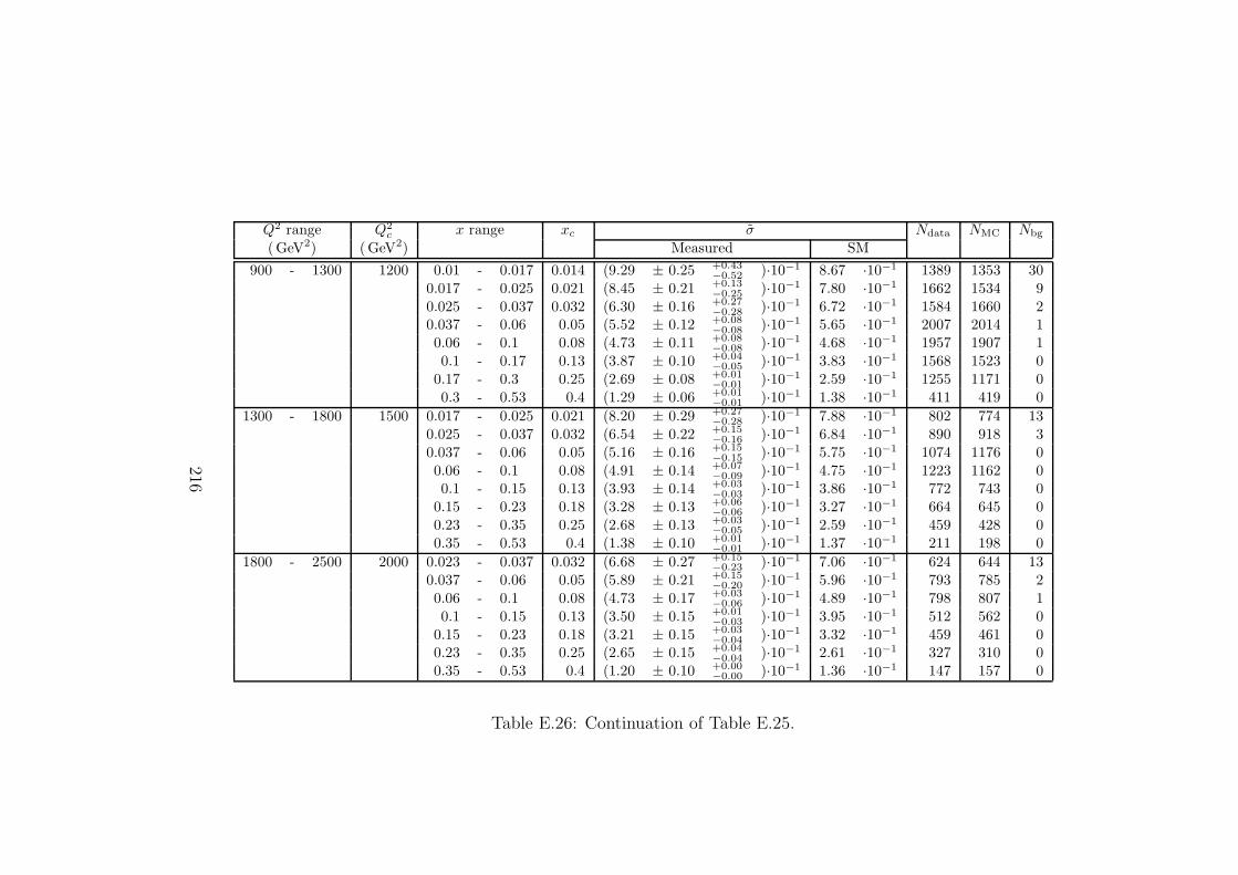
Q2 range Q2c x range xc σ Ndata NMC Nbg
(GeV2) (GeV2) Measured SM
900 - 1300 1200 0.01 - 0.017 0.014 (9.29 ± 0.25 +0.43−0.52 )·10−1 8.67 ·10−1 1389 1353 30
0.017 - 0.025 0.021 (8.45 ± 0.21 +0.13−0.25 )·10−1 7.80 ·10−1 1662 1534 9
0.025 - 0.037 0.032 (6.30 ± 0.16 +0.27−0.28 )·10−1 6.72 ·10−1 1584 1660 2
0.037 - 0.06 0.05 (5.52 ± 0.12 +0.08−0.08 )·10−1 5.65 ·10−1 2007 2014 1
0.06 - 0.1 0.08 (4.73 ± 0.11 +0.08−0.08 )·10−1 4.68 ·10−1 1957 1907 1
0.1 - 0.17 0.13 (3.87 ± 0.10 +0.04−0.05 )·10−1 3.83 ·10−1 1568 1523 0
0.17 - 0.3 0.25 (2.69 ± 0.08 +0.01−0.01 )·10−1 2.59 ·10−1 1255 1171 0
0.3 - 0.53 0.4 (1.29 ± 0.06 +0.01−0.01 )·10−1 1.38 ·10−1 411 419 0
1300 - 1800 1500 0.017 - 0.025 0.021 (8.20 ± 0.29 +0.27−0.28 )·10−1 7.88 ·10−1 802 774 13
0.025 - 0.037 0.032 (6.54 ± 0.22 +0.15−0.16 )·10−1 6.84 ·10−1 890 918 3
0.037 - 0.06 0.05 (5.16 ± 0.16 +0.15−0.15 )·10−1 5.75 ·10−1 1074 1176 0
0.06 - 0.1 0.08 (4.91 ± 0.14 +0.07−0.09 )·10−1 4.75 ·10−1 1223 1162 0
0.1 - 0.15 0.13 (3.93 ± 0.14 +0.03−0.03 )·10−1 3.86 ·10−1 772 743 0
0.15 - 0.23 0.18 (3.28 ± 0.13 +0.06−0.06 )·10−1 3.27 ·10−1 664 645 0
0.23 - 0.35 0.25 (2.68 ± 0.13 +0.03−0.05 )·10−1 2.59 ·10−1 459 428 0
0.35 - 0.53 0.4 (1.38 ± 0.10 +0.01−0.01 )·10−1 1.37 ·10−1 211 198 0
1800 - 2500 2000 0.023 - 0.037 0.032 (6.68 ± 0.27 +0.15−0.23 )·10−1 7.06 ·10−1 624 644 13
0.037 - 0.06 0.05 (5.89 ± 0.21 +0.15−0.20 )·10−1 5.96 ·10−1 793 785 2
0.06 - 0.1 0.08 (4.73 ± 0.17 +0.03−0.06 )·10−1 4.89 ·10−1 798 807 1
0.1 - 0.15 0.13 (3.50 ± 0.15 +0.01−0.03 )·10−1 3.95 ·10−1 512 562 0
0.15 - 0.23 0.18 (3.21 ± 0.15 +0.03−0.04 )·10−1 3.32 ·10−1 459 461 0
0.23 - 0.35 0.25 (2.65 ± 0.15 +0.04−0.04 )·10−1 2.61 ·10−1 327 310 0
0.35 - 0.53 0.4 (1.20 ± 0.10 +0.00−0.00 )·10−1 1.36 ·10−1 147 157 0
Table E.26: Continuation of Table E.25.
216
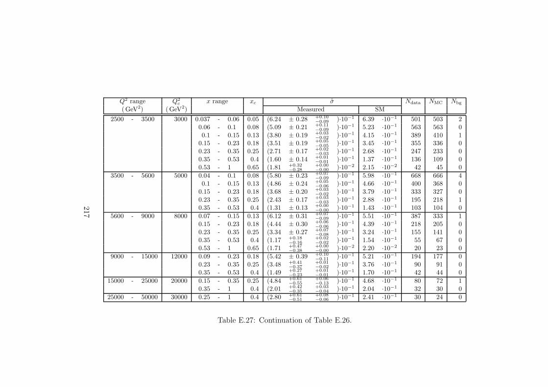
Q2 range Q2c x range xc σ Ndata NMC Nbg
(GeV2) (GeV2) Measured SM
2500 - 3500 3000 0.037 - 0.06 0.05 (6.24 ± 0.28 +0.10−0.09 )·10−1 6.39 ·10−1 501 503 2
0.06 - 0.1 0.08 (5.09 ± 0.21 +0.11−0.09 )·10−1 5.23 ·10−1 563 563 0
0.1 - 0.15 0.13 (3.80 ± 0.19 +0.03−0.02 )·10−1 4.15 ·10−1 389 410 1
0.15 - 0.23 0.18 (3.51 ± 0.19 +0.05−0.05 )·10−1 3.45 ·10−1 355 336 0
0.23 - 0.35 0.25 (2.71 ± 0.17 +0.02−0.03 )·10−1 2.68 ·10−1 247 233 0
0.35 - 0.53 0.4 (1.60 ± 0.14 +0.01−0.01 )·10−1 1.37 ·10−1 136 109 0
0.53 - 1 0.65 (1.81 +0.32−0.28
+0.00−0.00 )·10−2 2.15 ·10−2 42 45 0
3500 - 5600 5000 0.04 - 0.1 0.08 (5.80 ± 0.23 +0.07−0.09 )·10−1 5.98 ·10−1 668 666 4
0.1 - 0.15 0.13 (4.86 ± 0.24 +0.05−0.06 )·10−1 4.66 ·10−1 400 368 0
0.15 - 0.23 0.18 (3.68 ± 0.20 +0.03−0.02 )·10−1 3.79 ·10−1 333 327 0
0.23 - 0.35 0.25 (2.43 ± 0.17 +0.03−0.03 )·10−1 2.88 ·10−1 195 218 1
0.35 - 0.53 0.4 (1.31 ± 0.13 +0.00−0.00 )·10−1 1.43 ·10−1 103 104 0
5600 - 9000 8000 0.07 - 0.15 0.13 (6.12 ± 0.31 +0.07−0.09 )·10−1 5.51 ·10−1 387 333 1
0.15 - 0.23 0.18 (4.44 ± 0.30 +0.06−0.06 )·10−1 4.39 ·10−1 218 205 0
0.23 - 0.35 0.25 (3.34 ± 0.27 +0.07−0.08 )·10−1 3.24 ·10−1 155 141 0
0.35 - 0.53 0.4 (1.17 +0.18−0.16
+0.02−0.02 )·10−1 1.54 ·10−1 55 67 0
0.53 - 1 0.65 (1.71 +0.47−0.38
+0.00−0.00 )·10−2 2.20 ·10−2 20 23 0
9000 - 15000 12000 0.09 - 0.23 0.18 (5.42 ± 0.39 +0.10−0.11 )·10−1 5.21 ·10−1 194 177 0
0.23 - 0.35 0.25 (3.48 +0.41−0.37
+0.01−0.02 )·10−1 3.76 ·10−1 90 91 0
0.35 - 0.53 0.4 (1.49 +0.27−0.23
+0.01−0.01 )·10−1 1.70 ·10−1 42 44 0
15000 - 25000 20000 0.15 - 0.35 0.25 (4.84 +0.61−0.55
+0.06−0.13 )·10−1 4.68 ·10−1 80 72 1
0.35 - 1 0.4 (2.01 +0.42−0.35
+0.03−0.04 )·10−1 2.04 ·10−1 32 30 0
25000 - 50000 30000 0.25 - 1 0.4 (2.80 +0.61−0.51
+0.08−0.06 )·10−1 2.41 ·10−1 30 24 0
Table E.27: Continuation of Table E.26.
217
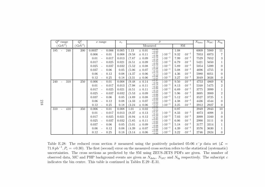
Q2 range Q2c x range xc σ Ndata NMC Nbg
(GeV2) (GeV2) Measured SM
185 - 240 200 0.0037 - 0.006 0.005 1.13 ± 0.01 +0.02−0.03 1.08 6009 5989 11
0.006 - 0.01 0.008 (9.58 ± 0.11 +0.21−0.38 )·10−1 9.32 ·10−1 7053 6973 7
0.01 - 0.017 0.013 (7.87 ± 0.09 +0.18−0.18 )·10−1 7.99 ·10−1 7529 7652 3
0.017 - 0.025 0.021 (6.51 ± 0.09 +0.24−0.22 )·10−1 6.79 ·10−1 5421 5650 1
0.025 - 0.037 0.032 (5.52 ± 0.08 +0.12−0.14 )·10−1 5.89 ·10−1 5054 5399 0
0.037 - 0.06 0.05 (5.06 ± 0.07 +0.08−0.10 )·10−1 5.08 ·10−1 4696 4755 0
0.06 - 0.12 0.08 (4.37 ± 0.06 +0.13−0.12 )·10−1 4.36 ·10−1 5980 6051 0
0.12 - 0.25 0.18 (3.31 ± 0.06 +0.06−0.07 )·10−1 3.27 ·10−1 3049 3026 0
240 - 310 250 0.006 - 0.01 0.008 (9.48 ± 0.14 +0.47−0.56 )·10−1 9.50 ·10−1 4753 4869 6
0.01 - 0.017 0.013 (7.98 ± 0.11 +0.14−0.24 )·10−1 8.13 ·10−1 5348 5475 2
0.017 - 0.025 0.021 (6.51 ± 0.11 +0.09−0.14 )·10−1 6.89 ·10−1 3775 3999 1
0.025 - 0.037 0.032 (5.53 ± 0.09 +0.04−0.06 )·10−1 5.96 ·10−1 3695 3989 2
0.037 - 0.06 0.05 (4.89 ± 0.08 +0.02−0.03 )·10−1 5.12 ·10−1 3527 3725 1
0.06 - 0.12 0.08 (4.33 ± 0.07 +0.03−0.04 )·10−1 4.38 ·10−1 4436 4544 0
0.12 - 0.25 0.18 (3.24 ± 0.06 +0.04−0.05 )·10−1 3.25 ·10−1 2912 2927 0
310 - 410 350 0.006 - 0.01 0.008 1.01 ± 0.02 +0.04−0.04 0.97 2949 2943 10
0.01 - 0.017 0.013 (8.37 ± 0.13 +0.41−0.44 )·10−1 8.33 ·10−1 4073 4098 3
0.017 - 0.025 0.021 (6.94 ± 0.12 +0.23−0.25 )·10−1 7.03 ·10−1 3099 3160 0
0.025 - 0.037 0.032 (5.85 ± 0.11 +0.05−0.05 )·10−1 6.06 ·10−1 2990 3111 0
0.037 - 0.06 0.05 (5.01 ± 0.09 +0.05−0.08 )·10−1 5.18 ·10−1 3177 3314 1
0.06 - 0.12 0.08 (4.39 ± 0.07 +0.03−0.06 )·10−1 4.39 ·10−1 3576 3630 1
0.12 - 0.25 0.18 (3.14 ± 0.06 +0.05−0.06 )·10−1 3.22 ·10−1 2746 2824 0
Table E.28: The reduced cross section σ measured using the positively polarised 05-06 e−p data set (L =71.8 pb−1, Pe = +0.30). The first (second) error on the measured cross section refers to the statistical (systematic)uncertainties. The cross sections as predicted by the SM using ZEUS-JETS PDFs are given. The number ofobserved data, MC and PHP background events are given as Ndata, NMC and Nbg respectively. The subscript cindicates the bin centre. This table is continued in Tables E.29 -E.31.
218
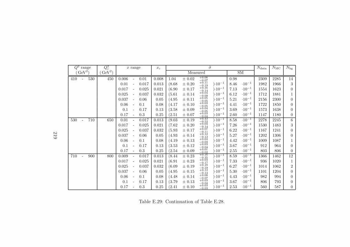
Q2 range Q2c x range xc σ Ndata NMC Nbg
(GeV2) (GeV2) Measured SM
410 - 530 450 0.006 - 0.01 0.008 1.04 ± 0.02 +0.06−0.07 0.98 2309 2285 14
0.01 - 0.017 0.013 (8.68 ± 0.20 +0.11−0.19 )·10−1 8.46 ·10−1 1982 1966 3
0.017 - 0.025 0.021 (6.90 ± 0.17 +0.16−0.14 )·10−1 7.13 ·10−1 1554 1623 0
0.025 - 0.037 0.032 (5.61 ± 0.14 +0.04−0.09 )·10−1 6.12 ·10−1 1712 1881 1
0.037 - 0.06 0.05 (4.95 ± 0.11 +0.05−0.05 )·10−1 5.21 ·10−1 2156 2300 0
0.06 - 0.1 0.08 (4.17 ± 0.10 +0.03−0.05 )·10−1 4.41 ·10−1 1722 1850 0
0.1 - 0.17 0.13 (3.58 ± 0.09 +0.04−0.05 )·10−1 3.69 ·10−1 1573 1638 0
0.17 - 0.3 0.25 (2.51 ± 0.07 +0.03−0.04 )·10−1 2.60 ·10−1 1147 1180 0
530 - 710 650 0.01 - 0.017 0.013 (9.03 ± 0.19 +0.43−0.52 )·10−1 8.58 ·10−1 2278 2245 6
0.017 - 0.025 0.021 (7.62 ± 0.20 +0.04−0.14 )·10−1 7.26 ·10−1 1530 1483 3
0.025 - 0.037 0.032 (5.93 ± 0.17 +0.07−0.11 )·10−1 6.22 ·10−1 1167 1241 0
0.037 - 0.06 0.05 (4.93 ± 0.14 +0.12−0.12 )·10−1 5.27 ·10−1 1202 1306 0
0.06 - 0.1 0.08 (4.19 ± 0.13 +0.04−0.03 )·10−1 4.42 ·10−1 1009 1087 1
0.1 - 0.17 0.13 (3.53 ± 0.12 +0.03−0.04 )·10−1 3.67 ·10−1 912 964 0
0.17 - 0.3 0.25 (2.54 ± 0.09 +0.01−0.02 )·10−1 2.55 ·10−1 803 806 0
710 - 900 800 0.009 - 0.017 0.013 (8.44 ± 0.23 +0.16−0.35 )·10−1 8.59 ·10−1 1366 1462 12
0.017 - 0.025 0.021 (6.91 ± 0.23 +0.03−0.17 )·10−1 7.33 ·10−1 936 1020 1
0.025 - 0.037 0.032 (6.09 ± 0.19 +0.18−0.19 )·10−1 6.27 ·10−1 1014 1062 2
0.037 - 0.06 0.05 (4.95 ± 0.15 +0.12−0.14 )·10−1 5.30 ·10−1 1101 1204 0
0.06 - 0.1 0.08 (4.48 ± 0.14 +0.08−0.07 )·10−1 4.43 ·10−1 982 994 0
0.1 - 0.17 0.13 (3.79 ± 0.13 +0.03−0.04 )·10−1 3.67 ·10−1 806 793 0
0.17 - 0.3 0.25 (2.41 ± 0.10 +0.03−0.03 )·10−1 2.53 ·10−1 560 587 0
Table E.29: Continuation of Table E.28.
219
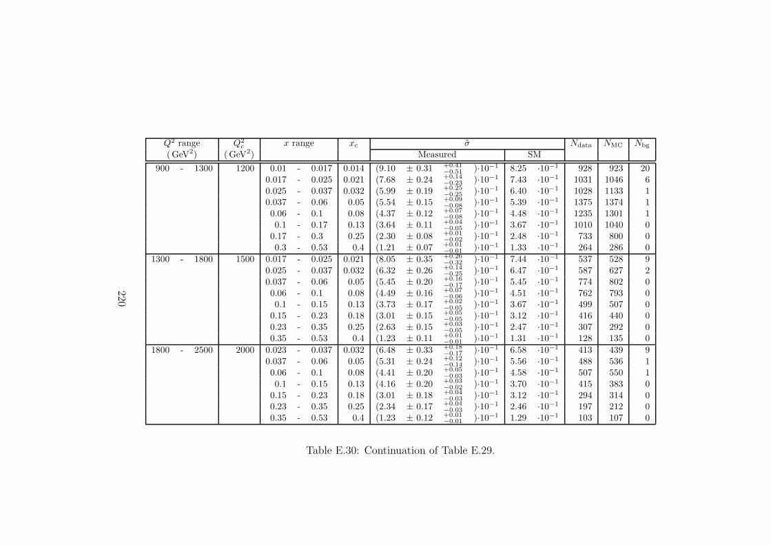
Q2 range Q2c x range xc σ Ndata NMC Nbg
(GeV2) (GeV2) Measured SM
900 - 1300 1200 0.01 - 0.017 0.014 (9.10 ± 0.31 +0.41−0.51 )·10−1 8.25 ·10−1 928 923 20
0.017 - 0.025 0.021 (7.68 ± 0.24 +0.14−0.23 )·10−1 7.43 ·10−1 1031 1046 6
0.025 - 0.037 0.032 (5.99 ± 0.19 +0.25−0.25 )·10−1 6.40 ·10−1 1028 1133 1
0.037 - 0.06 0.05 (5.54 ± 0.15 +0.09−0.08 )·10−1 5.39 ·10−1 1375 1374 1
0.06 - 0.1 0.08 (4.37 ± 0.12 +0.07−0.08 )·10−1 4.48 ·10−1 1235 1301 1
0.1 - 0.17 0.13 (3.64 ± 0.11 +0.04−0.05 )·10−1 3.67 ·10−1 1010 1040 0
0.17 - 0.3 0.25 (2.30 ± 0.08 +0.01−0.02 )·10−1 2.48 ·10−1 733 800 0
0.3 - 0.53 0.4 (1.21 ± 0.07 +0.01−0.01 )·10−1 1.33 ·10−1 264 286 0
1300 - 1800 1500 0.017 - 0.025 0.021 (8.05 ± 0.35 +0.26−0.32 )·10−1 7.44 ·10−1 537 528 9
0.025 - 0.037 0.032 (6.32 ± 0.26 +0.14−0.25 )·10−1 6.47 ·10−1 587 627 2
0.037 - 0.06 0.05 (5.45 ± 0.20 +0.16−0.17 )·10−1 5.45 ·10−1 774 802 0
0.06 - 0.1 0.08 (4.49 ± 0.16 +0.07−0.06 )·10−1 4.51 ·10−1 762 793 0
0.1 - 0.15 0.13 (3.73 ± 0.17 +0.02−0.05 )·10−1 3.67 ·10−1 499 507 0
0.15 - 0.23 0.18 (3.01 ± 0.15 +0.05−0.05 )·10−1 3.12 ·10−1 416 440 0
0.23 - 0.35 0.25 (2.63 ± 0.15 +0.03−0.05 )·10−1 2.47 ·10−1 307 292 0
0.35 - 0.53 0.4 (1.23 ± 0.11 +0.01−0.01 )·10−1 1.31 ·10−1 128 135 0
1800 - 2500 2000 0.023 - 0.037 0.032 (6.48 ± 0.33 +0.18−0.17 )·10−1 6.58 ·10−1 413 439 9
0.037 - 0.06 0.05 (5.31 ± 0.24 +0.12−0.14 )·10−1 5.56 ·10−1 488 536 1
0.06 - 0.1 0.08 (4.41 ± 0.20 +0.05−0.03 )·10−1 4.58 ·10−1 507 550 1
0.1 - 0.15 0.13 (4.16 ± 0.20 +0.03−0.02 )·10−1 3.70 ·10−1 415 383 0
0.15 - 0.23 0.18 (3.01 ± 0.18 +0.04−0.03 )·10−1 3.12 ·10−1 294 314 0
0.23 - 0.35 0.25 (2.34 ± 0.17 +0.04−0.03 )·10−1 2.46 ·10−1 197 212 0
0.35 - 0.53 0.4 (1.23 ± 0.12 +0.01−0.01 )·10−1 1.29 ·10−1 103 107 0
Table E.30: Continuation of Table E.29.
220
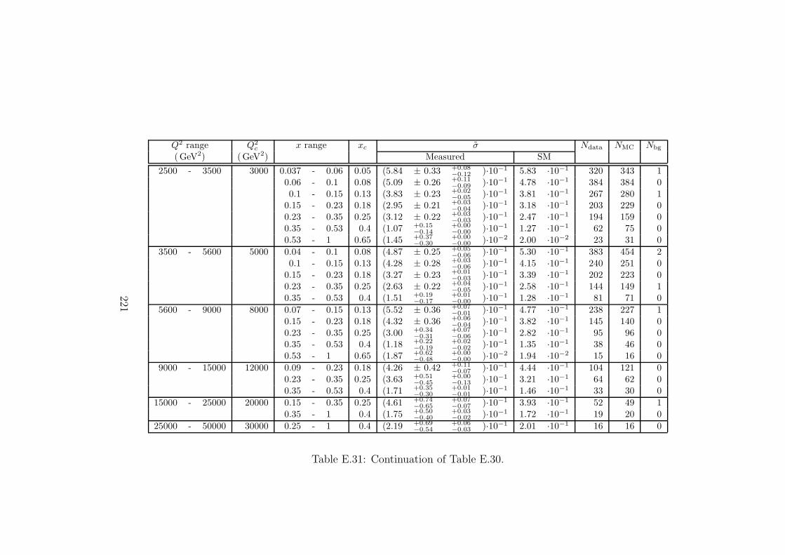
Q2 range Q2c x range xc σ Ndata NMC Nbg
(GeV2) (GeV2) Measured SM
2500 - 3500 3000 0.037 - 0.06 0.05 (5.84 ± 0.33 +0.08−0.12 )·10−1 5.83 ·10−1 320 343 1
0.06 - 0.1 0.08 (5.09 ± 0.26 +0.11−0.09 )·10−1 4.78 ·10−1 384 384 0
0.1 - 0.15 0.13 (3.83 ± 0.23 +0.02−0.05 )·10−1 3.81 ·10−1 267 280 1
0.15 - 0.23 0.18 (2.95 ± 0.21 +0.03−0.04 )·10−1 3.18 ·10−1 203 229 0
0.23 - 0.35 0.25 (3.12 ± 0.22 +0.03−0.03 )·10−1 2.47 ·10−1 194 159 0
0.35 - 0.53 0.4 (1.07 +0.15−0.14
+0.00−0.00 )·10−1 1.27 ·10−1 62 75 0
0.53 - 1 0.65 (1.45 +0.37−0.30
+0.00−0.00 )·10−2 2.00 ·10−2 23 31 0
3500 - 5600 5000 0.04 - 0.1 0.08 (4.87 ± 0.25 +0.05−0.06 )·10−1 5.30 ·10−1 383 454 2
0.1 - 0.15 0.13 (4.28 ± 0.28 +0.03−0.06 )·10−1 4.15 ·10−1 240 251 0
0.15 - 0.23 0.18 (3.27 ± 0.23 +0.01−0.03 )·10−1 3.39 ·10−1 202 223 0
0.23 - 0.35 0.25 (2.63 ± 0.22 +0.04−0.05 )·10−1 2.58 ·10−1 144 149 1
0.35 - 0.53 0.4 (1.51 +0.19−0.17
+0.01−0.00 )·10−1 1.28 ·10−1 81 71 0
5600 - 9000 8000 0.07 - 0.15 0.13 (5.52 ± 0.36 +0.07−0.01 )·10−1 4.77 ·10−1 238 227 1
0.15 - 0.23 0.18 (4.32 ± 0.36 +0.06−0.04 )·10−1 3.82 ·10−1 145 140 0
0.23 - 0.35 0.25 (3.00 +0.34−0.31
+0.07−0.06 )·10−1 2.82 ·10−1 95 96 0
0.35 - 0.53 0.4 (1.18 +0.22−0.19
+0.02−0.02 )·10−1 1.35 ·10−1 38 46 0
0.53 - 1 0.65 (1.87 +0.62−0.48
+0.00−0.00 )·10−2 1.94 ·10−2 15 16 0
9000 - 15000 12000 0.09 - 0.23 0.18 (4.26 ± 0.42 +0.11−0.07 )·10−1 4.44 ·10−1 104 121 0
0.23 - 0.35 0.25 (3.63 +0.51−0.45
+0.00−0.13 )·10−1 3.21 ·10−1 64 62 0
0.35 - 0.53 0.4 (1.71 +0.35−0.30
+0.01−0.01 )·10−1 1.46 ·10−1 33 30 0
15000 - 25000 20000 0.15 - 0.35 0.25 (4.61 +0.74−0.65
+0.07−0.07 )·10−1 3.93 ·10−1 52 49 1
0.35 - 1 0.4 (1.75 +0.50−0.40
+0.03−0.02 )·10−1 1.72 ·10−1 19 20 0
25000 - 50000 30000 0.25 - 1 0.4 (2.19 +0.69−0.54
+0.06−0.03 )·10−1 2.01 ·10−1 16 16 0
Table E.31: Continuation of Table E.30.
221

Q2 range Q2c x range xc xF3
( GeV2) ( GeV2) Measured SM
2500 - 3500 3000 0.037 - 0.06 0.05 (4.21 ± 2.74 +2.36−2.33 )·10−2 6.75 ·10−2
0.06 - 0.1 0.08 (1.08 ± 0.34 +0.08−0.10 )·10−1 0.77 ·10−1
0.1 - 0.15 0.13 (5.73 ± 5.55 +3.10−1.24 )·10−2 8.12 ·10−2
0.15 - 0.23 0.18 (2.66 ± 7.18 +1.43−3.10 )·10−2 7.79 ·10−2
0.23 - 0.35 0.25 (2.25 ± 0.94 +0.56−0.68 )·10−1 0.67 ·10−1
0.35 - 0.53 0.4 (1.52 ± 11.67 +6.31−6.16 )·10−2 3.69 ·10−2
0.53 - 1 0.65 (-3.89 +4.53−4.38
+2.76−1.72 )·10−2 0.59 ·10−2
3500 - 5600 5000 0.04 - 0.1 0.08 (8.06 ± 1.95 +1.93−1.82 )·10−2 10.95 ·10−2
0.1 - 0.15 0.13 (1.10 ± 0.36 +0.08−0.09 )·10−1 1.15 ·10−1
0.15 - 0.23 0.18 (1.26 ± 0.42 +0.09−0.13 )·10−1 1.09 ·10−1
0.23 - 0.35 0.25 (7.39 ± 5.39 +1.82−1.85 )·10−2 9.30 ·10−2
0.35 - 0.53 0.4 (9.89 ± 6.60 +2.20−1.41 )·10−2 5.05 ·10−2
5600 - 9000 8000 0.07 - 0.15 0.13 (1.88 ± 0.25 +0.13−0.14 )·10−1 1.50 ·10−1
0.15 - 0.23 0.18 (1.55 ± 0.35 +0.10−0.12 )·10−1 1.42 ·10−1
0.23 - 0.35 0.25 (1.61 ± 0.43 +0.11−0.09 )·10−1 1.20 ·10−1
0.35 - 0.53 0.4 (4.50 +4.90−4.72
+1.21−1.03 )·10−2 6.41 ·10−2
0.53 - 1 0.65 (1.88 +2.40−1.87
+0.47−0.51 )·10−2 0.97 ·10−2
9000 - 15000 12000 0.09 - 0.23 0.18 (1.07 ± 0.31 +0.14−0.18 )·10−1 1.70 ·10−1
0.23 - 0.35 0.25 (1.34 ± 0.43 +0.07−0.14 )·10−1 1.42 ·10−1
0.35 - 0.53 0.4 (9.75 +4.50−4.29
+1.40−1.61 )·10−2 7.55 ·10−2
15000 - 25000 20000 0.15 - 0.35 0.25 (2.08 ± 0.26 +0.22−0.23 )·10−1 1.68 ·10−1
0.35 - 1 0.4 (1.05 +0.41−0.31
+0.19−0.19 )·10−1 0.88 ·10−1
25000 - 50000 30000 0.25 - 1 0.4 (1.13 +0.32−0.25
+0.14−0.15 )·10−1 0.95 ·10−1
Table E.32: The structure function xF3 extracted using the combined 05-06 e−p data set (L =177.2 pb−1, Pe corrected to zero) and previously published NC e+p DIS results (L = 63.2 pb−1, Pe = 0). Thefirst (second) error on the measurement refers to the statistical (systematic) uncertainties. The SM prediction iscalculated using ZEUS-JETS PDFs. The subscript c indicates the bin centre.
222
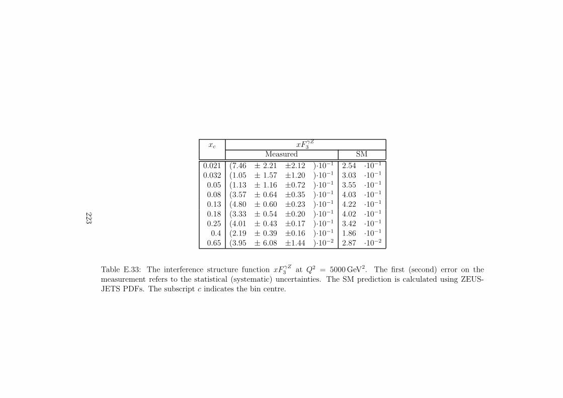
xc xF γZ3
Measured SM
0.021 (7.46 ± 2.21 ±2.12 )·10−1 2.54 ·10−1
0.032 (1.05 ± 1.57 ±1.20 )·10−1 3.03 ·10−1
0.05 (1.13 ± 1.16 ±0.72 )·10−1 3.55 ·10−1
0.08 (3.57 ± 0.64 ±0.35 )·10−1 4.03 ·10−1
0.13 (4.80 ± 0.60 ±0.23 )·10−1 4.22 ·10−1
0.18 (3.33 ± 0.54 ±0.20 )·10−1 4.02 ·10−1
0.25 (4.01 ± 0.43 ±0.17 )·10−1 3.42 ·10−1
0.4 (2.19 ± 0.39 ±0.16 )·10−1 1.86 ·10−1
0.65 (3.95 ± 6.08 ±1.44 )·10−2 2.87 ·10−2
Table E.33: The interference structure function xF γZ3 at Q2 = 5000 GeV2. The first (second) error on the
measurement refers to the statistical (systematic) uncertainties. The SM prediction is calculated using ZEUS-JETS PDFs. The subscript c indicates the bin centre.
223

References
[1] W.-M. Yao et al., Review of Particle Physics, J. Phys. G 33 (2006).
[2] F. Halzen and A.D. Martin, Quarks and Leptons: An Introductory Course in
Modern Particle Physics. John Wiley & Sons, Inc, 1984.
[3] G. Miller et al., Inelastic electron–proton scattering at large momentum
transfers, Phys. Rev. D 5, 528 (1972).
[4] H.W. Kendall, Deep inelastic scattering: Experiments on the proton and the
observation of scaling, Rev. Mod. Phys. 63, 597 (1991).
[5] ZEUS and H1 Collab., Combined ZEUS and H1 structure functions. Made
public for EPS 2003, Aachen, Germany, 2003.
[6] V.N. Gribov and L.N. Lipatov, Deep inelastic ep scattering in perturbation
theory, Sov. J. Nucl. Phys. 15, 438 (1972).
224

[7] Yu.L. Dokshitzer, Calculation of the structure functions for deep inelastic
scattering and e+e− annihilation by perturbation theory in Quantum
Chromodynamics, Sov. Phys. JETP 46, 641 (1977).
[8] G. Altarelli and G. Parisi, Asymptotic freedom in parton language, Nucl.
Phys. B 126, 298 (1977).
[9] ZEUS Collab., S. Chekanov et al., An NLO QCD analysis of inclusive
cross-section and jet-production data from the ZEUS experiment, Eur. Phys.
J. C 42, 1 (2005).
[10] CTEQ Collab., H.L. Lai et al., Global QCD analysis of parton structure of
the nucleon: CTEQ5 parton distributions, Eur. Phys. J. C 12, 375 (2000).
[11] J.E. Dodd, The ideas of particle physics. Cambridge University Press, 1984.
[12] Donald H. Perkins, Introduction to High Energy Physics. Cambridge U.
Press, 1972.
[13] K. Long, A pedagogical introduction to DIS, available on
http://www-zeus.desy.de/lectures/.
[14] M. Klein and T. Riemann, Electroweak interactions probing the nucleon
structure, Z. Phys. C 24, 151 (1984).
225

[15] R. Devenish and A. Cooper-Sarkar, Deep Inelastic Scattering. Oxford
University Press, 2003.
[16] ZEUS and H1 Collab., Electroweak Neutral Currents at HERA. Proceeding
submitted to the International Conference on High Energy Physics,
ICHEP06, Moscow, 2006.
[17] E. Rizvi and T. Sloan, xF γZ3 in charged lepton scattering, EPJdirect
CN2, 1 (2001).
[18] HERA – A Proposal for a Large Electron Proton Colliding Beam Facility at
DESY. DESY Report HERA 81-10, Hamburg, Germany (1981).
[19] ZEUS Collab., U. Holm (ed.), The ZEUS Detector. Status Report
(unpublished), DESY (1993), available on
http://www-zeus.desy.de/bluebook/bluebook.html.
[20] H1 Collab., I. Abt et al., The H1 detector at HERA, Nucl. Inst. Meth.
A 386, 310 (1997).
[21] K. Ackerstaff et al., The HERMES spectrometer, Nucl. Inst. Meth.
A 417, 230 (1998).
226
[22] HERA-B Collab., HERA–B: An Experiment to Study CP Violation in the B
System Using an Internal Target at the HERA Proton Ring, Design Report
DESY-PRC 95/01, DESY, 1995.
[23] ZEUS and H1 Collab., Combined ZEUS and H1 kinematic plane. Made
public for EPS 2003, Aachen, Germany, 2003.
[24] D.P. Barber et al., The HERA polarimeter and the first observation of
electron spin polarization at HERA, Nucl. Inst. Meth. A 329, 79 (1993).
[25] A.A. Sokolov and I.M. Ternov, On polarization and spin effects in the theory
of synchrotron radiation., Sov. Phys. Dokl. 8, 1203 (1964).
[26] D.P. Barber et al., The first achievement of longitudinal spin polarization in
a high energy electron storage ring, Phys. Lett. B 343, 436 (1995).
[27] J. Bohme, Precision measurement with the transverse polarimeter at HERA
II, Eur. Phys. J. C 33, S1067 (2004).
[28] M. Beckmann et al., The longitudinal polarimeter at HERA, Nucl. Inst.
Meth. A 479, 334 (2002).
[29] POL2000 Group, Using the HERA Polarization Measurements -
Recommendations for the Summer 2007 Conferences, June 2007, available on
http://www.desy.de/~pol2000/documents/documents.html.
227

[30] M. Derrick et al., Design and construction of the ZEUS barrel calorimeter,
Nucl. Inst. Meth. A 309, 77 (1991).
[31] A. Andresen et al., Construction and beam test of the ZEUS forward and rear
calorimeter, Nucl. Inst. Meth. A 309, 101 (1991).
[32] A. Bamberger et al., The presampler for the forward and rear calorimeter in
the ZEUS detector, Nucl. Inst. Meth. A 382, 419 (1996).
[33] ZEUS Collab., UK group, C.B. Brooks et al., Development of the ZEUS
central tracking detector, Nucl. Inst. Meth. A 283, 477 (1989).
[34] T. Haas, The ZEUS microvertex detector, Nucl. Inst. Meth.
A 549, 37 (2005).
[35] J. Andruszkow et al., Luminosity measurement in the ZEUS experiment,
Acta Phys. Pol. B 32, 2025 (2001).
[36] J.A. Crittenden et al., The C5 Upgrade (unpublished). ZEUS-01-002,
internal ZEUS note, 2001.
[37] ZEUS Collab., R. Carlin et al., The trigger of ZEUS, a flexible system for a
high bunch crossing rate collider, Nucl. Inst. Meth. A 379, 542 (1996).
228
[38] A. Quadt, Measurement and QCD Analysis of the Proton Structure Function
F2 from the 1994 HERA Data Using the ZEUS Detector. Ph.D. Thesis,
University of Oxford, Report RAL-TH-97-004, 1997.
[39] H. Spiesberger, heracles and djangoh: Event Generation for ep
Interactions at HERA Including Radiative Processes, 1998, available on
http://www.desy.de/~hspiesb/djangoh.html.
[40] H. Spiesberger, An Event Generator for ep Interactions at HERA Including
Radiative Processes (Version 4.6), 1996, available on
http://www.desy.de/~hspiesb/heracles.html.
[41] L. Lonnblad, ariadne version 4 – a program for simulation of QCD cascades
implementing the colour dipole model, Comp. Phys. Comm. 71, 15 (1992).
[42] T. Sjostrand, The Lund Monte Carlo for jet fragmentation and e+e− physics:
jetset version 6.2, Comp. Phys. Comm. 39, 347 (1986).
[43] G. Marchesini et al., HERWIG: A monte carlo event generator for
simulating hadron emission reactions with interfering gluons,
Comp. Phys. Comm. 67, 465 (1992).
[44] C. Catterall, Undestanding MOZART, available on
http://www-zeus.desy.de/lectures/.
229

[45] CERN Application Software Group, GEANT Detector description and
simulation tool. CERN Program Library Long Writeup W5013, available on
https://webafs08.cern.ch/wwwasdoc/.
[46] ZEUS Collab., Funnel - The ZEUS Monte Carlo Production Facility,
available on http://www-zeus.desy.de/components/funnel/.
[47] ZEUS Collab., ZEUS Monte Carlo Production and Data Analysis on the
Grid, available on http://www-zeus.desy.de/grid/.
[48] B. Straub, Introduction to orange, available on
http://www-zeus.desy.de/lectures/.
[49] J.R. Goncalo, Measurement of the High-Q2 Neutral Current Deep Inelastic
Scattering Cross Sections with the ZEUS Detector at HERA. Ph.D. Thesis,
University of London, Report DESY-THESIS-03-022, 2003.
[50] Y. Ri, Measurement of e−p Neutral-Current Deep Inelastic Scattering Cross
Sections with Longitudinally Polarised Electron Beams at√
s = 318 GeV.
Ph.D. Thesis, Tokyo Metropolitan University, 2007. In preparation.
[51] S. Bentvelsen, J. Engelen and P. Kooijman, Proc. Workshop on Physics at
HERA, W. Buchmuller and G. Ingelman (eds.), Vol. 1, p. 23. Hamburg,
Germany, DESY (1992).
230
[52] F. Jacquet and A. Blondel, Proceedings of the Study for an ep Facility for
Europe, U. Amaldi (ed.), p. 391. Hamburg, Germany (1979). Also in preprint
DESY 79/48.
[53] G.F. Hartner, VCTRAK Briefing: Program and Math (unpublished).
ZEUS-98-058, internal ZEUS Note, 1998.
[54] E. Maddoz, A Kalman filter track fit for the ZEUS microvertex detector
(unpublished). ZEUS-03-008, internal ZEUS Note, 2003.
[55] K. Oliver, Status of Z-Vertex measurement, June 2007. Talk given during
High-Q2 group meeting at DESY.
[56] A. Lopez-Duran Viani and S. Schlenstedt, Electron Finder Efficiencies and
Impurities. A Comparison Between SINISTRA95, EM and EMNET
(unpublished). ZEUS-99-077, internal ZEUS Note, 1999.
[57] B. Straub, The EM Electron Finder, available on
http://www-zeus.desy.de/~straub/ZEUS_ONLY/doc/em.ps.
[58] G.M. Briskin, Diffractive Dissociation in ep Deep Inelastic Scattering. Ph.D.
Thesis, Tel Aviv University, 1998.
231

[59] R. Sinkus and T. Voss, Particle identification with neural networks using a
rotational invariant moment representation, Nucl. Inst. Meth.
A 391, 360 (1997).
[60] R. Deffner, Measurement of the Proton Structure Function F2 at HERA
Using the 1996 and 1997 ZEUS Data. Ph.D. Thesis, Bonn University, 1999.
[61] A. Bernstein et al., Beam tests of the ZEUS barrel calorimeter, Nucl. Inst.
Meth. A 336, 23 (1993).
[62] J. Grosse-Knetter, Corrections for the Hadronic Final State (unpublished).
ZEUS-98-031, internal ZEUS Note, 1998.
[63] S. Catani et al., Longitudinally invariant kT clustering algorithms for hadron
hadron collisions, Nucl. Phys. B406, 187 (1993).
[64] S.D. Ellis and D.E. Soper, Successive combination jet algorithm for hadron
collisions, Phys. Rev. D 48, 3160 (1993).
[65] ZEUS Collab., ZeVis - Zeus Event Visualisation, A new Event Display for
the ZEUS Experiment, available on http://www-zeus.desy.de/~zevis/.
[66] F. Willeke, Summary of the HERA Proton-Positron Luminosity Run 2004.
HERA Note, HERA-04-01, 2004.
232

[67] M. Moritz, Measurement of the High Q2 Neutral Current DIS Cross Section
at HERA. Ph.D. Thesis, Hamburg University, 2001.
[68] H. Spiesberger, django6 Version 2.4 – A Monte Carlo Generator for Deep
Inelastic Lepton Proton Scattering Including QED and QCD Radiative
Effects, 1996, available on http://www.desy.de/~hspiesb/django6.html.
[69] ZEUS Collab.; S. Chekanov et al., High-Q2 neutral current cross section in
e+p deep inelastic scattering at√
s = 318 GeV , Phys. Rev.
D 70, 052001 (2004).
[70] ZEUS Collab., J. Breitweg et al., Measurement of high-Q2 neutral current
e+p deep inelastic scattering cross sections at HERA, Eur. Phys. J.
C 11, 427 (1999).
[71] L. Lyons, Statistics for nuclear and particle physicists. Cambridge University
Press, 1986.
[72] ZEUS Collab., S. Chekanov et al., Measurement of high-Q2 e−p neutral
current cross sections at HERA and the extraction of xF3, Eur. Phys. J.
C 28, 175 (2003).
[73] Argento, A. et al., Measurement of the interference structure function
xG(3)(x) in muon - nucleon scattering, Phys. Lett. B 140, 142 (1984).
233

[74] ZEUS Collab., An NLO QCD and EW analysis of inclusive e±p cross section
data from the ZEUS experiment. Proceeding submitted to the International
Conference on High Energy Physics, ICHEP06, Moscow, 2006.
234