The zero-sum assumption in neutral biodiversity theory
15
Journal of Theoretical Biology 248 (2007) 522–536 The zero-sum assumption in neutral biodiversity theory Rampal S. Etienne a, , David Alonso b , Alan J. McKane c a Community and Conservation Ecology Group, Centre for Ecological and Evolutionary Studies, University of Groningen, P.O. Box 14, 9750 AA Haren, The Netherlands b Ecology and Evolutionary Biology, University of Michigan, 830 North University Av, Ann Arbor, MI 48109-1048, USA c Theory Group, School of Physics and Astronomy, University of Manchester, Manchester M13 9PL, UK Received 8 March 2007; received in revised form 24 May 2007; accepted 6 June 2007 Available online 12 June 2007 Abstract The neutral theory of biodiversity as put forward by Hubbell in his 2001 monograph has received much criticism for its unrealistic simplifying assumptions. These are the assumptions of functional equivalence among different species (neutrality), the assumption of point mutation speciation, and the assumption that resources are continuously saturated, such that constant resource availability implies constant community size (zero-sum assumption). Here we focus on the zero-sum assumption. We present a general theory for calculating the probability of observing a particular species-abundance distribution (sampling formula) and show that zero-sum and non-zero-sum formulations of neutral theory have exactly the same sampling formula when the community is in equilibrium. Moreover, for the non- zero-sum community the sampling formula has this same form, even out of equilibrium. Therefore, the term ‘‘zero-sum multinomial (ZSM)’’ to describe species abundance patterns, as coined by Hubbell [2001. The Unified Neutral Theory of Biodiversity and Biogeography, Princeton University Press, Princeton, NJ], is not really appropriate, as it also applies to non-zero-sum communities. Instead we propose the term ‘‘dispersal-limited multinomial (DLM)’’, thus making explicit one of the most important contributions of neutral community theory, the emphasis on dispersal limitation as a dominant factor in determining species abundances. r 2007 Elsevier Ltd. All rights reserved. Keywords: Biodiversity; Neutral model; Species abundances; Allele frequencies; Ewens sampling formula; Etienne sampling formula 1. Introduction Biodiversity is not only determined by the number of different entities (species in community ecology or alleles in population genetics), but also by the abundance of these entities (Magurran, 2004). Traditionally, species abun- dances have been mostly studied for competitive commu- nities (Hubbell, 2001). Recently, they have also been heralded as important determinants in food webs (Cohen et al., 2003). Abundance data are relatively easy to collect, particularly in community ecology, and thus are good candidates to provide information on the processes that determine biodiversity. For many decades models have been proposed to describe and explain observed patterns in species abundances or allele frequencies (Fisher et al., 1943; Preston, 1948, 1962; MacArthur, 1957, 1960; Pielou, 1969, 1975; Ewens, 1972; Sugihara, 1980; Tokeshi, 1990, 1993, 1996; Engen and Lande, 1996a,b; Diserud and Engen, 2000; Dewdney, 1998, 2000; Hubbell, 2001; Harte et al., 1999; Etienne and Olff, 2005), but consensus on a single adequate model has not been reached. This has even led some scientists to claim that abundance data cannot distinguish between different models (Volkov et al., 2005; but see Etienne et al., 2007). Although it is true that patterns never uniquely imply process (Cohen, 1968; Clinchy et al., 2002; Purves and Pacala, 2005), scientific progress can still be made by testing whether different hypotheses on plausible processes can predict observed patterns. As for all scientific tests, no theory can be proved to be true, but inadequate theories can certainly be rejected. However, in comparisons of alternative abun- dance models, a solid sampling theory that provides the likelihoods of these models given the data (i.e. sampling ARTICLE IN PRESS www.elsevier.com/locate/yjtbi 0022-5193/$ - see front matter r 2007 Elsevier Ltd. All rights reserved. doi:10.1016/j.jtbi.2007.06.010 Corresponding author. Tel.: +31 503 63 2230. E-mail address: [email protected] (R.S. Etienne).
-
Upload
independent -
Category
Documents
-
view
0 -
download
0
Transcript of The zero-sum assumption in neutral biodiversity theory
ARTICLE IN PRESS
0022-5193/$ - se
doi:10.1016/j.jtb
�CorrespondE-mail addr
Journal of Theoretical Biology 248 (2007) 522–536
www.elsevier.com/locate/yjtbi
The zero-sum assumption in neutral biodiversity theory
Rampal S. Etiennea,�, David Alonsob, Alan J. McKanec
aCommunity and Conservation Ecology Group, Centre for Ecological and Evolutionary Studies, University of Groningen,
P.O. Box 14, 9750 AA Haren, The NetherlandsbEcology and Evolutionary Biology, University of Michigan, 830 North University Av, Ann Arbor, MI 48109-1048, USA
cTheory Group, School of Physics and Astronomy, University of Manchester, Manchester M13 9PL, UK
Received 8 March 2007; received in revised form 24 May 2007; accepted 6 June 2007
Available online 12 June 2007
Abstract
The neutral theory of biodiversity as put forward by Hubbell in his 2001 monograph has received much criticism for its unrealistic
simplifying assumptions. These are the assumptions of functional equivalence among different species (neutrality), the assumption of
point mutation speciation, and the assumption that resources are continuously saturated, such that constant resource availability implies
constant community size (zero-sum assumption). Here we focus on the zero-sum assumption. We present a general theory for calculating
the probability of observing a particular species-abundance distribution (sampling formula) and show that zero-sum and non-zero-sum
formulations of neutral theory have exactly the same sampling formula when the community is in equilibrium. Moreover, for the non-
zero-sum community the sampling formula has this same form, even out of equilibrium. Therefore, the term ‘‘zero-sum multinomial
(ZSM)’’ to describe species abundance patterns, as coined by Hubbell [2001. The Unified Neutral Theory of Biodiversity and
Biogeography, Princeton University Press, Princeton, NJ], is not really appropriate, as it also applies to non-zero-sum communities.
Instead we propose the term ‘‘dispersal-limited multinomial (DLM)’’, thus making explicit one of the most important contributions of
neutral community theory, the emphasis on dispersal limitation as a dominant factor in determining species abundances.
r 2007 Elsevier Ltd. All rights reserved.
Keywords: Biodiversity; Neutral model; Species abundances; Allele frequencies; Ewens sampling formula; Etienne sampling formula
1. Introduction
Biodiversity is not only determined by the number ofdifferent entities (species in community ecology or alleles inpopulation genetics), but also by the abundance of theseentities (Magurran, 2004). Traditionally, species abun-dances have been mostly studied for competitive commu-nities (Hubbell, 2001). Recently, they have also beenheralded as important determinants in food webs (Cohenet al., 2003). Abundance data are relatively easy to collect,particularly in community ecology, and thus are goodcandidates to provide information on the processes thatdetermine biodiversity. For many decades models havebeen proposed to describe and explain observed patterns inspecies abundances or allele frequencies (Fisher et al., 1943;
e front matter r 2007 Elsevier Ltd. All rights reserved.
i.2007.06.010
ing author. Tel.: +31503 63 2230.
ess: [email protected] (R.S. Etienne).
Preston, 1948, 1962; MacArthur, 1957, 1960; Pielou, 1969,1975; Ewens, 1972; Sugihara, 1980; Tokeshi, 1990, 1993,1996; Engen and Lande, 1996a,b; Diserud and Engen,2000; Dewdney, 1998, 2000; Hubbell, 2001; Harte et al.,1999; Etienne and Olff, 2005), but consensus on a singleadequate model has not been reached. This has even ledsome scientists to claim that abundance data cannotdistinguish between different models (Volkov et al., 2005;but see Etienne et al., 2007). Although it is true thatpatterns never uniquely imply process (Cohen, 1968;Clinchy et al., 2002; Purves and Pacala, 2005), scientificprogress can still be made by testing whether differenthypotheses on plausible processes can predict observedpatterns. As for all scientific tests, no theory can be provedto be true, but inadequate theories can certainly berejected. However, in comparisons of alternative abun-dance models, a solid sampling theory that provides thelikelihoods of these models given the data (i.e. sampling
ARTICLE IN PRESSR.S. Etienne et al. / Journal of Theoretical Biology 248 (2007) 522–536 523
formulas) has been lacking (Chave et al., 2006). In thispaper, we present such a sampling theory. For conveniencewe will speak only of species abundances in an ecologicalcommunity, but our results also apply to allele abundances(frequencies) in a population.
Our sampling theory is inspired by neutral theory, as thistheory provides a null model for abundance distributions,but we stress that the theory extends beyond neutraltheory. Nevertheless, we use our sampling theory here tosettle a debate in neutral theory concerning the zero-sumassumption (Hubbell, 2001). Neutral theory has three basicassumptions: the neutrality assumption (functional equiva-lence among different species), the point mutation assump-tion (speciation takes place by point mutation) and thezero-sum assumption, which have all received muchcriticism. Here we do not enter the debate concerning thefirst two assumptions, but focus on the third. The weakformulation of the zero-sum assumption states thatindividuals of different species in a community that arelimited by their environment (either because of limitedshared resource, e.g. space or light, or because of naturalenemies that restrain the otherwise unbridled growth of thespecies) will always saturate the environment, i.e. there arenever fewer individuals than allowed by the environment.The strong formulation states that the limitation by theenvironment (e.g. the number of resources or the numberof natural enemies) is constant and that therefore the totalnumber of individuals competing for the resource is alsoconstant. While there is some evidence for this assumption(Hubbell, 1979, 2001), this assumption (in either form) hasbeen felt to be too restrictive (Volkov et al., 2003; Poulin,2004). Here we show, however, that the zero-sum assump-tion is not crucial for one of the most important predictionsof the theory, the sampling formula, i.e. the formula thatgives the probability of observing abundances n1; . . . ; nS ina sample of J individuals. This is not trivial, as thecharacteristic time scales of zero-sum and non-zero-summodels are very different (see below).
We will first present our general sampling theory,particularly its fundamental assumptions and the generalsampling formula based on these assumptions. We willthen formulate a general master equation for a singlespecies and show how it can lead to a general samplingformula for multiple neutral species that have either fullyindependent (non-zero-sum) or fully dependent (zero-sum)dynamics. For the latter case we will introduce thesubsample approach. Up to this point, our treatment willbe quite general in the sense that it does not rely on anyassumptions concerning the dynamics of each species suchas intraspecific competition, or the source of new speciessuch as speciation or immigration. From this point we willproceed by inserting such details of the Hubbell model forthe metacommunity and for the local community and wewill subsequently link the two community scales. We dothis for the non-zero-sum case both in and out ofequilibrium and refer to the Appendix for the zero-sumequilibrium case. We will demonstrate that the sampling
formula for the zero-sum case in equilibrium also applies tothe non-zero-sum case, both in equilibrium and out ofequilibrium. We end with a discussion of our results. Forthe reader’s convenience the mathematical symbols used inthis paper are summarized in Table 1.
2. A sampling theory
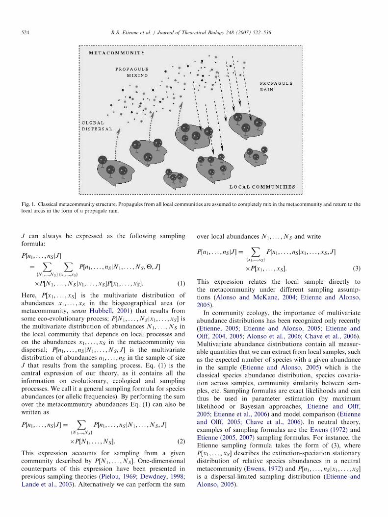
The metacommunity concept represents a powerfulframework to study the relative importance of local speciesinteractions and dispersal in determining communitycomposition and dynamics (Leibold et al., 2004; Holyoaket al., 2005). Our sampling theory is based on a classicalmetacommunity structure. First, we assume that localcommunities form a metacommunity by global migration(global dispersal, propagule mixing and propagule rain (seeFig. 1)). Such a migration assumption has a long traditionin metapopulation ecology (Gotelli and Kelley, 1993;Bascompte et al., 2002), and has been used to gain insightinto the processes underlying the distribution of speciesdiversity from local to global spatio-temporal scales(MacArthur and Wilson, 1967), has inspired currentneutral theory (Hubbell, 2001), and underlies recent studieson community similarity under neutrality (Dornelas et al.,2006). Second, as in Hubbell’s (2001) approach, our theorybuilds on the assumption that ecological and evolutionarytime scales are very different and can be decoupled. Underthese assumptions, our general framework requires thefollowing three general steps:
1.
We assume that ecological and evolutionary processeshave determined metacommunity composition (speciesabundances) at the largest spatio-temporal scale. Neu-tral speciation, adaptive speciation and trade-off invar-iance are possible mechanisms. We usually evaluate thestationary distribution of species abundances emergingfrom these processes. We do not require that thisdistribution is frozen-stable. We do require, however,that processes at the biogeographic level are at a muchlonger temporal scale relative to the process affecting theecological assembly of local communities. (See Valladeand Houchmandzadeh, 2006 for a relaxation of thisassumption.)2.
In local communities (or islands) mainly local ecologicalprocesses, but not speciation, are at play. Examples ofthese processes are dispersal-limitation, density depen-dence, habitat heterogeneity and species differentialadaptation to different habitats.3.
Sampling formulas contain information about bothlevels of description and about the sampling process.They enable us to empirically evaluate the imprint ofevolutionary processes at the biogeographic scale andecological processes at the local scale on the observeddiversity in our local samples.When sampling communities, the probability of obtain-ing S species with n1; . . . ; nS individuals in a sample of size
ARTICLE IN PRESS
Fig. 1. Classical metacommunity structure. Propagules from all local communities are assumed to completely mix in the metacommunity and return to the
local areas in the form of a propagule rain.
R.S. Etienne et al. / Journal of Theoretical Biology 248 (2007) 522–536524
J can always be expressed as the following samplingformula:
P½n1; . . . ; nSjJ�
¼X
fN1;...;NSg
Xfx1;...;xSg
P½n1; . . . ; nSjN1; . . . ;NS;Y; J�
�P½N1; . . . ;NSjx1; . . . ;xS�P½x1; . . . ;xS�. ð1Þ
Here, P½x1; . . . ; xS� is the multivariate distribution ofabundances x1; . . . ;xS in the biogeographical area (ormetacommunity, sensu Hubbell, 2001) that results fromsome eco-evolutionary process; P½N1; . . . ;NSjx1; . . . ; xS� isthe multivariate distribution of abundances N1; . . . ;NS inthe local community that depends on local processes andon the abundances x1; . . . ;xS in the metacommunity viadispersal; P½n1; . . . ; nSjN1; . . . ;NS; J� is the multivariatedistribution of abundances n1; . . . ; nS in the sample of sizeJ that results from the sampling process. Eq. (1) is thecentral expression of our theory, as it contains all theinformation on evolutionary, ecological and samplingprocesses. We call it a general sampling formula for speciesabundances (or allelic frequencies). By performing the sumover the metacommunity abundances Eq. (1) can also bewritten as
P½n1; . . . ; nSjJ� ¼X
fN1;...;NSg
P½n1; . . . ; nSjN1; . . . ;NS; J�
�P½N1; . . . ;NS�. ð2Þ
This expression accounts for sampling from a givencommunity described by P½N1; . . . ;NS�. One-dimensionalcounterparts of this expression have been presented inprevious sampling theories (Pielou, 1969; Dewdney, 1998;Lande et al., 2003). Alternatively we can perform the sum
over local abundances N1; . . . ;NS and write
P½n1; . . . ; nSjJ� ¼Xfx1;...;xSg
P½n1; . . . ; nSjx1; . . . ;xS; J�
�P½x1; . . . ;xS�. ð3Þ
This expression relates the local sample directly tothe metacommunity under different sampling assump-tions (Alonso and McKane, 2004; Etienne and Alonso,2005).In community ecology, the importance of multivariate
abundance distributions has been recognized only recently(Etienne, 2005; Etienne and Alonso, 2005; Etienne andOlff, 2004, 2005; Alonso et al., 2006; Chave et al., 2006).Multivariate abundance distributions contain all measur-able quantities that we can extract from local samples, suchas the expected number of species with a given abundancein the sample (Etienne and Alonso, 2005) which is theclassical species abundance distribution, species covaria-tion across samples, community similarity between sam-ples, etc. Sampling formulas are exact likelihoods and canthus be used in parameter estimation (by maximumlikelihood or Bayesian approaches, Etienne and Olff,2005; Etienne et al., 2006) and model comparison (Etienneand Olff, 2005; Chave et al., 2006). In neutral theory,examples of sampling formulas are the Ewens (1972) andEtienne (2005, 2007) sampling formulas. For instance, theEtienne sampling formula takes the form of (3), whereP½x1; . . . ; xS� describes the extinction-speciation stationarydistribution of relative species abundances in a neutralmetacommunity (Ewens, 1972) and P½n1; . . . ; nSjx1; . . . ;xS�
is a dispersal-limited sampling distribution (Etienne andAlonso, 2005).
ARTICLE IN PRESS
Table 1
Explanation of mathematical symbols
Symbol Explanation
nk ;Nk ;xk Abundance of species k in the sample, the local
community and the metacommunity
pk ; pk ; p! Relative abundance and rescaled relative abundance
of species k in a species pool, and the vector of
relative abundances
(this is an abstract pool for the metacommunity
model, and it is the metacommunity for the local
community model)
J; JL; JM Sum of abundances in the sample, the local
community and the metacommunity (i.e. their
respective sizes)
JL;k ; JM;k Sum of abundance of all species in the local
community and metacommunity, except species
1 . . . k � 1, Eq. (12)
S Number of species in the sample
ST Total number of species that can possibly exist (may
be infinite)
Fj The number of species in the sample that have
abundance j
P½ � Probability, sampling formula
PL½ �;PU ½ � Labeled and unlabeled version of the sampling
formula, Eqs. (8) and (9)
t; t;Tzero�sum;Tnon�zero�sum;T
Time, rescaled (dimensionless) time, characteristic
time scale for zero-sum dynamics and non-zero-sum
dynamics, number of censuses
gi; ri; gi; ri Probability rates of increase and decrease in
abundance and their rescaled versions
Y A general symbol for model parameters
s; sc; l Speciation rate, per capita speciation rate and
immigration rate (probability of speciation/
immigration per unit time)
y; I Fundamental biodiversity number and fundamental
dispersal number, Eqs. (15), (B.5), and (22)
n;m Dimensionless speciation and immigration rates
(probabilities), Eqs. (B.4) and (B.15)
I kFundamental dispersal number rescaled by relative
abundances of species 1 . . . k � 1 in the
metacommunity, Eq. (B.20)
b; d Birth rate and death rate (probability of birth/death
per unit time)
R;RðtÞ Reproduction number and reproduction number as a
function of time, Eqs. (16) and (28)
pð. . .Þ Permutation
OðpkÞ; f ðpkÞ Density and probability density of species k between
relative abundance pk and pk þ dpk, Eqs. (33) and
(34)
K Rescaling parameter, Eqs. (B.3) and (B.13)
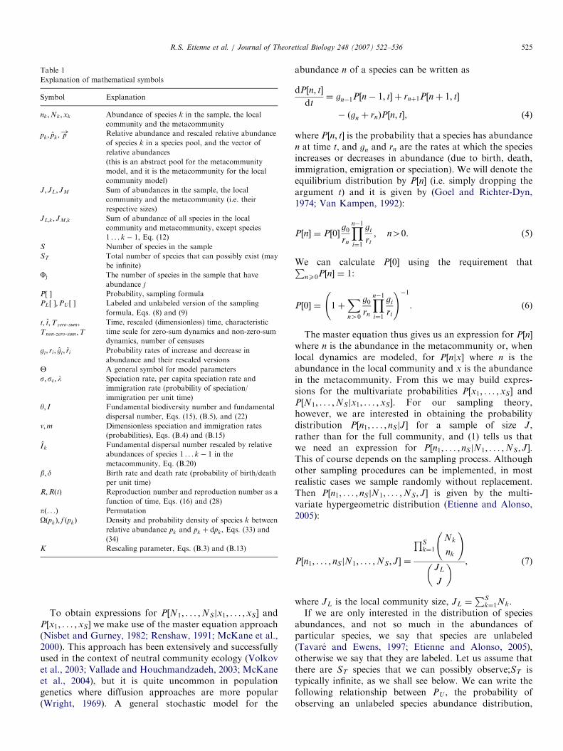
R.S. Etienne et al. / Journal of Theoretical Biology 248 (2007) 522–536 525
To obtain expressions for P½N1; . . . ;NSjx1; . . . ;xS� andP½x1; . . . ;xS� we make use of the master equation approach(Nisbet and Gurney, 1982; Renshaw, 1991; McKane et al.,2000). This approach has been extensively and successfullyused in the context of neutral community ecology (Volkovet al., 2003; Vallade and Houchmandzadeh, 2003; McKaneet al., 2004), but it is quite uncommon in populationgenetics where diffusion approaches are more popular(Wright, 1969). A general stochastic model for the
abundance n of a species can be written as
dP½n; t�
dt¼ gn�1P½n� 1; t� þ rnþ1P½nþ 1; t�
� ðgn þ rnÞP½n; t�, ð4Þ
where P½n; t� is the probability that a species has abundancen at time t, and gn and rn are the rates at which the speciesincreases or decreases in abundance (due to birth, death,immigration, emigration or speciation). We will denote theequilibrium distribution by P½n� (i.e. simply dropping theargument t) and it is given by (Goel and Richter-Dyn,1974; Van Kampen, 1992):
P½n� ¼ P½0�g0
rn
Yn�1i¼1
gi
ri
; n40. (5)
We can calculate P½0� using the requirement thatPnX0P½n� ¼ 1:
P½0� ¼ 1þXn40
g0
rn
Yn�1i¼1
gi
ri
!�1. (6)
The master equation thus gives us an expression for P½n�
where n is the abundance in the metacommunity or, whenlocal dynamics are modeled, for P½njx� where n is theabundance in the local community and x is the abundancein the metacommunity. From this we may build expres-sions for the multivariate probabilities P½x1; . . . ;xS� andP½N1; . . . ;NSjx1; . . . ; xS�. For our sampling theory,however, we are interested in obtaining the probabilitydistribution P½n1; . . . ; nSjJ� for a sample of size J,rather than for the full community, and (1) tells us thatwe need an expression for P½n1; . . . ; nSjN1; . . . ;NS; J�.This of course depends on the sampling process. Althoughother sampling procedures can be implemented, in mostrealistic cases we sample randomly without replacement.Then P½n1; . . . ; nSjN1; . . . ;NS; J� is given by the multi-variate hypergeometric distribution (Etienne and Alonso,2005):
P½n1; . . . ; nSjN1; . . . ;NS; J� ¼
QSk¼1
Nk
nk
!
JL
J
� � , (7)
where JL is the local community size, JL ¼PS
k¼1Nk.If we are only interested in the distribution of species
abundances, and not so much in the abundances ofparticular species, we say that species are unlabeled(Tavare and Ewens, 1997; Etienne and Alonso, 2005),otherwise we say that they are labeled. Let us assume thatthere are ST species that we can possibly observe;ST istypically infinite, as we shall see below. We can write thefollowing relationship between PU , the probability ofobserving an unlabeled species abundance distribution,
ARTICLE IN PRESSR.S. Etienne et al. / Journal of Theoretical Biology 248 (2007) 522–536526
and PL, the probability of observing abundances ofspecified species:
PU ½n1; . . . ; nSjJ� ¼X
fpðn1;...;nSTÞg
PL½n1; . . . ; nSTjJ�, (8)
where the sum is over all possible permutations of theobserved abundances n1; . . . ; nS over the species 1; . . . ;ST
(the remaining ST � S species receive abundance 0).When species are exchangeable (symmetric),PL½n1; . . . ; nST
jJ� is the same for all permutations andhence (8) simplifies to
PU ½n1; . . . ; nSjJ� ¼ST !
F0!QJ
j¼1Fj !PL½n1; . . . ; nS; 0; 0; 0; . . . jJ�,
(9)
where Fj is the number of species that have abundance j.Again, unobserved species naturally have abundance 0: Forconvenience, we have numbered the species on the right-hand side so that we first list the abundances of theobserved species and then the unobserved species, but thisis arbitrary, as long as it is understood that interchangingtwo unequal abundances generates a different distributionof labeled species, but the same distribution of unlabeledspecies. We will drop the subscripts U and L for notationalconvenience. Whenever zeros are added, it is clear that thelabeled version is meant, otherwise we are dealing with theunlabeled version.
We noted above that we need to build expressions for themultivariate probabilities P½N1; . . . ;NSjx1; . . . ;xS� andP½x1; . . . ;xS� from the results of the master equationapproach. These results of course depend on the model.We will consider two general models. The first is acommunity consisting of species with completely indepen-dent dynamics: the species do not ‘‘feel’’ the presence ofheterospecifics. The second is a community with a constanttotal number of individuals: a decrease of the abundance ofone species must be followed by an increase in the same oranother species. This is a community subject to the zero-sum constraint. Because we are considering models we willalso add to our expressions a parameter Y to denote themodel parameters.
2.1. Independent species
When species in a community grow independently of oneanother, P½x1; . . . ;xS� and P½N1; . . . ;NSjx1; . . . ;xS� aregiven by
P½x1; . . . ;xS; 0; 0; 0; . . . jY� ¼YS
k¼1
P½xkjY�YST
k¼Sþ1
P½0jY�,
(10a)
P½N1; . . . ;NS; 0; 0; 0; . . . jY�
¼YS
k¼1
P½NkjY; xk�YST
k¼Sþ1
P½0jY; xk�. ð10bÞ
2.2. Dependent species: the subsample approach
When species in a community experience the populationsizes of other species and of themselves, the stochasticvariables nk are not independent and (10) does not apply.We may then use the subsample approach (Etienne andAlonso, 2005):
P½x1; . . . ; xS; 0; 0; 0; . . . jY; JM �
¼YST
k¼1
P½xkjY;x1; ::; xk�1� ¼YST
k¼1
P½xkjYk; JM ;k�, ð11aÞ
P½N1; . . . ;NS; 0; 0; 0; . . . jY; JL�
¼YST
k¼1
P½NkjY;xk;N1; ::;Nk�1�
¼YST
k¼1
P½NkjYk;xk; JL;k�, ð11bÞ
where
JM ;k:¼JM �Xk�1i¼1
xi, (12a)
JL;k:¼JL �Xk�1i¼1
Ni (12b)
is the (meta- or local) community size that is still availableto species k, and where Yk also incorporates the fact that ni
is known for all species i ¼ 1; . . . ; k � 1. This will becomeclear below. The subsample approach is nicely illustratedby a very simple example, the extension of the binomialdistribution to the multinomial distribution. SeeAppendix A.
3. Non-zero-sum neutral communities
We will apply our theory to neutral models for themetacommunity (Hubbell, 2001) where there is onlyspeciation, and to the local community, where there isonly immigration from the metacommunity, in addition tothe standard birth and death processes. We will frequentlyuse the Pochhammer notation
ðaÞn:¼Yn
i¼1
ðaþ i � 1Þ ¼Yn�1i¼0
ðaþ iÞ. (13)
For n ¼ 0 we adhere to the convention that ðaÞ0 ¼ 1.Here we only derive the sampling formulas for the non-
zero-sum case, as they are well-known for the zero-sumcase (Ewens, 1972; Etienne, 2005). For completeness,however, Appendix B gives the full derivation for thezero-sum case using the subsample approach; this deriva-tion is different from the derivation originally used toobtain the sampling formulas in the zero-sum case and it isinstructive to see that, except for the subsample approach,the derivation is analogous to the non-zero-sum case.
ARTICLE IN PRESSR.S. Etienne et al. / Journal of Theoretical Biology 248 (2007) 522–536 527
3.1. Metacommunity
The distribution of species relative abundances in aneutral metacommunity in speciation–extinction equili-brium was given by Ewens (1972). This distribution is botha sampling formula and a full description of speciesabundances in a neutral metacommunity. While thisdistribution was found under the assumption of constantcommunity size, i.e. zero-sum dynamics, here we show thatit can be derived without making this assumption, butinstead assuming independent species with linear (densityindependent) growth rates.
In the metacommunity there is only speciation, inaddition to birth and death processes. We treat speciationas immigration from a species pool. Treating speciation asan immigration process is only realistic in the limit of aninfinite metacommunity. A model that explicitly accountsfor finite metacommunity size in speciation is much morecomplicated, unless metacommunity size is held constant,which is the zero-sum case of Appendix B. The one-stepstochastic birth–death–immigration model formulated inEqs. (14) and (21), was first fully solved by Kendall (1948).He introduced this birth–death–immigration process togive a mechanistic biological basis to Fisher’s empiricallogseries distribution when immigration is very low(McKane et al., 2000). More recently, the same argumenthas been used in the context of neutral theory to give anevolutionary explanation to Fisher’s logseries in themetacommunity through neutral speciation (Volkov etal., 2003). Here we give a more complete description andshow that it can also be used to derive the correspondingsampling formula. The derivation of this sampling formulaby taking the appropriate limit ST !1 was suggested byHoppe (1987) and Costantini and Garibaldi (2004), buthere it is made explicit in the immigration model for thefirst time.
We assume that there are ST species in the species poolwith ST !1 and each species in the pool having relativeabundance pk ¼ p! 0, such that
PST
k¼1 pk ¼ ST p ¼ 1(hence p ¼ 1=ST ). We denote the speciation rate by sand birth and death rates by b and d, respectively. Becausewe are dealing with neutral species, these rates (and also theimmigration rate l below) are assumed to be identical forall species. We will show, however, that this assumptioncan be somewhat relaxed without changing the results. Aspecies grows in abundance if a birth event happens in itspopulation or when it speciates from the species pool.Because p! 0, the probability that a species alreadypresent in the metacommunity enters the metacommunitythrough speciation approaches zero, but for new species (ofwhich there are infinitely many: ST � S) this probability isnon-zero. As stated above, we assume here that speciesgrow independently. Then, the dynamics of each speciescan be described by (4) with the following rates of increaseand decrease:
gx ¼ bxþ sp, (14a)
rx ¼ dx. (14b)
We now define
y:¼sb. (15)
In the limit of an infinite metacommunity, as we describedabove, this parameter is the non-zero-sum expression of thewell-known fundamental biodiversity number (Hubbell,2001). In this limit, it has the same biological interpreta-tion, namely as the number of new species arising in thesystem per birth. We further define
R:¼bd
(16)
which has the interpretation of a net reproduction number,i.e. the number of births per death. The solution for P½xk�,xk40, is, using (5) and (6),
P½xk� ¼ Pk½0�g0
rxk
Yxk�1
i¼1
gi
ri
¼ ð1� RÞyp Rxk
xk
ðypÞxk
ðxk � 1Þ!, ð17Þ
where Pk½0� ¼ ð1� RÞyp.Because we have independent species, we can apply (10)
to obtain
P½x1; . . . ;xS; 0; 0; 0; . . . jy� ¼YS
k¼1
RxkðypÞxk
xk!ð1� RÞyp
!
�YST
k¼Sþ1
ð1� RÞyp
!. ð18Þ
For a random sample from the metacommunity thesampling formula is given by (3) where P½n1; . . . ;nSjx1; . . . ;xS� is the hypergeometric distribution (7).
P½n1; . . . ; nS; 0; 0; 0; . . . jy; J�
¼X
x1;...;xS
QSk¼1
xk
nk
!ðypÞNk
xk!ð1� RÞypRxk ð
QST
k¼Sþ1ð1� RÞypÞ
JM
J
!
¼ J!X
x1;...;xS
YST
k¼1
ð1� RÞyp
!ðJM � JÞ!
JM !
YSk¼1
ðypÞxk
nk!ðxk � nkÞ!Rxk
¼ J!X
x1;...;xS
ð1� RÞyðJM � JÞ!
JM !RJM
YS
k¼1
ðypÞnkðypþ nkÞxk�nk
nk!ðxk � nkÞ!
¼ J!YS
k¼1
ðypÞnk
nk!
XJM
ð1� RÞyRJM
JM !
� ðJM � JÞ!X
ðx1;...;xS jPS
k¼1xk¼JM Þ
YSk¼1
ðypþ nkÞxk�nk
ðxk � nkÞ!
264
375
ARTICLE IN PRESSR.S. Etienne et al. / Journal of Theoretical Biology 248 (2007) 522–536528
¼ J!YS
k¼1
ðypÞnk
nk!
XJM
ð1� RÞyRJM
JM !
!
�X
ðK1;...;KS jPS
k¼1Kk¼KÞ
K !YS
k¼1
ðypþ nkÞKk
Kk!
264
375
¼J!
ðyÞJ
YS
k¼1
ðypÞnk
nk!
XJM
ð1� RÞyRJM
JM !
!ðyÞJ ½ðyþ JÞJM�J �
¼J!
ðyÞJ
YS
k¼1
ðypÞnk
nk!
XJM
ðyÞJMð1� RÞyRJM
JM !
!
¼J!
ðyÞJ
YS
k¼1
ðypÞnk
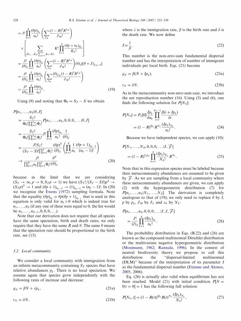
nk!. ð19Þ
Using (9) and noting that F0 ¼ ST � S we obtain
P½n1; . . . ; nSjy; J�
¼ST !
F0!QJM
j¼1Fj!P½n1; . . . ; nS; 0; 0; 0; . . . jy; J�
¼ST !
F0!QJM
j¼1Fj!J!YS
k¼1
ðypÞnk
nk!
1
ðyÞJ
¼J!ST !
ðST � SÞ!QJ
j¼1Fj!
ðypÞS
ðyÞJ
YS
k¼1
1
nk
ðypþ 1Þnk�1
ðnk � 1Þ!
!
!J!QS
k¼1nk
QJj¼1Fj !
yS
ðyÞJð20Þ
because in the limit that we are considering(ST !1; p! 0;ST p! 1) we have ðST !=ðST � SÞ!ÞpS !
ðST pÞS ! 1 and ðypþ 1Þnk�1! ð1Þnk�1
¼ ðnk � 1Þ!. In (20)we recognize the Ewens (1972) sampling formula. Notethat the equality ðypÞnk
¼ ypðypþ 1Þnk�1that is used in this
equation is only valid for nk40 which is indeed true forn1; . . . ; nS (if any one of these were equal to 0, the list wouldbe n1; . . . ; nS�1; 0; 0; 0; . . .).
Note that our derivation does not require that all specieshave the same speciation, birth and death rates; we onlyrequire that they have the same R and y. The same y meansthat the speciation rate should be proportional to the birthrate, see (15).
3.2. Local community
We consider a local community with immigration froman infinite metacommunity containing ST species that haverelative abundances pk. There is no local speciation. Weassume again that species grow independently with thefollowing rates of increase and decrease:
gN ¼ bN þ lpk, (21a)
rN ¼ dN, (21b)
where l is the immigration rate, b is the birth rate and d isthe death rate. We now define
I :¼lb. (22)
This number is the non-zero-sum fundamental dispersalnumber and has the interpretation of number of immigrantindividuals per local birth. Eqs. (21) become
gN ¼ bðN þ IpkÞ, (23a)
rN ¼ dN. (23b)
As in the metacommunity non-zero-sum case, we introducethe net reproduction number (16). Using (5) and (6), onefinds the following solution for P½Nk�:
P½Nk� ¼ Pk½0�Ipk
dnk
YNk�1
i¼1
bði þ IpkÞ
di
¼ ð1� RÞIpk RNkðIpkÞNk
nk!. ð24Þ
Because we have independent species, we can apply (10):
P½N1; . . . ;NS; 0; 0; 0; . . . jI ; p!�
¼ ð1� RÞIkpk
YSk¼1
ðIpkÞNk
Nk!RNk . ð25Þ
Note that in this expression species must be labeled becausetheir metacommunity abundances are assumed to be givenby p!. As we are sampling from a local community wherethese metacommunity abundances are given, we can apply(2) with the hypergeometric distribution (7) forP½n1; . . . ; nSjN1; . . . ;NS�. The derivation is completelyanalogous to that of (19); we only need to replace y by I,p by pk, JM by JL and xk by Nk:
P½n1; . . . ; nS; 0; 0; 0; . . . jI ; J; p!�
¼J!
ðIÞJ
YSk¼1
ðIpkÞnk
nk!. ð26Þ
The probability distribution in Eqs. (B.22) and (26) areknown as the compound multinomial Dirichlet distributionor the multivariate negative hypergeometric distribution(Mosimann, 1962; Rannala, 1996). In the context ofneutral biodiversity theory we propose to call thisdistribution the ‘‘dispersal-limited multinomial(DLM)’’ because of the interpretation of its parameter I
as the fundamental dispersal number (Etienne and Alonso,2005, 2006).Eq. (26) is actually also valid when equilibrium has not
been reached. Model (21) with initial condition P½N ¼
0jt ¼ 0� ¼ 1 has the following full solution:
P½Nk; t� ¼ ð1� RðtÞÞIpk RðtÞNkðIpkÞNk
Nk!, (27)
ARTICLE IN PRESSR.S. Etienne et al. / Journal of Theoretical Biology 248 (2007) 522–536 529
where
RðtÞ ¼
bðeðb�dÞt � 1Þ
b� d
1þbðeðb�dÞt � 1Þ
b� d
¼ R1� eðb�dÞt
1� Reðb�dÞt, (28)
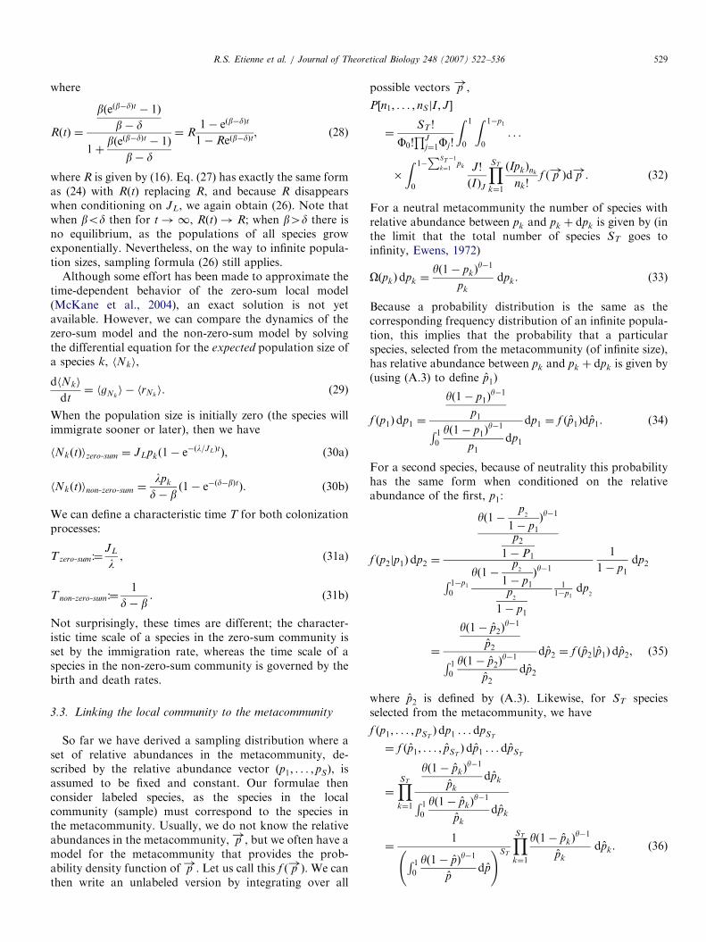
where R is given by (16). Eq. (27) has exactly the same formas (24) with RðtÞ replacing R, and because R disappearswhen conditioning on JL, we again obtain (26). Note thatwhen bod then for t!1, RðtÞ ! R; when b4d there isno equilibrium, as the populations of all species growexponentially. Nevertheless, on the way to infinite popula-tion sizes, sampling formula (26) still applies.
Although some effort has been made to approximate thetime-dependent behavior of the zero-sum local model(McKane et al., 2004), an exact solution is not yetavailable. However, we can compare the dynamics of thezero-sum model and the non-zero-sum model by solvingthe differential equation for the expected population size ofa species k, hNki,
dhNki
dt¼ hgNk
i � hrNki. (29)
When the population size is initially zero (the species willimmigrate sooner or later), then we have
hNkðtÞizero�sum ¼ JLpkð1� e�ðl=JLÞtÞ, (30a)
hNkðtÞinon�zero�sum ¼lpk
d� bð1� e�ðd�bÞtÞ. (30b)
We can define a characteristic time T for both colonizationprocesses:
Tzero�sum:¼JL
l, (31a)
Tnon�zero�sum:¼1
d� b. (31b)
Not surprisingly, these times are different; the character-istic time scale of a species in the zero-sum community isset by the immigration rate, whereas the time scale of aspecies in the non-zero-sum community is governed by thebirth and death rates.
3.3. Linking the local community to the metacommunity
So far we have derived a sampling distribution where aset of relative abundances in the metacommunity, de-scribed by the relative abundance vector ðp1; . . . ; pSÞ, isassumed to be fixed and constant. Our formulae thenconsider labeled species, as the species in the localcommunity (sample) must correspond to the species inthe metacommunity. Usually, we do not know the relativeabundances in the metacommunity, p!, but we often have amodel for the metacommunity that provides the prob-ability density function of p!. Let us call this f ð p!Þ. We canthen write an unlabeled version by integrating over all
possible vectors p!,
P½n1; . . . ; nSjI ; J�
¼ST !
F0!QJ
j¼1Fj!
Z 1
0
Z 1�p1
0
. . .
�
Z 1�PST�1
k¼1pk
0
J!
ðIÞJ
YST
k¼1
ðIpkÞnk
nk!f ð p!Þd p!. ð32Þ
For a neutral metacommunity the number of species withrelative abundance between pk and pk þ dpk is given by (inthe limit that the total number of species ST goes toinfinity, Ewens, 1972)
OðpkÞdpk ¼yð1� pkÞ
y�1
pk
dpk. (33)
Because a probability distribution is the same as thecorresponding frequency distribution of an infinite popula-tion, this implies that the probability that a particularspecies, selected from the metacommunity (of infinite size),has relative abundance between pk and pk þ dpk is given by(using (A.3) to define p1)
f ðp1Þdp1 ¼
yð1� p1Þy�1
p1R 10
yð1� p1Þy�1
p1
dp1
dp1 ¼ f ðp1Þdp1. (34)
For a second species, because of neutrality this probabilityhas the same form when conditioned on the relativeabundance of the first, p1:
f ðp2jp1Þdp2 ¼
yð1�p
2
1� p1
Þy�1
p2
1� P1
R 1�p10
yð1�p
2
1� p1
Þy�1
p2
1� p1
11�p1
dp2
1
1� p1
dp2
¼
yð1� p2Þy�1
p2R 10
yð1� p2Þy�1
p2
dp2
dp2 ¼ f ðp2jp1Þdp2, ð35Þ
where p2 is defined by (A.3). Likewise, for ST speciesselected from the metacommunity, we have
f ðp1; . . . ; pSTÞdp1 . . . dpST
¼ f ðp1; . . . ; pSTÞdp1 . . . dpST
¼YST
k¼1
yð1� pkÞy�1
pk
dpk
R 10
yð1� pkÞy�1
pk
dpk
¼1
R 10
yð1� pÞy�1
pdp
!ST
YST
k¼1
yð1� pkÞy�1
pk
dpk. ð36Þ
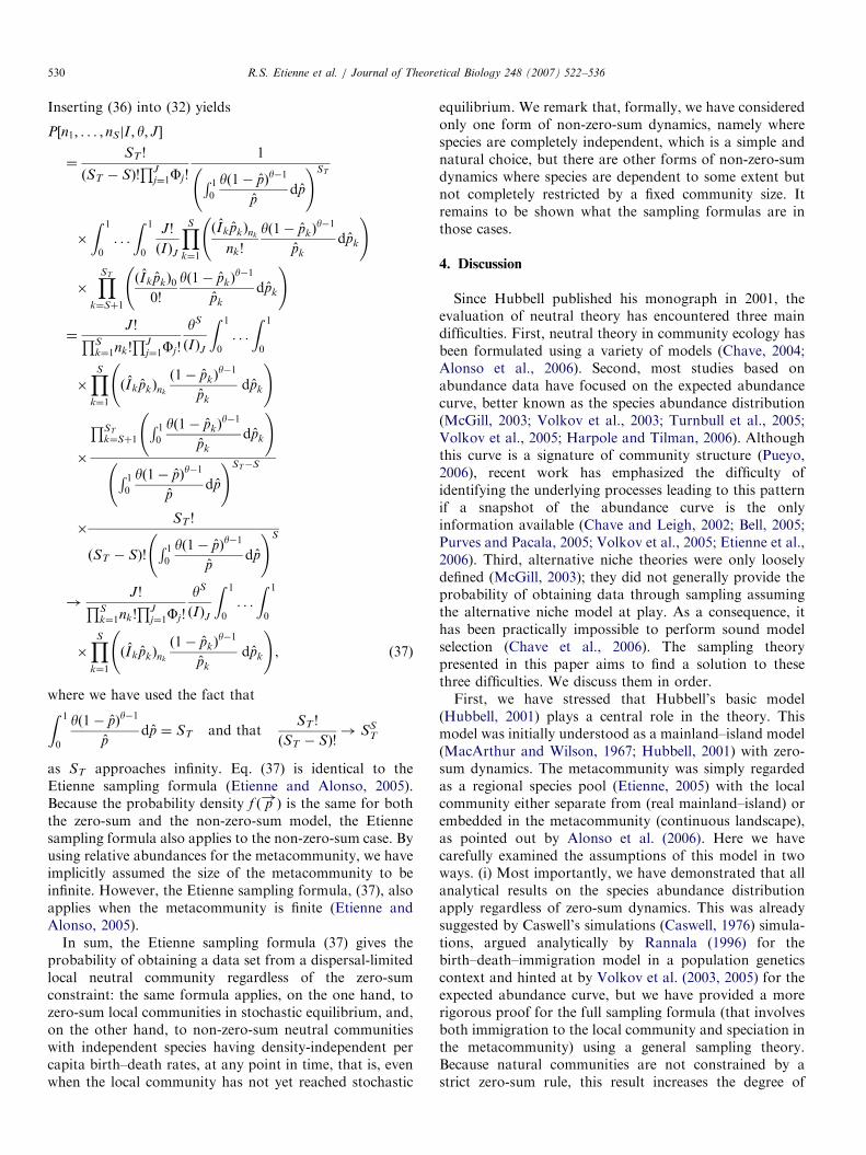
ARTICLE IN PRESSR.S. Etienne et al. / Journal of Theoretical Biology 248 (2007) 522–536530
Inserting (36) into (32) yields
P½n1; . . . ; nSjI ; y; J�
¼ST !
ðST � SÞ!QJ
j¼1Fj!
1
R 10
yð1� pÞy�1
pdp
!ST
�
Z 1
0
. . .
Z 1
0
J!
ðIÞJ
YS
k¼1
ðI kpkÞnk
nk!
yð1� pkÞy�1
pk
dpk
!
�YST
k¼Sþ1
ðI kpkÞ0
0!
yð1� pkÞy�1
pk
dpk
!
¼J!QS
k¼1nk!QJ
j¼1Fj!
yS
ðIÞJ
Z 1
0
. . .
Z 1
0
�YS
k¼1
ðI kpkÞnk
ð1� pkÞy�1
pk
dpk
!
�
QST
k¼Sþ1
R 10
yð1� pkÞy�1
pk
dpk
!
R 10
yð1� pÞy�1
pdp
!ST�S
�ST !
ðST � SÞ!R 10
yð1� pÞy�1
pdp
!S
!J!QS
k¼1nk!QJ
j¼1Fj!
yS
ðIÞJ
Z 1
0
. . .
Z 1
0
�YS
k¼1
ðI kpkÞnk
ð1� pkÞy�1
pk
dpk
!, ð37Þ
where we have used the fact thatZ 1
0
yð1� pÞy�1
pdp ¼ ST and that
ST !
ðST � SÞ!! SS
T
as ST approaches infinity. Eq. (37) is identical to theEtienne sampling formula (Etienne and Alonso, 2005).Because the probability density f ð p!Þ is the same for boththe zero-sum and the non-zero-sum model, the Etiennesampling formula also applies to the non-zero-sum case. Byusing relative abundances for the metacommunity, we haveimplicitly assumed the size of the metacommunity to beinfinite. However, the Etienne sampling formula, (37), alsoapplies when the metacommunity is finite (Etienne andAlonso, 2005).
In sum, the Etienne sampling formula (37) gives theprobability of obtaining a data set from a dispersal-limitedlocal neutral community regardless of the zero-sumconstraint: the same formula applies, on the one hand, tozero-sum local communities in stochastic equilibrium, and,on the other hand, to non-zero-sum neutral communitieswith independent species having density-independent percapita birth–death rates, at any point in time, that is, evenwhen the local community has not yet reached stochastic
equilibrium. We remark that, formally, we have consideredonly one form of non-zero-sum dynamics, namely wherespecies are completely independent, which is a simple andnatural choice, but there are other forms of non-zero-sumdynamics where species are dependent to some extent butnot completely restricted by a fixed community size. Itremains to be shown what the sampling formulas are inthose cases.
4. Discussion
Since Hubbell published his monograph in 2001, theevaluation of neutral theory has encountered three maindifficulties. First, neutral theory in community ecology hasbeen formulated using a variety of models (Chave, 2004;Alonso et al., 2006). Second, most studies based onabundance data have focused on the expected abundancecurve, better known as the species abundance distribution(McGill, 2003; Volkov et al., 2003; Turnbull et al., 2005;Volkov et al., 2005; Harpole and Tilman, 2006). Althoughthis curve is a signature of community structure (Pueyo,2006), recent work has emphasized the difficulty ofidentifying the underlying processes leading to this patternif a snapshot of the abundance curve is the onlyinformation available (Chave and Leigh, 2002; Bell, 2005;Purves and Pacala, 2005; Volkov et al., 2005; Etienne et al.,2006). Third, alternative niche theories were only looselydefined (McGill, 2003); they did not generally provide theprobability of obtaining data through sampling assumingthe alternative niche model at play. As a consequence, ithas been practically impossible to perform sound modelselection (Chave et al., 2006). The sampling theorypresented in this paper aims to find a solution to thesethree difficulties. We discuss them in order.First, we have stressed that Hubbell’s basic model
(Hubbell, 2001) plays a central role in the theory. Thismodel was initially understood as a mainland–island model(MacArthur and Wilson, 1967; Hubbell, 2001) with zero-sum dynamics. The metacommunity was simply regardedas a regional species pool (Etienne, 2005) with the localcommunity either separate from (real mainland–island) orembedded in the metacommunity (continuous landscape),as pointed out by Alonso et al. (2006). Here we havecarefully examined the assumptions of this model in twoways. (i) Most importantly, we have demonstrated that allanalytical results on the species abundance distributionapply regardless of zero-sum dynamics. This was alreadysuggested by Caswell’s simulations (Caswell, 1976) simula-tions, argued analytically by Rannala (1996) for thebirth–death–immigration model in a population geneticscontext and hinted at by Volkov et al. (2003, 2005) for theexpected abundance curve, but we have provided a morerigorous proof for the full sampling formula (that involvesboth immigration to the local community and speciation inthe metacommunity) using a general sampling theory.Because natural communities are not constrained by astrict zero-sum rule, this result increases the degree of
ARTICLE IN PRESSR.S. Etienne et al. / Journal of Theoretical Biology 248 (2007) 522–536 531
realism and makes the theory more robust and appealing.(ii) En passant, we have also clarified a differentinterpretation of this model within the context of anemerging paradigm, the metacommunity concept (Leiboldet al., 2004; Holyoak et al., 2005). The model has beenapplied not only to pure mainland–island systems, but also(and more frequently) to metacommunities in the truesense of the word (e.g. Dornelas et al., 2006): localcommunities that grow on fragmented patchy areas(Alonso and Pascual, 2006), and that are connected toeach other through migration, which is global in the model.So, partially isolated local communities host differentspecies brought together by random dispersal from a poolthat is only governed by evolutionary forces (speciation).Note that the per capita death rate d is actually death plusemigration. Any surplus of local production feeds themetacommunity (emigration) and returns to the localcommunity as a propagule rain or global immigration(l). The crucial assumptions made here are: (a) thatemigration does not affect the metacommunity composi-tion and a spatially implicit model can capture the essenceof the dynamics and (b) that evolutionary forces act on adifferent time scale than ecological forces. Under theseassumptions—which are not always justified, see e.g.Etienne (2007), Hairston et al. (2005)—the collectivebehavior of an ensemble of species performing these simpledynamics in the local community is adequately describedby the dispersal-limited sampling formula (Etienne, 2005;Etienne and Alonso, 2005, 2006), which gives a measure ofthe average degree of isolation of local communities by wayof I, the fundamental dispersal number, and of themetacommunity diversity by way of y, the fundamentalbiodiversity number.
Second, although we agree that the abundance curvemay not be enough to elucidate underlying processes, ourwork on species abundances is based instead on what wecall a general sampling formula, the central expression ofthe theory (1). This is a multivariate abundance distribu-tion that may encode much more information than thesimple abundance curve, the expected number of species ateach abundance level. Different processes can lead tosimilar, perhaps indistinguishable, average abundancecurves (Volkov et al., 2005). Because this curve istheoretically obtained by averaging the full samplingformula (Etienne and Alonso, 2005), it can be seen as afirst moment of a multivariate distribution. But the firstmoment of a distribution does not describe the distributioncompletely. So, it is possible that two processes lead to thesame average abundance curve (Volkov et al., 2005), butthe underlying multivariate distributions may be different(Chave et al., 2006). Moreover, because the multivariatedistribution keeps track of individual abundances, it can beextended to multiple samples across space or time. To date,most studies on species abundances dealing with neutraltheory have only used the abundance curve (McGill et al.,2006; Pueyo, 2006), rather than this powerful multivariaterepresentation of the community; hence conclusions that
species abundance distributions contain little informationare premature. The sampling formula under neutrality fora single sample is the Etienne sampling formula (Etienne,2005). It has recently been extended to multiple samplesacross space which conveys more information (Etienne,2007; Munoz et al., 2007). Also, most studies have analyzedonly snapshots of the community rather than dynamicaldata (but see Gilbert et al., 2006), which may contain moreinformation as well. Our framework can be easily extendedto deal with this type of data (38). When we sample thesame system at T different times (where the sample sizemay vary), yielding a time series of multivariate abundanceobservations Dt1 ;Dt2 ; . . . ;DtT
, we can calculate the like-lihood of this time series for the model that is assumed todescribe the assembly process, by simply multiplyingconditional transitional probabilities:
P½Dt1 ;Dt2 ; . . . ;DtTjY; J�
¼ P½DtTjDtT�1;Y; J� . . .P½Dt2 jDt1 ;Y; J�P½Dt1 jY; J�, ð38Þ
where Y ¼ fb; d; lg represents model parameters. Theprobability of observing the first abundance data set,P½Dt1 jY; J�, can be computed by assuming stochasticequilibrium, or by assuming some initial condition in thepast. The actual computation of the conditional probabil-ities in (38) may be quite involved and requires furthertheoretical development that is beyond the scope of thispaper.Third, here we have used the fundamental expression (1)
to derive sampling formulas in the context of neutraltheory, but we recall that this is a general expression thatcan be extended to situations beyond neutrality as well. Wehave used the hypergeometric distribution to describe thesampling process, but again our general expression allowsother forms for this distribution. Our expression doesassume that we sample randomly a predetermined numberof individuals. In the field, we can often adapt our samplingstrategy to meet this requirement. Some work has beendone to deal with the case where a predetermined numberof species is sampled instead (Etienne and Olff, 2005).However, the case where an area or a transect is sampledposes serious theoretical challenges. We hope that thispaper stimulates research on this problem.Thus, our sampling theory suggests routes to resolving
the three important limitations of recent studies on testingneutral theory vs. niche theories by using species abun-dance data. However, more interestingly, we provide asampling description of communities, where both evolu-tionary and ecological determinants of species coexistenceand composition can be analyzed. Hubbell (2001) alreadystudied how species origination influences communitypatterns. When we analyze our general sampling formula(1) or the particular example given in (32), we notice thatthis expression consist of two essential pieces. First, wehave the multivariate distribution at the metacommunitylevel (Pðx1; . . . ;xSÞ in (1) or f ð~pÞ in (32)). Species canpotentially diverge in their life history characteristics by
ARTICLE IN PRESSR.S. Etienne et al. / Journal of Theoretical Biology 248 (2007) 522–536532
creating and adapting to different biological and physicalniches. As a result of such processes some equilibriumbetween species origination and extinction is generallyreached, which can be described by a multivariatedistribution. For instance, the Ewens distribution describesthis distribution under neutrality and the point mutationmode of speciation. We provide a general method tointegrate over the Ewens distribution. A proper change ofvariables simplifies enormously our integration domain in(32) and leads to the integral expression of Etiennesampling formula (Etienne and Alonso, 2005). However,we can only reach this metacommunity distribution bysampling locally, that is, by looking at local communities.So, the second ingredient of our general sampling formulais a sampling distribution that gives the probability ofobtaining a given collection of species abundances giventhat we know exactly the species composition in themetacommunity (P½n1; . . . ; nSjx1; . . . ;xS; J� in (3)). Thisconditional probability is determined by the samplingprocess and the ecological processes assumed to play a roleduring the assembly of local communities. For instance, ifdispersal limitation is the main factor in the context ofecologically symmetric species, we obtain the DLM(Etienne and Alonso, 2005) given in (26).
Volkov et al. (2005) have also initiated a sampling theory(see their appendix), borrowing ideas from statisticalphysics on approximations for very large assemblages. Incontrast, our approach is exact and thus enables us toprove the exact equality of zero-sum and non-zero-sumcases in the context of neutral theory, but in other instancesit may become very complicated in which case the work byVolkov et al. (2005) presents a promising alternativedirection deserving further investigation.
In sum, our work considers current neutral theory as abasis to set up a general sampling theory able to go beyondneutrality and still analyze alternative models in terms ofthe extent to which empirical data statistically supportthem. As a first step, in our non-zero-sum example, weprovide sampling formulas that assume independence ofspecies. Although this is a valid assumption underneutrality and may be a still reasonable, particularly whenonly one trophic level is considered, more general commu-nity patterns may of course emerge from individual speciesinteractions, described by topologically complex networks.Further integration is needed between sampling theoriesand network ecology to pave the way for a sampling theoryfor food webs or mutualistic interaction networks (Bas-compte et al., 2003). We believe that our samplingapproach can be used to generate (null) models that arenecessary in assessing the plausibility of alternative net-work topologies on the basis of samples of complexcommunities.
Acknowledgments
We thank two anonymous reviewers for helpful com-ments. D.A. thanks the support of the James S. McDonnell
Foundation through a Centennial Fellowship to MercedesPascual.
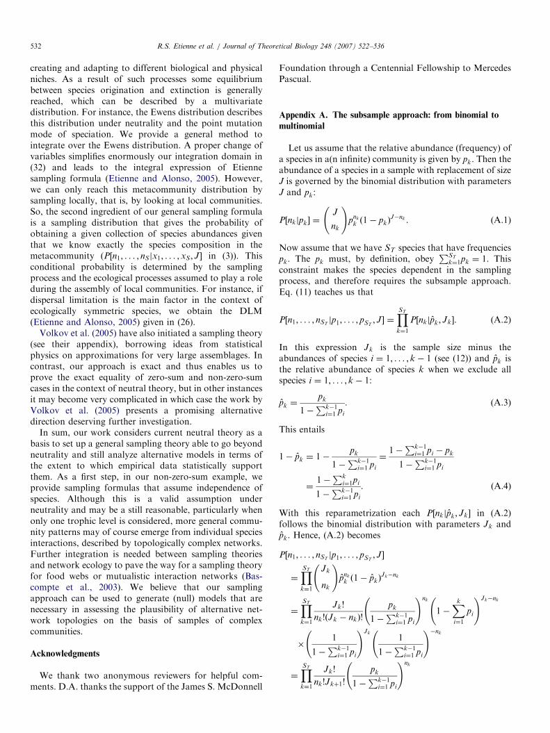
Appendix A. The subsample approach: from binomial to
multinomial
Let us assume that the relative abundance (frequency) ofa species in a(n infinite) community is given by pk. Then theabundance of a species in a sample with replacement of sizeJ is governed by the binomial distribution with parametersJ and pk:
P½nkjpk� ¼J
nk
!pnk
k ð1� pkÞJ�nk . (A.1)
Now assume that we have ST species that have frequenciespk. The pk must, by definition, obey
PST
k¼1pk ¼ 1. Thisconstraint makes the species dependent in the samplingprocess, and therefore requires the subsample approach.Eq. (11) teaches us that
P½n1; . . . ; nSTjp1; . . . ; pST
; J� ¼YST
k¼1
P½nkjpk; Jk�. (A.2)
In this expression Jk is the sample size minus theabundances of species i ¼ 1; . . . ; k � 1 (see (12)) and pk isthe relative abundance of species k when we exclude allspecies i ¼ 1; . . . ; k � 1:
pk ¼pk
1�Pk�1
i¼1 pi
. (A.3)
This entails
1� pk ¼ 1�pk
1�Pk�1
i¼1 pi
¼1�
Pk�1i¼1 pi � pk
1�Pk�1
i¼1 pi
¼1�
Pki¼1pi
1�Pk�1
i¼1 pi
. ðA:4Þ
With this reparametrization each P½nkjpk; Jk� in (A.2)follows the binomial distribution with parameters Jk andpk. Hence, (A.2) becomes
P½n1; . . . ; nSTjp1; . . . ; pST
; J�
¼YST
k¼1
Jk
nk
!pnk
k ð1� pkÞJk�nk
¼YST
k¼1
Jk!
nk!ðJk � nkÞ!
pk
1�Pk�1
i¼1 pi
!nk
1�Xk
i¼1
pi
!Jk�nk
�1
1�Pk�1
i¼1 pi
!Jk
1
1�Pk�1
i¼1 pi
!�nk
¼YST
k¼1
Jk!
nk!Jkþ1!
pk
1�Pk�1
i¼1 pi
!nk
ARTICLE IN PRESSR.S. Etienne et al. / Journal of Theoretical Biology 248 (2007) 522–536 533
� 1�Xk
i¼1
pi
!Jkþ1
1�Xk�1i¼1
pi
!�Jk
1�Xk�1i¼1
pi
!nk
¼YST
k¼1
Jk!
nk!Jkþ1!pnk
k
ð1�Pk
i¼1piÞJkþ1
ð1�Pk�1
i¼1 piÞJk
¼J
n1; . . . ; nST
!YST
k¼1
pnk
k ðA:5Þ
and in the last expression we recognize the multinomialdistribution with parameters J and p1; . . . ; pST
.
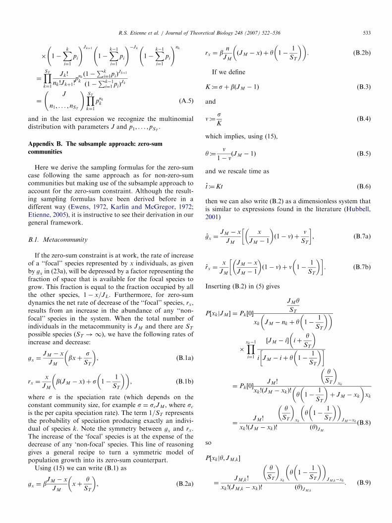
Appendix B. The subsample approach: zero-sum
communities
Here we derive the sampling formulas for the zero-sumcase following the same approach as for non-zero-sumcommunities but making use of the subsample approach toaccount for the zero-sum constraint. Although the result-ing sampling formulas have been derived before in adifferent way (Ewens, 1972, Karlin and McGregor, 1972;Etienne, 2005), it is instructive to see their derivation in ourgeneral framework.
B.1. Metacommunity
If the zero-sum constraint is at work, the rate of increaseof a ‘‘focal’’ species represented by x individuals, as givenby gx in (23a), will be depressed by a factor representing thefraction of space that is available for the focal species togrow. This fraction is equal to the fraction occupied by allthe other species, 1� x=JL. Furthermore, for zero-sumdynamics the net rate of decrease of the ‘‘focal’’ species, rx,results from an increase in the abundance of any ‘‘non-focal’’ species in the system. When the total number ofindividuals in the metacommunity is JM and there are ST
possible species (ST !1), we have the following rates ofincrease and decrease:
gx ¼JM � x
JM
bxþs
ST
� �, (B.1a)
rx ¼x
JM
bðJM � xÞ þ s 1�1
ST
� �� �, (B.1b)
where s is the speciation rate (which depends on theconstant community size, for example s ¼ scJM , where sc
is the per capita speciation rate). The term 1=ST representsthe probability of speciation producing exactly an indivi-dual of species k. Note the symmetry between gx and rx.The increase of the ‘focal’ species is at the expense of thedecrease of any ‘non-focal’ species. This line of reasoninggives a general recipe to turn a symmetric model ofpopulation growth into its zero-sum counterpart.
Using (15) we can write (B.1) as
gx ¼ bJM � x
JM
xþy
ST
� �, (B.2a)
rx ¼ bn
JM
ðJM � xÞ þ y 1�1
ST
� �� �. (B.2b)
If we define
K :¼sþ bðJM � 1Þ (B.3)
and
n :¼sK
(B.4)
which implies, using (15),
y :¼n
1� nðJM � 1Þ (B.5)
and we rescale time as
t :¼Kt (B.6)
then we can also write (B.2) as a dimensionless system thatis similar to expressions found in the literature (Hubbell,2001)
gx ¼JM � x
JM
x
JM � 1
� �ð1� nÞ þ
nST
� �, (B.7a)
rx ¼x
JM
JM � x
JM � 1
� �ð1� nÞ þ n 1�
1
ST
� �� �. (B.7b)
Inserting (B.2) in (5) gives
P½xkjJM � ¼ Pk½0�
JMyST
xk JM � nk þ y 1�1
ST
� �� �
�Yxk�1
i¼1
½JM � i� i þy
ST
� �
i JM � i þ y 1�1
ST
� �� �
¼ Pk½0�JM !
xk!ðJM � xkÞ!
yST
� �xk
y 1�1
ST
� �þ JM � xk
� �xk
¼JM !
xk!ðJM � xkÞ!
yST
� �xk
y 1�1
ST
� �� �JM�xk
ðyÞJM
ðB:8Þ
so
P½xkjy; JM ;k�
¼JM ;k!
xk!ðJM;k � xkÞ!
yST
� �xk
y 1�1
ST
� �� �JM;k�xk
ðyÞJM;k
. ðB:9Þ
ARTICLE IN PRESSR.S. Etienne et al. / Journal of Theoretical Biology 248 (2007) 522–536534
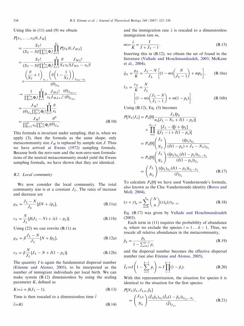
Using this in (11) and (9) we obtain
P½x1; . . . ;xSjy; JM �
¼ST !
ðST � SÞ!QJM
j¼1Fj!
YST
k¼1
P½xkjy; JM;k�
¼ST !
ðST � SÞ!QJM
j¼1Fj!
YS
k¼1
yST
JM ;k!
xk!ðJM ;k � xkÞ!
�
yST
þ 1
� �xk�1
y 1�1
ST
� �� �JM;k�xk
ðyÞJM
!1QJM
j¼1Fj!
YS
k¼1
yJM;k!
xkJM;kþ1!
ðyÞJM ;kþ1
ðyÞJM;k
¼JM !
ðyÞJM
QJM
j¼1Fj !
YSk¼1
yxk
¼JM !QS
k¼1xk
QJM
j¼1Fj!
yS
ðyÞJM
. ðB:10Þ
This formula is invariant under sampling, that is, when weapply (3), then the formula as the same shape; onlymetacommunity size JM is replaced by sample size J. Thuswe have arrived at Ewens (1972) sampling formula.Because both the zero-sum and the non-zero-sum formula-tions of the neutral metacommunity model yield the Ewenssampling formula, we have shown that they are identical.
B.2. Local community
We now consider the local community. The totalcommunity size is at a constant JL. The rates of increaseand decrease are
gN ¼JL �N
JL
½bN þ lpk�, (B.11a)
rN ¼N
JL
½bðJL �NÞ þ lð1� pkÞ�. (B.11b)
Using (22) we can rewrite (B.11) as
gN ¼ bJL �N
JL
½N þ Ipk�, (B.12a)
rN ¼ bN
JL
½JL �N þ Ið1� pkÞ�. (B.12b)
The quantity I is again the fundamental dispersal number(Etienne and Alonso, 2005), to be interpreted as thenumber of immigrant individuals per local birth. We canmake system (B.12) dimensionless by using the scalingparameter K, defined as
K :¼lþ bðJL � 1Þ. (B.13)
Time is then rescaled to a dimensionless time t
t:¼Kt (B.14)
and the immigration rate l is rescaled to a dimensionlessimmigration rate m,
m:¼lK¼
I
I þ JL � 1. (B.15)
Inserting this in (B.12), we obtain the set of found in theliterature (Vallade and Houchmandzadeh, 2003; McKaneet al., 2004),
gN ¼gN
K¼
JL �N
JL
ð1�mÞN
JL � 1
� �þmpk
� �, (B.16a)
rN ¼rN
K¼
N
JL
ð1�mÞJL �N
JL � 1
� �þmð1� pkÞ
� �. ðB:16bÞ
Using (B.12), Eq. (5) becomes
P½NkjJL� ¼ Pk½0�JLIpk
nk½JL �Nk þ Ið1� pkÞ�
�YNk�1
i¼1
½JL � i�½i þ Ipk�
i½JL � i þ Ið1� pkÞ�
¼ Pk½0�JL
Nk
!ðIpkÞNk
ðIð1� pkÞ þ JL �NkÞNk
¼ Pk½0�JL
Nk
!ðIpkÞNk
ðIð1� pkÞÞJL�Nk
ðIð1� pkÞÞJL
¼JL
Nk
!ðIpkÞNk
ðIð1� pkÞÞJL�Nk
ðIÞJL
. ðB:17Þ
To calculate Pk½0� we have used Vandermonde’s formula,also known as the Chu–Vandermonde identity (Boros andMoll, 2004),
ðxþ yÞn ¼Xn
n¼0
N
n
� �ðxÞnðyÞN�n. (B.18)
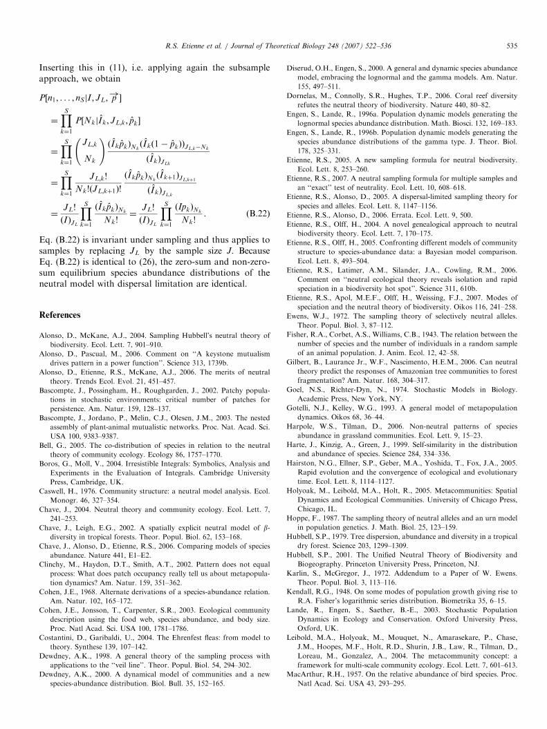
Eq. (B.17) was given by Vallade and Houchmandzadeh(2003).Each term in (11) requires the probability of abundance
nk where we exclude the species i ¼ 1 . . . k � 1. Thus, werescale all relative abundances in the metacommunity,
pk ¼pk
1�Pk�1
i¼1 pi
(B.19)
and the dispersal number becomes the effective dispersalnumber (see also Etienne and Alonso, 2005),
I k:¼I 1�Xk�1i¼1
pi
!¼ I
Yk�1i�1
ð1� piÞ. (B.20)
With this reparametrization, the situation for species k isidentical to the situation for the first species:
P½NkjIk; JL;k; pk�
¼JL;k
Nk
!ðI kpkÞNk
ðI kð1� pkÞÞJL;k�Nk
ðIÞJL;k
. ðB:21Þ
ARTICLE IN PRESSR.S. Etienne et al. / Journal of Theoretical Biology 248 (2007) 522–536 535
Inserting this in (11), i.e. applying again the subsampleapproach, we obtain
P½n1; . . . ; nSjI ; JL; p!�
¼YS
k¼1
P½NkjI k; JL;k; pk�
¼YS
k¼1
JL;k
Nk
!ðI kpkÞNk
ðI kð1� pkÞÞJL;k�Nk
ðI kÞJLk
¼YS
k¼1
JL;k!
Nk!ðJL;kþ1Þ!
ðI kpkÞNkðI kþ1ÞJL;kþ1
ðI kÞJL;k
¼JL!
ðIÞJL
YSk¼1
ðI kpkÞNk
Nk!¼
JL!
ðIÞJL
YSk¼1
ðIpkÞNk
Nk!. ðB:22Þ
Eq. (B.22) is invariant under sampling and thus applies tosamples by replacing JL by the sample size J. BecauseEq. (B.22) is identical to (26), the zero-sum and non-zero-sum equilibrium species abundance distributions of theneutral model with dispersal limitation are identical.
References
Alonso, D., McKane, A.J., 2004. Sampling Hubbell’s neutral theory of
biodiversity. Ecol. Lett. 7, 901–910.
Alonso, D., Pascual, M., 2006. Comment on ‘‘A keystone mutualism
drives pattern in a power function’’. Science 313, 1739b.
Alonso, D., Etienne, R.S., McKane, A.J., 2006. The merits of neutral
theory. Trends Ecol. Evol. 21, 451–457.
Bascompte, J., Possingham, H., Roughgarden, J., 2002. Patchy popula-
tions in stochastic environments: critical number of patches for
persistence. Am. Natur. 159, 128–137.
Bascompte, J., Jordano, P., Melin, C.J., Olesen, J.M., 2003. The nested
assembly of plant-animal mutualistic networks. Proc. Nat. Acad. Sci.
USA 100, 9383–9387.
Bell, G., 2005. The co-distribution of species in relation to the neutral
theory of community ecology. Ecology 86, 1757–1770.
Boros, G., Moll, V., 2004. Irresistible Integrals: Symbolics, Analysis and
Experiments in the Evaluation of Integrals. Cambridge University
Press, Cambridge, UK.
Caswell, H., 1976. Community structure: a neutral model analysis. Ecol.
Monogr. 46, 327–354.
Chave, J., 2004. Neutral theory and community ecology. Ecol. Lett. 7,
241–253.
Chave, J., Leigh, E.G., 2002. A spatially explicit neutral model of b-diversity in tropical forests. Theor. Popul. Biol. 62, 153–168.
Chave, J., Alonso, D., Etienne, R.S., 2006. Comparing models of species
abundance. Nature 441, E1–E2.
Clinchy, M., Haydon, D.T., Smith, A.T., 2002. Pattern does not equal
process: What does patch occupancy really tell us about metapopula-
tion dynamics? Am. Natur. 159, 351–362.
Cohen, J.E., 1968. Alternate derivations of a species-abundance relation.
Am. Natur. 102, 165–172.
Cohen, J.E., Jonsson, T., Carpenter, S.R., 2003. Ecological community
description using the food web, species abundance, and body size.
Proc. Natl Acad. Sci. USA 100, 1781–1786.
Costantini, D., Garibaldi, U., 2004. The Ehrenfest fleas: from model to
theory. Synthese 139, 107–142.
Dewdney, A.K., 1998. A general theory of the sampling process with
applications to the ‘‘veil line’’. Theor. Popul. Biol. 54, 294–302.
Dewdney, A.K., 2000. A dynamical model of communities and a new
species-abundance distribution. Biol. Bull. 35, 152–165.
Diserud, O.H., Engen, S., 2000. A general and dynamic species abundance
model, embracing the lognormal and the gamma models. Am. Natur.
155, 497–511.
Dornelas, M., Connolly, S.R., Hughes, T.P., 2006. Coral reef diversity
refutes the neutral theory of biodiversity. Nature 440, 80–82.
Engen, S., Lande, R., 1996a. Population dynamic models generating the
lognormal species abundance distribution. Math. Biosci. 132, 169–183.
Engen, S., Lande, R., 1996b. Population dynamic models generating the
species abundance distributions of the gamma type. J. Theor. Biol.
178, 325–331.
Etienne, R.S., 2005. A new sampling formula for neutral biodiversity.
Ecol. Lett. 8, 253–260.
Etienne, R.S., 2007. A neutral sampling formula for multiple samples and
an ‘‘exact’’ test of neutrality. Ecol. Lett. 10, 608–618.
Etienne, R.S., Alonso, D., 2005. A dispersal-limited sampling theory for
species and alleles. Ecol. Lett. 8, 1147–1156.
Etienne, R.S., Alonso, D., 2006. Errata. Ecol. Lett. 9, 500.
Etienne, R.S., Olff, H., 2004. A novel genealogical approach to neutral
biodiversity theory. Ecol. Lett. 7, 170–175.
Etienne, R.S., Olff, H., 2005. Confronting different models of community
structure to species-abundance data: a Bayesian model comparison.
Ecol. Lett. 8, 493–504.
Etienne, R.S., Latimer, A.M., Silander, J.A., Cowling, R.M., 2006.
Comment on ‘‘neutral ecological theory reveals isolation and rapid
speciation in a biodiversity hot spot’’. Science 311, 610b.
Etienne, R.S., Apol, M.E.F., Olff, H., Weissing, F.J., 2007. Modes of
speciation and the neutral theory of biodiversity. Oikos 116, 241–258.
Ewens, W.J., 1972. The sampling theory of selectively neutral alleles.
Theor. Popul. Biol. 3, 87–112.
Fisher, R.A., Corbet, A.S., Williams, C.B., 1943. The relation between the
number of species and the number of individuals in a random sample
of an animal population. J. Anim. Ecol. 12, 42–58.
Gilbert, B., Laurance Jr., W.F., Nascimento, H.E.M., 2006. Can neutral
theory predict the responses of Amazonian tree communities to forest
fragmentation? Am. Natur. 168, 304–317.
Goel, N.S., Richter-Dyn, N., 1974. Stochastic Models in Biology.
Academic Press, New York, NY.
Gotelli, N.J., Kelley, W.G., 1993. A general model of metapopulation
dynamics. Oikos 68, 36–44.
Harpole, W.S., Tilman, D., 2006. Non-neutral patterns of species
abundance in grassland communities. Ecol. Lett. 9, 15–23.
Harte, J., Kinzig, A., Green, J., 1999. Self-similarity in the distribution
and abundance of species. Science 284, 334–336.
Hairston, N.G., Ellner, S.P., Geber, M.A., Yoshida, T., Fox, J.A., 2005.
Rapid evolution and the convergence of ecological and evolutionary
time. Ecol. Lett. 8, 1114–1127.
Holyoak, M., Leibold, M.A., Holt, R., 2005. Metacommunities: Spatial
Dynamics and Ecological Communities. University of Chicago Press,
Chicago, IL.
Hoppe, F., 1987. The sampling theory of neutral alleles and an urn model
in population genetics. J. Math. Biol. 25, 123–159.
Hubbell, S.P., 1979. Tree dispersion, abundance and diversity in a tropical
dry forest. Science 203, 1299–1309.
Hubbell, S.P., 2001. The Unified Neutral Theory of Biodiversity and
Biogeography. Princeton University Press, Princeton, NJ.
Karlin, S., McGregor, J., 1972. Addendum to a Paper of W. Ewens.
Theor. Popul. Biol. 3, 113–116.
Kendall, R.G., 1948. On some modes of population growth giving rise to
R.A. Fisher’s logarithmic series distribution. Biometrika 35, 6–15.
Lande, R., Engen, S., Saether, B.-E., 2003. Stochastic Population
Dynamics in Ecology and Conservation. Oxford University Press,
Oxford, UK.
Leibold, M.A., Holyoak, M., Mouquet, N., Amarasekare, P., Chase,
J.M., Hoopes, M.F., Holt, R.D., Shurin, J.B., Law, R., Tilman, D.,
Loreau, M., Gonzalez, A., 2004. The metacommunity concept: a
framework for multi-scale community ecology. Ecol. Lett. 7, 601–613.
MacArthur, R.H., 1957. On the relative abundance of bird species. Proc.
Natl Acad. Sci. USA 43, 293–295.
ARTICLE IN PRESSR.S. Etienne et al. / Journal of Theoretical Biology 248 (2007) 522–536536
MacArthur, R.H., 1960. On the relative abundance of species. Am. Natur.
94, 25–36.
MacArthur, R.H., Wilson, E.O., 1967. Island Biogeography. Princeton
University Press, Princeton, NJ.
Magurran, A.E., 2004. Measuring Biological Diversity. Blackwell,
Oxford, UK.
McGill, B.J., 2003. A test of the unified neutral theory of biodiversity.
Nature 422, 881–885.
McGill, B.J., Maurer, B.A., Weiser, M.D., 2006. Empirical evaluation of
neutral theory. Ecology 87, 1411–1426.
McKane, A.J., Alonso, D., Sole, R.V., 2000. Mean field stochastic theory
for species rich assembled communities. Phys. Rev. E 62, 8466–8484.
McKane, A.J., Alonso, D., Sole, R.V., 2004. Analytic solution of
Hubbell’s model of local community dynamics. Theor. Popul. Biol.
65, 67–73.
Mosimann, J.E., 1962. On the compound multinomial distribution, the
multivariate beta-distribution, and correlations among proportions.
Biometrika 49, 65–82.
Munoz, F., Couteron, P., Ramesh, B.R., Etienne, R.S., 2007. Inferring
parameters of neutral communities: from one single large to several
small samples. Ecology, in press.
Nisbet, R.M., Gurney, W.S.C., 1982. Modelling Fluctuating Populations.
Wiley, New York, NY.
Pielou, E.C., 1969. An Introduction to Mathematical Ecology. Wiley,
New York, NY.
Pielou, E.C., 1975. Ecological Diversity. Wiley, New York, NY.
Poulin, R., 2004. Parasites and the neutral theory of biodiversity.
Ecography 27, 119–123.
Preston, F.W., 1948. The commonness, and rarity, of species. Ecology 29,
254–283.
Preston, F.W., 1962. The canonical distribution of commonness and
rarity. Parts i and ii. Ecology 43, 185–215, 410–432.
Pueyo, S., 2006. Diversity: between neutrality and structure. Oikos 112,
392–405.
Purves, D.W., Pacala, S.W., 2005. Ecological drift in niche-structured
communities: neutral pattern does not imply neutral process. In:
Burslem, D., Pinard, M., Hartley, S. (Eds.), Biotic Interactions in the
Tropics. Cambridge University Press, Cambridge, UK, pp. 107–138.
Rannala, B., 1996. The sampling theory of neutral alleles in an island
population of fluctuating size. Theor. Popul. Biol. 50, 91–104.
Renshaw, E., 1991. Modelling Biological Populations in Space and Time,
Cambridge Studies in Mathematical Biology, vol. 11. Cambridge
University Press, Cambridge, UK
Sugihara, G., 1980. Minimal community structure: an explanation of
species-abundance patterns. Am. Natur. 116, 770–787.
Tavare, S., Ewens, W.J., 1997. Multivariate Ewens distribution. In:
Johnson, N., Kotz, S., Balakrishnan, N. (Eds.), Discrete Multivariate
Distributions. Wiley, New York, NY, pp. 232–246.
Tokeshi, M., 1990. Niche apportionment or random assortment—species
abundance patterns revisited. J. Anim. Ecol. 59, 1129–1146.
Tokeshi, M., 1993. Species abundance patterns and community structure.
Adv. Ecol. Res. 24, 111–186.
Tokeshi, M., 1996. Power fraction: a new explanation of relative
abundance patterns in species-rich assemblages. Oikos 75, 543–550.
Turnbull, L.A., Manley, L., Rees, M., 2005. Niches, rather than
neutrality, structure a grassland pioneer guild. Proc. Roy. Soc.
London B 272, 1357–1364.
Vallade, M., Houchmandzadeh, B., 2003. Analytical solution of a neutral
model of biodiversity. Phys. Rev. E 68, 061902.
Vallade, M., Houchmandzadeh, B., 2006. Species abundance distribution
and population dynamics in a two-community model of neutral
ecology. Phys. Rev. E. 74, 051914.
Van Kampen, N.G., 1992. Stochastic Processes in Physics and Chemistry.
Elsevier, Amsterdam, The Netherlands.
Volkov, I., Banavar, J.R., Hubbell, S.P., Maritan, A., 2003. Neutral
theory and relative species abundance in ecology. Nature 424,
1035–1037.
Volkov, I., Banavar, J.R., He, F., Hubbell, S.P., Maritan, A., 2005.
Density dependence explains tree species abundance and diversity in
tropical forests. Nature 438, 658–661.
Wright, S., 1969. Evolution and Genetics of Populations. The theory of
gene frequencies. University of Chicago Press, Chicago, IL.