
modeling the neutral-atmospheric propagation delay in ...
378
MODELING THE NEUTRAL-ATMOSPHERIC PROPAGATION DELAY IN RADIOMETRIC SPACE TECHNIQUES V. B. MENDES April 1999 TECHNICAL REPORT NO. 199
-
Upload
khangminh22 -
Category
Documents
-
view
4 -
download
0
Transcript of modeling the neutral-atmospheric propagation delay in ...

MODELING THE NEUTRAL-ATMOSPHERIC PROPAGATION DELAY IN
RADIOMETRIC SPACE TECHNIQUES
V. B. MENDES
April 1999
TECHNICAL REPORT NO. 217
TECHNICAL REPORT NO. 199

PREFACE
In order to make our extensive series of technical reports more readily available, we have scanned the old master copies and produced electronic versions in Portable Document Format. The quality of the images varies depending on the quality of the originals. The images, in this version of the report, have been converted to searchable text.
MODELING THE NEUTRAL-ATMOSPHERIC PROPAGATION DELAY IN RADIOMETRIC
SPACE TECHNIQUES
V. B. Mendes
Department of Geodesy and Geomatics Engineering University of New Brunswick
P.O. Box 4400 Fredericton, N.B.
Canada E3B 5A3
September 1998
© V. B. Mendes 1998

PREFACE
This technical report is a reproduction of a dissertation submitted in partia1 fulfillment of
the requirements for the degree of Doctor of Philosophy in the Department of Geodesy and
Geomatics Engineering, September 1998. The research was supervised by Dr. Richard B.
Langley. Major funding was provided by the Programa Cicncia and PRAXIS XXI of
de Investiga<;ao Cientffica e Tecnol6gica (Portugal).
As with any copyrighted material, permission to reprint or quote extensively from this
report must be received from the author. The citation to this work should appear as
follows:
Mendes, V. B. (1999). Modeling the neutral-atmosphere propagation delay in radiometric space techniques. Ph.D. dissertation, Department of Geodesy and Geomatics Engineering Technical Report No. 199, University of New Brunswick, Fredericton, New Brunswick, Canada, 353 pp.

ABSTRACT
The propagation delay induced by the electrically-neutral atmosphere has been recognized
as the most problematic modeling error for radiometric space geodetic techniques. A
mismodeling of this propagation delay affects significantly the height component of
position and constitutes therefore a matter of concern in space-geodesy applications, such
as sea-level monitoring, postglacial rebound measurement, earthquake-hazard mitigation,
and tectonic-plate-margin deformation studies.
The neutral-atmosphere propagation delay is commonly considered as composed of two
components: a "hydrostatic" component, due essentially to the dry gases of the
atmosphere, and a "non-hydrostatic" component, due to water vapor. Each one can be
described as the product of the delay at the zenith and a mapping function, which models
the elevation angle dependence of the propagation delay.
This dissertation discusses primarily the accuracy of zenith delay prediction models and
mapping functions found in the scientific literature. This performance evaluation is based
on a comparison against 32,467 benchmark values, obtained by ray tracing one-year's
worth of radiosonde profiles from 50 stations distributed worldwide, and comprised
different phases: ray-tracing accuracy assessment, model development, and model
accuracy assessment.

We have studied the sensitivity of the ray-tracing technique to the choice of physical
models, processing strategies, and radiosonde instrumentation accuracy. We have
concluded that errors in ray tracing can amount to a few centimetres, under special
circumstances, but they largely average out for each station's time series of profiles.
In order to optimize the performance of the models, we have established databases of the
temperature-profile parameters using 50 additional sites, for a total of 100 radiosonde
stations. Based on these large databases, we have developed models for lapse rate and
tropopause height determination, which have improved significantly the performance of
models using the information.
From our model assessment we have concluded that the hydrostatic component of the
zenith delay can be predicted with sub-millimeter accuracy, using the Saastamoinen
model, provided accurate measurements of surface total pressure are available. The
zenith non-hydrostatic component is much more difficult to predict from surface
meteorological data or site dependent parameters, and the best models show values of
root--mean-square (rms) scatter about the mean of a few centimetres in the zenith
direction.
Notwithstanding the large number of mapping functions we have analyzed, only a small
group meet the high standards of modern space geodetic data analysis: Ifadis, Lanyi,
MTT, and NMF. For the total number of radiosonde stations analyzed, none of the
mapping functions revealed themselves to be superior for all elevation angles. For
elevation angles above 15 degrees, Lanyi, MTT, and NMF yield identical mean biases and
ii

the best total error performances. At lower elevation angles, Ifadis and NMF are clearly
superior. As regards the rms scatter about the mean, lfadis performs the best for all
elevation angles, followed closely by Lanyi.
iii

. '
TABLE OF CONTENTS
ABS"J-,RA(~1...,aoeooooooooooo•••lloooot~ooo•eoooooeooooooooolloo••••oooooooooooo••••••••••••••••••••••••oooollooooooa•ooooooooooooooooi
TA.JJl . .~J-{:. {)}~ CQNJ,ENTS ... , .. .,, ... , .... ,, .................................... a.••••~~~o•••••••••••••••••~~••••••••.,••••••iV
LIST OF T ABI.~I~S ·····a··············~~···················································.,··························· viii
I.JST o·F FIGlJRI~S .................................................................................................... xi
I~IS'f OF MAJOR SYMB()l,S ................................................................................ xvii
ACKN.OWJ..JI~l)GEMENTS ooooooooooooeoeooooo&ooooooooooooooa>•••••••••••••••••••••ooooooowaootoeooooooooaeoooolo XX
1. INTRODUC1"'ION .. 8., ............. "' ................................................................................. 1
1.1. Motivation .......................................................................................................... 1
l .2. Literature review ............................................................................................... 14
1 . 3. Dissertation contribution ................................................................................... 16
1.4. Dissertation outline ........................................................................................... 17
2. 'fi-lE EAI{'fi-I'S A'I'MOSPIIERE ...................................................................... 20
2. 1. c:omposition ..................................................................................................... 21
2.2. Vertical structure .............................................................................................. 24
2.3. Equations of state ............................................................................................. 30
2.4. Moisture variables ............................................................................................. 35
2.5. Model atmospheres ........................................................................................... 44
2.5.1. Homogeneous atmosphere ........................................................................ 44
2.5.2. Isothermal atmosphere .............................................................................. 46
2.5.3. Constant-lapse-rate atmosphere ................................................................. 47
2. 5.4. Standard atmospheres ............................................................................... 48
iv
3. NEUTRAL-ATMOSPHERE REFRACTION ................................................... 55
3.1. H.efractivity ....................................................................................................... 56
3 .1.1. Refractivity models .................................................................................... 65
3.2. Neutral--atmosphere propagation delay: a definition ........................................... 72
3.3. Neutral-atmosphere propagation delay modeling ............................................... 78
3.3.1. Hydrostatic and dry zenith delay models .................................................... 79
3.3.2. Non-hydrostatic and wet zenith delay models ............................................ 82
3.3.3. Mapping functions ..................................................................................... 92
3.3.4. Hybrid models for airborne positioning .................................................... 107
4. DATA DESCRIPTION AND ANALYSIS ....................................................... lll
4.1. Upper air observations .................................................................................... 112
4. 1.1. Radiosonde instrumentation .................................................................... 112
4.1.2. Measurement errors of radiosonde meteorological sensors ....................... 115
4.1.3. Radiosonde data selection ....................................................................... 119
4.2. Meteorological parameter databases ................................................................ 120
4.2.1. Tropopause height.. ................................................................................. 121
4.2.2. Inversion height ....................................................................................... 137
4.2.3. Lapse rate ............................................................................................... 141
5., R.A Y l,ll.ACING .......... e ••• , ••••••••••••••• ~~ .................................................................. l53
5.1. Software algorithms and models ...................................................................... 154
5.1.1. Profile extrapolation and interpolation ..................................................... 155
5 .1.2. Saturation vapor pressure computation .................................................... 157
5.1.3. Refractivity constants .............................................................................. 163
5. 1.4. Compressibility factors ............................................................................ 164
5. 1. 5. Enhancement factor ................................................................................. 164
5.1.6. Initial integration step .............................................................................. 165
5 .1. 7. Integration limits ..................................................................................... 166
5.1.8. Radiosonde data precision and accuracy .................................................. 168
v

5 .2. Ray tracing limitations ..................................................................................... 171
5.2.1. Propagation delay due to non-gaseous atmosphere constituents ............... 172
5.2.2. Horizontal gradients ................................................................................ 175
5.2.3. Hydrostatic equilibrium violation ............................................................. 178
5. 3. Product analysis .............................................................................................. 179
5.3.1. Precipitable water .................................................................................... 181
5.3.2. Geometric delay ...................................................................................... 188
6. MOI)El, ASSESSMEN'f .................................................................................. 192
6.1. Methodology and nomenclature ...................................................................... 192
6.2. Hydrostatic zenith delay prediction models ...................................................... 194
6.3. Non-hydrostatic zenith delay prediction models ............................................... 197
6.4. Zenith total delay models ................................................................................ 201
6.5. Hydrostatic mapping functions ........................................................................ 205
6.6. Non-hydrostatic mapping functions ................................................................. 212
6. 7. Total mapping functions ................................................................................... 217
6.8. :Hybrid models ................................................................................................. 240
7. CONCLUSIONS AND RECOMMENDATIONS ........................................... 244
REFERENCES •••••••lll••••eeeeeoeletteeo••eQoeteeeeeeeeee•••••••••••••oteeeD•••••••••••••••••••••••••••••••••••••••••••••• 249
APPENDIX I. Integral solution of the neutral-atmosphere delay ......................... 273
APPENDIX II. Mathematical structure of selected models ................................... 281
APPENDIX III. Locations and codes of the radiosonde stations ......................... 300
APPENDIX IV. Sample of statistical tables available in electronic format ......... 304
APPENDIX V. Tropopause height and lapse rate statistics .................................. 308
APPENDIX VI. Zenith hydrostatic delay model statistics .................................... 310
APPENDIX VII. Zenith non-hydrostatic delay model statistics ........................... 312
APPENDIX VIII. Zenith total delay model statistics ............................................. 316
vi

APPENDIX IX. Hydrostatic mapping function statistics ...................................... 319
APPENDIX X. Non-hydrostatic mapping function statistics ................................ 328
APPENDIX XI. Total mapping function statistics ................................................. 337
vii

Table 2.1 Main constituents of the earth's dry atmosphere below 80 krn. ................. 22
Table 3.1 Determinations of the refractivity constants .............................................. 59
Table 3.2 The value of K for the Berman wet zenith delay models ........................... 87
Table 3.3 Values of the empirical coefficient A ........................................................ 89
Table 3.4 Empirical coefficients to be used in the Baby et al. [1988] semiempirical
wet zenith delay model. ............................................................................ 91
Table 3.5 Input parameters (either directly or indirectly used) for the non-
Table 3.6
Table 4.1
Table 4.2
Table 4.3
Table 4.4
Table 4.5
Table 4.6
Table 4.7
Table 4.8
Table 4.9
Table 4.10
Table 4.11
Table 5.1
hydrostatic and wet zenith delay models ................................................... 91
Summary table of the main features of mapping functions ....................... 106
Characteristics of the Vaisala RS80 radiosonde ..................................... 115
Systematic errors and reproducibility of sensors (flight-to-flight
variation at the 2a level) for selected radiosondes ................................... 118
Basic statistics for the tropopause height. .............................................. 128
Mean annual tropopause heights for different latitude zones ................... 128
Least--squares adjustment results for UNB98TH1 .................................. 132
Least-squares adjustment results for UNB98TH2 .................................. 133
Least-squares adjustment results for UNB98TH3 .................................. 135
Basic statistics for the lapse rate ............................................................. 145
Mean annual lapse rates for different latitude zones ................................ 146
Least-squares adjustment results for UNB98LR1 ................................... 149
Least-squares adjustment results for UNB98LR2 ................................... 151
Zenith non-hydrostatic delay for USSA66, using different formulae in
the computation of the saturation vapor pressure .................................... 162
viii

Table 5.2 Ray-traced zenith hydrostatic delay for USSA66, using different sets of
refractivity constants .............................................................................. 164
Table 5.3 Effect of the enhancement factor on the zenith non-hydrostatic delay,
for lJSSA66 ........................................................................................... 165
Table 5.4 Effect of changing the upper boundary in the ray-tracing computations
of the zenith hydrostatic delay, for USSA66 ........................................... 167
Table 5.5 Effect of changing the upper boundary in the ray-tracing computations
of the zenith non-hydrostatic delay, for USSA66 .................................... 168
Table 5.6 Simulation of the effect of the limitations in precision of the radiosonde
instrumentation, for USSA66 ................................................................. 169
Table 5.7 Simulation of the effect of the limitations in precision of the radiosonde
instrumentation, for some radiosonde observations collected over
Table 5.8
Table 5.9
Table 5.10
Table 5.11
Table 5.12
Table 5.13
Table 5.14
Table 6.1
Table 6.2
Table 6.3
Table 6.4
Guan1. .................................................................................................... 170
Simulation of the effect of the limitations in accuracy of the radiosonde
instrumentation, for USSA66 ................................................................. 171
Settings for ray tracing computation ....................................................... 180
Basic statistics for the mean temperature ................................................ 184
Least-squares fit adjustment results for UNB98Tml.. ............................. 185
Least-squares adjustment results for UNB98Tm2 ................................... 187
Least-squares adjustment results for dg.vl.. ........................................... 189
Coefficients for the dg.v2 geometric delay model. .................................. 191
Names and codes for the tested zenith hydrostatic delay prediction
1nodels ................................................................................................... 194
Accuracy assessment for the zenith hydrostatic delay prediction models,
based on the total number of traces ........................................................ 195
Expected error in the zenith hydrostatic delay (applied to the
Saastamoinen model) due to random errors of the input parameters, for
different scenarios .................................................................................. 197
Names and codes for zenith non-hydrostatic delay prediction models ...... 198
ix

Table 6.5
Table 6.6
Table 6.7
Table 6.8
Table 6.9
Table 6.10
Table 6.11
Table 6.12
Table 6.13
Table 6.14
Propagated error in the zenith non-hydrostatic delay prediction due to
random errors of the input parameters, applied to Saastamoinen and
Ifadis ...................................................................................................... 201
Codes for zenith hydrostatic delay models .............................................. 202
Names and codes for hydrostatic and non-hydrostatic mapping
functions ................................................................................................ 206
Different processing strategies for CfA and UNSW mapping functions ... 218
Sensitivity of CfA to changes in lapse rate and tropopause height, for
an atmospheric zenith delay of 2.4 m. ..................................................... 219
U.S. Standard Atmosphere Supplements Profile Parameters ................... 223
Different processing strategies for the Lanyi mapping function ............... 224
Sensitivity of the Lanyi mapping function to changes in lapse rate,
inversion height and tropopause height, at 6° elevation angle .................. 226
Names and codes for the total mapping functions .................................. 230
Codes for hybrid models ....................................................................... 240
X

,.,.·.;;',···'····~:t:~~:•:o.c:~:hEtQ~~§ .. ' ' " ' ·" ' "-'.', :/~~' ', ,, . '
Figure 1.1 The left plot shows the neutral-atmosphere delay signature due to a
zenith delay of 2.4 m (solid line) compared with a signature due to a
station height offset of 2.4 m (dotted line). The right plot shows the
effect of 1-cm error in the zenith neutral-atmosphere delay (solid line),
as compared with a change of -2 em in the vertical position of a
receiver combined with a clock offset equivalent to 3-cm delay (dotted
line). In both cases, and especially for the second situation, the
inclusion of low elevation angle observations is essential to separate
both signatures ......................................................................................... 11
Figure 2.1 Enhancement factor variation ................................................................... 38
Figure 2.2 Error surface for Equation 2.46 ................................................................ 42
Figure 2.3 Temperature profiles for the U.S. Standard Atmosphere Supplements,
1966, for the first 50 km ........................................................................... 51
Figure 2.4 The global distribution of water vapor pressure, as a function of latitude
and height, as given by the IS082 atmospheres, for January (top plots)
and July (bottom plots) ............................................................................ 53
Figure 3.1 Contour plots in refractivity units of the non-hydrostatic refractivity
(left) and of the difference between the wet and the non-hydrostatic
refractivities (right), for a wide range of temperature and relative
humidity .................................................................................................. 64
Figure 3.2 Refractivity profile for different models, for heights below 20 km. ............ 68
Figure 3.3 The bending of the path of a radio wave ................................................... 7 4
Figure 4.1 Blunders in the temperature profile of a radiosonde sounding ................ 119
Xl

Figure 4.2 Tropopause heights for San Juan (top plot) and Kotzebue (bottom
plot), as reported in the NCAR archives (line with dots) and the FSL
archives (triangles), for soundings taken at same date and time ............... 124
Figure 4.3 Tropopause heights for Albany (top plot) and Whitehorse (bottom
plot), as reported in the FSL soundings (triangles) and as determined
using an ad-hoc procedure (lines with dots) ............................................ 125
Figure 4.4 Histograms for the differences in tropopause height determination, for
Albany (left plot) and Whitehorse (right plot) ......................................... 125
Figure 4.5 Six-year time series of Oh UTC (dots) and 12h UTC (lines) tropopause
heights for different stations ................................................................... 126
Figure 4.6 Histogram of the distribution of the tropopause heights ......................... 127
Figure 4.7 Lower triangular matrix of correlations between latitude, station height,
surface temperature, and tropopause height, for annual means of 100
radiosonde stations ................................................................................ 131
Figure 4.8 Tropopause height versus surface temperature, for 16,088 data points ... 132
Figure 4.9 Residual distribution for UNB98TH1. .................................................... 133
Figure 4. 10 Tropopause height versus station latitude, for 16,088 data points ........... 136
Figure 4.11 Residual distribution for UNB98TH3 ..................................................... 136
Figure 4.12 Top of the inversion boundary layer for stations with different climatic
characteristics, corresponding to the Oh UTC (triangles) and 12h UTC
(open circles) radiosonde launches ......................................................... 140
Figure 4.13 Effect of outliers in the determination of the lapse rate ........................... 142
Figure 4.14 Temperature lapse rate estimates using a least squares method (open
circles) and a robust estimator (triangles), for Oakland ........................... 143
Figure 4.15 Temperature lapse rate in the troposphere, assuming no inversion
(triangles) and considering the observed inversion height (open dots),
for Alert. ................................................................................................ 143
Figure 4.16 Histogram of the lapse rates database ..................................................... 145
Xll

Figure 4. 17 Lapse rates and respective error bars for stations with different climatic
characteristics ........................................................................................ 14 7
Figure 4.18 Lower triangular matrix of correlations between station latitude, height,
surface temperature, and lapse rate, for annual means of 100
radiosonde stations ................................................................................ 148
Figure 4.19 Lapse rate straight-line least-squares fit based on 16,088 data points
and 95% prediction bands ...................................................................... 149
Figure 4.20 Residual distribution for UNB98LR1 ..................................................... 150
Figure 4.21 Comparative histogram of residual distribution for UNB98LR1 and
UNB98LR2, for a set of -22,000 observations ....................................... 152
Figure 5.1 Saturation vapor pressure over water (esw) with extrapolation for
temperatures below 0 °C, and the difference between the saturation
vapor pressures over water (extrapolated) and over ice ( e5i) ................... 160
Figure 5.2 Percent deviation for the Tetens, Berry and Goff and Gratch formulae
as compared against the Wexler formula ................................................. 161
Figure 5.3 Differences in the zenith non-hydrostatic delay due to the use of
different formulae to compute the saturation vapor pressure ................... 163
Figure 5.4 Histograms of the traces of the zenith non-hydrostatic (left) and
hydrostatic (right) delays ........................................................................ 180
Figure 5.5 Correlation plot for the mean temperature, for annual means of ray-
traced radiosonde stations ...................................................................... 185
Figure 5.6 Plot of ray-traced mean temperature versus surface temperature, along
with the fitted straight line and associated 95% prediction band .............. 186
Figure 5.7 Distribution of the mean temperature observations (left) and of the
residuals of the least-squares straight line fit (right) ................................ 187
Figure 5.8 Plot of surface temperature versus ray-traced mean temperature ............. 188
Figure 5.9 Geometric delay prediction using dg. vl and Kouba [1979]. .................... 190
Figure 6.1 Box-and-whisker plot for the differences between the zenith hydrostatic
delay prediction models and ray tracing (model minus trace) .................. 195
xiii

Figure 6.2 Box-and-whisker plot for the differences between the zenith non
hydrostatic delay prediction models and ray tracing (model minus
trace) ..................................................................................................... 199
Figure 6.3 Ranking of the zenith non-hydrostatic models by absolute mean bias
(left) and total error (right) ..................................................................... 200
Figure 6.4 Box-and-whisker plot for the ditTerences between the total zenith delay
prediction models and ray tracing (model minus trace) ........................... 203
Figure 6.5 Ranking of the zenith total delay models based on the absolute mean
bias (left) and total error (right), for the total number of differences ........ 204
Figure 6.6 Box-and-whisker plot for the differences between the hydrostatic
mapping functions and ray tracing (model minus trace), for 10° (top),
6° (middle) and 3° (bottom) elevation angles .......................................... 207
Figure 6.7 Ranking of the hydrostatic mapping functions by absolute mean bias ...... 210
Figure 6.8 Ranking of the hydrostatic mapping functions by total error. .................. 211
Figure 6.9 Box-and-whisker plot for the differences between non-hydrostatic
mapping functions and ray tracing (model minus trace), for 10° (top),
6° (middle) and 3 o (bottom) elevation angles .......................................... 213
Figure 6.10 Ranking of the non-hydrostatic mapping functions by absolute mean
bias ........................................................................................................ 215
Figure 6.11 Ranking of the non-hydrostatic mapping functions based on the total
error. ..................................................................................................... 216
Figure 6.12 Box-and-whisker plot for the differences between the different versions
of CfA and UNSW mapping functions and ray tracing (models minus
trace), for 10° (top) and 6° (bottom) elevation angle .............................. 218
Figure 6.13 Mean bias (top plot) and associated nns scatter (bottom plot) for
CfAl__TMF (circle), CfA2_ TMF (square), and CfA3_TMF (triangle),
at 10° elevation angle, for 50 radiosonde stations ................................... 220
xiv

Figure 6.14 Mean bias (top plot) and associated rms scatter (bottom plot) for
UNSWl __ TMF (circle), UNSW2_TMF (square), and UNSW3_TMF
(triangle), at 10° elevation angle, for 50 radiosonde stations ................... 221
Figure 6.15 Box-and-whisker plot for the differences between the different versions
of the Lanyi mapping function and ray tracing (models minus trace), for
1 oo and 6° elevation angle ...................................................................... 225
Figure 6.16 Mean bias (top plot) and associated rms scatter (bottom plot) for
different parameterizations of the Lanyi mapping function, at 10°
elevation angle, for 50 radiosonde stations ............................................. 227
Figure 6.17 Residual differences (model minus trace) for the LA6_TMF with
UNB98TH1 and UNB98LR1 driven by the instantaneous surface
temperature (gray open circles) and driven by the mean monthly values
of temperature (black circles), for the station Denver, for 1 oo elevation
angle ...................................................................................................... 228
Figure 6.18 Box-and-whisker plot for the differences between the total mapping
functions and ray tracing (model minus trace), for 15° (top), 10°
(middle), and 6° (bottom) elevation angles ............................................. 231
Figure 6.19 Box-and-whisker plot for the differences between the total mapping
functions and ray tracing (models minus trace), at an elevation angle of
3° ........................................................................................................... 234
Figure 6.20 Ranking of the total mapping functions based on the absolute mean
bias ........................................................................................................ 236
Figure 6.21 Ranking of the total mapping functions based on the rms scatter.. ........... 237
Figure 6.22 Ranking of the total mapping functions based on the total error .............. 238
Figure 6.23 Box-and-whisker plot for the differences between total delay hybrid
models and ray tracing (model minus trace), for 30° (top left), 15° (top
right), 10° (bottom left) and 6° (bottom right) elevation angles ............... 241
XV

Figure 6.24 Diflerences between the Rahnemoon and NMFS atmospheric models
(Rahnemoon minus NMFS), at 10° (circles), 6° (squares) and 3°
(triangles) elevation angles, for 50 radiosonde stations ........................... 243
xvi

SYMBOL DESIGNATION UNITS SECTION
dg geometric delay (ray bending) m 5.3
dna neutral-atmosphere propagation delay m 3.2
dz h zenith hydrostatic delay m 3.2
dz 1;a zenith total delay m 3.2
dz nh zenith non--hydrostatic delay m 3.2
e water vapor pressure hPa 2.3
e· Sl saturation vapor pressure over ice hPa 2.4
esw saturation vapor pressure over pure water hPa 2.4
esw saturation vapor pressure over water (moist air) hPa 2.4
fw enhancement factor unit less 2.4
g magnitude of acceleration due to gravity ms-2 2.5
H height above sea level (orthometric height) km 3.1
H height above sea level (orthomctric height) m 3.3
~ scale height km 2.5
Ht tropopause height km 3.1
He d dry equivalent height (Hopfield) km 3.1
xvii

He wet equivalent height (Hopfield) km 3.1 w
Me~ mean molecular weight for dry air kg kmor1 2.3
Mw molecular weight of water vapor kg kmor 1 2.3
m total mapping function unitless 3.2
md mean mass of dry air kg 2.3
mh hydrostatic mapping function unit less 3.2
mnh non-hydrostatic mapping function unitless 3.2
lTiw mass of water kg 2.3
N total refractivity N-units 3.1
n refractive index unit less 3.1
p total pressure hPa 2.3
Pc partial pressure due to carbon dioxide hPa 3.1
pd partial pressure due to dry air hPa 2.3
q specific humidity g kg-! 2.4
R universal gas constant J kmor 1 K 1 2.1
Rd mean specific gas constant for dry air J kg-t KI 2.3
Rw specific gas constant water vapor Jkg-1 Kl 2.3
r mixing ratio unit less 2.4
T absolute temperature K 2.3
'T\n weighted mean temperature K 5.3
t temperature oc 2.3
tdew dew-point depression oc 2.4
xviii

tdry dry-bulb temperature oc 2.4
twet wet-bulb temperature oc 2.4
u relative humidity % 2.4
Zct compressibility factor for dry air unitless 2.3
Zw compressibility factor for water vapor unitless 2.3
a temperature lapse rate Kkm- 1 4.2
a temperature lapse rate K -1 m 3.3
Ow absolute humidity gm-3 2.4
£ geometric (true) elevation angle rad 3.2
<p latitude rad 3.1
'A water vapor lapse rate parameter unitless 3.3
8 refracted (apparent) elevation angle rad 3.2
p total density k -3 gm· 2.3
Pct density of dry air kgm-3 2.3
Pw density of water vapor kg m-3 2.3
XIX

.. ACKNOWLEDGEMENTS
I wish to express my gratitude to my supervisor Dr. Richard Langley for his continuous
guidance, encouragement, and support throughout these years of graduate studies. His
suggestions and thorough review of the draft manuscript lead to significant improvement
in the scientific quality of this dissertation.
The financial support of the Programa Ciencia and PRAXIS XXI by the former Junta
Nacional de Investiga<;;ao Cientffica e Tecnol6gica (Portugal) is gratefully acknowledged.
I would like to express my warmest thanks to Professor Raimundo Vicente for his
encouragement in pursuing an academic career and for his recommendations at the
beginning of my graduate studies.
Special thanks also go to fellow graduate students for fruitful exchange of ideas
(especially Marcelo Santos, Attila Komjathy, and Anthony van der Wal); to the Dixieland
Dandies and the Fredericton City Band for wonderful moments of joy; and to Isabel
Cavalcante, Gra<;a and Fernando Artilheiro for bearing with me in different occasions.
Many thanks to Jim Davis, Tom Herring, and Arthur Niell, for providing the ray-tracing
software and radiosonde data (Arthur Niell), to Gunnar Elgered and the Swedish
Meteorological and Hydrological Institute for providing radiosonde data, to Anthea
XX.

Coster and Arthur Niell for a rewarding expenence m participation in the WW AVE
project.
I would like to extend my appreciation to the members of the Examining Board (Dr. R.
Langley, Dr. I., Mayer, Dr. C. Bourque, Dr. A Kleusberg, and Dr. B. Colpitts) and the
External Examiner (Dr. G. Elgered) for valuable comments and suggestions made on the
draft manuscript, which contributed to improving this dissertation.
I wish to thank my wife Dulce and my son Tiago for their endless love, support, and
understanding.
This thesis is dedicated to my parents, Maria dos Anjos and Belarmino.
xxi

·' ~:h> c::/t~;;;j;;j·v·:~ :~;:~::; ,~
1.1. Motivation
The space age brought with it new technologies that have unequivocally revolutionized
geodesy and other sciences over the last three decades. The majority of these space-
based techniques usc radio signals that propagate through the earth's atmosphere. Both
the electrically-charged region of the earth's atmosphere, the ionosphere, and the
electrically-neutral region, predominantly the troposphere and the stratosphere, affect the
speed and direction of travel of radio waves. While the ionosphere behaves as a
dispersive medium at radio frequencies and poses no major problem to dual-frequency
radiometric techniques, the non-dispersive nature of the earth's electrically-neutral
atmosphere can be more problematic, requiring modeling or other techniques to reduce
its impact. The neutral-atmosphere delay is divided into two components: a hydrostatic
(dry) component, which is mostly due to the dry gases of the air, and a non-hydrostatic
(wet) component, which is due to the water vapor in the atmosphere.
The hydrostatic component contributes more than about 90% to the total delay and varies
smoothly both spatially and temporally, as the dry air is well mixed. For a sea-level
location and in the zenith direction, the hydrostatic delay is ~2.3 m; its non-hydrostatic
counterpart is normally less than ~0.4 m, and can be almost non-existent in polar and arid
1

regiOns. By comparison with the hydrostatic propagation delay, the non-hydrostatic
component is highly variable in time and space, as the water vapor content in the
atmosphere 1s inhomogeneous. Assuming a regionally-laterally-homogeneous
atmosphere, the delay at the zenith can be related to the delay at a given elevation angle
by using a mapping function. For an elevation angle of 5 degrees, the value of this "scale
factor" is ~ 10.
The propagation delay due to the neutral atmosphere has been recognized as a major (in
some cases the major) modeling error for many space-based electromagnetic ranging
techniques, such as very long baseline interferometry, one-way and two-way satellite
based positioning systems, satellite altimetry, satellite laser ranging, radio science
experiments, and planetary spacecraft tracking.
In ve_ry lo_ng baseline interferomG1IY (VLBI), the main observables are the difference in
arrival time at two earth-based antennas of radio waves emitted by an extragalactic radio
source (group delay) and the rate of change of the interferometric phase delay (phase
delay rate) (for details on the VLBI technique see, e.g., Whitney et al. [1976], Clark et al.
!1985], Thompson et al. [1986], Reid and Moran [1988], and Felli and Spencer [1989]).
Goutier et al. [1997] admit that "the correction of the tropospheric delay is currently the
major modeling error in astrometric and geodetic VLBI".
Although they use a different source of signals, satellite-based global positioning systems
have performances that are also limited by the influence of the earth's atmosphere. These
systems include the Navstar Global Positioning System (GPS), the Global Navigation
2

Satellite System (GLONASS), the Doppler Orbitography and Radiopositioning
Integrated by Satellite (DORIS) system, and the Precise Range and Range-rate
Experiment (PRARE).
QP.S and 0L-ONASS are one-way systems that primarily measure pseudoranges and
carrier phases of signals transmitted by satellites in the L band of the electromagnetic
spectrum. GPS satellites emit a signal composed of two carrier frequencies, which are
modulated with two pseudorandom noise (PRN) codes - termed P-code (precision code)
and CIA-code (coarse/acquisition code) --and referred to as Ll (1575.42 MHz) and L2
(1227.60 MHz). Those PRN codes are unique for each satellite (in the case of the P
code, they are one-week segments of the ful1 code, which are re-initialized each week at 0
hours Sunday) and therefore used to identify unambiguously each GPS satellite. High
precision applications rely on superior accuracy of carrier phase measurements.
GLONASS satellites on the other hand are identified by the frequency of the carrier
signal, as the system uses a frequency division multiple access technique. All GLONASS
satellites share the same PRN codes. The range of applications for these systems (in
particular GPS) largely exceeds those for geodetic VLBI, due to their ease of use and
relatively low cost. Details on these systems can be found in a number of monographs,
like Wells et al. [1986], Seeber [1993], 1-Iofman-Wellenhoff et al. l1997], Leick [1994],
Kleusberg and Teunissen [_ 1996], and Strang and Borre [ 1997]. As in VLBI, the effect of
the atmosphere is seen as the major limiting error source in high-precision applications.
3

POEJ.S. is a microwave one-way Doppler-tracking system that uses a set of ground
beacons broadcasting at 2.2 GHz (S-band) and 401 MHz (UHF). The main observable in
DORIS is the Doppler shift of the signals received on board a satellite from which the
radial velocity with respect to the ground station is determined and subsequently from
which range measurements are derived [Willis et al., 1990; Seeber, 1993; Cazenave et al.,
1993; Dow et al., 1994].
ER;\RE is a spaceborne tracking system which provide two-way range and range-rate
measurements to ground stations. The onboard system transmits two signals, at 2.2 GHz
(S-band) and 8.5 GHz (X-band) frequencies, modulated with pseudo-random noise
codes. The time delay in signal propagation provides range measurements, whereas the
Doppler-shifted carrier phase provides range-rate measurements [Seeber, 1993; Francis et
al., 1995; Schafer and Schumann, 1995].
Satellite laser ranging (SLR) measures the round-trip travel time of a laser signal
transmitted between a ground station and a satellite equipped with retroreflectors. A
major limitation in SLR ranging accuracy is the propagation delay due to the atmosphere
[Gardner, 1976; Herring and Pearlman, 1993; Degnan, 1993]. Degnan [ 1993] states that
"one centimeter systematic atmosphere-induced error is the dmninant error source in
nwdem day SLR measurements". However, the optical frequencies used in SLR are
almost insensitive to the ionosphere and water vapor content, and the hydrostatic
component is the main cause of atmospheric error in SLR [Abshire and Gardner, 1985;
Degnan, 1993]. Unlike its effect on radio waves, the neutral atmosphere is dispersive for
4

light waves. The problem of SLR neutral-atmosphere delay correction can therefore be
overcome in the future via two-color ranging systems [Degnan, 1993; Varghese et al.,
1993; Schluter et al., 1993]. The Marini-Murray model [Marini and Murray, 1973] is
generally used in SLR atmospheric correction, as the number of models developed for
laser data correction is very limited (see Yan [1996] for a recently-developed mapping
function for optical frequencies and Mironov [1993] for an analysis of the Marini-Murray
model). Due to the peculiarity of SLR, the models used for atmospheric correction in
this technique were not analyzed in our research.
The main goal of sate.!Jite altimetry is to measure the sea surface topography and to study
the circulation of the oceans. The source of information is radar altimetry measurements
from missions such as Seasat (see special issues of the Journal of Geophysical Research,
Vol. 87, No. C5, 1982, and Vol. 88, No. C3, 1983), Geosat (see special issues of the
Journal of Geophysical Research, Vol. 95, No. C3, 1990, and Vol. 95, No. ClO, 1990),
TOPEX/Poseidon (see special section of the Journal of Geophysical Research, Vol. 99,
No. C12, 1994; Ruf et al. [1995]; Keihm et al. [1995]; Zieger et al. [1995]; Keihm and
Ruf [1995]), and ERS-1 and ERS-2 (e.g. Albani et al. [1994]; Francis et al. [1995]; Dow
et al. [1996]). A radar altimeter on board a satellite transmits electromagnetic pulses and
measure the two-way travel time, from which the range measurements are derived. The
pulses emitted by the satellite-born radar altimeters are affected by the earth's neutral
atmosphere and have therefore to be corrected.
5

Radio science experiments designed to study a particular phenomenon and to conduct
spacecraft tracking (e.g. Keihm and Marsh [ 1996]), using one- or two-way phase
measurements between an earth station and a spacecraft, are among other kinds of
applications for which the effect of the neutral atmosphere reveals itself as the dominant
source of error.
As demonstrated by Beutler et al. [ 1988] for GPS networks, the effect of a differential
neutral--atmosphere error, A.d~a, induces an amplified relative height error, A.h, which is
given in a first approximation by the following rule-of-thumb:
( 1.1)
where £min is the cut-off angle (minimum elevation angle observed); so, for a cut-off angle
of 20°, a bias of 1 em in the zenith delay introduces a height bias of ~3 em. Even if we
assume a perfect zenith delay determination, mapping the zenith delay to other elevation
angles can still produce errors greater than that admissible for high-precision applications,
some of which require millimetre-level vertical accuracy, such as sea-level rise monitoring
[Pan and Sjoberg, 1993; Peltier, 1996], determination of vertical motion due to
postglacial rebound and ice thickness variation [Tushingham, 1991 ; James and Lambert,
1993; Mitrovica et al., 1993; Peltier, 1995; Argus, 1996; Trupin et al., 1996], studies of
regional deformation [Kroger et al., 1987; Ma et al., 1990; Lindqwister et al., 1991; Feigl
et al., 1993; Jackson and Bilham, 1994; Chen et al., 1996; Dunn et al., 1996; Tabei et al.,
1996], and earthquake hazard mitigation [Williams et al., 1993]. Other applications
6

whose success depends strongly on adequate neutral-atmosphere modeling are, for
example, the establishment of reference frames [IERS, 1994; IERS, 1995; IERS, 1997 a;
MacMillan and Ma, 1997], studies of earth's orientation and associated variations [Carter
et al., 1984; Carteret a!., 1985; Herring, 1988; Freedman, 1991; Herring et al., 1991;
Lindqwister et al., 1992; Li, 1994; Ray, 1996; Hefty and Gontier, 1997], monitoring plate
tectonic motion [Herring et al., 1986; Ward, 1990; Argus and Gordon, 1990; Matsuzaka
et al., 1991; Dixon et al., 1991; Soudarin and Cazenave, 1995; Larson et al., 1997;
Reilinger et al., 1997], high-accuracy ground and airborne positioning [Shi and Cannon,
1 99 5; Mendes et al., 199 5; Collins et al., 1996; Alber et al., 1997], and time transfer
[Lewandowski and Thomas, 1991; Lewandowski et al., 1992]. There is therefore a
strong motivation to evaluate the accuracy of the current strategies proposed for neutral
atmosphere propagation delay modeling. This dissertation focuses primarily on the
analysis of zenith delay prediction models and mapping functions.
There are essentially three methods to correct for the neutral-atmosphere delay: pure
modeling, direct calibration and self-calibration (or estimation). In pure modeling, the
zenith delay is generally predicted from surface meteorological measurements using a
prediction model, and subsequently projected to the desired line of sight by a mapping
function. In the direct calibration approach, the zenith hydrostatic component is
obtained from a prediction model driven by accurate measurements of pressure and the
non-hydrostatic component is directly measured by an independent technique. In the self
calibration approach this non-hydrostatic component is estimated from the positioning
7

system data along with other parameters of interest, using a least squares or Kalman filter
estimation technique.
• pure modeling
Pure modeling is the least effective of the three techniques, due to the difficulties in
accurately predicting the zenith non-hydrostatic delay. In most cases, this prediction is
no better than a few centimetres, resulting in unacceptable errors in positioning needed
for most of the space-based geodetic applications.
• direct calibration
There are a few instruments to estimate the non-hydrostatic component of the neutral
atmosphere delay (or the equivalent precipitable water) by direct calibration (see, e.g.,
Kuo ct al. [1993]), the most used of which are the water vapor radiometers (WVRs). A
WVR is a ground-based passive microwave instrument that determines the water vapor
content along a given line-of-sight by measuring the brightness temperature (equivalent
blackbody temperature) of the sky (for details on WVR see, e.g., Resch [1984], Davis
[19861, Elgered [1993], and Solheim [1993]). The water vapor molecules in the
atmosphere induce a peak in the radiation spectrum centered at 22.235 GHz, and
therefore a WVR operates at a frequency close to this value. A second frequency is used
to measure the highly variable background radiation level, which is mainly due to liquid
water droplets and oxygen (the choice of WVR frequencies is discussed by Wu [1979],
for example). The non-hydrostatic delay is obtained from the measured brightness
temperatures using an adopted algorithm (see Robinson [1988], Elgered [1993], and
8

Johansson et al. [1993]). Different WVR types are described in the literature (e.g.
Guiraud et al. [1979], Elgered et al. [1982], Janssen [1985], Hogg and Snider [1988],
BUrki et al. [1992], Peiyuan [1992], Kuehn et al. [1993], and Keihm [1995]). Elgered et
al. [1991] briefly describe different WVRs used in VLBI experiments. A large number of
intercomparison tests between different WVRs have been performed (e.g. Rocken et al.
[1991]; Kuehn et al. [1993]). Linfield et al. [1995] estimate the precision of current
WVRs at the 2-3 mm level, but they can have a small bias which is dependent on the site
location and season (see Solheim [1993] and Linfield et al. [1995] for discussion ofWVR
error sources) and are unreliable during rain.
There are a few alternatives to the WVRs in direct calibration of the non-hydrostatic
delay. However, except for radiosondes, the use of these instruments is very limited.
Comparisons between microwave radiometry and radiosondes are documented in Hogg
et al. ri 981], Elgered and Lundqvist [ 1984], Westwater et al. [ 1989], England et al.
[1993], and Kuehn et al. [1993]. England et al. [1992] compare radiometers against a
Raman lidar and Jackson and Gasiewski [1995] compare measurements made with the
NASA Goddard Space Flight Center's Millimeter-wave Imaging Radiometer (MIR)
against radiosondes and a Raman lidar; Elgered [ 1982] compares a microwave
radiometer, an infrared spectral hygrometer and radiosonde data; Sierk et al. [ 1997]
compare measurements from a solar spectrometer, a radiometer, and GPS. Walter and
Bender [1992] present a system that measures the difference in the travel times between
an optical and a microwave signal, designated as SPARC (Slant Path Atmospheric
Refraction Calibrator). As the main source of dispersion between the two signals is due
9

to the delay induced by the water vapor in the microwave signal, the non-hydrostatic
delay can be deduced.
Independent of the method used, the direct calibration is limited not only by the accuracy
and precision of the instrument used to measure the non-hydrostatic delay, but also by the
performance of the hydrostatic mapping function.
• self-calibration
In a first approximation, a residual neutral-atmosphere delay, ~dna, IS given by the
following expression:
~d z L\d~a na . ( 1.2)
Slll£
where L\d~a is the residual neutral-atmosphere delay at the zenith and £ is the elevation
angle. On the other hand, the change in the neutral-atmosphere delay, L\d~,, due to a
change in the vertical position of a receiver, L\ V, is given approximately by [Treuhaft,
1992]:
ild~, "" ~ V ·sin£ . ( 1.3)
As can be witnessed in Figure 1.1, the signatures of a station height error and of a
residual neutral-atmosphere error are quite similar for a large range of elevation angles,
and only the inclusion of observations taken at low elevation angles will help to separate
these effects. However, the errors in the mapping functions also increase at low elevation
10

2[-i -----------·--·------- 12 ,---------·-----·--·---·-------
§ 15 -
~ a:i 10 -Cl
5
0
10 30 50 70 90
Elevation angle (0 J
s 10
2 8 U)
~ 6 .c ()
l? 4 v Cl 2 -
. '•,, '• '•.
0 J----1----·-'-----c--~-------f-~---+----~------i
10 30 50 70 90
Elevation angle (OJ
Figure 1. 1 - The left plot shows the neutral-atmosphere delay signature due to a
zenith delay of 2.4 m (solid line) compared with a signature due to a station height
offset of 2.4 m (dotted line). The right plot shows the effect of 1-cm error in the
zenith neutral-atmosphere delay (solid line), as compared with a change of -2 em in
the vertical position of a receiver combined with a clock offset equivalent to 3-cm
delay (dotted line). In both cases, and especially for the second situation, the
inclusion of low elevation angle observations is essential to separate both signatures
(Adapted from Rogers [ 1990] and Treuhaft [ 1992]).
angles, hence the success of the method depends very much on the accuracy of the
mapping [·unctions.
There is a large variety of studies comparing the different mathematical procedures used
in self-calibration of the neutral-atmosphere delay (see, e.g., Herring et al. [1990] and van
der Wal [ 1995] for a review of the characteristics of some stochastic estimation
procedures) and comparison studies of the estimates obtained using different
instrumentation. Brunner and McCluskey [ 1991] promote the importance of estimating
corrections of all sites in a network. Tralli et al. [ 1992] compared GPS and VLBT
11
estimates and obtained an agreement of 3-11 mm (rms) for four of five sites analyzed.
Tralli and Lichten [ 1990] compared the estimates from first-order Gauss-Markov and
random walk processes. They conclude that the GPS self-calibration yields a precision
and accuracy in baseline determination comparable to or better than that obtained using
direct calibration with WVRs. Elgered et al. [1991] compared data from different WVRs
against Kalman filtering estimates from VLBI. They concluded that both methods
yielded to comparable accuracies for that particular experiment. Similar conclusions were
obtained by Tralli and Dixon [1988], that is, the estimation of tropospheric zenith delay
parameters and WVR direct calibration result in similar levels of accuracy in baseline
determinations.
Kuehn et al. [1993] have compared wet neutral-atmosphere delays from WVR,
radiosondes, and VLBI. They conclude that the use of WVR data and the estimation
technique are equivalent, and that the differences between WVRs, radiosonde and VLBI
estimates are up to -1 em. Linfield et al. [ 1997] compared GPS and WVR measurements
at Goldstone over an 82-day period and obtained an agreement in zenith delay estimates
of better than 6 mm (rms). Elgered et al. [1997] obtained an agreement of 1 mm (rms)
between the integrated precipitable water vapor estimates from GPS, radiosonde, and
WVR, using 4 days of data acquired in different Swedish locations.
Van der Wal [ 1995] investigated three different estimation methods used in self
calibration of the neutral-atmosphere delay. Based on the analysis of 10 days of GPS
data pertaining to 5 baselines, he concluded that the conventional weighted least squares,
12

the sequential weighted least squares and the Kalman filtering procedures "perform at
roughly the same level of accuracy and precision".
All these methods are also limited by the accuracy of the surface pressure measurements
used to predict the zenith hydrostatic delay, violations in the assumption of hydrostatic
equilibrium [Hauser, 1989], and horizontal atmospheric gradients [MacMillan and Ma,
1997; Chen and Herring, 1997]. The azimuthal dependence of the neutral-atmosphere
delay can however be included in the self-calibration technique, by introducing gradient
parameters as additional unknowns.
A by-product of the self-calibration technique, especially when applied to GPS, is the
estimate of the zenith non-hydrostatic delay of radio signals through the atmosphere,
which provides significant information for climate modeling and weather forecasting
[Bevis et al., 1992; Kuo et al., 1993; Bevis et al., 1994], and correction of synthetic
aperture radar (SAR) data [Goldstein, 1995; Rignot, 1996; Tarayre and Massonnet,
1996; IERS, 1997b]. The feasibility of "GPS-meteorology" is well documented in the
recent literature (e.g. Rocken et al. [1995]; Dodson and Shardlow [1995]; Dodson et al.
[1996]; Nam et al., 1996; Coster et al. [1996a; 1996b]; Derks et al. [1997]; Ware et al.
[ 1997]; Elgered et al. [ 1997]). The improvement of zenith non-hydrostatic delay
estimates seems to be dependent upon issues related to the adopted estimation strategy,
such as the elevation angle cutoff used (e.g. Bar-Sever and Kroger [1996]; Coster et al.
[1996b]), and errors in both the hydrostatic and the non-hydrostatic mapping functions,
which would corrupt the estimates of the zenith delay. Furthermore, the zenith non-
13

hydrostatic delay estimates have to be converted to values of precipitable water vapor by
using a conversion factor, a problem also of concern in the context of this dissertation.
1.2. Literature review
The relevant literature involving the problematic nature of the neutral-atmosphere
propagation delay correction for space geodetic systems is quite extensive, and fairly well
documented in Langley et al. [ 1995]. This section reviews the most significant
independent studies in assessing neutral-atmosphere propagation delay models (zenith
delay and/or mapping functions); a review of significant literature in different key areas
related to this dissertation was already presented in the previous section.
Recent work concerning the assessment of zenith delay prediction models and/or
mapping functions has been reported by Janes et al. [1991], Estefan and Sovers [1994],
MacMillan and Ma [1994], and Forgues [1996].
Janes et al. [1991] have assessed the performance of eight zenith delay prediction models
and ten mapping functions against benchmark values obtained by ray tracing the U.S.
Standard Atmosphere [NOAA/NASA/USAF, 1976] and the U.S. Standard Atmosphere
Supplements, 1966 [ESSA/NASA/USAF, 1966]. They concluded that the explicit forms
of the Saastamoinen zenith delay prediction models [Saastamoinen, 1973] coupled with
the CfA-2.2 hydrostatic mapping function [Davis et al., 1985], and the Goad and
Goodman wet mapping function [Goad and Goodman, 1974] would lead to the best
overall performance under most conditions. It is important to note that this study did not
14

evaluate the mapping function performance per se, but rather the ensemble zenith delay
prediction model plus mapping function.
MacMillan and Ma [ 1994] discuss the improvement in baseline length precision and
accuracy using the Ifadis [Ifadis, 1986] and MTT [Herring, 1992] mapping functions as
compared against the combination CfA-2.2 [Davis et al., 1985] and Chao [Chao, 1974].
The newer functions reduced the baseline length scatter by about 20%. They also
concluded that baseline length repeatabilities are optimum for a cutoff angle of 7-8 a.
Estefan and Sovers [ 1994] compared the performance of six mapping functions (and
different function variations) using VLBI measurements carried out over a 5-year period.
Based on the statistical analysis of the VLBI measurements, they concluded that Lanyi
[1984], CfA-2.2 [Davis et al., 1985], Jfadis [1986], MTT [Herring, 1992], and NMF
[Nicll, 1996] mapping functions performed better than the Chao [ 197 4] mapping
function; however, among those tested they found that "no one "best" tropospheric
mapping function existsfor every application and all ranges of elevation angles".
Forgues [ 1996] simulated the impact of 15 mapping functions on GPS positioning, as a
function of a large number of factors, such as the elevation angle, the site location, the
duration of the observation session, and the estimation of tropospheric parameters. Using
the MTT [Herring, 1992] function as reference, she concluded that, for the ensemble of
simulations used, the functions by Davis et a!. [ 1985], Lanyi [ 1984], Ifadis [ 1986], and
Niell [1996] performed the best, both in absolute and relative mode, for short and long
baselines.
15

1.3. Dissertation contribution
The main contributions of this dissertation can be summarized as follows:
• review and systematization of methods used in computation of water vapor pressure
from different meteorological parameters;
• establishment of large databases and statistics for various meteorological parameters
useful for the characterization of neutral-atmosphere refraction;
• development of models for tropopause height and temperature lapse rate
determination;
• thorough evaluation of ray-tracing accuracy by analyzing the effects of different
factors such as the computation of saturation vapor pressure, the choice of
refractivity constants, the use of the enhancement factor, the effects of radiosonde
data errors, and ray-tracing-computation strategies;
• development of models for the determination of geometric delay (ray bending);
• development and improvement of models for the computation of the mean
temperature;
• comprehensive assessment of zenith delay model and mapping function performance;
this dissertation constitutes the most comprehensive evaluation of zenith delay models
and mapping functions, not only by the number of models evaluated, but also by the
amount of benchmark data used. It reviews and analyzes the most significant models
and mapping functions developed in the last three decades against ray-tracing data
16

from 50 stations, which constitutes the only study that has evaluated such a large
number of models and under so many spatially and temporally varying climatic
conditions;
• optimization of mapping function performances based on some developed models.
1.4. Dissertation outline
Chapter 1: Introduction is the chapter that outlines the directions followed in the
dissertation development. It gives emphasis to the motivation for this particular research
subject, reviews the most significant literature related to the topic, and remarks on the
contributions of this dissertation.
Chapter 2: The Earth's Atmosphere reviews the main features of the earth's
atmosphere. The chapter reviews the classifications of the earth's atmosphere as a
function of its composition and vertical structure. It describes the physics of the earth's
atmosphere and summarizes the variables dominantly used to express the moisture
content of the atmosphere. Some forms of model atmospheres are presented.
Chapter 3: Neutral-Atmosphere Refraction introduces the main concepts used in this
dissertation. The chapter reviews the concept of refractivity and describes different
atmospheric refractivity models. It introduces the concepts of neutral-atmosphere
propagation delay, the zenith delay prediction model, and the mapping function. It
describes the models used m modeling the zenith delay and its elevation angle
dependence.
17

Chapter 4: Data Description and Analysis describes the data used in assessing the
neutral-atmosphere propagation delay models. The chapter initially describes the
radiosonde instruments generally used in upper-air data collection, and discusses their
precision. It follows with a full analysis of meteorological parameters additionally needed
in assessing the models (the tropopause height, inversion height, and lapse rate) and a
description of the methods used to build the associated databases. Finally it introduces
new models for tropopause height and lapse rate determination.
Chapter 5: Ray Tracing describes the algorithms used in ray tracing the radiosonde data
and builds the database of traces to be used as a "benchmark" against which the models
are compared. It fully describes the effect of the processing strategies, the choice of
physical models, and data precision on ray-tracing accuracy and discusses the ray-tracing
limitations due to unmodeled effects, such as horizontal atmospheric gradients. The
chapter also introduces the precipitable water and geometric delay databases obtained as
ray-tracing by-products and presents new models to determine those parameters.
Chapter 6: Model Assessment describes the results of the comparison of zenith delay
models and mapping functions against ray tracing. The chapter describes the
methodology used in the assessment and discusses the influence of different processing
strategies on the performance of the models. It presents full statistical analysis of the
performance of the models globally and locally, for 50 selected sites.
18

Chapter 7: Conclusions and Recommendations remarks on the maJor conclusions
drawn from the work documented in this dissertation, and suggests some
recommendations to be followed in neutral-atmosphere propagation delay modeling.
19

;:;;';;;,;',, ;{~~:< ,:,,/',1C."v'.
:::>:Js;,,~,;§~#h > _\}
The radio signals used by space techniques for geodetic positioning, such as very long
baseline interferometry (VLBI) and the Global Positioning System (GPS), have to
propagate through the earth's atmosphere. Along their paths, they are significantly
affected by free electrons present in the ionosphere and by the constituents of an
electrically neutral atmospheric layer, which includes the lower part of the stratosphere
and the troposphere. The effects on radio signals of these two media are of different
similitude. The ionosphere is a dispersive medium, that is, the free electrons of the
ionosphere cause a frequency dependent phase advance or a group delay; the first-order
effect can thus be almost completely removed by using dual-frequency observations. The
neutral atmosphere causes a non-dispersive delay and the modeling of this effect requires
the knowledge of the atmospheric properties in a tridimensional space.
The goal of this chapter is to give an overview of the main characteristics of the earth's
atmosphere and to introduce the "radio meteorology" terminology. Along with the
fundamentals of the composition, physics, and structure of the earth's atmosphere, a
review of the different moisture variables used to express atmospheric water vapor
content is also presented.
20

2.1. Cmnposition
The gaseous envelope surrounding the earth's surface, bounded to it by gravitational
attraction, is by definition the earth's atmosphere. It is composed of different
constituents, which can be grouped under three main categories: dry air, water substance,
and aerosols [Iribarne and Godson, 1973]. Other forms of classification can be found
(e.g. Fleagle and Businger [ 1980]; Rogers and Yau [ 1989]), but the former leads more
smoothly to the approach used in radiowave propagation, which considers the
atmosphere as a mixture of two ideal gases: dry air and water vapor.
Dry air is a mixture of gases, in which nitrogen, oxygen, and argon are the maJor
constituents and account for about 99.95% of the total volume, as shown in Table 2.1.
With the exception of carbon dioxide, ozone, and other minor constituents, all the gases
of this group are mixed in nearly-fixed proportions up to a height of 80-100 km. This
remarkable uniformity of proportions is due to the process of mixing associated with the
relative nuid motions of the air parcels. Above that limit, the influence of diffusion
supersedes mixing and an increase in the proportion of lighter gases with height is
observed (e.g. Iribarne and Godson [19731; Fleagle and Businger [1980]; Barry and
Chorley [ 1987]).
Carbon dioxide appears in variable concentration near the ground, as a result of various
phenomena, such as photosynthesis, absorption and release by the oceans, industrial
activities, volcanic eruptions, deforestation, and fires. Above this surface layer, it is about
21

Table 2. 1 - Main constituents of the earth's dry atmosphere below 80 km. The values
of the molecular weight (Mi) and volume fraction of each constituent (Ni) are from Lide
[ l997l For the other colurrms: Rt represent the computed values of the specific gas
constant of each constituent, that is, R1 = R/M1, where R is the universal gas constant
(R = 8314.510 ± 0.070 J kmor1 K 1 [Lide, 1997]); Mi·Ni represent the effective
molecular weight of each constituent; the sum of the individual contributions yields an
approximate value of 28.9644 kg kmor1 for the (mean effective) molecular weight of
dry air; mi represent the mass fraction of each constituent, using the computed mean
molecular weight.
Constituent Mi R1 (kg kmor1) (J kg-1 Kl) (kg kmor1)
Nitrogen N2 28.01348 0.78084 296.804 21.874 0.75520
Oxygen 02 31.9988 0.209476 259.838 6.7030 0.231421 --
Argon Ar 39.948 0.00934 208.133 0.3731 0.0129
Carbon dioxide C02 44.010 0.000314 188.923 0.0138 0.000477
Neon Ne 20.1797 18.18 ppm 412.02 0.000367 12.67 ppm
Helium He 4.002602 5.24 ppm 2077.28 0.000021 7.24 ppm
Krypton Kr 83.80 1.14 ppm 99.22 0.000096 3.30 ppm --
I-!Ydrogen H2 2.01588 0.5 ppm 4124.5 0.000001 0.03 ppm --
Ozone 03 47.9982 variable 173.225 - -
0.035% by volume at present (it is increasing at about 1.5 % per year [Peixoto and Oort,
1992]), and approximately constant with height [Iribarne and Godson, 1973; Wallace and
Hobbs, 1977; Ahrens, 1994].
Ozone is another of the constituents of dry air with variable concentration. The primary
source of ozone is the ultraviolet solar radiation impinging on the upper layers of the
atmosphere. Therefore, ozone is concentrated mainly between about 15 and 35 km
22

[Barry and Chorley, 1987]. Although a minor constituent of the atmosphere in respect to
relative concentration, ozone plays an important role as the principal absorber and emitter
of electromagnetic radiation in the earth's atmosphere. The ozone concentration is very
low over the equatorial regions and increases with latitude; it varies only slightly with
season in equatorial regions, but shows significant variation with season for higher
latitudes, reaching maximum values in spring (see WMO [1995] for details regarding
ozone variation in recent years).
Water can exist in the atmosphere in any of its three physical states: water vapor, liquid
droplets and ice crystals. Water in the form of vapor is a highly variable constituent of
the atmosphere, both in space and time. The main source of the atmospheric water vapor
is the evaporation from bodies of water and transpiration by plants. The concentration is
largest near the surface and drops to very small values at higher altitudes. On average,
the quantity of water vapor above 10 km is negligible [ESSA/NASA/USAF, 1966; ISO,
1983].
The water vapor content of the atmosphere is also a function of the local geographic
conditions and meteorological phenomena; its concentration is very small in the polar
regions and large desert regions, with amounts of less than 1% of the volume of the air,
but quite significant above tropical rain forests, reaching about 4% of the volume of the
air (e.g. Lutgens and Tarbuck [ 1979]).
The other two forms of water are water droplets and ice crystals, of which clouds are
made.
23

Aerosols are suspended particles of small size (such as smoke, dust, pollen, and organic
matter). The presence of aerosols in the atmosphere is the result of a great number of
activities, both human (e.g. industrial and urban pollution) and natural (e.g. volcanic
activity and wind-raised dust).
2.2. Vertical structure
The atmosphere can be divided into a series of layers, based on the chemical composition,
vertical distribution of temperature, or degree of ionization.
As regards to its chemical composition, the atmosphere is generally divided into two
layers: the homosphere and the heterosphere.
The homosphere is a layer of uniform and relatively well-mixed composition, with
respect to the major constituents, extending up to about 100 km (e.g. Wallace and Hobbs
[1977]; Miller and Thompson [1979]; Iribarne and Cho [1980]).
The heterosphere is the layer above the homosphere, with varying composition. In this
layer, molecular diffusion becomes an important process, responsible for the stratification
of the gases according to their molecular weight. Positively charged particles and free
electrons are a significant part of the air composition within this layer.
When the temperature distribution is used as the main property in the establishment of an
atmospheric segmentation, several layers are considered.
The lowest layer of the atmosphere is the troposphere. It is characterized by a general
constant decrease of the temperature with increasing height of about 6.5 oC/km, on
24

average. The actual value of this temperature gradient varies with height and season, and
geographically (see Chapter 4).
The troposphere is an unstable layer, with significant atmospheric turbulence due to
vertical convection currents, particularly in the region near the earth's surface,
denominated as the boundary layer. The thermal structure of this layer, whose thickness
can vary from tens of metres to one or two kilometres [Peixoto and Oort, 1992], is
mainly controlled by the heating of the earth's surface, due to solar radiation and
turbulent mixing. When the earth's surface cools, some locations may experience an
abnormal increase of temperature with increasing height, especially during the night.
These temperature inversions are frequent in the Arctic regions, for example, as a result
of an intense radiational cooling over a snow surface. The depth of a temperature
inversion is to a certain extent correlated with the length of the night and limited to - 1
km, except for the Arctic regions [Kyle, 1991].
The troposphere contains about 80% of the total molecular mass of the atmosphere (e.g.
Wallace and Hobbs [ 1977]; Fleagle and Businger [1980]) and, as mentioned before,
nearly all the water vapor and aerosols. The upper limit of the troposphere is
characterized by a sudden change in the temperature gradient, a level called the
tropopause, which marks the transition to the stratosphere. The tropopause height is
variable and depends on time and place. It typically ranges from -7-10 km, over the
polar regions, to -16-18 km, over the tropical and equatorial regions (e.g. Cole et al.
[1965]; Miller and Thompson [19791; Iribarne and Cho [1980]; Fleagle and Businger
25

ll980J; Barry and Chorley [1987]). This limit varies also from season to season (higher
in summer) and with the passage of air masses. The tropopause is clearly defined in the
tropical regions, less well defined at mid-latitudes and can be almost absent in the polar
regions, particularly in winter [Fleagle and Businger, 1980]. According to Barry and
Chorley [ 1987], there is a correlation between the tropopause height and the sea-level
temperature and pressure. Other correlations are studied in Chapter 4.
The stratosphere is the second largest layer of the atmosphere, extending upwards to -50
km. The temperature distribution in this layer is not uniform. In the lower part (up to
~20 km) the stratosphere is approximately isothermal. Then the temperature increases
gradually with the height, due to the presence of ozone, which absorbs the ultraviolet
solar radiation, reaching a maximum of about 0 °C, at -50 km [Iribarne and Cho, 1980].
The irregular distribution of ozone over the earth and its variability with the seasons leads
to a variable temperature distribution. The level at which the maximum temperatures are
reached is called the stratopause, and it marks the transition to the next layer, the
mesosphere.
The main characteristic of the mesosphere is the sharp decrease of temperature with
increasing height, at a rate of approximately 3 oC/km [Miller and Thompson, 1979]. The
temperature reaches a minimum of about -90 °C, at the height of -85 km (e.g. Fleagle
and Businger [1980]), the coldest point in the atmosphere. This is the level of transition
to the thermosphere, called the mesopause.
26

The thermosphere is a layer of rapidly increasing temperature, with variations associated
with solar activity. The maximum temperature, reached at -500 km, varies between
about 400 oC and about 2000 °C, depending on the time of day, latitude and solar activity
(e.g. Iribarne and Cho [1980]; Fleagle and Businger [1980]). Due to molecular diffusion,
a high concentration of light gases can be found in this layer, making the air density very
low. The process of dissociation of the molecular oxygen and other constituents is also
significant in this layer; above -130 km, most oxygen is in atomic form. The upper limit
of this layer is not well defined (300 - 500 km) and is bounded by a nearly isothermal
layer, the thermopause.
The exosphere is defined as the regiOn where the mean free path (average distance
traveled by a molecule between two collisions) is so great that the lighter particles tend to
escape from the atmosphere. The main constituents of this layer are atomic oxygen,
ionized oxygen, and hydrogen atoms.
The outermost layer of the atmosphere 1s the magnetosphere, characterized by a
supremacy of the earth's magnetic field over the gravitational field in the distribution of
electrons and protons. One peculiarity of this layer is the existence of the Van Allen
radiation belts, which are zones of a near-permanent concentration of charged particles.
Beyond this layer, the earth's atmosphere merges with that of the sun.
The ionization state of the atmosphere created by solar radiation has also been used to
characterize the atmosphere.
27

The radiation emitted by the sun produces significant ionization in the upper atmosphere.
The term ionosphere is used to designate the region of the atmosphere characterized by a
strong degree of ionization, produced mainly by solar ultraviolet and corpuscular
radiation. The free electrons in this layer affect significantly the propagation of the
electromagnetic radiation. The ionosphere extends from ~50 km to ~ 1000 km, that is, it
covers the region of the lower thermosphere and heterosphere.
The variability of the ionization leads to a classification of different ionospheric layers,
each one with boundaries not well defined. The ionospheric boundaries and structure
presented here follow Iribarne and Cho [ 1980].
The D layer is the ionospheric region up to ~90 km characterized by the lowest
concentration of electron density (1 03-104 electrons/em\ and observed during the day
only. It is composed of negative ions, positive ions and free electrons. Under normal
conditions, the degree of ionization is not strong enough to interfere with the propagation
of the radio waves.
The ionization on the E layer shows a high degree of correlation with the incident solar
radiation, making it almost absent during the night (most or the electrons recombine with
positive ions). During the day-time, the electron density is about one order of magnitude
greater than that observed in the D layer ( 105 electrons/cm3). It ranges from ~90 km to
~-140 km, and is composed of positive ions and free electrons. Within this layer, a thin
ionospheric layer with an augmented electron concentration is sometimes observed. Due
28

to its transient character, it is called sporadic E layer, Es, and is associated with quasi
periodic amplitude scintillations [Coco et al., 1995].
The highest ionospheric layer is the F layer, with a lower boundary of -140 km, which
involves two regions of different characteristics. The F 1 layer is the lowest layer, which
exists only during daytime. The F2 layer is the layer within the ionosphere with the
highest electron density, reaching a maximum concentration of 106 electrons/cm3 at 250-
500 km. Although it does not disappear during night-time, the electron density during
this period decreases by about one order of magnitude. It is also very sensitive to the
sunspot cycle. Further, sudden ionospheric disturbances due to coronal holes, solar
flares, and magnetic disturbances can affect the behavior of this and other ionospheric
layers, as a result of a significant increase in the electron density.
Below the ionosphere, the atmosphere is electrically neutral and this region is named the
neutral atmosphere. The neutral atmosphere includes the lower part of the stratosphere
and the troposphere.
Although both the ionosphere and the neutral atmosphere affect the propagation of radio
waves, the study of the resulting effects have to be addressed differently. Unlike the
neutral atmosphere, the ionosphere is a dispersive medium for radio waves, and its first
order effects can be removed almost completely by using two different carrier frequencies
(for discussion of residual effects see, e.g., Brunner and Gu [1991] and Bassiri and Hajj
[19931). As far as the neutral atmosphere is concerned, the effect on radio signal
propagation is a function of pressure, temperature, and water vapor content. Therefore,
29

the profiles of these variables have to be known accurately and the underlying physics
understood to properly model the effect. The following section addresses the last issue.
2.3. Equations of state
In a mixture of gases, the pressure that a particular gas would exert if it alone occupied
the whole volume at the same temperature is the partial pressure. If we assume that any
ith individual gas of the atmosphere behaves as an ideal gas, we can apply the equation of
state:
(2.1)
where for some volume of air V, P; is the partial pressure, T is the temperature, R is the
universal gas constant (see Table 2.1), and n; is the number of moles, for that particular
constituent. As
where m; is the gas mass, and M; the corresponding molecular weight, we can express
Equation (2. 1) as
(2.2)
where Ri = R/Mi is the specific gas constant for that particular constituent (see Table
2.1 ). Furthermore, if we introduce the !!.pecif'ic volume, a, we gel:
(2.3)
30

According to Dalton's law, the pressure P exerted by a mixture of k gases, each one
exerting a partial pressure Pi proportional to its molecular concentration, is given by the
sum of the partial pressures:
(2.4)
Consequently, for a mixture of k gases of total mass m, we have:
PV=mRmT, (2.5)
where Rm is a mean specific gas constant for the mixture. This constant is given by:
(2.6)
where mi and Ri are the mass and specific gas constant of the ith component of the
mixture, respectively.
Likewise, if the mean molecular weight of the mixture, Mm, given by:
M = _,_i=_,_I __ m n
is known, then
(2.7)
(2.8)
If we consider dry air as a mixture of ideal gases, we can use the mean molecular weight
for dry arr, Md, computed using the values given in Table 2.1 (and propagate the
31

uncertainties given in Lide [ 1997]), and obtain the (mean) specific gas constant for dry
air, RJ, that is,
The partial pressure due to dry air, PJ, is given by:
(2.9)
where mc1 is the mass of dry air. Introducing the density of the dry air, pd, we obtain
(2. 1 0)
which represents the equation of state for dry air (or the ideal gas law for dry air).
The water vapor can also be treated in a first approximation as an ideal gas and, in a
similar manner, using Mw == 18.0153 ± 0.0003 kg kmor1 for the molecular mass of water
vapor [Lide, 1997], the following value for the specific gas constant for water vapor, Rw,
is obtained:
Rw = 461.525 ±0.003 J kg-1 K-1•
The partial pressure exerted by water vapor is termed the water vapor pressure, e. As
with the procedure used for dry air, we get:
(2.1 1)
or, introducing the density of water vapor, pw,
32

(2.12)
which is the equation of state for water vapor.
If we consider a certain volume of moist air, consisting of a mass mct of dry air and a mass
rnw of water vapor, its total density is given by:
(2.13)
If the two components are well mixed, the total pressure, P, is:
p = pri +e' (2.14)
or, by using (2.9) and (2.11),
(2.15)
Substituting (2.13) in this expression,
or
[ rl 1+-
p == p Rei 1 + ~ T , (2.16)
where
33

(2.17)
is the mixing ratio (see next section), and
£ = Rd ""0.622. Rw
(2.18)
The similarity of Equation (2.16) with Equation (2. 1 0) is well known, showing clearly
that the factor in parentheses is nothing else than a correction arising from the presence of
the water vapor. If we define a new variable
T=--ET
[
1 + ~-] v 1 + r '
(2.19)
we obtain the following equation of state for moist air:
(2.20)
The introduced variable represents the temperature that dry air would have for identical
values of pressure and volume of moist air, and is denominated virtual temperature.
In the physical world, neither the dry air or the water vapor are ideal gases. The
departures of these mixtures of gases hom ideal gas behavior are functions of the
pressure and temperature and can be corrected using the compressibility factors. The
inverse of the compressibility factors for dry air, Zct1, and water vapor, Z~1 , are given by
Owens 11967]:
34

Z =l+P . X - +---__ 1 [
5790 10_8 9.458Ixl0-
4 0.25844]
u ct T T2 (2.21)
r·-1 ( r -4 )( --3 2.23366 710.792 7.75141xl04 J zw =1+-e 1+3.7xl0 e -2.37321xl0 + T -~-+ T 3
(2.22)
and rearranged by Thayer [19741 as:
' ·-1 [ --8( 0.52\ 461 10-4 t ] zd := 1 + Pd 57.90 x 10 1 + T-)- 9. 1 x T2 (2.23)
Z~1 "'~ 1 + 1650 X ( ~3- }1-- 0.01317t + 1.75 X 10--4 t 2 + 1.44 X 10- 6 t
3). (2.24)
As before, Pd and e are respectively the partial pressures of dry air and water vapor, in
hectopascals, Tis the absolute air temperature, in kelvins, and the new variable t is the air
temperature in degrees Celsius (T- 273.15 K; see also section 5.1.2). These units and
symbols will be always assumed throughout this dissertation, unless specified. The
reformulation used in Thayer [1974] allows simpler and easier computations.
2.4. Moisture variables
The determination of the amount of water vapor content in moist air is vital in many
applications. In addition to the water vapor pressure, already defined in the last section,
many other variables are used by meteorologists to express the water vapor content of
moist air. In this section, we define some of those variables and, whenever appropriate,
we establish the relations bet ween them and the water vapor pressure, a fundamental
35

quantity in radio wave propagation studies. This compilation of definitions results from a
comparative analysis based on different sources, namely List [1966], Fleagle and
Businger [1980], Iribarne and Cho [1980], Dutton [1986], Barry and Chorley [1987], and
Rogers and Yau [ 1989].
• saturation vapor pressure
For a given temperature and volume, there is a limit to the amount of water vapor this
volume can hold. When this limit is reached, the water vapor will coexist in equilibrium
with the condensed phase (water or ice) and the air is said to be saturated. The pressure
corresponding to the state of saturation is termed saturation vapor pressure. Depending
on whether saturation is reached over a planar surface of water or a planar surface of ice,
the saturation vapor pressure is classified respectively as over water, e.m, or over ice, e.,i·
Unless specified, hereafter the saturation vapor pressure over water will be always
assumed. Furthermore, hectopascal (hPa) units will always be assumed.
There is experimental evidence that the saturation vapor pressure is a function of
temperature only and the functional model defining this relationship is given by the
Clausius-Clapeyron equation (e.g. lribarne and Cho [ 1980]; Dutton [1986]):
c = e (T) = e cxp[ Lv_(_l _J:_)] sw sw sO R T T '
w 0
(2.25)
where Lv is the latent heat of vaporization (Lv "" 2.50xl06 J kg- 1, near 0 °C), e.,o IS a
reference saturation vapor pressure- usually the value of esw at 0 oc (6.11 hPa) --and 10
is the reference temperature (273.15 K). The latent heat of vaporization is not constant,
36

and depends on the temperature, changing about 6% over the temperature range between
-30 oc and 30 oc [Rogers and Yau, 1989].
There is a significant number of models available to compute the saturation vapor
pressure, mostly based on the Clausius-Clapeyron equation. Some of the models
available are analyzed in Chapter 4.
Moist air behaves ditierently from the ideal case of pure water vapor: the addition of
water vapor to dry air results in a mixture with slightly lower average molecular weight.
Therefore, for a given temperature, the saturation pressure of water vapor in moist air is
different from the saturation pressure of pure water vapor. Contrary to the case of pure
water vapor, the saturation vapor pressure for moist air, e:,w, depends not only on the
temperature but also on the pressure of the moist air. The ratio of saturation vapor
pressure of moist air to that of pure water is called the enhancement factor, .f;v. Buck
[ 1981] fitted several equations to the Hyland [ 1975] determinations of the enhancement
factor; for high-accuracy applications, Buck recommends the following equation:
fw = 1.00072 + 3.20 X 10⁻⁶ P +· 5.9 X 10-Jo P t 2. (2.26)
The saturation vapor pressure of moist air can then be computed as:
e,.,,. = e f _ S\V W (2.27)
Figure 2.1 shows the enhancement factor for different values of pressure, and for a
temperature range of [-50 °C, 50 °C], using Equation (2.26). Even for the worst
scenarios of temperature extremes, and for sea-level values of pressure, the enhancement
37

factor is about 1.005, representing a correction to the (pure water) saturation vapor
pressure of less than 0.5%. The effect of the enhancement factor in ray-tracing
computations is analyzed in Chapter 5.
Figure 2.1 - Enhancement factor variation.
• mixing ratio
In a given volume of moist air, the mixing ratio, r, is the mass of water vapor per unit
mass of dry air:
_ mw _ Pw r------. mct Pct
We can express the mixing ratio as a function of pressure using
e Pw::::: R T
w
38
(2.28)
(2.29)

and
then
Since e<<P, we can approximate Equation (2.31) as
e rz£-.
p
(2.30)
(2.31)
(2.32)
As an example, for a total pressure of 1013.25 hPa and a water vapor pressure of 30 hPa,
this approximation underestimates the mixing ratio by ~3%.
From the approximation given by Equation (2.32), we obtain:
EE (2.33)
• specific humidity
The spec~fic humidity, q, is defined as the mass of water vapor per unit mass of moist air:
mw Pw q=-=-. m p
This variable can also be written as
e q=£---
P-(1-E)e
(2.34)
(2.35)
39

or, in a good approximation,
e q ""£-. p
(2.36)
For the same conditions used before, that is, P = 1013.25 hPa and e = 30 hPa , this
approximation underestimates q by~ 1%. Using the approximate formula, we obtain:
(2.37)
The specific humidity is generally expressed in g/kg and has nearly the same values as the
mixing ratio. They can be related with one another by the following expressions:
and
r q=--,
l+r
r=-q-. 1-q
@ absolute humidity
(2.38)
(2.39)
The absolute humidity, Ow, also called vapor density or water vapor concentration, is
defined as the mass of water vapor per unit volume of moist air:
It is generally expressed in g/m3• For these units, and using Equation (2.11), we get
e 0 =---
w R T' w
40
(2.40)
(2.41)

that is,
. e * bw = 216.67 T .
Therefore, we have:
1 e=-----T8
216.67 w
• relative humidity
(2.42)
(2.43)
The relative humidity, U, is the most widely used measure of humidity. It is defined as
the ratio of the mixing ratio to the saturation mixing ratio, r.,, which is the saturation value
of the mixing ratio at the same temperature and total pressure fList, 1966], and is
generally expressed as a percentage:
U(%) = 100-~. (2.44) r,
Since the saturation mixing ratio is a function of the temperature, the relative humidity is
therefore very sensitive to temperature changes. The relative humidity can be
approximated by:
e q U(%)""" 100- ~ 100-,
e,w qs
then
---· ·-----------·--
*Conversion factor: 1 hPa J' kg= (102 Pa) J' (10' g) =10' (N m·') (N mY' g = 105 g rn·'.
41
(2.45)

u e =-~ c ---
sw 100. (2.46)
An exact formulation is presented in Crane [1976]:
(2.47)
The error committed by using the approximation (2.46) is expressed in Figure 2.2. for a
standard mean sea-level value of pressure (1 013.25 hPa) and for the range of
temperatures of meteorological interest, the maximum percentage error occurs for high
values of temperature and low values of relative humidity, reaching more than 10%
(underestimation). The error is negligible for temperatures below 0 °C. The introduction
of the total pressure in Equation (2.47) do not introduce any additional uncertainty in the
computation of e, as this equation is insensitive to errors in total pressure.
12
10
/ (oC)
Figure 2.2 -- Error surface for Equation 2.46.
42

111 dew~point temperature
The dew-point temperature, 1~1, of moist mr, at a certain temperature, pressure, and
mixing ratio, is the temperature to which the air must be cooled, keeping the pressure and
mixing ratio constant, for it to reach saturation with respect to liquid water. If the
saturation is reached with respect to ice, it is calledfrost-point temperature.
Dew-point temperature can be obtained using a dew-point hygrometer [Barry and
Chorley, 1987] and constitutes therefore a direct measure of the water vapor pressure, as
this quantity can be defined as the saturation vapor pressure at the dew point:
Another method to measure the amount of water vapor in the atmosphere is via the dew
point depression, tdew, which is the difference between the dry-bulb temperature and wet
bulb temperature. The dry-bulb temperature, ldn•, is the ambient temperature of moist air,
shielded from radiation, as measured by a standard thermometer. The wet-bulb
temperature, twet, is the lowest temperature obtainable by ventilating a standard
thermometer, whose bulb is covered with a wetted wick. At constant pressure and within
a closed thermodynamic system, this happens when saturation is reached. The water
vapor pressure can be computed from the wet-bulb temperature and dew-point
depression using the following recommended psychrometer formula [WMO, 1987al:
f = esw -· 0.000646 (1 + 0.000944twet )P tJ, (2.48)
43

with twet and tctcw in oc. This formula was used as a reference in an intercomparison test
involving psychrometer formulae from several countries [WMO, 1987aJ.
2.5. Model atmospheres
Different approximations to the earth's atmosphere are provided by model atmospheres.
Despite the limitations always involved in any type of representation, due to the actual
variability of atmospheric properties, such models are nevertheless useful as references
for the average properties of the earth's atmosphere. In this section we describe some
such models, using a terminology based on Hess [1959].
2.5.1. Homogeneous atmosphere
The homogeneous atmosphere is a dry atmosphere for which we assume a constant
density. Under this assumption, if we consider the atmosphere as a series of concentric
layers of equal thickness, each of these layers will equally contribute to the total pressure
at the earth's surface. However, as the surface pressure is finite, the number of layers,
and thus the height of the atmosphere, has a limit called the scale height, "#'. To
determine this height, we use the hydrostatic equation:
0 =-= -VP+pg (2.49)
where V is the gradient operator, and g the acceleration vector due to gravity [Dutton,
1986; Bannon et al., 1997]. Considering that all variables involved are just a function of
the height component, z, we obtain the approximation
44

dP=-pgdz, (2.50)
where g is the magnitude of the acceleration due to gravity and dz the differential height
between two layers, separated hy a differential pressure dP. As: ( 1) we are assuming a
constant density throughout the atmosphere (we can use the sea level density, po, as a
reference) and (2) we can also assume a constant acceleration of gravity (the acceleration
of gravity varies only slightly with height, decreasing no more than -1% for a height
variation of -30 km fVanfcek and Krakiwsky, 1986J), we can integrate Equation (2.50)
from sea level (z=O) to~ (top of the atmosphere), to which correspond pressures P0 and
0, respectively, to get:
0 7f
--· J dP == J Pogdz =-->Po= Pog~' (2. 51) Po 0
or
p '&' = __ o_. (2.52)
Pog
Using the equation of state for dry air, we get for the atmosphere scale height:
I~= R,gT, I (2.53)
where To is the sea level temperature. For a global value of temperature (T = 273 K), the
scale height is about 8 krn.
45

The homogeneous atmosphere is physically unrealistic, as it gives a high and constant
temperature lapse rate [Hess, 1959], but provides an easy way to compute the scale
height, a quantity useful in radio wave propagation studies.
2.5.2. Isothermal atmosphere
An isothermal atmosphere is a dry atmosphere of constant temperature. Applying the
equation of state for dry air to the hydrostatic equation, we get:
dP g -=---dz. P RdT
(2.54)
Integrating this equation from sea level to a height z, of pressure P,
PdP g z
J--=--Jdz, p p RctT o
0
(2.55)
we get
P=P exp(-~) 0 R T ' d
(2.56)
or, using (2.53),
(2.57)
This equation can therefore be used to give the profile of pressure as a function of height,
which approaches zero only for z -t oo. It also shows that within a region of constant g
and T, pressure decreases exponentially with height.
46
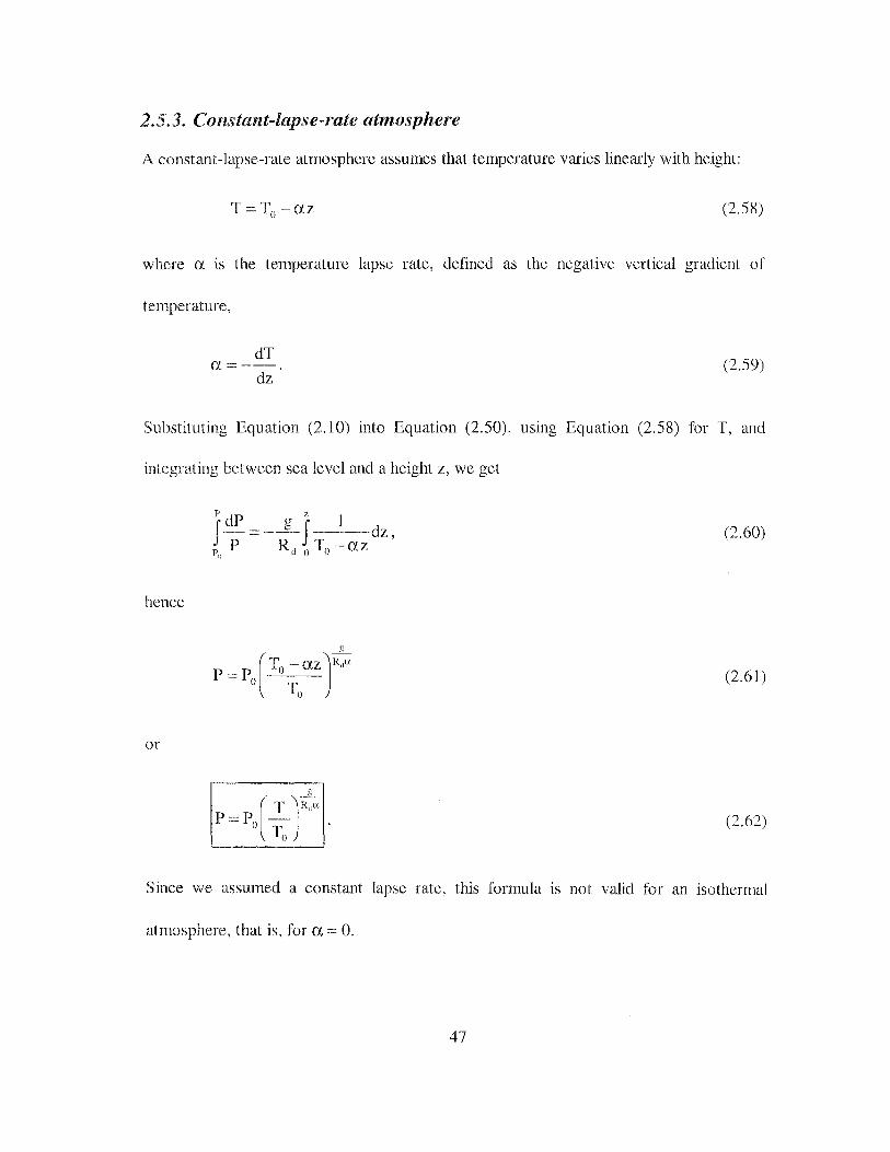
2.5.3. Constant-lapse-rate atmosphere
A constant-lapse-rate atmosphere assumes that temperature varies linearly with height:
T=T0 -az (2.58)
where a is the temperature lapse rate, defined as the negative vertical gradient of
temperature,
dT a=--.
dz (2.59)
Substituting Equation (2. 1 0) into Equation (2.50), usmg Equation (2.58) for T, and
integrating between sea level and a height z, we get
rdP g z 1 J -- = --J-, ---:-dz' r P Rct 0 10 - az
()
(2.60)
hence
(T - azJR~a p = p ____;;_0 --
0 T 0
(2.61)
or
(2.62)
Since we assumed a constant lapse rate, this formula is not valid for an isothermal
atmosphere, that is, for a= 0.
47

2.5.4. Standard atmospheres
The atmosphere models described so far were derived under very specific assumptions
and do not represent adequately the average properties of the actual atmosphere. The
first attempts to develop model atmospheres closely matching those properties date from
the 1920s, and are generally denominated standard atmospheres. The number of standard
atmospheres now available is very broad (see, e.g., ANSI/AIAA [ 1990]), but not all of
them fit the requisites demanded by radio wave propagation research. In order to be
useful, a standard atmosphere has to provide pressure, temperature, and moisture height
profiles, as well as information on latitudinal and seasonal variations of these parameters,
within the neutral-atmosphere region.
A large group of standard atmospheres was developed assuming that the air is moisture
free, in hydrostatic equilibrium, and behaving as a perfect gas. The first standard
atmospheres were developed in the 1920s by ICAO (International Civil Aviation
Organization), NACA (National Advisory Committee for Aeronautics), and !CAN
(International Commission for Air Navigation). Details on these atmospheres can be
found in List [1966]. One of the more recent models is the U.S. Standard Atmosphere,
1976 [NOAA/NASA/USAF, 1976], which is identical to the ICAO Standard
Atnwsphere, 1964, up to 32 km.
For this group of models, the structure of earth's atmosphere is described in terms of
temperature, pressure and density profiles, usually based on certain average conditions
for a specific latitude. In general, the atmosphere is divided into a series of layers, within
48

which a constant temperature gradient is assumed. For the height range of our interest
(the neutral atmosphere, essentially up to a height of about 50 km), the atmospheres of
this group differ mostly in the values of the temperature and height of the tropopause,
and the value of the acceleration of gravity.
The limitations of these atmospheres are obvious: they do not provide information on the
water vapor content of the atmosphere and on the seasonal and latitudinal variability of
the atmospheric properties with respect to the chosen reference values. Such kinds of
information is supported by the U.S. Standard Atmosphere Supplements, 1966
[ESSNNASA/USAF, 1966], the U.S. AFGL Air Force Reference Atmospheres [Cole
and Kantor, 1978], and the International Organization for Standardization (ISO)
Reference Atmospheres for Aerospace Use, 1982 [ISO, 1982; 1983], hereafter
designated as USSA66, AF78, and IS082, respectively.
USSAS66 consists of a set of hydrostatically consistent supplemental atmospheres,
developed for the latitudes of 15° N (tropical), 30° N (sub-tropical), 45° N (mid
latitude), 60° N (subarctic), and 75° N (arctic). The atmospheric properties are described
for heights up to 120 km, except for the arctic atmospheres, which arc limited to 30 km
due to lack of data.
The seasonal variability is accounted for by considering regimes for January and July,
except for 15° N, which is conveniently described by an annual regime, due to the small
seasonal variability of the tropical atmosphere. In addition, for the subarctic and arctic
atmospheres, two additional regimes are considered, to represent cold and warm
49

stratospheric regimes. Information on the moisture content of the atmosphere is provided
by values of relative humidity.
The temperature profiles for USSA66 atmospheres (depicted in Figure 2.3), are
composed of a series of layers, within which a constant temperature gradient is assumed.
These profiles show the occurrence of the tropopauses, as well as the clear winter surface
temperature inversions in the polar regions (see Chapter 4).
The pressure profiles are computed using the formulae of the pressure variation for an
isothermal atmosphere and constant-lapse-rate atmospheres, described earlier. The
surface pressure variations over the globe are very small (only a few percent), and
decrease exponentially with height, at nearly the same rate in summer and winter.
For USSA66, the amount of moisture in the atmosphere is given in terms of the relative
humidity, for the first 10 km.
AF78 describes seasonal, latitudinal and longitudinal variability of the atmosphere up to
90 km in a series of mean monthly atmospheric models, ranging from 0° to 90° N, with
15° interval. In the case of the North Pole, the atmosphere model is restricted to 55 km
height. The longitudinal variations of temperature, pressure and density with respect to
the monthly median values are described in a group of special models, restricted to 55 km
height and to latitudes of 60° Nand 75° N.
50

,.E bJJ
::2 20
10
0
40
~ 30
,.E bD
"i) 20 :r::
10
·::--..... ::---....
-- 15 '"l\ Annual
- 30 °N January 30 "N July
~-~-:.'-«..
:-..... ::---....
·-+--'-+---'---1---.L-+-·-"-+ ~-
·80 -60 -40 -20 0 20 40
Temperature CC)
- 60 1'N .JanUaL"J'
· · · · · 60 "N July
0 -+--'---+--'--~ -+..:.-'-+--80 -60 -40 -20 0 20 40
Temperature (0 C)
:: -,-----------~-r - . . :
~ 30
,.E bJ)
"i) 20 :r::
10
0
50
40
e 30 c ,.E bJJ
"(3 20 ::c:
10
0
-80
f--
-80
I
60 -40 -20 0 20 40
Temperature CC)
E'''"""'' ~July
-60 -40 -20 0 20 40
Temperature CC)
Figure 2.3 --Temperature profiles for the U.S. Standard Atmosphere Supplements,
1966, for the first 50 km.
IS082 consists of a set of reference atmospheres, developed for latitudes of 15° N
(tropical), 30° N (sub-tropical), 45° N (mid-latitude), 60° N (sub-arctic), and 80° N (sub-
arctic). For all latitudes, two regimes are defined (June-July and December-January),
51

except for the tropical atmosphere, which has an annual regime, as in USSA66. For
60°N, reference atmospheres for cold and warm stratospheric regimes (December
January) are also presented. The pressure and temperature profiles for IS082 are slightly
di1Ierent from the USSA66 profiles. As regards the moisture content, IS082 provide
values of mixing ratio, water vapor pressure (see Figure 2.4), and dew point temperature
(up to the height of 10 km), for the latitudes of 10° N, 30° N, 50° N, and 70° N. The
water vapor pressure is mainly concentrated in the first 2 km of the atmosphere, and
shows a large latitudinal and seasonal variation.
The moist-air standard atmospheres provide a valuable source of information, and have
been frequently used in a wide variety of applications, such as the development of
mathematical models for propagation delay correction (e.g. Niell [ 1996]) and generation
of reference values for assessment studies (e.g. Janes et al. [1991]). The main limitations
arc: ( 1) the fact that the atmosphere at any instant and location can behave much
differently from the average conditions they represent; (2) none of them provide
information for the southern hemisphere (in a first approximation it can be assumed anti
symmetrical). Even though IS082 provides information similar to USSA66, the latitudes
used to describe pressure and temperature do not match the ones used to describe the
moisture content. USSA66 is therefore the most adequate and consequently most used
for radiowave propagation studies, and selected in this dissertation to evaluate the ray
tracing algorithm accuracy to be presented in Chapter 5.
52

r"
"8 '-'
1.}
t3 cfl v. 1.) ;...
p.... '-< 0 0.. ~ '?
:c d ss
30
25
20
15
'10
10 20 0
30 ~ 40 o'
50 ~ 60 .$>0
'" 70 ./
10 20
(_"~ 30 40 if?'
50 ~0 60 !:§'
70 ·$> ~ -y
10 20 30 40 50 60 70
Latitude North (0)
2
~ ~ '[) ::r: 4
i
··-+---·-+~---! 30 40 50 60 70
Latitude North (0)
Figure 2.4 -- The global distribution of water vapor pressure, as a function of
latitude and height, as given by IS082 atmospheres, for January (top plots) and
July (bottom plots).
53

In this chapter we have presented the mam features and physics of the earth's
atmosphere. The variables used to describe the moisture content of the atmosphere and
their relationships were reviewed, and the model atmospheres which approximate the
actual earth's atmosphere were highlighted.
In the next chapter, the refraction within the neutral atmosphere will be analyzed.
54

,'·'' '
::if~~{: c;~;<
When radio signals traverse the earth's atmosphere, they are affected significantly by the
variability of the refractive index of the lower, electrically-neutral region. The refractive
index is greater than unity and, consequently, it causes an excess path delay. In addition,
the changes in the refractive index with varying height cause a bending of the ray. The
combination of these two effects is called neutral-atmosphere refraction or propagation
delay.
The neutral-atmosphere propagation delay is directly related to the refractive index (or
the refractivity), as it results from its integration with respect to height. At every point of
the atmosphere the refractive index of a parcel of air can be expressed as a function of
atmospheric pressure, temperature, and humidity. The neutral-atmosphere propagation
delay can be divided into an hydrostatic and a non-hydrostatic component and can be
determined from models that approximate the atmospheric profiles.
At the zenith, and for a sea-level location, the hydrostatic component of the propagation
delay is about 2.3 m and accounts for about 90% of the total delay. It can be accurately
determined using surface pressure values. The wet component has a very large spatial
and temporal variability and can not be accurately predicted from surface measurements
of any moisture variable, as the correlation with the conditions aloft is generally very
55

poor. For elevation angles other than the zenith, these delays have to be projected to an
arbitrary elevation angle, using a mapping function.
In this chapter, we first introduce the concept of refractivity and we review and compare
models proposed for representation of refractivity profiles. Secondly, we present the ray
trace equations and the terminology concerning refraction modeling. Finally, we describe
a series of models used to predict the neutral-atmosphere propagation effect on radio
signals.
3.1. Refractivity
The refractive index of a medium, n, is defined as the ratio of the speed of propagation
of an electromagnetic wave in a vacuum, c, to the (phase) speed of propagation in the
medium in question, v:
c n ==-.
v (3.1)
The refractive index of a parcel of moist air is different from unity because its constituents
suffer polarization induced by the electromagnetic field of the radio signals. The
molecules of water vapor have a permanent dipole moment: the induced polarization
produces an orientation effect, which contributes significantly to the variations of the
refractive index. The dry constituents have no permanent dipole moment, but their
molecules are displaced under the influence of the electromagnetic field and a dipole
moment is generated. The polarization effect is related to the dielectric constant of the
air, £, which can expressed as a function of the meteorological parameters by the
56

following expression [Bean and Dutton, 1966]:
(3.2)
where K: (i = 1 ,3), A, and B are constants, P; is the partial pressure of dry gases (C02-
free) and Pc is the partial pressure of C02• This formula considers the effects of non-
polar gases (COrfree dry air), C02 , and water vapor. If the dielectric constant is known,
the refractive index can then be obtained as a function of two constants, through
Maxwell's formula [Born and Wolf, 1975]:
n=-0l£, (3.3)
where f.l is the magnetic permeability (""' 1, for air).
It is important to note that the refractive index is actually a complex number, the
imaginary part of which corresponds to the absorption coefficient. For radio frequencies,
the refraction effects are only dependent on the real part of the refractive index and, with
exception of anomalous dispersion of the 22.235 GHz water vapor line and 60 GHz
absorption line of oxygen, air is essentially a non-dispersive medium [Bean and Dutton,
1966; Crane, 1976]. Liebe [ 1985] presents a formula for refractivity that takes into
account the anomalous dispersion.
As the electromagnetic waves in the atmosphere propagate just slightly slower than in a
vacuum, refractive index is more conveniently expressed by another quantity,
denominated refractivity, N:
(3.4)
57

From Equations (3.2) and (3.3), the following expression for the refractivity can be
derived [Bean and Dutton, 1966]:
Pd e e Pc N==K -+K -+K --+K -
1 T 2 T 3 T2 4 T , (3.5)
where Ki are constants to be determined, known as refractivity constants.
Equation (3.5) can simplified to the following three-term expression by adjusting the
constant K1 determined in laboratory under C02-free air to include the average amount of
C02 present in the atmosphere (see, e.g., Smith and Weintraub [1953] and Boudouris
[ 1963]). The resulting expression is thereafter given as
Pd e e N=K1-+K,-+Ko-
2, T ~ T _, T (3.6)
where P" is the partial pressure due to dry gases, including C02. In fact as the partial
pressure due to C02 is so small compared with the total pressure, the fourth term in
Equation (3.5) can be just omitted, without significant inf1uence on the accuracy of the
determination of N.
If we take into account the compressibility factors to account for the non-ideal behavior
of gases, we have:
(3.7)
The first term on the right-hand side of Equation (3.7) does not depend on the water
vapor content of the atmosphere and is therefore known as the dry component of the
58

refractivity; the terms in brackets represent the wet component of the refractivity.
The refractivity constants are determined empirically in a laboratory, by measuring the
resonance frequency of a cavity into which a known quantity of gas is introduced; the
obtained resonant frequency is then compared with the resonant frequency for the cavity
in vacuum conditions (for details see, e.g., Boudouris [1963]; Bean and Dutton [1966]).
Table 3.1 summarizes the most significant recent evaluations of the refractivity constants.
In this list, some refractivity constants were converted from the original values, to be in
accordance with values of pressure expressed in hectopascals. More complete tables of
experimental determinations of refractivity constants can be found in Hartmann and
Leitinger [1984], Hartmann [1993], and Bevis et al. [1994].
Table 3. 1 --Determinations of the refractivity constants.
K1 K2 K3 '
REFERENCE Kz (K hPa-1
) (K hPa- 1) (1 05 K2 hPa- 1
) (K hPa-1)
Boudouris [ 1963] 77.59±0.08 72±11 3.75±0.03 24±11
Smith and Weintraub [1953] 77.61±0.01 72ct9 3.75±0.03 24±9
Thayer [1974] 77.60±0.01 64.79:!0.08 3.776±0.004 17±10
Hill et al. [1982] - 98±1 3.583±0.003 -
Hill [1988] -- 102±1 3.578±0.003 -·
The Smith and Weintraub refractivity constants have been used extensively in radio wave
propagation studies. The resulting equation for the refractivity is estimated to have an
accuracy of about 0.5%, for the range of atmospheric parameters usually experienced in
the earth's atmosphere and frequencies below 30 GHz [Smith and Weintraub, 1953]. For
the frequency range below 20 GHz, Thayer [ 197 4] claims an accuracy in the
59

determination of N ranging from -0.02%, for dry air, to -0.05% (extremely moist air),
i.e., a significant improvement with respect to Smith and Weintraub [1953]. However,
there is some controversy about Thayer's refractivity constants.
In the determination of the refractivity constants, Thayer [ 197 4] assumed that K2 is the
same at radio and optical frequencies. Thayer claimed that this constraint results in better
determination of the refractivity constants. Such hypothesis was criticized by Hill et al.
[1982], who claimed that the contribution of the infrared resonances of water vapor to K2
is ignored. In their approach, the sum of the contributions of infrared water vapor
resonances is used to compute the radio refractive index. However, the calculated
constants obtained differ significantly from those determined experimentally by previous
researchers by several standard deviations. Although possible reasons for these
discrepancies have been pointed out in their paper, this disagreement could not be
satisfactorily explained and the authors recommended the use of a set of empirical
refractivity constants, such as those determined by Boudouris [ 1963]. The values
obtained by Hi11 [1988] showed the same disagreement as before, and the difference
remains unexplained.
If we assume that the air behaves as an ideal gas, then P d = P - e, and Equation (3.6)
becomes:
P . e e N = K - + (K - K )- + K --.
I T 2 I T 3 T2 (3.8)
An additional simplification can be introduced in Equation (3.8), to give the following
60

two-term expression:
p * e N=K1 -·+K3 -, T . T2
Noting that
K * e (K K k: K e "-2··= ?-] + 3-2, 'T - T · T
(3.9)
(3 .1 0)
we can divide both sides by (e/T) and solve for the new constant, K;. We therefore
obtain
(3 .11)
Using T = 273 K as a mean temperature value and the refractivity constants of Smith and
Weintraub [1953], we get:
p s e N ==77.61--+3.73x10 -
2,
T T (3 .12)
a simplification that gives values of N within 0.02% of those obtained using the 3-term
expression, for the same set of refractivity constants and temperature range of -50 oc to
40 oc [Bean and Dutton, 1966].
An alternate separation of the refractivity components was derived by Davis et al. [ 1985].
Using the equation of state for a non-ideal gas, we can write Equation (3.7) as:
(3.13)
61

Since p" = p- Pw, Equation (3.13) may be expressed as:
(3.14)
Using the equation of state for water vapor, we have:
(3 .15)
or
(3 .16)
Defining a new constant:
(3.17)
we can therefore rewrite Equation (3.7) as:
(3.18)
Using the Ki values determined by Thayer [1974], and assuming independent errors in K1
I
and K2, the value for K 2 is [Davis et al., 1985]:
K~ =(17±10) KhPa-1•
The high standard deviation associated with this determination, relative to the
uncertainties in Thayer's values, is explained by the fact that Davis et al. [ 1985] used for
62
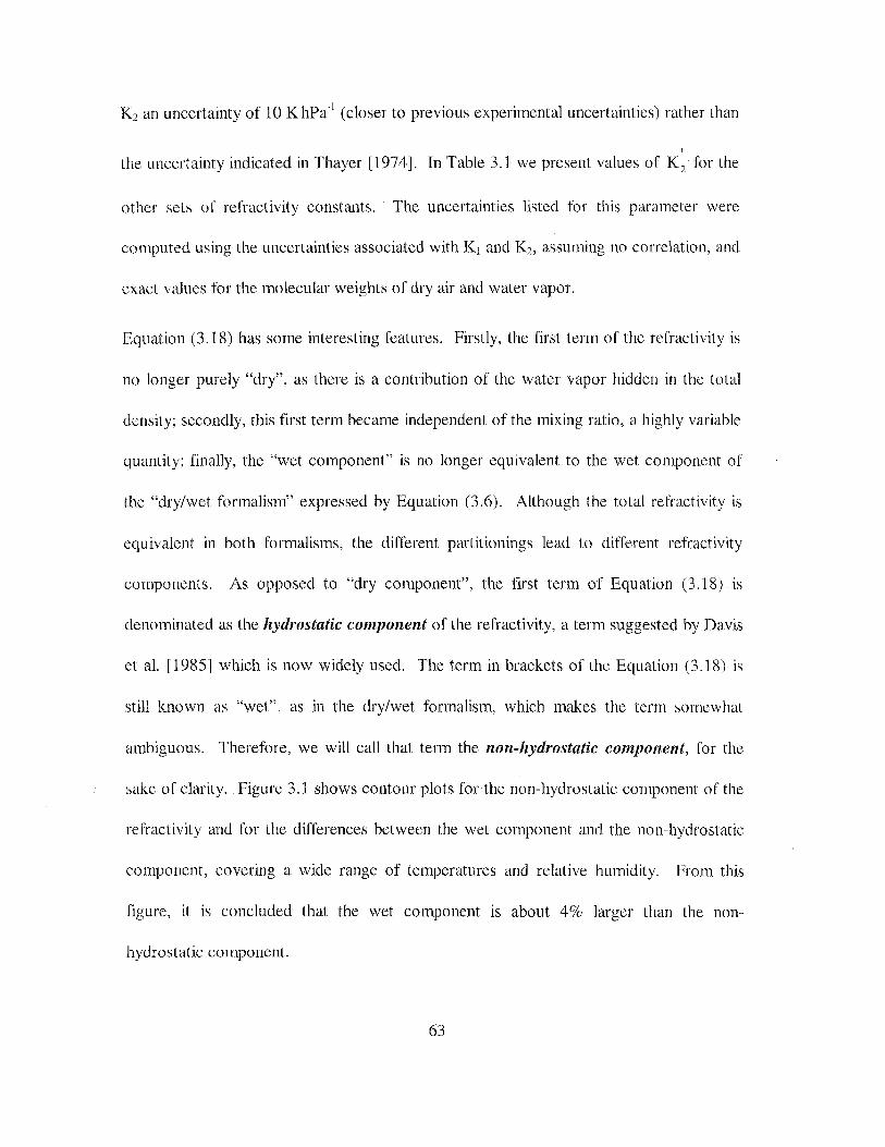
K2 an uncertainty of 10 KhPa- 1 (closer to previous experimental uncertainties) rather than
I
the uncertainty indicated in Thayer [1974]. In Table 3.1 we present values of K 2 for the
other sets of refractivity constants. The uncertainties listed for this parameter were
computed using the uncertainties associated with K1 and K2, assuming no correlation, and
exact values for the molecular weights of dry air and water vapor.
Equation (3.18) has some interesting features. Firstly, the first term of the refractivity is
no longer purely "dry", as there is a contribution of the water vapor hidden in the total
density; secondly, this first term became independent of the mixing ratio, a highly variable
quantity; finally, the "wet component" is no longer equivalent to the wet component of
the "dry/wet formalism" expressed by Equation (3.6). Although the total refractivity is
equivalent in both formalisms, the different partitionings lead to different refractivity
components. As opposed to "dry component", the first term of Equation (3.18) is
denominated as the hydrostatic component of the refractivity, a term suggested by Davis
et al. [1985] which is now widely used. The term in brackets of the Equation (3.18) is
still known as "wet", as in the dry/wet formalism, which makes the term somewhat
ambiguous. Therefore, we will call that term the non-hydrostatic component, for the
sake of clarity. Figure 3.1 shows contour plots for the non-hydrostatic component of the
refractivity and for the differences between the wet component and the non-hydrostatic
component, covering a wide range of temperatures and relative humidity. From this
figure, it is concluded that the wet component is about 4% larger than the non-
hydrostatic component.
63
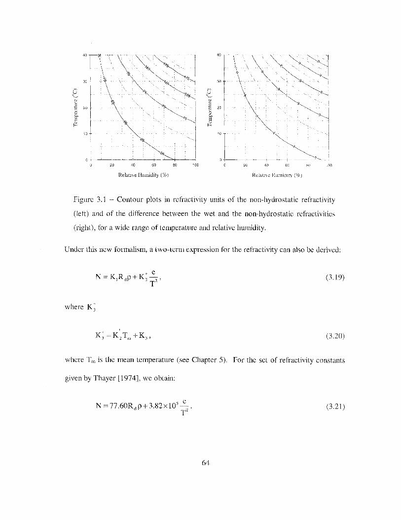
40 40 --
c~ ·. '•
·. . ., .
' '
:JO 30
~ E 2 "' H ::l :::l
I 2 20 '" 20 H
Q "' 0. a E Q "' E-< E-<
10- 10-
0 -~--+---~f----'-----t----~--~--- ---1 20 40 60 80 100 0 20 40 60 80 1 00
Relative Humidity(%) Relative Humtdny (%)
Figure 3.1 -- Contour plots in refractivity units of the non-hydrostatic refractivity
(left) and of the difference between the wet and the non-hydrostatic refractivities
(right), for a wide range of temperature and relative humidity.
Under this new formalism, a two-term expression for the refractivity can also be derived:
(3.19)
I
K; = K 2 Tm + K 3 , (3.20)
where Tm is the mean temperature (see Chapter 5). For the set of refractivity constants
given by Thayer [ 197 4], we obtain:
s e N =77.60Rc~p+3.82x10 -
2•
T (3.21)
64

In Chapter 5 we will investigate the implications of the choice of the different refractivity
formalisms in radio wave propagation studies.
3.1.1. Refractivity models
As suggested by its dependence on the meteorological parameters, the refractivity is
height dependent and different mathematical models have been proposed to represent
approximately the refractivity profile. In this section, some of these models are reviewed.
The simplest model to represent the variation of N with height is the linear model, also
known as 4/3 earth model, proposed by Schelleng et al. [1933]. In this model, the earth
is assumed to have an effective earth radius of about 4/3 of the actual earth radius ( ~8500
km), and allows consequently that the path of a radio ray be drawn as a straight line over
such earth as opposed to curve lines over the true earth; that is, as it propagates nearly
parallel to the earth's surface. Although very simple, this model describes adequately the
refractivity profile in the first kilometer above the earth's surface. For higher altitudes,
the refractivity gradient of the linear model is too large to adequately describe the
refractivity profile.
For an average atmosphere, an accepted standard value of the vertical gradient of the
refractivity, iJ.N, is -39 km- 1 [IEEE, 1990], which represents a typical median value for
temperate climate regions. The Standard Radio Atmof>phere [IEEE, 1990] is based on
the linear model and is expressed as:
(3.22)
65

where N, is the (total) surface refractivity (Ns = 315, for average conditions, at sea level),
II is the height above sea level, and Hs is the height above sea level of the surface point
used to compute the surface refractivity (note: in this section all heights are expressed in
At the time the analysis of refractivity profiles based on actual observations became
possible, the results obtained showed that for high altitudes N decreases not linearly but
approximately exponentially (Bean and Thayer, 1959; Bean and Dutton, 1966]:
N -- N exp[-_!i_J - 0 ";?' ' N
(3.23)
where No is a mean sea level (total) refractivity, and ?.111 is the scale height for the (total)
refractivity.
A single-exponential model was adopted, in 1958, by the IRCC (International Radio
Consultative Committee) of the International Telecommunication Union as a reference
atmosphere for refractivity (e.g. Bean and Thayer [1959]):
N=300exp (-0.139H). (3.24)
This single-exponential model is still used as basis for the Standard Atmosphere for
Refraction [IEEE, 1990]:
N=315exp (-0.136H). (3.25)
The CRPL Reference Atmosphere, 1958 [Bean and Thayer, 1959; Bean and Dutton,
19661 is a three-part hybrid model, which combines the linear model with the exponential
66

model; is based on the fact that: ( 1) the linear model is a very good approximation of the
refractivity profile in the first km above the earth's surface; (2) the mean refractivity index
gradient in the first km is inversely correlated with the surface refractivity; (3) the range
of typical N values has a minimum of~ 105, at the altitudes of about 8 to 9 km above sea
level; ( 4) above this height, the refractivity profile is well described by an exponential
model. The model is defined by the following set of equations:
N = Ns -7.32 exp(0.005577N,)·(H-Hs)
N =-= N exp --- In ·--{
[ ( H -- 1) - H, ] ( N 1 )}
1 8-Hs 105 (H, +1 km):s;H :s;9km (3.26)
N == 105 exp{- 0.1424(H- 9 )} , H~9km
where N1 is the value of the refractivity at 1 km above the surface. The profile is piece-
wise continuous.
The CRPL Exponential Reference Atmosphere, 1958 [Bean and Thayer, 1959] is a
simplification of the above model, by considering a single exponential model, given by:
N ~ N, exp {-In[~~ J·(H -H,)}. (3.27)
This model gives a good representation of the refractivity for the first 3 km, but gives low
values of N for higher altitudes. The profiles for a selected number of refractivity models
are presented in Figure 3.2.
67

20 ~~~---------------------------
13 1s --.-"<\ '..../
0
0 50
-- Linear Model (4/3 Earlh Model)
· · · · · · Standard Atmosphere for Refraction -- CRPL Reference Atmosphere, 1958 - · · CRPL Exponential Reference Atmosphere, 1958
--+- -'--+-·--·-'-----+--"---
100 150 200 250 300
Refractivity
Figure 3.2- Refractivity profile for different models, for heights below 20 km.
All these models do not separate the two components of refractivity. As the height
variation of each of these components is different, a model describing the individual
refractivity profiles should more accurately represent the refractivity profiles than a single
exponential profile. A hi-exponential model was proposed by Bean [ 1961]:
(3.28)
where Nds and Nws are the dry and wet surface refractivity components, and ~Nd and ~Nw
are the dry and wet scale heights, respectively. One advantage of the hi--exponential
model is that it attempts to account for the different scale heights of the dry and wet
68

components of moist air. Bean presents some typical average values of Nds• Nw"' 'liNd and
In order to better accommodate the changes in lapse rate above the tropopause, Bean et
al. [ 1966 J modified the hi-exponential model and defined a three-exponential model, in
which two exponentials for the dry component of the refractivity are proposed: a
tropospheric dry component and a stratospheric dry component. The model is expressed
as:
N = N cto exp[- ___!!__ \_,_ N wo exp[- __!!_] ';J,iNd ) ';J,iNw
N ( Ht H-Htl N ( H l N = dO exp ----·- + wO exp --- '
';~Nell ';J,iNd2 ';J,iNw
if H > Ht (3.29)
where Ndo and Nwo are the dry and wet mean sea level refractivity components, 'liNd! is
the tropospheric dry refractivity scale height, ?Nd2 is the stratospheric dry refractivity
scale height, and Ht is the tropopause height. All the parameters needed in the
application of this model can be roughly estimated from the proposed seasonal world
maps [Bean et al., 1966].
As already seen in Chapter 2, for an isothermal atmosphere (i.e. an atmosphere for a lapse
rate approaching zero) the pressure decreases exponentially with height and therefore the
refractivity profile approaches an exponential. Hopfield [ 1969] concluded that if the air
temperature varies linearly with the height at a constant lapse rate, the refractivity profile
69

is a polynomial function of the height rather than exponential, with a degree associated
with the value of the lapse rate. The general expression obtained by Hopfield is:
(3.30)
(3. 31)
where
and H~ and H: are the dry and wet equivalent heights (defined as the height above the
station at which Nd and Nw are zero, respectively; that is, H~ = H~ -· H, and
H: = H: -- Hs ), and g is assumed constant.
Helen Hopfield selected 1-L = 4, which corresponds to a :::: 6.8 K/km, a value considered
"normal" in the troposphere. The quartic expression was also found to be "a reasonably
good approximation to the usual decrease of Nw with heights" [Hopfield, 1969] and the
two refractivity profiles can therefore be written as (for heights below the associated
equivalent heights, otherwise Nct = Nw = 0):
(3.32)
and
70

(3.33)
She also investigated different approaches to express the equivalent dry height and
concluded [Hopfield, 1969] that H~ could be expressed as a function of the latitude of
the station <p, according to the following relation:
H~ =43.130-5.206sin 2 <p, (3.34)
where H~ is given in kilometres. Based on one-year sets of radiosonde data for different
locations, from Alaska to Antarctica, the equivalent dry height was later expressed as a
function of the surface temperature instead [Hopfield, 1971]. The new relation is:
H~ == 40.082 + 0.14898 t, , (3.35)
where t, is the surface temperature in °C.
An improved set of coefficients was proposed in Hopfield [ 1972]:
H~ ==40.136+0.14872t,. (3.36)
Hopficld did not find a satisfactory value for the wet equivalent height and its variations
were never fully understood [Hopfield, 1978; Hopfield, 1979]. In Hopfield [ 1969], the
wet equivalent height is postulated to be 12.0 km. In Hopfield [1971], the values range
Ji·om 8.6 km to 11.5 km, and a linear relation with the temperature was proposed:
H~v == 13.268--0.09796 t,. (3.37)
71

3.2. Neutral-atmosphere propagation delay: a definition.
The refractive index within the neutral atmosphere plays an important role in the
propagation of radio waves. On one hand, the velocity of propagation of a radio signal is
reduced when approaching the earth's surface, as the refractive index is higher than unity;
on the other hand, the continuous variation of the refractive index causes a deviation of
its trajectory from a straight line, a direct consequence of Fermat's principle, or the
principle of least time (see e.g. Born and Wolf [1975]).
Fermat's principle states that the travel time of light (or any electromagnetic wave)
between two arbitrary points, dt, is stationary with respect to neighboring paths, that is:
8 J dt = o, (3.38) ray
where the integration is performed along the ray path. In terms of path length, we have:
8 J edt= 0, ray
where c is the speed of light in vacuum. As
ds cdt=c--=nds,
v
(3.39)
(3.40)
where ds is a differential clement of length along the ray path and v the speed of
propagation of the ray in the specific propagation medium, we can also state the
variational equation for Fermat's principle as:
72

8 J nds = 0, (3 .41) ray
where n = n(s) . In this equation, the integral
L = J nds (3.42) ray
is the so-called optical path length or, in more generic terms, the electromagnetic path
length. As can be seen in Figure 3.3, the trajectory of a ray approaching the vicinity of
the earth's surface will penetrate through atmospheric layers of different refractivities;
consequently, it will change its direction, in order to follow a stationary path: the
resulting path is curved and concave downwards, in general. Therefore, and in terms of
distance, the electromagnetic path between any two points in the atmosphere is longer
than the corresponding straight-line path or geometric path, whose length G, is defined
as:
G = J ds, (3.43) vac
where the integration is now performed in vacuum.
We define neutral-atmosphere propagation delay, dna, as the difference between the
electromagnetic path length and the geometric path length:
(3.44) ray vac
73

Top of Neutral Atmosphere
Geometric Path
Figure 3.3 -The bending of the path of a radio wave. Due to variations in the refractive
index, the ray follows a curved path.
This terminology is not universal and different terms have appeared in literature, such as
atmospheric propagation delay, tropospheric (propagation) delay, tropospheric
refraction, excess (propagation) path, and path delay. Some of these terms are
unfortunately misleading, a fact that will be better understood if we split the two
components of the delay embodied in Equation (3.44).
Let S be the geometric length of the electromagnetic path followed by the ray, that is:
S = J ds. (3.45) ray
Using Equation (3.44) we get:
dna = J n ds - J ds + J ds - J ds ray ray ray vac
or
74

(3.46)
In this equation, the first term on the right-hand side is the excess path length due to the
delay experienced by the signal, or simply excess path delay (also called range error),
L1L; the second term is the delay due to the bending of the ray, called geometric delay,
ray bending or angular bending, t. Therefore, our definition of neutral-atmosphere
propagation delay encompasses h_oth, the excess path delay (although some authors use
this term to include the geometric delay) and the geometric delay. The term tropospheric
delay is frequently used to designate the neutral-atmosphere delay. Although not totally
correct, the designation is well accepted, as the major contribution to the neutral
atmosphere propagation delay comes from the troposphere; in particular, almost all the
water vapor occurs within the troposphere. Because the term refraction includes
implicitly the excess path delay and the ray bending, it also works well as an alternative
designation to propagation delay.
The separation of the neutral-atmosphere propagation delay into two components is
advantageous, as the geometric delay is only significant for radio signals coming from low
elevation angles (below about 1 0°); furthermore, for a horizontally stratified atmosphere,
S and G are identical in the zenith direction and the geometric delay is zero.
The next logic step is to derive an expression for the neutral-atmosphere propagation
delay. In order to derive such an expression, we have to assume the knowledge of the
refractive index at every position in a three-dimensional atmosphere. Under this
75

assumption, a solution can be sought in the field of variational calculus, by solving the
Euler-Lagrange equation. Integral expressions have been derived by, e.g., Wachowsky
[1973] and Davis [1986], upon which the development presented in Appendix I is based.
From this development we obtain the following expression:
where e is the refracted (apparent) elevation angle and£ is the geometric (true) elevation
angle.
In general, the direct integration of Equation (3.47) is not possible, as the refractivity
profile along the ray path is not known. Therefore it has to be numerically integrated (if
discrete values of the refractivity profile are available) or approximated analytically by a
model. The first solution will be studied in Chapter 5.
Before looking into the analytical approximations (modeling), let us consider the
particular case for which the incoming signal arrives from the zenith direction ( £ = 90°).
In this case, as we are assuming a spherically symmetrical atmosphere, there is no ray
bending and Equation (3.47) becomes:
or
r a
d~" = Jcn-l)dz, r s
r a
d~" =10-6 JNdz,
(3.48)
(3.49)
76

where the symbol "z" is used to denote integration in the zenith direction.
The delay just defined is named the neutral-atmosphere total zenith delay, or simply the
zenith delay. If we consider the refractivity to be composed of a hydrostatic and a non-
hydrostatic component, the zenith delay can also be split into two components, termed
the zenith hydrostatic delay and zenith non-hydrostatic delay (or dry and wet, if the
dry/wet formalism is used). Under this consideration, Equation (3.49) becomes:
ra ra
d ~. = 1 0 -6 f N h dz + 10-6 f N nh dz ,
or symbolically,
r s
d z dz d" na = h + nh'
r s
(3.50)
(3.51)
where d~ represents the zenith hydrostatic delay and d~11 represents the zenith non-
hydrostatic delay.
Another situation for which we have no bending is when we assume a flat earth and a
constant refractivity; in this case, the neutral-atmosphere propagation delay at any
elevation angle can be related to the zenith delay by the following expression:
(3.52)
The propagation delay obtained using this expression, usually recognized as the "cosecant
law", is obviously not very accurate, as it relies on invalid assumptions: a flat earth and
constant refractivity. Nevertheless, it suggests that it is possible to express the neutral-
77

atmosphere propagation delay as a product of the zenith delay and a function that relates
this delay to the delay at other elevation angles, that is,
(3.53)
This expression defines a mapping function, m(E). This particular mapping function
maps the total zenith delay. However, as the zenith delay can be expressed as the sum of
the two components, mapping functions can be developed in order to map separately the
hydrostatic and the non-hydrostatic component. Therefore, in general we have:
(3.54)
where mh( £) is a hydrostatic mapping function, and mnh( £) a non-hydrostatic mapping
function.
3.3. Neutral-atmosphere propagation delay modeling
In the previous section, it was suggested that the integral expression for the neutral
atmosphere propagation delay can be approximated by initially finding closed-form
analytical models for the zenith delay and then by mapping this delay to the elevation
angle of the incoming signal, using a mapping function. In this section, we review a very
significant number of analytical models reported in the scientific literature in the last few
decades. The formalism inherent to each model in the analysis is maintained in
accordance with their original formulation.
78

3.3.1. Hydrostatic and dry zenith delay models
Previously, we have defined the zenith hydrostatic delay as
ra
d~ =lo··6 JN 11 dz, r s
or, by using Equation (3.18),
r a
d~ = 10-6 K 1Rd pdz.
Using Equation (2.50), we have
r r a s dP J pdz = J-dz, r r g s a
or
r a p fpdz=-s' r gm s
(3.55)
(3.56)
(3.57)
(3.58)
where gm is the acceleration due to gravity at the center of mass of the vertical column of
air, and P,. is the surface pressure; hence:
(3.59)
The modeling of the zenith hydrostatic delay is therefore straightforward, and models can
only differ due to the choice of the refractivity constant and on the modeling of the height
and latitude dependence of acceleration of gravity. Models based on this theoretical
79

approach were developed by Saastamoinen [ 1973] - later modified by Davis et al. [ 1985]
- and Baby et a!. [1988], for example. Hopfield developed zenith dry models based on
the quartic refractivity profile. A brief summary of these models is given below. For the
sake of conciseness and intercomparison, the formulations for all models will be
presented to be conformable with the following units: metres, for delay; hectopascals, for
values of pressure; kelvins, for temperature; kelvins/metre, for temperature lapse rate;
metres, for heights; percentage, for relative humidity. Furthermore, the subscript "s" is
used to denote surface values or values relative to the station (as opposed to sea-level
values).
• Saastamoinen
Saastamoinen [1973] found that gm can be expressed (in ms-2) as
gm == 9.784(1-- 0.0026cos 2cp- 0.00000028Hs), (3.60)
where (p is the latitude of the station and H., is the station height above sea level, in
metres. Saastamoinen used the refractivity constant given by Essen and Froome. Using
Equation (3.59) and simplifying the relationship for standard conditions, he obtained:
dz h . (1- 0.0026 cos 2cp- 0.00000028 Hs) .
0.002277 Ps (3.61)
• Davis et al.
Davis ct al. [ 1985] used the K1 refractivity constant given by Thayer [ 197 4], and the
"improved version" of the Saastamoinen model became:
80

dz 0.0022768 Ps h - (1- 0.0026 COS 2<p- 0.00000028 Hs) .
• Baby et al.
Baby et al. [ 1988] suggested the acceleration of gravity be expressed as:
In this equation, gs is the surface gravity at the station,
a (j=--
T' s
and rs is the mean geocentric radius of the station, in metres, that is,
where r0 is the earth radius (the authors suggested r0 = 6 378 000 m).
(3.62)
(3.63)
(3.64)
(3.65)
Combining (3.63) with (3.59), and using the K1 refractivity constant given in Bean and
Dutton [1966] they obtained:
d z _ 0.022277Ps (l + 2 l h - gs rs (j (!l + 1)) (3.66)
The reader should be aware of a few typographical errors and inconsistencies in Baby et
al. [1988].
81

• Hopfield
A different strategy was followed by Hopfield [ 1969], who assumed that the theoretical
dry refractivity profile could be expressed by the quartic model:
(3.67)
Using Equation (3.55), the integration with respect to height leads to
dz = 10-6N H~ . d cts 5
(3.68)
Hopfield based her models on the two-term expression given by Equation (3.9) and the
refractivity constant determined by Smith and Weintraub [1953]; therefore, the final
expression is given by (with the equivalent height given in metres):
d' = 77.6x10⁻⁶ _?, H~ d T 5
s
(3.69)
Different models can therefore be obtained, depending on the choice of the expression for
the dry equivalent height (see section 3.1.1 ).
3.3.2. Non-hydrostatic and wet zenith delay models
The approach to be followed in the development of a zenith non-hydrostatic delay model
is similar to the one used in the previous paragraph. By definition, the zenith non-
hydrostatic delay is given by
82

ra
d ~h = 1 0 ~ 6 J N nh dz , r s
or, using Equation (3.18) and ignoring the compressibility factor,
(3.70)
(3. 71)
Whereas the hydrostatic component of the tropospheric delay can be determined very
accurately as a function of the surface pressure, assuming the condition of hydrostatic
equilibrium, the non-hydrostatic component requires a water vapor profile, which
generally shows no strong dependence on the surface conditions. Due to the difficulty of
handling this problem, a large number of wet and zenith non-hydrostatic delay models
have been attempted, and the most important of these are described herein.
• Hopfield
Hopfield [1969, 1971, 1972] followed the same procedure she used to derive the dry
zenith delay, and based her wet zenith delay models on the quartic atmospheric profile.
In a similar fashion to the dry zenith delay approach, we get:
(3.72)
where the wet component of the surface refractivity is the second term of the Smith and
Weintraub two-term expression, that is:
·N -373 105 es ws- . X T2.
s
(3.73)
83

• Saastamoinen
Saastamoinen [1973] assumes that there is a linear decrease of temperature with height,
and that the water vapor pressure decreases with height. This variation is described by
the following law:
(3.74)
where vis a numerical coefficient to be determined from local observations. Under these
assumptions, Saastamoinen obtained:
r
"e R J-- dz=-" e r T vg s s
(3.75)
and
(3.76)
Substituting (3.75) and (3.76) in (3.71), we get:
d' = 10-6 [(K _ K ~]~_<!__+ K3 ( Rcl ~~ e w 2 1R T ( R) s'
w vg s vg- a ct
(3.77)
where the variables involved can be chosen to represent the local conditions.
Using the refractivity constants by Essen and Froome and for mid-latitudes and average
conditions, Saastamoinen obtained the following simplified model:
84

dz =0.002277(1255
+0.05Jes. w T . s
(3.78)
• Chao
In 1971, Chao derived a zenith wet delay model based upon the application of the
hydrostatic law to the water vapor, and the ideal gas law [Chao, 197la]. As these
assumptions lead to unreasonable results when compared against the obtained using
radiosonde data, Chao replaced the ideal gas law equation of state by the adiabatic law
e == k~p~ w'
where ~ is the specific heat ratio ( -1.3 for water vapor), and obtained the following
expression [Chao, 1973]:
(3.79)
This model is not very sensitive to the temperature lapse rate and the use of a mean value
of a (e.g. 0.0065 K km-1) has no significant implications in the accuracy of the model.
• Callahan
The model developed by Callahan [ 1973] assumes a linear temperature lapse rate and is
based on an empirical exponential model of the water vapor pressure as a function of
height:
e = e, exp(- aH- bH 2 ), (3.80)
where a= 0.248 km- 1 and b = 0.048 km-2 are nominal values (H is the height above the
85

~lJifloi~~, in kilometres). In its full form the model is very complex, but the following
simplified version can be obtained for a set of nominal values:
(3.81)
• Berman
In the derivation of the several wet zenith delay models, Berman [ 1976] assumes that: (1)
the wet refractivity is zero at the tropopause (11 km); (2) the temperature decreases at a
constant rate a; (3) relative humidity is constant with altitude and equal to its value at the
surface. Under these assumptions, Berman derived the "Berman 70" model:
dz = 0.373 l --~ e ( ]
2
"' a(B-AC) T, ' ' (3.82)
where Us is the relative humidity (% ),
(AT -BJ e, =0.061Usexp --' -- , T -C s
(3.83)
A= 17.1485,
B = 4684.1,
c = 38.45.
The derivation of other improved Berman models are based on the existence of a strong
correlation between the ratios of the wet and zenith hydrostatic delays and the
corresponding refractivities:
86

(3.84)
where K is a constant to be determined.
These new models, named "Berman 74", "Berman (D/N)", and "Berman (TMOD)", are
of the form:
d~v = 10.946 K(~ l. TJ (3.85)
The values of K for the different models are shown in Table 3.2.
In the "Berman (D/N)" model, two coefficients are determined, one to be applied to day
profiles, the other to night profiles. Berman found a significant improvement of the
separate day-night profile over the composite "Berman 74". The "Berman (TMOD)"
profile is an attempt to moderate the systematic diurnal surface variations, producing
similar results to the "Berman (D/N)" profile.
Table 3.2- The value of K for the Berman wet zenith delay models.
·.Berman·7:4· }3erman (Q/N) Berman (TMOD)
K 0.3224 0.2896 (day) 0.3281 0.3773 (night)
• Ifadis
The set of models derived by If ad is [ 1986] is based on the fact that there is a linear
correlation between the zenith non-hydrostatic delay and the surface meteorological
87

parameters, although weak. A set of models dependent on the season, climate and a
global model were derived. The global model is given by:
(3.86)
• Askne and Nordius
Askne and Nordius [1987] derived a two-parameter closed form model, which attempts
to model seasonal and climatic variations of the zenith non-hydrostatic delay. They
assumed that the water vapor pressure decreases with height, at a much faster rate than
the total pressure, and according to the power law:
(3.87)
where A is a parameter dependent on season and latitude. Therefore, the zenith non-
hydrostatic wet delay is expressed as:
(3.88)
The evaluation of the integral after some manipulation leads to:
(3.89)
where the mean temperature is expressed as
88

T =T(l- aRct I. m s (A.+ l)gm)
(3.90)
As pointed out in their paper, this formula agrees with the one derived by Saastamoinen,
for a= 0.0062 Km-1 and A.= 3.
The zenith non-hydrostatic delay is especially sensitive to the variations in A, and the
authors suggested that both a and A. should be chosen to fit the location and season. As
options to obtain these parameters, the authors suggested the values of A. given in Smith
[1966] (see Table 3.3), whereas the values of a may be estimated from radiosonde
statistics, if available (see also Chapter 4). Ifadis [1993] estimated this parameter for a
number of sites for stations located mainly in the northern hemisphere and concluded that
the annual variation for A is characterized, in general, by a sinusoidal curve.
Table 3.3- Values of the empirical coefficient A. [Smith, 1966].
<p SEASON c Annual ("N) .. ·Winter Spring. .Summer Autumn Mean
0-10 3.37 2.85 2.80 2.64 2.91
10-20 2.99 3.02 2.70 2.93 2.91
20-30 3.60 3.00 2.98 2.93 3.12
30-40 3.04 3.11 2.92 2.94 3.00
40-50 2.70 2.95 2.77 2.71 2.78
50-60 2.52 3.07 2.67 2.93 2.79
60-70 1.76 2.69 2.61 2.61 2.41
70-80 1.60 1.67 2.24 2.63 2.03
80-90 1.11 1.44 1.94 2.02 1.62
Mean 2.52 2.64 ... 2'~62 2~70 2.61
89

• Baby et al.
Baby et al. [ 1988] used the two-term expression given by Equation (3 .19) to represent
the refractivity, and refractivity constants from Bean and Dutton [ 1966]. Two types of
models were proposed by Baby et al.. The first type is based on the assumptions that the
relative humidity is constant and equal to its surface value up to a height Hm, where it
reduces to zero, and that the temperature is assumed to decrease with increasing height at
a constant rate. They developed ad hoc expressions to compute the saturation pressure
and proposed two zenith non-hydrostatic delay models, which differ only in the saturation
pressure computation. However, they found that a semiempirical model lead to precision
comparable to the theoretical model, but with improved accuracy; the semiempirical
model is given by the expression:
(3.91)
where v and 'Y are empirical coefficients, associated with seasonal and climatic variations.
The coefficients were determined by fitting data from a one-year radiosonde campaign
(carried out in the context of the Global Atmospheric Research Pro gram, in 1979) and
are listed in Table 3.4.
To summarize, the input parameters for the described models are given in Table 3.5.
90

Table 3.4 - Empirical coefficients to be used in the Baby et al. [ 1988]
semiempirical wet zenith delay model (vis expressed in mm(%t1 and 'Yin °C1).
I Latitud~ ' ' :CLIMATE
oOOo ,, OoO
Intet'val oceanic, Continental 0:0
min- max v y v y
90° s- 70° s 0.6421 0.0290 0.4164 0.0193
70° s- 50° s 0.5864 0.0259 0.5593 0.0362
50° s- 30° s 0.6124 0.0247 0.5369 0.0285
30° s- 10° s 0.4729 0.0296 0.4229 0.0335
10° s- 10° N 1.0772 0.0192 0.6542 0.0269
10° N- 30° N 0.8063 0.0213 0.6626 0.0249
30° N- 50° N 0.6614 0.0241 0.7574 0.0224
50° N- 70° N 0.7075 0.0244 0.7652 0.0236
70° N- 90° N 0.7434 0.0256 0.7687 0.0257
Global .0 , ,.0/7284 0.0236' 0.7284 0.0236
Table 3.5 - Input parameters (either directly or indirectly used) for the non
hydrostatic and wet zenith delay models.
Model and Reference 0,
00
I• es .Ts a A u H other So
Hop field [ 1969] ./ ./
Hopfield [1972] ./ ./
Saastamoinen [ 1973] ./ ./
Chao [1973] ./ ./ ./
Callahan [ 197 3] ./ ./
Berman 70 [Berman, 1976J ./ ./ ./
Berman 74 [Berman, 1976] ./ ./
Berman TMOD [Berman, 1976] ./ ./
Ifadis [1986] ./ ./ Ps
Askne and Nordius [1987] ./ ./ ./ ./ ./ gm, cp
Baby et al. [1988] ./ ./ v,y
91

3.3.3. Mapping functions
In Section 3.3, it was suggested that the elevation dependence of the neutral-atmosphere
propagation delay could be related to the delay that the signal would experience at other
elevation angles through the use of mapping functions, and a simple mapping function to
map the total zenith delay was introduced.
In the early years of space geodesy, the zenith delay and the mapping function were not
clearly separated; the propagation delay was therefore determined using a "hybrid model"
that combined zenith delay model(s) and mapping function(s). The need of a complete
separation between zenith delay models and mapping function(s) is a requirement of the
new strategies in propagation delay modeling for high precision applications; due to the
poor modeling of the wet zenith delay from surface meteorological measurements, this
separation permits the zenith wet delay (or the residual delay) be estimated along with
other geodetic or geophysical parameters in the data reduction process or estimated from
an alternative method. In the last couple of decades, numerous hybrid models and
mapping functions have been developed. For our analysis all the hybrid models were
separated into their components, as a mapping function can always be defined [Davis,
1986].
The existing mapping functions can be distributed basically in three major groups. A first
group of mapping functions is based on the quartic profile developed by Hopfield [ 1969]
and include the 1-:Iopfield [1969], Yionoulis [1970], Moffett [1973], Goad and Goodman
[ 1974], Black [ 1978], Black and Eisner [ 1984], and Santerre [ 1987] mapping functions.
92
A second group is constituted by mapping functions based on the truncated form of a
continued fraction, and include the functions reported in Marini and Murray [1973], Chao
[1972], Davis et al. l1985], Ifadis [1986], Herring [1992], and Niell [1996]. The
mapping functions developed by Yan and Ping [ 1995] constitute a variant of the
continued fraction, as they are based on the complementary error function. A smaller
group is based on the expansion of the "cosecant law" and includes Saastamoinen [ 1973]
and Baby et al. [ 1988] mapping functions. The remaining mapping functions existing in
the literature do not fall directly under these categories. As a general rule, all the
mapping functions assume azimuthal symmetry of the neutral atmosphere and hydrostatic
equilibrium. A brief description of the main features of most extant mapping functions
(by category group) follows. Mathematical models will be given for a selected number of
functions, either in the text or in Appendix II. A comparative table of the mapping
functions' main features is also presented at the end of this section.
• Hopfield (HO)
The two-quartic refractivity profiles, given by Equations (3.30) and (3.31), are the basis
of the mapping functions derived by Hopfield [ 1969], even though the quartic profile for
the wet component has no physical or statistical justification. The mapping functions
assume therefore a constant lapse rate of ~6.8 K km- 1 for the neutral atmosphere,
azimuthal symmetry, and hydrostatic equilibrium. Moreover, ray bending is also ignored.
Under these assumptions, Hopfield arrived to the following expression for the total delay
(see full derivation in Wells [1974]):
93

(3.92)
where the two auxiliary variables are
and
x=H-H~,
r1ro, 1s the geocentric radius of the point at which Ni becomes negligible, rs is the
geocentric radius of the station, H., is the station's height, Hi" are the equivalent heights,
and H is the height above sea level. In all these expressions and hereafter, i = 1, 2,
denotes dry and wet components (or hydrostatic and non-hydrostatic, if applicable),
respectively. The solution at the zenith is readily obtained from Equation (3.92), making
(3.93)
Therefore Equation (3.92) can be explicitly expressed as the product of a zenith delay and
a mapping function:
(3.94)
94

The closed-form solution for the integral in Equation (3.92) obtained by Hopfield proved
to be very sensitive to roundoff errors for high elevation angles, even using double
precision. We have implemented the formulation in quadruple precision for a series of
tests and we obtained a numerically stable solution. The values obtained agree very well
with ones provided by the Yionoulis [ 1970] formulation and therefore we have not
considered it in our analysis.
• Yionoulis (YI)
To avoid the roundoff errors for high elevation angles in the Hopfield formulation,
Yionoulis [ 1970] proposed a series expansion form for the integrand in Equation (3. 92).
Due to the difficulty in finding a series expansion with a rate of convergence satisfactory
for the full range of elevation angles, Yionoulis presented two series expansions, one for
high elevation angles and another for lower elevation angles, with a large overlapping
region of convergence. This fact allows the choice of the boundary between high and
low elevation angles to be left to the user. Wells [ 197 4] suggested this boundary to be as
low as possible, in order to minimize the number of arithmetic operations. For a broad
set of meteorological conditions, he found that a changeover elevation angle of 17° gives
a convergence of 1 mm in the dry component, after three terms in the series summation.
The same convergence is obtained for the wet component with a changeover angle of 7°,
after 2 terms have been evaluated.
95

• Moffett (HM)
Simplified approximations of the Hopfield mapping functions are presented in Moffett
[ 1973] and are sometimes incorrectly referred to in the literature as the Hopfield model(s)
or mapping functions. These simplified mapping functions have been used extensively, as
they depend on the elevation angle only:
(3.95)
1 m (£)=-----
w . ( 2 2 250) sm £ + . (3.96)
• Goad and Goodman ( GG)
(}oad and Goodman [1974] modified the Hopfield model by assuming that the
temperature decreases linearly with increasing height in the troposphere, but that it
remains constant in the stratosphere (two-layer atmosphere), the same assumptions used
by Saastamoinen [1973] in deriving his mapping function. To accomplish that, the wet
and dry components of the Saastamoinen zenith corrections are used to calibrate the
equivalent heights H~ and H: . As regards the mapping function component, the
authors used a Taylor's series approximation for the integrand in Equation (3.92) and
obtained a series of coefficients from direct integration. The Goad and Goodman
mapping functions are sometimes referred to in the literature as Modified Hopfield. This
designation should be avoided, as it may be confused with the Moffett mapping functions.
96

• Santerre (ST)
The mapping functions developed by Santerre [1987] are a further modification of the
Goad and Goodman mapping functions, which takes into account ray bending for
elevation angles below 45°.
• Black (BL)
Black [1978] mapping functions are simple analytic forms derived from the integration of
a Taylor series expansion of a normalized integral obtained from geometric
considerations. They are based on the quartic profiles developed by Hop field [ 1969] and
use the equivalent heights proposed by Hopfield [ 1971]. In their simpler form, the
mapping functions are as follows:
2 1
2
(3.97)
where lc = 0.85. In the complete formulation (as used in our analysis), lc is a weak
function of surface temperature and elevation angle. These mapping functions were
recommended for elevation angles above 5°.
• Black and Eisner (BE)
The Black and Eisner [1984] mappmg function for the total delay is a further
modification of Black's, and is expressed as a simple geometrical model, which depends
97

on the elevation angle only, with one fitted parameter:
(3.98)
This mapping function is claimed to be valid for elevation angles greater than 7°.
• Chao (CH)
Marini [1972] showed that the elevation angle dependence of the atmospheric delay can
be expressed as a continued fraction form, in the sine of the elevation angle £:
m(£) = sin£+--
. b a
(3.99)
sm £ + ~-~-----sin£+
c
sin£+··
where the coefficients a, b, c, ... are constants or linear functions.
In the case of the Chao [1972, 1974] mapping functions, the continued fraction is
truncated to second order terms and the second order (sin £) is replaced by (tan £), to
ensure that the mapping function will be unity for signals observed in the zenith direction.
The mapping functions were obtained by an analytical fitting to radiosonde-derived
average refractivity profiles. The coefficients a and b are fitted numeric constants:
1 md (£) = ~----~----------
. 0.00143 (3.100)
sm £ + ----~---tan£+ 0.0445
98

1 mw (E)== . 0.00035
sm E + --------tanE+0.017
(3.101)
Estefan and Sovers [ 1994] also present a set of "revised" constants for the dry mapping
function, as well as a set of mapping tables ("look-up tables"), which were also developed
by Chao for both dry and wet components. These tables in particular (which were
assessed in our study) include the effect of ray bending, and are (theoretically) valid for
any elevation angle.
• Marini and Murray (MM)
The Marini and Murray [1973] mapping function (according to the explicit formulation
expressed in Davis [1986]) uses a second order continued ti·action, with the coefficient b
set as a fitted constant. It was designed to model the elevation dependence of the total
tropospheric delay for observations above 10°.
o Davis et al. (CJA)
The Davis et al. [ 1985] mappmg function for the hydrostatic component of the
atmospheric delay (also known as CfA-2.2) uses a third order continued fraction, with the
tangent as introduced by Chao. As pointed out in their study, the substitution of (sin E)
by (tan E) decreases the performance at high elevation angles (20° - 60°), as the tangent
does not approach the sine with the same speed, giving 1-2 mm error. The coefficients of
CfA-2.2 mapping function for the hydrostatic delay were derived from a ray tracing
analysis through idealized model atmospheres, down to 5° elevation; the coefficient c is
99

set as a constant and a and b are expressed as linear functions (of departures with respect
to standard values) of surface temperature, surface total pressure, partial water vapor
pressure, temperature lapse rate, and height of the tropopause. This mapping function
can also be used to map the zenith non-hydrostatic delay, although this introduces a
"small" error of uncertain magnitude [Davis et al., 1985]. For the sake of completeness,
the non-hydrostatic mapping function is also included in this analysis. The mathematical
formulation is presented in Appendix II.
Ifadis [1986], Herring [1992] and Niell [1996] expanded the continued fraction to three
terms, keeping the sinE in all terms. To ensure that the mapping function is unity at the
zenith, the unity numerator of the Chao-type fraction is substituted by the value of the
mapping function denominator at the zenith, i.e.:
m(E)= l+a/(l+b/(l+c)) sinE+ a/ (sin£+ b I (sin£ +c))
(3.102)
• Ifadis (IF)
The Ifadis [ 1986] mapping functions were fit down to a 2° elevation angle to ray traces
of radiosonde atmospheric profiles from an extensive selection of globally distributed
sites. Global and climate optimized mapping functions were derived. The coefficients a
and b are linear functions of surface temperature, pressure and partial water vapor
pressure and c is a fitted numerical constant. The mathematical formulation for these
mapping functions is presented in Appendix II.
100

• Herring (MTT)
The mapping functions developed by Herring [1992], also known as Mapping
Temperature Test (MTT), were determined from ray tracing through rawinsonde profiles
covering several locations in the United States, for elevation angles starting at 3°. The
coefficients in the mapping functions depend on the latitude, height of the site and surface
temperature, and were determined by a least squares fitting performed separately for the
hydrostatic and wet components, for latitudes covering 27° to 65° and station heights
ranging from 0 to 1600 m. The mathematical formulation for these mapping functions is
presented in Appendix II.
• ~iell (!VMJ7)
The Niell [1996] mapping functions (NMF- Niell (New) Mapping Functions) present no
direct dependence on specific meteorological parameters, and are based on temporal
fluctuations of the bulk of the atmosphere. The coefficients in the mapping functions
were derived from profiles of the U.S. Standard Atmosphere Supplements, 1966, down
to 3° elevation angle. In the case of the hydrostatic mapping function, the coefficients a
and b are functions of the day-of-year (or Modified Julian Date), station latitude, and
station height. For the wet mapping function, only the latitude of the site is used as
external information. The southern hemisphere is assumed to be anti-symmetric in time.
The mathematical formulation for these mapping functions and additional discussion is
presented in Appendix II.
101

• Yan and Ping (UNSW)
Yan and Ping [1995] developed a mapping function based on the continued expression of
the complementary error function. This mapping function uses the same input parameters
of CfA-2.2 and was adjusted for elevation angles above 2.5°. Yan and Ping proposed
two mapping functions. The first is based on the atmospheric profile provided by CfA-
2.2 and standard atmospheric parameter values and was called UNSW931 (UNSW, in
this dissertation). The second mapping function is based on the atmospheric profile given
by the Hopfield model, and was called UNSW932 (not analyzed in this dissertation).
Even though it is not explicitly specified by the authors, the UNSW931 mapping function
is to be applied for the hydrostatic component only [Y an, 1998]. Extending the use of
UNSW931 to map the non-hydrostatic component introduces a small error, as in the case
of CfA. The mathematical formulation for UNSW931 is presented in Appendix II.
• Lanyi (LA)
The Lanyi [ 1984] mapping function, which maps the total zenith delay, was developed
using an analytical approach, with the fitting performed to elevation angles above 6°. It
uses 3-linear section temperature profiles and the tropospheric delay is expanded up to
the third order in refractivity, where the second and third order terms describe the
bending effect. Latitude and site-dependent variations with respect to an average profile
can be modeled by tuning the temperature lapse rate and tropopause height for the
specific site. The mathematical formulation for the mapping function developed by Lanyi
is presented in Appendix II.
102

• Hartmann-Leitinger (HL)
Hartmann and Leitinger [ 1984] presented a mapping function for the total delay that
depends only on the height of the center of gravity of the vertical column of air, Hg,
which can in turn be fixed to a constant value (e.g. at a height of 8000 m):
[ [ ]2 l 1 0.85H
8 2 0.85H8 4 m(E)=-.- 1-----cot £+1.5 --- cot£ ,
sm(E) Re Re (3.103)
where Re is the earth radius.
Ray bending can be additionally computed from surface refractivity and atmosphere scale
height, allowing their model to be applied for elevation angles above 5°:
(3.104)
Unlike the mapping functions described so far, which use the non-refracted elevation
angle, the remaining mapping functions in this analysis use the refracted (apparent)
elevation angle. The difference between the angles is significant at low elevation angles.
In the analysis of space geodetic data, the elevation angle is generally derived from the
geometry of the source and the receiver, i.e., the refracted angle is not available.
Whereas Saastamoinen [1973] provides a simple formula to derive the non-refracted (or
geometric) from the refracted zenith angle, such is not provided by the Baby et a1. [1988]
and Rahnemoon [ 1988] formulations. This detail should not be neglected in any
implementation of these models in the analysis of geodetic data that require the use of the
103

non-refracted elevation angle, since it may significantly affect the results if low elevation
angles are used.
• Saastamoinen (SA)
Saastamoinen [1973] derived his mapping function based on Snell's law of refraction for
a spherically symmetric layered atmosphere. Under this assumption, and neglecting the
ray bending, the tropospheric delay can be written as:
r "N
dtrop = 10- 6 J-.-dr . r sm e s
(3.105)
Saastamoinen expands the 1/sin8 in a truncated binomial series, and integrates each term.
In its full version, mapping functions are derived for both components, and are
parameterized in terms of tropopause height, temperature lapse rate and water vapor
lapse rate parameter, in addition to the standard meteorological parameters. A simplified
version that maps the total delay was obtained from those solutions, and is often used in
analysis of space geodetic data, due to its simplicity and accuracy. It requires the
interpolation of correction quantities from two tables, which take into account the effect
of ray bending, but its use is limited to elevation angles above 10°. Janes et al. [ 1991]
have compared the performance of both versions. In this dissertation, only the simplified
version is analyzed.
104

• Baby et al. (BB)
Baby et al. [1988] used Snell's law of refraction to expand the 1/sinS and derived the
following mapping function:
(3.106)
where £H is a term depending on the refractive index and geocentric distance of the
station. For low observation angles (less than about 45°), a corrective term is introduced.
The ray bending is nevertheless neglected. The model was developed to map the total
delay for elevation angles above 10°.
• Rahnemoon (RA)
Rahnemoon [ 1988] derived a model that has to be seen in a different context, as it is a
numerical-integration-based model, similar to a ray tracing procedure program. This
represents a problem in the analysis of geodetic data, as the model is, computationally,
one to two orders of magnitude slower than the remaining mapping functions. It uses
meteorological surface data (temperature, pressure and relative humidity) to generate the
refractivity components at the surface and integrates along the ray path to generate the
profiles from which the delays are derived, using Snell's Jaw.
As can be concluded from the brief descriptions given, there is a significant variability in
the mathematical basis and parameterization of the available mapping functions. This is
summarized in Table 3.6 for convenience.
105

Table 3.6 ~Summary table of the main features of mapping functions.
M.F. P, L. tmin type
e n/a
"hydrostatic component only; ·;··1extended use of the function developed for the hydrostatic component; 4true elevation angle is converted to apparent elevation angle before computation of mapping factor; §geometric delay (ray bending) only.
Legend: Ps = surface total pressure; Ts = surface temperature; es = surface water vapor pressure; a = temperature lapse rate; T 11 = tropopause height; H = station orthometric height; <p =station latitude; Hg =height of center of gravity; Hi= inversion height; cloy= day of year; L. =type of elevation angle (8 = apparent angle; £=true elevation angle); Emin =minimum elevation angle for which the mapping function was designed (n/a = not specified or valid for any elevation angle); type = underlying formalism (d = dry; w = wet; h = hydrostatic; nh = non-hydrostatic; t =total); dg = geometric delay.
106

3.3.4. Hybrid models for airborne positioning
The development of atmospheric propagation delay models for navigation applications,
and specifically for airborne positioning, was partially carried out parallel to the
development of their counterparts for geodetic applications. Some of the reasons for this
separation can be explained by the characteristics intrinsic to those applications, such as
the absence of reliable real-time measurements of meteorological parameters, which are
the main input of most of the "geodetic models", the frequent changes in the height of the
receiving antenna in moving platforms, and the need for fast algorithms for real-time
computations, typically in small, computationally limited, navigation equipment. There
are clearly two classes of "navigation models": a class of models incorporated by different
manufactures in the GPS receivers (generally of very simple structure), and a class of
more sophisticated models, which are generally analytical approximations to refractivity
profile models. Examples of the first type of models can be found in Wachowski [ 1980],
Greenspan and Donna [1986], Brown [1989], Braasch [1990], and Lewandowski ct al.
[ 1992]. Examples of the second type of models can be found in Altshuler [ 1971],
Kalaghan and Altshuler [ 1973], Altshuler and Kalaghan [ 197 4], Mano and Altshuler
[1981], and NATO [1993].
For the sake of completeness of our study, we selected five navigation models to be
included in our analysis, some of which are of importance in the development and
implementation of the new concepts in airborne precise positioning.
107

• STI
This model is very popular and is commonly used in GPS receivers [Braasch, 1990].
According to Wachowski [ 1980] and Greenspan and Donna [ 1986], this model has been
adopted by Collins Radio Division of Rockwell International. Lewandowski et al. [ 1992]
stated that it is "implemented in receivers manufactured by Stanford Telecommunication
Inc.". We will label it as STI.
The only input required by the STI model is the user's orthometric height, H:
2.4224 drrop = -- . exp( -0.000 13345H)
0.026 + sm(£) (3.107)
• Brown
Brown [ 1989] refers to a model that is a function of the mean surface refractive index, ns,
user's altitude, H, and tropospheric scale height (J-{;::::, 6900 m):
H
nJ-feH d =-'---
trop sin(£)
• Altshuler and Kalaghan
(3.108)
Significant contributions to the atmospheric propagation modeling for airborne navigation
came from the Air Force Cambridge Research Laboratory (AFCRL), in the 1970s (e.g.
Altshuler [ 1971]; Kalaghan and Altshuler [ 1973]; Altshuler and Kalaghan [ 197 4 ]), and
some of the models currently used in airborne navigation are based on these
contributions. The model developed by Altshuler and Kalaghan [1974], in particular,
108

reached high popularity. The model is a function of the user's height, latitude and surface
refractivity, and was designed to be applied to elevation angles greater than 5°. A
standard value of refractivity can be used or, as an alternative, it can be estimated using a
proposed model, which is a function of the user's latitude, height above sea level, and
season. The elevation angle to be used as input in this model is the refracted elevation
angle. The reader should be aware that several typographical errors in the original report
have been corrected through an errata sheet. The full formulation of the model is
presented in Appendix II.
• NATO
The NATO standard troposphere model lNATO, 1993] combines a total zenith delay
model, based on the CRPL Reference Atmosphere - 1958, with the Chao [1972] ill:y
mapping function. This approach in modeling the elevation dependence of the
troposphere propagation delay will obviously introduce an additional error, as the fitted
parameters of this mapping function are not adequate to map the total delay. The zenith
delay model is a function of the antenna height and the mean sea-level refractivity, with a
global value of324.8 N-units recommended [NATO, 1993]. The model is fully described
in Appendix II.
• WAAS
Another model of interest to navigation users is that initially proposed for the Federal
Aviation Administration's (FAA) Wide Area Augmentation System (WAAS), which is
derived from the Altshuler and Kalaghan model [DeCleene, 1995]. This model is defined
109
for elevation angles greater than 5°, and is a function of the user's height above sea level,
latitude, and day of year. Details on the mathematical formulation are given in Appendix
II.
In this chapter, we have introduced important concepts in atmospheric propagation delay
modeling. We gave an historical overview of refractivity model evolution and we
established the radio wave propagation terminology. Zenith delay models and mapping
functions to be assessed were described and major differences were highlighted. In the
next chapter, we describe the data used in our accuracy assessment and we establish
databases of atmospheric parameters derived from radiosonde data we used in
optimization of model performance.
110

DATA DESCRIPTIONANDANALYSIS
ln order to apply the ray-tracing technique, temperature, pressure, and water vapor
profiles within the neutral atmosphere are required. Standard profiles of these parameters
are readily available through the standard atmospheres. However, even though these
standard profiles are a useful source of information and represent a variety of average
climatological conditions, they are far from representing accurately the state of the
atmosphere at every instant.
A better source of information of the state of the atmosphere is the set of routine
observations provided by radiosondes. Other observation systems are available, but the
radiosonde data have some advantages: relatively inexpensive data, with reasonable
vertical resolution within the troposphere, and global coverage.
This chapter gives an overview of the data to be used in the ray-tracing process, describes
the databases of additional meteorological parameters needed in neutral atmosphere
model analysis, and presents strategies in the development of new models to determine
the tropopause height and lapse rate.
111

4.1. Upper air observations
The most important source of information on the profile of the atmosphere is provided by
the synoptic upper air observations, carried out worldwide twice daily (at Oh and 12h
UTC) with weather measurement instruments called radiosondes [WMO, 1996a].
Radiosondes provide the meteorological community with height profiles of pressure,
temperature, and relative humidity, among other parameters of interest. Thereafter this
information is archived and generally reduced to the mandatory pressure levels - surface,
1000 hPa, 850 hPa, 700 hPa, 500 hPa, 400 hPa, 300 hPa - and significant pressure levels,
corresponding to the levels where significant changes in temperature or moisture occur.
Despite the global nature of radiosonde observations, the spatial and temporal resolution
is far from being ideal, due to the costs of operation. Moreover, the quality of the
observations- specifically measurements of the moisture content - degrades significantly
at high altitudes, as a result of contamination of the sensors during the flight and an
increase of their time constant of response [WMO, 1996a].
4.1.1. Radiosonde instrumentation
A complete radiosonde system consists of an instrument package carried aloft by a large
balloon, a ground radio receiver, and a microcomputer for data processing. If the
radiosonde system has also the capability to measure the wind velocity, either directly
using a radiotheodolite or radar, or aided with navigation systems (such as Omega,
Loran-C or GPS), it is denominated rawinsonde. In this dissertation, no distinction
112

bet ween the two kinds of system will be made. A variant of a radiosonde is the
dropsonde, which is literally dropped from ail·crafts or rockets [Cogan et al., 1996;
WMO, 1996a]. It is specially designed to study the lowermost atmosphere and is not
generally suitable for radio propagation studies.
The radiosonde instrument package consists of temperature, pressure, and humidity
sensors, which sample the atmosphere at time intervals of a few seconds; radio signals are
then frequency modulated with the data and transmitted to the ground system. The
received signals are subsequently demodulated and converted to values of pressure,
temperature and relative humidity. In order to certify that the data will contain no gross
systematic errors, the radiosonde sensors can be checked against reference sensors prior
to launch and these corrections can be introduced into the radiosonde data recording
equipment; this procedure assures that the measured values will be automatically
corrected during the ascent of the balloon.
The types of sensor used by the different radiosonde manufacturers are quite varied, but
their general principles of operation do not differ significantly. Detailed information on
radiosonde instrumentation is provided by the different manufacturers' literature and by
the technical reports of the World Meteorological Organization (WMO) - see, for
example, WMO [ 1986a; 1987b; 1996a; 1996b].
Two main types of pressure sensors are used widely: the baroswitch aneroid capsule and
the capacitive aneroid capsule. For the first older sensor type, the increase of volume of
the aneroid capsule with a decrease in air pressure is sensed through a mechanical
1 L 3

switching of a lever arm across a commutator bar. For the capacitive sensor, the volume
change of the aneroid capsule is sensed as a change of the electrical capacitance, which is
detected continuously.
The most used temperature sensors are of two types: thermistor and capacitive ceramic
chip. The electrical resistance of the thermistor sensor changes with a change of
temperature; they are generally coated with white paint, or vacuum-evaporated
aluminum, to balance the infrared radiation absorbed by the sensor from the atmospheric
environment, as white paints have a high emissivity in the infrared. The capacitive
ceramic chip senses the change of temperature as a change of the electrical capacitance.
The humidity sensors vary significantly from country to country and from manufacturer
to manufacturer. Five major sensor types are used: capacitive film element, carbon
hygristors, resistive lithium chloride elements, goldbeater' s skin hygrometer and hair
hygrometer. The humidity sensor is the most problematic of the meteorological sensors
and significant differences in humidity values given by the different sensors under similar
environmental conditions are common [WMO, 1987b; WMO, 1996a; WMO, 1996b].
These differences are mainly due to the different response times of the sensors: slower
response times result in higher values of humidity, as this variable has a tendency to
decrease with height. Examples of sensors with slow response time are the goldbeater's
skin and the lithium chloride elements [WMO, 1987b; Kitchen, 1989; WMO, 1996a]. All
the humidity sensors are generally unreliable at high altitudes (stratosphere), due to the
low number of water molecules in the air, and should be regarded as qualitative indicators
114

only [WMO, 1996a]. The most reliable humidity sensors, with good response times, are
the carbon hygristor and the capacitive film element. For the first type, changes of air
humidity are sensed as changes of the electrical resistance of the carbon element; the
capacitive sensor detects the changes of air humidity as changes in the electrical
capacitance of the element.
4.1.2. Measurement errors of radiosonde meteorological sensors
The performance of radiosonde meteorological sensors is generally assessed in terms of
their bias with respect to a reference (accuracy or systematic error) and flight-to-flight
sensor variation (reproducibility, precision, or sensor error). The performance of
radiosonde instrumentation has been a matter of concern and has been documented in the
literature (see, e.g., Lenhard [1973]; Schmidlin et al. [1982]; Kitchen [1989]; Elliott and
Gaffen [1991]; Schwartz and Doswell [1991]; Gaffen et al. [1991]; Gaffcn [1992]; Parker
and Cox [ 1995]). As a result of significant improvement in sensors performance, the
measurement errors claimed for modern radiosondes are usually small (see Table 4.1).
Table 4.1 -- Characteristics of the Vaisala RS80 radiosonde. The quoted accuracy (or
repeatability) corresponds to the standard deviation of differences between two
successive calibrations [Vaisala, 1996].
Sensor Type Range Resolution Accuracy
Pressure capacitive 1 060 hPa to 3 hPa 0.1 hPa 0.5 hPa aneroid
Temperature capacitive 60 ac to -90 oc 0.1 oc 0.2 oc bead
Humidity thin film 0% to 100% 1% 2% capacitor
115

Because of the large variety of radiosondes used worldwide [WMO, 1986a; WMO,
1993], the performance of radiosonde instruments is regularly analyzed through
intercomparison tests, carried out under the auspices of the WMO. This organization
also sets the accuracy requirements and performance limits for upper-air measurements to
be followed by its members [WMO, 1996a]: ± 1 hPa for pressure (from surface to 5 hPa),
± 0.5 oc for temperature(± 1 oc for the pressure range 100 hPa to 5 hPa), and± 5% for
relative humidity (within the troposphere).
International intercomparison of radiosonde instruments were performed recently [WMO,
1987b; WMO, 1996b]. It was concluded that most of the temperature sensors used in
the 1984-1985 intercomparison test, which include the widely used Finnish Vaisala (from
Vaisala Oy) and U.S. VIZ (from VIZ Manufacturing Company) radiosondes, presented a
reproducibility of 0.2 oc (all quotations will be given at the 1 cr level). As for relative
humidity measurements, they could be obtained with a reproducibility of about 3.5%, but
biases of more than 10% can be found in some sensors in certain circumstances; it is also
reported that the goldbeater's skin hygrometer sensors tested showed a clear negative
bias for very high values of relative humidity, and a positive bias for low relative humidity
conditions; the Vaisala radiosonde sensors give higher values of humidity than other
sensors when wet, for the relative humidity range 20% to 70%.
Similar conclusions were obtained during the phase IV of this intercomparison, which
involved also Japanese radiosondes. Comparison between the different instruments
revealed that the temperatures measured by the different sensors agreed within 0.3 oc, up
116

to the 70 hPa level. These biases increase with altitude and reach about 3 oc at the 1 0
hPa level. No significant biases were found between the different pressure sensors, which
were within 1.5 hPa up to the 200 hPa level. For the humidity sensors, the biases vary
according to the humidity range. Large humidity differences were observed for the low
humidity range (below 20%) and for the high humidity range (above 80%), depending on
the type of sensor. For example, for the high humidity range the VIZ radiosonde tended
to give higher humidity values than the other radiosondes and reported frequently 100%
humidity within moist layers [WMO, 1996b]. The performance of two popular
radiosondes, the Finnish Vaisala RS80 (RS80) and U.S. VIZ Mkii (VIZ), is summarized
in Table 4.2.
Despite the good performance of modern radiosonde observations, there are other issues
related with radiosonde data archives (such as changes in instrumentation, reporting
practices, and data-archiving procedures) that may cause time-varying systematic biases,
and need therefore to be taken into consideration when working with a large database
[Elliott and Gafien, 1991; Schwartz and Doswell, 1991; Gaffen, 1992; Parker and Cox,
1995]. Although these problems have a major impact in climatological studies, the
quality control of the archived data is of particular importance in the creation of a
database to be used as "ground truth".
The introduction of automated procedures in the dissemination of radiosonde data lead to
poorer qua1ity control of the data, a fact which is also common to data coded manually
[Schwartz and Doswell, 1991]. Even though quality control is performed before the
117

radiosonde data is archived, an additional check should be performed by the user, as it is
not rare to find observations that are totaHy useless, as shown in Figure 4.1.
Table 4.2 - Systematic errors and reproducibility of sensors (f1ight-to-flight
variation at the 2cr level) for selected radiosondes. The quoted (range) values are
compiled from the WMO international radiosonde intercomparison [WMO, 1996a].
Pressure Sensor
Systematic error (hPa) Reproducibility (hPa)
@ 850 hPa @ 100 hPa @ 10 hPa @ 850 hPa @ 100 hPa @ 10 hPa
RS80 1 to 0.5 -1 to -0.5 -0.5 to 0 1 0.6 0.4
VIZ 0 to 1 0.7 to 1.1 0.3 to 0.7 1 0.6 0.4
Temperature Sensor
Systematic error (K) Reproducibility (K) --
@ 300 hPa @ 30 hPa @ 10 hPa @ 100 hPa @ 30 hPa @ 10 hPa
RS80 0.9 2.2 2.8 -- 0.6 l
VIZ 0.4 1.6 2.5 -- 0.8 1.2
Humidity Sensor
Systematic error(%) Reproducibility (%)
80-90% u 40-60% u ]0 .. 20% u 80-90% u 40--60% u 10-20% u RS80 -1 0 0 6 6 4
VIZ 6 0 5 8 8 12
Among the obvious errors to be checked are missing surface data, unreasonable vertical
profiles, and an unsatisfactory number of observed levels, for example. Despite the
limited spatial and temporal coverage of the existing radiosonde network, the
118

heterogeneity of instrumentation, and other problems associated with radiosonde
observations, these are probably still the best and cheapest source of global atmospheric
profiles available.
18 ----·------·-----
16
14
,-...., 12 g ~ 10 ·-<
<l)
~ 8
6
-80 -60 -40 -20 0 20
Temperature (°C)
Figure 4. l -· Blunders in the temperature profile of a radiosonde sounding
(sounding for Mexico City, January 30, 1992, 1211 UTC, as given in the Radiosonde
Data of North America (1946--1995) CD-ROM) .
4.1.3. Radiosonde data selection
The data set chosen for this study is comprised of data from 1 00 stations, distributed
worldwide (unfortunately not as spatially regular as desired, due to data availability
constraints), and compiled from the Radiosonde Data of North America (1946-1995)
CD-ROM (produced by the U.S. Forecast Systems Laboratory (FSL) and the National
119

Climate Data Center (NCDC)), the National Center for Atmospheric Research (NCAR),
the Atmospheric Environment Service of Canada, and the Swedish Meteorological and
Hydrological Institute. The identity and locations of the radiosonde stations are given in
Appendix III. As a great number of the stations were provided with data for the year
1992 only, all of the analyses presented in this dissertation are based on data for this year,
to ensure a homogeneous data set. The main goal of establishing a fairly large primary
database is related to the need of creating accurate information concerning the three
meteorological parameters needed to drive some zenith delay models and mapping
functions: tropopause heights, inversion heights, and lapse rates. These three
meteorological parameters are analyzed in more detail in the following sections.
The number of stations actually used in ray tracing was reduced to 50. The reasoning for
this is two-fold: on one hand, the ray tracing technique is a very time-consuming task; on
the other hand, the traces obtained for stations experiencing similar climate types are very
similar. The 50 stations were selected in order to meet essentially three requirements:
large range of climate variability, large range of station height, and proximity to VLBI
and lGS (International GPS Service for Geodynamics) stations.
4.2. Meteorological parameter databases
The complete assessment of some neutral-atmosphere propagation models is only
possible if in addition to the standard meteorological information, such as surface values
of pressure, temperature and relative humidity, ancillary parameters related to the
temperature profile (tropopause height, inversion height, and temperature lapse rate
120

within the troposphere) are provided. In general, values of these parameters are not
available for arbitrary locations and we are not aware of any accurate model that could be
applied on a global basis in the determination of those parameters, as far as radio-
meteorology studies are concerned. The solution for this problem is generally sought in
interpolation schemes through derived tables of mean values for certain locations and
seasons (e.g. Collins et al. [ 1996]; Sovers and Jacobs [ 1996]). The establishment of large
databases of these parameters is therefore of great importance and will allow the
development of realistic global models for tropopause and lapse rate determinations.
4.2.1. Tropopause height
The traditional approach defines the tropopause as the boundary between the troposphere
and the stratosphere, characterized by a discontinuity in the temperature gradient (see
Chapter 2). This definition is rather ambiguous and a more refined definition is the one
adopted by the WMO [MO, 1991]:
" (i) The 'first tropopause' is the lowest level at which the lapse rate decreases to
2 oc lon·1 or less, provided also that the average lapse rate between this level and
all higher levels within 2 km does not exceed 2 °C km-1.
(ii) When, above the first tropopause, the average lapse rate between any level and
all higher levels within 1 km exceeds 3 °C km-1, then a 'second tropopause' can
occur and is defined by the criteria of (i) above. This tropopause can either he
above or within the 1 km layer.
(iii) Further tropopauses may he defined similarly."
Even though this definition removes some of the ambiguity in tropopause definition, its
121

application in regions of multiple stable areas or tropopause folding, such as in the
vicinity of jet streams and upper-level fronts, is troublesome [Defant and Taba, 1957;
Bean et al., 1966; Barry and Chorley, 1987; Hoerling et al., 1991]. Defant and Taba
[ 1957] distinguish three different regions with different characteristic tropopause heights:
the tropical tropopause (south of the subtropical jet stream), the middle tropopause, and
the polar tropopause (north of the subpolar jet stream). In the transition between the
tropical tropopause and the middle tropopause, two different tropopause levels are
frequently observed, whereas no clear tropopause can be observed in the region of
transition between the middle tropopause and the polar tropopause.
This lapse-rate-defined tropopause, also known as the thermal tropopause, is the basis
of available maps of tropopause heights (e.g. Bean et al. [1966]). The criteria defined by
the WMO are still used to operationally report the tropopause heights by radiosonde
systems.
In order to overcome some of the drawbacks of the thermal definition, alternative
definitions have been proposed, the most important of which is the dynamical tropopause.
The dynamical tropopause is based on the concept of potential vorticity [Hoskins et al.,
1985]. There is observational evidence that the tropopause delineates a discontinuity in
potential vorticity, which separates the low values characteristic of the troposphere from
the much higher values characteristic of the stratosphere [Shapiro, 1980; Hoerling et al.,
1991]. The dynamical tropopause has been defined as the surface with 1. 6 potential
vorticity units (PVU), where this unit is defined as 10-6 K m2 kg-1 s-1 [WMO, 1986b], but
122

there is no agreement on the best threshold to be used. Hoerling et al. [ 1991] discusses
this issue and shows comparative maps of dynamical and thermal tropopause
determinations for different scenarios.
Be than et al. [ 1996] also studied the feasibility of defining the tropopause in terms of
ozone concentration, as the tropopause also identifies an abrupt change in the
concentration of some chemical species [WMO, 1986b]. Be than et al. [ 1996] found that
this ozone tropopause was robust in situations of unambiguous thermal tropopause, but
not reliable in situations of interleaved layers of high and low ozone concentration; they
concluded that, on average, the ozone tropopause is about 800 m below the thermal
troposphere.
As stated by Be than et al. [ 1996], "no definition of the tropopause is perfect" and the
different concepts complement each other, in a certain way. Yet, the thermal tropopause
is still the most appropriate to be used by radiosonde data-processing algorithms and
radio propagation studies, as it is dependent on the temperature profile only.
Except for a few stations in our data set, the tropopause height is generally flagged. A
brief analysis of some radiosonde observations processed using different algorithms
illustrated that these algorithms can lead to different tropopause height reports, as
portrayed in Figure 4.2. This fact has been also noticed in the last WMO-sponsored
international radiosonde intercomparison tests. In WMO [ 1996b], it is concluded that
"the number of tropopause and the tropopause heights reported from the different
participating systems differed greatly among them."
123

18
E 16 ..:.::
14
0 50 100 150 200 250 300 350
14
12
8 10 ..:.::
8
6
0 50 100 150 200 250 300 350
Day of Year 1992
Figure 4.2 - Tropopause heights for San Juan (top plot) and Kotzebue (bottom
plot), as reported in the NCAR archives (line with dots) and the FSL archives
(triangles), for soundings taken at same date and time. Note the different number
of tropopause reports and different tropopause heights, which are likely due to
different processing strategies.
In the case of our data set, tropopause heights had to be determined only for a small
number of stations (8). As the archived data has lost much of the information needed to
strictly follow the WMO criteria, we found that more reliable determinations of the
tropopause could be obtained by looking for temperature inversions, constrained to
temperature limits, in order to avoid determining false tropopause heights (sensitivity
studies of tropopause determinations to modifications of the WMO criteria have been
carried out by Hoerling et al. [1991]). In order to test the reliability of our method, we
used a few stations for which the tropopause heights were known (as reported in the data
set), to allow a direct comparison. The method proves to be very efficient and shows no
significant bias with respect to radiosonde reported tropopauses, as shown in Figure 4.3.
124

16
14
§ 12
10
8
6 ~~~~--~-4~~--~--~~---r--~--r-~---+--'
() so 1 ()() 150 200 250 300 350
14
12
~ 10
8
6 ~~---r--J_--r-~---r--~·---r--~--r-~---r--~--~
() so 100 150 200 250 300 350
Day of Year 1992
Figure 4.3 - Tropopause heights for Albany (top plot) and Whitehorse (bottom
plot), as reported in the FSL soundings (triangles) and as determined using an ad
hoc procedure (lines with dots).
If we consider only the common determinations, our method is affected by a mean bias of
0.2 ± 1.3 km for Albany (for a total of 504 determinations) and 0.03 ± 0.62 km, for
Whitehorse (661 common determinations). The distribution of the differences is shown
in Figure 4.4.
500 ~-------~-----~~-----
400
G· 3ou -c u
& v
G: 200
100
0~
-5 -1 -3 -2 -1 0
Class Inlerval (Inn)
500 ,-----------------------
400
Class Interval (km)
Figure 4.4- Histograms for the differences in tropopause height determination, for
Albany (left plot) and Whitehorse (right plot).
125

Example time senes of tropopause heights are shown m Figure 4.5. We have also
analyzed the differences between the Oh and 12h UTC tropopause heights, which are
found to be not significant.
10 E ~
6
1990
16
14
8 12 ~
10
8
6
1990
.E 12
10
8
1990
1991
1991
1991
YLT
1992 1993 1994 1995 1996
INL
1992 1993 1994 1995 1996
WAL
1992 1993 1994 1995 1996
.JSJ 17.------------------------------------------------~
1990 1991 1992 1993
YEAR 1994 1995 1996
Figure 4.5- Six-year time series of Oh UTC (dots) and li' UTC (lines) tropopause
heights for different stations (YLT = Alert; INL = International Falls; W AL = Wallops Island; JSJ = San Juan). The raw reported tropopause heights were
filtered using a moving average of length five days.
126

The primary objectives delineated for our study of tropopause heights were the
determination of a global mean value, the creation of a database of monthly-average
tropopause heights for each station, and the development of a model allowing the
determination of the tropopause height at an arbitrary latitude and time of year, as a
function of readily available parameters. Before attempting any of these goals, all
tropopause determinations for each station were screened for outliers, here defined as any
tropopause height lying outside the interval [x-3cr, x+3cr] where X: is the station mean
annual tropopause height and a the associated standard deviation. Figure 4.6 represents
the histogram of the cleaned data set, a total of 51,429 determinations.
10000
9000
8000
7000
u 6000 ~ Q) ;j 5000 0"' Q)
G; 4000
3000
2000
1000
0
5 6 7 8 9 10 11 12 13 14 15 16 17 18 19
Class Interval (km)
Figure 4.6 - Histogram of the distribution of the tropopause heights. The mode
near 16 krn is a consequence of the stability of the tropopause at low-latitudes.
127

The mean value of our data set appears as a natural candidate for the global mean value
of the tropopause height. The analysis of this data set lead to the basic statistics shown in
Table 4.3.
Table 4.3 -Basic statistics for the tropopause height.
-Th ()Til T
hminmuun Thmaximum T
hmerhall
11.3km 2.6km 4.8 km 19.4 km 10.9 km
The mean value obtained is remarkably close to the one suggested by Davis et al. [1985],
that is, 11.231 km. However, as the distribution in latitude of the stations comprising our
database is not uniform, this simple approach may lead to a biased value. Therefore we
have also established another approach: we computed the means for different absolute
latitude ranges (see Table 4.4), and then we took the average of these "zonal" tropopause
heights.
Table 4.4 - Mean annual tropopause heights ( T11 ) for different latitude zones. The
values in parenthesis represent the standard deviation.
- - - -Latitude 1~, Latitude Th Latitude Th Latitude Th range (0
) (km) range (0) (km) range (0
) (km) range CO) (km)
0- 10 16.19
25-30 14.4
45-50 11.0
65-70 9.2
(0.79) (1.7) (1.5) (1.3)
10- 15 16.23
30-35 13.3
50-55 10.12
70-75 8.9 (0.77) (2.1) ( 1.6) ( 1.2)
15-20 15.66
35-40 12.7 55-60 9.6
75-80 8.7
(0.60) (2.2) (1.5) ( 1.1)
20-25 15.31
40-45 11.4
60-65 9.3
80-90 8.68 (0.96) (1.8) (1.5) (0.99)
128

This approach lead to a value of 11.908 km, which is slightly lower than the one
recommended by Lanyi [1984], which is 12.2 km. The mean of the zonal tropopause
heights may represent more adequately a global value, as it counterbalances the larger
number of high-latitude stations present in our database.
Annual and monthly means for every station - along with the associated standard
deviations -- were also computed and are available as electronic supplement to this
dissertation (http://mat.fc.ul.pt/eg/lattex/PhD_e_sup.html). Examples of the format of
these tables are presented in Appendix IV. The annual means and associated standard
deviations are shown in Appendix V.
From the analysis of our database of tropopause height determinations, we can draw
these major conclusions (see also the longer time series shown previously in Figure 4.5):
• the variations of tropopause height with latitude is very clear, whereas the longitudinal
variations are minor;
• the seasonal variations are also prominent for mid-latitude stations but less clear for
arctic and equatorial stations;
• in the tropics the summer tropopause is lower than the winter tropopause;
• the variation of the tropopause height with the station height is not very strong.
The development of any model for tropopause height determination requires an
exhaustive analysis of its relation with other parameters, such as latitude, height, season,
and surface temperature. The degree of correlation of the tropopause height with the
129

station latitude, station height, and surface temperature is well described by the
correlation matrix shown in Figure 4.7. In the construction of this plot we have only
considered the data for which simultaneous determinations of surface temperature,
tropopause height, and lapse rate were available; a total of 48,260 observations met this
requirement; furthermore, only the annual means for the 100 stations considered are
shown in the plots, for the sake of clarity. It does not show the correlation of tropopause
height with the day of year, which seems to exist if an analysis of longer records is
performed (see Figure 4.5). As we are limited to one-year's worth of data, the analysis of
the dependence on this parameter may be incomplete and we did not attempt to assess
any correlations involving this parameter. However, as the variation of the tropopause
height with the day of year (season) is generally in phase with the surface temperature
(not shown in these plots), this seasonal dependence will be certainly absorbed by the
temperature dependence. The correlation of the tropopause height with the stations
height is also very weak.
In conclusion the tropopause height is best described as a function of the surface
temperature and station latitude; moreover the correlation plot for annual means suggests
an exponential dependence of the tropopause height with temperature, whereas a sinusoid
type of equation seems to adequately describe the tropopause height dependence with
latitude. However a model based on the station latitude only is not advisable, as it can
not describe any seasonal variations. In our model development, and for sake of
computational time reduction, we decimated our data to about one third of the total data
130

points (16,088), using a sampling filter (average of 3 data points), to keep the data
features.
•
• • •
•
• ..
. •
• .. • •
• • • •••• . -D.L-.,.....
.. ·'-'~ ·~ -~ . .,.
,. • ~-· 0 :· ~· ...
•• • i&"
' •• r • .. ,.... .. • • •••• .. . :. P'"·
t .·. : •
oooo~mo~ • • ... ~
~ .. .p.\f: . • • • ,.sf. .... ,.
Figure 4.7 - Lower triangular matrix of correlations between latitude, station
height, surface temperature, and tropopause height, for annual means of 100
radiosonde stations. In this pictorial representation, the diagonal terms are the
histograms corresponding to the different variables, whereas the off-diagonal terms
are the scatter plots for each pair of variables, which express their correlation.
A great number of models were found to adequately describe the tropopause dependence
on the surface temperature, all yielding similar rms (root mean square) fits. Due to their
simplicity, two models are proposed here.
The first model (labeled UNB98THJ) has the form
(4.1)
131

and the least-squares fitting lead to coefficients and associated uncertainties shown in
Table 4.5.
Table 4.5- Least-squares adjustment results for UNB98TH1.
a b c rms of the fit (km) (km) cocl) (km)
7.508 ± 0.055 2.421 ± 0.056 22.90±0.35 1.3km
The curve-fit graph showing the observed data points, the fitted function, and the
prediction 95% confidence bands is shown in Figure 4.8. The residual distribution for the
model is presented in Figure 4.9.
19
17
~ 15
+-'
~ 13 ...... Cl.l ..c: Cl.l (/)
;::l 11 (1j 0.; 0 0..
9 0
~
7
5 -50 -40 -30 -20 -10 0 10 20 30 40
Surface temperature (°C)
Figure 4.8 --Tropopause height versus surface temperature, for 16,088 data points.
The graph shows the fitted function and the associated 95% prediction band.
132

3000
2500
2000 :>, C)
1=1 <1,)
1500 & <1,) 1-<
(I..
1000
500
0 --4 -3 -2 -1 0 1 2 3 4
Class Interval (km)
Figure 4. 9 - Residual distribution for UNB98TH 1.
The second model (named UNB98TH2) has the form
(4.2)
The coefficients for this model, resulting from the least squares fit, are summarized in
Table 4.6.
Table 4.6- Least-squares adjustment results for UNB98TH2.
a b rms of the fit (km-1
) COC km- 1) (km)
0.09443 ± 0.00012 -0.001100 ± 0.0000065 1.4km
133

The rms of the fit for UNB98TH2 is slightly larger than the rms obtained for UNB98THI,
hut its formulation is easier to apply.
The correlation between the tropopause height and surface temperature was also seen in
a recent study by Thuburn and Craig [1997]. In this study, the sensitivity of the height of
tropopause to various variables was investigated. They have found that T h was highly
sensitive to the surface temperature, and less sensitive to the ozone distribution.
The form of the equations expressing the relation between tropopause height and surface
temperature is very dependent on the wide range of latitudes used in the least -squares
fitting and therefore from the temperature range. If we ignore the stations above 60° N
and below 60° S, for example, the coefficients of the proposed equations will be less well
determined. At low latitudes, the tropopause height is better expressed by a straight-line
equation. This equation also applies to all data, but with a much larger rms for the fit.
The correlation between tropopause height and surface pressure suggested by Barry and
Chorley [1987] was also investigated. We found a weak linear correlation between the
two variables, but not strong enough to allow the determination of its coefficient with our
data.
Finally we have looked for a model based on the station latitude only. The correlation
plot presented in Figure 4.7 suggested that the dependence of tropopause height on
station latitude could be expressed by a sinusoidal. We tried different cosine functions,
the best of which turned to be a function of cos4 <p, as it yields lower rms of the fit. As a
134

compromise between accuracy and complexity, we have however selected a formulation
which depends on cos2 cp, since the difference in the rms fit is very small ( 1.5 km versus
1.4 km). The final expression for this model (UNB98TH3) is:
(4.3)
where a and b were listed in Table 4.7 (based on 16,088 data points).
Table 4.7- Least-squares adjustment results for UNB98TH3.
a b rms of the fit (km) (km) (km)
7.588 ± 0.025 8.186 ± 0.049 1.5km
Figure 4.10 shows the fitted function and associated 95% confidence prediction bands.
The rms of the fit for this model is almost identical to UNB98TH2, but as discussed
before, its use is not recommended for general application. This model is also biased for
low latitudes, and have a much larger spread of the residuals (see Figure 4.11),
confirming its poorer accuracy.
135

~ 15 'oJJ ...... Q.)
,..q Q.) 12.5 rJ]
~ p.. 0 p.. 0
~ 7
-90 -45 0 45 90 Station latitude (0
)
Figure 4.10 - Tropopause height versus station latitude, for 16,088 data points.
The lines shown in the graph are the fitted function (UNB98TJ-13) and the
associated 95% prediction intervals.
2000
0 l5oo t::: <!)
& ~ 1000
500
-4 -3 -2 -1 0
Class Interval (km}
Figure 4.11 -Residual distribution for UNB98TH3.
136
2 3 4

4.2.2. Inversion height
The planetary boundary layer is a region of turbulence where important phenomena of
temperature inversions can occur. The thickness of this layer is influenced by a series of
factors such as topographic effects, winds, and vertical motions and shows a daily
variation, as a response to the diurnal heating and cooling cycles [Peixoto, 1987; Peixoto
and Oort, 1992]. The following types of temperature inversions are identified [Crutcher,
1969; Lutgens and Tarbuck, 1979; Ahrens, 1994]: radiation inversion, subsidence
inversion, and frontal inversion.
Radiation inversion (or surface inversion) is the most common type of inversion and
results from the daily solar heating cycle. During the day, the earth's surface is warmer
than the lower atmosphere and a vertical transfer of heating into the atmosphere occurs.
An inverse situation is observed during night-time and early morning periods: because the
radiation is much stronger for the ground, the layers in contact with the earth's surface
cool much faster than the upper layers, and a temperature inversion is observed. This
temperature inversion is favored by long nights (e.g. arctic regions), no wind, dry air (e.g.
semiarid regions), and clear skies [Lutgens and Tarbuck, 1979; Ahrens, 1994].
Subsidence inversion results from an adiabatic heating of a layer of sinking air, as a
result of strong anticyclones or stable air masses. As the air is forced to sink to lower
altitudes, it will warm by adiabatic compression, the top layer being warmer than the
bottom layer. This kind of inversion rarely occurs near the earth's surface, but may
persist for several days. As an example, Los Angeles is subject to a strong subsidence
137

inversion which persists from June to October; the cooling of the surface water of the
Pacific, as a result of upwelling, creates a cold air mass below warm air mass, originating
a subsidence inversion [Ahrens, 1994].
Frontal inversion is formed when a warm air mass overrides a cold air mass.
The analysis of the temperature inversions and the determination of the top of the
inversion layer is in our case limited by the nature of our data. In most of the cases, the
radiosonde profiles are restricted to the Oh and 12h UTC observations, which do not
necessarily correspond to the hour of day at which stronger inversion heights may occur.
For the sake of convenience, we will refer to these observations as "night" and "day",
with the understanding that they do not necessarily represent local night and day.
The methodology used in determining the inversion heights is very simple and limited to
the radiation inversions: any increase of temperature observed from the surface level
upwards is flagged as a temperature inversion, and the top of the inversion layer
corresponds to the first level showing a decrease of the temperature with height.
Figure 4.12 shows a few case studies, involving stations with different characteristics.
The length of night is the main limiting factor on the depth of the temperature inversion
[Kyle, 1991]; therefore the top of the inversion layer is generally of only a few hundred
metres for low and mid-latitude stations, whereas the arctic stations show inversion
depths of more than two kilometres. Arctic stations (e.g. Alert) clearly show a seasonal
variation, with deep inversion layers in both night and day profiles during winter. The
number of observed inversions for tropical stations (e.g. San Juan) is very small, and of
138

very limited extent, throughout the year. Stations with a semi-arid climate show a
notorious difference between night and day profiles, which is associated with the high
daily amplitude in temperature.
Due to the specific nature of occurrence of the inversions and to the limitations imposed
by the temporal distribution of our data, any global statistics concerning this
meteorological parameter are of limited use. Nevertheless they are also available m
electronic supplement to this dissertation (see also Appendix IV) at
http://mat.fc.ul.pt/egllattex/PhD_e __ sup.html. The number of occurrence of these
temperature inversions shown in tables of the electronic supplement, as compared with
the total number of soundings (given approximately by the number of lapse rate
determinations, for example) will help to judge its importance.
139

2
8
8
E
JSJ 500 400 0
.. 0 0
300 0 .. 0
200 100
0 1990 1991 1992 1993 1994 1995 1996
DEN 1200 1000 0
0
800 0 0
600 400 200
0 1990 1991 1992 1993 1994 1995 1996
WAL 1200 1000 •o 800 600 400 200
0
1990 1991 1992 1993 1994 1995 1996
YLT 3000 2500
.. 2000 1500 1000 500
0 1990 1991 1992 1993 1994 1995 1996
YEAR
Figure 4.12 - Top of the inversion boundary layer for stations with different
climatic characteristics, corresponding to the Oh UTC (triangles) and 1 i' UTC
(open circles) radiosonde launches (JSJ = San Juan; DEN = Denver; WAL =
Wallops Island; YLT =Alert).
140

4.2.3. Lapse rate
The rate of change of temperature with height is the temperature lapse rate, a, defined as
[Dutton, 1966; Iribarne and Godson, 1973]:
dT a=-
dz (4.4)
that is, the negative of the vertical temperature gradient. The sign is conventionally
chosen so that the lapse rate is positive when the temperatures decrease with height (as it
normally does in the troposphere).
It is known that the lapse rate is highly variable in space in time, and with height [Kyle,
1991; Wallace and Hobbs, 1977; Barry and Chorley, 1987]. However there has been no
global quantitative study of these variations. Some of the models and mapping functions
used in modeling neutral-atmosphere propagation delay require the average value of lapse
rate in the troposphere. This computation requires the knowledge of both the tropopause
height and the top of any inversion layer, the meteorological parameters described in the
previous sections. The exact knowledge of these parameters is very important in order to
give unbiased solutions, as will be shown.
The lapse rate is nothing else but the (negative) slope of the line that best fits the
temperature profile. Both a classic least-squares straight-line fit and a robust fit, which
minimizes the absolute deviation of the observations to the fitted line [Press et al., 1989],
were used. The robust estimation is less sensitive to outliers than the method of least
squares, as illustrated in Figure 4.13. There are however advantages in using the method
141
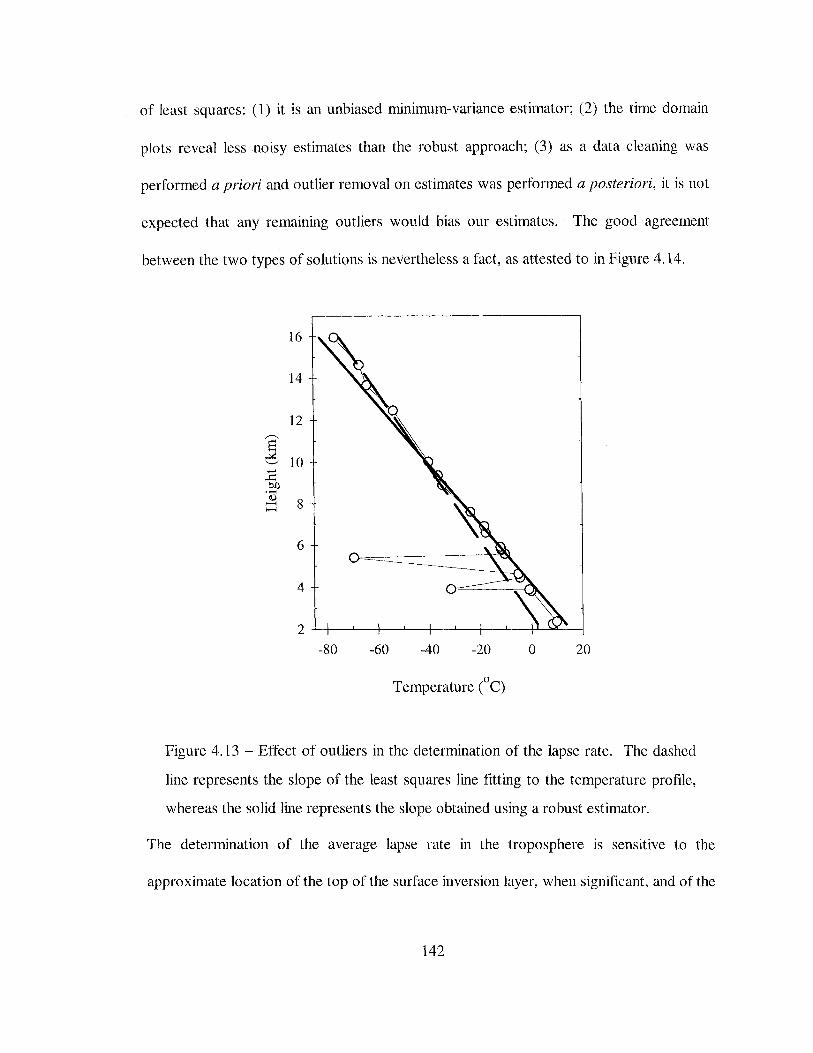
of least squares: (1) it is an unbiased minimum-variance estimator; (2) the time domain
plots reveal less noisy estimates than the robust approach; (3) as a data cleaning was
performed a priori and outlier removal on estimates was performed a posteriori, it is not
expected that any remaining outliers would bias our estimates. The good agreement
between the two types of solutions is nevertheless a fact, as attested to in Figure 4.14.
16
14
12 ~
~ 10 '-..../
...... ..c bil
•>-< Q)
8 0:::
6
4
2
-80 -60 -40 -20 0 20
0 Temperature ( C)
Figure 4.13 -Effect of outliers in the determination of the lapse rate. The dashed
line represents the slope of the least squares line fitting to the temperature profile,
whereas the solid line represents the slope obtained using a robust estimator.
The determination of the average lapse rate in the troposphere is sensitive to the
approximate location of the top of the surface inversion layer, when significant, and of the
142

tropopause. If these boundaries are not correctly defined, a biased lapse rate will be
determined, as the observations beyond the tropopause and below the inversion height
will act as outliers, modifying the slope of the fitted line, as in Figure 4.13. This fact is
well evident for the arctic stations, such Alert, and illustrated in Figure 4.15. When the
inversion height is not considered, the winter lapse rates will be much lower than the
actual lapse rates. Because of the seasonal variation of the inversion height in these
regions, a false seasonal variation will be induced in the lapse rate time series.
8
E 7
~ 6
5
0 50 100 150 200 250 300
Day of Year 1992
350
Figure 4.14 - Temperature lapse rate estimates using a least squares method (open
circles) and a robust estimator (triangles), for Oakland.
6 8
~
0 50 100 150 200 250 300 350
Day of Year 1992
Figure 4. 15 - Temperature lapse rate in the troposphere, assummg no inversion
(triangles) and considering the observed inversion height (open dots), for Alert.
143

The approach used in the lapse rate determination and analysis can be summarized as
follows: first we built the database of tropopause heights and inversion heights for each
station; second we performed the least-squares straight line fit to each individual
temperature profile; finally we carried out a screening of the determined lapse rates for
outlier removal.
As mentioned, the straight-line fit to the temperature profile is performed within the
troposphere. For each profile, an epoch synchronization with the observed tropopause
and inversion heights is tried. In the case of the inversion height, if that synchronization
fails, it is assumed that no inversion height is observed; in the case of the tropopause
height, a new synchronization is tried with the nearest tropopause height available (within
24 hours). If this second attempt fails, the annual mean for the station in analysis is
considered. This strategy allows the building of the largest database possible with
essentially no biased solutions.
The data screening removes not only the lapse rates not included in the [x-3a, x+3a]
interval, but also the lapse rates for which the quality of the fit was revealed to be poor
(based on an identical criterion).
The total number of lapse rates remaining after data cleaning totals 62,505, distributed as
shown in Figure 4.16.
144

21000-
18000
15000
c ~ 12000 (j)
g, 2::
(I.. 9000
6000
3000
2.5 3.0 3.5 4.0 4.5 5.0 5.5 6.0 6.5 7.0 7.5 8.0 8.5
Class Interval (K/km)
Figure 4.16- Histogram of the lapse rates database.
The basic statistics for this data set summarized in Table 4.8.
Table 4.8- Basic statistics for the lapse rate.
-a (ja C:Xminimum C:Xmaximurn C:Xmedian
6.17 K km-1 0.82 Kkm- 1 2.07 Kkm- 1 8.94 Kkm- 1 6.32 Kkm -1
The mean value obtained is lower than the value usually recommended, that is 6.5 K/km
(e.g. Davis et al. [1985]), which seems appropriate for lower to middle latitudes, as
shown in Table 4.9. Rennick [1977] have also concluded that such temperature lapse
rate yields a temperature profile cooler than the observed throughout the troposphere.
145

Table 4.9 - Mean annual lapse rates (a) for different latitude zones. The numbers in
parenthesis are the associated standard deviations.
Latitude - Latitude - Latitude - Latitude -a a a a range (0
) (Kkm-1) range CO) (Kkm-1
) range (0) (K km-1
) range (0) (K km- 1
)
0-10 6.61
25-30 6.49
45-50 6.20
65-70 5.78
(0.27) (0.41) (0.78) (0.96)
10- 15 6.47
30-35 6.43
50-55 6.00
70-75 5.29
(0.17) (0.52) (0.97) (0.86)
15-20 6.54
35-40 6.42
55-60 6.01
75-80 5.37
(0.26) (0.66) (0.89) (0.78)
20-25 6.34
40-45 6.38
60-65 5.89
80-90 5.17 (0.28) (0.73) (0.94) (0.96)
[f we take the average of the mean "zonal" lapse rates, we obtain 6.1 0±0.49 K km-1,
which is not significantly different from the simple average but, as in the case of the
tropopause height database, this value is not biased by the non-uniform distribution of
stations with latitude. The main statistics for each station (both on an annual and monthly
basis) were also computed and are available electronically (http://mat.fc.ul.pt/eg/
/lattex/PhD_e_sup.html); a sample of the tables of these statistics is shown in Appendix
IV. The variation of the annual mean lapse rate with latitude is shown in Appendix VI.
The analysis of our set of lapse rates allow us to draw these major conclusions: (a) the
lapse rate varies significantly with location and season; (b) as illustrated in Figure 4.17,
these seasonal variations are more distinct for continental stations with cold winters (e.g.
FAI), and of small magnitude for other climate types (e.g. PBI); (c) the highest lapse
rates occur in tropical and mid-latitude arid regions (e.g. DEN), reaching frequently 7- 8
oc km- 1; (d) the lapse rate for mediterranean climates (e.g. OAK) is greater in winter than
146

in summer, a fact corroborated by Kyle [1991].
PBI 7
E!
~ 6
5 0 50 100 150 200 250 300 350
OAK 8
E! 7
~ 6
5 0 50 100 150 200 250 300 350
DEN 9
8
E! 7 ~ 6
5
0 50 100 150 200 250 300 350
FAI 8 7
s 6
~ 5 4 3
0 50 100 150 200 250 300 350
Day of Year 1992
Figure 4.17 - Lapse rates and respective error bars for stations with different
climatic characteristics (PBI =West Palm Beach; OAK= Oakland; DEN= Denver;
FAI = Fairbanks). In order to emphasize the seasonal variations, different
amplitude of the vertical scale was used.
147

The correlation plots shown in Figure 4.18 help us to better understand the dependence
of the lapse rate on the same parameters used before. Once more, the annual means
pertaining to the 100 stations with simultaneous determinations of those parameters were
used in the creation of these correlation plots. It is interesting to note the weaker
dependence of the lapse rate on the latitude and surface temperature, in contrast with a
stronger correlation of the lapse rate with the height of the station.
H .. ~D-=~-~~~ • . . : ...
.. • • . ~ .,.... , .
• ··!-t~ E .... =· .•. : • .. ..~· '·. • ~ (~· . .,
.- .. ~ • • • • t.c.c-·,.: .. •• •
··~ • • •
• . of"' ~-:
"·~ r· •• ••
. ~ .. .· ··~;~~.·, ~ ., . ,.,. _, . .,. .... • • • ••••• •• . .. '
Figure 4.18 - Lower triangular matrix of correlations between station latitude,
height, surface temperature, and lapse rate, for annual means of 100 radiosonde
stations. Otherwise as in Figure 4.7.
As suggested by the correlation plot, the lapse rate seems to be linearly dependent on the
surface temperature, and approximately described by a simple straight line equation
(named as UNB98LRJ):
148

a= a+ bts (4.5)
From the least-squares straight line fit to the 16,088 data points (see Figure 4.19) we
obtained the parameters presented in Table 4.1 0. The residual distribution is shown in
Figure 4.20.
8
-~ 7
~ i:: 6
<l.l
~ 5 I!) rf]
j 4
3
z+-~~~-+~-4~~~~+-~~~~~+-~~
-50 -40 -30 -20 -10 0 10 20 30 40
Surface temperature (0 C)
Figure 4.19 - Lapse rate straight-line least-squares fit based on 16,088 data points
and 95% prediction bands.
Table 4.10- Least-squares adjustment results for UNB98LR1.
a b rms of the fit (°C km- 1
) (km-1) (°C krn-1
)
5.930 ± 0.0047 0.0359 ± 0.00028 0.55
149

4000
3500
3000
>, 2500 u >::: <l.J ;::l 2000 0' <l.J .... ~ 1500
1000
500
0 -2.0 -1.5 -1.0 -0.5 0.0 0.5 1.0 1.5 2.0
Class Interval (km)
Figure 4.20- Residual distribution for UNB98LRJ.
Rennick [ 1977] also found an empirical relation between lapse rate and surface
temperature. She concluded that the observed lapse rate could be compared with the
moist adiabatic lapse rate at the surface and that the ratio between these two quantities
could in turn be expressed as a third-order polynomial in T s· The model developed by
Rennick can not however be directly compared with the models proposed in this
dissertation, as her model gives values of a in K hPa-1 units. Furthermore, the use of
Rennick's model would be of little interest in the context of radio-meteorology
applications, as it would require the additional computation of the moist adiabatic lapse
rate, which is a function of several parameters (see, e.g., Hess [1959]). The range of
temperatures for Rennick's model is also limited to 250 K < T, < 300 K.
Stone and Carlson [ 1979] claim that the correlation of between lapse rate and surface
temperature "is likely to be purely statistical in nature", but even though this dependence
150

seems to model fairly well the latitudinal and seasonal variations of observed lapse rate in
a global basis.
Even though our correlation plots showed a weak dependence of the temperature lapse
rate on the height of the station, we were not able to derive an expression that could take
into account this dependence. As Rennick's model has an implicit dependence on the
surface pressure (in the computation of the moist adiabatic lapse rate), we were
motivated to develop a new model that could express this dependence. We found that
the lapse rate could also be expressed as a linear function of surface pressure, and we
established an alternative model for temperature lapse rate prediction that is a function of
the surface temperature and pressure (labeled UNB98LR2):
a=a+bts+cPs (4.6)
For the least-squares fit we used -11,000 observations, and we obtained the parameters
listed in Table 4.11.
Table 4.11- Least-squares adjustment results for UNB98LR2.
a b c rms of the fit (°C km-1
) (km-1) (hPa-1 oc km-1
) (°C km-1)
10.3 ± 0.10 0.03182 ± 0.00040 -0.00436 ± 0.00011 0.55
The rms of the fit is identical to that obtained for UNB98LR1 for a much larger number
of observations. The small improvement in scatter reduction contrasts with the
significant reduction in bias, namely for high-altitude stations, and is well evident in
151

Figure 4.21, which shows a comparative histogram of residual distribution for both
models, for a set of ~22,000 observations.
5000
4500 - UNB98LR2
4000 llf;$. UNB98LR1
3500
~ 3000 t:: Cl)
2500 & Cl)
rt 2000
1500
1000
500
0
-2.0 -1.5 -1.0 -0.5 0.0 0.5 1.0 1.5 2.0
Class Interval (km)
Figure 4.21 - Comparative histogram of residual distribution for UNB98LR 1 and
UNB98LR2, for a set of ~22,000 observations.
In this chapter we have described radiosonde instrumentation and addressed some issues
regarding data quality. Based on archived data from different sources we have
established large databases of meteorological parameters, which enabled us to develop
models for tropopause height and temperature lapse rate prediction.
The next chapter will discuss ray-tracing accuracy and will establish the database of
benchmark traces to be used in model assessment.
152
5. RAY TRACING
In general, the integration of the ray-trace equations established in Chapter 3 is not
possible, as it requires the exact knowledge of the refractivity profile along the whole ray
path as well as the elevation angle of the ray at the reception site. The problem can be
solved numerically, for any arbitrary elevation angle, by ray tracing, which is defined as
the process of determining the path of an electromagnetic signal, based on geometric
optics theory applied over a series of thin spherical shells, concentric with the earth, and
within which a constant refractivity (or some simple functional form of variation) is
assumed [Kerr, 1953; Bean and Dutton, 1966; Bradley, 1989]. The validity of this
technique relies on two basic assumptions: ( 1) the refractive index does not change
significantly within the signal's wavelength; (2) the fractional refractivity changes
between neighboring rays are small within a wavelength [Kerr, 1953; Bean and Dutton,
1966].
The ray-tracing technique implementation can vary substantially, reaching different
degrees of complexity and accuracy. Examples of ray tracing algorithms are given by
Bean and Dutton [1966], Thayer [1967], Davis [1986], and Schroeder and Westwater
[ 1991]. The ray-tracing software used in this dissertation (hereafter referred to as
153

TRACE) is a modified version of the software developed by J.L. Davis, T .A. Herring, and
A. E. Niell [Niell, 1994].
This chapter describes the different features of the ray-tracing software, discusses ray-
tracing model accuracy and limitations, and assesses the ray-tracing products.
5.1. Software algorithms and models
The determination of the atmospheric delay by ray tracing considers the earth's
atmosphere to be divided into a series of thin concentric spherical shells, within which a
constant refractivity is generally assumed. The ray-tracing computation of the neutral-
atmosphere delay is accomplished by adding the contribution of each spherical layer, until
the top of the atmosphere is reached. The thickness of each layer can be kept constant,
or it can vary in such a way that the changes of the refractivity within each layer are kept
below a certain level. If the refractivity is assumed constant within each layer i (and
represented by the average of the refractivity at the lower boundary and at the upper
boundary, for example), its contribution to the delay will be given by:
N 1 +N" (8d ) = 1 0-6
l l L1 na i 2 S, (5.1)
where N: and N ;' are the refractivities at the lower and upper boundaries of layer i,
respectively, and L1s the thickness of that layer (step size).
From Equation (5.1), it becomes clear that the computation of the refractivity at every
layer requires profiles of pressure, temperature, and water vapor pressure (computed
154

ti·om relative humidity, dew point or another moisture variable), based either on
theoretical or radiosonde profiles. Two main problems have to be solved for radiosonde
profiles: (1) most of the radiosonde profiles are vertically limited to the first 15-20 km of
the atmosphere; (2) the radiosonde databases constitute a reduced discrete sample of the
actual refractivity profile of the atmosphere. The approximation of the radiosonde
profiles to a continuous atmosphere has therefore to be performed using interpolation and
extrapolation schemes. By selecting the ray-tracing technique as the standard of
comparison, it is also important to evaluate how sensitive are these benchmark values to
changes in models and methods of computation. These issues are discussed in the
following sections.
5.1.1. Profile extrapolation and interpolation
In order to approximate the pressure, temperature and relative humidity profiles to a
continuous atmosphere covering the height limits of the integration process, each of the
profiles has to be interpolated between the reported levels and extrapolated beyond the
last (highest) reported level.
The temperature and relative humidity for each layer to be assessed is linearly
interpolated between the reported levels, that is, the observation e' at an interpolated
level H, is obtained from the observations at reported levels Hi and Hi+t using the
following scheme:
II = o e i-1-l - e i (H- H ) tH ~ + ..
1 Hi+l-Hi 1
(5.2)
155

A temperature profile that approximates the U.S. Standard Atmosphere, 1962 [NOAA,
1962] is used for extrapolation beyond the last reported level (for ray-tracing purposes,
this standard atmosphere is identical to the U.S. Standard Atmosphere, 1976
[NOAA/NASA/USAF, 1976]). This profile assumes a linear change of temperature
within the different layers considered. For heights between 25 km (a level at which a
standard value of 220 K is assigned) and 100 km, for example, the following lapse rates
are used:
{
-1.92Kkm-1
a= +2.27Kkm-1
--0.50 K km -l
, if HE [ 25 km, 50 km]
,if HE [50km,80km]
,if HE [80km,l00km]
The relative humidity radiosonde observations beyond the 10 km level are not considered
by TRACE as they are generally unreliable. For extrapolation purposes above that
height, the relative humidity is assumed to linearly decrease from 40% to 4% between 10
km and 16 km, and above 16 km the value of 4% is assumed constant. Above 32 km, the
relative humidity is not taken into account; this extrapolation profile was adopted from
Valley [ 1965].
The pressure at a given height is computed using the standard formulae for constant-
lapse-rate or isothermal atmospheres (see Chapter 2), according to the temperature
variation within the considered layer. The acceleration due to gravity is corrected for
latitude, using the international gravity formula, and for altitude, using the Bruns's
formula (see, e.g., Heiskanen and Moritz [1967]).
156
5.1.2. Saturation vapor pressure computation
Generally the moisture content in the atmosphere is expressed in the radiosonde
databases in terms of either relative humidity or dew point. The ray-tracing algorithms,
however, require the moisture to be expressed as water vapor pressure, which is in turn
related to the saturation vapor pressure, as mentioned in Chapter 2.
In order to compute the saturation vapor pressure (over a planar surface of water), a
large selection of formulae is available (e.g. Berry et al. [ 1945]; Goff and Gratch [ 1946];
Langlois [1967]; Tabata [19731; Wexler [1976]; Lowe [1977]; Rasmussen [1978]; Buck
[1981]; Baby eta!. [1988]; WMO [1993]). Most of these and other existing formulae are
approximations or simplifications of the Goff and Gratch formula, and to the more
recently developed one by Wexler [1976], and are typically the result of a search for
computationally more efficient models. The mathematical structure of the saturation
vapor pressure formulae fall in three main categories: exponential, polynomials, and
rational functions. At least partially, the accuracies of these formulae have been already
analyzed and discussed (e.g. Murray [1967]; Tabata [1973]; Riegel [1974]; Hull [1974];
Wigley [1974]; Lowe [1977]; Elliott and Gaffen [1991]). In order to study the effect of
the use of different formulae on ray tracing accuracy, which is clearly less well known (to
the best of our knowledge such studies do not appear to exist at all), we selected four of
the most widely used formulae, as described below.
157

One of oldest formulae used to compute the saturation vapor pressure is known in the
literature as the Magnus or Tetens formula, and is implicitly recommended by the
International Earth Rotation Service (IERS) [McCarthy, 1996]:
7.5t
e = 611x 10237.3+ t sw • ' (5.3)
where t is the temperature, in °C, and env is the saturation vapor pressure, in hPa (the
same symbol definitions and units also apply to the following formulae).
The default formula in TRACE is given by Berry et al. [1945], and will be referred to
hereafter as Berry:
(5.4)
where T is the absolute temperature, in K.
The Goff and Gratch [1946] formula was accepted internationally and was largely used as
a standard for comparison; it is the basis of the well-known Smithsonian Meteorological
Tables [List, 1966]. Murray [ 1967] transformed the original formula into a more
convenient formulation:
e,. ~ 7.95357242xl o" exp{ -18.1972839 -~:' + 5.02808 In(~: J
[ ] }
' (5.5)
-70242.1852exp -26 · 12~~253T +58.0691913exp[ -8.03945282 il]
158

where T, 1 = 373.16 K (steam point). This formula produces no significant differences
relative to the original version.
The Wexler [1976] saturation vapor formula is given as:
e,w = O.Olexp{-2991.2729r-2- 6017.0128T-1 + 18.87643854-0.028354721 T
-+-0.1783830lx10-4 T 2 -0.84150417x10⁻⁹ T 3 +0.44412543xl0-12 T 4 . (5.6)
+ 2.858487ln T}
The Wexler formula represents an improvement over the Goff and Gratch formula, as it is
based on more accurate experimental measurements, such as the experimental value of
the vapor pressure of water at its triple point [Guildner et al., 1976], and a new value of
the gas constant. The uncertainty associated with the formula is a few tens of parts per
million, at most. It represents nowadays the standard formula against which other
formulae are compared. The reader should be aware that there is a O.Ol K difference in
the definition of the absolute temperature for Berry and Goff and Gratch
(T = t +- 273.16) and Wexler (T = t + 273.15) formulations, corresponding to the pre-
1954 and post -1954 definitions, respectively.
The formulae above are to be used in the temperature range [0 °C, I 00 oq, but it is
current practice to use them in radiosonde data analysis in extrapolation, to compute
saturation vapor pressure below 0 oc (supercooled water) - a repercussion of the WMO
recommendation to have the relative humidity at temperatures below 0 oc evaluated with
respect to water [WMO, 1996a]. Among other advantages of this procedure, the
following are relevant: (1) the majority of clouds at temperatures below 0 oc consists of
159

water or mainly water; (2) nearly all the existing records of relative humidity below 0 oc
are expressed on the basis of saturation with respect to water. Figure 5.1 shows the
saturation vapor pressure for the temperature range [ -85 °C, 50 °C], normally
encountered in the region of interest for ray-tracing studies, as well as the difference
between the saturation vapor pressures over water and over ice, both computed using the
Wexler formulae [Wexler, 1976; Wexler, 1977].
120
0.3 100 /"'
~ / \
80 :S 0.2 (?
'ii) \ P-. "' / 6 60 ' \ ~ 0.1 ;s:
"' / (fJ
(].) 40
__./
0.0 .. ----· -80 -60 -40 -20
20 Ten1perature C)C)
0
-80 -60 -40 -20 0 20 40
Temperature (°C)
Figure 5.1 - Saturation vapor pressure over water (esw) with extrapolation for
temperatures below 0 °C, and the difference between the saturation vapor pressures
over water (extrapolated) and over ice (esD· The computation of esw and esi were
performed using the Wexler [1976] and Wexler [1977] formulae, respectively.
Figure 5.2 shows the percent deviation of the Goff and Gratch, Tetens, and Berry
formulae with respect to the Wexler over water formula, for the same temperature range,
where the percent deviation is defined as:
160

Percent Deviation (%) Formula- Wexler ------X 100.
Wexler (5.7)
Even though the percent deviation is smaller for high temperatures, it will affect more
significantly the determination of the atmosphere propagation delay, as will be shown.
The Goff and Gratch formula produce estimates of the saturation vapor pressure that are
systematically lower than Wexler's, particularly for low temperatures. The Berry formula
overestimates esw for temperatures above about -30 °C, and underestimates it below than
limit. The Tetens formula also performs poorly at low temperatures, but the differences
for temperatures greater than 0 ac are small.
0
...., 5 -20 u [)
p...
/ /
/
/ /
-/
I · · · · · · · Goff and Gratch I --Berry
-··-Wexler -- Tetens
-80 -60 -40
0 10
-20 0
Temperature (0 C)
20 30 40 50
Temperature (°C)
20 40
Figure 5.2- Percent deviation for the Tetens, Berry and Goff and Gratch formulae
as compared against the Wexler formula. All the formulae were extrapolated for
temperatures below 0 ac. The error curves for temperatures above 0 oc are
highlighted in the embedded plot.
The effect of the choice of the different formulae in ray tracing is analyzed in Table 5.1,
for the USSA66. From this table, it is concluded that, at the zenith, the Goff and Gratch
161

and the Tetens formula produce very small (less than -0.3 mm) differences in the traces,
as compared against Wexler. On the other hand, the Berry formula leads to errors that
can reach a few millimetres, at the zenith, notably for low latitude stations, as stressed in
Figure 5.3. It is therefore recommended that the Wexler formula be used whenever the
computation of the saturation vapor pressure is needed.
Table 5.1 - Zenith non-hydrostatic delay for USSA66, using different formulae in
the computation of the saturation vapor pressure. (Note: Be = Berry; Gg = Goff
and Gratch; Te = Tetens; We= Wexler).
USSA66 We Te Gg Be Te-We Gg-We Be-We
CON/Month) dz (m) nh
dz (m) nh
d' (m) nh
dz (m) nh
(m) (m) (m)
15 Annual 0.2443 0.2446 0.2442 0.2473 0.0003 -0.0001 0.0030
30 January 0.1323 0.1324 0.1322 0.1338 0.0001 -0.0001 0.0015
30 July 0.2577 0.2579 0.2576 0.2608 0.0002 -0.0001 0.0031
45 January 0.0573 0.0570 0.0572 0.0577 -0.0003 -0.0001 0.0004
45 July 0.1821 0.1823 0.1819 0.1842 0.0002 -0.0002 0.0021
60 January 0.0315 0.0312 0.0314 0.0317 -0.0003 -0.0001 0.0002
60 July 0.1347 0.1348 0.1346 0.1362 0.0001 -0.0001 0.0015
75 January 0.0151 0.0149 0.0150 0.0151 -0.0002 -0.0001 0.0000
75 July 0.0982 0.0981 0.0981 0.0991 -0.0001 -0.0001 0.0009
162

5.0 ~----------------------------------------------------T------,
4.0
3.0
T Berry -Wexler o Goff and Gratch -Wexler
-0.1
-0.2
-0.3 +--.1..---+---'----l---'---+---'---+---'---+---'---+---'---+----'
0 50 100 150 200 250 300 350
Day of Year 1992
Figure 5.3 - Differences in the zenith non-hydrostatic delay due to the use of
different formulae to compute the saturation vapor pressure (the Wexler formula
was used as the reference). The Berry formula overestimates the zenith non
hydrostatic delay by a few millimetres, whereas the Goff and Gratch formula
underestimates it at the sub-millimetre level. For this case study, radiosonde data
from a station with consistently high temperature and humidity was used (Guam).
5.1.3. Refractivity constants
Some sets of refractivity constants listed in Table 3.1 and the Essen and Froome
constants (as given in lAG [1963] and subsequently converted to the units used in Table
3. 1) were tested. At the zenith the trace values differ for the hydrostatic component only
at the sub-millimetre level. The Boudouris set of constants give the lowest values, and
163

Essen and Froome the highest (see Table 5.2). As the precision of the coefficients
determined by Thayer [1974] is better than the others, they will be used in our ray-tracing
computations.
Table 5.2- Ray-traced zenith hydrostatic delay for USSA66, using different sets of
refractivity constants. (Note: TH =Thayer; EF =Essen and Froome; SW =Smith
and Weintraub; BD = Boudouris).
USSA66 Zenith hydrostatic delay (m) Differences (m)
(0 N/Month) TH EF sw BD EF-TH SW-TH BD-TH
15 Annual 2.3126 2.3132 2.3129 2.3123 0.0006 0.0003 -0.0003
30 January 2.3278 2.3284 2.3281 2.3275 0.0006 0.0003 -0.0003
30 July 2.3110 2.3115 2.3113 2.3107 0.0005 0.0003 -0.0003
45 January 2.3177 2.3183 2.3180 2.3174 0.0006 0.0003 -0.0003
45 July 2.3078 2.3084 2.3081 2.3075 0.0006 0.0003 -0.0003
60 January 2.3043 2.3049 2.3046 2.3040 0.0006 0.0003 -0.0003
60 July 2.2967 2.2973 2.2970 2.2964 0.0006 0.0003 -0.0003
75 January 2.3019 2.3025 2.3022 2.3016 0.0006 0.0003 -0.0003
75 July 2.3001 2.3007 2.3004 2.2998 0.0006 0.0003 -0.0003
5.1.4. Compressibility factors
At the zenith, the error induced by not taking into account the non-ideal gas behavior of
dry air and water vapor is about 0.1-0.2 mm. This effect is visible only for the non-
hydrostatic delay, and is modeled in our ray-tracing computations.
5.1. 5. Enhancement factor
The saturation vapor pressure computation was performed by considering the water
vapor as pure, a situation for which the formulae analyzed apply. Rigorously, as we deal
164

with moist air rather than pure water vapor, computations have to be corrected using the
enhancement factor (cf. Chapter 2). As shown in Table 5.3, not taking into account the
enhancement factor in the computation of the saturation vapor pressure, induces an error
in the computation of the zenith non-hydrostatic delay that amounts to more than 1 mm,
for locations with high-humidity. The enhancement factor used in our ray-tracing
computations is given in Buck [ 1981].
Table 5.3 - Effect of the enhancement factor on the zenith non--hydrostatic
delay, for USSA66. (Note: pw =pure water; ma =moist air).
USSA66 Non-hydrostatic delay (m)
(0 N/Month) pw ma ma-pw
15 Annual 0.2443 0.2455 0.0012
30 January 0.1323 0.1330 0.0007
30 July 0.2577 0.2590 0.0013
45 January 0.0573 0.0574 0.0001
45 July 0.1821 0.1830 0.0009
60 January 0.0315 0.0316 0.0001
60 July 0.1347 0.1355 0.0008
75 January 0.0151 0.0152 0.0001
75 July 0.0982 0.0987 0.0005
5.1.6. Initial integration step
Under normal conditions, the refractivity decreases by about 40 N-units per kilometre in
the lower atmosphere. In order to meet the ray-tracing assumptions, the refractivity can
not change significantly within a signal carrier wavelength, a condition that is satisfied if
165

(5.8)
where L1n 1
is the gradient of the refractive index per kilometre, and f~ is the carrier
frequency, in kHz [Bean and Dutton, 1966]. Therefore, for radio frequencies this
postulate is accomplished easily, but the choice of the initial step size should be
nevertheless adequately small to prevent abnormal variations of the refractivity, to
approximate the series of layers to a smooth continuous atmosphere, and to assure that
the fractional changes between neighboring rays are kept small compared to a
wavelength, a basic requirement for the application of Fermat's principle.
The differences found by changing the initial integration step from 5 m up to 100 m were
at the sub--millimetre level, with the largest effect for the high latitude atmospheres. Small
step sizes provide smoother atmosphere profiles, but increase considerably the
computation time. Large step sizes allow faster computations, but may lead to violations
to the ray-tracing assumptions. In our ray-tracing computations, an initial step size of 5
m was used.
5.1. 7. Integration limits
As already mentioned, radiosonde profiles do not provide observations for all of the
neutral atmosphere and have therefore to be completed using an extrapolation scheme.
The effect of changes to the upper limit in the ray-tracing computations is presented in
Table 5 .4. From this table, it is concluded that the stratosphere contribution to the
hydrostatic delay is significant (and the reason why the term "tropospheric" delay is
166

misleading). This test shows how important is the extrapolation of the meteorological
parameter profiles in the generation of the traces to be used as benchmarks, as the
radiosonde profiles can terminate at low levels (below 20 km). The simplest approach for
extrapolating to upper levels is through the use of profiles of a standard atmosphere; a
more sophisticated and laborious approach is to use monthly mean values specific to each
radiosonde location, based on historical data, for example (the error introduced by
replacing the temperature profile of the USSA atmospheres by the U.S. Standard
Atmosphere - 1962 for heights above the 25-km limit is negligible (0.1-0.3 mm),
therefore no significant error is expected from this procedure). The contribution of the
atmosphere above 75 km can be ignored, even though we kept the 100 km boundary as
the upper limit in our ray-trace computations.
Table 5.4- Effect of changing the upper boundary in the ray-tracing computations
of the zenith hydrostatic delay, for USSA66.
USSA66 Zenith hydrostatic delay (m)
(0 N/Month) 100km 75km 50km 25 km 20km 15 km lOkm
15 Annual 2.3126 2.3125 2.3108 2.2537 2.1847 2.0117 1.6597
30 January 2.3278 2.3278 2.3261 2.2712 2.2031 2.0417 1.6984
30 July 2.3110 2.3109 2.3090 2.2514 2.1776 2.0079 1.6553
45 January 2.3177 2.3177 2.3163 2.2631 2.1959 2.0504 1.7323
45 July 2.3078 2.3077 2.3057 2.2445 2.1725 2.0115 1.6677
60 January 2.3043 2.3043 2.3030 2.2528 2.1889 2.0475 1.7421
60 July 2.2967 2.2966 2.2945 2.2339 2.1633 2.0108 1.6876
75 January 2.3019 2.3019 2.3006 2.2552 2.1973 2.0645 1.7716
75 July 2.3001 2.3000 2.2981 2.2354 2.1644 2.0165 1.7027
167

Table 5.5 -Effect of changing the upper boundary in the ray-tracing computations
of the zenith non-hydrostatic delay, for USSA66.
USSA66 Zenith non-hydrostatic delay (m)
(0 N/Month) 15 km 10 km 8km 6km 4km 2km 1km
15 Annual 0.2443 0.2434 0.2415 0.2347 0.2160 0.1633 0.0953
30 January 0.1323 0.1318 0.1307 0.1275 0.1178 0.0857 0.0512
30 July 0.2577 0.2567 0.2537 0.2442 0.2185 0.1542 0.0967
45 January 0.0571 0.0568 0.0563 0.0546 0.0489 0.0332 0.0193
45 July 0.1819 0.1811 0.1793 0.1741 0.1587 0.1138 0.0684
60 January 0.0313 0.0310 0.0309 0.0291 0.0250 0.0156 0.0083
60 July 0.1343 0.1336 0.1326 0.1285 0.1144 0.0782 0.0462
75 January 0.0150 0.0148 0.0147 0.0143 0.0128 0.0089 0.0044
75 July 0.0975 0.0964 0.0958 0.0932 0.0838 0.0555 0.0320
As the water vapor content of the atmosphere is mainly concentrated in the first few
kilometres above sea level, it is not surprising to see that the contribution of the layers
above 8 km is already less than 2% of the non-hydrostatic delay, being negligible beyond
a level of about 15 km (see Table 5.5).
5.1.8. Radiosonde data precision and accuracy
In order to evaluate the precision limitation of the radiosonde instrumentation in the ray-
tracing accuracy, a second set of profiles based on the USSA66 atmospheres was
generated by adding white noise (uncorrelated between levels). In the generation of this
simulated data, we used the standard deviations correspondent to the accuracy limits
established by the WMO for radiosonde instrumentation: 1 hPa for pressure, 0.5 oc for
168

temperature, and 5% for relative humidity [WMO, 1996a], even though such levels of
noise are likely not to appear in modern radiosonde instrumentation. It is concluded that
the influence of radiosonde random errors in the generation of the zenith traces can be of
a few millimetres, at most (see Table 5.6). Due to the higher noise attributed to the
relative humidity sensors, the accuracy of the ray tracing due to radiosonde errors is
much poorer for the non-hydrostatic component.
Table 5.6 - Simulation of the effect of the limitations in precision of the radiosonde
instrumentation, for USSA66. (Note: 0 ==Original data; S =Simulated data).
USSA66 Hydrostatic delay (m) Non-hydrostatic delay (m)
(0 N/Month) 0 s S-0 0 s S-0
15 Annual 2.3126 2.3100 -0.0026 0.2443 0.2480 0.0037
30 January 2.3278 2.3284 -0.0006 0.1323 0.1255 -0.0068
30 July 2.3110 2.3100 0.0010 0.2577 0.2415 -0.0162
45 January 2.3177 2.3195 0.0018 0.0573 0.0587 0.0014
45 July 2.3078 2.3088 0.0010 0.1821 0.1831 0.0010
60 January 2.3043 2.3031 -0.0012 0.0315 0.0302 -0.0013
60 July 2.2967 2.2969 0.0002 0.1347 0.1345 -0.0002
75 January 2.3019 2.3037 0.0018 0.0151 0.0144 -0.0007
75 July 2.3001 2.2989 -0.0012 0.0982 0.0975 -0.0007
The same simulation was performed with 9 randomly-chosen radiosonde soundings from
Guam, as shown in Table 5.7. The differences obtained were higher than in the case of
the USSA66 traces, which can be explained by the larger number of levels at which the
169

meteorological data is reported compared to the number of levels tabulated for the
USSA66, especially in the lower atmosphere.
Table 5.7 - Simulation of the effect of the limitations in precision of the
radiosonde instrumentation, for some radiosonde observations collected over
Guam. (Note: 0 - original data; S - Simulated data)
Hydrostatic delay (m) Non-hydrostatic delay (m)
RAOB 0 s S-0 0 s S-0
920101 2.2853 2.2827 -0.0026 0.2421 0.2388 -0.0033
920111 2.2758 2.2734 -0.0024 0.3577 0.3593 0.0016
920208 2.2881 2.2914 0.0033 0.2178 0.2186 0.0008
920412 2.2860 2.2905 0.0045 0.2250 0.2303 0.0053
920602 2.2826 2.2842 0.0016 0.2737 0.2692 -0.0045
920727 2.2815 2.2814 -0.0001 0.3669 0.3690 0.0021
920918 2.2861 2.2901 0.0040 0.3141 0.3117 -0.0024
921024 2.2804 2.2814 0.0010 0.3378 0.3386 0.0008
921225 2.2892 2.2889 -0.0003 0.2195 0.2174 -0.0021
If we assume a constant bias (equal to the upper boundary of the WMO accuracy limits )
throughout the radiosonde ascent path for those sensors (as a measure of accuracy), and
for the USSA66 profiles, the zenith hydrostatic delay will be biased by about 2.3 mm (as
it is essentially dependent on the surface pressure). The biases for the zenith non
hydrostatic component are larger, ranging from -2 mm to almost 3 em, as documented in
Table 5.8. Nevertheless, one should note that the accuracy of many of the current
radiosonde instruments is also better than the imposed WMO limits. Special care should
be given to the calibration of sensors prior to launch.
170
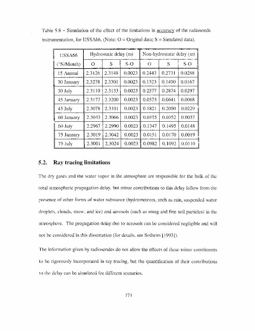
Table 5.8 - Simulation of the effect of the limitations in accuracy of the radiosonde
instrumentation, for USSA66. (Note: 0 =Original data; S =Simulated data).
USSA66 Hydrostatic delay (m) Non-hydrostatic delay (m)
CON/Month) 0 s S-0 0 s S-0
15 Annual 2.3126 2.3149 0.0023 0.2443 0.2731 0.0288
30 January 2.3278 2.3301 0.0023 0.1323 0.1490 0.0167
30 July 2.3110 2.3133 0.0023 0.2577 0.2874 0.0297
45 January 2.3177 2.3200 0.0023 0.0573 0.0641 0.0068
45 July 2.3078 2.3101 0.0023 0.1821 0.2050 0.0229
60 January 2.3043 2.3066 0.0023 0.0315 0.0352 0.0037
60 July 2.2967 2.2990 0.0023 0.1347 0.1495 0.0148
75 January 2.3019 2.3042 0.0023 0.0151 0.0170 0.0019
75 July 2.3001 2.3024 0.0023 0.0982 0.1092 0.0110
5.2. Ray tracing limitations
The dry gases and the water vapor in the atmosphere are responsible for the bulk of the
total atmospheric propagation delay, but minor contributions to this delay follow from the
presence of other forms of water substance (hydrometeors, such as rain, suspended water
droplets, clouds, snow, and ice) and aerosols (such as smog and fine soil particles) in the
atmosphere. The propagation delay due to aerosols can be considered negligible and will
not be considered in this dissertation (for details, see Solheim [1993]).
The information given by radiosondes do not allow the effects of these minor constituents
to be rigorously incorporated in ray tracing, but the quantification of their contributions
to the delay can be simulated for different scenarios.
171

5.2.1. Propagation delay due to non-gaseous atmosphere constituents
As in the case of dry gases and water vapor in the atmosphere, the zenith delay due to
any i1h atmospheric constituent can be evaluated if the real part of its refractive index (or
refractivity) is known:
r s
(5.9)
The refractivity model for all kinds of water substances and ice crystals in the atmosphere
are derived from the following basic model [Liebe et al., 1989]:
(5.10)
where, for each constituent i, W is the mass content per unit volume (kg m-3), p is the
density (kg m-3), and E is the relative permittivity.
• Propagation delay due to rain
Flock et al. [ 1982] present graphically values of refractivity for rain, Nrain, which are
function of the rain rate, signal frequency, and temperature. For extraordinary situations
of heavy rain (150 mm/h), and for a frequency of 1.5 GHz, the delay obtained is about 8
mm per each kilometre, which may be significant for rainstorm conditions. According to
Ishimaru [ 1985], the typical values of precipitation rate vary between 0.25 mm/h, for
drizzle, and 100 mrn!h, for extremely heavy rain; in general, the vertical thickness of rain
is of about 3-4 km.
172

If we follow Liebe et al. [ 1989], the refractivity for rain can be computed from Equation
(5.1 0); as PH,o ""103 kg m-3 [Lide, 1997], we obtain:
3 3[E 0 -1] N rain = 1 0 wrain 2 E 0 + 2 ' (5.11)
where W is the rain mass content per unit volume (kg m"3) and Eo is the relative
permitivitty of water, which can be computed using the following expression [Liebe et al.,
1989]:
(5.12)
• Propagation delay due to suspended water droplets
Suspended water droplets (SWDs) consist of water droplets whose size have radii small
enough to be kept suspended by turbulence c:s; 50jlm)' and are present in the atmosphere
in the form of clouds, fog, and haze. Taking into consideration that PswD ""103 kg m-3,
Equation ( 5.1 0) can be approximated by
(5.13)
which is in agreement with Flock et al. [1982].
According to this simplification, a cloud with a thickness of 1 km and
Wswo = 1 o--] kg m -3 (nonprecipitating clouds show generally a mass content of 10-4 - 1 o-3
kg m-3 lLiebe et al., 1989], but peak values of 5x 10⁻³ kg m-3 or greater are possible for
173

cumulus clouds when associated with thunderstorms [Ishimaru, 1985]) contributes about
1.5 mm of zenith delay. The effect can therefore be significant as the thickness of
cumulus clouds is typically 2-8 km [Ishimaru, 1985]. For fog conditions, the mass
content can vary between 1 o-6 kg m-3 and 1 o-3 kg m-3• Assuming the highest value for
mass content and a fog layer 500 m thick, which corresponds to a thick fog [Ahrens,
1994], the contribution to the propagation delay is less than 1 mm.
• Propagation delay due to ice crystals
Taking for the density of suspended ice crystals (SICs) - snow, ice fog, and glaciated
clouds-- the value Psrc =0.916xl03 kgm-3 [Liebe et al., 1989], we can approximate
Equation (5.10) with
(5.14)
The propagation effects induced by suspended ice crystals are insignificant, as they have a
very small associated mass content (less than ~ 1 o-6 kg m-3) and occur at high altitudes
[Liebe et al., 1989].
Even though the formulae presented here are easy to apply, the determination of the mass
content of the components along the signal path is naturally troublesome. As the
presence of significant values of SWDs is generally associated with saturated air masses,
it is nevertheless possible to simulate its effect by analyzing the radiosonde relative
humidity profiles (see, e.g., Schroeder and Westwater [1991 ]).
174

5.2.2. Horizontal gradients
The assumption we have made so far on the spherical symmetry of the atmosphere is only
approximately valid and the deliberate disregard of horizontal gradients is most likely the
largest error source in ray tracing, especially for low elevation angles. Saastamoinen
I 1973] estimated a maximum error due to horizontal gradients of 2.0 em at a I oo
elevation angle, which is equivalent to a zenith delay error of less than 4 mm. This
theoretical estimate of the gradient error was later confirmed by Gardner [1977],
considered the pioneer in the development of gradient correction models, who concluded
that the horizontal gradients introduce an rms error of almost 3 em at 1 0" elevation angle.
It is interesting to note that the size of this error is comparable to others resulting from
the incorrect use of models and processing strategies in ray tracing computations, as
analyzed in previous sections.
Most of the gradient correction models are still mostly based on local experiments and
small datasets, and a feasible model to be applied on a global scale has not been
developed yet. Judging by the recent literature in this domain, it seems that the
conclusions obtained by Gardner two decades ago are still valid and apropos of current
horizontal gradient studies.
Gardner [ 1977] derived his correction formula to compensate for the horizontal gradient
effects based on radiosonde data obtained from eight different locations near Washington,
D.C. The formula is for application to optical wavelengths, ignoring therefore the water
vapor gradient contribution. He concluded that the errors due to the horizontal gradients
175

are sinusoidal functions of the azimuth of the satellite a, comprising a sina dependence,
which is due to the east-west gradients induced by diurnal, seasonal and local variations
of the surface temperature profile, and a cosa dependence, which is due to the north-
south gradients induced by the decrease of the temperature from the equator to the poles.
Gardner found that the pressure gradients are dominated by the temperature gradients.
Variations on the model developed by Gardner [1977] are presented by Herring [1992],
Davis et al. [1992, 1993], and MacMillan [1995].
Herring [ 1992] presents an expression to model azimuthal asymmetry based on a "tilted"
atmosphere assumption:
(5.15)
where d~: represents the additional delay due to the horizontal gradients, 3Ns and SEw
are parameters representing the delays due to the azimuthal asymmetry (north and east
components of the gradient vector), and maz(E) is a mapping function for a tilted
atmosphere, given by the following expression:
1 m.,z(E) = . .
' · sm £tan£ + 0.0032 (5.16)
Based on the analysis of VLBI data spannmg a almost 3-year period (for stations
Westford, Richmond, Mojave, Wettzell, and Onsala), Herring concluded that the
atmospheric azimuthal asymmetry contribution is generally less than 10 em, at 5°
elevation angle, but can occasionally be highly significant.
176

MacMillan [ 1995] used a similar expression to model azimuthal asymmetry which allows
any choice of mapping function:
d~~' = m(£) cot(£) [ 3Ns cos a+ 3Ew sin a]. (5.17)
MacMillan concluded that the daily average gradient effects can amount to up to 5 em of
delay at 7" elevation angle (in his study only gradients varying on a time scale of one day
were considered).
A more complete model was adopted by Davis et al. [1992, 1993] to specifically model
horizontal gradients in the non-hydrostatic component of the delay for the Onsala VLBI
site determined by WVR. These horizontal gradients can be caused by weather front
passages, for example [Elgered, 1992]. The model allows for the temporal variation of
the non-hydrostatic component of the delay by including the gradient rates and a time
derivative of the zenith delay. From their analyses, it was concluded that the estimated
gradient and gradient-rate vectors had preferred directions, likely an indication of a
predominant structure in the three-dimensional temperature and humidity fields.
Chen and Herring [ 1997] applied different methods to evaluate azimuthal asymmetry
effects. They have used a 12-day series of experiments and concluded that there was a
good agreement between the atmospheric delay gradients estimated from VLBI data and
those calculated from three-dimensional weather analysis fields from the National Center
for Environmental Prediction. They have found that the north-south gradients have
average values of up to 20 mm of delay, for mid-latitude sites, and for an elevation angle
of 10°. The east-west gradients were found to be not as significant.
177

Additional information concerning horizontal gradients can be found in Chao [ 1 971 b],
von Roos [19711, Davis [1986], Ifadis [1986], Bender [1992], Rogers et al. [1993], and
Coster et al. [ 1997].
5.2.3. Hydrostatic equilibrium violation
Another assumption in our ray tracing computations is hydrostatic equilibrium of the
atmosphere. Saastamoinen [1973] estimated a maximum error from the violation of the
assumption of hydrostatic equilibrium of 1.5 em, at 10° elevation angle. Hauser [ 1989]
concluded that the expected error due to deviations from hydrostatic equilibrium is less
than 1 em most of the time, for elevation angles greater than 20° (about 3 mm at the
zenith) . This estimate is based on limited data for mountain sites and there is shortage of
information on the size and frequency of these deviations for other situations. The values
presented by Bender [ 1992] for three different datasets agree with this estimate, hut more
studies are needed in order to fully evaluate this effect.
From this discussion, we can identify three main areas that can contribute to errors in our
ray-trace values: errors in radiosonde data, effect of hydrometeors, and atmospheric
horizontal asymmetry. The exact quantification of these errors is however troublesome
or even impossible, due to the variability of the contribution of each of these errors for
each radiosonde profile. The good agreement between ray-traced radiosonde data and
independent techniques (see Chapter 1 for literature review about this subject) is
nevertheless a good indication that those values may be accurate to the 1-cm level or less
(rms).
178

5.3. Product analysis
The basic quantities determined by the ray-tracing program are the components of the
atmospheric propagation delay (hydrostatic and non-hydrostatic), at selected elevation
angles, which will constitute the benchmark values for model assessment. The
hydrostatic component includes the geometric delay (bending). As by-products, the
computation of the precipitable water vapor, and the mean temperature (as defined by
Equation 5.18) is also performed.
As already mentioned, a total of 50 radiosonde stations were selected for ray tracing
purposes. The ray tracing was performed using the settings summarized in Table 5.9, at
seven elevation angles: 90°, 30°, 20°, 15°, 10°, 6°, and 3°. For each elevation angle,
32,467 traces were generated (nominally two per day per station for the whole of 1992).
The ray-traced radiosonde data provided a full range of neutral atmosphere delays, which
express the meteorological conditions usually encountered all over the world. The
histograms of the zenith hydrostatic and non-hydrostatic delays corresponding to the
traces are presented in Figure 5.4. As the hydrostatic component is essentially a function
of the surface pressure (which in turn is a function of the station height), the histogram
clearly shows the uneven distribution with respect to the heights of the radiosonde
stations.
Other ray-tracing products (mean temperature, precipitable water, geometric delay) are
also of interest and will be analyzed in detail in the following sections.
179
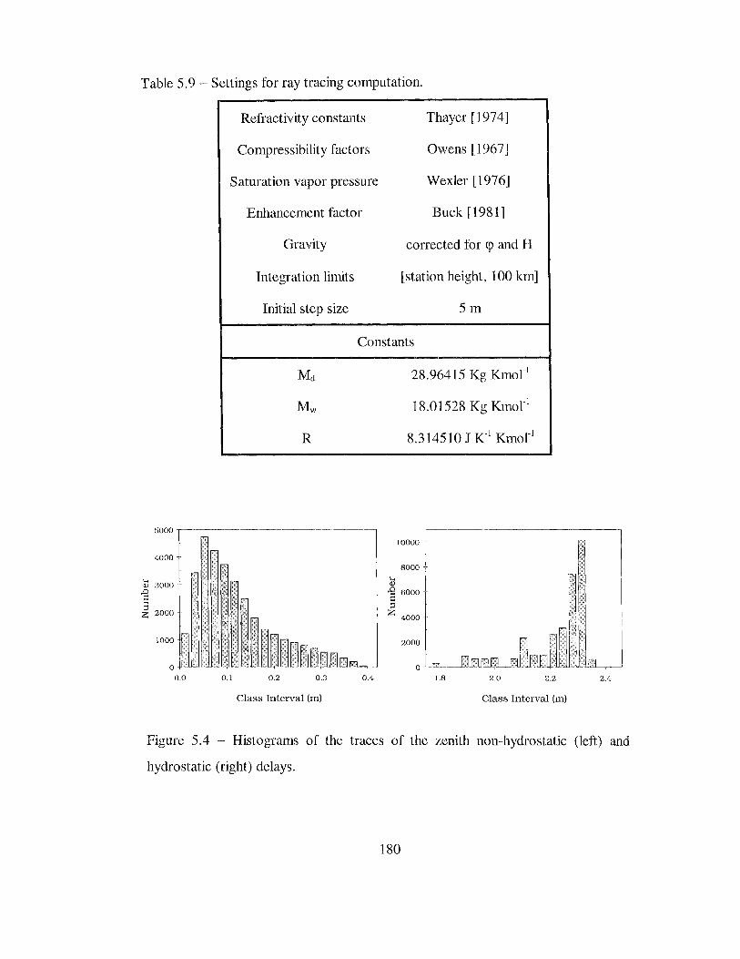
Table 5.9- Settings for ray tracing computation.
Refractivity constants Thayer [1974]
Compressibility factors Owens [ 1967]
Saturation vapor pressure Wexler [1976]
Enhancement factor Buck [1981]
Gravity corrected for <p and H
Integration limits [station height, 100 km]
Initial step size 5m
Constants
Me~ 28.96415 Kg Kmor 1
Mw 18.01528 Kg Kmor1
R 8 . .314510 J K 1 Kmor1
5000
10000
4000 8000 -
kJ 'S 6000 -
::l z 4000
kJ 3000-
'S :E 2000
0.0 0.1 0.2 0.3 0.4 1.8 2.0 2.2 2.4
Class Interval (m) Class Interval (m)
Figure 5.4 - Histograms of the traces of the zenith non-hydrostatic (left) and
hydrostatic (right) delays.
180

5.3.1. Precipitable water
One of the most interesting and innovative applications of space geodetic techniques
(namely GPS and VLBI) developed in recent years is the estimation of the precipitable
water vapor of the atmosphere. As a by-product of the estimation process of geodetic
parameters, the zenith non-hydrostatic delay is included as a nuisance parameter and can
subsequently be related to the precipitable water, according to the process described
hereafter.
In Chapter 3, we established that the neutral atmosphere delay is given by:
The zenith hydrostatic delay can be predicted with good accuracy provided good surface
pressure measurements are available. For example, considering the Saastamoinen [ 1973]
prediction model:
dz = 0.002277 Ps h ( ) ' 1- 0.0026 cos 2cp -0.000 000 28H
the partial derivative with respect to the surface pressure gives:
Jd~ (m hPa-I) = 0.002277 ()ps 1-0.0026cos(2cp )- 0.000000 28H
As an example, for <p = 45°, I-I= 100m, and Ps = 1013.25 hPa, we obtain:
dd~ (m) '"-"' 0.0023 ()ps .
181

If the measurements of surface pressure are kept below 0.5 hPa, we can expect an
accuracy in zenith hydrostatic delay of about 1 mm, assuming: ( 1) no error in the model;
(2) no errors in latitude determination; (3) no errors in height determination.
If we also assume no errors in the mapping functions (see the next chapter), the only
variable remaining is the zenith non-hydrostatic delay, which is very difficult to predict.
For high-precision applications of space techniques this quantity is therefore typically
estimated as a nuisance parameter in the adjustment process. Finally we need to establish
a relation between this estimated parameter and the precipitable water.
In Chapter 3 we concluded that
This expression can be further modified by introducing the weighted mean temperature of
the (wet part of the) atmosphere, defined as
(5.18)
in which case we get
(5.19)
Using the equation of state- see Equation (2.12) ·-we have
L82

and Equation (5.19) can therefore be written as
(5.20)
The integral in Equation (5.20) is the integrated water vapor (IWV) --the total mass of
water vapor in a column of air with cross section of 1 m2 extending from the surface to
the top of the atmosphere - and is usually given in units of kg m-2:
r s
(5.21)
This quantity can be easily converted to length units by dividing by the density of water
( p H2o ""-" 103 kg m -3
), in which case it can be interpreted as the height of an equivalent
column of liquid water that would result if the water vapor were condensed, denominated
as integrated precipitable water vapor (PW) or simply precipitable water (see Dutton
[1986]: Peixoto and Oort [1987 ]):
(5.22)
From these results it is clear that 1 kg m-2 IWV is equivalent to 1 mm PW.
Substituting Equation (5.21) into Equation (5.20), we obtain:
(5.23)
183

where ~ is a "constant" of proportionality given by:
(5.24)
The mean temperature is the only unknown in this equation. Being a function of the
water vapor pressure and temperature profiles, this parameter is therefore variable with
location and time. In order to provide accurate measurements of precipitable water from
estimates of zenith non-hydrostatic delay, the determination of Tm is therefore essential.
This quantity was calculated for each profile from our radiosonde stations, for a total of
32,467 profiles, with the basic statistics presented in Table 5.10.
Table 5.10 - Basic statistics for the mean temperature.
-Tm aT"' T
n1munmum T
111 maximmn
270K 11 K 232K 306K
As already discussed in Bevis et al. [ 1992], the mean temperature shows a strong
correlation with the surface temperature, as witnessed by our correlation plot in Figure
5.5, which shows the correlations of the annual means for the 50 stations we have ray-
traced. The correlation with latitude is also very clear, but the dependence on this
parameter is well modeled by the surface temperature, which shows a similar correlation.
The dependence on station height is very weak.
184

... ~ ,., T .. .
===o~O~oO • . ~ ... I••• • • • • •• r: :· ·. • I
• ··:. .... . . • • • • • ---------
,--- . -.. .- ,. .. • . a,; •-:.. . . • ':,II• 0
i '· •• • • ·-;. • • elf"•
•' ,., . . .~~o~"' • " ..... . • • • • • • • '----
Figure 5.5 - Correlation plot for the mean temperature, for annual means of ray
traced radiosonde stations. Otherwise as in Figure 4.7.
As suggested by the correlation plot, we fitted a straight line through our data (referred
to as UNB98Tml), which lead to the results presented in Table 5.11 and plotted, together
with the ray-traced values, in Figure 5.6.
Table 5.11 -Least-squares fit adjustment results for the UNB98Tm1 model.
Functional Model a b rms of the fit
Tm =a+ bTS 50.4 ±0.66 K 0.789 ± 0.0023 3.07 K
185

290
280 ~
<1.) 1-;
B 270 ro 1-; <1.)
0.. s ~ 260 .:: ro <1.)
~ 250
240
240 250 260 270 280 290 300 310
Surface Temperature {K)
Figure 5.6- Plot of ray-traced mean temperature versus surface temperature, along
with the fitted straight line and associated 95% prediction band.
The parameters of this straight line model are slightly different from the ones obtained by
Bevis et al. [ 1992], and there is a significant improvement concerning the quality of the fit
(rms of 3.07 K versus 4.7 K obtained by Bevis et al. [ 1992]). The residuals for this fit are
presented in Figure 5.7. Despite its simplicity, this model describes very accurately the
functional relationship between the two meteorological parameters.
186

'*1 1500 ;:l "0 '[j) <1,)
0:: 1000 4-< 0 ~ <1,)
'-< 0 ~-)00
~ 500
~~-ornl ;:l z
0
~ <1,)
~ 250 ;J z
.,..,. ~L r-
-40 -30 -20 -10 0 lO 20 -15 -10 -5 0 5 10 15
Class Interval (°C) Class Interval (°C)
Figure 5.7 - Distribution of the mean temperature observations (left) and of the
residuals of the least-squares straight line fit (right).
Another model that fits to the data better than the straight line model, particularly for
high latitudes (as depicted in Figure 5.8), was also derived (and named as UNB98Tm2).
The coefficients and associated uncertainties for the UNB98Tm2 model are presented in
Table 5.12.
Table 5.12- Least-squares adjustment results for UNB98Tm2.
Functional Model a b rms of the fit
T =a+ bT 3 m s 196.05 ± 0.23 K (3.402 ± 0.0098) X 10·6 K'2
3.01 K
This particular empirical model reflects the high variability of radiosonde stations used in
our study, which leads to a large temperature range. If we ignore some of the high-
latitude stations, different models and constants can be derived.
187

Once an expression for the mean temperature is established, a model to express the
relationship between the zenith non-hydrostatic delay and the precipitable water can be
determined using an appropriate set of refractivity constants.
290
280 ~
Cl.l H ;::l
270 "'i1j H Cl.l
s ~ 260 I:: cO Cl.l ;;s
250
240
240 250 260 270 280 290 300 310
Surface Temperature (K)
Figure 5.8 --Plot of surface temperature versus ray-traced mean temperature. The
dashed lines represent the least-squares fitted line and corresponding 95%
prediction band, whereas the solid line is the proposed UNB98Tm2 model.
5.3.2. Geometric delay
As a consequence of Fermat's principle, the variability of the refractive index in the
atmosphere induces an angular bending of the electromagnetic ray (ray bending), which
translates into an additional delay (geometric delay), as discussed in Chapter 3. The
188

geometric delay is essentially a function of the elevation angle, and it is significant at
elevation angles below 15°, reaching more than 50 em at 3 o.
Crane [ 197 6] concluded that most of the ray bending occurs near the earth's surface; for
each individual elevation angle studied, he also concluded that the ray bending is well
correlated with the surface refractive index. Saastamoinen [1973] also presents a formula
that allows the ray bending correction based on the surface pressure, temperature, and
water vapor pressure.
Kouba [1979] presents a simple formula to compute the geometric delay which is a
function of the elevation angle only:
1.92 d g = -( £-0 )--,.-2-+-0-.6 (5.25)
where dg is the geometric delay in metres, and £ 0 is the elevation angle, in degrees.
Hartmann and Leitinger [ 1984] use a more complex complete formula, also based on the
surface refractivity and the scale height of the atmosphere.
Based on the results of our ray tracing - and for a total of 4692 traces for each elevation
angle- we have derived a new expression for the geometric delay (dg. vi) as a function of
the elevation angle (see Table 5.13).
Table 5.13- Least-squares adjustment results.
Functional Model a b rms of the fit
dg = aexp(- ~) 2.256 ± 0.0092 m 2.072 ± 0.0054 ° 0.033 m
189

As depicted in Figure 5.9, the model by Kouba clearly underestimates the geometric delay
at low elevation angles, and overestimates it for high elevation, a fact already discussed
by van der Wal [1995].
0.6
0.5
s 0.4
~ QJ Q
0.3 .s: .t: OJ s 0 0.2 OJ ()
0.1
0.0
5
§ 0.30
2 0.2f'l
;::1
~ 0.20
r.fJ a O.lS
'§ 0.10 ,_.. ? 'Oi:J O.Oo '0
-- dg.vl ....... Kouba
0.00 -- -:-========i======== ~--t--~---1------•-
10 15 20
Elevation Angle (0)
10 15
Elevation Angle (0 )
Figure 5.9- Geometric delay prediction using dg.vl and Kouba [1979].
20
A better model can be derived by including the height of the station, which largely
absorbs the dependence of the geometric delay on the surface refractivity, avoiding the
computation of this quantity. The empirical functional model (dg. v2) that we found to
better describe this relationship is given by:
(5.26)
190
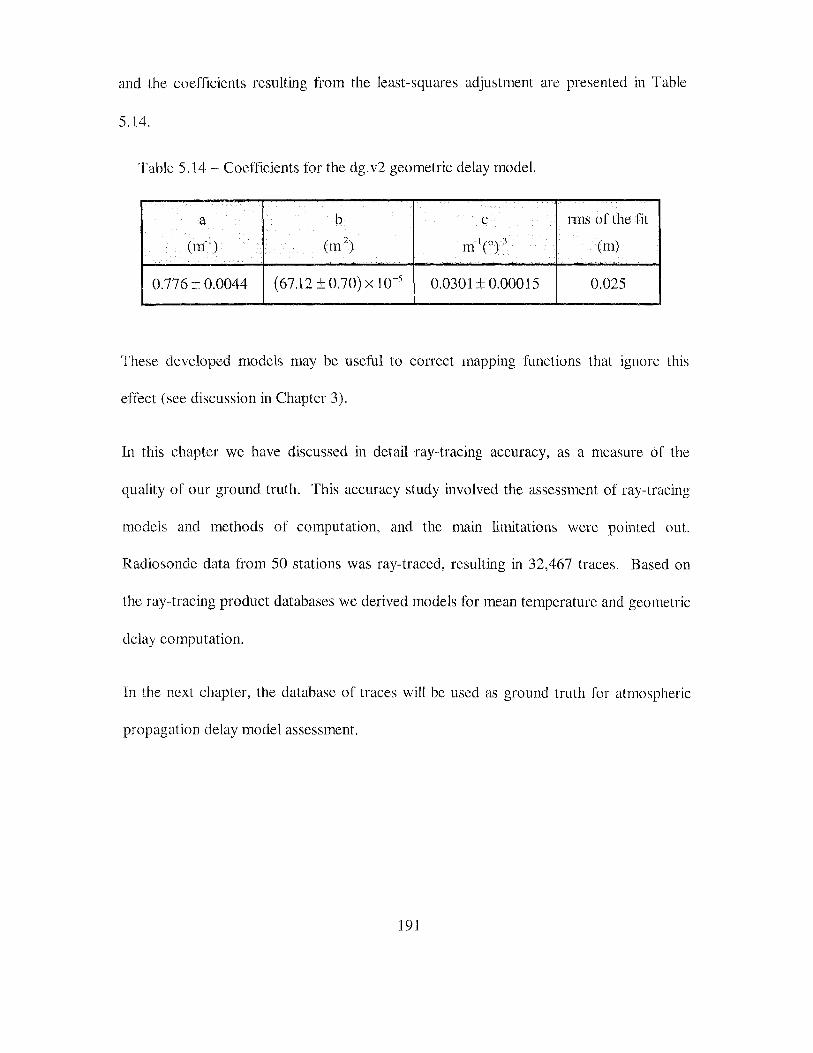
and the coefficients resulting fi·om the least-squares adjustment arc presented in Table
5.14.
Table 5.14 - Coefficients for the dg. v2 geometric delay model.
a b c rms of the fit
(rn-l) (m-2) m-lcor3 (m)
0.776 ± 0.0044 (67.12 ± 0.70) X 10-5 0.0301 ± 0.00015 0.025
These developed models may be useful to correct mapping functions that ignore this
effect (sec discussion in Chapter 3).
In this chapter we have discussed in detail ray-tracing accuracy, as a measure of the
quality of our ground truth. This accuracy study involved the assessment of ray-tracing
models and methods of computation, and the main limitations were pointed out.
Radiosonde data from 50 stations was ray-traced, resulting in 32,467 traces. Based on
the ray-tracing product databases we derived models for mean temperature and geometric
delay computation.
ln the next chapter, the database of traces will be used as ground truth for atmospheric
propagation delay model assessment.
191

This chapter presents the results of our assessment of atmospheric propagation delay
models against ray tracing. Fifty radiosonde stations covering a wide range of latitudes
and climate types were ray traced and a total of 32,467 benchmark traces was generated.
The assessment is performed for the zenith prediction models and mapping functions, and
separately for the hydrostatic, non-hydrostatic and total delays. A series of hybrid models
is also intercompared.
6.1. Methodology and nomenclature
The assessment methodology consists in evaluating the performance of the different
selected models and mapping functions against the ray-traced values obtained at the 50
radiosonde stations, which total 32,467 benchmark traces. As a rule, the models were
tested using the standard formulations specified by the authors. The general features of
each of the tested models were described in Chapter 3, which also presents the
mathematical formulation of selected zenith delay models. Additional mathematical
formulations for selected mapping functions are presented in Appendix II. For the sake
of simplicity, the models will be named in text after the author (or first author) of the
main reference, unless an acronym is provided by the author(s). In most cases, an
additional short code will be used to identify the models in graphs and figures.
192

When required, all models are driven by the standard meteorological parameters provided
by the radiosonde observations (P, T, e), and our databases of tropopause height,
inversion height, and lapse rate. As concerns the assessment of mapping functions, we
based our analysis on the differences of the projected delay and not of the "ratio" they
represent, as this is a more abstract entity for discussion. Therefore we used the ray
traced zenith delay values as the quantity to be mapped, and we assume those values
errorless (obviously an erroneous assumption with no consequences in this analysis).
The accuracy of a model will be evaluated in terms of its bias, rms scatter, and total error.
The bias ( 8) corresponds to the difference between the predicted value given by the
model and the ray-traced value (model minus trace). The rms scatter (cr) corresponds to
the standard deviation of the differences or rms scatter about the mean value. We will
use this term to be in agreement with other authors. For ranking purposes, we will define
the total error (s) of a model as
(6.1)
A series of tables presenting the bias and rms scatter for each model is electronically
available as an appendix to this dissertation (http://mat.fc.ul.pt/eg/lattex/PhD~e_sup.
html), but in order to facilitate the discussion of the analysis, a series of graphs will be
presented. A station-by--station intercomparison analysis for most of the models will be
represented in series of error bar plots (as a function of the radiosonde station latitude),
whereas box-and-whisker plots will be used to assess the global accuracy. The statistical
quantities represented in box-and-whisker plots are: median and mean (thinner and
193

thicker lines inside the boxes, respectively), 25t11 and 75th percentiles (vertical box limits),
lOth and 90111 percentiles (whiskers), and 5111 and 95th percentiles (open circles).
6.2. Zenith hydrostatic delay prediction models
Four different zenith hydrostatic delay models were selected for accuracy assessment (see
Table 6.1).
Table 6.1 - Names and codes for the tested zenith hydrostatic delay prediction
models.
. .. Model name Reference Code
Baby Baby et al. [1988] BB_ZH
Hopfield 1 Hopfield [ 1969] HO_ZH
Rahnemoon Rahnemoon [1988] RA_ZI-I
Saastamoinen Saastamoinen [1973] SA_ZH
·:The equivalent height was computed as in Hopfield [1972].
As mentioned in Chapter 3, the zenith hydrostatic delay is essentially a function of the
surface (station) pressure, with theoretical expressions similar in the case of the "dry" and
"hydrostatic" formalisms (except for the molar mass used):
(6.2)
The differences between models of this type include the gravity modeling strategy and
choice of the K1 refractivity constant. This is the case of the Saastamoinen and Baby
models. The two other models were chosen because they represent clear alternative
approaches.
194

Figure 6.1 shows a box-and-whisker plot for the differences (model minus trace) with
respect to ray tracing.
0.010
. ---1 ]: 0.005 ill I u ·j
ro ~ riJ
0.000 ;::l .8 s a) "d 0 -0.005
::E
-0.010 +------~ :r: ~ ~I N
I co' o' 01 "' :r: rJ]
Figure 6.1 - Box-and-whisker plot for the differences between the zenith
hydrostatic delay prediction models and ray tracing (model minus trace).
This global analysis shows clearly an outstanding performance of the Saastamoinen
model, which has submillimetre bias and submillimetre rms. The other models show
biases of 3-4 mm and rms scatter of 2-4 mm (see Table 6.2).
Table 6.2 -- Accuracy assessment for the zenith hydrostatic delay prediction
models, based on the total number of traces.
Bias 0.1 mm 3.6mm 3.8mm 3.3 mm
Rms scattet~·. · .•• : 0.2 mm 2.3mm 2.8 mm 3.9mm .. · ..
Total error' "n 0.2mm 4.3mm 4.7mm S.lmm
The evaluation of each model is better understood by analyzing its performance at each of
the radiosonde stations (Appendix VI). A residual latitudinal effect is clear for all
195

models, even though it may be considered insignificant for the Saastamoinen model (note
that the latitude is used as an input parameter in this model).
The visible latitude signature seen for the Hopfield model might be explained by partial
contributions of an inadequate value of the equivalent dry height, unmodeled gravity
variations, and variations of the molar mass of moist air (note that the Hopfield model is
based on a "dry/wet" formalism). The rms scatter is nevertheless not much different from
the expected, as Hopfield [ 1972] quotes values of 1-2 mm. Although less visible, the
Hopfield model shows also an additional mismodeling of station height, a fact that is also
shared by the Rahnemoon model.
The Baby model performs much like the Hopfield model in terms of mean bias, but shows
arms comparable to Saastamoinen. The results are in agreement with the ones obtained
in the comparison carried out by Baby et al. [ 1988]. In their study, biases as high as 6.1
mm were obtained, but the data set was much smaller than the one used in this study.
Even though the Rahnemoon model is the most complex, as it requires numerical
integration, its performance is exceeded by all of the other models in analysis. The mean
bias is similar to Baby and Hopfield for medium and high latitudes, but shows always the
largest rms scatter, which is likely an indication of unmodeled seasonal variations of the
delay. This high rms scatter was also seen in the comparison study against ray tracing
performed by Rahnemoon [1988].
Overall the models analyzed tend to over-predict the zenith delay, except for low
latitudes. The rms scatter is generally smaller at low latitudes (where the surface pressure
196

variation is also very small) and increases towards the high latitudes. The Saastamoinen
performance is extremely good for all the analyzed radiosonde stations and it is therefore
expected that this model will provide very accurate predictions of the zenith hydrostatic
atmospheric delay. The precision of the predictions is essentially a function of the
precision of the surface pressure measurements, as the model is not very sensitive to
errors in latitude and height, as confirmed in the sensitivity analysis shown in Table 6.3.
Table 6.3 -Expected error in the zenith hydrostatic delay (applied to the Saastamoinen
model) due to random errors of the input parameters, for different scenarios.
p <p H <Jp (j<p (jH (j z dh
1020 hPa 45° 10m l hPa 10 1m 2.3mm
1020 hPa 45° 10m 1 hPa 10 100m 2.3 mm
1020 hPa 45° 10m 0.5 hPa 10 lm 1.2mm
1020 hPa 45° 10m 0.5 hPa 10 100m 1.2mm
6.3. Zenith non-hydrostatic delay prediction models
For this analysis we selected a total of 12 models (see Table 6.4), a selection that
embodies an interesting range of approaches in zenith non-hydrostatic (and wet) delay
prediction, both regarding theoretical background and parameterization.
Despite the heterogeneity of models, the global analysis of the total number of differences
illustrated by the box-and-whisker plot shown in Figure 6.2 reveals an interesting feature:
with exception of the Berman 74, Berman TMOD, Callahan, and Chao models, all the
models show comparable rms scatter about the mean ( -3 em), with Saastamoinen,
197

Hopfield, Rahnemoon and Ifadis performing slightly better. As regards the bias, the best
global performance is attained by the Chao, Baby I, and Ifadis.
Table 6.4- Names and codes for zenith non-hydrostatic delay prediction models.
Model Name Reference Code
Askne Askne and Nordius [1987] AN_ZW
Baby 1' Baby et al. [ 1988] BBI_ZW
Baby 2t Baby et al. [ 1988] BB2_ZW
Berman 70 Berman [1976] B70_ZW
Berman 74 Berman [ 1976] B74_ZW
Berman TMOD Berman [1976] BTM_ZW
Callahan Callahan [ 1973] CA_ZW
Chao Chao [ 1973] CH_ZW
Hopfield Hopfield [ 1972] HO_ZW
If ad is Ifadis [ 1986] IF_ZW
Rahnemoon Rahnemoon [1988] RA_ZW
Saastamoinen Saastamoinen [ 1973] SA_ZW
'Baby 1 = "theoretical" version; Baby 2 = "semi-empirical" version.
The ranking of the functions based on their absolute mean bias and total error is
represented in Figure 6.3. This figure shows clearly that the differences between the
models are primarily in the mean bias; the differences concerning the total error are
minimum. The differences obtained for the models are in fact highly correlated; if we use
the Saastamoinen model as reference, for example, we will find correlation coefficients
ranging from 0.86 (for Berman TMOD) to 0.99 (for Rahnemoon).
198

0.10
s <l.l 0.05 u ('j
~ (/)
0.00 ::J >::: '§ ......
<l.l -0.05 "d 0 ~
Figure 6.2 - Box-and-whisker plot for the differences between the zenith non
hydrostatic delay prediction models and ray tracing (model minus trace).
A station-by-station analysis (see Appendix VII) reflects very much this coincidence,
which can be explained by the fact that all models depend strongly on the water vapor
pressure, a highly variable quantity. Even the more complex models, such as Rahnemoon
and Askne, achieved no better performance than simple models, such as Saastamoinen.
The relatively poor performance of all models is a clear warning of the weakness of the
zenith non-hydrostatic delay prediction based on surface meteorological measurements.
The equatorial and tropical regions are clearly the most problematic, likely due to high
and variable water vapor content in the atmosphere. The Berman 74, Berman TMOD,
Callahan and Chao perform particularly unsatisfactorily in these regions, with a clear
over--prediction of the delay. The best predictions are obtained by Hopfield, Ifadis,
Rahnemoon, and Saastamoinen, except for the radiosonde stations FOR (Fortaleza,
Brazil) and BLB (Balboa, Panama), which are quite troublesome for most of the models.
199

BTM __ zw CA zw
~-
B74 zw -
BB2_ZW
HO zw -
AN __ zw
SA ___ zw B70 zw --
IF zw --
BBl zw -CH zw --
0 5 10 15 20 25 0 2 3 4
Mean bias (mm) Total error (em)
Figure 6.3 - Ranking of the zenith non-hydrostatic models by absolute mean bias
(left) and total error (right).
5
Although the mid- and high-latitude regions show a marked seasonal variation of the
zenith non-hydrostatic delay, they are characterized by a small water vapor content and
practically all the models show comparable performances.
With such a wide choice of candidates exhibiting similar levels of accuracy, the most
adequate choice seems to be the one that combines minimum bias and simplicity, and that
depends on the minimum number of parameters, to avoid error propagation due to
measurement errors. Model complexity is the main handicap for choosing Rahnemoon,
whereas the lack of suitable information on temperature lapse rates may make Askne,
Baby I, Berman 70, and Chao also inconvenient. It is important to note that we have
only tested global versions of the models; Askne, Baby 2, and Ifadis models can be tuned
to a particular location or season. However, even admitting that the tuned versions may
lead to a reduction of the mean bias, a reduction of the rms scatter is very unlikely (see
also Ifadis [1986], Baby et al. [1988], and Mironov et al. [1993]).
200

In addition to the fact that Ifadis and Saastamoinen showed the best global accuracy, they
are also characterized by simplicity. Notwithstanding the Ifadis requirement of surface
pressure as an input parameter, this is no real issue as the model is not very sensitive to
changes in pressure, as shown by the error propagation analysis presented in Table 6.5.
In cases where the user relies totally on the use of models to predict the zenith delay, the
combination of the Saastamoinen hydrostatic with its non-hydrostatic counterpart may be
advantageous, yielding a more consistent zenith delay prediction.
Table 6.5 -- Propagated error in the zenith non-hydrostatic delay prediction due to
random errors of the input parameters, applied to Saastamoinen (SA) and lfadis
(IF).
p T e O'p crT O'e O'dz (SA) O'dz (IF) nh nh
1015 hPa 288.15 K 20 hPa 1 hPa 0.5 K 1 hPa 10.0 mm 9.9 mm
1015 hPa 288.15 K 30 hPa 1 hPa 0.5 K 1 hPa 10.0 mm 9.9mm
6.4. Zenith total delay models
In some zenith delay models, a separation between the two components of the delay is
not performed and a prediction of the zenith total delay is carried out instead. Such a
procedure is quite frequent in development of models designed for airborne applications
("navigation" models). We have selected some models of this type to be intercompared
with four "geodetic" models (Baby, Hopfield, Rahnemoon, and Saastamoinen); in this
case, the predicted zenith total delay is obtained by adding the contribution of the
201

hydrostatic and non-hydrostatic components. The set of models analyzed is listed m
Table 6.6.
Two versions for the Altshuler model were tested: in the first version (Altshuler 1) the
refractivity is computed using the surface meteorological parameters measured by the
radiosonde; the second version (Altshuler 2) computes the refractivity using the
formulation presented by the authors, which is based on the user's latitude and month of
year.
Table 6.6- Codes for zenith hydrostatic delay models.
'
Model Name Reference ,,Code
Baby 2' Baby et al. [ 1988] BB2_ZT
Altshuler 1 Altshuler and Kalaghan [1974] ALl_ZT
Altshuler 2 Altshuler and Kalaghan [ 197 4] AL2_ZT
Hopfield Hopfield [ 1972] HO_ZT
NATO NATO [1993] NATO_ZT
STI Wachowski [1980] STI_ZT
WAAS DeCleene [ 199 5] WAAS_ZT
Brown Brown [ 1989] BR_ZT
Rahnemoon Rahnemoon [ 1988] RA_ZT
Saastamoinen Saastamoinen [1973] SA_ZT
:The non-hydrostatic model chosen for Baby is the semi-empirical.
The assessment of the models' accuracy for the total number of traces (see Figure 6.4) is
essentially characterized by a clear separation between the two groups of models, with
the navigation group performing poorly both in a relative and absolute sense.
202
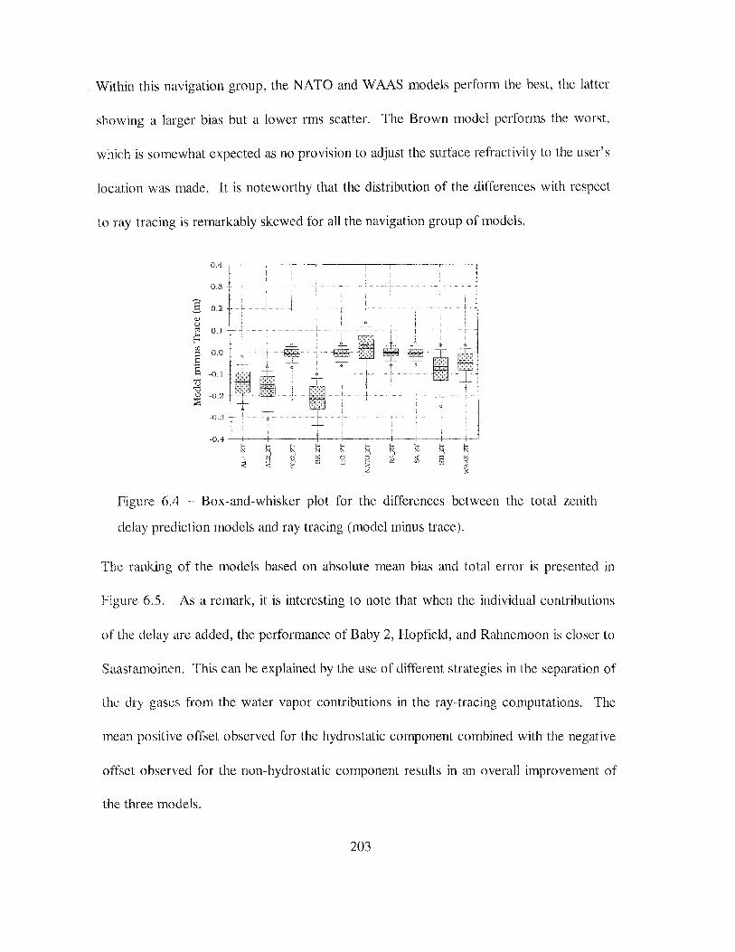
Within this navigation group, the NATO and WAAS models perform the best, the latter
showing a larger bias but a lower rms scatter. The Brown model performs the worst,
which is somewhat expected as no provision to adjust the surface refractivity to the user's
location was made. It is noteworthy that the distribution of the differences with respect
to ray-tracing is remarkably skewed for all the navigation group of models.
0.4
0.3
E: 0.2 Q)
~ 0.1 t-1::
~ ~ (fJ 0.0 ;:!
·§ =F ~
·-0.1 v "d 0 -0.2 ;;;
-0.3
-0.4
~'
Figure 6.4 - Box-and-whisker plot for the differences between the total zenith
delay prediction models and ray tracing (model minus trace).
The ranking of the models based on absolute mean bias and total error is presented in
Figure 6.5. As a remark, it is interesting to note that when the individual contributions
of the delay are added, the performance of Baby 2, Hopfield, and Rahnemoon is closer to
Saastamoinen. This can be explained by the use of different strategies in the separation of
the dry gases from the water vapor contributions in the ray-tracing computations. The
mean positive offset observed for the hydrostatic component combined with the negative
offset observed for the non-hydrostatic component results in an overall improvement of
the three models.
203

BR __ ZT
AL2 __ ZT !~!!!!!!!iii___;_____;___J ALl __ ZT=-~ STI __ ZT
WAAS_ZT
NATO~_ZT
BB2_ZT
SA_ZT
0 5 10 15 20
Mean bias (mm)
BR ___ ZT
AL2 __ ZT --~~~~~~~~~~---------____J ALl_ZT ~ STI_ZT-
NATO_ZT
WAAS_ZT -i
BB2_ZT J . :_] HO ZT .
:=:: f· J ~-~--+---'-----t---~-+--
25 0 5 10 15
Total error (em)
Figure 6.5 - Ranking of the zenith total delay models based on the absolute mean
hias (left) and total error (right), for the total number of differences.
If we observe the distribution of the mean differences at every radiosonde station (see
Appendix VIII), we conclude that the NATO model performs reasonably well at mid-
latitudes but degrades towards high and low latitudes. The W AAS model does not show
this latitudinal effect as much, but the model clearly under-predicts the zenith delay at
almost all the stations analyzed. In addition to the clear under-prediction of the delay, the
Altshuler 2 model (Altshuler 1 and Brown are not shown in these detailed graphs) shows
an additional mismodeling of the station height, clearly observed as 'jumps" in the graph
of mean differences. The STI model is visibly biased in the equatorial and tropical
regions, but shows an acceptable performance level at high latitudes, with small mean
offsets.
We therefore conclude that all the navigation models have clear limitations in predicting
the zenith delay, with serious implications in precise positioning. However the prediction
204

of the zenith delay for airborne applications is a rather complex problem, as
meteorological data to be used with the geodetic models is rarely available. This
difficulty can be somehow mollified by assuming average profiles, an approach that has
been investigated recently (see, e.g., Collins and Langley [1996]; Collins et al. [1996]).
6.5. Hydrostatic mapping functions
As in the case of the atmospheric zenith delay models, some mapping functions do not
map separately the two components of the atmospheric delay. Usually we are interested
in modeling the elevation dependence of the total atmospheric delay, but certain
applications may require independent modeling of each component. As an example, if a
WVR is used to estimate the non-hydrostatic component of the delay, we only need to
map the hydrostatic component. Keeping in mind these possible applications, we will
briefly discuss the hydrostatic and non-hydrostatic mapping functions performance. A
more detailed analysis is carried out in Section 6.7, in the context of the total atmospheric
delay elevation dependence modeling.
The hydrostatic mapping functions to be analyzed are evaluated in a single version only
(for the cases where multiple functions have been published or multiple parameterizations
are possible), corresponding to the one expected to perform the best. Other options will
be discussed later. A total of twelve mapping functions have been analyzed (the
respective names and codes are listed in Table 6. 7). The model by Rahnemoon [ 1988]
will not be included in this discussion, as breaking the model into the zenith delay
components and corresponding mapping functions would constitute in our opinion a
205
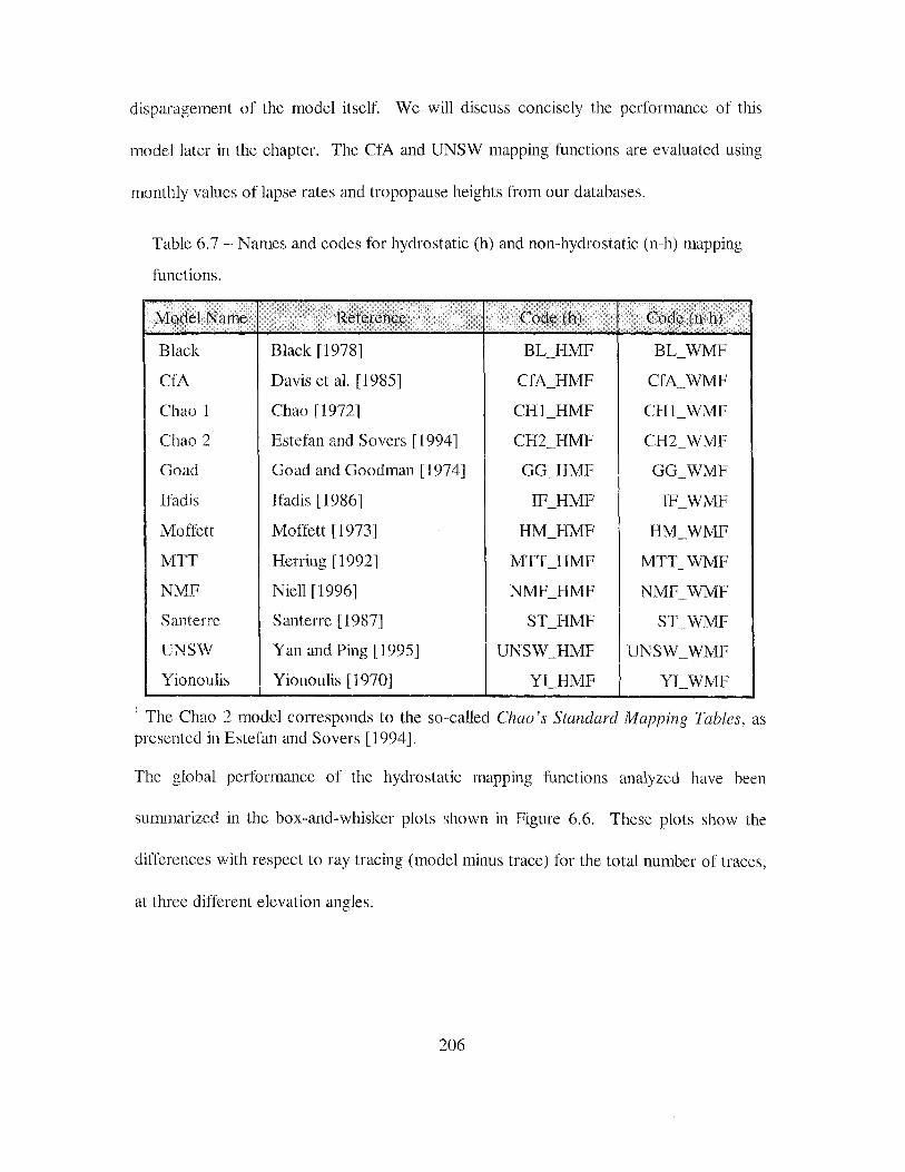
disparagement of the model itself. We will discuss concisely the performance of this
model later in the chapter. The CfA and UNSW mapping functions are evaluated using
monthly values of lapse rates and tropopause heights from our databases.
Table 6.7 -·Names and codes for hydrostatic (h) and non-hydrostatic (n-h) mapping
functions.
Model Name ' ':, ..
-- ,_ Code (h) Code (n~h) Reference ... -· . ·-- . .'',
Black Black [1978] BL_HMF BL_WMF
CIA Davis et al. [ 1985] CfA_HMF CfA_WMF
Chao 1 Chao [1972] CHI - HMF CHl_WMF
Chao 2i Estefan and Savers [ 1994] CH2_HMF CH2_WMF
Goad Goad and Goodman [1974] GG_HMF GG_WMF
Ifadis Ifadis [ 1986] IF_HMF IF_WMF
Moffett Moffett [ 1973] HM_HMF HM_WMF
MTT Herring [ 1992] MTT_HMF MTT_WMF
NMF Niell [ 1996] NMF_HMF NMF_WMF
Santerre Santerre [ 1987] ST_HMF ST_WMF
UNSW Yan and Ping [ 1995] UNSW_HMF UNSW_WMF
Yionoulis Yionoulis [ 1970] YI_HMF YI_WMF
' The Chao 2 model corresponds to the so-called Chao's Standard Mapping Tables, as presented in Estefan and Savers [ 1994].
The global performance of the hydrostatic mappmg functions analyzed have been
summarized in the box-·and-·whisker plots shown in Figure 6.6. These plots show the
differences with respect to ray tracing (model minus trace) for the total number of traces,
at three different elevation angles.
206

.,., g '7:1 ::::: aq" 0.. '0 ;::: w '0 >-; 0 s· (!)
,.-.._ (Jq 0\ o"
"" 0 :=" ,....,. ,.....
;:l I 0 (") g ,....,. ...... to 0 (!) ;:l 0 - (FJ >< (il I
< .,., .,., .,., ;:l ::::: ...... 0.. 0.. ...... I 0 >-; ~ ::::: .,.,
.,., <...:::; ::;' ...... ;:l ,....,. (FJ
(Jq >-; ~ - ~ (!) (il >-; (FJ s·
'0 (Jq -,.-.._ 0 a ...... 0 8'
N 0.. >-; (!) 0 - ...... -...l §.
::;' (!)
::::: 0.. ;::: (FJ ~ ..... (!) >-; >-;
~ (!) ;:l
(il (") '--' (!)
(FJ
8' o" >-; (!) - ...... 0 ~
0 (!) (!) ,.-.._ ;:l .....
0 ..... '0 ::;' '--' (!)
0\ ::;' 0 <...:::;
,.-.._ 0.. §. >-;
0 0.. (FJ .....,. 0.. .,., - ...... (il ()" '--'
0
BL_HMF
CfA_HMF
CHl_HMF
CH2_HMF
GG_HMF J
"::t MTI_HMF T NMF_HMF T.
Model minus Trace (m)
0
"' 0 0
0 Ol
0~---·
+il+···
0
"':::j ... .... . .;~~~····: YI_HMF t ... -~- f--ID-1 ol
'
Model minus Trace (m)
0
"' 0
,:, Ol
0 0 0
0
Ol t' ' ' = t: ··~~.~ ~;~--~ ,. CHI_HMF r- ·----------------; --- --
0
f:5
·::r=--=·~~~-~ IF_HMF t · · ·1!Itr ...... . --1·
MTCHMF +-- --- --- -~HI+ -------- -
N:~:::t+ - •l~••f{l}l~-- •• lf UNSW.HMF · ···· ... of-ilto- .. .. ~ .. :·--······ ...
Yf_HMF . - --- -- _,______ -----.. ---4-~ ~------ l
0 0
Model minus Trace (m)
0 0 "'
0 0 0
0 0 "'
0
0
eu••t - -~ ·~· 1 CfA_HMF ·· .............. -+IJ1o ........... . .... ~
CH!HMF I ~ I . T ., "", -·- - ··-J
-~~1. ~-~--~~ MTI.HMFt·· ....•
1\MF HMF- -------- --- - -1fto t . .. =- ;:-11!11 I T- -----------0-
f
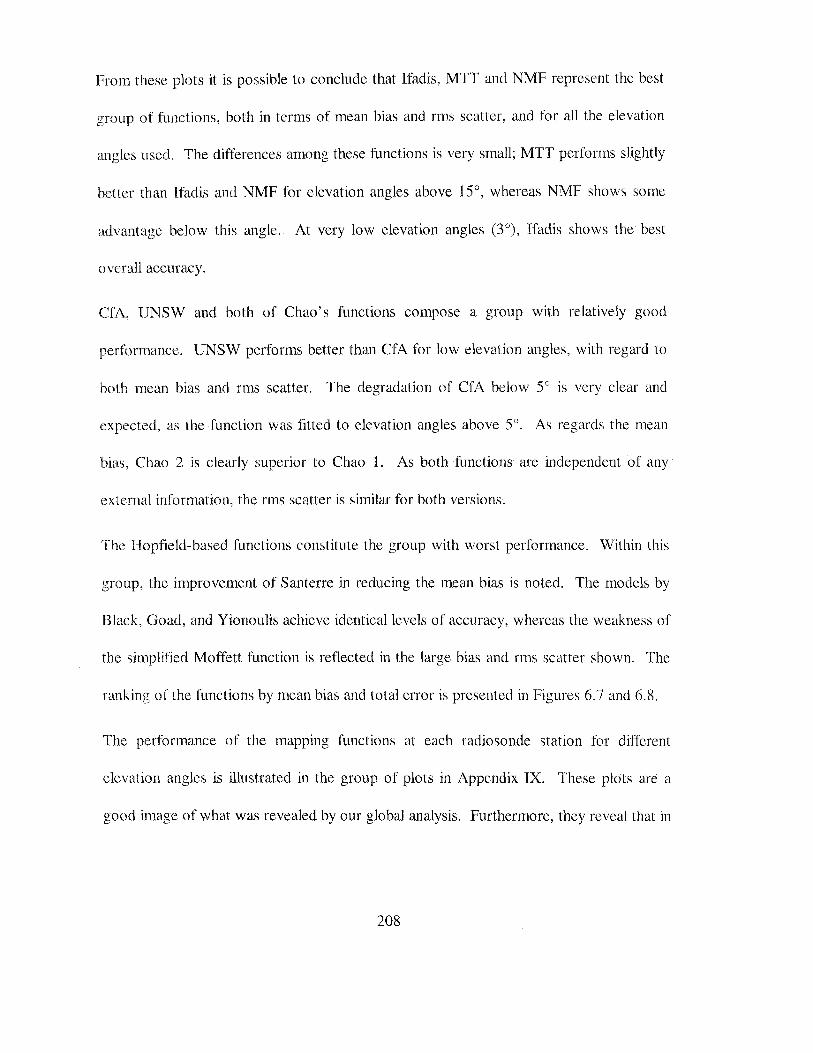
From these plots it is possible to conclude that Ifadis, MTT and NMF represent the best
group of functions, both in terms of mean bias and nns scatter, and for all the elevation
angles used. The differences among these functions is very small; MTT performs slightly
better than Ifadis and NMF for elevation angles above 15°, whereas NMF shows some
advantage below this angle. At very low elevation angles (3°), Ifadis shows the best
overall accuracy.
CfA, UNSW and both of Chao's functions compose a group with relatively good
performance. UNSW performs better than CfA for low elevation angles, with regard to
both mean bias and rms scatter. The degradation of CtA below 5° is very clear and
expected, as the function was fitted to elevation angles above 5°. As regards the mean
bias, Chao 2 is clearly superior to Chao 1. As both functions are independent of any
external information, the nns scatter is similar for both versions.
The Hopfield-based functions constitute the group with worst performance. Within this
group, the improvement of Santerre in reducing the mean bias is noted. The models by
Black, Goad, and Yionoulis achieve identical levels of accuracy, whereas the weakness of
the simplified Moffett function is reflected in the large bias and rms scatter shown. The
ranking of the functions by mean bias and total error is presented in Figures 6.7 and 6.8.
The performance of the mapping functions at each radiosonde station for different
elevation angles is illustrated in the group of plots in Appendix IX. These plots are a
good image of what was revealed by our global analysis. Furthermore, they reveal that in
208

general the worst performance of most of the functions happens at high and low latitude
stations, as well at high altitude stations.
The importance of these plots is also evident in analyzing certain trends that were not
revealed previously, as in the case of the Chao functions. Despite the reasonable
performance in terms of total error, the Chao functions show a very clear trend for the
mean bias (the best performance of Chao 1 and Chao 2 are at mid-latitudes, and degrade
rapidly towards lower and higher latitudes). By way of illustration, at 10° elevation angle
the peak-to-peak variation of the mean bias for these functions is greater than 3 em, much
larger than that achieved by UNSW, for instance ( -1 em), which ranks lower than Chao 1
regarding the total error.
209

HM_HMF I fA;;;rA UNSW_HMF
IF __ HMF
NMF_HMF
MTT __ HMF
0 2 4 6 8 Mean bias at 30" elevation angle (mm)
~------------------------:=:: r;:; 17' .. : -GG __ HMF !!!~!~~~-
UNSW __ HMF t::::f ST ___ HMF
CHl_HMF
CfA_HMF
CH2_HMF
MTT_HMF
HM_HMF
YI __ HMF
GG_HMF
BL_HMF
ST __ HMF
CHl __ HMF
CfA_HMF
CH2 HMF ·-
UNSW __ HMF
MTT_HMF
IF __ HMF
NMF_HMF
0 2 3 Mean bias at 15" elevation angle (em)
; ; I
=-~ 0 6 12 18 24
Mean bias at 6" elevation angle (em)
CHl_HMF ..... ' ·:·. I YI _HMF
GG_HMF ::'ii,·;;:::::;;;: .. : :-::· :::
BL_HMF
ST HMF -CH2 - HMF • IF - HMF ~ NMF - HMF I
CfA_HMF
MTT HMF -
0 3 6 9 12 Mean bias at 20" elevation angle (mm)
:=:: r:t-:rr·-BL __ HMF ·!!!!!~·· ST __ HMF
CfA_HMF
UNSW_HMF
CH2_HMF-
IF_HMF
CHl_HMF
MTT_HMF
NMF_HMF
0
--~---+-----~---1---~-----···
3 6 9 Mean bias at l 0" elevation angle (em)
YI_HMF
GG_HMF
BL_HMF
CfA __ HMF
CHl_HMF
CH2_HMF
HM_HMF
MTT_HMF
NMF_HMF
IF_HMF
0 16 32 48 64
Mean bias at 3" elevation angle (em)
Figure 6.7- Ranking of the hydrostatic mapping functions by absolute mean bias.
210

UNSW_:_HMF
1;-;;;;;;;;fr:::::~~~-~-~~~~·-CHl_HMF
HM_HMF
YI __ HMF !!!!r GG_HMF ~··· BL_HMF jl
CfA_HMF
ST_HMF
CH2_HMF
IF __ HMF
NMF_HMF
MTT_HMF
0 2 4 6 8 Total error at 30° elevation angle (mm)
HM_HMF
YI HMF --
BL HMF -
GG __ HMF
ST HMF -
UNSW __ HMF
CHl HMF -
CH2 HMF -CfA_ HMF
IF HMF ·-
NMF HMF -
MTT HMF -- f----
0 2 3
Total error at 15° elevation angle (em)
HM_HMF
YI HMF -· GG HMF -
BL HMF -ST __ HMF
CHl HMF -
CH2 HMF --
CfA_HMF
UNSW HMF -
MTT_ HMF
NMF HMF -
IF HMF -
0 10 20
Total error at 6° elevation angle (em)
HM_HMF
UNSW_HMF-
CHl_HMF YI __ HMF
GG_HMF
BL_HMF
ST_HMF
CH2_HMF
IF_HMF
CfA_HMF
NMF_HMF
MTT_HMF ~-4-~--4--~---4
0 3 6 9 12 Total error at 20° elevation angle (mm)
HM_HMF
YI __ HMF
GG HMF -
BL __ HMF
ST HMF --
CfA_ HMF
CH2 HMF -CHl HMF -
UNSW_HMF
MTT HMF -
IF _HMF
NMF HMF -
0 3 6 9 Total error at 10" elevation angle (em)
YI_HMF -;;;;;;;;;l GG_HMF i! BL_HMF
CfA __ HMF !!!!!!!!!!!!!!f CHl __ HMFe~
ST_HMF
CH2_HMF
HM_HMF
UNSW_HMF
MTT_HMF
NMF_HMF
0 20 40 60
Total error at 3° elevation angle (em)
Figure 6.8- Ranking of the hydrostatic mapping functions by total error.
211

6.6. Non-hydrostatic mapping functions
The distribution of the differences with respect to ray tracing for the non-hydrostatic
mapping functions is illustrated in the box-and-whisker plots of Figures 6.9. We have
restricted these plots to elevation angles below 1 oo, as the differences for elevation angles
above 10° are very small (mean bias and rms scatter less than -2 mm, for an elevation
angle of 15°, as an example).
From the analysis of these plots, we conclude that the non-hydrostatic mapping functions
can be grouped according to their performance into three major classes. As in the case of
the non-hydrostatic functions, the Ifadis, MTT, and NMF functions are superior to any of
the others, both regarding mean bias and rms scatter.
The worst group is constituted by CfA and UNSW. This is explained by the fact that
these mapping functions were not designed to map the non-hydrostatic component of the
atmospheric delay (although this is not totally clear in Yan and Ping [ 1995], such has
been confirmed [Yan, 1998]). Both Chao versions and all the Hopfield-based functions
show identical mean bias, except at 3 o elevation angle, for which a greater dissimilarity
between functions is observed. As a remark, it is interesting to notice the good
performance of Moffett, in contrast to the poor quality of its hydrostatic counterpart.
The box-and-whisker plot also warns about the skewness of the residuals' distribution.
This fact is easily understood if we analyze the behavior of the functions at each
radiosonde station separately, shown in the series of plots of Appendix X.
212

w g '"l'j 0 aq'
/"""'._ '"d c u '"d '""! 0 ::r 0 .-.. ....... ao 0\ 0 :3 2' \o
'-.../ ::::; (j) 0 I (p' .-.. < s· to P:> ::::;
0 ...... [/]
s· P:> >< I ::::; ::::; P:>
P:> 0... ::::; 0... ::::; '""! I ao ~ ~ -(j) ....... :::;' [/]
'""! ::;;;· P:> r;-0 G ::r '""!
l3L_WMF
ao '"d /"""'._
:3 0 0
....... 0... 8' ~
'""!
N ..... ::::; ....... >-' s· :::;' w c (j)
GG_WMF
HM_\VMF [/]
....... 0... '""!
~ P:> 0 (j) (j) '""!
'-.../ (j) MTIWMF
lF_WMF
. ::::; 8' 0
(j) NMF~WMF
'""! [/]
........ u 0 (j) 0 ....... UNSW_WMF
ST_WMF
/"""'._ ~ ....... 0 (j)
'"d (j)
'--' ::::; YI_WMJ<'
0\ ::::; 0 0
/"""'._ ::::;
§. I
:::;' '-< 0... 0... 0... '""! - 0 (D
'--' (/) ....... P> P> ::::; ....... 0... (=)'
Model minus Trace (m) Model minus Trace (m)
6 0 0 0 0
Cl1 "' 0 t-o '" 0 '" 0 Cl1 0
0 6
"' 0 0
0 0 0 m o m
0
"' BL WY!F i . --- ·- ·-- -·-4{[1}----+ -•-- 1 CfA~WMF L r--------0:0-+ ·--··-·
I ~WL__j • _l. Clll_WMF ~·- -------- --~
Cl!2 WMF' I -----'' ·+ ···4ffil I • HM_WMF~·-
IF_WMF f-· · -·-- ----.. 411+
~_WMFt ~· i NMF_WMF t·- ·-·-.. 11•- i'
ST _ WVI F --------- - - c-KJI]----1---o-.
UNSW_WM. J 1---IIE!ili+ 00
• ···."
YI_WMF l tEtl.}------1 .. ~
CfA_WMF
CHl_\VMF
CH2_WMF
GG_WMF
HM_\VMF
IF_WMF
MTI_WM:F
t\:MF_WI\tlF
ST_WM:F
UNSW_WY!.F
YI_WMF
6 0
""
Model minus Trace (m)
6 0
"' 0 0 0
0 c "'
0 0 ""

These plots show that all functions show larger bias and rms scatter at low latitudes,
which is a result of the higher water vapor content and variability associated to these
regions.
The ranking of the non-hydrostatic mapping functions by absolute mean bias and total
error are also presented in Figure 6.10 and Figure 6.11, respectively. The plots shown in
these figures clearly illustrate the good performance of the group Ifadis, MTT and NMF
functions and the poor performance of the two functions due to the error introduced in
using these hydrostatic functions in mapping the non-hydrostatic component also. The
remaining functions have very similar performances.
214

YI_WMF --~--l UNSW~WMF ', ;;;;::::----------··---· UNSW~WMF ~ CfA~WMF
GG_WMF
BL_WMF
ST_.WMF
NMF __ .WMF
MTT~WMF
IF~WMF
0 2 Mean bias at 30" elevation angle (mm)
UNSW_.WMF ~;;;;;:::::·~ CfA_WMF ·~ YI~WMF
BL._WMF !~~~!"""' GG __ WMF
CHl_WMF 1;;;; ST~WMF
liM._WMF
CH2. __ WMF
NMF __ WMF iL--~---+----~--1·---~---0 2 4 6 Mean bias at 15" elevation angle (mm)
MTT __ WMF J NMF __ WMF ~-~--+-~- f--~-------t-~-
0 13 26 39 52
Mean bias at 6" elevation angle (mm)
CfA~WMF
YI~WMF
GG~WMF !!!!--'--' BL._WMF ~-<::::n~:i.l ST __ WMF ·
CH2~WMF
CHl~WMF
HM~WMF
IF~WMF I MTT~WMF ~ NMF __ WMF
0 2 3 Mean bias at 20° elevation angle (mm)
UNSW._WMF
CfA~WMF
YI~WMF I CHl~WMF-
BL~WMF ·:c:' ::::,::: I GG~WMF
ST~WMF
HM~WMF
CH2~WMF I IF~WMF
~ MTT~WMF
NMF~WMF I 0 5 10 15 Mean bias at 1 0" elevation angle (mm)
~::==~ ;;;-;-;r;-;;;;~;-;-;-;·-:-:·==~----~ YI_WMF
c=~=:~ f~~~-~ :<~~~~·-·~::-~,--~-~-~~~~~~.!~ GG~WMF
ST~WMF
CH2~WMF
HM~WMF I
IF._WMF -~ MTT~WMF l_l
NMF ~WMF L~--~-----~~----t--~"---1---~ 0 6 12 18
Mean bias at 3" elevation angle (em) 24
Figure 6.10 -·- Ranking of the non-hydrostatic mapping functions by absolute mean
bias.
215

YI __ WMF ;;;;::=----~ CfA_WMF
GG __ WMF
BL __ WMF
ST_WMF
CH2_WMF
HM_WMF CHl ___ WMF
NMF_WMF
MTT __ WMF
IF __ WMF f"-~~~~~-t~~~~
0 1 2 Total error at 30° elevation angle (mm)
UNSW_WMF
CfA_WMF
YI_WMF
GG_WMF
BL __ WMF
CHl_WMF
ST_WMF
HM_WMF
CH2_WMF
NMF_WMF
MTT_WMF
IF_WMF
' : .....
~ .. 0
.. :n;;;;;:;y::,i"
.<J+t :-1-A
;;;)!i!iifil
2 4 6 Total error at 15° elevation angle (mm)
UNSW_WMF -;;;;;;:::~ CfA_WMF!
YI_WMF ;··:;,: ·, · ,i: .!'"!
CHl __ WMFif BL_WMF
GG_WMF
ST._WMF
CH2_WMF
HM_WMF •Wi!!:•· I NMF_WMF
IF_WMF
MTT_WMF = F·=--~--1--L----+--~-~
UNSW __ WMF ,;;;~~~~===~~~~~~~l CfA_WMF 1 YI_WMF . '"'":''''i'r·:•:.,;.:. ,_.,.,, ..• ,.,, •. ;,..! GG_WMF
BL_WMF
ST_WMF
CH2_WMF
CHl_WMF
HM_WMF - : ;.:·;:<ifF:ii :,:;.1
NMF_WMF •
MTT_WMF ~
IF __ WMF ·F---~~~-t-~~-~--f--~~~--0 2 3 Total error at 20° elevation angle (mm)
UNSW_WMF ~;;;;;;;;;;;;;;;:::::::::::::====~-, CfA __ WMF 1 YI_WMF 1!1"'• :C"!l:;iti: !•;
CHl_WMF
GG_WMF _,·; ; !1!!!'-i d
BL_WMF
ST_WMF
HM_WMF
CH2_WMF ! "'·!::: : ·;·;::; :. •i' <
NMF_WMF.
IF_WMF.
MTT_WMF. i="--~~~---~~--+------'------41-~~~-
0 4 8 12 16 Total error at l oo elevation angle (mm)
~::=::; ;;;;;;;;;;;;;--;·;-;-;-;·-;-:::::r·~ YI_WMF
BL_.WMF !ilr CHl_WMF
GG_WMF
ST_WMF
CH2_WMF
HM_WMF
NMF_WMF
IF_WMF
0 20 40 60 0 10 20 Total error at 6° elevation angle (mm) Total error at 3° elevation angle (em)
Figure 6.11 - Ranking of the non-hydrostatic mapping functions based on the total
error.
216

6.7. Total mapping functions
The group of mapping functions that model the elevation dependence of the atmospheric
delay is significantly larger than the group that allows a separate modeling of its
components. Moreover there are mapping functions that can be driven using different
input settings, which permits an adjustment to local conditions. Examples of mapping
functions of this type are the ones developed by Lanyi [1984], Davis et al. [1985], and
Y an and Ping [ 1995]. In order to systematize our analysis we chose therefore to initially
evaluate the accuracy of these functions under different input strategies and select the
best versions for intercomparison assessment with other mapping functions.
The CfA and UNSW mapping functions were tested under three different inputs for
tropopause height and lapse rate: a) monthly mean of our databases at each radiosonde
station; b) global default values suggested by the authors for these parameters, 11.231 km
and 6.5 K km-1, respectively c) predictions given by our models (UNB98TH1 and
UNB98LR1 ), using the surface temperature of radiosonde soundings. The code names
for these "versions" are presented in Table 6.8. The global performance of the different
versions (for 10° and 6° elevation angles) is illustrated in Figure 6.12.
CfA's performance is clearly superior for the last strategy, as the rms scatter 1s
significantly reduced. In order to better understand this improvement, it is useful to
analyze the sensitivity of CfA to changes in tropopause height and lapse rate, presented in
Table 6.9.
217
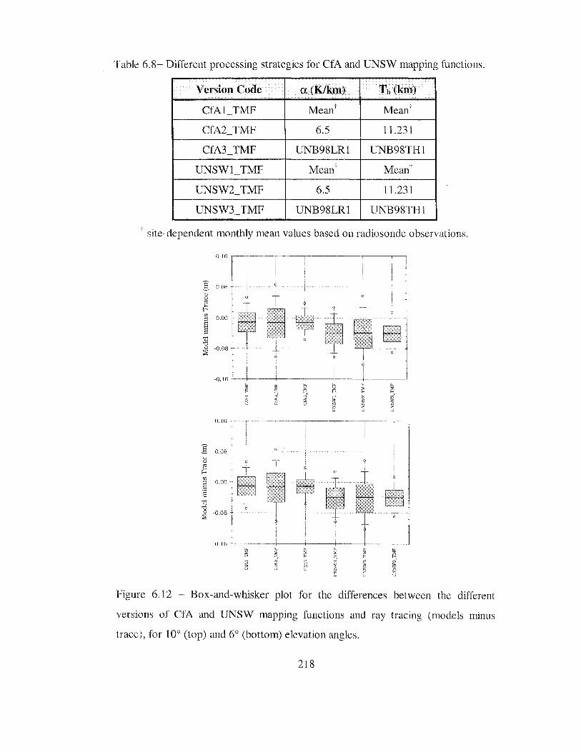
Table 6.8- Different processing strategies for CfA and UNSW mapping functions.
Version Code a (Kikm) Th (km)
CfAl_TMF Mean _,_
Mean
CfA2_TMF 6.5 11.231
CfA3_TMF UNB98LR1 UNB98TH1
UNSWl_TMF Mean -;- Meant
UNSW2_TMF 6.5 11.231
UNSW3_TMF UNB98LR1 UNB98TH1
' site-dependent monthly mean values based on radiosonde observations.
O.lO
§ 0.08 0 0 ro f:: if!
0.00 ::J .8 s 0) '1j 0 -0.08 ~
-0.16 0. 0. 0. "· 0. 0.
~' ~' ~' ~. ~. ~ '
~ ,; ~ ~ ~ ~ u "' 5 2 2 :0 :0
fl.lR
§ 0.08 --<J) u
"' CI f:: "' ::J 0.00- y .8 s 0) '0 0 -0.08 ~
-0.16 --+----~----+~ "' 0. " 0. "' " ~ ~. ~'
:,; "' ~
[-, f-<
~· ~ ~ :;; " "' " " u u u "' if) if) z 2 '" " u :0
Figure 6.12 - Box-and-whisker plot for the differences between the different
versions of CiA and UNSW mapping functions and ray tracing (models minus
trace), for 10° (top) and 6° (bottom) elevation angles.
218

Table 6.9 - Sensitivity of CfA to changes in lapse rate and tropopause height, for
an atmospheric zenith delay of 2.4 m (From Davis et al. [ 1985]).
-44 11
From this table, we conclude that changes in the lapse rate value will more likely affect
the high-latitude stations, as the differences with respect to the nominal value of 6.5 K
km-1 will be in most cases very significant. Despite the apparent lower sensitivity of CfA
to changes in tropopause height, the large variations of this meteorological parameter will
likely be responsible for the bulk of the variations between the different strategies. This
fact is corroborated by the plots presented in Figure 6.13.
From this figure, we can conclude that the improvement in performance for CfA (when
using site-specific values of tropopause height and lapse rate and, particularly, when
parameterized with the predictions for these parameters given by our models) is
especially considerable for low- and high-latitude stations. At low latitudes this
improvement is certainly due to the better modeling of the tropopause height, as the lapse
rates do not deviate significantly from the nominal value of 6.5 K km- 1• At high latitudes
both the changes in lapse rate and tropopause height are expected to contribute to this
improvement, as the nominal values are particularly high in both cases. At mid-latitudes
this improvement is marginal as far as the mean bias, but the reduction of the rms scatter
is still significant, and again better when our models are used.
219

8 0.04 ,,,-,,..,-,,-., ,,,,,,,,,-~~~~~~~-.r.-'~'''''"'''"""~.,-, D
rn Q) 0.02 (.)
~ Q) ;..,
0.00 ~ '-<
8 § -0.02
Cl.l
~ -0.04
0.02
8 D D
h Q) ~ -' (\j 0.01 (.)
([)
ill
&
Figure 6.13 -- Mean bias (top plot) and associated rms scatter (bottom plot) for
CfAL_TMF (circle), CfA2 _ _TMF (square), and CfA3_TMF (triangle), at 10°
elevation angle, for 50 radiosonde stations.
The mapping function has a good global performance at 1 oo elevation angle, but a small
bias can be observed at 6°, worsening significantly for lower elevation angles.
The improvement in the reduction of the mean bias in the UNSW mapping functions
under strategies a) and c) is not as significant as in the case of CiA, as illustrated in
Figure 6.14. As far as the rms scatter is concerning, the improvement under both
strategies a) and c) is notable for virtually all stations. Our models yield once again the
best solution of all.
UNSW is characterized by a marked bias with respect to our traces, at all elevation
angles, and for most of the stations analyzed. The rms scatter for the different strategies
is essentially identical to that observed for CfA.
220

§ 0.06 ~~~~~~.-.TITI-rT'I"-,1 'I '1'1'1'1'1,-'1 oiOTI'I'I'I-rl oiTTI'I'I,-rl r1 TITI'I-rn
ifJ <!) 0.03 (..)
~ <!) 0 H 0.00 ~
4-;
i5 ~
-0.03
<!)
~ -0.06
0.02 0
§ 0
1-< <!)
-:3 cU 0.01 (..)
(f)
ifJ
& 0.00
Figure 6.14 -- Mean bias (top plot) and associated rms scatter (bottom plot) for
UNSWl __ TMF (circle), UNSW2_TMF (square), and UNSW3_TMF (triangle), at
I oo elevation angle, for 50 radiosonde stations.
In summary, we can conclude that both CfA and UNSW perform significantly better if
parameterized by UNB98TH1 and UNB98LR1. In addition to their efficiency, these
models also share the ease of use in obtaining those meteorological parameters, avoiding
therefore the use of nominal values, which generally lead to a serious degradation in the
performance of these mapping functions. Therefore, and for mapping function
intercomparison purposes, we will use these "optimized versions"; the statistics for the
other versions will be presented in the tables available as a supplement to this dissertation
(http ://mat.fc. ul. pt/eg/lattex/PhD _e_sup.html).
The Lanyi mapping function was tested using six different parameter settings, as follows:
a) In this strategy, all the default nominal values suggested by Lanyi [ 1984] were used.
221

The surface temperature is based on the average temperature of the Deep Space Network
(DSN) stations. According to Estefan and Sovers [1994] and Sovers and Jacobs [1996],
this parameter represents not the actual surface temperature but the average temperature
of the surface layer.
b) The temperature profile parameters (surface temperature, lapse rate, and tropopause
height) used for this version are based on an interpolation scheme through the U.S.
Standard Atmosphere Supplements, recommended by Sovers and Jacobs [1996], and
based on the scheme used by Niell [ 1996] in the development of his mapping functions.
The estimated temperature profile parameters corresponding to each of the atmospheres
are presented in Table 6.1 0. Those parameters are subsequently linearly interpolated to
match the latitude and height of the station of interest, and finally interpolated to the
appropriate day of year, using a sinusoid with extrema in January and July. As in Niell
[1996], the southern hemisphere is considered to be half a year out of phase with respect
to the northern hemisphere. The inversion height in this version is set to zero.
c) In this strategy, we use the mean monthly values for the inversion height, tropopause
height and lapse rate of each station in our databases, coupled with the radiosonde
surface temperature and pressure for each launch.
d) As strategy c), but with mean monthly values of surface temperature at every
radiosonde station. The motivation for this strategy is to avoid the use of the actual true
surface temperature. The monthly values are used as the best representation of the
average temperature of the surface layer.
222

Table 6.10 - U.S. Standard Atmosphere Supplements Profile Parameters (from
Sovers and Jacobs [1996]).
'>>>;1,, ·····' ~> I <.
'1' ,; ' ,,h ,. ·B:l >;·•>. Hr ,, .•.. >.,,
Date ·.·. C!?· , I . a;:.
:> (0) >·>·· cf<> ;;; > (K/krn) (km) ...
·(km) > ·.
15 300.940 6.33961 0 13.7889
30 291.642 6.19987 0 12.1382
January 28 45 275.593 5.43813 0 9.83468
60 266.007 5.37249 0 8.51284
75 256.212 4.21860 0 11.5115
15 300.940 6.33961 0 13.7889
30 301.074 6.14791 0 13.6649
July 28 45 296.381 6.01369 0 12.6266
60 288.455 5.93926 0 9.67076
75 283.577 5.84173 0 9.50090
e) The mean monthly values of temperature of our database, coupled with global values
of lapse rate and tropopause height suggested by Davis et al. [ 1985] were used as input.
As in strategy b), the observed pressure was used and the inversion height was set to
zero.
f) ln this strategy we use the predictions of lapse rate and tropopause height given by our
models (UNB98LR1 and UNB98TH1).
A comparative summary of different Lanyi versions is presented in Table 6.11.
The global performance of the different versions (for 10° and 6° elevation angles) is
illustrated in Figure 6.15.
223

Table 6.11 - Different processmg strategies for the Lanyi mapping function
(S - associated symbol in graphs; RAOB - radiosonde observed values; SJ96 -
interpolation scheme suggested by Sovers and Jacobs [1996] (see text for details);
Mean-- monthly mean values based on radiosonde observations).
p T a Hi Ht Version s (hPa) (K) (Kikm) (km) (km)
LAl_TMF 0 1013.25 292 6.8165 1.25 12.2
LA2_TMF 0 RAOB SJ96 SJ96 0 SJ96
LA3_TMF ~ RAOB RAOB Mean Mean Mean
LA4_TMF <> RAOB Mean Mean Mean Mean
LA5_TMF v RAOB Mean 6.5 0 11.231
LA6_TMF 0 RAOB Mean UNB98LR1 0 UNB98TH1
This global analysis allows us to conclude that the two versions driven with nominal
values for the tropopause height and lapse rate, that is, strategies a) and e) present high
rms scatter as compared with the other versions. Furthermore, the distribution of the
differences with respect to ray tracing is unequivocally skewed towards the lower end, in
the case a), and the upper end, in the case of e). The strategies that yield the best
performances are clearly b) and d), despite the small bias (note the opposite sign of the
bias in the two approaches). This last strategy improved significantly the rms scatter with
respect to strategy c), but the reduction of the mean bias is marginal. The solution using
UNB98TH1 and UNB98LR1 lead to an improvement comparatively to LAl_TMF,
LA5 __ TMF, and LA3_ __ TMF (in this case just slightly), but did not exceed the performance
ofLA2_TMF and LA4_TMF.
224

0.03
0.02
]: 0
0 0
a) 0.01 u
ITJ
~ [fJ
0.00-;:J .8 a Q) -0.01
'8 ~
-0.02-
0
-0.03
"' ~I :5
0.!0
0
]: 0.05-a) u ITJ
~ [fJ
0.00 ;:J
.8 0 a Q
Q) '0 0 -0.05 ~
-0.10
"' "' ~. '" "' "' :;: :;: :;: " ;; :;: .... , ,_. .... , ~, '" '" I
j N ,., .. "' "' ::i :5 :5 :5 :5
Figure 6.15 -- Box-and-whisker plot for the differences between the different
versions of the Lanyi mapping function and ray tracing (models minus trace), for
1 oo and 6° elevation angle.
The Lanyi mapping function is less sensitive than CfA to changes in the lapse rate and
tropopause height, but it is very sensitive to changes in the inversion height, as illustrated
in Table 6.12. This will pose some problems at high latitude stations, where a large
variability of this parameter is expected.
225

Table 6.12 - Sensitivity of the Lanyi mapping function to changes in lapse rate,
inversion height and tropopause height, at 6° elevation angle. (From Sovers and
Jacobs [1996]).
Figure 6. 16 shows the mean differences and corresponding rms scatter for the 50
radiosonde stations, for an elevation angle of 10°.
The version parameterized with the default values suggested by Lanyi [ 1984] performs
very well at low latitudes (low bias and low rms scatter), but degrades rapidly with the
increase in latitude. The same applies to strategy e), which shows a significant bias for
high latitudes.
The use of a mean instead of the instantaneous surface temperature leads to an identical
mean bias but it improved remarkably the rms scatter at all radiosonde stations. This fact
also explains the relative bad performance of the parameterization with our models.
These were also driven by the instantaneous surface temperature. Due to the high
correlation of the derived temperature-profile parameters with the surface temperature,
and to the high sensitivity of the Lanyi mapping function to changes in temperature, our
models induce a large scatter. When we drive our models with site-specific monthly
means of temperature, we obtain levels of performance close to strategy b), as confirmed
in Figure 6.17, which shows the residual differences at station Denver. We have adopted
to set the inversion height to zero.
226

o· 0.. '"rj Rms Scatter (m) -· ciQ' Mean Differences (m)
>-; ......, lJi (ti ~
0 0 >-; >-; 0 0 0 6 6 6
('D ('D 0 0 0 0 0 0 0 0
>-; ::l 0 0 .... '"' 0 0 0 0 0 0 0
~ ....... 01 0 Ill 0 Ill ljj ~ '"' 0 .... N ljj
0.. '0 - I ~ I
~ ! I ,..... BEL I BEL'- o' I D ~<JO
0 ~ 01 HOB~ en i-! HOB <00> 0 &:1 0 0 a j QUI ¢lH>
~! <D <l 0
::l BLO t:O <PI> 0 D 0 ~
0.. ('D ~ FOR 01> FOR <l ~ D 0 0 ('D ,_..
('D ('D BLB 4:>1> BLB <l D 0 ¢:>
en >-; ~ KPP 101> KPP <l D 0~ 0 ....... N. ::l GUA 4:>1> GUA <l D 0~0 ~ ....... ~ JSJ ft)l> JSJ <l D 0 4>0
a· ....... cr a· ~-MEX m:lO I> MEX C3:l a l)
::l LIH €):01> LIH [- <l DOC> 0
en :::s r:n MZT DO)t:l MZT <l D 0 ~ 0 r:n
"'""" "'""" EYW ~ EYW <J D~ 0 en 0
,...,. PBI !CO I> PBI <l DO ¢ 0
('D 0 ('D
......, '0 CRP D (» Q:l I> j CRP <l D) !) 0
>-3 ...... MAF ro O<l 0 I> MAF <lO D «> ';:r" '0 TUS 0 <DOl> TUS <J 0 0¢0
& ('D -0 JAN 0 <)0 O<J I> JAN <l (IJ ¢ 0
- r ...... NKX !s:D a> NKX <l OD ¢0 ('D
~ '-.../ ABQ 00 (QI> ABQ 0 <l DO!>
01 ::l ~ TAT Oll>o::J 0 TAT OD<l !) 0 - '-< ::l GSO DO CD<I> GSO 0 <l D ¢0
N .......
0.. N
....... BNA DO <D:II> BNA O<lO ¢0
-...) 2' 8 ~ OAK D <l 00 I> OAK C3:l D ¢0
~ r:n WAL 0 !XXlO WAL 0 D<l ~ 0
>-; '0 r:n DEN 00 .<D I> DEN 0 <J DO ¢
('D '0 0 MAD ro O<D MAD 0<1 D a> s· ()
~ ~- BRI l!)::!Cl> 0 BRI <J 0 0 ¢a
'0 (Jq SLC DO O!Xl "' SLC 0 <l DO 4>
p;- ...... 0 O<l I> ~
OVN 0 «> 8'
(1.) OVN D 0
::l 0.. CHH o-o 0 CHH 0 D <J ¢0
~ ::l >-; MFR 0 <D 0 I> MFR O<l D 00 ....... () ro ALB 0 <l ¢ ,..... 8 ALB <Ml D 0
0 ...... YSA 01::(] 0 YSA 0 D <l ~ 0 ...... a· r.n ...... YYT 1!>0 0 YYT 0 D <l> 0
0 ? r.n GGW DOOOI> GGW 0 <ID C)
......, () MUN roo r;;l MUN 0 <l D <»
....... ~ ~ INL DO <D!><l INL 0 D <l~O
';:r" ....... ,....
YZT t ¢KID YZT 0 <lD 4D (1.) (1.) - >-; WSE lOOO WSE 0 i!:l 0~
r:n 0 YQD DO co <l YQD 0 D <!>O '-< 0 "'""" §. cr LAN 0 <()1>0 LAN 0 <l D¢ 0
('D 0 YSM D 0 0 1>0 <l YSM 0 D .:)0
(D ....... YXY OJ 00 <!> "' YXY 0 D<l a> 0 ....... - < 0 SUN 00 r;;l ~ SUN 0 <D ¢o
(/) ~ 8 YVN D Orx> O<l ..J YVN 0 D DO O<J '-.../ .......
~ ...... FAI D 0 0 I> <J FAI 0 D ~0
0 "0 LUL 010 ro LUL 0 <l [1) 0
::l - OTZ DOOCl><l OTZ 0 D 00 0
~ ....... YLT D 0 l><l 0 YLT 0 D ~ 0 <I
::l '._/
(Jq ._., -~('D 0 >-;

g ().()3
v 0.02 C) (\j
~ 0.01
(/) 0.00 ;:::l
~ ...... s -0.01 ........ v -0.02 '"d 0 ~ -0.03
0 50 100 150 200 250 300 350
Day ofYear (1992)
Figure 6.17 - Residual differences (model minus trace) for the LA6_TMF with
UNB98TH1 and UNB98LR1 driven by the instantaneous surface temperature (gray
open circles) and driven by the mean monthly values of temperature (black circles),
for the station Denver, for 10° elevation angle.
As conclusion, the solutions LA4_TMF and LA2_TMF constitute the best optimizations
for the Lanyi mapping function we have generated (the parameterization with our models
driven by mean temperature was performed only for a limited set of stations); as they
represent two different approaches in parameter settings for Lanyi, both versions will be
used in our intercomparison assessment. The statistics for the other versions are included
in our supplemental statistical tables (http://mat.fc.ul.pt/eg/lattex/PhD_e_sup.html).
The mapping functions that model the elevation dependence of the zenith total delay to
be intercompared will include the optimized versions of CfA, UNSW, and Lanyi just
selected, the mapping functions developed by Saastamoinen [ 1973], Black and Eisner
[19841, Marini and Murray [1973], Baby et al. [1988], and the mapping functions already
analyzed in terms of delay components. For these functions, the total delay is obviously
228

defined as the sum of the hydrostatic and non-hydrostatic delays. As an exception, we
wi11 not include the Chao 2 functions in this analysis. The complete list is presented in
Table 6.13.
The global performance of the total mapping functions is illustrated in Figure 6.18, for
15°, 1 oo and 6° elevation angles. From the analysis of this group of plots, the following
conclusions can be drawn:
+ The Moffett simplification to the Hopfield mapping function performs poorly at all
elevation angles, both concerning its mean bias and rms scatter. The performance of
this function degrades significantly both in equatorial/tropical regions and for stations
with high altitude, as illustrated in the supplementary series of error bar plots
presented in Appendix XI.
+ A large group of functions, which includes all the remaining functions based on the
Hopfield quartic model and the Marini-Murray mapping function, tends to over
estimate the delay at all three elevation angles. Furthermore the following features are
observed:
• Black, Goad, and Yionoulis perform similarly at all elevation angles both regarding
mean bias and rms scatter. All these functions perform worst for the arctic high
latitude stations (see Appendix XI). The Marini-Murray function presents a mean
bias that is close to the values achieved by that small group, but the rms scatter is
significantly higher. The performance of Marini-Murray degrades towards the
equatorial/tropical regions.
229

Table 6.13 - Names and codes for the total mapping functions .
Model Name . Reference Code'.
Baby Baby et al. [ 1988] BB_TMF
Black Black [ 1978] BL_TMF
Black-Eisner Black and Eisner [ 1984] BE_TMF
CfA Davis et al. [ 1985] CfA_TMF
Chao Chao [1972] CH_TMF
Goad Goad and Goodman [ 197 4] GG_TMF
Hartmann Hartmann and Leitinger [1984] HL_TMF
If a dis Ifadis [ 1986] IF_TMF
Lanyi2 Lanyi [ 1984] LA2_TMF
Lanyi4 Lanyi [ 1984] LA4_TMF
Marini-Murray Marini and Murray [1973] MM_TMF
Moffett Moffett [ 1973] HM_TMF
MTT Herring [ 1992] MTT_TMF
NMF Niell [ 1996] NMF_TMF
Saastamoinen Saastamoinen [1973] SA_TMF
Santerre Santerre ll987] ST_TMF
UNSW Yan and Ping [ 1995] UNSW_TMF
Yionoulis Yionoulis [ 1970] YI_TMF
• Black-Eisner is less accurate than Black, Goad, and Yionoulis for high elevation
angles, but more accurate for low elevation angles. The performance of this
function is less dependent of the latitude of the stations, but shows a slight handicap
concerning stations with high altitudes (see Appendix XI).
230

~ 2' 'TJ 0"' ...... 0 :::::1 (Jq ,...., 0 c ,...., ...... ...., 0 a· (i) s :::::1 0\ '-._/ [FJ
(i) !=ll CXl -(i) :::::1
< 0.. I !=ll ....,
to ....,. a· !=ll
'< 0 :::::1 ...... ~ !=ll
...., I
:::::1 !=ll !=ll (Jq 0 :::::1
::r 0.. 15' I [FJ (Jq ~ ~ ~ ::r (/) s ......
rz; !=ll 0 r;--!=ll 0.. (i) [FJ ,....,
~ ....,
!=ll '0 g §. 0 ....... ::r :::::1 (i) c 6 :::::1
[FJ ...., N ,...,. ,...,. w ::::; ...., ::r 0 !=ll (i) ,...., n
[FJ (i)
0.. ::r '-._/ ...... -. 0 6 (t' ~ ...., ...., :::::1 (i)
,_.,., - ::::; 0 VI 0
(i) ...., 0 [FJ - ~
0"' 0 ,...., 0 (]) 0 '0 ...... '-._/
~ '---' (]) (i)
0 :::::1 0 ,...,. ~ ::r a (i)
0: ,...,. 0
0.. ,...., 15' ~
'-._/ g . ~ '0 0.. '0 0\ s·
0 (Jq
Model minus Trace (m)
6 6 0 0 0 :.. "' 0 "' :..
l3G_TMF f- o~fn+ -~· -~- -,
I .. +n:Ho. . ., BE.T\1F T-· I
-~1-{[l-1 0 BL_Th1F r ---- -- I +mi~ j CfA_TMF r------
-+-m-+~-CH TMF -··--
GG~TMF I 0 f-fiH 0 - -·- -··- ··-
HL TMF f . . I
-0-t-----ID-t£< . ·---··-~
H)lf~TV!F r ~~OJ IF_TMF I
-·· _;- I LA2 TMF l
---·--··- ·· --·#IH~r-02;}-+o ••. --.--~ LA4_TMF -_:--·
:~:l .. ··- 4illf
-··-·--·--···1 • NMF_ fMF I -SA_"T?vl.F + --STTMF ·f ~ +JJ-io
---··irn+- -+~=~-·--i UNSW Tl\<1F t Yl_ TMF t.~~- ·
BB_TMF
BE_TMF
BL_TMF
CfA_TMF
C!I_T:\tfF
GG T!V!F
HL_TMF
HM_TMF
iF_Th'IF
Lt\2_Tl\liF
LA4 n1F
MM_1MF
MIT_TMF
KMF_Th1F
SA_TVfF
STTh!fF
U;-.J;:.iW_T\1F
YI_TMf<'
6
"'
Model minus Trace (m)
6 0 Ol
+rn-lo
0 0 0
0 0 m
0
"' 13D_1~F
BETMF
BL_TMF
CfA_TMF
CI-I_TMF
GG_T)I!F
I!L_1MF
HM_TMF
W_T.vW
LA2_'IMF
LA4_TMF
MM_TMF
MTI_TMF
J\'VfF_TMF
SA_TMF
ST_TVIF
U:"JSW_T!V!F
YI_TM:F
6 ~
Model minus Trace (m)
0 0
"' 0 0 0
0 0
"' 0 0 ""

• Santerre is clearly superior to any of the functions of this group, as the mean bias is
reduced by the inclusion of the effect of the ray bending. Nevertheless the
degradation in performance for the arctic stations is still manifest.
+ Baby's precision is at the same level as Goad and Black. The absolute value of the
mean bias is also identical to those functions, but Baby under-estimates the delay.
The degradation of Baby towards the lower elevation angles is expected, as it also
neglects the ray bending. Despite the similarity of this global performance, Baby is
less dependent on the latitude and height of the stations than Goad and Black (sec
Appendix XI).
+ Saastamoinen and Hartmann achieve a fair performance for elevation angles above
l oo, but both break down rapidly at lower elevation angles. This fact is not surprising
for Saastamoinen, as it was developed for observations above 10o and no correction
tables are provided below this cutoff angle. These functions also share a high degree
of skewness of the differences with respect to our traces. As regards Hartmann, this
is explained by the poor performance at low latitudes; as regards Saastamoinen, by
the poor performance at high latitudes (see Appendix XI). This function has also a
poor accuracy for the radiosonde stations at high altitudes.
+ The Chao function reveals a fair global performance for elevation angles above 10°
(curiously the function shows the best agreement with our traces at this angle), but
degrades significantly for lower elevation angles. This global accuracy is nevertheless
misleading, as the mean bias is very much latitude-dependent. The function over-
232

estimates the delay for low latitudes and under-estimates it for high latitudes, with an
additional erratic behavior for stations at high altitudes (see Appendix XI).
+ The error introduced by the CfA and UNSW non-hydrostatic mapping functions
produces different results in the accuracy of the total contribution. In the case of
UNSW, the negative bias of the non-hydrostatic component adds to the already
negative bias of the hydrostatic component, resulting in an increased bias concerning
the total contribution. Yet CtA improves the already good performance of the
hydrostatic mapping function, as the mean bias achieved by the non-hydrostatic
component is of the opposite sign. Both functions perform less well for lower
latitudes.
+ The accuracy of CfA is at the same level as the best group of functions analyzed,
which encompasses Ifadis, Lanyi (both versions), MTT and NMF. However the rms
scatter is much higher than that achieved by this group of functions.
+ The differences between the best group of functions is relatively small and almost
insignificant for certain elevation angles. MTT is more accurate for higher elevation
angles (above 15°), whereas NMF's accuracy is best at lower elevation angles. As
regards the rms scatter, Ifadis has the best performance, for all elevation angles,
followed closely by Lanyi 2. Both Lanyi versions show poor overall accuracy for the
arctic regions. Some stations at these latitudes are also problematic for the remaining
functions of this group.
233

' ' ' ' -1.2 ' i '
-1.8 -i- i---i--i--1 "' "' "' "' "' "' "' "' "' "' "" "" "" "" "" "" "- "" ~ ~ ~I ~I ~I ~I ~I
:;:
:I ~I ~ ~ ~ ~ ~ ~ ~I ~I
d "'I f--<1 I I
!=I ._I ;))' f--<1
" :r: 0 :;: N "' :;: ;;: "' "' "' u 0 :r: - j j :;: rJl u :r: :;: :;: if;
z z :J
Figure 6.19 -Box-and-whisker plot for the differences between the total mapping
functions and ray tracing (models minus trace), at an elevation angle of 3°. The
plot for the Saastamoinen model is not shown, as it exceeds the limits of the graph.
Lanyi was developed to handle observations above 6°, a fact well evidenced in the graph
of differences observed at the 3 o elevation angle of Figure 6.19.
At this elevation angle only Ifadis, MTT and NMF perform with a reasonable level of
accuracy. NMF is the least biased, whereas Ifadis maintains the best overall precision.
The ranking of the mapping functions by mean bias, rms scatter and total error is
presented in Figures 6.20, 6.21, and 6.22, respectively.
The selection of "the best" mapping function based on "accuracy" criteria only is a
arduous task, as the best functions do not show large differences among them and they
rank differently according to the criteria and elevation angle we use. In spite of the
closeness of the mean bias and rms scatter values shown by the different functions in
some cases, the differences are nevertheless statistically different, as a result of the large
234

sample of data used. A suitable choice will definitely embrace the Ifadis, Lanyi, MTT,
and NMF mapping functions, for a cutoff angle of 6°, whereas only Ifadis, MTT, and
NMF will be adequate for lower observation angles. A more refined choice will have to
consider other aspects, such as ease of use, computational speed, and versatility.
As regards ease of use, NMF is the best choice, as it requires no meteorological data. In
our analysis, we have always assumed that the surface meteorological data obtained from
the radiosonde was errorless. Therefore the overall accuracy of the functions based on
meteorological data may degrade if accurate information is not provided. This is
particularly important if the meteorological parameter values are obtained from standard
atmospheres.
lfadis, MTT, and NMF are all based upon the same mathematical structure and will
therefore provide identical levels of computational speed; NMF is the slowest of these
functions, due to the interpolation schemes required. Lanyi is clearly the most complex
of all the functions. Mendes and Langley [1993] concluded that Lanyi is 4-5 times slower
than the Marini-based algorithms, which may be significant in processing large amounts
of data or for real-time applications.
235

UNSW_TMFCH_TMFYI_TMF SA_TMF BE_TMF HM __ TMF MM_TMF GG_TMF BL_TMFBB_TMF
CfA __ TMF ST __ TMF
LA4 __ TMF IF __ TMF
NMF TMF-
HL __ TMF r ~;:~~~;:~ - ----'------t----~-----+---'--~f---~
0 2 4 6 8
Mean bias at 30° elevation angle (mm)
HM_TMF BE_TMF MM_TMF YI __ TMF BL_TMF GG ____ TMF BB __ TMF
UNSW_TMF ST_TMF CH __ TMF SA __ TMF
LA4 __ TMF IF_TMF
CfA_TMF HL_TMF
LA2 __ TMF NMF __ TMF
=
MTT __ TMF !'-----~-----+-------~-
UNSW __ TMF LA4_TMF CfA_TMF MTT_TMF LA2 __ TMF
IF __ TMF NMF __ TMF
0 10 20 30 Mean bias at 15° elevation angle (mm)
HM_TMF UNSW_TMF
BE_TMF MM_TMF YI_TMF GG __ TMF BL_TMF BB_TMF CH_TMF ST_TMF
CfA __ TMF SA_TMF HL_TMF
LA4_TMF IF_TMF
NMF_TMF LA2_TMF MTT_TMF
0 3 6 9 12
Mean bias at 20° elevation angle (mm)
HM_TMF BE_TMFMM_TMF YI_TMF GG_TMF BL_TMF-BB_TMF ST_TMF
UNSW_TMF SA_TMF HL __ TMF
LA4_TMF CH __ TMF IF_TMF
MTT_TMF LA2_TMF
:!:=;:~ l--~--f-----~~-t-----~-----0 3 6
Mean bias at 10° elevation angle (em) 9
YI __ TMFI!IF-GG __ TMF BL_TMF IZi., CH_TMF BE_TMF ST_TMF
CfA_TMF • i_'l LA4_TMF
0 7 14 21 28 0 20 40 60 80 Mean bias at 6° elevation angle (em) Mean bias at 3o elevation angle (em)
Figure 6.20 - Ranking of the total mapping functions based on the absolute mean
bias.
236

YI_TMF UNSW_TMF
MM_TMF HM_TMF BB_TMF CH_TMF BL_TMF GG_~TMF
ST_TMF SA_TMF
CfA_TMF BE_TMF HL_TMF
LA4 TMF -MTT_TMF NMF_TMF LA2 TMF IF~_TMF
0.0 0.6 1.2
MM TMF HM~~TMF BB_TMF CH~_TMF
SA_TMF YI_~TMF
BL_TMF GG_TMF
UNSW_TMF ST_.TMF BE_TMF HL_TMF
CfA_~TMF LA4_TMF MTT_TMF NMF_TMF LA2._TMF
IF __ TMF
Rms scatter at 30" elevation ;-mgle (mm)
1--
0 2 6
Rms scatter at 15" elevation angle (mm)
0 2 4 6 8
Rms scatter at 6" elevation angle (em)
MM_TMF HM_TMF BB_TMF YI_TMF CH_TMF
UNSW_TMF SA_TMF BL_TMF GG_TMF ST._TMF BE_TMF
CfA_~TMF HL_TMF
LA4_TMF MTT_TMF NMF_~TMF
LA2 TMF IF_TMF
0 2 3
Rms scatter at 20" elevation <mgle (mm)
MM __ TMF HM_TMF CH_TMF SA_TMF BB_TMF YI_TMF BL_TMF GG_TMF ST_TMF
UNSW_TMF HL_TMF BE_TMF
CfA_TMF LA4_TMF MTT_TMF NMF_TMF LA2_TMF
IF_TMF
MM_TMF SA_TMF CH_TMF HM_TMF HL_TMF YI_TMF BL_TMF GG_TMF
UNSW_TMF ST_TMF BB_TMF
CfA __ TMF LA4_TMF
BE_TMF LA2_TMF NMF __ TMF MTT_TMF
IF_TMF
0 5 10 15 20 Rms scatter at l 0" elevation angle (mm)
0 10 20 30 Rms scatter at 3" elevation angle (em)
Figure 6.21 -Ranking of the total mapping functions based on the rms scatter.
237

UNSW_TMF CH_TMF YI_TMF SA_TMF BE_TMF HM ___ TMF MM_TMF GG_TMF BL_TMF BB_TMF
CfA_TMF ST_TMF HL_TMF
LA4_TMF IF_TMF
NMF_TMF MTT_TMF LA2 __ TMF
0 2 4 6 8
Total error at 30° elevation angle (mm)
HM_TMF BE_TMF MM_TMF YI __ TMF BL_TMF BB __ TMF GG_TMF
UNSW __ TMF ST_TMF CH_TMF SA_TMF HL __ TMF
CfA_TMF LA4 TMF
IF_TMF MTT __ TMF NMF_TMF LA2 TMF -
0 10 20 30 Total error at 15° elevation angle (mm)
~=~=~ ~-~~~·(i'~L·~"'iii!·jj~~·~·-!·~·i··i,i~'~'!r~~~~~~~----o BL~_TMF ,''<itFWWJr ;(~;r@f#ffi'k''%1WillMMMRJI@$1
MM_TMF BB_TMF BE __ TMF
HL_TMF t~=·--•~-::::: ST_TMF CH_TMF
UNSW __ TMF 1·--CfA_TMF LA4_TMF MTT_TMF LA2 __ TMF NMF_TMF
IF __ TMF
HM __ TMF UNSW __ TMF
BE_TMF MM __ TMF YI_TMF GG_TMF BL_TMF BB_TMF CH_TMF ST_TMF
CfA_TMF SA_TMF HL_TMF
LA4_TMF IF_TMF
NMF_TMF MTT_TMF LA2_TMF
0 4 8 12 Total error at 20° elevation angle (mm)
HM_TMF MM_TMF BE_TMF YI_TMF GG_TMF BL_TMF BB_TMF ST_TMF
UNSW_TMF SA_TMF CH_TMF HL_TMF
CfA_TMF LA4_TMF MTT_TMF LA2 TMF NMF_TMF
IF_TMF
0 3 6 9 Total error at 10° elevation angle (em)
YI_TMF """ BL __ TMF GG_TMF CH_TMF BE_TMF ST_TMF
CfA_TMF MM_TMF
LA4_TMF BB_TMF HM __ TMF
UNSW_TMF LA2_TMF MTT __ TMF NMF_TMF
IF __ TMF
0 10 20 30 0 20 40 60 80 Total error at 6° elevation angle (em) Total error at 3o elevation angle (em)
Figure 6.22 - Ranking of the total mapping functions based on the total error.
238

Lanyi is no doubt the most versatile of the functions analyzed, and can therefore be tuned
for a particular location, if all the meteorological parameters are available. CfA also
presents some tuning capability, as regards the tropopause height and lapse rate
parameterization. However, in both cases this versatility may become the major problem
in using these functions, as nominal values lead to a considerable worsening in the
functions' accuracy. In the absence of meteorological data describing the temperature
profile at a given location, the Lanyi parameterization scheme proposed by Savers and
Jacobs [1996] or the use of UNB98TH1 and UNB98LR1 driven by average values of
surface temperature is recommended.
In summary, we recommend NMF in all space geodetic data analysis where no reliable
meteorological data is available. If this information (including the temperature vertical
profile) is available to the user, then Ifadis, Lanyi and MTT are expected to provide
essentially identical levels of accuracy. For very low elevation angles (below -6°), Ifadis,
NMF, and MTT are preferred.
239

6.8. Hybrid models
For the sake of completeness we conclude our assessment study with an analysis of a
selection of models for navigation applications which are listed in Table 6.14.
Table 6.14- Codes for hybrid models.
Model Name Reference ·'·
Cod~ .,.
Altshuler t Altshuler and Kalaghan [ 197 4] AL_HM
NATO NATO [1993] NATO_HM
STI Wachowski [1980] STI_HM
WAAS DeCleene [ 1995] WAAS_HM
Rahnemoon Rahnemoon [ 1988] RA_HM
NMFS::: - NMFS_HM
-:Surface refractivity predicted by the model; 1See text for details.
This analysis was carried out using a different strategy, as we evaluated the models in
their full formulation, that is, the differences with respect to ray tracing include both the
error in zenith delay prediction and the error in mapping that delay to a certain elevation
angle. The main reason that lead us to adopt a different strategy is the existence of
models for which the separation of the "zenith delay prediction" and "mapping"
components is not totally clear; furthermore, in some cases the mapping-function
component of the model is based either on a "flat earth" (or a modification of it) or an
other already analyzed mapping function, which is listed in our supplementary tables. In
order to compare the performance of these models with their geodetic counterparts, we
also include two other hybrid models. The first of these models is the one developed by
Rahnemoon, which we deliberately decided to keep as a full model; the second is a
240

combination of the Saastamoinen [1973] hydrostatic and the lfadis [1986] non-zenith
hydrostatic prediction models (due to their good performance), coupled with the NMF
(total) mapping function, and designated as NMFS (see Table 6.14). As the performance
in zenith delay prediction is expected to be similar in both cases, the qualitative
assessment of the mapping component of Rahnemoon can also be done by comparison
with NMF.
The accuracy of the different models can be inferred from the analysis of the distribution
of the differences with respect to ray tracing presented in the plots of Figure 6.23.
0.6
:S rfJ 0.3 I!) ()
.:: I!) h
0.0 ~ i5 c: -0.3 ro I!)
~ -0.6
;;: ;;: :;: :;: :;: ;;§ ~ :r: :r: ~ :r: J I
rJJ I I I il -< ~ "- ~ t;; :;; z z
1.0 ---~--------------
:S ~ 0.5 .:: ~ ~ 0.0 c.,
i5 @ -0.5 I!)
~
:S rfJ I!) u c: 1:: ~ 4-<
i5 c: ro Q)
~
:S rJJ I!) ()
c: I!) h ~ 4-<
i5 c: ro I!)
~
0.8.
0.4
0.0
-0.4
-0.8
~ :;: ~ :?. ;;: :r: :r: :r:
I ~I I
~· ~' :.i i= [2 < ;;; z z
1.6
0.8
0.0
-0.8
-1.6 ;l ~ ;;: ~ ~ ~I
~
o' ~· iZI rn
!< "- :::: :;: z z
"'
Figure 6.23 -- Box-and-whisker plot for the differences between total delay hybrid
models and ray tracing (model minus trace), for 30° (top left), 15° (top right), 10°
(bottom left) and 6° (bottom right) elevation angles.
241

The plot for 30° elevation angle shows already clearly that all the navigation models have
large rms scatters as compared to the two selected geodetic models. The STI model, in
particular, has a large bias and the largest rms scatter of the navigation models. The
further degradation of this model with decrease of the elevation angle is very abrupt, as
expected from a flat earth mapping function (we have removed it from the plots for other
elevation angles to highlight the differences among the remaining models). As regards
the other navigation models, the W AAS model shows consistently the smallest rms
scatter. The NATO has the smallest bias for elevation angles above 10°, and the
Altshuler for elevation angles below 10°. These two models present identical levels of
rms scatter. All the models are characterized by a skewness of the differences
distribution.
The analysis of these plots reveal a good performance of the Rahnemoon model, with
mean bias and rms scatter close to NMFS, for elevation angles above 10°. At lower
elevation angles, the differences between these models increases significantly and is very
large for an elevation angle of 3°, as illustrated in Figure 6.24.
From Figure 6.24 it is possible to conclude that the differences are more significant than
the box plots may suggest, and that they are especially high for low- and high-latitude
regions. This analysis suggests that the mapping component of Rahnemoon will not
perform better than the mapping functions recommended in Section 6. 7.
242

0.8orTO-rrTTO-rTT-rl'l"l <1"1'1-rTTol'l"l TTiol"""l'l-ri·TI""""""""n
s 0.4-
(fJ (()
~ e::
fH_(() 8 -0.4
Figure 6.24 -- Differences between the Rahnemoon and NMFS atmospheric models
(Rahnemoon minus NMFS), at 10° (circles), 6° (squares) and 3° (triangles)
elevation angles, for 50 radiosonde stations.
In this chapter, we have performed the assessment of virtually all neutral-atmosphere
propagation delay models used in space data analysis. The results of this assessment
against near 32,467 benchmark values, obtained by ray tracing through radiosonde data,
allowed us to set recommendations on the best choices for zenith delay prediction and
elevation angle dependence modeling of this delay.
The next chapter gives a syllabus of this dissertation and reinforces the recommendations
that result from our research study.
243

7. CONCLUSlONSANDRECOMME"NDATlONS
In this dissertation we have assessed a large number of models used in neutral
atmosphere propagation delay modeling. These models are separated into two major
groups: prediction models, which predict the propagation delay at the zenith; and
mapping functions, which model the elevation angle dependence of the propagation
delay. The assessment was performed using 32,467 benchmark values obtained from ray
tracing through one-year radiosonde data relative to fifty stations, covering a broad
variety of climatological conditions. In order to fully accomplish our goal, other related
issues were also pointed at in our research: the analysis of the accuracy and precision of
our ground-truth, the establishment of databases for meteorological parameters, and
development of models for their determination. The main conclusions to be withdrawn
for the different research areas are summarized in the following paragraphs.
We have studied the sensitivity of ray tracing to data extrapolation and interpolation
schemes, saturation vapor pressure computation formulae, refractivity constants,
compressibility and enhancement factors use, and initial integration step and integration
limits changes. The effect of radiosonde instrumentation precision in ray-tracing
precision was also simulated.
244

As concerns the choice of physical models, the factors contributing with less weight in
ray-tracing accuracy are related to the choice of refractivity constants, and to
disregarding the compressibility and enhancement factors. The use of different
refractivity constants produced differences in traces at the sub-millimetre level, for the
zenith hydrostatic delay only. From the tested set of refractivity constants, the ones
determined by Boudouris produce the lowest traces, whereas the ones by Essen and
Froome yield to the highest values. Neglecting the compressibility factor induces a ray
tracing error of less than 0.2 mm, for the zenith non-hydrostatic delay. The omission of
the effect of the enhancement factor in ray-tracing computations contributes with about 1
mm in zenith non-hydrostatic delay traces.
The computation of the saturation vapor pressure revealed an important 1ssue m ray
tracing, with implications in other routine computations of water vapor pressure. We
have tested four of the most widely used formulae, and we found differences as large as
~3 mm, for the zenith non-hydrostatic delay. The differences between the Wexler, Goff
and Gratch, and Tetens formulae are not significant (less than 0.3 mm, at the zenith), but
we recommend the Wexler formula to be used in saturation vapor pressure
computations, as it based in more accurate experimental measurements.
One significant shortcoming in radiosonde data is the limited height extent of the profiles.
This limitation is not very crucial in computing the non-hydrostatic delay, as the
atmosphere above 8 km contributes with less than ~2% of the total non-hydrostatic delay.
[n contrast, we have found that the layers above 20 km, for example, still contributes with
245

-5% of the zenith hydrostatic delay. We therefore recommend that ray-tracing
computations should be performed up to at least 75 km, using appropriated extrapolation
schemes to complement the radiosonde data. Changing the initial integration step from 5
m to I 00 m produces trace differences at the sub-millimetre level, but a low value ( 5 - 20
m, depending on computational limitations) is nevertheless recommended.
We concluded that the limitations in radiosonde instrumentation precision and accuracy
produce variations in ray-tracing computations that can amount to a few centimetres.
The use of large amounts of data, as in the case of our study, will likely average out this
effect.
In addition to the surface temperature, pressure, and water vapor pressure, some models
require information concerning the temperature profile. In order to optimize the
performance of these models, we have created large databases of inversion heights,
tropopause heights, and lapse rates. Based upon these databases we have developed
models for tropopause height and lapse rate determination. Furthermore, as a by-product
of our ray-tracing computations, models for the computation of the mean temperature
and geometric delay were also developed.
Our models for tropopause height and lapse rate determination are based on radiosonde
profiles relative to 100 stations.
Our recommended model for tropopause height (UNB98TH1) is an exponential function
of the surface temperature and is based on a set of 16,088 data points. For lapse rate
determination, we recommend the UNB98LR2 model, which is a linear function of
246

surface temperature and pressure, and based on ~ 1 I ,000 data points. The usc of our
model lead to a significant improvement in mapping function performance that use this
information, both in bias and rms scatter reduction.
In our research, we have developed new models for mean temperature determination,
which are of interest in the context of GPS-meteorology applications. The models are a
function of the surface temperature only and yield identical precision.
Our assessment of prediction models indicated that the zenith hydrostatic delay can be
predicted from surface pressure measurements with a total error below 5 mm. The
Saastamoinen model performed the best, and the predictions obtained with this model
agreed with our ray-tracing results at the sub-millimetre level. Consequently, we
reconnnend the Saastamoinen model to be used in predicting the zenith hydrostatic
delay. Contrariwise all the 12 prediction models for the zenith non-hydrostatic delay we
have analyzed revealed that it is very unlikely that this component can be predicted from
surface meteorology with an accuracy better than a few centimetres. Due to its simplicity
and consistency with the prediction of the hydrostatic component, we recommend the
Saastamoinen model to be used in predicting the zenith non-hydrostatic delay. We have
also studied the performance of a few models used in navigation applications. We
concluded that these models perform poorly and we recommend these models not to be
used in airborne precise positioning.
247

We performed the assessment of 12 hydrostatic and non-hydrostatic mapping functions
and 17 total mapping functions. In the cases of mapping functions allowing input
settings, different versions were also analyzed. For the hydrostatic mapping functions,
we concluded that Ifaclis, MTT, and NMF perform the best, with very small differences in
mean bias and rms scatter. We have also reached similar conclusions in the analysis of
the non-hydrostatic mapping functions. For the total delay, the mapping function
developed by Lanyi provides a good level of accuracy, for elevation angles above 6°, as
long as accurate temperature profile information is provided. Below this elevation angle,
the degradation in performance is significant. The choice of "the best" mapping function
has to be based in other criteria than the overall accuracy, as no mapping function has a
clear improved performance at all elevation angles. The Lanyi mapping function is the
only one providing tuning capability. In general, NMF - which is independent of
meteorological measurements ·-provides an overall accuracy at least at the same level of
the one provided by Ifadis and MTT, which are driven by surface meteorological
measurements. In the cases where no reliable meteorological measurements are
available, we recommend NMF to be used in modeling the elevation dependence of the
zenith delay. ff that information is available, and .for elevation angles above 6°, I.fadis,
Lanyi, and MIT will likely lead to identical results. For elevation angles below 6°, the
Lanyi mapping function is no longer recommended.
248

REFERENCES
Abshire, J.B. and C.S. Gardner (1985). "Atmospheric refractivity corrections in satellite laser ranging." IEEE Transactions on Geoscience and Remote Sensing, Vol. GE-23, No.4, pp. 414-425.
Ahrens, C.D. (1994). Meteorology Today -An Introduction to Weather, Climate, and the Environment. 5th ed., West Publishing Company, New York.
Alhani, M., V. Beruti, and S. D'Elia (1994). "Two years of ERS-1 data exploitation." ESA Bulletin, No. 77, pp. 87-97.
Alber, C., R. Ware, C. Rocken, and F. Solheim (1997). "GPS surveying with 1 mm precision using corrections for atmospheric slant path delay." Geophysical Research Letters, Vol. 24, No. 15, pp. 1859-1862.
Altshuler, E.E. (1971). "Corrections for tropospheric range error." AFCRL-71-0419, Air Force Cambridge Research Laboratories, Bedford, Mass.
Altshuler, E.E. and P.M. Kalaghan (1974). "Tropospheric range error corrections for the NAVSTAR system." AFCRL-TR-74-0198, Air Force Cambridge Research Laboratories, Bedford, Mass.
American National Standards Institute, and American Institute of Aeronautics and Astronautics (ANSI/AIAA) (1990). Guide to Reference and Standard Atmosphere Models. ANSI/ AIAA G-003-1990, American Institute of Aeronautics and Astronautics, Washington, D.C.
Argus, D.F. (1996). "Postglacial rebound from VLBI geodesy: On establishing vertical reference." Geophysical Research Letters, Vol. 23, No.9, pp. 973-976.
Argus, D.F. and R.G. Gordon (1990). "Pacific-North American plate motion from very long baseline interferometry compared with motion inferred from magnetic anomalies, transform faults, and earthquake slip vectors." Journal o,t' Geophysical Research, Vol. 95, No. Bll, pp. 17,315-17,324.
Askne, J. and H. Nordius (1987). "Estimation of tropospheric delay for microwaves from surface weather data." Radio Science, Vol. 22, No. 3, pp. 379-386.
Baby, I--LB., P. Gole, and J. Lavergnat (1988). "A model for the tropospheric excess path length of radio waves from surface meteorological measurements." Radio Science, Vol. 23, No.6, pp. 1023-1038.
249

Bannon, P.R., C.H. Bishop, and J.B. Kerr. (1997). "Does the surface pressure equal the weight per unit area of a hydrostatic atmosphere?" Bulletin of the American Meteorological Society, Vol. 78, No. 11, pp. 2637-2642.
Barry, R.G. and R.J. Chorley (1987). Atmosphere, Weather, and Climate. 5th ed., Methuen, New York.
Bar-Sever, Y.E. and P.M. Kroger (1996). "Strategies for GPS-based estimates of troposphere delay." Proceedings of ION GPS-96, the 9th International Technical Meeting of the Satellite Division of The Institute of Navigation, Kansas City, Mo., 17-20 September, pp. 615-623.
Bassiri, S. and G.A. Hajj ( 1993). "Higher-order ionospheric effects on the global positioning system observables and means of modeling them." Manuscripta geodaetica, Vol. 18, pp. 280-289.
Bean, B .R. ( 1961). "Concerning the hi-exponential nature of the tropospheric radio refractive index." Beitrage zur Physik der Atmosphare, Vol. 34, pp. 81-91.
Bean, B.R. and E.J. Dutton (1966). Radio Meteorology. National Bureau of Standards Monograph 92, U.S. Government Printing Office, Washington, D.C.
Bean, B.R. and G.D. Thayer (1959). "Models of the atmospheric radio refractive index." Proceedings of the Institute of Radio Engineers, pp. 740-755.
Bean, B.R., B.A. Cahoon, C.A. Samson, and G.D. Thayer (1966). A World Atlas of Atmospheric Radio Refractivity. Environmental Sciences Service Administration, Monograph 1, U.S. Department of Commerce, Washington, D.C.
Bender, P.L. (1992). "Atmospheric refraction and satellite laser ranging." Proceedings of Symposiwn on Refraction of Transatmospheric Signals in Geodesy, J.C. de Munck and T.A.Th. Spoelstra (Eds.), The Hague, The Netherlands, 19-22 May, Netherlands Geodetic Commission, Publications on Geodesy, Delft, The Netherlands, No. 36, New Series, pp. 117-125.
Berman, A.L. (197 6). "The prediction of zenith range refraction from surface measurements of meteorological parameters." JPL Technical Report 32-1602, Jet Propulsion Laboratory, California Institute of Technology, Pasadena, Calif.
Berry, F.A., E. Bollay, and N.R. Beers (1945). Handbook of Meteorology. McGraw--Hill Book Co., New York.
Bethan, S., G. Vaughan, and S.J. Reid (1996). "A comparison of ozone and thermal tropopause heights and the impact of tropopause definition on quantifying the ozone content of the troposphere." Quarterly Journal of the Royal Meteorological Society, Vol. 122, No. 532, pp. 929-944.
250

Beutler, G., I. Bauersima, W. Gurtner, M. Rothacher, T. Schildknecht, and A Geiger (1988). "Atmospheric refraction and other important biases in GPS carrier phase observations." In Atmospheric E-]fects on Geodetic Space Measurements, Ed. F.K. Brunner. Monograph 12, School of Surveying, The University of New South Wales, Kensington, New South Wales, Australia, pp. 15-43.
Bevis, M., S. Businger, S. Chiswell, T.A Herring, R.A Anthes, C. Rocken, and R.H. Ware (1994). "GPS meteorology: Mapping zenith wet delays onto precipitable water." Journal ofApplied Meteorology, Vol. 33, No. 3, pp. 379-386.
Bevis, M., S. Businger, T.A Herring, C. Rocken, R.A Anthes, and R.H. Ware (1992). "GPS meteorology: Remote sensing of atmospheric water vapor using the Global Positioning System." Journal of Geophysical Research, Vol. 97, No. Dl4, pp. 15,787-15,801.
Black, H.D. (1978). "An easily implemented algorithm for the tropospheric range correction." Journal of Geophysical Research, Vol. 83, No. B4, pp. 1825-1828.
Black, H. D. and A Eisner (1984 ). "Correcting satellite Doppler data for tropospheric effects." Journal of Geophysical Research, Vol. 89, No. D2, pp. 2616-2626.
Born, M. and E. Wolf(l975). Principles of Optics. 5th ed., Pergamon Press, New York.
Boudouris, G. (1963). "On the index of refraction of air, the absorption and dispersion of centimeter waves by gases." Journal o.l Research of the National Bureau of Standards --D. Radio Propagation, Vol. 67D, No.6, pp. 631-684.
Braasch, M.S. (1990). "A signal model for GPS." Navigation, Journal of The Institute of Navigation (U.S.), Vol. 37, No.4, pp. 363-377.
Bradley, P.A. (1989). "Propagation of radiowaves in the ionosphere." In Radiowave Propagation, M.P.M. Hall and L.W. Barclay (Eels.), lEE Electromagnetic Waves Series, Peter Peregrinus Ltd. on behalf of the Institution of Electrical Engineers, London.
Brown, A. ( 1989). "Extended differential GPS." Navigation, Journal of The Institute of Navigation (U.S.), Vol. 36, No. 3, pp. 265-285.
Brunner, F.K. and M. Gu (1991). "An improved model for the dual frequency ionospheric correction of GPS observations." Manuscripta geodaetica, Vol. 16, pp. 205-214.
Brunner, F.K. and S. McCluskey (1991). "Tropospheric zenith delay parameters: How many should be estimated in GPS processing." Australian Journal of Geodesy, Photogrammetry, and Surveying, No. 55, pp. 67-75.
Buck, AL. (1981 ). "New equations for computing vapor pressure and enhancement factor." Journal o.l Applied Meteorology, Vol. 20, pp. 1527-1532.
251

Bi.irki, B., M. Cocard, A. Geiger, R. Gyger, and H.-G. Kahle (1992). "Development of a portable dual frequency microwave water vapor radiometer for geodetic applications." Proceedings of Symposium on Refraction of Transatmospheric Signals in Geodesy, Eds. J.C. de Munck and T.A.Th. Spoelstra, The Hague, The Netherlands, 19-22 M~y, Netherlands Geodetic Commission, Publications on Geodesy, Delft, The Netherlands, No. 36, New Series, pp. 129-133.
Callahan, P.S. (1973). "Prediction of tropospheric wet-component range error from surface measurements." Jet Propulsion Laboratory, California Institute of Technology, Pasadena, Calif., JPL Technical Report 32-1526, Vol. XVIII, pp. 41-46.
Carter, W.E., D.S. Robertson, and J.R. MacKay (1985). "Geodetic radio interferometric surveying: Applications and results." Journal of Geophysical Research, Vol. 90, No. B6, pp. 4577-4587.
Carter, W.E., D.S. Robertson, J.E. Pettey, B.D. Tapley, B.E. Schutz, R.I. Eanes, and M. Lufeng (1984). "Variations in the rotation of the earth." 'Science, Vol. 224, pp. 957-961.
Cazenave, A., P. Gegout, L. Souclarin, K. Dominh, F. Earlier, P. Exertier, and Y. Bouclon (1993). "Geodetic results from Lageos 1 and Doris satellite data." In Contributions of Space Geodesy to Geodynamics: Crustal Dynamics, Eels. D.E. Smith, and D.L. Turcotte. Geodynamics Series, Vol. 23, American Geophysical Union, Washington, D.C., pp. 81-98.
Chao, C.C. (1971a). "New tropospheric range corrections with seasonal adjustment." Jet Propulsion Laboratory, California Institute of Technology, Pasadena, Calif., JPL Technical Report 32-1526, Vol. VI, pp. 67-82.
Chao, C. C. (197 1 b). "Tropospheric range effect due to simulated inhomogeneities by ray tracing." Jet Propulsion Laboratory, California Institute of Technology, Pasadena, Calif., .TPL Technical Report 32-1526, Vol. VI, pp. 57-66.
Chao, C.C. ( 1972). "A model for tropospheric calibration from daily surface and radiosonde balloon measurement." Technical Memorandum 391-350, Jet Propulsion Laboratory, Pasadena, Calif.
Chao, C.C. (1973). "A new method to predict wet zenith range correction from surface measurements." In: The Deep Space Network Progress Report, Jet Propulsion Lab, Pasadena, Calif., JPLTechnical Report 32-1526, Vol. XIV, pp. 33-41.
Chao, C.C. (1974). "The tropospheric calibration model for Mariner Mars 1971." Jet Propulsion Laboratory, California Institute of Technology, Pasadena, Calif., JPL Technical Report 32-1587, pp. 61-76.
Chen, G. and T.A. Herring (1997). "Effects of atmospheric azimuthal asymmetry on the analysis of space geodetic data." Journal of Geophysical Research, Vol. 102, No. B9, pp. 20,489-20,502.
252

Chen, X., R.B. Langley, and H. Dragert (1996). "Investigation of annual variations in the WCDA GPS solutions." Proceedings of ION GPS-96, the 9th International Technical Meeting of the Satellite Division of The Institute o.f Navigation, Kansas City, Mo., 17-20 September, pp. 1809-1818.
Clark, T.A., B.E. Corey, J.L. Davis, G. Elgered, T.A. Herring, H.F. Hinteregger, C.A. Knight, J.I. Levine, G. Lundqvist, C. Ma, E.F. Nesman, R.B. Phillips, A.E.E. Rogers, B.O. Ronnang, J.W. Ryan, B.R. Schupler, D.B. Shaffer, I.I. Shapiro, N.R. Vandenberg, J.C. Webber, and A.R. Whitney (1985). "Precision geodesy using the Mark-III very-long-baseline interferometer system." IEEE Transactions on Geoscience and Remote Sensing, Vol. GE-23, No.4, pp. 438-449.
Coco, D.S., T.L. Guassiran II, and C. Coker (1995). "Passive detection of sporadic E using GPS phase measurements." Radio Science, Vol. 30, No. 6, pp. 1869-1874.
Cogan, J., T. Greenling, S.A. Luces, and J. Thomas (1996). "Dropsondes with GPS windfinding". Meteorological Applications, Vol. 3, No. 3, pp. 223-228.
Cole, A. E. and A.J. Kantor (1978). "Air Force Reference Atmospheres." AFGL-TR-78-0051; AFSG-382, Air Force Geophysics Laboratory, Meteorology Division, Hanscom AFB, Mass.
Cole, A.E., A. Court, and A.J. Kantor (1965). "Model atmospheres." In Handbook of Geophysics and Space Environments, Ed. S.L. Valley. McGraw-Hill Book Company, New York.
Collins, J.P. and R.B. Langley (1996). "Mitigating tropospheric propagation delay errors in precise airborne GPS navigation." Proceedings of IEEE Position, Location and Navigation Symposium, Atlanta, Georgia, April22-26, pp. 582-589.
Collins, J.P., R.B. Langley, and J. LaMance (1996). "Limiting factors in tropospheric propagation delay error modelling for GPS airborne navigation." Proceedings of The Institute of Navigation 52"d Annual Meeting, Cambridge, Mass., 19--21 June, pp. 519-528.
Coster, A.J., A.E. Niell, F.S. Solheim, V.B. Mendes, P.C. Toor, and R.B. Langley (1997). "The effect of gradients in the GPS estimation of tropospheric water vapor." Proceedings of The Institute of Navigation 53rd Annual Meeting, Albuquerque, New M., 30 June-2 July, pp. 107-114.
Coster, A..T., A.E. Niell, F.S. Solheim, V.B. Mendes, P.C. Toor, K.P. Buchmann, and C. A. Upham ( 1996a). "Measurements of precipitable water vapor by GPS, radiosondes, and a microwave water vapor radiometer." Proceedings o.f ION GPS-96, the 9th International Technical Meeting of the Satellite Division of The Institute of Navigation, Kansas City, Mo., 17-20 September, pp. 625-634.
Coster, A.J., A.E. Niell, F.S. Solheim, V.B. Mendes, P.C. Toor, R.B. Langley, and C.A. Ruggles (1996b). "The Westford water vapor experiment: Use of GPS to determine total precipitable water vapor." Proceedings of the Institute of Navigation 52n" Annual Meeting, Cambridge, Mass., 19-21 June, pp. 529-538.
253

Crane, R.K. (1976). "Refraction effects in the neutral atmosphere." In Methods of Experimental Physics, Vol. 12B, Ed. M.L. Meeks. Academic Press, New York, pp. 186-200.
Crutcher, H.L. (1969). "Temperature and humidity in the troposphere." In Climate of the Free Atmosphere, Ed. D.F. Rex, World Survey of Climatology, Vol. 4, Elsevier Publishing Company, New York, pp. 45-83.
Davis, J.L. ( 1986). "Atmospheric propagation effects on radio interferometry." AFGL Technical Report 86-0243, U.S. Air Force Geophysics Laboratory, Hanscom AFB, Mass ..
Davis J.L., G. Elgered, A.E. Niell, and I.I. Shapiro (1992). "Horizontal gradients in the 'wet' atmospheric propagation delay." Proceedings of Symposium on Refraction of Transatmospheric Signals in Geodesy, J.C. de Munck and T.A.Th. Spoelstra (Eds.), The Hague, The Netherlands, 19-22 May, Netherlands Geodetic Commission, Publications on Geodesy, Delft, The Netherlands, No. 36, New Series, pp. 25-28.
Davis, J.L., G. Elgered, A.E. Niell, and C.E. Kuehn (1993). "Ground-based measurement of gradients in the 'wet' radio refractivity of air." Radio Science, Vol. 28, No. 6, pp. 1003-1018.
Davis, J.L., T.A. Herring, I.I. Shapiro, A.E.E. Rogers, and G. Elgered (1985). "Geodesy by radio interferometry: Effects of atmospheric modeling errors on estimates of baseline length." Radio Science, Vol. 20, No. 6, pp. 1593-1607.
DeCleene, B. (1995). Personal communication, Federal Aviation Administration, May.
Defant, F. and H. Taba (1957). "The threefold structure of the atmosphere and the characteristics of the tropopause." Tell us, Vol. 9, pp. 259-274.
Degnan, J.J. (1993). "Millimeter accuracy satellite laser ranging: A review." In Contributions of Space Geodesy to Geodynamics: Technology, Eds. D.E. Smith, and D.L. Turcotte. American Geophysical Union, Washington, D.C., Geodynamics Series, Vol. 25, pp. 133-162.
Derks, H., H.K. Baltink, A. van Lammeren, B. Ambrosius, H. van der Marel, and A Kosters (1997). "GPS water vapour meteorology - status report." Scientific report: WR 97-04, Koninklijk Nederlands Meteorologisch Instituut, De Bilt, The Netherlands.
Dixon, T.H., G. Gonzalez, S.M. Lichten, D.M. Tralli, G.E. Ness, and J.P. Dauphin ( 1991). "Preliminary determination of Pacific-North America relative motion in the southern Gulf of California using the Global Positioning System." Geophysical Research Letters, Vol. 18, No.5, pp. 861-864.
Dodson, A and P. Shardlow (1995). "The Global Positioning System as a passive integrated atmospheric water vapour sensing device." Atmospheric Sensing and Modeling II, Proceedings Series, SPIE, Vol. 2582, pp. 166-177.
254

Dodson, A.H., P.J. Shardlow, L.C.M. Hubbard, G. Elgered, and P.O.J. Jarlemark (1996). "Wet tropospheric effects on precise relative GPS height determination." Journal of Geodesy, Vol. 70, No.4, pp. 188-202.
Dow, J.M., M. Rosengren, X. Marc, R. Zandbergen, R. Piriz, and M.R. Merino (1996). "Achieving, assessing and exploiting the ERS-1/2 tandem orbit configuration." ESA Bulletin, No. 85, pp. 13-21.
Dow, J.M., T.J.M. Mur, and M.M.R. Merino (1994). "ESA's precise orbit determination facility." ESA Bulletin, No. 78, pp. 40-49.
Dunn, P.J., J.W. Robbins, J.M. Bosworth, and R. Kolenkiewicz (1996). "Crustal deformation around the Gulf of California." Geophysical Research Letters, Vol. 23, No.2, pp. 193-196.
Dutton, J.A. (1986). The Ceaseless Wind: An Introduction to the Theory of Atmospheric Motion. Dover Publications, New York.
Elgered, G. (1992). "Refraction in the troposphere." Proceedings of Symposium on Refraction of Transatmospheric Signals in Geodesy, .T.C. de Munck and T.A.Th. Spoelstra (Eds.), The Hague, The Netherlands, 19-22 May, Netherlands Geodetic Commission, Publications on Geodesy, Delft, The Netherlands, No. 36, New Series, pp. 13-19.
Elgered, G. (1993). "Tropospheric radio-path delay from ground-based microwave radiometry." In Atnwspheric Remote Sensing by Microwave Radiometry, Ed. M.A. Janssen, John Wiley & Sons, pp. 215-258.
Elgered, G. and G. Lundqvist (1984). "A three-year study of radio wave propagation delays due to tropospheric water vapor." IEEE Transactions on Antennas and Propagation, Vol. AP-32, No.4, pp. 390-395.
Elgered, G., B.O. Ronnang, and J.I.H. Askne (1982). "Measurements of atmospheric water vapor with microwave radiometry." Radio Science, Vol. 17, No. 5, pp. 1258-1264.
Elgered, G., J.L. Davis, T.A. Herring, and I.I. Shapiro (1991). "Geodesy by radio interferometry: Water vapor radiometry for estimation of the wet delay." Journal of Geophysical Research, Vol. 96, No. B4, pp. 6541-6555.
Elgered, G., J.M. Johansson, B. Ronnang, and J.L. Davis (1997). "Measuring regional atmospheric water vapor using the Swedish permanent GPS network." Geophysical Research Letters, Vol. 24, No. 21, pp. 2663-2666.
Elgered, G.K. (1982). "Tropospheric wet path-delay measurements." IEEE Transactions on Antennas and Propagation, Vol. AP-30, No.3, pp. 502-505.
Elliott, W.P. and D.J. Gaffen (1991). "On the utility of radiosonde humidity archives for climate studies." Bulletin of the American Meteorological Society, Vol. 72, No. 10, pp. 1507-1520.
255

England, M.N., F.J. Schmidlin, and J. M. Johansson (1993). "Atmospheric moisture measurements: A microwave radiometer-radiosonde comparison." IEEE Transactions on Geoscience and Remote Sensing, Vol. 31, No.2, pp. 389-398.
England, M.N., R.A. Ferrare, S.H. Melfi, D.N. Whiteman, and T.A. Clark (1992). "Atmospheric water vapor measurements: Comparison of microwave radiometry and lidar." Journal of Geophysical Research, Vol. 97, No. D1, pp. 899-916.
Environmental Science Services Administration, National Aeronautics and Space Administration, and United States Air Force (ESSA/NASNUSAF) (1966). U.S. Standard Atmosphere Supplements, 1966. U.S. Government Printing Office, Washington, D.C.
Estcfan, J.A. and O.J. Sovers (1994). "A comparative survey of current and proposed tropospheric refraction-delay models for DSN radio metric data calibration." JPL Publication 94-24, Jet Propulsion Laboratory, California Institute of Technology, Pasadena, Calif.
Feigl, K.L., D.C. Agnew, Y. Bock, D. Dong, A. Donnellan, B.H. Hager, T.A. Herring, D.D. Jackson, T.H. Jordan, R.W. King, S. Larsen, K.M. Larson, M.H. Murray, Z. Shen, and F.H. Webb (1993). "Space geodetic measurement of crustal deformation in central and southern California, 1984-1992." Journal of Geophysical Research, VoL 98, No. Bl2, pp. 21,677-21,712.
Felli, M. and R.E. Spencer (Eds.) (1989). Very Long Baseline Interferometry. Techniques and Applications. Proceedings of the NATO Advanced Study Institute, Bologna, Italy, 12-23 September, Kluwer Academic Publishers, Dordrecht, The Netherlands.
Fleagle, R.G. and J.A. Businger (1980). An Introduction to Atmospheric Physics, 2nd ed., Academic Press, New York.
Flock, W.L., S.D. Slobin, and E.K. Smith (1982). "Propagation effects on radio range and noise in earth-·space telecommunications." Radio Science, Vol. 17, No. 6, pp. 1411-1424.
Forgues, I. ( 1996). Etude de F onctions de Projection Tropo.spherique et de Leurs Impacts Dans le Positionnement GPS. M.Sc. thesis, Department des Sciences Geomatiques, Faculte de Foresterie et de Geomatique, Universite Laval, Quebec.
Francis, C.R., G. Graf, P.G. Edwards, M. McCaig, C. McCarthy, A. Lefebvre, B. Pieper, P.-Y. Pouvreau, R. Wall, F. Weschler, J. Louet, W. Schumann, and R. Zobl (1995). "The ERS-2 spacecraft and its payload." ESA Bulletin, No. 83, pp. 13-31.
Freedman, A.P. (1991). "Measuring Earth orientation with the global positioning system." Bulletin Geodesique, Vol. 65, No. 1, pp. 53-65.
Gaffen, D.J. (1992). "Observed annual and interannual variations in tropospheric water vapor." NOAA Technical Memorandum ERL ARL-198, Air Resources Laboratory, Silver Spring, Md.
256

Gaflen, D.J., T.P. Barnett, and W.P. Elliott (1991 ). "Space and time scales of global tropospheric moisture." Journal of Climate, Vol. 4, No. 10, pp. 989-1008.
Gardner, C.S. (1976). "Effects of horizontal refractivity gradients on the accuracy of laser ranging to satellites." Radio Science, Vol. 11, No. 12, pp. 1037-1044.
Gardner, C.S. (1977). "Correction of laser tracking data for the effects of horizontal refractivity gradients." Applied Optics, Vol. 16, No. 9, pp. 2427-2432.
Goad, C. C. and L. Goodman ( 197 4). "A modified Hopfield tropospheric refraction correction model." Paper presented at the AGU Fall Annual Meeting, 12-17 December, San Francisco, Calif. (abstract: EOS, Vol. 55, p. 1106, 1974)
Goff, J.A. and S. Gratch (1946). "Low-pressure properties of water from -160 to 212 F." Transactions of the American Society of Heating and Ventilating Engineers, pp. 95-122.
Goldstein, R. (1995). "Atmospheric limitations to repeat-track radar interferometry." Geophysical Research Letters, Vol. 22, No. 18, pp. 2517-2520.
Gontier, A.-M., M. Feissel, and C. Ma (1997). "The contribution of VLBI to the realization of a celestial reference system." In Definition and Realization of the International Celestial Reference System by VLBI Astrometry of Extragalactic Objects. IERS Technical Note 23, Eds. C. Ma, and M. Feissel, Observatoirc de Paris, Paris, pp. I3-I20.
Greenspan, R.L. and J.I. Donna (1986). "Measurement errors in GPS observables." Navigation, Journal of The Institute of Navigation (U.S.), Vol. 33, No. 4, pp. 319-334.
Guildner, L.A., D.P. Johnson, and F.E. Jones (1976). "Vapor pressure of water at its triple point." Journal of Research of the National Bureau of Standards - A. Physics and Chemistry, Vol. 80A, No.3, pp. 505-521.
Guiraud, F.O., J. Howard, and D.C. Hogg (1979). "A dual-channel microwave radiometer for measurement of precipitable water vapor and liquid." IEEE Transactions on Geoscience Electronics, Vol. GE-17, No.4, pp. 129-136.
Hartmann, G.K. (1993). "The determination of tropospheric conditions (especially H20) affecting the accuracy of position measurements." In Environmental Effects on Spacecraft Positioning and Trajectories. Ed. A. Vallance Jones, International Union of Geodesy and Geophysics and the American Geophysical Union, Washington, D.C., Geophysical Monograph 73, IUGG Volume 13, pp. 73-82.
Hartmann, G.K. and R. Leitinger (1984). "Range errors due to ionospheric and tropospheric effects for signal frequencies above 100 MHz." Bulletin Geodesique, Vol. 58, pp. 109-136.
Hauser, J.P. ( 1989). "Effects of deviations from hydrostatic equilibrium on atmospheric corrections to satellite and lunar laser range measurements." Journal of Geophysical Research, Vol. 94, No. B8, pp. 10,182-10,186.
257

Hefty, J. and A.M. Goutier (1997). "Sensitivity of UTI determined by single-baseline VLBI to atmospheric delay model, terrestrial and celestial reference frames." Journal of Geodesy, Vol. 71, No.5, pp. 253-261.
Heiskanen, W.A. and H. Moritz (1967). Physical Geodesy. W. H. Freeman and Company, San Francisco.
Herring, T.A. ( 1988). "VLBI studies of the nutations of the earth." In The Impact of VLBI on Astrophysics and Geophysics, Eds. M.J. Reid, and J.M. Moran. Kluwer Academic Publishers, Dordrecht.
Herring, T.A. (1992). "Modeling atmospheric delays in the analysis of space geodetic data." Proceedings of Symposium on Refraction of Transatmospheric Signals in Geodesy, J.C. de Munck and T.A.Th. Spoelstra (Eds.), The Netherlands, 19-22 May, Netherlands Geodetic Commission, Publications on Geodesy, Delft, The Netherlands, No. 36, New Series, pp. 157-164.
Herring, T.A. and M.R. Pearlman (1993). "Future developments and synergism of space geodetic measurement techniques." In Contributions of Space Geodesy to Geodynamics: Technology, Eds. D.E. Smith, and D.L. Turcotte. American Geophysical Union, Washington, D.C., Geodynamics Series, Vol. 25, pp. 21-25.
Herring, T.A., D. Dong, and R.W. King (1991). "Sub-milliarcsecond determination of pole position using Global Positioning System data." Geophysical Research Letters, Vol. 18, No. 10, pp. 1893-1896.
Herring, T.A., I.I. Shapiro, T.A. Clark, C. Ma, J.W. Ryan, B.R. Schupler, C.A. Knight, G. Lundqvist, D.B. Shaffer, N.R. Vandenberg, B.E. Corey, H.F. Hinteregger, A.E.E. Rogers, J.C. Weber, A.R. Whitney, G. Elgered, B.O. Ronnang, and J.L. Davis (1986). "Geodesy by radio interferometry: Evidence for contemporary plate motion." Journal ofGephysical Research, Vol. 91, No. B8, pp. 8341-8347.
Herring, T.A., J.L. Davis, and I.I. Shapiro (1990). "Geodesy by radio interferometry: The application of Kalman filtering to the analysis of very long baseline interferometry data." Journal of Geophysical Research, Vol. 95, No. B8, pp. 12,561-12,581.
Hess, S.L. (1959). Introduction to Theoretical Meteorology. Krieger Publishing Company, Malabar, Flor. (Reprint 1979)
Hill, R.J. (1988). "Dispersion by atmospheric water vapor at frequencies less than 1 THz." IEEE Transactions on Antennas and Propagation, Vol. 36, No. 3, pp. 423-430.
Hill, R.J., R.S. Lawrence, and J.T. Priestley (1982). "Theoretical and calculational aspects of the radio refractive index of water vapor." Radio Science, Vol. 17, No. 5, pp. 1251-1257.
Hoerling, M.P., T.K. Schaack, and A.J. Lenzen (1991). "Global objective tropopause analysis." Monthly Weather Review, Vol. 119, No.8, pp. 1816-1831.
258

Hofmann-Wellenhof, B., H. Lichtenegger, and J. Collins (1997). GPS 17wory and Practice. 4th rev. ed., Springer-Verlag, Wien.
Hogg, D.C. and J.B. Snider (1988). "Microwave radiometry in measurement of radio path length through the troposphere." In Atmospheric Effects on Geodetic Space Measurements. Ed. F. K. Brunner. Monograph 12, School of Surveying, The University of New South Wales, Kensington, New South Wales, Australia, pp. 63-70.
Hogg, D.C., F.O. Guiraud, and M.T. Decker (1981). "Measurement of excess radio transmission length on earth-space paths." Astronomy and Astrophysics, Vol. 95, pp. 304-307.
J1opfield, H.S. (1969). "Two-quartic tropospheric refi·activity profile for correcting satellite data." Journal of Geophysical Research, Vol. 74, No. 18, pp. 4487-4499.
Hopfield, H.S. (1971). "Tropospheric effect on electromagnetically measured range: Prediction from surface weather data." Radio Science, Vol. 6, No.3, pp. 357-367.
Hopfield, H.S. (1972). "Tropospheric refraction effects on satellite range measurements." APL Technical Digest, Vol. 11, No.4, pp. 11-21.
Hopfield, H.S. ( 1978). "Tropospheric correction of electro-magnetic ranging signals to a satellite: Study of parameters." In: Proceedings of the International Symposium on Electromagnetic Distance Measurement and the Influence of Atmospheric Refraction, Ed. P. Richardus, Wageningen, The Netherlands, 23-28 May 1977, Netherlands Geodetic Commission, Delft, The Netherlands, pp. 205-215.
Hopfield, H.S. (1979). "Improvements in the tropospheric refraction correction for range measurement." Philosophical Transactions of the Royal Society of London, Vol. 294, pp. 341-352.
Hoskins, B.J., M.E. Mcintyre, and A.W. Robertson (1985). "On the use and significance of isentropic potential vorticity maps." Quarterly Journal of the Royal Meteorological Society, Vol. 111, No. 470, pp. 877-946.
Hull, AN. (1974). "Comments on <<A simple but accurate formula for the saturation vapor pressure over liquid water»- 2." Journal of Applied Meteorology, Vol. 13, p. 607.
Hyland (1975). "A correlation for the second interaction virial coefficients and enhancement factors for moist air." Journal of Research of the National Bureau of Standards, Vol. A79, pp. 551-560.
Ifadis, I. ( 1986). ''The atmospheric delay of radio waves: Modeling the elevation dependence on a global scale." Technical Report No. 38L, School of Electrical and Computer Engineering, Chalmers University of Technology, Goteborg.
Ifadis, I. (1 993). "Space to earth techniques: some considerations on the zenith wet path delay parameters." Survey Review, Vol. 32, No. 249, pp. 130-144.
259

Institute of Electrical and Electronics Engineers, The ( 1990). IEEE Standard Definitions of Terms for Radio Wave Propagation. IEEE Std 211-1990 (Revision of IEEE Std 21 l-1977), The Institute of Electrical and Electronics Engineers, New York.
International Association of Geodesy (lAG) (1963). "Resolutions." Bulletin Geodesique, Vol. 70, pp. 389-415.
International Earth Rotation Service (IERS) (1994). Results from the SEARCH'92 Campaign. IERS Technical Note 16, Eds . .T.O. Dickey and M. Feissel, Observatoire de Paris, Paris.
International Earth Rotation Service (IERS) (1995). Earth orientation, reference frames and atmospheric excitation functions submitted for the 1994 IERS annual report. IERS Technical Note 19, Ed. P. Charlot, Observatoire de Paris, Paris.
International Earth Rotation Service (IERS) (1997a). Definition and realization of the international celestial reference system by VLBI astrometry of extragalactic objects. IERS Technical Note 23, Eds. C. Ma and M. Feissel, Observatoire de Paris, Paris.
International Earth Rotation Service (IERS) (1997b ). IERS missions, present and future. Report on the 1996 IERS workshop. IERS Technical Note No. 22, Eds. C. Reigber, and M. Feissel, Observatoire de Paris, Paris.
International Organization for Standardization (ISO) ( 1982). Reference Atmospheres for Aerospace Use. ISO International Standard 5878-1982, Technical Committee ISO/TC 20, International Organization for Standardization, Geneva.
International Organization for Standardization (ISO) (1983). Reference Atmospheres for Aerospace Use, Addendum 2: Air Humidity in the Northern Hemisphere. ISO International Standard 5878-1982/Addendum 2-1983, Technical Committee ISO/TC 20, International Organization for Standardization, Geneva.
lribarne, J.V. and H.-R. Cho (1980). Atmospheric Physics, D. Reidel Publishing Company, Dordrecht, Holland.
lribarne, J.V. and W.L. Godson (1973). Atmospheric Thermodynwnics. Geophysics and Astrophysics Monographs, Vol. 6, D. Reidel Publishing Company, Dordrecht, Holland.
Ishimaru, A. (1985). "Wave propagation." In Handbook of Applied Meteorology. Ed. D.D. Houghton, John Wiley & Sons, New York. pp. 1031-1064.
Jackson, D.M. and A.J. Gasiewski (1995). "Millimeter-wave radiometric observations of the troposphere: A comparison of measurements and calculations based on radiosonde and Raman lidar." IEEE Transactions on Geoscience and Remote Sensing, Vol. 33, No. 1, pp. 3-14.
Jackson, M.E. and R. Bilham (1994). "1991-1992 GPS measurements across the Nepal Himalaya." Geophysical Research Letters, Vol. 21, No. 12, pp. 1169-1172.
James, T.S. and A. Lambert (1993). "A comparison of VLBI data with the ICE-3G glacial rebound model." Geophysical Research Letters, Vol. 20, No.9, pp. 871-874.
260

Janes, H.W., R.B. Langley, and S.P. Newby (1991). "Analysis of tropospheric delay prediction models: Comparisons with ray-tracing and implications for GPS relative positioning." Bulletin Geodesique, Vol. 65, No.3, pp. 151-161.
Janssen, M.A. (1985). "A new instrument for the determination of radio path delay variations due to atmospheric water vapor." IEEE Transactions on Geoscience and Renwte Sensing, Vol. GE-23, No.4, pp. 485-490.
Johansson, J.M., G. Elgered, and J.L. Davis (1993). "Wet path delay algorithms for use with microwave radiometer data." In Contributions of Space Geodesy to Geodynamics: Technology, Eds. D.E. Smith, and D.L. Turcotte, Geodynamics Series, Vol. 25, American Geophysical Union, Washington, D.C., pp. 81-98.
Kalaghan, P.M. and E.E. Altshuler (1973). "Tropospheric refraction corrections for airborne systems." AFCRL-TR-73-0376, Air Force Cambridge Research Laboratories, Bedford, Mass.
Keihm, S.J. (1995). "Water vapor radiometer measurements of the tropospheric delay fluctuations at Goldstone over a full year." The Telecommunications and Data Acquisition Progress Report 42-122, Jet Propulsion Laboratory, Pasadena, Calif., pp. 1-11.
Keihm, S.J. and C.S. Ruf (1995). "Role of water vapor radiometers for in-flight calibration ofthe TOPEX microwave radiometer." Marine Geodesy, Vol. 18, pp. 139-156.
Keihm, S.J. and K.A. Marsh (1996). "Advanced algorithm and system development for Cassini radio science tropospheric calibration." The Telecommunications and Data Acquisition Progress Report 42-127, Jet Propulsion Laboratory, Pasadena, Calif., pp. 1-20.
Keihm, S.J., M.A. Janssen, and C.S. Ruf (1995). "TOPEX/Poseidon microwave radiometer (TMR): III. Wet troposphere range correction algorithm and pre-launch error budget." IEEE Transactions on Geoscience and Remote Sensing, Vol. GE-33, No.1, pp. 147-161.
Kerr, D.E. (Ed.) (1953). Propagation a,{ Short Radiowaves. McGraw-Hill, New York.
Kitchen, M. (1989). "Representativeness errors for radiosonde observations." Quarterly Journal of the Royal Meteorological Society, Vol. 115, pp. 673-700.
Kleusbcrg, A. and P.J.G. Teunissen (1996). GPS for Geodesy. Springer-Verlag, New York.
Kouba (1979) . "Improvements in Canadian geodetic Doppler programs." Proceedings of the Second International Geodetic Symposium on Satellite Doppler Positioning, Applied Research Laboratories, University of Texas at Austin, Austin, Texas, pp. 63-82.
261

Kroger, P.M., G.A. Lyzenga, K.S. Wallace, and J.M. Davidson (1987). "Tectonic motion in the western United States inferred from very long baseline interferometry measurements, 1980-1986." Journal of Geophysical Research, Vol. 92, No. B 13, pp. 14,151-14,163.
Kuehn, C.E., G. Elgered, J.M. Johansson, T.A. Clark, and B.O. Ronnang (1993). "A microwave radiometer comparison and its implication for the accuracy of wet delays." In Contributions of Space Geodesy to Geodynamics: Technology, Eds. D.E. Smith, and D.L. Turcotte, Geodynamics Series, Vol. 25, American Geophysical Union, Washington, D.C., pp. 99-114.
Kuo, Y.-H., Y.-R. Guo, and E.R. Westwater (1993). "Assimilation of precipitable water measurements into a mesoscale numerical model." Monthly Weather Review, Vol. 121, No.4, pp. 1215-1238.
Kyle, T.G. (1991). Atmospheric Transmission, Emission, and Scattering. Pergamon Press, New York.
Langley, R.B., W. Wells, and V.B. Mendes (1995). "Tropospheric propagation delay: A bibliography." 2nd ed., unpublished report, Department of Geodesy and Geomatics Engineering University of New Brunswick, Fredericton, New Brunswick, Canada. Report available at http://gauss.gge.unb.ca/papers.pdf/TropoBiblio.pdf.
Langlois, W.E. ( 1967). "A rational approximation for saturation vapor pressure over the temperature range of sea water." Journal of Applied Meteorology, Vol. 6, p. 451.
Lanyi, G. (1984). "Tropospheric delay effects in radio interferometry." The Telecommunications and Data Acquisition Progress Report 42-78, Jet Propulsion Laboratory, Pasadena, Calif., pp. 152-159.
Larson, K.M., J.T. Freymueller, and S. Philipsen (1997). "Global plate velocities from the Global Positioning System." Journal of Geophysical Research, Vol. 102, No. B5, pp. 9961-9981.
Leick, A. (1994). GPS Satellite Surveying. 2nd ed., John Wiley & Sons, New York.
Lenhard, R.W. (1973). "A revised assessment of radiosonde accuracy." Bulletin of the American Meteorological Society, Vol. 54, pp. 691-693.
Lewandowski, W. and C. Thomas (1991 ). "GPS time transfer". Proceedings of the IEEE, Vol. 79, No.7, pp. 991-1000.
Lewandowski, W., G. Petit, and C. Thomas (1992). "GPS standardization for the needs of time transfer." Proceedings of the 6th European Frequency and Time Forum, Noordwijk, The Netherlands, 17-19 March, ESA SP-340, pp. 243-248.
Li, P. (1994). Determination of Earth Rotation Parameters and Adjustment of a Global Geodetic Network Using the Global Positioning System. M.Sc.E. thesis, Department of Geodesy and Geomatics Engineering Technical Report No. 171, University of New Brunswick, Fredericton, New Brunswick.
262
Lide, D.R. (Ed.) (1997). CRC Handbook of Chemistry and Physics. 78th ed., CRC Press, Boca Raton, Flor.
Liebe, H.J. (1985). "An updated model for millimeter wave propagation in moist air." Radio Science, Vol. 20, No.5, pp. 1069-1089.
Liebe, I-I.J., T. Manabe, and G.A. Hufford (1989). "Millimeter-wave attenuation and delay rates due to fog/cloud conditions." IEEE Transactions on Antennas and Propagation, Vol. 37, No. 12, pp. 1617-1623.
Lindqwister, U.J., A.P. Freedman, and G. Blewitt (1992). "Daily estimates of the earth's pole position with the Global Positioning System." Geophysical Research Letters, Vol. 19, No.9, pp. 845-848.
Lindqwister, U.J., J.F. Zumberg, F.H. Webb, and G. Blewitt (1991). "Few millimeter precision for baselines in the California permanent GPS geodetic array." Geophysical Research Letters, Vol. 18, No.6, pp. 1135-1138.
Linfield, R., Y. Bar-Sever, P. Kroger, and S. Keihm (1997). "Comparison of Global Positioning System and water vapor radiometer wet tropospheric delay estimates." The Telecommunications and Data Acquisition Progress Report 42-130, Jet Propulsion Laboratory, Pasadena, Calif., pp. 1-9.
Linfield, R.P, L.P. Teitelbaum, L.J. Skjerve, S.J. Keihm, S.J. Walter, M.J. Mahoney and R.N. Treuhaft (1995). "A test of water vapor radiometer-based troposphere calibration using VLBI observations on a 21-kilometer baseline." The Telecommunications and Data Acquisition Progress Report 42-122, Jet Propulsion Laboratory, Pasadena, Calif., pp. 12-31.
List, R.J. (1966). Smithsonian Meteorological Tables. 6th rev. ed., Smithsonian Miscellaneous Collections, Vol. 114, Smithsonian Institution Press, Washington, D.C.
Lowe, P.R. (1977). "An approximating polynomial for the computation of saturation vapor pressure." Journal of Applied Meteorology, Vol. 16, pp. 100-103.
Lutgens, F.K. and E.J. Tarbuck (1979). The Atmosphere - An Introduction to Meteorology. Prentice-Hall, Englewood Cliffs, New Jersey.
Ma, C., J.M. Sauber, L.J. Bell, T.A. Clark, D. Gordon, W.E. Himwich, and J.W. Ryan (1990). "Measurement of horizontal motion in Alaska using very long baseline interferometry." Journal of Geophysical Research, Vol. 95, No. B13, pp. 21 991-22 011.
MacMillan, D.S. (1995). "Atmospheric gradients from very long baseline interferometry observations." Geophysical Research Letters, Vol. 22, No.9, pp. 1041-1044.
MacMillan, D. S. and C. Ma (1994). "Evaluation of very long baseline interferometry atmospheric modeling improvements." Journal of Geophysical Research, Vol. 99, No. B I, pp. 637-651.
263

MacMillan, D.S. and C. Ma (1997). "Atmospheric gradients and the VLBI terrestrial and celestial reference frames." Geophysical Research Letters, Vol. 24, No. 4, pp. 453-456.
Mano, K. and E.E. Altshuler (1981). "Tropospheric refractive angle and range error corrections utilizing exoatmospheric sources." Radio Science, Vol. 16, No. 2, pp. 191-195.
Marini, J.W. (1972). "Correction of satellite tracking data for an arbitrary tropospheric profile." Radio Science, Vol. 7, No.2, pp. 223-231.
Marini, J.W. and C.W. Murray (1973). "Correction of laser range tracking data for atmospheric refraction at elevations above 10 degrees." NASA-TM-X-70555, Goddard Space Flight Center, Greenbelt, Md.
Matsuzaka, S., M. Tobita, andY. Nakahori (1991). "Detection of Philippine Sea plate motion by very long baseline interferometry." Geophysical Research Letters, Vol. 18, No.8, pp. 1417-1419.
McCarthy, D.D. (Ed.) (1996). IERS Conventions. IERS Technical Note 21, Central Bureau of IERS, Observatoire de Paris, Paris.
Mendes, V .B. and R.B. Langley (1993). "Application of the Global Positioning System to' the assessment of crustal deformation in the Charlevoix seismic zone." Proceedings of ION GPS-93, the Sixth International Technical Meeting of the Satellite Division of The Institute of Navigation, Salt Lake City, Utah, 22-24 September, The Institute of Navigation, Alexandria, Va., Vol. II, pp. 1205-1219.
Mendes, V.B., P. Collins, and R.B. Langley (1995). "The effect of tropospheric propagation delay errors in airborne GPS precision positioning." Proceedings qf ION GPS-95, the 8th International Technical Meeting of the Satellite Division of The Institute of Navigation, Palm Springs, Calif., 12-15 September, pp. 1681-1689.
Meteorological Office (MO) (1991). Meteorological Glossary. 6th ed., HMSO, London.
Miller, A. and J.C. Thompson (1979). Elements qf Meteorology. 3rd ed., Charles E. Merril Publishing Company, Toronto.
Mironov, N.T. (1993). "Correction of satellite laser ranging for atmospheric retraction." Art(ficial Satellites, Planetary Geodesy No. 20, Vol. 28, No.3, pp. 171-177.
Mironov, N.T., K. Linkwitz, and J. Bahndorf (1993). "Wet component of tropospheric delay for microwaves from surface meteorological data." Artificial Satellites, Planetary Geodesy No. 20, Vol. 28, No.3, pp. 151-170.
Mitrovica, J.X., J.L. Davis, and I.I. Shapiro (1993). "Constraining proposed combinations of ice history and earth rheology using VLBI determined baseline length rates in North America." Geophysical Research Letters, Vol. 20, No. 21, pp. 2387-2390.
264

Moffett, J.B. (1973). "Program requirements for two-minute integrated Doppler satellite navigation solution." Technical Memorandum TG 819-1 (rev. 2), The Johns Hopkins University, Applied Physics Laboratory, Silver Spring, Md.
Murray, F.W. (1967). "On the computation of saturation vapor pressure." Journal of Applied Meteorology, Vol. 6, pp. 203-204.
Narn, Y.S., D. Kuang, and B.E. Schutz (1996). "Comparison of GPS estimates of wet tropospheric delays with WVR measurements." Proceedings of ION GPS-96, the 9th International Technical Meeting of the Satellite Division of The Institute of Navigation, Kansas City, Mo., 17-20 September, pp. 641-646.
National Oceanic and Atmospheric Administration (NOAA) (1962). U.S. Standard Atmosphere Supplements, 1962. U.S. Government Printing Office, Washington, D.C.
National Oceanic and Atmospheric Administration, National Aeronautics and Space Administration, and United States Air Force (NOAA/NASA/USAF) (1976). U.S. Standard Atmosphere, 1976. U.S. Government Printing Office, Washington, D.C., NOAA-SIT 76-1562.
North Atlantic Treaty Organization (NATO) (1993). Standardization Agreement (STANAG) Doc. 4294 EL (Edition 1), Appendix 6 to Annex A, pp. A-6-34 -- A-6-37. North Atlantic Treaty Organization, Brussels.
Niell, A.E. ( 1994). Personal communication. MIT Haystack Observatory, Westford, MA, April.
Niell, AE. ( 1996). "Global mapping functions for the atmosphere delay at radio wavelengths." Journal of Geophysical Research, Vol. 101, No. B2, pp. 3227-3246.
Owens, J.C. (1967). "Optical refractive index of air: Dependence on pressure, temperature and composition." Applied Optics, Vol. 6, No. 1, pp. 51-59.
Pan, M. and L.E. Sjoberg (1993). "Baltic sea level project with GPS." Bulletin Geodesique, Vol. 67, No.1, pp. 51-59.
Parker, D.E. and D.I. Cox (1995). "Towards a consistent global climatological rawinsonde data-base." International Journal of Climatology, Vol. 15, pp. 473-496.
Peixoto, J.P. (1987). 0 Sistema Climatico e as Bases Fisicas do Clima. Gabinete de Estudos e Planeamento da Administra<;ao do Territ6rio, Secretaria de Estado do Ambiente e dos Recursos N aturais, Ministerio do Plano e da Administra<;ao do Territ6rio, Lisboa.
Peixoto, J.P. and A.H. Oort (1992). Physics of Climate. American Institute of Physics, New York.
265
Pciyuan, X. (1992). "Water vapor radiometer for Chinese VLBI and GPS geodesy." Proceedings of Symposiwn on Refraction of Transatmospheric Signals in Geodesy, Eds. J.C. de Munck, T.A. Th. Spoelstra, The Hague, The Netherlands, 19-22 May, Netherlands Geodetic Commission, Publications on Geodesy, Delft, The Netherlands, No. 36, New Series, pp. 147-150.
Peltier, W.R. (1995). "VLBI baseline variations from the ICE-4G model of postglacial rebound." Geophysical Research Letters, Vol. 22, No.4, pp. 465-468.
Peltier, W.R. (1996). "Global sea level rise and glacial isostatic adjustment: An analysis of data from the east coast of North America." Geophysical Research Letters, Vol. 23, No.7, pp. 717-720.
Press, W.H., B.P. Flannery, S.A. Teukolsky, and W.T. Vetterling (1989). Numerical Recipes- The Art of Scientific Computing. Cambridge University Press, New York.
Rahnemoon, M. (1988). Ein neues Korrekturmodell fur Mikrowellen Entfernungsmessungen zu Satelliten. Dr.-Ing. Dissertation, Bayerischen Akademie der Wissenschaften, Deutsche Geodatische Kommission, Reihe C, Heft Nr. 335, Mtinchen.
Rasmussen, L.A. (1978). "On the approximation of saturation vapor pressure." Journal ofApplied Meteorology, Vol. 17, pp. 1564-1565.
Ray, J.R. (1996). "Measurements of length of day using the Global Positioning System." Journal of Geophysical Research, Vol. 101, No. B9, pp. 20,141-20,149.
Reid, M . .T. and J.M. Moran (Eds.) ( 1988). The Impact of VLBI on Astrophysics and Geophysics. Proceedings of the 129th Symposium of the IAU, Cambridge, Mass., May 10-15, 1987, Kluwer Academic Publishers, Dordrecht.
Reilinger, R.E., S.C. McClusky, M.B. Oral, R.W. King, M.N. Toksoz, A.A. Barka, I. Kinik, 0. Lenk, and I. Sanli (1997). "Global Positioning System measurements of present-day crustal movements in the Arabia-Africa-Eurasia plate collision zone." Journal of Geophysical Research, Vol. 102, No. B5, pp. 9983-9999.
Rennick, M.A. (1977). "The parameterization of tropospheric lapse rates in terms of surface temperature." Journal of the Atmospheric Sciences, Vol. 34, No. 6, pp. 854-862.
Resch, G.M. ( 1984). "Water vapor radiometry in geodetic applications." Chapter E in Geodetic Refraction Effects of Electromagnetic Wave Propagation Through the Atmosphere, Ed. F.K. Brunner, Springer-Verlag, New York, pp. 53-84.
Riegel, C.A. (1974). "Comments on «A simple but accurate formula for the saturation vapor pressure over liquid water»- 1." Journal o.f'Applied Meteorology, Vol. 13, pp. 606-607.
Rignot, E. (1996). "Dual-frequency interferometric SAR observations of a tropical rainforest." Geophysical Research Letters, Vol. 23, No.9, pp. 993-996.
266

Robinson, S.E. (1988). "The profile algorithm for microwave delay estimation from water vapor radiometer data." Radio Science, Vol. 23, No.3, pp. 401-408.
Rocken, C., J.M. Johnson, R.E. Neilan, M. Cerezo, J.R. Jordan, M.J. Falls, L.D. Nelson, R.H. Ware, and M. Hayes (1991). "The measurement of atmospheric water vapor: Radiometer comparison and spatial variations." IEEE Transactions on Geoscience and Remote Sensing, Vol. GE-29, No. 1, pp. 3-8.
Rocken, C., T. van Hove, J. Johnson, F. Solheim, R. Ware, M. Bevis, S. Chiswell, and S. Businger (1995). "GPS/STORM - GPS sensing of atmospheric water vapor for meteorology." Journal of Atmospheric and Oceanic Technology, Vol. 12, pp. 468-478.
Rogers, A.E.E. (1990). "The accuracy of position determination by VLBI expected by the year 2000." In Geodesy in the Year 2000. Committee on Geodesy, Board on Earth Sciences and Resources, Commission on Physical Sciences, Mathematics, and Resources, National Research Council, National Academy Press, Washington, D.C., pp.ll4-123.
Rogers, A.E.E., R.J. Cappallo, B.E. Corey, H.F. Hinteregger, A.E. Niell, R.B. Phillips, D.L. Smythe, A.R. Whitney, T.A. Herring, J.M. Bosworth, T.A. Clark, C. Ma, J.W. Ryan, J.L. Davis, I.L Shapiro, G. Elgered, K. Jaldehag, J.M. Johansson, B.O>, Ronnang, W.E. Carter, J.R. Ray, D.S. Robertson, T.M. Eubanks, K.A. Kingham, R.C. Walker, W.E. Himwich, C.E. Kuehn, D.S. MacMillan, R.I. Potash, D.B. Shaffer, N.R. Vandenberg, J.C. Webber, R.L. Allshouse, B.R. Schupler, and D. Gordon (1993). "Improvements in the accuracy of geodetic VLBI." In Contributions of Space Geodesy to Geodynamics: Technology, Eds. D.E. Smith and D.L. Turcotte, Geodynamics Series, Vol. 25, American Geophysical Union, Washington, DC, pp. 47-63.
Rogers, R.R. and M.K. Yau (1989). A Short Course in Cloud Physics. 3rd ed. Pergamon Press, New York.
Ruf, C.S., S.J. Keihm, and M.A. Janssen (1995). "TOPEX/Poseidon microwave radiometer (TMR): I. Instrument description and antenna temperature calibration." IEEE Transactions on Geoscience and Remote Sensing, Vol. GE-33, No. 1, pp. 125-137.
Saastamoinen, J. (1973). "Contributions to the theory of atmospheric refraction." In three parts. Bulletin Geodesique, No. 105, pp. 279-298; No. 106, pp. 383-397; No. 107, pp. 13-34.
Santerre, R. ( 1987). "Modification to the Goad and Goodman tropospheric refraction model." Unpublished internal report of the Department of the Surveying Engineering, University of New Brunswick, Fredericton, New Brunswick, Canada.
Schafer, W. and W. Schumann (1995). "PRARE-2 - Building on the lessons learnt from ERS-1." ESA Bulletin, No. 83, pp. 38-40.
267
Schelleng, J.C., C.R. Burrows, and E.B. Ferrell (1933). "Ultra-short-wave propagation." Proceedings of the Institute of Radio Engineers, Vol. 21, pp. 427-463.
SchlUter, W., R. Dassing, K-H Haufe, S. Riepl, W. Maier, and U. Schreiber (1993). "First results with two-colour satellite laser ranging at the Fundamentalstation Wettzell." In Geodesy and Physics of the Earth, Eds. H. Montag and C. Reigber, Proceedings of the International Association of Geodesy Symposium 112, Potsdam, October 5-10, 1992, Springer-Verlag, pp. 56-60.
Schmidlin, F.J., J.J. Olivero, and M.S. Nestler (1982). "Can the standard radiosonde system meet special atmospheric research needs?" Geophysical Research Letters, Vol. 9, No. 9, pp. 1109-1112.
Schroeder, J.A. and E.R. Westwater (1991). "Users' guide to WPL microwave radiative transfer software." NOAA Technical Memorandum ERL WPL-213, Wave Propagation Laboratory, Boulder, Colo.
Schwartz, B.E. and C. A Doswell III (1991 ). "North American rawinsonde observations: Problems, concerns, and a call to action." Bulletin of the American Meteorological Society, Vol. 72, No. 12, pp. 1885-1896.
Seeber, G. (1993). Satellite Geodesy: Foundations, Methods, and Applications. Walter de Gruyter, New York.
Shapiro, M.A. (1980). "Turbulent mixing within tropopause folds as a mechanism for the exchange of chemical constituents between the stratosphere and the troposphere." Journal of Atmospheric Sciences, Vol. 37, No. 5, pp. 994-1004.
Shi, J. and M.E. Cannon (1995). "Critical error effects and analysis in carrier phase-based airborne GPS positioning over large areas." Bulletin Geodesique, Vol. 69, No.4, pp. 261-273.
Sierk, B., B. BUrki, H. Becker-Ross, S. Florek, R. Neubert, L.P. Kruse, and H.-G. Kahle (1997). "Tropospheric water vapor derived from solar spectrometer, radiometer, and GPS measurements." Journal of Geophysical Research, Vol. 102, No. B 10, pp. 22,411-22,424.
Smith, E.K. and S. Weintraub (1953). "The constants in the equation for atmospheric refractive index at radio frequencies." Proceedings of the Institute of Radio Engineers, Vol. 4, pp. 1035-1037.
Smith, W.L. (1966). "Note on the relationship between total precipitable water and surface dew point." Journal ofApplied Meteorology, Vol. 5, pp. 726-727.
Solheim, F.S. (1993). "Use of pointed water vapor radiometer observations to improve vertical GPS surveying accuracy." Ph.D. dissertation, Department of Physics, University of Colorado, Boulder, Colo.
Soudarin, L. and A Cazenave ( 1995). "Large-scale tectonic plate motions measured with the DORIS space geodesy system." Geophysical Research Letters, Vol. 22, No.4, pp. 469-472.
268

Savers, O.J. and C.S. Jacobs (1996). "Observation model and parameter partials for the JPL VLBI parameter estimation software "MODEST" - 1996", JPL Publication 83-39, Rev. 6, Jet Propulsion Laboratory, California Institute of Technology, Pasadena, Calif.
Stone, P .H. and J.I-l. Carlson ( 1979). "Atmospheric lapse rate regimes and their parameterization." Journal of the Atmospheric Sciences, Vol. 36, No.3, pp. 415-423.
Strang, G. and K. Borre (1997). Linear Algebra, Geodesy, and GPS. WellesleyCambridge Press, Wellesley, Mass ..
Tabata, S. (1973). "A simple but accurate formula for the saturation vapor pressure over liquid water." Journal of Applied Meteorology, Vol. 12, pp. 1410-1411.
Tabei, T., T. Ozawa, Y. Date, K. Hirahara, and T. Nakano ( 1996). "Crustal deformation at the Nankai subduction zone, southwest Japan, derived from GPS measurements." Geophysical Research Letters, Vol. 23, No. 21, pp. 3059-3062.
Tarayrc, H. and D. Massonnet (1996). "Atmospheric propagation heterogeneities revealed by ERS-1 interferometry." Geophysical Research Letters, Vol. 23, No. 9, pp. 989-992.
Thayer, G.D. (1967). "A rapid and accurate ray tracing algorithm for a horizontally stratified atmosphere." Radio Science, Vol. 1, No. 2, pp. 249-252.
Thayer, G.D. (1974). "An improved equation for the radio refractive index of air." Radio Science, Vol. 9, No. 10, pp. 803-807.
Thompson, A.R., J.M. Moran, and G.W. Swenson (1986). Intnjerometry and Synthesis in Radio Astronomy. John Wiley & Sons, New York.
Thuburn, J. and G. Craig (1997). "GCM tests of theories for the height of the tropopause." Journal of Atmospheric Sciences, Vol. 54, No.7, pp. 869-882.
Tralli, D.M. and S.M. Lichten (1990). "Stochastic estimation of tropospheric path delays in Global Positioning System geodetic measurements." Bulletin Geodesique, Vol. 64, No.2, pp. 127-159.
Tralli, D.M. and T.H. Dixon (1988). "A few parts in 108 geodetic baseline repeatability in the Gulf of California using the Global Positioning System." Geophysical Research Letters, Vol. 15, No.4, pp. 353-356.
Tralli, D.M., S.M. Lichten, and T.A. Herring (1992). "Comparison of Kalman filter estimates of zenith atmospheric path delays using the Global Positioning System and very long baseline interferometry." Radio Science, Vol. 27, No.6, pp. 999-1007.
Treuhaft, R.N. (1992). "Tropospheric and charged particle propagation errors in very long baseline interferometry." Proceedings of Symposium on Refraction of Transatnwspheric Signals in Geodesy, Eds. J.C. de Munck, T.A.Th. Spoelstra, The Hague, The Netherlands, 19-22 May, Netherlands Geodetic Commission, Publications on Geodesy, Delft, The Netherlands, No. 36, New Series, pp. 45-53.
269

Trupin, A.S., D.A. Easson, and D. Han (1996). "Vertical motion and ice thickness variation in western North America." Geophysical Research Letters, Vol. 23, No. 3, pp. 253-256.
Tushingham, A.M. (1991 ). "Potential effects of ongoing postglacial adjustment on very long baseline interferometry measurements." Geophysical Research Letters, Vol. 18, No.7, pp. 1281-1284.
Vaisala (1996). RS80 Radiosondes. Ref. A571 en 1996-01, Vaisala Oy, Finland.
Valley, S.L. (Ed.) (1965). Handbook of Geophysics and Space Environments. McGrawHill Book Company, New York.
van der Wal, A.D. (1995). Evaluation of Strategies for Estimating Residual NeutralAtnwsphere Propagation Delay in High Precision Global Positioning System Data Analysis. M.Sc.E. thesis, Department of Geodesy and Geomatics Engineering Technical Report No. 177, University of New Brunswick, Fredericton, New Brunswick, Canada.
Vanfcek, P. and E. Krakiwsky (1986). Geodesy: The Concepts. 2nd ed., Elsevier Science Publishers, Amsterdam.
Varghese, T., C. Clarke, T. Oldham, and M. Selden (1993). "Streak camera based SLR receive system for high accuracy multiwavelength atmospheric differential delay measurements." In Contributions of Space Geodesy to Geodynamics: Technology, Eds. D.E. Smith, and D.L. Turcotte. American Geophysical Union, Washington, D.C., Geodynamics Series, Vol. 25, pp. 163-173.
von Roos, O.H. (1971 ). "Tropospheric and ionospheric range corrections for an arbitrary inhomogeneous atmosphere (first-order theory)." Jet Propulsion Laboratory, California Institute of Technology, Pasadena, Calif., JPL Technical Report 32-1526, Vol. VI, pp. 99-105.
Wachowski, H.M. (1973). "A model for correcting radar tracking data for the effects of tropospheric refraction." Aerospace Report No. TOR-0074( 4461-02)-4, The Aerospace Corporation, El Segundo, Calif.
Wachowski, H.M. (1980). "A program for the computation of tropospheric range corrections from meteorological data." Aerospace Report No. TOR-0080(5473-04)-6, The Aerospace Corporation, El Segundo, Calif.
Wallace, J.M. and P.V. Hobbs (1977). Atmospheric Science : An Introductory Survey. Academic Press, New York.
Walter, S.J. and P.L. Bender (1992). "The slant path atmospheric refraction calibrator: An instrument to measure the microwave propagation delays induced by atmospheric water vapor." IEEE Transactions on Geoscience and Remote Sensing, Vol. GE-30, No. 3, pp. 462-471.
270

Ward, S.N. (1990). "Pacific-North America plate motions: New results from very long baseline interferometry." Journal of Geophysical Research, Vol. 95, No. B13, pp. 21,965-21,981.
Ware, R., C. Alber, C. Rocken, and F. Solheim (1997). "Sensing integrated water vapor along GPS ray paths." Geophysical Research Letters, Vol. 24, No.4, pp. 417-420.
Wells, D., N. Beck, D. Delikaraoglou, A. Klcusberg, E.J. Krakiwsky, G. Lachapelle, R.B. Langley, M. Nakiboglou, K.P. Schwarz, J. Tranquilla, and P. Vanicek (1986). Guide to GPS Positioning. Canadian GPS Associates, Fredericton, New Brunswick.
Wells, D.E. (1974). "Doppler satellite control." Ph.D. dissertation, Department of Surveying Engineering Technical Report No. 29, University of New Brunswick, Fredericton, New Brunswick.
Westwater, E.R., M.J. Falls, and I.A.P. Fotino (1989). "Ground-based microwave radiometric observations of precipitable water vapor: A comparison with ground truth from two radiosonde observing systems." Journal of Atmospheric and Oceanic Technology, Vol. 6, No.4, pp. 724-730.
Wexler, A. (1976). "Vapor pressure formulation for water in range 0 to 100 oc. A revision." Journal of Research of the National Bureau of Standards -A. Physics and Chemistry, Vol. 80A, Nos. 5 and 6, pp. 775-785.
Wexler, A. (1977). "Vapor pressure formulation for ice." Journal of Research of the National Bureau of Standards- A. Physics and Chemistry, Vol. 81A, No. 1, pp. 5-20.
Whitney, A.R., A.E.E. Rogers, H.F. Hinteregger, C.A. Knight, J.I. Levine, S. Lippincott, T.A. Clark, I.I. Shapiro, and D.S. Robertson (1976). "A very-long-baseline interferometer system for geodetic applications." Radio Science, Vol. 11, No. 5, pp. 421-432.
Wigley, T.M.L. (1974). "Comments on «A simple but accurate formula for the saturation· vapor pressure over liquid water»- 3." Journal of Applied Meteorology, Vol. 13, p. 608.
Williams, C.R., T. Arnadottir, and P. Segall (1993). "Coseismic deformation and dislocation models of the 1989 Lorna Prieta earthquake derived from Global Positioning System measurements." Journal (~j' Geophysical Research, Vol. 98, No. B3, pp. 4567-4578.
Willis, P., C. Boucher, M. Kasser, R. Biancale, A. Cazenave, M. Dorrer, and F. Nouel ( 1990). "The DORIS satellite radio tracking system: Status and plans." In Global Positioning System: An Overview, Proceedings of International Association of Geodesy Symposium No. 102, Eds. Y. Bock, and N. Leppard, Edinburgh, Scotland, 7-8 August 1989, Springer-Verlag, New York, pp. 391-399.
World Meteorological Organization (WMO) (1986a). "WMO catalogue of radiosondes and upper-air wind systems in use by members." Instruments and Observing Methods Report No. 27, WMO/TD-No. 176, Geneva.
271

World Meteorological Organization (WMO) (1986b). "Atmospheric ozone 1985." WMO Report No. 16, Geneva.
World Meteorological Organization (WMO) (1987a). "WMO Assmann aspiration psychrometer intercomparison (Potsdam, GDR, 1987): Final report (D. Sonntag)" Instruments and Observing Methods Report No. 34, WMO/TD-No. 289, Geneva.
World Meteorological Organization (WMO) (1987b). "WMO international radiosonde comparison (UK, 1984, USA, 1985): Final report (J. Nash and F.J. Schmidlin)." Instruments and Observing Methods Report No. 30, WMO/TD-No. 195, Geneva.
World Meteorological Organization (WMO) (1993). "Historical changes in radiosonde instruments and practices: Final report (D.J. Gaffen)." Instruments and Observing Methods Report No. 50, WMO/TD-No. 541, Geneva.
World Meteorological Organization (WMO) ( 1995). Scient~fic Assessment of Ozone Depletion: 1994. WMO Global Ozone Research and Monitoring Project, Report No. 37, Geneva.
World Meteorological Organization (WMO) (1996a). Guide to Meteorological Instruments and Methods of Observation. 6th eel., WMO-No. 8, Secretariat of the World Meteorological Organization, Geneva.
World Meteorological Organization (WMO) (1996b ). "WMO international radiosonde comparison - Phase IV: Final report (S. Yagi, A. Mita, and N. Inoue)." Instruments and Observing Methods Report No. 59, WMO/TD-No. 742, Geneva.
Wu, S.C. (1979). "Optimum frequencies of a passive microwave radiometer for tropospheric path-length correction." IEEE Transactions on Antennas and Propagation, Vol. AP-27, No.2, pp. 233-239.
Yan, H. ( 1996). "A new expression for astronomical refraction." The Astronomical Journal, Vol. 112, No.3, pp. 1312-1316.
Yan, H. (1998). Personal communication. Shanghai Astronomical Observatory, Shanghai, China, March.
Yan, H. and J. Ping (1995). "The generator function method of the tropospheric refraction corrections." The Astronomical Journal, Vol. 110, No.2, pp. 934-939.
Yionoulis, S.M. (1970). "Algorithm to compute tropospheric refraction effects on range measurements." Journal of Geophysical Research, Vol. 75, No. 36, pp. 7636-7637.
Zieger, A.R., G.C. Cleven, E.S. Davis, F.S. Soltis, and C.L. Purdy (1995). "Satellite/Sensors for monitoring earth's oceans from space." Marine Geodesy, Vol. 18,pp.1-24.
272

APPENDIX]
Integral s.olution ·ofthe neutral·atmosphere propagatie)n delay
273

Any point on the ray path can be uniquely defined by a set of generalized coordinates,
such as the spherical coordinates. If we assume a spherically symmetric atmosphere, for
which the properties are only a function of the radial variable, two spherical coordinates
are needed: the geocentric radius, r, and geocentric angle, ¢ = ¢(r) . Hence, expressing
the differential element ds in terms of the spherical coordinates leads to (see Figure 1.1):
or
Denoting <P' = <P' (r) = d<j) , we write equivalently: dr
Substituting Equation (1.3) into the variational equation for Fermat's principle,
o J nds =0, ray
we get the variational:
ray
(I.l)
(1.2)
(1.3)
(1.4)
where the refractive index is now expressed as a function of the geocentric radius,
n = n(r). The problem can be solved applying the Euler-Lagrange equation:
274

c
Figure I.l - The ray trace geometry
275

(1.5)
where Lis the Lagrangian:
(1.6)
Expanding Equation (1.5), we get:
(1.7)
or, as the Lagrangian Lis independent of <P:
(1.8)
that is,
(1.9)
where K is a constant to be determined.
Therefore, let's consider the triangle ABC, shown in Fig. I.l. Applying the sine law, we
have:
sin( \V- dcp) _ sin \V
r r + dr (I. 1 0)
276

where {/! is the angle between the radial vector and the tangent to the ray (zenith angle),
at the position (r,<j)), dr and d<j) are respectively the differential geocentric radius and
angle, when the ray travels from B to A Noting that
1 1 ( dr J ---- 1 -r+dr-r r
and
sin( \jf - d<j)) =: sin \jf- d<j) cos \jf ,
we write Equation (I.1 0) as
or
d<j) 1 -=-tan \j/ dr r
1 <?' = - tan \jf .
r
Using the following identity
sec \jf = ~ 1 + tan 2 'V ,
we can express (I. 14) as
r<j)' sin \jf = .
~1 + tan2
'I'
and, again from Equation (1.14)
277
(I.ll)
(1.12)
(1.13)
(I.l4)
(1.15)
(I.l6)

Substituting Equation (1.17) into Equation (I.8), we get
-~-- ( n r sin \jf) == 0 dr
that is, nrsin \jf is a constant, or
(1.17)
(1.18)
(1.19)
where the subscript "s" denotes values at a reference position (e.g. surface level). The
equation just derived can be recognized as the Snell's law.
From this equation, we have:
. n r sin \jf SlJ1 \jf = _S_§._ ____ s • (1.20)
nr
From the triangle in Figure J.1, we write:
dr ds:::: sec \jfdr = ---=-= -J1= sin 2
\jf (1.21)
and, from Equation (1.20),
(1.22)
To derive an expression for the geocentric angle at position (r, ¢),we integrate both sides
of Equation (1.13), the integration being performed between the reference position (e.g. a
278
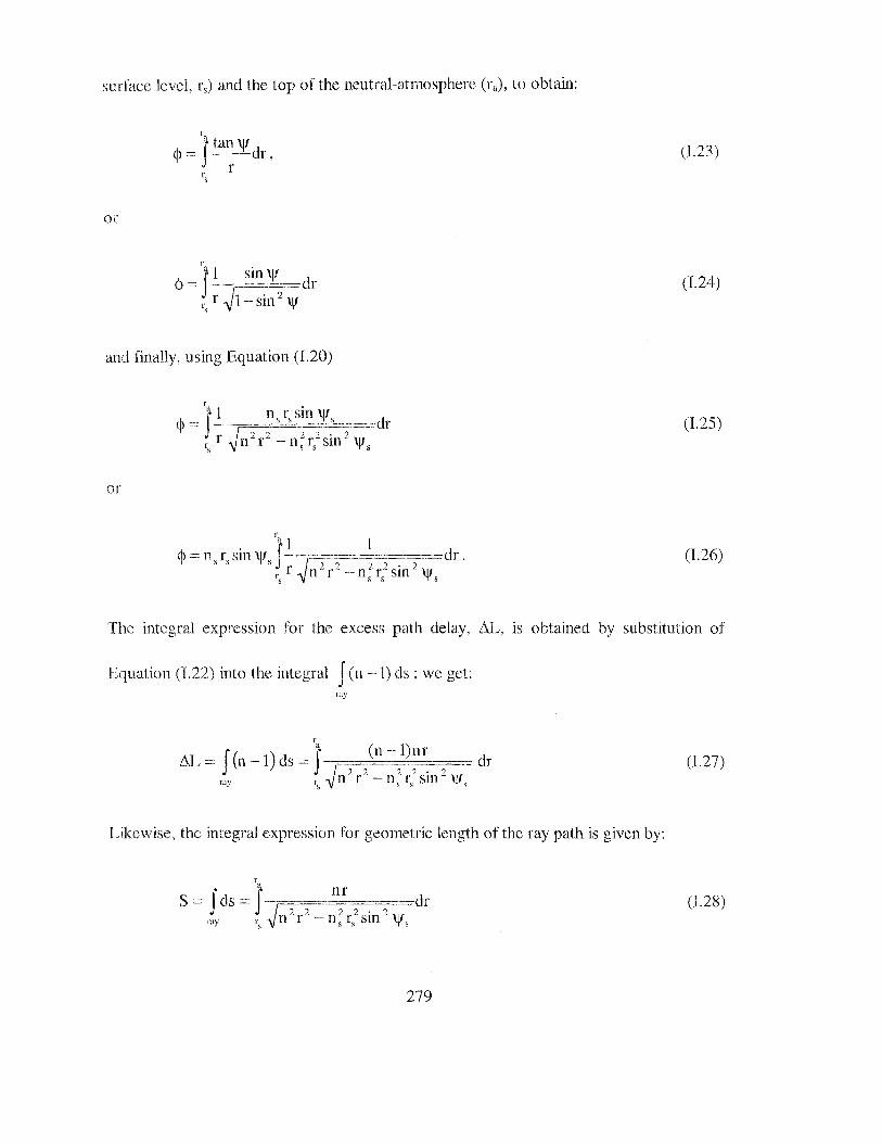
surface level, rs) and the top of the neutral-atmosphere (ra), to obtain:
(I.23)
or
<P = J -~ sin \If dr rs r F- sin
2 '-1' (L24)
and finally, using Equation (I.20)
(I.25)
or
r " 1 1
th = n r sin \Jf J-·~· --·-····=-=--=---==dr. 'I' s s s 2 2 2 ? 2 r r n -r - n c sin '-1' s s s s
(1.26)
The integral expression for the excess path delay, ~L, is obtained by substitution of
Equation (I.22) into the integral J (n --1) ds; we get: ray
r
~L= J(n--l)ds=J' {r; (n:-l)nr _ dr 22 22· 2
ray r, I1 f - I1 s f 5 SIB \If s
(1.27)
Likewise, the integral expression for geometric length of the ray path is given by:
(1.28)
279

The last integral expression to he evaluated concerns the geometric path, G. As the
integration is performed in vacuum, the refractive index at every point along the ray path
is equal to unity; the angle between the radial vector and the ray is now a non--refracted
(geometric or true) zenith angle (or distance), Z. Therefore, the integral expression
sought is given by:
r a r
G = J ds == J-p-"--===.,==dr 2 ry • 2 z
vac r r - r .- Sln s s
(I.29)
Finally, by substitution of (1.27), (I.28), and (I.29) into the equation defining the neutral··
atmosphere propagation delay:
we get the complete integral expression:
's'" (n -l)nr rJ" nr r ---- - ·----l d . = - - - .... dr + -------=--==---==--== -- · - . ..: r (130)
,, ,[n' r - n0 r0 Sin \j/0 ,J ,/n'r _:::_ n, r, sm \j/0 Fr, sm Z} nd 22 22·2 22 22·2 2 2·2 · ·
Using elevation angles rather than zenith angles, the equivalent expression is:
where e is the refracted (apparent) elevation angle and£ is the geometric (true) elevation
angle.
280

.APPENDIX ... II
. M<:tthemattcal strncture of sele.cted models
Mathematical structure of selected mapping functions and hybrid models.
);;- CfA-2.2 [Davis et al., 1985]
)..- lfadis [lfadis, 1986 J
Y Lanyi [Lanyi, 1984]
';- MTT [Herring, 1992]
> NMF [Niell, 1996]
~ UNSW931 [Yan and Ping, 1995]
'r Altshuler and Kalaghan [Altshuler and Kalaghan, 197 4]
~ NATO [NATO, 1993]
> W AAS [DeCJeene, 1995]
281

Mathematical model:
l mhnh(£)::::-- a-----··
sinE+--· -----b
tan£+---~--sin£+ c
where:
a=-" 0.001185 {H-0.6071x 10⁻⁴ (P, --1000 )- 0.1471 xl o-3 e, +0.3072x 10--2 (t, ---20)
+ 0.019 65 (6.5 ---a)- 5.645x 10⁻⁶ (H1 -11231)}
b =: 0.001144 { 1 + 0.1164 X 10⁻⁴ (P, -1000 )+ 0.2795 X 10⁻³ e, + 0.3109 X 10 2 (t, --20)
+ 0.03038 (6.5- a)-1.217 x w-s (H1
-11231)}
c c:.: --0.0090.
Comment: The mapping function was designed for the hydrostatic component only, but
may be used for the non-hydrostatic component also.
Symbols and Units
mh,nh hydrostatic (non-hydrostatic) mapping function (unitless)
£ elevation angle (rad)
Ps surface total pressure (hPa)
e, water vapor pressure (hPa)
t, surface temperature COC)
a temperature lapse rate (Kkm-1)
H1 tropopause height (m)
282

Mathematical model:
a 1+-~L __ _
b 1+~'-
1 +c; ·---
sin£+ b. sin £ + ----'--
sin c:+c;
where, for i ::: h (hydrostatic mapping function),
Ifadis [Ifadts. 1986:1
ah = 0.001237 + 0.1316x 1 0 .. 6 (P, -1000 )+ 0.1378x 10⁻⁵ (t, -15)+ 0.8057 X 10'5 F,
ch = 0.078;
for i = nh (non-·hydrostatic mapping function),
an11 = 0.0005236 +0.2471xl0 6 (Ps --1000 )-0.1724x 10⁻⁶ (ts -15)+ 0.1328x 1 o-4 ~~
bllh = 0.001705 ·J- 0.7384x 1 o·6 (P, --1000 )-J-0.3767x 10⁻⁶ (t, --15)+ 0.2147x 10·-'~ Fs
cnh = 0.05917 0
Comment: the coefficients for the b11 term are incorrect in some publications. The ones
listed here agree with the original publication and have been conjirrned by Joannis
ff'adis (personal communication, Aristotle University of Thessaloniki - School of
Engineering, June, 1994 ). Optimized clinwte-dependent mapping functions were also
developed by ffadis [ 1986].
283

Symbols and Units
mh,nh hydrostatic (non-hydrostatic) mapping function (unitless)
E elevation angle (rad)
P, surface total pressure (hPa)
es water vapor pressure (hPa)
ts surface temperature (°C)
284
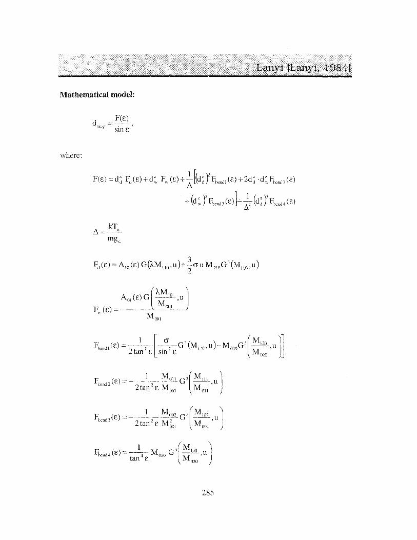
Mathematical model:
where:
d = F(E) trop sin E '
F(E):::: d~ Fct (E)+ ct: Fw (E)+_!_ [(ct~ y Fbenc!1 (E)+ 2d~ · ct:~f<~cnc! 2 (c) L1
,t1 = kT0 .
mgc
+ (d~~ YF;,cml3 (E) ]+-~2 (d~ YFhenc\4 (E)
A (c) G A.MI_Ql uJ o1 M '
Fw(E)= om -MooJ
. 1 r () 3 ( " ) 3( M120 Jl Fbendl(£) =-2---2 --:-2-G MllO'U -"MozoG -M ,U tan E "- sm £ 020
F (E)==- 1 Mo11 G3(M111 uJ " hend 2 2 2 " M ' tan £ Mom " 011
F -(E)=--1_:M_ggz._G3[Mlm u] bend "l 2 t 2 M 2 M ' an £ 001 oo2
F'ocnd4(E)=-4-Mmo G ---,u 1 3(M13o J tan E M 030
285

1 G(q, u )= -J1+<
l+qu
2cr u=--
tan2 E
The quantities A1m(E), which involve the dry (lm=lO) and wet (lm=Ol) components of the
refractivity, are defined as:
A (')=M + ~~(-l)n+k (2n-1)!!M<n--k)Jm [ (l+A Mnm l-]]n[AM1!!!!_1k Jm E mm L.JL..i 2nk'( k)' u u M M ' n=l k=O · n - · Olm Olm
where A is a scale factor (A = 3, for E < 10°, and A = 1, for E > 10°).
The n-order moments of the dry and wet refractivities can be expressed as function of the
surface-normalized dry and wet refractivity, fd_w(q),fJ_w(q) and f~_w(q):
=
M,Jij = f qn f~ (q)f~ (q) dq ()
where n ranges from 0 to 10, i from 0 to 3, and j from 0 to 2 (not all combinations are
needed).
l<'or a three-section temperature profile model, in particular, we have:
M =n' [-~-nq,--+e-"'~'(1-i'b+n+l(q ,q ))(Tin X ]+ e-nq,T~'·-n-•-J(ql,q2)] nij • , n+l 2 I 2 b + · + 1 , n+l
a i=o 1 a
where
286

CAr ( ) 1 q2- ql 0 q ,q = -------- I .2 X
mgc x=-ka
The parameters a and b dependent on the powers of the refractivities i and j pertaining to
the moment definitions are listed in Table II. 1.
Comment: As pointed out in Lanyi [1984], the Saastamoinen and Black mapping
functions can be obtained by neglecting the bending terms and setting some of the
variables to constant values. The term Fhend4 was correct for a misprint in Lanyi 's
original publication (see also Savers and Jacobs [1996]).
Table II. 1 -Dependence of the constants a and b ori the dry and wet model parameters X
and ~ [Lanyi, 1984].
Moment type
M110- dry
M 101 --wet
M020 - dry squared
M 111 - product of dry and wet
M002 - wet squared
M 130 - dry cubed
0
2
0
3
287
j
0
1
0
2
0
a b
1 X- 1
~ ~X- 2
2 2X- 2
~+I ~(X+l)-3
2~ 2~x-4
3 3x-3

Symbols, Units and Nominal Values (default)
dtrop total neutral atmospheric propagation delay (m)
d~ zenith dry delay (m)
d~, zenith wet delay (m)
£ elevation angle (rad)
To average temperature of the surface layer (292 K)
m mean molecular mass (4.8097x10.26 kg)
gc gravity acceleration at the center of gravity of the air column (9. 7837 m s·2)
k Boltzmann's constant (1.380658xl0.23 J K 1)
Rc earth's radius of curvature (6 378 140m)
a temperature lapse rate (6.8165 Kkm-1)
h1 inversion height ( 1.25 km)
h2 tropopause height (12.2 km)
X dry model parameter (5)
~ wet model parameter (3.5)
,6. atmospheric scale height (8.567 km)
q1 scale height-normalized inversion height (0.1459)
q2 scale height-normalized tropopause height ( 1.424)
288

Mathematical model:
a 1+--'~
b. 1+-'--
rni(E)=--- 1+ci . ai sm£+· ·
. bi sm£+------sin £+c1
where, fori= h (hydrostatic mapping function),
ah = {1.2320+0.0139cos<p--0.0000209Hs +0.00215(ts -lO)}xl0-3
bh = { 3.1612-- 0.1600cos<p- 0.0000331Hs + 0.00206(t, -10 )}x 10-3
ch = {71.244-4.293cos<p-0.000149H, -0.0021(ts -lO)}xl0-3;
for i = nh (non-hydrostatic mapping function),
anh ={0.583-0.0llcos<p-0.000052Hs +0.0014(ts -lO)}xl0-3
bnh = {1.402-0.102cos<p-0.000101Hs +0.0020(ts -lO)}xlo-·3
cn11 ={45.85·--·1.9lcoscp--0.00129H, +0.015(ts -lO)}xl0-3•
Symbols and Units
mh,nh hydrostatic (non-hydrostatic) mapping function (unitless)
£ elevation angle (rad)
<p station latitude (rad)
Hs station orthometric height (m)
t, surface temperature (°C)
289

Mathematical model:
a. 1+---1 -
b. 1 +---!.___
l+ci mi(E)=----- +H
8Xl0-3
. ai sm £ + ----------. bi sm £ + -----
sin E+ci
1+-a_h_t __
1 +~\_It_ 1 +cht ---------
sin£ · aht sm £ + -------. bht smE+------
sin £+cht
The second term of the right-hand-side of this equation represents an analytic height
correction to be applied to the hydrostatic component only. The fitted parameters
are for this correction term are:
bh1 = 5.49xl0-3
The coefficients for the hydrostatic component are functions of the station latitude and
day of year (identical formulae forb and c coefficients):
where ahavg (average) and a 11 amp (amplitude) are coefficients determined for the five
latitudes correspondent to the U.S. Standard Atmosphere Supplements (see Table
290

below). For latitudes at and below 15'\ the parameters are constant. The coefficients for
non-tabulated latitudes are obtained by linear interpolation.
For the non-hydrostatic component, the coefficients are a function of the latitude only,
and as in the case of the hydrostatic counterpart, linear interpolation is used to obtain the
coefficients for non-tabulated latitudes.
Latitude
Coefficients 15° 30° 45° 60° 75°
a havg
xl03 1.2769934 1.2683230 1.2465397 1.2196049 1.2045996
b havg
><103 2.9153695 2.9152299 2.9288445 2.9022565 2.9024912
'avg xl03 62.610505 62.837393 63.721774 63.824265 64.258455
a 11 amp X 105 0 1.2709626 2.6523662 3.4000452 4.1202191
hhamp xJO' 0 2.1414979 3.0160779 7.2562722 11.723375
ch amp
X 105 0 9.0128400 4.3497037 84.795348 170.37206
a 1111 X 104 5.8021897 5.6794847 5.8118019 5.9727542 6.1641693
bnh xl03 1.4275268 1.5138625 1.4572752 1.5007428 1.7599082
cnh xl02 4.3472961 4.6729510 4.3908931 4.4626982 5.4736038
Symbols and Units
mh,nh hydrostatic (non-hydrostatic) mapping function (unitless)
E elevation angle (rad)
<p station latitude (rad)
Hs station orthometric height ( m)
doy day of year (UT days past January 0.0)
291

Mathematical model:
1 mh,nh(£)= . a-----
sm £ + --------------------2 b I esc£+----------~--
. c sm £ + ----------e CSCE+d
where:
I==J¥i-tan£,
a= 0.461398 3 + 2.864x 10 5 (P, -1013.25)+ 8.99x 1 o-6 e,- 6.98x w--6 e;
-1.0914x 1 o-4 (t, --15)+ 1.30x 1 o-6 (ts -15? + 9.4694x 10""3 (6.5- a)
--2.4946xl0 6 (H 1 --11231)+1.8072x10--10 (H 1 -11231?
b == 0.827 647 6 + 2.056xl0-5 (Ps --1013.25)+ 2.382x 10- 4 e, - 4.76x 10⁻⁶ e~
+ 5.1125x 10""4 (ts -15)+ 1.23x 10⁻⁶ (ts -15Y + 3.6479x 10⁻² (6.5- a)
--1.532lx10-5 (H1 --11231)+ 9.4802x 10⁻¹⁰ (H
1 -11231 y
c == 2.531 492 + 1.093X 10⁻⁴ (Ps --1013.25)+ 2.6179Xl0""3 e, + 1.33X 10- 5 e;
+ 3.71 03xl 0"3 (ts -15)+ 4.95x 10⁻⁶ (t, -15)2 + 0.160 22 (6.5- a)
-- 8.9980x10⁻⁵ (H 1 --11231 )+ 4.9496x10- 9 (H1 --11231 Y
d == 47.078 44+ 1.595x10⁻³ (P, --1013.25)+ 3.9026xl0-2 es + 2.41xl0-4 e; - 4.1713x 10⁻² (ts -15)+ 2.16x 1 0""4 (t, -15? + 1.6313 (6.5- a).
- 9.9757x 10""4 (HI -11 231)+ 4.4528x 10" 8 (HI -11 231?
292

Comment: Although not clearly stated, this mapping function is to be applied to the
hydrostatic component only (Haojian Yan, personal communication, Shanghai
Astronomical Observatory, March 1998).
Symbols and Units
m11 ,n11 hydrostatic (non-hydrostatic) mapping function (unitless)
r elevation angle (rad)
Re earth radius (km)
H effective (scale) height of (dry) atmosphere (km)
P, surface total pressure (hPa)
e, water vapor pressure (hPa)
ts surface temperature (0 C)
a temperature lapse rate (K km" 1)
Ht tropopause height (m)
293

Mathematical model:
where
s= sin(nM) 12 ) '
As mentioned in the errata to the Altshuler and Kalaghan [ 197 4] report, the height
dependence in Equation (5) is to be considered only if the user at the surface. For
situations in which the antenna is airborne, the formula to compute Ns reduces to:
N =a +a mo +a <p 0 s2 +a moe. s 0 2'rs 4 s 6'1's
The coefficients for equations ( 1) to (8) are listed in Table 1.
294

0
2
3
4
5
6
gi bi Ci ai
0.1556 0.00970 3.28084 369.03000
138.8926 -2.08809 6.81758 -0.01553
-105.0574 122.73592 0.30480 -0.92442
31.5070 -703.82166 0.00423 0.00160
1.0000 1.33333 0.19361
30.0000 1.41723 X 10⁻⁶ 0.00063
0.0001 315.00000 -0.05958
Table 1 -Coefficients for equations (1) to (8).
Symbols and Units
dtror atmosphere propagation delay, in metres
eo apparent elevation angle, in degrees
H~r user's orthometric height, in thousands of feet
I-I: user's orthometric height, in feet
N s surface refractivity
cp~ user's latitude, in degrees
M calendar month
295

Mathematical model:
where:
dtrop = d~;op 0.00143 sin(£)+----------
tan(£)+ 0.0455
• For 0 km < H k < 1 km - s --
• For 1 km < H k < 9 km - ·s-
• For Hk > 9 km s-
z { 105 [ ( k )J} -3 dtrop = 0.1424
exp- 0.1424 Hs -9 X 10
i'iN = -7.32exp{0.005577N s}
N := N +i'iN 1 s
296
NATO [NATO, 198Sl

Comment: the mapping function associated to this model is the Chao [ 1972] dD.
mapping function.
Symbols and Units
dtror atmosphere propagation delay, in metres
d;;op atmosphere zenith propagation delay, in metres
£ elevation angle, in radians
H ~ orthometric height, in kilometres
N s mean sea level surface refractivity
N t refractivity at l km above sea level
297

. .
' WM§ [JjeC~een~.. 19,:951
Mathematical model:
( )[1-1.264xl0-4H,l
dtrop := 2.506 1 + 0.001258N s . 0 0 ,
sm(8 +0.35 )
if Hs ::::; 1500 m; for Hs > 1500 m, the model is written as:
where
d =2.484[1+0.0015363ex {-2.l33xl0-4 H l·N lexp{-l.509 Xl0-4
H,}1 trop P sF s ,· ( o 0 350) ' sm 8 + .
8N 11 = J , [2TC(doy -152)] 3.61 x 10-. H, cos
365 ,
l .. , [2TC(doy-335)] 3.61xiO·H,cos 365
-,
J (i<~''il( o s22s+ o !cor"< doy- 213)]) if'~': > oo
ON' ~ l (l~:ll(~ 08225 +OJ cos~"( d;;:- )O) n if '1': < 0'
Note: The model is not defined for <p~ == oo.
298

Symbols and Units
drrop atmosphere propagation delay, in metres
E0 elevation angle, in degrees
H s orthometric height, in metres
SN s correction to the surface refractivity
<p~ latitude, in degrees
doy day of year
299

List of the approximate geographic coordinates of the radiosonde stations (as given in the
Radiosonde Data from North America 1946 - 1995, produced by the U.S. Forecast
Systems Laboratory and the U.S. National Climatic Data Center [1996]) used in
computing databases of tropopause heights, inversion heights, and lapse rates, along with
an identifying three-letter code. A subset of these radiosonde stations, shown in bold in
the table, was used in computing traces used in model and mapping function assessment.
300

STATION
Bellingshausen, BTA
Hobart, Tasmania, Australia
Quintero, Chile
Bloemfontein, South Africa
Fortaleza, Brazil
Balboa, Panama
Trinidad, Trinidad and Tobago
Curacao, Netherlands
Seawell APT, Bahamas
Guam, Mariana Islands, USA
'T'egucigalapa, Honduras
Point a Pitre, Guatemala Belize, Belize
San Juan, Puerto Rico
Manzanillo, Mexico
Grand Cayman, Cayman Islands
Mexico City, Mexico
Lihue, HI, USA
Mazatlan Sinaloa, Mexico
Key West, FL, USA
Nassau, Bahamas
Brownsville, TX, USA
West Palm Beach, FL, USA
Cape Kennedy, FL, USA
Chihuahua , Mexico
Corpus Christi, TX, USA Waycross, GE, USA
Midland, TX, USA
Tuscon, AZ, USA
Jackson, MS, USA
Miramar, CA, USA
Charlston, SC, USA
Little Rock, AR, USA Albuquerque, NM, USA Norman, OK, USA
Tateno, Japan
Greensboro, NC
CODE
301
BEL
HOB
QUI
BLO
FOR
BLB
KPP
ACC
BDI
GUA
HTG
FFR
ZBZ
JSJ
MAN
KCR
MEX
LIH
MZT
EYW
YNN
BRO
PBI
XMR MCV CRP
AYS
MAF
TUS
JAN
NKX
CHS
1M1
ABQ
OUN TAT
GSO
cp (o N)
-62.20
-42.83
-32.78
-29.10
-3.72
8.98
10.58
12.20
13.07
13.55
14.03
16.27
17.53
18.43
19.07 19.30
19.43
21.98
23.18
24.55
25.05
25.90
26.68
28.48 28.70
29.77
31.25 31.93
32.12
32.32
32.87
32.90
34.83
35.05 35.23
36.05
36.08
A H (o E) (m)
-58.93 46
147.50 28
-71.52 8
26.30 1359
-38.55 19
-79.60 66
-61.35 12
-68.97 54
-59.50 47
144.83 111
-87.23 1014
-61.52 8 -88.30 5
-66.00 3
-104.33 3
-81.37 3
-99.07 2234
-159.35 36
-106.42 4
-81.75 3
-77.47 2
-97.43 7
-80.12 7
-80.55 5
-106.07 1428
-97.50 14 -82.40 44
-102.20 873
-110.93 788
-90.07 91
-117.15 147
-80.03 15
-92.27 172
-106.62 1619 -97.47 362
140.13 27
-79.95 277

Nashville, TN, USA BNA 36.25 -86.57 180
Oakland, CA, USA OAK 37.75 -122.22 6
Wallops Island, VA, USA WAL 37.93 -75.48 13
Denver, CO, USA DEN 39.77 -104.88 1611
Madrid, Spain MAD 40.50 -3.58 633
Pittsburgh, PA, USA PIT 40.53 -80.23 360
Brindisi, Italy BRI 40.65 17.95 15
Salt Lake City, UT, USA SLC 40.77 -111.97 1288
Omaha, NE, USA OVN 41.37 -96.02 400
Chatha.m, MA, USA CHH 41.67 -69.97 16
Medford, OR, US.A MFR 42.37 --122.87 397
Albany, NY, USA ALB 42.75 -73.80 85
Boise, ID, USA BOI 43.57 -116.22 871
Sable Island, NS, Canada YSA 43.93 -60.02 4
Rapid City, SD, USA RAP 44.05 -103.07 966
Green Bay, WI, USA GRB 44.48 -88.13 210
Salem, OR, USA SLE 44.92 -123.02 61
St.John's, NF, Canada YYT 47.67 -52.75 140
Glasgow, MT, USA GGW 48.22 -106.62 696
Munique 6 Germany MUN 48.25 11.58 484
International Falls, MN, USA INL 48.57 -93.38 359 Garmersdorf, Germany GAR 49.43 11.90 419
Sept Iles, PQ, Canada YZV 50.22 -66.27 52
Port Hardy, BC, Canada YZT 50.68 -127.37 17 Moosonee, PQ, Canada YMO 51.27 -80.65 10 Goose Bay, NFW, Canada YYR 53.30 -60.37 36 Edmonton, AB, Canada WSE 53.55 -114.10 766 La. Grande, PQ, Canada YAH 53.75 -73.67 307 Prince George, BC, Canada YXS 53.88 -122.68 675 The Pas, MB, Canada YQD 53.97 -101.10 273 Annette Island, AK, USA. ANN 55.03 -131.57 37 Cold Bay, AK, USA CDB 55.20 -162.72 30 Copenhagen, Denmark COP 55.77 12.52 40 St. Paul Island, AK, USA SNP 57.15 -·170.22 10 Landvetter, Sweden LAN 57.67 12.30 155 Kuujjuaq, PQ, Canada YVP 58.10 -68.42 60 Inukjuak, PQ, Canada YPH 58.45 -78.12 7 King Salmon, AK, USA AKN 58.68 -156.65 15 Churchill, MB, Canada YYQ 58.75 -94.07 29 Fort Nelson, BC, Canada YYE 58.83 -122.60 377 Bromma, Sweden BRM 59.35 17.95 22
302

Yakutat, AK, USA YAK 59.52 -139.67 12
Ft. Smith, NWT, Canada YSM 60.03 ---111.95 203
Gardermoen, Norway GMO 60.20 11.10 201
Whitehorse, YK, Canada YXY 60.72 -135.07 704
Bethel, AK, USA BET 60.78 -161.80 36
Sundsvall, Sweden SUN 62.53 17.45 6
Iqaluit, NWT, Canada YVN 63.75 -68.55 21
Coral Harbour, NWT, Canada YZS 64.20 -83.37 57
Baker Lake, AK, USA YBK 64.30 -96.00 49
Nome, AK, USA OME 64.50 -165.43 5
Fairbanks, AK, USA FAI 64.82 -147.87 135
Norm.an Wells, NWT, Canada YVQ 65.28 -126.75 95
Lulea, Sweden LUL 65.55 22.13 34
Kotzebue, AK, USA OTZ 66.87 -162.63 5
Inuvik, NWT, Canada YEV 68.32 -133.53 103
Hall Lake NWT, Canada YUX 68.78 -81.25 7
Cambx:idge Bay, NWT, Canada YCB 69.10 --105.12 25
Point Barrow, AK, USA BRW 71.30 -156.78 12
Resolute, NWT, Canada YRB 74.72 --94.98 40 Mould Bay, NWT, Canada YMD 76.23 --119.33 58 Eureka, NWT, Canada YEU 79.98 -85.93 10
Alertr NWT, Canada YLT 82.50 -62.33 66
303

Samples of statistical tables of tropopause heights, inversion heights, and lapse rates for
the stations listed in Appendix III. The full tables are electronically available in
http://mat.fc.ul.pt/eg/lattex/PhD_e_sup.html.
Notation:
MEA,.l\T
STD
MIN
MAX
#
SIGB
STDS
Mean
Standard deviation
Minimum value
Maximum value
Number of determinations
Precision of the b coefficient in the least-squares fit of the line
y =a+ bx
Standard deviation of the SIGB.
304

STATION MONTH ME .AN STD MIN M.AX # (km) (km)
BEL J.ANU.ARY 9.230 0.915 7.999 11.007 19 FEBRUARY 9.329 0.914 8.007 11.012 13 MARCH 9.073 1.161 7.499 11.977 21 .APRIL 9.745 1.407 6.491 12.496 23 M.AY 10.214 1.413 8.523 12.490 9 OCTOBER 12.656 3.030 9.000 17.113 7 NOVEMBER 12.776 2.420 8.489 18.247 23 DECEMBER 11.958 1.501 9.998 15.031 12
ANNUAL 10.466 2.187 6.491 18.247 127 =============================================
HOB JANUARY 11.599 1.233 8.790 14.485 59 FEBRUARY 11.798 1.444 8.441 15.517 51 MARCH 12.089 1.018 9.163 14.670 55 APRIL 11.612 1.120 8.120 13.242 60 MAY 11.298 1.017 8.078 13.106 60 JUNE 10.370 1.150 6.973 12.056 58 JULY 10.380 1.079 7.342 12.272 57 AUGUST 9.714 0.974 6.987 11.463 54 SEPTEMBER 9.802 0.992 6.995 11.233 39 OCTOBER 10.657 1.131 8.068 13.194 52 NOVEMBER 10.724 1. 245 7.644 14.377 57 DECEMBER 11.488 0.991 9.007 13.763 57
.ANNUAL 10.995 1.339 6.973 15.517 659 ======================~======================
QUI JANUARY 14.187 2.214 10.281 18.118 42 FEBRUARY 14.045 2.064 11.384 17.840 38 MARCH 14.278 2.051 10.351 17.795 56 APRIL 12.998 1.594 10.494 18.384 54 M.AY 12.256 1.299 9.636 15.982 59 ,JUNE 11.700 1.246 7.483 13.060 49 JULY 11.445 1.406 8.692 16.713 49 AUGUST 11.223 1. 221 7.702 15.092 42 SEPTEMBER 11.305 0.939 9.206 12.527 25 OCTOBER 12.210 1.830 9.366 18.525 48 NOVEMBER 12.128 1.774 9.687 16.721 50 DECEMBER 14.096 2.439 9.685 18.266 57
ANNUAL 12.721 2.073 7.483 18.525 569 =============================================
IIA- Tropopause height statistics for BEL, HOB, and QUI.
305

STATION MONTH MEAN STD MIN MAX # (m) (m) (m) (m)
BEL FEBRUARY 262.0 181.9 157.0 472.0 3 MARCH 321.6 356.9 160.0 960.0 5 APRIL 512.6 367.7 8.0 1165.0 7 MAY 88.3 80.6 7.0 162.0 4 OCTOBER 123.7 66.5 47.0 166.0 3 NOVEMBER 224.7 114.7 155.0 357.0 3 DECEMBER 197.4 87.7 153.0 354.0 5
ANNUAL 277.8 262.9 7.0 1165.0 32 =============================================
HOB JANUARY 72.8 49.6 42.0 146.0 4 FEBRUARY 130.9 167.2 41.0 532.0 8 MARCH 103.4 91.9 42.0 348.0 10 APRIL 93.2 64.5 32.0 267.0 17 MAY 137.7 125.4 33.0 753.0 44 JUNE 144.0 97.7 16.0 452.0 45 ,JULY 109.3 65.4 8.0 303.0 44 AUGUST 99.5 75.8 8.0 323.0 30 SEPTEMBER 58.9 24.6 16.0 121.0 16 OCTOBER 68.9 50.7 8.0 252.0 18 NOVEMBER 48.1 31.1 8.0 118.0 9 DECEMBER 67.0 34.7 49.0 119.0 4
ANNUA.L 109.1 91.4 8.0 753.0 249 =============================================
QUI JANUARY 394.8 400.8 74.0 1149.0 12 FEBRUARY 297.3 245.6 32.0 778.0 20 MARCH 269.8 265.0 66.0 1036.0 24 APRIL 218.0 190.2 40.0 867.0 46 MAY 203.5 188.3 40.0 984.0 50 JUNE 250.3 247.8 39.0 913.0 44 JULY 173.2 144.4 40.0 858.0 43 AUGUST 488.8 337.6 88.0 1254.0 25 SEP'I'EMBER 349.9 328.8 48.0 1024.0 11 OCTOBER 280.3 208.5 40.0 718.0 32 NOVEMBER 235.1 21'7.5 48.0 746.0 14 DECEMBER 377.4 311.6 40.0 1166.0 24
ANNUAL 270.2 252.6 32.0 1254.0 345 =============================================
IIA- Inversion height statistics for BEL, HOB, and QUI.
306

STATION MONTH MEAN STD SIGB STDS MIN MAX # (K/km) (K/km) (K/km)
BEL JANUARY 5.87 0.45 0.17 0.05 5.05 6.51 19 FEBRUARY 5.77 0.46 0.16 0.05 5.06 6.60 13 MARCH 5.87 0.59 0.15 0.07 4.45 6.79 21 APRIL 6.11 0.54 0.21 0.07 4.93 7.37 24 MAY 6.12 0.37 0.19 0.07 5.26 6.45 9 OCTOBER 5.52 0.70 0.18 0.05 4.39 6.72 8 NOVEM.BER 4.91 0.69 0.18 0.06 3.59 5.93 23 DECEMBER 5.26 0.59 0.17 0.06 4.47 6.13 12 ANNUAL 5.67 0.70 0.18 0.06 3.59 7.37 129 ===================================================
HOB JANUARY 6.22 0.33 0.16 0.05 5.55 6.90 56 FEBRUARY 6.11 0.38 0.17 0.05 5.25 7.06 54 MARCH 6.24 0.30 0.17 0.06 5.65 6.91 58 APRIL 6.54 0.31 0.15 0.04 5.73 7.08 60 MAY 6.67 0.22 0.14 0.04 6.10 7.13 60 JUNE 6.79 0.33 0.15 0.04 6.16 7.47 58 JULY 6.68 0.38 0.15 0.05 5.74 7.71 57 AUGUST 6.82 0.33 0.16 0.04 6.11 7.48 54 SEPTEMBER 6.53 0.39 0.18 0.07 5.87 7.59 37 OCTOBER 6.46 0.37 0.17 0.06 5.71 7.31 51 NOVEMBER 6.46 0.36 0.14 0.05 5.19 7.01 51 DECEMBER 6.38 0.31 0.16 0.04 5.66 6.89 56 ANNUAL 6.49 0.40 0.16 0.05 5.19 7.71 652 ===================================================
QUI JANUARY 6.16 0.36 0.18 0.06 5.40 6.89 53 FEBRUARY 6.26 0.38 0.16 0.05 5.53 7.17 50 MARCH 6.40 0.44 0.17 0.04 5.50 7.34 56 .APRIL 6.52 0.48 0.15 0.05 5.07 7.58 54 MAY 6.51 0.30 0.13 0.04 5.79 7.10 58 JUNE 6.61 0.48 0.13 0.04 5.73 7.60 48 JULY 6.49 0.41 0.18 0.07 5.11 7.39 48 AUGUST 6.82 0.48 0.19 0.08 5.83 7.78 42 SEPTEMBER 6.67 0.33 0.19 0.06 6. 1:1. 7.47 24 OCTOBER 6.42 0.45 0.20 0.08 5.05 7.63 47 NOVEMBER 6.46 0.32 0.20 0.07 5.57 7.03 49 DECEMBER 6.31 0.39 0.14 0.04 5.40 7.09 56 ANNUAL 6.45 0.44 0.17 0.06 5.05 7.78 585 ======================~==========================
IIA- Lapse rate statistics for BEL, HOB, and QUI.
307

Annual mean tropopause heights and lapse rates for the 100 stations listed in Appendix
III ordered by increasing absolute latitude. The error bars represent the associated·
standard deviation.
308

FOR BLB KPP ACC BDI GUA HTG FFR ZBZ JSJ MAN KCR MEX LIH MZT EYW YNN BRO PBI XMR MCV BLO CRP AYS MAFTUS Jl\N QUI NKX CHS lMl ABQ DUN TAT GSO BNA OAK WAL DEN MAD PIT BRI SLC OVN CHH MFR ALB HOB BOI YSA RAP GRB SLE YYT GGW MUN INL GAR YZV YZT YMO YYR WSE YAH YXS YQD ANN
Lapse Rate (K/km)
1----<·-------1
,' • ·' --1 • I ~· r '
• I I •
• I • I •
• gg~ I • • II SNP e
Ll\N f,~~~ ~·~I Wa AKN YYQ YYE BRM YAK YSM GMO -YXY BET BEL SUN YVN YZS YBK OME FAI YVQ LUL OTZ YEV YUX YCB BRW YRB YMD YEU YLT
I
I
• I
•
• I • • •
I • ., • •
60£
Tropopause Height (km)
.... 0
• • • •
•• • I'
.... "'
.... 00

Annual mean bias and rms scatter (one-sigma level) of the differences with respect to ray
tracing for different zenith hydrostatic delay prediction models, for 50 radiosonde stations''
listed in Appendix Ill.
310

Mean Differences (m) Mean Differences (m) Mean Differences (m) Mean Differences (m) I
I I I 0 0 0 0 0 0 0 0 0 0 0 0 0 0 0 0 0 0 0 0 0 0 0 0 0 0 0 1-" 0 f-S f-lo 0 1--'- }-1 0 1---l }-I 0 f-1>
BEL lei BEL • BEL • BEL E' I f+l HOB H>-l HOB t HOB Ill HOB f+l QUI f+l QUI t QUI Ill QUI f+l BLO J-+--j BLO t BLO lei BLO ~ H>-J FOR t-e-l FOR e FOR ~ t FOR e BLB f+l BLB t BLB t BLB e KPP 1+1 KPP t KPP t KPP e GUA H>-l GUA e GUA t GUA r e JSJ HH JSJ • JSJ ' • JSJ I • MEX b*-J MEX t MEX ill MEX [- e LIH f--+-1 LIH t LIH It LIH [- e
MZT 1---+--i MZT ~ t MZT Ill MZT t f+l . l. EYW 1---+--1 EYW 't EYW Ill EYW f+l PBI ~ PBI t PBI ill PBI , f+l CRP 1--+---i CRP t CRP lei CRP ,_ f+l MAF ~ MAF t MAF lei MAF f+l TUS f--e---1 TUS ! t TUS f*i TUS f-*-i JAN ~ JAN t JAN lei JAN f+l NKX , f--e---1 NKX t NKX . lei NKX f+l ABQ 1-*-i ABQ t ABQ ' lei ABQ f-*-i
(.;.) TAT ~ ~ TAT t TAT ~ lei TAT f+l. 1 _. GSO f----e---j GSO t GSO ~ lei GSO f+l ~ _. BNA 1--+---i BNA t BNA lei BNA f+l ~
OAK r+-1 OAK t OAK ill OAK f+l WAL 1--+---i WAL t t WAL lei WAL f+l DEN 1-*-i DEN t DEN f*i DEN f+l MAD !- b*--1 MAD t MAD lei MAD f+l BRI r 1---+-J BRI t BRI lei BRI f+l SLC f+l SLC t SLC ~ SLC f+l OVN ~ OVN t OVN ~ OVN f+l CHH 1---+--i CHH t CHH lei CHH ~ MFR b*--1 MFR t MFR ~ MFR f+l ALB ~ ALB t ALB ~ ALB f+l YSA f---+--1 YSA t YSA lei YSA f+l YYT f--+-1 YYT t YYT lei YYT f+l GGW t-e-l GGW t GGW 1+1 GGW f+l MUN r----1 MUN t MUN lei MUN f+l
INL f--+-1 INL I . INL f+l INL 1+1 YZT f+i YZT t YZT Ill YZT f+i WSE t-e-l WSE t WSE 1+1 WSE 1+1 YQD f--*--1 YQD t YQD f+l YQD 1+1 LAN r+-1 LAN t LAN lei LAN 1+1 YSM 1-*-i YSM t l YSM ~ b*--1 YSM 1+1 YXY f+l YXY t YXY ;... f+l YXY 1+1 SUN t-e-l SUN t SUN f ~ SUN 1+1 YVN f+l YVN • YVN I r+-1 YVN f+l FAI 1-+-i FAI It ~ FAI f-+-1 FAI 1+1 LUL 1--+-i~ LUL ~ It LUL f*i LUL f+i OTZ 1-+-i OTZ t OTZ H>-l OTZ f+l YL'I' ~ • YL'I' t YL'I' 1-e-i YL'I' f---+--1
RA_ZH BB_ZH HO_ZH SA_ZH

Annual mean bias and rms scatter (one-sigma level) of the differences with respect to ray
tracing for different zenith non-hydrostatic delay prediction models, for 50 radiosonde
stations listed in Appendix III.
312

w _.. w
Mean Differences (m) Mean Differences (m)
' 0
..... "'
I 0
0 0\
0
0 0
0
0
"'
0
... "'
BEL I t-'-+-JI I BEL
I 0
... "'
~g~ ~ 1 ~g~c BLO !---*-; BLO FOR I e . I FOR BLB I '1 BLB KPP ·• KPP GUA GUA JSJ JSJ ~X ~X
LIH LIH MZT MZT E= E=. PBI I PB:t I
CRP ~ CRI?
~~,_ ~ ~~ JA!IJ • ~ JA!IJ NKX ~ NKX ABQ 1--*'-1 ABQ TAT 1-----8---i TAT GSO r------1 GSO BNA r------1 BNA OAK f--'-+----1 OAK WAL ~ ~ WAL DEN f-*-1 DEN MAD f--*-i MAD BRI ~ BRI SLC f-*-1 SLC OVN ~ OVN.
I 0
0
"'
0
0 0
~ 1---*rl ~
.- ---- ------- ---. I •: I ~
~ t-----+-'-l ~ ~
1---+-'-1 1-----8---i
f---+-----l 1---+-'--1
1---*rl ~
f--*--1 f--*-i 1----+-1
f--*--1 f--'-+----1
I e· I MFR 1--+--i MFR 1---*---i CHH I •: I CHH~ ALB ~ ALB 1---*--'--i YSA ~ YSA t------e'----i ~T ~ ~T ~ GGW 1--*'-1 GGW f--*-i MUN r.---l MUN f--+-i INL ~ INL ~ r.---l YZT ~ YZT~ ~ WSE ~ WSE~ ~ YQD f--*--1 YQD f--*-i LAliT t-*-l LAN 1---*---i YSM f-*-1 ~ YSM f-*-1. YXY f-*-1 YXY 1--+,i
FAI l-+7i. FAI 1-+-1 LUL r.---l LUL 1---*--i OTZ f-*-i; j OTZ f-*,-1
0
0 0\
0
... "'
~ ~ j ~~ ~ YLT /4-l. YLT ~ 1
B70_ZW RA_ZW
Mean Differences (m)
BEL HOB QUI BLO FOR BLB KPP GUA JSJ MEX
' 0
:;;
I 0
0 0\
0
0 0
I • I
f~f ~~t ~~. I TUS ~ JA!IJ ~ NKX f--'-e----1
r;l~ ,:~.':,, WAL f-----e---1 DEN ~ MAD i---4--1 BRI r------1 SLC ~ OVN f--'-+----1 CHH ~ ; MFR r f--+-i ALBL ~ YSA ~ YYT f-----'--1 =w 1-+-l
0
0 0\
0
... "'
MUN f---*--1 . INL ~ 1 YZT ~
~i~~ ~ SUN 1--+-'-1 YVN ~ FAI f-*-i LUL ~ 1---*--i OTZ J-+i -j
YLT ~~~----~----~~ SA_ZW
Mean Differences (m)
I 0
..... "'
I 0
0 0\
0
0 0
0
0 0\
0
... "'
BEL~ I ~ I I ~
1~~ r· I e
111
1 :•: I -l KPP f----<1----1 GUA JSJ ~X
LIH MZT L E=~ PBI I CRP F
~~ ·~~R ABQ 1---*--i TAT 1-----8---i GSO ,1---+-'--1 BNA f---+----j OAK 1---*rl WAL f--'-e----1 DEN . f--*-1 MAD f--*-i BRI ~ SLC f--*--1 OVN ~ CHH MFR t--+-; ALB ~
YSA r-------1 ~T f-----e---1
~IE \':j,','' l-LAN f--+-i YSM f-*-1 j YXY 1-+7i ~
E~ ~I l LUL 1---*--i ~j OTZ 1-+-1 YLT ~
IF_ZW

U-l -+>-
Mean Differences (m)
BEL HOB QUI BLO
BLB
I 0
.... I>J
I 0
0 0\
0
0 0
0
0 0\
FOR~ I e I
Kl?P I • I GUA I e I JSJ f------*---,l MEX 1---+---1 LIH ~ MZT .
EYW I' e I l?BI f-----+----1 CRl? . ~lAF ~ TUS 1--+---i JAN ~
NKX ! r------'-i ABQ f-*--j . TAT f-----,+--1 GSO ~ BNA ~ . OAK 1--+--i
~!~E ~. MAD r----1 BRI 1----*----1 SLC f-*--j OVN~ ~ CHH ~ I e I MFR f-'+-i ALB J----.--1 YSA I :• I YYT f------*---,l GGW f--+-i
0
.... I>J
= ~ j. YZT r------1 WSE f-'+-j
r~ ~ j. YSM ~.: ' YXY f--+-1 SUN f-+-i
YVN t 1-+-l FAI ~ J LUL f-'+-i OTZ~ ~ YLT 1-*J
AN_ZW
Mean Differences (m)
I 0
.... .,
I 0
0 0\
0
0 0
~ IL' ~f'-· -~·~-----... • -II GUA . . JSJ ~ MEX 1---+---1 L!H ~
~~E I • :I CRl? ~ I • , I MAF ~ r--------1
~ ~l I ', /: .:~~ I I
GSO ~ BNA ~ OAK . 1---+---1 WAL !--+--! DEN f-+-i
~~~ ~~.·~ I OVN r--------1 CHH MFR~ ~ ALB !-----*-'--~ YSA ~ YYT ~ GGW 1---+-,j MUN ~ INL ~ YZT 1---*--i WSE f-+-i
0
0
"'
0
.... .,
~ ~ 1' YSM ~
YXY ~ f-+-1 SUN r--e--1
illr~ ~I OTZ ~
YLT ~-~1-ei~-----~ BB2_ZW
I 0
.... I>J
Mean Differences (m)
I 0
0 0\
0
0 0
0
0 0\
0
.... "'
BELl= I ~ I ~ HOB~ QUI BLO
BLB
f-+-i t---'+--1 f-+-i
I e' I FOR~ Kl?l? GUA JSJ MEX LIH MZT EYW l?BI
~ ~ 1--'-+---1
CRl? ~ MAF TUS JANNKX ABQ TAT GSO BNA OAK WAL DEN MAD BRI SLC OVN CHH
r--------1 1--+--i
f---*-'---1 f---,-4---1 r--+--l
!--+--! , II : \
1---+---1 ~
f-*--1 ~ 1---*--i ~
1---+---1 I • I
MFR f---+--1 ALB ~ YSA ~ YYT ~ GGW ~ MUN f-+-j
WSE ~ YQD f-*--j LAN f---+--1 YSM 1--*ci YXY ~ SUN ~ YVN f-+-1 FAI 1-+-\ LUL r--e--1 OTZ 1--*ci YLT ~
HO_ZW
I 0
Mean Differences (m)
I 0 0 0 0
~ 0 0 0 ~ ~ ~ 0 ~ N :t • I '§:: I J
E~~~ · ·.~~.~~ l j GUA I e I JSJ f------*---,l MEX 1--*-1 LIH 1---*--i MZT EYW I e I l?BI I 'e I CRl? f'----. .---1, MAF 1--*---J TUS ~ JAN ~ NKX f-----,+--1 : ABQ ~ TAT r----+---i
~E ~ :1 ~· ~II I DEN J-+4 MAD f--+-i BRI ~ SLC J-+4 OVN 1---+----i CHH I e I MFR f-*---1 ALB t--'-+----1 YSA I e YYT j----e---1 GGW !--+-{ MUN f-*---1 INL f-+-i YZT t--'-+----1 WSE ~
YQD t f-*--j LAN (:: f---+--1
~Er- F.l~ YVN~ f-+-1 FAI f-- 1-*-J LUL ~ f---e-4 OTZ I 1--*-1 YLT r- ~
BBl_ZW

w -Ul
Mean Differences (m)
BEL HOB
I 0
'-' "'
~~~ ~· FOR BLB KPP GUA L
JSJ t E~~~-EYW PBI CRP MAF
NKX
' 0
0
"'
0
0 0
0
0
"'
1------*--1. ~
~~t ABQ ~ . TAT[- ~
GSOF ~. Bt;JA ~ OAK ~
WAL~ ~ DEN f---*-1 MAD ~ BRI I e I
;~r- ~ CF-H ~ I e I MFR ~ ALB f----'*-----1 YSA I e f
~~ ~ MUN f-*-1 INL ~
~;~~ I~ YQD r ~ LAN,_ f------e--1
~~~~~-- ~ . SUN f-*-1 YVN f-+--1 FAI f---*-1 LUL f-'---*--1
0
f-'
"'
OTZ r f---*-1 YLT f- ~ -j
BTM_ZW
I 0
f-'
"'
Mean Differences (m]
I 0
0 0\
0
0 0
0
0
"'
0
f-'
"' BEL ~ I ' Fi=l ' I 4 HOB!-
QUI~' BLO FOR BLB KPP GUAtJSJ !-
~~~~ MZT EYW
PBI ~ CRP MAF
~~t NKX ABQ TAT
GSO t BNA OAK WAL ~ DENt MAD' BRI fSLC f-CHH
~ ~
i----+------1 ~ ~ ~
f---*-1 1--*---1
f---*-1 1---*--1 .__..., OVN ~
MFR f-*-1 ALB I- 1---*--1 YSA l- I e YYTi- ~ GGW ~ }--+--1 }lUN !- f-*-1 INL ~ YZT r-----1 WSE !---+---1 YQD f---*-1 LAN ~ YSM }--+--1 YXY f--+-i SUN f-*-1 YVN f-+--1 FAI }--+--1
LUL ~ f--+---1 OTZ }--+--1 YLT ~ 4
B74_ZW
' 0
f-'
"'
Mean Differences (m)
I 0
0
"'
0
0 0
0
0 m
0
f-'
"' BEL f- I d.:::::J ' I J HOB QUI BLO FORi BLB I KPP f-
GUA ~ JSJ MEX LIH MZT E>:"W ~ PBI tCRP ~ M.'!.F r TUSfJAN NKX
f---*-1 ~ ~
I • I ____,
1-----*"'-----1 ~
r-----J
I • I I • . I
f------*---1 f------+----l ~
ABQ 1---+--i TAT ~ GSO 1---*--1 BNA 1---*--1 OAK ~ WAL f------*---1 DEN ~ MAD .~ BRI ~ SLC 1--'+---i OVN f-*------1 CHH t I • I MFR f------e--1 ALB 1- f-*------1 YSA ~ . YYT ~
::~ ~ INL f---+--1 YZT ~ WSE 1--1- 1--'-e--i
i:~ ~ f---*-j.f------e--1 YSM f---*-1 YXY f--+-i SUN ~ -YVN!- ~ -l FAI I- f-4--1 I LUL t. r-----1 I OTZ f-4--1 I YLT f-*1
CA_ZW
' 0
Mean Differences (m)
I 0 0 0 0
~ 0 0 0 ~ ~ m o ~ N
BEL ~ I p:.-j I J
~~~t 11~1 I I l BLB ~ I e I KPP -~ f--1 --4e,__-41 GUA JSJ !-----*"'-----1 MEXI- ~ LIH I- f----'*-----1
~E~ I • I
~! TUS JAN NKX ABQ TAT GSO L
~~ 1-
=ri-BRI SLC OVN CHH MFR ALB YSA
r--------1 ~ !---+-----1
r----e-----1 ~
r-----1 1------*--1
f-*--1 f---*-1 1--+-----1
f---*-1 f-*------1
1'-----1 f-*-1
f-*------1 I • I
YYT ~ !-----*"'-----1 GGW f-*--1 MUN [ ,__...____,
~~~ ~· T:, I YQD f-*--1 LAN f-*-1 YSM I- f-*--1 YXY t f--*-1
~! ~ FAI [ f-+--1 LUL ~ 1----*---1
~i:;r- ~ _, CH_ZW

APPENDIX Vlll
. Zenith total delay model statistics
Annual mean bias and rms scatter (one-sigma level) of the differences with respect to ray
tracing for different zenith total delay prediction models, for 50 radiosonde stations listed
in Appendix III.
316

w ,_. .__.]
Mean Differences (m)
BEL
l 0
..... "'
l 0
0
"'
0
0 0
HOB t f----*--4 QUI ~
BLO ~· t--*-1 FOR I .• I BLB KPP 1 I. • . I GUA 1- I • I JSJ ' f---+------'-l MEXI ~ LIH ~ 1---it-i !~ZT rEYWPBI ~ CRP F MAF ~ TUS ~ JAN\ ~ NKXr ~ ABQ f- f----*--4 TATt- ~
GSO~ ~ BNA r------'-1 OAK ~
WALf ~.· DEN[- ~
MAD f- f-*--1 BRI I f---*---l SLC r ;.--.....; OVN [- i-----*'---1 CHH [-MFR f 1---*---i ALB 1 1--*------i
MUN f----*--4 INL f----*--4
0
0
"'
0
..... "'
E!~ ~ YZT 1--*------i . WSE ;.--.....; _j YQD r ;.--.....; --J LAN r- f---.-e---1 -1 YSM [- 1-4--i. ~ YXY [- 1-+-1
~E~- ~ FAI 1-+-1 LUL ~ OTZ , 1-+-1 ~ YLT f- f*j
BB2_ZT
Mean Differences (m)
' 0
..... "'
l 0
0
"'
0
0 0
SELl- 1 -,~
HOB t 1--+-i QUI ~
BLO f---.-e---1 FOR t f-----,--+-----1
~~ ~ I •f-1 --<~.-.------11 GUA~' I •. I JSJ ~ MEX ~ LIH. ~
MZT ~· EYW PBI
CRP E'
~~~ 11···11 JAN . f----e---'--1 NKX r------'-1
~~~ ':17\' OAK~ ~
0
0
"'
0
1-'
"'
WAL f- ' 1----*-'-1
~~~ I:•l I ~ OVN ~ l CHH MFR f---.-e---1 ALB 1---+---1 YSA r------+---1 YYT[- r------'-1 GGW I 1---*-l
=t ~
~E ~ 'IL.·~ I II l' YXY' 1-4-i SUN E ;.--.....; YVN 1-<H
FAI 1-+-1 ~ LUL I- ;.--.....; OTZ f- 1--+--i YLT~ t-e-l 1
HO_ZT
Mean Differences (m)
l 0
,_. "'
BEL E' HOB
~~; ~ FOR f-~~~ ~~-GUA JSJ MEX
LIH F MZT EYW PBI [
~r-
l 0
0 0'1
0
0 0
~ ~
!---'e--1
.--------c- ' I •
f----+.'--1 ~ ~
~ 1----*-----l ~ ~
f-*--j
f-----+--1 ,____.___, ~ ~
1----*-'-1 f-*--j ,__.___., ~
1---*-l ~
TUS }JAN NKX ABQ TAT GSO BNA OAK WAL DEN MAD BRI SLC
OVN I ~~ ~[ I r!-, i ALB f----*-:-1 YSA ~
YYT ~ f---+------'-l. GGW ;-.-,-! MUN ~
INL ~ 1--+-i YZT ~ WSE f-*--j YQD f-*--j LAN f---.-e---1
i~~ ~ ~ SUN L f-*--j
YVN ~ Hi-! FAI r 1-+-i
~~~~ ~ YLT ~ I*!
0
0
"'
0
,_. "'
RA_ZT
Mean Differences (m)
I 0
l-'
"'
l 0
0
"'
0
0 0
0
0 0\
0
1-' ...,
BEL ~ I Fi=4 I ~I HOB ~ QUI ~ BLO !---'e--1 FOR f_ I • I j BLB '-KPP 1- I • I I
GUA }-- I •. I l ~~~L ~ LIH ~ MZT EYW I 8 I PBI I • I ~ CRP ~· l MAF ~
~ ~.· ~ ~
(.;.) ...... 00
Mean Differences (m)
BEL HOB QUI BLO FOR BLB K?P GUA JSJ MEX LIH MZT EYW PBI CRP l'...AF TUS JAN NKX ABQ TAT GSO BNA
DEN MAD BRI SLC
I 0
II>
I*!
I 0 .,
!*I f*l f*l
1+1 1-+-l
1+1 1+1 I*!
f*1 1--*-4 1-+-l 1+1 1-4--1
1-+-l
1-4--11+1
1-+-l 1-+l
1+1 1+1 1-*i
I*! 1-+l
1-+l 1*1
f.-! 1-+l
~~~· OVN 1*1 CHH f-*.1 MFR f-+.l ALB 1-+l YSA f-*.1 YY'l' f-*.1 GGW 1+1 MUN f*j INL I*! YZT I*! WSE f.-! YQD .1-+l LAN I*! YSM 1-+l YXY t*J SUN f*1 YVN J-+-1 FAI f-*.1 LUL f.-! OTZ f.-!
0
0
YLT 1-+-l
0
., 0
II>
AL2_ZT
Mean Differences (m)
BEL HOB QUI BLO
I 0
II>
I 0
.,
FOR~ 1-+;i BLB 1-+-1 K?P J-+-1 GUA I 1--*-4
JSJ ~ 1-+-l. MEX f.-! LJ:H f-*-1 MZT ~· f---+---1 EYW f--*-1 PBI ~ CRl? 1---*-!
MAF~ 1--*-4 TUS 1--*-4 JAN f--+-i NKX I J-+-1
0
0
ABQ r- 1-+-l TAT~ f--+-i;
GSO E t-+-1 BNA f--+-i OAK f.-! WALL t-+-1 DEN I 1-+-l
MAD~ 1*1 BRI 1+1 SLC f*j OVN 1 1--*-4
~~~t ~ ALB 1---*-! YSA f--*-1 YY'l' ,_._.,
GGW 1+1 MUN J-+-1 • INL J-+-1 YZT t J-+-1 WSE 1-+l YQD f- f+i
YXY f-e:-1 SUN l-4--l YVN f-e:-1
0 ., 0
...
~~ ~>- '";:\.·
FAI ~ J-+-1 ~ ~~~ ~
STI_ZT
Mean Differences (m)
BEL HOB
I 0 ., ""'
I 0
f-' .,
FOR t-+-1 BLB ~ KPP t---+-i GUA ~ JSJ 1--*-1 MEX 1--*-4
0
0 0
~~~·
LIH ~ 1-*--J MZT I .·· e ... 1 EYW ~ PBI f----+---i· CRl? ~ ~IAF : ~
JA.."' I • . I NKX f--+-i
0
1-' ., 0 ., ...
Mean Differences (m)
BEL HOB QUI BLO FOR BLB Kl?l? GUA JSJ MEX LIH MZT
I 0
"' ... I
0
f-' ., 0
0 0
1---+-l t-+-1
1---*-1' f---+--1
f---*--1 f--+-i ~ 1--*--l
1-•+ . f--*-1 I • I,
EYW 1 ~ l?BI E f-----'-----t
CRP! ~ MAF t-+-1 TUS ~ JAN f-'---+---i NKX f--<0'-i ABQ t-+--1 .
0
f-'
"'
0
"' ..
TUS ~ i---+--1
ABQ 1--*-i TAT t I e I
;~~ f- II : \
-i TATt. ~ GSO f----+---l ~ BNA 1-'---+---'i
j OAK~ re-i
1 OAK f- 1--*-4 WAL !- I e I
~!t E SLC J-+-1 OVN f--'-*---j CHH f---e---i MFR ~ . ALB f-;-e---l · YSA ~· YYT ~
j WAL 1-'----+---'-i. DEN 1-;-e--j MAD f-4-i BRI 1--*-4 SLC 1+1 OVN f---+---1 CHH ~ MFR \-+-1 ALB f--*-r--1 YSA f--'-*---j YYT ~
GGW f--*-1 GGW 1-4--1 MUN f--+-i MUN f-*--j:
INL f--+-i INL f--*-1 YZT 'f--+-i YZT f--*--'1 WSE f---e-,1 YQD f---e-,1 LAN f---*--1• .
YSM t f-*-1. ~ YXY f--*-1
E! ~. j LUL f--+-1 OTZ f---*--1 YLT re-i
WSE J-+-1 YQD ~
~~ ~ YXY J-+-1 SUN 1--*-1 YVN ~ FAI f--*-1 LUL 1--*-1 -i OTZ I t-+--1 I YLT c 1-+l j
~ NATO_ZT WAAS_ZT

Annual mean bias and rms scatter (one-sigma level) of the differences with respect to ray
tracing for different hydrostatic mapping f1.mctions, for 50 radiosonde stations listed in
Appendix III, and at different elevation angles.
319

~ > 5. '"0 ~ ·-g Mean Differences (m) Mean Differences (m) Mean Differences (m) 0 ::::s
0 0... ' ' ' ' ' ' ~ >:;• ? ? ? ? ? ? ? ? ? ? ? ? ? ? ? 0 0 0 0 0 0 0 0 0 0 0 0 0 0 0 0
- ~ ~ 0 0 0 ~ ~ 0 0 0 ~ ~ 0 0 0 ~ ~ ~ ~ ~ 0 ~ ~ ~ ~ 0 ~ ~ ~ ~ 0 ~ ~
::::s > BEL I Q---!--l BEL . BEL ~ c=b 0 ,, I ' 3
D HOB l 8--1 HOB t-O 0.: HOB r--D ._, ~. i QUI 1- f-- D---1 QUI ;---.-D QUI t--O o-J s ..,..__ BLO E r---<0----1 BLO ~--'-i BLO ~~ -l (P ,_,. FOR ®-l FOR . 1-0 • FOR <10 ..j
..___, r:! BLB L ,.. 0--1 BLB 'c f--()o-': BLB E. ~ j (P ~ KPP I K>--1 KPP 1 t-O *l KPP H3l _j
~ a MEX l ""'. Q--1 MEX f--0"1 MEX 1-- f-@1 ~ (D ~ GUA E 1'01 GUA I J-0 ~ GUA '10 I ,_. JSJ 1<0-i JSJ 1-0 "i JSJ ~
C. LIH I ®-l LIH f--0 "i LIH t 1-® 1 0 (j) MZT ~ ,.. 0--i MZT f--Clo-1 MZT E ~ 'i ::::l ~ EYW r&-1 EYW t--O --1 EYW ~ ~ ~ ::::l PBI ~ PBI f----0--1 PBI f--..:3 ::::l CJ" CRP ~0---1 CRP f----0--1 CRP ~
(Jq - • M..'U' ~ f-o 0---l MAF 1---<}-1 MAF ~ (D [;; TUS ~ TUS , }--{Jo-1 TUS ~ 1----9 .. ':/1 JAN f-- Q---1 JAN 1----@-1 JAN ~
• ~ NKX 1-" o-----; NKX J----&! NKX 1----9 '2 5. ABQ f-oQ--l ABQ E 1-{)., ABQ ~ f--()-1 ..,
VJ 0 · TAT t f-4 Q--1 TAT f- f-()o-j TAT f----0 e-j -1 N ::::J ~ GSO
1 f-o 0---1 GSO f- f---G-! GSO 1---CJo-i -j
0 ,...._ g; BNA 1- f- cr--1 BNA f- f----0'-1 BNA }--{Jo-1 -1 0 ,:.. OAK ~I 1--o Q---j OAK I f-------(j-ci OAK 1---<El -j C v WAL f-o cr--1 WAL · ~ WAL 1--0-i (1) [? · DEN f-o. 0---1 DEN [ r-Q *l · DEN !----@: ~ 0... g MAD ~ MAD f._ 1-C __, MAD }---{}4 ~
'--" (P BRI a--! BRI f- t--O ., BRI ~ 0... SLC F f->0---1 SLC F f----0--1 SLC 1--<El ,_, Ov'N f-o cr--1 OVN 1----{)-l OVN ~ - CHH f f- Q--l CHH r 1--{)-l CHH f----0 ._, ~ MFR 1-{)--j ..l MFR f- f---0 e-J MFR f----oG
ALB f-o o-----; ALB E ~ ALB f----0 e-j ~ YSA c. Q--l YSA }---{}4 YSA f----0 ._,
YYT C. Q--l YYT 1---<}-1 YYT 1-----0 ._, g GG\'1 f-- o---1 GGW ~o-J GGW f-----&1 ..-. MUN I~ MUN 1--0 o-J MUN 1-----@-1 ~ INL 1 1--- 0-----l INL 1---{)-j INL f---0 e-j
ci WSE 1-" 0----i WSE f--0 --1 WSE ~ >-; YQD , 1--- o---1 ~ YQD t f----Oe-j YQD f-----<J--1
LAN L fG'----1 LAN 1--'--0 --1 LAN 1---c--0 G; YSM ~ r-- o-----1 YSM ~ f----Oo-J YSM f------€-1
0 YXY L 1-"0-----l YXY ~ >-< YXY 1----<91 SUN f-(}----i SUN f----0 ._, SUN f----+-0
~ YVN 1-" Q-----1 YVN ~ f--{) o.-J. YVN L. f----0 o-J ;:2: FAI ~ 1--" Q--------1 FAI 1- 1----0._:, FAI L ~ ~ LUL L 1--f)-----\ -j LUL f.- t------'-0 ,.._, · LUL L f-----() R- OTZ l f-- o---1 l OTZ f- r--D o-J OTZ ~ f----0•1
YLT [.. f-o 0--1 YLT r f----0 o-J YLT f--0 --1
§" MTT_HMF IF _HMF NMF _HMF .......
'--"

w N
ld:l ;::s 0-. -0
0
~
0 '"d 0 ::: 0 :::::;· 0 (C
'---" (i)
(C
~-0 ::: p:J :::
(fq (C [/]
,-..._ 0 0 g :r :::::: (i) 0-.
"--"
:;c.. '"d '"d 0 :::::: 0-. x· -~ > I
> :::::: ::: :::::: e:.. :::::: (5 p:J :::::: u ....... p:J [/]
p:J ::: 0-. p:J [/] [/]
0 0 s· .-.. 0 0-. >-!
3 [/]
[/]
0
~ ,..... (D >-!
0' '-1
Ul 0
,-..._ u ff ;.;-'
0-. 0 .-;.
"--"
Mean Differences (m)
6 0 ,;.
6 0 1>0
0 0 0
0 0 N
0 0 ""
BEL ·E' rLo ' ., I I ~ HOB f--0 ., QUI f--0
BLO ~ f---0 ., FOR BLB
~~i ~ JSJ r
j 0 ~10 <10 •o ;p
MEX[ p; LIH [ .;p MZT ~ EYW ·~
PBI ~ i'iO CRP ~ MAF f---0 "1 TUS ~L /-{).;, JAN f---0
~~ ~ /-{) ~ TAT ~ GSO f---0-1 BNA f---0-1 OAK 1---01 WAL r- 1---<Joj DEN f- f---0 oi MAD f- !-{) '"'· BRI [- f-Ooi SLC ~ f---0 oi OVN f-0 oi CHH 1--0 a.J MFR f-- f-0 01 ALB f- 1--0 a.J Y SA I- f---0 a.J YYT f- 1--0 a.J GGW r f-0 _,. MUNt f-0 -1 INL
1 1--0 a.J
~g~ ~ £.;; ~· LAN f- f--0 oi Y Sl1 !- 1----0 o-1
YXY ~ f--0 -1 SUN 1--0 a.J YVN 1-----0 __,
FAI E ,__:...a o-1 LUL 1--0 o-1 ~ OTZ 1-----D o-1 YLT , r-----o .._,
CH2_HMF
Mean Differences (m) Mean Differences (m)
6 0 1>0
"" ~~~! QUI[:: BLO L FOR f-. BLB 1-KPP tGUA fJSJ tMEX 1-LIH f-MZT ~ EYW PBI CRP r MAFr TUS L
~[:
~~~ t~ GSO BNA OAK WAL DEN MAD BRI SLC
~ii f~ ALB YSA YYT GGW MUN INL YZT WSE YQD F LAN
6 0 ... N
!®--1 1@-1
0 0 0 0
,_. Q--j
~ ;.()-{
f4 0-l f4 Q-1 ~ 01 ,. ()-j
f-<D---l fV--1
f4 ()--J f4()--J t-o 0---l r--- o----1 f-0-----1
fGo------1 i--<0---1 i-"0------1
C@----1 K)--1 f--oO--i HJ----1 i-" 0------1 r----0--i . 1---0----'l ~ ~ f--&--1
f--<)-----1
1-<>-1 1--f)------1
~ f-<D---l f-(}--1
~ H)--1
~ f-(}--1
1-<0------i f--.Q----1
~
SUN ~ YVN ~
0 0 ... N
0 6 6 0 0 0 0 0 0 0 0 0 ~ ~ ~ 0 ~ ~
"" "" 1>0 0 1>0 ""
BEL l: Fb:=i I I ~I HOB f- . f-o o--l
g~6 ~ ~ Q---1 0---i FOR !o a BLB f4 0-l KPP 1- 01 GUA !o a
~~ ~· a ~ LIH !o ~·
MZT E fe 0-l EYW fe 0-l PBI f4 Q--J CRP r- o--1 ~ MAF I- t-o Q--1 -i TUS ~ t-o Q--1 -j
~~-- ;: ~ ~· ABQ f-oQ---l TAT 1·- 0-------1
GSO r- Q-1 ~ BNA t-o o---1 OAK t-o Q-1 WAL f--o 0---1 DEN f-0--1 MAD t-o o--'-i BRI t-o 0------1
g~ ~. Q-1 o----; -1 CHH i--< 0---1 l
§i 6G ~-; YYT i--< 0---1 GGW t-oo----; M1JN r- ,__. 0----1
INL E 1--- 0-----i YZT t-o Q-1
iih ~ ~ SUN f- t-- 0-------1 ~ ~~~- ~
i~~~ ~~ ::j OTZ 1--< 0----'-1 l YLT !----- 0-------l :1
mt~ l LUL f- i--< 0---1 ~ OTZ t- f-0-----l YLT f-o~·~•-LI __________ ~--~
UNSW_HMF CHI HMF

w N N
~ ~ 0... 1-'
0 0
~
0 "d
(1)
~ n r::;· n (D'
'-..../
0 (D' < ~ ,...,. a· ~
~ (Jq
0 :/)
~
n 0 ~ ,..... s· c 0 0... '--'
~ "d
(1)
~ 0.. x· ,......, :>< > > ~ ~ c 2. 8 0
5 u ~-[JJ
~ 0.. ~ rn rn 0 n ~-G 0.. >-;
B rn [JJ
n ~ ,.... ..... G >-;
0' >-;
VI 0
~
u ~ ;>;"'
0.. 0 M '--'
Mean Differences (rn)
6 0 Cl:>
6 0 ...
BEL~ j
~g¥ ~~-BLO FOR BLB ~ KPP GUA JSJ 1-MEX'LIH! MZT r:: EYW fPBI f-~E TUS ~ JAN NKX ABQ TAT GSO i-
~~ ~--~ WAL = BRI SLC' OVN E
~iS ~f-YSA YYT GGW MUN INL r YZT fWSE 1-YQD iLAN r
YVN FAI LUL OTZ
0 0 0
0 0 ...
0 0 Cl:>
....- I ~· I 01' J ~ a • 01
I" 0--'1
,. Ol
0 a a 0 a
" 01 • 01 " 01 ;o Ol ;o 0-l
1- 0--i 1- 0--i
"' 0--i ;e 0\
1- Q--1 \e 01
1- Q--1 t- 0-1 fo 0-l fo 0-l
1- Q--1 • Oi
" Ol ~ 0--i "' . 0--i • Oi ~ 0--'1
f< 0--i
" 01 ;o Oi f< o--1 fo Oi ~ 0--'1
" Ol I" o--; ,. Q-i
" 0-l 1-o D---1 I" 0--'1 ~ 0-1 f< Q-i
1-o o-J 1-e o--1 f< Q-i
f~~r YLT , ~
BL_HMF
Mean Differences (m)
6 6 0 0 0> "'
0 0 0 0 0 "'
BEL ~f-----r- T- V I Oi HOB lo 01 QUI I< .Oi BLO ro D---1 . FOR !o a , BLB !> 01 KPP I ;o 01 GUA 1 !o a , JSJ r- • a MEX t. ·I< Oi LIH !o 01 MZT L' iO Oi EYW 1 iO Oi · PBI r !0 Oi
~~ :~ TUS t f.o 0--i JAN co Q-i NKX ~ ;o 0-1 ABQ I fo Q--1 TAT · iO Oi GSO ~ fo Q--1 BNA Lt fo Q--1 OAK I" Q--1 WAL fo Q--1 DEN f< 0--'1 MAD f- I< 0-1 BRI r fe Oi SLC 1 I" 0--i OVN 1- f< o--1 CHH f- I< Oi MFR r f.o Q--l ALB ~ ro o--1 YSA " Oi
~~ ~ : 0---1 o-; MUN 1- 0--i INL f.o D---1 YZT fe Oi WSE I• Q-i YQD !-o . o-J LAN fe 0-1 YSM !-o o--1 YXY !-o Q--l SUN !• Q--1 YVN !-o D--1 FAI ,_. o----1 LUL ro Q--1 OTZ 1- o-J YLT 1-
0 0 0>
ST_HMF
Mean Differences (m)
6 0 !.:> 0>
6 0 ,_.
"'
0 0 0 0
0 0 ,... "'
BELt 1
1-o HOB ro o--1 QUI 1-o BLO L r-- 0'-----1 FOR f.- !o Oi
0 0 "' 0>
BLB [- fo Q--1 KPP [ ,. 0-1 1
~~~f.- : g;~-' MEX r 1-o .•0---i LIH f.o Q--1 MZT 1-o 0---l EYW fo ,Q--1 PBI !-o 0---i ~ CRP t-o •o----1 l MJ<..F 1-- cr----1
TUS f f-- cr----1 JAN ' f-o 0-----1 NKX 1-- o-----1 ,
~~~ r- t-;. ~ ~ ~~~[ .;: ~ j
OAK ~ 1-- 0-------i ~ WAL 1-o 0---i DEN 1-- (),------1 MAD 1-o D---1 BRI r 1-o D---1 _j~ SLC f- 1-- 0------i J OVN I t-o o---l CHH E 1-o 0---i I MFR r-- Q-,-----1 j
~~~ ';: ~ ~ YYT ,!-o 0--1 GGW t-o 0-'------1
MUN ~ ·1-< o----1 INL f-- 0------i YZT ·~-o D--1 WSE f-- o---l YQD I-" 0-----1 LA.'i' r-- Q--J -YSM r ·,__. 0-'------1 ~ YXY r i-" o-----1 SUN 1- ~ o-----1
YVN ~ ~ 0------i -j F AI ,.__. o---------1 I LUL ,._ Q------1 I OTZ 1 1-- o-------1 1 YLT t . f-o o-----1
CfA_HMF

w N w
~ :::s P.. -0
0
~
0 '"d g 0 ;:;· 0 (D '-' (P
(D' < ~ ..... a· :::s §
(fq
(D' Cfl
> '"d '"d (P :::s P.. ~-,....., ~ > I
> 5 c ~ -a (P ~ :::s u ~-'-" ~ :::s P.. ~ Cfl Cfl 0 0 ~-..... ("D p.. .....,
a Cfl
Cfl 0 ~ ..... ..... (P .....,
":tl 0 .....,
Vl 0
~
u -~ 0 ~
0... 0 ..... '--'
? , BEL HOB QUI BLO FOR· BLB ~
~~i fi-JSJ MEX LIH MZT 'EYW l PBI L CRP l
~t JAN I NKX f= ABQt TAT GSO BNA OAX WAL DEN MAD BRI SLC OVN CHH MFR ALB YSA YYT GGW
~~~ WSE YQD LAN YSM
YVN FAI LUL OTZ
Mean Differences (m)
? ... 0 0
~ .... .0-l----i ~
9----l ~ Q------1
f-oQ-----1 Qo!
Kl--1 @--1
®-i ®-1 i-- o---1
0--1 ,. o----1
Et--i CQ-------1 f:<(}-----1 ~Q-----1
iG------1 c-~ ~ Q-----1 ~Q----1 i-- 0----1 ~ D----1 ~ ()----j
f-o 0--------1 i-- D-1 ~ Q-----j ~
o-"'--1 ~(}----I
c- D----1 ~ Q----1.
f--<)----j
f--4 Q-----1 j-a 0-------i i-- Q----1
f-o 0-----1 K)--1
f--4 ()-----,-1 f-(}-----1 f--4 Q-----1 f-o 0-----1 KJ--j f-o o------1 f--40-----1 f--4~
f--4 Q-----1 ,_.. 0----1
1-"C>----i f-o 0--------1
Mean Differences (m)
0 ~
6 ~
i:> 0 0
BELt~ ' __,,
HOB ~ f------0 "'! QUI f----0 ""· BLO t-------{)-1 FOR ~
~~L ~ GUA L «J JSJ~ ~ MEX' K:l LIH ~ 1-@
MZT t ~
~~~ 1- ~ CRP t HD ~.Fr ~
TUS ~ f--------0 JAN ~ NKX 1----o\D ABQ f--------@i TAT t- f----0 "'! GSO f- 1-------0>-1 BNA f- 1-----0'1
. OAX '- f------+{) -j WAL I 1------<)o-i
j DEN F f------'Q
~ r t-;=: SLC ~ f---*o OVNf- . ~ CHH r 1----0 ""1
MFR ~ 1---0 ALB t-----0 ""1
~~~~ ~~ GGW ~ MUN ~ INL t----0 ""1 YZT 1----+-0 WSE 1-----'"Gl YQD !--Do-l LA.."l' f---'-+-0 YSME ~ YXY t-------"181 SUN 1----c+-+0 YVN ~ 1---0 o-i FAif- ~ L UL r r------+<:l
~ ....
Mean Differences (m)
0 6 6 0 0 0 ~ ~ ~ b ~ N
~~~~i I~!~ QUI 1>+--0 ~ BLO ~ FOR f-01 BLB ~ KPP ~ GUA f--();
~~ t- ~ ~ LIH ~
MZ T E f---'ID
~~I ~ CRP I= f------e 1 MAFf- f--------0 -; TUS r f-----(l j JAN r- f-----0 NKX L r----10 ABQ L f----G1 --l TAT ~ f-<€l --j GSO !-----*{) -'
BNA f----08 --1 g~ [ I ,___:_g l DEN l f-----$ J
iffi:~ ~~ ~ ~ g~ ~ I CHH f---+0 3 ~~ ~ 3 YSA t 1------+0 YYT 1-----0 GGW ~ t----f)l MUN r----0 <>1 __j_j
i~~t ~ ~ WSE ~ YQD ~ LAN f----0 .; YSM ~
YXY f----0 00-f ~ SUN~ f----0 "'! YVN r-----<J-1 FAI f---4-i LUL f----0 -i ~ ~~~
YLT ~ ~ OTZ ~ r------D ---; d YLT f-----{l 00-f .
OTZ j:: ~ ~ YLT ~
MTT_HMF NMF_HMF IF_HMF

"' > ~ '1:j ::; 16 Mean Differences (m) Mean Differences (m] Mean Differences (m) 0 ::J ~ p_. I 1 ; I I l
0 ,.... 0 0 0 0 0 0 0 0 0 0 0 0 0 0 0 "d ;;< ~ ;... 0 ;.... ~ 1..; ;... 0 ;... i.-. ~ ;... 0 ;... i.-.
g ~ BEL r ()-'------j BEL E p:::=Jo. • ._,l I __ BEL ~L ......, HOB 9--1 HOB f----0 o-i HOB 1----0-1 8· IN QUI f-0 0-----1 QUI f----0~ QUI i'-+---0
;:!.. i ~~~ '(:; 0-----"-1 ~~~ ~ . r-----o;6 ~~~ ~ ~ > BLB f'0---1 BLB 1-'-0 BLB !---@
::J KPP B---1 KPP Hi> KPP f-{)SI S!... GUA ®-1 GUA oiO GUA 1-01 (0 § JSJ ~ i®-1 JSJ [ f.iJ JSJ ~ l-()o1 i < »' MEX I- ;-. o-i MEX 1 K) MEX 1---{j J ~ ,....... LIH ~ 0-l LIH f-- Hi> LIH , f----Of
0,_;. ~ MZT f<oo--J MZT ~ f-<0. MZT f- 1-----<0. 3
p EYW !}----1 EYW f-'<0 EYW E 1--0.; ::J rD PBI K)--l PBI f-----€l PBI f------@1
~ S CRP [- !-<0------i CRP ~ ~ CRP f---B ::l MAF ~ 0-----l MAF f----.€1 MAF t---0
(Jq r::f TUS ~ 19----i. TUS t---0 TUS ~t J-------i3. ~ (D s· JAN '[ r,-. c:r---1 JAN 1----@i JAN 1----+-0 C/l C/l NKX ~ o-----1 NKX 1---...:D NKX f----+-tO ~ "' ABQ f.. f-00----1 ABQ r------<eJi ABQ ~ ~ () ...- TAT f<o o--J TAT f-------(J o-i TAT f--i€J
V.) 0 g. GSO r f-0 Q-----1 GSO ~ f-----00-i GS 0 1----D ~-::J BNA ~ ,_ 0-----1 BNA E f------0-i BNA ~
~ C. p OAK f-- r,-. 0----i OAK t----0 OAK f----0 SJ C/l WAL r f-0 0-----i · WAL I f--------()>-i WAL 1----0 (D 0 DEN F ,_ o---i DEN r- ~ DEN f------(JO ' MAD ____, MAD 1- f-----€1 MAD 1--0.;
C 2 · BRI f o+--i BRI [.. !-----€A BRI f----0 oi ~ ~ SLC f-oo---i SLC ~ t---0 SLC ~ (0 OVN I- Q-----1 OVN ~ OVN f---(1) 0.. CHH r f-o 0----1 CHH f----{) o.-J CHH 1----0 ~
MFR f- 1--<)---------- MFR 1- r----D MFR ~ :::J ALB 1- ~ 0-----l ALB f-- f---{l o.-J ALB f---"(1)
p YSA .,_. 0----1 YSA r f----D o.-J YSA 1---D ~ C/l YYT f-o 0----1 YYT r 1-----0 -1 YYT 1-----+0 1JJ GGW r,-. o----1 GG\'f . }------49 GGW 1------e 0 MUN f-()------1 MUN f----'19 MUN f----0 0-J ~ INL !'-- o-----1 INL ~ ~ INL 1-------8 -1 :;;:; YZT f-0 0----l . YZT r------D YZ T f-----{)o-i -1 ;:_; WSE ~ o----1 WSE 1-------9 WSE ~
2 YSM ~ r,-. Q----"--l YSM 1- ~. , YSM f--'SI --j ' YXY r c~ o----1 YXY I- f----<19. YXY f-------(J a-1 -j
0\ SUN r r,-. o-----1 SUN ~1- f---++{) SUN f-------(J o-i J o YVN ;-.. o-----l YVN f-----0 o-J YVN !------@-!
,---.... FAI f-<o o------1 FAI ~ FAI ~- -j r::f LUL t--0-------1 LUL 1- t--------+0 LUL r- f-----0 <>-1 1 ~ OTZ ,__. 0------l OTZ ~ J--------0 ~ OTZ f- ~ ! () YLT I- YLT f--0 a-1 YLT 1--- f----'19 -1 ~ MTT_HMF NMF_HMF IF_HMF 0.. 0 ,...,.
'---'

VJ 1:0 Vl
;:,: :::l 0. w
0
~
0 '0 (D
:::l
D. >-\ ()
(D' "--' (D
(D' < ;:,: c-+ a· :::l ;:,: :::l
(fq
(5"' Cf;
~ ()
0 :::: ..... ~r (D
0. "--'
~ 'd 0 :::l 0.. $<' ,__, ~ td
~ =... 3 0 ;:,: :::l
u p;· r:n ;:,: :::: 0. p:l (ll (ll
0 n s· ..... (D
0.
3 (ll
en n p:l ..... ,.... (D >-\
b' >-\
0\ 0
~
~ p:l n ;:>;"
0. 0 ......
'---'
Mean Differences (m)
6 01
6 (..;
0 0
0 (..;
BELf fiO' "i' I
~g~ !- H)~ BLO f--0 "i FOR '0 BLB .; P KPP ~ P
~~~~ :g MEX~ P o•
~i~ ~~ :g EYW .;~ PBI ;.Q CRP ~ MAF f--0 "I TUS f--0~ JAN[-- 1--9
~!r- f--0 ~ TAT ~ GSO f--Ool BNA 1--0oi OAK f---0 WAL 1---<Jol DEN, 1--0 oi. MAD t f--0 •! BRI , 1--CJo! SLC t f--0 "i· OVN · r-o "l
CHH ~ 1---<J -1 MFR f--0 "i ALB f--0 --1 YSA r- 1---<J .j YYT L 1---<J --1
GGW ~ 'r-D oi MUN f-D "i INL 1--<J -1 YZT '- f--0 oi WSE ~ f--0 "i YQD t f--0 -1
~~L~~ YXY f--0 "i SUN f--0 "i YVN ~ --1 FAI f--0 --1 L UL f----0 •I OTZ f--0 --1 YLT ~
0 01
6 ~
BEL HOB.
QUI~ BLO FOR BLB [-Kl?l? '-GUA 1
JSJ ~ MEX t LIH 1 MZT t-EYW' l?BI t CRP I MAF F J~~ NKX ABQ TAT GSO
~~!· WAL DEN
~ SLC ~~ OVN CHH MFR ALB YSA ~ YYTGGW f.. MUN f-
Mean Differences (m)
6 1.;,
1-'-0
0 0
0 1.;,
f--{J oj
1---<J 1--0 oj .,
~
f--0
f--0
r!l IGI !()
t1 p
IOi 1-0'. 1-0'
1-0'1 1'--0 o;
1---<J '" 1---<J '" f--0 .,
1---<J ., ., r--o .., f--0 '" r---o .,
r---o o-1 ~·..,
'" 1---<J f--0
., o-1
1-D f--0 1-----0 1--0
f-----{) f--'-{)
1-----0 r--o
1--0 1----0
1--<J
"" 0-j ....;
0-j o-j ...,
....; .., 0-j ...,
WSE 1--0 i~!· '" .., YQD f----0 LAN 1--0 YSM !--------0 YXY r f--0 SUN r 1--0
o-j 0-j
o-j
o-j
Mean Differences (m)
6 6 0 0 0 ~ ~ ;... 0 ;... (..; ~ 0 ~ 0 ~ 0
BEL~' I' ,loc;l ~ HOB ;. o---; QUI ~ ~
BLO~ ~ ~ FOR ·~ o-1 EB ~ o-1 ~ KPP 1< 01 -j GUA[ • 01 ~ JSJ t ~ CH MEX f-e 0------1
~~~ ~ ,. ~ o--1 o--1 ~ .... EYW [- 1- 0--l PBI- ,_. 0--1 CRP ~ ;- 0-------l MAF ~ e- o------1
TUS ~ f-4 0------1 JAN e-. o------1 NKX f-4 o--------1 ~ ABQ ,_.. o--1 TAT ~ o---;
GSO ~ f-4 o----1
~~~ r,: ~ ~~ WAL ~ 0--1 - DEN f-4 ~
J~~~ ~?;:::::\. SLC f- c.- o--------1 OVN t ra o----c---1 CHH ~ 1'- 0--1
~~· \: ~ j YSA E }-e 0-------l -i YYT 1 ;. 0--1 j GGW~ ~ ~ MON f- o--------; INL r- o------1 !
YZT 1-e. ~ ~ WSEr f-4 ~ YQD E f--o cr-------1 LAN f- 0-------l
YSM t-- ~ 3 YXY I f--o cr-------1
YVN r- ~ YVN t i----0
-i i:Mw~ ~ -10TZ~ .y YLT · . o-1
..., o-1 ....; ...,
SUN~ ra ~ FAI ~ Q---c-----i 3 LULl- f--0 ~ OTZ r "- o-------1 YLT t f--o o-------1
CH2_HMF HM_HMF UNSW_HMF

UJ N 0\
~ ::l 0... UJ
0
~
0 Fd G ::l ()
~--G '-../
(D
0 < ~ ,.... a· ::l
~ CJq
0 r.n ~ (")
0 g :r c G 0.. '--'
> Fd Fd (!)
::l 0... ;;;;· -Ed I
> § ~
g ~ ::l
cr -· ~ r.n p: ::l 0... ~ r.n r.n 0 ()
g_· (!) 0.. ..., ~ r.n (") p: ...... ...... (!) ..., ...,., 0 ..., 0\
0
~
cr ~ (") ;:>;"
0.. 0 ...... '-'
... 0
Mean Differences (m)
6 in
0 0
~ Cl
BEL~. 01 HOB !> a Qm ~ 01 BLO te 0-1 FOR ~ 0 BLB
1 ~ 0
Kl?P t • 0 GUA 1 ~ 0 JSJ 1 ; o MEX 1 I" 01 LIH r ;o 0 MZT f- i' a EYWt- o 0 l?BI f- I" 01 CRl? f- I" 01 MAF '- ;- 01
TUS ~ fo 01 JAN :0 01 NKX fo 01
~~ r ; 0101 GSO fo 01 BNA ;. 01 OAK ~ 01 WAL io 01 DEN Jo 0; MAD • 01 BRI • 01 SLC Jo 01 OVN ;o 01 CHH I" 01 MFR fo 0-1 ALB Jo 01 YSA t ;o Oi YYT Jo 01 GGW fo o-1 MUNL Jo Oi INL [._ ;. 01 YZT ~ i' 01 WSE ;. 01
YQD ~ :0 01 LAN > 01 YSM ;. o-1 YXY fe 01 SUN ~ 01
YVNE !o 01 FAI fo 0-1 LUL I> 01 OTZ [._ fo o-1 YLT~ fo 01
... 0
CfA_HMF
Mean Differences {m)
.:.. 0
BEL HOB f-
6 in
~ 0
fo
0 in
01
g~f-! • 01 I" 01
FOR BLB Kl?P
" 0 0 0 0 GUA
JSJ fMEX r LIH I MZT tEYW fPBI fCRl? fMAF L
• 0
~~E ~~ TAT r GSO BNA OAK WAL DEN MAD BRI
,. 0 • 0 • q • q " a • 01
• 01 • 01 • 01 ,.- 01
• fe I" ,. fe
• i" I"
•
o-1
01
o-; 01 0-1 0-1 o-;
01 01
SLC ~ io o-1 OVN fo 0-i CHH io 0-\ MFR , fe o-1 ALB~ fe 0-\ YSA I fe 0-\
YYT f fe 0-\ GGW ·;o 0-1 MUN ,fo 0-1 I~ fo 0-\ YZT f- I" 01
~g~ ~t : ~ LAN fo 0-1 YSM .fo 0;-i YXY ·;. 0-1. SUN .;. 0-1 YVN i- o-1 FAI fo 0-\ LUL t ;. Q--1
~i; 1- : Q-i 0;-i
0
CHI HMF
Mean DilTerences (m)
... 0
6 in
0 0
HOB > a
~ Cl
QUI ;o 01 BLO ;. 0;-i
BEL f I ;o
FOR " 0 BLB I> a KPP i' q GUA " 0 g~~t / 01° LIH ~ o 01 MZT i' 01 EYW io 01 l?BI ;. 01 CRPf- I" 01 MAF 1- fo o--1 TUS f- fo 0-1 JAN fo 0-\ NKX ·I" 01 ABQ foo-1 TAT !o 01 GSO fo 0-1 BNA ;. 0-1 OAK io 01 WAL I" 01 DEN fo o--1 MAD Jo 01
BRI ! I> 01 SLC fo 0-\ OVN fo o--1 CHH i' 01 MFR io D---1 ALB~ fo o--1 YSA !> 01 YYT ." Oi
MUN !o o-1
0
I~ fo 0;-i -; GGW ~ ;. (}--{
~g! ~ ~ ~j LANf- io 01 Y SM f- fo ()--{ YXY f- fo 0;-i
~! ::. 0-10--1
FAI F f-o G-----1 ' LUL 1 1< 0-! --' OTZ ~ ;. o--i __j YLT '- 0--1 -!
ST_HMF

u:; N --)
p; ::l 0... u:;
0
,--._ 0
'"d (i)
::l () -· ,..., ()
cr '-" (D
0 < ~ a· ::l
5 ((3.. (D en
> '"d '"d (i) ::l 0... ):"<" ......., ~ t;O
~ ::l ;::::: 2:..
~ p; ::l
g: p) en p) ::l 0... p) en en 0 0 ~· (D
0... ,..., 8 en en () p; .....,. ...... (j) ,...,
2' ,..., 0\
0
~
cr'
~ ?';"'
0... 0 ...... '-"
Mean Differences (m)
.... f.,
BEL.
HOB~ QUI BLO FORt
BLB t KPP GUA JSJ MEX
0 Cl
0 0
'"
• ..
~~~ ~t ~ EYW ~ PBI 0
~~ L :
~1:~ ~[ ;.!< NKX • ABQ ~
~~6 ~ : BNA ~ OAK •
0 Cl
01 01
01 ~-
0 a a 0 a
Oi a 01
01 Oi 01
0-1 ()-{ ~ Oi
0-i
WAL ~
Oi 0-i 0-i 01 01
DEN El ;. 0-i MAD I> Oi BRI i" Of
SLC ~ fo 0-1 OVN fo 0-1 CHH " Of MFR fo ~
.... i.:>
YSA • Of -ALB~ fo 0-1
YYT I> Oi~ GG>'i I fo o-1_ MUN(::: ~ 01
i~~ t- ~ .g-' J r~~~~ : ~ YSM fo 0--1 YXY fo ~
SUN • 0-i YVN ;. 0-1
r~l c ; 0-10---1 -1 OTZ f- fo _ ~ YLT r ~~-~----~~~
YI_HMF
Mean Differences (m)
.... ~
6 Cl
0 0
0 :n
BEL -.- .. ·1 .- ' I 01 HOB r I> a QUI f- i" 01 BLO r !• ~-FORt > Q• BLB L I> 0
~~i~ : g JSJ ~~ • a MEX I> Oi LIH I> 01 MZT I> 01 EYW l > 01 PBI / I> Of CRP r i" 01 MAF, ;. 0-1 TUS ~ ;. 0-1
JANE fo ()-{ NKX • Oi ABQ i' 0-i TAT i' Of GSO f.- ;. Q-1 BNA '- io 0-i OAK C I> Oi WAL ~ . I> Oi DEN • I< 0-i MAD I> Oi BRI I> 01 SLC 1 ;. Q-l OWj ;. 0-i CHH r I> 01 MFR~ fo ~ ALB I< 0-1 YSA i' 01 YYT '- I> Oi GGW f-- fo 0--i MONt i" 01 INL fo o-1 YZT f-- i" Of WSE f- ;. Q-l
£~ t : Oio-1 YSM f- ;. Q--1
... ~
YXY j- ,. ()-1
SUN[. I< 01 ~ YW ;. 0-1 FAI "' 0---1 LUL fo 0-i OTZ fo 0-1 YLT ~ ~
GG_HMF
Mean Differences (m)
~ 6 0 0 N m o m i.:>
t I •' I~· 1 ' " (
!. / 0--i
• 0 • a
KPP • 0 GUA I> 0 JSJ I 1> a MEX !- I> Of LIH t- o 01 MZT t !" 01 EYW. i' 01 PBI E' • Of --1 CRP i' Oi MAF "' 0-f ' TUS ~ ~ 0-1_ ~ JAN~ ·"' 0-1 NKX I> 01 ABQ ~ 01 -j TAT o Oi -j GSO ~L fo 0-i J ~~ : ~ j WAL I> Oi ~ DEN L '1< 0-i MADI " o; BRI r " 01 SLC f-- " 0-1 OVN f- fo D-l CHH t. 1> Of MFR I• ~ ALB, I< 0-1 YSA ~ I> 01 YYT i> Oi GGW io Q--i
MUN~ i" 01 INL ;. o-1
~~i! : o':i YQD ;. 0-1 LAN "' Oi YSM c.. Q--1
YXY ;. o-1 ~ SUN i" 0-i YVN fe 0---l FAI ~- r- 0--1 . LUL ;. 0-1 -j OTZ ~ 0-1 :-J YLT f-- ·"'
BL_HMF

Annual mean bias and rms scatter (one-sigma level) of the differences with respect to ray
tracing for different non-hydrostatic mapping functions, for 50 radiosonde stations listed
in Appendix III, and at different elevation angles.
328

\.)..)
N \0
[ _.. 0
0 ,-..,. 0 '0
(D
::l (")
~· (")
(D '-' (D
0 < ~ ...... a· :::::1 ~ ::l
!JQ (i) [J:
~ (")
0 :::::1 ......
~r (D
0.. '-'
~ 'D
(D
::l 0.. ><.
>< >
> ::l § 2..
~ ~ ::l
g p; en
§ 0.. p; en en 0 (")
~· ,....,. (D 0.. ....,
~ en (")
~ ....... (D ...., ....., 0 ...., __. Ul
0
~
cr" E3"' (") ::>':;-'
0.. 0 ......
'..__/
6 0 0 Ol
Mean Differences (m)
6 0 0 c.:>
0 0 0 0
0 0 0
"'
0 0 0 Ol
6 0 0 Ol
Mean Differences (m)
6 0 0
"'
0 0 0 0
0 0 0
"'
0 0 0 Ol
6 0 0 Ol
Mean Differences (m)
6 0 0
"'
0 0 0 0
0 0 0 c.:>
BEL t I iEl-1 ' I BEL t ~o--; I BEL . HOB @-l HOB 1&-1 HOB ~ @-l QUI f- fi>-l QUI t 1@---i QUI @-i BLO 1- a; BLO iEl-1 BLO !<0-1 FOR I-- (}-----l FOR ,._.. cr-----:-1 FOR I-- o----1 BLB t ,._.. b---1 BLB ~ ,._.. cr-----:-1 BLB t--" o----1 KPP f-o o-----1 KPP t f-o o---1 KPP f-o o---1 GUA I ,..... <r---1 GUA IE ,.....~ GUA ~Q------1 JSJ r leo 0--1 JSJ K>----l JSJ Kl----1 MEX Ll. Q-ila MEX , 1()--1 MEX ~ f"o 0-1 L IH <!7*--1 L IH [- o---1 L IH t- 01-+'-1 MZT !E ,..... Q------1 MZT I ,c.. 0-----f MZT E f-o o------! E'Yt>! f-o 0------1 EYW I f-o o---1 EYW f-oo---t PBI ,._.. D----1 PBI t- f-o o-----1 PBI f-oo----l
CRP f- '-- o---1 CRP ~ f-o 0--1 CRP ~ f--'()-----i MAF @-l MAF !<>-i MAF f00-l TUS ~ ~ TUS fo 0--l TUS fo()--j JAN 1- f-o o-----1 JAN f-o 0--1 JAN ~ f-o. o-----1 NKX I h()-------1 NKX ~ NKX ' f&----1 ABQ I <Jlo1 ABQ K)--J ABQ t ~ Q-i TAT t- leo 0--1 TAT !co0---i TAT !co()------1 GSO t !coo-l GSO ce o---1 GSO leo o---1 BNA t !coo-l BNA f00---l BNA f'<l-------1 OAK ~ OAK ~ OAK ®---1 WAL , f-o o---1 WAL leo 0--1 WAL leo 0--1 DEN ~ OOl DEN !<0-1 DEN 1<0-l MAD <il'i MAD 1&-1 MAD 1&-1 BRI , 9--1 BRI ®---1 BRI ~ (1)--i SLC f- &l SLC K)--J SLC 1<0-l OVN f- ®---1 OVN f>0--1 OVN c<>--i CHH L h()-------1 CHH ~ !coo-l CHH lcoo---1 MFR l ®---1 MFR f-- fOo-l MFR 10---1
YSA ! ~ YSA f<)------1 YSA fc-0---l YYT ~ YYT fe()--j YYT K>--1 GGW &l GGW K)--J GGW 1<0-1 MUN IEJo---l MUN c-&---1 MUN f-€)--------l INL 9-i INL i<D--i I NL i<D--i YZT ~ t&--1 YZT K}--1 YZT f<)---l
0 0 0 Ol
ALB ~ fOo-l ALB f-- . fa. 0-1 ALB ~ f00--l
WSE L <il'i WSE IQ-j WSE IQ-j YQD f- ®-i YQD 1•0-l YQD 1<0-1 I LAN 'F Qlo-1 LAN 1-<H LAN ~ ®-I I YSM &; YSM 1-01 YSM 1<0-1 j YXY 01 YXY IQj YXY IQj SUN [ 9-i SUN loQ-i SUN It)-! --j YVN 1 IQj ~ YVN 1-- K)-1 YVN K>-1 --l FAI ;-- &! FAI !.-- 1'0-1 FAI .K>-1 --j LUL f- 1®---1 LUL L f<)------1 LUL i..o------1 --j OTZ 1- ®i OTZ ~ OTZ i01 --j YLT f- ~ --; YLT ~ i'OI 1 YLT ~ i'OI =i
NMF_ WMF IF _WMF MTT_WMF

~ > :::: 0... '"d
'"d Mean Differences (m) Mean Differences (m) Mean Differences (m) ,..... (ll
0 :::: 0 0.. 6 6 6 ~ 6 6 ~ ;;:;· 0 0 0 0 0 0 0 0 0
0 0 0 0 0 0 0 0 0 0 0 0 0 0 0 0
'"d >< ~ .... 0 .... !.;) !.;) .... 0 ... !.;) !.;) ... 0 ... !.;)
(ll I
BEL E I '~ Oi :::: > BEL ~a BEL ~Oi I I
(') HOB ~ Oi HOB foo-l HOB, foo-l
....... I om~ ~ Oi QUI fo Oi =f
foOi
""' BLO '~ Oi BLO i'Oi BLO i'Oi (') 5- FOR fo Q-i FOR ,_. o---1 FOR ,_. o---1 ........ (ll BLB fo o-; BLB ,_. o-t BLB ,_. o-;
"---" :::: KPP fo Q-1 KPP ~
,_. Q----1 KPP r- Q----1
(ll ~ GOA fo o-; GOA ,_. 0-----l GOA ,_. 0-----l ........ ., JSJ fo Oi JSJ c. Q--l JSJ c. Q--l (ll
< - MEX foOi MEX ~Oi
~~ i'Oi
~ ~ LIH fo Oi LIH' c. Q--J: ·c. Q-i
,...,. MZ'I' f4 0---l MZ'I' 1-4 0------j 1-4 o---i
a· ~ EYW c. 0--l EYW f4 o---1 EYW ,_. o---1
:::: :::: PBI ,r- o---; PBI ,_. Q----l PBI 1-4 0-----l
~ cr" CRP ,_. Q----1 CRP ,_. 0'-1 CRP ,_. o-t
:::: ....... MAF ,. Q-i MAF 1"0-i MAF foo-l
(1q ., 'I' US ,,. Q-i 'I' OS :c. Q-i TUS foQ--j
- [;l JAN ,_. 0'-1 JAN 1-4 o-1 JANE ,_. o-1 (ll
~ NKX fo o-; NKX .fo Q-i NKX foQ-i
[;l
~ ::::
~~I !oOi ABQ ~Oi ABQ ~Oi
(') 0.. ,_. Q----1 'I' A 'I' ,_. o-1 TAT ,_. o-----1
I w 0 GSO ,_. Q----1 GSO :r- o-t
GSO ~ ,_. 0----+
w :::: ~ BNA ,_. Q--l BNA r- o-t BNA ,_. o-t [;l
0 ,...,. [;l OAK I" Oi
~[ ~ Oi OAK ~ Oi
....... 0 WAL :,_. o---1 WAL ,,_. 0-----l WAL ,_. o-1
::: ~ (') DEN foG-! DEN 1-0i ~~I ~Oi
(ll ...... MAD .1' Oi ~
i'Oi .~ Oi
0.. ~ BRI !o o-; 1"0-l BRI [ ~Q-1
'-"' (ll SLC i"Oi SLC i'Oi SLC ·i"Oi
0..
~~ ,. Q-i OVN :r- Q-i OVN 1-e o--;
'"'! foo-l CHH r- 0---i CHH r- 0---i
I 8 MFR I" Oi MFR ~Oi MFR i"Oi
[;l ALB ,. 0---j ALB :c. Q--i ALB f4 Q--i
YSA foQ-i YSA c. Q--l YSA .fo Q--l
[;l YYT f---4 o------l YY'I' fo Q-i YYT foQ--j
(')
~[ !oOi GGW joQ-1 GGW i"Q-1
~ foo-l MUN fo 0---j MUN fo 0---j .-.. ..... ·fo 0-1 INL
''" Q-1 INL i"o-!
(ll YZ'I' i' Oi YZ'I' 'fo Q--l YZ'I', foo-l '"'!
WSE ~Oi WSE i'Oi WSE t I"Oi
8' YQD JeQ-1 YQD ~Q-1 ~L ~Q-1 ~
'"'! LAN ~Oi LAN ·r- Oi i"Q-i
YSM foo-l YSM i"Q-1 YSM i"Q-1 ,..... YXY 1-0i YXY 'I' OJ YXY JoOi
VI SUN r-01 ~[ ~Q-1 SUN foQ-j
0 YVN 1<0-l i'Q-1 YVN I"Oi
~ FAI coo---l FAI ~Q-1 FAI 1-Q-1
cr" Lt1L foo-l LUL !oo-1 LUL ioo-!
~ O'I'Z foo-l O'I'Z !oOi OTZ loQ-1
(') YL'I' i0-1 YL'I' i'OI YLT KJI
:>';'" ST_WMF HM_WMF CH2_WMF
0.. 0 ,...,. '-"

w w _.
§ 0.. ,_... 0
0
,---., 0
'"d (D ::::;
D. >-; n -(il '-" (D
0 < P' -a· ::::;
§ (JQ
(D CZl
~
n 0 ::::; ....... s· c (D
0.. '-'
> '"d '"d (D ::::; 0.. ;;:;· >< >
> ::l ::::; ::::: c... g P' ::::;
cr" ~-C/)
s 0.. P' CZl CZl 0 n ~· (D
0..
a CZl
CZl n P' ....... ,.,... (D >-;
0' >-;
_. VI
0
~
cr" ~ n ?;'"
0.. 0 ....... '-'
Mean Differences (m)
6 0 t.;l
""
6 0 ,_. !>)
~ 0 0 0
BEL f- I~ 01
QUI ie 01 BLO 1<01
~ 0 .... t.;l
HOB~ I< 01
FOR ~ ·0-1 BLB CL ~ Q---j KPP ~ Q--1 GUA
1 f-e ()--1
JSJ r- 1o Q-1 MEX .t iO 01 LIH. io 0-1 MZT f- r- o--J EYW f- r- 0-1 PBI r ra ()--1 CRP I ~ Q---j MAF ~ ,eo Q-l .
TUS f- io 0-1 ~ I ;: 0-1 ()--1
ABQ ~ 1<01 TAT~ ~ ()--1 GSO r r- Q---1
~~~ t ~ 01 Q---j
WAL ~ r- ()--1 DEN[- 1<01 MAD f- le 01 BRI f.. iO 01 SLC LL •01 OVN io 0-1 CHH [I ;. Q-1 MFR. ie01 ALB f.. f<o ()--l
YSA ~ lo ()--l YYT lo 0-1 GGW "01 MUN f- io 0-1
INL ~ fe 01 YZT fe Q-l WSE .•01 YQD "01 LAN f- le 01 YSM t foOl YXY 1<01 SUN, fa 01 YVN' 1<01
LUL 1> Q-i OTZ JoOi
~ 0 t.;l
""
FAI ~ "Oi
YLT K:i .., CHl_WMF
Mean Differences (m) Mean Differences (m)
BEL HOB QUI BLO
6 ~ o!>
~z~ ~ KPP f-GUA' JSJ ~ MEX fLIH jMZT [
~~L~ CRP MAF TUS JAN NKX
ABQ! TAT GSO BNA OAK WAL DEN MAD BRI SLC OWl" CHH ~R ALB YSA YYT GGW MUN INL YZT WSE YQD LAN
YSM ~-YXY SUN YVN
LUL OTZ
6 0 .... t.:>
FAIl
YLT ·--··
~ :!:> #;; ~ ~ ~ 0 0 0 0 0 0
0 0 0 0 0 .... 0 t.J
!') t..:J !-1 0 t-1 t.,j
"" o!> "' 0 t.:> o!>
~d ' I BEL ~ I I. 01 I I ~ • 01 HOB 1e 01 -l i' 01 QUI fe 01 -1
Jo Oi BLO •01 -1 fo 0-1 FOR~ ~ 'Q---1 -'
fe 01 BLB f-o Q---1 l fe 01 KPP ~ 0--1 lo Q-l GUA f-e ()--1 le Q-i DJ ~ ~
fe01 ~X 1'01 le 01_ LIH F~ lo 0-1
~ ~ ~~ ~ g:::; j
~ Q-1 PBI ! . f-e o-i _j ra Q---1 CRP f-e 0---l _j :fo o-; MAF ,. Q-l . fo 0-1 TUS lo o-; r- 0-1 JAN L r- o-; lo 0-1 NKX L lo 0-1
r-~ ~ ~~[L ~01~ ra Q-1 BNA f-e 0---l i' 01 OAK le 01
f-o 0-1 WAL r- 0-1 1"01 DEN Joo-1 :I' 01 MAD ·i' Oi
lo Q-l BRI .• Q-i i'OI SLC i'OI 1o o-; OVN io 0-1 1o 0-1 CHH io Q-1 1'01 ~R le01
f<o ()--l ALB 1o Q-1 l• 0-1 YSA lo ()--l
!--'- 0------1 YYT I< G--1 foOl GGW feo-1 fe Q-l MUN 1o o-;
1> 01 INL fe 01 [e 01 YZT ·re Q-l
too-l WSE •01 feQ-i 3 YQD • 01 "01 LAN .r-01
feQ-l YSM I< 01 foOl YXY •01
-~ ~ ""'· -~ foOl YVN JoOi '"'" ,., f ·~ ·"' Q-l LUL ~~ ,. 01 1e0i OTZ i<Oi ®-! YLT K;i
GG_WMF BL_WMF

w w N
p.l ::l p_. ...... 0
0
~
0 '"d 0 ::l
~->-! ()
0 '-" 0 0 < ~ a· ::l p.l ::l
[Jq
(D 'fl
> '"d '"d 0 ::l p_. >"<"
>< > > ::l § 2.. 8 (!) p.l ::l c" p_;· [/)
p.l
g_ p.l /fl /fl c ()
p:;· .(i; 0.. >-!
~ [/) ()
~ .-0 >-;
b' >-;
........ Ut
0
~
c" -p.l n i" p_. 0 .'-"
Mean Differences (m)
~ .... !,j
6 0 Cl
0 0 0
QUI ~ BLO Qiol
9 0 Cl
~~~ ~· :::1 FOR ;-. D-----1 BLB L ·~-o o-----1
~~i!L c': ~ JSJ r- o----; MEX Q-lo LIH 0:+-l b!ZT 1-< D-----1 EYW ;-. 0---1
PBI ~ .f.< 0--l CRP ,. o---! MAF @-1 TUS ~ JAN I eo o---1 NKX! i<0--1
~~ ~ ~ 0-----1
GSO ~ foo---l BNA foo--l OAK ~ WAL ,... 0----1
~~~L ~ BRI ~ SLC ~
g~~ ~ MFR @-i ALB !<0--1 YSA ~ YYT 1{}-1 GGW ~ MUN (9o--l INL 9--1 YZT ~ WSE Qol YQD ~ LAN Qo-l YSM ~ YXY ~ SUN ()-1 YVN &I FAI @-J LUL H OTZ ~ YLT t:l
9 .... !,j
NMF_WMF
Mean Differences (m)
~ ;:;
BEL r
HOB f-QUI~ BLO FOR BLB KPP L GUA 1 JSJ ,_ MEXL LIH f.. MZT L EYW f.. PBI fCRP' MAF[
6 0 Cl
!=' 0 0
loQ-l' ®--i ®---1 &-!
9 0 Cl
1-< o-----1 c- o-----1
;:. o-----:-1 ;-. o-----1 '-oo---1 ~
Of*-\ '-o Q-------1 '-o o---1 '-o o---1 ,_. 0----1 foO-i
TUS f.. fO (}--l JAN f- '-o o---! NKX I ;.()---j ABQ - i-0-l TAT t ;.. o----; GSO I ro o--1
~~r~ ~o--1 WAL ,. o----; DEN 10--i MAD &-! BRI l!l-1 SLC ~0-l OVN i"O--I CHH roo---i MFR f- [<.()--1 ALB r I< o--1 YSA- ro(}--l YYT ~ ro(}--l GGW ~0-l MUN f'()----1
INL ~ i-0-l. ' YZT ~ WSE ~ YQD ~~ LAN &-;
YSM t 1'0-l YXY ~ SUN .c>-1 YVN I ~Q-1 FAI E jo()-j
9 .... !,j
LUL fo0---1
~~~ ~ ~ d u· WMF
p ,.. !,j
Mean Differences [m)
6 0 Cl
9 0 0
9 0 Cl
::> .... !,j
BEL ~ t ' .10--i ' I 3 HOB @-l QUI 9-1 BLO r .'0-l • -j FOR r 1-< D-----1 j BLB E j-o o-----1 -l KPP '-o o---1 GUA f-o D-----1 -' JSJ f- r-0---1 ~ MEX L l< o--1
LIH~ ~ MZT f-o o-----1 ~ EYW '-o o---!
PB I E ,. o---1 CRP ,.o----; MAF ,.()--1 TUS foo--l ~ JAN s' '-o o---! j NKX ~
~~ ~~ ~ GS 0 r ro 0----i BNA I- F• o--1 OAK ®--i
WAL ~ ro 0---1 DEN ~0-l MAD ®-1 BRI ~ SLC f- ~~ OVN ,.. foO--i CHH }- Kr---1 MFR f- ~ ALB ~ t-Q---1 YSA fo(}--l YYT ro(}--l GGWf- !o0-1
MUN F f.O--l INL ~ YZT ~
WSE ~ 10-i YQD 10-1 LAN @-l YSM ["" 10-i
~gr:: ~ YvNL ~ FAI f- Fo-1 LUL [- 10-i OTZ t 10i YLT ~ I
MTT_WMF

w w w
w 0
~
0 '"d (i> :::: (") ::;· (")
(D '-..-../
(i)
(D' < ..., ....... a· :::: ..., ::::
(fq
0 [f;
~
(") 0 :::: ....... ::r c 0 p.
'-...-/
~ '"d (P ;::I p. ;;:;· >< to I
? § :::.. § § cr" p;· [f;
[ p C/J C/J 0 (")
p;· ....... 0 p. >-;
B C/J
C/J (") p ....... ....... 0 >-;
'":+> 0 >-;
0\ 0
~
u p (")
"' p. 0 .......
'-..-../
p :::: p.
p
Mean Differences (m)
0 0 0
9 0 m
9 ... ~
~ ... ~
Mean Differences (m)
6 8
0
8 0 0 m
Mean Di±Terences (m)
0 6 6 0 0 0 ~ ~ 0 0 0 ~ ~ ~ m o m ~
:BEL ~ - ' @-I ' BEL ~ I io6-i' I BEL ~I I b=J I I I ~ HOB ~ HOB &-I HOB ~ QUI ®-l QUI ®--I QUI 9---l
BLO <»l :BLO &-1 :BLO ~ ~ FOR f- 1~ 0----i FOR ,_... D-----1 FOR ,_... D-----1 BL:B J- ,_... o-----1 :BLB ro D-----1 BLB l- o-----1 KPP f-o Q---,-1 KPP 1'- ~ KPP 1'- o-----l
GUA E ,..... 0----i GUA ~[ ,..... D-----1 GUA ~ ,.... o----/.
6 0 m
.... I"
~~i f- ~'" ()---1 ~i ~ ~~i ';.~ LIH [- a--1 LIH ~ LIH o-t-1 -; MZT ;... ,_... 0----i MZT 1'- o-----1 MZT '-" o-----1 ~ EYW J- f-4 c:r-----1 EYW , 1'- o-----l EYW 1'-~ PBI ~ ;:... o-----1 PBI 1 1'- o-----l PBI C. Q---,-1
CRP I- r- ()---! CRP [F r- 0-----1 CRP ~ r-0-----1 MAF ~ @-l MAF fo()-J MAF ~()-j ~ TUS fO--i TUS fo o----1 TUS ~Q--i JAN co o-----l JAN ~ 1-o ~ JAN co o-----l NKX ' ~ NKX i<>---1 NKX C€l---l ABQ ~ CJo-l ABQ Jo0--1 ABQ ~ 0-1 -' TAT t- r- D---1 TAT f-o 0---1 TAT E <-0---1 -l GSO 1- 1-4 o---1 GSO E. 1-4 o---1 GSO f- .. o---1 ~-:BNA 1- f. o---1 BNA fo o----i BNA ~ f< o----i OAK J- 1&---1 OAK i'O--i OAK ®-I WAL f- !-< 0-----1 WAL t !-< ()---1 WAL fe 0---1 DEN ~ a-1 DEN lO-! DEN r- ~ 0-1 ~ MAD CJ01 MAD l&-1 MAD j- ®-1 BRI ~ :BRI 1- ®-I BRI . ~ SLC ()-l SLC I- ~0-1 SLC ~ • 0-i ~ OVN ®--1 OVN J- 10()-J OVN f- i'O--i 3 CHH Lt 1-0--l CHH ~ foo---1 CHH ~ foo----1 MFR @---1 MFR foC>--1 MFR !'0--i ALB 1"0---1 ALB ;. Q--i ALB ~Q--i YSA ~-L K>--l YSA i- ~. o----1 YSA ~o----1 ~ YYT I()--! YYT ~ fo o----1 YYT fo o----1 GGW ().-j GGW ~0-1 GGW ~ MUN GJ--1 MUN rQ-----1 MUN . f-0---i INL · @--! INL Jo0--1 INL . 10-i ~ YZT E' ®-l YZT ~0---1 YZT t ~ j WSE Qol WSE i<H WSE ~ !0-i YQD ~ ~ YQD i- foQ-i YQD J- !'0-1 -1 LAN Qo-1 LAN f- ~ LAN ! ~ YSM ~ YSM [-- i'0--1 YSM I- !0-i ~ YXY Cl! YXY t- 101 YXY ' Pi SUN o>-i SUN i- iO-t SUN &-1 YVN t>1 YVN [- foo-1 YVN fo01
FAI ~ 1!>-1 FAIl -~ FA'~ '" LUL @---i ~ LUL ~o-1 LUL i'O--i OTZ <8-1 OTZ K>i OTZ iO-I -i YLT '----- €! YLT ~ YLT 1'0 --j
NMF _ WMF IF_ WMF MTT _ WMF
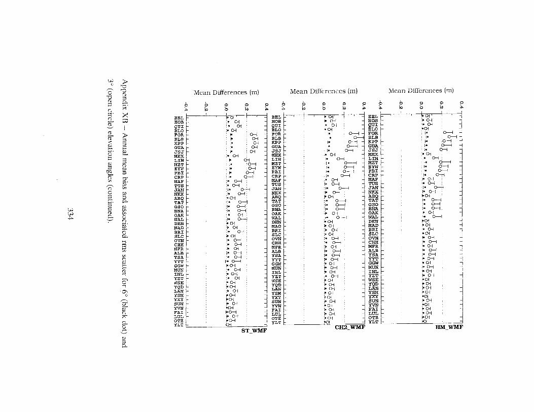
w w ~
w 0
~
0 'd
(D ::l n ;::;· n 0 ..___, (D
(D' < p ,..,. a· ::l p ::l
(Jq
(D' (fJ
,-.. n 0 ::l ,.... s· ;::: (P 0.. ..___,
> 'd "d
(D ::l 0.. x· >< o::;l
I
~ ::l ;::: 2:.. § p ::l 0" p;· 'Jl
~ 0.. p (fJ (fJ
0 n p;· ...... (D 0..
a 'Jl
'Jl n p ....... ,...... (P ""!
b' '""1
0'1 0
~
cr' ~ n
"' 0.. 0 ,-.
"---'
~ p..
BEL
6 ;;:.
~g~ Er-BLo FOR, BLB f-
MEX
Mean Differences (m)
b ~
0 0
I' a jo 01
" 01 loQ-i I< I" I" ;-~
.~ Q-1
0 ~
I> Q-1
Q-i 0-i Oi
Q-1 0-i ~~;~!
LIH MZT EYW PBI CRP i-
fo 0---1
MAF t ~~~· ABQ
1- 0--l 1- ()--j fo Q--1
1- o--1 1- Q-i ,. D---1 ;. Q-i
1-01 fo 0--l ,. 0-1 to Q--l
" Q-i 1- D---1 :001 jo 01
TAT GSO BNA, OAK r WAL fDEN j MAD· BRI I SLC ~ !o 01
1- Q--1'
OVN L 1- Q-i CHH L 1- Q-i
MFR ~ !o 01 ALB ·t- o--1 YSA 1- o-i YYT f-o 0--l GGW ~ 1<0-\ MUN .1- 0-l INL ;. Q-l
YZT ~ i' 01 WSE 1"0-i YQD I< 0-i LAN •I> 0-1 YSM 1>0-l YXY 1>01 SUN •I< Q-\ YVN 't 1>01 FAI I 100--i LUL [ •1- Q-1
~~~ L ~0-l
0 ;;:.
ST_WMF
Mean Differences (m)
6 ;.,.
6 ~
0 0
0 ~
BEL ~ I I. 01' t HOB j 1- 0-l QUI r 1- 0-i BLO f- )o Oi FOR f- 1-BLB l fo KPP [ 1- 0--i GUA fo 0----1 JSJ I< 0---1 14EX !o Oi LIH ~~ I< o--1 MZT f-o 0---i EYW !-< 0--1 PBI fo 0----1 CRP f- 14 0--i MAF[- i-0-i
~~[ ·~ ~ NKX t 1- 0--i ABQ .i" Q-\
TAT ~ 1- 0----l GSO fo o----1 BNA 1- o----1 OAK f- !o 0-l WAL [- fo 0--1
DEN~ i-01 MAD "Q-i BRI I< 0-i SLC I )o 01 OVN r- 1- o-i
~~~t ~ ~ ALB ~~ 1- Q---1 YSA 1- Q---1 YYT 1- o-i GGW 1> Q-i
~~~ ~t ~ g; YZT 1- 0-i WSE )o 01 YQD I> 0-i LAN ~ 01 YSM i' Q-1 YXY i'Q-1 SUN lo Q-1 YVN l )oQ-1 FAI [- I> 01 LUL ~ ~ Q-1 OTZ )oQ-1 YLT )oQ
Mean Differences (mj
0 b 6 0 0 0 ;.,. ;.,. ~ 0 ~ ;.,.
BBL~ I 1,"', I '~ HOB 1- ·• Q-1 QUI f- 1- Q-\ BLO' 1-01
FOR E fo D---1 ~ BLB ro 0--i KPP ~ 1- 0-1 GUA ,- fo 0--1 JsJ r- ,. o--1
~~~ I •,. 01 0--l MZT ~ f-o 0---i EYW t !-< o--1 PBI . f<' o------; CRP f- ,. 0-1 MAF' ;. Q-1 TUS [ ;. 0--l JAN 1- . 1- D---1 NKX 1- 1- 0-i
ABQ t 1-01 TAT 1- D---1 GSO 1- 0-1 BNA 1- 0-1 OAK~- 1> 01 WAL 1- D---1 DEN !oQ-1
M . .lUl ~ ;.01 BRI ;. Q-\ SLC io01 OVN 1- 0-i CHH 1- o--1 MFR 1- 01 ALB 1- o--1 YSA [ 1- 0--i YYT ;o 0--l GGW I> 0-1
~lt ~~ ~ WSE 1<01 YQD ·1> 0-1 LAN ;.Q-1 YSM 1>0-1
~~ ~~ -l YVN 1>01 -j FAI 1> 0-1 j LULL 1"0-i j OTZ b 1<0-1 1 YLT ~ ~
CH2_WMF HM_WMF

\.;.) > 0 "d ~ "d Mean Differences (m) 0 (P Mean Differences (m) Mean Differences (m) "d ~ (P 0... :::J
><" 6 6 0 0 0 0 ~ 0 0 0 6 ~ 0 0 0
() :n i:.l 0 i:.l Cl Cl IN 0 1N Cl ;;. ~ 0 N ;;. ::;· X BELL I I
~ Uj BEL ,Ol
:~~ r . Ol. ~~a
(P HOB ,. 0-i ;.Q-i ~g~! ,. 0-i
'.._./ I QUI ,. 01 QUI jo 01 ,. 01
(P > BLO JoOi BLO ~Ol BLO 1>0-i
....... FOR fo 0---1 FOR fo {)-I FOR fe Q-i G ~ BLB fo ~1 BLB fo Q-i BLB ~ ~
< ~ KPP F fo Q-i KPP fo Q-1 KPP ~ Q-1
"' ,..... ~ GUA ;. (}-j ~~~ ~
fo (}-j GUA ~ ~
a· 2. JSJ ~ :0 0---i • ~ JSJ L • Q-1
:::J s MEX t • 01 MEX r- ;.o; MEX ~ • Q-1
~ LIH :0 Q-1 LIH E :0 Q-1 LIH ,. Q-1
"' (P MZT f- fo ()----l MZT fo ()----l
:~~ fo (}-j -;
:::J 5 EYW i- .fo 0--1 ~~~ ;. 0-1 fo o-J l
(fq PBI ~
~ (P
;. (}-j ;. (}-j PBI fo 0--1
C) CRP I- ;. 0---1 CRP !-- fo Q-i CRP fo G--1 [/J
~- ~~ " 0-1 !<!AF ~ " Q-1 MAF fo 0---1
~ .. ~ TUS ,. Q-1 TUS ,. Q-i () [/1
0 JAN r- .fo (}-j JAN:..- ·r- 0--l JAN~ ~ ()----l
"' NKX ['- • Q-1 NKX t " Q-1 NKX 10 Q-i•
:::J ~ ABQ JoD-i ABQ i'Ol ABQ 100-i ..... 0... ::r TAT~ ~ o---1 TAT r ;. (}-j TAT~ -~ G--1
\.;.) c "' GSO 10 0---1 GSO ,. 0---1 GSO fo o---1 _j [/1
~~[ 10 0--1 BNA ;. 0---1 BNA fo (}-j
w (P [/1
V1. 0.. 0 ;.01 OAK !o01 OAK • Q-1 ..J
'.._./ () WAL ~ fo (}-j WAL ;. 0--1 WAL r- ()----l
"' ~ joQ-1 DEN l'Oi DEN r :00-i
~ ;.01 MAD jo()l MADr • 01
(P BRI r • 01 BRI • 0-i BRI ;. Q-1
0... SLC ~ ;.01 SLC ~Ol SLC • 01
>-I g~~ ,. Q-1 OVN • Q-1 OVN fo 0-1
s jo Q-i CHH ~ Q-1 CHH ;. Q-1
[/1 MFR • 01 MFR • 01 MFR ,. 01
C/0 ALB F i" Q-1 ALB i" Q-1 ALB .,. 0--1
0 YSA ,te 0---i YSA fo Q-1 1 YSA :~ Q-i
~ YYT jo Q-1 YYT .• Q-1 YYT f;e o---1
.-.. GGW~ ;.01 GGW joQi GGW joQ-1
(P MUN 100-i ... ~ :00-i MUliT fo Q-1
~ >-I INL joQ-1 INL JoD-i INL ~ fo~
,_.,., YZT .• 0-i YZT joQ-1 YZT • 01 1 0 WSE i'Ol WSE >Ol WSE jeQ-1
~ >-I YQD I !o01 YQD JoD-i YQD 1"0-i
0'1 LAN~ .01 LAN ,.01 LAN'- • 0-i 0 YSM loD-i YSM t l-01 YSM ~ i-o-1
r-.. YXY ~ 1>01 YXY !oOl YXY r- joOJ
C) SUN ;.o-J SUN 1 ,. 0-i SUN r- Joo-i ~
~ m~ i'Oi YVN r joOj YVN. JoD-i l 0 >01 FAI F •OJ FAI E foo-l -,
i"';" LUL JoD-i LUL JoD-i LUL te o-;
~ 0.. OTZ loQ-1 OTZ ~ joQ-1 OTZ L,_ foo-l
0 YLT 10 YLT !0 YLT, ~
,_ BL_WMF CHI_WMF GG_WMF '-/
"' ~ 0...

VJ VJ 0\
VJ c
,-..._ 0
'""d (i) :::::J
~-'""! ()
(p '-" (i)
(D < ~ ...... 0 :::::J
El (jq (D rn
> '""d '""d (i) ;::l 0... ;;<" ;>< to i
i ~ ;........
~ "' :::::J
0"' j33" rn
"' :::::J 0...
"' rn rn 0 ()
§." (i) 0... '""'i
a rn rn ()
"' ,..... ,...,. (i) '""'i >-:+, 0 '""'i
0\ 0
~
0"'
~ ~
0... 0 ,..... ~
"' :::::J p..
Mean Differences (m)
~ "'
0 0
0 ~
0 m 6 m
Mean Differences (m) Mean Differences (m)
6 0 ~ 0
0 0 6 6 0 0 0 ~ m m w o ~ m
BEL ~ I I K5 ,I BEL ~ 10 " BEL ~ i I, ot I I ~ HOB f-0 o! HOB f-0 o HOB >-~ !o Oi QUI f-0 • QUI f-0 • • QUI .• 01
BLO f-0 o1 BLO ! f-0 o! BLO iO ot ~
6
"' FOR f-0 oj FOR f{) oi . FOR i* 0--i BLB ~f-0 • BLB f{) • BLB E i* 0--i KPP '- f-0 o! KPP f{) oj KJ?P fo 0-1
GUA ~ f-0 o! GUA f-0 " GUA i* o--1 l JSJ f-0 o! JSJ fD o! JSJ I !" 0-i MEX f-0 <! MEX f-0 < MEX " 01 LIH r-o .; LIH f.. ro • LIH F • o-; MZT f--0 ., MZT f.. f--0 ., MZT F 1- (}---i
EYW t f-0 o1 EYW ~ f-{) o1 EYI'l r i* a-t PBI 1--0 ~ PBI ~ 1-0 Oi PBI f fo o--1 .., CRP 1- 1--0 ., CRP f-0 Oi CRP ~ fo 0--i -j MAF r f-0 "I MAF f-{) "i MAF " 0-i TUS 1 1-0 -1 TUS f-0 -1 TUS 10 0-l JAN r t--0 eo JAN f 1--0 "1 JAN i* o--i NKX f- t--0 -1 NKX f-0 "! NKX .!< 0-l ABQ f-0 o1 ABQ f-0 ol. ABQ " 01 TAT ~ f--0 eo TAT f,---0. "1 TAT i* o--i GSO f--0 "1 GSO ~ 1--0 "I GSO .fo 0--1 BNA f--0 "I 1 BNA 1--0 -1 BNA !< 0--1 OAK f-0 'i -j OAK f-0 o! OAK !o 01 WAL - 1---D - WAL f,---0 -1 WAL '" o--i DEN ~ f-0 o! DEN f-0 " DEN !o 01 MAD f-0 o! MAD fD <! MAD iO 01 . BRI .f-0 .; BRI r f-0 o! BRI !o Oi
3 SLC f-0 < SLC r fD 'i SLC iO ot OVN ~ f,---0 -1 OVN I 1-0 ., OVN • 0-l CHH 1--0 eo CHH I f-0 "I CHH .1< 0-1 MFR f-0 ol MFR ~ f-0 ". MFR !o 01 ALB 1--0 Oi ALB f-0 -1 ALB fo 0-1 YSA f--0 o1 YSA f-<l "' YSA !< 0-1 YYT 1-0 -1 YYT f- f-{) o1 YYT ~ fo 0-l GGW f-0 .; l GGW r f-0 o! GGW > 01 MUN 1-0 ol l MUN r-- f-0 .; MUN !o 0-i
INL 1-0 -1
3 INL r 1-0 -1. INL ~ .• Oi YZT f-0 • YZT f-0 ~ YZT !o 0-i
WSE f-0 ol WSE f-0 ' J WSE !o Oi YQD f-0 "I J YQD f-0 ~ YQD iO 01 ~~~ ~~ ~~~! ~~ ~~~ :.g: . YXY E ro • -j YXY f-0 • YXY •ot l sUN f-0 ~ .., sUN I ro • sUN • oo YVN , f-0 'i -1 YVN f-0 'i YVN "ot FAI 1-0 '" ..j FAI f-0 .;· FAI
1 " 01
LUL t f-0 ~· 3 LUL ~ f-0 "1. l LUL ~ • Oi OTZ ~ f-0 "' OTZ f-0. OTZ ~ 1>01 -1 YLT r fOo! YLT IOo! YLT Kl -J
UNSW_WMF CfA_WMF YI_WMF

APPENDIX XI
Annual mean bias and nns scatter (one-sigma level) of the differences with respect to ray
tracing for different total mapping functions, for 50 radiosonde stations listed in
Appendix III, and at different elevation angles.
337

v.l v.l 00
§ 0.. ,...... 0
0
~
0 '"d (1) :::l (') ~· (')
(P '-" (1)
0 < ~ ...... a· :::l
§ (1q
0 "' ~ (') 0 :::l ...... -· :::l ~ (1) 0.. '-"
.-6' '"d g 0.. ...... X
~ ,._.. > I
5-§ a ~ § 0"' ~-
§ 0.. ~
"' "' 0 (')
~· (1)
0..
a "' rn (')
~ ....... (1) ..., b' ...,
-VI 0
~
0"' -~ (')
i>' 0.. 0 ...... '-"
b 0 .. ""
Mean Differences (m)
(::J 0
~
0
8 0
0
§ 0 0 .... ""
BEL I I 6:==tr::4J I I ~ HOB . o-+--{ QUI 0--t-•{ BLO CJl-o'----1 FOR D-ll* BLB ~ KPP o-tto GUA 0-io JSJ Q-l !"' MEX Ool L!H o-i,., MZT ~ EYW t 0!--1 PBI I 0+-o-i
~!~r ~ JAN o----1 NKX e---1 ABQ (90--i TAT o-t-:'
GSO ~ ot-oH BNA 0+-o<i OAK 90----1 WAL ~ DEN ~ MAD G<>;-1 BRI ~ SLC i- f3--l OVN f- o---! CHH t- 0+--l MFR f- f-3-----i
~~~t ~ YYT ~ GGW ~ MUN o----1
~~~~ ~ WSE f-tlo-------1 YQD (])--o----1 LAN HO----I YSM ~ YXY re.------1
SUN~ ~.' ; YVN o---J-lo • FAI !--®----i LUL ~ r-- o------:---1 d OTZ ~ YLT ~
LA2_TMF
Mean Differences (m) Mean Differences (m)
b 8 -.j
0
§ 0
8 -.j
0 0 .... ""
b 0 .... ""
b 0 0 -.j
0
§ BEL~~ '----11 ' I BEL HOB H---0 --j HOB 1-0 0.: QUI : 1--0-.j QUI r---10 BLO 1-'----0 -....;.·. BLO r--<l----1 FOR l-+0 FOR f--(H BLB ~ BLB ~ KPP 1-;"+0 KPP 1----0,_, · GUA f*tQ GUA f-0<1
~ir ~ ~i ~~ LIH ~ ~. LIH f-0 <1 MZT ~ MZT 1--@l EYW 1--+0 EYW f----0 ._, PBI f- r-;-0 PBI f----<l'-i CRP I 1--0 CRP t----<)--i
~~~ ~ ~~ ~ JAN 1---<Q JAN ~ NKX 1----e NKX ~ ABQ , 1---0rl ABQ 1----0<1 TAT 'f-------Oo-1 TAT ~ GSO ·~ GSO ~ BNA I-----Ori BNA ~ OAK f-----iE! OAK ~ WAL f------$-1 WAL f----oe DEN 1--<Ji DEN 1---0 •I
~~ ~.· ~~ ~~ SLC ~ SLC 1--0._, OVN I-----Ori OVN f----0-l CHH r----o o-1 CHH 1---®'1 MFR ~ MFR f-------0---'1 ALB r----oo-,; ALB J----®oi YSA f----0 o-1 YSA t-------el YYT f-------0 -" YYT ~ GGW t-----tr1 GGW f---Oo-1 MUN ~ MUN f----0 ._,
YZT 1-----G YZT f---<) o-!
9 0 0 -.j
0 0 ... ""
INL f-------0. ---'1 INL ~I •· 1----<)C! .• WSE ~ WSE !---0 o-i
YQD ~ YQD f----()--l ~· LAN . ~ LAN f-'--<) ._, . YSM ~ YSM f----()o--,j YXY ~ YXY f----0 ._, SUN ~ SUN f---<) o--J.
yVN >--C<> ~ """ • c---<>~ ~ FAI ~ FAI' ·~ LUL t-----o-lD LUL ;-----o ----1 OTZ t-----Oo--j OTZ E . f----{)00--j YLT !--0 ._, YLT f---<)o-i
NMF _TMF IF _TMF

'-.H (J.l
1.0
~
5. -0 0
~
0 '"d g ()
~· ()
(D '-" (D
0 < ~ .-.. o· ~
§ CfQ
0 r:n ~
r. 0 ::1 ..... s· c: (])
0... '-"
~ '"d
(1) ::1 0... >i" X ,...... >
~ § ~
8 (') ~ ::1 C) p;· r:n
P:l ::1 0... P:l r:n r:n 0 ()
p· ,_.,. (D
0... >-\
8 r:n r:n () P:l ,_.,. ,_.,. (]) >-\
8' >-\
........ Vl
0
~
2:: P:l () :>';""'
0... 0 .....
'-.-/
Mean Differences (m)
6 0
"' ,. 9 0 .... "'
0 0 0 0
~~~ ~'-" f+oO QUI ~ BLO t------+0 FOR l--0 <-BLB 1----0 f-o KPP r 1---0 f-o GUA f- 1--0 f-o
~~~ ~t ~ \: LIH ~ MZ T f------0-o EYW 1--0,_. PBI 1---0--CRP 1------0-MAF 1--+D TUS 1 f--+0
~ t J-----+-{)li--{)
ABQ ~ f----0 TAT H--0 GSO ~ BNA ~ OAK f- f+-+-0 WAL~ ~ DEN ~
~~~ ~ SLC r+0 OVN 1----t-+0 CHH 1!-*-0 MFR E H--0 ALB 1-t--+-0
YSA ~· 11-0 YYT H---0 GGW ~ MUN f----Kl INL ~ YZT ~
LAN f-K) YSM ~ YXY 1----t-+0 SUN H-0
!=' 0 ,_.
"'
0 s ,.
~~~~ ~
~ ~ J LUL f- f+--0 OTZ r i+<-------0 YLT 1- ,_. !--0
CfA_TMF
Mean Differences (m)
9 0
"' 6 0 ....
!=' 0 0
!=' 0 ....
BEL HOB QUI ~ o1 r-----0 BLO FOR f-0
~~!~' :£ JSJ ro MEX •f-0 LIH K}l MZT r 1>+-0 EYWt ~ PBI
1 f-4-0
CRP '-t f-!0 MAF 1-+0 TUS f--c€) JAN f---+0 NKX M-0 ABQ [- l-+iO TATj ~ GSO I f-o+O BNAj ~ OAK 1- t--+-+0 WAL r f-o-K)
DEN~ ;t-0 MAD 1-0 BRI ~ SLC ~ OVN f-+0 CHH f- . 1-i---0 MFR f f--0 ALB r f-++0 YSA 1- f---+<J YYT f- 1++-0 GGW [- 1--+0 MUN r f-++0 INL '- t--+-+0 YZT f- ~
YQD J---o--+-0 LAN ~
!=' 0
"'
WSE ~ 1--+0
ii~~r ·~ l SUN 1--10 YVN /0-+----0 FAI f- r----+---0 LULf- ~ OT Z oH------D YLT ~ ___, t-----0
LA4_TMF
Mean Differences (m)
6 0 "'
6 0 ....
0 0 0
BEL ~ f-loo---L-1 HOB ~ QUI f-o 0----1 BLO ~ FOR ~ BLB f- 0-1 KPP ~ GUA c-o--1
JSJ t 10-i MEX c. o--! LIH C>-l MZT f-o Q--1 EYW ' i-0----i PBI F f-oQ---1 CRP r f-o()---1
p 0 ....
JAN t--~ ~~l' ~ NKX f-4(}------j ABQ f-oo----1 TAT coo----1 GSO I- 0--l BNA f-oD--1 OAK f-'oo-------1
WAL ~1
f-. o------l DEN f-oD--1 MAD 0'-l BRI ~ SLC ~ OVN t-0---1 CHH F f-o 0---1 MFR ~ ALB I- o------l YSA f-o 0----1 YYT f-o 0---1 GGW !-C>--1 MUN ro------1 INL I- ()------j YZT f-o()------j WSE f-oo---1 YQD I- 0------i LAN ICi-i YSM f-'o o-------1 YXY t f-C>----1 SUN f-0------1 YVN f- I- 0--l FAI ' f-' o-------; L UL [ 1-0-------i OTZ f- f-o 0-------i YLT f- f-o 0--l
0 0 "'
MTT._TMF

\.;J ~ 0
[ -0
0
~
0 '"d
(D :::::l () ;:;· ()
(D '-' () -(D
< ~ ,._,. ,_.. 0 ::::;
§ (Jq
0 en ~
()
0 ::::; .-..
~r (i) p_. '-'
>'"d '"d (? ::::; p_. :;;;· >< ...... >-
>-::::;
2 E.. :3 (D
§ u p;· en ~
B. ~ en en 0 ()
s;· ,...,. (D p_.
§ en [fJ () ~ ..... ,...,. (i) >-!
8' >-!
Vl 0
~
v [ ~
p_. 0 .-.. '-'
Mean Differences (m)
6 0 (»
6 0 c.:>
0 0 0
BEL r-:f-()' •L HOB 1-0 Oi QUI !-0! BLO f-0 oi
FOR~ f-Oe BLB 1-0 ~ KPl? fO "i GUA ~ fO " JSJ ~ fO ~ MEX fO " LIH 1-0 ~ MZT r 1-0 <I EYW f- 1-001 l?BI r I-OOJ CRl? [ r-Ooi MAFI- f-0 "i
I~~ L f-0~ NKX 1- r-Ooi ABQ L K) ol TAT f- I-Ool
GSO ~ 1-0 ~ BNA 1-0 ~ OAK f-O'i WAL I-O-DEN r-0 oi
~ ~ f-0 1-0~ SLC t f-0 ~ OVN 1-0 ~·
CHH f- 1-0 ~ MFR t' f-0 >1
~~~ ~ \::2: YYT f-0 "i GGW f-0 oi MUN f-0 oJ INL f~-0 >0 YZT f-0 oJ WSE r-0 oi YQD f-0 "i LAN' r-0 "i YSM E f-0 .,. YXY .1- f-0 "i SUN. f-0 .; YVN ~ f--'--0 0-i : FAI f--0 -i
0 0 c.:>
!=' 0 (»
LUL f--0 o.J OTZ ~ f--0 "i d YLT r r--0 ~
SA_TMF
Mean Differences (m)
6 0 ~
BEL. HOB f.QUIt
~~~ ~ BLB 'Kl?l? 1-GUA fJSJ,
~~ r~ MZT
6 0 ~
? 0 0
f-e .Q--j <- . Q-i
;.. 0--i <-<~ ~
'" •OJ ~ ;.. ;.. ~
;.. ~
fo Q--j
0--'-1
0 0 ~
o-1 o-1
Q-1 Q-i
01
01 0--l .o-i
0---i 0--i
EYW PBI .CRl? fMAF I TUS [
~~ ABQE
~ ;..
;..Q--i f-e
o---1 Q--j
TAT
~~~ ~ OAK WAL DEN ~
c. ~ ;..
H
0---1 0----i 0----i 0---i o----1
~~t ~~ SLC L ;.. 0--l OVN L c. D---i CHH ~ f- G-------l MFR f- ~ Q--l ALB [- r- G-------l YSA r f-e 0---l YYT f- f- Q---1 GGW r c• 0--'-1 MUN 1- ~ 0--1 INL ~ f- o---J YZT ~ Q--l WSE ~0--'-1
YQD ~ f-e o---1 LAN ~ 0--'-1 YSM f-e o---J YXY ~ SUN 1~ o---1 YVN fa----1 . FAI f-o---J LUL f-e o---J
~£~[ ~
0
~
CH_TMF
Mean Differences (m)
6 0 ,;.
6 0 ~
? 0 0
BEL 1- flO loj HOB f- 1-0 o1 QUI r f-0 oJ BLO 1- f-0 o.J FOR f- f-0 "i BLB 'E f-0 .,: KPl? r-0 oJ GUA f-0 oJ JSJ f- r-0 oi
MEX f- r-0 "'· LIH f- f-0 "i
MZ T ~ f----.,-0 "cl EYt'l r--0 0-i PBI f----.,-0 ~ CRl? }-------() "cl MAF f---0 • "i TUS i--O"i JAN f----0 ·~ NKX f---0 oi ABQ r-0 oJ TAT f---0 "i GSO f--'--0 .~ BNA f--'--0 ·~
OAK f-0 "i WAL t---0 "i
0 0
g ~
DEN K)ol ..; MAD H) oi -i BRI i--0 o! -I SLC f-0 >0 l OVN f-0 o1 ., CHH 1-D oi l MFR f--0, ~ _, ALB f-0 oJ -j YSA f-0 oJ -j YYT 1-0 "i 3 GGW H) oJ MUN f-0 .;
INL ~ i--0 .;
YZT f-0 oi, 1 WSE f-0 oi YQD r-0 oi LAN r-0 <>i YSM t r-0 -', YXY ~ 1-0 oi
SUN t f-0 o! YVN f--0 -1 FAI f-0 ~ -J LUL f-0 -i -j OTZ ~ f-0 oJ ~ YLT t---0 •i
HL_TMF

\j.) _p,.. ......
s CL -0
0
~
0 '"d (D
0 (") -· '-I (")
(D '--' (P
(5" < ~ ,...,. a· 0 ~ ::l
{JQ
(5" [f)
~ (")
0 0 ,...,. ::r c (P
CL '--'
~ '"d (D
0 CL ...... ><:
>< ....... > I
5' § 2.. 3 (D ~ ::l
o" ~-[f)
~ 0 CL ~ [f) [f)
0 (")
~-(',)
CL '-I
3 [f)
(ZJ (")
;:;. ,....,. (P '-I
b' '-I
Ul 0
~
o"
~ ;r;"
CL 0 ...... '--'
Mean Differences (m)
6 0 00
BEL HOB QUI BLO FOR BLB KPP GUA JSJ MEX LIH MZT EYW f-
f-0
6 0 ..
f-0 1-Q
1-0 1--0
1:-0 1-0 K)
1-Q f-0 r.:o
1-0 PBI 1- 1--0 CRP t 1-0 MAF f--0 TUS G......:.r, JANL ~ NKXf-1-0
~~~~ ~ GSO 1-0 BNA 1-0 OAK 1-0 WAL 1-Q
DEN~ 1-Q MAD i-0
~~~ ~ ~ OVN 1-0 CHH f--0 MFR 1--0 ALB 1-0
YSA E' 1-Q YYT 1-0
~I' 1f YZT 1-0 WSE i-0 YQD 1-0 LAN i-0 YSM 1-0 YXY 1-0 SUN 1-0 YVN f-0 FAI f.. i-0 LUL f- i-0 OTZ f- f-0 YLT t:::...._jQ
ej oj
.; "l oj
"l oj
~
o-1 oj
o-; oj
oj o-j
-i -i
o-j o-j
o-j
oj a-]
o-; ., ., ., oj
o-j ., o-; <-1 ., ., ., oj
oj oj
oj
~ ~ ~ oj ., Oj
of 'i oj
of
" •
p 0 0
9 0 .. p
0 00
BB_TMF
6 iii
BEL HOB· QUI 1
BLOt: FOR L BLB
1
KPP ~ GUAt ~~~-LIH ~ MZT !-
~~~ CRP t MAF
~~~ NKXt
~~r~' BNA OAK WAL DEN
MAD I BRI SLC OVN CHH MFR ALB YSA YYT GGW
~t YZT fWSE L YQD I
~F YVN FAI
Mean Diilerences (m)
6 0 "'
9 0 0
p 0
"' ]0.--- I 01 ~ ,Oi ~ . 01
,. 0--i
'" Oi '" Oi '" 01 '" a '" a fo 01
'" • '" ~ '"
01 01
Oi Oi Oi
,.. ()--j ,. Q--j
,.. 0--l fo 0-j
,.. 0--l
'" 10 10 10
'" ,.. '" '" ,. r-
'" j-o
r-
'" I~
j-o
fo I•
'" ,.. ,.. 1-j-o ,.. '" j-o
f-o
0--l Oi
01 Q-1 Q-1 Q-1 01
01 Q--j
0-1 Oi
0--i 0-1
01 0--1
0--i 0-j
0--1 Oi
0--1 ()--j
01 ~
()--j
0-1 ()--j ~~~~
LUL. fo ~
0-l ()--j OTZ f- ;.
YLT fo
0 0 Cl
ST_TMF
Mean Differences (rn)
6 0 Cl
6 0 "'
BEL f- fC'i HOB [- 10 o!
~~~ t ~: FOR 10 '! BLB KJ '! KPP KJ <i GUA KJ ~ JSJ 1-0 .; MEX f-0 o! LIH 1-0 • MZT 1--0 &i EYW f-0 .; PBI i-0 ~. CRP i-0 -; MAF L i-0 .;
TUS ~ i-0 -i JAN 1-Q o-; NKX I-O"i ABQ 1-0 "I TAT t 1-0 Oi GSO. 1-0 o-1 BNA t 1-0 o-;
~~I ~~ DEN 1-0 Oi MAD 10 'i BRI 1-0 o SLC f-0 el OVN 1-0 "l CHH 1-0 ~ MFR 1--0 oi ALB 1-0.;
YYT I-O"i
p 0 0
9 0
"' 9 0 Cl
YSA ~ I-Oof
GGW ·1-0"1 .
~~~- ~-~ ~ YZT 1-0 <I WSE f-0 Oi
~! ss ~ YXY i-0 Oi -j SUN . f-<)01 -j YVN f--{§1 -j F AI 1---{)o-1
LUL f-0•1 3 OTZ b 1--@i YLT 1--<D
UNSW_TMF

w .j:::.. N
§ 0..
0 0
~
0 '"0 ~ ::I 0 ~=;· 0 ~
'-..-'
(i)
~ < ~ a· ::l PJ ::l
(fq
~ [fJ
~
0 0 ::l c. ::l .:: (i)
0.. '-"'
~ '"0 ~ ::I 0.. ><·
:>< ;-<
>-
~ =-. 3 (i)
§ cr p,;· [fJ
PJ ::I 0.. PJ [fJ [fJ
0 0 P3" ....... (i)
0..
"" 3 [fJ
[fJ
0 PJ ....... ....... (i)
"" '="> 0 "" ....... Vt
0
~
u ~ 0
"' 0.. 0 ,....,.
'-..-'
Mean Differences (m)
~ ..... 0
6 0 01
0 0 0
0 0 01
BELr-,- ~· I~ HOB l ;. a QUI r ~ 01 BLO r fo <)-i
~~~ ~ ~ ~ KPP t !o , 01 GUA t )o 01 JSJ • a MEX I> 01 LIH f- !o 0 MZT f- )o 01 EYW I )o 01 PBI I ~ '01 CRP I )o ~ MAF r fo 0-l TUS -~ fo o.j J~ fo 0-l NKX ie ~ ABQI- I< ~ TAT f- ~ 01 GSO r I< ,~
BNAt fo ~ OAK L I< ~ WALL 1< ~ =I ~ ~ BRI ~r )o a SLC fo 0-l OVN I< ~
CHH~ iO 01 MFR 1- <)-1 ALB 1- ~ YSA 1 )o 01 YYTt )o 01 GGW 1- <)-i MUN fo ~ INL ~ fo <)-i
YQD fo 0-i L~ lo ~ YSM !• D--1 YXY fo <)-i SUN 1< ~ YVN I• <)-i FAI ~ 0-1
~ ~ ... ,...
0 0
BEL HOB QUI,
BLO E FOR BLB KPP fGUA r JSJ I
Mean Differences (m)
6 0 01
0 0 0
0 0 01
)o' Ia • a a
,. Q-1
• a • a • 0 • 0 • 0
• 01 LIH i' a MEX ~ MZT iO a
~~~ f>- ~ % CRP iO 01 MAF fo 0-l TUS fo <)-i JAN fo 0-l NKX I< Oi ABQ "' 0-l TAT lo a G~ ~ ~
~;:~ ~L : ~ WAL • Oi DEN fo 0-l MAD ie 01 BRI )o a SLC , fo <)-i OVN 1- 1- ~ CHH I )o 'a MFR f= '- <)-i ALB 1- 1- ~ YSA 1- )o a YYT fo 0-l GGW fo <)-i MUN fo ~ INL i" 0-1 YZT !o 01 WSE fo 0-l YQD fo <)-i LAN )o Oi YSM fo 0-i YXY fo 0-l SUN ~ ~ YVN fo <)-i FAI fo 0-i
~~i ~~ : 0-l 01
LUL ~ 1- 0-l ~ OTZ fo 0-i YLT co <)-i
LUL i" Oi OTZ I" <)-i YW i" 0-l
~ ... 0
YI_TMF GG_TMF
Mean Differences (m)
p ~
6 0 01
0 0 0
0 0 01
BELl I I •' b HOB • a QUI )o '01 BLO FOR,
JSJ
,. )o
• • • •
Q-j
01 a a 01 a
BLB F KPP ~ GUA
~~I MZT ~ EYW t PBI
~ 01 • • )o
CRP )o
MAF !o TUS !o JAN ~ NKX ;. ABQ ~ TAT !o GSO I< BNA I< OAK 1< WALL )o
a a 0! Oi 01
0-l 0-l
0-l Oi
~ 01 ~ ~ ~ 01
DEN f- fo ~ MAD r )o 01 BRI f- !o a SLC t fo 0-l OVN I" ~ CHH 1o 01 MFR 1- o-1 ALB!- !o ~ YSA t )o a YYT L ~ 01 GGW, 1< Q-1
~~r- ~ ~ YZT ~ !o 01 WSE fO 0-l YQD fo 0-i LAN f- " 01
~ .... 0
YSM r ~ D--1 YXY 1 fo o-1 , SUN[- 1< ~ -i m~ : ~ ~ LUL fo 0-l OTZ fo , 0-i YLT fo 0-1 -l
BL __ TMF

\.).) _J::,. \.).)
:oJ ~ 0.. -0
0
~
0 "d (i)
= 0 ,_.. ""i 0 (C
'-..../
(i)
0 < ;:::; .-a· = 5
(jq (5"' [FJ
> '""d "0 g 0.. ~·
>< ,....., >
> = = ;::: ~ :::;; 0 ;:::;
= :::r s;~
[FJ
;:::; ~ 0.. ;:::; [FJ [FJ
0 0 ~-(i) 0.. ""i
8 [FJ
[FJ () ;:::; ,...,. .-(i) '"""I
8' >-!
........ U1
0
~
:::r ~ I';"
0.. c ...... '--.../
Mean Differences (m)
? -;;. BEL· HmoF QUI ;BLO ;FOR: BLB f= Kli?P f-q~~ I ME:xr LIH [ MZT lEY\'!/ f-
~i~ ~ I>1AF fTUS ;JAN t--
6 0 ...
0
g ~
I> ~
•
[o
• [o
• [o ;.
• )o
" ~
• lo
9 0 -.]
a Q
01
0
01 01
a a 0 Q 0
Q 01 a 01 a
NKX'
~~ ~ ~ Oi GSO r- ~ Ol
01
Ol 01
BNAf-- ;. Oi OAK f-- ~ 01
~~~ /' 01 Oi MADf-- to 01 :SRI f- ~ 01 SLC f- lo 01 mm:- ~ o; CHH i-- ;. Of MFR i--1-. ~ 01 ALB ~ Of YSA [- ~ Oi YYTI ~ Oi GGWr ;o Ol MUN [- to Ol INL r ;. _Ol YZT f- i' 01 WSE f- lo 01
9 ,_. ...
YQD [- ;o Oi
~~~ : ~ ~ yxyL ~ 01 SUN 1- ~ Ol YVNL ;. Oi FAI 1- I< Oi LUL f- I< Of ~ ~[; ~ : 0101
HM_TMF
Mean Differences (m) Mean Differences
;:: 6 0
0 p 0
p 6 6 0 0 0 ~ 0 0 0 ~ 0
0 (,~ 0 "" ,_. 0 0 ~ 0 ~ 0
' ' ' I lsi I BEL ~ ~ Q-1 . BEL f= ; ' !o' -; -~ HOB r fo 0-1 HOB t I> Cl QUI (- lo . Oi QUI r ~ Q BLO t- f- 01 BLO f- ;a Ol FOR [-- ~ Of FOR '[ > Q , BLB r I< BLB · i" a --j KPP f- ~ Ol KP!? 1- i' 0 -1 ~USAJ ! : OiOi GJUS~ f- : 00 l .., r . 1.,;' r · !
~~~ ";. a 01 ~ii~ •.o 0 j ~!ZT l- !< Q-1 MZT ·c' • 01 ~ EY\1f-- fo 0-1 ETw, lo 01 -; PBI f- !< Q-1 PBI f- i' a ll CR!? r ~ 0-1 CRl? f- i' 0 -
I-L'I.F f-. fo Q-1 1 :!<!AF 1- !' C!_ ~ TUS ~ ~ D-! TTJS !- /9 Q -l JAN r ~o Q-1 Ji'..N r- • 01 -i NKX , I" 0-1 ~"KX [. i' Oi -, ABQ L 1< Q-1 ABQ 1 i> 01 -j TAT 1- f<o D-1 TAT !- • Cl -l GSO r f<o Q--l GSO f- lo Q -I BNA f- co Q-1 BNA f- • C! -! OA.T"f- ;o 0-1 OAK f- i' Ol -j WAL ~ !< Q--l WAL ;- ~ 01 DEN 1- ;. Q-i DEN f- • Q ~Dl- ;. Oi ~Dr- to 0! BRI t ;. 0-1 BRI f- i' 0! SLC r I> 0-1 SLC (- I> 0!
g~c ~ ~ g~Hc ~ c;, I · .....,----, 1 '
MFR [-- !< o-1 MFR j- • 01 ALB ~c· !< 0---l ALB j- • 01 YSA !< Q--l YSA [-- " 0! YYT f<o Q--l YYT f- ~ Oi GGW I- I> Q-1 GGW I ;. 0! MUN 'c ;. 0-1 MUN E • 01 INL , !< Q-1 INL io 0! YZT f- 1< Q-1 YZT . " 01 WSE t I> D-1 WSE ~ • 01
~~-- ~ ~ ~~ : ~ YSM 1- !< o-i YSM E " 0{ YXY f- !< Q-1 YXY io 0! SUN '-- !< 0-i SUN f.. " Ol YVN 1 !< Q--l YVN f- fo Oi FAI ~ !< 0-i FAI >-- " Oi . LUL i- f<o Q--l j LUL [I fo Oi -i OTZ [-- r. Q-1 OTZ ~ Ol -I YLT r r. Q--l YLT I> Q-1 --'
~
MM_TMF BE_TMF
w ..j::. ..j::.
~ ::;1 0... w
0
~
0 "Ci ~ ::= (") ~::;· (")
~ '---"' ~ (P < ~ -· 0 ::;1
El CJQ
~ Cfl
,-..... (") 0 g ~§" ~ 0..
'....-'
> "Ci "Ci ~ :::: 0.. x· ;x 63
> § ~
g ~ ::;1
cr' s;· Cfl
§ 0.. ~ Cfl Cfl 0 (") -· a (;) 0.. --;
a Cfl
Cfl (")
~ .... ~ --;
""' 0 --;
0\ 0
,--., g: ~ ~
0.. 0 ......
'....-'
6 ~ ,p.
Mean Differences (m)
? ... !>:>
0
8 ? ... 1.:>
0 i..:> ,p.
' ' , I l BEL ~ I 1
f):; o-L--i HOB ~ QUI r- ~ BLO r-'- 0--------1 FOR f4D---l BLB ~ f4 o--1 KPP f-- feo--1 . GOA >- 14 D---l JSJ I ;.()---!
!-!EX ~ 'f4 o-i L!H '[ Ot+-l MZT 1 ~ D---l
~r~t ~ CR.P r f-oc----i MAF I f-o Q-----1
~~[ ~ N"!<X L ~ D-----i ABQ ~ 1'4~ TAT E ;.. a-----; GSO f-. Q-----1 BNA 1 f-o 0------i OAK j ~ o----; WAL l f-o 0----i DENj f-o a-----; MAD;- ~ BRI L a--1 SLC l ~a-----; OVN L r- 0----i . CHH ~ ... Q-----1 MFR r f--oO---l ALB r i-> D-----i YSA f- f-. Q-----1 YYT l f-< o--1 =I ~ INL t 1'-- o---'J YZT r- f-o o---; WSE r f-< D----1 YQDt f--4 ~ LA."i, ~
~~t ~0~ ~· SUN ~ f--4D-----i. YVN f- i-o 0------i FAI r- H o---'--1 I LUL 1 ~o----i l OTZ r f--4 o------;----; ~ YLT C f--41 : 0-----1
MTT_TMF
Mean Differences (m)
6 i.:>
BEL.
? ,... 0 0
HOB f- r----o --1 QUI 1- 1---C"-1 BLO ~ 'i---Oe--1 FOR r 1-*-0 BLBr *--0 KPP t 1'40 GUA. b++-0 JSJ f- !-,of() MEXI- 1--01
~~~ t f-{)j r+1-0 EYW f- 1-"+-0 PBI r r-ro CRP '- 1--i-0 MAF
1 1---f:!
TUS t f---+0 JAN f-----4-0 NKX ~ ABQ ! 1----Gi TAT ~ f------Oe--1 GSOf- ~ BNAf- ~
OAK~ f---+0 WAL f----61 DEN 1-----@li
~~~· ~ SLC ~ OVN 1-----4-i CHH , f'-------0 o-J MFR I- . 1----'-0 ALB 1- r:----o e--1 YSA L 1--------0 o-j
YYT ~ f-----0 o-J GGW ~ MUN . ~ INL f-- f------0 -'-J YZT r f-------{) WSE t , f------e1
~~ 1'-----0~ YSM . I Ell YXY 1------f)-1 SUN f--4-+0 YVN f---iO o-J FAif- ~ LUL j- t-----+--+0
? .... ? !>:>
OTZ r- f------0 ori YLT f- f--0 "-1 -j
NMF_TMF
~ ,... !>:>
Mean Differences (m)
6 8
? 0 0
0
~ ? .... !>:>
BEL F 1 i ct=-1 I ::4 HOB
g~~ ~· FOR BLB KPP
~~~f.. MEXfLIH >MZT iEYW 1-PBI ~ CRl? MAF TUS >JAN 1
NKXI ABQ t ~~6 ~~ BNA OAK WAL
~gL BRI r.. SLC fOVN r CHH I ALB YSA YYT
f---iO o-j t-t--<J
;----:.+-o H--0
f---4-0 1----'>-0 ~~
r----o ~ i-----091 ' 1---------0 f-------4-{)
r-----+0 f-----+-lO I I 0 I I 0
f---el 1-----'++0 f--l-O
f----+--t-0 I • 10 ~ ~
·r----o-o f'-------0 orl . t-----ei
1-----'--Kl f------+-0
MFR~ GGW I . 0 MUN f---'-----0 o-i INL I ·, 0 YZT f- I CJ--1 WSE f- f---'-----0----1
£~~ ~ ~·ID YSM t I ;o, YXY . 1-------0 --1
YVN I oOI SUN~ ~.._,., FAI . . , LUL 1- . o----1 3 OTZ f- I i01
YLTf-- ~ ,
IF_TMF

~ ~ t:l 0... '0 Mean Differences (m) Mean Differences (m} Mean Differences (m) w (p
0 ::l ~ 0... 6 ~ 6 6 6 6 0 s:;· 0 0 0 0 0 0 0 0 0
'0 a, ~ 0 w a, :::. i..; 0 i..; ;;.. ;;.. i..; 0 i..; ;;.. (p >< I ::l - BEL ., BEL 1-<Jo BEL~' ~
() to HOB f-0 ., HOB f-0 ,. HOB fa: ()--.1
-· QUI ~ QUI f-{}o QUI~ ,.. D--1 >-I () I BLO f-0 >{ BLO 1-----0 f-4 BLO f-o. Q-1
0 FOR of 1-0 FOR ~ FOR~ I> 01
'-" > BLB ~ BLB ,. BLB ~ Oi
(l) ::l KPP ~ 1-0 KPP f-0 ,. KPP ~. Oi
0 :::::: GUA of 1-0 GUA r-o ,. GUA it. Ol
s= JSJ ol 1-0 JSJ f-0 ,. JSJ " Ol
< e. MEX to • MEX 1---0 f-o MEX • Oi
~ LIH :'i-0 LIH f--0 f-o LIH ~· 0-l ....... o· § .,. r ott--O MZT !---0 r- MZT ~ 0--l
:::::: EYW ~ EYW t---0 ~ EYW ,. 0--l
~ PBI .!>t-O PBI 1-----0 ~ PBI .. 0--i
~ :::::: CRP 1+1-0 CRP ~· ~ CRP ~ 0--i
:::::: MAF 1---0 ., MAF 1-----0 f-o MAF ~ o-1 aq cr' TUS f--0., TUS ~ f-o TUS ;. o-1
(i) ;:;;· ~ 1---o
JANE j-------'-0 :--- JAN ~ (}--1
rn rn f-01 ~ i----0 ~ NKX ,. D--1
,......, ~
ABQ~ 1---0 ., t--O ~
~~I 10 Q--1
() TAT f----{)o-1 TAT 1 t---0 ~ ;. Q--1
0 ::l GSO ~ w :::::: 0.. ~--{)>{ GSO ;- 1----'--0 ,__. GSO fa D--1
-+::- ....... BNA ~ t-----01 BNA ~ ~
,__. BNA io D--1:
Ul sr ~ OAK t----<>1 OAK f--0~ OAK ,. (}--1
rn WAL 1---0-1 WAL !---0 f-o WAL ~ Q-'1
s= rn (l) 0 DEN~ 1--(i ., DEN 1-:----0 ~ DEN ;. o-1
0... (") MAD f--0 ..,,
~~ r--o ,. MAD ,. 0-'-i
'-" s;· BRI f- 1--0., r--o ,. BRI ,. 0--l
....... SLC E 1--0 ., SLC t t--O ~ SLC io 0--l (1) OVN t--O .,
~~ !---0 r- OVN io (}--1
0... CHH f---0 .., 1-:----0~ CHH ~ ,. 0-'-i
>-I ... ! 1--0 ., 1----0 ~ MFR ,. ()--.1
s ALB f:--0 .., ALB !---Of- ALB ,. 0--1
YSA 1----0 .., YSA f----0-o YSA f- fa 0-1 rn YYT f---{) ..,,
m~ 1---<IJo . YYT r f-o 0--'-1
"' GGW f--'-0 ., GGW 1--------0 f-o ~t f-o 0---l (") MUN t--0 ., MUN t--O ~
,. Q-i ~ INL t---0 .., INL ~ INL ~ ,. 0--:-1 ....... ....... YZT :1--0 ., YZT 1---0 ,. YZT ~ ~ 0-----i (l) WSE f--0 ., WSE t---0 f4 WSE 1 f-o 0-----i >-I YQD F YQD t---0 ..,
i:~. 1-------19' f-o 0'--l
b' LAN 1---0 ., ,1--0 f-o. ~~~ f-o . 0-----i
>-I YSM f---{) ., YSM t f----+(t f4 D---1
YXY 1--0 ., YXY ~ ,f---{)f-o: YXY[ f-o ()----j
0'1 SUN t--O ., SUN f----0 f-o ~t f-o D---1 0 YVN ·f----0 .., YVN f--++-0 f-o 0-1
,......, FAI 1-----0 .., FAI f-------+<!1 FAI F f-o 0-----i
cr' LUL t--O .., LUL 'f--Qf4 LUL f-o o-~ OTZ f---0:
.., OTZ f-----t-o() OTZ r f-o o---t (") YLT J---0 .., YLT H+--0 YLT ,. 0--l
:;>:;" HM_TMF UNSW_TMF LA2_TMF 0... 0 ....... '-"
VJ ~ Q\
po :::1 0... VJ
0
~
0 '"d (P
::l
8. 1-l n ('0
'-..../
(D
(D < ;:;. a· ::l po 0
(Jq -(D
"" ~
n 0 :::1 -~r (D
0... '.._/
? '"d '"d
(D
::l 0...
><" >< s I
> 0 ::l c ~
s (D po ::l
cr' ~-::n
5 0... po
"" "" 0 n p;· ,.... (D
0...
8 "" "" n po ,..... .....,. (D 1-l
0' """!
0'\ 0
~
cr' p) n :>"
0... 0 .....,.
'---'
6 ;,
Mean Differences (m)
6 ~
0 0
0 ;..
BEL ~0'--l
HOB~ QUI BLO
0--1 ()-j
o-1 oj
~~~ ~ KPP GUA JSJ MEX LIH fMZT r
~ii t MAF[ 5~~ NKX["ABQ I TAT fGSO fBNA IOAK 1-WAL fDEN'
~~~~ OVN CHH MFR ALB YSA YYT GGW
~~~ YZT WSE YQD [-
YXY
OoH &-1
OoH O>H
Q-<1 Oi
()-j ~
Q---o-11 (}-o1j
()--+j
0--1"1 0--1 oj 0--1 oj
Q---!o--: 0--1 ., 0--1 .,
o--'-1 "" ~~ ~~
()--j oj
Q----le-1 0--1 .,
()--j ol 0--1 ., ()-l oj
o--1 "" 0-----j ~
0--1 .,
0-----j "" ()----1 ~
Q----j "" 0--1 oj Q---l o-1
o--1 ., Q---l ., 0--1 .,
Q---l ., o--1 .,
o--1 •I 0--1 .,
0 ;,
LAN~ YSM
~Gr ~ -3; 3_, LUL ~ ~ OTZ ~ ~
YLT -~~--------~ MM_TMF
Mean Differences (m)
0 c, ~
"' 0 0
]0
0
"' BEL E' HOB Jo f-{)
• f-{)
~~6 ~ FOR ~ ~ BLB !o to KPP ~ to GUA • 10 JSJ • 10
~~~~ : ~
'- f--0
MZT ~ f-0 EYW ~ 1-0 PBI ~ f-0 CRP ~ 1-0 MAF ~ f-0 TUS Jo f-0 JAN fe f-0 NKX Jo 1-0 ABQ fe f-{) TAT i> 1-0 GSO io f--0• BNA fe f--0 OAK I< f--0 WAL Jo i-0 DEN JO f-0 MAD I< f--0 BRI I' 1-D SLC ~ 1-0 OVN f-- fe f-0 CHH r ~ f-0 MFR r I" f--0 ALB f- fe f--0 YSA r Jo f--0
YYT E fe f--0 GGW fe f-0 MUN fe f--0 INL Jo 1--0 YZT ~ ;. f-0 WSE fe 1--0 YQD fo f--0
~~ r' ~ 1-0 f--{). YXY Jo f-0 SUN Jo f--0 YVN Jo f--0 FAI , t"" f--{)
LUL t fe r-0 OTZ fo f--0 YLT , Jo f--0
0 ill
LA4 __ TMF
Mean Differences (m)
6 6 0 0 0 ~ ~ 0 ~ ~ o m o m o
BEL!I I'-Oio! l I ~ HOB f-0 o1 I
QUI f--<)-1 ~ BLO f----0""" FOR f--0 >-1 BLB I f--0 o>-1 KPP r f--O"i
GUA t f--0>-1 JSJ 1--D o-J MEX }----{)-1 LIH 1--Qo-j MZT 1- 1--'--0--1 EYW f- f----0 """ PBI t 1--0 o>-1 CRl? [ f---0. --1 MAF f---0 <>-1 TUS . 1--D --1 JAN f- f----0 e-i
NKX F f---()-1 ABQ 1--0 """ TAT f--0 >-j GSO r f--0 o>-1
~~~L f--0~ WAL f--0 e-i DEN f--0 o>-1 MAD. f--0 o-J
BRI [ r--'0 --1 SLC f--0 ~ OVN 1--0 o>-1 CHH 1--D -i MFR L t--0 ., ALB f.- f--0 o>-1 YSA f-- 1--D >-j
GGW t--0 o>-1 MUN f--0 o-J INL 1--0 o-J YZT 1--Ci s--1 WSE 1--D o-J
YYT ~ f--0 >-1
YQD f-0 . o-J j
~~~[- ~· 5 ~~ SUN 1--0 o-J YVN f-0 oJ FAI f-0 "'i LUL E r-o ~ J ~i; t ';::g ~ d
BB_TMF

UJ ..j:.. --..)
§ 0... w
0
~
0 "d 0 ::l 0 :::;· 0 0
'--' (p
0 < ~ a· ::l ~ ::l
aq 0 C/l
,.-.., 0 0 ::l ,.., s· c 0 0...
'-.../
~ "d (D ::l 0... ~-
~ !--<
ti:i
~ ~
s 0 ~ ::l
c" ~-C/l
5 0.. ~ C/l C/l 0 0 p;· .-(D 0...
8 C/l
C/l 0 ~ ..-;..... (p -;
0" -;
0\ 0
~
c" ~ 0 i"' 0.. 0 ...... '--'
Mean Differences (m)
6 00
6 ~
BEL t '1-0 HOB f-0. QUI f- f-0 BLO f- 1-0 FOR E 1-0 BLB f-0 KPP 1-0 GUA f- f-0 JSJ f 1-0
~~f.... 1-01-0 MZT f-<J EYW 1-0 PBI 1-0
CRP E 1-0 MAF f-0 TUS 1-0 JAN 1-0.
~~ lL f-01-0 TAT 1-0 GSO 1-0 BNA 1-0 OAK 1-0 WAL 1-0 DEN f-0 MAD f-0 BRI L 1-0 SLC I 1-0 OVN ..- f-0 CHH f- 1-0 MFR t 1-0 ALB f-0
YYT 1-0
0 0
..
• • • ~ ;
• • • " • •
• • • • • • " • " " • • • • •
YSA t 1-0
GGW I 1-0 o! MUN r 1-0 o!
INLf 1-0 o! YZT 1-0 or WSE 1-0 o! YQD f-0 o!
LAN~ f-0 • YSM 1 f-0 o!
0 ~
0 (J)
YXY[- 1-0 o!
~~ ~ : ~· FAI E f-0 • LUL 1-0 • OTZ f-0 • YLT f-<J oJ
BE_TMF
BEL HOB QUI BLO
6 Oo
FOR 'F BLB KPP GUA JSJ MEX LIH MZT EYW PBI CRP M.."-F TUS JAN'NKX I ABQ ~ TAT I GSO ~ BNA
~~~ ~ BRI SLC OVN t CHH F MFR ALB
YSA E YYT GGW MUN 1 INL 1 YZT [WSE tYQD r-
~~~>-YXY SUN
~~ LUL [-
Mean Differences (m)
6 ~
0 0
0 ;..
Oi Oi
~ 01 fa Q---j
~ Oi ~ 01 .• a • 01 • a
~ o-! .• 01 • 01 • 01 1- Q-1 }e o-J
fe Q--j fa Q---j
;-. 0---1 fo o-!
fe 0--1 ~ 01 ,. 'o-! !- D--1 fe o-1 }0 Q-i
fe 0--1 ~ Q-i • 01
'fo o-'l fo o-!
fo Oi fo Q---j
fo o-! • Oi fe 0-1
fe Q---j }0 o-! fe 0--1 • 01
fe Q-j fe Q--j
'" 0-1 fa 0--1
fe Q--j }0 o-! fa Q--j
f-o Q--j
fe o-1 fo Q--j
0 00
OTZ [- ,.
YLT ST_TMF
Mean Differences (m)
6 00
6 ;..
0 0
0 ;..
QUI ~ 01 BLO fe o-1 FOR i' 01 BLB !" Oi
0 (J)
~~~If- .~ I~
KPP ~ • Oi . GUA ~ 01 -1
JSJ ". Oi ~ MEX ~ 01 l LIH ~. 01 1 MZT fe 0--1 ~ EYW :< o-! PBI r 10 o-1 CRP >- Jo Q-l l MAFf- fo o-! I
~~~ ~ ~ ~· N~f- 1- Q-i
ABQ~ ~ 01 TAT fo Q-i GSO fe 0--l BNA i" 0--1 OAK fo . o-! WAL fo 0--1 DEN 1- Q-i
MAD " Oi BRI • 01 SLC !o 0-i OVN eo Q-l CHH :0 Q-i MFR to o-! ALB fo Q-l
i~;r ~ ~ GGW r~ I" o-! MUN fo Q-i INL ,. Q-l YH ~ 01 WSE r- :0 0-1 YQD >- fo Q-l LANf- ~ 01
i~~L ~ ~ SUN ~ 0-i YVN fe o-! FAI fo Q---j LUL jO Q-i OTZ f- fe 0--1 YLT i-- fo o-!
CfA_TMF
(.;.) .j::. 00
~ :::l 0... (.;.)
0
~
0 'U (i)
:::l 0 ~=;· 0 0
'...../
G -G < ;:;.; ..... .... 0 :::l ;:;.; :::l
(Jq
0 r:n
........-. 0 0 :::l ..... ::r c (P
0... '...../
>'U 'U 0 :::l 0... ;;;;·
>< -t:Jj I
5' :::l c =... 8 (P ;:;.; ::l
a" p;· r:n
5 0... ;:;.; r:n r:n 0 0 ~-..... (P
0...
a r:n :/0 0 ~ ...... 0 >-;
b' >-;
Q\ 0
........-. 9:: fS :;>;"
0... 0 .......
'---"'
Mean Differences (m) Mean Differences (m)
,_. ;;,.
6 ~
0 0
0 ~
... .... ;;:,. ;.,.
6 ~
0 0
0 ~
BEL~ I ~ 'Ol BEL I ~ IQ HOB e a HOB L ~ a Qor • , a Qur f- • a BLO fo 0-i BLO f- ;o 0-i FOR 1o 01 FOR [- • a BLB > 01 BLB f- i' a KPP [:: i> Ol KPP f- !> a ~~~ f- : '61 ~~~ [ : g MEX f- .• Ol MEX ~ :0 01 LIH i- " Ol LIH r )o d MZT f- ~ 01 MZT t- > a Enq- ;. 01 Enq- • a ~~~ t : g: ~~~ ~ : gj MAF !- ~ Q-1 MAF f- ~ 0-1 TOS f- ~ 0-1 TUS I ;o 0-i JAN f- to 0-i JAN f !o 0-i
NKXt I> 01 NKX~ '" Oi ABQ I> 01 ABQ !o 0-i TAT
1 !o , 01 TAT i' 01
GSO I !o 01 GSO !o Oi BNA I • Oi BNA • Oi OAK ~ " Oi OAK i" 01 WAL 1- i' Oi WAL i' Of DEN !- • 01 DEN 1- 0-1 MAD f- ;. 01 MAD i' Ol BRI ~ • 01 BRI • a SLC r 1- 0-1 SLC !o 0-1 ~·t ~ 01 ~ [o Oi CHH
1 i' 01 CHH i' a
MFR r ~ 0--l MFR !e 0-i ALB f- [o Q-j ALB 1- 01 YSA [- • Of YSA P a YYTr i' 01 YYT • 01
GGW ~ ;o 0-i GGW lo 0-i MUN "' 01 MUN iO 01 INL 4 0-i INL f- ~ Q-1 YZT • 01 YZT [- io 01 WSE .• 0'1 ~ WSE f- !o 0-1 YQD ~ !e Q-1 YQD ~ [o 0-i LAN " Oi LAN ;o 01 YSM !• 0-1 YSM 1- o-J YXY I< 0-1 ~ YXY r ~ 0-i SUN 1> 0-i SUN t' • 01 YVN !e 0-l YVN io 0-i FAI ~ 1- 0---i l FAI 1- !< 0-1 LOL I ;o Q-1 -, LUL f- [o 01 OTZ r io o-J ~ OTZ f- fo 0-i YLT i- ;o o-; YLT r- ~ 0-i
.. ;;:,.
BL_TMF GG_TMF
... ;;:,.
BEL HOB f-QUI I BLOt-
FORE BLB KPP GUA fJSJ I MEXr
Mean Differences (m)
0 :..
0 0
!I-
)o
• • • • '" ;.
" •
01
0 :..
01 Ol
01
a
01 01
Ol 01 01
01 0-i
... ~
~~~ ~ EYW, PBI f CRP ~ MAF TUS
JAN l ;. [o [o
[o
[o [o
•
0-1 E~
~ 0-i o--;
o-; NKX ABQ TAT GSO BNA OAK WAL
[o ,. [o ;o
;o
0-1
DEN !o 0-1
0---i 0-1 0-1 01 0---i
BRI !o 0-1 MAD~' i' 01 SLC !o 0-1 OVN ;o 0-l CHH fo 0-1 MFR F [o 0-i ALB 1- 0--l YSA ~ 0-1 YYT iO 0-1 GGW io 0-i MUN ~ 0-i INL !o o-J YZT [o Q-1 WSE I< 0-i YQD i" D--1 LAN [o 0-1 YSM "' o-J YXY !o 0-1 SUN i" 0-l YVN lo 0-1 FAI ,eo o-; LUL fo o-J OTZ !< 0-1 YLT 1- D--1
CH_TMF

UJ ..p. \0
§ 0... UJ
0
~
0 "d (I) ;:l
2. ..., (")
(D' '--" (I)
(D' < p.J ,....,. 5" ;:l p.J ;::;
\JQ
(D [/]
> "d '0 (i) ;:::; 0...
><" >< ,....., td
> 0
2 2-g p.J ;:l
cr" ~-[/)
p.J ;::; 0... p.J C!'J [/)
0 (") ....... p.J ....... (1)
0... ,...,
~ [/] (") p.J ,....,. ....... (1) ,...,
b' ,..., 0\
0
,---__ cr" p) (")
"'"' 0... 0 ,....,.
'--"
Mean Differences (m)
w ~ 0 ~ ~ o m o m o I I
BELt 0' I ~-1 HOB 0 •
~~61· g : FOR 0 ;. BLB 0 ;. Kl?P 0 i' GUA 0 • JSJ 0 ;. MEX 0 ;. LIH 0 i' MZT 0 ; EYW 0 ;. PBI ~ 0 o CRPr-- 0 • MAFf-0 i' TUS f- 0 JAN f- 0 NKX 0 ABQ 0 TAT 0 GSO 0 BNA 0 OAK 0 WAL 0 • DEN 0 i' MAD 0 ;. BRI 0
~~~,_ g CHH 0 MFR 0 ALB a YSA a YYT 0 GGW 0 MUN 0 INL f-- 0 YZT f- 0 WSE I 0
YQD ~ 0 LAN 0 YSM 0 YXY 0
~tLg FAI 0 LUL Q OTZ 0 YLT f.- 0 •.
SA_TMF
Mean Differences (m) Mean Differences (m)
i,) ,:.. 0 ... I"
~ 6 0 0 ~ ~ ~ 0 ~ ~
BEL' pi '0 HOB ~ i' 01 QUI i' 01 BLO • 01
FOR~ • 01 BLB • ·01 KPP ~ 01 GUA j 1> 01
~~it ·• 0101 LIH L • 01 MZT ~ ~ 0-1
EYW ~ 1o 0-1 PBI ,o 0-1 CRl? lo Q--1
MAF " Q-1 TUS f.- ~ Q-1 JAN. » Q--1 NKX • Q-1 ABQ " Ol TAT • 0-1 ~0 ~- 0-1 BNA ~ 0-1 OAK )o Ol WAL ~ 0-1 DEN .- Ol MAD i' Ol BRI i' 01 nc • 01 OVN ~ 0-l CHH " 01 MFR~ lo 01 ALBf-- )o 01 YSA f- > Ol
YYT~ i' Ol GGW i' Ol MUN • 01 INL i' 01 YZT • 01
~g~ [~ : ~ LAN i' 01 YSM i' 01 YXY !' 01
~~ = g FAI f- i' 01
LUL t ; 01 ~ OTZ 1 • 0 YLT r lo Ol
BEL E I I • I Ol ~ HOB !> 01 ~ QUI 1 • 01
~~~ ~ \ Q-j 01 1 BLB f i' 01 Kl?P [ " 01 GUA 1 • 01 JSJ r • 01 MEXt i' Ol
LIH ~ :0 01 ~ MZT i" 01 EYW I> 01 PBI '- lo 01 CRP f.- lo 01 ~ MAF t- ~ 0-l TUS r lo 0-l
g~ [ : Olo-J l ABQi- ~ 01 ~ TAT f-- lo 01 GSO f- ~ 0-l BNAj i' 01 ·
OAK~ lo 01 WAL ;. 01 DEN • 01 MAD I' Ol
~~~ ~f-- : 0101 OVN ~ 0-l CHH lo . 01 MFR ~ 0-1 ALB lo 01 YSA i' Ol YYT !o Ol GGW ~ 0-1
MUN~ i' 01 INL ~ 0-1 YZT lo 01 WSE ~ Q-j
~~ ~~ ~ at YXY ~ 0-\ SUN lo 01 YVN ~ 0-\ FAI "' ()----j L~ ~ 0-l OTZ ~ 0-1 YLT lo 0-1
HL_TMF YI_TMF

Candidate's Full Name: Virgilio de Brito Mendes
Place and Date of Birth: Seia, Portugal, 6th June 1958
Permanent Address: Praceta Annada das indias, 6 - 3° D
2735 Cacem, Portugal
Schools Attended: Escola Secundaria de Seia
Universities Attended: Faculdade de Ciencias da Universidade de Lisboa
Diploma in Geographic Engineering (1987)
Publications and conference presentations:
Mendes, V.R. (1988). "Os erros nas efemerides dos satelites do Sistema de Posicionamento Global (GPS)." Revista do Instituto Geografico e Cadastral, No. 8, pp. 1-6.
Mendes, V.B. (1989). "Perspectivas do Sistema de Posicionamento Global." Congresso 89, Ordem dos Engenheiros, October 9-·13, Coimbra, Portugal.
Mendes, V.B. (1990). "Perturba<;:oes nas 6rbitas dos satelites do Sistema de Posicionamento Global." Provas de Aptidao Pedag6gica e Capacidade Cient(fica, Faculdade de Ciencias da Universidade de Lisboa, Lisboa.
Mendes, V.B. (1990). "TRANSIT e GPS: dois conceitos no posicionamento por satelitc". Provas de Aptid.ilo Pedag6gica e Capacidade Cientfjica, Faculdade de Ciencias da Universidade de Lisboa, Lisboa.

Mendes, V.B. (1992). "Posicionamento relativo de alta precisao com o Sistema de Posicionamento Global." Revista do Instituto Geografico e Cadastral, No. 11, pp. 57-61.
Mendes, V.B. and R.B. Langley (1993). "Application of the Global Positioning System to the assessment of cmstal defom1ation in the Charlevoix Seismic Zone." in Proceedings of ION GPS - 93, 6th International Technical Meeting of the Satellite Division of The Institute of Navigation, Salt Lake City, Utah, September 22 - 24, 1993; Vol. II, pp. 1205-1219.
Mendes, V.B. and R.B. Langley (1993). "Assessment of cmstal deformation in the Charlevoix Seismic Zone using the Global Positioning System." International Association of Geodesy General Meeting, August 8-13, Beijing.
Mendes, V.B. and R.B. Langley (1994). "Modeling the tropospheric delay from meteorological surface measurements: comparison of models." American Geophysical Union Spring Meeting, Baltin1ore, MD, May 23-27 (Abstract: EOS, Transactions of the American Geophysical Union, Vol. 75, No. 16, p. 105).
Mendes, V.B. and R.B. Langley (1994). "A comprehensive analysis of mapping functions used in modelling tropospheric propagation delay in space geodetic data." Proceedings of the International Symposium on Kinematic ~-~ystems in Geodesy, Geomatics and Navigation (KIS94), Banff, Canada, August 30 - September 2, pp. 87-98.
Mendes, V .. B. and R.B. Langley (1995). "Modelling of the elevation dependence of the tropospheric delay: accuracy analysis of mapping functions." Paper presented at the 1995 International Earth Rotation Service (IERS) Workshop, May 10-12, Paris Observatory, Paris.
Mendes, V.B. and R.B. Langley (1995). "Zenith tropospheric delay determination using prediction models: accuracy analysis." Cartografia e Cadastro, Instituto Portugues de Cartografia e Cadastro, No 2, pp. 41-47.
Mendes, V.B., J.P. Collins, and R.B. Langley (1995). "The effect of tropospheric propagation delay errors in airborne GPS precision positioning." in Proceedings of ION GPS - 95, 8th International Technical Meeting of the Satellite Division of The Institute ofNavigation, 12-15 September, Palm Springs, CA, Vol. II, pp. 1681-1689.
Mendes, V.H. and R.B. Langley (1995). "Modeling the elevation angle dependence of the tropospheric delay in GPS-meteorology applications." Presented at the AGU Fall Meeting, 11-15 December, S. Francisco, CA. (Abstract: EOS, Transactions of the American Geophysical Union, Vol. 76, No. 46, p. F145).

Niell, A.E., A.J. Coster, F.S. Solheim, V.B. Mendes, P.C.P. Toor, and R.B. Langley (1995). "Comparison of the measurements of atmospheric water vapor by GPS, VLBI, WVR, and radiosondes during CONT95." Presented at the AGU Fall Meeting, 11-15 December, S. Francisco, CA (Abstract: EOS, Transactions of the American Geophysical Union, Vol. 76, No. 46, p. F146).
Pagarete, J.F., and V.B. Mendes (1996). "Application ofthe Global Positioning System to the determination of Crustal Deformation in the Lower Tagus Valley Area". Paper presented at the EGS XXI General Assembly, May 6-10, The Hague.
Pagarete, J., J.T. Pinto, V.B. Mendes, C. Antunes, and H. Ribeiro (1996). "The importance of classical geodetic observations for analyzing the geodynamic behaviour ofthe A9ores archipelago." Paper presented at the Wegener Assembly, June 3-7, Vila Nova de Gaia, Portugal (accepted for publication at Tectonophysics).
Martins, J.A., J.F.P. Varela, V.B. Mendes e J. Pagarete (1996). "Geodesia de precisao com GPS: uma analise dos efeitos dos erros das 6rbitas e do atraso troposferico." Cartografia e Cadastro, Inst:ituto Portugues de Cartografia e Cadastro, N° 4, pp. 39-45.
Coster, A.J., A.E. Niell, F.S. Solheim, V.B. Mendes, P.C. Toor, R.B. Langley, and C.A. Ruggles (1996). "The Westford water vapor experiment: use of GPS to determine total precipitable water vapor." in Proceedings of the 52nd Annual Meeting of The Institute qfNavigation, 19-21 June, Cambridge, MA, pp. 529-538
Niell, A.E., A.J. Coster, F.S. Solheim, V.B. Mendes, P.C. Toor, R.B. Langley, and C.A. Ruggles (1996). "Measurement of water vapor by GPS, VLBI, WVR, and radiosonde." Presented at the Eleventh Working Meeting on European VLBI for Geodesy and Astrometry, August 24-25, Onsala, Sweden.
Coster, A.J., A.E. Niell, F.S. Solheim, V.B. Mendes, P.C. Toor, K.P. Buchmann, C.A. Ruggles, and R.B. Langley (1996). "Measurements of precipitable water vapor by GPS, radiosondes, and a microwave water vapor radiometer." Presented at ION GPS-·96, 9th International Technical Meeting of the Satellite Division of the Institute ofNavigation, 17-20 September, Kansas City, MI.
Martins, J.A., J.F.P. Varela, V.B. Mendes e J.A.C.F. Pagarete (1996). "Geodesia de precisao com GPS: uma analise dos efeitos dos enos das 6rbitas e do atraso troposferico." Cartografia e Cadastro, Instituto Portugues de Cartografia e Cadastro, N° 4, pp. 39-45.
S.B. Bisnath, V.B. Mendes and R.B. Langley (1997). "Effects of tropospheric mapping functions on space geodetic data." Proceedings of the IGS Analysis Center Workshop, Jet Propulsion Laboratory, Pasadena, CA, 12-14 March, in press.

Coster, A.J., A.E. Niell, F.S. Solheim, V.B. Mendes, P.C. Toor, and R.B. Langley (1997). "The effect of gradients in the GPS estimation of tropospheric water vapor." Proceedings of The Institute of Navigation 53rd Annual Meeting, Albuquerque, NM, U.S.A., 30 June- 1 July 1997; pp. 107-114.
Coster, A.J., A.E. Niell, F.S. Soll1eim, V.B. Mendes, P.C. Toor, R.B. Langley, and C.A. Upham (1998). "The Westford Water Vapor Experiment: Accuracy issues involving the use of GPS to measure total precipitable water vapor." Proceedings of the lOth Symposium on lvfeteorological Observations and Instrumentation, 78th Annual Meeting of the American Meteorological Society, Phoenix, AZ, 11-16 January. pp. 170-175.
Guarda, C., M. Gon<;alves, G. Prates, L. Santos, L. Sousa, V.B. Mendes, e J. Pagarete (1998). "Impacto da duras;ao da sessao de ohserva<;ao no posicionamento relativo estutico GPS." Presented at the 1 a Assembleia Luso-Espanhola de Geodesia e Geofisica, Aguadulce (Almeria, Spain), 9-13 February.
Pagarete, J. e V.B. Mendes (1998). "Controlo das deformas;oes da crusta no Vale Inferior do Tejo usando GPS." Presented at the P Assembleia Luso-Espanhola de Geodesia e Geofisica, Aguadulce (Almeria, Spain), 9-13 February.
Pagarete, J. and V.B. Mendes (1998). "Global Positioning System crustal deformation studies in the Lower Tagus Valley area from 1994 to 1997." Presented at the European Geophysical Society XXIII General Assembly, Nice, France, 20-24 April.
Niell, A.E., A.J. Coster, F.S. Solheim, V.B. Mendes, P.C. Toor, R.B. Langley, and C.A. Upham (1998). "Measurements of water vapor in the atmosphere: comparison of radiosonde, water vapor radiometer, GPS, and VLBI." Presented at the European Geophysical Society XXIII General Assembly, Nice, France, 20-24 April.
Mendes, V.B. and R.B. Langley (1998). "An analysis of high-accuracy tropospheric delay mapping functions." Presented at the European Geophysical Society XIII General Assembly, 20 - 24 April 1998, Nice, France (Submitted to Physics and Chemistry of the Earth).
Mendes, V.B. and R.B. Langley (1998). "Optimization of tropospheric delay mapping function perfonnance for high-precision geodetic applications." Proceedings of DORIS Days, 27 - 29 April 1998, Toulouse, France.
Mendes, V.B. and R.B. Langley (1998). "Tropospheric zenith delay prediction accuracy for airborne GPS high-precision positioning." Proceedings of The Institute of Navigation 54th Annual Meeting, Denver, CO, June 1 - 3; in press.