Highway Vehicular Delay Tolerant Networks:Information Propagation Speed Properties

Emmanuel Baccelli∗, Philippe Jacquet∗, Bernard Mans†, Georgios Rodolakis†∗INRIA, France, firstname.lastname@inria.fr

†Macquarie University, Australia, firstname.lastname@mq.edu.au

Abstract—In this paper, we provide a full analysis of theinformation propagation speed in bidirectional vehicular delaytolerant networks such as roads or highways. The providedanalysis shows that a phase transition occurs concerning the in-formation propagation speed, with respect to the vehicle densitiesin each direction of the highway. We prove that under a certainthreshold, information propagates on average at vehicle speed,while above this threshold, information propagates dramaticallyfaster at a speed that increases quasi-exponentially when thevehicle density increases. We provide the exact expressions ofthe threshold and of the average information propagation speednear the threshold, in case of finite or infinite radio propagationspeed. Furthermore, we investigate in detail the way informationpropagates under the threshold, and we prove that delay tolerantrouting using cars moving on both directions provides a gain inpropagation distance, which is bounded by a sub-linear powerlaw with respect to the elapsed time, in the referential of themoving cars. Combining these results, we thus obtain a completepicture of the way information propagates in vehicular networkson roads and highways, which may help designing and evaluatingappropriate VANET routing protocols. We confirm our analyticalresults using simulations carried out in several environments (TheOne and Maple).

I. INTRODUCTION

The limits of the performance of multi-hop packet radionetworks have been studied for more than a decade, yieldingfundamental results such as those of Gupta and Kumar [12]on the capacity of fixed ad hoc networks. These studiesassume that either end-to-end paths are available or packetsare dropped on the spot. Following seminal works such as[11] evaluating the potential of mobility to increase capacity,recent research studies focussed on the limits of the perfor-mance beyond the end-to-end hypothesis, i.e., when end-to-endpaths may not exist and communication routes may only beavailable through time and mobility. In this context nodes maycarry packets for a while until advancing further towards thedestination is possible. Such networks are generally referred asIntermittently Connected Networks (ICNs) or Delay TolerantNetworks (DTNs). Interest in DTN modeling and analysis hasrisen as novel network protocols and architectures are beingelaborated to accommodate various forms of new, intermit-tently connected networks, which include vehicular ad hocnetworks (VANETs), power-saving sensor networks, or evenInterplanetary Internet [7].

In this paper, we study the information propagation speedin the typical case of bidirectional vehicular DTNs, such asroads or highways (e.g., about 75% of the total statute milesin the USA [18]). Our objective consists in determining the

maximum speed at which a packet (or beacon) of informationcan propagate in such a bidirectional vehicular network. Ouranalysis shows that a phase transition occurs concerninginformation propagation speed, with respect to the vehicledensity. We prove that under a certain threshold, informationpropagates on average at vehicle speed, while above thisthreshold, information propagates much faster. We providethe exact expressions of the threshold and of the averagepropagation speed near the threshold.

With applications such as safety, ad hoc vehicular networksare receiving increasing attention (see recent surveys [6], [17]).Delay tolerant architectures have thus been considered in thiscontext in recent studies, and various analytical models havebeen proposed. In [19], the authors study vehicle traces andconclude that vehicles are very close to being exponentiallydistributed on highways. The authors of [5] also base them-selves on traces gathered in DieselNET (the experimentalvehicular network deployed by UMass) to elaborate andevaluate a novel DTN routing algorithm. In [10], the authorsprovide a model for critical message dissemination in vehicularnetworks and derive results on the average delay in delivery ofmessages with respect to vehicle density. The authors of [21]propose an alternative model for vehicular DTNs and derivedresults on node connectivity, under the hypothesis that vehiclesare exponentially distributed. The study is based on queuingtheory techniques and characterizes the relationship betweennode connectivity and several parameters including speeddistribution and traffic flow. In [20], the authors model vehicleson a highway, and study message propagation among vehiclesin the same direction, taking into account speed differencesbetween vehicles, while in [16] authors study message dissem-ination among vehicles in opposing directions and concludethat using both directions increases dissemination significantly.

Several studies focus on characterizing the packet propa-gation delay in DTNs: [8] which models DTNs as Erdos-Renyi random graphs to derive results concerning packetpropagation delay, [22] which uses fluid limit techniques toderive relationships between buffer space, packet duplicationand dissemination delay. Other studies focus on informationpropagation speed in DTNs. In [15] the authors show thatwhen a two-dimensional network is not percolated, the latencyscales linearly with the Euclidean distance between the senderand the receiver, while in [13], the authors obtained analyticalestimates of the constant bounds on the speed at whichinformation can propagate in two-dimensional DTNs. Studies

such as [1], [2], [3] are the closest related work, also focusingon information propagation speed in one-dimensional DTNs.These studies introduce a model based on space discretizationto derive upper and lower bounds in the highway modelunder the assumption that the radio propagation speed is finite.Their bounds, although not converging, clearly indicates theexistence of a phase transition phenomenon for the informationpropagation speed. Comparatively, we introduce a model basedon Poisson point process on continuous space, that allows bothinfinite and finite radio propagation speed, and derive morefine-grained results above and below the threshold (some ofthe work described in the following was presented in [4]).Using our model, we prove and explicitly characterize thephase transition.

In this context, our contributions are as follows: (1) wedevelop a new vehicule-to-vehicule model for informationpropagation in bidirectional vehicular DTNs in Section II;(2) we show the existence of a threshold (with respect to thevehicle density), above which the information speed increasesdramatically over the vehicle speed, and below which theinformation propagation speed is on average equal to thevehicle speed, and (3) we give the exact expression of thisthreshold, in Section III; (4) in Section IV, we prove that, un-der the threshold, even though the average propagation speedequals the vehicle speed, DTN routing using cars moving onboth directions provides a gain in the propagation distance,and this gain follows a sub-linear power law with respect tothe elapsed time, in the referential of the moving cars; (5)we characterize information propagation speed as increasingquasi-exponentially with the vehicle density when the latterbecomes large above the threshold, in Section V; (6) we coverboth infinite radio propagation speed cases, then finite radiopropagation speed cases in Section VI, and (7) we validate theprovided analysis with simulations in multiple environments(The One and Maple), in Section VII.

II. MODEL AND RESULTS

WestboundWestbound cluster

Eastbound clusterEastbound

Fig. 1. Model of a bidirectional vehicular network on a highway.

In the following, we consider a bidirectional vehicular net-work, such as a road or a highway, where vehicles move in twoopposite directions (say east and west, respectively) at speedv, as depicted in Figure 1. Let us consider eastbound vehicledensity as Poisson with intensity λe, while westbound vehicledensity is Poisson with intensity λw. We note that the Poissondistribution is indeed a reasonable approximation of vehiclesmoving on non-congested highways [19]. Furthermore, weconsider that the radio propagation speed (including store and

Fig. 2. Information propagation threshold with respect to (λe, λw). Belowthe curve, the average information propagation speed is limited to the vehiclespeed (i.e., the propagation speed is 0 in the referential of the eastbound cars),while above the curve, information propagates faster on average.

forward processing time) is infinite, and that the radio rangeof each transmission in each direction is of length R.

The main result presented in this paper is that, concerningthe information propagation speed in such an environment, aphase transition occurs when λeR and λwR coincide on thecurve y = xe−x, i.e.,

λeRe−λeR = λwRe

−λwR. (1)

Figure 2 shows the corresponding threshold curve for R = 1(in the following, we will always consider the case R = 1,without loss of generality). We show that below this threshold,the average information propagation speed is limited to thevehicle speed, while above the curve, information propagatesfaster on average.

We focus on the propagation of information in the eastboundlane. Our aim is the evaluation of the maximum speed atwhich a packet (or beacon) of information can propagate.An information beacon propagates in the following manner,illustrated in Figure 3: it moves toward the east jumping fromcar to car until it stops because the next car is beyond radiorange. The propagation is instantaneous, since we assume thatradio routing speed is infinite. The beacon waits on the lasteastbound car until the gap is filled by westbound cars, so thatthe beacon can move again to the next eastbound car.

We denote Ti the duration the beacon waits when blockedfor the ith time and Di the distance traveled by the beaconjust after. The random variables Ti and Di are dependent but,due to the Poisson nature of vehicle traffic, the tuples in the

v

v

(a)

v

v

(b)

Fig. 3. Eastbound information propagation: the beacon waits on the lasteastbound car (a), until the gap is bridged by westbound cars so that thebeacon can move again (b).

sequence (Ti,Di) are i.i.d.. From now on, we denote (T,D)the independent random variable.

We denote L(t) the distance traveled by the beacon during atime t on the eastbound lane. We consider the distance traveledwith respect to the referential of the eastbound cars. We alsodefine the average information propagation speed vp as:

vp = limt→∞

E(L(t))

t. (2)

By virtue of the renewal processes, we have

vp =E(D)

E(T). (3)

We prove that vp is well-defined because E(D) is finite, inSection III-F. For the remainder of the paper, for x > 0, wedenote x∗ the conjugate of x with respect to the function xe−x:x∗ is the alternate solution of the equation x∗e−x

∗= xe−x.

Notice that x∗∗ = x and 1∗ = 1.We prove the following theorems, concerning the informa-

tion propagation phase transition threshold (Theorem 1), thedistribution of the waiting time spent by information packetsin the phase depicted in Figure 3a (Theorem 2), and thetotal propagation distance achieved (under the phase transitionthreshold) because of multi-hop bridging using nodes in bothtraffic directions, as depicted in Figure 3b (Theorem 3).

Theorem 1. For all (λe, λw), the information propagationspeed vp with respect to the referential of the eastbound carsis vp <∞, and,

λe < λ∗w ⇒ vp = 0, (4)λe > λ∗w ⇒ vp > 0. (5)

Theorem 2. When t→∞,

P (T > t) = A(λe, λw)(2vt)− λeλ∗w (1 + o(1)) , (6)

for some A(λe, λw), function of (λe, λw).

Notice that Theorem 1 is in fact a corollary of Theorem 2.

Theorem 3. When λ∗w > λe (case vp = 0), when t→∞,

E(L(t)) = B(λe, λw)(2vt)λeλ∗w +O(t

2 λeλ∗w−1

) . (7)

for some B(λe, λw), function of (λe, λw).

III. PHASE TRANSITION: PROOF OF THEOREM 1

A. Proof Outline

We call cluster a maximal sequence of cars such thattwo consecutive cars are within radio range. A westbound(respectively, eastbound) cluster is a cluster made exclusivelyof westbound (respectively, eastbound) cars. A full cluster ismade of westbound and eastbound cars.

We define the length of the cluster as the distance be-tween the first and last cars augmented by a radio range.We denote Lw a westbound cluster length. We start byproving in Section III-B that the Laplace transform of Lw:fw(θ) = E(e−θLw) equals:

fw(θ) =(λw + θ)e−λw−θ

θ + λwe−λw−θ, (8)

and the exponential tail of the distribution of Lw is given by

P (Lw > x) = Θ(e−λ∗wx). (9)

To evaluate how information will propagate according toFigure 3, we compute the distribution of the gap length Gebetween the cluster of eastbound cars on which the beacon isblocked and the next cluster of eastbound cars. We show inSection III-D that P (Ge > x) = O(e−λex).

Now, let T(x) be the time needed to meet a westboundcluster long enough to fill a gap of length x (i.e., a westboundcluster of length larger than x). We show in Section III-C that:

E(T(x)) = Θ(1

vP (Lw > x)) = Θ(eλ

∗wx) . (10)

Therefore, the average time T to get a bridge over all possiblegaps is

E(T) =

∫ ∞1

E(T(x))e−xλedx

=1

2v

∫ ∞1

Θ(exp((λ∗w − λe)x))dx . (11)

As a result, the threshold with respect to (λw, λe) where E(T)diverges is clearly when we have:

λ∗w = λe, (12)

or, in other words, since λ∗we−λ∗w = λwe

−λw , when we have:

λwe−λw = λee

−λe . (13)

B. Cluster Length Distribution

Lemma 1. The Laplace transform of the westbound clusterlength fw(θ) = E(e−θLw) satisfies:

fw(θ) =(λw + θ)e−λw−θ

θ + λwe−λw−θ. (14)

Proof: The length of the cluster is counted from the firstcar. The random variable Lw satisfies:

• Lw = 1, with probability e−λw , when the first car has nocar behind within the radio range;

• Lw = gw + Lw, with probability 1− e−λw , where gw isthe distance to the next car and gw < 1.

Translating this in terms of Laplace transforms yields:

fw(θ) = e−λw−θ + fw(θ)

∫ 1

0

λwe−(λw+θ)xdx (15)

= e−λw−θ + fw(θ)λw

λw + θ(1− e−λw−θ) . (16)

In passing, we get E(Lw) = −f ′w(0) = eλw−1λw

.

Lemma 2. We have the asymptotic formula:

P (Lw > x) =(λw − λ∗w)eλ

∗w−λw

(1− λ∗w)λ∗we−λ

∗wx(1 + o(1)) (17)

Proof: The asymptotics on P (Lw > x) are given byinverse Laplace transform:

P (Lw > x) = − 1

2iπ

∫ −ε+i∞−ε−i∞

fw(θ)

θeθxdθ

= − 1

2iπ

∫ −ε+i∞−ε−i∞

(λw + θ)e−λw

(θeθ + λwe−λw)θeθxdθ ,

for some ε > 0 small enough. For <(θ) < 0 the denominator(θeθ + λwe

−λw) has two simple roots at θ = −λ∗w andθ = −λw and is absolutely integrable elsewhere. The root−λw does not lead to a singularity since it is canceled by thenumerator λw + θ. The residues theorem neutralizes the poleat −λw, therefore for some ε > 0:

P (Lw > x) =(λw − λ∗w)eλ

∗w−λw

(1− λ∗w)λ∗we−λ

∗wx +O(e−(λ

∗w+ε)x) .

C. Road Length to Bridge a Gap

Now, let us assume that we want to fill a gap of length x. Wewant to know the average length of westbound road until thefirst cluster that has a length greater than x−1. Figure 4 depictsa gap of length x, and the length of westbound road until acluster is encountered which can bridge the gap. Let fw(θ, x)be the Laplace transform of the cluster length, under the con-dition that it is smaller than x: fw(θ, x) = E(1(Lw<x)e

−θLw).

(starting from arbitrary cluster)

v

v

Lw1 < x − 1 Lw2 < x − 1

Unbridged gap length x

Lw3 > x − 1

R = 1

Road length to bridge gap Bw(x)

(a)

R = 1

v

v

Lw3 > x − 1

(b)

Fig. 4. Illustration of the road length Bw(x) until a gap x is bridged: (a)smaller clusters cannot bridge the gap, (b) until a westbound cluster of lengthat least x− 1 is encountered.

Lemma 3. The Laplace transform of the road length Bw(x)to bridge a gap of length x, starting from the beginning of anarbitrary cluster, is:

βw(θ, x) = E(e−θBw(x)) =P (Lw > x− 1)

1− λwλw+θfw(θ, x− 1)

, (18)

and,

E(Bw(x)) =(1 +O(e−εx)

) eλwλw

(1− λ∗w)λ∗w(λw − λ∗w)eλ

∗w−λw

e(x−1)λ∗w .

(19)

Proof: Before a cluster of length greater than x appearsthere is a succession of clusters L1, L2, . . . each of lengthsmaller than x (see Figure 4b). Several cases are possible:• the first cluster to come is a cluster of length greater thanx, with probability P (Lw > x − 1); the road length tothis cluster is equal to 0.

• the first cluster greater than x is the second cluster; inthis case, the road length Laplace transform is equal tofw(θ, x) λw

λw+θ , i.e., the Laplace transform of a clustermultiplied the Laplace transform of the exponentially dis-tributed inter-cluster distance, namely λw

λw+θ (as Laplacetransform multiplication represents the addition of thecorresponding independent random variables).

• or, in general, the first cluster greater than x is the kthcluster; in this case, the road length Laplace transform is

equal to(fw(θ, x) λw

λw+θ

)kTherefore, the Laplace transform of the road length to thecluster of length greater than x is equal to the sum of theLaplace transforms of the previous cases, i.e., P (Lw > x −1)∑∞k=0

(fw(θ, x) λw

λw+θ

)k.

Thus, the average is (combining with Lemma 2):

E(Bw(x)) = − ∂

∂θβw(0, x)

= −(∂

∂θfw(0, x− 1)− 1

λwfw(0, x− 1)

)× 1

P (Lw > x− 1)

=

(eλw

λw+O(e−(x−1)λ

∗w)

)1

P (Lw > x− 1)

=(1 +O(e−εx)

) eλw(1− λ∗w)λ∗wλw(λw − λ∗w)eλ

∗w−λw

e(x−1)λ∗w

D. Gap Distribution

Let us call Ge an eastbound gap which is not bridged (seeFigure 5). As illustrated in Figure 6, Ge can be decomposedinto a westbound cluster length L∗w without eastbound cars,plus a random exponentially distributed distance Ie to the nexteastbound car.

Unbridged eastbound gap Ge

Eastbound

Westbound

Bridged eastbound gap Ge

Fig. 5. Illustration of a bridged gap Ge, and an unbridged gap Ge.

R

Lw*

Distance to nexteastbound car

Gap length Ge

Fig. 6. Unbridged gap Ge model; L∗w corresponds to a westbound cluster

length without eastbound cars.

Lemma 4. The distribution of Ge satisfies

E(e−θGe) =fw(θ + λe)

fw(λe)

λeλe + θ

, (20)

which is defined for all <(θ) > −λe, and

E(Ge) = −f′w(λe)

fw(λe)+

1

λe. (21)

Proof: Let pw(x) be the probability density of a west-bound cluster length Lw. The probability that a westboundcluster has no eastbound cars is:∫ ∞

0

pw(x)e−λexdx = fw(λe). (22)

The Laplace transform of the westbound cluster lengthwithout eastbound cars, defined for all <(θ) > λ∗w+λe, equals:

E(e−θL∗w) =

∫∞0pw(x)e−λexe−θxdx

Pr(no eastbound)=fw(θ + λe)

fw(λe). (23)

and the Laplace transform of Ge = L∗w + Ie follows, as wellas its average estimate.

Lemma 5. The probability density pe(x) of Ge is:

pe(x) =λe

fw(λe)e−λex(1 +O(e−εx)) . (24)

Proof: The proof comes from a straightforward singular-ity analysis on the inverse Laplace transform.

E. Distribution of Waiting Time T

Lemma 6. We have 2vT = L∗w + Iw + Bw − 1 (whereIw is a random exponentially distributed distance to the nextwestbound car), and, therefore,

2vE(T) = E(L∗w)−1+1

λw+

∫ ∞1

E(Bw(x))pe(x)dx . (25)

R = 1Lw

*

Distance to nextwestbound car

Road length to bridge gap Bw

Total distance to bridge gap: 2vT

R = 1

Fig. 7. Waiting time T: the total distance to bridge a gap is L∗w+Iw+Bw−1.

Proof: The total distance to bridge a gap, as depictedin Figure 7, equals the distance to the beginning of the firstwestbound cluster (L∗w + Iw) plus the road length to bridgea gap starting from an arbitrary cluster (Bw) minus 1, sincecommunication can start at exactly one radio range. Since thedistance is covered by cars moving in opposite directions, wehave 2vT = L∗w + Iw + Bw − 1. We complete the proofby taking the expectations, and averaging on all possible gaplengths x.

Corollary 1. The quantity E(T) converges when λe > λ∗wand diverges when λe < λ∗w.

Proof: The proof comes from the leading terms ofE(Bw(x)) and pe(x).

F. Distance D Traveled after Waiting Time T

We denote Ce the distance traveled beyond the first gap. Asdepicted in Figure 8, we have D = Ge + Ce.

Lemma 7. The Laplace transform E(e−θCe) is defined for all<(θ) > −(λe + λw)∗.

Proof: The random variable Ce is smaller in probabilitythan a full cluster.

Bridged distance after gap Ce

v

v

Gap Ge

Distance travelled in bridging D

Fig. 8. Total distance D traveled when a bridge is created D = Ge + Ce.

Lemma 8. The average value of Ce satisfies:

E(Ce) =1

λe

1− fw(λe)

fw(λe)+f ′w(λe)

fw(λe). (26)

Proof: From (22), the probability that an eastbound caris not bridged to the next eastbound car equals fw(λe). Theunconditional gap length is 1

λe. We define Ge as an eastbound

gap, under the condition that the gap is bridged (see Figure 5).Therefore, the average gap length Ge satisfies the following:

fw(λe)E(Ge) + (1− fw(λe))E(Ge) =1

λe, (27)

which gives E(Ge) = 1λe

+f ′w(λe)

1−fw(λe).

The distance Ce traveled in bridging (beyond the first gap,and extended to the next cluster, which is eventually bridged)satisfies:

E(Ce) = (1− fw(λe))(E(Ge) + E(Ce)

)(28)

=1

λe

1− fw(λe)

fw(λe)+f ′w(λe)

fw(λe). (29)

Corollary 2. The total distance De traveled including the firstgap satisfies E(De) = E(Ge) + E(Ce) = 1

λefw(λe), which

remains finite for all vehicle densities.

Since E(De) is finite (Corollary 2) and E(T) convergeswhen λe > λ∗w, and diverges when λe < λ∗w (Corollary 1),we obtain the proof of Theorem 1.

IV. POWER LAWS: PROOF OF THEOREMS 2 AND 3

A. Waiting Time Distribution

In this section, we are interested in finding an evaluationof the waiting time distribution P (T > y), when y → ∞, incase λe < λ∗w, i.e., when the information propagation speedis 0 on average.

Lemma 9. When y tends to infinity,

P (Bw > y) = A(λe, λw)y− λeλ∗w (1 + o(1)),

with

A(λe, λw) =λee−λe

λ∗wfw(λe)Γ

(λeλ∗w

)β− λeλ∗w ,

where Γ(.) is the Euler “Gamma” function, β =λw(λw−λ∗w)eλ

∗w−2λw

1−λ∗w.

Proof: See appendix.

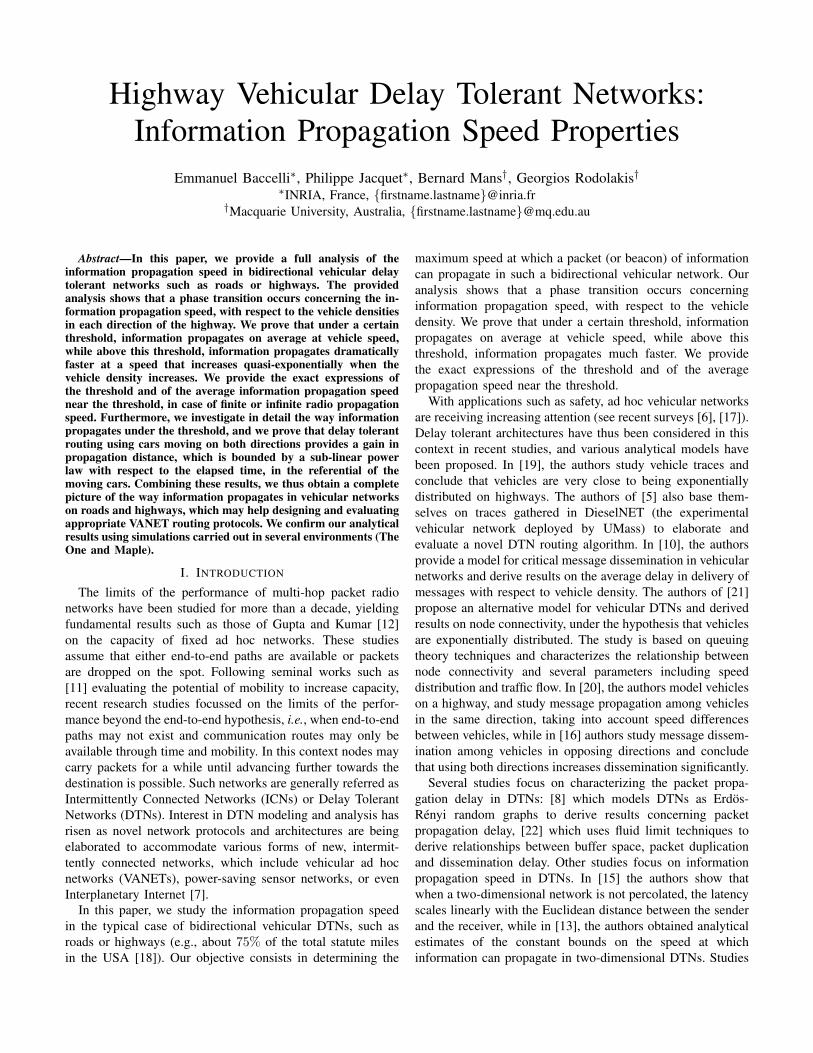
Lemma 10. When t→∞:

P (T > t) = A(λe, λw) (t2v)− λeλ∗w (1 + o(1)) . (30)

Proof: We have the relation T2v = Gew + Bw, with

Gew = L∗w + Iw − 1. We know that Gew, in analogy withGe, has an exponential tail, i.e., E(e−θGew) < ∞ for allθ > −λw. In other words P (Gew > y) = O(exp(−θy)).The other particularity is that Gew and Bw are dependent.First we have the inequality for all y

P (Gew +Bw > y) ≥ P (Bw > y),

therefore, we have P (T > t) ≥ A(λe, λw) (t2v)− λeλ∗w (1 +

o(1)). Second, we have the other inequality for all (y, z):

P (Gew +Bw > y) ≤ P (Gew > z) + P (Bw > y − z) .

Thus, by selecting z = O(log t) such thatP (Gew > z) = o(t

− λeλ∗w ), we get P (T > t) ≤

A(λe, λw) (t−O(log t)2v)− λeλ∗w + o(t

− λeλ∗w )

Therefore, we conclude the proof of Theorem 2.

B. Traveled Distance Distribution

Now, we focus on the renewal process made of the var-ious waiting time intervals T, experienced by the informa-tion beacon. Considering the sequence of waiting phases,T1,T2, . . . ,Tn, . . .: the beacon moves at time T1, then attime T1+T2, T1+T2+T3, etc. We denote n(t) the numberof phases achieved before time t:

i=n(t)∑i=1

Ti ≤ t <i=n(t)+1∑i=1

Ti .

Since the Ti are independent, this is a renewal process, andwe have the identity:

P (n(t) ≤ n) = P (T1 + · · ·+ Tn ≥ t) .

We can get a precise estimate of the average number ofrenewals E(n(t)) during time t.

Lemma 11. There exists b > 0 such that, when t → ∞, thefollowing estimate is valid:

E(n(t)) =sin2(π λeλ∗w

)

bπ2Γ(λeλ∗w

)tλeλ∗w +O(t

2 λeλ∗w−1

) . (31)

Proof: See appendix.In parallel to the sequence of waiting intervals Tii≥1,

we have the sequence Dii≥1 the distances traveled by thebeacon after every waiting interval Ti. Now we denote L(t) =∑i=n(t)i=1 Di which is the total distance traveled by the beacon

until time t.

Lemma 12.E(L(t)) = E(n(t))E(D) .

Proof: We have the identity:

E(L(t)) =∑n>0

E(1n(t)≥nDn), (32)

where 1n(t)≥n is the indicative function of the event n(t) ≥ n.Since, from the definition of n(t), we have the equivalence:n(t) ≥ n⇔ T1+· · ·+Tn−1 < t, then 1n≤n(t) and Dn are in-dependent random variables and, therefore, E(1n(t)≥nDn) =P (n(t) ≥ n)E(D).

Quantity E(D) has a closed expression (E(D) = 1λefw(λe)

,from Corollary 2. Substituting and using Lemma 11, the powerlaw for E(L(t)) in Theorem 3 is shown.

V. ASYMPTOTIC ESTIMATES

A. Near the Threshold

First, we investigate the case where (λe, λw) is close to thethreshold boundary.

Corollary 3. When λe → (λ∗w)+:

vp ∼ 2v(λw − λ∗w)λwλ2e(1− λ∗w)λ∗w

(λe − λ∗w)eλ∗w+λe−2λw . (33)

Proof: Using Lemma 6, we have:

2vE(T) = −f′w(λe)

fw(λe)+

∫ ∞1

E(Bw(x))pe(x)dx

∼∫ ∞1

eλw

λw

(1− λ∗w)λ∗wλw − λ∗w

eλw−λ∗we(x−1)λ

∗w

× λefw(λe)

e−λexdx .

Integrating, we obtain vp = E(D)E(T) .

B. Large Densities

Corollary 4. When the vehicle densities become large, i.e.,λe, λw →∞:

vp ∼ 2veλe+λw

1 + λwλe

+ λeλw

. (34)

Proof: According to Lemma 4, we have:

E(L∗w) = 1 +λw

λe(λw + λe), (35)

and the expected gap length tends to 1. The average roadlength to bridge such a gap tends to 1

λw. From Lemma 6:

2vE(T) ∼ E(L∗w)− 1 +1

λw. (36)

From corollary 2, the average distance traveled in bridging is:

E(D) =1

λefw(λe)∼ eλe+λw

λe + λw, (37)

and we obtain vp = E(D)E(T) .

Note that the information propagation speed grows quasi-exponentially with respect to the total vehicle density.

VI. FINITE RADIO PROPAGATION SPEED

If the radio propagation speed (including store and forwardtimings) is finite and constant, equal to vr, then the averageinformation propagation speed becomes:

s =E(Tw)v + E(De)

E(Tw) + 1vrE(De)

. (38)

But the speed vr impacts the random variables Ge and Tw. Themain impact is that, to fill an eastbound gap of length x, oneneeds a westbound cluster of length at least x(1+γ)

1−γ with γ =vvr

, otherwise the message will be off the gap when arriving

at the end of the cluster. Thus, E(Tw(x)) = O(e(1+γ)θw

1−γ x).The gap length is also modified, since we must consider

1−γ1+γL

∗w:

E(e−θGe) =fw( 1−γ

1+γ (θ + λe))

fw( 1−γ1+γλe)

λeλe + θ

. (39)

But, this does not change the exponential term e−λex inthe asymptotic expression of pe(x). Therefore, the thresholdcondition becomes:

λwe−λw =

1− γ1 + γ

λee− 1−γ

1+γ λe . (40)

This corresponds to a dilatation by a factor 1+γ1−γ of the

horizontal axis in the diagram of Figure 2. Notice how thediagram then loses its symmetry with respect to λe versusλw, which can be observed in Figure 9.

Notice also that, when vr decreases to v, the threshold limittends to infinity.

Similarly, in correspondance to Theorem 3, we haveE(L(t)) = Ω(t

1−γ1+γ

λeλ∗w ), due to the dilatation by the factor

1+γ1−γ .

VII. SIMULATIONS

In this section, we present simulation results obtained withMaple on one hand, and the Opportunistic Network Environ-ment (ONE [14]) simulator on the other hand.

A. Maple Simulations

We first compare the theoretical analysis with measure-ments performed using Maple. In this case, the simulationsfollow precisely the bidirectional highway model describedin Section II: we generate Poisson traffic of eastbound andwestbound traffic on two opposite lanes moving at constantspeed, which is set to v = 1m/s. The radio propagation rangeis R = 1m, and radio transmissions are instantaneous; thelength of the highway is sufficiently large to provide a largenumber of bridging operations (of order at least 103) for allconsidered traffic densities.

We measure the information propagation speed which isachieved using optimal DTN routing, by selecting a sourceand destination pairs at large distances, taking the ratio of thepropagation distance over the corresponding delay, and aver-aging over multiple iterations of randomly generated traffic.We vary the total traffic density, and we plot the resulting

Fig. 9. Threshold zones for (λe, λw) for various γ = vvr

, γ = 0 red,γ = 0.1 blue, γ = 0.5 green, γ = 0.8 yellow.

information propagation speed. Figures 10 and 11 show theevolution of the information propagation speed near the thresh-old versus the total vehicle density, when λe = λw, in linearand semilogarithmic plots, respectively. We can observe thethreshold at λe + λw = 2 in Figure 10, which confirms theanalysis presented previously in Section III, and correspondsto λe = λw = 1 in Figure 2. In semilogarithmic scale(Figure 11), we observe that the simulation measurementsquickly approach a straight line, and therefore are close tothe theoretically predicted exponential growth above the phasetransition threshold, in Section V. In Figure 12, we present a3-dimensional plot of the eastbound information propagationspeed vp by varying the vehicle densities in both eastbound(λe) and westbound (λw) traffic.

Finally, we perform detailed measurements of the waitingtime T that each packet of information spends in the buffer ofan eastbound car until it encounters a westbound cluster whichallows it to propagate faster to the next eastbound car. For themeasurements, we set the vehicle densities to λe = λw = 0.9;thus the conjugate λ∗w = 1.107 . . . . In Figure 13, (i.e., belowthe phase transition threshold), we plot the distribution of thewaiting time T, and we compare it to the predicted power lawin Theorem 2: P (T > t) = t

− λeλ∗w .

B. ONE Simulations

In this section, we depart from the exact Poisson model sim-ulations in Maple, and we present simulation results obtainedwith the Opportunistic Network Environment (ONE [14]) sim-ulator. Vehicles are distributed uniformly on the length of bothlanes of a road, and move at a constant unit speed. The total

Fig. 10. Maple simulations. Information propagation speed vp for λe = λw ,versus the total vehicle density λe + λw .

Fig. 11. Maple simulations. Information propagation speed vp for λe = λw ,versus the total vehicle density λe + λw , in semi-log scale, compared to thetheoretically predicted asymptotic exponential growth.

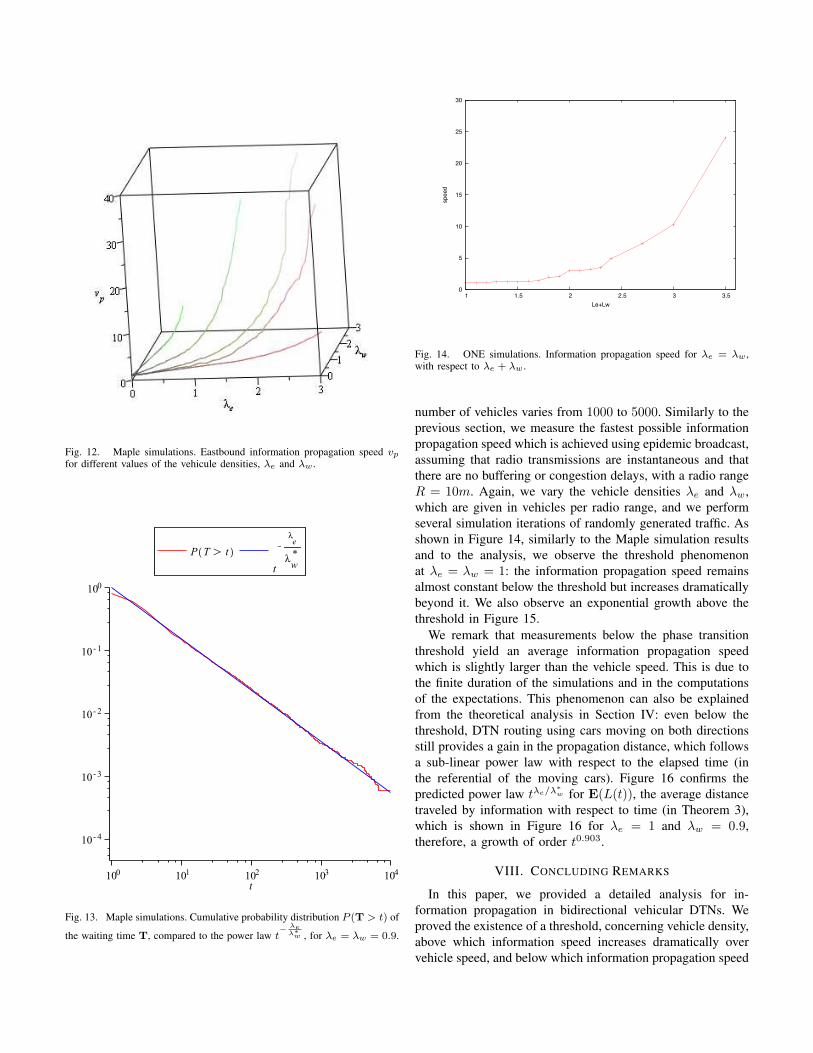
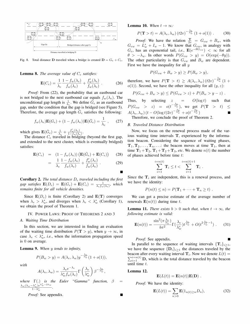
Fig. 12. Maple simulations. Eastbound information propagation speed vpfor different values of the vehicule densities, λe and λw .

Fig. 13. Maple simulations. Cumulative probability distribution P (T > t) of

the waiting time T, compared to the power law t− λeλ∗w , for λe = λw = 0.9.

0

5

10

15

20

25

30

1 1.5 2 2.5 3 3.5

spee

d

Le+Lw

Fig. 14. ONE simulations. Information propagation speed for λe = λw ,with respect to λe + λw .

number of vehicles varies from 1000 to 5000. Similarly to theprevious section, we measure the fastest possible informationpropagation speed which is achieved using epidemic broadcast,assuming that radio transmissions are instantaneous and thatthere are no buffering or congestion delays, with a radio rangeR = 10m. Again, we vary the vehicle densities λe and λw,which are given in vehicles per radio range, and we performseveral simulation iterations of randomly generated traffic. Asshown in Figure 14, similarly to the Maple simulation resultsand to the analysis, we observe the threshold phenomenonat λe = λw = 1: the information propagation speed remainsalmost constant below the threshold but increases dramaticallybeyond it. We also observe an exponential growth above thethreshold in Figure 15.

We remark that measurements below the phase transitionthreshold yield an average information propagation speedwhich is slightly larger than the vehicle speed. This is due tothe finite duration of the simulations and in the computationsof the expectations. This phenomenon can also be explainedfrom the theoretical analysis in Section IV: even below thethreshold, DTN routing using cars moving on both directionsstill provides a gain in the propagation distance, which followsa sub-linear power law with respect to the elapsed time (inthe referential of the moving cars). Figure 16 confirms thepredicted power law tλe/λ

∗w for E(L(t)), the average distance

traveled by information with respect to time (in Theorem 3),which is shown in Figure 16 for λe = 1 and λw = 0.9,therefore, a growth of order t0.903.

VIII. CONCLUDING REMARKS

In this paper, we provided a detailed analysis for in-formation propagation in bidirectional vehicular DTNs. Weproved the existence of a threshold, concerning vehicle density,above which information speed increases dramatically overvehicle speed, and below which information propagation speed

5

10

15

20

1 2 3 4

spee

d

Le+Lw

Fig. 15. ONE simulations. Information propagation speed for λe = λw ,with respect to λe + λw , in semi-log scale, compared to the theoreticallypredicted asymptotic exponential growth.

1

2

3

4

5

6

7

8

9

10

250 300 400 500 1000

dist

ance

/ tLe

/Lw

*

time

Fig. 16. ONE simulations. Average distance traveled by information withrespect to elapsed time E(L(t)), divided by the predicted power law tλe/λ

∗w

for λe = 1 and λw = 0.9, compared to the constant value 1.80 (dash).

is on average equal to vehicle speed (in Theorem 1), andwe computed the exact expression of this threshold. Weexactly characterized the information speed near the threshold(Corollary 3), and we showed that, above the threshold, theinformation propagation speed increases quasi-exponentiallywith vehicle density (Corollary 4). We also analyzed in detailthe way information propagates under the threshold, and weshowed that DTN routing using bidirectional traffic providesa gain in the propagation distance, which follows a sub-linearpower law with respect to the elapsed time (Theorems 2 and 3).Combining all these different situations, we obtain a completeimage of the way information propagates in vehicular networkson roads and highways, which is useful in determining the per-

formance limits and designing appropriate routing protocolsfor VANETs. All our theoretical results were validated withsimulations in several environments (The One and Maple).

Our analysis can be extended to investigate other modelsof vehicle traffic and radio propagation. In future works, weintend to provide a detailed expression of this threshold inspecific VANET models (e.g., intersections). Finally, an inter-esting direction for further research consists in collecting largetraces of real traffic on roads and highways, and evaluating theinformation propagation properties in this context.

REFERENCES

[1] A. Agarwal, D. Starobinski and T. Little, “Phase Transition Behavior ofMessage Propagation in Delay Tolerant Vehicular Ad Hoc Networks”.MCL Technical Report No. 12-12-2008, 2008.

[2] A. Agarwal, D. Starobinski and T. Little, “Analytical Model for MessagePropagation in Delay Tolerant Vehicular Networks”. Proceedings of theVehicular Technology Conference (VTC). Singapore, 2008.

[3] A. Agarwal, D. Starobinski and T. Little, “Exploiting Mobility to AchieveFast Upstream Propagation”. Proceedings of Mobile Networking forVehicular Environments (MOVE) at IEEE INFOCOM. Anchorage, 2007.

[4] E. Baccelli, P. Jacquet, B. Mans and G. Rodolakis, “Information Propaga-tion Speed in Bidirectional Vehicular Delay Tolerant Networks”, Infocom,2011.

[5] J. Burgess, B. Gallagher, D. Jensen and B. Levine, “MaxProp: Routingfor Vehicle-Based Disruption-Tolerant Networks”. In Infocom, 2006.

[6] A. Casteigts, A. Nayak and I. Stojmenovic, ”Communication protocolsfor vehicular ad hoc networks”. Wireless Communications and MobileComputing,

[7] V. Cerf, S. Burleigh, A. Hooke, L. Torgerson, R. Durst, K. Scott, K. Falland H. Weiss, “Delay-Tolerant Networking Architecture”, IETF RequestFor Comment RFC 4838, Internet Engineering Task Force, 2007.

[8] F. De Pellegrini, D. Miorandi, I. Carreras and I. Chlamtac, “A Graph-based model for disconnected ad hoc networks”, Infocom, 2007.

[9] P. Flajolet, A. Odlyzko, “Singularity analysis of generating functions”,SIAM Journal Disc. Math.,Vol. 3, No. 2, pp. 216-240, May 1990.

[10] R. Fracchia and M. Meo, “Analysis and Design of Warning DeliveryService in Inter-vehicular Networks”. IEEE Transactions on MobileComputing. 2008.

[11] M. Grossglauser and D. Tse, “Mobility increases the capacity of ad hocwireless networks”, Infocom, 2001.

[12] P. Gupta and P. R. Kumar, “The capacity of wireless networks”, IEEETrans. on Info. Theory, vol. IT-46(2), pp. 388-404, 2000.

[13] P. Jacquet, B. Mans and G. Rodolakis, “Information propagation speedin mobile and delay tolerant networks”, Infocom, 2009.

[14] A. Keranen, J. Ott and T. Karkkainen, “The ONE Simulator for DTNProtocol Evaluation”. SIMUTools’09: 2nd International Conference onSimulation Tools and Techniques. Rome, 2009.

[15] Z. Kong and E. Yeh, “On the latency for information dissemination inMobile Wireless Networks”, MobiHoc, 2008.

[16] T. Nadeem, P. Shankar, and L. Iftode, “A Comparative Study of DataDissemination Models for VANETs”, in Proc. of MOBIQUITOUS, 2006.

[17] Y. Toor, P. Muhlethaler, A. Laouiti, A. de la Fortelle, ”Vehicle ad hocnetworks: Applications and related technical issues”. IEEE Communica-tions Surveys and Tutorials 10(1-4), pp. 74-88 (2008)

[18] US-Department of Transportation. National Transportation Statistics,2010. US Government printing Office, Washington, DC.

[19] N. Wisitpongphan, F. Bai, P. Mudalige, and O. Tonguz, “On the RoutingProblem in Disconnected Vehicular Ad-hoc Networks,” in Infocom, 2007.

[20] H. Wu, R. Fujimoto, and G. Riley, “Analytical Models for InformationPropagation in Vehicle-to-Vehicle Networks”, in Proc. Fall VTC 04, LosAngeles, CA, USA, 2004.

[21] S. Yousefi, E. Altman, R. El-Azouzi and M. Fathy, “Analytical Modelfor Connectivity in Vehicular Ad Hoc Networks”. IEEE Transactions onVehicular Technology. Nov. 2008.

[22] X. Zhang, G. Neglia, J. Kurose and D. Towsley, “Performance modelingof epidemic routing”, Computer Networks, Vol. 51, 2007.

APPENDIX

A. Proof of Lemma 9

Proof: We want to find an evaluation of P (T > y) wheny →∞. For this we will evaluate for x given P (Bw(x) > y).We know that

E(eθBw(x+1)) = βw(θ, x+ 1) =λwP (Lw > x)

θ − λw(fw(θ, x+ 1)− 1)

Since P (Lw > x) = αλ∗we−λ

∗wx(1 + o(e−εx)), with α =

(λw−λ∗w)eλ∗w−λw

1−λ∗w, we have

fw(θ, x) = fw(θ)− αe−λ∗wx

θ + λ∗w(1 + o(e−εx)) (41)

From here we drop the o(e−εx) for simplicity, since it willjust bring an exponentially small factor. Therefore we have

βw(θ, x+ 1) =λwλ∗w

αe−λ∗wx

θ − λw(fw(θ)− 1− αe−λ∗wx

θ+λ∗w)

(42)

We have

P (Bw(x+ 1) = y) =1

2iπ

∫βw(θ, x+ 1)eyθdθ .

Let θ(x) be the root of θ − λw(fw(θ) − 1 − αe−λ∗wx

θ+λ∗w).

Straightforward analysis gives θ(x) = −βe−λ∗wx+O(e−2λ∗wx),

with β = λw1−λw ∂

∂θ fw(0)αλ∗w

. Via singularity analysis we have

P (Bw(x+ 1) = y) =λwαe

−λ∗wx

λ∗w

× eθ(x)y

1− λw ∂∂θfw(θ(x))− αe−λ

∗wx

(θ(x)+λ∗w)2

+O(e(θ(x)−ε)y)

Omitting the O( ) terms we get

P (Bw(x+ 1) = y) =λwαe

−λ∗wx

λ∗w

e−βe−λ∗wxy

1− λw ∂∂θfw(0)

= βe−θx exp(−βe−λ∗wxy) ,

OrP (Bw(x+ 1) > y) = exp(−βe−λ

∗wxy) . (43)

Therefore stating P (Bw > y) =∫pe(x)P (Bw(x) > y)dx we

get, omitting O( ) terms

P (Bw > y) =

∫λe

fw(λe)e−(x+1)λe exp(−βe−λ

∗wxy)dx .

(44)with the change of variable u = e−λ

∗wx we get

P (Bw > y) =

∫λee−λe

λ∗wfw(λe)uλeλ∗w−1

exp(−βyu)du

=λee−λe

λ∗wfw(λe)Γ

(λeλ∗w

)(βy)

− λeλ∗w ,

which is in power law as claimed.

B. Proof of Lemma 11

We first prove the property for an hypothetic renewalprocess based on the B′is on the real line. Let b(x) be thisrenewal process at time t:

E(b(y)) = P (B1 < y) + P (B1 +B2 < y)

+ · · ·+ P (B1 + · · ·+Bn < y) + · · ·

Let us define β = 1−E(e−θBw). We also define NB(θ) =∫∞0

E(b(y))e−yθ the Laplace transform of E(b(y)). We have:

NB(θ) =1−B(θ)

θB(θ).

Lemma 13. When θ → 0, then B(θ) = b πθa

sin(πa) for some band a = λe

λ∗w.

Proof: We start from

β(θ, x+ 1) =λwP (Lw > x+ 1)

θ − λw(fw(θ, x+ 1)− 1),

and

B(θ) = 1−∫ ∞1

pe(x)β(θ, x)dx =

∫ ∞1

pe(x)(1−β(θ, x))dx .

We denote

1− β(θ, x) =θ

θ + θ(x)g(θ, x) ,

with g(θ, x) bounded and uniformly integrable when <(θ)remains in a compact set and x→∞. Indeed we have

g(θ, x) = 1 +O(θ(x))

ThusB(θ) =

∫ ∞1

θ

θ + θ(x)g(θ, x)pe(x) .

By change of variable y = θ(x) we get

B(θ) =

∫ θ(1)

0

θ

θ + yg(θ, θ−1(y))pe(θ

−1(y))(θ−1(y))′dy .

We use together the following estimates θ(x) = −βe−λ∗wx +O(e−2λ

∗wx), and pe(x) = λe

fw(λe)e−λex(1 +O(e−εx)) to state

pe(θ−1(y))(θ−1(y))′ =

λefw(λe)

(y

β)λeλ∗w−1

(1 +O(yε)) ,

for some ε > 0.Then, we use the fact that∫ ∞

0

ya−1

θ + ydy =

πθa−1

sin(πa),

and, when θ → 0, ∫ ∞θ(1)

ya−1

θ + ydy = O(1)

Therefore, B(θ) = b πθa

sin(πa) +O(θ) for some b and a = λeλ∗w

when θ → 0. This is also true for complex θ.We can now prove Lemma 11 for the original renewal

process.

Proof: From the previous lemma, we have that: NB(θ) =sin(πa)bπ θ−a−1 +O(θ−1 + θ−2a), when θ → 0.The inversion of the Laplace transform yields

E(b(y)) =1

2iπ

∫ c+i∞

c−i∞NB(θ)eθydθ .

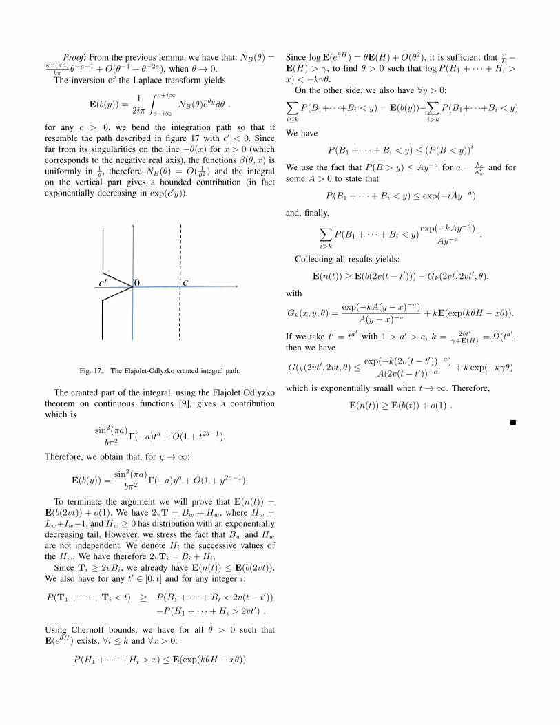
for any c > 0. we bend the integration path so that itresemble the path described in figure 17 with c′ < 0. Sincefar from its singularities on the line −θ(x) for x > 0 (whichcorresponds to the negative real axis), the functions β(θ, x) isuniformly in 1

θ , therefore NB(θ) = O( 1θ2 ) and the integral

on the vertical part gives a bounded contribution (in factexponentially decreasing in exp(c′y)).

€

c

€

ʹ′ c

€

0

Fig. 17. The Flajolet-Odlyzko cranted integral path.

The cranted part of the integral, using the Flajolet Odlyzkotheorem on continuous functions [9], gives a contributionwhich is

sin2(πa)

bπ2Γ(−a)ta +O(1 + t2a−1).

Therefore, we obtain that, for y →∞:

E(b(y)) =sin2(πa)

bπ2Γ(−a)ya +O(1 + y2a−1).

To terminate the argument we will prove that E(n(t)) =E(b(2vt)) + o(1). We have 2vT = Bw + Hw, where Hw =Lw+Iw−1, and Hw ≥ 0 has distribution with an exponentiallydecreasing tail. However, we stress the fact that Bw and Hw

are not independent. We denote Hi the successive values ofthe Hw. We have therefore 2vTi = Bi +Hi.

Since Ti ≥ 2vBi, we already have E(n(t)) ≤ E(b(2vt)).We also have for any t′ ∈ [0, t] and for any integer i:

P (T1 + · · ·+ Ti < t) ≥ P (B1 + · · ·+Bi < 2v(t− t′))−P (H1 + · · ·+Hi > 2vt′) .

Using Chernoff bounds, we have for all θ > 0 such thatE(eθH) exists, ∀i ≤ k and ∀x > 0:

P (H1 + · · ·+Hi > x) ≤ E(exp(kθH − xθ))

Since logE(eθH) = θE(H) +O(θ2), it is sufficient that xk −

E(H) > γ, to find θ > 0 such that logP (H1 + · · · + Hi >x) < −kγθ.

On the other side, we also have ∀y > 0:∑i≤k

P (B1+· · ·+Bi < y) = E(b(y))−∑i>k

P (B1+· · ·+Bi < y)

We have

P (B1 + · · ·+Bi < y) ≤ (P (B < y))i

We use the fact that P (B > y) ≤ Ay−a for a = λeλ∗w

and forsome A > 0 to state that

P (B1 + · · ·+Bi < y) ≤ exp(−iAy−a)

and, finally,∑i>k

P (B1 + · · ·+Bi < y)exp(−kAy−a)

Ay−a.

Collecting all results yields:

E(n(t)) ≥ E(b(2v(t− t′)))−Gk(2vt, 2vt′, θ),

with

Gk(x, y, θ) =exp(−kA(y − x)−a)

A(y − x)−a+ kE(exp(kθH − xθ)).

If we take t′ = ta′

with 1 > a′ > a, k = 2vt′

γ+E(H) = Ω(ta′,

then we have

G(k(2vt′, 2vt, θ) ≤ exp(−k(2v(t− t′))−a)

A(2v(t− t′))−α+ k exp(−kγθ)

which is exponentially small when t→∞. Therefore,

E(n(t)) ≥ E(b(t)) + o(1) .