Time-difference-of-arrival target localization processing in real ...
38
Defence Research and Development Canada Scientific Report DRDC-RDDC-2019-R095 June 2019 CAN UNCLASSIFIED CAN UNCLASSIFIED Time-difference-of-arrival target localization processing in real time S. Wong R. Jassemi-Zargani D. Brookes B. Kim DRDC – Ottawa Research Centre
-
Upload
khangminh22 -
Category
Documents
-
view
0 -
download
0
Transcript of Time-difference-of-arrival target localization processing in real ...
Defence Research and Development CanadaScientific ReportDRDC-RDDC-2019-R095June 2019
CAN UNCLASSIFIED
CAN UNCLASSIFIED
Time-difference-of-arrival target localization processing in real time
S. WongR. Jassemi-ZarganiD. BrookesB. KimDRDC – Ottawa Research Centre
CAN UNCLASSIFIED
Template in use: EO Publishing App for SR-RD-EC Eng 2018-12-19_v1 (new disclaimer).dotm
© Her Majesty the Queen in Right of Canada (Department of National Defence), 2019© Sa Majesté la Reine en droit du Canada (Ministère de la Défense nationale), 2019
CAN UNCLASSIFIED
IMPORTANT INFORMATIVE STATEMENTS
This document was reviewed for Controlled Goods by Defence Research and Development Canada (DRDC) using the Schedule to the Defence Production Act.
Disclaimer: This publication was prepared by Defence Research and Development Canada an agency of the Department of National Defence. The information contained in this publication has been derived and determined through best practice and adherence to the highest standards of responsible conduct of scientific research. This information is intended for the use of the Department of National Defence, the Canadian Armed Forces (“Canada”) and Public Safety partners and, as permitted, may be shared with academia, industry, Canada’s allies, and the public (“Third Parties”). Any use by, or any reliance on or decisions made based on this publication by Third Parties, are done at their own risk and responsibility. Canada does not assume any liability for any damages or losses which may arise from any use of, or reliance on, the publication.
Endorsement statement: This publication has been peer-reviewed and published by the Editorial Office of Defence Research and Development Canada, an agency of the Department of National Defence of Canada. Inquiries can be sent to: [email protected].
DRDC-RDDC-2019-R095 i
Abstract
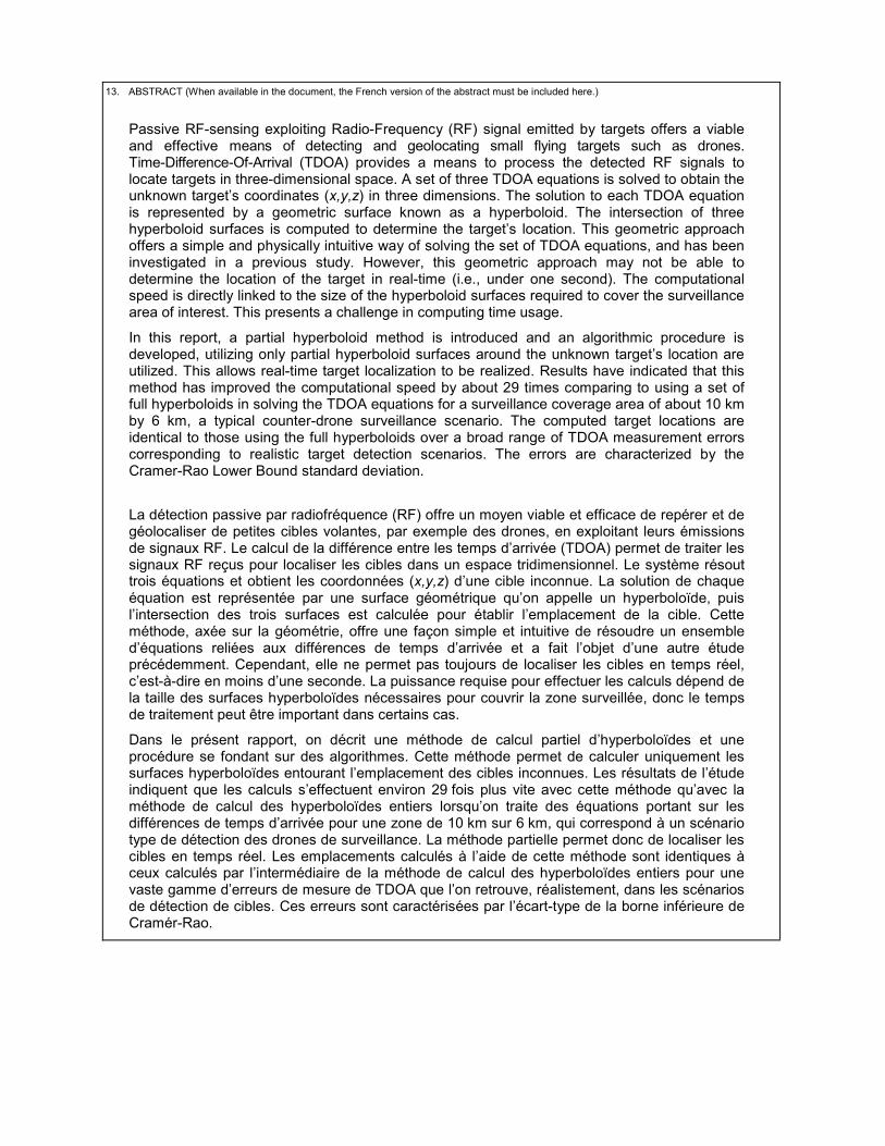
Passive RF-sensing exploiting Radio-Frequency (RF) signal emitted by targets offers a viable and effective means of detecting and geolocating small flying targets such as drones. Time-Difference-Of-Arrival (TDOA) provides a means to process the detected RF signals to locate targets in three-dimensional space. A set of three TDOA equations is solved to obtain the unknown target’s coordinates (x,y,z) in three dimensions. The solution to each TDOA equation is represented by a geometric surface known as a hyperboloid. The intersection of three hyperboloid surfaces is computed to determine the target’s location. This geometric approach offers a simple and physically intuitive way of solving the set of TDOA equations, and has been investigated in a previous study. However, this geometric approach may not be able to determine the location of the target in real-time (i.e., under one second). The computational speed is directly linked to the size of the hyperboloid surfaces required to cover the surveillance area of interest. This presents a challenge in computing time usage.
In this report, a partial hyperboloid method is introduced and an algorithmic procedure is developed, utilizing only partial hyperboloid surfaces around the unknown target’s location are utilized. This allows real-time target localization to be realized. Results have indicated that this method has improved the computational speed by about 29 times comparing to using a set of full hyperboloids in solving the TDOA equations for a surveillance coverage area of about 10 km by 6 km, a typical counter-drone surveillance scenario. The computed target locations are identical to those using the full hyperboloids over a broad range of TDOA measurement errors corresponding to realistic target detection scenarios. The errors are characterized by the Cramer-Rao Lower Bound standard deviation.
Significance to defence and security
One of the future challenges in Intelligence, Surveillance and Reconnaissance (ISR) for the Canadian Armed Forces (CAF) is to monitor air activities in the Arctic. Awareness of foreign commercial and military activities will enable Canada to address potential threats to Arctic sovereignty. In particular, there have been increasing concerns on the use of drones by foreign entities for military surveillance purposes and natural resource prospecting by multi-national corporations. Strategic and sensitive areas are vulnerable to these types of intrusions and threaten Canada’s national and economic interests. As drones are becoming more affordable and more accessible, there will be more occurrences of drone surveillance activities. A real-time passive RF-sensing capability in countering drone surveillance activities will enable Canada to act on potential threats in a timely manner.
Furthermore, the advent of drone, sensor and data communication technologies will undoubtedly pose serious threats to the CAF’s operations, especially those in the Arctic. It is foreseen that the CAF could be deploying an expeditionary force patrolling the Arctic in the future to maintain sovereignty; this could potentially bring them in contact with foreign state-armed or privately-armed forces. This potential threat was examined in a CAF exercise, “The Methodology for Assessing Technology Triggered Threats (MAT3),” RCAF/DRDC war-game exercise, Canadian Forces Aerospace Warfare Centre, Trenton Air Force Base, April 24–25, 2013. Mobile forward operating base camps for the CAF and sensitive operating areas will be vulnerable to foreign drone ISR activities. It is imperative that the CAF should have a means to detect any adversarial spying activities monitoring its operations. A real-time RF-sensing

ii DRDC-RDDC-2019-R095
system would provide a situational awareness capability to protect the CAF, allowing them to conduct their operations effectively and safely in the Arctic.
Passive RF-sensing of drones can also provide security warnings against covert surveillance of high-value infrastructure assets by rogue elements or foreign state perpetrators; these targets include Parliament Hill, National Defence Headquarters, and nuclear power generating plants. There are also increasing concerns over drone-airplane collisions around airports and military air-fields. These problems can be addressed by passive RF-sensing, providing timely warning of air targets intruding into restricted airspace.
DRDC-RDDC-2019-R095 iii
Résumé
La détection passive par radiofréquence (RF) offre un moyen viable et efficace de repérer et de géolocaliser de petites cibles volantes, par exemple des drones, en exploitant leurs émissions de signaux RF. Le calcul de la différence entre les temps d’arrivée (TDOA) permet de traiter les signaux RF reçus pour localiser les cibles dans un espace tridimensionnel. Le système résout trois équations et obtient les coordonnées (x,y,z) d’une cible inconnue. La solution de chaque équation est représentée par une surface géométrique qu’on appelle un hyperboloïde, puis l’intersection des trois surfaces est calculée pour établir l’emplacement de la cible. Cette méthode, axée sur la géométrie, offre une façon simple et intuitive de résoudre un ensemble d’équations reliées aux différences de temps d’arrivée et a fait l’objet d’une autreétude précédemment. Cependant, elle ne permet pas toujours de localiser les cibles en temps réel, c’est-à-direen moins d’une seconde. La puissance requise pour effectuer les calculs dépend de la taille des surfaces hyperboloïdes nécessaires pour couvrir la zone surveillée, donc le temps de traitement peut être importantdans certains cas.
Dans le présent rapport, on décrit une méthode de calcul partiel d’hyperboloïdes et une procédure se fondant sur des algorithmes. Cette méthode permet de calculer uniquement les surfaces hyperboloïdes entourant l’emplacement des cibles inconnues. Les résultats de l’étude indiquent que les calculs s’effectuent environ 29 fois plus vite avec cette méthode qu’avec la méthode de calcul des hyperboloïdes entiers lorsqu’on traite des équations portant sur les différences de temps d’arrivée pour une zone de 10 km sur 6 km, qui correspond à un scénario type de détection des drones de surveillance. La méthode partielle permet donc de localiser les cibles en temps réel. Les emplacements calculés à l’aide de cette méthode sont identiques à ceux calculés par l’intermédiaire de la méthode de calcul des hyperboloïdes entiers pour une vaste gamme d’erreurs de mesure de TDOA que l’on retrouve, réalistement, dans lesscénarios de détection de cibles. Ces erreurs sont caractérisées par l’écart-type de la borne inférieure de Cramér-Rao.
Importance pour la défense et la sécurité
L’un des prochains enjeux en matière de renseignement, de surveillance et de reconnaissance (RSR) pour les Forces armées canadiennes (FAC) consistera à surveiller les activités aériennes dans l’Arctique. La vigilance relative aux activités commerciales et militaires étrangères permettra au Canada de répondre aux menaces potentielles à l’égard de sa souveraineté dans l’Arctique. Plus particulièrement, l’utilisation de drones par des entités étrangères aux fins de surveillance militaire et par des corporationsmultinationales aux fins de prospection de ressources naturelles soulève des préoccupations croissantes.Des secteurs stratégiques et sensibles sont vulnérables à ces types d’intrusion, lesquels constituent une menace pour les intérêts nationaux et économiques du Canada. Plus les drones deviendront abordables et accessibles, plus on risque d’en trouver qui effectuent de la surveillance. Pouvoir localiser les drones par détection passive par RF afin de contrer les activités indésirables de surveillance permettra au Canada de faire face à cette menace potentielle en temps opportun.
De plus, les nouvelles technologies relatives aux drones, aux capteurs et à la communication de données constitueront indubitablement une menace sérieuse pour les opérations des FAC, particulièrement celles qui se tiendront dans l’Arctique. On prévoit que les FAC pourraient devoir déployer un corps
iv DRDC-RDDC-2019-R095
expéditionnaire de patrouille sur ce territoire pour préserver la souveraineté du Canada. Ce corps pourrait être amené à entrer en contact avec les forces armées d’États étrangers ou des forces armées privées. Afin de se préparer à faire face aux menaces potentielles, les FAC ont réalisé un exercice sous forme de jeu de guerre au Centre de guerre aérospatiale des Forces canadiennes de la base aérienne de Trenton les 24 et 25 avril 2013. L’exercice s’intitulait « Méthodologie d’évaluation des menaces découlant de la technologie » (MEMT) et a été dirigé par l’Aviation royale canadienne et RDDC. Les bases d’opérations avancées mobiles des FAC et les secteurs d’opérations sensibles seront vulnérables aux activités de collecte de renseignements, de surveillance et de reconnaissance qui pourraient être effectuées par desdrones étrangers. Les FAC devront donc être en mesure de détecter les activités d’espionnage ciblantleurs opérations. Un système de détection par RF en temps réel leur permettrait d’exercer une vigilance,de se protéger et de réaliser leurs opérations dans l’Arctique efficacement et de façon sécuritaire.
La détection passive des drones par RF permettrait aussi de produire des avertissements si des cas desurveillance secrète d’infrastructures à valeur élevée – comme la Colline du Parlement, les quartiers généraux de la Défense nationale et les centrales nucléaires – par des éléments indésirables ou des agents de pays hostiles sont détectés. Les collisions entre drones et avions près des aéroports civils et militaires sont aussi de plus en plus préoccupantes. La détection passive par RF apporterait une solution à ces problèmes en sonnant l’alarme rapidement en cas d’intrusion dans un espace aérien réglementé.
DRDC-RDDC-2019-R095 v
Table of contents
Abstract . . . . . . . . . . . . . . . . . . . . . . . . . . . . . . . . . . . i Significance to defence and security . . . . . . . . . . . . . . . . . . . . . . . . . i Résumé . . . . . . . . . . . . . . . . . . . . . . . . . . . . . . . . . . iii Importance pour la défense et la sécurité . . . . . . . . . . . . . . . . . . . . . . iii Table of contents . . . . . . . . . . . . . . . . . . . . . . . . . . . . . . . . v List of figures . . . . . . . . . . . . . . . . . . . . . . . . . . . . . . . . vi List of tables. . . . . . . . . . . . . . . . . . . . . . . . . . . . . . . . . vii 1 Introduction . . . . . . . . . . . . . . . . . . . . . . . . . . . . . . . . 1 2 Geometric approach to solving the TDOA equations . . . . . . . . . . . . . . . . . 3
2.1 TDOA equations for target localization . . . . . . . . . . . . . . . . . . . . 3 2.2 A brief description on the geometric approach . . . . . . . . . . . . . . . . . 4 2.3 TDOA measurements error. . . . . . . . . . . . . . . . . . . . . . . . . 6
2.3.1 Error-free TDOA measurements . . . . . . . . . . . . . . . . . . . . 7 2.3.2 TDOA measurements with error . . . . . . . . . . . . . . . . . . . . 7
3 Real-time geometric approach . . . . . . . . . . . . . . . . . . . . . . . . . 10 3.1 A faster geometric algorithm for target localization . . . . . . . . . . . . . . . 10 3.2 Computing speed comparisons . . . . . . . . . . . . . . . . . . . . . . 14 3.3 Target localization accuracy . . . . . . . . . . . . . . . . . . . . . . . 14
3.3.1 Coplanar configuration case study . . . . . . . . . . . . . . . . . . 17 3.3.2 Comparison using error free TDOA measurements . . . . . . . . . . . . 20
4 conclusions. . . . . . . . . . . . . . . . . . . . . . . . . . . . . . . . 22 References . . . . . . . . . . . . . . . . . . . . . . . . . . . . . . . . . 23 Annex A TDOA measurements for coplanar receivers configuration. . . . . . . . . . . . 25 List of symbols/abbreviations/acronyms/initialisms . . . . . . . . . . . . . . . . . . 26
vi DRDC-RDDC-2019-R095
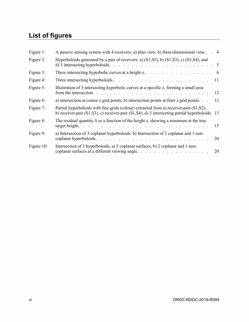
List of figures
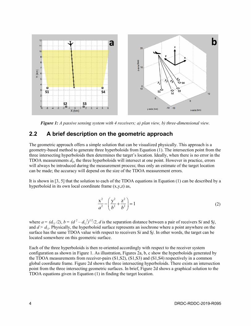
Figure 1: A passive sensing system with 4 receivers; a) plan view, b) three-dimensional view. . . 4
Figure 2: Hyperboloids generated by a pair of receivers: a) (S1,S2), b) (S1,S3), c) (S1,S4), andd) 3 intersecting hyperboloids. . . . . . . . . . . . . . . . . . . . . . . . 5
Figure 3: Three intersecting hyperbolic curves at a height z.. . . . . . . . . . . . . . . . 6
Figure 4: Three intersecting hyperboloids. . . . . . . . . . . . . . . . . . . . . . . 11
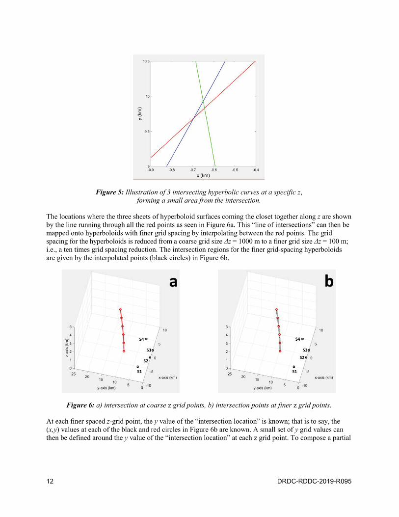
Figure 5: Illustration of 3 intersecting hyperbolic curves at a specific z, forming a small area from the intersection. . . . . . . . . . . . . . . . . . . . . . . . . . . 12
Figure 6: a) intersection at coarse z grid points, b) intersection points at finer z grid points. . . 12
Figure 7: Partial hyperboloids with fine grids (colour) extracted from a) receiver-pair (S1,S2), b) receiver-pair (S1,S3), c) receiver-pair (S1,S4), d) 3 intersecting partial hyperboloids. 13
Figure 8: The residual quantity S as a function of the height z, showing a minimum at the true target height.. . . . . . . . . . . . . . . . . . . . . . . . . . . . . . 15
Figure 9: a) Intersection of 3 coplanar hyperboloids. b) Intersection of 2 coplanar and 1 non-coplanar hyperboloids.. . . . . . . . . . . . . . . . . . . . . . . . . . 20
Figure 10: Intersection of 3 hyperboloids, a) 3 coplanar surfaces, b) 2 coplanar and 1 non-coplanar surfaces at a different viewing angle. . . . . . . . . . . . . . . . . 20

DRDC-RDDC-2019-R095 vii
List of tables
Table 1: Non-coplanar receiver system configuration. . . . . . . . . . . . . . . . . . . 8
Table 2: TDOA measurement values dij with no errors for a non-coplanar receiver configuration. . . . . . . . . . . . . . . . . . . . . . . . . . . . . . . 8
Table 3: TDOA measurement values dij with errors for a non-coplanar configuration. CRLB parameters: and (S/N)T = 16. . . . . . . . . . . . . . . . . . . . 8
Table 4: TDOA measurement values dij with errors for a non-coplanar configuration. CRLB (S/N)T = 16 . . . . . . . . . . . . . . . . . . . . 9
Table 5: TDOA measurement errors . CRLB parameters: = 20 MHz and (S/N)T = 16 . . . . 9
Table 6: TDOA measurement errors . CRLB parameters: = 1 MHz and (S/N)T = 16 . . . . 9
Table 7: Computing time consumed using the full and partial hyperboloid algorithmic procedures. . . . . . . . . . . . . . . . . . . . . . . . . . . . . . . 14
Table 8: Computed target locations at 10 time instants using 3 full hyperboloids in the geometric approach, non-coplanar configuration. . . . . . . . . . . . . . . . 15
Table 9: Computed target locations at 10 time instants using 3 partial hyperboloids in the geometric approach, non-coplanar configuration. . . . . . . . . . . . . . . . 16
Table 10: Computed target locations at 10 time instants using 3 full hyperboloids in the geometric approach, non-coplanar configuration. . . . . . . . . . . . . . . . 16
Table 11: Computed target locations at 10 time instants using 3 partial hyperboloids in the geometric approach, non-coplanar configuration. . . . . . . . . . . . . . . . 16
Table 12: Computed target locations at 10 time instants using 3 full hyperboloids in the geometric approach, coplanar configuration. . . . . . . . . . . . . . . . . . 17
Table 13: Computed target locations at 10 time instants using 3 partial hyperboloids in the geometric approach, coplanar configuration. . . . . . . . . . . . . . . . . . 18
Table 14: Computed target locations at 10 time instants using 3 full hyperboloids in the geometric approach, coplanar configuration. . . . . . . . . . . . . . . . . . 18
Table 15: Computed target locations at 10 time instants using 3 partial hyperboloids in the geometric approach, coplanar configuration. . . . . . . . . . . . . . . . . . 18
Table 16: Computed target locations at 10 time instants from three full hyperboloids in the geometric approach, non-coplanar configuration. . . . . . . . . . . . . . . . 21
Table 17: Computed target locations at 10 time instants from three partial hyperboloids in the geometric approach, non-coplanar configuration. . . . . . . . . . . . . . . . 21
Table A.1: TDOA measurement values and their associated errors for CRLB parMHz, (S/ . . . . . . . . . . . . . . . . . . . . . . . 25
Table A.2: TDOA measurement values and their associated errors MHz, (S/ . . . . . . . . . . . . . . . . . . . . . . . . 25

DRDC-RDDC-2019-R095 1
1 Introduction
Passive RF-sensing (also known as passive emitter tracking) offers a convenient and simple way to detect and to pinpoint the location of a target. They are widely used in many applications such as navigation surveillance, electronic warfare, public security, and air defence. One means of applying passive target detection and localization is to exploit the target’s own Radio-Frequency (RF) emissions. For example in public security application, an emerging threat of drone-plane collision near airport has been increasingly attracting attention from the proliferation of drone use such as the popular recreational quadcopters. RF signal from First Person View (FPV) video for remote piloting these drones can be monitored for detection and tracking of drone targets near airports and provide warnings.
As another example, it is widely expected that climate warming will open up many commercial activities in the Arctic in the near future; this will create sovereignty related issues and threats against national interests. One foreseen likely scenario is an increase in natural resource prospecting by multi-national corporations or foreign states. The use of drone or small aircraft will become common occurrence with the advent of remote sensing technology for natural resource prospecting [1]. Commercial Identification Friend or Foe (IFF) transponder emissions from small air targets will likely be spoofed to mask their activities. But the RF emissions can be monitored to provide situational awareness of suspicious flight activities over sensitive areas.
Passive RF-sensing offers an economically viable means for conducting detection and tracking of small air targets in these applications. Only passive receivers are required; i.e., there is no active transmitter required as part of the system, thus reducing the over-all system hardware complexity, power consumption and operating cost. In the case of detecting drones around airports, passive RF-sensing is desirable since it does not add any RF clutter and interference to an already congested RF environment. In Arctic monitoring of potential natural resources prospecting activities conducted by drones and small aircraft, large swath of areas may need to be covered. Passive RF detection offers a technically viable and cost effective means for wide-area surveillance coverage; as few as 4 receivers are needed to provide adequate coverage, even for a surveillance area as large as 320 km by 220 km in size [2]. For security patrol in the Arctic to assert sovereignty, future Canadian Arctic expeditionary forces can deploy passive RF-sensing to detect drone-surveillance activities against their operational base camps by adversaries.
A well-established method for passive target detection and localization by exploiting the target’s RF emission is the Time-Difference-Of-Arrival (TDOA) method [3, 4]. It requires just four time-synchronizedreceivers to obtain a fix on the target’s position in three-dimensions. A TDOA method for processing target localization based on a geometric approach to solving the set of TDOA equations derived from the receiver measurements has been developed and discussed in [5]. The geometric approach uses intersecting hyperboloid surfaces constructed from the TDOA measurements made by the passive receivers to determine the target locations. This method is capable of localizing target position quite accurately even when there are errors in the TDOA measurements; however, processing of the data may not be in real-time. It takes many seconds to process the TDOA data. In order for passive sensing to be practical in real-world applications, it is desirable to have real-time processing; this means processing of data in under one second. For example, being able to detect and pinpoint the location of drones near an airport in real-time is critical in providing timely warning of potential drone-plane collisions. Also, real-time situational awareness of drone activities would be of importance for the Arctic expeditionary force base camp in counter-surveillance defence.
2 DRDC-RDDC-2019-R095
There are other mathematical techniques for solving the TDOA equations, iterative numerical methods [6, 7, 8], and closed-form algebraic solution [9, 10, 11, 12]. Since the set of TDOA equations is non-linear in nature, it is a complex problem to work with iterative non-linear numerical method [13]. Numerical convergence of the solution can also be a challenge [14], and hence real-time processing is not likely to be achieved by iterative numerical technique. A closed-form algebraic solution can be obtained from a set of linearized equations derived from the TDOA equations. This approach is very efficient computationally; but its solution can be ambiguous with 2 possible target locations. This would require a fifth receiver to make an extra TDOA measurement to resolve the ambiguity [9, 11, 15]. In this report, a study is conducted to develop an algorithmic procedure based on the geometric approach to process target locations from TDOA data in real-time.
DRDC-RDDC-2019-R095 3
2 Geometric approach to solving the TDOA equations
In this section, target localization using the geometric approach to solve the TDOA equations is described. The geometric approach is based on the principles of locating a target on a 3D hyperboloid surface where the time difference of arrival of a target signal between a pair of synchronized receivers is constant. Using a set of four receivers stationed at different locations, three independent TDOA measurements can be made. From each TDOA measurement, a hyperboloid surface can be defined. Three hyperboloid surfaces can then be generated to triangulate the target’s location in 3D.
2.1 TDOA equations for target localization
Figure 1 shows a schematic of a set of 4 receivers configured to monitor an area of interest indicated by the orange shaded region. Details on how TDOA measurements are made from the data collected by the receivers are described in details in a previous report on TDOA analysis [5]. Using four receivers, three independent TDOA measurements can be made, and they are given by,
12 12 1 2
13 13 1 3
14 14 1 4
d c r rd c r rd c r r
(1)
where dij ij is the range-difference (i.e., TDOA measurements expressed in length unit) of the target relative to receiver i and receiver j, c is the speed of light, and ri = ((x – Xi)2 + (y – Yi)2 + (z – Zi)2 )1/2 is the L2 –norm (Euclidean) distance between the target (x,y,z) and the i-th receiver (Xi ,Yi ,Zi) (see Figure 1b),and i,j = 1,2,3,4. For simplicity and consistency, dij will be referred to as the “TDOA measurement.” The measured dij values will be subjected to error in a real detection system; the measurement error in dij will be further discussed in Section 2.3.
Each of the equations in Equation (1) represents a three-dimensional hyperboloid surface geometrically; this will be discussed in more details in Section 2.2. Since the receiver positions (Xi ,Yi ,Zi) are known and the TDOA measurement values dij made by the receivers are also known, Equation (1) with three independent equations can hence be solved for the unknown target location (x,y,z).
4 DRDC-RDDC-2019-R095
Figure 1: A passive sensing system with 4 receivers; a) plan view, b) three-dimensional view.
2.2 A brief description on the geometric approach
The geometric approach offers a simple solution that can be visualized physically. This approach is a geometry-based method to generate three hyperboloids from Equation (1). The intersection point from the three intersecting hyperboloids then determines the target’s location. Ideally, when there is no error in the TDOA measurements dij, the three hyperboloids will intersect at one point. However in practice, errors will always be introduced during the measurement process; thus only an estimate of the target location can be made; the accuracy will depend on the size of the TDOA measurement errors.
It is shown in [3, 5] that the solution to each of the TDOA equations in Equation (1) can be described by a hyperboloid in its own local coordinate frame (x,y,z) as,
2 2 2
2 2 2
x y z 1a b b
(2)
where a = (di j /2), b = (d 2 – di j2)1/2/2, d is the separation distance between a pair of receivers Si and Sj,
and d > di j. Physically, the hyperboloid surface represents an isochrone where a point anywhere on the surface has the same TDOA value with respect to receivers Si and Sj. In other words, the target can be located somewhere on this geometric surface.
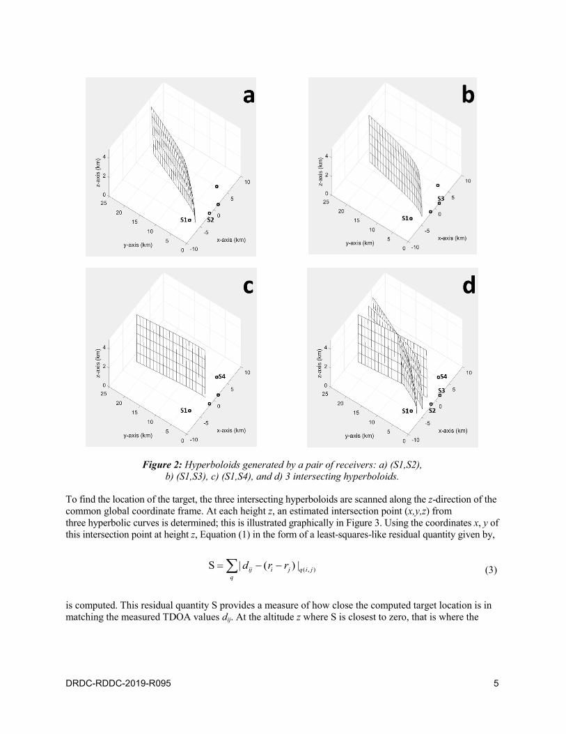
Each of the three hyperboloids is then re-oriented accordingly with respect to the receiver system configuration as shown in Figure 1. As illustration, Figures 2a, b, c show the hyperboloids generated by the TDOA measurements from receiver-pairs (S1,S2), (S1,S3) and (S1,S4) respectively in a common global coordinate frame. Figure 2d shows the three intersecting hyperboloids. There exists an intersection point from the three intersecting geometric surfaces. In brief, Figure 2d shows a graphical solution to the TDOA equations given in Equation (1) in finding the target location.
DRDC-RDDC-2019-R095 5
Figure 2: Hyperboloids generated by a pair of receivers: a) (S1,S2), b) (S1,S3), c) (S1,S4), and d) 3 intersecting hyperboloids.
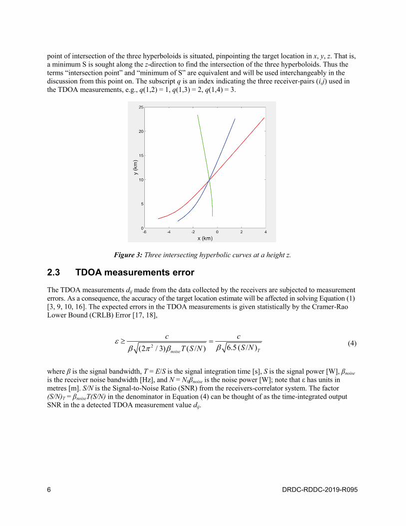
To find the location of the target, the three intersecting hyperboloids are scanned along the z-direction of the common global coordinate frame. At each height z, an estimated intersection point (x,y,z) fromthree hyperbolic curves is determined; this is illustrated graphically in Figure 3. Using the coordinates x, y of this intersection point at height z, Equation (1) in the form of a least-squares-like residual quantity given by,
( , )S | ( ) |ij i j q i jq
d r r (3)
is computed. This residual quantity S provides a measure of how close the computed target location is in matching the measured TDOA values dij. At the altitude z where S is closest to zero, that is where the
6 DRDC-RDDC-2019-R095
point of intersection of the three hyperboloids is situated, pinpointing the target location in x, y, z. That is, a minimum S is sought along the z-direction to find the intersection of the three hyperboloids. Thus the terms “intersection point” and “minimum of S” are equivalent and will be used interchangeably in the discussion from this point on. The subscript q is an index indicating the three receiver-pairs (i,j) used in the TDOA measurements, e.g., q(1,2) = 1, q(1,3) = 2, q(1,4) = 3.
Figure 3: Three intersecting hyperbolic curves at a height z.
2.3 TDOA measurements error
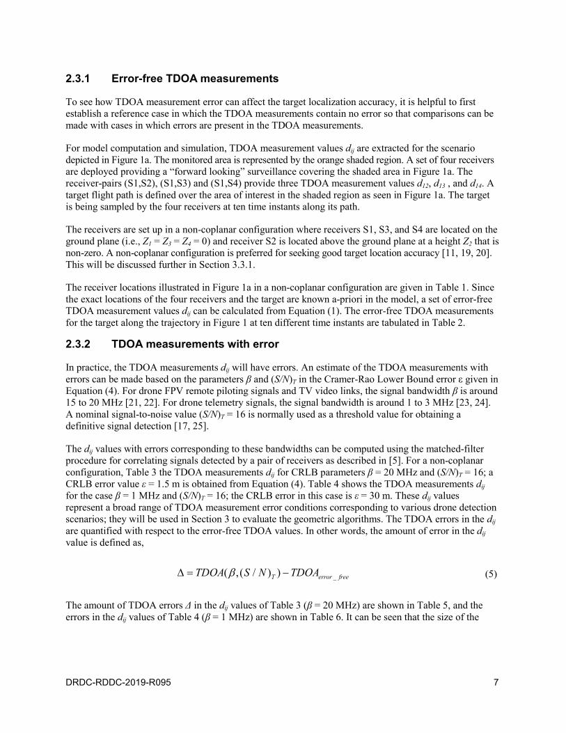
The TDOA measurements dij made from the data collected by the receivers are subjected to measurement errors. As a consequence, the accuracy of the target location estimate will be affected in solving Equation (1)[3, 9, 10, 16]. The expected errors in the TDOA measurements is given statistically by the Cramer-Rao Lower Bound (CRLB) Error [17, 18],
2 6.5 ( / )(2 / 3) ( / ) Tnoise
c cS NT S N
(4)
where is the signal bandwidth, T = E/S is the signal integration time [s], S is the signal power [W], noiseis the receiver noise bandwidth [Hz], and N = N0 noise is the noise power [Wmetres [m]. S/N is the Signal-to-Noise Ratio (SNR) from the receivers-correlator system. The factor (S/N)T = noiseT(S/N) in the denominator in Equation (4) can be thought of as the time-integrated output SNR in the a detected TDOA measurement value dij.
DRDC-RDDC-2019-R095 7
2.3.1 Error-free TDOA measurements
To see how TDOA measurement error can affect the target localization accuracy, it is helpful to first establish a reference case in which the TDOA measurements contain no error so that comparisons can be made with cases in which errors are present in the TDOA measurements.
For model computation and simulation, TDOA measurement values dij are extracted for the scenario depicted in Figure 1a. The monitored area is represented by the orange shaded region. A set of four receiversare deployed providing a “forward looking” surveillance covering the shaded area in Figure 1a. The receiver-pairs (S1,S2), (S1,S3) and (S1,S4) provide three TDOA measurement values d12, d13 , and d14. A target flight path is defined over the area of interest in the shaded region as seen in Figure 1a. The target is being sampled by the four receivers at ten time instants along its path.
The receivers are set up in a non-coplanar configuration where receivers S1, S3, and S4 are located on the ground plane (i.e., Z1 = Z3 = Z4 = 0) and receiver S2 is located above the ground plane at a height Z2 that is non-zero. A non-coplanar configuration is preferred for seeking good target location accuracy [11, 19, 20].This will be discussed further in Section 3.3.1.
The receiver locations illustrated in Figure 1a in a non-coplanar configuration are given in Table 1. Since the exact locations of the four receivers and the target are known a-priori in the model, a set of error-free TDOA measurement values dij can be calculated from Equation (1). The error-free TDOA measurements for the target along the trajectory in Figure 1 at ten different time instants are tabulated in Table 2.
2.3.2 TDOA measurements with error
In practice, the TDOA measurements dij will have errors. An estimate of the TDOA measurements with errors can be made based on the parameters and (S/N)T in the Cramer-Equation (4). For drone FPV remote piloting signals and TV video links, the signal bandwidth is around 15 to 20 MHz [21, 22]. For drone telemetry signals, the signal bandwidth is around 1 to 3 MHz [23, 24]. A nominal signal-to-noise value (S/N)T = 16 is normally used as a threshold value for obtaining a definitive signal detection [17, 25].
The dij values with errors corresponding to these bandwidths can be computed using the matched-filter procedure for correlating signals detected by a pair of receivers as described in [5]. For a non-coplanar configuration, Table 3 the TDOA measurements dij for CRLB parameters = 20 MHz and (S/N)T = 16; a CRLB error value = 1.5 m is obtained from Equation (4). Table 4 shows the TDOA measurements dijfor the case = 1 MHz and (S/N)T = 16; the CRLB error in this case is = 30 m. These dij values represent a broad range of TDOA measurement error conditions corresponding to various drone detection scenarios; they will be used in Section 3 to evaluate the geometric algorithms. The TDOA errors in the dijare quantified with respect to the error-free TDOA values. In other words, the amount of error in the dijvalue is defined as,
_( , ( / ) )T error freeTDOA S N TDOA (5)
The amount of TDOA errors in the dij values of Table 3 ( = 20 MHz) are shown in Table 5, and the errors in the dij values of Table 4 ( = 1 MHz) are shown in Table 6. It can be seen that the size of the
8 DRDC-RDDC-2019-R095
errors is scattered statistically roughly around the “one sigma” point as a bound. The variations in the TDOA errors are a consequence of temporal phase fluctuation in the moving target’s signal and the target’s changing position respect to the receivers [5]. Phase variations affect the match-filter process that determines the TDOA measurement values dij and hence causing some variations in dij. These values will be used in the target location estimation in Section 3.
Table 1: Non-coplanar receiver system configuration.
receivers X (m) Y (m) Z (m)S1 -5000 3400 0S2 -1600 0 200S3 1600 0 0S4 5000 3400 0
Table 2: TDOA measurement values dij with no errors for a non-coplanar receiver configuration.
Time (time index) TDOA1, d12 (m) TDOA2, d13 (m) TDOA3, d14 (m) 12345678910
-2113.51-1969.77-1801.20-1602.24-1366.13-1084.98-750.05-352.59114.63655.06
-2338.51-2193.04-2022.44-1821.07-1582.05-1297.33-957.94-554.76-80.02470.63
-789.87-776.71-759.11-735.75-704.95-664.82-613.45-549.26-471.74-382.01
Table 3: TDOA measurement values dij with errors for a non-coplanar configuration. CRLB parameters:and (S/N)T = 16.
Time (time index) TDOA1, d12 (m) TDOA2, d13 (m) TDOA3, d14 (m) 12345678910
-2110.50-1968.00-1798.50-1600.50-1363.50-1083.00-748.50-351.00115.50657.00
-2335.50-2190.00-2020.50-1818.00-1579.50-1294.50-955.50-553.50-78.00472.50
-789.00-775.50-759.00-735.00-703.50-664.50-612.00-549.00-471.00-381.00
DRDC-RDDC-2019-R095 9
Table 4: TDOA measurement values dij with errors for a non-coplanar configuration. CRLB parameters: (S/N)T = 16
Time (time index) TDOA1, d12 (m) TDOA2, d13 (m) TDOA3, d14 (m) 12345678910
-2100.00-1950.00-1800.00-1590.00-1350.00-1050.00
-720.00-330.00150.00690.00
-2340.00-2190.00-2010.00-1800.00-1560.00-1290.00-930.00-540.00-60.00510.00
-780.00-780.00-750.00-720.00-690.00-660.00-600.00-540.00-480.00-390.00
Table 5: TDOA measurement errors . CRLB parameters: = 20 MHz and (S/N)T = 16
Time (time index) 12 in d12 (m) 13 in d13 (m) 14 in d14 (m) 12345678910
3.011.772.701.742.631.981.551.590.871.94
3.013.041.943.072.552.832.441.262.021.87
0.871.210.110.751.450.321.450.260.741.01
Table 6: TDOA measurement errors . CRLB parameters: = 1 MHz and (S/N)T = 16
Time (time index) 12 in d12 (m) 13 in d13 (m) 14 in d14 (m) 12345678910
13.5119.771.2012.2416.1334.9830.0522.5935.3734.94
-1.493.04
12.4421.0722.057.33
27.9414.7620.0239.37
9.87-3.299.11
15.7514.954.82
13.459.26
-8.26-7.99
10 DRDC-RDDC-2019-R095
3 Real-time geometric approach
The geometric algorithmic computing process for finding the target location from the intersection point of 3 hyperboloids described in [5] reveals that much of the computed time consumed is being taken up in the re-computing of the x,y,z grid coordinates of the tilted hyperboloid from receiver-pair S1–S2 due to the non-coplanar receiver system configuration. The non-coplanar geometry is used because it offers better target location accuracy in TDOA processing. This will be further elaborated in Section 3.3.1.
In the non-coplanar set-up, the hyperboloid surface generated by receiver pair (S1,S2) is tilted at an angle in the x-z plane due to a 200 m elevation of receiver S2 out of the common ground plane where the other three receivers are situated (see Table 1). The coordinates of the tilted (S1,S2) hyperboloid have to be re-gridded to the common global frame coordinates so that they are aligned with the coordinates of the other two hyperboloids formed by receiver pairs (S1,S3) and (S1,S4). This is necessary in order to find the intersection point from the three hyperboloids in the target localization process.
To find the intersection point of the three hyperboloids at a height z to locate the unknown target, all three hyperboloid surfaces must be large enough to cover the surveillance area of interest indicated by the shaded region in Figure 1. This ensures that the three hyperboloids will intersect somewhere within the surveillance area that corresponds to the target’s location. It is realized that for large hyperboloid surface, the re-gridding of the x,y,z coordinates presents a bottleneck in the computation, thus preventing real-time target localization to be achieved. In this section, a partial hyperboloid procedure is introduced to reduce the computation time needed in determining the target location.
3.1 A faster geometric algorithm for target localization
Working with large hyperboloid surfaces is computationally inefficient. It is obvious that not all of the surfaces of the hyperboloids are needed in target localization processing. It would be much more efficient if only the region near where the 3 hyperboloids intersect can be isolated and the computation is focused in this selected region only. This provides a basis for developing a procedure to identify the regions from the three hyperboloids that are relevant to the target localization computation.
The hyperboloids for computational process are constructed with mesh of a specified grid-size spacing; the grids accommodate the search for the minimum of the residual quantity S in Equation 3 by scanning the z-direction in the target localization algorithm. The finer the resolution of the target location that is desired in the z-direction, the smaller the grid spacing is required. For a z-axis grid spacing of 100 m, the hyperboloids will have grid spacing of 100 m x 100 m in both the x-z plane and x-y plane. This grid spacing is used for target location computations.
It is observed that the computing time increases as the square power of the number of grid points that are used in the hyperboloids. Hence, it seems logical that an effective strategy would be one that can reduce the number of grid points to be processed in extracting the target’s location. In this section, a more efficient algorithmic procedure is described.
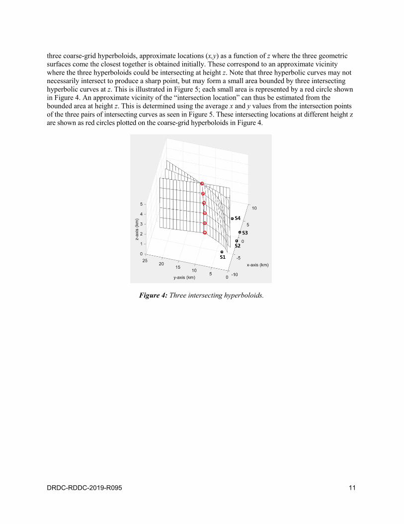
For an intended hyperboloid grid size of 100 m to be used as parametric value in the actual target localization process, the hyperboloids are first meshed using a coarser grid size of 1000 m; i.e., ten timescoarser grid size. The three hyperboloids with coarse grids are illustrated in Figure 4 in black. From these
DRDC-RDDC-2019-R095 11
three coarse-grid hyperboloids, approximate locations (x,y) as a function of z where the three geometric surfaces come the closest together is obtained initially. These correspond to an approximate vicinity where the three hyperboloids could be intersecting at height z. Note that three hyperbolic curves may not necessarily intersect to produce a sharp point, but may form a small area bounded by three intersecting hyperbolic curves at z. This is illustrated in Figure 5; each small area is represented by a red circle shown in Figure 4. An approximate vicinity of the “intersection location” can thus be estimated from the bounded area at height z. This is determined using the average x and y values from the intersection points of the three pairs of intersecting curves as seen in Figure 5. These intersecting locations at different height z are shown as red circles plotted on the coarse-grid hyperboloids in Figure 4.
Figure 4: Three intersecting hyperboloids.
12 DRDC-RDDC-2019-R095
Figure 5: Illustration of 3 intersecting hyperbolic curves at a specific z,forming a small area from the intersection.
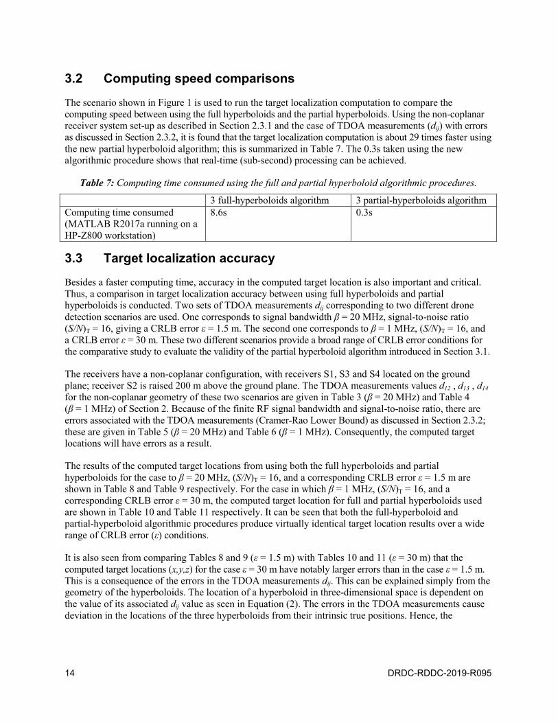
The locations where the three sheets of hyperboloid surfaces coming the closet together along z are shown by the line running through all the red points as seen in Figure 6a. This “line of intersections” can then be mapped onto hyperboloids with finer grid spacing by interpolating between the red points. The grid spacing for the hyperboloids is reduced from a coarse grid size = 1000 m to a finer grid size = 100 m;i.e., a ten times grid spacing reduction. The intersection regions for the finer grid-spacing hyperboloids are given by the interpolated points (black circles) in Figure 6b.
Figure 6: a) intersection at coarse z grid points, b) intersection points at finer z grid points.
At each finer spaced z-grid point, the y value of the “intersection location” is known; that is to say, the (x,y) values at each of the black and red circles in Figure 6b are known. A small set of y grid values can then be defined around the y value of the “intersection location” at each z grid point. To compose a partial

DRDC-RDDC-2019-R095 13
hyperboloid, a total of 50 y-grid values are created with spacing of 100 m between adjacent y grid points. Having a set of known y-grid and z-grid values, Equation (2) describing a hyperboloid can be used to generate a partial hyperboloid. Three partial hyperboloids are created in this manner. These partial hyperboloids are shown as colour strips (blue, red, green) in Figures 7a, 7b, 7c; these correspond to hyperboloids for receiver-pairs (S1,S2), (S1,S3) and (S1,S4) respectively. The three intersecting partial hyperboloids with finer grid spacing are illustrated in Figure 7d. These much smaller partial hyperboloids are then used for computing the target locations.
Figure 7: Partial hyperboloids with fine grids (colour) extracted from a) receiver-pair (S1,S2), b) receiver-pair (S1,S3), c) receiver-pair (S1,S4), d) 3 intersecting partial hyperboloids.
14 DRDC-RDDC-2019-R095
3.2 Computing speed comparisons
The scenario shown in Figure 1 is used to run the target localization computation to compare the computing speed between using the full hyperboloids and the partial hyperboloids. Using the non-coplanarreceiver system set-up as described in Section 2.3.1 and the case of TDOA measurements (dij) with errors as discussed in Section 2.3.2, it is found that the target localization computation is about 29 times faster using the new partial hyperboloid algorithm; this is summarized in Table 7. The 0.3s taken using the new algorithmic procedure shows that real-time (sub-second) processing can be achieved.
Table 7: Computing time consumed using the full and partial hyperboloid algorithmic procedures.
3 full-hyperboloids algorithm 3 partial-hyperboloids algorithmComputing time consumed(MATLAB R2017a running on a HP-Z800 workstation)
8.6s 0.3s
3.3 Target localization accuracy
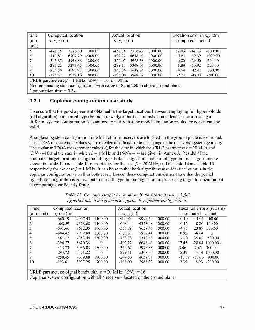
Besides a faster computing time, accuracy in the computed target location is also important and critical. Thus, a comparison in target localization accuracy between using full hyperboloids and partial hyperboloids is conducted. Two sets of TDOA measurements dij corresponding to two different drone detection scenarios are used. One corresponds to signal bandwidth = 20 MHz, signal-to-noise ratio (S/N)T = 16, giving a CRLB error = 1.5 m. The second one corresponds to = 1 MHz, (S/N)T = 16, and a CRLB error = 30 m. These two different scenarios provide a broad range of CRLB error conditions for the comparative study to evaluate the validity of the partial hyperboloid algorithm introduced in Section 3.1.
The receivers have a non-coplanar configuration, with receivers S1, S3 and S4 located on the ground plane; receiver S2 is raised 200 m above the ground plane. The TDOA measurements values d12 , d13 , d14for the non-coplanar geometry of these two scenarios are given in Table 3 ( = 20 MHz) and Table 4( = 1 MHz) of Section 2. Because of the finite RF signal bandwidth and signal-to-noise ratio, there are errors associated with the TDOA measurements (Cramer-Rao Lower Bound) as discussed in Section 2.3.2;these are given in Table 5 ( = 20 MHz) and Table 6 ( = 1 MHz). Consequently, the computed target locations will have errors as a result.
The results of the computed target locations from using both the full hyperboloids and partialhyperboloids for the case to = 20 MHz, (S/N)T = 16, and a corresponding CRLB error = 1.5 m are shown in Table 8 and Table 9 respectively. For the case in which = 1 MHz, (S/N)T = 16, and a corresponding CRLB error = 30 m, the computed target location for full and partial hyperboloids used are shown in Table 10 and Table 11 respectively. It can be seen that both the full-hyperboloid and partial-hyperboloid algorithmic procedures produce virtually identical target location results over a wide range of CRLB error ( ) conditions.
It is also seen from comparing Tables 8 and 9 ( = 1.5 m) with Tables 10 and 11 ( = 30 m) that the computed target locations (x,y,z) for the case = 30 m have notably larger errors than in the case = 1.5 m.This is a consequence of the errors in the TDOA measurements dij. This can be explained simply from the geometry of the hyperboloids. The location of a hyperboloid in three-dimensional space is dependent on the value of its associated dij value as seen in Equation (2). The errors in the TDOA measurements cause deviation in the locations of the three hyperboloids from their intrinsic true positions. Hence, the
DRDC-RDDC-2019-R095 15
intersection point of the three displaced hyperboloids would be shifted from its true position, resulting in errors in the (x, y, z) locations.
Note that the z m case. This is due to the large z-scan step size used; that is, the z output is resolved to the nearest 100 m. The computed output z corresponds to the location along the z-direction where the TDOA residual quantity S in Equation (3) is a minimum. This is shown in Figure 8 where the quantity S is plotted as a function of the height z, showing a minimum at the target’s height. The minimum S also allows the x and y coordinates of the target’s location to be determined from the intersection of the three hyperbolic curves at z as described in Section 2.2.
Figure 8: The residual quantity S as a function of the height z, showing a minimum at the true target height.
Table 8: Computed target locations at 10 time instants using 3 full hyperboloids in the geometric approach, non-coplanar configuration.
time(arb. unit)
Computed target location x,y,z (m)
Actual target location (m)x,y,z (m)
Location error in x,y,z (m)= computed—actual
12345678910
-658.60 9984.45 1000.00-606.24 9323.21 1000.00-556.89 8647.97 1000.00-503.65 7984.19 1000.00-452.92 7312.62 1000.00-401.31 6644.30 1000.00-349.48 5976.49 1000.00-299.13 5305.89 1000.00-246.71 4637.45 1000.00-195.65 3966.36 1000.00
-660.00 9998.50 1000.00-608.44 9328.48 1000.00-556.89 8658.46 1000.00-505.33 7988.44 1000.00-453.78 7318.42 1000.00-402.22 6648.40 1000.00-350.67 5978.38 1000.00-299.11 5308.36 1000.00-247.56 4638.34 1000.00-196.00 3968.32 1000.00
1.40 -14.05 02.20 -5.27 0
-0.00 -10.49 01.69 -4.25 00.86 -5.80 00.91 -4.10 01.19 -1.89 0
-0.01 -2.48 00.85 -0.89 00.35 -1.96 0
CRLB parameters: = 20 MHz; (S/N)T m.Non-coplanar system configuration with receiver S2 at 200 m above ground plane. Computation time = 8.6s.
16 DRDC-RDDC-2019-R095
Table 9: Computed target locations at 10 time instants using 3 partial hyperboloids in the geometric approach, non-coplanar configuration.
time(arb. unit)
Computed location x, y, z (m)
Actual location X, y, z (m)
Location error in x,y,z (m)= computed—actual
12345678910
-658.61 9984.41 1000.00-606.24 9323.19 1000.00-556.90 8647.94 1000.00-503.65 7984.19 1000.00-452.92 7312.60 1000.00-401.32 6644.29 1000.00-349.48 5976.48 1000.00-299.13 5305.88 1000.00-246.71 4637.45 1000.00-195.65 3966.37 1000.00
-660.00 9998.50 1000.00-608.44 9328.48 1000.00-556.89 8658.46 1000.00-505.33 7988.44 1000.00-453.78 7318.42 1000.00-402.22 6648.40 1000.00-350.67 5978.38 1000.00-299.11 5308.36 1000.00-247.56 4638.34 1000.00-196.00 3968.32 1000.00
1.39 -14.09 02.20 -5.29 0
-0.01 -10.53 01.68 -4.25 00.86 -5.83 00.91 -4.12 01.18 -1.90 0
-0.01 -2.48 00.85 -0.89 00.35 -1.95 0
CRLB parameters: = 20 MHz; (S/N)T m.Non-coplanar system configuration with receiver S2 at 200 m above ground plane. Computation time = 0.3s.
Table 10: Computed target locations at 10 time instants using 3 full hyperboloids in the geometric approach, non-coplanar configuration.
time(arb. unit)
Computed target locationx,y,z (m)
Actual target location (m)x,y,z (m)
Location error in x,y,z(m)= computed—actual
12345678910
-674.93 10186.19 1900.00-625.02 9396.35 1700.00-544.20 8602.28 600.00-490.30 7937.96 800.00-441.73 7276.37 900.00-417.82 6707.86 2000.00-343.86 5948.93 1200.00-297.22 5297.46 1300.00-254.50 4595.93 1300.00-198.33 3919.12 800.00
-660.00 9998.50 1000.00-608.44 9328.48 1000.00-556.89 8658.46 1000.00-505.33 7988.44 1000.00-453.78 7318.42 1000.00-402.22 6648.40 1000.00-350.67 5978.38 1000.00-299.11 5308.36 1000.00-247.56 4638.34 1000.00-196.00 3968.32 1000.00
-14.93 187.69 900.00-16.57 67.87 700.0012.69 -56.18 -400.0015.03 -50.48 -200.0012.05 -42.05 -100.00
-15.59 59.45 1000.006.81 -29.45 200.001.89 -10.90 300.00
-6.94 -42.42 300.00-2.32 -49.20 -200.00
CRLB parameters: = 1 MHz; (S/N)T m.Non-coplanar system configuration with receiver S2 at 200 m above ground plane. Computation time = 8.6s.
Table 11: Computed target locations at 10 time instants using 3 partial hyperboloids in the geometric approach, non-coplanar configuration.
time(arb. unit)
Computed location x, y, z (m)
Actual location X, y, z (m)
Location error in x,y,z(m)= computed—actual
1234
-674.95 10186.05 1900.00-625.04 9396.19 1700.00-544.22 8602.17 600.00-490.30 7937.96 800.00
-660.00 9998.50 1000.00-608.44 9328.48 1000.00-556.89 8658.46 1000.00-505.33 7988.44 1000.00
-14.95 187.55 900.00-16.60 67.71 700.0012.67 -56.29 -400.0015.03 -50.48 -200.00
DRDC-RDDC-2019-R095 17
time(arb. unit)
Computed location x, y, z (m)
Actual location X, y, z (m)
Location error in x,y,z(m)= computed—actual
5678910
-441.75 7276.30 900.00-417.83 6707.79 2000.00-343.87 5948.88 1200.00-297.22 5297.45 1300.00-254.50 4595.93 1300.00-198.31 3919.16 800.00
-453.78 7318.42 1000.00-402.22 6648.40 1000.00-350.67 5978.38 1000.00-299.11 5308.36 1000.00-247.56 4638.34 1000.00-196.00 3968.32 1000.00
12.03 -42.13 -100.00-15.61 59.39 1000.00
6.80 -29.50 200.001.89 -10.92 300.00
-6.94 -42.41 300.00-2.31 -49.17 -200.00
CRLB parameters: = 1 MHz; (S/N)T m.Non-coplanar system configuration with receiver S2 at 200 m above ground plane. Computation time = 0.3s.
3.3.1 Coplanar configuration case study
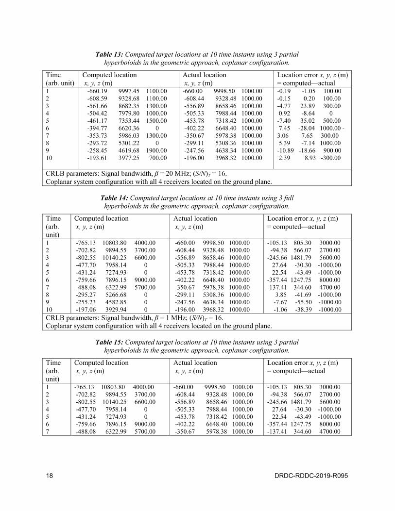
To ensure that the good agreement obtained in the target locations between employing full hyperboloids (old algorithm) and partial hyperboloids (new algorithm) is not just a coincidence, scenario using a different system configuration is examined to verify that the model simulation results are consistent and valid.
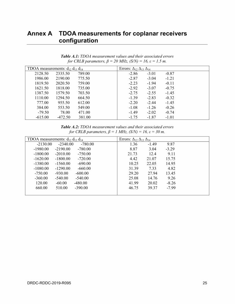
A coplanar system configuration in which all four receivers are located on the ground plane is examined. The TDOA measurement values dij are re-calculated to adjust to the change in the receivers’ system geometry. The coplanar TDOA measurement values dij for the case in which the CRLB parameters = 20 MHz and (S/N)T =16 and the case in which = 1 MHz and (S/N)T =16 are given in Annex A. Results of the computed target locations using the full hyperboloids algorithm and partial hyperboloids algorithm are shown in Table 12 and Table 13 respectively for the case = 20 MHz, and in Table 14 and Table 15respectively for the case = 1 MHz. It can be seen that both algorithms give identical outputs in the coplanar configuration as well in both cases. Hence, these computations demonstrate that the partial hyperboloid algorithm is equivalent to the full hyperboloid algorithm in processing target localization but is computing significantly faster.
Table 12: Computed target locations at 10 time instants using 3 full hyperboloids in the geometric approach, coplanar configuration.
Time(arb. unit)
Computed location x, y, z (m)
Actual location x, y, z (m)
Location error x, y, z (m)= computed—actual
12345678910
-660.19 9997.45 1100.00-608.59 9328.68 1100.00-561.66 8682.35 1300.00-504.42 7979.80 1000.00-461.17 7353.44 1500.00-394.77 6620.36 0-353.73 5986.03 1300.00-293.72 5301.22 0-258.45 4619.68 1900.00-193.61 3977.25 700.00
-660.00 9998.50 1000.00-608.44 9328.48 1000.00-556.89 8658.46 1000.00-505.33 7988.44 1000.00-453.78 7318.42 1000.00-402.22 6648.40 1000.00-350.67 5978.38 1000.00-299.11 5308.36 1000.00-247.56 4638.34 1000.00-196.00 3968.32 1000.00
-0.19 -1.05 100.00-0.15 0.20 100.00-4.77 23.89 300.000.92 -8.64 0
-7.40 35.02 500.007.45 -28.04 1000.00 -
3.06 7.65 300.005.39 -7.14 1000.00
-10.89 -18.66 900.002.39 8.93 -300.00
CRLB parameters: Signal bandwidth, = 20 MHz; (S/N)T = 16.Coplanar system configuration with all 4 receivers located on the ground plane.
18 DRDC-RDDC-2019-R095
Table 13: Computed target locations at 10 time instants using 3 partial hyperboloids in the geometric approach, coplanar configuration.
Time(arb. unit)
Computed location x, y, z (m)
Actual location x, y, z (m)
Location error x, y, z (m)= computed—actual
12345678910
-660.19 9997.45 1100.00-608.59 9328.68 1100.00-561.66 8682.35 1300.00-504.42 7979.80 1000.00-461.17 7353.44 1500.00-394.77 6620.36 0-353.73 5986.03 1300.00-293.72 5301.22 0-258.45 4619.68 1900.00-193.61 3977.25 700.00
-660.00 9998.50 1000.00-608.44 9328.48 1000.00-556.89 8658.46 1000.00-505.33 7988.44 1000.00-453.78 7318.42 1000.00-402.22 6648.40 1000.00-350.67 5978.38 1000.00-299.11 5308.36 1000.00-247.56 4638.34 1000.00-196.00 3968.32 1000.00
-0.19 -1.05 100.00-0.15 0.20 100.00-4.77 23.89 300.000.92 -8.64 0
-7.40 35.02 500.007.45 -28.04 1000.00 -
3.06 7.65 300.005.39 -7.14 1000.00
-10.89 -18.66 900.002.39 8.93 -300.00
CRLB parameters: Signal bandwidth, = 20 MHz; (S/N)T = 16.Coplanar system configuration with all 4 receivers located on the ground plane.
Table 14: Computed target locations at 10 time instants using 3 full hyperboloids in the geometric approach, coplanar configuration.
Time(arb. unit)
Computed location x, y, z (m)
Actual location x, y, z (m)
Location error x, y, z (m)= computed—actual
12345678910
-765.13 10803.80 4000.00-702.82 9894.55 3700.00-802.55 10140.25 6600.00-477.70 7958.14 0-431.24 7274.93 0-759.66 7896.15 9000.00-488.08 6322.99 5700.00-295.27 5266.68 0-255.23 4582.85 0-197.06 3929.94 0
-660.00 9998.50 1000.00-608.44 9328.48 1000.00-556.89 8658.46 1000.00-505.33 7988.44 1000.00-453.78 7318.42 1000.00-402.22 6648.40 1000.00-350.67 5978.38 1000.00-299.11 5308.36 1000.00-247.56 4638.34 1000.00-196.00 3968.32 1000.00
-105.13 805.30 3000.00-94.38 566.07 2700.00
-245.66 1481.79 5600.0027.64 -30.30 -1000.0022.54 -43.49 -1000.00
-357.44 1247.75 8000.00-137.41 344.60 4700.00
3.85 -41.69 -1000.00-7.67 -55.50 -1000.00-1.06 -38.39 -1000.00
CRLB parameters: Signal bandwidth, = 1 MHz; (S/N)T = 16.Coplanar system configuration with all 4 receivers located on the ground plane.
Table 15: Computed target locations at 10 time instants using 3 partial hyperboloids in the geometric approach, coplanar configuration.
Time(arb. unit)
Computed location x, y, z (m)
Actual location x, y, z (m)
Location error x, y, z (m)= computed—actual
1234567
-765.13 10803.80 4000.00-702.82 9894.55 3700.00-802.55 10140.25 6600.00-477.70 7958.14 0-431.24 7274.93 0-759.66 7896.15 9000.00-488.08 6322.99 5700.00
-660.00 9998.50 1000.00-608.44 9328.48 1000.00-556.89 8658.46 1000.00-505.33 7988.44 1000.00-453.78 7318.42 1000.00-402.22 6648.40 1000.00-350.67 5978.38 1000.00
-105.13 805.30 3000.00-94.38 566.07 2700.00
-245.66 1481.79 5600.0027.64 -30.30 -1000.0022.54 -43.49 -1000.00
-357.44 1247.75 8000.00-137.41 344.60 4700.00
DRDC-RDDC-2019-R095 19
Time(arb. unit)
Computed location x, y, z (m)
Actual location x, y, z (m)
Location error x, y, z (m)= computed—actual
8910
-295.27 5266.68 0-255.23 4582.85 0-197.06 3929.94 0
-299.11 5308.36 1000.00-247.56 4638.34 1000.00-196.00 3968.32 1000.00
3.85 -41.69 -1000.00-7.67 -55.50 -1000.00-1.06 -38.39 -1000.00
CRLB parameters: Signal bandwidth, = 1 MHz; (S/N)T = 16.Coplanar system configuration with all 4 receivers located on the ground plane.
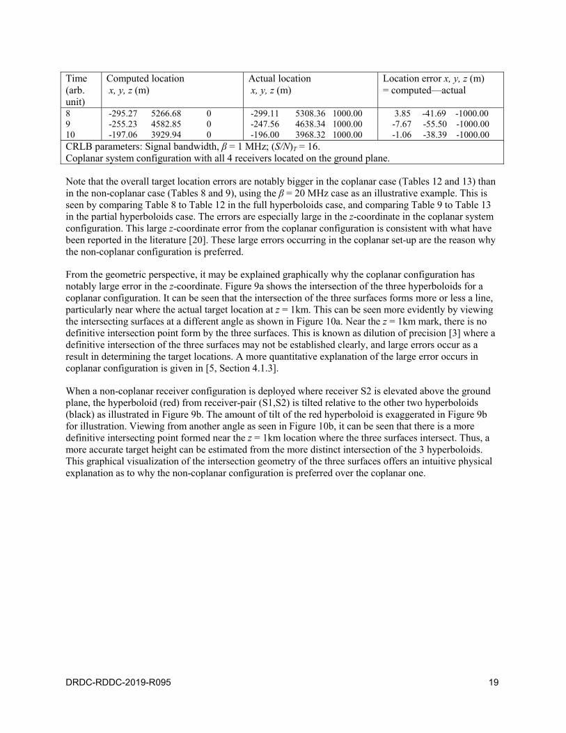
Note that the overall target location errors are notably bigger in the coplanar case (Tables 12 and 13) than in the non-coplanar case (Tables 8 and 9), using the = 20 MHz case as an illustrative example. This is seen by comparing Table 8 to Table 12 in the full hyperboloids case, and comparing Table 9 to Table 13in the partial hyperboloids case. The errors are especially large in the z-coordinate in the coplanar system configuration. This large z-coordinate error from the coplanar configuration is consistent with what have been reported in the literature [20]. These large errors occurring in the coplanar set-up are the reason why the non-coplanar configuration is preferred.
From the geometric perspective, it may be explained graphically why the coplanar configuration has notably large error in the z-coordinate. Figure 9a shows the intersection of the three hyperboloids for a coplanar configuration. It can be seen that the intersection of the three surfaces forms more or less a line, particularly near where the actual target location at z = 1km. This can be seen more evidently by viewing the intersecting surfaces at a different angle as shown in Figure 10a. Near the z = 1km mark, there is no definitive intersection point form by the three surfaces. This is known as dilution of precision [3] where a definitive intersection of the three surfaces may not be established clearly, and large errors occur as a result in determining the target locations. A more quantitative explanation of the large error occurs in coplanar configuration is given in [5, Section 4.1.3].
When a non-coplanar receiver configuration is deployed where receiver S2 is elevated above the ground plane, the hyperboloid (red) from receiver-pair (S1,S2) is tilted relative to the other two hyperboloids(black) as illustrated in Figure 9b. The amount of tilt of the red hyperboloid is exaggerated in Figure 9bfor illustration. Viewing from another angle as seen in Figure 10b, it can be seen that there is a more definitive intersecting point formed near the z = 1km location where the three surfaces intersect. Thus, a more accurate target height can be estimated from the more distinct intersection of the 3 hyperboloids. This graphical visualization of the intersection geometry of the three surfaces offers an intuitive physical explanation as to why the non-coplanar configuration is preferred over the coplanar one.

20 DRDC-RDDC-2019-R095
Figure 9: a) Intersection of 3 coplanar hyperboloids. b) Intersection of 2 coplanar and 1 non-coplanar hyperboloids.
Figure 10: Intersection of 3 hyperboloids, a) 3 coplanar surfaces, b) 2 coplanar and 1 non-coplanar surfaces at a different viewing angle.
3.3.2 Comparison using error free TDOA measurements
As a final example to show that the target location results are the same using the full hyperboloids and partial hyperboloids, a non-coplanar receiver system set-up is re-deployed, and error-free TDOA measurements dij are used (see Table 2). Table 16 and Table 17 show the computed target location results using the full hyperboloids and the partial hyperboloids respectively. It can be seen that using the error-free dij values, the computed target locations are nearly perfect in accuracy in both the full hyperboloids and the partial hyperboloids cases. These very accurate results are expected in a scenario
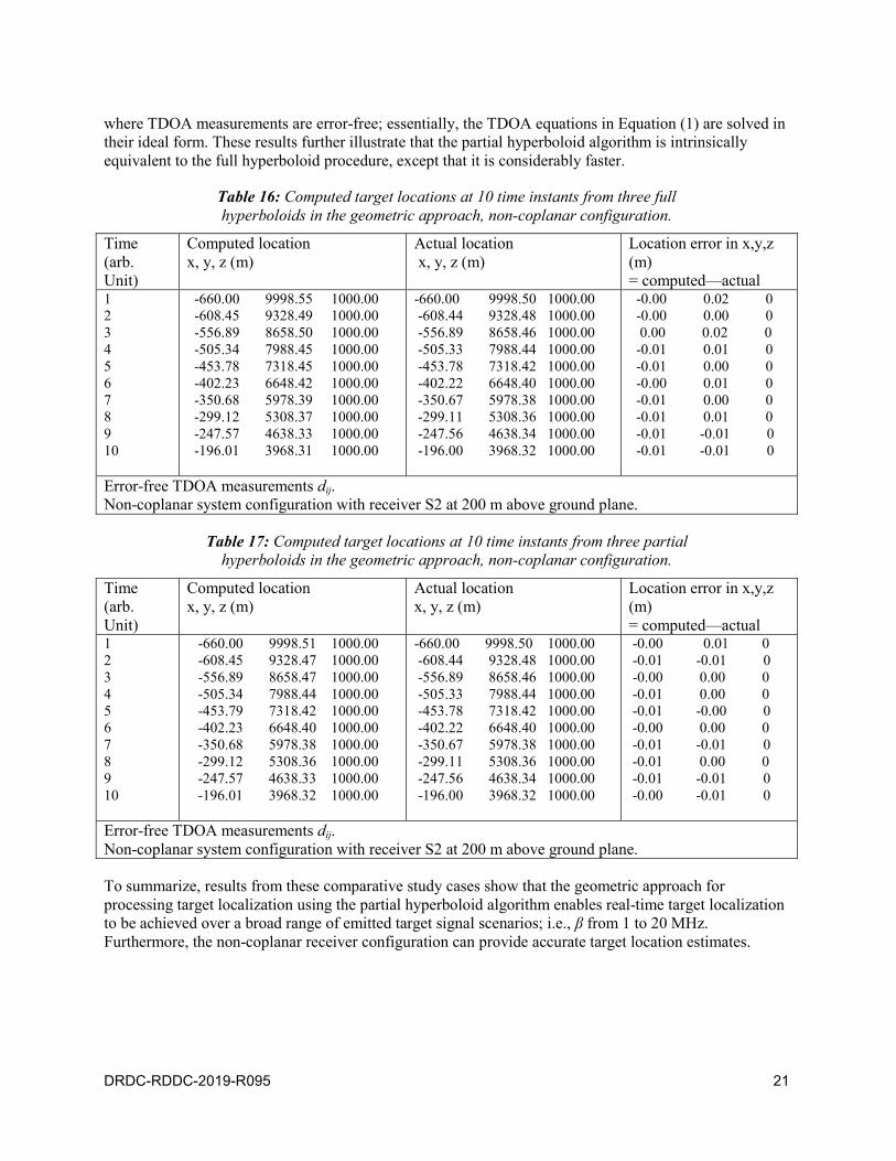
DRDC-RDDC-2019-R095 21
where TDOA measurements are error-free; essentially, the TDOA equations in Equation (1) are solved in their ideal form. These results further illustrate that the partial hyperboloid algorithm is intrinsically equivalent to the full hyperboloid procedure, except that it is considerably faster.
Table 16: Computed target locations at 10 time instants from three full hyperboloids in the geometric approach, non-coplanar configuration.
Time(arb. Unit)
Computed location x, y, z (m)
Actual locationx, y, z (m)
Location error in x,y,z (m)= computed—actual
12345678910
-660.00 9998.55 1000.00-608.45 9328.49 1000.00-556.89 8658.50 1000.00-505.34 7988.45 1000.00-453.78 7318.45 1000.00-402.23 6648.42 1000.00-350.68 5978.39 1000.00-299.12 5308.37 1000.00-247.57 4638.33 1000.00-196.01 3968.31 1000.00
-660.00 9998.50 1000.00-608.44 9328.48 1000.00-556.89 8658.46 1000.00-505.33 7988.44 1000.00-453.78 7318.42 1000.00-402.22 6648.40 1000.00-350.67 5978.38 1000.00-299.11 5308.36 1000.00-247.56 4638.34 1000.00-196.00 3968.32 1000.00
-0.00 0.02 0-0.00 0.00 00.00 0.02 0
-0.01 0.01 0-0.01 0.00 0-0.00 0.01 0-0.01 0.00 0-0.01 0.01 0-0.01 -0.01 0-0.01 -0.01 0
Error-free TDOA measurements dij.Non-coplanar system configuration with receiver S2 at 200 m above ground plane.
Table 17: Computed target locations at 10 time instants from three partial hyperboloids in the geometric approach, non-coplanar configuration.
Time(arb. Unit)
Computed location x, y, z (m)
Actual location x, y, z (m)
Location error in x,y,z (m)= computed—actual
12345678910
-660.00 9998.51 1000.00-608.45 9328.47 1000.00-556.89 8658.47 1000.00-505.34 7988.44 1000.00-453.79 7318.42 1000.00-402.23 6648.40 1000.00-350.68 5978.38 1000.00-299.12 5308.36 1000.00-247.57 4638.33 1000.00-196.01 3968.32 1000.00
-660.00 9998.50 1000.00-608.44 9328.48 1000.00-556.89 8658.46 1000.00-505.33 7988.44 1000.00-453.78 7318.42 1000.00-402.22 6648.40 1000.00-350.67 5978.38 1000.00-299.11 5308.36 1000.00-247.56 4638.34 1000.00-196.00 3968.32 1000.00
-0.00 0.01 0-0.01 -0.01 0-0.00 0.00 0-0.01 0.00 0-0.01 -0.00 0-0.00 0.00 0-0.01 -0.01 0-0.01 0.00 0-0.01 -0.01 0-0.00 -0.01 0
Error-free TDOA measurements dij.Non-coplanar system configuration with receiver S2 at 200 m above ground plane.
To summarize, results from these comparative study cases show that the geometric approach for processing target localization using the partial hyperboloid algorithm enables real-time target localization to be achieved over a broad range of emitted target signal scenarios; i.e., from 1 to 20 MHz. Furthermore, the non-coplanar receiver configuration can provide accurate target location estimates.
22 DRDC-RDDC-2019-R095
4 conclusions
A more efficient algorithm for the geometric approach has been developed to allow real-time processing of TDOA data for target localization. A partial hyperboloid method is deployed to enable faster TDOA processing. Using realistic target detection scenarios that cover a broad range of TDOA measurement error values, the partial hyperboloid algorithm is validated by demonstrating that it produces the same target localization results as the full hyperboloid procedure. A processing time of 0.3s has been attained, compare to 8.6s taken in the former geometric approach using full hyperboloids as described in [5]. Thus, real-time target localization has been realized, making TDOA-based passive RF-sensing practical in many target detection and tracking, and counter-surveillance applications.
Furthermore, a non-coplanar receiver system configuration where one of the four receivers is not located on the same plane as the other three receivers is found to be a better geometrical system set-up than a coplanar configuration. Better target location accuracy can be attained from a non-coplanar set-up. A qualitative geometrical explanation is given to explain why a non-coplanar configuration is preferred.

DRDC-RDDC-2019-R095 23
References
[1] J. Zhou, “NASA Wants to Fly Drones on Mars to Look For Natural Resources,” Epoch Times,August 5, 2015. http://www.theepochtimes.com/n3/1706045-nasa-wants-to-fly-drones-on-mars/(Access date: January 2017).
[2] S. Wong, R. Jassemi-Zargani, D. Brookes, B. Kim and B. Kaluzny, “Target localization over the Earth’s curved surface,” Scientific Report, DRDC-RDDC-2018-R136, Defence Research and Development Canada, May 2018.
[3] R.A. Poisel, “Electronic Warfare Target location Methods,” ArtTech House, Boston, 2005.
[4] D. Munoz, F. Bouchereau, C. Vargas and R. Enriquez-Caldera, “Position Location Techniques and Applications,” Academic Press, Burlington MA, 2009.
[5] S. Wong, R. Jassemi-Zargani, D. Brookes and B. Kim, “Passive target localization using a geometric approach to the time-difference-of-arrival method,” Scientific Report, DRDC-RDDC-2017-R079, Defence Research and Development Canada, June 2017.
[6] J.WH. Foy, “Position Location Solution by Taylor Series Estimation,” IEEE Transactions on Aerospace and Electronic Systems, Vol. AES-12, pp. 183–198, March 1976.
[7] T. Sathyan, A. Sinha and T. Kirubarajan, “Passive Geolocation and Tracking of an Unknown Number of Emitters,” IEEE Transactions on Aerospace and Electronic Systems, Vol. 42, No. 2, pp. 740–750,April 2006.
[8] D.J. Torrieri, “Statistical Theory of Passive Location Systems,” IEEE Transactions on Aerospace andElectronic Systems, Vol. AES-20, No. 2, pp. 183–197, March 1984.
[9] H.C. Schau and A.Z. Robinson, “Passive Sources Localization Employing Intersecting Spherical Surfaces from Time-of-Arrival Differences,” IEEE Transactions on Acoustics, Speech, and Signal Processing, Vol. ASSP-35, No. 8, pp. 1223–1225, August 1987.
[10] Y.T. Chan and K.C. Ho, “A Simple and Efficient Estimator for Hyperbolic Location,” IEEE Transactions on Signal Processing, Vol. 42, No. 8, pp. 1905–1915, August 1994.
[11] G. Mellen, M. Pachter and J. Raquet, “Closed-Form Solution for Determining Emitter Location using Time Difference of Arrival Measurements,” IEEE Transactions on Aerospace and Electronic Systems, Vol. 39, No. 3, pp. 1056–1058, July 2003.
[12] B. Fang, “Simple Solution for Hyperbolic and Related Position Fixes,” IEEE Transactions on Aerospace and Electronic Systems, Vol. 26, No. 5, pp. 748–753, September 1990.
[13] J.O. Smith and J.S. Abel, “Closed-Form Least-Square Source Location Estimation from Range-Difference Measurements,” IEEE Transactions on Acoustics, Speech, and Signal Processing, Vol. ASSP-35, No. 12, pp. 1661–1669, December 1987.
24 DRDC-RDDC-2019-R095
[14] J. Abel and J. Chaffe, “Existence and Uniqueness of GPS Solutions,” IEEE Transactions on Aerospace and Electronic Systems, Vol. 27, No. 6, pp. 952–956, November 1991.
[15] J. Bard, F.M. Ham and W.L. Jones, “An Algebraic Solution to the Time-Difference of Arrival Equations,” Southeastcon ’96, Proceedings of the IEEE, pp. 313–319, Tampa, FL, 11–14 April 1996.
[16] R. Schmidt, “Least Squares Range Difference Location,” IEEE Transactions on Aerospace and Electronic Systems, Vol. 32, No. 1, pp.234–242, January 1996.
[17] S. Stein, “Algorithms for Ambiguity Function Processing,” IEEE Transactions on Acoustics, Speech, and Signal Processing, Vol. ASSP-29, No.3 pp.588–599, June 1981.
[18] A.H. Quazi, “An Overview on the Time Delay Estimation in Active and Passive Systems for Target Localization,” IEEE Transactions on Acoustics, Speech, and Signal Processing, Vol. ASSP-29,No.3 pp.527–533, June 1981.
[19] R.O. Schmidt, “A New Approach to Geometry of Range Difference Location,” IEEE Transactions on Aerospace and Electronic Systems, Vol. AES-8, No. 6, pp.821–835, November 1972.
[20] M. Khalaf-Allah, “A Modified Closed-Form Time-Difference-Of-Arrival Positioning Algorithm,”Proc. Of World Symposium on Computer Network and Information Security, http://nngt.org/digital-library/upload/conference2/p2.pdf (Access date: March 2016).
[21] “Definition of: video bandwidth, Bandwidth Requirement,” PC Magazine, Ziff Davis LLC, New York, NY, https://www.pcmag.com/encyclopedia/term/53823/video-bandwidth (Access date: October 2015).
[22] M. Niggel, “Video Frequency Management: Keeping Multiple Quads in the Air,” May 1, 2017,Propwashed, Anaheim, CA 92809, https://www.propwashed.com/video-frequency-management/,(Access date: June 2019).
[23] “Quadcopter Telemetry Signal,” Sigidwiki.com, https://www.sigidwiki.com/wiki/Quadcopter_Telemetry_Signal, Sigidwiki.com, (Access date: September, 2018).
[24] “Telemetry Standard, IRIG Standard 106-15 (Part 1) Appendix A, July 2015,” Secretariat, Range Commanders Council, White Sands Missile Range, New Mexico, 88002,www.irig106.org/docs/106-15/appendixA.pdf (Access date: September 2018).
[25] S. Henriksen, “Unmanned Aircraft Control and ATC Communications Bandwidth Requirements,”NASA/CR-2008-214841, National Aeronautics and Space Administration, Washington D. C. 20546, 2008.
DRDC-RDDC-2019-R095 25
Annex A TDOA measurements for coplanar receivers configuration
Table A.1: TDOA measurement values and their associated errors for CRLB par MHz, (S/
TDOA measurements: d12 d13 d14 12 13 14
2128.50 2335.50 789.001986.00 2190.00 775.501819.50 2020.50 759.001621.50 1818.00 735.001387.50 1579.50 703.501110.00 1294.50 664.50777.00 955.50 612.00384.00 553.50 549.00-79.50 78.00 471.00
-615.00 -472.50 381.00
-2.86 -3.01 -0.87-2.87 -3.04 -1.21-2.23 -1.94 -0.11-2.92 -3.07 -0.75-2.75 -2.55 -1.45-1.39 -2.83 -0.32-2.20 -2.44 -1.45-1.08 -1.26 -0.26-1.49 -2.02 -0.74-1.75 -1.87 -1.01
Table A.2: TDOA measurement values and their associated errors MHz, (S/
TDOA measurements: d12 d13 d14 12 13 14
-2130.00 -2340.00 -780.00-1980.00 -2190.00 -780.00-1800.00 -2010.00 -750.00-1620.00 -1800.00 -720.00-1380.00 -1560.00 -690.00-1080.00 -1290.00 -660.00-750.00 -930.00 -600.00-360.00 -540.00 -540.00120.00 -60.00 -480.00660.00 510.00 -390.00
1.36 -1.49 9.87 8.87 3.04 -3.29
21.73 12.4 9.11 4.42 21.07 15.75
10.25 22.05 14.95 31.39 7.33 4.82 29.20 27.94 13.45 25.08 14.76 9.26 41.99 20.02 -8.2646.75 39.37 -7.99
26 DRDC-RDDC-2019-R095
List of symbols/abbreviations/acronyms/initialisms
CAF Canadian Armed Forces
CRLB Cramer-Rao Lower Bound
FPV First Person View
IFF Identification Friend or Foe
ISR Intelligence, Surveillance and Reconnaissance
RF Radio Frequency
TDOA Time-Difference-Of-Arrival

DOCUMENT CONTROL DATA*Security markings for the title, authors, abstract and keywords must be entered when the document is sensitive
1. ORIGINATOR (Name and address of the organization preparing the document.A DRDC Centre sponsoring a contractor's report, or tasking agency, is entered in Section 8.)
DRDC – Ottawa Research CentreDefence Research and Development Canada, Shirley's Bay3701 Carling AvenueOttawa, Ontario K1A 0Z4Canada
2a. SECURITY MARKING(Overall security marking of the document including special supplemental markings if applicable.)
CAN UNCLASSIFIED
2b. CONTROLLED GOODS
NON-CONTROLLED GOODSDMC A
3. TITLE (The document title and sub-title as indicated on the title page.)
Time-difference-of-arrival target localization processing in real time
4. AUTHORS (Last name, followed by initials – ranks, titles, etc., not to be used)
Wong, S.; Jassemi-Zargani, R.; Brookes, D.; Kim, B.
5. DATE OF PUBLICATION(Month and year of publication of document.)
June 2019
6a. NO. OF PAGES(Total pages, including Annexes, excluding DCD, covering and verso pages.)
34
6b. NO. OF REFS(Total references cited.)
25
7. DOCUMENT CATEGORY (e.g., Scientific Report, Contract Report, Scientific Letter.)
Scientific Report
8. SPONSORING CENTRE (The name and address of the department project office or laboratory sponsoring the research and development.)
DRDC – Ottawa Research CentreDefence Research and Development Canada, Shirley's Bay3701 Carling AvenueOttawa, Ontario K1A 0Z4Canada
9a. PROJECT OR GRANT NO. (If appropriate, the applicable research and development project or grant number under which the document was written. Please specify whether project or grant.)
05eb
9b. CONTRACT NO. (If appropriate, the applicable number under which the document was written.)
10a. DRDC PUBLICATION NUMBER (The official document number by which the document is identified by the originating activity. This number must be unique to this document.)
DRDC-RDDC-2019-R095
10b. OTHER DOCUMENT NO(s). (Any other numbers which may be assigned this document either by the originator or by the sponsor.)
11a. FUTURE DISTRIBUTION WITHIN CANADA (Approval for further dissemination of the document. Security classification must also be considered.)
Public release
11b. FUTURE DISTRIBUTION OUTSIDE CANADA (Approval for further dissemination of the document. Security classification must also be considered.)
12. KEYWORDS, DESCRIPTORS or IDENTIFIERS (Use semi-colon as a delimiter.)
EW Modelling and Simulation (EW M&S)
13. ABSTRACT (When available in the document, the French version of the abstract must be included here.)
Passive RF-sensing exploiting Radio-Frequency (RF) signal emitted by targets offers a viable and effective means of detecting and geolocating small flying targets such as drones.Time-Difference-Of-Arrival (TDOA) provides a means to process the detected RF signals to locate targets in three-dimensional space. A set of three TDOA equations is solved to obtain the unknown target’s coordinates (x,y,z) in three dimensions. The solution to each TDOA equation is represented by a geometric surface known as a hyperboloid. The intersection of three hyperboloid surfaces is computed to determine the target’s location. This geometric approach offers a simple and physically intuitive way of solving the set of TDOA equations, and has been investigated in a previous study. However, this geometric approach may not be able to determine the location of the target in real-time (i.e., under one second). The computational speed is directly linked to the size of the hyperboloid surfaces required to cover the surveillance area of interest. This presents a challenge in computing time usage.
In this report, a partial hyperboloid method is introduced and an algorithmic procedure is developed, utilizing only partial hyperboloid surfaces around the unknown target’s location are utilized. This allows real-time target localization to be realized. Results have indicated that this method has improved the computational speed by about 29 times comparing to using a set of full hyperboloids in solving the TDOA equations for a surveillance coverage area of about 10 km by 6 km, a typical counter-drone surveillance scenario. The computed target locations are identical to those using the full hyperboloids over a broad range of TDOA measurement errors corresponding to realistic target detection scenarios. The errors are characterized by the Cramer-Rao Lower Bound standard deviation.
La détection passive par radiofréquence (RF) offre un moyen viable et efficace de repérer et de géolocaliser de petites cibles volantes, par exemple des drones, en exploitant leurs émissions de signaux RF. Le calcul de la différence entre les temps d’arrivée (TDOA) permet de traiter les signaux RF reçus pour localiser les cibles dans un espace tridimensionnel. Le système résout trois équations et obtient les coordonnées (x,y,z) d’une cible inconnue. La solution de chaque équation est représentée par une surface géométrique qu’on appelle un hyperboloïde, puis l’intersection des trois surfaces est calculée pour établir l’emplacement de la cible. Cette méthode, axée sur la géométrie, offre une façon simple et intuitive de résoudre un ensemble d’équations reliées aux différences de temps d’arrivée et a fait l’objet d’une autre étudeprécédemment. Cependant, elle ne permet pas toujours de localiser les cibles en temps réel, c’est-à-dire en moins d’une seconde. La puissance requise pour effectuer les calculs dépend dela taille des surfaces hyperboloïdes nécessaires pour couvrir la zone surveillée, donc le temps de traitement peut être important dans certains cas.
Dans le présent rapport, on décrit une méthode de calcul partiel d’hyperboloïdes et uneprocédure se fondant sur des algorithmes. Cette méthode permet de calculer uniquement lessurfaces hyperboloïdes entourant l’emplacement des cibles inconnues. Les résultats de l’étudeindiquent que les calculs s’effectuent environ 29 fois plus vite avec cette méthode qu’avec la méthode de calcul des hyperboloïdes entiers lorsqu’on traite des équations portant sur lesdifférences de temps d’arrivée pour une zone de 10 km sur 6 km, qui correspond à un scénario type de détection des drones de surveillance. La méthode partielle permet donc de localiser les cibles en temps réel. Les emplacements calculés à l’aide de cette méthode sont identiques àceux calculés par l’intermédiaire de la méthode de calcul des hyperboloïdes entiers pour une vaste gamme d’erreurs de mesure de TDOA que l’on retrouve, réalistement, dans les scénarios de détection de cibles. Ces erreurs sont caractérisées par l’écart-type de la borne inférieure de Cramér-Rao.