Iterative HOS-SOS (IHOSS) Algorithm for Direction-of-Arrival Estimation and Sensor Localization

IEEE TRANSACTIONS ON SIGNAL PROCESSING, VOL. 58, NO. 12, DECEMBER 2010 6181

Iterative HOS-SOS (IHOSS) Algorithm forDirection-of-Arrival Estimation and Sensor

LocalizationMetin Aktas and T. Engin Tuncer

Abstract—A new method for joint direction-of-arrival (DOA)and sensor position estimation is introduced. The sensors areassumed to be randomly deployed except two reference sen-sors. The proposed method exploits the advantages of bothhigher-order-statistics (HOS) and second-order-statistics (SOS)with an iterative algorithm, namely Iterative Higher-OrderSecond-Order Statistics (IHOSS). A new cumulant matrix estima-tion technique is proposed for the HOS approach by convertingthe multisource problem into a single source one. IHOSS per-forms well even in case of correlated source signals due to theeffectiveness of the proposed cumulant matrix estimate. A costfunction is defined for the joint DOA and position estimation.The iterative procedure is guaranteed to converge. The ambiguityproblem in sensor position estimation is solved by observing thesource signals at least in two different frequencies. The conditionson these frequencies are presented. Closed-form expressions arederived for the deterministic Cramér-Rao bound (CRB) for DOAand unknown sensor positions for noncircular complex Gaussiannoise with unknown covariance matrix. Simulation results showthat the performance of IHOSS is significantly better than theHOS approaches for DOA estimation and closely follows the CRBfor both DOA and sensor position estimations.

Index Terms—Cumulant matrix, deterministic Cramér-Raobound (CRB), direction-of-arrival (DOA) estimation, higher-order-statistics (HOS), sensor localization.

I. INTRODUCTION

P REVIOUS literature on direction-of-arrival (DOA) esti-mation is mostly based on the assumption that the sensor

geometry is fixed and sensor positions are known. In certain ap-plications such as the antennas placed on the wing tips of a planeor in case of distributed sensors, perfect knowledge of the sensorlocations is impractical. In this paper, joint DOA and sensor po-sition estimation problem is investigated when the sensors arerandomly deployed to unknown positions except two referencesensors.

The DOA estimation in the presence of array imperfectionsis investigated as an array calibration problem and many tech-niques are proposed in [4]–[6], [8], and [9]. Previous methods inthis context assume that the nominal sensor positions are knownand the uncertainty in sensor positions is small [4], [5], [7]. Inaddition, sources are assumed to be spatially and temporally dis-

Manuscript received January 11, 2010; accepted August 07, 2010. Date ofpublication September 02, 2010; date of current version November 17, 2010.The associate editor coordinating the review of this manuscript and approvingit for publication was Prof. Andreas Jakobsson.

The authors are with the Department of Electrical and Electronics Engi-neering, Middle East Technical University, Ankara, 06531 Turkey (e-mail:[email protected]; [email protected]).

Digital Object Identifier 10.1109/TSP.2010.2071868

joint [6] or the source DOA angles are known [8], [9]. Therefore,array calibration algorithms can only be applied with certainlimitations on the array structure and the source characteristics.

Some of the limitations for array calibration methods areeliminated with the VESPA algorithm [10]. In [10] it is shownthat the combination of higher-order-statistics (HOS) approachand the ESPRIT algorithm allows the computation of the DOAestimates for arbitrary sensor geometries without knowing thesensor positions. Therefore, the requirement for a special arraygeometry for the ESPRIT algorithm as well as the requirementfor the nominal sensor positions for the array calibration algo-rithms are eliminated. In this approach, the cumulant matrix,which has the same information as the correlation matrix of theESPRIT structure, is obtained from the cumulants of the arrayoutput. In [10], relative positions of the two reference sensorsare required to be known. Also it is assumed that the sourcesignals are independent. When this assumption is not satisfied,the cumulant matrix has error terms. These error terms becomesignificant for finite length signals and decrease the accuracyof the VESPA algorithm, generating the flooring effect forthe multiple sources [11]. The approach in [10] is extendedto the case of dependent source signals in [12]. In this case,it is assumed that the sensor array is composed of calibratedand uncalibrated subarrays where the calibrated subarray is auniform linear array. It is known that the method in [10] canonly be used to estimate the DOA angles. In other words, sensorpositions cannot be found with the approach in [10].

In this paper, a new technique, IHOSS, is presented in orderto find the DOA angles as well as the sensor positions when thesensors are randomly deployed with unknown positions. Theproposed technique finds the unknown parameters using onlythe sensor array output and the positions of the two referencesensors. There is no other a priori information including thenominal sensor positions in contrast to the array calibration ap-proaches [4], [5], [7]. To our knowledge, this is the only workthat gives a solution for this problem. IHOSS method has severaladvantages. It eliminates the need to know the nominal sensorpositions for the joint DOA and sensor position estimation. Itcan perform well even for the correlated source signals unlikethe work in [10]. Therefore, IHOSS algorithm can be used forthe unknown parameter estimation in a more general problemsetting.

IHOSS method uses the HOS and SOS approaches in an it-erative framework in order to take the advantage of both tech-niques. HOS approach is used to compute the DOA and arraysteering matrix estimates without knowing the sensor positionsexcept the two reference sensors. A new cumulant matrix esti-mation technique, which is more robust to the correlation be-

1053-587X/$26.00 © 2010 IEEE

6182 IEEE TRANSACTIONS ON SIGNAL PROCESSING, VOL. 58, NO. 12, DECEMBER 2010

tween source signals, is presented for the HOS approach. Inthis technique, the error terms in the cumulant matrix due to thecorrelation between source signals are decreased by convertingthe multisource problem into a single-source case [13], [14]using the array steering matrix estimate. While this conversionis not perfect, it effectively decreases the undesired signal com-ponents in the measurements. The performance of the IHOSSdepends on the accuracy of the array steering matrix estimate.If the array steering matrix is perfectly known, the error termsin the cumulant matrix are completely eliminated. In IHOSS,the accuracy of the array steering matrix estimate is improvediteratively with the joint use of the HOS and SOS approaches.SOS approach is more robust to the estimation errors than theHOS approach especially when the number of observations issmall [11]. In order to use the SOS approach, the sensor posi-tions should be found. A new method to find the sensor positionsunambiguously is proposed by using multiple frequencies [15].The conditions for unambiguous sensor position estimation aregiven. IHOSS uses an iterative process which is guaranteed toconverge. The performance of the IHOSS algorithm is investi-gated in detail in order to show the effectiveness of the iterativeapproach. The deterministic Cramér-Rao bound (CRB) expres-sions for the DOA and sensor position estimations are derivedfor the described problem setting. It is shown that the proposedapproach performs well for a variety of scenarios and closelyfollows the CRB.

The rest of the paper is organized as follows. In Section II,the problem is defined and the assumptions required for the so-lution are presented. Section III describes the IHOSS approachfor finding the DOA and array steering matrix estimates whenthe sensor positions are unknown. It is shown that the error termsin the cumulant matrix for the dependent source signals changesthe desired form of the cumulant matrix, generating problemsfor the application of the ESPRIT algorithm. A method for abetter estimation of the cumulant matrix is explained in this sec-tion. Iterative use of the HOS and SOS approaches in the IHOSSalgorithm and the unambiguous sensor localization algorithmare also presented in this section. The deterministic CRB expres-sions are given in Section IV. The performance of the IHOSSalgorithm is presented in Section V. The proofs of the lemmaand theorem presented in this paper are given in the Appendix.

The notation used in this paper is as follows. Matrices andvectors are represented by bold uppercase and bold lowercasecharacters, respectively. and stand forthe transpose, conjugate transpose, conjugate and trace oper-ator, respectively. and represent the Kronecker product andHadamard matrix product, respectively. is used to definethe Moore-Penrose pseudoinverse. and are the realand the imaginary part operators. is the smallest integer notless than and is the rounding operator that rounds to thenearest integer.

II. PROBLEM STATEMENT

It is assumed that the array is composed of randomly de-ployed sensors on a plane and there are far-field sources.The transmitting source signals are assumed to be wideband.The received signal at the sensor can be written as

(1)

where and are the source and noise signals, respec-tively. is the propagation delay from the th source to the

th sensor and it can be written as [25]

(2)

where is the DOA angle of the th source in azimuth.is the two dimensional position of the th sensor

and is the speed of propagation.It is assumed that multiple wideband signals are observed

with overlapping spectra. Narrowband bandpass filters with dif-ferent center frequencies are used to extract thenarrowband signals. If we assume that the frequency responseof the filters is flat over the passband and the signal spectrumvaries over the filter passband, the output of the th sensor forthe th filter can be written as [24]

(3)

where and are the outputs of the th filter whenthe inputs are and , respectively. By substituting (2)into (3), the received signal vector for the sensor array at fre-quency can be written in a more compact form as

(4)

where is the number of snapshots,is the vector of source signals

for the frequency . is thevector of noise for the frequency , which is assumed

to be Gaussian. is the array steeringmatrix for the frequency . Source signals are assumed tobe non-Gaussian and they can be correlated but not coherent.Noise is assumed to be statistically independent with thesource signals. Given the DOA vector andthe sensor positions , the array steeringmatrix for frequency is written as

.... . .

... (5)

where the array steering matrix element for th sensor and thsource at frequency is written as

(6)

Two sensors are selected as the reference with known posi-tions. In order to avoid the ambiguity problem in DOA esti-mation, it is also assumed that the distance between the refer-ence sensors is less than or equal to , where is the wave-length corresponding to the largest frequency of interest, i.e.,

.The objective in this paper is to estimate the DOA angles of

sources and the positions of the sensors simultaneouslygiven the array output and the positions of the two referencesensors.

AKTAS AND TUNCER: IHOSS ALGORITHM FOR DOA ESTIMATION 6183

III. IHOSS ALGORITHM

In this section, IHOSS algorithm is introduced for a solutionto the problem described in Section II. IHOSS is an iterativealgorithm that jointly uses HOS and SOS approaches at eachiteration sequentially. The idea behind the IHOSS algorithm isto use the advantages of both HOS and SOS approaches in orderto improve the accuracy of the parameter estimation.

IHOSS uses HOS approach to find the DOA and arraysteering matrix estimates for the arbitrary sensor geometrieswithout knowing the sensor positions except the two referencesensors. In this respect, fourth-order cumulants are used to-gether with the ESPRIT algorithm. It is known that the ESPRITalgorithm can be employed for DOA estimation for the givenproblem setting as long as the source signals are independent[10]. The performance of [10] degrades significantly due tofinite length effects and correlation between source signals[11]. This point is discussed in Section III-A.

In order to overcome the limitations in [10], IHOSS proposesa new cumulant matrix estimation technique. This technique ismore robust to the correlation between source signals. It is basedon estimating the cumulant matrix as the sum of the cumulantmatrices corresponding to the case where each source is actingalone. SOS approach is known to be more robust to the esti-mation errors than the HOS approach for finite length signals[11]. Therefore SOS approach is used to improve the DOA andarray steering matrix estimates obtained from HOS approach.Sensor positions should be found in order to use the SOS ap-proach. A new sensor position estimation algorithm is proposedfor this purpose. The sensor positions are found unambiguouslyusing multiple frequencies [15]. The details of the sensor po-sition estimation algorithm is given in Section III-B. Initially,IHOSS assumes that the array steering matrix is zero. Then thearray steering matrix estimation is iteratively improved with thejoint use of HOS and SOS approaches. A MUSIC cost functionis used to select the best array steering matrix at each iteration.This is done in such a way that the non-negative cost function isimproved at each iteration. Therefore IHOSS algorithm is guar-anteed to converge. The details of the iterative approach and thecost function are explained in Section III-D.

A. HOS-Based Blind DOA Estimation

HOS approach is used to generate a virtual sensor array [16]aligned with the reference sensor such that two translationallyinvariant arrays are obtained, namely, the real sensor array andthe virtual sensor array. This structure is suitable for the appli-cation of the ESPRIT algorithm [2] as shown in [10].

The relation between the actual and virtual sensors is obtainedfrom the fourth-order cumulants by the “virtual cross-correla-tion computation” approach [10]. When the sensors 1 and 2 areselected as the reference sensors, this relation can be written inmatrix form [3] as

(7)

where is the th row of the array steering matrix, , in (5)and is the source cumulant matrix in the form of

(8)

Note that the frequency dependency of the cumulant matrix in(7) is dropped for simplicity. The same form of the cumulantmatrix is obtained for each frequency, .

The source cumulant matrix in (7), , involves an error term,, due to the dependency of the source signals, i.e.

(9)

In (9), is the desired source cumulant matrix which repre-sents the part assuming that the source signals are statisticallyindependent, i.e.

(10)

and

(11)

As shown in (11), the nonzero diagonal elements are locatedwith the indices for . The relation in(10) is based on the fact that if a subset of random variablesare independent of the rest, then the cumulant of these randomvariables is equal to zero as stated in [10] as [CP5]. When thesource signals are independent, , and in (7) has thedesired form.

When the source signals are not independent, (9) can be usedin (7) to obtain the following cumulant matrix:

(12)

is the desired cumulant matrix assuming that the source sig-nals are statistically independent and represents the errorterm due to the dependency of the source signals, i.e.

(13)

(14)

where diagonal matrices and are defined as

(15)

(16)

The reference sensors are assumed to be located at andon the coordinate system for simplicity where .

Note that in (13) has the similar form of a correlation ma-trix used in the ESPRIT algorithm. Therefore, it can be usedto find the DOA and array steering matrix estimates as in [2].


However, the desired cumulant matrix, , can only be ob-tained when the source signals are independent, i.e., .In practical situations, where there is limited number of obser-vations, source signals cannot be assumed to be independent.In this case, the cumulant matrix in (12) is not in the form of acorrelation matrix suitable for the ESPRIT algorithm. In [10],the error term is assumed to be zero even for the limitednumber of observations and the DOA estimates are found fromthe cumulant matrix in (12) by using the ESPRIT algorithm. Itis known that the nonzero matrix significantly degrades theperformance of the DOA estimation [11].

In the IHOSS algorithm, a new cumulant matrix estimationtechnique, which is more robust to the correlation betweensource signals, is proposed. In this technique, the effect of theerror term in (12) is decreased by exploiting the fact given inLemma-1.

Lemma-1: Assume that the noise is Gaussian and indepen-dent of the source signals. Then, the desired cumulant matrix,

, in (13) can be written as the sum of the cumulant matrices, , i.e.

(17)

where corresponds to the cumulant matrix in (7) when onlythe th source is received.

Therefore, if the array outputs for each source is available, itis possible to obtain the desired cumulant matrix, in (13),even when the source signals are not independent. The proof ofLemma-1 is given in Appendix A.

For the practical applications, IHOSS estimates the array out-puts for each source by suppressing the components of the othersource signals in the measurements [13], [14]. If we assume that

is the array steering matrix estimate, IHOSS estimates thesource signals as

(18)

Then, the array output for the th source is found as

(19)

where is the th column of the array steering matrix estimate,, and is the estimate of the th source found from (18).

By substituting (18) into (19), the array output for the th sourcecan be rewritten as

(20)

where matrix, is defined as

(21)

is the diagonal matrix whose diagonal elements areone except the th element. The th element is set to zero. Theestimate of the desired cumulant matrix, , is found from(17) by using (20) for the computation of , i.e.

(22)

where and is the complex conjugateof the th row of the matrix . is the cumulantmatrix which contains all the cumulants of the array output, i.e.

(23)

can be written in matrix form as

(24)

The derivation of (22) is given in Appendix B.IHOSS algorithm finds the DOA and array steering matrix

estimates from the eigenvalue decomposition of , i.e.,as in the ESPRIT algorithm [2]. is the

diagonal matrix composed of the largest eigenvalues of thematrix and matrix is obtainedfrom the eigenvectors corresponding to these eigenvalues.and are matrices. The DOA and the array steeringmatrix estimates are found by applying the ESPRIT algorithm[2], i.e.

(25)

(26)

where is the phase angle of the th diagonal element ofthe matrix . diagonal matrix and matrix arerelated as

(27)

As it can be seen from (27), is the diagonal matrix composedof the eigenvalues of the matrix and is the matrix whosecolumns are the corresponding eigenvectors.

Note that, the proposed cumulant matrix in (22) can be seenas the weighted sum of all the possible cumulants that can befound from the given array output as in (23). The weight terms,

are determined from the array steeringmatrix estimation as in (21). The effect of the weight terms canbe easily seen by substituting (24) into (22), which results

(28)

where .If in (21) is obtained by taking the initial estimate for the

array steering matrix as and substituted in (28), we ob-tain which is used in [10]. On the other hand, thedesired cumulant matrix in (13), is obtained when ,namely . In this case, the desired cumulant matrix

is obtained even when the source signals are dependent. Inthis respect, the proposed cumulant matrix estimate is a gener-alized cumulant matrix estimate which improves the parameterestimates depending on the accuracy of the array steering ma-trix estimation.

B. Unambiguous Sensor Localization

In this section, the algorithm for unambiguous sensor local-ization is introduced. It is assumed that, the DOA and arraysteering matrix estimates are obtained for multiple frequencies


[15]. The conditions for the frequencies for unambiguous local-ization are also given in this section.

Let , represent the frequencies, where the arrayoutput is observed for the same sources. Then, the elements ofthe array steering matrix estimate corresponding to th sensorand th source with frequency can be written in the followingform:

(29)

where is an integer specified for the frequency and the th

source due to ambiguity. is the DOA angle estimateof the th source for frequency . is the unit directionvector estimate, i.e., .When all the incoming sources for frequency are considered,the following relation can be specified from (29):

(30)

where

(31)

(32)

(33)

is the phase term of the array steering matrix elementin (29), i.e.

(34)

Since is unknown, the th sensor position estimate from(30) is ambiguous. Therefore, is defined as the ambiguityterm for the frequency . The ambiguity problem can only besolved by finding unique values for which the righthand side of (30) is the same for different frequencies. Whenthere are errors in estimated parameters , unambiguoussensor positions can be found as long as the errors are boundedby a limiting value. This fact is discussed in Theorem-1 givenhere.

The desired values are found by solving the fol-lowing minimization problem, i.e.

(35)

Since the minimum value of the sum of positive quantities isobtained by minimizing each quantity separately, (35) can berewritten as

(36)

Then, the unambiguous position of the th sensor is found bysubstituting (36) into (30), i.e.

(37)

It is important to note that, the frequencies should satisfycertain conditions in order to obtain unambiguous sensor posi-tion estimates. The constraints on the frequencies are given inTheorem-1.

Theorem-1: Let the coordinate of the most distant sensor withrespect to the reference sensor positioned at (0, 0) is given as

and be the minimum frequency, i.e.,. Also let the ratio of the frequencies

be bounded by

(38)

where . Then, theambiguity in sensor positions is resolved if the followingconstraints on the frequencies and the estimation errors aresatisfied, i.e.

(39)

(40)

where and is the integer bounded by

(41)

and is the estimation error for the phase term of thearray steering matrix element for th sensor and th source atfrequency , i.e.

(42)

When the constraints in Theorem-1 are not satisfied, there aremany possible solutions for the sensor positions for the givenarray steering matrix and the DOA angle estimates. The con-straints in (39) guarantee that there is a single solution for theposition estimate for each sensor. Note that, the integers used inthis constraint are bounded by the deployment area of the sen-sors as given in (41). However, this position estimate may notnecessarily correspond to the true sensor position due to the er-rors in the estimated phase terms, . If the condition in(40) is satisfied and the error is bounded, then the ambiguity insensor positions is resolved correctly.


The proof of Theorem-1 is presented in Appendix C. Whiletwo frequencies constrained as in Theorem-1 are sufficient forunambiguous sensor position estimation, more than two fre-quencies can improve the performance especially at low SNR.

C. SOS-Based Music Algorithm

Sensor position matrix estimate is constructed using (37)and used in the MUSIC algorithm to generate the MUSIC pseu-dospectrum [1], i.e.

(43)

is the matrix whose columns are composed ofthe eigenvectors corresponding to smallest eigenvaluesof the correlation matrix obtained in the SOS approach. Notethat for the proposed IHOSS algorithm, MUSIC pseudospec-trum is constructed for each frequency separately as it is ex-plained in Section III-D. The DOA and the array steering ma-trix estimates for the SOS approach are obtained by finding the

largest peaks of the MUSIC pseudospectrum, i.e.

(44)

(45)

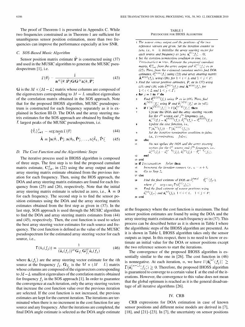
D. The Cost Function and the Algorithmic Steps

The iterative process used in IHOSS algorithm is composedof three steps. The first step is to find the proposed cumulantmatrix estimate, , in (22) using the array output and thearray steering matrix estimate obtained from the previous iter-ation for each frequency. Then, using the HOS approach, theDOA and array steering matrix estimates are found for each fre-quency from (25) and (26), respectively. Note that the initialarray steering matrix estimate is selected as zero, i.e.,for each frequency. The second step is to find the sensor po-sition estimates using the DOA and the array steering matrixestimates obtained from the first step as given in (37). In thelast step, SOS approach is used through the MUSIC algorithmto find the DOA and array steering matrix estimates from (44)and (45), respectively. Then, the cost function is used to selectthe best array steering vector estimates for each source and fre-quency. The cost function is defined as the value of the MUSICpseudospectrum for the estimated array steering vector for eachsource, i.e.,

(46)

where are the array steering vector estimate for the thsource at the frequency . is the matrixwhose columns are composed of the eigenvectors correspondingto smallest eigenvalues of the correlation matrix obtainedfor frequency in the SOS approach [1]. In order to guaranteethe convergence at each iteration, only the array steering vectorsthat increase the cost function value over the previous iterationare selected. If the cost function is not increased, the previousestimates are kept for the current iteration. The iterations are ter-minated when there is no increment in the cost function for anysource and any frequency. After the iterations are completed, thefinal DOA angle estimate is selected as the DOA angle estimate

TABLE IPSEUDOCODE FOR IHOSS ALGORITHM

at the frequency where the cost function is maximum. The finalsensor position estimates are found by using the DOA and thearray steering matrix estimates at each frequency as in (37). Thisprocess can be described better as it is shown in Table I wherethe algorithmic steps of the IHOSS algorithm are presented. Asit is shown in Table I, IHOSS algorithm takes only the sensoroutputs as input. In this respect, there is no need to know or es-timate an initial value for the DOA or sensor positions exceptthe two reference sensors to start the iterations.

The convergence of the proposed IHOSS algorithm is es-sentially similar to the one in [26]. The cost function in (46)is nonnegative. At each iteration, , we have

. Therefore, the proposed IHOSS algorithmis guaranteed to converge to a certain value at the end of the it-erations. However, the convergence to this value does not meanthat the global optimum is reached as it is the general disadvan-tage of all iterative algorithms [26].

IV. CRB

CRB expressions for DOA estimation in case of knownsensor positions and different noise models are derived in [7],[18], and [21]–[23]. In [7], the uncertainty on sensor positions


is considered and the CRB for sensor position estimation ispresented. It is assumed that the nominal sensor positions areknown and the small displacement from the nominal locationsis modeled as Gaussian. In this work, there is no a prioriinformation about the sensor positions except the two referencesensors. Therefore, none of the previous CRB expressions inliterature can be used for the DOA and sensor position estima-tions in this paper, and a new CRB expression is derived for theproblem setting in this paper.

The signal waveforms are considered to be deterministic un-known process and the noise is assumed to be temporally uncor-related complex Gaussian process. It is also assumed that noiseis uncorrelated for different frequencies. In this paper, CRBexpressions are derived by considering a noncircular complexGaussian distribution for the noise with unknown covariancematrix. The modification for circular case is also given. Noisemay be spatially correlated. Then, the CRB for DOA, ,and sensor position estimation are given by

(47)

(48)

where is the number of unknownsensor positions, and the matrices and are defined as

(49)

(50)

(51)

The matrix is defined as in (54). matrixis the real covariance matrix of the noise for time and

frequency defined as

(52)

The matrix is defined for real and complex source sig-nals as

(53)

The matrices and are defined in (55)and (56), respectively.

(54)

(55)

(56)

is the 2 2 identity matrix and is the vectorcomposed of all ones and

(57)

(58)

(59)

(60)

(61)

is the matrix whose columns contain onlyone nonzero element which is set to one. The location ofthe nonzero element at each column is determined by thesensor index with unknown positions. If it is assumed thatthe positions of the first two sensor are known and the othersensor positions are unknown, the matrix is composed of

. The subscripts are used to definethe dimensions of the zero matrix and identity matrix .

Note that the CRB expressions in (47) and (48) are given fornoncircular complex Gaussian noise case. When the noise is cir-cular, expressions given above are valid with the change in noisecovariance matrix in (52). Forcircular noisecase, the real covari-ance matrix to be used in CRB expressions is found as [17]

(62)

where matrix is defined as

(63)

V. PERFORMANCE RESULTS

The performance of the IHOSS algorithm is evaluated for dif-ferentcases forboth DOAandpositionestimation.VESPA[10] isconsidered only for DOA estimation comparison since it cannot


Fig. 1. SNR performance for (a) DOA and (b) position estimation.

estimate the sensor positions. The CRB expressions in (47) and(48) are used to show the effectiveness of the IHOSS algorithm.

It is assumed that there are two far-field sources and .The received wideband source signals are passed through threenarrowband bandpass filters with center frequencies which sat-isfy the conditions in Theorem-1, i.e., MHz,

MHz and MHz. Each sensor position except thetwo reference sensors is randomly selected from a uniform distri-bution in the deployment area of 50 50 meters. The referencesensors are placed at (0, 0) and (15, 0) in meters where the wave-length corresponding to the highest frequency is meters.For the parameter estimation, snapshots are collectedfor each frequency. The performance results are the average of100 trials. At each trial, source signals, noise, the sensor posi-tions except the reference sensors and the DOA angles of sourcesignals are changed randomly. The difference between the DOAangles of the source signals is set to 40 degrees. The source sig-nals have a uniform distribution and the noise is additive whiteGaussian and uncorrelated with the source signals.

For the simulation, a maximum number of iterations, ,is defined for the iterative approach. When a predefined max-imum number of iterations are reached, iterative approach isterminated even if the termination condition given in Table I isnot satisfied. The performance results of the IHOSS algorithmis illustrated for three different maximum number of iterations,

Fig. 2. (a) DOA and (b) position estimation for varying number of snapshotsat �� dB.

namely and in order to showthe convergence of the IHOSS algorithm.

The performance results for the DOA and sensor position es-timations at different SNR values and maximum number of iter-ations are illustrated in Fig. 1. In Fig. 1(a), it is seen that VESPAhas a flooring effect. This is due to the errors in the cumulant ma-trix for finite length data and multiple sources. IHOSS performswell and closely follows the CRB as the number of iterations isincreased. This is due to the fact that IHOSS converts the mul-tiple source problem into a single source case and effectivelyuses HOS and SOS techniques with a robust cumulant matrix(22). The position estimation accuracy in Fig. 1(b) is especiallygood at high SNR, where the position ambiguity is solved ac-curately. The performance degradation at low SNR is relatedwith the condition in Theorem-1. In this case, the errors in arraysteering matrix estimates are higher than the threshold given inTheorem-1. It is also seen that the required number of iterationsfor the best result in DOA and sensor position estimation is SNRdependent. As the SNR increases, IHOSS requires more itera-tion in order to follow the CRB closely. As it is seen in Fig. 1, theperformance results for and , are almostthe same. Therefore, a small number of iterations are sufficientto get a satisfactory performance.

In Fig. 2, the performance of the algorithm is shown when thenumber of snapshots is changed. SNR is set to 20 dB. Fig. 2(a)shows that the IHOSS algorithm performs significantly better


Fig. 3. (a) DOA and (b) position estimation performance for varying distancebetween source DOAs at �� dB.

than VESPA and approaches to the CRB even when is small.In Fig. 2(b), it is seen that IHOSS finds the sensor positions ef-fectively and closely follows the CRB after snapshots.When is small, the accuracy of the array steering matrix es-timation is not sufficient to satisfy the condition in Theorem-1and a significant performance degradation in sensor position es-timation is observed as illustrated in Fig. 2(b).

The effect of the difference between the DOA angles of thesources on the performance of DOA and sensor position esti-mations is illustrated in Fig. 3. In this example, two sourcesare located randomly in a 100 degrees sector between 40 and140 degrees. The difference between the DOA angles of the twosources is changed from 1 to 50 degrees. SNR is set to 20 dB. Asit is seen in Fig. 3(a), IHOSS follows the CRB after the DOAseparation of approximately 10 degrees and performs signifi-cantly better than VESPA whose performance is also reportedin [11]. The DOA RMSE of IHOSS increases as the source sep-aration is increased for four iterations (IHOSS, ).CRB also increases with the source separation even though theincrease is small. Note that this is due to the fact that the sourceDOA’s are close to the endfire of the baseline determined by thetwo reference sensors as the source separation increases. IHOSSmakes larger errors for small number of iterations. This problemis solved by increasing the maximum number of iterations. Asit is seen in Fig. 3(a), a few iterations are enough to obtain agood accuracy. The sensor position estimation performance is

Fig. 4. (a) DOA and (b) position estimation performance for varying sensordensity at �� dB.

illustrated in Fig. 3(b). It is seen that IHOSS solves the positionambiguity effectively when two sources are separated by morethan 18 degrees. For the closely spaced sources, the conditionon estimation errors in Theorem-1 is not satisfied and the ambi-guity problem is not solved accurately.

Fig. 4 shows the performance results of the DOA and sensorposition estimations when the sensor density is changed. Thesensor density is defined as , where is the area in squarewavelength, i.e., . andare the lengths of the sensor deployment area in the x and yaxis, respectively. The number of sensors is set as .Two reference sensors are located at (0,0) and (15,0) coordi-nates in meters and the remaining sensors are randomlydeployed. The positions of the randomly deployed sen-sors are scaled to change the sensor density without changingthe sensor geometry. Two far-field sources are located randomlyin the range of 40–140 degrees with a DOA separation of 40 de-grees. SNR is set to 20 dB. The sensor positions except the ref-erence sensors and source DOAs are changed at each trial. Asit is seen in Fig. 4(a), IHOSS closely follows the CRB for theDOA estimation. It is also seen that DOA RMSE increases by in-creasing the sensor density. In this case, sensors are close to eachother. When the sensors are very close to each other, a small per-turbation on sensor positions results large DOA deviations.


Fig. 5. (a) DOA and (b) position estimation performance for different fre-quency differences. �� dB.

The sensor position estimation performance is shown inFig. 4(b). Since sensor density is varied by changing the de-ployment area, the sensor position estimation error is shownby scaling with the size of the deployment area. It is seen thatIHOSS closely follows the CRB when the sensor density isgreater than 1. For small sensor densities, the position estima-tion performance is decreased due to the large errors in arraysteering matrix estimates as explained in Theorem-1.

Since IHOSS uses multiple frequencies to resolve the ambi-guity problem in sensor position estimation, the effect of thefrequency selection on DOA and sensor position estimations isalso investigated. For this example, it is assumed that there aretwo different frequencies that the array output is observed forthe same sources. SNR is set to 20 dB. The first frequency isfixed at 9.75 MHz and the second frequency is varied from 9.75MHz to 10 MHz, in such a way that the conditions in Theorem-1are satisfied. The performance results are shown in Fig. 5. As itis seen in Fig. 5(a), the frequency difference does not signifi-cantly effect the DOA estimation performance of the IHOSS.On the other hand, the sensor position performance is sensitiveto the difference between the frequencies as seen in Fig. 5(b).The ambiguity problem in position estimation is solved effec-tively when the frequency difference is greater than 100 kHz.Note that as mentioned in Section III.B, the required frequencydifference for the best position estimation performance can be

decreased by using more than two frequencies. When three fre-quencies are used, it is possible to decrease the overall frequencydifference to less than 50 kHz.

VI. CONCLUSION

In this paper, IHOSS algorithm is presented for the DOA andsensor position estimations in a joint manner. This algorithmfinds the DOA and sensor position estimation by using the HOSand SOS approaches in an iterative manner. The sensors are de-ployed to unknown random positions and the source signals areobserved at least in two different frequencies for the resolutionof sensor position ambiguity. The positions of the two referencesensors are assumed to be known and the distance between themis set to the half of the minimum wavelength of the incomingsignals. A new cumulant matrix estimate is proposed for the ef-fective implementation of the HOS technique when the sourcesignals are dependent. This cumulant matrix estimate can beseen as the generalization of the approaches known in the lit-erature. The sensor positions are estimated unambiguously byusing multiple frequencies. The constraints on the frequenciesand the steering matrix estimation errors are given. Proposediterative approach is guaranteed to converge since the cost func-tion is non-negative and improved at each iteration. Determin-istic CRB expressions for the DOA and sensor position estima-tion are derived. Several simulations are done and it is shownthat IHOSS performs well for multiple sources and closely fol-lows the CRB for both DOA and sensor position estimations.

APPENDIX APROOF OF LEMMA-1

By substituting (16) and (15) into (13), the desired cumulantmatrix is rewritten as

(64)

where is the th column of array steering matrix, and isthe th diagonal element of matrix in (16). When it is assumedthat only the th source is received, the cumulant matrix for thearray output is written as in the same form of (7), i.e.

(65)

where is the th sensor outputfor the th source. is the th row and th column of arraysteering matrix, . It is assumed that the noise is Gaussian andindependent with the source signals. Using this fact and the cu-mulant properties [CP1] and [CP4] in [10], the matrix elementsin (65) can be rewritten in a more compact form by substituting(5), (16), and (10) into (65) such as

(66)

Substituting (66) into (65) and summing up for all of the sourcesgives us the desired cumulant matrix in (64).


APPENDIX BDERIVATION OF (22)

The cumulants corresponding to the th source are found bysubstituting (20) into (65), i.e.

(67)

where and is the th row andth column of matrix in (20). From the cumulant properties

[CP1], [CP2], and [CP4] in [10], and in (67) can bewritten as

(68)

where is the complex conjugate of the th row of the matrixand is defined in (23). Substituting (68) into (65) and

summing up for all of the incoming sources results (22), whichis the estimate of desired cumulant matrix in (13).

APPENDIX CPROOF OF THEOREM-1

Let and be the correct ambiguity termsfor the unambiguous sensor positions and the estimated ambi-guity terms as in (36) for . To resolve the ambiguity insensor positions, the minimization problem in (36) should haveunique solution, which is .

The minimization in (36) is done over the summation of pos-itive terms. Therefore, the uniqueness of only one term of thesummation is sufficient for the overall uniqueness. This fact re-sults that (36) has a unique solution, if the following inequalityis satisfied for at least one of the frequencies,for

(69)

where corresponds to the minimum distance between pos-sible dot products of th sensor and th source for and ,i.e.

(70)

and is an integer, i.e.

(71)

Substituting (70) and (71) into (69) simplifies the inequalityand the required condition on the frequencies to satisfy (69) forall possible values of is found as

(72)

Note that for the error free case, the dot products for the twofrequencies are the same at the correct ambiguity terms

, i.e.

(73)

When there are errors in estimated parameters, , theequality in (73) is not satisfied and a nonzero value isobtained. Since the possible values of the dot product are sym-metric with the correct ambiguity term, it is found that the max-imum value of is bounded, i.e.

(74)

The inequality in (74) is valid, if the following conditions aresatisfied for all values of

(75)

Substituting (74) into (75) simplifies the inequalities, i.e.

(76)

Substituting (74) into (72) results

(77)

Note that the equality in (77) is due to the fact that the ambi-guity in sensor positions cannot be solved via frequency selec-tion when . There are two possible ambiguity

terms at which whatever the selected fre-quencies are as in

(78)

This problem can be solved by constraining . In this case,

there is no two ambiguity terms which return the same


terms. This constraint which guarantees the correct ambiguityresolution is given as

(79)

Since the value of is determined by the errors of the es-timated parameters in (36), to satisfy the condition in (79), theestimation errors should also be bounded. For this case, the termthat is tried to be minimized in (36) can be written for the cor-rect ambiguity term by substituting (42) into (36), i.e.

(80)

Using the relation in (73), (80) can be simplified as

(81)

For the unique solution of (36) to be the correct ambiguity term,i.e., should be equal to the solution

of the minimization problem in (36), i.e., .Using (79) and (81) in this relation simplifies the conditions onestimation errors for unambiguous sensor positions as in (40).

To complete the proof, we should specify the possible rangesof and , which depend on the search region for . Thelimiting value for the search region is found from (29) by con-sidering the position of the most distant sensor with respect tothe reference sensor defined as in Theorem-1, i.e.

(82)

where . Note that the inequalityin (29) is based on the fact that (29) is in the range of .The limits of satisfied for all values of is found by usingsimple trigonometric identities for , i.e.

(83)

Then, the possible ranges for can befound from (83) and (71) such as

(84)

Since conditions in (75) should be satisfied for all possible dotproduct values , in the deployment area, the maximumvalue of is found from (83) as

(85)

Substituting (85) into (76) gives the condition in (38).APPENDIX D

CRB

In this section, we derive the general deterministic CRB ex-pressions for the DOA and sensor position estimations. Sourcesignals are assumed to be deterministic unknown processes andnoise is temporally uncorrelated zero-mean Gaussian process.It is also assumed that the array output is available at multiplefrequencies for the same sources. Noise is uncorrelated for dif-ferent frequencies. There is no circularity and spatial correlationassumption about the complex Gaussian noise.

The complex valued array output given in (4) can be rewrittenin terms of real and imaginary parts for and

as

(86)

Then according to the given assumptions, the distribution

of can beexpressed as, . vector and

block diagonal matrix are defined asshown in (87)-(88) at the bottom of the page. is definedfor noncircular and circular noise cases in (52) and (62), re-spectively. is a real-valued parameter vector that completelyand uniquely specifies the distribution of and in our caseit is defined as

(89)

for, sensor indices with unknown positions, and .

is the th row and th column of the matrix .Using the definitions in (87) and (88), the Fisher information

matrix corresponding to the distribution of is written as in[18], i.e.

(90)

(87)

(88)


(99)

(100)

(101)

(102)

where denotes the th component of .Note that, since the vector is independent of the

elements of covariance matrix and is depends ononly its elements, the following relations are satisfied

(91)

When all the unknown parameters in (89) are considered withthe relations in (91), the Fisher Information matrix can be ex-pressed as

(92)

is the Fisher Information submatrix corresponding tothe DOA angles and obtained by substituting (91) into (90) for

, i.e.

(93)

where matrix is found as

(94)

Taking the derivative of with respect to forsimplifies the expression in (94) as in (55).

The Fisher Information submatrix corresponding to the DOAangles and unknown sensor positions, , is obtainedby substituting (91) into (90) for and

, i.e.

(95)

where is the number of sensors with unknown positions andmatrix is found as

(96)

Taking the derivative of with re-spect to the position of the th sensor for

sim-plifies the expression in (96) as in (56).

The Fisher Information submatrix corresponding to theDOA angles and source signals, , is obtainedby substituting (91) into (90) for and

and , i.e.

(97)

where matrix is found by taking thederivative of with respect to the real and imaginaryparts of the source signals at each frequency, i.e.

(98)

where is the zero matrix. Substituting (98) into (97)simplifies the relation as in (99), shown at the top of the page.In a similar way, the other Fisher Information submatrices areobtained as in (100), (101), and (102), also at the top of the page.

Applying the partitioned matrix inversion formula [19], wecan obtain the submatrices of inverse Fisher Information matrixcorresponding to the DOA and sensor position estimation, i.e.

(103)

(104)

where

(105)

(106)

(107)

Substituting (93), (95), (99), (100), (101), and (102) into (105),(106), and (107) results a more compact form of and

as in (49)–(51).

REFERENCES

[1] R. Schmidt, “Multiple emitter location and signal parameter esti-mation,” in Proc. RADC Spectrum Estimation Workshop, 1979, pp.243–258.

[2] R. Roy and T. Kailath, “ESPRIT—Estimation of signal parameters viarotational invariance techniques,” IEEE Trans. Acoust., Speech, SignalProcess., vol. 37, no. 7, pp. 984–995, Jul. 1989.


[3] M. Aktas and T. E. Tuncer, “Iterative HOS-SOS (IHOSS) based sensorlocalization and direction-of-arrival estimation,” in Proc. IEEE Int.Conf. Acoust., Speech, Signal Process. (ICASSP 2010), Mar. 2010.

[4] A. J. Weiss and B. Friedlander, “Array shape calibration usingsources in unknown locations—A maximum likelihood approach,”IEEE Trans. Acoust., Speech Signal Process., vol. 37, no. 12, pp.1958–1966, Dec. 1989.

[5] B. P. Flanagan and K. L. Bell, “Array self calibration with large sensorposition errors,” in Proc. 33rd IEEE Asilomar Conf. Signals, Syst.Comp., Oct. 1999, pp. 258–261.

[6] C. S. See and B. Poh, “Parametric sensor array calibration usingmeasured steering vectors of uncertain locations,” IEEE Trans. SignalProcess., vol. 47, no. 4, pp. 1133–1137, Apr. 1999.

[7] Y. Rockah and P. M. Schulthesis, “Array shape calibration usingsources in unknown locations—Part I: Far-field sources,” IEEE Trans.Acoust., Speech Signal Process., vol. ASSP-35, no. 3, pp. 286–299,Mar. 1987.

[8] H. S. Mir, J. D. Sahr, G. F. Hatke, and C. M. Keller, “Passive sourcelocalization using an airborne sensor array in the presence of mani-fold perturbations,” IEEE Trans. Signal Process., vol. 55, no. 6, pp.2486–2496, Jun. 2007.

[9] M. Lanne, A. Lundgren, and M. Viberg, “Optimized beamforming cal-ibration in the presence of array imperfections,” in IEEE Int. Conf.Acoust., Speech Signal Process. (ICASSP 2007), Apr. 2007, vol. 2, pp.973–976.

[10] M. C. Dogan and J. M. Mendel, “Applications of cumulants to arrayprocessing—Part I: Aperture extension and array calibration,” IEEETrans. Signal Process., vol. 43, no. 5, pp. 1200–1216, May 1995.

[11] N. Yuen and B. Friedlander, “Asymptotic performance analysis of ES-PRIT, higher order ESPRIT, and virtual ESPRIT algorithms,” IEEETrans. Signal Process., vol. 44, no. 10, pp. 2537–2550, Oct. 1996.

[12] E. Gönen, J. M. Mendel, and M. C. Dogan, “Applications of cumu-lants to array processing—Part IV: Direction finding in coherent sig-nals case,” IEEE Trans. Signal Process., vol. 45, no. 9, pp. 2265–2276,Sep. 1997.

[13] T. E. Tuncer and B. Friedlander, Classical and Modern Direction-of-Arrival Estimation. New York: Academic, 2009.

[14] T. E. Tuncer and M. T. Özgen, “No-search algorithm for direction ofarrival estimation,” Radio Sci., vol. 44, pp. 1–14, Sept. 30, 2009.

[15] M. G. Amin, “Sufficient conditions for alias-free direction of arrivalestimation in periodic spatial spectra,” IEEE Trans. Antennas Propag.,vol. 41, no. 4, pp. 508–511, Apr. 1993.

[16] P. Chevalier, L. Albera, A. Ferrol, and P. Comon, “On the virtualarray concept for higher order array processing,” IEEE Trans. SignalProcess., vol. 53, no. 4, pp. 1254–1271, Apr. 2005.

[17] B. Picinbono, “Second-order complex random vectors and normaldistributions,” IEEE Trans. Signal Process., vol. 44, no. 10, pp.2637–2640, Oct. 1996.

[18] J. Delmas and H. Abeida, “Stochastic Cramér-Rao bound for noncir-cular signals with application to DOA estimation,” IEEE Trans. SignalProcess., vol. 52, no. 11, pp. 3192–3199, Nov. 2004.

[19] S. M. Kay, Fundamentals of Statistical Signal Processing: EstimationTheory. Upper Saddle River, NJ: Prentice-Hall, 1993.

[20] C. W. Therrien, Discrete Random Signals and Statistical Signal Pro-cessing. Upper Saddle River, NJ: Prentice-Hall, 1992.

[21] M. Pesavento and A. B. Gershman, “Maximum-likelihood direc-tion-of-arrival estimation in the presence of unknown nonuniformnoise,” IEEE Trans. Signal Process., vol. 49, no. 7, pp. 1310–1324,Jul. 2001.

[22] P. Stoica and A. Nehorai, “Performance study of conditional andunconditional direction-of-arrival estimation,” IEEE Trans. SignalProcess., vol. 38, no. 10, pp. 1783–1795, Oct. 1990.

[23] A. J. Weiss and B. Friedlander, “On the Cramér-Rao Bound for Direc-tion Finding of Correlated Signals,” IEEE Trans. Signal Process., vol.41, no. 1, pp. 495–499, Jan. 1993.

[24] P. Stoica and R. Moses, Spectral Analysis of Signals. Upper SaddleRiver, NJ: Prentice-Hall, 2005.

[25] H. L. Van Trees, Optimum Array Processing. New York: Wiley-In-tersci., 2002.

[26] A. J. Weiss and B. Friedlander, “DOA and steering vector estimationusing a partially calibrated array,” IEEE Trans. Aerosp. Electron. Syst.,vol. 32, pp. 1047–1057, 1996.

Metin Aktas received the B.S. degree from DokuzEylul University, Izmir, Turkey, in 2002 (with highhonors) and the M.S. degree from Middle East Tech-nical University, Ankara, Turkey, in 2004, all in elec-trical engineering.

He is currently pursuing the Ph.D. degree in elec-trical engineering at Middle East Technical Univer-sity. His research interests are in the areas of statis-tical signal processing, array signal processing, wire-less sensor networks, and wireless communications.

T. Engin Tuncer received the B.S. and M.S. degreesin electrical and electronics engineering from theMiddle East Technical University (METU), Ankara,Turkey, in 1987 and 1989, respectively, and thePh.D. degree in electrical engineering from BostonUniversity, Boston, MA, in 1993.

From 1991 to 1993, he was an instructor andAdjunct Professor with Boston University. He joinedthe Electronics Engineering Department, AnkaraUniversity, in 1993. Since 1998, he has been with theElectrical and Electronics Engineering Department,

METU, as a Professor. His research interests include array signal processing,antenna and array design for direction finding and target localization, mul-tichannel systems and blind identification, statistical signal processing, andsignal processing for communications.

Iterative HOS-SOS (IHOSS) Algorithm for Direction-of-Arrival Estimation and Sensor Localization

Documents

Transcript of Iterative HOS-SOS (IHOSS) Algorithm for Direction-of-Arrival Estimation and Sensor Localization