Market efficiency and continuous information arrival: evidence from prediction markets

1

Market efficiency and continuous information arrival: evidence from

prediction markets

Paul Docherty and Steve Easton1

Newcastle Business School, University of Newcastle, NSW 2308, Australia

Abstract

Two regularities in financial economics are that prices underreact to news events and

that they display short-term momentum. This paper tests for the presence of these

regularities in prediction markets offered by the betting exchange Betfair on the 2008

Ryder Cup Golf Competition. Betfair offered in-play prediction markets on the

individual match-play pairings and on the Cup result, with trading being virtually

continuous in all markets.

Modelled probabilities of the Cup result were updated continuously using trades in the

individual match-play pairings. These probabilities were then compared with the

probabilities of the Cup result implied by odds in that market.

The odds in the market for the Cup result underreact to both good and bad news that

is provided by changes in the odds in the markets for the individual pairings. Further,

these modelled probabilities Granger cause changes in the probabilities of the Cup

result implied by odds in the market on that outcome. In addition, economically and

statistically significant evidence of momentum is found in the odds in the market on

the Cup result.

Corresponding Author: Steve Easton, Newcastle Business School, University of

Newcastle, NSW 2308, Australia

Email: [email protected]

1 We thank Betfair Ltd for making this study possible by providing us with the complete transaction file of all trading that occurred in the prediction markets for the 2008 Ryder Cup.

2

1 Introduction

Empirical research in financial economics has identified a number of regularities.

Two of these regularities are that prices underreact to news events and that they

display short-term momentum. Examples of the former regularity include analysts’

recommendations (Womack (1996) and Busse and Green (2002)), dividend initiations

and omissions (Michaely et al. (1995)), seasoned equity issues (Loughran and Ritter

(1995)), and earnings announcements (Bernard and Thomas (1989, 1990)). Examples

of studies reporting evidence of short-term momentum include Lo and MacKinlay

(1988), Lehmann (1990) and Conrad et al. (1991).2

The cause of these regularities is disputed. Fama (1998) argues that they are not

regularities but chance deviations that are to be expected under market efficiency.

However, Barberis et al. (1998) and Hong and Stein (1999), amongst others, argue

that their strength and pervasiveness rules out the possibility of their being chance

deviations. Further, they provide theoretical foundations by developing models of

investor sentiment that seek to explain these regularities. While the models vary in

levels of sophistication, a central component is the psychological phenomenon of

conservatism, defined by Edwards (1968) as the slow updating of expectations in the

face of new information. While they differ, both underreaction and momentum are

consistent with conservatism. Slow updating of expectations is consistent with

underreaction; that is, with prices increasing (decreasing) following good (bad) news

events. It is also consistent with momentum whereby past returns are positively

correlated with future returns.

2 Over very short horizons, negative autocorrelation is found (see Jegadeesh (1990) and Lehmann (1990). This finding is attributed to bid-ask spreads and other measurement problems (see, for example, Kaul and Nimalendran (1990)). While our paper examines a very short horizon the results are robust to these measurement problems.

3

These models also rely on there being limits to arbitrage, limits that prevent rational

investors from undertaking trades that remove biases caused by psychological

phenomenon. As detailed by De Long et al. (1990) and Shleifer and Vishny, (1997),

limits to arbitrage occur due to, inter alia, implementation costs.

This paper tests for the presence or absence of these regularities in a unique laboratory

setting where trading is virtually continuous, as is the arrival of information. The

market is characterised by limits to arbitrage and the results are robust to market

microstructure issues such as bid-ask spreads and other measurement problems.

The laboratory in question is the prediction markets offered by the betting exchange

Betfair (www.betfair.com) for the final day’s play in the 2008 Ryder Cup Golf

Competition between the United States and Europe. On that day (21 September 2008)

Betfair provided prediction markets on each of the twelve single match-play pairings

and on the overall Cup result.

With the twelve markets on each pairing each having three possible outcomes

(namely a win to the United States player, a win to the European player, or a tie), the

probabilities of the three Cup outcomes (namely a win to the United States team, a

win to the European team, or a tie) may be determined by the mathematically simple

but computationally complex 312 or 531 441 possible outcomes from the twelve

pairings. A comparison of these modelled probabilities with the probabilities of each

outcome implied by the odds offered on the Cup result provide an examination of

whether the market reacts efficiently to the arrival of continuous information.

4

This paper examines whether the information provided by trades in the twelve

markets on the individual pairings was incorporated instantaneously and without bias

into the prices in the overall Cup market or whether the regularities observed in

security markets were also present in this market.

The paper is structured as follows. Section II presents the methodology and describes

the data. Hypotheses are presented in Section III and the effectiveness of the model is

analysed in Section IV. Results are reported in Sections V and VI respectively and a

summary is presented in Section VI1.

II Methodology and Data

The Ryder Cup is a match play golf competition played biennially between teams

from the United States and Europe. There are twenty eight matches in the competition

with the winner of each match scoring a point for the team. A half a point is awarded

for a tied match. The final day’s play comprises twelve matches.

The 2008 Ryder Cup was held from 19 to 21 September in Louisville, Kentucky. The

matches played on 19 and 20 September resulted in a score of 9 points to the United

States to 7 points to Europe. Therefore on the final day the United States needed to

score 5 points from the twelve matches to tie the competition and 5.5 or more points

to win the competition.

Using its Internet platform, the betting exchange Betfair offered simultaneous world-

wide markets in each of the twelve player pairings, with in each case possible

outcomes being a win to the United States player, a win to the European player, or a

5

tied match. Simultaneously a market was offered on the Cup outcome, again with

outcomes being a win to the United States team, a win to the European team, or a tied

competition.

Betfair operates as a clearing house and does not take positions itself. It provides

markets whereby traders seeking to back outcomes are matched with traders seeking

to lay or bet against outcomes. For example, Betfair may match a trader who agrees to

pay $1.60 if the United States wins the Cup with another trader who agrees to pay $1

if the United States does not win. Betfair charges a maximum commission of 5 per

cent of net profit. The data used in this study was obtained from Betfair, and consists

of every trade that occurred on its Internet platform on the final day of the 2008 Ryder

Cup in the twelve markets on the individual pairings and the market on the winner of

the competition.

The analysis is divided into two periods. The out-of-play period is defined as the

period from 4:00 am to 12:03 pm (the tee-off time for the first pairing). The in-play

period is defined as the period from 12:03 pm to 5:17 pm.3 The competition was

assumed to have ended at 5:17 pm when the modelled probability of the United States

winning the Cup exceeded 99 per cent for the first time and trading became thin.

Analysis of both out-of-play and in-play periods provides an examination of this

market during periods when information arrival would have been in the first period

virtually non-existent and in the second period virtually continuous.

3 The time 4:00 am in Kentucky corresponds to 8:00 am London time. The robustness of the results was examined by defining the start of the in-play period as 1:09 pm (the tee-off time of the seventh pairing) and 2:04 pm (the tee-off time of the final pairing). The results were substantively unchanged.

6

Descriptive statistics for each of the thirteen betting markets (for the twelve individual

pairings plus the Cup result) are reported in Table 1. Trading during the in-play period

was virtually continuous in the markets for the twelve individual pairings and in the

market for the Cup result. A trade in the market for the Cup result occurred on

average every 1.84 seconds, while a trade in one of the markets for the individual

pairings occurred on average every 1.31 seconds. The maximum period between a

trade in one of the markets for the individual pairings was 15 seconds. The liquidity in

these markets is also evident in the number and volume of trades. After tee-off time

on the final day, there were over 54 000 trades in the market for the Cup result and

over 41 000 trades in the markets for the individual pairings. The total dollar volume

of trade in the market for the Cup result exceeded $US 34 million, while in the

markets for the individual pairings the volume of trade exceeded $US 7 million.

[TABLE 1 ABOUT HERE]

For each of the thirteen markets, using standard methodology from the prediction

markets literature, the probability of each outcome is found by dividing the reciprocal

of the odds by the sum of the reciprocal of the odds in that markets.4 Using trinomial

distributions, the probabilities of the outcomes from each of the twelve pairings are

4 For example, the implied probability of the United States winning the overall Cup may be calculated

as: where PROBUS is the probability of the United States winning the overall Cup, ODDSUS is the overall Cup market odds for a win to the United States, ODDSEUR is the overall Cup market odds for a win to Europe and ODDSTIE is the overall Cup market odds for a tied outcome. Dividing by the sum of the reciprocal of the odds ensures that the implied probabilities of the three outcomes (United States win, European win and tie) sum to unity. For a detailed discussion of this approach see, for example, Wolfers and Zitzewitz (2006).

7

then used to provide the probabilities of the 312 or 531 441 possible permutations from

these pairings, and in turn to derive the modelled probability of each of the three Cup

outcomes.

The only assumption employed in using the trinomial distribution is that the outcomes

from the individual pairings are independent, an assumption that is intuitively

appealing, especially given that due to the staggered tee-off times each pairing plays

on a different hole at a different point in time. Empirical support for this assumption is

provided by an examination of the correlation coefficients between changes in the

implied probabilities provided by the odds for each of the individual pairings. The

average correlation coefficient was 0.008, with a minimum of -0.147 and a maximum

of +0.148. None of the 66 coefficients were significantly different from zero at the

0.05 level. The analysis in this paper would therefore appear to suffer less from the

joint test problem than the vast majority of studies that examine market efficiency.

Each time there was a trade in one of the markets for the individual pairings (on

average every 1.31 seconds) the updated odds were used to compute updated

probabilities of the outcomes of the individual pairings. These updated probabilities

were in turn used to compute updated modelled probabilities of the Cup result. While

trading is virtually continuous, to ensure the results are robust to market

microstructure issues such as bid-ask spreads and other measurement problems, the

analysis is restricted to a minute-by-minute examination of the relationships between

changes in modelled probabilities and changes in the probabilities of each outcome

implied by the odds offered on the Cup result.

8

As noted above, the market is characterised by clear limits to arbitrage. One such limit

is that while the odds in the markets for the individual pairings may be used to

provide modelled probabilities of the Cup result, if these probabilities differ from the

implied probabilities provided by the odds offered on that outcome, arbitrage is not

possible.

In order to profit from any mispricing in either market, an arbitrager would need to

trade in the market for the overall Cup result and simultaneously in real time establish

offsetting positions in each of the three possible outcomes in each of the twelve

markets for the individual pairings. Therefore in total 36 offsetting positions would

need to be undertaken. Further, the amount of money placed in each of these positions

would not be equal but would need to be weighted based on the probabilities of the

312 or 531 441 possible outcomes from those individual pairings. Such arbitrage is not

possible in an environment of continuous information arrival in all of these markets.

III Hypotheses

Two hypotheses are examined. Firstly, to examine whether the market on the Cup

result is efficient or whether psychological biases and limits to arbitrage result in

underreaction to information arrival, the following hypothesis is tested:

Hypothesis 1:

Implied probabilities in the Cup result market change in an unbiased manner with

respect to changes in the modelled probabilities provided by the odds from the

markets for the individual pairings.

9

Second, to examine whether psychological biases and limits to arbitrage result in

momentum in prices, the following hypothesis is tested:

Hypothesis 2:

Implied probabilities in the Cup result market are not autocorrelated.

IV Descriptive Comparison of Modelled and Implied Probabilities

Panel A of Figure 1 provides the minute-by-minute modelled probabilities of a United

States win, together with the probability of a United States win implied by the odds

offered in the market on the Cup result. Panels B and C provide these probabilities for

a European win and a tied competition respectively. While formal tests are conducted

below, the results presented in Figure 1 suggest that during the out-of-play period

when information arrival would have been minimal, there was a strong relationship

between the modelled and implied probabilities for each of the three possible

outcomes. However, this relationship was less apparent for the in-play period, with

the results suggestive that the odds in the market on the Cup result and therefore the

implied probabilities provided by these odds underreacted to the information provided

by the changes in probabilities provided by the individual pairings.

[FIGURE 1 ABOUT HERE]

V Tests for Unbiased Reaction

Decile analysis

The first hypothesis was tested using the following procedure. First, modelled

probabilities of the Cup result provided by the odds in the markets for the individual

pairings were obtained. While these modelled probabilities were updated each time

10

there was a trade in one of the markets for the individual pairings (on average every

1.31 seconds), as noted above to ensure that the result are robust to market

microstructure only those probabilities pertaining at the beginning of each minute

were used. Minute-by-minute changes in modelled probabilities were then obtained

and those observations sorted into deciles. These minute-by-minute changes in

modelled probabilities were then compared with minute-by-minute changes in

implied probabilities provided by the odds in the market for the Cup result. The

results are reported in Table 2.5


For the three deciles with the greatest positive changes in modelled probabilities of

the United States winning the competition, the average change in implied probabilities

were statistically significantly less positive at the 0.01 level, with the difference in

changes in probabilities decreasing from 3.474 per cent for the first decile to 0.786 per

cent for the third decile. These results suggest that the odds in the market for the Cup

result underreact to the good news provided by changes in the odds in the markets for

the individual pairings. Further, for the three deciles with the greatest negative

changes in modelled probabilities of the United States winning the Cup, the average

change in implied probabilities provided by the odds observed in the market for the

Cup result were statistically significantly less negative at the 0.01 level, in this case

with the difference in changes in probabilities increasing from -0.886 per cent for the

eighth decile to -3.312 per cent for the tenth decile. These results suggest in turn that

5 These tests and all subsequent tests reported in the paper were also undertaken for the probabilities of Europe winning the competition and for the probabilities of a tie. These results are substantively the same as those for the United States and for the sake of brevity are not reported.

11

the odds in the market for the Cup result underreact to the bad news that is provided

by changes in the odds in the markets for the individual pairings.

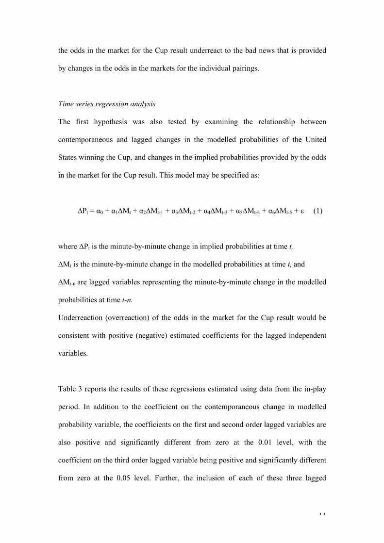
Time series regression analysis

The first hypothesis was also tested by examining the relationship between

contemporaneous and lagged changes in the modelled probabilities of the United

States winning the Cup, and changes in the implied probabilities provided by the odds

in the market for the Cup result. This model may be specified as:

∆Pt = α0 + α1∆Mt + α2∆Mt-1 + α3∆Mt-2 + α4∆Mt-3 + α5∆Mt-4 + α6∆Mt-5 + ε (1)

where ∆Pt is the minute-by-minute change in implied probabilities at time t,

∆Mt is the minute-by-minute change in the modelled probabilities at time t, and

∆Mt-n are lagged variables representing the minute-by-minute change in the modelled

probabilities at time t-n.

Underreaction (overreaction) of the odds in the market for the Cup result would be

consistent with positive (negative) estimated coefficients for the lagged independent

variables.

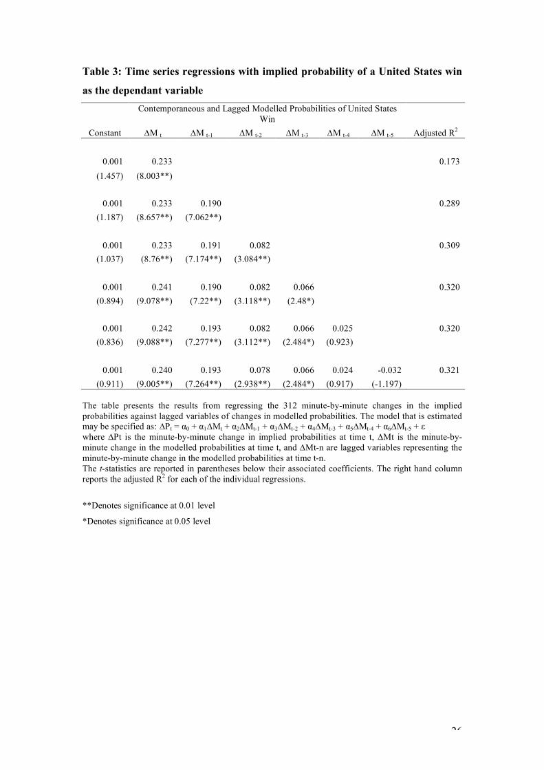
Table 3 reports the results of these regressions estimated using data from the in-play

period. In addition to the coefficient on the contemporaneous change in modelled

probability variable, the coefficients on the first and second order lagged variables are

also positive and significantly different from zero at the 0.01 level, with the

coefficient on the third order lagged variable being positive and significantly different

from zero at the 0.05 level. Further, the inclusion of each of these three lagged

12

variables increases the adjusted R2 of the regression. The statistically significant

positive coefficients for these lagged variables suggests that the first hypothesis may

be rejected and that the odds in the market for the Cup result take up to three minutes

to react to the news that is provided by changes in the odds in the markets for the

individual pairings.


To examine the causality of the relationship between changes in modelled

probabilities and changes in implied probabilities provided by the odds in the market

for the Cup result, time-series regressions were also performed with changes in

modelled probabilities as the dependant variable and both contemporaneous and

lagged values of changes in the implied probabilities as independent variables.

This regression model may be specified as:

∆Mt = α0 + α1∆Pt + α2∆Pt-1 + α3∆Pt-2 + α4∆Pt-3 + α5∆Pt-4 + α6∆Pt-5 (2)

where, in addition to those variables defined above, ∆Pt-n are lagged variables

representing the minute-by-minute change in the implied probabilities at time t-n.

If the results from Equation 1 are due to changes in modelled probabilities causing

changes in implied probabilities and not reverse causality, then we would expect the

13

estimated coefficients for the lagged independent variables to not be significantly

different from zero.

Table 4 reports the results of these regressions estimated using data from the in-play

period. During the period of continuous information arrival, only the

contemporaneous change in implied probabilities of a United States win provided by

the odds observed in the market for the Cup result is significant in explaining changes

in modelled probabilities. When the model is augmented with lagged variables of

implied probabilities none of the coefficients are significantly different to zero at the

0.05 level and the adjusted R2 doesn’t increase.


Granger causality

To more formally examine causality between contemporaneous and lagged changes in

modelled and implied probabilities of a United States win, Granger causality tests

were also performed. A time series (x) is said to Granger cause another time series (y)

if y can be better forecast using past values of both x and y as opposed to using

historical values of y alone. Therefore, a necessary condition for a time series x to be

a leading indicator of a time series y is:

σ2(y│y',x') < σ2(y│y')

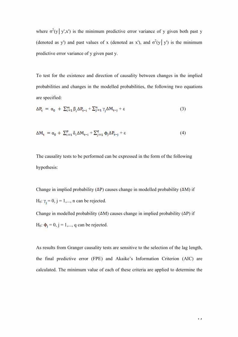
14

where σ2(y│y',x') is the minimum predictive error variance of y given both past y

(denoted as y') and past values of x (denoted as x'), and σ2(y│y') is the minimum

predictive error variance of y given past y.

To test for the existence and direction of causality between changes in the implied

probabilities and changes in the modelled probabilities, the following two equations

are specified:

+ + ε (3)

+ + ε (4)

The causality tests to be performed can be expressed in the form of the following

hypothesis:

Change in implied probability ( P) causes change in modelled probability ( M) if

H0: = 0, j = 1,..., n can be rejected.

Change in modelled probability ( M) causes change in implied probability ( P) if

H0: = 0, j = 1,..., q can be rejected.

As results from Granger causality tests are sensitive to the selection of the lag length,

the final predictive error (FPE) and Akaike’s Information Criterion (AIC) are

calculated. The minimum value of each of these criteria are applied to determine the

15

optimal lag length to apply to the variables in the equation6. The results of the FPE

and AIC calculations are reported in Table 5 and indicate that the optimal lag-length

is 3.

F-statistics are calculated to test the null hypotheses that the variables are not causally

related. The F-statistic corresponding to Equation 3 that has degrees of freedom equal

to n and T – (m + n+ 1) may be specified as:

where SSRr is the sum of squared errors associated with the restricted form of

Equation 3 and SSRu is the sum of squared errors associated with the unrestricted

form of Equation 3.

The results of the Granger causality tests for the in-play period are reported in Table

5. For all lag-lengths examined, the null hypothesis that changes in the modelled

probabilities of a United States win do not Granger cause changes in the implied

probabilities of a United States win may be rejected at the 0.01 level. In contrast, the

null hypothesis that changes in the implied probabilities do not Granger cause changes

in the modelled probabilities is not rejected for any of the lag-lengths specified.

The results provided in Tables 2 to 5 are consistent in suggesting that the null

hypothesis that implied probabilities in the Cup result market change in an unbiased

6 For more information regarding FPE and AIC, see Hsaio (1981) and Akaike (1974) respectively. The formulae used to determined the optimal lag length according to each search criteria may be specified as follows: FPE = [(T+n+1) / (T-n-1)] x SSR(n) / T AIC = ln [ SSR(n) / T] + 2n / T where T is the sample size, n is the lag-length being tested and SSR is the sum of squared residuals.

16

manner with respect to changes in the modelled probabilities may be rejected. All

results are consistent with underreaction in the Cup result market to news provided by

changes in modelled probabilities.


V Tests for Momentum

Autocorrelation

To test the second hypothesis, time-series regressions were performed to test for

autocorrelation. Changes in the probability of the United States winning as implied by

the odds in the market for the Cup result were regressed against lagged values of this

time series. The equation may be specified as:

∆Pt = α0 + α1∆Pt-1 + α2∆Pt-2 + α3∆Pt-3+ ε (5)

where ∆Pt is the minute-by-minute change in the implied probabilities at time t, and

∆Pt-n are lagged variables representing the minute-by-minute change in the implied


Regressions are also estimated to test for the presence of autocorrelation in changes in

the modelled probabilities. This equation may be specified as:

∆Mt = α0 + α1∆Mt-1 + α2∆Mt-2 + α3∆Mt-3 + ε (6)

where ∆Mt is the minute-by-minute change in the modelled probabilities at time t, and

17

∆Mt-n are lagged variables representing the minute-by-minute change in the modelled


The results of the regressions used to estimate Equation 5 are reported in Panel A of

Table 6. In all three equations the coefficient on the variable representing a one-

minute lag in implied probabilities is significantly different to zero at the 0.01. None

of the other coefficients are significant. There is therefore evidence of momentum in

implied probabilities but that momentum is limited to a minute.7

Panel B of Table 6 reports the results of the regressions used to estimate Equation 6.

None of the coefficients on the independent variables are significantly different from

zero for any of the regressions. Therefore, while there is evidence of momentum in

the implied probabilities, there is no evidence of momentum in modelled

probabilities.

Trading strategy

To examine whether the statistical evidence of momentum in implied probabilities

was also economically significant, a trading strategy was adopted. This strategy was

constructed as follows. First, implied probabilities of the United States winning the

Cup were obtained at the beginning of each minute. Minute-by-minute changes in

those probabilities were then obtained and those observations sorted into quintiles.

Second, for those changes in the top quintile, the United Sates was then backed to win

at the traded odds that existed at the beginning of the subsequent minute. Therefore a

bet was placed on the United States winning where its implied probabilities of doing

7 As noted at footnote 2 above, this result is not attributable to bid-ask spreads or other measurement problems – problems that result in negative autocorrelation.

18

so had increased by the most in the previous minute. Further, for those changes in the

bottom quintile, a bet was placed against the United States winning at the traded odds

that existed at the beginning of the subsequent minute. Therefore a bet was placed

against the United States winning where its implied probabilities of doing so had

decreased by the most in the previous minute. Third, those positions backing the

United States were reversed out one minute later by betting against the United States

and conversely those positions betting against the United States were reversed out one

minute later by backing the United States. This third step was required to ensure that

net positions did not accumulate. Again it should be noted that trades in this market

occurred on average every 1.84 seconds and traded prices were used. Therefore the

returns from this trading strategy do not require adjustment for any bid-ask spread and

are earned virtually instantaneously. To remove any possible transaction costs, all

returns were also multiplied by 0.95 to allow for the maximum commission of 5 per

cent charged by Betfair.

This momentum-based trading strategy was replicated using the probabilities of a

European win and of a tied Cup result. The results are reported in Table 7.

The average return from the 62 bets placed on a United States win, with those bets

reversed out one minute later by betting against a United States win, was 0.513 per

cent. Further the average return from the 62 bets placed against a United States win,

again with those bets reversed out one minute later by in this case backing a United

States win, was 0.257 per cent. The average return from all 124 bets was 0.380

percent. The average return for all 124 bets placed using the same strategy but based

on probabilities of a European win was 0.171 per cent and the strategy based on

19

probabilities of a tied Cup provided an average return of 0.209 per cent. For the

strategies based on the probabilities of the United States win and on a tied result the

average returns from the 124 bets placed were both significantly different from zero at

the 0.01 level.


VI Summary

There is evidence from securities markets that prices underreact to news events and

that they display short-term momentum. This paper tests for the presence of these

regularities in a unique prediction-markets setting where trading is virtually

continuous, as is the arrival of information. Underreaction to both good and bad news

is observed in this market. Further, economically and statistically significant evidence

of momentum is found.

20

References

Akaike, H. (1974), A new look at the statistical model identification, IEEE

Transactions on Automatic Control, 19, 716–723

Barberis, N., Shleifer, A. and Vishny, R. (1998), A model of investor sentiment,

Journal of Financial Economics, 49, 307-343.

Bernard, V. and Thomas, J. (1989), Post-earnings-announcement drift: delayed

response or risk premium?, Journal of Accounting Research, 27, 1-48.

Bernard, V. and Thomas, J. (1990), Evidence that stock prices do not fully reflect the

implications of current earnings for future earnings, Journal of Accounting and

Economics, 13, 305-340.

Busse, J.A. and Green, T.C. (2002), Market efficiency in real time, Journal of

Financial Economics, 65, 415-437.

Cain, M., and Peel, D. (2004), The utility of gambling and the favourite-longshot bias,

European Journal of Finance, 10, 379-390.

Conrad, J., Kaul, G., and Nimalendran, M. (1991), Components of short-horizon

individual security returns, Journal of Financial Economics 29, 365-384.

De Long, J.B., Shleifer, A., Summers, L., and Waldmann, R. (1990), Noise trader risk

in financial markets, Journal of Political Economy, 98, 703-738.

Edwards, W. (1968), Conservatism in Human Information Processing, in Kleinmutz,

B. (ed), Formal Representation of Human Judgment, John Wiley and Sons, New

York, pp. 17-52.

Fama, E. (1998), Market efficiency, long-term returns and behavioral finance, Journal

of Financial Economics, 49, 283-306.

21

Gandar, J., Zuber, R., Johnson, R. and Dare, W. (2002), Re-examining the betting

market on major league baseball games: is there a reverse favourite-longshot bias?,

Applied Economics, 34, 1309-1317.

Hsaio, C. (1981), Autoregressive modelling and money-income causality detection,

Journal of Monetary Economics, 7, 85-106.

Hong, H. and Stein, J. (1999), A unified theory of underreaction, momentum trading,

and overreaction in asset markets, Journal of Finance, 54, 2143-2184.

Jegadeesh, N. (1990), Evidence of predictable behavior of security returns, Journal of

Finance, 49, 881-898.

Kaul, G. and Nimalendran, M. (1990), Price reversals: bid-ask errors or market

overreaction?, Journal of Financial Economics, 28, 67-93.

Lehmann, B. (1990), Fads, martingales, and market efficiency, Quarterly Journal of

Economics, 105, 1-28.

Lo, A., and MacKinlay, C. (1988), Stock market prices do not follow random walks:

evidence from a simple specification test’, Review of Financial Studies 1, 41-66.

Michaely, R., Thaler, R., and Womack, K. (1995), Price reactions to dividend

initiations and omissions: overreaction or drift?’, Journal of Finance, 50, 573-608.

Loughran, T. and Ritter, J. (1995), The new issues puzzle, Journal of Finance, 50, 23-

52.

Snowberg, E. and Wolfers, J. (forthcoming), Explaining the favorite-longshot bias: is

it risk-love or misperceptions, Journal of Political Economy.

Shleifer, A. and Vishny, R. (1997), The limits of arbitrage, Journal of Finance, 52,

35-55.

Wolfers, J. and Zitzewitz, E. (2006), Interpreting prediction market prices as

probabilities, Working Paper Series 2006-11, Federal Reserve Bank of San Francisco.

22

Womack, K., (1996), Do brokerage analysts’ recommendations have investment

value?’, Journal of Finance, 51, 137-168.

Woodland, L. and Woodland, B. (1994), Market efficiency and the favourite-longshot

bias: the baseball betting market’, Journal of Finance, 49, 269-379.

Woodland, L. and Woodland, B. (1999), Expected utility, skewness and the baseball

betting market’, Applied Economics, 31, 337-345.

23

Table 1: Descriptive statistics

Market Final Day Tee-Off Time Number of Trades

Average Time Between Trades After Tee-Off (seconds)

Total Volume Traded ($US)

Overall Competition 12:03 PM 54 037 1.84 34 709 399 Pairing 1 12:03 PM 6200 2.76 1 399 295 Pairing 2 12:14 PM 5386 3.94 957 306 Pairing 3 12:25 PM 2732 11.09 482 585 Pairing 4 12:36 PM 3776 7.31 522 293 Pairing 5 12:47 PM 2905 8.27 441 975 Pairing 6 12:58 PM 2854 11.51 452 075 Pairing 7 1:09 PM 2881 9.56 481 495 Pairing 8 1:20 PM 2759 10.68 629 249 Pairing 9 1:31 PM 2597 14.03 392 111 Pairing 10 1:42 PM 2784 18.43 675 456 Pairing 11 1:53 PM 2854 10.62 615 374 Pairing 12 2:04 PM 3579 6.51 666 488 All Pairings 41 307 1.31 7 715 701

The table provides descriptive statistics for trades that took place during the in-play period in the individual pairings and the overall market. The tee-off times reported are in Kentucky time (Eastern Time Zone). The cumulative data across all pairings is reported in the final row.

24

Figure 1 - Panel A: Implied and modelled probabilities of United States win

Panel B: Implied and modelled probabilities of European win

Panel C: Implied and modelled probabilities of a tie

25

Table 2: Test for unbiased reaction to changes in modelled probabilities

The table reports the results from forming deciles based on changes in modelled probabilities. The average changes in the modelled and implied probabilities are reported in columns 2 and 3 respectively. The final column reports for each decile the t-statistic for the test of whether the differences between the modelled and implied probabilities are different from zero.

**Denotes significance at 0.01 level

*Denotes significance at 0.05 level

Deciles

Average Change In Modelled Probability (%)

Average Change In Implied Probability (%)

Average Difference Between Change In Modelled and Implied Probability (%)

t-statistic of difference

1 4.630 1.156 3.474 7.081**

2 2.189 0.493 1.696 7.214**

3 1.204 0.418 0.786 4.532**

4 0.607 0.152 0.455 2.827*

5 0.174 0.311 -0.137 -0.844

6 -0.261 0.242 -0.503 -2.925*

7 -0.514 -0.372 -0.142 -0.836

8 -1.183 -0.297 -0.886 -4.163**

9 -1.866 -0.212 -1.654 -7.651**

10 -3.940 -0.628 -3.312 -7.684**

26

Table 3: Time series regressions with implied probability of a United States win

as the dependant variable

Contemporaneous and Lagged Modelled Probabilities of United States

Win Constant ∆M t ∆M t-1 ∆M t-2 ∆M t-3 ∆M t-4 ∆M t-5 Adjusted R2

0.001 0.233 0.173 (1.457) (8.003**)

0.001 0.233 0.190 0.289

(1.187) (8.657**) (7.062**)

0.001 0.233 0.191 0.082 0.309 (1.037) (8.76**) (7.174**) (3.084**)

0.001 0.241 0.190 0.082 0.066 0.320

(0.894) (9.078**) (7.22**) (3.118**) (2.48*)

0.001 0.242 0.193 0.082 0.066 0.025 0.320 (0.836) (9.088**) (7.277**) (3.112**) (2.484*) (0.923)

0.001 0.240 0.193 0.078 0.066 0.024 -0.032 0.321

(0.911) (9.005**) (7.264**) (2.938**) (2.484*) (0.917) (-1.197) The table presents the results from regressing the 312 minute-by-minute changes in the implied probabilities against lagged variables of changes in modelled probabilities. The model that is estimated may be specified as: ∆Pt = α0 + α1∆Mt + α2∆Mt-1 + α3∆Mt-2 + α4∆Mt-3 + α5∆Mt-4 + α6∆Mt-5 + ε where ∆Pt is the minute-by-minute change in implied probabilities at time t, ∆Mt is the minute-by-minute change in the modelled probabilities at time t, and ∆Mt-n are lagged variables representing the minute-by-minute change in the modelled probabilities at time t-n. The t-statistics are reported in parentheses below their associated coefficients. The right hand column reports the adjusted R2 for each of the individual regressions.



27

Table 4: Time series regressions with modelled probability of a United States win

as the dependant variable

Contemporaneous and Lagged Implied Probabilities of United States Win Constant ∆P t ∆P t-1 ∆P t-2 ∆P t-3 ∆P t-4 ∆P t-5 Adjusted R2

0.000 0.756 0.173 (0.238) (8.003**)

0.000 0.766 -0.051 0.171

(0.280) (7.945**) (-0.527)

0.000 0.772 -0.040 -0.061 0.169 (0.326) (7.96**) (-0.411) (-0.626)

0.001 0.774 -0.025 -0.033 -0.160 0.174

(0.444) (8.01**) (-0.253) (-0.341) (-1.655)

0.001 0.775 -0.025 -0.035 -0.162 0.016 0.172 (0.430) (7.989**) (-0.257) (-0.355) (-1.656) (0.164)

0.001 0.763 -0.027 -0.032 -0.156 0.026 -0.062 0.170

(0.484) (7.709**) (-0.278) (-0.325) (-1.575) (0.262) (-0.625) The table presents the results from regressing the 312 minute-by-minute changes in the modelled probabilities against lagged variables of changes in the implied probabilities. This model may be specified as: ∆Mt = α0 + α1∆Pt + α2∆Pt-1 + α3∆Pt-2 + α4∆Pt-3 + α5∆Pt-4 + α6∆Pt-5 where ∆Mt is the minute-by-minute change in the modelled probabilities at time t, ∆Pt is the minute-by-minute change in implied probabilities at time t, and ∆Mt-n are lagged variables representing the minute-by-minute change in the modelled probabilities at time t-n. The t-statistics are reported in parentheses below their associated coefficients. The right hand column reports the adjusted R2 for each of the individual regressions. **Denotes significance at 0.01 level


28

Table 5: Granger causality tests

Lag

F-Statistic Modelled probability does not

Granger cause implied probability

F-Statistic Implied probability does not

Granger cause modelled probability

Final Prediction Error

Akaike Information

Criterion

0 15.812** 0.506 2.88e-07 -9.385 1 27.112** 0.960 2.54e-07 -9.512 2 15.812** 0.506 2.50e-07 -9.525 3 11.112** 1.097 2.44e-07^ -9.548^ 4 8.032** 1.078 2.49e-07 -9.529 5 6.613** 1.844 2.45e-07 -9.548 6 6.149** 1.839 2.47e-07 -9.537 7 5.251** 1.395 2.51e-07 -9.524 8 4.655** 1.235 2.56e-07 -9.502

The table reports the results from Granger causality tests. The null hypotheses tested are: H0: Changes in modelled probabilities do not Granger cause changes in the implied probabilities; and H0: Changes in implied probabilities do not Granger cause changes in the modelled probabilities For completeness, the Granger causality tests are reported for 0-8 lags. The second and third columns report the F-statistics used to calculate whether we can reject to two null hypotheses outlined above. Columns 4 and 5 report the final prediction error and Akaike Information Criterion for each lag-length.



^ Denotes the minimum value for the FPE and AIC values

29

Table 6: Time series tests for autocorrelation Panel A

Lagged Variables Constant ∆P t-1 ∆P t-2 ∆P t-3 Adjusted R2

0.001 0.193 0.034 (1.323) (3.404**)

0.001 0.174 0.099 0.040

(1.185) (3.020**) (1.715)

1.185 3.020 1.715 0.015 0.037 (1.161) (2.975**) (1.644) (0.252)

Panel B

Lagged Variables Constant ∆M t-1 ∆M t-2 ∆M t-3 Adjusted R2

0.001 -0.004 -0.003 (0.944) (-0.066)

0.001 -0.004 0.006 -0.007

(0.935) (-0.066) (0.111)

0.001 -0.003 0.006 -0.106 0.006 (1.058) (-0.052) (0.103) (-1.926)

Panel A presents the results from regressing the 312 minute-by-minute changes in the implied probabilities against lagged variables of changes in the implied probabilities. This model may be specified as: ∆Pt = α0 + α1∆Pt-1 + α2∆Pt-2 + α3∆Pt-3 Where ∆Pt is the minute-by-minute change in implied probabilities at time t, and ∆Pt-n are lagged variables representing the minute-by-minute change in the implied probabilities at time t-n. The t-statistics are reported in parentheses below their associated coefficients. The right hand column reports the adjusted R2 for each of the individual regressions. Panel B presents the results from regressing the 312 minute-by-minute changes in the modelled probabilities against lagged variables of changes in the modelled probabilities. This model may be specified as: ∆Mt = α0 + α1∆Mt-1 + α2∆Mt-2 + α3∆Mt-3 Where ∆Mt is the minute-by-minute change in modelled probabilities at time t, and ∆Mt-n are lagged variables representing the minute-by-minute change in the modelled probabilities at time t-n. The t-statistics are reported in parentheses below their associated coefficients. The right hand column reports the adjusted R2 for each of the individual regressions. **Denotes significance at 0.01 level


30

Table 7: Returns on momentum-based trading strategy

Number of Observations

Average Return for United States

Win (%)

Average Return for

European Win (%)

Average Return for

Tie (%) Bet on Outcome 62 0.513 0.114 0.257 (2.622**) (0.944) (2.818**) Bet Against Outcome

62 0.257 0.228 0.162

(1.507) (2.219*) (2.077*)

All Bets 124

0.380 0.171 0.209

(3.868**) (1.881) (3.463**) The table reports the results from the trading strategy of betting on (betting against) an outcome if the previous minutes’ change in implied probability of that outcome was in the top (bottom) quintile. The average returns are reported for a United States win, European win and the tie. t-statistics are reported in parentheses. **Denotes significance at 0.01 level


Market efficiency and continuous information arrival: evidence from prediction markets

Documents

Transcript of Market efficiency and continuous information arrival: evidence from prediction markets