inverse problems, sparsity and sensor placement - Infoscience
209
POUR L'OBTENTION DU GRADE DE DOCTEUR ÈS SCIENCES acceptée sur proposition du jury: Prof. P. Dillenbourg, président du jury Prof. M. Vetterli, Dr A. Chebira, directeurs de thèse Prof. M. Fickus, rapporteur Prof. M. C. Gastpar, rapporteur Prof. S. Mallat, rapporteur Sensing the real world: inverse problems, sparsity and sensor placement THÈSE N O 6349 (2014) ÉCOLE POLYTECHNIQUE FÉDÉRALE DE LAUSANNE PRÉSENTÉE LE 26 SEPTEMBRE 2014 À LA FACULTÉ INFORMATIQUE ET COMMUNICATIONS LABORATOIRE DE COMMUNICATIONS AUDIOVISUELLES PROGRAMME DOCTORAL EN INFORMATIQUE ET COMMUNICATIONS Suisse 2014 PAR Juri RANIERI
-
Upload
khangminh22 -
Category
Documents
-
view
1 -
download
0
Transcript of inverse problems, sparsity and sensor placement - Infoscience

POUR L'OBTENTION DU GRADE DE DOCTEUR ÈS SCIENCES
acceptée sur proposition du jury:
Prof. P. Dillenbourg, président du juryProf. M. Vetterli, Dr A. Chebira, directeurs de thèse
Prof. M. Fickus, rapporteur Prof. M. C. Gastpar, rapporteur
Prof. S. Mallat, rapporteur
Sensing the real world: inverse problems, sparsity and sensor placement
THÈSE NO 6349 (2014)
ÉCOLE POLYTECHNIQUE FÉDÉRALE DE LAUSANNE
PRÉSENTÉE LE 26 SEPTEMBRE 2014
À LA FACULTÉ INFORMATIQUE ET COMMUNICATIONSLABORATOIRE DE COMMUNICATIONS AUDIOVISUELLES
PROGRAMME DOCTORAL EN INFORMATIQUE ET COMMUNICATIONS
Suisse2014
PAR
Juri RANIERI


Acknowledgments
I would like to express my deepest gratitude to my two thesis advisors: Martin and Amina.Martin is the best thing that could happen to a PhD student and I wish there were moreprofessors like him in the academic world. Thanks for for taking me back after the disastrousstart at IBM, for the freedom, for the trust, for the discussions, for the ideas, for your purescientific spirit. I learned a lot from you, and not only about signal processing. Grazie mille!.Amina, you have taught so many things that I cannot even count them. Thanks to you I joinedEPFL for my internship after my master and you even came to the train station to help me tofind my room at Mouline. Thanks for believing in me, for spending hours reading our papers,my thesis, for dry-running my presentations and trying to slow down my speeches, for showingme the importance of writing and presenting opportunely my results. You were great!
I would like to thank my committee members, Prof. Stephane Mallat, Prof. Matthew Fickusand Prof. Michael Gastpar, for accepting to assess my thesis and taking the time to read it.
I would like to thank Jacqueline, the big boss of the lab. She is always there when youneed anything and really helps us to work without thinking and stressing about administrativeproblems.
The best things that happened during my PhD was to meet Laura. She is just great. Thanksfor everything, for teaching me how to ski, for baking the best desserts I have ever had, for doingsports together, for picking me up at EPFL at midnight while I was writing this thesis, for thetrips around the world, for loving me. You motivate me to do better every day and I wish thateverything will keep going better and better. Grazie Lauretta!
Thanks to my office mate, Ivan. I shared almost every day of my PhD with him: coffee breaks,conferences, hotels, trips, really everything. He is unique: great researcher, great musician, crazyenough and fun out of the office. Seeing Ivan everyday in the office, working on great projectsand having impressing results was a great motivation for me. I feel very lucky to know you andwish you all the best for your future!
Thanks to the two old Italians of the lab: Andrea e Paolo. You are unique and it is alwaysgreat to chat with you about everything. Thanks to Robin and Anıl, who saved me during theZurich period. I had with them many of my most memorable nights of my life. Thanks again!
Thanks to Prof. Riccardo Rovatti and Prof. Gianluca Setti, two great professors who in-troduced me to the world of research and gave me the opportunity to come to EPFL after mymaster thesis. Working with you has been a fundamental step to start my PhD. Grazie di tutto!
Thanks to Davide, who made my days a bit different by forcing me to go out of my office,walk to UNIL and have a lunch out of the engineering world. You are crazy enough to make anystupid lunch a very enjoyable moment.
I would like to express my gratitude to Federico, Gabriele, Leonardo, Marco, Emanuele, Luca,Matthias, Andrea, Valetina. Thanks for the parties, thanks for the runs, thanks for the skiingweekends, thanks for making my stay here in Switzerland a bit more warm, a bit more Italian.
iii

iv Acknowledgments
It was great and I hope to see you around for a long time!Thanks to Francois Regis, Caroline C., Cecilia, David, Caroline B., for the dinners, for helping
me learning French, for the fun in Verbier and much more. You are one of the main reason whyI learned French so fast and every moment spent with you was memorable. Merci!
Thanks to Karin, Bob and Kalle! It is hard to say how nice and welcoming you have beenwith me. Thanks for everything!
An infinitely long “Thank you”, goes to Chicca and Margherita, two of my best friends. Yousupported me when I needed it the most, and you are always there for a chat. You are so nice!Un abbracco amiche!
Two other people I met during my Bologna years and need a special mention are Marcelloand Gerry. Discussing with you about anything is such a mind-widening experience! I hope tosee you around for many years, every time I pass by Bologna. I will always love the definition ofcavaliers without a king...
Then, there are the cavemen. While it sounds ugly, it is a wonderful group of people fromRavenna. Thanks to Antonio, Andrea, Alessandro M., Luca, Alessandro P., Riccardo, Luigi,Giorgio, Lorenzo! It is always nice to join the cave to relax a bit when I spend my time inRavenna. But you should try to explore the external world sometimes, it is not that dangerous!
My deepest gratitude goes to Marco B., Marco M., Stefano, Filippo, Matteo. We know eachother since the first year of high school (and even more) and we shared together so many thingsthat it is hard to quantify how important our friendship is to me. Even if we live at the fourcorners of the world, you are like my brothers. Un isola di intelligenza, in un mare di ignoranza.
A great thank you goes to my sister, Ambra. Our differences are our strength and motivatedus to be better everyday. It is a bit easier to live abroad when you know that there is a personwho is always at home in case of need. Un abbraccio Ambrina!
This thesis is dedicated to my parents, Loredana and Maurizio, for their unconditional love,support and dedication. They gave me everything I needed to be here and even more. I wish tobe with my future children half as good as they have been with me. Grazie di cuore!
Abstract
A sensor is a device that detects or measures a physical property and records, indicates, orotherwise responds to it. In other words, a sensor allows us to interact with the surroundingenvironment, by measuring qualitatively or quantitatively a given phenomena. Biological evolu-tion provided every living entity with a set of sensors to ease the survival to daily challenges. Inaddition to the biological sensors, humans developed and designed “artificial” sensors with theaim of improving our capacity of sensing the real world.
Today, thanks to technological developments, sensors are ubiquitous and thus, we measurean exponentially growing amount of data. Here is the challenge—how do we process and use thisdata? Nowadays, it is common to design real-world sensing architectures that use the measureddata to estimate certain parameters of the measured physical field. This type of problems areknown in mathematics as inverse problems and finding their solution is challenging. In fact, weestimate a set of parameters of a physical field with possibly infinite degrees of freedom with onlya few measurements, that are most likely corrupted by noise. Therefore, we would like to designalgorithms to solve the given inverse problem, while ensuring the existence of the solution, itsuniqueness and its robustness to the measurement noise.
In this thesis, we tackle different inverse problems, all inspired by real-world applications.First, we propose a new regularization technique for linear inverse problems based on the
sensor placement optimization of the sensor network collecting the data. We propose Frame-Sense, a greedy algorithm inspired by frame theory that finds a near-optimal sensor placementwith respect to the reconstruction error of the inverse problem solution in polynomial time.We substantiate our theoretical findings with numerical simulations showing that our methodimproves the state of the art. In particular, we show significant improvements on two real-world applications: the thermal monitoring of many-core processors and the adaptive samplingscheduling of environmental sensor networks.
Second, we introduce the dual of the sensor placement problem, namely the source place-ment problem. In this case, instead of regularizing the inverse problem, we enable a precisecontrol of the physical field by means of a forward problem. For this problem, we propose anear-optimal algorithm for the noiseless case, that is when we know exactly the current state ofthe physical field.
Third, we consider a family of physical phenomena that can be modeled by means of graphs,where the nodes represent a set of entities and the edges model the transmission delay of aninformation between the entities. Examples of this phenomena are the spreading of a viruswithin the population of a given region or the spreading of a rumor on a social network. Inthis scenario, we identify two new key problems: the source placement and vaccination. Forthe former, we would like to find a set of sources such that the spreading of the informationover the network is as fast as possible. For the latter, we look for an optimal set of nodes tobe “vaccinated” such that the spreading of the virus is the slowest. For both problems, we
v

vi Abstract
propose greedy algorithms directly optimizing the average time of infection of the network. Suchalgorithms out-perform the current state of the art and we evaluate their performance with a setof experiments on synthetic datasets.
Then, we discuss three distinct inverse problems for physical fields characterized by a diffusivephenomena, such as temperature of solid bodies or the dispersion of pollution in the atmosphere.We first study the uniform sampling and reconstruction of diffusion fields and we showthat we can exploit the kernel of the field to control and bound the aliasing error. Second, westudy the source estimation of a diffusive field given a set of spatio-temporal measurementsof the field and under the assumption that the sources can be modeled as a set of Dirac’s deltas.For this estimation problem, we propose an algorithm that exploits the eigenfunctions represen-tation of the diffusion field and we show that this algorithm recovers the sources precisely. Third,we propose an algorithm for the estimation of time-varying emissions of smokestacks fromthe data collected in the surrounding environment by a sensor network, under the assumptionthat the emission rates can be modeled as signals lying on low-dimensional subspaces or with afinite rate of innovation.
Last, we analyze a classic non-linear inverse problem, namely the sparse phase retrieval.In such a problem, we would like to estimate a signal from just the magnitude of its Fouriertransform. Phase retrieval is of interest for many scientific applications, such as X-ray crystal-lography and astronomy. We assume that the signal of interest is spatially sparse, as it happensfor many applications, and we model it as a linear combination of Dirac’s delta. We derive suf-ficient conditions for the uniqueness of the solution based on the support of the autocorrelationfunction of the measured sparse signal. Finally, we propose a reconstruction algorithm for thesparse phase retrieval taking advantage of the sparsity of the signal of interest.
Keywords: inverse problems, regularization methods, sensor placement, source placement,vaccination, diffusion equation, sparse signals, atmospheric emission, phase retrieval, turnpikeproblem.

Resume
Un capteur est un dispositif qui detecte ou mesure une caracteristique physique et enregistre,indique, ou y repond d’une faon ou d’une autre. En d’autres mots, un capteur permet d’interagiravec l’environnement au travers de la mesure qualitative ou quantitative d’un certain phenomene.L’evolution biologique a donne a toute creature vivante un ensemble de capteurs afin de permettrela survie face aux defis quotidiens. En outre des capteurs biologiques, l’homme a developpe etconu des capteurs“artificiel” afin d’ameliorer notre capacite a percevoir le monde.
Aujourd’hui, grace au developpement technologique, les capteurs sont omnipresents et, enconsequence, nous mesurons une quantite exponentiellement croissante de donnees. C’est la quele bat blesse - comment traiter et utiliser ces donnees ? De nos jours, il est habituel de concevoiren pratique des architectures de capteurs qui utilisent les mesures faites pour estimer certainsparametres du champs physique mesure. Les problemes de ce type sont connu en mathematiquesous le nom de problemes inverses et les resoudre est un veritable defi. En fait, on estime unensemble de parametres du champs physique, dont le nombre de degres de liberte est potentiel-lement infini, a partir de seulement quelques mesures, probablement bruitees. Nous desirerionsdonc concevoir des algorithmes pour la resolution de problemes inverses assurant l’existence dela solution, son unicite, et sa robustesse en presence de bruit de mesure.
Dans cette these, nous abordons differents problemes inverses, tous inspires par des applica-tions concretes.
Premierement, nous proposons une nouvelle technique de regularisation pour les problemes in-verses lineaires fondee sur l’optimisation du placement de capteurs pour le reseau de capteurscollectant les donnees. FrameSense, un algorithme glouton inspire de la theorie des frames quiobtient un placement de capteurs quasi-optimal en terme d’erreur de reconstruction de la solutiondu probleme inverse. Nous etoffons ces resultats theoriques avec des simulations numeriques quidemontres que notre methode surpasse les autres techniques de pointes actuelles. En particulier,nous demontrons une amelioration significative sur deux applications pratiques: le controle de latemperature des processeurs many-core et l’echantillonnage-planning adaptatif dans les reseauxde capteurs environnementaux.
Deuxiemement, nous presentons le probleme dual du placement de capteurs, c’est-a-dire leprobleme du placement de sources. Dans ce cas, a la place de regulariser le probleme inverse,nous rendons possible le controle precis du champs physique par l’intermediaire d’un problemedirect. Pour ce probleme, nous proposons un algorithme quasi-optimal pour le cas non-bruite,c’est-a-dire quand nous connaissons exactement l’etat actuel du champs physique.
Troisiemement, nous considerons la famille des phenomenes physiques pouvant etre modelerau moyen d’un graphe, o les noeuds sont un ensemble d’entites et les arretes modelent le delaide transmission d’une information entre les entites. Des exemples de ces phenomenes sont lapropagation d’un virus dans une population, ou d’une rumeur sur un reseau social. Dans cescenario, nous identifions deux nouveaux problemes cles: le placement de source et la vac-
vii

viii Resume
cination. Pour le premier, nous voulons trouver une liste de sources tel que la propagation del’information a l’ensemble du reseau est aussi rapide que possible. Pour le second, nous cherchonsun ensemble de noeuds optimal a ”vacciner” de faon a ralentir au maximum la propagation d’unvirus. Pour les deux problemes, nous proposons des algorithmes gloutons optimisant directementle temps moyen d’infection du reseau. De tels algorithmes surpasses les algorithmes existant lesplus efficaces et nous evaluons leur performance au travers d’experiences sur des jeux de donneessynthetiques.
Ensuite, nous traitons trois problemes inverses distincts pour les champs physiques sont ca-racterises par un processus de diffusion, par exemple la temperature de corps solides ou la disper-sion de polluants dans l’atmosphere. Premierement, nous etudions l’echantillonnage uniformeet la reconstruction de champs de diffusion et montrons qu’il est possible d’exploiter lenoyau du champs pour controler et borner l’erreur de repliement de spectre. Deuxiemement, nousetudions l’estimation de source d’un champs de diffusion etant donne un ensemble de me-sures spatio-temporelles du champs et avec l’hypothese que les sources peuvent etre modeleespar un ensemble de fonctions delta de Dirac. Pour ce probleme d’estimation, nous proposons unalgorithme qui exploite la representation en fonctions propres du champs de diffusion et montronsque cet algorithme retrouve precisement les sources d’emissions. Troisiemement, nous proposonsun algorithme pour l’estimation d’emissions de cheminees industrielles variant avec letemps a partir de donnees mesurees aux alentours par un reseau de capteurs, faisant l’hypotheseque les taux d’emission peuvent etre modeler par des signaux vivant dans un sous-espace de faibledimension ou par un processus a taux d’innovation fini.
Enfin, nous analysons un probleme inverse non-lineaire classique, la recuperation de phaseparcimonieuse. Dans un tel probleme, nous desirons estimer le signal a partir du module de satransformee de Fourier uniquement. La recuperation de phase est un probleme pertinent a plu-sieurs domaines scientifiques tels que la cristallographie a rayons X et l’astronomie. Nous faisonsl’hypothese que le signal d’interet est spatialement parcimonieux, a l’image de plusieurs cas pra-tiques, et le modelons par une combinaison lineaire de fonctions delta de Dirac. Nous deduisonsdes conditions suffisantes pour l’unicite de la solution sur la base de la fonction d’auto-correlationdu signal parcimonieux mesure. Finalement, nous proposons un algorithme de reconstructionpour la recuperation de phase parcimonieuse tirant avantage de la parcimonie du signal d’interet.
Mots-cles: problemes inverses, methodes de regularisation, placement de capteurs, place-ment de sources, equation de diffusion, signeux parcimonieux, emissions atmospheriques, recuperationde phase, probleme de turnpike.

Contents
Acknowledgments ii
Abstract v
Resume vii
1 Introduction 11.1 Sensing the real world . . . . . . . . . . . . . . . . . . . . . . . . . . . . . . . . . . 11.2 Inverse problems . . . . . . . . . . . . . . . . . . . . . . . . . . . . . . . . . . . . . 3
1.2.1 Ill-posed inverse problems . . . . . . . . . . . . . . . . . . . . . . . . . . . . 41.3 NP-hard problems, relaxations and approximation algorithms . . . . . . . . . . . . . 81.4 Our contributions and thesis outline . . . . . . . . . . . . . . . . . . . . . . . . . . 9
2 Sensors and sources placement optimization 132.1 Introduction . . . . . . . . . . . . . . . . . . . . . . . . . . . . . . . . . . . . . . . 13
2.1.1 Sensor and source placement for linear physical fields . . . . . . . . . . . . . 142.1.2 Infection spreading over a graph . . . . . . . . . . . . . . . . . . . . . . . . 18
2.2 Our contributions . . . . . . . . . . . . . . . . . . . . . . . . . . . . . . . . . . . . 202.3 Near-optimal sensor placement for linear physical fields . . . . . . . . . . . . . . . . 22
2.3.1 Related work . . . . . . . . . . . . . . . . . . . . . . . . . . . . . . . . . . . 222.3.2 The frame potential in frame theory . . . . . . . . . . . . . . . . . . . . . . 242.3.3 FrameSense . . . . . . . . . . . . . . . . . . . . . . . . . . . . . . . . . . . 252.3.4 Near-optimality of FrameSense with respect to FP . . . . . . . . . . . . . . 262.3.5 Near-optimality of FrameSense with respect to MSE . . . . . . . . . . . . . 292.3.6 Practical considerations on FrameSense . . . . . . . . . . . . . . . . . . . . 322.3.7 Experimental results . . . . . . . . . . . . . . . . . . . . . . . . . . . . . . . 33
2.4 From linear models to a union of linear models . . . . . . . . . . . . . . . . . . . . 362.4.1 FrameSense for union of subspaces . . . . . . . . . . . . . . . . . . . . . . . 392.4.2 Experimental results . . . . . . . . . . . . . . . . . . . . . . . . . . . . . . . 42
2.5 Near-optimal source placement for linear physical fields . . . . . . . . . . . . . . . . 432.5.1 A near-optimal algorithm for the noiseless source placement . . . . . . . . . 44
2.6 Application: thermal monitoring of many-core processors . . . . . . . . . . . . . . . 462.6.1 Prior art . . . . . . . . . . . . . . . . . . . . . . . . . . . . . . . . . . . . . 472.6.2 A near-optimal thermal monitoring framework . . . . . . . . . . . . . . . . . 502.6.3 Sensing and recovery of thermal distributions . . . . . . . . . . . . . . . . . 51
ix

x Contents
2.6.4 Training the linear model for thermal distributions . . . . . . . . . . . . . . . 522.6.5 Optimization of sensor placement . . . . . . . . . . . . . . . . . . . . . . . 532.6.6 Numerical experiments on a 64 cores SoC . . . . . . . . . . . . . . . . . . . 542.6.7 Comparison of the computational complexity . . . . . . . . . . . . . . . . . 622.6.8 Tomographic thermal monitoring . . . . . . . . . . . . . . . . . . . . . . . . 65
2.7 Application: adaptive scheduling of sensor networks . . . . . . . . . . . . . . . . . . 692.7.1 Problem statement . . . . . . . . . . . . . . . . . . . . . . . . . . . . . . . 722.7.2 Components of DASS . . . . . . . . . . . . . . . . . . . . . . . . . . . . . . 752.7.3 State-of-the-art methods for sparse sampling . . . . . . . . . . . . . . . . . 802.7.4 Evaluation of DASS and comparison with other sparse sensing methods . . . 812.7.5 Components of DASS . . . . . . . . . . . . . . . . . . . . . . . . . . . . . . 822.7.6 Experimental results . . . . . . . . . . . . . . . . . . . . . . . . . . . . . . . 842.7.7 DASS on multiple sensor nodes . . . . . . . . . . . . . . . . . . . . . . . . . 862.7.8 Energy Saving over traditional data collection schemes . . . . . . . . . . . . 87
2.8 Source placement and vaccination on graphs . . . . . . . . . . . . . . . . . . . . . . 902.8.1 Near-optimal source placement on graphs . . . . . . . . . . . . . . . . . . . 912.8.2 Vaccination on graphs . . . . . . . . . . . . . . . . . . . . . . . . . . . . . . 942.8.3 Computing the cost functions of Algorithms 2.10-2.11 . . . . . . . . . . . . 952.8.4 Experimental results . . . . . . . . . . . . . . . . . . . . . . . . . . . . . . . 97
2.9 Conclusions . . . . . . . . . . . . . . . . . . . . . . . . . . . . . . . . . . . . . . . 1012.10 Appendix . . . . . . . . . . . . . . . . . . . . . . . . . . . . . . . . . . . . . . . . . 103
2.10.1 Proof of Lemma 2.2 . . . . . . . . . . . . . . . . . . . . . . . . . . . . . . . 1032.10.2 Reconstruction error characterization for thermal monitoring . . . . . . . . . 1042.10.3 Parametric control of the temperature in many-core processors . . . . . . . . 104
3 Inverse problems for the diffusion equation 1093.1 Introduction . . . . . . . . . . . . . . . . . . . . . . . . . . . . . . . . . . . . . . . 1093.2 The diffusion equation . . . . . . . . . . . . . . . . . . . . . . . . . . . . . . . . . . 112
3.2.1 The Green’s function method . . . . . . . . . . . . . . . . . . . . . . . . . . 1123.2.2 Eigensolutions method . . . . . . . . . . . . . . . . . . . . . . . . . . . . . 114
3.3 Problem statements and our contributions . . . . . . . . . . . . . . . . . . . . . . . 1163.4 Uniform sampling and reconstruction of diffusion fields . . . . . . . . . . . . . . . . 118
3.4.1 The spatial bandwidth of a diffusive field . . . . . . . . . . . . . . . . . . . . 1183.4.2 Sampling and reconstruction using Shannon’s Theorem . . . . . . . . . . . . 120
3.5 Reconstruction of the sources of a diffusion field . . . . . . . . . . . . . . . . . . . . 1233.5.1 Tradeoffs in diffusion sampling . . . . . . . . . . . . . . . . . . . . . . . . . 1243.5.2 Solving the initial source problem . . . . . . . . . . . . . . . . . . . . . . . . 1253.5.3 Spatio-temporal reconstruction of fields with bounded release rate . . . . . . 1283.5.4 Online estimation of parameters for an arbitrary number of sources . . . . . . 1293.5.5 Experimental results . . . . . . . . . . . . . . . . . . . . . . . . . . . . . . . 131
3.6 Reconstruction of time-varying atmospheric emissions . . . . . . . . . . . . . . . . . 1333.6.1 Recovering emission rates lying in a linear subspace . . . . . . . . . . . . . . 1353.6.2 Recovering emission rates modeled as FRI signals . . . . . . . . . . . . . . . 1363.6.3 Experimental results . . . . . . . . . . . . . . . . . . . . . . . . . . . . . . . 140
3.7 Conclusions . . . . . . . . . . . . . . . . . . . . . . . . . . . . . . . . . . . . . . . 140
Contents xi
4 Sparse phase retrieval 1454.1 Introduction . . . . . . . . . . . . . . . . . . . . . . . . . . . . . . . . . . . . . . . 1454.2 Problem statement and applications . . . . . . . . . . . . . . . . . . . . . . . . . . 146
4.2.1 PR on continuous domains . . . . . . . . . . . . . . . . . . . . . . . . . . . 1464.2.2 Sparse signals . . . . . . . . . . . . . . . . . . . . . . . . . . . . . . . . . . 1474.2.3 Applications . . . . . . . . . . . . . . . . . . . . . . . . . . . . . . . . . . . 148
4.3 Our contributions . . . . . . . . . . . . . . . . . . . . . . . . . . . . . . . . . . . . 1514.4 Literature review . . . . . . . . . . . . . . . . . . . . . . . . . . . . . . . . . . . . . 152
4.4.1 Continuous phase retrieval . . . . . . . . . . . . . . . . . . . . . . . . . . . 1524.4.2 Discrete phase retrieval . . . . . . . . . . . . . . . . . . . . . . . . . . . . . 153
4.5 Uniqueness of the sparse PR problem . . . . . . . . . . . . . . . . . . . . . . . . . . 1544.5.1 Uniqueness condition: collision-free 1-dimensional ACFs . . . . . . . . . . . . 1554.5.2 Uniqueness condition: collision-free D-dimensional ACFs . . . . . . . . . . . 158
4.6 Reconstruction of the sparse PR: the peeling algorithm . . . . . . . . . . . . . . . . 1614.6.1 The main iteration . . . . . . . . . . . . . . . . . . . . . . . . . . . . . . . 1624.6.2 Initialization . . . . . . . . . . . . . . . . . . . . . . . . . . . . . . . . . . . 1634.6.3 Analysis of the peeling algorithm . . . . . . . . . . . . . . . . . . . . . . . . 1654.6.4 The peeling algorithm applied to speckle imaging . . . . . . . . . . . . . . . 168
4.7 Conclusions . . . . . . . . . . . . . . . . . . . . . . . . . . . . . . . . . . . . . . . 1714.8 Appendix . . . . . . . . . . . . . . . . . . . . . . . . . . . . . . . . . . . . . . . . . 172
4.8.1 Proof of Theorem 4.2: [Uniqueness condition for the 1-dimensional
PR problem] . . . . . . . . . . . . . . . . . . . . . . . . . . . . . . . . . 1724.8.2 Proof of Proposition 4.1 . . . . . . . . . . . . . . . . . . . . . . . . . . . . 1734.8.3 Proof of Theorem 4.4: [Uniqueness condition for the D-dimensional
PR problem] . . . . . . . . . . . . . . . . . . . . . . . . . . . . . . . . . 1744.8.4 Recovering the amplitudes of deltas from the support and the ACF . . . . . . 175
5 Conclusion 179
Bibliography 183
Curiculum Vitæ 195


Chapter 1
Introduction
He talks at random, sure the man is mad.
William Shakespeare
Everyday, we experience the world through sensors, such as our eyes and ears, and interact
accordingly with the surrounding environment. These sensing capabilities are fundamental and
every living entity developed and specialized them to survive in nature. Moreover, while most
of the species developed better sensors through evolution, mankind designed external tools to
expand these capabilities and track phenomena that are otherwise imperceptible. Note that the
design of new sensing tools is not just a recent phenomena and a sensor is not always a high tech
device. The proverbial canary in the coal mine is a sensor for poisonous gases; a blind man’s
cane is a sensor for objects just ahead. A sensor is anything that reacts to the state of the real
world.
1.1 Sensing the real world
With the advancement of sensor technologies, we have new types of sensors on the market,
that are cheaper, collect more data, and are almost pervasive. Clearly, these advancements gener-
ate an increasing necessity for tools and methods to store and process the information measured
by the sensors. In fact, the desire of having access to more information of higher quality catalyzed
the progress of many fields within signal processing, such as sampling, denoising, compression
and estimation. At the same time, these signal processing techniques had to specialize for the
different sensing scenario which can be classified according to the sensors characteristics. In what
follows, we describe the most significant differentiating aspects of sensors, that we consider to
identify some signal processing challenges.
1

2 Introduction
Sampling domain
We can sense a physical field in different domains. Often, sensors measure a physical field
varying over time at a given location, meaning that we sample in the temporal domain. Other
sensors, like imaging ones, sense the physical field in the spatial domain. There exists also sensors
that sample a physical field on a domain that is neither temporal nor spatial. For example, in
X-ray crystallography, we sample the diffraction pattern of a crystallized molecule, representing
its Fourier transform.
Number of sensors
Historically, sensing was designed around a single sensor measuring the temporal evolution
of a physical field at a given spatial location. Classic examples are the electromagnetic radiation
and the sound propagation, that have been recorded, stored and reproduced since the end of the
19th century. However, the idea of using multiple sensors at different spatial locations was also
considered very early. For example, the first demonstration of the reproduction of a stereophonic
sound was given in 1881 by Clement Ader at the Opera of Paris.
Sampling pattern
Very often, the sampling of physical fields is uniform. For instance, audio, video, biometric
parameters are sampled uniformly over time. This is considered optimal due to the guarantees
given by Shannon’s sampling theorem [142]. However, there are certain scenarios where uniform
sampling is not possible.
For example, there exists sensor network architectures where the nodes move without our
direct control and collect samples whenever they can. In this case, we sense the physical field
on a non-uniform and time-varying spatio-temporal grid, increasing the challenges when we use
some measured data to extract more information.
Independently from the architecture we use for sampling and whichever physical field we are
collecting measurements of, what do we do with the collected measurements?
In general, there are two possible answers to this question:
– The measured data is the only information we are interested in, therefore it is stored and/or
made available to the end-user. As an example of this scenario, consider the thermometer
measuring the temperature in a room.
– The measured data is used as the input of an inverse problem to infer additional informa-
tion, such as parameters/features of the measured physical field.
The first setting is quite common and usually has few scientific challenges, which mostly
revolve around the design of the sensor and of the signal processing chain. While the second
setting used to be rare, nowadays it is of interest for many real-world applications and generates
challenging scientific questions, whose solutions are fundamental for the success of those sensing
architecture. In the following section, we sketch the most interesting aspects of inverse problems,
starting from their definition.

1.2 Inverse problems 3
1.2 Inverse problems
The definition of an inverse problem starts with that of a mapping between objects of inter-
est, which we call parameters, and the acquired information about these objects, which we call
measurements. Solving the inverse problem amounts to recovering the parameters from the in-
formation given by the measurements. The following example describes a classic inverse problem
of the heat equation.
Example 1.1 (Locating the heat source)
Consider an object and its temperature distribution. Assume that its temperature distri-
bution is induced by a point source and evolves over time and space according to the heat
equation. Assume that we measure the temperature of the object in set of locations, can we
estimate the intensity and the location of the source?
The dual of an inverse problem is called a forward problem and it attempts to construct a
model for the available measurements, which depends on the sought parameters. In the case of
Example 1.1, the forward problem is the following one.
Example 1.2 (Estimating the temperature distribution of an object)
Consider a known object with a known thermal behavior and a set of known sources generating
heat on the object. Can we estimate the temperature distribution of the object at any given
time t?
Both the forward and the inverse problems are of interest for important scientific and indus-
trial fields. For example, the forward problem is often studied during the design of an object
so that its behavior is well-known when the object is built. Note that both problems rely on
the knowledge of a physical model characterizing the physical field of interest. In Example 1.1
and 1.2, such a physical field is the temperature distribution and we would like to model its
diffusion from the sources. However, such a physical model is only approximatively known and
its tuning may not be straightforward. For instance, we may not know the diffusion coefficient
of the object’s material in Example 1.1.
Note that most of the signal processing problems can be seen as inverse problems. Examples
of inverse problems in signal processing are:
– The interpolation of a bandlimited signal from its uniform samples, where we estimate the
original continuous-time signal from a limited number of discrete samples.
– The denoising of a signal, where we estimate a signal from its noisy version, given a noise
model.
– The channel estimation in communications, where we are given the input and the output
of the channel and we aim at estimating the channel.
For 1-dimensional signals, tools and methods to solve inverse problems are available in the litera-
ture and used commonly in numerous applications. Unfortunately, when the data is collected by
a sensor network in a non-uniform heterogeneous domain, such tools show quickly their limits.
To illustrate these limits, let us consider the previously mentioned sampling and interpolation
of 1-dimensional bandlimited signals. We know from Shannon’s sampling theorem [141], that
there exists a minimum sampling frequency and a simple interpolation algorithm to recover
exactly the original bandlimited signal. If the temporal bandwidth of the measured field is not
naturally limited, we can control it with a low-pass filter implemented before sampling.

4 Introduction
Let us now consider a generic physical field that is uniformly spatially sensed by a sensor
network. In this case, we could think of using the strategy designed for the 1-dimensional case,
extended to the multi-dimensional domain:
1. We measure the physical field at different locations and aim at reconstructing the entire
field from these samples,
2. If we know that the physical field is spatially band-limited, we can use extensions of Shan-
non’s sampling theorem to reconstruct the whole physical field.
3. If the physical field is not spatially bandlimited, we generally cannot use a low-pass fil-
ter on the data because we do not have access to the entire spatial distribution of the
field. Therefore, the interpolated physical field is compromised by a potentially unbounded
aliasing error.
This simple scenario highlights the necessity of new methods and techniques to process the
data measured from the real world. This is particularly important when we aim at solving inverse
problems to maximize the amount of information we can infer from the measurements.
1.2.1 Ill-posed inverse problems
The previous section showcased a possible challenge we may face in an inverse problem
based on real-world measurements. In general, these challenges may hinder the solution of an
inverse problem, making impossible the extraction of meaningful information from the collected
measurements.
First, even for the simplest inverse problem, finding a reasonable solution may be difficult
or even impossible. In fact, we have access to a limited number of measurements of a physical
field that potentially has infinite degrees of freedom. Second, an inverse problem requires a
model characterizing the measurements as a function of the parameters. Such a model is usually
unknown and must be fitted to the specific scenario. Third, we always have noise perturbing the
measurements, which significantly complicates the design of algorithms to compute the solution.
In mathematics, the concept of well-posed inverse problems has been defined to determine
when a given inverse problem can be properly solved with the measured information. Such a
mathematical term stems from a definition given by Jacques Hadamard [63]. He believed that
mathematical models of a physical phenomena should have the following properties:
– Existence: a solution to the inverse problem exists,
– Uniqueness: the solution to the inverse problem is unique,
– Stability: the solution’s behavior changes continuously with the initial conditions, that is
the the solution is stable to measurements noise.
Problems that are not well-posed in the sense of Hadamard are termed ill-posed. Hadamard
believed that ill-posed problems were “artificial” in that they would not describe real physical
systems. He was wrong though, and today there is a vast amount of known ill-posed problems
arising in many areas of science and engineering. For example, the inverse problem of the heat
equation described in Example 1.1, is ill-posed in that the solution is highly sensitive to changes
in the final data, due for example to noise in the measurements.
If the measurements are defined as a set of solutions to the direct problem, it is trivial to
show that the solution exists. If the measurements come from a real physical field, the solution
again exists provided that the model is sufficiently precise. However, a solution may fail to exist
if the measurements are corrupted by noise.

1.2 Inverse problems 5
Obviously, the uniqueness of a solution to an inverse problem is an important issue: we
would like to be sure that the obtained solution is the only possible one. Otherwise, we cannot
be completely certain that when solving the inverse problem we obtain the desired parameters.
For example, if we are measuring biological parameters of a person, we would like to avoid the
scenario where such measurements can fit both a healthy and a sick organism. Unfortunately, it
is not easy to prove the uniqueness of the solution for many inverse problems. If the uniqueness
is not guaranteed by the given measurements, we have two possible strategies: collect more
measurements or restrict the set of possible solutions with additional assumptions on the model,
given the available a-priori knowledge on the solution. In other words, if we cannot guarantee the
uniqueness of the solution, we may need a reformulated, or more constrained, inverse problem.
Among the three Hadamard criteria, a failure to meet the third one is the most delicate to
deal with. In this case, the inevitable measurement noise can be amplified by an arbitrarily
large factor, causing the obtained solution to be potentially useless. Until the beginning of the
last century, scientists generally believed that the solution of natural problems always depended
continuously on the data. A principle of natural philosophy was “natura non facit saltus”,
meaning that nature does not jump. Only in the second half of the last century, scientists realized
that a large number of problems arising in science and engineering are ill-posed in any reasonable
mathematical setting. This initiated a large amount of research in stable and accurate methods
for the numerical solution of ill-posed problems, mostly based on regularization techniques.
Regularization techniques
If a particular inverse problem is well-posed, then we are likely able to design an algorithm
that computes correctly the solution to the inverse problem.
On the other hand, facing an ill-posed inverse problem does not mean that a correct approx-
imate solution cannot be computed. Rather, the ill-conditioning implies that standard methods
cannot be used in a straightforward manner to compute such a solution. Instead, more so-
phisticated methods must be applied in order to ensure the computation of a correct solution.
Typically, we need to add more assumptions to the model, based on the a-priori knowledge we
possess about the solution. These methods are known as regularization.
To introduce the fundamental regularization techniques, consider the inversion of a discrete
linear problem, that is a classic example of inverse problems. We define the measurements of the
physical field as f ∈ RN , the linear model as a matrix Ψ ∈ R
N×K and the desired parameters
as α ∈ RK . We consider some noise n ∈ R
N and formulate the forward problem as
f = Ψα+ n. (1.1)
Then, the inverse problem is defined as the estimation of the parameters α given f and Ψ.
First, we observe that the matrix Ψ is in general not a square matrix. Consequently, the
system itself is by definition over- or underdetermined and it has no solution or has many,
respectively. Clearly, if Ψ is not square, the inverse problem induced by (1.1) does not respect
the first and the second condition proposed by Hadamard and the problem is ill-posed. For a
general matrix Ψ, the third condition may not hold. In fact, if Ψ is poorly conditioned, the
estimate of α could be arbitrarily corrupted by the noise n.
Since the matrix Ψ is not square in general, we cannot compute its inverse. However, we
can replace it with the pseudoinverse Ψ†, which is induced by the solution of the following least

6 Introduction
square problem,
argminα
‖y −Ψα‖22. (1.2)
If the inverse problem is overdetermined, that is rank(Ψ) > K, we have Ψ† = (Ψ∗Ψ)−1Ψ∗,while for rank(Ψ) < K we have Ψ† = Ψ∗(ΨΨ∗)−1. Note that the use of a pseudoinverse to
solve the inverse problem guarantees the existence and the uniqueness of the obtained solution.
In fact, the optimization problem defined in (1.2) has always one and only one solution, being a
convex unconstrained optimization problem. Nonetheless, we cannot guarantee the stability of
the solution, which depends on the spectrum of Ψ.
Many approaches have been proposed to obtain an inverse problem whose solution is stable
with respect to noise. The general idea is to add more constraints to the optimization problem
defined in (1.2) to induce a solution with desirable properties.
An example of a regularization technique that has been successfully used for a wide family of
inverse problems is known as Tikhonov regularization, named after Andrey Tikhonov [153]. We
modify (1.2) as
argminα
‖Ψα− f‖22 + λ‖Γα‖22,
for some carefully designed matrix Γ. In many cases, Γ is chosen to be the identity matrix of size
K, that is Γ = I, favoring solutions with smaller �2 norm. If we expect the solution to be smooth,
we can use high-pass operators, that are difference operators or weighted Fourier transforms. For
many matrices Γ, it is possible to show that Tikhonov regularization improves the conditioning
of the problem [154], enabling the computation of a solution by numerical methods. Note that
the parameter λ controls the strength of the regularization: for λ = 0 we have the standard least
square solution, while for a larger λ we impose a stronger regularization on the solution.
While being a great trick of the trade, Tikhonov regularization is not functional for all inverse
problems. For example, let us assume that the parameters α are not smooth but sparse in a
known dictionary Π ∈ RN×D, meaning that α = Πs where s ∈ R
D has very few elements dif-
ferent from zero. Note that this scenario is of current interest for many real-world applications,
for example when the parameters are compressible in the dictionary Π or when the parame-
ters represent the source of a physical field and such sources can be modeled as point sources.
In this context, sparsity-based regularization methods have been introduced as the following
optimization problem,
argmins
‖ΨΠs− f‖22 + λ‖s‖0, (1.3)
where α = Πs. Again, the coefficient λ tunes the trade-off between the least-square error and
the sparse representation. As for the Tiknovov regularization, the sparsity-based regularization
improves the conditioning of the problem. Unfortunately, we cannot solve exactly (1.3) in poly-
nomial time for any Ψ and Π. In fact, it is possible to prove that this problem is NP-hard. A
practical approach relaxes the �0 norm to the �1 norm,
argmins
‖ΨΠs− f‖22 + λ‖s‖1, (1.4)
that can be solved more easily, being a convex optimization problem. However, such a relaxation
is not always guaranteed to obtain the same solution as (1.3).

1.2 Inverse problems 7
Note that for a given sensing scenario and a given set of parameters that we would like
to estimate, we can define different inverse problems, characterized by different assumptions
regarding the measured field and the parameters. Choosing the right inverse problem is critical
to successfully solve it. In the following, we describe a simple sensing scenario and the different
strategies to achieve the desired result.
Estimation of the temperature of a 2-dimensional plate
(a) The temperature field (b) The sensor network
(c) The measurements (d) Interpolation
Figure 1.1
Consider a metallic plate that
is heated by five unknown point
sources, as in Figure 1.1a. We
deploy a sensor network composed
of 441 nodes measuring the tem-
perature field uniformly in space,
as in Figure 1.1b. Given the col-
lected measurements, shown in Fig-
ure 1.1c, we would like to esti-
mate the temperature distribution
of the plate as precisely as possi-
ble. Note that the collected mea-
surements are corrupted by noise.
The classic signal processing ap-
proach to solve this inverse problem
is based on the interpolation of the
measurements. More precisely, we
assume that the measured field has
a spatial bandwidth lower than half
of the sampling frequency. Then,
we interpolate the measurements
using the sinc kernel. The results of
the interpolation are shown in Fig-
ure 1.1d, where we note a significant error. This error is due to aliasing in the frequency
domain, since the original field is not exactly bandlimited.
On the other hand, we notice that the field has only twenty degrees of freedom. In
fact, we have five sources and each one is characterized by four parameters: its two
spatial coordinates, its amplitude and the width of its kernel. Given that we have 441
measurements of the field, we should have enough information to estimate the source
parameters. Note that if we know the sources exactly, we can reconstruct precisely the
current state of the field if we know the physical model of the problem. However, this
precision comes at a cost: the design of algorithms is generally more complex and we
must be extremely careful about our assumptions. This approach is usually termed
as parametric regularization, to differentiate it from the discretized approaches, such
as the Tikhonov regularization. Note that we can find many examples of parametric
regularization in signal processing, such as the sampling of finite rate of innovation
signals [161].

8 Introduction
Regularizing by optimal sensor placement
When the measurements are collected by a sensor network that we design and place on the
physical field, we may take a different angle of attack to regularize a given inverse problem based
on the measured data. More precisely, if we have some knowledge about the spatio-temporal
statistic of the physical field, we can place the sensors in those locations where the measured
information about the desired parameters is maximized. In other words, instead of collecting
more measurements, we select the locations where the measurements are more effective.
Traditionally, sensors have always been designed to measure a physical field uniformly in
space because with such an arrangement, we can recover exactly bandlimited fields. However,
in many applications, it may not be possible to measure the physical field with a sufficiently
high density to match the bandwidth of the field. Moreover, the use of a low-pass filter before
the sampling may not be feasible. Therefore, we should consider other models for the signals
and understand where to measure the physical field, such that the inverse problem is better
conditioned.
For the case of discrete linear inverse problems, we consider (1.1) and assume that it is well-
conditioned. We also assume that due to the sensing circumstances, we do not have enough
resources to measure the whole f . In other words, we can only measure L ≤ K elements of f
and solve the following inverse problem,
fL = ΨLα+ nL, (1.5)
where L is the set indicating the locations of the measurements.
While we assumed the original problem defined in (1.1) to be well-conditioned and therefore
its least square inverse problem to be well-posed, we cannot guarantee the same for the inverse
problem defined in (1.5). In fact, the reduced amount of measurements may dramatically reduce
the stability to noise in the measurements.
A possibly successful strategy to regularize (1.5) is to optimize the sensor placement L such
that the least square solution is minimized for every set of parameters α. We define the optimal
sensor placement as the solution of the following optimization problem,
argminA
‖fA −ΨAα‖22 ∀α ∈ RK . (1.6)
While this approach could bring significant improvements to the solution of real-world in-
verse problems, the problem defined in (1.6) is again an NP-hard problem. Nonetheless, many
algorithms have been proposed to solve it approximatively and are based on different strategies,
such as greedy and convex relaxations.
1.3 NP-hard problems, relaxations and approximation algorithms
As seen in the previous section, certain inverse problems or their regularizations are NP-hard.This means that unless P = NP, there exists no algorithm that
1. Finds the optimal solution of the problem,
2. To all the instances of the problem,
3. In polynomial time with respect to the size of the input.

1.4 Our contributions and thesis outline 9
Clearly, all these properties are desirable for an algorithm solving an optimization problem.
However, since such an ideal algorithm most likely does, we may relax one of the conditions
to derive a good algorithm finding an acceptable, yet sub-optimal, solution. Among the vast
literature dealing with NP-hard problems, most of the works focus on relaxing the first or the
second condition posed by Hadamard. In what follows, we introduce two classical strategies to
practically solve NP-hard problems.
First, assume that we would be satisfied with an algorithm that solves such a problem for all
its instances in polynomial time, with guaranteed sub-optimal performance. The guarantee is
often expressed with the concept of near-optimality and is measured by the approximation factor,
a multiplicative factor bounding the worst-case distance between the approximated solution and
the optimal one. Thus, a minimization algorithm with an approximation factor of 2 always
generates a solution whose cost function is at most two times larger than the optimal solution. An
example of this strategy is the approximation of subset selection problems by greedy algorithms
maximizing submodular cost functions, that are provably near-optimal [112]. These algorithms
are known as approximation algorithms.
A second family of approaches relaxes the second characteristic: we would like to design
algorithms that find the optimal value in polynomial time for a possibly large subset of instances
of the problem. An example of this approach is the previously mentioned sparsity-based regu-
larization (1.3), where if the model Ψ and the dictionary Π satisfy certain properties, such as
the restricted isometry property [33], we are guaranteed to obtain the optimal solution with high
probability by solving the convex relaxation defined in (1.4). Note that it is always appealing
to define as precisely as possible the subset of instances of the original optimization problem for
which the relaxation is exact. These algorithms are generally knowns as relaxations.
1.4 Our contributions and thesis outline
Each result presented in this thesis has originated from and was motivated by a practical
problem in the field of inverse problems and signal processing. In particular, we tackled different
inverse problems whose solution cannot be obtained by traditional signal processing methods.
In the following, we present a brief summary of each chapter and its contributions. While
the discussed results span a wide spectrum of applications, there is a common thread connecting
the topics:
– We consider real-world inverse problems, where our assumptions about the parameters α
are designed to fit the considered sensing scenario,
– When needed, we analyze the existence and the uniqueness of the solution,
– We design algorithms, often approximating NP-hard problems, minimizing the number of
required measurements while guaranteeing their performance.
Sensors and sources placement optimization
In Chapter 2, we discuss the sensor placement problem introduced in (1.6), a set of possible
variations on the problem and two real-world applications showing the benefits of our approach.
As previously mentioned, the sensor placement for linear inverse problems is NP-hard. Thereforewe cannot design an algorithm with all three desirable properties described in Section 1.3. For
this problem:

10 Introduction
1. We propose a greedy algorithm called FrameSense based on a cost function inspired by
frame theory.
2. We show that this algorithm is near-optimal with respect to the MSE of α. Note that
FrameSense is the first algorithm in the literature for which such guarantees have been
proven.
3. We substantiate our theoretical findings by describing the improvements that FrameSense
brings to two real-world applications: the thermal monitoring of many-core processors and
the adaptive scheduling in environmental sensor networks. For both applications, we show
significant improvements over the state of the art, proposing algorithms with the lowest
computational complexity and the best estimation precision.
4. We extend FrameSense to parameters lying on union of subspaces. This is an interesting
signal model for real-world applications, such as the thermal monitoring of many-core
processors, where each subspace models a different workload. We show on synthetic data
that this approach can reduce the number of required sensors if the parameters are well
modeled as a union of subspaces.
Subsequently, we introduce and discuss the dual problem of sensor placement, that is, source
placement. Shortly speaking, the optimization of the source placement aims at improving the
control of the forward problem by carefully choosing the locations of the sources of the physical
field. For such a problem,
5. We propose a near-optimal algorithm for the noiseless source placement, that is when the
current state of the physical field is known exactly.
Note that we just scratched the surface of the source placement problem, but we believe that it
has the potential of being very interesting for certain applications. For example, if we consider
the thermal monitoring of many-core processors, we can think of optimizing the location of the
processor components to simplify the control of the thermal distribution of the die.
Last, we consider an alternative model for the physical field. Instead of the linear model
introduced in (1.1), we propose a graph modeling the propagation of an information between
nodes. This model is a realistic characterization of phenomena such as a virus spreading in
a community or a rumor diffusing on a social network. While the sensor placement has been
already discussed in this scenario by Pinto et al. [120], we propose and discuss two other NP-hardproblems:
6. The source placement, where we would like to find the set of sources spreading the infor-
mation as fast as possible. Here, we propose a near-optimal algorithm with respect to the
average time of propagation and we show with experimental results that such an algorithm
has interesting performance.
7. The vaccination, where we would like to find a set of nodes to vaccinate such that the
spreading is slowed as much as possible. For this problem, we propose a greedy algorithm
that does not have guaranteed performance but outperforms nonetheless other possible
algorithms.
Inverse problems for the diffusion equation
In Chapter 3, we discuss our results on three different linear inverse problems related to
physical fields that can be modeled by the diffusion equation. Historically, engineers focused

1.4 Our contributions and thesis outline 11
on studying and proposing solutions to inverse problems relating to the wave equation, because
most of the applications where centered around sound or electromagnetic radiation. Nowadays,
it is more and more frequent to sense physical fields with diffusive components, such as tem-
perature and pollution. However, these inverse problems are usually ill-conditioned and novel
regularization techniques are necessary to correctly estimate the parameters α.
The first problem we study is the uniform sampling and reconstruction of diffusive fields.
Essentially, we analyze the feasibility of using traditional signal processing techniques in modern
sensing architecture. Here, the main challenge is the lack of a spatial low-pass filter to minimize
the aliasing error in the reconstruction. In this thesis,
1. We show that a diffusive field naturally has a low-pass spectrum and we can use this
characteristic to reconstruct the field from uniform samples.
2. We compute the bandwidth of diffusion fields driven by different types of sources and
propose bounds for the aliasing error affecting the reconstruction.
The second inverse problem aims at the localization of the sources of a diffusion field from
the measurements collected in space and time by a sensor network. This inverse problem is
extremely ill-conditioned and we regularize it by assuming that the sources are sparse in the
spatio-temporal domain, as in the case of explosions and localized releases of pollutants. In this
thesis,
4. We propose a parametric regularization, where the sources are modeled on a continuous
space-time source model as in the sampling of finite rate of innovation signals [161].
5. We design an algorithm that is guaranteed to recover the location and the amplitude of
the sources, provided that the sources do not appear too close to each other.
Note that, as it happens for many real-world sensing scenarios, we cannot design the model Ψ
because it is given by the nature of the field. Therefore, we cannot use the sparsity-based regular-
ization defined in (1.3) because it is impossible to guarantee the tightness of the regularization.
The third inverse problem is inspired by the monitoring of atmospheric emissions of smokestacks,
another real-world application. We assume that a sensor network is measuring the concentration
of the substance of interest, that is released by a set of smokestacks at known locations. We
aim at the reconstructing the time-varying emission rate of each smokestack and we obtain the
following results:
6. We consider two possible parametric models for the unknown emission rates: signals with
finite rate of innovations and signals lying on a known subspace. Both models give enough
flexibility to deal with many real-world scenarios.
7. We propose algorithms that recover the emission rates precisely even in presence of noise,
provided that the model used for the atmospheric dispersion is sufficiently precise and that
the number of measurements is larger than the degrees of freedom of the emission rates.
Sparse phase retrieval
So far, we sketched the fundamentals of inverse problems and regularizations for linear discrete
inverse problems. However, many problems cannot be precisely characterized by a linear model.
A classic example of a non-linear inverse problem arises in X-ray crystallography, where we
measure the magnitude of the Fourier transform of a molecule and we would like to recover the
molecule itself. This problem is also known as phase retrieval and arises in other domains, such
as astronomy and communication systems.

12 Introduction
Note that the non-linearity of the inverse problem complicates significantly its analysis, start-
ing from the uniqueness of its solution. In fact, it is possible to prove that, without further con-
straints on the signal of interest, we have infinitely many solutions matching our measurements.
In Chapter 4,
1. We assume that the original signal is defined as a stream of Diracs, a suitable assumption
for the applications of interest.
2. We propose a sufficient uniqueness condition for 1-dimensional and multi-dimensional
sparse signals that is based on the support of the autocorrelation function of the signal
of interest.
3. We propose an algorithm that solves the sparse phase retrieval for noiseless measurements
and a possible regularization that stabilizes the proposed algorithm in the presence of a
moderate amount of noise in the measurements.

Chapter 2
Sensors and sources placementoptimization
L’istruzian l’e quall ch’avanza quand as e
dscurde tott quall ch’as’ e impare.
(Education is what remains after we have for-
gotten all we learned.)
Local proverb
2.1 Introduction
Many real-world signal processing problems involve the sensing and the control of a physical
field. Consider as an example the temperature in a building as represented in Figure 2.1: we
measure it with a sensor network (SN), e.g. a group of thermometers, and we control the sources,
e.g. the heaters, to have a temperature distribution of the entire building as close as possible to
the desired one.
In these types of scenarios, we face several joint problems, such as:
– The control of the physical field using a set of sources,
– The sampling of the physical field at certain locations using a set of sensors,
– The reconstruction of the physical field from the measurements taken by the set of sensors.
These problems already receive significant attention in the literature because of their fun-
damental role. However, there are two aspects that are often neglected and may significantly
impact the performance of the system: the optimization of the sensor placement to improve
the reconstruction of the physical field from the measurements, and of the sources placement
13

14 Sensors and sources placement optimization
to improve the control of the physical field. In this chapter, we discuss the optimization of the
locations of the sensors and of the source for two different scenarios, characterized by how we
model the physical field. In particular, we consider physical fields that are modeled with linear
low-dimensional models and graphs.
2.1.1 Sensor and source placement for linear physical fields
First, we consider a linear physical field sensed and generated by linear sensors and sources,
respectively. Without any loss of generality, we define the physical field as a 1-dimensional vector
f ∈ RN , where N amounts to the resolution of the discretized physical field.
The physical field f is measured by a SN in L locations. One of the key aspects to design
a successful SN is the optimization of the spatial locations L of the sensors nodes, given the
location’s impact on many relevant indicators, such as coverage, energy consumption and con-
nectivity. When the data collected by the SN is used to solve inverse problems, the optimization
of the sensor locations becomes even more critical. In fact, the location of the sensor nodes
Control of the sources
Temperature sensor
Heater
Estimate of the field
Figure 2.1: An example of the temperature control in a building, where we show the floor’s
temperature distribution, measured by a set of sensors and controlled by a set of heaters. The
control of the sources attempts to achieve the target field.

2.1 Introduction 15
determines the error of the solution to the inverse problem and its optimization represents the
difference between being able to obtain a reasonable solution or not. For example, we consider
a linear inverse problem defined as
f = Ψα, (2.1)
where α ∈ RK are the parameters to be estimated and Ψ ∈ R
N×K is the known linear model
representing the relationship between the measurements and the parameters. Note that we also
assume that the columns of Ψ are orthonormal for avoid an unnecessarily complex notation.
While this assumption may look restrictive, all of our results can be extended to any Ψ with
rank(Ψ) = K.
The role of α depends on the specific inverse problem. For example, if the SN is designed
for source localization, α represents the location and the intensity of the field sources. On the
other hand, if we are planning to interpolate the measured samples to recover the entire field,
we may think of α as its low-dimensional representation. In other scientific applications, e.g.
[14, 27, 161], the solution of a linear inverse problem is a step within a complex procedure and α
may not have a direct interpretation. Nonetheless, the accurate estimation of α is of fundamental
importance.
Note that we have shown that model defined in (2.1) is valuable for different real-world
applications such as thermal monitoring of many-core processors [128, 129] and the adaptive
scheduling of environmental wireless SNs [39].
It is generally too expensive or even impossible to sense the physical field f with N sensor
nodes, where N is determined by the resolution of the discrete physical field. Assume we only
have L < N sensors, then we need to analyze how to choose the L sampling locations such that
the solution of the linear inverse problem (2.1) has the least error. Namely, we would like to
choose the most informative L rows of Ψ out of the N available ones.
The measured field is denoted as fL ∈ RL, where the subscript represents the selection of
the elements of f indexed by L. Consequently, we define a pruned matrix ΨL ∈ RL×K , where
we only kept the rows of Ψ indexed by L. We obtain a pruned linear system of equations,
fL = ΨLα, (2.2)
where we still recover α, but with a reduced set of measurements, L ≥ K. We define the set of
available locations as N = {1, . . . , N} and we note that ΨN = Ψ and fN = f .
Given the set of measurements fL, there may not exist an α that solves (2.2). If it exists,
the solution may not be unique. To overcome this issue, we usually look for the least squares
solution, defined as α = argminα ‖ΨLα−fL‖22. Assume that ΨL has rank K, then this solution
is found using the Moore-Penrose pseudoinverse,
α = Ψ†LfL,
where Ψ†L = (Ψ∗
LΨL)−1Ψ∗L. The pseudoinverse generalizes the concept of inverse matrix to non-
square matrices and is also known as the canonical dual frame in frame theory. For simplicity
of notation, we introduce TL = Ψ∗LΨL ∈ R
K×K , a Hermitian-symmetric matrix that strongly
influences the reconstruction performance. More precisely, the error of the least squares solution
depends on the spectrum of TL. That is, when the measurements fL are perturbed by a zero-
mean i.i.d. Gaussian noise with variance σ2, the mean square error (MSE) of the least squares

16 Sensors and sources placement optimization
solution [54] is
MSE(ΨL) = ‖α−α‖22 = σ2K∑
k=1
1
λk, (2.3)
where λk is the k-th eigenvalue of the matrix TL. Note that the considered notation for the MSE
highlights its dependency on the sensor location L.Then, we state the sensor placement problem as follows.
Problem 2.1 (Sensor placement)
Given a matrix Ψ ∈ RN×K and a number of sensors L < N , find the sensor placement L
such that
argminL
K∑k=1
1
λksubject to |L| = L.
Note that if TL is rank deficient, that is rank(TL) < K, then the MSE is not bounded.
Problem 2.1 can be recast as a subset selection problem with (2.3) as a cost function. It
is well-known that such a problem is combinatorial and in general NP-hard [48]. In fact, we
need to test all the(NL
)possible sensors subsets to find the optimal one. It is thus necessary
to design and study approximation algorithms with polynomial time and guarantees about the
performance. A trivial choice would be to design algorithms minimizing directly the MSE with
some approximation procedure, such as greedy ones. In practice, the MSE is not used as a
cost function in an approximation algorithm because it has many unfavorable local minima.
Therefore, the research effort is focused in finding tight proxies of the MSE that can be efficiently
optimized. In Section 2.3, we survey different approximation strategies and proxies from the
literature and we follow up with our results.
In most of the cases, we consider sensors that measure a physical quantity locally. However,
there are also interesting sensing scenario where the sensors measure the field by means of a
sampling kernel. A classical scenario is tomography, where we measure the average value of the
physical field f along a certain trajectory. We can generalize our work on sensor placement by
considering different trajectories and choose the optimal ones to recover precisely the parameters
α. More precisely, we define the i-th generalized sensor measurement yi as
yi = υi∗f , (2.4)
where υi is the i-th sampling kernel. A classical sensor measuring the field at the j-th location
can be defined according to (2.4) by taking υi = ej , where ej is the j-th vector of the canonical
basis. Then, we define the sampling matrix Υ ∈ RW×N as a collection of W sampling kernels,
Υ =
⎡⎢⎢⎢⎣υ1
υ2
...
υW
⎤⎥⎥⎥⎦ . (2.5)
The set of generalized measurement y is obtained by the following matrix multiplication,
y = Υf = ΥΨα.
2.1 Introduction 17
Similarly to Ψ for the classic sensor placement problem, Υ defines a set of possible W sampling
kernels where we can select a subset of L optimal ones. We underline that we can use the same
algorithms designed for Problem 2.1, taking care to use as an input the product matrix ΥΨ. A
significant difference between the classic and the generalized sensor placement problem is that it
is numerically impossible to enumerate all the possible sampling kernels. Nonetheless, we show in
Section 2.6.8 that we can use this model to find the optimal placement of wires for an innovative
thermal monitoring architecture for many-core processors.
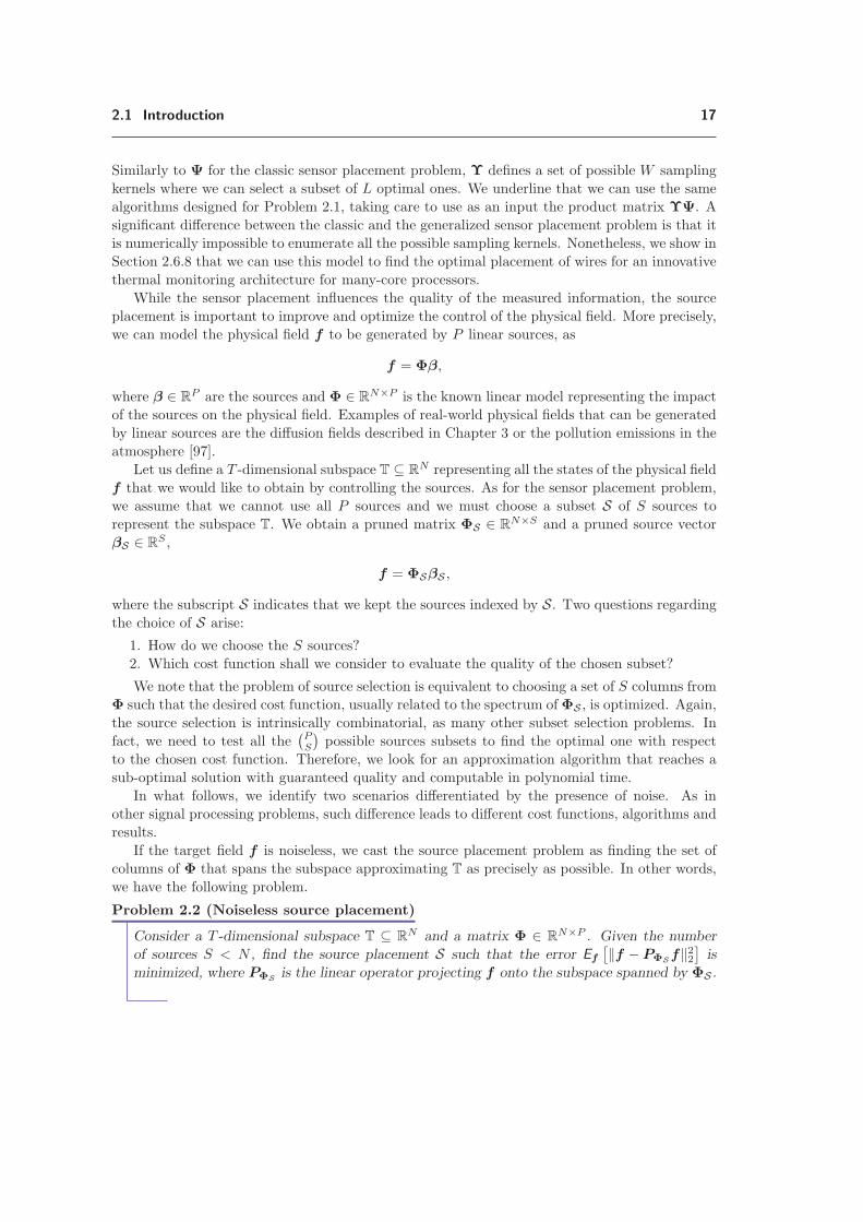
While the sensor placement influences the quality of the measured information, the source
placement is important to improve and optimize the control of the physical field. More precisely,
we can model the physical field f to be generated by P linear sources, as
f = Φβ,
where β ∈ RP are the sources and Φ ∈ R
N×P is the known linear model representing the impact
of the sources on the physical field. Examples of real-world physical fields that can be generated
by linear sources are the diffusion fields described in Chapter 3 or the pollution emissions in the
atmosphere [97].
Let us define a T -dimensional subspace T ⊆ RN representing all the states of the physical field
f that we would like to obtain by controlling the sources. As for the sensor placement problem,
we assume that we cannot use all P sources and we must choose a subset S of S sources to
represent the subspace T. We obtain a pruned matrix ΦS ∈ RN×S and a pruned source vector
βS ∈ RS ,
f = ΦSβS ,
where the subscript S indicates that we kept the sources indexed by S. Two questions regarding
the choice of S arise:
1. How do we choose the S sources?
2. Which cost function shall we consider to evaluate the quality of the chosen subset?
We note that the problem of source selection is equivalent to choosing a set of S columns from
Φ such that the desired cost function, usually related to the spectrum of ΦS , is optimized. Again,
the source selection is intrinsically combinatorial, as many other subset selection problems. In
fact, we need to test all the(PS
)possible sources subsets to find the optimal one with respect
to the chosen cost function. Therefore, we look for an approximation algorithm that reaches a
sub-optimal solution with guaranteed quality and computable in polynomial time.
In what follows, we identify two scenarios differentiated by the presence of noise. As in
other signal processing problems, such difference leads to different cost functions, algorithms and
results.
If the target field f is noiseless, we cast the source placement problem as finding the set of
columns of Φ that spans the subspace approximating T as precisely as possible. In other words,
we have the following problem.
Problem 2.2 (Noiseless source placement)
Consider a T -dimensional subspace T ⊆ RN and a matrix Φ ∈ R
N×P . Given the number
of sources S < N , find the source placement S such that the error Ef
[‖f − PΦSf‖22]is
minimized, where PΦS is the linear operator projecting f onto the subspace spanned by ΦS .

18 Sensors and sources placement optimization
Note that we must define a probability distribution for f to have a meaningful cost function
in Problem 2.2. In fact, if we consider f ∈ T, the error would be either zero or infinite. In
Section 2.5, we consider f = ΘTx, where ΘT is an orthonormal basis for the subspace T and x
is a set of i.i.d. Gaussian random variables with zero mean and unit variance, and we propose a
near-optimal algorithm for Problem 2.2.
A different problem arises if we assume that an i.i.d. Gaussian noise n with a variance σ2 is
corrupting f : in fact, the noise perturbing f propagates to the estimated sources and complicates
the control of the physical field. Such a noise could be due to the reconstruction error of the
actual state of the physical field. Therefore, we consider a given target field f = ΘTx+n, where
ΘT is a basis for the T -dimensional subspace T. Here, we aim at finding the sources βS such
that the produced physical field f minimizes the �2 distance ‖f − f‖2.If S ≥ T and rank (Θ†
TΦS) = T , we estimate βS as
βS = ΦS†f = (ΦS∗ΦS)−1Φ∗Sf ,
where † indicates the Moore-Penrose pseudoinverse. Then, if ΦS spans T, the error on the
controlled sources is
‖β − β‖22 = σ2K∑i=1
1
λi(PTΦS)(2.6)
where λi(PTΦS) is the i-th eigenvalue of PTΦSPT∗ΦS∗ and PT is the projection operator onto
the subspace T. Therefore, we characterize the noisy source placement problem as follows.
Problem 2.3 (Noisy source placement)
Consider a physical system modeled as Φ ∈ RN×P and a T -dimensional subspace T ⊆ R
N .
Assume that the target fields f ∈ T are corrupted by i.i.d. Gaussian noise n with variance
σ2. Find the source location S such that (2.6) is minimized for all f ∈ T.
2.1.2 Infection spreading over a graph
Consider a population in a given region and assume that we know it social network, that is
for example how often they meet each other. Moreover, assume that somebody on this network
caught a virus that is passed to everybody he/she meets. We could imagine many interesting
and fundamental questions around this scenario:
– Assume we know the time of infection of a sub-population. Can we estimate the origin of
the infection, that is the first entity who was infected by the virus?
– Assume we have a vaccine for a part of the population. Who should receive the vaccine
first to slow the infection spread as much as possible?
– Assume an enemy decides to infect the population. Who are the most sensible targets?
Who are the targets leading to the fastest infection of the population?
The importance of these questions is clear as can be exemplified by the recent efforts of
“The Bill and Melinda Gates Foundation” to eradicate certain viruses such as tuberculosis [100].
However, this is just an example of a wider family of problems. Other examples include:
– Worms/viruses infecting a computer network,

2.1 Introduction 19
0 0.1 0.2 0.3 0.4 0.5 0.6 0.70
0.1
0.2
0.3
0.4
0.5
0.6
0.7
0.8
0.9
X
Y
Figure 2.2: An example of the graph G considered to model the spreading of an information
between entities: ni is the i-th node, sj is the j-th source of the infection and di,j is the distance
between the nodes i and j.
– Rumor spreading on a social network, e.g. Twitter,
– Electrical perturbations and failures on the power gird.
It is extremely difficult to tackle this family of problems with the linear models we described
in Section 2.1.1. Inspired by the work of Pinto et al. [120] on source localization on graphs, we
propose to model the infection by a finite, undirected graph G{N ; E}, where the vertex set Nhas N nodes, and the edge set E has E edges, see Figure 2.2 for an example of such graphs.
The graph G is assumed to be known, at least approximately, as is often verified in practice–e.g.
rumors spreading in a social network, or electrical perturbations propagating on the electrical
grid.
The graph G models a temporally driven infection process: there exists some sources of
infection at time t = 0 and the infection passes to the nodes connected to sources after a certain
time. Once a node is infected, it also acts as a source. The temporal delay after which a source
infects its neighbors is modeled by the edge weights. More precisely, assume that the node ni is
infected at time t0 and connected to the node nj , then the j-th node is infected after t0 + di,jseconds, where di,j is the weight of the edge ei,j
1. These weights are stored on the adjacency
matrix A, where each element is defined as
Ai,j =
{di,j if ∃ ei,j
0 otherwise. (2.7)
Note that the time delays di,j can be either a deterministic value or defined as a random variable
with a known probability distribution.
1. We assume a symmetrical model, where the infection from the node ni to the node nj is as fast as theinfection from the node nj to the node ni.

20 Sensors and sources placement optimization
The set S defines the S sources that are infected at t = 0 and are able to infect the neighbors.
Then, we denote as ti the average time at which the node ni is infected. Two facts should be
noted here:
– it is an average time because of the possible random nature of the infection times,
– ti = 0 if ni ∈ S.Having properly defined the model, we can identify the following three challenging optimiza-
tion problems based on the three questions we highlighted at the beginning of this section.
First, we would like to know which nodes we should monitor to discover an infection and
localize the source of the infection as precisely as possible.
Problem 2.4 (Sensor placement on graphs)
Consider a known graph G(N , E) and assume that an infection starts from one node chosen
uniformly at random. Assume that we can observe L nodes and measure their infection time.
Our aim is to localize the source of infection. Which nodes should we monitor so that the
estimation error is minimized?
Second, we would like to find optimal strategies to spread the infection over the network.
While such a problem may look wicked 2, understanding which nodes are able to spread an
infection faster is fundamental to design effective defensive schemes.
Problem 2.5 (Source placement on graphs)
Consider a known graph G(N , E) and assume that we are given the number of nodes S that
we can infect at t = 0. Which nodes should be infected such that the average time of infection
Ei∈N [ti] is minimized?
Third, we are interested in the optimization of vaccination protocols. We define the vacci-
nation as the removal of a node from the graph G: once a node is removed it cannot catch and
re-transmit the infection. We would like to know which nodes we should vaccinate to slow down
the infection as much as possible.
Problem 2.6 (Vaccination on graphs)
Consider a known graph G(N , E) and assume that an infection starts from a set of S nodes
chosen uniformly at random, where S is known. If we are given a set of V < N vaccines, which
nodes should we vaccinate such that the average time of infection Ei∈N [ti] is maximized?
In this thesis, we present our results for Problem 2.5 and 2.6. Interesting theoretical results
together with practical algorithms for Problem 2.4 have already been proposed by Pinto et al.
[120].
2.2 Our contributions
1. We propose FrameSense, a greedy sensor placement method that minimizes the frame
potential to choose the sensing locations L. We briefly summarize the innovative aspects
of the proposed algorithm:
2. In the case of rumors spreading over a social network, it can be seen as a task of interest.

2.2 Our contributions 21
– Under some stability conditions on the spectrum ofΨ and to the best of our knowledge,
FrameSense is the only known near-optimal algorithm with respect to the MSE.
– FrameSense outperforms other greedy algorithms in terms of MSE.
– FrameSense is on par in terms of quality of the solution with the method based on
convex relaxation [73], which uses heuristics to improve the local solution and has a
significantly higher computational complexity.
– The computational complexity of FrameSense is significantly lower with respect to the
other considered algorithms.
– We extend FrameSense to union of subspaces, where we have a set of linear models
that can generate the measured physical field.
– We show that FrameSense can be used for the selection of a set of sampling kernels
from a larger collection, as in tomographic sensing.
2. We design an efficient thermal monitoring system for many-core processors capable of
precisely estimating the temperature distribution on the whole die with a few measurements
and optimize the sensor placement such that we maximize the precision of the reconstructed
thermal distributions.
– We use linear low-dimensional models for the thermal distribution and we learn such
a model by principal component analysis. We show that such models are easy to learn
and precise, while requiring limited computational power.
– We show that the performance of linear models depends strongly on the locations of
the sensors and propose to optimize the sensor placement using FrameSense.
– The proposed framework improves significantly the monitoring performance over the
state of the art. For example, in a typical scenario of a 64-cores architecture with
one temperature sensor per core corrupted by a noise with variance σ2 = 4, we can
improve the reconstruction error from ≈ 3◦C to less than 1.4◦C.
– We propose an innovative thermal monitoring architecture based on tomographic mea-
surements, where we use wires as sensors by measuring their resistance. We show that
the proposed architecture achieves similar reconstruction performance to the tradi-
tional scheme based on local CMOS sensors with a limited increase of the sensing
resources.
3. We propose DASS, an algorithm for the adaptive sampling scheduling of wireless sensor
networks (WSN), where we minimize the number of collected measurement by the WSN
to increase its lifetime with minimal losse of information.
– We model the measured physical field with a time-varying low-dimensional linear
model that we learn online from the measured data.
– We decide when and where we measure the physical field so that the energy used for
sampling is minimized while we collect as much information as possible. The sampling
pattern is dynamically adapted to the low dimensional model of the signal using a
generalized version of FrameSense.
– We show a significant number of numerical experiments on real-world data where we
reduce the energy consumption of a WSN by 15% without any significant loss in the
collected information.

22 Sensors and sources placement optimization
4. We study the dual problem of sensor placement on physical fields, that is source placement.
We assume to have a set of sources among which we have to pick a subset of size S that
spans a given subspace T as precisely as possible.
– We choose the approximation error on the given subspaces as a cost function and we
show that it is submodular.
– We propose an algorithm based on such a cost function and we prove that it is near-
optimal.
5. We generalize the source/sensor problem to the spreading of an information/infection over a
graph and state three different problems: sensor placement, source placement, and vaccina-
tion. Such model fits many real-world scenarios as the spreading of a virus in a population.
– We propose a near-optimal algorithm for the source placement, that attempts to find
the set of sources such that the average time of infection of the nodes is minimized.
We show that our algorithm outperforms other algorithms based on different cost
functions, such as the connectivity of the nodes.
– For the vaccination problem, we propose an algorithm that attempts to maximize the
time of infection of the graph by vaccinating a proper subset of nodes. Unfortunately,
it was not possible to prove the near-optimality nor other bounds on the performance
of this algorithm. Nonetheless, we show with an extensive set of experiments that the
proposed algorithm outperforms other plausible algorithms.
2.3 Near-optimal sensor placement for linear physical fields
In this section, we propose one of the core results of the thesis: a near-optimal algorithm
solving Problem 2.1. As we previously mentioned, such a problem is NP-hard: it is impossible
to find the optimal solution to all instances of the problem in polynomial time. Therefore, we
would like to design an algorithm with guaranteed performance and polynomial complexity.
2.3.1 Related work
Classic solutions to the sensor placement problem can be classified in three categories: convex
optimization, greedy methods and heuristics.
Convex optimization methods [73, 140] are based on the relaxation of the Boolean constraints
{0, 1}N representing the sensor placement to the convex set [0, 1]N . This relaxation is not usually
tight as heuristics are needed to choose the sensor locations and there is no a-priori guarantee
on the distance from the optimal solution. The authors in [73] define an online bound for the
quality of the obtained solution by looking at the gap between the primal and the dual problem.
Heuristic methods [4, 40, 82, 96, 106, 165] are valid options to reduce the cost of the exhaustive
search, which has a prohibitive cost. Again, even if the methods work in practice, little can be
said about the quality or the optimality of the solution.
Greedy algorithms leveraging the submodularity of the cost function [112] are a class of
algorithms with polynomial complexity and guaranteed performance with respect to the chosen
cost function [47, 48, 80, 108, 140]. Since the MSE is not submodular in general [47, 48],
alternative cost functions have been considered [47, 48, 80, 108, 140]. The proposed methods
are theoretically near-optimal with respect to the chosen cost function, but little can be said

2.3 Near-optimal sensor placement for linear physical fields 23
about the achieved MSE. Moreover, the local optimization of the proposed cost functions are
computationally demanding, often requiring the inversion of large matrices [80]. Therefore,
approximations of the cost functions have been proposed [80], offering a significant speedup for
an acceptable reduction of the solution’s quality.
Beside the approximation strategy, approximation algorithms are differentiated by the chosen
cost function. Under restrictive assumptions, the MSE can be chosen as a cost function, see
[47, 59]. In [48], the authors bounded the performance of greedy algorithms optimizing R2, a
measure of goodness of fit based on the MSE, using the concept of submodularity ratio. However,
such algorithms are generally less performant than the greedy algorithms optimizing proxies of
the MSE. Common proxies of the MSE are inspired by information theoretic measures such
as entropy [165], cross-entropy [108, 123] and mutual information [80]. A popular choice is the
maximization of the log determinant of TL, being the volume of the confidence ellipsoid given
by the measurements. This proxy has been historically introduced in D-Optimal experiment
design [150], but has also been successfully proposed as a cost function for a convex relaxed
method [73] and greedy algorithms [140]. Other proxies have also been introduced in optimal
experiment design, such as maximization of the smallest eigenvalue λK (E-Optimal design) or
the maximization of the trace of TL (T-Optimal design). A detailed description of the different
choices available for experiment design can be found in [150].
Note that there exists optimal strategies with a reasonable computational cost for some
specific scenarios. This is the case when we have the freedom of completely designing the matrix
ΨL given the dimensions L and K. More precisely, if L = K, the optimal basis corresponds to
an orthonormal basis, while if L > K, then we are looking for a unit-norm tight frame [19, 61].
Benedetto et al. showed that each tight frame is a non-unique global minimizer of the frame
potential (FP), that is a scalar property of the frame defined as
FP(ΨL) =∑i,j∈L
| 〈ψi,ψj〉 |2,
where ψi is the ith row ofΨL. One of the reasons for the popularity of the FP in the frame theory
community is its interesting physical interpretation [35]. Namely, it is the potential energy of the
so-called frame force, a force between vectors inspired by the Coulomb force. The frame force
and its potential energy have been introduced for their orthogonality encouraging property: the
force is repulsive when the angle between the two vectors is acute, null when they are orthogonal
and attractive when the angle is obtuse. A graphical explanation of this physical interpretation
is given in Figure 2.3, where the unit-norm rows of two matrices Ψ and Φ belonging to R3×2
are represented. While Ψ is the unit-norm tight frame minimizing the FP, has vectors as close
to orthogonality as possible and therefore in equilibrium with respect to the frame force, the
vectors of Φ are further away from being orthogonal and the FP is thus not minimized. Note
that according to frame theory [19], Ψ is the matrix that also achieves the minimum MSE (per
component).
The FP is also known as the total summed correlation in communication theory [133]. It is
used to optimize the signatures of CDMA systems to achieve the Welch lower bound [79] and to
maximize the capacity of the channel.
Given its interpretation and its role in defining the existence of tight frames—the optimal
frames in terms of MSE—we observe that the FP is an interesting cost function for an approxi-
mation algorithm.

24 Sensors and sources placement optimization
Figure 2.3: A graphical representation of the unit-norm rows of two matrices Ψ and Φ. On
the left, the rows Ψ are optimally spread on R2 minimizing the FP and the MSE. This is also
known as the Mercedes-Benz frame and is a typical example of a unit-norm tight frame. On
the right, Ψ is the frame built by adding a vector to the orthonormal basis of R2 [φ1,φ2]. The
three vectors do not minimize the FP and therefore are not in equilibrium with respect to the
frame force. You can envision a parallel example with three electrons on a unit circle under the
Coulomb force. If the three electrons are free to move, they would reach an equilibrium when
located as the vectors of Ψ, up to a rotation factor.
2.3.2 The frame potential in frame theory
This section briefly introduces some of the basic concepts of frame theory that are useful to
understand and analyze the proposed algorithm. Frame theory studies and designs families of
matrices ΨL such that TL is well-conditioned. More precisely, ΨL is a frame for a Hilbert space
H if there exists two scalars A and B such that 0 < A ≤ B < ∞ so that for every x ∈ H we have
A‖x‖22 ≤ ‖ΨLx‖22 ≤ B‖x‖22,where A and B are called frame bounds. A frame ΨL is tight when A = B and its columns
are orthogonal by construction. Of particular interest is the case of unit norm tight frames
(UNTF); these are tight frames whose frame elements—the rows ψi—have unit norm. These
provide Parseval-like relationships, despite the non-orthogonality of the frame elements of ΨL.In addition to (2.3), there are other interesting relationships between the characteristics of ΨLand the spectrum of TL. For example, we can express the FP as
FP(ΨL) = Trace(TL∗TL) =K∑
k=1
|λk|2.
Moreover, the sum of the eigenvalues of TL is equal to the sum of the norm of the rows,∑Li=1 ‖ψi‖2 =
∑Kk=1 λk.
These quantities of interest take a simplified analytical form for UNTFs. In this scenario,
we know [19] that the FP is minimum with respect to all other matrices of the same size with
unit-norm rows, and it is equal to FPUNTF = L2
K . According to [19], the optimal MSE is also
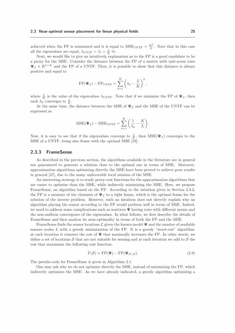
2.3 Near-optimal sensor placement for linear physical fields 25
achieved when the FP is minimized and it is equal to MSEUNTF = K2
L . Note that in this case
all the eigenvalues are equal, λUNTF = λi =LK ∀i.
Next, we would like to give an intuitively explanation as to the FP is a good candidate to be
a proxy for the MSE. Consider the distance between the FP of a matrix with unit-norm rows
ΨL ∈ RL×K and the FP of a UNTF. Then, it is possible to show that this distance is always
positive and equal to
FP(ΨL)− FPUNTF =
K∑k=1
(λk − L
K
)2
,
where LK is the value of the eigenvalues λUNTF. Note that if we minimize the FP of ΨL, then
each λk converges to LK .
At the same time, the distance between the MSE of ΨL and the MSE of the UNTF can be
expressed as
MSE(ΨL)−MSEUNTF =
K∑k=1
(1
λk− K
L
).
Now, it is easy to see that if the eigenvalues converge to LK , then MSE(ΨL) converges to the
MSE of a UNTF, being also frame with the optimal MSE [19].
2.3.3 FrameSense
As described in the previous section, the algorithms available in the literature are in general
not guaranteed to generate a solution close to the optimal one in terms of MSE. Moreover,
approximation algorithms optimizing directly the MSE have been proved to achieve poor results
in general [47], due to the many unfavorable local minima of the MSE.
An interesting strategy is to study proxy cost functions for the approximation algorithms that
are easier to optimize than the MSE, while indirectly minimizing the MSE. Here, we propose
FrameSense, an algorithm based on the FP. According to the intuition given in Section 2.3.2,
the FP is a measure of the closeness of ΨL to a tight frame, which is the optimal frame for the
solution of the inverse problem. However, such an intuition does not directly explain why an
algorithm placing the sensor according to the FP would perform well in terms of MSE. Indeed,
we need to address some complications such as matrices Ψ having rows with different norms and
the non-uniform convergence of the eigenvalues. In what follows, we first describe the details of
FrameSense and then analyze its near-optimality in terms of both the FP and the MSE.
FrameSense finds the sensor locations L given the known modelΨ and the number of available
sensors nodes L with a greedy minimization of the FP. It is a greedy “worst-out” algorithm:
at each iteration it removes the row of Ψ that maximally increases the FP. In other words, we
define a set of locations S that are not suitable for sensing and at each iteration we add to S the
row that maximizes the following cost function:
F (S) = FP(Ψ)− FP(ΨN\S). (2.8)
The pseudo-code for FrameSense is given in Algorithm 2.1.
One may ask why we do not optimize directly the MSE, instead of minimizing the FP, which
indirectly optimizes the MSE. As we have already indicated, a greedy algorithm optimizing a
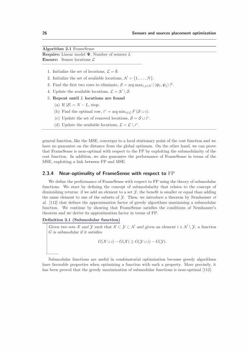
26 Sensors and sources placement optimization
Algorithm 2.1 FrameSense
Require: Linear model Ψ, Number of sensors L
Ensure: Sensor locations L
1. Initialize the set of locations, L = ∅.2. Initialize the set of available locations, N = {1, . . . , N}.3. Find the first two rows to eliminate, S = argmaxi,j∈N | 〈ψi,ψj〉 |2.4. Update the available locations, L = N \ S.5. Repeat until L locations are found
(a) If |S| = N − L, stop.
(b) Find the optimal row, i∗ = argmini∈L F (S ∪ i).
(c) Update the set of removed locations, S = S ∪ i∗.
(d) Update the available locations, L = L \ i∗.
general function, like the MSE, converges to a local stationary point of the cost function and we
have no guarantee on the distance from the global optimum. On the other hand, we can prove
that FrameSense is near-optimal with respect to the FP by exploiting the submodularity of the
cost function. In addition, we also guarantee the performance of FrameSense in terms of the
MSE, exploiting a link between FP and MSE.
2.3.4 Near-optimality of FrameSense with respect to FP
We define the performance of FrameSense with respect to FP using the theory of submodular
functions. We start by defining the concept of submodularity that relates to the concept of
diminishing returns: if we add an element to a set Y, the benefit is smaller or equal than adding
the same element to one of the subsets of Y . Then, we introduce a theorem by Nemhauser et
al. [112] that defines the approximation factor of greedy algorithms maximizing a submodular
function. We continue by showing that FrameSense satisfies the conditions of Nemhauser’s
theorem and we derive its approximation factor in terms of FP.
Definition 2.1 (Submodular function)
Given two sets X and Y such that X ⊂ Y ⊂ N and given an element i ∈ N \ Y, a function
G is submodular if it satisfies
G(X ∪ i)−G(X ) ≥ G(Y ∪ i)−G(Y).
Submodular functions are useful in combinatorial optimization because greedy algorithms
have favorable properties when optimizing a function with such a property. More precisely, it
has been proved that the greedy maximization of submodular functions is near-optimal [112].

2.3 Near-optimal sensor placement for linear physical fields 27
Theorem 2.1 (Near-optimal maximization of submodular function [112])
Let G be a normalized, monotone, submodular set function over a finite set N . Let L be the
set of L elements chosen by the greedy algorithm, and let OPT = maxA⊂N ,|A|=L G(A) be
the optimal set of elements. Then
G(L) ≥(1− 1
e
)G(OPT),
where e is Euler’s number.
Namely, if G satisfies the conditions of Theorem 2.1, then the solution of the greedy algorithm
is always close to the optimal one. These conditions are satisfied by the cost function F in (2.8),
as shown in the following lemma.
Lemma 2.1 (Submodularity of the cost function)
The set function maximized in Algorithm 2.1,
F (S) = FP(Ψ)− FP(ΨN\S),
is a normalized, monotone, submodular function.
Proof.
The set function F is normalized if F (∅) = 0. Here, normalization is trivially shown since
Ψ = ΨN by definition. To show monotonicity, we pick a generic matrix Ψ of N rows, a set Xand an index i /∈ X . Then, we compute the increment of F due to i with respect to the set X ,
showing that it is always positive.
F (X ∪ i)− F (X ) = FP(ΨN\X )− FP(ΨN\X∪i)
(a)=
∑n,m∈A∪i
|〈ψn,ψm〉|2 −∑
n,m∈A|〈ψn,ψm〉|2
= 2∑n∈A
|〈ψn,ψi〉|2 + |〈ψi,ψi〉|2 ≥ 0,
where (a) is due to a change of variable N \ X = A. Assuming without loss of generality that
Y = X ∪ j, we check the submodularity according to Definition 2.1 .
F (X ∪ i)− F (X )− F (Y ∪ i) + F (Y)
= F (X ∪ i)− F (X )− F (X ∪ {i, j}) + F (X ∪ j)
= FP(ΨA∪{i,j})− FP(ΨA∪j)− FP(ΨA∪i) + FP(ΨA)
= 2∑
n∈A∪j
|〈ψn,ψi〉|2 − 2∑n∈A
|〈ψn,ψi〉|2
= 2|〈ψi,ψj〉|2 ≥ 0.
Now, we use Theorem 2.1 to derive the approximation factor of FrameSense with respect to the
FP.

28 Sensors and sources placement optimization
Theorem 2.2 (FP approximation factor)
Consider a matrix Ψ ∈ RN×K and a given number of sensors L, such that K ≤ L < N .
Denote the optimal set of locations as OPT = argmaxA⊂N ,|A|=L FP(ΨA) and the greedy
solution found by FrameSense as L. Then, L is near-optimal with respect to the FP,
FP(ΨL) ≤ γ FP(ΨOPT),
where γ =(1 + 1
e
(FP(Ψ) K
LMIN2 − 1
))is the approximation factor and LMIN = min|L|=L
∑i∈L ‖ψi‖2
is the sum of the norms of the L rows with the smallest norm.
Proof.
According to Lemma 2.1, the cost function used in FrameSense satisfies the conditions of Theorem
2.1. Therefore,
F (OPT)− F (S) ≤ 1
e(F (OPT)),
where F (S) = FP(Ψ)−FP(ΨN\S) is the considered cost function, S is the set of rows eliminated
by FrameSense and OPT = N \OPT. If we consider the cost function, we obtain
FP(ΨN\S) ≤(1− 1
e
)FP(ΨN\OPT) +
1
eFP(Ψ). (2.9)
Then, we note that the following minimization problem,
minimizeL FP(ΨL) subject to |L| = L,
is equivalent, under the change of variable L = N \ S, tominimizeS FP(ΨN\S) subject to |S| = N − L.
Using the equivalence in (2.9), we obtain
FP(ΨL) ≤(1 +
1
e
(FP(Ψ)
FP(ΨOPT)− 1
))FP(ΨOPT),
To conclude the proof, we bound from above the term 1e
FP(Ψ)FP(ΨOPT) . First, we consider the optimal
solution OPT to select a tight frame whose rows have a summed norm of LOPT =∑
i∈OPT ‖ψi‖2,
FP(ΨL) ≤(1 +
1
e
(FP(Ψ)
K
LOPT2 − 1
))FP(ΨOPT).
Then, we assume that OPT selects the rows having the smallest norm, LOPT ≥ LMIN =
min|L|=L
∑i∈L ‖ψi‖2.
Note that the FP of the original matrix influences significantly the final result: the lower the
FP ofΨ, the tighter the approximation obtained by the greedy algorithm. Therefore, FrameSense
performs better when the original matrix Ψ is closer to a tight frame. In fact, the FP is bounded
as follows, (∑Ni=1 ‖ψi‖2
)2
K≤ FP(Ψ) ≤
(N∑i=1
‖ψi‖2)2
,

2.3 Near-optimal sensor placement for linear physical fields 29
where the lower bound is reached by tight frames and the upper bound by rank 1 matrices.
Moreover, Theorem 2.2 suggests to remove from Ψ the rows whose norm is significantly
smaller with respect to the others to improve the performance of FrameSense. This suggestion
is intuitive, since such rows are also the least informative.
2.3.5 Near-optimality of FrameSense with respect to MSE
Having a near-optimal FP does not necessarily mean that the obtained MSE is also near-
optimal. Here, we show that, under some assumptions on the spectrum of Ψ, FrameSense is
near-optimal with respect to the MSE .
Before going to the technical details, we generalize the concept of number of sensors to account
for the norms of the rows of Ψ. More precisely, we keep L as the number of rows and we define
LA =∑
i∈A ‖ψi‖2 as the sum of the norms of the rows of ΨA for a generic set A. We also define
the two extremal values of LA,
LMIN = minA∈N ,|A|=L
∑i∈A
‖ψi‖2, (2.10)
LMAX = maxA∈N ,|A|=L
∑i∈A
‖ψi‖2, (2.11)
indicating respectively the minimum and the maximum value of LA among all possible selections
of L out of N rows of Ψ. LA is also connected to the spectrum of TA. Indeed, LA is the trace
of TA and thus it is also the sum of its eigenvalues,
LA =∑i∈A
‖ψi‖2 = Trace(TA) =∑i∈A
λi.
If Ψ has rows with unit-norm, then LA = LMIN = LMAX = L.
As a first step to prove the near-optimality with respect to MSE, we consider a possible
placement A and we bound the MSE of the matrix ΨA using its FP and the spectrum of TA. Toobtain such a bound, we use a known inequality [144] involving variance, arithmetic mean and
harmonic mean of a set of positive bounded numbers, in this case the eigenvalues of TA. The
following lemma describes the bound, while its proof is given in Appendix 2.10.1.
Lemma 2.2 (MSE bound)
Consider any ΨA ∈ RL×K with |A| = L ≤ K and denote the spectrum of TA as λ1 ≥ . . . ≥
λK . Then the MSE is bounded according to the FP as,
MSE(ΨA) ≤ K
LMIN
FP(ΨA)λK
2 , (2.12)
MSE(ΨA) ≥ K
LMAX
FP(ΨA)λ1
2 , (2.13)
where LMIN and LMAX are defined as in (2.10) and (2.11).
Lemma 2.2 is key to study the approximation factor with respect to the MSE. Specifically,
it allows to analyze the two extremal cases:
– Given the optimal FP, what is the lowest MSE we can achieve?

30 Sensors and sources placement optimization
– Given the worst case FP according to Theorem 2.2, what is the largest MSE we may
encounter?
Lemma 2.2 implies the necessity to properly bound the spectrum of any ΨA with a given FP
obtained from Ψ. While it is possible to bound λ1 with the FP, it is also easy to build matrices
with λK = 0, compromising the bound given in (2.12). Therefore, we introduce the following
property to control the eigenvalues of any TA.
Definition 2.2 ((δ, L)-bounded frame)
Consider a matrix Ψ ∈ RN×K where N ≥ L and N > K. Then, we say that Ψ is (δ, L)-
bounded if, for every A ⊆ N such that |A| = L, TA has a bounded spectrum
LMEAN
K− δ ≤ λi ≤ LMEAN
K+ δ,
where 1 ≤ i ≤ K, δ ≥ 0 and LMEAN = LN
∑i∈N ‖ψi‖2 is average value of LA.
The concept of (δ, L)-bounded frames is similar to the notion of matrices satisfying the re-
stricted isometry property, that are used in compressive sensing to guarantee the reconstruction
of a sparse vector from a limited number of linear measurements [33]. Moreover, it allows us to
define an approximation factor for the MSE that does not depend on the FP, the cost-function
we minimize.
Theorem 2.3 (MSE approximation factor for (δ, L)-bounded frames)
Consider a matrix Ψ ∈ RN×K and L ≥ K sensors. Assume Ψ to be a (δ, L)-bounded
frame, let d be the ratio LMEAN/K and define the optimal placement in terms of MSE as
OPT = argminA∈N ,|A|=L MSE(ΨA). Then the solution L of FrameSense is near-optimal
with respect to the MSE,
MSE(ΨL) ≤ ηMSE(ΨOPT) with η = γ(d+ δ)2
(d− δ)2LMAX
LMIN,
where η is the approximation factor of the MSE and γ is the approximation factor of the FP.
Proof.
First, we compute the worst case MSE when FrameSense yields the worst FP, that is for
FP(ΨL) = γ FP(ΨOPT). Using the upper bound (2.12) and the bounds on the spectrum for
(δ, L)-bounded frames, we have
MSE(ΨL) ≤ K
LMIN
γ FP(ΨOPT)
(d− δ)2. (2.14)
Then, we compute the best case MSE when the FP is optimal. We note that the lower bound
(2.13) of the MSE is monotonically decreasing with respect to the FP. Therefore, we use the
same strategy considered for the lower bound, and obtain
MSE(ΨOPT) ≤ K
LMAX
FP(ΨOPT)
(d+ δ)2. (2.15)
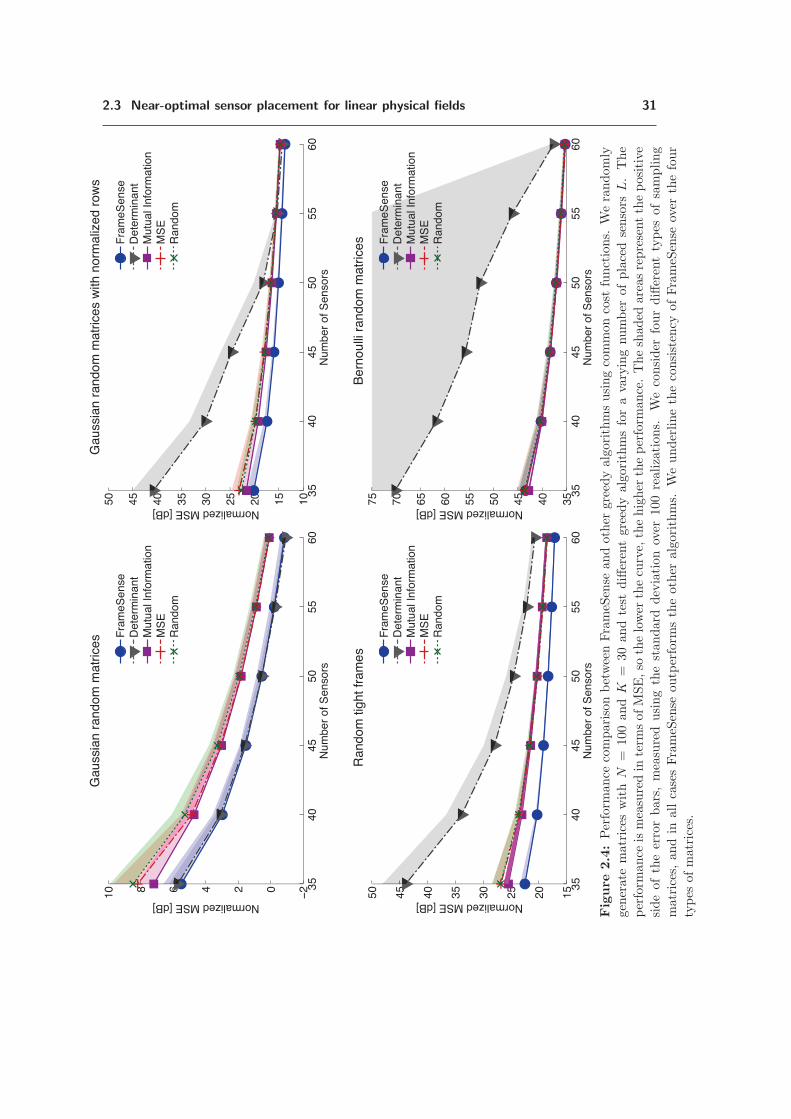
2.3 Near-optimal sensor placement for linear physical fields 31
3540
4550
5560
��0�46810
Num
ber
of S
enso
rs
Normalized MSE [dB]
Gau
ssia
n ra
ndom
mat
rices
Fra
meS
ense
Det
erm
inan
tM
utua
l Inf
orm
atio
nM
SE
Ran
dom
3540
4550
5560
101520253035404550
Num
ber
of S
enso
rs
Normalized MSE [dB]
Gau
ssia
n ra
ndom
mat
rices
with
nor
mal
ized
row
s
Fra
meS
ense
Det
erm
inan
tM
utua
l Inf
orm
atio
nM
SE
Ran
dom
3540
4550
5560
1520253035404550
Num
ber
of S
enso
rs
Normalized MSE [dB]
Ran
dom
tigh
t fra
mes
Fra
meS
ense
Det
erm
inan
tM
utua
l Inf
orm
atio
nM
SE
Ran
dom
3540
4550
5560
354045505560657075
Num
ber
of S
enso
rs
Normalized MSE [dB]
Ber
noul
li ra
ndom
mat
rices
Fra
meS
ense
Det
erm
inan
tM
utua
l Inf
orm
atio
nM
SE
Ran
dom
Figure
2.4:Perform
ance
comparisonbetweenFrameSense
andother
greedyalgorithmsusingcommoncost
functions.
Werandomly
generate
matrices
withN
=100andK
=30
andtest
differentgreedyalgorithmsforavaryingnumber
ofplacedsensors
L.The
perform
ance
ismeasuredin
term
sofMSE,so
thelower
thecurve,
thehigher
theperform
ance.Theshaded
areasrepresentthepositive
sideoftheerrorbars,measuredusingthestandard
deviationover
100realizations.
Weconsider
fourdifferenttypes
ofsampling
matrices,andin
allcasesFrameSense
outperform
stheother
algorithms.
Weunderlinetheconsistency
ofFrameSense
over
thefour
types
ofmatrices.

32 Sensors and sources placement optimization
20 40 60 80 100 120 140 160��
0
�
Number of available sensor locations
Com
puta
tiona
l tim
e [lo
g s]
Computational time comparison
FrameSenseDeterminantMutual InformationMSERandom
Figure 2.5: Comparison in terms of computational time as a function of N between FrameSense
and other greedy algorithms using commonly considered cost functions. The lower the curve the
faster the algorithm. Note how FrameSense is the fastest algorithm, the exception being the
random selection. Moreover, observe how the different algorithms scales equivalently with N .
Errors bars are not shown because they are smaller than the markers.
Note that we consider that the optimal MSE is achieved for the optimal FP because the lower
bound of the MSE is monotonically decreasing with respect to FP . Finally, we compute the MSE
approximation ratio as the ratio between (2.14) and (2.15), obtaining the desired result.
The definition of (δ, L)-bounded frames is key to the proof. It turns out that many families of
adequately normalized random matrices satisfy Definition 2.2, but it is hard to build deterministic
matrices with such property. Nonetheless, FrameSense works well even for Ψ that are not
provably (δ, L)-bounded. Note that a similar phenomena is observed for compressed sensing and
RIP matrices [104].
2.3.6 Practical considerations on FrameSense
One point of FrameSense that needs improvement is the optimization of the sensing energy
LL. In fact, the FP tends to discard the rows having a larger norm, which in theory could be
more relevant to minimize the MSE. As an example, consider a matrix Ψ built as follows,
Ψ =
[Ψ0
CΨ0
],
where Ψ0 is a generic matrix and C > 1 is a constant. FrameSense would sub-optimally pick rows
from the first matrix, discarding the ones from the second matrix and creating a sub-optimal
sensor placement. In fact, the second matrix would have a lower MSE thanks to the multiplicative
constant C. To limit such a phenomenon, we optimize the sensor location on Ψ′, that is a Ψ
with unit-norm rows. This solution is not perfect: it removes the negative bias introduced by
the norm of ψi, but it does not exploit the sensing energy to improve the sensor placement L.We leave to future work the study of a new FP-based algorithm able to exploit the information
contained in the norm of the rows.

2.3 Near-optimal sensor placement for linear physical fields 33
We conclude this section with a quantification of the bounds given in Theorem 2.2 and
Theorem 2.3 in a simple scenario. Consider a matrix Ψ ∈ CN×K filled with i.i.d. Gaussian
complex random variables with zero mean and variance σ2 = 1/K. Assume that L = c1K and
N = c2K, with c2 > 1 > c1. Then, we have the following inequalities verified in expectation,
‖ψi‖2 = 1 ∀i,K
LMIN2 =
1
c12K,
FP(Ψ) = c22c1
2K.
According to Theorem 2.2, the approximation factor of the FP is equal to γ = 1 +c22−1e . We
assume that K is sufficiently large and we consider the Marchenko-Pastur law [45] to compute
the following approximated bounds for the eigenvalues of ΨL,
d− δ =
√1
c1(1−√
c1)2 ≤ λi ≤
√1
c1(1 +
√c1)
2= d+ δ.
In this scenario, the MSE approximation factor is equal to,
η =
(1 +
c22 − 1
e
)(1 +
√c1
1−√c1
)4
.
For example, if c1 = 0.25 and c2 = 6, then we have γ ≈ 14 and η ≈ 50.
2.3.7 Experimental results
We analyze the performance of FrameSense and compare it with state-of-the-art algorithms
for sensor placement.
First, we compare the FP with other cost functions when used in a naive greedy algorithm.
Among the ones listed in Section 2.3, we select the following three cost functions: mutual in-
formation [80], determinant of TL [140], and MSE [47]. We also consider an algorithm that
randomly places the sensors to relate the obtained results to a random selection.
The greedy algorithms are tested on different types of sensing matrices Ψ:
– Random matrices with Gaussian i.i.d. entries,
– Random matrices with Gaussian i.i.d. entries whose rows are normalized,
– Random matrices with Gaussian i.i.d. entries with ortho-normalized columns, that we call
random tight frame due to the Naimark theorem [78],
– Random matrices with Bernoulli i.i.d. entries.
Note that the use of random matrices is sub-optimal, since we would rarely encounter such a
case in a real-world scenario. However, it is the only available dataset that allows us to test
thoroughly the different algorithms.
We consider Ψ ∈ R100×30 and evaluate the performance in terms of MSE for
L = {35, 35, 40, 45, 50, 55, 60}. We use 100 different instances for each combination, and we
compute the average MSE as a function of L. Note that the MSE is always computed using (2.3),
which assumes i.i.d. Gaussian noise perturbing the measurements f and a uniform distribution
on α. The relatively small size of Ψ and the low number of trials are due to the lack of scalability

34 Sensors and sources placement optimization
��
��
��
��
��
0�
0 � � � � � 6
Com
putational time [log s]
Normalized MSE [dB]
Gaussian random
matrices
Fram
eSense
Determ
inantM
utual Information
MS
ER
andomC
onvex Opt. M
ethod [6]
��
��
��
��
��
0�
��� �� �� �� ��
Com
putational time [log s]
Normalized MSE [dB]
Gaussian random
matrices w
ith normalized row
s
Fram
eSense
Determ
inantM
utual Information
MS
ER
andomC
onvex Opt. M
ethod [6]
��
��
��
��
��
0�
�� �� �� �� �� ��
Com
putational time [log s]
Normalized MSE [dB]
Random
tight frames
Fram
eSense
Determ
inantM
utual Information
MS
ER
andomC
onvex Opt. M
ethod [6]
��
��
��
��
��
0�
�� �� �� �� �� 60 �
Com
putational time [log s]
Normalized MSE [dB]
Bernoulli random
matrices
Fram
eSense
Determ
inantM
utual Information
MS
ER
andomC
onvex Opt. M
ethod [6]
Figure
2.6:Tradeoffbetw
eencomputatio
naltim
eandMSE.Werandomly
genera
tematrices—
acco
rdingto
fourdifferen
tmodels—
with
N=
100,K
=30
andL=
50sen
sors.
Theperfo
rmance
ismeasured
interm
sofMSE,therefo
rethelow
erthedot,thehigher
the
perfo
rmance.
Thecomputatio
naltim
eis
measured
inseco
nds.
Theerro
rbars
arerep
resented
asellip
soids,
where
thelen
gth
ofthe
axes
represen
tthesta
ndard
deviatio
nofthedata
point.
Note
that,FrameSense
isthefastest
algorith
mbyanorder
ofmagnitu
deand
itis
theseco
ndbest
algorith
min
termsof
MSE.W
hen
theleg
endrefer
toacost
functio
n,weconsid
eredanaive
greedyalg
orith
m
optim
izingthatcost
functio
n.Ontheother
hand,werefer
totheauthors’
papers
forspecifi
calgorith
msim
plem
entin
gcomplica
ted
schem
esan
d/orheuristics.

2.3 Near-optimal sensor placement for linear physical fields 35
�� �� �� �� 0 ����
���
��
0
�
��
Computational time [log s]
Nor
mal
ized
MS
E [d
B]
Gaussian random matrices
FrameSenseConvex Opt. Method [6]
Figure 2.7: Analysis of the tradeoff between computational time and MSE for FrameSense
and the convex relaxed algorithm proposed by Joshi et al. [73]. We generate 100 Gaussian
matrices with K = 20 and of increasing size N = {50, 100, 150, 200, 300, 400, 500}, while we placeL = 0.5N sensors. The error bars are represented as ellipsoids, where the length of the axes
represent the standard deviation of the data point. We measure the average computational time
together with the average MSE, showing that while FrameSense is significantly faster than the
convex algorithm, the difference in MSE is minimal. Moreover, the gap in the quality of the
solution decreases for an increasing size of the problem N .
of certain cost functions, which require the computation of large matrices. The results are given
in Figure 2.4. We note that FrameSense is consistently outperforming all other cost functions.
In the random Gaussian matrices case, the determinant shows similar results. However, looking
at the Bernoulli matrices case, we see that the determinant leads to a significantly worse MSE.
Note that certain cost functions show worse performance than a random selection of the rows.
While this phenomena could be partially explained by the special properties of certain families of
random matrices, it indicates the importance of choosing a well-studied cost function for which
we can obtain performance bounds with respect to the MSE.
According to the theory of random matrices, any selection of rows should have the same spec-
trum on expectation. Therefore, it should not be possible to outperform the random selection
of rows. However, the theoretical analysis of random matrices is generally valid only asymptoti-
cally, while here we show results for relatively small matrices. This phenomenon could also be of
interest for other domains, such as compressed sensing, indicating the possibility of optimizing
the spectrum of random matrices to improve their performance.
In Figure 2.5, we show the average computational time with respect to the number of possible
sensor locations N = {20, 50, 80, . . . , 200}. We consider 100 random Gaussian matrices Ψ ∈R
N×10 and we place 0.5N sensors. We underline that FrameSense is significantly faster than any
other greedy algorithm, the only exception being the random selection that has a computational
time close to zero. Note that the other parameters, such as L and K, have little influence on the
computational time, which strongly depends on N .
In a second experiment, we compare FrameSense with a state-of-the-art method based on
convex optimization [73]. Since the algorithm proposed by Joshi et al. [73] is structurally
36 Sensors and sources placement optimization
different from FrameSense, we focus this analysis on two parameters: the computational time
and the MSE. We fix K = 20 and the ratio between the number of sensors and the num-
ber of available locations as L/N = 0.5. Then, we vary the number of possible locations as
N = {50, 100, 150, 200, 300, 400, 500}. The results for Gaussian random matrices are given in
Figure 2.7. First, we note that the convex method achieves a lower MSE, however the per-
formance gap decreases when we increase the number of sensors. This is not surprising, since
FrameSense is a greedy algorithm that does not require parameter fine-tuning nor heuristics,
while the convex relaxation method integrates some efficient heuristics. For example, at every
iteration, it refines the selection by looking at all the possible swaps between the chosen locations
and the discarded ones. This strategy is particularly effective when L ≈ K: in fact, swapping
just one row can improve significantly the spectrum of TL, and consequently the MSE achieved
by ΨL. The heuristic, while effective in terms of MSE, also increases the computational cost. In
fact, FrameSense is significantly faster.
The last comparison also opens an interesting direction for future work. In fact, the convex
relaxed algorithm optimizes the determinant of TL and its near-optimality in terms of MSE has
not been shown. Moreover, this cost function has been proven to be less effective compared to
FP when used in a greedy algorithm (see Figure 2.4). Therefore, we expect that a convex relaxed
scheme based on the FP has the potential to define a new state of the art, mixing the advantages
of FP and the heuristics proposed in [73].
To conclude the performance analysis, we study the trade-off between computational com-
plexity and performance for all the considered algorithms, greedy and not. We picked 100
instances of each of the random matrices proposed in the first experiment with N = 100, L = 40
and K = 30. We measured the average computational time and average MSE obtained by each
algorithm and the results are given in Figure 2.6. We note a general trend connecting the four
subfloats: FrameSense is the fastest algorithm, by at least an order of magnitude, while its per-
formance is just second, as previously shown, to the convex relaxed method proposed by Joshi
et al. [73].
Since the sensor placement is an off-line procedure, we may argue that the computational
time is of secondary importance. While this is true in many applications, there are certain
applications where it is necessary to recompute L regularly. This is usually the case when Ψ
changes in time due to changes of the physical field and it is possible to adaptively reallocate the
sensors. In other applications, such as the ones where we attempt to interpolate the entire field
from L measurements, the number of possible locations N grows with the desired resolution. In
this case, a lower computational time is of critical importance.
2.4 From linear models to a union of linear models
The linear model defined in (2.1) assumes that the signal f lies on a subspace of dimension
K, that is f ∈ span(Ψ). However, such a model may not be sufficiently descriptive for certain
applications. Here, we extend our work on sensor placement described in Section 2.3 to the
following, more complex, model.

2.4 From linear models to a union of linear models 37
20 25 30 35 40 4520
40
60
80
100
120
140
160
180
Number of Sensors
MS
E [d
B]
Sensor placement for thermal maps with EigenMaps
FrameSenseDeterminantMutual InformationMSERandomCoherence
20 25 30 35 40 4520
40
60
80
100
120
Number of Sensors
MS
E [d
B]
Sensor placement for thermal maps with DCT
FrameSenseDeterminantMutual InformationMSERandomCoherence
Figure 2.8: Comparison between FrameSense, the other greedy algorithms and a coherence-
based greedy algorithm proposed in [128]. In this experiment, we consider the sensors placement
to estimate the temperature of an 8-core microprocessor using a limited number of sensors. Two
different matrices are proposed: on the left, the matrix Ψ ∈ R420×16 is generated from a principal
component analysis of known thermal maps as in [128]; on the right, the matrix Ψ ∈ R420×16
is the subsampled DCT matrix proposed in [113]. The shaded area represents the positive side
of the error bar for the random sensor placement, measured using the standard deviation over
100 realizations. Note that FrameSense significantly outperforms the previous coherence-based
method and the other greedy algorithms, in particular when the number of sensors is close to
the number of estimated parameters, that is K = 16.

38 Sensors and sources placement optimization
Definition 2.3 (Union of Subspaces (UoS) [89])
A union of Q subspaces is defined as
Q =⋃
t=1,...,Q
span(Ψt) (2.16)
where Ψt ∈ RN×Kt is the basis for the k-th subspace of dimension Kt.
That is to say that we consider the physical field f to lie in a union of lower-dimensional
subspaces. More precisely, f ∈ Q if there exists a q such that f = Ψtα.
An example of scenario where we can use the UoS model (2.16) is the thermal monitoring of
microprocessors, where the temperature map f could be modeled as an UoS where each subspace
corresponds to a different workload performed by the processor.
As we mentioned in Section 2.1, measuring all the elements of f using N sensors is often
too expensive or impractical. In reality, we would like to place only L < N nodes, estimate
the parameters α by solving the linear inverse problem, and then successively interpolate the
measurements to reconstruct f . The accuracy of the estimation, and subsequently of the recon-
struction, is directly related to the sensor placement and the noise corrupting the measurements.
It is therefore crucial to place those L sensors in the locations where the most information can
be collected.
For the UoS model and when only L sensors are available, the system of equations (2.2)
becomes
fL = Ψt,Lα,
where t indicates the subspace and is generally unknown, L is the set of indices corresponding
to the L chosen sensor locations, and Ψt,L is the matrix formed by the rows of Ψt indexed by L.Note that if we use the standard linear model of Section 2.3, we would have ΨL instead of Ψt,L.
When a set of measurements fL is available, we would like to solve the following optimization
problem,
mint,α
‖fL −Ψtα‖2. (2.17)
Therefore, it is of interest to choose L such that the MSE of the solution of the inverse problem
2.17 is minimized, as defined in (2.3). Differently from Section 2.3, we do not know beforehand
which subspace produces the measurements in fL. Therefore, the sensor locations should be
chosen such that the MSE is minimized for all subspaces.
Note that for an UoS model represented by Q matrices Ψt, there is an equivalent model using
only one matrix. We refer to the latter as the Span of Subspaces (SoS) model since it represents
the at most KTOT =(∑Q
t=1 Kt
)-dimensional space spanned by all Q subspaces.
It is interesting to compare the two models in terms of the minimum number of sensors
necessary to ensure the uniqueness of inverse problem solution α. For the SoS model, we can
easily show using standard linear algebra results that L ≥ Q. On the other hand, L = maxt Kt
sensors are not enough to distinguish between the T > 1 subspaces of the UoS model, i.e. to
ensure a one-to-one mapping between the observed measurements fL and the parameters α.
According to the theory of the sampling from UoS [23, 90], if we define Hi,j to be the convex

2.4 From linear models to a union of linear models 39
Figure 2.9: A union of three 1-dimensional subspaces embedded in a 3-dimensional space. The
data is generated from either Ψ1, Ψ2 or Ψ3. Note that if we model the data as coming from the
entire space (i1 ⊕ i2 ⊕ i3) we need three parameters, while only two are necessary for the union
of subspaces (S1 ∪ S2 ∪ S3).
hull of span(Ψi)⋃span(Ψj), then the minimum number of sensors L is defined as
L ≥ supi,j
dim(Hi,j).
Note that if the subspaces are independent from each other and of the same dimensionality K,
we obtain L = 2K.
These considerations regarding the minimum number of sensors underline one of the main
motivations inspiring the work presented in this section: if the physical field is well modeled
by a UoS, then we may be able to reduce the number of sensors needed to solve the inverse
problem. We can see an example of such a scenario in Figure 2.9, where we depicted a 3D space
and three 1D subspaces, representing the SoS and the UoS model respectively. In this case, only
two parameters are needed to uniquely determine the signal in the UoS model: one to select
the subspace and one to describe the signal in the selected subspace, whereas we need three
parameters for the SoS model.
In this section, we extend the methods presented in Section 2.3 to physical fields modeled
as UoS and demonstrate the possibility of using fewer sensors while still maintaining the recon-
struction accuracy. More precisely, we propose a cost function and a greedy algorithm to choose
the optimal L rows from the matrices Ψt such that the MSE of the reconstruction for all ma-
trices is jointly minimized. Then, building upon the results obtained in Section 2.3 for the SoS
model, we derive the theoretical bounds on the performance of the proposed algorithm showing
that it is near-optimal with respect to the joint MSE. Finally, we present experimental results
highlighting the advantages of the UoS model and of the proposed sensor placement algorithm
with respect to the previous approaches.
2.4.1 FrameSense for union of subspaces
First, we introduce two cost functions used to select the optimal rows from the matrices for
the UoS model and to evaluate the performance of the sensor placement, respectively. Then, we

40 Sensors and sources placement optimization
describe a greedy sensor placement algorithm and prove its near-optimality in terms of the two
cost functions.
Again, we assume throughout this section that the measured samples of the physical field
fL are corrupted by i.i.d. Gaussian noise with zero-mean and variance σ2. For the chosen noise
model, the MSE of the linear inverse problem defined in (2.2) is equal to
MSE(Ψt,L) = σ2K∑
k=1
1
λt,k,
where λt,k are the eigenvalues of the matrix Tt,L = Ψt,L∗Ψt,L, see [54].
For the joint optimization of the MSE for all subspaces in the UoS model, we propose to use
a weighted sum of the MSE for the matrices {Ψt,L}Qt=1,
MSEu(QL) =Q∑t=1
wt MSE(Ψt,L), (2.18)
where wt > 0 and
Q∑t=1
wt = 1. The weights represent the probability that the measured signal
lies in the corresponding subspace. If we assume that the signals are uniformly generated by the
subspaces, then wt =1Q . A higher weight for a specific subspace will bias the sensor placement
towards better estimates for that subspace.
However, directly minimizing the MSE can lead to a placement with an arbitrarily bad MSE
[47] and a proxy should be used instead to improve the performance of the sensor placement
algorithm. As we have shown in Section 2.3, minimizing the FP for a SoS model provides a
solution that is near-optimal in terms of MSE. Here, we extend those results to the UoS case by
considering a weighted sum of the FP of the matrices describing the different subspaces:
FPu(QL) =Q∑t=1
wt FP(Ψt,L), (2.19)
where the weights are equal to the ones introduced in (2.18). Consistently, we propose an
extension of FrameSense to the UoS model, where we consider the FPu (2.19) in place of the
FP and its pseudocode is given in Algorithm 2.2. Note that the chosen L sensor locations are
selected by optimizing the following cost function
F(S) = FPu(Q)− FPu(QN\S) (2.20)
where QN\S refers to the set of matrices{Ψt,N\S
}Q
t=1that are formed by the remaining rows
after removing the set S of rows corresponding to eliminated sensor locations.
It should be noted that the chosen cost function (2.20) is submodular and that the algorithm
implements a greedy worst-out strategy, meaning that at each iteration we remove the row having
the worst cost in terms of FPu. Using these two characteristics jointly with Theorem 2.1 which
bounds the performance of greedy algorithms maximizing submodular cost functions, we are able
to bound the worst case performance of Algorithm 2.2 with respect to both the FPu and the
MSEu.
Before stating the results, we need to introduce the following quantities related to the sensing
energies of the selected rows. For a given matrix, we define Lt,L as the sum of the norm of L
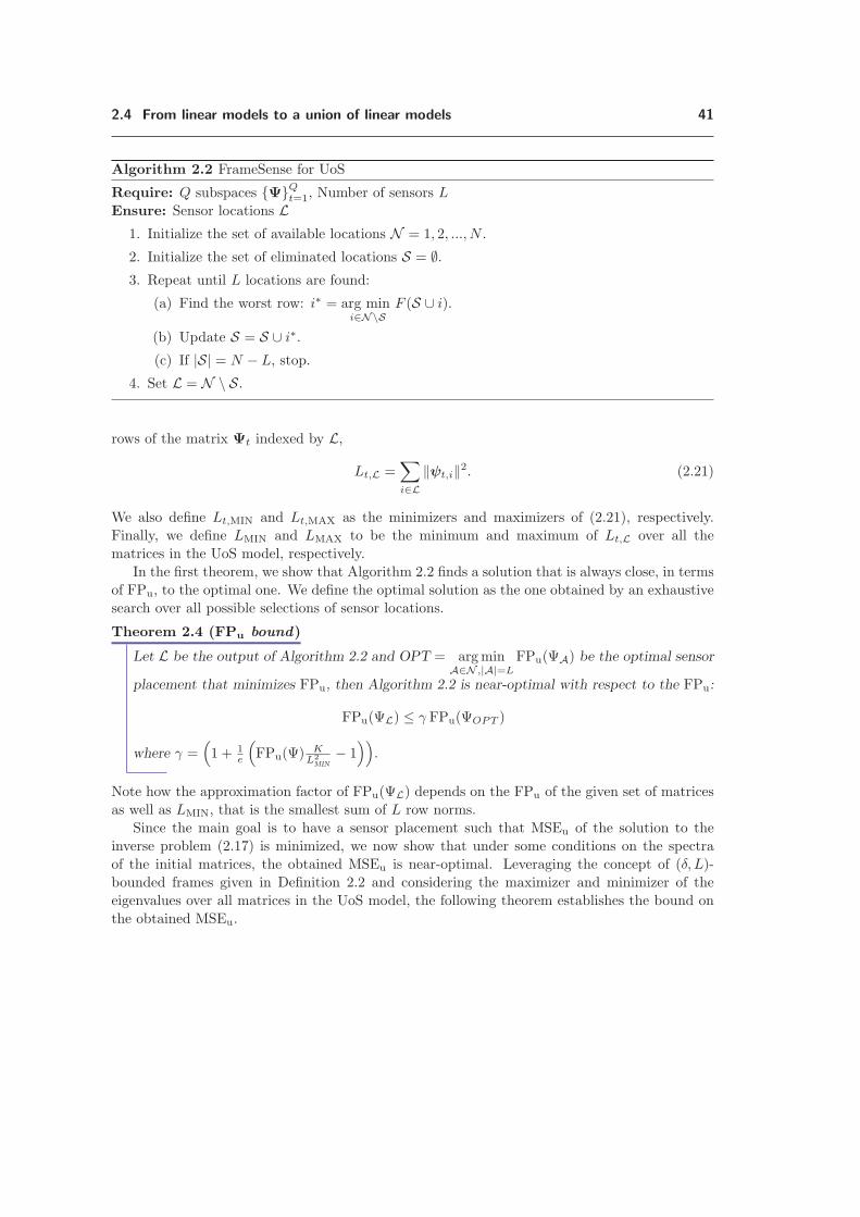
2.4 From linear models to a union of linear models 41
Algorithm 2.2 FrameSense for UoS
Require: Q subspaces {Ψ}Qt=1, Number of sensors L
Ensure: Sensor locations L1. Initialize the set of available locations N = 1, 2, ..., N .
2. Initialize the set of eliminated locations S = ∅.3. Repeat until L locations are found:
(a) Find the worst row: i∗ = arg mini∈N\S
F (S ∪ i).
(b) Update S = S ∪ i∗.
(c) If |S| = N − L, stop.
4. Set L = N \ S.
rows of the matrix Ψt indexed by L,
Lt,L =∑i∈L
‖ψt,i‖2. (2.21)
We also define Lt,MIN and Lt,MAX as the minimizers and maximizers of (2.21), respectively.
Finally, we define LMIN and LMAX to be the minimum and maximum of Lt,L over all the
matrices in the UoS model, respectively.
In the first theorem, we show that Algorithm 2.2 finds a solution that is always close, in terms
of FPu, to the optimal one. We define the optimal solution as the one obtained by an exhaustive
search over all possible selections of sensor locations.
Theorem 2.4 (FPu bound)
Let L be the output of Algorithm 2.2 and OPT = argminA∈N ,|A|=L
FPu(ΨA) be the optimal sensor
placement that minimizes FPu, then Algorithm 2.2 is near-optimal with respect to the FPu:
FPu(ΨL) ≤ γ FPu(ΨOPT )
where γ =(1 + 1
e
(FPu(Ψ) K
L2MIN
− 1))
.
Note how the approximation factor of FPu(ΨL) depends on the FPu of the given set of matrices
as well as LMIN, that is the smallest sum of L row norms.
Since the main goal is to have a sensor placement such that MSEu of the solution to the
inverse problem (2.17) is minimized, we now show that under some conditions on the spectra
of the initial matrices, the obtained MSEu is near-optimal. Leveraging the concept of (δ, L)-
bounded frames given in Definition 2.2 and considering the maximizer and minimizer of the
eigenvalues over all matrices in the UoS model, the following theorem establishes the bound on
the obtained MSEu.

42 Sensors and sources placement optimization
Theorem 2.5 (MSEu bound for (δ, L)-bounded frames)
For a set of Q (δ, L)-bounded frames {Ψt}Qt=1, let L be the output of Algorithm 2.2 and
OPT = argminA∈N ,|A|=L
MSEu(QA) be the optimal sensor placement that minimizes MSEu, then
Algorithm 2.2 is near-optimal with respect to the MSEu:
MSEu(QL) ≤ ηMSEu(QOPT )
with η = γ LMAX
LMIN
(d+δ)2
(d−δ)2 where d = LMEANQKTOT
and LMEAN is the average value of Lt,L and γ is the
approximation factor for the FPu introduced in Theorem 2.4.
Thus, minimizing FPu also results in a placement that is near-optimal with respect to MSEu as
desired. Note that Theorem 2.4 and 2.5 are respectively the extensions of Theorem 2.2 and 2.3
for the FrameSense algorithm adapted to the UoS model.
Note that the proofs of the Theorem 2.4 and 2.5 follow the same strategy used for Theorem
2.2 and 2.3, respectively. Therefore, they do not provide a significant amount of information and
are omitted.
2.4.2 Experimental results
In this section we aim at evaluating two factors: how well Algorithm 2.2 performs with
respect to other sensor placement algorithms for the UoS model and the advantages of using a
UoS model over a standard approach based on the SoS one. For both experiments, we considered
three subspaces spanned by Gaussian random matrices Ψt ∈ R100×10. Therefore, we assume the
physical field f ∈ R100 to lie in three 1-dimensional subspaces.
In the first experiment, we compared Algorithm 2.2 with a greedy algorithm optimizing
directly the MSEu and a random algorithm choosing uniformly among all the possible locations.
We varied the number of placed sensors and measured the MSEu obtained by each algorithm.
The results are shown in Figure 2.10, where we note that the algorithm based on FPu outperforms
the other two. Furthermore, we underline that a direct greedy optimization of the MSE is not
effective and does not show any performance gains compared to a random placement.
In the second experiment, we compared the quality of the inverse problem solution when the
physical field f is modeled as a UoS or a SoS, respectively. As mentioned in Section 2.4, it is
possible to represent a UoS modeled by Q matrices with a single matrix spanning the SoS. For
each model, the FPu is used to select the rows and we measure the MSEu on the output matrices.
For the UoS, we assign equal weights to the different subspaces. The results are shown in Figure
2.11. Notice that the SoS model is 30-dimensional since the three subspaces are with probability
one orthogonal to each other. Therefore, the solution of the inverse problem for the SoS model
when L < 30 is not unique and the obtained MSE values for the SoS model under this threshold
cannot be fairly compared to the UoS case. However, when we compare the performance for
L ≥ 30, we highlight that UoS has on average a 48.5 dB advantage. Therefore, we underline two
significant advantages of the UoS model over the SoS model:
1. It is possible to use less sensors while obtaining a higher precision.
2. The achieved MSEu for UoS is significantly better even for the same number of sensors.
While this result was expected, it is not trivial. In fact, finding a sensor placement that achieves
a good MSE for all the three matrices is a harder problem and could have counterbalanced the

2.5 Near-optimal source placement for linear physical fields 43
20 30 40 50 60
10��
100
Number of sensors L
MS
Eu
FPu
MSEu
Random
Figure 2.10: Performance evaluation of the three sensor placement algorithms on randomly
generated subspaces. We considered Ψ ∈ R100×10 and varied the number of sensors placed while
measuring the obtained MSEu. Note how the algorithm based on the FP outperforms the other
two.
reduced number of parameters to estimate.
2.5 Near-optimal source placement for linear physical fields
In Section 2.1, we introduced the concept of physical fields linearly generated by a set of
sources and stated the source placement problem as the selection of the optimal sources to
generate a set of physical fields lying on a known subspace T. We differentiated between two
scenarios according the presence of noise in the target field f . The source placement problem
shares the same challenges as sensor placement and the design of approximation algorithms is
not straightforward.
Up to the author’s knowledge, the problem of source placement is new and has not been
studied, at least in the signal processing community. However, there are four problems that are
closely related: sensor placement, dictionary learning, dictionary selection and dimensionality
reduction.
In the first problem, we attempt to choose L rows from a matrixΨ ∈ RN×M with N > L ≥ M
such that the recovery of a vector of parameters α ∈ RM from f = ΨLα is more stable to noise.
This problem is equivalent to finding the L rows that forms the ΨL closest to a tight frame. The
details of such a problem and near-optimal algorithmic solutions were given in Section 2.3. Note
that the sensor placement problem is extremely similar to the noisy source placement, the main
difference being the possibility of the latter to define a subspace T instead of RN .
In dictionary learning, we learn a dictionary such that a set of given test vectors are precisely
represented, usually under a sparse prior. Note that dictionary learning is different from source
placement for two principal reasons: (i) the reference is not a given subspace but a set of vectors
F and (ii) we can freely optimize the dictionary elements without being forced to pick them from
Ψ. See [155] for a review of this topic.

44 Sensors and sources placement optimization
20 30 40 50 60
100
105
1010
Number of sensors L
MS
Eu
UoSSoS
Figure 2.11: Performance comparison for the linear inverse problem when the physical field f
is modeled as a UoS or a SoS. For each realization of the experiment, we randomly generated
three matrices Ψt ∈ R100×10 and Ψ is a basis for the SoS model. For both models, we considered
the greedy algorithm minimizing the FPu and we compare the obtained MSEu. Note that the
MSEu achieved by the UoS model is significantly better for all L. For L < 30 the performance of
the SoS is not measurable since the solution of its inverse problem is not unique. If we consider
L ≥ 30, the average improvement of the MSE given by the UoS model is 48.5 dB.
In dictionary selection, we form a dictionary picking a subset of elements from a larger
dictionary such that a set of given test vectors is precisely represented, usually under a sparse
prior. Dictionary selection is very similar to source placement, the main difference being the
optimization target: a subspace T ⊆ RN for source placement and a set of vectors F for dictionary
learning. The two options are equivalent when the elements of F are lying on T. If this is not
the case, we may require a different optimization strategy, such as one promoting a sparse
representation. See [36] for a detailed problem statement and a state-of-the-art solution.
Another similar problem is dimensionality reduction, where we usually attempt to approxi-
mate a set of vectors F with a K-dimensional manifold. A classical example of such a technique
is principal component analysis, where we find the K-dimensional linear subspace that minimizes
the �2 error with respect to F . Note that the noiseless source placement is a principal component
analysis constrained to select the components from a matrix Ψ instead of learning them from
the available data.
In this section, we present a set of near-optimal algorithms to solve in polynomial time
Problem 2.2 and 2.3 with guaranteed performance.
2.5.1 A near-optimal algorithm for the noiseless source placement
First, we present an approximation algorithm that solves Problem 2.2 in polynomial time
while being near-optimal with respect to the average approximation error,
Ef
[‖f − PΦSf‖22], (2.22)

2.5 Near-optimal source placement for linear physical fields 45
where PΦS is the projection operator on the subspace spanned by ΦS . Here, we assume f = ΘTx
with x being a set of i.i.d. random Gaussian variables with zero mean and unitary variance.
The proposed algorithm removes at every iteration the source that maximally reduces the
approximation error (2.22) and its details are given in Algorithm 2.3. It is a near-optimal
algorithm with respect to (2.22) and to prove such a characteristic, we first show that the chosen
cost function is supermodular, i.e. the negated cost function is submodular.
Proposition 2.1
For any source modelΦ and source placementA, the cost functionG(A) = Ef
[‖f − PΦAf‖22]
is decreasing and supermodular with A.
Proof.
First, we know that the rank of the projection operator PΦA is equal to the rank ofΦA. Moreover,
we can show that
G(A) = Ef
[‖P⊥,ΦAf‖22]=
R∑i=1
|〈f ,vi〉|2, (2.23)
where P⊥,ΦA is the orthogonal projection on the complement of the space spanned by ΦA, vi are
the eigenvector of such projection and R = N − rank(ΦA) is the dimension of the complement
space to A. Assume that an initial set A is given and consider i to be another element that we
can add to A. According to (2.23), we have two possible outcomes when we add a new element
to A:
– rank(ΦA) increases by one, we loose the i∗-th eigenvector of P⊥,ΦA and G(A) diminishes
by |〈f ,vi∗〉|2.– rank(ΦA) and G(A) do not change.
Note that these outcomes indicate that the function G(A) is always decreasing and supermodular.
In fact, the function is modular except when we add an element that does not increase rank(ΦA),making it supermodular.
We can use Proposition 2.1 jointly with Theorem 2.1 [112] to show the near-optimality of
Algorithm 2.3.
Proposition 2.2 (Near-optimality of Algorithm 2.3)
Consider a matrix Φ ∈ RN×M , a T -dimensional subspace T and assume that we want to find
the S sources S minimizing G(S). Then, Algorithm 2.3 is near-optimal and we can bound
its performance as,
G(S) ≤ 1
eG(OPT) +
(1− 1
e
)Ex
[‖f‖22] ,where S and OPT are the set optimized by Algorithm 2.3 and by an optimal algorithm,
respectively.
The proof follows from the result given in [112] and the strategy is the same as in Section 2.3.3.
Note that Algorithm 2.3 has to be worst-out greedy algorithm to satisfy the conditions given in
Nemhauser’s theorem.

46 Sensors and sources placement optimization
Finally, we explain how to compute G(A) without testing all the infinite f ∈ T. Assume that
f = ΘTx and x are i.i.d. zero-mean Gaussian random variables with σ2 = 1. For any given set
A, it is possible to prove the following equality,
G(A) =∑i∈A
R∑j=1
|〈θi,vj〉|2,
where θi is the i-th column of ΘT. In other words, it is just possible to test each column of ΦSto compute exactly G(A).
Algorithm 2.3 Noiseless Source Placement
Require: Linear Model Φ, Number of sources S
Ensure: Sources locations S
1. Initialize the available source locations, S = {1, . . . ,M}.2. Repeat until L locations are found
(a) If |S| = L, stop.
(b) Find the optimal column to remove, i∗ = argmaxi∈S G (S \ i).(c) Update the available source locations, S = S \ i∗.
2.6 Application: thermal monitoring of many-core processors
An application where our sensor placement algorithm shows its performance at its best is
the thermal monitoring of many-core processors. In this section, we first state and motivate the
problem and then we describe the details of our state-of-the-art solution.
Technological advancements of the lithographic process steadily increase the amount of com-
ponents that can be placed on a single die. If we assume that the power consumed by these
components does not decreases significantly with technological advances [25], we have an in-
crease of the power density, and subsequently, of the produced heat.
Most of many-core system-on-chips (SoC) have their performance limited by such increased
heat density. More precisely, unfavorable thermal patterns increase the overall failure rate of
the system [118], reduce performance [26], significantly increase leakage power consumption and
cooling costs [44, 118].
In the past, passive thermal management schemes were used to limit the problems induced by
thermal phenomena. For example, designers would organize the floorplan by placing the highest
power density components closer to the heat sink [69]. However, in recent architectures such
components are not easily identifiable since they depend on the workload execution patterns
and, unfortunately, these patterns are not fully known at design time. Furthermore, these issues
are amplified in many-core designs, where thermal hot-spots are generated without a clear spatio-
temporal pattern due to the dynamic execution of tasks, based on external service requests, as
well as the dynamic assignment to cores by the many-core OS [43, 44]. An example of these
architecture and their critical thermal behavior is shown in Figure 2.12, where one can observe
the layout of a 64-cores architecture designed by STM [20, 102] and an example of its thermal

2.6 Application: thermal monitoring of many-core processors 47
distribution at run-time. Note how the cores are not anymore regularly organized and how they
tend to spread non-uniformly. Such irregularity is forced by the complex constraints imposed
during the floorplanning optimization and generates irregular thermal distributions with possibly
many unpredictable hot-spots.
Thermal sensors have been already included into SoC designs [20], however positions have
only been manually tuned because the knowledge of the temperature in a couple of locations was,
until now, sufficient. Nowadays, it has become necessary to precisely measure the temperature
distribution of the entire die and optimize the workload of the different components to maximize
the performance while avoiding hotspots or large gradients of temperature.
At the same time, each temperature sensor has a significant impact in terms of occupied area
and consumed power, therefore we would like to place as few sensors as possible. Moreover, it is
not yet clear how to optimize their placement to maximize the collected information about the
thermal distribution. In fact, such aspects are quite complex and recently received significant
attention [42, 106, 113, 128, 132, 143, 176].
2.6.1 Prior art
The thermal distribution of a SoC can be estimated using three different strategies:
– Solution of the direct problem, given the heat sources and the physical model of the tem-
perature diffusion process,
– Solution of an optimization problem, given the value of the temperature in some locations
and some a-priori model for the thermal distributions.
– Empirical approaches, where the thermal distribution is estimated by means of external
devices, such as infrared cameras.
The first approach requires the knowledge of the heat sources, that can be ascribed to the
knowledge of the detailed power consumption of the different components. Often, performance
counters [81, 83] are used to estimate the power traces at run-time. However, the estimation of
the thermal distributions from the power traces is a computationally expensive task, requiring
complex thermal models characterizing the thermal dissipation of the SoC. Recently, [88] pro-
posed to reduce the complexity of these methods by using directly the performance counter to
estimate the temperature, without the intermediate step represented by the power traces.
On the other hand, the optimization problems are generally ill-posed. In fact, it is impossible
to solve the inverse problem from few, spatially localized, noisy measurements without some
a-priori constraints on the thermal map, such as limited bandwidth [42]. The performance is
significantly impacted by the small number of available sensors and the structure we consider
for the thermal map, i.e. the a-priori information. Nowroz et al. [113] proposed a low-pass
approximation strategy to reduce the number of sensors that are placed using an energy-based
algorithm. This sensor allocation algorithm has been improved by Reda et al. [132] using a
heuristic iterative approach to approximate an NP-hard problem. The authors in [87] proposed a
grid-based uniform sensor placement followed by interpolation to approximate the temperature.
These works estimated entire thermal maps, but the precision of the estimates is limited by the
sub-optimality of the chosen models for the thermal distribution.
Other works have notable performance but are not focused on the estimation of the entire
thermal map. Namely, the approach in [174] employs the correlation in power distribution to
estimate the expected value of temperature at different locations of the chip using a dynamically

48 Sensors and sources placement optimization
(a)
(b)
Figure 2.12: (a) The layout of the considered 64 cores processor designed by STM, where
each color represents a different core connected to its own L1 cache. The white part contains
components with a limited thermal impact. (b) An example of a thermal distribution of such a
processor, where the colormap spans the temperature between 65◦C (dark blue) and 90◦C (red).
tuned Kalman filter. The problem of noisy measurements has also been already considered; for
example, a method based on the correlation between the different sensor has been presented in
[173].
Recently, different researchers studied the estimation of the entire thermal map based on
the temperature correlation between different locations [128, 176]. First, we have proposed in
[128] an approach where we approximate the data with a low dimensional linear model based

2.6 Application: thermal monitoring of many-core processors 49
on such correlations. Such method brought an intuitive interpretation of the sensor placement
problem together with appealing performance. However, we have showed in [127] that the sensor
placement algorithms can be further improved. Contemporaneously, Zhou et al. proposed a
reconstruction algorithm and an optimization of the sensor placement based on information
theory [176]. Their reconstruction algorithm is essentially equivalent to the one proposed in [128],
without the low-dimensional approximation. Such difference, as we will see in the numerical
experiments, has a significant impact on the stability with respect to the noise affecting the
measurements.
The methods based on external cameras [8–10, 85, 132] are generally considered to be the
most precise ones. However, the increased precision comes at the cost of practical considerations.
In fact, such methods cannot be used for run-time operations and are generally studied for two
different purposes: the calibration of the on-chip temperature sensors [85] or the study of the
thermal behavior of prototypes at design phase [8–10, 132].
We underline the existence of hybrid methods, mixing techniques taken by the different
methods. For example, the authors of [143, 174] propose to use the information coming from
the thermal sensors together with the performance counters to estimate the thermal distribution.
This approach reduces the computational complexity of the methods solely based on performance
counters and mitigates the effects of the noise corrupting the thermal sensors. The fusion and the
integration of the two data sources to obtain the thermal distributions is usually accomplished by
a Kalman filter. Such implementations have shown the ability to track precisely the temperature
profile at the cost of the computational complexity, which is significantly higher than standard
approaches.
In this section, we consider the following two sub-problems as core to design an efficient
thermal monitoring system:
– Thermal distribution reconstruction: Given the temperature measured with L sensors
at known locations, how do we precisely estimate the temperature distribution on the whole
die?
– Sensor placement optimization: Given a fixed amount of sensors, where do we place
them so that we maximize the precision of the reconstructed thermal distributions?
Then, we propose to base the solutions of the aforementioned two sub-problems on the use
of a linear low-dimensional subspace to represent the thermal distributions. Such models are
interesting because they are sufficiently precise while being extremely simple, thus requiring
limited computational resources.
Linear models have been already considered in the past for thermal monitoring applications
[42, 128], but many questions have been raised regarding their practical feasibility.
First, such models must be optimized and they require a set of thermal distributions representing
the operations of the SoC under all the possible workloads. It is clear that such data is hard
to gather at the design phase; that is when we would like to optimize the sensors locations.
More precisely, we need to know three main inputs to simulate the thermal distributions : the
floorplan, the workload of the SoC, and the power traces of the components under such workload.
In this chapter of the thesis, we show that it is not necessary to have an exact description of the
typical workload at design-time to reconstruct precisely the thermal distribution at run-time. In
fact, we show that it is possible to optimize the model and place the sensors using a randomly
generated workload without having significant losses in terms of reconstruction error.
Second, the performance of linear models depends strongly on the locations of the sensors. In fact,

50 Sensors and sources placement optimization
Floorplan Expected workload
Thermal simulation
Linear model training
Thermal distributions
Sensor placement
Linear model
Sensor placement
Design-time Flow
Thermal distribution estimator
Thermal distribution
Run-time Flow
Sensor measurements
Figure 2.13: Flow of the proposed framework, where data structures and algorithms are de-
picted with white and gray blocks, respectively. Note that the flow is divided in two parts: one
for the design of the system and one for the run-time operations. The inputs to the systems
are the floorplan of the SoC and the expected workload, while the outputs are a training set
F of thermal distributions f , the linear model Ψ obtained from the training set F , the sensor
placement L and the estimated thermal distribution f .
the noise corrupting the collected measurements can be dramatically amplified if the sensors are
misplaced. We propose to optimize the sensor placement using FrameSense, the greedy algorithm
proposed in Section 2.3.3.
The proposed framework improves significantly the monitoring performance over the state
of the art. For example, consider the 64-cores architecture shown in Figure 2.12a and typical
scenario of one temperature sensor per core corrupted by a noise with variance σ2 = 4, we can
improve the reconstruction error from ≈ 3◦C to less than 1.4◦C. Even if we increase the amount
of temperature sensors by 50%, that is from 64 to 96, the previous methods [113, 176] can only
reach an average reconstruction error of ≈ 2.4◦C, while our method can go down to almost 1◦C.
2.6.2 A near-optimal thermal monitoring framework
Here, we propose a framework for the problem of thermal monitoring of a many-core SoC.
We assume we know the floorplan of the SoC and the time-varying power consumption of its
components when handling some expected workload. The proposed framework is divided in two
parts: design-time and run-time algorithms. We give a visual description of the framework in
Figure 2.13. At design-time, we have three main phases:
– Thermal simulation, that provides a set F of thermal distributions representing the thermal
behavior of the considered SoC.
– Model learning, where we learn the structure of the thermal distribution from the given
set F . We call the model Ψ and it has a fundamental role both for the reconstruction of

2.6 Application: thermal monitoring of many-core processors 51
thermal distribution and the optimization of the sensor placement.
– Sensor placement optimization, where we choose the optimal sensor positions L according
to the model Ψ.
The thermal simulation part is not covered in this thesis, since it is possible to choose different
algorithms and methods depending on the SoC architecture. In our case, we use 3D-ICE [148],
a flexible fast compact transient thermal model for the thermal simulations of SoCs.
At run-time, the system is extremely simple: we collect the measurements from the sensors
and, knowing the linear model and the sensors positions, we estimate the thermal distribution
using an optimal least square estimator.
In what follows, we describe in details each part of the framework in terms of mathematical
abstraction and algorithmic solutions.
2.6.3 Sensing and recovery of thermal distributions
We start the description of the proposed framework from the run-time phase. More precisely,
we mathematically state the concept of temperature sensing and the recovery of the thermal
distribution using the sensed data.
Consider a given SoC die and its thermal distribution f(x) at a given time, where x indicates
the multi-dimensional spatial location. While f(x) is a continuous spatial function, we consider
it to be discretized and vectorized as a vector f ∈ RN , where N represents the desired resolution.
Note that the vectorization of the thermal distribution does not induce any loss of information
beside the one given by the discretization.
We denote the set indicating the L < N sensor positions as L and we define the measured
temperatures as fL ∈ RL. Note that the subscript L indicates that we kept only the elements
of f indexed by the elements of L.The problem of recovering a complex information, such as the thermal distribution f , from
a limited number of measurements, i.e. fL, must rely on some hidden structure available in the
thermal distribution. In fact, without a structure we would face an undetermined problem and
it would be impossible to uniquely recover the data f from the measurements fL.While there exists many strategies to model data structures, the thermal monitoring scenario
constrains the choice to models allowing a fast, efficient and reliable reconstruction. In this
work, we consider a linear subspace model, such as the one in [128]. More precisely, given a K-
dimensional linear model defined by a matrixΨ ∈ RN×K , we model the temperature distributions
as,
f = Ψα,
where α ∈ RK is the K-dimensional parametrization of Ψ. In other words, if the model Ψ
is sufficiently precise for the thermal distributions, then α is a compact representation of f .
Namely, knowing α is equivalent to know the temperature distribution f .
Then, when we consider a set of measurements fL we obtain the following pruned linear
system,
fL = ΨLα, (2.24)
where ΨL ∈ RL×K is the collection of L rows of Ψ indexed by L. We note that if L ≤ K and if
rank (ΨL) = K, we can uniquely reconstruct f from the measured data fL as
f = ΨΨL†(fL + n), (2.25)

52 Sensors and sources placement optimization
Algorithm 2.4 Thermal distribution estimator
Require: Linear model Ψ, Sensor locations L, thermal distribution mean μ
Ensure: Estimated thermal distribution f
1: Collect the sensor measurements fL2: Estimate thermal distribution: f = ΨΨL†(fL − μL)†μ
where f is the estimated thermal distribution, n represents the noise in the measurements and
ΨL† is the Moore-Penrose pseudoinverse of ΨL.The pseudo code of the thermal distribution estimator is given in Algorithm 2.4, where we
note the simplicity of the operations. Nonetheless, such an estimator is optimal if the noise n
satisfies certains statistical conditions, such as being i.i.d. Gaussian. The performance of such an
estimator depends mostly on two aspects: the quality of the linear model and the optimization
of the sensor locations L.More precisely, the following two questions must be answered to validate and strengthen the
proposed framework:
– How can we design a reliable and precise model Ψ?
– How do we choose the optimal sensor placement L?In what follows, we discuss and answer these two questions.
2.6.4 Training the linear model for thermal distributions
Assume that we are given a representative set of M possible thermal maps F = {fi}Mi=1 and
we would like to find a model Ψ that can precisely represent such a dataset with K-dimensional
parameters α. In theory, the set F should represent all the possible thermal distributions that
the SoC could produce during operations. While this assumption is necessary in theory, we will
show in the numerical experiments that we can relax it significantly.
Given the model Ψ ∈ RN×K and a thermal distribution f , we obtain the approximated
thermal distribution f by the following projection onto the model,
f = ΨΨ†f .
Then, we evaluate the quality of the model by measuring the approximation error ε, that is
defined as
ε = EF‖f − f‖2,
where the subscript F indicates that the expectation is taken over all the training set F .
In what follows, we propose to learn the model Ψ from the principal component analysis
(PCA) of the temperature distributions. Note that we considered also other models, such as
the one based on non-negative matrix factorization, but their performance were not sufficiently
interesting for thermal monitoring.
Principal component analysis
Given F , the PCA generates the model Ψ formed by a set of K orthonormal vectors, known
as principal components. The PCA is defined so that the first principal component corresponds

2.6 Application: thermal monitoring of many-core processors 53
Algorithm 2.5 Linear model training
Require: Training set F .
Ensure: Linear model Ψ, thermal distribution mean μ.
1: Compute the mean: μ = EF [f ].2: Compute the covariance matrix: Σf = EF [ff∗].3: Compute the first K eigenvectors of Σf .
4: Form Ψ by using the eigenvectors as its columns.
to the direction of the largest variance (i.e. representing as much of the variability in the data
as possible), and each successive component has the highest variance in the subspace orthogonal
to one spanned by the preceding components. Therefore, the PCA finds an orthonormal basis
that spans the K dimensional subspace containing the largest amount of information on F (in
the MSE sense). In other words, the PCA generates the optimal K-dimensional subspace that
minimizes the approximation error of the given the training set F .
The solution of the PCA can be analytically computed as the K eigenvectors corresponding
to the K largest eigenvalues of the correlation matrix Σf = Ef [ff∗]. Consequently, most of
the technical difficulties of PCA relate to the estimation of Σf , in particular when the data is
incomplete or noisy.
PCA has been already proposed to model thermal distributions and showed promising results
[128]. In fact, if the thermal distributions of F are well approximated by a K dimensional
subspace, then the PCA generates the optimal model Ψ.
In certain scenarios, characterized by a limited amount of available resources, we may prefer
other methods. For example, certain architectures cannot afford the memory load to store the
matrix Ψ. Prior works [42, 113] proposed to use models based on the discrete cosine transform
(DCT). Such models have a clear advantage in terms of memory used, since they do not require
to store Ψ in the system.
Unfortunately, the DCT based models do not outperform the PCA model as we do not design
entirely Ψ. Moreover, it is not possible to exploit all the traditional computational advantages
of DCT transforms. In fact, while we can compute efficiently the DCT transform, once we select
some rows to represent the sensors measurements we destroy the structure of the DCT transform
and loose most computational advantages.
A comparison of the reconstruction performance between PCA and DCT is proposed in
Section 2.6.6 and it shows that PCA is always the best choice unless there exist stringent limits
on the memory available for run-time operations. Therefore, we assume to use the PCA for the
linear model training and we show its pseudo-code in Algorithm 2.5.
2.6.5 Optimization of sensor placement
As explained in Section 2.6.3, the reconstruction of thermal distributions relates to precisely
estimating f from possibly noisy measurements fL.In a typical scenario, we are given a number of sensors L and a set P of P possible locations,
that is a subset of the area of the SoC. Moreover, assume that either we have or can find an
optimized linear model Ψ for the thermal distributions F , as described in Section 2.6.4. Then,
we would like to find the sensor placement L that minimizes the reconstruction error ξ of the

54 Sensors and sources placement optimization
Name of the dataset Content is parallel? is realistic? Resolution # of thermal maps
Dataset 0 Matrix mult. � � 20× 28 3000
Dataset 1 Merge-sort � � 20× 28 3000
Dataset 2 Random (�) � 20× 28 3000
Table 2.1: Characteristics of the considered datasets for the training of the proposed method
and the evaluation of its performance
thermal distributions,
ξ = E‖f − f‖22.
The reconstruction error depends mostly on the eigenvalues λi of the matrix Ψ∗LΨL, see Ap-
pendix 2.10.2 for a formal proof. If the model Ψ is sufficiently precise, that is the approximation
error ε is smaller than the noise power σ2, the reconstruction error can be approximated as
ξ = E‖f − f‖22 ≈ σ2K∑i=1
1
λi(ΨL).
Significant research efforts have been directed towards the design of an efficient algorithm
with polynomial complexity that can find a sensor placement minimizing the reconstruction
error. For the specific case of thermal management, early efforts focused on the localization of
hotspots, which are localized peaks of temperature. However, such techniques are bound to fail
as technology progresses, since the number and the unpredictability of hotspots are increasing.
Recently, researchers refocused their efforts on studying methods to estimate the entire thermal
distribution from the few collected measurements. Such methods are similar in terms of scope and
approach to the ones designed for generic linear problems, see Section 2.3. For this application,
we propose to use FrameSense, the algorithm presented in Section 2.3.3, for which we proved the
near-optimality in terms of MSE.
2.6.6 Numerical experiments on a 64 cores SoC
The experimental setup
In this section we test the proposed models with a real high-end many-core architecture
designed for signal processing and data-intensive embedded applications that has been already
taped out. This architecture hosts 64 cores designed for multiple program multiple data parallel
computing. The cores are grouped in four clusters with independent power and clock domains and
connected with a fully asynchronous network-on-chip, see Figure 2.12a. The chip is implemented
with STM 28nm CMOS technology [149] and each cluster has a power density of 55 W/cm2.
Note that we have also analyzed the performance of the proposed thermal monitoring algorithm
on a 8-core Niagara [131]. However, we do not describe the latter experiment in this thesis given
the similarity of the results.
The power traces of the SoC components are generated by running benchmarks on an
instruction-level architectural simulator equipped with an accurate and detailed power model.
Such power traces are generated with a time resolution of 1 ms and are successively used to
generate a set of thermal distributions representing the temperature of the SoC at run-time. As

2.6 Application: thermal monitoring of many-core processors 55
46
810
1214
16�
��
���
���
���
���
���
�����0�10
Num
ber
of p
aram
eter
s
MSE [dB]A
ppro
xim
atio
n er
ror
for
Dat
aset
0
PC
AD
CT
(a)Matrix-vectormultiplica
tion
46
810
1214
16�
��
���
���
���
���
���
�����0�10
Num
ber
of p
aram
eter
s
MSE [dB]
App
roxi
mat
ion
erro
r fo
r D
atas
et 1
PC
AD
CT
(b)Sortingalgorith
m
46
810
1214
16�
��
���
���
���
���
���
�����0�10
Num
ber
of p
aram
eter
s
MSE [dB]
App
roxi
mat
ion
erro
r fo
r D
atas
et 2
PC
AD
CT
(c)Random
workload
Figure
2.14:Approxim
ationerrors
asafunctionofthenumber
ofparametersK
ofthelinearmodel
Ψforeach
dataset.
Theshaded
areabou
ndsthe5thandthe95th
percentile
oftheap
proxim
ationerrorof
theestimatedthermaldistributionsforeach
dataset.
First,
note
thatPCA
isalwaystheoptimalmodelandthesignificantperform
ance
gapcomparedto
theDCTone.
Thisisnotsurprisingsince
theDCTmodelhasfewer
degrees
offreedom.Second,weunderlinethatthediffi
cultyoflearningthemodeldep
endsonthecomplexity
ofthedataset.
Forexample,Dataset1describes
thethermaldistributionsforasortingalgorithm
thatcannotbeim
plementedwith
highparallelism.Such
thermaldistributionsare
extrem
elyheterogeneousan
dharder
torepresents
withalinearmodel,leadingto
a
higher
approxim
ationerrorcomparedto
theother
twodatasets.Third,thevariationforDataset2is
significantlyhigher
dueto
the
random
nature
oftheworkload.

56 Sensors and sources placement optimization
a thermal simulator, we chose 3D-ICE [148], that is based on a transient and compact thermal
model, and we tuned it for the STM technology [20, 102].
To insure that the thermal distributions match correctly the layout of the many-core archi-
tecture, the floorplan that maps the power consumption of the hardware units (cores, memories,
interconnects, etc.) to the surface of the silicon die has been extracted by processing the post
synthesis layout.
Moreover, to compute precise and realistic temperatures, we initially implemented a model of
the chip on a commercial computational fluid dynamics program, ANSYS CFX [7]. The purpose
of this setup is to extract the correct values for the boundary conditions of the heat dissipation
in a steady state worst case simulation. Once the heat transfer coefficients are obtained, the
silicon die is modeled in 3D-ICE to perform the transient thermal simulations. Note that the
thermal properties of materials as well as geometries of the package are taken from [164].
While we analyzed thermal distributions originated by several workloads, in this section we
discuss the results for three fundamental ones. Such workloads are designed to represent exhaus-
tively the thermal scenarios that can be expected by such a 64-cores SoC. The characteristics of
the three datasets are summarized in Table 2.1 and described more in details in what follows.
The first benchmark is a parallel 64x64 matrix-matrix multiplication that distributes the load
evenly among the 64 available processing units. The multiplication is repeated to generate a load
of 75 ms during which a uniform and constant heat flux is produced as in the typical scenario of
an extremely parallel application.
The second benchmark is a two-phases sorting algorithm run on a vector storing 16K float
values. In the first phase, individual cores are activated in sequence to sort their corresponding
sixteenth part of the input using the insertion sort algorithm. Then, in the second phase, the
cores run in parallel to merge the ordered sub-vectors to get the final output, as in the merge
sort algorithm. The number of active cores in this latter phase is halved at every iteration. The
whole application is repeated on different input vectors to generate a trace of 150 ms reproducing
the scenario of a parallel application with data dependencies.
The third dataset is generated by means of Poisson processes bounded by the idle and max-
imum power consumptions of cores, memories and other hardware modules in the chip. Such
a workload, while being synthetic and randomly generated, has a significant role since we show
the possibility to use it to train the model and optimize the sensor placement successfully for
the real data.
The obtained thermal distributions are further processed for Matlab. Given the symmetry of
the architecture, all the numerical simulations consider each cluster of 16 cores independently.
Note that such strategy does not imply any loss of detail or precision.
Performance comparison between the different approximation models
In this section, we compare the performance of the linear model based on PCA proposed in
Section 2.6.4 against the model based on the DCT transform on the three dataset representing the
different workloads described in Section 2.6.6. For the DCT model, we considered an optimized
version of the model proposed in [113], where the components of the model are chosen by assuming
a generic low-pass profile without studying the distribution of the specific architecture. More
precisely, we select the components of the DCT transform showing the average largest coefficients
over the thermal distributions belonging to the chosen training set.
For each dataset, we measure the approximation error ε given by each model for an increasing

2.6 Application: thermal monitoring of many-core processors 57
0.1 1 10 100���
���
���
���
���
��
0
�
10
Percentage of the available training dataset
Qua
lity
ratio
[
dB]
Approximation error when learning the PCA model
Random workloadMultiplicationSort
Figure 2.15: Quality of the linear model learned by the PCA, when only a random part of the
training set is available. We measure the quality using the cost function (2.26). Note that if
ρ(δ) = 1, there is no loss of precision and if ρ(δ) < 10 the reconstruction errors have the same
order of magnitude with respect to the model learned by an exact and complete dataset. These
results indicate that the quality of the model is not severely impacted by imprecise or incomplete
training sets A.
number of parameters, K = {4, 6, 8, 10, 12, 14, 16}. The results are given in Figure 2.14. We note
two main facts:
– The performance achieved by the PCA is significantly better in terms of SNR ( ≥ 10dB)
than that of the DCT model. This is expected since the PCA generates an optimized
model, while the DCT-based model simply selects K columns out of a given set.
– The performance gap between PCA and DCT increases with K, meaning that PCA better
exploits the increased degrees of freedom.
With this numerical experiment, we tested the capability of the proposed techniques to cap-
ture a precise low-dimensional linear modelΨ from a training set F . Note that the approximation
error is just one of the aspects that defines the performance of a thermal monitoring system, but
it is often the critical one to have a precise thermal reconstruction.
Learning individual models for temperature distributions
When learning the model Ψ for a certain SoC under a given workload, it is fundamental to
understand how difficult it is to learn Ψ reliably when a part of the training set is not available.
In other words, we would like to evaluate the error caused by the use of incomplete training sets
F .

58 Sensors and sources placement optimization
Consider a training set F of M thermal maps and define A ⊆ F a subset of �δM� randomly
selected thermal distributions. Note that, the parameter δ ∈ [0, 1] represents the percentage of
thermal maps that we use for training. Then, we use A to train the linear model and we measure
the approximation error on the entire dataset F . Note that when δ = 0 it is impossible to learn
the model and it is easier for increasing values of δ.
For each dataset F , we fix K and test the performance of the PCA for a varying value of
δ. We measure the performance reduction as the ratio ρ(δ) between the approximation error
obtained while learning with the reduced training set, denoted as ε(δ), and the approximation
error with an entire training set, denoted as ε. More precisely, we define such ratio as
ρ(δ) = 10 log10ε
ε(δ). (2.26)
When ρ(δ) is close to one, the performance of the model is not significantly impacted by the lack
of data; the lower the value, the higher the sensitivity of the model to the lack of training data.
The results are given in Figure 2.15, where we note that for each dataset, a subset of 1% of
randomly selected thermal distributions is enough to have ρ(δ) close to one. Therefore, having
a non-exhaustive dataset is in general not critical to successfully learn the PCA model. We can
further strengthen such a result by showing in the next section that random power traces on a
realistic floorplan are sufficient to learn a reliable model Ψ.
Learning with random workloads
While designing an SoC and its thermal monitoring system, we may not yet know the work-
load. It would be then impossible to optimize the model and the sensor placement. Here, we
show that actually we do not need the power-traces. In particular, we can use the randomly
generated ones while maintaining reasonably good performance.
In an ideal scenario, we know exactly the thermal distributions set F generated by the
expected workload. Assume that �δM� thermal distributions of F are not known, where δ is
defined as in Section 2.6.6. We replace the missing thermal distributions with the ones obtained
using random power traces, such as the ones generated for the first dataset. We would like to
measure the loss of precision of the learned model due to the increasing use of random data.
Again, we use the cost function defined in (2.26) and the results are given in Figure 2.16. While
a certain loss of precision can be observed, it is extremely limited. Moreover, if we consider to
train the model exclusively with the thermal distributions generated by random power-traces,
that is δ → 0, then the reconstruction error is of the same order of magnitude, that is ρ(δ) < 10.
Our result indicates the possibility to learn the model and place the sensors without knowing
the expected workload, it suffices to use a random one.
Reconstruction error comparison between different approximation models
The approximation error ε defines the quality of the model but it is not the only merit
figure. Once we place the sensors, the reconstruction error ξ may significantly vary due to the
conditioning of the inverse problem (2.24). Therefore, we compare the different models described
in Section 2.6.4 according to their reconstruction error for different amounts of sensors.
We test each model for K = {4, 6, 8, . . . , 16} and L = {4, 6, 8, . . . , 16}. Note that if K
decreases, it is easier to estimate the parameters but then the approximation error increases. On
the other hand, if K increases it is harder to estimate the parameters α but the model Ψ is more

2.6 Application: thermal monitoring of many-core processors 59
0.1 1 10 100���
��
0
�
Percentage of the real dataset used for learning
Qua
lity
ratio
[d
B]
Cross learning with random data
MultiplicationSort
Figure 2.16: Quality of the linear model learned by PCA, when only a random part of the
training set is exact, and the other one is produced by random power traces. We measure the
quality using the cost function (2.26). Note that if ρ(δ) = 1, there is no loss of precision and if
ρ(δ) < 10 the reconstruction errors have the same order of magnitude with respect to the model
learned by an exact and complete dataset. Even in the worst case scenario, the approximation
error is of the same order of magnitude with respect to the optimal one.
precise. The choice of the optimal K is not trivial and we perform a search over the parameter
space. More precisely, for each L and each model, we measure the minimum reconstruction error
obtained with respect to the varying model complexity K.
The results are given in Figure 2.17, where we note that the PCA is the best model in terms
of reconstruction error. Moreover, the advantage of the PCA with respect to the DCT in terms
of approximation error is maintained in terms of reconstruction error. Therefore, according to
our experiments, PCA is the technique generating the model with the best approximation and
least reconstruction error.
Performance comparison between sensor placement algorithms
As we have already mentioned, there are many parameters impacting the performance of
a thermal monitoring system, such as the number of parameters, the chosen model and the
reconstruction technique. Here, we would like to compare the quality of different sensor placement
algorithms while maintaining all other parameters fixed.
Therefore, we choose as a linear model the one optimized using the PCA. Then, we optimize
the sensor placement using a few algorithms from the literature and measure the reconstruction
error. For each algorithm, the reconstruction error is computed for different errors of L and K,

60 Sensors and sources placement optimization
46
810
1214
16�
��
���
���
���
���
���
���
�� 0 � 10
Num
ber of sensors
MSE [dB]
Reconstruction error for D
ataset 0
PC
AD
CT
(a)Matrix
-vecto
rmultip
licatio
n
46
810
1214
16�
��
���
���
���
���
���
���
�� 0 � 10
Num
ber of sensorsMSE [dB]
Reconstruction error for D
ataset 1
PC
AD
CT
(b)Sortin
galgorith
m
46
810
1214
16�
��
���
���
���
���
���
���
�� 0 � 10
Num
ber of sensors
MSE [dB]
Reconstruction error for D
ataset 2
PC
AD
CT
(c)Random
workload
Figure
2.17:Reco
nstru
ctionerro
rsasafunctio
nofthenumber
ofsen
sors
Softhelin
earmodel
Ψforeach
dataset
usin
gFrameSense
asasen
sorplacem
entalgorith
m.Theshaded
area
bou
ndsthe5th
andthe95th
percen
tileofthereco
nstru
ctionerro
rforthedifferen
t
models.
First,
note
thatthePCA
isalwaystheoptim
almodel
andthesig
nificantperfo
rmance
gapcompared
totheDCT
one.
Such
a
gapisaroundorlarger
than10dB
meaningthatthereco
nstru
ctionerro
rofthePCA
model
isatlea
stoneorder
ofmagnitu
desm
aller
thantheon
eoftheDCT
model.
Seco
nd,weunderlin
ehow
homogeneoustherm
aldistrib
utio
ns,
such
astheones
genera
tedbythe
extrem
elyparallel
workloadofDataset
0,are
easier
toreco
nstru
ct.

2.6 Application: thermal monitoring of many-core processors 61
5 10 15 2010
��
10��
100
101
Number of sensors
MS
E [d
B]
Comparison of the sensor placement algorithms
IT method�� �������� �������FrameSenseCoherence
Figure 2.18: Comparison of the reconstruction error between different sensor placement algo-
rithms when Ψ is optimized using PCA. Note that the number of parameters K is optimized
by a local search independently for each value of the number of sensors L. We underline how
FrameSense always generates a sensor placement that is either optimal or close to the optimal
value for every L.
and for each L we pick the minimum value achieved with respect to the number of parameters
K.
We tested three algorithms:
– FrameSense, based on the theoretical results we proposed in [127],
– A method based on the coherence of the measurements, that we considered in [128] for the
thermal monitoring problem,
– The information-theoretic approach described in [176], that maximizes the information
collected by the sensors,
– The energy-center allocation method proposed in [113], that places the sensors where the
temporal energy of the temperature distribution is higher.
Note that these algorithms have been designed to optimize the sensor placement for different sce-
narios and models. However, the proposed experiment is still interesting to see the performance
of such algorithms when all other parameters are fixed.
The results for the three considered datasets are shown in Figure 2.18, where we note that
FrameSense is significantly better than the other algorithms for almost every L.

62 Sensors and sources placement optimization
Performance comparison between thermal monitoring techniques
In the previous experiment, we compared the performance of the sensor placement algo-
rithms when using the linear model Ψ. As we previously mentioned, the results are interesting
and informative but they cannot be considered as a global measure of the different sensor place-
ment algorithms because most of the algorithms are designed to work jointly with a specific
reconstruction model, that may be significantly different from the considered linear one.
Therefore, we compare the following three thermal monitoring techniques:
– Our proposed method that is based on a linear model optimized using PCA and FrameSense
as sensor placement algorithm. This is an improved version of the algorithm described in
[128]; in particular, FrameSense has been proved to be theoretically near-optimal,
– The thermal monitoring approach based on spectral methods described in [113], that uses
a linear model based on the DCT and the energy-center algorithm previously described,
– The information-theoretic method proposed in [176], that uses the correlation matrix Σf
and an algorithm derived from information theory to recover the thermal distributions.
Each technique is composed by a sensor placement algorithm, a model for the temperature
distributions and a reconstruction algorithm.
In this experiment, we vary the number of sensors L = {4, 5, . . . , 23, 24} and the number
of parameters K = {4, 5, . . . , 23, 24}. We added some noise to the measured values in the
form of i.i.d. random Gaussian variables with variance σ2 = 4 ◦C to simulate the presence of
measurement errors. Then, for each L we picked the minimum reconstruction error achieved
across all possible values of K. The results are shown in Figure 2.19 where we note that for a
small number of sensors, i.e. L < 10, the performance of our proposed method and information-
theoretic method are similar. However, the gap between the two methods increases with K
in favor of FrameSense. Therefore, FrameSense with the PCA linear model achieves the best
performance. Note that the spectral method is significantly worse than the other two methods,
but this is not surprising given the use of a DCT basis, that cannot be deeply optimized.
Another interesting aspect is the role of the low-dimensional model Ψ as a regularization
mitigating the measurement noise. In fact, when using the PCA model and FrameSense and if
the number of sensors is sufficiently high, the reconstructed thermal distributions have a lower
error level with respect to the noise in the measurements collected by the sensors.
2.6.7 Comparison of the computational complexity
As a final part of the numerical experiments, we would like to analyze the computational
complexity and the memory cost of the different reconstruction methods. Note that we do not
analyze such costs for the sensor placement algorithms because it is an offline procedure and its
costs are generally not critical.
The analysis is summarized in Table 2.2. First, we note that the only significant difference
concerns the memory cost of the methods. In particular, the spectral method does not need to
store an entire matrix ΨL because the coefficients are usually stored in the system. However, if
we choose not to store the matrix but just the indices of the sensor positions and of the chosen
components, we need to compute the matrix multiplication (2.25) and the pseudo-inverse of ΨLat run-time, resulting in a significantly higher computational cost.
Therefore, the benefits of the DCT models are very limited and we indicate the PCA model to
be the optimal one for the thermal monitoring applications. As a conclusive remark, we underline

2.6 Application: thermal monitoring of many-core processors 63
5 10 15 20
100
101
102
Number of Sensors
MS
E [d
B]
Comparison of thermal monitoring algorithms ( � 2= 4)
IT methodSpectral methodPCA+FrameSenseNoise level
Figure 2.19: Comparison of the reconstruction error between different thermal monitoring
techniques when noise is perturbing the measurements. We considered an i.i.d. Gaussian noise
with variance σ2 = 4◦C, a reasonable value according to the literature [173]. Note that our
proposed method based on the PCA model and FrameSense as a sensor placement algorithm
always achieves the lowest reconstruction error. For example, if we consider S = 16 sensors we
reduce the reconstruction error by 42% when compared to the spectral method. The achieved
error is even lower than the noise level, due to the regularization induced by the low-dimensional
subspace Ψ.
Reconstruction method Memory cost Comp. complexity
FrameSense NL O(NL)
IT-based method [176] NL O(NL)
Spectral method 3 [42] KL or NL O(NL) or O(N3)
Table 2.2: Computational complexity and memory cost of the thermal reconstruction methods
that part of the computational complexity of the thermal reconstruction can be mitigated if we
merge such operation within the workload optimization. We describe the details of such an idea
in Appendix 2.10.3.

64 Sensors and sources placement optimization
35 5535 40 55
Real thermal distribution
Spectral method [8]
40 45 50
Worst case PM
45 50
Worst case SP
35 40 45 50 55
Worst case IT
Noisy m
easurements
Proposed method
IT method [12]
Figure
2.20:Example
ofreco
nstru
ctedtherm
aldistrib
utio
nswith
thedifferen
ttech
niques.
Weconsid
eredS
=24sen
sors,
K=
8
parameters
andi.i.d
.Gaussia
nnoise
with
varia
nce
σ2=
4.Foreach
row,wepicked
theworst-ca
setherm
aldistrib
utio
nforeach
technique.
Thecolumnrep
resenttheorig
inaldistrib
utio
n,thenoisy
onean
dthethree
reconstru
ctionwith
thedifferen
ttech
niques,
respectively.
Thecolorm
aphasbeen
fixed
andis
thesameforeach
plot;
dark
blueis
35
◦C,while
redis
55 ◦C.First,
theproposed
meth
od,thatis
show
nin
thethird
column,reco
nstru
ctsatherm
aldistrib
utio
nthatis
alwaysclo
serto
therea
lonethanthesta
teof
theart.
Seco
nd,thespectra
lmeth
odten
dsto
over-smooth
thereco
nstru
ctedtherm
aldistrib
utio
ndueto
thelow
-pass
assumptio
n.
Third
,wenote
how
theinform
atio
n-th
eoretic
meth
odis
very
sensitive
tonoise
dueto
thelack
ofreg
ulariza
tion.Asaconclu
ding
remark,thebord
eringeff
ectthatis
often
noticea
ble
isdueto
theindep
endentanalysis
ofeach
cluster,
asexplained
inSectio
n2.6
.6.
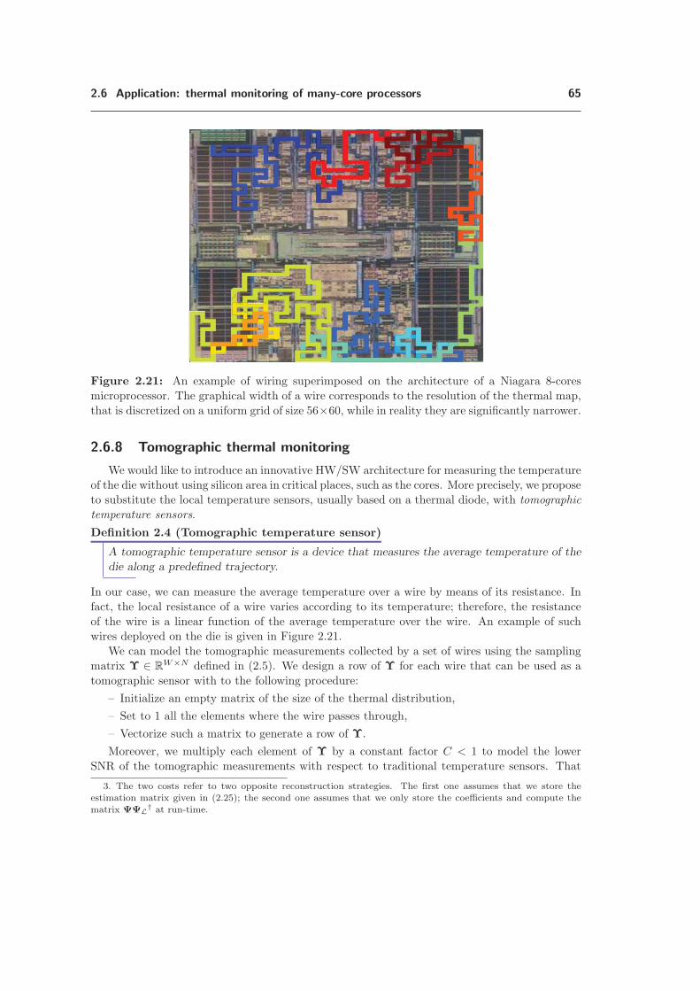
2.6 Application: thermal monitoring of many-core processors 65
Figure 2.21: An example of wiring superimposed on the architecture of a Niagara 8-cores
microprocessor. The graphical width of a wire corresponds to the resolution of the thermal map,
that is discretized on a uniform grid of size 56×60, while in reality they are significantly narrower.
2.6.8 Tomographic thermal monitoring
We would like to introduce an innovative HW/SW architecture for measuring the temperature
of the die without using silicon area in critical places, such as the cores. More precisely, we propose
to substitute the local temperature sensors, usually based on a thermal diode, with tomographic
temperature sensors.
Definition 2.4 (Tomographic temperature sensor)
A tomographic temperature sensor is a device that measures the average temperature of the
die along a predefined trajectory.
In our case, we can measure the average temperature over a wire by means of its resistance. In
fact, the local resistance of a wire varies according to its temperature; therefore, the resistance
of the wire is a linear function of the average temperature over the wire. An example of such
wires deployed on the die is given in Figure 2.21.
We can model the tomographic measurements collected by a set of wires using the sampling
matrix Υ ∈ RW×N defined in (2.5). We design a row of Υ for each wire that can be used as a
tomographic sensor with to the following procedure:
– Initialize an empty matrix of the size of the thermal distribution,
– Set to 1 all the elements where the wire passes through,
– Vectorize such a matrix to generate a row of Υ.
Moreover, we multiply each element of Υ by a constant factor C < 1 to model the lower
SNR of the tomographic measurements with respect to traditional temperature sensors. That
3. The two costs refer to two opposite reconstruction strategies. The first one assumes that we store theestimation matrix given in (2.25); the second one assumes that we only store the coefficients and compute thematrix ΨΨL† at run-time.
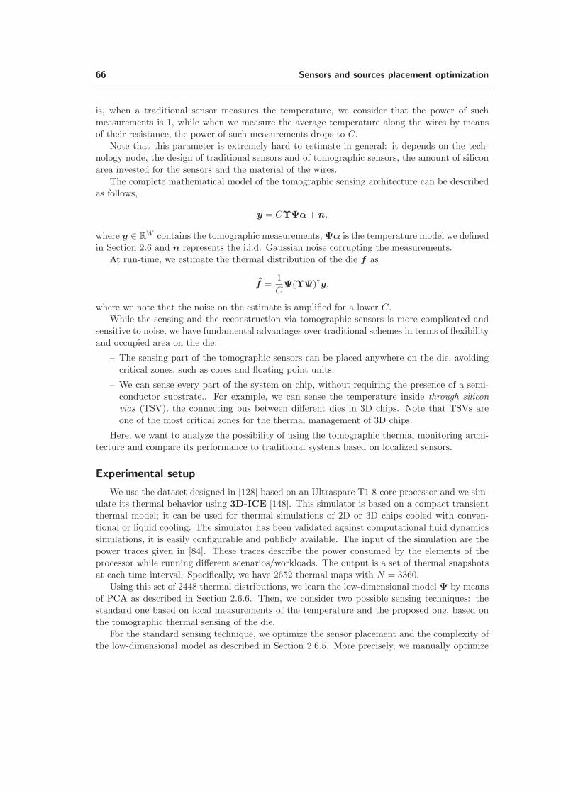
66 Sensors and sources placement optimization
is, when a traditional sensor measures the temperature, we consider that the power of such
measurements is 1, while when we measure the average temperature along the wires by means
of their resistance, the power of such measurements drops to C.
Note that this parameter is extremely hard to estimate in general: it depends on the tech-
nology node, the design of traditional sensors and of tomographic sensors, the amount of silicon
area invested for the sensors and the material of the wires.
The complete mathematical model of the tomographic sensing architecture can be described
as follows,
y = CΥΨα+ n,
where y ∈ RW contains the tomographic measurements, Ψα is the temperature model we defined
in Section 2.6 and n represents the i.i.d. Gaussian noise corrupting the measurements.
At run-time, we estimate the thermal distribution of the die f as
f =1
CΨ(ΥΨ)†y,
where we note that the noise on the estimate is amplified for a lower C.
While the sensing and the reconstruction via tomographic sensors is more complicated and
sensitive to noise, we have fundamental advantages over traditional schemes in terms of flexibility
and occupied area on the die:
– The sensing part of the tomographic sensors can be placed anywhere on the die, avoiding
critical zones, such as cores and floating point units.
– We can sense every part of the system on chip, without requiring the presence of a semi-
conductor substrate.. For example, we can sense the temperature inside through silicon
vias (TSV), the connecting bus between different dies in 3D chips. Note that TSVs are
one of the most critical zones for the thermal management of 3D chips.
Here, we want to analyze the possibility of using the tomographic thermal monitoring archi-
tecture and compare its performance to traditional systems based on localized sensors.
Experimental setup
We use the dataset designed in [128] based on an Ultrasparc T1 8-core processor and we sim-
ulate its thermal behavior using 3D-ICE [148]. This simulator is based on a compact transient
thermal model; it can be used for thermal simulations of 2D or 3D chips cooled with conven-
tional or liquid cooling. The simulator has been validated against computational fluid dynamics
simulations, it is easily configurable and publicly available. The input of the simulation are the
power traces given in [84]. These traces describe the power consumed by the elements of the
processor while running different scenarios/workloads. The output is a set of thermal snapshots
at each time interval. Specifically, we have 2652 thermal maps with N = 3360.
Using this set of 2448 thermal distributions, we learn the low-dimensional model Ψ by means
of PCA as described in Section 2.6.6. Then, we consider two possible sensing techniques: the
standard one based on local measurements of the temperature and the proposed one, based on
the tomographic thermal sensing of the die.
For the standard sensing technique, we optimize the sensor placement and the complexity of
the low-dimensional model as described in Section 2.6.5. More precisely, we manually optimize

2.6 Application: thermal monitoring of many-core processors 67
the dimension K by a global search: for a given number of sensors L, we test all K ≤ L and we
choose the K minimizing the reconstruction error ξ. The sensor placement is always optimized
using FrameSense, our near-optimal greedy algorithm described in Section 2.3.3.
For the thermal monitoring based on tomographic sensors, the setup has an additional chal-
lenge: the design of the wire trajectories. In fact, while for the traditional sensing scheme we
can easily enumerate the N possible locations, the number of wires that can be traced on the
die grows exponentially with N . Three different strategies can be envisioned to solve such a
problem:
– Design an algorithm aiming at the optimization of the wire trajectories so that the recon-
struction error of the thermal distributions f is minimized.
– After the routing of the processor has been done, consider all the empty space in the
interconnections layer and trace a set of possible wires. Select a set of L near-optimal wires
using FrameSense.
– Trace a set of R � L wires at random and select the set of L near-optimal ones using
FrameSense.
Clearly, the first strategy is optimal but the design of this optimization algorithm is complex
and beyond the scope of this work. The second strategy is realistic but requires the knowledge of
the routing information, that is usually not publicly available. The third strategy is the easiest
to test, but the farthest from reality.
Our target is to show the theoretical feasibility of the tomographic thermal monitoring system
and we opt for the third strategy. More precisely, we consider four sensing locations located on
the corners of the IC die. At these locations, there is a multiplexer to select a wire at a time
and a sensor that measures the resistance of each wire. Note that, we can increase the precision
of the sensors measuring the resistance by investing more area on the die, given their limited
number and their non-critical locations. Then, we randomly generates R = 1000 wires starting
from the four resistance sensors using a discrete random walk process.
As for the traditional thermal monitoring system, we want to use the minimal amount of
wires to minimize the necessary resources. Therefore, we select the set of wires that minimizes
the reconstruction error of the thermal maps f . We use FrameSense as selection algorithm, but
it considers as input the matrix ΥΨ instead of solely Ψ. After the optimal wires W are chosen,
we obtain the pruned sampling matrix ΥW .
The reader can see this as a simplified wire placement: checking all the possible wires is
exponentially complex in N and unfeasible, therefore we generate a set of random wires and we
choose the optimal L out of them. This selection process models a possible strategy at design
phase: after the floorplanning and routing of the system on chip are done, we are given many
possible wires out of which we have to choose L ones such that the reconstruction performance
is optimized.
A fundamental detail is the quantification of the parameter C. As we previously mentioned,
it represents the difficulty of measuring the resistance of the wire with respect to the difficulty
of measuring the local temperature with a traditional sensor. Such a parameter is hard to
estimate without a complex study of the design of thermal sensors, involving simulations of
their architectures via SPICE-like softwares [109]. Here, we choose three different values, C =
{1, 0.75, 0.5}, meaning that the temperature information measured through a wire is 0%, 25%,
and 50% less amplified than the one obtained by standard sensors, respectively.

68 Sensors and sources placement optimization
0 5 10 15 20 25 30 35��
�
��
��
0
2
�
�
10
12Comparison of the reconstruction error
RMSE wiresRMSE sensors
Number of Sensors
MS
E [d
B]
(a) σ2 = 1, C = 1
0 5 10 15 20 25 30 35��
�
��
��
0
2
�
�Comparison of the reconstruction error
RMSE wiresRMSE sensors
Number of Sensors
MS
E [d
B]
(b) σ2 = 1, C = 0.75
0 5 10 15 20 25 30 35��
�
��
��
0
2
�
�Comparison of the reconstruction error
Number of Sensors
MS
E [d
B]
RMSE wiresRMSE sensors
(c) σ2 = 1, C = 0.5
Figure 2.22: Comparison of the reconstruction error of the two sensing methods (traditional
thermal sensing and tomographic wire sensing) in terms of MSE as a function of the number of
sensors/wires used. For each plot, we consider a measurement noise with a variance σ2 = 1 and
we vary the parameter C. We note that for a lower value of C we have a larger gap between the
two methods and we must increase the number of wires to obtain the same reconstruction error.
If we consider our target to be the performance achieved with ten thermal sensors, we need 20
and 32 wires for C = 1 and C = 0.75, respectively. Unfortunately, the number of necessary wires
is significantly higher for C = 0.5.
Experimental results
We now propose some initial results showing the feasibility of the tomographic thermal sens-
ing. We measure the MSE as a function of the number of the sensors/wires for both methods,
with a Gaussian noise with variance σ2 = 1 applied to the measurements, fL or fW respectively.
We replicate this experiment with three different values of the parameter C, to represent different
sensing architectures for the tomographic approach.
The results are shown in Figure 2.22, where we note that the tomographic sensing is worse

2.7 Application: adaptive scheduling of sensor networks 69
than the localized sensors when we consider the same amount of sensing elements. This is not a
surprise, since the design of the wire is not optimal and each wire carries less information about
the thermal map. However, we note that we can compensate for such difference by increasing
the number of wires: with C = 1, we achieve the same reconstruction performance of 10 local
sensors with 20 wires, a very reasonable amount.
If C is lower, that is C = 0.75, we can still compensate by increasing the number of wires.
Unfortunately, such a compensation looks unfeasible when C = 0.5.
Nonetheless, such results are encouraging for future work. Two directions are possible:
– Show that the values of C = [0.75, 1] are feasible without investing too many resources
(area and power), for the design of the sensors measuring the resistance of the wires.
– Improve the design of the wires with an algorithm minimizing the conditioning of the
inverse problem. Note that this problem is most likely NP-hard due to the exponential
number of possible wires, but approximation algorithms with good performance may still
exist.
2.7 Application: adaptive scheduling of sensor networks
In a wireless sensor network (WSN), sensor nodes are deployed to take periodical mea-
surements of a certain physical field at different locations. Consider a continuous-time spatio-
temporal field f(p, t) that we would like to monitor with the WSN, where p and t define the
location in space and time, respectively. Moreover, we define a vector f ∈ RN containing a
discretization of such a field with a sufficiently high resolution for our purposes. The goal of the
WSN is to recover f with the maximum precision.
One of the primary aims in designing a WSN is the reduction of its energy consumption,
to extend its lifetime without replacing or recharging the batteries of sensor nodes. The energy
consumption of a sensor node is mainly due to three activities: sensing, data-processing and com-
munication. Traditionally, the costs for processing and communication are assumed to dominate
the overall energy consumption, while the cost for sensing is considered negligible. Therefore, a
traditional WSN collects as much data as possible which is subsequently compressed and trans-
mitted at the lowest possible rate. In other words, it collects a vector of samples y equal to the
discretized physical field f with some additive noise,
y = If + n, (2.27)
where I is the identity matrix of size N and n represents the noise; see Figure 2.23a for an
example.
Ignoring the energy cost for sensing is sub-optimal, if sensing consumes a comparable amount
of energy to communication and data processing. In fact, new sampling paradigms optimizing the
overall energy consumption have been proposed and show that further reductions of the energy
consumption are possible. The basic idea involves a reduction of the number of collected samples
and a reconstruction of the missing data using algorithms exploiting the structure available in
the measured data. The reduction of the collected samples is done by designing a sampling
operator Υ ∈ RL×N with L < N , that it is used instead of the identity matrix as,
y = Υf + n, (2.28)

70 Sensors and sources placement optimization
(a) Traditional Sensing (b) CS - Dense Matrix
(c) CS - Sparse Matrix (d) Sparsity Dictionary
Figure 2.23: Comparison of various sensing schemes proposed in the literature (the noise term
ε is omitted for simplicity). We consider a discretized version of the sampled physical field that
is contained into a vector f . In (a) we depict the traditional approach where we measure the
physical field in each spatio-temporal location, thus having an identity operator I. In (b), we
reduce the number of samples by taking random projections of the measurements. Note that we
need to measure all the elements of f and we are just reducing the number of stored samples. On
the other hand, in (c) we are reducing the number of measured samples using a sparse sampling
matrix Υ. Note that the methods in (b) and (c) require a set of conditions regarding f and Υ to
be satisfied [33]. Among these conditions, we note that f must be sparse under a certain known
dictionary Π, see (d).
where y ∈ RL denotes the set of measured elements of f . Note that y is significantly shorter
than f and the reconstruction algorithm must estimate a significant amount of information from
a limited amount of data. Therefore, regularization and constraints are added to the problem so
that a stable solution can be obtained. Moreover, the reconstruction algorithm must be jointly
designed with the sampling matrix Υ to obtain a precise estimate of f .
Pioneering work on sparse sampling considered compressive sensing (CS) as a reconstruction
scheme. CS attempts to recover f by solving a convex optimization problem, under the assump-
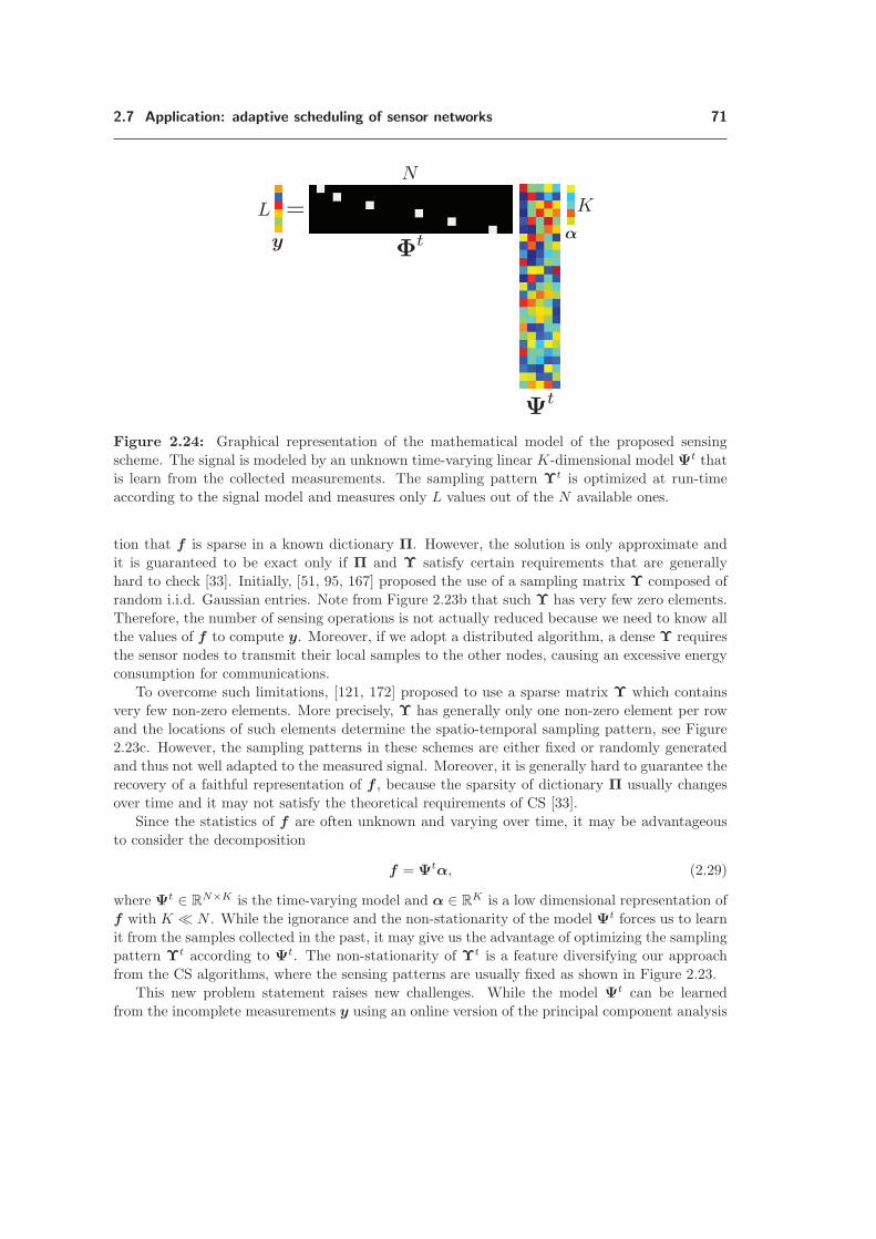
2.7 Application: adaptive scheduling of sensor networks 71
Figure 2.24: Graphical representation of the mathematical model of the proposed sensing
scheme. The signal is modeled by an unknown time-varying linear K-dimensional model Ψt that
is learn from the collected measurements. The sampling pattern Υt is optimized at run-time
according to the signal model and measures only L values out of the N available ones.
tion that f is sparse in a known dictionary Π. However, the solution is only approximate and
it is guaranteed to be exact only if Π and Υ satisfy certain requirements that are generally
hard to check [33]. Initially, [51, 95, 167] proposed the use of a sampling matrix Υ composed of
random i.i.d. Gaussian entries. Note from Figure 2.23b that such Υ has very few zero elements.
Therefore, the number of sensing operations is not actually reduced because we need to know all
the values of f to compute y. Moreover, if we adopt a distributed algorithm, a dense Υ requires
the sensor nodes to transmit their local samples to the other nodes, causing an excessive energy
consumption for communications.
To overcome such limitations, [121, 172] proposed to use a sparse matrix Υ which contains
very few non-zero elements. More precisely, Υ has generally only one non-zero element per row
and the locations of such elements determine the spatio-temporal sampling pattern, see Figure
2.23c. However, the sampling patterns in these schemes are either fixed or randomly generated
and thus not well adapted to the measured signal. Moreover, it is generally hard to guarantee the
recovery of a faithful representation of f , because the sparsity of dictionary Π usually changes
over time and it may not satisfy the theoretical requirements of CS [33].
Since the statistics of f are often unknown and varying over time, it may be advantageous
to consider the decomposition
f = Ψtα, (2.29)
where Ψt ∈ RN×K is the time-varying model and α ∈ R
K is a low dimensional representation of
f with K � N . While the ignorance and the non-stationarity of the model Ψt forces us to learn
it from the samples collected in the past, it may give us the advantage of optimizing the sampling
pattern Υt according to Ψt. The non-stationarity of Υt is a feature diversifying our approach
from the CS algorithms, where the sensing patterns are usually fixed as shown in Figure 2.23.
This new problem statement raises new challenges. While the model Ψt can be learned
from the incomplete measurements y using an online version of the principal component analysis

72 Sensors and sources placement optimization
(PCA), selecting the sampling pattern Υt for minimizing the construction error is a combinato-
rial problem. In this work, we propose a generalized version of FrameSense, the algorithm that
generates a near-optimal sensor placement for inverse problems proposed in Section 2.3.3. More
precisely, instead of optimizing the sensor placement, we optimize the spatio-temporal sampling
pattern of the WSN. The obtained sampling pattern is generally irregular, time-varying and op-
timized to gather the maximum amount of information. In particular, it simultaneously exploits
the intra-node (temporal) and inter-node (spatial) correlation potentially present in the data.
See Figure 2.24 for a graphical illustration of the low-dimensional model and of the irregular
sampling patterns.
Our method derives from and extends the sparse sensing framework proposed by Quer et
al. [121]: the signal is first approximated by a linear model Ψt, and the sampling scheduling is
defined in space and time by a sampling matrix Υt. Our major contribution is that we improve
the way in which the spatio-temporal correlation is exploited, such that the sampling pattern is
dynamically adapted to the low dimensional model of the signal, as defined in (2.29).
It is worth mentioning that our proposed method does not require any on-sensor computation
nor inter-node communication. Each sensor node simply collects measurements according to a
designated sampling pattern and transmits the data to a common server. The server receives all
the data from one or multiple sensor nodes and performs signal reconstruction. This is actually in
accordance with the setup of distributed source coding [162], where no inter-node communication
is used. Hence, our proposed algorithm provides an alternative solution to the distributed coding
problem: the communication rate is reduced and the reconstruction error is bounded without
using any inter-node communication.
Our algorithm is tested on different sets of real-world data, outperforming both the traditional
sensing schemes and the state-of-the-art sparse sensing schemes, in terms of reconstruction quality
of f given a fixed amount of measurements. We name the proposed method “Distributed Adaptive
Sparse Sensing”, (DASS ).
2.7.1 Problem statement
In this section, we first state the sampling scheduling problem for a WSN with one sensor. We
then generalize the problem statement to a WSN with multiple nodes. We consider a block-based
sensing strategy, meaning that the WSN samples the field for a certain time T after which, we
reconstruct the vector f from the collected samples. Note that the block length is known and
defined a-priori.
For each temporal block, the discrete physical field f is composed of N samples of f(p, t),
f = [f(p, 0), f(p,ΔT ), · · · , f(p, (N − 1)ΔT )],
where p indicates the sensor node location and ΔT is the sampling period. Note that ΔT
determines the desired temporal resolution and its inverse is the sampling frequency, ω = 1/ΔT .
The temporal duration of a block is T = NΔT and is also the maximum delay occurring with this
sensing scheme—the larger T , the longer the delay. See Figure 2.25 for a graphical representation
of the physical field and its discrete version f .
We denote the reconstructed physical field obtained from the WSN samples as f . In a sparse
sampling scenario, we aim at reconstructing f from a subset of few elements of f . More precisely,
we measure L elements out of N , where L < N . The set of indices τ t = {τ ti }Li=1 denotes the
indices of these L samples and is chosen adaptively according to the previous measurements.

2.7 Application: adaptive scheduling of sensor networks 73
block length N=12
Time
Time
0 Block 1 Block 2
L=4
DASS
���������Ses�g
Figure 2.25: Upper figure: optimized temporal sampling pattern of DASS. Lower figure: tra-
ditional sensing scheme, where samples are collected regularly in time. The subsampling factor
is ζ = 1/3, since we collect 4 samples instead of 12 in each block.
The sampling pattern τ t uniquely determines the sampling matrix Υt ∈ RL×N that previously
appears in (2.28):
Υti,j =
{1 if j = τ ti
0 otherwise.
The sampling matrix Υt has exactly one non-zero element per row, and usually a maximum of
one non-zero element per column. Here either Υti,j or τ
ti can be interpreted as a temporal selector
deciding when the node should take a sample – the index j indicates the time index within a
block. It is important to underline that Υt and τ t are time-varying and potentially changing at
every block to adapt to the signal model Ψt. Figure 2.25 shows an example of sampling patterns
where τ t changes for each block.
We define ωs = LN ω = ζω to be the average sampling frequency of the sensor node 4. The
subsampling rate ζ = ωs/ω < 1 is an important figure of merit for a sparse sampling algorithm—
the lower the ζ, the lower the energy consumed for sensing.
The measured signal y ∈ RM is defined as
y = Υtf + n,
where n represents the measurement noise modeled as an additive white Gaussian noise (AWGN),
since the thermal effects [72] or/and quantization [170] are often the dominating terms 5. Through-
out the chapter, we mainly discuss the simpler case of i.i.d. noise; however, we will shortly discuss
4. Note that we denote ωs as an average sampling frequency given the irregular and time-varying samplingpattern.
5. Other noise models may be of interest for specific sensors; for example the noise term of a Geiger counteris usually modeled as a Poisson process.

74 Sensors and sources placement optimization
Concatenated at the server
Figure 2.26: Signals of multiple distributed sensor nodes can be concatenated into a single
signal stream at the server for recovery.
the extension to the generic case of noise having a correlation matrix Σn. We define the signal-
to-noise ratio (SNR) of the measurement as following, which will be used in the evaluations:
SNR (dB) = 10 log10
(‖f‖22‖n‖22
). (2.30)
The target of DASS is to optimize the sampling pattern Υt at the t-th block according to Ψt
such that we collect the minimum number of samples L while still being able to recover precisely
the original signal. Since we model the noise as a AWGN, we assess the quality of the recovered
signal by using the MSE:
ξ =1
N‖f − f‖2,
where f is the estimated physical field.
Multiple-node scenario: while the above problem statement focuses on a single-sensor sce-
nario for simplicity of notation, it is simple to generalize the statement to a WSN with more
than one sensor node. More precisely, we assume that the nodes are synchronized 6, so that
we can concatenate all the measured blocks at different locations pi in a unique signal block
f . Figure 2.26 shows an example. fA,fB ,fC are signal blocks from three different locations,
6. Note that our method does not require a precise synchronization. In fact, eventual variations of the modeldue to the lack of synchronization are handled by the proposed method thanks to the adaptive learning of themodel.
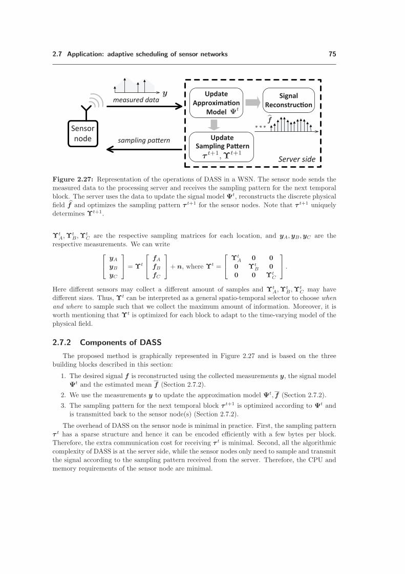
2.7 Application: adaptive scheduling of sensor networks 75
measured data
����������� �
Update� ���������
Model
����������������
Update��� ��������
Server side
Sensor node
Figure 2.27: Representation of the operations of DASS in a WSN. The sensor node sends the
measured data to the processing server and receives the sampling pattern for the next temporal
block. The server uses the data to update the signal model Ψt, reconstructs the discrete physical
field f and optimizes the sampling pattern τ t+1 for the sensor nodes. Note that τ t+1 uniquely
determines Υt+1.
ΥtA,Υ
tB ,Υ
tC are the respective sampling matrices for each location, and yA,yB ,yC are the
respective measurements. We can write⎡⎣ yA
yB
yC
⎤⎦ = Υt
⎡⎣ fA
fB
fC
⎤⎦+ n, where Υt =
⎡⎣ ΥtA 0 0
0 ΥtB 0
0 0 ΥtC
⎤⎦ .
Here different sensors may collect a different amount of samples and ΥtA,Υ
tB ,Υ
tC may have
different sizes. Thus, Υt can be interpreted as a general spatio-temporal selector to choose when
and where to sample such that we collect the maximum amount of information. Moreover, it is
worth mentioning that Υt is optimized for each block to adapt to the time-varying model of the
physical field.
2.7.2 Components of DASS
The proposed method is graphically represented in Figure 2.27 and is based on the three
building blocks described in this section:
1. The desired signal f is reconstructed using the collected measurements y, the signal model
Ψt and the estimated mean f (Section 2.7.2).
2. We use the measurements y to update the approximation model Ψt,f (Section 2.7.2).
3. The sampling pattern for the next temporal block τ t+1 is optimized according to Ψt and
is transmitted back to the sensor node(s) (Section 2.7.2).
The overhead of DASS on the sensor node is minimal in practice. First, the sampling pattern
τ t has a sparse structure and hence it can be encoded efficiently with a few bytes per block.
Therefore, the extra communication cost for receiving τ t is minimal. Second, all the algorithmic
complexity of DASS is at the server side, while the sensor nodes only need to sample and transmit
the signal according to the sampling pattern received from the server. Therefore, the CPU and
memory requirements of the sensor node are minimal.

76 Sensors and sources placement optimization
In what follows, we analyze each block explaining the challenges and the proposed solution.
Signal approximation and reconstruction
Due to the nature of most physical fields, a signal block is partially predictable by analyzing
past data. In many cases, this predictability can be expressed by assuming that the signal belongs
to a K-dimensional linear subspace Ψt ∈ RN×K . Such a subspace approximates f as
f = Ψtα+ f ,
where f is the approximated field, α ∈ RK is the vector of the projection coefficients and f is
the mean of f .
If the modeling subspace Ψt is well designed and K is sufficiently large compared to the com-
plexity of f , the signal realization f can be accurately expressed with just K << N coefficients
contained in α. To find such a subspace, we analyze all the past signal realizations and estimate
at the t-th block the K-dimensional subspace Ψt that minimizes the expected approximation
error
ε =1
NE(‖f − f‖22
).
E This is a dimensionality reduction problem that can be solved by the well known technique
of principal component analysis (PCA) 7. It has an analytic solution but it requires the covariance
matrix Σf .
Unfortunately, in our scenario it is hard to estimate Σf since we have access only to L out
of N elements of f . However, if the L sampled elements are varying at each temporal block t,
we may collect enough information to have a sufficiently precise estimate of Σf . We present a
set of methods to estimate Σf in Section 2.7.2.
Note that the approximation through Ψt exploits the spatial and temporal correlation among
the elements of f . The higher the correlation available in f , the lower the dimensionality of the
subspace Ψt, the number of parameters K and the necessary measurements L. Hence, one of
the key aspects is the choice of the signal block length T . In fact, it should be chosen such that
the delay of the WSN respects the design specification while maximizing the correlation among
the blocks. For example, a sensor measuring the outdoor light intensity naturally shows diurnal
patterns. Therefore, if we choose a block length of one hour, the correlation within the signal
block is usually weak. On the other hand, if we choose a block length of one day, the correlation
is stronger.
Once the approximation modelΨt is estimated, recovering the signal f amounts to estimating
α from the measurements y when considering the approximated signal model,
y ≈ Υtf + ε = Υt(Ψtα+ f) + ε. (2.31)
If n is an i.i.d. Gaussian random noise, we can recover α by solving an Ordinary Least Square
(OLS) problem [121]:
α = argminα
‖y −Υtf −ΥtΨtα‖22,
7. The CS-based sparse sensing methods in [121] also used PCA for subspace learning.

2.7 Application: adaptive scheduling of sensor networks 77
Algorithm 2.6 Signal reconstruction
Require: Ψt, f , τ t and Υt
Ensure: f
1: Measure the signal y according to τ t.
2: f = Ψt(ΥtΨt)†(y −Υtf) + f .
which has the following analytic solution,
α = (ΥtΨt)†(y −Υtf),
where (ΥtΨt)† is the Moore-Penrose pseudoinverse of ΥtΨt. We can slightly vary the recon-
struction technique to account for more complicated noise models. For example, if the noise is
distributed according a known covariance matrix Σn, we can estimate α as
α = ((ΥtΨt)∗Σ−1n ΥtΨt)−1(ΥtΨt)∗Σ−1
n (y −Υtf).
We can generalize such an estimator to other additive noise models, see [77]. Nonetheless, for
the remainder we keep considering the simpler case of i.i.d. Gaussian noise.
Once we define the estimator for α, the reconstruction algorithm is straightforward and is
described in Algorithm 2.6. The following proposition states the necessary conditions to find a
unique solution and provides an upper bound for the reconstruction error, that is going to be
fundamental when optimizing the sampling pattern. Such a result is an adaption of two classic
results of linear algebra [60].
Proposition 2.3
Consider a WSN measuring a physical field as in (2.31) where the L measurements are
collected according to the scheduling τ t and are corrupted by an i.i.d. Gaussian noise with
variance σ2. If L ≥ K, Ψt ∈ RN×K is formed by orthonormal columns and rank(ΥtΨt) = K,
then f can be uniquely determined using Algorithm 2.6. The reconstruction error is bounded
by
ξ =1
N‖f − f‖22 ≤
(1 +
1
λK
)ε2 + σ2
K∑i=1
1
λi=
(1 +
1
λK
)ε2 + κ(τ t),
where ε is the approximation error due to the signal model Ψt and λi (1 ≤ i ≤ K) is the i-th
largest eigenvalue of the matrix Ψt∗Υt∗ΥtΨt. We denote the error due to the measurement
noise at the t-block as κ(τ t). Note its strong dependency on the sampling scheduling τ t.
Proof.
See Appendix 2.10.2.
The upper-bound of the reconstruction error ξ is a function of both the approximation error ε
and the measurement noise n. The former term depends on the number of parameters K: when
K = N , we have ε = 0 and it grows when we decrease K. However, the rate at which the error
increases depends on the spectrum of Σf . In fact, if f has elements that are highly correlated, a
small K could be sufficient to model f with a small approximation error. The latter term can be
controlled directly by optimizing the sampling pattern. More precisely, we cannot reduce σ but

78 Sensors and sources placement optimization
Algorithm 2.7 Updating Ψt,f using a buffer
Require: y, L
Ensure: Ψt,f
1: interpolate y → finterp.
2: insert finterp into a buffer storing the most recent R blocks.
3: estimate Σf and f from the buffer.
4: Ψt is formed by the eigenvectors corresponding to the K largest eigenvalues of the matrix
Σf .
we can reduce the amplification due to the spectrum λk through an optimization of the sampling
matrix Υt.
Note that the part involving ε only depends on the smallest eigenvalue because we are not
guaranteed that the approximation error spreads over all the eigenvectors of ΥtΨt. In fact, the
worst case scenario is represented by the approximation error being in the same direction of the
eigenvector with the smallest eigenvalue and ε is consequently maximally amplified.
Compared to the methods based on CS, our approach based on a low-dimensional model
and OLS has the following advantages: i) the solution is easy to compute and it requires a
single matrix inversion, ii) it enables an analysis of the reconstruction error and a consequent
optimization of the sampling pattern τ t such that the upper-bound of the reconstruction error
ξ is minimized.
Learning from incomplete data over time
In Section 2.7.2, we have highlighted some challenges regarding the estimation of the covari-
ance matrix Σf—a fundamental step to determine the approximation model Ψt. Most of the
challenges derive from the lack of a sufficiently large set of realizations of f , that are needed
to estimate Σf . First, there is virtually no past data for a newly installed WSN. Second, Σf
is likely to vary over time. Third, a high ratio of data points (1 − ζ) are not available for the
estimation since we collect sparse measurements. Therefore, we need an on-line algorithm that
estimates and adaptively updates the covariance matrix Σf from incomplete data.
The main difficulty is the lack of complete realizations of f . Two strategies are generally
considered to overcome such a problem. The first one proposes to estimate from y an interpola-
tion finterp using classic methods such as linear, polynomial or spline interpolation. The second
strategy skips the estimation of Σf and attempts to perform directly the principal component
analysis on the data having missing entries, see [122].
According to our quantitative results, the second class of algorithms is less powerful for
our purposes. Therefore, we focus our attention on the interpolation methods. More precisely,
we analyze two different methods that implement an adaptive learning and updating of the
approximation model Ψt from the interpolated signal finterp.
The first, whose pseudocode is given in Algorithm 2.7, uses a FIFO buffer to store the most
recent R blocks. Whenever a new block is added into the buffer, the oldest block in the buffer
is excluded. As the approximation model is estimated according to the signal realizations in the
buffer, this scheme is able to capture the variation of signal statistics over time.
The second one, see Algorithm 2.8, adaptively updates the approximation model via a tech-
nique called incremental PCA [64]. It does not keep signal realizations in memory, instead,

2.7 Application: adaptive scheduling of sensor networks 79
Algorithm 2.8 Updating Ψt,f using incremental PCA
Require: y, L, Ψt−1, νt−1,ft−1
Ensure: Ψt,νt,ft
1: interpolate y → finterp.
2: a = Ψt−1∗(finterp − ft−1
).
3: b =(Ψt−1a+ f
t−1))− finterp, and then normalize b.
4: c = b∗(finterp − ft−1
).
5: D = 1R+1
[diag(νt−1) 0
0∗ 0
]+ R
(R+1)2
[aa∗ ca
ca∗ c2
].
6: Solve the eigenproblem: D = Rdiag(ν′)R−1, ν ′ is sorted in decreasing order.
7: Ψ′ =[Ψt−1 b
]R.
8: update Ψt as the first K columns of Ψ′.9: update νt as the first K values of ν ′.
10: update ftas
(Rf
t−1+ finterp
)/(R+ 1).
it stores the largest K eigenvalues of Σf , ν = {νi}, for i = 1, · · · ,K. This method requires
significantly less memory (K versus N × R), and shows better performance when compared to
Algorithm 2.7. Note that in both algorithms, the choice of R depends on the variability of the
signal statistics for each specific application. In practice, we can cross-validate this parameter
to find a suitable value (e.g., R = 30). We discuss and compare the performance of these two
algorithms in the experimental results.
Sampling scheduling algorithm
According to Proposition 2.3, minimizing the overall error ε is equivalent to finding the opti-
mal sampling pattern τ that minimizes (2.3). We fix the values of K and M in the optimization
process, and hence the approximation error ε is fixed. In this work, we assume that the model
Ψt is sufficiently precise and the dimensions K is large enough so that the term due to the white
noise n is dominant. Note that if the approximation error decays exponentially fast with K,
there exists always a small K such that ε � σ2. We will show in the experimental part that
such decay is actually present in meteorological data.
To optimize the scheduling pattern, we would like to find the sampling pattern that minimizes
the MSE of the estimate of f . Note that if we define the linear inverse problem to be the
estimation of f from y, then the sensor scheduling problem is equivalent to the optimization
of the sensors locations. Therefore, the proposed sampling scheduling algorithm is based on an
equivalent greedy “worst-out” procedure: as input we have the signal model Ψt and we initially
consider the identity matrix of size N as the sampling matrix Υt+1. At each iteration, we
remove the row of Υt+1 that maximizes the cost function (2.8). After N − L + 1 iterations,
we are left with an optimized Υt+1 that has only L elements different from zero and has near-
optimal performance when reconstructing f from the measurements y. Note that if Ψt satisfies
the conditions given in Section 2.3, the obtained sampling matrix Υt+1 stably recovers f from
the measurements y.
Furthermore, since a uniform sampling schedule is a commonly-used strategy that yields good

80 Sensors and sources placement optimization
Algorithm 2.9 Greedy sampling scheduling
Require: Ψt, L
Ensure: τ t+1 for the next temporal block
1: Initialize the set of selected sampling indices: L = {1, · · · , N}.2: Find the first two rows to eliminate, {i∗, j∗} = argmaxi,j∈R | 〈ψi,ψj〉 |2.3: Update L = L\{i∗, j∗}.4: repeat
5: Find the optimal row, i∗ = argmaxi∈L FP(ΨtL\i).
6: Update the set of selected indices, L = L\i∗.7: until |L| = L
8: τ t+1 = argminτ {κ(τ ), τ is uniform pattern or L}.
performance in real applications [172], we compare it with the result returned by the greedy
algorithm and opt for the one with smallest reconstruction error. This error is approximated by
the bound provided by Proposition 2.3. A detailed description of the overall algorithm is given
in Algorithm 2.9. Note that for the very first block of data during system startup, the uniform
sampling schedule is used for initialization.
2.7.3 State-of-the-art methods for sparse sampling
In this section, we briefly summarize the state-of-the-art methods for the sparse sensing
problem. They will serve as the baseline for comparisons in Section 2.7.4.
The first category of methods [121, 172] is based on CS. With the notations introduced in
Section 2.7.1, f is the unknown signal, y contains the incomplete measurements, and Υ is a
sparse sampling matrix with only L elements different from zero. We assume f to be sparse with
respect to a dictionary Π. More precisely, we have f = Πs and s has just a few coefficients
different from zero, that is ‖s‖0 � N (see [29] for more details). By approximating the �0 norm
with the �1 norm [31], the reconstruction method for the noiseless case is:
mins∈RN
‖s‖1, s.t. y = ΥΠs,
while the one for the noisy case is
mins∈RN
‖s‖1, s.t. ‖y −ΥΠs‖2 ≤ β, (2.32)
where β measures the energy of the noise. Problem (2.7.3) and (2.32) are both convex and
can be solved [31] in polynomial time using various solvers, in general iterative or based on
convex optimization. In both methods, we use uniform sampling as the sampling scheduler —
τ tj = �jN/L�.The second category of baseline methods [121] are based on learning the K-dimensional
time-varying model Ψt and a reconstruction via OLS as in Algorithm 2.6. We use two sampling
schedulers, namely, a uniform sampling, and a random sampling where τ tj is randomly selected
with a uniform distribution.
Table 2.3 lists all the methods (including DASS) that are evaluated in the experiments. To

2.7 Application: adaptive scheduling of sensor networks 81
Table 2.3: Summary of methods used in experiments
AbbreviationReconstructionAlgorithm
SamplingScheduling
CS [121, 172] (2.7.3) uniform
CSN [31, 121] (2.32) uniform
OLS-random [121] Alg. 2.6 random
OLS-uniform [121] Alg. 2.6 uniform
DASS Alg. 2.6 Alg. 2.9
have a fair comparison, Π in CS-based methods and Ψt in OLS-based methods are both learnt 8
by the incremental PCA described in Algorithm 2.8.
2.7.4 Evaluation of DASS and comparison with other sparse sensing meth-ods
In this section we evaluate the performance of DASS and compare it with the state-of-the-art
sparse sensing methods. Besides the experiments on the single-node case, we also verify DASS
in the multi-node case where nearby sensor nodes measure spatially correlated signals. We use
two real-world meteorological datasets as the ground truth, namely Payerne and Valais :
– Payerne is provided by MeteoSwiss [1]. This dataset contains 1500 days of continuous
measurements for two physical quantities (temperature and solar radiation) 9, which are
suitable for studying long-term performance of DASS. As MeteoSwiss only deployed a few
observation stations across the whole nation, we use Payerne for evaluating the single-node
case.
– Valais is provided by a microclimate monitoring service provider [70]. A total of 20 stations
are deployed in a mountain valley. Figure 2.28 shows six of them, covering an area of around
18 km2. The deployments were started in March 2012 and collected 125 days of continuous
temperature measurements. We use Valais for evaluating the multi-node case.
The two datasets are summarized in Table 2.4. For both datasets, there are 144 uniformly
sampled data points for each day. We choose the day as the length of each block, that is,
N = 144.
One of the targets of this section is to evaluate DASS and compare it with other algorithms
when the sensing device induces measurement noise. Since we do not know the groundtruth of
the physical field, we assume that Payerne and Valais represent the real value of the field f .
Then, we add white Gaussian noise to simulate the effect of noisy measurements. We evaluate
the algorithms for different SNR of the measurement, as defined in (2.30).
Note that the main merit figure considered in this section is the final reconstruction error
under a fixed subsampling rate ζ. Since all sparse sensing schemes directly transmit the sensing
samples without further data compression, two schemes with the same ζ have the same amount
of energy consumed for sensing and communication 10, regardless of which sensing platform is
used.
8. The experimental results show that K = L is the best choice for CS-based methods, while K < L is aparameter which needs to be optimized for OLS-based methods, see Section 2.7.5.
9. We denote by Payerne-temperature the dataset of temperature measurements. The notation is similar forsolar radiation.10. The processing costs of the considered sparse sensing methods are negligible.

82 Sensors and sources placement optimization
Figure 2.28: Locations of the sensor nodes that collected the data-set Valais .
Table 2.4: Summary of experimental datasets
Datasetname
Physical quantityNumber ofnodes
Numberof days
Payernetemperature, solarradiation
1 1500
Valais temperature 20 125
2.7.5 Components of DASS
In this section, we evaluate the key components of DASS, including the optimal choice of K,
the cost function κ(τ t) in the sampling scheduling algorithm, and the performance of adaptive
learning algorithms.
Optimal choice of dimension K
First, we note that the larger the K the smaller the approximation error for any dataset,
the only difference being the decay rate of such an error. Such aspect for the two considered
datasets is depicted in Figure 2.29, where the data has been normalized for K = 0. Note that
for both datasets we have an exponential decay of the approximation error as a function of K.
Therefore, there exists a small K for which the approximation error is negligible with respect to
the Gaussian noise corrupting the measurements, as we have previously assumed.
As stated in Proposition 2.3, the overall reconstruction error ξ is a function of both the
approximation error ε (2.7.2) and the measurement noise n. Generally, ε decreases with K
while κ(τ t) increases with K, hence there is an optimal choice of K for minimizing the overall
error. The optimal K depends on the data statistics, the subsampling rate, and the SNR of
the measurement. By cross- validation, Figure 2.30 shows the optimal ratio K/L for Payerne-
temperature. We can see that DASS generally opts for a larger K when the SNR of measurement
increases. This is intuitive since with better measurements we can afford a more complicated
model with a weaker regularization.

2.7 Application: adaptive scheduling of sensor networks 83
0 2 4 6 8 10 12 14
10��
10��
100
K
norm
ailiz
ed2
���������������� �������������� ��������
Figure 2.29: Normalized approximation error for the two considered datasets as a function of
the model parameterK. Note how the error monotonically decreases withK given the optimality
of PCA. Moreover, we highlight how the approximation error shows an exponential decay with
K, confirming our assumption described in Section 2.7.2.
20 30 40 500.2
0.4
0.6
0.8
1
SNR of the measurement [dB]
Opt
imal
K/L
5%
10%
subsampling rate
Figure 2.30: Optimal ratio K/L of DASS for a fixed subsampling rate with respect to the
SNR of the measurement (Payerne-temperature dataset). First, we note that K/L must be
smaller than 1 according to Proposition 2.3. Second, we note that for an increasing quality of
the measurements we can collect just L ≈ K samples, meaning that the reconstruction algorithm
is less influenced by the noise and we need less samples. As a conclusive note, we would expect
the plots to be monotonically increasing. However, this is not the case due to the random nature
of the noise model and to the near-optimality of scheduling algorithm.
Sampling scheduling
The greedy algorithm proposed in Section 2.7.2 (Algorithm 2.9) finds an approximate solution
of the sampling scheduling problem. By Proposition 2.3, the measurement noise and the sampling
scheduling affects the reconstruction error according to κ(τ t). Table 2.5 shows the value of κ(τ t)
achieved by different sampling scheduling methods for different datasets, where a higher value
indicates worse stability with respect to noise. We can see that the greedy algorithm achieves the
best result for the two datasets. In particular, it is substantially better than uniform sampling
for solar radiation data.
In Section 2.7.6, we demonstrate how these improvements translate into better reconstruction
performance for DASS.

84 Sensors and sources placement optimization
Table 2.5: Average Θ(ΥtΨt) achieved by different sampling scheduling methods (ζ = 10%,
SNR of the measurement=30dB)
����������PayerneMethod
uniform random Alg. 2.9
Temperature 0.56 4.9×10¹⁵ 0.54
Solar radiation 4.5×10⁵ 1.8×10¹⁵ 0.97
0 200 400 600 800 10000.3
0.35
0.4
0.45
Time [day]
RM
SE
per
day
[°C
]
Algorithm 3 (L=30 days)Algorithm 2 (L=30 days) .One−time learning (600 days)
Figure 2.31: Learning curves of DASS (Payerne-temperature, ζ = 10%, SNR of the measure-
ment=30dB): Comparisons of two online learning algorithms and a one-time learning algorithm
with long backlog of past data. Note that Algorithm 2.8 achieves always the lowest error.
Learning over time
DASS is designed to learn the signal statistics from past data. In practical scenarios, a long
backlog of data is usually unavailable and thus DASS should be designed to learn the model
from scratch. We proposed Algorithm 2.7 and Algorithm 2.8 for this task. Figure 2.31 shows the
learning curves of these two algorithms over three years of data. As a benchmark, we considered
an offline method that learns the model from 600 days of past data and is represented by the
red-dotted curve. The offline method derives the transform matrix once for all from the complete
signal. However, using this matrix may still provide worse results as the signal is non-stationary.
Note how Algorithm 2.7 and Algorithm 2.8 capture the signal statistics precisely. In particu-
lar, it is interesting to note that even if they use less data—the last 30 days—they are generally
better than the offline method that considers 600 days of data. It is clear that the non-stationary
signal model Ψt is captured only by the adaptive on-line algorithms. Moreover, Algorithm 2.8
with incremental PCA performs better than the buffer-based Algorithm 2.7.
In the following experiments, we will only consider Algorithm 2.8 due to its better performance
and lower memory requirements.
2.7.6 Experimental results
Here, we compare DASS with the baseline methods introduced in Table 2.3, namely, CS,
CSN, OLS-random, and OLS-uniform.
Known Noise Level: For DASS, we need to choose the optimal K according to the cross-

2.7 Application: adaptive scheduling of sensor networks 85
20 25 30 35 40
0.4
0.6
0.8
1
SNR of the measurement [dB]
RM
SE
[°C
]
DASSOLS−uniformOLS−randomCS .CSN
(a)
20 25 30 35 40 45 50
48
50
52
54
56
58
60
62
SNR of the measurement [dB]
RM
SE
[W/m
2 ]
DASSOLS−uniformOLS−randomCS .CSN
(b)
Figure 2.32: Reconstruction error (RMSE) with respect to SNR of the measurement, of DASS,
OLS-uniform, OLS-random, CS and CSN, respectively (ζ = 10%). The SNR is assumed to be
accurately estimated. (a) Payerne-temperature. (b) Payerne-solar radiation. DASS is either on
par with the best method, see (a), or significantly better, see (b). Note that in (b) OLS-random
is not visible in the plot because it is significantly worse than the other methods.
validation studied in Figure 2.30. A similar parameter tuning is necessary for CSN, where β
in Problem (2.32) represents the noise level. Therefore, whenever we consider the case of noisy
measurements, an estimate of the SNR of the measurement is necessary to avoid degradations
of the reconstruction quality.
In the first experiment, we assume that the estimation of the SNR is exact. Figure 2.32 shows
the comparison results of DASS, OLS-uniform, OLS-random, CS and CSN, for both temperature
and solar radiation data. First, note that OLS-uniform generally performs better than the two
CS-based schemes, especially in low SNR regime. In high SNR regime (> 35dB), OLS-uniform,
CS and CSN tend to have similar performance. Second, the bad performance of OLS-random
indicates that random sampling is not a valid sampling strategy for neither temperature nor
solar radiation signals. Third, while DASS and OLS-uniform perform almost equivalently for
temperature data, we highlight that DASS is substantially better for solar radiation data. This
fact is in accordance with the analysis of κ(τ t) given in Table 2.5: if κ(τ t) is minimized by the
proposed adaptive scheduling, e.g. the solar radiation data, then the reconstruction performance
of DASS are significantly better than the state of the art.
Error in noise estimation
In practice, the estimation of the noise level might be not exact. Here, we study the perfor-
mance deviation of the considered algorithms when there is an error in such estimates. More
precisely, we fix all the parameters and we vary the estimation error of the SNR and then measure

86 Sensors and sources placement optimization
−10 −5 0 5 100.4
0.5
0.6
0.7
0.8
Estimation error of the SNR of the measurement [dB]
RM
SE
[°C
]
DASSOLS−uniformCSN .
Figure 2.33: Reconstruction error (RMSE) with respect to estimation error of the SNR of the
measurement, of OLS-uniform, DASS and CSN, respectively (Payerne-temperature, ζ = 10%).
The true SNR is 30dB. Note that the proposed method is more robust to errors in the estimation
of the noise power, when compared to other methods.
the performance of the algorithms in terms of MSE.
Figure 2.33 shows the reconstruction error with respect to the estimation error of SNR,
whereas the true SNR is 30dB. We can see that DASS performs the best, and generally DASS
and OLS-uniform are both stable with respect to errors in the SNR estimation. However, the
performance of CSN degrades severely when the SNR is underestimated. The reason behind this
large gap is that the convex optimization problem in CSN is more sensible to a mismatch in the
estimated SNR, when compared to least-square techniques, such as DASS and OLS.
According to results given in Figure 2.32 and Figure 2.33, DASS is both more accurate and
robust when compared to the state-of-the-art sparse sensing methods.
2.7.7 DASS on multiple sensor nodes
As discussed in Section 2.7.1, the concept of DASS can be extended to multiple sensor nodes
by concatenating the collected samples in a single vector y and using the same strategy as for
the single-node case.
Merging the data of all the spatial nodes possibly augments the correlation; DASS may
exploits such correlation to reduce the sampling rate. In fact, if all the measurements collected
by the sensors are linearly independent then DASS generates the same sampling scheduling that
would have been optimized for each sensor individually. However, if there exists some correlation
between the different sensor nodes, then DASS jointly optimizes the sensor scheduling so that
the total average sampling rate is reduced.
We denote by Joint DASS the scheme that jointly reconstructs the signals of the WSN
(Figure 2.26), and Independent DASS the scheme that independently reconstructs the signals
of each node. Note that in both schemes, sensor nodes are operating in a purely distributed
manner; the difference is that Joint DASS aggregates the sensed data of all nodes and jointly
processes them.
Figure 2.34 shows the ratio between the subsampling rates of Joint DASS and Independent
DASS, using the data-set Valais . We only show up to six nodes because the benefit stabilized at

2.7 Application: adaptive scheduling of sensor networks 87
1 2 3 4 5 60
20
40
60
80
100
Number of sensor nodes
Rat
io o
f Sub
sam
plin
g ra
te [%
]
Figure 2.34: Ratio of sampling rate between Joint DASS and Independent DASS, such that
both schemes have the same reconstruction error (Valais , SNR of the measurement=20dB). Note
that the joint scheme always reduces the number of samples required, this is due to the spatial
correlation available in the sampled data.
30% with more than 4 nodes in the experiments. We can see that as the number of sensor nodes
increases, the required sampling rate of Joint DASS gradually decreases. In particular, with 4
nodes we can reduce the number of samples by 70% with Joint DASS. Therefore, exploiting the
spatial correlation further enhances the energy reduction of DASS. On the other hand, the benefit
flatten out when we consider 5 or more sensor nodes. The intuition behind this phenomenon is
that as the number of nodes increases, there are more nodes far apart from each other and hence
the spatial correlations reduce accordingly.
2.7.8 Energy Saving over traditional data collection schemes
In Section 2.7.4, we have shown that DASS achieves better sensing precision with respect
to the state-of-the-art sparse sensing schemes. In this section, we study the overall energy
saving of DASS with respect to the traditional data collection schemes [134, 177]. The energy
saving is particularly significant on platforms where the energy consumed for sensing is more
pronounced. This is intuitive since DASS can substantially reduce the number of sensing samples.
Nevertheless, our analysis shows that this saving is also noticeable on platforms with small sensing
cost, e.g. a Tmote-sky node [169].
The traditional data collection schemes typically sample the physical field at a high frequency
ω as in (2.27) and then compress the samples to reduce the communication rate, see Figure 2.35a.
In contrast, DASS collects measurements using an optimized sampling pattern and a reduced
average sensing frequency ζω, where ζ < 1. Then, each sensor node transmits the raw data
points without any compression, see Figure 2.35b. In both traditional schemes and DASS, we
aim at precisely reconstructing the signal f .
We restrict the discussion to the single node scenario for a fair comparison. In factm while,
our scheme can exploit both temporal and spatial correlations among the data gathered, the
traditional schemes can only achieve energy savings by exploiting the temporal correlation on a
single sensor node, because joint compression from multiple sensor nodes requires higher energy
cost for the inter-node communications.
It is clear that DASS reduces the energy consumption for the sensing operations over the
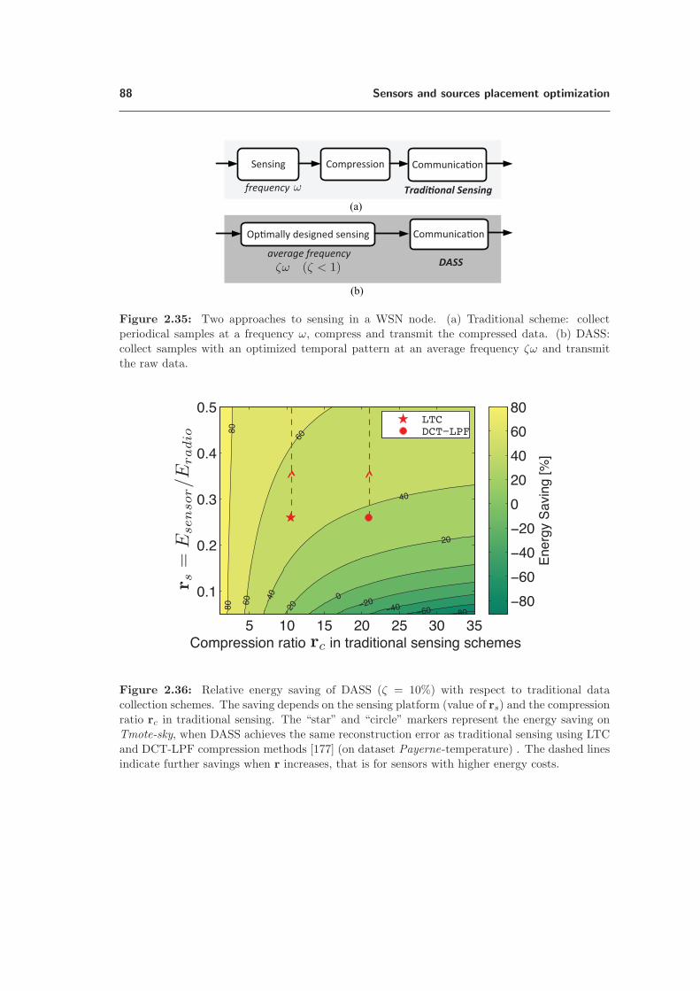
88 Sensors and sources placement optimization
Sensing Compression Communica��n
������� designed sensing Communica�on
frequency
average frequencyDASS
������onal Sensing
Figure 2.35: Two approaches to sensing in a WSN node. (a) Traditional scheme: collect
periodical samples at a frequency ω, compress and transmit the compressed data. (b) DASS:
collect samples with an optimized temporal pattern at an average frequency ζω and transmit
the raw data.
�������������
��
��
��
��
��
��
����
Compression ratio in traditional sensing schemes
5 �� 15 �� � � 35
���
���
��
���
��
Ene
rgy
Sav
ing
[%]
���
���
���
���
�
��
��
��
��LTC�������
Figure 2.36: Relative energy saving of DASS (ζ = 10%) with respect to traditional data
collection schemes. The saving depends on the sensing platform (value of rs) and the compression
ratio rc in traditional sensing. The “star” and “circle” markers represent the energy saving on
Tmote-sky, when DASS achieves the same reconstruction error as traditional sensing using LTC
and DCT-LPF compression methods [177] (on dataset Payerne-temperature) . The dashed lines
indicate further savings when r increases, that is for sensors with higher energy costs.

2.7 Application: adaptive scheduling of sensor networks 89
0 2 40
1
2
3
4
Time [ms]
Con
sum
ptio
n [m
W]
(a)
0 10 200
10
20
30
40
50
Time [ms]
Con
sum
ptio
n [m
W]
(b)
Figure 2.37: Energy consumptions of a Tmote-sky sensor: (a) while the node measures one
sample of light intensity (two-bytes), Esensor = 7.5 × 10⁻⁶J; (b) while the node transmits a
packet with 24 bytes of payload, 24Eradio = 6.9× 10⁻⁴J.
traditional scheme. However, DASS may not necessarily consume less communication energy,
since the compression ratio rc11 used in traditional sensing is generally better than 1/ζ. In fact,
existing data compression schemes can achieve a compression ratio rc of 1.5 ∼ 5 for lossless
coding [134], and 5 ∼ 50 for lossy coding [177], while a typical value of ζ used in DASS is 0.1.
Hence, there is a tradeoff between the energy saved on sensing and communications.
Such a tradeoff between the different energy consumption depends on platform-specific pa-
rameters. In particular, we denote the energy consumption for collecting and transmitting one
sample as Esensor and Eradio, respectively. An interesting figure is the ratio between the two
energy values, that we denote as rs = Esensor/Eradio. Intuitively, the larger rs, the larger the en-
ergy savings obtained by DASS. For the traditional data collection schemes, we assume that the
compression step has a negligible energy cost. For DASS we use a subsampling rate of ζ = 0.1,
which means that 10% of the original signal is sampled and transmitted.
Under these assumptions, we can quantitatively analyze the relative energy savings of DASS
with respect to the traditional sensing as a 2-D function of the platform parameter rs and the
compression ratio rc achieved by the compression stage of the traditional scheme. Such function
representing the energy saving is plotted in Figure 2.36. We see that there is a line, indicated by
the zero value, that defines where DASS is more energy-efficient than the traditional schemes.
Above the line, a WSN consumes less energy if it uses DASS and vice versa. Note that DASS is
only less efficient in the scenarios where the compression ratio rc is very high and the platform
parameter rs is very low.
We also looked at the energy savings for a plausible real world scenario. More precisely, we
consider Tmote-sky, a low-power sensing platform widely used in WSNs [169]; it has a photodi-
ode sensor that measures the light intensity of the surroundings and communicates with others
through short-range radio. We measured the two energy consumptions Esensor and Eradio of
11. rc equals uncompressed size / compressed size.

90 Sensors and sources placement optimization
Tmote-sky in a set of experiments, and an example of the results is given in Figure 2.37. In
particular, the experiments indicate that rs = 0.26. To evaluate the energy consumption of a
traditional scheme, we need to choose a specific compression algorithm and measure the achieved
rc. Zordan et al. [177] have recently compared various lossy compression algorithms and showed
that DCT-LPF [177] achieves the best performance in terms of compression ratio. However, it is
also a complex algorithm and may have a significant energy consumption on a resource-limited
platform such as Tmote-sky. Therefore, we also consider a lightweight algorithm, LTC [138],
that achieves the lowest energy consumption on WSN nodes if the energy cost for compression
is considered.
Here, we ignore the energy cost of compression and we compare both algorithms with DASS.
Note that, if we consider computational energy cost, the benefit of DASS will be even larger
since it requires minimal on-board computation. We implement and evaluate the two algorithms
on the dataset Payerne-temperature, and record the corresponding compression ratio rc when
their reconstruction errors are the same as those achieved by DASS.
The “star” and “circle” markers in Figure 2.36 show the energy savings of DASS over a
Tmote-sky that compresses the data with LTC and DCT-LPF, respectively. The energy savings
for the two cases are equal to 50% and 35%. It is worth mentioning that the compression ratios
achieved in Figure 2.36 ( “star” and “circle” markers) are specific of the considered meteorological
datasets. There might be extreme cases where traditional compression schemes achieve a very
high compression ratio (e.g., rc = 100), and the respective saving falls below zero. However, we
observe in Figure 2.36 that the energy savings can still be obtained in such cases, if rs increases
due to a higher energy cost for sensing, as denoted by the dashed lines. This scenario could be
realistic for many WSNs, in particular those using sensor belonging to the following two classes:
– Sensors with high energy consumption: for example an air pollution sensors consume 30 ∼50 mW instead of the 3 mW of a Tmote-sky ’s light sensor.
– Sensors with long sampling time: for example the anemometer, a sensor that measures
wind’s direction and strength, requires 1 ∼ 3 seconds of continuous measurement per
sample instead of the 4 ms of the Tmote-sky ’s light sensor.
2.8 Source placement and vaccination on graphs
Let us focus on the optimization of sources and vaccines on graphs. As described in Section
2.1.2, we model a set of entities as the nodes of the graphs, while the edges describe the temporal
dynamics of the infection between the nodes. In what follows, we propose a theoretical analysis
and a set of initial experimental results for two different optimization problems:
– Source placement on graphs as defined in Problem 2.5,
– Vaccination on graphs as defined in Problem 2.6.
For the first problem, we propose a near-optimal greedy algorithm that has bounded worst-
case performance with respect to the optimal solution. Again, we obtain this bound exploiting
the submodularity of the cost function in conjunction with Theorem 2.1. For the second problem,
we propose an algorithm that has interesting performance. Unfortunately, we are not yet able
to prove performance bounds.
Before describing our results, we would like to describe the mechanics of the infection spread-
ing on the graph G. More precisely, we underline that the infection spreads along paths. For

2.8 Source placement and vaccination on graphs 91
0 0.1 0.2 0.3 0.4 0.5 0.6 0.70
0.1
0.2
0.3
0.4
0.5
0.6
0.7
0.8
0.9
X
Y
Figure 2.38: An example of the considered graph G: ni is the i-th node, sj is the j-th source
of the infection,di,j is the distance between the nodes i and j and μs1,nj is the path transmitting
the infection between the source s1 and the node nj .
simplicity’s sake, let us analyze first the deterministic case, when the weights of the edges are
deterministic. In this scenario, for any given source sj and node ni, there exists a set of edges,
that we call path, that carries the infection from the source to the node. Such path is also
deterministic and can be found as the shortest path connecting the source and the node. Many
algorithms finding the shortest path between the nodes of a graph in polynomial time have been
described in the literature, e.g. the Dijkstra’s algorithm [49]. Here, we denote the shortest path
between sj and ni as μsj ,ni, see an example depicted in Figure 2.38. Then, we define the time
taken by the infection to travel such path as d(μs1,nj).
If we consider the probabilistic case, that is when the weights are random variables, the
infection process is more complicated. In fact, we have generally a multitude of possible paths
between any source and any node on the graph. We define the set of possible U paths between a
source sj and a node ni as Msj ,ni= {μ1
sj ,ni, . . . , μU
sj ,ni}, where U depends also on the indices i
and j. Each sub-path is traveled by the infection in a time, characterized by a random variable.
We also note that the k-th path is the shortest path according to a probability pk defined as
pk = p{μksj ,ni
= minMsj ,ni}.
2.8.1 Near-optimal source placement on graphs
Here, we propose an approximation algorithm for Problem 2.5. More precisely, we design a
greedy sensor placement algorithm that finds a near-optimal set of sources S by a local mini-
mization of the average time of infection of the entire network. For a given source placement A,

92 Sensors and sources placement optimization
the average time of infection is defined as,
H(A) =1
N
∑∀i|ni∈N
ti(A), (2.33)
where ti(A) is the infection time of the node ni when the sources are located in A and N is the
number of nodes in the graph G.The greedy algorithm adds at each iteration a source at the location that maximizes (2.33)
and its pseudo-code is given in Algorithm 2.10.
Algorithm 2.10 Source placement algorithm for graphs
Require: Graph G, Number of sensors S
Ensure: Source locations S
1. Initialize the set of allocated sources, S = ∅.2. Initialize the set of available locations, N = {1, . . . , N}.3. Repeat until S sources are chosen
(a) Find the optimal source,
s∗ = argmini∈N T (S ∪ ni).
(b) Update the set of removed locations, S = S ∪ s∗.
(c) Update the available locations, N = N \ s∗.
Despite the simplicity of the algorithm, we show interesting results on its performance. In
fact, we can prove that Algorithm 2.10 has near-optimal performance with respect to the chosen
cost function (2.33).
Then, we proceed as for FrameSense: if H(S) satisfies the conditions of Theorem 2.1, then
the solution of the greedy algorithm is always close to the optimal one. To simplify the notation
of certain proofs, we use the concept of the discrete derivative of a generic set function J .
Definition 2.5 (Discrete derivative)
Given a set function J : 2N → R, a set A ∈ N and an element n ∈ N \ A, we define the
discrete derivative of J at A with respect to n as ΔJ(n|A) = J(A ∪ n)− J(A).
Note that using the discrete derivative, we can express the submodularity as
ΔJ(i|X ) ≥ ΔJ(i|Y),
for any X ,Y ∈ N and a generic element i ∈ N \Y. Note that if f(X ) is submodular, then −f(X )
is termed as supermodular.
Then, to prove the near-optimality of Algorithm 2.10, we study the characteristic of (2.33),
that are described in the following lemma.
Lemma 2.3 (Properties of H(S))
The set function H(S) is supermodular, monotonically decreasing, always positive and not
normalized.

2.8 Source placement and vaccination on graphs 93
Proof.
For simplicity’s sake we prove the lemma for deterministic edges. Note that we can easily
extend the proof to the random case.
A normalized set function must satisfy H(∅) = 0; in our case, when no sources are placed on
the graph the time of infection is infinite H(∅) = +∞. Therefore H is not normalized.
Then, we want to show that H(A) is monotonically decreasing, that is for every A ⊂ N and
for every e ∈ N \ A we have
ΔH(e|A) ≤ 0,
where ΔH is the discrete derivative.
For each node ni, the infection time ti is given by the shortest path between ni itself and all
the sources. We write the relationship for the i-th node as
min{μsj ,ni}sj∈A∪e ≤ min{μsj ,ni}sj∈A,
which is always true thanks to the definition of minimum.
Then, we show the supermodularity of H(A) by using its definition,
ΔH(i|X ) ≤ ΔH(i|Y),
and picking X = m and Y = {m, l}. Using the definition of ΔH and of H while analyzing the
node n∗, we obtain
min{μm,n∗} −min{μm,n∗ , μi,n∗} ≤ min{μm,n∗ , μl,n∗} −min{μm,n∗ , μl,n∗ , μi,n∗}. (2.34)
By checking all the six possible orderings of the three path’s lengths, we can verify that (2.34)
holds.
Last, the cost function is always positive because the times of infection are bounded between
zero, when the node is actually a source, and infinity, when there are no sources on the graph.
Using Lemma 2.3, we can prove that Algorithm 2.10 has near-optimal performance with
respect to (2.33) as we show in the following proposition. Note that the result is slightly different
from Theorem 2.1 because of Lemma 2.3.
Proposition 2.4 (Performance of Algorithm 2.10)
Given a graph G{N , E} and a number of sources S, Algorithm 2.10 returns a set of sources S.Consider the optimal algorithm that returns the source placement S∗ that globally minimize
the cost function (2.33). Then, Algorithm 2.10 has near-optimal performances, that is
H(S∗1 )−H(S) ≥ 1
e(H(S∗
1 )−H(S∗)),
where H(S∗1 ) is the minimum average infection time achievable by only one source.
Proof.
The proof follows the one of Theorem 2.1, with the necessary modifications given the character-
istics of the cost function H(S). We denote as Si the output of the algorithm at the i-th iteration

94 Sensors and sources placement optimization
and the optimal solution as S∗ = {v1, v2, . . . , vS}. Then, we bound of the optimal solution as
follows,
H(S∗) ≥ H(S∗ ∪ Si) (2.35a)
= H(Si) +
S∑j=1
ΔH(vj |Si ∪ {v1, . . . , vj−1}) (2.35b)
≥ H(Si) +∑v∈S∗
ΔH(v|Si) (2.35c)
≥ H(Si) +∑v∈S∗
(H(Si+1)−H(Si)) (2.35d)
≥ H(Si) + S(H(Si+1)−H(Si)), (2.35e)
where (2.35a) is due to the monotonicity of the cost function, (2.35b) is just a telescopic sum of
the impact of each element of S∗ added to Si, the supermodularity of the cost function justifies
(2.35c), (2.35d) results from the fact that the chosen location at the i-th iteration is the greedy
one and (2.35e) comes from the sum of S elements.
We rearrange (2.35e) as
H(S∗)−H(Si) ≥ S(H(Si+1)−H(Si))
and by defining δi = H(S∗)−H(Si), we obtain δi ≥ S(δi − δi+1). With further rearrangements
and considering i = S − 1, we obtain
δi+1 ≥(1− 1
S
)δi
δi+1 ≥(1− 1
S
)i−1
δ1
δS ≥(1− 1
S
)S−1
≥(1− 1
S
)S
δ1,
δS ≥(1− 1
e
)δ1.
To conclude the proof, we use the definition of δi and note that H(S1) = H(S∗1 ).
Note that we could not use the original results of Nemhauser et al. [112] because the cost
function H(A) is infinite when A = ∅. Therefore, instead of a classical near-optimal bound, we
obtain a bound on the distance between the performance of Algorithm 2.10 and the performance
of an optimal algorithm based on the optimal solution when only one source is present. We
underline that the optimal solution with only one source H(S∗1 ) is the output by Algorithm 2.10
with S = 1.
2.8.2 Vaccination on graphs
We now propose an approximation algorithm for Problem 2.6: a greedy algorithm that re-
moves nodes from the graph—the vaccination—so that the average time of infection of the

2.8 Source placement and vaccination on graphs 95
network is maximized. Assuming that the graph G is fully connected and the infection starts
from a single node chosen uniformly at random from N , such a cost function is defined as
W (A) =1
N
∑i=N
qi(A), (2.36)
where qi is the infection time of the node ni when the nodes in A are removed from G.The proposed algorithm implements a simple greedy strategy: at each iteration we remove
from the graph G the node that maximizes the cost function 2.36. Its pseudocode is given in
Algorithm 2.11.
Algorithm 2.11 Vaccination algorithm for graphs
Require: Graph G, Number of vaccine V
Ensure: Vaccine locations V
1. Initialize the set of vaccinated nodes, V = ∅.2. Initialize the set of available nodes, N = {1, . . . , N}.3. Repeat until V vaccine targets are chosen
(a) Find the optimal node to vaccinate, i∗ = argmaxi∈N W (V ∪ i).
(b) Update the set of vaccinated nodes, V = V ∪ i∗.
(c) Update the available nodes, N = N \ i∗.
Unfortunately, the cost function defined in (2.36) is not submodular and we cannot guarantee
the performance of Algorithm 2.11. Nonetheless, it is worth mentioning such an algorithm
because it shows good performance when compared to other possible approaches, such as the
vaccination of the nodes with the largest amount of connections.
2.8.3 Computing the cost functions of Algorithms 2.10-2.11
When describing Algorithm 2.10 and 2.11, we did not discuss the computation of (2.33) and
(2.36), which are in general not trivial. Here, we explain this computation when the weights of
the edges are either deterministic or random.
For the deterministic case, the time of infection of each node is simply computed as the
minimum between the shortest paths between the node and each source. The shortest path can
be computed between all the nodes of the graph using various algorithms, such as Dijkstra’s
algorithm [49].
However, the computations of these cost functions is significantly more complex for graphs
where the edges have weights defined as random variables. To the best of our knowledge, there
exists no algorithm in the literature that computes exactly the average length of the shortest
path between two nodes in polynomial time for these graphs. The main difficulty is caused by
the large number, generally exponential in N , of possible paths between any two nodes of the
graph. Even if it was possible to enumerate all the paths, it is simply difficult to compute the
expected value of the minimum length of all the paths.
The simplest strategy to implement such a computation for the random case is described in
Algorithm 2.12 and it is based on a MonteCarlo approach. Unfortunately, it is hard to control
the estimation error of this approach.

96 Sensors and sources placement optimization
00.05
0.10.15
0.20.25
0 20 40 60 80
100
Tim
e
Number of healthy nodes
Tem
poral evolution of healthy people
Greedy M
ean time
Random
Greedy M
ax Conn.
(a)AB
graphwith
Gaussia
ned
ges
00.02
0.040.06
0.080 20 40 60 80
100
Tim
e
Number of healthy nodes
Tem
poral evolution of healthy people
Greedy M
ean time
Random
Greedy M
ax Conn.
(b)AB
graphwith
Exp.ed
ges
00.1
0.20.3
0.40 20 40 60 80
100
Tim
e
Number of healthy nodes
Tem
poral evolution of healthy people
Greedy M
ean time
Random
Greedy M
ax Conn.
(c)AB
graphwith
Unifo
rmed
ges
00.05
0.10.15
0.20.25
0 20 40 60 80
100
Tim
e
Number of healthy nodes
Tem
poral evolution of healthy people
Greedy M
ean time
Random
Greedy M
ax Conn.
(d)W
Sgraphwith
Gaussia
ned
ges
00.02
0.040.06
0 20 40 60 80
100
Tim
e
Number of healthy nodes
Tem
poral evolution of healthy people
Greedy M
ean time
Random
Greedy M
ax Conn.
(e)W
Sgraphwith
Exp.ed
ges
00.1
0.20.3
0.40 20 40 60 80
100
Tim
e
Number of healthy nodes
Tem
poral evolution of healthy people
Greedy M
ean time
Random
Greedy M
ax Conn.
(f)W
Sgraphwith
Unifo
rmed
ges
Figure
2.39:Tem
poralevo
lutio
noftheinfectio
nover
agraphfordifferen
tgraphtopologies
andweig
hts
oftheedges,
when
S=
3
sources
are
infected
.Note
thattheproposed
algorith
m,”G
reedyMeanTim
e”,red
uces
thenumber
ofhealth
ynodes
atan
ytim
eby
selectingthenear-o
ptim
alset
ofsources
toinfect
att=
0when
compared
tothebenchmark
algorith
ms.

2.8 Source placement and vaccination on graphs 97
Algorithm 2.12 Computation of the average time of infection for a graph
Require: Graph G, Sources S, Max iteration MAX
Ensure: Average time of infection E[ti] ∀i
1. Repeat MAX times
(a) Sample from the random distributions of every edge of the graph.
(b) Compute the adjacency matrix (2.7) for these edges.
(c) Compute the shortest paths between all the nodes using Dijkstra’s Algorithm.
(d) Store the length of the shortest path between all the nodes of the graph and the
sources S.2. For every node, compute the average time of infection as the average of the stored values.
Note that more efficient approaches can be designed by constraining the probability distri-
butions of the edges to specific cases, e.g. i.i.d. Gaussian random variables.
2.8.4 Experimental results
As a conclusion, we present some experimental results for Algorithm 2.10 and 2.11 based on
synthetic datasets generated by two topologies of random graphs:
– Watts-Strogatz (WS) graph [168]: we place N nodes on a 2D circle, connect each edge with
the D/2 neighbors on the right and on the left, then we reallocate with a probability Pe
these edges to other random nodes.
– Albert-Barabasi (AB) graph: a scale-free graph with a given node degree D that is ran-
domly generated as described in [5].
Then, we assign the weights of the edges according to three different models,
– Constant values uniformly picked between 0 and 10,
– Gaussian random variables with variance σ2 = 1,
– Exponential random variables with mean 1λ = 5.
We choose the two following algorithms as a performance benchmark for the proposed algo-
rithms:
– A greedy algorithm that chooses the nodes with the largest amount of connections,
– A random algorithm that picks S nodes at random.
Note that the greedy algorithm choosing the nodes with the highest connectivity represents the
algorithm that would be used intuitively in a real-world scenario: if you want to spread the
virus/information as fast as possible on the graph, pick the nodes that have as many neighbors
as possible.
We design a set of experiments to analyze the performance of Algorithm 2.10 and 2.11 and
these experiments are described in the following sections.

98 Sensors and sources placement optimization
0200
400600
8001000
4 6 8 10 12
Num
ber of nodes of the graph
Time
Average tim
e of infection on random graphs
Greedy M
ean time
Random
Greedy M
ax Conn.
(a)AB
graphwith
Gaussia
ned
ges
0200
400600
8001000
3 4 5 6 7 8 9 10
Num
ber of nodes of the graph
Time
Average tim
e of infection on random graphs
Greedy M
ean time
Random
Greedy M
ax Conn.
(b)AB
graphwith
Exp.ed
ges
0200
400600
8001000
4 6 8 10 12 14 16
Num
ber of nodes of the graph
Time
Average tim
e of infection on random graphs
Greedy M
ean time
Random
Greedy M
ax Conn.
(c)AB
graphwith
Unifo
rmed
ges
0200
400600
8001000
0 5 10 15 20 25
Num
ber of nodes of the graph
Time
Average tim
e of infection on random graphs
Greedy M
ean time
Random
Greedy M
ax Conn.
(d)W
Sgraphwith
Gaussia
ned
ges
0200
400600
8001000
0 5 10 15 20 25 30
Num
ber of nodes of the graph
Time
Average tim
e of infection on random graphs
Greedy M
ean time
Random
Greedy M
ax Conn.
(e)W
Sgraphwith
Exp.ed
ges
0200
400600
8001000
5 10 15 20 25 30 35
Num
ber of nodes of the graph
Time
Average tim
e of infection on random graphs
Greedy M
ean time
Random
Greedy M
ax Conn.
(f)W
Sgraphwith
Unifo
rmed
ges
Figure
2.40:Avera
geinfectio
ntim
eover
agraphfordifferen
tgraphtopologies
andweig
hts
oftheedges,
asafunctio
nofthenumber
ofnodes
when
S=
3sources
are
infected
.Note
thattheproposed
algorith
m,”Greed
yMeanTim
e”,outperfo
rmstheother
two
algorith
msforanysize
ofthegraph.

2.8 Source placement and vaccination on graphs 99
Temporal evolution of the infection for Problem 2.5
First, we are interested in understanding qualitatively how fast the infection spreads over a
graph when the different algorithms are used to optimize the sources placement.
We generate 100 graphs at random, for each graph we optimize the locations of S = 3 sources
according to the different algorithms and we record the infection time of each node. Then, we
measure how many nodes are healthy on average at a given time and the results are given in
Figure 2.39. For each graph topology, we have the following parameters:
– WS graphs: number of nodes N = 100, nodes are connected with D = 3 neighbors on the
right and on the left, and edges are re-connected with a probability Pe = 0.2.
– AB graphs: number of nodes N = 100, out-degree of nodes= 7,
For both topologies, Algorithm 2.10 achieves the fastest infection rate. We also note that
the greedy algorithm minimizing the time of infection of the whole graph is acting as expected:
the time at which the infection is completed is on average equal or lower than the competing
algorithms. Another interesting aspect is that the algorithm picking the maximally connected
nodes is not efficient at all, which seems counterintuitive.
Average infection time for Problem 2.5
Then, we focus on the average infection time as a function of the number of nodes of the
graph. Therefore, we measure such parameter for N = {10, . . . , 200}, averaging its value over 100
realization of the random graph, using the same values for the graph parameters. The results are
given in Figure 2.40 and we note that the performance of Algorithm 2.10 is significantly better
than the two algorithms used as a benchmark.
For an increasing size of the graph, the average time converges to an asymptotic value for
AB graphs, while it steadily increases for WS graphs.
Vaccination on graphs
Last, we want to evaluate the efficacy of the vaccination algorithm described in Algorithm
2.11. As we have previously mentioned, this algorithm does not have any guarantee on its
performance. Nonetheless, we show here that Algorithm 2.11 outperforms other strategies, such
as vaccinating the nodes with the largest number of connections.
We designed our experiment as follows: we randomly generate 10 graphs with N = 128 nodes
and assume to have vaccines sufficient for half of the population, that is V = 64. Then, we
distribute those vaccines according to the different algorithms and we measure the number of
healthy nodes as time passes. The results are depicted in Figure 2.41. We note that for all
the graph topologies, our algorithms outperforms the others. More precisely, at any given time
we have the largest percentage of the population that is still healthy. Note that the number
of healthy people converges for certain combination of algorithm and graph to a constant value
larger than V , meaning that the vaccination disconnected part of the graph. However, this is not
true for all algorithms: the random algorithm for AB graphs and the ”Greedy Max Connectivity”
algorithm for WS graphs converge to the value of 64, the number of healthy nodes thanks to the
vaccine.

100 Sensors and sources placement optimization
020
4060
80100
0 50
100
150
200
Tim
e
Healthy nodes
Tem
poral evolution of healthy nodes
Greedy M
ean time
Greedy M
ax Connectivity
Random
No V
accine
(a)AB
graphwith
Gaussia
ned
ges
020
4060
80100
0 50
100
150
200
Tim
e
Healthy nodes
Tem
poral evolution of healthy nodes
Greedy M
ean time
Greedy M
ax Connectivity
Random
No V
accine
(b)AB
graphwith
Exp.ed
ges
020
4060
80100
0 50
100
150
200
Tim
e
Healthy nodes
Tem
poral evolution of healthy nodes
Greedy M
ean time
Greedy M
ax Connectivity
Random
No V
accine
(c)AB
graphwith
Unifo
rmed
ges
020
4060
80100
0 50
100
150
200
Tim
e
Healthy nodes
Tem
poral evolution of healthy nodes
Greedy M
ean time
Greedy M
ax Connectivity
Random
No V
accine
(d)W
Sgraphwith
Gaussia
ned
ges
020
4060
80100
0 50
100
150
200
Tim
e
Healthy nodes
Tem
poral evolution of healthy nodes
Greedy M
ean time
Greedy M
ax Connectivity
Random
No V
accine
(e)W
Sgraphwith
Exp.ed
ges
020
4060
80100
0 50
100
150
200
Tim
e
Healthy nodes
Tem
poral evolution of healthy nodes
Greedy M
ean time
Greedy M
ax Connectivity
Random
No V
accine
(f)W
Sgraphwith
Unifo
rmed
ges
Figure
2.41:Tem
poralevo
lutio
nof
theinfectio
nover
agraphof
N=
128nodes,
with
onenodeinfected
atrandom
usin
gV
=64
vaccines.
Thetopolo
gyandtheweig
hts
ofthegraphsare
specifi
edin
thecaptio
nsofthesubfigures.
Thevaccin
esare
given
tothe
nodes
selectedbythedifferen
talgorith
ms,
and”G
reedyMeanTim
e”refers
toAlgorith
m2.11.Note
thattheproposed
algorith
m
outperfo
rmstheconten
ders
forall
thetopologies
since
itkeep
thelargest
part
ofthepopulatio
nhealth
yforalm
ost
everytim
et.

2.9 Conclusions 101
2.9 Conclusions
Sensor placement for linear physical fields
In Section 2.3.3, we studied the optimization of sensor placement when the collected mea-
surements are used to solve a linear inverse problem. The problem is equivalent to choosing L
rows out of N from a matrix Ψ such that the resulting matrix has favorable spectral properties.
The problem is intrinsically combinatorial and approximation algorithms are necessary for real-
world scenarios. While many algorithms have been proposed, none has guaranteed performance
in terms of the MSE of the solution of the inverse problem, which is the key merit figure.
We proposed FrameSense, a greedy worst-out algorithm minimizing the FP. Even if this
chosen cost function is well-known in frame theory for its fundamental role in the construction of
frames with optimal MSE, FrameSense is the first algorithm exploiting it as a cost function for
the sensor placement problem. Our theoretical analysis demonstrates the following innovative
aspects:
– FrameSense is near-optimal with respect to the FP, meaning that it always places the
sensors such that the obtained FP is guaranteed to be close to the optimal one.
– Under RIP-like assumptions for Ψ, FrameSense is also near-optimal with respect to the
MSE. Note that FrameSense is the first algorithm with this important property.
We provided extensive numerical experiments showing that FrameSense achieves the best
performance in terms of MSE while having the lowest computational complexity when compared
to many other greedy algorithms. FrameSense is also competitive performance-wise with a state-
of-the-art algorithm based on a convex relaxation proposed in [73], while having a substantially
smaller computational time.
Future work will be three-fold. First, it is foreseeable to relax the RIP-like condition on Ψ by
considering that the characteristics of the FP are potentially sufficient to avoid ΨL matrices with
an unfavorable spectral distribution. Moreover, it would be interesting to show that there exists
matrices, random or deterministic, that are (δ, L)-bounded frames. Second, we believe that a
convex relaxed scheme based on the FP integrating the heuristics proposed by Joshi et al. [73]
could improve significantly the MSE of the obtained solution, while keeping the near-optimality
thanks to the FP. Third, we would like to derive a new cost function that exploits the sensing
energy of the rows, as described in Section 2.3.6.
Source placement for linear physical fields
We studied the source placement problem as the dual of sensor placement: a column selection
out of a linear model Ψ. We defined two problems differentiated by the presence of noise and each
problem optimizes a different cost function. For the noiseless case, we proposed an algorithm
that approximate any given subspace S using the span of a set L of columns of Ψ and it is near-
optimal with respect to the approximation error. For the noisy case, we proposed an algorithm,
based on a previous work [127], that optimizes the frame potential as a proxy of the mean-square
error. Such an algorithm is near optimal under a given condition on Ψ, but it can only deal with
the case S = RN .
Future work will consider the extension of Algorithm 2.3 to a generic subspace with noise
on the measurements. Such work will be centered on the definition of a cost function that

102 Sensors and sources placement optimization
promotes the choice of a subspace that is close to S and it is formed by a set of columns that are
well-conditioned.
Thermal monitoring of microprocessors
In Section 2.6, we proposed a framework to optimally reconstruct thermal maps of many-core
SoC using a small number of sensors. We defined an optimal approximation of thermal maps
to reduce the number of parameters to estimate, without loosing precision. We reconstructed
the thermal maps using a least square approach and we exposed the critical role of the sensor
location for the quality of the thermal monitoring. We concluded proposing a greedy sensor
allocation algorithm that minimizes the reconstruction error by minimizing a proxy function,
namely the frame potential. The sensor placement algorithm improves the coherence-based one
we previously proposed [128] and is inspired by theoretical findings described in Section 2.3.
We compared the proposed method against two algorithms among the state of the art, namely
the information-theoretic method [176] and the spectral method [113]. We demonstrated the
higher fidelity of our reconstruction using a smaller number of sensors. We showed how the
proposed reconstruction algorithm is more stable with respect to the noise introduced by the
electronics or by sensor calibration inaccuracies, thanks to the regularization imposed by the
linear model Ψ.
Moreover, we investigated the challenges surrounding the learning and the optimization of the
linear model Ψ, one of the main critical points of the framework. We showed that a training set
formed by an incomplete collection of thermal distributions is enough to learn a precise model Ψ.
We remarked that even a training set generated by random power traces leads to a reasonably
good model. Note that such discovery has a great potential, since it allows the design of thermal
monitoring systems without knowing precisely the workload of the SoC.
Adaptive scheduling of sensor networks
In Section 2.7, we proposed DASS, a novel approach for sparse sampling that optimizes
sparse sampling patterns for precisely recovering spatio-temporal physical fields. DASS is based
on three main blocks. First, it adaptively learns the signal statistics from past data. Second, it
dynamically adjusts the sampling pattern according to the time–varying signal statistics. Third,
it recovers the signal from the limited amount of collected samples and according to the learnt
signal statistics.
We demonstrated the effectiveness of DASS through extensive experiments using two real-
world meteorological datasets. The results show significant improvements over the state-of-the-
art methods. These improvements are more pronounced in the presence of significant spatial
and/or temporal correlation in the sampled data by WSN.
We evaluated DASS on static WSNs; however, DASS is flexible and can be applied to other
sensing scenarios such as mobile WSNs. For instance, sensors are installed on top of buses for
collecting various environmental data along their trajectories [3]. The collected samples show
strong correlation due to the fixed route periodically taken by the buses. In future work, we will
analyze the advantages of an optimized sensing schedule in such cases, where the constraint is not
the energy consumption but the relatively slow speed of sampling of certain pollution sensors.

2.10 Appendix 103
Near-optimal source placement and vaccination on graphs
In Section 2.8, we analyzed possible algorithmic solutions for the source placement on graphs,
as defined in Problem 2.5, and vaccination on graphs, as defined in Problem 2.6. For the source
placement, we proposed a near-optimal algorithm that selects the set of nodes to infect to min-
imize the infection time of the entire graph. We showed that such an algorithm significantly
improves other algorithms that selects the source at random or according to their connectivity
degree. For the vaccination problem, we proposed an algorithm that removes the nodes of the
graph such that the average time of infection of the entire graph is maximized. While we were
not able to derive performance bound for such an algorithm, we showed with several numerical
experiments on different topologies of graphs that it outperforms the contenders. Note that while
both problems are relatively new in the literature, we believe that can raise a potential interest
in many scenarioes, such as the optimization of the vaccination strategies to eradicate viruses
[100] and the optimal spreading of rumors in social networks.
2.10 Appendix
2.10.1 Proof of Lemma 2.2
In this section, we bound the MSE of a matrix ΨA ∈ RL×K as a function of its FP and the
spectrum {λi}Ki=1 of TL.First, consider the harmonic mean H = K∑
k1λj
, the arithmetic mean A =∑
k λk
K and the
standard deviation S =√
1K
∑k (λk −A)
2of the eigenvalues of TL. All these quantities are
linked to MSE (ΨA),the number of sensors L and FP (ΨA). More precisely, we have
H =K
MSE (ΨA),
A =LAK
,
S =
√1
K
(FP (ΨA)− LA2
K
).
Then, we consider the following bounds for the harmonic mean of a set of positive numbers
derived by Sharma [144],
(M − S)2
M(M − 2 S)≤ A
H≤ (m+ S)2
m(m+ 2S),
where m and M are the smallest and the largest number in the set. We use the expressions of
A and H and we remove the mixed term in the denominator to obtain,
K2
LA
(1 +
S2
M2
)≤ MSE (ΨA) ≤ K2
LA
(1 +
S2
m2
).
As expected when the FP achieves its global minima, that is S = 0, we achieve the optimal MSE
of a tight frame.
104 Sensors and sources placement optimization
To conclude the proof, we consider the two bounds separately starting from the lower one. Let
M = λ1 and we plug in the value of S. We also consider without loss of generality LA ≤ LMAX,
since we can always improve the MSE by increasing the sensing power LA. Then,
MSE (ΨL) ≥ K2
LMAX
(1 +
FP(ΨA)Kλ1
2 − LMAX2
K2λ12
).
We obtain the final result by using lower bound on the largest eigenvalue: λ1 ≥ LMAX
K .
The approach to prove the upper bound is exactly symmetrical. Specifically, consider m =
λN , LA ≥ LMIN and use the upper bound on the smallest eigenvalue λN ≤ LMAX
K .
2.10.2 Reconstruction error characterization for thermal monitoring
Proposition 2.5
Consider a thermal map f ∈ RN , a given linear model Ψ ∈ R
N×K and sensor placement L.Then, the reconstructed thermal map is equal to
f = ΨΨL†(fL − εL) +ΨΨL†(nL + εL),
where nL is the measurement noise and εL = fL − fL is the approximation error due to the
linear model Ψ. Assume that nL is modeled as a vector of i.i.d. Gaussian random variables
with variance σ2 and that ΨL has rank K, then we can bound the reconstruction error as
‖f − f‖22 ≤ σ2K∑i=1
1
λi+
(1 +
1
λK
)‖ε‖2, (2.37)
where λi is the i-th eigenvalue of the operator ΨL∗ΨL.
Proof.
We present a sketch of the proof due to its simplicity. First, we note that we have two independent
components in the error: the white noise generated during the measurement of the temperature
and the approximation error due to the linear model Ψ. Given their independence, we analyze
them separately.
For the Gaussian part, we use a known result [127] to obtain the first component of (2.37). For
the approximation error, we have to consider it twice. First, when we reconstruct the thermal
map, such an approximation error is amplified by the projection onto span(Ψ). The worst
case scenario being the approximation error aligned with the eigenvalue with λK , the smallest
eigenvalue of (ΨL∗ΨL). Second, by assumption our reconstruction lies on the subspace spanned
by Ψ, therefore we must add ε, leading to the(1 + 1
λK
)factor.
2.10.3 Parametric control of the temperature in many-core processors
The main possible drawback of a linear model based on the PCA is the occupation in memory
and its computational cost. In fact, consider the N × L matrix Θ = Ψ(ΨL)†, then we are
supposed to store Θ and to compute a matrix-vector multiplication with it to estimate the
current thermal distribution. Note thatN can be quite a large number, being the resolution of the

2.10 Appendix 105
estimated thermal distribution. Consequently, the cost in terms of memory and computational
power is significant.
Such cost is unavoidable if our target is to actually estimate the thermal distribution. How-
ever, in most of the applications of thermal monitoring we aim at controlling of the temperature.
That is, we generally aim at solving a control problem similar to the following one,
maxw
P (w)
subject to f ≤ tmax
|Df | ≤ dmax
,
where P (w) is a cost function representing the performance of the system, w is the optimized
workload, f is the temperature, tmax is the maximum allowed temperature and |Df | ≤ dmax
represents the maximum gradient allowed for the thermal distribution. Note that there could
be more constraints and a different cost function, but such changes would not invalidate the
following observations.
Note that we can generalize the temperature constraints as,
Bf ≤ a, (2.38)
where B is a generic linear operator that generalizes the previous constraints. Solving an opti-
mization problem with the constraint defined as (2.38) clearly requires the temperature of the
die, and therefore the computation and the storing of the matrix Ψ.
However, the recovery of the coefficients α is sufficient, since we can rewrite the constraint
as
Cα ≤ a,
where C = BΨ is a matrix containing both the low-dimensional linear model and the constraint.
If the solution of the optimization problem is too expensive due to the size of the constraints,
we can reduce such cost by reducing their dimensions at the cost of a reduced spatial resolution.

106 Sensors and sources placement optimization
Table of notations
x,x,p spatial variables
f original signal
f expected value of f
Σf covariance matrix of f
f reconstructed signal
f approximated signal
fL measured values of f at Ly generalized measurements
υi i-th sampling kernel
Υ sampling matrix
W number of generalized measurements
n measurement noise
σ2 variance of n
Σn covariance matrix of n
Ψ,Ψt model of f
ψi i-th row of Ψ
FP(A) frame potential of the matrix A
MSE(A) mean square error for the matrix A
F (A) cost function of Algorithm 2.1 for sensors placed in AL sensor placement
N available sensor positions
OPT set representing the optimal solution
OPT complementary set of OPT, OPT = N \OPT
Φ source linear model
β source coefficients
P number of available sources
S number of selected sources
S set of selected sources
T target subspace for the source placement problem
T dimensionality of T
P projection operator
λk(A) k-th eigenvalue of A∗ATA Ψ∗
AΨALMIN, LMAX, LMEAN, Lt,MIN, Lt,MAX functions of the row norms of Ψ and Ψt
α low dimensional representation of f
α reconstructed parameters
N length of f
K number of parameters α
L number of measurements
Q union of subspaces Ψt
Q number of subspaces in QHi,j convex hull of Ψi and Ψj
Kt dimension of the subspace spanned by Ψt
γ approximation factor of the FP
η approximation factor of the MSE

2.10 Appendix 107
F training set for the thermal monitoring
M number of thermal maps in Fδ fraction of the thermal maps of F used for training
ρ(δ) performance of the model learning algorithm
Π sparsity dictionary
s sparse decomposition of f in Π
ΔT temporal resolution of original signal
ω sampling frequency of original signal, equals 1/ΔT
ωs average sampling frequency of the sensor with DASS
ζ subsampling rate ζ = ωs/ω
y collected data by the sensor network
τ t sampling pattern of the t-th block
Υt sampling matrix of the t-th block
κ(τ t) reconstruction error due to the noise with the sampling scheduling τ t
R number of blocks used to learn the model
β noise parameters of the CSN sampling algorithm


Chapter 3
Inverse problems for the diffusionequation
An expert is a person who has made all the
mistakes that can be made in a very narrow
field.
Niels Bohr
3.1 Introduction
Sensor networks (SN) are systems composed by a set of sensor nodes and can be considered as
spatio-temporal sampling devices. Often, they are used to sense phenomena driven by well-known
physical fields, such as the wave or the diffusion field.
In the case of diffusion fields, we can use classic tools developed for multidimensional signal
processing to extract the maximal amount of information from the measured data. Unfortu-
nately, the dimensions of the sampling domain—space and time—are not homogeneous. Even
if multidimensional sampling is well documented in the literature, many of the known results
cannot be easily extended to fields with non-homogeneous dimensions.
The following example describes a scenario showing the limits of classical signal processing
tools when dealing with multi-dimensional physical fields.
109

110 Inverse problems for the diffusion equation
Example 3.1
Consider a SN that collects samples of a physical field aiming at reconstructing the entire
field. Note that the spatial density is given by the average number of sensors deployed while
the temporal density is defined by the temporal sampling frequency of each sensor. The
former is limited by the physical space that every sensor occupies and by its economical cost,
the latter is usually limited by the analog-to-digital converters characteristics, the channel
capacity and by the energy consumption bounds. Therefore, it is often easier to increase the
temporal sampling frequency or the channel capacity than to increase the number of sensors.
Is it possible to increase the temporal sampling density and reduce the spatial one without
any precision loss when reconstructing the entire field?
We underline that traditional signal processing tools are not suited to answer such a ques-
tion because the dimensions are usually considered to be homogeneous and interchangeable.
In this work, we consider the spatio-temporal sampling of the diffusion equation to infer
specific information regarding the measured physical field. While such a partial differential
equation is rather simple, it can model efficiently many real world scenarios. The classic example
of diffusion field is the temperature of a solid object, whose estimation is of great importance
for the thermal management of multi-core processors [128]. Then, we would like to mention the
pollution detection problem [53], the plume sources detection [105], atmospheric plumes [151],
short pulse laser applications [62, 160], and temperature distribution in a server room [38] to
name a few. Recently, the temperature estimation in solid bodies showed its importance
As we have mentioned in the Chapter 1, two different problems are involved in the study of
partial differential equations (PDEs): the forward problem and the inverse problem. The former
implies the knowledge of the boundary conditions and the field distribution at a given time t0;
the desired solution is the field f(x, t) for every x and t > t0. The latter belongs to a vast
family of problems where we have (partial) knowledge of the field and we would like to estimate
some unknown information of the field. For example, we may want to recover the entire field
distribution f(x, t) or the initial field distribution from a set of measured samples of the field.
Most of the aforementioned applications can be modeled as inverse problems of the diffusion
equation. Unfortunately, such inverse problems are often ill-conditioned: the slightest error
in the measured data can lead to extremely large errors in the solution, and standard solving
methods are imprecise and inefficient [65]. Therefore, new approaches are needed and often must
be tailored to each specific problem according to the available a-priori information.
The first known inverse problem of the diffusion equation goes back to Fourier and Kelvin
[34], who tried to estimate the initial temperature of the Earth from the current temperature
distribution. Unfortunately, it is known that many inverse problems involving the diffusion
equation are severely ill-conditioned [65]. Recent works considered the spatial sparsity of the
initial distribution as a regularization technique. For example, Nehorai et al. [111] studied
the detection and the localization of a single vapor-emitting source by a maximum likelihood
estimator. More recently, Al Masood et al. considered a hyperbolic heat equation that is well
conditioned [99] or a Bessel operator [98] to estimate the initial temperature distribution in
a diffusion field. Instead, Nakamura et al. [110] used transform techniques to solve the initial
inverse problem in heat conduction, while Takeuchi et al. [86] defined the existence of the solution
and a possible numerical method to find point sources distributed on a 2D domain.
Lu and Vetterli introduced two different approaches to the reconstruction of a sparse source
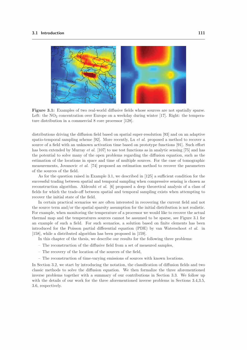
3.1 Introduction 111
Figure 3.1: Examples of two real-world diffusive fields whose sources are not spatially sparse.
Left: the NO2 concentration over Europe on a weekday during winter [17]. Right: the tempera-
ture distribution in a commercial 8 core processor [128].
distributions driving the diffusion field based on spatial super-resolution [93] and on an adaptive
spatio-temporal sampling scheme [92]. More recently, Lu et al. proposed a method to recover a
source of a field with an unknown activation time based on prototype functions [91]. Such effort
has been extended by Murray et al. [107] to use test functions as in analytic sensing [75] and has
the potential to solve many of the open problems regarding the diffusion equation, such as the
estimation of the locations in space and time of multiple sources. For the case of tomographic
measurements, Jovanovic et al. [74] proposed an estimation method to recover the parameters
of the sources of the field.
As for the question raised in Example 3.1, we described in [125] a sufficient condition for the
successful trading between spatial and temporal sampling when compressive sensing is chosen as
reconstruction algorithm. Aldroubi et al. [6] proposed a deep theoretical analysis of a class of
fields for which the trade-off between spatial and temporal sampling exists when attempting to
recover the initial state of the field.
In certain practical scenarios we are often interested in recovering the current field and not
the source term and/or the spatial sparsity assumption for the initial distribution is not realistic.
For example, when monitoring the temperature of a processor we would like to recover the actual
thermal map and the temperatures sources cannot be assumed to be sparse, see Figure 3.1 for
an example of such a field. For such scenarios, a solution based on finite elements has been
introduced for the Poisson partial differential equation (PDE) by van Waterschoot et al. in
[158], while a distributed algorithm has been proposed in [159].
In this chapter of the thesis, we describe our results for the following three problems:
– The reconstruction of the diffusive field from a set of measured samples,
– The recovery of the location of the sources of the field,
– The reconstruction of time-varying emissions of sources with known locations.
In Section 3.2, we start by introducing the notation, the classification of diffusion fields and two
classic methods to solve the diffusion equation. We then formalize the three aforementioned
inverse problems together with a summary of our contributions in Section 3.3. We follow up
with the details of our work for the three aforementioned inverse problems in Sections 3.4,3.5,
3.6, respectively.

112 Inverse problems for the diffusion equation
3.2 The diffusion equation
In this section, we sketch the basic concepts connected to the solution of the diffusion equation.
First, we characterize the diffusion equation according to the presence of external sources or drift,
then we outline two of the standard approaches to solve this family of differential equations.
Consider a field f(x, t) with one spatial variable x and one temporal variable t. We define
the generic diffusion equation as
∂f(x, t)
∂t= γ
∂2f(x, t)
∂x2+ μ
∂f(x, t)
∂x+ g(x, t), (3.1)
where t > 0, g(x, t) represents the external source, γ is the diffusion coefficient and μ is the
advection speed. When t = 0, the field f(x, 0) represents the initial field distribution and is also
denoted as f0(x).
We can define three versions of (3.1), that suit different diffusion situations:
– If g(x, t) = 0 and μ = 0, we obtain the homogeneous linear equation (also known as the
heat equation)∂f(x, t)
∂t= γ
∂2f(x, t)
∂x2, (3.2)
that models physical fields such as the temperature diffusion in a solid body.
– If μ = 0, we obtain the non-homogeneous linear equation
∂f(x, t)
∂t= γ
∂2f(x, t)
∂x2+ g(x, t), (3.3)
that models the temperature diffusion in a solid body in the presence of external heat
sources.
– Otherwise, we get the advection-diffusion equation
∂f(x, t)
∂t= γ
∂2f(x, t)
∂x2+ μ
∂f(x, t)
∂x+ g(x, t), (3.4)
that models a broader range of diffusive phenomena such as pollution and plume dispersion.
A fundamental requirement to understand and to expand the theory of inverse problems of
the diffusion equation is the understanding of its forward problems. In what follows, we describe
two classical methods to obtain the field f(x, t) from the sources and the boundary conditions.
3.2.1 The Green’s function method
One of the simplest techniques to compute the solution of the forward problem is known as
the Green’s function method or the fundamental solution method. The latter name explains the
strategy: we compute a fundamental solution using the boundary conditions and we use it to
compute any other solution [101].
For simplicity, we assume γ = 1, namely a unitary diffusion coefficient. Note that this
assumption is not a restriction since for different values of γ, it is sufficient to rescale the time axis.
We also consider the boundary conditions corresponding to an infinite 1-dimensional domain, that
is x ∈ R and t > 0, to be able to analytically compute the results.
In what follows, we describe the use of this method for the three aforementioned cases of
diffusion equation, (3.2),(3.3),(3.4).
3.2 The diffusion equation 113
The homogeneous diffusion equation
Let f(ω, t) and f0(ω) be the spatial Fourier transform (FT) of f(x, t) and f0(x) respectively.
Then, from (3.2) we have
f(ω, t) = f0(ω)e−ω2t, (3.5)
where the derivative property of the FT has been used.
Therefore, if we have the FT of f0, we can obtain the FT of the field. The fundamental solution,
that is also known as the Green’s function, is the solution of the heat equation when f0(x) = δ(x),
a Dirac’s delta located at x = 0. The Green’s function G(x, t) can be obtained recalling that
δ(x) = 1 and using (3.5)
G(x, t) =
∫R
e−ω2te−i2πωxdω =1
2√πt
e−x2
4t . (3.6)
The Green’s function represents the kernel of the partial differential equation, just like the
impulse response represents the behavior of a linear filter. Indeed, it is easy to verify that for a
generic initial field distribution f0(x), the solution to (3.2) is obtained by the convolution of G
and f0(x),
f(x, t) = (G ∗ f0) (x) =∫R
G(x− s, t)f0(s)ds.
Note that the spatial and temporal dimensions are strictly connected in the diffusion equation.
Indeed, scaling in the spatial domain can be compensated by scaling in the time domain. We
observe this phenomena in the Green’s function (3.6), since
Gρ(ρx, t) =1
ρG
(x,
t
ρ2
),
where ρ is a scaling parameter.
If the diffusion equations is defined on a periodic domain, then we can obtain the proper
Green’s function from (3.6). In fact, considering f0(x) as a P -periodic function on the whole
spatial domain, that is f0(x+ nP ) = f0(x), we obtain
f(x, t) =
∫R
G(x− s)f0(s)ds =
∫ P
0
GP (x− s, t)f0(s)ds, (3.7)
where GP is the Green’s function for the periodic heat equation, which is defined as the periodic
extension of G. Namely GP (x, t) =∑
n G(x + nP, t). This series is usually convergent due to
the exponential decay of (3.6).
The non-homogeneous diffusion equation
When we consider the non-homogeneous case (3.3), we can obtain its solution by exploiting
the linearity of the problem. More precisely, the idea is to separate the effect given by the sources
from the effect of the initial field distribution.
First, we find the Green’s function of the non-homogeneous term solving the heat equation
with a null initial field distribution and a concentrated source applied instantaneously in a certain
position and time. Formally, we have f0(x) = 0, g(x, t) = δ(x, t) and we consider the standard

114 Inverse problems for the diffusion equation
boundary conditions, that is x ∈ R, t > 0. Hence, we find a Green’s function that is equal to
(3.6). The partial solution given by the external sources is
f1(x, t) =
∫ t
0
∫R
G(x− s, t− u)g(s, u)dsdu,
while the other partial solution given by f0(x) is
f2(x, t) =
∫R
G(x− s, t)f0(s)ds.
The complete solution is the sum of the two partial ones, that is
f(x, t) =f1(x, t) + f2(x, t)
=
∫R
G(x− s, t)f0(s)ds+
∫ t
0
∫R
G(x− s, t− u)g(s, u)dsdu.
The advection-diffusion equation
Once more, we can analytically solve the advection-diffusion equation (3.4) using the Green’s
function method.
For a field defined over x ∈ R and t > 0, the Green’s function is defined as
GA(x, t) =1
2√πt
e−(x−μt)2
4t ,
and the solution to a generic initial field distribution f0(x) is given by:
f(x, t) =
∫R
f0(s)GA(x− s, t)ds.
3.2.2 Eigensolutions method
Another method used to solve the forward problem for the diffusion equation is based on the
use of the eigensolution of the diffusion field [114]. Here, we consider the diffusion field f(x, t)
to be defined on a circle of length 2π. That is, the mapping (x, t) �→ f(x, t) is 2π-periodic in x
and we now impose a periodic boundary condition by requiring that
f(x+ 2kπ, t) = f(x, t), ∀k ∈ Z.
Note that having a periodic domain is not necessary to use successfully this solution method.
However, the eigenvalue solution with a periodic domain reduces to the spatial Fourier series of
the field and we can compute it analytically.
In addition, let the field be driven by a point source occurring at time t = 0 and at location
x = x0. Namely, we have
∂2f
∂x2− ∂f
∂t= δ(x− x0)δ(t),
f(x+ 2kπ, t) = f(x, t), ∀k ∈ Z, t ≥ 0. (3.8)

3.2 The diffusion equation 115
We know that the solution to this equation is given by the convolution of the source distribution
g(x, t) with the Green’s function GD(x, t).
For certain purposes, a more convenient expression of the Green’s function is obtained by
computing the eigensolution solution to (3.2). Assume that f(x, t) = χ(x)e−ω2t, where χ does
not depend on time. Then, (3.2) becomes
e−ω2t ∂2χ
∂x2+ ω2e−ω2tχ(x) = 0.
and we require it to hold for every t, obtaining
∂2χ
∂x2= −ω2χ(x). (3.9)
We note that the possible solutions to (3.9) are sin(ωx), cos(ωx) or eiωx. The periodic boundary
condition forces ω’s into the form ωn = n, so the homogeneous solution to (3.8) corresponding
to ωn is
fn(x, t) = eiωnxe−ω2nt = einxe−n2t.
Then, the general homogeneous solution is a linear combination of {fn}n∈Z,
f(x, t) =∑n∈Z
cneinxe−n2t, (3.10)
where the coefficients cn are computed from the given initial value of f .
A Dirac delta source at t = 0 can be cast as an initial value problem by requiring that
f(x, t) → δ(x− x0) as t → 0, or equivalently,∫A
f(x, t) dx = 1, as t → 0, (3.11)
for every open set A ⊂ S1 containing x0, where S
1 is the unit circle. Combining (3.10) with
this initial condition yields the coefficients cn as the coefficients of a basis expansion of a Dirac’s
delta in the orthogonal basis of eigensolutions{einx
}n∈Z
. The general solution with the initial
value (3.11) can therefore be written as
f(x, t) =1
2π
∑n∈Z
e−inx0einxe−n2t =1
2π
∑n∈Z
ein(x−x0)−n2t. (3.12)
This is an alternative form of the Green’s function (3.7) for the initial boundary value problem
of (3.2).
Note that the elements of the series in (3.12) decay rapidly to zero due to the e−n2t term,
so we can approximate the sum by truncating the series. To do so, we keep 2N + 1 elements
centered around n = 0,
f(x, t) ≈ 1
2π
N∑n=−N
ein(x−x0)−n2t. (3.13)
Note that for the periodic 1D diffusion equation, cn = e−inx0−n2t are also the Fourier series
coefficients of the diffusion field. This also means that the field is approximately bandlimited in
space, in fact cn → 0 exponentially fast for t � 0.

116 Inverse problems for the diffusion equation
3.3 Problem statements and our contributions
In this thesis, we study different inverse problems of the diffusion equation. For each problem,
we have a SN sampling the diffusion field f(x, t) and we aim at estimating different parameters
of the field, such as its sources.
First, we consider a traditional sampling scenario: we sample the diffusion field in space
with a SN and we would like to reconstruct the entire field via the interpolation of the collected
samples.
Problem 3.1 (Uniform sampling and reconstruction of diffusion fields)
Consider a SN deployed on a known domain where a diffusion field is present. Assume that
the SN collects a set of samples of the field at a given time t∗.
– How can we interpolate the samples to reconstruct the diffusion field?
– How many samples do we need to recover precisely the entire field f(x, t∗)?
We could think of solving Problem 3.1 using classical signal processing tools such as Shannon’s
sampling theorem. Unfortunately, the solution is not so straightforward. In fact, the bandwidth
of the field is generally infinite and it is physically impossible to apply a spatial low-pass filter
before sampling. Therefore, the interpolated data could be severely corrupted by the aliasing
error.
In Section 3.4, we describe our contributions [130] to Problem 3.1:
– We show that diffusion fields have a natural spatial low-pass filter, that spatially smoothen
the field over time.
– We exploit this low-pass filter to show that we can obtain, under certain conditions, a
faithful reconstruction with bounded aliasing error.
– Such conditions depend on the activity of the source term g(x, t) and we study different
cases, such as point sources and time-varying sources.
However, there exist sources for which such a natural low-pass filter is not sufficient. For
example, if we have a point source appearing just before the sampling instant t∗, the bandwidth
of f(x, t) is extremely high and an excessive number of sensors nodes are necessary to achieve
good reconstruction performance. Nonetheless, we note that we can reconstruct any diffusion
field from the knowledge of the boundary conditions and the source term. Therefore, we study
a different inverse problem where we aim at the reconstruction of the source term from the
collected samples, assuming that the boundary conditions are known.
Problem 3.2 (Reconstruction of the sources of a diffusion field )
Consider a SN deployed on a known domain where a diffusion field generated by unknown
sources is present. Assume that the SN collects samples in space and time.
– How can we recover the source term g(x, t) from the collected samples?
– What are the limits of such recovery in terms of the source’s characteristics and the
number of samples?
If there are no assumptions on the source term, Problem 3.2 is ill-posed. In fact, given the
finite number of samples, we cannot estimate the possibly infinite degrees of freedom of the

3.3 Problem statements and our contributions 117
sources. However, we can foresee that such problem may become tractable once we assume a
source model.
In Section 3.5, we describe our work [50] on Problem 3.2:
– We assume that the source term is composed by K Dirac’s deltas appearing at unknown
time and location with unknown amplitude.
– Such source model reduces the unknowns to a finite number, that is 3K, and we design
reconstruction algorithms with provable performance for different sampling scenarios.
– Such
Note that such a model is of interest for many real-world applications such as the detection of
gaseous leakages [111]. The proposed algorithms are mainly based on two results: the approxima-
tion of the eigensolutions of the diffusion field described in Section 3.2.2 and the reconstruction
of FRI signals [22, 161].
The point-source model considered in Section 3.5 may be too limited for many real-world
applications. For example, assume that we are given a SN measuring the atmospheric emissions
of a group of smokestacks with known locations. In such a scenario, we may need a more flexible
source model, because these emissions are not always well-characterized by point-sources. As
stated in the following problem, we trade such flexibility by requiring the knowledge of the source
locations.
Problem 3.3 (Reconstruction of time-varying sources of atmospheric emissions)
Consider a SN deployed on a known domain where an advection-diffusion field generated by
unknown sources is present. Assume that the SN collects samples in space and time and we
know the locations of the sources.
– How can we recover the time-varying emissions of each source from the collected sam-
ples?
– What are the limits of this recovery in terms of the source’s characteristics and number
of measured samples?
Since we assume to measure the emissions of smokestacks, we consider a diffusion field with
an advection component that models the additional dispersion due to possible wind. Moreover,
Problem 3.3 is potentially ill-posed and may require a model for the time-varying component of
the sources.
In Section 3.6, we describe our work on Problem 3.3:
– We consider two possible models for the sources:
– The time-varying functions belong to a low-dimensional subspace defined by the span
of known functions,
– The time-varying functions are defined as FRI signals [22]. Namely, each source pro-
duces only a finite number of innovations over the considered period of time. Using this
hypothesis, we can model many types of signals that fits the emission of smokestacks,
including streams of Dirac’s delta, piecewise constant functions and piecewise poly-
nomials.
– These models regularize the inverse problem by reducing the degrees of freedom and we
derive algorithms able to reconstruct the time-varying emissions precisely from the collected
samples.
– We derive the theoretical conditions under which such reconstruction is guaranteed.

118 Inverse problems for the diffusion equation
3.4 Uniform sampling and reconstruction of diffusion fields
In this section, we study Problem 3.1 in the following simplified setup: the diffusive field is
defined on a 1D domain and uniformly sampled in space. We propose a solution based on a
classic result, the Shannon’s sampling theorem [141]. This famous theorem states that a signal
f(t) with bandwidth B is described completely by a set of its samples {f(nT )}n, where T ≤ 12B .
If the signal is not bandlimited, a proper low-pass filter should be considered ahead of sampling
to avoid aliasing error. However, if we apply this theory to spatial sampling of diffusive fields
we may face two problems:
– The spatial bandwidth is infinite. In fact, given a non-zero diffusion field f(x, t∗), the
support of the Fourier transform (FT) f(x, t∗) is not finite,
– It is physically impossible to apply a spatial low-pass filter on the field before sampling: it
is reasonable to expect a significant aliasing error.
In what follows, we propose a study of the bandwidth of such 1D diffusion fields and we show
that for many typologies of sources we can safely assume the bandwidth to be approximatively
finite. Therefore, we can control the reconstruction error due to aliasing by deploying a sufficient
number of sensors.
3.4.1 The spatial bandwidth of a diffusive field
The study of the spatial bandwidth of a diffusion field is complicated by the fact that the
bandwidth changes over time. In what follows, we consider three simplified scenarios:
– A point source appearing at a known time,
– A generic distribution appearing at a known time,
– A spatially localized time-varying source.
A point source at t = 0
Assume that at t = 0 we have a Dirac’s delta in x = 0 1, that is f(x, 0) = δ(x) and that this
source diffuses as time passes on an infinite domain. According to the Green’s function method
described in Section 3.2.1, the field evolves for t > 0 as
f(x, t) = G(x, t) =1√4πt
exp
{−x2
4t
}. (3.14)
and the FT of (3.14) for t > 0 is
f(ω, t) = G(ω, t) = exp{−tω2
}, (3.15)
where ω is the spatial frequency and the hat indicates the FT as in the rest of the thesis.
We note from (3.15) that:
– If we define the bandwidth as the difference between the highest and the lowest value of
the support for which (3.15) is different from zero, we have an infinite bandwidth.
– The magnitude of f decreases exponentially fast with ω2 and t.
1. A different source location does not influence the magnitude of the FT of the field, since it is a constantphase term.

3.4 Uniform sampling and reconstruction of diffusion fields 119
Space
Am
plitu
de
Initial distribution and diffusive field
�� ��5 ��0 �5 0 5 �0 �5 �00
����
0.04
0.06
0.08
���
����
0 0 20 40 60 80 100 120 140 160 180 200����
���
���
� �
���
��
���
��
���
Frequency (Hz)
Pow
er/fr
eque
ncy
(dB
/Hz)
Power spectral density estimate
Figure 3.2: Left: an initial distribution f(x, 0) (blue) and the diffusive field f(x, t∗) (green) ata certain time t∗. Right: the power spectrum of the two fields with the respective confidence
intervals. Note the significant decrease of power for frequencies above 20Hz for the diffusive field,
leading to an eventual reduction of the aliasing error.
A generic initial distribution
If we consider an initial distribution f(x, 0) that diffuses in free space, the field is the convo-
lution between the initial distribution and the kernel given in (3.14). Therefore, in the Fourier
domain we have the following,
f(ω, t) = f(ω, 0)G(ω, t).
Given the Gaussian profile of G(ω, t), see (3.15), the asymptotic behavior of f(ω, 0) and using
the Riemann-Lebesgue lemma [24], the bandwidth of f(ω, t) is upper bounded by the one of
the initial distribution f(ω, 0). Moreover, the low-pass filter acting on the diffusion field has an
increasingly small bandwidth with t, until the field has constant value at t → ∞. See Figure 3.2
for an example of initial distribution smoothed by the diffusion kernel and the respective spectra.
A time-varying source
Now, we assume that the source g(x, t) of the field is diffusing on an infinite domain since
t = −∞, is spatially located at x = 0 and its amplitude is time-varying, that is
g(x, t) = δ(x)g(t) for t ∈ R. (3.16)
Then, according to the theory of linear PDEs introduced in Section 3.2.1, the field f(x, t)
induced by the source term (3.16) evolves in time and space as,
f(x, t) =
∫ t
−∞
∫ ∞
−∞G(x− s, t− u)g(s, u)dsdu,
120 Inverse problems for the diffusion equation
which is the convolution in space and time with the Green’s function (3.6). First, we consider
the spatial integral and we exploit the definition of the Dirac’s delta,
f(x, t) =
∫ t
−∞G(x, t− u)g(u)du.
Then, we obtain the spatial bandwidth of the diffusive field by computing the spatial FT of
f(x, t) as
f(ω, t) =
∫R
f(x, t) exp {−iωx} dx
=
∫ t
−∞
1√4π(u− t)
g(u)
∫R
exp
{− x2
4(t− u)− iωx
}dxdu
= exp{−tω2
}∫ t
−∞exp
{uω2
}g(u)du.
More information can be obtained if we consider particular functions g(t). For example, if
g(t) = δ(t) we obtain again (3.15). If we consider a sinusoid with a frequency ω0 as a source
term, that is
g(t, ω0) = sin(w0t),
then the diffusive field induced by this sinusoid evolves with t in the Fourier domain as
f(ω, ω0, t) =ω2 sin(ω0t)− ω0 cos(ω0t)
ω4 + ω20
. (3.17)
Note that we can remove the time-dependency of (3.17) by taking its maxima with respect to
time,
f(ω, ω0) ≤ maxt
f(ω, ω0, t) =1√
ω4 + ω20
. (3.18)
We conclude this section underlining that independently of the source term, the diffusive
phenomena is characterized by the exp{−tω2} term. Such a frequency domain term acts as a
natural low-pass filter with a cutoff frequency that is decreasing over time. Therefore, we can
expect to sample and successfully reconstruct the diffusion field with a bounded aliasing error.
3.4.2 Sampling and reconstruction using Shannon’s Theorem
In this section, we study the uniform sampling and the reconstruction of diffusive fields using
Shannon’s theorem. In particular, we are interested in characterizing the aliasing error as a
function of the number of sensors.
Assume that we have a deployed SN that uniformly samples the diffusive field f(x, t) at a
given time t with a spatial density ωs. The FT of the samples fs(ω, t) is the periodic repetition
of (3.15) with period ωs,
fs(ω, t) =∑k∈Z
f(ω − kωs, t),

3.4 Uniform sampling and reconstruction of diffusion fields 121
Space
Am
plitu
de
Reconstruction of the diffusive field
��0 �8 �6 �� �� 0 � � 6 8 �0����
0
���
���
���
���
���
��
(a) Diffusion field and its reconstruction at t = 0.01
Space
Am
plitu
de
Reconstruction of the diffusive field
��0 �8 �6 �� �� 0 � � 6 8 �0����
0
���
���
���
���
���
��
(b) Diffusion field and its reconstruction at t = 1
Time
Err
or
Mean aliasing error and its bound
10�
10��
10��
100
10�
10��
10��
100
101
10�
Upper bound
Average Error
(c) Average aliasing error and its bound
Figure 3.3: Example of reconstructions at different times of a diffusive field generated by an
initial distribution (blue). In (a), we show the field (green) at t = 0.01 and its reconstruction
(red) from 25 spatial samples. In (b), we show the field (green) at t = 1 and its reconstruction
(red) from 25 spatial samples. Note that for t = 1 the reconstruction error is significantly
reduced due to the low-pass effect of the diffusion phenomena. The comparison between the
upper bound computed in Proposition 3.1 and the average error computed over 100 random
initial distributions is given in (c). Note that the upper bound correctly determines the worst
case aliasing error at any time t.
and we define the aliasing error ε as the L2-norm of the difference between f(ω, t) and fs(ω, t)
for ω ∈ {−ωs
2 , ωs
2
},
ε(ωs, t) =
∫ ωs2
−ωs2
|f(ω, t)− fs(ω, t)|2dω.
Given the Gaussian profile of f(ω), we expect the aliasing error to be exponentially decreasing

122 Inverse problems for the diffusion equation
with the sampling density ωs and the time t. We confirm this intuition with the following
worst-case bound on the aliasing error.
Proposition 3.1 (Aliasing error of diffusion field induced by point sources)
Consider a diffusive field generated by a point source appearing at t0 = 0, spatially sampled
at time t with a spatial density of ωs. Even if the bandwidth of the field is infinite, the
aliasing error is upper-bounded according to
ε(ωs, t) ≤√
π
2tErfc
(ωs
√t
2
),
where the complementary error function is defined as Erfc(ω) =∫∞x
exp{−ω2}dω.
Proof.
First, we simplify the aliasing error using Cauchy-Schwarz inequality and an opportune change
of variable,
ε(ωs) =
∫ ωs2
−ωs2
∣∣∣∣∑k �=0
f(ω − kωs)
∣∣∣∣2dω≤∑k �=0
∫ ωs2
−ωs2
|f(ω − kωs)|2dω
= ‖f(ω)‖2 −∫ ωs
2
−ωs2
|f(ωf(ω)|2dω, (3.19)
where we omitted the time dependency of the aliasing error for simplicity’s sake. Then, we
consider the FT of the field given in (3.15) to obtain the following bound,
ε(ωs, t) ≤ 2
∫ ∞
ωs2
exp{−2ω2t}dω =
√π
2tErfc
(ωs
√t
2
).
Since Erfc is upper bounded by a Gaussian, the aliasing error decays exponentially fast with
ωs and t. Even if the bandwidth is technically infinite, we can always sample a diffusion field
induced by a point source and make the aliasing error as small as desired. We can extend this
result to fields induced by any initial distribution f0(x).
A similar result can be obtained for the time-varying point sources defined in (3.16). When
we consider a sinusoid at a frequency ω0, the diffusion field in the spatial Fourier domain is
maximized according to (3.18). This expression decays quickly with respect to ω2 and indicates
that even if the bandwidth is again theoretically infinite, we can still limit the aliasing error by
increasing the number of sensors. This is the subject of the following proposition.

3.5 Reconstruction of the sources of a diffusion field 123
Proposition 3.2 (Aliasing error of diffusion field induced by sinusoidal point sources)
Consider a diffusive field generated by a single sinusoidal source located at x = 0 with a
frequency ω0, then the bandwidth of the field is infinite. Assume we sample the field with a
spatial density ωs � ω0, then the aliasing error is upper bounded as follows
ε(ωs) ≤π − 2 arctan
(ωs√2ω0
)√2ω0
3.
Proof.
We consider the maximizer of f(ω, ω0) (3.18) into the upper bound of the aliasing error (3.19),
ε(ωs, ω0) ≤ π√2ω0
3−∫ ωs
2
−ωs2
1
w4 + w20
dω. (3.20)
It is possible to show that the integral in (3.20) is lower bounded for ωs � ω0 as∫ ωs2
−ωs2
1
w4 + w20
dω ≥√
2
ω30
arctan
(ωs√2ω0
),
proving the result.
3.5 Reconstruction of the sources of a diffusion field
In this section, we study Problem 3.2 under the assumption that the diffusion field is driven
by point sources. More precisely, we assume that a SN samples the field in space and time and
we use this data to perform a parametric reconstruction of the sources.
The reconstruction method is based on the approximation of the eigensolution solution of the
diffusion equation given in Section 3.2.2. The precision of this approximation highly depends
on the effective bandwidth of the diffusion field: the precision increases with time after the
appearance of the point sources. On the other hand, the signal-to-noise ratio (SNR) of the
collected samples is also a decreasing function of time. These two figures of merit define the
natural trade-off for the sampling of diffusion sources and indicate the existence of a “sweet
spot” sampling window.
We then propose a non-iterative algorithm for the estimation of an initial point source dis-
tribution and an online algorithm able to estimate the release times. The latter enables us to
recover the field’s parameters in real-time. To ensure recovery, we require the releases to take
place at distinct times. Both algorithms use over-parameterization to transform a nonlinear
problem into a larger linear system of equations. The source parameters are then obtained using
the annihilation filter method, common in FRI sampling [22, 161]. For simplicity, we develop
the theory in one dimension. We note that the proposed framework can be extended to more
general domains.
Finally, we show through a series of numerical experiments that the proposed algorithms
accurately reconstruct the field. We emphasize the experiments that verify the capability of
the second algorithm to recover an arbitrary number of sources with unknown release times—a
scenario not well developed in the literature. The problem setup is illustrated in Figure 3.4.

124 Inverse problems for the diffusion equation
tem
pora
l sam
ples
sensor nodes
time
space
Reconstruction
Figure 3.4: Illustration of the problem, where we reconstruct the diffusion field driven by K
instantaneous sources from spatio-temporal samples, that are collected by a SN with ¡
3.5.1 Tradeoffs in diffusion sampling
The proposed diffusion field sampling involves three quantities: the spatial sampling fre-
quency, the temporal sampling frequency, and the approximation order N of the eigensolution
given in (3.13). If we sample too late after the source has appeared, the SNR is too low to make
any reasonable inference from these samples. On the other hand, if we sample too close to the
source (in time and space), the bandwidth is too large and we incur a large aliasing error. There-
fore, for a fixed N , the truncated approximation may be inaccurate, leading to the failure of the
reconstruction algorithm. This shows that we should choose N according to the desired spatial
and temporal sampling frequencies. We formalize this reasoning in the following proposition.
Proposition 3.3 (Approximation error of the truncated eigensolution)
Let f(x, t) be a diffusion field on a unit circle, driven by a point source of unit intensity
appearing at (t, x) = (0, x0). Furthermore, let f (N)(x, t) be the (2N +1)-term approximation
of f(x, t). Then the following bound on the approximation error holds∣∣∣∣f(x, t)− f (N)(x, t)
f(x, t)
∣∣∣∣ ≤ 4
√t
πexp
{‖x− x0‖24t
} ∑n>N
exp{−n2t}. (3.21)
Furthermore, f(x, t) → 1/(2π) as t → ∞.
Proof.
First, we derive the residual error due to the truncation of the eigensolution as
|f(x, t)− f (N)(x, t)| ≤ 1
2π
∑|n|>N
exp{−n2t} =1
π
∑n>N
exp{−n2t}.

3.5 Reconstruction of the sources of a diffusion field 125
Second, we compute the relative approximation error as∣∣f(x, t)− f (N)(x, t)∣∣
|f(x, t)| ≤1π
∑n>N exp{−n2t}∑
k GP (x− x0 − 2kπ, t)
≤1π
∑n>N exp{−n2t}
GP (x− x0, t)
≤ 1
π
√4πt exp
{−‖x− x0‖2
4t
} ∑n>N
exp{−n2t},
proving the desired result.
Proposition 3.3 shows that the approximation error decays rapidly in time, and that the SNR
goes to zero with time. The bound on the approximation error (3.21) is drawn in Figure 3.5.
The same figure also depicts the corresponding field as a function of time, to show that the error
decays much faster than the field.
3.5.2 Solving the initial source problem
In this section, we give a step-by-step derivation of the algorithm for reconstructing the initial
distribution f0(x) of a diffusion field induced by point sources, that is
f0(x) =
K∑k=1
skδ(x− xk),
where sk and xk are the unknown amplitudes and locations of the sources, respectively.
The following three steps consider various scenarios of increasing complexity.
Step 1: One unit source, one sample
If we have a sensor at location ξ observing the field at time τ , then we have access to
f(ξ, τ) ≈ 1
2π
N∑n=−N
ein(ξ−x0)−n2τ ,
where the approximation is due to the truncation of the eigensolution. Let andef= 1
2π einξ−n2τ ,
z = e−ix0 , and φ = f(ξ, τ). Assuming that an is known by design, we obtain an equation in z of
the formN∑
n=−N
anzn ≈ φ. (3.22)
After multiplying by zN this becomes a polynomial equation. It is not difficult to compute the
roots of (3.22) and find the source location. Due to symmetry, we obtain two feasible locations.
We only use this very simple case to illustrate the principle and to establish the notation, without
discussing it further.

126 Inverse problems for the diffusion equation
0.2 0.25 0.3 0.35 0.4 0.45
10-6
10-4
10-2
100
Rel
ativ
e er
ror
Time [s]
(a)
0 0.5 1 1.5 2 2.5 3 3.5 40
0.05
0.1
0.15
0.2
Fie
ld
Time [s]
(b)
Figure 3.5: Comparison of the relative approximation error and measured information for
a diffusion field induced by one source at t = 0 and sampled by three sensors. In (a), we
plot the relative approximation error as a function of time for three sensor locations. Such an
approximation error is shown for the truncation order N = 5 and we note that the approximation
error decays exponentially fast over time (given this fast decay, we show it only up to t = 0.5s.)
In (b), we show the measured samples by the three sensors as a function of time. The amount of
information captured by the sensors can be qualitatively measured as the difference between the
signals in (b): if the three signals are all the same, we have zero information about the source
location. We thus highlight the “sweet spot” sampling window, where the error is negligible and
the field measurements still carry information.
Step 2: One unit source, multiple samples
Consider now the set of measurements {φm}Mm=1, taken at different times and different lo-
cations. Arrange the measurements in a vector φ such that φ[m] = φm. Let also amn =
amn(ξm, τm) be the coefficient multiplying zn in the summation (3.22), corresponding to the
mth measurement, and define the matrix A by A[m,n] = amn. Finally, let z denote the vector
[z−N , z−(N−1), ..., zN−1, zN ]T . Then, if we treat the powers of z as independent linear unknowns,
we have the following linear system of equations
Az ≈ φ. (3.23)
Provided that the measurement setup is such that rank(A) = 2N + 1, we can find z ≈ e−ix0 by
solving the linear system (3.23).
Note that both the approximation precision and the conditioning of the linear system (3.23)
depend on the sampling parameters of the sensor network. More precisely, finding the source

3.5 Reconstruction of the sources of a diffusion field 127
⎧⎪⎪⎪⎪⎨⎪⎪⎪⎪⎩s1z
−N1 + · · · + sKz−N
K ≈ z[−N ]
s1z−(N−1)1 + · · · + sKz
−(N−1)K ≈ z[−(N − 1)]
...
s1zN1 + · · · + sKzNK ≈ z[N ].
Algorithm 3.1 Initial distribution parametric reconstruction
Require: Sensor locations {xk}Kk=1, sampling times {τm}Mm=1
Ensure: Locations and magnitudes of the sources
1. Collect samples from sensors and arrange them in a vector φ,
2. Build the sampling matrix A,
3. Solve for z, z ≈ A \ φ,4. Using the annihilation filter on vector z, recover the source locations and then magnitudes.
parameters may be prone to error if one of the two following situations appears:
– The sensors are too far away from one or more sources,
– The sensors are sampling the field too close to the appearance of the sources.
In fact, the former reduces the SNR of the measurements, while latter influences the quality of
the approximation of the eigensolution.
Step 3: Multiple sources, multiple samples
Let the K diffusion sources with magnitudes {sk}Kk=1 be located at {xk}Kk=1. Then the
measurement (3.22) can be rewritten as follows
N∑n=−N
αmn (s1zn1 + s2z
n2 + · · · sKznK) ≈ φm, 1 ≤ m ≤ M. (3.24)
We can again write (3.24) in a matrix form Az = φ, where we have redefined z as z[n]def=
s1zn1 + · · ·+sKznK . Repeating the reasoning from the previous step, if we treat each z[n] as being
independent, we can find z by solving a linear system, provided that rank(A) = 2N + 1. After
computing z, we have the following nonlinear system of equations
The signal z is a sum of K complex exponentials. To find the frequencies of the individual
exponentials, we use the annihilation filter method [161]. Intensities {sk}Kk=1 are then found by
solving a linear system.
From here on, we consider the following sampling scenario: consider K sources at locations
{xk}Kk=1 with intensities {sk}Kk=1. Assume that we have L sensors at locations {ξl}Ll=1, each of
which takes M measurements at times {τm}Mm=1. This results in a nonuniform but rectangular
spatio-temporal sampling lattice. Note that the proposed solution does not require any regularity
128 Inverse problems for the diffusion equation
of the sampling lattice. The recovery of the initial source distribution is summarized in Algorithm
3.1.
We conclude this part by noting that the sampling process can be described in a compact
matrix form. Let Φ be an M×L matrix such that Φ[m, l] = f(ξl, τm), T an M×(2N+1) matrix
such that T [m,n] = e−n2τm , Z a diagonal (2N+1)×(2N+1) matrix such thatZ[n, n] =∑
k skznk ,
and Ξ a (2N + 1)× L matrix such that Ξ[n, l] = einξl . Then we have the following,
Φ ≈ TZΞ, (3.25)
where the matrix T depends only on the temporal sampling pattern, the matrix Ξ depends only
on the spatial SN configuration, and the matrix Z depends on the source locations. For clarity,
we give an expanded form of (3.25) in (3.26).⎡⎢⎣ f(ξ1, τ1) · · · f(ξL, τ1)...
. . ....
f(ξ1, τM ) · · · f(ξL, τM )
⎤⎥⎦ ≈ 1
2π
⎡⎢⎣ e−(−N)2τ1 · · · e−N2τ1
.... . .
...
e−(−N)2τM · · · e−N2τM
⎤⎥⎦⎡⎢⎢⎢⎣∑
k skz−Nk 0 · · · 0
0∑
k skz−(N−1)k · · · 0
0 0. . . 0
0 0 0∑
k skzNk
⎤⎥⎥⎥⎦⎡⎢⎣e
i(−N)ξ1 · · · ei(−N)ξL
.... . .
...
eiNξ1 · · · eiNξL
⎤⎥⎦ (3.26)
3.5.3 Spatio-temporal reconstruction of fields with bounded release rate
A challenging issue in spatio-temporal reconstruction of a diffusion field is the reconstruction
of the unknown release times. We propose an algorithm to reconstruct both the unknown release
times and the unknown source locations. The proposed algorithm is an online algorithm and
assumes that the deployed SN uninterruptedly samples the field with a given sampling frequency.
For the algorithm to operate correctly we must constrain the allowed temporal release patterns.
This is summarized in the following definition.
Definition 3.1 (Diffusion field with bounded release rates)
We say that a diffusion field driven by point sources appearing at times {tk}∞k=1 has a bounded
release rate if D = infi�=j |ti − tj | > 0. We call 1/D the maximum release rate.
The proposed algorithm is applicable to diffusion fields with a bounded release rate, that is a
reasonable assumption for many interesting real-world diffusion fields. For such fields, we show
that the algorithm is capable of estimating parameters for an arbitrary number of sources. Note
that the temporal sampling frequency must be chosen according to the maximum release rate of
the field, as in the sampling of signals with a FRI.
3.5 Reconstruction of the sources of a diffusion field 129
Estimating the release time for a unique source
A field generated by a point source appearing at (t0, x0) with magnitude s0 is given as
f(x, t) ≈ s02π
N∑n=−N
ein(x−x0)−n2(t−t0), (3.33)
where we assume that the choice ofN is such that the approximation error is negligible. As before,
we assume we have L sensors at locations {ξl}Ll=1, each of which takes M measurements at times
{τm}Mm=1. Let bmndef= 1
2π e−n2τm+inξm and yn
def= s0 · e−inx0+n2t0 . Arranging the measurements
in a vector φ of length LM , we obtain the following system of equations,
N∑n=−N
bmnyn ≈ φm, m ∈ {1, . . . , LM} . (3.34)
We can again cast this system of nonlinear equations as a linear system by treating the y’s as
independent linear unknowns,
By ≈ φ. (3.35)
The estimation of the parameters of a unique source is summarized in the following proposi-
tion.
Proposition 3.4 (Parametric recovery of a single source)
Consider the diffusion field f(x, t) driven by a point source of intensity s0, appearing at
(t0, x0). Let the sampling setup be such that all samples are accurately represented by an
N -term truncation. Then the source parameters are given as follows,
s0 ≈ y[0],
t0 ≈ log |y[−1]/s0| ,x0 ≈ arg y[−1],
where y is the solution of (3.34).
Proof.
Assume that the truncation error is limited with respect to the noise in the collected samples,
then the three relationships are straightforward from the definition of yn.
One might be tempted to simply take N = 1 and have a very small system, requiring a small
number of measurements. This is not feasible since the assumed field model would be inaccurate.
We note again that it is necessary to take care of the precision of the field approximation with
the eigensolutions and of the conditioning of B.
3.5.4 Online estimation of parameters for an arbitrary number of sources
We now give a list of observations which, together with Proposition 3.4, enable us to design
an efficient spatio-temporal reconstruction algorithm that can estimate release times, locations
and intensities:

130 Inverse problems for the diffusion equation
Algorithm 3.2 Online reconstruction of a diffusion field
Require: Nsamp, Nguard, maximum release rate 1/D, detection threshold
Ensure: Release times t, locations x and magnitudes s
1. Compute the sampling period as Δ = D/(Nsamp +Nguard),
2. Initialize circular buffers of depth Nsamp +Nguard to store magnitudes s, locations x and
times t of the detected sources,
3. Repeat:
(a) j ← j + 1
(b) Collect samples at jΔ,
(c) For k ∈ 1 : # (detected sources)
– Subtract s[k]g(t− t[k], x− x[k]) from the collected samples,
(d) Buffer the samples for t = jΔ,
(e) If min(collected samples) > detection threshold,
– Discard the oldest Nguard samples,
– Compute y according to (3.35),
– s0 ← y[0], t0 ← log |y[−1]/s0| , x0 ← arg y[−1],
– Add s0, t0 and x0 to s, x and t, and increment the number of detected sources,
– Clear sample buffer.
1. After we detect one source, we can cancel it from subsequent measurements, by simply
subtracting the estimated value of the field generated by that source.
2. For the estimation algorithm in Proposition 3.4 to be correct, the SN must collect Nsamp
samples, where Nsamp depends on the network’s configuration, and we assume that it is
known. If we collect a sample too close in time to the release (see Figure 3.5(a)), the
truncated model will be inaccurate. We avoid this problem by discarding the first Nguard
samples before running the estimation.
3. If we use absolute time in the estimation algorithm, the coefficients b in (3.34) become too
small for the machine precision due to the e−n2τ term. This is avoided if we use local time
by rewriting (3.33) as follows,
f(x, t) ≈ s02π
N∑n=−N
ein(x−x0)−n2(t−toff−(t0−toff )),
where toff is arbitrary, and we choose it to ensure the numerical stability of the estimation.
Note that toff changes for each sample.
Sufficiently high spatial and temporal sampling densities are fundamental for the success of
the reconstruction:
– Since we do not know where and when the releases take place, and since the quality of
the information available from the field decays rapidly with time (see Proposition 3.3), we
must ensure that the spatial sampling is sufficiently dense. We leave the precise theoretical
analysis of such aspect to future work.

3.5 Reconstruction of the sources of a diffusion field 131
(a) (b) (c)
0 1 2 3 4 5 6
0.2
0.40.6
0.8
0
2
4
6
8
10 f(x,t)
t
x
(d)
0 1 2 3 4 5 6
0.2
0.40.6
0.8
0
2
4
6
8
10f(x,t)
t
x
(e)
0 1 2 3 4 5 6
0.2
0.4
0.6
0.8
��
0
5
10
15
20
25f(x,t)
t
x
(f)
Figure 3.6: Reconstruction of the source configuration for three initial value problems. The
field is generated by 4 randomly located sources and we measure it with L = 13 uniformly spaced
sensors, each collecting M = 4 samples. True source positions in (a), (b) and (c) are marked by
blue dots, while the estimated locations are denoted with a diamond. The reconstructed field is
shown in (d), (e) and (f) as a solid surface, where the unit circle is mapped onto an interval for
visualization. The mesh represents the true field. Note that even when some source locations
are inaccurately estimated as in (c), the field estimation is still accurate.
– The diffusion field is causal, meaning that there is absolutely no information in the field
about sources that are yet to appear. Each source introduces the need to sample it, but
only after it has appeared. Therefore, we argue that any robust reconstruction scheme
must sample continuously in time.
The complete online estimation process is presented in Algorithm 3.2.
3.5.5 Experimental results
We have validated Algorithm 3.1 and 3.2 on a number of numerical simulations, which we
present in Figure 3.6 and Figure 3.7.
In Figure 3.6, we show the reconstructed source locations and the field profile for a field
generated by four randomly located sources. The sensing network comprises 12 sensors, each
taking four samples of the field, and the source locations are estimated using Algorithm 3.1. We
see from Figure 3.6 (a) and Figure 3.6 (b) that the sources are accurately located. From the
reconstructed fields, Figure 3.6 (d) and Figure 3.6 (e), we further note that the magnitudes are
estimated correctly.
We deliberately show a degenerate case in Figure 3.6 (c), and Figure 3.6 (f) to conclude that
even when some of the sources are not localized correctly, the error in the field reconstruction
is small. Intuitively, the reason for inaccurate localization is that the sources are all clustered

132 Inverse problems for the diffusion equation
01
23
45
6
02
46
810
0
0.5 1
1.5 2
2.5 3
s(x,t)
tx
(a)
01
23
45
67
89
0 1 2
01
23
45
60 1 2
xt
s(x)
s(t)
(b)
01
23
45
6
02
46
810
0 2 4 6 8 10 12
01
23
45
6
02
46
810
0 2 4 6 8 10 12
f(x,t)
tx
(c)
01
23
45
6
0
10
20
30
0
0.5 1
1.5 2
2.5 3
s(x,t)
tx
(d)
01
23
45
60 1 2 3
05
10
15
20
25
30
0 1 2 3
s(x)
s(t)
t x
(e)
01
23
45
6
0
10
20
30
0 5 10 15 20
45
6
10
20
f(x,t)
tx
(f)
Figure
3.7:
Reco
nstru
ctionofrelea
setim
es,locatio
nsan
dmagnitu
des
with
Algorith
m3.2
fortw
odifferen
tsources
distrib
utio
ns
with
K=
4andK
=10
sources,
respectively.
Thefirst
diffusio
nfield
issampled
byL
=5sen
sors
measurin
gevery
0.3s,
while
the
secondoneis
sampled
byL
=7sen
sors
measurin
gevery
0.1s.
Note
thatweincrea
sedthespatio
-temporalsamplin
gdensity
forthe
secondfield
dueto
thelarger
number
ofsources.
Reco
nstru
ctedsources
are
show
nin
(a)an
d(d)in
blue,
with
truesources
show
nas
redcircles.
Thecorresp
ondingtem
poralandspatia
lprojectio
nsare
givenin
(b)an
d(e).
Red
crosses
show
thesamplin
ginsta
nts
in
space
andtim
e,an
dthereco
nstru
ctedfield
sare
show
nin
(c)an
d(f).
Tosim
plify
thevisu
aliza
tion,weomitto
indica
tethetem
pora
l
samplin
ginsta
nts
in(e)

3.6 Reconstruction of time-varying atmospheric emissions 133
Figure 3.8: A sketch of the sensing scenario. The K smokestacks are at known locations
{xj} and are emitting a certain amount of a given substance in the atmosphere. The spatio-
temporal concentration of the substance f(x, t) is measured by a set of sensors, located at {ζi}and represented as blue circles. We aim at estimating the flow of substance that is released by
each smokestack sk(t).
together, yielding a unimodal field as shown in Figure 3.6 (f).
Figure 3.7 shows the reconstruction of two different diffusion fields driven by sources randomly
appearing in both space and time. The diffusion fields have bounded release rates, as established
in Definition 3.1, and the sources are retrieved using Algorithm 3.2. In Figure 3.7 (a) and Figure
3.7 (d) we show the release times, locations and magnitudes of the estimated sources (blue),
compared to the parameters of the true sources (red). Spatial and temporal projections of the
field are shown in Figure 3.7 (b) and Figure 3.7 (e), with the sampling instants denoted by red
crosses. The recovered fields are given as surface plots in Figure 3.7 (c) and Figure 3.7 (f). Last,
we highlight how Algorithm 3.2 is able to reconstruct the locations and the magnitudes of sources
inducing a diffusion field from the samples collected by a SN.
3.6 Reconstruction of time-varying atmospheric emissions
Consider an industrial zone with multiple smokestacks releasing plumes. Each smokestack
emits the same substance with a time-varying concentration. The transport of the substance
in the atmosphere is mainly the result of three physical phenomena: advection from the wind,
diffusion from turbulent eddy motion and deposition due to gravitational settling. We examine
an instance of Problem 3.3: the estimation the emission rates of each smokestack, without having
direct access to them. More precisely, we measure the substance concentration in different spatio-
temporal locations using an opportunely designed SN.
This scenario has critical importance in designing citizen sensing projects, such as OpenSense
[135] and SafeCast [2], and in enforcing environmental laws. Even if we focus on this scenario, the
proposed techniques can be successfully used in other sensing scenarios. Namely, if we consider
any physical field modeled by a linear partial differential equation, we can recover the emission
rates of its sources from the measurements collected by a SN.

134 Inverse problems for the diffusion equation
We consider K smokestacks with emission rates {sk(t)}Kk=1 and a SN composed of L sensors
measuring the local concentration of the emitted substance. The substance concentration is a
spatio-temporal physical field that can be mathematically modeled by the advection-diffusion
equation [151]. We assume we know the locations of the smokestacks {xj}Kj=1 and the locations
of the sensors {ζi}Li=1. Each sensor collects a set of T samples at different time instants {τl}Tl=1.
These samples are local measurements of the field, f(ζi, τl). An illustration of the sensing scenario
is given in Figure 3.8. We assume that the PDE is linear; thus, we can derive the spatio-temporal
concentration f(x, t) of the substance using the convolution of the field’s sources with a Green’s
function GA(x, t) [52]. Here, we use a bold character for the spatial variable x since we assume
the field to be multi-dimensional.
Note that turbulent diffusion is usually modeled using Navier-Stokes equations that are non-
linear and therefore prevent the use of the Green’s function. However, for the specific case of
atmospheric dispersion, the advection-diffusion equation and the Gaussian plume approximation
are considered sufficiently accurate by environmental engineers [151]. Throughout this section,
we do not specify a particular Green’s function to keep the description as general as possible. In
fact, GA(x, t) changes according to the examined scenario, the boundary conditions and several
other environmental factors.
Our second important assumption concerns the characteristics of the emission rates. We
assume that the k-th smokestack is a point source in the spatial domain and the respective
emission rate is a time-varying function sk(t). We consider two distinct models for the emission
rates. Both models have a limited number of degrees of freedom:
1. Model 1: The waveform sk(t) belongs to the subspace HQ,k defined by the span of Q
known functions φk,i(t):
sk(t) =
Q∑i=1
αk,ihk,i(t), (3.36)
where the αk,i are the unknown parameters of the kth source.
2. Model 2: The waveform sk(t) is defined using the concept of a FRI signal [22]. Namely,
each smokestack produces only Q innovations over the considered period of time. Using
this abstraction, we can model many types of signals, including streams of Dirac’s deltas,
piecewise constant and piecewise polynomials signals.
The assumed source models are important for the following reasons:
– They are sufficiently flexible to deal with many types of sources, and provide an elegant
way to solve the problem of estimating their appearance times [50, 91, 111].
– They effectively regularize the otherwise ill-conditioned inverse problem.
An example of the field generated by a dispersive phenomenon driven by a constant wind and
time-varying emission rates is given in Figure 3.9.
To summarize, given the set of LT samples of the field collected in space and time by the
SN, we aim at the recovery of the emission rate waveforms sk(t), knowing the Green’s function
GA(x, t) of the dispersive phenomenon. The main contributions of this thesis for Problem 3.3
are:
– An efficient algorithm to reconstruct the concentration field generated by sources lying in
HQ,k. This reconstruction is stable to the noise corrupting the measured samples;

3.6 Reconstruction of time-varying atmospheric emissions 135
WIND
Figure 3.9: A simulation of atmospheric dispersion. Three sources, the white circles, are
emitting the same substance with emission rates sk(t) ∈ HQ,k. The value of the field is color
coded: red represents the highest concentration, while dark blue representes the lowest one.
– An efficient algorithm to recover a concentration field generated by an FRI source, that is
optimal in the number of necessary sensors and stable to noise.
3.6.1 Recovering emission rates lying in a linear subspace
In this section, we design an algorithm for the recovery of the emission rates living in the
linear subspace HQ,k.
Namely, the emission rates are defined according to (3.36) and the diffusion field generated
by one smokestack located at x1 is a convolution with the Green’s function GA(x, t),
f(x, t) = GA(x, t) ∗ [δ(x− x1)s(t)], (3.37)
where ∗ is the convolution operation, δ is a Dirac’s delta that defines the spatial location of the
smokestack and s(t) is the emission rate.
Given the linearity of the PDE, if we have K smokestacks we rewrite (3.37) as
f(x, t) =K∑
k=1
GA(x, t) ∗ [δ(x− xk)sk(t)]. (3.38)
Plugging the source model (3.36) into the field equation (3.38) and using the definition of the
Dirac’s delta, we obtain
f(x, t) =
Q∑i=1
K∑k=1
αk,iGA(x− xk, t) ∗ hk,i(t). (3.39)

136 Inverse problems for the diffusion equation
Let θk,i(x, t)def= GA(x− xk, t) ∗ hk,i(t). We can rewrite (3.39) as
f(x, t) =
Q∑i=1
K∑k=1
αk,iθk,i(x, t) = θ(x, t)Tα,
where in the last step we vectorize the double sum and obtain an inner product between two
vectors of length QK. Note that the vector θ(x, t) is known, since we know the functions hk,i(t).
On the other hand, the QK elements of α are the unknown parameters that we want to estimate
using local concentration measurements.
Now, let us consider having L sensors located at {ξi}Li=1, each taking T samples of the
concentration at times {τl}Tl=1. We obtain LT measurements that can be represented as the
product between a known matrix Θ and the vector of unknowns α,⎡⎢⎣ f(ξ1, t1)...
f(ξL, tT )
⎤⎥⎦ =
⎡⎢⎣ θ(ξ1, t1)T
...
θ(ξL, tT )T
⎤⎥⎦α = Θα,
where Θ is a LT ×QK known matrix. We can now state the following result—a sufficient condi-
tion for a numerically stable recovery of a signal lying in a subspace spanned by {hk,i(t)}K,Qk=1,i=1.
Proposition 3.5 (Parametric recovery of emission rates belonging to a subspace)
Consider a concentration of a substance released by K smokestacks, whose dispersion is
described by a PDE having the Green’s function GA(x, t). Assume that the emission rate
waveforms {sk(t)}Kk=1 belong to a subspace HQ,k and that the concentration is measured in
space and time by a SN composed of L sensors. If we collect enough measurements so that
LT ≥ QK and rank(Θ) = QK; then we can uniquely estimate the parameters of the sources
α using least square estimation. If the measurements are corrupted by an i.i.d. Gaussian
noise with variance σ2, then the estimation error on α is
‖α−α‖22 = σ2
QK∑i=1
1
λi(Θ∗Θ),
where α is the least square estimate of α and λi(Θ∗Θ) is the i-th largest eigenvalue of Θ∗Θ.
The proof of Proposition 3.5 is a classic result of linear algebra. Note that the rank of Θ and
its conditioning strictly depend on the subspace HQ,k and on the spatio-temporal sampling grid.
This fundamental problem is still open and requires more work.
3.6.2 Recovering emission rates modeled as FRI signals
In this section, we derive a reconstruction algorithm for emission rates sk(t) that are P -
periodic and have at most Q innovations per period [22]. First, we show how to recover the
Fourier series of the emission rates sk(t) from the Fourier series of the sensors measurements
considering the physical field as a communication channel. Second, we use the annihilation filter
to determine the location and the amplitude of the Q innovations of each signal sk(t). We further
specialize the result for singular Gaussian puffs and for piecewise constant emission rates, two

3.6 Reconstruction of time-varying atmospheric emissions 137
interesting signal models for monitoring smokestacks [151]. Note that using these signal models,
we can easily represent sources appearing at unknown time instants.
First, let us also assume that the emission rates are absolutely integrable over the period of
sk(t), sk(t) ∈ L1([0, P ]). Then, we can define the coefficients of the Fourier series Cn(sk) with
n ∈ Z. Let f i(t) be the field f(ξi, t) measured by the ith sensor. If the Green’s function is
absolutely integrable, g ∈ L1(R), then we have
f i(t) =
K∑j=1
GA(ξi − xk, t) ∗ sk(t),
and f i(t) ∈ L1([0, P ]). Under these assumptions, the Fourier series Cn(fi) exists and is given as
a filtering of Cn(sk) in the Fourier domain as
Cn(fi) =
K∑j=1
GA
(ξi − xk,
n
P
)Cn(sk),
where g is the Fourier transform of the Green’s function. First, we compute the coefficients
Cn(fi) by sampling the signal f i(t) after a temporal anti-aliasing filter. Then, for each n, we
compute the Fourier coefficients of each source’s emission rate by solving the following linear
system of equations⎡⎢⎣Cn(f1)...
Cn(fL)
⎤⎥⎦=⎡⎢⎣ GA
(ξ1 − x1,
nτ
). . . GA
(ξ1 − xK , n
τ
)...
...
GA
(ξL − x1,
nτ
). . . GA
(ξL − xK , n
τ
)⎤⎥⎦⎡⎢⎣Cn(s1)
...
Cn(sK)
⎤⎥⎦ . (3.40)
For convenience, we define the matrix G(n) as (G(n))i,kdef= GA(ξi − xk,
nP ). Again, the number
and the locations of the sensors are fundamental to determine the rank and the condition number
of the matrices G(n). In fact, they also determine the uniqueness and the stability of the recovery
of the coefficients Cn(sk).
This result is particularly interesting when applied to emission rates with FRI. Assume that
each smokestack emits Q puffs of a substance with unknown concentrations {Δj,k} and at un-
known time instants {tj,k},
sk(t) =
Q∑j=1
Δj,kδ(t− tj,k).
Using the annihilation filter on the Fourier coefficients Cn(sk) as described in [22], we can stably
recover the amplitudes and the release times of the puffs once we have 2Q+1 contiguous Fourier
coefficients for each source’s emission rate.
We can further extend this result to a piecewise constant source model with jumps of height
Δj,k and at time instant tj,k. We define one period of the kth emission rate as
sk(t) =
Q∑j=1
∫ t
0
Δj,kδ(s− tj,k) ds, t ∈ [0, τ ] (3.41)

138 Inverse problems for the diffusion equation
and its Fourier transform as
sk (f) = Q∑j=1
Δj,k
i2πfexp {−i2πftj,k} . (3.42)
Emission rates are now the periodic version of (3.41), that is
sk(t) =∑n∈Z
s(t− nP ).
We use the Poisson summation formula to obtain
sk(t) =1
P
∑n∈Z
sk ( n
P
)exp
{i2π
nt
P
},
where sk (n/P ) are the samples of (3.42) and the Fourier series coefficients Cn(sk). Starting
from this expansion, the reconstruction algorithm recovers the piecewise constant emission rates
using an annihilation filter. These steps are summarized in Algorithm 3.3.
Algorithm 3.3 Recovery of Finite Rate of Innovation Emission Rates
Require: Sensor locations {ξi}Li=1, smokestack locations {xk}Kk=1
Ensure: Smokestacks’ emission rates sk(t)
1. Collect samples of the field from each sensor, low-pass them according to the temporal
sampling frequency, and recover S(2Q+ 1) coefficients Cn(fi),
2. Build 2Q+ 1 linear systems as in (3.40) and retrieve 2Q + 1 Fourier coefficients for every
emission rate sk(t),
3. Use the annihilation filter method to recover the Q innovations from the Fourier series
coefficients (3.42).
When designing the SN, certain tradeoffs must be considered. The number of time mea-
surements per period P determines the cutoff frequency of the low-pass filter and therefore the
number of Fourier coefficients we can recover. This defines a clear upper bound on the number
of innovations that we can recover. The number of sensors must be at least equal to the number
of smokestacks: the larger it is, the better the conditioning of the linear systems (3.40). If we
sample the field more frequently, we gain stability in estimating the innovation amplitudes and
locations. Note that it is possible to use effective denoising techniques to reduce errors due to
ill conditioning in (3.40), such as Cadzow’s method [28]. Furthermore, the maximum number of
innovations that we can retrieve depends also on the bandwidth of the Green’s function. In fact,
it might happen that the system matrix in (3.40) is rank-deficient, thus limiting the number of
Fourier coefficients we can consider.
We conclude this section with the proposition that summarizes the derived results for the
recovery of FRI emission rates.

3.6 Reconstruction of time-varying atmospheric emissions 139
��� � �� �� �� �� �����
���
���
�
��
��
�
WIND
(a)
��� � �� �� �� �� �����
���
���
�
��
��
�
WIND
(b)
0 10 20 30 40 500
0.2
0.4
0.6
0.8
1
Innovations
Pro
babili
ty o
f su
ccess
(c)
Figure 3.10: (a) Concentration of the substance at t = 2000s with a constant wind speed
μ = 20m/s, when the emission rates are random piecewise constant functions with Q = 10
innovations. (b) Location of the sources (blue crosses) and of the sensors (light blue circles). (c)
Probability of success of Algorithm 3.3 as a function of the number of innovations Q. The SN
showed in (b) collected 100 Fourier coefficients Cn(fi) from each sensor.
Proposition 3.6 (Parametric recovery of FRI emission rates)
Assume that the emission rates of each of the K smokestacks have Q innovation per period.
Assume further that we collect enough measurements in space and time so that LT ≥ K(2Q+
1) and rank(G(n)) = QK. Then, we can uniquely recover the locations and the amplitudes
of the Q innovations using the annihilation filter method.
Note that it is in general hard to theoretically study the reconstruction of FRI signals in
presence of noise. Nonetheless, the aforementioned denoising algorithms show satisfactory results

140 Inverse problems for the diffusion equation
when moderate noise is present in the measurements.
3.6.3 Experimental results
For the recovery of emission rates belonging to a subspace HQ,k we run multiple numerical
simulations. As expected, the reconstruction performance largely depends on the locations of the
sensors and on the wind speed. First, we note that the wind has a positive impact on the recovery.
Indeed, a higher wind speed is equivalent to having the sensors closer to the smokestacks.
Since the estimation of FRI emission rates includes the estimation of parameters from a
subspace, namely the Fourier coefficients, we propose an experiment that shows the reconstruc-
tion performance of Algorithm 3.3. We place three sources at x1 = (0, 0), x2 = (−20, 10) and
x3 = (20, 10). Each source has Q random innovations. We measure the field with L = 8 sen-
sors placed at random. In Figure 3.10, we show the percentage of successful reconstructions
as a function of the number of innovations, together with two plots representing the field at a
particular time instant and the locations of sources and sensors. We underline that the number
of recoverable innovations depends on the bandwidth of the Green’s function GA(x, t) and not
on the number of sensors, as long as L ≤ K. In fact, the performance starts to decrease when
the low-pass effect of the diffusive phenomena prevents us from recovering a sufficient number
of Fourier coefficients Cn(sk). We can study how many Fourier coefficients we can recover by
studying the bandwidth of the diffusion field, as explained in Section 3.4.1.
3.7 Conclusions
In this chapter of the thesis, we studied three inverse problems related to the diffusion equa-
tion. These problems were stated in Section 3.3 and model sensing scenarios inspired by real-
world applications. In what follows, we summarize our results for each problem.
Uniform sampling and reconstruction of diffusion fields
First, we study the classic signal processing approach for reconstructing a uniformly spatially
sampled physical field via interpolation, as described in Shannon’s sampling theorem.
The main challenge of this approach is the lack of a spatial low-pass filter to control the
aliasing error in the reconstructed field. However, we note that the diffusion field is naturally
low-passed by a Gaussian kernel. The main results are described in Section 3.4 and can be
summarized as follows:
– We study in the Fourier domain the diffusion fields generated by three families of sources:
point sources, initial spatial distribution and time-varying point source. For each one, we
derive bounds on the magnitude of their FT.
– Using these bounds on the magnitude of the FT, we study the interpolation of the samples
and we derive rigorous upper bound on the aliasing error. These bounds show that it is
possible to reconstruct these fields precisely with a limited number of samples.
Reconstruction of the sources of a diffusion field
Second, we consider the sampling of a diffusion field generated by a set of sparse sources and
exploit this parametric model to reconstruct the field with a minimal number of samples. The

3.7 Conclusions 141
results are described in Section 3.5 and can be summarized as follows:
– We approximate the diffusion field using the eigensolutions approach, that is described in
Section 3.2.2, and we study the approximation error in Proposition 3.3.
– We design Algorithm 3.1 that recovers the parameters of sources appearing at a known
time using the spatio-temporal samples collected by the SN.
– Exploiting the eigensolution approximation of a field generated by a single source, we design
Algorithm 3.2 that reconstructs the set of sources of the diffusion field in an online fashion,
that is every source is estimated whenever it appears on the domain.
Reconstruction of time-varying sources atmospheric emissions
Third, we tackle a specific real-world problem: the monitoring of the atmospheric emissions
of a group of smokestacks. For this specific scenario, the source models and the assumptions
used in Section 3.5 are too restrictive. In particular, the sources cannot be generally modeled
as Dirac’s delta and the diffusion field has an advection component due to the wind. Note
that the increased flexibility of the source model comes at a cost; in Section 3.6, we assume to
know the source location, a reasonable assumption for this specific scenario. Our results can be
summarized as follows:
– We define two possible models for the sources, one based on the FRI framework and one
based on low-dimensional subspaces.
– For each source model, we design a reconstruction algorithm that is stable with respect
to moderate noise in the measured samples and is able to reconstruct the time-varying
emissions with the minimal number of samples. This minimal number is determined by
the degrees of freedom of the source model.

142 Inverse problems for the diffusion equation
Table of notations
x, s spatial variables
t, u temporal variable
ω frequency
z, z (vector of the powers of) complex exponential(s)
f(x, t) diffusion field
f(x, t) Fourier transform of the field
g(x, t) sources of the diffusion field
f0(x) initial distribution of the diffusion field
f1(x, t), f2(x, t) auxiliary diffusion field
γ diffusion coefficient
μ drift coefficient
δ(x) Dirac’s delta
G(x, t) Green’s function for the diff. eq. in a for the infinite domain
GP (x, t) Green’s function for the diff. eq. in a P -periodic domain
GA(x, t) Green’s function for the advenction-diffusion equation Fourier transform
K number of sources
sk amplitude of the k-th source
xk,xk location of the k-th source
tk appearance time of the k-th source
cn coefficient of the eigensolution
ωs spatial sampling frequency
ε aliasing error
φm m-th measurement of the field
φ set of measurements
M number of measurements
ξm spatial location of the m-th measurement
τm temporal location of the m-th measurement
a sampling parameter for the mth measurement
A matrix of the sampling parameter for the measurement
Φ,T ,Z,Ξ auxiliary matrices used to represent the sampling operator
D−1 maximum release rate of the sources
toff, Nsamp, Nguard parameters of Algorithm 3.2
bmn,B elements and matrix used for the estimation in Algorithm 3.2
y source parameters to be estimated in Algorithm 3.2
sk(t) time-varying emission rates of the k-th source
Cn n-th Fourier coefficient
hk,j function spanning the subspace HQ,j
Q dimension of the subspace HQ,j or number of innovations
L number of sensors in the sensor network
T number of samples collected by each sensor
P period of the emission rates or period of the domain
Θ measurement matrix for the recovery of emission rates on a subspace
α,α (vector of) parameter of the sources on the subspace
κ(·) condition number of a matrix
Δk,j amplitudes of innovations in the signals with FRI

3.7 Conclusions 143
Table of abbreviations
FT Fourier transform
SN sensor network
PDE partial differential equation
FRI finite rate of innovation
SNR signal-to-noise ratio


Chapter 4
Sparse phase retrieval
Work It Harder, Make It Better
Do It Faster, Makes Us stronger
More Than Ever Hour After
Our Work Is Never Over
Daft Punk
4.1 Introduction
In many real-world scenarios, we naturally measure the Fourier transform (FT) of a signal
of interest instead of the signal itself. During the measuring process, it may happen that the
phase of the FT is lost or irremediably distorted. The recovery of the phase is fundamental to
reconstructing the signal, and this recovery process is known as phase retrieval (PR). Phase loss
problems occur in many scientific fields, particularly those involving optics and communications.
For example, in X-ray crystallography, the measurements are the diffraction patterns of a crys-
tallized molecule, such diffractions patterns are 2-dimensional slices of the 3-dimensional FT of
the molecule and we would like to recover the molecule itself.
Although the PR problem has a long history with a rich literature [55, 103], there are still
open questions regarding the uniqueness of the solution and the existence of reliable algorithms
to recover the signal. We underline that in many applications the signal of interest is sparse:
for example, the atoms of a molecule are distinct elements in the spatial domain. However, a
review of the main results related to PR reveals that sparsity has only rarely been exploited
to obtain uniqueness conditions or efficient reconstruction algorithms. Moreover, we note that
the problem is usually defined on the discrete domain for simplicity, while most of applications
involve continuous signals.
145

146 Sparse phase retrieval
In this chapter, we present a uniqueness condition for 1-dimensional sparse signals exploiting
a previous result related to the turnpike problem, a classic combinatorial problem. We show that
the same uniqueness condition holds for multidimensional signals. Note that these results are
valid both for discrete and continuous domains, as this condition relies solely on the sparsity
and on the characteristics of the support of the signal. The only difference between the discrete
and the continuous problem is the probability of a signal satisfying the uniqueness condition. In
the second part of the chapter, we propose the peeling algorithm, that solves the sparse phase
retrieval for signals defined on a continuous domain from noiseless measurements. Moreover, we
propose a possible regularization that stabilizes the peeling algorithm to a moderate presence of
noise in the measurements
In what follows, we set the notation and precisely state the PR problem for continuous signals.
We then describe a number of applications, emphasizing the role of sparsity in these scenarios,
and we show that this property can be further exploited to obtain a uniqueness condition.
4.2 Problem statement and applications
We state the phase retrieval problem for signals defined on D-dimensional continuous do-
mains. We underline the difficulties characterizing these problems and we define the non-trivial
concept of unique solution. We introduce a sparse model for continuous signals and we present
a number of applications that can exploit such a model. Unless otherwise stated, we use the
following notation:
– Bold lower case symbols, such as x, for vectors,
– Bold capital symbols, such as A, for matrices,
– xn is the n-th element of the vector x, Am,n is the element in the m-th row and the
n-column of A,
– Capital calligraphic letters, such as X , for sets.
4.2.1 PR on continuous domains
Consider a D-dimensional continuous real-valued signal f(x) : RD → R, where x is the
position vector in the spatial domain. While all the presented work is focused on continuous
signals, our analysis is also valid for discrete signals, it is then sufficient to restrict the domain
of the function f(x) to ZD.
We define the FT of the signal f(x) 1 as
f(ω)def=
∫RD
f(x) exp(−j 〈ω,x〉)dx,
where ω ∈ RD is the position vector in the Fourier domain, 〈·, ·〉 is the inner product between two
vectors and the hat indicates the FT. If we measure f(ω), the signal can be directly recovered
by the inverse FT (IFT),
f(x)def=
∫RD
f(ω) exp(j 〈ω,x〉)dω.
1. Here we assume that the FT of f(x) exists. For instance, we can guarantee such an existence by assumingthat f(x) belongs to the function space L1(R) or when f(x) is a tempered distribution.

4.2 Problem statement and applications 147
We can represent the FT in polar form as
f(ω) = |f(ω)| exp(j∠f(ω)
)We define the PR problem as follows: given the magnitude |f(ω)| of the FT, recover the originalsignal f(x).
Problem 4.1 (PR for continuous signals)
Given the magnitude |f(ω)| of the FT or the ACF a(x) of a signal of interest f(x), recover
the signal itself.
Since the FT is a bijective mapping, the problem is equivalent to recovering the phase term
∠f(ω), hence the name phase retrieval. It is easy to show that the knowledge of |f(ω)| is
equivalent to the knowledge of the autocorrelation function (ACF), defined as
a(x)def=
∫RD
f(s)f∗(x+ s)ds.
More precisely, the ACF is the IFT of |f(ω)|2. Now, we have all the ingredients to state the PR
problem for a continuous signal f(x).
We can show that in the general case, the solution of Problem 4.1 is not unique. In fact, we
can simply assign a random phase to the measured magnitudes. Moreover, some information on
the signal f(x) is entirely embedded into the phase of its FT and we cannot hope to recover this
information from the magnitude only. Namely, the following transformations of f(x),
f(−x),−f(x), f(x− s),
do not influence the magnitude of the FT. Hence, time-reversal, sign change and absolute position
cannot be recovered once the phase is lost. It is then appropriate to define what “unique” means
with the following equivalence class. We say that two signals f1(x) and f2(x) belong to the same
equivalence class if we have,
f1(x) ∼ f2(x), if f1(x) = ±f2(s± x), (4.1)
for any s ∈ RD. Then, we say that a PR problem has a unique solution if all the solutions are
in the same equivalence class.
4.2.2 Sparse signals
A natural question arises from Problem 4.1: “What are the conditions that f(x) must satisfy
to have a unique PR?”
In this thesis, we constrain the PR problem using a sparse model for f(x). More precisely, we
define a N -sparse signal using the Dirac delta notation, that is
f(x) =
N∑n=1
c(n)δ(x− x(n)), (4.2)
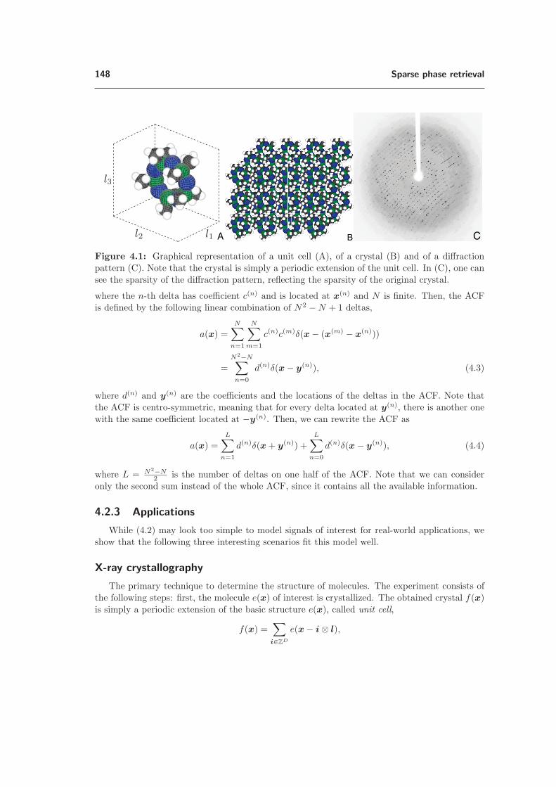
148 Sparse phase retrieval
A B C
Figure 4.1: Graphical representation of a unit cell (A), of a crystal (B) and of a diffraction
pattern (C). Note that the crystal is simply a periodic extension of the unit cell. In (C), one can
see the sparsity of the diffraction pattern, reflecting the sparsity of the original crystal.
where the n-th delta has coefficient c(n) and is located at x(n) and N is finite. Then, the ACF
is defined by the following linear combination of N2 −N + 1 deltas,
a(x) =N∑
n=1
N∑m=1
c(n)c(m)δ(x− (x(m) − x(n)))
=
N2−N∑n=0
d(n)δ(x− y(n)), (4.3)
where d(n) and y(n) are the coefficients and the locations of the deltas in the ACF. Note that
the ACF is centro-symmetric, meaning that for every delta located at y(n), there is another one
with the same coefficient located at −y(n). Then, we can rewrite the ACF as
a(x) =L∑
n=1
d(n)δ(x+ y(n)) +
L∑n=0
d(n)δ(x− y(n)), (4.4)
where L = N2−N2 is the number of deltas on one half of the ACF. Note that we can consider
only the second sum instead of the whole ACF, since it contains all the available information.
4.2.3 Applications
While (4.2) may look too simple to model signals of interest for real-world applications, we
show that the following three interesting scenarios fit this model well.
X-ray crystallography
The primary technique to determine the structure of molecules. The experiment consists of
the following steps: first, the molecule e(x) of interest is crystallized. The obtained crystal f(x)
is simply a periodic extension of the basic structure e(x), called unit cell,
f(x) =∑i∈ZD
e(x− i⊗ l),

4.2 Problem statement and applications 149
where l is a vector containing the sizes of the unit cell in each dimension. Second, the crystal
is exposed to an X-ray beam, under different angles. For each angle, we have a diffraction
pattern that, mathematically speaking, is a slice of the three-dimensional FT of the crystal.
See Figure 4.1 for a graphical depiction of a unit cell, a crystal and a diffraction pattern. The
diffraction patterns are recorded using traditional imaging techniques, such as CCDs, and only
the magnitude is acquired. Hence, we aim at recovering the spatial distribution e(x) of the
molecule, called electron density, from the magnitude of the FT of f(x).
Due to the periodicity of the crystal, we are in fact measuring the magnitude of the Fourier
series coefficients of the crystal, |fω|. This set of coefficients is equal, up to a constant factor, to
samples of the magnitude of the unit cell FT, |e(x)|.Remark 4.1
The PR problem in X-ray crystallography is more complex than Problem 4.1. In fact, the set
of measured samples is not sufficiently dense to reconstruct |e(ω)|2 using Shannon’s sampling
theorem. More precisely, we have an undersampling factor of two for each dimension and we
do not dispose of the entire ACF of e(x). See [103] for more details about this remark.
There is some a-priori information about the crystal that we can exploit. For example, we
can realistically model the unit cell e(x) as
e(x) =N∑
n=1
c(n)φ(x− x(n)),
where φ(x) is the electron density of a single atom 2 that has a positive coefficient c(n) and is
located at x(n). We can now specify the PR problem for crystallography.
Problem 4.2 (PR for Crystallography)
Consider a unit cell e(x) with N positive atoms on a bounded domain. Given a set of
magnitudes of the Fourier series coefficients |fω|, estimate the locations and amplitudes of
the atoms.
Speckle imaging in astronomy
Another example of the PR problem can be found in astronomy, namely an imaging method
known as speckle imaging. This technique attempts to mitigate the resolution downgrade in-
troduced by atmospheric turbulences. Namely, the atmosphere blurs M images {p (i)(x)}Mi=1
collected by a telescope and the blurring is modeled as a linear filter {φ(i)(x)}Mi=1, that may vary
for each image. The i-th measured image, also called speckle, is the convolution between the
astronomic object f(x) and the i-th linear filter
p (i)(x) = f(x) ∗ φ (i)(x), i = 1, . . . ,M.
See Figure 4.2 for an example of the speckles g (i)(x) and the target of the astronomic observations
f(x).
2. In reality, every atom has a different electron density φ(x). However, this assumption is reasonable andmany reconstruction methods used in crystallography consider similar assumptions [171].

150 Sparse phase retrieval
A B
Figure 4.2: An example of the input and output data of Problem 4.3. In (A) we can see a
set of 10 speckle images of a double star called ε Lyrae collected by Josef Popsel at the Capella
Observatory, Mount Skinakas, Crete, Greece [68]. In (B), the high resolution image of the stars
obtained through PR.
We reduce the atmospheric distortion and some potential additive white noise by taking the
average of the squared magnitudes of FT of the images as
1
M
M∑i=1
|p (i)(ω)|2 = |f(ω)|2 1
M
M∑i=1
|φ (i)(ω)|2,
where p (i)(ω), f(ω) and φ (i)(ω) are the FT of the measured image, the object of interest,
and the transfer function of the atmosphere, respectively. Note that the averaging strategy is
effective since we assume that the atmospheric transfer functions generally affects only the phases
of f(ω) [166]. The averaged atmospheric transfer function∑M
k=1 |φ (i)(ω)|2 is estimated using
atmospheric models or images of a reference astronomical object.
PR is necessary to recover the high resolution image of the astronomic object of interest
from |f(ω)|2. Note that we introduced the problem considering a continuous model for both the
astronomical object and the measured images. However, since the images are generally measured
and processed as sampled data, we may consider a set of discrete images {p (i)k }Mi=1 and the DFT
is usually employed.
We assume that f(x) is sparse,
f(x) =N∑
n=1
c(n)δ(x− x(n)),
since the astronomical object is composed of a set of stars that can be modeled as Dirac deltas.
Therefore, we have the following PR problem for speckle imaging.
Problem 4.3 (PR for Speckle Imaging)
Let f(x) be a N -sparse function and {p(i)(x)}Mi=1 be a set of speckle images distorted by the
atmosphere. Assume we measure a set of sampled images {p(i)k }Mi=1, where k ∈ ZD, D ≥ 2.
Estimate the locations x(n) and the coefficients c(n) of the stars.
Blind channel estimation
We conclude this section with an interesting example of 1-dimensional PR: blind estimation
of a communication channel. The knowledge of the channel impulse response is fundamental
4.3 Our contributions 151
for wireless communications systems, such as the ones based on Orthogonal Frequency Division
Multiplexing [157]. According to the theory of multi-path propagation [76], the channel f(t) can
be faithfully modeled as
f(t) =
N∑n=1
c(n)δ(t− t(n)), (4.5)
where t is the time variable and the N deltas describe the multi-path phenomenon. More
precisely, each delta represents a secondary communication path generated by a reflective body
between the source and the receiver.
We would like to estimate the locations and the coefficients of the deltas, without having
direct control of the channel input, hence the “blind estimation”. We only measure samples of
the output u(t) of the channel, that is the convolution between the input p(t) and the channel
itself,
u(t) = (p ∗ f)(t).
The input data p(t), which is the result of the modulation of a discrete sequence, is usually
whitened to achieve the maximum capacity of the channel. If the input sequence is statistically
white, then the magnitude of the FT of the output signal is equal in expectation to the magnitude
of the FT of the channel. Once more, we cannot access the continuous-time output u(t), but only
a set of M samples {uk}Mk=1. To recover the channel f(t), we can take the DFT of the collected
samples, keep the magnitudes and solve the following PR problem.
Problem 4.4 (PR for Blind Channel Estimation)
Let f(t) be a multi-path fading communication channel as defined in (4.5), where N is finite
and generally small. Assume the input of the channel to be properly whitened. Then, estimate
the channel impulse response f(t) from a set of samples {uk}Mk=1 of the output u(t).
We conclude this list of applications emphasizing the leitmotif connecting all the different
applications: we are interested in PR for N -sparse signal f(x) defined on a D-dimensional
continuous domain. We collect samples of the signal and the phase information is lost, as in
blind channel estimation, or irreparably distorted, as in speckle imaging. We would like to
recover the sparse components in the continuous domain, without discretization of the solution’s
domain.
This approach already proved beneficial in other domains. For example, it has been shown
that it is possible to recover a N -sparse signal f(x) from only 2N + 1 samples of the filtered
signal (g ∗ f)(x), see [161]. Another example where the continuous-time model has been proven
to be effective is in channel estimation. In [15], the authors demonstrated that the channel
estimator based on the continuous-time model achieves better performance when compared to
the state-of-the-art discrete approaches.
4.3 Our contributions
In this thesis, we first focus on the following definition of a sparse PR problem.

152 Sparse phase retrieval
Problem 4.5
(Sparse Phase Retrieval) Let f(x) ∈ RD be aD-dimensional signal composed of N Dirac’s
deltas,
f(x) =
N∑n=1
c(n)δ(x− x(n)).
Recover f(x) from f(ω), that is the magnitude of its FT. Equivalently, recover f(x) from
a(x), that is, the ACF of the signal.
We study when the solution to Problem 4.5 is unique and we show that the uniqueness of
the solution depends on the presence of collisions in the ACF, that are deltas of the ACF having
the same locations. More precisely, the solution is always unique for signals that are embedded
on 2 or more dimensions and whose ACFs do not have collisions. For 1-dimensional signals, we
show the uniqueness for most of the signals with a collision-free ACF. The only counterexample
being signals composed of N = 6 deltas having equal coefficients supported on a set of points
belonging to the unique family of counterexamples described in [18]. Such uniqueness conditions
are valid for both discrete and continuous PR problems and are described in [126].
Second, we propose an algorithm to find a solution to Problem 4.5. We call it as peeling
algorithm, due to its construction: at each iteration, we estimate one delta of f(x) and we
remove, or ”peel”, its influence, from the measured ACF. Such peeling overcomes the limitations
resulting from collisions, by only keeping the informative elements of the measured ACF. One of
the main drawbacks of the peeling algorithm is the instability with respect to noise that can be
controlled but not eliminated by a regularization technique we propose.
The algorithm is interesting for the following reasons
– It recovers precisely sparse signals from their ACF, defined either on discrete or continuous
domains,
– It shows that sparse signals can be reconstructed even with a moderate presence of colli-
sions,
– It shows that an iterative approach is possible and has interesting features for the recovery
of sparse signals.
Finally, we extend the peeling algorithm to multi-dimensional signals and to the case where
we measure only samples of the magnitude of the FT, as in the applications we have described
in Section 4.2.3.
4.4 Literature review
We present a literature review that covers theoretical and algorithmic results for both con-
tinuous and discrete PR. Note that most of the works focus on the latter given the difficulties of
treating the PR for continuous signals.
4.4.1 Continuous phase retrieval
Most of the relevant works connected to the continuous sparse PR problem was developed in
combinatorics for the turnpike problem [146]. The turnpike problem deals with the recovery of

4.4 Literature review 153
the locations of a set of points from their unlabeled distances with respect to each other. Note
that we can show that the recovery of the support of f(x) from the support of a(x) is an instance
of such a problem. A theorem presented by Piccard in 1939 [119] gives a sufficient condition
for the uniqueness of the solution to the turnpike problem. Unfortunately, a counterexample to
the theorem was first found by Bloom et al. [21] and its generalization was recently obtained by
Bekir et al. [18]. A similar but weaker condition for multidimensional signals has been recently
obtained by Senechal in 2008 [139]. Skiena et al. [146] proposed an algorithm for solving the
problem. It is known as the backtracking algorithm and solves any instance of the turnpike
problem providing the existence of (possibly multiple) valid solutions. The algorithm has a
polynomial computational complexity when the set {x(n)} is drawn at random. Zhang [175]
showed how to build sets of points achieving the worst case computational complexity of the
backtracking algorithm, O(2NN logN).
The turnpike problem appears also for the restriction site mapping, an interesting task in
computational molecular biology, where a particular enzyme is added to a DNA sample, so that
the DNA is cut at particular locations {x(n)}Nn=1, known as ”restriction sites”. One can find
the distance between each pair of restriction sites, {x(n) − x(m)}Nn,m=1, using gel electrophoresis.
Then, given the distances, we would like to recover the locations of the sites. This technique is
used for DNA mapping and it usually involves different enzymes. When a single enzyme is used,
it is known as partial digest [147]. Note that it has been shown by Cieliebak et al. [41] that
the partial digest problem with noisy measurements is NP-hard. The partial digest problem is
in fact a turnpike problem with integer locations—a bridge between continuous and discrete PR
problems.
4.4.2 Discrete phase retrieval
Most of the literature focuses on the discrete PR, that is when x ∈ ZD, aiming to reduce
the complexity of finding the solution. The first studies of the discrete PR problem appeared
in control theory and signal processing, where PR has been studied for the estimation of the
Wiener filter. In these fields, PR is known as spectral factorization and a review of its theory
and of the related algorithms is given in [136]. Among the presented methods, the so-called
“Bauer” method, described in [16], is the most interesting one given its performance and its
elegant matrix formulation. However, the theory of spectral factorization is focused on minimum
phase solutions, that are stable and causal. These solutions are not of interest for the applications
given in Section 4.2.3.
The uniqueness of the discrete PR problem has been studied for multidimensional discrete
signals. One of the main results is given by Hayes [66]: the set of positive finitely supported
images fk which are not uniquely recoverable has measure zero. The results are derived using
the theory of multidimensional polynomials. A possible algorithm to recover signals from the
magnitudes of the FT is also given, but it does not achieve satisfactory reconstruction precision
according to the authors. Note that this uniqueness result cannot be directly applied to X-ray
crystallography due to the presence of spatial undersampling, see Remark 4.1.
On the algorithmic front, many reconstruction algorithms were developed for Problem 4.2
and a review is given in [137]. Among them, ab-initio or direct methods were introduced in the
late 50s and have the considerable advantage of not requiring any prior information regarding
the crystals. The state of the art among these type of algorithms is charge flipping [115]. It
performs two operations iteratively, one in the spatial domain,, where it imposes the positiveness

154 Sparse phase retrieval
of the electron density and the bounded support, and one in the Fourier domain where it imposes
the measured magnitudes. This algorithm was first presented in 2004 [115], while some of the
recent developments are described in [116]. It can be seen as a version of the Gerchberg-Saxton
algorithm [57], where the positivity constraint is enforced if the electron density is above a certain
threshold or set to zero otherwise.
Recent work defined efficient convex relaxations for solving discrete PR problems. These
approaches are potentially more stable with respect to noise and are capable of avoiding local
minima. This strategy has been introduced by Lu et al. [94], who described a necessary condition
for the uniqueness of PR for discrete 1-dimensional sparse signals together with a reconstruction
algorithm based on the lifting of the problem in a higher dimensional linear space that is solved
by traditional convex optimization solvers. A similar approach, but introducing random masks to
improve the redundancy of measurements, has been introduced by Candes et al., [30, 32]. Hassibi
and his collaborators [71] proposed an improved algorithm and sufficient probabilistic uniqueness
conditions based on the sparsity of the signal of interest. Waldspurger et al. [163] formulated
another tractable convex relaxation similar to the classical MaxCut semidefinite program [58]
that achieves better reconstruction performance when compared to other convex relaxations.
PR has been generalized to any linear operator beyond the FT. More precisely, we choose
a frame {Fi}Ki=1 and we collect measurements of an unknown signal f using the expansion
coefficients {wi}Ki=1 = {〈Fi, f〉}Ki=1. Equivalently to the PR problem, we assume we can only
rely on the magnitude of the measurements and obtain a generalized PR problem: from the
magnitude of the expansion {|wi|}Ki=1, recover the original signal f . Note that if the chosen
frame is the Fourier frame, then we have an instance of PR on a discrete domain. Balan et al.
formulated the problem and studied different theoretical and algorithmic aspects of the recovery
of signals from the magnitude of generic frame coefficients. Specifically, fast algorithms are given
in [11], while the statement of equivalent problems and the construction of particular frames for
which the reconstruction is unique are given in [12, 13], respectively. Relevant uniqueness results
are given by Chebira et al. [37], where a necessary and sufficient condition for uniqueness has
been described, however it requires exponential time to be checked. Note that the aforementioned
convex relaxations can be applied to this generalized PR.
Other generalization of the PR problem have been considered. Oppenheim et al. proved the
uniqueness of PR problems up to the knowledge of the signs of the Fourier coefficients in [156].
A general analysis of the phase loss and the magnitude loss is given in [67] and an extension to
the multidimensional case is given in [66].
4.5 Uniqueness of the sparse PR problem
In this section, we state sufficient conditions to have a unique PR for sparse signals, whether
discrete or continuous. We use the same notation for both problems, f(x) =∑N
n=1 c(n)δ(x −
x(n)), where x(n) is constrained to the set of integers ZD for the discrete problem.
We use a divide and conquer approach to derive the uniqueness condition. First, we notice
that the locations of the deltas of the ACF contain more information than their amplitudes.
In fact, if all the deltas have the same amplitude, the coefficients of the ACF do not carry any
information. Therefore, we consider the problem of recovering the support of f(x) given the
support of its ACF a(x). We then use the coefficients to further restrict the possibility of having
a non-unique solution.

4.5 Uniqueness of the sparse PR problem 155
We consider the set of locations{x(n)
}N
n=1and derive the set of differences D =
{x(n) − x(m)
}N,N
n,m=1.
Given the possibility of repeated elements, D is formally a multiset. From (4.3), we also notice
that all the elements of a sparse ACF are supported on the set of differences, that is, y(n) ∈ D.
If we attempt to recover the support of a sparse signal from the support of its ACF, we realize
that the lack of labeling of the elements of D makes the problem combinatorial. That is, all the
possible labellings must be tested to find the optimal solution. Moreover, the solution may be
even more complex if the ACF has “collisions”: two deltas of the ACF located at the same
position due to two couples of equi-spaced deltas in the signal f(x).
Definition 4.1 (Collision)
We say that there exists is a collision in the ACF when ∃n �= m such that y(n) = y(m).
In other words, let x(i),x(j),x(k) and x(l) be the locations of four distinct deltas of a sparse
signal f(x), then we have a collision in the ACF if x(i) − x(j) = x(k) − x(l).
Note that collisions are problematic because of the impossibility of knowing a-priori how
many y(n) are colliding on the same element of the ACF that we observe. In what follows, we
show that if the observed ACF a(x) does not have collisions, we are able to recover uniquely the
sparse signal f(x) in most of the cases.
4.5.1 Uniqueness condition: collision-free 1-dimensional ACFs
As we have previously mentioned, the recovery of the support is the challenging part of the
PR problem. In fact, once we have the support there exist algorithms to recover the signal v(x).
Therefore, we assume that we first want to recover the support of f(x) from the support of a(x).
Moreover, we study the problem for a one-dimensional signal f(x) and we extend later our work
to multi-dimensional signals.
We consider the set of differences D as the input and the locations of the deltas{x(n)
}N
n=1as the output of the following problem:
Problem 4.6 (Support Recovery)
Given all the pairwise distances {x(n) − x(m)}N,Nn,m=1 between a set of N points lying on a
1-dimensional domain, recover their locations {x(n)}Nn=1.
Note that we have no information about the labeling of the pairwise differences in D. Therefore,
Problem 4.6 is combinatorial and is equivalent to an instance of the turnpike problem [146]. If
the labellings were known, the problem would be easily solved by multidimensional scaling [46].
We now introduce the definition of homometric sets, that we successively use to define the
uniqueness of Problem 4.6.
Definition 4.2 (Homometric Sets)
Two sets X and Y are said to be homometric if and only if their difference sets are congruent,
that is DX = DY .
In this section, we assume that all the elements of D are different from each other, i.e. we do
not have any collision in the ACF. This is equivalent to saying that the set D has no repeated
elements.
The problem of the support recovery was first posed by Patterson [117] and a possible solution
was proposed by Piccard in 1939 [119]. More precisely, Piccard suggested that if there are no

156 Sparse phase retrieval
collisions, the solution of the turnpike problem is always unique. Unfortunately, a counterexample
to this result was found in 1975 by Bloom [21]. Indeed, consider X = {0, 1, 4, 10, 12, 17} and
Y = {0, 1, 8, 11, 13, 17}, then
DX = DY = {0, 1, 2, 3, 4, 5, 6, 7, 8, 9, 10, 11, 12, 13, 16, 17} .
Recently, this counterexample has been proved to belong to a unique parametric family of coun-
terexamples by Bekir [18].
Theorem 4.1 (Bekir [18])
If X and Y are finite sets of points whose differences sets, DX and DY , contain no repeated el-
ements, then the turnpike problem has always a unique solution unless the elements of X and
Y belong to single and unique infinite parametric family of six elements. More precisely, given
p = (p1, p2) ∈ R2 and the two following parametric sets, X = {0, p1, p2 − 2p1, 2p2 − 2p1, 2p2, 3p2 − p1}
and Y = {0, p1, 2p1 + p2, p1 + 2p2, 2p2 − p1, 3p2 − p1}, the two difference sets are congruent,
DX = DY .
Note that the equations defining the elements of the sets X and Y are linear combinations of
p. This suggests that we can geometrically characterize (with linear subspaces) the supports of
signals that generate a turnpike problem with no unique solution.
Corollary 4.1
The sets of points that generate a turnpike problem without a unique solution belong to the
following 2-dimensional linear subspaces⎡⎢⎢⎢⎢⎢⎢⎣
0 0
1 0
−2 1
−2 2
0 2
−1 3
⎤⎥⎥⎥⎥⎥⎥⎦[p1p2
]= QXp,
⎡⎢⎢⎢⎢⎢⎢⎣
0 0
1 0
2 1
1 2
−1 2
−1 3
⎤⎥⎥⎥⎥⎥⎥⎦[p1p2
]= QYp.
Even if these two linear subspaces define completely the sets X and Y, we need to define
a proper ordering of the elements. In fact, while the sets do not have by definition a preset
order, the two linear subspaces induce a precise ordering. We can choose any permutation as
soon as it is unequivocally defined: in what follows, we always consider the permutations ΠY,p
and ΠX ,p that sort in an increasing order the elements of the vectors ΠY,pQYp and ΠX ,pQXp,
respectively. Equivalently, we always consider an operator that takes the elements from the sets
X and Y and sorts them in an increasing order.
Note that the permutation and the operator are unique for each p and depend only on the
direction of p: in fact, for different magnitudes of p, the ordering does not change. Moreover, it
is easy to show that we have a finite number of permutations for all the points p ∈ R2. In fact,
the number of permutations is upper bounded by 6!, being the number of possible permutations
of six elements in a set.
We define the geometry of these sets of points as a manifold generated by a linear model and
a varying permutation. In what follows, we take the span of these permuted linear systems to
describe the sets of supports without a unique solution to the turnpike problem.

4.5 Uniqueness of the sparse PR problem 157
Figure 4.3: A low-dimensional projection of the two 6-dimensional spaces representing the
supports X (red) and Y (green) introduced in Corollary 4.1. Note that both are formed by the
union of many subsets of 2-dimensional subspaces, one for each permutation. Moreover, the
intersection between the two sets has measure zero in set of all the projections.
Corollary 4.2
The set of supports for a signal f(x) that generate a turnpike problem without a unique
solution is described as,
S = X ∪ Y = span(ΠY,pQY) ∪ span(ΠX ,pQX ).
A graphical representation of this set of elements is given in Figure 4.3, where we observe the
subset of linear subspaces mixed by the permutations. This geometrical intuition is useful for
two reasons:
– If we have no collisions and unless N = 6, we can always recover uniquely the support of
the signal from the support of the ACF,
– Even if N = 6, the supports without a unique recovery lie on the 2-dimensional manifold
defined in Corollary 4.2, and this manifold has measure zero in the set of all the supports
of 6 elements.
Note that we have not used the coefficient information so far. The following theorem merges the
previous results in terms of phase retrieval for sparse signals and considers the coefficients of the
ACF to obtain a sufficient condition for the uniqueness of 1-dimensional sparse PR problems.

158 Sparse phase retrieval
Theorem 4.2 (Uniqueness condition for the 1-dimensional PR problem)
Assume we measure the 1-dimensional ACF a(x) of a signal f(x) with N deltas, and the
elements of the ACF have no collisions. Then,
– If N �= 6, the PR problem has a unique solution.
– If N = 6 and not all the coefficients c(n) have the same value, the PR problem has a
unique solution.
– If N = 6 and all the c(n) have the same value, the PR problem has almost surely a
unique solution.
The proof of Theorem 4.2 is given in Appendix 4.8.1. The existence of the three cases is due to
the parametric family of turnpike problems without a unique solution previously described, and
the additional information that may be available from the coefficients c(n) of the deltas of the
ACF.
4.5.2 Uniqueness condition: collision-free D-dimensional ACFs
The previous analysis applies only to 1-dimensional signals, that is D = 1. Senechal [139]
proposed an analysis of the uniqueness of the turnpike problem in higher dimensions, D ≥ 2.
Unfortunately, their result is too conservative and cannot cover very simple examples such as
1-dimensional sets of points embedded in higher dimensional spaces.
In what follows, we describe the result of Senechal and then propose a sufficient condition
for the uniqueness of the PR for multi-dimensional sparse signals, that significantly extends the
previous result.
First, we define when a point is ”visible”, a necessary property to recover the support of the
signal.
Definition 4.3 (Visible Point)
A point belonging to a multi-dimensional difference set, or equivalently a delta belonging to
an ACF, is visible if the line through the origin and the point contains only the origin, the
point itself and another point in the centro-symmetric position with respect to the origin.
Note that there is always a point in a centro-symmetric position, see (4.4). In Figure 4.4, we
show an ACF with some visible deltas, such as y(j), and some deltas that are not visible, such
as y(n).
Then, if all the points are visible, we say that they are in ”general position”.
Definition 4.4 (General Position)
A signal f(x) composed of N deltas has its elements in general position if every delta of the
ACF is visible.
Senechal [139] showed that having the points in general position is a sufficient condition to recover
uniquely the support of a sparse signal f(x) from the support of its ACF.
Theorem 4.3 (Senechal [139])
Let the signal f(x) be supported on{x(n)
}N
n=1in R
D and let the deltas of its ACF be in
general position. Then, we can uniquely recover the support of f(x) from its ACF.

4.5 Uniqueness of the sparse PR problem 159
Figure 4.4: A graphical representation of a 2-dimensional ACF generated by a 4-sparse signal,
where the blue dots represent the location of the deltas. Note that the delta located at y(j) is
”visible” while the one located at y(n) is not, since there is another delta aligned on the line
passing through the origin.
Theorem 4.3 gives a sufficient condition for the uniqueness of the support recovery. For
example, Theorem 4.3 does not guarantee a unique recovery of the signal generating the ACF
given in Figure 4.4, due to existence of deltas being not visible.
Note that while the proposed uniqueness condition for the one-dimensional PR problem
described in Theorem 4.2 and the one for multi-dimensional ones given in Theorem 4.3 are both
sufficient, the latter is fairly constraining. For example, if we pick a 1-dimensional sets of points
that generates a turnpike problem with a unique solution and embed it into a higher dimensional
domain, then Theorem 4.3 cannot guarantee anymore the uniqueness of the solution.
This example inspired our idea of solving a D-dimensional PR as a set of multiple 1-
dimensional PR problems. In fact, if we can solve uniquely a sufficient number of sub-problems,
then the original problem has a unique solution. In this section, we show that this divide and
conquer strategy leads to a tighter necessary and sufficient condition: given an ACF a(x) of a
N -sparse D-dimensional signal f(x), the PR problem has a unique solution.
We show the result as follows: first we consider a set of projections of the ACF to many
1-dimensional subspaces 3. See Figure 4.5 for an example of a projection onto a subspace defined
by a vector P . Second, we show that the projection of the ACF is the ACF of the projected
signal. Third, we show that a finite number of different projections is necessary and sufficient to
recover the deltas of f(x). We conclude by proving that we can find these projections for every
N -sparse f(x) that is embedded in a D-dimensional space, with D ≥ 2.
3. It is possible to consider projections onto subspaces of any dimensionality. Here, we consider only 1-dimensional projections for simplicity of notation.

160 Sparse phase retrieval
Figure 4.5: The projection of a 2-dimensional ACF onto a 1-dimensional subspace defined by a
vector P . Note that the main properties of an ACF, such as the centro-symmetry, are preserved
in the projected domain.
Proposition 4.1
Let f(x) be a signal composed of N deltas lying on RD and let a(x) be its ACF. Define a
projection over a 1-dimensional space as Px, where P is a 1×D vector onto which we project
the spatial domain and x are the coordinates in the original domain. Then the projected
ACF is the ACF of the projected signal.
The proof is given in Appendix 4.8.2.
Given Proposition 4.1, we can project aD-dimensional ACF a(x) onto P different 1-dimensional
subspaces. If the projected ACF satisfies the conditions given in Theorem 4.2, we recover the
projected signal, namely the deltas with the proper coefficients and the projected locations. As
shown in [145], we need (N +1)(D−1) projections to reconstruct exactly the location of N deltas
in a D-dimensional space. It is possible to reduce the number of required projection to D + 1
accepting to take random projections and exactly recovering the support with probability 1.
Finally, we show the existence of the projections with a unique PR for any D-dimensional
ACF withD ≥ 2. More precisely, a projection may unfortunately belong to the parametric family
described in Theorem 4.1 or it can have collisions in the projected points. In what follows, we
show that the projections without collisions and with a unique PR exist and are easy to find
for all the D-dimensional signals with D ≥ 2. Indeed, it is simple to show that for any ACF
without collisions, the projected ACF on a random subspace has no collisions with probability
one. In the following theorem, we show that the set of projections with a unique PR does not
have measure zero in the set of all projections for any ACF with D ≥ 2. In other words, the
multi-dimensional sparse PR problem has always a unique solution.
Theorem 4.4 (Uniqueness condition for the D-dimensional PR problem)
Let f(x) be a D-dimensional N -sparse signal and let a(x) be its ACF. Assume that a(x) has
no collisions and D ≥ 2. Then the set of projections onto 1-dimensional domains that gener-
ates a 1-dimensional PR problem with a unique solution has a measure strictly larger than
zero in the set of all the possible projections. Therefore, the solution to the D-dimensional
PR of f(x) is always unique.
The proof is given in Appendix 4.8.3.
We conclude this section underlying that the uniqueness of the solution to the sparse PR
problem does not depend on the type of domain-that is continuous or discrete. The presence of

4.6 Reconstruction of the sparse PR: the peeling algorithm 161
collisions is a better characterizing feature. However, the amount of collisions depends on the
domain: if we randomly distribute the deltas of f(x) on a continuous domain, we have almost
surely no collision, while the probability of collisions for discrete signals is always larger than
zero for N ≥ 4.
4.6 Reconstruction of the sparse PR: the peeling algorithm
In this section, we present the second main result of this chapter regarding the PR problem:
the peeling algorithm (PA), a reconstruction algorithm that recovers a signal f(x) composed of
N deltas from the deltas of the ACF a(x). We call it peeling algorithm (PA) because it finds
one element at a time and peels the ACF from the deltas of the signal that have already been
found. The PA has an interesting advantage: while removing elements from the ACF it may
also remove some collisions, simplifying the successive iterations. The algorithm is designed for
1-dimensional signals, but can be straightforwardly extended to higher dimensional spaces using
the reduction technique introduced in Section 4.5.2. One of the main drawbacks of the algorithm
is its sensitivity to noise. In fact, one of the fundamental steps looks for deltas located at specific
locations; if noise is present, the procedure fails. Nonetheless, we describe the algorithm for two
reasons:
– It shows that sparse signals can be uniquely reconstructed even with a moderate amount
of collisions, indicating that it may be possible to improve the results presented in Section
4.5,
– It is the only algorithm in the literature performing the PR for continuous signals,
– It shows the feasibility of an iterative approach for the PR problem of sparse signals.
First, we introduce a few definitions and partial results that are useful to describe the
algorithm and its performance. The input of the algorithm are the set of differences D =
{x(m) − x(n)}Nm,n=1 and set of amplitude products P ={c(n)c(m)
}N
m,n=1. The desired outputs
are the estimated locations{x(n)
}N
n=1and the amplitudes
{c(n)
}N
n=1of the deltas of f(x). Note
that we consider 1-dimensional signals; the extension to multi-dimensional ones is given later
and is based on the solution of many projected problems, similarly to what we have described in
Section 4.5.
One information that we can extrapolate directly from the sets of differences is the distance
between the first and the last delta of f(x).
Lemma 4.1
Given a set of 1-dimensional differences D,
maxn
x(n) −minn
x(n) = maxn
y(n) = maxD.
Recalling the shift invariance of the ACF mentioned in (4.1), Lemma 4.1 is sufficient to place the
first and the last delta of f(x): x(1) = 0 and x(N) = maxD. Moreover, the length of f(x) has a
fundamental role for reducing the search space for the locations of the other deltas, as explained
in what follows.

162 Sparse phase retrieval
Definition 4.5 (Twin)
We denote as twin a pair of deltas of the ACF located at y(i) and y(j) such that y(i) + y(j) =
maxD = x(N).
With the following lemma, we describe the existence of twins.
Lemma 4.2
Given an ACF a(x) generated by a signal f(x) with N deltas, there are at least N − 2 twins.
Proof.
Let us consider all the deltas of f(x) beside the first and last one, that is {x(n)}N−1n=2 . By
construction, there exists N − 2 twins in the ACF located at (x(n) − x(1), x(N) − x(n)) with
amplitudes (c(1)c(n), c(n)c(N)).
If there are more than N − 2 twins in the ACF, then we call them fake twins and these are
generated as follows.
Definition 4.6 (Fake Twin)
A fake twin is generated by four deltas in the signal f(x) satisfying x(n)−x(j)+x(l)−x(n) =
x(N), with j �= 1 and l �= N .
Lemma 4.2 states that there are always N − 2 twins directly generated by the N deltas of f(x).
Given the structure of the twins, if we pick a real twin located at (y(i), y(j)), then one delta of the
signal is located either at y(i) or y(j). Assume that y(i) is the right location, the corresponding
delta in the time-reversed signal 4 is located at y(j).
4.6.1 The main iteration
Now, assume that we have a partial estimate fK(x) of the signal f(x), that is formed by K
out of N estimated deltas,
fK(x) =∑n∈K
= c(n)δ(x− x(n)), where |K| = K < N.
We define the partial ACF as aK(x) = fK(x) ∗ fK(−x) and the residual ACF as the difference
between the ACF and the residual, rK(x) = a(x) − aK(x). In what follows, we show how to
estimate a new delta of the signal, exploiting the partial information we already posses. We
denote the location and the amplitude of the new estimated delta as x∗ and c∗.
1. Consider a twin located at (y(i), y(j)) with amplitudes (d(i), d(j)), whose elements are still
in the residual rK(x). Assume that the twin is without collision and real. Under these two
assumptions, Lemma 4.2 guarantees that the generating delta of the twin is located either
at y(i) or y(j). Then, we consider both locations as possible values for x∗, and we denote
them as x∗1 and x∗
2.
4. The time-reversed signal has the same ACF, according to (4.1).
4.6 Reconstruction of the sparse PR: the peeling algorithm 163
2. We would like to use the partial estimate fK(x) to determine its possible amplitude c∗.Therefore, we first consider x∗
1 = y(i) and we compute multiple estimates of the amplitude
with respect to the elements belonging to the partial signal estimate fK(x) as,
cn1 =a(x∗
1 − x(n))
c(n), where n ∈ K. (4.6)
We also consider the other possibility, that is x∗2 = y(j) and we compute multiple estimates
of the amplitude dn2 as we did for the other location,
cn2 =a(x∗
2 − x(n))
c(n), where n ∈ K. (4.7)
3. We avoid errors estimating the location x∗ and amplitude c∗ of a new delta using the
multitude of estimates. More precisely, we cluster the solutions according to their values.
If there is a set of two or more estimates in {cn1}n∈K agreeing on the same value, we denote
such value as d∗. Then c∗ = d∗ and x = y(i). Equivalently, if there is a larger cluster in
the estimates {cn2}n∈K agreeing on a value d∗, then c∗ = d∗ and x∗ = y(j).
This procedure is the main tool of the PA: at each iteration we find a new delta of f(x) and
in case of success, we add it to the partial signal fK(x). We iterate this process until all the N
deltas are estimated. We interrupt the algorithm whenever all the twins left are fake or with
collisions, that is whenever there are not at least two estimates with the same value.
Three outcomes of the process are possible:
– The largest cluster indicates a correct estimate of a delta of f(x),
– The largest cluster indicates a wrong estimate of a delta of f(x),
– There is no cluster with more than 1 element.
Errors are due to the selection of fake twins, the selections of elements having collisions or the
existence of many elements of the ACF satisfying particular combinations with their amplitudes,
so that a cluster indicates a wrong estimate. The analysis of the such errors is complex and
goes beyond the work done for this thesis. However, if the amplitudes{c(n)
}N
n=1are taken from
a continuous probability distribution and a(x) is not affected by noise, the error probability is
zero.
Note that the estimation process is unstable with respect to noise. More precisely, if the
locations of the deltas in a(x) are measured with some noise, the estimates are zero or completely
wrong. We can attempt to stabilize the algorithm by considering different estimators in (4.6),
(4.7). For example, we can relax the estimator as
cn =
∫ x(n)+ε
x(n)−ε
a(x− s)
c(n)ds, where n ∈ K, (4.8)
that accounts for noise in the locations smaller than ε. Unfortunately, the estimate will be
erroneous again when two deltas in a(x) are closer than ε. A numerical analysis of the tradeoff
between the benefits and the drawbacks of such relaxation is given in Section 4.6.3.
4.6.2 Initialization
We initialize the algorithm locating the first and the last delta using Lemma 4.1 and estimat-
ing their amplitudes using the information contained in the twins. More precisely, we consider a
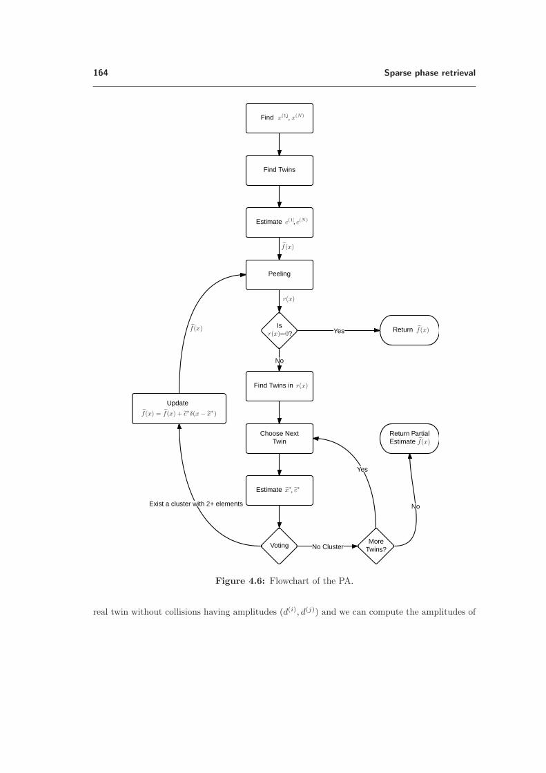
164 Sparse phase retrieval
Figure 4.6: Flowchart of the PA.
real twin without collisions having amplitudes (d(i), d(j)) and we can compute the amplitudes of

4.6 Reconstruction of the sparse PR: the peeling algorithm 165
�� ��� � � �� �
A
0 5 10 15
B
Figure 4.7: (A) The ACF of a discrete signal, that is the input of the PA. (B) Reconstructed
sparse signal (green) obtained with the PA compared with the original discrete signal (blue).
Note that the PA recovers almost perfectly the original signal.
the first and last delta as
c(1) =
√d(i)d(L)
d(j)and c(N) =
√d(j)d(L)
d(i),
where L is the index of the delta located further away, that is L = argmaxn y(n). Note that the
(unknown) labellings of the elements in the first twin fixes the time direction, that is one of the
free parameters we have, see (4.1). This procedure has a major flaw: we need a real twin and
without collisions, two conditions that are hard to check. We solve this problem using a voting
strategy similar to the one described in Section 4.6.1: we pick the available twins, compute the
amplitudes c(1) and c(N) according to the two possible orderings, and we pick the estimate which
is confirmed by the majority of twins. If there are at least two real twins without collisions, there
are at least two equal estimates. This estimate is correct unless there are 2 or more fake twins
and/or with collision that agree on a wrong estimate. Again, if the probability distribution of
the {c(n)}Nn=1 is continuous, this event has probability zero.
A flowchart of the algorithm is given in Figure 4.6, while the Matlab implementation is
available [124].
4.6.3 Analysis of the peeling algorithm
In this section, we analyze the performance of the PA and its fundamental aspects. We show
reconstruction examples for both discrete and continuous PR, the impact of collisions in the
discrete case, and the impact of noise on the ACF deltas locations in the continuous case. Note

166 Sparse phase retrieval
5 10 15 20 25 30 350
0.2
0.4
0.6
0.8
1 Success Rate of PA
Collisions Rate
Sparsity
%
Success Rate of CF
Figure 4.8: Performance of the PA as a function of the sparsity. For each value of the sparsity,
we solved 1000 random discrete PR using the peeling algorithm and we compare it with a state-
of-the-art algorithm for discrete PR, known as charge flipping (CF) [116]. The reconstruction
is considered to be successful when the MSE is smaller than 10−4. Note that when the signal
is sufficiently sparse, the peeling algorithm outperforms charge flipping. We also measure the
average number of collisions in the ACF; note that even if the algorithm can manage the presence
of some collisions, it starts to fail when there are too many of them.
that we do not consider the impact of collisions for continuous PR because they have probability
zero. According to the same philosophy, we do not consider noise in the deltas locations for the
discrete problem because noise generally affects the amplitudes.
First, we present an example of input and output of the PA when applied to a discrete sparse
PR problem. Figure 4.7 shows the recovery of a 6-sparse discrete signal from its ACF using
the PA. This is compared with the original signal, showing perfect recovery. Note that the
reconstructed signal has been shifted and properly time-reversed to match the original signal,
according to (4.1).
Second, we analyze the impact of collisions on the reconstruction performance for the discrete
PR problem. In general, according to the theory presented in Section 4.5, the reconstruction is
unique whenever there are no collision. As we previously mentioned, we designed the iterative
peeling action of the PA to reduce the negative impact of collisions in the reconstruction and
to exploit the sparsity of the signal. Therefore, we are interested to see the success rate of
PA as a function of collisions and we consider the following simulation setup: we pick discrete
signals of length l = 128 with a sparsity N ∈ [6, 34]. For each N , we consider 1000 randomly
generated sparse signals and we measure the percentage of successful reconstructions and the
percentage of elements of the ACF with collisions. As a reference, we compare the reconstruction
performance to the one obtained by charge flipping (CF) [115, 116], the reference algorithm for
the reconstruction of X-ray crystallographic data. The results are shown in Figure 4.8, where
we first note that PA outperforms CF for very sparse signals, that is N ≤ 16. Moreover, we
underline that for low sparsities, that is N ≤ 16, and consequently a small number of collisions,
the reconstruction is often successful. On the other hand, as the number of collisions grows, the
PA fails to reconstruct properly most of the sequences.

4.6 Reconstruction of the sparse PR: the peeling algorithm 167
10-1
25 A
0.5 100
1
2B
Figure 4.9: (A) The sparse ACF of a signal, which is the input of the PA. (B) The original
sparse (blue) signal and the reconstructed one (green) by the PA. Note that both signals are
defined on a continuous domain and a proper constant phase term has been chosen to show the
equivalence of the two signals. The reconstruction is exact up to the machine precision.
Rec
onst
ruct
ion
Err
or
Measurement Noise��� �� �� 0
���
��
��
0
��� �� �� 0
���
��
��
0
��� �� �� 0
���
��
��
0
��� �� �� 0
���
��
��
0
Figure 4.10: For each plot, we show the reconstruction error of PA as a function of the noise
in the measured ACF and for a specific relaxation parameter ε. Each point in the scatter plot is
an instance of PA for a random continuous signal. The point location is given by the noise in the
measured deltas of the ACF (x axis) and the reconstruction error (y axis). Both axes are in a
log10 scale and the red line is located at the value of ε that we considered. The red dots represent
those signals whose reconstruction failed due to the negative effects of the relaxation. Note that,
the ratio of red-to-blue dots grows with the measurement noise, showing the instability of the
PA to such a noise.
Next, we analyze the behavior of the PA when reconstructing sparse signals defined on a
continuous domain.
First, we consider an example of reconstruction of a 10-sparse signal and we show the results
in Figure 4.9. Note that the locations of the deltas and their amplitudes are perfectly recovered,

168 Sparse phase retrieval
up to the constant phase term that has been found a-posteriori.
Second, we analyze the reconstruction performance of the PA as a function of noise. More
precisely, we consider to measure an ACF with errors in the delta’s locations, {y(n)+w(n)}, wherew(n) are independent random variables uniformly distributed on ±ξ. We vary the maximum noise
amplitude ξ = {10−7, 10−5, 10−3, 10−1} and the relaxation parameter ε = [10−14, 1] as defined in
(4.8), and we observe the error of the reconstructed sparse signal. The sparsity of the signal is
fixed to N = 20 and the deltas are uniformly distributed as x(n) ∈ [0, 1]. The results are shown
in Figure 4.10: four scatter plots (one for each ξ) show the relationship between the noise in
the deltas of the ACF and the respective noise in the reconstructed signal. More precisely, each
point represents a randomly generated signal; its horizontal position is given by ξ and its vertical
position is given by the error in the reconstruction of the locations of the deltas, defined as∑n
|x(n) − x(n)|2.
Due to the absence of denoising, we would expect reconstruction error to be of the same order
of magnitude as the measurement noise. Nonetheless, as soon as ξ > ε, the relaxation is not
sufficiently strong to counterbalance the measurement noise w(n), and the PA fails. Another case
of failure is introduced by the relaxation itself: if there are deltas closer than ε to each other, the
estimator defined by (4.8) is incorrect. The red dots in Figure 4.10 are examples of the described
negative effect introduced by the relaxation.
4.6.4 The peeling algorithm applied to speckle imaging
In this section, we show how the PA, the theory for D-dimensional signals described in Section
4.5.2, and the sampling of finite rate of innovation signals [22, 161], can be applied to practical
problems, such as the ones described in Section 4.2.3. The main challenge is introduced by the
measuring setup of Problems 4.2, 4.3 and 4.4: we measure a set of samples of the FT of a sparse
function f(x), we loose the phase of the samples and we would like to recover the deltas of f(x).
Moreover, a kernel φ(x), that may or may not be known depending on the application, usually
filters the deltas and is generally introduced by the measurement method. Here, we focus on
the speckle imaging problem, thanks to the availability of a set of speckle images of a twin star,
ε-lyrae.
First, we describe in general terms the reconstruction technique, that is how we go from the
sets of discrete speckle images to the location and the amplitude of the stars on a continuous
domain. More precisely, the reconstruction is performed as follows:
– We take the speckle images, see Figure 4.11(C), and compute the discrete ACF using the
FT without the phases, see Figure 4.11(D).
– We project the ACF on three (or more) 1-dimensional domains and estimate the locations
of the ACF deltas on the continuous domain, see Figure 4.11(E).
– We solve the three PR problems on a continuous domain and recover the projected stars
on these domains. Using the projections of the stars, we recover their locations on R2, see
the red crosses in Figure 4.11(F).
It is fundamental to describe a few technical details regarding the recovery of the ACF deltas
on a continuous domain from the discrete filtered image of the ACF. First, we interpolate the
image using a sinc interpolation and we take the projection on the discrete 1-dimensional domain.

4.6 Reconstruction of the sparse PR: the peeling algorithm 169
0.5
0.5
00
��� 0 0.5
0
0.5
���
00.5
0.5
0
A B C
D E F
Figure 4.11: Speckle imaging on synthetic data. (A) Four stars are modeled as deltas on a
continuous time two-dimensional domain. (B) The stars are filtered by a low pass kernel φ(t),
representing the measuring device, a telescope for example. (C) The images are corrupted by
additive white Gaussian noise to account for the measurement noise and the phase of their FTs
are distorted by the atmosphere. (D) The discrete ACF is computed by removing the phase of
the FT. (E) The ACF in the continuous domain is computed using FRI techniques—the black
dots—and three projections on 1-dimensional domains—the dashed lines—are computed. (F)
Three PR problems are solved independently on the 1-dimensional domains and the location of
the stars are recovered. The reconstructed stars are displayed as red crosses while the original
one are the black dots; note that they perfectly match. We underline that the reconstructed
stars lie on the continuous domain R2 while the measured speckles are discrete images.
Second, we compute the Fourier series coefficients of the sequence and we compensate for the
kernel modulation. Finally, we estimate the projected deltas using the annihilation filter method,
that has been proposed for the sampling of FRI signals, see [161]. Note that at least 2L + 1
Fourier series coefficients are needed to recover the L deltas of the ACF and this process is
complicated by the deconvolution with the kernel. In fact, we may not know precisely the kernel
and the deconvolution itself may be highly unstable with respect to noisy images. In what
follows, we present two examples of speckle imaging, one with synthetic data and one based on
real measurements.
Synthetic data: we consider four stars distributed on R2 as represented in Figure 4.11(A)
and we measure M = 48 speckles of size 101 × 101 pixels. Each speckle is the convolution of
the stars with three filtering processes: a low pass filter induced by non-ideal lenses (Figure
4.11(B)), a phase distortion introduced by the atmosphere modeled according to [166], and

170 Sparse phase retrieval
A
B
Figure 4.12: Speckle imaging on the dataset of the twin star ε-lyrae, also shown in Figure 4.2.
In (A) we show a superimposition of a crop of the discrete ACF-the background image-and the
three considered projections-the three dashed lines. The dots plotted over the three projections
subspaces are the locations of the deltas obtained through the annihilation filter method, while
the violet dots are the estimated locations of the deltas of the two-dimensional ACF. in (B), we
show a superimposition between the locations of the star according to the PA (orange) and an
image showing the solutions obtained by a blind deconvolution method based on super-resolution
[68]. While previous approaches find a discretization of the sparse object, our method locates
the stars on the continuous domain.
additive white Gaussian noise to account for the measurement noise, (Figure 4.11(C). We obtain
the reconstruction of the stars as described previously using random projections and the results
are shown in Figure 4.11. Note that the stars have been perfectly recovered on R2 even if their
location was not aligned with the discrete grid given by the imaging sensor.
Real data: We applied the same reconstruction technique to the set of M = 40 speckle
images of size 111 × 111 of the twin stars called ε-lyrae. The images were collected by Josef
Popsel at the Capella Observatory, Mount Skinakas, Crete, Greece [68]. We consider the kernel

4.7 Conclusions 171
φ(x) due to the lenses to be a Gaussian function defined as,
φ(x) = exp{−x2/σ},
where we manually fit σ = 176. The discrete ACF—the background image—and the estimated
deltas of the continuous ACF—the violet dots—are given in Figure 4.12(A). Note the three
projections used for locating the deltas of the ACF using the annihilation filter method. The
estimated location of the two stars using the PA algorithm are depicted as orange dots in Figure
4.12(B). The background image is the result of the super-resolution based blind deconvolution,
a state-of-the-art method described in [68]. Two things should be noted here:
– Our method gives the stars locations on the continuous domain while traditional techniques
generate a discretized approximation.
– There is a small discrepancy between the two different estimates and it is mainly due to
the sub-optimal estimation of the kernel φ(x). If we have access to the telescope, we could
estimate the kernel with higher precision by taking a sufficient number of images of a single
known star.
4.7 Conclusions
In this chapter, we analyzed a challenging non-linear inverse problem: the sparse phase
retrieval problem on continuous and discrete domains. We showed that the uniqueness of the
solution of such a problem depends on the presence of collisions. More precisely, we proved that
when the ACF of the signal is without collision the solution of the phase retrieval problem is
always unique, beside a very small set of corner cases. In fact, the only counterexample is when
the signal is defined on a 1-dimensional domain, it has sparsity equal to six and all the deltas
have equal amplitude.
We proposed a reconstruction algorithm, the peeling algorithm, that solves the PR problem
for sparse signals on 1-dimensional domains. We explained how the algorithm can be used to
solveD-dimensional problems by solvingD+1 PR problems on 1-dimensional projected domains.
When the discrete signal is sparse, the performance is better than state of the art. Moreover,
it is the first algorithm that solves the continuous PR problem. Unfortunately, it appears to be
unstable when the locations of the ACF deltas are perturbed by noise.
We used a combination of PA and sampling of FRI signals to tackle an application of our
PR method: speckle imaging, a classic problem in astronomy. We considered real and synthetic
data, showing promising results in recovering the locations of stars on a continuous domain from
discrete images perturbed by heavy noise.
Future work will be focused on optimizing the main iteration of the PA so that it is more
stable with respect to noise. Another critical aspects is the recovery of a sparse continuous ACF
from a set of its samples; more precisely, a naive sampling of FRI signals outputs a sparse signal
that is not necessarily an ACF and it requires at least N2 samples. On the other hand, it looks
reasonable to constrain the obtained deltas to be an ACF of a N–sparse signal using just a set
of N–samples. This aspect is fundamental when the signal f(x) is not exactly sparse, such as
in the case of blind channel estimation. The last aspect worth investigation is the PR of aliased
ACFs, such as in the case of X-ray crystallography.

172 Sparse phase retrieval
0 5 10 15
A
0 5 10 15
B
�� ��� � � �� �
C
�� ��� � � �� �
D
Figure 4.13: In (A) and (B), two random signals supported on X and Y are shown. In (C) and
(D), the respective ACF are given. Note that even if the supports of the ACFs are the same,
the coefficients of the ACF depend significantly on the coefficients of the original signals. Here
we considered as supports the first counterexample found by Bloom [21]. An equivalent analysis
can be done for the family of counterexamples described by Bekir et al. [18].
4.8 Appendix
4.8.1 Proof of Theorem 4.2: [Uniqueness condition for the 1-dimensionalPR problem]
We divide the proof in three parts, one for each case given in the theorem’s statement.
• For N �= 6 we can always recover uniquely the locations of the deltas from the sets of differ-
ences, see Theorem 4.1. Once the locations are known, the coefficients are uniquely determined,
see Appendix 4.8.4.
• If N = 6 and all the c(n) have the same coefficient, and the signal does not have a unique PR,
then its support lies on the manifold defined in Corollary 4.2 and we cannot use the coefficients to
enforce uniqueness. Note that all possible signals span a six-dimensional space, representing the
N = 6 locations. Given that the manifold containing the signals without a unique reconstruction
is 2-dimensional, then the set of these signals has measure zero with respect to the set of all the
signals with N = 6.
• If N = 6 and not all the c(n) have the same coefficient, there is always only one set between
X and Y that is a possible support of the signal f(x). To prove this statement, we assume
without loss of generality 5 that all d(n) are positive and we would like to show that it is always
possible to discern the actual support of f(x) from the two possible ones using the coefficients.
First, let us define two vectors q and r containing the logarithms of the coefficients of the
ACF and of the signal, respectively. Then, given the absence of collision and the linearization
introduced by the logarithm, we can write two systems of equations. Each equation represents
the coefficient of one element of the ACF given the coefficients of two elements of the original
signal, see Figure 4.13. The two systems assume that f(x) is supported on X and Y, respectively.
5. If the deltas of the f(x) are not positive, we can always take the absolute value thanks to the absence ofcollisions, which is one of our assumptions.
4.8 Appendix 173
More precisely, if we assume that f(x) is supported on X we have
q = CX r, (4.9)
while if we consider Y to be the support of f(x) we get a different system of equations,
q = CYr. (4.10)
We note that if all the coefficients have the same value, that is c(n) = C ∀n = {1, . . . , N},then all the ACF elements have the same coefficient as well, d(n) = C2. In this case, (4.9) and
(4.10) are equivalent and we cannot distinguish between the two possible supports, X and Y.
Note that the set of signals having c(n) = C ∀n form a 1-dimensional subspace in the coefficient
domain. In what follows, we show that this is the only subspace where X and Y cannot be
distinguished from the coefficients.
Consider the intersection between the two columns spaces of CX and CY . This intersection
contains all the coefficients of the ACF that could be equivalently generated by two signals, one
supported on X and the other on Y. The dimensionality of this intersection can be computed as
dim(span(CX ) ∩ span(CY)) = (4.11)
rank(CX ) + rank(CY)− rank([CX ,CY ]) = 1
where [CX ,CY ] is a symbol representing the concatenation of the columns of two matrices CXand CY . It is possible to verify that (4.11) holds for the example of Bloom and by linearity to
any other element of the set of counterexamples.
We deduce from (4.11) that the ACFs with coefficients{d(n)
}N2−N
n=0that can be generated
by the two different supports lie on a 1-dimensional subspace. Given that we have already
characterized this 1-dimensional subspace as the one where all the{c(n)
}5
n=0have the same
value, this concludes the proof.
4.8.2 Proof of Proposition 4.1
First, we define the projection f(s) of the signal f(x) over the subspace indicated by P as
the following inner product
f(s) =
∫RD
δ(s− Px)f(x)dx =
N∑n=1
c(n)δ(s− Px(n)).
Then, we compute the ACF of the projected signal as
a(s) = f(s) ∗ f(−s)
=
∫RD
N∑n=1
c(n)δ(h− Px(n))
N∑m=1
c(m)δ(h+ s− Px(m))dh
=
N2−N∑n=0
d(n)δ(s− Py(n)), (4.12)

174 Sparse phase retrieval
where the δ(s) are located on the 1-dimensional domain defined by the projection. Finally, we
compute the projection of the ACF according to (4.3) as
a(s) =
∫RD
δ(s− Py)a(y)dy
=
∫RD
δ(s− Py)
N2−N∑n=0
d(n)δ(y − y(n))dy
=
N2−N∑n=0
d(n)δ(s− Py(n)),
that is equal to (4.12), which proves the proposition.
4.8.3 Proof of Theorem 4.4: [Uniqueness condition for the D-dimensionalPR problem]
First, we introduce some notation. The projected deltas are located on {w(n)}N2−Nn=0 . These
locations can be computed with the following matrix vector multiplications
w =
⎡⎢⎢⎢⎣w(0)
w(1)
...
w(N2−N)
⎤⎥⎥⎥⎦
=
⎡⎢⎢⎢⎢⎣y(0)0 y
(0)1 · · · y
(0)D−1
y(1)0 y
(1)1 · · · y
(1)D−1
......
...
y(N2−N)0 y
(N2−N)1 · · · y
(N2−N)D−1
⎤⎥⎥⎥⎥⎦⎡⎢⎢⎢⎣
p0p1...
pD−1
⎤⎥⎥⎥⎦= Y P T ,
where Y is a matrix containing on each row the locations of the points{y(n)
}N2−N
n=0. Note
that the set of all possible projections from a D-dimensional to a 1-dimensional space forms a
rank(Y )-dimensional space. More precisely, unless the locations of the deltas of f(x) are lying
on a lower dimensional subspace, it forms a D-dimensional subspace.
Similarly to the analysis proposed in Section 4.5.1, we can geometrically characterize the
supports of the ACFs for which we cannot solve the turnpike problem uniquely. We build
a linear model Q from the difference set induced by X , or Y equivalently. Then, we define
a permutation matrix Πp to match the ordering given by the linear model with the ordering
chosen for the set of points representing the ACF support. Assume that the projected points{w(n)
}N2−N
n=0are supported on a set of points without a unique PR. Then, we have
w = ΠA,pQp,
where Q spans a 2-dimensional linear subspace and when combined with the p-dependent per-
mutation ΠA,p, it defines a 2-dimensional manifold. Note that we have either A = X or A = Y,
depending on which one of two counterexamples of the turnpike problem we have found.

4.8 Appendix 175
The permutation is fixed by p and we have an intersection between the D-dimensional sub-
space spanned by Y and the 2-dimensional subspace spanned by Q. We analyze the possible
cases with respect to the dimensionality of the original ACF, given by rankY :
– If the ACF is 1-dimensional and we have an intersection between span(Y ) and span(Q),
this intersection has necessarily the size of all the possible projections rank(Y ∩ Q) = 1.
Changing the direction of the projection has no effect beside a scaling. In this case, the
original signal is not uniquely recoverable from the support (see Theorem 4.1).
– If the ACF is 2-dimensional and the intersection is 1-dimensional, there is only one pro-
jection that does not have a unique reconstruction and we can pick any other P to have a
unique PR. On the other hand, if the intersection is 2-dimensional, then the signal subspace
is the same as the one spanned by the matrix Q. However, we can change p such that
the permutation Πp changes and the projected points have a unique 1-dimensional PR.
Given the structure of the manifold induced by the permutations, the good projections are
relatively easy to find.
– If the ACF is D-dimensional and D > 2, the set of projections P that generates projected
PR problems with a unique solutions is dense in the set of the projections. In fact, the set of
projections without a unique solutions is a 2-dimensional manifold while all the projections
are a D-dimensional set. We always find sufficient projections to recover the support of
f(x) and therefore all the f(x) without collisions have a unique PR.
4.8.4 Recovering the amplitudes of deltas from the support and the ACF
In general, the problem of recovering the amplitudes {c(n)}Nn=1 of a N sparse signal f(x)
given the support {x(n)}Nn=1 and its ACF a(x) is not trivial. It is equivalent to solve a system of
quadratic forms and a possible convex relaxation is given in [71], for which it is not possible to
guarantee the success of reconstruction.
The problem has the same formulation whether the domain is discrete or continuous. In what
follows we derive an algorithm that recovers the coefficients of a sparse signal whose support and
ACF are both known while we assume the absence of collisions in the ACF.
Let c = [c(1), c(2), . . . , c(N)] be a vector containing the coefficients of the N -sparse signal
f(x) and define a rank-one matrix C = cc∗
Given that we know the ACF and the support of f(x), then we know all the off-diagonal
elements of the matrix C. Therefore, we can reformulate the task of recovering the coefficients
from the support as follows.
Problem 4.7
Consider a rank-one matrix C whose elements are all known except the ones on the main
diagonal. Can we uniquely reconstruct the elements on the main diagonal?
There exists many alternative approaches to solve Problem 4.7. We choose to describe a
method that requires a single matrix inversion.
Let αk � |ck|2 ∀k = 1, . . . , N , and define a matrix A = C − diag(α1, . . . , αN ). Note that
A is known and we aim to recover the matrix C. The following result describes a method that
requires a single matrix inversion to find the unique solution of Problem 4.7.

176 Sparse phase retrieval
Proposition 4.2
Assume that N > 2, then
Ck,k = |ck|2 =N − 2
1−N
1
A−1k,k
,
where Ck,k and A−1k,k are the k-th element on the main diagonal of C and A−1, respectively.
Proof.
Denote by D = diag(α1, . . . , αN ), then we have A = −D + cc∗. Applying the matrix inversion
lemma, we obtain
A−1 = −D−1 − (D−1c)(1− c∗D−1c)−1(c∗D−1)
= −D−1 − (D−1c)(c∗D−1)1
1−N.
We conclude the proof noticing that the k-th element on the main diagonal of A−1 is a function
of N and αk,
A−1k,k =
1
αk− 1
1−N
1
αk=
N − 2
1−N
1
αk.
Once we have recovered C, we obtain the coefficients c by taking the eigenvector of C corre-
sponding to the largest eigenvalue. Note that all the matrices are invertible by construction.

4.8 Appendix 177
Table of notations
x,x, s spatial variables
t temporal variable
ω Fourier domain variable
f(x) signal to recover
fK(x) partial estimate of the signal f(x)
f(x) projection of the signal f(x)
a(x) autocorrelation function of f(x)
aK(x) partial estimate of the autocorrelation function a(x)
a(x) projection of the autocorrelation function a(x)
f(x) Fourier transform of f(x)
fω Fourier series of f(x)
D dimensions of f(x)
c(n) amplitude of the nth delta of f(x)
c(n) amplitude of the estimated nth delta of f(x)
x(n) location of the nth delta of f(x)
x(n) location of the estimated nth delta of f(x)
d(n) amplitude of the nth delta of a(x)
y(n) location of the nth delta of a(x)
N number of deltas of f(x)
L number of deltas of a(x) for x > 0
e(x) unit cell of a crystallyzed molecule
φ(x) kernel interpolating the deltas the signal f(x)
p(i)(x) speckle images measured by a telescope
φ(i)(x) time-varying kernel of the telescope and the atmosphere
M number of speckle images or samples of a channel outputg(t)
p(i)k discrete speckle images sampled by a telescope
f(t) communication channel impulse response
p(t) input of the channel
u(t) output of the channel
uk samples of the channel output
{Fi}Ki=1 a generic frame
{wi}Ki=1 expansion coefficients of the frame ΠXD sets of differences
P sets of products
ΠX ,ΠY ,QX ,QY ,p matrices and vectors used to model the uniqueness condition
P projection matrix
P projection matrix
rK(x) residual of the autocorrelation function
x∗1, x
∗2 candidate locations in an iteration of the PA
cn1 , cn2 nth estimated amplitude in an iteration of the PA
K set of estimated deltas
ε regularization parameter of the PA
ξ noise amplitude in the locations
l length of a discrete f(x)
CX ,CY matrices used to model the supports of non-unique supports


Chapter 5
Conclusion
This thesis proposed and discussed a set of results having a common thread: inverse problems
stemming from real-world sensing scenarios. Here, we review our results, emphasizing the open
problems and possible future work.
1. Sensor placement optimization: we introduced a new regularization technique based
on the optimization of the sensor locations for linear inverse problems. More precisely, we
are given a linear inverse problem, a set of N possible sensing locations and we would like
to choose the L locations that minimize the ill-conditioning of the inverse problem. We
proposed FrameSense, a near-optimal greedy algorithm based on the frame potential. We
show with experiments on synthetic dataset, that FrameSense improves in reconstruction
precision and computational complexity the state of the art. Moreover, we extend Frame-
Sense to parameters lying on a union of subspaces, an interesting model for applications
like the thermal monitoring of many-core processors. Last, we study the application of
FrameSense to two real-world applications: the thermal monitoring of many-core proces-
sors and the adaptive sampling scheduling for environmental sensor networks. For both
applications, we show that our method is significantly better in terms of reconstruction
precision and computational complexity with respect to the state of the art. Last, we de-
scribe a proof of concept for a new thermal monitoring architecture based on tomographic
measurements collected by interconnection wires.
Future work should be focused on the following aspects:
– FrameSense assumes that each sensor has the same sensing “energy”; we would like
to improve FrameSense for sensor networks where each sensor has different signal-to-
noise ratios.
– FrameSense could have a significant impact to improve the sensing strategies after
environmental disasters. For example, many sensors were deployed in the ocean to
measure the water contamination surrounding the Fukushima’s nuclear power plant.
Unfortunately, their locations were not well-chosen and many measurements carried
little information. Knowing the meteorological conditions, the sea currents and the
location of the leak, we could have modeled the transport of the radioactive material
using a linear model Ψ and choosen better sensing locations.
– The tomographic thermal monitoring architecture introduced in Section 2.6.8 is ex-
tremely interesting in theory but we did not study the problem sufficiently in depth to
179

180 Conclusion
declare it feasible in practice. We should design integrated circuits measuring the wire
resistance, simulate them and compare their signal-to-noise ratio to the traditional lo-
cal sensors. Once this aspect is properly investigated, we could obtain significant
experimental results showing an improvement of the performance sufficient to moti-
vate further research on real hardware.
2. Source placement optimization: we considered a physical field that is linearly con-
trolled by a set of possible sources with the aim of controlling the future states of the
field. We introduced a different view on the control of this forward problem based on an
optimized choice of the source locations and we proposed an algorithm that finds the near-
optimal source placement given the linear forward problem. This is a brand-new problem
and it does not appear in the scientific literature, therefore it was hard to compare it and
understand its performance with respect to other methods.
In the future,
– We plan to evaluate its performance in a real-world application such as the thermal
management of many-core processors. More precisely, we would like to study if it
is possible to choose the locations of the main components, such as the cores and
the caches, such that the control of the temperature distribution at runtime is more
effective.
– We will study the noisy source placement problem, where the current state of the
field is only known with a certain precision. A possible strategy could be to use a
combination of the approximation error used for the noiseless source placement and
of the frame potential used in FrameSense.
3. Source placement and vaccination on graphs: we considered a graph modeling the
transmission of an information between entities to model phenomena such as epidemics
and rumors on a social network. We analyzed two dual problems: the selection of a
set of nodes to spread the information faster and the removal of a set of nodes to slow
the spreading. For the first problem, we proposed a greedy algorithm and proved its near-
optimal performance in terms of the average time of spreading. For the second problem, we
were able to design a greedy algorithm with a good performance but without a theoretical
guarantee about the quality of the solution. We compared the two algorithms with other
approaches on synthetic data and highlighted the obtained improvements. These results
are just scratching the surface of a very interesting problem.
In the future, we would like to:
– Test the algorithms on real-world datasets, such as the social network of a population
in a given region, and analyze if we can improve the vaccination policies. These
improvements could lead to a cost reduction for vaccination campaigns.
– Design an algorithm for the vaccination problem with bounds guaranteeing the per-
formance for the worst-case scenario.
4. Uniform sampling and reconstruction of diffusion fields: we demonstrated that
diffusion fields, at least for three different source models, are approximatively bandlimited.
Therefore, it is possible to interpolate uniformly collected samples and reconstruct the
entire field with a bounded aliasing error. More precisely, the aliasing error decreases
exponentially fast with a linear increase of the spatial sampling density.

181
5. Reconstruction of the sources of a diffusion field: we considered a sensor network
collecting spatio-temporal samples of a diffusion field induced by point sources appearing at
unknown times and locations. We designed an algorithm, that under the assumptions given
in Section 3.5, is guaranteed to recover the sources exactly. Such an algorithm works in a
streaming fashion and recovers the sources one by one whenever they appear on the field.
Future work should be focused on designing a stronger algorithm, that directly estimates
all the parameters of the sources at once. During the redaction of this thesis, we were
informed by Pier Luigi Dragotti and John Murray, that they will soon submit a paper
describing a result in this direction.
6. Reconstruction of time-varying atmospheric emissions: we considered a physical
field generated by localized time-varying sources non-uniformly sampled in space and time
by a sensor network. We designed two algorithms to recover the time-varying emission
rates when the sources are modeled either as finite rate of innovations signals or as signals
lying on low-dimensional subspaces. We showed the feasibility of the proposed algorithm
on synthetic data, using a diffusion-advection equation to model the dispersion.
As future work, it would be interesting to test the proposed algorithm on a real-world
sensing scenario. For example, we could pick a region with a set of known smokestacks,
measure with a sensor network the pollutant density at different locations of the region
and attempt to recover the emission rates with our method. Last, we should compare our
estimates with the real emissions, that could be obtained having access to the smokestacks.
Note that we could model the atmospheric dispersion using FLEXPART [152], a numerical
tool used in environmental engineering.
7. Sparse phase retrieval: we discussed this classical non-linear inverse problem, where we
would like to recover a signal from the magnitude of its Fourier transform. An everlasting
open problem of the phase retrieval problem is the definition of conditions on the signal so
as we have guarantees for a unique solution to the phase retrieval problem. Here, we assume
that the original signal is a stream of Dirac’s deltas and derive a sufficient condition for the
uniqueness of the solution based on the support of the autocorrelation function of the signal.
Such a condition applies to 1-dimensional and multi-dimensional signals and significantly
extends the class of sparse signals with a unique solution to the phase retrieval. In addition,
we proposed the peeling algorithm, a sparse phase retrieval algorithm that reconstructs the
signal on the continuous domain. Note that the peeling algorithm is sensitive to noise in
the measurements and we propose a possible regularization to mitigate this issue. Future
work will be focused on the following topics:
– Design a reconstruction algorithm with an improved stability with respect to the
measurements noise. A possible approach could be inspired by the recent results on
near-optimal algorithms for combinatorial problems via convex relaxation proposed
by Fogel et al. [56].
– Design a algorithm that takes as an input the samples of the magnitude of the Fourier
transform and as an output the parametric description of the Dirac’s delta in the orig-
inal signal. Our current strategy is to recover the ACF using the collected samples
and then solve the phase retrieval problem with the ACF. Unfortunately, this ap-
proach tends to be extremely unstable to noise. Therefore, we should try to directly
estimate the parameters of the signal of interest from the collected samples, without
the intermediate estimation of the ACF.


Bibliography
[1] MeteoSwiss: the Federal Office of Meteorology and Climatology of Switzerland.
[2] “Safecast,” http://blog.safecast.org/.
[3] K. Aberer, S. Sathe, D. Chakraborty, A. Martinoli, G. Barrenetxea, B. Faltings, and
L. Thiele, “Opensense: open community driven sensing of environment,” in Proc. Proc.
IWGS, pp. 39–42. ACM, 2010.
[4] M. Al-Obaidy, A. Ayesh, and A. F. Sheta, “Optimizing the communication distance of an
ad hoc wireless sensor networks by genetic algorithms,” Artif. Intell. Rev., vol. 29, no. 3-4,
June 2008.
[5] R. Albert and A.-L. Barabasi, “Statistical mechanics of complex networks,” Reviews of
modern physics, vol. 74, no. 1, p. 47, 2002.
[6] A. Aldroubi, J. Davis, and I. Krishtal, “Dynamical sampling: Time–space trade-off ,”
Applied and Computational Harmonic Analysis, vol. 34, no. 3, pp. 495–503, May 2013.
[7] ANSYS, Inc., “ANSYS CFX.”
[8] E. K. Ardestani, E. Ebrahimi, G. Southern, and J. Renau, “Thermal-Aware Sampling in
Architectural Simulation,” in Proc. ISLPED, pp. 33–38. ACM, 2012.
[9] E. K. Ardestani, F. J. Mesa-Martinez, G. Southern, E. Ebrahimi, and J. Renau, “Sampling
in Thermal Simulation of Processors: Measurement, Characterization, and Evaluation,”
IEEE Trans. Computer-Aided Design Integr. Circuits Syst., vol. 32, no. 8, pp. 1187–1200,
2013.
[10] E. K. Ardestani and J. Renau, “ESESC: A fast multicore simulator using time-based
sampling,” in Proc. HPCA, pp. 448–459. IEEE, 2013.
[11] R. M. Balan, B. G. Bodmann, P. G. Casazza, and D. Edidin, “Fast algorithms for sig-
nal reconstruction without phase,” SPIE Optical Engineering+Applications, pp. 67 011L–
67 011L–9, 2007.
[12] R. M. Balan, P. G. Casazza, and D. Edidin, “On signal reconstruction from absolute value
of frame coefficients,” Proc. SPIE, Wavelets XI, 2005.
[13] ——, “Equivalence of reconstruction from the absolute value of the frame coefficients to
a sparse representation problem,” IEEE Signal Process. Lett., vol. 14, no. 5, pp. 341–343,
2007.
183

184 Bibliography
[14] R. G. Baraniuk and M. B. Wakin, “Random projections of smooth manifolds,” Found.
Comput. Math., vol. 9, no. 1, pp. 51–77, 2009.
[15] Y. Barbotin and M. Vetterli, “Fast and robust parametric estimation of jointly sparse
channels,” IEEE J. Emerg. Sel. Topics Circuits Syst., vol. PP, no. 3, pp. 1–11, 2012.
[16] F. Bauer, “Ein direktes iterationsverfahren zur hurwitz-zerlegung eines polynoms,” Arch.
Elektr. Uebertragung, vol. 9, pp. 285–290, 1955.
[17] S. Beirle, U. Platt, M. Wenig, and T. Wagner, “Weekly cycle of NO2 by GOME mea-
surements: a signature of anthropogenic sources,” Atmos. Chem. Phys., vol. 3, no. 6, pp.
2225–2232, 2003.
[18] A. Bekir and S. W. Golomb, “There are no further counterexamples to S. Piccard’s theo-
rem,” IEEE Trans. Inf. Theory, vol. 53, no. 8, pp. 2864–2867, 2007.
[19] J. Benedetto and M. Fickus, “Finite normalized tight frames,” Adv. Comput. Math., vol. 18,
no. 2, pp. 357–385, 2003.
[20] L. Benini, E. Flamand, D. Fuin, and D. Melpignano, “P2012: Building an ecosystem for a
scalable, modular and high-efficiency embedded computing accelerator,” in Proc. Design,
Automation & Test in Europe Conference & Exhibition (DATE), pp. 983–987, 2012.
[21] G. S. Bloom, “A counterexample to a theorem of S. Piccard,” J. Comb. Theory A, vol. 22,
no. 3, pp. 378–379, Nov. 1975.
[22] T. Blu, P. L. Dragotti, M. Vetterli, P. Marziliano, and L. Coulot, “Sparse sampling of
signal innovations,” IEEE Signal Process. Mag., vol. 25, no. 2, pp. 31–40, 2008.
[23] T. Blumensath, “Sampling and Reconstructing Signals From a Union of Linear Subspaces,”
IEEE Trans. Inf. Theory, vol. 57, no. 7, pp. 4660–4671, 2011.
[24] S. Bochner and K. Chandrasekharan, Fourier Transforms, Annals of Mathematics Studies.
Princeton University Press, 1949.
[25] S. Borkar, “Design challenges of technology scaling,” Micro, IEEE, vol. 19, no. 4, pp. 23–29,
1999.
[26] D. Brooks, R. Dick, R. Joseph, and L. Shang, “Power, Thermal, and Reliability Modeling
in Nanometer-Scale Microprocessors,” Micro, IEEE, vol. 27, no. 3, pp. 49–62, 2007.
[27] A. M. Bruckstein, D. L. Donoho, and M. Elad, “From sparse solutions of systems of
equations to sparse modeling of signals and images,” SIAM Review, vol. 51, no. 1, pp.
34–81, 2009.
[28] J. A. Cadzow, “Signal enhancement-a composite property mapping algorithm,” IEEE
Trans. Acoust. Speech Signal Process., vol. 36, no. 1, pp. 49–62, 1988.
[29] E. J. Candes, “Compressive sampling,” in Proc. Proceedings of the International Congress
of Mathematicians: invited lectures, pp. 1433–1452, 2006.
[30] E. J. Candes, Y. C. Eldar, T. Strohmer, and V. Voroninski, “Phase retrieval via matrix
completion,” arXiv, Sept. 2011.

Bibliography 185
[31] E. J. Candes, J. K. Romberg, and T. Tao, “Stable signal recovery from incomplete and
inaccurate measurements,” Comm. Pure Appl. Math., vol. 59, no. 8, pp. 1207–1223, 2006.
[32] E. J. Candes, T. Strohmer, and V. Voroninski, “PhaseLift: Exact and stable signal recovery
from magnitude measurements via convex programming,” Comm. Pure Appl. Math., 2012.
[33] E. J. Candes and M. B. Wakin, “An introduction to compressive sampling,” IEEE Signal
Process. Mag., vol. 25, no. 2, pp. 21–30, 2008.
[34] H. S. Carslaw and J. C. Jaeger, Conduction of Heat in Solids, 2nd ed. Oxford University
Press, USA, 1986.
[35] P. G. Casazza, M. Fickus, J. Kovacevic, M. Leon, and J. Tremain, “A physical inter-
pretation of tight frames,” in Harmonic analysis and applications. Springer, 2006, pp.
51–76.
[36] V. Cevher and A. Krause, “Greedy Dictionary Selection for Sparse Representation,” Se-
lected Topics in Signal Processing, IEEE Journal of, vol. 5, no. 5, pp. 979–988, 2011.
[37] A. Chebira, M. Fickus, and M. Vetterli, “Frame domain signal processing: framework and
applications,” in Proc. ICASSP, Dallas, 2010.
[38] K. Chen, C. E. Bash, D. M. Auslander, and C. D. Patel, “Local temperature control in
data center cooling: Part II, Statistical Analysis,” HP Laboratories Palo Alto, 2006.
[39] Z. Chen, J. Ranieri, R. Zhang, and M. Vetterli, “DASS: Distributed Adaptive Sparse
Sensing,” Submitted to IEEE TCOMM, pp. 1–31, Apr. 2014.
[40] P. L. Chiu and F. Y. S. Lin, “A simulated annealing algorithm to support the sensor
placement for target location,” in Proc. Canadian Conference on Electrical and Computer
Engineering, pp. 867–870. IEEE, 2004.
[41] M. Cieliebak, S. Eidenbenz, and P. Penna, “Noisy data make the partial digest problem
NP-hard,” WABI, pp. 111–123, 2003.
[42] R. Cochran and S. Reda, “Spectral techniques for high-resolution thermal characterization
with limited sensor data,” in Proc. Design Automation Conference (DAC), pp. 478–483.
IEEE, June 2009.
[43] A. K. Coskun, T. S. Rosing, and K. C. Gross, “Utilizing Predictors for Efficient Ther-
mal Management in Multiprocessor SoCs,” IEEE Trans. Computer-Aided Design Integr.
Circuits Syst., vol. 28, no. 10, pp. 1503–1516, 2009.
[44] A. K. Coskun, T. Rosing, K. Whisnant, and K. C. Gross, “Static and Dynamic
Temperature-Aware Scheduling for Multiprocessor SoCs,” IEEE Trans. Very Large Scale
Integr. (VLSI) Syst., vol. 16, no. 9, pp. 1127–1140, 2008.
[45] R. Couillet and M. Debbah, “Signal processing in large systems: a new paradigm,” IEEE
Signal Process. Mag., vol. 30, no. 1, pp. 24–39, 2013.
[46] T. F. Cox and M. A. A. Cox, Multidimensional scaling, 2nd ed. Chapman and Hall/CRC,
2001.
186 Bibliography
[47] A. Das and D. Kempe, “Algorithms for subset selection in linear regression,” in Proc. ACM
Symposium on Theory of Computing (STOC), pp. 45–54. ACM, July 2009.
[48] ——, “Submodular meets spectral: greedy algorithms for subset selection, sparse approxi-
mation and dictionary selection,” in Proc. International Conference on Machine Learning
(ICML), 2011.
[49] E. W. Dijkstra, “A note on two problems in connexion with graphs,” Numerische mathe-
matik, vol. 1, no. 1, pp. 269–271, 1959.
[50] I. Dokmanic, J. Ranieri, A. Chebira, and M. Vetterli, “Sensor networks for diffusion fields:
Detection of sources in space and time,” in Proc. Communication, Control, and Computing
(Allerton), 2011 49th Annual Allerton Conference on, pp. 1552–1558, 2011.
[51] M. F. Duarte, M. B. Wakin, D. Baron, and R. G. Baraniuk, “Universal Distributed Sensing
via Random Projections,” in Proc. Proc. IPSN, pp. 177–185, Nashville, TN, Apr. 2006.
[52] D. Duffy, Green’s functions with applications. Chapman and Hall/CRC, 2001.
[53] A. El Badia and T. Ha-Duong, “An inverse problem in heat equation and application to
pollution problem,” Inverse and ill-Posed Problems, vol. 10, pp. 585–599, 2002.
[54] M. Fickus, D. G. Mixon, and M. J. Poteet, “Frame completions for optimally robust
reconstruction,” arXiv, July 2011.
[55] J. R. Fienup, “Phase retrieval algorithms: a comparison,” Applied Optics, 1982.
[56] F. Fogel, R. Jenatton, F. Bach, and A. d’Aspremont, “Convex Relaxations for Permutation
Problems,” arXiv, June 2013.
[57] R. W. Gerchberg and W. O. Saxton, “A practical algorithm for the determination of the
phase from image and diffraction plane pictures,” Optik, vol. 35, p. 237, 1972.
[58] M. X. Goemans and D. P. Williamson, “Improved approximation algorithms for maximum
cut and satisfiability problems using semidefinite programming,” J. ACM, vol. 42, no. 6,
pp. 1115–1145, 1995.
[59] D. Golovin, M. Faulkner, and A. Krause, “Online distributed sensor selection,” in Proc.
International Conference on Information Processing in Sensor Networks (IPSN), pp. 220–
231. ACM, 2010.
[60] G. H. Golub and C. F. Van Loan, Matrix Computations (3rd Ed.). Baltimore, MD, USA:
Johns Hopkins University Press, 1996.
[61] V. K. Goyal, M. Vetterli, and N. Thao, “Quantized overcomplete expansions in IRn: Anal-
ysis, synthesis, and algorithms,” IEEE Trans. Inf. Theory, vol. 44, no. 1, pp. 16–31, 1998.
[62] U. Gratzke, P. D. Kapadia, and J. Dowden, “Heat conduction in high-speed laser welding,”
J. of Physics D: Applied Physics, vol. 24, p. 2125–2134, 1991.
[63] J. Hadamard, “Sur les problemes aux derivees partielles et leur signification physique,”
Princeton university bulletin, vol. 13, no. 49-52, p. 28, 1902.

Bibliography 187
[64] P. M. Hall, D. Marshall, and R. R. Martin, “Incremental Eigenanalysis for Classification,”
in Proc. Proc. BMVC, pp. 286–295, 1998.
[65] C. Hansen, Rank-Deficient and Discrete Ill-Posed Problems: Numerical Aspects of Linear
Inversion. Soc. for Industrial Math., 1987.
[66] M. H. Hayes, “The reconstruction of a multidimensional sequence from the phase or mag-
nitude of its Fourier transform,” IEEE Trans. Acoust. Speech Signal Process., vol. 30, no. 2,
pp. 140–154, 1982.
[67] M. H. Hayes, J. S. Lim, and A. V. Oppenheim, “Signal reconstruction from phase or
magnitude,” IEEE Trans. Acoust. Speech Signal Process., vol. 28, pp. 672–680, Dec. 1980.
[68] M. Hirsch, S. Harmeling, S. Sra, and B. Scholkopf, “Online multi-frame blind deconvolution
with super-resolution and saturation correction,” Astron. Astrophys., vol. 531, p. A9, May
2011.
[69] W. Huang, M. R. Stan, K. Sankaranarayanan, R. J. Ribando, and K. Skadron, “Many-Core
Design from a Thermal Perspective,” in Proc. Design Automation Conference (DAC), p.
746. New York, New York, USA: ACM Press, 2008.
[70] F. Ingelrest, G. Barrenetxea, G. Schaefer, M. Vetterli, O. Couach, and M. Parlange, “Sen-
sorScope: Application-specific sensor network for environmental monitoring,” ToSN, vol. 6,
Mar. 2010.
[71] K. Jaganathan, S. Oymak, and B. Hassibi, “Recovery of sparse 1-D signals from the mag-
nitudes of their Fourier transform,” ISIT, pp. 1473–1477, 2012.
[72] J. B. Johnson, “Thermal agitation of electricity in conductors,” Physical Review, vol. 32,
no. 1, p. 97, 1928.
[73] S. Joshi and S. Boyd, “Sensor selection via convex optimization,” IEEE Trans. Signal
Process., vol. 57, no. 2, pp. 451–462, 2009.
[74] I. Jovanovic, L. Sbaiz, and M. Vetterli, “Tomographic approach for parametric estimation
of local diffusive sources and application to heat diffusion,” ICIP, vol. 4, pp. IV–153–IV–
156, Aug. 2007.
[75] D. Kandaswamy, T. Blu, and D. Van De Ville, “Analytic Sensing: Noniterative Retrieval
of Point Sources from Boundary Measurements,” SIAM J. Sci. Comput., vol. 31, no. 4, pp.
3179–3194, Jan. 2009.
[76] I. Kang, M. P. Fitz, and S. B. Gelfand, “Blind estimation of multipath channel parameters:
a modal analysis approach,” IEEE Trans. Commun., vol. 47, no. 8, pp. 1140–1150, 1999.
[77] S. M. Kay, Fundamentals of statistical signal processing: estimation theory. Prentice-Hall,
Inc., Mar. 1993.
[78] J. Kovacevic and A. Chebira, “Life beyond Bases: The advent of frames (Part I),” IEEE
Signal Process. Mag., vol. 24, no. 4, pp. 86–104, 2007.

188 Bibliography
[79] J. Kovacevic and A. Chebira, “Life beyond bases: The advent of frames (Part II),” IEEE
Signal Process. Mag., vol. 24, no. 5, pp. 115–125, 2007.
[80] A. Krause, A. Singh, and C. Guestrin, “Near-optimal sensor placements in Gaussian pro-
cesses: Theory, efficient algorithms and empirical studies,” J. Mach. Learn. Res., vol. 9,
pp. 235–284, 2008.
[81] A. Kumar, L. Shang, L.-S. Peh, and N. K. Jha, “System-level dynamic thermal manage-
ment for high-performance microprocessors,” IEEE Trans. Computer-Aided Design Integr.
Circuits Syst., vol. 27, no. 1, pp. 96–108, 2008.
[82] S. Lau, R. Eichardt, L. Di Rienzo, and J. Haueisen, “Tabu search optimization of magnetic
sensor systems for magnetocardiography,” IEEE Trans. Magn., vol. 44, no. 6, pp. 1442–
1445, 2008.
[83] K.-J. Lee and K. Skadron, “Using performance counters for runtime temperature sensing
in high-performance processors,” in Proc. Parallel and Distributed Processing Symposium,
2005.
[84] A. S. Leon, K. W. Tam, J. L. Shin, D. Weisner, and F. Schumacher, “A Power-Efficient
High-Throughput 32-Thread SPARC Processor,” IEEE J. Solid-State Circuits, vol. 42,
no. 1, pp. 7–16, Jan. 2007.
[85] C. Lian, M. Knox, K. Sikka, X. Wei, and A. J. Weger, “Development of a flexible chip
infrared (IR) thermal imaging system for product qualification,” in Proc. SEMI-THERM,
pp. 337–343. IEEE, 2012.
[86] L. Ling, M. Yamamoto, Y. C. Hon, and T. T, “Identification of source locations in two-
dimensional heat equations,” Inverse Problems, vol. 22, no. 4, pp. 1289–1305, 2006.
[87] J. Long, S. O. Memik, G. Memik, and R. Mukherjee, “Thermal monitoring mechanisms
for chip multiprocessors,” ACM Trans. Archit. Code Optim., vol. 5, no. 2, pp. 1–33, 2008.
[88] S. J. Lu, R. Tessier, and W. Burleson, “Collaborative Calibration of on-Chip Thermal
Sensors Using Performance Counters,” in Proc. ICCAD, pp. 15–22. ACM, 2012.
[89] Y. M. Lu and M. N. Do, “A theory for sampling signals from a union of subspaces,” Signal
Processing, IEEE Transactions on, vol. 56, no. 6, pp. 2334–2345, 2008.
[90] ——, “Sampling signals from a union of subspaces,” IEEE Signal Process. Mag., vol. 25,
no. 2, pp. 41–47, 2008.
[91] Y. M. Lu, P. L. Dragotti, and M. Vetterli, “Localizing point sources in diffusion fields
from spatioremporal samples,” in Proc. Proc. 9th Intern. Conf. on Sampling Theory and
Applications, Singapore, Feb. 2011.
[92] Y. M. Lu and M. Vetterli, “Distributed Spatio-Temporal Sampling of Diffusion Fields
from Sparse Instantaneous Sources,” in Proc. Proc. 3rd Int. Workshop on Comp Adv. in
Multi-Sensor Adaptive Proc., 2009.
[93] ——, “Spatial super-resolution of a diffusion field by temporal oversampling in sensor
networks,” in Proc. ICASSP, pp. 2249–2252, Taiwan, 2009.

Bibliography 189
[94] ——, “Sparse spectral factorization: unicity and reconstruction algorithms,” in Proc.
ICASSP, pp. 1–4, Prague, Feb. 2011.
[95] C. Luo, F. Wu, J. Sun, and C. W. Chen, “Compressive data gathering for large-scale
wireless sensor networks,” in Proc. Proc. Mobicom, pp. 145–156. ACM, 2009.
[96] D. J. C. MacKay, “Information-based objective functions for active data selection,” Neural
Comput., vol. 4, no. 4, pp. 590–604, 1992.
[97] M. Martinez-Camara, I. Dokmanic, J. Ranieri, R. Scheibler, M. Vetterli, and A. Stohl,
“The Fukushima inverse problem,” in Proc. ICASSP, pp. 4330–4334, 2013.
[98] K. Masood, S. Messaoudi, and F. D. Zaman, “Initial inverse problem in heat equation with
Bessel operator,” Int. J. of Heat and Mass Transfer, vol. 45, no. 14, pp. 2959–2965, 2002.
[99] K. Masood and F. D. Zaman, “Investigation of the Initial Inverse Problem in the Heat
Equation,” J. of Heat Transfer, vol. 126, no. 2, pp. 294–296, 2004.
[100] D. McCoy, G. Kembhavi, J. Patel, and A. Luintel, “The Bill & Melinda Gates Foundation’s
grant-making programme for global health,” The Lancet, vol. 373, no. 9675, pp. 1645–1653,
May 2009.
[101] R. McOwen, Partial Differential Equations: Methods and Applications, 2nd ed. Prentice
Hall, 2002.
[102] D. Melpignano, L. Benini, E. Flamand, B. Jego, T. Lepley, G. Haugou, F. Clermidy, and
D. Dutoit, “Platform 2012, a many-core computing accelerator for embedded SoCs: Perfor-
mance evaluation of visual analytics applications,” in Proc. Design Automation Conference
(DAC), pp. 1137–1142, 2012.
[103] R. P. Millane, “Phase retrieval in crystallography and optics,” J. Opt. Soc. Am. A, vol. 7,
no. 3, pp. 394–411, Mar. 1990.
[104] H. Monajemi, S. Jafarpour, M. Gavish, D. L. Donoho, S. Ambikasaran, S. Bacallado,
D. Bharadia, Y. Chen, Y. Choi, and M. Chowdhury, “Deterministic matrices matching the
compressed sensing phase transitions of Gaussian random matrices,” Proc. Natl. Acad. Sci.
U.S.A., vol. 110, no. 4, pp. 1181–1186, 2013.
[105] D. M. Moreira, T. Tirabassi, and J. C. Carvalho, “Plume dispersion simulation in low wind
conditions in stable and convective boundary layers,” Atmos. Environ., vol. 39, no. 20, pp.
3643–3650, 2005.
[106] R. Mukherjee and S. Memik, “Systematic temperature sensor allocation and placement for
microprocessors,” in Proc. Design Automation Conference (DAC), 2006.
[107] J. Murray-Bruce and P. L. Dragotti, “Spatio-Temporal Sampling and Reconstruction of
Diffusion Fields induced by Point Sources,” in Proc. ICASSP, pp. 31–35, Florence, Italy,
2014.
[108] M. Naeem, S. Xue, and D. C. Lee, “Cross-Entropy optimization for sensor selection prob-
lems,” in Proc. International Symposium on Communications and Information Technology,
pp. 396–401. IEEE, 2009.

190 Bibliography
[109] L. W. Nagel and D. O. Pederson, “SPICE (Simulation Program with Integrated Circuit
Emphasis),” Tech. Rep., 1973.
[110] G. Nakamura, S. Saitoh, and A. Syarif, “Representations of initial heat distributions by
means of their heat distributions as functions of time,” Inv. Prob., vol. 15, p. 1255–1261,
1999.
[111] A. Nehorai, B. Porat, and E. Paldi, “Detection and localization of vapor-emitting sources,”
IEEE Trans. Signal Process., vol. 43, no. 1, pp. 243–253, 1995.
[112] G. Nemhauser, L. Wolsey, and M. Fisher, “An analysis of approximations for maximizing
submodular set functions—I,” Math. Prog., vol. 14, pp. 265–294, 1978.
[113] A. N. Nowroz, R. Cochran, and S. Reda, “Thermal monitoring of real processors: tech-
niques for sensor allocation and full characterization.” in Proc. Design Automation Con-
ference (DAC), p. 56. New York: ACM Press, 2010.
[114] P. J. Olver, “Introduction to partial differential equations,” 2014.
[115] G. Oszlanyi and A. Suto, “Ab initio structure solution by charge flipping,” Acta Crystal-
logr., Sect. A: Found. Crystallogr., vol. 60, no. 2, pp. 134–141, Mar. 2004.
[116] ——, “The charge flipping algorithm,” Acta Crystallogr., Sect. A: Found. Crystallogr.,
vol. 64, no. 1, pp. 123–134, 2007.
[117] A. L. Patterson, “A direct method for the determination of the components of interatomic
distances in crystals,” Zeitschrift fur Kristallographie, vol. 90, 1935.
[118] M. Pedram and S. Nazarian, “Thermal Modeling, Analysis, and Management in VLSI
Circuits: Principles and Methods,” Proc. IEEE, vol. 94, no. 8, pp. 1487–1501, Aug. 2006.
[119] S. Piccard, Sur les ensembles de distances des ensembles de points d’un espace euclidien.
Paris: Librairie Gauthier-Villars, Aug. 1939.
[120] P. C. Pinto, P. Thiran, and M. Vetterli, “Locating the Source of Diffusion in Large-Scale
Networks,” Phys. Rev. Lett., vol. 109, no. 6, p. 068702, Aug. 2012.
[121] G. Quer, R. Masiero, G. Pillonetto, M. Rossi, and M. Zorzi, “Sensing, Compression, and
Recovery for WSNs: Sparse Signal Modeling and Monitoring Framework,” 2012.
[122] T. Raiko, A. Ilin, and J. Karhunen, “Principal component analysis for sparse high-
dimensional data,” in Proc. Proc. ICONIP, pp. 566–575. Springer, 2008.
[123] N. Ramakrishnan, C. Bailey-Kellogg, S. Tadepalli, and V. N. Pandey, “Gaussian processes
for active data mining of spatial aggregates,” in Proc. International Conference on Data
Mining (SDM), p. 427. Society for Industrial Mathematics, 2005.
[124] J. Ranieri. LCAV Webpage. [Online]. Available: http://lcav.epfl.ch/people/juri.ranieri.
[125] J. Ranieri, A. Chebira, Y. M. Lu, and M. Vetterli, “Sampling and reconstructing diffusion
fields with localized sources,” in Proc. ICASSP, pp. 4016–4019. Prague: IEEE, 2011.

Bibliography 191
[126] ——, “Phase Retrieval for Sparse Signals: Uniqueness Conditions,” submitted to IEEE
Trans. Inf. Theory, pp. 1–13, July 2013.
[127] J. Ranieri, A. Chebira, and M. Vetterli, “Near-Optimal Sensor Placement for Linear Inverse
Problems,” Signal Processing, IEEE Transactions on, vol. 62, no. 5, pp. 1135–1146, 2014.
[128] J. Ranieri, A. Vincenzi, A. Chebira, D. Atienza, and M. Vetterli, “EigenMaps: algorithms
for optimal thermal maps extraction and sensor placement on multicore processors,” in
Proc. Design Automation Conference (DAC), pp. 636–641. San Francisco: ACM Request
Permissions, June 2012.
[129] ——, “Near-optimal thermal monitoring framework for many-core systems on chip,” sub-
mitted to IEEE Trans. Comp., pp. 1–13, 2014.
[130] J. Ranieri and M. Vetterli, “Sampling and reconstructing diffusion fields in presence of
aliasing,” in Proc. ICASSP, pp. 5474–5478, 2013.
[131] J. Ranieri, A. Vincenzi, A. Chebira, D. Atienza, and M. Vetterli, “EigenMaps: algorithms
for optimal thermal maps extraction and sensor placement on multicore processors,” in
Proc. Proc. DAC, pp. 636–641. ACM, 2012.
[132] S. Reda, R. Cochran, and A. N. Nowroz, “Improved thermal tracking for processors using
hard and soft sensor allocation techniques,” IEEE Trans. Comput., vol. 60, no. 6, pp.
841–851, Nov. 2011.
[133] M. Rupf and J. L. Massey, “Optimum sequence multisets for synchronous code-division
multiple-access channels,” IEEE Trans. Inf. Theory, vol. 40, no. 4, pp. 1261–1266, 1994.
[134] C. M. Sadler and M. Martonosi, “Data compression algorithms for energy-constrained
devices in delay tolerant networks,” in Proc. Proc. SenSys. ACM, 2006.
[135] S. Sathe, D. Chakraborty, M. Vetterli, G. Barrenetxea, B. Faltings, and L. Thiele,
“OpenSense: open community driven sensing of environment,” in Proc. ACM SIGSPA-
TIAL Intern. Workshop on Geostreaming. New York: ACM Press, 2010.
[136] A. H. Sayed and T. Kailath, “A survey of spectral factorization methods,” Numer. Linear
Algebr., vol. 8, pp. 467–496, 2001.
[137] D. Sayre, “X-ray crystallography: the past and present of the phase problem,” J. Struct.
Chem., vol. 13, pp. 81–96, 2002.
[138] T. Schoellhammer, B. Greenstein, E. Osterweil, M. Wimbrow, and D. Estrin, “Lightweight
temporal compression of microclimate datasets,” in Proc. Proc. 29th Annual IEEE Inter-
national Conference on Local Computer Networks, pp. 516–524, 2004.
[139] M. Senechal, “A point set puzzle revisited,” European J. Combin., vol. 29, no. 8, pp.
1933–1944, Oct. 2008.
[140] M. Shamaiah, S. Banerjee, and H. Vikalo, “Greedy sensor selection: Leveraging submod-
ularity,” in Proc. IEEE Conference on Decision and Control (CDC), 2010.

192 Bibliography
[141] C. E. Shannon, “Communication in the presence of noise,” Proceedings of the IRE, vol. 37,
no. 1, pp. 10–21, 1949.
[142] ——, “A mathematical theory of communication,” Bell Systems Technical Journal, vol. 27,
pp. 379–423,623–656, 1948.
[143] S. Sharifi and T. S. Rosing, “Accurate direct and indirect on-chip temperature sensing
for efficient dynamic thermal management,” IEEE Trans. Computer-Aided Design Integr.
Circuits Syst., vol. 29, no. 10, pp. 1586–1599, 2010.
[144] R. Sharma, “Some more inequalities for arithmetic mean, harmonic mean and variance,”
J. Math. Inequal, vol. 2, pp. 109–114, 2008.
[145] P. Shukla and P. L. Dragotti, “Tomographic approach for sampling multidimensional sig-
nals with finite rate of innovation,” in Proc. ICIP, Atlanta, USA, 2006.
[146] S. S. Skiena, W. D. Smith, and P. Lemke, “Reconstructing sets from interpoint distances,”
in Proc. Symposium on Computational Geometry, pp. 332–339. ACM, 1990.
[147] S. S. Skiena and G. Sundaram, “A partial digest approach to restriction site mapping,” B.
Math. Biol., vol. 56, no. 2, pp. 275–294, 1994.
[148] A. Sridhar, A. Vincenzi, M. Ruggiero, T. Brunschwiler, and D. Atienza, “3D-ICE: Fast
compact transient thermal modeling for 3D ICs with inter-tier liquid cooling,” in Proc.
ICCAD, pp. 463–470, 2010.
[149] ST Microelectronics, “STMicroelectronics in cooperation with Soitec makes 28nm FD-SOI
CMOS process available through CMP,” 2012.
[150] D. M. Steinberg and W. G. Hunter, “Experimental design: review and comment,” Tech-
nometrics, vol. 26, no. 2, pp. 71–97, 1984.
[151] J. M. Stockie, “The mathematics of atmospheric dispersion modeling,” SIAM Review,
vol. 53, no. 2, p. 349, 2011.
[152] A. Stohl, C. Forster, A. Frank, P. Seibert, and G. Wotawa, “Technical note: The La-
grangian particle dispersion model FLEXPART version 6.2,” Atmos. Chem. Phys. Discuss.,
vol. 5, no. 4, pp. 4739–4799, 2005.
[153] A. N. Tikhonov, “Solution of incorrectly formulated problems and the regularization
method,” Soviet Math Dokl 4, 1963.
[154] A. N. Tikhonov and V. I. A. Arsenin, Solutions of ill-posed problems, Scripta series in
mathematics. Winston, 1977.
[155] I. Tosic and P. Frossard, “Dictionary Learning,” IEEE Signal Process. Mag., vol. 28, no. 2,
pp. 27–38, Mar. 2011.
[156] P. Van Hove, M. H. Hayes, J. S. Lim, and A. V. Oppenheim, “Signal reconstruction from
signed Fourier transform magnitude,” IEEE Trans. Acoust. Speech Signal Process., vol. 31,
no. 5, pp. 1286–1293, 1983.

Bibliography 193
[157] R. van Nee and R. Prasad, OFDM for wireless multimedia communications, 1st ed. Nor-
wood, MA, USA: Artech House, Inc., 2000.
[158] T. van Waterschoot and G. Leus, “Static field estimation using a wireless sensor network
based on the finite element method,” Computational Advances in Multi-Sensor Adaptive
Processing (CAMSAP), 2011 4th IEEE International Workshop on, pp. 369–372, 2011.
[159] ——, “Distributed estimation of static fields in wireless sensor networks using the finite
element method,” in Proc. ICASSP, pp. 2853–2856, Kyoto, 2012.
[160] A. Vedavarz, K. Mitra, and S. Kumar, “Hyperbolic temperature profiles for laser surface
interactions,” J. of Applied Physics, vol. 76, no. 9, p. 5014, 1994.
[161] M. Vetterli, P. Marziliano, and T. Blu, “Sampling signals with finite rate of innovation,”
IEEE Trans. Signal Process., vol. 50, no. 6, pp. 1417–1428, 2002.
[162] K. Viswanatha, S. Ramaswamy, A. Saxena, and K. Rose, “Error-resilient and complexity-
constrained distributed coding for large scale sensor networks,” in Proc. Proc. IPSN, pp.
293–304. ACM, 2012.
[163] I. Waldspurger, A. d’Aspremont, and S. Mallat, “Phase recovery, MaxCut and complex
semidefinite programming,” arXiv, June 2012.
[164] Z. Wan, X. Luo, and S. Liu, “Thermal stress analysis of PBGA under natural convection
using a fluid-solid coupling method,” in Proc. ICEPT-HDP, pp. 1–7, 2011.
[165] H. Wang, K. Yao, G. Pottie, and D. Estrin, “Entropy-based sensor selection heuristic for
target localization,” in Proc. International Conference on Information Processing in Sensor
Networks (IPSN), pp. 36–45. ACM, 2004.
[166] J. Y. Wang and J. K. Markey, “Modal compensation of atmospheric turbulence phase
distortion,” J. Opt. Soc. Am., vol. 68, no. 1, pp. 78–87, 1978.
[167] W. Wang, M. Garofalakis, and K. W. Ramchandran, “Distributed sparse random projec-
tions for refinable approximation,” in Proc. Proc. IPSN, pp. 331–339. IEEE, 2007.
[168] D. J. Watts and S. H. Strogatz, “Collective dynamics of ‘small-world’networks,” Nature,
vol. 393, no. 6684, pp. 440–442, 1998.
[169] G. Werner-Allen, K. Lorincz, M. Ruiz, O. Marcillo, J. Johnson, J. Lees, and M. Welsh,
“Deploying a wireless sensor network on an active volcano,” vol. 10, 2006.
[170] B. Widrow and I. Kollar, Quantization noise. Cambridge University Press, 2008.
[171] M. M. Woolfson, “Direct methods in crystallography,” Rep. Prog. Phys, vol. 34, no. 2, p.
369, 1971.
[172] X. Wu and M. Liu, “In-situ soil moisture sensing: measurement scheduling and estimation
using compressive sensing,” in Proc. Proc. IPSN. ACM, 2012.
[173] Y. Zhang and A. Srivastava, “Accurate temperature estimation using noisy thermal sensors
,” in Proc. Design Automation Conference (DAC), p. 472. New York, USA: ACM Press,
2009.

194 Bibliography
[174] ——, “Adaptive and autonomous thermal tracking for high performance computing sys-
tems,” in Proc. Design Automation Conference (DAC), pp. 1–6, Nov. 2010.
[175] Z. Zhang, “An exponential example for a partial digest mapping algorithm,” J. Comp.
Biol., vol. 1, no. 3, pp. 235–239, 1994.
[176] H. Zhou, X. Li, C.-Y. Cher, E. Kursun, H. Qian, and S.-C. Yao, “An information-theoretic
framework for optimal temperature sensor allocation and full-chip thermal monitoring,” in
Proc. Design Automation Conference (DAC), pp. 642–647, 2012.
[177] D. Zordan, B. Martinez, I. Vilajosana, and M. Rossi, “On the Performance of Lossy Com-
pression Schemes for Energy Constrained Sensor Networking,” ACM Transactions on Sen-
sor Networks, 2014.

Juri Ranieri
30, avenue de Cour Phone (Office): (+41) 021 69356291007 Lausanne Phone (Mobile): (+41) 078 8731757Switzerland E-mail: [email protected]
ContactInformation
23 September 1984Date of Birth
ItalianCitizenshipGender Male
Signal processing, compressed sensing, embedded systems, sensors networks, phaseResearchInterests retrieval, combinatorial optimization, optimal sensor allocation, audio processing.
EPFL, Lausanne, Switzterland.Education
• PhD Signal Processing, September 2014 (Expected).
Universita di Bologna, Bologna, ITALY
• MSc Electronic Engineering, June 2009. Grade: 110/110 With Honours.
• BSc Electronic Engineering, January 2007. Grade: 108/110.
LanguagesSkills andCompetences Italian, English (fluent), French (Intermediate), German (beginner)
Technical SkillsMatlab, Mathematica, MS Office, Latex, Adobe Illustrator and InDesign.
Soft SkillsOrganization/management of group/social events, student supervision, teaching,grant writing.
Sports (triathlon, running, beach volley, skiing), traveling, photography, bartending,PersonalInterests cooking.
Academicexperience
PhD (EPFL, Switzerland) September 2010 to now
• Supervisors: Dr. Amina Chebira and Prof. Martin Vetterli.• Subject: Sparse phase retrieval, sensor placement, epidemiology on graphs,
sampling of diffusive fields, compressive sensing, parametric estimation.
Internship (Analog Devices, USA) April 2013 to July 2013
• Supervisors: Dr. Noah Stein and Dr. David Wingate.• Subject: Noise removal, sources separation, calibration algorithms for mobile
phones with a compact microphone array.
PreDoc (IBM Research Labs, Switzerland) January 2010 to August 2010
• Supervisors: Dr. Paul Hurley and Dr. Patrick Droz.• Subject: Signal processing tools for lithographic imaging.
Internship (EPFL, Switzerland) July 2009 to December 2009
• Supervisors: Dr. Amina Chebira, Dr. Yue M. Lu and Prof. Martin Vetterli• Subject: Compressive sensing of a diffusion field using a sensor network.
MSc Thesis (Universita di Bologna, Italy) October 2008 to April 2009
• Advisors: Professors Riccardo Rovatti and Gianluca Setti

• Thesis Title: Statistical optimization of sampling sequences in compressivesensing.
BSc Thesis (Universita di Bologna, Italy) March 2006 to December 2006
• Advisor: Professors Tullio S. Cinotti• Thesis Title: HW/SW design of a tilt-compensated embedded compass based
on a magnetic sensor and accelerometer.
AwardsAwards,Publicationsand Patents
1. Outstanding Teaching Assistant Awards 2013 at EPFL.
2. HiPEAC Excellence Paper Award for “EigenMaps: algorithms for optimal thermalmaps extraction and sensor placement on multicore processors” presented at DAC2012.
Journal Papers
1. J. Ranieri and M. Vetterli, “Near-optimal sensor placement for linear physical fields”,IEEE Transaction of Signal Processing, 2014.
2. Z. Chen, J. Ranieri, R. Zhang and M. Vetterli, “DASS: Distributed Adaptive SparseSensing”, submitted to IEEE Transactions on Communications.
3. J. Ranieri, A. Chebira, Y. M. Lu and M. Vetterli, “Phase Retrieval for Sparse Signals:Uniqueness Conditions”, submitted to IEEE Transactions on Information Theory.
4. J. Ranieri, A. Vincenzi, A. Chebira, D. Atienza and M. Vetterli, “Near-optimal ther-mal monitoring framework for many-core systems on chips”, submitted to IEEETransactions on Computers.
Conference Papers
1. D. El Badawi, J. Ranieri and M. Vetterli, “Sensor placement optimization for sam-pling signals from union of subspaces”, EUSIPCO 2014.
2. J. Ranieri and M. Vetterli, “Near-optimal source placement for linear physical fields”,ICASSP 2014.
3. J. Ranieri and M. Vetterli, “Sampling and reconstructing diffusion fields in presenceof aliasing”, ICASSP 2013.
4. M. Martinez-Camara, I. Dokmanic, J. Ranieri, R. Scheibler, A. Stohl and M. Vetterli,“The Fukushima inverse problem”, ICASSP 2013.
5. J. Ranieri, A. Vincenzi, A. Chebira, D. Atienza, and M. Vetterli, “EigenMaps: al-gorithms for optimal thermal maps extraction and sensor placement on multicoreprocessors”, DAC 2012.
6. J. Ranieri, I. Dokmanic, A. Chebira, and M. Vetterli, “Sampling and reconstructionof time-varying atmospheric emissions”, ICASSP 2012.
7. I. Dokmanic, J. Ranieri, A. Chebira, and M. Vetterli, “Sensor networks for diffusionfields: detection of sources in space and time”, Allerton Conference 2011.
8. J. Ranieri, A. Chebira, Y. M. Lu, and M. Vetterli, “Sampling and reconstructingdiffusion fields with localized sources”, ICASSP 2011.
9. J. Ranieri, R. Rovatti, and G. Setti, “Compressive sensing of localized signals: ap-plication to analog-to-information conversion”, ISCAS 2010.
Patents
1. J. Ranieri, A. Vincenzi, A. Chebira, D. Atienza, M. Vetterli, “Method to estimate thetemperature field of a processor by means of interconnection wires,” Patent pending,2014
2. J. Ranieri, A. Vincenzi, A. Chebira, D. Atienza, M. Vetterli, “Method to determinethe distribution of temperature sensors, method to estimate the spatial and temporalthermal distribution and apparatus,” Patent issued, 2013
3. K. Kryszczuk, P. Hurley, R. Scheibler, and J. Ranieri,“Assessing Printability of Very-Large-Scale Integration Design,” Patent issued, 2010.
References and recommendations letters are available upon request.ReferenceLetters