Learning-from-data-inverse-problems-model-reduction ...

Acta Numerica (2021), pp. 445–554 Printed in the United Kingdomdoi:10.1017/S0962492921000064

Learning physics-based models fromdata: perspectives from inverseproblems and model reduction

Omar GhattasOden Institute for Computational Engineering & Sciences,

Departments of Geological Sciences and Mechanical Engineering,The University of Texas at Austin, TX 78712, USA

E-mail: [email protected]

Karen WillcoxOden Institute for Computational Engineering & Sciences,

Department of Aerospace Engineering & Engineering Mechanics,The University of Texas at Austin, TX 78712, USA

E-mail: [email protected]

This article addresses the inference of physics models from data, from the perspect-ives of inverse problems and model reduction. These fields develop formulationsthat integrate data into physics-based models while exploiting the fact that manymathematical models of natural and engineered systems exhibit an intrinsically low-dimensional solution manifold. In inverse problems, we seek to infer uncertaincomponents of the inputs from observations of the outputs, while in model reductionwe seek low-dimensional models that explicitly capture the salient features of theinput–output map through approximation in a low-dimensional subspace. In bothcases, the result is a predictive model that reflects data-driven learning yet deeplyembeds the underlying physics, and thus can be used for design, control and decision-making, often with quantified uncertainties. We highlight recent developments inscalable and efficient algorithms for inverse problems and model reduction governedby large-scale models in the form of partial differential equations. Several illustrativeapplications to large-scale complex problems across different domains of science andengineering are provided.

© The Author(s), 2021. Published by Cambridge University Press.This is an Open Access article, distributed under the terms of the Creative Commons Attributionlicence (http://creativecommons.org/licenses/by/4.0/), which permits unrestricted re-use, distribution,and reproduction in any medium, provided the original work is properly cited.

https://www.cambridge.org/core/terms. https://doi.org/10.1017/S0962492921000064Downloaded from https://www.cambridge.org/core. IP address: 47.234.171.56, on 04 Aug 2021 at 12:52:36, subject to the Cambridge Core terms of use, available at

https://www.cambridge.org/core/terms

https://doi.org/10.1017/S0962492921000064

https://www.cambridge.org/core

446 O. Ghattas and K. Willcox

CONTENTS

PART 1: Learning physics-based models from data 4461 Introduction 446

PART 2: Large-scale inverse problems 4482 Ill-posedness of inverse problems 4493 Regularization framework and inexact Newton-CG 4614 Bayesian framework and Laplace approximation 4705 Computing the Hessian action 4796 Case study: an inverse problem for the Antarctic

ice sheet 498

PART 3: Model reduction 5067 Projection-based model reduction 5078 Non-intrusive model reduction 5179 Non-linear model reduction 523

References 538

PART ONELearning physics-based models from data

1. Introduction

Computational science and engineering – the combination of mathematical mod-elling of physical phenomena with numerical analysis and scientific computing –historically has largely focused on the so-called forward problem. That is, giventhe inputs (e.g. initial conditions, boundary conditions, sources, geometry, systemproperties) to a model of a physical system, solve the forward problem to determinethe system state and associated output quantities of interest. Significant progresshas been made over the past century on solving the forward problem, resulting inpowerful and sophisticated numerical discretizations and solvers tailored to a widespectrum ofmodels representing complex applications across science, engineering,medicine and beyond.

With the maturation of numerical methods for the forward problem – and withthe explosion of observational, experimental and simulation data – interest in learn-ing physics models from data has intensified in recent years. This interest has been



https://doi.org/10.1017/S0962492921000064


Learning physics-based models from data 447

fuelled by rapid advances in machine learning representations and algorithms.Often lost amidst the excitement of machine learning approaches is the fact thatinference of physics-based models from data has long been a subject of ‘classical’applied mathematics. In particular, decades of research in the distinct but com-plementary fields of inverse problems and model reduction have led to rigorous,efficient and scalable methods for inferring uncertain components of complex mod-els – or reducedmodels in their entirety – from complex and large-scale data. Thesemethods integrate data into physics-based models (conservation laws, constitutiverelations, closures, subgrid-scale models, etc.) to reduce their uncertainties andyield predictive outputs that can be used for design, control and more generaldecision-making, often with quantified uncertainties. It is unlikely that extractinggeneric models solely from data – the province of traditional machine learning –will be reliable and predictive outside the regime in which the data were acquired.Instead, we must learn from data through the lens of physics models.The purpose of this article is to highlight recent developments in learning physics

models from data, focusing on scalable and efficient algorithms for large-scaleinverse problems (Part 2) and model reduction (Part 3). In this article we focuson systems governed by partial differential equations (PDEs), although the theoryand methods (with appropriate modifications) apply broadly to other types ofmathematical models, such as integral equations, ordinary differential equationsand N-body problems. Large-scale inverse problems and model reduction are twoostensibly disparate approaches to inference of models, yet the two approaches areinherently connected: in both cases, we exploit the fact that many PDE models ofnatural and engineered systems exhibit an intrinsically low-dimensional solutionmanifold. That is, the map from inputs to outputs often admits a low-dimensionalrepresentation. This low-dimensionality stems from the common situation in whichboth the inputs and outputs are infinite-dimensional fields (high-dimensional afterdiscretization), and the map from inputs to outputs is often smoothing or otherwiseresults in loss of information.This fundamental property of the map is exploited in different ways. In in-

verse problems, in which we seek to infer uncertain components of the inputsfrom observations of the outputs, the intrinsic low-dimensionality is exploitedto design fast preconditioned Newton–Krylov methods for solving deterministicinverse problems, and to construct Laplace approximations of Bayesian inversesolutions, both with dimension-independent complexity. In model reduction, weseek low-dimensional models that explicitly capture the salient features of theinput–output map through approximation in a low-dimensional subspace. In bothcases, we infer a model that reflects data-driven learning yet deeply embeds theunderlying physics model and its associated mathematical properties. Indeed, weargue that for complex physical systems, it is only through the mathematical per-spectives of inverse theory and model reduction that we can address the crucialchallenges of ill-posedness, uncertainty quantification and under-sampling.



https://doi.org/10.1017/S0962492921000064



Notation

Throughout, we will use lower-case italic letters to denote scalar functions in R2 orR3, such as the state u, the parameter field m, the observed data d and the quantityof interest q. We denote the discretized versions of these quantities in Rn (with nas the discretization dimension) with lower-case upright boldface: u, m, d and q.Vector functions in R2 or R3, such as the velocity field v, are denoted by lower-caseitalic boldface. We use a calligraphic typeface to indicate both infinite-dimensionaloperators (e.g. the forward operatorA) and function spaces (e.g. the state space U).The standard Sobolev spaces are an exception to this, and are denoted by upper-case italic letters such as H1 or its vector counterpart H1. Discretized operators aredenoted by upper-case upright boldface (e.g. the discretized forward operator A).Finally, Greek letters denote scalars, except when convention dictates otherwise.Any exceptions to the above will be clear from the context. When we discussspecific PDE examples, we may unavoidably overload notation locally (e.g. p todenote pressure in the Euler equations versus p the adjoint state variable), but wewill ensure that there is no ambiguity.

PART TWOLarge-scale inverse problems

Many PDE models of natural and engineered systems exhibit an intrinsically low-dimensional solutionmanifold. That is, themap from inputs to outputs often admitsa low-dimensional representation. The inputs can represent distributed sources,initial conditions, boundary conditions, coefficients or geometry, and the outputsare some function of the state variables obtained by solving the PDEs governing thesystem – the forward problem. The low-dimensionality stems from the commonsituation in which both the inputs and outputs are often infinite-dimensional fields(high-dimensional after discretizations), and themap from inputs to outputs is oftensmoothing or otherwise results in loss of information. In the inverse problem, weattempt to infer the inputs – i.e. the parameters – from possibly noisy observationsof the outputs – i.e. the data. This intrinsic low-dimensionality of the map impliesthat inference of the parameters from the data is unstable in the presence of noisein those parameter field components that are annihilated by the parameter-to-observable map: the inverse problem is ill-posed. The noise can stem from theobservation process, or from the model uncertainty itself, and ill-posedness can befurther amplified by sparse or incomplete data.To address the challenges of learning models from data in the large-scale setting

of PDEs, we must exploit the low-dimensional structure of the map from inputsto outputs. One way to do this is to construct a reduced model of the forwardproblem that parsimoniously exploits the low-dimensional solution manifold; thisis discussed in Part 3. Alternatively, here in Part 2 we pose the learning-from-data



https://doi.org/10.1017/S0962492921000064



problem as an inverse problem governed by the forward (PDE) problem, and thenexploit the low-dimensionality of the parameter-to-observable map to efficientlyand scalably recover the informed components of the model at a cost – measured inforward model solutions – that scales independent of the parameter or data dimen-sions. Our singular focus is on scalable algorithms for large-scale inverse problemsstemming from discretizations of PDEs with infinite-dimensional parameter fields(high-dimensional after discretization). For background and further information,the reader is directed to a number of monographs on inverse problems, includingthose by Banks and Kunisch (1989), Engl, Hanke and Neubauer (1996), Hansen(1998), Vogel (2002), Kaipio and Somersalo (2005), Tarantola (2005), Kirsch(2011), Mueller and Siltanen (2012), Smith (2013), Aster, Borchers and Thurbur(2013), Sullivan (2015), Asch, Bocquet and Nodet (2016), Hanke (2017), Tenorio(2017) and Bardsley (2018).Section 3 addresses the deterministic inverse problem in the regularization frame-

work; dimension-independence is provided by the inexact Newton–conjugate gradi-ent method. The statistical inverse problem is addressed in the Bayesian frameworkin Section 4; low-rank approximation of the Hessian of the log likelihood exploitsthe low-dimensionality, also resulting in dimension-independence. In both cases,efficient computation of the action of the Hessian in an arbitrary direction is critical;the adjoint method for doing so is described in Section 5. We begin Part 2 witha discussion of ill-posedness, and several model elliptic, parabolic and hyperbolicinverse problems intended to illustrate the underlying concepts.

2. Ill-posedness of inverse problemsWe begin with a general discussion of ill-posedness in inverse problems, and thengive illustrations in the form of elliptic, parabolic and hyperbolic model problemsthat illustrate different manifestations of ill-posedness. These problems are simpleenough to admit explicit characterization of the eigenfunctions and eigenvaluesof the parameter-to-observable map, which provides intuition about the limitedmanner in which the model parameters influence the data, and thus the limitedmanner in which the model can be inferred from the data. The former propertymotivates the development of reduced-order models (Part 3) to represent the systembehaviour, while the latter motivates the regularization and Bayesian inversionmethods of Part 2.We address the inverse problem of inferring themodel parameterm ∈ X from ob-

served data d ∈ Y , where typically X andY are normed spaces, and the relationshipbetween the parameter and the data is represented by

F(m) = d. (2.1)

Here the mapping F : X → Y is the parameter-to-observable map representingthe process that predicts the data for a given parameter. For our purposes, thismapping is given by a (possibly non-linear) observation operator B(u) : U → Y



https://doi.org/10.1017/S0962492921000064



that extracts the observables from the state u ∈ U, where u depends on m viasolution of a PDE system known as the forward problem or the state equation,abstractly represented as

r(u,m) = 0, r : U × X → Z . (2.2)

The state equation residual r is assumed to be continuously Fréchet-differentiable.Its Jacobian is assumed to be a continuous linear operator with continuous inverse.The implicit function theorem then implies that u = u(m) depends continuously onm. Thus, to compute F for a given m, we solve the forward problem to obtain thestate, and then apply the observation operator to obtain the predicted observables.

The observation operator can involve localization in space and time (e.g. fromsensors), imaging of a surface or along a path (e.g. from satellites), differentiating toobtain a flux, etc. We wish to find the parameter m such that the observables F(m)fit the observed data d. We focus on parameters that represent infinite-dimensionalfields such as a distributed source, initial condition, boundary condition, PDE coef-ficients or geometry. The PDEs model any physical phenomenon of interest, suchas heat conduction, wave propagation, elasticity, viscous flow, electromagnetics,transport or couplings thereof, and the observed state can represent the temperat-ure, pressure, displacement, velocity, stress, electric field, species concentrationand so on.We assume that there exists additive noise η that represents the discrepancy

between the data and the model output for the ‘true’ parameter mtrue:

F(mtrue) + η = d. (2.3)

This noise can be due to noise in the instrument or its environment, model error,or numerical error in approximating F on the computer. The precise form of η istypically not known; however, its statistical properties (e.g. mean, covariance) areoften available. The fundamental difficulty of solving (2.1) is that in the typicalcase of F governed by PDEs with infinite-dimensional parameters, the inverseproblem is ill-posed.

Hadamard (1923) postulated three conditions for a problem of the form (2.1) tobe well-posed.

(i) Existence. For all d ∈ Y , there exists at least one m ∈ X such that F(m) = d.

(ii) Uniqueness. For all d ∈ Y , there is at most one m ∈ X such that F(m) = d.

(iii) Stability. The parameter m depends on d continuously.

If any of these three conditions is violated, the inverse problem is said to be ill-posed. Condition (i) can be violated when d fails to belong to the range space ofF ,for example when the system is over-determined and noise is present. Condition (ii)may not be satisfied when d is finite-dimensional. In this case many different mmay fit the data due to a non-trivial null space of F . (For the discretized inverseproblem, this condition amounts to fewer non-redundant data than parameters.)



https://doi.org/10.1017/S0962492921000064



Finally, F−1, if it exists, may be unbounded, which leads to instability and aviolation of condition (iii). Noise in the data may be amplified and pollute thesolution. Below we illustrate these forms of ill-posedness via model elliptic,parabolic and hyperbolic inverse problems.

2.1. Inference of the source term in a Poisson equation

We begin with the most basic model problem: inference of the source term m(x)of a Poisson equation with constant coefficient k > 0,

−k∂2u∂x2 = m(x), 0 < x < L, (2.4)

u(0) = u(L) = 0, (2.5)

from an observation d(x) of the state u(x) everywhere in the domain (0, L). Theparameter-to-observable map F maps the source m(x) to the observable u(x), andis defined by

F( f ) := u(x),

where u(x) satisfies (2.4)–(2.5) for a given m(x). It can be verified easily that F isself-adjoint and its eigenfunctions vj(x), j = 1, 2, . . . ,∞, are given by

vj(x) =√

2L

sin(

jπxL

),

with corresponding eigenvalues

λj(F) =1k

(Ljπ

)2.

We see that λj → 0 as j →∞, with increasingly oscillatory eigenfunctions vj(x).Thus F is a compact operator. It acts to damp highly oscillatory modes: it is asmoothing operator.Let us attempt to solve for the source m(x) given d(x), the observation of u(x).

ThenF(m) = d =⇒ m = F−1d.

Making use of the spectral decomposition of F ,

m = F−1d =∞∑j=1

〈vj, d〉λj

vj,

where the inner product 〈vj, d〉 =∫ L

0 vj d dx. In order for a solution m to exist, wesee that the Fourier coefficients of the data, 〈vj, d〉, must decay to zero faster thanthe eigenvalues λj . This is known as the Picard criterion.



https://doi.org/10.1017/S0962492921000064



What is the relationship between the resulting m(x) and the true source mtrue(x)?Recalling the noise model (2.3), we can write

m = F−1d,

= F−1(Fmtrue + η),

= mtrue +

∞∑j=1

〈vj, η〉

λjvj . (2.6)

Or, defining the Fourier components of the noise, ηj = 〈vj, η〉,

‖m − mtrue‖2 =

∞∑j=1

η2j

λ2j

. (2.7)

We see that the error in inferring the source, m − mtrue, can be written as a linearcombination of eigenfunctions of F , with weights that depend on the Fouriercoefficients of the noise and on the inverse of the corresponding eigenvalues. Sinceλ−1j = O( j2), the error grows like O( j2) in the mode number. The inference of

m(x) is thus unstable to small perturbations in the data: a perturbation η in ahigh-frequency direction vj(x) will be amplified by a large factor j2. Modes vjfor which the Fourier coefficients of the noise are larger than λj cannot be reliablyreconstructed. The inverse problem is thus ill-posed in the sense of Hadamard’sinstability condition.For example (with kπ2/L2 = 1), a component of the noise of magnitude 10−4 in

the 100th eigenfunction direction contributes an O(1) error in the inference of min that mode. This also implies that two observations that differ by O(10−4) in thedirection of the 100th eigenfunction cannot be used to differentiate between twoparameters that differ to O(1). This is important, since in practice noise usuallycontains high-frequency components. So, in the presence of noise, we effectivelylose uniqueness.These properties carry over to the discretized problem as well. Let F denote

the discrete form of F based on discretizing the Laplacian by a standard centraldifference three-point stencil on a uniform mesh with spacing h, and then invertingit. The eigenvalues λj(F), j = 1, 2, . . . , L/h, of F are then given by

λj(F) =h2

4kcsc2

(jπh2L

).

The corresponding eigenvectors v j of F are just interpolants of the continuouseigenvectors vj(x), that is, the ith component of the jth eigenvector is given by

(v j)i =√

2L

sin(

i jπhL

).



https://doi.org/10.1017/S0962492921000064



0 20 40 60 80 100

10-4

0.001

0.010

0.100

1

j

λj

λ(F)

λ(F 100)

λ(F 200)

Figure 2.1. Spectrumof the continuous parameter-to-observable operatorF (green)versus that of the discretized operator F for 100 (blue) and 200 (orange) meshpoints, indicating four orders of magnitude decay over the first 100 eigenvalues.

In the discrete case, the error in the inference is now

m − mtrue =

L/h∑j=1

λ−1j (vTj η)v j .

We see that, similar to the continuous case, inference of rough components (i.e.those for which λj is small) is unstable: the error in the jth eigenvector directionis amplified by its Fourier coefficient divided by λj . When the mesh size his sufficiently small relative to the frequency j, we can invoke a small angleapproximation for cosecant to give the asymptotic expression

λj(F)) ≈1k

(Ljπ

)2for jh

π

2L,

which for fixed frequency shows that the discrete eigenvalues converge to those ofthe continuous operator:

λj(F)→ λj(F) as h→ 0.

Figure 2.1 plots the first 100 eigenvalues of the continuous operator F as well asthose of the discrete operator for two discretizations (100 and 200 mesh points). Ascan be seen, the discrete eigenvalues converge from above. Thus discretization hasa regularizing effect, and for a sufficiently coarse mesh we might be able to stablyinfer m(x), especially if the noise level is low. However, as the mesh is refined,the discrete eigenvalues approach their continuous counterparts, and the inferencebecomes unstable. This is true even for observations that are free of instrumentnoise: round-off errors alone are sufficient to trigger instabilities.



https://doi.org/10.1017/S0962492921000064



This example demonstrates that attempting to infer rough components of thesource of a Poisson equation from observations of the state is unstable. The data –even when infinite-dimensional and possessing small-amplitude noise – inform justa low-dimensional subspace of modes of the source. This is evidenced by the four-orders-of-magnitude eigenvalue reduction over the first 100 eigenvalues. Since theinferable components are smooth, they do not depend on the discretization (beyonda sufficiently fine mesh), and thus the data inform the model in an effectivelyfinite-dimensional subspace, which remains independent of the parameter and datadimensions as they increase with mesh refinement.While this is perhaps the simplest PDE-based inverse problem one can imagine,

it does illustrate the futility of fully learning parameter fields (let alone entiremodels) from data, a property that characterizes many large-scale inverse problemsthat are governed by more complex forward models and more complex observationoperators. Instead, wemust be content to learn just the data-informedmodes, whichare low-dimensional. What constitutes the low-dimensionality and the informedmodes will depend on the character of the parameter-to-observable map and theassociated noise model. For the Poisson source inversion problem, the eigenvaluesdecay like j−2 for the one-dimensional problem. More generally, for a Poissonoperator in ω space dimensions, the eigenvalues decay like j−2/ω. This algebraicdecay rate is characteristic of other inverse problems governed by elliptic forwardproblems as well; these problems are referred to as mildly or moderately ill-posed.In the next section we will obtain a significantly worse decay rate for a parabolicinverse problem.

2.2. Inference of initial condition in a heat equation

Here we consider the problem of inferring the initial condition in the one-dimen-sional heat equation from observations of the temperature field at time T . Letu(x, t) denote the temperature field and u(x, 0) = m(x) the initial temperature.Given the length of the rod L, the thermal diffusivity k > 0, the final time Tand homogeneous Dirichlet boundary conditions, the parameter-to-observable mapF(m) can be written as

F(m) := u(x,T),

where for a givenm(x), the observable u(x,T) is given by the solution at observationtime T of the heat equation

∂u∂t− k

∂2u∂x2 = 0, 0 < x < L, 0 < t ≤ T, (2.8)

u(x, 0) = m(x), 0 < x < L, (2.9)u(0, t) = u(L, t) = 0, 0 < t ≤ T . (2.10)



https://doi.org/10.1017/S0962492921000064



As with the Poisson source inversion problem, F is self-adjoint and compactwith eigenfunctions vj , j = 1, . . . ,∞, given by

vj(x) =√

2L

sin(

jπxL

).

However, the eigenvalues are now given by

λj = e−kT (π j/L)2,

which decay exponentially. The rapid decay of the eigenvalues is a consequenceof the information lost in diffusion of the initial temperature field. The moreoscillatory modes of the initial temperature field decay more rapidly – the smallereigenvalues correspond to more oscillatory eigenfunctions. Thus F is again asmoothing operator. In contrast with the Poisson source inversion problem, herewe see nearly four orders of magnitude drop in the eigenvalues over just the firstthree eigenvalues (for kTπ2/L2 = 1). Thus the noise in the third mode is amplifiedby a factor of O(104). In fact, assuming exact observational data, rounding errorsalone (of order 10−16 for double precision) will already corrupt the sixth mode.As a result, we can hope to reliably recover only a handful of modes. A largerdiffusion coefficient or a later observation time will result in even more rapid decayin the eigenvalues and thus further deterioration in the ability to infer the initialcondition. Inverse problems exhibiting exponential decay such as we see here forthe inverse heat equation are termed severely ill-posed. This is typical of parabolicproblems.

2.3. Inference of initial condition in a wave equation

Nowwe study the stability of the inverse problem governed by the one-dimensionalwave equation. The forward problem is to find the transverse displacement u(x, t)of a cable of length L, tension k and mass density ρ, and fixed at both ends. Thecable is initially at rest and is pluckedwith an initial displacement of u(x, 0) = m(x).The forward problem is then: Given m(x), solve

∂u2

∂t2 − c2 ∂2u∂x2 = 0, 0 < x < L, 0 < t ≤ T,

u(x, 0) = m(x), 0 < x < L,∂u∂t

(x, 0) = 0, 0 < x < L,

u(0, t) = u(L, t) = 0, 0 < t ≤ T,

for the displacement field u(x, t), where c :=√

k/ρ is the wave propagation speed.The inverse problem is to infer the initial displacement m(x) from observation of



https://doi.org/10.1017/S0962492921000064



the cable’s position at a later time t = T . Thus the parameter-to-observable map isgiven by F(m) := u(x,T).

Once again, the eigenfunctions vj, j = 1, . . . ,∞, of F are given by

vj(x) =√

2L

sin(

jπxL

).

However, the eigenvalues are now

λj = cos(

jπcTL

),

which do not decay but instead oscillate. In fact, if we choose the observation timeto be 2L/c, i.e. the time taken for the cable to return to its initial position, we seethat the λj = 1 for j = 1, . . . ,∞. This results in a perfect reconstruction of theinitial displacement, and the inverse problem is well-posed.However, this one-dimensional model problem fails to capture the ill-posedness

characteristic of realistic inverse wave propagation problems (Colton and Kress2019). For example, an important class of problems is seismic inversion (Symes2009), in which one seeks to infer mechanical properties of Earth’s interior (suchas wave speeds) from reflected waves produced by seismic sources and measured atreceiver locations on its surface. (This is a coefficient inverse problem, an exampleof which we will see in the next section.) In such cases, ill-posedness can arisefor multiple reasons. First, the wavefield is observed at distinct receiver locations,not everywhere. Second, real Earth media are dissipative: wave amplitudes areattenuated, resulting in a loss of information. Third, the Earth is a semi-infinitemedium, and geometric spreading of waves results in amplitude decay and againloss of information. Fourth, the subsurface typically contains multiple interfacesbetween distinct rock types, and primary reflections are often buriedwithinmultiplereflected signals, making it difficult for the inversion to disentangle the informationcontained within them. Fifth, features beneath high-contrast interfaces will bedifficult to recover due to the limited ability of waves to reach them. And sixth,seismic waves are typically band-limited; feature sizes can be reconstructed at bestto within an order of a wavelength, and thus sub-wavelength length scales belongto the null space of the parameter-to-observable map.While ultimately most realistic inverse wave propagation problems are ill-posed,

the model problem considered in this section at least highlights one importantfeature of hyperbolic inverse problems: preservation – or at least not significantloss – of information. This typically manifests as slowly decaying eigenvalues orsingular values. In the context of seismic inversion, the rate of decay weakensas the numbers of sources and receivers increase, and as the source frequenciesincrease. This presents difficulties for the low-rank-based algorithms discussed inthe next two sections. We will return to this point at the conclusion of Section 3.



https://doi.org/10.1017/S0962492921000064



2.4. Inference of coefficient of a Poisson equation

The final model problem is to infer the coefficient of a Poisson equation (a non-linear inverse problem) from observations of the entire solution as well as at pointsin the domain. The results in this section are from Flath (2013). We reparametrizethe coefficient in terms of its logarithm m(x) (to maintain its positivity). Theforward problem is: Given m(x), find the state u(x) by solving

−d

dx

(em

dudx

)= 0 for x ∈ (0, L),

u(0) = u0,

u(L) = uL .

The inverse problem is to infer the log coefficient m(x) from observations of u(x).We will consider two types of observations: (i) full observations, i.e. u(x), x ∈(0, L)), and (ii) point observations at nd equally spaced points xk = L/nd(k −1/2),k = 1, . . . , nd. Although the forward problem is linear, the inverse problem is non-linear, since the parameter appears as a (log) coefficient in the forward problem. Sowe linearize the parameter-to-observable map around a constant log coefficient m0and study its spectral properties. The linearizedmapF is no longer self-adjoint, butwe can derive expressions for its singular values and functions from the eigenvaluesand eigenfunctions of F∗F , which is known as the Gauss–Newton Hessian (moreon this in Section 3). Here F∗ is the adjoint of F .In the full observation case, the singular values and right singular functions

(σj, vj) of F are given for j = 1, . . . ,∞ by

σfullj =

uL − u0jπ

,

vfullj (x) =√

2L

cos(

jπxL

).

The singular values decay algebraically as for the Poisson source inversion problem,but at a reduced rate, O( j−1). As with the previous elliptic and parabolic modelproblems, F damps more oscillatory modes more strongly, and is thus a smoothingoperator.In the case of point observations, the singular values of F are given by

σpointj =

uL − u0

2nd sin( jπ/2nd)j = 1, . . . , nd,

0 j = nd + 1, . . . ,∞.

The singular values σpointj are seen to decay with j, though only nd of them are non-

zero. This makes sense, since there are only nd point observations, and thus at mostjust nd modes can be informed by the data. Thus F has a finite-dimensional rangespace. Since the parameter is infinite-dimensional, this introduces severe non-uniqueness to the inverse problem. Small angle approximation of the sine shows



https://doi.org/10.1017/S0962492921000064



Point10

Full

5 10 15 20 25index

0.02

0.05

0.10

0.20

sigma

(a)

Point250

Full

100 200 300 400 500index

0.001

0.005

0.010

0.050

0.100

sigma

(b)

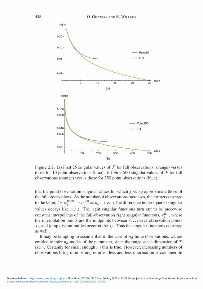
Figure 2.2. (a) First 25 singular values of F for full observations (orange) versusthose for 10 point observations (blue). (b) First 500 singular values of F for fullobservations (orange) versus those for 250 point observations (blue).

that the point observation singular values for which j nd approximate those ofthe full observations. As the number of observations increases, the former convergeto the latter, i.e. σpoint

j → σfullj as nd →∞. (The difference in the squared singular

values decays like n−2d.) The right singular functions turn out to be piecewise

constant interpolants of the full-observation right singular functions, vfullj , wherethe interpolation points are the midpoints between successive observation pointsxj , and jump discontinuities occur at the xj . Thus the singular functions convergeas well.It may be tempting to assume that in the case of nd finite observations, we are

entitled to infer nd modes of the parameter, since the range space dimension of Fis nd. Certainly for small enough nd this is true. However, increasing numbers ofobservations bring diminishing returns: less and less information is contained in



https://doi.org/10.1017/S0962492921000064



the data, and we are back to the fundamental difficulty underlying the first threemodel problems, i.e. eigenvalues/singular values decaying to zero and leading toinstability in the inference of the more oscillatory modes. Thus, for sufficientlylarge values of nd, the smallest non-zero σj will amplify the noise (by a factor σ−1

j )leading to an unstable reconstruction. So the number of inferrable modes may bejust a fraction of nd. To illustrate these points, Figure 2.2 plots the singular values ofF for three cases: 10 point observations (plot (a)), 250 point observations (plot (b)),and full observations (both). The convergence of the σpoint

j to σfullj with increasing

nd can be seen. With 10 observations, the singular values (blue curve in (a))remain sufficiently large that the inference will avoid pollution from observationalnoise of order 0.05. However, plot (b) shows that with 250 point observations,high-frequency noise of order 0.002 can lead to unstable reconstructions.

Thus, restricting the observations to a finite collection of points introducessevere ill-posedness in the now under-determined inverse problem, even when thefull-observation case is only moderately ( j−1) ill-posed. Moreover, increasingthe number of observations leads to diminishing returns, as the point observationsingular values converge to their full observation counterparts and instability ensuesfor small singular values. This discussion of point observations is of courseapplicable to many other inverse problems.

2.5. Summary

The model elliptic, parabolic and hyperbolic inverse problems discussed aboveillustrate ill-posedness due to lack of existence, uniqueness or stability. (Theunrealistically formulated hyperbolic inverse problem was in fact well-posed, butwe discussed a number of features that make more realistic variants of the problemill-posed.) Lack of existence (due to inconsistent data) and uniqueness (due tosparse data) can be addressed by solving (2.1) using theMoore–Penrose generalizedinverse F† (Engl et al. 1996). The stability condition is more pernicious, and isthe central cause of numerical difficulties in solving inverse problems. The lack ofstability stems from the collapse of the spectrum of F , the dominant eigenvaluesof which correspond to modes of m that can be reliably inferred from the data. (InSection 4 we will make an information-theoretic connection between the spectrumof F and the information contained in the data.)

As (2.6) and (2.7) make evident, (inverses of) small eigenvalues amplify noisecomponents in directions of the corresponding eigenfunctions, leading to unstableinference of these modes (for non-self-adjoint F , the singular value decompositionreplaces the spectral decomposition). The more rapid the decay of the spectrum ofF , and the higher the noise level, the fewer eigenvalues will be above the noise level,and the fewer modes of m that can be reliably inferred from the data. The modelproblems exhibit algebraic (in the elliptic case) or exponential (in the paraboliccase) decay of the spectrum, accumulating at zero, reflecting different degrees of



https://doi.org/10.1017/S0962492921000064



severity of ill-posedness. Moreover, even for a finite number of observations nd –meaning that the range space ofF is finite-dimensional – if nd is large enough, therecan be significant decay of the spectrum (due to near-redundancy in informationcontained within the data) such that small eigenvalues can trigger instability.The loss of information in F(m), the map from parameters to observables –

and the resulting inability to recover the lost information via the inverse map – is afundamental property of the inverse problem. No amount ofmathematical wizardrycan recover the lost information. The best we can hope to do is recover componentsof m lying in the ‘effective’ range space of F , that is, those eigenfunction modescorresponding to eigenvalues that are large enough to dominate the noise. Howto do this efficiently and scalably for problems characterized by high-dimensionalparameters (resulting from discretization of m) and for expensive forward problems(involving solutions of PDEs) will be the subject of the next two sections, in thecontext of both regularization and Bayesian frameworks. The essential idea is todesign algorithms that exploit the intrinsic low-dimensionality of the informationcontained within the data by requiring an amount of work (measured in PDE solves)that scales with the intrinsic ‘information dimension’, not the apparent dimension.As we will see, these algorithms depend fundamentally on the rapid spectral de-

cay (of F∗F). Rapid spectral decay has been demonstrated, not just for the modelproblems of this section, but for a broad set of inverse problems arising in scienceand engineering, either explicitly through low-rank approximation of the Hessianof the data misfit (Section 4) or implicitly through rapid convergence of conjugategradients for the Hessian system (Section 3). These include ice sheet dynamics(Petra et al. 2012, Petra, Martin, Stadler and Ghattas 2014, Isaac, Petra, Stadlerand Ghattas 2015, Zhu et al. 2016b, Babaniyi, Nicholson, Villa and Petra 2021),shape and medium acoustic and electromagnetic scattering (Akçelik, Biros andGhattas 2002, Bui-Thanh and Ghattas 2012a,b, 2013, Chaillat and Biros 2012, Am-bartsumyan et al. 2020, O’Leary-Roseberry, Villa, Chen and Ghattas 2020, Chen,Haberman and Ghattas 2021), seismic wave propagation (Akçelik et al. 2003a,Epanomeritakis, Akçelik, Ghattas and Bielak 2008, Martin, Wilcox, Bursteddeand Ghattas 2012, Bui-Thanh et al. 2012a, Bui-Thanh, Ghattas, Martin and Stadler2013, Zhu et al. 2016a), mantle convection (Worthen et al. 2014), viscous incom-pressible flow (Biros and Ghattas 1999, 2005a,b, Yang, Stadler, Moser and Ghattas2011), atmospheric transport (Akçelik et al. 2003b, 2005, Bashir et al. 2008, Flathet al. 2011, Alexanderian, Petra, Stadler and Ghattas 2014, Wu, Chen and Ghattas2020, Villa, Petra and Ghattas 2021), ocean dynamics (Kalmikov and Heimbach2014), turbulent combustion (Chen, Villa andGhattas 2019a), poroelasticity (Hesseand Stadler 2014, Alghamdi, Hesse, Chen andGhattas 2020, Alghamdi et al. 2021),infectious disease spread (Chen and Ghattas 2020a,b), tumour growth modelling(Subramanian, Scheufele, Mehl and Biros 2020), tsunami extreme events (Tong,Vanden-Eijnden and Stadler 2020), joint inversion (Crestel, Stadler and Ghattas2018) and subsurface flow (Alexanderian, Petra, Stadler and Ghattas 2016, 2017,Chen, Villa and Ghattas 2017, Chen and Ghattas 2019, 2020c).



https://doi.org/10.1017/S0962492921000064



3. Regularization framework and inexact Newton-CG3.1. Regularization framework

We return to the task of solving the inverse problem (2.1), that is, attempting toinfer the parameter m ∈ X from given data d ∈ Y from

F(m) = d.

We saw in Section 2 that a fundamental feature of many ill-posed inverse problemsis the decay of the spectrum of F to zero. As we saw in (2.6) and (2.7), smalleigenvalues of F (smaller than the Fourier coefficients of the noise) amplify thenoise in the data, rendering the inversion unstable for small enough eigenvalues andlarge enough noise. Since these eigenvalues correspond to eigenfunctionmodes thatdo not influence the data (above the noise threshold) – and are thus unrecoverable –a reasonable strategy is to annihilate them. WhenF is a linear operator, this can beaccomplished by a truncated singular value decomposition (TSVD), in which theeigenvalues of F below a certain threshold are truncated, so that TSVD acts likea filter. A preferable alternative is Tikhonov regularization, which most stronglyattenuates the smallest eigenvalues, with the amount of attenuation falling off withlarger eigenvalues. Thus Tikhonov regularization acts like a ‘softer’ version ofTSVD. Rather than apply the regularization as a filter (with varying filter factor),an equivalent formulation is to solve the optimization problem

minm∈X

φ(m) :=12‖F(m) − d‖2 +

β

2‖m‖2, (3.1)

where the observable F(m) ∈ Y depends on the parameter m via solution of thegoverning PDE (2.2), yielding u ∈ U and application of an observation operator,that is,

F(m) := B(u(m)), where u(m) solves r(u,m) = 0 for given m.

The regularization term (β/2)‖m‖2 imposes a penalty on the norm of m, withthe regularization parameter β controlling the strength of the penalty. Solution ofthe regularized least-squares problem (3.1) has several advantages over the filterformulation: (i) it avoids computation of the spectral decomposition or SVD ofF , (ii) it extends easily to non-linear parameter-to-observable maps, (iii) it allowsfor more general norms and regularization operators, (iv) it permits additionalequality or inequality constraints (such as bounds) on m, and (v) it admits differentnorms besides L2 in the data misfit term ‖F(m) − d‖, such as the more robust (tooutliers) L1.

The most popular regularization is the H1 seminorm∫∇m · ∇m dx, which

amounts to an increasing penalty on the more oscillatory modes of m. Its specificaction for themodel problems described in Section 2 is to damp the components ofmin the eigenfunction directions vj(x) with increasing weights j2 (the eigenvalues ofthe one-dimensional Laplacian underlying the H1 seminorm), thereby stabilizing



https://doi.org/10.1017/S0962492921000064



the inference of those components. Many other choices of regularization termshave been employed, including other Hilbert space norms expressing differentsmoothness preferences, total variation (which expresses a preference for piecewiseconstant m), total generalized variation (piecewise smooth), sparsity-promotingand directional sparsity-promoting functionals, and a variety of statistical and data-driven regularizers. See the comprehensive accounts in Arridge, Maass, Öktemand Schönlieb (2019) and Benning and Burger (2018).The regularization parameter β is chosen to balance the error due to instability

caused by noise amplification and the error due to bias caused by the regularization.The tension is between too large a β, in which case modes that are well informedby the data are damped, and too small a β, in which case modes that are poorlyinformed by the data become unstable in the reconstruction. If δ = ‖η‖ representsthe magnitude of the noise, it can be shown (e.g. Vogel 2002) that the choiceβ = O(δp), 0 < p < 2 guarantees that both sources of error vanish as δ → 0.However, this a priori estimate does not provide a constructive formula for choosingβ. Instead, we appeal to an a posteriori formula. The Morozov discrepancyprinciple is a popular choice: Find the largest value of β that satisfies

‖F(mβ) − d‖ ≤ δ, (3.2)

where

mβ := arg minm∈X

12‖F(m) − d‖2 +

β

2‖m‖2

.

Thus we seek the smallest regularization penalty ‖m‖2 that results in an m that fitsthe data to within the noise. The resulting choice of β∗ can also be derived fromthe following optimization problem:

minm∈X

12‖m‖2,

subject to ‖F(m) − d‖2 = δ2.

The value of the Lagrange multiplier µ∗ for the constraint at optimality is thenrelated to Morozov’s choice of β by β∗ = 1/(2µ∗).

3.2. Inexact Newton–conjugate gradient methods

We now turn to the main topic of this section, which is efficient and scalableNewton algorithms for the optimization problem (3.1). This problem belongs tothe class of PDE-constrained optimization problems; for discussion of the under-lying theoretical, as well as other computational methods, see e.g. Biegler, Ghattas,Heinkenschloss and van Bloemen Waanders (2003), Gunzburger (2003), Biegleret al. (2007), Ito and Kunisch (2008), Hinze, Pinnau, Ulbrich and Ulbrich (2009),Tröltzsch (2010), Ulbrich (2011), Borzì and Schulz (2012), Leugering et al. (2012),De los Reyes (2015) and Antil, Kouri, Lacasse and Ridzal (2018). By virtue of the



https://doi.org/10.1017/S0962492921000064



implicit function theorem, we will consider the state u to be an implicit function ofm via solution of the PDE r(u,m) = 0, resulting in the unconstrained optimizationproblem (3.1). While this greatly simplifies the optimization problem, this implicitdependence complicates the computation of the gradient and Hessian of the ob-jective functional Φ(m), which are required for the Newton iterations. (A detailedconcrete example of how to compute them is provided in Section 5.) For stationaryand highly non-linear problems, significantly greater efficiency may be obtained bysolving the inverse problem as a constrained optimization problem, which relaxesthe PDE solution by imposing the PDEs as constraints, iterating toward both feas-ibility (satisfying the PDEs) and optimality (minimizing the objective) (e.g. Birosand Ghattas 2005a,b).We assume (3.1) has been suitably discretized (see Section 5 for a discussion of

discretization issues), resulting in the finite-dimensional optimization problem

minm∈Rnm

Φ(m) :=12‖f(m) − d‖2 +

β

2‖m‖2Hreg, (3.3)

where m ∈ Rnm and d ∈ Rnd are the finite-dimensional representations of theparameter and data, f : Rnm → Rnd is the discrete parameter-to-observable map,Φis the discrete regularized least-squares function, Hreg is a regularization operator(for simplicity, we assume quadratic regularization) and f depends implicitly on mvia solution of a discretized forward PDE problem.In this section we will describe the inexact Newton–conjugate gradient method

for solving (3.3) with specialization to large-scale inverse problems governed byPDEs. We describe the components of the method that are salient for the targetedproblem class. See Kelley (1999) and Nocedal andWright (2006) for further detailsand analysis. Newton’s method is the gold standard for fast solution of discretizedinfinite-dimensional optimization problems such as (3.3). For a wide varietyof problems, it converges in a mesh-independent (or nearly mesh-independent)number of iterations (Allgower, Böhmer, Potra and Rheinboldt 1986, Kelley andSachs 1991, Heinkenschloss 1993). Our experience is that this is generally themost effective method for this class of problems, converging with far fewer forwardPDE solves than methods that rely only on gradient information. Define g(m) asthe gradient vector of Φ(m) and H(m) as its Hessian matrix, that is,

g(m) ∈ Rnm :=DΦ(m)

Dm,

H(m) ∈ Rnm×nm :=D2Φ(m)

Dm2 ,

where D/Dm denotes total derivative (taking into account implicit dependence off on m via solution of the PDE). The kth Newton iteration solves the linear system

Hkpk = −gk (3.4)



https://doi.org/10.1017/S0962492921000064



for the search direction pk , followed by the parameter update

mk+1 = mk + αkpk .

Here αk is a step length chosen according to an appropriate line search strategy,and gk := g(mk) and Hk := H(mk). Assuming Φ is twice Lipschitz continuouslydifferentiable, then near a local minimizer m∗ the Newton iteration (3.4) convergesq-quadratically. Global convergence (i.e. from any starting point) to at least astationary point (g(m) = 0) can be established under reasonable assumptions(which are frequently satisfied in practice) by:(i) ensuring that pk is a descent direction, i.e. pT

kgk < 0,

(ii) taking a step length αk that ensures sufficient decrease of Φ(mk+1) and suffi-ciently large steps αkpk .

Condition (i) can be satisfied by maintaining a positive definite approximation tothe Hessian. Condition (ii) can be satisfied by an Armijo backtracking line search.

1 Start with a trial step of α0k= 1.

2 Check for sufficient descent:Φ(mk + α

ikpk) − Φ(mk)

αikpTkgk

≥ c.

3 (a) If step 2 is satisfied, mk+1 = mk + αikpk .

(b) Else, backtrack using αi+1k= γαi

kand repeat from 2.

Typical choices of constants are c = 10−4 and γ = 1/2. Initializing the backtrackingwith α = 1 asymptotically ensures the correct initial choice of step length, sinceNewton’s quadratic approximation of Φ becomes increasingly accurate near aminimizer.Several difficulties are encountered in specializing the globalized Newton op-

timization framework outlined above to large-scale inverse problems governed byPDEs.• The major challenge faced by Newton methods for the targeted class of in-verse problems is that explicit construction of the Hessian H(m) is typicallyintractable. Each column of the Hessian requires the solution of a pair oflinearized forward/adjoint PDEs (see Section 5); these PDE solution costsoverwhelmingly dominate all other costs of solving the optimization problem(such as linear algebra). For example, in the ice sheet flow inverse problemdiscussed in Section 6, solving a single linearized forward problem requiresabout oneminute on 1024 processor cores. Thus constructing a singleHessianfor the one million parameters that characterize this problem would requireabout two years of supercomputing time! How can we enjoy the benefits ofNewton’s asymptotic quadratic convergence without explicitly forming thisHessian?



https://doi.org/10.1017/S0962492921000064



• Unless the inverse problem is linear, the usual situation is that Φ(m) is non-convex. As a result, theHessian can be indefinite away from a localminimizer.To ensure a descent direction far from a local minimizer, we must maintaina positive definite approximation to the Hessian, H. How can this be donewhen the Hessian itself cannot even be formed? Moreover, how can we avoidmodifying the Hessian in the vicinity of a local minimizer so as not to interferewith the asymptotic convergence rate?

• Since manipulating the Hessian is so expensive (in terms of PDE solves), canwe lessen our reliance on Newton steps far from a minimizer (when Newtonis only linearly converging)?

• The Hessian can be decomposed into the Hessian of the data misfit functionaland the Hessian of the regularization functional:

H = Hdata + βHreg.

As we saw in the model problems in Section 2, typically for ill-posed inverseproblems, Hdata is a (discretized) compact operator. On the other hand,typically it is the highly oscillatory modes of m that are poorly determinedby the data and require regularization, and as a result the regularization istypically smoothing. Thus the regularization operator Hreg is often chosenas a elliptic differential operator. Can we take advantage of this ‘compact +differential’ structure in addressing the two challenges listed above?

The inexact Newton–conjugate gradient (Newton-CG) method addresses all ofthese issues. The basic idea is to solve (3.4) with the (linear) CG method in amatrix-free manner, terminating early to enforce positive definiteness and avoidover-solving (Dembo, Eisenstat and Steihaug 1982, Eisenstat and Walker 1996).

1 Solve Hkpk = −gk iteratively using preconditioned CG.

(a) At each CG iteration where di is the ith CG search direction, form theproduct of Hk with di in a matrix-free manner via a pair of ‘incremental’forward/adjoint PDE solves (see Section 5).

(b) Terminate CG iteration when a direction of negative curvature is en-countered, i.e. when

diTHkdi ≤ 0,

and use the current CG solution pikas the Newton search direction (unless

it is the first CG iteration, inwhich case use the steepest descent direction).

(c) Also terminate the CG iterations when the Newton system is solved‘accurately enough’, i.e. when

‖Hkpik + gk ‖ ≤ ηk ‖gk ‖,

where the tolerance with which this system is solved tightens as the



https://doi.org/10.1017/S0962492921000064



minimizer is approached (‖gk ‖ → 0 as k → ∞). The choice of theforcing term ηk affects the Newton convergence rate:

ηk =

0.5 linear,min(0.5,

√‖gk ‖) superlinear,

min(0.5, ‖gk ‖) quadratic.

(d) Precondition the CG iterations with regularization operator Hreg.

2 Perform Armijo backtracking line search with pikas Newton search direction.

3 Update mk+1 = mk + αkpikand repeat from step 1 until convergence.

In step 1(a), the Hessian-vector product is carried out without explicitly formingthe Hessian, forming only its action on a vector (CG is a matrix-free algorithm,and requires only the matrix action on a given vector). This can be done at thecost of solving a pair of linearized PDEs, one forward and one adjoint. Section 5illustrates how this can done in the context of a specific non-linear, non-self-adjoint,time-dependent PDE. (In the time-dependent case, several additional PDE solveswill be required in the memory-bound setting due to the necessity of checkpointing;this will be explained in Section 5). This avoids the need to store Hk , which is(formally) dense and would require O(n2

m) storage. More important, it avoids theprohibitive cost of explicitly forming Hk column by column. To be successful, ofcourse, few Hessian actions – i.e. few CG iterations – should be required. We willreturn to this shortly.By terminating CG when negative curvature is encountered, step 1(b) ensures

that a descent direction is maintained. This is because each CG iterate pikis a linear

combination of the negative gradient and the previous iterate pi−1k

, back to the firstiterate, which itself is taken as the negative gradient. Thus the Newton-CG methodis globally convergent (with appropriate line search). (The CG termination criteriacan be easily extended to allow for a trust region globalization.)Step 1(c) is intended to avoid ‘over-solving’. Since Newton’s method entails

minimization of a quadratic approximation of Φ, and this quadratic approximationmay be a poor predictor of the actual change in Φ for large steps far from a localminimizer, there is no point in solvingHkpk = −gk accurately early in the iterations.The linear system is solved more accurately as the iterations progress by choosingηk < 1. Quadratic convergence can be preserved by taking ηk to be of the order ofthe norm of the gradient. On the other hand, a constant ηk results in a reductionto linear convergence. A more rapidly shrinking ηk will lead to faster Newtonconvergence, at the expense of increased CG iterations, while the converse is truewith a more slowly shrinking η. A good compromise is often ηk = O(‖gk ‖1/2),which tends to result in the fewest overall CG iterations and thus Hessian actions.As remarked above, it is crucial that CG take few iterations, since each iteration

entails a pair of linearized forward/adjoint PDE solves (see Section 5). Can we



https://doi.org/10.1017/S0962492921000064



be assured that this is indeed the case? CG has the property that it minimizes theenergy norm of the error at the ith iteration with respect to a polynomial of degree i.The energy norm of the error ei can be written as (Shewchuk 1994, Nocedal andWright 2006)

‖ei ‖2H =nm∑j=1

λj[Pi(λj)]2ξ2j , (3.5)

where

• ei = p∗k− pi

k, with p∗

kas the exact solution to (3.4),

• ξj is the participation factor of the jth eigenvector vj in the initial error, i.e.e0 =

∑nmj=1 vjξj , and

• Pi(λ) is an ith-order polynomial in λ, with the property that P0(λ) = 1 andthe constraint Pi(0) = 1.

Since CGminimizes the left-hand side of (3.5) with respect to Pi, it also minimizesthe right-hand side with respect to Pi, that is,

Pi∗(λ) = arg minPi (λ)

nm∑j=1

λj[Pi(λj)]2ξ2j . (3.6)

From this expression, we see that at the ith iteration, CG finds the ith degreepolynomial that best fits the eigenvalues on the positive real axis, in a weightedleast-squares sense. It minimizes the squared misfit at each eigenvalue, [Pi(λj)]2,weighted by the magnitude of the eigenvalue λj , and by the squared component ofthe initial error in the direction of the corresponding eigenvalue, ξ2

j . We see thatCG favours the elimination of error components associated with eigenvectors that(i) correspond to large eigenvalues, (ii) correspond to clustered eigenvalues (sincePi(λ) is small in their vicinity), and (iii) are most aligned with the initial error.As illustrated in the examples of Section 2, the spectrum of a typical data misfit

HessianHdata collapses, with smaller eigenvalues corresponding tomore oscillatoryeigenvectors. What happens when CG is applied to such an operator? Initially iteliminates error components associated with the large eigenvalues (thus behavingas a smoother), and then begins to attack the smaller eigenvalues that accumulate atzero. In fact, as an alternative to Tikhonov regularization, early termination of CGiterations can be used as a regularization (Hanke 1995): initially, error componentsof the solution in smooth (data-informed) eigenfunction directions are eliminated,and the CG iteration is then terminated (e.g. by the Morozov criterion (3.2)) asnoise-amplified unstable modes begin to be picked up.However, here we are interested in the use of CG for solving the Newton system

with the regularizedHessian,H := Hdata+βHreg, since oftenwewant to incorporateadditional prior information on m via the regularization term. Toward this end, we



https://doi.org/10.1017/S0962492921000064



recognize that the regularization operator Hreg is typically an elliptic differentialoperator (possibly heterogeneous and anisotropic). This suggests preconditioningby Hreg, so that the preconditioned Hessian operator is Hreg−1

kHk , and the Newton

system becomes (Hreg−1

kHdata

k + βI)pk = −Hreg−1

kgk . (3.7)

In the common case where Hreg is an elliptic differential operator, its inverseis compact, and thus the product of its inverse with Hdata, the regularization-preconditioned data misfit Hessian, is also compact. Then the operator

(Hreg−1

kHdata

k + βI)

has the form of a (discretized) Fredholm second-kind integral operator. For suchproblems, the conjugate gradient method (as well as other Krylov methods) isknown to converge superlinearly; moreover, for nm sufficiently large, the numberof iterations required to solve (3.7) to a given accuracy is constant, independent ofthe parameter dimension nm (Fortuna 1979, Flores 1993, Campbell, Ipsen, Kelleyand Meyer 1994, Atkinson 1997, Axelsson and Karatson 2007, Herzog and Sachs2015).

This mesh-independence of the (inner) CG iterations when using regularizationpreconditioning can be understood to be a consequence of the effectively finite-dimensional and mesh-independent range space of both the Hessian of F∗F aswell as the inverse regularization operator. CG takes O(r) iterations to eliminateerror components associated with the r dominant eigenvalues (i.e. those for whichλi > β) of Hreg−1

kHdata

k, and then very quickly dispenses with the remaining error

components associated with eigenvalues that cluster around β. Since the dominantcost of the CG iterations is the PDE solves associatedwith theHessian action at eachiteration, fully solving (3.7) requires about r forward/adjoint PDE solves, whereusually r nm. Moreover, the inexactness of the method (i.e. early termination ofCG when far from a local minimum) means that CG converges in just a handful ofiterations in the early Newton iterations.This combination of mesh-independence of (outer) Newton iterations, mesh-

independence of (inner) CG iterations and inexactness to prevent oversolving resultsin a method for solving PDE-based inverse problems that requires a parameter-dimension-independent number of PDE solves. Thus the method is scalable.When the eigenvalues of the regularization-preconditioned data misfit Hessiandecay sufficiently rapidly, r is small, and the method is then also efficient, in thesense that the required number of PDE solves is small. To understand how rapidlythe eigenvalues decay, consider the model problems of Section 2. For the parabolicinverse problem, the exponential decay of the eigenvalues of the parameter-to-observable mapF renders r very small, on the order of a handful of modes. For theelliptic inverse problem, the eigenvalues of F decay only algebraically, O( j−2) forthe specific problem considered. However, the spectrum of the data misfit Hessian



https://doi.org/10.1017/S0962492921000064



squares this to O( j−4). Moreover, the common choice of H1 regularization leadsto preconditioning by −∆−1, which in this case has the same eigenfunctions asF∗F , and eigenvalues that decay (in one dimension) like j−2. Thus, overall,the eigenvalues of Hreg−1

kHdata

kdecay like j−6, which is very rapid decay indeed.

Thus, while this operator’s effective range space dimension r for elliptic inverseproblems is typically large relative to those of parabolic problems, one often stillhas sufficiently rapid spectral decay that the average number of CG iterations perNewton iteration is in the 10s–100s, even for inverse problems with millions ofparameters. Combined with a typically modest number of Newton iterations, thisoften means solution of large-scale inverse problems at a cost of 100s–1000s oflinearized PDE solves. Section 6 presents a case study that illustrates this behaviourfor inexact Newton-CG solution of a large-scale regularized inverse problem forthe flow of the Antarctic ice sheet with O(106) parameters.

To conclude this section, we note an important class of inverse problems forwhich r , the number of dominant eigenvalues of the regularization-preconditioneddata misfit Hessian, is large in absolute terms, even if it is small or moderate relativeto the parameter dimension nm. In such problems, the required number of PDEsolves using regularization preconditioning may be unacceptably large. This canresult from a low data noise level, which reduces the regularization parameter β,allowing us to extract more information from the data (up to a point of course:ultimately instability takes over). By exposing additional smaller eigenvaluesabove the β threshold, CG is forced to iterate longer to resolve the associatedmodes. Another source of large r is more informative data, which results ina spectrum of Hdata that decays more slowly. As suggested by the hyperbolicinverse problem of Section 2, this can stem from inverse problems in which theloss of information in the parameter-to-observable map is more muted. Examplesinclude flows that are increasingly advection-dominated, wave propagation withhigher frequencies and more sources, and more generally problems with largenumbers of informative observations and/or informative experiments. For these andother problems, finding effective Hessian preconditioners beyond the regularizationoperator remains an active area of research; see Battermann and Heinkenschloss(1998), Arian and Ta’asan (1999), Gunzburger, Heinkenschloss and Lee (2000),Dreyer, Maar and Schulz (2000), Haber and Ascher (2001), Battermann and Sachs(2001), Akçelik et al. (2002), Borzì (2003), Ascher and Haber (2003), Akçeliket al. (2005), Borzì and Griesse (2005), Heinkenschloss (2005), Biros and Ghattas(2005a), Akçelik et al. (2006), Heinkenschloss andNguyen (2006), Heinkenschlossand Herty (2007), Schöberl and Zulehner (2007), Drăgănescu and Dupont (2008),Herrmann, Moghaddam and Stolk (2008), Biros and Dogan (2008), Adavani andBiros (2008), Borzì and Schulz (2009), Adavani and Biros (2010), Herzog andSachs (2010), Rees, Dollar and Wathen (2010a), Nielsen and Mardal (2010), Rees,Stoll and Wathen (2010b), Benzi, Haber and Taralli (2011), Takacs and Zulehner(2011), Rees and Wathen (2011), Chaillat and Biros (2012), Pearson, Stoll and



https://doi.org/10.1017/S0962492921000064



Wathen (2012), Pearson and Wathen (2012), Borzì and Schulz (2012), Demanetet al. (2012), Nielsen andMardal (2012), Pearson, Stoll andWathen (2014), Schielaand Ulbrich (2014), Benner, Onwunta and Stoll (2016), Barker, Rees and Stoll(2016), Gholami, Mang and Biros (2016), Zhu et al. (2016a), Alger, Villa, Bui-Thanh and Ghattas (2017), Mardal, Nielsen and Nordaas (2017), Ambartsumyanet al. (2020) and Alger et al. (2019).

4. Bayesian framework and Laplace approximationThe regularization framework of Section 3 – while admitting scalable and efficientinverse solvers – provides just a point estimate of the inverse solution, and is notcapable of quantifying the uncertainty in the inferred parameters. For a well-posedproblem, thismay be acceptable. But for an ill-posed problem, particularly onewithnon-negligible noise, where many parameter choices are consistent with the datato within the noise, this point estimate is not very useful. The Bayesian framework,on the other hand, states the inverse problem as one of statistical inference over thespace of uncertain parameters (Tarantola 2005, Kaipio and Somersalo 2005, Stuart2010, Dashti and Stuart 2017). The resulting solution to this statistical inverseproblem is a posterior probability distribution that describes the probability ofthe parameter conditioned on the data. It combines a prior distribution, whichencodes any prior knowledge or assumptions about the parameters before dataare collected, with a likelihood, which explicitly represents the probability that agiven set of parameters might give rise to the observed data. The central task ofBayesian solution then is to characterize or explore the posterior: drawing samples,estimating themean, covariance or highermoments, determining credible intervals,or evaluating the posterior probabilities of particular events.Unfortunately, Bayesian solution of inverse problems – i.e. fully characterizing

the posterior – is often intractable for expensive PDE forward models and in highparameter dimensions, as results from discretization of infinite-dimensional para-meter fields. This stems from the need to sample a posterior distribution in highdimensions, where each sample requires (at least) evaluation of the posterior, andthus solution of the forward problem. Markov chain Monte Carlo (MCMC) meth-ods are usually themethod of choice for sampling complex distributions, but in theirblack-box forms will often require many millions of evaluations of the posterior toproduce reliable statistical estimates, making their use prohibitive for PDE-basedinverse problems. In recent years, a number of methods for Bayesian inverse prob-lems governed by PDEs have emerged that exploit structure of parameter space in-cluding geometry (locally approximated by the Hessian and higher derivatives) andintrinsic low-dimensionality (dictated by the compactness of the data-misfit Hes-sian), mirroring the structure-exploiting properties of inexact Newton-CGmethods(Section 3) for deterministic inverse problems. These range from Hessian-awareGaussian process approximation of the parameter-to-observable map (Bui-Thanh,Ghattas and Higdon 2012b), to projection-type forward model reduction (Galbally,



https://doi.org/10.1017/S0962492921000064



Fidkowski, Willcox and Ghattas 2010, Lieberman, Willcox and Ghattas 2010, Cui,Marzouk and Willcox 2015), to polynomial chaos approximations of the stochasticforward problem (Badri Narayanan and Zabaras 2004, Ghanem and Doostan 2006,Marzouk and Najm 2009), to Markov chain Monte Carlo (MCMC) proposals ex-ploiting log-likelihood Hessian approximations (Girolami and Calderhead 2011,Flath et al. 2011, Martin et al. 2012, Bui-Thanh et al. 2012a, 2013, Bui-Thanhand Girolami 2014, Petra et al. 2014, Cui et al. 2014, Cui, Law and Marzouk2016, Beskos et al. 2017), to randomize-then-optimize sampling methods (Oliver,He and Reynolds 1996, Bardsley, Solonen, Haario and Laine 2014, Wang et al.2017, Oliver 2017, Wang, Bui-Thanh and Ghattas 2018, Bardsley, Cui, Marzoukand Wang 2020, Ba, de Wiljes, Oliver and Reich 2021), to adaptive sparse quad-rature combined with reduced basis approximations (Schillings and Schwab 2013,Chen and Schwab 2015, 2016a,b, Chen et al. 2017), to optimal transport-basedvariational methods using parametric and non-parametric transport maps (Moselhyand Marzouk 2012, Liu and Wang 2016, Marzouk, Moselhy, Parno and Spantini2016, Detommaso et al. 2018, Chen et al. 2019b, Chen and Ghattas 2021, 2020a).

These methods have shown considerable promise by tackling certain PDE-governed Bayesian inverse problems with exploitable structure. Further devel-opments in such structure-exploiting methods – in conjunction with the modelreduction methods described in Part 3 – offer hope that full Bayesian solutionof complex PDE-governed high-dimensional inverse problems will become morecommon over the coming decade. These methods are undergoing rapid develop-ment today and we will not discuss them further. However, we will describe indetail the Laplace approximation of the posterior, which becomes tractable to com-pute – and even scalable and efficient – when one exploits the same properties thatmade inexact Newton-CG so powerful for the regularization formulation. Thus themethods of this section are intimately connected to those of the previous one andthe properties of the model inverse problems highlighted in Section 2. Moreover,the Laplace approximation and related tools often play an important role in thesampling, variational and transport methods mentioned above.The discussion below is based on the finite-dimensional form of the Bayesian

inverse problem, i.e. after parameter space has been discretized. Conditionson the prior and the parameter-to-observable map that result in a well-definedand well-posed Bayesian inverse problem in infinite dimensions are presented inStuart (2010) and Dashti and Stuart (2017), and summarized in Arridge et al.(2019). Infinite-dimension-consistent discretizations are discussed in Bui-Thanhet al. (2013) and Petra et al. (2014).

4.1. Bayesian formulation

Denote by πpr(m) the prior probability density of the model parameters m ∈ Rnm ,πlike(d|m) the likelihood of the data d ∈ Rnd given the parameters, and πpost(m) :=π(m|d) the posterior density reflecting the probability of the parameters conditioned



https://doi.org/10.1017/S0962492921000064



on the data. Then Bayes’ rule can be written as

πpost(m) =1Zπlike(d|m) πpr(m), (4.1)

where the normalizing constant Z is given by

Z =∫

πlike(d|m) πpr(m) dm,

and is often called the evidence.We restrict our discussion to a Gaussian prior m ∼ N (mpr, Γpr), that is,

πpr(m) ∝ exp−

12‖m −mpr‖

2Γ−1pr

, (4.2)

where mpr ∈ Rnm and Γpr ∈ Rnm×nm are respectively the mean and covariance

of the prior distribution. Here, Γpr must be chosen to be sufficiently smoothingin order to ensure a well-posed Bayesian inverse problem; this is the Bayesianequivalent of regularization. One attractive choice is for Γpr to be taken as thediscretization of the inverse of the νth power of an elliptic differential operator:

Γpr = (−γ∆h + δIh)−ν, (4.3)

where γ > 0 and δ > 0 are positive constants and h indicates discretization. Forwell-posedness, ν > ω/2, where ω is the spatial dimension (Stuart 2010). So inone dimension ω = 1 is sufficient, whereas in two and three dimensions we oftentake ω = 2 to avoid solving a fractional PDE. The parameters γ and δ are chosento impose prior knowledge of the correlation length ρ (distance for which thetwo-point correlation coefficient is 0.1) and the pointwise variance σ2 of the prioroperator; specifically ρ ∝

√γ/δ and σ2 ∝ δ−νρ−ω. This form of prior is equivalent

to a subset of the Matérn covariance family (Lindgren, Rue and Lindström 2011).To incorporate anisotropy in correlation lengths, the Laplacian in (4.3) can bereplaced by an anisotropic Poisson operator. These choices ensure that the priorcovariance (−γ∆ + δI)−ν is a trace-class operator, leading to bounded pointwisevariance and a well-posed infinite-dimensional Bayesian inverse problem (Stuart2010). Appropriate boundary conditions can be chosen to mitigate the influenceof the boundary (Daon and Stadler 2018).To construct the likelihood, we consider the discretized form of the additive

noise model (2.3),d = f(m) + η, η ∼ N (0, Γnoise),

with the noise η ∈ Rnd taken to be a normally distributed random variable withmean zero and covariance Γnoise ∈ Rnd×nd , and as before f(m) is the discretizedparameter-to-observable map. The likelihood then becomes

πlike(d|m) ∝ exp−

12‖f(m) − d‖2

Γ−1noise

.



https://doi.org/10.1017/S0962492921000064



(See Dunlop 2019 for extensions to other noise models.)With this choice of Gaussian prior and Gaussian additive noise, we arrive at the

expression for the posterior,

πpost(m) ∝ exp−

12‖f(m) − d‖2

Γ−1noise−

12‖m −mpr‖

2Γ−1pr

. (4.4)

After discretization, the posterior (4.4) is a probability density in nm dimensions,which can be in the millions (or much higher) for complex PDEmodels, such as theexample in Section 6. Moreover, evaluating πpost(m) at any point in parameter spacerequires solution of the forward PDE problem embedded within the parameter-to-observable map f(m). As such, exploring the posterior to, for example, computestatistics of quantities of interest (mean, variance, quantiles) is typically prohibit-ive, due to the high-dimensionality of the parameters and the expense of solvingthe forward PDE problems. We will restrict ourselves here to the Laplace approx-imation, which is a Gaussian centred on the maximum a posteriori (MAP) point,with covariance equal to the inverse of the Hessian of the negative logarithm of theposterior evaluated at the MAP point. The Laplace approximation is exact whenthe parameter-to-observable map f(m) is linear, and often provides a reasonableapproximation to the posterior, since the error is of the order of the departurefrom linearity of the parameter-to-observable map (Helin and Kretschmann 2020).Moreover, in the limit of small noise or large data, the Laplace approximationconverges to the posterior (Schillings, Sprungk and Wacker 2020).

4.2. Finding the MAP point

The maximum a posteriori point mmap is the point that maximizes the posteriordensity with respect to m,

mmap := arg maxm∈Rnm

1Zπpost(m)

= arg minm∈Rnm

− log πpost(m)

= arg minm∈Rnm

12‖f(m) − d‖2

Γ−1noise+

12‖m −mpr‖

2Γ−1pr.︸︷︷︸

Φ(m)

(4.5)

Notice the equivalence between finding the MAP point and solving the regular-ized inverse problem (3.3) by minimizing Φ(m). The prior term is analogous toa regularization (with regularization operator taken as Γ−1

pr ), and the data misfit isweighted by the noise covariance Γ−1

noise, but otherwise the two are equivalent. Thismeans the MAP point can be found efficiently and scalably using the machineryintroduced for the regularized inverse problem in Section 3: inexact Newton-CGwith early termination, regularization preconditioning, and adjoint-based gradientand matrix-free Hessian actions.



https://doi.org/10.1017/S0962492921000064



4.3. The Laplace approximation

The MAP point, while useful, is still a point estimate and does not provide uswith any estimate of uncertainty in the inverse solution. We define the Laplaceapproximation πLpost(m) of the posterior as

πpost(m) ' πLpost(m) ∝ exp−

12‖m −mmap‖

2H(mmap)

.

The Laplace approximation is a Gaussian, centred at the MAP point mmap, withcovariance equal to the inverse of the Hessian of the negative log posterior,− log πpost(m), i.e. the Hessian of Φ(m). This can be seen by expanding Φ(m)in a Taylor series to second order, around the MAP point:

Φ(m) ' ΦQ(m) := Φ(mmap) + g(mmap)T(m −mmap)

+12

(m −mmap)TH(mmap)(m −mmap),

where as before g(m) is the gradient of Φ(m) with respect to m, and H(m) is itsHessian. Since g(mmap) = 0 (i.e. mmap minimizes Φ(m)), and defining Hmap :=H(mmap), we obtain

ΦQ(m) = Φ(mmap) +

12‖m −mmap‖

2Hmap

.

With this approximation,

πLpost(m) ∝ exp−ΦQ(m)

∝ exp−Φ(mmap)︸︷︷︸constant that

can be absorbedinto normalization

exp−

12‖m −mmap‖

2Hmap

,

∝ exp−

12‖m −mmap‖

2Hmap

.

Thus we obtain a Gaussian N (mmap,H−1map). Since this is a Gaussian, we can

compute its normalizing constant to give

πLpost(m) :=det(H1/2

map)(2π)nm/2

exp−

12‖m −mmap‖

2Hmap

. (4.6)

Here nm is the dimension of m. The covariance H−1map should be positive definite,

which is assured since the Hessian is evaluated at mmap (making it at least positivesemidefinite), and assuming the prior covariance has been chosen appropriately toannihilate zero eigenvalues ofH, i.e. to provide prior information (or regularization)in directions in parameter space that are not informed by the data.

As stated above, when the parameter-to-observable map f(m) is linear – i.e.we have a linear inverse problem – then Φ(m) is quadratic, and so the quadratic



https://doi.org/10.1017/S0962492921000064



Taylor approximation is exact. Thus the Laplace approximation is exact for a linearinverse problem. For non-linear but unimodal posteriors, it may still provide usefulinformation, since − log πLpost and − log πpost agree to two derivatives at mmap.Finally, the Laplace approximation is accurate not only in poorly data-informeddirections (since the posterior reverts to the Gaussian prior in those directions) butalso in highly data-informed directions, since the small posterior variance in thosedirections implies that linearization of the parameter-to-observable map over thesupport of the posterior is viable.The expression above for πLpost(m) is easy to write, but it becomes clear that there

are significant challenges to computing it. In particular, we are interested in thefollowing operations on the Laplace approximation of the posterior.

1 Compute posterior covariance Γpost(m) := H−1map.

2 Compute normalizing constant, requiring det(H1/2map).

3 Sample from the posterior, i.e. compute H−1/2map x, x ∼ N (0, I).

4 Compute pointwise variance field, diag(H−1map).

Recall that we cannot even construct the Hessian H (which would require as manylinearized forward model solves as we have parameters, i.e. millions). So how arewe going to compute H−1

map, diag(H−1map), H−1/2

map , and det(H1/2map)?

The key is to recognize that H has special structure – the same structure thatallows conjugate gradients to converge in a small and dimension-independent num-ber of iterations. Namely, the Hessian is composed of a compact operator (witheigenvalues that collapse to zero) and a differential operator (when Γpr is taken asthe inverse of an elliptic differential operator):

Hmap = Hdatamap + Γ

−1pr ,

where as before

Hdata(m) :=D2

Dm212‖f(m) − d‖2

Γ−1noise

is the Hessian of the data misfit. We have seen that for ill-posed inverse problems,Hdata often has eigenvalues that decay rapidly to zero. In this case we can make alow-rank approximation of Hdata

map by solving the generalized eigenvalue problem

Hdatamapvj = λjΓ

−1pr vj (4.7)

for the first r eigenvalues and eigenvectors, r N . Define

Vr ∈ Rnm×r := [v1, v2, . . . , vr ],

Λr ∈ Rr×r := diag(λj),

where Vr is Γ−1pr -orthogonal, i.e. VT

r Γ−1pr Vr = Ir . With this truncated spectral

decomposition, and using the Sherman–Morrison–Woodbury formula, it can be



https://doi.org/10.1017/S0962492921000064



shown that (Isaac et al. 2015)

ΓLpost := H−1map

= (Hdatamap + Γ

−1pr )−1

= Γpr − VrDrVTr +O

( nm∑j=r+1

λj

1 + λj

),

where Dr = diag(λj/λj+1). The error term, which depends on the discardedeigenvalues λj , j = r +1, . . . , nm, suggests that when the eigenvalues decay rapidly(as is typical of ill-posed inverse problems), truncating the spectrum when λj issmall relative to 1 incurs small and controllable error. Thus we can approximate(with arbitrary accuracy) the posterior covariance of the Laplace approximation by

ΓLpost := H−1map ' Γpr − VrDrVT

r . (4.8)

The posterior covariance can be compactly represented by a low-rank perturbation(the data-informed modes) of the inverse of an elliptic operator (the prior). Theavailability of the low-rank decomposition VrDrVT

r permits us to compute or com-pactly represent H−1

map, diag(H−1map), H−1/2

map and det(H1/2map). See Villa et al. (2021),

which describes algorithms provided by the hIPPYlib software framework to com-pute these and other quantities relevant to exploring the Laplace approximationposterior for PDEs.

All of this assumes we can solve the generalized eigenvalue problem (4.7) for thedominant eigenpairs. How can this be done when we cannot even compute Hdata

map?The answer is a randomized eigensolver (see e.g. Halko, Martinsson and Tropp2011, Villa et al. 2021). This family of algorithms has the following properties.

(i) The matrix Hdata is not needed explicitly; only its action in a random directionis needed. This requires solution of a linearized forward problem and alinearized adjoint problem, i.e. two linearized PDE solves per Hessian action.This will be illustrated in Section 5.

(ii) The prior inverse Γ−1pr is not needed; only the ability to solve systems involving

Γ−1pr is required, and this is efficiently done with the choice of prior covariance

(4.3), since this involves solving elliptic PDEs with operators given by powersof −γ∆ + δI, which can be done in O(nm) work using a multigrid method (atleast when the power is an even integer).

(iii) The number of necessary products of Hdatamap with a vector is just O(r) (in fact

it is r plus a few additional oversampling Hessian-vector products to controlerror). Recall that in the usual case of ill-posed inverse problems, r N .

(iv) As illustrated in Section 2, for many ill-posed inverse problems, the dominanteigenvalues (λi, i = 1, . . . , r) correspond to smooth eigenfunctions (i.e. thedata are informative about smooth components of the parameter field). Thus,once these eigenfunctions are well-resolved on a given grid (which is usually



https://doi.org/10.1017/S0962492921000064



coarse, since they are smooth), further grid refinement does not affect them.Thus the effective rank r is independent of mesh size. So we can construct anaccurate approximation of the posterior covariance (of the Laplace approxim-ation) at a cost, measured in the number of (linearized) forward/adjoint PDEsolves (r), that is independent of the parameter dimension, as well as the datadimension, and depends only on the information dimension.

Thus, once theMAP point has been found, we can compactly represent the posteriorcovariance via (4.8), sample from the posterior distribution, and compute the pos-terior variance field, all at a cost of r pairs of linearized forward/adjoint PDEs andr prior elliptic PDE solves, where r is typically small and dimension-independent.There are several randomized generalized eigensolver variants depending on de-sired accuracy and work; see Villa et al. (2021).

4.4. Optimal experimental design

One of the attractions of the Bayesian framework for inverse problems is the abilityto pose the following meta-question: How do we optimally acquire the data inthe first place? In other words, what, where, when and under which conditionsshould we observe in order to minimize the uncertainty in the inferred parameters,or in some predictive goal depending on the parameters? This is the optimalexperimental design (OED) problem. The Bayesian solution – in particular theLaplace approximation – allows us to pose the OED problem as a minimizationproblem involving the posterior covariance, reflecting uncertainty in the parameters.Given experimental design variables z ∈ Rnz (e.g. locations of sensors), we

can pose the OED problem as minimizing with respect to z some invariant of theposterior covariance Γpost, which is approximated by the inverse of the Hessianat the MAP point. Two popular choices are minimizing the trace of the inverseHessian, i.e. A-optimal design,

minz∈Rnz

tr(H(mmap(z), z)−1), (4.9)

and minimizing its determinant, i.e. D-optimal design,

minz∈Rnz

det(H(mmap(z), z)−1). (4.10)

For linear inverse problems, the D-optimal design is equivalent to maximizing theexpected information gain (EIG) from the data – that is, the expectation over thedata of the Kullback–Leibler divergence of prior to posterior. The availability ofthe low-rank-based approximation of the posterior covariance (4.8) facilitates notonly the direct computation of the trace in (4.9) (Alexanderian et al. 2016),

tr(H−1map) '

r∑j=1

λj

1 + λj,

but also the computation of the EIG for linear inverse problems (Alexanderian,



https://doi.org/10.1017/S0962492921000064



Gloor and Ghattas 2015),

EIG := Ed[DKL(πpost(m|d)‖πpr(m))] 'r∑j=1

log(1 + λj).

Here the λj are the dominant eigenvalues of the generalized eigenvalue problem(4.7). For non-linear inverse problems under the Laplace approximation, similareasily computable approximations of the EIG are available once (4.7) has beensolved (Wu et al. 2020).Note from (4.9) and (4.10) that the Hessian’s dependence on the experimental

design variables z is complicated. For example, if z represents the sensor locations,then the observation operator and hence the Hessian depend on z explicitly. But theMAP point mmap also depends on the sensor locations, so the Hessian depends onz implicitly via solution of the optimization problem (4.5). Thus (4.9) and (4.10)are bilevel optimization problems, where the inner optimization problem finds theMAP point and expresses the eigenvalue problem (4.7) at this point, and the outeroptimization problem maximizes the EIG or minimizes the trace or determinant ofthe posterior covariance.

Moreover, unless the inverse problem is linear, the Hessian depends on the ac-tual data d, which are not yet available when designing the experiment or dataacquisition strategy. This problem is typically addressed by synthesizing predicteddata from a prior parameter model (which could stem from an existing observa-tion network in a sequential design strategy). The resulting optimization problemis fantastically difficult to solve. It is bad enough that traces or determinants ofinverses of Hessians are required at each optimization iteration; worse, efficientsolution requires gradients of (4.9) and (4.10) with respect to z, which means dif-ferentiating through these traces/determinants, Hessian inverses and inner inverseproblems to find the MAP point. Because of these difficulties, OED for large-scaleinverse problems governed by PDE forward models with large numbers of designvariables remained out of reach. In the last several years, a number of advanceshave made the solution of such OED problems tractable, at least for simpler PDEsystems (the OED problem is still several orders of magnitude more expensive thanthe inverse problem, which in turn is several orders of magnitude more expensivethan the forward problem). The critical ingredients often end up being the toolsdescribed in this section and the previous one: regularization-preconditioned in-exact Newton-CG with adjoint-based Hessian actions for finding the MAP point;Laplace approximation for characterizing the posterior along with a randomizedeigensolver to reveal the dominant spectrum and induce a low-rank approximation,facilitating computation of traces or determinants and their derivatives.While the resulting algorithms for OED can require a dimension-independent

number of PDE solves, the absolute number can be very large – several ordersof magnitude greater than required for the ‘inner’ inverse problem. Thus OEDremains a frontier problem for large-scale inverse problems governed by PDEs.



https://doi.org/10.1017/S0962492921000064



Despite the computational challenges, the promise of designing optimal data ac-quisition systems and campaigns for complex inverse problems governed by PDEsin a rigorous and systematic way is motivating much current research (Huan andMarzouk 2013, 2014, Attia, Alexanderian and Saibaba 2018, Alexanderian andSaibaba 2018, Feng and Marzouk 2019, Koval, Alexanderian and Stadler 2020,Wu et al. 2020, Alexanderian 2020, Herman, Alexanderian and Saibaba 2020,Jagalur-Mohan and Marzouk 2020, Wu, Chen and Ghattas 2021, Alexanderian,Petra, Stadler and Sunseri 2021).

5. Computing the Hessian actionAs we have seen, the linchpin of the Newton-CG and randomized eigensolveralgorithms of the previous sections is the Hessian action. This is the operator thatenables scalable and efficient solution of inverse problems in the regularized orBayesian frameworks. Scalability implies that the number of forward/adjoint PDEsolves remains independent of the parameter or data dimensions; efficiency meansthat this number is small relative to the parameter dimension nd.

Unfortunately, explicit construction of the discretized Hessian requires nd lin-earized PDE solves (one per column), which is intractable for anything other thanthe simplest problems. Fortunately the Newton-CG and randomized eigensolveralgorithms are matrix-free: what is needed is not the Hessian itself, but its action inan arbitrary direction. Adjoint methods along with the Lagrangian formalism canbe used to efficiently form the Hessian action, at the cost of just a pair of linearizedforward/adjoint PDE solves. In this section we will illustrate the derivation of theHessian action in the context of a specific problem, described in Section 5.1. Thegradient – needed for the Newton algorithm as well as to find the MAP point for theLaplace approximation – is derived in Section 5.2. Finally, the Hessian action isderived in Section 5.3. Checkpointing and discretization issues are also discussed.

5.1. An advection–diffusion–reaction inverse problem

To illustrate the derivation of the gradient and the Hessian action, we consideran inverse problem governed by a time-dependent advection–diffusion–reaction(ADR) model with a simple cubic reaction term. This forward problem is chosensince it elaborates the roles of time-dependence, non-self-adjoint operators andnon-linearity. To contrast the structure of the gradient and Hessian action forcoefficient (parameter) estimation with those of state estimation, we will jointlyinfer the unknown diffusion coefficient field mκ , and the unknown initial conditionfield m0. Tikhonov H1 regularization is employed for both. The inverse problemis stated as

min(mκ,m0)∈H1(Ω)

φ(mκ,m0) (5.1)

:=12

∫ T

0

∫Ω

(Bu − d)2 dx dt +βκ2

∫Ω

∇mκ · ∇mκ dx +β02

∫Ω

∇m0 · ∇m0 dx,



https://doi.org/10.1017/S0962492921000064



where the state u(t, x) implicitly depends on the parameters (mκ ,m0) through thesolution of the forward advection–diffusion–reaction initial-boundary value prob-lem

∂u∂t+ v · ∇u − ∇ · (mκ∇u) + cu3 = f in Ω × (0,T) (PDE), (5.2)

u = 0 on ∂Ω × (0,T) (BC), (5.3)u|t=0 = m0 in Ω (IC), (5.4)

where (5.2) represents the ADR PDE, (5.3) the (homogeneous Dirichlet) boundarycondition and (5.4) the initial condition. Here

• φ(mκ,m0) : H1(Ω) × H1(Ω)→ R is the regularized data misfit functional,

• B : L2((0,T); H10 (Ω)) → D is the space-time observation operator, which

prescribes locations in space and instants in time at which observations aremade,

• d ∈ D is the corresponding observed data at these locations/instants andD isthe corresponding data space,

• (0,T) is the observation time window,

• u(t, x) ∈ L2((0,T); H10 (Ω)) is the state concentration field,

• mκ(x) ∈ H1(Ω) is the diffusion coefficient inversion parameter field,

• m0(x) ∈ H1(Ω) is the initial condition inversion parameter field,

• βκ is the regularization parameter for mκ ,

• β0 is the regularization parameter for m0,

• v(t, x) ∈ L2((0,T); H1(Ω)) is the advection velocity field,

• c(x) ∈ L2(Ω) is the reaction coefficient,

• f (t, x) ∈ L2((0,T); H−1(Ω)) is the source term, and

• Ω is a bounded domain in R2 or R3, and ∂Ω is its boundary.

Here we have employed standard Sobolev spaces: L2(Ω) is the space of square-integrable functions over Ω, H1(Ω) is the space of functions whose derivativesbelong to L2(Ω), H1(Ω) is the space of vector-valued functions whose componentsbelong to H1(Ω), and H1

0 (Ω) is the space of functions in H1(Ω) that vanish on ∂Ω.We shall sometimes omitΩ if no ambiguity results. We shall remain agnostic to theparticular form of the observation operatorB, which depends on the data acquisitionsystem; typically it will involve local or path integrals, including mollified Diracdeltas, of the state or its flux, or more general functions of the state.



https://doi.org/10.1017/S0962492921000064



Let us define the spaces

U = u ∈ L2((0,T); H10 (Ω)),

P = p ∈ L2((0,T); H1(Ω)).

To derive the gradient via the Lagrangian, we require the space–time weak formof the forward ADR problem. Multiplying the residual of the PDE (5.2) by atest function p(t, x) ∈ P , integrating the diffusion term by parts, and weaklyincorporating the initial condition (5.4) via another test function q(x) ∈ L2(Ω), weobtain the space–time weak form of the forward ADR problem: Find u ∈ U suchthat∫ T

0

∫Ω

[p∂u∂t+ pv · ∇u + mκ∇u · ∇p + cpu3 − p f

]dx dt

−

∫ T

0

∫∂Ω

p mκ∇u · n ds dt +∫Ω

q [u(0, x) − m0] dx for all p ∈ P . (5.5)

It is important to enforce the initial condition weakly, since we wish to ‘expose’the initial condition inversion parameter m0 to the Lagrangian (and hence thegradient and Hessian), rather than build it into the admissible space for u. In thederivation of the gradient and Hessian action, p will play the role of the adjointstate variable (adjoint from now on), and thus for now we do not assume it vanisheson the boundary and instead take it to be arbitrary on ∂Ω. In the next section, theboundary condition for the adjoint ADR problem will emerge from stationarity ofthe Lagrangian. Notice that this weak form is different from the usual weak formsused in (spatial) finite element methods for time-dependent problems, in which thetest function p is defined in space only.

5.2. The gradient

Here we derive expressions for the gradient of φ with respect to mκ and m0, usingthe formal Lagrange method. We begin by forming the Lagrangian functional Lg

that combines the regularized data misfit φ(mκ,m0) in (5.1) with the weak form ofthe ADR problem (5.5),

Lg(u, p, q,mκ,m0) :=12

∫ T

0

∫Ω

(Bu − d)2 dx dt

+βκ2

∫Ω

∇mκ · ∇mκ dx +β02

∫Ω

∇m0 · ∇m0 dx

+

∫ T

0

∫Ω


]dx dt

−

∫ T

0

∫∂Ω


q [u(0, x) − m0] dx (5.6)



https://doi.org/10.1017/S0962492921000064



for functions (u, p,mκ,m0, q) ∈ U ×P × H1(Ω) × H1(Ω) × L2(Ω). The superscriptg in Lg indicates that this is the Lagrangian used to derive the gradient (a differentLagrangian will be employed for the Hessian in the next section).To derive an expression for the gradient of φ with respect to (mκ,m0), we seek

conditions that make the Lagrangian Lg stationary with respect to its arguments(u, p,mκ,m0, q). Taking variations of Lg with respect to p ∈ P and q ∈ L2(Ω)and requiring them to vanish for all admissible variations simply recovers the weakforms of the forward ADR equation and its initial condition,

δpLg = 0 for all p ∈ P =⇒ weak form of PDE,δqLg = 0 for all q ∈ L2(Ω) =⇒ weak form of IC,

where p is the variation of p, and q is the variation of q. Restating this weak formof the forward ADR problem, now in the context of the inverse problem: Given(mκ,m0) ∈ H1(Ω) × H1(Ω), find (u, q) ∈ U × L2(Ω) such that∫ T

0

∫Ω


]dx dt (5.7)

−

∫ T

0

∫∂Ω


q [u(0, x) − m0] dx for all (p, q) ∈ P × L2(Ω).

Next we require that variations of Lg with respect to u vanish for all admissiblevariations u ∈ U ,

δuLg = 0 for all u ∈ U =⇒ weak form of adjoint PDE.

This condition yields the weak form of the adjoint advection–diffusion–reactionproblem: Given (mκ,m0) ∈ H1(Ω) × H1(Ω) and (u, q) ∈ U × L2(Ω), find p ∈ Psuch that∫ T

0

∫Ω

[p∂u∂t+ pv · ∇u + mκ∇u · ∇p + 3cpu2u + (Bu − d)Bu

]dx dt

−

∫ T

0

∫∂Ω


q u(0, x) dx for all u ∈ U . (5.8)

To recover the strong form of the adjoint problem (5.8), we integrate the timederivative term p(∂u/∂t) by parts in time, and the advection and diffusion termspv ·∇u and mκ∇u ·∇p by parts in space, to remove derivatives of u; then, combiningterms, we obtain∫ T

0

∫Ω

u[−∂p∂t− ∇ · (pv) − ∇ · (mκ · ∇p) + 3cpu2 + B∗(Bu − d)︸︷︷︸

A

]dx dt

+

∫Ω

u(T, x) p(T, x)︸︷︷︸B

dx +∫Ω

u(0, x) [q − p(0, x)︸︷︷︸C

] dx



https://doi.org/10.1017/S0962492921000064



−

∫ T

0

∫∂Ω

(mκ∇u · n

)p︸︷︷︸D

ds dt

+

∫ T

0

∫∂Ω

u (pv · n + mκ∇p · n) ds dt = 0 for all u ∈ U, (5.9)

where B∗ : D → U∗ is the adjoint of the observation operator. Since u ∈ U , uvanishes on ∂Ω × (0,T), and the last term in (5.9) vanishes. Now we proceed tomake arguments about the arbitrariness of u on different portions of the space–time cylinder Ω × (0,T) to recover the adjoint ADR equation and its boundary andterminal conditions (TC):

u is arbitrary in Ω × (0,T) =⇒ A = 0 in Ω × (0,T) (PDE),u is arbitrary on Ω × t = T =⇒ B = 0 on Ω × t = T (TC),

mκ∇u · n is arbitrary on ∂Ω × (0,T) =⇒ D = 0 on ∂Ω × (0,T) (BC).

This leads to the strong formof the adjoint advection–diffusion–reaction terminal-boundary value problem:

−∂p∂t− ∇ · (pv) − ∇ · (mκ∇p) + 3cu2p = −B∗(Bu − d) in Ω × (0,T), (5.10)

p = 0 on ∂Ω × (0,T), (5.11)p|t=T = 0 in Ω. (5.12)

Note the following properties of the adjoint problem (5.10)–(5.12), which areshared more generally with many other systems.

• The condition (5.12) is a terminal condition (it holds at t = T), which meansthe adjoint problem (5.10)–(5.12) is solved backward in time for p(t, x) fromt = T to t = 0.

• The sign of the time derivative and of the advective velocity are reversed.The equation remains stable, since the time reversal and sign change makethe adjoint equation’s operator equivalent to that of the forward problem(modulo the non-linear term, and for a divergence-free velocity).

• The adjoint problem is linear in the adjoint variable p, and depends non-linearly on the state u. Thus the forward-in-time computed state is requiredto backward-in-time compute the adjoint. Typically main memories of com-puters are not sized to store the entire space–time state, and remote memoriesare too slow to retrieve it at each time step. Rather than store the entire state,one can periodically store checkpoints of the state, and then recompute thestate forward over each time interval, starting from each checkpoint, whileintegrating the adjoint equation backward in time. This is the simplest of afamily of checkpointing methods; it avoids storage of the entire space–time



https://doi.org/10.1017/S0962492921000064



state at the cost of an additional solve of the forward problem. More soph-isticated schemes that trade off additional forward solves for reduced storageare also possible (Griewank 1992, Griewank and Walther 2008).

• The adjoint problem inherits a homogeneous form of the forward problem’sDirichlet boundary condition.

• The source term for the adjoint PDE is given by B∗(Bu − d), i.e. the datamisfit mapped back to the PDE residual space. This is the only source termfor the adjoint problem. Thus, when the predicted observables fit the data,the adjoint variable p(t, x) is identically zero.

Finally, there is onemore termwe have not used in (5.9), and that is the one involvingexpression C. Since the initial condition was imposed weakly, u is arbitrary onΩ × t = 0, which implies that C = 0 on Ω × t = 0. This provides an identityfor q ∈ L2(Ω), the Lagrange multiplier for the initial condition:

q(x) = p(0, x) in Ω × t = 0.

This identity plays no role in the adjoint problem, but we will need it in theexpression for the gradient.At last we are in a position to derive expressions for the gradient, or rather the

Fréchet derivative of φ, which we denoteDφ, with respect to both mκ and m0. Thisis given by variations of the Lagrangian Lg with respect to the diffusion coefficientmκ ∈ H1 and the initial condition m0 ∈ H1:

δmκLg = Dmkφ := Fréchet derivative of φ at mκ in direction mκ for all mκ ∈ H1,

δm0Lg = Dm0φ := Fréchet derivative of φ at m0 in direction m0 for all m0 ∈ H1,

where mκ is the variation of mκ , and m0 is the variation of m0.Thus, given (mκ,m0) ∈ H1×H1, the Fréchet derivative of φ(mκ,m0) with respect

to mκ in an arbitrary direction mκ evaluated at (mκ,m0) is given by δmκLg, namely

Dmkφ(mk,m0, mk)

:= βκ∫Ω

∇mκ · ∇mκ dx +∫ T

0

∫Ω

mκ∇u · ∇p dx dt for all mκ ∈ H1, (5.13)

where u ∈ U satisfies the forwardADRproblem (5.7) and p ∈ U satisfies the adjointADR problem (5.8) for given (mκ,m0). Note that in δmκLg we have discarded theterm

−

∫ T

0

∫∂Ω

mκ∇u · n p ds dt

due to the adjoint Dirichlet boundary condition p = 0 on ∂Ω × (0,T).The gradient G with respect to mk is defined as the Riesz representer of the

Fréchet derivative of φ in (5.13) with respect to a chosen inner product:

(Gκ(mκ,m0), mκ) := Dmkφ(mk,m0, mk).



https://doi.org/10.1017/S0962492921000064



For the L2 inner product, Gκ can be extracted from the Fréchet derivative byintegrating the regularization term by parts to remove the derivative off of mκ ,which yields

(Gκ(mκ,m0), mκ) :=∫Ω

mκ

[−βκ ∆mκ +

∫ T

0∇u · ∇p dt

]dx

+

∫∂Ω

mκ βκ∇mκ · n ds for all mκ ∈ H1.

Arguing that mκ is arbitrary in Ω and on ∂Ω leads to

Gκ(mκ,m0) :=−βκ∆mκ +

∫ T

0∇u · ∇p dt in Ω,

βκ∇mκ · n on ∂Ω.(5.14)

The Neumann boundary term for mκ is tied to the choice of the regularization: weassume that either mκ is known on the boundary, in which case the gradient of φis defined as zero on ∂Ω, or else the normal derivative of mκ vanishes. We havemade the latter choice.Similarly (mκ,m0) ∈ H1×H1, the Fréchet derivative of φ(mκ,m0) with respect to

m0 in an arbitrary direction m0 evaluated at (mκ,m0), is given by δm0Lg, namely

Dm0φ(mk,m0, m0) := β0

∫Ω

∇m0 · ∇m0 dx +∫Ω

m0 p(0, x) dx for all m0 ∈ H1,

(5.15)

where again u ∈ U satisfies the forward ADR problem (5.7) and p ∈ U satisfies theadjoint ADR problem (5.8), for given (mκ,m0). Note that in δmκLg we have madeuse of the identity for the Lagrange multiplier for the initial condition, q = p(0, x).The gradient G0 with respect to m0 is again defined as the Riesz representer of

the Fréchet derivative in (5.15). It can be extracted by integrating the regularizationterm by parts and arguing that m0 is arbitrary in Ω and on ∂Ω, to obtain

G0(mκ,m0) :=−βκ∆mκ + p(0, x) in Ω,βκ∇mκ · n on ∂Ω.

(5.16)

In summary, to compute the gradients Gκ and G0 at (mκ,m0), we do the following.

1 Solve the forward ADR problem (5.7) for u, given (mκ,m0).

2 Solve the adjoint ADR problem (5.8) for p, given (mκ,m0) and u.

3 Evaluate Fréchet derivatives (5.13) and (5.15) given u, p and (mκ,m0).

A number of observations can bemade about the structure of the Fréchet derivatives(5.13) and (5.15) or their gradient counterparts (5.14) and (5.16) (to which we referbelow as the ‘gradient’, accepting some abuse of terminology in exchange forsimplicity of presentation).



https://doi.org/10.1017/S0962492921000064



• As can be seen from the gradient expressions, the cost of computing thegradient (beyond solving the forward problem as required by the objective)is just solution of the adjoint ADR problem. When the forward problem isnon-linear, the additional cost of solving the (linear) adjoint problem, andthus evaluating the gradient, may be negligible. (Here our unit of cost isthe PDE solve, since all remaining linear algebra is negligible for large-scale problems.) What makes the adjoint ADR solve even cheaper is thefact that the adjoint operator is just the adjoint of the forward operator, andthus preconditioner construction or factorization are done just once for theforward problem and are available for free in the adjoint problem. (Morediscussion about amortizing forward problem computations will follow aftertheHessian discussion in Section 5.3.) So adjoint-based gradient computationcan essentially come for free in the case of a highly non-linear forward solve,but is at most twice the cost of the forward solve when the forward problemis linear and explicitly integrated (but see the discussion on checkpointingbelow). This situation is far superior to the direct method for computinggradients (using sensitivity equations, e.g. Gunzburger 2003), which costs asmany linearized forward PDE solves as there are parameters, nm. Moreover,finite difference approximation of the gradient would require at least nmnon-linear forward solves, and would likely produce unreliable gradients fora sufficiently complex forward problem. Automatic differentiation of thecomputer code provides another route to the gradient; see the discussionbelow after the Hessian derivation.

• As can be seen in the expressions for the gradient (5.13) or (5.14), the termsthat come from the data misfit (the ones involving the adjoint p) vanish whenp = 0, i.e. when the data misfit is zero. However, the terms in the gradientstemming from the regularization functional (the ones involving βκ and β0)prevent the gradients Gκ and G0 from vanishing with p = 0 for βκ, β0 > 0.The regularization parameters act to avoid overfitting (i.e. fitting the noise)by balancing the data misfit with the smoothing of mκ and m0.

• The gradient of the data misfit term with respect to the initial condition m0 isgiven simply by the value of the adjoint variable p at time t = 0. Of courseone needs to integrate the adjoint ADR equation backward in time to arrive atthis value, which in turn requires solving the forward ADR equation, forwardin time. Were it not for the non-linear reaction term cu3, one could avoidstorage of the full space–time state u and record only the state at observationlocations, which are then used to drive the adjoint ADR equation backward intime. This is in contrast to the gradient with respect to the diffusion coefficientmκ , in which the state u and adjoint p are accumulated over time to form thegradient, and thus both are required to be available at each time instant.As mentioned above, checkpointing circumvents the storage difficulties thiscauses, at the cost of an additional forward solve.



https://doi.org/10.1017/S0962492921000064



• In the state estimation case, m0 appears linearly in the forward ADR problem(5.2). Thus, if the forward problem is linear (c = 0), then the state u dependslinearly onm0, the adjoint p depends linearly on u and thusm0, and the gradient(5.15), which is linear in p, depends linearly on m0. Since in this case thegradient is linear in m0, the inverse problem (Gd

0 = 0) is linear. (Linearityof the inverse problem is of course lost when the forward ADR problem isnon-linear.) The same cannot be said about the coefficient estimation case:even when the forward problem is linear, the diffusion term is bilinear in u andmκ , u thus depends on mκ non-linearly, and the inverse problem is non-linear.

• With the gradient now determined, we could solve the joint inverse problemin the regularization framework (5.1) using the steepest descent method, bysearching in a direction (mi

κ, mi0) ∈ H1 × H1 such that

(miκ, mκ)

(mi0, m0)

= −

(Gκ(mi

κ,mi0), mκ)

(G0(miκ,m

i0), m0)

for all (mκ, m0) ∈ H1 × H1, (5.17)

and then updating the parameter fields bymi+1κ

mi+10

= −

miκ + α

imiκ

mi0 + α

imi0

for anαi obtained by a suitable line search. However, steepest descent is a poorchoice for solving inverse problems governed by PDEs, typically requiringa discretization-dependent and very large number of iterations. Instead, theNewton-CG method typically converges in a discretization-independent andsmall number of iterations. In addition to the gradient, it requires the actionof the Hessian in a given direction. How to obtain this Hessian action for theinverse problem (5.1) is discussed next. Of course, as explained in Section 4,efficient methods for Laplace approximation of the Bayesian inverse solutionrequire the Hessian action as well.

5.3. The Hessian action

Explicit construction of the (discrete) Hessian itself is prohibitive, since it requiresas many linearized forward solves as there are parameters. Instead, as we will showin this section, the action of the Hessian of φ in an arbitrary direction (mκ, m0) canbe computed at the cost of a pair of linearized forward/adjoint solves.We will follow a path similar to that used for the gradient, except now the Fréchet

derivatives (5.13) and (5.15) themselves are the functions we seek to differentiate inorder to form the Hessian actions. That is, we construct a Lagrangian functionalLh

that consists of the Fréchet derivatives of φ with respect to mκ and m0 in directionsmκ ∈ H1 and m0 ∈ H1, respectively (so we replace mκ and m0 in (5.13) and (5.15)with mκ and m0), along with residuals of the PDEs that must be satisfied to evaluatethe Fréchet derivatives. These include not only the forward ADR problem but alsothe adjoint ADR problem. The forward ADR problem (5.7) is enforced in Lh via



https://doi.org/10.1017/S0962492921000064



the Lagrange multiplier p ∈ P , which replaces p in (5.7). Similarly, the adjointADR problem (5.8) is enforced in Lh via the Lagrange multiplier u ∈ U , whichreplaces u in (5.8). (We wish to retain the notation u and p for variations of u and p,respectively.) We will refer to the Lagrange multipliers u and p as the incrementalstate and the incremental adjoint variables, respectively, and below we will derivePDEs that govern their behaviour. This superscript h in Lh denotes the role of thisLagrangian in deriving the Hessian.The Lagrangian for the Hessian then reads

Lh(u, p,mκ,m0, u, p, mκ, m0)

:= βκ∫Ω

∇mκ · ∇mκ dx +∫ T

0

∫Ω

mκ∇u · ∇p dx dt︸︷︷︸Fréchet derivative with respect to mκ in direction mκ

+ β0

∫Ω

∇m0 · ∇m0 dx +∫Ω

m0 p(0, x) dx︸︷︷︸Fréchet derivative with respect to m0 in direction m0

+

∫ T

0

∫Ω


]dx dt︸︷︷︸

weak form of forward ADR equation

(5.18)

+

∫ T

0

∫Ω

[p∂u∂t+ pv · ∇u + mκ∇u · ∇p + 3cpu2u + (Bu − d)Bu

]dx dt︸︷︷︸

weak form of adjoint ADR equation

+

∫Ω

p(0, x)[u(0, x) − m0] dx︸︷︷︸weak forward initial condition

+

∫Ω

p(0, x) u(0, x) dx,︸︷︷︸forward initial condition from adjoint equation

where (u, p,mκ,m0, u, p, mκ, m0) ∈ U ×U ×H1 ×H1 ×U ×P ×H1 ×H1. Note thatin the expression for Lh above, we have not included the boundary terms

−

∫ T

0

∫∂Ω

p mκ∇u · n ds dt

from the forward ADR problem (5.7) and

−

∫ T

0

∫∂Ω

p mκ∇u · n ds dt

from the adjoint ADR problem (5.8), since we deduced that p satisfies the homo-geneous adjoint Dirichlet boundary condition p(t, x) = 0 on ∂Ω × (0,T) whilederiving the adjoint ADR problem. As a consequence, we have updated our know-ledge of the admissible space for p, and have written p ∈ U . Notice also that



https://doi.org/10.1017/S0962492921000064



we have replaced q, the Lagrange multiplier for the initial condition in (5.7), withp(0, x), as deduced in the derivation of the adjoint ADR equation.To derive an expression for the action of the Hessian of φ with respect to mκ,m0

in a direction mκ, m0, we take variations of the Lagrangian Lh (5.18) with respectto its arguments (u, p,mκ,m0). First, requiring variations of Lh with respect tothe adjoint p to vanish for all admissible variations p ∈ P yields the so-calledincremental forward problem,

δpLh = 0 for all p ∈ P =⇒ weak form of incremental forward problem.

The weak form of the incremental forward advection–diffusion–reaction problemthen takes the form: Given (mκ,m0) ∈ H1 × H1, (mκ , m0) ∈ H1 × H1 and u ∈ U ,find the incremental state u ∈ U such that∫ T

0

∫Ω

[p∂u∂t+ pv · ∇u + mκ∇p · ∇u + 3cpu2u + mκ∇p · ∇u

]dx dt

+

∫Ω

p(0, x)[u(0, x) + m0] dx = 0 for all p ∈ P . (5.19)

Integrating by parts the two diffusion terms to remove the derivatives from p,invoking the condition p = 0 in ∂Ω × (0,T) and arguing that p is arbitrary inΩ × (0,T) and on Ω × t = 0, yields the strong form of the incremental forwardadvection–diffusion–reaction problem:

∂u∂t+ v · ∇u − ∇ · (mκ∇u) + 3cu2u = ∇ · (mκ∇u) in Ω × (0,T),

u = 0 on ∂Ω × (0,T), (5.20)u|t=0 = −m0 in Ω.

Similarly, taking variations of Lh with respect to u ∈ U and requiring them tovanish for all admissible variations yields the incremental adjoint problem,

δuLh = 0 for all u ∈ U =⇒ weak form of incremental adjoint problem.

The weak form of the incremental adjoint advection–diffusion–reaction problemthen takes the form: Given (mκ,m0) ∈ H1×H1, (mκ , m0) ∈ H1×H1, u ∈ U , p ∈ Pand u ∈ U , find the incremental adjoint p ∈ P such that∫ T

0

∫Ω

[p∂u∂t+ p v · ∇u + mκ∇u · ∇p + 3cu2 pu + 6cpuuu

+ BuBu + mκ∇u · ∇p]

dx dt +∫Ω

p(0, x) u(0, x) = 0 for all u ∈ U . (5.21)

Integrating by parts the time derivative, advection and two diffusion terms toremove the derivatives from u, invoking the condition u = 0 in ∂Ω × (0,T) andarguing that u is arbitrary in Ω × (0,T) and on Ω × t = T yields the strong form



https://doi.org/10.1017/S0962492921000064



of the incremental adjoint advection–diffusion–reaction problem:

−∂ p∂t− ∇ · (pv) − ∇ · (mκ∇p) + 3cu2 p

= −B∗Bu − 6cpuu + ∇ · (mκ∇p) in Ω × (0,T),p = 0 on ∂Ω × (0,T),

p|t=T = 0 in Ω. (5.22)

We make the following observations about the incremental forward ADR prob-lem (5.19) or (5.20), and the incremental adjoint ADR problem (5.21) or (5.22),both defined for a given direction (mκ, m0) in which wewish to compute the Hessianaction.

• The incremental forward problem (5.20) is a linearization of the forward prob-lem (5.2)–(5.4) with respect to both the state u and the parameters (mκ,m0),with u and (mκ, m0) playing the role of the infinitesimals. Its operator isthus the linearized forward operator or the adjoint of the adjoint operator. Itinherits the homogeneous Dirichlet condition from the forward problem, andits source term is the (negative of the) variation of the residual of the forwardproblem in the direction (mκ, m0). Even if the inverse problem is non-linear(because the inversion parameter enters non-linearly into the forward prob-lem), if the forward problem is linear in the state, then the incremental forwardproblem has the same operator as the forward problem.

• The incremental adjoint problem (5.22) is a linearization of the adjoint prob-lem (5.10)–(5.12) with respect to u, p and (mκ,m0), with u, p and (mκ, m0)as infinitesimals. Its operator is thus identical to that of the adjoint prob-lem, since that problem is already linear in the adjoint p. The incrementaladjoint problem inherits the homogeneous Dirichlet condition from the ad-joint problem, along with the adjoint problem’s terminal condition, leading top|t=T = 0. Its source term is given by the (negative of the) linearization of theadjoint equation residual with respect to u and (mκ,m0). In the incrementaladjoint ADR problem (5.22), the observation operatorB appears in the sourceterm (as it does for the adjoint equation), as a consequence of our assumptionthat the observations are acquired in Ω × (0,T). Had they been acquired onthe boundary ∂Ω or at final time t = T , the observation operator would haveshown up respectively as a source term for the Dirichlet boundary conditionor the terminal condition on p,

• The incremental forward problem requires the state u, while the incrementaladjoint problem requires the state u, the adjoint p and the incremental stateu. Since u and u are solved forward in time and p is solved backward in time,a more involved checkpointing strategy will be required to solve backward-in-time for p. We defer this discussion of checkpointing until after we havederived the form of the Hessian action below.



https://doi.org/10.1017/S0962492921000064



Finally D2φ, the second Fréchet derivative of φ, i.e. the action of the Hessian of φwith respect to (mκ,m0) in a direction (mκ, m0) ∈ H1×H1, for all (mκ, m0) ∈ H1×H1,can be determined from variations of the Lagrangian Lh with respect to (mκ,m0).Since we are simultaneously inverting for the two parameter fields, the Hessian isa block operator, that is,

H(mκ,m0) :=[Hκκ Hκ0H0κ H00

].

Thus, given (mκ,m0), the action of the first block row ofH in the direction (mκ, m0),evaluated at (mκ,m0), for all mκ , is given by variations of Lh with respect to mκ ,yielding

δmκLh := (mκ,Hκκ mκ) + (mκ,Hκ0 m0) := βκ∫Ω

∇mκ · ∇mκ dx

+

∫ T

0

∫Ω

[mκ∇u · ∇p + mκ∇u · ∇p] dx dt for all mκ ∈ H1. (5.23)

Similarly, the action of the second block row of H in the direction (mκ, m0),evaluated at (mκ,m0), for all m0, is given by variations of Lh with respect to m0,yielding

δm0Lh := (m0,H0κ mκ) + (m0,H00 m0)

:= β0

∫Ω

∇m0 · ∇m0 dx −∫Ω

m0 p(0, x) dx for all m0 ∈ H1. (5.24)

In the Hessian action expression (5.23) (corresponding to mκ), u satisfies theforward ADR problem (5.5), p satisfies the adjoint ADR problem (5.8), u satisfiesthe incremental forward ADR problem (5.19) and p satisfies the incremental adjointproblem (5.21). On the other hand, the Hessian action (5.24) (corresponding to m0)depends only on p, though this variable in turn depends on the u, p and u throughthe solution of the incremental adjoint ADR problem.As with the gradients, ‘strong’ forms of the Hessian action in the direction

(mκ, m0) can be extracted from the second Fréchet derivatives (5.23) and (5.24),leading to the strong form of the action of the first block row,

Hκκmκ +Hκ0m0 :=−βκ∆mκ +

∫ T

0[∇u · ∇p + ∇u · ∇p] dt in Ω,

βκ∇mκ · n on ∂Ω,(5.25)

and the strong form of the action of the second block row,

H0κmκ +H00m0 :=−β0∆m0 + p(0, x) in Ω,β0∇m0 · n on ∂Ω.

(5.26)

In summary, to compute the Hessian action at a point in parameter space (mκ,m0)in the direction (mκ, m0), we do the following.



https://doi.org/10.1017/S0962492921000064



1 Solve the forward ADR problem (5.7) for u, given (mκ,m0).

2 Solve the adjoint ADR problem (5.8) for p, given (mκ,m0) and u.

3 Solve the incremental forward ADR problem (5.19) for u, given (mκ,m0),(mκ, m0) and u.

4 Solve the incremental adjoint ADR problem (5.21) for p, given (mκ,m0),(mκ, m0), u, p and u.

5 Evaluate the Hessian actions (5.23) and (5.24), given (mκ,m0), (mκ, m0), u, p,u and p.

In contrast with the steepest descent iteration (5.17) and with the Hessian actions(5.23) and (5.24) now elaborated, we can now can state aNewton method for solvingthe joint inverse problem (5.1): Search in a direction (mi

κ, mi0) ∈ H1 ×H1 such that

(mκ,Hκκ mκ) + (mκ,Hκ0 m0)(m0,H0κ mκ) + (m0,H00 m0)

= −

(Gκ(mi

κ,mi0), mκ)

(G0(miκ,m

i0), m0)

(5.27)

for all (mκ, m0) ∈ H1 × H1, and then update the parameter fields bymi+1κ

mi+10

= −

miκ + α

imiκ

mi0 + α

imi0

for an αi obtained by a suitable line search.

A number of observations can be made about the Hessian actionHm (5.23) and(5.24) or its strong form counterpart (5.25) and (5.26), both in the context of theadvection–diffusion–reaction problem and for more general PDEs.

Structure of the Hessian action. The action of the first block row ((5.23) or (5.25)),which represents a linearization of the gradient Gκ ((5.13) or (5.14)) in the direc-tion mκ , resembles Gκ but with a linearized ∇u · ∇p term (integrated over time).Similarly, the action of the second block row ((5.24) or (5.26)), which representsa linearization of the gradient G0 in the direction m0 ((5.15) or (5.16)), resemblesG0. No linearization is needed in this case, since the initial condition parameter m0appears linearly in the gradient, and the data misfit portion of the Hessian actioninvolves just the evaluation of p at t = 0 (after integrating backward from t = T).

The compute-bound case. As mentioned above, both Hessian action expressionsdepend on all four fields u, p, u and p (explicitly for the first block row, andimplicitly through the dependence of p on u, p and u for the second block row). Ifsufficient (fast)memory is available, the simplest andmost computationally efficientapproach is to store all four fields when solving the corresponding state, adjoint,incremental state and incremental adjoint equations, and then evaluate the Hessianactions using these fields. The forward and adjoint problems would be solved justonce to compute the gradient, and then their solution incorporated into solutions ofthe incremental forward and incremental adjoint problems for each Hessian action



https://doi.org/10.1017/S0962492921000064



required in the algorithms of Sections 3 and 4. Since the incremental problemsare linear, the cost of the two linearized PDE solves comprising the Hessian actionmay be substantially less than that of the gradient, depending on the non-linearityof the forward problem. When the forward problem is linear, all four systems havethe same operator or its adjoint, and thus the costs of the gradient and the Hessianaction are comparable (modulo the possibly more complex source terms of theincremental problems, which involve variations of the forward PDE residual withrespect to the parameters).

The memory-bound case. However, as mentioned in the discussion of the gradient,main memories of computers are typically not sized to store entire space–timefields. Instead we must resort to checkpointing schemes. The most straightforwardstrategy is as follows. Solve the forward (5.2)–(5.4) and incremental forward (5.20)(which depends on u) problems simultaneously forward in time to yield u and u,checkpointing them at regular intervals based on available memory. Then solve theadjoint (5.10)–(5.12) (which depends on u) and incremental adjoint (5.22) (whichdepends on u, p and u) problems backward in time, re-solving the forward andincremental forward problems forward in time from their checkpoints over eachinterval to supply the adjoint and incremental adjoint equations with the neededfields u and u within that interval. The four fields at each time step are accumulatedover time to compute the

∫ T

0 [∇u ·∇p+∇u ·∇p] dt term in the Hessian action. On theother hand, the term p(0, x) is directly extracted at the end of the backward-in-timeincremental adjoint solution. Storage of u and u over a typical time interval mustbe taken into account when deciding on the frequency of checkpoints. Altogether,two (non-linear) forward problems, two (linear) incremental forward problems,one (linear) adjoint problem and one (linear) incremental adjoint problem mustbe solved for each Hessian action. For highly non-linear forward problems, theHessian action will be close to twice the cost of a gradient evaluation when thenon-linear forward PDE solve dominates. For linear forward problems, it is threetimes the cost (these are all asymptotic costs, measured in units of PDE solves).

The Gauss–Newton approximation. Motivated by the fact that the only source termin the adjoint problem (5.10)–(5.12) is the data misfit B∗(Bu − d), and this adjointproblem determines the adjoint variable p, the Gauss–Newton approximation ofthe Hessian is obtained by setting p = 0 in the incremental adjoint problem andin the Hessian action expression. When the model fits the data exactly at theinverse solution or MAP point (as is the case for a sufficiently well-parametrizedmodel in the absence of data noise and model error), then quadratic convergenceto the solution can be expected (Kelley 1999). With real data, a zero data misfit isunrealistic; instead, if the data misfit is small, we can expect fast linear convergence.One benefit of this approximation is that the resulting Gauss–Newton Hessian isguaranteed, with appropriate regularization, to be positive definite everywhere(while the full Hessian is positive definite only in the vicinity of a local minimum)(Kelley 1999, Nocedal and Wright 2006). This guarantees a descent direction, and



https://doi.org/10.1017/S0962492921000064



global convergence with a suitable globalization strategy. However, as discussedin Section 3, the inexact Newton-CG method terminates the inner CG iterationearly when it detects a negative curvature direction, and this allows it to maintain adescent direction. So theGauss–Newton approximation does not offer an advantagein this sense. On the other hand, an advantage of the Gauss–Newton approximationis that it avoids having to solve the adjoint problem when solving the incrementaladjoint problem (since p = 0), thereby reducing to five the number of PDE solvesrequired in the basic checkpointing scheme described above. Moreover, when theforward problem is linear (in the state u), the incremental adjoint problem no longerdepends on u, and since its dependence on p is suppressed, we no longer have tore-solve the forward problem from its checkpoints when solving the incrementaladjoint problem. This reduces the number of PDE solves per Hessian action to justfour with the Gauss–Newton approximation. Whether the trade-off of fewer PDEsolves per Hessian action is worth the reduction to linear convergence (and whatthe convergence constant will be) will depend on the particular problem. Finally,a special case is when the forward problem is both linear in the state and in theparameter (and thus the inverse problem is linear). For example, this is the casefor the example problem (5.1)–(5.4) when the reaction term vanishes (c = 0) andwhen we invert for the initial condition m0 (i.e. mκ = 0). In this case the Gauss–Newton approximation is exact, since p no longer appears in the incremental adjointproblem (5.22). However, this does not change the required number of PDE solvesin the checkpointing scheme.

Summary of PDE solves for each Hessian action. Summarizing the above, we candistinguish the number of non-linear PDE solves (for the forward problem) andlinear PDE solves (for the adjoint, incremental forward and incremental adjointproblem) for each Hessian action, based on the Hessian approximation and thenon-linearity of the forward problem as follows, assuming the basic checkpointingscheme described above is employed.

• Full Hessian, non-linear time-dependent forward problem. Here, two non-linear and four linear PDEs must be solved: two forward, two incrementalforward, one adjoint and one incremental adjoint.

• Full Hessian, linear time-dependent forward problem. In this case the forwardproblem is linear, so six linear PDEs must be solved, distributed as for thenon-linear forward case above.

• Gauss–Newton Hessian, non-linear time-dependent forward problem. TheGauss–Newton approximation eliminates the adjoint solve, so two non-linearand three linear PDEsmust be solved: two forward, two incremental forwardand one incremental adjoint.

• Gauss–NewtonHessian, linear time-dependent forward problem. In the linearforward problem case, the incremental adjoint problem does not depend onu, further eliminating a (non-linear) forward solve. Thus four linear PDEs



https://doi.org/10.1017/S0962492921000064



must be solved: one forward, two incremental forward and one incrementaladjoint.

• Time-independent forward problem. In this case no checkpointing is required,all four fields can be stored, and the Hessian action simply requires two linearPDE solves for the forward and adjoint pair of incremental problems.

Amortizing the cost of incremental PDE solves over multiple Hessian actions. Thediscussion above counts each PDE solve required across Hessian actions (for asingle Newton step) as an independent solve. However, all of these PDE solvesshare the same operator or its adjoint, which is evaluated at the same point inparameter space. (In the case of a non-linear forward problem, the linearizedforward operator at the solution is identical to the incremental forward operator,and its adjoint identical to the adjoint and incremental adjoint operators.) Moreover,these operators are also independent of the direction (mκ, m0) in which the Hessianaction is sought, which appears in the source terms of the forward and adjointincremental PDEproblems. Thus there is an opportunity to exploit the commonalityof the PDE operator to greatly reduce the cost of solving the PDEs across the rHessian actions required by CG in Section 3 and randomized eigensolvers inSection 4. This can be achieved in several ways. The most effective is when adirect linear solver is viable; in this case the triangular factorization of the forwardoperator can be carried out once, and the factors re-used across the multiple right-hand sides during the triangular solves. With iterative solvers, the opportunity foramortizing the offline computations is not as great as with triangular factorization,but opportunities still do exist in re-using the preconditioner construction. Fordomain decomposition preconditioners, the local subdomain factorizations, as wellas coarse grid factorization, can be amortized across the right-hand sides. Formultigrid preconditioners, the set-up of the coarse grid hierarchy can be re-used(e.g. prolongation/restriction operators, coarse grid factorization, AMG hierarchy).The opportunities for solver re-use, ranging from none to full, are distinguished bythe following problem classes.

• Explicitly integrated time-dependent forward problems. No linear solves areexecuted in explicit integration, so no solver re-use is possible. There stillexist opportunities to exploit simultaneous multiple right-hand sides in therandomized eigensolver algorithm, by blocking together a batch of right-handsides, which increases the ratio of flops tomemory accesses and thus improveslocality and cache performance. So speed-ups can be obtained, but not at thescale of those described below.

• Implicitly integrated time-dependent forward problems. In this case solverre-use is possible. However, the operators of the adjoint and two incrementalPDEs, although they are linear, do depend on the state u, which varies fromtime step to time step. It would be prohibitive to store the factors (or precon-ditioner) of the time-stepping operator at each time step (we usually cannot



https://doi.org/10.1017/S0962492921000064



store even the state at all time steps). In the special case of a linear for-ward problem, the adjoint and two incremental operators are independent ofu, so there is just a single time-stepping operator. Thus storing its factorsor preconditioner and re-using them within the related PDE solves duringa Hessian action, and across all r Hessian actions, becomes attractive. Fora direct solver, the entire Newton step within Newton-CG, or the truncatedspectral decomposition for randomized eigensolver, comes nearly for free,since triangular solves are asymptotically negligible relative to the factoriza-tion. The savings are not as dramatic for iterative PDE solution, dependingon how much is invested in the preconditioner construction, but can still besubstantial for a sophisticated preconditioner.

• Time-independent forward problem. Regardless of whether the forward prob-lem is linear or non-linear, in the time-independent case, the problem ofstoring factors or preconditioners at each time step is avoided, and the singleoperator factorization or preconditioner construction can be amortized over rHessian actions. Thus again, depending on the offline versus online cost, thecost of the Hessian system solve or spectral decomposition can be negligibleonce the gradient has been computed (which is where the factorization orpreconditioner is constructed).

Discretize-then-optimize versus optimize-then-discretize. Ultimately the expres-sions for the gradient and Hessian presented above must be discretized for com-puter implementation. The most natural choice is to directly discretize them usingsuitably chosen bases for the field variables (u, p, mκ , m0, u, p, mκ , m0) and theirassociated variations/test functions (u, p, mκ , m0). This transforms the infinite-dimensional Newton iteration (5.27) into the finite-dimensional method discussedin Section 3. However, another approach could be taken: first discretize the optim-ization problem (5.1) and its governing initial-boundary value problem (5.2)–(5.4),and then derive the corresponding finite-dimensional gradient and Hessian expres-sions, employing a finite-dimensional Lagrangian approach analogous to the onedescribed in this section. The resulting finite-dimensional gradient and Hessianexpressions then lead to a finite-dimensional Newton iteration as in Section 3. Theformer approach is often referred to as optimize-then-discretize (OTD), and thelatter as discretize-then-optimize (DTO). Unfortunately the two approaches are notgenerally guaranteed to yield the same gradient and Hessian. Whether differenti-ation and discretization commute depends on the discretization method used. Forexample, use of a Galerkin or least-squares method in space and a Crank–Nicolsonor four-stage fourth-order Runge–Kutta method in time are commutative, but dis-continuous Galerkin or SUPG in space, or backward Euler or certain Runge–Kuttamethods in time, may not be. Since a particular discretization method such asGalerkin may not be appropriate for a given problem (e.g. one prefers a stablilizedmethod or discontinuous Galerkin for a convection-dominated problem), whatshould one do? DTO has the advantage that it leads to a consistent gradient (and



https://doi.org/10.1017/S0962492921000064



Hessian), that is, the gradient that is computed is the gradient of the discretizedobjective function. Lack of consistency in the gradient, as can happen with OTDin the pre-asymptotic regime, may lead to a search direction that is not a descentdirection with respect to the discretized objective, and thus lack of convergence ofthe optimization solver (Gunzburger 2003, Wilcox, Stadler, Bui-Thanh and Ghattas2015). This would seem to favour DTO. However, deriving the gradient and Hes-sian with DTO can be tedious and error-prone, since one is differentiating throughall of the components of the discretization (e.g. for finite element methods thisincludes element shape functions, numerical quadrature, imposition of boundaryconditions, assembly, etc.). In contrast, the variationally based infinite-dimensionalderivations illustrated in this section are more compact and ‘clean’ due to their dif-ferentiating the underlying PDEs. Indeed, there exist variationally based finiteelement frameworks such as FEniCS and Firedrake and inversion libraries built ontop of them such as hIPPYlib that provide the functionality for automating the vari-ational calculus needed to derive OTD-based gradients and Hessians, making theprocess even faster and less error-prone. More importantly, use of an inconsistentdiscretization may lead to deterioration in rates of convergence of the DTO-baseddiscrete gradient to the infinite-dimensional gradient, or even non-convergence(Collis and Heinkenschloss 2002, Heinkenschloss and Leykekhman 2010). Sincethis gradient characterizes the first-order necessary condition for an optimum, thisis problematic. This would seem to favour OTD. But, as mentioned above, oneoften prefers certain discretization methods that are well suited to the problem athand, for example stabilized methods for hyperbolic systems. This has led to asearch for discretization methods that are both ‘optimal’ for the PDE at hand aswell as gradient-consistent (e.g. in the context of stabilization methods (Beckerand Vexler 2007, Braack 2009, Leykekhman 2012, Yücel, Heinkenschloss andKarasözen 2013) or time integration of the semi-discrete system (Hager 2000)), orelse aim to recover the lost convergence rate through such devices as regularization(Liu and Wang 2019).

Automatic differentiation. While a large body of work on automatic differentiation(AD) theory and tools is available to automate the DTO process (Griewank 2003,Griewank and Walther 2008, Naumann 2012), ultimately AD differentiates thecode, as opposed to the model, meaning that it will differentiate through precon-ditioner and solver construction and non-linear iterations. This is not necessaryfor the adjoint, incremental state and incremental adjoint solves, which are linearproblems and share the same coefficient matrix or its transpose with each otherand with the linearized forward problem. Thus, while AD does deliver exact de-rivatives, it does so at a significant increase in cost. Moreover, the development ofautomatic differentiation tools for parallel distributed memory code remains chal-lenging (Heimbach, Hill and Giering 2002, Utke et al. 2009). Nevertheless, ADmay be the only realistic option for legacy codes or those with complex internalrepresentations (such as look-up tables or subgrid-scale models).



https://doi.org/10.1017/S0962492921000064



6. Case study: an inverse problem for the Antarctic ice sheetIn this section we illustrate the application of the large-scale inversion methods ofSection 3 (regularization-based) and Section 4 (Bayesian) to an inverse problemfor the flow of the Antarctic ice sheet. A brief description of this problem andillustrative results are provided below; a more detailed presentation can be foundin Isaac et al. (2015). The mass flux of ice from the Antarctic and Greenland icesheets to the polar oceans is expected to be the dominant contributor to sea level risethis century. There is great uncertainty in the projections of land ice contributionsto sea level rise from ice sheet models (Meehl et al. 2007). Satellite observationaldata can be used to reduce uncertainties in the ice sheet parameters via solution ofan inverse problem. The greatest uncertainty in ice sheet models lies in the basalfriction parameter, a heterogeneous field at the base of the ice sheet representing theresistance to sliding due to various difficult-to-model phenomena such as frictionalbehaviour of the ice, roughness of the bedrock and presence of water. We seekto infer this field from interferometric synthetic aperture radar (InSAR) satelliteobservations of the ice flow velocity on the top surface of the ice sheet, along withan ice flow model.

6.1. Forward and inverse ice flow

The ice is modelled as a creeping, viscous, incompressible, non-Newtonian fluidwith strain-rate- and temperature-dependent viscosity (Hutter 1983). For an icesheet occupying a three-dimensional volume Ω, with top surface Γt and basalsurface Γb, the forward problem can be stated as a non-linear Stokes problem:

−∇ · [µeff(u)(∇u + ∇uT) − Ip] = ρg in Ω, (6.1)∇ · u = 0 in Ω, (6.2)σn = 0 on Γt , (6.3)

u · n = 0, Tσn + exp(m)Tu = 0 on Γb, (6.4)

where u, p, ρ and µeff are the velocity, pressure, mass density and effective viscosityof the ice, respectively, g is the gravitational acceleration, n is the outward unitnormal, T := I − n ⊗ n is the projection operator onto the tangent plane on theboundary, and m is the log basal friction parameter. The ice rheology is shear-thinning with stress tensor σ related to the strain rate tensor Ûε := 1

2 (∇u +∇uT) viathe constitutive law

σ := 2µeff(u) Ûε − Ip, with µeff(u) :=12

A−1/n(

12tr( Ûε2)

)(1−n)/(2n),

where n ≥ 1 is the Glen’s flow law exponent, typically taken as 3, and A is aflow rate factor accounting for temperature-dependence of the ice viscosity, hererepresented by the Paterson–Budd relationship (Paterson and Budd 1982); µeff isregularized to prevent the vanishing of the viscosity when Ûε = 0. In this model,



https://doi.org/10.1017/S0962492921000064



(6.1) represents the balance of linearmomentum, (6.2) the balance ofmass, (6.3) thetraction-free condition on the top surface and (6.4) the basal boundary conditions.On the basal boundary, we assume zero normal velocity, and a Robin condition inthe tangential direction. This Robin condition is a phenomenological relationshipthat mediates between no-slip (exp(m) ≈ ∞) and free-slip (exp(m) ≈ 0) boundaryconditions. Thus the distribution of exp(m) along the basal surface can representany intermediate point between these two extremes. The challenge is that thisboundary is not directly observable; instead we must infer the basal friction fromsatellite observations of the surface velocity.To solve the inverse problem, we express the negative log posterior as

φ(m) :=12‖C−1/2

noise(Bu(m) − d)‖2L2(Γt ) +

12‖A(m − mpr)‖2L2(Γb ), (6.5)

where u is a solution of the non-linear Stokes forward problem (6.1)–(6.4) fora given log basal friction m, Cnoise is the noise covariance operator, B is theobservation operator that restricts the velocity to the top surface of the ice sheet, dis the InSAR-image-based top surface velocity, Cpr := A−2 is the prior covarianceoperator and mpr is the prior mean of the log basal friction. The differential operatorA is defined by

A(m) :=−γ∆Γm + δm in Γb,(γ∇Γm) · ν on ∂Γb,

where∆Γ is the Laplace–Beltrami operator on the basal boundary, the roles of γ > 0and δ > 0 are described just below (4.3), ∇Γ is the tangential gradient and ν is theoutward unit normal on ∂Γb, the boundary of Γb. This choice of prior is sufficientlysmoothing to ensure that Cpr is trace-class, leading to bounded pointwise varianceand a well-posed infinite-dimensional Bayesian inverse problem (Stuart 2010).Expressions for the adjoint-based gradient, and incremental forward/adjoint-

based Hessian action, can be found in Isaac et al. (2015). To solve this inverseproblem numerically, all field quantities and operators are discretized by Galerkinfinite elements, resulting in 3 785 889 unknowns for each state-like field (state,adjoint, incremental state, incremental adjoint) and 409 545 uncertain basal frictionparameters. A prior mean of zero and covariance parameters γ = 10, δ = 10−5

are chosen. A diagonal noise covariance matrix with noise given by 10% of theobserved signal is prescribed. This results in the finite-dimensional posterior

πpost(m) ∝ exp(−Φ(m)). (6.6)

6.2. The MAP point

Our first task is to find the maximum a posteriori (MAP) point,

mmap := arg minm∈Rnm

Φ(m). (6.7)



https://doi.org/10.1017/S0962492921000064



Table 6.1. Performance and scalability of inexact Newton-CG for Pine Island Gla-cier inverse problem. The columns report the number of state variable unknowns(#sdof), basal friction parameter unknowns (#pdof), Newton iterations (#N), totaland average (per Newton iteration) number of CG iterations (#CG, avgCG) andtotal number of linear(ized) Stokes solves (from forward, adjoint and incrementalforward and adjoint problems) (#Stokes). The iterations are terminated when thenorm of the gradient is decreased by a factor of 105. The superlinear choice of theforcing term is made, i.e. ηk = ‖gk ‖0.5.

#sdof #pdof #N #CG avgCG #Stokes

95 796 10 371 42 2718 65 7031233 834 25 295 39 2342 60 6440848 850 91 787 39 2577 66 6856

3 372 707 364 649 39 2211 57 619322 570 303 1 456 225 40 1923 48 5376

We employ the inexact Newton-CG method of Section 3 to solve the optimizationproblem (6.7), which is equivalent to solving a regularized inverse problem. Webegin by studying the scalability of this method for an inverse problem posed ona portion of the Antarctic ice sheet, the region around the Pine Island Glacier.This scalability test is run for synthetic data (contaminated by 10% additive noise).Table 6.1 reports the computational effort as the parameter mesh is refined (alongwith the mesh representing the state-like quantities). The numbers of Newtoniterations, total CG iterations and average CG iterations per Newton iteration areshown in the table. As can be seen by the essentially constant number of iterationsas the parameter dimension increases from 10K to 1.5M, the inexact Newton-CG method results in dimension-independent convergence. Since the top surfacemesh is refined along with the volume and parameter meshes, the InSAR image isrepresented on successively finer meshes as well. Thus the results indicate scalingindependent of the data dimension, in addition to the parameter dimension.Note that despite the extrinsic dimension of the problem (up to 1.5 million

parameters), on average just ∼ 60 CG iterations are required per Newton iteration.This is a consequence of the relatively small intrinsic ‘information’ dimension ofthe problem, i.e. the number of modes in parameter space that are informed by thedata, filtered through the prior. This is also a consequence of the inexactness ofthe method that provides early termination of CG in the pre-asymptotic phase (thesuperlinear choice of the forcing term, ηk = O(‖gk ‖1/2), is taken).Having demonstrated scalability, we next proceed to scaling up the inversion

to the full Antarctic ice sheet with its 410K basal friction parameters, using realInSAR data from 900 satellite tracks over the period 2007–2009 (Rignot, Mouginot



https://doi.org/10.1017/S0962492921000064



(a) (b)

(c) (d)

Figure 6.1. Inference of basal friction in Antarctic ice sheet. (a) InSAR observedvelocity field on top surface, ranging from several m/yr (dark blue) to several km/yr(bright red). (b) MAP point of inferred basal friction field, ranging from an essen-tially no-slip (dark blue) to an essentially free slip (dark red) boundary condition,representing nine orders of magnitude variation in basal friction. (c) Reconstruc-ted surface velocity. (d) Laplace approximation-based standard deviation of basalfriction, with two orders of magnitude variation from grey (low) to blue (high).(Adapted from Isaac et al. 2015, with permission. Copyright © 2015 Elsevier.)



https://doi.org/10.1017/S0962492921000064



and Scheuchl 2011). To find the MAP point, we minimize Φ(m) in (6.7). Weterminate after a 1000-fold reduction in the norm of the gradient of Φ, whichrequires 213 Newton iterations – a reflection of the strong non-linearity of theinverse problem. Each Newton iteration required an average of 239 CG iterations.We shall see below (in Figure 6.2) that the prior-preconditioned data misfit Hessianhas ∼5000 data-informed eigenmodes. So 239 CG iterations is about as few asone can hope for with regularization preconditioning. Nevertheless, finding theMAP point entails a total of 107 578 linear(ized) Stokes solves (executed whilesolving the non-linear forward problem at each Newton iteration and during theline search, as well during adjoint, incremental forward and incremental adjointsolves). This is quite substantial. Since a typical (non-linear Stokes) forward solvemight require ∼10 Stokes solves, the inverse problem is about 104 times as costlyas the forward problem. This is the price of inversion. Only through the use of aparallel computer for the Stokes solves (in this case 1024 processor cores), couldthe MAP point be computed in acceptable time (and even then the regularizationparameter was chosen based on the smaller Pine Island problem). So, while theinexact Newton-CGmethod is observed to scale in an ideal manner, and the numberof CG iterations per Newton iteration is relatively small (239 5000 409 545),improving on the regularization preconditioning described in Section 3 is an activearea of research (see the discussion at the end of Section 3).Figure 6.1 depicts the results of inversion. Figure 6.1(a) is the InSAR observed

velocity field on the top surface of the Antarctic ice sheet, which ranges from a fewmetres per year in the interior of the ice sheet (dark blue) to several kilometres peryear in the fast-flowing ice streams (dark red). Figure 6.1(b) shows the distributionof the basal friction at the MAP point, ranging from near no-slip in the dark blueregions to near free-slip in the dark red, which implies essentially no resistance tobasal sliding. Figure 6.1(c) depicts the reconstructed ice surface velocity (computedby forward-propagating the inferred basal friction to the surface velocity via solutionof the forward problem), showing excellent fits to the data in ice stream regions,which play a critical role in the sea level rise, with somewhat lower fidelity to thedata in the interior (though still within the range of the InSAR noise level). Whilethe MAP solution allows us to find a basal friction field that results in a good fit tothe data, it does not characterize uncertainty in the inversion, which is the subjectof the next section.

6.3. Computing the Laplace approximation of the posterior

In this section we construct the Laplace approximation of the posterior, madetractable by the low-rank-based representation (4.8). We begin by computing thedominant eigenvalues of the generalized eigenvalue problem (4.7), which identifythe data-informed modes of the basal friction field. A randomized generalizedeigensolver is used (Villa et al. 2021, Isaac et al. 2015). Figure 6.2 plots the dom-inant spectrum of this eigenvalue problem for two meshes: the baseline, with 410K



https://doi.org/10.1017/S0962492921000064



0 1000 2000 3000 400010

−2

100

102

104

106

108

number

eig

envalu

e

409,545 parameters

1,190,403 parameters

Figure 6.2. Spectrum of the generalized eigenvalue problem (4.7) on successivelyrefined meshes with 410K and 1.19M basal friction parameters, capturing 5000dominant data-informed modes. Spectrum decays like j−3. (Adapted from Isaacet al. 2015, with permission. Copyright © 2015 Elsevier.)

basal friction parameters, and a refined mesh, with 1.19M parameters. The twospectra lie on top of each other, suggesting dimension-independence of the data-informed modes. The eigenvalues are observed to decay like j−3. We truncate theeigensolver at ∼5000 modes, at which point the eigenvalues have decayed by nineorders of magnitude. Thus we retain just 0.42%–1.2% of the modes, dependingon the parameter dimension. This corresponds to an expected information gain inthe 5000th mode that is ∼0.5% of that in the first mode (ln(λ1 + 1)/ln(λ5000 + 1)).The number of required Hessian actions is ∼5000, which corresponds to ∼10 000linear(ized) Stokes solves in the incremental forward and incremental adjoint prob-lems. Thus finding theMAP point (107 578 Stokes solves) is an order of magnitudemore costly than constructing the low-rank, Laplace-based approximation of theposterior covariance matrix (10 000 Stokes solves). A parameter-to-observablemap with a lower degree of non-linearity combined with more informative datamight yield the opposite result.Figure 6.3 displays select eigenfunctions (namely 1, 7, 10, 100, 1000, 4000)

corresponding to dominant eigenvalues of Figure 6.2. As can be seen, thesedominant eigenfunctions start off very smooth, and become more oscillatory asthe eigenvalues decrease in magnitude, and as a result the information gain inthe eigenfunctions decreases. The decreasing length scales in the eigenfunctionscorresponding to smaller eigenvalues reflect the smaller feature sizes that can beinferred from the data in that eigenfunction direction in parameter space. But thereare diminishing returns: by the 5000th eigenfunction, the information provided bythe (noisy) data is dominated by the prior information, and so the inference of these



https://doi.org/10.1017/S0962492921000064



(a) (b)

(c) (d)

(e) (f)

Figure 6.3. Eigenfunctions 1 (a), 7 (b), 10 (c), 100 (d), 1000 (e) and 4000 (f) ofthe generalized eigenvalue problem (4.7). (Adapted from Isaac et al. 2015, withpermission. Copyright © 2015 Elsevier.)



https://doi.org/10.1017/S0962492921000064



smallest scales becomes unreliable and the spectrum is truncated in favour of theprior.Note that the dominant eigenfunctions are (relatively) smooth, and thus once

the mesh is sufficiently fine to resolve them, further mesh refinement (and thusa higher-dimensional parameter space) does not permit the extraction of addi-tional information from the data. Hence the inverse problem is effectively finite-dimensional, despite the infinite-dimensional parameter space, and the effectivelyinfinite-dimensional data space (the satellite images are represented on amuch finergrid than the velocity field).The eigenfunctions in Figure 6.3 are seen to be highly heterogeneous and loc-

alized; the smallest basal friction length scales occur beneath the fast-flowing icestreams nearer to the coast, with intermediate length scales in the catchments ofthese ice streams, and the largest length scales in the interior of the continent. Theeigenfunctions can also be seen to be highly anisotropic: zooming into the icestream regions in the electronic version of the figure, one can see oscillations inthe basal friction developing in the streamwise directions of the ice streams in thehigher modes, while the spanwise directions remain smooth. In contrast, the eigen-functions are essentially flat in the interior for most of the dominant eigenvalues,and only in the highest of the dominant modes does one begin to see their supportpenetrating into the interior of the ice sheet. Thus most of the information gainedfrom the data about the basal friction, as indicated by the dominant eigenfunctions,is restricted to the coastal regions, and particularly along the base of fast-flowingice streams.These highly heterogeneous, localized and anisotropic dominant eigenfunctions

suggest that a Karhunen–Loève approximation –which retains the smoothest eigen-functions of the prior covariance Cpr – would be a poor choice for a parameterreduction strategy, since these modes amount to the smoothest modes of the (homo-geneous, isotropic) Laplacian in the usual case of constant γ and δ. In contrast, thedominant eigenfunctions of the generalized eigenvalue problem (4.7) are informednot just by prior information but importantly also by the parameter-to-observablemap. They are the modes that are both observable and consistent with prior know-ledge, with the balance between the two mediated by the noise in the data, thestrength of the prior knowledge, and the decay rate of the singular values of thelinearized map (which in turn depends on the observation operator, how the para-meter field enters into the forward PDE, and the smoothing nature of the forwardproblem). The generalized eigenvalue problem (4.7) combines all of these factorstogether, and its dominant eigenfunctions describe the intrinsic low-dimensionalsubspace in which we learn from the data.Finally, Figure 6.1(d) displays the posterior standard deviation of the basal fric-

tion field, which is taken as the diagonal of the posterior covariance based onthe Laplace approximation. Fully exploring the O(105–106)-dimensional posteriorusing state-of-the-art MCMC methods is prohibitive for this problem: the non-linear Stokes forward problem alone requires ∼1 minute on 1024 cores, and many



https://doi.org/10.1017/S0962492921000064



millions of forward solves would be required. Instead, the Laplace approximationis constructed here at the cost of ∼104 forward solves. Experience with a modeltwo-dimensional ice sheet inverse problem suggests that this approximation maybe a reasonable one (Petra et al. 2014). The standard deviation field in Figure 6.1indicates two orders of magnitude variation in σ, ranging from high values inthe interior of the ice sheet (blue) to the lowest values in ice streams (grey) andintermediate values in their catchments (white). Thus, while the inference of thebasal friction in the interior is unreliable, significantly higher credibility can beassigned to the inference of the basal friction in the fast-flowing ice streams andtheir catchment regions nearer to the coast – which are the regions in which thebasal friction has the greatest influence on ice mass flux into the ocean, and thuspotential sea level rise (Joughin, Alley and Holland 2012).In summary, this case study of a large-scale, complex ice sheet flow inverse

problem has demonstrated that the combination of an inexact Newton-CG methodfor finding the MAP point – providing dimension-independent Newton iterations –with an effectively low-dimensional manifold in which the data inform the modelparameters – providing dimension-independence of both CG iterations and pos-terior covariance construction – leads to a scalable method that can tractably inferthe O(105–106)-dimensional basal friction field and quantify its uncertainty underthe Laplace approximation. Nevertheless, despite the resulting ability to solvethe inverse problem at a cost, measured in forward problem solves, that scalesindependent of the parameter and data dimensions, the number of (equivalent)non-linear Stokes forward solves, ∼104, remains large. This is due to both thenon-linearity of the inverse problem and the fact that the number of data-informedmodes in parameter space, while just a fraction of the overall parameter dimension(∼1%), remains large (5000) in absolute terms. This motivates research in methodsthat can tame the non-linearities, such as non-linear preconditioning (e.g. Cai andKeyes 2002) and full space PDE-constrained optimization methods (e.g. Biros andGhattas 2005a,b), as well as methods that can better tame the Hessian in the data-informed regime, such as more effective preconditioners for, and more compactrepresentations of, the Hessian (see the references at the end of Section 3).

PART THREEModel reduction

In Part 3 we approach the task of exploitation of system structure from a comple-mentary viewpoint and consider the task of deriving a computationally efficientsurrogate model. Many different surrogate modelling methods exist. For dec-ades the engineering and science communities have used surrogate models – alsocalled metamodels and emulators – to reduce computational burden in applicationssuch as design, control, optimization and uncertainty quantification. Examples



https://doi.org/10.1017/S0962492921000064



include polynomial response surfaces (Kaufman et al. 1996, Giunta et al. 1997,Venter, Haftka and Starnes 1998, Eldred, Giunta and Collis 2004), radial basisfunctions (Wild, Regis and Shoemaker 2008), Gaussian process models (Kennedyand O’Hagan 2001, Rasmussen and Williams 2006), Kriging models (Simpson,Mauery, Korte and Mistree 2001) and stochastic spectral approximations (Ghanemand Spanos 1991, Xiu and Karniadakis 2002, Marzouk, Najm and Rahn 2007).Surrogate models are receiving increased attention with the growing popularity ofmachine learning.Herewe focus on reduced-ordermodels as one specific class of surrogatemodels.

Reduced-order modelling differs from other surrogate modelling approaches in thatit explicitly appeals to the structure of the physical problem being modelled. Just asin the inverse problem formulations of Part 2, this structure manifests through thegoverning equations and the mathematical properties of their operators. Reduced-order modelling embeds this structure in the constructed surrogate models.We begin Part 3 by presenting the projection framework of model reduction

in Section 7. We discuss its mathematical properties as a general frameworkfor deriving surrogate models and present reduced models derived using properorthogonal decomposition combined with Galerkin projection for time-dependentand parametrized systems. Then in Section 8 we show how this classical projectionviewpoint paves the way for a class of structure-preserving non-intrusive surrogatemodelling approaches, and we present Operator Inference – where the task ofderiving a reduced model is viewed as an inverse problem in which we infer thereduced operators – as a bridge between model reduction and machine learning.We close Part 3 with a discussion of the state of the art and open challenges innon-linear model reduction in Section 9.

7. Projection-based model reductionThis section presents the general mathematical framework for low-dimensionalapproximation of continuous and semi-discrete systems via projection onto a low-dimensional subspace. As a concrete example, we present computation of the low-dimensional subspace using the proper orthogonal decomposition (POD) method.Wediscuss approaches for embedding parametric dependence into projection-basedreduced models, which is essential for applications in inverse problems, optimiza-tion and uncertainty quantification where the reduced model will be invoked overa range of parameter values. We close this section by reminding the reader that theavailability of error estimates for a large class of problems is one of the advantagesof projection-based reduced models over other data-driven surrogate models.

7.1. Low-dimensional approximation via projection

Projection is broadly applicable to linear and non-linear systems, but in orderto highlight its structure-exploiting properties, let us begin with a linear system.



https://doi.org/10.1017/S0962492921000064



Consider the linear PDE defined on the domain Ω and time horizon (0, t f ),

∂u∂t= A(u) in Ω × (0, t f ), (7.1)

with appropriate boundary and initial conditions, and where u(x, t) ∈ U is the stateat spatial location x and time t, andA : U → U∗ is the linear PDE operator with U∗the dual of U . The projection-based reduced model of (7.1) is defined by restrictingthe state to lie in a rank r subspace Ur ⊂ U . Define r basis vectors v1(x), . . . , vr (x)that span Ur and that form an orthonormal set, i.e. 〈vi, vj〉 = δi j , where δi j denotesthe Kronecker delta and 〈·〉 the appropriate inner product or duality pairing. Then

u(x, t) ≈r∑j=1

vj(x)u j(t), (7.2)

where u j , j = 1, . . . , r are the reduced model’s coefficients of expansion in the basisvj . Substituting the approximation (7.2) into the governing equation (7.1) yieldsthe residual

r(x, t) =r∑j=1

vjdu j

dt−

r∑j=1

A(vj)u j . (7.3)

We will use a Galerkin projection to define the reduced model (noting that Petrov–Galerkin projection is also possible and is desirable in some settings), meaning thatwe impose the condition 〈r, vi〉 = 0, i = 1, . . . , r . This yields the reduced model

duidt=

r∑j=1

Ai j u j, i = 1, . . . , r, (7.4)

where Ai j = 〈vi,A(vj)〉 is the reduced linear operator, which can be precomputedonce the basis is defined.The preservation of linear structure in the reduced model can be seen by compar-

ing (7.1) and (7.4). This structure preservation is not just limited to linear systems.Consider the linear-quadratic PDE

∂u∂t= A(u) +H(u, u) in Ω × (0, t f ), (7.5)

where we now introduce the bilinear operator H : U × U → U∗ which representsquadratic terms in the PDE such as u2 and u(∂u/∂x). As in the linear case, werestrict the state to lie in a rank r subspace Ur ⊂ U and employ Galerkin projection.This leads to the reduced model

duidt=

r∑j=1

Ai j u j +

r∑j=1

r∑k=1

Hi jk u j uk, i = 1, . . . , r, (7.6)

where Hi jk = 〈vi,H(vj, vk)〉 is the reduced quadratic operator. Comparing (7.5)and (7.6), again we see the preservation of the linear-quadratic structure in the



https://doi.org/10.1017/S0962492921000064



reduced model. Furthermore, the reduced linear and quadratic operators can beprecomputed, which will lead to efficient solution of the reduced model. Followingsimilar steps for systems with higher-order polynomial terms shows that structurepreservation holds similarly for cubic and higher-order polynomial terms.This preservation of polynomial structure has been well known for decades in

the projection-based model reduction community. Indeed, many of the earliestreduced-order modelling papers exploited this property. For example, Graham,Peraire and Tang (1999) exploited the quadratic structure of the incompressibleNavier–Stokes equations to derive a POD reducedmodel. Even thoughwell known,the projection’s preservation of polynomial structure has arguably become under-appreciated in the face of more recent work for handling general non-linear terms.Yet the preservation of structure is fundamental, because this structure directlyreflects the underlying physics – such as the linear form of a diffusion term or thequadratic form of the convective transport of momentum. And so while general-purpose non-linear approximations are needed, and have been developed as wediscuss in Section 9, the structure of the underlying governing physics equationsshould not be overlooked when seeking a physics-informed approximation. Wereturn to this discussion in Section 9.3.

7.2. General projection framework for semi-discrete systems

Wenowpresent the general projection framework in theODE setting, which directlyparallels the PDE setting just presented. Consider the linear system of ODEs

dudt= Au, u(0) = u0, (7.7)

and the linear-quadratic system of ODEs

dudt= Au +H(u ⊗ u), u(0) = u0, (7.8)

where u(t) ∈ Rn is the state at time t, with dimension n, and u0 ∈ Rn is the

specified initial condition. A ∈ Rn×n is the linear ODE operator and H ∈ Rn2×n

is the quadratic ODE operator. Here ⊗ denotes the Kronecker product (followingthe notation in Kolda and Bader 2009), which for an n-dimensional column vectoru = [u1, u2, . . . , un]T is given by

u ⊗ u = [u21, u1u2, . . . , u1un, u2u1, u2

2, . . . , u2un, . . . , u2n] ∈ R

n2.

In some applications, the governing equations manifest directly as systems ofODEs. In many cases of interest, the systems (7.7) and (7.8) result from spatialdiscretization of PDEs of the general form (7.1) and (7.5), respectively. In suchcases, the state dimension is large, typically ranging from n ∼ 103 to n ∼ 109.



https://doi.org/10.1017/S0962492921000064



To form reduced models of (7.7) and (7.8), the state is approximated in anr-dimensional orthonormal basis,

u(t) ≈r∑j=1

vj u j(t) = Vu(t), (7.9)

where vj ∈ Rn is the jth basis vector and V ∈ Rn×r is the basis matrix that has

vj as its jth column. The column space of V defines an r-dimensional subspaceof the full state space Rn. The reduced state u(t) ∈ Rr represents the coefficientsof expansion in the basis V. Using a Galerkin projection, we obtain the reducedmodel of (7.7) as

dudt= Au, u(0) = VTu0, (7.10)

and the reduced model of (7.8) asdudt= Au + H(u ⊗ u), u(0) = VTu0, (7.11)

where A ∈ Rr×r and H ∈ Rr×r2 are the reduced-order operators, defined byprojection of the full-order operators onto the subspace defined by V:

A = VTAV, (7.12)H = VTH(V V). (7.13)

Here denotes the Khatri–Rao product of twomatrices (which is also known as thecolumn-wise Kronecker product; see Kolda and Bader 2009), which for a matrixV = [v1 v2 · · · vr ] ∈ Rn×r is given by

V V = [v1 ⊗ v1 v2 ⊗ v2 · · · vr ⊗ vr ] ∈ Rn2×k .

The reduced-order operators (7.12) and (7.13) can be precomputed, so that solu-tion of the reduced models (7.10) and (7.11) does not scale with the full-orderdimension n.The ODE setting clearly shows the preservation of linear structure in the reduced

model (7.10) of (7.7) and quadratic structure in the reduced model (7.11) of (7.8).The parallel definition of the reducedmodels between continuous and semi-discretesetting can also be seen, for example, in the analogous definitions of Ai j in (7.4) andA in (7.12), and of Hi jk in (7.6) and H in (7.13). For the methods and algorithmspresented in the remainder of Part 3, we will work with the semi-discrete ODE formbecause its linear algebraic form lends a more compact presentation. However, it isimportant to note that the approaches apply to systems arising from PDEs; indeed,large-scale simulations of PDEs are the most common target for model reduction.

7.3. Proper orthogonal decomposition

Proper orthogonal decomposition (POD) (Lumley 1967, Sirovich 1987, Berkooz,Holmes and Lumley 1993), which also goes by the names Karhunen–Loève



https://doi.org/10.1017/S0962492921000064



expansions in stochastic process modelling (Loève 1955, Kosambi 1943), principalcomponent analysis (PCA) in statistical analysis (Hotelling 1933, Jolliffe 2005) andempirical orthogonal eigenfunctions in atmospheric modelling (North, Bell, Ca-halan andMoeng 1982), is one method to define the basis matrixV. The POD basisis computed empirically from training data in the form of system solutions, andthus applies to both linear and non-linear systems. POD can be applied over bothtime-varying and parametrically varying conditions. To compute the POD basis,consider a set of ns snapshots, u1, u2, . . . , uns , which are state solutions computedat different instants in time and/or different parameter values, with uj ∈ R

n denot-ing the jth snapshot. Define the snapshot matrix U ∈ Rn×ns whose jth column isthe snapshot uj . The singular values of U are denoted σ1 ≥ σ2 ≥ · · · ≥ σns ≥ 0.The POD basis vectors are the left singular vectors of U corresponding to the rlargest singular values. This yields an orthonormal basis, i.e. VTV = I.The POD basis minimizes the least-squares error of snapshot reconstruction.

That is, over all r-dimensional orthonormal basis choices V, the POD basis isgiven by

V = arg minV∈Rn×rVTV=I

‖U − VVTU‖2F = arg minV∈Rn×rVTV=I

ns∑i=1‖ui − VVTui ‖

22 . (7.14)

The familiar singular value decomposition result yields the snapshot reconstructionerror as being the sum of the squares of the singular values corresponding to thoseleft singular vectors not included in the POD basis,

‖U − VVTU‖2F =ns∑i=1‖ui − VVTui ‖

22 =

ns∑i=r+1

σ2i . (7.15)

The size of the POD basis is thus typically chosen using the singular values as aguide. A typical approach is to choose r so that∑r

i=1 σ2i∑ns

i=1 σ2i

> κ, (7.16)

where κ is a user-specified tolerance, often taken to be 99.9% or greater (see e.g.Algorithm 1). The left-hand side of (7.16) is often referred to as the ‘relativecumulative energy’ captured by the r POD modes.The performance of POD reduced models depends heavily on the choice of

the snapshots. In any given setting, the snapshots should be representative of theconditions over which the reduced model is expected to issue predictions. For time-dependent systems, the snapshots are typically generated by sampling trajectoriesgenerated by different initial conditions and/or different forcing scenarios. Inthe case of a parametrized system (discussed further in Section 7.4), the snapshotsmust be generated over different parameter values. For problems where the varyingcondition (parameter, initial condition, forcing) is represented with low dimensionand the variation in dynamics is relatively benign, it is typically tractable to use



https://doi.org/10.1017/S0962492921000064



Algorithm 1 Computing the POD basis.Inputs: snapshots U ∈ Rn×ns , POD cumulative energy threshold κ1: Centre and/or scale snapshots Especially important if each snapshot contains

multiple physical quantities2: Compute the SVD of U3: r ← choose r such that (

∑ri=1 σ

2i )/(

∑nsi=1 σ

2i ) > κ Determine the dimension

of the POD basis4: V← the r leading left singular vectors of U Compute the POD basis5: return V, r

brute-force sampling (e.g. grid sampling) over the desired range of conditions. Forhigher-dimensional and/or more complex problems, it is essential to use a tailoredsnapshot selection strategy. For parametrized problems, the common approach isadaptive greedy sampling, discussed in Section 7.4. Kunisch and Volkwein (2010)considered optimal snapshot selection for non-parametric POD, where the timelocations of snapshots are chosen to minimize the error between the POD solutionand the trajectory of the original dynamical system. For initial condition problems,Bashir et al. (2008) showed that the eigenvectors of the Hessian yield an optimalPOD sampling strategy.Another practical consideration is that of scaling. In practice, one must pay

close attention to the scaling of the snapshots in order to obtain an adequate basis.Typically the snapshot set is centred (i.e. shifted to have zero mean). This cen-tering may be combined with particular solutions to account for inhomogeneousboundary conditions and other imposed conditions (Swischuk, Mainini, Peher-storfer and Willcox 2019). Preprocessing of the snapshot set to address scalingand to extract particular solutions is often overlooked, but is an essential elementof achieving accurate and efficient POD representations. Scaling is particularlyimportant when the snapshots contain multiple physical variables (e.g. velocity,pressure, temperature, concentration).Extended versions of POD expand the snapshot set to include adjoint solutions

(Lall, Marsden and Glavaski 2002, Willcox and Peraire 2002), sensitivity inform-ation (Hinze and Volkwein 2008, Hay, Borggaard and Pelletier 2009) and timederivatives of the states (Kunisch and Volkwein 2001). Iliescu and Wang (2014)showed that including snapshots of the time derivatives when computing the PODbasis (as proposed in Kunisch and Volkwein 2001) is needed in order to achievean optimal convergence rate of the error of the reduced model with respect tothe number of POD basis functions. The gappy POD is another variant of PODthat deals with so-called gappy (incomplete/missing) data. The gappy POD wasintroduced by Everson and Sirovich (1995) for facial image reconstruction andwas first applied to PDEs in the aerodynamic modelling examples of Bui-Thanh,Damodaran and Willcox (2004).



https://doi.org/10.1017/S0962492921000064



Other methods exist to compute the basis V (see Benner, Gugercin and Willcox2015 for a review), most notably the reduced basis method (which is similar toPOD but with a prescribed adaptive approach for generating snapshots), rationalinterpolation methods and balanced truncation. We summarize here only POD,because it is the most common, flexible and easily applied of the methods, but notethat in some settings there may be advantages to using the other basis computationmethods. In particular, Antoulas, Beattie andGugercin (2020) provided an in-depthpresentation of the state of the art in rational interpolation methods, a powerful setof approaches with deep connections to system-theoretic approximation methods.

7.4. General projection framework for parametrized systems

Parametric model reduction considers the dependence of the governing equationson one or more parameters and reflects this dependence explicitly in the reducedmodel. This is important for design, uncertainty quantification, control and in-version applications, where the reduced model will be invoked over a range ofparameter values. Benner et al. (2015) surveyed parametric model reduction meth-ods in depth; here we discuss the two main challenges in creating a parametrizedreduced model. The first challenge is to expose the parametric dependence in thereduced model in a way that leads to efficient computations. The second chal-lenge is to ensure that the reduced-order representation is sufficiently rich to yieldaccurate predictions over the desired range of parameter values.To see how the first challenge manifests, consider first the linear system with

dependence on nm parameters m ∈ Rnm ,

dudt= A(m) u, u(0) = u0. (7.17)

This system might arise, for example, from semi-discretization of the paramet-rized PDE ∂u/∂t = A(u; m), where m could be a spatial field, m(x), or a finite-dimensional vector containing multiple parameters. The state u(t; m) is now afunction of both time t and discretized parameters m. Following the same steps asin Section 7.2, the Galerkin-reduced model of (7.17) is

dudt= VTA(m)V u, u(0) = VTu0. (7.18)

Equation (7.18) reveals the first challenge of parametric model reduction: in thenon-parametric case, the reduced operator A = VTAV could be precomputed,avoiding O(n) computations in the solution of the reduced model; however, thisis not true for the parametric case without additional treatment because of thedependence on m.As discussed in Benner et al. (2015), there are several strategies to address this

challenge. In many cases, the governing equations admit an affine representationof the system’s dependence on the parameters m. In such cases, the parametrized



https://doi.org/10.1017/S0962492921000064



linear system (7.17) may be written as

dudt=

na∑i=1

ϑi(m)Ai u (7.19)

and a parametrized quadratic system as

dudt=

na∑i=1

ϑi(m)Ai u +nh∑i=1

$i(m)Hi(u ⊗ u), (7.20)

where there are na terms in the affine representation of A(m) and nh terms inthe affine representation of H(m). The scalar functions ϑi(m), i = 1, . . . , na

and $i(m), i = 1, . . . , nh capture the parametric dependence, and the operatorsAi ∈ R

n×n, i = 1, . . . , na andHi ∈ Rn2×n, i = 1, . . . , nh are parameter-independent.

The reduced models of (7.19) and (7.20) are respectively

dudt=

na∑i=1

ϑi(m)Ai u (7.21)

anddudt=

na∑i=1

ϑi(m)Ai u +nh∑i=1

$i(m)Hi(u ⊗ u), (7.22)

where the reduced operators Ai = VTAiV ∈ Rr×r and Hi = VTHi(V V) ∈ Rr×r2

can be precomputed, meaning that efficient solution of the parametric reducedmodel is recovered.If the operators of the governing equations do not directly admit an affine para-

metric representation, it can be introduced approximately as in Drohmann, Haas-donk and Ohlberger (2012) for PDE operators using the empirical interpolationmethod (EIM) of Barrault, Maday, Nguyen and Patera (2004) or as in Benner et al.(2015) forODEoperators using the discrete empirical interpolationmethod (DEIM)of Chaturantabut and Sorensen (2010). An alternative strategy is to precomputemultiple reduced models at selected parameter points and then interpolate thesereduced models to issue predictions at a new parameter point (Amsallem, Cortial,Carlberg and Farhat 2009, Degroote, Vierendeels and Willcox 2010, Lohmann andEid 2009, Panzer, Mohring, Eid and Lohmann 2010, Amsallem and Farhat 2011).The second main challenge to be addressed in parametric model reduction is

ensuring that the reduced-order basis is sufficiently rich so that its span allows theprojected model to yield accurate predictions over the desired range of parametervalues. One approach is to compute a global basis with span encompassing thedesired range of dynamics. This can be achieved, for example, using a POD basiswhere the snapshots input to Algorithm 1 are sampled in both time and parameterspace. For systems with just one or two parameters, it may be feasible to generatethese snapshots in a single pass by dense sampling over the entire parameter space.For higher-dimensional parameters, it is essential to use some kind of intelligent



https://doi.org/10.1017/S0962492921000064



Algorithm 2 Greedy sampling for a linear system with affine parametric depen-dence.Inputs: Initial snapshot setU ∈ Rn×ns , POD cumulative energy threshold κ, desiredreduced model accuracy level ε, full-order model matrices Ai ∈ R

n×ni=1,...,na

(or function computing action of Ai on a vector)1: V← compute the POD basis using Algorithm 1 Initialize the POD basis2: Ai ← VTAiV, i = 1, . . . , na Initialize the reduced model (7.21)3: m∗ ← the parameter value for which the reduced model has maximum in-

dicated error Worst-case prediction of the current reduced model using anerror indicator or error estimator, found using grid search (low-dimensionalparameters) or scalable optimization (nm > 3)

4: ε ← reduced model error evaluated at m∗5: while ε > ε do6: U← augment U with new snapshots evaluated at m∗7: V ← compute the POD basis using Algorithm 1 Update the POD basis

(can be done with incremental updates)8: Ai ← VTAiV, i = 1, . . . , na Update the reduced model9: m∗ ← the parameter value for which the reduced model has maximum

indicated error10: ε ← reduced model error evaluated at m∗11: end while12: return V, Aii=1,...,na

and/or adaptive sampling strategy. For example, greedy sampling (Prud’hommeet al. 2002, Rozza, Huynh and Patera 2008) is a common method for adaptiveselection of snapshots using an error estimator or error indicator to identify thenext sample location in parameter space. As the number of parameters increases, itbecomes essential to combine greedy sampling with a scalable optimization searchmethod as in Bui-Thanh, Willcox and Ghattas (2008a).

Algorithm 2 summarizes the adaptive greedy parameter sampling approach for alinear systemwith affine parametric dependence, which has full-order model (7.19)and reduced model (7.21). Figure 7.1 shows model reduction results for a systemof this form from Bui-Thanh, Willcox and Ghattas (2008b) for forced response of asubsonic rotor blade undergoing rigid body motions. The problem is characterizedby nm = 10 parameters representing blade geometric variations that arise frommanufacturing variability. The parametric reduced model is derived using greedyparameter sampling via the scalable optimization formulation of Bui-Thanh et al.(2008a). The histograms show representative results of the work per cycle for5000 randomly sampled geometries computed using a linearized discontinuousGalerkin computational fluid dynamics (CFD) analysis (n = 103 008 dof (degreesof freedom)) and a parametric POD reduced model (r = 307 dof).



https://doi.org/10.1017/S0962492921000064



(a)

(b)

(c)

Figure 7.1. Model reduction results for compressor blade example of Bui-Thanhet al. (2008b). (a) Representative CFD pressure fields. (b) Histograms of workper cycle computed over 5000 different blade geometries using linearized CFD(n = 103 008 dof) and a parametric POD reduced model (r = 307 dof). (c) Close-up of one sampled blade geometry compared to the nominal blade.

An alternative to a global basis is to employ multiple local bases throughoutthe parameter space. The localized strategy may be particularly appropriate asthe number of parameters increases, since a single global basis may require thereduced dimension r to be large, which compromises the computational efficiencyof the reduced model. As discussed in detail in Benner et al. (2015), there area number of strategies to achieve localized reduced models. These strategiesinclude interpolation of localized bases (Amsallem and Farhat 2008), interpolationof localized reduced model operators (Amsallem et al. 2009, Degroote et al. 2010,Lohmann and Eid 2009, Panzer et al. 2010, Amsallem and Farhat 2011), adaptiveparameter domain partitioning (Haasdonk, Dihlmann and Ohlberger 2011, Eftangand Stamm 2012), partitioning into multiple reduced models by clustering andclassification (Amsallem, Zahr and Farhat 2012, Peherstorfer, Butnaru, Willcoxand Bungartz 2014) and adaptive updating of the reduced model through trustregion model management (Arian, Fahl and Sachs 2002, Qian, Grepl, Veroy andWillcox 2017). We do not attempt to describe all these approaches here, but ratherpoint the reader to Section 4 of Benner et al. (2015) for a comparative discussion.



https://doi.org/10.1017/S0962492921000064



7.5. Model generalization, error estimates, stability guarantees and other metricsof success

Surrogate modelling, whether achieved through projection-based model reduc-tion, machine learning or response surface fitting, typically leads to models thatprovide significant computational savings. But how good are the surrogate mod-els? Can they be used with confidence, especially in settings where predictionsinform high-consequence decisions? In machine learning this notion is referredto as generalization: the ability of the model to issue predictions for previouslyunseen data. In computational science this notion is often referred to as predict-ive modelling or predictive computational science, defined in Oden, Babuška andFaghihi (2017) as ‘the scientific discipline concerned with assessing the predictab-ility of mathematical and computational models of physical events in the presenceof uncertainties’.The availability of rigorous error bounds or error estimates for a large class

of systems is one advantage of projection-based reduced models over other sur-rogate modelling approaches. These bounds/estimators depend on exploiting theproperties of the underlying system being approximated (e.g. the properties of theoperatorsA(u) andA) combinedwith the properties of the projection-based approx-imation. The reduced basis methodology in particular has had a strong emphasison the derivation of a posteriori error estimates, including for elliptic (Patera andRozza 2006, Rozza et al. 2008, Veroy and Patera 2005, Veroy, Prud’homme, Rovasand Patera 2003), parabolic (Grepl and Patera 2005) and hyperbolic (Haasdonkand Ohlberger 2008) parametrized PDEs. These approaches have paved the way toerror estimation for a broader class of problems, including general linear dynam-ical systems (Haasdonk and Ohlberger 2011), parametrized saddle point problems(Gerner and Veroy 2012), variational inequalities (Zhang, Bader and Veroy 2016)and 4D-Var data assimilation (Kaercher, Boyaval, Grepl and Veroy 2018). Keyin all of these works is that the error estimates are computed without recourse tothe full model – that is, they can be computed cheaply so that the reduced modelcan rapidly issue both predictions and a rigorous estimate of the quality of thosepredictions.

8. Non-intrusive model reductionThe vast majority of model reduction methods are intrusive, but there is grow-ing recognition of the importance of non-intrusive methods. This section firstdefines the properties of intrusive, non-intrusive and black-box methods. We thenpresent Operator Inference (OpInf), a non-intrusive projection-based model reduc-tion method. We close this section with a discussion of the relationship betweenmodel reduction and machine learning.



https://doi.org/10.1017/S0962492921000064



8.1. Non-intrusive versus black-box methods

Consider the task of deriving a reduced model of a particular high-fidelity model.The high-fidelity model comprises a problem definition that includes the domain,governing equations, parameters, boundary conditions, initial conditions, etc. anda numerical implementation that solves the specified problem. The numericalimplementation of the high-fidelity model is sometimes referred to as the full-ordermodel.In the context of model reduction, we put forward the following definitions.

• An intrusive method computes the reduced model by applying the basisexpansions and projections to the operators implemented in the full-ordermodel. For example, computing the reduced operators A and H in (7.12) and(7.13) requires access to the full-order operators A and H (or access to theiractions on a vector). This typically requires intrusive access to the sourcecode that implements the full-order model.

• A black-box method computes the reduced model without using a priori orexplicit knowledge of the form of the high-fidelity problem definition or itsnumerical implementation. A black-box method operates on outputs of thefull-order model, but does not require access to the full-order operators anddoes not use knowledge of their particular structure. For example, one black-box formulation is to fit a generic surrogate model (e.g. a polynomial responsesurface or a neural network) to the POD coefficients of sampled snapshot data(Ly and Tran 2001, Mainini and Willcox 2015, Swischuk et al. 2019, Wang,Hesthaven and Ray 2019).

• A non-intrusive method computes the reduced model using outputs of thefull-order model but without access to the full-order operators (or to theiraction on a vector). Black-box methods are non-intrusive, but not all non-intrusive methods are necessarily black-box: a non-intrusive method canexploit knowledge of the high-fidelity problem definition and the full-ordermodel structure, even though it does not access the full-order operators them-selves. McQuarrie, Huang and Willcox (2021) refer to this as a ‘glass-boxmethod’: one in which the form of the governing equations is known (e.g.the partial differential equations that define the problem of interest) but we donot have internal access to the code that produces the simulation data. TheOpInf method of Peherstorfer and Willcox (2016), described in more detailin Section 8.2, is an example of a non-intrusive model reduction approachthat is not black-box. Another example is the dynamic mode decompositionDMD (Schmid 2010, Kutz, Brunton, Brunton and Proctor 2016).

The distinction between non-intrusive and black-box methods is particularly im-portant in the model reduction setting, where the goal is to obtain an approximationof a known high-fidelity model. Black-box methods are appealing because they are



https://doi.org/10.1017/S0962492921000064



easy to apply, but they offer little in the way of scalability or mathematical guaran-tees of quality: the best one can do is hope that the training snapshots have beensufficiently rich and that the approximate representation is sufficiently expressive.Intrusive projection approaches are more difficult to apply, especially when thefull-order model involves an industrial or legacy code, but have the advantage oferror estimates for a large class of parametrized PDEs (Veroy et al. 2003, Veroy andPatera 2005, Grepl and Patera 2005, Rozza et al. 2008). Non-intrusive approachesoffer a viable middle ground – providing ease of implementation in situationswhere an intrusive reduced model is not possible, but exploiting knowledge of theunderlying problem to retain some form of mathematical accuracy guarantees.

8.2. Non-intrusive model reduction via Operator Inference

TheOpInf approach proposed in Peherstorfer andWillcox (2016) uses the structure-preserving projection lens of Section 7 but infers the reduced model directly fromsnapshot data rather than computing the reduced operators via intrusive projectionas in (7.12) and (7.13). More specifically, OpInf solves a regression problem tofind the reduced operators that yield the reduced model that best matches projectedsnapshot data in a minimum residual sense.Consider the task of determining a reduced model of (7.8). We first present

OpInf in this quadratic setting and then discuss the more general non-linear setting.As before, we compute the POD basis by collecting the snapshots u1, . . . , uns

and computing the dominant r left singular vectors of the snapshot matrix U(Algorithm 1). The next step in OpInf is to compute the representation of eachsnapshot in the POD coordinates, uj = VTuj , j = 1, . . . , ns. In addition, we collectthe time derivative of each snapshot and compute its representation in the PODcoordinates, Ûuj = VT Ûuj , j = 1, . . . , ns. Defining U as the matrix of projectedsnapshots, with uj as its jth column, and ÛU as the matrix of projected snapshottime derivatives, with Ûuj as its jth column, OpInf solves the least-squares problem

minA∈Rr×r ,H∈Rr×r2

ns∑j=1‖Auj + H(uj ⊗ uj) − Ûuj ‖

22 . (8.1)

This regression problem seeks the reduced operators A and H that minimize theresidual of the snapshot data evaluated in the form of the reduced model definedby (7.11). In other words, if the high-fidelity model to be approximated has theform (7.5) or (7.8), a projection-based reduced model has the form (7.6) or (7.11),and thus (8.1) seeks a model of that quadratic form that minimizes the residualof projected snapshot data. Another way to view this is that we are defining thefunctional form of the system input–output map and then inferring from data therepresentation of the map in the POD coordinate system.As shown in Peherstorfer andWillcox (2016), the residual formulation employed

in (8.1) can be separated into r independent least-squares problems that solve for



https://doi.org/10.1017/S0962492921000064



each row of A and H independently. We write the full OpInf regression problemin matrix form as

minO‖DOT − RT‖2F, (8.2)

where

O =[A H

]∈ Rr×d(r) (unknown operators),

D =[UT (U U)T

]∈ Rns×d(r) (snapshot training data),

U =[u1 u2 · · · uns

]∈ Rr×ns (projected snapshots),

R =[Ûu1 Ûu2 · · · Ûuns

]∈ Rr×ns (snapshot time derivatives).

The r independent least-squares problems are then given by

minoi ∈Rd(r )

‖Doi − ri ‖2, i = 1, . . . , r, (8.3)

where oi is a column of OT and ri is a column of RT. Each least-squares problemin (8.3) has d(r) reduced operator coefficients to be inferred. Enforcing symmetryof H, we have d(r) = r + r(r + 1)/2.1The forms of (8.2) and (8.3) show clearly that the OpInf least-squares problem

is linear in the coefficients of the unknown reduced operators. Equation (8.3) has aunique solution if the data matrix D has full rank (noting again that the redundantterms in (U U) are eliminated). This implies that the number of snapshots mustsatisfy ns ≥ d(r). Even when the data matrix has full rank, for some problemsthe OpInf problem may require regularization to avoid overfitting. There are threesources of noise that affect the solution of (8.3): numerical error in the estimates ofthe time derivatives Ûuj , closure error from the neglected POD modes, and modelmisspecification error (i.e. if the full-order model used to generate the snapshotsdoes not have the exact quadratic form of (7.8)). Tikhonov regularization has beenshown to be effective (Swischuk, Kramer, Huang and Willcox 2020, McQuarrieet al. 2021), yielding a regularized OpInf problem of the form

minA∈Rr×r ,H∈Rr×r2

ns∑j=1‖Auj + H(uj ⊗ uj) − Ûuj ‖

22 + λ1‖A‖2F + λ2‖H‖2F, (8.4)

where λ1 and λ2 are regularization parameters, here chosen to weight A and Hdifferently (because they typically have different scales).Algorithm 3 presents the steps of the regularized OpInf approach. A key point

to emphasize is that the reduced model operators A and H are computed withoutneeding explicit access to the original high-dimensional operators A and H. All

1 To keep the notation simple, we write O = [A H], which suggests a dimension of r + r2, but notethat in implementation we do not solve for the redundant terms in H. Similarly we eliminate theredundant terms in the Khatri–Rao product defining the data matrix D.



https://doi.org/10.1017/S0962492921000064



Algorithm 3 Non-intrusive regularized OpInf approach for a quadratic system(Peherstorfer and Willcox 2016, McQuarrie et al. 2021).Inputs: snapshots U ∈ Rn×ns , snapshot time derivatives ÛU ∈ Rn×ns , POD cumu-lative energy threshold κ1: Compute the SVD of U2: r ← choose r such that (

∑ri=1 σ

2i )/(

∑nsi=1 σ

2i ) > κ Determine the reduced

model dimension3: V ← the r leading left singular vectors of U Compute the POD basis from

the snapshots4: U← VTU Project snapshots onto the r-dimensional POD subspace5: R← VT ÛU Time derivatives of the projected snapshots6: λ1, λ2 ← Set regularization parameters by hyper-parameter optimization7: A, H ← solve regularized OpInf regression (8.4) via r independent least-

squares problems8: return A, H

steps of Algorithm 3 can be computed non-intrusively, that is, by operating only onsnapshots output by the full-order model. However, Algorithm 3 uses knowledgeof the equations being solved by the full-order model to postulate the form of thereduced model. Thus Algorithm 3 is non-intrusive but it is not black-box.Algorithm 3 presents the regularized OpInf approach of McQuarrie et al. (2021)

for the quadratic system (7.8). It is straightforward to see how the approachextends to systems with forcing terms, and cubic and higher-order polynomialstate-dependence. In these cases, the least-squares optimization problems remainlinear, but the number of coefficients to be inferred in each least-squares problem,d(r), grows. For a cubic system, d(r) ∼ O(r3) and it becomes increasingly difficultto maintain a well-conditioned least-squares problem. Benner et al. (2020) havedeveloped an extension of OpInf to systems with spatially local non-polynomialnon-linear terms. We also note that the OpInf approach is presented here using thePOD basis, but any low-dimensional coordinate system can be used as long as thecorresponding projected snapshot data can be computed.What can we say about the properties of an OpInf reduced model, particularly

its accuracy in issuing predictions beyond the training data? The OpInf method,while non-intrusive itself, is set up to mimic the approximations employed inintrusive projection-basedmodel reduction. The original OpInf paper (Peherstorferand Willcox 2016) shows that, subject to having sufficient snapshot data, theintrusive POD reduced models can be recovered asymptotically. Of more practicalsignificance, Peherstorfer (2020) shows that if the snapshot data have Markoviandynamics in the reduced space, OpInf achieves exact recovery of the intrusivereduced model pre-asymptotically. Peherstorfer (2020) derives a data generationscheme that achieves this pre-asympotic recovery. These recovery results areimportant because they guarantee that the non-intrusive OpInf reduced models



https://doi.org/10.1017/S0962492921000064



inherit the properties of intrusive projection-based models, which are well studiedfor a large class of systems as discussed in Section 7.5. Furthermore, the polynomialstructure of an OpInf reduced model makes it more amenable to stability analysis.For example, Benner and Breiten (2015) and Kramer (2020) analyse the stabilityof quadratic-bilinear reduced models.

8.3. Model reduction and its relationship to machine learning

What is the connection between model reduction and machine learning? Modelreduction methods have grown from the computational science community, with afocus on reducing high-dimensional models that arise from physics-based model-ling, whereas machine learning has grown from the computer science community,with a focus on learning models from black-box data streams. The perspectivesare traditionally different, yet there are clear connections between the two fields.These connections are becoming particularly pertinent with the growing interest inapplying machine learning to problems in science and engineering, where there isa need to embed physics constraints within the machine learning method.Broadly speaking, the three main algorithmic steps of projection-based model

reduction are as follows.

1 Training data generation. Solve the full-order model to generate trainingdata. These training data are typically in the form of snapshots.

2 Identify structure. Define a low-dimensional representation based on thetraining data and, in some cases, based also on the properties of the full-ordermodel. Many, but not all, methods define the reduced-order representationthrough a low-dimensional basis that defines a linear subspace of the full-orderstate space.

3 Reduction. Derive the reduced model as a projection of the full-order modelonto the reduced space.

These three steps manifest in different ways for different model reduction methods.In step 1, POD and reduced basis model reduction methods compute the basisentirely from snapshot training data, while rational interpolation methods employfull-order solves at system-specific optimal interpolation points (Gugercin, Ant-oulas and Beattie 2008, Antoulas et al. 2020). In step 2 there are many differentways to compute the low-dimensional representation, with POD discussed in thispaper being the most widely applied. Step 3 has classically been implemented byexplicit projection of the full-order operators onto the reduced space, but emergingdata-driven methods such as OpInf instead cast step 3 as an inference task. It isalso important to note that in many cases these steps are performed iteratively. Thisis the case, for example, in adaptive snapshot generation with greedy sampling(Prud’homme et al. 2002) and in the iterative rational Krylov algorithm (IRKA)(Gugercin et al. 2008). In both cases the three steps are repeated iteratively untilthe desired accuracy levels are achieved.



https://doi.org/10.1017/S0962492921000064



Casting model reduction in this way reveals both the commonalities and thedifferenceswithmachine learning. The first two steps – training data generation andidentification of structure – are shared. Not only are they common in philosophy butthey are also common at a deeper algorithmic level. For example, the workhorsesof structure identification via linear subspaces – POD and PCA – are equivalentmethods, both based on singular value decomposition. Step 3 – reduction – is wheremachine learning and model reduction methods differ. This point of departure isdue to their respective origins in computer science and computational science,as discussed above. However, as increasing attention is given to the areas ofscientific machine learning and physics-informed machine learning, which seekto embed physics constraints within machine learning methods, it is importantnot to overlook the relevance of model reduction theory and methods. Indeed,viewing the reduction step as an inference problem, as in the OpInf method,brings model reduction much closer to the perspectives of machine learning: thechosen representation is informed by the physics (projected operators of a PDEor a state-space system, rather than a generic neural network representation) andthe loss function is the residual of the governing equations represented in thelow-dimensional space.

9. Non-linear model reductionWe discuss the challenges of model reduction for non-linear systems and thendiscuss different strategies to address these challenges. We first discuss the use ofhyper-reduction methods such as DEIM to approximate non-linear terms. We thendiscuss alternative strategies based on variable transformations and present the Lift& Learn approach, which is based on the OpInf method of Section 8.2.

9.1. Challenges of model reduction for non-linear systems

Let us now return to the general projection framework, but consider a non-linearsystem. Consider the non-linear system of ODEs

dudt= f(u), u(0) = u0, (9.1)

where as before u(t) ∈ Rn is the state at time t, with dimension n, and the non-linearfunction f : Rn → Rn maps the state u(t) to its derivative du/dt. A typical case ofinterest is where the system (9.1) results from the spatial discretization of a systemof non-linear PDEs. A general non-linear PDE defined on the domain Ω and timehorizon (0, t f ) may be written

∂u∂t= F(u) in Ω × (0, t f ), (9.2)

with appropriate boundary and initial conditions, where F : U → U∗ is the non-linear PDE operator.



https://doi.org/10.1017/S0962492921000064



Working with the ODE representation (9.1), we approximate the state in an r-dimensional orthonormal basis as in Section 7, u(t) ≈

∑rj=1 vj u j(t) = Vu(t). Using

a Galerkin projection, we obtain the reduced model of (9.1) as

dudt= VTf(Vu), u(0) = VTu0. (9.3)

While (9.3) is of reduced dimension, its solution still requires computations thatscale with the full-order dimension n, because of the non-linear term f(·) on theright-hand side of the state equation. Therefore an extra layer of approximation isrequired to achieve a reduced model that is efficient to solve.One approach is to approximate the non-linear system by a set of piecewise

linear models (Rewienski and White 2003). Each linear model can then be re-duced by straightforward projection as in Section 7, and the resulting piecewiselinear reduced model is computationally efficient. A second class of methods re-tain the form of the non-linear reduced model (9.3) but introduce an extra layer ofapproximation to make the right-hand side computationally efficient. This extralayer of approximation is sometimes referred to as ‘hyper-reduction’. The em-pirical interpolation method (EIM) (Barrault et al. 2004) and its discrete variant,the discrete empirical interpolation method (DEIM) (Chaturantabut and Sorensen2010), achieve hyper-reduction by interpolation on a low-dimensional basis forthe non-linear term. Other hyper-reduction methods include the missing pointestimation (MPE) (Astrid, Weiland, Willcox and Backx 2008), the masked projec-tion formulation of Galbally et al. (2010) and Gauss–Newton with approximatedtensors (GNAT) (Carlberg, Farhat, Cortial and Amsallem 2013), which all employthe gappy POD method of Everson and Sirovich (1995).

9.2. Discrete empirical interpolation method

As one example of a non-linear model reduction method that includes hyper-reduction, we describe the widely used POD-DEIM approach (Chaturantabut andSorensen 2010). This requires the following additional steps over the POD modelreduction described in Section 7. First, during the snapshot generation phase, wecollect snapshots of the non-linear term f(u), in addition to snapshots of the states.This leads to the non-linear term snapshots f(u1), . . . , f(uns ). Define the non-linearterm snapshot matrix F ∈ Rn×ns whose jth column is the non-linear term snapshotf(uj). Note that we have written these non-linear term snapshots as being evaluatedat the state snapshots; this does not necessarily need to be the case. That is, onecould in principle generate the state snapshots and non-linear term snapshots atdifferent conditions, but doing so would be computationally inefficient because itwould require additional runs of the expensive full-order model.

The second step in the POD-DEIM approach is to apply POD to the non-linearterm snapshot set to compute the DEIM basis. That is, we compute rd DEIM basisvectors as the left singular vectors ofF. This leads to the DEIMbasis vectors, which



https://doi.org/10.1017/S0962492921000064



Algorithm 4 Computing the POD-DEIM reduced model.Inputs: POD basis V ∈ Rn×r computed using Algorithm 1, non-linear term snap-shots F ∈ Rn×ns , DEIM basis cumulative energy threshold κd1: Compute the SVD of F2: rd ← choose rd such that (

∑rdi=1 σ

2i )/(

∑nsi=1 σ

2i ) > κd Determine the dimension

of the DEIM basis3: W← the r leading left singular vectors of F Compute the DEIM basis4: p1, . . . , prd ← choose rd interpolation points p1, . . . , prd ∈ 1, . . . , n

Choose DEIM interpolation points, e.g. using the point selection approach inChaturantabut and Sorensen (2010)

5: P← [ep1, . . . , eprd ] Define the DEIM points selection matrix6: POD-DEIM reduced model← du/dt = VTW(PTW)−1PTf(Vu)7: return W,P, rd

we denote w1, . . . ,wrd . We define the DEIM basis matrix W ∈ Rn×rd , which haswj as its jth column. The number of DEIM basis vectors rd is typically chosenaccording to the decay of the singular values of W, using a condition analogous to(7.16).The third step is to select a set of rd DEIM interpolation points. These are the

elements of f(·) at which the full-order model’s non-linear function must be evalu-ated in order to construct the hyper-reduction approximation. Consider rd pairwisedistinct interpolation points p1, . . . , prd ∈ 1, . . . , n. The DEIM interpolationpoints matrix is then defined as P = [ep1, . . . , eprd ] ∈ R

n×rd , where ei ∈ 0, 1n isthe ith canonical unit vector. This interpolation point selection can be done using agreedy selection as in Chaturantabut and Sorensen (2010) or via QR decompositionas in Drmac and Gugercin (2016).The DEIM approximation of the non-linear function f evaluated at the state

vector u is then

f(u) ≈W(PTW)−1PTf(u), (9.4)

where PTf(u) samples the non-linear function at rd components only, and thusrequires rd < n function evaluations. The DEIM interpolation points matrix P andthe DEIM basis W are selected such that the matrix (PTW)−1 ∈ Rrd×rd has fullrank. Employing the approximation (9.4) in the Galerkin-reduced model (9.3), weobtain the POD-DEIM reduced model as

dudt= VTW(PTW)−1PTf(Vu). (9.5)

Algorithm 4 summarizes the derivation of a POD-DEIM reduced model.For systems where the non-linear term has a local dependence on the state, i.e.

where the ith element of f depends only on the ith element of u, we can write the



https://doi.org/10.1017/S0962492921000064



POD-DEIM reduced model asdudt= VTW(PTW)−1PTf(PTVu). (9.6)

In this case all terms involving the full-order dimension n can be computed offline,and the cost of evaluating terms online in the POD-DEIM model scales with thenumber of POD basis vectors, r , and the number of DEIM basis vectors, rd, butnot with n.Peherstorfer, Drmac and Gugercin (2020) showed the potential numerical ad-

vantages of oversampling with DEIM, that is, choosing more than rd points, whichleads to hyper-reduction via regression rather than interpolation.POD-DEIM and the other hyper-reduction methods have been successfully ap-

plied across a broad range of problems with different forms of non-linear structure.An incomplete list of compelling examples includes data assimilation for geophys-ical flows (Ştefănescu, Sandu and Navon 2015), viscoplasticity in solid mechanics(Ghavamian, Tiso and Simone 2017), electrocardiology (Yang andVeneziani 2017)and rocket combustion (Huang, Duraisamy andMerkle 2019). However, it remainsa challenge to achieve efficient model reduction for highly non-linear systems, espe-cially those that exhibit behaviour across a range of time scales. In such cases, thecomplexity of the hyper-reduction term (e.g. the dimension of the DEIM basis rd)can become so large that the reduced models are not computationally efficient. Forexample, Huang, Xu, Duraisamy and Merkle (2018) demonstrated the difficultiesof reducing the complex dynamics in rocket combustion applications.

9.3. Exploiting variable transformations in non-linear model reduction

POD-DEIM and other hyper-reduction methods target generic non-linear systemsof the form (9.1) and achieve efficiency through selective sampling of f(u) butwithout otherwise exploiting known structure of f(·). An alternative approach is toinstead employ variable transformations to manipulate the form of (9.1), therebyexposing structure that is amenable to projection-based approximation without theneed for hyper-reduction.The idea of variable transformations to promote system structure has a long

history in many different fields. For example, McCormick (1976) used variablesubstitutions to solve non-convex optimization problems. In operations research,the reformulation of a problem in higher dimensions is referred to as an ‘extendedformulation’ or ‘lifting’ (Balas 2005). Hughes, Franca and Mallet (1986) usedthe entropy variables to derive finite element methods for solving the Euler andNavier–Stokes equations that automatically satisfy the second law of thermody-namics and thus guarantee stability of the discrete solution. Kerner (1981) showedhow general non-linear ODEs can be written as ‘polynomial ordinary differentialsystems (PODS)’ through the introduction of additional variables. In biology, vari-able transformations called ‘recasting’ are used to transform non-linear ODEs to



https://doi.org/10.1017/S0962492921000064



the so-called S-system form, a polynomial form that is faster to solve numerically(Savageau and Voit 1987). Approaches based on the Koopman operator lift a non-linear dynamical system to an infinite-dimensional space in which the dynamicsare linear (Mezić 2013, Korda and Mezić 2018). It is important to emphasize thatextended formulations, lifting and recasting employ problem reformulation, notproblem approximation.Gu (2011) introduced the idea of reformulating non-linear dynamical systems

in quadratic form for model reduction and showed that the number of auxiliaryvariables needed to lift a system to quadratic-bilinear form is linear in the numberof elementary non-linear functions in the original state equations. The work in(Gu 2011) shows that a large class of non-linear terms that appear in engineeringsystems (including monomial, sinusoidal and exponential terms) may be lifted toquadratic form. Benner and Breiten (2015), Kramer and Willcox (2019, 2021) andQian, Kramer, Peherstorfer andWillcox (2020) extended lifting to model reductionof problems governed by PDEs, and show that it is a competitive alternative tohyper-reduction methods.The relevance of variable transformations tomodel reduction can be seen through

an illustrative example. Consider the Euler equations describing the dynamics ofinviscid compressible flow. In one spatial dimension, the Euler equations arewritten in conservative form (here in strong form for the simple case of no sourceterms and an ideal gas) as

∂

∂t

ρρυρe

= − ∂

∂x

ρυρυ2 + p

(ρe + p)υ

, (9.7)

where t is time, x is the spatial dimension, and the conservative state variablesu = (ρ ρυ ρe)T are the density ρ, specific momentum ρυ and total energy ρe. Theequation of state

ρe =p

γ − 1+

12ρυ2 (9.8)

relates energy and pressure, p, via the heat capacity ratio γ. The structure of thesystem can be seen in the PDE operators in (9.7). For example, the first equation∂ρ/∂t = −∂ρυ/∂x describing conservation of mass is linear in the conservativestate variables ρ and ρυ; however, the other two equations are non-linear and, whilesome structure is apparent, the non-linear terms are non-polynomial. Working withthis form of the governing equations would require hyper-reduction, a piecewiselinear representation or some other form of approximation in order to make thereduced model efficient.It is well known that the Euler equations can be alternatively formulated in the

specific volume form, using the state u = (υ p ζ)T, where ζ = 1/ρ is the specificvolume, υ the velocity and p the pressure. The conservation equations expressed



https://doi.org/10.1017/S0962492921000064



in (9.7) then take the form

∂

∂t

υpζ

= − ∂

∂x

υ∂υ

∂x+ ζ

∂p∂x

γp∂υ

∂x+ υ

∂p∂x

υ∂ζ

∂x− ζ

∂υ

∂x

, (9.9)

where it can now be seen that the equations contain only quadratic non-lineardependences on the transformed state u and its spatial derivatives. This exampleillustrates that the choice of state variables impacts the structure of the resultingequations – by nomeans a surprising result, but one that has been under-appreciatedin model reduction methods. For this illustrative example of the Euler equations,working with the conservative variables leads to a system of the general non-linearform (9.2) while working with the specific volume variables leads to the quadraticform (9.9). The former is most common in computational fluid dynamics (CFD)codes, while the latter has clear advantages for model reduction. By discretizingthe conservative form of the equations in a CFD method, one can craft a numericalsolution method that has desirable properties (such as respecting conservationlaws). However, if the goal is not to create a physics-based solver but rather to usethe physical equations as a way to identify, represent and exploit system structure,then we can see immediately that the specific volume form (9.9) yields a moreattractive set of equations to work with because of the quadratic structure.The Euler equations provide an illustrative example that highlights the power of

variable transformations, but in many cases the governing PDEs do not obviouslyadmit a variable transformation that yields a polynomial representation. This iswhere the idea of lifting comes in: the introduction of auxiliary variables that exposepolynomial structure in the system. Classical system theory defines a system stateas a set of quantities that provide a minimal representation of the system whilecontaining enough information to determine the system’s future behaviour underknown input conditions. Lifting introduces (‘unnecessary’) auxiliary variables andtheir evolution equations, with the key idea that the dynamics of the lifted systemare polynomial in the expanded set of variables.2 To illustrate lifting, consider thesimple non-linear PDE

∂u∂t= u − eu, (9.10)

with scalar state u(x, t). To lift (9.10) to quadratic form, define the auxiliary variable−eu and the lifted state u = (u1 u2)T = (u − eu)T. The governing equations can

2 We loosely call the expanded set of variables the ‘lifted state’ even though technically this is nota ‘state’ in the system-theoretic sense.



https://doi.org/10.1017/S0962492921000064



then be written

∂

∂t

(u1u2

)=

(1−eu)∂u∂t=

(1−eu)

(u − eu) =(

u1 + u2u1u2 + (u2)2

). (9.11)

The lifted equation (9.11) is quadratic in the lifted state u.Qian et al. (2020) defines lifting in a general form for systems of PDEs. Con-

sider the non-linear PDE (9.2) where the (continuous) state comprises nu dif-ferent quantities. That is, u(x, t) = (u1(x, t), . . . , unu (x, t))T and F(u) =(F1(u), . . . , Fnu (u))T. Define the lifting map, T , as the map that lifts theoriginal state u(x, t) to the lifted state u(x, t) with lifted state dimension nu ≥ nu.That is, u(x, t) = T (u(x, t)). Qian et al. (2020) define the map T to be a quadraticlifting of (9.2) if the following conditions are met.

(i) The map T is differentiable with respect to u with bounded derivative, that is,if J (u) is the Jacobian of T with respect to u, then

supu∈U‖J (u)‖ ≤ c, (9.12)

for some constant c > 0.

(ii) The lifted state u satisfies

∂ u∂t=∂T (u)∂t

= J (u)F(u) = A(u) +H(u, u), (9.13)

where

A(u) =

A1(u)...

Anu (u)

, H(u, u) =

H1(u, u)...

Hnu (u, u)

, (9.14)

for some linear functions Aj and quadratic functions Hj , j = 1, 2, . . . , nu.

Equation (9.13) is the lifted PDE, which contains only quadratic non-linear terms.In other words we have identified a lifted state u for which the governing PDEscould be written in quadratic form.Conditions (9.12)–(9.14) define a map T that leads to a quadratic lifting. Con-

dition (9.13) can be modified to define maps to cubic and higher-order polynomialforms by adding the appropriate polynomial functions of u.

As an illustrative example, consider the non-adiabatic tubular reactor model withArrhenius single reaction terms of Heinemann and Poore (1981). We present thelifting of this model from Kramer and Willcox (2019). The governing equations



https://doi.org/10.1017/S0962492921000064



describe the evolution of the species concentration ψ(x, t) and temperature θ(x, t)with spatial variable x ∈ (0, 1) and time t > 0, via the coupled set of PDEs

∂ψ

∂t=

1Pe∂2ψ

∂x2 −∂ψ

∂x−Dψ eγ−γ/θ, (9.15)

∂θ

∂t=

1Pe

∂2θ

∂x2 −∂θ

∂x− β(θ − θref) + BDψ eγ−γ/θ . (9.16)

Here the parameters are the Damköhler number D, Péclet number Pe and knownconstants B, β, θref and γ. Robin boundary conditions are imposed on the leftboundary of the domain and Neumann boundary conditions on the right:

∂ψ

∂x(0, t) = Pe(ψ(0, t) − 1),

∂θ

∂x(0, t) = Pe(θ(0, t) − 1),

∂ψ

∂x(1, t) = 0,

∂θ

∂x(1, t) = 0.

The initial conditions are prescribed as ψ(x, 0) = ψ0(x) and θ(x, 0) = θ0(x).To lift the equations (9.15) and (9.16), we introduce the auxiliary variables

u3 = eγ−γ/θ , u4 = 1/θ2 and u5 = 1/θ. The lifting map is thus

T :(ψθ

)7→

ψθ

eγ−γ/θ1θ2

1θ

≡

u1u2u3

u4

u5

. (9.17)

Working with the five-dimensional lifted state u and applying the chain rule toderive the auxiliary equations leads to the following set of lifted PDEs, in whichall non-linear terms have polynomial form in the lifted variables:

∂ψ

∂t=

1Pe∂2ψ

∂x2 −∂ψ

∂x︸︷︷︸linear

− Dψu3,︸︷︷︸quadratic

(9.18)

∂θ

∂t=

1Pe

∂2θ

∂x2 −∂θ

∂x− β(θ − θref)︸︷︷︸

linear

+ BDψu3︸︷︷︸quadratic

, (9.19)



https://doi.org/10.1017/S0962492921000064



∂u3∂t= γu3u4

∂θ

∂t︸︷︷︸quartic

, (9.20)

∂u4∂t= −2u4u5

∂θ

∂t︸︷︷︸quartic

, (9.21)

∂u5∂t= −u4

∂θ

∂t︸︷︷︸cubic

, (9.22)

where we compactly write ∂θ/∂t on the right-hand sides of (9.20)–(9.22) but re-cognize that this term is given by (9.19). At the level of the continuous formulation,the lifted system (9.18)–(9.22) is equivalent to the original equations (9.15)–(9.16).The polynomial structure of the lifted equations could be directly exploited in theprojection-based model reduction framework of Section 7, while the original equa-tions would require hyper-reduction or some other approximate treatment of thenon-linear terms.In practice, a quartic non-linear term would likely prove to be computationally

unmanageable, since the dimension of the reduced fourth-order tensor would ber × r4. The tubular reactor system can be further lifted by the introduction of threeadditional auxiliary variables: u6 = ψu3, u7 = u4u5 and u8 = u3u4. The systemwith eight-dimensional lifted state u = (ψ θ u3 u4 u5 u6 u7 u8)T has onlyquadratic and linear terms, but the three new equations are algebraic:

0 = u6 − u3ψ, (9.23)0 = u7 − u4u5, (9.24)0 = u8 − u3u4. (9.25)

This quadratic system can still be directly reduced via projection, but special careis needed with the differential algebraic equation (DAE) structure; see e.g. Bennerand Stykel (2017) for a discussion of the challenges and methods for reduction ofDAE systems.We have presented this tubular reactor example in some detail to emphasize the

point that the choice of state variables plays a central role in defining problemstructure. With the derivations presented, we now have three options: reducethe original non-linear system (9.15)–(9.16) using hyper-reduction or a trajectorypiecewise polynomial approximation, or introduce three auxiliary variables andreduce (9.18)–(9.22) exploiting the quartic structure, or introduce six auxiliaryvariables and reduce (9.18)–(9.25) exploiting the quadratic structure while treatingthe DAE form.Kramer and Willcox (2019) presented a numerical study of this tubular reactor

example, comparing POD model reduction of the lifted quartic system (9.18)–(9.22), POD model reduction of the lifted quadratic DAEs (9.18)–(9.25) and



https://doi.org/10.1017/S0962492921000064



(a) (b)

Figure 9.1. Model reduction results for tubular reactor of Kramer and Willcox(2019, Figure 5). The reduced model uses lifting to quadratic-bilinear (QB) DAEform, r1 = 30 POD modes to approximate the differential equations and r2 = 9POD modes to approximate the algebraic equations. (a) D = 0.162 (stable case).(b) D = 0.167 (unstable case).

(a) (b)

Figure 9.2. Model reduction results for tubular reactor of Kramer and Willcox(2019, Figure 6), showing the relative state errors for several different reducedmodels as a function of the reduced model dimension. Here D = 0.167.

POD-DEIM model reduction of the original non-linear system (9.15)–(9.16). Fig-ure 9.1 shows an illustrative result of a reduced model prediction of the temper-ature at the reactor exit compared to the full-order model prediction. In this casethe reduced model is a POD model of the lifted quadratic DAEs (9.18)–(9.25)with r1 = 30 POD modes to approximate the differential equations and r2 = 9POD modes to approximate the algebraic equations. Predictions for two differentDamköhler numbers are shown, one in the stable regime and one that leads to alimit cycle oscillation.



https://doi.org/10.1017/S0962492921000064



Figure 9.2 shows the relative state errors as a function of reduced model di-mension for D = 0.167. Plot (a) compares POD-DEIM approximations withrd = 14, 16, 20 DEIM interpolation points, the lifted quartic POD reduced model,and a POD baseline with no hyper-reduction. Plot (b) compares the lifted quarticPOD model and lifted quadratic POD models using r2 = 12, 15, 18 POD modes toapproximate the algebraic equations. The levelling-off behaviour of the error in theplots is a typical result for non-linear model reduction. In plot (a) it is due to theerror introduced by the DEIM approximation, which does not reduce if rd is fixed.In plot (b) it is due to the error introduced by the approximation of the algebraicequations that appear in the quadratic lifting.For this tubular reactor problem, hyper-reduction via DEIM is more effective

than lifting. We see that the POD-DEIM models recover the performance of PODapplied directly to the non-linear system (i.e. the inefficient baseline PODmodel asin (9.3)), provided that number of DEIM points rd is chosen to be sufficiently large.For the results in Figure 9.2, choosing rd = r yields excellent results. In othercomplex PDE models, lifting has been found to have benefits over hyper-reduction,especially when the nature of the non-linear dynamics requires rd > r . Thisincludes rocket engine combustion (Swischuk et al. 2020, McQuarrie et al. 2021)and solidification in additive manufacturing (Khodabakhshi and Willcox 2021).The lifting map T is not unique, and for any given non-linear system there may

be a myriad of options to reformulate it in a polynomial form. These optionsoften reveal trade-offs between the number of auxiliary variables, the order of thepolynomial terms in the lifted systems, and other system properties such as sparsityand algebraic structure. Current lifting strategies aremanual, based on inspection ofthe governing equations. The automated identification of optimal lifting strategiesis an open research question. Lastly, we comment on the important question oftranslating lifted formulations into numerical implementations. In most situationsit will not be viable, or evenmathematically sound, to discretize the lifted equations.Discretization intricacies, such as stabilization terms, may destroy the polynomialstructure. Numerical approximation errors will destroy the equivalence of the liftedstate variables and will make the reverse lifting map ill-posed (e.g. in (9.17) wecan see that issues may arise when the computations yield u5 , 1/u2). Thereforein the next section we discuss how the non-intrusive algorithms of OpInf can beemployed to take lifting from a valuable thought exercise to a practical and scalableapproach for non-linear model reduction.

9.4. Non-intrusive model reduction via Lift & Learn

The Lift & Learn method of Qian et al. (2020) combines lifting with OpInf toachieve model reduction of non-linear systems. The conditions (9.12)–(9.14)define a quadratic lifting map T that permits the non-linear governing equations(9.2) to be written in the quadratic form (9.13). As illustrated in Section 9.3, sucha lifting map can be derived analytically for many classes of non-linear PDEs;



https://doi.org/10.1017/S0962492921000064



Algorithm 5 Lift & Learn for non-intrusive model reduction of a non-linear systemof PDEs (Qian et al. 2020).Inputs: snapshots U ∈ Rn×ns , snapshot time derivatives ÛU ∈ Rn×ns , POD cumu-lative energy threshold κ1: Analyse (pencil and paper) the form of the governing PDEs to identify a lifting

map T that defines a polynomial (e.g. quadratic) lifting at the PDE level2: Apply the lifting map to the snapshot data: U = T (U), ÛU = T ( ÛU)3: Compute the SVD of U4: r ← choose r such that (

∑ri=1 σ

2i )/(

∑nsi=1 σ

2i ) > κ Determine the reduced

model dimension5: V ← the r leading left singular vectors of U Compute the POD basis from

the lifted snapshots6: U← VTU Project lifted snapshots onto the r-dimensional POD subspace7: R← VT ÛU Time derivatives of the projected lifted snapshots8: λ1, λ2 ← Set regularization parameters by hyper-parameter optimization9: A, H ← solve regularized OpInf regression (8.4) via r independent least-

squares problems10: return A, H, T

however, from a numerical standpoint it will be difficult/impossible to compute thediscretized lifted operators needed to derive a reduced model of the lifted systems.The non-intrusive formulation of OpInf provides an alternative path: we define thequadratic (or other polynomial) lifting map T by analysing the PDEs, as discussedin Section 9.3. But rather than apply this lifting map to the PDE operators, weapply it to snapshot data computed using the original PDE simulation. The liftedsnapshot data are then used within the OpInf approach of Algorithm 3 to learn thereduced model operators. In other words, lifting defines the polynomial form of thereduced model we seek, and OpInf permits us to learn that reduced model directlyfrom snapshot data, without any modifications to the original full-order simulation.Algorithm 5 summarizes the Lift & Learn approach for the example of a systemlifted to quadratic form.Swischuk et al. (2019), McQuarrie et al. (2021) and Qian (2021) present de-

tailed studies that combine variable transformations and OpInf for a single-injectorcombustion process. In all three works, the snapshot data are generated using theGeneral Equation and Mesh Solver (GEMS), a finite-volume based CFD solver(Harvazinski et al. 2015). McQuarrie et al. (2021) consider the two-dimensionalNavier–Stokes equations with a global one-step chemical reaction model. TheGEMS snapshot data are transformed to provide snapshots of the learning vari-ables u = (p υx υy T ζ c1 c2 c3 c4), which are respectively the pressure,x-velocity, y-velocity, temperature, specific volume and species molar concentra-tions of CH4, O2, H2O and CO2. As discussed in McQuarrie et al. (2021), thistransformation makes many, but not all, terms in the governing equations quadratic.



https://doi.org/10.1017/S0962492921000064



0.015 0.017 0.019 0.021

Time [s]

1.00

1.25

Pressure

[Pa]

×106 Location 3

GEMS POD-DEIM, r = 70 OpInf, r = 43

0.015 0.017 0.019 0.021

Time [s]

1.3

1.4

1.5

O2Concentration

Integral

[kmol/m

3 ] ×103

0.015 0.017 0.019 0.021

Time [s]

0.75

1.00

CO

2Concentration

Integral

[kmol/m

3 ] ×102

Figure 9.3. Model reduction results for the single-injector rocket combustionprocess of McQuarrie et al. (2021, Figure 6). Pressure trace at a monitor location(top) and spatially integratedO2 and CO2 molar concentrations (bottom), computedby GEMS (308 184 dof), a POD-DEIM reduced model (70 dof), and an OpInfreduced model (43 dof). POD basis computation and reduced model training usedthe first two milliseconds of data. (Figure reproduced with permission. Copyright© 2021 Taylor & Francis Ltd., www.tandfonline.com.)

Figures 9.3 and 9.4 show representative results comparing the performance ofOpInf and POD-DEIM on this challenging problem. Both OpInf and POD-DEIMreduced models are able to accurately predict pressure dynamics, while transport-dominated quantities such as temperature and chemical concentrations are morechallenging to capture in a reduced-ordermodel. The non-intrusiveOpInf approachcompares favourably in predictive accuracy to the intrusive POD-DEIM approachfor this problem. OpInf reducedmodels are faster to solve than POD-DEIMmodelsby several orders of magnitude (less than one second compared to approximately30minutes) because DEIM requires repeated queries of the GEMS code to evaluatethe non-linear function as in (9.6), whereas the OpInf quadratic reduced model isdefined entirely by A and H and thus can be solved completely independently ofGEMS.A larger-scale three-dimensional combustion example is considered in Qian

(2021). OpInf reducedmodels for the three-dimensional Navier–Stokes with flame-let progress variable model for the chemistry show six orders of magnitude speed-ups (reducing the dimension from 18M dof in the GEMS model to ∼ 102 dof inthe OpInf reduced models) while achieving accurate predictions of the pressurefield and the large-scale structures in the temperature and chemistry variables.Representative results for this test problem are shown in Figure 9.5.


https://www.tandfonline.com


https://doi.org/10.1017/S0962492921000064



Figure 9.4. Model reduction results for the single-injector rocket combustion pro-cess of McQuarrie et al. (2021, Figure 8). Molar concentrations of CH4 producedby GEMS (308 184 dof, left column), POD-DEIM (70 dof, middle column), andOpInf (43 dof, right column). POD basis computation and reduced model train-ing used the first two milliseconds of data. (Figure reproduced with permission.Copyright © 2021 Taylor & Francis Ltd., www.tandfonline.com.)

We close this section by observing some of the relative advantages and disad-vantages of the Lift & Learn approach compared to hyper-reduction approaches.Lift & Learn is informed by the structure of the lifted PDE, but makes no attemptto mimic the function of the full-order discretized model. Lift & Learn is agnosticto the numerical discretization, other than how the discretization is reflected in thesnapshot data. In contrast, a hyper-reduction method such as DEIM interpolates thenon-linear function through selective evaluations of f(·) as in (9.5). In doing so, itexplicitly embeds elements of the numerical discretization into the reduced modelapproximation. Neither approach is clearly better than the other – both introduceadditional approximations to the model reduction process. Lift & Learn has a clearadvantage in being non-intrusive, which in turn broadens its potential to be appliedin industrial and other settings that use commercial and legacy codes.


https://www.tandfonline.com


https://doi.org/10.1017/S0962492921000064



Figure 9.5. Model reduction results for the CVRC combustor from Qian (2021).OpInf reduced models are derived from snapshots generated using the GeneralEquation and Mesh Solver (GEMS) to solve the Navier–Stokes equations with aflamelet model. Here we show representative results comparing GEMS (18M dof)with OpInf reduced models of dimension r = 60 and r = 80 for pressure traces andtemperature fields.



https://doi.org/10.1017/S0962492921000064



AcknowledgementsWe gratefully acknowledge the numerous contributions of students, postdoctoralresearchers, research scientists and collaborators who have contributed to the workdescribed here. While we cannot list them all, we wish to acknowledge by namethe students and postdoctoral researchers whose results have appeared in this art-icle: T. Bui-Thanh, T. Isaac, B. Kramer, S. McQuarrie, B. Peherstorfer, N. Petra,E. Qian and G. Stadler. We also gratefully acknowledge US Department of En-ergy grants SC0019303 and DE-SC0021239, US Air Force Office of ScientificResearch grants FA9550-21-1-0084 and FA9550-17-1-0195, US Advanced Re-search Projects Agency–Energy grant DE-AR0001208 and US National ScienceFoundation cooperative agreement OAC-1854828.

ReferencesS. S. Adavani and G. Biros (2008), Multigrid algorithms for inverse problems with linear

parabolic PDE constraints, SIAM J. Sci. Comput. 31, 369–397.S. S. Adavani and G. Biros (2010), Fast algorithms for source identification problems with

elliptic PDE constraints, SIAM J. Imag. Sci. 3, 791–808.V. Akçelik, J. Bielak, G. Biros, I. Epanomeritakis, A. Fernandez, O. Ghattas, E. J. Kim,

J. Lopez, D. R. O’Hallaron, T. Tu and J. Urbanic (2003a), High resolution forward andinverse earthquake modeling on terascale computers, in SC ’03: Proceedings of the2003 ACM/IEEE Conference on Supercomputing, IEEE, p. 52.

V. Akçelik, G. Biros and O. Ghattas (2002), Parallel multiscale Gauss–Newton–Krylovmethods for inverse wave propagation, in SC ’02: Proceedings of the 2002 ACM/IEEEConference on Supercomputing, IEEE, pp. 41–41.

V. Akçelik, G. Biros, A. Drăgănescu, O. Ghattas, J. Hill and B. van Bloemen Waanders(2005), Dynamic data-driven inversion for terascale simulations: Real-time identi-fication of airborne contaminants, in SC ’05: Proceedings of the 2005 ACM/IEEEConference on Supercomputing, IEEE, p. 43.

V. Akçelik, G. Biros, O. Ghattas, J. Hill, D. Keyes and B. van Bloemen Waanders (2006),Parallel PDE-constrained optimization, in Parallel Processing for Scientific Comput-ing (M. Heroux, P. Raghaven and H. Simon, eds), Society for Industrial and AppliedMathematics (SIAM).

V. Akçelik, G. Biros, O. Ghattas, K. R. Long and B. van Bloemen Waanders (2003b), Avariational finite element method for source inversion for convective-diffusive transport,Finite Elem. Anal. Des. 39, 683–705.

A. Alexanderian (2020), Optimal experimental design for Bayesian inverse problems gov-erned by PDEs: A review. Available at arXiv:2005.12998.

A. Alexanderian and A. K. Saibaba (2018), Efficient D-optimal design of experimentsfor infinite-dimensional Bayesian linear inverse problems, SIAM J. Sci. Comput. 40,A2956–A2985.

A. Alexanderian, P. J. Gloor and O. Ghattas (2015), On Bayesian A- and D-optimalexperimental designs in infinite dimensions, Bayesian Anal. 11, 671–695.

A. Alexanderian, N. Petra, G. Stadler and O. Ghattas (2014), A-optimal design of ex-periments for infinite-dimensional Bayesian linear inverse problems with regularized`0-sparsification, SIAM J. Sci. Comput. 36, A2122–A2148.


https://arxiv.org/abs/2005.12998


https://doi.org/10.1017/S0962492921000064



A. Alexanderian, N. Petra, G. Stadler and O. Ghattas (2016), A fast and scalable methodfor A-optimal design of experiments for infinite-dimensional Bayesian nonlinear inverseproblems, SIAM J. Sci. Comput. 38, A243–A272.

A. Alexanderian, N. Petra, G. Stadler and O. Ghattas (2017), Mean-variance risk-averseoptimal control of systems governed by PDEs with random parameter fields usingquadratic approximations, SIAM/ASA J. Uncertain. Quantif. 5, 1166–1192.

A. Alexanderian, N. Petra, G. Stadler and I. Sunseri (2021), Optimal design of large-scaleBayesian linear inverse problems under reducible model uncertainty: Good to knowwhat you don’t know, SIAM/ASA J. Uncertain. Quantif. 9, 163–184.

N. Alger, V. Rao, A. Meyers, T. Bui-Thanh and O. Ghattas (2019), Scalable matrix-freeadaptive product-convolution approximation for locally translation-invariant operators,SIAM J. Sci. Comput. 41, A2296–A2328.

N. Alger, U. Villa, T. Bui-Thanh and O. Ghattas (2017), A data scalable augmentedLagrangian KKT preconditioner for large scale inverse problems, SIAM J. Sci. Comput.39, A2365–A2393.

A. Alghamdi, M. Hesse, J. Chen and O. Ghattas (2020), Bayesian poroelastic aquifer char-acterization from InSAR surface deformation data, I: Maximum a posteriori estimate,Water Resour. Res. 56, e2020WR027391.

A. Alghamdi, M. Hesse, J. Chen, U. Villa and O. Ghattas (2021), Bayesian poroelasticaquifer characterization from InSAR surface deformation data, II: Quantifying the un-certainty, Water Resour. Res. Submitted.

E. L. Allgower, K. Böhmer, F. A. Potra andW. C. Rheinboldt (1986), Amesh-independenceprinciple for operator equations and their discretizations, SIAM J. Numer. Anal. 23, 160–169.

I. Ambartsumyan, W. Boukaram, T. Bui-Thanh, O. Ghattas, D. Keyes, G. Stadler,G. Turkiyyah and S. Zampini (2020), Hierarchical matrix approximations of Hessiansarising in inverse problems governed by PDEs, SIAM J. Sci. Comput. 42, A3397–A3426.

D. Amsallem and C. Farhat (2008), Interpolation method for the adaptation of reduced-order models to parameter changes and its application to aeroelasticity, AIAA J. 46,1803–1813.

D. Amsallem and C. Farhat (2011), An online method for interpolating linear parametricreduced-order models, SIAM J. Sci. Comput. 33, 2169–2198.

D. Amsallem, J. Cortial, K. Carlberg and C. Farhat (2009), A method for interpolatingon manifolds structural dynamics reduced-order models, Internat. J. Numer. MethodsEngng 80, 1241–1258.

D. Amsallem, M. J. Zahr and C. Farhat (2012), Nonlinear model order reduction based onlocal reduced-order bases, Internat. J. Numer. Methods Engng 92, 891–916.

H. Antil, D. P. Kouri, M. Lacasse and D. Ridzal, eds (2018), Frontiers in PDE-ConstrainedOptimization, Springer.

A. C. Antoulas, C. A. Beattie and S. Gugercin (2020), Interpolatory Methods for ModelReduction, Society for Industrial and Applied Mathematics (SIAM).

E. Arian and S. Ta’asan (1999), Analysis of the Hessian for aerodynamic optimization:Inviscid flow, Comput. Fluids 28, 853–877.

E. Arian, M. Fahl and E. Sachs (2002), Trust-region proper orthogonal decompositionmod-els by optimization methods, in Proceedings of the 41st IEEE Conference on Decisionand Control, pp. 3300–3305.



https://doi.org/10.1017/S0962492921000064



S. Arridge, P. Maass, O. Öktem and C.-B. Schönlieb (2019), Solving inverse problemsusing data-driven models, in Acta Numerica, Vol. 28, Cambridge University Press,pp. 1–174.

M. Asch, M. Bocquet and M. Nodet (2016), Data Assimilation: Methods, Algorithms, andApplications, Society for Industrial and Applied Mathematics (SIAM).

U.M.Ascher and E. Haber (2003), Amultigridmethod for distributed parameter estimationproblems, Electron. Trans. Numer. Anal. 15, 1–17.

R. C. Aster, B. Borchers and C. H. Thurbur (2013), Parameter Estimation and InverseProblems, Academic Press.

P. Astrid, S. Weiland, K. Willcox and T. Backx (2008), Missing point estimation in modelsdescribed by proper orthogonal decomposition, IEEETrans. Automat. Control 53, 2237–2251.

K. E. Atkinson (1997), The Numerical Solution of Integral Equations of the Second Kind,Cambridge University Press.

A. Attia, A. Alexanderian and A. K. Saibaba (2018), Goal-oriented optimal design ofexperiments for large-scale Bayesian linear inverse problems, Inverse Problems 34,095009.

O. Axelsson and J. Karatson (2007), Mesh independent superlinear PCG rates via compact-equivalent operators, SIAM J. Numer. Anal. 45, 1495–1516.

Y. Ba, J. de Wiljes, D. S. Oliver and S. Reich (2021), Randomised maximum likelihoodbased posterior sampling. Available at arXiv:2101.03612.

O. Babaniyi, R. Nicholson, U. Villa and N. Petra (2021), Inferring the basal slidingcoefficient field for the Stokes ice sheet model under rheological uncertainty,Cryosphere15, 1731–1750.

V. A. Badri Narayanan and N. Zabaras (2004), Stochastic inverse heat conduction using aspectral approach, Internat. J. Numer. Methods Engng 60, 1569–1593.

E. Balas (2005), Projection, lifting and extended formulation in integer and combinatorialoptimization, Ann. Oper. Res. 140, 125.

H. T. Banks and K. Kunisch (1989), Estimation Techniques for Distributed ParameterSystems, Systems & Control: Foundations & Applications, Birkhäuser.

J. M. Bardsley (2018), Computational Uncertainty Quantification for Inverse Problems,Society for Industrial and Applied Mathematics (SIAM).

J. M. Bardsley, T. Cui, Y. M. Marzouk and Z. Wang (2020), Scalable optimization-basedsampling on function space, SIAM J. Sci. Comput. 42, A1317–A1347.

J. Bardsley, A. Solonen, H. Haario and M. Laine (2014), Randomize-then-optimize: Amethod for sampling from posterior distributions in nonlinear inverse problems, SIAMJ. Sci. Comput. 36, A1895–A1910.

A. Barker, T. Rees andM. Stoll (2016), A fast solver for an H1 regularized PDE-constrainedoptimization problem, Commun. Comput. Phys. 19, 143–167.

M. Barrault, Y. Maday, N. C. Nguyen and A. T. Patera (2004), An ‘empirical interpola-tion’ method: Application to efficient reduced-basis discretization of partial differentialequations, C. R. Math. Acad. Sci. Paris I, 339–667.

O. Bashir, K. Willcox, O. Ghattas, B. van Bloemen Waanders and J. Hill (2008), Hessian-based model reduction for large-scale systems with initial condition inputs, Internat. J.Numer. Methods Engng 73, 844–868.




https://doi.org/10.1017/S0962492921000064



A. Battermann and M. Heinkenschloss (1998), Preconditioners for Karush–Kuhn–Tuckersystems arising in the optimal control of distributed systems, in Optimal Control ofPartial Differential Equations (W. Desch, F. Kappel and K. Kunisch, eds), Vol. 126 ofInternational Series of Numerical Mathematics, Birkhäuser, pp. 15–32.

A. Battermann and E. W. Sachs (2001), Block preconditioners for KKT systems in PDE-governed optimal control problems, in Fast Solution of Discretized Optimization Prob-lems (Berlin, 2000) (K.-H. Hoffmann, R. H. W. Hoppe and V. Schulz, eds), Vol. 138 ofInternational Series of Numerical Mathematics, Birkhäuser, pp. 1–18.

R. Becker and B. Vexler (2007), Optimal control of the convection–diffusion equationusing stabilized finite element methods, Numer. Math. 106, 349–367.

P. Benner and T. Breiten (2015), Two-sided projection methods for nonlinear model orderreduction, SIAM J. Sci. Comput. 37, B239–B260.

P. Benner and T. Stykel (2017), Model order reduction for differential-algebraic equations:A survey, in Surveys in Differential-Algebraic Equations IV (A. Ilchmann and T. Reis,eds), Springer, pp. 107–160.

P. Benner, P. Goyal, B. Kramer, B. Peherstorfer and K. Willcox (2020), Operator inferencefor non-intrusive model reduction of systems with non-polynomial nonlinear terms,Comput. Methods Appl. Mech. Engng 372, 113433.

P. Benner, S. Gugercin and K. Willcox (2015), A survey of projection-based model reduc-tion methods for parametric dynamical systems, SIAM Rev. 57, 483–531.

P. Benner, A. Onwunta and M. Stoll (2016), Block-diagonal preconditioning for optimalcontrol problems constrained by PDEswith uncertain inputs, SIAM J.Matrix Anal. Appl.37, 491–518.

M. Benning and M. Burger (2018), Modern regularization methods for inverse problems,in Acta Numerica, Vol. 27, Cambridge University Press, pp. 1–111.

M. Benzi, E. Haber and L. Taralli (2011), A preconditioning technique for a class ofPDE-constrained optimization problems, Adv. Comput. Math. 35, 149–173.

G. Berkooz, P. Holmes and J. L. Lumley (1993), The proper orthogonal decomposition inthe analysis of turbulent flows, Annu. Rev. Fluid Mech. 25, 539–575.

A. Beskos, M. Girolami, S. Lan, P. E. Farrell and A. M. Stuart (2017), Geometric MCMCfor infinite-dimensional inverse problems, J. Comput. Phys. 335, 327–351.

L. T. Biegler, O. Ghattas, M. Heinkenschloss and B. van Bloemen Waanders, eds (2003),Large-Scale PDE-Constrained Optimization, Vol. 30 of Lecture Notes in ComputationalScience and Engineering, Springer.

L. T. Biegler, O. Ghattas, M. Heinkenschloss, D. Keyes and B. van BloemenWaanders, eds(2007), Real-Time PDE-Constrained Optimization, Society for Industrial and AppliedMathematics (SIAM).

G. Biros and G. Dogan (2008), A multilevel algorithm for inverse problems with ellipticPDE constraints, Inverse Problems 24, 034010.

G. Biros and O. Ghattas (1999), Parallel Newton–Krylov methods for PDE-constrainedoptimization, in SC ’99: Proceedings of the 1999 ACM/IEEE Conference on Supercom-puting, IEEE, pp. 28–28.

G. Biros and O. Ghattas (2005a), Parallel Lagrange–Newton–Krylov–Schur methods forPDE-constrained optimization, I: The Krylov–Schur solver, SIAM J. Sci. Comput. 27,687–713.

G. Biros and O. Ghattas (2005b), Parallel Lagrange–Newton–Krylov–Schur methods forPDE-constrained optimization, II: The Lagrange–Newton solver and its application tooptimal control of steady viscous flows, SIAM J. Sci. Comput. 27, 714–739.



https://doi.org/10.1017/S0962492921000064



A. Borzì (2003), Multigrid methods for parabolic distributed optimal control problems,J. Comput. Appl. Math. 157, 365–382.

A. Borzì and R. Griesse (2005), Experiences with a space-time multigrid method for theoptimal control of a chemical turbulence model, Internat. J. Numer. Methods Fluids 47,879–885.

A. Borzì and V. Schulz (2009), Multigrid methods for PDE optimization, SIAM Rev. 51,361–395.

A. Borzì andV. Schulz (2012),Computational Optimization of SystemsGoverned by PartialDifferential Equations, Society for Industrial and Applied Mathematics (SIAM).

M. Braack (2009), Optimal control in fluid mechanics by finite elements with symmetricstabilization, SIAM J. Control Optim. 48, 672–687.

T. Bui-Thanh and O. Ghattas (2012a), Analysis of the Hessian for inverse scatteringproblems, I: Inverse shape scattering of acoustic waves, Inverse Problems 28, 055001.

T. Bui-Thanh and O. Ghattas (2012b), Analysis of the Hessian for inverse scatteringproblems, II: Inversemedium scattering of acousticwaves, Inverse Problems 28, 055002.

T. Bui-Thanh and O. Ghattas (2013), Analysis of the Hessian for inverse scattering prob-lems, III: Inverse medium scattering of electromagnetic waves, Inverse Probl. Imaging7, 1139–1155.

T. Bui-Thanh and M. A. Girolami (2014), Solving large-scale PDE-constrained Bayesianinverse problems with Riemann manifold Hamiltonian Monte Carlo, Inverse Problems30, 114014.

T. Bui-Thanh, C. Burstedde, O. Ghattas, J. Martin, G. Stadler and L. C. Wilcox (2012a),Extreme-scale UQ for Bayesian inverse problems governed by PDEs, in SC ’12: Pro-ceedings of the International Conference on High Performance Computing, Networking,Storage and Analysis, IEEE, pp. 1–11.

T. Bui-Thanh, M. Damodaran and K. Willcox (2004), Aerodynamic data reconstructionand inverse design using proper orthogonal decomposition, AIAA J. 42, 1505–1516.

T. Bui-Thanh, O. Ghattas and D. Higdon (2012b), Adaptive Hessian-based nonstationaryGaussian process response surface method for probability density approximation withapplication to Bayesian solution of large-scale inverse problems, SIAM J. Sci. Comput.34, A2837–A2871.

T. Bui-Thanh, O. Ghattas, J. Martin and G. Stadler (2013), A computational framework forinfinite-dimensional Bayesian inverse problems, I: The linearized case, with applicationto global seismic inversion, SIAM J. Sci. Comput. 35, A2494–A2523.

T. Bui-Thanh, K. Willcox and O. Ghattas (2008a), Model reduction for large-scale systemswith high-dimensional parametric input space, SIAM J. Sci. Comput. 30, 3270–3288.

T. Bui-Thanh, K. Willcox and O. Ghattas (2008b), Parametric reduced-order models forprobabilistic analysis of unsteady aerodynamic applications, AIAA J. 46, 2520–2529.

X. C. Cai and D. E. Keyes (2002), Nonlinearly preconditioned inexact Newton algorithms,SIAM J. Sci. Comput. 24, 183–200.

S. L. Campbell, I. C. F. Ipsen, C. T. Kelley and C. D. Meyer (1994), GMRES and theminimal polynomial, BIT 36, 664–675.

K. Carlberg, C. Farhat, J. Cortial and D. Amsallem (2013), The GNAT method for nonlin-ear model reduction: Effective implementation and application to computational fluiddynamics and turbulent flows, J. Comput. Phys. 242, 623–647.

S. Chaillat and G. Biros (2012), FaIMS: A fast algorithm for the inverse medium prob-lem with multiple frequencies and multiple sources for the scalar Helmholtz equation,J. Comput. Phys. 231, 4403–4421.



https://doi.org/10.1017/S0962492921000064



S. Chaturantabut and D. Sorensen (2010), Nonlinear model reduction via discrete empiricalinterpolation, SIAM J. Sci. Comput. 32, 2737–2764.

P. Chen and O. Ghattas (2019), Hessian-based sampling for high-dimensional model re-duction, Internat. J. Uncertain. Quantif. 9, 103–121.

P. Chen and O. Ghattas (2020a), Projected Stein variational gradient descent, in Advancesin Neural Information Processing Systems 33 (NeurIPS 2020) (H. Larochelle et al., eds),Vol. 33, Curran Associates, pp. 1947–1958. Available at https://proceedings.neurips.cc/paper/2020.

P. Chen and O. Ghattas (2020b), Stochastic optimization of heterogeneous epidemic mod-els: Application to COVID-19 spread accounting for long-term care facilities. Preprint.

P. Chen and O. Ghattas (2020c), Taylor approximation for chance constrained optimiza-tion problems governed by partial differential equations with high-dimensional randomparameters. Available at arXiv:2011.09985.

P. Chen and O. Ghattas (2021), Stein variational reduced basis Bayesian inversion, SIAMJ. Sci. Comput. 43, A1163–A1193.

P. Chen and C. Schwab (2015), Sparse-grid, reduced-basis Bayesian inversion, Comput.Methods Appl. Mech. Engng 297, 84–115.

P. Chen and C. Schwab (2016a), Adaptive sparse grid model order reduction for fastBayesian estimation and inversion, in Sparse Grids and Applications (Stuttgart 2014),Vol. 109 of Lecture Notes in Computational Science and Engineering, Springer, pp. 1–27.

P. Chen and C. Schwab (2016b), Sparse-grid, reduced-basis Bayesian inversion: Nonaffine-parametric nonlinear equations, J. Comput. Phys. 316, 470–503.

P. Chen, M. Haberman and O. Ghattas (2021), Optimal design of acoustic metamaterialcloaks under uncertainty, J. Comput. Phys. 431, 110114.

P. Chen, U. Villa and O. Ghattas (2017), Hessian-based adaptive sparse quadrature forinfinite-dimensional Bayesian inverse problems, Comput. Methods Appl. Mech. Engng327, 147–172.

P. Chen, U. Villa and O. Ghattas (2019a), Taylor approximation and variance reduction forPDE-constrained optimal control under uncertainty, J. Comput. Phys. 385, 163–186.

P. Chen, K. Wu, J. Chen, T. O’Leary-Roseberry and O. Ghattas (2019b), Projected Steinvariational Newton: A fast and scalable Bayesian inference method in high dimensions,in Advances in Neural Information Processing Systems 32 (NeurIPS 2019) (H. Wallachet al., eds), Curran Associates. Available at https://proceedings.neurips.cc/paper/2019.

S. S. Collis and M. Heinkenschloss (2002), Analysis of the streamline upwind/PetrovGalerkin method applied to the solution of optimal control problems. Report TR02–01,Department of Computational and AppliedMathematics, Rice University, Houston, TX.

D. Colton and R. Kress (2019), Inverse Acoustic and Electromagnetic Scattering Theory,Vol. 93 of Applied Mathematical Sciences, fourth edition, Springer.

B. Crestel, G. Stadler and O. Ghattas (2018), A comparative study of regularizations forjoint inverse problems, Inverse Problems 35, 024003.

T. Cui, K. J. H. Law and Y. M. Marzouk (2016), Dimension-independent likelihood-informed MCMC, J. Comput. Phys. 304, 109–137.

T. Cui, J. Martin, Y. M.Marzouk, A. Solonen and A. Spantini (2014), Likelihood-informeddimension reduction for nonlinear inverse problems, Inverse Problems 30, 114015.

T. Cui, Y. M. Marzouk and K. E. Willcox (2015), Data-driven model reduction for theBayesian solution of inverse problems, Internat. J. Numer. Methods Engng 102, 966–990.


https://proceedings.neurips.cc/paper/2020





https://doi.org/10.1017/S0962492921000064



Y. Daon and G. Stadler (2018), Mitigating the influence of the boundary on PDE-basedcovariance operators, Inverse Probl. Imaging 12, 1083–1102.

M. Dashti and A. M. Stuart (2017), The Bayesian approach to inverse problems, in Hand-book of Uncertainty Quantification (R. Ghanem, D. Higdon and H. Owhadi, eds),Springer, pp. 311–428.

J. C. De los Reyes (2015), Numerical PDE-Constrained Optimization, Springer.J. Degroote, J. Vierendeels and K. Willcox (2010), Interpolation among reduced-order

matrices to obtain parameterized models for design, optimization and probabilisticanalysis, Internat. J. Numer. Methods Fluids 63, 207–230.

L. Demanet, P.-D. Létourneau, N. Boumal, H. Calandra, J. Chiu and S. Snelson (2012),Matrix probing: A randomized preconditioner for the wave-equation Hessian, Appl.Comput. Harmon. Anal. 32, 155–168.

R. S. Dembo, S. C. Eisenstat and T. Steihaug (1982), Inexact Newton methods, SIAM J.Numer. Anal. 19, 400–408.

G. Detommaso, T. Cui, Y. M. Marzouk, A. Spantini and R. Scheichl (2018), A Steinvariational Newton method, in Advances in Neural Information Processing Systems 31(NeurIPS 2018) (S. Bengio et al., eds), Curran Associates, pp. 9187–9197.

T. Dreyer, B.Maar andV. Schulz (2000), Multigrid optimization in applications, J. Comput.Appl. Math. 120, 67–84.

Z. Drmac and S. Gugercin (2016), A new selection operator for the discrete empiricalinterpolation method: Improved a priori error bound and extensions, SIAM J. Sci.Comput. 38, A631–A648.

M. Drohmann, B. Haasdonk and M. Ohlberger (2012), Reduced basis approximation fornonlinear parametrized evolution equations based on empirical operator interpolation,SIAM J. Sci. Comput. 34, 937–969.

A. Drăgănescu and T. Dupont (2008), Optimal order multilevel preconditioners for regu-larized ill-posed problems, Math. Comp. 77, 2001–2038.

M. M. Dunlop (2019), Multiplicative noise in Bayesian inverse problems: Well-posednessand consistency of MAP estimators. Available at arXiv:1910.14632.

J. L. Eftang and B. Stamm (2012), Parameter multi-domain ‘hp’ empirical interpolation,Internat. J. Numer. Methods Engng 90, 412–428.

S. C. Eisenstat and H. F. Walker (1996), Choosing the forcing terms in an inexact Newtonmethod, SIAM J. Sci. Comput. 17, 16–32.

M. Eldred, A. Giunta and S. Collis (2004), Second-order corrections for surrogate-basedoptimization with model hierarchies, in 10th AIAA/ISSMO Multidisciplinary Analysisand Optimization Conference. AIAA paper 2004-4457.

H. W. Engl, M. Hanke and A. Neubauer (1996), Regularization of Inverse Problems, Vol.375 of Mathematics and its Applications, Springer.

I. Epanomeritakis, V. Akçelik, O. Ghattas and J. Bielak (2008), A Newton-CG method forlarge-scale three-dimensional elastic full-waveform seismic inversion, Inverse Problems24, 034015.

R. Everson and L. Sirovich (1995), The Karhunen–Loève procedure for gappy data, J. Op-tical Soc. Amer. 12, 1657–1664.

C. Feng and Y. M. Marzouk (2019), A layered multiple importance sampling scheme forfocused optimal Bayesian experimental design. Available at arXiv:1903.11187.

P. H. Flath (2013), Hessian-based response surface approximations for uncertainty quan-tification in large-scale statistical inverse problems, with applications to groundwaterflow. PhD thesis, The University of Texas at Austin.





https://doi.org/10.1017/S0962492921000064



P. H. Flath, L. C. Wilcox, V. Akçelik, J. Hill, B. van Bloemen Waanders and O. Ghattas(2011), Fast algorithms for Bayesian uncertainty quantification in large-scale linear in-verse problems based on low-rank partial Hessian approximations, SIAM J. Sci. Comput.33, 407–432.

J. D. Flores (1993), The conjugate gradient method for solving Fredholm integral equationsof the second kind, Int. J. Comput. Math. 48, 77–94.

Z. Fortuna (1979), Some convergence properties of the conjugate gradient method inHilbert space, SIAM J. Numer. Anal. 16, 380–384.

D.Galbally, K. Fidkowski, K.Willcox andO.Ghattas (2010), Nonlinearmodel reduction foruncertainty quantification in large-scale inverse problems, Internat. J. Numer. MethodsEngng 81, 1581–1608.

A.-L. Gerner and K. Veroy (2012), Certified reduced basis methods for parametrized saddlepoint problems, SIAM J. Sci. Comput. 34, A2812–A2836.

R. G. Ghanem and A. Doostan (2006), On the construction and analysis of stochasticmodels: Characterization and propagation of the errors associated with limited data,J. Comput. Phys. 217, 63–81.

R. G. Ghanem and P. D. Spanos (1991), Stochastic Finite Elements: A Spectral Approach,Springer.

F. Ghavamian, P. Tiso and A. Simone (2017), POD–DEIM model order reduction forstrain-softening viscoplasticity, Comput. Methods Appl. Mech. Engng 317, 458–479.

A. Gholami, A. Mang and G. Biros (2016), An inverse problem formulation for parameterestimation of a reaction–diffusion model of low grade gliomas, J. Math. Biol. 72, 409–433.

M. Girolami and B. Calderhead (2011), Riemann manifold Langevin and HamiltonianMonte Carlo methods, J. R. Stat. Soc. Ser. B. Stat. Methodol. 73, 123–214.

A. A. Giunta, V. Balabanov, M. Kaufman, S. Burgee, B. Grossman, R. T. Haftka, W. H.Mason and L. T. Watson (1997), Variable-complexity response surface design of anHSCT configuration, inMultidisciplinary Design Optimization: State of the Art (N. M.Alexandrov and M. Y. Hussaini, eds), Society for Industrial and Applied Mathematics(SIAM).

W. R. Graham, J. Peraire and K. Y. Tang (1999), Optimal control of vortex shedding usinglow-order models, I: Open-loop model development, Internat. J. Numer. Methods Engng44, 945–972.

M. Grepl and A. Patera (2005), A posteriori error bounds for reduced-basis approximationsof parametrized parabolic partial differential equations, ESAIM Math. Model. Numer.Anal. 39, 157–181.

A. Griewank (1992), Achieving logarithmic growth of temporal and spatial complexity inreverse automatic differentiation, Optim. Methods Software 1, 35–54.

A. Griewank (2003), A mathematical view of automatic differentiation, in Acta Numerica,Vol. 12, Cambridge University Press, pp. 321–398.

A. Griewank and A. Walther (2008), Evaluating Derivatives: Principles and Techniquesof Algorithmic Differentiation, second edition, Society for Industrial and Applied Math-ematics (SIAM).

C. Gu (2011), QLMOR: A projection-based nonlinear model order reduction approachusing quadratic-linear representation of nonlinear systems, IEEE Trans. Computer-AidedDes. Integr. Circuits Syst. 30, 1307–1320.



https://doi.org/10.1017/S0962492921000064



S. Gugercin, A. C. Antoulas and C. A. Beattie (2008), H2 model reduction for large-scalelinear dynamical systems, SIAM J. Matrix Anal. Appl. 30, 609–638.

M. D. Gunzburger (2003), Perspectives in Flow Control and Optimization, Society forIndustrial and Applied Mathematics (SIAM).

M. D. Gunzburger, M. Heinkenschloss and H. K. Lee (2000), Solution of elliptic partialdifferential equations by an optimization based domain decomposition method, Appl.Math. Comput. 113, 111–139.

B. Haasdonk and M. Ohlberger (2008), Reduced basis method for finite volume approxim-ations of parametrized linear evolution equations, ESAIM Math. Model. Numer. Anal.42, 277–302.

B. Haasdonk and M. Ohlberger (2011), Efficient reduced models and a posteriori errorestimation for parametrized dynamical systems by offline/online decomposition, Math.Comput. Model. Dyn. Syst. 17, 145–161.

B. Haasdonk, M. Dihlmann and M. Ohlberger (2011), A training set and multiple basesgeneration approach for parameterized model reduction based on adaptive grids inparameter space, Math. Comput. Model. Dyn. Syst. 17, 423–442.

E. Haber and U. Ascher (2001), Preconditioned all-at-once methods for large, sparseparameter estimation problems, Inverse Problems 17, 1847–1864.

J. Hadamard (1923), Lectures on the Cauchy Problem in Linear Partial Differential Equa-tions, Yale University Press.

W. W. Hager (2000), Runge–Kutta methods in optimal control and the transformed adjointsystem, Numer. Math. 87, 247–282.

N. Halko, P. G. Martinsson and J. A. Tropp (2011), Finding structure with randomness:Probabilistic algorithms for constructing approximate matrix decompositions, SIAMRev. 53, 217–288.

M. Hanke (1995), Conjugate Gradient Type Methods for Ill-Posed Problems, Vol. 327 ofPitman Research Notes in Mathematics, Longman Scientific & Technical.

M. Hanke (2017), A Taste of Inverse Problems: Basic Theory and Examples, Society forIndustrial and Applied Mathematics (SIAM).

P. C. Hansen (1998), Rank Deficient and Discrete Ill-Posed Problems: Numerical Aspectsof Linear Inversion, Society for Industrial and Applied Mathematics (SIAM).

M. E. Harvazinski, C. Huang, V. Sankaran, T. W. Feldman, W. E. Anderson, C. L. Merkleand D. G. Talley (2015), Coupling between hydrodynamics, acoustics, and heat releasein a self-excited unstable combustor, Phys. Fluids 27, 045102.

A. Hay, J. T. Borggaard and D. Pelletier (2009), Local improvements to reduced-ordermodels using sensitivity analysis of the proper orthogonal decomposition, J. FluidMech. 629, 41–72.

P. Heimbach, C. Hill and R. Giering (2002), Automatic generation of efficient adjoint codefor a parallel Navier–Stokes solver, in Computational Science: ICCS 2002 (P. M. A.Sloot et al., eds), Vol. 2330 of Lecture Notes in Computer Science, Springer, pp. 1019–1028.

R. F. Heinemann and A. B. Poore (1981), Multiplicity, stability, and oscillatory dynamicsof the tubular reactor, Chem. Engng Sci. 36, 1411–1419.

M. Heinkenschloss (1993), Mesh independence for nonlinear least squares problems withnorm constraints, SIAM J. Optim. 3, 81–117.

M. Heinkenschloss (2005), Time-domain decomposition iterative methods for the solutionof distributed linear quadratic optimal control problems, J. Comput. Appl. Math. 173,169–198.



https://doi.org/10.1017/S0962492921000064



M. Heinkenschloss and M. Herty (2007), A spatial domain decomposition method forparabolic optimal control problems, J. Comput. Appl. Math. 201, 88–111.

M.Heinkenschloss andD. Leykekhman (2010), Local error estimates for SUPG solutions ofadvection-dominated elliptic linear-quadratic optimal control problems, SIAM J. Numer.Anal. 47, 4607–4638.

M. Heinkenschloss and H. Nguyen (2006), Neumann–Neumann domain decompositionpreconditioners for linear-quadratic elliptic optimal control problems, SIAM J. Sci.Comput. 28, 1001–1028.

T. Helin and R. Kretschmann (2020), Non-asymptotic error estimates for the Laplaceapproximation in Bayesian inverse problems. Available at arXiv:2012.06603.

E. Herman, A. Alexanderian and A. K. Saibaba (2020), Randomization and reweighted`1-minimization for A-optimal design of linear inverse problems, SIAM J. Sci. Comput.42, A1714–A1740.

F. J. Herrmann, P. Moghaddam and C. C. Stolk (2008), Sparsity- and continuity-promotingseismic image recovery with curvelet frames, Appl. Comput. Harmon. Anal. 24, 150–173.

R. Herzog and E. Sachs (2010), Preconditioned conjugate gradient method for optimalcontrol problems with control and state constraints, SIAM J. Matrix Anal. Appl. 31,2291–2317.

R. Herzog and E. Sachs (2015), Superlinear convergence of Krylov subspace methods forself-adjoint problems in Hilbert space, SIAM J. Numer. Anal. 53, 1304–1324.

M. Hesse and G. Stadler (2014), Joint inversion in coupled quasistatic poroelasticity,J. Geophys. Research: Solid Earth 119, 1425–1445.

M. Hinze and S. Volkwein (2008), Error estimates for abstract linear-quadratic optimalcontrol problems using proper orthogonal decomposition, Comput. Optim. Appl. 39,319–345.

M. Hinze, R. Pinnau, M. Ulbrich and S. Ulbrich (2009), Optimization with PDE Con-straints, Vol. 23 of Mathematical Modelling: Theory and Applications, Springer.

H. Hotelling (1933), Analysis of a complex of statistical variables with principal compon-ents, J. Educ. Psychol. 24, 417–441,498–520.

X. Huan and Y. M. Marzouk (2013), Simulation-based optimal Bayesian experimentaldesign for nonlinear systems, J. Comput. Phys. 232, 288–317.

X. Huan and Y. M. Marzouk (2014), Gradient-based stochastic optimization methods inBayesian experimental design, Internat. J. Uncertain. Quantif. 4, 479–510.

C. Huang, K. Duraisamy and C. L. Merkle (2019), Investigations and improvement ofrobustness of reduced-order models of reacting flow, AIAA J. 57, 5377–5389.

C. Huang, J. Xu, K. Duraisamy and C.Merkle (2018), Exploration of reduced-order modelsfor rocket combustion applications, in AIAA Aerospace Sciences Meeting. AIAA paper2018-1183.

T. J. R. Hughes, L. P. Franca and M. Mallet (1986), A new finite element formulationfor computational fluid dynamics, I: Symmetric forms of the compressible Euler andNavier–Stokes equations and the second law of thermodynamics, Comput. MethodsAppl. Mech. Engng 54, 223–234.

K.Hutter (1983), TheoreticalGlaciology,MathematicalApproaches toGeophysics, Reidel.T. Iliescu and Z. Wang (2014), Are the snapshot difference quotients needed in the proper

orthogonal decomposition?, SIAM J. Sci. Comput. 36, A1221–A1250.




https://doi.org/10.1017/S0962492921000064



T. Isaac, N. Petra, G. Stadler and O. Ghattas (2015), Scalable and efficient algorithms forthe propagation of uncertainty from data through inference to prediction for large-scaleproblems, with application to flow of the Antarctic ice sheet, J. Comput. Phys. 296,348–368.

K. Ito and K. Kunisch (2008), Lagrange Multiplier Approach to Variational Problems andApplications, Society for Industrial and Applied Mathematics (SIAM).

J. Jagalur-Mohan and Y. M. Marzouk (2020), Batch greedy maximization of non-submodular functions: Guarantees and applications to experimental design.Available at arXiv:2006.04554.

I. Jolliffe (2005), Principal component analysis, in Encyclopedia of Statistics in BehavioralScience, Wiley.

I. Joughin, R. B. Alley and D. M. Holland (2012), Ice-sheet response to oceanic forcing,Science 338 (6111), 1172–1176.

M. Kaercher, S. Boyaval, M. A. Grepl and K. Veroy (2018), Reduced basis approximationand a posteriori error bounds for 4D-Var data assimilation, Optim. Engng 19, 663–695.

J. Kaipio and E. Somersalo (2005), Statistical and Computational Inverse Problems, Vol.160 of Applied Mathematical Sciences, Springer.

A. G. Kalmikov and P. Heimbach (2014), A Hessian-based method for uncertainty quanti-fication in global ocean state estimation, SIAM J. Sci. Comput. 36, S267–S295.

M. Kaufman, V. Balabanov, A. A. Giunta, B. Grossman, W. H. Mason, S. L. Burgee, R. T.Haftka and L. T. Watson (1996), Variable-complexity response surface approximationsfor wing structural weight in HSCT design, Comput. Mech. 18, 112–126.

C. T. Kelley (1999), Iterative Methods for Optimization, Society for Industrial and AppliedMathematics (SIAM).

C. T. Kelley and E. W. Sachs (1991), Mesh independence of Newton-like methods forinfinite dimensional problems, J. Integral Equations Appl. 3, 549–573.

M. C. Kennedy and A. O’Hagan (2001), Bayesian calibration of computer models, J. R.Stat. Soc. Ser. B. Stat. Methodol. 63, 425–464.

E. H. Kerner (1981), Universal formats for nonlinear ordinary differential systems, J. Math.Phys. 22, 1366–1371.

P. Khodabakhshi and K. Willcox (2021), Non-intrusive data-driven model reduction fordifferential algebraic equations derived from lifting transformations. Oden InstituteReport 21-08, University of Texas at Austin.

A. Kirsch (2011), An Introduction to the Mathematical Theory of Inverse Problems, secondedition, Springer.

T. G. Kolda and B. W. Bader (2009), Tensor decompositions and applications, SIAM Rev.51, 455–500.

M. Korda and I. Mezić (2018), Linear predictors for nonlinear dynamical systems: Koop-man operator meets model predictive control, Automatica 93, 149–160.

D. D. Kosambi (1943), Statistics in function space, J. Indian Math. Soc. 7, 76–88.K. Koval, A. Alexanderian and G. Stadler (2020), Optimal experimental design under

irreducible uncertainty for linear inverse problems governed by PDEs, Inverse Problems36, 075007.

B.Kramer (2020), Stability domains for quadratic-bilinear reduced-ordermodels. Availableat arXiv:2009.02769.

B. Kramer and K. Willcox (2019), Nonlinear model order reduction via lifting transform-ations and proper orthogonal decomposition, AIAA J. 57, 2297–2307.





https://doi.org/10.1017/S0962492921000064



B. Kramer and K.Willcox (2021), Balanced truncation model reduction for lifted nonlinearsystems, in Realization and Model Reduction of Dynamical Systems: A Festschrift inHonor of the 70th Birthday of Thanos Antoulas (C. Beattie et al., eds), Springer. Toappear.

K. Kunisch and S. Volkwein (2001), Galerkin proper orthogonal decomposition methodsfor parabolic problems, Numer. Math. 90, 117–148.

K. Kunisch and S. Volkwein (2010), Optimal snapshot location for computing POD basisfunctions, ESAIM Math. Model. Numer. Anal. 44, 509–529.

J. N. Kutz, S. L. Brunton, B. W. Brunton and J. L. Proctor (2016), Dynamic ModeDecomposition: Data-Driven Modeling of Complex Systems, Society for Industrial andApplied Mathematics (SIAM).

S. Lall, J. E. Marsden and S. Glavaski (2002), A subspace approach to balanced truncationfor model reduction of nonlinear control systems, Internat. J. Robust Nonlinear Control12, 519–535.

G. Leugering, S. Engell, A. Griewank, M. Hinze, R. Rannacher, V. Schulz, M. Ulbrichand S. Ulbrich, eds (2012), Constrained Optimization and Optimal Control for PartialDifferential Equations, Birkhäuser.

D. Leykekhman (2012), Investigation of commutative properties of discontinuous Galerkinmethods in PDE constrained optimal control problems, J. Sci. Comput. 53, 483–511.

C. Lieberman, K. Willcox and O. Ghattas (2010), Parameter and state model reduction forlarge-scale statistical inverse problems, SIAM J. Sci. Comput. 32, 2523–2542.

F. Lindgren, H. Rue and J. Lindström (2011), An explicit link between Gaussian fields andGaussian Markov random fields: The stochastic partial differential equation approach,J. R. Stat. Soc. Ser. B. Stat. Methodol. 73, 423–498.

J. Liu and Z. Wang (2019), Non-commutative discretize-then-optimize algorithms forelliptic PDE-constrained optimal control problems, J. Comput. Appl. Math. 362, 596–613.

Q. Liu and D.Wang (2016), Stein variational gradient descent: A general purpose Bayesianinference algorithm, in Advances in Neural Information Processing Systems 29 (NIPS2016) (D. D. Lee et al., eds), Curran Associates, pp. 2378–2386.

M. Loève (1955), Probability Theory, Van Nostrand.B. Lohmann and R. Eid (2009), Efficient order reduction of parametric and nonlinear

models by superposition of locally reduced models, inMethoden und Anwendungen derRegelungstechnik: Erlangen-MünchenerWorkshops 2007 und 2008 (G. Roppencker andB. Lohmann, eds), Shaker, pp. 27–36.

J. L. Lumley (1967), The structure of inhomogeneous turbulent flow, in AtmosphericTurbulence and Radio Wave Propagation (A. M. Yaglom and V. I. Tartarsky, eds),Nauka, pp. 166–178.

H. V. Ly and H. T. Tran (2001), Modeling and control of physical processes using properorthogonal decomposition, J. Math. Comput. Model. 33, 223–236.

L. Mainini and K. Willcox (2015), Surrogate modeling approach to support real-timestructural assessment and decision making, AIAA J. 53, 1612–1626.

K.-A. Mardal, B. Nielsen and M. Nordaas (2017), Robust preconditioners for PDE-constrained optimization with limited observations, BIT 57, 405–431.

J. Martin, L. C. Wilcox, C. Burstedde and O. Ghattas (2012), A stochastic Newton MCMCmethod for large-scale statistical inverse problems with application to seismic inversion,SIAM J. Sci. Comput. 34, A1460–A1487.



https://doi.org/10.1017/S0962492921000064



Y. M. Marzouk and H. N. Najm (2009), Dimensionality reduction and polynomial chaosacceleration of Bayesian inference in inverse problems, J. Comput. Phys. 228, 1862–1902.

Y. M. Marzouk, T. Moselhy, M. Parno and A. Spantini (2016), Sampling via measuretransport: An introduction, in Handbook of Uncertainty Quantification (R. Ghanemet al., eds), Springer, pp. 1–41.

Y.M.Marzouk, H. N. Najm and L. A. Rahn (2007), Stochastic spectral methods for efficientBayesian solution of inverse problems, J. Comput. Phys. 224, 560–586.

G. P. McCormick (1976), Computability of global solutions to factorable nonconvex pro-grams, I: Convex underestimating problems, Math. Program. 10, 147–175.

S. A. McQuarrie, C. Huang and K. Willcox (2021), Data-driven reduced-order models viaregularised operator inference for a single-injector combustion process, J. Royal Soc.New Zealand 51, 194–211.

G. A. Meehl, T. F. Stocker, W. D. Collins, A. T. Friedlingstein, A. T. Gaye, J. M. Gregory,A. Kitoh, R. Knutti, J. M. Murphy, A. Noda, S. C. B. Raper, I. G. Watterson, A. J.Weaver and Z.-C. Zhao (2007), Global climate projections, in Climate Change 2007:The Physical Science Basis (S. D. Solomon et al., eds), Cambridge University Press,pp. 747–845.

I. Mezić (2013), Analysis of fluid flows via spectral properties of the Koopman operator,Annu. Rev. Fluid Mech. 45, 357–378.

T. A. E. Moselhy and Y. M. Marzouk (2012), Bayesian inference with optimal maps,J. Comput. Phys. 231, 7815–7850.

J. L.Mueller and S. Siltanen (2012), Linear and Nonlinear Inverse Problems with PracticalApplications, Society for Industrial and Applied Mathematics (SIAM).

U. Naumann (2012), The Art of Differentiating Computer Programs: An Introduction toAlgorithmic Differentiation, Society for Industrial and Applied Mathematics (SIAM).

B. Nielsen and K.-A. Mardal (2010), Efficient preconditioners for optimality systemsarising in connection with inverse problems, SIAM J. Control Optim. 48, 5143–5177.

B. Nielsen and K.-A. Mardal (2012), Analysis of the minimum residual method applied toill posed optimality systems, SIAM J. Sci. Comput. 35, A785–A814.

J. Nocedal and S. J. Wright (2006), Numerical Optimization, second edition, Springer.G. R. North, T. L. Bell, R. F. Cahalan and F. J. Moeng (1982), Sampling errors in the

estimation of empirical orthogonal functions, Mon. Weather Rev. 110, 699–706.J. T. Oden, I. Babuška and D. Faghihi (2017), Predictive computational science: Computer

predictions in the presence of uncertainty, inEncyclopedia of ComputationalMechanics,second edition, Wiley Online Library, pp. 1–26.

T. O’Leary-Roseberry, U. Villa, P. Chen and O. Ghattas (2020), Derivative-informedprojected neural networks for high-dimensional parametric maps governed by PDEs.Available at arXiv:2011.15110.

D. S. Oliver (2017), Metropolized randomizedmaximum likelihood for improved samplingfrom multimodal distributions, SIAM/ASA J. Uncertain. Quantif. 5, 259–277.

D. S. Oliver, H. He and A. C. Reynolds (1996), Conditioning permeability fields to pressuredata, in 5th European Conference on the Mathematics of Oil Recovery (ECMOR V),European Association of Geoscientists & Engineers, pp. 1–11.

H. Panzer, J. Mohring, R. Eid and B. Lohmann (2010), Parametric model order reductionby matrix interpolation, Automatisierungstechnik 58, 475–484.




https://doi.org/10.1017/S0962492921000064



A. T. Patera and G. Rozza (2006), Reduced basis approximation and a posteriori errorestimation for parametrized partial differential equations. Version 1.0, Copyright MIT.

W. S. B. Paterson and W. F. Budd (1982), Flow parameters for ice sheet modeling, ColdReg. Sci. Technol. 6, 175–177.

J. W. Pearson and A. Wathen (2012), A new approximation of the Schur complementin preconditioners for PDE-constrained optimization, Numer. Linear Algebra Appl. 19,816–829.

J. W. Pearson, M. Stoll and A. Wathen (2012), Regularization-robust preconditioners fortime-dependent PDE-constrained optimization problems, SIAM J. Matrix Anal. Appl.33, 1126–1152.

J. W. Pearson, M. Stoll and A. J. Wathen (2014), Preconditioners for state constrainedoptimal control problems withMoreau–Yosida penalty function, Numer. Linear AlgebraAppl. 21, 81–97.

B. Peherstorfer (2020), Sampling low-dimensionalMarkovian dynamics for preasymptotic-ally recovering reduced models from data with operator inference, SIAM J. Sci. Comput.42, A3489–A3515.

B. Peherstorfer and K. Willcox (2016), Data-driven operator inference for nonintrusiveprojection-based model reduction, Comput. Methods Appl. Mech. Engng 306, 196–215.

B. Peherstorfer, D. Butnaru, K. Willcox and H. J. Bungartz (2014), Localized discreteempirical interpolation method, SIAM J. Sci. Comput. 36, A168–A192.

B. Peherstorfer, Z. Drmac and S. Gugercin (2020), Stability of discrete empirical interpol-ation and gappy proper orthogonal decomposition with randomized and deterministicsampling points, SIAM J. Sci. Comput. 42, A2837–A2864.

N. Petra, J. Martin, G. Stadler and O. Ghattas (2014), A computational framework forinfinite-dimensional Bayesian inverse problems, II: Stochastic Newton MCMC withapplication to ice sheet flow inverse problems, SIAM J. Sci. Comput. 36, A1525–A1555.

N. Petra, H. Zhu, G. Stadler, T. J. R. Hughes and O. Ghattas (2012), An inexact Gauss–Newton method for inversion of basal sliding and rheology parameters in a nonlinearStokes ice sheet model, J. Glaciology 58, 889–903.

C. Prud’homme, D.Rovas, K.Veroy, Y.Maday, A. T. Patera andG. Turinici (2002), Reliablereal-time solution of parameterized partial differential equations: Reduced-basis outputbound methods, J. Fluids Engng 124, 70–80.

E. Qian (2021), A scientific machine learning approach to learning reduced models fornonlinear partial differential equations. PhD thesis, Massachusetts Institute of Techno-logy.

E. Qian, M. Grepl, K. Veroy and K. Willcox (2017), A certified trust region reduced basisapproach to PDE-constrained optimization, SIAM J. Sci. Comput. 39, S434–S460.

E. Qian, B. Kramer, B. Peherstorfer andK.Willcox (2020), Lift & Learn: Physics-informedmachine learning for large-scale nonlinear dynamical systems, Phys. D 406, 132401.

C. E. Rasmussen and C. K. Williams (2006), Gaussian Processes for Machine Learning,MIT Press.

T. Rees and A. Wathen (2011), Preconditioning iterative methods for the optimal controlof the Stokes equations, SIAM J. Sci. Comput. 33, 2903–2926.

T. Rees, S. H. Dollar and A. J. Wathen (2010a), Optimal solvers for PDE-constrainedoptimization, SIAM J. Sci. Comput. 32, 271–298.

T. Rees, M. Stoll and A. Wathen (2010b), All-at-once preconditioning in PDE-constrainedoptimization, Kybernetika 46, 341–360.



https://doi.org/10.1017/S0962492921000064



M. Rewienski and J. White (2003), A trajectory piecewise-linear approach to model orderreduction and fast simulation of nonlinear circuits and micromachined devices, IEEETrans. Computer-Aided Des. Integr. Circuits Syst. 22, 155–170.

E. Rignot, J. Mouginot and B. Scheuchl (2011), Ice flow of the Antarctic ice sheet, Science333 (6048), 1427–1430.

G. Rozza, D. B. P. Huynh and A. T. Patera (2008), Reduced basis approximation anda posteriori error estimation for affinely parametrized elliptic coercive partial differentialequations: Application to transport and continuum mechanics, Arch. Comput. MethodsEngng 15, 229–275.

M. A. Savageau and E. O. Voit (1987), Recasting nonlinear differential equations as S-systems: A canonical nonlinear form, Math. Biosci. 87, 83–115.

A. Schiela and S. Ulbrich (2014), Operator preconditioning for a class of inequality con-strained optimal control problems, SIAM J. Optim. 24, 435–466.

C. Schillings and C. Schwab (2013), Sparse, adaptive Smolyak quadratures for Bayesianinverse problems, Inverse Problems 29, 065011.

C. Schillings, B. Sprungk and P. Wacker (2020), On the convergence of the Laplaceapproximation and noise-level-robustness of Laplace-based Monte Carlo methods forBayesian inverse problems, Numer. Math. 145, 915–971.

P. J. Schmid (2010), Dynamic mode decomposition of numerical and experimental data,J. Fluid Mech. 656, 5–28.

J. Schöberl and W. Zulehner (2007), Symmetric indefinite preconditioners for saddle pointproblems with applications to PDE-constrained optimization problems, SIAM J. MatrixAnal. Appl. 29, 752–773.

J. Shewchuk (1994), An introduction to the conjugate gradient method without the agon-izing pain. Report, Carnegie Mellon University.

T. W. Simpson, T. M. Mauery, J. J. Korte and F. Mistree (2001), Kriging models for globalapproximation in simulation-based multidisciplinary design optimization, AIAA J. 39,2233–2241.

L. Sirovich (1987), Turbulence and the dynamics of coherent structures, 1: Coherentstructures, Quart. Appl. Math. 45, 561–571.

R. C. Smith (2013), Uncertainty Quantification: Theory, Implementation, and Applica-tions, Society for Industrial and Applied Mathematics (SIAM).

R. Ştefănescu, A. Sandu and I. M. Navon (2015), POD/DEIM reduced-order strategies forefficient four dimensional variational data assimilation, J. Comput. Phys. 295, 569–595.

A. M. Stuart (2010), Inverse problems: A Bayesian perspective, in Acta Numerica, Vol. 19,Cambridge University Press, pp. 451–559.

S. Subramanian, K. Scheufele, M. Mehl and G. Biros (2020), Where did the tumor start?An inverse solver with sparse localization for tumor growth models, Inverse Problems36, 045006.

T. J. Sullivan (2015), Introduction to Uncertainty Quantification, Springer.R. Swischuk, B. Kramer, C. Huang and K. Willcox (2020), Learning physics-based

reduced-order models for a single-injector combustion process, AIAA J. 58, 2658–2672.R. Swischuk, L. Mainini, B. Peherstorfer and K. Willcox (2019), Projection-based model

reduction: Formulations for physics-based machine learning, Comput. Fluids 179, 704–717.

W.W. Symes (2009), The seismic reflection inverse problem, Inverse Problems 25, 123008.



https://doi.org/10.1017/S0962492921000064



S. Takacs and W. Zulehner (2011), Convergence analysis of multigrid methods with col-lective point smoothers for optimal control problems, Comput. Vis. Sci. 14, 131–141.

A. Tarantola (2005), InverseProblemTheory andMethods forModel ParameterEstimation,Society for Industrial and Applied Mathematics (SIAM).

L. Tenorio (2017), An Introduction to Data Analysis and Uncertainty Quantification forInverse Problems, Society for Industrial and Applied Mathematics (SIAM).

S. Tong, E. Vanden-Eijnden and G. Stadler (2020), Extreme event probability estimationusing PDE-constrained optimization and large deviation theory, with application totsunamis. Available at arXiv:2007.13930.

F. Tröltzsch (2010), Optimal Control of Partial Differential Equations: Theory, Methodsand Applications, Vol. 112 ofGraduate Studies inMathematics, AmericanMathematicalSociety.

M. Ulbrich (2011), Semismooth Newton Methods for Variational Inequalities and Con-strained Optimization Problems in Function Spaces, Society for Industrial and AppliedMathematics (SIAM).

J. Utke, L. Hascoët, P. Heimbach, C. Hill, P. Hovland and U. Naumann (2009), TowardadjoinableMPI, in IEEE International Symposium on Parallel &Distributed Processing(IPDPS 2009), IEEE, pp. 1–8.

G. Venter, R. Haftka and J. H. Starnes (1998), Construction of response surface approxim-ations for design optimization, AIAA J. 36, 2242–2249.

K. Veroy and A. Patera (2005), Certified real-time solution of the parametrized steadyincompressible Navier–Stokes equations: Rigorous reduced-basis a posteriori errorbounds, Internat. J. Numer. Methods Fluids 47, 773–788.

K. Veroy, C. Prud’homme, D. V. Rovas and A. T. Patera (2003), A posteriori error boundsfor reduced-basis approximation of parametrized noncoercive and nonlinear ellipticpartial differential equations, in Proceedings of the 16th AIAA Computational FluidDynamics Conference. AIAA paper 2003-3847.

U. Villa, N. Petra and O. Ghattas (2021), hIPPYlib: An extensible software framework forlarge-scale inverse problems governed by PDEs, I: Deterministic inversion and linearizedBayesian inference, ACM Trans. Math. Software 47, 16.

C. R. Vogel (2002), Computational Methods for Inverse Problems, Frontiers in AppliedMathematics, Society for Industrial and Applied Mathematics (SIAM).

K. Wang, T. Bui-Thanh and O. Ghattas (2018), A randomized maximum a posteriorimethod for posterior sampling of high dimensional nonlinear Bayesian inverse problems,SIAM J. Sci. Comput. 40, A142–A171.

Q. Wang, J. S. Hesthaven and D. Ray (2019), Non-intrusive reduced order modeling ofunsteady flows using artificial neural networkswith application to a combustion problem,J. Comput. Phys. 384, 289–307.

Z. Wang, J. M. Bardsley, A. Solonen, T. Cui and Y. M. Marzouk (2017), Bayesian inverseproblems with l1 priors: A randomize-then-optimize approach, SIAM J. Sci. Comput.39, S140–S166.

L. C. Wilcox, G. Stadler, T. Bui-Thanh and O. Ghattas (2015), Discretely exact derivativesfor hyperbolic PDE-constrained optimization problems discretized by the discontinuousGalerkin method, J. Sci. Comput. 63, 138–162.

S. M.Wild, R. G. Regis and C. A. Shoemaker (2008), ORBIT: Optimization by radial basisfunction interpolation in trust-regions, SIAM J. Sci. Comput. 30, 3197–3219.




https://doi.org/10.1017/S0962492921000064



K. Willcox and J. Peraire (2002), Balanced model reduction via the proper orthogonaldecomposition, AIAA J. 40, 2323–2330.

J. Worthen, G. Stadler, N. Petra, M. Gurnis and O. Ghattas (2014), Towards adjoint-basedinversion for rheological parameters in nonlinear viscous mantle flow, Phys. EarthPlanet. Inter. 234, 23–34.

K. Wu, P. Chen and O. Ghattas (2020), A fast and scalable computational framework forlarge-scale and high-dimensional Bayesian optimal experimental design. Available atarXiv:2010.15196.

K. Wu, P. Chen and O. Ghattas (2021), A fast and scalable computational frameworkfor goal-oriented linear Bayesian optimal experimental design: Application to optimalsensor placement. Available at arXiv:2102.06627.

D. Xiu and G. E. Karniadakis (2002), The Wiener–Askey polynomial chaos for stochasticdifferential equations, SIAM J. Sci. Comput. 24, 619–644.

H. Yang and A. Veneziani (2017), Efficient estimation of cardiac conductivities via POD–DEIM model order reduction, Appl. Numer. Math. 115, 180–199.

S. Yang, G. Stadler, R. Moser and O. Ghattas (2011), A shape Hessian-based boundaryroughness analysis of Navier–Stokes flow, SIAM J. Appl. Math. 71, 333–355.

H. Yücel, M. Heinkenschloss and B. Karasözen (2013), Distributed optimal controlof diffusion–convection–reaction equations using discontinuous Galerkin methods, inNumerical Mathematics and Advanced Applications 2011 (A. Cangiani et al., eds),Springer, pp. 389–397.

Z. Zhang, E. Bader and K. Veroy (2016), A slack approach to reduced-basis approximationand error estimation for variational inequalities, Comptes Rendus Mathématique 354,283–289.

H. Zhu, S. Li, S. Fomel, G. Stadler and O. Ghattas (2016a), A Bayesian approach toestimate uncertainty for full waveform inversion with a priori information from depthmigration, Geophysics 81, R307–R323.

H. Zhu, N. Petra, G. Stadler, T. Isaac, T. J. R. Hughes and O. Ghattas (2016b), Inversion ofgeothermal heat flux in a thermomechanically coupled nonlinear Stokes ice sheet model,Cryosphere 10, 1477–1494.





https://doi.org/10.1017/S0962492921000064


Learning-from-data-inverse-problems-model-reduction ...

Documents

Transcript of Learning-from-data-inverse-problems-model-reduction ...