University of WindsorScholarship at UWindsor

Electronic Theses and Dissertations

2012

DAMAGE AND MATERIALIDENTIFICATION USING INVERSEANALYSISLi LiUniversity of Windsor

Follow this and additional works at: http://scholar.uwindsor.ca/etd

This online database contains the full-text of PhD dissertations and Masters’ theses of University of Windsor students from 1954 forward. Thesedocuments are made available for personal study and research purposes only, in accordance with the Canadian Copyright Act and the CreativeCommons license—CC BY-NC-ND (Attribution, Non-Commercial, No Derivative Works). Under this license, works must always be attributed to thecopyright holder (original author), cannot be used for any commercial purposes, and may not be altered. Any other use would require the permission ofthe copyright holder. Students may inquire about withdrawing their dissertation and/or thesis from this database. For additional inquiries, pleasecontact the repository administrator via email (scholarship@uwindsor.ca) or by telephone at 519-253-3000ext. 3208.

Recommended CitationLi, Li, "DAMAGE AND MATERIAL IDENTIFICATION USING INVERSE ANALYSIS" (2012). Electronic Theses and Dissertations.Paper 5382.

DAMAGE AND MATERIAL IDENTIFICATION USING INVERSE ANALYSIS

by

Li Li

A Dissertation

Submitted to the Faculty of Graduate Studies

through Department of Civil and Environmental Engineering

in Partial Fulfillment of the Requirements for

the Degree of Doctor of Philosophy

at the University of Windsor

Windsor, Ontario, Canada

2012

© 2012 Li Li

DAMAGE AND MATERIAL IDENTIFICATION USING INVERSE ANALYSIS

BY

Li Li

APPROVED BY:

______________________________________________

R. Ben Mrad, External Examiner

University of Toronto

______________________________________________

N. Zamani

Department of Mechanical, Automotive & Materials Engineering

______________________________________________

B. Budkowska

Department of Civil & Environmental Engineering

______________________________________________

S. Cheng

Department of Civil and Environmental Engineering

______________________________________________

F. Ghrib, Advisor

Department of Civil and Environmental Engineering

______________________________________________

J. Albanese, Chair of Defense

Department of Sociology, Anthropology & Criminology

September 11, 2012

iii

DECLARATION OF ORIGINALITY

I hereby certify that I am the sole author of this thesis and that no part of this thesis has

been published or submitted for publication.

I certify that, to the best of my knowledge, my thesis does not infringe upon

anyone‘s copyright nor violate any proprietary rights and that any ideas, techniques,

quotations, or any other material from the work of other people included in my thesis,

published or otherwise, are fully acknowledged in accordance with the standard

referencing practices. Furthermore, to the extent that I have included copyrighted

material that surpasses the bounds of fair dealing within the meaning of the Canada

Copyright Act, I certify that I have obtained a written permission from the copyright

owner(s) to include such material(s) in my thesis and have included copies of such

copyright clearances to my appendix.

I declare that this is a true copy of my thesis, including any final revisions, as

approved by my thesis committee and the Graduate Studies office, and that this thesis has

not been submitted for a higher degree to any other University or Institution.

iv

ABSTRACT

In this thesis, we formulate novel solutions to two inverse problems using optical

measurements as input data: i) local level damage identification of beams, and ii) material

constitutive parameter identification using digital image correlation measurement of

surface strain/displacements.

A novel photogrammetric procedure based on edge-detection was devised to

measure the quasi-continuous deflection of beams under given loading. This method is

based on the close-range photogrammetry technique made possible through recent

developments of image processing algorithms and modern digital cameras.

Two computational procedures to reconstruct the stiffness distribution and to

detect damage in Euler-Bernoulli beams are developed in this thesis. The first

formulation is based on the principle of the equilibrium gap along with a finite element

discretization. The solution is obtained by minimizing a regularized functional using a

Tikhonov Total Variation (TTV) scheme. The second proposed formulation is a

minimization of a data discrepancy functional between measured and model-based

deflections. The optimal solution is obtained using a gradient-based minimization

algorithm and the adjoint method to calculate the Jacobian. The proposed identification

methodology is validated using experimental data. The proposed methodology has the

potential to be used for long term health monitoring and damage assessment of civil

engineering structures.

The identification of material plasticity parameters is carried out by minimizing a

least-square functional measuring the gap between inhomogeneous displacement fields

obtained from measurements and finite element simulations. The material parameters are

v

identified simultaneously by means of direct, derivative-free optimization methods where

the finite element simulation is treated as a black-box procedure. Methods verifying and

validating the identified results are given. Particular interest is given to the identifiability

issue in deterministic and statistical sense. The validation procedure intends to detect

false positive results (type-II errors). The performance of the computational procedures

is illustrated by numerical and experimental examples. The proposed approach avoids

using the gradient of the cost function in the identification process; it has the benefit of

allowing the use of any finite element code as a black box to solve the direct problem.

vi

ACKNOWLEDGEMENTS

First, I would like to express my sincere gratitude to my advisor Dr. F. Ghrib for his

patient instructions, insightful comments and financial assistance during the research

program. I also would like to thank my committee members, Dr. Zamani, Dr.

Budkowska, and Dr. Cheng, for their valuable suggestions to improve this thesis. I owe

much thanks to Dr. W. Altenhof, Dr. H.K. Kwan, for their teaching during my training at

the University of Windsor. My deep appreciation and gratitude goes to Dr. Green of the

department of Mechanical Engineering for providing me the ARAMIS optical testing

system. I would like to thank the technical staff in the Civil and Mechanical Engineering

Laboratories, to their assistance during the test programs. I would also like to recognize

individually, friends and staff in the University of Windsor: Catherine Wilson, Lucian

Pop, Pat Seguin, Andrew Jenner, Matt St. Louis, Wafa Polies; their help and support

during the test programs are greatly appreciated.

vii

TABLE OF CONTENTS

DECLARATION OF ORIGINALITY .............................................................................. iii

ABSTRACT ....................................................................................................................... iv

ACKNOWLEDGEMENTS ............................................................................................... vi

LIST OF TABLES ...............................................................................................................x

LIST OF FIGURES AND ILLUSTRATIONS................................................................. xii

LIST OF SYMBOLS, ABBREVIATIONS AND NOMENCLATURE ...........................xv

CHAPTER ONE: INTRODUCTION ..................................................................................1

1.1 General .......................................................................................................................1

1.2 Optical full-field measurements using digital cameras ..............................................4

1.3 Damage identification based on static tests ...............................................................5

1.4 Material parameter identification using full-field measurements ..............................6

1.5 Hyperelasticity model parameter identification for rubber and rubber-like solids ....8

CHAPTER TWO: OPTICAL MEASUREMENT USING DIGITAL CAMERAS:

DIGITAL IMAGE CORRELATION AND CLOSE-RANGE

PHOTOGRAMMETRY .............................................................................................9

2.1 Introduction ................................................................................................................9

2.2 Close-range photogrammetry and applications in civil engineering .......................10

2.2.1 Overview .........................................................................................................10

2.2.2 Applications of close-range photogrammetry in civil engineering .................24

2.3 Close-range photogrammetry for beam deflection measurement ............................26

2.3.1 Overview .........................................................................................................26

2.4 Photogrammetric measurement of beam deflection using an edge-based

approach .................................................................................................................30

2.5 Photogrammetric measurement of beam deflection using a surface-based

approach .................................................................................................................40

2.6 Digital image correlation .........................................................................................40

2.7 Summary ..................................................................................................................45

CHAPTER THREE: DAMAGE IDENTIFICATION OF EULER-BERNOULLI

BEAMS USING FULL-FIELD MEASUREMENTS ..............................................46

3.1 Introduction and background ...................................................................................46

3.1.1 An introduction to damage identification problem .........................................46

3.1.2 Material-level methods ....................................................................................47

3.1.3 System identification .......................................................................................48

3.1.4 Model updating ................................................................................................49

3.1.5 Finite element model updating ........................................................................50

3.1.6 The four levels of damage assessment ............................................................50

3.1.7 Classification of damage identification methods ............................................51

3.1.8 Overview of this chapter .................................................................................53

3.2 Literature review ......................................................................................................54

viii

3.2.1 Dynamic damage identifications .....................................................................54

3.2.2 Static response data-based damage identification ...........................................60

3.2.3 Advantages and disadvantaged of static and dynamic identifications ............68

3.3 Equilibrium gap method ..........................................................................................72

3.4 Data discrepancy-based FE model updating ............................................................80

3.5 Examples ..................................................................................................................85

3.5.1 Numerical examples ........................................................................................85

3.5.1.1 Validation of the Equilibrium Gap Method ...........................................85

3.5.1.2 Validation of the Data Discrepancy Functional Method .......................87

3.5.2 Experimental examples ...................................................................................90

3.5.2.1 Test # 1: Step-wise damage detection ....................................................91

3.5.2.2 Test # 2: Single saw-cut damaged beam ................................................94

3.5.2.3 Test # 3: Discrete three saw-cuts damaged beam ..................................96

3.5.2.4 Test #4: Combination of discrete and step cuts damaged beam ............98

3.6 Conclusions ............................................................................................................104

3.7 Extension and envision: .........................................................................................105

CHAPTER FOUR: MATERIAL PARAMETER IDENTIFICATION USING FULL-

FIELD MEASUREMENTS ...................................................................................107

4.1 Introduction and literature review of related research ...........................................107

4.1.1 General review ...............................................................................................107

4.1.2 Outline of the proposed methodology ...........................................................111

4.1.3 The advantages of using DIC ........................................................................113

4.1.4 Organization of this chapter ..........................................................................115

4.2 Overview of elasto-plasticity .................................................................................116

4.3 General methodology .............................................................................................118

4.4 Nonlinear regression theory: parameter estimation using statistical inference .....120

4.5 Least-squares formulation and solution of the identification problem ..................122

4.6 Overview and selection of optimization techniques ..............................................127

4.7 Statistical inference with DIC data ........................................................................136

4.7.1 Nonlinear regression inference using linear approximation ..........................137

4.7.2 Calculation of Sensitivity ..............................................................................140

4.7.3 Checking response fit ....................................................................................141

4.8 Identifiability issues ...............................................................................................142

4.8.1 General ..........................................................................................................142

4.8.2 Ill-posed or well-posed ..................................................................................143

4.8.3 Model and parameter identifiability ..............................................................144

4.8.4 Verification and validation (V&V) ...............................................................144

4.8.5 Quality and nature of information from data .................................................146

4.8.6 Curvature measure of nonlinearity: checking the adequacy of linearized

covariance analysis (LCA) .............................................................................148

4.8.7 Summary of procedures addressing the identifiability issue .........................152

4.9 Examples and results .............................................................................................154

4.9.1 Numerical example ........................................................................................154

4.9.2 Example 2: identification of model parameters of a cast iron component ....160

ix

4.10 Summary of this study .........................................................................................175

CHAPTER FIVE: HYPERELASTICITY MODEL IDENTIFICATION FOR

RUBBER AND RUBBER-LIKE SOLIDS ............................................................177

5.1 Introduction and literature review of related research ...........................................177

5.2 Hyperelastic models for rubber-like materials .......................................................185

5.3 Methodological and analytical approaches used for this project ...........................192

5.4 Results and illustrative examples ...........................................................................193

5.4.1 Rubber block .................................................................................................193

5.4.2 Engine mount .................................................................................................195

5.5 Summary ................................................................................................................205

CHAPTER SIX: CONCLUSION AND FUTURE WORK .............................................207

REFERENCES ................................................................................................................209

VITA AUCTORIS ............................................................................................................229

x

LIST OF TABLES

Table 3.1: A synopsis for the classification of damage identification methods ............... 53

Table 3.2: Damage identification algorithm using the adjoint-optimization method. ...... 84

Table 3.3: Identified stiffness of test #1 .......................................................................... 101

Table 3.4: Identified stiffness of test #2 .......................................................................... 102

Table 3.5: Identified stiffness of test #3 .......................................................................... 103

Table 3.6: Identified stiffness of test #4 .......................................................................... 103

Table 4.1: identified solution with and without synthetic noise (load factor = 1.1) ....... 157

Table 4.2: Comparison of identification solution with and without synthetic noise to

Nelder-Mead and Genetic Algorithm (GA) methods (load factor = 1.1) ............... 158

Table 4.3: Identification solution without synthetic noise (load factor = 1.05)

IM=0.0001 ............................................................................................................... 159

Table 4.4: identification solution without synthetic noise (load factor = 1.1)(Tresca

yield criterion) IM= 0.0002 ..................................................................................... 160

Table 4.5: Re-identified parameters with and without synthetic noise ........................... 168

Table-4.6: Parameter identification with Stage 10 measurement data (elastic response)171

Table-4.7: Identification with Stage 50 data ................................................................... 172

Table 5.1: Popular constitutive models for compressible rubberlike materials in FE

analysis .................................................................................................................... 191

Table 5.2: numerical test of the inverse problem (IM = 0.0001) .................................. 194

Table 5.3: numerical test of the inverse problem with 5% synthetic noise (IM =0.0004) ................................................................................................................... 195

Table 5.4: numerical test of the inverse problem using simulated surface

displacements (IM = 0.0006) ................................................................................. 199

Table 5.5: numerical test of the inverse problem using simulated surface

displacements with synthetic noise (IM = 0.0013) ................................................ 200

Table 5.6: The identified model parameters using experimental data ............................ 203

xi

Table 5.7: Sensitivity of the identified model parameters with introduced noise in the

test data ................................................................................................................... 205

xii

LIST OF FIGURES AND ILLUSTRATIONS

Figure 2.1: Examples of patterns targeted in close-range photogrammetry. a) Targets

attached to the surface and used for measuring displacements of concrete beams

(Niederöst and Maas, 1997); and b) a dense grid of circles printed on the surface

of testing structures (Cardenas-Garcia, Wu et al., 1997) (Hegger, Sherif et al.,

2004) (Franke, Franke et al., 2007). .......................................................................... 12

Figure 2.2: Procedural steps for beam deflection measurement using photogrammetry

based on edge-detection. ........................................................................................... 31

Figure 2.3. The laboratory set-up for tests of a step-cut beam. ........................................ 32

Figure 2.4. The detected upper-edge of a cantilever beam: a) a cut-out RGB image; b)

the detected edge in a grey-scale image; and c) a binary image of the edge

generated using a pixel threshold. ............................................................................. 33

Figure 2.5: The experimental set-up for close-range photogrammetric measurement of

the displacement of a loaded cantilever beam with a high-contrast stable

background using consumer-grade optical equipment. ............................................ 38

Figure 2.6: Beam deflection: Experimentally-obtained measurements using edge-

detection methods and close-range photogrammetry technique. .............................. 39

Figure 2.7: Beam Deflection: Theoretical deflections with E = 66 GPa and E = 72

GPa, and correspondence of the predicted values to the experimentally-measured

deflection profile shown in the previous figure. Predictions were based on

elastic beam theory. The elasticity modulus of the aluminum alloy material was

calibrated at 70.14 GPa. Measurements were obtained using edge-detection

methods and close-range photogrammetry techniques. ............................................ 39

Figure 2.8: Rotation computation from the mollified displacement measurements. ....... 40

Figure 2.9: the ARAMIS system of the GOM Company ................................................. 44

Figure 3.1: Internal force equillibrium in Euler-Bernoulli beams subjected to flexure. ... 74

Figure 3.2: Identified damage indices of a simply-supported beam using the

equilibrium gap method. (a): no noise, (b): 2.5% noise, (c): 5% noise, (d): 10%

noise. ......................................................................................................................... 87

Figure 3.3: Comparison of the identified damage indices of a simply-supported beam

using equilibrium gap and data discrepancy formulation. ........................................ 88

xiii

Figure 3.4: Identified stiffness factor distribution for a simply-supported beam with

constant stiffness using the data discrepancy functional method ............................. 89

Figure 3.5: Identified stiffness factor distribution for a simply-supported beam with

parabolic stiffness variation. ..................................................................................... 90

Figure 3.6. The cantilever beam with a distributed damage. ............................................ 91

Figure 3.7. Damage detection of the cantilever beam with distributed damage using

the equilibrium gap method. ..................................................................................... 92

Figure 3.8. Identified stiffness factor distribution of the cantilever beam with

distributed damage using the data discrepancy formulation. .................................... 92

Figure 3.9. Performance of the adjoint based method for solving the data discrepancy

problem, (a) convergence rate, (b) influence of the initial guess, (c) iteration

process for initial guess EI0 and (d) iteration process for intial guess 1.2 EI0. ......... 94

Figure 3.10: Uniform cantilever beam with a saw-cut damage ........................................ 95

Figure 3.11: Damage detection of saw-cut beam using the equilibrium gap method ....... 96

Figure 3.12: Identified stiffness factor distribution of the saw-cut beam using the data

discrepancy formulation. ........................................................................................... 96

Figure 3.13. The cantilever beam with three saw-cuts damage. ....................................... 97

Figure 3.14. Damage detection of the beam with three saw-cuts using the equilibrium

gap method. ............................................................................................................... 98

Figure 3.15. Identified stiffness factor distribution of the beam with three saw-cuts

using the data discrepancy formulation. ................................................................... 98

Figure 3.16. Cantilever beam with double saw-cuts and a distributed damage. ............... 99

Figure 3.17. Damage detection of the beam with saw-cuts and step damage using the

equilibrium gap method. ......................................................................................... 100

Figure 3.18. Identified stiffness factor distribution of the beam with saw-cuts and step

damage using the data discrepancy formulation. .................................................... 100

Figure 4.1: Flowchart of material parameter identification using optimization-based

FE-model updating .................................................................................................. 119

Figure 4.2: Plate with a hole under tension ..................................................................... 155

Figure 4.3: Plasticity range in the final loading stage ..................................................... 156

xiv

Figure 4.4: the bearing cap .............................................................................................. 162

Figure 4.5: photo of the bearing cap on the testing machine and two cameras taking

images ..................................................................................................................... 163

Figure 4.6: FE model of the bearing cap......................................................................... 163

Figure 4.7: Horizontal strain μx simulated by the FE model .......................................... 164

Figure 4.8: typical stress-strain curves for cast iron materials under tension and

compression ............................................................................................................ 165

Figure 4.9: a bilinear approximation model for cast iron material ................................. 165

Figure 4.10: typical images from a DIC test result in ARAMIS; data measured inside

the red rectangle are used in the identification pocess ............................................ 166

Figure 4.11: the sensitivity of the identification of one parameter E. (Left: the

sensitivity surface of identified E with respect to the errors in the x- and y-

translation; Right: sensitivity of the surface of the objective function with respect

to the errors in the x- and y- translation) ................................................................. 173

Figure 4.12: the sensitivity of the identification of four parameters Et, Ec, ϵt, ϵcand the

objective function. ................................................................................................... 174

Figure 5.1: The simulated strain contours of a rubber block using COMSOL ............... 193

Figure 5.2: The engine mount and the DIC test using the ARAMIS DIC system .......... 197

Figure 5.3: The geometry model and finite element model of the engine mount ........... 198

Figure 5.4: The DIC measurements of displacement in the 7.8 kN load case ................ 202

Figure 5.5: The FE simulation of displacement at the 7.8 kN load case using

identified Mooney-Rivlin model ............................................................................. 202

Figure 5.6: The experimental and simulated load-displacement curves ......................... 203

xv

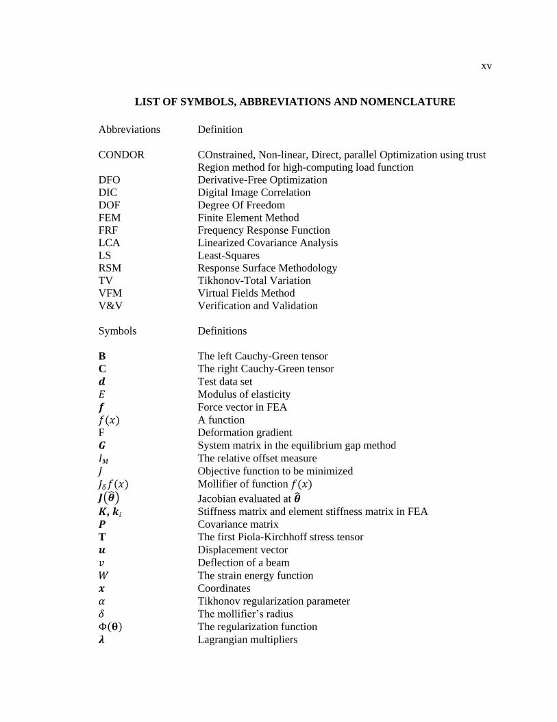
LIST OF SYMBOLS, ABBREVIATIONS AND NOMENCLATURE

Abbreviations Definition

CONDOR COnstrained, Non-linear, Direct, parallel Optimization using trust

Region method for high-computing load function

DFO Derivative-Free Optimization

DIC Digital Image Correlation

DOF Degree Of Freedom

FEM Finite Element Method

FRF Frequency Response Function

LCA Linearized Covariance Analysis

LS Least-Squares

RSM Response Surface Methodology

TV Tikhonov-Total Variation

VFM Virtual Fields Method

V&V Verification and Validation

Symbols Definitions

B The left Cauchy-Green tensor

C The right Cauchy-Green tensor

𝒅 Test data set

𝐸 Modulus of elasticity

𝒇 Force vector in FEA

𝑓(𝑥) A function

F Deformation gradient

𝑮 System matrix in the equilibrium gap method

𝐼𝑀 The relative offset measure

𝐽 Objective function to be minimized

𝐽𝛿𝑓(𝑥) Mollifier of function 𝑓(𝑥)

𝑱 𝜽 Jacobian evaluated at 𝜽

𝑲, 𝒌𝑖 Stiffness matrix and element stiffness matrix in FEA

𝑷 Covariance matrix

T The first Piola-Kirchhoff stress tensor

𝒖 Displacement vector

𝑣 Deflection of a beam

𝑊 The strain energy function

𝒙 Coordinates

𝛼 Tikhonov regularization parameter

𝛿 The mollifier‘s radius

Φ 𝛉 The regularization function

𝝀 Lagrangian multipliers

xvi

𝜃 Rotation angle of a beam

𝜽, 𝜃𝑖 Parameter vector and its components

Ω A region or a subset

𝝈 Cauchy stress

Finite element assembly operator

1

CHAPTER ONE: INTRODUCTION

“The mere formulation of a problem is far more essential than its solution, which may be

merely a matter of mathematical or experimental skills. To raise new questions, new

possibilities, to regard old problems from a new angle require creative imagination and

marks real advances in science.” Albert Einstein

1.1 General

Traditional techniques in experimental mechanics rely on displacement or strain

transducers carefully placed in a small number of positions on the surface of the tested

specimen. The data usually consist of series of test data correlated with the applied load

and the measured field (usually a displacement or strain component). The recent

development of new technologies combining low-cost CCD cameras and computer vision

led to novel experimental methods to assess solids and structures. Non-contact

measurement techniques are now becoming affordable for research and development

purposes in laboratories as well as for on-site monitoring of structures.

Digital image correlation (DIC), moiré and speckle interferometry, and grid

methods are among the many new technologies that can be utilized in the field of

experimental mechanics. The fundamental shift in the possibilities offered by these new

technologies is related to the spatial properties of the collected data. For example, a

typical DIC test system commonly has the capability of collecting up to 10,000

independent displacement measurements from the surface of the specimen. The large

amount of information available to the experimentalist opens new horizons that would

2

not be possible using traditional transducers. For example, in the context of constitutive

laws identification, the geometry and the boundary conditions must be very simple when

traditional transducers are used, so that an analytical solution of the stress/strain field is

possible; the stress and strain fields must be homogeneous in order to determine the

material properties. Consequently, the identification of constitutive laws requires more

than one test, since only the mechanical properties associated with the mechanisms

activated during the test can be identified. When non-contact measurement techniques

are used along with the finite element method (FEM), however, the need for simplified

loading and boundary conditions is relaxed. Non-contact measurement techniques with a

single test set-up can replace the large number of test set-ups involving various

combinations of experimental parameters that are necessary when local transducers are

used.

Full-field displacement measurements allow much greater flexibility as they

provide very rich experimental data and allow the use of tests under non-homogeneous

conditions. However, the large amount of data produced by full-field measurement

techniques requires suitable computational methods to extract the information

encapsulated within the non-homogeneous displacement and strain fields. The effort to

integrate new measurement technologies in experimental mechanics has introduced a

completely new research area, referred to as inverse problems in solid mechanics.

Full-field displacement measurements can also be integrated with numerical

simulation techniques such as FEM to build health monitoring systems for structures in

service. The methodology consists of incorporating the measured displacement or strain

field parameters with the mathematical model of the structure in order to estimate the

3

location and severity of damage. The formulation of a health monitoring problem as an

inverse problem has become a very important subject that has attracted a great deal of

interest and research activity over the last decade.

This thesis concerns two aspects of research based on the use of full-field

measurement techniques and finite element simulations for the health monitoring of

structures and for constitutive law identification. In the first part of this work, we

formulate the problem of reconstruction of the stiffness of beams through the

measurement of displacements along the beam. In the second part of this thesis, we study

the implementation of this material identification problem using DIC to measure the

displacement and strain on the surface of a specimen.

Each of these issues is of the utmost importance in practice. Currently, there is an

increasing demand for effective methods to identify complex nonlinear material models.

The competitive industrial environment leads engineers to develop better, but also more

complex models of complicated systems. These models are generally difficult to define,

and the work presented here is a step towards the development of a systematic approach

for material characterisation. Furthermore, the problem of reconstruction of a beam‘s

stiffness can be considered as one of the fundamental problems in the health monitoring

of these important structural elements.

From a mathematical point of view, the problems mentioned above can be

considered as two examples of inverse problems. However, the stiffness reconstruction

of beams is typically classified as an ill-posed functional identification problem, whereas

the identification of material properties is considered a well-posed parameter

identification problem. Traditional problems in structural mechanics consist of

4

evaluating the response of the studied structure to a known force or displacement where

the basic parameters, such as the geometry of the structure and the mechanical properties

of the materials, are known. Inverse problems, on the other hand, seek to determine

unknown geometrical and/or mechanical parameters from the known measured responses

of the system.

A direct procedure can rarely compute material and geometric properties from

measurable responses, such as displacements or strains. Inverse methods usually

formulate the problem as a minimization of error function between measured and

computed responses; this is also called an estimation function. These inverse procedures

usually involve finite-element (FE) model-updating techniques.

1.2 Optical full-field measurements using digital cameras

The damage identification methods developed in this thesis require a technique to

measure the displacements during static loading tests. In optical measurements, objects

are measured without being touched. A novel procedure based on edge-detection was

devised to measure the quasi-continuous deflection of beams under given loading, and is

presented in Chapter 2. This method is based on the close-range photogrammetry

technique made possible through recent developments of image processing algorithms

and modern digital cameras. These studies demonstrate that modern consumer cameras

can be used in optical measurement procedures, offering an additional advantage in terms

of cost.

The studies of material parameter identification presented in this thesis employ

DIC to provide full-field displacement/strain measurements for the surface of complex

5

3D components as input for the inverse analysis. DIC is an image analysis technique

based on grey-value digital images that can determine the contour and the displacements

of an object under load in three dimensions with sub-pixel precision. This technique is

already mature and commercialized; Chapter 2 provides a brief description of the DIC

technique, and the commercial DIC system employed in the current work.

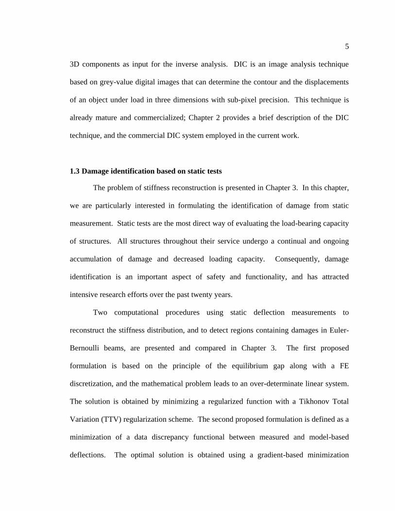
1.3 Damage identification based on static tests

The problem of stiffness reconstruction is presented in Chapter 3. In this chapter,

we are particularly interested in formulating the identification of damage from static

measurement. Static tests are the most direct way of evaluating the load-bearing capacity

of structures. All structures throughout their service undergo a continual and ongoing

accumulation of damage and decreased loading capacity. Consequently, damage

identification is an important aspect of safety and functionality, and has attracted

intensive research efforts over the past twenty years.

Two computational procedures using static deflection measurements to

reconstruct the stiffness distribution, and to detect regions containing damages in Euler-

Bernoulli beams, are presented and compared in Chapter 3. The first proposed

formulation is based on the principle of the equilibrium gap along with a FE

discretization, and the mathematical problem leads to an over-determinate linear system.

The solution is obtained by minimizing a regularized function with a Tikhonov Total

Variation (TTV) regularization scheme. The second proposed formulation is defined as a

minimization of a data discrepancy functional between measured and model-based

deflections. The optimal solution is obtained using a gradient-based minimization

6

algorithm and the adjoint method to calculate the Jacobian. The two proposed

methodologies are validated using experimental data.

1.4 Material parameter identification using full-field measurements

Modern design and performance evaluation requires realistic simulations of

structural and material behaviour, and nonlinear FE simulation has become a fundamental

engineering tool. FE approaches are increasingly popular among engineers from

different industries. Constitutive parameters associated with nonlinear models are not

always available in standard material databases; therefore, engineers need to identify

them experimentally.

Although the identification of plasticity material parameters is the focus of the

current work (presented in Chapter 4), this study aims to provide a unified identification

methodology. In light of recent developments in direct optimization and regression

analysis, particularly the verification and validation of the material parameter

identification using statistical tools, this thesis proposes novel procedures for the

identification of material parameters in any given model.

The problem of material parameter identification is formulated as a nonlinear

regression problem using DIC measurement data as the input. The study presented in

Chapter 4 includes the following topics: definition of the inverse problem; a brief

description of the derivative-free optimization scheme; discussion of the identifiability

issues related to the inverse approach; and the application of statistical inference with a

non-dimensional measure of response fit.

7

Solution of the material parameter identification problem was performed by

minimizing a least-squares (LS) function measuring the gap between inhomogeneous

displacement fields obtained from DIC measurements and FE simulations. Specifically,

a LS formulation of a cost function consisting of a norm for the discrepancies between

the experimental data and the simulated data was minimized; the simulated data was

obtained by the FE method using commercial software. Direct, derivative-free

optimization methods, which treat the FE simulation as a black-box procedure, identified

the material parameters simultaneously. Particular attention was paid to the

identifiability and numerical stability issues of this approach, and methods for verifying

and validating the identified results are discussed. In particular, consideration is given to

the identifiability issue in the deterministic and the statistical sense. Sampling-based

statistical inference derived from nonlinear regression theory was adopted to quantify the

quality of the identification procedure, the rationale being that DIC provides a large

amount of data, and thus allows the use of statistical inference. Sampling-based

inference and sensitivity analysis were used to check the adequacy of the identification

solution, thus avoiding Type-2 errors (i.e., the acceptance of incorrect results). Several

recommended numerical approaches for validating the identification results are presented.

Linearized covariance analysis (LCA) was adopted to check the fit of the parameters. An

index derived from the response surface geometry was used to check the response fit, and

relative curvature measures proposed to check the adequacy of LCA. The proposed

validation procedure is primarily intended to detect false positives (i.e., Type-II errors).

The proposed approach avoids using the gradient of the cost function in the

identification process, and has the benefit of allowing the use of any FE code as a black

8

box to solve the direct problem. The quantification of the quality of the result is of

paramount importance to the practical application of any identification methodology.

1.5 Hyperelasticity model parameter identification for rubber and rubber-like solids

The mechanical behaviour of rubber-like materials is usually characterized by a

strain energy density function 𝑊; the parameters of the 𝑊 function may be considered as

material parameters. Traditional laboratory techniques require several tests — using

different homogeneous deformation modes and standard cut-out samples — to determine

the appropriate strain energy form and parameters.

The general approach for material parameter identification (described in Chapter

4) was used to determine the parameters of strain energy functions (𝑊) with DIC test

data collected for the original structural components. In this approach, whole field

displacement/strain on the surface of components is measured by a DIC-based technique,

which provides massive amounts of experimental data in a single test. The DIC-based

methodology for parameter identification in hyperelasticity models (presented in Chapter

5) replaces the performance of multiple tests on simple-shape specimens with supposed

uniform state variable distributions that are required by traditional techniques.

9

CHAPTER TWO: OPTICAL MEASUREMENT USING DIGITAL CAMERAS:

DIGITAL IMAGE CORRELATION AND CLOSE-RANGE PHOTOGRAMMETRY

“It is necessary to measure everything that can be measured and to try making

measurable what isn’t as yet.” Galileo

2.1 Introduction

The technique of obtaining information from photographs is called photogrammetry. The

most important feature of photogrammetry is that objects are measured without being

touched. The development of photogrammetry has a long history, particularly the branch

related to aerial photogrammetry. Currently, with the development of computer and

digital photography, photogrammetric technology has changed dramatically from purely

optical equipment to fully digital workflow (i.e. without any type of film or plotter), and a

new branch — close-range photogrammetry, also termed vision metrology or

videogrammetry, is developing rapidly. Furthermore, inexpensive digital consumer

cameras have reached a high technical standard with good geometric resolution, and can

replace expensive metric cameras for close-range photogrammetry as long as the

accuracy/precision required for the measurement is not too high (Linder, 2009).

While close-range photogrammetry is used primarily for field measurements, the

application of optical measurements in an experimental setting has aroused interest. For

example, holographic interferometry, moiré and moiré interferometry, and speckle

methods are among the optical techniques available for strain measurements. An

10

innovation, digital image correlation (DIC), developed in the 1980s is now

commercialized for use in industrial processes.

Close-range photogrammetry and DIC developed independently from each other.

Nevertheless, DIC can be regarded as a branch of close-range photogrammetry. The

research presented in this thesis uses digital cameras to optically measure beam deflection

profiles and full-field displacements/strains on the surface of specimens and components

for inverse identification processes. This chapter briefly reviews some of the concepts

and procedures involved in close-range photogrammetry and its application to civil

engineering. Two novel techniques proposed for the measurement of beam deflection

profiles in a laboratory setting are presented: 1) an edge-based technique using edge-

detection suitable for beams with a clean surface and smooth edges; and 2) a surface-

based technique using image correlation. Finally, DIC methods are briefly described.

The novel methods are presented in the following sections: Section 2 describes

the new approach: edge-based deflection measurement of beams is introduced with

example. The data of this example is served as the input to the new damage

identification method to be introduced in Chapter 3. In Section 3, the fundamental theory

and characteristics of DIC measurement is described. Beam deflection measurement

using image correlation is presented in Section 5, with example of a concrete beam.

2.2 Close-range photogrammetry and applications in civil engineering

2.2.1 Overview

The primary purpose of a photogrammetric measurement, both aerial and

terrestrial, is the reconstruction of a three-dimensional object in digital form (coordinates

11

and derived geometric elements). For every image point, values in the form of

radiometric data (intensity, grey value, and color value) and geometric data (position in

image) can be obtained.

Close-range photogrammetry differs from traditional far-field photogrammetry

and image-based measurement systems as the primary task in close-range

photogrammetry is to measure the three-dimensional coordinates of targets placed on all

areas of interest on a structure or system, whereas the primary tasks in traditional

photogrammetry and image-based measurements are feature extraction, object

identification, and metrological measurement at relatively lower accuracy (Heijden,

1994). Thus, the key to the technique of close-range photogrammetry is the precise

calculation of the positions of each of the targets in the field of view; see (Luhmann,

Robson et al., 2006) for an overview of traditional methods and models in close-range

photogrammetry.

Laser-scanning measurement is an alternative to photogrammetry. The advantage

of laser-scanning methods is that the object can be low-textured while photogrammetric

techniques often require highly textured objects. On the other hand, laser-scanning

techniques are time-consuming and usually very expensive.

Visible patterns are a very important feature of photogrammetry, particularly

patterns that can be identified using pixel or color information. Patterns targeted in close-

range photogrammetry are usually simply attached metallic stickers. Popular types of

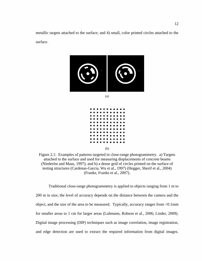
surface patterns targeted in photogrammetry are illustrated in Figure 1 and may include:

1) black and white sprays on the surface; 2) patterns etched onto the raw material; 3)

12

metallic targets attached to the surface; and 4) small, color printed circles attached to the

surface.

(a)

(b)

Figure 2.1: Examples of patterns targeted in close-range photogrammetry. a) Targets

attached to the surface and used for measuring displacements of concrete beams

(Niederöst and Maas, 1997); and b) a dense grid of circles printed on the surface of

testing structures (Cardenas-Garcia, Wu et al., 1997) (Hegger, Sherif et al., 2004)

(Franke, Franke et al., 2007).

Traditional close-range photogrammetry is applied to objects ranging from 1 m to

200 m in size; the level of accuracy depends on the distance between the camera and the

object, and the size of the area to be measured. Typically, accuracy ranges from <0.1mm

for smaller areas to 1 cm for larger areas (Luhmann, Robson et al., 2006; Linder, 2009).

Digital image processing (DIP) techniques such as image correlation, image registration,

and edge detection are used to extract the required information from digital images.

13

General information related to: a) basic procedures; b) digital images; c) image

coordinate systems and orientation; and d) reference or control points are briefly

summarized in the following pages.

Close-range photogrammetric measurement procedures

The fundamental procedures of a close-range photogrammetric measurement

include the preparation and recording of images, pre-processing, orientation calculations,

measurement, and image analysis. The steps in the general protocol for close-range

photogrammetry can be summarized as follows:

1. Preparation and recording of images

a) Application of surface targets.

b) Determination of control points or scaling lengths.

c) Image recording.

2. Pre-processing

a) Computation: calculate reference point coordinates and/or distances

from survey observations.

3. Orientation and measurement calculation

a) Measurement of image points: identification and measurement of

reference and scale points, including tie points (points observed in

multiple images).

b) Bundle adjustment: simultaneously calculate both interior and exterior

orientation parameters as well as the object point coordinates required

for subsequent analysis.

c) Removal of outliers.

14

4. Measurement and analysis

a) Single point measurement: identify the pixel coordinates of each point

to be measured in the image, and transform to physical coordinates.

b) Calculate displacements.

c) Field measurement: with interpolation and smoothing, measured points

can be connected and interpolated to make a field measurement.

Specific experimental procedures for the research presented in this thesis are

described in later sections. Some general concepts related to the composition of digital

images, image coordinate systems and the use of reference points to establish their

relationship to object coordinates (orientation), and digital imaging systems are

introduced in the following pages.

Digital images:

The essential advantage in using digital images over traditional photos is the ease

in image-processing, such as image enhancement, deblurring, edge-sharpening and de-

noising, thus attains the maximal utilization of information contained in images. The

digital image is actually a rectangular array composed of picture elements called pixels.

Each pixel is assigned an intensity value meant to characterize the color of a small

rectangular segment of the scene. A high-resolution picture can contain 5 to 10 million

pixels, while a low-resolution picture small picture may contain comparatively few pixels

(e.g. 256 × 256 = 65536 pixels). Digital image processing is thus notorious for its

intensive computation.

Grey-scale images are typically recorded by means of a charge-coupled device

(CCD), an array of tiny detectors arranged in a rectangular grid, which is able to record

15

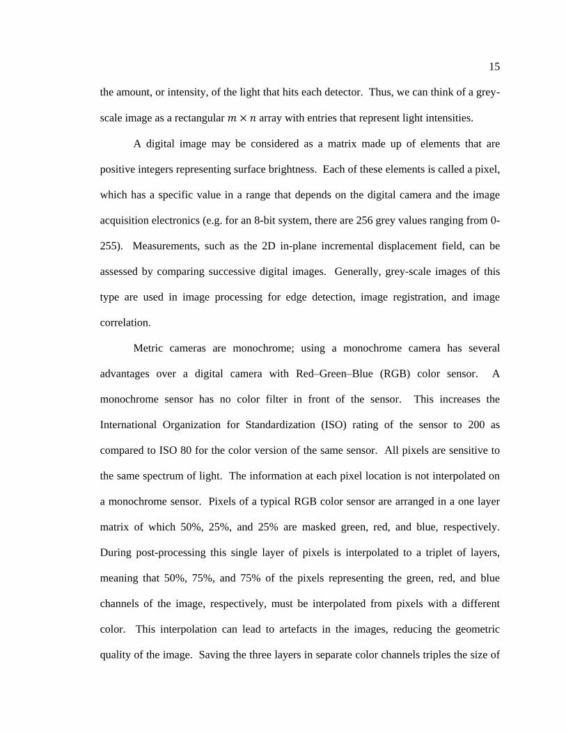
the amount, or intensity, of the light that hits each detector. Thus, we can think of a grey-

scale image as a rectangular 𝑚 × 𝑛 array with entries that represent light intensities.

A digital image may be considered as a matrix made up of elements that are

positive integers representing surface brightness. Each of these elements is called a pixel,

which has a specific value in a range that depends on the digital camera and the image

acquisition electronics (e.g. for an 8-bit system, there are 256 grey values ranging from 0-

255). Measurements, such as the 2D in-plane incremental displacement field, can be

assessed by comparing successive digital images. Generally, grey-scale images of this

type are used in image processing for edge detection, image registration, and image

correlation.

Metric cameras are monochrome; using a monochrome camera has several

advantages over a digital camera with Red–Green–Blue (RGB) color sensor. A

monochrome sensor has no color filter in front of the sensor. This increases the

International Organization for Standardization (ISO) rating of the sensor to 200 as

compared to ISO 80 for the color version of the same sensor. All pixels are sensitive to

the same spectrum of light. The information at each pixel location is not interpolated on

a monochrome sensor. Pixels of a typical RGB color sensor are arranged in a one layer

matrix of which 50%, 25%, and 25% are masked green, red, and blue, respectively.

During post-processing this single layer of pixels is interpolated to a triplet of layers,

meaning that 50%, 75%, and 75% of the pixels representing the green, red, and blue

channels of the image, respectively, must be interpolated from pixels with a different

color. This interpolation can lead to artefacts in the images, reducing the geometric

quality of the image. Saving the three layers in separate color channels triples the size of

16

one image to 18 MB for a sensor with 6 million pixels and 8 Bit color depth, as compared

to a monochrome image, while no information is added. Image correlation software

typically employs only one color channel of an image for analysis (ERDAS, 2002). This

implies that 100% of the original information of a monochrome sensor can be utilized by

the software while a single layer of a colour image will carry at most only 50% of the

original resolution of an RGB sensor. At the same time, image file size is reduced and

light sensitivity of the sensor is increased when using a monochrome camera. An image

size of 6MB allowed analysis to be performed on uncompressed Tagged Image File

Format (TIFF) images. The image compression in JPEG format may bring more blurring

and loss of information (Li, Yuan et al., 2002).

However, consumer cameras typically use color sensors. Color images in the

RGB format can be separated into three grey-scale images or matrices; one of these can

then be used for image processing. Alternatively, one can calculate a mixed

monochrome image matrix using the following well-known formula (Linder, 2009):

grey value = 0.3 × red(R) + 0.11 × green(G) + 0.59 × blue(B)

Generally, this calculation can be easily performed with image-processing

software by activating the option ―mixed image‖ when importing images (Linder, 2009;

Umbaugh, 2011).

World and camera coordinates

In measuring the position and orientation of objects with computer vision

methods, we have to couple the coordinates of the camera system (coordinates of the

image plane) to some reference coordinates (world coordinates) in the physical space.

17

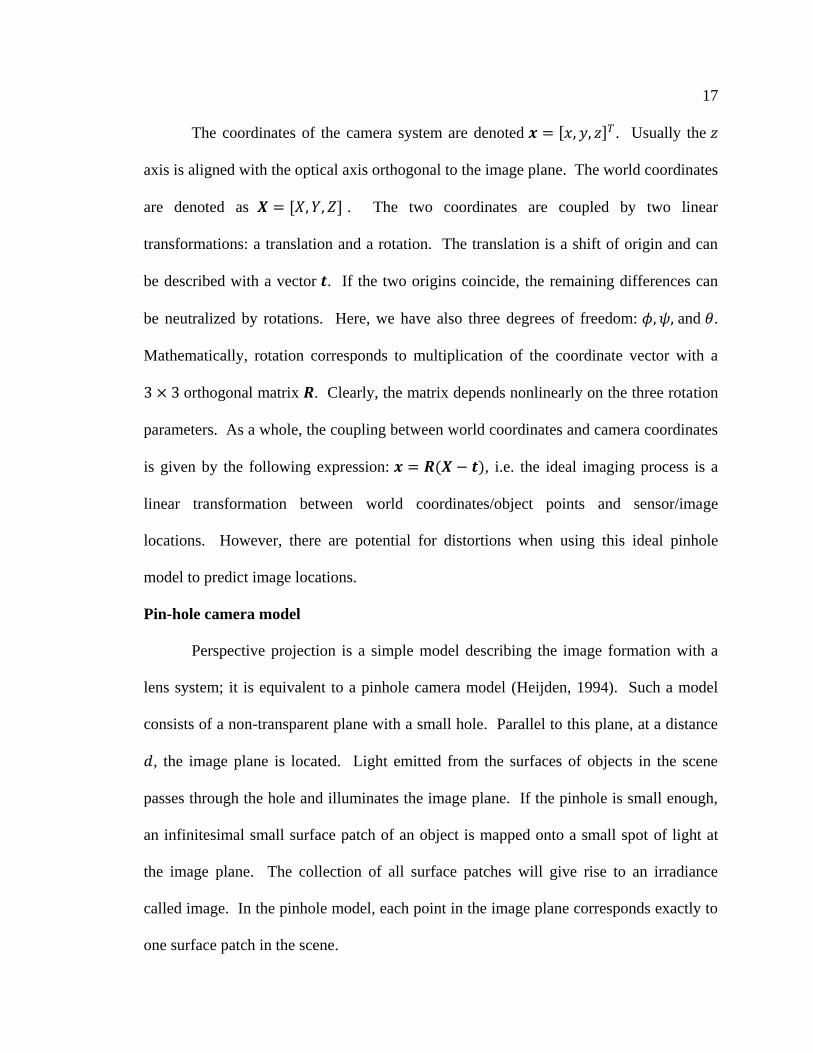
The coordinates of the camera system are denoted 𝒙 = 𝑥, 𝑦, 𝑧 𝑇 . Usually the 𝑧

axis is aligned with the optical axis orthogonal to the image plane. The world coordinates

are denoted as 𝑿 = [𝑋,𝑌,𝑍] . The two coordinates are coupled by two linear

transformations: a translation and a rotation. The translation is a shift of origin and can

be described with a vector 𝒕. If the two origins coincide, the remaining differences can

be neutralized by rotations. Here, we have also three degrees of freedom: 𝜙,𝜓, and 𝜃.

Mathematically, rotation corresponds to multiplication of the coordinate vector with a

3 × 3 orthogonal matrix 𝑹. Clearly, the matrix depends nonlinearly on the three rotation

parameters. As a whole, the coupling between world coordinates and camera coordinates

is given by the following expression: 𝒙 = 𝑹(𝑿 − 𝒕), i.e. the ideal imaging process is a

linear transformation between world coordinates/object points and sensor/image

locations. However, there are potential for distortions when using this ideal pinhole

model to predict image locations.

Pin-hole camera model

Perspective projection is a simple model describing the image formation with a

lens system; it is equivalent to a pinhole camera model (Heijden, 1994). Such a model

consists of a non-transparent plane with a small hole. Parallel to this plane, at a distance

𝑑, the image plane is located. Light emitted from the surfaces of objects in the scene

passes through the hole and illuminates the image plane. If the pinhole is small enough,

an infinitesimal small surface patch of an object is mapped onto a small spot of light at

the image plane. The collection of all surface patches will give rise to an irradiance

called image. In the pinhole model, each point in the image plane corresponds exactly to

one surface patch in the scene.

18

The pinhole camera model is based on the principle of collinearity, where each

point in the object space is projected by a straight line through the projection center into

the image plane. Usually, the pinhole model is a basis that is extended with some

corrections for the systematically distorted image coordinates. The most commonly used

correction is for the radial lens distortion that causes the actual image point to be

displaced radially in the image plane.

Image coordinate system (pixel coordinate system) and orientation

In principle, the one-to-one correspondence between the physical and image

coordinates of the object has to be established via a camera/lens calibration procedure.

The image coordinate system described above is defined by a two-dimensional image-

based reference system of rectangular Cartesian coordinates. Its physical relationship to

the camera is defined by reference points.

Camera calibration in the context of three-dimensional machine vision is the

process of determining the internal camera geometric and optical characteristics (intrinsic

parameters) and/or the 3-D position and orientation of the camera frame relative to a

certain world coordinate system. In geometrical camera calibration the objective is to

determine a set of camera parameters that describe the mapping between 3-D reference

coordinates and 2-D image coordinates. The whole calibration procedure may include

control point extraction from images, model fitting, image correction, and an additional

step to compensate for radial and tangential distortions of the lens. Correction of other

error sources in feature extraction, like changes in the illumination, may also be required,

especially in field measurements. Various methods for camera calibration can be found

from the literature.

19

Physical camera parameters are commonly divided into extrinsic and intrinsic

parameters. Extrinsic parameters are needed to transform object coordinates to a camera

centered coordinate frame. In multi-camera systems, the extrinsic parameters also

describe the relationship between the cameras. The intrinsic camera parameters usually

include the effective focal length, scale factor, and the image center also called the

principal point. These coefficients can be typically obtained from the data sheets of the

camera and frame-grabber.

Methods where the camera model is based on physical parameters, like focal

length and principal point, are called explicit methods. In most cases, the values for these

parameters are in themselves useless, because only the relationship between 3-D

reference coordinates and 2-D image coordinates is required. In implicit camera

calibration, the physical parameters are replaced by a set of non-physical implicit

parameters that are used to interpolate between some known reference points.

In traditional aerial and terrestrial analogue photogrammetry, orientation is

performed with the use of fiducial marks superimposed on the images and their nominal

coordinates in the camera calibration certificate. Measuring (digitizing) the fiducial

marks can set up the transformation between camera and pixel coordinates. Exterior

orientation must be carried out for each image independently. It can be manually

performed by measuring control points (reference points) or automatically using a

method called bundle triangulation. The following section describes the use of reference

points in establishing exterior orientation.

In these experiments, interior orientation was ignored, thus no lens calibration for

lens distortion or check of camera quality was conducted. Measurements presented in

20

this thesis were taken in a laboratory setting, the camera used was new, and the distance

between the object and the camera was short. Our findings show that the accuracy of the

measurements was sufficient without accounting for interior orientation. Exterior

orientation was determined using marks (reference points) with known (pre-measured)

coordinates.

Determining the exterior orientation of an image in an automated fashion is

considerably more difficult to implement than line following or driveback. The

orientation of an image is typically determined by identifying four or more points of

known approximate XYZ coordinates. Once these have been identified, the camera

exterior orientation can be computed using a closed-form space resection. To automate

the space resection procedure it is necessary to use exterior orientation devices and/or

coded targets. Examples of these are shown in Figures 2.1a and 2.1b. If either an

exterior orientation device or coded targets are seen in any image they are identified and

decoded, and if enough object points with approximately known 3D coordinates are

available the exterior orientation can be completed (and even automated with the so-

called intelligent camera devices).

Reference points (control points)

Ultimately, the objective of determining the orientation of known coordinates is to

calculate the relationship between all image and object coordinates. In order to determine

the orientation, several control points printed on the surface of the object must be

measured (coordinated). A control point is a point on an object that is represented in the

image and for which the three-dimensional object coordinates (x, y, z) are known. After

obtaining suitable grey-scale or mixed monochrome digital images of the object, we

21

identify these control points in the image, and determine the coordinates of the control

point in the array of image coordinates.

Plane affine transformation can be used to obtain a two-dimensional

transformation of the image based on the relationship between the object and image

coordinates of the control points (Heijden, 1994). Over-determination of object reference

points is required for plane affine transformation; at least three control points are

necessary. In general, in order to obtain a stable over-determination, the more control

points used, the better the outcome. The research presented in this thesis required at least

five well-distributed control points (where three well-distributed control points would

form a triangle, not a line).

Optimal accuracy is achieved in areas contained within the control points.

Consequently, if multiple cameras are needed to photograph a single object, it is

beneficial to include as many identical reference points as possible in neighbouring

images. Two types of reference or control points can be used: 1) signalized (or targeted)

points that have been applied to the surface of the object; and 2) the object‘s natural

features. Control points need to be highly visible in the images captured for

photogrammetry by digital imaging systems. The following section provides a brief

overview of the camera features needed for photogrammetric measurement.

Digital imaging systems

Traditional photogrammetry uses metric cameras to acquire images for analysis.

A metric camera is characterized by stability rather than flexibility, and has the following

features: a known and stable interior orientation, a fixed focal length (i.e., no zoom

capability), good lens correction, and a central shutter. Recently, with the rapid

22

development of digital photography, consumer-grade digital cameras have become

commonplace; there is significant potential for their use in photogrammetric applications

when calibrated (Cronk, Fraser et al., 2006). In general, the differences between metric

and consumer cameras are due to the quality and stability of the camera body and the

lens. Consumer cameras often have a zoom lens with large distortions that are

inconsistent (e.g. can vary with focal length); thus, it is difficult to correct these

distortions using calibration procedures (Linder, 2009).

Linder notes that a consumer-grade camera suitable for use in photogrammetric

measurement should have the following properties (Linder, 2009):

It should be possible to set the parameters for focal length, focus, exposure

time and f-number manually.

The resolution needs to be sufficient for photogrammetry. Generally, the

higher the number of pixels, the better the resolution; however, small chips

with a large number of pixels have a very small pixel size, and are not very

light sensitive. The signal-to-noise ratio is poor, particularly for high ISO

values (>200) and in dark parts of the image. In general, lighting

requirements are more demanding when using consumer-grade cameras.

It should be possible to deactivate the auto focus, and manually set the

distance parameters.

The digital images should be saved in a standard format (e.g. JPEG or TIFF).

The image compression rate must be selectable; the best option is to turn off

compression to minimize possible loss of quality.

23

Accessories to reduce unwanted movement and optimize lighting should

include a tripod, a remote release control, and an adapter for an external flash.

Note that the focal length or pixel size is required for digital image processing and

analysis; pixel size can be obtained from the calibration process. In order to obtain

accurate measurements using consumer-grade cameras, usually both interior orientation

and exterior orientation determinations are required.

Captured image may be corrupted by noise due to low lighting conditions, which

affect the sensors, or due to the noise generated by the electronic circuitry of the imaging

hardware. Impulse noise is also commonly referred to as salt and pepper noise. Blurring

is caused by a relative motion between camera and object or out of focusing or due to

corruption by noise. Blurring is typically modeled by linear operation on the image.

Hence restoration is also known as inverse filtering or deconvolution. Pre-processing

including deblurring or restoration may be required in photogrammetry.

Illumination

The particular type of image formation we discuss is the formation based on

radiant energy, reflection at the surface of the objects, and perspective projection. The

information of the scene is found in the contrasts (local differences in irradiance).

Carefully choosing the illumination of the objects is important in enhancing the contrasts

for accurate measurements. The purpose of front illumination is to illuminate the objects

such that the reflectance distribution of the surface becomes the defining features in the

image. Many applications require this type of illumination: detection of flaws, scratches

and other damages on the surface of material, DIC, etc. In outdoor applications, specular

illumination or diffuse illumination may be considered.

24

2.2.2 Applications of close-range photogrammetry in civil engineering

Measurements in civil and mechanical engineering, particularly structural

engineering applications have been made without physical contact by using

interferometry, moiré technology, holographic and laser speckle interferometry, and

theodolite measurement systems (Durelli and Parks, 1970) (Vest, 1979) (Ransom, Sutton

et al., 1987) (Post, Han et al., 1994). Recent technological improvements in image

acquisition and image analysis opened new possibilities in many fields of engineering

and science; the use of close-range photogrammetry in civil engineering is the focus of

recent research. Early applications of this technique at large civil engineering sites

included measurements of excavation sites and damage assessment after an earthquake

(Teimouri, Delavar et al., 2008). Optical methods and image analysis were applied to the

observation of cracks in mortar and concrete; the analyses included RGB combination,

image filtering, binarization, and shape and fractal analysis of crack patterns (Ringot and

Bascoul, 2001).

Numerous laboratory and field studies have been conducted. These include a

pilot study of beam deformation measurement using digital close-range terrestrial

photogrammetry. Jauregui et al reported the photogrammetric measurement of global

deflected shape of structures, which is not practical using traditional instruments

(Jauregui, White et al., 2002) (Jauregui, White et al., 2003); in this exercise, the initial

camber and dead-load deflection of pre-stressed concrete bridge girders were measured

photogrammetrically and compared with level rod and total station readings, and also

with dead-load deflection diagrams. Niederost et al. reported using a digital still video

camera to measure deformations occurring during the dehydration process of concrete

25

parts over several months where displacement vectors were obtained through tracking

targets (Niederöst and Maas, 1997). Similarly, Maas made photogrammetric

measurements of the 3-D coordinates of signalized targets on a large water reservoir wall

in Switzerland (Maas, 1998). Measurement of concrete cracks using digitized close-

range photographs was reported by several researchers (Barazzetti and Scaioni, 2010)

(Chen, Jan et al., 2001); in these works, edge-detection was used to identify the cracks;

researchers inspected localized changes in the width of cracks. Franke et al. conducted

strain analysis of solid wood and glued laminated timber constructions using close-range

photogrammetry; measurements were made of the progression of deformations, cracks

and deterioration when loading and relieving the specimens (Franke, Franke et al., 2007).

Hegger et al. studied the crack-opening process in pre-stressed concrete beams using a

photogrammetric technique called grid-method (Hegger, Sherif et al., 2004). Whiteman

et al. described the use of digital photogrammetry for measurement of deflections in

concrete beams (Whiteman, Lichti et al., 2002); a precision of 0.25 mm was achieved for

deflections and comparisons were made with linear variable differential transformer

(LVDT) deflection measurements. Other works of metrological digital photogrammetry

include testing of concrete and column (Woodhouse, 1999), thermal deflection of steel

beams (Fraser, 2000), pavement deformation under rolling load (Mills, 2001), and

deformation of a coal dredger (Fraser, 1995). In these tests, retro-reflective targets were

usually attached to and around the beams. Both stable targets on walls and deforming

targets on beams were used.

Consumer-grade digital camera was used for measuring soil erosion, generating

digital elevation models from soil surfaces for a planimetric area of 16𝑚2 with high

26

spatial and temporal resolution (Rieke-Zapp and Nearing, 2005). A consumer-grade

digital camera was used for image acquisition. The camera was calibrated using BLUH

software (Jacobsen, 2000). The program system BLUH is a commercial bundle block

adjustment program that allows camera calibration of the interior orientation including

parameters to account for radial symmetric lens distortion as well as other systematic

deviations of the camera geometry from the frame camera model. Homologous points in

overlapping images were identified with least squares matching.

Photogrammetric analysis of photographs taken from a fixed viewpoint at

different times during the loading process has been applied to soil mechanics experiments

to capture non-homogeneous deformation throughout a test (Desrues and Viggiani,

2004). The photographed surface was textured, the scale of the photograph was

determined from six or more reference marks placed on the specimen side. ,

2.3 Close-range photogrammetry for beam deflection measurement

2.3.1 Overview

Although various close-range photogrammetric techniques have been proposed

and applied to structural engineering problems, human knowledge, experience and skill

still play a significant role in current photogrammetric measurement applications. In

particular, these experiential factors determine the extent to which the reconstructed

model corresponds to the physical object or fulfils the task‘s objectives. On the other

hand, digital image processing (DIP) has achieved a level of maturity, and MATLAB and

public domain DIP programs are widely available (Thyagarajan, 2006) (Semmlow, 2004)

(Umbaugh, 2011).

27

In this thesis, we examined two simple methods for measuring a quasi-continuous

deflection profile of beams in the laboratory by processing camera photographs, and

compared the results with dial-gauge readings and the predictions of elastic beam theory.

The data obtained with these methods can be used as input for inverse damage

identification. In this research, we used consumer-grade cameras obtained in the

marketplace, and the widely available MATLAB image-processing toolbox to process the

images for photogrammetric analysis.

The first method is an edge-based approach; the procedures can be summarized

as:

a) An ordinary consumer-grade camera (Nikon D300S single lens reflex (SLR)

digital camera, with an array of 2848 × 4288 pixels in each RGB image) was

used to take colored photos of the beam with and without loading. The

images were saved as a RGB matrix with the following characteristics:

Size Bytes Data Class

2848×4288×3 36636672 Unit8 array

b) The contrast between structure and background was enhanced using contrast

enhancement in Adobe Photoshop. This step is not necessary, but was shown

to be useful.

c) Since the cameras were not fixed to the ground, there were always small

movements of the camera during photo-capture. The detrimental effects of

camera motion were reduced using image-registration; the image-registration

technique detected camera movement, which was deleted from the calculated

displacements.

d) Image-segmentation and edge-detection were used to identify the continuous

boundary between structure and background. This was the key step in this

procedure. Edge-detection can be done manually, at a very high cost of time

and patience; however, advanced automatic edge-detection techniques have

28

been developed that can do this job quickly (Semmlow, 2004) (Louban, 2009).

Our research found that the performance of automated edge-detection

algorithms depends on the level of contrast between the structure and the

background and automated edge-detection tools varied in their sensitivity to

contrast. For example, in preliminary tests we did not attend to the contrast

between the background and the beam; the MATLAB toolbox methods failed

to reliably detect edges in these images. Another application, the GROWCUT

freeware program (a cellular automata algorithm for edge-detection

[www.shawnlankton.com]), worked well with these images, however.

Consequently, attention should be paid to lighting and background screening

to improve the appearance of the targets in the photographs and enhance the

effectiveness of automatic edge-detection techniques.

e) The detected edges were saved as a black-and-white binary image, which is a

binary matrix in MATLAB. An averaging process called mollification was

used to calculate displacement in pixel coordinates.

f) The displacement solutions in the form of pixel coordinates were transformed

to physical coordinates via homogeneous transformation.

Image-registration

Image registration is the alignment of two or more images so that they are

optimally superimposed. In order to achieve the best alignment, it may be necessary to

transform the images using affine transformations (displacement and rotation). Image

registration can be assisted or unassisted; we need to perform an unassisted image

registration, which relies on an optimization technique that maximizes the correlation

between the images.

Unaided image registration usually involves the application of an optimization

algorithm to maximize the correlation, or some measure of similarity, between the

29

images. The structure in the image and in the loading device moved during the tests

presented in this thesis, but the supporting frame and the wall in the background

remained immobile; therefore, these parts of the fixed background were cut from the

whole picture. The appropriate transformation was applied to one of the images, the

deformed image, and a comparison was made between this transformed image and the

reference image (also termed the base image). The optimization routine seeks to vary the

transformation until the correlation is optimal. In the research presented here, image

registration was used to detect movement of the camera mounted on a tripod.

Segmentation and edge-detection

Image segmentation is the identification and isolation of components of an image

into regions that correspond to structural units. Segmentation is used to isolate the

structure of interest in both the deformed and the reference images, and thus enable the

identification of displacements of the structure. The problems associated with

segmentation have been well-studied and a large number of approaches have been

developed, many specific to a particular type of image (Heijden, 1994). General

approaches to segmentation can be grouped into three classes: pixel-based methods,

regional methods, and edge-based methods. Pixel-based methods are the easiest to

understand and to implement, but are also the least powerful and, since they operate on

one element at a time, are particularly susceptible to noise. Continuity-based and edge-

based methods approach the segmentation problem from different angles: edge-based

methods search for differences while continuity-based methods search for similarities in

the image. The second method is a surface-based approach, in which image correlation is

used to find the displacement of a subset of pixels.

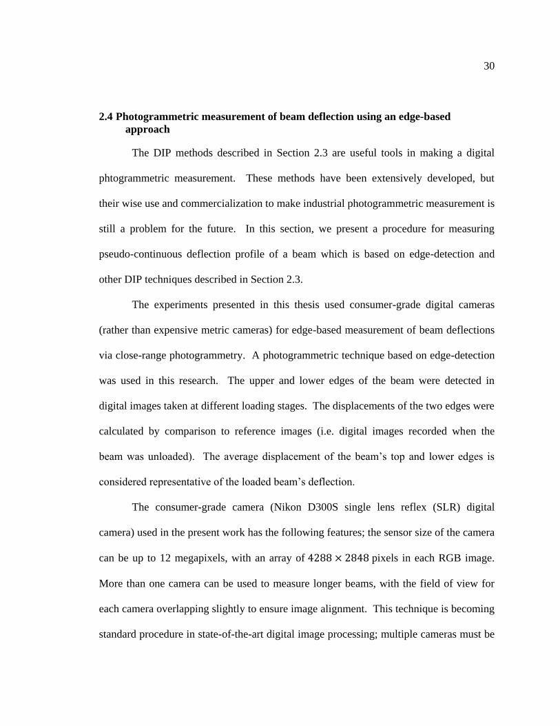
30

2.4 Photogrammetric measurement of beam deflection using an edge-based

approach

The DIP methods described in Section 2.3 are useful tools in making a digital

phtogrammetric measurement. These methods have been extensively developed, but

their wise use and commercialization to make industrial photogrammetric measurement is

still a problem for the future. In this section, we present a procedure for measuring

pseudo-continuous deflection profile of a beam which is based on edge-detection and

other DIP techniques described in Section 2.3.

The experiments presented in this thesis used consumer-grade digital cameras

(rather than expensive metric cameras) for edge-based measurement of beam deflections

via close-range photogrammetry. A photogrammetric technique based on edge-detection

was used in this research. The upper and lower edges of the beam were detected in

digital images taken at different loading stages. The displacements of the two edges were

calculated by comparison to reference images (i.e. digital images recorded when the

beam was unloaded). The average displacement of the beam‘s top and lower edges is

considered representative of the loaded beam‘s deflection.

The consumer-grade camera (Nikon D300S single lens reflex (SLR) digital

camera) used in the present work has the following features; the sensor size of the camera

can be up to 12 megapixels, with an array of 4288 × 2848 pixels in each RGB image.

More than one camera can be used to measure longer beams, with the field of view for

each camera overlapping slightly to ensure image alignment. This technique is becoming

standard procedure in state-of-the-art digital image processing; multiple cameras must be

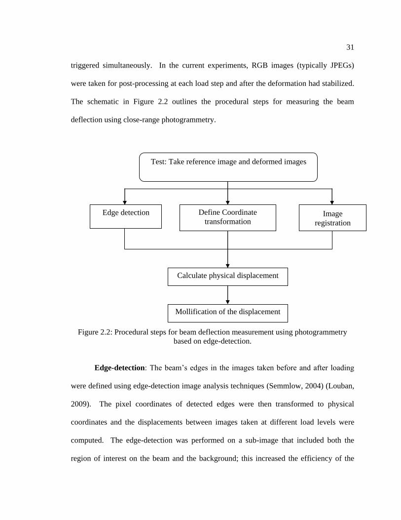
31

triggered simultaneously. In the current experiments, RGB images (typically JPEGs)

were taken for post-processing at each load step and after the deformation had stabilized.

The schematic in Figure 2.2 outlines the procedural steps for measuring the beam

deflection using close-range photogrammetry.

Figure 2.2: Procedural steps for beam deflection measurement using photogrammetry

based on edge-detection.

Edge-detection: The beam‘s edges in the images taken before and after loading

were defined using edge-detection image analysis techniques (Semmlow, 2004) (Louban,

2009). The pixel coordinates of detected edges were then transformed to physical

coordinates and the displacements between images taken at different load levels were

computed. The edge-detection was performed on a sub-image that included both the

region of interest on the beam and the background; this increased the efficiency of the

Test: Take reference image and deformed images

Edge detection Define Coordinate

transformation Image

registration

Calculate physical displacement

Mollification of the displacement

32

algorithm. The edge detection algorithm operated on the original RGB image; the

portion of the image containing the detected edge was transferred to a grey-scale image,

and a threshold in pixel values was set to separate the edge from the background. The

criteria would either be set manually by observing the grey-scale values of the image or

through the histogram of pixel values. To enhance the edge-detection operation, a black

screen was placed behind the beam to enhance the contrast. The image was then

transformed to a binary grey-scale format. The experimental set-up is shown in Figure

2.3; and one set of detected edges is shown in Figure 2.4. The edge-based

photogrammetric measurement technique was shown to be feasible in laboratory settings.

Figure 2.3. The laboratory set-up for tests of a step-cut beam.

33

a)

b)

c)

Figure 2.4. The detected upper-edge of a cantilever beam: a) a cut-out RGB image; b) the

detected edge in a grey-scale image; and c) a binary image of the edge generated using a

pixel threshold.

Perspective projection is a simple model describing the image formation with a

lens system. It is equivalent to a pinhole camera model. Homogeneous coordinates are a

powerful concept to describe the transformations. Translation, rotation, scaling and

perspective projection can be handled mathematically with a single matrix multiplication.

The transformations can be expressed as 𝒙 = 𝑴𝑿 . In principle, the one-to-one

correspondence between the physical and image coordinates of the object has to be

established via a camera/lens calibration procedure.

Coordinate transformation

Mechanical devices, such as dial gauges, require a stable base for mounting;

photogrammetric measurements require the selection of stable reference points on a

stable background to calibrate coordinate transformation from pixel coordinates to global

physical coordinates. In this study, several stable points in the background and geometric

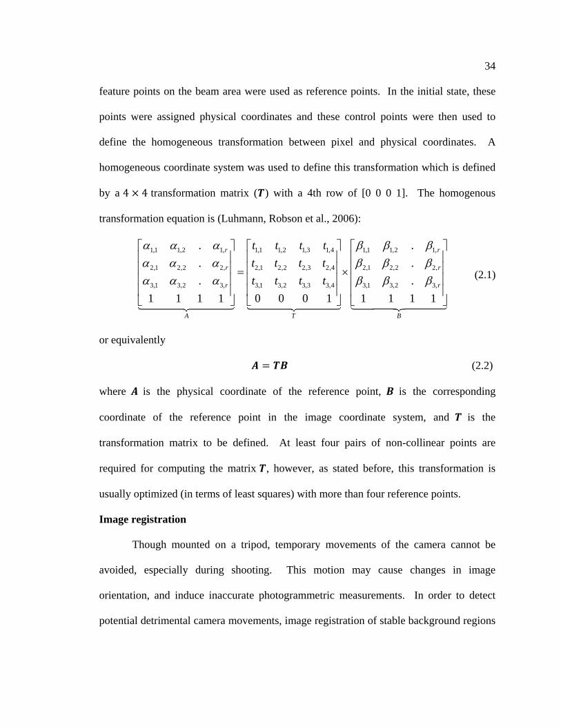
34

feature points on the beam area were used as reference points. In the initial state, these

points were assigned physical coordinates and these control points were then used to

define the homogeneous transformation between pixel and physical coordinates. A

homogeneous coordinate system was used to define this transformation which is defined

by a 4 × 4 transformation matrix (𝑻) with a 4th row of [0 0 0 1]. The homogenous

transformation equation is (Luhmann, Robson et al., 2006):

1,1 1,2 1, 1,1 1,2 1,3 1,4 1,1 1,2 1,

2,1 2,2 2, 2,1 2,2 2,3 2,4 2,1 2,2 2,

3,1 3,2 3, 3,1 3,2 3,3 3,4 3,1 3,2 3,

. .

. .

. .

1 1 1 1 0 0 0 1 1 1 1 1

r r

r r

r r

A T B

t t t t

t t t t

t t t t

(2.1)

or equivalently

𝑨 = 𝑻𝑩 (2.2)

where 𝑨 is the physical coordinate of the reference point, 𝑩 is the corresponding

coordinate of the reference point in the image coordinate system, and 𝑻 is the

transformation matrix to be defined. At least four pairs of non-collinear points are

required for computing the matrix 𝑻, however, as stated before, this transformation is

usually optimized (in terms of least squares) with more than four reference points.

Image registration

Though mounted on a tripod, temporary movements of the camera cannot be

avoided, especially during shooting. This motion may cause changes in image

orientation, and induce inaccurate photogrammetric measurements. In order to detect

potential detrimental camera movements, image registration of stable background regions

35

in the image sequence was used to detect any changes in camera orientation; when

detected, the change in image orientation was corrected (Semmlow, 2004).

Mollification

Model updating and damage identification are often performed with FE models;

however, the number of points measured along the beam (>4000 in this research) is much

higher than the number of nodes in a FE model. A mollification-based procedure was

used for noise-filtering and data reduction. The mollification method is an inverse-

problem technique, and has multiple applications when implemented as a filtering

algorithm, including the reduction of data through filtering and numerical differentiation

(Murio, 1993) (Murio, Mejia et al., 1998). Furthermore, although displacements can be

obtained directly through close-range photogrammetry, the rotation angles are indirectly

accessible, and the mollification technique allows their approximation (Murio, Mejia et

al., 1998).

To illustrate the mollification technique, let us consider the locally integrable two-

dimensional function 𝑓(𝑥) in a domain 𝛺 in 𝑅2. The mollifier of 𝑓, denoted as 𝐽𝛿𝑓(𝑥), is

defined as:

𝐽𝛿𝑓 𝑥 = 𝑤𝛿 𝑥 − 𝑦 𝑓 𝑦 𝑑𝑦𝑅2 (2.3)

The mollifier‘s radius is 𝛿 . For any number 𝛿 > 0, we define the family of

functions 𝑤𝛿 𝑥 as:

𝑤𝛿 𝑥 =1

𝛿2 𝑤(𝑥

𝛿) (2.4)

The weight function 𝑤(𝑥) is characterized as 𝐶∞ , is non-negative, has a total

integral of 1, and vanishes outside the unit ball centered at 0: 𝐵 0,1 = 𝑥 ∈ 𝑅 : 𝑥 <

36

1 . Under such conditions, it is clear that 𝑤𝛿 ∈ 𝐶0∞(𝐵(0, 𝛿)) , and moreover, that

𝑤𝛿(𝑥)𝑅2 𝑑𝑥 = 1.

In the present study, we selected the following weight function:

𝑤 𝑥 = 𝐶𝑒𝑥𝑝 −

1

1− 𝑥 2 𝑓𝑜𝑟 𝑥 < 1

0 𝑓𝑜𝑟 𝑥 ≥ 1 (2.5)

where 𝐶 represents a constant normalizing the kernel function. It is evident that the

corresponding discretized version of the mollification can be computed using a numerical

convolution. The numerical convolution and the optimal selection of the mollifier‘s

radius using cross-validation (Woodbury, 2003) was used to filter the data and

numerically compute the derivatives in the current research.

Within the Euler-Bernoulli beam theory, the rotation angle is the derivative of the

deflection, 𝜃 = 𝑑𝑣/𝑑𝑥. It is well known that direct numerical differentiation of the raw

data is an ill-posed problem. The mollification approach to numerical differentiation can

be used to substitute the original ill-posed problem of finding the derivative of the

deflection , 𝑣′, by a new problem of finding the derivative of its mollifier (𝐽𝛿𝑣)′. It is

demonstrated that this numerical technique is consistent and stable (Murio, Mejia et al.,

1998). This means that the reconstruction of the derivative of the mollified data function

is stable with respect to the noise existing in the measurements. The central difference

scheme is applied to evaluate the first derivative. The rotation at a given node 𝑥𝑖 is

obtained as follows:

𝜃 𝑥 = 𝜃𝑥𝑖 = 𝐷0 𝐽𝛿𝑣 =𝑣 𝑥𝑖+∆𝑥 −𝑣 𝑥𝑖−∆𝑥

2∆𝑥 (2.6)

where ∆𝑥 is the distance between two successive nodes.

37

The following example illustrates the implementation of the measurement

technique described above; a cantilever beam subjected to a concentrated load was tested.

The experimental set-up is shown in Figure 2.5. The camera-to-object distance was

approximately 0.5 m, which is sufficient for one-camera measurement of a 1 m-long

beam depending on the range of view. The deflection profile and rotation angle that was

obtained using the described edge-detection based method are reported in Figure 2.6 and

2.7. These results were compared with the predicted theoretical deflections, and the

photogrammetric measurements were found to be accurate.

38

Figure 2.5: The experimental set-up for close-range photogrammetric measurement of the

displacement of a loaded cantilever beam with a high-contrast stable background using

consumer-grade optical equipment.

39

0 20 40 60 80 100

Distance (cm)

-8

-6

-4

-2

0

Defl

ection

(mm

)

Figure 2.6: Beam deflection: Experimentally-obtained measurements using edge-

detection methods and close-range photogrammetry technique.

Figure 2.7: Beam Deflection: Theoretical deflections with 𝑬 = 𝟔𝟔 GPa and 𝑬 = 𝟕𝟐

GPa, and correspondence of the predicted values to the experimentally-measured

deflection profile shown in the previous figure. Predictions were based on elastic beam

theory. The elasticity modulus of the aluminum alloy material was calibrated at

𝟕𝟎.𝟏𝟒 𝑮𝑷𝒂. Measurements were obtained using edge-detection methods and close-

range photogrammetry techniques.

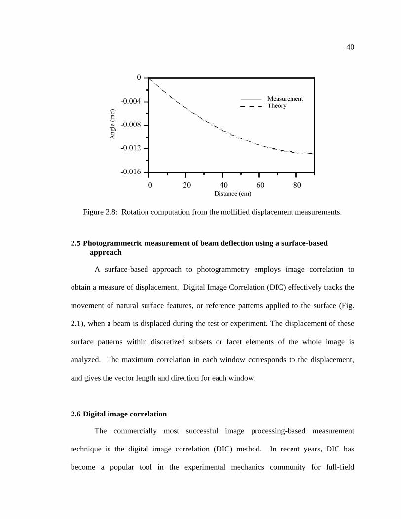
40

Figure 2.8: Rotation computation from the mollified displacement measurements.

2.5 Photogrammetric measurement of beam deflection using a surface-based

approach

A surface-based approach to photogrammetry employs image correlation to

obtain a measure of displacement. Digital Image Correlation (DIC) effectively tracks the

movement of natural surface features, or reference patterns applied to the surface (Fig.

2.1), when a beam is displaced during the test or experiment. The displacement of these

surface patterns within discretized subsets or facet elements of the whole image is

analyzed. The maximum correlation in each window corresponds to the displacement,

and gives the vector length and direction for each window.

2.6 Digital image correlation

The commercially most successful image processing-based measurement

technique is the digital image correlation (DIC) method. In recent years, DIC has

become a popular tool in the experimental mechanics community for full-field

41

displacement measurement and experimental strain analysis. A wide range of

applications demonstrate the versatility of this technique.

Digital Image Correlation is a full-field image analysis method, based on grey

value digital images that can determine the contour and the displacements of an object

under load in three dimensions. A recent review on 2-dimensional DIC for in-plane

displacement measurement is given in (Pan, Qian et al., 2009); a more comprehensive

review of DIC, including both 2D and 3D measurements, and also a comprehensive

presentation is given in the book (Sutton, Orteu et al., 2009).

Peters and Ranson (1982) proposed and implemented a DIC technique that is

applicable to the computation of surface strains and displacements (Peters and Ranson,

1982) (Chu, Ranson et al., 1985) (Sutton, Turner et al., 1991). This technique relies on

the analysis of intensity patterns in digital images of the object under consideration

(reference/undeformed and deformed), with a random pattern of white speckles on its

surface. (Digitizers were used before the invention of digital CCD cameras). The digital

image is actually a rectangular array made up of picture elements called pixels. The

determination of local disparities existing between pairs of images, or the problem of

image registration, is a basic requirement of computer vision. In image registration,

cross-correlation is frequently used to detect local similarities between two images. A

common correlation function is the least-squares correlation function (sum of squared

differences):

𝐶 = 𝑓−𝑔 2𝑆

𝑓2𝑆

(2.7)

42

It is non-negative and approaches 0 when the values for 𝑓 and 𝑔 are similar.

Different alternative versions of the sum of squares exist: normalized sum of squared

differences and zero-normalized sum of squared differences; the latter was shown to be

the most reliable and robust criterion in case of image blurring and variations in lighting

and exposure conditions while taking reference and deformed photos (Tong, 2005). The

image correlation algorithm is actually the pattern matching techniques used to compute

image motion from a sequence of two or more images (Giachetti, 2000),

Another option is the normalized cross-correlation coefficient (Giachetti, 2000):

𝐶 = 𝑓∗𝑔 𝑆

𝑓2∗𝑔2 𝑆 12

(2.8)

Unlike the least-squares correlation function (which should be minimized in the

search for matched pairs of pixel subsets), the cross-correlation function should be

maximized.

The DIC technique for the research presented in this thesis consisted of the

following: a) Consider two images of the same object before and after deformation. b)

Define a subset Ω in the undeformed image, centered at point 𝐴(𝑖, 𝑗), as an (𝑛 × 𝑛) pixels

reference area. c) Define a bigger subset Ω∗ in the deformed image, centered at the same

position, as an (m × m) pixel area (m > 𝑛).

The normalized cross-correlation coefficient as a function of position coordinate

(x, y) is written as:

𝐶 𝑥,𝑦 = 𝐼(𝑖 ,𝑗 )𝑛

𝑗=1𝑛𝑖=1 ∙𝐼∗(𝑖+𝑥 ,𝑗+𝑦)

𝐼2(𝑖 ,𝑗 )𝑛𝑗=1

𝑛𝑖=1 ∙ 𝐼∗2(𝑖+𝑥 ,𝑗+𝑦)𝑛

𝑗=1𝑛𝑖=1

(2.9)

43

where 𝐼(𝑖, 𝑗) is the grey value of the subset Ω at the point (𝑖, 𝑗), and 𝐼∗(𝑖 + 𝑥, 𝑗 + 𝑦) is the

grey value of the subset Ω∗ at the point (𝑖 + 𝑥, 𝑗 + 𝑦). For the DIC analysis using the

ARAMIS system presented in this thesis, the 𝑛 value was chosen to be 15.

In order to achieve sub-pixel accuracy (so that the maximum correlation

coefficient value can be located between two pixels, rather than at a discrete pixel

position), a continuous correlation distribution is constructed by fitting the discrete

correlation coefficients to a 2D curved surface. From this theoretical continuous

distribution, the maximum correlation coefficient value can be determined using an

optimum search technique, thus achieving sub-pixel accuracy.

Before evaluating the similarity between reference and deformed subsets using

the correlation criterion, the intensity of these points with subpixel locations must be

provided. Thus, a certain subpixel interpolation scheme should be utilized. In the

literature, various sub-pixel interpolation schemes including bilinear interpolation,

bicubic interpolation, bicubic B-spline interpolation, biquintic B-spline interpolation and

bicubic spline interpolation have been used. A high-order interpolation scheme (e.g.

bicubic spline interpolation or biquintic spline interpolation) is recommended by Schreier

et al (Schreier, Braasch et al., 2000) since they provide higher registration accuracy and

better convergence character of the algorithm than the simple interpolation schemes do.

Basic principles of DIC measurement

DIC is an optical full-field measurement technique that measures the deformation

of an object‘s surface. The image correlation system tracks random grey-value patterns in

small areas (image subsets) of images taken during deformation. Two cameras (placed

according to triangulation principle) can be used along with stereo vision models to

44

obtain 3D deformation measurements. The corresponding surface strains are calculated

from surface deformations or calculated simultaneously with displacement, depending on

the method and representation used.

Several commercial DIC systems have already been developed and

commercialized, including: ARAMIS, Correlated Solutions, and LaVision‘s StrainMaster

DIC system (LaVision). The work presented in this thesis was conducted using the

ARAMIS DIC system (GOM and Trillion Quality Systems).

Figure 2.9: the ARAMIS system of the GOM Company

Figure 2.8 shows a typical experimental setup using the ARAMIS DIC system. A

random speckle pattern using black and white spray paints is applied to the surface of the

specimen. Note that two cameras are positioned on a special tripod with a stable

mounting base and with support bars that allow flexibility in positioning the cameras.

45

External light was used to provide optimal exposure. The lighting is especially important

and the contrast between the object and the background affects the quality of the

measurements. The stability of the camera set-up is particularly important when

capturing images; camera movement and vibration causes errors in calibration and

deformation calculations. Trials were conducted to determine optimal conditions for a)

camera placement and b) random speckle pattern.

High zoom lengths can be used in the ARAMIS system along with a 1-inch2 (25.4

mm) calibration block to measure a small region. A calibration block is a target with a

dedicated pattern with known pattern dimensions, and is used to calibrate the cameras.

The calibration block must be produced with special care to ensure the accuracy of the

pattern‘s dimensions. The ARAMIS system comes with pre-manufactured calibration

blocks. Random speckle patterns were created and optimized using trial and error.

2.7 Summary

In this chapter we developed one photogrammetric measurement for beam

deflection and presented the optical method – DIC, for obtaining strain/displacements on

the surface of a specimen. The edge-detection-based photogrammetric measurement of

beam deflection profiles provide input data to drive a damage identification procedure

which is to be developed in the next chapter. The results were comparable to the

predictions of calculated dead-load deflection diagrams. The DIC measurement provides

input data to drive the material parameter identification procedures which will be

presented in chapters 4 and 5.

46

CHAPTER THREE: DAMAGE IDENTIFICATION OF EULER-BERNOULLI

BEAMS USING FULL-FIELD MEASUREMENTS

“To perform an effective analysis is an art (K.J. Bathe)”, to perform an effective

damage identification is even a finer art.

3.1 Introduction and background

3.1.1 An introduction to damage identification problem

Structural systems undergo degradation processes and become aged through the

course of time, or may deteriorate suddenly for a variety of reasons, such as unexpected

loading or natural causes. As a result, damage occurs, generally in the form of localized

stiffness decrease in structural members. In general, early detection of damage is vital in

order to monitor the continuous degradation of the structure. Without monitoring,

continuous damage can ultimately lead to catastrophic failure of the system.

Recent events show that structures are not immune from disastrous collapse.

From some of these events we list: The Silver Bridge failure in West Virginia in 1967

caused 46 deaths; the collapse of the Mianus Bridge in 1983; the de la Concorde overpass

collapse in Quebec crushed five people to death; and, on August 1, 2007, the I-35W St.

Anthony Falls Bridge over the Mississippi River in Minneapolis, Minnesota collapsed in

the middle of rush hour. The collapse of the Minneapolis Bridge in particular has raised

a public safety issue concerning the 73,784 bridges in U.S.A that are rated ―structurally

deficient‖ by the U.S.A Department of Transportation (Arnoldy, 2007). In response to

disasters, there is an ever-increasing demand for assessment of the integrity and

47

reliability of structures in service. As such, the identification of structural damage has

attracted intensive research efforts in the past thirty years.

Structural damage identification technique involves the localization and detection

of damages that occur in a structure from measurements of its dynamic and static

responses. The process of implementing a damage identification strategy for aerospace,

civil and mechanical engineering infrastructure is referred to as Structural Health

Monitoring (SHM) (Farrar and Worden, 2007) (Worden, Farrar et al., 2007). This area

involved a full research specialization in the last two decades. For example, when

replacing the I-35W St. Anthony Falls Bridge, vibrating-wire strain gauges were

positioned inside piers and shafts to monitor the new bridge. SHM has become a

fundamental tool in maintaining safety and integrity of structures and avoiding loss of life

and property, as can be testified by the dedicated academic journal. Since 2002, the

journal ―Structural Health Monitoring‖ is fully dedicated to this entire area of research

(http://shm.sagepub.com/). In the following, we give a brief presentation of the most

used approaches for damage identification.

3.1.2 Material-level methods

Some visual and localized experimental techniques are widely used for

monitoring structural behaviours, these techniques include acoustic emission tests,

ultrasonic methods, magnetic field methods, radiographs, and eddy-current methods

(Phares, Rolander et al., 2001) (Kundu, 2004). These techniques have been called local

methods (Doebling, Farrar et al., 1996), but they should more appropriately be referred to

as material-based methods, as they detect defects on the material level. The results of

these techniques do not directly translate to stiffness changes on the structural level.

48

3.1.3 System identification

Many investigators have used system identification techniques for the non-

destructive assessment of structural integrity. System identification refers to the

determination of a mathematical model through observation of the relationships between

a system‘s inputs and the corresponding outputs (Juang, 1994) (Ljung, 1999). System

identification approaches are commonly used for the dynamic systems employed in

electrical and mechanical engineering. In civil engineering, the application of system

identification focuses on the estimation of modal properties: modal frequencies, damping,

modal shapes, etc. Standard techniques exist for selecting the mathematical model

structure from a set of model candidates (Ljung, 1999), including physical and non-

physical classes of models, such as ARMA models or state-space models. Popular

methods for model determination include least squares and recursive least square

methods, maximum likelihood methods, and Bayesian methods. System identification

relates strongly to theory of optimal controls.

Unfortunately, mathematical models such as state space models and ARMA

models are generally not directly applicable to structural damage identification because

damage needs to be associated to physical changes; in particular, through the use of

parameters that define the structural properties, such as the reduction in stiffness or

material modulus, or the size and location of cracks. In contrast, system identification

techniques usually provide a phenomenological mathematical model, which requires

additional effort to translate changes in the model to damage states in the structure. For

example, ARMA models were used for SHM (Peeters, 2000), where modal frequencies

49

and modal damping could be obtained, the change in these two parameters was used to

indicate possible damage.

In structural damage assessment, damage is usually related to changes in the

internal material structure for ductile behaviour such as steel materials and/or the

appearance of cracks for geomaterials. Damage accumulation is associated with a

reduction of the structural members stiffness, and is generally expressed as a ―damage

variable‖ comparing the remaining stiffness with a reference value (Bicanic and Chen,

1997) (Kokot and Zambaty, 2009a).

3.1.4 Model updating

Damage identification can be formulated as a parameter-based model updating

problem. Model updating focuses on the improvement of a mathematical model using

experimental data. Usually a mathematical model is defined to translate parameters

describing structural damage to measurable responses or data characteristic of the

structure, such as modal characteristics, static deflections, strains, derived characteristics,

and dynamic time response history. An optimization problem is usually formulated to

minimize a measure of the difference between the experimental and computed outputs.

Model updating is solved as an estimation of predefined uncertain structural parameters

involving least-square output matching.

As defined, model updating is often solved as a parameter identification problem.

Formally, parameter identification is the process used to inversely determine or update a

set of unknown parameters from a mathematical model through the examination of

measured responses and derived data to a given input. This process is usually called

parameter estimation, and statistical analyses are often associated with the estimation

50

process to determine a confidence region for the estimated parameters. Within structural

health monitoring literature, terms such as model identification, structural identification,

or damage identification are often used inter-changeably. Thus, these terms are used

somewhat arbitrarily.

The model-updating problem is also considered as an inverse problem; depending

on the definition of the cost function, the type of data, and the amount of data available,

the mathematical problems need to be solved can be well-conditioned or ill-conditioned.

3.1.5 Finite element model updating

Since the FE model has been proven to be the most appropriate tool for modeling

structures, model updating for structures usually refers to FE model updating. The

purpose of damage identification is to update the parameters of the FE model to match

the results with measured data.

Research in the area of FE model-updating methods were initiated in the 1990‘s

to identify the state of structures from given measurements. Generally, in damage

identification problems, a finite-element model of the studied structure, with a known

geometry and topology, is constructed with parameterized constitutive models at the

element level. Identifying these parameters provides the location and severity of

structural damage; understanding of the damage state and prediction of future

performance can also be achieved with an updated FE model (Brownjohn, Xia et al.,

2001).

3.1.6 The four levels of damage assessment

A system of classification for damage-identification methods, as presented by

(Doebling, Farrar et al., 1996), who defined four levels of damage identification:

51

Level 1 (Existence): Determination that damage is present in the structure.

Level 2 (Location): Determination of the geometric location of the

damage.

Level 3 (Severity): Quantification of the severity of the damage.

Level 4 (Diagnosis & prognosis): Prediction of the remaining service life

of the structure.

Levels 1 to 3 pertain to the problem of damage identification. Different methods

are used to solve the various levels of a damage identification problem with various

degrees of precision. Level 4 refers specially to structural health monitoring after

damage is located and quantified or when an updated model is developed to precisely

describe the structure‘s behaviour. The identified structural parameters or member

properties (e.g. 𝐸𝐴 for trusses or 𝐸𝐼 for beams) can be used for damage assessment, and

for load rating in the management of structural systems (e.g. bridge management

systems). Model-based updating and detection techniques are necessary for the

assessment of damage severity and the prognosis of the future behaviour of the structure.

3.1.7 Classification of damage identification methods

Nowadays, an extensive literature for damage identification in structures is

available. The majority of existing approaches can often be classified into two major

categories: i) dynamic damage identification methods using dynamic testing and dynamic

test data (modal properties, time histories, etc.); and ii) static damage identification

methods using static test data (displacements, strains, etc.).

We can also adopt another classification for damage identification methods to

distinguish between model-based and non-model-based methods. As stated before, the

52

model-based methods are usually FE model updating techniques for damage

identification; these methods can be further divided into two classes: i) matrix updating

that are non-parametric methods based on property matrix updating; and ii) parametric

updating that use a parameterized representation of the model. Most FE model updating

methods for damage identification are parametric-based techniques. Non-model-based

methods include matching response contours, checking irregularity (often called damage

index in the response data and/or derived data from responses), and detection of

nonlinearity and pattern recognition paradigms using neural networks and time series

analysis models such as AR models, ARMA models (Sohn, Worden et al., 2002)

(Omenzetter and Brownjohn, 2006).

The classification of damage identification methods can be based on the targeted

application to define two classes: 1) local level damage identification; and 2) global level

damage identification. The local level methods focus on the details related to the damage

in a given structural member. Usually for a beam member or a plate/shell member, the

problem is to locate and quantify localized damage in the form of discrete cracks, or to

reconstruct a spatially distributed damage field. A great deal of work has been done to

address the problem of crack localization in a beam, using dynamic or static test data.

Recently, the problem of identification of stiffness variation in a beam has also attracted

interests among researchers. Local level methods reveal details about damage to a

structural member. By exhaustive application to an entire structure, these local level

methods could provide a complete picture of the current damage state, or health state, of

the structure. For large and complex structures, these methods are best used to

periodically monitor specific parts of the structure.

53

A structural model consisting of an assembly of many members is considered

when applying global level methods. Parameters are defined as the stiffness of a cross

section area/inertia of each member, i.e. damages are defined as the ―average‖ reduction

of stiffness for a member, which is usually modeled as one element or a substructure in

the FE model. After the localization of a possible damage in a structural member, usually

a truss or beam, a direct examination of that member is thereafter performed to determine

its condition in detail.

Table 3.1: A synopsis for the classification of damage identification methods

Model-based methods

Matrix updating

Parametric updating

Non-model-based methods, i.e. response-based methods

3.1.8 Overview of this chapter

In Section 3.2, the state-of-the-art of damage identification methodologies is

reviewed with an emphasis on the static response-based methods. We will also discuss

some related issues including measurement of responses, quantification of damage,

identifiability, and regularization of ill-posed inverse problems in Sections 3.2 to 3.5.

Next, we propose a new methodology for damage identification in Euler-Bernoulli beams

using measurements of static deflections. Two formulation techniques are discussed: (i)

The first method uses the equilibrium gap concept; and (ii) the second technique employs

the adjoint optimization technique to minimize a data discrepancy functionally expressed

as a misfit between the measured and model-based deflections. To overcome the ill-

posedness inherent in these types of formulations, a regularization technique based on the

54

Tikhonov-Total Variation (TTV) is used. The proposed methodology is validated using

synthetic data for beams with known damage locations and levels (i.e., the distribution of

stiffness is known). In the second phase of validation, a series of experiments are

presented; four beams with different types of predefined damage were tested and used for

validation.

3.2 Literature review

3.2.1 Dynamic damage identifications

The dynamic identification techniques are by large account more extensively

studied than the static-based methods, and the corresponding literature is quite extensive.

The main assumption is that damages alter the dynamic response of the structure;

difference between the predicted and measured dynamic characteristics can be used to

retrieve damage information.

Engineers and researchers in the aerospace and offshore oil industries began to

study vibration-based damage detection during the late 1970s and early 1980s. Early

works used correlation changes in the modal properties to the changes in structural

properties (Silva and Maia, 1999). Afterwards different types of dynamic characteristics

have been employed, including natural frequencies (Bicanic and Chen, 1997) (Salawu,

1997), modal shapes (Doebling, Farrar et al., 1996) (Kim, Ryu et al., 2003), modal shape

derivatives (Maeck and Roeck, 1999) (Ndambi, Vantomme et al., 2002), frequency

response function shapes (Liu, Lieven et al., 2009), response time histories, wavelet

analysis of dynamic signals (Kim and Melhelm, 2004), and harmonic responses (Kokot

and Zambaty, 2009a) (Liu and Chen, 2002) (Kokot and Zambaty, 2009b), impulse

responses (Sophia and Karolos, 1997) (Mangal, Idichandy et al., 2001).

55

The literature on vibration-based damage identification methods is extensive, as

testified by the number of reviews published. We cite few review papers in this area:

Natke reviewed the FE model updating techniques in frequency domain (Natke, 1988).

Friswell and Mottershead gave an extensive review of FE model updating using dynamic

data (Friswell and Mottershead, 1995), a special issue of Mechanical Systems and Signal

Processing is devoted to this topic (Mottershead and Friswell, 1998), and a recent

overview of dynamic based methods is available in (Friswell, 2007).

Literature review with a focus on the statistical pattern recognition viewpoint, and

emphasized data fusion, cleansing, outlier analysis was given in (Doebling, Farrar et al.,

1996), later extended in (Sohn, Farrar et al., 2003), the authors referred to these

techniques as statistical models. Other important reviews include (Lynch and Loh, 2006)

(Carden and Fanning, 2004) (Doebling, Farrar et al., 1998) (Doebling and Farrar, 1997).

A recent literature review that includes the basic approaches of dynamic

monitoring, and guidelines for sensor selection, data collection is available in (Hsieh,

Halling et al., 2006). In this review, the experimental approaches were separated into

ambient vibration, forced vibration (usually harmonic), and free vibration monitoring.

Ambient vibration tests are easiest to conduct; however, in ambient vibration methods,

stationarity, whiteness, and unidirectional excitation are often assumed.

Because of the extensive literature for vibration-based damage identification and

health monitoring research, an adequate classification is necessary to simplify the review.

In the classical review by Doebling et al, dynamic identification methods were

categorized as (Doebling, Farrar et al., 1996):

Modal frequency Based Methods

56

Modal Shape Based Methods

Modal Shape Derivatives such as Curvature/Strain Modal Shape Based

Methods

Dynamically Measured Flexibility Based Methods

Matrix Update Based Methods (direct, non-parametric updating method)

Non-linear Methods (detection of nonlinearity)

Neural Network Based Methods

Other Methods

This categorization is mainly based on the types of dynamic characteristics

employed; this classification paradigm was later followed in many other reviews, with

sometimes minor modification (Carden and Fanning, 2004).

We had given a different synopsis in section 3.1.7: model-based methods, and

non-model-based methods. Most damage identification methods are model-based

approach, in which a model (usually a FE model) is updated to minimize the difference

between measured and calculated properties; therefore model-based methods are

normally FE model updating methods, and can be further divided into two classes: matrix

updating and parametric updating.

Model-based methods - I: Matrix updating for dynamic FE model updating

The non-parametric, matrix updating methods adjusts the stiffness, mostly along

with the mass, and in some cases, the damping matrices, from measured data (mostly

modal testing data or dynamic FRFs). These methods tend to fit the available

experimental data exactly, update the mathematical model, but generally do not provide

57

any direct physical meanings, and thus they are usually not suitable for damage

assessment purposes, but they are useful for control design and predictive modeling.

This type of methods have been called ―direct updating‖ methods in the literature since

no iterative solution process is required (Caesar and Pete, 1987), but we prefer to call

them ―non-parametric updating‖ methods, or ―matrix-updating‖ over ―direct methods‖ or

―direct updating methods‖, since the name ―direct methods‖ is widely associated to

optimization algorithms without utilizing gradient information.

Non-parametric updating methods are global level methods; although they can be

performed to deal with any level of complexity, for damage identification purposes, the

mathematical models need to be very simple, such as discrete spring-mass systems.

Model-based methods - II: parametric updating methods for dynamic FE model

updating

In parametric-updating methods, the problem of damage identification is

formulated as a parameter estimation problem where an error function is defined as the

discrepancy between a mathematical model response and measured data. The formulated

problem is in the form of an optimization problem where the unknowns are the

parameters defining the mathematical model that fit the best the measured data.

Parametric model updating methods can be subdivided according to the nature of the

measured data they use which can be: mode frequency, mode shapes, mode shape

curvatures, etc, as in the classification we have mentioned by Doebling et al. (Doebling,

Farrar et al., 1996).

58

Based on the optimization scheme employed to solve the problem, a model-

updating problem can be divided as iterative or non-iterative methods, in the latter direct

analytical solutions are possible and the former require iterative updating. Furthermore,

iterative methods include sensitivity-based and non-sensitivity-based; the former employ

gradient-based optimization schemes, and the latter, direct search methods such as

response surface methods, genetic algorithms, Nelder-Mead simplex method, particle

swarm, cluster-based stochastic search, etc.

In the early 1990‘s most of parametric model updating formulation employ

gradient-based search methods. For this reason, the parameter estimation methods for

damage identification have been referred to as sensitivity-based methods (Doebling,

Farrar et al., 1996) (Farhat and Hemez, 1993), because they usually make use of

sensitivity of the stiffness matrix to the unknown structural parameters in the gradient-

based iterative updating process. However, sensitivity evaluations are not always

necessary in solving optimization problems, direct derivative-free methods and

evolutionary methods can be considered as an alternative to solve the parameter

identification problems for damage identification as they have specific advantages such

as stability and exhaustiveness of search space. Recent reviews of the alternative shows

that methods based on derivative-free algorithms are becoming a competitive choice.

Response-based Dynamic Identification Methods without reference to models

Dynamic identification methods that do not use a specific mathematical model are

called response-based. Techniques used in these methods include direct matching

contours, irregularity checking in responses and derived properties, damage index from

59

response data or derived data. In response-based approaches, no baseline model is

required, and the irregularities are detected from the measured or derived responses, such

as curvature mode shapes.

Possibly the first work in this category is made in (Lifshitz and Rotem, 1969),

who proposed a method for damage detection from measure frequencies. The authors

related the changes in the dynamic moduli to the frequency changes in particle-filled

elastomers. Most of early work of vibration-based damage identification focused on

rotating blades and machinery. An early literature survey of damage detection using

modal properties was due to (Richardson, 1980), which cites large amount of research

work dealing with rotating machinery.

Masoud and Al-Said (2009) developed a crack localization algorithm exploring

the variation in a single frequency of a beam as a function of rotor speeds (which is

equivalent to varying axial loading of the beam) to detect and localize a crack. The

frequencies are obtained analytically using Lagrange equations and an assumed mode

method (Masoud and Al-Said, 2009); the contour lines of the cracked beam frequencies

are plotted with crack location and crack depth as its axis; the identification procedure is

developed utilizing the contour plots. Similar crack identification procedures in

cantilever beams based on contour plots of modal frequencies in terms of crack depth and

crack location were developed by (Nahvi and Jabbari, 2005) (Batabyal, Sankar et al.,

2008), in which FEA are used to evaluate modal parameters. It is worth mentioning that

these methods are non-model-based methods, because the analytical or FEA solutions are

used to obtain the contour plots only, and the identification is performed with the contour

plots without reference to any model.

60

Pandey, Biswas et al (1991) suggested another damage identification method

based on curvature mode shape of beam, instead of natural frequencies changes, to

identify the location of a crack (Pandey, Biswas et al., 1991). It is assumed that large

change in curvature indicates the location of damage. This method is further improved

by Ratcliffe (Ratcliffe, 1997) (Ratcliffe and Bagaria, 1998); he suggested using the third

order polynomial interpolation of the second-order finite difference of modal shapes; this

indicator is more sensitive than the curvature. One limitation of these methods is that

only a single crack can be considered in the beam to be detected. Beams with more than

one single crack cannot be analysed with this methodology.

3.2.2 Static response data-based damage identification

In comparison to dynamic-based identification methods, the literature of damage

identification methods based on quasi-static responses is rather limited. The synopsis

table in section 3.1.7 can also be used to group static identification methods, in which

most static identification methods belong to the group of parametric updating, and the

non-model based methods include only a few works using signal processing to detect

irregularities in static deflection.

Early work on static-based methods started in the 1980s. Sheena et al presented a

method for improving the analytical stiffness matrix from noise-free static measurements,

in which they optimize the difference between the theoretical and correct stiffness

subjected to measured displacements constraints (Sheena, Zalmanovitch et al., 1982b)

(Sheena, Zalmanovitch et al., 1982a). The method requires the measurement of the

displacements at all the active DOFs associated to a FE model. If only a limited number

61

of DOFs are measured, spline interpolation can be used to create the complete set of

displacement data. Within this formulation, the stiffness is computed as a whole matrix,

not directly related to the internal parameters controlling the properties of each element.

To the author‘s best knowledge, this is the only published work on matrix updating using

static responses.

Most static response-based identification methods can be considered as part of

parametric FE model updating group. Early research in this area was due to a group of

researchers including Sanayei, Hajela, Banan, Hjelmstad. For example, Sanayei and

Scampoli presented an identification procedure of plate-bending stiffness parameters for

a one-third scale, reinforced-concrete pier-deck model; the formulation is based on FE

model updating using static test results through minimization of the equilibrium gap

functional (Sanayei and Scampoli, 1991). Sanayei and Onipede presented an analytical

method for the identification of properties of structural elements using static test data

(Sanayei and Onipede, 1991). In this approach, the forces are applied to a set of DOFs

and the associated displacements are measured at another set of DOFs. An iterative

procedure is used to minimize the difference between the measured and the model

response. The sensitivity analysis proposed by Adelman and Haftka (1986) is used at the

heart of this iterative method to identify directly the structural element parameters

(Adelman and Haftka, 1986). The stiffness matrix properties such as element

connectivity, positive definiteness, symmetry and bandedness are automatically

preserved.

Hajela and Soeiro (1990) presented a review on damage detection techniques; the

authors classified both static and dynamic identification techniques into three categories:

62

the equation error approach, the output error approach, and the minimum deviation

approach (Hajela and Soeiro, 1990a). Given an equilibrium equation in the form

𝑲(𝜽)𝒙 = 𝒇, where 𝒙 is the state variable, and 𝒇 is the excitation, 𝜽 is a set of internal

variables, then the equation error, also called force error estimator is defined as:

min𝜽𝑲 𝜽 𝒖 − 𝒇 , and the output error (displacement error) estimator is defined as

min𝜽𝑸𝑲−𝟏 𝜽 𝒇 − 𝒖𝒎𝒆𝒂𝒔𝒖𝒓𝒆𝒅 , where 𝑸 is a Boolean matrix extracting the measured

responses from the whole set of DOFs. The advantage of the equation error approach is

that the error is a linear function of the entries in 𝑲(𝜽). Its disadvantage lies in the

necessity to measure all the DOFs in the model. The advantage of the output error

approach is that the minimization can be operated on the measured DOFs and therefore

no need to measure all the DOFs. The disadvantage of the output error estimator is that

the error is now a highly nonlinear function of the entries in 𝑲(𝜽).

The equation error and output error approaches applied for static identification are

studied in details by Banan et al (Banan, Banan et al., 1994a) (Banan, Banan et al.,

1994b). In 1994, the authors studied the two formulations for estimating the constitutive

parameters needed to calibrate finite-element model results with measured displacements

from known static loading. The authors solved the problem by minimizing the error

between the simulated displacements and the on-site measurements using sensitivity-

based optimization which is similar to the method developed by Sanayei and Onipede in

1991 (Sanayei and Onipede, 1991). The problem was formulated as a constrained

nonlinear optimization using either a force-error (output error) estimator or a

displacement (equation error) estimator. The methodology was tested on a simulated 25

member bowstring truss; Monte Carlo simulations are used to study the performance.

63

Later, Sanayei and Saletnik conducted a similar work as that of Banan et al, but

used static strain measurements instead of the displacements (Sanayei and Saletnik,

1996a) (Sanayei and Saletnik, 1996b). The internal parameters were estimated by

minimizing the error between the theoretical and measured strains in the structure

resulting from a series of loading cases of concentrated forces. A similar approach was

used by Hjelmstad and Shin, where they proposed to group the parameter reduce the

number of unknowns, especially in case of inadequate measurements (Hjelmstad and

Shin, 1997).

In 1997, Liu and Chian developed a procedure for identifying the cross-sectional

areas of a truss using static strain measurements resulting from a series of concentrated

force loading cases (Liu and Chian, 1997). A closed-form solution was obtained for the

truss. A numerical example is presented along with model test results.

Chou and Ghaboussi (Chou and Ghaboussi, 2001) used a genetic algorithm to

identify damage in a truss based on measured deflections and verified with numerical

examples. An optimization problem is formulated for the detection and identification of

structural damage. Both the ―‗output error‘‘ defined as a measure of the difference

between the measured and computed responses under static loading condition and the

‗‗equation error‘‘ indicating the residual force in the system of equilibrium equations are

used to formulate the objective function to be optimized. Recently, Shenton and Hu used

a misfit cost function using strain measurements and a genetic based minimization

algorithm to identify damage in beams subjected to static loading (Shenton and Hu, 2006)

(Hu and Shenton, 2007). Shenton and Hu proposed a damage distribution formulation

based on the re-distribution of the dead load strain taking place in a structure when

64

damage occurs; since the structure‘s own weight is always present, this method

eliminates the need for an external loading apparatus and is also suited for designing a

permanent SHM system. In this technique, the damage is identified by minimizing the

error between the measured strain changes and the model strains prediction in the

damaged structure. The problem is formulated as a constrained optimization problem

and solved by a real-coded genetic algorithm; the basic procedure is introduced for an

example of a single-span fixed-fixed beam using a closed-form solution (Shenton and

Hu, 2006) (Hu and Shenton, 2006). In a later paper, this procedure was extended to use

finite elements (Hu and Shenton, 2007).

In 2005, Nejad et al. presented a method to describe the change in the static

displacement of certain degrees of freedom by minimizing the difference between the

load vectors of damaged and undamaged structures (Nejad, Rahai et al., 2005).

From the review of the literature, it appears that all of the static-based methods

developed to date require one or more external loading cases to be applied to the structure

and that the corresponding static responses being measured. The loading configuration to

excite the structure needs to be designed to make sensitive results. One may note that in

practice, this requirement might be feasible in bridges, but may pose a difficulty in many

other types of structures.

Choi et al. presented a solution based on the conjugate beam method; it was

shown that for determinate beams, the shape of the displacement variation due to damage

is related to the influence line of the moment in the conjugate beam (Choi, Lee et al.,

2004). Other research work proposed a formulation of locating cracks through wavelet

65

analysis of the static deflection profile using signal processing techniques (Rucka and

Wilde, 2006).

Some authors proposed that static response data to be combined with dynamic

data in the damage identification. It is believed that more information can be available by

combining different type of measurements. Hajela and Soeiro proposed that static

displacement information be incorporated to supplement the modal data for damage

detection (Hajela and Soeiro, 1990b). Simulated static deflections and vibration mode

data are used successfully for parameter estimations (Hajela and Soeiro, 1990b). Another

method making use of composite data was proposed by Wang et al.; the proposed method

can be considered a two-stage identification algorithm for identifying the structural

damages by employing the changes in natural frequencies and measured static

displacements (Wang, Hu et al., 2001).

Oh and Jung proposed a method combining both static displacements

measurement and identified dynamic modes (Oh and Jung, 1998); the proposed approach

allows the use of composite data consisting of a combination of static displacements and

eigen-modes. In dynamic tests the curvature and slope of mode shapes are included in

the formulation of the error responses. To examine the capability of the proposed

damage assessment algorithm a series of tests for a predetermined damaged two-span

continuous beam and a planar bowstring truss structure were performed. This work

showed that the combination of the curvature or slope of mode shape and the static

displacement data results a superior capabilities for the damage detection and assessment.

66

However, conducting dynamic and static tests complicates the application in real world

structures.

The methods reviewed before are global level methods, which the damage is

identified as average stiffness reduction of a structural member. Local level methods can

be divided into two groups based on the way of parameterization.

Most existing damage detection methods aim at identifying localized damage

zones and quantifying their intensity (Yang, 2002) (Buda, 2006) (Nikolakopoulos, 1997)

(Chen, 2005). Within this approach, cracks are usually parameterized beforehand

assuming accurate knowledge of the structure stiffness distribution.

For methods developed to localize and quantify concentrated cracks, it is usually

assumed that an accurate knowledge of the stiffness distribution of the undamaged

structure is available, and the unknown parameters define the crack location and depth.

Buda and Caddemi presented a crack identification scheme for Euler-Bernoulli beams

based on static displacements (Buda and Caddemi, 2007).

For methods developed to localize and quantify concentrated cracks, it is usually

assumed that an accurate knowledge of the stiffness distribution of the undamaged

structure is available. Earlier research showed that numerical algorithms that perform

well for the discrete damage identification may be inefficient for the stiffness

reconstruction problem.

Lesnic et al. presented a mathematical analysis of the identification of a

heterogeneous flexural stiffness distribution of an Euler-Bernoulli beam. The authors

established the conditions for the well-posedness of the associated inverse problem

(Lesnic, Elliott et al., 1999).

67

All of the static-based methods developed to date require one or more cases of

external loadings to be applied to the structure and corresponding static responses to be

measured. The loading configuration to excite the structure need to be designed to make

sensitive results; one may note that in practice, this requirement is simple for bridges, but

may pose a difficulty in many types of structures.

For methods dealing with the identification of distributed stiffness, the problem

consists of recovering a continuous distribution of the beam‘s stiffness using

experimental data. Mathematically, the problem involves a minimization of a functional,

and it is generally more difficult inverse problem to solve than the identification of

discrete cracks. Usually, the identification of distributed stiffness requires extensive

amount of information than for the case of discrete cracks. Focusing on the theoretical

aspect of the problem, it is worth to mention the work Lesnic et al. who presented a

mathematical analysis of the identification of a heterogeneous flexural stiffness

distribution of an Euler-Bernoulli beam. The authors established the conditions for the

well-posedness of the associated inverse problem (Lesnic, 1999). Earlier research

showed that numerical algorithms that perform well for the discrete damage identification

may be inefficient for the stiffness reconstruction problem.

Chou and Ghaboussi (Chou and Ghaboussi, 2001) used a genetic algorithm to

solve an optimization problem formulated for detection and identification of structural

damage. The ‗‗output error‘‘ indicating the difference between the measured and

computed responses under static loading and the ‗‗equation error‘‘ indicating the residual

force in the system of equilibrium equations are used to formulate the objective function

to be optimized.

68

The response surface methodology, which is a combination of statistical and

mathematical techniques, was employed by Ren et al to update a FE model based on

static responses of structures (Ren, Fang et al., 2011); uniform DOE was used in building

the response surface models. This method was verified in a numerical beam and an

experimental box-girder bridge.

3.2.3 Advantages and disadvantaged of static and dynamic identifications

Advantages and disadvantaged of dynamic identification

Vibration testing is easier to conduct; it is generally easier to excite a large

structure dynamically, particularly with harmonic loading or environmental loading,

although one often cited challenging problem when applied to real structures is that it is

often impractical to excite full scale structures in controlled way. It is also easier to

measure and continuously monitor acceleration response.

One significant disadvantage of dynamic identification is the requirement of mass

matrix and damping in dynamic model, while the required results are usually of stiffness

only. Estimating damping is difficult, and although model masses can be estimated from

structural drawings, it adds uncertainty in modeling errors.

Soil-structure interaction poses another difficulty in dynamic identification, but

not for static identification; non-structural elements is another source of uncertainty need

to be considered in dynamic identification. Dynamic-based identifications are mostly

based on modal identification results. In modal identification, only lowest frequencies

and modal properties can be estimated with certainty. For ordinary structures, no more

than 3~5 frequencies can be accurately identified; for very large bridges, this number can

69

be 10. However, Damage is typically a local phenomenon. Localized damages often

require higher modes to be accurately measured which are impossible.

Some modal shape-based algorithms require complete mode shapes to be

measured. When only a small number of sensors are installed, one can use either system

condensation techniques or modal expansion techniques. Some methods require a very

dense measurement of displacement or strain mode shape (Goldfeld, 2007);

System condensation techniques reduce the DOFs defined in the analytical model

to the measured DOFs. Reduction techniques often produce a condensed matrix that does

not resemble the member connectivity of the original model. On the other hand, modal

expansion methods generally do not produce the results that are accurate enough to

provide reliable information about damaged DOFs or damaged structural members.

Up to date the most successful dynamic-based damage identification practice is

the local-level frequency-based detections of rotating blades which is already a tool in

routine practice for rotating machinery. Rotating blades can be regarded as cantilever

beams under various axial loads induced by centrifugal forces; however this type of

cantilever beams is scarce in real civil infrastructures. Furthermore in civil structures, it

can be difficult to isolate local modes, generally a global mean, some local identification

using modal properties, this is the major difficulty; another problem is that cracks in truss

behaviour members are not revealed by frequency-change, but are dangerous. One needs

to use local bending models to identify cracks, i.e. local level test need local bending

modes.

In beam damage identification using dynamic responses, most of the

investigations reported in the literature focused on testing single free–free beams, for

70

example, references: (Maeck, Wahab et al., 2000) (Ren and De Roeck, 2002) (Cerri and

Vestroni, 2003) (Wahab, De Roeck et al., 1999), i.e. the global and local modes are

identical and are for the beam only; this type of condition rarely occur in real practice.

Another difficulty using dynamic properties is the variability of dynamic

parameters identified using system identification techniques as a result of environmental

and operational conditions, such as temperature, moisture, wind and others (Cornwell,

Farrar et al., 1999). It has been demonstrated that changes in modal parameters due to

environmental and operational factors may well exceed those caused by even severe

damage, and thus if this variability is neglected, it is very difficult to draw reliable

conclusions about structural condition (Sohn, Dzwonczyk et al., 1999) (Farrar, Cornwell

et al., 2000).

If measured over a fair frequency range, frequency response functions (FRF) is

high density data and generally contain much more data and information than frequencies

and modal shapes, however the difficulty is that FRFs are heavily influenced by damping,

and it is generally difficult to model damping exactly in a FE model. One may try to

assume Rayleigh damping and identify the damping ratios or Rayleigh coefficients

multiplying the mass and stiffness matrices. Some modal identification methods give

complex modal shapes in most types of damping; in this case a complex transformation is

often required to transform a complex modal shape to a real one (Niedbal, 1984). This

may introduce further uncertainties in following damage identification.

Frequency response functions (FRFs) contain a large amount of redundant

information since there are many more points in a FRF than parameters in the model. It is

71

therefore necessary to choose which points of the FRF should be used in updating the

model. On the other hand, if the sensitivity is too high, it will suffer from noise since it

will be highly sensitive to noise. Another advantage of FRF is that they are not restricted

to linear systems, and modal parameters in structures with high modal density are

difficult to identify.

Advantage and disadvantages of static identification:

There is no need to assume mass, damping in static identification, and in some

cases, the test is easier, especially when optical measurements are used. The

measurement devices are being developed, including inclinometers, strain gauges, and

especially the close-range photogrammetry, which considered by the author as one very

promising development for civil engineering in future.

In global level identification, the effect of the damage may be concealed due to

the limitation of load paths. For a real structure, the damaged components which have

fairly little contribution to structural deformations under a certain load case will be

difficult to identify. These kinds of limitations can be practically overcome by optimizing

the loading scheme according to the proper pre-analysis or loading several groups of load

synthetically. A static test is easy to excite the whole structure in local level. Multiple

loading cases are usually required in global level identification.

Some of the most successful results of damage identification have been achieved

on laboratory scale truss structures, both dynamic and static identifications, in dynamic

tests, the lack of rotational degrees of freedom and ease of accessibility allow entire mode

shapes to be measured (Kosmatka and Ricles, 1999); while in static tests, displacements

72

can be measured at joints only or strains to be measured in each single bar member

(Hjelmstad and Shin, 1997) (Liu and Chian, 1997).

Successful damage identification and stiffness recovery require efficient

measurement techniques of the structural response. Traditional measurement techniques

using LVDTs and strain gauges allow only localized measurements along the beam and

therefore provide reduced amount of information. Recent progresses in image processing

techniques and digital cameras permit a quasi-continuous deflection profile

measurements of beams (Jiang, 2008). This progress offers new possibilities in structural

parameter identification, damage localization. Unlike localized testing sensors, digital

images (Digital Image Correlation and close range digital photogrammetry) are able to

provide a large number of spatially distributed measurements. The large quantity of

experimental data in the form of quasi-continuous measurements of the deflection profile

becomes a valuable input for the damage identification problem.

3.3 Equilibrium gap method

Claire et al. (Claire, 2004) developed the general concept of the equilibrium gap

to identify damages in 2D structures. When restricted to the elasticity domain and in the

absence of volumetric loading, the continuous format of the equilibrium equation is given

by: 𝑑𝑖𝑣 𝝈 𝒖 = 𝟎, or equivalently 0)))(,(( xuσ Ediv , where the Cauchy stress σ is a

function of the displacement field, )(xu , and the material parameters 𝐸 and 𝜈. Using

finite element discretization, the continuous equilibrium equations can be written as a set

of discrete equations in the form of 𝝈 ∙ 𝒏 = 𝟎, where ∗ denotes the jump of the

73

quantity * in the continuum. The stress jump equations can also be given as 𝝈𝑖𝒏 = 𝝈𝑗𝒏,

where 𝒏 denotes the normal of an interface between the two sides of a section. Given a

measured displacement field, a piecewise-constant material parameter distribution is

assumed and the distribution is evaluated through a finite element formulation.

The principle of equilibrium gap formulation can be applied specifically for

beams where the equilibrium equations can be written as functions of the generalized

forces at any given section:

l r lrF F P (3.1-a)

l r lrM M M (3.1-b)

where the indices 𝑙 and 𝑟 denote the internal force to the left and right of the section,

respectively. The variables 𝑃𝑙𝑟 and 𝑀𝑙𝑟 denote the external force and moment at the

cross section. Equations (3.1-a) and (3.1-b) are the equilibrium conditions associating the

external and internal forces; in each material point, the sum of all internal forces arising

from various adjacent elements equals the applied load (Figure 3.1).

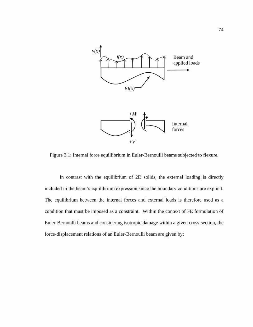
74

Figure 3.1: Internal force equillibrium in Euler-Bernoulli beams subjected to flexure.

In contrast with the equilibrium of 2D solids, the external loading is directly

included in the beam‘s equilibrium expression since the boundary conditions are explicit.

The equilibrium between the internal forces and external loads is therefore used as a

condition that must be imposed as a constraint. Within the context of FE formulation of

Euler-Bernoulli beams and considering isotropic damage within a given cross-section, the

force-displacement relations of an Euler-Bernoulli beam are given by:

Beam and

applied loads

v(x)

f(x)

x

Internal

forces

+M

+V

EI(x)

75

1 1

2 2

1 10

3

2 2

2 2

2 2

(1 )

12 6 12 6

6 4 6 2(1 )

12 6 12 6

6 2 6 4

d

D

v VL L

ML L L LEID

v VL LL

ML L L L

0

k d f

k d f

(3.2)

where 1 2 1 2, , ,T

v v are the nodal degrees of freedom (vertical deflection, rotation

angle), and 1 1 2 2, , ,V M V M are the dual variables (shear, moment). The stiffness matrix

of the element at the damaged state is denoted 𝐤𝐝 and is proportional to a reference value

for stiffness 𝐤𝟎. The variable 𝐷 (0 ≤ D ≤ 1) is a scalar indicating the damage level

(stiffness decrease). When 𝐷 = 0, the beam element is considered undamaged and its

stiffness is equal to the reference value. At the other limit, the ultimate condition 𝐷 = 1

represents a complete loss of the beam‘s stiffness. This definition for damage is in

accordance to the continuum damage mechanics (Lemaitre, 1996). When the axial

deformation is neglected, the stiffness matrix depends only on the flexural stiffness 𝐸𝐼,

and the beam‘s element length. For each element, we define a reference value for

stiffness 0EI , and note that its value can vary along the beam. We will assume that a

reference distribution is 𝐸𝐼0 𝑥 , and take this as the initial estimate for the identification

process. For example, this reference stiffness can, but not necessarily, correspond to the

stiffness of the undamaged beam. From Eq. (3.2), a possible definition for the damage

variable would be 𝐷(𝑥) = 1 −𝐸𝐼(𝑥)

𝐸𝐼0(𝑥), where 𝐸𝐼(𝑥) is the actual stiffness of the cross-

section at a position 𝑥. It is clear that when EI decreases, damage increases linearly, so

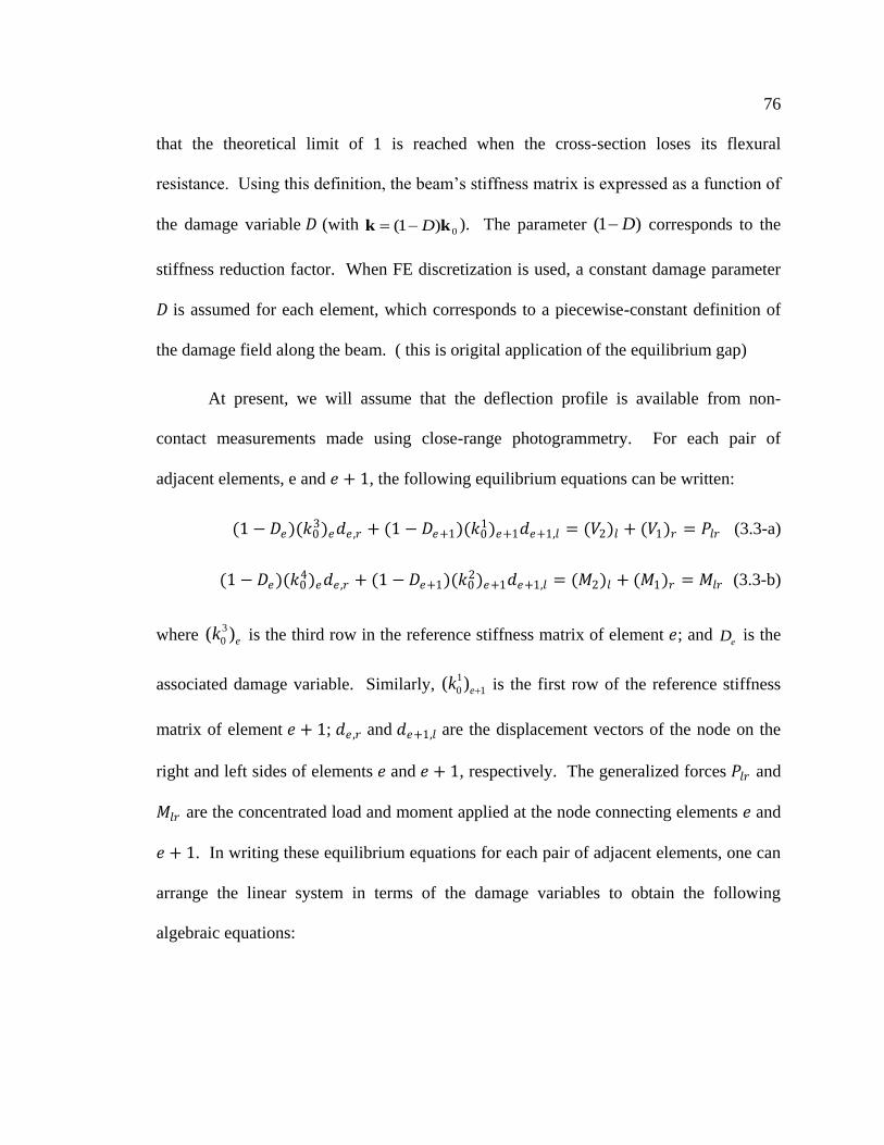
76

that the theoretical limit of 1 is reached when the cross-section loses its flexural

resistance. Using this definition, the beam‘s stiffness matrix is expressed as a function of

the damage variable 𝐷 (with 0)1( kk D ). The parameter )1( D corresponds to the

stiffness reduction factor. When FE discretization is used, a constant damage parameter

𝐷 is assumed for each element, which corresponds to a piecewise-constant definition of

the damage field along the beam. ( this is origital application of the equilibrium gap)

At present, we will assume that the deflection profile is available from non-

contact measurements made using close-range photogrammetry. For each pair of

adjacent elements, e and 𝑒 + 1, the following equilibrium equations can be written:

(1 − 𝐷𝑒)(𝑘03)𝑒𝑑𝑒 ,𝑟 + (1 − 𝐷𝑒+1)(𝑘0

1)𝑒+1𝑑𝑒+1,𝑙 = (𝑉2)𝑙 + (𝑉1)𝑟 = 𝑃𝑙𝑟 (3.3-a)

(1 − 𝐷𝑒)(𝑘04)𝑒𝑑𝑒 ,𝑟 + (1 − 𝐷𝑒+1)(𝑘0

2)𝑒+1𝑑𝑒+1,𝑙 = (𝑀2)𝑙 + (𝑀1)𝑟 = 𝑀𝑙𝑟 (3.3-b)

where 3

0( )ek is the third row in the reference stiffness matrix of element 𝑒; and eD is the

associated damage variable. Similarly, 1

0 1( )ek is the first row of the reference stiffness

matrix of element 𝑒 + 1; 𝑑𝑒 ,𝑟 and 𝑑𝑒+1,𝑙 are the displacement vectors of the node on the

right and left sides of elements 𝑒 and 𝑒 + 1, respectively. The generalized forces 𝑃𝑙𝑟 and

𝑀𝑙𝑟 are the concentrated load and moment applied at the node connecting elements 𝑒 and

𝑒 + 1. In writing these equilibrium equations for each pair of adjacent elements, one can

arrange the linear system in terms of the damage variables to obtain the following

algebraic equations:

77

(k03)1d1 (k0

1)2d2

(k04)1d1 (k0

2)2d2

(k03)2d2 (k0

1)3d3

(k04)2d2 (k0

2)3d3

(k03)3d3

(k04)3d3

⋮

………

1 − D1

1 − D2

⋮ ⋮

1 − Dnel

=

P1

M1

P2

⋮⋮

Pnel

Mnel

(3.4)

Finally, the problem for identification of the damage variable is written as:

𝐹𝑖𝑛𝑑 𝜽 = 1 − 𝐷1 1 − 𝐷2 … 1 − 𝐷𝑛𝑒𝑙 𝑇

𝑠𝑢𝑐𝑕 𝑡𝑕𝑎𝑡 𝑮𝜽 = 𝑹 (3.5)

where 𝜽 is the set associated with the damage variables corresponding to each element

𝜽 = (1 − 𝐷1 , 1 − 𝐷2 ,… .1 − 𝐷𝑛𝑒𝑙 ), and 𝐑 = 𝑃1,𝑀1 ,… ,𝑃𝑖 ,𝑀𝑖 ,… T is the external force

at the nodes associated with the generalised degrees of freedom (i.e. displacements)

(𝑑1 ,𝑑2,… ,𝑑𝑛).

This formulation leads to a typical inverse problem, where the coefficient matrix

𝑮 defines the mathematical model. Generally, the forward problem associated with Eq.

(3.5) would be to solve the system 𝑲𝒅𝒅 = 𝑹 given a set 𝜽. In the inverse problem

associated with Eq. (3.5), the matrix 𝑮 encapsulates both the model and the data. The

discretization process leads inevitably to modeling errors in forming the system, whereas

measurement errors in the data affect the solution of the inverse problem. These two

phenomena lead to the ill-posedness of the inverse problem for Eq. (3.5), therefore

indicating the need for a regularization procedure. Eq. (3.5) is typical to problems in

many engineering areas, including biomedical and seismic imaging, digital tomography

and digital image reconstruction. A detailed analysis of regularization techniques and

78

solution methods for such inverse problems can be found in (Aster, Borchers et al.,

2005).

In this study, a Tikhonov-Total Variation (TTV) regularization scheme is used to

solve Eq. (3.5) (Aster, Borchers et al., 2005). The problem is treated in the least-square

sense augmented with the TTV regularization, leading to:

𝑚𝑖𝑛 1

2 𝐺𝜽 − 𝑹 2 + 𝛼𝛷(𝜽) (3.6)

where α is the Tikhonov parameter controlling the relative weight between the least

squares and the regularization term Φ 𝛉 . In this thesis, the value of this parameter

chosen is 10−4, which is found to be a sub-optimal choice in most practical applications.

A better value can be chosen for this parameter is possible using selecting methods such

as the L-curve method (Hansen, 1992) (Hansen, 1998). The function Φ(𝜽) represents the

total variation (TV) functional of the vector 𝜽. Minimization of the regularized TTV

functional yields an efficient scheme to solve the discrete inverse problem. This type of

regularization penalizes highly oscillatory solutions while allowing jumps-like

discontinuities. Vogel (Vogel, 2002) showed that in the case of two-dimensional image

deblurring, TTV regularization tends to produce qualitatively correct reconstructions of

blocky images (Dobson, 1996).

The accuracy of the regularized solution depends very much on the smoothness of

the true model. If 𝐦true is not smooth, then Tikhonov regularization solution simply will

not give an accurate solution.

𝜽

79

To obtain the numerical scheme for calculating Φ(𝜽), consider the following

general definition of the total variation (TV) of a function 𝑓(𝑥) on the interval [0, 1]:

𝑇𝑉 𝑓 ≝ sup |𝑓(𝑥𝑖) − 𝑓 𝑥𝑖−1 |𝑖 (3.7)

where the index, 𝑖 , is taken over all partitions (0 = 𝑥0 < 𝑥1 < ⋯ < 𝑥𝑛 = 1 ) of the

interval. In the one-dimensional case, the smooth form of TV functional defines the total

variance function Φ as:

Φ 𝑓 = 𝑑𝑓

𝑑𝑥

2d𝑥

L0 (3.8)

This equation is a continuous form of the discrete total variation that includes the

sum of the magnitude of the jumps for 𝒇. However, due to the non-differentiability of

the Euclidean norm at the origin, special attention is required for numerical

implementation. One can select a smooth approximation to the Euclidean norm, |x|, such

as x 2 + β2, where β is a small positive parameter giving rise to the following smooth

total variance functional:

Φ θ(x) = dθ

dx

2+ β2dx

L

0 (3.9)

To derive the discrete form of the TTV term, let ∆𝑥 be the interval distance used

to discretize 𝜽(𝑥) (i.e. the length of a beam element in our case), and assume that the

number of elements is 𝑛𝑒𝑙 (i.e. the index of 𝜽 ranging from 1 to nel); then, the discretized

version of Eq. (3.9) can be written as:

Φ 𝛉 = ψ Δi𝛉 2 Δxn

i=2 , and ψ Δi𝛉 2 =

θi−θi−1

Δx

2+ β2 (3.10)

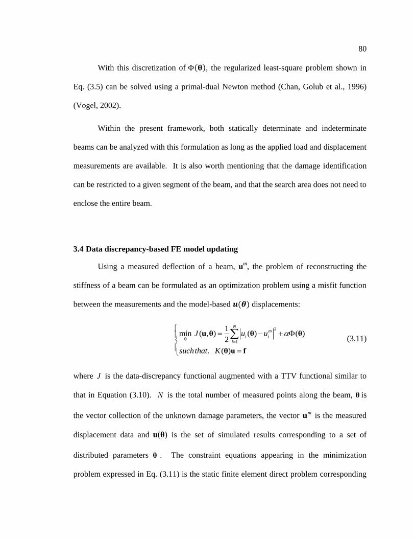
80

With this discretization of Φ 𝛉 , the regularized least-square problem shown in

Eq. (3.5) can be solved using a primal-dual Newton method (Chan, Golub et al., 1996)

(Vogel, 2002).

Within the present framework, both statically determinate and indeterminate

beams can be analyzed with this formulation as long as the applied load and displacement

measurements are available. It is also worth mentioning that the damage identification

can be restricted to a given segment of the beam, and that the search area does not need to

enclose the entire beam.

3.4 Data discrepancy-based FE model updating

Using a measured deflection of a beam, um, the problem of reconstructing the

stiffness of a beam can be formulated as an optimization problem using a misfit function

between the measurements and the model-based 𝒖(𝜽) displacements:

2

1

1min ( , ) ( ) ( )

2

. ( )

Nm

i i

i

J u u

suchthat K

θ

u θ θ θ

θ u f

(3.11)

where J is the data-discrepancy functional augmented with a TTV functional similar to

that in Equation (3.10). N is the total number of measured points along the beam, θ is

the vector collection of the unknown damage parameters, the vector m

u is the measured

displacement data and )(θu is the set of simulated results corresponding to a set of

distributed parameters θ . The constraint equations appearing in the minimization

problem expressed in Eq. (3.11) is the static finite element direct problem corresponding

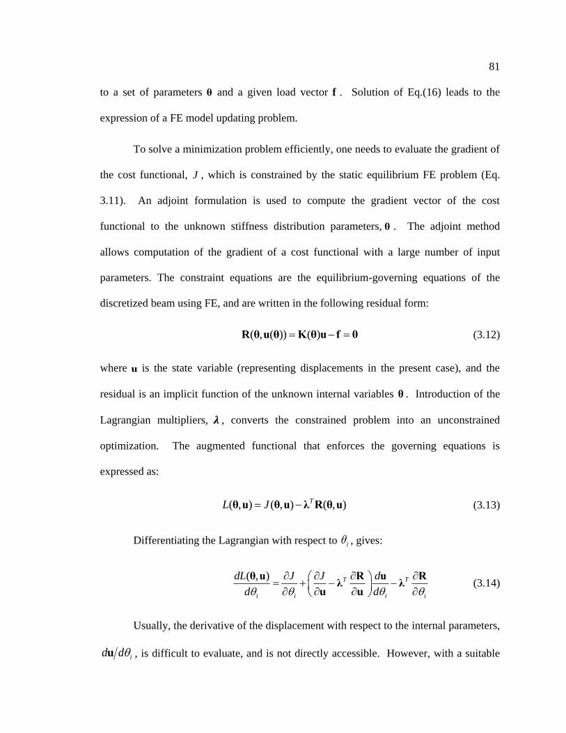
81

to a set of parameters θ and a given load vector f . Solution of Eq.(16) leads to the

expression of a FE model updating problem.

To solve a minimization problem efficiently, one needs to evaluate the gradient of

the cost functional, J , which is constrained by the static equilibrium FE problem (Eq.

3.11). An adjoint formulation is used to compute the gradient vector of the cost

functional to the unknown stiffness distribution parameters, θ . The adjoint method

allows computation of the gradient of a cost functional with a large number of input

parameters. The constraint equations are the equilibrium-governing equations of the

discretized beam using FE, and are written in the following residual form:

( , ( )) ( ) R θ u θ K θ u f 0 (3.12)

where u is the state variable (representing displacements in the present case), and the

residual is an implicit function of the unknown internal variables θ . Introduction of the

Lagrangian multipliers, 𝝀 , converts the constrained problem into an unconstrained

optimization. The augmented functional that enforces the governing equations is

expressed as:

( , ) ( , ) ( , )TL J θ u θ u λ R θ u (3.13)

Differentiating the Lagrangian with respect to i , gives:

( , ) T T

i i i i

dL J J d

d d

θ u R u Rλ λ

u u (3.14)

Usually, the derivative of the displacement with respect to the internal parameters,

id du , is difficult to evaluate, and is not directly accessible. However, with a suitable

82

choice of λ , it is possible to make the term in the bracket,

u

Rλ

u

TJ, equal zero,

thus avoiding the need to evaluate the gradient id du . Therefore, an additional equation

can be written as:

0

u

Rλ

u

TJ (3.15)

Equation (3.15) is the adjoint equation, which is solved for Tλ ; this equation

reduces to the following linear system:

( ) ( )m T u u λ K θ (3.16)

where u is the displacement vector computed from the FE model in Eq.(16), and m

u is

the corresponding measured displacement vector. Therefore, Eq. (3.14) is simplified to:

( , ) T

i i i

dL J

d

θ u Rλ (3.17)

in which the two derivative terms can be easily computed as:

J

θ θ

and ( )

i i i

R K θ fu (3.18)

The regularized TV-functional ( ) θ is defined in the previous section (see Eq.

3.9 and Eq. 3.10). In order to calculate the gradient of the TV term J , J

θ θ

, it is

easy to deduce from Eq.(3.10) that

'( )Tx diag

Δ θ Δ θθ

(3.19)

83

x is the size of the beam element, and the term in the brackets,

'( )T diag Δ θ Δ , is a positive, semi-definite, symmetric matrix. The Δ matrix has

( 1)n rows and ( )n columns, with the ith

row being i (see Eq.11). The '( )diag θ

matrix is a ( 1) ( 1)n n diagonal matrix with the ith

diagonal entry equal to ' 2( )i θ .

The global stiffness matrix K is the classical assembly of the elements‘ stiffness

matrices ik :

1 (1 )Nel

i i iD K k (3.20)

where is the FE assembly operator, and Nel is the number of elements in the FE

model. As stated earlier, we assume that for each element, the damage is represented by a

scalar parameter, iD , in the interval [0,1]. Therefore, the derivative of the stiffness matrix

with respect to θ can be computed analytically given a specific beam element

formulation. For the Euler-Bernoulli bending element the following expression holds:

1 1

( )( )j jNel Nel

j j i

ii

kk

K θ (3.21)

In conclusion, the adjoint method leads to an efficient computational method to

calculate the gradient of the cost functional and consists of two consecutive steps: 1)

solve the adjoint equation (3.17) for Tλ , then insert T

λ into Eq. (3.18) to calculate the

gradient of the Lagrangian. With the gradient calculated, any efficient gradient-based

optimization technique can be used to find the optimal solution. A procedure based on the

BFGS pseudo-Newton optimization technique is summarized in Table-2. The algorithm

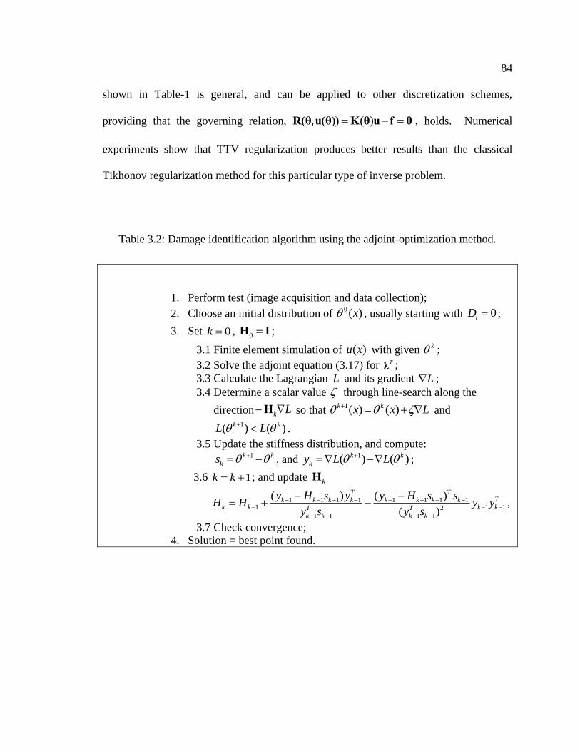
84

shown in Table-1 is general, and can be applied to other discretization schemes,

providing that the governing relation, ( , ( )) ( ) R θ u θ K θ u f 0 , holds. Numerical

experiments show that TTV regularization produces better results than the classical

Tikhonov regularization method for this particular type of inverse problem.

Table 3.2: Damage identification algorithm using the adjoint-optimization method.

1. Perform test (image acquisition and data collection);

2. Choose an initial distribution of 0 ( )x , usually starting with 0iD ;

3. Set 0k , 0 H I ;

3.1 Finite element simulation of ( )u x with given k ;

3.2 Solve the adjoint equation (3.17) for Tλ ;

3.3 Calculate the Lagrangian L and its gradient L ;

3.4 Determine a scalar value through line-search along the

direction LkH so that 1( ) ( )k kx x L and

1( ) ( )k kL L .

3.5 Update the stiffness distribution, and compute: 1k k

ks , and 1( ) ( )k k

ky L L ;

3.6 1k k ; and update kH

T

kk

k

T

k

k

T

kkk

k

T

k

T

kkkkkk yy

sy

ssHy

sy

ysHyHH 112

11

1111

11

11111

)(

)()(

,

3.7 Check convergence;

4. Solution = best point found.

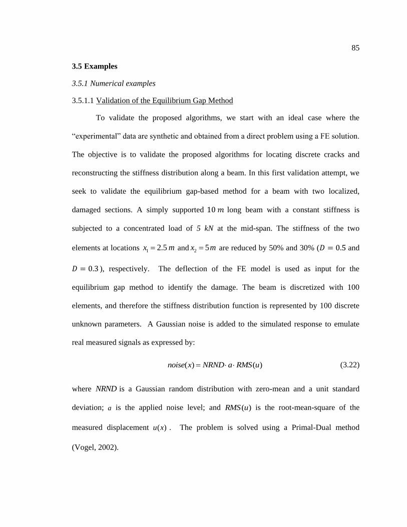
85

3.5 Examples

3.5.1 Numerical examples

3.5.1.1 Validation of the Equilibrium Gap Method

To validate the proposed algorithms, we start with an ideal case where the

―experimental‖ data are synthetic and obtained from a direct problem using a FE solution.

The objective is to validate the proposed algorithms for locating discrete cracks and

reconstructing the stiffness distribution along a beam. In this first validation attempt, we

seek to validate the equilibrium gap-based method for a beam with two localized,

damaged sections. A simply supported 10 𝑚 long beam with a constant stiffness is

subjected to a concentrated load of 5 kN at the mid-span. The stiffness of the two

elements at locations 1 2.5x m and 2 5x m are reduced by 50% and 30% (𝐷 = 0.5 and

𝐷 = 0.3 ), respectively. The deflection of the FE model is used as input for the

equilibrium gap method to identify the damage. The beam is discretized with 100

elements, and therefore the stiffness distribution function is represented by 100 discrete

unknown parameters. A Gaussian noise is added to the simulated response to emulate

real measured signals as expressed by:

( ) ( )noise x NRND a RMS u (3.22)

where NRND is a Gaussian random distribution with zero-mean and a unit standard

deviation; a is the applied noise level; and )(uRMS is the root-mean-square of the

measured displacement )(xu . The problem is solved using a Primal-Dual method

(Vogel, 2002).

86

Figure 3.2-(a) shows the damage pattern when no noise is added to the deflection

measurements; in this case the two damaged zones (cracks) and damage levels are

identified with very good accuracy. In Figures 3.2-(b) and 3.2-(c), noise levels of 2.5%

and 5% are added to the measured deflection data, respectively. The numerical simulation

is capable of identifying the positions and levels of the damage under these noise

conditions. However, it is observed that the noise added to the synthetic measurements

can mask the damage at the fine-scale level. If the noise level is known, the minimum

scale of detectable damage corresponding to this level of noise can be approximately

estimated by inspecting the variations of the identified damage indices. For example, at a

5% noise level, the finest detectable level of damage seems to be 10%, as it can be seen

from inspection of Figure 3.2-(c).

To demonstrate the effect of noise in masking fine-scale damage, the beam is re-

simulated using a different damage scenario, the beam‘s stiffness is reduced by 30% and

10% at two locations, 2.5 𝑚 and 6 𝑚 from the left support, (i.e. 𝐷(2.5𝑚) = 0.3 and

𝐷(6𝑚) = 0.1). A 5 % level of noise is added, and the identified damage indices are

shown in Figure 3.2-(d), in which only the damage at location 2.5 m (𝐷(2.5𝑚) = 0.3 ) is

identifiable; damage at the 6 m location is indistinguishable from the noise.

87

Figure 3.2: Identified damage indices of a simply-supported beam using the equilibrium

gap method. (a): no noise, (b): 2.5% noise, (c): 5% noise, (d): 5% noise.

3.5.1.2 Validation of the Data Discrepancy Functional Method

The previously described problem is solved again using the data discrepancy

functional method and the results are shown in Figure-3.3. Both the equilibrium gap and

data discrepancy functional methods are in good agreement with the baseline solution.

0 2 4 6 8 10

Distance (m)

-0.2

0

0.2

0.4

0.6

Dam

ag

ein

dex

(D)

b

0 2 4 6 8 10

Distance (m)

-0.2

0

0.2

0.4

0.6

Dam

ag

ein

dex

(D)

a

0 2 4 6 8 10

Distance (m)

-0.2

0

0.2

0.4

0.6

Dam

ag

ein

dex

(D)

c

0 2 4 6 8 10

Distance (m)

-0.2

0

0.2

0.4

0.6

Dam

ag

ein

dex

(D)

d

88

Figure 3.3: Comparison of the identified damage indices of a simply-supported beam

using equilibrium gap and data discrepancy formulation.

In a second example, a 10 m long, simply-supported beam is simulated to validate

the data discrepancy functional method. The beam is assumed to have a constant

stiffness; a concentrated load of 5kN is applied at the mid-span. The beam is discretized

using 100 beam elements; hence, the continuous stiffness distribution function is

represented by 100 discrete unknown stiffness parameters. A FE simulation is used to

calculate the deflection profile. A Gaussian noise level of 5% is added to the synthetic

displacement field that is to be used as input for the identification.

For the first validation test, we try to recover the stiffness of a beam with constant

stiffness. The initial estimate is based on a uniform stiffness factor of 0.5 (i.e. half of the

true stiffness value). The results from the application of the adjoint optimization method

are illustrated in Figure 3.4. In the second test case, the beam is assumed to have a

continuous parabolic stiffness distribution. Again, a constant stiffness factor of 0.5 is

89

used to initiate the iteration process. The results of the data discrepancy-based method in

comparison to the reference stiffness distribution are shown in Figure 3.5.

The results shown in Figures 3.4 and 3.5 illustrate the performance of the data

discrepancy formulation, and show that, at a distance from the supports, the identification

is in good agreement with the expected stiffness values. The displacements of a simply

supported beam close to the support are very small (zero at the support), and the lack of

information in this region is not capable to improve the initial guess locally. This explains

the drift between the expected results and the results from the simulation near the ends of

the beam.

Figure 3.4: Identified stiffness factor distribution for a simply-supported beam with

constant stiffness using the data discrepancy functional method

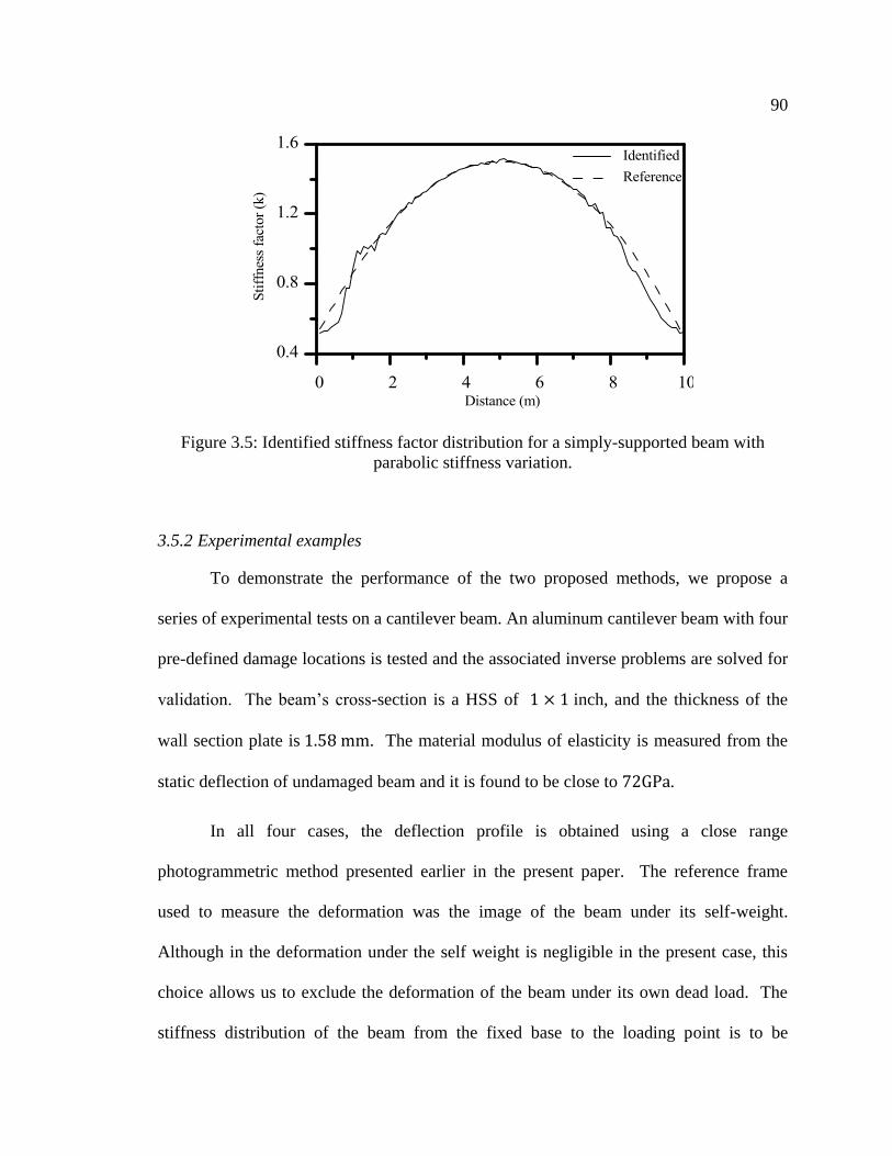
90

Figure 3.5: Identified stiffness factor distribution for a simply-supported beam with

parabolic stiffness variation.

3.5.2 Experimental examples

To demonstrate the performance of the two proposed methods, we propose a

series of experimental tests on a cantilever beam. An aluminum cantilever beam with four

pre-defined damage locations is tested and the associated inverse problems are solved for

validation. The beam‘s cross-section is a HSS of 1 × 1 inch, and the thickness of the

wall section plate is 1.58 mm. The material modulus of elasticity is measured from the

static deflection of undamaged beam and it is found to be close to 72GPa.

In all four cases, the deflection profile is obtained using a close range

photogrammetric method presented earlier in the present paper. The reference frame

used to measure the deformation was the image of the beam under its self-weight.

Although in the deformation under the self weight is negligible in the present case, this

choice allows us to exclude the deformation of the beam under its own dead load. The

stiffness distribution of the beam from the fixed base to the loading point is to be

91

identified, while the stiffness distribution in the region of the free tip beyond the loading

is not taken into consideration, since no information is available in that region.

3.5.2.1 Test # 1: Step-wise damage detection

The first test setup is shown in Figure 3.6. The total length of the beam is

L = 130 cm. A concentrated load of 21 𝑁 is applied at a location 90 cm away from the

fixed end. To induce a predefined damage, the bottom face of the HSS section is cut out

between 50 cm and 70 cm from the fixed end as illustrated. The stiffness in the damaged

region is reduced to 0.83% of the original cross-section (𝐷 = 0.17).

Figure 3.6. The cantilever beam with a distributed damage.

The identified damage variable profile using the equilibrium gap method is shown

in Figure 3.7, it is clear that the results reproduce the expected damage location and level

with very good accuracy. The recovered stiffness factor of each element using the data

discrepancy method and reference values are plotted in Figure 3.8. The step damage is

clearly visible despite the oscillatory nature of the identified stiffness distribution; the

amplitudes of oscillations are generally less than 5%, with exception of regions near the

beam‘s ends. The larger errors in the two ends can be attributed to the measurement

𝑙𝑜𝑎𝑑

50 𝑐𝑚

20 𝑐𝑚

20 𝑐𝑚

92

errors of the displacement close to the loading point and the lack of information close to

the fixed end (theoretical displacements close to zero).

Figure 3.7. Damage detection of the cantilever beam with distributed damage using the

equilibrium gap method.

Figure 3.8. Identified stiffness factor distribution of the cantilever beam with distributed

damage using the data discrepancy formulation.

93

Figure 3.9 illustrates the performance of the adjoint based optimization algorithm

for solving the inverse problem formulated using the data discrepancy functional. Figure

3.9(a) shows the convergence of the cost function minimization, whereas Figure 3.9(b)

illustrates that at convergence, the solution is independent of the initial guess of the

beam‘s stiffness. The intermediate results during the iteration processes are shown in

Figure 3.9(c) and 3.9(d) as they illustrate the convergence process.

(a)

(b)

94

Figure 3.9. Performance of the adjoint based method for solving the data discrepancy

problem, (a) convergence rate, (b) influence of the initial guess, (c) iteration process for

initial guess EI0 and (d) iteration process for intial guess 1.2 EI0.

3.5.2.2 Test # 2: Single saw-cut damaged beam

In this example, a single saw-cut was created on the tested beam to simulate

damage in the form of a crack, as shown in Figure 3.10. The length of the beam is

𝐿 = 95.5𝑐𝑚, and a concentrated load of 17 𝑁 is applied at a distance of 89 𝑐𝑚 away

from the support. The location of the saw-cut is 50 𝑐𝑚 from the base; the cut is 1.5 𝑚𝑚

wide and 15 𝑚𝑚 in depth, corresponding to a 86% reduction in stiffness (D= 0.86).

(c)

(d)

95

Figure 3.10: Uniform cantilever beam with a saw-cut damage

Using the equilibrium gap method, the damage distribution along the beam is

shown in Figure 3.11. The sharp peak is captured by the solution, indicating a clearly

concentrated damage. The recovered stiffness factor profile using the data discrepancy

method is plotted in Figure 3.12. The identification of the single concentrated damage is

also clear, however small amplitudes oscillations similar to test 1 are observed. The

larger errors close to the free-end can be attributed to the errors in the displacement

measurement close to the loading point.

𝑙𝑜𝑎𝑑

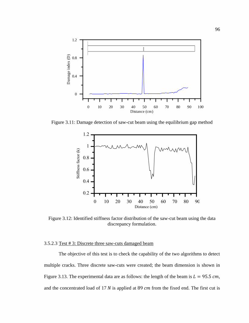
96

Figure 3.11: Damage detection of saw-cut beam using the equilibrium gap method

Figure 3.12: Identified stiffness factor distribution of the saw-cut beam using the data

discrepancy formulation.

3.5.2.3 Test # 3: Discrete three saw-cuts damaged beam

The objective of this test is to check the capability of the two algorithms to detect

multiple cracks. Three discrete saw-cuts were created; the beam dimension is shown in

Figure 3.13. The experimental data are as follows: the length of the beam is 𝐿 = 95.5 𝑐𝑚,

and the concentrated load of 17 𝑁 is applied at 89 𝑐𝑚 from the fixed end. The first cut is

0 10 20 30 40 50 60 70 80 90 100

Distance (cm)

0

0.4

0.8

1.2

Dam

ag

ein

dex

(D)

97

30.6 𝑐𝑚 away from the base, with a depth of 1.5 𝑚𝑚, corresponding to 17% stiffness

reduction; the second cut is located at 50 𝑐𝑚 away from the base, having a depth of 15

𝑚𝑚, corresponding to a 86% reduction in stiffness; the third cut is at 70 𝑐𝑚 from the

base, and is of 2 𝑚𝑚 in depth, corresponding to 20% stiffness reduction. All introduced

cuts have a width of 1.5 𝑚𝑚.

Figure 3.13. The cantilever beam with three saw-cuts damage.

The results of the equilibrium gap and the data discrepancy methods are

illustrated in Figures 3.14 and 3.15, respectively. The sharp peaks are clear in the

identified damage variables obtained by the equilibrium gap method (Figure 3.14), the

identification of the location and magnitude of the damage is in good agreement with the

expected results. From the stiffness factors obtained using the data discrepancy method,

shown in Figure 3.15, it can be seen that although the location and magnitude of the

damage have been captured, oscillations of the solution are still visible.

𝑙𝑜𝑎𝑑

30.6 𝑐𝑚

19.4 𝑐𝑚

20 𝑐𝑚

19 𝑐𝑚

98

Figure 3.14. Damage detection of the beam with three saw-cuts using the equilibrium gap

method.

Figure 3.15. Identified stiffness factor distribution of the beam with three saw-cuts using

the data discrepancy formulation.

3.5.2.4 Test #4: Combination of discrete and step cuts damaged beam

In this example, a step-cut damage was added to the previously discussed beam; a

step-cut is added between the second and the third saw-cuts (Figure 3.16). The depth of

99

the step cut is 2 𝑚𝑚, equal to the depth of the original third saw-cut at the location of 70

𝑐𝑚 from the base; thus, the third saw-cut becomes part of the step-cut, but the second cut

still displays as a discrete cut attached to the continuous step material removal.

Figure 3.16. Cantilever beam with double saw-cuts and a distributed damage.

The identified damage indices and stiffness factors, using the two proposed

methods, are shown in Figure 3.17 and Figure 3.18. The results of the equilibrium gap

method show two sharp peaks and the flat stiffness region of the step damage are clearly

identified. The overall predictions are consistent with expected damage location and

levels. We observe an error close to the location of the loading larger than in the rest of

the beam, this error can be attributed to the measurement variability in this region and the

influence of the concentrated load. On the other hand, the results of the data discrepancy

method display a similar trend of oscillations as was observed in the previous example;

however, the damage locations and magnitude are easily identifiable.

𝑙𝑜𝑎𝑑

19.4 𝑐𝑚

20 𝑐𝑚

30.6 𝑐𝑚

100

Figure 3.17. Damage detection of the beam with saw-cuts and step damage using the

equilibrium gap method.

Figure 3.18. Identified stiffness factor distribution of the beam with saw-cuts and step

damage using the data discrepancy formulation.

The identified damage indices and stiffness factors of several critical sections in

the four test cases are transformed to stiffness (𝐸𝐼) and are displayed in Tables 3.3 to 3.6.

Note that the identified values of saw-cuts are taken as the peak value around the

101

location, but the identified step-cut or original beam section stiffness values are taken as

average of five values around the approximate location since there can be some

oscillations in the identified stiffness of a constant section, especially for the data-

discrepancy formulation.

Table 3.3: Identified stiffness of test #1

Stiffness (unit: 108 𝑀𝑃𝑎 ∙ 𝑚𝑚4) 𝐸𝐼1 𝐸𝐼2 𝐸𝐼3

Expected values 5.5259 4.5865 5.5259

Equilibrium gap

Identified values 5.5143 4.4533 5.4651

Errors -0.2% -2.9% -1.1%

Data discrepancy

Identified values 5.4485 4.3655 5.4430

Errors -1.4% -4.8% -1.5%

1 2 3

102

Table 3.4: Identified stiffness of test #2

Stiffness (unit: 108 𝑀𝑃𝑎 ∙ 𝑚𝑚4) 𝐸𝐼1 𝐸𝐼2 𝐸𝐼3

Expected values 5.5259 0.7737 5.5259

Equilibrium

gap

Identified

values

5.5093 0.7644 5.4430

Errors -0.003 -1.2% -1.5%

Data

discrepancy

Identified

values

5.6088 2.4739 5.3049

Errors 1.5% 219% -4.0%

1 2 3

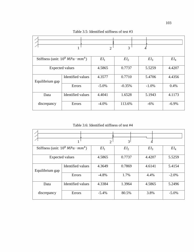
103

Table 3.5: Identified stiffness of test #3

Stiffness (unit: 108 𝑀𝑃𝑎 ∙ 𝑚𝑚4) 𝐸𝐼1 𝐸𝐼2 𝐸𝐼3 𝐸𝐼4

Expected values 4.5865 0.7737 5.5259 4.4207

Equilibrium gap

Identified values 4.3577 0.7710 5.4706 4.4356

Errors -5.0% -0.35% -1.0% 0.4%

Data

discrepancy

Identified values 4.4041 1.6528 5.1943 4.1173

Errors -4.0% 113.6% -6% -6.9%

Table 3.6: Identified stiffness of test #4

Stiffness (unit: 108 𝑀𝑃𝑎 ∙ 𝑚𝑚4) 𝐸𝐼1 𝐸𝐼2 𝐸𝐼3 𝐸𝐼4

Expected values 4.5865 0.7737 4.4207 5.5259

Equilibrium gap

Identified values 4.3649 0.7869 4.6141 5.4154

Errors -4.8% 1.7% 4.4% -2.0%

Data

discrepancy

Identified values 4.3384 1.3964 4.5865 5.2496

Errors -5.4% 80.5% 3.8% -5.0%

4 2 3 1

4 2 3 1

104

3.6 Conclusions

Two inverse problem based formulations are proposed to identify damage in

Euler-Bernouilli beams using the equilibrium gap concept and a data discrepancy

functional. The static deflection profile of the beam is obtained from close range

photogrammetric technique. A quasi-continuous measurement of the deflection became

possible with the use of digital image processing based technology. We describe a

technique to measure the displacement of beams based on an edge detection algorithm.

The first inverse problem formulation uses the equilibrium gap principle along with a

finite element forward problem solver. An over-determinate algebraic system is obtained

and solved in the least squares sense with a TTV regularization scheme. The second

formulation is based on a data discrepancy expression of the measured and model based

deflection. The minimization of the functional is obtained through an adjoint method and

a TTV regularization.

The proposed methodology is validated by a series of synthetic data generated

from simulations of a damaged beam. The identification of the location and level of

damage is verified and the effect of noise is reported. The reconstruction of a

continuously varying stiffness beam is also validated. Four tests were conducted on

beams with different damage scenarios. The two methodologies were validated and

showed overall good performance within a laboratory conditions. In each test, the

location and level of damage were identified with a good level of accuracy. However, the

formulation based on the equilibrium gap functional performed better and showed closer

solutions to the real damage state. The data discrepancy based formulation depicts a

slight oscillatory phenomenon in the solution, but the results are acceptable from a

105

practical point of view. A validation on more complex systems, such as rehabilitated

reinforced concrete beams is underway.

As for any inverse problem formulation, the quality of the data measurements is

essential to the performance of the algorithm. Two aspects need to be addressed in future

work: (i) develop a reliable methodology for deflection measurements using digital image

correlation, and (ii) include error uncertainty in the formulation of the inverse problems.

These two enhancements will allow practical use of the proposed methodologies for the

health monitoring of structures.

The proposed methodology deals with two broad activities: (i) periodic non-

destructive damage localization and severity estimation; and (ii) the assessment of

structural safety based on the results of the non-destructive damage detection.

Once the identification of the structure has been accomplished, subsequent

analyses, e.g. the determination of load capacity, rating, reliability and useful life

determination of the structure can then be conducted

3.7 Extension and envision:

Field testing and identification is different from lab setting. In the published

results, some are validated using pure simulated data to small-scale structures (Banan,

Banan et al., 1994b) (Sanayei, Imbaro et al., 1997) , some using test data in lab

experiments on small scale structures; nonetheless, in-situ testing is challenging.

Experimental design, testing, acquisition of data, data processing and data quality

assessment, all involve some difficulties. Acquiring a topologically correct a priori FE

106

model can also be a problem, boundary conditions are needed to be identified first before

damage identification.

There is a long history of research in full-scale testing for assessment of highway

bridge (Phares, Rolander et al., 2001) (Bakht and Jaeger, 1990). While for large and

exotic bridges the SHM systems are more an academic performance, for smaller bridges

the global response is more sensitive to defects, visual inspection is less frequent and

SHM systems can make a real contribution (Heywood, Roberts et al., 2000).

107

CHAPTER FOUR: MATERIAL PARAMETER IDENTIFICATION USING FULL-

FIELD MEASUREMENTS

Give me matter, and I will construct a world out of it. (Immanuel Kant)

4.1 Introduction and literature review of related research

4.1.1 General review

Modern design and performance evaluation requires realistic simulation of structural and

material behaviours; the corresponding theories are classified as models of elasticity,

plasticity, hyperelasticity, rate-dependent viscoelasticity/viscoplasticity, as well as

additional models of continuum damage and fracture mechanics at material and structural

levels. For background material about the different classes of inelastic constitutive

models for isotropic materials and numerical solution schemes, we cite, for example:

(Kojic and Bathe, 2005; Neto, Peric et al., 2008).

In today‘s practice of inelastic FE analysis using commercial programs, extensive

libraries of material models are available. Constitutive parameters associated with

inelastic models are not necessarily available in standard material databases, but are

essential input data for any finite element simulation. Therefore, unknown material

parameters must be identified experimentally. Traditionally, the identification of material

parameters is performed using standard testing procedures on regularly shaped cut-outs

or machined specimens. In these tests, it is generally assumed that the mechanical fields

are homogeneous, and that the experimental specimen gauge response can be associated

108

to the simulated material response through simple fitting of the analytical relationships

(Bell, 1984).

However, even in the case of simple tests, obtaining a perfectly homogeneous

deformation field is not certain. For example, the accurate estimation of plastic material

properties from a simple tensile test can be difficult due to the non-uniform stress/strain

distribution in the necking zone. Generally, it is not possible to determine the hardening

parameters from direct measurement of specimen elongations. In order to calculate the

stress accurately, the Bridgman correction needs to be applied, and this requires

additional measurements of the contractions and curvature of the necking zone

(Bridgman, 1952). To overcome these limitations, Rodic et al. used an inverse approach,

referred to as the ―error minimization concept‖, to estimate the hardening parameters in a

Nadai-type constitutive law (Rodic, Gresovnik et al., 1995). In this approach, the

parameters are estimated by minimizing an error function between the experimental and

predicted load-displacement responses. Consequently, the necking distortion present in

the specimens is implicitly included in the analysis; this approach does not require

additional measurements to be obtained from the necking zone as is required for

application of the Bridgman correction. Rodic and Gresovnik developed an identification

system based on the finite element code, ―Elfen‖, and an inverse program, ―Inverse‖, to

solve a minimization problem (Rodic and Gresovnik, 1998). A similar method was

adopted by Mahken and Stein, but they included the observed contours of the necking

zone during the loading process as additional experimental information to calculate the

elasto-plastic material parameters of a mild steel (Mahnken and Stein, 1997).

109

A technique called the ―mixed numerical experimental‖ method parallels the error

minimization concept, but the deformation mode does not need to be pre-determined, so

general specimen geometries and loading conditions can be chosen (Hendricks, 1991;

Meuwissen, 1998; Meuwissen, Oomens et al., 1998). For example, Meuwissen (1998)

applied the mixed technique to identify the mechanical parameters of aluminum and steel

alloy materials, where the specimens were plate with holes so the geometries were not

standard and deformation was inhomogeneous. Measurements included displacement

fields on the surface of specimens determined by the grid or grating method; the

combination of Von Mises yield criterion with nonlinear hardening laws was validated.

This family of identification procedures derives from formulation as an optimization

problem to minimize the difference between the computed and the measured responses.

Typically, these procedures employ a pseudo-Newton method to search for the minimum,

and dedicated gradient computation schemes, such as direct differentiation or finite

difference, are required (Meuwissen, 1998; Meuwissen, Oomens et al., 1998; Mahnken,

2004) (Springmann and Kuna, 2003; Springmann and Kuna, 2005) (Zentar, Hicher et al.,

2001) (Mahnken, 2000) (Mahnken, 2002).

Subsequently, due to the rapid development of finite element analysis of nonlinear

materials and optimization techniques that accompanied the extraordinary development

of computer hardware and software in the last twenty years, this method has been studied

and applied extensively to determine different material parameters in a variety of tests.

The mixed numerical experimental technique has been examined under names such as the

―inverse identification approach‖, or the ―simultaneous determination of material

110

parameters‖ (Springmann and Kuna, 2003; Springmann and Kuna, 2005) (Zentar, Hicher

et al., 2001) (Mahnken, 2000) (Mahnken, 2002).

In addition to gradient-based local deterministic methods, the application of

evolutionary algorithms to solve optimization problems, and identify inelastic material

parameters with finite element model updating based on uni-axial load-displacement data

has been investigated (Hwang, Wu et al., 2010) (Müller and Hartmann, 1989; Furukawa

and Yagawa, 1997) (Munoz-Rojas, Cardoso et al., 2010). For example, Dusunceli et al.

proposed a formulation based on error minimization of the stress-strain curve from

homogeneous uni-axial tension tests along with a genetic algorithm-based solver

(Dusunceli, Colak et al., 2010).

Alternatively, artificial neural networks (ANN) have been used to determine

material properties from load-displacement data (Aguir, BelHadjSalah et al., 2011)

(Mahnken, 2004) (Lefik and Schrefler, 2002). The ANNs can be trained using FEA

simulations to build a mapping from measurement data to material parameters. ANNs

are tolerant of measurement errors. The ANN model is used as an alternative to the finite

element calculations to evaluate the objective functions.

One may classify the different methods of correlating test data and model

parameters as:

1) methods based on theoretical/analytical relationships (analytical fitting);

2) methods based on numerical simulations of the test (mixed-numerical

experimental methods); and

3) methods based on empirical relationships, including empirical

relationships using artificial neural networks.

111

The mixed-numerical experimental method provides not only more flexibility in

test design, but also more accurate and complete assessment of constitutive models. For

example, this method allows the design of experiments in which conditions are much

closer to those of practical situations; this is especially important in mechanical

component analysis since it minimizes the extrapolation of results obtained under testing

conditions to practical conditions. Thus, the mixed numerical-experimental method is a

perfect candidate for designing experiments that approximate real-world conditions. This

is especially important if in-situ testing is required, in which the specimen is tested within

the assembly.

Generally, forward simulation is performed with finite element analysis, so this

inverse identification is actually a problem of finite element model updating (see Chapter

3 for discussion of FE model updating in damage identification). Since the 1980s, finite

element model updating has emerged as an important aspect of the design of mechanical

systems and civil structures, especially in the development of automotive and aerospace

systems; it quickly became the most popular branch of model-updating (Keane and Nair,

2005; Arora, 2007).

4.1.2 Outline of the proposed methodology

The research presented in this chapter considers the problem of identification of

material plasticity parameters. We developed an identification method based on the

minimization of a least-squares error function between the inhomogeneous displacement

fields measured by digital image correlation (DIC) and a finite element simulation under

a given load. The material parameters are identified simultaneously by means of a direct

112

derivative-free optimization method that uses the finite element code as a black-box

procedure.

The three components of this inverse identification procedure are: (i) nonlinear

finite element analysis, (ii) direct optimization algorithm, and (iii) digital image

correlation (DIC) test results. One of the fundamental aims of this work is to reformulate

the algorithm to minimize the cost function, and thus remove the need to evaluate the

gradient of the cost function. Derivative-free optimization methods allow us to avoid the

tedious coding of numerical gradient computation associated with a material constitutive

model. The second objective of this work is to exploit the use of a full-field

measurement technique based on DIC as input. DIC is capable of capturing

heterogeneous deformation fields and provides an excellent source of data for both

deterministic and statistical analysis. Furthermore, both finite element analysis and DIC

are now standard tools widely available in industry. Therefore, the proposed

methodology can be easily adopted for practical use. Finally, this work employs

statistical studies of nonlinear regression analysis in this inverse identification procedure

to verify and validate the identified material parameters. DIC provides a large amount of

data and thus allows the use of statistical inference; whereas homogeneous tests seldom

provide enough data for statistical inference unless they are associated with random

simulations (Seibert, Lehn et al., 2000a) (Harth, 2003) (Harth, Schwan et al., 2004)

(Harth and Lehn, 2007).

Taken together, finite element analysis, optical full-field measurement techniques

(such as DIC or advanced grid methods), and direct optimization techniques comprise a

standard tool for the determination of material properties. Moreover, since these

113

components of the proposed inverse identification procedure (not only finite element

analysis, but also the DIC technique and finite element model updating through direct

optimization), have become commercialized, they are currently available for general

industrial use.

4.1.3 The advantages of using DIC

Different optical measurement techniques have been used in material

characterization studies. For example, an optical method called ―silhouette analysis‖ was

used to obtain the section profile of a cylindrical specimen during necking; these data,

along with load-displacement curves, were used to identify parameters in a damage

model (Broggiato, Campana et al., 2007). Likewise, the moiré method was used to

obtain planar displacements (Kreißig, Benedix et al., 2007), while a grid method was

used by Meuwissen and Mahken (Meuwissen, 1998) (Mahken, 1998). However, the

commercially most successful image processing-based measurement technique is the

digital image correlation (DIC) method (Louban, 2009) (see Chapter 2 for a list of current

commercial DIC systems and software). Sutton et al. presented details of the DIC

technique and a review of its applications in a recent book (Sutton, Orteu et al., 2009).

Many researchers have noted the advantages of using inhomogeneous

displacement fields in material parameter identification (Kleuter, Menzel et al., 2007)

(Cooreman, Lecompte et al., 2008). Recently, investigators in France developed a

methodology based on the principle of virtual work, the ―virtual fields method (VFM)‖,

that allows the development of simple or more complex analytical models for the

constitutive equations of the material under investigation. The VFM assumes that the

input will consist of full-field measurement data obtained using DIC or the grid method

114

(Grediac, Toussaint et al., 2002) (Grediac, 2004) (Grédiac and Pierron, 2006) (Toussaint,

Grediac et al., 2006) (Promma, Raka et al., 2009) (Grédiac, 2011). In addition,

inhomogeneous displacement fields must be provided for the VFM; otherwise, the

resulting linear system of equations becomes ill-conditioned as the data may not contain

sufficient information for more than two parameters. Intuitively, although homogeneous

displacement fields are adequate for identification of the elastic modulus, the deformation

must be heterogeneous for the determination of elasto-plastic parameters. Section 4.8

presents further discussion of the issue of identifiability.

There is an additional advantage arises from the large amount of data generated

by DIC: the valid use of statistical inference. For example, the estimate of the covariance

is valid when the amount of data is large. On the other hand, unless used in conjunction

with random simulation, homogeneous tests seldom provide enough data to support

statistical inference (Seibert, Lehn et al., 2000a) (Harth, 2003) (Harth, Schwan et al.,

2004) (Harth and Lehn, 2007).

Another significant advantage to using DIC is that the identification of parameters

in material models can be performed with non-standard specimens and even with original

components, so in-situ testing becomes possible. The use of non-standard specimens

under non-standard loading conditions is not only an intellectual curiosity, but is

particularly useful in some practical applications. For example, Partheepan et al used

miniature specimens, thus avoiding the removal of large material samples, for the

evaluation of current material properties of an in-service component (Partheepan, Sehgal

et al., 2008).

115

4.1.4 Organization of this chapter

Chapter 4 is organized as follows: Section 4.2 outlines the formulation of

continuous functions in solid mechanics and gives an overview of popular material

constitutive models that are widely used in engineering finite element analysis. Section

4.3 outlines the approaches used in the current work, and describes the identification

method in detail; including the least squares solution and the validation procedures based

on theories in nonlinear regression analysis. Section 4.4 summarizes the relevant theories

in nonlinear regression related to this work. Section 4.5 presents the inverse

identification problem using nonlinear least squares estimation. Section 4.6 is an

overview of state-of-the-art numerical optimization methods, with emphasis on direct

derivative-free techniques developed in recent years. Section 4.7 describes the statistical

inference procedures for the DIC test data; these procedures employ linearized

covariance analysis (LCA) of uncertainty for the identified parameters and sampling-

based statistical inferences of the response fit.

Identifiability issues are discussed in Section 4.8. Numerical and experimental

examples are presented in Section 4.9; the first validation is based on synthetic data, and

the experimental example deals with a cast iron bearing cap component, where the

displacement field was obtained using the ARAMIS DIC system (ARAMIS). Four direct

optimization methods are compared using these examples, including (i) the derivative-

free CONDOR algorithm which is based upon the trust-region algorithm and response

surface exploration techniques, (ii) the Nelder-Mead simplex method, (iii) a response

surface method in FE software, and (iv) a pseudo-Newton method using finite difference

approximation to gradients. The fourth method is usually considered as first-order,

116

gradient-based method with an approximate gradient evaluation; this type of methods

have been used in material parameter identification. However, since in this type of

methods, the FE simulation process can actually be treated as black-box, we consider it

also as a derivative-free method; i.e. in this thesis the term ―derivative-free‖ is associated

with methods in which the objective-function evaluation process can be treated as an

external black box. Section 4.10 summarizes the findings of this work.

4.2 Overview of elasto-plasticity

In this section, we summarize the general theory of elasto-plasticity. By

definition, the theory of elasto-plasticity is concerned with solids that, after being

subjected to a loading program, may sustain permanent (or plastic) deformations after

complete unloading. Elasto-plasticity theory has been successfully applied to metals, and

it is nowadays theoretically consolidated and well-studied phenomenological constitutive

model.

The basic components of the general elasto-plastic constitutive model include:

The strain decomposition principle where the total strain 𝜖 is assumed to

be the sum of an elastic, 𝜖𝑒 , and a plastic components, 𝜖𝑝 : 𝜖 = 𝜖𝑒 + 𝜖𝑝 ,

A yield criterion usually expressed in the stress space, 𝛷(𝜎), that defines

the onset of plasticity. Classical yield criteria widely used in engineering

practice include Tresca, von Mises, Mohr-Coulomb and Drucker-Prager

criteria.

A plastic flow rule defining the evolution of the plastic strain, the flow

rule is usually defined as a flow potential. In the case of associative flow

rule, the flow rule is described from the gradient of the yield function

117

which leads to the fact that the plastic strain rate is a tensor normal to the

yield surface in the stress space.

A hardening law, characterizing the evolution of the yield surface (i.e.

deformation after yielding occurred). The hardening rule describes the

evolution of the yield function over time, usually identified from a

uniaxial specimen.

To express the irreversibility of the plastic deformation, the Kuhn-Tucker

conditions must be applied.

The identification of an associative elasto-plastic constitutive model consists of

finding the parameters that define the yield function and the hardening surface. In FE

analysis, the hardening law is generally expressed as a one-dimensional function

describing the full stress-strain curve during uniaxial loading (Ramberg and Osgood,

1943) (ASTM, 2011).

For example, in the case of the linear hardening law: 𝜎 = 𝜎0 + 𝐻𝜖𝑝 , where 𝜎 is

the current yield stress, 𝜎0 is the initial yield stress, 𝜖𝑝 = 𝜖 − 𝜖𝑒 is the equivalent plastic

strain, 𝜖 is the total strain and 𝜖𝑒 is the elastic strain, 𝐻 is the hardening modulus. In this

simple model, the parameters that need determined are 𝜎0 and 𝐻. In most FEA programs,

the data required for an elasto-plastic behaviour is a multi-linear function that is the best

fitting of the stress-strain curve. There exist a variety of nonlinear hardening laws for

metals including the Nadai hardening law: 𝜎 = 𝜎0 + 𝑐𝜖𝑝𝑛 , defined by the three parameters

𝜎0, 𝑐 and 𝑛.; the rigid-plastic power hardening law: 𝜎 = 𝑐𝜖𝑝𝑛 ; and the Ramberg-Osgood

118

hardening law: 𝜖 =𝜎

𝐸+ 𝐾

𝜎

𝐸 𝑛

, where 𝐸 is the Young‘s modulus, and 𝐾 and 𝑛 are the

two material parameters.

4.3 General methodology

Material parameter identification is a particular type of parameter identification

problem. Parameter identification problems arise in all fields of engineering science.

Consequently, parameter identification has attracted considerable research interest since

the mid-seventies; a number of books describe standard treatment of parameter

identification using deterministic and statistical methods (Bard, 1974) (Beck and Arnold,

1977) (Bates and Watts, 1988) (Tarantola, 2004) (Seber and Wild, 2005). In the current

research, we focus on a formulation for the identification of constitutive parameters based

on the least-squares cost function measuring the gap between a FE model prediction and

the results of experimental measurements. The least-squares estimation is a fundamental

approach to system identification problems, and has already become a classic method

frequently practiced by scientists and engineers in a wide variety of applications.

The principle components of the inverse identification technique are presented

schematically in Figure 4.1:

119

Figure 4.1: Flowchart of material parameter identification using optimization-based FE-

model updating

In this procedure, the post-processing phase performs a coordinate transformation

and interpolation to correlate the coordinates used in the DIC experiment with those of

the FE simulation results. When commercial FEA software is involved in the

optimization process, the data flow between the optimization algorithm and the FEA code

is maintained through file exchanges. This process requires the optimization algorithm to

modify the input file iteratively and submit the modified data to the FEA software.

Modern commercial design software packages developed for coupling with FE analysis

(e.g. iSIGHT or HYPERSTUDY) have interfaces that simplify the data flow process.

120

The research presented in this chapter uses ANSYS software for the FE analyses.

MATLAB programs implementing CONDOR and Nelder-Mead simplex algorithms are

used as well, and the interaction with the ANSYS FE software is performed through

modification of the ANSYS APDL modeling file. For purposes of comparison, a

response surface methodology included in the ANSYS DesignSpace software package is

also used; in this case, the interaction between the optimization algorithm and the FE

code is internal to the software.

4.4 Nonlinear regression theory: parameter estimation using statistical inference

Due to unavoidable systematic inaccuracies inherent in loading, boundary conditions, and

measurement devices, the recorded experimental data includes errors. Therefore, the

sensitivity and inferences on the calculated parameters represents important information

to the user regarding the precision of the combined testing/modeling procedures.

The parametric nonlinear regression model is written as: 𝒀 = 𝑓 𝒙,𝜽 + 𝝐; where

the response vector 𝒀 is observed for each value of the independent variable 𝒙, it is

assumed that the true regression relationship between 𝑌 and 𝑥 is a sum of a systematic

(physical) part and a random part; generally, the true system function is approximated by

a parametric function 𝑓 , called the regression function, that depends on unknown

parameters 𝜃. The function 𝑓 does not need to be knowm explicitly, in many cases it is a

function of the solution of differential equations. 𝜖 is a random error equal, by

construction, to the discrepancy between observation 𝑌 and 𝑓.

121

The problem is to estimate the unknown parameter vector 𝜃 . A natural and

popular choice is the least squares estimator, and the LS estimator is also the maximum

likelihood estimator (MLE) in the case of Gaussian observations.

The inverse identification process described in Section 4.3 can be interpreted as a

statistical parameter estimator using nonlinear regression. Statistical inference can be

employed to study the reliability of the parameter identification, and to provide an

assessment of the quality of the results (Huet, Bouvier et al., 2004). In using statistical

inference, a set of parameters (𝜽) are considered as random variables; thus, their accuracy

is related to the shape of the probability distribution function. Accuracy is often

expressed in terms of a confidence region for the parameter vector, or as the confidence

interval of its components. A 100(1-α)% confidence region is a region of parameter

space that contains the true parameters with a probability of 1 − α; therefore, 1 − α is the

confidence level for this region (Huet, Bouvier et al., 2004).

There are three methods for statistical inference:

I. Likelihood approach,

II. Sampling theory approach,

III. Bayesian approach.

All three methods produce the same point estimates for 𝜽. They also produce

similar confidence regions of reasonable parameter values.

In nonlinear regression inference, the success of parameter identification can be

checked by: 1) expectation function fit and 2) parameter fit. If a model gives a smaller

residual response and/or smaller confidence regions in the expectation function and

122

response function, the model is said to be phenomenologically better, or the model

parameter set yields a better description of the model‘s behaviour.

The most accurate way to perform a sensitivity analysis is through Monte Carlo

methods in which properties of the distributions of random variables are investigated by

use of simulated random numbers (Gentle, 2003). In the random simulation, scattered

data from simulated identification experiments is collected, and analyzed statistically

(Mosegaard and Sambridge, 2002). For example, researchers used stochastic search and

Monte Carlo analyses to study viscoplasticity models; their test data were homogeneous

responses and their models were ordinary differential equations (ODE) solved

numerically using the Runge-Kutta method. This type of forward analysis is easy to

solve, and computationally inexpensive, therefore stochastic techniques can be applied

without difficulty (Seibert, Lehn et al., 2000a) (Harth, Schwan et al., 2004) (Harth and

Lehn, 2007).

Nevertheless, due to the complex geometry and nonlinear FEA, we cannot

recommend this approach for industrial applications. With current computing power, if

optimization and validation require between 20 to 50 FE analyses, then this approach is

affordable; however, if these processes require 5000 FE analyses, the computational cost

is too high. For the same reason, global stochastic optimization methods are not

applicable to this problem.

4.5 Least-squares formulation and solution of the identification problem

In the mixed numerical-experimental method using a least squares estimator, the

set of parameters 𝜽 of the material model are determined by minimizing the difference

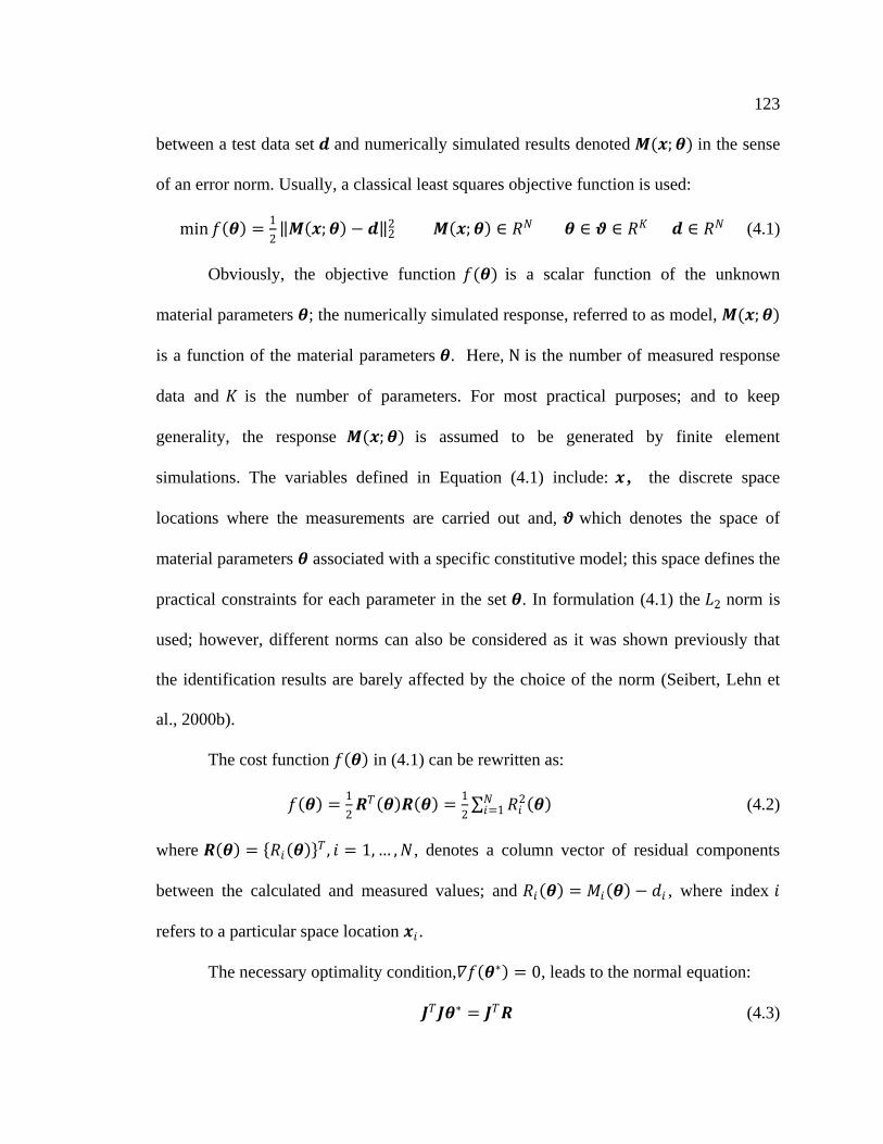
123

between a test data set 𝒅 and numerically simulated results denoted 𝑴(𝒙;𝜽) in the sense

of an error norm. Usually, a classical least squares objective function is used:

min 𝑓 𝜽 =1

2 𝑴 𝒙;𝜽 − 𝒅 2

2 𝑴 𝒙;𝜽 ∈ 𝑅𝑁 𝜽 ∈ 𝝑 ∈ 𝑅𝐾 𝒅 ∈ 𝑅𝑁 (4.1)

Obviously, the objective function 𝑓(𝜽) is a scalar function of the unknown

material parameters 𝜽; the numerically simulated response, referred to as model, 𝑴(𝒙;𝜽)

is a function of the material parameters 𝜽. Here, N is the number of measured response

data and 𝐾 is the number of parameters. For most practical purposes; and to keep

generality, the response 𝑴(𝒙;𝜽) is assumed to be generated by finite element

simulations. The variables defined in Equation (4.1) include: 𝒙 , the discrete space

locations where the measurements are carried out and, 𝝑 which denotes the space of

material parameters 𝜽 associated with a specific constitutive model; this space defines the

practical constraints for each parameter in the set 𝜽. In formulation (4.1) the 𝐿2 norm is

used; however, different norms can also be considered as it was shown previously that

the identification results are barely affected by the choice of the norm (Seibert, Lehn et

al., 2000b).

The cost function 𝑓 𝜽 in (4.1) can be rewritten as:

𝑓 𝜽 =1

2𝑹𝑇 𝜽 𝑹 𝜽 =

1

2 𝑅𝑖

2 𝜽 𝑁𝑖=1 (4.2)

where 𝑹 𝜽 = 𝑅𝑖 𝜽 𝑇 , 𝑖 = 1,… ,𝑁, denotes a column vector of residual components

between the calculated and measured values; and 𝑅𝑖 𝜽 = 𝑀𝑖 𝜽 − 𝑑𝑖 , where index 𝑖

refers to a particular space location 𝒙𝑖 .

The necessary optimality condition,𝛻𝑓 𝜽∗ = 0, leads to the normal equation:

𝑱𝑇𝑱𝜽∗ = 𝑱𝑇𝑹 (4.3)

124

where 𝑱 denotes the Jacobian matrix of the residuals with respect to the parameters; that

is:

𝐽𝑖𝑗 =𝜕𝑅𝑖

𝜕𝜃𝑗 (4.4)

If the model mapping 𝑴(𝒙;𝜽) is linear, this normal equation leads to a direct

solution of the unknown parameters 𝜽. In general, the mapping is implicit and nonlinear;

therefore, an iterative procedure needs to be used.

Without loss of generality, the problem expressed by Equation (4.1) can be

considered as finite element model updating through minimization of the cost function

defined in (4.2). This general formulation is flexible as different types of experimental

data can be combined. For example, DIC data and load-displacement data can be

combined and input together, or DIC data at different loading stages and/or under

different loading configurations can be defined as an input ensemble. In the present

work, we used DIC measurements as input, but the solution methodology can be

generalized to data acquired with different measurement techniques.

In practice, the data 𝒅 is unavoidably affected by measurement errors, and a

weight can be applied to be cost function. Theoretically, the ideal weight used should be

the inverse of the covariance matrix of the observed data. In the current study, we

assumed that the noise from different sources of error is independent and identically

distributed; the cost function with these ideal weights can be expressed as:

𝑓 𝜽 =1

2

𝑅𝑖2 𝜽

𝜎𝑖2

𝑁𝑖=1 (4.5)

where 𝜎𝑖2 is the expected error variance of measurement data 𝑑𝑖 . Thus, the least squares

estimate is identical to the maximum likelihood one.

125

From examination of currently available optimization algorithms, one may

distinguish between schemes that make use of the gradient of the objective function, and

those that do not rely on gradient estimations. Most of the existing mixed numerical-

experimental approaches use gradient-based optimization methods, and the gradient is

generally derived analytically using either direct differentiation or adjoint formulation

techniques, or calculated numerically using finite difference. An iterative method is

adopted along with the gradient information to solve the nonlinear least-squares problem

(Kreißig, Benedix et al., 2007) (Mahnken, 2004) (Springmann and Kühhorn, 2009).

In this study, direct optimization methods were preferred to solve the least squares

identification problem expressed by Equation (4.2). Note that the terms direct search,

derivative-free search, and zero-th order search are sometimes used interchangeably in

the literature. According to Conn et al, for state-of-the-art research and development,

derivative-free optimization methods are best for dealing with noisy data; the

performance of these methods is notably better than gradient-based methods using finite

difference approximations, especially in cases of noisy data (Conn, Scheinberg et al.,

2009).

Powell (1964) originally proposed a derivative-free version of the nonlinear

conjugate gradient method consisting of the construction of a sequence of at most 𝐾 +

1 one-dimensional searches (𝐾 being the number of unknown parameters); each one-

dimensional search is conducted by finding the exact minimum of a quadratic interpolant

(Powell, 1964). The interpolant used in Powell‘s method is similar to the response

surface methodology (RSM) in stochastic optimization.

126

In Monte Carlo analyses, model parameters simulate real world conditions by

varying randomly, whereas response surface methodology combines global and local

analyses to create a simple mathematical equation of the complex and implicit

relationship between different factors.

In the last twenty years, with the exception of a few heuristic-based searches and

cluster-based random searches, direct optimization algorithms developed extensively

primarily due to the efficient use of response surface exploration in combination with

different efficient optimization, line-search and trust-region algorithms. Recently,

considerable research progress in code development of derivative-free Newton-based

methods has taken place, including DFO (Conn, Scheinberg et al., 1997), Powell‘s

UOBYQA (Powell, 2002), CONDOR (Berghen, 2004) (Berghen and Bersini, 2005), and

NEWUOA (Powell, 2006).

Berghen developed CONDOR (COnstrained, Non-linear, Direct, parallel

Optimization using trust Region method for high-computing load function) for expensive

optimizations, such as objective functions evaluated from the output of nonlinear FEA or

Computational Fluid Dynamics (CFD) simulations. CONDOR was designed mainly for

unconstrained optimization problems and for easy (box) constraints. The algorithms in

CONDOR are based on a derivative-free trust region method using a surrogate model that

approximates the objective function by a quadratic polynomial, which is then minimized

by sequential quadratic programming (SQP). Descent conditions from trust region

methods enforce convergence properties. CONDOR has been compared to DFO (Ugur,

Karasozen et al., 2008) and genetic algorithms (Harth, Sun et al., 2007) in designs

involving flow problems, and its performance was found to be better.

127

In the present study, the CONDOR method was used to minimize the least

squares cost function and to obtain the list of unknown parameters. For comparison, we

also used the original Nelder-Mead simplex method, a pseudo-Newton method based on

finite difference derivatives, and a response surface method to illustrate the superiority of

a derivative-free algorithm in the context of parameter identification.

The use of derivative-free optimization methods provides the level of generality

and modularity necessary for the optimization tool if the objective is to use the finite

element code as a black box. Some of the modern derivative-free methods are considered

globally convergent, since they include techniques such as line-search, reinforcing good

geometry and trust region, thus ensuring a global optimum. Note, however, that because

of the lack of rigorous convergence properties of derivative-free methods, the solutions

must be considered local. One simple way to address this issue is to vary the starting

point and the trust region radius to validate the final optimal solution.

In summary, for the solution of the optimization problem, the following

recommendations are made:

Use justification to give box-constraints to define the acceptable search

region.

If possible, have more than one method to solve the problem.

Start from several different starting points.

4.6 Overview and selection of optimization techniques

The material parameter identification requires the solution of a nonlinear

optimization problem:

128

minimize 𝑓 𝜽 ; 𝜽 ∈ 𝑅𝐾

𝑠. 𝑡. 𝜃𝑖 ∈ 𝜃𝑖𝑙 ,𝜃𝑖

𝑢 , 𝑖 = 1,…𝐾

where 𝜽 ∈ 𝑅𝐾 is the vector of unknown parameters, and 𝜽𝑙 and 𝜽𝑢 are vectors of lower

and upper bounds, respectively. Comparing to the general nonlinear optimization

problem, there is no present of equality and inequality constraints.

The major concern is that the evaluation of 𝑓 𝜽 is computationally expensive.

This fact rules out the application of stochastic optimization methods, such as

evolutionary algorithms and other heuristic-based global optimization methods.

Intuitively, the most straightforward way to tackle the computational cost issue is to use a

strategy that employs computationally cheap surrogate models for the objective to solve

an approximation to 𝑓 𝜽 . Surrogate-assisted search algorithms are the choice.

They can be classified into zero-order methods, first order-methods, and second-

order methods. The zero-order methods use only the objective function values to

determine the optimum values. The first-order methods use the objective function and the

gradient of the objective function to construct search directions during iterations. The

second-order methods use second-derivatives (Hessian) to construct the search directions.

Nonlinear least squares problems can be solved in two ways: 1) as nonlinear least

squares optimization problems or 2) as PDE-constrained optimization problems. In this

study, only the first category of these solutions is considered. Various numerical solution

methods for optimization problems are available. For example, one may distinguish

schemes by whether or not the solution uses gradients of the objective function. In

general, published accounts describing mixed-numerical-experimental approaches used

129

gradient-based optimization methods. Usually formulas to evaluate a gradient were

derived analytically, and an iterative method was adopted along with the gradient

information to solve the nonlinear least-squares problem (Kreißig, Benedix et al., 2007)

(Mahnken, 2004) (Springmann and Kühhorn, 2009). The most frequently used iterative

approaches for solving nonlinear least-square problems include the pseudo-Newton

methods, such as the Gauss-Newton method or the BFGS method, and trust region

methods, such as the Levenberg-Marquardt method. In these approaches, the Hessian

𝛻2𝑓(𝜽) is not required, which is a great advantage over complete Newton methods since

derivation of analytical Hessian is more complicated than analytical gradients. A

summary of the fundamental aspects of gradient-based methods for solving the

optimization problem follows.

The iterative schemes can be expressed as:

𝜽𝑘+1 = 𝜽𝑘 − 𝛼𝑗𝑯𝑗∇𝑓 𝜽𝑗 (4.6)

where 𝛼𝑗 is the step size at the 𝑘𝑡𝑕 iteration and 𝑯𝑘 is the pseudo-Newton iteration

matrix at the 𝑘𝑡𝑕 iteration.

The pseudo-Newtonian iteration matrices defined for each method are:

Method 𝑯

Gauss-Newton 𝑱𝑇𝑱 −1

Levenberg-Marquardt 𝑱𝑻𝑱 + 𝛾𝑰 −1

BFGS 𝑯(𝑯𝑗−1 ,∇𝑓,𝜽)

130

Gradient methods are efficient and often require fewer forward simulations. In

the case of practical applications where the data are associated with noise, the

convergence rate of gradient-based methods depends closely on the initial estimate of the

parameters. Apart from the problem of local minimum, the major difficulty in using

gradient-based methods lies in the implementation of gradient-evaluation procedures.

These are tedious and require a great deal of additional effort in addition to the FE

analysis. Furthermore, users generally do not have access to commercial codes; this

prevents users of complex commercial numerical analysis programs from obtaining

reliable derivative information for the requested numerical analysis. Another hindrance

is that the evaluation of gradients can vary for different material models, element types,

deformation levels, integration schemes, or even the type of response data.

In the FE model updating and material identification literature, gradient

evaluations are often referred to as sensitivity analyses. A sensitivity analysis using DIC-

measured surface strains was reported by (Cooreman, Lecompte et al., 2007). This

particular analysis applies only to simple tensile tests, however, and since the return-

mapping scheme was considered in the derivation, it cannot be directly applied to FE

programs using other schemes, such as the effective stress integration scheme in ADINA

(ADINA). Some researchers have used finite difference approximation of the gradients

as an alternative (Meuwissen, 1998) (Meuwissen, Oomens et al., 1998) (Haber, Tortorelli

et al., 1993) (Springmann and Kuna, 2003) (Ghouati and Gelin, 2001), but this approach

is considered unreliable, especially when the noise in the experimental data is not

negligible (Springmann and Kuna, 2003) (Ghouati and Gelin, 2001) (Fraś, Nowak et al.,

131

2011). Of course, the poor reputation of this method may stem from the fact that its

simplicity is not persuasive for application to scholarly research.

Gradient methods are more efficient, and require fewer forward simulations. On

the other hand, they are local methods; if the objective function is multi-modal (the multi-

modality can be essential or caused by noise in the data), convergence is highly

dependent on the initial estimates of the parameters. A local minimum solution is easily

found; a global minimum may be found using multiple initial guesses.

There are also a variety of direct search methods based on heuristics, which are

often without theoretical justification; these include random search, evolutionary

algorithms, and taboo search. The most significant advantage of these methods is that

they are generally global; however, they are also often slow. In other words, these

methods are ‗slow, but sure‘. Simulated annealing and genetic algorithms are among the

leading candidates for global optimization applications. Nevertheless, these methods are

also problem-specific, and require user-intervention and learning. Consequently, standard

implementation of these methods has yet to coalesce. The cluster-oriented controlled

random search method proposed by Price (Price, 1983) was used by (Harth and Lehn,

2007) to identify material parameters in Chaboche‘s viscoplastic model for solution of an

error minimization problem with data from homogeneous tension/compression tests and

creep tests. Since the strain was homogeneous, the model was an ODE model solved

using Runge-Kutta methods. The random search direct method requires extensive

forward simulations, but is affordable for ODE models. However, if an FE model is used,

and the model is geometrically complicated and nonlinear, the random search will

become unaffordable with current computational resources.

132

In this paper, direct optimization methods are used to solve the least square

identification problem. The phrase ―direct search‖ was coined by Hooke and Jeeves in

(Hooke and Jeeves, 1961); they proposed a pattern search method based on heuristics.

The terms direct search, derivative-free search, and zero-th order search are sometimes

used interchangeably, especially in finite element design software. There is no unanimity

among researchers in their use of these terms. This is of no great consequence in practice,

and to some extent simply reflects historical developments.

Conn et al. defined derivative-free methods as ―methods without explicit

approximation to derivatives of objective or constraints‖ (Conn, Scheinberg et al., 2009).

However, optimization with finite difference derivatives is excluded from Conn et al.‘s

definition, and in our study, ―derivative-free‖ means any method that treats the FEA

forward solution as a black box. In this way, finite difference gradient-based pseudo-

Newtonian methods can also be considered as derivative-free. Under this condition, the

requirements from a user are minimal, since the simulation code is used in the manner of

a black-box. According to (Conn, Scheinberg et al., 2009), with current state-of-the-art

derivative-free optimization methods one can expect to successfully address problems:

1) which do not possess more than 100 variables, 2) problems which are reasonably

smooth, and 3) problems in which the evaluation of the function is expensive and

computed with noise.

There are four main classes of methods for designing a derivative-free method:

I. Coordinate search: these methods are slow, robust and capable of handling

noise. The HYPERSTUDY/HYPERWORK program implemented a

133

simple version of this type of method, which is called ―alternative-

direction method‖ in the menu.

II. Nelder-Mean simplex method: the most popular method, but is not robust

or reliable in some cases. The MATLAB program implemented an

original version of this method in the Optimization toolbox (Nelder and

Mead, 1965).

III. Implicit filtering algorithm: a line-search algorithm that imposes sufficient

decrease along a quasi-Newton direction. The main difference from

derivative-based methods is that the true gradient is replaced by the

simplex gradient; so, this method resembles to some extent a pseudo-

Newton method using finite difference approximation to gradients. This

implementation of pseudo-Newton methods is deemed by Kelley to be

particularly well-equipped to handle noisy functions since there is implicit

filtering of noise due to the use of the simplex gradient corresponding to

the gradient of a regression model and to an inaccurate line-search (Kelley,

1999). To our knowledge, this class of methods has not been implemented

in any FE/design software.

IV. Interpolation-based trust region approach: trust region-based algorithms in

which interpolation models are built from polynomial interpolation or

regression. The interpolation is often called response surface and the term

―response surface method‖ is frequently used in FEA and engineering

design software (e.g. ANSYS includes several response surface methods).

However, in the derivative-free optimization literature, the term ―response

134

surface‖ is rarely used, and is generally reserved for experimental design

and stochastic optimization.

Most recent progress in derivative-free optimization has focused on the fourth of

these method categories. Powell‘s celebrated method (1964) is a derivative-free version

of the nonlinear conjugate gradient method. It consists in each stage of a sequence of

𝐾 + 1 one-dimensional searches, and each one-dimensional search is conducted by

finding the exact minimization of a quadratic interpolant. This method is thus a first-

order method with a Q-property. The interpolant used in Powell‘s method is actually the

response surface methodology from stochastic optimization. Response surface is the idea

that if the function evaluation is exact, one can use finite difference to approximate the

derivative. If the function evaluation is uncertain, however, one can design an

appropriate experiment and perform a regression analysis to obtain a surrogate of the

original function, and thus estimate the derivative and update the search directions.

Powell‘s work has spawned considerable research and code development of

derivative-free Newtonian-based methods, including DFO (Conn, Scheinberg et al.,

1997), Powell‘s UOBYQA (Powell, 2002), and CONDOR (Berghen, 2004) (Berghen and

Bersini, 2005), and recently, NEWUOA (Powell, 2006). Conn et al. (1997) constructed

a multivariate DFO algorithm that uses a surrogate model for the objective function

within a trust region method. In that work, points were sampled to obtain a well-defined

quadratic interpolation model, and descent conditions from trust region methods enforced

convergence properties. The trust region method can be used to globalize Newton-based

methods and to avoid most of the local instability within Newton-based methods. The

CONDOR method for high-computing load function developed by Berghen, is based on

135

the UOBYQA of Powell, and was developed mainly for unconstrained optimization

problems and for easy (box) constraints. The algorithms are based on a derivative-free

trust region method approximating the objective function by a quadratic polynomial,

which is then minimized by a sequential quadratic programming (SQP) method. This

method was developed for expensive optimizations, such as objective functions evaluated

from the output of nonlinear FE or CFD simulations, and is based on the assumption that

the function evaluation is time-consuming. Details of this method can be found in

(Berghen, 2004) (Berghen and Bersini, 2005). DFO was applied as a black-box

optimization routine in optimizing energy systems (Lee, Terlaky et al., 2001) and for

helicopter rotor blade design (Scheinberg, 2000). Numerical tests in both of these reports

show that DFO is faster and more accurate than derivative-based methods such as the

quasi-Newton methods. However, CONDOR was also compared to DFO (Ugur,

Karasozen et al., 2008) and genetic algorithms (Harth, Sun et al., 2007) in designs

involving flow problems, and its performance was found to be better. Several derivative-

free methods are available in software or freeware; (Conn, Scheinberg et al., 2009) list a

collection of freely-available derivative-free programs.

The present study used the CONDOR method to minimize the least squares cost

function and to obtain the requested list of parameters. As mentioned above, this method

is a trust region method combined with response surface technique that finds the

minimum 𝒙∗ ∈ 𝑅𝑛 of an objective function 𝐹(𝒙) ∈ 𝑅. For the purpose of comparison,

the original Nelder-Mead simplex method, a pseudo-Newtonian method based on the

finite difference derivative, and a response surface method in ANSYS were also used in

this study. The use of derivative-free optimization methods provides generality and

136

modularity to the approach considered here. One advantageous by-product of this

approach is that direct methods are usually more robust and more global than their

derivative-counterparts.

4.7 Statistical inference with DIC data

Estimating the level of uncertainty associated with the identification of the

parameters is a new trend in material testing. It is good practice in any measurement to

evaluate and report the uncertainty associated with the test results. A customer who

wishes to know the limits within which the reported result may be assumed to lie may

require a statement of uncertainty, or the test laboratory itself may wish to develop a

better understanding of which particular aspects of the test procedure have the greatest

effect on results so that this may be monitored more closely. A Code of Practice (CoP)

was developed by UNCERT (a project funded by the European Commission‘s Standards,

Measurement and Testing programme under reference SMT4-CT97-2165) to simplify the

way in which uncertainties are evaluated. This CoP is one of seventeen produced by the

UNCERT consortium for the estimation of uncertainties associated with mechanical tests

on metallic materials.

The inverse identification process outlined in Section 4.4 can be interpreted as a

statistical parameter estimator using nonlinear regression. Statistical inference can then

be employed to study the reliability of the identification and to provide a measure of

quality. In using statistical inference, the material parameters set 𝜽 are considered

random variables, so their accuracy is related to the shape of the probability distribution

function. Generally, accuracy is defined in terms of a confidence region for the

137

parameter vector, or as the confidence interval of its components. A 100(1-α )%

confidence region is a region of parameter space that contains the real parameters with a

probability of 1-α, where 1-α is the confidence level of this particular region.

In deterministic inverse problem formulation, 𝑴(𝜽) is called the model; in

statistical inverse problem formulation of nonlinear regression, it is called the expectation

function. In nonlinear regression inference, the success of the identification can be

checked by two measures: (i) expectation function fit and (ii) parameter fit. If a model

gives a smaller residual in the response function, and/or a smaller confidence region in

the expectation function and response function, the model is said to be

phenomenologically better (i.e., the model parameter set yields a better description of the

model‘s behaviour).

The most accurate way to perform the statistical analysis is through Monte Carlo

(MC) methods. The Monte Carlo method has been used to validate the linearized

covariance analysis (LCA) for nonlinear parameter estimation problems (Grimstad,

Kolltveit et al., 2001). However, this method requires the solution of a large number of

related parameter identification problems. Considering the complex geometry and

nonlinearity involved in the identification of plasticity models, the Monte Carlo approach

is not feasible for the present study.

4.7.1 Nonlinear regression inference using linear approximation

From a statistical perspective, the identification of constitutive laws using full-

field measurements can be considered as a problem where the sample is essentially the

complete population. The LCA method is the most computationally efficient method and

138

the most used one. It was shown previously that, for normally distributed errors, LCA is

equivalent to the likelihood method (Uusipaikka, 2009) (Seber and Wild, 2005).

The covariance matrix 𝑷 of the model parameters can be approximated from the

linearization of the cost function 𝑓(𝜽) around the solution 𝜽 :

𝑓 𝜽 ≅ 𝑓 𝜽 + 𝑱 𝜽 (𝜽 − 𝜽 ) (4.6)

where 𝑱 𝜽 is the Jacobian of the cost function 𝑓(𝜽) evaluated at the solution 𝜽 . The

matrix 𝑷 is then given by:

𝑷 = cov 𝜽 ≅ s2 𝑱T 𝜽 𝑱 𝜽 −1

(4.7)

Recalling expansion (2), the residual mean square estimate, 𝑠2 , is given as

follows:

𝜎2 ≅ 𝑠2 =𝑹𝑇 𝜽 𝑹 𝜽

𝑁−𝐾 (4.8)

where 𝑁 is the sample size and 𝐾 is the number of parameters.

The associated correlation matrix is defined as:

𝐶𝑖𝑗 =𝑃𝑖𝑗

𝑃𝑖𝑖𝑃𝑗𝑗 (4.9)

The off-diagonal elements of the 𝐶𝑖𝑗 matrix represent the correlation between two

parameters 𝜃𝑖 and 𝜃𝑗 . A strong correlation often indicates over-parameterization due to

either a fault or true redundancy within the model. The diagonal elements of the

covariance matrix 𝑷 represent the estimated values of the variances of the parameters 𝜃𝑗 .

𝜎𝜃𝑗2 ≅ 𝑃𝑗𝑗 (4.10)

which is a measure of confidence for the identified parameters 𝜃𝑗 .

The 100 1 − 𝛼 % joint confidence region is an ellipsoid and can be defined as:

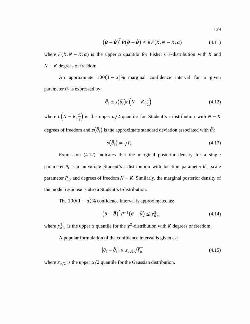
139

𝜽 − 𝜽 𝑇𝑷 𝜽 − 𝜽 ≤ 𝐾𝐹(𝐾,𝑁 − 𝐾;𝛼) (4.11)

where 𝐹(𝐾,𝑁 − 𝐾;𝛼) is the upper 𝛼 quantile for Fisher‘s F-distribution with 𝐾 and

𝑁 − 𝐾 degrees of freedom.

An approximate 100 1 − 𝛼 % marginal confidence interval for a given

parameter 𝜃𝑖 is expressed by:

𝜃 𝑖 ± 𝑠 𝜃 𝑖 𝑡 𝑁 − 𝐾;𝛼

2 (4.12)

where 𝑡 𝑁 − 𝐾;𝛼

2 is the upper 𝛼/2 quantile for Student‘s t-distribution with 𝑁 − 𝐾

degrees of freedom and 𝑠 𝜃 𝑖 is the approximate standard deviation associated with 𝜃 𝑖 :

𝑠 𝜃 𝑖 = 𝑃𝑖𝑖 (4.13)

Expression (4.12) indicates that the marginal posterior density for a single

parameter 𝜃𝑖 is a univariate Student‘s t-distribution with location parameter 𝜃 𝑖 , scale

parameter 𝑃𝑖𝑖 , and degrees of freedom 𝑁 − 𝐾. Similarly, the marginal posterior density of

the model response is also a Student‘s t-distribution.

The 100 1 − 𝛼 % confidence interval is approximated as:

𝜃 − 𝜃 𝑇𝑃−1 𝜃 − 𝜃 ≤ 𝜒𝐾,𝛼

2 (4.14)

where 𝜒𝐾,𝛼2 is the upper 𝛼 quantile for the 𝜒2-distribution with 𝐾 degrees of freedom.

A popular formulation of the confidence interval is given as:

𝜃𝑖 − 𝜃 𝑖 ≤ 𝑧𝛼/2 𝑃𝑖𝑖 (4.15)

where 𝑧𝛼/2 is the upper 𝛼/2 quantile for the Gaussian distribution.

140

If the model-data combination is not highly nonlinear, the minimum of the

paraboloid approximation is close to the minimum of the true cost function, and the

inference can be considered reliable.

The LCA-based inference can also be used in other ways, including model

selection and design of experiments (DOE); this is best achieved through Bayesian

inference. The Bayesian marginal posterior density for material parameters 𝜽 (Seber and

Wild, 2005) is formulated as:

𝑝 𝜽 𝒅 ∝ 1 + 𝜽−𝜽

𝑇𝑷−1 𝜽−𝜽

𝑁−𝐾 −𝑁/2

(4.16)

This probability distribution is in the form of a 𝐾-variate Student‘s t-density with

location parameter 𝜽 , scaling matrix 𝑷 , and 𝑁 − 𝐾 degrees of freedom. If a non-

informative prior density for 𝜽 is assumed, the Bayesian identification and Bayesian

inference will be identical to the results based on sampling theory given above.

Bayesian inference possesses a great advantage because prior information can be

naturally incorporated into the identification process, and model selection is also

convenient (Koch, 2007). However, this aspect is for the focus of future work, and will

not be addressed in this thesis.

4.7.2 Calculation of Sensitivity

The sensitivity of the response function is required in the LCA inference, the

expectation fit check, and the calculation of curvature measures; the gradient is obtained

by finite differentiation. While the cost function involves non-negligible errors

associated with the measurement data, the response function is evaluated using the

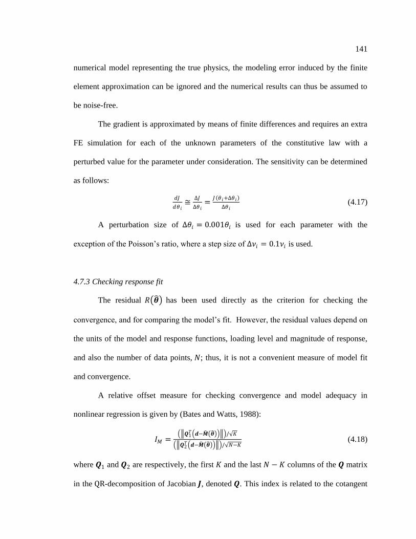
141

numerical model representing the true physics, the modeling error induced by the finite

element approximation can be ignored and the numerical results can thus be assumed to

be noise-free.

The gradient is approximated by means of finite differences and requires an extra

FE simulation for each of the unknown parameters of the constitutive law with a

perturbed value for the parameter under consideration. The sensitivity can be determined

as follows:

𝑑𝐽

𝑑𝜃𝑖≅

∆𝐽

∆𝜃𝑖=

𝐽 𝜃𝑖+∆𝜃𝑖

∆𝜃𝑖 (4.17)

A perturbation size of ∆𝜃𝑖 = 0.001𝜃𝑖 is used for each parameter with the

exception of the Poisson‘s ratio, where a step size of ∆𝜈𝑖 = 0.1𝜈𝑖 is used.

4.7.3 Checking response fit

The residual 𝑅 𝜽 has been used directly as the criterion for checking the

convergence, and for comparing the model‘s fit. However, the residual values depend on

the units of the model and response functions, loading level and magnitude of response,

and also the number of data points, 𝑁; thus, it is not a convenient measure of model fit

and convergence.

A relative offset measure for checking convergence and model adequacy in

nonlinear regression is given by (Bates and Watts, 1988):

𝐼𝑀 = 𝑸1

𝑇 𝒅−𝑴 𝜽 / 𝐾

𝑸2𝑇 𝒅−𝑴 𝜽 / 𝑁−𝐾

(4.18)

where 𝑸1 and 𝑸2 are respectively, the first 𝐾 and the last 𝑁 − 𝐾 columns of the 𝑸 matrix

in the QR-decomposition of Jacobian 𝑱, denoted 𝑸. This index is related to the cotangent

142

of the angle that the residual vector makes with the tangent plane, so that a small relative

offset corresponds to an angle near 90𝑜 , and validates the model‘s accuracy. Bates and

Watts suggested the use of the criterion 𝐼𝑀<=0.001, reasoning that any inference will not

be affected because the current parameter vector is less that 0.1% of the radius of the

confidence region disk from the least squares point (Bates and Watts, 1988). Considering

that the Jacobian is evaluated using finite difference in the present work, the criterion

𝐼𝑀 < 0.01 is used to check response fit.

4.8 Identifiability issues

4.8.1 General

One of the fundamental problems in any inverse analysis is the justification and

assessment of the credibility of inversely identified results. The difficulty inherent in the

substantiation of a specific material identification problem is that without reference

values for comparison, how can we trust the identified material model parameters,

especially for in-situ determination of material properties where no ―reference‖ for

parameter values exists?

The principle that the parameters in a model can be consistently estimated is often

referred to as the identifiability of a model (Hsia, 1977). Identifiability is necessary to

draw consistent statistical inferences. The problem of identifiability and the stability of

numerical results are examined in this section; scepticism is the attitude we take in

addressing this issue.

143

4.8.2 Ill-posed or well-posed

The definition of well-posed problems given by Hadamard refers to the existence,

uniqueness and stability of solutions to differential equations (Tikhonov and Arsenin,

1977). Thus, in the case of inverse problems, the concept of well-posedness is related to

the existence and uniqueness of the solution to an inverse problem; the data must be

sufficient (i.e. contain enough information for simultaneous determination of all the

unknown parameters), and the global optimal must be unique and stable when there is

noise in the data.

The problem of material parameter identification has been described as ill-posed

(Mahnken, 2004); in practice, however, the material parameter identification problem

must be well-posed, with a few specific exceptions, such as the non-uniqueness of

parameters in the creep test for viscoplasticity (Seibert, Lehn et al., 2000a) (This

particular model is phenomenological, and is a summation of an arbitrary number of

Dirichrit-Prony exponentials chosen by the user). One indicator of ill-posedness is the

need for regularization. There should not be any regularization terms in the least square

objective function (4.1) for an unbiased solution of material parameters. In general, the

number 𝑁 of samples of experimental data has to be much larger than the number 𝐾 of

parameters; when these conditions are met, the resulting material parameter identification

problem is usually a well-posed problem.

Essentially, whether the problem is ill-posed or well-posed lies in whether the

problem is a function parameter identification problem or a functional identification

problem (i.e. problem of identification of a parameterized continuous field). The problem

outlined in Chapter 3 is indeed ill-posed, since it is a parameterized functional

144

identification problem. Functional identification problems are affluent in geophysical

and medical tomography (Snieder and Trampert, 1999). In functional identification

problems, whether the forward problem is represented as a linear system 𝑨𝒎 = 𝒅 or a

nonlinear system 𝑨 𝒎 = 𝒅 , where 𝑨 defines a nonlinear operator, it is ill-posed if the

information contained in data 𝒅 alone cannot guarantee a unique and stable solution of

model parameters 𝒎.

4.8.3 Model and parameter identifiability

Katafygiotis and Beck (1998) made a distinction between ―model identifiability‖

and ―parameter identifiability‖ (Katafygiotis and Beck, 1998). The former has also been

called ―structural identifiability‖ (Cobelli and DiStefano, 1980; Hof, 1998). The model

identification problem is to find all of the structural models within a specified model class

that are able to produce the same output within a set of observed degrees of freedom

when the models are all subjected to the same input. However, in our material parameter

identification problem, the model is selected via the judgement of the engineer, not

through the identification process; thus, we need only focus on the parameter

identifiability issue.

4.8.4 Verification and validation (V&V)

The assessment of the credibility of a numerical procedure is typically called

verification and validation (V&V), and is closely connected to the problem of

identifiability. The verification process can be defined as verification of the model

response obtained from data, and the validation process as the comparison of the model

145

response with data that was not used in the identification. In the professional literature,

verification is usually defined as the process of assessing software correctness and the

numerical accuracy of the solution to a given model; validation is the process of assessing

the physical accuracy of a model (ASME, 2006).

A more straightforward definition of V&V is that verification is ―solving the

equations right‖, and validation is ―solving the right equations‖ (Oberkampf and Roy,

2010). In material identification, verification can be defined as the correct solution of the

inverse problem (i.e. the global optimal of the multi-modal LS objective function is

determined), and validation is that the problem is defined correctly (i.e. the data contain

enough information, the global optimum is unique, and the FE model (mesh, element

type, boundary conditions, etc.) represents the reality well, so that the nonlinear

regression model (data-model set) is correctly defined).

Thus, V&V can be described as the process of providing evidence of the

correctness and accuracy of the parameter identification results; V&V procedures are

founded on the concept of quantitative accuracy assessment. While V&V do not entirely

answer the question of identification credibility, they are the keys to establishing

credibility. Traditionally, one needs to have accurate benchmarks or reference values for

comparison. Reference values are not generally available for complex material model

parameters, however, especially for individual components. For this reason, numerical

studies and statistical tools are used to assess uncertainty during V&V of the inverse

identification process.

In material parameter identification, V&V is concerned with two issues: (i) to

verify that the solution is a global optimum; and (ii) to validate the global optimum by

146

ensuring that it corresponds to a set of parameters that are similar enough to the correct

values. When using local optimization methods, techniques based on the re-identification

of the parameters using different initial solutions is widely used to verify that the

optimum is a global solution. Although derivative-free methods, such as CONDOR, are

considered to be robust and globally convergent, the use of multiple-initial estimates is

still recommended for V&V. Alternatively, re-identification of the parameters using

synthetic data can also serve as a verification tool for assessing the identifiability of a

given experimental/estimation solution.

4.8.5 Quality and nature of information from data

Besides the problem of local minimum, the quality and nature of the available

data also needs to be considered carefully. There are two causes for unsuccessful

identifications: (i) the minimization process leads to a local minimum; and/or (ii) the data

are insufficient. For example, the parameters of the Rousselier damage mechanics model

were identified by updating a FE model to match a simulated 2D displacement field on a

tensile specimen using synthetic data at every FE node (Springmann and Kuna, 2003). If

only one material parameter was under consideration, the identification was successful;

however, simultaneous updating of two or more parameters was less successful because,

in some cases, only a local optimum could be found. One possible reason for

unsuccessful identification may be due to the fact that the information contained in the

collected data is insufficient for simultaneous updating of all of the parameters.

The nature of the data can lead to over-parameterization; i.e. when one or more of

the mechanical properties associated with the parameters are not activated during the

147

experiment. For example, if, when attempting the identification of a hardening law in an

elasto-plastic constitutive model, the material remains largely in the elastic range under a

given load. In the case of DIC, the large amount of data with an elastic nature may

overwhelm the small fraction of data in the plastic range. This situation is called fault

redundancy induced within the experiment.

A quantitative approach to determining identifiability is based on Fisher

information; a parameter vector is identifiable from a particular set of observed responses

if the associated Fisher information matrix is nonsingular (Bos, 2007). The Fisher

information is related to the sensitivity of the Jacobian with respect to parameters.

𝐹𝜃 = 𝐸 𝑺𝜽𝑺𝜽𝑻 = 𝐸

𝜕𝑞(𝒘;𝜽)

𝜕𝜽

𝜕𝑞(𝒘;𝜽)

𝜕𝜽𝑇

is the Fisher information matrix of the observed data d , where q(𝐰;𝛉) is the log-

probability density function of the response, and 𝐒θ is the Fisher score vector. The Fisher

score and Fisher information are connected to the sensitivities of the response to the

unknown parameters.

However, local sensitivity at a single point may not be sufficient; the singularity

of Fisher information not only depends on the local sensitivity at a point in parameter

space, but also depends on the global sensitivity in a finite region. Global sensitivity

analysis techniques deal with the entire range of variation of the input parameters.

Sensitivity analysis allows one to study the relationships of response variances and

parameter variances, and to identify adequacies in the numerical-experimental setting. In

particular, global sensitivity analysis allows analysts to perform model calibration, model

validation, and decision making; i.e. global sensitivity analysis enables any process where

148

it is useful to know which of the variables contribute most to the variability of the output.

One should note that while sensitivity analysis quantifies the influence of the input

parameters on the model‘s response, uncertainty analysis is used to evaluate statistical

parameters, confidence intervals and probability laws for the model‘s responses.

Thus, inadequacy and faulty parameter redundancy due to the quality and nature

of the data can be detected through global sensitivity analysis and/or statistical inference

(Patelli, Pradlwarter et al., to appear) (Saltelli, Ratto et al., 2008).

4.8.6 Curvature measure of nonlinearity: checking the adequacy of linearized covariance

analysis (LCA)

Uncertainty quantification is an important aspect of V&V. Linearized covariance

analysis (LCA) is used to check the fit of parameters, and provides a quantitative measure

of uncertainty. LCA is an approximation of a nonlinear problem. Whether this

approximation is valid, and produces results that are adequate is addressed in this section

by adopting an attitude of scepticism.

The most reliable check of the adequacy of LCA is through the use of Monte

Carlo analyses. However, as noted previously, the research presented here is based on

the assumption that Monte Carlo analyses are not affordable, so curvature measures of

nonlinearity are substituted as an alternative to Monte Carlo techniques in this study.

Curvature measures are able to detect only incorrect results that are false positives (type-

II errors). In other words, it is possible for nonlinearity measures to give a false alarm

indicating a problem with the LCA when the LCA is actually adequate; however,

nonlinearity measures will correctly detect all instances when the LCA is inadequate. In

149

fact, type-I error rarely happens in material testing and parameter identification if sound

judgement is employed; so, focusing on avoidance of type-II error is sufficient for our

purposes.

When deciding whether to reject the null hypothesis that H0: 𝛉 = 𝛉 , there are two

fundamental errors to be identified by inference:

Type-I error: the hypothesis is actually true, but we think it is wrong, i.e.

the LCA is adequate, but we think that there is a problem with the solution.

Type-II error: the hypothesis is actually wrong, but we think it is true, i.e.

the LCA is inadequate, but we think that the solution is correct.

In the context of statistical regression analysis, the cost function 𝑓(𝜽) , is

considered as an expectation function. The noise associated with measurement and

modeling errors is assumed to have spherical normal distribution. The expectation

function can be considered as an N-dimensional response surface. The vector 𝑴(𝒙;𝜽)

defines a 𝐾-dimensional surface, and is called the expectation surface in the response

space. The Least Square estimates thus correspond to a point on the expectation surface

𝑴 = 𝑴 (𝜽 ) , which is the closest point to data vector 𝒅 . For nonlinear models, the

expectation surface is curved and bounded (Green, 1988) (Seber and Wild, 2005).

The LCA involves two distinct approximations (Bates and Watts, 1988):

I. The planar assumption, where the expectation surface 𝑴(𝜽) near 𝑴 (𝜽 ) is

approximated by its tangent plane at 𝑴 (𝜽 ).

II. The uniform coordinate assumption, in which a linear coordinate system

𝐽(𝜽 − 𝜽 ), is imposed to the approximation of tangent plane defined in 1).

150

To validate these two assumptions, one can use the curvature of the expectation

surface at the solution 𝜽 . The curvature of the expectation surface depends on the testing

and simulation procedures, and will also depend on the type and amount of data used in

the identification procedure. For example, an identification based on a load-displacement

curve is expected to produce a higher curvature than a technique using full-field data

from DIC measurements.

In summary, the LCA uses local information to generate a tangent plane with a

linear coordinate system defined by the derivative vectors, projects the residual vector

onto that tangent plane, and then maps the tangent plane coordinates onto the parameter

plane using linear mapping. If we assume that the tangent plane forms a good

approximation to the expectation surface near 𝜽 , then the likelihood region for 𝜽

corresponds to a disk on the tangent plane with a radius proportional to 𝑆(𝜽 ) with

𝑆 𝜽 = 𝑴 𝜽 − 𝒅 2.

While LCA is used to characterize the quality of the estimates using inference

intervals, the adequacy of the LCA can also be checked. The relative curvature measure

enables us to assess the intrinsic and parameter-effects (PE) nonlinearity, and the validity

of LCA inference. The LCA method is based on the linearization of the model function

at a given point; it is of fundamental importance therefore, to verify the validity of the

LCA. An accurate method of assessing the validity of LCA, and the global sensitivity

analysis is with Monte Carlo analysis, but as noted previously, this method is

computationally expensive due to the complex geometry and nonlinearity of the model.

The curvature measures of nonlinearity approach are a potential alternative to the Monte

151

Carlo approach. Curvature measures of nonlinearity are approximations, but are

considerably less expensive to compute. In this study, the curvature measures are used to

check the validity of LCA inference; as noted previously, this approach can prevent type-

II errors, but not type-I errors. If the LCA is deemed to be adequate, then the validity is

assured; on the other hand, if the curvature measures of nonlinearity indicate that the

LCA is inadequate, it does not necessarily follow that the LCA inference is wrong.

Bates and Watts (1980) employed differential geometry to construct a relative

intrinsic and a parameter-effects curvature measure, which provide global measures of

nonlinearity of the model (Bates and Watts, 1980). Threshold values for curvature

measures of nonlinearity have been published for which application of the LCA may be

justified as inadequate, but not necessarily wrong, based on the shape of linearized

confidence regions (Bates and Watts, 1988) (Seber and Wild, 2005) (Grimstad, Kolltveit

et al., 2001) (Haines, O'Brien et al., 2004). Donaldson and Schnabel (Donaldson and

Schnabel, 1987) performed extensive evaluation of LCA predictions for a series of

different nonlinear models using Monte Carlo analyses; the recommended thresholds for

the curvature measures of nonlinearity constructed by Bates and Watts were found to

give good indications as to when the LCA may be insufficient (Donaldson and Schnabel,

1987).

The use of nonlinearity measures to validate LCA, and thus avoid type-II errors,

is proposed in this chapter, but is not implemented in the examples. It is left for future

investigation in which a Monte Carlo analysis can be performed to determine an accurate

threshold for this specific problem, for comparison of the results of LCA, curvature

measures of nonlinearity and Monte Carlo approaches.

152

4.8.7 Summary of procedures addressing the identifiability issue

In summary, the fundamental elements that build credibility into computational

results are: (a) the quality of the physics modeling; (b) V&V activities; (c) uncertainty

quantification; and (d) sensitivity analyses. All four of these elements are necessary to

establish credibility, and none is sufficient in itself. The first element is a pre-

requirement for the estimator. Approaches addressing the latter three can be summarized

as follows:

1) One may try different optimization algorithms (if required) with different

initial values to ensure that the minimization achieves a global minimum.

2) Re-identify the model: perform a numerical study before testing to re-

identify parameters of a given material model. This is the verification

procedure in V&V. This numerical test needs to be based on both

synthetic noise-free data and noise-polluted data to ensure the well-

posedness of the inverse problem defined by the data-optimizer

combination. In other words, not only the existence and uniqueness of

the solution, but also the stability of the solution need to be assured. From

the results of numerical tests, one can determine whether or not all of the

unknown model parameters could be identified from the response of the

selected system. Unlike functional identification problems, the material

parameter identification problem must be a well-posed problem.

3) Validation using different data sets: depending on the type of test, the test

data can be divided as 𝑫 = 𝑫𝟏 + 𝑫𝟐 . The material parameters are

153

determined based on data set 𝑫1 (parameter identification), and

investigation of the model quality can be performed using another set of

data 𝑫𝟐 (validation) for extrapolation. Extrapolation (validation) is an

assessment performed by using the identified parameters to predict the

response of the material in experiments that were not used to supply data

for the identification. If the difference is significant in all or part of the

responses, then this is an indication of potential problems in the choice of

model, the experimental setup, or the design of the identification process.

Furthermore, if the errors between predicted and measured responses show

a deterministic pattern that cannot be explained by stochastic distribution

of errors, this also indicates potential problems.

4) Inference using LCA: to consider the parameters as random variables. The

transfer process of uncertainty from data to the identified parameters is

studied, and a quantitative evaluation of uncertainty is determined.

5) In the optimization process, checking expectation (response) fit using the

offset index 𝐼𝑀 in addition to the convergence check inherent in the

adopted optimization algorithm. This gives a non-dimensional indication

of the level of response fit. If the final residual 𝑹(𝜽 ) is too high as

demonstrated by a high value of non-dimensional index 𝐼𝑀 , it is an

indication to increase the complexity of the model (i.e., increase the

number of parameters 𝐾 ), to reconsider the underlying physics for

selection of a different model, or to re-examine the modeling process and

test setup. For example, the Bauschinger effect can be included, or

154

exponential hardening changed to piecewise linear hardening laws,

bilinear hardening changed to multi-linear hardening, or a power type

Norton law could be used. More complicated models may be involved,

such as anisotropic models (Hill models).

6) Curvature measure of nonlinearity: for checking whether the LCA

inference is adequate or not. This procedure completely removes type-II

errors from material parameter identification, which is of greater concern

than type-I errors.

7) If necessary, perform a global sensitivity analysis.

The above procedures can be implemented with software for general purpose

material parameter identification in industrial applications.

4.9 Examples and results

4.9.1 Numerical example

The first example uses artificial data generated from numerical simulation; the intent is to

test the optimization algorithm and demonstrate the proposed methodology. We consider

a plate with a hole subjected to a tension load above the elasticity limit where the

deformation is heterogeneous (Figure 4.2). The boundary value problem is solved using

a standard finite element method with reference parameters. The goal is to re-identify the

parameters using synthetic displacement data collected at 25 scattered points on the

surface of the specimen from evenly distributed grids that simulate DIC measurements,

since DIC measurement is based on a regular grid pattern defined by a fixed number of

pixels.

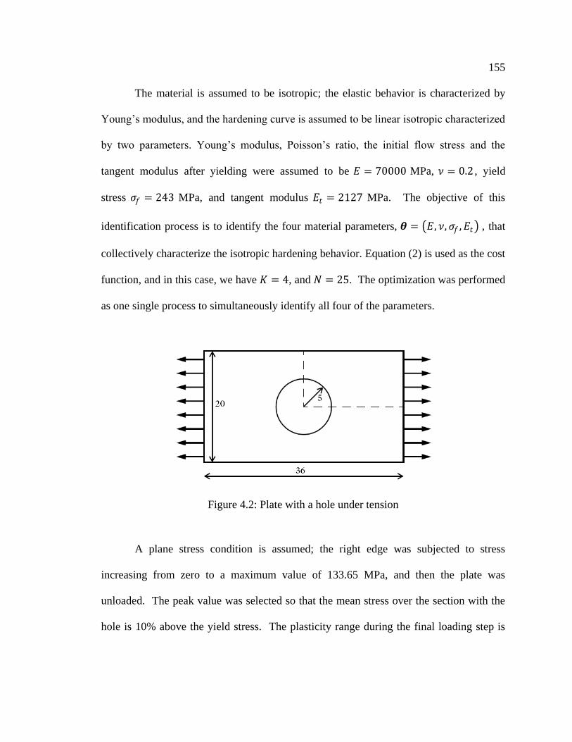
155

The material is assumed to be isotropic; the elastic behavior is characterized by

Young‘s modulus, and the hardening curve is assumed to be linear isotropic characterized

by two parameters. Young‘s modulus, Poisson‘s ratio, the initial flow stress and the

tangent modulus after yielding were assumed to be 𝐸 = 70000 MPa, 𝜈 = 0.2 , yield

stress 𝜎𝑓 = 243 MPa, and tangent modulus 𝐸𝑡 = 2127 MPa. The objective of this

identification process is to identify the four material parameters, 𝜽 = 𝐸, 𝜈,𝜎𝑓 ,𝐸𝑡 , that

collectively characterize the isotropic hardening behavior. Equation (2) is used as the cost

function, and in this case, we have 𝐾 = 4, and 𝑁 = 25. The optimization was performed

as one single process to simultaneously identify all four of the parameters.

Figure 4.2: Plate with a hole under tension

A plane stress condition is assumed; the right edge was subjected to stress

increasing from zero to a maximum value of 133.65 MPa, and then the plate was

unloaded. The peak value was selected so that the mean stress over the section with the

hole is 10% above the yield stress. The plasticity range during the final loading step is

156

shown in Figure 4.3. Second-order triangular elements with four Gauss points were used

in the simulation.

Figure 4.3: Plasticity range in the final loading stage

Several inverse analyses were performed with different initial estimates, and the

results show that the solution produces a global minimum; this is the first indication that

the problem is not ill-posed and that the solution is stable. To evaluate the sensitivity of

these methods to uncertainty in the measurement, a 5% white noise measure was added to

the synthetic data. The noise was defined as:

𝑛𝑜𝑖𝑠𝑒 𝒙 = 𝑁𝑅𝐴𝑁𝐷 ∙ 𝛼 ∙ 𝑢 𝒙 (4.18)

where 𝑁𝑅𝐴𝑁𝐷 is a Gaussian random distribution with zero-mean and a unit standard

deviation; α = 5% is the applied noise level; and 𝑢(𝑥) is the displacement response at

location 𝑥 . The corresponding identification solution is given in the fifth column of

Plasticity range

157

Table 4.1; while the initial estimates used to start the optimization process is given in the

fourth column.

Table 4.1: identified solution with and without synthetic noise (load factor = 1.1)

noise parameter Target

values

Initial

guesses

Obtained

values

(CONDOR)

Variance

(LCA) 𝜎𝜃𝑗2

relative

offset

measure 𝐼𝑀

0%

𝐸1

𝜈

𝜎𝑦

𝐸2

70000

0.2

243

2127

50000

0.3

500

10000

70001

0.215

243

2126.8

2.86

0.114

2.5

11.9

singular

5%

𝐸1

𝜈

𝜎𝑦

𝐸2

70000

0.2

243

2127

50000

0.3

500

10000

70006.1

0.216

240.4

2141.2

2.86

0.116

12.7

31.4

0.0004

For comparison, two additional direct search methods were also used; namely, (i)

the Nelder-Mead simplex method and (ii) the genetic algorithm in the MATLAB

toolboxes. Table 4.1 summarizes the results. Both methods produced similar solutions to

the method proposed here, but with different levels of efficiency. The proposed solution

required nine iterative steps of optimization when using CONDOR, 29 iterative steps of

optimization using the Nelder-Mead simplex method, and 3500 function evaluations

using the MATLAB genetic algorithm.

158

Table 4.2: Comparison of identification solution with and without synthetic noise to

Nelder-Mead and Genetic Algorithm (GA) methods (load factor = 1.1)

Noise Parameter Target

values

Initial

estimates

Obtained

values

(Nelder-

Mead)

Obtained

values

(GA)

0%

E1

ν

σy

E2

70000

0.2

243

2127

50000

0.3

500

10000

70001.5

0.217

243

2126.5

70002

0.216

242

2129

5%

E1

ν

σy

E2

70000

0.2

243

2127

50000

0.3

500

10000

70008

0.217

238

2143

70005

0.214

240

2141

It is clear that the identification results depend highly on the quality of the input

data. The plasticity mechanism must be fully activated in order to identify the model

parameters. To study this aspect of the proposed method, the identification was repeated

with simulated inhomogeneous displacement field data at the loading stage where the

mean stress is 5% above the yield stress. The identified model parameters calculated

without synthetic noise are shown in Table 4.3. The deterioration of the identified

plasticity parameters is evident. It is interesting that the evaluations for the initial tangent

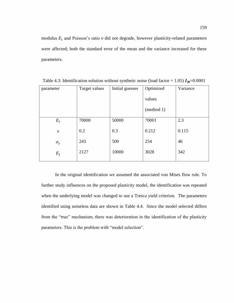
159

modulus 𝐸1 and Poisson‘s ratio 𝜈 did not degrade, however plasticity-related parameters

were affected; both the standard error of the mean and the variance increased for these

parameters.

Table 4.3: Identification solution without synthetic noise (load factor = 1.05) 𝑰𝑴=0.0001

parameter Target values Initial guesses Optimized

values

(method 1)

Variance

𝐸1

𝜈

𝜎𝑦

𝐸2

70000

0.2

243

2127

50000

0.3

500

10000

70001

0.212

254

3028

2.3

0.115

46

342

In the original identification we assumed the associated von Mises flow rule. To

further study influences on the proposed plasticity model, the identification was repeated

when the underlying model was changed to use a Tresca yield criterion. The parameters

identified using noiseless data are shown in Table 4.4. Since the model selected differs

from the ―true‖ mechanism, there was deterioration in the identification of the plasticity

parameters. This is the problem with ―model selection‖.

160

Table 4.4: identification solution without synthetic noise (load factor = 1.1)(Tresca yield

criterion) 𝑰𝑴= 0.0002

Parameters Target values Initial

estimates

Optimized

values

Variance

𝐸1

𝜈

𝜎𝑦

𝐸2

70000

0.2

243

2127

50000

0.3

500

10000

70001

0.25

244

2124

2.78

0.13

11.5

14.7

4.9.2 Example 2: identification of model parameters of a cast iron component

In this example, a grey cast iron engine bearing cap subjected to vertical

compressive loading is analyzed (Figure 4.4). The load was applied on a Tinius–Olsen

hydraulic universal testing machine with a load capacity of 300 kN. A maximum load of

150 KN was applied to the top of the bearing cap. The ARAMIS-DIC system was used to

measure the deformation and the strain on the surface of the specimen. An automatic

data acquisition system coupled with the testing machine was also used to collect the data

for the load—displacement curve.

A random pattern was applied to the specimen‘s surface; a flat white paint was

applied to the surface in order to reduce the glare in the camera image. A black speckle

pattern was then applied using spray paint in order to provide contrast with the white

surface coating, and to provide surface target points from which strain and displacement

measurements were evaluated using digital image correlation photogrammetry. Speckle

161

points were approximately 3 to 5 pixels in diameter, and the correlated subset size chosen

was 15 pixels. According to (Tong, 2005) and (Robert, Nazaret et al., 2007), 5% of RMS

error is a conservative estimate of the error in measurement for a speckle pattern with

speckle sizes smaller than the subset size.

The test data was comprised of the force-load curves and the three-dimensional

displacement/strain fields on the surface of the component, measured by using the

ARAMIS commercial DIC system. Two CCD cameras with a 510 mm object-camera

distance were used to acquire synchronized stereo images of the component under

compression at different load levels during the test (Figure 4.5).

By means of photogrammetrical procedures and image processing, the data

acquisition system evaluated the three dimensional displacement field associated with

each respective loading step. Although the ARAMIS system provides three-dimensional

displacements and two-dimensional strains on the surface, only the horizontal strains (𝜇𝑥)

and vertical strains (𝜇𝑦 ) were used in the identification of model parameters. In DIC

measurement, the primary results consist of displacements, and the deformation data are

obtained by post-acquisition processing techniques. Equation 4.2 was used as the cost

function, where the data vector 𝒅 consists of 120 measurement points inside the rectangle

(shown in Figure 4.10), and the corresponding numerical responses 𝑀𝑖 𝜽 are the

simulated results from the same points. It was found that strains in this region are

sensitive to the material parameters, and that the DIC-measured data are reliable in this

region (located in the center of the images). In total, 53 images were taken during the

loading process at one second time intervals. The load was measured with a Tinius-Olsen

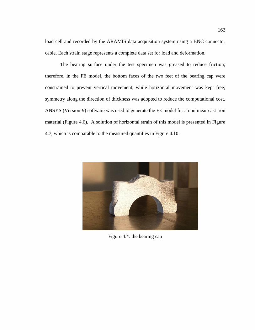
162

load cell and recorded by the ARAMIS data acquisition system using a BNC connector

cable. Each strain stage represents a complete data set for load and deformation.

The bearing surface under the test specimen was greased to reduce friction;

therefore, in the FE model, the bottom faces of the two feet of the bearing cap were

constrained to prevent vertical movement, while horizontal movement was kept free;

symmetry along the direction of thickness was adopted to reduce the computational cost.

ANSYS (Version-9) software was used to generate the FE model for a nonlinear cast iron

material (Figure 4.6). A solution of horizontal strain of this model is presented in Figure

4.7, which is comparable to the measured quantities in Figure 4.10.

Figure 4.4: the bearing cap

163

Figure 4.5: photo of the bearing cap on the testing machine and two cameras taking

images

Figure 4.6: FE model of the bearing cap

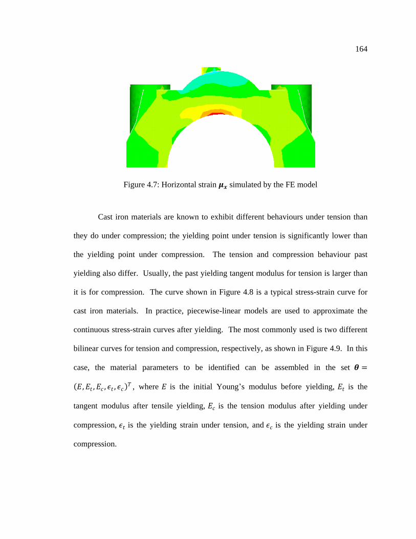
164

Figure 4.7: Horizontal strain 𝝁𝒙 simulated by the FE model

Cast iron materials are known to exhibit different behaviours under tension than

they do under compression; the yielding point under tension is significantly lower than

the yielding point under compression. The tension and compression behaviour past

yielding also differ. Usually, the past yielding tangent modulus for tension is larger than

it is for compression. The curve shown in Figure 4.8 is a typical stress-strain curve for

cast iron materials. In practice, piecewise-linear models are used to approximate the

continuous stress-strain curves after yielding. The most commonly used is two different

bilinear curves for tension and compression, respectively, as shown in Figure 4.9. In this

case, the material parameters to be identified can be assembled in the set 𝜽 =

𝐸,𝐸𝑡 ,𝐸𝑐 , 𝜖𝑡 , 𝜖𝑐 𝑇 , where 𝐸 is the initial Young‘s modulus before yielding, 𝐸𝑡 is the

tangent modulus after tensile yielding, 𝐸𝑐 is the tension modulus after yielding under

compression, 𝜖𝑡 is the yielding strain under tension, and 𝜖𝑐 is the yielding strain under

compression.

165

Figure 4.8: typical stress-strain curves for cast iron materials under tension and

compression

Figure 4.9: a bilinear approximation model for cast iron material

E: Young‘s modulus

Compression

c

cE

Compression

Tension

t

tE

Tension

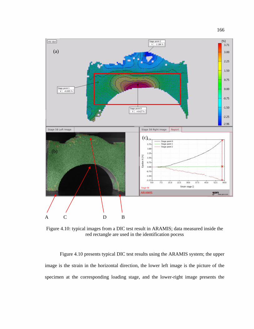
166

A C D B

Figure 4.10: typical images from a DIC test result in ARAMIS; data measured inside the

red rectangle are used in the identification pocess

Figure 4.10 presents typical DIC test results using the ARAMIS system; the upper

image is the strain in the horizontal direction, the lower left image is the picture of the

specimen at the corresponding loading stage, and the lower-right image presents the

(c)

(b)

(a)

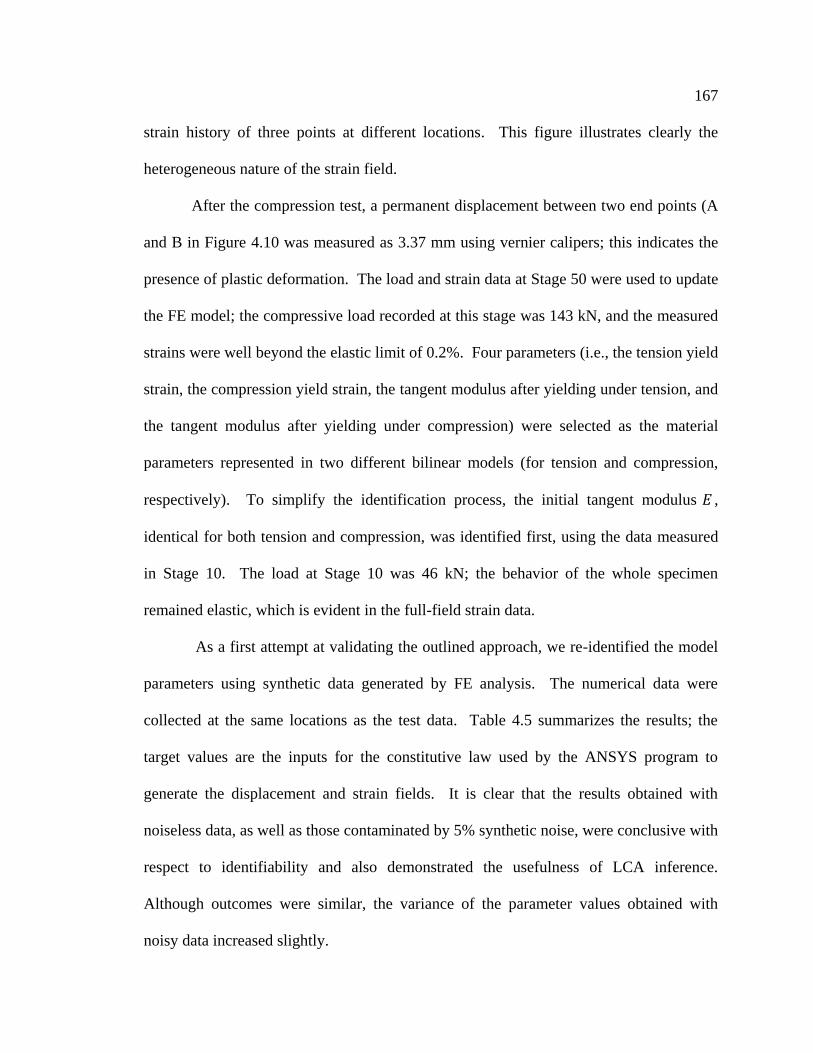
167

strain history of three points at different locations. This figure illustrates clearly the

heterogeneous nature of the strain field.

After the compression test, a permanent displacement between two end points (A

and B in Figure 4.10 was measured as 3.37 mm using vernier calipers; this indicates the

presence of plastic deformation. The load and strain data at Stage 50 were used to update

the FE model; the compressive load recorded at this stage was 143 kN, and the measured

strains were well beyond the elastic limit of 0.2%. Four parameters (i.e., the tension yield

strain, the compression yield strain, the tangent modulus after yielding under tension, and

the tangent modulus after yielding under compression) were selected as the material

parameters represented in two different bilinear models (for tension and compression,

respectively). To simplify the identification process, the initial tangent modulus 𝐸 ,

identical for both tension and compression, was identified first, using the data measured

in Stage 10. The load at Stage 10 was 46 kN; the behavior of the whole specimen

remained elastic, which is evident in the full-field strain data.

As a first attempt at validating the outlined approach, we re-identified the model

parameters using synthetic data generated by FE analysis. The numerical data were

collected at the same locations as the test data. Table 4.5 summarizes the results; the

target values are the inputs for the constitutive law used by the ANSYS program to

generate the displacement and strain fields. It is clear that the results obtained with

noiseless data, as well as those contaminated by 5% synthetic noise, were conclusive with

respect to identifiability and also demonstrated the usefulness of LCA inference.

Although outcomes were similar, the variance of the parameter values obtained with

noisy data increased slightly.

168

Table 4.5: Re-identified parameters with and without synthetic noise

Parameters Target

values

Initial

estimates

without synthetic noise

𝐼𝑀 = 0.0019

with 5% synthetic noise

𝐼𝑀 = 0.0044

Estimated

values

Variance Estimated

values

Variance

E1 70000 50000 70002 5.6 70006 9.3

ϵt 0.3 0.2 0.305 0.09 0.312 0.11

𝜖𝑐 0.4 0.2 0.396 0.08 0.405 0.09

𝐸t 56000 50000 56050 83 56110 102

𝐸𝑐 55000 50000 55046 74 54434 76

Correlating DIC to FEA

The calibration process in ARAMIS system provide physical coordinates for each

pixel point in the image; this data must be mapped to the FE model coordinates and the

corresponding FE solutions are extracted at that coordinates. In this work, the selected

reference points to build the mapping were the four physical points shown in Figure 4.10:

two corner points (A and B), the top of the semi-circle (C), and the top of the cap (D).

These points can be identified in the image taken before loading; furthermore, their pixel

coordinates within the image can be easily identified, and the mapping between the image

and the finite element coordinates can be established for transformation. In some cases,

when no physical target points were clearly visible in the image taken by camera (such as

points A and B in Figure 4.10), pre-printed target points applied to the specimen surface

were used to define the transformation.

169

Results and analysis

The elastic modulus was identified using data from an elastic stage (Stage 10),

and the results are shown in Table 4.6. The other parameters were identified using data

from Stage 50; the identified yielding stress points for tension and compression, and

tangent moduli after yielding are tabulated in Table 4.7 (The variance is given in brackets

under each identified value). Three different optimization methods were used to obtain

the parameters: 1) CONDOR; 2) the response surface method using quadratic

interpolation, denoted as response surface in ANSYS DesignSpace; and 3) the BFGS

pseudo-Newtonian method with finite difference approximated numerical gradient,

denoted as numerical gradient.

The best parameter identification obtained for Stage 50 (in comparison to the

reference values from Stage 10 shown in Table 4.6) was for the elasticity modulus 𝐸

apart from the ―1-parameter‖ case shown in the first row of Table 4.7. In the ―1-

parameter‖ case, the response surface procedure assumes that the only design variable to

be updated is Young‘s modulus 𝐸, meaning that the whole material is elastic in this

loading stage. Obviously, the identification of 𝐸 differs greatly from the reference values

(Table 4.6; 70037 [Stage 10] compared to 51251 [Stage 50]), and the inadequacy of the

response surface model can also be seen by comparing the 𝐼𝑀 values [0.0041 [Stage 10]

versus 0.1125 [Stage 50]). The outcomes for the response surface model (second row),

the numerical gradient model (third row), and CONDOR model (fourth row) are

compared in Table 4.7 using the ―2-parameter‖ procedure, in which two parameters,

strain threshold and hardening modulus, are considered simultaneously. In other words,

the models are assumed to be formulations of a bilinear hardening law that does not

170

distinguish the difference between compression and tension. Although the two-parameter

procedure is still an inadequate approach to modelling the cast iron material considered

here, the differences between the ―2-parameter‖ and the ―4-parameter‖ cases are less

evident than those observed with the elasticity model in the ―1-parameter‖ case,

suggesting that ―2-parameter‖ models are closer to the ―true‖ one. In the ―4-parameter‖

cases (compared in the bottom three rows of Table 4.7), all four parameters

𝐸𝑡 ,𝐸𝑐 , 𝜖𝑡 , 𝜖𝑐 𝑇 were included in the identification of material parameters using the three

derivative-free methods; the table shows the minimum variances and the minimum

objective function values, along with minimum 𝐼𝑀 measures.

The differences between the outcomes of the three derivative-free methods were

found to be small, but consistent (Table 4.7). The ―numerical gradient‖ method, had the

worst performance indicators, as can be seen from comparison of the objective function

values and 𝐼𝑀 measures for the three methods (numerical gradient>response

surface>CONDOR). Although the algorithmic details of the ―response surface‖ method

are not clear, its performance was found to be better than that of the ―numerical gradient‖

method. Nevertheless, the CONDOR method was shown to be the best method for

identifying model parameters in a cast iron component. The identification of model

parameters was consistent with reference values for an elastic stage, and CONDOR

produced better performance indicators (objective function values and 𝐼𝑀 measures) than

the other methods.

171

Table-4.6: Parameter identification with Stage 10 measurement data (elastic response)

Method E (MPa) Objective Variance 𝐼𝑀

1-parameter

(response surface)

70037 1.6428 25.6 0.0041

1-parameter**

(CONDOR)

70037 1.6427 25.5 0.0040

1-parameter

(numerical gradient)

70101 1.6744 54.2 0.0058

**: the best model

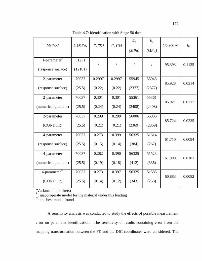
172

Table-4.7: Identification with Stage 50 data

Method E (MPa) t (%) c (%) tE

(MPa)

cE

(MPa)

Objective 𝐼𝑀

1-parameter*

(response surface)

51251

(12101)

/ / / / 95.393 0.1125

2-parameter

(response surface)

70037

(25.5)

0.2997

(0.22)

0.2997

(0.22)

55945

(2377)

55945

(2377)

85.928 0.0314

2-parameter

(numerical gradient)

70037

(25.5)

0.301

(0.24)

0.301

(0.24)

55361

(2408)

55361

(2408)

85.921 0.0317

2-parameter

(CONDOR)

70037

(25.5)

0.299

(0.21)

0.299

(0.21)

56006

(2369)

56006

(2369)

85.724 0.0235

4-parameter

(response surface)

70037

(25.5)

0.273

(0.15)

0.399

(0.14)

56325

(384)

51614

(267)

61.710 0.0094

4-parameter

(numerical gradient)

70037

(25.5)

0.282

(0.19)

0.390

(0.18)

56325

(412)

51523

(336)

61.998 0.0101

4-parameter**

(CONDOR)

70037

(25.5)

0.273

(0.14)

0.397

(0.12)

56325

(343)

51585

(258)

60.883 0.0082

(Variance in brackets) * : inappropriate model for the material under this loading

**: the best model found

A sensitivity analysis was conducted to study the effects of possible measurement

error on parameter identification. The sensitivity of results containing error from the

mapping transformation between the FE and the DIC coordinates were considered. The

173

errors in the x- and y- coordinate transformation (expressed as a percentage) are denoted

as 𝑑𝑥 and 𝑑𝑦, respectively. The variation of the identified initial tangent modulus 𝐸 and

the objective function value are plotted in Figure 4.11. Figure 4.12 shows the variation of

the initial tangent modulus, the tangent modulus for tension and compression as well as

the initial yield strain for tension and compression.

Figure 4.11: the sensitivity of the identification of one parameter 𝑬. (Left: the sensitivity

surface of identified 𝑬 with respect to the errors in the x- and y-translation; Right:

sensitivity of the surface of the objective function with respect to the errors in the x- and

y- translation)

174

Figure 4.12: the sensitivity of the identification of four parameters 𝑬𝒕,𝑬𝒄, 𝝐𝒕, 𝝐𝒄 and

the objective function.

It can be seen in these figures that transformation errors introduce uncertainty into

the identification results. Nonetheless, the sensitivity surfaces are relatively flat,

175

especially for transformation errors near the center (zero coordinate). This indicates that

the identification function is well-posed with respect to coordinate transformation errors.

4.10 Summary of this study

The problem of parameter identification in plasticity constitutive models is

formulated as an inverse problem (i.e., mixed-numerical experimental inverse

identification of material model parameters) in this study. The data were obtained from

full-field measurement of the displacement/strain on the surface of structures using the

digital image correlation (DIC) technique. Our objective was to develop a procedure that

uses derivative-free optimization algorithms available in commercial FE software (e.g.

ABAQUS, ANSYS, COMSOL, MARK, etc.); the derivative-free optimization

algorithms were used to determine the parameters by minimizing the gap between

measured data and simulated responses.

The proposed methodology is general and appropriate for any material model

implemented in commercial software or codes. The method consists of three building

blocks: (i) commercial finite element analysis, (ii) direct optimization algorithms, and

(iii) digital image correlation test results. The latter two are currently highly

commercialized and available for general industrial use.

The focus of this study was on checking the quality and reliability of the

solutions. Methodology for validating experiments was presented and demonstrated. A

systematic verification and validation process, using statistical and sensitivity analyses,

was proposed for use in cases where no reference values of the true parameters are

available a priori. If we state that the null hypothesis 𝐻0 is that the identified parameters

176

are similar to the ―true‖ parameters, then the proposed validation process can prevent

Type-2 error (i.e., acceptance of incorrectly identified parameters), which is the most

important requirement for industrial applications.

In conclusion, the direct optimization technique, finite element simulation, and

digital image correlation can be combined into a useful, efficient and industrially-

applicable technique for the accurate selection and validation of material models and

model parameters. Furthermore, all of the techniques involved in the proposed

methodology are readily available on the commercial market.

177

CHAPTER FIVE: HYPERELASTICITY MODEL IDENTIFICATION FOR

RUBBER AND RUBBER-LIKE SOLIDS

“The life of rubber is like the life of human.” (Anonymous)

5.1 Introduction and literature review of related research

Components comprised of rubbery materials play very important roles in

engineering processes and products. The use of sophisticated mathematical constitutive

models capable of accurate representation of stress/deformation responses (e.g. finite

element analysis) is a key ingredient in the design of engineering components and

structures under general loading conditions. Usually, the mechanical behavior of rubber-

like materials is characterized by hyperelastic constitutive models in which the existence

of a strain energy function is postulated; elastic materials that possess a strain energy

function are called ‗Green-elastic‘ or ‗hyperelastic‘ (Ciarlet, 1988; Doghri, 2000).

Strain energy functions are usually defined in terms of the strain invariants (e.g.

the polynomial forms), or in terms of the principal stretches (e.g. the Ogden forms).

Various types of strain energy functions have been proposed; the most popular of these

include the Mooney-Rivlin model and the Yeoh model, based on the phenomenological

framework of finite elasticity, and the Arruda-Boyce model, which is founded on the

statistical mechanics-based kinetic theory of polymer chain deformations (Boyce and

Arruda, 2000; Saccomandi and Ogden, 2004).

There is not a single constitutive model currently available, which can reproduce

all aspects of the behavior of real rubber. The selection of the type of strain energy

178

function and the essential parameters of the model must be determined through

appropriate laboratory and/or field tests. In contrast to most material constitutive models,

the parameters in rubber constitutive models often have no physical

counterparts/meanings, and therefore cannot be measured directly; in general, they must

be estimated through an inverse approach (i.e., by fitting the model to experimental data,

or by empirical correlations, such as the correlation between rubber stiffness and

hardness) (Gent, 2001).

Traditional laboratory techniques for determining the appropriate form of strain

energy function and corresponding parameters require homogeneous deformation tests

performed on cutout standard samples; these include tests of uniaxial tension and

compression, planar shear, and equibiaxial tension and compression. The task is to find

the strain energy model that fits the observational data exactly, and will behave

reasonably and predictably in other deformation modes.

Initially, elementary methods were utilized to determine the material constants of

an isotropic material from simple observational data (Ogden, 1972), such as Treloar‘s

(Treloar, 1944) data for samples cut from a single sheet of vulcanized natural rubber.

Several researchers have used Treloar‘s experimental data in simple tension, pure shear,

and equibiaxial tension to develop their models for rubber-like materials. For example,

Ogden (Ogden, 1972) used a simplified stress-deformation function to model Treloar‘s

(1944) data; 𝑃 = 𝜇𝑖(𝜆−1+𝛼𝑖 − 𝜆−1+𝑐𝛼 𝑖𝑁

𝑖=1 ) , where 𝑃 represents the force per unit

undeformed area, 𝜆 is the principal stretch, 𝜇𝑖 and 𝛼𝑖 are the material parameters, and 𝑐 is

related to deformation type which is equal to -0.5, -2, -1 for simple tension, equibiaxial

tension, and pure shear, respectively. Thus, Ogden (1972) developed an ad hoc method

179

to obtain parameters based on elementary test data, employing the fact that at small strain

values, only one term is dominant. The obvious limitation to this approach is that the

model provides good fit for only a limited range of strain with such sets of material

parameters.

Recently, researchers improved the estimation by using optimization algorithms,

such as the Levenberg-Marquardt least-square optimization algorithm, to determine the

material constants for each set of the homogeneous deformation data. Many studies that

focus on the identification of Rivlin- or Ogden-type polynomial functions use the load-

displacement curves or stress-strain relations of a specially shaped sample to formulate a

least-square problem. Analytical sensitivity relations can be derived for Rivlin- and

Ogden-type strain energy functions; Rivlin models are polynomial functions based on the

invariants of the Right Cauchy-Green tensor, and Ogden models are power functions of

the eigenvalues of the right stretch tensor with real exponents (Benjeddou, Jankovich et

al., 1993) (Gendy and Saleeb, 2000). The major drawback is that the optimization

procedure is based on the analytical solution for the deformation observed in simple

experiments with a specific form of hyperelastic strain energy; it does not generalize to

deformations that differ from those used by the researcher to develop the model or to a

different stress-deformation function (Gendy and Saleeb, 2000).

Physical parameters for an in vivo hyperelastic model in living soft tissue were

identified in a similar fashion by using the analogy between experimental and predicted

numerical results (Tsuta, Yamazaki et al., 1996). The tests were performed on a regular

circular area of soft tissue on the human forehead; force-displacement data were collected,

and the analytical gradient of displacement for a specific model-type was determined and

180

parameters were computed for the two-dimensional axi-symmetric model using a steepest

descent method. Currently, the most typical approach used is the general FE-based

procedure for determination of the constitutive law of rubber-like hyperelasticity (Wang

and Lu, 2003). First, uniaxial tension and compression tests of rubber specimens are

conducted; then, tension and compression test simulations with a one-element model and

with FE models of the experimental specimen are performed, and suitable rubber-like

hyperelastic constitutive laws are obtained. Finally, candidate constitutive laws for

hyperelastic and rubber-like materials are selected through comprehensive comparison of

the simulation results (from the FE analysis for real working conditions) with the

experimental observations.

Although parameters can be estimated from the results of a single test, tests

conducted at different deformation modes are usually required to obtain a strain energy

function that is adequate for predicting material behaviour under a variety of deformation

modes. As an alternative to homogeneous experiments, Hartmann, Mars and Fatemi

proposed specially-designed experiments that would be conducted using a novel

specimen, a short, thin-walled cylindrical specimen subjected to combined axial and twist

displacements, in order to study the mechanical response of rubber-like materials under

multiaxial loading (Hartmann, 2001) (Mars and Fatemi, 2003) (Mars and Fatemi, 2004).

Hartmann identified parameters in Rivlin‘s hyperelasticity model using tension, torsion,

and combined tension-torsion tests with cylindrical rubber specimens where the

analytical solutions to the extension and torsion of a cylindrical body subjected to

incompressibility are known (Hartmann, 2001). The solution to the resulting boundary

value problem is known, and is used to formulate the least-square optimization algorithm.

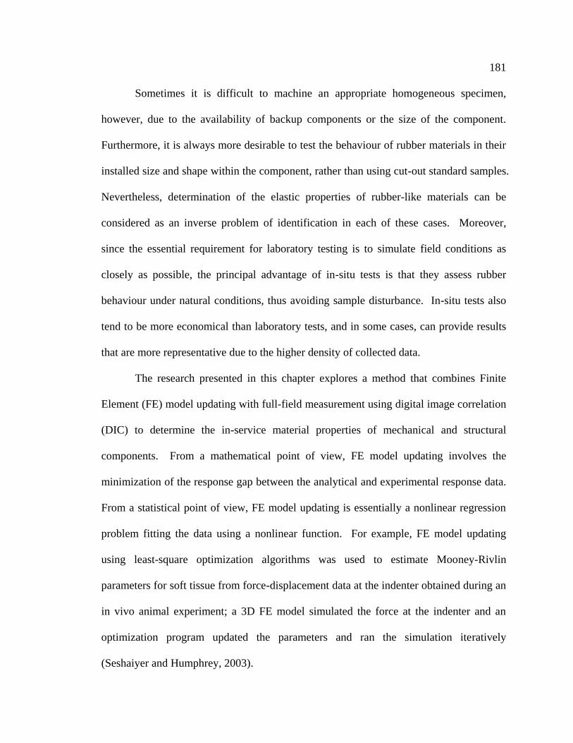
181

Sometimes it is difficult to machine an appropriate homogeneous specimen,

however, due to the availability of backup components or the size of the component.

Furthermore, it is always more desirable to test the behaviour of rubber materials in their

installed size and shape within the component, rather than using cut-out standard samples.

Nevertheless, determination of the elastic properties of rubber-like materials can be

considered as an inverse problem of identification in each of these cases. Moreover,

since the essential requirement for laboratory testing is to simulate field conditions as

closely as possible, the principal advantage of in-situ tests is that they assess rubber

behaviour under natural conditions, thus avoiding sample disturbance. In-situ tests also

tend to be more economical than laboratory tests, and in some cases, can provide results

that are more representative due to the higher density of collected data.

The research presented in this chapter explores a method that combines Finite

Element (FE) model updating with full-field measurement using digital image correlation

(DIC) to determine the in-service material properties of mechanical and structural

components. From a mathematical point of view, FE model updating involves the

minimization of the response gap between the analytical and experimental response data.

From a statistical point of view, FE model updating is essentially a nonlinear regression

problem fitting the data using a nonlinear function. For example, FE model updating

using least-square optimization algorithms was used to estimate Mooney-Rivlin

parameters for soft tissue from force-displacement data at the indenter obtained during an

in vivo animal experiment; a 3D FE model simulated the force at the indenter and an

optimization program updated the parameters and ran the simulation iteratively

(Seshaiyer and Humphrey, 2003).

182

Full-field optical techniques for displacement or strain measurements are now

widely used in experimental mechanics. The main techniques reported are

photoelasticity, geometric moiré, moiré interferometry, holographic interferometry,

speckle interferometry (ESPI), grid method and DIC (Rastogi, 2000). Due to its

simplicity and versatility, the DIC method is one of the most commonly used techniques.

Many applications for DIC can be found in the professional literature, including research

related to the heterogeneous deformation of foams (Wang and Cuitino, 2002), large

deformation of polymers (Chevalier, Calloch et al., 2001) (Parsons, Boyce et al., 2004),

and measurement of small strains in fiber-reinforced refractory castables (Robert, Nazaret

et al., 2007). The DIC method can be used with a single camera (standard DIC) to

measure in-plane displacement/strain fields on planar objects, or with two cameras (3D

DIC) to measure 3D displacement/strain fields on any 3-D object (Rastogi, 2000).

The DIC technique provides a number of benefits; DIC measures whole field

displacement/strain on the surface of a component, generates massive amounts of

experimental data in a single test (replacing traditional techniques involving multiple

tests with multidimensional loading paths), and thus provides enough information to

formulate an inverse problem. The full-field measurement in DIC allows better

characterization of the behavior of materials and the response of structural components to

external loadings. The problem of ill-conditioning, which is often encountered in FE-

model updating, can be avoided to a large extent. Furthermore, although the deformation

includes multiple modes, the FE-model formulated using DIC includes coefficients that

reproduce the complex deformation modes exactly; thus, the estimate function will be

better at predicting the behavior of the material. The large amount of full-field data from

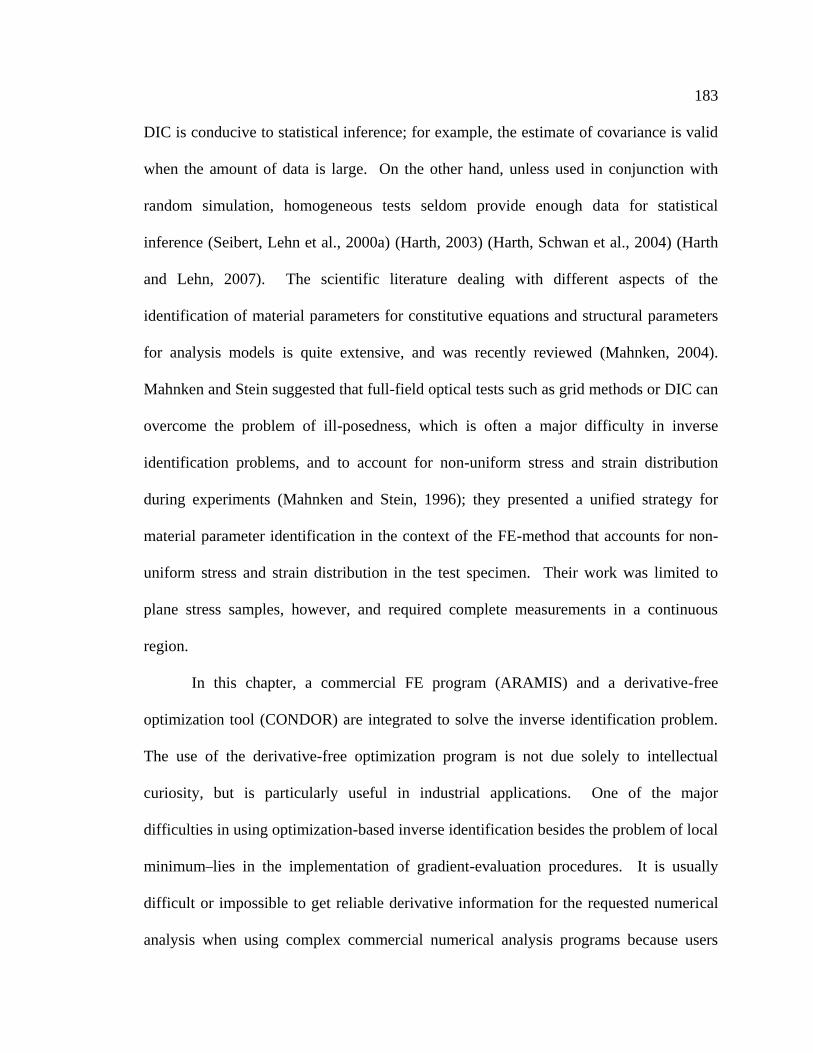
183

DIC is conducive to statistical inference; for example, the estimate of covariance is valid

when the amount of data is large. On the other hand, unless used in conjunction with

random simulation, homogeneous tests seldom provide enough data for statistical

inference (Seibert, Lehn et al., 2000a) (Harth, 2003) (Harth, Schwan et al., 2004) (Harth

and Lehn, 2007). The scientific literature dealing with different aspects of the

identification of material parameters for constitutive equations and structural parameters

for analysis models is quite extensive, and was recently reviewed (Mahnken, 2004).

Mahnken and Stein suggested that full-field optical tests such as grid methods or DIC can

overcome the problem of ill-posedness, which is often a major difficulty in inverse

identification problems, and to account for non-uniform stress and strain distribution

during experiments (Mahnken and Stein, 1996); they presented a unified strategy for

material parameter identification in the context of the FE-method that accounts for non-

uniform stress and strain distribution in the test specimen. Their work was limited to

plane stress samples, however, and required complete measurements in a continuous

region.

In this chapter, a commercial FE program (ARAMIS) and a derivative-free

optimization tool (CONDOR) are integrated to solve the inverse identification problem.

The use of the derivative-free optimization program is not due solely to intellectual

curiosity, but is particularly useful in industrial applications. One of the major

difficulties in using optimization-based inverse identification besides the problem of local

minimum lies in the implementation of gradient-evaluation procedures. It is usually

difficult or impossible to get reliable derivative information for the requested numerical

analysis when using complex commercial numerical analysis programs because users

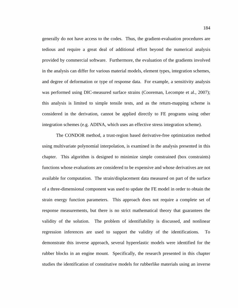
184

generally do not have access to the codes. Thus, the gradient-evaluation procedures are

tedious and require a great deal of additional effort beyond the numerical analysis

provided by commercial software. Furthermore, the evaluation of the gradients involved

in the analysis can differ for various material models, element types, integration schemes,

and degree of deformation or type of response data. For example, a sensitivity analysis

was performed using DIC-measured surface strains (Cooreman, Lecompte et al., 2007);

this analysis is limited to simple tensile tests, and as the return-mapping scheme is

considered in the derivation, cannot be applied directly to FE programs using other

integration schemes (e.g. ADINA, which uses an effective stress integration scheme).

The CONDOR method, a trust-region based derivative-free optimization method

using multivariate polynomial interpolation, is examined in the analysis presented in this

chapter. This algorithm is designed to minimize simple constrained (box constraints)

functions whose evaluations are considered to be expensive and whose derivatives are not

available for computation. The strain/displacement data measured on part of the surface

of a three-dimensional component was used to update the FE model in order to obtain the

strain energy function parameters. This approach does not require a complete set of

response measurements, but there is no strict mathematical theory that guarantees the

validity of the solution. The problem of identifiability is discussed, and nonlinear

regression inferences are used to support the validity of the identifications. To

demonstrate this inverse approach, several hyperelastic models were identified for the

rubber blocks in an engine mount. Specifically, the research presented in this chapter

studies the identification of constitutive models for rubberlike materials using an inverse

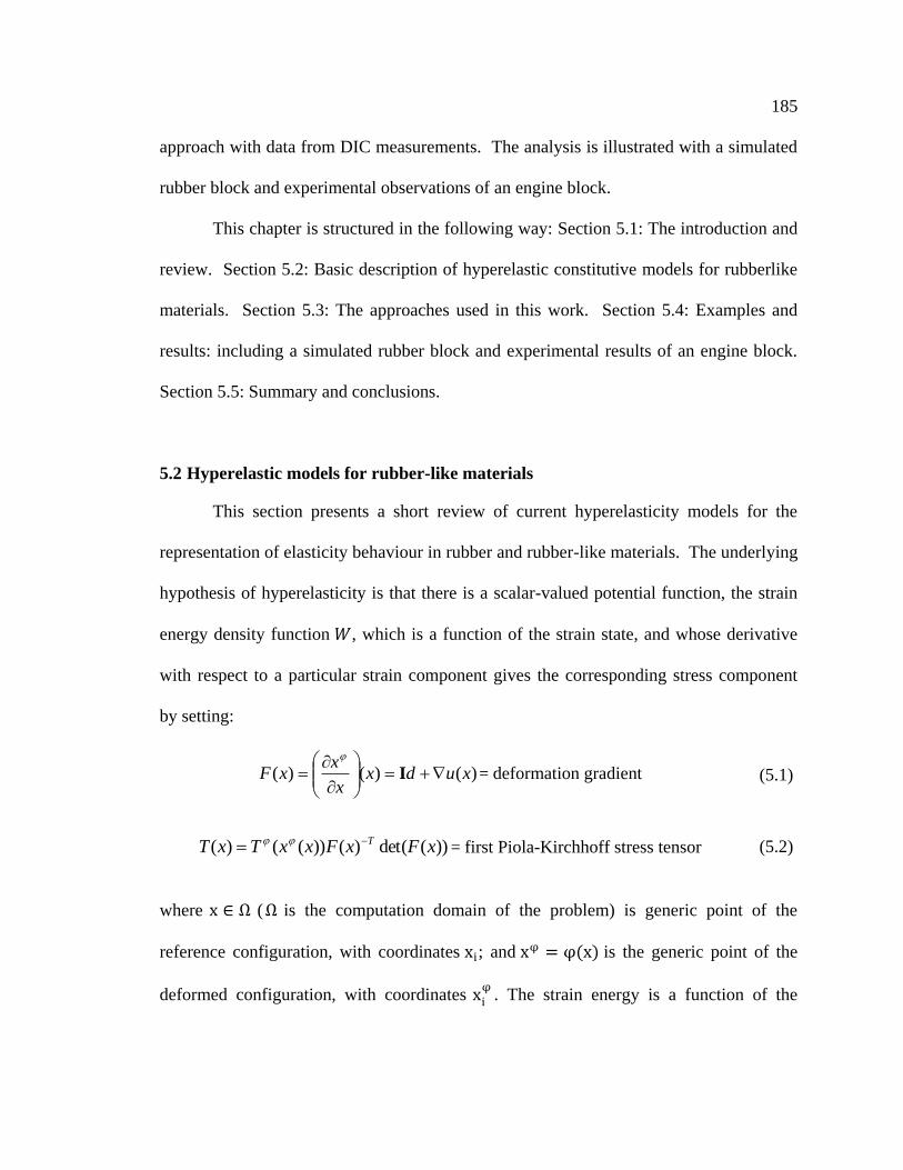
185

approach with data from DIC measurements. The analysis is illustrated with a simulated

rubber block and experimental observations of an engine block.

This chapter is structured in the following way: Section 5.1: The introduction and

review. Section 5.2: Basic description of hyperelastic constitutive models for rubberlike

materials. Section 5.3: The approaches used in this work. Section 5.4: Examples and

results: including a simulated rubber block and experimental results of an engine block.

Section 5.5: Summary and conclusions.

5.2 Hyperelastic models for rubber-like materials

This section presents a short review of current hyperelasticity models for the

representation of elasticity behaviour in rubber and rubber-like materials. The underlying

hypothesis of hyperelasticity is that there is a scalar-valued potential function, the strain

energy density function 𝑊, which is a function of the strain state, and whose derivative

with respect to a particular strain component gives the corresponding stress component

by setting:

)()()( xudxx

xxF

I

= deformation gradient (5.1)

))(det()())(()( xFxFxxTxT T = first Piola-Kirchhoff stress tensor (5.2)

where x ∈ Ω (Ω is the computation domain of the problem) is generic point of the

reference configuration, with coordinates xi; and xφ = φ(x) is the generic point of the

deformed configuration, with coordinates xiφ

. The strain energy is a function of the

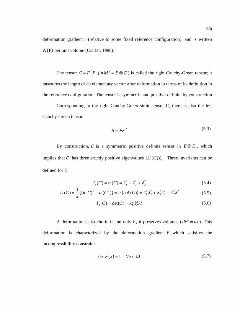
186

deformation gradient F (relative to some fixed reference configuration), and is written

W(F) per unit volume (Ciarlet, 1988).

The tensor FFC T (in EEM 3 ) is called the right Cauchy-Green tensor; it

measures the length of an elementary vector after deformation in terms of its definition in

the reference configuration. The tensor is symmetric and positive-definite by construction.

Corresponding to the right Cauchy-Green strain tensor C, there is also the left

Cauchy-Green tensor

TFFB (5.3)

By construction, 𝐶 is a symmetric positive definite tensor in EE , which

implies that 𝐶 has three strictly positive eigenvalues 3

1

2 ))(( ii C . Three invariants can be

defined for 𝐶

2

3

2

2

2

11 )()( CtrCI (5.4)

2

1

2

3

2

3

2

2

2

2

2

1

22

2 ))(()}(){(2

1)( CcoftrCtrCtrCI (5.5)

2

3

2

2

2

13 )det()( CCI (5.6)

A deformation is isochoric if and only if, it preserves volumes ( dxdx ). This

deformation is characterized by the deformation gradient 𝐹 which satisfies the

incompressibility constraint

xxF 1)(det (5.7)

187

Thus, the hyperelastic theory states that the first Piola-Kirchhoff stress tensor T is

given as:

2W W

T FF C

(5.8)

The Cauchy stress tensor T is automatically symmetric, and is now given by:

1 1(det ) 2(det )T TW

T F TF F F FC

(5.9)

As for compressible materials, the axiom of indifference implies that 𝑊 is a

function of the right Cauchy-Green strain tensor only (Tallec, 1994). The constitutive law

therefore becomes

TpF

C

WFT

~

2 (5.10)

dpFC

WFT T

I

~

2 (5.11)

Similarly, for isotropic materials, 𝑊 is again a function of the invariants of C

only. Thus, in this case we have simply

1

1 2 2

W W W WI d C

C I I I

I (5.12)

TpFFC

I

WF

I

WI

I

WT

22

1

1

22 (5.13)

In all of these constitutive laws, the hydrostatic pressure 𝑝 is an additional

unknown element, determined by the Lagrange multiplier associated with the additional

nonlinear kinematic constraint

1det FJ (5.14)

188

Various forms of the strain energy function 𝑊 have been proposed for rubber-like

materials. The choice of 𝑊 usually reflects the experience and preferences of the

individual researchers rather than objective criteria. In general, the proposed models can

be categorized into two classes: (1) phenomenological descriptions; and (2) descriptions

based on statistical mechanics (Horgan and Saccomandi, 2006).

Phenomenological descriptions (based on continuum mechanics analysis) assume

that rubber-like materials in the undeformed state are isotropic; i.e., the long molecular

chains are distributed randomly, which allows formulation of a strain energy density

description in volume element units. The strain energy function is either: 1) a function of

the principal invariants of the right Cauchy-Green strain tensor; or 2) a symmetric

function of the principal stretches. The former includes the popular Mooney-Rivlin

model and the Yeoh model, which are appropriate for strains of medium magnitude;

while the latter includes the Ogden model, which is considered to be an effective model

for very large strains (Horgan and Saccomandi, 2006).

The strain energy functions for rubber-like materials based on statistical

mechanics assume that the elastic restoring force is related to the decrease of entropy, and

that elongation of the material‘s fibers reduces disorder within the material. Essentially,

these models make assumptions about the length and direction of molecular chains; the

constitutive models are obtained via statistical analysis (Treloar, 1975). The Arruda-

Boyce and Van der Waals are important forms of the models in this class (Boyce and

Arruda, 2000) (Horgan and Saccomandi, 2004).

189

The Arruda-Boyce model of strain energy is the most popular of the 𝑊 functions

based on statistical molecular theory. The strain energy function is expressed in terms of

𝐼1 and needs only two parameters, namely 𝜇 and 𝜆𝑚 , for incompressible rubber material,

and one additional parameter, 𝐷 , for a compressible case (Arruda and Boyce, 1993). The

strain energy function is:

25

12 21

1 1( 3 ) ln

2

i ii

ii m

C JW I J

D

(5.15)

where: 1 2 3 4 5

1 1 11 19 519, , , ,

2 20 1050 7050 673750C C C C C . The Arruda-Boyce strain

energy model is also called the eight-chain model. The values for 𝐶𝑖 (𝑖 = 1,… ,5) are

obtained from statistical thermodynamics, and therefore they are physically meaningful.

The parameter 𝜇 represents the initial shear modulus of the material. The parameter 𝜆𝑚 is

the locking stretch, which location is around the sharpest point on the stress-strain curve.

This type of strain energy function has been shown to be accurate for engineering most

elastic materials.

The polynomial form of the strain energy function is written as:

2

1 2

1 1

1( 3) ( 3) ( 1)

N Ni j i

ij

i j i i

W C I I JD

(5.16)

This function denote 𝐼1 and 𝐼2 as the first and second invariants of the deviatoric

part of right-Cauchy-Green deformation tensor, respectively; 𝐽 = 𝑑𝑒𝑡(𝑭) is the ratio of

deformed volume over the undeformed volume of the material, and 𝑭 is the deformation

gradient. The parameter 𝑁 is the order of the polynomial chosen for a specific material.

The parameters 𝐷𝑖 determines the compressibility of the material; the material is

190

incompressible if all values of 𝐷𝑖 are equal to zero. For polynomial models, the initial

shear modulus 𝜇0 and volume modulus 𝑘0 are determined by the first-order polynomial

(𝑁 = 1) no matter how many orders are selected for the polynomial model.

)(2 01100 CC , and 1

0

2

Dk (5.17)

The famous Mooney-Rivlin strain energy form can be obtained by retaining only

the linear part of strain energy, that is, 𝑁 = 1.

2

10 1 01 2

1( 3) ( 3) ( 1)

i

W C I C I JD

(5.18)

The Mooney-Rivlin form is a very popular one; although it cannot model the

sharp upturn of the stress-strain curve under large strains, it is effective for small and

medium strain ranges. The first term of this form dictates a linear shear modulus model -

the neo-Hookean model:

10 1( 3)U C I (5. 19)

Treloar constructed the so-called neo-Hookean form of the strain energy on the

basis of Gaussian statistics and molecular network theory (Treloar, 1975) as:

𝑊 =1

2𝜇 𝐼1 − 3 (5. 20)

where 𝜇 is the shear modulus in the ground state. It is easy to see that the Neo-Hookean

model can be obtained by retaining only the first term in Equation (5.18). Actually the

neo-Hookean form is the first W function proposed by Treloar in 1943.

The reduced polynomial forms are obtained from the polynomial models by

setting all of the 0ijC for 0j :

191

N

i

N

i

i

i

i

i JD

ICU1 0

2

10 )1(1

)3( (5.21)

A special form of the reduced polynomial is the Yeoh model which is the reduced

polynomial function at N=3:

3

1

3

0

2

10 )1(1

)3(i i

i

i

i

i JD

ICU

(5.22)

The Yeoh model, is another popular model, and is effective for modeling the large

deformation of rubber-like materials.

To obtain accurate estimates of material parameters, the data space of 𝜆1 − 𝜆2

must be sampled thoroughly. While this is not easily done using traditional tests on

homogeneous stress-strain fields, it is easy to do with tests of the original components, so

that the test configuration generates a complicated strain/displacement pattern. The

mechanical response of a rubber-like material is then defined by choosing a constitutive

model with a strain energy function that fits the experimental behavior of the tested

components. Several of the most widely applied hyperelastic constitutive models are

summarized in Table-5.1.

Table 5.1: Popular constitutive models for compressible rubberlike materials in FE

analysis

Constitutive models based on statistical mechanics Number of material parameters

1. Arruda-Boyce model

2. Van der Waals model

3

4

Phenomenological models Number of material parameters

1. Polynomial models (N-th order)

2. Reduced polynomial models (Yeoh)

2N

N

192

The number of items included in the polynomial and reduced-polynomial models

can be infinitely high, making it possible to represent stress-strain behaviors of any

shape. High order strain energy functions are of little practical value, however, because

rubber materials are not sufficiently reproducible to allow one to evaluate a large number

of coefficients with any accuracy. Generally, the extra terms usually only do a good job

in fitting experimental errors. Therefore, the Mooney-Rivlin model remains the most

widely used strain energy function in FEA, and should be the first choice due to its

simplicity and robustness (Saccomandi and Ogden, 2004). The Mooney-Rivlin model is

used in the example presented in Section 5.4.1.

5.3 Methodological and analytical approaches used for this project

The research presented in this chapter is based on the same methodology as the research

presented in Chapter 4. Briefly, the ARAMIS commercial DIC system was used to

measure displacements and strains on the surface of the test component. A finite element

model of the component was developed and correlated with the experimental

measurements. Direct optimization algorithms and regression analysis techniques were

employed to evaluate and validate this nonlinear optimization problem. Procedural

details are provided in Chapter 4, sections 4.2 to 4.7. The results of applying this

approach to hyperelasticity in rubberlike materials (a rubber block and an engine mount

with a rubber component) are described in Section 5.4.

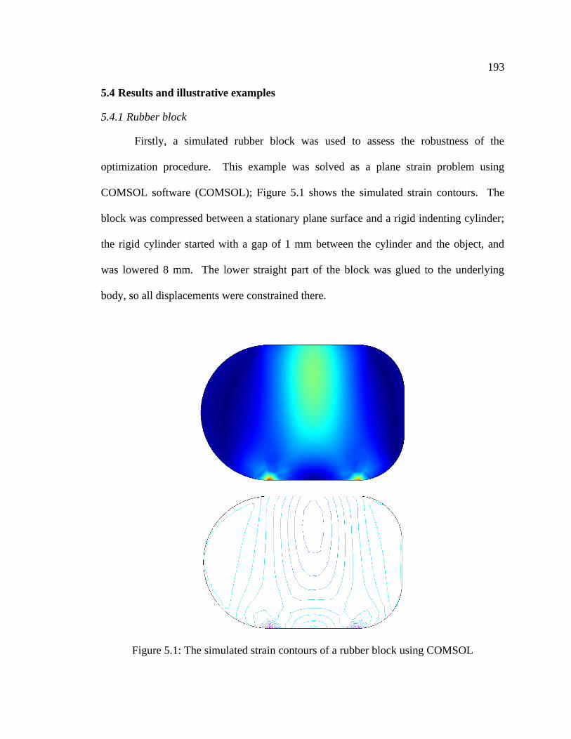
193

5.4 Results and illustrative examples

5.4.1 Rubber block

Firstly, a simulated rubber block was used to assess the robustness of the

optimization procedure. This example was solved as a plane strain problem using

COMSOL software (COMSOL); Figure 5.1 shows the simulated strain contours. The

block was compressed between a stationary plane surface and a rigid indenting cylinder;

the rigid cylinder started with a gap of 1 mm between the cylinder and the object, and

was lowered 8 mm. The lower straight part of the block was glued to the underlying

body, so all displacements were constrained there.

Figure 5.1: The simulated strain contours of a rubber block using COMSOL

194

The rubber material used in this experiment is hyperelastic and was approximated

as a Mooney-Rivlin material with 𝐶10 = 0.37𝑀𝑃𝑎 and 𝐶01 = 0.11𝑀𝑃𝑎. The material is

almost incompressible, so the bulk modulus was set to 104 MPa , and the mixed

formulation option was used. The simulated surface normal strains along a vertical

direction were used for updating the model to define the parameters (Table 5.2).

Table 5.2: numerical test of the inverse problem (𝑰𝑴 = 𝟎.𝟎𝟎𝟎𝟏)

Parameter Reference value Re-identified

value

Relative error Variances

𝐂𝟏𝟎 0.37 0.3704 0.11% 0.02

𝐶01 0.11 0.1106 0.55% 0.02

1/𝐷1 104 103.6 -0.38% 4.8

Studies examining the performance of DIC suggest that a 5% RMS error in strain

measurement is a safe estimation (Tong, 2005) (Robert, Nazaret et al., 2007). Therefore,

5% synthetic noise was added to the simulated strains. The results show that this

procedure produces good solutions even with potential noise in the DIC measurements

(Table 5.3).

195

Table 5.3: numerical test of the inverse problem with 5% synthetic noise (𝑰𝑴 = 𝟎.𝟎𝟎𝟎𝟒)

Parameter Reference value Re-identified

value

Relative error Variances

𝐂𝟏𝟎 0.37 0.3647 -1.43% 0.09

𝐶01 0.11 0.1189 8.09% 0.05

1/𝐷1 104 106.3 2.21% 17.4

5.4.2 Engine mount

An engine mount with a rubber component was tested in the second numerical

example. The FE simulation is performed using commercial FE software ANSYS

(ANSYS). In the FE model, totally 9454 solid185 hyperelastic elements are used to mesh

one rubber block in the engine mount; symmetry condition is used to reduce the

computation cost in the FE simulation.

Figure-5.2 shows a typical experimental setup using ARAMIS DIC system. A

random speckle pattern using black and white spray paints was coated on the surface of

the specimen. The two cameras are shown mounted on a stable base with a special

support tripod and support bars that allowed flexibility in positioning the cameras.

External light was used to provide optimal exposure. The lighting is especially important

as the contrast between white and black speckles can determine the success of a

measurement. Likewise, stabilizing the camera, in order to minimize movement and

vibration while capturing images, is particularly important. camera movement causes

errors in the camera calibration and deformation calculations. Preliminary trials were

conducted to optimize the camera placement and the random speckle pattern.

196

A small region on the randomly speckled surface of the object was measured

using high zoom ratios along with the 1-inch2 (25.4 mm) pre-manufactured calibration

block that comes with the ARAMIS DIC system. Random speckle patterns were created

using 15-pixel subsets that were three times larger than the mean speckle size (5-6 pixels).

(DIC measurement depends on the surface speckle pattern of the component to be

measured. Um and Kim (2007) studied the effects of subset size, subset shape, and step

size on correlation error. Robert et al. (2007) examined the effects of factors such as

speckle size and geometry and image noise in speckle patterns. In general, the findings

indicate that if the size of a large speckle is larger than the subset, poor correlation scores

will result. Thus, a practical rule of thumb is that the subset should be three times larger

than the mean speckle size).

The DIC measurement depends on the surface speckle pattern of the component

to be measured. Um and Kim conducted experimental research of a paper tensile

specimen to study the effect of subset size, subset shape, and step size, on the correlation

error (Um and Kim, 2007). Robert et al studied the effect of speckle patterns, i.e., factors

such as speckle size and geometry, image noise, etc. (Robert, Nazaret et al., 2007). It was

found that if the size of a large speckle is larger than the subset, bad correlation scores

will results. A practical rule of thumb is that the subset 3 times larger than the mean

speckle size. A subset size of 15 pixels was used in our DIC test; an optimal speckle size

should be 5 to 6 pixels.

The frontal surface of the mount was first painted white, and then a black speckle

pattern was randomly sprayed onto the white painted surface. Efforts were made to

obtain an evenly distributed homogeneous pattern of black paint drops on the undeformed

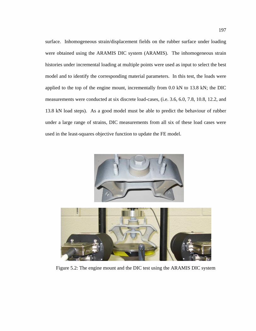
197

surface. Inhomogeneous strain/displacement fields on the rubber surface under loading

were obtained using the ARAMIS DIC system (ARAMIS). The inhomogeneous strain

histories under incremental loading at multiple points were used as input to select the best

model and to identify the corresponding material parameters. In this test, the loads were

applied to the top of the engine mount, incrementally from 0.0 kN to 13.8 kN; the DIC

measurements were conducted at six discrete load-cases, (i.e. 3.6, 6.0, 7.8, 10.8, 12.2, and

13.8 kN load steps). As a good model must be able to predict the behaviour of rubber

under a large range of strains, DIC measurements from all six of these load cases were

used in the least-squares objective function to update the FE model.

Figure 5.2: The engine mount and the DIC test using the ARAMIS DIC system

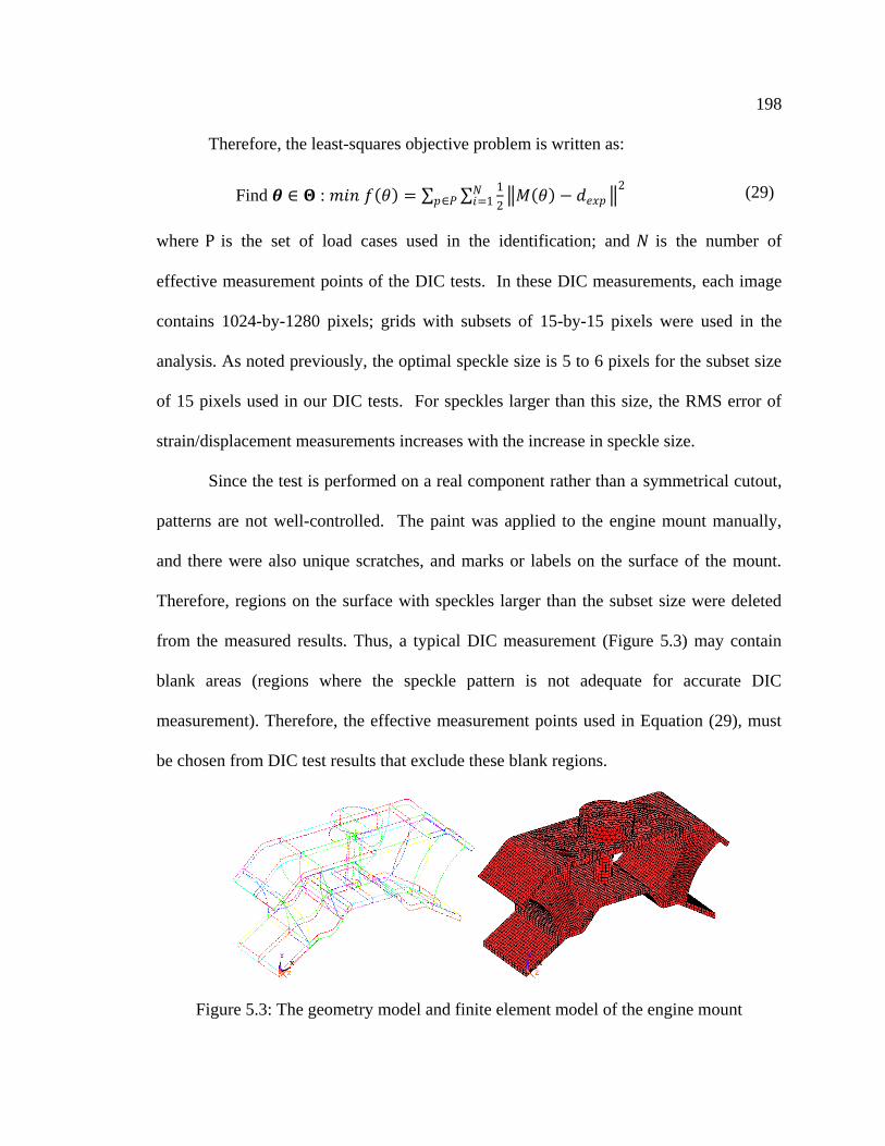
198

Therefore, the least-squares objective problem is written as:

Find 𝜽 ∈ 𝚯 : 𝑚𝑖𝑛 𝑓 𝜃 = 1

2 𝑀 𝜃 − 𝑑𝑒𝑥𝑝

2𝑁𝑖=1𝑝∈𝑃 (29)

where P is the set of load cases used in the identification; and 𝑁 is the number of

effective measurement points of the DIC tests. In these DIC measurements, each image

contains 1024-by-1280 pixels; grids with subsets of 15-by-15 pixels were used in the

analysis. As noted previously, the optimal speckle size is 5 to 6 pixels for the subset size

of 15 pixels used in our DIC tests. For speckles larger than this size, the RMS error of

strain/displacement measurements increases with the increase in speckle size.

Since the test is performed on a real component rather than a symmetrical cutout,

patterns are not well-controlled. The paint was applied to the engine mount manually,

and there were also unique scratches, and marks or labels on the surface of the mount.

Therefore, regions on the surface with speckles larger than the subset size were deleted

from the measured results. Thus, a typical DIC measurement (Figure 5.3) may contain

blank areas (regions where the speckle pattern is not adequate for accurate DIC

measurement). Therefore, the effective measurement points used in Equation (29), must

be chosen from DIC test results that exclude these blank regions.

Figure 5.3: The geometry model and finite element model of the engine mount

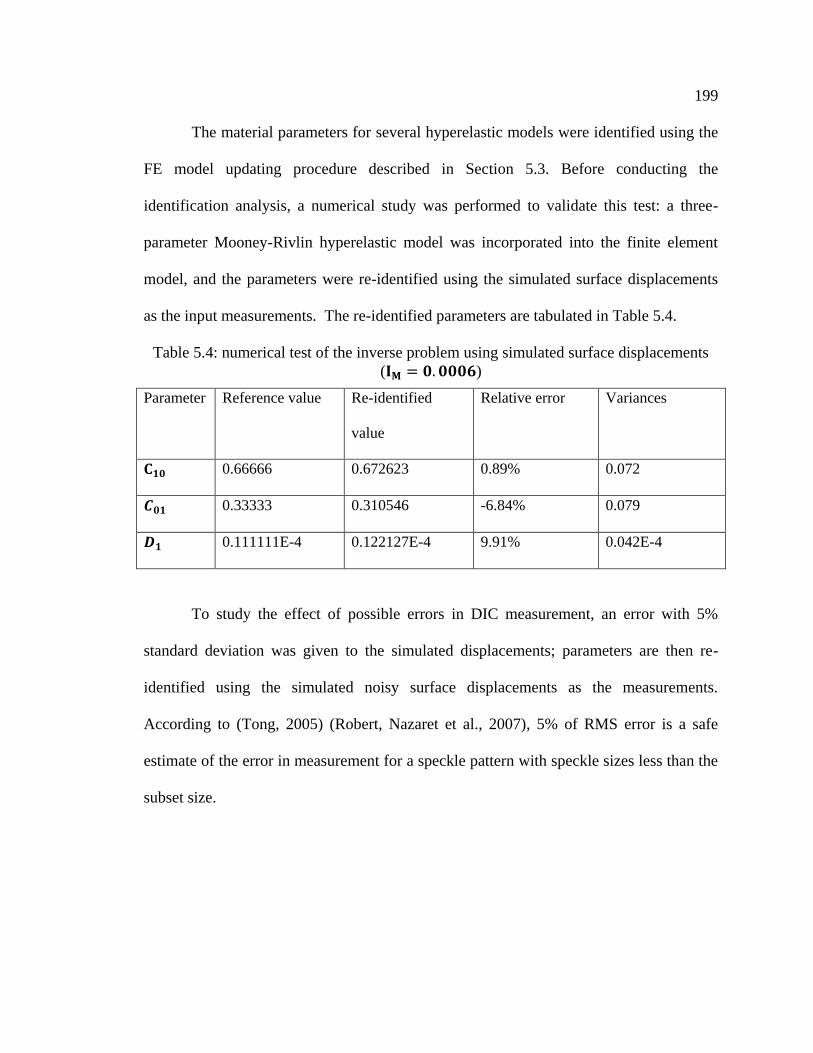
199

The material parameters for several hyperelastic models were identified using the

FE model updating procedure described in Section 5.3. Before conducting the

identification analysis, a numerical study was performed to validate this test: a three-

parameter Mooney-Rivlin hyperelastic model was incorporated into the finite element

model, and the parameters were re-identified using the simulated surface displacements

as the input measurements. The re-identified parameters are tabulated in Table 5.4.

Table 5.4: numerical test of the inverse problem using simulated surface displacements

(𝐈𝐌 = 𝟎.𝟎𝟎𝟎𝟔)

Parameter Reference value Re-identified

value

Relative error Variances

𝐂𝟏𝟎 0.66666 0.672623 0.89% 0.072

𝑪𝟎𝟏 0.33333 0.310546 -6.84% 0.079

𝑫𝟏 0.111111E-4 0.122127E-4 9.91% 0.042E-4

To study the effect of possible errors in DIC measurement, an error with 5%

standard deviation was given to the simulated displacements; parameters are then re-

identified using the simulated noisy surface displacements as the measurements.

According to (Tong, 2005) (Robert, Nazaret et al., 2007), 5% of RMS error is a safe

estimate of the error in measurement for a speckle pattern with speckle sizes less than the

subset size.

200

Table 5.5: numerical test of the inverse problem using simulated surface displacements

with synthetic noise (𝑰𝑴 = 𝟎.𝟎𝟎𝟏𝟑)

Parameter Reference value Re-identified

value

Relative error Variances

𝐂𝟏𝟎 0.66666 0.67812 1.72% 0.091

𝑪𝟎𝟏 0.33333 0.31735 -4.79% 0.099

𝑫𝟏 0.111111E-4 0.12472E-4 12.25% 0.048E-4

Tables 5.4 and 5.5 show that, for the identification of parameters in a Mooney-

Rivlin hyperelastic model, the accuracy of the identified 𝐶10 parameter is very good,

while the potential errors in identification of the 𝐶01 parameter and the 𝐷1 parameter are

relatively high. The identified strain energy function is sufficient to describe the behavior

of this rubber, however, because the contribution of the 𝐶10 parameter is dominant in the

Mooney-Rivlin strain energy function. Furthermore, the effects of parameter 𝐶01 and the

compressibility parameter 𝐷1 are relatively insignificant for a strain range up to 150%,

so this level of error can be regarded as acceptable in FE analysis.

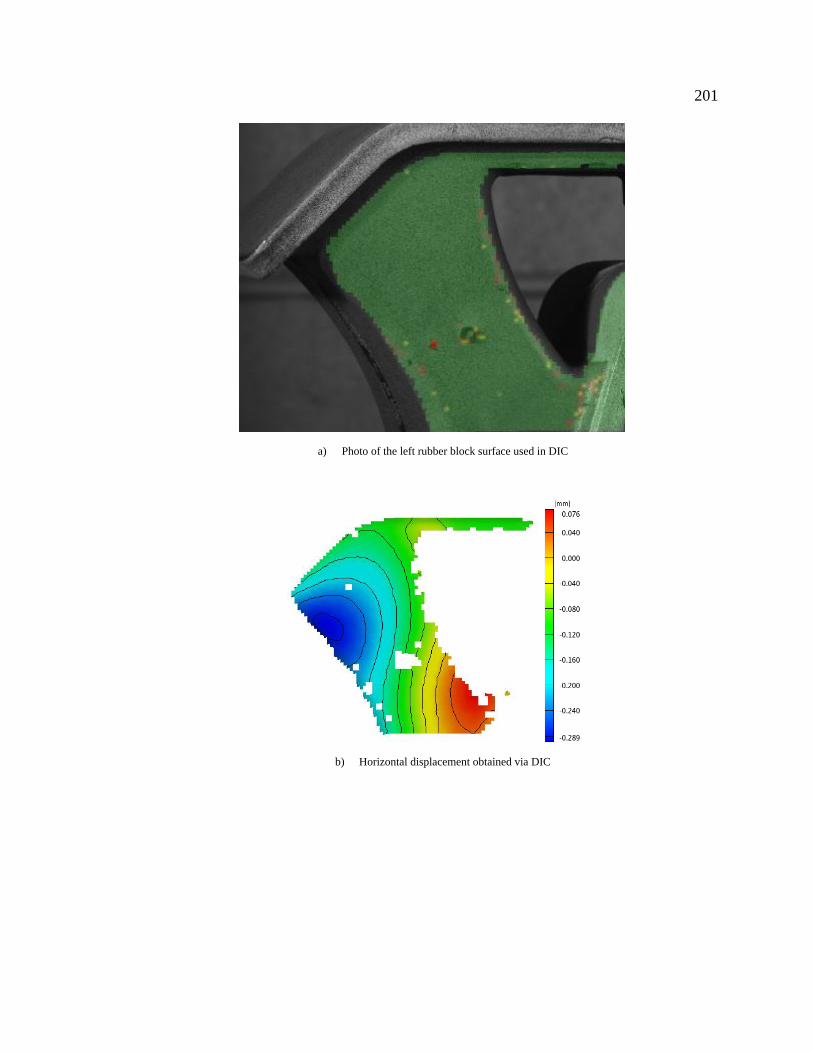
201

a) Photo of the left rubber block surface used in DIC

b) Horizontal displacement obtained via DIC

202

c) Vertical displacement obtained via DIC

Figure 5.4: The DIC measurements of displacement in the 7.8 kN load case

a) Horizontal displacement b) Vertical displacement

Figure 5.5: The FE simulation of displacement at the 7.8 kN load case using identified

Mooney-Rivlin model

The parameters identified for four different strain energy functions using the

experimental data are tabulated in Table 5.6. The estimated variance for each parameter

is given in brackets. Note that, as the measure derives from different models in this case,

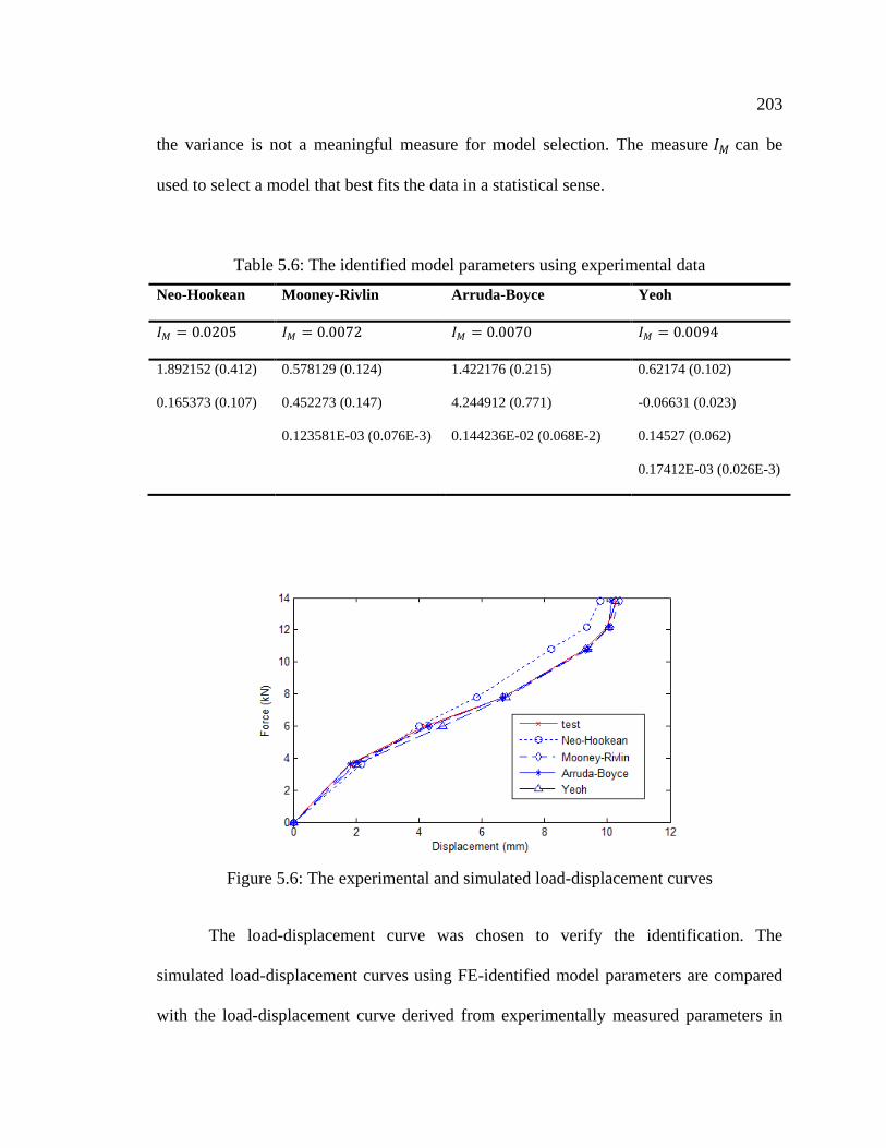
203

the variance is not a meaningful measure for model selection. The measure 𝐼𝑀 can be

used to select a model that best fits the data in a statistical sense.

Table 5.6: The identified model parameters using experimental data

Neo-Hookean Mooney-Rivlin Arruda-Boyce Yeoh

𝐼𝑀 = 0.0205 𝐼𝑀 = 0.0072 𝐼𝑀 = 0.0070 𝐼𝑀 = 0.0094

1.892152 (0.412)

0.165373 (0.107)

0.578129 (0.124)

0.452273 (0.147)

0.123581E-03 (0.076E-3)

1.422176 (0.215)

4.244912 (0.771)

0.144236E-02 (0.068E-2)

0.62174 (0.102)

-0.06631 (0.023)

0.14527 (0.062)

0.17412E-03 (0.026E-3)

Figure 5.6: The experimental and simulated load-displacement curves

The load-displacement curve was chosen to verify the identification. The

simulated load-displacement curves using FE-identified model parameters are compared

with the load-displacement curve derived from experimentally measured parameters in

204

Figure 5.6. The Neo-Hookean model does not perform well for high load ranges because

it is a linear shear modulus model. The simulated load-displacement curves generated by

the three other FE-identified models compare well with the experimental load-

displacement curve. In particular, the Mooney-Rivlin and Arruda-Boyce models

produced the best outcomes in terms of accurately simulating the experimental load-

displacement curve. Thus, designers can use FE-identified models, such as the Mooney-

Rivlin and Arruda-Boyce models in this case, to assess a static stiffness measure for the

design of a component under different load configurations and strain ranges. Moreover,

the examination of relative error when artificial noise was added to the test data indicates

that the level of error in FE-models is comparable to that seen in experimental tests.

The Mooney-Rivlin strain energy function parameters, which were identified after

introducing noise (5% error to the DIC experimental data), are given in Table 5.7. The

relative error shown in this table was calculated with respect to the model parameters

identified without artificial noise in the test data. Therefore, according to this numerical

analysis, the identification of model parameters is not overly sensitive to measurement

error; since error of ±5% is well within the range of potential error in a well-controlled

DIC test, this level of error is acceptable for numerical analysis. Likewise, the speckle

points applied to the surface were approximately 3 to 5 pixels (less than 0.05mm) in

diameter; the corresponding subset size chosen was 15 pixels. According to Tong and

Robert, RMS error of 5% is a safe estimate of the measurement error for a speckle pattern

with speckle sizes smaller than the subset size (Tong, 2005) (Robert, 2007)).

205

Table 5.7: Sensitivity of the identified model parameters with introduced noise in the test

data

Identified Mooney-Rivlin

model without artificial noise in

test data

Identified Mooney-Rivlin

model with artificial noise in

test data

Relative error

0.578129

0.452273

0.123581E-03

0.581362

0.474483

0.136529E-03

0.56%

4.91%

10.48%

5.5 Summary

This chapter provides a methodology for rapid model selection and identification

of model parameters for rubber-like materials in structural components. This method is

based on an inverse problem approach which uses displacement/strain data measured by

digital image correlation (DIC) as input. A least-squares objective function is minimized

by use of a trust region-based derivative-free optimization method. An engine mount

with rubber components was tested to demonstrate and validate this approach.

The concept proposed in this chapter is a flexible methodology for the

identification of effective material models of rubber-like materials. The identifiability of

model parameters and numerical stability issues arising from this approach are discussed;

several numerical analyses are recommended to validate model identification.

In particular, this chapter considers the identification of constitutive parameters of

rubberlike materials under monotonic loading. Future research would include the

identification of constitutive parameters of rubber-like materials under cyclic loading,

enabling study of parameters defining hysteresis and the Mullins effect. The Mullins

effect is closely related to the fatigue of elastomeric parts used in engineering

206

applications. Quantitative study of the Mullins effect is thus a necessary step towards the

scientific evaluation of the fatigue life of rubber and rubber-like materials.

207

CHAPTER SIX: CONCLUSION AND FUTURE WORK

Contribution is sometimes a reward in itself. Recognition of the value of an idea is a

further reward. Edward de Bono

This thesis solves two inverse problems: (i) reconstruction of stiffness distribution of

beams which can serve as damage identification and structural monitoring technique, and

(ii) the identification of nonlinear material model parameters of components/specimens

which is a topic in more and more demanding as engineers today have the ambition to

describe comprehensively the nonlinear deformation processes of materials and structures.

The two inverse problems are different, one is ill-posed functional identification and one

is well-posed parameter identification, although the former must also be solved in

parametric ways.

In this work, optically measured beam deflection profiles and full-field

displacements/strains on the specimen surface using digital cameras are used as inputs to

inverse identification processes. The author believes that optical measuring techniques

are very promising, and whence combined with modern parameter identification

techniques, offers great potentials to engineering problems including damage and

material identification.

A novel methodology of damage identification is developed using static

deflection measurements. Two FE model updating methods for beams were proposed in

this work; they can be used as damage identification methods. The methods presented in

this work depart from traditional damage identification techniques by trying to

208

reconstruct the complete stiffness distribution of a beam. Although a baseline model is

required, only boundary conditions need to be accurately modeled.

Throughout this work, a number of ―future work‖ have appeared in text. This is

not an indication of a lack of effort; rather, it reflects the fact of the research,

1) Measurements: photogrammetry, camera calibration, metric cameras, other

measurement techs, fibre optic, inclinometers, etc.

2) Additional field testing: the primary focus of future efforts should be on continued

testing with field testing on real structures, to see how well the methods will

perform in practice. Loading is a problem, especially bridges, issues like lighting,

requirement of stable mounting base, calibration of cameras may arise and need to

be studied in practice. Another interesting issue can be the permanent mounting of

inspecting cameras and data transition through cables, in a time that cameras are

installed everywhere for security of humans, it would a more though to use

cameras for safety of structures.

3) Combination of different damage identification techniques: local+global, dynamic

+ static, irregularity detection from static deflection measurements.

209

REFERENCES

Adelman, H. M. and Haftka, R. T. (1986). "Sensitivity analysis of discrete structural

systems." AIAA Journal 24(5).

ADINA. "ADINA software, www.adina.com." Retrieved September 1, 2011.

Aguir, H., BelHadjSalah, H. and Hambli, R. (2011). "Parameter identification of an

elasto-plastic behaviour using artificial neural networks-genetic algorithm method."

Materials and Design 32: 48-53.

ANSYS. "the ANSYS software, http://www.ansys.com, Swanson Analysis Systems,

Inc.". Retrieved May 1, 2011.

ARAMIS. "ARAMIS system, http://www.trilion.com ". Retrieved September 1, 2008.

Arnoldy, B. (2007). How to pay for US road and bridge repair? . The Christian Science

Monitor. August 10.

Arora, J. S. (2007). Optimization of structural and mechanical systems, World Scientific.

Arruda, E. M. and Boyce, M. C. (1993). "A three-dimensional constitutive model for the

large stretch behavior of rubber elastic materials." Journal of the Mechanics and Physics

of Solids 41(2): 389-412.

ASME (2006). Guide for Verification and Validation in Computational Solid Mechanics,

American Society of Mechanical Engineers.

Aster, R. C., Borchers, B. and Thurber, C. H. (2005). Parameter estimation and inverse

problems. Amsterdam, Elsevier Academis Press.

ASTM (2011). Standard test methods for tension testing of metallic materials. E8M-11.

Bakht, B. and Jaeger, L. G. (1990). "Bridge testing: a surprise every time." Journal of

Structural Engineering 116: 1370-1383.

Banan, M. R., Banan, M. R. and Hjelmstad, K. D. (1994a). "Parameter estimation of

structures from static response. I. computational aspects." Journal of Structural

Engineering 120(11): 3243-3258.

Banan, M. R., Banan, M. R. and Hjelmstad, K. D. (1994b). "Parameter estimation of

structures from static response. II. numerical simulation studies." Journal of Structural

Engineering 120(11): 3259-3283.

210

Barazzetti, L. and Scaioni, M. (2010). "Development and Implementation of Image-based

Algorithms for Measurement of Deformations in Material Testing." Sensors 10: 7469-

7495.

Bard, Y. (1974). Nonlinear parameter estimation. New Tork, Academic Press.

Batabyal, A. K., Sankar, P. and Paul, T. K. (2008). Crack detection in cantilever beam

using vibration response. Vibration Problems ICOVP-2007. Inan, E., Springer Science.

Bates, D. M. and Watts, D. G. (1980). "Relative curvature measures of nonlinearity (with

discussion)." Journal of Royal Statistical Society B 42(1): 1-25.

Bates, D. M. and Watts, D. G. (1988). Nonlinear regression analysis and its applications,

John Wiley & Sons, Inc.

Beck, J. V. and Arnold, K. J. (1977). Parameter estimation in engineering and science.

NY, John Wiley & Sons.

Bell, J. F. (1984). The experimental foundations of solid mechanics. Berlin and New

York, Springer-Verlag.

Benjeddou, A., Jankovich, E. and Hadri, T. (1993). "Determination of the parameters of

Ogdens law using biaxial data and Levenberg-Marquardt-Fletcher algorithm." Journal of

Elastomers and Plastics 25: 224-248.

Berghen, F. V. (2004). CONDOR: a constrained, non-linear, derivative-free parallel

optimizer for continuous, high computing load, noisy objective functions. Belgium,

Universite Libre de Bruxelles. PhD.

Berghen, F. V. and Bersini, H. (2005). "CONDOR, a new parallel, constrained extension

of Powell's UOBYQA algorithm: Experimental results and comparison with the DFO

algorithm." Journal of Computational and Applied Mathematics 181: 157-175.

Bicanic, N. and Chen, H. P. (1997). "Damage identification in framed structures using

natural frequencies." International Journal for Numerical Methods in Engineering 40:

4451-4468.

Bos, A. V. D. (2007). Parameter estimation for scientists and engineers, John Wiley &

Sons.

Boyce, M. C. and Arruda, E. M. (2000). "Constitutive models of rubber elasticity: a

review." Rubber Chemistry Technology 73: 504-523.

Bridgman, P. W. (1952). Studies in Large Plastic Flow and Fracture. New York, McGraw

Hill.

211

Broggiato, G. B., Campana, F. and Cortese, L. (2007). "Identification of material

damage model parameters: an inverse approach using digital image processing."

Meccanica 42: 9-17.

Brownjohn, J. M. W., Xia, P., Hao, H. and Xia, Y. (2001). "Civil structure condition

assessment by FE model updating: methodology and case studies." Journal of Finite

Elements in analysis and Design 37: 761-775.

Buda, G. and Caddemi, S. (2007). "Identification of concentrated damages in Euler-

Bernoulli beams under static loads." Journal of Engineering Mechanics 133(8): 942-956.

Caesar, B. and Pete, J. (1987). "Direct update of dynamic mathematical models from

model test data." AIAA Journal 25: 1494-1499.

Carden, E. P. and Fanning, P. (2004). "Vibration based condition monitoring: a review."

Structural Health Monitoring 3(4): 355-377.

Cardenas-Garcia, J. F., Wu, M. M. and Hashemi, J. (1997). A review of strain

measurement techniques using the grid method. Nontraditional methods of sensing stress,

strain, and damage in materials and structures. Lucas, G. F. and Stubbs, D. A., ASTM,

Philadelphia.

Cerri, M. N. and Vestroni, F. (2003). "Use of frequency change for damage identification

in reinforced concrete beams." Journal of Vibration and Control 9(3-4): 475-491.

Chan, T. F., Golub, G. H. and Mulet, P. (1996). A nonlinear primal-dual method for total

variation-based image restoration. Lecture Notes in Control and Information Sciences.

219: 241-252.

Chen, L. C., Jan, H. H. and Huang, C. W. (2001). Measurement of concrete cracks using

digitized close-range photographs. 22nd Asian Conference on Remote Sensing.

Singapore.

Chevalier, L., Calloch, S., Hild, F. and Marco, Y. (2001). "Digital image correlation used

to analyze the mul-tiaxial behaviour of rubberlike materials." Europian Journal of

Mechanics A 20: 169-187.

Choi, I. Y., Lee, J. S., Choi, E. and Cho, H. N. (2004). "Development of elastic damage

load theorem for damage detection in a statically determinate beam." Computers and

Structures 82: 2483-2492.

Chou, J.-H. and Ghaboussi, J. (2001). "Genetic algorithm in structural damage detection."

Computers and Structures 79: 1335-1353.

212

Chu, T. C., Ranson, W. F., Sutton, M. A. and Peters, W. H. (1985). "Applications of

digital image correlation techniques to mechanics." Experimental Mechanics 25(3): 232-

244.

Ciarlet, P. G. (1988). Mathematical elasticity, Volume 1: Three dimensional elasticity,

Elsevier.

Cobelli, C. and DiStefano, J. J. (1980). "Parameter and structural identifiability concepts

and ambiguities: a critical review and analysis." American Journal of Physiology 239(1):

R7-R24.

COMSOL. "COMSOL software, www.comsol.com." Retrieved May 1, 2009.

Conn, A. R., Scheinberg, K. and Toint, P. L. (1997). "Recent progress in unconstrained

nonlinear optimization without derivatives." Mathematical Programming 79: 397-414.

Conn, A. R., Scheinberg, K. and Vicente, L. N. (2009). Introduction to derivative-free

optimization. Philadelphia, SIAM.

Cooreman, S., Lecompte, D., Sol, H., Vantomme, J. and Debruyne, D. (2007). "Elasto-

plastic material parameter identification by inverse methods: Calculation of

the sensitivity matrix." International Journal of Solids and Structures 44: 4329 - 4341.

Cooreman, S., Lecompte, D., Sol, H., Vantomme, J. and Debruyne, D. (2008).

"Identification of Mechanical Material Behavior Through Inverse Modeling and DIC."

Experimental Mechanics 48: 421-433.

Cornwell, P. J., Farrar, C. R., Doebling, S. W. and Sohn, H. (1999). "Environmental

variability of modal properties." Experimental Techniques 23: 45-48.

Cronk, S., Fraser, C. and Hanley, H. (2006). "Automated metric calibration of colour

digital cameras." The Photogrammetric Record 21(116): 355-372.

Desrues, J. and Viggiani, G. (2004). "Strain localization in dans: an overview of the

experimental results obtained in Grenoble using stereophotogrammetry." International

Journal for Numerical and Analytical Methods in Geomechanics 28: 279-321.

Doebling, S. W. and Farrar, C. R. (1997). Using Statistical Analysis to Enhance Modal-

Based Damage Identification. Structural Damage Assessment Using Advanced Signal

Processing Procedures, Proceedings of DAMAS'97. University of Sheffield, UK: 199-

210.

Doebling, S. W., Farrar, C. R. and Prime, M. B. (1998). "A summary review of vibration-

based damage identification methods." The Shock and Vibration Digest 30(2): 91-105.

213

Doebling, S. W., Farrar, C. R., Prime, M. B. and Shevitz, D. W. (1996). Damage

identification and health monitoring of structural and mechanical systems from changes

in their vibration characteristics: a literature review Research Report, LA-13070-MS,

ESA-EA. Los Alamos, N.M., USA. , Los Alamos National Laboratory.

Doghri, I. (2000). Mechanics of deformable solids. Berlin, Heidelberg, Springer Verlag.

Donaldson, J. R. and Schnabel, R. B. (1987). "Computational Experience With

Confidence Regions and Confidence Intervals for Nonlinear Least Squares."

Technometrics 29(1): 67-82.

Durelli, A. J. and Parks, V. J. (1970). Moiré analysis of strain. Eaglewood Cliffs, NJ,

Prentice-Hall.

Dusunceli, N., Colak, O. U. and Filiz, C. (2010). "Determination of material parameters

of a viscoplastic model by genetic algorithm." Materials and Design 31: 1250-1255.

ERDAS (2002). IMAGINE OrthoBASE user‘s guide Version 8.6. Atlanta, USA, Leica

Geosystems.

Farhat, C. and Hemez, P. M. (1993). "Updating finite element dynamics models using an

element-by-element sensitivity methodology." AIAA Journal 31(9): 1702-1711.

Farrar, C. R., Cornwell, P. J., Doebling, S. W. and Prime, M. B. (2000). Structural Health

Monitoring Studies of the Alamosa Canyon and I-40 Bridges. Los Alamos, NM, USA,

Los Alamos National Laboratory.

Farrar, C. R. and Worden, K. (2007). "An introduction to structural health monitoring."

Philosophical Transactions of the Royal Society A 365: 303-315.

Franke, S., Franke, B. and Rautenstrauch, K. (2007). "Strain analysis of wood

components by close range photogrammetry." Materials and Structures 40: 37-46.

Fraś, T., Nowak, Z., Perzyna, P. and Pecherski, R. B. (2011). "Identification of the model

describing viscoplastic behaviour of high strength metals." Inverse Problems in Science

and Engineering 19(1): 17-30.

Friswell, M. I. (2007). "Damage identification using inverse methods." Philosophical

Transactions of the Royal Society A 365: 393-410.

Friswell, M. I. and Mottershead, J. E. (1995). Finite element model updating in structural

dynamics. Dordecht, The Netherlands, Kluwer Academic Publishers.

214

Furukawa, T. and Yagawa, G. (1997). "Inelastic constitutive parameter identification

using an evolutionary algorithm with continuous individuals." International Journal for

Numerical Methods in Engineering 40: 1071-1090.

Gendy, A. S. and Saleeb, A. F. (2000). "Nonlinear material parameter estimation for

characterizing hyperelastic large strain models." Computational Mechanics 25: 66-77.

Gent, A. (2001). Engineering with rubber, how to design rubber components. 2nd Ed.

Munich, Germany, Hanser Publishers.

Gentle, J. E. (2003). Random Number Generation and Monte Carlo Methods. New York,

NY, Springer-Verlag.

Ghouati, O. and Gelin, J.-C. (2001). "A finite element-based identification method for

complex metallic material behaviour." Computational Materials Science 21: 57-68.

Giachetti, A. (2000). "the pattern matching techniques used to compute image motion

from a sequence of two or more images." Image and Vision Computing 18(3): 247-260.

Goldfeld, Y. (2007). "Identification of the stiffness distribution in statically indeterminate

beams." Journal of Sound and Vibration 304: 918-931.

Grediac, M. (2004). "The use of full-field measurement methods in composite material

characterization: interest and limitations." Composites Part A 35: 751-761.

Grédiac, M. (2011). "the Virtual Fields Method website: http://www.camfit.fr/."

Retrieved September 20, 2011.

Grédiac, M. and Pierron, F. (2006). "Applying the Virtual Fields Method to the

identification of elasto-plastic constitutive parameters." International Journal of Plasticity

22: 602-627.

Grediac, M., Toussaint, E. and Pierron, F. (2002). "Special virtual fields for the direct

determination of material parameters with the virtual fields method. 1–Principle and

definition." International Journal of Solids and Structures(39): 2691-2705.

Green, P. J. (1988). "Regression, curvature and weighted least squares." Mathematical

Programming 42: 41-51.

Grimstad, A.-A., Kolltveit, K., Mannseth, T. and Nordtvedt, J.-E. (2001). "Assessing the

validity of a linearized accuracy measure for a nonlinear parameter estimation problem."

Inverse Problems 17: 1373-1390.

Haber, R. B., Tortorelli, D. A. and Vidal, C. A. (1993). Design sensitivity analysis of

nonlinear structures I: large-deformation hyperelasticity and history-dependent material

215

response. Structural optimization: status and promise. Kamat, M. P. Washington DC,

American Institute of Aeronautics and Astronautics 369-405.

Haines, L. M., O'Brien, T. E. and Clarke, G. P. Y. (2004). "Kurtosis and curvature

measures for nonlinear regression models." Statistica Sinica 14: 547-570.

Hajela, P. and Soeiro, F. J. (1990a). "Recent developments in damage detection based on

system identification methods." Structural Optimization 2: 1-10.

Hajela, P. and Soeiro, F. J. (1990b). "Structural damage detection based on static and

modal analysis." AIAA Journal 28(6): 1110-1115.

Hansen, P. C. (1992). "Analysis of discrete ill-posed problems by means of the L-curve."

SIAM Rev. 34: 561-580.

Hansen, P. C. (1998). Rank-deficient and discrete ill-posed problems: numerical aspects

of linear inversion. Philadelphia, SIAM.

Harth, T. (2003). Identification of material parameters for inelastic constitutive models:

stochastic simulation and design of experiments. Fechbereich Mathematik (Department

of Mathematics), Darmstadt University of Technology. PhD.

Harth, T. and Lehn, J. (2007). "Identification of material parameters for inelastic

constitutive models using stochastic methods." GAMM-Mitt. 30(2): 409-429.

Harth, T., Schwan, S., Lehn, J. and Kollmann, F. G. (2004). "Identification of material

parameters for inelastic constitutive models: statistical analysis and design of

experiments." International Journal of Plasticity 20: 1403-1440.

Harth, Z., Sun, H. and Schafer, M. (2007). "Comparison of derivative free Newton-based

and evolutionary methods for shape optimization of flow problems." International Journal

for Numerical Methods in Fluids 53: 753-775.

Hartmann, S. (2001). "Numerical studies on the identification of the material parameters

of Rivlin's hyperelasticity using tension-torsion tests." Acta Mechanica 148: 129-155.

Hegger, J., Sherif, A. and Gortz, S. (2004). "Investigation of Pre- and Postcracking Shear

Behavior of Prestressed Concrete Beams Using Innovative Measuring Techniques." ACI

Structural Journal 101(2): 183-192.

Heijden, F. v. d. (1994). Image based measurement systems: object recognition and

parameter estimation. New York, NY, John Wiley & Sons.

Hendricks, M. A. N. (1991). Identification of the mechanical behavior of solid materials.

Eindhoven, The Netherlands, Eindhoven University of Technology. PhD.

216

Heywood, R. J., Roberts, W., Taylor, R. and Anderson, R. (2000). "Fitness-for-purpose

evaluation of bridges using health monitoring technology." Transportation Research

Record 1696: 193-201.

Hjelmstad, K. D. and Shin, S. (1997). "Damage detection and assessment of structures

from static response." Journal of Engineering Mechanics 123(6): 568-576.

Hof, J. M. v. d. (1998). "Structural Identifiability of Linear Compartmental Systems."

IEEE Transactions on Automatic Control 43(6): 880-818.

Hooke and Jeeves (1961). "Direct search solution of numerical and statistical problems.

." Journal of the Association for computing Machinery 8: 212-229.

Horgan, C. O. and Saccomandi, G. (2004). "Constitutive models for compressible

nonlinearly elastic materials with limiting chain extensibility." Journal of Elasticity 77:

123-138.

Horgan, C. O. and Saccomandi, G. (2006). "Phenomenological hyperelastic strain-

stiffening constitutive models for rubber." Rubber Chemistry Technology 79: 152-169.

Hsia, T. C. (1977). System identification: least-squares methods. Lexington,

Massachusetts, Lexington Books.

Hsieh, K. H., Halling, M. W. and Barr, P. J. (2006). "Overview of Vibrational Structural

Health Monitoring with Representative Case Studies." Journal of Bridge Engineering

11(6): 707-715.

Hu, X. and Shenton, H. W. (2006). "Damage identification based on dead load

redistribution: effect of measurement error." Journal of Structural Engineering 132(8):

1264-1273.

Hu, X. and Shenton, H. W. (2007). "Dead load based damage identification method for

long term structural health monitoring." Journal of Intelligent Material systems and

Structures 18: 923-938.

Huet, S., Bouvier, A., Poursat, M.-A. and Jolivet, E. (2004). Statistical Tools for

Nonlinear Regression. New York, NY, Springer-Verlag.

Hwang, S.-F., Wu, J.-C., Barkanovs, E. and Belevicius, R. (2010). "Elastic constants of

composite materials by an inverse determination method based on a hybrid genetic

algorithm." Journal of Mechanics 26(3).

Jacobsen, K. (2000). Program system BLUH user‘s manual. Hanover, Institute of

Photogrammetry and Engineering Surveys, University of Hanover: 444 pages.

217

Jauregui, D. V., White, K. R., Woodward, C. B. and Leitch, K. R. (2002). Static

measurement of beam deformations via close-range photogrammetry. Transportation

Research Record. Las Cruces, New Mexico, USA, New Mexico State University,

Department of Civil and Geological Engineering. 1814: 3-8.

Jauregui, D. V., White, K. R., Woodward, C. B. and Leitch, K. R. (2003). "Noncontact

Photogrammetric Measurement of Vertical Bridge Deflection." Journal of Bridge

Engineering 8(4): 212-222.

Juang, J. N. (1994). Applied system identification. Englewood Cliffs, NJ, Prentice Hall.

Katafygiotis, L. S. and Beck, J. L. (1998). "Updating models and their uncertainties. II:

model identifiability." Journal of Engineering Mechanics 124(4): 463-467.

Keane, A. J. and Nair, P. B. (2005). Computational approaches for aerospace design,

John Wiley & Sons

Kelley, C. T. (1999). Iterative methods for optimization. Philadelphia, USA, SIAM.

Kim, H. and Melhelm, H. (2004). "Damage detection of structures by wavelet analysis."

Engineering Structures 26: 347-362.

Kim, J. T., Ryu, Y. S., Cho, H. M. and Stubbs, N. (2003). "Damage identification in

beam-type structures: frequency-based method vs. mode-shape-based method."

Engineering Structures 25: 57-67.

Kleuter, B., Menzel, A. and Steinmann, P. (2007). "Generalized parameter identification

for finite viscoelasticity." Computer Methods in Applied Mechanics and Engineering

196: 3315-3334.

Koch, K.-R. (2007). Introduction to Bayesian Statistics. Berlin Heidelberg, Springer-

Verlag.

Kojic, M. and Bathe, K.-J. (2005). Inelastic Analysis of Solids and Structures. Berlin

Heidelberg, Springer-Verlag.

Kokot, S. and Zambaty, Z. (2009a). "Damage reconstruction of 3D frames using genetic

algorithms with Levenberg-Marquardt local search." Soil Dynamics and Earthquake

Engineering 29(2): 311-323.

Kokot, S. and Zambaty, Z. (2009b). "Vibration based stiffness reconstruction of beams

and frames by observing their rotations under harmonic excitations - numerical analysis."

Engineering Structures 31: 1581-1588.

218

Kosmatka, J. B. and Ricles, J. M. (1999). "Damage detection in structures by modal

vibration characterization." Journal of Structural Engineering 125(12): 1384-1392.

Kreißig, R., Benedix, U., U.-J.Gorke and Lindner, M. (2007). "Identification and

estimation of constitutive parameters for material laws in elastoplasticity." GAMM-Mitt.

30(2): 458-480.

Kundu, T. (2004). Ultrasonic nondestructive evaluation: engineering and biological

material characterization. Boca Raton, FL, CRC Press.

LaVision. "StrainMaster system of LaVision,

http://www.lavision.de/en/products/strainmaster.php."

Lee, P. v. d., Terlaky, T. and Woudstra, T. (2001). "A new approach to optimizing energy

systems." Computer Methods in Applied Mechanics and Engineering 190: 5297-5310.

Lefik, M. and Schrefler, B. A. (2002). "Artificial neural network for parameter

identifications for an elasto-plastic model of superconducting cable under cyclic loading."

Computers and Structures 80: 1699-1713.

Lemaitre, J. (1996). A Course on Damage Mechanics. 2nd ed. , Springer.

Lesnic, D., Elliott, L. and Ingham, D. B. (1999). "Analysis of coefficient identification

problems associated to the inverse Euler-Bernoulli beam theory." IMA Journal of

Applied Mathematics 62: 101-116.

Li, Z., Yuan, X. and Lam, K. W. K. (2002). "Effects of JPEG compression on the

accuracy of photogrammetric point determination." Photogrammetric Engineering &

Remote Sensing 68(8): 847-853.

Lifshitz, J. M. and Rotem, A. (1969). "Determination of Reinforcement Unbonding of

Composites by a Vibration Technique." Journal of Composite Materials 3: 412-423.

Linder, W. (2009). Digital Photogrammetry: A Practical Course, Springer-Verlag Berlin

Heidelberg.

Liu, G. R. and Chen, S. C. (2002). "A novel technique for inverse identification of

distributed stiffness factor in structures." Journal of Sound and Vibration 254(5): 823-

835.

Liu, P. L. and Chian, C. C. (1997). "Parametric identification of truss structures using

static strains." Journal of Structural Engineering 123(7): 927-933.

219

Liu, X., Lieven, N. A. J. and Escamilla-Ambrosio, P. J. (2009). "Frequency response

function shape-based methods for structural damage localization." Mechanical Systems

and Signal Processing 23: 1243-1259.

Ljung, L. (1999). System identification: theory for the user. Englewood Cliffs, NJ,

Prentice Hall.

Louban, R. (2009). Image processing of edge and surface defects: theoretical basis of

adaptive algorithms with numerous practical applications. Berlin, Germany, Springer-

Verlag.

Luhmann, T., Robson, S., Kyle, S. and Harley, I. (2006). Close-range Photogrammetry,

principles, techniques and applications, Whittles Publishing.

Lynch, J. P. and Loh, K. J. (2006). "A Summary Review of Wireless Sensors and Sensor

Networks for Structural Health Monitoring." The Shock and Vibration Digest 38(2): 91-

128.

Maas, H. G. (1998). Photogrammetric Techniques For Deformation Measurements On

Reservoir Walls. Proceedings Of The IAG Symposium On Geodesy For Geotechnical

And Structural Engineering. Eisenstadt, Austria: 319-324.

Maeck, J. and Roeck, G. D. (1999). "Dynamic bending and torsion stiffness derivation

from modal curvatures and torsion rates." Journal of Sound and Vibration 251(1): 153-

170.

Maeck, J., Wahab, M. A., Peeters, B., De Roeck, G., De Visscher, J., De Wilde, W. P.,

Ndambi, J.-M. and Vantomme, J. (2000). "Damage identification in reinforced concrete

structures by dynamic stiffness determination." Engineering Structures 22(1339-1349).

Mahnken, R. (2000). "An inverse finite-element algorithm for parameter identication of

thermoelastic damage models." International Journal for Numerical Methods in

Engineering 48: 1015-1036.

Mahnken, R. (2002). "Theoretical, numerical and identification aspects of a new model

class for ductile damage." International Journal of Plasticity 18: 801-831.

Mahnken, R. (2004). Identification of Material Parameter for Constitutive Equations.

Encyclopedia of Computational Mechanics-Volume 2: Solids and Structures. Stein, E.,

Borst, R. d. and Hughes, T., John Wiley & Sons.

Mahnken, R. and Stein, E. (1996). "A unified approach for parameter identification of

inelastic material models in the frame of the finite element method." Computational

Methods in Applied Mechanics and Engineering 136: 225-258.

220

Mahnken, R. and Stein, E. (1997). "Parameter identification for finite deformation elasto-

plasticity in principal directions." Computational Methods in Applied Mechanics and

Engineering 147: 17-39.

Mangal, L., Idichandy, V. G. and Ganapathy, C. (2001). "Structural monitoring of

offshore platforms using impulse and relaxation response." Ocean Engineering 28: 689-

705.

Mars, W. V. and Fatemi, A. (2003). "A Novel Specimen for Investigating Mechanical

Behavior of Elastomers under Multiaxial Loading Conditions." Journal of Experimental

Mechanics 44(2): 136-146.

Mars, W. V. and Fatemi, A. (2004). "Observations of the Constitutive Response and

Characterization of Filled Natural Rubber under Monotonic and Cyclic Multiaxial Stress

States." Journal of Engineering Materials and Technology 126: 19-28.

Masoud, A. A. and Al-Said, S. (2009). "A new algorithm for crack localization in a

rotating Timoshenko beam." Journal of Vibration and Control 15(10): 1541-1561.

Meuwissen, M. H. H. (1998). An inverse method for the mechanical characterization of

metals. Eindhoven, The Netherlands, Eindhoven Technical University. PhD.

Meuwissen, M. H. H., Oomens, C. W. J., Baaijens, F. P. T., Petterson, R. and Janssen, J.

D. (1998). "Determination of the elasto-plastic properties of aluminium using a mixed

numerical–experimental method." Journal of Materials Processing Technology 75: 204-

211.

Mosegaard, K. and Sambridge, M. (2002). "Monte Carlo analysis of inverse problems."

Inverse Problems 18: 29-54.

Mottershead, J. E. and Friswell, M. I. (1998). "Model updating, special issue of

Mechanical systems and Signal Processing." 12(1).

Müller, D. and Hartmann, G. (1989). "Identification of Materials Parameters for Inelastic

Constitutive Models Using Principles of Biologic Evolution." Journal of Engineering

Materials and Technology 111(3): 299-305.

Munoz-Rojas, P. A., Cardoso, E. L. and Jr., M. V. (2010). "Parameter identification of

damage models using genetic algorithms." Experimental Mechanics 50: 627-634.

Murio, D. A. (1993). The mollification method and the numerical solution of ill-posed

problems, John Wiley & Sons.

Murio, D. A., Mejia, C. E. and Zhan, S. (1998). "Discrete mollification and automatic

numerical differentiation." Computers & Mathematics with Applications 35(5): 1-16.

221

Nahvi, H. and Jabbari, M. (2005). "Crack detection in beams using experimental modal

data and finite element model." International Journal of Mechanical Sciences 47: 1477.

Natke, H. G. (1988). "Updating computational models in the frequency domain based on

measured data: a survey." Probabilistic Engineering Mechanics 3(1): 28-35.

Ndambi, J. M., Vantomme, J. and Harri, K. (2002). "Damage assessment in reinforced

concrete beams using eigenfrequencies and mode shape derivatives." Engineering

Structures 24(4): 501-515.

Nejad, F. B., Rahai, A. and Esfandiarib, A. (2005). "A structural damage detection

method using static noisy data." Engineering Structures 27: 1784-1793.

Nelder, J. A. and Mead, R. (1965). "A simplex method for function minimization." The

Computer Journal 7: 308-313.

Neto, E. A. d. S., Peric, D. and Owen, D. R. J. (2008). Computational methods for

plasticity: theory and applications, John Wiley & Sons.

Niedbal, N. (1984). Analytical determination of real normal modes from measured

complex responses. 25th Structures, Structural Dynamics and Materials Conference.

Palm Springs: 292-295.

Niederöst, M. and Maas, H.-G. (1997). Automatic Deformation Measurement with a Still

Video Camera. Gruen/Kahmen (Eds.) Optical 3-D Measurement Techniques IV.

Heidelberg, Germany, Wichmann Verlag: 266-271.

Oberkampf, W. L. and Roy, C. J. (2010). Verification and validation in scientific

computing. Cambridge, UK, Cambridge University Press.

Ogden, R. W. (1972). "Large deformation isotropic elasticity: on the correlation of theory

and experi-ment for incompressible rubberlike solids." Proceedings of the Royal Society

A 326: 565-584.

Oh, B. H. and Jung, B. S. (1998). "Structural damage assessment with combined data of

static and modal tests." Journal of Structural Engineering 124(8): 956-965.

Omenzetter, P. and Brownjohn, J. M. W. (2006). "Application of time series analysis for

bridge monitoring." Smart Materials and Structures 15: 129-138.

Pan, B., Qian, K., Xie, H. and Asundi, A. (2009). "Two-dimensional digital image

correlation for in-plane displacement and strain measurement: a review." Measurement

Science and Technology 20(4): 1-17.

222

Pandey, A. K., Biswas, M. and Samman, M. M. (1991). "Damage detection from changes

in curvature mode shapes." Journal of Sound and Vibration 145(2): 321-332.

Parsons, E., Boyce, M. and Parks, D. (2004). "An experimental investigation of the large-

strain tensile beha-vior of neat and rubber toughened polycarbonate." Polymer 45: 2665-

2684.

Partheepan, G., Sehgal, D. K. and Pandey, R. K. (2008). "Finite Element Application to

Estimate Inservice Material Properties using Miniature Specimen." International Journal

of Aerospace and Mechanical Engineering 2(2): 130-136.

Patelli, E., Pradlwarter, H. J. and Schueller, G. I. (to appear). "Global Sensitivity of

Structural Variability by Random Sampling."??? ??: ??

Peeters, B. (2000). System identification and damage detection in civil engineering.

Belgium, Katholieke Universiteit Leuven. PhD: 256.

Peters, W. H. and Ranson, W. F. (1982). "Digital imaging techniques in experimental

stress analysis." Optical Engineering 21(3): 427-431.

Phares, B. M., Rolander, D. D., Graybeal, B. A. and Washer, G. A. (2001). "Reliability of

visual bridge inspection." Public Roads 64(5): 22-29.

Post, D., Han, B. and Ifju, O. (1994). High sensitivity moiré. New York, NY, Springer-

Verlag.

Powell, M. J. D. (1964). "An efficient method for finding the minimum of a function of

several variables without calculating derivatives." Comput. J. 7: 155-162.

Powell, M. J. D. (2002). "UOBYQA: unconstrained optimization by quadratic

approximation." Mathematical Programming Series B 92: 555-582.

Powell, M. J. D. (2006). "The NEWUOA software for unconstrained optimization

without derivatives." Large Scale Nonlinear Optimization: 255-297.

Price, W. L. (1983). "Global optimization by controlled random search." Journal of

Optimization Theory and Applications 40(3): 333-348.

Promma, N., Raka, B., Grediac, M., Toussaint, E., Cam, J. B. L., Balandraud, X. and

Hild, F. (2009). "Application of the virtual fields method to mechanical characterization

of elastomeric materials." International Journal of Solids and Structures 46: 698-715.

Ramberg, W. and Osgood, W. R. (1943). Description of stress-strain curves by three

parameters, National Advisory Committee for Aeronautics.

223

Ransom, W. F., Sutton, M. A. and Peters, W. H. (1987). Holographic and laser speckle

interferometry. Handbook on experimental mechanics. Kobayashi, A. S. Englewood

Cliffs, NJ, Prentice-Hall. Chap.8.

Rastogi, P. K. (2000). Photomechanics, topics in applied physics, (Ed.) Springer-Verlag

Berlin Heidelberg.

Ratcliffe, C. P. (1997). "Damage detection using a modified Laplacian operator on mode

shape data." Journal of Sound and Vibration 204(3): 505-517.

Ratcliffe, C. P. and Bagaria, W. J. (1998). "A vibration technique for locating

delamination in a composite beam." AIAA Journal 36(6): 1074-1077.

Ren, W.-X., Fang, S.-E. and Deng, M.-Y. (2011). "Response surface-based finite-

element-model updating using structural static responses." Journal of Engineering

Mechanics 137(4): 248-257.

Ren, W. X. and De Roeck, G. (2002). "Structural damage identification using modal data

I: simulation verification." Journal of Structural Engineering 128(1): 87-95.

Richardson, M. H. (1980). Detection of Damage in Structures from Changes in their

Dynamic (Modal) Properties- A survey, . Washington, D.C., U.S. Nuclear Regulatory

Commission. NUREG/CR-1431.

Rieke-Zapp, D. H. and Nearing, M. A. (2005). "Digital close range photogrammetry for

measurement of soil erosion." The Photogrammetric Record 20(109): 69-87.

Ringot, E. and Bascoul, A. (2001). "About the analysis of microcracking in concrete."

Cement & Concrete Composites 23: 261-266.

Robert, L. (2007). Estimation of digital image correlation (DIC) performances.

Experimental Analysis of Nano and Engineering Materials and Structures, Proceedings of

the 13th International Conference on Experimental Mechanics July 1–6, 2007,

Alexandroupolis, Greece. B, 2T18: 347-348.

Robert, L., Nazaret, F., Cutard and Orteu, J. J. (2007). "Use of 3-D Digital Image

Correlation to Characterize the Mechanical Behavior of a Fiber Reinforced Refractory

Castable." Experimental Mechanics 47: 761-773.

Rodic, T. and Gresovnik, I. (1998). "A computer system for solving inverse and

optimization problems." Engineering Computations 15(7): 893-907.

Rodic, T., Gresovnik, I. and Owen, D. R. J. (1995). Application of error minimization

concept to estimation of hardening parameters in the tension test. Proceedings of the

224

Fourth International Conference on Computational Plasticity, Barcelona, Spain, Swansea,

Pineridge Press.

Rucka, M. and Wilde, K. (2006). "Crack identification using wavelets on experimental

static deflection profiles." Engineering Structures 28: 279-288.

Saccomandi, G. and Ogden, R. W. (2004). Mechanics and thermomechanics of

rubberlike solids. NY, USA, Springer.

Salawu, O. S. (1997). "Detection of structural damage through changes in frequency: a

review." Engineering Structures 19(9): 718-723.

Saltelli, A., Ratto, M., Andres, T., Campolongo, F., Cariboni, J., Gatelli, D., Saisana, M.

and Tarantola, S. (2008). Global sensitivity analysis, the primer, John Wiley & Sons.

Sanayei, M., Imbaro, G., McClain, J. A. S. and Brown, L. C. (1997). "Parameter

estimation of structures using NDT data: Strains or displacements." Journal of Structural

Engineering 123(6): 792-798.

Sanayei, M. and Onipede, O. (1991). "Damage assessment of sructures using static test

data." AIAA Journal 29(7): 1174-1179.

Sanayei, M. and Saletnik, M. J. (1996a). "Parameter estimation of structures from static

strain measurements. I: formulation." Journal of Structural Engineering 122(5): 555-562.

Sanayei, M. and Saletnik, M. J. (1996b). "Parameter estimation of structures from static

strain measurements. II: error sensitivity analysis." Journal of Structural Engineering

122(5): 563-572.

Sanayei, M. and Scampoli, S. F. (1991). "Structural element stiffness identification from

static test data." Journal of Engineering Mechanics 117: 1021-1036.

Scheinberg, K. (2000). Derivative free optimization method. New York,, Technical

report, IBM T.J. Watson Research Center,.

Schreier, H. W., Braasch, J. R. and Sutton, M. A. (2000). "Systematic Errors in Digital

image Correlation caused by Gray-value Interpolation." Optical Engineering 39(11):

2915-2921.

Seber, G. A. F. and Wild, C. J. (2005). Nonlinear regression, Wiley-Interscience.

Seibert, T., Lehn, J., Schwan, S. and Kollmann, F. G. (2000a). "Identification of material

parameters for inelastic constitutive models: stochastic simulations for the analysis of

deviation." Continuum Mechanics and Thermodynamics 12: 95-120.

225

Seibert, T., Lehn, J., Schwan, S. and Kollmann, F. G. (2000b). "Identification of material

parameters for inelastic constitutive models: stochastic simulations for the analysis of

deviations." Continuum Mechanics and Thermodynamics 12: 95-120.

Semmlow, J. L. (2004). Biosignal and Biomedical Image Processing: MATLA B-Based

Applications. New York, NY, USA, Marcel Dekker, Inc.

Seshaiyer, P. and Humphrey, J. D. (2003). "A sub-domain inverse finite element

characterization of hyper-elastic membranes including soft tissues." Journal of

Biomedical Engineering, ASME 125: 363-371.

Sheena, Z., Zalmanovitch, A. and Unger, A. (1982a). "Theoretical stiffness matrix

correction by static test results." Israel Journal of Technology 20: 245-253.

Sheena, Z., Zalmanovitch, A. and Unger, A. (1982b). Theoretical stiffness matrix

correction by using static test results. 24th Israel Annual Conference of Aviation and

Astronautics.

Shenton, H. W. and Hu, X. (2006). "Damage identification based on dead load

redistribution: methodology." Journal of Structural Engineering 132(8): 1254-1263.

Silva, J. M. M. and Maia, N. M. M. (1999). Modal Analysis and Testing. Dordrecht,

Netherlands, Kluwer Academic Publishers.

Snieder, R. and Trampert, J. (1999). Inverse problems in geophysics. Wavefield

inversion. Virgin, A. New York, USA, Springer Verlag: 119-190.

Sohn, H., Dzwonczyk, M., Straser, E. G., Kiremidjian, A. S., Law, K. H. and Meng, T.

(1999). "An experimental study of temperature effect on modal parameters of the

Alamosa Canyon Bridge." Earthquake Engineering and Structural Dynamics 28: 879-

897.

Sohn, H., Farrar, C. R., Hemez, F. M., Shunk, D. D., Stinemates, D. W. and Nadler, B. R.

(2003). A review of structural health monitoring literature: 1996-2001, Los Alamos

National Laboratory. LA-13976-MS.

Sohn, H., Worden, K. and Farrar, C. R. (2002). "Statistical Damage Classification Under

Changing Environmental and Operational Conditions." Journal of Intelligent Material

Systems and Structures 13: 561-574.

Sophia, H. and Karolos, G. (1997). "Damage detection using impulse response."

Nonlinear Analysis, Theory, Methods & Applications 30(8): 4757-4764.

226

Springmann, M. and Kühhorn, A. (2009). "Influence of Strain Localization on Parameter

Identification." Journal of Engineering Materials and Technology 131: 011003-011001-

011009.

Springmann, M. and Kuna, M. (2003). "Identification of material parameters of the

Rousselier model by non-linear optimization. 26 (2003) 202–209." Computational

Materials Science 26: 202-209.

Springmann, M. and Kuna, M. (2005). "Identification of material parameters of the

Gurson-Tvergaard-Needleman model by combined experimental and numerical

techniques." Computational Materials Science 33: 501-509.

Sutton, M. A., Orteu, J.-J. and Schreier, H. W. (2009). Image Correlation for Shape,

Motion and Deformation Measurements: Basic Concepts, Theory and Applications,

Springer.

Sutton, M. A., Turner, J. L., Bruck, H. A. and Chae, T. A. (1991). "Full-field

representation of discretly sampled surface deformation for displacement and strain

analysis." Experimental Mechanics 31(2): 168-177.

Tallec, P. L. (1994). Numerical methods for nonlinear three-dimensional elasticity.

Handbook of numerical analysis, Vol. 3, Elsevier Science.

Tarantola, A. (2004). Inverse problem theory and methods for model parameter

estimation. Philadelphia, SIAM.

Teimouri, M., Delavar, M. R., Kolyaie, S., Chavoshi, S. H. and Moghaddam, H. K.

(2008). A SDSS-BASED EARTHQUAKE DAMAGE ASSESSMENT FOR

EMERGENCY RESPONSE: CASE STUDY IN BAM. The International Archives of the

Photogrammetry, Remote Sensing and Spatial Information Sciences, Vol. XXXVII, Part

B8. Beijing, PR. China.

Thyagarajan, K. S. (2006). Digital image processing with application to digital cinema.

Burlington, MA, USA, Elsevier Inc.

Tikhonov, A. N. and Arsenin, V. Y. (1977). Solutions of ill-posed problems. Washington,

DC, Winston.

Tong, W. (2005). "An evaluation of digital image correlation criteria for strain mapping

applications." Strain 41: 167-175.

Toussaint, E., Grediac, M. and Pierron, F. (2006). "The virtual fields method with

piecewise virtual fields." International Journal of Mechanical Sciences 48: 256-264.

227

Treloar, L. R. (1975). The Physics of Rubber Elasticity, 3rd ed. Oxford, Oxford

University Press.

Treloar, L. R. G. (1944). "Stress-strain data for vulcanized rubber under various types of

deformations." Transaction of Faraday Society 40: 59-70.

Tsuta, T., Yamazaki, T. and Li, M. (1996). Finite element analysis of permanent facial

wrinkling. Computer methods in biomechanics & biomedical engineering. Middleton, J.,

Jones, M. L. and Pande, G. N., Gordon and Breach Publishers.

Ugur, O., Karasozen, B., Schafer, M. and Yapıcı, K. (2008). "Derivative free

optimization methods for optimizing stirrer configurations." European Journal of

Operational Research 191: 855-863.

Um, G. J. and Kim, H.-J. (2007). "Experimental Error Assessment for Image Correlation

Analysis on a Paper Tensile Specimen." Journal of Industrial and Engieering Chemistry

13(2): 214-218.

Umbaugh, S. E. (2011). Digital image processing and analysis: human and computer

vision applications with CVIPtools. Boca Raton, FL, CRC Press.

Uusipaikka, E. (2009). Confidence intervals in generalized regression models, CRC

Press.

Vest, V. M. (1979). Holographic interferometry. New York, NY, John Wiley & Sons.

Vogel, C. R. (2002). Computational methods for inverse problems. Philadelphia, SIAM.

Wahab, M. M. A., De Roeck, G. and Peeters, B. (1999). "Parameterization of damage in

reinforced concrete structures using model updating." Journal of Sound and Vibration

228(4): 717-730.

Wang, L. R. and Lu, Z. H. (2003). "Finite element simulation based modeling method for

constitutive law of rubber hyperelasticity." Rubber Chemistry Technology 76: 270-284.

Wang, X., Hu, N., Fukunaga, H. and Yao, Z. H. (2001). "Structural damage identification

using static test data and changes in frequencies." Engineering Structures 23(6): 610-621.

Wang, Y. and Cuitino, A. (2002). "Full-field measurements of heterogeneous

deformation patterns on polymeric foams using digital image correlation." International

Journal of Solids and Structures 39: 3777-3796.

Whiteman, T., Lichti, D. D. and Chandler, I. (2002). Measurement of deflections in

concrete beams by close-range digital photogrammetry. Symposium on Geospatial

228

Theory, Processing and Applications, International Archives of Photogrammetry and

Remote Sensing, Volume XXXIV, Part 4. Ottawa, Canada.

Woodbury, K. A. (2003). Inverse engineering handbook, CRC Press.

Worden, K., Farrar, C. R., Manson, G. and Park, G. (2007). "The fundamental axioms of

structural health monitoring." Proceedings of the Royal Society A 463: 1639-1664.

Zentar, R., Hicher, P. Y. and Moulin, G. (2001). "Identification of soil parameters by

inverse analysis." Computers and Geotechnics 28: 129-144.

229

VITA AUCTORIS

Li Li was born in 1973 in Hefei, China. He completed a engineer degree in

construction management at the Anhui University, Hefei, China, in 1992 before he

worked as a highway and bridge construction superintendent and project manager in

Anhui Provincial Road and Bridge Construction Company, Anhui Provincial Ministry of

Highway Transportation from 1992 to 1995. He went on to the Xi‘an Highway

University, Xi‘an, China, where he obtained a Master of Engineering degree in Bridge

and Tunnel Engineering in 1998. Afterwards he had worked as bridge engineer at a

consulting company in Beijing, China.

Li Li came to Canada in 2003 and obtained a Master of Applied Science degree in

Civil Engineering in 2005 at the University of Windsor, Windsor, Ontario. Presently Li

Li is a candidate for Doctor of Philosophy degree with specialization in Structural

Engineering at the University of Windsor, Windsor, Ontario; he finished his final defense

on September 11 and expects to graduate in October 2012.