Negativity compensation in the nonnegative inverse eigenvalue problem
Upload
independentCategory
view
4download
0
139
10The Magnetic Inverse ProblemEduardo Andrade Lima, Andrei Irimia and John P. Wikswo
10.1 The Peculiarities of the Magnetic Inverse Problem 14110.2 The Magnetic Forward Problem 14510.2.1 Introduction 14510.2.2 Magnetic Fields from Magnetization Distributions 14610.2.2.1 Field and Moment of a Magnetic Dipole 14610.2.2.2 Magnetic Fields from Ferromagnetic Materials 14710.2.2.3 Magnetic Fields from Paramagnetic and Diamagnetic Materials 14810.2.3 Magnetic Fields from Current Distributions 14910.2.4 Magnetic Fields from Multipole Sources 15210.2.4.1 Introduction 15210.2.4.2 Poisson’s and Laplace’s Equations 15210.2.4.3 Magnetic Multipoles 15910.2.4.4 Current Multipoles in Conducting Media 16510.3 The Magnetic Inverse Problem 16810.3.1 Introduction 16810.3.2 Inverting the Law of Biot and Savart 16810.3.2.1 Nonuniqueness of Inverse Solutions 16810.3.2.2 The Spatial Filtering Approach 16910.3.2.3 Dipole Fitting 20810.3.2.4 Methods for Regularization 20910.3.2.5 Lead Field Analysis 21010.3.2.6 The Finite-Element Method 21610.3.2.7 Phase-Sensitive Eddy-Current Analysis 22610.3.2.8 Summary of Inverse Magnetic Imaging of Current Distributions 22710.3.3 Imaging Magnetization Distributions 22710.3.3.1 The Dipole Field Equation 22710.3.3.2 Inverting the Dipole Field Equation for Diamagnetic and Paramagnetic
Materials 23010.3.3.3 Two-Dimensional Magnetization Imaging 23110.3.3.4 Magnetic Susceptibility Tomography 23210.3.4 The Inverse Problem and Silent Sources 237
The SQUID Handbook. Vol. II: Applications of SQUIDs and SQUID Systems.John Clarke and Alex I. Braginski (Eds.)Copyright 7 2006 WILEY-VCH Verlag GmbH & Co. KGaA, WeinheimISBN: 3-527-40408-2

10.3.4.1 Introduction 23710.3.4.2 The Helmholtz Decomposition 23710.3.4.3 Electrically Silent Sources 23910.3.4.4 Multipole Expansions 24110.3.4.5 Multiple Dipole Models 24310.3.5 Three-Dimensional Inverse Algorithms 24510.3.5.1 Introduction 24510.3.5.2 Beamformers 24510.3.5.3 Minimum Norm Techniques 24610.3.5.4 FOCUSS 24810.3.5.5 MUSIC 24910.3.5.6 Principal and Independent Component Analysis 25110.3.5.7 Signal Space Projection 25210.3.5.8 Other Three-Dimensional Methods 25310.4 Conclusions 254
10 The Magnetic Inverse Problem140
10.1The Peculiarities of the Magnetic Inverse Problem
In the early days of SQUID magnetometry, a researcher was fortunate to have asingle SQUID magnetometer to measure the magnetic field at a small number oflocations outside of an object such as the human head or chest, a rock, a thin met-al film, or a block of superconductor. The nature of the source being studied andthe type of information being obtained would dictate the number of locationswhere the field had to be measured and how the data were to be analyzed. Thefact that the magnetic field was measured from outside the object rather thanfrom within meant that the description of the object was in fact inferred from themagnetic field by using the measurements to specify a limited number of param-eters of a model that might describe the object. This process is known as the“magnetic inverse problem” and involves obtaining a description of the magneticsources from measurements of their magnetic field.An extremely simple example of the magnetic inverse problem would be to
determine the average remanent magnetization of a large spherical object froman external magnetic field measurement. If the sphere were known to be homoge-neously magnetized, the magnetic field outside of the sphere would be identicalto that of a point magnetic dipole located at the center of the sphere. The magneticfield~BB at the point~rr produced by a point magnetic dipole ~mm at the point ~r¢r¢ is givenby
~BB ~rrð Þ ¼ l04p
3~mm � ~rr � ~r¢r¢� �
~rr � ~r¢r¢��� ���5 ~rr � ~r¢r¢
� �� ~mm
~rr � ~r¢r¢��� ���3
8><>:
9>=>;: (10:1)
Since this equation is linear in the dipole moment ~mm, if the location of the dipoleis known, this equation can be inverted to obtain the three components of ~mm frommeasurement of the three components of ~BB at a single point~rr 1)
14110.1 The Peculiarities of the Magnetic Inverse Problem
1) Taking the dot product of (10.1) with
~rr � ~r¢r¢� �
and rearranging terms, we get
~mm � ~rr � ~r¢r¢� �
¼ 2pl0
~rr � ~r¢r¢��� ���3~BB ~r¢r¢
� �� ~rr � ~r¢r¢� �
.
By substituting this expression into (10.1)we obtain (10.2) after some manipulation(Mark Leifer, personal communication).
10 The Magnetic Inverse Problem
~mm ¼ 4pl0
~rr � ~r¢r¢��� ���3 3
2
~BB ~r¢r¢� �
� ~rr � ~r¢r¢� �
~rr � ~r¢r¢��� ���2 ~rr � ~r¢r¢
� ��~BB ~r¢r¢
� �8><>:
9>=>;: (10:2)
Hence it is sufficient to measure the magnetic field ~BB at a single known location~rroutside of the sphere. However, if our sphere has only a small number of smallregions that are magnetized but at unknown locations within the sphere, wewould need multiple dipoles to describe the field. Since the location of thesedipoles is unknown, the nonlinearity of (10.1) in~rr and ~r¢r¢ makes the inverse pro-cess much harder; in general, there is no closed-form analytical solution for deter-mining both ~mm and ~r¢r¢ from measurements of ~BB at multiple locations. In this con-text, there is another serious implication of (10.1): the fall-off of the field with dis-tance serves as a harsh low-pass spatial filter, so that the further a magnetic objectis from the measurement location, the greater is the spatial blurring of the contri-bution of adjacent source regions. The loss of information with distance is so rap-id that it often cannot be balanced by realistic reductions of sensor noise.More importantly, were the object we were studying to contain a spherical shell
of uniform radial magnetization, the integration of (10.1) over that shell wouldproduce a zero magnetic field outside of the shell. Hence no magnetic measure-ments and inverse process would be able to detect the presence of such a closedshell were it somewhere inside the object. Similar problems occur in the interpre-tation of magnetic fields from current sources in conducting objects, whetherthey are a heart, a brain, or a corroding aircraft wing: whenever a measured fieldobeys Laplace’s equation, there exists the possibility of source distributions withsymmetries such that they produce no externally detectable fields. The ability toadd or subtract such silent sources at will without altering the measured field cor-responds to the lack of a unique solution to an inverse problem.The nonuniqueness of the solution to the inverse problem was first realized by
Helmholtz [1] in 1853, but was described in the context of electrostatics. Helm-holtz stated [2], in now-archaic terminology, that “… the same electromotoric sur-face may correspond to infinitely many distributions of electromotoric forces in-side the conductors, which have only in common that they produce the same ten-sions (voltages) between given points on the surface.” As we will see in the follow-ing sections, both electric and magnetic fields satisfy Laplace’s and Poisson’sequations in the static limit and, consequently, have many properties in common,such as nonuniqueness. We will weave aspects of silent source distributionsthroughout this chapter.Added problems, or at least confusion, can arise from the vector nature of the
magnetic field, in that often an array of SQUIDs may not measure all three com-ponents of the magnetic field vector. To explore this, let us consider an infinitevolume divided into upper and lower semi-infinite half spaces. Current and mag-netization distributions occupy the lower half space, while the upper half space isvacuum. We further restrict our problem by placing our SQUIDs only on a hori-
142
10.1 The Peculiarities of the Magnetic Inverse Problem
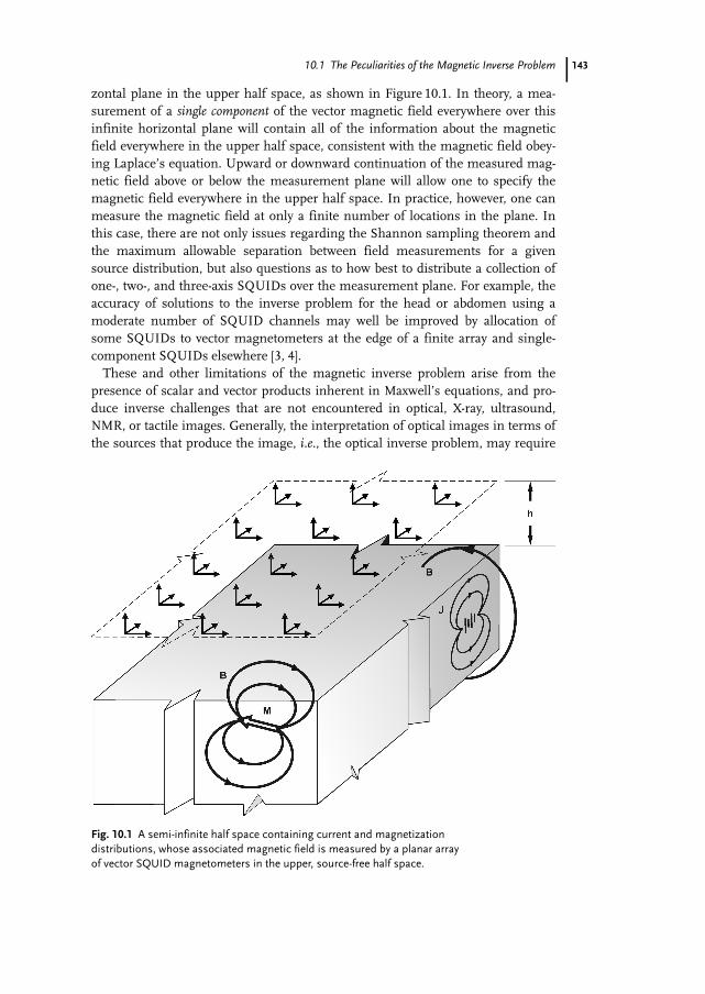
zontal plane in the upper half space, as shown in Figure 10.1. In theory, a mea-surement of a single component of the vector magnetic field everywhere over thisinfinite horizontal plane will contain all of the information about the magneticfield everywhere in the upper half space, consistent with the magnetic field obey-ing Laplace’s equation. Upward or downward continuation of the measured mag-netic field above or below the measurement plane will allow one to specify themagnetic field everywhere in the upper half space. In practice, however, one canmeasure the magnetic field at only a finite number of locations in the plane. Inthis case, there are not only issues regarding the Shannon sampling theorem andthe maximum allowable separation between field measurements for a givensource distribution, but also questions as to how best to distribute a collection ofone-, two-, and three-axis SQUIDs over the measurement plane. For example, theaccuracy of solutions to the inverse problem for the head or abdomen using amoderate number of SQUID channels may well be improved by allocation ofsome SQUIDs to vector magnetometers at the edge of a finite array and single-component SQUIDs elsewhere [3, 4].These and other limitations of the magnetic inverse problem arise from the
presence of scalar and vector products inherent in Maxwell’s equations, and pro-duce inverse challenges that are not encountered in optical, X-ray, ultrasound,NMR, or tactile images. Generally, the interpretation of optical images in terms ofthe sources that produce the image, i.e., the optical inverse problem, may require
143
Fig. 10.1 A semi-infinite half space containing current and magnetizationdistributions, whose associated magnetic field is measured by a planar arrayof vector SQUID magnetometers in the upper, source-free half space.
10 The Magnetic Inverse Problem
deconvolution but will not require the inversion of a Laplacian field, but the mag-netic inverse problem does. This should give an indication of the difficulties thatwill be encountered in attempting to use magnetic field measurements to discernthe magnetic or electric sources hidden from direct view within an object.In the days of a single SQUID and simple models, or instruments dedicated to
measuring a single physical property, the appropriate equation for a simple modelcould be selected with care and intuition to obtain the required information. How-ever, complex models, as would be required to describe spatially distributed het-erogeneous sources in the brain or a thin slice of a meteorite, require measure-ment of the magnetic field at the least at as many points as there are model pa-rameters. If the source distribution is either time-independent or periodic, a sin-gle magnetometer can be used to make sequential measurements at multiplelocations. Today, the number of points where a scanned SQUID measures themagnetic field may exceed 125 000 [5, 6]. If the time-varying source distribution isaperiodic with a time variation that exceeds the rate at which the SQUID can bemoved, one has no choice but to use multiple SQUIDs to record simultaneouslythe field at the required number of locations. For this reason, the number ofSQUID sensors in a magnetoencephalogram (MEG) system is now approaching1000. In these two cases it is reasonable to consider this as a problem in magneticimaging: a magnetometer produces a vector or scalar “image” of the magneticfield, and the magnetic inverse problem becomes one of determining an “image”of the associated source distribution. In many situations, a source image can beobtained only after performing some sort of vector processing, as both the sourcesand their fields usually have a vector nature and are not colinear. In the limit ofmagnetic imaging of distributed, vector sources, our intuition based upon singlepoint dipoles may fail us and there may not be a simple vector manipulation thatcan provide us with the answer.What began 35 years ago as a SQUID measurement of the magnetic field at a
single point above the human chest [7] has now progressed to the point of truemagnetic images created by scanning a high-resolution SQUID microscope over ahighly heterogeneous section of a Martian meteorite [8]. Hence the magneticinverse problem has now evolved to include problems in image deconvolutionthat are potentially complicated by the nonuniqueness of the magnetic inverseproblem. In this chapter, we establish a firm mathematical foundation for themagnetic inverse problem and present a number of simple examples, drawn pri-marily from our research in the field, borrowing extensively from and buildingupon an earlier book chapter [9]. We concentrate on the general issues of the mag-netic inverse problem, and leave the discussion of MEG and magnetocardiogram(MCG) applications of three-dimensional inverse algorithms to Chapter 11. Thepresent chapter is intended to serve as a tutorial, and not an all-inclusive review ofthe literature.
144
10.2 The Magnetic Forward Problem
10.2The Magnetic Forward Problem
10.2.1Introduction
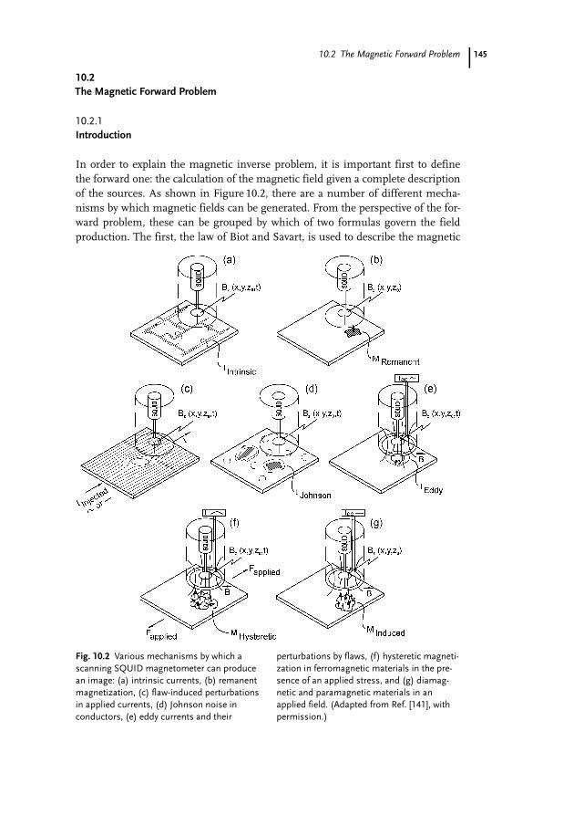
In order to explain the magnetic inverse problem, it is important first to definethe forward one: the calculation of the magnetic field given a complete descriptionof the sources. As shown in Figure 10.2, there are a number of different mecha-nisms by which magnetic fields can be generated. From the perspective of the for-ward problem, these can be grouped by which of two formulas govern the fieldproduction. The first, the law of Biot and Savart, is used to describe the magnetic
145
Fig. 10.2 Various mechanisms by which ascanning SQUID magnetometer can producean image: (a) intrinsic currents, (b) remanentmagnetization, (c) flaw-induced perturbationsin applied currents, (d) Johnson noise inconductors, (e) eddy currents and their
perturbations by flaws, (f) hysteretic magneti-zation in ferromagnetic materials in the pre-sence of an applied stress, and (g) diamag-netic and paramagnetic materials in anapplied field. (Adapted from Ref. [141], withpermission.)
10 The Magnetic Inverse Problem
fields produced by intrinsic currents, for example the magnetocardiogram (MCG)and MEG produced by current sources in the heart and brain, or from currentsapplied to a printed or integrated circuit, as is shown in Figure 10.2(a). Johnsonnoise arising from thermal motion of electrons in a conductor (Figure 10.2(d)) canproduce measurable magnetic fields, as can inhomogeneity-induced perturbationsin applied currents (Figure 10.2(c)). The second, the equation for the magneticfield of a point magnetic dipole, governs the field from remanent magnetizationfrom ferromagnetic objects or inclusions (Figure 10.2(b)), ferromagnetic materialsunder stress, with or without an applied field (Figure 10.2(f)), or from paramag-netic or diamagnetic objects in an applied, static magnetic field (Figure 10.2(g)). Ifone applies an oscillating field, SQUIDs can be used to image the eddy currents(Figure 10.2(e)). After we examine the two governing equations in some detail,i.e., the magnetic forward problem, we will then examine their inversion, i.e., themagnetic inverse problem.In this chapter, we will limit our discussion to the quasistatic magnetic field,
i.e., the field determined by the instantaneous sources. We do not consider therate of change of the magnetic field, retarded potentials, etc. The time variationmust be slow enough that inductive effects can be ignored, appropriate for mostlow-frequency SQUID applications except those involving eddy currents in met-als.In this chapter, we also do not address the numerous computational techniques
that have been developed for the forward problem of calculating the magneticfield from current and magnetization distributions, but instead will outline thegeneral principles that govern the forward problem for a variety of source andsample geometries.
10.2.2Magnetic Fields from Magnetization Distributions
10.2.2.1 Field and Moment of a Magnetic Dipole
In the quasistatic limit, the magnetic field of a magnetostatic dipole is given by(10.1). For an object with a distributed magnetization ~MMð~r¢r¢Þ, which is equivalentto a dipole density, each differential volume element d3r ¢ in the object is assigneda dipole moment ~mmð~r¢r¢Þ that is equal to ~MMð~r¢r¢Þd3r ¢, so that we can simply integrate(10.1)
~BB ~rrð Þ ¼ l04p
ZV
3~MM ~r¢r¢� �
� ~rr � ~r¢r¢� �
~rr � ~r¢r¢��� ���5 ~rr � ~r¢r¢
� ��
~MM ~r¢r¢� �
~rr � ~r¢r¢��� ���3
8><>:
9>=>;d3r ¢: (10:3)
The magnetization can either be permanent, e.g., ferromagnetic remanent magne-tization, or induced through diamagnetic, paramagnetic, or ferromagnetic effects.Let us suppose that an object made of magnetically linear, isotropic material is
146

10.2 The Magnetic Forward Problem
placed in a magnetic field produced by a distant electromagnet. The magnetiza-tion ~MMð~r¢r¢Þ at a source point ~r¢r¢ is determined by the product of the magnetic sus-ceptibility vð~r¢r¢Þ and the applied magnetic field intensity ~HHð~r¢r¢Þ
~MM ~r¢r¢� �
¼ v ~r¢r¢� �
~HH ~r¢r¢� �
: (10:4)
The magnetic induction field ~BB, hereafter referred to as the “magnetic field,” atthe same source point ~r¢r¢ is given by
~BB ~r¢r¢� �
¼ l0~HH ~r¢r¢� �
þ ~MM ~r¢r¢� �n o
; (10:5)
where l0 is the permeability of free space. We can express this in terms of thesusceptibility v by substituting (10.4) into (10.5) to obtain
~BB ~r¢r¢� �
¼ l0 1þ v ~r¢r¢� �n o
~HH ~r¢r¢� �
(10:6)
¼ l0lr~r¢r¢� �
~HH ~r¢r¢� �
(10:7)
¼ l ~r¢r¢� �
~HH ~r¢r¢� �
; (10:8)
where the relative permeability lr is given by
lr~r¢r¢� �
¼ 1þ v ~r¢r¢� �
(10:9)
and the absolute permeability l is
l ~r¢r¢� �
¼ l0lr~r¢r¢� �
: (10:10)
As we shall see, the difficulty with susceptibility and magnetization imaging isthat the field measured by the SQUID is not the local field within the object, butthe field in the source-free region outside of the object.
10.2.2.2 Magnetic Fields from Ferromagnetic MaterialsSoft ferromagnetic materials have high permeabilities, in the approximate range103 £ lr £ 105, so that
lr ¼ 1þ v » v: (10:11)
In general for these materials, v, and hence lr, are functions of the applied field.If the materials are “hard,” they exhibit significant hysteresis; if they are “soft,”
147
10 The Magnetic Inverse Problem
they do not. Soft materials may exhibit a range of fields for which v is approxi-mately constant, but in general for ferromagnetic materials, v has a strong depen-dence on the applied field. In either case, there is an applied ~HH above which thematerial saturates and the magnetization ~MM in (10.4) attains a maximum value.Above that value, any increases in ~BB in (10.5) are due only to the increase in ~HH.Since the magnetic field within soft ferromagnetic materials can be from 103 to105 times the applied field, the determination of the magnetization within a ferro-magnetic material must be made in the strong-field limit: ~BB ¼ l0
~HH þ ~MM� �
¼ l~HHat any point in the material, so that ~MM at one point is affected by ~MM at other pointsin the material. Self-consistency requires simultaneous solution of ~HH and ~MMeverywhere, since ~MM ~rrð Þ is determined by both ~HH ~rrð Þ and v ~rrð Þ, even if the appliedfield ~HH was initially uniform before the object was placed in the field. In thisstrong-field case, the magnetic inverse problem, i.e., the inversion of (10.3) todetermine ~MM ~rrð Þ, is difficult to impossible, particularly if there is a remanent(hard) magnetization superimposed upon the induced (soft) magnetization. Whileit is difficult to induce a soft, spherically symmetric, magnetically silent magnetwith external fields, it is in principle possible to have such a distribution in a hardcomponent of magnetization, and this leads to the previously discussed nonuni-queness problem.
10.2.2.3 Magnetic Fields from Paramagnetic and Diamagnetic MaterialsThe situation is much friendlier for the magnetic imaging of paramagnetic0£ v£ 10�3ð Þ and diamagnetic �10�6 £ v£ 0ð Þmaterials, in that
lr ¼ 1þ v » 1: (10:12)
As a result, the variation in the magnitude of the induced magnetic field ~BB is 10�6
to 10�3 times the magnetic field in free space, and is proportional to the appliedfield, since paramagnetic and diamagnetic materials are linear and nonhystereticat practical applied fields. The most significant feature of the low susceptibility ofthese materials is that (10.3) can be evaluated in the weak-field limit, also knownas the Born approximation: at any point in the material we can ignore the contri-butions to the applied field at ~r¢r¢ from the magnetization elsewhere in the objectand consider the applied magnetic intensity ~HH as it would be in the absence of themagnetic material. In that case, we immediately know the magnetic field ~BB every-where as well. In the Born approximation, the magnetization is independent ofthe magnetization elsewhere in the sample, and hence is a local phenomenon, incontrast to ferromagnetism. Because ~MM is so weak for diamagnetic and paramag-netic materials, if we know ~HH everywhere, we shall then know ~BB to at least onepart in 103 for a paramagnetic material with v ¼ 10�3, and to one part in 106 for adiamagnetic one with v ¼ �10�6. Thus, we have eliminated a major problem inobtaining a self-consistent, macroscopic solution that is based upon the micro-scopic constitutive equation given by (10.5). Because of their periodic flux-voltagecharacteristic, and the ability to thermally release magnetic flux trapped in pickup
148
10.2 The Magnetic Forward Problem
coils, SQUID magnetometers readily can measure only the very small perturba-tion ~BBp ~rrð Þ in the applied magnetic field [10]. We thereby can eliminate ~BB and ~HHfrom the imaging problem, and need them only to determine the magnetization.The measured magnetic field, ~BBp ~rrð Þ, thus is given by (10.3) where
~MM ~r¢r¢� �
¼v ~r¢r¢� �l0
~BB ~r¢r¢� �
¼ v ~r¢r¢� �
~HH ~r¢r¢� �
: (10:13)
If ~HHð~r¢r¢Þ is uniform, then the spatial variation of ~MMð~r¢r¢Þ is determined only by vð~r¢r¢Þ.For isotropic materials, v is a scalar, and the direction of ~MM is the same as that of~BB; otherwise, a tensor susceptibility is required.
10.2.3Magnetic Fields from Current Distributions
The calculation of the magnetic fields from magnetizations is conceptuallystraightforward because the only vector operation is the dot product in the firstterm of (10.3). In contrast, the law of Biot and Savart contains a vector cross prod-uct which complicates the problem. Let us start with the simplest case of deter-mining the distribution of currents in a planar circuit, as shown, for example, inFigures 10.2(a), 10.3, and 10.4. In general, the magnetic field ~BB ~rrð Þ at the point~rr isgiven by the law of Biot and Savart
~BB ~rrð Þ ¼ l04p
ZV
~JJ ~r¢r¢� �
· ~rr � ~r¢r¢� �
~rr � ~r¢r¢��� ���3 d3r ¢; (10:14)
where~JJð~r¢r¢Þ is the current density at point ~r¢r¢. It is also instructive to rewrite (10.14)in terms of the curl of the current distribution [11, 12]
~BB ~rrð Þ ¼ l04p
ZS
~JJ ~r¢r¢� �
· nn
~rr � ~r¢r¢��� ��� d2r ¢þ l0
4p
ZV
�¢ ·~JJ ~r¢r¢� �
~rr � ~r¢r¢��� ��� d3r ¢; (10:15)
where nn is the normal to the surface S that bounds the object or regions withinthe object with differing conductivities. The first integral represents the magneticfield due to the discontinuity of the tangential component of the current at anyexternal or internal boundaries of the object, and the second is that produced byany curl within the object. Note that within a homogeneous conductor, any cur-rent distribution that has zero curl will not contribute to the external magneticfield and, hence, will be magnetically silent [13–15]. This implies that in homoge-neous, three-dimensional conductors, currents that obey Ohm’s law, relating thecurrent density to either the electric field~EE or the electric scalar potential V , e.g.,
~JJ ~rrð Þ ¼ r~EE ~rrð Þ ¼ �r�V ~rrð Þ; (10:16)
149
10 The Magnetic Inverse Problem
do not contribute to the magnetic field because the curl of a gradient is identicallyzero, and the conductivity r is a constant within the volume V and passes throughthe curl operator. Batteries, such as a dry cell dropped into a conducting medium(Figure 10.4), or the microscopic equivalent, a current dipole [16, 17], are non-Ohmic and hence can have curl. The first term in (10.15) would indicate thatwhenever Ohmic currents encounter a boundary or a discontinuity in conductiv-ity, a magnetic field could be produced, since a discontinuity in the component ofthe current density tangential to a boundary is equivalent to a curl.2) In a thinsheet that would approximate a two-dimensional conductor, the sample has twoparallel surfaces in proximity that have curls of opposite sign which cancel each
150
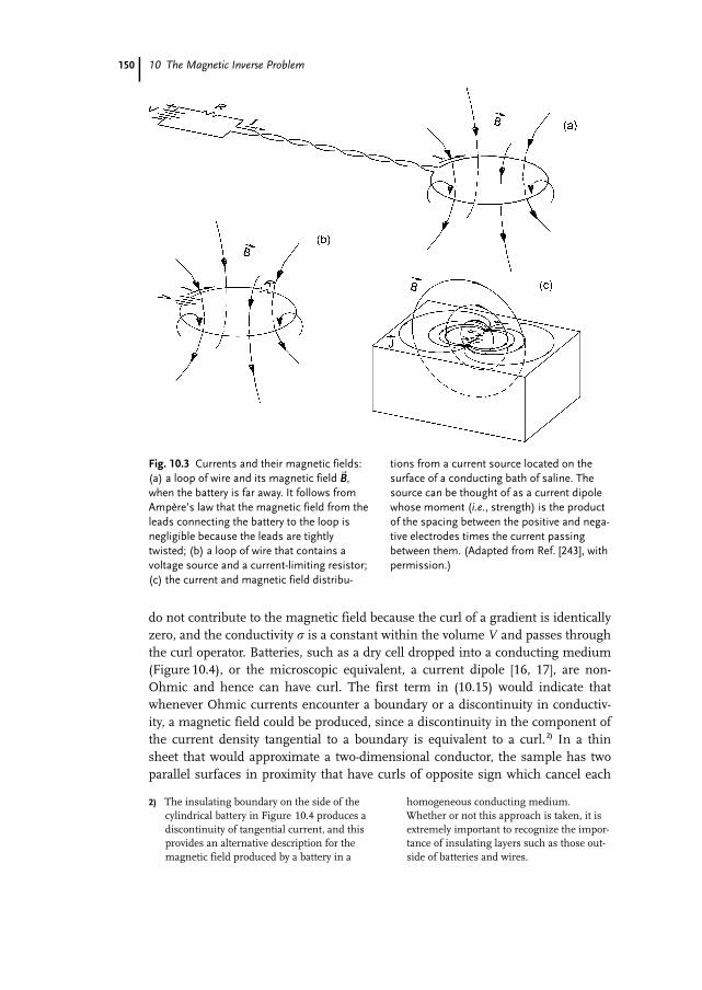
Fig. 10.3 Currents and their magnetic fields:(a) a loop of wire and its magnetic field~BB,when the battery is far away. It follows fromAmp.re’s law that the magnetic field from theleads connecting the battery to the loop isnegligible because the leads are tightlytwisted; (b) a loop of wire that contains avoltage source and a current-limiting resistor;(c) the current and magnetic field distribu-
tions from a current source located on thesurface of a conducting bath of saline. Thesource can be thought of as a current dipolewhose moment (i.e., strength) is the productof the spacing between the positive and nega-tive electrodes times the current passingbetween them. (Adapted from Ref. [243], withpermission.)
2) The insulating boundary on the side of thecylindrical battery in Figure 10.4 produces adiscontinuity of tangential current, and thisprovides an alternative description for themagnetic field produced by a battery in a
homogeneous conducting medium.Whether or not this approach is taken, it isextremely important to recognize the impor-tance of insulating layers such as those out-side of batteries and wires.
10.2 The Magnetic Forward Problem
other far from the sheet; the curl that contributes most strongly to the magneticfield is that from any edges in the conductor. A current-carrying wire, bent into apattern, has a curl all along its surface. We shall address the role of spatial varia-tions in the conductivity r in two-dimensional conductors in a later section. Fornow, we shall concentrate on sheet conductors with a constant (homogeneous)conductivity r.
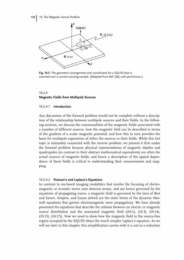
In typical measurements, the component of the magnetic field normal to thesample, Bz, is mapped by scanning the SQUID pickup coil of radius a over thesample, at a fixed height z0, as shown in Figure 10.5. In this case, we can expandthe cross product in (10.14) and rewrite the law of Biot and Savart as a pair of inte-grals
Bz ~rrð Þ ¼l04p
ZV
Jx~r¢r¢� �
y� y¢ð Þ
~rr � ~r¢r¢��� ���3 d3r ¢� l0
4p
ZV
Jy~r¢r¢� �
x � x ¢ð Þ
~rr � ~r¢r¢��� ���3 d3r ¢: (10:17)
Equations (10.14) and (10.17) are convolution integrals. The source of the field isthe current density~JJð~r¢r¢Þ; the remaining terms of the integrand are a function ofboth~rr and ~r¢r¢ and form the Green’s function Gð~rr � ~r¢r¢Þ. To calculate the magneticfield, we integrate the product of~JJ and G over the entire region where~JJ is non-zero, i.e., we convolve~JJ and G to determine ~BB. Note that in (10.14), G is a vectorfunction that contains the cross product, but in (10.17), it is a pair of scalar func-tions. It is worth noting that identical arguments starting with (10.3) show thatthe magnetic field from a magnetization distribution can be expressed as the con-volution of ~MMð~r¢r¢Þ with another vector Green’s function.
151
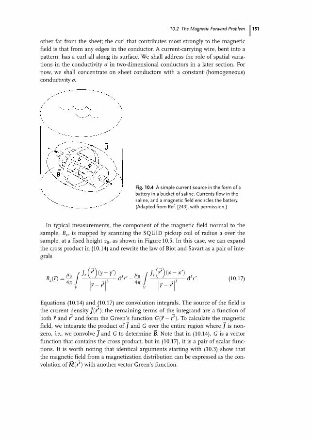
Fig. 10.4 A simple current source in the form of abattery in a bucket of saline. Currents flow in thesaline, and a magnetic field encircles the battery.(Adapted from Ref. [243], with permission.)
10 The Magnetic Inverse Problem
10.2.4Magnetic Fields from Multipole Sources
10.2.4.1 Introduction
Any discussion of the forward problem would not be complete without a descrip-tion of the relationship between multipole sources and their fields. In the follow-ing sections, we discuss the commonalities of the magnetic fields associated witha number of different sources, how the magnetic field can be described in termsof the gradient of a scalar magnetic potential, and how this in turn provides thebasis for multipole expansions of either the sources or their fields. While this lasttopic is intimately connected with the inverse problem, we present it first underthe forward problem because physical representations of magnetic dipoles andquadrupoles (in contrast to their abstract mathematical equivalents) are often theactual sources of magnetic fields, and hence a description of the spatial depen-dence of these fields is critical to understanding their measurement and map-ping.
10.2.4.2 Poisson’s and Laplace’s EquationsIn contrast to ray-based imaging modalities that involve the focusing of electro-magnetic or acoustic waves onto detector arrays, and are hence governed by theequations of propagating waves, a magnetic field is governed by the laws of Biotand Savart, AmpMre, and Gauss (which are the static limits of the dynamic Max-well equations that govern electromagnetic wave propagation). We have alreadypresented the equations that describe the relation between an electric or magneticsource distribution and the associated magnetic field ((10.1), (10.3), (10.14),(10.15), (10.17)). Now we need to show how the magnetic field in the source-freeregion occupied by the SQUID obeys the much simpler Laplace’s equation. As wewill see later in this chapter, this simplification carries with it a cost in a reduction
152
Fig. 10.5 The geometric arrangement and coordinates for a SQUID that isscanned over a current-carrying sample. (Adapted from Ref. [56], with permission.)
10.2 The Magnetic Forward Problem
of the information contained in the field and a corresponding restriction on theinvertibility of the field equations and the solution to the inverse problem. Thissection draws extensively from Ref. [18].To aid in our development of an intuition regarding Laplace’s equation, it is
worthwhile to begin with electrostatic fields. Let us first consider a quasistaticcharge distribution given by the charge density r ~rrð Þ. In vacuum, Gauss’ law forthe electric field~EE reduces to
� �~EE ~rrð Þ ¼ r ~rrð Þ=e0 ; (10:18)
where e0 is the electrical permittivity of free space. Because the differential formof Faraday’s law reduces to � ·~EE ~rrð Þ ¼~00 for a quasistatic charge distribution, theelectric field can be described as the negative gradient of the scalar electrostaticpotential V ~rrð Þ, where
~EE ~rrð Þ ¼ ��V ~rrð Þ : (10.19)
Equations (10.18) and (10.19) can be combined to obtain Poisson’s equation
�2V ~rrð Þ ¼ �r ~rrð Þ=e0 ; (10.20)
which is known to have the solution
V ~rrð Þ ¼ 14pe0
ZV
r ~r¢r¢� �
~rr � ~r¢r¢��� ��� d
3r ¢: (10:21)
This equation shows that, in the mathematical sense, the charge density r ~rrð Þ isthe “source” of the scalar potential.3) Most importantly, if we restrict our attentionto source-free regions where r ~rrð Þ ¼ 0, we find that the electrostatic potential obeysLaplace’s equation
�2V ~rrð Þ ¼ 0 , (10.22)
and the entire armamentarium of techniques to solve Laplace’s equation can bebrought to bear on the problem.We can now extend our analysis to consider the electric field of current sources
in a homogeneous conductor. In an infinite, homogeneous, isotropic, linear con-ductor, containing sources of electromotive force (EMF), the quasistatic currentdensity~JJ ~rrð Þ obeys Ohm’s law, which can be written as
~JJ ~rrð Þ ¼ r~EE ~rrð Þ þ r~EiEi ~rrð Þ ¼ r~EE ~rrð Þ þ~JiJi ~rrð Þ ; (10.23)
153
3) A purist would argue that one cannot havethe electrostatic potential without thecharge, and vice versa, so that it is better todescribe the charge and the potential as
being “associated” with each other, ratherthan having the charge as the “source” of afield.
10 The Magnetic Inverse Problem
where the impressed voltage ~EiEi ~rrð Þ is zero, where there are no EMFs, and r is theelectrical conductivity of the conductor. Alternatively, the effect of the EMFs canbe described in terms of the impressed current density ~JiJi. It can be shown that ~EiEi
can be described as an EMF dipole density and ~JiJi can be interpreted as a currentdipole density [19]. Because of the high impedance of the cellular membranesacross which bioelectric currents are driven by transmembrane concentration gra-dients, bioelectric sources are almost always described in terms of ~JiJi rather than~EiEi. It is important to note that in the quasistatic limit conservation of chargerequires that � �~JJ ~rrð Þ ¼ 0. Taking the divergence of (10.23) and using (10.19), weonce again obtain Poisson’s equation
�2V ~rrð Þ ¼ 1r� �~JiJi ~rrð Þ ; (10.24)
which has the solution
V ~rrð Þ ¼ 14pr
ZV
��¢ �~JiJi ~r¢r¢� �
~rr � ~r¢r¢��� ��� d3r ¢; (10:25)
and we see that � �~JiJi ~rrð Þ is the source of the scalar potential. In regions withinthe conductor where � �~JiJi ¼ 0, this reduces to Laplace’s equation.The extension of this formalism to the magnetic field of steady-state current dis-
tributions is straightforward. We have already shown that the law of Biot andSavart can be written as
~BB ~rrð Þ ¼ l04p
ZV
�¢ ·~JJ ~r¢r¢� �
~rr � ~r¢r¢��� ��� d3r ¢ : (10:26)
We now recognize this as the solution to a vector form of Poisson’s equation,
�2~BB ~rrð Þ ¼ �l0� ·~JJ ~rrð Þ ; (10.27)
wherein each Cartesian component of ~BB is Laplacian, with a source that is the cor-responding Cartesian component of � ·~JJ. In the event that the current density isproduced by impressed current sources in an unbounded homogeneous mediumthat obeys Ohm’s law, (10.23) reduces to
~JJ ~rrð Þ ¼ �r�V ~rrð Þ þ~JiJi ~rrð Þ ; (10.28)
such that
� ·~JJ ~rrð Þ ¼ � ·~JiJi ~rrð Þ ; (10.29)
154
10.2 The Magnetic Forward Problem
so that the solution for infinite homogeneous conductors reduces to Poisson’sequation for which the integration can be restricted to the region containingimpressed currents
~BB ~rrð Þ ¼ l04p
ZV
�¢ ·~JJi ~r¢r¢� �
~rr � ~r¢r¢��� ��� d3r ¢ : (10:30)
This equation is particularly significant in that it shows that for unbounded con-ductors, the Ohmic currents do not contribute to the magnetic field, and the fieldis determined by the impressed currents alone.This result also leads to an important equation for the case where the source is
a current dipole~PP located at ~r†r†, i.e.,
~JiJi ~r¢r¢� �
¼ ~PPd ~r¢r¢ � ~r†r†� �
; (10:31)
where dð~r¢r¢ � ~r†r†Þ is the Dirac delta function. We can apply (10.31) to (10.23) towrite (10.14) as
~BB ~rrð Þ ¼ l04p
~PP · ~rr � ~r†r†� �
~rr � ~r†r†��� ���3 : (10:32)
It is vital to note that deeply embedded in the derivation of this equation is theassumption that we are dealing with an unbounded homogeneous conductor. Thefascinating aspect of this equation is that it is, in effect, a differential form of thelaw of Biot and Savart, operating on only one portion of the complete “circuit.”While in general this would raise concerns over current continuity and Newton’sthird law, in this special case of an unbounded conductor, ~PP is a point source ofcurrent, and the magnetic field contributions of each differential element of thereturn Ohmic current integrate exactly to zero. Figure 10.4 shows how a currentdipole or a small battery has an encircling magnetic field, which in an unboundedconductor would be given by (10.32). In the limit of a very large bucket and a bat-tery that reduces to a current dipole, the magnetic field can be calculated by con-sidering only the current dipole moment of the battery. For small buckets, the dis-continuity in the tangential current at the wall of the bucket will also contribute tothe magnetic field. As will be apparent in the subsequent discussion of edgeeffects, it is important to appreciate that magnetic fields can be exquisitely sensi-tive to discontinuities in the tangential current!For completeness, it is important to point out that the addition of boundary sur-
faces Sj within the conductor, thereby making the conductor only piecewise homo-geneous, will add secondary current sources ~KKi that are given by the product ofthe difference in conductivities across the boundary with the potential at the
155
10 The Magnetic Inverse Problem
boundary, with an orientation specified by the normal nnj to the boundary [20],such that
~KKi ~rrð Þ ¼ �ðr¢� r†ÞVð~rrÞnnjð~rrÞ for~rr on all Sj, (10.33)
~KKi ~rrð Þ ¼~00 for~rr not on any Sj
In this case, our equations for the electric potential and magnetic field become[21, 22]
V ~rrð Þ ¼ 14pr
ZV
��¢ � ~JJi ~r¢r¢� �
þ ~KKi ~r¢r¢� �n o
~rr � ~r¢r¢��� ��� d3r ¢; (10:35)
~BB ~rrð Þ ¼ l04p
ZV
�¢ · ~JJi ~r¢r¢� �
þ ~KKi ~r¢r¢� �n o
~rr � ~r¢r¢��� ��� d3r ¢ : (10:36)
As we will see later, these two equations are critical in understanding the relationbetween bioelectric and biomagnetic fields.If the current distribution is bounded, as it would be for a conductor bounded
by a surface S, the curl of ~BB, as given by Maxwell’s fourth equation, must be zerooutside of S, i.e.,
� ·~BB ~rrð Þ ¼~00 : (10:37)
Any field that has no curl can be described in terms of the gradient of the mag-netic scalar potential, so that we can now write
~BB ~rrð Þ ¼ �l0�Vm ~rrð Þ outside S : (10:38)
Since � �~BB ~rrð Þ is zero everywhere,
�2Vm ¼ 0 outside S ; (10:39)
and we see that the quasistatic magnetic field in a current-free region can be de-rived from a scalar potential obeying Laplace’s equation. The identical resultapplies to a bounded object with a quasistatic magnetization ~MM ~rrð Þ: the magneticinduction outside the object must satisfy (10.39).Inside a magnetized object, ~BB ~rrð Þ is given by
~BB ~rrð Þ ¼ �l0�Vm ~rrð Þ þ l0~MM ~rrð Þ : (10:40)
156
10.2 The Magnetic Forward Problem
If we take the divergence of each term and note that � �~BB ~rrð Þ ¼ 0, we obtain Pois-son’s equation for Vm
�2Vm ~rrð Þ ¼ � � ~MM ~rrð Þ : (10:41)
This has the solution
Vm ~rrð Þ ¼ 14p
ZV
��¢ � ~MM ~r¢r¢� �
~rr � ~r¢r¢��� ��� d3r ¢; (10:42)
which shows that �� � ~MM ~rrð Þ can be interpreted as an effective magnetic chargedensity that is the source of Vm. Similar to the constraint on � �~JJ for the electricfield of a distributed current, the condition that � �~BB ¼ 0 implies that
ZV
�¢ � ~MM ~r¢r¢� �
d3r ¢ ¼ 0 : (10:43)
Equation (10.41) shows that the magnetic field outside of a magnetized object isalso Laplacian, so we can describe the current-related source of Vm in (10.38) asan effective magnetization given by [18, 23]
~MM ~rrð Þ ¼ 12~rr ·~JJ ~rrð Þ : (10:44)
The divergence of ~MM becomes
� � ~MM ~rrð Þ ¼ � � 12~rr ·~JJ ~rrð Þ
� �¼ � 1
2~rr � � ·~JJ ~rrð Þ� �
: (10:45)
Thus the magnetic scalar potential outside the bounded current distribution satis-fies the equation
Vm ~rrð Þ ¼ 14p
ZV
12~r¢r¢ � �¢ ·~JJ ~r¢r¢
� �~rr � ~r¢r¢��� ��� d3r ¢; (10:46)
and we identify the source of Vm to be one-half the radial component of the curlof ~JJ. In unbounded homogeneous media with impressed current sources, ~JJ canbe replaced by ~JJi. In the piecewise homogeneous case, it is necessary to includethe secondary sources ~KKi.We close the loop on boundary effects by noting that the symmetry of a
bounded conductor may lead to several interesting results. A radial current dipolein a spherical conductor and a current dipole perpendicular to the surface of asemi-infinite conductor produce no magnetic field outside the conductor. A current
157
10 The Magnetic Inverse Problem
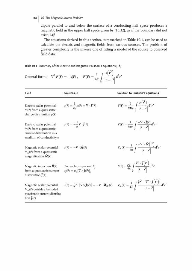
dipole parallel to and below the surface of a conducting half space produces amagnetic field in the upper half space given by (10.32), as if the boundary did notexist [24]!The equations derived in this section, summarized in Table 10.1, can be used to
calculate the electric and magnetic fields from various sources. The problem ofgreater complexity is the inverse one of fitting a model of the source to observedfield data.
158
Table 10.1 Summary of the electric and magnetic Poisson’s equations [18]
General form: �2W ~rrð Þ ¼ �s ~rrð Þ ; W ~rrð Þ ¼ 14p
ZV
s ~r¢r¢� �
~rr � ~r¢r¢��� ��� d
3r ¢
Field Sources, s Solution to Poisson’s equations
Electric scalar potentialV ~rrð Þ from a quasistaticcharge distribution r ~rrð Þ
s ~rrð Þ ¼ 1e0r ~rrð Þ ¼ � �~EE ~rrð Þ V ~rrð Þ ¼ 1
4pe0
ZV
r ~r¢r¢� �
~rr � ~r¢r¢��� ��� d
3r ¢
Electric scalar potentialV ~rrð Þ from a quasistaticcurrent distribution in amedium of conductivity r
s ~rrð Þ ¼ � 1r� �~JJ ~rrð Þ V ~rrð Þ ¼ 1
4pr
ZV
��¢ �~JJ ~rrð Þ~rr � ~r¢r¢��� ��� d3r ¢
Magnetic scalar potentialVm ~rrð Þ from a quasistaticmagnetization ~MM ~rrð Þ
s ~rrð Þ ¼ �� � ~MM ~rrð Þ Vm ~rrð Þ ¼ 14p
ZV
��¢ � ~MM ~r¢r¢� �
~rr � ~r¢r¢��� ��� d3r ¢
Magnetic induction~BB ~rrð Þfrom a quasistatic currentdistribution~JJ ~rrð Þ
For each component Bj
sj ~rrð Þ ¼ l0 � ·~JJ ~rrð Þ� �
j
B ~rrð Þ ¼ l04p
ZV
�¢ ·~JJ ~r¢r¢� �
~rr � ~r¢r¢��� ��� d3r ¢
Magnetic scalar potentialVm ~rrð Þ outside a boundedquasistatic current distribu-tion~JJ ~rrð Þ
s ~rrð Þ ¼ 12~rr � � ·~JJ ~rrð Þ� �
¼ �� � ~MMeff ~rrð Þ Vm ~rrð Þ ¼ 14p
ZV
12~r¢r¢ � �¢ ·~JJ ~r¢r¢
� �h i~rr � ~r¢r¢��� ��� d3r ¢
10.2 The Magnetic Forward Problem
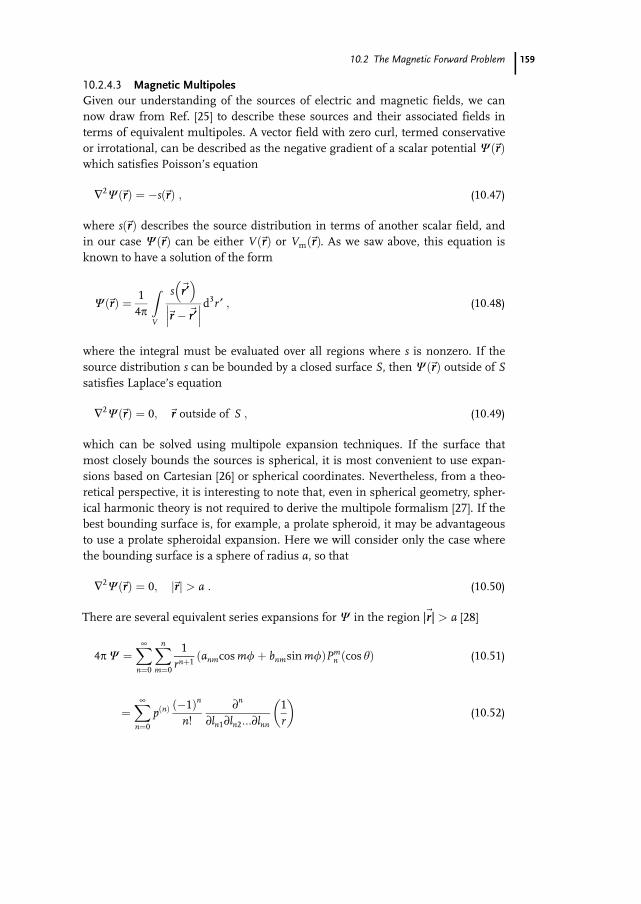
10.2.4.3 Magnetic MultipolesGiven our understanding of the sources of electric and magnetic fields, we cannow draw from Ref. [25] to describe these sources and their associated fields interms of equivalent multipoles. A vector field with zero curl, termed conservativeor irrotational, can be described as the negative gradient of a scalar potential W ~rrð Þwhich satisfies Poisson’s equation
�2W ~rrð Þ ¼ �s ~rrð Þ ; (10:47)
where s ~rrð Þ describes the source distribution in terms of another scalar field, andin our case W ~rrð Þ can be either V ~rrð Þ or Vm ~rrð Þ. As we saw above, this equation isknown to have a solution of the form
W ~rrð Þ ¼ 14p
ZV
s ~r¢r¢� �
~rr � ~r¢r¢��� ��� d
3r ¢ ; (10:48)
where the integral must be evaluated over all regions where s is nonzero. If thesource distribution s can be bounded by a closed surface S, then W ~rrð Þ outside of Ssatisfies Laplace’s equation
�2W ~rrð Þ ¼ 0; ~rr outside of S ; (10:49)
which can be solved using multipole expansion techniques. If the surface thatmost closely bounds the sources is spherical, it is most convenient to use expan-sions based on Cartesian [26] or spherical coordinates. Nevertheless, from a theo-retical perspective, it is interesting to note that, even in spherical geometry, spher-ical harmonic theory is not required to derive the multipole formalism [27]. If thebest bounding surface is, for example, a prolate spheroid, it may be advantageousto use a prolate spheroidal expansion. Here we will consider only the case wherethe bounding surface is a sphere of radius a, so that
�2W ~rrð Þ ¼ 0; ~rrj j > a : (10:50)
There are several equivalent series expansions for W in the region ~rj jrj j > a [28]
4pW ¼X¥n¼0
Xn
m¼0
1rnþ1 anmcosmfþ bnmsinmfð ÞPm
n cos hð Þ (10:51)
¼X¥n¼0
p nð Þ �1ð Þn
n!¶n
¶ln1¶ln2:::¶lnn
1r
� �(10:52)
159
10 The Magnetic Inverse Problem
¼X¥n¼0
Xn
l¼0
Xn�l
k¼0
�1ð Þn
l!k! n� l � kð Þ! cnkl¶n
¶xl¶yk¶zn�l�k·
1r
� �; (10:53)
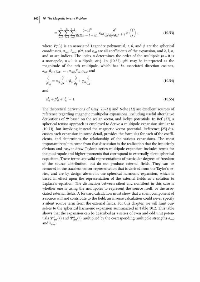
where Pmn ð�Þ is an associated Legendre polynomial, r, h, and f are the spherical
coordinates, anm, bnm, p(n), and cnkl are all coefficients of the expansion, and k, l, n,and m are indices. The index n determines the order of the multipole (n = 0 isa monopole, n = 1 is a dipole, etc.). In (10.52), p(n) may be interpreted as themagnitude of the nth multipole, which has 3n associated direction cosines,an1; bn1; cn1; ::: ; ann; bnn; cnn, and
¶¶lni¼ ani
¶¶xþ bni
¶¶yþ cni
¶¶z
(10.54)
and
a2ni þ b2ni þ c2ni ¼ 1. (10.55)
The theoretical derivations of Gray [29–31] and Nolte [32] are excellent sources ofreference regarding magnetic multipolar expansions, including useful alternativederivations of W based on the scalar, vector, and Debye potentials. In Ref. [27], aspherical tensor approach is employed to derive a multipole expansion similar to(10.53), but involving instead the magnetic vector potential. Reference [25] dis-cusses each expansion in some detail, provides the formulas for each of the coeffi-cients, and determines the relationship of the various expansions. The mostimportant result to come from that discussion is the realization that the intuitivelyobvious and easy-to-draw Taylor’s series multipole expansion includes terms forthe quadrupole and higher moments that correspond to externally silent sphericalcapacitors. These terms are valid representations of particular degrees of freedomof the source distribution, but do not produce external fields. They can beremoved in the traceless tensor representation that is derived from the Taylor’s se-ries, and are by design absent in the spherical harmonic expansion, which isbased in effect upon the representation of the external fields as a solution toLaplace’s equation. The distinction between silent and nonsilent in this case iswhether one is using the multipoles to represent the source itself, or the asso-ciated external fields. A forward calculation must show that a silent component ofa source will not contribute to the field; an inverse calculation could never specifya silent source term from the external fields. For this chapter, we will limit our-selves to the spherical harmonic expansion summarized in Table 10.2. This tableshows that the expansion can be described as a series of even and odd unit poten-tials We
nm rð Þ and Wonm rð Þ multiplied by the corresponding multipole strengths anm
and bnm.
160
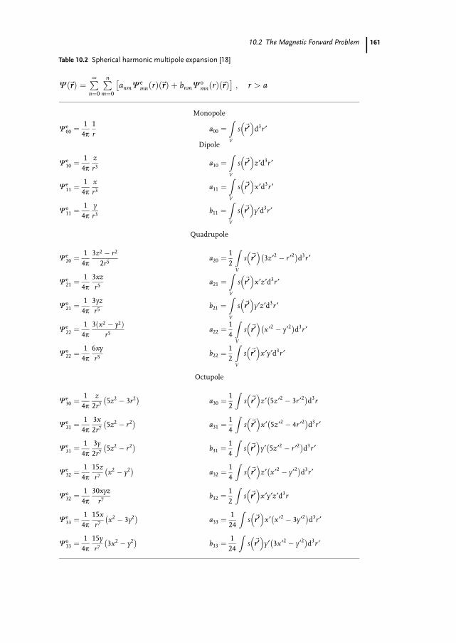
10.2 The Magnetic Forward Problem 161
Table 10.2 Spherical harmonic multipole expansion [18]
W ~rrð Þ ¼P¥n¼0
Pnm¼0
anmWemn rð Þ ~rrð Þ þ bnmW
omn rð Þ ~rrð Þ
� �; r > a
Monopole
We00 ¼
14p
1r
a00 ¼ZV
s ~r¢r¢� �
d3r ¢
Dipole
We10 ¼
14p
zr3
a10 ¼ZV
s ~r¢r¢� �
z¢d3r ¢
We11 ¼
14p
xr3
a11 ¼ZV
s ~r¢r¢� �
x ¢d3r ¢
Wo11 ¼
14p
yr3
b11 ¼ZV
s ~r¢r¢� �
y¢d3r ¢
Quadrupole
We20 ¼
14p
3z2 � r2
2r5a20 ¼
12
ZV
s ~r¢r¢� �
3z¢2 � r ¢2� �
d3r ¢
We21 ¼
14p
3xzr5
a21 ¼ZV
s ~r¢r¢� �
x ¢z¢d3r ¢
Wo21 ¼
14p
3yzr5
b21 ¼ZV
s ~r¢r¢� �
y¢z¢d3r ¢
We22 ¼
14p
3 x2 � y2ð Þr5
a22 ¼14
ZV
s ~r¢r¢� �
x ¢2 � y¢2� �
d3r ¢
Wo22 ¼
14p
6xyr5
b22 ¼12
ZV
s ~r¢r¢� �
x ¢y¢d3r ¢
Octupole
We30 ¼
14p
z2r7
5z2 � 3r2� �
a30 ¼12
Zs ~r¢r¢� �
z¢ 5z¢2 � 3r ¢2� �
d3r
We31 ¼
14p
3x2r7
5z2 � r2� �
a31 ¼14
Zs ~r¢r¢� �
x ¢ 5z¢2 � 4r ¢2� �
d3r ¢
We31 ¼
14p
3y2r7
5z2 � r2� �
b31 ¼14
Zs ~r¢r¢� �
y¢ 5z¢2 � r ¢2� �
d3r ¢
We32 ¼
14p
15zr7
x2 � y2� �
a32 ¼14
Zs ~r¢r¢� �
z¢ x ¢2 � y¢2� �
d3r ¢
Wo32 ¼
14p
30xyzr7
b32 ¼12
Zs ~r¢r¢� �
x ¢y¢z¢d3r
We33 ¼
14p
15xr7
x2 � 3y2� �
a33 ¼124
Zs ~r¢r¢� �
x ¢ x ¢2 � 3y¢2� �
d3r ¢
Wo33 ¼
14p
15yr7
3x2 � y2� �
b33 ¼124
Zs ~r¢r¢� �
y¢ 3x ¢2 � y¢2� �
d3r ¢
10 The Magnetic Inverse Problem
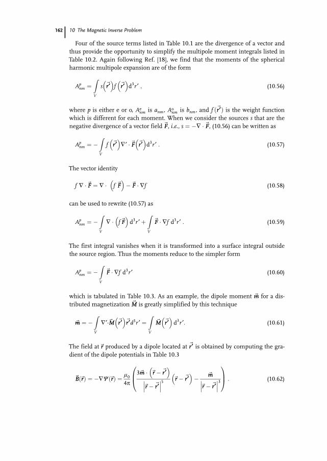
Four of the source terms listed in Table 10.1 are the divergence of a vector andthus provide the opportunity to simplify the multipole moment integrals listed inTable 10.2. Again following Ref. [18], we find that the moments of the sphericalharmonic multipole expansion are of the form
Apnm ¼
ZV
s ~r¢r¢� �
f ~r¢r¢� �
d3r ¢ ; (10:56)
where p is either e or o, Aenm is anm, Ao
nm is bnm, and f ð~r¢r¢Þ is the weight functionwhich is different for each moment. When we consider the sources s that are thenegative divergence of a vector field~FF, i.e., s ¼ �� �~FF, (10.56) can be written as
Apnm ¼ �
ZV
f ~r¢r¢� �
�¢ �~FF ~r¢r¢� �
d3r ¢ : (10:57)
The vector identity
f � �~FF ¼ � � f ~FF� �
�~FF � �f (10:58)
can be used to rewrite (10.57) as
Apnm ¼ �
ZV
� � f~FF� �
d3r ¢þZV
~FF � �f d3r ¢ : (10:59)
The first integral vanishes when it is transformed into a surface integral outsidethe source region. Thus the moments reduce to the simpler form
Apnm ¼ �
ZV
~FF � �f d3r ¢ (10:60)
which is tabulated in Table 10.3. As an example, the dipole moment ~mm for a dis-tributed magnetization ~MM is greatly simplified by this technique
~mm ¼ �ZV
�¢ ~�M�M ~r¢r¢� �
~r¢r¢d3r ¢ ¼ZV
~MM ~r¢r¢� �
d3r ¢: (10:61)
The field at~rr produced by a dipole located at ~r¢r¢ is obtained by computing the gra-dient of the dipole potentials in Table 10.3
~BB ~rrð Þ ¼ ��W ~rrð Þ ¼ l04p
3~mm � ~rr � ~r¢r¢� �
~rr � ~r¢r¢��� ���5 ~rr � ~r¢r¢
� �� ~mm
~rr � ~r¢r¢��� ���3
0B@
1CA : (10:62)
162
10.2 The Magnetic Forward Problem
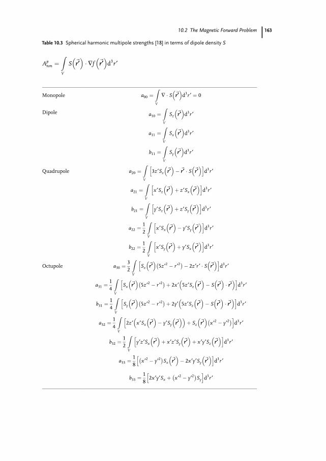
Table 10.3 Spherical harmonic multipole strengths [18] in terms of dipole density S
Apnm ¼
ZV
S ~r¢r¢� �
� �f ~r¢r¢� �
d3r ¢
Monopole a00 ¼ZV
� � S ~r¢r¢� �
d3r ¢ ¼ 0
Dipole a10 ¼ZV
Sz~r¢r¢� �
d3r ¢
a11 ¼ZV
Sx~r¢r¢� �
d3r ¢
b11 ¼ZV
Sy~r¢r¢� �
d3r ¢
Quadrupole a20 ¼ZV
3z¢Sz~r¢r¢� �
� ~r¢r¢ � S ~r¢r¢� �h i
d3r ¢
a21 ¼ZV
x ¢Sz~r¢r¢� �
þ z¢Sx~r¢r¢� �h i
d3r ¢
b21 ¼ZV
y¢Sz~r¢r¢� �
þ z¢Sy~r¢r¢� �h i
d3r ¢
a22 ¼12
ZV
x ¢Sx~r¢r¢� �
� y¢Sy~r¢r¢� �h i
d3r ¢
b22 ¼12
ZV
x ¢Sy~r¢r¢� �
þ y¢Sx~r¢r¢� �h i
d3r ¢
Octupole a30 ¼32
ZV
Sz~r¢r¢� �
5z¢2 � r ¢2� �
� 2z¢r ¢ � S ~r¢r¢� �h i
d3r ¢
a31 ¼14
ZV
Sx~r¢r¢� �
5z¢2 � r ¢2� �
þ 2x ¢ 5z¢Sz~r¢r¢� �
� S ~r¢r¢� �
� ~r¢r¢� �h i
d3r ¢
b31 ¼14
ZV
Sy~r¢r¢� �
5z¢2 � r ¢2� �
þ 2y¢ 5z¢Sz~r¢r¢� �
� S ~r¢r¢� �
� ~r¢r¢� �h i
d3r ¢
a32 ¼14
ZV
2z¢ x ¢Sx~r¢r¢� �
� y¢Sy~r¢r¢� �� �
þ Sz~r¢r¢� �
x ¢2 � y¢2� �h i
d3r ¢
b32 ¼12
ZV
y¢z¢Sx~r¢r¢� �
þ x ¢z¢Sy~r¢r¢� �
þ x ¢y¢Sz~r¢r¢� �h i
d3r ¢
a33 ¼18
x ¢2 � y¢2� �
Sx~r¢r¢� �
� 2x ¢y¢Sy~r¢r¢� �h i
d3r ¢
b33 ¼18
2x ¢y¢Sx þ x ¢2 � y¢2� �
Sy
h id3r ¢
163
10 The Magnetic Inverse Problem
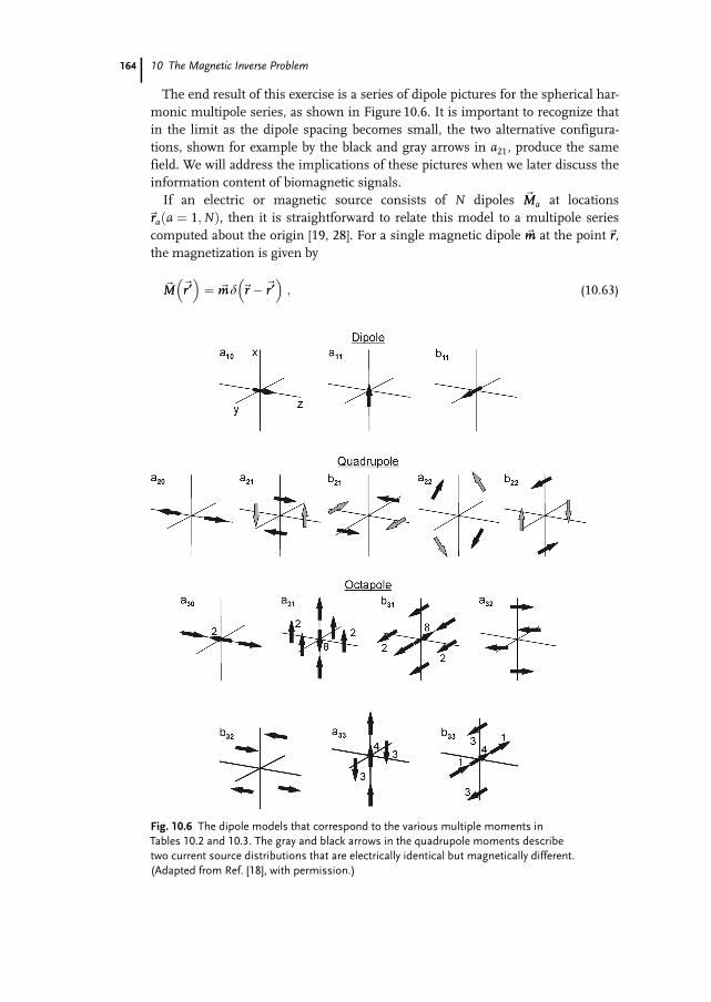
The end result of this exercise is a series of dipole pictures for the spherical har-monic multipole series, as shown in Figure 10.6. It is important to recognize thatin the limit as the dipole spacing becomes small, the two alternative configura-tions, shown for example by the black and gray arrows in a21, produce the samefield. We will address the implications of these pictures when we later discuss theinformation content of biomagnetic signals.If an electric or magnetic source consists of N dipoles ~MMa at locations
~rra a ¼ 1;Nð Þ, then it is straightforward to relate this model to a multipole seriescomputed about the origin [19, 28]. For a single magnetic dipole ~mm at the point~rr,the magnetization is given by
~MM ~r¢r¢� �
¼ ~mm d ~rr � ~r¢r¢� �
; (10:63)
164
Fig. 10.6 The dipole models that correspond to the various multiple moments inTables 10.2 and 10.3. The gray and black arrows in the quadrupole moments describetwo current source distributions that are electrically identical but magnetically different.(Adapted from Ref. [18], with permission.)
10.2 The Magnetic Forward Problem
where dð~rr � ~r¢r¢Þ is the Dirac delta function. Substitution of this into the integralsin Table 10.3 can be used to obtain the dipole through octapole moments of adipole displaced from the origin [18].
10.2.4.4 Current Multipoles in Conducting MediaThe advantage of the multipole approach is that it provides a mathematically com-pact, orthogonal description of a source distribution, which is particularly advanta-geous in an inverse calculation. Moreover, it has been pointed out in the literature[33–35] that the classic equivalent current dipole model can sometimes lead todangerous oversimplification of the inverse problem, partly because dipoles alonedescribe spatially extended sources rather poorly. We refer the reader to the workof Mosher et al. [33, 34, 36] for excellent and up-to-date reviews of MEG forwardmodeling using multipole expansions.The challenge is to establish an appropriate interpretation of the higher order
multipole moments. To explore the relationship between multipole moments anddistributed dipole sources, we draw from a detailed discussion of the uniformdouble-layer model [22].Figure 10.7 shows a schematic representation of a cardiac activation wave front.
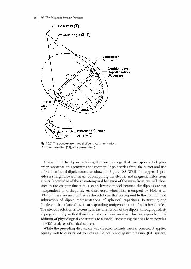
In the uniform double-layer model of cardiac activation, the active sources of thecardiac electric and magnetic fields are constrained to an expanding wave front,which is assumed to be thin, and have an impressed current density ~JiJi that is ev-erywhere uniform and perpendicular to the wave front [37]. It is termed a doublelayer because current is injected by the wave front into the medium at the outersurface, and withdrawn with an equal strength at the inner one. In this case, thesolid angle theorem [23] states that the electric potential at any point in an infinite,homogeneous conductor containing such a uniform double-layer source is deter-mined by the solid angle subtended by the rim of the double layer. The projectedarea of this rim is proportional to the dipole moment of this source and field; thecurvature and detailed shape of the rim contribute to the quadrupole and highermoments [22]. It also follows that the external potential is independent of any per-turbations of the layer that do not affect the shape or location of the rim, in thatthey are equivalent to the addition or subtraction of closed double layers, whichare equivalent to externally silent, spherical capacitors. If the origin of the multi-pole series does not correspond to the center of the surface enclosed by the rim,there will be additional terms to the multipole expansion that are described by thedipole shift equations [18, 28]. Conversely, the center of the wave front can in prin-ciple be located by determining the location for the multipole origin that mini-mizes higher order moments [22]. Interpretation is even more complicated when,late in cardiac depolarization, the wave front expands until it breaks through theepicardial surface, adding a second, or third rim to the wave front, each with itsown shifted multipole series!
165
10 The Magnetic Inverse Problem
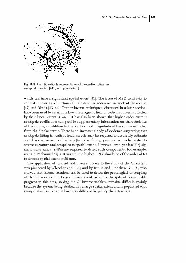
Given the difficulty in picturing the rim topology that corresponds to higherorder moments, it is tempting to ignore multipole series from the outset and useonly a distributed dipole source, as shown in Figure 10.8. While this approach pro-vides a straightforward means of computing the electric and magnetic fields froma priori knowledge of the spatiotemporal behavior of the wave front, we will showlater in the chapter that it fails as an inverse model because the dipoles are notindependent or orthogonal. As discovered when first attempted by Holt et al.[38–40], there are instabilities in the solutions that correspond to the addition andsubtraction of dipole representations of spherical capacitors. Perturbing onedipole can be balanced by a corresponding antiperturbation of all other dipoles.The obvious solution is to constrain the orientation of the dipole, through quadrat-ic programming, so that their orientation cannot reverse. This corresponds to theaddition of physiological constraints to a model, something that has been popularin MEG analyses of cortical sources.While the preceding discussion was directed towards cardiac sources, it applies
equally well to distributed sources in the brain and gastrointestinal (GI) system,
166
Fig. 10.7 The double-layer model of ventricular activation.(Adapted from Ref. [22], with permission.)
10.2 The Magnetic Forward Problem
which can have a significant spatial extent [41]. The issue of MEG sensitivity tocortical sources as a function of their depth is addressed in work of Hillebrand[42] and Okada [43, 44]. Fourier inverse techniques, discussed in a later section,have been used to determine how the magnetic field of cortical sources is affectedby their linear extent [45–48]. It has also been shown that higher order currentmultipole coefficients can provide supplementary information on characteristicsof the source, in addition to the location and magnitude of the source extractedfrom the dipolar terms. There is an increasing body of evidence suggesting thatmultipole fitting in realistic head models may be required to accurately estimateand characterize neuronal activity [49]. Specifically, quadrupoles can be related tosource curvature and octapoles to spatial extent. However, large (yet feasible) sig-nal-to-noise ratios (SNRs) are required to detect such components. For example,using a 49-channel SQUID system, the highest SNR should be of the order of 60to detect a spatial extent of 20 mm.The application of forward and inverse models to the study of the GI system
was pioneered by Allescher et al. [50] and by Irimia and Bradshaw [51–53], whoshowed that inverse solutions can be used to detect the pathological uncouplingof electric sources due to gastroparesis and ischemia. In spite of considerableprogress in this area, solving the GI inverse problem remains difficult, mainlybecause the system being studied has a large spatial extent and is populated withmany distinct sources that have very different frequency characteristics.
167
Fig. 10.8 A multiple-dipole representation of the cardiac activation.(Adapted from Ref. [243], with permission.)
10 The Magnetic Inverse Problem
10.3The Magnetic Inverse Problem
10.3.1Introduction
Given our brief introduction to the magnetic forward problem, we now addressthe inverse problem of determining sources from fields. We showed above thatthe magnetic field represents a convolution of a source distribution with a Green’sfunction. In this light, the inverse problem simply reduces to the deconvolution ofthese convolution integrals. Therein lies the challenge.
10.3.2Inverting the Law of Biot and Savart
10.3.2.1 Nonuniqueness of Inverse Solutions
The fundamental difficulty in magnetic imaging of currents is that there is nounique solution to the inverse problem of determining the three-dimensional cur-rent distribution in (10.14) from the measurements of the magnetic field outsideof the object. As mentioned in Section 10.1, the easiest proof of nonuniqueness isto note that it is possible to superimpose on any three-dimensional current distri-bution another source distribution that is magnetically silent, such as when theradial internal currents of a spherically symmetric battery are superimposed uponan infinite, homogeneous conductor. This is exactly analogous to the electrostaticcase where there is no electric field outside a spherical capacitor formed by a pairof concentric spherical shells carrying opposite charge. In an electrostatics inverseproblem, spherical capacitors of arbitrary radius, charge, and sphere separationcan be added or subtracted from the source distribution without changing thepotentials measured on the surface that bounds all sources. Hence, any attempt tosolve such an inverse problem will be unable to determine which spherical capaci-tor configurations exist, and which do not. Constraints might be used to preventthe inverse algorithm from creating spherical capacitors de novo, but there is awhole class of higher-order silent sources. As we saw above, the spherical harmon-ic multipole solution to Laplace’s equation is designed specifically to eliminatethose silent sources [18, 25]. The usual approach to this problem for either theelectric or magnetic inverse is to restrict the possible sources and invert the result-ing set of constrained equations.In contrast to the three-dimensional current-imaging problem, the two-dimen-
sional problem does have a unique inverse. As we shall see in this chapter, thereis a wide variety of inverse algorithms for magnetic imaging of two-dimensionalcurrent distributions, including spatial filtering, dipole fitting, the Hosaka-Cohentransformation, alternating projections, lead-field analysis, the finite-elementmethod, and blind deconvolution. While there may be a unique inverse solution,even the two-dimensional inverse problem can be ill-conditioned, in that the abil-
168
10.3 The Magnetic Inverse Problem
ity to determine the inverse solution with the desired accuracy or spatial resolu-tion can be strongly dependent upon measurement noise, source-detector dis-tance, and the exact nature of the source current distribution. We shall show thatthis can be overcome in part by applying constraints to limit the effects of noise orto utilize most fully a priori knowledge of the current distribution.
10.3.2.2 The Spatial Filtering ApproachThe most elegant method to obtain a two-dimensional current image from a mag-netic field map is to use Fourier-transform deconvolution (inversion) of the law ofBiot and Savart [54–59]. Following the notation of Roth [56], let us assume that weare imaging the magnetic field produced by a two-dimensional current~JJ x; yð Þ dis-tributed through a slab of conducting material of thickness d that extends to infi-nity in the xy-plane. We shall assume that we measure the component Bx at aheight z >> d, so that we can integrate (10.14) over z¢ and immediately obtain4)
Bx x; y; zð Þ ¼ l0d4p
zZ ¥
�¥
Z ¥
�¥
Jy x ¢; y¢ð Þ
x � x ¢ð Þ2þ y� y¢ð Þ2þz2h i3=2 dx ¢dy¢: (10:64)
We can write this equation as the convolution of the current distribution with aGreen’s function that represents the magnetic source-to-field transfer function:
Bx x; y; zð Þ ¼Z ¥
�¥
Z ¥
�¥Jy x ¢; y¢ð ÞG x � x ¢ð Þ; y� y¢ð Þ; zð Þ dx ¢dy¢; (10:65)
where the Green’s function is given by
G x � x ¢ð Þ; y� y¢ð Þ; zð Þ ¼ l0d4p
z
x � x ¢ð Þ2þ y� y¢ð Þ2þz2h i3=2 : (10:66)
Rather than computing this through integration in Cartesian space, we caninstead compute the spatial Fourier transform ðFTÞ5) of Jy using the fast Fouriertransform (FFT) or more accurate techniques [60], so that
169
4) Hereafter, when we are discussing the two-dimensional current image, we shall assumethat the sample has a thickness d that is neg-ligible compared to z, so that~JJ has neither az-component nor z-dependence. Thus, weshall be able to use the standard currentdensity~JJ, with units of amperes/meter2,rather than a two-dimensional equivalent.The thickness d will be written explicitly inthe equations.~JJd is simply a two-dimen-sional current density with units ofamperes/meter.
5) We use the following definition of the two-dimensional Fourier transform pair in thischapter:
f ðkx ; kyÞ ¼Zþ¥�¥
Zþ¥�¥
Fðx; yÞe�iðkx xþkyyÞdxdy
Fðx; yÞ¼ 1
ð2pÞ2Zþ¥�¥
Zþ¥�¥
f ðkx ;KyÞeiðkxxþkyyÞdkxdky
This may lead to slight differences betweensome of the equations presented herein andthose in the original papers.
10 The Magnetic Inverse Problem
jy kx; ky
� �¼ FT Jy x; yð Þ
n o: (10:67)
Similarly, we can write
bx kx; ky; z� �
¼ FT Bx x; y; zð Þf g: (10:68)
The Green’s function has the Fourier transform [56]
g kx; ky; z� �
¼ l0d2
e�zffiffiffiffiffiffiffiffiffik2xþk2yp
; (10:69)
where kx ¼ 2p=x and ky ¼ 2p=y are the spatial frequencies, in m�1, in the x and ydirections. We can then use the convolution theorem to write the law of Biot andSavart as a simple multiplication in the spatial frequency domain
bx kx; ky; z� �
¼ g kx; ky; z� �
jy kx; ky
� �: (10:70)
This process allows us to start with a known y component of the current density,Jyðx; yÞ, and then calculate the x component of the magnetic field, Bxðx; y; zÞ.Note that the spatial filter that corresponds to the magnetic forward problem, g,falls exponentially with both k and z, so that the high-spatial-frequency contribu-tions to the current distribution are attenuated in the magnetic field, i.e., theGreen’s function acts as a spatial low-pass filter. The farther the magnetometer isfrom the current distribution, the harsher is the filtering.
Inverse Spatial FilteringA supposedly simple division allows us to solve (10.70) for jyðkx; kyÞ and hencesolve in Fourier space the inverse imaging problem of determining~JJ from ~BB
jy kx; ky
� �¼
bx kx; ky; z� �
g kx; ky; z� � : (10:71)
The desired image of Jy x ¢; y¢ð Þ is obtained with the inverse Fourier transform
Jy ¼ FT�1 jy kx; ky
� �n o. (10.72)
A similar set of equations would allow us to determine Jx from a map of By. Thisinverse solution is unique [56].As we shall see in more detail shortly, the problem with this inverse process, in
general, is in the division in (10.71). If g is small, but nonzero, at spatial frequen-cies for which 1=g is large, jy tends toward infinity. Unfortunately, g falls exponen-tially with k, so that 1=g diverges exponentially. Since noise is always present inexperimental data, bx is certainly nonzero at high frequencies, even if the theoreti-cal magnetic field associated with the source does not contain high-spatial-fre-
170
10.3 The Magnetic Inverse Problem
quency components. Therefore, (10.71) is destined to “blow up” due to excessiveamplification of noise. Before we see how this can be avoided, it is useful to lookat the z component of the field.From (10.17), it follows that the Fourier transform of Bz is [56]
bz kx; ky; z� �
¼ il0d2
e�zffiffiffiffiffiffiffiffiffik2xþk2yp kx jy kx; ky
� �ffiffiffiffiffiffiffiffiffiffiffiffiffiffiffik2x þ k2y
q �ky jx kx; ky
� �ffiffiffiffiffiffiffiffiffiffiffiffiffiffiffik2x þ k2y
q0B@
1CA: (10:73)
This shows us, in general, that a single image of Bz would be inadequate to deter-mine both Jx and Jy, and would provide only a linear combination of the two.However, if we assume that the current distribution is continuous, it must havezero divergence in the quasistatic limit, i.e.,
� �~JJ x; yð Þ ¼ 0 . (10.74)
For two-dimensional current with no source or sinks, this reduces to
¶Jx
¶xþ¶Jy
¶y¼ 0 . (10.75)
If we compute the Fourier transform of this equation, we then have the addedconstraint
ikx jx kx; ky
� �þ iky jy kx; ky
� �¼ 0 , (10.76)
which allows us to solve (10.73) for either Jx or Jy and then use the continuityequation to obtain the other. While this procedure works well for planar currentdistributions, it may not be applicable for mapping effective surface currents onthe upper boundary of three-dimensional current distributions in thick objects,since current flowing on the surface can disappear as Jz into the bulk conductorof the object without affecting Bz.
Noise and WindowingWe now can address briefly the issue of noise and windowing, which is treated ingreater detail elsewhere for two-dimensional imaging [56], for fetal MCG noiseremoval [61], and for cylindrical models of the head [45, 47, 48] and abdomen [62].The value of jy in (10.71) will diverge if there is noise in the absence of signal, i.e.,if the denominator goes to zero faster than does the numerator. However, becausethe noise in a SQUID measurement is white at high temporal frequencies, ascanned SQUID image will have white noise at high spatial frequencies. The low-pass characteristic of the law of Biot and Savart is manifest as a Green’s functionthat tends towards zero exponentially at high spatial frequencies, so that anunstable inverse is almost guaranteed except in cases where the magnetometer isvery close to the current distribution. The solution to this dilemma is to filter spa-tially the magnetic field data by eliminating all contributions at high spatial fre-quencies, so that the numerator is identically zero above a frequency kc. The pro-
171
10 The Magnetic Inverse Problem
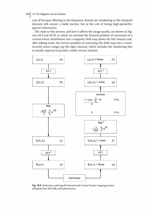
cess of low-pass filtering in the frequency domain (or windowing in the temporaldomain) will ensure a stable inverse, but at the cost of losing high-spatial-fre-quency information.The steps in this process, and how it affects the image quality, are shown in Fig-
ures 10.9 and 10.10, in which we simulate the forward problem of conversion of acurrent source distribution into a magnetic field map (down the left column) and,after adding noise, the inverse problem of converting the field map into a recon-structed source image (up the right column), which includes the windowing thatis usually required to provide a stable inverse solution.
172
Fig. 10.9 Schematic outlining the forward and inverse Fourier imaging process.(Adapted from Ref. [56], with permission.)
10.3 The Magnetic Inverse Problem
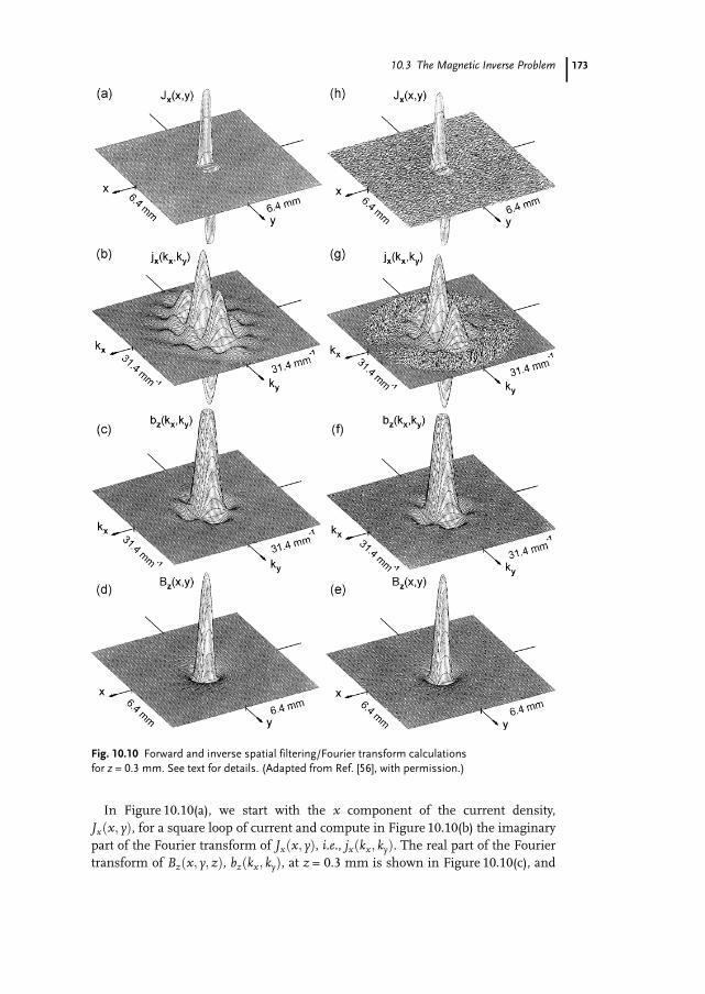
In Figure 10.10(a), we start with the x component of the current density,Jxðx; yÞ, for a square loop of current and compute in Figure 10.10(b) the imaginarypart of the Fourier transform of Jxðx; yÞ, i.e., jxðkx; kyÞ. The real part of the Fouriertransform of Bzðx; y; zÞ, bzðkx; kyÞ, at z = 0.3 mm is shown in Figure 10.10(c), and
173
Fig. 10.10 Forward and inverse spatial filtering/Fourier transform calculationsfor z = 0.3 mm. See text for details. (Adapted from Ref. [56], with permission.)
10 The Magnetic Inverse Problem
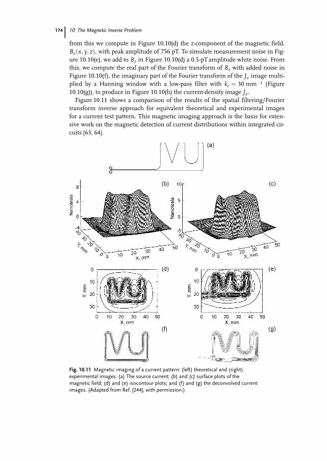
from this we compute in Figure 10.10(d) the z-component of the magnetic field,Bzðx; y; zÞ, with peak amplitude of 756 pT. To simulate measurement noise in Fig-ure 10.10(e), we add to Bz in Figure 10.10(d) a 0.5-pT amplitude white noise. Fromthis, we compute the real part of the Fourier transform of Bz with added noise inFigure 10.10(f), the imaginary part of the Fourier transform of the Jx image multi-plied by a Hanning window with a low-pass filter with kc ¼ 30 mm�1 (Figure10.10(g)), to produce in Figure 10.10(h) the current-density image Jx.Figure 10.11 shows a comparison of the results of the spatial filtering/Fourier
transform inverse approach for equivalent theoretical and experimental imagesfor a current test pattern. This magnetic imaging approach is the basis for exten-sive work on the magnetic detection of current distributions within integrated cir-cuits [63, 64].
174
Fig. 10.11 Magnetic imaging of a current pattern: (left) theoretical and (right)experimental images. (a) The source current; (b) and (c) surface plots of themagnetic field; (d) and (e) isocontour plots; and (f) and (g) the deconvolved currentimages. (Adapted from Ref. [244], with permission.)
10.3 The Magnetic Inverse Problem 175
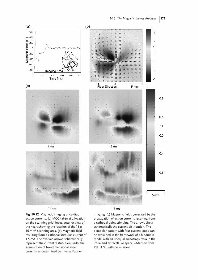
Fig. 10.12 Magnetic imaging of cardiacaction currents. (a) MCG taken at a locationon the scanning grid. Inset: anterior view ofthe heart showing the location of the 16 >16 mm2 scanning area. (b) Magnetic fieldresulting from a cathodal stimulus current of1.5 mA. The overlaid arrows schematicallyrepresent the current distribution under theassumption of two-dimensional sheetcurrents as determined by inverse Fourier
imaging. (c) Magnetic fields generated by thepropagation of action currents resulting froma cathodal point stimulus. The arrows showschematically the current distribution. Theoctupolar pattern with four current loops canbe explained in the framework of a bidomainmodel with an unequal anisotropy ratio in theintra- and extracellular space. (Adapted fromRef. [174], with permission.)
10 The Magnetic Inverse Problem
Figure 10.12 shows a magnetic field map obtained with the original Micro-SQUID magnetometer and the corresponding current image for a slice of isolatedcardiac tissue [65, 66]. These measurements provided some of the first proof thatcardiac tissue is best described by bidomain models6) with unequal anisotropyratios in the intracellular and extracellular spaces [67].
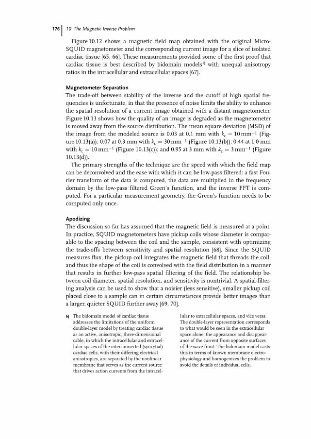
Magnetometer SeparationThe trade-off between stability of the inverse and the cutoff of high spatial fre-quencies is unfortunate, in that the presence of noise limits the ability to enhancethe spatial resolution of a current image obtained with a distant magnetometer.Figure 10.13 shows how the quality of an image is degraded as the magnetometeris moved away from the source distribution. The mean square deviation (MSD) ofthe image from the modeled source is 0.03 at 0.1 mm with kc ¼ 10mm�1 (Fig-ure 10.13(a)); 0.07 at 0.3 mm with kc ¼ 30mm�1 (Figure 10.13(b)); 0.44 at 1.0 mmwith kc ¼ 10mm�1 (Figure 10.13(c)); and 0.95 at 3 mm with kc ¼ 3mm�1 (Figure10.13(d)).The primary strengths of the technique are the speed with which the field map
can be deconvolved and the ease with which it can be low-pass filtered: a fast Fou-rier transform of the data is computed, the data are multiplied in the frequencydomain by the low-pass filtered Green’s function, and the inverse FFT is com-puted. For a particular measurement geometry, the Green’s function needs to becomputed only once.
ApodizingThe discussion so far has assumed that the magnetic field is measured at a point.In practice, SQUID magnetometers have pickup coils whose diameter is compar-able to the spacing between the coil and the sample, consistent with optimizingthe trade-offs between sensitivity and spatial resolution [68]. Since the SQUIDmeasures flux, the pickup coil integrates the magnetic field that threads the coil,and thus the shape of the coil is convolved with the field distribution in a mannerthat results in further low-pass spatial filtering of the field. The relationship be-tween coil diameter, spatial resolution, and sensitivity is nontrivial. A spatial-filter-ing analysis can be used to show that a noisier (less sensitive), smaller pickup coilplaced close to a sample can in certain circumstances provide better images thana larger, quieter SQUID further away [69, 70].
176
6) The bidomain model of cardiac tissueaddresses the limitations of the uniformdouble-layer model by treating cardiac tissueas an active, anisotropic, three-dimensionalcable, in which the intracellular and extracel-lular spaces of the interconnected (syncytial)cardiac cells, with their differing electricalanisotropies, are separated by the nonlinearmembrane that serves as the current sourcethat drives action currents from the intracel-
lular to extracellular spaces, and vice versa.The double-layer representation correspondsto what would be seen in the extracellularspace alone: the appearance and disappear-ance of the current from opposite surfacesof the wave front. The bidomain model caststhis in terms of known membrane electro-physiology and homogenizes the problem toavoid the details of individual cells.
10.3 The Magnetic Inverse Problem
One would suspect that a deconvolution approach could be used to eliminatethe effect of the finite coil area. The image processing approach can be extendedto examine and correct for the effects of finite-diameter pickup coils [71]. We dis-cuss the flux-field deconvolution in greater detail later in this chapter. For aSQUID with a finite-diameter pickup coil, the magnetic field Bz will be convolvedwith the spatial sampling (or turns) function H of the coil to give the detected fluxU. Figure 10.14 shows four different pickup coils [71]. In Fourier space, the mag-netic field distribution from the sample bðkx; kyÞ will be multiplied by the turnsfunction hðkx; kyÞ to give the flux fðkx; kyÞ. Ideally, the effect of the coil could becorrected by dividing fðkx; kyÞ by hðkx; kyÞ to obtain bðkx; kyÞ, so that an inverseFourier transform would give the coil-corrected Bz. Unfortunately, for typical coils,the edges of the coil introduce zeros in their spatial frequency transfer function,hðkx; kyÞ, which complicate deconvolution of the images at high spatial frequen-cies: the zero in the forward transfer function produces an infinity in the inversefunction, making it difficult to obtain any information from the field at or evennear that spatial frequency. This could be ameliorated with windowing, as before,but this leads once again to the loss of high-frequency information instead of to
177
Fig. 10.13 Spatial filtering/Fourier transforminverse image of the current density for fourdifferent values of h kx ; ky
� �, calculated from
the e�a2r2 component of the magnetic fieldproduced by the square current loop used inthe simulations of Fig. 10.10 after magnet-ometer noise of 0.5 pT has been added to the
magnetic field. Plots of both Jx x; yð Þ and thecurrent lines (upper right inset) are shown.Each line corresponds to 0.1 lA, except in (d),where each line is 0.05 lA. (a) z = 0.1 mm,(b) 0.3 mm, (c) 1.0 mm, (d) 3.0 mm.(Adapted from Ref. [56], with permission.)
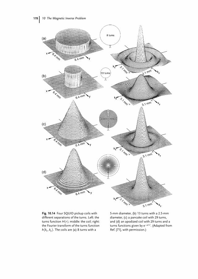
10 The Magnetic Inverse Problem178
Fig. 10.14 Four SQUID pickup coils withdifferent separations of the turns. Left: theturns function H rð Þ; middle: the coil; right:the Fourier transform of the turns functionh kx ; ky
� �. The coils are (a) 8 turns with a
5-mm diameter, (b) 13 turns with a 2.5-mmdiameter, (c) a pancake coil with 29 turns,and (d) an apodized coil with 29 turns and aturns functions given by e�a2r2. (Adapted fromRef. [71], with permission.)
10.3 The Magnetic Inverse Problem
the desired extent of resolution enhancement. As shown in Figure 10.15, evenwith windowing, the contribution near the zeros produces spikes that appear inthe frequency domain at the edge of the window, and these spikes produce noisein the spatial images.A solution to this problem that has been demonstrated theoretically [71] but not
yet implemented is to adjust the spacing of individual turns in a planar coil, asshown in Figures 10.14(c) and (d), so that the zeros in the transfer function
179
Fig. 10.15 A comparison of the imaging abil-ity of the four different SQUID pickup coils inFig. 10.14. Left: the x-component of the cur-rent density; center: current lines of the imageof the current; right: the imaginary part of the
Fourier transform of the current densityimages. The source current is (a¢), and(a)–(d) are the density images from the fourcoils. (Adapted from Ref. [71], with permis-sion.)
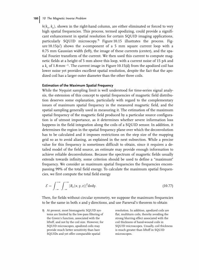
10 The Magnetic Inverse Problem
hðkx; kyÞ, shown in the right-hand column, are either eliminated or forced to veryhigh spatial frequencies. This process, termed apodizing, could provide a signifi-cant enhancement in spatial resolution for certain SQUID imaging applications,particularly SQUID microscopy.7) Figure 10.15 illustrates the process. Fig-ure 10.15(a¢) shows the x-component of a 5 mm square current loop with a0.75 mm Gaussian width (left), the image of these currents (center), and the spa-tial Fourier transform of the current. We then used this current to compute mag-netic fields at a height of 5 mm above this loop, with a current noise of 15 pA anda kc of 1:8mm�1. The current image in Figure 10.15(d) from the apodized coil haslower noise yet provides excellent spatial resolution, despite the fact that the apo-dized coil has a larger outer diameter than the other three coils.
Estimation of the Maximum Spatial FrequencyWhile the Nyquist sampling limit is well understood for time-series signal analy-sis, the extension of this concept to spatial frequencies of magnetic field distribu-tion deserves some explanation, particularly with regard to the complementaryissues of maximum spatial frequency in the measured magnetic field, and thespatial sampling generally used in measuring it. The estimation of the maximumspatial frequency of the magnetic field produced by a particular source configura-tion is of utmost importance, as it determines whether severe information losshappens in the field integration along the coils of a SQUID sensor. In addition, itdetermines the region in the spatial frequency plane over which the deconvolutionhas to be calculated and it imposes restrictions on the step size of the mappinggrid so as to avoid aliasing, as explained in the next subsection. While a precisevalue for this frequency is sometimes difficult to obtain, since it requires a de-tailed model of the field source, an estimate may provide enough information toachieve reliable deconvolutions. Because the spectrum of magnetic fields usuallyextends towards infinity, some criterion should be used to define a “maximum”frequency. We consider as maximum spatial frequencies the frequencies encom-passing 99% of the total field energy. To calculate the maximum spatial frequen-cies, we first compute the total field energy
E ¼Z þ¥�¥
Z þ¥�¥
Bzðx; y; zÞj j2dxdy: (10:77)
Then, for fields without circular symmetry, we suppose the maximum frequenciesto be the same in both x and y directions, and use Parseval’s theorem to obtain
180
7) At present, most biomagnetic SQUID sys-tems are limited by the low-pass filtering ofthe Green’s function, associated with theliftoff, and not by the coil size. However, forSQUID microscopes, apodized coils mayprovide much better sensitivity than bareSQUIDs and yet offer comparable spatial
resolution. In addition, apodized coils areflat, multiturn coils, thereby avoiding thestrong blurring effect associated with thecoil thickness of hand-wound coils inSQUID microscopes. Usually, coil thicknessis much greater than liftoff in SQUIDmicroscopes.
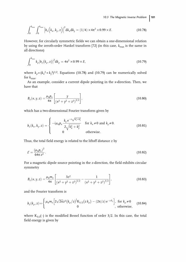
10.3 The Magnetic Inverse Problem
Z kmax
0
Z kmax
0bz kx; ky; z� ���� ���2dkxdky ¼ ð1=4Þ · 4p2 · 0:99 ·E: (10:78)
However, for circularly symmetric fields we can obtain a one-dimensional relationby using the zeroth-order Hankel transform [72] (in this case, kmax is the same inall directions)
Z kmax
0kr bz kr; z
� ��� ��2dkr ¼ 4p2 · 0:99 ·E; (10:79)
where kr= (kx2 + ky
2)1/2. Equations (10.78) and (10.79) can be numerically solvedfor kmax.As an example, consider a current dipole pointing in the x-direction. Then, we
have that
Bzðx; y; zÞ ¼l0px
4py
x2 þ y2 þ z2ð Þ3=2
" #; (10:80)
which has a two-dimensional Fourier transform given by
bzðkx; ky; zÞ ¼�il0px
ky e�z
ffiffiffiffiffiffiffiffiffik2xþk2yp
2ffiffiffiffiffiffiffiffiffiffiffiffiffiffiffik2x þ k2y
q for kx „ 0 and ky „ 0:
0 otherwise:
8>><>>: (10:81)
Thus, the total field energy is related to the liftoff distance z by
E ¼ l0pxð Þ2
64p z2: (10:82)
For a magnetic dipole source pointing in the z-direction, the field exhibits circularsymmetry
Bzðx; y; zÞ ¼l0mz
4p3z2
x2 þ y2 þ z2ð Þ5=2� 1
x2 þ y2 þ z2ð Þ3=2
" #; (10:83)
and the Fourier transform is
bzðkr; zÞ¼l0mz 2
ffiffiffiffiffiffi2pp
z2 kr$
z� �3
2K3=2 z kr� �
� ð2p=zÞ e�z krh i
; for kr „ 00 ; otherwise;
((10:84)
where K3/2(·) is the modified Bessel function of order 3/2. In this case, the totalfield energy is given by
181
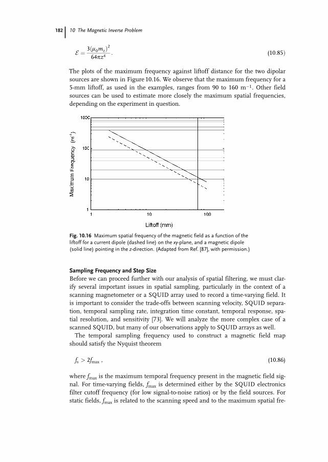
10 The Magnetic Inverse Problem
E ¼ 3 l0mzð Þ2
64pz4: (10:85Þ
The plots of the maximum frequency against liftoff distance for the two dipolarsources are shown in Figure 10.16. We observe that the maximum frequency for a5-mm liftoff, as used in the examples, ranges from 90 to 160 m�1. Other fieldsources can be used to estimate more closely the maximum spatial frequencies,depending on the experiment in question.
Sampling Frequency and Step SizeBefore we can proceed further with our analysis of spatial filtering, we must clar-ify several important issues in spatial sampling, particularly in the context of ascanning magnetometer or a SQUID array used to record a time-varying field. Itis important to consider the trade-offs between scanning velocity, SQUID separa-tion, temporal sampling rate, integration time constant, temporal response, spa-tial resolution, and sensitivity [73]. We will analyze the more complex case of ascanned SQUID, but many of our observations apply to SQUID arrays as well.The temporal sampling frequency used to construct a magnetic field map
should satisfy the Nyquist theorem
fs > 2fmax , (10.86)
where fmax is the maximum temporal frequency present in the magnetic field sig-nal. For time-varying fields, fmax is determined either by the SQUID electronicsfilter cutoff frequency (for low signal-to-noise ratios) or by the field sources. Forstatic fields, fmax is related to the scanning speed and to the maximum spatial fre-
182
Fig. 10.16 Maximum spatial frequency of the magnetic field as a function of theliftoff for a current dipole (dashed line) on the xy-plane, and a magnetic dipole(solid line) pointing in the z-direction. (Adapted from Ref. [87], with permission.)
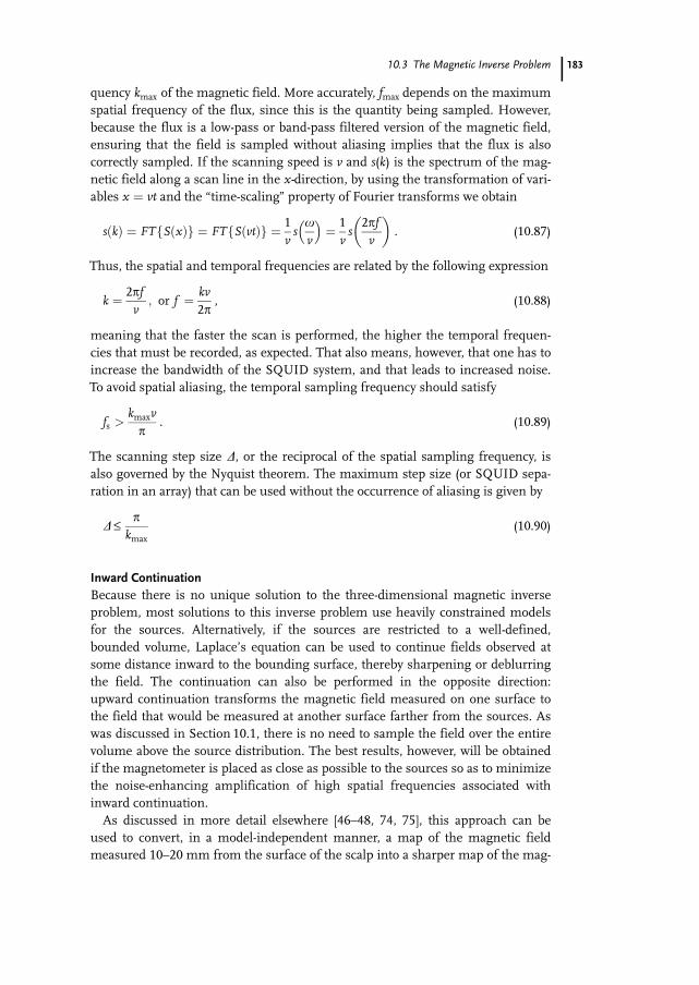
10.3 The Magnetic Inverse Problem
quency kmax of the magnetic field. More accurately, fmax depends on the maximumspatial frequency of the flux, since this is the quantity being sampled. However,because the flux is a low-pass or band-pass filtered version of the magnetic field,ensuring that the field is sampled without aliasing implies that the flux is alsocorrectly sampled. If the scanning speed is v and s(k) is the spectrum of the mag-netic field along a scan line in the x-direction, by using the transformation of vari-ables x ¼ vt and the “time-scaling” property of Fourier transforms we obtain
sðkÞ ¼ FT SðxÞf g ¼ FT SðvtÞf g ¼ 1v
sx
v
� �¼ 1
vs
2pfv
� �. (10.87)
Thus, the spatial and temporal frequencies are related by the following expression
k ¼ 2pfv
; or f ¼ kv2p
, (10.88)
meaning that the faster the scan is performed, the higher the temporal frequen-cies that must be recorded, as expected. That also means, however, that one has toincrease the bandwidth of the SQUID system, and that leads to increased noise.To avoid spatial aliasing, the temporal sampling frequency should satisfy
fs >kmaxvp
. (10.89)
The scanning step size D, or the reciprocal of the spatial sampling frequency, isalso governed by the Nyquist theorem. The maximum step size (or SQUID sepa-ration in an array) that can be used without the occurrence of aliasing is given by
D £p
kmax(10.90)
Inward ContinuationBecause there is no unique solution to the three-dimensional magnetic inverseproblem, most solutions to this inverse problem use heavily constrained modelsfor the sources. Alternatively, if the sources are restricted to a well-defined,bounded volume, Laplace’s equation can be used to continue fields observed atsome distance inward to the bounding surface, thereby sharpening or deblurringthe field. The continuation can also be performed in the opposite direction:upward continuation transforms the magnetic field measured on one surface tothe field that would be measured at another surface farther from the sources. Aswas discussed in Section 10.1, there is no need to sample the field over the entirevolume above the source distribution. The best results, however, will be obtainedif the magnetometer is placed as close as possible to the sources so as to minimizethe noise-enhancing amplification of high spatial frequencies associated withinward continuation.As discussed in more detail elsewhere [46–48, 74, 75], this approach can be
used to convert, in a model-independent manner, a map of the magnetic fieldmeasured 10–20 mm from the surface of the scalp into a sharper map of the mag-
183
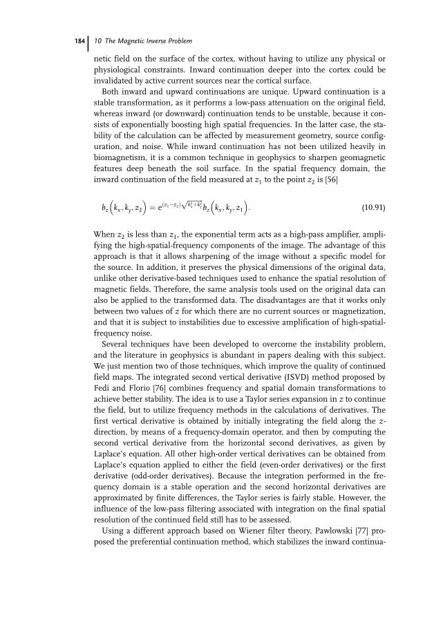
10 The Magnetic Inverse Problem
netic field on the surface of the cortex, without having to utilize any physical orphysiological constraints. Inward continuation deeper into the cortex could beinvalidated by active current sources near the cortical surface.Both inward and upward continuations are unique. Upward continuation is a
stable transformation, as it performs a low-pass attenuation on the original field,whereas inward (or downward) continuation tends to be unstable, because it con-sists of exponentially boosting high spatial frequencies. In the latter case, the sta-bility of the calculation can be affected by measurement geometry, source config-uration, and noise. While inward continuation has not been utilized heavily inbiomagnetism, it is a common technique in geophysics to sharpen geomagneticfeatures deep beneath the soil surface. In the spatial frequency domain, theinward continuation of the field measured at z1 to the point z2 is [56]
bz kx; ky; z2� �
¼ e z1�z2ð Þffiffiffiffiffiffiffiffiffik2xþk2yp
bz kx; ky; z1� �
: (10:91)
When z2 is less than z1, the exponential term acts as a high-pass amplifier, ampli-fying the high-spatial-frequency components of the image. The advantage of thisapproach is that it allows sharpening of the image without a specific model forthe source. In addition, it preserves the physical dimensions of the original data,unlike other derivative-based techniques used to enhance the spatial resolution ofmagnetic fields. Therefore, the same analysis tools used on the original data canalso be applied to the transformed data. The disadvantages are that it works onlybetween two values of z for which there are no current sources or magnetization,and that it is subject to instabilities due to excessive amplification of high-spatial-frequency noise.Several techniques have been developed to overcome the instability problem,
and the literature in geophysics is abundant in papers dealing with this subject.We just mention two of those techniques, which improve the quality of continuedfield maps. The integrated second vertical derivative (ISVD) method proposed byFedi and Florio [76] combines frequency and spatial domain transformations toachieve better stability. The idea is to use a Taylor series expansion in z to continuethe field, but to utilize frequency methods in the calculations of derivatives. Thefirst vertical derivative is obtained by initially integrating the field along the z-direction, by means of a frequency-domain operator, and then by computing thesecond vertical derivative from the horizontal second derivatives, as given byLaplace’s equation. All other high-order vertical derivatives can be obtained fromLaplace’s equation applied to either the field (even-order derivatives) or the firstderivative (odd-order derivatives). Because the integration performed in the fre-quency domain is a stable operation and the second horizontal derivatives areapproximated by finite differences, the Taylor series is fairly stable. However, theinfluence of the low-pass filtering associated with integration on the final spatialresolution of the continued field still has to be assessed.Using a different approach based on Wiener filter theory, Pawlowski [77] pro-
posed the preferential continuation method, which stabilizes the inward continua-
184
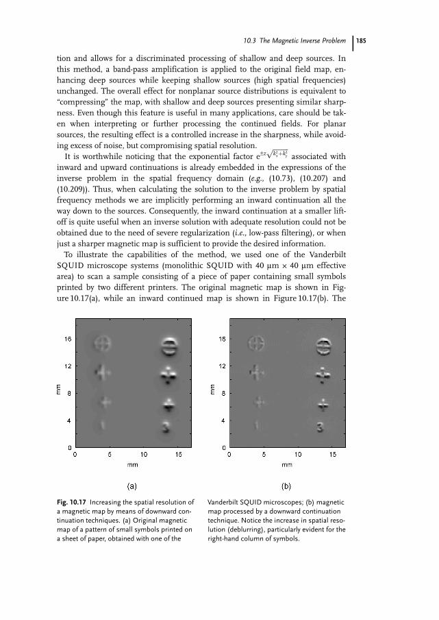
10.3 The Magnetic Inverse Problem
tion and allows for a discriminated processing of shallow and deep sources. Inthis method, a band-pass amplification is applied to the original field map, en-hancing deep sources while keeping shallow sources (high spatial frequencies)unchanged. The overall effect for nonplanar source distributions is equivalent to“compressing” the map, with shallow and deep sources presenting similar sharp-ness. Even though this feature is useful in many applications, care should be tak-en when interpreting or further processing the continued fields. For planarsources, the resulting effect is a controlled increase in the sharpness, while avoid-ing excess of noise, but compromising spatial resolution.It is worthwhile noticing that the exponential factor e–z
ffiffiffiffiffiffiffiffiffik2xþk2yp
associated withinward and upward continuations is already embedded in the expressions of theinverse problem in the spatial frequency domain (e.g., (10.73), (10.207) and(10.209)). Thus, when calculating the solution to the inverse problem by spatialfrequency methods we are implicitly performing an inward continuation all theway down to the sources. Consequently, the inward continuation at a smaller lift-off is quite useful when an inverse solution with adequate resolution could not beobtained due to the need of severe regularization (i.e., low-pass filtering), or whenjust a sharper magnetic map is sufficient to provide the desired information.To illustrate the capabilities of the method, we used one of the Vanderbilt
SQUID microscope systems (monolithic SQUID with 40 lm U 40 lm effectivearea) to scan a sample consisting of a piece of paper containing small symbolsprinted by two different printers. The original magnetic map is shown in Fig-ure 10.17(a), while an inward continued map is shown in Figure 10.17(b). The
185
Fig. 10.17 Increasing the spatial resolution ofa magnetic map by means of downward con-tinuation techniques. (a) Original magneticmap of a pattern of small symbols printed ona sheet of paper, obtained with one of the
Vanderbilt SQUID microscopes; (b) magneticmap processed by a downward continuationtechnique. Notice the increase in spatial reso-lution (deblurring), particularly evident for theright-hand column of symbols.
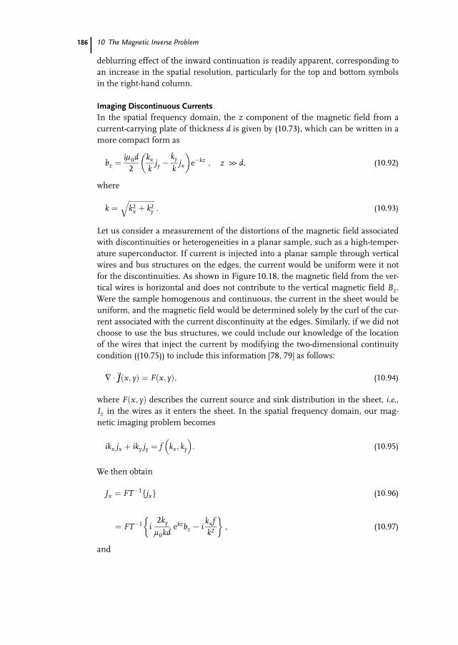
10 The Magnetic Inverse Problem
deblurring effect of the inward continuation is readily apparent, corresponding toan increase in the spatial resolution, particularly for the top and bottom symbolsin the right-hand column.
Imaging Discontinuous CurrentsIn the spatial frequency domain, the z component of the magnetic field from acurrent-carrying plate of thickness d is given by (10.73), which can be written in amore compact form as
bz ¼il0d2
kx
kjy �
ky
kjx
� �e�kz ; z >> d, (10.92)
where
k ¼ffiffiffiffiffiffiffiffiffiffiffiffiffiffiffik2x þ k2y
q. (10.93)
Let us consider a measurement of the distortions of the magnetic field associatedwith discontinuities or heterogeneities in a planar sample, such as a high-temper-ature superconductor. If current is injected into a planar sample through verticalwires and bus structures on the edges, the current would be uniform were it notfor the discontinuities. As shown in Figure 10.18, the magnetic field from the ver-tical wires is horizontal and does not contribute to the vertical magnetic field Bz.Were the sample homogenous and continuous, the current in the sheet would beuniform, and the magnetic field would be determined solely by the curl of the cur-rent associated with the current discontinuity at the edges. Similarly, if we did notchoose to use the bus structures, we could include our knowledge of the locationof the wires that inject the current by modifying the two-dimensional continuitycondition ((10.75)) to include this information [78, 79] as follows:
� �~JJ x; yð Þ ¼ F x; yð Þ; (10:94)
where F x; yð Þ describes the current source and sink distribution in the sheet, i.e.,Iz in the wires as it enters the sheet. In the spatial frequency domain, our mag-netic imaging problem becomes
ikx jx þ iky jy ¼ f kx; ky
� �: (10:95)
We then obtain
Jx ¼ FT�1 jxf g (10:96)
¼ FT�1 i2ky
l0kdekzbz � i
kxfk2
& ', (10.97)
and
186
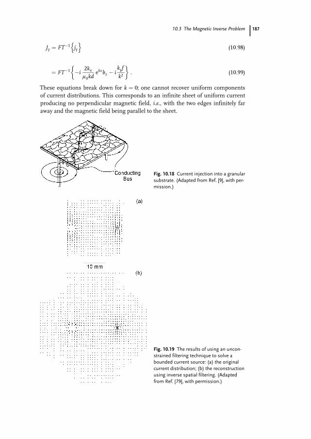
10.3 The Magnetic Inverse Problem
Jy ¼ FT�1 jyn o
(10:98)
¼ FT�1 �i2kx
l0kdekzbz � i
kyf
k2
& '. (10.99)
These equations break down for k ¼ 0; one cannot recover uniform componentsof current distributions. This corresponds to an infinite sheet of uniform currentproducing no perpendicular magnetic field, i.e., with the two edges infinitely faraway and the magnetic field being parallel to the sheet.
187
Fig. 10.18 Current injection into a granularsubstrate. (Adapted from Ref. [9], with per-mission.)
Fig. 10.19 The results of using an uncon-strained filtering technique to solve abounded current source: (a) the originalcurrent distribution; (b) the reconstructionusing inverse spatial filtering. (Adaptedfrom Ref. [79], with permission.)
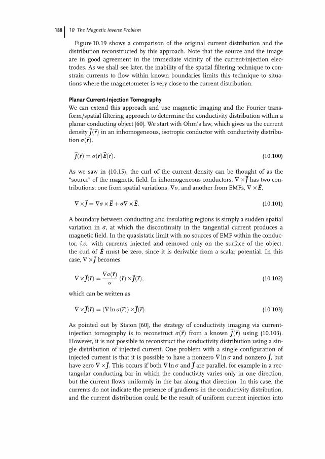
10 The Magnetic Inverse Problem
Figure 10.19 shows a comparison of the original current distribution and thedistribution reconstructed by this approach. Note that the source and the imageare in good agreement in the immediate vicinity of the current-injection elec-trodes. As we shall see later, the inability of the spatial filtering technique to con-strain currents to flow within known boundaries limits this technique to situa-tions where the magnetometer is very close to the current distribution.
Planar Current-Injection TomographyWe can extend this approach and use magnetic imaging and the Fourier trans-form/spatial filtering approach to determine the conductivity distribution within aplanar conducting object [60]. We start with Ohm’s law, which gives us the currentdensity~JJ ~rrð Þ in an inhomogeneous, isotropic conductor with conductivity distribu-tion r ~rrð Þ,
~JJ ~rrð Þ ¼ r ~rrð Þ~EE ~rrð Þ: (10:100)
As we saw in (10.15), the curl of the current density can be thought of as the“source” of the magnetic field. In inhomogeneous conductors, � ·~JJ has two con-tributions: one from spatial variations, �r, and another from EMFs, � ·~EE,
� ·~JJ ¼ �r ·~EE þ r� ·~EE: (10:101)
A boundary between conducting and insulating regions is simply a sudden spatialvariation in r, at which the discontinuity in the tangential current produces amagnetic field. In the quasistatic limit with no sources of EMF within the conduc-tor, i.e., with currents injected and removed only on the surface of the object,the curl of ~EE must be zero, since it is derivable from a scalar potential. In thiscase, � ·~JJ becomes
� ·~JJ ~rrð Þ ¼ �r ~rrð Þr
~rrð Þ ·~JJ ~rrð Þ; (10:102)
which can be written as
� ·~JJ ~rrð Þ ¼ � ln r ~rrð Þð Þ ·~JJ ~rrð Þ: (10:103)
As pointed out by Staton [60], the strategy of conductivity imaging via current-injection tomography is to reconstruct r ~rrð Þ from a known ~JJ ~rrð Þ using (10.103).However, it is not possible to reconstruct the conductivity distribution using a sin-gle distribution of injected current. One problem with a single configuration ofinjected current is that it is possible to have a nonzero � ln r and nonzero~JJ, buthave zero � ·~JJ. This occurs if both � ln r and~JJ are parallel, for example in a rec-tangular conducting bar in which the conductivity varies only in one direction,but the current flows uniformly in the bar along that direction. In this case, thecurrents do not indicate the presence of gradients in the conductivity distribution,and the current distribution could be the result of uniform current injection into
188
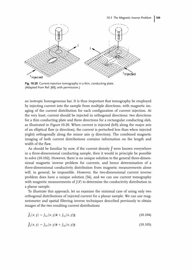
10.3 The Magnetic Inverse Problem
an isotropic homogeneous bar. It is thus important that tomography be employedby injecting current into the sample from multiple directions, with magnetic im-aging of the current distribution for each configuration of current injection. Atthe very least, current should be injected in orthogonal directions: two directionsfor a thin conducting plate and three directions for a rectangular conducting slab,as illustrated in Figure 10.20. When current is injected (left) along the major axisof an elliptical flaw (x direction), the current is perturbed less than when injected(right) orthogonally along the minor axis (y direction). The combined magneticimaging of both current distributions contains information on the length andwidth of the flaw.As should be familiar by now, if the current density~JJ were known everywhere
in a three-dimensional conducting sample, then it would in principle be possibleto solve (10.102). However, there is no unique solution to the general three-dimen-sional magnetic inverse problem for currents, and hence determination of athree-dimensional conductivity distribution from magnetic measurements alonewill, in general, be impossible. However, the two-dimensional current inverseproblem does have a unique solution [56], and we can use current tomographywith magnetic measurements of J ~rrð Þ to determine the conductivity distribution ina planar sample.To illustrate this approach, let us examine the minimal case of using only two
orthogonal distributions of injected current for a planar sample. We can use mag-netometer and spatial filtering inverse techniques described previously to obtainimages of the two resulting current distributions
~JJ1 x; yð Þ ¼ J1x x; yð Þxx þ J1y x; yð Þyy; (10:104)
~JJ2 x; yð Þ ¼ J2x x; yð Þxx þ J2y x; yð Þyy: (10:105)
189
Fig. 10.20 Current-injection tomography in a thin, conducting plate.(Adapted from Ref. [60], with permission.)
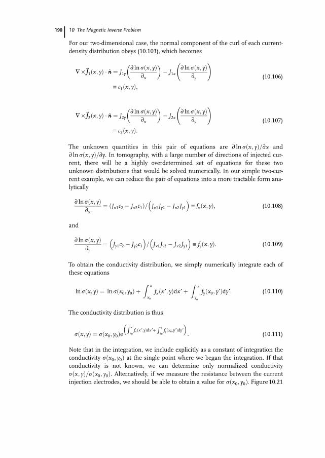
10 The Magnetic Inverse Problem
For our two-dimensional case, the normal component of the curl of each current-density distribution obeys (10.103), which becomes
� ·~JJ1 x; yð Þ � nn ¼ J1y¶ ln r x; yð Þ
¶x
� �� J1x
¶ lnr x; yð Þ¶y
!
” c1 x; yð Þ;(10:106)
� ·~JJ2 x; yð Þ � nn ¼ J2y¶ ln r x; yð Þ
¶x
� �� J2x
¶ lnr x; yð Þ¶y
!
” c2 x; yð Þ:(10:107)
The unknown quantities in this pair of equations are ¶ ln rðx; yÞ=¶x and¶ ln rðx; yÞ=¶y. In tomography, with a large number of directions of injected cur-rent, there will be a highly overdetermined set of equations for these twounknown distributions that would be solved numerically. In our simple two-cur-rent example, we can reduce the pair of equations into a more tractable form ana-lytically
¶ lnr x; yð Þ¶x
¼ Jx1c2 � Jx2c1ð Þ= Jx1Jy2 � Jx2Jy1
� �” fx x; yð Þ; (10:108)
and
¶ lnr x; yð Þ¶y
¼ Jy1c2 � Jy2c1� �
= Jx1Jy2 � Jx2Jy1
� �” fy x; yð Þ: (10:109)
To obtain the conductivity distribution, we simply numerically integrate each ofthese equations
ln r x; yð Þ ¼ ln r x0; y0ð Þ þZ x
x0
fx x ¢; yð Þdx ¢þZ y
y0
fy x0; y¢ð Þdy¢: (10:110)
The conductivity distribution is thus
r x; yð Þ ¼ r x0; y0ð ÞeR x
x0fx x ¢;yð Þdx ¢þ
R y
y0fy x0;y ¢ð Þdy ¢
� �: (10:111)
Note that in the integration, we include explicitly as a constant of integration theconductivity r x0; y0ð Þ at the single point where we began the integration. If thatconductivity is not known, we can determine only normalized conductivityr x; yð Þ=r x0; y0ð Þ. Alternatively, if we measure the resistance between the currentinjection electrodes, we should be able to obtain a value for r x0; y0ð Þ. Figure 10.21
190
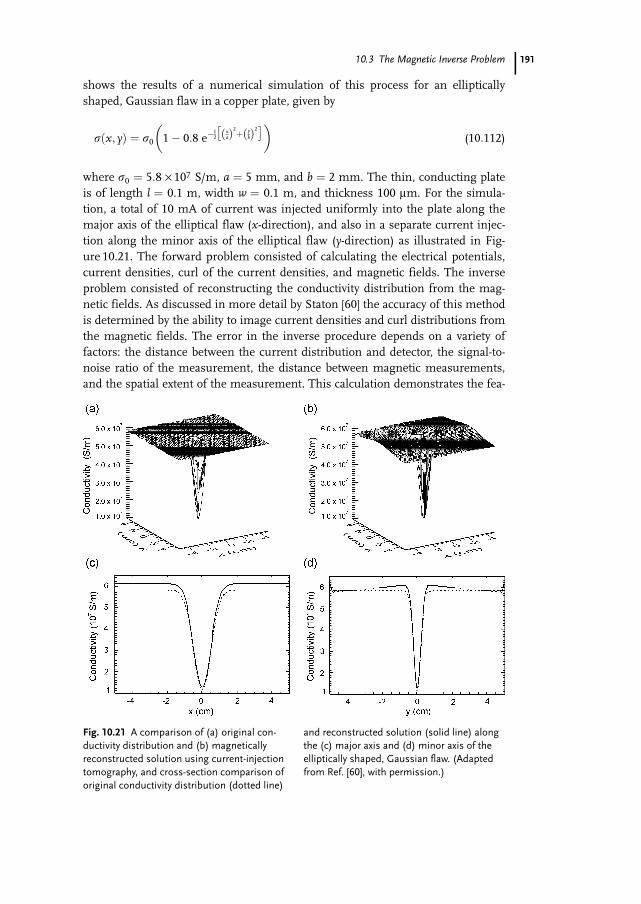
10.3 The Magnetic Inverse Problem
shows the results of a numerical simulation of this process for an ellipticallyshaped, Gaussian flaw in a copper plate, given by
r x; yð Þ ¼ r0 1� 0:8 e�12
xað Þ2þ y
bð Þ2� �� �
(10:112)
where r0 ¼ 5:8 · 107 S/m, a ¼ 5 mm, and b ¼ 2 mm. The thin, conducting plateis of length l ¼ 0.1 m, width w ¼ 0.1 m, and thickness 100 lm. For the simula-tion, a total of 10 mA of current was injected uniformly into the plate along themajor axis of the elliptical flaw (x-direction), and also in a separate current injec-tion along the minor axis of the elliptical flaw (y-direction) as illustrated in Fig-ure 10.21. The forward problem consisted of calculating the electrical potentials,current densities, curl of the current densities, and magnetic fields. The inverseproblem consisted of reconstructing the conductivity distribution from the mag-netic fields. As discussed in more detail by Staton [60] the accuracy of this methodis determined by the ability to image current densities and curl distributions fromthe magnetic fields. The error in the inverse procedure depends on a variety offactors: the distance between the current distribution and detector, the signal-to-noise ratio of the measurement, the distance between magnetic measurements,and the spatial extent of the measurement. This calculation demonstrates the fea-
191
Fig. 10.21 A comparison of (a) original con-ductivity distribution and (b) magneticallyreconstructed solution using current-injectiontomography, and cross-section comparison oforiginal conductivity distribution (dotted line)
and reconstructed solution (solid line) alongthe (c) major axis and (d) minor axis of theelliptically shaped, Gaussian flaw. (Adaptedfrom Ref. [60], with permission.)
10 The Magnetic Inverse Problem
sibility of the technique; further studies will require adding noise and varying thesampling parameters, and should also address the possible advantages of applyingcurrent to the sample from multiple directions (more than the minimally requirednumber of two or three).
The Hosaka-Cohen TransformationA “current pattern” in the xy-plane can be obtained from Bz by the Hosaka-Cohen(HC) transformation [80]
HC ӦBz
¶yxx � ¶Bz
¶xyy; (10:113)
where the field is measured a distance z above the currents. The components ofHC resemble the currents, i.e.,
Jx ¶Bz
¶y” HCx (10:114)
Jy ¶Bz
¶x” HCy: (10:115)
The HC transformation is believed valid for two-dimensional current distribu-tions, but has been applied to data from three-dimensional sources [80, 81]. Theuncertainty lies with the derivation of the HC transformation, which is basedupon the curl of ~BB. AmpMre’s law states that
~JJ ¼ 1l0
� ·~BB
¼ 1l0
¶Bz
¶y�¶By
¶z
� �xx � ¶Bz
¶x� ¶Bx
¶z
� �yyþ
¶By
¶x� ¶Bx
¶y
� �zz
& ':
(10:116)
Within a current distribution of infinite extent with no z-dependence,
¶By
¶z.
¶Bx
¶z. 0 . (10.117)
If we add the tighter constraint that Jz ¼ 0 everywhere, then
~JJ .1l0
¶Bz
¶yxx � ¶Bz
¶xyy
& ': (10:118)
Within a constant, this is the same as (10.113). However, this equation, as derived,applies only within the conductor, since outside a conductor both~JJ and � ·~BB areeverywhere zero in the quasistatic limit. In practice, one cannot readily measure ~BBinside a conductor. However, the symmetry for a two-dimensional planar currentdistribution is the same as for a three-dimensional current distribution with no Jz
192
10.3 The Magnetic Inverse Problem
and no z-dependence of either Jx or Jy. The validity of the HC transformation isunclear when it is possible only to measure ~BB at height z above the xy-plane.We can shed some light on the meaning of the HC transformation by using
Fourier spatial filtering [78]. In the spatial-frequency domain, we had the exactinverse solution for two-dimensional current distributions
jx kx; ky
� �¼ i
2l0d
kyffiffiffiffiffiffiffiffiffiffiffiffiffiffiffik2x þ k2y
q ezffiffiffiffiffiffiffik2xþk2y
pbz kx; ky
� �(10:119)
jy kx; ky
� �¼ �i
2l0d
kxffiffiffiffiffiffiffiffiffiffiffiffiffiffiffik2x þ k2y
q ezffiffiffiffiffiffiffik2xþk2y
pbz kx; ky
� �: (10:120)
This can be expanded in a Taylor series
jx kx; ky
� �¼ i
2l0d
kybz kx; ky
� �k
1þ kzþ 12!
k2z2 þ :::
� �; (10:121)
where
k ¼ffiffiffiffiffiffiffiffiffiffiffiffiffiffiffik2x þ k2y
q: (10:122)
If k and z are sufficiently small, then
jx kx; ky
� �. i
2l0d
kybz kx; ky
� �f ; (10:123)
where
f ¼ 1=kþ zþ kz2=2: (10:124)
Similarly,
jy kx; ky
� �. � i
2l0d
� �kxbz kx; ky
� �f : (10:125)
For comparison, the two-dimensional Fourier transform of HC is
jx kx; ky
� � ikybz kx; ky
� �(10:126)
jy kx; ky
� � � ikxbz kx; ky
� �: (10:127)
By fitting a straight line to the exact expression, we obtain [78]
193
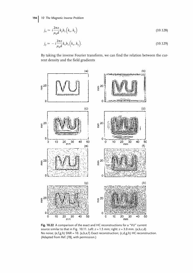
10 The Magnetic Inverse Problem
jx . i2pzl0d
kybz kx; ky
� �(10:128)
jy . � i2pzl0d
kxbz kx; ky
� �: (10:129)
By taking the inverse Fourier transform, we can find the relation between the cur-rent density and the field gradients
194
Fig. 10.22 A comparison of the exact and HC reconstructions for a “VU” currentsource similar to that in Fig. 10.11. Left: z = 1.5 mm; right: z = 3.0 mm. (a,b,c,d)No noise; (e,f,g,h) SNR = 10. (a,b,e,f) Exact reconstruction; (c,d,g,h) HC reconstruction.(Adapted from Ref. [78], with permission.)
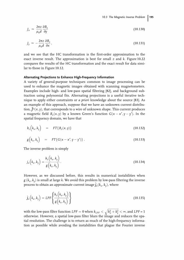
10.3 The Magnetic Inverse Problem
Jx .2pzl0d
¶Bz
¶y(10:130)
Jy . � 2pzl0d
¶Bz
¶x; (10:131)
and we see that the HC transformation is the first-order approximation to theexact inverse result. The approximation is best for small z and k. Figure 10.22compares the results of the HC transformation and the exact result for data simi-lar to those in Figure 10.12.
Alternating Projections to Enhance High-Frequency InformationA variety of general-purpose techniques common to image processing can beused to enhance the magnetic images obtained with scanning magnetometers.Examples include high- and low-pass spatial filtering [82], and background sub-traction using polynomial fits. Alternating projections is a useful iterative tech-nique to apply either constraints or a priori knowledge about the source [83]. Asan example of this approach, suppose that we have an unknown current distribu-tion,~JJu x; yð Þ, that corresponds to a wire of unknown shape. This current producesa magnetic field Bz x; yð Þ by a known Green’s function G x � x ¢; y� y¢ð Þ. In thespatial frequency domain, we have that
bz kx; ky
� �¼ FT Bz x; yð Þf g (10:132)
g kx; ky
� �¼ FT G x � x ¢; y� y¢ð Þf g . (10.133)
The inverse problem is simply
jx kx; ky
� �¼
bz kx; ky
� �g kx; ky
� � : (10:134)
However, as we discussed before, this results in numerical instabilities wheng ðkx; kyÞ is small at large k. We avoid this problem by low-pass filtering the inverseprocess to obtain an approximate current image jjxðkx; kyÞ, where
jjx kx; ky
� �¼ LPF
bz kx; ky
� �g kx; ky
� �8<:
9=; (10:135)
with the low-pass filter function LPF ¼ 0 when kLPF <ffiffiffiffiffiffiffiffiffiffiffiffiffiffiffik2x þ k2y
q< ¥, and LPF = 1
otherwise. However, a spatial low-pass filter blurs the image and reduces the spa-tial resolution. The challenge is to return as much of the high-frequency informa-tion as possible while avoiding the instabilities that plague the Fourier inverse
195
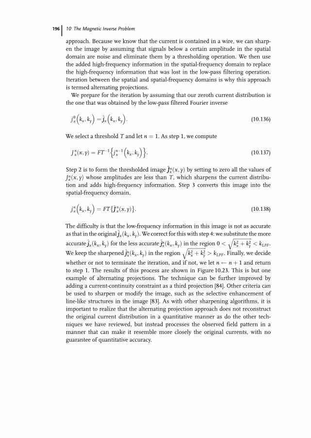
10 The Magnetic Inverse Problem
approach. Because we know that the current is contained in a wire, we can sharp-en the image by assuming that signals below a certain amplitude in the spatialdomain are noise and eliminate them by a thresholding operation. We then usethe added high-frequency information in the spatial-frequency domain to replacethe high-frequency information that was lost in the low-pass filtering operation.Iteration between the spatial and spatial-frequency domains is why this approachis termed alternating projections.We prepare for the iteration by assuming that our zeroth current distribution is
the one that was obtained by the low-pass filtered Fourier inverse
j0x kx; ky
� �¼ jjx kx; ky
� �: (10:136)
We select a threshold T and let n ¼ 1. As step 1, we compute
J nx x; yð Þ ¼ FT�1 j n�1
x kx; ky
� �n o: (10:137)
Step 2 is to form the thresholded image ~JJnx x; yð Þ by setting to zero all the values of
Jnx x; yð Þ whose amplitudes are less than T , which sharpens the current distribu-tion and adds high-frequency information. Step 3 converts this image into thespatial-frequency domain,
j nx kx; ky
� �¼ FT ~JJ n
x x; yð Þ+ ,
: (10:138)
The difficulty is that the low-frequency information in this image is not as accurateas that in the original jjxðkx; kyÞ. We correct for this with step 4: we substitute themore
accurate jjxðkx; kyÞ for the less accurate jjnxðkx; kyÞ in the region 0 <ffiffiffiffiffiffiffiffiffiffiffiffiffiffiffik2x þ k2y
q< kLPF.
We keep the sharpened jjnxðkx; kyÞ in the regionffiffiffiffiffiffiffiffiffiffiffiffiffiffiffik2x þ k2y
q> kLPF. Finally, we decide
whether or not to terminate the iteration, and if not, we let n nþ 1 and returnto step 1. The results of this process are shown in Figure 10.23. This is but oneexample of alternating projections. The technique can be further improved byadding a current-continuity constraint as a third projection [84]. Other criteria canbe used to sharpen or modify the image, such as the selective enhancement ofline-like structures in the image [83]. As with other sharpening algorithms, it isimportant to realize that the alternating projection approach does not reconstructthe original current distribution in a quantitative manner as do the other tech-niques we have reviewed, but instead processes the observed field pattern in amanner that can make it resemble more closely the original currents, with noguarantee of quantitative accuracy.
196
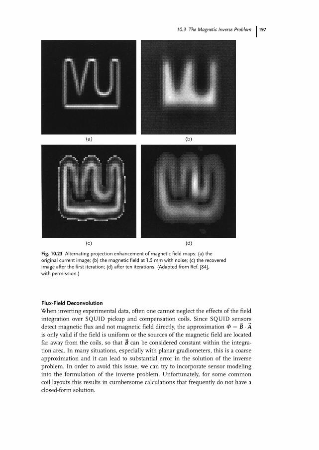
10.3 The Magnetic Inverse Problem
Flux-Field DeconvolutionWhen inverting experimental data, often one cannot neglect the effects of the fieldintegration over SQUID pickup and compensation coils. Since SQUID sensorsdetect magnetic flux and not magnetic field directly, the approximation U ¼ ~BB �~AAis only valid if the field is uniform or the sources of the magnetic field are locatedfar away from the coils, so that ~BB can be considered constant within the integra-tion area. In many situations, especially with planar gradiometers, this is a coarseapproximation and it can lead to substantial error in the solution of the inverseproblem. In order to avoid this issue, we can try to incorporate sensor modelinginto the formulation of the inverse problem. Unfortunately, for some commoncoil layouts this results in cumbersome calculations that frequently do not have aclosed-form solution.
197
Fig. 10.23 Alternating projection enhancement of magnetic field maps: (a) theoriginal current image; (b) the magnetic field at 1.5 mm with noise; (c) the recoveredimage after the first iteration; (d) after ten iterations. (Adapted from Ref. [84],with permission.)
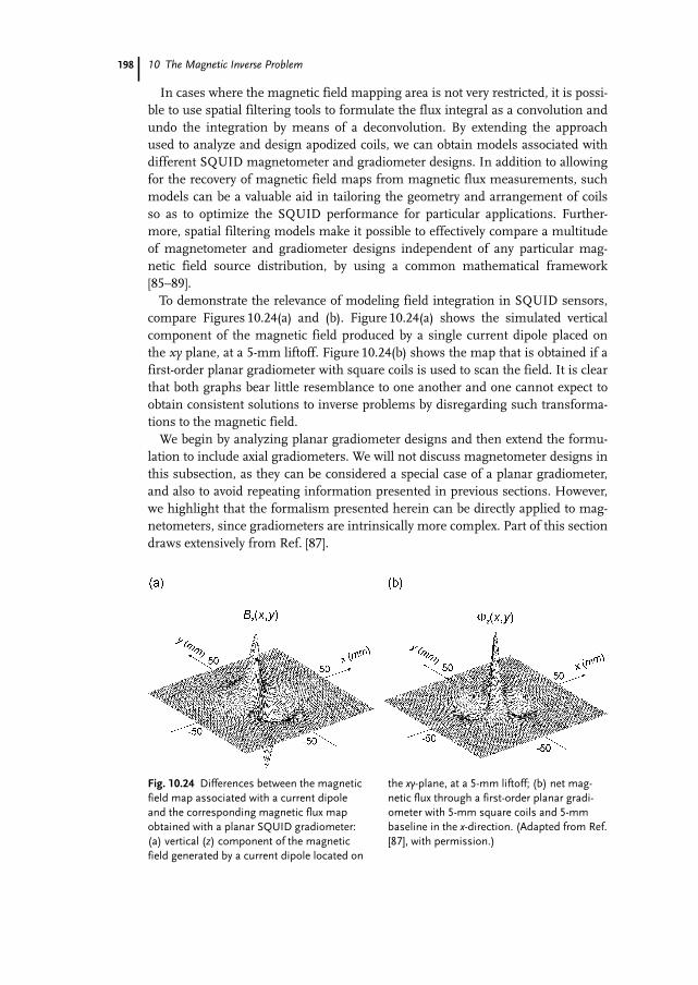
10 The Magnetic Inverse Problem
In cases where the magnetic field mapping area is not very restricted, it is possi-ble to use spatial filtering tools to formulate the flux integral as a convolution andundo the integration by means of a deconvolution. By extending the approachused to analyze and design apodized coils, we can obtain models associated withdifferent SQUID magnetometer and gradiometer designs. In addition to allowingfor the recovery of magnetic field maps from magnetic flux measurements, suchmodels can be a valuable aid in tailoring the geometry and arrangement of coilsso as to optimize the SQUID performance for particular applications. Further-more, spatial filtering models make it possible to effectively compare a multitudeof magnetometer and gradiometer designs independent of any particular mag-netic field source distribution, by using a common mathematical framework[85–89].To demonstrate the relevance of modeling field integration in SQUID sensors,
compare Figures 10.24(a) and (b). Figure 10.24(a) shows the simulated verticalcomponent of the magnetic field produced by a single current dipole placed onthe xy plane, at a 5-mm liftoff. Figure 10.24(b) shows the map that is obtained if afirst-order planar gradiometer with square coils is used to scan the field. It is clearthat both graphs bear little resemblance to one another and one cannot expect toobtain consistent solutions to inverse problems by disregarding such transforma-tions to the magnetic field.We begin by analyzing planar gradiometer designs and then extend the formu-
lation to include axial gradiometers. We will not discuss magnetometer designs inthis subsection, as they can be considered a special case of a planar gradiometer,and also to avoid repeating information presented in previous sections. However,we highlight that the formalism presented herein can be directly applied to mag-netometers, since gradiometers are intrinsically more complex. Part of this sectiondraws extensively from Ref. [87].
198
Fig. 10.24 Differences between the magneticfield map associated with a current dipoleand the corresponding magnetic flux mapobtained with a planar SQUID gradiometer:(a) vertical (z) component of the magneticfield generated by a current dipole located on
the xy-plane, at a 5-mm liftoff; (b) net mag-netic flux through a first-order planar gradi-ometer with 5-mm square coils and 5-mmbaseline in the x-direction. (Adapted from Ref.[87], with permission.)
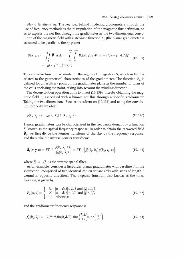
10.3 The Magnetic Inverse Problem
Planar Gradiometers. The key idea behind modeling gradiometers through theuse of frequency methods is the manipulation of the magnetic flux definition, soas to express the net flux through the gradiometer as the two-dimensional convo-lution of the magnetic field with a stepwise function FG (the planar gradiometer isassumed to be parallel to the xy-plane)
Uðx; y; zÞ ¼ZZ
S
~BB � nn da ¼Zþ¥�¥
Zþ¥�¥
Bzðx ¢; y¢; zÞFGðx � x ¢; y� y¢Þ dx ¢dy¢
¼ FGðx; yÞ*Bzðx; y; zÞ:
(10:139)
This stepwise function accounts for the region of integration S, which in turn isrelated to the geometrical characteristics of the gradiometer. The function FG isdefined for an arbitrary point on the gradiometer plane as the number of turns ofthe coils enclosing the point, taking into account the winding direction.The deconvolution operation aims to invert (10.139), thereby obtaining the mag-
netic field Bz associated with a known net flux through a specific gradiometer.Taking the two-dimensional Fourier transform on (10.139) and using the convolu-tion property, we obtain
uðkx; ky; zÞ ¼ fGðkx; kyÞ bzðkx; ky; zÞ. (10.140)
Hence, gradiometers can be characterized in the frequency domain by a functionfG known as the spatial frequency response. In order to obtain the recovered field~BBz, we first divide the Fourier transform of the flux by the frequency response,and then take the inverse Fourier transform:
~BBzðx; y; zÞ ¼ FT�1uðkx; ky; zÞfGðkx; kyÞ
" #¼ FT�1 f IGðkx; kyÞuðkx; ky; zÞ
h i; (10:141)
where f IG ¼ 1=fG is the inverse spatial filter.As an example, consider a first-order planar gradiometer with baseline d in the
x-direction, comprised of two identical N-turn square coils with sides of length Lwound in opposite directions. The stepwise function, also known as the turnsfunction, is given by
FGðx; yÞ ¼N; x � d=2j j £ L=2 and yj j £ L=2�N; x þ d=2j j £ L=2 and yj j £ L=20; otherwise;
8<: (10:142)
and the gradiometer frequency response is
fGðkx; kyÞ ¼ �2iL2 N sin kxd=2ð Þ sinc kxL2p
� �sinc
kyL
2p
� �; (10:143)
199
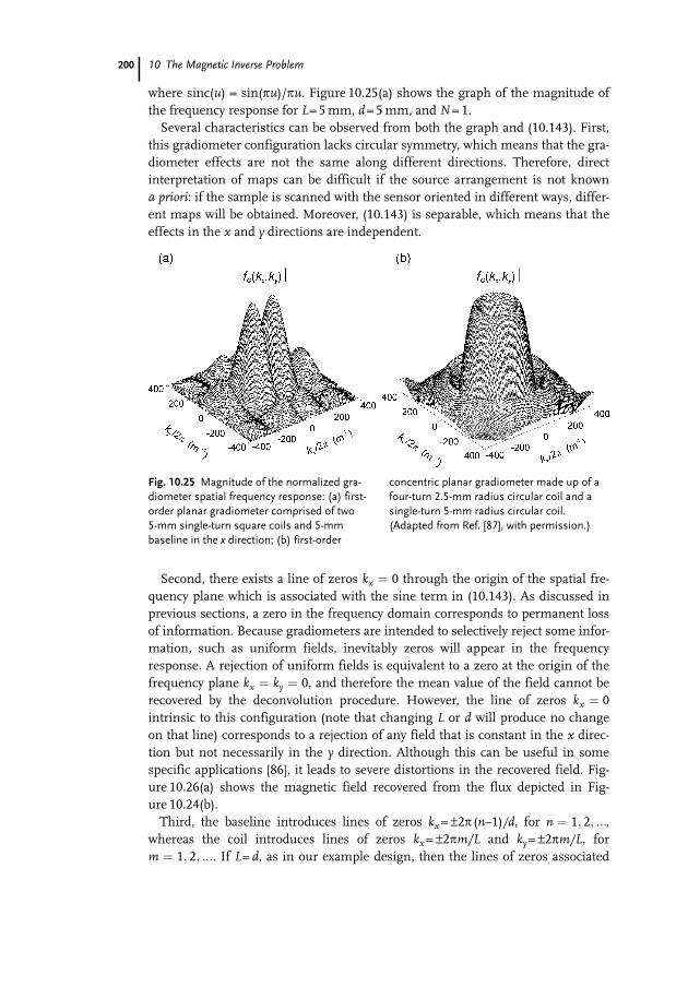
10 The Magnetic Inverse Problem
where sinc(u) = sin(pu)/pu. Figure 10.25(a) shows the graph of the magnitude ofthe frequency response for L= 5mm, d= 5mm, and N= 1.Several characteristics can be observed from both the graph and (10.143). First,
this gradiometer configuration lacks circular symmetry, which means that the gra-diometer effects are not the same along different directions. Therefore, directinterpretation of maps can be difficult if the source arrangement is not knowna priori: if the sample is scanned with the sensor oriented in different ways, differ-ent maps will be obtained. Moreover, (10.143) is separable, which means that theeffects in the x and y directions are independent.
Second, there exists a line of zeros kx ¼ 0 through the origin of the spatial fre-quency plane which is associated with the sine term in (10.143). As discussed inprevious sections, a zero in the frequency domain corresponds to permanent lossof information. Because gradiometers are intended to selectively reject some infor-mation, such as uniform fields, inevitably zeros will appear in the frequencyresponse. A rejection of uniform fields is equivalent to a zero at the origin of thefrequency plane kx ¼ ky ¼ 0, and therefore the mean value of the field cannot berecovered by the deconvolution procedure. However, the line of zeros kx ¼ 0intrinsic to this configuration (note that changing L or d will produce no changeon that line) corresponds to a rejection of any field that is constant in the x direc-tion but not necessarily in the y direction. Although this can be useful in somespecific applications [86], it leads to severe distortions in the recovered field. Fig-ure 10.26(a) shows the magnetic field recovered from the flux depicted in Fig-ure 10.24(b).Third, the baseline introduces lines of zeros kx= –2p (n–1)/d, for n ¼ 1; 2; :::,
whereas the coil introduces lines of zeros kx= –2pm/L and ky= –2pm/L, form ¼ 1; 2; :::. If L= d, as in our example design, then the lines of zeros associated
200
Fig. 10.25 Magnitude of the normalized gra-diometer spatial frequency response: (a) first-order planar gradiometer comprised of two5-mm single-turn square coils and 5-mmbaseline in the x direction; (b) first-order
concentric planar gradiometer made up of afour-turn 2.5-mm radius circular coil and asingle-turn 5-mm radius circular coil.(Adapted from Ref. [87], with permission.)
10.3 The Magnetic Inverse Problem
with the baseline (for n ‡ 2) coincide with the lines of zeros in the same directionwhich are related to the coil geometry. If the source distribution generates a mag-netic field with information at higher spatial frequencies, reaching those otherlines of zeros, then additional information is lost and more distortion is intro-duced in the recovered field. Figure 10.26(b) shows the recovered field obtainedfrom the same flux map, but with a gradiometer with L = d = 10 mm. (Note thatincreasing L or d results in moving the lines of zeros closer to the origin.)It is worthwhile observing that other configurations of planar gradiometers
have better spatial frequency characteristics and do not suffer from some of thepathologies described above. For instance, Figure 10.26(c) shows the recoveredfield obtained using a concentric planar design with circular coils (four-turn 5-mmradius coil surrounded by a single-turn 10-mm coil). It can be seen that an excel-lent recovery of the magnetic field could be obtained in this case. For this config-uration, we have
201
Fig. 10.26 Magnetic field maps recovered bythe flux-field deconvolution for different gradi-ometer designs: (a) first-order gradiometercomprised of 5-mm single-turn square coilsand 5-mm baseline in the x direction;(b) same as (a) except for 10-mm coils and
10-mm baseline; (c) first-order concentricplanar gradiometer made up of a four-turn2.5-mm radius circular coil and a single-turn5-mm radius circular coil. (Adapted from Ref.[87], with permission.)
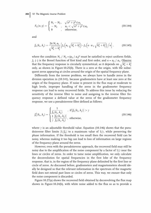
10 The Magnetic Inverse Problem
FGðx; yÞ ¼N1 � N2 ;
ffiffiffiffiffiffiffiffiffiffiffiffiffiffiffix2 þ y2
p£ a1
� N2 ; a1 <ffiffiffiffiffiffiffiffiffiffiffiffiffiffiffix2 þ y2
p£ a2
0 ; otherwise;
8<: (10:144)
and
fGðkx; kyÞ ¼2pN1 a1ffiffiffiffiffiffiffiffiffiffiffiffiffiffiffi
k2x þ k2yq J1 a1
ffiffiffiffiffiffiffiffiffiffiffiffiffiffiffik2x þ k2y
q� ��
hJ1 a � a 1
ffiffiffiffiffiffiffiffiffiffiffiffiffiffiffik2x þ k2y
q� �.ai; (10:145)
where the condition N1 / N2 = (a2 / a1)2 must be satisfied to reject uniform fields,J1 (·) is the Bessel function of first kind and first order, and a = a2 / a1. Observethat the frequency response is circularly symmetrical, as it depends on
ffiffiffiffiffiffiffiffiffiffiffiffiffiffiffik2x þ k2y
qonly, as shown in Figure 10.25(b). There is a zero at the origin, with the subse-quent zeros appearing at circles around the origin of the spatial frequency plane.Differently from the inverse problem, we always have to handle zeros in the
division operation in (10.141), because gradiometers have at least one zero at theorigin of the frequency plane. If noise is present in the flux map at moderate tohigh levels, improper handling of the zeros in the gradiometer frequencyresponse can lead to noisy recovered fields. To address this issue by reducing thesensitivity of the inverse filter to noise and assigning to the inverse filter fre-quency response a defined value at the zeros of the gradiometer frequencyresponse, we use a pseudoinverse filter defined as follows:
f IGðkx; kyÞ ¼
1fGðkx; kyÞ
; if fGðkx; kyÞ�� �� > c
1c
fGðkx; kyÞ�� ��fGðkx; kyÞ
; otherwise;
8>>><>>>:
(10:146)
where c is an adjustable threshold value. Equation (10.146) shows that the pseu-doinverse filter limits 1=fGj j to a maximum value of 1/c, while preserving thephase information. If the threshold is too small then the recovered field can benoisy, whereas making it too big can lead to loss of information on large regionsof the frequency plane around the zeros.However, even with the pseudoinverse approach, the recovered field may still be
noisy due to the amplification of the noise component by a factor of 1/c near thelines or circles of zeros. In order to tame noise amplification, we only calculatethe deconvolution for spatial frequencies in the first lobe of the frequencyresponse, that is, in the region of the frequency plane delimited by the first line orcircle of zeros. As discussed before, gradiometers and magnetometers should ide-ally be designed so that the relevant information in the spectrum of the magneticfield does not extend past lines or circles of zeros. This way, we ensure that onlythe noise component is discarded.Figure 10.27(a) shows the recovered field obtained by deconvolving the flux map
shown in Figure 10.24(b), with white noise added to the flux so as to provide a
202
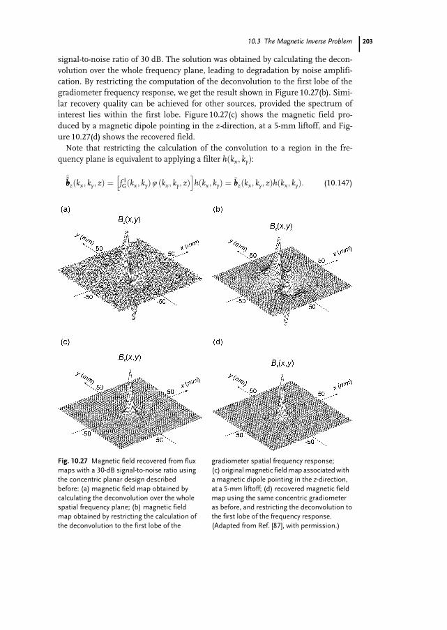
10.3 The Magnetic Inverse Problem
signal-to-noise ratio of 30 dB. The solution was obtained by calculating the decon-volution over the whole frequency plane, leading to degradation by noise amplifi-cation. By restricting the computation of the deconvolution to the first lobe of thegradiometer frequency response, we get the result shown in Figure 10.27(b). Simi-lar recovery quality can be achieved for other sources, provided the spectrum ofinterest lies within the first lobe. Figure 10.27(c) shows the magnetic field pro-duced by a magnetic dipole pointing in the z-direction, at a 5-mm liftoff, and Fig-ure 10.27(d) shows the recovered field.Note that restricting the calculation of the convolution to a region in the fre-
quency plane is equivalent to applying a filter hðkx; kyÞ:
~~bb~bbzðkx; ky; zÞ ¼ f IGðkx; kyÞu ðkx; ky; zÞh i
hðkx; kyÞ ¼ ~bbzðkx; ky; zÞhðkx; kyÞ: (10:147)
203
Fig. 10.27 Magnetic field recovered from fluxmaps with a 30-dB signal-to-noise ratio usingthe concentric planar design describedbefore: (a) magnetic field map obtained bycalculating the deconvolution over the wholespatial frequency plane; (b) magnetic fieldmap obtained by restricting the calculation ofthe deconvolution to the first lobe of the
gradiometer spatial frequency response;(c) originalmagnetic fieldmap associatedwithamagnetic dipole pointing in the z-direction,at a 5-mm liftoff; (d) recovered magnetic fieldmap using the same concentric gradiometeras before, and restricting the deconvolution tothe first lobe of the frequency response.(Adapted from Ref. [87], with permission.)
10 The Magnetic Inverse Problem
In the simplest case, h is a two-dimensional rectangular window: hðkx; kyÞ ¼ 1within the first lobe and hðkx; kyÞ ¼ 0 everywhere else. In the space domain, thisis equivalent to convolving the recovered field ~BBzðx; y; zÞ with the inverse Fouriertransform of hðkx; kyÞ, yielding ~~BB~BBzðx; y; zÞ. Depending on how narrow this windowis, perceptible ringing can be introduced in ~~BB~BBzðx; y; zÞ, as a consequence of convol-ving with sinc or jinc8) functions associated with the impulse response of ideallow-pass filters. Choosing other window types with smaller sidelobes or two-dimensional nonrecursive filters may considerably improve the quality of therecovered field.
Axial Gradiometers. In order to extend the modeling to include axial gradi-ometers, we first realize that the baseline effect is now decoupled from the fieldintegration. Therefore, it is necessary to increase the dimension of the model. Letus suppose a generic axial gradiometer made up of N identically shaped coils withnegligible thickness along the z-direction. The net flux in the gradiometer canthen be expressed as
Uðx; y; zÞ ¼Zþ¥�¥
Zþ¥�¥
Zþ¥�¥
Bzðx ¢; y¢; z¢ÞFGðx � x ¢; y� y¢; z� z¢Þdx ¢dy¢dz¢; (10:148)
where
FGðx; y; zÞ ¼ FFðx; yÞXN�1j¼0
nj dðz� djÞ: (10:149)
The stepwise function FFðx; yÞ is related to a normalized (single-turn) coil, whilethe number of turns and winding direction of each coil is given by nj. Assumingthe origin of the coordinate system at the center of the bottommost (pickup) coil,we have d0 = 0 and each dj is the distance of the jth coil to the pickup coil. Notethat the delta function represents that the coils have no thickness, and thereforeare “concentrated” at discrete values of z.Taking the three-dimensional Fourier transform on (10.149), we obtain
fGðkx; ky; kzÞ ¼ ff ðkx; kyÞXN�1j¼0
nje�ikzdj
!¼ f1ðkx; kyÞ f2ðkzÞ; (10:150)
which is the general expression for the spatial frequency response of an axial gra-diometer. Even though fG is separable, it is also a function of three variables, andtherefore a graphic visualization is difficult to attain. However, if the coils are cir-cular, (10.150) can be further simplified, since it becomes a function of just twospatial variables kr ¼
ffiffiffiffiffiffiffiffiffiffiffiffiffiffiffik2x þ k2y
qand kz.
204
8) jincðxÞ ¼ J1ðxÞ=x.
10.3 The Magnetic Inverse Problem
As an example, consider an ordinary second-order axial gradiometer design,comprised of three circular coils of radius a, with N, 2N, and N turns, separatedby a baseline d. In this case, the gradiometer frequency response is given by
fGðkr; kzÞ ¼ ff ðkrÞN 1� 2e�ikzd þ e�i2kzd� �
¼ 4paNJ1ðakrÞ
kre�ikz cosðkzdÞ � 1½ �: (10:151)
Should we wish to take the coil thickness into account, (10.150) can still be used,provided that we model a multi-turn coil as a stack of single-turn coils. In thisway, j now sequentially indexes the turns of the coils and dj stands for the distancebetween the (cumulative) jth turn and the first turn of the pickup coil. We observethat only f2 is affected by this change.It should be highlighted that (10.148) and (10.149) can also be used to model
planar gradiometers, providing a way to compare the frequency responses ofaxial and planar configurations. By having N = 1 and d0 = 0 in (10.150), and havingff ðkx; kyÞ represent the two-dimensional planar gradiometer frequency response,we obtain the simple equation
fGðkx; ky; kzÞ ¼ ff ðkx; kyÞ: (10:152)
This equation expresses that the three-dimensional gradiometer frequencyresponse is independent of kz. Thus, the gradiometer behaves as an all-pass filterin the z-direction.The deconvolution of (10.148) is much more complex than the two-dimensional
case. In principle, a two-dimensional map is not enough to invert the equationand the flux must be known in a volume. This poses some serious experimentalproblems, as it requires mapping the field at several liftoffs and then interpolatingthe scans in order to generate a uniform three-dimensional grid of data. However,for deconvolution purposes an alternative approach is possible. Although it is notsuitable to analyze the spatial frequency characteristics of gradiometers, it enablesus to perform a two-dimensional deconvolution of a single flux map obtainedwith an axial gradiometer.Let Uðx; y; z0Þ denote the net magnetic flux through the generic axial gradi-
ometer described above, whose pickup coil is placed at a fixed height z0:
Uðx; y; z0Þ ¼XN�1j¼0
nj
Z¥�¥
Z¥�¥
Bzðx ¢; y¢; z0 þ djÞFFðx � x ¢; y� y¢Þ dx ¢dy¢: (10:153)
We can take the Fourier transform to obtain
uðkx; ky; z0Þ ¼XN�1j¼0
njbzðkx; ky; z0 þ djÞff ðkx; kyÞ: (10:154)
205
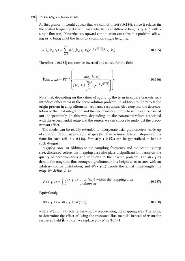
10 The Magnetic Inverse Problem
At first glance, it would appear that we cannot invert (10.154), since it relates (inthe spatial frequency domain) magnetic fields at different heights z0 þ dj with asingle flux at z0. Nevertheless, upward continuation can solve this problem, allow-ing us to bring all of the fields to a common single height z0:
uðkx; ky; z0Þ ¼XN�1j¼0
njbzðkx; ky; z0Þe�dj
ffiffiffiffiffiffiffiffiffik2xþk2yp
ff ðkx; kyÞ: (10:155)
Therefore, (10.155) can now be inverted and solved for the field
~BBzðx; y; z0Þ ¼ FT�1uðkx; ky; z0Þ
ff ðkx; kyÞPN�1j¼0
nje�dj
ffiffiffiffiffiffiffiffiffik2xþk2yp" #
8>>>><>>>>:
9>>>>=>>>>;: (10:156)
Note that, depending on the values of nj and dj, the term in square brackets mayintroduce other zeros in the deconvolution problem, in addition to the zero at theorigin present in all gradiometer frequency responses. Also note that the deconvo-lution of the field integration and the deconvolution of the baseline can be carriedout independently. In this way, depending on the parameter values associatedwith the experimental setup and the sensor, we can choose to undo just the predo-minant effect.The model can be readily extended to incorporate axial gradiometers made up
of coils of different sizes and/or shapes [68] if we assume different stepwise func-tions for each coil in (10.148). Similarly, (10.153) can be generalized to handlesuch designs.
Mapping Area. In addition to the sampling frequency and the scanning stepsize, discussed before, the mapping area also plays a significant influence on thequality of deconvolutions and solutions to the inverse problem. Let Uðx; y; zÞdenote the magnetic flux through a gradiometer at a height z, associated with anarbitrary source distribution, and U¢ðx; y; zÞ denote the actual finite-length fluxmap. We define U¢ as
U¢ðx; y; zÞ ¼ Uðx; y; zÞ ; for ðx; yÞ within the mapping area0 ; otherwise:
&(10:157)
Equivalently,
U¢ðx; y; zÞ ¼ Uðx; y; zÞWðx; yÞ, (10.158)
where Wðx; yÞ is a rectangular window representing the mapping area. Therefore,to determine the effect of using the truncated flux map U¢ instead of U on therecovered field ~~BB~BBzðx; y; zÞ, we replace u by u¢ in (10.141):
206
10.3 The Magnetic Inverse Problem
~~BB~BBzðx; y; zÞ ¼ FT�1 f IGðkx; kyÞu¢ðkx; ky; zÞh i
¼ FT�1 f IGðkx; kyÞ uðkx; ky; zÞ � wðkx; kyÞ� �h i
;(10:159)
where � represents a convolution performed in the frequency domain. If themapping area is large enough to ensure that U¢ðx; y; zÞ » Uðx; y; zÞ then the con-volution with the product of sinc functions, which is associated with a two-dimen-sional rectangular window, can be neglected. Otherwise, significant distortionmay be introduced in the recovered field, as it creates edges in the flux map andoscillations in the spectrum due to the sincs. An artifice that can be used todecrease this sort of distortion consists of generating a larger map by appendingflipped/mirrored versions of the original map at its edges. Additional nonrectan-gular windows may then be applied to the enlarged map so as to taper the edges,thereby decreasing ringing in the recovered map.A final remark is in order regarding computer implementation of deconvolu-
tion algorithms: when using FFT algorithms, one should be careful to sample (inthe frequency domain) the continuous transforms, such as (10.143) and (10.145),the same way the FFT does. Otherwise, symmetries in the spectrum are brokenand the recovered field contains a large complex component, besides being inac-curate.
Other Applications of Spatial FilteringAs can be seen from the breadth of applications we have just outlined, spatial fil-tering is a powerful approach. There are further applications of the technique rele-vant to magnetic imaging, including the interpretation of gradiometers as one-dimensional spatial filters, neglecting area effects [90–93], and the use of filters todetermine multipole moments from measurement of the normal component ofthe field above the surface of a sphere or plane [94]. As a final remark, severalimprovements have been made to the inverse filtering method, notably for appli-cations in magnetooptical imaging. In particular, Jooss and co-workers [95]extended the method to handle samples with finite thickness, and correctionshave been introduced for the in-plane field effect [96]. In addition, there have beendetailed studies of the influence of noise on the spatial resolution of the inversefiltering method [97].
Summary of Findings for Spatial FilteringFrom this overview and the more detailed analyses of spatial filtering in the litera-ture, we find that the coil-to-source spacing limits spatial resolution, that coil di-ameter should equal coil-to-source spacing, that inverse spatial filtering is uniquein one and two dimensions, that inward continuation separates the problems ofuniqueness from those of instability, that noise limits stability, that apodizing canimprove spatial resolution and sensitivity, and that windowing to filter out noiseand improve stability compromises spatial resolution. The spatial filteringapproach is powerful and easy to implement with commercial software packages,
207
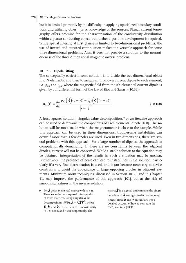
10 The Magnetic Inverse Problem
but it is limited primarily by the difficulty in applying specialized boundary condi-tions and utilizing other a priori knowledge of the sources. Planar current tomo-graphy offers promise for the characterization of the conductivity distributionwithin a planar conducting object, but further algorithm development is required.While spatial filtering at first glance is limited to two-dimensional problems, theuse of inward and outward continuation makes it a versatile approach for somethree-dimensional problems. Alas, it does not provide a solution to the nonuni-queness of the three-dimensional magnetic inverse problem.
10.3.2.3 Dipole FittingThe conceptually easiest inverse solution is to divide the two-dimensional objectinto N elements, and then to assign an unknown current dipole to each element,i.e., px;i and py;i, where the magnetic field from the ith elemental current dipole isgiven by our differential form of the law of Biot and Savart ((10.32))
Bz;i ~rrð Þ ¼l04p
px;i~r¢ir¢i� �
y� y¢ið Þ � py;i~r¢ir¢i� �
x � x ¢ið Þ
~rr � ~r¢ir¢i��� ���3 : (10:160)
A least-squares solution, singular-value decomposition,9) or an iterative approachcan be used to determine the components of each elemental dipole [100]. The so-lution will be most stable when the magnetometer is close to the sample. Whilethis approach can be used in three dimensions, troublesome instabilities canoccur if more than a few dipoles are used. Even in two dimensions, there are sev-eral problems with this approach. For a large number of dipoles, the approach iscomputationally demanding. If there are no constraints between the adjacentdipoles, current will not be conserved. While a stable solution to the equation maybe obtained, interpretation of the results in such a situation may be unclear.Furthermore, the presence of noise can lead to instabilities in the solution, partic-ularly if a very fine discretization is used, and it can become necessary to deviseconstraints to avoid the appearance of large opposing dipoles in adjacent ele-ments. Minimum norm techniques, discussed in Section 10.3.5 and in Chapter11, may improve the performance of this approach [101], but at the risk ofsmoothing features in the inverse solution.
208
9) Let ~~AA~AA be an m U n real matrix with m > n.Then ~~AA~AA can be decomposed into a productof three matrices, using singular-value
decomposition (SVD), ~~AA~AA ¼ ~~UU~UU ~~RR~RR~~VV~VVT, where
~~UU~UU, ~~RR~RR, and ~~VV~VV are matrices of dimensionalitym U n, n U n, and n U n, respectively. The
matrix ~~RR~RR is diagonal and contains the singu-
lar values of ~~AA~AA arranged in decreasing mag-
nitude. Both ~~UU~UU and ~~VV~VV are unitary. For adetailed account of how to compute theSVD, see Refs. [98,99].
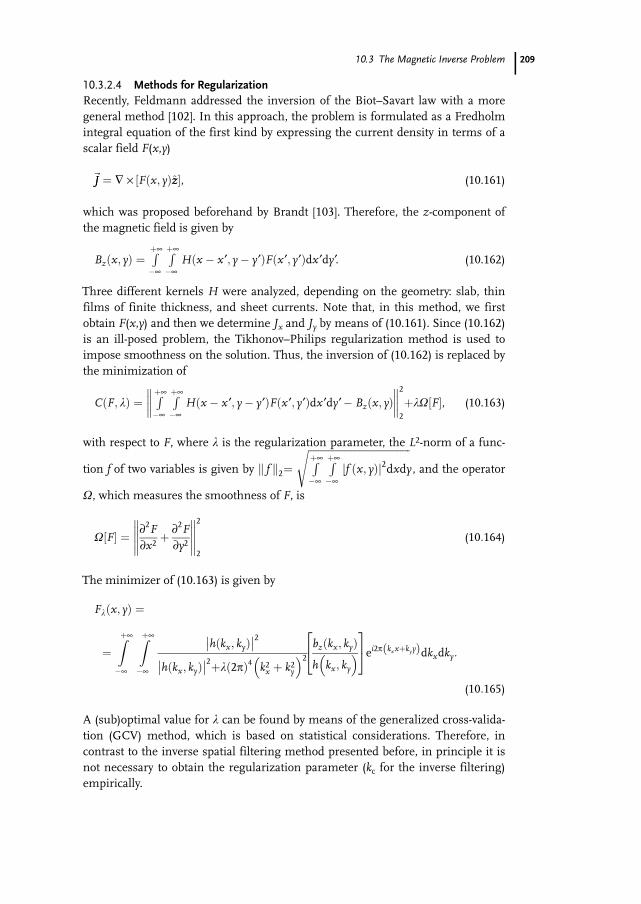
10.3 The Magnetic Inverse Problem
10.3.2.4 Methods for RegularizationRecently, Feldmann addressed the inversion of the Biot–Savart law with a moregeneral method [102]. In this approach, the problem is formulated as a Fredholmintegral equation of the first kind by expressing the current density in terms of ascalar field F(x,y)
~JJ ¼ � · Fðx; yÞzz½ �, (10.161)
which was proposed beforehand by Brandt [103]. Therefore, the z-component ofthe magnetic field is given by
Bzðx; yÞ ¼Rþ¥�¥
Rþ¥�¥
Hðx � x ¢; y� y¢ÞFðx ¢; y¢Þdx ¢dy¢. (10.162)
Three different kernels H were analyzed, depending on the geometry: slab, thinfilms of finite thickness, and sheet currents. Note that, in this method, we firstobtain F(x,y) and then we determine Jx and Jy by means of (10.161). Since (10.162)is an ill-posed problem, the Tikhonov–Philips regularization method is used toimpose smoothness on the solution. Thus, the inversion of (10.162) is replaced bythe minimization of
CðF; kÞ ¼Rþ¥�¥
Rþ¥�¥
Hðx � x ¢; y� y¢ÞFðx ¢; y¢Þdx ¢dy¢� Bzðx; yÞ////
////2
2
þkX F½ �, (10.163)
with respect to F, where k is the regularization parameter, the L2-norm of a func-
tion f of two variables is given by fk k2¼ffiffiffiffiffiffiffiffiffiffiffiffiffiffiffiffiffiffiffiffiffiffiffiffiffiffiffiffiffiffiffiffiffiffiffiffiffiffiffiffiRþ¥�¥
Rþ¥�¥
f ðx; yÞj j2dxdy
s, and the operator
X, which measures the smoothness of F, is
X F½ � ¼ ¶2F¶x2þ ¶2F
¶y2
//////////2
2
(10:164)
The minimizer of (10.163) is given by
Fkðx; yÞ ¼
¼Zþ¥�¥
Zþ¥�¥
hðkx; kyÞ�� ��2
hðkx; kyÞ�� ��2þkð2pÞ4 k2x þ k2y
� �2 bzðkx; kyÞ
h kx; ky
� �24
35ei2p kxxþkyyð Þdkxdky:
(10:165)
A (sub)optimal value for k can be found by means of the generalized cross-valida-tion (GCV) method, which is based on statistical considerations. Therefore, incontrast to the inverse spatial filtering method presented before, in principle it isnot necessary to obtain the regularization parameter (kc for the inverse filtering)empirically.
209
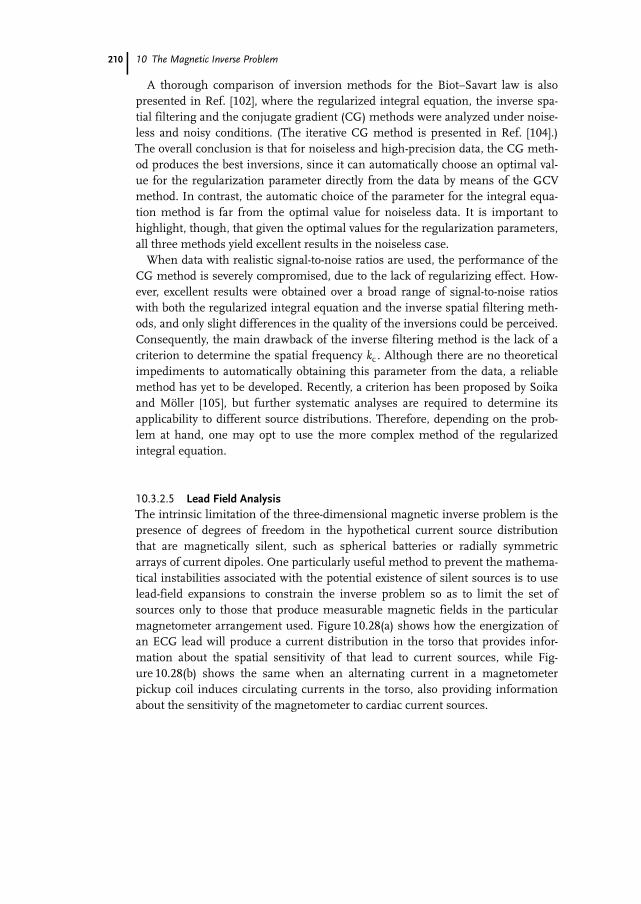
10 The Magnetic Inverse Problem
A thorough comparison of inversion methods for the Biot–Savart law is alsopresented in Ref. [102], where the regularized integral equation, the inverse spa-tial filtering and the conjugate gradient (CG) methods were analyzed under noise-less and noisy conditions. (The iterative CG method is presented in Ref. [104].)The overall conclusion is that for noiseless and high-precision data, the CG meth-od produces the best inversions, since it can automatically choose an optimal val-ue for the regularization parameter directly from the data by means of the GCVmethod. In contrast, the automatic choice of the parameter for the integral equa-tion method is far from the optimal value for noiseless data. It is important tohighlight, though, that given the optimal values for the regularization parameters,all three methods yield excellent results in the noiseless case.When data with realistic signal-to-noise ratios are used, the performance of the
CG method is severely compromised, due to the lack of regularizing effect. How-ever, excellent results were obtained over a broad range of signal-to-noise ratioswith both the regularized integral equation and the inverse spatial filtering meth-ods, and only slight differences in the quality of the inversions could be perceived.Consequently, the main drawback of the inverse filtering method is the lack of acriterion to determine the spatial frequency kc . Although there are no theoreticalimpediments to automatically obtaining this parameter from the data, a reliablemethod has yet to be developed. Recently, a criterion has been proposed by Soikaand MWller [105], but further systematic analyses are required to determine itsapplicability to different source distributions. Therefore, depending on the prob-lem at hand, one may opt to use the more complex method of the regularizedintegral equation.
10.3.2.5 Lead Field AnalysisThe intrinsic limitation of the three-dimensional magnetic inverse problem is thepresence of degrees of freedom in the hypothetical current source distributionthat are magnetically silent, such as spherical batteries or radially symmetricarrays of current dipoles. One particularly useful method to prevent the mathema-tical instabilities associated with the potential existence of silent sources is to uselead-field expansions to constrain the inverse problem so as to limit the set ofsources only to those that produce measurable magnetic fields in the particularmagnetometer arrangement used. Figure 10.28(a) shows how the energization ofan ECG lead will produce a current distribution in the torso that provides infor-mation about the spatial sensitivity of that lead to current sources, while Fig-ure 10.28(b) shows the same when an alternating current in a magnetometerpickup coil induces circulating currents in the torso, also providing informationabout the sensitivity of the magnetometer to cardiac current sources.
210
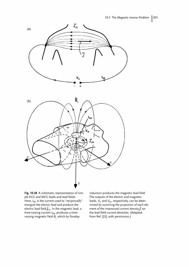
10.3 The Magnetic Inverse Problem 211
Fig. 10.28 A schematic representation of sim-ple ECG and MCG leads and lead fields.Here, IRE is the current used to “reciprocally”energize the electric lead and produce theelectric lead field~JJLE. In the magnetic lead, atime-varying current IRM produces a time-varying magnetic field BL which by Faraday
induction produces the magnetic lead field.The outputs of the electric and magneticleads, VE and VM, respectively, can be deter-mined by summing the projection of each ele-ment of the impressed current density~JJi onthe lead field current densities. (Adaptedfrom Ref. [22], with permission.)
10 The Magnetic Inverse Problem
Lead FieldsTo understand quantitatively the process outlined in Figure 10.28, we first need todefine the lead fields [22, 106, 107]. Note that this analysis is valid either for a fixedarray of N sensors, or for a scanning SQUID sensor that samples the magneticfield at N different positions ~riri. Suppose that a magnetometer measures Bz at aspecific point~rr. As shown in (10.65), this measurement represents a convolutionof the source current distribution~JJð~r¢r¢Þ and the Green’s function Gð~rr; ~r¢r¢Þ over thepoints ~r¢r¢ where both~JJ and G are nonzero. This Green’s function is equivalent to amutual inductance, Mpq, between a particular source element, d~pp, of a currentdipole distribution and a single, specific pick-up coil, q. The principle of recipro-city states that Mpq equals Mqp, which is equivalent to saying that the Green’sfunction is the same whether the current source is at~rr and the coil is at ~r¢r¢ or visaversa, i.e., Gð~rr; ~r¢r¢Þ ¼ Gð~r¢r¢;~rrÞ. The lead field~LLJ
i ð~r¢r¢Þ for the ith magnetometer at~rri issimply the current distribution~JJ that would be produced were the magnetometerpickup loop replaced by a coil carrying a low-frequency ac current. In thisapproach, the output of the ith SQUID magnetometer, a scalar variable, is simplythe convolution of the source currents and the lead field for that magnetometer
Bi ~rrð Þ ¼ZV
~LLJi~r¢r¢� �
�~JJ ~r¢r¢� �
d3r ¢: (10:166)
Note the index i in ~LLJi contains within it the location ~riri, and hence we need not
carry the dual-position notation of Gð~rr; ~r¢r¢Þ. If a current source at a particular point~r¢r¢ is orthogonal to~LLJ
i ð~r¢r¢Þ at that same point, then that source cannot contribute tothe field detected by the SQUID at~riri. Reciprocally, a measurement of that compo-nent of the magnetic field cannot determine the strength of that component ofthe current source at ~r¢r¢, although it may be able to detect another component atthat location.10) The requirement that the solution set is to be restricted to thosecurrents that produce fields that can be measured by the chosen magnetometersis equivalent to stating that all of the imaged currents have to lie along the lines ofthe lead fields of one or more of the magnetometers.
Lead Field ExpansionsEquation (10.166) suggests that we use the set of lead fields for our N magnet-ometers to constrain the inverse source distribution [78, 107, 108]. While lead-fieldexpansions were originally developed for three-dimensional inverse problems, tomaintain the consistency of our derivations we shall restrict ourselves to measure-ment of two-dimensional current distributions. We begin with the law of Biot and
212
10) This is an easy explanation for the inabilityof a SQUID to measure magnetic fieldsfrom radial dipoles in a conducting sphere:it is impossible, by means of external coils,to induce in the sphere eddy currents withradial components, i.e., radial lead fields.For this reason, it is impossible to use exter-
nal coils to create a lead field that woulddetect a spherical battery. Also note thatwere we trying to measure a magnetization~MM rather than a current~JJ, we would utilizethe magnetic lead field~LLB, rather than thecurrent lead field~LLJ .
10.3 The Magnetic Inverse Problem
Savart for Bx at the ith measurement point above a two-dimensional current dis-tribution
Bx;i ~ririð Þ ¼l0d4p
� � ZS
Jy~r¢r¢� �
zi � z¢ð Þ
~riri � ~r¢r¢��� ���3 dx ¢dy¢; (10:167)
where S is the surface containing the sources. We can write this in terms of thelead field for that magnetometer
Bx;i ~ririð Þ ¼ZS
~LLJi~r¢r¢� �
�~JJ ~r¢r¢� �
d2r ¢: (10:168)
The dot product and the orientation of the lead field automatically selects the Jy
component of the source current.Let us suppose that we can expand~JJð~r¢r¢Þ in terms of the nonorthogonal set of m
lead-field functions~LLJi
~JJð~r¢r¢Þ ¼Xmk¼1
Ak~LLJ
k~r¢r¢� �
w ~r¢r¢� �
; (10:169)
where wð~r¢r¢Þ is the a priori probability density for the current density, and Ak arethe expansion coefficients. If we know, for example, that the currents in a particu-lar region are zero, then we can at the beginning of our calculation set wð~r¢r¢Þ tozero at those locations. To determine Ak, we substitute (10.169) into (10.168), andexchange the order of summation and integration
Bx;i ~ririð Þ ¼Xmk¼1
Ak
ZS
~LLJi~r¢r¢� �
�~LL Jk~r¢r¢� �
w ~r¢r¢� �
d2r ¢: (10:170)
The field is thus
Bx;i ¼Xmk¼1
PikAk i ¼ 1; 2 . . . ;Nð Þ (10:171)
where
Pik ¼ZS
~LLJi~r¢r¢� �
�~LL Jk~r¢r¢� �
w ~r¢r¢� �
d2r ¢: (10:172)
While computation of Pik can be tedious, it needs to be done only once for a partic-ular measurement geometry. Singular-value decomposition or some other numer-ical technique is used to solve this set of linear equations for Ak, which are then
213
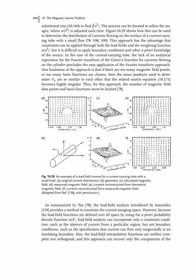
10 The Magnetic Inverse Problem
substituted into (10.169) to find~JJð~r¢r¢Þ. The process can be iterated to refine the im-ages, where wð~r¢r¢Þ is adjusted each time. Figure 10.29 shows how this can be usedto determine the distribution of currents flowing on the surface of a current-carry-ing tube with a small flaw [78, 108, 109]. This approach has the advantage thatconstraints can be applied through both the lead fields and the weighting functionwð~r¢r¢Þ, but it is difficult to apply boundary conditions and other a priori knowledgeof the source. In the case of the current-carrying tube, the lack of an analyticalexpression for the Fourier transform of the Green’s function for currents flowingon the cylinder precludes the easy application of the Fourier transform approach.One limitation of the approach is that if there are too many magnetic field points,or too many basis functions are chosen, then the inner products used to deter-mine Pik are so similar to each other that the related matrix equation (10.171)becomes highly singular. Thus, for this approach, the number of magnetic fielddata points and basis functions must be limited [78].
As summarized by Tan [78], the lead-field analysis introduced by Ioannides[110] provides a method to constrain the current-imaging space. However, becausethe lead-field functions are defined over all space by using the a priori probabilitydensity function w ~rrð Þ, lead-field analysis can incorporate only a constraint condi-tion, such as the absence of current from a particular region, but not boundaryconditions, such as the specification that current can flow only tangentially to aninsulating boundary. Also, the lead-field interpolation functions are neither com-plete nor orthogonal, and this approach can recover only the components of the
214
Fig. 10.29 An example of a lead-field inverse for a current-carrying tube with asmall hole: (a) original current distribution; (b) geometry; (c) calculated magneticfield; (d) measured magnetic field; (e) currents reconstructed from theoreticalmagnetic field; (f) currents reconstructed from measured magnetic field.(Adapted from Ref. [136], with permission.)
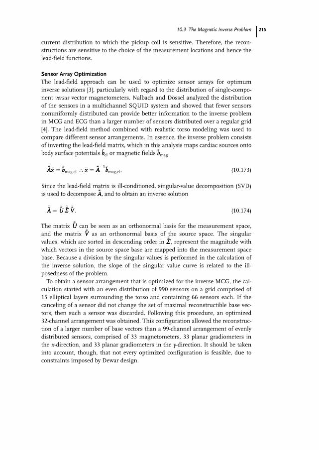
10.3 The Magnetic Inverse Problem
current distribution to which the pickup coil is sensitive. Therefore, the recon-structions are sensitive to the choice of the measurement locations and hence thelead-field functions.
Sensor Array OptimizationThe lead-field approach can be used to optimize sensor arrays for optimuminverse solutions [3], particularly with regard to the distribution of single-compo-nent versus vector magnetometers. Nalbach and DWssel analyzed the distributionof the sensors in a multichannel SQUID system and showed that fewer sensorsnonuniformly distributed can provide better information to the inverse problemin MCG and ECG than a larger number of sensors distributed over a regular grid[4]. The lead-field method combined with realistic torso modeling was used tocompare different sensor arrangements. In essence, the inverse problem consistsof inverting the lead-field matrix, which in this analysis maps cardiac sources ontobody surface potentials ~bbel or magnetic fields ~bbmag
~~AA~AA~xx ¼ ~bbmag;el \ ~xx ¼ ~~AA~AA�1~bbmag;el: (10:173)
Since the lead-field matrix is ill-conditioned, singular-value decomposition (SVD)is used to decompose ~~AA~AA, and to obtain an inverse solution
~~AA~AA ¼ ~~UU~UU ~~RR~RR ~~VV~VV : (10:174)
The matrix ~~UU~UU can be seen as an orthonormal basis for the measurement space,and the matrix ~~VV~VV as an orthonormal basis of the source space. The singularvalues, which are sorted in descending order in ~~RR~RR, represent the magnitude withwhich vectors in the source space base are mapped into the measurement spacebase. Because a division by the singular values is performed in the calculation ofthe inverse solution, the slope of the singular value curve is related to the ill-posedness of the problem.To obtain a sensor arrangement that is optimized for the inverse MCG, the cal-
culation started with an even distribution of 990 sensors on a grid comprised of15 elliptical layers surrounding the torso and containing 66 sensors each. If thecanceling of a sensor did not change the set of maximal reconstructible base vec-tors, then such a sensor was discarded. Following this procedure, an optimized32-channel arrangement was obtained. This configuration allowed the reconstruc-tion of a larger number of base vectors than a 99-channel arrangement of evenlydistributed sensors, comprised of 33 magnetometers, 33 planar gradiometers inthe x-direction, and 33 planar gradiometers in the y-direction. It should be takeninto account, though, that not every optimized configuration is feasible, due toconstraints imposed by Dewar design.
215
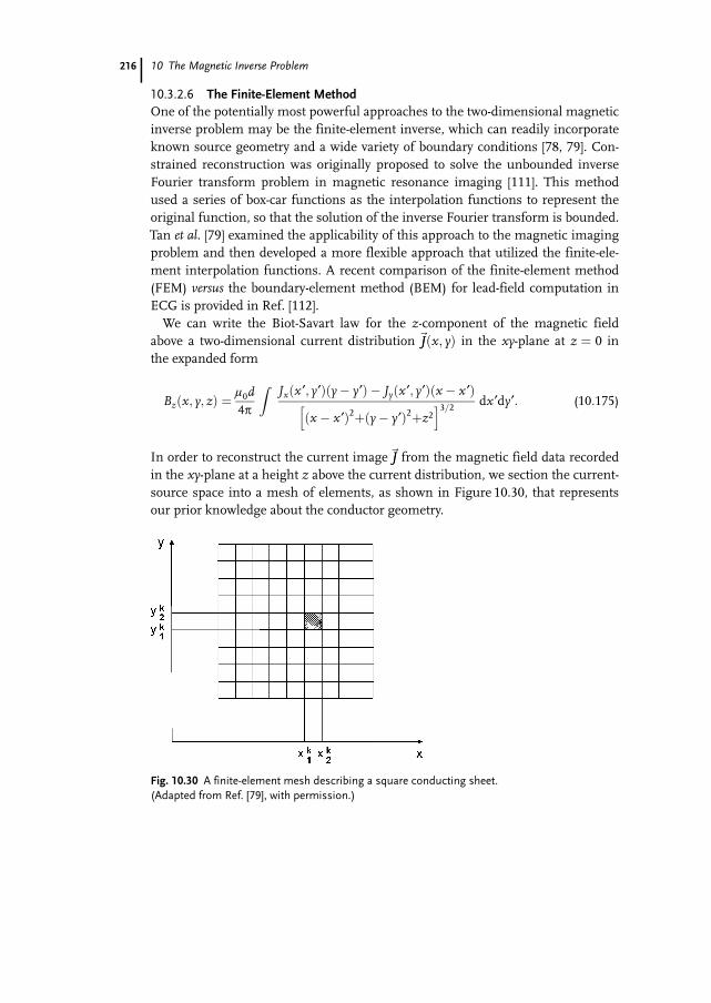
10 The Magnetic Inverse Problem
10.3.2.6 The Finite-Element MethodOne of the potentially most powerful approaches to the two-dimensional magneticinverse problem may be the finite-element inverse, which can readily incorporateknown source geometry and a wide variety of boundary conditions [78, 79]. Con-strained reconstruction was originally proposed to solve the unbounded inverseFourier transform problem in magnetic resonance imaging [111]. This methodused a series of box-car functions as the interpolation functions to represent theoriginal function, so that the solution of the inverse Fourier transform is bounded.Tan et al. [79] examined the applicability of this approach to the magnetic imagingproblem and then developed a more flexible approach that utilized the finite-ele-ment interpolation functions. A recent comparison of the finite-element method(FEM) versus the boundary-element method (BEM) for lead-field computation inECG is provided in Ref. [112].We can write the Biot-Savart law for the z-component of the magnetic field
above a two-dimensional current distribution ~JJ x; yð Þ in the xy-plane at z ¼ 0 inthe expanded form
Bz x; y; zð Þ ¼ l0d4p
ZJx x ¢; y¢ð Þ y� y¢ð Þ � Jy x ¢; y¢ð Þ x � x ¢ð Þ
x � x ¢ð Þ2þ y� y¢ð Þ2þz2h i3=2 dx ¢dy¢: (10:175)
In order to reconstruct the current image~JJ from the magnetic field data recordedin the xy-plane at a height z above the current distribution, we section the current-source space into a mesh of elements, as shown in Figure 10.30, that representsour prior knowledge about the conductor geometry.
216
Fig. 10.30 A finite-element mesh describing a square conducting sheet.(Adapted from Ref. [79], with permission.)
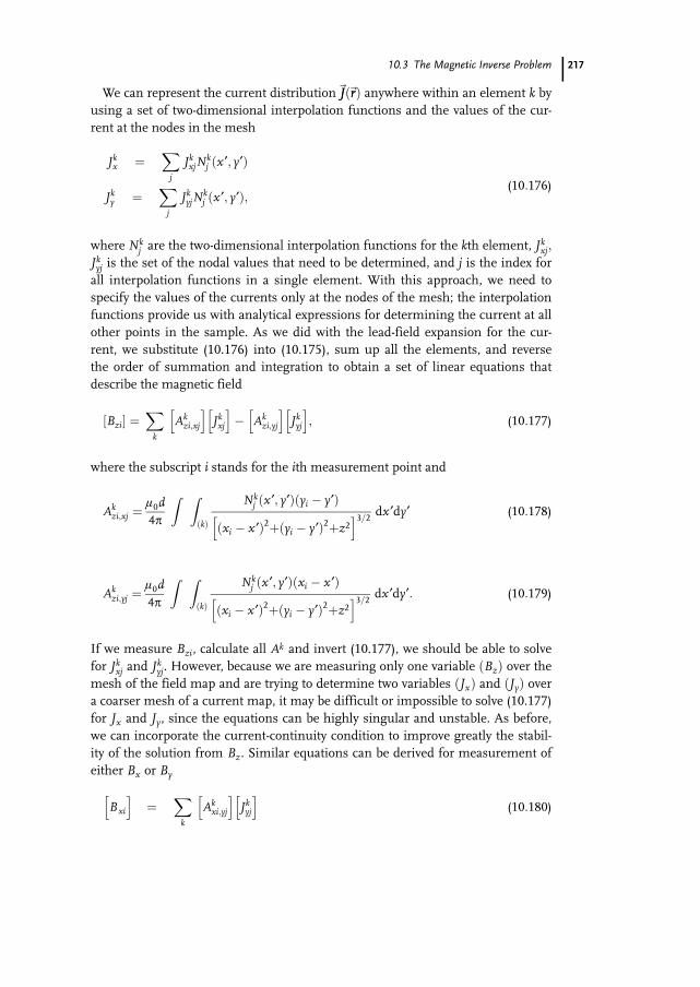
10.3 The Magnetic Inverse Problem
We can represent the current distribution~JJ ~rrð Þ anywhere within an element k byusing a set of two-dimensional interpolation functions and the values of the cur-rent at the nodes in the mesh
Jkx ¼
Xj
JkxjN
kj x ¢; y¢ð Þ
Jky ¼
Xj
JkyjN
kj x ¢; y¢ð Þ;
(10:176)
where Nkj are the two-dimensional interpolation functions for the kth element, Jk
xj;
Jkyj is the set of the nodal values that need to be determined, and j is the index forall interpolation functions in a single element. With this approach, we need tospecify the values of the currents only at the nodes of the mesh; the interpolationfunctions provide us with analytical expressions for determining the current at allother points in the sample. As we did with the lead-field expansion for the cur-rent, we substitute (10.176) into (10.175), sum up all the elements, and reversethe order of summation and integration to obtain a set of linear equations thatdescribe the magnetic field
Bzi½ � ¼X
k
Akzi;xj
h iJkxj
h i� Ak
zi;yj
h iJkyj
h i; (10:177)
where the subscript i stands for the ith measurement point and
Akzi;xj ¼
l0d4p
Z Zkð Þ
Nkj x ¢; y¢ð Þ yi � y¢ð Þ
xi � x ¢ð Þ2þ yi � y¢ð Þ2þz2h i3=2 dx ¢dy¢ (10:178)
Akzi;yj ¼
l0d4p
Z Zkð Þ
Nkj x ¢; y¢ð Þ xi � x ¢ð Þ
xi � x ¢ð Þ2þ yi � y¢ð Þ2þz2h i3=2 dx ¢dy¢: (10:179)
If we measure Bzi, calculate all Ak and invert (10.177), we should be able to solvefor Jk
xj and Jkyj. However, because we are measuring only one variable Bzð Þ over the
mesh of the field map and are trying to determine two variables Jxð Þ and ðJyÞ overa coarser mesh of a current map, it may be difficult or impossible to solve (10.177)for Jx and Jy, since the equations can be highly singular and unstable. As before,we can incorporate the current-continuity condition to improve greatly the stabil-ity of the solution from Bz. Similar equations can be derived for measurement ofeither Bx or By
Bxi
h i¼
Xk
Akxi;yj
h iJkyj
h i(10:180)
217
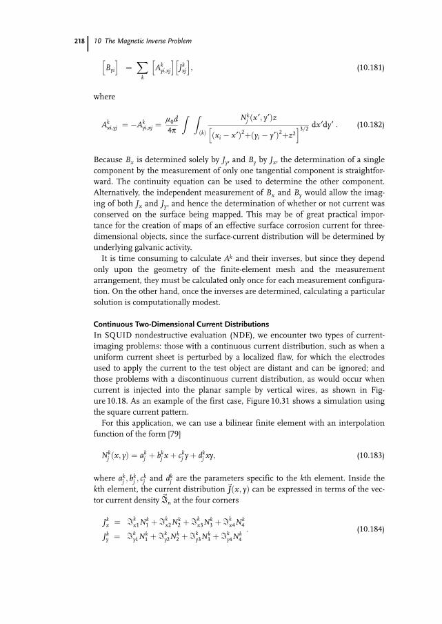
10 The Magnetic Inverse Problem
Byi
h i¼X
k
Akyi;xj
h iJkxj
h i; (10:181)
where
Akxi;yj ¼ �Ak
yi;xj ¼l0d4p
Z ZðkÞ
Nkj x ¢; y¢ð Þz
xi � x ¢ð Þ2þ yi � y¢ð Þ2þz2h i3=2 dx ¢dy¢ : (10:182)
Because Bx is determined solely by Jy, and By by Jx, the determination of a singlecomponent by the measurement of only one tangential component is straightfor-ward. The continuity equation can be used to determine the other component.Alternatively, the independent measurement of Bx and By would allow the imag-ing of both Jx and Jy, and hence the determination of whether or not current wasconserved on the surface being mapped. This may be of great practical impor-tance for the creation of maps of an effective surface corrosion current for three-dimensional objects, since the surface-current distribution will be determined byunderlying galvanic activity.It is time consuming to calculate Ak and their inverses, but since they depend
only upon the geometry of the finite-element mesh and the measurementarrangement, they must be calculated only once for each measurement configura-tion. On the other hand, once the inverses are determined, calculating a particularsolution is computationally modest.
Continuous Two-Dimensional Current DistributionsIn SQUID nondestructive evaluation (NDE), we encounter two types of current-imaging problems: those with a continuous current distribution, such as when auniform current sheet is perturbed by a localized flaw, for which the electrodesused to apply the current to the test object are distant and can be ignored; andthose problems with a discontinuous current distribution, as would occur whencurrent is injected into the planar sample by vertical wires, as shown in Fig-ure 10.18. As an example of the first case, Figure 10.31 shows a simulation usingthe square current pattern.For this application, we can use a bilinear finite element with an interpolation
function of the form [79]
Nkj x; yð Þ ¼ ak
j þ bkj x þ ck
j yþ dkj xy; (10:183)
where akj ; b
kj ; c
kj and dk
j are the parameters specific to the kth element. Inside thekth element, the current distribution~JJ x; yð Þ can be expressed in terms of the vec-tor current density ~IIn at the four corners
Jkx ¼ Ik
x1Nk1 þ Ik
x2Nk2 þ Ik
x3Nk3 þ Ik
x4Nk4
Jky ¼ Ik
y1Nk1 þ Ik
y2Nk2 þ Ik
y3Nk3 þ Ik
y4Nk4
: (10:184)
218

10.3 The Magnetic Inverse Problem
We can utilize within each element a set of normalized, local coordinates, termednatural coordinates g and n, that range from þ1 to �1, so that we can write thecontinuity condition ((10.75)) as
¶Jx
¶n¶n¶xþ¶Jy
¶g¶g¶y¼ 0: (10:185)
Substituting (10.184) into the above equation and sorting the coefficients by theorder of the polynomial, we obtain a polynomial expression for the continuityequation [79]
1ak�Ik
x1 þ Ikx2 � Ik
x3 þ Ikx4
� �þ 1
bk�Ik
y1 � Iky2 þ Ik
y3 þ Iky4
� �þ
1ak
Ikx1 � Ik
x2 � Ikx3 þ Ik
x4
� �gþ 1
bkIk
y1 � Iky2 � Ik
y3 þ Iky4
� �n ¼ 0:
(10:186)
Since the coordinates n and g are independent of each other, each term of thepolynomial must be individually zero to ensure that the continuity condition issatisfied in every element. Thus, we obtain a set of equations governing the coeffi-cients Jk
xj and Jkyj
1ak�Ik
x1 þ Ikx2 � Ik
x3 þ Ikx4
� �þ 1
bk�Ik
y1 � Iky2 þ Ik
y3 þ Iky4
� �¼ 0
Ikx1 � Ik
x2 � Ikx3 þ Ik
x4
� �¼ 0
Iky1 � Ik
y2 � Iky3 þ Ik
y4
� �¼ 0:
(10:187)
219
Fig. 10.31 Finite-element model for a bounded source: (a) the simulated currentsource used to test the continuous-current reconstruction algorithm; (b) the gridused to section the current space corresponding to (a). (Adapted from Ref. [79],with permission.)
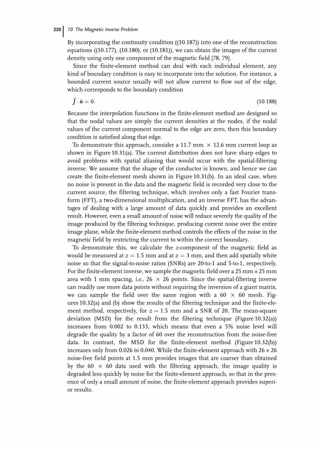
10 The Magnetic Inverse Problem
By incorporating the continuity condition ((10.187)) into one of the reconstructionequations ((10.177), (10.180), or (10.181)), we can obtain the images of the currentdensity using only one component of the magnetic field [78, 79].Since the finite-element method can deal with each individual element, any
kind of boundary condition is easy to incorporate into the solution. For instance, abounded current source usually will not allow current to flow out of the edge,which corresponds to the boundary condition
~JJ � nn ¼ 0: (10:188)
Because the interpolation functions in the finite-element method are designed sothat the nodal values are simply the current densities at the nodes, if the nodalvalues of the current component normal to the edge are zero, then this boundarycondition is satisfied along that edge.To demonstrate this approach, consider a 11.7 mm · 12.6 mm current loop as
shown in Figure 10.31(a). The current distribution does not have sharp edges toavoid problems with spatial aliasing that would occur with the spatial-filteringinverse. We assume that the shape of the conductor is known, and hence we cancreate the finite-element mesh shown in Figure 10.31(b). In an ideal case, whenno noise is present in the data and the magnetic field is recorded very close to thecurrent source, the filtering technique, which involves only a fast Fourier trans-form (FFT), a two-dimensional multiplication, and an inverse FFT, has the advan-tages of dealing with a large amount of data quickly and provides an excellentresult. However, even a small amount of noise will reduce severely the quality of theimage produced by the filtering technique, producing current noise over the entireimage plane, while the finite-element method controls the effects of the noise in themagnetic field by restricting the current to within the correct boundary.To demonstrate this, we calculate the z-component of the magnetic field as
would be measured at z ¼ 1:5 mm and at z ¼ 3 mm, and then add spatially whitenoise so that the signal-to-noise ratios (SNRs) are 20-to-1 and 5-to-1, respectively.For the finite-element inverse, we sample themagnetic field over a 25mm U 25mmarea with 1 mm spacing, i.e., 26 · 26 points. Since the spatial-filtering inversecan readily use more data points without requiring the inversion of a giant matrix,we can sample the field over the same region with a 60 · 60 mesh. Fig-ures 10.32(a) and (b) show the results of the filtering technique and the finite-ele-ment method, respectively, for z ¼ 1:5 mm and a SNR of 20. The mean-squaredeviation (MSD) for the result from the filtering technique (Figure 10.32(a))increases from 0.002 to 0.133, which means that even a 5% noise level willdegrade the quality by a factor of 60 over the reconstruction from the noise-freedata. In contrast, the MSD for the finite-element method (Figure 10.32(b))increases only from 0.026 to 0.040. While the finite-element approach with 26 U 26noise-free field points at 1.5 mm provides images that are coarser than obtainedby the 60 · 60 data used with the filtering approach, the image quality isdegraded less quickly by noise for the finite-element approach, so that in the pres-ence of only a small amount of noise, the finite-element approach provides superi-or results.
220
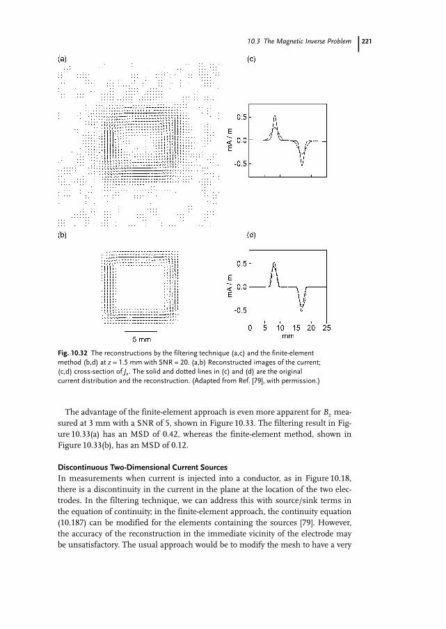
10.3 The Magnetic Inverse Problem
The advantage of the finite-element approach is even more apparent for Bz mea-sured at 3 mm with a SNR of 5, shown in Figure 10.33. The filtering result in Fig-ure 10.33(a) has an MSD of 0.42, whereas the finite-element method, shown inFigure 10.33(b), has an MSD of 0.12.
Discontinuous Two-Dimensional Current SourcesIn measurements when current is injected into a conductor, as in Figure 10.18,there is a discontinuity in the current in the plane at the location of the two elec-trodes. In the filtering technique, we can address this with source/sink terms inthe equation of continuity; in the finite-element approach, the continuity equation(10.187) can be modified for the elements containing the sources [79]. However,the accuracy of the reconstruction in the immediate vicinity of the electrode maybe unsatisfactory. The usual approach would be to modify the mesh to have a very
221
Fig. 10.32 The reconstructions by the filtering technique (a,c) and the finite-elementmethod (b,d) at z = 1.5 mm with SNR = 20. (a,b) Reconstructed images of the current;(c,d) cross-section of Jx . The solid and dotted lines in (c) and (d) are the originalcurrent distribution and the reconstruction. (Adapted from Ref. [79], with permission.)
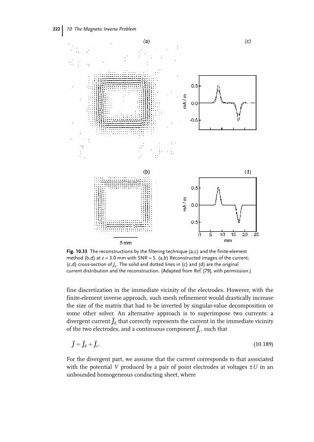
10 The Magnetic Inverse Problem
fine discretization in the immediate vicinity of the electrodes. However, with thefinite-element inverse approach, such mesh refinement would drastically increasethe size of the matrix that had to be inverted by singular-value decomposition orsome other solver. An alternative approach is to superimpose two currents: adivergent current~JJd that correctly represents the current in the immediate vicinityof the two electrodes, and a continuous component~JJc, such that
~JJ ¼~JJd þ~JJc: (10:189)
For the divergent part, we assume that the current corresponds to that associatedwith the potential V produced by a pair of point electrodes at voltages –U in anunbounded homogeneous conducting sheet, where
222
Fig. 10.33 The reconstructions by the filtering technique (a,c) and the finite-elementmethod (b,d) at z = 3.0 mm with SNR = 5. (a,b) Reconstructed images of the current;(c,d) cross-section of Jx . The solid and dotted lines in (c) and (d) are the originalcurrent distribution and the reconstruction. (Adapted from Ref. [79], with permission.)
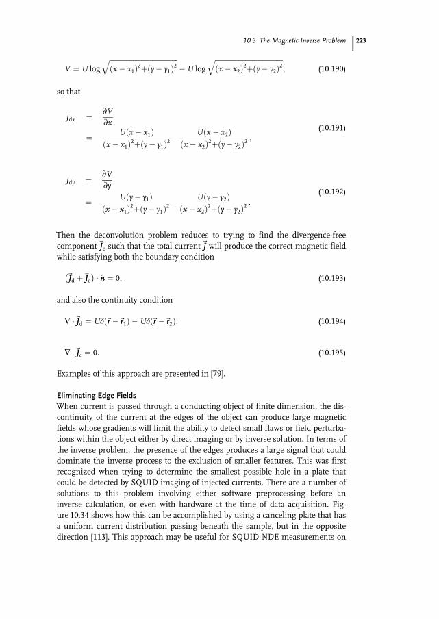
10.3 The Magnetic Inverse Problem
V ¼ U logffiffiffiffiffiffiffiffiffiffiffiffiffiffiffiffiffiffiffiffiffiffiffiffiffiffiffiffiffiffiffiffiffiffiffiffiffiffiffiffix � x1ð Þ2þ y� y1ð Þ2
q�U log
ffiffiffiffiffiffiffiffiffiffiffiffiffiffiffiffiffiffiffiffiffiffiffiffiffiffiffiffiffiffiffiffiffiffiffiffiffiffiffiffix � x2ð Þ2þ y� y2ð Þ2
q; (10:190)
so that
Jdx ¼ ¶V¶x
¼ U x � x1ð Þx � x1ð Þ2þ y� y1ð Þ2
� U x � x2ð Þx � x2ð Þ2þ y� y2ð Þ2
;(10:191)
Jdy ¼ ¶V¶y
¼ U y� y1ð Þx � x1ð Þ2þ y� y1ð Þ2
� U y� y2ð Þx � x2ð Þ2þ y� y2ð Þ2
:
(10:192)
Then the deconvolution problem reduces to trying to find the divergence-freecomponent~JJc such that the total current~JJ will produce the correct magnetic fieldwhile satisfying both the boundary condition
~JJd þ~JJc� �
� nn ¼ 0; (10:193)
and also the continuity condition
� �~JJd ¼ Ud ~rr �~rr1ð Þ �Ud ~rr �~rr2ð Þ; (10:194)
� �~JJc ¼ 0: (10:195)
Examples of this approach are presented in [79].
Eliminating Edge FieldsWhen current is passed through a conducting object of finite dimension, the dis-continuity of the current at the edges of the object can produce large magneticfields whose gradients will limit the ability to detect small flaws or field perturba-tions within the object either by direct imaging or by inverse solution. In terms ofthe inverse problem, the presence of the edges produces a large signal that coulddominate the inverse process to the exclusion of smaller features. This was firstrecognized when trying to determine the smallest possible hole in a plate thatcould be detected by SQUID imaging of injected currents. There are a number ofsolutions to this problem involving either software preprocessing before aninverse calculation, or even with hardware at the time of data acquisition. Fig-ure 10.34 shows how this can be accomplished by using a canceling plate that hasa uniform current distribution passing beneath the sample, but in the oppositedirection [113]. This approach may be useful for SQUID NDE measurements on
223
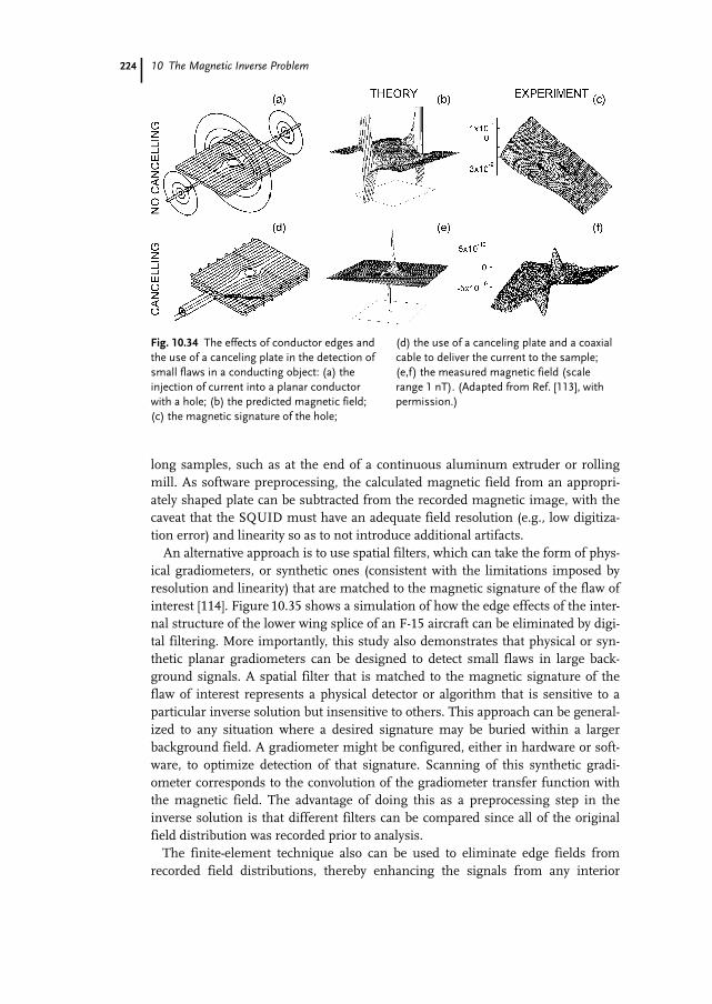
10 The Magnetic Inverse Problem
long samples, such as at the end of a continuous aluminum extruder or rollingmill. As software preprocessing, the calculated magnetic field from an appropri-ately shaped plate can be subtracted from the recorded magnetic image, with thecaveat that the SQUID must have an adequate field resolution (e.g., low digitiza-tion error) and linearity so as to not introduce additional artifacts.An alternative approach is to use spatial filters, which can take the form of phys-
ical gradiometers, or synthetic ones (consistent with the limitations imposed byresolution and linearity) that are matched to the magnetic signature of the flaw ofinterest [114]. Figure 10.35 shows a simulation of how the edge effects of the inter-nal structure of the lower wing splice of an F-15 aircraft can be eliminated by digi-tal filtering. More importantly, this study also demonstrates that physical or syn-thetic planar gradiometers can be designed to detect small flaws in large back-ground signals. A spatial filter that is matched to the magnetic signature of theflaw of interest represents a physical detector or algorithm that is sensitive to aparticular inverse solution but insensitive to others. This approach can be general-ized to any situation where a desired signature may be buried within a largerbackground field. A gradiometer might be configured, either in hardware or soft-ware, to optimize detection of that signature. Scanning of this synthetic gradi-ometer corresponds to the convolution of the gradiometer transfer function withthe magnetic field. The advantage of doing this as a preprocessing step in theinverse solution is that different filters can be compared since all of the originalfield distribution was recorded prior to analysis.The finite-element technique also can be used to eliminate edge fields from
recorded field distributions, thereby enhancing the signals from any interior
224
Fig. 10.34 The effects of conductor edges andthe use of a canceling plate in the detection ofsmall flaws in a conducting object: (a) theinjection of current into a planar conductorwith a hole; (b) the predicted magnetic field;(c) the magnetic signature of the hole;
(d) the use of a canceling plate and a coaxialcable to deliver the current to the sample;(e,f) the measured magnetic field (scalerange 1 nT). (Adapted from Ref. [113], withpermission.)
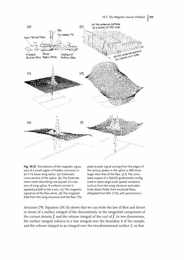
10.3 The Magnetic Inverse Problem
structure [79]. Equation (10.15) shows that we can write the law of Biot and Savartin terms of a surface integral of the discontinuity in the tangential component ofthe current density~JJ, and the volume integral of the curl of~JJ. In two dimensions,the surface integral reduces to a line integral over the boundary b of the sample,and the volume integral to an integral over the two-dimensional surface S, so that
225
Fig. 10.35 Simulations of the magnetic signa-ture of a small region of hidden corrosion inan F-15 lower wing splice. (a) Schematiccross-section of the splice. (b) The finite-ele-ment mesh describing one-quarter of a sec-tion of wing splice. A uniform current isapplied parallel to the x-axis. (c) The magneticsignature of the flaw alone. (d) The magneticfield from the wing structure and the flaw. The
peak-to-peak signal arising from the edges ofthe various plates in the splice is 400 timeslarger than that of the flaw. (e,f) The simu-lated output of a SQUID gradiometer config-ured to reject large-scale spatial variationssuch as from the wing structure and selec-tively detect fields from localized flaws.(Adapted from Ref. [114], with permission.)
10 The Magnetic Inverse Problem
Bz ~rrð Þ ¼l0d4p
Ib
~JJ ~r¢r¢� �
� d~l¢l¢
~rr � ~r¢r¢��� ��� þ
l0d4p
ZS
�¢ ·~JJ ~r¢r¢� �h i
z
~rr � ~r¢r¢��� ��� dx ¢dy¢: (10:196)
Following the approach in Tan et al. [79], we can use Ohm’s law
~JJ ¼ �r�V ; (10:197)
the curl of this expression,
� ·~JJ ¼ �� · r�Vð Þ¼ ��r ·�V
¼ � · V�rð Þ;(10:198)
and standard vector identities to rewrite (10.196) as
Bz ~rrð Þ ¼l0d4p
Ib
~JJ ~r¢r¢� �
� d~l¢l¢
~rr � ~r¢r¢��� ��� þ
l0d4p
ZS
V ~r¢r¢� �
�¢r ~r¢r¢� �
·~r¢r¢h i
z
~rr � ~r¢r¢��� ��� dx ¢dy¢: (10:199)
If the medium is homogeneous and isotropic, �¢r ¼~00, and the second integral iszero, which means that the magnetic field depends only on the current tangentialto the edge, i.e., the first integral. If the test object has a nonuniform or anisotrop-ic conductivity, the second term will contribute. The finite-element technique pro-vides us with a powerful tool for separating these two contributions: the magneticfield is used with the finite-element inverse to determine the current distributionin a homogeneous, isotropic sample of the correct shape. This current is thenused with the first integral of (10.199) to compute the magnetic field produced bythe edges. If this is identical to the measured field, the sample is homogeneousand isotropic. If the two fields differ, then there are internal inhomogeneities oranisotropies. This approach may provide a means for enhancing the sensitivity ofSQUID imaging to detect internal flaws in metallic structures.
10.3.2.7 Phase-Sensitive Eddy-Current AnalysisSo far, we have discussed only the injection of current into conducting samples.While the injected-current technique is useful for high-precision measurementson test samples, the need to make good electrical contact with the sample wouldmake it difficult to use on painted structures such as airplanes. It is also possibleto use sheet inducers, first demonstrated with the MagnetoOptic Imager (MOI)[115, 116] in which the oscillating magnetic field is applied tangential to the sur-face of the test object by a sheet conductor or set of wires parallel to the test sur-face. This induces a large-extent sheet current in the test specimen, and thus pro-duces flaw perturbation fields quite similar to those obtained with direct-current
226
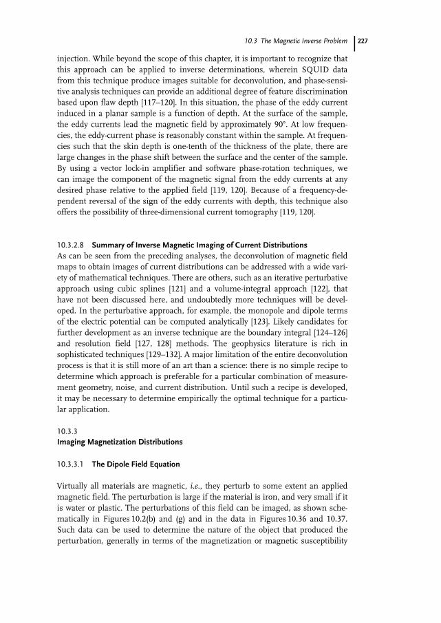
10.3 The Magnetic Inverse Problem
injection. While beyond the scope of this chapter, it is important to recognize thatthis approach can be applied to inverse determinations, wherein SQUID datafrom this technique produce images suitable for deconvolution, and phase-sensi-tive analysis techniques can provide an additional degree of feature discriminationbased upon flaw depth [117–120]. In this situation, the phase of the eddy currentinduced in a planar sample is a function of depth. At the surface of the sample,the eddy currents lead the magnetic field by approximately 90X. At low frequen-cies, the eddy-current phase is reasonably constant within the sample. At frequen-cies such that the skin depth is one-tenth of the thickness of the plate, there arelarge changes in the phase shift between the surface and the center of the sample.By using a vector lock-in amplifier and software phase-rotation techniques, wecan image the component of the magnetic signal from the eddy currents at anydesired phase relative to the applied field [119, 120]. Because of a frequency-de-pendent reversal of the sign of the eddy currents with depth, this technique alsooffers the possibility of three-dimensional current tomography [119, 120].
10.3.2.8 Summary of Inverse Magnetic Imaging of Current DistributionsAs can be seen from the preceding analyses, the deconvolution of magnetic fieldmaps to obtain images of current distributions can be addressed with a wide vari-ety of mathematical techniques. There are others, such as an iterative perturbativeapproach using cubic splines [121] and a volume-integral approach [122], thathave not been discussed here, and undoubtedly more techniques will be devel-oped. In the perturbative approach, for example, the monopole and dipole termsof the electric potential can be computed analytically [123]. Likely candidates forfurther development as an inverse technique are the boundary integral [124–126]and resolution field [127, 128] methods. The geophysics literature is rich insophisticated techniques [129–132]. A major limitation of the entire deconvolutionprocess is that it is still more of an art than a science: there is no simple recipe todetermine which approach is preferable for a particular combination of measure-ment geometry, noise, and current distribution. Until such a recipe is developed,it may be necessary to determine empirically the optimal technique for a particu-lar application.
10.3.3Imaging Magnetization Distributions
10.3.3.1 The Dipole Field Equation
Virtually all materials are magnetic, i.e., they perturb to some extent an appliedmagnetic field. The perturbation is large if the material is iron, and very small if itis water or plastic. The perturbations of this field can be imaged, as shown sche-matically in Figures 10.2(b) and (g) and in the data in Figures 10.36 and 10.37.Such data can be used to determine the nature of the object that produced theperturbation, generally in terms of the magnetization or magnetic susceptibility
227
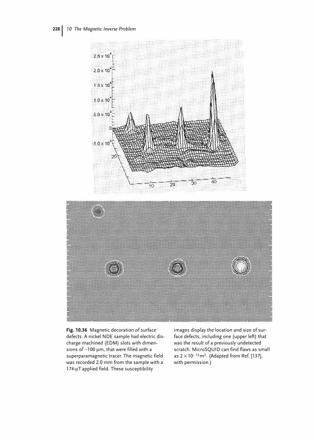
10 The Magnetic Inverse Problem228
Fig. 10.36 Magnetic decoration of surfacedefects. A nickel NDE sample had electric dis-charge machined (EDM) slots with dimen-sions of ~100 lm, that were filled with asuperparamagnetic tracer. The magnetic fieldwas recorded 2.0 mm from the sample with a174-lT applied field. These susceptibility
images display the location and size of sur-face defects, including one (upper left) thatwas the result of a previously undetectedscratch. MicroSQUID can find flaws as smallas 2 · 10�12m3. (Adapted from Ref. [137],with permission.)
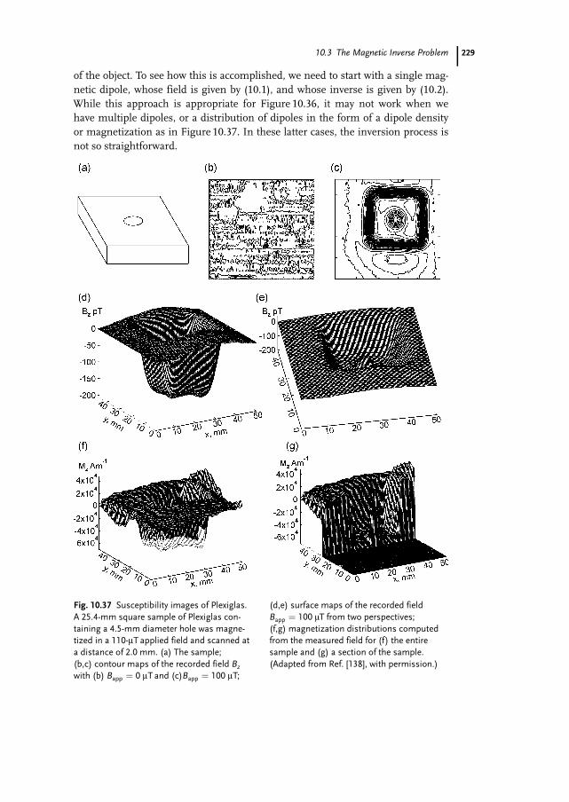
10.3 The Magnetic Inverse Problem
of the object. To see how this is accomplished, we need to start with a single mag-netic dipole, whose field is given by (10.1), and whose inverse is given by (10.2).While this approach is appropriate for Figure 10.36, it may not work when wehave multiple dipoles, or a distribution of dipoles in the form of a dipole densityor magnetization as in Figure 10.37. In these latter cases, the inversion process isnot so straightforward.
229
Fig. 10.37 Susceptibility images of Plexiglas.A 25.4-mm square sample of Plexiglas con-taining a 4.5-mm diameter hole was magne-tized in a 110-lT applied field and scanned ata distance of 2.0 mm. (a) The sample;(b,c) contour maps of the recorded field Bz
with (b) Bapp ¼ 0 lT and (c)Bapp ¼ 100 lT;
(d,e) surface maps of the recorded fieldBapp ¼ 100 lT from two perspectives;(f,g) magnetization distributions computedfrom the measured field for (f) the entiresample and (g) a section of the sample.(Adapted from Ref. [138], with permission.)
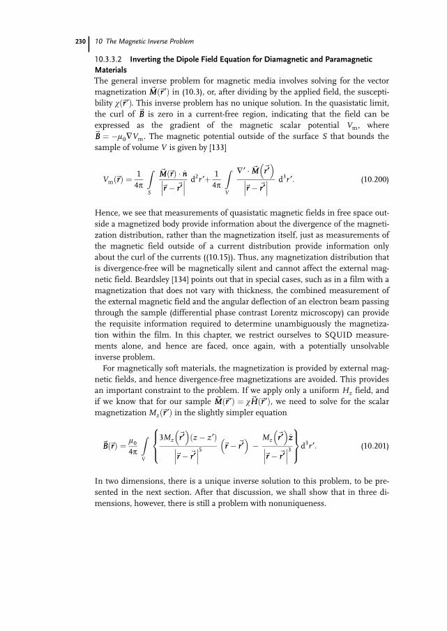
10 The Magnetic Inverse Problem
10.3.3.2 Inverting the Dipole Field Equation for Diamagnetic and ParamagneticMaterialsThe general inverse problem for magnetic media involves solving for the vectormagnetization ~MM ~rr ¢ð Þ in (10.3), or, after dividing by the applied field, the suscepti-bility v ~rr ¢ð Þ. This inverse problem has no unique solution. In the quasistatic limit,the curl of ~BB is zero in a current-free region, indicating that the field can beexpressed as the gradient of the magnetic scalar potential Vm, where~BB ¼ �l0�Vm. The magnetic potential outside of the surface S that bounds thesample of volume V is given by [133]
Vm ~rrð Þ ¼ 14p
ZS
~MM ~rrð Þ � nn~rr � ~r¢r¢��� ��� d2r ¢þ 1
4p
ZV
�¢ � ~MM ~r¢r¢� �
~rr � ~r¢r¢��� ��� d3r ¢: (10:200)
Hence, we see that measurements of quasistatic magnetic fields in free space out-side a magnetized body provide information about the divergence of the magneti-zation distribution, rather than the magnetization itself, just as measurements ofthe magnetic field outside of a current distribution provide information onlyabout the curl of the currents ((10.15)). Thus, any magnetization distribution thatis divergence-free will be magnetically silent and cannot affect the external mag-netic field. Beardsley [134] points out that in special cases, such as in a film with amagnetization that does not vary with thickness, the combined measurement ofthe external magnetic field and the angular deflection of an electron beam passingthrough the sample (differential phase contrast Lorentz microscopy) can providethe requisite information required to determine unambiguously the magnetiza-tion within the film. In this chapter, we restrict ourselves to SQUID measure-ments alone, and hence are faced, once again, with a potentially unsolvableinverse problem.For magnetically soft materials, the magnetization is provided by external mag-
netic fields, and hence divergence-free magnetizations are avoided. This providesan important constraint to the problem. If we apply only a uniform Hz field, andif we know that for our sample ~MM ~rr ¢ð Þ ¼ v~HH ~rr ¢ð Þ, we need to solve for the scalarmagnetization Mz ~rr ¢ð Þ in the slightly simpler equation
~BB ~rrð Þ ¼ l04p
ZV
3Mz~r¢r¢� �
z� z¢ð Þ
~rr � ~r¢r¢��� ���5 ~rr � ~r¢r¢
� ��
Mz~r¢r¢� �
zz
~rr � ~r¢r¢��� ���3
8><>:
9>=>;d3r ¢: (10:201)
In two dimensions, there is a unique inverse solution to this problem, to be pre-sented in the next section. After that discussion, we shall show that in three di-mensions, however, there is still a problem with nonuniqueness.
230
10.3 The Magnetic Inverse Problem
10.3.3.3 Two-Dimensional Magnetization ImagingFor two-dimensional samples, we can apply our inverse spatial filtering approachto determine the magnetization or susceptibility distributions from the magneticfield [78, 135, 136]. If the source is restricted to two dimensions, such as a thinsheet of diamagnetic or paramagnetic material, (10.201) reduces to a two-dimen-sional surface integral. We shall for now assume that we are applying only a z-component field H0zz, and are measuring only the z-component of the sample-induced magnetic field ~BB at a height z� z¢ð Þ above the two-dimensional sampleof infinite extent, so that we have
Bz ~rrð Þ ¼l04p
Z¥x ¢¼�¥
Z¥y ¢¼�¥
3Mz~r¢r¢� �
z� z¢ð Þ2
~rr � ~r¢r¢��� ���5 �
Mz~r¢r¢� �
~rr � ~r¢r¢��� ���3
8><>:
9>=>;dx ¢dy¢: (10:202)
In practice, the integrals need not extend beyond the boundary of the sourceobject, outside of which ~MM ”~00. In order to solve this equation for ~MMz ~rr ¢ð Þ, wedefine a Green’s function
Gz ~rr � ~r¢r¢� �
¼ l04p
3 z� z¢ð Þ2
~rr � ~r¢r¢��� ���5 �
1
~rr � ~r¢r¢��� ���3
8><>:
9>=>;; (10:203)
so that (10.202) becomes
Bz ~rrð Þ ¼Z ¥
�¥
Z ¥
�¥Mz
~r¢r¢� �
Gz ~rr � ~r¢r¢� �
dx ¢dy¢: (10:204)
We compute the two-dimensional spatial Fourier transform of the magnetic field
bz kx; ky; z� �
¼ FT Bz x; y; zð Þf g; (10:205)
so that we can use the convolution theorem to express (10.202) in the spatial fre-quency domain as
bz kx; ky; z� �
¼ gz kx; ky; z� z¢� �
mz kx; ky
� �; (10:206)
where gz kx; ky; z� z¢� �
is the two-dimensional spatial Fourier transform of theGreen’s function, i.e.,
gz kx; ky; z� z¢� �
¼ l04p
2pk e�k z�z ¢ð Þn o
; (10:207)
with
231
10 The Magnetic Inverse Problem
k ¼ k2x þ k2y
� �12
(10:208)
and mzðkx; kyÞ is the Fourier transform of the magnetization Mz x; yð Þ. The inverseproblem then reduces to a division in the spatial frequency domain
mz kx; ky
� �¼
bz kx; ky; z� �
gz kx; ky; z� z¢� � : (10:209)
As we have seen before, it may be necessary to use windowing techniques to pre-vent this equation from “blowing up” because of zeros in the Green’s functionoccurring at spatial frequencies for which there is a contribution to the magneticfield from either the sample or from noise. Typically, the window wðkx; kyÞ is alow-pass filter which attenuates high-frequency noise in the vicinity of the zerosof gz, so that (10.209) becomes
my kx; ky
� �¼
bz kx; ky; z� �
gz kx; ky; z� z¢� �w kx; ky
� �: (10:210)
As the final step, we use the inverse Fourier Transform FT�1ð Þ to obtain an imageof the magnetization distribution
Mz x; yð Þ ¼ FT�1 mz kx; ky
� �n o; (10:211)
which can then be used to obtain the desired susceptibility image
v x; yð Þ ¼ Mz x; yð ÞH0
~r¢r¢� � : (10:212)
This outlines the basic approach to two-dimensional magnetic susceptibility imag-ing; many of the techniques demonstrated for current-density imaging also willbe applicable. It is important to note that once the Green’s function (and itsinverse) and the window have been specified, it also is possible to proceed directlyfrom Bz x; yð Þ to v x; yð Þ by evaluating the appropriate convolution integral inxy-space. Applications of this technique include localizing dilute paramagnetictracers [137] and the imaging of plastic [138] (as shown in Figure 10.37), rock[8, 139, 140], and even water [141].
10.3.3.4 Magnetic Susceptibility TomographyIf the source is three-dimensional, a somewhat more general approach mustbe taken. We can start with (10.1), the dipole field equation for the magnetic field
232
10.3 The Magnetic Inverse Problem
d~BB ~rrð Þ produced by a single magnetic dipole d~mmð~r¢r¢Þ. If the dipole moment arisesfrom the magnetization of an incremental volume dv in an applied field ~HHð~r¢r¢Þ, wehave that
d~mm ~r¢r¢� �
¼ v ~r¢r¢� �
~HH ~r¢r¢� �
dv¢: (10:213)
The dipole field equation then becomes
d~BB ~rrð Þ ¼l0v
~r¢r¢� �4p
3~HH ~r¢r¢� �
� ~rr � ~r¢r¢� �
~rr � ~r¢r¢��� ���5 ~rr � ~r¢r¢
� ��
~HH ~r¢r¢� �
~rr � ~r¢r¢��� ���3
8><>:
9>=>;dv¢: (10:214)
This equation can be written as
d~BB ~rrð Þ ¼ ~GG ~rr; ~r¢r¢; ~HH� �
v ~r¢r¢� �
dv¢; (10:215)
where we introduce a vector Green’s function
~GG ~rr; ~r¢r¢; ~HH� �
¼ l04p
3~HH ~r¢r¢� �
� ~rr � ~r¢r¢� �
~rr � ~r¢r¢��� ���5 ~rr � ~r¢r¢
� ��
~HH ~r¢r¢� �
~rr � ~r¢r¢��� ���3
8><>:
9>=>;: (10:216)
The components of ~GG are simply
~GG ¼ Gxxx þGyyyþGzzz; (10:217)
where
Gx ~rr; ~r¢r¢; ~HH� �
¼ l04p
3~HH � ~rr � ~r¢r¢� �
~rr � ~r¢r¢��� ���5 x � x ¢ð Þ � Hx
~rr � ~r¢r¢��� ���3
8><>:
9>=>;; (10:218)
Gy ~rr; ~r¢r¢; ~HH� �
¼ l04p
3~HH � ~rr � ~r¢r¢� �
~rr � ~r¢r¢��� ���5 y� y¢ð Þ �
Hy
~rr � ~r¢r¢��� ���3
8><>:
9>=>;; (10:219)
Gz ~rr; ~r¢r¢; ~HH� �
¼ l04p
3~HH � ~rr � ~r¢r¢� �
~rr � ~r¢r¢��� ���5 z� z¢ð Þ � Hz
~rr � ~r¢r¢��� ���3
8><>:
9>=>;: (10:220)
The three components of the magnetic field in (10.215) now can be written as
233
10 The Magnetic Inverse Problem
dBx ~rrð Þ ¼ v ~r¢r¢� �
Gx ~rr; ~r¢r¢; ~HH� �
; (10:221)
dBy ~rrð Þ ¼ v ~r¢r¢� �
Gy ~rr; ~r¢r¢; ~HH� �
; (10:222)
dBz ~rrð Þ ¼ v ~r¢r¢� �
Gz ~rr; ~r¢r¢; ~HH� �
: (10:223)
Note that ~HH may in turn be a function of x ¢; y¢, and z¢. In contrast, the Green’sfunction in (10.203) does not contain ~HH. However, ~HH is assumed to be known andonly adds a geometrically variable scale factor into the Green’s function. Theincreased complexity of (10.218) through (10.220) arises from our desire toinclude ~HH as a vector field with three independently specified components.If we know both the location ~r¢r¢ of a source that is only a single dipole, and also
the strength and direction of ~HH at that point, we can make a single measurementof the magnetic field at~rr to determine vð~r¢r¢Þ. It is adequate to measure only a sin-gle component of ~BBð~r¢r¢Þ as long as that component is nonzero. The problembecomes somewhat more complex when there are either multiple dipoles or acontinuous distribution of dipoles. In that case, we need to sum or integrate(10.215) over the entire source object
~BB ~rrð Þ ¼Zx ¢
Zy ¢
Zz ¢
~GG ~rr; ~r¢r¢; ~HH� �
v ~r¢r¢� �
dv¢ (10:224)
To proceed numerically, we shall assume that we can discretize the source objectinto m elements of volume or voxels vj, where 1£ j £m. The field from this objectis then
~BB ~rrð Þ ¼Xmj¼1
~GG ~rr; ~r¢jr¢j ; ~HH� �
v ~r¢jr¢j� �
vj: (10:225)
A single measurement of ~BB will be inadequate to determine the susceptibility val-ues for the m elements. Thus, we must make our measurements at n measure-ment points~rri, where 1 £ i £ n identifies each such measurement. The three fieldcomponents measured at a single point would constitute, in this notation, threeindependent scalar measurements which happen to have the same value for ~rr.Equation (10.225) becomes
~BiBi ~ririð Þ ¼Xmj¼1
~GG ~riri;~r¢jr¢j ; ~HH
� �v ~r¢jr¢j� �
vj: (10:226)
To simplify the analysis, we can convert to matrix notation. In this case, the vectorGreen’s function ~GG becomes an n ·m matrix ~~GG~GG that contains as each of its rowsthe Green’s functions that relate a single measurement to every source element,i.e., (10.221) – (10.223). The n field measurements can be written as the n ele-ments of an n · 1 column matrix ~BB. The magnetic susceptibility of each of the m
234
10.3 The Magnetic Inverse Problem
source elements can be described by an m · 1 column matrix ~vv. The volume ofeach source element can be incorporated into either the ~~GG~GG or ~vvmatrices. The mea-surements are related to the sources by
~BB ¼ ~~GG~GG~vv: (10:227)
If n ¼ m the system of equations will be exactly determined, but it may not bepossible to obtain a solution because of measurement noise or nonorthogonality,i.e., linear dependence of the n equations. The alternative is to choose n > m, sothat the system becomes overdetermined, and a least-squares solution can beattempted. Ideally, only those measurements needed to increase the indepen-dence of the equations will be added. While there are several ways to proceed, weshall consider only the general approach of multiplying both sides of (10.227) by~~GG~GG
T
, the transpose of ~~GG~GG, also known as the normal equations
~~GG~GGT~BB ¼ ~~GG~GG
T ~~GG~GG~vv: (10:228)
The product ~~GG~GGT ~~GG~GG is now an m ·m matrix that in principle can be inverted. This
allows us to solve for ~vv
~~GG~GGT ~~GG~GG
h i�1 ~~GG~GGT~BB ¼ ~vv: (10:229)
The ability to compute the inverse of the ~~GG~GGT ~~GG~GG matrix is determined by the mea-
surement noise, by how well the measurements span the source space, and by thewell-conditioning of the G matrix. Typically, if this inversion process is attemptedfor measurements made in a single plane over a complex source, the near ele-ments of the source will dominate, and the matrix will be ill-conditioned.Magnetic susceptibility tomography [142–147] can be used to avoid the ill-condi-
tioned nature of (10.229) by applying the magnetic field from a number of differ-ent directions and by measuring the magnetic field at multiple locations allaround the object. Since n >> m, the system of equations becomes highly overde-termined, and standard techniques, such as singular value decomposition, can beused to determine the susceptibility of each voxel. Since the direction of the mag-netization of each voxel of the material is known for every measurement, and thisdirection is varied, the domination of the ~~GG~GG
T ~~GG~GG matrix by a small set of measure-ments can be avoided. The stability of the inversion of (10.229) can be enhancedby using nonuniform magnetizing fields [142]. The first demonstration of thistechnique, shown in Figure 10.38, used a uniform magnetizing field and a 64-voxel cube [145]. The reconstruction was reasonably accurate in the absence ofnoise, but the matrix was sufficiently ill-conditioned that stable inverse solutionswere difficult to obtain with modest amounts of noise. The matrix will be morereadily inverted if nonuniform magnetizing fields are utilized, since there areonly three independent uniform fields that can be applied to an object [142–144],
235
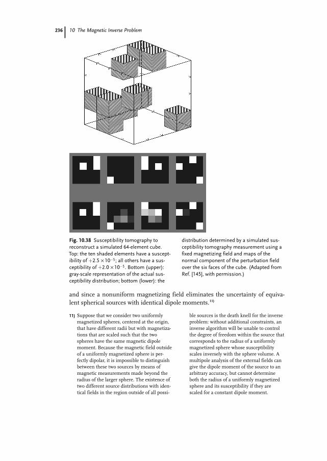
10 The Magnetic Inverse Problem
and since a nonuniform magnetizing field eliminates the uncertainty of equiva-lent spherical sources with identical dipole moments.11)
236
Fig. 10.38 Susceptibility tomography toreconstruct a simulated 64-element cube.Top: the ten shaded elements have a suscept-ibility of þ2:5 · 10�5; all others have a sus-ceptibility of þ2:0 · 10�5. Bottom (upper):gray-scale representation of the actual sus-ceptibility distribution; bottom (lower): the
distribution determined by a simulated sus-ceptibility tomography measurement using afixed magnetizing field and maps of thenormal component of the perturbation fieldover the six faces of the cube. (Adapted fromRef. [145], with permission.)
11) Suppose that we consider two uniformlymagnetized spheres, centered at the origin,that have different radii but with magnetiza-tions that are scaled such that the twospheres have the same magnetic dipolemoment. Because the magnetic field outsideof a uniformly magnetized sphere is per-fectly dipolar, it is impossible to distinguishbetween these two sources by means ofmagnetic measurements made beyond theradius of the larger sphere. The existence oftwo different source distributions with iden-tical fields in the region outside of all possi-
ble sources is the death knell for the inverseproblem: without additional constraints, aninverse algorithm will be unable to controlthe degree of freedom within the source thatcorresponds to the radius of a uniformlymagnetized sphere whose susceptibilityscales inversely with the sphere volume. Amultipole analysis of the external fields cangive the dipole moment of the source to anarbitrary accuracy, but cannot determineboth the radius of a uniformly magnetizedsphere and its susceptibility if they arescaled for a constant dipole moment.
10.3 The Magnetic Inverse Problem
Two- and three-dimensional magnetic susceptibility imaging offers potentialadvantages for imaging magnetically labeled flaws or composites impregnatedwith dilute magnetic tracers [137, 148, 149], for magnetic imaging of materialssuch as plastic, titanium, or aluminum that are normally considered nonmag-netic, monitoring macrophage activity [150, 151], and, with susceptibility tomogra-phy, three-dimensional magnetic images of metabolism and iron storage in theliver and possibly regional oxygenation of the brain. In particular, while magneticresonance imaging (MRI) is highly sensitive to spatial variations in magneticsusceptibility [152–155], the calibration of MRI susceptibility measurements foriron storage or other measurements of susceptibility effects in the body remainselusive, and hence SQUID susceptometry remains the gold standard [156–158].However, additional improvements to both SQUID instruments and algorithms[142–144, 159] will be required before magnetic susceptibility tomography cancompete with the more conventional, nonimaging methods for SQUID measure-ments of biosusceptibilities. Ongoing work in MRI inverse models and measure-ment protocols may eventually provide a noninvasive means for measuring bio-susceptibility distributions in humans [160].
10.3.4The Inverse Problem and Silent Sources
10.3.4.1 Introduction
In the preceding sections, we presented a wide variety of techniques for address-ing the magnetic inverse problem. The lack of a unique solution to the magneticor electric inverse problems is a general issue that applies to either field alone.However, in biomagnetism, the electric sources produce both electric and mag-netic fields. This coupling of the fields in turn leads to new complexities that wewill now explore. Sections 10.3.4.2 and 10.3.4.4 draw extensively from Ref. [13].
10.3.4.2 The Helmholtz DecompositionIn Section 10.2.4.2, we saw that the electric potential in an infinite homogeneousconductor is determined solely by the divergence of the primary current, while themagnetic field is determined by its curl. This leads to an interesting, and some-what controversial, observation about the primary current distribution. If ~JiJið~rrÞ isan arbitrary vector field, it can be represented by a Helmholtz decomposition [161]
~JiJið~rrÞ ¼ ~JiFJiFð~rrÞ þ ~Ji
VJiVð~rrÞ; where � · ~Ji
FJiFð~rrÞ ¼~00 and � � ~Ji
VJiVð~rrÞ ¼ 0: (10:230)
Thus ~JiFJiF has no curl and is called a “flow field,” while ~Ji
VJiV has no divergence and
is called a “vortex field.” In an infinite homogeneous conductor, represented byonly the first terms in (10.35) and (10.36) (i.e., ~KiKi ¼~00), the electric potential isthereby determined solely by the pattern of ~Ji
FJiF and the magnetic field only by the
237
10 The Magnetic Inverse Problem
pattern of ~JiVJiV ; if ~Ji
FJiF and ~Ji
VJiV are independent, then V and ~BB will likewise be indepen-
dent. This observation has been the basis for the controversy regarding possibleindependent information in the MCG. As we will see, the answer to this contro-versy may lie in the clarification of either the physiological constraints on ~JiJi, sinceany constraint that prevents ~JiJi from being the most general form of vector fieldwill also cause ~Ji
FJiF and ~Ji
VJiV to be related, or in the effects of inhomogeneities at the
cellular level.The question of constraints on ~JiJi can be addressed using a simple variable-
counting argument [22]. If the primary current distribution is a general vectorfield, it will have three degrees of freedom. The Helmholtz decomposition is sim-ply a statement that such a vector field can be described by a scalar potential withone degree of freedom (consistent with ~Ji
FJiF having no curl), and a vector potential
with two degrees of freedom (consistent with ~JiVJiV having no divergence). As first
pointed out by Rush [162], there are physiological constraints on ~JiJi that leave itwith less than three degrees of freedom. As a result, the electric and magneticfields cannot be completely independent.The question of independence becomes more complicated in a conductor with
boundaries or internal inhomogeneities. Then V is still determined solely by ~JiFJiF,
but ~BB now receives contributions from both ~JiVJiV and ~Ji
FJiF through the appearance of
V in the second term of the integrand in (10.36). The magnetic field contributionfrom ~Ji
VJiV may still contain independent information consistent with our preceding
discussion, but the contribution associated with the inhomogeneities is deter-mined by ~Ji
FJiF. This would provide a mixing of the information in the MCG and
ECG, which could be particularly important in situations where the second termof the integrand in (10.36) dominates the first. At first glance the second term isgoverned by V, which is described by ~Ji
FJiF. However, the integration of ~KiKi in both
equations incorporates the boundary geometry differently and the effect of the ge-ometry on the relative information content of these two integrals is not yet under-stood. Using the variable counting approach, the secondary source contributionshould contain at least two degrees of freedom, since V contains one and theboundary that specifies the orientation of the secondary sources will containanother. How these two or more degrees of freedom couple to the ECG and theMCG is in need of clarification.The ideal way to demonstrate the independence (or dependence) of the two inte-
grals on the boundary geometry would be to demonstrate (or to prove the nonexis-tence of) examples in which a particular boundary or internal inhomogeneityaffects either the electric field or the magnetic field from a particular source butnot both, i.e., an inhomogeneity that would be silent to only one of the two fields.A simple example is a horizontal current dipole in a conducting half spacebeneath a horizontal boundary: the normal component of the magnetic field inthe air above the boundary is not affected by the inhomogeneity but the electricfield above is. Many theoretical and experimental studies have compared theeffects of the geometry of macroscopic inhomogeneities on the MCG and ECGwith the hope of determining which measurement is least sensitive to the bound-ary and most sensitive to the primary sources. The situation is reversed at the cel-
238
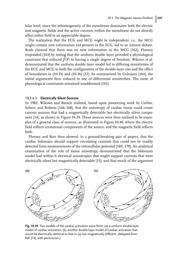
10.3 The Magnetic Inverse Problem
lular level, since the inhomogeneity of the membrane dominates both the electricand magnetic fields and the active currents within the membrane do not directlyaffect either field to an appreciable degree.The realization that the ECG and MCG might be independent, i.e., the MCG
might contain new information not present in the ECG, led to an intense debate.Rush claimed that there was no new information in the MCG [162], Plonseyresponded [163] by noting that the uniform double layer provided a physiologicalconstraint that reduced ~JiJi ~rrð Þ to having a single degree of freedom. Wikswo et al.demonstrated that the uniform double layer model led to differing sensitivities ofthe ECG and MCG to both the configuration of the double-layer rim and the effectof boundaries in (10.35) and (10.36) [22]. As summarized by Gulrajani [164], theinitial arguments then reduced to one of differential sensitivities. The issue ofphysiological constraints remained unaddressed [165].
10.3.4.3 Electrically Silent SourcesIn 1982, Wikswo and Barach realized, based upon pioneering work by Corbin,Scherr, and Roberts [166–168], that the anisotropy of cardiac tissue could createcurrent sources that had a magnetically detectable but electrically silent compo-nent [14], as shown in Figure 10.39. These sources were then realized to be exam-ples of a general class of sources, as illustrated in Figure 10.40, where the electricfield reflects irrotational components of the source, and the magnetic field reflectsboth.Plonsey and Barr then showed, in a ground-breaking pair of papers, that the
cardiac bidomain should support circulating currents that could not be readilydetected from measurements of the extracellular potential [169, 170]. An analyticalexamination of the role of tissue anisotropy demonstrated that the bidomainmodel had within it electrical anisotropies that might support currents that wereelectrically silent but magnetically detectable [15], and that much of the argument
239
Fig. 10.39 Two models of the cardiac activation wave front: (a) a uniform double-layermodel of cardiac activation; (b) another double-layer model of cardiac activation thatwould be electrically identical to that in (a) but magnetically different. (Adapted fromRef. [14], with permission.)
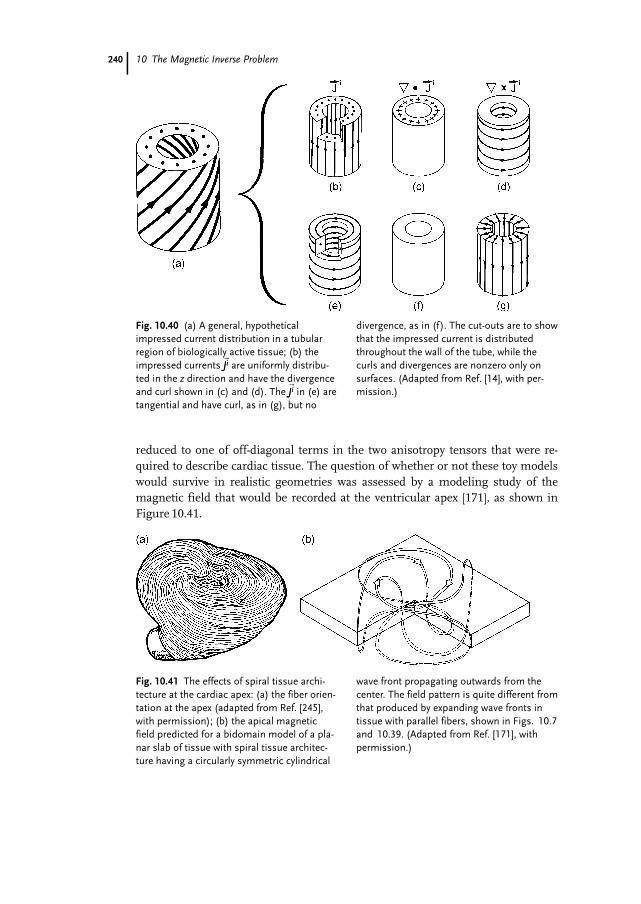
10 The Magnetic Inverse Problem
reduced to one of off-diagonal terms in the two anisotropy tensors that were re-quired to describe cardiac tissue. The question of whether or not these toy modelswould survive in realistic geometries was assessed by a modeling study of themagnetic field that would be recorded at the ventricular apex [171], as shown inFigure 10.41.
240
Fig. 10.40 (a) A general, hypotheticalimpressed current distribution in a tubularregion of biologically active tissue; (b) theimpressed currents~JiJi are uniformly distribu-ted in the z direction and have the divergenceand curl shown in (c) and (d). The~JiJi in (e) aretangential and have curl, as in (g), but no
divergence, as in (f). The cut-outs are to showthat the impressed current is distributedthroughout the wall of the tube, while thecurls and divergences are nonzero only onsurfaces. (Adapted from Ref. [14], with per-mission.)
Fig. 10.41 The effects of spiral tissue archi-tecture at the cardiac apex: (a) the fiber orien-tation at the apex (adapted from Ref. [245],with permission); (b) the apical magneticfield predicted for a bidomain model of a pla-nar slab of tissue with spiral tissue architec-ture having a circularly symmetric cylindrical
wave front propagating outwards from thecenter. The field pattern is quite different fromthat produced by expanding wave fronts intissue with parallel fibers, shown in Figs. 10.7and 10.39. (Adapted from Ref. [171], withpermission.)
10.3 The Magnetic Inverse Problem
From the perspective of the inverse problem, the issue then reduces to whetherthe appropriate model fitted to magnetic and electric data could distinguish be-tween these two types of cardiac sources, i.e., use the MCG to detect the effects ofspiral anisotropy that could not be discerned from the ECG [70]. To date, therehave yet to be incontrovertible demonstrations of new information in the humanMCG, although magnetic fields recorded from the surface of an isolated rabbitheart during stimulation and propagation of action potentials clearly support thebidomain model and its representation of the magnetic field [65, 172–175].
10.3.4.4 Multipole ExpansionsThe relation of the electric and magnetic fields of current sources is also presentin multipole expansions, as evidenced by the gray and black arrows representingdipole models in Figure 10.6. Both sets of current dipoles in the quadrupoleexpansion produce, in the appropriate limit, indistinguishable electric fields, butdifferent magnetic fields. In the simple multipole expansions discussed in Ref.[18], there is in fact a series of electrically silent multipole terms. To better demon-strate this point, we analyze the current multipole expansions for the electricpotential and magnetic field, such as the ones derived by Katila and Karp [176].These authors emphasized that the leading term of each expansion has the cur-rent dipole as its source, and therefore to first order the two measures of cardiacactivity yield identical information. Independently we have noted that the nextterm of the expansion has the current quadrupole coefficients aij appearing as thesource, but different combinations of aij enter the expression for Vð~rrÞ than for~BBð~rrÞ. In particular, the field depends on asymmetric terms of the quadrupole ten-sor that do not contribute to the potential. We shall briefly elaborate on this pointof view.The aij represent particular integrals of each Cartesian component of the current
density [176]
aij ¼Z
r ¢iJijð~r¢r¢Þdv¢; (10:231)
where both indexes i and j stand for any of the three axes x, y, and z, leading tonine possible combinations. The set of quadrupole terms can be arrayed in amatrix denoted by the symbol ~~AA~AA
~~AA~AA ¼axx axy axz
ayx ayy ayz
azx azy azz
24
35: (10:232Þ
Each of the terms can be represented by a pair of opposing dipoles placed side-by-side or in a line, with an appropriate distance of separation. The terms of thequadrupole tensor of (10.232) can thus be displayed pictorially as in Fig-ure 10.42(a). This tensor at first glance appears to have nine independent terms.
241
10 The Magnetic Inverse Problem
However, the sum of axx, ayy, and azz, known as the “trace” of the tensor, must beset equal to zero, because this sum must be electrically silent, i.e., the electricpotential outside this combined source would be zero everywhere, and the sum ofaxx, ayy, and azz would otherwise be indeterminate. Because of this constraint,there are only eight independent terms in the tensor. While the act of setting thetrace to zero will also modify the pictures in Figure 10.42(a) [177], we shall not dothis so as to simplify the discussion.We can write ~~AA~AA as the sum of symmetric and antisymmetric tensors
~~AA~AA ¼ ~~AA~AAs þ ~~AA~AA
a, (10.233)
where ~~AA~AAsand ~~AA~AA
aare given by combining ~~AA~AA with its mathematical transpose, indi-
cated by ~~AA~AAT
~~AA~AAs ¼ 1
2~~AA~AAþ ~~AA~AA
T� �
~~AA~AAa ¼ 1
2~~AA~AA� ~~AA~AA
T� �
: (10:234)
The pictorial representation of ~~AA~AA and ~~AA~AATis shown in Figures 10.42(b) and (c),
respectively. The symmetric tensor ~~AA~AAscontains combinations of aij that appear in
the current multipole expansion for the electrical potential distribution from a pri-mary current source. It contains five independent terms, when we take account ofthe constraint that the trace must be zero. The antisymmetric tensor ~~AA~AA
acontains
three independent terms, since the three terms in the lower left corner of Fig-ure 10.42(c) are simply the negative of the respective three terms in the upperright corner across the diagonal. We also see that these three terms in the currentquadrupole tensor represent current loops (magnetic dipoles) oriented normal tothe three axes of the Cartesian coordinate system. Each is electrically “silent,” so itis apparent that these three terms can be determined only by magnetic measure-ments and not by electric ones. One advantage of analyzing a field pattern withthe current multipole expansion, as opposed to the magnetic multipole expansion,is that it allows extraction of the maximal information from the magnetic fieldwhile also providing equivalent primary current generators that can be readilyinterpreted in terms of various physiological current source distributions.More sophisticated vector expansions of the source can also be obtained, which
contain electric-like and magnetic-like terms. The electric field depends only onthe former, whereas the magnetic field depends on both [165].
242
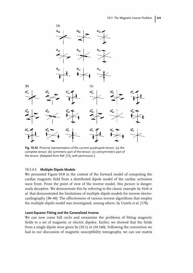
10.3 The Magnetic Inverse Problem
10.3.4.5 Multiple Dipole ModelsWe presented Figure 10.8 in the context of the forward model of computing thecardiac magnetic field from a distributed dipole model of the cardiac activationwave front. From the point of view of the inverse model, this picture is danger-ously deceptive. We demonstrate this by referring to the classic example by Holt etal. that demonstrated the limitations of multiple dipole models for inverse electro-cardiography [38–40]. The effectiveness of various inverse algorithms that employthe multiple dipole model was investigated, among others, by Uutela et al. [178].
Least-Squares Fitting and the Generalized InverseWe can now come full circle and reexamine the problems of fitting magneticfields to a set of magnetic or electric dipoles. Earlier, we showed that the fieldsfrom a single dipole were given by (10.1) or (10.160). Following the convention wehad in our discussion of magnetic susceptibility tomography, we can use matrix
243
Fig. 10.42 Pictorial representation of the current quadrupole tensor: (a) thecomplete tensor; (b) symmetric part of the tensor; (c) antisymmetric part ofthe tensor. (Adapted from Ref. [13], with permission.)
10 The Magnetic Inverse Problem
notation to write the magnetic field as the product of a Green’s function matrixand a source vector
~BB ~rrð Þ ¼Xmj¼1
~GG ~rr; ~r¢jr¢j� �
S ~r¢jr¢j� �
vj; (10:235)
where S ~r¢jr¢j� �
is either an electric or magnetic dipole at point ~r¢jr¢j . This becomes
~BB ¼ ~~GG~GG~SS: (10:236)
As before, if n ¼ m the system of equations will be exactly determined, but it maynot be possible to obtain a solution because of measurement noise, i.e., lineardependence of the n rows of ~~GG~GG. The alternative is to choose n > m, so that thesystem becomes over-determined, and we can proceed with the least-squares gen-eralized inverse solution
~SS ¼ ~~GG~GGT ~~GG~GG
h i�1 ~~GG~GGT~BB: (10:237)
The ability to compute the inverse of the ~~GG~GGT ~~GG~GG matrix is determined by the mea-
surement noise, by how well the measurements span the source space, and by thewell-conditioning of the G matrix. It may be that ~~GG~GG
T ~~GG~GG is sufficiently ill-condi-tioned or singular that its inverse cannot be computed, in which case one mustresort to SVD or some other regularization technique to determine those contri-butions to ~~GG~GG
T ~~GG~GG that can be determined by the measurement set. However, as wewill now show, physiological constraints on the source distribution may producecomputational problems far beyond what might be addressed with SVD. To showthis, we will now examine the multiple-dipole model of the cardiac activationwave front as shown in Figure 10.8.
Multiple Dipoles and Cardiac ActivationAs electrocardiography became more sophisticated and multiple recording leadsbecame available, there was great interest in moving beyond the simple dipolemodel of the heart [179–181]. The obvious next step was to use two dipoles, onefor each ventricle, and then multiple dipoles, such that the time dependence of asingle dipole might reflect regional ischemia or infarction, and hence the inver-sion of Figure 10.8 comes to the fore. As discovered when first attempted by Holtet al. [38–40], there are instabilities in the solutions that correspond to the additionand subtraction of dipole representations of spherical capacitors. Perturbing onedipole can be balanced by a corresponding antiperturbation of all other dipoles.The obvious solution is to constrain the orientation of the dipole, through quadrat-ic programming, so that their orientation cannot reverse. This corresponds to theaddition of physiological constraints to a model, something that has been popularin MEG analyses of cortical sources. However, it must remembered that at least inthe uniform double-layer model of cardiac activation, any perturbation of the wave
244
10.3 The Magnetic Inverse Problem
front that does not affect the shape of the rim will not affect the external poten-tials, so physiological constraints such as a priori knowledge of wave front geome-try will help, if at all, only as long as the actual geometry for the disease subject isclose to what was assumed in creating the model. The situation is even more com-plicated when we consider the bidomain effects discussed above.
10.3.5Three-Dimensional Inverse Algorithms
10.3.5.1 Introduction
In the cases presented up to this point, we generally considered only the simplestconstraints with respect to whether an object is two- or three-dimensional, orwhether we know where the current is injected and withdrawn, or what theboundary conditions are. For the MEG and to some extent the MCG, physiologicalinformation, obtained by MRI or other imaging modalities, can provide valuableinformation. One must be cautious, particularly when dealing with pathologicalconditions, that the data from a patient are not interpreted solely on the basis of amodel designed for normal subjects. The question then reduces to one of decidingwhere best to place the uncertainties intrinsic to the magnetic inverse problem:stable solutions that specify diffuse effective sources, or highly localized modelsthat may be overly simplistic. Undoubtedly, the best results will be obtained if thegreatest amount of complementary information can be included in the analysis.There are a number of three-dimensional inverse algorithms, such as beamfor-
mers, minimum norm techniques, the focal undetermined system solver, multi-ple signal classification, principal and independent component analysis, low-reso-lution electromagnetic tomography, magnetic field tomography, etc. (Some ofthose techniques have been reviewed in the context of magnetocardiography inRef. [182].) The remainder of this section briefly reviews these important meth-ods, which are further discussed in Chapter 11. It must be emphasized that noneof these techniques can create new information beyond what is provided to themodel. It should also be mentioned that the three-dimensional techniques dis-cussed below can be applied in the context of both the current and magneticdipole models, provided of course that appropriate modifications are made toaccommodate the two formalisms.
10.3.5.2 BeamformersBeamformers [183, 184] are spatial filters that were originally introduced in tele-communications [185] to provide an efficient method for the estimation of signalsoriginating from a source located in a certain direction in the presence of noiseand other signals. Their purpose is to spatially filter signals that have overlappingtemporal frequencies but distinct sources. Historically, the term originates fromthe fact that early spatial filters were akin to pencil beams that preferentiallyallowed signals from a specific location to be received by a detector, while others
245
10 The Magnetic Inverse Problem
were attenuated [183]. The use of beamformers in biomagnetism was pioneeredby van Veen, van Drongelen et al. [183, 186], and Robinson and Vrba [187].Through the use of multiple beamformers with different passbands, one can
construct a neural power map that depicts neural power as a function of passbandlocation [183]. Beamformer outputs are formed as weighted sums of sensorresponses that specify spatial filtering features and increase sensitivity to signalsfrom a preferred location. Strategies for determining the optimal set of weightslead to various distinct implementations of the beamformer method, includingthe linearly constrained minimum-variance (LCMV) [188] and nonlinearly con-strained beamformers [187] used in synthetic aperture magnetometry (SAM). Inthe latter case, weights are computed for a unique orientation of the target sourcevia a nonlinear optimization process that seeks to maximize the neural activityindex, also known as the pseudo-Z statistic [189]. Various other adaptations of thismethod exist, including, for example, adaptive beamformers [190, 191].
10.3.5.3 Minimum Norm TechniquesMinimum norm techniques are optimal when minimal a priori information aboutthe source is provided [192]. In this approach, the inverse problem is addressedusing a combination of magnetometer lead fields to estimate the primary currentdistribution. As already explained in this chapter, one can write, in terms of thecurrent dipole~PP,
Bið~r¢r¢Þ ¼~LLið~r¢r¢Þ �~PP;
where Bi is the field component parallel to ~LLi measured at location i of the mag-netometer coil, and ~LLi is the lead field associated with that location. Primary cur-rent distributions can be considered as elements of a so-called current space Fthat includes all square-integrable current distributions whose locations are lim-ited to the conductor V. Since the field measurements Bi only convey informationabout a subspace F ¢ of F, it follows that this subspace is spanned by the lead fields.One can define the inner product of two currents~JJ1 and~JJ2 in F as
~JJ1;~JJ267¼ZV
~JJ1ð~rrÞ �~JJ2ð~rrÞd3r (10:238)
with norm
~JJk
// //2¼ ZV
~JJkð~rrÞ�� ��2d3r (10:239)
The basic idea of the minimum norm technique is to identify an estimate J* thatis a linear combination of lead fields
246
10.3 The Magnetic Inverse Problem
~JJ* ¼XMj¼1
wj~LLj; (10:240)
where wj are real coefficients. Such an estimate must be confined to F ¢ and mustalso reproduce the measured signals Bi. The process described above can be car-ried out by solving the set of linear equations
~bb ¼ ~~CC~CC ~ww; (10:241)
where
~bb ¼ ðB1; :::;BmÞT (10:242)
is the set of measured data,
~ww ¼ ðw1; :::;wmÞT (10:243)
is the set of lead field coefficients to be found, and ~~CC~CC is an m · m matrix withentries that are lead field inner products of the form
C ij ¼ ~LLi;~LLj
ED(10:244)
Solutions to this set of equations are not unique because any current~JJ? satisfyingthe equality ~JJ?;~LLi
67= 0 (i.e., perpendicular to the lead field~LLi) can be added to~JJ*,
yielding another solution to our set of equations. The physical meaning of thisstatement is that any current distribution that the magnetometer cannot detectcan be added to the solution [192]. Mathematically, ~~CC~CC is nonsingular if the leadfields are linearly independent. In practical situations, however, this is not thecase: ~~CC~CC can have very small eigenvalues, which leads to large errors in the calcula-tion of the lead field coefficients wj. In such cases, a regularization method can beapplied, as discussed in a previous section of this chapter. Two minimum normalgorithms worth mentioning are the L1 and L2 norms, where L1 is characterizedby a limited number of focused sources, while L2 (also known as minimum normleast squares or MNLS) is associated with a broad distribution of many sources[193].The value and effectiveness of classic minimum norm techniques has been rec-
ognized in the EEG and MEG community particularly in cases where a priorisource information is not available and/or very noisy data are analyzed. It hasbeen shown that, although these methods are generally unable to accuratelyretrieve the depth of sources, they are quite effective at reconstructing two-dimen-sional projections of current distributions [192, 194–196].
247
10 The Magnetic Inverse Problem
10.3.5.4 FOCUSSThe FOCal Undetermined System Solver (FOCUSS) algorithm [197, 198] is atomographic reconstruction method that aims to tame the major problem asso-ciated with typical minimum norm techniques: the lack of spatial resolutionresulting in diffuse solutions, especially for deeper sources. In this method, adipole is assigned to each voxel of the reconstruction volume, meaning that thenonlinear position parameters are completely specified. The Cartesian compo-nents of the dipole moments are thus the only unknowns to be estimated, andthey are linearly related to the measurements. Provided that we make a suffi-ciently fine sampling of the volume relative to the spatial smoothness of thesource distribution, the accuracy of the method is limited mainly by noise andother modeling errors. In some applications, such as MEG, it may be advanta-geous to use spherical coordinates and to recover only the two orthogonal vectorcomponents of the moment tangential to the radius of the sphere. In this way, weavoid the ill-posedness associated with radially oriented currents in the head,which cannot be observed with external field measurements, as discussed pre-viously. For time-varying fields, reconstructions are calculated for each time slice.The major strength of the FOCUSS algorithm lies in the reconstruction of local-
ized sources. Unlike minimum norm estimates, which tend to produce manynonzero dipoles corresponding to a dispersion of the sources over a large volume,FOCUSS only selects a small number of elements that can generate the observedfield.We can express the system of linear equations in matrix form. Assuming a Car-
tesian coordinate system and numbering the dipole components sequentially, wehave
~bb ¼ ~~GG~GG~pp, (10.245)
or
b1...
bm
264
375 ¼ G1;x G1;y G1;z G2;x G2;y . . . Gn=3;z
� � p1...
pn
264
375 (10:246)
where ~bb is an m U 1 vector containing m measurements of a magnetic field com-ponent, ~~GG~GG is the m U n basis matrix or Green’s function matrix, whose elementsare determined by the model geometry, and ~pp is an n U 1 vector containing the nunknown components of n/ 3 dipoles. Since ~~GG~GG depends solely on the geometry ofthe sources and sensors, it needs to be calculated only once for a particular config-uration, allowing for realistic, complex, and detailed modeling.In essence, the algorithm starts with a distributed estimate, which can be
obtained, for example, by the minimum norm method. Then, FOCUSS recur-sively enhances some of the sources while attenuating the rest of the elementsuntil they become zero. Only a small number of dipoles is therefore selected,
248

10.3 The Magnetic Inverse Problem
yielding a localized energy solution. Specifically, at each iteration of the algorithm,a solution is obtained by means of the weighted minimum norm
~pp ¼ ~~WW~WW ~~GG~GG ~~WW~WW� �þ
~bb ¼ ~~WW~WW ~~WW~WWT ~~GG~GG
T ~~GG~GG ~~WW~WW ~~WW~WWT ~~GG~GG
T� ��1
~bb; (10:247)
where + stands for the Moore–Penrose inverse, or pseudo-inverse, of a matrix and~~WW~WW is an n U n weighting matrix comprised of dimensionless scaling factors, whosepurpose is to enhance some of the elements in ~pp. At each step, only ~~WW~WW is changed,leading to a new (partial) solution.Different definitions of ~~WW~WW are possible, but a common choice is to make it a
diagonal matrix whose elements are the elements of ~pp obtained in the previousiteration. Another choice, which proves to be more robust, consists of defining ~~WW~WWas the compound product of the weighting matrices obtained in the precedingsteps. FOCUSS stops when the solution ~pp no longer changes, and it has beenshown that the algorithm always converges to a localized solution with no morethan m nonzero elements [198].Since FOCUSS is an initialization-dependent algorithm, care should be taken
in calculating this particular step. An unbiased minimum norm solution, whichcompensates for the bias associated with the magnetic field falloff, may be used toprovide an initialization within proximity of the true sources. In addition, inmany applications, the matrix ~~GG~GG is ill-conditioned, thereby requiring the use ofsome regularization technique to achieve a compromise between stability and aclose fit to the data. Truncated SVD, where singular values below a certain thresh-old are discarded, may be used to address this problem.
10.3.5.5 MUSICThe MUSIC algorithm was first proposed by Schmidt [199] to address the process-ing of signals from sensors with arbitrary locations and directional characteristics.It was then applied to biomagnetism by Mosher and co-workers [200, 201]; in ourdescription of this method, we rely heavily on their work. Because our discussionis nevertheless introductory in nature, we refer the reader to the original literature[199, 200] for a detailed description of the method.Let the m U n matrix ~~FF~FF contain the spatiotemporal data for n time samples and
m SQUID magnetometer channels. One can define an m U r “hybrid” gain matrix~~HH~HH that represents some mix of rotating or fixed dipoles in a noisy data model; therank of ~~HH~HH is equal to R = 2pR + pF, where pR and pF represent the number of rotat-ing and fixed dipoles, respectively, for a total number of p dipoles. ~~HH~HH contains the3p unknown location parameters of these dipoles as well as the corresponding pFunknown constraint moment parameters.The matrix equation for this model assumes the form
~~FF~FF ¼ ~~HH~HH~~SS~SSþ ~~NN~NN; (10:248)
249
10 The Magnetic Inverse Problem
where ~~FF~FF contains the magnetometer data, ~~SS~SS is a scalar time series matrix, and ~~NN~NNrepresents the error between the measurements and our model; dimensionally, ~~SS~SSis r U n. In MUSIC, ~~HH~HH is assumed to be of full column rank r for p dipoles. Let ~~RR~RRF
denote a square symmetric matrix representing the spatial autocorrelation of thedata, which can be computed using
~~RR~RRF ¼ E ~~FF~FF~~FF~FFTon; (10:249)
where E �gf is the expectation operator. Then ~~RR~RRF can be written in terms of itseigendecomposition
~~RR~RRF ¼ ~~UU~UU~~KK~KK~~UU~UUT ¼ ~~UU~UUs
~~UU~UUn
h i ~~KK~KKs~~KK~KKn
" #~~UU~UUs
~~UU~UUn
h iT; (10:250)
where ~~KK~KKs is a diagonal matrix containing the largest R eigenvalues, while ~~UU~UUs con-tains the corresponding eigenvectors. One assumption of the MUSIC algorithm isthat the additive noise in the data is white and that it has a temporal and spatialmean of zero; this condition can be used to show that ~~KK~KKn ¼ r~~II~II, where r is thenoise variance [200]. This variance is also equal to an eigenvalue k with multipli-city m–r, which can be used to show that ~~UU~UUn contains the remaining m–r eigenva-lues. The MUSIC algorithm computes the eigendecomposition
~~RR~RR~~RR~RRF ¼1N
~~FF~FF~~FF~FFT ¼ ~~UU~UU~~UU~UU ~~KK~KK~~KK~KK ~~UU~UU~~UU~UU
T; (10:251)
where ~~RR~RR~~RR~RRF is the data estimate of ~~RR~RRF (the caret throughout this section refers todata estimate matrices of statistical quantities). The algorithm then orders theeigenvalues k1; :::; km thus computed in descending order of their magnitude andfinds a separation point D between the signal and noise subspace eigenvalues(where 1£D < m) based on the criterion that a distinct drop in eigenvalue magni-tude occurs between kD and kDþ1 (see also Ref. [202] on alternative critera forselecting the separation point). Next, the m U 2 gain matrix ~~GG~GGi is computed over afine grid of three-dimensional locations. For each entry in this matrix, the princi-pal left eigenvectors ~~UU~UUGi
of ~~GG~GGi are computed using an SVD of the form
~~GG~GGi ¼ ~~UU~UUGi
~~RR~RRGi
~~VV~VVTGi: (10:252)
This in turn allows one to compute
JhðiÞ ¼ kmin~~UU~UUTGi
~~UU~UU~~UU~UUT
n~~UU~UU~~UU~UUn
~~UU~UUGi
'&; (10:253)
250
10.3 The Magnetic Inverse Problem
i.e., the minimum eigenvalue of the expression in brackets. If, at each minimumof Jh, the subspace of ~~GG~GGi is orthogonal to the noise subspace, then the dipole isrotating. An alternative way of determining this is by computing the cost function
JrðiÞ ¼
~~UU~UU~~UU~UUT
n~~UU~UUGi
~~RR~RRGi
////////2F
~~RR~RRGi
/// ///2F
; (10:254)
where the subscript F refers to the Frobenius norm;12) in this case, a rotatingdipole satisfies JhðiÞ » JrðiÞ » 0. If the location of the dipole is fixed (JhðiÞ » 0,JrðiÞ „ 0), its orientation can be estimated by computing the eigenvector of kmin.The process described above is then repeated until pR rotating dipoles and pF fixeddipoles are found such that R = 2pR + pF. Refinement of the solution can beachieved by further application of the same algorithm on a finer local grid.
10.3.5.6 Principal and Independent Component AnalysisAnother method related to MUSIC that has been used perhaps less successfully[203, 204] is the principal component analysis (PCA) algorithm. In this approach,the data matrix ~~FF~FF is first decomposed using the SVD
~~FF~FF ¼ ~~UU~UU ~~RR~RR~~VV~VVT: (10:255)
The columns of ~~UU~UU contain information referring to the spatial distribution of prin-cipal components while those of ~~VV~VV are the corresponding time functions. If oneforms the matrix ~~RR~RR ¢ containing only the R principal singular terms, the ith dipolelocation and moment can be found from a least squares minimization of thequantity
min~LLi; ~QQi
~~GG~GGið~LLiÞ ~QQi � ~~UU~UU ~~RR~RR¢~~CC~CCi
////// 2
2; (10:256)
where ~~GG~GGið~LLiÞ is the usual gain matrix for a dipole at location ~LLi with componentsspecified by ~QQi. Several methods exist for choosing the so-called rotation factorsClmgf [205, 206]; the error in the equation above can be written as [200]
JPCAðiÞ ¼ ~~UU~UU ~~RR~RR ¢~~CC~CCi � ~~GG~GGi~QQ////// 2
2¼ ~~PP~PP
?Gi
~~UU~UU ~~RR~RR¢~~CC~CCi
////// 2
2; (10:257)
where ~~PP~PP?Gi
is the orthogonal projection for a unique dipole.
251
12) The Frobenius norm of an m U n matrix ~~AA~AA is
defined as ~~AA~AA//////F¼
ffiffiffiffiffiffiffiffiffiffiffiffiffiffiffiffiffiffiffiffiffiffiffiPmi¼1
Pnj¼1
aij
��� ���2s
.
10 The Magnetic Inverse Problem
Independent component analysis (ICA) is an extension of PCA that was devel-oped in relation to the blind source separation (BSS) problem, where ICA is verycommon [207, 208]. Several ICA algorithms exist, such as SOBI [209], Infomax[210], and fICA [211]; the fundamental assumption common to all of these, how-ever, is that distinct sources generate uncorrelated (i.e., unrelated) and statisticallyindependent signals. The process of finding an appropriate set of such signals iscarried out in ICA by minimizing a measure of joint entropy of the signals underconsideration. Another assumption of this technique which has been criticized asa weakness is that the number of sources cannot exceed the number of sensors[212]. However, to have more sources than sensors (as in a fixed MEG measure-ment, for example) would violate our principle of a model not creating new infor-mation.Two phases are involved in ICA: learning and processing. In the first of these, a
weighting matrix ~~WW~WW is found, which minimizes the mutual information betweenchannels. This process effectively makes output signals that are statistically inde-pendent, such that the multivariate probability density function of the input sig-nals f becomes equal to
f ¼Y
i
fi ; (10:258)
i.e., to the product of probability density functions of every independent variable[213]. In the second phase of ICA, the matrix ~~WW~WW is applied to the signal subspacedata and the parameters of the dipoles are found using a search method (e.g., thesimplex algorithm). A very common application of ICA is in EEG, where themethod is used, for example, to recover brain signals associated with the detectionof visual targets [212, 214] or to extract ocular artifacts from EEG data [215, 216].Detailed theoretical discussions of both BSS and ICA are provided in Refs. [208,217, 218].
10.3.5.7 Signal Space ProjectionIn the signal space projection (SSP) approach, the magnetic field signals mi ,i = 1, … m, are assumed to form a time-dependent signal vector ~mmðtÞ in anm-dimensional signal space. The measured signal vector ~mmðtÞ can be written as
~mmðtÞ ¼XMi¼1
aiðtÞ~ssi þ ~nnðtÞ; (10:259)
where ~ssi are the elements of an orthonormal basis spanning the m-dimensionalmagnetic signal space F, aiðtÞ contains the time-dependence information of ~ssi,and ~nnðtÞ is the noise. Because ~ssi are basis objects spanning F that specify the orien-tations of the field vectors, the former are held fixed. In other words, as HZmZlZi-nen and Ilmoniemi put it, “each source corresponds to a constant output patternwhose amplitude changes with time” [192]. One advantage of this approach over
252
10.3 The Magnetic Inverse Problem
other methods such as PCA is that, if the aiðtÞ coefficients are estimated directlyfrom ~mmðtÞ, no conductivity or source model is required [219].The SSP method was introduced by Ilmoniemi et al. [220] and was applied for
the first time by Miettinen [221]. To carry out SSP, two projection operators, ~~PP~PP?and ~~PP~PPk, are required to divide the signal ~mmðtÞ into two parts ~ss? and ~ssk, respectively.The first part contains information belonging to the subspace spanned by compo-nent vectors 1, … , k and the matrix ~~KK~KK ¼ ~ss1 ~ss2 ::: ~ssk Þð is associated with it. Thesecond part ~ssk cannot be reproduced by any of the sources in ~~KK~KK. Thus
~ssk ¼ ~~PP~PPk ~mm and ~ss? ¼ ~~PP~PP? ~mm: (10:260)
The matrix representations of the operators ~~PP~PP? and ~~PP~PPk can be computed using theSVD of ~~KK~KK
~~KK~KK ¼ ~~UU~UU ~~KK~KK~~VV~VVT: (10:261)
The first k columns of the matrix ~~UU~UU form an orthonormal basis for the columnspace of ~~KK~KK, yielding the results
~~PP~PPk ¼ ~~UU~UUk~~UU~UUTk (10:262)
and
~~PP~PP? ¼ ~~II~II � ~~PP~PPk: (10:263)
The data estimates ~aa~aaðtÞ of the theoretical amplitudes aiðtÞ are then computedfrom
~aa~aaðtÞ ¼ ~~VV~VV ~~KK~KK�1 ~~UU~UU
T~mmðtÞ: (10:264)
The operators ~~PP~PP? and ~~PP~PPk effectively form a spatial filter since they allow one toisolate signals that were generated only by the sources of interest. If the sourcesincluded in ~~KK~KK are only artifact-related, the information contained in the artifact-free signal can be separated into ~ss?. For this reason, the SSP method is particular-ly valuable as an artifact removal tool [222, 223] and has been used as such in avariety of applications [192, 224–226] including, among others, neuronal sourcecharacterization [227] and gastrointestinal inverses [47].
10.3.5.8 Other Three-Dimensional MethodsLORETA (low resolution electromagnetic tomography) was introduced by Pascual-Marqui et al. [228], who proposed that the inverse solution describing the currentdensity throughout the full volume of the conductor can be selected based on thecriterion of smoothness associated with the spatial distribution of sources. Mathe-matically, this method minimizes the squared norm of the Laplacian of the
253
10 The Magnetic Inverse Problem
weighted three-dimensional current density vector field [229]. One of the demon-strated advantages of this algorithm is that it provides small localization errors fordeep sources; the method has been applied successfully to study auditory event-related potentials [230] and epileptiform activity [229]. A more recent algorithm,dubbed standardized LORETA (sLORETA) [191, 231, 232], does not use the Lapla-cian as a measure of spatial smoothness in computing the inverse solution. Itrelies instead on the calculation of statistical maps indicating the probable loca-tions of sources. The performance of this method under the presence of noise isevaluated in Ref. [232].Many other inverse techniques exist, such as the maximum entropy of the
mean (MEM) method of Clarke and Janday [233, 234], probabilistic reconstructionof multiple sources (PROMS) [235], and magnetic field tomography (MFT) [236],all of which make use of probabilistic methods to estimate the detectableimpressed current ~JiJi. In MFT [110], the value of the impressed current is com-puted independently for each time slice; the method is also best adapted to thedetection of distributed sources. In the Bayesian approach [237, 238] the priorknowledge regarding the nature of the sources is represented as a prior probabil-ity, which is combined with a probabilistic description of the data to compute aposterior distribution by making use of Bayes’ theorem; the optimal distributionof sources maximizes this probabilistic quantity.As a final remark, it is interesting to note that most common linear inverse
algorithms are highly related at a theoretical level and differ mostly in how thesource covariance matrix of the data is constructed. As demonstrated by Mosheret al. [239], the method of estimating data and noise covariances used in a particu-lar technique is important because many minimum norm algorithms are inti-mately dependent on these parameters. Conceptually, this is essential because theestimation of covariances is strongly related to the distinction between data andnoise, which plays a vital role in the source recovery process.
10.4Conclusions
Very few of the peculiarities or techniques described above to solve the magneticinverse problem are unique to SQUID magnetometers, but in fact arise from thenature of the fields themselves. SQUIDs are among the most sensitive magnet-ometers, and all of this sensitivity is generally required to measure biomagneticfields. With few exceptions, the biomagnetic inverse problem is a three-dimen-sional one, and has no unique solution. As a result, a wide range of techniques isutilized to convert biomagnetic images into approximations or constraineddescriptions of bioelectric sources. The NDE and geomagnetic applications ofSQUIDs are more forgiving, in that often the samples are two-dimensional, forwhich there are unique inverse solutions, or applied fields can be controlled in amanner that provides additional information required to solve the inverse prob-lem. It is important to realize, however, that many of the techniques outlined in
254
References
this chapter, even in their present rudimentary state of development, can be usedto analyze field images obtained from optical, fluxgate, Hall probe, and magnetor-esistive magnetometers. Given the promise of these and other advanced imagingtechniques, it is enticing to consider the future use of SQUID cameras basedupon digital SQUID techniques to provide a thousand integrated digital magnet-ometers on a single chip [240, 241], or imaging optical magnetometers [242].Meanwhile, there is much work that can be done to explore even more fully themathematics and experimental techniques of magnetic imaging with SQUIDsand other magnetometers.
Acknowledgments
Much of the research described within this chapter was funded by grants from theAir Force Office of Scientific Research, the Electric Power Research Institute, andthe National Institutes of Health. We are indebted to Afshin Abedi, John Barach,Alan Bradshaw, James Cadzow, Anthony Ewing, Luis Fong, Jenny Holzer, WilliamJenks, Xangkang Li, Yu Pei Ma, Bradley Roth, Nestor Sepulveda, Daniel Staton,Shaofen Tan, and Ian Thomas for their major contributions to the Vanderbiltmagnetic imaging effort, and their papers from which we have drawn heavily inpreparing this chapter. We thank Hans Koch and Wolfgang Haberkorn for provid-ing the historical background on the nonuniqueness of the inverse problem solu-tion. We also thank William Jenks, Margaret Khayat, Eduardo Parente Ribeiro,Daniel Staton, and Leonora Wikswo for their comments on predecessors of thismanuscript, and Licheng Li for her care in preparing many of the illustrations.We especially thank Harold Weinstock for his encouragement and support of thisresearch. We are deeply indebted to Don Berry, Cheryl Cosby, and Allison Pricefor their unflagging assistance and attention to detail in preparing the manuscriptfor this chapter, including but not limited to maintaining the reference database,typing the many equations, revising or creating each of the drawings, and verycareful editing.
255
References
1 Helmholtz, H. (1853) Ueber einigeGesetze der Vertheilung elektrischerStrWme in kWrperlichen Leitern mitAnwendung auf die thierisch-elektri-schen Versuche, Ann. Phys. Chem. 89,211–233, 353–377.
2 Braginski, A.I. (2005) Personal commu-nication.
3 Bradshaw, L.A. and Wikswo, J.P., Jr.(1999) Vector or scalar magnetometerarrays?, in Proceedings of the First Joint
BMES/EMBS Conference, Vol. 2, Atlanta,GA, p. 888.
4 Nalbach, M. and Dossel, O. (2002) Com-parison of sensor arrangements ofMCG and ECGwith respect to informa-tion content, Physica C 372, 254–258.
5 Baudenbacher, F., Peters, N. T. andWikswo, J. P., Jr. (2002) High resolutionlow-temperature superconductivitysuperconducting quantum interferencedevice microscope for imaging mag-
10 The Magnetic Inverse Problem256
netic fields of samples at room tempera-tures, Rev. Sci. Instrum. 73, 1247–1254.
6 Fong, L. E., Holzer, J. R., McBride, K. K.,Lima, E. A., Baudenbacher, F. and Rad-parvar, M. (2005) High-resolution room-temperature sample scanning supercon-ducting quantum interference devicemicroscope configurable for geologicaland biomagnetic applications, Rev. Sci.Instrum. 76, 053703.
7 Cohen, D., Edelsack, E. A. and Zimmer-man, J. E. (1970) Magnetocardiogramstaken inside a shielded room with asuperconducting point-contact magnet-ometer, Appl. Phys. Lett. 16, 278–280.
8 Weiss, B. P., Kirschvink, J. L., Bauden-bacher, F. J., Vali, H., Peters, N. T., Mac-donald, F. A. and Wikswo, J. P. (2000) Alow temperature transfer of ALH84001from Mars to Earth, Science 290,791–795.
9 Wikswo, J. P., Jr. (1996) The magneticinverse problem for NDE, in SQUIDSensors: Fundamentals, Fabrication andApplications, Weinstock, H. (ed.),Kluwer, The Netherlands, pp. 629–695.
10 Ma, Y. P., Thomas, I. M., Lauder, A. andWikswo, J. P., Jr. (1993) A high resolu-tion imaging susceptometer, IEEETrans. Appl. Supercond. 3, 1941–1944.
11 Wikswo, J. P., Jr. (1978) The calculationof the magnetic field from a current dis-tribution: application to finite elementtechniques, IEEE Trans. Magn. Mag14,1076–1077.
12 Geselowitz, D. B. (1970) On the mag-netic field generated outside an inho-mogeneous volume conductor by inter-nal current sources, IEEE Trans. Magn.Mag6, 346–347.
13 Wikswo, J. P., Jr. (1983) Theoreticalaspects of the EEG-MEG relationship,in Biomagnetism: An InterdisciplinaryApproach, Williamson, S. J., Romani,G.-L., Kaufman, L. and Modena, I.(eds.), Plenum, New York, pp. 311–326.
14 Wikswo, J. P., Jr. and Barach, J. P.(1982) Possible sources of new informa-tion in the magnetocardiogram, J. Theor.Biol. 95, 721–729.
15 Roth, B. J. and Wikswo, J. P., Jr. (1986)Electrically silent magnetic fields,Biophys. J. 50, 739–745.
16 Demunck, J. C., Vandijk, B. W. andSpekreijse, H. (1988) Mathematicaldipoles are adequate to describe realisticgenerators of human-brain activity,IEEE Trans. Biomed. Eng. 35, 960–966.
17 Williamson, S. J. and Kaufman, L.(1981) Biomagnetism topical review,J. Magn. Magn. Mater. 22, 129–201.
18 Wikswo, J. P., Jr. and Swinney, K. R.(1985) Scalar multipole expansions andtheir dipole equivalents, J. Appl. Phys.57, 4301–4308.
19 Brody, D. A. (1968) The inverse determi-nation of simple generator configura-tions from equivalent dipole and multi-pole information, IEEE Trans. Biomed.Eng. BME15, 106–110.
20 Horacek, B. M. (1973) Digital model forstudies in magnetocardiography, IEEETrans. Magn. Mag9, 440–444.
21 Grynszpan, F. (1971) Relationship be-tween the surface electromagnetic fieldsand the electrical activity of the heart,Ph.D. Dissertation, University of Penn-sylvania.
22 Wikswo, J. P., Jr., Malmivuo, J. A. V.,Barry, W. H., Leifer, M. C. and Fairbank,W. M. (1979) The theory and applicationof magnetocardiography, in Advances inCardiovascular Physics, Vol. 2. Ghista,D. N., Vollenhoven, V. E. and Yang, W.(eds.), Karger, Basel/New York, pp. 1–67.
23 Jackson, J. D. (1975) Classical Electrody-namics, Wiley, New York.
24 Cohen, D. and Hosaka, H. (1976) Mag-netic field produced by a current dipole,J. Electrocardiol. 9, 409–417.
25 Wikswo, J. P., Jr. and Swinney, K. R.(1984) A comparison of scalar multipoleexpansions, J. Appl. Phys. 56,3039–3049.
26 Castellanos, A., Panizo, M. and Rivas, J.(1978) Magnetostatic multipoles in car-tesian coordinates, Am. J. Phys. 46,1116–1117.
27 Gonzalez, H., Juarez, S. R., Kiela-nowski, P. and Loewe, M. (1998) Multi-pole expansion in magnetostatics, Am. J.Phys. 66, 228–231.
28 Geselowitz, D. B. (1965) Two theoremsconcerning the quadrupole applicable toelectrocardiography, IEEE Trans.Biomed. Eng. BM12, 164–168.
References 257
29 Gray, C. G. (1978) Simplified derivationof magnetostatic multipole expansionusing scalar potential, Am. J. Phys. 46,582–583.
30 Gray, C. G. (1979) Magnetic multipoleexpansions using the scalar potential,Am. J. Phys. 47, 457–459.
31 Gray, C. G. (1980) Definition of themagnetic quadrupole-moment, Am. J.Phys. 48, 984–985.
32 Nolte, G. and Curio, G. (1997) On thecalculation of magnetic fields based onmultipole modeling of focal biologicalcurrent sources, Biophys. J. 73,1253–1262.
33 Mosher, J. C., Leahy, R. M., Shattuck,D. W. and Baillet, S. (1999) MEG sourceimaging using multipolar expansions,in Information Processing in Medical Im-aging: 16th International Conference,IPMI ’99, Visegrad, Hungary, Kuba, A.,Samal, M. and Todd–Pokropek, A.(eds.), Springer, Berlin/New York,pp. 15–28.
34 Jerbi, K., Mosher, J. C., Baillet, S. andLeahy, R. M. (2002) On MEG forwardmodelling using multipolar expansions,Phys. Med. Biol. 47, 523–555.
35 Jerbi, K., Baillet, S., Mosher, J. C., Nolte,G., Garnero, L. and Leahy, R. M. (2004)Localization of realistic cortical activityin MEG using current multipoles, Neu-roImage 22, 779–793.
36 Ermer, J. J., Mosher, J. C., Baillet, S. andLeahy, R. M. (2001) Rapidly recomputa-ble EEG forward models for realistichead shapes, Phys. Med. Biol. 46,1265–1281.
37 Brody, D. A. and Bradshaw, J. C. (1962)The equivalent generator componentsof uniform double layers, Bull. Math.Biophys. 24, 183–195.
38 Lynn, M. S., Barnard, A. C. L. and Holt,J. H. (1967) A proposed method for theinverse problem in electrocardiology,Biophys. J. 7, 925–945.
39 Holt, J. H., Barnard, A. C. L. and Lynn,M. S. (1969) A study of the human heartas a multiple dipole electrical source; II.Diagnosis and quantitation of left ven-tricular hypertrophy, Circulation 40,697–718.
40 Holt, J. H. and Barnard, A. C. L. (1973)Body surface potentials in ventricular
hypertrophy – analysis using a multi-pole dipole model of the heart, in Com-puter application on ECG and VCG analy-sis, Proceedings of the 2nd IFIP TC-4Working Conference on Computer Applica-tion on ECG and VCG Analysis, NorthHolland, Amsterdam, pp. 333–349.
41 Wikswo, J. P., Jr., Gevins, A. and Wil-liamson, S. J. (1993) The future of theEEG and MEG, Electroencephalogr. Clin.Neurophysiol. 87, 1–9.
42 Hillebrand, A. and Barnes, G. R. (2002)A quantitative assessment of the sensi-tivity of whole-head MEG to activity inthe adult human cortex, NeuroImage 16,638–650.
43 Okada, Y., Lauritzen, M. and Nicholson,C. (1987) MEG source models and phy-siology, Phys. Med. Biol. 32, 43–51.
44 Okada, Y. C., Lahteenmaki, A. and Xu,C. B. (1999) Experimental analysis ofdistortion of magnetoencephalographysignals by the skull, Clin. Neurophysiol.110, 230–238.
45 Wikswo, J. P., Jr. and Roth, B. J. (1988)Magnetic determination of the spatialextent of a single cortical current source:a theoretical analysis, Electroencephalogr.Clin. Neurophysiol. 69, 266–276.
46 Bradshaw, L. A. and Wikswo, J. P.(2001) Spatial filter approach for evalua-tion of the surface Laplacian of the elec-troencephalogram and magnetoence-phalogram, Ann. Biomed. Eng. 29,202–213.
47 Bradshaw, L. A., Wijesinghe, R. S. andWikswo, J. P. (2001) Spatial filterapproach for comparison of the forwardand inverse problems of electroencepha-lography and magnetoencephalography,Ann. Biomed. Eng. 29, 214–226.
48 Tan, S., Roth, B. J. and Wikswo, J. P., Jr.(1990) The magnetic field of corticalcurrent sources: the application of a spa-tial filtering model to the forward andinverse problems, Electroencephalogr.Clin. Neurophysiol. 76, 73–85.
49 Nolte, G. and Curio, G. (2000) Currentmultipole expansion to estimate lateralextent of neuronal activity: a theoreticalanalysis, IEEE Trans. Biomed. Eng. 47,1347–1355.
50 Allescher, H. D., Abraham-Fuchs, K.,Dunkel, R. E. and Classen, M. (1998)
10 The Magnetic Inverse Problem258
Biomagnetic 3-dimensional spatial andtemporal characterization of electricalactivity of human stomach, Dig. Dis. Sci.43, 683–693.
51 Irimia, A. and Bradshaw, L. A. (2003)Theoretical ellipsoidal model of gastricelectrical control activity propagation,Phys. Rev. E 68, 051905.
52 Irimia, A., Beauchamp, J. J. and Brad-shaw, L. A. (2004) Theoretical and com-putational multiple regression study ofgastric electrical activity using dipoletracing from magnetic field measure-ments, J. Biol. Phys. 30, 239–259.
53 Irimia, A. and Bradshaw, L. A. (2004)Theoretical and computational methodsfor the noninvasive detection of gastricelectrical source coupling, Phys. Rev. E69, 051920.
54 Dallas, W. J. (1985) Fourier space solu-tion to the magnetostatic imaging prob-lem, Appl. Opt. 24, 4543–4546.
55 Kullmann, W. H. and Dallas, W. J.(1987) Fourier imaging of electrical cur-rents in the human brain from theirmagnetic fields, IEEE Trans. Biomed.Eng. BME34, 837–842.
56 Roth, B. J., Sepulveda, N. G. andWikswo, J. P., Jr. (1989) Using a mag-netometer to image a two-dimensionalcurrent distribution, J. Appl. Phys. 65,361–372.
57 Alvarez, R. E. (1990) Biomagnetic Fouri-er imaging, IEEE Trans. Med. Imaging 9,299–304.
58 Smith, W. E., Dallas, W. J., Kullmann,W. H. and Schlitt, H. A. (1990) Linearestimation theory applied to the recon-struction of a 3-D vector current distri-bution, Appl. Opt. 29, 658–667.
59 Alvarez, R. E. (1991) Filter functions forcomputing multipole moments fromthe magnetic-field normal to a plane,IEEE Trans. Med. Imaging 10, 375–381.
60 Staton, D. J., Rousakov, S. V. andWikswo, J. P., Jr. (1996) Conductivityimaging in plates using current injec-tion tomography, Rev. Prog. Quant. Non-destr. Eval. 15, 845–851.
61 Wakai, R. T. and Lutter, W. J. (2002)Matched-filter template generation viaspatial filtering: application to fetal bio-magnetic recordings, IEEE Trans.Biomed. Eng. 49, 1214–1217.
62 Bradshaw, L. A., Richards, W. O. andWikswo, J. P., Jr. (2001) Volume conduc-tor effects on the spatial resolution ofmagnetic fields and electric potentialsfrom gastrointestinal electrical activity,Med. Biol. Eng. Comp. 39, 35–43.
63 Chatraphorn, S., Fleet, E.F. and Well-stood, F.C. (1999) High-Tc scanningSQUID microscopy: imaging integratedcircuits beyond the standard near-fieldlimit, Bull. APS 44, 1554.
64 Chatraphorn, S., Fleet, E. F., Wellstood,F. C., Knauss, L. A. and Eiles, T. M.(2000) Scanning SQUID microscopy ofintegrated circuits, Appl. Phys. Lett. 76,2304–2306.
65 Staton, D. J., Friedman, R. N. andWikswo, J. P., Jr. (1993) High-resolutionSQUID imaging of octupolar currentsin anisotropic cardiac tissue, IEEETrans. Appl. Supercond. 3, 1934–1936.
66 Staton, D.J. (1994) Magnetic imaging ofapplied and propagating action currentin cardiac tissue slices: determination ofanisotropic electrical conductivities in atwo dimensional bidomain, Ph.D. Dis-sertation, Vanderbilt University.
67 Wikswo, J. P., Jr. (1994) The complex-ities of cardiac cables: virtual electrodeeffects, Biophys. J. 66, 551–553.
68 Wikswo, J.P., Jr. (1978) Optimization ofSQUID differential magnetometers,AIP Conf. Proc. 44, 145–149.
69 Wikswo, J. P., Jr. (1988) High-resolutionmeasurements of biomagnetic fields, inAdvances in Cryogenic Engineering, Fast,R. W. (ed.), Plenum, pp. 107–116.
70 Wikswo, J. P., Jr. (1996) High-resolutionmagnetic imaging: cellular action cur-rents and other applications, in SQUIDSensors: Fundamentals, Fabrication andApplications, Weinstock, H. (ed.),Kluwer, The Netherlands, pp. 307–360.
71 Roth, B. J. and Wikswo, J. P., Jr. (1990)Apodized pickup coils for improvedspatial resolution of SQUID magnet-ometers, Rev. Sci. Instrum. 61,2439–2448.
72 Poularikas, A. D. (1996) The Transformsand Applications Handbook, CRC Press,Boca Raton, FL.
73 Abedi, A., Fellenstein, J., Lucas, A. J.and Wikswo, J. P., Jr. (1999) A supercon-ducting quantum interference device
References 259
magnetometer system for quantitativeanalysis and imaging of hidden corro-sion activity in aircraft aluminum struc-tures, Rev. Sci. Instrum. 70, 4640–4651.
74 Bradshaw, L.A. (1995) Measurementand modeling of gastrointestinal bio-electric and biomagnetic fields, Ph.D.Dissertation, Vanderbilt University.
75 Blakely, R. J. (1995) Potential Theory inGravity and Magnetic Applications, Cam-bridge University Press, New York.
76 Fedi, M. and Florio, G. (2002) A stabledownward continuation by using theISVD method, Geophys. J. Int. 151,146–156.
77 Pawlowski, R. S. (1995) Preferentialcontinuation for potential-field anomalyenhancement, Geophysics 60, 390–398.
78 Tan, S. (1992) Linear system imagingand its applications to magnetic mea-surements by SQUID magnetometers,Ph.D. Dissertation, Vanderbilt Univer-sity.
79 Tan, S., Sepulveda, N. G. and Wikswo,J. P., Jr. (1995) A new finite-elementapproach to reconstruct a bounded anddiscontinuous two-dimensional currentimage from a magnetic field map,J. Comput. Phys. 122, 150–164.
80 Hosaka, H. and Cohen, D. (1976) Visualdetermination of generators of the mag-netocardiogram, J. Electrocardiol. 9,426–432.
81 Thomas, I. M., Freake, S. M.,Swithenby, S. J. and Wikswo, J. P., Jr.(1993) A distributed quasi-static ioniccurrent source in the 3–4 day oldchicken embryo, Phys. Med. Biol. 38,1311–1328.
82 Barbosa, C. H., Bruno, A. C., Scavarda,L. F., Lima, E. A., Ribeiro, P. C. and Kel-ber, C. (1995) Image-processing tech-niques for NDE SQUID systems, IEEETrans. Appl. Supercond. 5, 2478–2481.
83 Oh, S., Ramon, C., Marks, R. J., II, Nel-son, A. C. and Meyer, M. G. (1993) Res-olution enhancement of biomagneticimages using the method of alternatingprojections, IEEE Trans. Biomed. Eng.40, 323–328.
84 Li, X., Cadzow, J.A. and Wikswo, J.P.(1996) Reconstruction of electric currentdensity distribution from magnet-ometer measurements (unpublished).
85 Lima, E. A., Bruno, A. C. and Szczupak,J. (1999) Two-dimensional spatial fre-quency response of SQUID planar gra-diometers, Supercond. Sci. Technol. 12,949–952.
86 Lima, E. A. and Bruno, A. C. (2001)Improving the detection of flaws in steelpipes using SQUID planar gradi-ometers, IEEE Trans. Appl. Supercond.11, 1299–1302.
87 Lima, E. A., Bruno, A. C. and Szczupak,J. (2002) Two-dimensional deconvolu-tion technique to recover the originalmagnetic field from the flux measuredby SQUID planar gradiometers, Super-cond. Sci. Technol. 15, 1259–1267.
88 Lima, E. A. and Bruno, A. C. (2002)Experimental verification of a spatialdeconvolution procedure for planar gra-diometer configurations, Physica C 368,100–104.
89 Lima, E. A. and Bruno, A. C. (2003) Spa-tial frequency response of conventionaland non-conventional SQUID gradi-ometers, IEEE Trans. Appl. Supercond.13, 735–738.
90 Bruno, A. C., Ribeiro, P. C., von derWeid, J. P. and Symko, O. G. (1986) Dis-crete spatial filtering with SQUID gradi-ometers in biomagnetism, J. Appl. Phys.59, 2584–2589.
91 Bruno, A.C., Guida, A.V. and Ribeiro,P.C. (1987) Planar gradiometer inputsignal recovery using a Fourier tech-nique, in Biomagnetism ’87, 6th Int.Conf., Tokyo, pp. 454–457.
92 Ribeiro, P. C., Bruno, A. C., Paulsen,C. C. and Symko, O. G. (1987) SpatialFourier transform method for evaluat-ing SQUID gradiometers, Rev. Sci.Instrum. 58, 1510–1513.
93 Bruno, A. C. and Ribeiro, P. C. (1989)Spatial deconvolution algorithm forsuperconducting planar gradiometerarrays, IEEE Trans. Magn. 25,1219–1222.
94 Alvarez, R. E. (1991) Filter functions forcomputing multipole moments fromthe magnetic-field normal to a plane,IEEE Trans. Med. Imaging 10, 375–381.
95 Jooss, C., Warthmann, R., Forkl, A. andKronmuller, H. (1998) High-resolutionmagneto-optical imaging of critical cur-
10 The Magnetic Inverse Problem260
rents in YBa2Cu3O7–d thin films, Phy-sica C 299, 215–230.
96 Laviano, F., Botta, D., Chiodoni, A., Ger-baldo, R., Ghigo, G., Gozzelino, L., Zan-nella, S. and Mezzetti, E. (2003) Animproved method for quantitative mag-neto-optical analysis of superconduc-tors, Supercond. Sci. Technol. 16, 71–79.
97 Chatraphorn, S., Fleet, E. F. and Well-stood, F. C. (2002) Relationship betweenspatial resolution and noise in scanningsuperconducting quantum interferencedevice microscopy, J. Appl. Phys. 92,4731–4740.
98 Press, W. H., Flannery, B. P. and Teu-kolsky, S. A. (1992) Singular valuedecomposition, in Numerical Recipes inFORTRAN: The Art of Scientific Comput-ing. Press, W. H. (ed.), Cambridge Uni-versity Press, Cambridge, UK/NewYork, pp. 51–63.
99 Golub, G. H. and Van Loan, C. F. (1996)Matrix Computations, Johns HopkinsUniversity Press, Baltimore, MD.
100 Benzing, W., Scherer, T. and Jutzi, W.(1993) Inversion calculation of twodimensional current distributions fromtheir magnetic field, IEEE Trans. Appl.Supercond. 3, 1902–1905.
101 Ramon, C., Meyer, M. G., Nelson, A. C.,Spelman, F. A. and Lamping, J. (1993)Simulation studies of biomagnetic com-puted tomography, IEEE Trans. Biomed.Eng. 40, 317–322.
102 Feldmann, D. M. (2004) Resolution oftwo-dimensional currents in supercon-ductors from a two-dimensional mag-netic field measurement by the methodof regularization, Phys. Rev. B 69,144515.
103 Brandt, E. H. (1995) Square and rectan-gular thin superconductors in a trans-verse magnetic-field, Phys. Rev. Lett. 74,3025–3028.
104 Wijngaarden, R. J., Heeck, K., Spoelder,H. J. W., Surdeanu, R. and Griessen, R.(1998) Fast determination of 2D currentpatterns in flat conductors from mea-surement of their magnetic field, Phy-sica C 295, 177–185.
105 Soika, E. and Moller, H. J. (2004) Mag-netic field measurements and numeri-cal simulation of the current distribu-tion in the emitter region of solar cells,
J. Magn. Magn. Mater. 272–276,667–668.
106 Tripp, J. H. (1983) Physical conceptsand mathematical models, in Biomag-netism: An Interdisciplinary Approach,Williamson, S. J. (ed.), Plenum, NewYork, pp. 101–138.
107 Jenkins, J., Wu, D. and Arzbaecher, R.(1976) Use of the atrial electrogram incomputer detection and classification ofcardiac arrhythmias, in Proceedings ofthe 29th ACEMB Conference, Boston,MA, p. 128.
108 Hurley, D. C., Ma, Y. P., Tan, S. andWikswo, J. P., Jr. (1993) Imaging ofsmall defects in nonmagnetic tubingusing a SQUID magnetometer, Res.Nondestr. Eval. 5, 1–29.
109 Hurley, D. C., Ma, Y. P., Tan, S. andWikswo, J. P., Jr. (1993) A comparisonof SQUID imaging techniques for smalldefects in nonmagnetic tubes, Rev. Prog.Quant. Nondestr. Eval. 12, 633–640.
110 Ioannides, A. A., Bolton, J. P. R. andClarke, C. J. S. (1990) Continuous prob-abilistic solutions to the biomagneticinverse problem, Inverse Problems 6,523–542.
111 Haacke, E. M., Liang, Z. P. and Izen,S. H. (1989) Constrained reconstruction– a superresolution, optimal signal-to-noise alternative to the Fourier-trans-form in magnetic-resonance imaging,Med. Phys. 16, 388–397.
112 Seger, M., Fischer, G., Modre, R., Mess-narz, B., Hanser, F. and Tilg, B. (2005)Lead field computation for the electro-cardiographic inverse problem – finiteelements versus boundary elements,Comp. Meth. Programs Biomed. 77,241–252.
113 Wikswo, J. P., Jr., Sepulveda, N. G., Ma,Y. P., Henry, W. P., Crum, D. B. and Sta-ton, D. J. (1993) An improved methodfor magnetic identification and localiza-tion of cracks in conductors, J. Nondestr.Eval. 12, 109–119.
114 Sepulveda, N.G. and Wikswo, J.P.(1994) Differential operators and theirapplications to magnetic measurementsusing SQUID magnetometers (unpub-lished).
115 Thome, D. K., Fitzpatrick, G. L. andSkaugset, R. L. (1996) Aircraft corrosion
References 261
and crack inspection using advancedmagneto-optic imaging technology,Proc. SPIE 2945, 365–373.
116 Fitzpatrick, G. L., Thome, D. K., Skaug-set, R. L., Shih, E. Y. C. and Shih,W. C. L. (1993) Magnetooptic eddy-cur-rent imaging of aging aircraft – a newNDI technique, Mater. Eval. 51,1402–1407.
117 Ma, Y. P. and Wikswo, J. P., Jr. (1994)SQUID eddy current techniques fordetection of second layer flaws, Rev.Prog. Quant. Nondestr. Eval. 13, 303–309.
118 Ma, Y. P. and Wikswo, J. P., Jr. (1995)Techniques for depth-selective, low-fre-quency eddy current analysis forSQUID-based nondestructive testing,J. Nondestr. Eval. 14, 149–167.
119 Ma, Y. P. and Wikswo, J. P., Jr. (1996)Depth-selective SQUID eddy currenttechniques for second layer flaw detec-tion, Rev. Prog. Quant. Nondestr. Eval.15, 401–408.
120 Ma, Y. P. and Wikswo, J. P., Jr. (1998)SQUID magnetometers for depth-selec-tive, oriented eddy current imaging, Rev.Prog. Quant. Nondestr. Eval. 17A,1067–1074.
121 Ioannides, A. A. and Grimes, D. I. F.(1987) Line current source reconstruc-tions from magnetic-flux measure-ments, Phys. Med. Biol. 32, 146.
122 McKirdy, D. M., Cochran, A. andDonaldson, G. B. (1996) Forward andinverse processing in electromagneticNDE using SQUIDs, Rev. Prog. Quant.Nondestr. Eval. 15A, 347–354.
123 Nolte, G. and Curio, G. (1999) Perturba-tive analytical solutions of the electricforward problem for realistic volumeconductors, J. Appl. Phys. 86,2800–2811.
124 Cruse, T. A., Ewing, A. P. and Wikswo,J. P., Jr. (1999) Green’s function formu-lation of Laplace’s equation for electro-magnetic crack detection, Computat.Mech. 23, 420–429.
125 Ewing, A. P., Cruse, T. A. and Wikswo,J. P., Jr. (1998) A SQUID NDE measure-ment model using BEM, Rev. Prog.Quant. Nondestr. Eval. 17A, 1083–1090.
126 Ewing, A. P., Barbosa, C. H., Cruse,T. A., Bruno, A. C. and Wikswo, J. P., Jr.(1998) Boundary integral equations for
modeling arbitrary flaw geometries inelectric current injection NDE, Rev.Prog. Quant. Nondestr. Eval. 17A,1011–1015.
127 Lutkenhoner, B. and Menendez,R. G. D. P. (1997) The resolution-fieldconcept, Electroencephalogr. Clin. Neuro-physiol. 102, 326–334.
128 Lutkenhoner, B. (2003) Magnetoence-phalography and its Achilles’ heel,J. Physiol. Paris 97, 641–658.
129 Lines, L. R. and Treitel, S. (1984) Tutor-ial, a review of least-squares inversionand its application to geophysical prob-lems, Geophys. Prospect. 32, 159–186.
130 Oldenburg, D. (1990) Inversion of elec-tromagnetic data: an overview of newtechniques, Surv. Geophys. 11, 231–270.
131 Marcuello–Pascual, A., Kaikkonen, P.and Pous, J. (1992) 2-D inversion of MTdata with a variable model geometry,Geophys. J. Int. 110, 297–304.
132 Parker, R. L. (1977) Understandinginverse theory, Annu. Rev. Earth Plane-tary Sci. 5, 35–64.
133 Reitz, J. R. and Milford, F. J. (1967)Foundations of Electromagnetic Theory,Addison–Wesley, Reading, MA.
134 Beardsley, I. A. (1989) Reconstruction ofthe magnetization in a thin film by acombination of Lorentz microscopy andfield measurements, IEEE Trans. Magn.25, 671–677.
135 Tan, S., Ma, Y. P., Thomas, I. M. andWikswo, J. P., Jr. (1996) Reconstructionof two-dimensional magnetization andsusceptibility distributions from themagnetic field of soft magnetic materi-als, IEEE Trans. Magn. 32, 230–234.
136 Tan, S., Ma, Y. P., Thomas, I. M. andWikswo, J. P., Jr. (1993) High resolutionSQUID imaging of current and magne-tization distributions, IEEE Trans. Appl.Supercond. 3, 1945–1948.
137 Thomas, I. M., Ma, Y. P. and Wikswo,J. P., Jr. (1993) SQUID NDE: detectionof surface flaws by magnetic decoration,IEEE Trans. Appl. Supercond. 3,1949–1952.
138 Thomas, I. M., Ma, Y. P., Tan, S. andWikswo, J. P., Jr. (1993) Spatial resolu-tion and sensitivity of magnetic suscep-tibility imaging, IEEE Trans. Appl. Super-cond. 3, 1937–1940.
10 The Magnetic Inverse Problem262
139 Thomas, I. M., Moyer, T. C. andWikswo, J. P., Jr. (1992) High resolutionmagnetic susceptibility imaging of geo-logical thin sections: pilot study of a pyr-oclastic sample from the Bishop Tuff,California, U.S.A., Geophys. Res. Lett. 19,2139–2142.
140 Weiss, B. P., Baudenbacher, F. J.,Wikswo, J. P. and Kirschvink, J. L.(2001) Magnetic microscopy promises aleap in sensitivity and resolution, EoSTrans. AGU 82, 513–518.
141 Wikswo, J. P., Jr., Ma, Y. P., Sepulveda,N. G., Tan, S., Thomas, I. M. and Lau-der, A. (1993) Magnetic susceptibilityimaging for nondestructive evaluation,IEEE Trans. Appl. Supercond. 3,1995–2002.
142 Ribeiro, E. P., Wikswo, J. P., Jr., Ribeiro,P. C. and Szczupak, J. (1996) Magneticsusceptibility tomography with nonuni-form field, in Biomag 96: Proceedings ofthe 10th Int. Conf. on Biomagnetism,Aine, C. J., Okada, Y. C., Stroink, G. andSwithenby, S. J. (eds.), Springer, NewYork, pp. 671–674.
143 Ribeiro, E.P., Wikswo, J.P., Jr., Ribeiro,P.C. and Szczupak, J. (1997) Magneticsusceptibility tomography with filteredsingular values, Med. Biol. Eng. Comp.35 (Suppl. I), 14.
144 Ribeiro, E.P. (1996) Magnetic suscepti-bility tomography with superconductingmagnetometer SQUID, Ph.D. Disserta-tion, PUC-Rio, Rio de Janeiro.
145 Sepulveda, N. G., Thomas, I. M. andWikswo, J. P., Jr. (1994) Magnetic sus-ceptibility tomography for three-dimen-sional imaging of diamagnetic and para-magnetic objects, IEEE Trans. Magn. 30,5062–5069.
146 Thomas, I.M., Sepulveda, N.G. andWikswo, J.P., Jr. (1993) Magnetic sus-ceptibility tomography: a new modalityfor three-dimensional biomedical imag-ing, in Proceedings of the 15th AnnualInternational Conference of the IEEE Engi-neering in Medicine and Biology Society,Engineering Solutions to Current HealthCare Problems, Vol. 15, Part I, SanDiego, CA, pp. 94–95.
147 Wikswo, J. P., Jr., Sepulveda, N. G. andThomas, I. M. (1995) Three-dimen-sional biomagnetic imaging with mag-
netic susceptibility tomography, in Bio-magnetism: Fundamental Research andClinical Applications: Proceedings of the9th International Conference on Biomag-netism, Baumgartner, C., Deecke, L.,Stroink, G. and Williamson, S. J. (eds.),IOS Press, Burk, VA, pp. 780–784.
148 Jenks, W. G., Sadeghi, S. S. H. andWikswo, J. P., Jr. (1997) SQUIDs fornondestructive evaluation, J. Phys. D:Appl. Phys. 30, 293–323.
149 Jenks, W.G., Ma, Y.P., Parente Ribeiro,E. and Wikswo, J.P. (1997) SQUID NDEof composite materials with magnetictracers (unpublished).
150 Thomas, I. M. and Friedman, R. N.(1993) Magnetic susceptibility imagingof macrophage activity in rat liver usingintravenous superparamagnetic tracers,in Proceedings of the Annual InternationalConference of the IEEE Engineering inMedicine and Biology Society, Szeto,A. Y. J. and Rangayyan, R. M. (eds.),IEEE, San Diego, CA, pp. 503–504.
151 Thomas, I. M. and Friedman, R. N.(1995) Study of macrophage activity inrat liver using intravenous superpara-magnetic tracers, in Biomagnetism: Fun-damental Research and Clinical Applica-tions, Baumgartner, C. (ed.), ElsevierScience, pp. 809–813.
152 Weisskoff, R. M. and Kiihne, S. (1992)MRI susceptometry – image-based mea-surement of absolute susceptibility ofMR contrast agents and human blood,Magn. Reson. Med. 24, 375–383.
153 Yamada, N., Imakita, S., Sakuma, T.,Nishimura, Y., Yamada, Y., Naito, H.,Nishimura, T. and Takamiya, M. (1990)Evaluation of the susceptibility effect onthe phase images of a simple gradientecho, Radiology 175, 561–565.
154 Weis, J., Nilsson, S., Ericsson, A., Wik-strom, M., Sperber, G. O. and Hem-mingsson, A. (1994) Measurement ofmagnetic-susceptibility and MR contrastagent concentration, Magn. Reson. Imag-ing 12, 859–864.
155 Chu, S. C. K., Xu, Y., Balschi, J. A. andSpringer, C. S. (1990) Bulk magnetic-susceptibility shifts in NMR-studies ofcompartmentalized samples – use ofparamagnetic reagents, Magn. Reson.Med. 13, 239–262.
References 263
156 Farrell, D. E. (1993) Assessment of ironin human tissue: the magnetic biopsy,in Biomagnetism: An InterdisciplinaryApproach, Williamson, S. J. (ed.), Ple-num Press, New York, pp. 483–499.
157 Brittenham, G. M., Sheth, S., Allen, C. J.and Farrell, D. E. (2001) Noninvasivemethods for quantitative assessment oftransfusional iron overload in sickle celldisease, Semin. Hematol. 38, 37–56.
158 Paulson, D. N., Engelhardt, R., Fischer,R. and Heinrich, H. C. (1989) The Ham-burg biosusceptometer for liver ironquantification, in Advances in Biomag-netism, Williamson, S. J., Hoke, M.,Stroink, G. and Kotani, M. (eds.), Ple-num Press, New York, pp. 497–500.
159 Ribeiro, E.P., Wikswo, J.P., Jr., Ribeiro,P.C., Monteiro, E.C., Bruno, A.C. andSzczupak, J. (1996) Tomografia de sus-ceptibilidade magnetica com campo gra-diente, in III National Forum on Scienceand Technology in Health, Campos DoJordao, SP, Brazil.
160 Wang, Z. Y. J., Li, S. C. and Haselgrove,J. C. (1999) Magnetic resonance imag-ing measurement of volume magneticsusceptibility using a boundary condi-tion, J. Magn. Reson. 140, 477–481.
161 Plonsey, R. (1972) Capability and limita-tions of electrocardiography and magne-tocardiography, IEEE Trans. Biomed.Eng. BM19, 239–244.
162 Rush, S. (1975) Independence of mag-netic and electric body surface record-ings, IEEE Trans. Biomed. Eng. BME22,157–167.
163 Plonsey, R. and Barr, R. C. (1982) Thefour-electrode resistivity technique asapplied to cardiac muscle, IEEE Trans.Biomed. Eng. BME29, 541–546.
164 Gulrajani, R. M. (1998) Bioelectricity andBiomagnetism, Wiley, New York.
165 Koch, H. and Haberkorn, W. (2001)Magnetic field mapping of cardiac elec-trophysiological function, Philos.Trans. R. Soc. London A 359, 1287–1298.
166 Corbin, L. V., II and Scher, A. M. (1977)The canine heart as an electrocardio-graphic generator. Dependence on car-diac cell orientation, Circ. Res. 41,58–67.
167 Roberts, D. E., Hersh, L. T. and Scher,A. M. (1979) Influence of cardiac fiber
orientation on wavefront voltage, con-duction velocity, and tissue resistivity inthe dog, Circ. Res. 44, 701–712.
168 Roberts, D. E. and Scher, A. M. (1982)Effect of tissue anisotropy on extracellu-lar potential fields in canine myocar-dium in situ, Circ. Res. 50, 342–351.
169 Plonsey, R. and Barr, R. C. (1984) Cur-rent flow patterns in two-dimensionalanisotropic bisyncytia with normal andextreme conductivities, Biophys. J. 45,557–571.
170 Barr, R. C. and Plonsey, R. (1984) Propa-gation of excitation in idealized aniso-tropic two-dimensional tissue, Biophys. J.45, 1191–1202.
171 Roth, B. J., Guo, W.-Q. and Wikswo,J. P., Jr. (1988) The effects of spiral an-isotropy on the electric potential and themagnetic field at the apex of the heart,Math. Biosci. 88, 191–221.
172 Staton, D. J. and Wikswo, J. P., Jr.(1995) High-resolution imaging of mag-netic fields from injected and action cur-rents in slices of anisotropic cardiac tis-sue, in Biomagnetism: FundamentalResearch and Clinical Applications: Pro-ceedings of the 9th International Confer-ence on Biomagnetism, Baumgartner, C.,Deecke, L., Stroink, G. and Williamson,S. J. (eds.), IOS Press, Amsterdam,pp. 684–687.
173 Staton, D. J. and Wikswo, J. P., Jr.(1995) Magnetic imaging of currents intwo-dimensional cardiac tissue: experi-mental and theoretical studies of electri-cal activity in mammalian cardiac slices,in Biomagnetism: Fundamental Researchand Clinical Applications: Proceedings ofthe 9th International Conference on Bio-magnetism, Baumgartner, C., Deecke, L.,Stroink, G. and Williamson, S. J. (eds.),IOS Press, Amsterdam, pp. 647–651.
174 Baudenbacher, F., Peters, N. T., Bauden-bacher, P. and Wikswo, J. P. (2002)High resolution imaging of biomagneticfields generated by action currents incardiac tissue using a LTS-SQUID mi-croscope, Physica C 368, 24–31.
175 Fong, L. E., Holzer, J. R., McBride, K.,Lima, E. A., Baudenbacher, F. and Rad-parvar, M. (2004) High-resolution imag-ing of cardiac biomagnetic fields usinga low-transition-temperature supercon-
10 The Magnetic Inverse Problem264
ducting quantum interference devicemicroscope, Appl. Phys. Lett. 84,3190–3192.
176 Katila, T. and Karp, P. (1983) Magneto-cardiography: morphology and multi-pole presentations, in Biomagnetism: AnInterdisciplinary Approach, Williamson,S. J. (ed.), Plenum Press, New York,pp. 237–263.
177 Wikswo, J.P., Jr., Griffin, J.C., Leifer,M.C. and Harrison, D.C. (1978) Vectormagnetocardiography: the effect of theheart lung boundary, Clin. Res. 26, 486a.
178 Uutela, K., Hamalainen, M. and Salme-lin, R. (1998) Global optimization in thelocalization of neuromagnetic sources,IEEE Trans. Biomed. Eng. 45, 716–723.
179 Wilson, F. N., Johnston, F. D., Rosen-baum, F. F. and Barker, P. S. (1946) OnEinthoven’s triangle, the theory of uni-polar electrocardiographic leads, andthe interpretation of the precordial elec-trocardiogram, Am. Heart J. 32,277–310.
180 Wilson, F. N. and Bayley, R. H. (1950)The electric field of an eccentric dipolein a homogeneous spherical conductingmedium, Circulation 1, 84–92.
181 Gonnelli, R. S. and Agnello, M. (1987)Inverse problem solution in cardiomag-netism using a current multipole expan-sion of the primary sources, Phys. Med.Biol. 32, 133–142.
182 Dossel, O. (2000) Inverse problem ofelectro- and magnetocardiography:review and recent progress, URL:http://www.ijbem.org/volume2/num-ber2/doessel/paper_ijbem.htm.
183 VanVeen, B. D. and Buckley, K. M.(1988) Beamforming: a versatileapproach to spatial filtering, IEEE ASSPMagazine 5, 4–24.
184 Liu, T. C. and VanVeen, B. D. (1992)Multiple window based minimum var-iance spectrum estimation for multidi-mensional random-fields, IEEE Trans.Signal Process. 40, 578–589.
185 Lacoss, R. T. (1968) Adaptive combiningof wideband array data for optimalreception, IEEE Trans. Geosci. Electron.GE 6, 78–86.
186 van Drongelen, W., Yuchtman, M.,VanVeen, B. D. and vanHuffelen, A. C.(1996) A spatial filtering technique to
detect and localize multiple sources inthe brain, Brain Topogr. 9, 39–49.
187 Robinson, S.E. and Vrba, J. (1999) Func-tional neuroimaging by synthetic aper-ture magnetometry (SAM), in Bio-mag98: 11th International Conference onBiomagnetism, Sendai, Japan, TohokuUniversity Press, pp. 302–305.
188 VanVeen, B. D., van Drongelen, W.,Yuchtman, M. and Suzuki, A. (1997) Lo-calization of brain electrical activity vialinearly constrained minimum variancespatial filtering, IEEE Trans. Biomed.Eng. 44, 867–880.
189 Hillebrand, A. and Barnes, G. R. (2003)The use of anatomical constraints withMEG beamformers, NeuroImage 20,2302–2313.
190 Sekihara, K., Nagarajan, S. S., Poeppel,D. and Marantz, A. (2004) Performanceof an MEG adaptive-beamformer sourcereconstruction technique in the pres-ence of additive low-rank interference,IEEE Trans. Biomed. Eng. 51, 90–99.
191 Schimpf, P. H., Liu, H. S., Ramon, C.and Haueisen, J. (2005) Efficient electro-magnetic source imaging with adaptivestandardized LORETA/FOCUSS, IEEETrans. Biomed. Eng. 52, 901–908.
192 Hamalainen, M. S. and Ilmoniemi, R. J.(1994) Interpreting magnetic-fields ofthe brain – minimum norm estimates,Med. Biol. Eng. Comp. 32, 35–42.
193 Haan, H., Streb, J., Bien, S. and Rosler,F. (2000) Individual cortical currentdensity reconstructions of the semanticN400 effect: using a generalized mini-mum norm model with different con-straints (L1 and L2 norm), Hum. BrainMapp. 11, 178–192.
194 Hauk, O. (2004) Keep it simple: a casefor using classical minimum norm esti-mation in the analysis of EEG and MEGdata, NeuroImage 21, 1612–1621.
195 Hamalainen, M., Hari, R., Ilmoniemi,R. J., Knuutila, J. and Lounasmaa, O. V.(1993) Magnetoencephalography – the-ory, instrumentation, and applicationsto noninvasive studies of the workinghuman brain, Rev. Mod. Phys. 65,413–497.
196 Uutela, K., Hamalainen, M. and Somer-salo, E. (1999) Visualization of magne-toencephalographic data using mini-
References 265
mum current estimates, NeuroImage 10,173–180.
197 Gorodnitsky, I. F., George, J. S. andRao, B. D. (1995) Neuromagnetic sourceimaging with FOCUSS – a recursiveweighted minimum norm algorithm,Electroencephalogr. Clin. Neurophysiol. 95,231–251.
198 Gorodnitsky, I. F. and Rao, B. D. (1997)Sparse signal reconstruction from lim-ited data using FOCUSS: a re-weightedminimum norm algorithm, IEEE Trans.Signal Process. 45, 600–616.
199 Schmidt, R. O. (1986) Multiple emitterlocation and signal parameter-estima-tion, IEEE Trans. Antenn. Propag. AP-34,276–280.
200 Mosher, J. C., Lewis, P. S. and Leahy,R. M. (1992) Multiple dipole modelingand localization from spatio-temporalMEG data, IEEE Trans. Biomed. Eng. 39,541–557.
201 Mosher, J. C. and Leahy, R. M. (1998)Recursive MUSIC: a framework forEEG and MEG source localization, IEEETrans. Biomed. Eng. 45, 1342–1354.
202 Chen, W. G., Wong, K. M. and Reilly,J. P. (1991) Detection of the number ofsignals – a predicted eigen-thresholdapproach, IEEE Trans. Signal Process. 39,1088–1098.
203 Maier, J., Dagnelie, G., Spekreijse, H.and Vandijk, B. W. (1987) Principalcomponents-analysis for source localiza-tion of veps in man, Vision Res. 27,165–177.
204 Achim, A., Richer, F. and Saint-Hilaire,J. M. (1988) Methods for separatingtemporally overlapping sources of neu-roelectric data, Brain Topogr. 1, 22–28.
205 Mocks, J. and Verleger, R. (1986) Princi-pal component analysis of event-relatedpotentials – a note on misallocation ofvariance, Electroencephalogr. Clin. Neuro-physiol. 65, 393–398.
206 Wood, C. C. and Mccarthy, G. (1984)Principal component analysis of event-related potentials – simulation studiesdemonstrate misallocation of varianceacross components, Electroencephalogr.Clin. Neurophysiol. 59, 249–260.
207 Jutten, C. and Herault, J. (1991) Blindseparation of sources: 1. An adaptive
algorithm based on neuromimeticarchitecture, Signal Process. 24, 1–10.
208 Comon, P. (1994) Independent compo-nent analysis, a new concept?, SignalProcess. 36, 287–314.
209 Tang, A. C., Pearlmutter, B. A., Malas-zenko, N. A., Phung, D. B. and Reeb,B. C. (2002) Independent componentsof magnetoencephalography: localiza-tion, Neural Comput. 14, 1827–1858.
210 Bell, A. J. and Sejnowski, T. J. (1995) Aninformation maximization approach toblind separation and blind deconvolu-tion, Neural Comput. 7, 1129–1159.
211 Hyvarinen, A. (1999) Survey on inde-pendent component analysis, NeuralComput. Surv. 2, 94–128.
212 Stone, J. V. (2002) Independent compo-nent analysis: an introduction, TrendsCognitive Sci. 6, 59–64.
213 Zhukov, L., Weinstein, D. and Johnson,C. (2000) Independent component anal-ysis for EEG source localization – analgorithm that reduces the complexityof localizing multiple neural sources,IEEE Eng. Med. Biol. Magazine 19,87–96.
214 Makeig, S., Jung, T. P., Bell, A. J., Ghah-remani, D. and Sejnowski, T. J. (1997)Blind separation of auditory event-related brain responses into indepen-dent components, Proc. Nat. Acad. Sci.USA 94, 10979–10984.
215 Vigario, R. N. (1997) Extraction of ocularartefacts from EEG using independentcomponent analysis, Electroencephalogr.Clin. Neurophysiol. 103, 395–404.
216 Vigario, R., Sarela, J., Jousmaki, V.,Hamalainen, M. and Oja, E. (2000) In-dependent component approach to theanalysis of EEG and MEG recordings,IEEE Trans. Biomed. Eng. 47, 589–593.
217 Amari, S. and Cardoso, J. F. (1997)Blind source separation – semipara-metric statistical approach, IEEE Trans.Signal Process. 45, 2692–2700.
218 Ikeda, S. and Toyama, K. (2000) Inde-pendent component analysis for noisydata – MEG data analysis, Neural Net-works 13, 1063–1074.
219 Uusitalo, M. A. and Ilmoniemi, R. J.(1997) Signal-space projection methodfor separating MEG or EEG into compo-
10 The Magnetic Inverse Problem266
nents, Med. Biol. Eng. Comp. 35,135–140.
220 Ilmoniemi, R. (1997) Method and appa-ratus for separating the different com-ponents of evoked response and sponta-neous activity brain signals as well as ofsignals measured from the heart, USPatent 5655534, PCT/F193/00504.
221 Miettinen, M. (1992) Magnetic measure-ments of visually evoked responses,M.Sc. Thesis, Helsinki University ofTechnology.
222 Nolte, G. and Curio, G. (1999) Theeffect of artifact rejection by signal-space projection on source localizationaccuracy in MEG measurements, IEEETrans. Biomed. Eng. 46, 400–408.
223 Nolte, G. and Hamalainen, M. S. (2001)Partial signal space projection for arte-fact removal in MEG measurements: atheoretical analysis, Phys. Med. Biol. 46,2873–2887.
224 Huotilainen, M., Ilmoniemi, R. J., Tiiti-nen, H., Lavikainen, J., Alho, K., Kajola,M., Simola, M. and Naatanen, R. (1993)Eye-blink removal for multichannelMEG measurements, in Recent Advancesin Biomagnetism: 9th International Con-ference on Biomagnetism, Deecke, L.,Baumgartner, C., Stroink, G. and Wil-liamson, S. J. (eds.), Vienna, Austria,pp. 209–210.
225 Vrba, J., Robinson, S. E., McCubbin, J.,Lowery, C. L., Eswaran, H., Wilson, J. D.,Murphy, P. and Preissl, H. (2004) FetalMEG redistribution by projection opera-tors, IEEE Trans. Biomed. Eng. 51,1207–1218.
226 Hamalainen, M. S. (1995) Functional lo-calization based on measurements witha whole-head magnetometer system,Brain Topogr. 7, 283–289.
227 Tesche, C. D., Uusitalo, M. A., Ilmo-niemi, R. J., Huotilainen, M., Kajola, M.and Salonen, O. (1995) Signal-spaceprojections of MEG data characterizeboth distributed and well-localized neu-ronal sources, Electroencephalogr. Clin.Neurophysiol. 95, 189–200.
228 Pascual-Marqui, R. D., Michel, C. M.and Lehmann, D. (1994) Low-resolutionelectromagnetic tomography – a newmethod for localizing electrical-activity
in the brain, Int. J. Psychophysiol. 18,49–65.
229 Lantz, G., Michel, C. M., Pascual-Mar-qui, R. D., Spinelli, L., Seeck, M., Seri,S., Landis, T. and Rosen, I. (1997) Extra-cranial localization of intracranial inter-ictal epileptiform activity using LOR-ETA (low resolution electromagnetictomography), Electroencephalogr. Clin.Neurophysiol. 102, 414–422.
230 Anderer, P., Pascual-Marqui, R. D.,Semlitsch, H. V. and Saletu, B. (1998)Differential effects of normal aging onsources of standard N1, target N1 andtarget P300 auditory event-related brainpotentials revealed by low resolutionelectromagnetic tomography (LORETA),Electroencephalogr. Clin. Neurophysiol./Evoked Potent. 108, 160–174.
231 Pascual-Marqui, R. D. (2002) Standard-ized low-resolution brain electromag-netic tomography (sLORETA): technicaldetails, Methods Findings Exp. Clin. Phar-macol. 24, 5–12.
232 Wagner, M., Fuchs, M. and Kastner, J.(2004) Evaluation of sLORETA in thepresence of noise and multiple sources,Brain Topogr. 16, 277–280.
233 Clarke, C. J. S. and Janday, B. S. (1989)The solution of the biomagnetic inverseproblem by maximum statisticalentropy, Inverse Problems 5, 483–500.
234 Amblard, U., Lapalme, E. and Lina, J. M.(2004) Biomagnetic source detection bymaximum entropy and graphical mod-els, IEEE Trans. Biomed. Eng. 51,427–442.
235 Greenblatt, R. E. (1993) Probabilisticreconstruction of multiple sources inthe bioelectromagnetic inverse problem,Inverse Problems 9, 271–284.
236 Gross, J., Ioannides, A. A., Dammers, J.,Maess, B., Friederici, A. D. and Muller-Gartner, H. W. (1998) Magnetic fieldtomography analysis of continuousspeech, Brain Topogr. 10, 273–281.
237 Phillips, J. W., Leahy, R. M., Mosher,J. C. and Timsari, B. (1997) Imagingneural activity using MEG and EEG,IEEE Eng. Med. Biol. 16, 34–42.
238 Baillet, S. and Garnero, L. (1997) ABayesian approach to introducing ana-tomo-functional priors in the EEG/MEG
References 267
inverse problem, IEEE Trans. Biomed.Eng. 44, 374–385.
239 Mosher, J.C., Baillet, S. and Leahy, R.M.(2003) Equivalence of linear approachesin bioelectromagnetic inverse solutions,in IEEE Workshop on Statistical SignalProcessing, St. Louis, MO, pp. 294–297.
240 Wikswo, J. P., Jr. (1995) SQUID mag-netometers for biomagnetism and non-destructive testing: important questionsand initial answers, IEEE Trans. Appl.Supercond. 5, 74–120.
241 Wikswo, J. P., Jr. (2000) Applications ofSQUID magnetometers to biomagnet-ism and nondestructive evaluation, inApplications of Superconductivity, Wein-stock, H. (ed.), Kluwer Netherlands,pp. 139–228.
242 Kominis, I. K., Kornack, T. W., Allred,J. C. and Romalis, M. V. (2003) A sub-femtotesla multichannel atomic mag-netometer, Nature 422, 596–599.
243 Wikswo, J. P., Jr. (1990) Biomagneticsources and their models, in Advances inBiomagnetism, Williamson, S. J. (ed.),Plenum Press, New York, pp. 1–18.
244 Wikswo, J. P., Jr., van Egeraat, J. M., Ma,Y. P., Sepulveda, N. G., Staton, D. J.,Tan, S. and Wijesinghe, R. S. (1990)Instrumentation and techniques forhigh-resolution magnetic imaging, Proc.SPIE 1351, 438–470.
245 Mall, F. P. (1911) On the musculararchitecture of the ventricles of thehuman heart, Am. J. Anat. 11,211–266.

Copyright © 2022 FDOKUMEN