This article was published in an Elsevier journal. The attached copyis furnished to the author for non-commercial research and

education use, including for instruction at the author’s institution,sharing with colleagues and providing to institution administration.

Other uses, including reproduction and distribution, or selling orlicensing copies, or posting to personal, institutional or third party

websites are prohibited.

In most cases authors are permitted to post their version of thearticle (e.g. in Word or Tex form) to their personal website orinstitutional repository. Authors requiring further information

regarding Elsevier’s archiving and manuscript policies areencouraged to visit:

http://www.elsevier.com/copyright

Author's personal copy

Multiple sparse priors for the M/EEG inverse problem

Karl Friston,a,⁎ Lee Harrison,a Jean Daunizeau,a Stefan Kiebel,a Christophe Phillips,b

Nelson Trujillo-Barreto,c Richard Henson,d Guillaume Flandin,e and Jérémie Mattoutf

aThe Wellcome Trust Centre for Neuroimaging, Institute of Neurology, UCL, 12 Queen Square, London, WC1N 3BG, UKbCentre de Recherches du Cyclotron, Université de Liège, BelgiumcCuban Neuroscience Centre, Havana, CubadMRC Cognition & Brain Sciences Unit, Cambridge, UKeService Hospitalier Frédéric Joliot, CEA-SHFJ, Orsay, FrancefINSERM U821-Dynamique Cérébrale et Cognition, Lyon, France

Received 15 May 2007; revised 19 September 2007; accepted 22 September 2007Available online 10 October 2007

This paper describes an application of hierarchical or empirical Bayesto the distributed source reconstruction problem in electro- andmagnetoencephalography (EEG and MEG). The key contribution isthe automatic selection of multiple cortical sources with compactspatial support that are specified in terms of empirical priors. Thisobviates the need to use priors with a specific form (e.g., smoothness orminimum norm) or with spatial structure (e.g., priors based on depthconstraints or functional magnetic resonance imaging results).Furthermore, the inversion scheme allows for a sparse solution fordistributed sources, of the sort enforced by equivalent current dipole(ECD) models. This means the approach automatically selects either asparse or a distributed model, depending on the data. The scheme iscompared with conventional applications of Bayesian solutions toquantify the improvement in performance.© 2007 Elsevier Inc. All rights reserved.

Keywords: Variational Bayes; Free energy; Expectation maximization;Restricted maximum likelihood; Model selection; Automatic relevancedetermination; Sparse priors

Introduction

Bayesian approaches to the inverse problem in EEG representan exciting development over past years (see Baillet and Garnero,1997; Russell et al., 1998; Sato et al., 2004; Jun et al., 2006;Nagarajan et al., 2006; Daunizeau et al., 2007; Nummenmaa et al.,2007 for some important developments). A special instance ofBayesian analysis rests on empirical Bayes in which spatial priorsare estimated from the data. Parametric empirical Bayesian (PEB)

models are simple hierarchical linear models under parametricassumptions (i.e., additive Gaussian random effects at each level).Their hierarchical form enables one level to constrain theparameters of the level below and therefore act as empirical priors(Efron and Morris, 1973; Kass and Steffey, 1989). In the context ofthe EEG inverse problem, the parameters correspond to unknownsource activity and the priors represent spatially varying constraintson the values the parameters can take. PEB models furnish priorson the parameters through hyperparameters encoding the covar-iance components of random effects at each level. However, thesemodels can also be extended hierarchically by inducing hyper-priors on the hyperparameters themselves (see Trujillo-Barretoet al., 2004; Sato et al., 2004; Daunizeau and Friston, 2007). This isthe hierarchical extension considered in Sato et al. (2004) andevaluated using sampling techniques in Nummenmaa et al. (2007).Under these models, it is possible to estimate the inverse variance(i.e., precision) of each prior, even when the number ofhyperparameters exceeds the number of observations. Sato et al.used this to estimate an empirical prior precision on a large numberof sources on the cortical mesh. This estimation used standardvariational techniques to estimate the conditional density of theparameters and precision hyperparameters. In this context, non-informative gamma hyperpriors on the precision of random effectsare also known as automatic relevance determination or ARDpriors (Neal, 1998; Tipping, 2001). This approach gives betterresults, in terms of location and resolution, compared to standardminimum norm estimators.

The approach taken here uses covariance as opposed toprecision hyperparameters (see also Wipf et al., 2006). This hastwo advantages: first the fixed-form variational scheme used forestimation reduces to a very simple and efficient classicalcovariance component estimation based on ReML (Patterson andThompson, 1971, Harville, 1977; Friston et al., 2007). This meansone can consider a large range of models with additive covariancecomponents in source space (e.g., different source configurations)using exactly the same variational scheme (i.e., there is no need to

www.elsevier.com/locate/ynimgNeuroImage 39 (2008) 1104–1120

⁎ Corresponding author. Fax: +44 207 813 1445.E-mail address: k.friston@fil.ion.ucl.ac.uk (K. Friston).Available online on ScienceDirect (www.sciencedirect.com).

1053-8119/$ - see front matter © 2007 Elsevier Inc. All rights reserved.doi:10.1016/j.neuroimage.2007.09.048

Author's personal copy

derive special update rules for different components). Second, oneavoids the improper densities associated with non-informativeARD priors based on the gamma density (see Gelman, 2006).

Empirical Bayes

Previously, we have described the use of parametric empiricalBayes (PEB) to invert electromagnetic models and localizedistributed sources in EEG and MEG (Phillips et al., 2002a,b,2005). Empirical Bayes provides a principled way of quantifyingthe relative importance of spatial priors that replaces heuristicslike L-curve analysis. Furthermore, PEB can accommodatemultiple priors and provides more accurate and efficient sourcereconstruction than its precedents (Phillips et al., 2002a,b). Afterthis, we explored the use of PEB to identify the most likelycombination of priors using model selection, where each modelcomprises a different set of priors (Mattout et al., 2006). Thiswas based on the fact that the restricted maximum likelihood(ReML) objective function used in the optimization of the modelparameters is the log-likelihood, lnp(y|λ,m), of the covariancehyperparameters, λ for a model m and data y; a model is definedby its covariance components associated with activity oversources. We have since applied the ensuing inversion schemes toevoked and induced responses in both EEG and MEG (seeFriston et al., 2006).

Finally, we showed that adding the entropy of the conditionaldensity on the hyperparameters to the ReML objective functionprovides a free energy bound on the log-evidence or marginallikelihood lnp(y|m) of the model itself (Friston et al., 2007).Although this result is well-known to the machine learningcommunity, it is particularly important here because it means onecan use ReML within an evidence (i.e., free energy) maximiza-tion framework to optimize the parameters and hyperparametersof electromagnetic forward models. The key advantage of ReMLis that optimization can proceed using the sample covariance ofthe data in measurement or channel space, which does notincrease in size with the number of sources. The result is anefficient optimization, which uses classical methods, designedoriginally to estimate Gaussian covariance components (Pattersonand Thompson, 1971). The ensuing approach is related formallyto Gaussian process modeling (Ripley, 1994; Rasmussen, 1996;Kim and Ghahramani, 2006), where empirical Gaussian processpriors are furnished by a hierarchical (PEB; Kass and Steffey,1989) model.

Model selection and ARD

The fact that ReML can be used to optimize a bound on themarginal likelihood or evidence means that it can be used formodel selection, specifically to select or compare models withdifferent Gaussian process priors. Furthermore, under simplehyperpriors, ReML selects the best model automatically. This isbecause the hyperpriors force the conditional variance of hyper-parameters to zero, when their conditional mean is zero. Thismeans the free energy is the same that one would obtain withformal model comparison. In short, ReML can be used toestimate the hyperparameters controlling mixtures of covariancecomponents in both measurement and source space that generatedata. If there are redundant components, ReML will automaticallyswitch them off, or suppress them, to provide a forward modelwith the greatest evidence or marginal likelihood. This is an

example of automatic relevance determination (ARD). ARDrefers to a general phenomenon, in hierarchical Bayesian models,where maximizing the evidence (often through EM-like algo-rithms) leads to pruning away of unnecessary model components(see Neal, 1996, 1998).

Recently, Wipf et al. (2006) provided an extremely usefulformulation of empirical Bayesian approaches to the electro-magnetic inverse problem and show how existing schemes “canbe related via the notion of automatic relevance determination(Neal, 1996) and evidence maximization (MacKay, 1992)”. Theapproach adopted here conforms exactly to the principlesarticulated in Wipf et al. and re-iterates the generality of freeenergy or evidence maximization. Wipf et al. (2006) alsoconsider particular maximization schemes, based on standardvariational updates, under inverse gamma hyperpriors. We use anReML scheme, which is much simpler and uses log-normalhyperpriors. This allows us to use the Laplace approximation tothe curvatures of the log-evidence during optimization (Friston etal., 2007).

In summary, this paper takes the application of ReML to theEEG inverse problem to its natural conclusion;1 instead of using asmall number of carefully specified prior covariance components(e.g., Laplace, minimum norm, depth constraints etc.) we use alarge number of putative sources with compact (but not neces-sarily continuous) support on the cortical surface. The inversionscheme automatically selects which priors are needed, furnishingsparse or distributed solutions, depending on the data. Thisprovides a graceful balance between the two extremes offered bysparse ECD models and the distributed source priors implicit inweighted minimum norm solutions (see also Daunizeau andFriston, 2007). Critically, the inversion scheme is fast, principledand uses a linear model, even when sparse ECD-like solutions areselected.

Overview

This paper comprises three sections. In the first, we present thetheory and operational details of the inversion scheme. We thencompare its performance to existing applications using distributedconstraints and simulated EEG data. In the final section, weillustrate its application to a real data set that is available at http://www.fil.ucl.ac.uk/spm.

Theory

This section describes the model and inversion scheme. In brief,we use ReML to estimate covariance hyperparameters at both thesensor and source levels. Once these hyperparameters have beenoptimized, the posterior mean and covariance of the parameters(source activity) are given by simple functions of the data andhyperparameters. Here, ReML can be regarded as operating in anevidence optimization framework, which leads to ARD phenomenaand the elimination of redundant sources. We will show exactlyhow a Laplace approximation to the posterior of the hyperpara-meters allows one to invert models with multiple sparse priors,quickly and efficiently.

1 Although we anticipate further developments to cover full hierarchicalmodels for multiple subject analysis and non-stationary spatial priors.

1105K. Friston et al. / NeuroImage 39 (2008) 1104–1120

Author's personal copy

A parametric empirical Bayes model

We start with a hierarchical linear model of EEG or MEG dataY∈Rn×s over n channels and s samples.2

Y ¼ Lhþ Xbþ 1h ¼ e

1fNð0;V ;R1ÞefNð0;V ;ReÞ

R1ðkÞ ¼ expðk11ÞQ11

ReðkÞ ¼ expðke1ÞQe1 þ N þ expðkemÞQe

m

ð1Þ

where L=Rn×d is a known gain or lead-field matrix and θ=Rd×s

are the unknown source dynamics at d dipoles. We have alsoincluded some confounds, X and their parameters, β as fixed effectsin this model. X could be a column of ones, which restricts theestimation of covariance components to data that are meancorrected over channels (i.e., re-referenced to the mean). Theterms ς and ε represent random fluctuations in channel and sourcespace respectively. Their temporal correlations are denoted by V,which, for simplicity, we assume are fixed and known. Theirspatial covariances are mixtures of covariance components Q={Qς,Qε} at each level, controlled by unknown hyperparameters,λ={λς,λε}. The first-level hyperparameters λς encode thecovariance of measurement or sensor noise; here we will consideronly one component, Qς= I, noting that independence overchannels does not preclude serial correlations over time. Similarly,λε encodes the contribution of multiple empirical covariance priorsQε on the sources. Note that we are parameterizing the covariancecomponents in both sensor and source space in exactly the sameway. The scalar function exp(λi

ε) returns the covariance scaleparameters as a non-negative function of the hyperparameters. Eq.(1) allows us to specify a full generative model whose parametersand hyperparameters we seek to infer. This model comprises alikelihood and priors:

pðyjh; b; kÞ ¼ NðLhþ Xb;V ;R1ðkÞÞ

pðhÞ ¼ Nð0;V ;ReðkÞÞ

pðkÞ ¼ Nðg;P�1Þ ð2Þ

with flat priors on the parameters of the confounds. Note that thismodel entails the specification of hyperpriors; p(λ)=N(η,Π− 1)with mean η and precision Π. It is these (shrinkage) hyperpriorsthat lead to ARD and automatic model selection (see below).

Empirical priors

Under a given lead-field and the form of spatiotemporal corre-lations in the noise, the model is defined by the number and com-position of the empirical priors on the sources;Qε={Q1

ε,…,Qmε }. It is

these priors and the ensuing model space we want to explore. Thenumber of components could range from one, e.g., Qε= I as aclassical minimum norm model, to thousands, with one component

for each source (cf. Sato et al., 2004; Wipf et al., 2006). Thecomposition of each component encodes the a priori deployment ofsource activity, for example, Qε=KKT=G (where K=Rd×d is aspatial convolution matrix) would correspond to a smooth orcoherence prior, a component with off-diagonal terms could modeltwo correlated sources and so on. In fact, we can model a distributedpattern of sources, qi=R

d×1 with a separate covariance component,Qiε=qiqi

T. In this framework, the conventional minimum norm priorQε= I encodes the highly improbable prior that sources areexpressed everywhere, are of equal amplitude and are nevercorrelated. We will show that there are much better a priori modelsfor EEG responses. We will focus on source components withcompact support and introduce the idea of modeling correlatedsources explicitly, with components that have two ormore regions ofcompact support.

The basic idea behind this approach is that any combination ofprior components can be optimized and, critically, differentcombinations can be compared using their evidence (i.e., usingBayesian model comparison). If each component corresponds to amixture of patterns; i.e., Qe

i ¼P

jai qjqTj , we face the problem of

searching a large model space, where each model corresponds toone partition of the patterns. Clearly, the number of partitions isenormous, ranging from one component with m patterns to mcomponents with one pattern. These extremes could correspond toa minimum norm constraint and ARD respectively. In our currentsoftware implementation, we provide two approaches to thisproblem; first a greedy search that successively splits thecomponent with the highest variance (hyperparameter) into two,using the activity (parameter) of the component's constituentpatterns. The hyperparameters of the new partition (i.e., model) areoptimized and the procedure repeated until the evidence stopsincreasing (this procedure is described in Friston et al., 2007).Alternatively, one can start with one component per pattern and useARD to eliminate patterns. This effectively assigns redundantpatterns to a null component with negligible variance. In short, thegreedy search starts with one component and considers increasingnumbers, while the ARD scheme starts with the maximum number,which it tries to reduce; both are guided by the model evidence. Inthis paper, we focus on the second (ARD) approach. In whatfollows, we describe how the model parameters and hyperpara-meters are optimized and how this furnishes the model evidence.

Model inversion

Inversion of this model proceeds in two variational steps that,for linear models of this sort, corresponds to expectation maxi-mization (EM; Dempster et al., 1977): an E-step optimizes theparameters, holding the hyperparameters constant and the M-stepoptimizes the hyperparameters, holding the parameters constant.The reason that there are two steps is that we assume that theconditional density on the parameters and hyperparameters can befactorized. In statistical physics, this is called a mean-fieldassumption. In what follows, we will eliminate the parameters bysubstituting the source level into the sensor level of the model. Thismeans we only have to iterate the M-step to optimize thehyperparameters. In this instance, the E-step reduces to a singleoperation, after the M-step has converged.

First, the model is reduced by projection using spatial U andtemporal S projector matrices (cf. Phillips et al., 2002a,b). Thetemporal matrix defines a temporal subspace spanned by thesignal; in our implementation, we use the principal eigenvectors of

2 Where we use a matrix-normal notation ς∼N(0,V,Σς)⇔vec(ς)∼N(0,V⊗Σς) to denote a multivariate Gaussian density on a matrix and ⊗ is theKronecker tensor product.

1106 K. Friston et al. / NeuroImage 39 (2008) 1104–1120

Author's personal copy

the sample covariance matrix over time.3 The temporal projectioncan also incorporate any band-pass filtering (we use 1→64 Hz).The spatial projector would normally be the residual formingmatrix, U= I−XX− that restricts the estimation to the null space ofconfounds,4 hence ReML. This gives a simplified model in whichthe confounds disappear because UTX=0:

Y ¼ L θ þ ςθ ¼ ε

ςfNð0; V; Σ1ÞεfNð0; V;ReÞ

Σ1ðkÞ ¼ expðk1ÞUTQ1UV ¼ STVS ð3Þ

where Y ¼ UTYS L ¼ UTL h ¼ hS 1 ¼ UT1S e ¼ eS.Notice that the spatial projection in channel or sensor space

only affects the first-level terms and does not change the spatialpriors on source space, encoded by Σε. This reduction projects allthe spatiotemporal information in Y∈Ru×v into u spatial and vtemporal modes.

Second, the source level is projected onto measurement space togive random effects that are a mixture of first-level and second-level components

Y ¼ Lεþ ς

YfNð0; V; ΣÞRðkÞ ¼ expðk1ÞQ1 þ N þ expðkmþ1ÞQmþ1

Q ¼ UTQ1U; LQe1L

T; N ; LQe

mLT

k ¼ k1; ke1; N ; kem ð4Þ

Eq. (4) is exactly the same as Eq. (3) but we have eliminated theparameters by substituting the second level into the first. Thismeans we can dispense with the E-step because only the hyper-parameters remain. Furthermore, we have reduced the problem toestimating the covariance components of the (projected) data,which can proceed in channel space as opposed to high-dimen-sional source space (cf. Gaussian process modeling). In this form,the covariance components from the source level are now simplycovariance components LQi

εLT of the data.Finally, the moments of the hyperparameters are estimated

iteratively in an M-step that is formally equivalent to ReML. Theseare then used to evaluate the conditional density of the parameters(in a single E-step) and a bound on the model evidence. ReML orrestricted maximum likelihood was introduced by Patterson andThompson (1971) as a technique for estimating variance compo-nents, which accounts for the loss in degrees of freedom that resultfrom estimating fixed effects (Harville, 1977). Here, we simplysupplement ReML with Gaussian hyperpriors; p(λ)=N(η,Π−1),converting the maximum likelihood estimates into conditionalmodes (and the ReML objective function into a free energy bound

on the log-evidence). Gaussian hyperpriors are equivalent toplacing log-normal priors on the scale parameters. Critically, as theconditional mode of the scale parameter exp(μi

λ) goes to zero, sodoes its conditional variance and the corresponding component isswitched off, enabling ARD.

Under a Laplacian fixed-form assumption the conditionaldensity of the hyperparameters is simply q(λ)=N(μλ,Σλ), whereμλ and Σλ are the conditional mode or expectation and covarianceof the hyperparameters respectively. Under this assumption the freeenergy bound on the log-evidence is

F ¼ � v2trðRðAkÞ�1

CÞ � v2lnjR Ak

� �j � uv2ln2p

þ 12lnjRkPj � 1

2Ak � gÞTP Ak � g

� �� ð5Þ

where C ¼ 1vY V �1Y

Tis the sample covariance matrix of the data

over time bins, trials or conditions being analyzed. See Friston etal. (2007) for a detailed discussion of this objective function and itsrole in expectation maximization and variational Bayes.

The M-step: hyperparameter estimation

The hyperparameters are optimized by entering the samplecovariance matrix C into the following M-step and iterating, untilconvergence

Fki ¼ � v2tr Pi C� R Ak

� �� �� ��Pii Aki � gi� �

Fkkij ¼ � v2tr PiR Ak

� �PjR Ak

� �� ��Pij

DAk ¼ �F�1kk Fk

Rk ¼ �F�1kk ð6Þ

This is simply a Fisher-scoring scheme that optimizes the freeenergy with respect to the hyperparameters. Fλ and Fλλ are thegradient and expected curvature of the free energy.5 Notice that weonly have to update the conditional expectation of the hyperpara-meters because their conditional covariance is simply the curvatureof the free energy; this follows from the Laplace assumption. Herethe matrix Pi=−exp(λi)Σ

−1QiΣ−1 is the derivative of the data

precision, Σ(μλ)− 1 with respect to the i-th hyperparameter,evaluated at the conditional expectations (see Eq. (4)). See Fristonet al. (2007) for derivations of Eq. (6) and associated variables.When there are large numbers of covariance components, withsmall rank, it is computationally more efficient to compute thesederivatives using a singular value decomposition of the compo-nents; see Appendix A for details. This is particularly useful whencomponents have the form; Qi

ε=qiqiT.

This optimization scheme is very simple and reasonablyefficient because it uses the expected curvature of the objectivefunction. Wipf et al. (2006) present some alternative schemes,under additional assumptions, but consider only Gaussian processpriors that are linear in the hyperparameters. By using the nonlinearhyperparameterization Σ(λ)=exp(λ1)Q1+… in Eq. (4), we can

3 The principal vectors are defined operationally as those eigenvectorswhose normalized eigenvalues are greater than 1 /512 (cf. the Kaisercriterion). This generally retains over 99% of the data variance.4 Or the principal singular vectors of the adjusted data, Y−XX−Y; if one

wanted to put an upper bound on the number of spatial modes. X− is thegeneralized inverse of X.

5 Here, and in Appendix A, we denote differentiation using a subscriptnotation, such that Fλ≡∂λF≡∂F /∂λ.

1107K. Friston et al. / NeuroImage 39 (2008) 1104–1120

Author's personal copy

ensure positive semi-definite covariances, while exploiting theReML scheme for optimization. It is this nonlinear hyperparame-terization that underlies ARD behavior (see below).

Technically speaking, optimizing the log-evidence bound withReML is a much simpler alternative to standard variationalschemes, which entail the use of (improper) conjugate hyperpriors.It allows one to use any hyperprior and formulate an efficientascent, using gradients and curvatures in the normal way. Thereason that the M-step does not need quantities from the E-step isthat any dependence on the parameters has been eliminated bycollapsing the hierarchical model down to the data level. This is akey advantage of ReML and renders it formally the same asGaussian process modeling, which uses a density on the space offunctions causing the data. In our case, the data are a mixture ofcovariance components, which are a nonlinear function of thehyperparameters (and only the hyperparameters).

E-step: parameter estimation

After the M-step has converged the hyperparameter estimatesare used to reconstitute the source covariance in Eq. (1) to computethe conditional density q(θ )=N(μθ,Σθ) of the sources using thematrix inversion lemma:

M ¼ ReðAkÞLTRðAkÞ�1

Ah ¼ MY

Rh ¼ Re �MLRe ð7Þ

Notice that, at no point in the M- or E-step, do we have toinvert matrices larger than n×n, where n is the number of channels.A key aspect of this scheme is that the maximum a posteriori orMAP estimator matrix M=ΣεLTΣ−1 needs only to be computedonce for any trial or collection of trials (depending on the data onewants to optimize the estimates over). This estimator can then beapplied to any mixture of responses over time bins, trials orconditions to obtain the conditional expectation of that mixture orcontrast. For example, the conditional expectation of a contrast ofresponses in source space that is specified by a time–frequencycontrast6 matrix W∈Rs×u, over time bins, is

EfhWg ¼ MY W

W ¼ SSTW

M ¼ UMUT ð8Þ

These contrasts generally test for specific time–frequencycomponents by defining a temporal subspace of interest (e.g.,gamma oscillations between 300 and 400 ms after stimulus onset).This contrast has conditional covariance, WTVW⊗UΣθUT. Thecontrast matrix can be a simple vector; for example a Gaussianwindow W∈Rs×1 over a short period of peristimulus time or coverspecified frequency ranges (with one frequency per column) over

extended periods of peristimulus time (Kiebel and Friston, 2004).The conditional expectation of the energy in a contrast is

EðhWWThT Þ ¼ MY WWTYTM

T þ RhtrðW TV W Þ ð9Þ

See Friston et al. (2006) for details. Both the conditional esti-mates of contrasts and their energy can then be used as summaries ofcondition-specific responses for each subject and entered intostatistical models of between subject responses in the usual way.

Conditional contrasts

Although we will focus on reconstructing event-relatedpotentials (ERP) averaged over a single trial-type in this paper,contrasts can cover both peristimulus time and conditions. Thisextension induces a factorization of the contrast matrix W→c⊗Winto a peristimulus time factor, W over time bins and a contrastvector over trial-types or conditions; e.g., c=[1; −1] would test fora larger response in the first condition. In this instance theconditional expectation of the contrast is M[Y1,…,YN](c⊗W) for Ncondition-specific event-related potentials in Y=[Y1,…,YN].

This factorization of the contrast matrix into within andbetween-trial effects can be particularly useful for estimatingenergy over individual trials of the same type (cf. inducedresponses7). In this instance, W→ I⊗W and the induced responseis

MY ðI �W W ÞTYTMT þ RhtrðI � W

TV W Þ

¼Xi

MYiWWTYTi M

T þ NRhtrðW TVW Þ ð10Þ

This is simply the sum of squared conditional estimates fromeach trial plus a term that depends on the conditional covariance.This term corrects for bias due to the implicit shrinkage priors wehave used (see Friston et al., 2006 for more details). In this paper,we will not consider contrasts over trials or conditions furtherbecause our focus is on comparing the models that underlie theestimators. Furthermore, most inference in ERP research is at thebetween-subject level and only requires a summary of eachsubject's condition-specific response. This summary is usually theconditional estimates considered here.

Model comparison and the log-evidence

To compare different models (defined by different priors) weneed their log-evidence or marginal likelihood (see also Serina-gaoglu et al., 2005). The log-evidence is bounded by the freeenergy optimized in the M-step, such that when the free energy ismaximized, so is the model evidence and we have the approximateequality ln p(Y |m)≈F. This rests on the Laplace approximation forboth the parameters and hyperparameters and is derived from basicprinciples in Friston et al. (2007).

It is interesting to consider the behavior of the last two(complexity) terms of the free energy in Eq. (5); when a covariancecomponent is not necessary to explain data its hyperparameterapproaches its prior expectation; μλ→η. In this instance, the

6 A contrast matrix refers to a set of weights that are applied to parametersto form a mixture or compound (if this compound is estimable, it is referredto as a contrast in classical statistics).

7 In this paper, we make no distinction between the total energy inducedby a stimulus or event and the energy remaining after the evoked (i.e.,average) response has been removed.

1108 K. Friston et al. / NeuroImage 39 (2008) 1104–1120

Author's personal copy

conditional precision approaches its upper bound, Σλ− 1

→Π, whichis the prior precision and both the complexity terms approach zero.In other words, provided one uses a non-informative hyperpriorwith a very low prior expectation, redundant covariance compo-nents will be switched off and will not affect the free energy bound.This is because they do not increase accuracy or complexity. In ourwork,8 we use η=−32 and Π=1/256.

A relatively flat Gaussian hyperprior effectively places a Jeffreysprior on the scale parameters, exp(μλ) of the covariance compo-nents; this hyperprior is always a proper density, which may beuseful in a sampling context. However, the Gaussian is notcompletely flat and enables us to preclude unreasonably large scaleparameters; for example, for a scale parameter of one, thehyperparameter must be two prior standard deviations; 32 ¼2

ffiffiffiffiffiffiffiffi256

pfrom its prior mean. Strictly speaking, this is a weakly

informative hyperprior, as characterized by Gelman (2006); i.e., aweakly informative proper distribution “that is set up so that theinformation it does provide is intentionally weaker than whateveractual prior knowledge is available”.

To compare two or more models we simply look at the diffe-rence in log-evidence; this is the log of the Bayes factorcomparing two models (Kass and Raftery, 1995). By convention,a difference in log-evidence of about three or more is taken asstrong evidence in favor of the model with the greater likelihood.We will demonstrate this approach to model comparison in thefinal section to look at different models and to optimize a modelwithin a given class. This concludes the specification of the for-ward model and its inversion. See Fig. 1 for a schematic summaryand the central role of the M-step (augmented ReML). In the nextsection, we look at some specific examples, with a special focus onmodel comparison.

Simulations

In this section, we use simulations to evaluate the performanceof various models. We will look at model evidence, variance ex-plained and pragmatic measures of spatial and temporal accuracy.We describe how the data were simulated and the models con-sidered and then report comparative analyses. First, we consider thegenerative models used to simulate data. These models comprisethe conventional forward model encoded in the lead-field matrixand the priors on the sources.

Fig. 1. Schematic showing the architecture of the inversion scheme. This comprises a model reduction, by projection onto a spatiotemporal subspace, followed byvariational inversion of the ensuing hierarchical or parametric empirical Bayes model. In this instance, the variational scheme, under a Laplace assumption,reduces to expectation maximization. The products of this scheme, which rests on iteration of the M-step, are the conditional density of the model parameters(and hyperparameters) and a variational bound on the model's log-evidence or marginal likelihood. Note the central role of theM-step in furnishing the sufficientstatistics necessary for evaluating the free energy bound and the conditional expectations of the parameters or sources and of any contrasts.

8 To ensure this prior is only weakly informative, we scale the samplecovariance and its components so that their trace is one.

1109K. Friston et al. / NeuroImage 39 (2008) 1104–1120

Author's personal copy

The forward model

The forward models in this paper use a high-density canonicalcortical mesh. These meshes were obtained by warping a templatemesh to match the structural anatomy of an individual subject asdescribed in Mattout et al. (2007). The template mesh of aneurotypical male was extracted from a structural MRI, usingBrainVISA and Anatomist.9 This furnished a high-density meshwith a uniform and discrete coverage of the gray–white matterinterface. After down-sampling to various sizes, this meshcorresponds to the templates currently available in the latestrelease of the SPM software package (see Software note). Here, weuse a mesh down-sampled to 4004 vertices. For any given mesh,each vertex location corresponds to a dipole position, whoseorientation is fixed perpendicular to the surface.

The lead-field or gain matrix was computed for the canonicalmesh and coregistered channel locations using a three-sphere headmodel for EEG using routines from BrainStorm (http://neuroimage.usc.edu/brainstorm/). The coregistration and forward model wascomputed within SPM5 (http://www.fil.ion.ucl.ac.uk/spm). Thisprovided the gain matrix; L⊗R128 ×4004 coupling 4004 corticalsources to 128 EEG channels, where each source has a uniquelocation in the standard anatomical space of Talairach and Tournoux(1988). See Fig. 2 for the spatial configuration of sources andsensors used for the simulations. In fact, this configuration is fromthe single subject, whose data are analyzed in the next section.

Three spatiotemporal prior models

Fig. 3 shows the three prior models for the deployment ofactivity over cortical sources considered in this paper. For all three

models, temporal priors were fixed by assuming Gaussianautocorrelations; V(τ):τ=4 among channel noise with a standarddeviation of four milliseconds; i.e.,

V ðsÞ ¼ KðsÞKðsÞT

KðsÞij ¼ expð� 12ði� jÞ2s�2Þ ð11Þ

This is roughly the autocorrelation of white noise that has beenfiltered with the band-pass filter we used in pre-processing. Themodels differed in terms of their empirical spatial priors. Thesemodels included a conventional minimum norm model (MNM)where Qε= I. As mentioned above, this model asserts that allsources are active, with equal a priori probability and that none arecorrelated. We then consider a more realistic model (COH) withtwo components modeling independent and coherent sourcesrespectively; Qε={I,G} (cf. Pascual-Marqui, 2002), where

G rð Þ ¼ exp rAð ÞcX8i¼0

ri

i!Ai ð12Þ

is a spatial coherence prior, which is a Green function of anadjacency matrix A. This matrix encodes the neighborhoodrelationships, Aij∈ [0,1], between nodes of the cortical meshdefining the solution space; see LeSage and Pace (2000) andHarrison et al. (2007) for more details on this Gaussian processprior. The Taylor approximation above ensures that only eighth-order neighbors (i.e., nodes connected by eight or less edges)have non-zero values. This enforces priors with compact andsparse support on the cortical mesh nodes. The smoothness para-meter, σ, can be thought of as an autoregression coefficient andvaries between zero and one. In this paper, we used a spatialcoherence prior, G(σ):σ=0.6, which propagates spatial depen-dences over three or four mesh vertices that are, on average,about 6 mm apart.

Fig. 2. Meshes and locations used to define the forward model. The threeconcentric meshes correspond to the scalp, the skull and cortex; the cortexmesh comprises 4004 vertices, which constitute source space. The greendots indicate the position of the 128 channels. Channel locations wereregistered to the meshes using fiducials in both spaces (cyan cortex andmagenta diamonds) and the subject's head shape, as digitized with aPolhemus Isotrak (red dots). This display format is the standard SPM output.

9 Cointepas et al. (2001) and http://brainvisa.info/doc/brainvisa/en/processes/aboutBrainVISA.html.

Fig. 3. Schematic illustrating the three models we focus on in this paper.These include an MNM model with a single covariance componentencoding identically and independently distributed sources, a modelaccommodating spatial dependencies through an additional componentmodeling spatial coherence. This component is a Greens function based onthe adjacency matrix of a cortical mesh modeling source space; finally weconsider multiple sparse priors by modeling multiple source components aspatterns with compact support. In fact, these are sparsely sampled columnsof the Green function matrix.

1110 K. Friston et al. / NeuroImage 39 (2008) 1104–1120

Author's personal copy

Finally, we consider a multiple sparse prior (MSP) model withcomponents Qε={q1q1

T,…,qNqNT} modeling activity in N patterns,

q1,…,qN. These source components were formed by sampling fromevenly spaced columns of the coherence matrix above. This ensuredthat each source component had compact support and was locallycoherent. Note that there are many fewer patterns than dipoles. Onecan imagine these components as being formed by selecting a dipoleand propagating a proportion (i.e., σ) of its activity to connecteddipoles and then repeating this eight times. We sampled componentsfrom homologous (nearest neighbor) nodes in each hemisphere togive right, qi

right and left, qileft hemispheric components. We then

added the homologues to give a bilateral component; qiboth =

qiright +qi

left, modeling correlated sources in each hemisphere. Allthree components entered the model. Unless otherwise stated, weuse 128 components per hemisphere. This number is based on themodel optimization procedure described in the next section. Notethat these components are not proper (i.e., they have a rank of onlyone); however, this is not an issue, provided we restrict ourselves toinference using the marginal posteriors at each dipole.

Note that if bilateral sources are truly correlated the unilateralcomponents are redundant and will not be selected; conversely, in

the absence of correlations, the bilateral component will be irrele-vant. The motivation for using this particular set of components isbased on prior knowledge about extrinsic cortico-cortical connec-tions in the brain that mediate long-range synchrony and coherence;these can be loosely classified as intra-hemispheric ‘U’ fibers andinter-hemispheric trans-callosal connections coupling homologousregions (Salin and Bullier, 1995). These two sources of correlationare reflected in the local coherence modeled in all components andthe possibility for inter-hemispheric correlations that are accom-modated by the bilateral source components. Clearly, there aremany other priors on functional anatomy that we could explore;however, the current MSP model is sufficiently different from theconventional and smoothness-constraint models to make acomparative evaluation interesting.

Synthetic data

We took care to simulate realistic data using as many empiricalconstraints as possible. Our strategy was to use empirical data todefine temporal dynamics of evoked responses (and the level ofnoise) and assign these dynamics to distributed but contiguous

Fig. 4. Schematic illustrating the construction of synthetic data. The upper panels pertain to the signal; the middle panel shows the synthetic signal in channelspace, which was obtained by projecting the signal in source space through the lead-field matrix. Source activity is composed of five compact sources distributedover dipoles on the cortical mesh (left panel). The dynamics of these sources conform to principal eigenvariates of real data (right panel) computed following asingular value decomposition of real channel data (the color of the time course encodes the corresponding spatial support in the left panel). Gaussian noise (lowerright) is added to the synthetic signal (lower middle) to provide simulated data. For comparison, real data (used in the third section) is also shown (lower left).Data are shown for 100 ms before stimulus onset to 400 ms after.

1111K. Friston et al. / NeuroImage 39 (2008) 1104–1120

Author's personal copy

nodes on a cortical mesh. Using the real EEG data described in thenext section, we performed a singular value decomposition inchannel space to identify its principal time courses over 821(∼1 ms) time bins, starting 200 ms before the presentation of astimulus. We retained the first five singular vectors, Tθ∈R5× 821

and deployed these over five distributed sources. These sources,qθ∈R4004 ×5 were columns of a smooth spatial coherence prior; G(σ):σ=0.8. Critically, these columns were selected at random andwere not the same components used by the MSP model, whichused different columns of the spatial coherence prior and adifferent value of spatial coherence, 0.8 vs. 0.6. By constructionthe time courses of the five sources were orthogonal; however, no

special measures were taken to prevent them overlapping in spaceor time.

The ensuing source activity was projected through the lead-fields to simulate signals in channel space, LqθTθ. Serially corre-lated noise ς∈R128 × 821 was created by sampling from a Gaussiandistribution and smoothing with a Gaussian convolution matrix,KðsÞ: τ ¼ ffiffiffiffiffiffiffiffi

128p

, which modeled serial correlations with a correla-tion length of about 10 ms. The noise was scaled to a tenth of the L1-norm of the simulated signal; this provided a signal to noise ratio ofabout ten, in terms of relative power or variance. The signal andnoise were mixed to provide simulated data. An example from thisprocedure is shown in Fig. 4 for 512 time bins.

Fig. 5. True (left) and estimated (right) responses for one realization. The upper panels show the time course from the dipole with the maximum activity over alldipoles and time bins. The conditional estimate of this response is shown on the right, along with its 95% confidence intervals. The agreement is self-evident. Thelower panels show the spatial deployment of activity for the time bin with the biggest absolute response (inducted by the broken lines in the upper panels). Theseconditional reconstructions are shown in maximum intensity projection format and highlight the 64 dipoles with the largest activity (true response; left) and thosewhich are estimated with 95% confidence to be greater than zero (estimated response; right); this constitutes a posterior probability map or PPM. The location andtime course of the dipole with the true and estimated maximum responses (indicated with arrows) are used to measure spatial and temporal accuracy respectively.Data are shown for 100 ms before stimulus onset to 400 ms after.

1112 K. Friston et al. / NeuroImage 39 (2008) 1104–1120

Author's personal copy

Simulations and accuracy measures

We employed four comparative metrics: the log of the marginallikelihood or model evidence as approximated with free energy inEq. (5); the percent variance explained over all channels and timebins by the conditional estimates (cf. coefficient of determination);spatial accuracy was assessed with the Euclidean distance inmillimeters between the most active [unsigned] dipole over timebins and the dipole with the largest [unsigned] conditional ex-pectation at the same time. Temporal accuracywas assessed with thesquared correlation (i.e., the coefficient of determination) betweenthe true time course of the most active dipole and the conditionalestimate from the dipole used to assess spatial accuracy. It should benoted that this is a rather severe test of localization performancebecause it requires the inversion to find the correct (i.e., largest)among five distributed but compact sources. Furthermore, thetemporal accuracy can be subverted, if the wrong dipole has beenidentified due to spatial inaccuracies. The Euclidean distance is arather unsophisticated measure (a Geodesic metric would be moreprincipled in a single-subject setting); however, this assessment oflocalization error is commonplace and is more relevant to inferenceat the between-subject level in three-dimensional anatomical space(see Henson et al., 2007 for a fuller discussion).

Fig. 5 shows an example of one simulation and the conditionalexpectations following its inversion. The upper panels show thetime courses for the dipoles used to assess spatial and temporalaccuracy. The lower panels show the responses over dipoles usinga maximum intensity projection. This uses the same formatcommonly employed by SPM for other imaging modalities andprovides orthogonal, glass brain views of responses or regionaleffects in the standard anatomical space of Talairach and Tournoux(1988). This is possible because each vertex in the canonical meshhas a direct mapping to standard space. In the figure we have calledthis a PPM or posterior probability map. This is because we cancompute the posterior probability that dipole activity is greater thanzero and determine the lower bound on the probability, overdipoles or voxels, at the time-point displayed.

Simulation results

We generated 256 synthetic data sets and inverted the threemodels above for each realization using V(τ):τ=4. Fig. 6 (upperpanel) shows the distribution of the signal to noise ratio over thesimulations; these levels are fairly typical of ERP data that weacquire, with an SNR of about ten (min, 8.2; max, 19.2; mean, 12.1).As might be expected, under these levels of noise the percent ofvariance explained is about 90%, as shown in the lower panel. Notethat, without constraints, one could easily account for all thevariance because we are dealing with an over-determined problem.The reason that some variance is unexplained is that the empiricalpriors are enforcing constraints on the solution. If these empiricalpriors have been optimized properly, one would like to see about92.37%=12.1 / (1+12.1) of the variance explained because this isthe proportion that is true signal. Happily, the MSP model explainedalmost exactly this proportion (92.30%). The simpler COH andMNM models explained substantially less (50.46% and 52.15%respectively) and showed a greater variability over realizations; seeFig. 6 (lower panel). This is because they are poorer models of thedata.

This was confirmed by examining the evidence of the threemodels over simulations. Fig. 7 (upper panel) shows that the

likelihood of the MSP model is vastly greater than the other twomodels, although there is strong evidence for COH over MNM.This formal model assessment reflects both accuracy and complex-ity. However, if we focus on simple measures of accuracy, the MSPmodel still supervenes. This has to be the case because the MSP ismore complex and must pay the price for its extra parameters withan improved fit. The lower panels of Fig. 7 show the averagetemporal and spatial accuracy measures and the dispersion overrealizations for the three models. The same data are plotted in termsof cumulative frequency in Fig. 8 to disclose the quantitativedifferences more clearly. In terms of spatial accuracy, the maindifference appears in the more pronounced mislocalizations;quantitatively, 81.6% of all MSP models located the maximumsource within 40 mm of the true maximum. In contrast, only 69.9%of the COH models and 64.4% of the MNM models were able toattain this spatial accuracy. This represents a two-fold increase infalse localizations for the simpler models over MSP, which isremarkable. In relation to some simulations, these localization

Fig. 6. Top: frequency distribution of signal to noise over the 256 simu-lations. Lower: the percent variance explained by the conditional estimatesfor the three models: the bars encode the mean over simulations andthe broken lines show the variance explained by the models for eachrealization.

1113K. Friston et al. / NeuroImage 39 (2008) 1104–1120

Author's personal copy

errors may appear to be large; however, recall that we are usingmultiple distributed sources, where each source is itself dispersedover the cortical sheet. Furthermore, a proportion of realizations had

fairly low signal to noise levels. Adding dipoles and noise tosimulations characteristically compromises localization perfor-mance (see Mosher et al., 1993; Russell et al., 1998). The key

Fig. 7. Top: model comparison in terms of log-evidence or marginal likelihood for the three models under each of the 256 realizations of simulated data. The barsencode the mean log-evidence and the broken lines link the model evidence for each realization (these also indicate any multimodal distribution about themeans). Lower panels: accuracy measures for the three models using the same format. Temporal accuracy (left) is measured in terms of the squared correlation orcoefficient of determination for the true time course at the true maximum and the time course estimated at the estimated maximum (see Fig. 5). Spatial accuracy(right) is expressed as the Euclidean distance between the true and estimated maximum of source activity in millimeters.

Fig. 8. Representation of spatial and temporal accuracy for the MSP (solid line), COH (dashed line) and MNM (dotted line) models over 256 simulations. Left:cumulative frequency of realizations where the localization error fell below an upper bound (x-axis). Right: cumulative frequency over realizations, where thecoefficient of determination fell below an upper bound (x-axis). The dotted lines represent threshold on accuracy of 32 mm (spatial) and a coefficient ofdetermination of one half (temporal).

1114 K. Friston et al. / NeuroImage 39 (2008) 1104–1120

Author's personal copy

metric here is not absolute error but the improvement affordedby a more accommodating model.

Similarly, in terms of temporal accuracy, 13.6% of all MSPmodels failed to reach a coefficient of determination of one half(i.e., half the estimated variance over time could be regarded asveridical; equivalently, the correlation was less than 0:7 ¼ ffiffiffiffiffiffiffiffi

1=2p

).This contrasts with 27.3% and 33.9% of COH and MNM modelsrespectively that failed to reach this temporal accuracy. Again thisis a two-fold increase in reconstruction failure. Interestingly, theCOH model performed much better than the classical MNM modelon temporal accuracy, despite the fact that they differ only in theirspatial priors.

To emphasize the superiority of the MSP solutions, weexamined them for a common failing of simple models, namelya bias toward superficial sources (Fuchs et al., 1999). Fig. 9 showsthe localization error as a function of the distance between the truemaximum and the origin of standard anatomical space (i.e., close tothe center of the spherical head model). The difference between theMSP solution (left panel) and the simpler MNM solution isobvious; ‘deep’ dipoles that are close to the origin are more thanlikely to be misplaced by the MNM model. For example, 81.6% ofdeep sources (less than 50 mm from the origin) were misplaced byat least 32 mm; this compares to only 28.9% for superficial sources(more than 50 mm from the origin). This bias is reducedsubstantially in the MSP solutions, with 44.8% and 20.2% ofsolutions misplaced by 32 mm or more, for deep and superficialsources respectively.

On all the metrics considered, the MSP model outperformedoptimized conventional models. This is not too surprising becausethe data were generated in a way that the MSP model couldreproduce. This does not mean that the comparative analysis isspecious; it reflects that fact that the MSP model is the mostgeneral among the three models; if we had generated data using theCOH priors, the MSP would select its components to emulate theperformance of the COH model. Note that simulating data withuncorrelated sources of equal amplitude, at every dipole, would notgenerate very plausible data. In other words, COH priors are not, inall senses, plausible priors but they are certainly much better thanMNM priors. We now turn to explorations of model space usingreal data.

Analyses of real data

In this section, we use real data to provide some provisionalvalidation of the MSP model through model comparison. We startby optimizing the number of MSPs, in the context of real data, andthen compare the three models from the previous section, using anoptimum MSP model. We conclude with anecdotal evaluations inrelation to ECD and fMRI analyses, of the same experimentaleffects, which try to establish some construct and face validity.

The EEG data

The EEG data were acquired from a subject who participated ina multimodal study on face perception (for detailed description ofthe paradigm see Henson et al., 2003 and http://www.fil.ion.ucl.ac.uk/spm, where these data can be downloaded). The subject madesymmetry judgments on faces and scrambled faces. Faces werepresented for 600 ms, every 3600 ms while data were acquired on a128-channel ActiveTwo system, sampled at 2048 Hz, pluselectrodes on left earlobe, right earlobe, to measure eye movement.After artifact rejection,10 the epochs (80 face trials, collapsingacross familiar and unfamiliar faces) were baseline-corrected from−100 ms to 0 ms, averaged and down-sampled to 1024 Hz. Thesubject's T1-weighted MRI was obtained at a resolution of 1 mm3

and was used to map a canonical template mesh from standardanatomical space into the individual's space. The subject's headshape was digitized with a Polhemus Isotrak, which was used tocoregister the channel locations and cortical mesh using a rigid-body (six-parameter) affine transformation (see Fig. 2).

Optimizing the number of sparse priors

In the previous section, we used 128 patterns or source com-ponents per hemisphere (i.e., 384 prior components). This numberwas chosen on the basis of a model comparison using the real dataconsidered next: Because our Bayesian inversion furnishes themodel evidence and the model can be defined in terms of the

Fig. 9. Detailed analysis of localization error in terms of the depth of the true location of the maximum dipole. This depth is expressed as the distance inmillimeters from the origin of standard space. The results on the left (for the MSP model) show that there is a slight depth effect in the sense that the localizationerrors for deep and superficial sources are roughly the same. In contrast, the MNMmodel failed to locate deep sources (right panel). The dotted line correspondsto a partitioning of deep and superficial sources at 50 mm and a localization error of 32 mm.

10 Artifacts were defined as epochs in which a time bin exceeded anabsolute threshold of 120 μV.

1115K. Friston et al. / NeuroImage 39 (2008) 1104–1120

Author's personal copy

number or form of its components, we can use the free energybound on the log-evidence to search model space and optimize anymodel within a specified family. In this case, we can explore thenumber of MSPs and optimize the model complexity using anyempirical data. Fig. 10 shows the results of this analysis for thecurrent data, plotting the log-evidence as a function of the numberof components for each hemisphere. It can be seen that the modelevidence exhibits a sigmoid behavior jumping sharply after eightand then increasing more slowly (note the logarithmic scaling overthe number of components). This suggests that models with fewercomponents are compromised, in terms of being able to explainobserved data, by insufficient degrees of spatial freedom. Increasingthe number of MSPs further led to an actual reduction in the freeenergy. In principle, this should not happen but, in practice, the EMscheme can converge on local minima, or more precisely, a morecomplex model with additional hyperparameters may increase thechance of local minimum problems.

The lower panels of Fig. 10 show the [unsigned] source activityas a maximum intensity projection. These images show the 512dipoles with the greatest activity at 170 ms and can be regarded asX-rays of activity. In all cases there are bilateral extrastriate andmedial and lateral temporal responses with a more unilateral (right-

sided) frontal component. As the model evidence increases themedial sources migrate laterally and posteriorly into the ventralfusiform gyrus. Qualitatively, there is a marked change in sourcereconstruction (lower panels) as number of components goes from8 to 32 but a smaller difference from 32 to 128. It takes about 10 sto fit an MSP model with 128 components per hemisphere and weconsider this number a useful compromise between the quality ofthe model and computational cost. In the remainder of this paper,all the MSP modes employ 128 source components per hemisphere(i.e., 384=3×128 components in all).

We performed similar analysis for the coherence parameter ofthe Green function. These analyses showed much less dependenceon coherence, provided that it was in the range; 0.2≤ s≤0.8. Themaximum was usually around 0.6, but changed with the number ofMSPs and clearly the number of mesh vertices (which determinesthe vertex spacing) (results not shown).

Model comparison

Having optimized the MSP model, we then compared the threemodels of the previous section using the ERPs evoked by faces. Theresults of this analysis are shown in Fig. 11, using the same format as

Fig. 10. Exploring model space in terms of the number of multiple sparse priors. Upper panel: the free energy bound or log-evidence for models with increasingnumber of MSPs (x-axis). These are expressed as the number of source components per hemisphere. Lower panels: maximum intensity projections of the spatialactivity at 170 ms for exemplar models (with 8, 32 and 128 MSPs per hemisphere).

1116 K. Friston et al. / NeuroImage 39 (2008) 1104–1120

Author's personal copy

Fig. 10. It is evident that, both in terms of model evidence andaccuracy (explained variance) the MSP model is substantially betterthan the other models. It is also interesting to note that the spatiallycoherent model is better than the classical minimum norm, althoughthis difference is much smaller. The maximum intensity projectionsor glass brains show nicely the effect of increasing the constraints onthe model as one goes from multiple sparse priors to a singleminimum norm prior; as expected the profile of activity becomessimpler and less informative. Specifically, the reconstructed profilesbecome more superficial and dispersed.

Face validity

The results of theMSP inversion are largely consistent with whatwe would expect from an ERP elicited by face stimuli. This isillustrated in Fig. 12. In the top middle panel, we show theconditional estimate of the time course over peristimulus time for themaximally responsive dipole in the left fusiform region (at −23,−54, 0 mm). There is a pronounced N170, with reasonably tightconditional confidence intervals. The bilateral maxima at this timebin, in the glass brain, agree very well with the locations of twoequivalent current dipoles fitted to the same data (left panels);however, the conventional ECD solution was obtained by averagingthe ERP over 150 to 200 ms, during which time the MSP recon-struction changes. There is an equally good correspondence with theprofile of activation measured in a group of eighteen subjects using

fMRI (see Henson et al., 2007). In both the single-subject MSPreconstruction and the fMRI results, there are three bilateral pairs ofventral occipito-temporal responses in conjunction with a ventralprefrontal source, with right hemisphere emphasis.

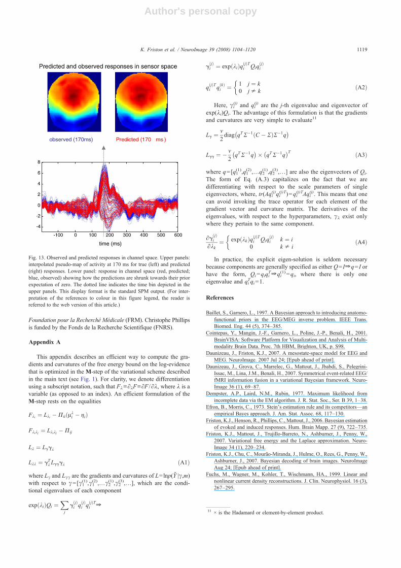
Finally, we show in Fig. 13 the correspondence betweenobserved response and conditional expectation in channel space.Although we can only show a single time slice here (the responseat 170 ms); the equivalent movies of the evoked dynamics inchannel space and their prediction show a pleasing similarity. Moreimportantly, the reconstructed time courses in channel spaceillustrate a ubiquitous feature of empirical shrinkage priors of thesort we have used here, namely the shrinkage of conditionalestimates to their prior expectation of zero. The shrinkage accountsfor the fact that only about 90% of the observed variance isexplained by optimum models. The remaining variance is, onehopes, largely noise.

Conclusion

This paper has described a new application of hierarchical orempirical Bayes to the distributed source reconstruction problemin EEG and MEG. The key contribution is the automaticselection of multiple cortical sources with compact spatial supportthat are specified in terms of empirical priors. This obviates theneed to use priors with a specific form (e.g., smoothness orminimum norm) or with spatial structure (e.g., priors based on

Fig. 11. Model comparison between MSP, COH and MNM models using the empirical ERPs evoked by faces. This uses the same format as the previous figureand shows that the MSP model supervenes. The spatial structure in the maximum intensity projections (lower panels) reflects the complexity of the modelsemployed.

1117K. Friston et al. / NeuroImage 39 (2008) 1104–1120

Author's personal copy

depth constraints or functional magnetic resonance imagingresults). Furthermore, the inversion scheme allows for a sparsesolution, of the sort enforced by equivalent current dipole models,for distributed sources. This means that the approach automati-cally selects either a sparse or a distributed model, depending onthe data.

There are a number of aspects of the scheme we have notdemonstrated in this paper, specifically the derivation of conditionalcontrasts over time–frequency windows and their correspondingconditional energy (cf. induced responses). In a practical setting, weenvisage that the source reconstruction described above would beused to summarize the responses of each subject to each ex-perimental trial or condition. In our [academic freeware] imple-mentation, these contrasts are projected from a two-dimensionalcortical manifold to a full three-dimensional anatomical space. Thisenables the conditional estimate to be smoothed and entered intostandard SPM analyses for inference at the between-subject level.We deliberately smooth in three-space to ensure that variations ingyral anatomy from subject to subject (which are not confined to atwo-dimensional manifold) are accommodated by smoothing, inaccord with the matched filter theorem (see Henson et al., 2007 fora fuller discussion).

Further constraints on the solutions under MSP can be enforcedby specifying volumes of interest, within which to reconstructcurrent source density. This effectively forces solutions to occupyvolumes of interest and can be a useful device when the regionsinvolved are known in advance. These and other model selectionissues will be the subject of future papers that use the techniquesdescribed in this paper.

Software note

The inversion scheme and models considered in this paper areimplemented in the SPM academic software, which is availablefreely from http://www.fil.ion.ucl.ac.uk/spm. The MSP and othermodels are an integral part of the source reconstruction stream,which allows one to create conditional contrasts and their energyfor any number of trials or types. The display format used by SPMadopts the same format used in Figs. 2, 12 and 13.

Acknowledgments

The Wellcome Trust, the Medical Research Council and BritishCouncil funded this work. Jérémie Mattout is funded by the

Fig. 12. Comparative results for the N170 as reconstructed using the MSP model (middle panels) and a two-ECD solution (obtained with SPM5 using exactlysame data) based on the same three-sphere head model (left panels). The cortical renderings (right panels) show voxels that survived an uncorrected threshold ofpb0.001, when testing for face-selective responses in a group of eighteen normal subjects using fMRI. The lower inset is of the conditional [unsigned] activity at187 ms, rendered on the canonical cortical mesh used to model source space (the mesh has been made slightly transparent so that deep sources can be seen easily).Equivalent results are shown in maximum intensity projection format in three-dimensional space (lower panel). This spatial profile is expressed at the same timeof the maximum [unsigned] response over all voxels and time bins, at 161 ms. These display formats are the standard SPM output.

1118 K. Friston et al. / NeuroImage 39 (2008) 1104–1120

Author's personal copy

Foundation pour la Recherché Médicale (FRM). Christophe Phillipsis funded by the Fonds de la Recherche Scientifique (FNRS).

Appendix A

This appendix describes an efficient way to compute the gra-dients and curvatures of the free energy bound on the log-evidencethat is optimized in the M-step of the variational scheme describedin the main text (see Fig. 1). For clarity, we denote differentiationusing a subscript notation, such that Fλ≡∂λF≡∂F /∂λ, where λ is avariable (as opposed to an index). An efficient formulation of theM-step rests on the equalities

Fki ¼ Lki �PiiðAki � giÞ

Fkikj ¼ Lkikj �Pij

Lk ¼ Lggk

Lkk ¼ gTkLgggk ðA1Þ

where Lγ and Lγγ are the gradients and curvatures of L=lnp(Y |γ,m)with respect to γ=[γ1

(1),γ1(2),…γ2

(1),γ2(3),…], which are the condi-

tional eigenvalues of each component

expðkiÞQi ¼Xj

gðjÞi qðjÞi qðjÞTi Z

gðjÞi ¼ expðkiÞqðjÞTi Qiq

ðjÞi

qðjÞTi qðkÞi ¼ 1 j ¼ k0 j p k

�ðA2Þ

Here, γi(j) and qi

(j) are the j-th eigenvalue and eigenvector ofexp(λi)Qi. The advantage of this formulation is that the gradientsand curvatures are very simple to evaluate11

Lg ¼ v2diag qTR�1 C � Rð ÞR�1q

� �

Lgg ¼ � v2

qTR�1q� �� ðqTR�1qÞT ðA3Þ

where q=[q1(1),q1

(2),…q2(1),q2

(3),…] are also the eigenvectors of Qi.The form of Eq. (A.3) capitalizes on the fact that we aredifferentiating with respect to the scale parameters of singleeigenvectors, where, tr(Aqi

(j)qi(j)T)=qi

(j)TAqi(j). This means that one

can avoid invoking the trace operator for each element of thegradient vector and curvature matrix. The derivatives of theeigenvalues, with respect to the hyperparameters, γλ exist onlywhere they pertain to the same component.

∂gðjÞi∂kk

¼ expðkkÞqðjÞTi QiqðjÞi k ¼ i

0 k p i

�ðA4Þ

In practice, the explicit eigen-solution is seldom necessarybecause components are generally specified as either Q= IZ q= I orhave the form, Qi=qiqi

TZ qi(1) =qi, where there is only one

eigenvalue and qiTqi=1.

References

Baillet, S., Garnero, L., 1997. A Bayesian approach to introducing anatomo-functional priors in the EEG/MEG inverse problem. IEEE Trans.Biomed. Eng. 44 (5), 374–385.

Cointepas, Y., Mangin, J.-F., Garnero, L., Poline, J.-P., Benali, H., 2001.BrainVISA: Software Platform for Visualization and Analysis of Multi-modality Brain Data. Proc. 7th HBM, Brighton, UK, p. S98.

Daunizeau, J., Friston, K.J., 2007. A mesostate-space model for EEG andMEG. NeuroImage. 2007 Jul 24; [Epub ahead of print].

Daunizeau, J., Grova, C., Marrelec, G., Mattout, J., Jbabdi, S., Pelegrini-Issac, M., Lina, J.M., Benali, H., 2007. Symmetrical event-related EEG/fMRI information fusion in a variational Bayesian framework. Neuro-Image 36 (1), 69–87.

Dempster, A.P., Laird, N.M., Rubin, 1977. Maximum likelihood fromincomplete data via the EM algorithm. J. R. Stat. Soc., Ser. B 39, 1–38.

Efron, B., Morris, C., 1973. Stein's estimation rule and its competitors—anempirical Bayes approach. J. Am. Stat. Assoc. 68, 117–130.

Friston, K.J., Henson, R., Phillips, C., Mattout, J., 2006. Bayesian estimationof evoked and induced responses. Hum. Brain Mapp. 27 (9), 722–735.

Friston, K.J., Mattout, J., Trujillo-Barreto, N., Ashburner, J., Penny, W.,2007. Variational free energy and the Laplace approximation. Neuro-Image 34 (1), 220–234.

Friston, K.J., Chu, C., Mourão-Miranda, J., Hulme, O., Rees, G., Penny, W.,Ashburner, J., 2007. Bayesian decoding of brain images. NeuroImageAug 24; [Epub ahead of print].

Fuchs, M., Wagner, M., Kohler, T., Wischmann, HA., 1999. Linear andnonlinear current density reconstructions. J. Clin. Neurophysiol. 16 (3),267–295.

Fig. 13. Observed and predicted responses in channel space. Upper panels:interpolated pseudo-map of activity at 170 ms for true (left) and predicted(right) responses. Lower panel: response in channel space (red, predicted;blue, observed) showing how the predictions are shrunk towards their priorexpectation of zero. The dotted line indicates the time bin depicted in theupper panels. This display format is the standard SPM output. (For inter-pretation of the references to colour in this figure legend, the reader isreferred to the web version of this article.)

11 × is the Hadamard or element-by-element product.

1119K. Friston et al. / NeuroImage 39 (2008) 1104–1120

Author's personal copy

Gelman, A., 2006. Prior distributions for variance parameters in hierarchicalmodels. Bayesian Anal. 1 (3), 515–533.

Harrison, L.M., Penny, W., Ashburner, J., Trujillo-Barreto, N., Friston, K.J.,2007. Diffusion-based spatial priors for imaging. NeuroImage (Aug 8;electronic publication ahead of print).

Harville, D.A., 1977. Maximum likelihood approaches to variancecomponent estimation and to related problems. J. Am. Stat. Assoc. 72,320–338.

Henson, R.N., Goshen-Gottstein, Y., Ganel, T., Otten, L.J., Quayle, A.,Rugg, M.D., 2003. Electrophysiological and haemodynamic correlatesof face perception, recognition and priming. Cereb. Cortex 13 (7),793–805.

Henson, R.N., Mattout, J., Singh, K.D., Barnes, G.R., Hillebrand, A.,Friston, K.J., 2007. Population-level inferences for distributed MEGsource localization under multiple constraints: application to face-evoked fields. NeuroImage 38 (3), 422–438.

Jun, S.C., George, J.S., Plis, S.M., Ranken, D.M., Schmidt, D.M., Wood,CC., 2006. Improving source detection and separation in a spatiotem-poral Bayesian inference dipole analysis. Phys. Med. Biol. 51 (10),2395–2414.

Kass, R.E., Steffey, D., 1989. Approximate Bayesian inference inconditionally independent hierarchical models (parametric empiricalBayes models). J. Am. Stat. Assoc. 407, 717–726.

Kass, R.E., Raftery, A.E., 1995. Bayes factors. J. Am. Stat. Assoc. 90,773–795.

Kiebel, S.J., Friston, KJ., 2004. Statistical parametric mapping for event-related potentials (II): a hierarchical temporal model. NeuroImage 22 (2),503–520.

Kim, H.-C., Ghahramani, Z., 2006. Bayesian Gaussian process classificationwith the EM-EP algorithm. IEEE Trans. Pattern Anal. Mach. Intell. 28(12), 1948–1959.

LeSage, J.P., Pace, R.K., 2000. Using Matrix Exponentials to ExploreSpatial Structure in Regression Relationships. Working Paper, Depart-ment of Economics, University of Toledo.

MacKay, D.J.C., 1992. Bayesian interpolation. Neural Comput. 4 (3),415–447.

Mattout, J., Phillips, C., Penny, W.D., Rugg, M.D., Friston, KJ., 2006. MEGsource localization under multiple constraints: an extended Bayesianframework. NeuroImage 30, 753–767.

Mattout, J., Henson, R.N., Friston, K.J., 2007. Canonical SourceReconstruction for MEG. Computational Intelligence and NeuroscienceArticle ID 67613.

Mosher, J.C., Spencer, M.E., Leahy, R.M., Lewis, PS., 1993. Error boundsfor EEG and MEG dipole source localization. Electroencephalogr. Clin.Neurophysiol. 86 (5), 303–321.

Neal, R.M., 1996. Bayesian Learning for Neural Networks. Springer-Verlag,New York.

Neal, R.M., 1998. Assessing relevance determination methods usingDELVE. Neural Networks andMachine Learning. Springer, pp. 97–129.

Nagarajan, S.S., Portniaguine, O., Hwang, D., Johnson, C., Sekihara, K.,2006. Controlled support MEG imaging. NeuroImage 15 (33(3)),878–885.

Nummenmaa, A., Auranen, T., Hamalainen, M.S., Jaaskelainen, I.P.,Lampinen, J., Sams, M., Vehtari, A., 2007. Hierarchical Bayesianestimates of distributed MEG sources: theoretical aspects and compar-ison of variational and MCMC methods. NeuroImage 35 (2), 669–685.

Pascual-Marqui, R.D., 2002. Standardized low-resolution brain electro-magnetic tomography (sLORETA): technical details. Methods Find.Exp. Clin. Pharmacol. 24 (Suppl. D), 5–12.

Patterson, H.D., Thompson, R., 1971. Recovery of inter-block informationwhen block sizes are unequal. Biometrika 58, 545–554.

Phillips, C., Rugg, M.D., Friston, KJ., 2002a. Anatomically informed basisfunctions for EEG source localization: combining functional andanatomical constraints. NeuroImage 16 (3 Pt 1), 678–695.

Phillips, C., Rugg, M., Friston, K.J., 2002b. Systematic regularisation oflinear inverse solutions of the EEG source localisation problem.NeuroImage 17, 287–301.

Phillips, C., Mattout, J., Rugg, M.D., Maquet, P., Friston, K.J., 2005. Anempirical Bayesian solution to the source reconstruction problem inEEG. NeuroImage 24, 997–1011.

Rasmussen, C.E., 1996. Evaluation of Gaussian Processes and OtherMethods for Non-Linear Regression. PhD thesis, Dept. of ComputerScience, Univ. of Toronto, 1996. Available from http://www.cs.utoronto.ca~carl/.

Ripley, B.D., 1994. Flexible non-linear approaches to classification. In:Cherkassy, V., Friedman, J.H., Wechsler, H. (Eds.), From Statistics toNeural Networks. Springer, pp. 105–126.

Russell, G.S., Srinivasan, R., Tucker, DM., 1998. Bayesian estimates oferror bounds for EEG source imaging. IEEE Trans. Med. Imag. 17 (6),1084–1089.

Salin, P.-A., Bullier, J., 1995. Corticocortical connections in the visualsystem: structure and function. Psychol. Bull. 75, 107–154.

Sato, M.A., Yoshioka, T., Kajihara, S., Toyama, K., Goda, N., Doya, K.,Kawato, M., 2004. Hierarchical Bayesian estimation for MEG inverseproblem. NeuroImage 23 (3), 806–826.

Serinagaoglu, Y., Brooks, D.H., MacLeod, RS., 2005. Bayesian solutionsand performance analysis in bioelectric inverse problems. IEEE Trans.Biomed. Eng. 52 (6), 1009–1020.

Talairach, J., Tournoux, P., 1988. Co-planar Stereotaxic Atlas of the HumanBrain: 3-Dimensional Proportional System—An Approach to CerebralImaging. Thieme Medical Publishers, New York, NY.

Tipping, M.E., 2001. Sparse Bayesian learning and the Relevance VectorMachine. J. Mach. Learn. Res. 1, 211–244.

Trujillo-Barreto, N., Aubert-Vazquez, E., Valdes-Sosa, P., 2004. Bayesianmodel averaging. NeuroImage 21, 1300–1319.

Wipf, D.P., Ramırez, R.R., Palmer, J.A., Makeig, S., Rao, B.D., 2006.Automatic Relevance Determination for Source Localization with MEGand EEG Data, Technical Report, University of California, San Diego.

1120 K. Friston et al. / NeuroImage 39 (2008) 1104–1120