arX

iv:1

310.

0985

v2 [

cond

-mat

.dis

-nn]

10

Dec

201

3

Average synaptic activity and neural networks topology: a global inverse problem

Raffaella Burioni,1, 2 Mario Casartelli,1, 2 Matteo di Volo,1, 3, 2 Roberto Livi,4, 5, 6, 3 and Alessandro Vezzani7, 1

1Dipartimento di Fisica e Scienza della Terra, Universita di Parma, via G.P. Usberti, 7/A - 43124, Parma, Italy2INFN, Gruppo Collegato di Parma, via G.P. Usberti, 7/A - 43124, Parma, Italy

3Centro Interdipartimentale per lo Studio delle Dinamiche Complesse, via Sansone, 1 - 50019 Sesto Fiorentino, Italy4Dipartimento di Fisica, Universita di Firenze, via Sansone, 1 - 50019 Sesto Fiorentino, Italy

5Istituto dei Sistemi Complessi, CNR, via Madonna del Piano 10 - 50019 Sesto Fiorentino, Italy6INFN Sez. Firenze, via Sansone, 1 -50019 Sesto Fiorentino, Italy

7 S3, CNR Istituto di Nanoscienze, Via Campi, 213A - 41125 Modena, Italy

The dynamics of neural networks is often characterized by collective behavior and quasi-synchronous events, where a large fraction of neurons fire in short time intervals, separated byuncorrelated firing activity. These global temporal signals are crucial for brain functioning andthey strongly depend on the topology of the network and on the fluctuations of the connectivity.We propose a heterogeneous mean–field approach to neural dynamics on random networks, thatexplicitly preserves the disorder in the topology at growing network sizes, and leads to a set of self-consistent equations. Within this approach, we provide an effective description of microscopic andlarge scale temporal signals in a leaky integrate-and-fire model with short term plasticity, wherequasi-synchronous events arise. Our equations provide a clear analytical picture of the dynam-ics, evidencing the contributions of both periodic (locked) and aperiodic (unlocked) neurons to themeasurable average signal. In particular, we formulate and solve a global inverse problem of recon-structing the in-degree distribution from the knowledge of the average activity field. Our method isvery general and applies to a large class of dynamical models on massive random networks.

PACS numbers:

I. INTRODUCTION

Topology has a strong influence on phases of dynamical models defined on a network. Recently, this topic hasattracted the interest of both theoreticians and applied scientists in many different fields, ranging from physics, tobiology and social sciences [1–6]. Research has focused in two main directions. The direct problem aims at predictingthe dynamical properties of a network from its topological parameters [7]. The inverse problem is addressed to thereconstruction of the network topological features from dynamic time series [8–10]. The latter approach is particularlyinteresting when the direct investigation of the network is impossible or very hard to be performed.Neural networks are typical examples of such a situation. In local approaches to inverse problems [8–10], the

network is reconstructed through the knowledge of long time series of single neuron dynamics, a methods that appliesefficiently to small systems only. Actually, the signals emerging from neural time evolution are often records of theaverage synaptic activity from large regions of the cerebral cortex – a kind of observable likely much easier to bemeasured with respect to signals coming from single neuron activities [11, 12]. Inferring the topological properties ofthe network from global signals is still an open and central problem in neurophysiology. In this paper we investigatethe possibility of formulating and solving such a global version of the inverse problem, reconstructing the networktopology that has generated a given global (i.e. average) synaptic-activity field. The solution of such an inverseproblem could also imply the possibility of engineering a network able to produce a specific average signal.As an example of neural network dynamics, we focus on a system of leaky integrate–and–fire (LIF) excitatory

neurons, interacting via a synaptic current regulated by the short–term plasticity mechanism [13, 14]. This model isable to reproduce synchronization patterns observed in in vitro experiments [16–18]. As a model for the underlyingtopology we consider randomly uncorrelated diluted networks made of N nodes. In general N is considered quite alarge number, as well as the number of connections between pairs of neurons. This suggests that the right frameworkfor understanding large–population neural networks should be a mean–field approach, where the thermodynamic limit,N → ∞, is expected to provide the basic ingredients for an analytic treatment. On the other hand, the way such athermodynamic limit is performed may wipe out any relation with the topological features that are responsible, forfinite N , of relevant dynamical properties.In Erdos–Renyi directed networks, where each neuron is randomly and uniformly connected to a finite fraction

of the other neurons (massive connectivity), the fluctuations of the degree determine a rich dynamical behavior,characterized in particular by quasi-synchronous events (QSE). This means that a large fraction of neurons fire in ashort time interval of a few milliseconds (ms), separated by uncorrelated firing activity lasting over some tens of ms.Such an interesting behavior is lost in the thermodynamic limit, as the fluctuations of the connectivity vanish and the”mean-field-like” dynamics reduces to a state of fully synchronized neurons (e.g., see [19]). In order to maintain the

2

QSE phenomenology in the large N limit, we can rather consider the sequence of random graphs that keep the samespecific in-degree distribution P (k), where ki = ki/N is the fraction of incoming neurons connected to neuron i forany finite N , similarly to the configuration models [20]. This way of performing the thermodynamic limit preservesthe dynamical regime of QSE and the difference between synchronous and non-synchronous neurons according to theirspecific in-degree k. By introducing explicitly this N → ∞ limit in the differential equations of the model, we obtain aheterogeneous mean–field (HMF) description, similar to the one recently introduced in the context of epidemiologicalspreading on networks [2, 3]. Such mean–field like or HMF equations can be studied analytically by introducing the

return maps of the firing times. In particular, we find that a sufficiently narrow distributions of P (k) is necessary to

observe the quasi–synchronous dynamical phase, which vanishes on the contrary for broad distributions of k.More importantly, these HMF equations allow us to design a ”global” inverse–problem approach, formulated in

terms of an integral Fredholm equation of the first kind for the unknown P (k) [15]. Starting from the dynamical

signal of the average synaptic-activity field, the solution of this equation provides with good accuracy the P (k) of the

network that produced it. We test this method for very different uncorrelated network topologies, where P (k) rangesfrom a Gaussian with one or several peaks, to power law distributions, showing its effectiveness even for finite sizenetworks.The overall procedure applies to a wide class of network dynamics of the type

wi = F

(

wi,g

N

∑

j 6=i

ǫjiG(wj))

, (1)

where the vector wi represents the state of the site i, F(wi, 0) is the single site dynamics, g is the coupling strength,G(wj) is a suitable coupling function and ǫj,i is the adjacency matrix of the directed uncorrelated massive network,whose entries are equal to 1 if neuron j fires to neuron i, and 0 otherwise.

II. RESULTS

A. The LIF model with short term plasticity

Let us introduce LIF models, that describe a network of N neurons interacting via a synaptic current, regulatedby short–term–plasticity with equivalent synapses [16]. In this case the dynamical variable of the neuron i is wi =(vi, xi, yi, zi) where vi is the rescaled membrane potential and xi, yi, and zi represent the fractions of synaptictransmitters in the recovered, active, and inactive state, respectively (xi + yi + zi = 1). Eq. (1) then specializes to:

vi = a− vi +g

N

∑

j 6=i

ǫjiyj (2)

yi = −yiτin

+ uxiSi (3)

zi =yiτin

−ziτr

. (4)

Whenever the potential vi(t) reaches the threshold value vth = 1, it is reset to vr = 0, and a spike is sent towardsthe postsynaptic neurons. The spike is assumed to be a δ–like function of time. Accordingly, the spike-train Sj(t)produced by neuron j, is defined as Sj(t) =

∑

m δ(t − tj(m)), where tj(m) is the time when neuron j fires its m-th spike. The transmission of the field Sj(t) is mediated by the synapse dynamics. Only the active transmittersreact to the incoming spikes Si(t): the parameter u tunes their effectiveness, τin is the characteristic decay time ofthe postsynaptic current, while τr is the recovery time from synaptic depression. We assume that all parametersappearing in the above equations are independent of the neuron indices, and that each neuron is connected to amacroscopic number, O(N), of pre-synaptic neurons: this is the reason why the interaction term is divided by thefactor N . In all data hereafter reported we have used phenomenological values of the rescaled parameters: τin = 0.2,τr = 133τin, a = 1.3, g = 30 and u = 0.5 [19]. Numerical simulations can be performed effectively by transformingthe set of differential equations (2)–(4) into an event–driven map [19, 21, 22]. On Erdos–Renyi random graphs, whereeach link is accepted with probability p, so that the average in-degree 〈k〉 = pN , the dynamics has been analyzed indetail [19]. Neurons separate spontaneously into two different families: the locked and the unlocked ones. The lockedneurons determine quasi-synchronous events (QSE) and exhibit a periodic dynamics. The unlocked ones participateto the uncorrelated firing activity and exhibit a sort of irregular evolution. Neurons belong to one of the two familiesaccording to their in-degree ki. In this topology, the thermodynamic limit can be simply worked out. Unfortunately,

3

356 358 360 362 364t

0

100

200

300

400

500

FIG. 1: Raster plot representation of the dynamics of a network of N = 500 neurons with a Gaussian in-degree distribution(〈k〉 = 0.7, σ = 0.077). Black dots signal single firing events of neurons at time t. Neurons are naturally ordered along thevertical axis according to the values of their in-degree. The global field Y (t) (red line) is superposed to the raster plot forcomparison (its actual values are multiplied by the factor 103, to make it visible on the vertical scale).

this misses all the interesting features emerging from the model at finite N . Actually, for any finite value of N , thein–degree distribution is centered around 〈k〉, with a variance σ ∼ N

12 . The effect of disorder is quantified by the

ratio σ/〈k〉, that vanishes for N → ∞. Hence the thermodynamic limit reproduces the naive mean–field like dynamicsof a fully coupled network, with rescaled coupling g → pg, that is known to eventually converge to a periodic fullysynchronous state [19].

B. The LIF model on random graphs with fixed in–degree distribution

At variance with the network construction discussed in previous section, uncorrelated random graphs can be de-fined by different protocols, that keep track of the in-degree inhomogeneity in the thermodynamic limit. In ourconstruction, we fix the normalized in–degree probability distribution P (k), so that σ/〈k〉 is kept constant for any

N [20]. Accordingly, P (k) is a normalized distribution defined in the interval k ∈ [0, 1] (while the number of inputs

k ∈ [0, N ]). In particular, if P (k) is a truncated Gaussian distribution, the dynamics reproduces the scenario observedin [19] for an Erdos–Renyi random graph. In fact, also in this case neurons are dynamically distinguished into two

families, depending on their in–degree. Precisely, neurons with k in between two critical values, kc1 and kc2 ≈ 〈k〉,

are locked and determine the QSE: they fire with almost the same period, but exhibit different (k-dependent) phases.All the other neurons are unlocked and fire in between QSE displaying an aperiodic behavior. Notice that the range0 < k < kc1 corresponds to the left tail of the truncated Gaussian distribution; accordingly, the large majority ofunlocked neurons is found in the range kc2 < k < 1 (see Fig. 1). In order to characterize the dynamics at increasingN , we consider for each neuron its inter-spike-interval (ISI), i.e. the lapse of time in between consecutive firing events.

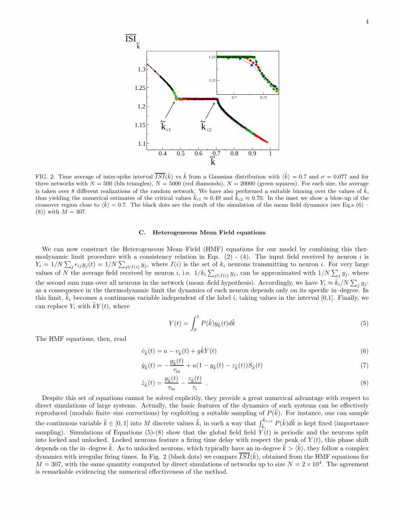
In Fig.2 we show the time-average of ISI vs k, or ISI(k). One can clearly observe the plateau of locked neurons and

the crossover to unlocked neurons at the critical values kc1 and kc2.Remarkably, networks of different sizes (N = 500, 5000 and 20000) feature the same ISI(k) for locked neurons,

and almost the the same values of kc1 and kc2. There is not a sharp transition from locked to unlocked neurons,because for finite N the behavior of each neuron depends not only on its k, but also on the neurons sending it theirinputs. Nevertheless, in the inset, the crossover appears to be sharper and sharper for increasing N , as expected fortrue critical points. Furthermore, the fluctuations of ISI(k) over different realizations, by P (k), of three networks of

different size exhibit a peak around kc1 and kc2, while they decrease with N as ∼ N−1/2 (data not shown). Thus, thequalitative and quantitative features of the QSE at finite sizes are expected to persist in the thermodynamic limit,where fluctuations vanish and the dynamics of each neuron depends only on its in–degree.

4

0.7 0.71

1.21

1.22

0.4 0.5 0.6 0.7 0.8 0.9 1~k

1.1

1.15

1.2

1.25

1.3

ISI~k

~k c1~k c2

FIG. 2: Time average of inter-spike interval ISI(k) vs k from a Gaussian distribution with 〈k〉 = 0.7 and σ = 0.077 and forthree networks with N = 500 (blu triangles), N = 5000 (red diamonds), N = 20000 (green squares). For each size, the average

is taken over 8 different realizations of the random network. We have also performed a suitable binning over the values of k,thus yielding the numerical estimates of the critical values kc1 ≈ 0.49 and kc2 ≈ 0.70. In the inset we show a blow-up of thecrossover region close to 〈k〉 = 0.7. The black dots are the result of the simulation of the mean field dynamics (see Eq.s (6) –(8)) with M = 307.

C. Heterogeneous Mean Field equations

We can now construct the Heterogeneous Mean–Field (HMF) equations for our model by combining this ther-modynamic limit procedure with a consistency relation in Eqs. (2) - (4). The input field received by neuron i isYi = 1/N

∑

j ǫijyj(t) = 1/N∑

j∈I(i) yj, where I(i) is the set of ki neurons transmitting to neuron i. For very large

values of N the average field received by neuron i, i.e. 1/ki∑

j∈I(i) yj , can be approximated with 1/N∑

j yj, where

the second sum runs over all neurons in the network (mean–field hypothesis). Accordingly, we have Yi ≈ ki/N∑

j yj :as a consequence in the thermodynamic limit the dynamics of each neuron depends only on its specific in–degree. Inthis limit, ki becomes a continuous variable independent of the label i, taking values in the interval [0,1]. Finally, we

can replace Yi with kY (t), where

Y (t) =

∫ 1

0

P (k)yk(t)dk (5)

The HMF equations, then, read

vk(t) = a− vk(t) + gkY (t) (6)

yk(t) = −yk(t)

τin+ u(1− yk(t)− zk(t))Sk(t) (7)

zk(t) =yk(t)

τin−

zk(t)

τr. (8)

Despite this set of equations cannot be solved explicitly, they provide a great numerical advantage with respect todirect simulations of large systems. Actually, the basic features of the dynamics of such systems can be effectivelyreproduced (modulo finite–size corrections) by exploiting a suitable sampling of P (k). For instance, one can sample

the continuous variable k ∈ [0, 1] into M discrete values ki in such a way that∫ ki+1

kiP (k)dk is kept fixed (importance

sampling). Simulations of Equations (5)-(8) show that the global field field Y (t) is periodic and the neurons splitinto locked and unlocked. Locked neurons feature a firing time delay with respect the peak of Y (t), this phase shift

depends on the in–degree k. As to unlocked neurons, which typically have an in-degree k > 〈k〉, they follow a complex

dynamics with irregular firing times. In Fig. 2 (black dots) we compare ISI(k), obtained from the HMF equations forM = 307, with the same quantity computed by direct simulations of networks up to size N = 2× 104. The agreementis remarkable evidencing the numerical effectiveness of the method.

5

0 0.2 0.4 0.6 0.8 1t(n)___

T

0

0.2

0.4

0.6

0.8

1

t(n+1)____T

0.42t(n+1) = t(n)0.480.630.6980.77

FIG. 3: The return map Rkin Eq. (10) of the rescaled variables t

k(n)/T for different values of k, corresponding to lines of

different colors, according to the legend in the inset: the black line is the bisector of the square.

D. The direct problem: stability analysis and the synchronization transition

In the HMF equations, once the global field Y (t) is known, the dynamics of each class of neurons with in-degree

k can be determined by a straightforward integration, and we can perform the stability analysis that Tsodyks et al.applied to a similar model [23]. As an example, we have considered the system studied in Fig.2. The global field Y (t)

of the HMF dynamics has been obtained using the importance sampling for the distribution P (k). We have fittedY (t) with an analytic function of time Yf (t), continuous and periodic in time, with period T . Accordingly, Eq. (6)can be approximated by

vk(t) = a− vk(t) + gkYf (t). (9)

Notice that, by construction, the field Yf (t) features peaks at times t = nT , where n is an integer. In this way wecan represent Eq. (9) as a discrete single neuron map. In practice, we integrate Eq.(9) and determine the sequence

of the (absolute value of the) firing time–delay, tk(n), of neurons with in–degree k with respect to the reference timenT . The return map Rk of this quantity reads

tk(n+ 1) = Rktk(n). (10)

In Fig. 3 we plot the return map of the rescaled firing time–delay tk(n)/T for different values of k. We observe that

in-degrees k corresponding to locked neurons (e.g., the brown curve) have two fixed points tskand tu

k, the first one

is stable and the second unstable. Clearly, the dynamics converges to the stable fixed point displaying a periodicbehavior. In particular, the firing times of neurons k are phase shifted of a quantity ts

kwith respect the peaks of the

fitted global field. The orange and violet curves correspond to the dynamics at the critical in-degrees kc1 and kc2where the fixed points disappear (see Fig.(2)). The presence of such fixed points influences also the behavior of the

unlocked component (e.g., the red and light blue curves). In particular, the nearer k is to kc1 or to kc2, the closer isthe return map to the bisector of the square, giving rise to a dynamics spending longer and longer times in an almostperiodic firing. Afterwards, unlocked neurons depart from this almost periodic regime, thus following an aperiodicbehavior. As a byproduct, this dynamical analysis allows to estimate the values of the critical in–degrees. For thesystem of Fig.1, kc1 = 0.48 and kc2 = 0.698, in very good agreement with the numerical simulations (see Fig. 2).Still in the perspective of the direct problem, the HMF equations provide further insight on how the network

topology influences the dynamical behavior. We have found that, in general, the fraction of locked neurons increasesas P (k) becomes sharper and sharper, while synchronization is eventually lost for broader distributions. In Fig. 4

we report the fraction of locked neurons, fl, as a function of the deviation σ, for different kinds of P (k) (singleor double–peaked Gaussian, power law) in the HMF equations. For the truncated power law distribution, we set

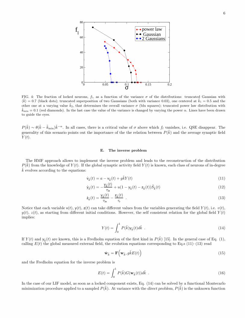
6

0 0.05 0.1 0.15 0.2σ

0

20

40

60

80

fl

power law Gaussian2 Gaussians

FIG. 4: The fraction of locked neurons, fl, as a function of the variance σ of the distributions: truncated Gaussian with〈k〉 = 0.7 (black dots); truncated superposition of two Gaussians (both with variance 0.03), one centered at k1 = 0.5 and the

other one at a varying value k2, that determines the overall variance σ (blu squares); truncated power law distribution with

kmin = 0.1 (red diamonds). In the last case the value of the variance is changed by varying the power α. Lines have been drawnto guide the eyes.

P (k) ∼ θ(k − kmin)k−α. In all cases, there is a critical value of σ above which fl vanishes, i.e. QSE disappear. The

generality of this scenario points out the importance of the the relation between P (k) and the average synaptic fieldY (t).

E. The inverse problem

The HMF approach allows to implement the inverse problem and leads to the reconstruction of the distributionP (k) from the knowledge of Y (t). If the global synaptic activity field Y (t) is known, each class of neurons of in-degree

k evolves according to the equations:

vk(t) = a− vk(t) + gkY (t) (11)

yk(t) = −yk(t)

τin+ u(1− yk(t)− zk(t))Sk(t) (12)

zk(t) =yk(t)

τin−

zk(t)

τr. (13)

Notice that each variable v(t), y(t), z(t) can take different values from the variables generating the field Y (t), i.e. v(t),y(t), z(t), as starting from different initial conditions. However, the self consistent relation for the global field Y (t)implies:

Y (t) =

∫ 1

0

P (k)yk(t)dk . (14)

If Y (t) and yk(t) are known, this is a Fredholm equation of the first kind in P (k) [15]. In the general case of Eq. (1),calling E(t) the global measured external field, the evolution equations corresponding to Eq.s (11)–(13) read

wk = F

(

wk, gkE(t))

(15)

and the Fredholm equation for the inverse problem is

E(t) =

∫ 1

0

P (k)G(wk(t))dk . (16)

In the case of our LIF model, as soon as a locked component exists, Eq. (14) can be solved by a functional Montecarlo

minimization procedure applied to a sampled P (k). At variance with the direct problem, P (k) is the unknown function

7

0

2

4

6

8

10

P(~k)

0 0.2 0.4 0.6 0.8~k

0

10

P(~k)

0.1 1

10-4

10-2

100

102

0 0.2 0.4 0.6 0.8 1~k

2

4

6

FIG. 5: Inverse problem for P (k) from the global field Y (t). The upper and lower–left panels show three distributions of thekind considered in Fig. (4) (black continuous curves) for the HMF equations and their reconstructions (circles) by the inverse

method. The parameters of the three distributions are σ = 0.043, k2 = 0.7 and α = 4.9. In the lower–right panel we showthe reconstruction (crosses) of P (k) (black continuous line) by the average field Y (t) generated by the dynamics of a finite size

network with N = 500.

and, accordingly, we have to adopt a uniform sampling of the support of k. A sufficiently fine sampling has to beused for a confident reconstruction of P (k) (See methods section).

To check our inverse method, we choose a distribution P (k), evolve the system and extract the global synaptic field

Y (t). We then verify if the procedure reconstructs correctly the original distribution P (k). In the first three panels

of Fig. 5 we show examples in which Y (t) has been obtained from the simulation of the HMF with different P (k)(Gaussian, double peak Gaussian and power law). We can see that the method determines confidently the original

distribution P (k). Notice that the method fails as soon as the locked component disappears. Remarkably, the method

can recognize the discontinuity of the distribution in k = kmin and the value of the exponent of the power law α = 4.9.Finally, in the last panel of Fig.5, we show the result of the inverse problem for the distribution P (k) obtained from aglobal signal generated by a finite size realization with N = 500. The significant agreement indicates that the HMFand its inverse problem are able to infer the in–degree probability distribution P (k) even for a realistic finite sizenetwork. This last result is particularly important, as it opens new perspectives for experimental data analysis, wherethe average neural activity is typically measured from finite size samples.

III. DISCUSSION

The direct and inverse problem for neural dynamics on random networks are both accessible through the HMFapproach proposed in this paper. The mean-field equations provide an analytic form for the return map of the firingtimes of neurons and they allow to evidence the effects of the in-degree distribution on the synchronization transition.This phenomenology is not limited to the LIF model analyzed here and it is observed in several neural models onrandom networks. We expect that the HMF equations could shed light on the nature of this interesting, but stillnot well understood, class of synchronization transitions [24–26]. The mean field nature of the approach does notrepresent a limitation, since the equations are ecpected to give a faithful description of the dynamics also in networkswith finite but large average in-degree, corresponding to the experimental situation observed in many cortical regions.The inverse approach, although tested here only on numerical experiments, gives excellent results on the recon-

struction of a wide class of in-degree distributions and it could open new perspectives on data analysis, allowingto reconstruct the main topological features of the neural network producing the QSE. The inversion appears to bestable with respect to noise, as clearly shown by the effectiveness of the procedure tested on a finite realization, wherethe temporal signals of the average synaptic activity is noisy. We also expect our inverse approach to be robust withrespect to the addition of limited randomness in leaky currents, and also with respect to a noise compatible withthe signal detection from instruments. Finally, the method is very general and it can be applied to a wide class ofdynamical models on networks, as those described in Eq. (1).Further developments will allow to get closer to real experimental situations. We mention the most important, i.e.

the introduction of inhibitory neurons and the extension of our approach by taking into account networks with degree

8

correlations [3], that are known to characterize real structures, and sparse networks. The HMF equations appear tobe sufficiently flexible and simple to allow for the introduction of these extensions.

IV. METHODS

A. Montecarlo approach to the inverse problem

In this section we provide details of the algorithmic procedure adopted for solving the inverse problem, i.e. recon-structing the distribution P (k) from Eq. (14). In the HMF formulation, the field Y (t) is generated by an infinite

number of neurons and k is a continuous variable in the interval [0, 1]. In practice, we can sample uniformly this unitinterval by L disjoint subintervals of length 1/L, labelled by the integer i. This corresponds to an effective neural

index i, that identifies the class of neurons with in-degree ki = i/L. In this way we obtain a discretized definitionconverging to Eq.(14) for L → ∞:

Y (t) =

∫ 1

0

P (k)yk(t)dk ≃1

L

L−1∑

i=0

P (ki)yki(t) . (17)

In order to improve the stability and the convergence of the algorithm by smoothing the fluctuations of the fieldsyki

(t), it is convenient to consider a coarse–graining of the sampling by approximating Y (t) as follows

Y (t) =1

L′

L′−1∑

i=0

P (ki)〈yki(t)〉. (18)

where 〈yki(t)〉 is the average of L/L′ synaptic fields of connectivity k ∈ [ki, ki+1]. This is the discretized Fredholm

equation that one can solve to obtain P (ki) from the knowledge of 〈yki(t)〉 and Y (t). For this aim we use a Monte

Carlo (MC) minimization procedure, by introducing at each MC step, n, a trial solution, Pn(ki), in the form of anormalized non-negative in-degree distribution. Then, we evaluate the field Yn(t) and the distance γn defined as:

Yn(t, Pn(ki)) =1

L′

L′−1∑

i=0

Pn(ki)〈yki(t)〉 (19)

γn(Pn(ki))2 =

1

t2 − t1

∫ t2

t1

[

Yn(t, Pn(ki))− Y (t))]2

Y 2(t)dt . (20)

The time interval [t1, t2] has to be taken large enough to obtain a reliable estimate of γn. For instance, in the case shownin Fig.1, where Y (t) exhibits an almost periodic evolution of period T ≈ 1 in the adimensional units of the model, wehave used t2− t1 = 10. The overall configuration of the synaptic fields, at iteration step n+1, is obtained by choosingrandomly two values kj and kl, and by defining a new trial solution Pn+1(k) = Pn(k)+ǫδk,kj

−ǫδk,kl, so that, provided

both Pn+1(kj) and Pn+1(kl) are non-negative, we increase and decrease Pn(kj) of the same amount, ǫ, in kj and klrespectively. A suitable choice is ǫ ∼ O(10−4). Then, we evaluate γn+1(Pn+1(ki)): If γn+1(Pn+1(ki)) < γn(Pn(ki))the step is accepted i.e. Pn+1 = Pn+1, otherwise Pn+1 = Pn. This MC procedure amounts to the implementation

of a zero temperature dynamics, where the cost function γn(Pn(ki)) can only decrease. In principle, the inverse

problem in the form of Eq.(18) is solved, i.e. Yn(t, Pn(ki)) = Y (t), if γn(Pn(ki)) = 0. In practice, the approximations

introduced by the coarse-graining procedure do not allow for a fast convergence to the exact solution, but Pn(ki) can

be considered a reliable reconstruction of the actual P (k) already for γn < 10−2. We have checked that the results of

the MC procedure are quite stable with respect to different choices of the initial conditions P0(ki), thus confirmingthe robustness of the method. We give in conclusion some comments on the very definition of the coarse-grainedsynaptic field 〈yki

(t)〉. Since small differences in the values of ki reflect in small differences in the dynamics, for not

too large intervals [ki, ki+1] the quantity 〈yki(t)〉 can be considered as an average over different initial conditions. For

locked neurons the convergence of the average procedure defining 〈yki(t)〉 is quite fast, since all the initial conditions

tend to the stable fixed point, identified by the return map described in the previous subsection. On the otherhand, the convergence of the same quantity for unlocked neurons should require an average over a huge number ofinitial conditions. For this reason, the broader is the distribution, i.e. the bigger is the unlocked component (see

9

Fig.4), the more computationally expensive is the solution of the inverse problem. This numerical drawback for broaddistributions emerges in our tests of the inversion procedure described in Fig. 5. Moreover, such tests show thatthe procedure works insofar the QSE are not negligible, but it fails in the absence of the locking mechanism. In thiscase, indeed, the global field Y (t) is constant and also 〈yki

(t)〉 become constant, when averaging over a sufficiently

large number of samples. This situation makes Eq.(18) trivial and useless to evaluate P (ki). We want to observethat, while in general yki

(t) 6= yki(t), one can reasonably expect that 〈yki

(t)〉 is a very good approximation of 〈yki(t)〉.

This remark points out the conceptual importance of the HMF formulation for the possibility of solving the inverseproblem.

[1] Xiao Fan Wang, Int. J. Bifurcation Chaos, 12, 885 (2002).[2] A. Barrat, M. Barthelemy, and A. Vespignani, Dynamical Processes on Complex Networks, Cambridge University Press,

Cambridge, UK (2008).[3] S. N. Dorogovtsev, A.V. Goltsev, and J. F. F. Mendes, Rev. Mod. Phys. 80, 1275 (2008).[4] R. Cohen, S, Havlin, Complex Networks: Structure, Robustness and Function, Cambridge University Press, Cambridge,

UK, 2010.[5] A. Arenas, A. Daz-Guilera, J Kurths, Y. Moreno, C. Zhou, Phys. Rep. 469, 93 (2008).[6] S. Boccaletti, V. Latorab, Y. Morenod, M. Chavez, D.-U. Hwanga, Phys. Rep. 424, 175 (2006).[7] L. Donetti, P. I. Hurtado, and M. A. Munoz , Phys. Rev. Lett. 95, 188701 (2005).[8] E. Schneidman, M. J. Berry, R. Segev, and W. Bialek, Nature 440, 1007 (2006); S. Cocco, S. Leibler, R. Monasson, Proc.

Natl. Acad. Sci. U.S.A. 106 14058 (2009).[9] S. G. Shandilya and M. Timme, New J. Phys. 13 013004 (2011).

[10] Hong-Li Zeng, Mikko Alava, Erik Aurell, John Hertz, and Yasser Roudi, Phys. Rev. Lett. 110, 210601 (2013).[11] E. Niedermeyer, F. H. Lopes da Silva, Electroencephalography: Basic Principles, Clinical Applications, and Related Fields,

Lippincott Williams & Wilkins, (2005).[12] S.A. Huettel, A.W Song & G. McCarthy Functional Magnetic Resonance Imaging, Sunderland, MA: Sinauer Associates,

(2009).[13] M. Tsodyks and H. Markram, Proc. Natl. Acad. Sci. USA 94, 719 (1997).[14] M. Tsodyks, K. Pawelzik and H. Markram, Neural Comput. 10, 821, (1998).[15] R. Kress, Linear Integral equations Applied numerical sciences, v.82, Springer-Verlag, New York, (1999).[16] M. Tsodyks, A. Uziel and H. Markram, The Journal of Neuroscience 20, RC1 (1-5) (2000).[17] V. Volman, I. Baruchi, E. Persi and E. Ben-Jacob, Physica A 335, 249 (2004).[18] M. di Volo and R. Livi, J. of Chaos Solitons and Fractals 57, 54–61 (2013).[19] M. di Volo, R. Livi, S. Luccioli, A. Politi and A. Torcini, Phys. Rev. E 87, 032801 (2013).[20] F. Chung, Linyuan Lu: Complex Graphs and Networks , CBMS Series in Mathematics, AMS (2004).[21] R. Brette, Neural Comput. 18, 2004 (2006).[22] R. Zillmer, R. Livi, A. Politi, and A. Torcini, Phys. Rev. E 76, 046102 (2007).[23] M. Tsodyks, I. Mitkov, and H. Sompolinsky, Phys. Rev. Lett. 71, 1280 (1993).[24] P K Mohanty and Antonio Politi, J. Phys. A: Math. Gen. 39 L415-L421 (2006)[25] S. Olmi, R. Livi, A. Politi, A. Torcini, Phys. Rev. E 81 046119 (2010).[26] S. Luccioli, S. Olmi, A. Politi, A. Torcini, Phys. Rev. Lett. 109, 138103 (2012).