Nonlinear Dynamics (2006) 44: 29–36

DOI: 10.1007/s11071-006-1932-6 c© Springer 2006

Synaptic Coupling Between Two Electronic Neurons

SABIR JACQUIR1, STEPHANE BINCZAK1,∗, JEAN-MARIE BILBAULT1,

VIKTOR KAZANTSEV2, and VLADIMIR NEKORKIN2

1Laboratoire LE2I UMR CNRS 5158, Aile des Sciences de l’Ingenieur, Universite de Bourgogne, BP 47870, Dijon Cedex,France; 2Institute of Applied Physics of RAS, 46 Uljanov str., 603950 Nizhny Novgorod, Russia;∗Author for correspondence (e-mail: stbinc@u-bourgogne.fr; fax: +33-380395910)

(Received: 30 August 2004; accepted: 17 March 2005)

Abstract. An electrical circuit is proposed to realize an unidirectional coupling between two cells, mimicking chemical synaptic

coupling. Each cell represents the FitzHugh–Nagumo (FHN) model of neuron with a modified exitability (MFHN). We present

experimental results on frequency doublings and on the chaotic dynamics depending on the coupling strength in a master–slave

configuration. In all experiments, we stress the influence of the coupling strength on the control of the slave neuron.

Key words: bifurcation, electronic neuron, FitzHugh–Nagumo model, synaptic coupling

Abbreviations: MFHN – modified FitzHugh–Nagumo

1. Introduction

Although the differential equations are used to model the nerve membrane, we suggest describing the

overall activity of neurons by one of these models. Moreover, we propose an experimental electronic

implementation of it. Indeed in the literature, some electronic neurons, such as the Nagumo’s lattice

[1] and the Neuristor device [2], have been realized. In the first section of this paper, the FitzHugh–

Nagumo (FHN) equation with modified excitability has been used to conceive the electronic MFHN

neuron [3]. Its experimental bifurcation curves in the dimensionless plane (η, ε) is given. This MFHN

circuit leads to complex dynamics of traveling waves [4, 5] emerging from saddle homoclinic loop

bifurcations. In the second section, we use the MFHN circuit as a basic cell to realize a master–slave

configuration. Two cells are coupled in an unidirectional manner, which would correspond to two

neurons coupled synaptically. After the presentation of the electronic circuit giving this coupling, we

discuss the experimental conditions for which the master dynamics controls the excitability of the

slave neuron leading to a shift of bifurcation curves, a variation of an eigen interspike frequency or a

phenomenon of intermittency route to chaos.

2. Experimental Description of One Cell

2.1. ELECTRICAL CIRCUIT

The nonlinear circuit, as sketched in Figure 1, can be described as follows: Part (A) is a parallel

association of three different branches, two of them being resistive and commuted by silicium diodes

(V d = 0.6 V ), while the third is a negative resistor obtained with an operational amplifier.

hal-0

0583

790,

ver

sion

1 -

6 Ap

r 201

1Author manuscript, published in "Nonlinear Dynamics 44 (2006) 29-36"

DOI : 10.1007/s11071-006-1932-6

30 S. Jacquir et al.

R5

R6

U ini

+

-

RR

3

4

R2

R1

C

D

L

R7

21L

1E 2E

(A)

D2

D1 D

D

3

4

D5 D6

U

7

I I 21

I NLV syn

Figure 1. Diagram of the nonlinear circuit.

Due to diodes’ commuting behavior, the resulting I –V characteristic is nonlinear and can be modeled

by a cubic polynomial function for an appropriate set of parameters so that

INL = f (U ) = 1

R0

[U − γ 2U 3

3

](1)

where U and INL are respectively the voltage and the corresponding current. The parameters R0 and

γ are obtained by a fitting approximation, e.g. by least mean square method. We obtain a good match

between experimental results and Equation (1) by setting R0 = 1023 � and γ = 1.138 V−1 [3]. This

nonlinear resistor is in parallel with a capacitance and two branches in parallel including inductances,

resistances and voltage sources, one of them being commuted by a silicium diode so that setting the

conditions R6

L1= R7

L2, E2 = −V d, and using a piecewise linear I –V description for diode D7, I2 = 0 if

U < 0. Therefore, using Kirchhoff’s laws, the system of equations can be expressed in a normalized

way by:⎧⎪⎪⎨⎪⎪⎩dV

dτ=

[V − V 3

3

]− W

dW

dτ= ε[g(V ) − W − η]

(2)

where V = γU and W = γ R0(I1 + I2) correspond, in biological terms, to the membrane voltage and

the recovery variable; τ = tR0C is a re-scaled time, ε = R0 R6C

L1the recovery parameter and η = γ R0

R6E1

a bifurcation parameter. g(V ) is a piecewise linear function, g(V ) = αV if V ≤ 0 and g(V ) = βV if

V > 0 where α = R0

R6and β = L1+L2

L2

R0

R6control the shape and location of the W-nullcline [3].

2.2. EXPERIMENTAL BIFURCATION CURVES OF MFHN CIRCUIT

This section presents different dynamics of the MFHN neuron [3]. In the case, α = β = 1, the system

corresponds to the standard FHN equation where nullcline can only intersect at a single equilibrium

point leading to Andronov–Hopf bifurcations. In the general case α �= β, resolving Equation (2),

three nullcline points are expected. The phase portrait is very similar to the one occurring from the

modified Morris–Lecar Equations [6, 7] proposed to model barnacle muscle fibres and pyramidal cells.

hal-0

0583

790,

ver

sion

1 -

6 Ap

r 201

1

Synaptic Coupling Between Two Electronic Neurons 31

0.1 0.12 0.14 0.16 0.18 0.2 0.22 0.24 0.26 0.28 0.30

0.1

0.2

0.3

0.4

0.5

0.6

η

ε

(1)

(2)

(3)

(4)

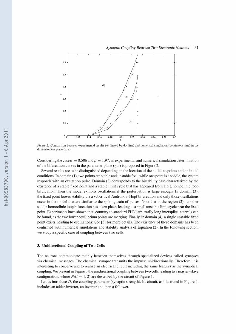
Figure 2. Comparison between experimental results (+, linked by dot line) and numerical simulation (continuous line) in the

dimensionless plane (η, ε).

Considering the case α = 0.506 and β = 1.97, an experimental and numerical simulation determination

of the bifurcation curves in the parameter plane (η,ε) is proposed in Figure 2.

Several results are to be distinguished depending on the location of the nullcline points and on initial

conditions. In domain (1), two points are stable and unstable foci, while one point is a saddle, the system

responds with an excitation pulse. Domain (2) corresponds to the bistability case characterized by the

existence of a stable fixed point and a stable limit cycle that has appeared from a big homoclinic loop

bifurcation. Then the model exhibits oscillations if the perturbation is large enough. In domain (3),

the fixed point looses stability via a subcritical Andronov–Hopf bifurcation and only those oscillations

occur in the model that are similar to the spiking train of pulses. Note that in the region (2), another

saddle homoclinic loop bifurcation has taken place, leading to a small unstable limit cycle near the fixed

point. Experiments have shown that, contrary to standard FHN, arbitrarily long interspike intervals can

be found, as the two lower equilibrium points are merging. Finally, in domain (4), a single unstable fixed

point exists, leading to oscillations; See [3] for more details. The existence of these domains has been

confirmed with numerical simulations and stability analysis of Equation (2). In the following section,

we study a specific case of coupling between two cells.

3. Unidirectional Coupling of Two Cells

The neurons communicate mainly between themselves through specialized devices called synapses

via chemical messages. The chemical synapse transmits the impulse unidirectionally. Therefore, it is

interesting to conceive and to realize an electrical circuit including the same features as the synaptical

coupling. We present in Figure 3 the unidirectional coupling between two cells leading to a master–slave

configuration, where Ni (i = 1, 2) are described by the circuit of Figure 1.

Let us introduce D, the coupling parameter (synaptic strength). Its circuit, as illustrated in Figure 4,

includes an adder-inverter, an inverter and then a follower.

hal-0

0583

790,

ver

sion

1 -

6 Ap

r 201

1

32 S. Jacquir et al.

N 1 N 2

D

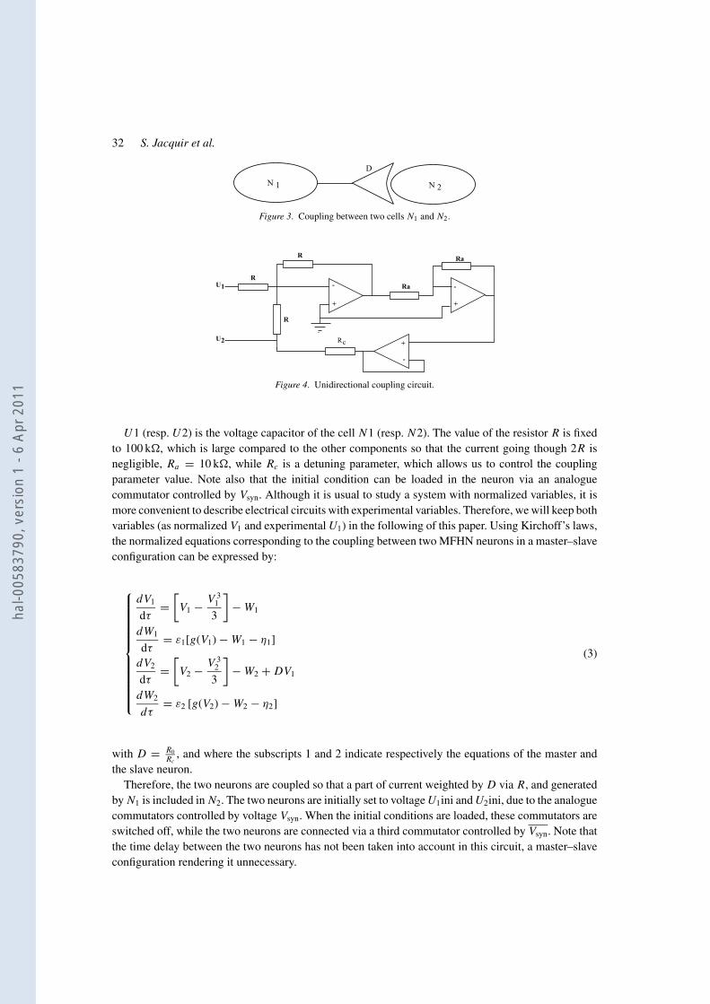
Figure 3. Coupling between two cells N1 and N2.

c

-

+

-

+

R

R

R

Ra

Ra

U1

U2

-

+R

Figure 4. Unidirectional coupling circuit.

U1 (resp. U2) is the voltage capacitor of the cell N1 (resp. N2). The value of the resistor R is fixed

to 100 k�, which is large compared to the other components so that the current going though 2R is

negligible, Ra = 10 k�, while Rc is a detuning parameter, which allows us to control the coupling

parameter value. Note also that the initial condition can be loaded in the neuron via an analogue

commutator controlled by Vsyn. Although it is usual to study a system with normalized variables, it is

more convenient to describe electrical circuits with experimental variables. Therefore, we will keep both

variables (as normalized V1 and experimental U1) in the following of this paper. Using Kirchoff’s laws,

the normalized equations corresponding to the coupling between two MFHN neurons in a master–slave

configuration can be expressed by:

⎧⎪⎪⎪⎪⎪⎪⎪⎪⎪⎪⎪⎨⎪⎪⎪⎪⎪⎪⎪⎪⎪⎪⎪⎩

dV1

dτ=

[V1 − V 3

1

3

]− W1

dW1

dτ= ε1[g(V1) − W1 − η1]

dV2

dτ=

[V2 − V 3

2

3

]− W2 + DV1

dW2

dτ= ε2 [g(V2) − W2 − η2]

(3)

with D = R0

Rc, and where the subscripts 1 and 2 indicate respectively the equations of the master and

the slave neuron.

Therefore, the two neurons are coupled so that a part of current weighted by D via R, and generated

by N1 is included in N2. The two neurons are initially set to voltage U1ini and U2ini, due to the analogue

commutators controlled by voltage Vsyn. When the initial conditions are loaded, these commutators are

switched off, while the two neurons are connected via a third commutator controlled by Vsyn. Note that

the time delay between the two neurons has not been taken into account in this circuit, a master–slave

configuration rendering it unnecessary.

hal-0

0583

790,

ver

sion

1 -

6 Ap

r 201

1

Synaptic Coupling Between Two Electronic Neurons 33

0.8 1 1.2 1.4 1.6 1.8 20

0.02

0.04

0.06

0.08

0.1

0.12

0.14

η2(D,V

1)/η

2(D=0)

D

Figure 5. Shifted bifurcation curve of the slave neuron N2 between domains (1) and (3). Parameters: master neuron N1: α1 =0.506, β1 = 1.97, ε1 = 0.01, η1 = 0.01 leading to V1 = −1.05 (i.e. U1 = −921 mV). Slave neuron N2: α2 = 0.506, β2 = 1.97,

ε2 = 0.01. Comparison between Equation (4) (continuous line) and experimental results (+).

3.1. THE MASTER IN A RESTING STATE

When the voltage is so that V1 is constant (the cell N1 is in a resting state); it is straightforward to show

that the variable W2 and the bifurcation parameter η2 of the cell N2 are given by:{η2(V1) = η2(V1 = 0) + DV1

W2(V1) = W2(V1 = 0) − DV1(4)

Therefore, it implies a modification of the excitability of the cell N2 corresponding to a shift in the (η, ε)

plane illustrated in Figure 5. The initial conditions are so that, when D = 0, the master neuron N1 lies in

domain (1), while the slave neuron N2 is in domain (3) and generates a spiking train of pulses. When the

unilateral coupling is increased and reaches a critical value, the neuron N2 ceases to oscillate and stays

in the resting state, meaning that the slave neuron has been moved from domain (3) to domain (1) of

Figure 2. This ability of neuron N1 to inhibit neuron N2 corresponds to the shift predicted by Equation

(4): As V1 < 0, increasing D implies to increase η2(D, V1) and therefore the bifurcation curves of

Figure 2 are translated along abscissa, while the value of η2 defined by the electrical parameters of

neuron N2 has not been changed. This result suggests that, for a defined activity of a slave neuron, the

strength of a unilateral coupling should be above a critical value to give to the master neuron the control

on the slave neuron.

In Figure 5, experimental values (D, η[D, V1]) correspond to the shifted bifurcation curve between

domains (1) and (3) of the neuron N2 with ε2 = 0.01 and when the master neuron N1 lies in domain (1)

in a resting state so that V1 = −1.05. Comparison shows a good match between experimental results

(+) and Equation (4) (continuous line), validating the unilateral coupling circuit.

3.2. THE MASTER IN A SPIKING REGIME

In this section, we present some results when the master is in domain (2) and oscillates. As V1 is varying

in time, we cannot express a simple relationship between the parameters of neuron N2 and V1, as in

hal-0

0583

790,

ver

sion

1 -

6 Ap

r 201

1

34 S. Jacquir et al.

0.045 0.05 0.055 0.06 0.065 0.070

0.2

0.4

0.6

0.8

1

D

f s /

fm

a

b

c

d

ef

g

Figure 6. Normalized eigen interspike slave frequency fs by interspike master frequency fm versus D with C = 0.001 nF,

ε1 = ε2 = 0.002, η1 = 0.199 and η2 = 0.109.

Equation (4). Nevertheless, oscillations of neurons N1 let V1 be alternatively positive and negative,

which implies that the bifurcation curves of neurons are translated along the abscissa in the plane (η, ε)

in a periodic manner (the position of saddle points of the cell N2 is moved periodically). Thus, the

slave neuron N2 initially situated in the vicinity of a bifurcation curve may be able to cross sometimes

this curve and develop a different dynamical behavior. Therefore, we have investigated the unilateral

coupling influence on N2, in the case when neuron N1 is initially (i.e. when D = 0) in domain (3) and

oscillating, while the slave neuron N2 is in domain (1).

According to the value of D, several different dynamical behaviors can be identified, as illustrated

in Figures 6 and 7:

– In case (a), the coupling strength is small, leading to subthreshold oscillations of fm frequency, which

are not taken into account in Figure 6 but are observable in Figure 7.

– In cases (b)–(f), stable periodic oscillations appear whose eigen interspike frequency follows a devil’s

staircase-like curve. Only specific values of fs/ fm are obtainable. Increasing the coupling strength

causes the period doubling in the slave cell, that is the period is multiplied by 2, 4, 8, 16, and so on.

– In case (g), N2 is fully synchronized with N1. The slave neuron oscillates in the same manner as the

master.

The slave neuron shows also a chaotic sequence of spikes resulting with variable interspike intervals.

This chaotic regime, corresponding to the dot lines in Figure 6, between the period-doubling plateaus

is so that the interspike slave period is varying during the experiments. When the coupling parameter

is gradually increased, we firstly proceed from a periodic spiking regime to a chaotic regime via a

sequence of period-doubling bifurcations. Finally, it leads to the reappearance of periodic dynamics

inserted in the chaotic zones.

The chaotic puffs disturb the periodic spiking regime. Increasing the coupling parameter causes the

increase of the frequency disturbances and then the chaos dominates the regime in the slave cell [8, 9].

An illustration of a chaotic signal is given in Figure 8 for D = 0.0535. The corresponding probability

of normalized interspike slave frequency fs/ fm is presented in Figure 9. This figure shows that in a

chaotic regime, the interspike frequencies are distributed widely in the range [0, 0.4 fm].

These experiments show that the unilateral coupling strength controls the slave neuron, from a silent

to a chaotic dynamical behavior.

hal-0

0583

790,

ver

sion

1 -

6 Ap

r 201

1

Synaptic Coupling Between Two Electronic Neurons 35

Figure 7. Temporal evolution of experimental voltage U2 for different values of D corresponding to cases (a)–(g) of Figure 6.

Voltage of the master neuron N1 is shown on top. Abscissa: 0.1 ms per division; ordinate: 2 V per division.

Figure 8. Chaotic signal in the case where D = 0.0535. Abscissa: 5 μs per division; ordinate: 2 V per division.

4. Conclusion

We have introduced an electrical circuit that allowed an unidirectional coupling without delay between

two cells in a master–slave configuration. We have shown that the intervals between successive spikes

can be chaotic and depend on the coupling strength. We suggest that this study can be helpful in

understanding the different dynamics of potential propagation in brain cells. To complete this work, it

would be of interest to study the bidirectional coupling corresponding to the electric synapse case and

hal-0

0583

790,

ver

sion

1 -

6 Ap

r 201

1

36 S. Jacquir et al.

0 0.05 0.1 0.15 0.2 0.25 0.3 0.35 0.40

0.01

0.02

0.03

0.04

0.05

0.06

0.07

0.08

0.09

0.1

fs/fm

P

Figure 9. Normalized distribution of the interspike frequency of N2 corresponding to the signal in Figure 8.

the influence of the size of the network on the fractal dimension of the information [10]. This nonlinear

electrical circuit cell indeed gives the opportunity to realize a large-scale network.

5. Acknowledgements

This research has been supported by the Russian–French program of joint research (grant 04610PA),

the Russian Foundation for Basic Research (grant 03-02-17135) and INTAS grant (YSF 2001-2/24).

References

1. Nagumo, J., Arimoto, S., and Yoshizawa, S., ‘An active impulse transmission line simulating nerve axon’, Proceedings ofIRE 50, 1962, 2061–2070.

2. Scott, A. C., Neuroscience: A Mathematical Primer, Springer-Verlag, New York, 2002.

3. Binczak, S., Kazantsev, V. B., Nekorkin, V. I., Bilbault, J. M., ‘Experimental study of bifurcations in modified FitzHugh–

Nagumo cell’, Electronic Letter 39, 2003, 961–962.

4. Dawson, S. P., D’Angelo, M. V., and Pearson, J. E., ‘Towards a global classification of excitable reaction-diffusion systems’,

Physics Letter A 265, 2000, 346–352.

5. Kazantsev, V. B., Nekorkin, V. I., Binczak, S., and Bilbault, J. M., ‘Spiking patterns emerging from wave instabilities in a

one-dimensional neural lattice’, Physical Review E 68, 2003, 017201, 1–4.

6. Rinzel, J. and Ermentrout, B. B., ‘Analysis of neural excitability and oscillations’, in Methods in Neuronal Modeling, C.

Koch and I. Segev (eds.), 2nd edn., MIT press, Cambridge, MA, 1998, pp. 251–292.

7. Koch, C., Biophysics of Computation: Information Processing in Single Neurons, Oxford University Press, Oxford, 1998.

8. Ott, E., Grebogi, C., and Yorke, J. A., Physical Review Letters 64, 1990, 1196–1199.

9. Nayfeh, A. H. and Balachandran, B., Applied Nonlinear Dynamics: Analytical,Computational, and Experimental Methods,

Wiley-Interscience, New York, 1995.

10. Kazantsev, V. B., ‘Selective communication and information processing by excitable systems’, Physical Review E 64, 2001,

056210.

hal-0

0583

790,

ver

sion

1 -

6 Ap

r 201

1