PARAMETRIC SHAPE AND TOPOLOGY OPTIMIZATION WITH RADIAL BASIS FUNCTIONS
Upload
khangminh22Category
view
1download
0
STRUCTURAL TOPOLOGY OPTIMIZATIONVIA THE GENETIC ALGORITHM
by
Colin Donald Chapman
Bachelor of Science in Mechanical EngineeringThe University of Washington
August 1991
Submitted to the Department of Mechanical Engineeringin Partial Fulfillment of the Requirements for the Degree of
Master of Sciencein Mechanical Engineering
at the
MASSACHUSETTS INSTITUTE OF TECHNOLOGY
May 1994
© Massachusetts Institute of Technology 1994All rights reserved.
Signature of AuthorColin D. Chapman
Department of Mechanical EngineeringMay 6, 1994
Certified byMark J. Jakiela
Robert N. Noyce Assistant Professor, Mechanical EngineeringThesis Supervisor
Accepted byAin A. Sonin
Chairman, Departmental Graduate Committee
ARCHNIVESMASSACHlsn~'S !NSTITuT
AUG 011994

2

STRUCTURAL TOPOLOGY OPTIMIZATIONVIA THE GENETIC ALGORITHM
by
Colin Donald Chapman
Submitted to the Department of Mechanical Engineeringon May 6, 1994 in Partial Fulfillment of the Requirements for the Degree of
Master of Science in Mechanical Engineering
ABSTRACT
The genetic algorithm, a search and optimization technique based on the theory of
natural selection, is applied to problems of structural topology optimization. Given a
structure's boundary conditions and allowable design domain, a discretized design
representation is created. The genetic algorithm then generates an optimal structure
topology by evolving a population of "chromosomes," where each chromosome, after
mapping into the discretized design representation, creates a potentially-optimal structure
topology. Specifically, using an evolutionary, survival-of-the-fittest optimization
mechanism, the genetic algorithm allows structure topologies in the population to compete
against one another to serve as parent topologies. Parent topologies then pair and mate,swapping portions of their "genetic code" to create a population of child topologies of
hopefully higher quality. After undergoing infrequent, random mutation, the child
population replaces the original population, and the process then iterates until an optimal
structure topology is located.
In this thesis, the use of the genetic algorithm in structural topology optimization is
presented. After defining structural topology optimization and detailing the genetic
algorithm, a review of previous research in structural optimization is provided. The
implementation of this investigation's genetic algorithm-based structural topology
optimization approach is then detailed, and several examples are presented: optimizations
of beam cross-section topologies and cantilevered plate topologies are described, as are
methods for the efficient use of finite element analysis in a genetic algorithm-based search.
The optimization of finely-discretized design domains is then examined. The genetic
algorithm's ability to generate design families, as well as designs combining high structural
performance with high manufacturability, is then demonstrated. Structures created using
this investigation's genetic algorithm-based approach are then compared to those obtained
utilizing homogenization-based techniques. Finally, potential future work in suggested.
Thesis Advisor: Professor Mark J. Jakiela

4

5
ACKNOWLEDGMENTS
First and foremost, I would like to thank my thesis advisor, Professor MarkJakiela. Serving as advisor, friend, and occasional critic, Mark believed in my abilities,even when I didn't. He taught me the value of preparation. He transformed my rambling,incoherent writing style into one which is at least somewhat presentable. He encouragedme to live a balanced life. He understood that sometimes the things which seem so vitallyimportant can, with a single phone call, become totally insignificant. Thanks, Mark.
Of course, heartfelt gratitude, appreciation, thanks, and love go to my parents. Tomy mother, for giving me determination and motivation, and to my late father, for inspiringme to follow my passions both in my hobbies and in my career. While my father wasaround to share in my anxiety and fear about coming to MIT, I hope that somehow he willbe able to see or sense that I actually made it through.
Thanks must also go to my brother, John, and to my sisters, Christina and Linda.The cards, camping trips, Thanksgiving dinners, and dinners at The Keg were great!
To my friends here in Boston (Amy, Arlene, Becca, Brian, Chris, Christine,Dalila, Dan, Dave, Doug, Eric, Erin, Frank, Hal, Mike, Paul, and Robin), who alwaysdragged me out of the office: Thanks for making my two years in grad school a lot of fun!
And thanks must certainly go out to my friends in the Pacific Northwest: to Daneand Carolyn for always reminding me about how nice it is back in Washington, to Markfor helping me get out of the predicaments in which I always seem to find myself, to Seanfor repeatedly trying to get me to relive the old college days, to Tom and Shari for beingexcited about engineering (Tom) and putting up with a bunch of geeking out (Shari), and toWarren and Karen for reminding me about how much I miss my road bike and stereosystem. Many miles were between us, but I think we did a good job of keeping in touch!
I must also thank the MIT CADLAB, directed by Professor David Gossard, forproviding the computational resources needed for this project. Barbara Balents, LoriHumphrey, Jay Krishnasamy, Kate Melvin, Narendra Soman, Dave Wallace, and JohnYoon all made the MIT CADLAB a decent place to work. Also, the assistance andsoftware from Ashok Kumar and Kazuhiro Saitou were instrumental to the success of thisproject.
Finally, I must thank Lisa for all of the care, support, patience, and understandingwhich she has selflessly provided during the past few months. It hasn't been long, but itsure has been fun!

6

7
TABLE OF CONTENTS
A B ST R A C T ....................................................................................... 3ACKNOWLEDGMENTS ..................................................................... 5TABLE OF CONTENTS ........................................................................ 7L IST O F FIG U R E S .............................................................................. 11LIST OF TABLES.............................................................................. 15IN TR O D U C TIO N ................................................................................ 19
1.1 O verview .......................................................................... 191.2 M otivation .......................................................................... 191.3 O bjective ............................................................................. 201.4 Problem S tatem ent.................................................................. 2 11.5 O rganization ....................................................................... 22
BACKGROUND ............................................................................... 252.1 O verview .......................................................................... 252.2 Structural Optimization.......................................................... 25
2.2.1 Introduction........................................................... 252.2.2 Structural Optimization Techniques................................. 262.2.3 Problem Formulation .................................................. 272.2.4 Structural Optimization Subroutines ............................... 302.2.5 Structural Optimization Categories................................. 39
2.3 The Genetic Algorithm........................................................... 432.3.1 Introduction........................................................... 432.3.2 Similarities with Biological Systems.............................. 442.3.3 Design Variables as Chromosomes .................................. 442.3.4 Optimization Through Evolution ................................... 482.3.5 Optimization Parameters............................................. 562.3.6 GA's vs. Traditional Optimization Methods ........................ 582.3.7 Sum m ary ................................................................ 60
PREVIOUS WORK ............................................................................ 633.1 O verview ......................................................................... . 33.2 Non-Genetic-Algorithm-Based Topology Optimization ...................... 64
3.2.1 Homogenization Method ............................................. 643.2.2 Simulated Annealing ................................................. 67
3.3 Genetic Algorithm-Based Structural Optimization............................ 703.3.1 Introduction........................................................... 703.3.2 Sizing Optimization .................................................. 703.3.3 Shape Optimization .................................................. 733.3.4 Topology Optimization ............................................... 75
THIS INVESTIGATION ....................................................................... 854 .1 O verview .......................................................................... 854.2 The Technique ..................................................................... 85
4.2.1 Introduction........................................................... 854.2.2 Performing Optimization ............................................. 85
4.3 Extensions of Previous Work..................................................... 86
8
4.3.1 Introduction............................................................864.3.2 Specific Extensions of Previous Work............................864.3.3 Fundamental Differences Between the Techniques ............... 87
4.4 Implementation ................................................................... 904.4.1 Introduction............................................................904.4.2 Design Representation.............................................. 914.4.3 Converting a Chromosome into a Topology.....................934.4.4 Connectivity Analysis ................................................ 944.4.5 Structural Analysis......................................................974.4.6 Fitness Calculations .................................................... 1014 .4 .7 S um m ary ................................................................. 105
E X A M P L E S ........................................................................................ 1075 .1 O verview ............................................................................. 1075.2 Example 1: Beam Cross-Section.................................................107
5 .2 .1 Introduction .............................................................. 1075.2.2 Design Domain..........................................................1075.2.3 Fitness Calculations-Part A..........................................1085.2.4 Results-Part A.........................................................1095.2.5 Fitness Calculations-Part B..........................................1105.2.6 Results-Part B.........................................................112
5.3 Example 2: Small Cantilevered Plate ............................................ 1155 .3.1 Introdu ction .............................................................. 1155.3.2 Design Domain..........................................................1155.3.3 Fitness Calculations .................................................... 1165 .3 .4 R esults ................................................................... 118
5.4 Example 3: Comparison of Finite Element Meshing Techniques ............ 1205 .4 .1 Introduction .............................................................. 1205.4.2 Adaptive Finite Element Meshing.....................................1205.4.3 Constant Finite Element Meshing.....................................1215.4.4 Comparison of Adaptive and Constant Meshing....................122
5.5 Example 4: Large Cantilevered Plate ............................................ 1275 .5 .1 Introduction .............................................................. 1275.5.2 Design Domain..........................................................1275.5.3 Fitness Calculations .................................................... 1285 .5 .4 R esults ................................................................... 129
5.6 Example 5: Hierarchical Design Domain Subdivision.........................1325.6.1 Introduction .............................................................. 1325.6.2 Overview of the Technique ............................................ 1325.6.3 Details of the Technique................................................1325 .6 .4 E xam ple..................................................................138
5.7 Example 6: Design Families......................................................1435 .7 .1 Introduction .............................................................. 1435.7.2 Design Domain..........................................................1445.7.3 Fitness Calculations .................................................... 1445 .7 .4 R esults ................................................................... 14 6
5.8 Example 7: Manufacturability Considerations..................................148

9
5.8.1 Introduction ............................................................. 1485.8.2 Design Domain......................................................... 1495.8.3 Fitness Calculations.................................................... 1505.8.4 Experiment Design..................................................... 1535 .8 .5 R esu lts................................................................... 154
5.9 Example 8: Comparison with Homogenization-Based Techniques......... 1615.9.1 Introduction ............................................................. 16 15.9.2 Design Domain ......................................................... 1615.9.3 Fitness Calculations.................................................... 1625.9.4 Hierarchical Subdivision Parameters ................................ 1645 .9 .5 R esu lts................................................................... 165
C O N C L U SIO N S ................................................................................. 1696 .1 O verview ............................................................................ 1696.2 Contributions of This Investigation .............................................. 1696 .3 C onclusions ......................................................................... 1726.4 F uture W ork ......................................................................... 174
R E F E R E N C E S .................................................................................... 177INDEX .......................................................................... 187

10

1]
LIST OF FIGURES
Figure 1.1:
Figure 2.1:
Figure 2.2:
Figure 2.3:
Figure 2.4:
Figure 2.5:
Figure 2.6:
Figure 2.7:
Figure 2.8:
Figure 2.9:
Figure 2.10:
Figure 2.11:
Figure 2.12:
Figure 3.1:
Figure 3.2:
Figure 3.3:
Figure 3.4:
Figure 3.5:
Figure 3.6:
Figure 3.7:
Figure 3.8:
Figure 3.9:
Figure 3.10:
Figure 3.11:
Figure 3.12:
Figure 3.13:
Figure 3.14:
Figure 3.15:
Figure 3.16:
Figure 4.1:
Figure 4.2:
Figure 4.3:
A schematic representation of genetic algorithm-based structuraltopology optim ization............................................................ 21
Interaction between structural optimization subroutines ................... 30Sizing optimization............................................................. 40
Shape optim ization ............................................................... 4 1
Topology optimization......................................................... 43
A typical genetic algorithm population......................................... 45
The chromosome decoding process.......................................... 48
One "generation" of genetic algorithm optimization.......................... 49
Fitness evaluation .............................................................. 49
Parent selection ................................................................... 5 1
Single point crossover ......................................................... 53
M utation ........................................................................... 54
Genetic algorithm flowchart.................................................. 55
Rectangular hole microstructure ................................................ 65
Rank-2 microstructure ......................................................... 65
Square hole design variables.................................................... 66
Rectangular hole design variables ........................................... 66
Design domain to topology mapping....................................... 68
Beam cross-section optimization .............................................. 69
Compliance minimization...................................................... 69
10-member truss structure with applied loads ................................ 71
Control points defining the component's shape ............................. 74
Shape representation using FFD............................................ 75
Points used to define the nature of a truss structure.......................... 77
An example ground structure .................................................. 78
Multi-segmented beam optimization............................................ 80
Single-segment beam optimization ........................................... 81
Optimal beam cross-sections for (a) plastic, (b) aluminum, and (c)steel ............................................................................. . . 8 1
Cantilevered plate optimization ................................................. 82
Two-dimensional crossover.................................................. 88
Design domain discretization.................................................. 92
Design domain material distribution to structure topologycorrespondence ................................................................... 92

12
Figure 4.4:
Figure 4.5:
Figure
Figure
Figure
Figure
Figure
Figure
Figure
Figure
4.6:
4.7:
4.8:
4.9:
4.10:
5.1:
5.2:
5.3:
Figure 5.4:
Figure 5.5:
Figure 5.6:
Figure
Figure
Figure
Figure
Figure
Figure
Figure
5.7:
5.8:
5.9:
5.10:
5.11:
5.12:
5.13:
Figure 5.14:
Figure 5.15:
Figure 5.16:
Figure
Figure
Figure
Figure
5.17:
5.18:
5.19:
5.20:
Chromosome population representing a population of structuretopologies ........................................................................ 93
Mapping a genetic algorithm chromosome into the design domain tocreate a structure topology ..................................................... 94C onnectivity analysis ............................................................. 95(a) Connected and (b) disconnected material elements....................95Finite element mesh generation...............................................98
Adaptive meshing technique .................................................. 99
Constant meshing technique ..................................................... 100
Example 1 design domain........................................................108
Best-of-generation beam cross-sections........................................109
Maximum, average, and minimum beam cross-section fitness vs.generation .......................................................................... 110
Optimal cross-section topologies for applied moments of (a) 150,000N -m and (b) 200,000 N -m ....................................................... 112
Maximum stress vs. generation with applied moment of 150,000N -m ................................................................................. 1 13
Maximum stress vs. generation with applied moment of 200,000N -m ................................................................................. 1 13
Exam ple 2 design dom ain........................................................116
Best-of-generation plate topologies ............................................. 119
Maximum, average, and minimum plate topology fitness vs.generation .......................................................................... 119
Example 3 design domain........................................................123
Optimal plate topologies obtained using the constant meshingtechn ique ........................................................................... 12 6
Example 4 design domain........................................................127
Optimal plate topologies using (a) 10 x 16, (b) 15 x 24, and (c)20 x 32 design domain discretizations ......................................... 130An example optimization problem and an example coarse designdomain discretization corresponding to the problem..........................133
The genetic algorithm creating an example optimal coarse platetopology in the example coarse design domain................................134Mapping the optimal coarse plate topology into an example finely-discretized design dom ain........................................................134
Population-to-design-domain mapping after hierarchical subdivision ...... 135
Example optimization of the finely-discretized plate topology...............137
Exam ple 5 design dom ain........................................................138
Optimal plate topologies generated using (a) 10 x 16, (b) 20 x 32,and (c) 40 x 64 design domain discretizations ................................ 141

13
Figure 5.21: Example 6 design domain ....................................................... 144
Figure 5.22: Family of plate topologies with (a) 0, (b) 1, (c) 2, (d) 3, (e) 4, and (f)5 intern al holes.................................................................... 147
Figure 5.23: Example 7 design domain ....................................................... 149
Figure 5.24: High stiffness-to-weight ratio, low-porosity plate topologies .............. 155
Figure 5.25: Mean stiffness-to-weight ratio vs. mean number of internal holes ......... 157
Figure 5.26: Stiffness-to-weight ratio vs. number of internal holes....................... 157
Figure 5.27: Example 8 design domain ....................................................... 162
Figure 5.28: Genetic algorithm-based optimal plate topology.............................. 166
Figure 5.29: Homogenization-based optimal plate topology ............................... 166
Figure 5.30: Family of minimum mean compliance plate topologies...................... 168

14
15
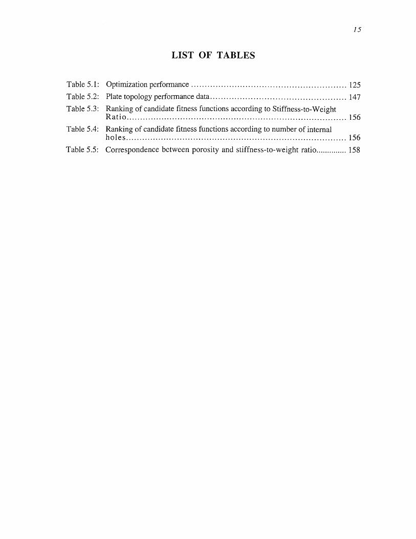
LIST OF TABLES
Table 5.1: Optimization performance ......................................................... 125
Table 5.2: Plate topology performance data.................................................. 147
Table 5.3: Ranking of candidate fitness functions according to Stiffness-to-WeightR a tio .................................................................................. 15 6
Table 5.4: Ranking of candidate fitness functions according to number of internalh o le s .................................................................................. 15 6
Table 5.5: Correspondence between porosity and stiffness-to-weight ratio.............. 158

16

17
To my parents
"Be bold and courageous. When you lookback on your life, you'll regret the thingsyou didn't do more than the ones you did."
H. Jackson Brown, Jr.Author of Life's Little Instruction BookRutledge Hill Press, Nashville, Tennessee

18

Chapter I Introduction 19
Introduction I
1.1 Overview
This chapter first presents the motivation behind this investigation and then details
the investigation's specific objectives. A typical problem statement is then provided, after
which the organization of this thesis is detailed.
1.2 Motivation
Design is an iterative process divided into stages. After first recognizing a need for
a device (Shigley and Mischke, 1989) and defining a set of specifications and functional
requirements, a designer must develop a conceptual design establishing the overall form of
the device, optimize the conceptual design so that it best satisfies the specifications and
functional requirements, and then finally detail the design to account for manufacturability
and aesthetic (among others) considerations. During this process, the designer will often
find that the current design is inadequate and will therefore return to an earlier phase of the
design procedure to account for the inadequacy.
Hence, the design process begins with theformulation offunctional requirements
and then continues with conceptual design, optimization, and finally detailing (Kirsch,1993). Again, design is very much an iterative process, in that a designer will often return
to earlier stages of the process to account for observed inadequacies in a design.
Of the four main stages of the design process, the conceptual design stage is
typically regarded as critical, for it is an early phase of the design process yet establishes
much of the device's overall design. Consequently, because design revisions become
increasingly expensive in subsequent phases of the design process, design decisions made

20 Chapter 1 - Introduction
in the conceptual design stage must be thoroughly planned and carefully executed.
Unfortunately, even though the conceptual design stage is one of the most critical elements
of the design process and must be carefully planned and executed, few computational tools
which aid a designer with conceptual design are available-the success (or failure) of
conceptual design is, for the most part, left entirely to the ingenuity, intuition, and
judgement of the designer (Kirsch, 1993).
In an attempt to aid the designer with the conceptual design stage, this investigation
develops a computer-based system which automates conceptual design by modeling a
conceptual design problem as an optimization problem and then using a numerical
optimization procedure to search the "space" of possible designs for the optimal design.
As no single computer-based system is applicable to all conceptual design
problems, this investigation focuses on developing a system which automates the
conceptual design of load-bearing structures. Specifically, this investigation examines the
automated generation of optimal topologies for load-bearing structures, i.e., structural
topology optimization. While structural topology optimization is a very specific conceptual
design problem, the optimization algorithm used by this investigation to perform structural
topology optimization, the genetic algorithm (Goldberg, 1989a), is very general. In fact,
the genetic algorithm, a search and optimization technique based on the theory of natural
selection, is not peculiar to any particular design domain and can therefore be applied to
many other classes of conceptual design problems.
1.3 Objective
The general objective of this investigation is to help determine the utility of genetic
algorithms in conceptual design, while the specific objective is to use the genetic algorithm
to perform structural topology optimization. In particular, this investigation intends to
accomplish the following:
- Develop a genetic algorithm-based approach for the structural topology
optimization of continuum structures, where the optimal distribution of material
and void within a discretized design domain is found.
- Apply this genetic algorithm-based structural topology optimization approach to
a variety of examples in an attempt to establish the feasibility, demonstrate the
capabilities, and increase the performance of the approach.
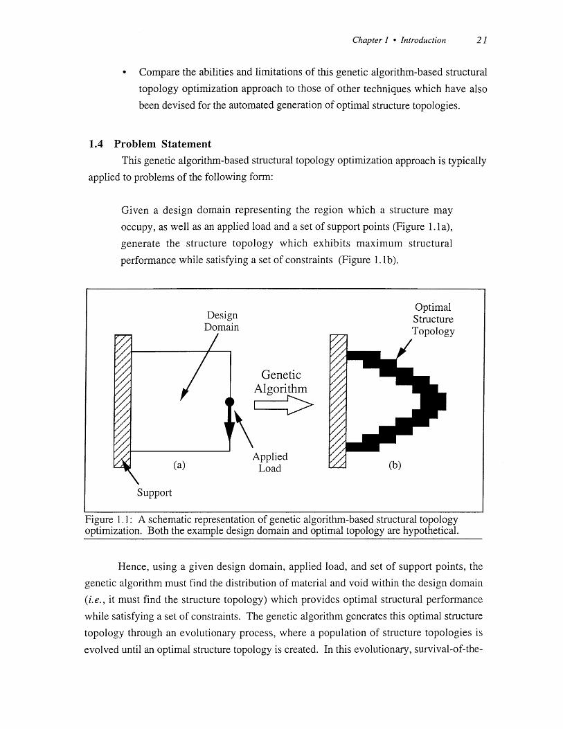
DesignDomain
Chapter 1 - Introduction 21
. Compare the abilities and limitations of this genetic algorithm-based structural
topology optimization approach to those of other techniques which have also
been devised for the automated generation of optimal structure topologies.
1.4 Problem Statement
This genetic algorithm-based structural topology optimization approach is typically
applied to problems of the following form:
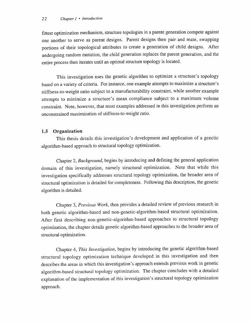
Given a design domain representing the region which a structure may
occupy, as well as an applied load and a set of support points (Figure 1.la),generate the structure topology which exhibits maximum structural
performance while satisfying a set of constraints (Figure 1. 1b).
OptimalStructureTopology
GeneticAlgorithm
AppliedLoad
Support
Figure 1.1: A schematic representation of genetic algorithm-based structural topologyoptimization. Both the example design domain and optimal topology are hypothetical.
Hence, using a given design domain, applied load, and set of support points, the
genetic algorithm must find the distribution of material and void within the design domain
(i.e., it must find the structure topology) which provides optimal structural performance
while satisfying a set of constraints. The genetic algorithm generates this optimal structure
topology through an evolutionary process, where a population of structure topologies is
evolved until an optimal structure topology is created. In this evolutionary, survival-of-the-
I Z AWN&
22 Chapter 1 - Introduction
fittest optimization mechanism, structure topologies in a parent generation compete against
one another to serve as parent designs. Parent designs then pair and mate, swapping
portions of their topological attributes to create a generation of child designs. After
undergoing random mutation, the child generation replaces the parent generation, and the
entire process then iterates until an optimal structure topology is located.
This investigation uses the genetic algorithm to optimize a structure's topology
based on a variety of criteria. For instance, one example attempts to maximize a structure's
stiffness-to-weight ratio subject to a manufacturability constraint, while another example
attempts to minimize a structure's mean compliance subject to a maximum volume
constraint. Note, however, that most examples addressed in this investigation perform an
unconstrained maximization of stiffness-to-weight ratio.
1.5 Organization
This thesis details this investigation's development and application of a genetic
algorithm-based approach to structural topology optimization.
Chapter 2, Background, begins by introducing and defining the general application
domain of this investigation, namely structural optimization. Note that while this
investigation specifically addresses structural topology optimization, the broader area of
structural optimization is detailed for completeness. Following this description, the genetic
algorithm is detailed.
Chapter 3, Previous Work, then provides a detailed review of previous research in
both genetic algorithm-based and non-genetic-algorithm-based structural optimization.
After first describing non-genetic-algorithm-based approaches to structural topology
optimization, the chapter details genetic algorithm-based approaches to the broader area of
structural optimization.
Chapter 4, This Investigation, begins by introducing the genetic algorithm-based
structural topology optimization technique developed in this investigation and then
describes the areas in which this investigation's approach extends previous work in genetic
algorithm-based structural topology optimization. The chapter concludes with a detailed
explanation of the implementation of this investigation's structural topology optimization
approach.

w~ ~w
Chapter I Introduction 23
Chapter 5, Examples, details the application of this investigation's genetic
algorithm-based structural topology optimization approach to a variety of increasingly-
complex example problems.
Chapter 6, Conclusions, overviews the contributions of this investigation and
provides conclusions regarding the abilities and limitations of its genetic algorithm-based
structural topology optimization approach. The chapter concludes by offering potential
areas of future research.
Chapter 7, References, provides a list of previous work cited in this thesis.
Chapter 8, Index, provides lists of authors cited and subjects detailed in this thesis.

24 Chapter I Introduction

Chapter 2 Background 25
Background
2.1 Overview
This chapter first introduces and defines the application domain of this research,structural optimization, and then details the technique used to perform the optimization, the
genetic algorithm.
2.2 Structural Optimization
2.2.1 Introduction. Structural optimization is the automated synthesis of a
mechanical component based on structural considerations. In other words, structural
optimization generates a mechanical component design which exhibits optimal structural
performance. Falling under the broader category of design optimization, where the design
of a device is optimized so that the device exhibits maximum utility subject to a given set of
functional requirements and performance constraints, structural optimization is the design
optimization of mechanical components where the utility, functional requirements, and/or
performance constraints are structural in nature (Kumar, 1993).
Utility, in the context of structural optimization, is a measure of a component's
structural performance, effectiveness, and desirability. For example, maximizing a
component's utility could include maximizing stiffness, maximizing manufacturability,
minimizing weight, or minimizing cost. Functional requirements, again in the context of
structural optimization, are specifications which define the intended use of the component
and the conditions under which the component will operate. Typical specifications include
size and weight limitations, material properties, locations of support points, and locations,
directions, and magnitudes of applied loads. Lastly, performance constraints are defined
ranges of acceptable structural behavior. For example, constraints can specify maximum
26 Chapter 2 * Background
allowable stress levels, maximum acceptable weight levels, maximum deflection levels,
minimum heat dissipation rates, etc.
As demonstrated above, a wide variety of properties can serve as measures of utility
or as performance constraints. These properties, which all influence a component's
design, are commonly referred to as design criteria. Design criteria typically used in
structural optimizations include, but are not limited to, a component's stiffness, strength,
stress levels, weight, volume, thermal properties, manufacturability, fatigue life, dynamic
behavior, deflection, or cost. Structural optimization problems never simultaneously
account for all design criteria-the particular design criteria addressed in a given problem's
utility and constraint calculations depend upon the problem's domain and the available
computational resources.
Hence, structural optimization generates a component design which exhibits
maximum structural utility subject to a set of functional requirements and constraints on the
component's structural behavior. Examples of structural optimization include the
minimization of the volume of a cantilevered plate in tension subject to a maximum
deflection constraint, or the maximization of the stiffness of a simply-supported beam
under pure bending subject to a maximum mass constraint.
2.2.2 Structural Optimization Techniques. Either analytical or numerical
techniques can be used to solve structural optimization problems (Kirsch, 1993).
Analytical structural optimization techniques, pioneered by Mitchell (Mitchell, 1904),
typically employ mathematical approaches such as calculus or variational methods to find
optimum structure designs. Equations describe a component's design, and an optimum
design is found when systems of equations defining the conditions for optimality are
solved analytically. While analytical techniques do provide an exact solution to the
optimization problem, they can only solve straightforward problems. Design problems
with complex boundary conditions or multiple components are generally not solvable using
analytical techniques. Analytical techniques in structural optimization, with particular
emphasis on the creation of "Mitchell Structures," are detailed by Cox (Cox, 1965) and
Hemp (Hemp, 1973).
To facilitate the solution of highly-complex problems, numerical structural
optimization techniques have been developed. These methods numerically approximate the
design and then iteratively modify the design until a near-optimum solution is obtained.
Chapter 2 - Background 27
While numerical techniques are unable to obtain exact solutions to an optimization problem,
they can address problems of great complexity. All discussion in this article is concerned
with numerical structural optimization techniques.
2.2.3 Problem Formulation. Before conducting a structural optimization, the
qualitative problem description (e.g., minimize the mass of a cantilevered plate in tension
subject to a maximum stress constraint) must first be formulated as a quantitative
mathematical statement (Arora, 1989). This begins with the definition of design variables,which are parameters controlling the component's design. One design variable is needed
for every component attribute allowed to vary during optimization. Because the design
variables control the component's design, assigning numerical values to the design
variables results in the creation of a particular component design. Note that a particular set
of design variable values represents both a particular component design and a particular
location, or point, in the search space. A vector of N design variables is shown below:
X T [X X 2 XN-I XN] (2.1)
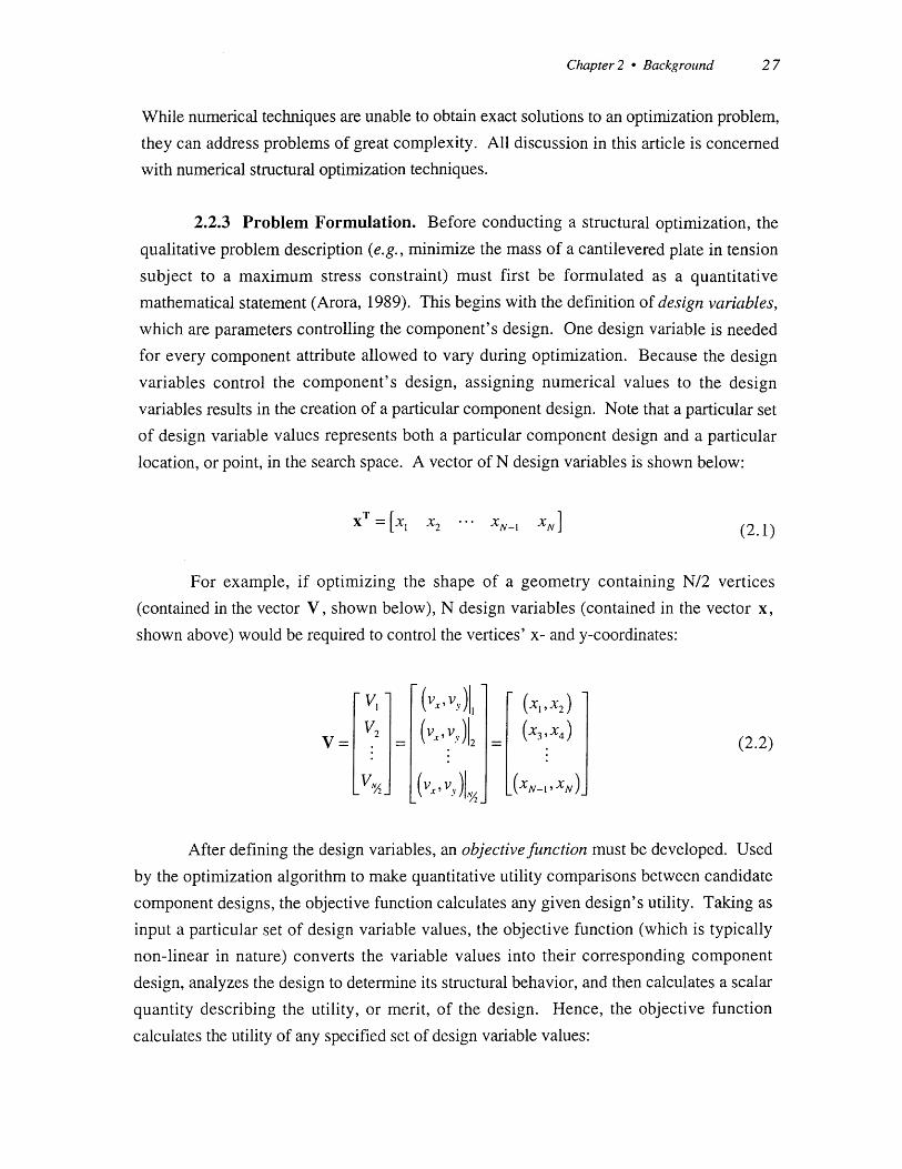
For example, if optimizing the shape of a geometry containing N/2 vertices
(contained in the vector V, shown below), N design variables (contained in the vector x,shown above) would be required to control the vertices' x- and y-coordinates:
V2 (vX ,vp (XI IX4)
V L (VI2 (2.2)
V2 (y,, xN-I'IXN)
After defining the design variables, an objective function must be developed. Used
by the optimization algorithm to make quantitative utility comparisons between candidate
component designs, the objective function calculates any given design's utility. Taking as
input a particular set of design variable values, the objective function (which is typically
non-linear in nature) converts the variable values into their corresponding component
design, analyzes the design to determine its structural behavior, and then calculates a scalar
quantity describing the utility, or merit, of the design. Hence, the objective function
calculates the utility of any specified set of design variable values:
28 Chapter 2 - Background
Utility = U(x) U(xiIX2,- -- xN) (2-3)
Note that many structural optimizations attempt to minimize a component's cost
instead of maximizing its utility. In fact, most optimization algorithms (mathematical
programming, optimality criteria, and simulated annealing-see Section 2.2.4) are cost
minimization algorithms. However, the optimization technique used in this research, the
genetic algorithm, is a maximization algorithm. Hence, the mathematical problem
formulation is stated as a utility maximization.
A set of design constraints must then be created. Typically used to represent a
component's functional requirements and performance constraints, design constraints are
(often non-linear) mathematical equalities or inequalities defining constraints on the
component's structural behavior. Note that in addition to being functions of the design
variables, constraint calculations typically require structural analysis results. An example
set of design constraints is depicted below:
h (x) h (xlx 2 ,- -,xN)=0; j= 1 top (2.4)
(xi=tom (2.5)
Design constraints establish a component's feasibility-components which do not
violate any design constraints are considered feasible, while those violating one or more
design constraints are considered infeasible. For a given set of design variable values x(k),
an inequality constraint is violated when positive in value (i.e., gi(x(k))> 0), while an
equality constraint is violated when non-zero (i.e., h (x(k)) #0). Also, inequality
constraints satisfied as equalities (i.e., g,(x(k))= 0) are considered active, while inequality
constraints with negative values (i.e., g,(x(k)) < 0) are inactive. Inequality constraints
which are inactive at an optimal solution x* can be removed without affecting the optimality
of x* (i.e., x* remains optimal), while removing inequality constraints which are active at
x* will likely change the optimality of x* (i.e., x* will likely no longer be optimal).
Likewise, removing any equality constraint (which must be satisfied at the optimal solution
x*) will likely change the optimality of x*. Note that removing any equality constraint or
inequality (whether active or inactive at the optimal solution x') constraint from the
optimization problem statement and then re-running the optimization would likely result in
the generation of a different optimal solution.

Chapter 2 - Background 29
Finally, side constraints must be developed to define the allowable ranges of design
variable values. As design variable values control the component's design, side constraints
define the range of possible designs. An example set of side constraints is depicted below:
ak ! xk b,; k= 1 to N (2.6)
Note that side constraints are often incorporated into the set of inequality designconstraints, with each side constraint converting into two inequality design constraints:
ak -Xk 0 (2.7a)
Xk -bk 0 (2.7b)
After the definition of side constraints, the problem formulation is complete.
Hence, the standard design optimization problem statement is given by:
Find the vector x of design variable values
X T=[X x 2 XN]
which maximizes a utility function
U(x)= U(xI, x 2, ... , XN)
subject to p equality constraints
hi (X) - hi (xi, 3x21- -. IN) = 0; j = 1 to p
m inequality constraints
gi;(X) =g(i, ( X 2- -. -, XN) :! 0; i = I t0 M
and N side constraints
ak Xk b,; k = I to N
Hence, structural optimization procedures attempt to find the set of design variable
values which maximizes an objective function subject to a set of equality and inequality
constraints. The set of optimum design variable values represents the optimum component
design, while the objective function measures the component's structural performance and

30 Chapter 2 - Background
the set of equality and inequality constraints represents limitations imposed on the
component's structural behavior.
2.2.4 Structural Optimization Subroutines. After creating a mathematical
formulation of the structural optimization problem, optimization is performed. The
optimization is controlled by an optimization algorithm, which first chooses a set of initial
design variable values. These variable values are then sent to the objective function, which
uses a modeler to convert the variable values into a component design. The design is then
subjected to structural analysis to determine its structural performance. Utilizing results of
the structural analysis, the objective function calculates the design's utility and returns the
value to the optimization algorithm. The optimization algorithm then modifies the design
variable values in an attempt to increase the component's utility while satisfying all
constraints. The process then iterates until the optimal component design is found (Figure
2.1).
Figure 2.1: Interaction between structural optimization subroutines.
Optimization Algorithm. The main subroutine in a structural optimization procedure
is the optimization algorithm. Having overall control of the structural optimization process,
the optimization algorithm is responsible for guiding the search to the set of design variable

Chapter 2 * Background 31
values (corresponding to a particular component design and a particular location in the
search space) which maximizes the objective function while satisfying all constraints.
Optimization algorithms used in structural optimization procedures generally fall into one offour categories:
Mathematical Programming Techniques. Often referred to as direct methods,
mathematical programming techniques perform optimization by deterministically"climbing" to the top of the nearest locally-optimum peak in the search space.
This peak corresponds to a set of locally-optimum design variable values and a
locally-optimum component design. Search begins with the selection of a set of
design variable values corresponding to an initial component design which does
not necessarily satisfy any constraints or provide maximum utility. In an
iterative process, the design variable values are modified so that thecorresponding design's utility is increased and the constraints are satisfied.
When all constraints are satisfied and the design can no longer be improved, the
design and the design variable values are considered optimal.
Specifically, any iteration k begins when the values and gradients of the
objective function and constraint functions are calculated using the current set of
design variable values, x(k). This information is then used to compute a search
direction d(k) and step size a(k), which indicate where in the search space the
optimization algorithm should "move" to obtain maximum improvement in the
design's quality. Finally, new design variable values, given by x(k**) are
obtained using the equation:
x(k+I) = X(k) + a(k) d(k) (2.8)
Mathematical programming algorithms, by utilizing gradient information, can
obtain optimal component designs with relatively little computational expense.
However, because these algorithms climb to the top of the nearest locally-
optimum peak in the search space, they may avoid globally-optimum peaks in
other areas of the search space. Hence, "optimum" component designs
generated with mathematical programming algorithms are typically local optima.
Therefore, mathematical programming-based structural optimizations should be
32 Chapter 2 - Background
executed with a variety of initial conditions to increase the likelihood of finding
globally-optimum component designs.
Many mathematical programming algorithms, each using a different technique
to calculate search direction and step size, have been developed for applications
in a variety of fields (e.g., engineering, science, and management). Because
these algorithms are, in general, specially-tailored to particular problem
domains, there is unfortunately no single mathematical programming technique
which performs well in all domains. However, techniques such as Quadratic
Programming, Sequential Linear Programming, and the Constrained Quasi-
Newton method provide satisfactory structural optimization performance
(Arora, 1989). Vanderplaats (1993, 1992a, 1992b) details several other
mathematical programming algorithms often used to perform structural
optimization, as well as state-of-the-art approximation methods which enhance
the efficiency of mathematical programming-based structural optimizations.
For a comprehensive introduction to mathematical programming-based
structural optimization, please refer to books by Kirsch (Kirsch, 1993), Haftka
and GUrdal (Haftka and Glirdal, 1992), and Arora (Arora, 1989).
Optimality Criteria Methods. Developed specifically for applications in
structural optimization, optimality criteria methods (often referred to as indirect
methods) use an iterative redesign algorithm to generate the component design
which satisfies a set of optimality criteria defining the structural behavior
required for optimality. Prior to optimization, these criteria are derived and then
used to develop the iterative redesign procedure, which defines how any given
design should be modified so that it better satisfies the optimality criteria. After
the definition of the optimality criteria and the redesign procedure, optimization
begins with the selection of an initial component design. Using the design
variable values corresponding to the design, the optimality criteria are then
evaluated to determine if the current design is optimal. If the criteria are
satisfied by the design, optimization is complete. Otherwise, the design
variable values are modified according to the redesign procedure and the
process is repeated. Over many iterations, the design is gradually modified
until the optimality criteria are satisfied.

Chapter 2 Background 33
There are two main components of the optimality criteria method, the first being
a set of optimality criteria. Typically differential equations which must be
satisfied by the optimal design, optimality criteria define the necessary, and insome cases sufficient, conditions for the optimality of a structure. Note thatoptimality criteria serve as necessary and sufficient conditions only in a limited
number of practical structural optimization problems. These criteria, whichmust be derived prior to optimization, are based on either intuitive physical
considerations, such as the requirement that each member in an optimal
structure be subjected to its maximum allowable stress, or on rigorous
mathematical considerations, such as the Kuhn-Tucker conditions (Arora,1989).
The second required component of the optimality criteria method is an iterativeredesign procedure. This procedure is a mathematical expression which defines
how any given set of design variable values should be modified so that the
corresponding design better satisfies the optimality criteria. Specifically, at any
iteration k, the redesign procedure relates the current set of design variable
values (x(k)) to a new set of design variable values (X(k+1)) which correspond to
a design of higher quality:
X(k+1) f(X(k)) (2.9)
As in the derivation of optimality criteria, the iterative redesign procedure can be
based on either intuitive heuristics, such as the stipulation that material should
be removed from members in a structure which are not fully stressed, or on
rigorous mathematical considerations such as the Kuhn-Tucker conditions.
Hence, depending upon the techniques used to derive the optimality criteria and
the redesign procedure, optimality criteria methods are classified as either
intuitive or rigorous. Intuitive methods, which motivated much of the initial
interest in optimality criteria techniques and led to the development of rigorous
optimality criteria methods, are typically more efficient than rigorous methods.
However, while rigorous methods always converge to either locally- or
globally-optimal solutions, intuitive methods can converge to non-optimal
solutions. Also, intuitive methods are less general than rigorous methods.
-U
34 Chapter 2 * Background
The optimality criteria and redesign procedures used for a given structural
optimization problem depend upon the structure's boundary and loading
conditions, functional requirements, performance constraints, and anticipated
structural behavior, as well as the particular design criteria used in utility
evaluations. Consequently, a large number of optimality criteria and redesign
procedures have been developed for various structural optimization problems
(Rozvany, 1989). An early, intuitive optimality criteria method is the Fully
Stressed Design (FSD) technique (Rozvany (1989), Kirsch (1993), Haftka and
Gtirdal (1992)), where material is removed from structural members which are
not subjected to their maximum allowable stress. Other early, intuitive
optimality criteria include Simultaneous Failure Mode (SFM) and Uniform
Energy Density (UED) (Rozvany (1989), Haftka and Girdal (1992)). Modem
optimality criteria methods typically use a rigorous optimality criterion based on
the Kuhn-Tucker conditions and a redesign procedure based on heuristics
(Haftka and GUrdal (1992)).
Because optimality criteria methods were designed specifically to perform
structural optimization, they offer performance and efficiency advantages over
mathematical programming techniques. Additionally, while mathematical
programming techniques have a maximum problem size of approximately 102
design variables (Rozvany et al. (1993), Rozvany and Zhou (199 1a, 199 1b),
Zhou and Rozvany (1991)), optimality criteria methods can be applied to
problems with several million design variables (Rozvany and Zhou, 1991b).
However, the performance of optimality criteria methods is limited by the
number of displacement (and in some cases stress) constraints in the problem
(Rozvany et al., 1993). Also, while the specialized nature of optimality criteria
methods enhances their structural optimization performance, it makes them
unsuitable for use in other optimization domains (e.g., science and management
applications) and necessitates lengthy analytical derivations of optimality criteria
for each type of structure and design condition (Rozvany and Zhou, 199 1a).
Optimality criteria methods have received only limited acceptance in the
structural optimization community because, unlike mathematical programming
techniques, they are not necessarily mathematically rigorous. Hence,
depending upon the particular optimality criteria selected for a given
optimization problem, convergence to a local optimum is not always guaranteed

Chapter 2 - Background 35
with optimality criteria methods. As in mathematical programming-based
structural optimizations, optimizations using optimality criteria techniques
should be initiated with a variety of initial conditions to increase the likelihood
of generating a globally-optimum component design. While mathematical
programming techniques and optimality criteria methods are generally
considered to be two distinct types of optimization algorithms, Fleury and
Geradin (1978) have demonstrated similarities between the formulations of
particular mathematical programming techniques and optimality criteria
methods.
Rozvany (1989), Haftka and GUrdal (1992), Kirsch (1993), and Kirsch (1981)
provide comprehensive introductions to optimality criteria techniques.
Simulated Annealing. Simulated annealing is a global optimization procedure
based on statistical mechanics (Kirkpatrick et al., 1983). In a simulated
annealing optimization, a set of initial design variable values is first brought to
an elevated energy state by a high "control temperature." At this high energy
state, the design variable values may change (i.e., the component design may
be modified) with ease, much like atoms at an elevated energy state move
throughout their domain with ease. The optimization then progresses by slowly
reducing the control temperature to a minimum value. As in an actual annealing
process, where atoms tend to place themselves in ground states (i.e., minimal
energy configurations) as the temperature reaches its final value, it is hoped that
gradually reducing the control temperature of a simulated annealing optimization
will enable the set of design variable values to place itself at a search space
location corresponding to a globally-optimum component design.
Simulated annealing optimization begins with the selection of a set of design
variable values corresponding to an initial component design. Using these
design variable values, objective function and constraint calculations are
performed, and the design's "energy" (E), or cost, is determined. Note that a
particular design's energy is a measure of how well the design minimizes or
maximizes the objective function without violating any constraints. Because
simulated annealing is a minimization process, a set of design variable values
corresponding to a high-quality component design should receive a low energy
value, while design variable values corresponding to a low-quality design

36 Chapter 2 - Background
should receive a high energy value. After evaluating the energy of the current
component design, a new design in the vicinity of the current design is chosen
(i.e., the current design is perturbed to create a new design), and the new
design's energy (E') is calculated. If the new design's energy is less than or
equal to that of the current design, the new design is automatically accepted to
replace the current design. Otherwise, if the new design's energy is greater
than that of the current design, the new design is accepted with a probability
(P) of:
P = e T, (2.10)
where T represents the artificial control temperature. After the new design is
either accepted or rejected, the process (i.e., perturbing the current design to
create a new design, calculating the new design's energy, comparing the new
design's energy to that of the current design, and either accepting or rejecting
the new design) is repeated for a pre-determined number of iterations at the
current control temperature. The control temperature is then decreased, and the
entire process then iterates until the temperature reaches a minimum value.
As shown in Equation 2.10, the probability of accepting an inferior design
decreases as the control temperature decreases. Hence, during the initial stages
of a simulated annealing optimization, the algorithm will often accept new,
inferior component designs with the hope that the new design might lead to a
globally-optimum design elsewhere in the search space. However, as the
search progresses and the control temperature decreases, the algorithm becomes
less inclined to explore new, inferior regions of the search space. During the
final stages of optimization, the algorithm is heavily biased towards fine-tuning
the current design instead of exploring new areas of the search space.
As in actual annealing processes, the rate at which the control temperature is
decreased has a large effect on the optimization's outcome. Quickly reducing
the temperature minimizes the number of iterations needed to obtain a solution,
but the solution will likely be sub-optimal. Conversely, solutions obtained with
a slow, gradual temperature reduction are typically locally- or globally-
optimum. However, many iterations will be required. The particular frequency

Chapter 2 - Background 37
and magnitude of temperature reductions, as well as the initial and final control
temperatures, are dictated by an annealing schedule (sometimes referred to as a
cooling schedule). Initial control temperatures should be chosen so that
virtually all new component designs are accepted, while final control
temperatures should result in the acceptance of only those designs which
improve on the current design. Aarts and van Laarhoven (1987) and Delyon
(1988) detail simulated annealing convergence theory and cooling schedules.
By not using gradient information and by probabilistically accepting inferior
component designs with the hope that the inferior designs may eventually lead
to globally-optimal designs, simulated annealing optimizations are not usually
trapped by local optima-convergence to globally-optimum designs may occur.
Hence, unlike mathematical programming techniques and optimality criteria
methods, there is no need to start the optimization with a variety of initial
conditions in an attempt to obtain a globally-optimum design. Unfortunately,
the slow, gradual control temperature decreases required to obtain global optima
result in high computational expense.
Simulated annealing is a robust optimization technique applicable to a variety of
domains. Unlike optimality criteria methods, no major modifications must be
made to the search algorithm when applying simulated annealing to a new
domain-only the design variable representation, design perturbation technique
(i.e., the technique used to find a new design in the vicinity of the current
design), and the energy evaluation function require modification. Because
simulated annealing algorithms do not use gradient information, they are ideally
suited to multi-modal search spaces and domains using discrete design
variables.
For a detailed overview of simulated annealing, please refer to the textbooks by
van Laarhoven and Aarts (1987) and van Laarhoven (1988).
- Genetic Algorithm. The genetic algorithm is a global optimization procedure
based on the theory of natural selection. Optimization occurs through an
evolutionary process-populations of chromosomes, where each chromosome
represents a possibly-optimal set of design variable values (i.e., a possibly-
optimal component design), are created in generations, with child populations

38 Chapter 2 - Background
arising from parent populations. One "generation" of evolution, or search,
begins when a merit function individually evaluates the "fitness" of each
chromosome (i.e., component design) in a parent population. The most highly-
fit component designs in the parent population are then selected to serve as
parents. These parent designs pair and mate via genetic crossover, with each
pair of parent designs creating two child designs which each possess traits from
both parents. Component designs in the resulting child population are then
subjected to infrequent, random mutation, and the child population then replaces
the parent population. The process then iterates. After many generations of
evolution, the overall quality of component designs should increase because
better design characteristics are more likely to propagate into child generations.
This investigation uses the genetic algorithm to perform structural optimization.
For a comprehensive introduction to and description of the genetic algorithm,
please refer to Section 2.3.
Modeler. When an objective function receives a set of design variable values for
utility evaluation, a modeler is used to convert the variable values into their corresponding
component design. Conversion begins when the value of each design variable is assigned
to the particular component attribute which it controls. Note that relationships between
design variables and component attributes are stipulated during problem formulation
(Section 2.2.3), and that design variables control various attributes of a component's
design (Section 2.2.5). This assignment of component attribute values results in the
generation of the component design corresponding to the current set of design variable
values. So that the design's structural performance can be evaluated, the modeler then
creates a mathematical description of the design. This description, commonly referred to as
a geometric model (Mortenson, 1985), is a mathematical representation of the component's
geometric characteristics. In most cases, the mathematical representation is a finite element
mesh which defines the component's size, shape, and topology. After creating the
component's geometric model, the conversion process is complete and the geometric model
is then sent to structural analysis routines for evaluation.
Hence, the modeler converts a set of design variable values into a mathematical
representation of the component design corresponding to the design variable values.
Because this conversion process is specialized, in that it depends upon the geometric
characteristics of the component undergoing optimization, the attributes of the component

Chapter 2 - Background 39
which are allowed to vary, and the design representation requirements of the structural
analysis package, there is no single modeler which works for all optimization problems. In
fact, most structural optimization problems will necessitate the development of a modeler
which is specially tailored to the particular problem.
Structural Analysis. After the current set of design variable values is converted into
a mathematical description of the design (i.e., a geometric model), structural analysis isperformed. As mentioned previously, most mathematical descriptions are created in theform of a finite element mesh, and most structural analyses are performed using the finite
element method (Bathe (1982), Zienkiewicz (1989)). During optimization, when providing
finite element routines with a finite element mesh defining the component's design, material
properties (e.g., Young's Modulus, Poisson's Ratio) and boundary conditions (e.g.,applied loads, support points) must also be supplied. In addition to the finite element
method, the boundary element method (Brebbia (1978), Banerjee and Butterfield (1981))has demonstrated satisfactory structural analysis performance when used in structural
optimizations (Sandgren and Wu, 1988). Note that while analytical structural analysis
techniques may suffice when optimizing simple structures, nearly all practical problems
require numerical analysis techniques such as the finite element or boundary element
methods.
2.2.5 Structural Optimization Categories. As detailed in Section 2.2.3,design variables control different attributes of a component's design, and assigning
numerical values to the design variables results in the generation of a component design
corresponding to the design variable values. Depending upon the type of component
attributes controlled by the design variables in a particular structural optimization, the
optimization is considered a sizing, shape, or topology optimization. Hence, structural
optimization routines iteratively modify either a design's size, shape, or topology until the
design exhibits maximum utility subject to performance constraints.
Sizing Optimization. Sizing optimization, the least-complex of the three structural
optimization categories, performs optimization by holding a design's shape and topology
constant while modifying specific dimensions of the design. Hence, the design variables
control particular dimensions of the design, and the values of the design variables define
the values of the dimensions. Optimization therefore occurs through the determination of
the design variable values which correspond to component dimensions providing optimum
structural behavior.

40 Chapter 2 - Background
Examples of sizing optimization include the calculation of an optimum cylinder wall
thickness, truss member cross-sectional area, or column diameter. Figure 2.2 depicts an
example sizing optimization of a beam cross-section. Prior to optimization, the engineer
must first define the component's material properties (e.g., Young's Modulus, Poisson's
Ratio) and boundary conditions (e.g., simply supported beam under pure bending). The
engineer must then specify the structure's shape and topology and indicate which
dimensions shall be optimized. In this example, the engineer specified that the beam would
have an I-beam type of shape, that no interior holes would exist, and that the web height,
flange width, and flange thickness should be optimized. Using the objective function and
constraints provided by the engineer (e.g., minimize mass subject to a maximum stress
constraint), sizing optimization then determines the optimal dimension values. Note that
while the "optimal" answer is likely either locally- or globally-optimal in the search space
established by the problem formulation, changes to the beam's shape and topology could
possibly provide even higher structural performance.
SizingOptimization
Figure 2.2: Sizing optimization.
Shape Optimization. Shape optimization, which is of intermediate difficulty,
performs optimization by holding a design's topology constant while modifying the
design's shape. Hence, the design variables control the design's shape, and the values of
the design variables define the particular shape of the design. Optimization therefore occurs
through the determination of the design variable values which correspond to the component
shape providing optimal structural behavior. Note that sizing optimization typically occurs
as an incidental byproduct of the shape optimization process.
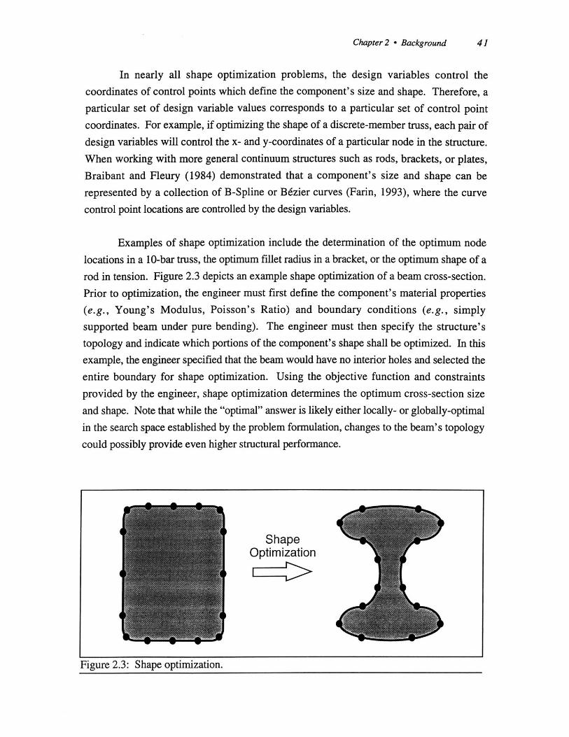
Chapter 2 - Background 41
In nearly all shape optimization problems, the design variables control the
coordinates of control points which define the component's size and shape. Therefore, a
particular set of design variable values corresponds to a particular set of control point
coordinates. For example, if optimizing the shape of a discrete-member truss, each pair of
design variables will control the x- and y-coordinates of a particular node in the structure.
When working with more general continuum structures such as rods, brackets, or plates,
Braibant and Fleury (1984) demonstrated that a component's size and shape can be
represented by a collection of B-Spline or Bdzier curves (Farin, 1993), where the curve
control point locations are controlled by the design variables.
Examples of shape optimization include the determination of the optimum node
locations in a 10-bar truss, the optimum fillet radius in a bracket, or the optimum shape of a
rod in tension. Figure 2.3 depicts an example shape optimization of a beam cross-section.
Prior to optimization, the engineer must first define the component's material properties
(e.g., Young's Modulus, Poisson's Ratio) and boundary conditions (e.g., simply
supported beam under pure bending). The engineer must then specify the structure's
topology and indicate which portions of the component's shape shall be optimized. In this
example, the engineer specified that the beam would have no interior holes and selected the
entire boundary for shape optimization. Using the objective function and constraints
provided by the engineer, shape optimization determines the optimum cross-section size
and shape. Note that while the "optimal" answer is likely either locally- or globally-optimal
in the search space established by the problem formulation, changes to the beam's topology
could possibly provide even higher structural performance.
Figure 2.3: Shape optimization.
ShapeOptimization

42 Chapter 2 - Background
Topology Optimization. Topology optimization, perhaps the most difficult of the
three structural optimization categories, performs optimization by modifying the topology
of a design. Hence, the design variables control the design's topology, and the values ofthe design variables define the particular topology of the design. Optimization therefore
occurs through the determination of the design variable values which correspond to the
component topology providing optimal structural behavior. Note that sizing and shape
optimization typically occur as incidental byproducts of the topology optimization process.
While a set of design variables can easily control a design's size or shape (the
design variable values are simply assigned to their corresponding dimension sizes or
control point locations), controlling a design's topology is considerably more difficult. In
addition to controlling the design's outer boundary, the design variables must create and
remove, as well as define the size and shape of, any number of holes in the design's
interior. To allow for flexibility in creating, reshaping, and removing internal holes during
the course of optimization, the optimization algorithm could use a varying number of
design variables, where new design variables are added to control the location and shape of
newly-created internal holes and existing design variables are deleted if their corresponding
hole is removed. Unfortunately, the computational complexity of this design variable
representation renders it unsuitable for topological optimization.
A more general, less complex design representation used by nearly all topological
optimization algorithms treats the problem as a configuration design problem, where the
overall, complex design is created by assembling a large number of basic elements, or
"building blocks." By beginning with a set of building blocks representing the structure's
maximum allowable "design domain" (i.e., region in space which the structure may
occupy) and then allowing each block to either exist or vanish, a unique design is created.
Hence, a design is modified by simply changing the states of individual building blocks
making up the design. During topological optimization, a design's building blocks are
controlled by the design variables, where the value of each design variable determines the
existence and characteristics of its corresponding building block. For example, in the
topological optimization of a cantilevered plate, the plate is typically discretized into small,rectangular elements, where each element is controlled by a design variable which can vary
continuously between 0 and 1. When a particular design variable has a value of 0, the
corresponding element is assumed to be a hole. Likewise, when a design variable is equal
to 1, its corresponding element contains fully-dense material. Lastly, design variables with
intermediate values correspond to elements containing material of intermediate density. So,
Chapter 2 - Background 43
to create a hole at a particular location in a design, the design variable corresponding to the
element at that location is simply set equal to zero. To make the hole larger, the design
variables corresponding to elements immediately surrounding the hole are also set equal to
zero. Similarly, holes are removed from a design by assigning non-zero values to the
design variables corresponding to the elements at the hole location. Hence, because no
addition or deletion of design variables is required during optimization, this building block
design representation is suitable for topology optimization problems. Chapter 3, which
discusses previous work in structural topology optimization, further details the design
representations typically used in topological optimization problems.
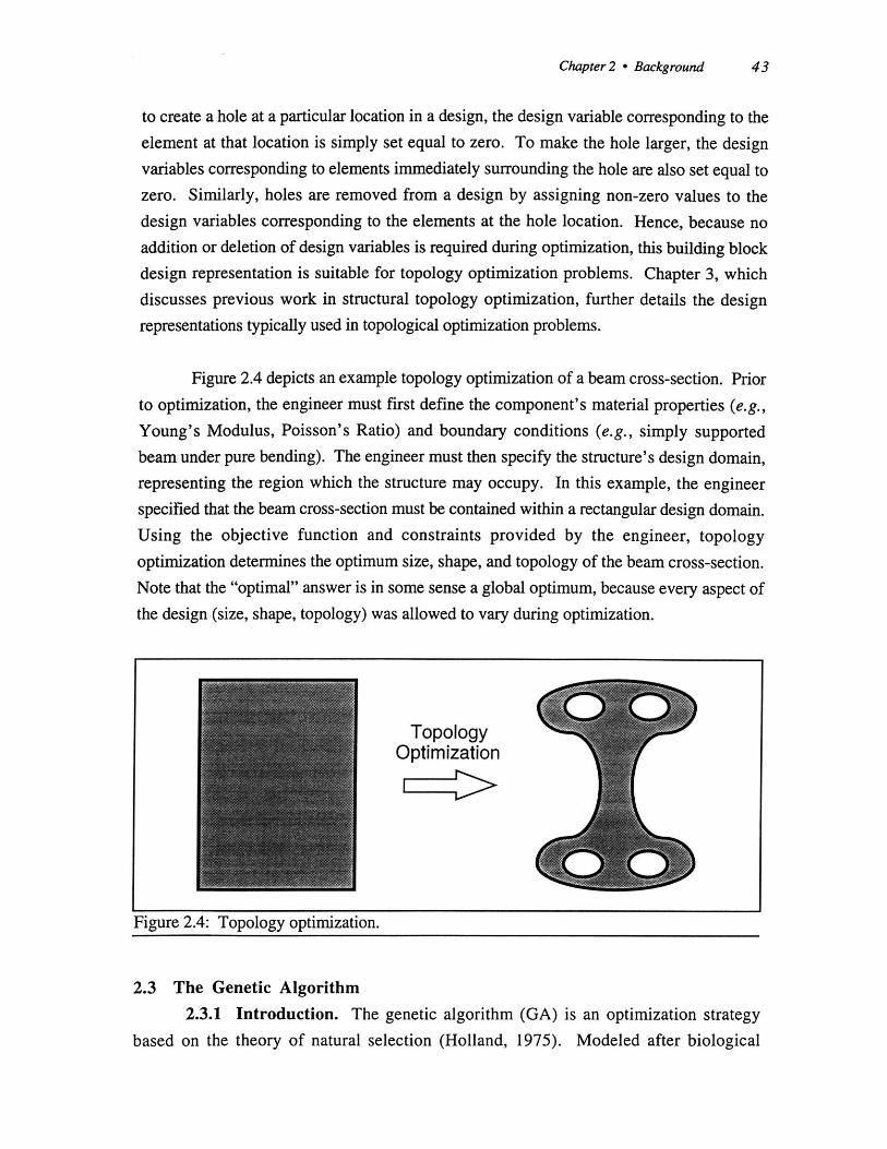
Figure 2.4 depicts an example topology optimization of a beam cross-section. Prior
to optimization, the engineer must first define the component's material properties (e.g.,Young's Modulus, Poisson's Ratio) and boundary conditions (e.g., simply supported
beam under pure bending). The engineer must then specify the structure's design domain,representing the region which the structure may occupy. In this example, the engineer
specified that the beam cross-section must be contained within a rectangular design domain.
Using the objective function and constraints provided by the engineer, topology
optimization determines the optimum size, shape, and topology of the beam cross-section.
Note that the "optimal" answer is in some sense a global optimum, because every aspect of
the design (size, shape, topology) was allowed to vary during optimization.
TopologyOptimization
Figure 2.4: Topology optimization.
2.3 The Genetic Algorithm
2.3.1 Introduction. The genetic algorithm (GA) is an optimization strategy
based on the theory of natural selection (Holland, 1975). Modeled after biological

44 Chapter 2 - Background
systems, where populations of organisms evolve (over many generations) so as to best
survive in their environment, the genetic algorithm performs optimization through the
"evolution" of a population of artificial organisms. These organisms, which each represent
a possibly-optimal solution to the optimization problem, compete against one another to
best solve the problem. Those organisms which are most highly-fit are allowed to serve as
parents, mating with each other to create child organisms. After undergoing random
mutation, the child organisms replace the parents, and the evolutionary process iterates.
Optimization occurs, therefore, when many generations of evolution improve the quality of
the artificial organisms.
2.3.2 Similarities with Biological Systems. In addition to its
evolutionary, "survival-of-the-fittest" optimization mechanism, the genetic algorithm shares
other similarities with biological systems. For example, each organism in a genetic
algorithm population is typically represented by a character string analogous to a
chromosome, with each character position being analogous to a gene and each character
value being analogous to an allele. As in biological systems, genes in a genetic algorithm
chromosome correspond to particular organism traits (e.g., a gene corresponding to hair
color), while allele values control trait characteristics (e.g., an allele value corresponding to
brown hair).
The genetic algorithm also uses reproductive and mutation operators which are
modeled after the mechanics of chromosome recombination and mutation found in
biological genetics.
2.3.3 Design Variables as Chromosomes. As detailed above, the genetic
algorithm performs optimization through the evolution of a population of chromosomes.
Each chromosome in a population is a coded representation of the optimization problem's
design variables, with the chromosome's genes corresponding to the design variables and
the genes' allele values controlling the design variable values. Note that there isn't
necessarily a 1-to-i correspondence between genes and design variables-as detailed
below, genes in a chromosome are typically grouped into multi-gene sub-strings, or
"parameters," where each parameter corresponds to, and controls the value of, a particular
design variable. Consequently, the number of genes in a chromosome is typically much
greater than the number of design variables controlled by the chromosome, while the
number of parameters in a chromosome is exactly equal to the number of design variables
controlled by the chromosome.

Chapter 2 - Background 45
Hence, a chromosome with a particular set of allele values corresponds to a
particular set of design variable values, and each chromosome in a genetic algorithm
population therefore corresponds to a possibly-optimal set of design variable values. In
other words, each chromosome in a genetic algorithm population represents a particular
point in the search space, and a population of chromosomes represents a population of
points in the search space. By evolving a population of chromosomes, where each
chromosome represents a set of possibly-optimal design variable values, the genetic
algorithm is able to locate the set of optimal design variable values which minimizes or
maximizes the given objective function.
Because every optimization problem has different numbers and types of design
variables, there is no single chromosome structure or chromosome-to-design-variable
decoding algorithm. In fact, one of the most difficult aspects of configuring a genetic
algorithm system is developing a chromosome structure and chromosome-to-design-
variable decoding which work well.
1011010 lo01010
Figure 2.5: A typical genetic algorithm population.
Fortunately, there is a general chromosome structure which is applicable to most
optimization problems. As shown in Figure 2.5 (which depicts a genetic algorithm
population with eight 18-bit chromosomes), genetic algorithm chromosomes are typically
one-dimensional strings of genes, where the allele values (i.e., the values assigned to each
gene location) are binary in nature-they can be equal to either 0 or 1. Because
chromosomes must each define the value of all design variables in the optimization, they
are divided into parameters, where the number of parameters in each chromosome equals
46 Chapter 2 - Background
the number of design variables in the optimization. So, while appearing to be large, multi-
bit binary numbers, chromosomes are actually concatenations of many smaller multi-bit
binary numbers (parameters), each of which corresponds to, and controls the value of, a
particular design variable.
For example, the 18-bit chromosomes of Figure 2.5 could be comprised of one 18-
bit parameter (controlling 1 design variable), two 9-bit parameters (controlling 2 design
variables), three 6-bit parameters (controlling 3 design variables), one 6-bit parameter and
one 12-bit parameter (controlling 2 design variables), or any other combination of
parameters containing a total of 18 bits. The length (in bits) of any given parameter
depends upon the range, and possibly resolution, of its corresponding design variable's
allowable values. For example, the length of a parameter controlling an integer-valued
design variable depends upon the range of the design variable's allowable values: a 2-bit
parameter can control a design variable which varies between 0 and 3 (or any other range
containing 4 values), while a 6-bit parameter can control a design variable which varies
between 1 and 64 (or any other range containing 64 values). Likewise, the length of a
parameter controlling a floating-point design variable depends upon the range and desired
resolution of the design variable's allowable values: a 4-bit parameter can control a design
variable which varies between 0 and 3 in increments of 0.2, while a 5-bit parameter can
control a design variable which varies between 0 and 3 in increments of 0.09677 or a
design variable which varies between 0 and 6 in increments of 0.1935. In general, the
required length (in bits) of a parameter controlling an integer-valued design variable (Xi)with an allowable range of ( VMN X. VMAX) is given by:
In1=In 2 . ln[(VMAX - VMN) + 1], (2.11)
while the required length (in bits) of a parameter controlling a floating-point design variable
(X,) with an allowable range of (VMIN Xi VMAX) and a desired resolution of (Resolution
= Increment;) is given by:
1 .n- VMAX VMN + (2.12)In 2 Increment, )

Chapter 2 - Background 47
Note that the programmer must specify, a priori, the number of parameters in each
chromosome and the length (in bits) of each parameter.
When using binary allele values, a chromosome of length 1 (in bits) corresponds to
a search space containing 21 distinct locations. Hence, when developing a chromosome
structure for a particular optimization, care must be taken to minimize chromosome length.
The number of design variables should be kept to a minimum, as should design variable
ranges and resolution.
To decode a chromosome (with the structure defined above) into its corresponding
design variable values, the chromosome must first be divided into its multi-bit parameters.
The binary-valued parameters are then converted into either integer or floating-point
numbers, depending upon the nature of the corresponding design variables. Note that
chromosomes can simultaneously represent both integer and floating-point design
variables. While converting a binary-valued parameter into an integer-valued design
variable value is relatively straightforward, conversions to floating-point design variable
values require slightly more effort. When decoding a parameter of length 1 into a floating-
point design variable (Xi: VMIN <X. VMAX), the design variable's value is given by:
Xi = ParameterValue - "^A, MIN + YMIN' (2.13)
where ParameterValue represents the value of the (binary-valued) parameter after
conversion into decimal.
As an example, Figure 2.6 details the decoding process for a chromosome
representing 3 design variables. Parameter #1, controlling the value of an integer design
variable (X,: 0 X, 7), is 3 bits in length and easily converts from binary into the
corresponding integer design variable value. Likewise, Parameter #3 controls an integer
design variable (X3: 0 X3 : 31) and is 5 bits in length. Parameter #2, controlling the
value of a floating-point design variable (X2 : 1.0 X 2 6.0), is 10 bits long and converts
from a binary-valued parameter into a floating-point design variable value according to
Equation 2.13:
60-1.0X2 = 485. - +1.0 = 3.37 (2.14)
210-1

48 Chapter 2 - Background
Once a chromosome's parameters have been converted into their corresponding
design variable values, the chromosome decoding process is complete.
101011110010101101
1010111100101 01101
Parameter #1 Parameter #2 Parameter #3(0 X 7) (1.0 ! X2 6.0) (0 X3 ! 31)
5 3.37 13
Figure 2.6: The chromosome decoding process.
2.3.4 Optimization Through Evolution. Again, the genetic algorithm uses
an evolutionary, "survival-of-the-fittest" optimization mechanism. A population of
chromosomes is allowed to evolve, with generations of child chromosomes arising from,
and replacing, parent generations. Chromosomes in a parent generation are first evaluated
for fitness, or quality. Highly-fit chromosomes are then selected to serve as parents of the
subsequent child generation. Reproduction occurs when parent chromosomes then pair
and mate to create a new generation of child chromosomes. Mutation is then performed on
the child chromosomes. Finally, the child generation replaces the parent generation, and
the process iterates. After many generations of evolution, the overall quality of
chromosomes should increase because characteristics of better chromosomes are more
likely to propagate into child generations.
Hence, the genetic algorithm utilizes genetics-based operators such as evaluation,
selection, reproduction, and mutation to evolve a population of artificial chromosomes
(Figure 2.7). Because each chromosome in the population corresponds to particular set of
design variable values (and therefore a possibly-optimal solution to the optimization
problem), evolution of the chromosomes results in optimization of the design variables. As
in the evolution of actual biological systems, genetic algorithm-based optimization takes
place over hundreds, if not thousands, of "generations."

Chapter 2 - Background 49
Generation(t)
- Selection* Reproduction Generation(t+1)- Mutation
Figure 2.7: One "generation" of genetic algorithm optimization.
Evaluation. One "generation" of optimization begins with evaluation, where the"fitness," or quality, of each chromosome in the parent generation is determined. As inbiological systems, where organisms are implicitly "graded" according to their prey-catching and predator-avoidance abilities, the genetic algorithm assigns fitness values tochromosomes according to their objective function minimization or maximization abilities.
Fitness evaluation is performed by a "fitness function," which takes an individualchromosome as input, decodes the chromosome into its corresponding design variablevalues (as detailed in Section 2.3.3), evaluates the objective function using the designvariable values, and then returns a fitness value quantitatively describing the extent towhich the design variable values minimized or maximized the objective function withoutviolating any constraints (Figure 2.8).
Figure 2.8: Fitness evaluation.

50 Chapter 2 - Background
As with the chromosome decoding process, every optimization problem has a
unique objective function, and therefore no single algorithm exists for converting the
results of an objective function evaluation (using a particular chromosome's design variable
values) into a fitness value (for the chromosome). In general, however, calculations must
be performed so that high fitness is assigned to chromosomes corresponding to design
variable values which do an excellent job of minimizing or maximizing the objective
function while satisfying all constraints. Likewise, low fitness should be assigned to
chromosomes corresponding to design variable values which violate constraints and/or do a
poor job of minimizing or maximizing the objective function. Note that the genetic
algorithm is naturally a maximization algorithm. Hence, if you wish to minimize an
objective function, the fitness function value must increase as the objective function value
decreases and must decrease as the objective function value increases. This is typically
accomplished by setting the fitness value equal to the reciprocal of the objective function
value or equal to the objective function value subtracted from a large constant.
After the fitness function returns the chromosome's fitness to the genetic algorithm
routines, the fitness value is assigned to the chromosome. The evaluation process is then
repeated for all chromosomes in the population.
Note that, particularly in early generations, large differences in fitness values will
exist between chromosomes in any given generation. These differences, if unaddressed,would allow the highest-performance chromosomes to quickly dominate the parenting
process, filling subsequent generations with a particular "breed" of possibly-suboptimal
design variable values. At the same time, low-performance chromosomes, which likely
contain some desirable genetic material, would quickly die off. To prevent this, "fitness
scaling" (Goldberg, 1989a) is performed to attenuate fitness value differences. In the
procedure, the fitness of high-performance chromosomes is slightly reduced while the
fitness of low-performance chromosomes is increased.
Selection. After fitness scaling has been completed, selection is performed to
determine which chromosomes in the parent generation will serve as parents of the child
generation (Figure 2.9). As in actual biological systems, where organisms highly adept at
catching prey and avoiding predators are more likely to survive and create offspring,
highly-fit genetic algorithm chromosomes are more likely to serve as parents of child
generations.

Chapter 2 - Background 51
Figure 2.9: Parent selection.
During selection, the number of chromosomes selected to serve as parents must
equal the number of chromosomes in the population. However, because the genetic
algorithm attempts to obtain increasingly-fit generations of chromosomes, highly-fit
chromosomes are likely to serve as a parent multiple times in a single generation, while
low-fitness chromosomes are likely to "die off' and not serve as a parent. Additionally,
while the selection algorithm must choose a proper number of highly-fit parent
chromosomes to insure that child chromosomes will be highly-fit, it must also choose a
number of average-to-poor-quality chromosomes in the hope that they contain some
desirable genetic material.
The number of times a chromosome serves as a parent in one generation is based on
its fitness performance in relation to the performance of other chromosomes in the parent
generation. As detailed in Baker (1987), the selection process must first determine the
"expected value" of each chromosome in the parent generation, and it must then convert the
expected values into discrete numbers of parentings. For example, if a chromosome has an
expected value of 1.8, it should, on average, serve as a parent 1.8 times in one generation.
Note that a chromosome's expected value is equal to its fitness divided by the average
fitness of the entire population:
ExpectedValuei = N 'Fitness (2.15)I Fitnessj=0
Parent
Parent2
ParentNl
-ParentN

52 Chapter 2 - Background
The most straightforward selection algorithm is "Stochastic Sampling with
Replacement" (Baker, 1987), otherwise known as "Roulette Wheel" selection. In the
algorithm, a "roulette wheel" with an area equal to the number of chromosomes in the
population (N) is created. Each chromosome in the population is allocated a slice on the
wheel, where the area of the slice is exactly equal to the chromosome's expected value. To
choose a parent, a random location on the wheel is chosen (i.e., the wheel is "spun"), and
the chromosome located at that position is selected to serve as a parent. To select the N
required parent chromosomes, the wheel is simply "spun" N times.
Reproduction. After a group of parents have been selected, reproduction must take
place to create a generation of child chromosomes. The genetic algorithm's reproduction
operator is modeled after biological systems, where "evolution" occurs when highly-fit
parent organisms mate to create child organisms (containing genetic material from both
parents) which are of higher fitness (i.e., better adapted to their environment) than the
parents. Similarly, the genetic algorithm allows pairs of parent chromosomes to mate,
creating pairs of child chromosomes containing genetic material from both parents. It is
hoped that when two highly-fit chromosomes combine their genetic material to create two
children, at least one of the child chromosomes will contain the best "attributes" of both
parents, resulting in a chromosome of exceptionally high fitness.
A great amount of previous and ongoing research (Goldberg (1989a), Holland
(1975)) has proven that the genetic algorithm's reproduction operator does indeed
propagate the best genetic material from generation to generation. Specifically, the Schema
Theorem (Goldberg, 1989a) states that the genetic algorithm "allocates exponentially
increasing (decreasing) numbers of trials to above- (below-) average schemata." Schemata,
or genetic "building blocks," are "similarity templates" describing subsets of chromosomes
with similar allele values at particular gene locations. In other words, if the genetic
algorithm finds that highly-fit chromosomes generally have similar allele values at a
particular set of gene locations, it will propagate this high-fitness group of genes to
exponentially increasing numbers of child chromosomes. Likewise, if the genetic
algorithm finds that low-fitness chromosomes generally have similar allele values at a
particular set of gene locations, it will propagate this low-fitness group of genes to
exponentially decreasing numbers of child chromosomes. The beauty of the genetic
algorithm is that the propagation of highly-fit genetic building blocks is performed in
parallel (i.e., many highly-fit building blocks are propagated at once), and it is performed

Chapter 2 - Background 53
automatically-no explicit correlations between building block configuration and
chromosome quality need to be made (Goldberg, 1989a).
The genetic algorithm's reproduction operator is inspired by the mechanics of
chromosome recombination found in biological systems. Commonly referred to as"genetic crossover" in the genetic algorithm research community, chromosome
recombination is the swapping of genetic material between parent chromosomes to createchild chromosomes containing genetic material from both parents. As in biologicalsystems, genetic algorithm-based reproduction occurs only between pairs of chromosomes,with each pair of parents creating a pair of children.
The most straightforward reproduction operator, "single point" crossover, isdepicted in Figure 2.10. In the technique, two of the chromosomes selected (by theselection algorithm) to serve as parents are randomly paired, and a location along the lengthof the pair is selected at random. "Crossover" then takes place when genetic informationbeyond the location is swapped, creating two child chromosomes which each possessgenetic material from both parents. The child chromosomes are then inserted into the childgeneration, and the two parent chromosomes are removed from the parent "pool." Theprocess is then repeated until all of the parent chromosomes have mated and generatedchildren.
Parentl 111111111111111111000000000000000000
Parent1 111010111
* 111111111111 111111 1010551100 10 01 1o0,- 000000000000 000000 7
11 70,10 11j11111111000000 %%%%,
Parent N 1
111111111111000000 Generation(t+1)
Parent 000000000000111111 (N=8)
Figure 2.10: Single point crossover.
Note that crossover is not performed on every pair of parent chromosomes.
Rather, with every pair of parent chromosomes, a "weighted coin toss" determines whether

54 Chapter 2 * Background
crossover will take place. The probability that crossover will be performed (i.e., the
probability that the coin will land on "perform crossover") must be specified a priori by the
programmer. If crossover is not performed, the two parent chromosomes are inserted into
the child generation without any recombination of genetic material.
During the course of this investigation, the performance of single-point crossover
was compared with that of uniform crossover (Syswerda, 1989), a reproductive technique
shown to outperform single-point crossover in certain problem domains. However, in this
investigation (i.e., in the examples presented in Chapter 5), single-point crossover
demonstrated superior optimization performance.
Mutation. After the child generation has been created, mutation is performed on the
child chromosomes. As with the genetic algorithm's reproduction operator, the mutation
operator is modeled after biological systems, where random, infrequent mutation
introduces new, possibly-desirable characteristics into the population. Used in the genetic
algorithm, mutation modifies the genetic material in child chromosomes, allowing the
genetic algorithm to explore new areas of the search space. Whereas reproduction swaps
portions of genetic material between chromosomes, creating new combinations of the same
genetic material, mutation slightly changes the genetic material. Hence, if a particular
chromosome corresponds to a solution close to the globally-optimum solution, it is hoped
that mutation will make the slight changes needed to obtain the optimum solution.
10101111001010110100r0" 1, 11 010 110 1 0100101011
101011110010101101 10101
07 11111 1110000000 0 7 0 0 1 0 7 ,
101010111010100101Generation(t+1)
Figure 2.11: Mutation.
Specifically, the mutation algorithm (Figure 2.11) examines every gene of every
child chromosome and, using a "weighted coin toss," determines whether the gene's allele
value should be toggled. As with the crossover probability discussed in previous

Chapter 2 * Background 55
paragraphs, the probability that any given gene will mutate (i.e., the probability that thecoin will land on "perform mutation") must be specified a priori by the programmer. Ifmutation is performed on a particular gene, the gene's allele value is toggled from 0 to 1 orfrom 1 to 0. If mutation is not performed on a particular gene, the gene's allele value is notmodified.
Figure 2.12: Genetic algorithm flowchart.

56 Chapter 2 Background
At the conclusion of mutation, the child generation is complete and is allowed to
replace the parent generation. The entire evolution process then iterates (Figure 2.12) until
the population has converged to an optimum or has "evolved" for a pre-determined number
of generations. Note that Section 2.3.6 provides a brief discussion on determining when a
genetic algorithm-based search should end. After many generations of evolution, the
overall quality of chromosomes (i.e., the quality of the solutions to the optimization
problem) should increase because better chromosomes (i.e., those chromosomes which
represent the best solutions to the optimization problem) are more likely to propagate into
child generations.
2.3.5 Optimization Parameters.
parameters must typically be specified:
- Probability of Crossover(PCROSSOVER)
- Probability of Mutation(PMUTATION)
- Fitness Scaling Coefficient(FMULT)
- Population Size
- Selection Algorithm
- Crossover Operator
When using the genetic algorithm, several
The probability that crossover will beperformed between a particular pair of parentchromosomes.
The probability that any given gene on anygiven chromosome will mutate.
A measure of the magnitude of fitness valueattenuation. Typically represents the desiredratio of the maximum fitness in a populationto the average fitness of the population.
Number of chromosomes in each geneticalgorithm generation.
The technique used to determine whichchromosomes in a population will serve asparents for the next generation.
The method used to mate, or combine, twoparent chromosomes to create two childchromosomes containing attributes from bothparents.
These parameters have a great effect on the performance and efficiency of the
search. For example, high crossover and mutation probabilities favor exploration of the
search space, while low crossover and mutation probabilities favor exploitation of current
genetic material. Likewise, high fitness scaling coefficients bias the search towards
immediately-promising areas of the search space at the risk of prematurely converging to a
local optimum, while low fitness scaling coefficients avoid premature convergence at the

Chapter 2 - Background 57
risk of not fully utilizing highly-fit genetic material. Population size also affects search
performance, in that large populations are inefficient (i.e., large populations exhibit slow
convergence and require more function analyses per generation) while small populations donot provide the variety of genetic material needed to fully explore the search space. Finally,different selection schemes choose parents with varying degrees of accuracy and
consistency (Baker, 1987), while different crossover operators offer varying levels of
positional and distributional bias (Eshelman et al., 1989) toward genetic "building blocks."
Unfortunately, it is difficult to determine proper parameter values a priori. The first
comprehensive study of the effects of genetic algorithm parameters was conducted by De
Jong (1975). Recently, empirical studies attempting to determine optimum crossover and
mutation probabilities as well as population sizes have been conducted by Schaffer et al.
(1989) and Grefenstette (1986). Goldberg et al. (1992) and Goldberg (1989b) conducted
analytical studies of optimum population sizes, while Kreinovich et al. (1993), Goldberg
(1989a), and Grefenstette (1986) provide details on selecting appropriate fitness scaling
coefficients. de la Maza and Tidor (1993), Back and Hoffmeister (1991), Goldberg and
Deb (1991), Grefenstette and Baker (1989), and Baker (1989, 1987, 1985) have
investigated parent selection schemes which improve on the standard roulette-wheel
selection algorithm. The relative performance of different reproduction operators has been
investigated by Spears and De Jong (1991), Eshelman et al. (1989), Syswerda (1989),Schaffer and Morishima (1987), and Goldberg and Lingle (1985).
Using the suggestions of Goldberg (1989a), Schaffer et al. (1989), Baker (1987),and Grefenstette (1986), the following parameter values were used during the course of
this investigation:
PCROSSOVER = 0.95PMUTATION -0.01
FMULT 1.4Population Size = 30Selection Algorithm = "Elitist" Stochastic Universal Sampling (Baker, 1987)Crossover Operator = Single-Point Crossover
In addition, this investigation's genetic algorithm routines utilized binary-coded
chromosomes (i.e., allowable allele values of either 0 or 1) and randomly-generated initial
populations (i.e., chromosome allele values in the initial generation were determined at

58 Chapter 2 - Background
random). The routines were based on the Simple Genetic Algorithm detailed in Goldberg
(1989a).
Note that "elitist" selection strategies differ from normal selection algorithms in that
immediately before a parent generation is replaced by its corresponding child generation, a
randomly-chosen child chromosome is eliminated and replaced with the parent generation's
most-highly-fit chromosome. Because a parent chromosome's highly-fit building blocks
may be "destroyed" by crossover (i.e., split between two child chromosomes) or mutation
(i.e., erased by allele value changes), highly-fit parent chromosomes do not always
produce highly-fit child chromosomes. Hence, "elitist" re-insertion is performed to insure
that the child generation's best chromosome is not of lower quality than the parent
generation's most-highly-fit chromosome. Elitist selection strategies are particularly useful
when using relatively high crossover and mutation probabilities, which tend to destroy
highly-fit building blocks in parent chromosomes.
In addition to the above parameters, which define the operation of the genetic
algorithm, chromosome fitness value calculations also affect search performance.
Specifically, when representing constraints as penalty terms in a fitness function, care must
be taken to normalize, or balance, the penalty terms with the actual "quality" terms of the
function. Excessive constraint violation penalties typically result in sub-optimal solutions
which satisfy all constraints but do not minimize or maximize the objective function.
Likewise, insufficient penalties typically result in infeasible solutions which minimize or
maximize the objective function but are unable to satisfy the constraints.
While several constraint-representation techniques have been developed (Goldberg,
1989a), most are tailored to a particular problem domain. During the course of this
research, a linear penalty term which penalized the objective function value P% for every
10% constraint violation was found to work well. Unfortunately, a great deal of
experimentation is generally required to develop a fitness function which correctly balances
constraint violation terms (P in this investigation) with objective function "quality" terms.
2.3.6 GA's vs. Traditional Optimization Methods. Several fundamental
differences exist between the genetic algorithm and more traditional optimization methods
such as mathematical programming techniques, optimality criteria methods, and exhaustive
searches.

Chapter 2 * Background 59
The most dramatic difference between the genetic algorithm and other techniques isthat the GA conducts optimization through the use of a population of points distributed(initially at random) throughout the search space. By gradually combining and modifyingthe best attributes of the points through probabilistic pairing, crossover, and mutation, thegenetic algorithm is able to simultaneously evaluate different areas of the search space,avoiding local optima as it converges on a globally-optimum solution. This differs frommathematical programming and optimality criteria techniques, which start from a singlepoint and then use deterministic "hillclimbing" or heuristic redesign procedures to ascendthe nearest peak in the search space. Unfortunately, particularly in multi-modal searchspaces, the nearest peak is most likely locally-optimum, with globally-optimum peakslocated elsewhere. Hence, with highly multi-modal search spaces, the genetic algorithmwill avoid local optima and converge on the globally-optimum solution, while mathematical
programming and optimality criteria techniques will likely converge to a local optimum.
Unlike mathematical programming techniques, which utilize gradient information tomove from one point in the search space to another, the genetic algorithm uses onlyobjective function evaluations and probabilistic operators such as pairing, crossover, andmutation to move through the search space. Hence, the genetic algorithm is ideally suitedto discrete, discontinuous search spaces where derivative information is not available.
Another advantage of the genetic algorithm over other techniques is its ability towork with a variety of design variable types. While the discrete allele values used ingenetic algorithm chromosomes are ideally-suited to integer design variables, they canreadily represent floating-point design variables with fairly high resolution by using multi-bit, binary encodings. Mathematical programming techniques, on the other hand, aredesigned specifically for either integer or continuous variables-changes in variable typenecessitate the use of a different optimization algorithm.
Unlike mathematical programming and optimality criteria techniques, which obtain
only one solution to any given optimization problem, the genetic algorithm obtains apopulation of solutions. Hence, one optimization run provides the user with a "family" ofsolutions, where each solution offers varying levels of objective function minimization-
maximization and constraint satisfaction abilities. The user can then evaluate the solutions
to determine which best satisfies several alternate performance criteria, much like a pareto
optimization study. In contrast, when using mathematical programming or optimality
I . - MUM _* - J I ,

60 Chapter 2 - Background
criteria techniques, all alternate performance criteria must be explicitly incorporated into the
objective and gradient functions.
One difficulty with the genetic algorithm is determining when a search should end.
Because the genetic algorithm is probabilistic in nature and does not utilize function
gradient information, it is able to search in discrete, discontinuous, multi-modal search
spaces. However, these non-deterministic attributes prevent the genetic algorithm from
determining whether an optimum has been reached. So, unlike mathematical programming
and optimality criteria techniques, which use gradient information or optimality criteria
values to explicitly determine if an optimum has been found, the genetic algorithm must
rely on "convergence criteria." Typically, the criterion for ending the search is based on the
percentage of chromosomes in the population which have converged to similar points in the
search space. There is little value in continuing the search when most chromosomes have
converged, because the fitness of further generations will increase only through the
inefficient method of random gene mutation. Once the convergence criterion is met, it is
unknown whether or not the population's highest-fitness chromosome represents an actual
optimum. Hence, genetic algorithm searches produce a "pseudo-optimum." The
advantage of genetic algorithm search is that it does produce these pseudo-optima in
discrete, discontinuous, multi-modal search spaces which would be troublesome to
mathematical programming and optimality criteria techniques using gradient or other
sensitivity information.
Another disadvantage of the genetic algorithm is computation cost. In general, the
genetic algorithm will perform thousands of function evaluations before converging on a
solution. Mathematical programming techniques, and particularly optimality criteria
methods, typically require many fewer evaluations. Hence, the genetic algorithm is most
practical in domains where function evaluations are relatively inexpensive.
2.3.7 Summary. In summary, the genetic algorithm is a robust, general search
and optimization technique applicable to a variety of problem domains and design variable
types. In many ways, it is a useful compromise between strong and weak search methods.
Strong search methods, such as mathematical programming techniques and expert system-
based approaches, perform search in an informed manner-there is a rationale for moving
from one point in the design space to another. In contrast, weak methods, such as
exhaustive or random searches, perform search in an uninformed manner-they
exhaustively enumerate, or at least extensively sample, the design space in order to find an

Chapter 2 * Background 61
optimum. Weak methods are computationally expensive, but are more likely to find global
optima; strong methods are computationally inexpensive, but are more likely to settle forlocal suboptima. The genetic algorithm, in contrast to both, uses the weak operations ofprobabilistic pairing, crossover, and mutation to obtain a strong progression towardglobally-optimum solutions.
Interested readers should refer to the Genetic Algorithms chapter in (Levy, 1992)for a discussion of the history of the approach and descriptions of some interesting
applications. For a comprehensive introduction to genetic algorithms, including sample
computer code, (Goldberg, 1989a) is recommended.

62 Chapter 2 - Background

Chapter 3 - Previous Work 63
Previous Work
3.1 Overview
Sizing and shape optimization based upon structural considerations (i.e., structuralsizing and shape optimization) have been active research areas for some time (Schmit(1981), Vanderplaats (1982), Haftka and Grandhi (1986)). However, because of
limitations in computer technology, optimization algorithm performance, and structural
analysis efficiency, topology optimization based upon structural considerations has onlyrecently been investigated. Nevertheless, structural topology optimization has quickly
become an active research area, and several innovative approaches have been developedand applied to a variety of continuum and discrete-membered (i.e., truss) structures.
As detailed in Chapter 1, this investigation addresses the genetic algorithm-basedstructural topology optimization of continuum structures, where the optimal distribution ofmaterial within a discretized design domain is found. So that the genetic algorithm'sperformance in this domain can be compared with that of other optimization algorithms,this chapter begins by detailing non-genetic-algorithm-based approaches to the topologicaloptimization of continuum structures. Note that non-genetic-algorithm-based topologicaloptimizations of discrete-membered structures are not reviewed. Then, to demonstrate thegenetic algorithm's general structural optimization capabilities, genetic algorithm-based
approaches to sizing and shape optimization of continuum and discrete-membered
structures, as well as topological optimization of discrete-membered structures, are
described. Finally, to facilitate the evaluation of this investigation's contributions, previous
research in genetic algorithm-based topological optimization of continuum structures is
detailed.

64 Chapter 3 - Previous Work
For a comprehensive introduction to the current state-of-the-art in structural
topology optimization research, please refer to the proceedings of several recent
conferences focused on the subject: Bends0e and Soares (1993), Rozvany (1993), and
Eschenauer et al. (1991).
3.2 Non- Genetic-Algorithm-Based Topology Optimization
3.2.1 Homogenization Method. Perhaps the most prominent technique used
to perform structural topology optimization is the variable density approach based upon
material homogenization methods (Strang and Kohn (1986), Kohn and Strang (1986)).
Bendsoe and Kikuchi (1988) and associated researchers have applied the method, which
minimizes a component's compliance subject to a maximum volume constraint, to a variety
of structural topology optimization problems (Bendsoe et al. (1993), Bendsse et al. (1991),Diaz and Belding (1993), Fukushima et al. (1993), Suzuki and Kikuchi (1993, 1991,
1990)). Current research issues in homogenization-based structural topology optimization
are summarized by Kohn (1993).
In the procedure, a design domain is discretized into small, rectangular elements,
where each element is assumed to contain composite material of continuously-variable
density and orientation. Each element's structural properties are a function of the element's
material density and orientation, and are calculated using material homogenization methods.
Hence, assigning density and orientation values to each element in the design domain
results in the generation of a particular component design with particular structural
characteristics. Likewise, modifying the material density or orientation in any element
results in the modification of the component's design and structural characteristics.
Consequently, because the component's design and structural properties are controlled by
the material density and orientation in each design domain element, each element's material
density and orientation serve as design variables during optimization. Optimization begins
when an initial component design is created by assigning initial material density and
orientation values to each design domain element. An optimality criteria method then
determines how the material density and orientation in each element should change so that
the compliance of the component design is minimized subject to a maximum volume
constraint. In an iterative process, an optimal design is generated.
Several different microstructure models have been suggested for use with material
homogenization methods when determining the composite material's structural properties.
All of the models allow full rotation of the microstructure and enable the material's density

Chapter 3 - Previous Work 65
to vary continuously between 0 (void) and 1 (solid). Bends0e and Kikuchi (1988)
introduce a "non-optimal" material microstructure comprised of either square or rectangular
microscale holes (Figure 3.1), where the size of the holes defines the density of the
composite. Other research (Allaire and Francfort (1993), Allaire and Kohn (1993),Bends0e et al. (1993), Jog et al. (1993)) studies an "optimal" microstructure created by"Rank-2" layering, which creates a two-scale, orthogonal laminate (Figure 3.2). The
volume fractions of strong and weak material define the composite's density. After the
microstructure model is defined, material homogenization techniques are then used to
determine the relationship between the material's 'density' (i.e., the composite's hole sizes
or volume fractions) and orientation and its structural properties. Note that Bendsoe et al.
(1993) propose an "artificial composite," which eliminates the need for material
homogenization methods by using approximate, analytical relationships between material
density and orientation and the corresponding structural properties.
Figure 3.1: Rectangular hole microstructure. Adapted from Bendsoe et al. (1993).
Figure 3.2: Rank-2 microstructure. Adapted from Bendsoe et al. (1993).
a

66 Chapter 3 - Previous Work
Figure 3.3: Square hole design variables. Adapted from Suzuki and Kikuchi (1991).
Figure 3.4: Rectangular hole design variables. Adapted from Suzuki and Kikuchi (1991).
Hence, during optimization, the number of design variables required to control the
density and structural characteristics of any single design domain element depends upon the
microstructure used to model the composite material in the design domain. When using a
square or rectangular hole microstructure, either two (square size and orientation-Figures
3.3a-b) or three (rectangle height, width, and orientation-Figures 3.4a-b) design variables
are needed for each design domain element. Likewise, Rank-2 microstructure models
require the use of three (strong material volume fraction, weak material volume fraction,
and material orientation) design variables for each design domain element. Artificial
composite microstructure models require two (material density and orientation) design
variables. So, the total number of design variables required in an optimization is equal to
1
1 lb
a
(a)(b

Chapter 3 - Previous Work 67
the number of elements in the design domain multiplied by the number of design variables
required by each element. Note that Figures 3.3 and 3.4 depict an individual unit cell,which defines the elementary form of the material microstructure-the composite materialin each design domain element is assumed to contain many of these unit cells.
Strang and Kohn (1986) recommend the use of composites in structuraloptimization problems, stating that a "0-1 dichotomy between holes and material" results inan "ill-posed" minimization problem, where the optimal solution is difficult, if notimpossible, to obtain. They suggest that a "relaxation" of the problem, where material in
the design domain is modeled as a composite with continuously-varying density, is needed
to transform the original problem into one which has a solution. Hence, by modeling the
material as a composite and then using material homogenization techniques to determine the
composite's structural properties, a minimization problem is created which can be solved
by common optimization algorithms.
Optimality criteria methods are typically used to solve the minimization problem
created by this "relaxation." Specifically, an iterative redesign procedure gradually
modifies an initial component design (i.e., an initial set of material density and orientation
values) until the design satisfies a set of optimality criteria. While an optimum design has
been generated when the problem's optimality criteria are satisfied, there is no guarantee
that the design is globally optimum. Bendsse et al. (1993) demonstrate that an optimal
component design's shape depends upon both the initial material density values and the
material microstructure model when using homogenization-based techniques.
Another problem with homogenization-based approaches is that elements of
intermediate density may exist in the optimal component design-boundary definition
using a density threshold may be necessary to create a design containing only solid
material. Papalambros and Chirehdast (1990) and Chirehdast et al. (1992) use binary
image analysis approaches to extract precise topological boundaries, while Olhoff et al.
(1991) rely on manual boundary definition by the user. The resulting shape can then be
modeled with a set of spline curves and subjected to classical, mathematical programming-
based shape optimization.
3.2.2 Simulated Annealing. Another approach to the topological optimization
of structural components is the work by Anagnostou et al. (1992) and Ghaddar et al.

68 Chapter 3 - Previous Work
(1993), who use simulated annealing to perform topology optimization based on strength,manufacturability, and heat transfer considerations.
In the technique, a design domain is discretized into small, rectangular elements,where each element can contain either material or void-no intermediate densities are
allowed. Assigning material or void to each element in the design domain (i.e., designating
the state of each design domain element) defines the distribution of material and void within
the design domain, and therefore establishes the component's topology (Figure 3.5).
Likewise, modifying the state of any element (i.e., toggling a material element to void or a
void element to material) results in the modification of the component's topology. Hence,the material-void states of the design domain elements serve as design variables during
optimization. Optimization begins when an initial component design is generated by
assigning initial states to the elements in the design domain. Simulated annealing is then
used to determine the optimal configuration of material and void within the design domain
(i.e., the optimal set of design domain element states) such that the component's structural
performance is maximized and all constraints are satisfied.
000000000000
O 01 O l O polO0o0o0 oo 00010001000100010
Figure 3.5: Design domain to topology mapping. Adapted from Ghaddar et al. (1993).
Anagnostou et al. (1992) first investigate the topological optimization of a beam,
where the beam's volume, surface area, and number of edges are minimized while the
beam's strength is maximized. Another example determines the topology of a thermal fin
which provides minimum volume, surface area, and number of edges while exhibiting
maximum heat dissipation abilities. Ghaddar et al. (1993) extend the work of Anagnostou
et al. by investigating the previous beam example at a finer discretization (Figure 3.6
provides optimization results using three different disc retizations) and optimizing the
topology of a cantilevered plate subject to a downward vertical load (Figure 3.7). Similar
to optimizations performed using homogenization-based techniques, the cantilevered

Chapter 3 - Previous Work 69
plate's compliance (as well as its perimeter and number of corners) is minimized subject toa maximum volume constraint. While satisfactory cantilevered plate topologies areobtained, slight differences in objective function and volume constraint formulation preventdirect comparison with structures obtained using homogenization-based techniques.
Figure 3.6: Beam cross-section optimization. Adapted from Ghaddar et al. (1993).
Figure 3.7: Compliance minimization. Adapted from Ghaddar et al. (1993).
MENOEM.
NE.MEN.MEN.mommom
1.0 x
1.6
EE...MEu...E
70 Chapter 3 - Previous Work
3.3 Genetic Algorithm-Based Structural Optimization
3.3.1 Introduction. A third approach, which has been applied by a variety of
researchers and serves as the focus of this investigation, is genetic algorithm-based
structural topology optimization. This section details previous efforts in genetic algorithm-
based structural topology optimization, and, in an attempt to demonstrate the genetic
algorithm's general structural optimization capabilities, describes previous investigations of
genetic algorithm-based structural sizing and shape optimization.
As detailed in Section 2.2.4, the genetic algorithm performs structural optimization
by "evolving" a population of artificial chromosomes, where each chromosome represents
a possibly-optimal component design and the population of chromosomes therefore
represents a population of component designs. Optimization begins when an initial
population of designs is generated. After first evaluating the structural performance and
constraint satisfaction abilities of each design in the population, the highest-quality designs
are then selected to serve as parents. Parent designs then pair and mate via genetic
crossover, creating a population of child designs. These child designs are then subjected to
random, infrequent mutation, after which they replace the parent designs. The process then
iterates until an optimal component design is found.
Because each chromosome in a genetic algorithm population is a coded
representation of the optimization problem's design variables (Section 2.3.3), the particular
design characteristics controlled by a chromosome depend upon the type of structural
optimization which is being performed (Section 2.2.5). For example, each chromosome in
a genetic algorithm-based sizing optimization represents a particular set of component
dimensions. Likewise, chromosomes in a genetic algorithm-based shape optimization each
represent a particular component shape, and chromosomes in a genetic algorithm-based
topology optimization each represent a particular component topology.
3.3.2 Sizing Optimization. The first investigation (to the investigator's
knowledge) of genetic algorithm-based structural optimization is that of Goldberg and
Samtani (1986), who examine the sizing optimization of a 10-member truss structure
(Figure 3.8). In the investigation, the truss structure's geometry and topology are held
constant, and the optimal cross-sectional area of each truss member is determined. Hence,
the truss member cross-sectional areas, which may vary continuously between given
minimum and maximum values, serve as design variables. Each genetic algorithm
chromosome in the optimization is therefore divided into 10 parameters, where each

Chapter 3 - Previous Work 71
parameter specifies the floating-point cross-sectional area of a particular truss member.(Refer to Section 2.3.3 for details on how genetic algorithm chromosomes areconcatenations of parameters, where each parameter controls the value of a particularinteger or floating-point design variable.) The optimization, which attempts to minimizethe structure's weight subject to minimum and maximum stress constraints in eachmember, produces satisfactory results.
Figure 3.8: 10-member truss structure with applied loads. Adapted from Goldberg andSamtani (1986).
Hajela (1990) also investigates the sizing optimization of a 10-member truss.However, instead of the time-invariant loading used by Goldberg and Samtani, the trussexamined by Hajela is subjected to harmonic excitation. In the example, the structure'sweight is minimized subject to a maximum displacement constraint at a particular node. Asecond example in the investigation describes the sizing optimization of a two-element,thin-walled, cantilever torsional rod. Using the rod's thicknesses as design variables, therod's weight is minimized subject to maximum stress constraints. Finally, the cross-sectional areas of a two-beam grillage structure are optimized in an attempt to minimize thestructure's weight subject to maximum stress constraints.
Hajela (1992) provides additional examples of genetic algorithm-based sizing
optimization of discrete-membered truss structures. The investigation first details thesizing optimization of a single bay, single story portal frame, where the frame's cross-
sectional areas serve as design variables. In the example, the frame's weight is minimized
subject to several plastic collapse constraints. Three other examples in the investigation

72 Chapter 3 - Previous Work
detail the sizing optimization of 3-, 6-, and 25-member truss structures. All three examples
attempt to minimize weight subject to maximum stress and displacement constraints. As in
other sizing optimization examples, the cross-sectional areas of the truss members serve as
design variables during optimization.
Rajeev and Krishnamoorthy (1992) extend the work of Goldberg and Samtani by
optimizing the member cross-sectional areas of 10-, 25-, and 160-member truss structures.
All three examples attempt to minimize weight subject to maximum stress and displacement
constraints. As opposed to the truss structure sizing optimizations detailed above, which
allow truss member cross-sectional areas to vary continuously between given minimum
and maximum values, Rajeev and Krishnamoorthy specify that truss member cross-
sectional areas must be selected from a list of standardized cross-sectional areas. Hence,
each truss member's cross-sectional area serves as a discrete design variable, where the
variable's value specifies a particular entry, or cross-sectional area, from the list of
allowable cross-sectional areas. So, just as genetic algorithm chromosomes controlled
floating-point design variables (i.e., continuously-variable cross-sectional areas) in other
investigations, Rajeev and Krishnamoorthy use genetic algorithm chromosomes to control
integer-valued design variables (i.e., discrete cross-sectional areas).
Lin and Hajela (1993) investigate an innovative technique for optimizing the
member cross-sectional areas of discrete-member truss structures. As in the sizing
optimization studies detailed above (with the exception of Rajeev and Krishnamoorthy),
Lin and Hajela use genetic algorithm chromosomes divided into parameters, where each
parameter controls, with a particular resolution, the floating-point cross-sectional area of an
individual truss member. However, Lin and Hajela modify this standard, generation-
invariant chromosome-to-design-variable representation by introducing a "multistage,"
variable-granularity genetic search strategy. The procedure, which enables the genetic
algorithm to quickly evaluate large regions of the search space in early generations and then
"fine-tune" a high-quality design in final generations, periodically increases the resolution
with which floating-point truss member cross-sectional areas are represented. This
increase in design variable resolution is achieved by increasing the length (in bits) of the
parameters in each chromosome. For example, optimization begins with a coarse design
variable representation--each truss member's cross-sectional area may vary between AMIN
and AMAX in increments of AAO (where AAO depends upon the length of the parameters
controlling the truss member cross-sectional areas and the range of allowable area values,
AMAX - AMIN). Optimization is then performed for a given number of generations, after

Chapter 3 - Previous Work 73
which the design is assumed to have converged to a "coarse optimum." The lengths of the
chromosome parameters (and therefore the lengths of the chromosomes) are then increasedso that each truss member's cross-sectional area may vary between AMIN and AMAX in
increments of AA1, where AA, < AAO. Optimization is again performed for a certain
number of generations, and the entire resolution enhancement procedure is then repeated in
an iterative process. Lin and Hajela use this multistage technique to optimize the cross-
sectional areas of 10-, 25-, and 72-member truss structures. The 10-member truss
structure is optimized for minimum weight subject to maximum tensile and compressive
stress constraints, while the 25- and 72-member truss structures are optimized for
minimum weight subject to stress and displacement constraints.
Finally, Wang et al. (1993) investigate the genetic algorithm-based sizing
optimization of several three-dimensional structures. In one example, a structure
comprised of truss, plate, and brick elements is optimized. Specifically, the truss cross-
sectional areas and the plate thicknesses serve as design variables, and the structure's
weight is minimized subject to stress and displacement constraints. A second example,which optimizes a similar structure comprised of plate elements, determines the plate
thicknesses which minimize the structure's weight subject to stress and displacement
constraints.
3.3.3 Shape Optimization. The sizing optimization studies detailed above
optimized only cross-sectional dimensions of structures-the shape and topology of the
designs remained constant. Consequently, while the "optimal" designs which were
obtained are likely either locally- or globally-optimal in the search spaces established by the
problem formulations, modifications to the shape or topology of the designs could possibly
lead to higher structural performance. The following investigations, which perform genetic
algorithm-based shape optimization, modify the shape of designs in an attempt to obtain
structural performance greater than that possible through sizing optimization alone. Note
that these investigations typically perform sizing optimization during the shape optimization
process.
Jenkins (1991a, 1991b), in addition to performing sizing optimizations of a 3-
member truss structure and a thin-walled cross-section, studies the shape optimization of
several discrete-member truss structures. In one example, the geometry of a trussed-beam
roof structure is optimized in an attempt to minimize the structure's mass subject to stress
and deflection constraints. A second example, which optimizes the shape of an 18-member

74 Chapter 3 - Previous Work
truss structure, uses the structure's nodal point coordinates as design variables. The
example obtains an optimal truss geometry with a volume only 5% greater than the
corresponding Mitchell structure (see Section 2.2.2 for a list of textbooks detailing Mitchell
structures). In another study, Jenkins (1992) details the shape optimization of a cable-
stayed bridge, where the locations of the cable attachment points on the girder and tower,as well as the cable cross-sectional areas, serve as design variables.
Richards and Sheppard (1992) investigate the use of a genetic algorithm-based
classifier system in the shape optimization of a two-dimensional structural component
under tensile loading. Much like an expert system, a classifier system (Goldberg, 1989a)
uses a set of rules to govern its behavior in a particular environment. However, unlike
expert systems, which commonly employ pre-coded rule sets, classifier systems use the
genetic algorithm to learn rules. Hence, in the example detailed by Richards and Sheppard,
a classifier system uses the genetic algorithm to learn which component shape
modifications result in a shape of maximum structural performance. Specifically, the
classifier system-based shape optimization attempts to find the component shape providing
minimum mass subject to a maximum stress constraint. During optimization, cubic spline
curves represent the component's shape, and the curves' control point locations serve as
design variables. Note that the control points are evenly distributed along the x-direction
length of the component, and that the y-coordinates of the control points serve as the actual
design variables (Figure 3.9).
Control Points
x -
Figure 3.9: Control points defining the component's shape. Adapted from Richards andSheppard (1992).
Finally, Watabe and Okino (1993) study the shape optimization of a 20-member
truss structure. Specifically, they use the genetic algorithm to generate the truss structure

Chapter 3 - Previous Work 75
shape which provides minimum mass subject to a maximum stress constraint. Whileprevious truss structure shape optimizations (e.g., Jenkins (1991a, 1991b)) performedoptimization by directly modifying truss node locations, Watabe and Okino use a uniquedesign representation in which the structure's nodal coordinates do not serve as designvariables. Instead, using a technique called Free-Form Deformation (FFD), the geneticalgorithm chromosomes control the locations of a set of control points which, in turn,define the locations of the structure's nodes. Hence, by specifying the locations of the
control points (which are initially configured in a grid pattern), the genetic algorithm is able
to specify the locations of the structure's nodes and therefore optimize the truss structure's
shape (Figure 3.10).
Control Points(Design Variables)
Applied Loads
Structure Nodes
Figure 3.10: Shape representation using FFD. Adapted from Watabe and Okino (1993).
3.3.4 Topology Optimization. The shape optimization studies detailed above
optimized only the shapes of structures-the topology of the designs remained constant.
Consequently, while the "optimal" designs which were obtained are likely either locally- or
globally-optimal in the search spaces established by the problem formulations,
modifications to the topology of the designs could possibly lead to higher structural
performance. The following investigations, which perform genetic algorithm-based
topology optimization of discrete-member and continuum structures, modify the topology
of structures in an attempt to obtain structural performance greater than that possible

76 Chapter 3 * Previous Work
through sizing and shape optimization alone. Note that these investigations typically
perform sizing and shape optimization during the topology optimization process.
Discrete-Member Truss Structures. The first investigation of genetic algorithm-
based topology optimization of discrete-member truss structures is that of Shankar and
Hajela (1991), who attempt to find a truss topology with minimum weight subject to
displacement, stress, and natural frequency constraints. Given a set of required load
application points and candidate support locations, a heuristics-based, "stagewise
decomposition approach" is first used to create an initial population of stable truss
topologies (i.e., topologies which can support the applied loads). These topologies,
containing truss members of nominal cross-sectional dimensions, then serve as the initial
population for a genetic algorithm-based topological optimization which generates an
optimal truss topology. This optimum truss topology, again containing members of
nominal cross-sectional dimensions, then serves as the initial seed of a second genetic
algorithm-based optimization which determines the optimal cross-sectional areas of the
truss structure's members.
Hajela et al. (1993) perform a similar two-level-GA topological optimization of
truss structures, where an initial genetic algorithm optimization generates stable topologies
and a second genetic algorithm optimization then performs sizing optimization on the stable
topologies. Specifically, optimization begins with the definition of candidate support
points, required load application points, and allowable truss member connection points
(Figure 3.11). Using this information, an initial genetic algorithm search generates a
population of stable truss topologies, where each topology's members are of nominal
cross-sectional area. The least-weight topologies generated by this first optimization then
serve as the initial population of a second genetic algorithm-based search which performs
sizing optimization on the topologies. Hence, this second genetic algorithm-based search
generates the truss topology and corresponding cross-sectional dimensions which provide
minimum weight and satisfy maximum stress and displacement constraints.
Grierson and Pak (1993) investigate the topological optimization of skeletal
building structures. Specifically, they attempt to generate the cross-sectional dimensions,
member lengths, and structure topologies which provide minimum weight subject to a
maximum displacement constraint. However, unlike the topological optimizations detailed
above (Shankar and Hajela (1991), Hajela et al. (1993)), which utilize large search spaces
(i.e., the total number of possible topologies is large), the example provided by Grierson
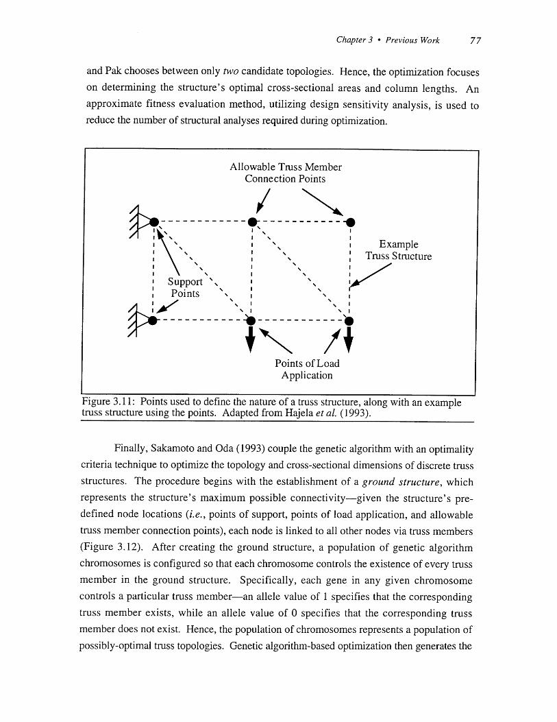
Chapter 3 - Previous Work
and Pak chooses between only two candidate topologies. Hence, the optimization focuseson determining the structure's optimal cross-sectional areas and column lengths. Anapproximate fitness evaluation method, utilizing design sensitivity analysis, is used toreduce the number of structural analyses required during optimization.
Figure 3.11: Points used to define the nature of a truss structure, along with an exampletruss structure using the points. Adapted from Hajela et al. (1993).
Finally, Sakamoto and Oda (1993) couple the genetic algorithm with an optimalitycriteria technique to optimize the topology and cross-sectional dimensions of discrete trussstructures. The procedure begins with the establishment of a ground structure, whichrepresents the structure's maximum possible connectivity-given the structure's pre-defined node locations (i.e., points of support, points of load application, and allowabletruss member connection points), each node is linked to all other nodes via truss members(Figure 3.12). After creating the ground structure, a population of genetic algorithm
chromosomes is configured so that each chromosome controls the existence of every trussmember in the ground structure. Specifically, each gene in any given chromosome
controls a particular truss member-an allele value of 1 specifies that the corresponding
truss member exists, while an allele value of 0 specifies that the corresponding truss
member does not exist. Hence, the population of chromosomes represents a population of
possibly-optimal truss topologies. Genetic algorithm-based optimization then generates the
Allowable Truss MemberConnection Points
-0--- --- - -- - --- -0Example
Truss Structure
SupportPoints I I
Points of LoadApplication
77

78 Chapter 3 - Previous Work
truss topology with minimum weight subject to a maximum displacement constraint. Note
that the genetic algorithm is only responsible for the topological optimization of the truss-
all sizing optimization is performed by an optimality criteria-based algorithm.
Figure 3.12: An example ground structure. Adapted from Sakamoto and Oda (1993).
Continuum Structures. In addition to the genetic algorithm-based topological
optimizations detailed above, which generate the optimal topologies of discrete-membered
truss structures, the genetic algorithm has also been applied to the topological optimization
of continuum structures. Similar to the homogenization- and simulated annealing-based
techniques detailed in Section 3.2, these genetic algorithm-based approaches attempt to find
the optimal distribution of material and void within a discretized design domain.
While genetic algorithm-based topological optimization of continuum structures is
the focus of this investigation, the first efforts in this field are those of Jensen and
associated researchers (Sandgren et al. (1990), Sandgren and Jensen (1992), Jensen
(1992)), who apply the genetic algorithm to the topological optimization of a variety of
continuum structures. Specifically, Jensen and associated researchers use the genetic
algorithm to generate component topologies with minimum weight subject to displacement
and (in some cases) stress constraints.
Jensen utilizes a variety of design domain representations to convert genetic
algorithm chromosomes into component topologies during optimization. In most
examples, Jensen uses a representation similar to that of the previously-detailed simulated

Chapter 3 - Previous Work 79
annealing-based investigations, where the design domain is discretized into small,rectangular elements and each element can contain either material or void-no intermediate
densities are allowed. With this representation, each chromosome in a genetic algorithm
population controls the material-void states of the elements in the design domain, andtherefore corresponds to a particular distribution of material and void within the domain.Hence, evolving a population of chromosomes using this binary, material-void
representation generates the optimal distribution of material and void within the design
domain. Other examples detailed by Jensen use design domain elements of variable
thickness, where each element can assume one of three allowable material thickness values.
In this representation, each chromosome in a genetic algorithm population controls the
thicknesses of the design domain elements, and therefore corresponds to a particular
material thickness distribution within the domain. Hence, evolving a population of
chromosomes using this three-thickness representation generates an optimal distribution of
material thickness within the design domain. Finally, one of Jensen's examples models the
design domain as an assemblage of beam elements, where each beam element may either
exist or vanish. With this representation, each chromosome in a genetic algorithm
population controls the existence of the beam elements, and therefore corresponds to a
particular configuration of existing and non-existing beam elements within the design
domain. Hence, evolving a population of chromosomes using this beam-element
representation generates an optimal configuration of existing and non-existing beam
elements within the design domain.
Jensen's initial efforts in genetic algorithm-based structural optimization, detailed
by Sandgren et al. (1990), optimize the topology of an automotive bumper beam's cross-
section as well as the topology of an automotive body panel. The automotive bumper beam
example, which uses a binary, material-void design domain to represent the beam's cross-
section, attempts to generate the beam cross-section topology which provides minimum
weight subject to a maximum stress constraint. In the automotive body panel example, the
topology of an automobile trunk lid is optimized so that it provides minimum weight and
satisfies maximum stress and displacement constraints. During optimization, the trunk
lid's topology is modeled using a three-thickness design domain representation.
Sandgren and Jensen (1992) also examine the topological optimization of bumper
beam cross-sections and trunk lids. However, they extend the original work of Sandgren
et al. by providing new design representations and obtaining improved results. The
automotive trunk lid example, instead of using the previous investigation's three-thickness

80 Chapter 3 - Previous Work
design domain representation, models the structure as an assemblage of 110 beam
elements. Note that the example attempts to generate the trunk lid topology with minimum
weight subject to a maximum displacement constraint. In the automotive bumper beam
example, the bumper is modeled as a multi-segmented, simply-supported beam subject to
bending and shear (Figure 3.13). Using a binary, material-void design domain
representation, the beam's three individual cross-section topologies are optimized for
minimum weight subject to a maximum displacement constraint.
Optimize Topology ~of Beam's ThreeCross-Sections
Plane ofSymmetry
Figure 3.13: Multi-segmented beam optimization. Adapted from Sandgren and Jensen(1992).
A comprehensive overview of the investigation is provided by Jensen (1992).
First, to obtain values of genetic algorithm control parameters (i.e., population size,
mutation rate, etc.) which are appropriate for structural topology optimization, Jensen
conducts experiments with a "similarly formed" pattern matching problem. Actual
structural topology optimization examples are then detailed, the first being an automotive
bumper beam optimization. In addition to containing the multi-segmented bumper beam
example detailed by Sandgren and Jensen (1992), the example details the topological
optimization of a simpler, single-segment beam (Figure 3.14). As in the more
complicated, multi-segmented example, the beam's cross-section is modeled with a binary,
material-void design domain, and the optimization attempts to generate the beam cross-
section providing minimum weight subject to a maximum displacement constraint. Results
of the optimization are depicted in Figure 3.15.

Chapter 3 - Previous Work 81
Figure 3.14: Single-segment beam optimization. Adapted from Jensen (1992).
(a) (b)
(c)
Figure 3.15: Optimal beam cross-sections for (a) plastic, (b) aluminum, and (c) steel.Adapted from Jensen (1992).
Another example detailed by Jensen (1992) attempts to find the optimal topology of
a tall, thin cantilevered plate subject to a downward vertical load. Using a binary, material-
void design domain, the optimization attempts to minimize the structure's weight subject to
Optimize Topologyof Beam's
Cross-Section
Plane ofSymmetry
ONE MENMENEM MENEMENEEN ENNNEMEMMIN IMEMMINMENEM NOMMEmom ONE

82 Chapter 3 - Previous Work
a maximum displacement constraint. Jensen's cantilevered plate example is similar to the
examples detailed in this investigation, in that the topology of a cantilevered plate is
optimized using a binary, material-void design domain discretization. However, whereas
this investigation's use of Connectivity Analysis (Section 4.4.4) prevents the generation of
structure topologies containing material elements connected only at corners, Jensen's
"optimal" plate topology is a very thin, "chain-link" topology comprised almost entirely of
material elements connected only at corners (Figure 3.16). Note that planar material
elements connected only at corners (i.e., planar material elements which do not share
edges) cannot support torques or compressive loads and can therefore lead to an unstable
structure. Hence, Jensen's topology should collapse when subjected to the given loading
condition. Section 5.5.4 provides further details of the plate topology generated by Jensen
and also demonstrates how the topology differs from topologies generated using this
investigation's technique.
Figure 3.16: Cantilevered plate optimization. Adapted from Jensen (1992).
Finally, Jensen (1992) provides two automotive body panel examples. The first
example, which attempts to generate the trunk lid topology providing minimum weight
subject to a maximum displacement constraint, models the trunk lid with three-thickness
design domain elements and is nearly identical to the automotive body panel optimization
LZZ~

Chapter 3 - Previous Work 83
detailed by Sandgren et al. (1990). The second body panel optimization, which also uses a
three-thickness design domain to model a trunk lid, attempts to generate the trunk lid
topology which provides minimum weight subject to maximum stress and displacement
constraints. In addition to using a slightly different objective function, this second trunk
lid optimization uses six different loading conditions and uses a slightly finer design
domain discretization.
The only other investigation (to the investigator's knowledge) of genetic algorithm-
based structural topology optimization of continuum structures is that described in this
article. Detailed in subsequent chapters, this investigation extends Jensen's work in the
topological optimization of mechanical components modeled with binary, material-void
design domains. Specifically, this investigation examines, in great detail, problems similar
to Jensen's beam cross-section and cantilevered plate optimizations. For further details
regarding this investigation, please refer to articles by Chapman and Jakiela (1994) and
Chapman et al. (1993a, 1993b).

84 Chapter 3 - Previous Work

Chapter 4 - This Investigation 85
ThisInvestigation
4.1 Overview
This chapter first introduces the genetic algorithm-based structural topologyoptimization technique developed in this investigation and then describes the areas in whichthis investigation extends previous work in genetic algorithm-based structural topologyoptimization. Finally, details regarding the implementation of this investigation's techniqueare provided.
4.2 The Technique
4.2.1 Introduction. This investigation uses the genetic algorithm to performstructural topology optimization of continuum structures, where the optimal distribution ofmaterial within a discretized design domain is found. The technique developed in thisinvestigation can be applied to a variety of structures, which may be optimized based onstrength, stiffness, compliance, or manufacturability considerations.
4.2.2 Performing Optimization. In the technique, a design domain is firstdiscretized into small, square elements, where each element can contain either material orvoid-no intermediate densities are allowed. Hence, defining the material-void state ofeach element in the design domain establishes a particular structure topology, andmodifying the material-void state of any design domain element results in a modification ofthe structure's topology. Prior to optimization, a population of genetic algorithmchromosomes is configured so that each chromosome controls the material-void state ofevery element in the design domain. Consequently, each chromosome in the geneticalgorithm population represents a possibly-optimal structure topology, and the population
of chromosomes therefore represents a population of structure topologies.
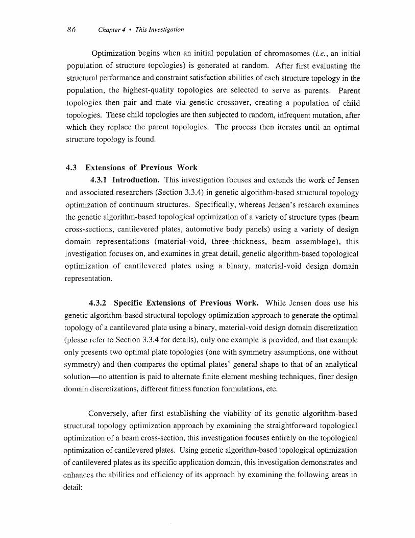
86 Chapter 4 - This Investigation
Optimization begins when an initial population of chromosomes (i.e., an initial
population of structure topologies) is generated at random. After first evaluating the
structural performance and constraint satisfaction abilities of each structure topology in the
population, the highest-quality topologies are selected to serve as parents. Parent
topologies then pair and mate via genetic crossover, creating a population of child
topologies. These child topologies are then subjected to random, infrequent mutation, after
which they replace the parent topologies. The process then iterates until an optimal
structure topology is found.
4.3 Extensions of Previous Work
4.3.1 Introduction. This investigation focuses and extends the work of Jensen
and associated researchers (Section 3.3.4) in genetic algorithm-based structural topology
optimization of continuum structures. Specifically, whereas Jensen's research examines
the genetic algorithm-based topological optimization of a variety of structure types (beam
cross-sections, cantilevered plates, automotive body panels) using a variety of design
domain representations (material-void, three-thickness, beam assemblage), this
investigation focuses on, and examines in great detail, genetic algorithm-based topological
optimization of cantilevered plates using a binary, material-void design domain
representation.
4.3.2 Specific Extensions of Previous Work. While Jensen does use his
genetic algorithm-based structural topology optimization approach to generate the optimal
topology of a cantilevered plate using a binary, material-void design domain discretization
(please refer to Section 3.3.4 for details), only one example is provided, and that example
only presents two optimal plate topologies (one with symmetry assumptions, one without
symmetry) and then compares the optimal plates' general shape to that of an analytical
solution-no attention is paid to alternate finite element meshing techniques, finer design
domain discretizations, different fitness function formulations, etc.
Conversely, after first establishing the viability of its genetic algorithm-based
structural topology optimization approach by examining the straightforward topological
optimization of a beam cross-section, this investigation focuses entirely on the topological
optimization of cantilevered plates. Using genetic algorithm-based topological optimization
of cantilevered plates as its specific application domain, this investigation demonstrates and
enhances the abilities and efficiency of its approach by examining the following areas in
detail:
- - I NAWMMMW M
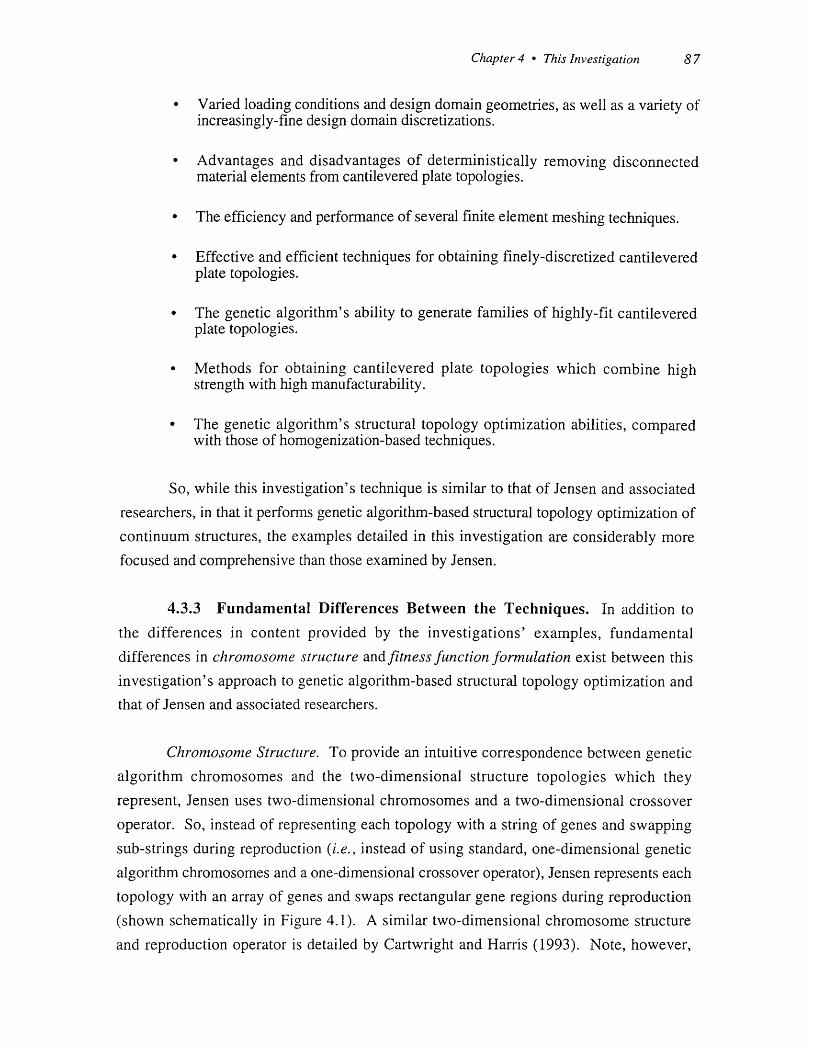
Chapter 4 - This Investigation 87
* Varied loading conditions and design domain geometries, as well as a variety ofincreasingly-fine design domain discretizations.
- Advantages and disadvantages of deterministically removing disconnectedmaterial elements from cantilevered plate topologies.
* The efficiency and performance of several finite element meshing techniques.
. Effective and efficient techniques for obtaining finely-discretized cantileveredplate topologies.
- The genetic algorithm's ability to generate families of highly-fit cantileveredplate topologies.
- Methods for obtaining cantilevered plate topologies which combine highstrength with high manufacturability.
- The genetic algorithm's structural topology optimization abilities, comparedwith those of homogenization-based techniques.
So, while this investigation's technique is similar to that of Jensen and associated
researchers, in that it performs genetic algorithm-based structural topology optimization of
continuum structures, the examples detailed in this investigation are considerably more
focused and comprehensive than those examined by Jensen.
4.3.3 Fundamental Differences Between the Techniques. In addition to
the differences in content provided by the investigations' examples, fundamental
differences in chromosome structure and fitness function formulation exist between this
investigation's approach to genetic algorithm-based structural topology optimization and
that of Jensen and associated researchers.
Chromosome Structure. To provide an intuitive correspondence between genetic
algorithm chromosomes and the two-dimensional structure topologies which they
represent, Jensen uses two-dimensional chromosomes and a two-dimensional crossover
operator. So, instead of representing each topology with a string of genes and swapping
sub-strings during reproduction (i.e., instead of using standard, one-dimensional genetic
algorithm chromosomes and a one-dimensional crossover operator), Jensen represents each
topology with an array of genes and swaps rectangular gene regions during reproduction
(shown schematically in Figure 4.1). A similar two-dimensional chromosome structure
and reproduction operator is detailed by Cartwright and Harris (1993). Note, however,

88 Chapter 4 - This Investigation
that the Schema Theorem (Section 2.3.4) is not applicable to these two-dimensional
chromosomes.
Figure 4.1: Two-dimensional crossover.
This investigation utilizes one-dimensional chromosomes and a one-dimensional
crossover operator to represent and mate two-dimensional structure topologies. Hence,each structure topology is represented by a string of genes, and reproduction occurs by
swapping sub-strings between parents. While this chromosome representation and
crossover operator are the simplest possible and do not provide the intuitive 2D-
chromosome-to-2D-design-domain correspondence of Jensen's chromosome
representation, they have provided satisfactory results during the course of this
investigation and are applicable to the Schema Theorem. Note that no experimentation with
two-dimensional chromosomes or crossover was undertaken in this investigation.
Fitness Function Formulation. The topological optimizations examined by Jensen
and associated researchers all attempt to minimize a structure's weight subject to maximum
displacement and (in some cases) maximum stress constraints. Hence, the fitness
functions (to be maximized) used by Jensen during chromosome fitness calculations are
generally of the form:

Chapter 4 - This Investigation 89
Fitness = f (Weight) - g(Displacement, Stress), (4.1)
where f(Weight) represents a function which increases in value as the structure's weightdecreases and g(Displacement, Stress) represents a function which increases in value asthe structure's constraint satisfaction abilities diminish and decreases in value as thestructure's constraint satisfaction abilities improve. Note that a great amount ofexperimentation is required to use these fitness functions effectively, for the magnitude ofthe penalty terms must be properly balanced with the quality terms. In other words,g(Displacement,Stress) must be properly balanced with f(Weight). If the penalty termsare given too much emphasis, the optimization process will typically result in a structurewith low stress and deflection levels, but which contains an excessive amount of material.Likewise, if the penalty terms are given too little emphasis, the optimization will likelyresult in a light structure with high levels of stress and deflection. Jensen examines asituation where these fitness functions can lead to "optimal" structures containing nomaterial (termed null structures), and details techniques for avoiding such situations. Notethat because these fitness functions attempt to minimize weight subject to maximumdisplacement and stress constraints, the optimal topology generated by the techniquedepends upon the structure's material properties and the magnitude of the applied load.Hence, optimization simultaneously addresses the structure's size, shape, and topology.
In an attempt to avoid the penalty term scaling problems inherent with constrainedoptimization fitness functions, this investigation introduces an unconstrained fitnessfunction (to be maximized) which bases a structure's fitness on its Strength-to-Weight orStiffness-to-Weight ratio:
Fitness = Strength (4.2a)Weight
or
Fitness = Stiffness (4.2b)Weight
Note that these fitness functions automatically assign the highest fitness value to the
structure which offers the best combination of light weight and load-carrying ability.
Hence, there is no need to carefully balance magnitudes of quality terms with those of
penalty terms-these unconstrained fitness functions eliminate all penalty coefficients and

90 Chapter 4 - This Investigation
penalty term scaling. This normalization allows the genetic algorithm to focus on
optimizing the structure's shape and topology, independent of the magnitude of the applied
load or the structure's material properties. Hence, the proper size of the structure is left for
later sizing optimization.
While the majority of the examples provided in this investigation utilize the
unconstrained fitness functions detailed above, these fitness functions can easily be
modified to account for various constraints. A linear penalty term, penalizing the strength-
to-weight or stiffness-to-weight ratio by P% for every 10% constraint violation, provides
satisfactory performance in many of the examples detailed in Chapter 5. However, as with
Jensen's fitness functions, great care is required when choosing a penalty parameter
magnitude (in this case, P) which is well balanced with the quality terms of the fitness
function. This investigation uses penalty-based fitness functions to generate structures
combining high strength-to-weight ratio with low stress levels, structures combining high
stiffness-to-weight ratio with high manufacturability, and structures with minimum mean
compliance subject to a maximum volume constraint.
4.4 Implementation
4.4.1 Introduction. When applying the genetic algorithm to a particular
application domain, several points are worthy of note. First, the general structure of the
genetic algorithm requires no modification-optimization always occurs through an
"evolutionary" process, where a population of artificial chromosomes is subjected to
genetics-based operators such as evaluation, selection, reproduction, mutation, and
replacement (detailed in Section 2.3.4). Second, the specific operation of the selection,
reproduction, mutation, and replacement operators also requires no modification-these
operators perform their duties without regard to the particular application domain (again,
detailed in Section 2.3.4). These operators, however, do require modification if the
general one-dimensional, string-of-binary-digits chromosome structure is modified.
Finally, because each chromosome in the population is a coded representation of the
optimization problem's design variables, the chromosome structure must be specially-
tailored to the design variables of the optimization problem to which the genetic algorithm is
being applied (detailed in Section 2.3.3). Likewise, because the fitness function must take
an individual chromosome as input, decode the chromosome into its corresponding design
variable values, and then quantitatively grade the chromosome according to the objective
function minimization (or maximization) and constraint satisfaction abilities of its

Chapter 4 - This Investigation 91
corresponding design variable values, the fitness function must also be specially-tailored to
the particular optimization problem (detailed in Section 2.3.4).
Hence, in this work, where the genetic algorithm is used to optimize the topology
of structural components, each chromosome must be configured so that it represents a
structure topology. Likewise, the fitness function must be formulated so that it can take an
individual chromosome as input, convert the chromosome into its corresponding structure
topology, evaluate the topology's structural performance, and then assign a quantitative
fitness value to the chromosome according to the topology's structural performance and
constraint satisfaction abilities.
The following sections describe the technique used to represent structure topologies
with chromosomes (i.e., the design representation), the specific procedures used to convert
any given chromosome into a structure topology, the technique used to remove
disconnected material elements from a structure topology, the methods used to analyze a
topology's structural performance, and the approaches taken to convert a topology's
structural performance into a quantitative fitness value for the corresponding chromosome.
4.4.2 Design Representation. During optimization, this investigation uses a
rectangular, two-dimensional design domain to establish the maximum allowable size of the
component being optimized. This design domain is discretized into small, square elements,where each element can contain either material or void-no intermediate densities are
allowed. Figure 4.2 depicts an example design domain discretization for a square,cantilevered plate subject to a downward vertical load. Note that the design domain shape
and the discretization resolution depend upon the particular problem and the available
computational resources. Once the discretized design domain has been created, assigning
material or void to each element in the domain (i.e., designating the state of each design
domain element) defines a distribution of material and void within the design domain,therefore establishing a structure topology. Likewise, modifying the state of any element
(i.e., toggling a material element to void or a void element to material) results in a
modification of the structure's topology. Hence, the material-void states of the design
domain elements serve as design variables during optimization. Figure 4.3 depicts an
example distribution of material and void within the example design domain, along with the
structure topology corresponding to this example material-void distribution.
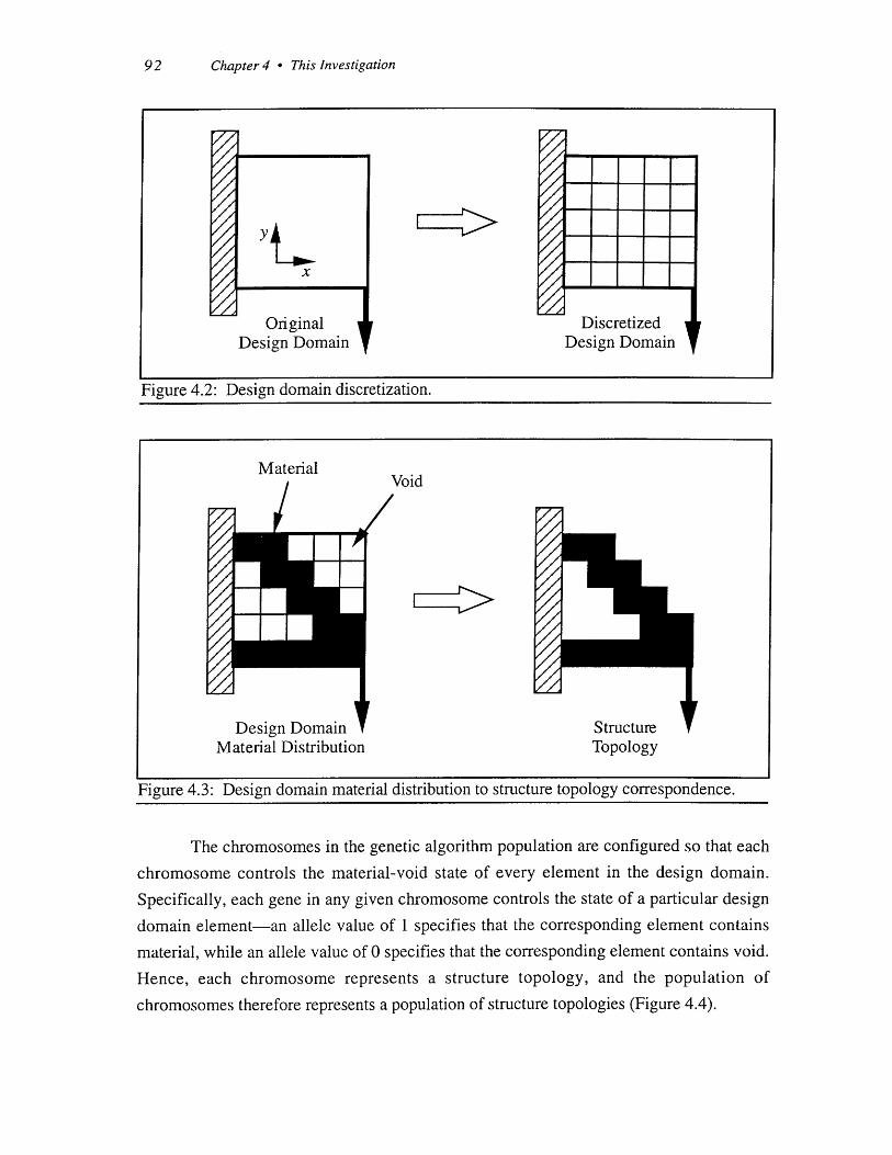
92 Chapter 4 - This Investigation
Figure 4.2: Design domain discretization.
Figure 4.3: Design domain material distribution to structure topology correspondence.
The chromosomes in the genetic algorithm population are configured so that each
chromosome controls the material-void state of every element in the design domain.
Specifically, each gene in any given chromosome controls the state of a particular design
domain element-an allele value of 1 specifies that the corresponding element contains
material, while an allele value of 0 specifies that the corresponding element contains void.
Hence, each chromosome represents a structure topology, and the population of
chromosomes therefore represents a population of structure topologies (Figure 4.4).
MaterialVoid
Design Domain StructureMaterial Distribution Topology
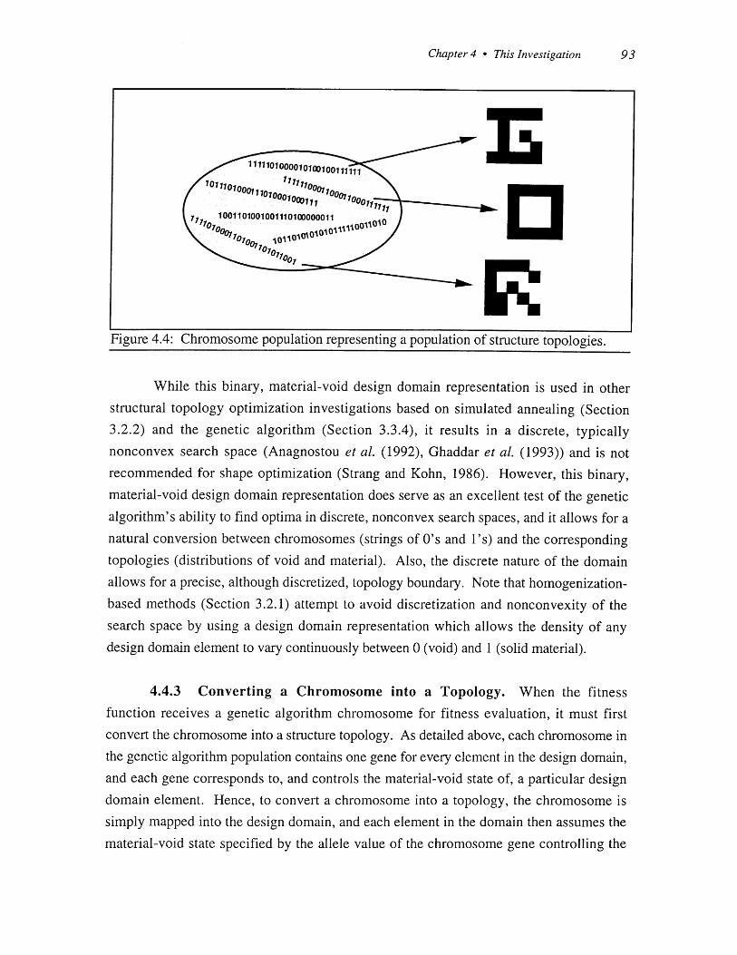
Chapter 4 - This Investigation 93
Figure 4.4: Chromosome population representing a population of structure topologies.
While this binary, material-void design domain representation is used in otherstructural topology optimization investigations based on simulated annealing (Section3.2.2) and the genetic algorithm (Section 3.3.4), it results in a discrete, typicallynonconvex search space (Anagnostou et al. (1992), Ghaddar et al. (1993)) and is notrecommended for shape optimization (Strang and Kohn, 1986). However, this binary,material-void design domain representation does serve as an excellent test of the genetic
algorithm's ability to find optima in discrete, nonconvex search spaces, and it allows for anatural conversion between chromosomes (strings of O's and l's) and the corresponding
topologies (distributions of void and material). Also, the discrete nature of the domain
allows for a precise, although discretized, topology boundary. Note that homogenization-
based methods (Section 3.2.1) attempt to avoid discretization and nonconvexity of the
search space by using a design domain representation which allows the density of any
design domain element to vary continuously between 0 (void) and 1 (solid material).
4.4.3 Converting a Chromosome into a Topology. When the fitness
function receives a genetic algorithm chromosome for fitness evaluation, it must first
convert the chromosome into a structure topology. As detailed above, each chromosome in
the genetic algorithm population contains one gene for every element in the design domain,and each gene corresponds to, and controls the material-void state of, a particular design
domain element. Hence, to convert a chromosome into a topology, the chromosome is
simply mapped into the design domain, and each element in the domain then assumes the
material-void state specified by the allele value of the chromosome gene controlling the
B
Ob.- 13
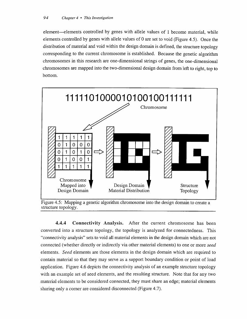
94 Chapter 4 - This Investigation
element-elements controlled by genes with allele values of 1 become material, while
elements controlled by genes with allele values of 0 are set to void (Figure 4.5). Once the
distribution of material and void within the design domain is defined, the structure topology
corresponding to the current chromosome is established. Because the genetic algorithmchromosomes in this research are one-dimensional strings of genes, the one-dimensional
chromosomes are mapped into the two-dimensional design domain from left to right, top tobottom.
1111101000010100100111111Chromosome
0 1 0 0 00 1 110 1 100 1 0 0 1
ChromosomeMapped into
Design DomainDesign Domain
Material Distribution
Figure 4.5: Mapping a genetic algorithm chromosome into the design domain to create astructure topology.
4.4.4 Connectivity Analysis. After the current chromosome has been
converted into a structure topology, the topology is analyzed for connectedness. This
"connectivity analysis" sets to void all material elements in the design domain which are not
connected (whether directly or indirectly via other material elements) to one or more seed
elements. Seed elements are those elements in the design domain which are required to
contain material so that they may serve as a support boundary condition or point of load
application. Figure 4.6 depicts the connectivity analysis of an example structure topology
with an example set of seed elements, and the resulting structure. Note that for any two
material elements to be considered connected, they must share an edge; material elements
sharing only a corner are considered disconnected (Figure 4.7).
StructureTopology

Chapter 4 - This Investigation 95
Figure 4.6: Connectivity analysis.
(a) (b)
Figure 4.7: (a) Connected and (b) disconnected material elements.
When connectivity analysis is activated, disconnected material elements are treated
as if they are void-they are assigned zero weight and volume and are considered to be
void when performing structural analysis. Conversely, when connectivity analysis is
deactivated, disconnected material elements are treated as if they are material-they are
counted in weight and volume calculations and are considered to be material when
performing structural analysis. Note that when connectivity analysis is performed, the
corresponding chromosome allele value is not modified when a disconnected material
element is switched to void or a seed element is switched to material-only the state of the
design domain element is changed. In other words, connectivity analysis does not alter a
chromosome's genotype (i.e., the chromosome's genetic code) and instead alters the
chromosome's phenotype (i.e., the design variable values corresponding to the
chromosome genotype).
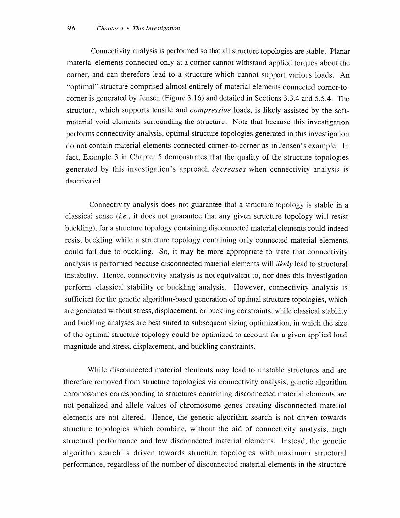
96 Chapter 4 - This Investigation
Connectivity analysis is performed so that all structure topologies are stable. Planar
material elements connected only at a corner cannot withstand applied torques about the
corner, and can therefore lead to a structure which cannot support various loads. An
"optimal" structure comprised almost entirely of material elements connected corner-to-
corner is generated by Jensen (Figure 3.16) and detailed in Sections 3.3.4 and 5.5.4. The
structure, which supports tensile and compressive loads, is likely assisted by the soft-
material void elements surrounding the structure. Note that because this investigation
performs connectivity analysis, optimal structure topologies generated in this investigation
do not contain material elements connected corner-to-corner as in Jensen's example. In
fact, Example 3 in Chapter 5 demonstrates that the quality of the structure topologies
generated by this investigation's approach decreases when connectivity analysis is
deactivated.
Connectivity analysis does not guarantee that a structure topology is stable in a
classical sense (i.e., it does not guarantee that any given structure topology will resist
buckling), for a structure topology containing disconnected material elements could indeed
resist buckling while a structure topology containing only connected material elements
could fail due to buckling. So, it may be more appropriate to state that connectivity
analysis is performed because disconnected material elements will likely lead to structural
instability. Hence, connectivity analysis is not equivalent to, nor does this investigation
perform, classical stability or buckling analysis. However, connectivity analysis is
sufficient for the genetic algorithm-based generation of optimal structure topologies, which
are generated without stress, displacement, or buckling constraints, while classical stability
and buckling analyses are best suited to subsequent sizing optimization, in which the size
of the optimal structure topology could be optimized to account for a given applied load
magnitude and stress, displacement, and buckling constraints.
While disconnected material elements may lead to unstable structures and are
therefore removed from structure topologies via connectivity analysis, genetic algorithm
chromosomes corresponding to structures containing disconnected material elements are
not penalized and allele values of chromosome genes creating disconnected material
elements are not altered. Hence, the genetic algorithm search is not driven towards
structure topologies which combine, without the aid of connectivity analysis, high
structural performance and few disconnected material elements. Instead, the genetic
algorithm search is driven towards structure topologies with maximum structural
performance, regardless of the number of disconnected material elements in the structure
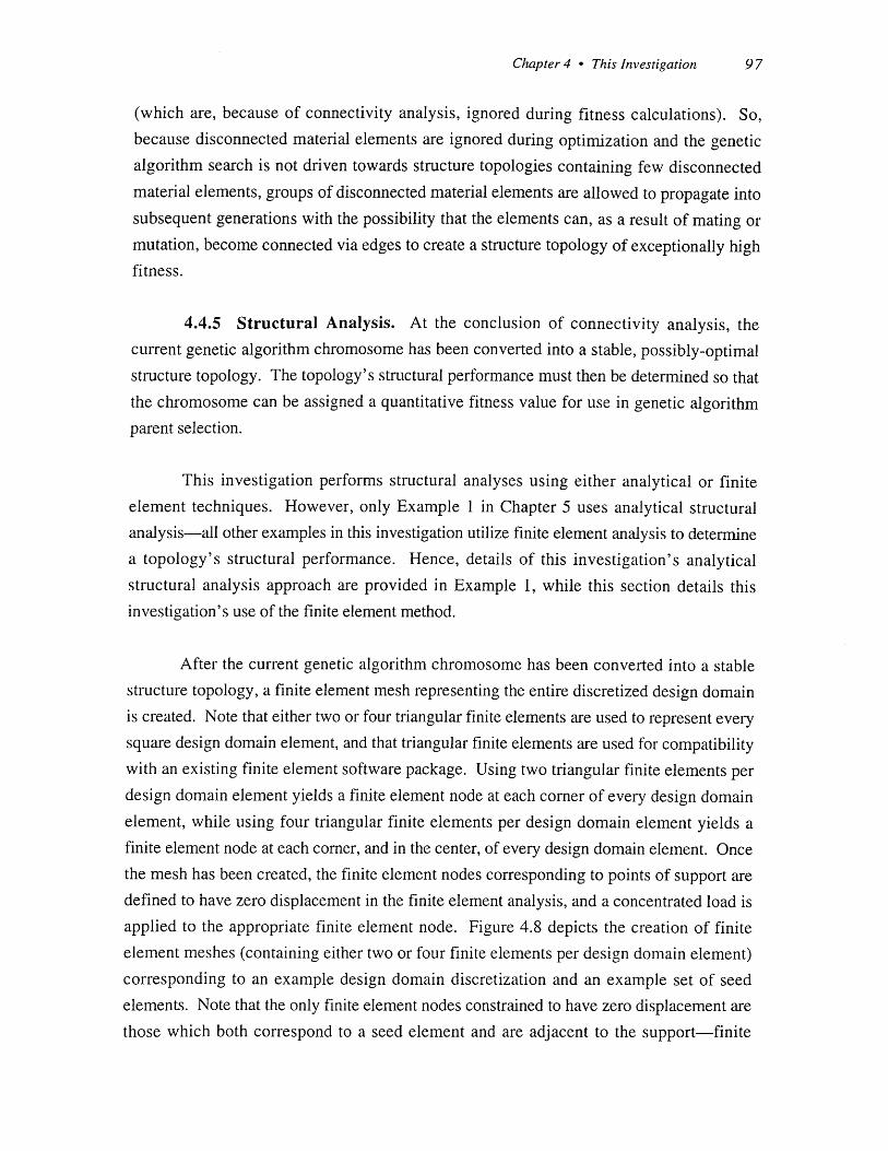
Chapter 4 - This Investigation 97
(which are, because of connectivity analysis, ignored during fitness calculations). So,because disconnected material elements are ignored during optimization and the geneticalgorithm search is not driven towards structure topologies containing few disconnectedmaterial elements, groups of disconnected material elements are allowed to propagate intosubsequent generations with the possibility that the elements can, as a result of mating ormutation, become connected via edges to create a structure topology of exceptionally highfitness.
4.4.5 Structural Analysis. At the conclusion of connectivity analysis, thecurrent genetic algorithm chromosome has been converted into a stable, possibly-optimal
structure topology. The topology's structural performance must then be determined so that
the chromosome can be assigned a quantitative fitness value for use in genetic algorithm
parent selection.
This investigation performs structural analyses using either analytical or finiteelement techniques. However, only Example 1 in Chapter 5 uses analytical structuralanalysis-all other examples in this investigation utilize finite element analysis to determine
a topology's structural performance. Hence, details of this investigation's analytical
structural analysis approach are provided in Example 1, while this section details this
investigation's use of the finite element method.
After the current genetic algorithm chromosome has been converted into a stable
structure topology, a finite element mesh representing the entire discretized design domain
is created. Note that either two or four triangular finite elements are used to represent everysquare design domain element, and that triangular finite elements are used for compatibility
with an existing finite element software package. Using two triangular finite elements per
design domain element yields a finite element node at each corner of every design domain
element, while using four triangular finite elements per design domain element yields afinite element node at each corner, and in the center, of every design domain element. Once
the mesh has been created, the finite element nodes corresponding to points of support are
defined to have zero displacement in the finite element analysis, and a concentrated load is
applied to the appropriate finite element node. Figure 4.8 depicts the creation of finite
element meshes (containing either two or four finite elements per design domain element)
corresponding to an example design domain discretization and an example set of seed
elements. Note that the only finite element nodes constrained to have zero displacement are
those which both correspond to a seed element and are adjacent to the support-finite

98 Chapter 4 - This Investigation
element nodes adjacent to the support which correspond to non-seed design domain
elements are not constrained to have zero displacement (except in Example 8 of Chapter 5,
where all finite element nodes adjacent to the support, regardless of whether or not they
correspond to a seed element, are constrained to have zero displacement).
Figure 4.8: Finite element mesh generation.
After a finite element mesh corresponding to the discretized design domain has been
created, the mesh must be modified so that it represents the current structure topology (and
therefore the current genetic algorithm chromosome). This modification is performed using
either an adaptive or a constant meshing technique. Once the mesh has been modified,
finite element analysis takes place.
Adaptive Meshing Technique. To create a finite element mesh corresponding to the
current structure topology, the adaptive meshing technique begins with the finite element
mesh corresponding to the entire discretized design domain and then removes all finite
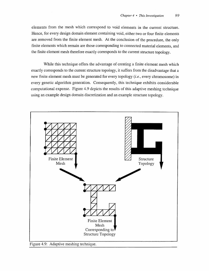
Chapter 4 - This Investigation 99
elements from the mesh which correspond to void elements in the current structure.
Hence, for every design domain element containing void, either two or four finite elements
are removed from the finite element mesh. At the conclusion of the procedure, the onlyfinite elements which remain are those corresponding to connected material elements, andthe finite element mesh therefore exactly corresponds to the current structure topology.
While this technique offers the advantage of creating a finite element mesh which
exactly corresponds to the current structure topology, it suffers from the disadvantage that a
new finite element mesh must be generated for every topology (i.e., every chromosome) in
every genetic algorithm generation. Consequently, this technique exhibits considerable
computational expense. Figure 4.9 depicts the results of this adaptive meshing technique
using an example design domain discretization and an example structure topology.
Finite Element StructureMesh Topology t
Finite ElementMesh
Corresponding tolStructure Topology
Figure 4.9: Adaptive meshing technique.
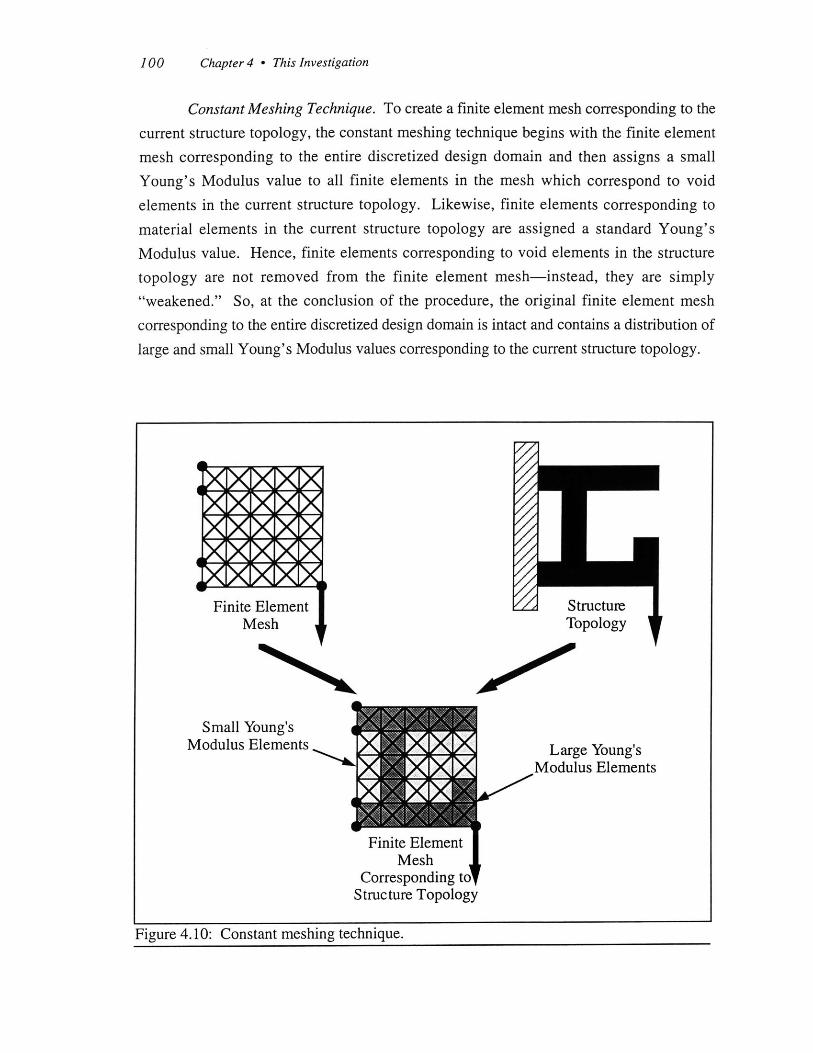
100 Chapter 4 - This Investigation
Constant Meshing Technique. To create a finite element mesh corresponding to the
current structure topology, the constant meshing technique begins with the finite element
mesh corresponding to the entire discretized design domain and then assigns a small
Young's Modulus value to all finite elements in the mesh which correspond to void
elements in the current structure topology. Likewise, finite elements corresponding to
material elements in the current structure topology are assigned a standard Young's
Modulus value. Hence, finite elements corresponding to void elements in the structure
topology are not removed from the finite element mesh-instead, they are simply
"weakened." So, at the conclusion of the procedure, the original finite element mesh
corresponding to the entire discretized design domain is intact and contains a distribution of
large and small Young's Modulus values corresponding to the current structure topology.
Figure 4.10: Constant meshing technique.
Finite ElementMesh
Corresponding to
Chapter 4 - This Investigation 101
While the finite element mesh generated by this technique does not exactlycorrespond to the structure topology (i.e., finite elements, albeit of low strength, exist inareas where no material is present), this technique does not require the generation of a newfinite element mesh for every structure topology in every genetic algorithm generation.Consequently, this technique is relatively inexpensive computationally. In fact, as detailedby Example 3 in Chapter 5, the constant meshing technique provides, at much lesscomputational expense, optimization and finite-element analysis performance comparable tothat of the adaptive technique. Figure 4.10 depicts the results of this constant meshingtechnique using an example design domain discretization and an example structuretopology.
The use of "soft" material elements to represent void is suggested by Bendsoe andKikuchi (1988), who state that soft material can be considered a void or hole if its Young'sModulus is 10-2 to 10-3 times that of a hard material. Jensen (Section 3.3.4) uses a similarapproach to create finite element meshes, although he reduces the thicknesses of finiteelements corresponding to void elements instead of reducing their Young's Modulusvalues. Because reducing a finite element's thickness is equivalent to reducing its Young's
Modulus value, Jensen's meshing technique is identical to this investigation's constant
meshing technique. However, while Jensen specifies that the thickness of void elements
should be 10-2 times that of material elements, this investigation stipulates that void
elements receive a Young's Modulus 10-5 times that of a material element.
Finite Element Analysis. After the finite element mesh corresponding to the currentstructure topology has been created, finite element analysis is performed. This finite
element analysis determines the displacement, in the x- and y-directions, of every node in
the finite element mesh. Note that no stress calculations are performed by the finite element
routines.
4.4.6 Fitness Calculations. At the conclusion of finite element analysis,results of the analysis are used to calculate a fitness value which quantitatively describes the
quality of the genetic algorithm chromosome which created the current structure topology.
Again, while fitness calculations performed by Example 1 in Chapter 5 are based on the
results of analytical structural analyses, all other examples in this investigation utilize finite
element analysis results to calculate a topology's fitness. Hence, details of fitness
calculations based on analytical analyses are provided in Example 1, while this section
details fitness calculations based on finite element analyses.

102 Chapter 4 - This Investigation
Because all finite element analysis-based examples in this investigation attempt to
optimize structures which are subject to a single applied load, all finite element analyses in
this investigation use a single concentrated load applied to a single finite element node.
Consequently, these finite element analysis-based optimizations utilize the current
structure's displacement at the point of load application (u) as the basis for all fitness
calculations. So, after performing finite element analysis on the current structure topology,
u is set equal to:
U= [s, (4.3)
where u, and u, represent the displacement, in the x- and y-directions, of the finite element
node where the load was applied. After u has been determined, fitness calculations may
begin.
The fitness calculations performed in this investigation attempt to either maximize a
structure's stiffness-to-weight ratio or minimize a structure's compliance subject to a
maximum volume constraint. Again, the fitness calculations performed in Example 1,
which attempt to drive the genetic algorithm search towards structure topologies with
maximum strength-to-weight ratio, are detailed in the text of Example 1.
Stiffness-To-Weight Ratio Maximization. As detailed in Section 4.3.3, most
examples provided in this investigation attempt to maximize a structure's stiffness-to-
weight ratio. Hence, the fitness value which these examples assign to any given genetic
algorithm chromosome is equal to the stiffness-to-weight ratio of the structure topology
corresponding to the chromosome. Stiffness-to-weight ratio calculations begin when a
structure's "stiffness" is assumed to be inversely proportional to the magnitude of the
structure's displacement at the point of load application:
Stiffness = 1 (4.4)I uj )2 + (1)2
Using the area of connected material in the structure as a qualitative measure of the
structure's weight, the structure's stiffness-to-weight ratio (and therefore the fitness, to be
maximized, of the chromosome corresponding to the structure) is given by:
Chapter 4 - This Investigation 103
Stiffness(iFitness - - Ara- . (4.5)
Weight Area Area )2+(U
Note that disconnected material elements which were switched to void by
connectivity analysis are not counted in the above "weight" calculations.
Compliance Minimization. Example 8, detailed in Chapter 5, does not attempt to
maximize a structure's stiffness-to-weight ratio. Rather, it attempts to minimize a
structure's mean compliance subject to a maximum volume constraint. Hence, any given
chromosome's fitness is determined by the compliance minimization and volume constraint
satisfaction abilities of the structure topology corresponding to the chromosome.
Specifically, fitness calculations are performed so that high fitness is assigned to
chromosomes corresponding to structures exhibiting low mean compliance without
violating the maximum volume constraint. Likewise, low fitness is assigned to
chromosomes corresponding to structures exhibiting large mean compliance and/or
violating the maximum volume constraint.
Instead of using a structure's displacement at the point of load application (u) to
calculate stiffness, these fitness calculations use u to determine the structure's mean
compliance. Note that a structure's mean compliance represents twice the strain energy of
the structure as it supports the applied load(s). In Example 8, where a single concentrated
load is applied to a single finite element node, a structure's mean compliance is equal to the
applied load vector (FAPPLIED) multiplied by the structure's displacement at the point of load
application (u T):
Compliance = u -FAPPLJED (4.6)
where
uT =[ux u .] (4.7)
and
F APPLIED ' (4.8)

104 Chapter 4 - This Investigation
Note that F, and F, represent the magnitude, in the x- and y-directions, of the
single concentrated load acting on the structure.
In addition to the structure's compliance, these fitness calculations also require the
structure's volume. So, just as the stiffness-to-weight ratio fitness calculations use a
structure's area to represent weight, these calculations use the area of connected material in
a structure as a qualitative measure of the structure's volume. Note that disconnected
material elements which were switched to void by connectivity analysis are not counted in
"volume" calculations.
After determining a structure's volume and mean compliance, the structure's fitness
(to be maximized) is initially set equal to:
1Fitness = . (4.9)
ln( Compliance)
Two clarifications are needed regarding the above fitness value. First, as opposed
to the unconstrained stiffness-to-weight ratio fitness calculations detailed above, fitness
calculations for this constrained optimization problem require the use of a linear penalty
term to penalize a structure's mean compliance based on the extent of volume constraint
violation. However, mean compliance values typically decrease by several orders of
magnitude during optimization, creating difficulty in selecting volume constraint violation
penalty coefficients which work well for both early and mature genetic algorithm
populations. Hence, to reduce this variation, the natural log of mean compliance is used in
fitness calculations. Second, the reciprocal of the natural log of mean compliance is used
because the genetic algorithm is naturally a maximization algorithm and this optimization
attempts to minimize the structure's mean compliance. By maximizing the above fitness
function, the genetic algorithm generates structures with minimum mean compliance.
After the above fitness value is determined, the structure's volume is compared to
the maximum allowable volume. If there is no constraint violation, the chromosome
corresponding to the structure is assigned the fitness value above. If there is a violation,
the structure's fitness is penalized by 6% for every 10% volume constraint violation. Note
that the fitness penalty is linearly attenuated according to the current generation number,
with no penalty at generation 0 and full (6%) penalty at generation 175. Hence, prior to

Chapter 4 - This Investigation 105
generation 175, the fitness of a chromosome corresponding to a structure topology
violating the maximum volume constraint is given by:
generation 0.06 V -VM 1Fitness = 1175 0.10 Vmx ln(Compliance)' (4.10)
where generation represents the current generation of genetic algorithm evolution, V
represents the volume (i.e., the area) of the current structure topology, and VmA represents
the maximum allowable volume of the structure. After generation 175, the fitness of a
chromosome corresponding to a structure topology violating the maximum volume
constraint is given by:
Fitness = 1. 0.0 V 1 1 (4.11)0.10 Vm4x, ln(Compliance)
4.4.7 Summary. After calculating the fitness value of the current structure
topology and then assigning the value to the chromosome corresponding to the topology,the entire fitness evaluation process is repeated for every chromosome in the current genetic
algorithm generation. This fitness evaluation process is performed during each generation
of genetic algorithm-based structural topology optimization.

106 Chapter 4 - This Investigation

Chapter 5 * Examples 107
Examples
5.1 Overview
This chapter details the application of this investigation's genetic algorithm-based
structural topology optimization approach to a variety of example problems.
5.2 Example 1: Beam Cross-Section.
5.2.1 Introduction. This example attempts to establish the viability of this
investigation's genetic algorithm-based structural topology optimization approach by
examining the relatively straightforward topological optimization of a beam cross-section.
Specifically, this example first attempts to generate the cross-section topology of a simply-
supported beam in pure bending which provides maximum strength-to-weight ratio,
independent of the magnitude of bending stresses in the beam. A second portion of this
example then attempts to generate the cross-section topology of a simply-supported beam in
pure bending which provides maximum strength-to-weight ratio subject to a maximum
stress constraint.
5.2.2 Design Domain. The beam's cross-section is modeled using a square
design domain discretized into a 15 x 15 grid of binary, material-void elements (Figure
5.1). Because each genetic algorithm chromosome must contain one gene for every
element in the design domain, this 15 x 15 design domain discretization results in a
chromosome length of 225 genes. Hence, the search space contains 2225 distinct locations.
During optimization, no symmetry constraints are imposed on the beam cross-section, and
the cross-section topology is assumed to be constant throughout the length of the beam.
Also, the middle design domain element along the cross-section's top surface serves as a
seed element. During structural analysis, no particular assumption is made as to how the

108 Chapter 5 - Examples
moments are physically applied to the beam-analysis routines simply use a stress
distribution which would result from pure bending.
Figure 5.1: Example 1 design domain.
5.2.3 Fitness Calculations-Part A. This first portion of Example 1
attempts to generate the beam cross-section topology which exhibits maximum strength-to-
weight ratio. As detailed in Section 4.4, the fitness of any given genetic algorithm
chromosome is determined by converting the chromosome into its corresponding structure
topology, analyzing the structure topology for connectedness, evaluating the topology's
structural performance, and then converting the topology's structural performance into a
quantitative fitness value for the corresponding chromosome. Hence, fitness calculations
in this example convert a chromosome into its corresponding beam cross-section topology,
perform connectivity analysis on the cross-section topology, calculate the cross-section's
strength-to-weight ratio, and then set the chromosome's fitness value equal to the cross-
section's strength-to-weight ratio:
Fitness = Strength (5.1)Weight
SeedElement
15
.15

Chapter 5 * Examples 109
Strength-to-weight ratio calculations begin when a cross-section's moment of
inertia is determined using analytical techniques and then used to represent the cross-
section's strength. Likewise, as in the stiffness-to-weight ratio fitness calculations detailedin Section 4.4.6, the cross-section's "weight" is assumed to be equal to the area ofconnected material elements in the cross-section topology. Hence, the strength-to-weight
ratio of any given cross-section topology (and therefore the fitness, to be maximized, of the
chromosome corresponding to the cross-section topology) is given by:
Moment of Inertia (52)Fitness =.(52
Area
As detailed in Sections 4.4.5 and 4.4.6, this example's fitness calculations differ
from all other examples in this investigation in that they are based on the results of
analytical structural analysis techniques instead of finite element analysis.
5.2.4 Results-Part A. Results of the optimization are shown in Figure 5.2,which depicts best-of-generation cross-section topologies at 50-generation intervals, and in
Figure 5.3, which plots the genetic algorithm population's maximum, average, and
Generation 0 Generation 50 Generation 100 Generation 150 Generation 200r -- -1 -I r rr
Generation 250 Generation 300 Generation 350 Generation 400 Generation 450
Generation 500 Generation 550 Generation 600)
Figure 5.2: Best-of-generation beam cross-sections.
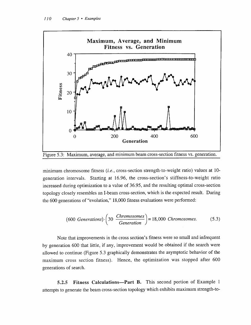
110 Chapter 5 - Examples
Figure 5.3: Maximum, average, and minimum beam cross-section fitness vs. generation.
minimum chromosome fitness (i.e., cross-section strength-to-weight ratio) values at 10-
generation intervals. Starting at 16.96, the cross-section's stiffness-to-weight ratio
increased during optimization to a value of 36.95, and the resulting optimal cross-section
topology closely resembles an I-beam cross-section, which is the expected result. During
the 600 generations of "evolution," 18,000 fitness evaluations were performed:
('Chromosomes(600 Generations). 30 = 18,000 Chromosomes. (5.3)
Generation
Note that improvements in the cross section's fitness were so small and infrequent
by generation 600 that little, if any, improvement would be obtained if the search were
allowed to continue (Figure 5.3 graphically demonstrates the asymptotic behavior of the
maximum cross section fitness). Hence, the optimization was stopped after 600
generations of search.
5.2.5 Fitness Calculations-Part B. This second portion of Example 1
attempts to generate the beam cross-section topology which exhibits maximum strength-to-
Maximum, Average, and MinimumFitness vs. Generation
40
30 .
20-
10-
00 200 400 600
Generation
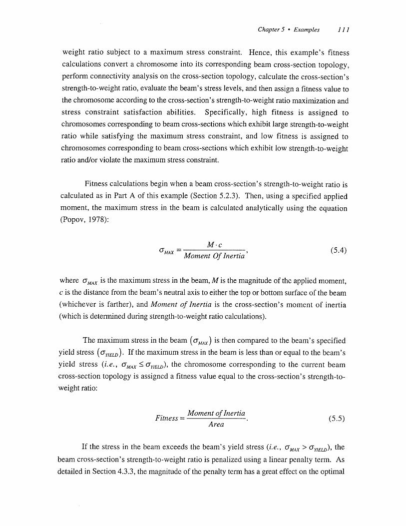
Chapter 5 - Examples 11
weight ratio subject to a maximum stress constraint. Hence, this example's fitnesscalculations convert a chromosome into its corresponding beam cross-section topology,perform connectivity analysis on the cross-section topology, calculate the cross-section's
strength-to-weight ratio, evaluate the beam's stress levels, and then assign a fitness value to
the chromosome according to the cross-section's strength-to-weight ratio maximization and
stress constraint satisfaction abilities. Specifically, high fitness is assigned to
chromosomes corresponding to beam cross-sections which exhibit large strength-to-weight
ratio while satisfying the maximum stress constraint, and low fitness is assigned to
chromosomes corresponding to beam cross-sections which exhibit low strength-to-weight
ratio and/or violate the maximum stress constraint.
Fitness calculations begin when a beam cross-section's strength-to-weight ratio is
calculated as in Part A of this example (Section 5.2.3). Then, using a specified applied
moment, the maximum stress in the beam is calculated analytically using the equation
(Popov, 1978):
M -cUMAX = C (5.4)
Moment Of Inertia(
where amAx is the maximum stress in the beam, M is the magnitude of the applied moment,
c is the distance from the beam's neutral axis to either the top or bottom surface of the beam
(whichever is farther), and Moment of Inertia is the cross-section's moment of inertia
(which is determined during strength-to-weight ratio calculations).
The maximum stress in the beam (r,,x) is then compared to the beam's specified
yield stress (YYIELD). If the maximum stress in the beam is less than or equal to the beam's
yield stress (i.e., JmAx < ayELD), the chromosome corresponding to the current beam
cross-section topology is assigned a fitness value equal to the cross-section's strength-to-
weight ratio:
Moment of Inertia (55)Fitness =. 55)
Area
If the stress in the beam exceeds the beam's yield stress (i.e., rMAX > UYIELD), the
beam cross-section's strength-to-weight ratio is penalized using a linear penalty term. As
detailed in Section 4.3.3, the magnitude of the penalty term has a great effect on the optimal
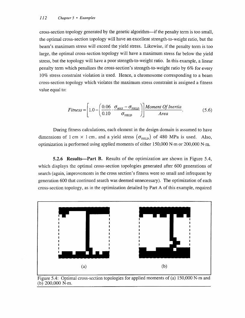
112 Chapter 5 Examples
cross-section topology generated by the genetic algorithm-if the penalty term is too small,
the optimal cross-section topology will have an excellent strength-to-weight ratio, but the
beam's maximum stress will exceed the yield stress. Likewise, if the penalty term is too
large, the optimal cross-section topology will have a maximum stress far below the yield
stress, but the topology will have a poor strength-to-weight ratio. In this example, a linear
penalty term which penalizes the cross-section's strength-to-weight ratio by 6% for every
10% stress constraint violation is used. Hence, a chromosome corresponding to a beam
cross-section topology which violates the maximum stress constraint is assigned a fitness
value equal to:
FitnessF1.0 _ (0.06 aMAX - UYIELD Moment Of Inertia (5.6)0.10 OYIELD Area
During fitness calculations, each element in the design domain is assumed to have
dimensions of I cm x 1 cm, and a yield stress (UYIELD) of 480 MPa is used. Also,
optimization is performed using applied moments of either 150,000 N-m or 200,000 N.m.
5.2.6 Results-Part B. Results of the optimization are shown in Figure 5.4,
which displays the optimal cross-section topologies generated after 600 generations of
search (again, improvements in the cross section's fitness were so small and infrequent by
generation 600 that continued search was deemed unnecessary). The optimization of each
cross-section topology, as in the optimization detailed by Part A of this example, required
Figure 5.4: Optimal cross-section topologies for applied moments of (a) 150,000 N-m and(b) 200,000 N-m.

Chapter 5 * Examples 113
Figure 5.5: Maximum stress vs. generation with applied moment of 150,000 N.m.
Figure 5.6: Maximum stress vs. generation with applied moment of 200,000 N-m.
Maximum Stress vs. Generation900
800
700
600
500 -. ..... ..
400-
300-
200-
100
0 200 400 600Generation

114 Chapter 5 - Examples
18,000 fitness evaluations. Note that Figure 5.4a depicts the optimal cross-section
topology for the applied moment of 150,000 N-m, while Figure 5.4b depicts the optimal
cross-section topology for the applied moment of 200,000 N.m. As expected, the optimal
cross-section topologies closely resemble I-beam cross-sections, and the outer flanges
become thicker and the web remains thin as the applied moment is increased. Figure 5.5
depicts, in 10-generation intervals, the maximum stress in the beam subject to the applied
moment of 150,000 N-m. During optimization, the maximum stress in the beam decreased
from 860.95 MPa to a final value of 477.65 MPa. Likewise, Figure 5.6 shows the
maximum stress in the beam subject to the applied moment of 200,000 N-m. In this
second beam, the maximum stress decreased from an initial value of 909.69 MPa to a final
value of 481.5 MPa.
When examining these results, it is interesting to make comparisons between the
genetic algorithm and other basic search techniques which are also able to search in
discrete, discontinuous, multi-modal search spaces (e.g., exhaustive and random
searches). In this example, a near-optimum beam cross-section is found after 18,000
function evaluations, i.e., after examining 18,000 locations in the search space. As the
search space contains 2225 distinct locations, the genetic algorithm searches only a tiny
fraction of the space before finding a near-optimum location. This is compared to an
exhaustive search, which would examine all 2225 locations. A random search would likely
find the optimum location after searching one-half of the 2225 locations (note that the
random search would not know that it had found the optimum because it does not use
gradient information). Hence, when attempting to locate near-optimum topologies, the
genetic algorithm is much more efficient than other basic techniques which are also able to
search ill-conditioned search spaces.
As detailed in Section 4.4.4, this investigation uses connectivity analysis to insure
that material elements connected only at corners are removed from topologies. While these
disconnected material elements cannot withstand any applied torque and could therefore
lead to an unstable structure, they can withstand the bending stresses encountered in this
example. Hence, utilizing disconnected material elements in this example's moment of
inertia and area calculations (i.e., deactivating connectivity analysis) might have resulted in
higher-fitness beam cross-section topologies. However, any cross-section topology
containing such elements would be unrealistic and nearly impossible to manufacture.
Hence, connectivity analysis is used to eliminate these disconnected material elements.

Chapter 5 - Examples 115
Note that placing a seed element on the beam cross-section's upper surface couldpossibly bias the genetic algorithm search towards topologies with material along the uppersurface. However, the results given in Figures 5.2 and 5.4 show that while materialcongregates along the upper surface of the design domain, material also congregates alongthe lower surface. Because the stress distribution resulting from a pure bending loadingconfiguration is symmetric about the neutral axis, the configuration of material should alsobe symmetric about the neutral axis. Hence, the fact that material places itself along thelower surface of the design domain without the "assistance" of a material constraintsuggests that the material along the upper design domain surface is an unbiased optimalconfiguration of material.
5.3 Example 2: Small Cantilevered Plate.
5.3.1 Introduction. This example details this investigation's first attempt at
using the genetic algorithm in conjunction with finite element analysis to perform structuraltopology optimization. This example's use of finite element analysis techniques is asignificant enhancement over the previous example's analytical techniques, as nearly allpractical structural topology optimization problems require the use of numerical analysismethods such as the finite element method. In the example, the genetic algorithm is used togenerate the topology of a square cantilevered plate in tension which provides maximumstiffness-to-weight ratio.
5.3.2 Design Domain. The plate is modeled using a square design domaindiscretized into a 12 x 12 grid of binary, material-void elements (Figure 5.7). Duringoptimization, the plate is constrained to be symmetric about the x-axis, and geneticalgorithm chromosomes therefore control the material distribution in one-half of the designdomain. Hence, fitness calculations must map each chromosome into one-half of thedesign domain and then "mirror" the resulting distribution of material and void elements
about the line of symmetry. This design domain discretization consequently requires a
chromosome length of 72 genes (6 -12 = 72) and corresponds to a search space containing
272 distinct locations. To allow for the application of the horizontal concentrated load, the
two design domain elements on the plate's right-hand surface immediately adjacent to the
point of load application (which is in the middle of the plate's right-hand surface) serve as
seed elements. Likewise, two seed elements corresponding to the points of support are
placed at the top and bottom of the plate's left-hand surface.

116 Chapter 5 - Examples
Figure 5.7: Example 2 design domain.
5.3.3 Fitness Calculations. As this example attempts to maximize the plate's
stiffness-to-weight ratio, all fitness calculations are performed as detailed in Section 4.4.
Hence, to evaluate the fitness of a particular chromosome, the chromosome is first
converted into its corresponding plate topology (i.e., mapped into one-half of the design
domain and then mirrored about the line of symmetry) and connectivity analysis is then
performed. A finite element mesh containing two triangular finite elements for every
material design domain element is then generated using the adaptive meshing technique
(Section 4.4.5), and structural analysis is performed using the finite element method.
Finally, the plate topology's stiffness-to-weight ratio, and therefore the fitness (to be
maximized) of the chromosome corresponding to the plate topology, is given by:
Stffness 1Fitness = - (5.7)
Weight Area - ((u,5 +(u,7
where Area is equal to the area of connected material elements in the plate topology and u,and u, represent the displacement, in the x- and y- directions, of the finite element node
where the concentrated load is applied.
Note that while stress or displacement constraints could be used with this stiffness-
to-weight ratio fitness function (just as stress constraints were used in Example 1, Part B),
a finer design domain discretization would be needed so that the genetic algorithm could
satisfy the constraint(s) without adding excessive amounts of material.

Chapter 5 - Examples 117
The above fitness calculations assume that the plate topology contains materialelements connecting the point of load application to the points of support (again, all of thematerial elements connecting the point of load application to the points of support must beconnected along edges). If the plate topology does not contain material connecting thepoint of load application to the points of support, the topology cannot withstand any tensileload, and the corresponding finite element mesh cannot connect the point of loadapplication to the points of support via finite elements. Hence, any finite element analysis
is meaningless in this situation. Unfortunately, particularly in early generations, many
genetic algorithm chromosomes correspond to plate topologies which do not connect the
point of load application to the points of support with material elements.
Consequently, before generating a finite element mesh and performing fitnesscalculations for the current chromosome and its corresponding plate topology, thisexample's fitness function first evaluates the plate topology to determine if the point of loadapplication is indeed connected to the points of support with material elements.
Specifically, a graph search (Nilsson, 1971) is used to determine if the plate topology
provides a path of connected material elements between the seed elements corresponding to
the points of support and the seed elements corresponding to the point of load application.
If the plate topology does connect the point of load application to the points of support
(i.e., if the plate topology is connected), fitness calculations proceed as detailed above. If
the plate topology is unable to connect the point of load application to the points of support
(i.e., if the plate topology is disconnected), the chromosome corresponding to the topology
is assigned a small, non-zero fitness value. While the particular fitness value assigned to
these disconnected plate topologies has no physical significance, it was chosen so that
disconnected plate topologies always have lower fitness than any connected plate
topology-the genetic algorithm is therefore driven towards connected plate topologies.
Note that fitness values of zero are not assigned to chromosomes corresponding to these
disconnected plate topologies, as most of these chromosomes contain some high-quality
genetic material-assigning them a fitness value of zero would automatically prevent them
from mating with other chromosomes in an attempt to generate high-quality child
chromosomes.
A brief explanation of the terminology used in this article: a plate topology is
considered connected if the point of load application is connected to the points of support
via material elements, while a plate topology is considered disconnected if it does not
connect the point of load application to the points of support via material elements.

118 Chapter 5 - Examples
Conversely, individual material elements in the design domain are considered to be either
connected or disconnected during connectivity analysis (Section 4.4.4). So, during fitness
evaluation, a plate topology is first subjected to connectivity analysis, which removes all
disconnected material elements from the topology. Hence, after connectivity analysis, the
plate topology is comprised entirely of connected material elements. If these remaining
material elements connect the point of load application to the points of support, the plate
topology, as well as the chromosome corresponding to the plate topology, are considered
connected. Likewise, if these remaining material elements do not connect the point of load
application to the points of support, the plate topology and the chromosome corresponding
to the plate topology are considered disconnected.
5.3.4 Results. Results of the optimization are shown in Figure 5.8, which
displays the best-of-generation plate topologies at 12-generation intervals, and in Figure
5.9, which plots the genetic algorithm population's maximum, average, and minimum
chromosome fitness (i.e., plate topology stiffness-to-weight ratio) values at 4-generation
intervals. During optimization, the plate topology's stiffness-to-weight ratio increased
from an initial value of 2.0 (corresponding to an unconnected plate topology) to a final
value of 20.47. Because the optimization "evolved" for 160 generations, a total of 4,800
fitness evaluations were performed:
(160 Generations) (30 Chromosomes 4,800 Chromosomes. (5.8)Generation
However, because many chromosomes, particularly in early generations, created
disconnected plate topologies which did not require finite-element analysis (e.g., the
Generation 0 plate topology in Figure 5.8), less than 4,800 structural analyses were
performed during the optimization.
As shown in Figure 5.8, the optimization provides reasonable results. Note that the
symmetric 12 x 12 design domain discretization, corresponding to a 72-gene chromosome,
is rather small and the genetic algorithm therefore has little difficulty finding a near-optimal
plate topology. However, even with short chromosome lengths, the adaptive meshing
technique used to create a unique finite element mesh for each connected chromosome in
each generation is very computationally expensive. Also, in the early stages of
optimization, few chromosomes correspond to plate topologies which connect the point of
load application to the points of support. Hence, many chromosomes cannot be subjected

Chapter 5 * Examples 119
Figure 5.8: Best-of-generation plate topologies.
Figure 5.9: Maximum, average, and minimum plate topology fitness vs. generation.

120 Chapter 5 - Examples
to finite element analysis and instead must be assigned a small, non-zero fitness value.
Unfortunately, it is then impossible for the genetic algorithm to give preference to any of
these chromosomes, as they all have the same fitness value. For example, one
chromosome might correspond to a disconnected plate topology which would require major
modification to become connected (i.e., the chromosome is truly of poor quality), while
another chromosome might correspond to a disconnected plate topology which requires
only slight modification to become connected (i.e., the chromosome is of reasonably-high
quality, and mating it with another chromosome may generate a highly-fit child
chromosome). While preference should be given to the second chromosome, this fitness
formulation would assign the same small, non-zero fitness value to both of these example
chromosomes. In another example situation, if the genetic algorithm population contains
only one chromosome which creates a connected plate topology, this fitness formulation
will assign to the chromosome a fitness value which is much higher than that assigned to
the other chromosomes in the population. Consequently, this highly-fit chromosome will
quickly dominate the genetic algorithm population, and high-quality genetic material in
chromosomes corresponding to disconnected topologies will be ignored.
Because the adaptive meshing technique used in this example's fitness calculations
results in high computational expense and difficulties in finding connected plate topologies,using a finer design domain discretization would only increase the computational expense
and enhance the difficulty of finding high-quality topologies. Hence, the following
examples describe this investigation's examination of other techniques which allow for
better computational speed and finely-discretized design domains.
5.4 Example 3: Comparison of Finite Element Meshing Techniques.
5.4.1 Introduction. This example attempts to establish the viability of the
constant finite element meshing technique (detailed in Section 4.4.5) as well as compare the
constant meshing technique's optimization capabilities and computational expense to those
of the adaptive meshing technique (also detailed in Section 4.4.5) used in Example 2. Also
examined are the advantages and disadvantages of performing connectivity analysis
(detailed in Section 4.4.4) during optimization.
5.4.2 Adaptive Finite Element Meshing. As detailed in Example 2, the
adaptive finite element meshing technique results in considerable computational expense,
for a unique finite element mesh must be generated for each chromosome in every genetic
algorithm generation which corresponds to a connected plate topology. Another problem

Chapter 5 - Examples 121
with the adaptive meshing technique is that connected topologies are difficult to obtain inearly generations, leading to the undesireable situation where only a few plate topologiesare submitted to finite element analysis while the vast majority of topologies aredisconnected and must be assigned small, non-zero fitness values.
While the optimization detailed in Example 2 avoided the above shortcomings ofadaptive meshing by using a relatively coarse design domain discretization, the adaptivemeshing technique typically cannot be used with finely-discretized design domains such asthose common to homogenization-based structural topology optimization examples (Section3.2.1). In addition to increasing the computational expense to prohibitive levels, usingfiner discretizations only enhances the difficulty of finding connected topologies in earlygenerations. During the course of this investigation, the adaptive meshing technique wasapplied to a variety of finely-discretized design domains, and the technique demonstratedextreme computational expense and was unable, after many generations of search, to findany connected plate topologies.
5.4.3 Constant Finite Element Meshing. In an effort to increase theefficiency of finite element meshing and allow for fine design domain discretizations, theconstant finite element meshing technique was developed. Unlike the adaptive meshingtechnique, which generates a new finite element mesh for each chromosome in everygenetic algorithm generation, the constant meshing technique uses a single finite elementmesh throughout the duration of an optimization and simply modifies the Young's Modulusvalues of the mesh's finite elements according to each chromosome. Because changing theYoung's Modulus values of a mesh's finite elements is much easier than generating a newfinite element mesh, the constant meshing technique is considerably less expensivecomputationally than the adaptive meshing technique.
Also, whereas the adaptive meshing technique cannot create finite element meshesfor disconnected plate topologies, the constant meshing technique can generate a valid finiteelement mesh for any plate topology, regardless of whether or not the topology connectsthe point of load application to the points of support via material elements. Specifically,because the constant meshing technique begins with a finite element mesh representing theentire design domain and then assigns small Young's Modulus values to finite elementscorresponding to void elements in a plate topology, the point of load application is alwaysconnected to the points of support via finite elements. So, while some of these finiteelements may be of small Young's Modulus (i.e., the plate topology may be disconnected),
122 Chapter 5 - Examples
the finite elements always connect the point of load application to the points of support, and
finite element analysis can therefore be performed on any plate topology.
Hence, when using the constant finite element meshing technique, the fitness
evaluation process does not examine plate topologies to determine if they are connected or
disconnected, and disconnected plate topologies are therefore never simply assigned small,
non-zero fitness values. Instead, all plate topologies, whether or not they connect the point
of load application to the points of support with material, are evaluated using finite element
analysis, and all fitness calculations are based on a plate's displacement at the point of load
application. So, plate topologies which connect the point of load application to the points
of support will exhibit little displacement and will therefore receive high fitness, while plate
topologies which do not connect the point of load application to the points of support with
material elements will exhibit large displacements and will therefore receive low fitness.
Also, unlike the adaptive meshing technique, the constant meshing technique allows fitness
calculations to distinguish between different qualities of disconnected plate topologies. For
example, a disconnected plate topology which would require major modification to become
connected will exhibit greater displacement than a disconnected plate topology which
requires only slight modification to become connected. Hence, the chromosome
corresponding to the disconnected plate topology requiring only slight modification will
receive a higher fitness value than the chromosome corresponding to the disconnected plate
topology requiring major modification, and both of these chromosomes will receive a
fitness lower than that assigned to a chromosome corresponding to a plate topology which
connects the point of load application to the points of support with material elements.
5.4.4 Comparison of Adaptive and Constant Meshing. In an attempt to
determine if the constant meshing technique can provide optimization results similar to
those obtained using the adaptive meshing technique, the topological optimization of a
square, cantilevered plate detailed in Example 2 is now re-examined using the constant
meshing technique. Hence, the results of Example 2, which used the adaptive meshing
technique, serve as the benchmark for evaluating the performance of the constant meshing
technique. In addition to establishing the viability of the constant meshing technique, this
example also hopes to determine the proper relationship between the Young's Modulus
value assigned to finite elements representing void design domain elements and that
assigned to finite elements representing material design domain elements (otherwise
referred to as the "Young's Modulus Ratio"). Finally, this example provides insight
regarding the effectiveness of connectivity analysis.
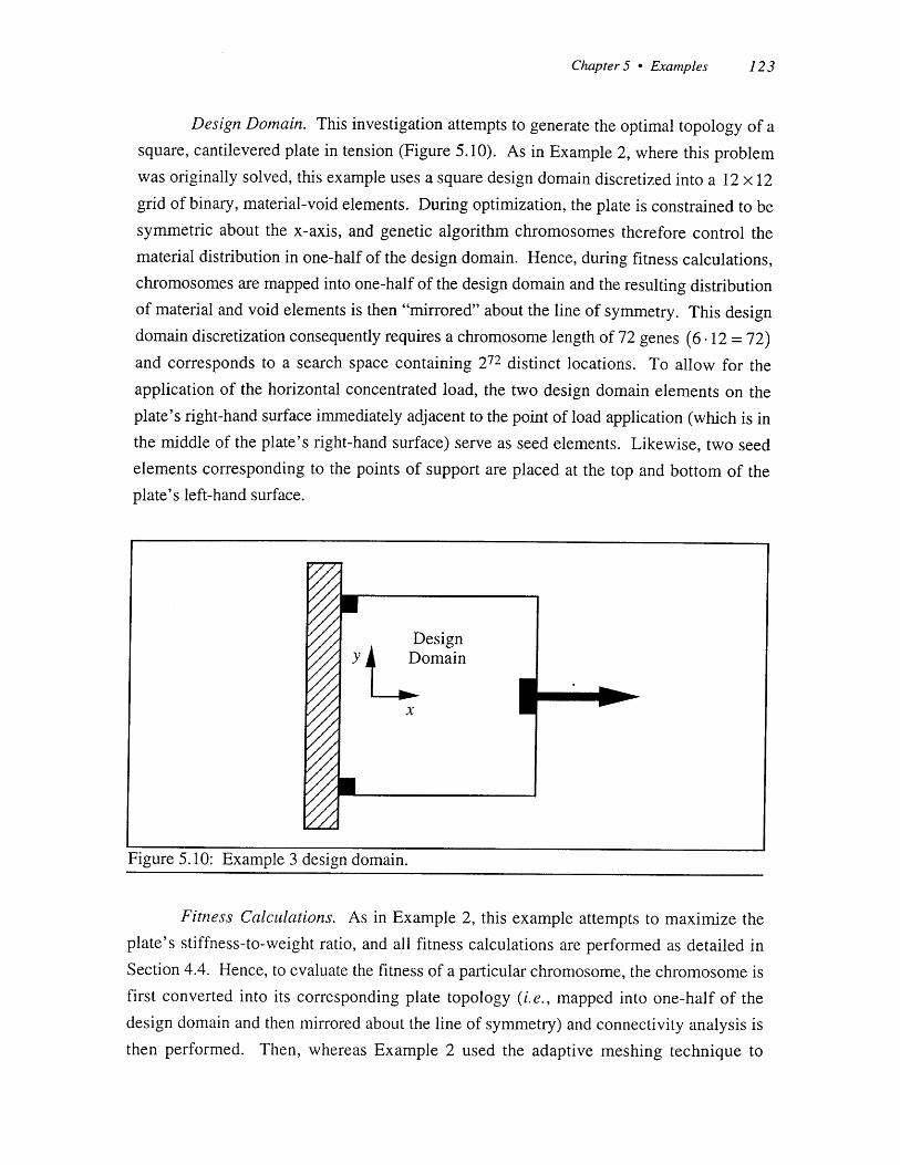
Chapter 5 - Examples 123
Design Domain. This investigation attempts to generate the optimal topology of asquare, cantilevered plate in tension (Figure 5.10). As in Example 2, where this problemwas originally solved, this example uses a square design domain discretized into a 12 x 12grid of binary, material-void elements. During optimization, the plate is constrained to besymmetric about the x-axis, and genetic algorithm chromosomes therefore control thematerial distribution in one-half of the design domain. Hence, during fitness calculations,chromosomes are mapped into one-half of the design domain and the resulting distributionof material and void elements is then "mirrored" about the line of symmetry. This designdomain discretization consequently requires a chromosome length of 72 genes (6.12 = 72)and corresponds to a search space containing 272 distinct locations. To allow for theapplication of the horizontal concentrated load, the two design domain elements on theplate's right-hand surface immediately adjacent to the point of load application (which is inthe middle of the plate's right-hand surface) serve as seed elements. Likewise, two seedelements corresponding to the points of support are placed at the top and bottom of theplate's left-hand surface.
DesignY Domain
x
Figure 5.10: Example 3 design domain.
Fitness Calculations. As in Example 2, this example attempts to maximize theplate's stiffness-to-weight ratio, and all fitness calculations are performed as detailed inSection 4.4. Hence, to evaluate the fitness of a particular chromosome, the chromosome isfirst converted into its corresponding plate topology (i.e., mapped into one-half of thedesign domain and then mirrored about the line of symmetry) and connectivity analysis isthen performed. Then, whereas Example 2 used the adaptive meshing technique to

124 Chapter 5 - Examples
generate a finite element mesh representing the plate topology, this example uses the
constant meshing technique to create a mesh containing two triangular finite elements for
every design domain element. After a finite element mesh has been created, structural
analysis is performed using the finite element method. Note that during finite element
analysis, the four nodes along the finite element mesh's left-hand surface which correspond
to the two seed elements are constrained to have zero displacement, while the concentrated
load is applied to the middle node along the finite element mesh's right-hand surface.
Finally, the plate topology's stiffness-to-weight ratio, and therefore the fitness (to be
maximized) of the chromosome corresponding to the plate topology, is given by:
Stiffness 1Fitness =- - (5.7)
Weight Area -(uy
+5(u
where Area is equal to the area of connected material elements in the plate topology and u,and u, represent the displacement, in the x- and y- directions, of the finite element node
where the concentrated load is applied.
Unlike Example 2, where disconnected plate topologies are given small, non-zero
fitness values, this example's use of the constant meshing technique enables all plate
topologies, regardless of whether or not they connect the point of load application to the
points of support with material elements, to be subjected to finite element analysis to
determine u, and u,.
Experiment Design. In an effort to establish the viability of the constant meshing
technique, as well as determine the proper Young's Modulus Ratio and evaluate the
effectiveness of connectivity analysis, optimization is performed using four different values
of Young's Modulus Ratio and with Connectivity Analysis activated and deactivated.
Specifically, topological optimizations are run using the following parameter settings:
- Young's Modulus Ratio10-2, 10-3, 10-4, and 10-5
- Connectivity AnalysisActivated and Deactivated
Eight unique combinations of Young's Modulus Ratio and Connectivity Analysis
activation are represented in the above list of parameter settings. In the experiment,

Chapter 5 * Examples 125
optimization is performed twice using each of the eight combinations (for a total of 16optimization runs). At the conclusion of each optimization, the optimum plate topology isrecorded, as is the plate's stiffness-to-weight ratio. Note that each genetic algorithm-basedoptimization is evolved for 200 generations, and that random initial seeds (i.e., different,randomly-generated initial populations) are used in each optimization. Hence, eachoptimization performs 6,000 structural analyses:
Chromosomes(200 Generations) = 6,000 Chromosomes. (5.9)
Generation
Results. Table 5.1 details the results of the experiment. Note that each of the eight
fitness values listed in the table represents the average of the two optimal stiffness-to-
weight ratios obtained for a particular combination of Young's Modulus Ratio and
Connectivity Analysis activation. Also, of the 8 genetic algorithm optimizations conducted
using connectivity analysis, Figure 5.11 depicts the plate topologies with highest stiffness-
to-weight ratio for each of the four different Young's Modulus Ratio values.
Young's Modulus RatioMaximum Maximum
EvO Stiffness-to-Weight Ratio Stiffness-to-Weight Ratio
E with Connectivity Analysis without Connectivity Analysis
10-2 20.46 19.2610-3 20.44 18.0710-4 20.12 17.7710-5 20.47 18.24
Table 5.1: Optimization performance.
From these results, it is evident that the constant finite element meshing technique,when used with connectivity analysis, generates plate topologies and plate topology
stiffness-to-weight ratios comparable to those found using the adaptive meshing technique.
In fact, the constant meshing technique, when used with connectivity analysis and a
Young's Modulus Ratio of 10-5, obtains the exact plate topology found using adaptive
meshing. Furthermore, when using connectivity analysis and a Young's Modulus Ratio of10-2, the constant meshing technique is able to generate a slightly better plate topology than
that obtained using adaptive meshing. Note that while the topologies resulting from the
two meshing techniques are similar, the computational expense of the constant meshing
technique is much less than that of the adaptive meshing technique. Consequently, using

126 Chapter 5 - Examples
the constant meshing technique with connectivity analysis provides, at considerably less
computational expense, optimization performance equal to that of the adaptive meshing
technique. Hence, the constant meshing technique (with a Young's Modulus ratio of 10-5)
and connectivity analysis are used in all subsequent examples in this investigation.
Young's Modulus Ratio = 10-2Stiffness-to-Weight Ratio = 20.70
Young's Modulus Ratio = 10-4
Stiffness-to-Weight Ratio = 20.23
Young's Modulus Ratio = 10-3Stiffness-to-Weight Ratio = 20.52
Young's Modulus Ratio = 10-5Stiffness-to-Weight Ratio = 20.47
Figure 5.11: Optimal plate topologies obtained using the constant meshing technique.
As depicted in Table 5.1, the optimal plate topologies generated with connectivity
analysis deactivated have considerably lower stiffness-to-weight ratios than topologies
generated with connectivity analysis activated. This decrease in performance is most likely
caused by the fact that when connectivity analysis is deactivated, disconnected material
elements are included in weight calculations but cannot significantly assist in supporting the
applied load. Hence, these disconnected material elements increase the plate's weight but

Chapter 5 - Examples 127
do little to increase the plate's stiffness. However, it is possible that disconnected materialelements could arrange themselves in a "chain-link" (i.e., a group of material elementsconnected corner-to-corner, creating a chain-like structure), which, if situated in a suitablelocation within the structure, could assist in withstanding a tensile load. In that situation, ifconnectivity analysis is deactivated, the disconnected material elements might increase thetopology's structural performance. This, however, was rarely found to occur.
5.5 Example 4: Large Cantilevered Plate.
5.5.1 Introduction. This example details the topological optimization of a largecantilevered plate. While similar to the topological optimizations detailed in Examples 2and 3, in that it uses the genetic algorithm in conjunction with finite element analysis tooptimize the topology of a cantilevered plate, this example extends the work of Examples 2and 3 by using a much finer design domain discretization, unsymmetric loading, nosymmetry constraints, and the constant meshing technique. Specifically, this exampleattempts to generate the topology of a rectangular cantilevered plate subject to a downwardvertical load which provides maximum stiffness-to-weight ratio. This example is a firstattempt to determine if this investigation's genetic algorithm-based topology optimizationapproach can perform optimization using design domain discretizations approaching thoseused by homogenization-based methods.
DesignDomain 10
16
Figure 5.12: Example 4 design domain.
5.5.2 Design Domain. The cantilevered plate is modeled using a rectangular
design domain discretized into 10 x 16 (i.e., 10 elements tall by 16 elements wide),

128 Chapter 5 - Examples
15 x 24, or 20 x 32 grids of binary, material-void elements (Figure 5.12). During
optimization, no symmetry constraints are imposed on the plate topology, and the genetic
algorithm chromosomes control the distribution of material and void throughout the entire
design domain. As each genetic algorithm chromosome must therefore contain one gene
for every design domain element, these design domain discretizations result in chromosome
lengths of 160, 360, and 640 genes. Hence, the search space contains either 2160, 2360, or
2640 distinct locations. To allow for the application of the vertical concentrated load, the
design domain element on the plate's right-hand surface immediately below the point of
load application (which is 2 of the distance from the bottom) serves as a seed element.
Likewise, two seed elements corresponding to the points of support are placed at the top
and bottom of the plate's left-hand surface.
5.5.3 Fitness Calculations. As this example attempts to maximize the plate's
stiffness-to-weight ratio, all fitness calculations are performed as detailed in Section 4.4.
Hence, to evaluate the fitness of a particular chromosome, the chromosome is first
converted into its corresponding plate topology (because no symmetry constraints are
imposed, the chromosome is mapped into the entire discretized design domain to create a
plate topology) and connectivity analysis is then performed. A finite element mesh
containing four triangular finite elements for every design domain element is then generated
using the constant meshing technique (Section 4.4.5), and structural analysis is performed
using the finite element method. Note that during finite element analysis, the four nodes
along the finite element mesh's left-hand surface which correspond to the two seed
elements are constrained to have zero displacement, while the concentrated load is applied
to the node on the finite element mesh's right-hand surface which is -1 of the distance from
the bottom. Finally, the plate topology's stiffness-to-weight ratio, and therefore the fitness
(to be maximized) of the chromosome corresponding to the plate topology, is given by:
Stiffness 1Fitness = (5.7)
Weight Area - (u) 2 +(u.) 2
where Area is equal to the area of connected material elements in the plate topology and u,and u, represent the displacement, in the x- and y- directions, of the finite element node
where the concentrated load is applied.

Chapter 5 - Examples 129
5.5.4 Results. Results of the optimization are shown in Figure 5.13, which
displays the plates generated at the three different discretizations with maximum stiffness-to-weight ratio. Figure 5.13a depicts the optimal topology generated using the 10 x 16design domain discretization, obtained after 225 generations of genetic algorithm search.Hence, 6,750 fitness evaluations were performed during the generation of the 10 x 16 platetopology:
Chromosomes(225 Generations) 30 = 6,750 Chromosomes. (5.10)
Generation
Note that because the constant finite element meshing technique was used,structural analysis was performed in all of the above 6,750 fitness evaluations.
Figures 5.13b and 5.13c display the optimal topologies generated using the 15 x 24and 20 x 32 design domain discretizations. As these two finely-discretized design domainscorrespond to exceptionally long chromosome lengths and therefore create optimizationproblems of considerable difficulty, 600 generations of search were required to generate theplate topologies. Hence, 18,000 fitness evaluations (and therefore 18,000 structural
analyses) were performed during each of the two optimizations:
(60 Geertios).30Chromosomes(600 Generations) 30 r= 18,000 Chromosomes. (5.11)Generation
Note that whereas improvements in the plate topology's fitness became small and
infrequent by generation 225 when using the 10 x 16 design domain discretization, 600generations of search were performed using the 15 x 24 and 20 x 32 design domain
discretizations before improvements in the structure's fitness became small and infrequent.
Examining the results in Figure 5.13, it is interesting to note that the topologies
have well-defined solid-material outer boundaries, while the interior regions generally have
a composite-like internal structure comprised of equally-distributed material and void. The
20 x 32 topological optimization was able to "hollow out" several large holes in the interior
region, producing truss-like members. While homogenization-based methods minimize
mean compliance subject to a maximum volume constraint, and this genetic algorithm-

130 Chapter 5 * Examples
(a)
(b)
(c)
Figure 5.13: Optimal plate topologies using (a) 10 x 16, (b) 15 x 24, and (c) 20 x 32design domain discretizations.

Chapter 5 Examples 131
based method maximizes stiffness-to-weight ratio, results of the two methods share some
general similarities. As in this example's 20 x 32 optimization, homogenization-based
methods result in a topology with a well-defined, solid-material outer boundary and a large
internal section of voids traversed by small truss members (see Papalambros and
Chirehdast (1990) for the homogenization-based solution to a problem using boundary
conditions, loading conditions, and a design domain geometry similar to those used in this
example). Also, the outer boundaries of the structures found using the two methods are
somewhat similar in shape.
Jensen (1992) also investigates the topological optimization of a finely-discretized
cantilevered plate subject to a downward concentrated load. The example attempts to
generate the plate topology which provides minimum weight subject to a maximum
displacement constraint. Similar to the examples provided in this investigation, Jensen's
example uses a binary, material-void design domain discretization and a constant finite
element meshing technique. However, as opposed to the design domains used in this
investigation, the design domain examined by Jensen is more than twice as tall as it is wide
(Figure 3.16), and is discretized into a 19 x 9 grid. Hence, Jensen uses 171-gene
chromosomes in his example. Note that the constant meshing technique used by Jensen
varies the thickness of finite elements by a factor of 100 to represent material and void
design domain elements, which is exactly equivalent to using a 10-2 Young's Modulus
Ratio with this investigation's constant meshing technique.
Using a population size of 140 chromosomes, Jensen's example generates an
optimal plate topology after 150 generations of search. However, the optimal plate
topology is a very thin, "chain-link" topology almost entirely comprised of material
elements connected at corners. As detailed in Section 4.4.4, groups of material elements
connected only at corners (i.e., elements which do not share edges) cannot support torques
or compressive loads. Hence, the plate topology generated by Jensen should collapse
when subjected to the given loading condition. Jensen's plate topology most likely does
not collapse because it is "supported" by the void finite elements surrounding it, which
have a thickness 0.01 times that of the material finite elements comprising the topology.
Consequently, the plate topology generated in Jensen's example must be thought of as a
"topology schematic" which the designer may use, along with his or her knowledge of the
application domain, to create a physically-realizable topology.

132 Chapter 5 - Examples
This investigation's use of connectivity analysis guarantees that an unstable plate
topology such as that obtained by Jensen cannot be generated-referring to the plate
topologies depicted in Figure 5.13, please note that every material element in the design
domain shares an edge with at least one other material element.
5.6 Example 5: Hierarchical Design Domain Subdivision.
5.6.1 Introduction. While the resolutions of the plate topologies generated in
Example 4 are satisfactory for determining the general shape of the load-bearing structure,
they are much coarser than the finely-discretized domains used in homogenization-based
methods. Unfortunately, attempts to increase the design domain discretization beyond the
maximum 20 x 32 resolution in Example 4 were unsuccessful, as the system was unable to
create plate topologies where the point of load application was connected to the points of
support with high-Young's-Modulus material. Specifically, whereas the genetic algorithm
was able to locate connected plate topologies within the first few generations of search
when using the 10 x 16, 15 x 24, and 20 x 32 design domain discretizations, the genetic
algorithm was unable to find connected topologies for finer discretizations, even after
hundreds of generations. This poor performance with fine design domain discretizations is
most likely caused by the exceptionally large search spaces resulting from the long
chromosome lengths required for the fine discretization. When searching in these large
search spaces, the genetic algorithm is simply unable to locate, with its population of 30
chromosomes, regions of the search space which correspond to connected plate topologies.
5.6.2 Overview of the Technique. In an attempt to obtain finely-discretized
plate topologies, this example introduces a hierarchical design domain subdivision
technique. The technique, which enables the genetic algorithm to determine the general
shape of the optimal plate topology in early generations and then "fine-tune" the high-
quality topology in final generations, periodically increases both the resolution of a design
domain's discretization and the number of genetic algorithm populations controlling the
distribution of material and void throughout the domain.
5.6.3 Details of the Technique. The hierarchical subdivision technique
begins genetic algorithm-based structural topology optimization with a coarse design
domain discretization, resulting in short chromosomes and a correspondingly small search
space. (Figure 5.14 depicts, for an example optimization problem, an example coarse
design domain discretization.) As demonstrated in Examples 2 and 3, short chromosomes
and small search spaces enable the genetic algorithm to easily generate connected plate
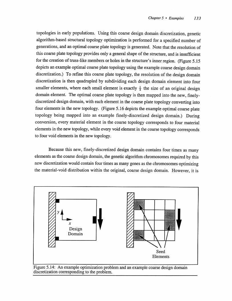
Chapter 5 - Examples 133
topologies in early populations. Using this coarse design domain discretization, geneticalgorithm-based structural topology optimization is performed for a specified number ofgenerations, and an optimal coarse plate topology is generated. Note that the resolution ofthis coarse plate topology provides only a general shape of the structure, and is insufficientfor the creation of truss-like members or holes in the structure's inner region. (Figure 5.15depicts an example optimal coarse plate topology using the example coarse design domaindiscretization.) To refine this coarse plate topology, the resolution of the design domaindiscretization is then quadrupled by subdividing each design domain element into foursmaller elements, where each small element is exactly I the size of an original designdomain element. The optimal coarse plate topology is then mapped into the new, finely-discretized design domain, with each element in the coarse plate topology converting intofour elements in the new topology. (Figure 5.16 depicts the example optimal coarse platetopology being mapped into an example finely-discretized design domain.) Duringconversion, every material element in the coarse topology corresponds to four materialelements in the new topology, while every void element in the coarse topology correspondsto four void elements in the new topology.
Because this new, finely-discretized design domain contains four times as manyelements as the coarse design domain, the genetic algorithm chromosomes required by thisnew discretization would contain four times as many genes as the chromosomes optimizingthe material-void distribution within the original, coarse design domain. However, it is
Figure 5.14: An example optimization problem and an example coarse design domaindiscretization corresponding to the problem.

134 Chapter 5 - Examples
Figure 5.15: The genetic algorithm creating an example optimal coarse plate topology inthe example coarse design domain.
Mapping IFigure 5.16: Mapping the optimal coarse plate topology into an example finely-discretizeddesign domain.
beneficial to keep chromosome length constant, for genetic algorithm performance typically
diminishes as chromosome length (and therefore search space size) increases. Hence,
instead of increasing the lengths of the chromosomes in the genetic algorithm population
and then using the population to optimize the material-void distribution within the finely-
discretized design domain, hierarchical subdivision divides the new, finely-discretized
design domain into four "quadrants" and uses four genetic algorithm populations to
optimize the distribution of material and void within the quadrants (Figure 5.17). So,
whereas a single genetic algorithm population was used to optimize the distribution of
material and void within the original coarse design domain, four genetic algorithm
populations are used to optimize the distribution of material and void within the new,
finely-discretized design domain. Specifically, each of the four populations optimizes the
I
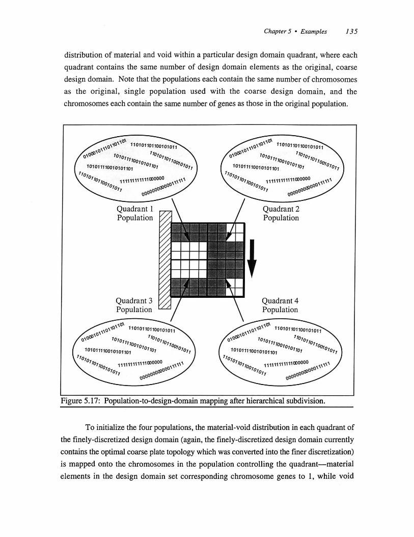
Chapter 5 Examples 135
distribution of material and void within a particular design domain quadrant, where each
quadrant contains the same number of design domain elements as the original, coarse
design domain. Note that the populations each contain the same number of chromosomes
as the original, single population used with the coarse design domain, and the
chromosomes each contain the same number of genes as those in the original population.
Figure 5.17: Population-to-design-domain mapping after hierarchical subdivision.
To initialize the four populations, the material-void distribution in each quadrant of
the finely-discretized design domain (again, the finely-discretized design domain currently
contains the optimal coarse plate topology which was converted into the finer discretization)
is mapped onto the chromosomes in the population controlling the quadrant-material
elements in the design domain set corresponding chromosome genes to 1, while void
I

136 Chapter 5 - Examples
elements in the design domain set corresponding chromosome genes to 0. Hence, after
initialization, all chromosomes in each population correspond to the distribution of material
and void within the design domain quadrant controlled by the population. To create
diversity in each population, the chromosomes are then subjected to high-probability
mutation (performed on every gene of every chromosome with a 0.15 probability) similar
to a "nuking" procedure used by Jensen (1992).
Before any optimization is performed in the four populations, the fitness of each
recently-nuked chromosome must be evaluated. Again, the distribution of material and
void in the finely-discretized design domain currently corresponds to the optimal coarse
plate topology which was previously mapped into the domain. So, beginning with the
population controlling Quadrant 1 of the finely-discretized design domain, a chromosome
in the population is mapped into the quadrant to create a distribution of material and void
within the quadrant. This distribution of material and void, when used with the
distributions of material and void within the three other quadrants, creates a material
distribution throughout the entire design domain and consequently generates a finely-
discretized plate topology. This finely-discretized plate topology is then subjected to
connectivity analysis, and the constant meshing technique is used to generate a finite
element mesh corresponding to the plate topology. Finite element analysis is then
performed on the plate topology, and fitness calculations are conducted as in previous
examples. The resulting fitness value is then assigned to the chromosome which created
the current material-void distribution in Quadrant 1. This process (i.e., mapping a
chromosome into the quadrant, generating a plate topology from the material-void
distribution throughout the entire domain, performing connectivity analysis on the plate
topology, creating a finite element mesh corresponding to the plate topology, performing
finite element analysis on the plate topology, and then assigning a fitness value to the
chromosome) is then repeated for each chromosome in the population controlling Quadrant
1. After all of the chromosomes in the population have been evaluated, the most-highly-fit
chromosome in the population is mapped back into Quadrant 1 so that it may be used in the
fitness calculations of the other quadrants. The populations controlling Quadrants 2, 3, and
4 are then evaluated (in that order) using the same technique.
Optimization proceeds by performing standard genetic algorithm optimizations in
each of the four quadrants. First, the population controlling Quadrant 1 is evolved a single
generation: parents are selected and mated to create a generation of child topologies, each
of which is subjected to mutation and then evaluated for fitness (fitness evaluations are

Chapter 5 - Examples 137
performed as detailed in the previous paragraph). The child population then replaces the
parent population, and the most-highly-fit child chromosome is mapped into Quadrant 1.
The populations controlling Quadrants 2, 3, and 4 (in that order) are then evolved a single
generation. After each quadrant has evolved one generation (with the resulting optimal
chromosome from each population being mapped into its corresponding design domain
quadrant), the "cycle" is repeated. Figure 5.18 depicts an example finely-discretized plate
topology after several cycles of optimization.
Figure 5.18: Example optimization of the finely-discretized plate topology.
After a pre-determined number of cycles, the entire subdivision process is repeated.
Each quadrant of the design domain is divided into four sub-quadrants, where each sub-
quadrant has the same resolution as the original quadrant. The resulting design domain has

138 Chapter 5 - Examples
16 times the resolution of the original, coarse design domain discretization and is controlled
by 16 genetic algorithm populations, where each population's chromosomes are equal in
length to the original chromosomes which controlled the coarse design domain. The
optimization then proceeds by cycling through the 16 sub-quadrants (from left to right, top
to bottom), allowing each population to evolve one generation during each cycle. This
process could be repeated indefinitely.
5.6.4 Example. In an attempt to establish the viability of the hierarchical
subdivision technique, the topological optimization of a cantilevered plate detailed in
Example 4 is now re-examined using the hierarchical subdivision technique. Specifically,this example uses hierarchical subdivision to generate the finely-discretized topology of a
rectangular cantilevered plate subject to a downward vertical load which provides maximum
stiffness-to-weight ratio. This example is a first attempt to determine if the hierarchical
subdivision technique enables the genetic algorithm to perform optimization using design
domain discretizations higher than those investigated in previous examples.
DesignDomain 10
x
16
Figure 5.19: Example 5 design domain.
Design Domain. As in Example 4, the cantilevered plate is modeled using a
rectangular design domain 10 units tall by 16 units wide (Figure 5.19), and no symmetry
constraints are imposed on the plate topology. The design domain is initially discretized
into a 10 x 16 grid of binary, material-void elements, and subsequent hierarchical
subdivision-based resolution increases result in design domain discretizations of 20 x 32
and finally 40 x 64. Hence, as the initial design domain discretization (10 x 16) establishes

Chapter 5 * Examples 139
the genetic algorithm chromosome length, all chromosomes used in the optimization
(regardless of the design domain discretization or number of genetic algorithm populations
controlling the plate's topology) contain 160 genes. To allow for the application of the
vertical concentrated load, the design domain element on the plate's right-hand surface
immediately below the point of load application (which is - of the distance from the
bottom) serves as a seed element. Likewise, two seed elements corresponding to the points
of support are placed at the top and bottom of the plate's left-hand surface.
Fitness Calculations. As this example uses hierarchical subdivision to maximize the
plate's stiffness-to-weight ratio, fitness calculations begin when a chromosome is
converted into its corresponding plate topology as detailed in Section 5.6.3. Then, once
the plate topology has been generated, connectivity analysis, constant finite element
meshing (using four triangular finite elements for every design domain element), and finite
element analysis are performed. Note that during finite element analysis, the four nodes
along the finite element mesh's left-hand surface which correspond to the two seed
elements are constrained to have zero displacement, while the concentrated load is applied
to the node on the finite element mesh's right-hand surface which is -1 of the distance from
the bottom. Finally, the plate topology's stiffness-to-weight ratio, and therefore the fitness
(to be maximized) of the chromosome corresponding to the plate topology, is given by:
Fitness Stiess (5.7)Weight Area- (uX)+(u)(
where Area is equal to the area of connected material elements in the plate topology and u,and u, represent the displacement, in the x- and y- directions, of the finite element node
where the concentrated load is applied.
Hierarchical Subdivision Parameters. Optimization begins with a single genetic
algorithm population optimizing the plate topology with a coarse, 10 x 16 design domain
discretization. Note that this population contains 30 160-gene chromosomes. After
performing 250 generations of evolution at this initial discretization, hierarchical
subdivision is performed to quadruple the resolution of the design domain. Hence,
following hierarchical subdivision, four genetic algorithm populations optimize the plate's
topology using a 20 x 32 design domain discretization. At this discretization, each design
domain element is I the size of the original, coarse design domain elements, and each of

140 Chapter 5 - Examples
the four populations contains 30 160-gene chromosomes. Then, after performing
optimization for 50 cycles (i.e., 50 generations of evolution in each design domainquadrant) at the 20 x 32 discretization, the resolution of the design domain is againquadrupled. After this second hierarchical subdivision, sixteen genetic algorithmpopulations optimize the plate's topology using a 40 x 64 design domain discretization. Atthis discretization, each design domain element is ' the size of the original, coarse designdomain elements, and each of the sixteen populations contains 30 160-gene chromosomes.
Optimization concludes after 10 cycles at this discretization.
Results. Results of the optimization are shown in Figure 5.20, which displays theoptimal plate topologies generated at the three different discretizations. 7,500 structuralanalyses were performed during the generation of the coarse, 10 x 16 plate topology:
250 Generations -30 Chromosomes = 7,500 Chromosomes, (5.12)Generation
while an additional 6,000 structural analyses were performed to obtain the 20 x 32 plate
topology:
Generations Chromosomes50 Cycles -4 -30 = 6,000 Chromosomes (5.13)
Cycle Generation
and an additional 4,800 analyses were performed to obtain the 40 x 64 plate topology:
Generations Chromosomes10 Cycles -16 -30 = 4,800 Chromosomes. (5.14)
Cycle Generation
Hence, a total of 18,300 finite element analyses were required to obtain the 40 x 64
plate topology.
As shown in Figure 5.20, this investigation's hierarchical subdivision technique
provides reasonable results. While the 40 x 64 plate's outer boundaries are somewhat
jagged, the inner region does contain several well-defined, truss-like members and several
large areas of void. Comparing the plate topologies generated in this example to those
detailed in Example 4 (Figure 5.13), which are generated using a constant design domain
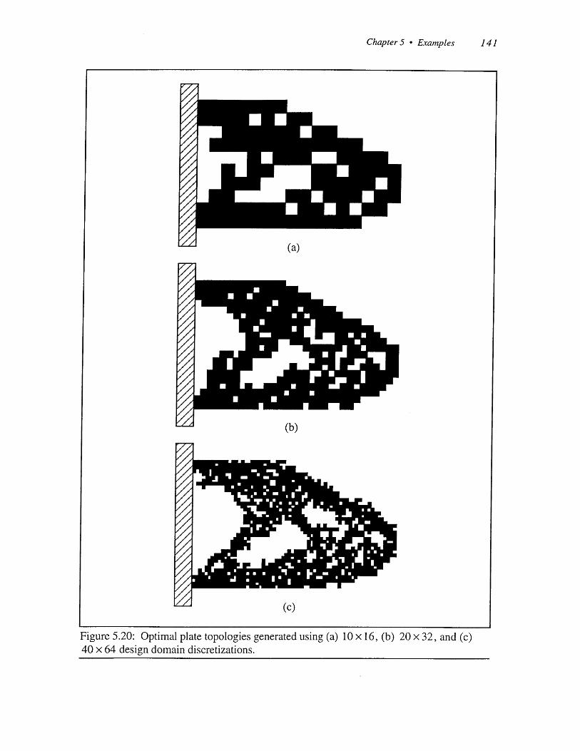
Chapter 5 - Examples 141
Figure 5.20: Optimal plate topologies generated using (a) 10 x 16, (b) 20 x 32, and (c)40 x 64 design domain discretizations.
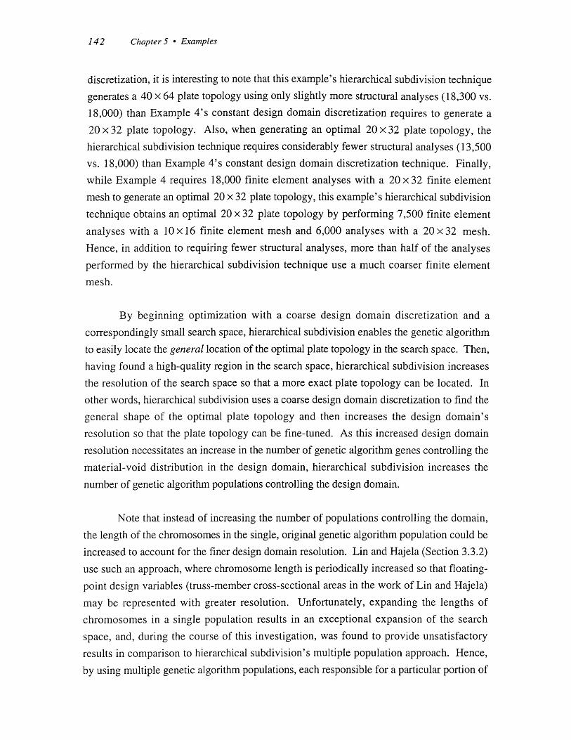
142 Chapter 5 - Examples
discretization, it is interesting to note that this example's hierarchical subdivision technique
generates a 40 x 64 plate topology using only slightly more structural analyses (18,300 vs.
18,000) than Example 4's constant design domain discretization requires to generate a
20 x 32 plate topology. Also, when generating an optimal 20 X 32 plate topology, the
hierarchical subdivision technique requires considerably fewer structural analyses (13,500
vs. 18,000) than Example 4's constant design domain discretization technique. Finally,while Example 4 requires 18,000 finite element analyses with a 20 x 32 finite element
mesh to generate an optimal 20 x 32 plate topology, this example's hierarchical subdivision
technique obtains an optimal 20 x 32 plate topology by performing 7,500 finite element
analyses with a 10 x 16 finite element mesh and 6,000 analyses with a 20 x 32 mesh.
Hence, in addition to requiring fewer structural analyses, more than half of the analyses
performed by the hierarchical subdivision technique use a much coarser finite element
mesh.
By beginning optimization with a coarse design domain discretization and a
correspondingly small search space, hierarchical subdivision enables the genetic algorithm
to easily locate the general location of the optimal plate topology in the search space. Then,
having found a high-quality region in the search space, hierarchical subdivision increases
the resolution of the search space so that a more exact plate topology can be located. In
other words, hierarchical subdivision uses a coarse design domain discretization to find the
general shape of the optimal plate topology and then increases the design domain's
resolution so that the plate topology can be fine-tuned. As this increased design domain
resolution necessitates an increase in the number of genetic algorithm genes controlling the
material-void distribution in the design domain, hierarchical subdivision increases the
number of genetic algorithm populations controlling the design domain.
Note that instead of increasing the number of populations controlling the domain,
the length of the chromosomes in the single, original genetic algorithm population could be
increased to account for the finer design domain resolution. Lin and Hajela (Section 3.3.2)
use such an approach, where chromosome length is periodically increased so that floating-
point design variables (truss-member cross-sectional areas in the work of Lin and Hajela)
may be represented with greater resolution. Unfortunately, expanding the lengths of
chromosomes in a single population results in an exceptional expansion of the search
space, and, during the course of this investigation, was found to provide unsatisfactory
results in comparison to hierarchical subdivision's multiple population approach. Hence,
by using multiple genetic algorithm populations, each responsible for a particular portion of

Chapter 5 - Examples 143
the design domain, hierarchical subdivision increases the resolution of the overall search
space while keeping the size of each individual population's search space constant.
Because the constant design domain discretization used in previous examples forces
the genetic algorithm to generate both the general plate topology and the finely-tuned,optimal plate topology using a highly-discretized design domain, the genetic algorithm
experiences great difficulty in finding either. On the other hand, hierarchical subdivision's
use of a variable-resolution design domain enables the genetic algorithm to find the general
shape of the optimal plate topology using a coarse design domain discretization and then
fine-tune the optimal plate topology using a highly-discretized design domain.
Consequently, when generating finely-discretized plate topologies, the hierarchical
subdivision technique outperforms the constant design domain discretization used in
previous examples.
5.7 Example 6: Design Families.
5.7.1 Introduction. Throughout this investigation, the genetic algorithm has
been used to evolve a population of plate topologies in an attempt to generate an optimal
plate topology. Hence, at the conclusion of any given optimization, a population of highly-
fit plate topologies has been created. However, while nearly all of the plate topologies in a
final population are highly-fit, previous examples have considered only the most-highly-fit
plate topology in a final population. Unfortunately, by examining only the plate topology
which maximizes the optimization problem's fitness function (which certainly does not
consider all possible design criteria), previous examples have ignored other highly-fit plate
topologies in the final population which, when evaluated using alternate design criteria,may outperform the most-highly-fit plate topology.
This example attempts to demonstrate the genetic algorithm's ability to obtain,during a single optimization, a family of plate topologies which a designer can evaluate
using alternate, secondary criteria not addressed in the fitness function which generated the
designs. Specifically, this example uses the genetic algorithm to obtain a family of plate
topologies with maximum stiffness-to-weight-to-perimeter ratio, which the designer can
then select from using manufacturing, weight, and/or displacement criteria. Note that this
new stiffness-to-weight-to-perimeter ratio fitness function, which will be detailed in
Section 5.7.3, is used in an attempt to drive the genetic algorithm search towards plate
topologies which combine high stiffness-to-weight ratio with high manufacturability. As in
Examples 4 and 5, this example optimizes the topology of a rectangular, cantilevered plate

144 Chapter 5 - Examples
subject to a downward vertical load and uses unsymmetric loading, no symmetry
constraints, and the constant meshing technique. Note that this example does not use
hierarchical subdivision.
5.7.2 Design Domain. As in Examples 4 and 5, the cantilevered plate is
modeled using a rectangular design domain discretized into a 10 x 16 grid of binary,material-void elements (Figure 5.21). During optimization, no symmetry constraints are
imposed on the plate topology, and the genetic algorithm chromosomes control the
distribution of material and void throughout the entire design domain. As each genetic
algorithm chromosome must therefore contain one gene for every design domain element,this 10 x 16 design domain discretization results in a chromosome length of 160 genes and
a search space containing 2160 distinct locations. To allow for the application of the vertical
concentrated load, the design domain element on the plate's right-hand surface immediately
below the point of load application (which is - of the distance from the bottom) serves as a
seed element. Likewise, two seed elements corresponding to the points of support are
placed at the top and bottom of the plate's left-hand surface.
DesignDomain 10
16
Figure 5.21: Example 6 design domain.
5.7.3 Fitness Calculations. As this example attempts to maximize the plate's
stiffness-to-weight-to-perimeter ratio, fitness calculations are based on the stiffness-to-
weight ratio calculations detailed in Section 4.4 and used in Example 4. Specifically, to
evaluate the fitness of a particular chromosome, the chromosome is first converted into its
corresponding plate topology (because no symmetry constraints are imposed and

Chapter 5 - Examples 145
hierarchical subdivision is not used, the chromosome is mapped into the entire discretized
design domain to create a plate topology) and connectivity analysis is then performed. Afinite element mesh containing four triangular finite elements for every design domainelement is then generated using the constant meshing technique, and structural analysis isperformed using the finite element method. Note that during finite element analysis, thefour nodes along the finite element mesh's left-hand surface which correspond to the two
seed elements are constrained to have zero displacement, while the concentrated load is
applied to the node on the finite element mesh's right-hand surface which is 1 of the
distance from the bottom. As in Examples 4 and 5, the plate topology's stiffness-to-weight
ratio is then set equal to:
Stiffness 1Weight Area - u5 +
where Area is equal to the area of connected material elements in the plate topology and uxand u, represent the displacement, in the x- and y- directions, of the finite element node
where the concentrated load is applied.
Again, this example attempts to drive the genetic algorithm towards plate topologies
which combine high stiffness-to-weight ratio with high manufacturability. While
manufacturability can have various definitions and any given plate's manufacturability can
be based on a variety of different attributes, this example assumes that a plate'smanufacturability is based entirely on the plate's porosity-highly-porous plate topologiesare considered to have low manufacturability, while plate topologies with low porosity areconsidered to have high manufacturability. Note that a plate's porosity is assumed to beequal to the number of internal holes in the structure. Hence, fitness calculations areformulated so that plate topologies which combine high stiffness-to-weight ratio with a lownumber of internal holes receive high fitness, while plate topologies with low stiffness-to-
weight ratio and/or a high number of internal holes receive low fitness.
A variety of fitness formulations can be used to simultaneously maximize stiffness-
to-weight ratio and minimize internal holes. For example, an optimization could attempt to
maximize stiffness-to-weight ratio subject to a constraint on the maximum number of
internal holes in the structure; maximize stiffness-to-weight ratio subject to a constraint on
the maximum area of internal holes; or maximize the value of the stiffness-to-weight ratio

146 Chapter 5 * Examples
divided by the number of internal holes in the structure. Again, these examples represent
only a partial list of the possible fitness formulations. As in any optimization, the particular
fitness formulation chosen depends upon the available computational tools as well as the
intuition of the designer.
To simultaneously maximize stiffness-to-weight ratio and minimize internal holes,this example attempts to drive the genetic algorithm towards plate topologies with a high
stiffness-to-weight ratio and a small perimeter. Hence, this example's fitness formulation
maximizes a plate topology's stiffness-to-weight-to-perimeter ratio. Note that in this
example, a plate's perimeter is assumed to be equal to the sum of the plate's outer perimeter
and the perimeter of the plate's internal holes.
So, after calculating a plate topology's stiffness-to-weight ratio (given by Equation
5.15), the plate's perimeter is calculated. The plate topology's stiffness-to-weight-to-
perimeter ratio, and therefore the fitness (to be maximized) of the chromosome
corresponding to the plate topology, is then given by:
Stiffness
Weight) 1Fitness .eih (5.16)
Perimeter Area -Perimeter - (uc ) +(u)5
5.7.4 Results. After 225 generations of genetic algorithm-based evolution, a
population, or family, of 30 possibly-optimal plate topologies was generated. During the
search, a total of 6,750 structural analyses were performed:
225 Generations -30 Chromosomes = 6,750 Chromosomes. (5.17)Generation
Figure 5.22 depicts the plate topologies which exhibit, for the six minimum
possible levels of porosity, maximum stiffness-to-weight ratio. In other words, of the
plate topologies in the family which have either 0, 1, 2, 3, 4, or 5 internal holes, Figure
5.22 depicts the plate topologies with maximum stiffness-to-weight ratio. Also, Table 5.2
quantifies each plate topology's number of internal holes (i.e., manufacturability),
stiffness-to-weight ratio, displacement, and weight. Note that while the genetic algorithm-
based optimization only addressed the minimization of internal holes and the maximization

Chapter 5 - Examples 147
Figure 5.22: Family of plate topologies with (a) 0, (b) 1, (c) 2, (d) 3, (e) 4, and (f) 5internal holes.
Table 5.2: Plate topology performance data.
Number of s Stiffness-to-Weight Displacement WeightTopology Internal Holes Ratio I I(a) 0 1.19 0.0092 91(b) 1 1.15 0.0102 85(c) 2 1.11 0.0106 85(d) 3 1.20 0.0094 89(e) 4 1.14 0.0102 86(f) 5 1.14 0.0101 87
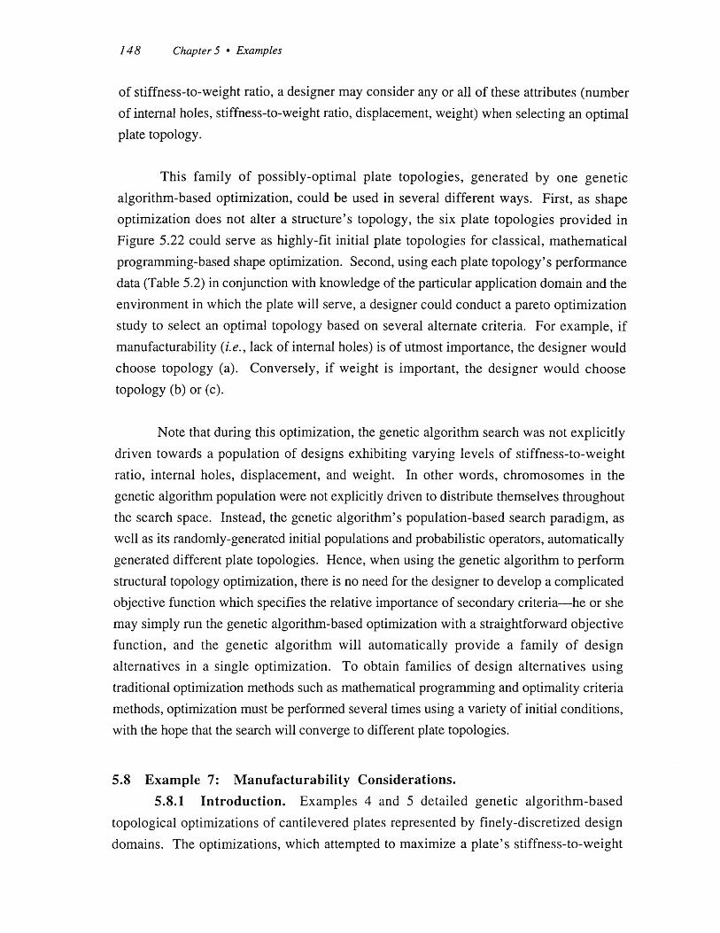
148 Chapter 5 - Examples
of stiffness-to-weight ratio, a designer may consider any or all of these attributes (number
of internal holes, stiffness-to-weight ratio, displacement, weight) when selecting an optimal
plate topology.
This family of possibly-optimal plate topologies, generated by one genetic
algorithm-based optimization, could be used in several different ways. First, as shape
optimization does not alter a structure's topology, the six plate topologies provided in
Figure 5.22 could serve as highly-fit initial plate topologies for classical, mathematical
programming-based shape optimization. Second, using each plate topology's performance
data (Table 5.2) in conjunction with knowledge of the particular application domain and the
environment in which the plate will serve, a designer could conduct a pareto optimization
study to select an optimal topology based on several alternate criteria. For example, if
manufacturability (i.e., lack of internal holes) is of utmost importance, the designer would
choose topology (a). Conversely, if weight is important, the designer would choose
topology (b) or (c).
Note that during this optimization, the genetic algorithm search was not explicitly
driven towards a population of designs exhibiting varying levels of stiffness-to-weight
ratio, internal holes, displacement, and weight. In other words, chromosomes in the
genetic algorithm population were not explicitly driven to distribute themselves throughout
the search space. Instead, the genetic algorithm's population-based search paradigm, as
well as its randomly-generated initial populations and probabilistic operators, automatically
generated different plate topologies. Hence, when using the genetic algorithm to perform
structural topology optimization, there is no need for the designer to develop a complicated
objective function which specifies the relative importance of secondary criteria-he or she
may simply run the genetic algorithm-based optimization with a straightforward objective
function, and the genetic algorithm will automatically provide a family of design
alternatives in a single optimization. To obtain families of design alternatives using
traditional optimization methods such as mathematical programming and optimality criteria
methods, optimization must be performed several times using a variety of initial conditions,with the hope that the search will converge to different plate topologies.
5.8 Example 7: Manufacturability Considerations.
5.8.1 Introduction. Examples 4 and 5 detailed genetic algorithm-based
topological optimizations of cantilevered plates represented by finely-discretized design
domains. The optimizations, which attempted to maximize a plate's stiffness-to-weight
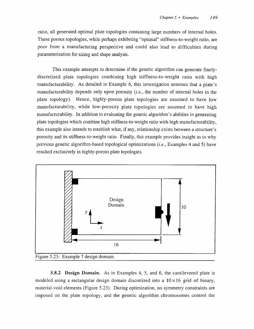
Chapter 5 Examples 149
ratio, all generated optimal plate topologies containing large numbers of internal holes.
These porous topologies, while perhaps exhibiting "optimal" stiffness-to-weight ratio, are
poor from a manufacturing perspective and could also lead to difficulties during
parameterization for sizing and shape analysis.
This example attempts to determine if the genetic algorithm can generate finely-
discretized plate topologies combining high stiffness-to-weight ratio with high
manufacturability. As detailed in Example 6, this investigation assumes that a plate's
manufacturability depends only upon porosity (i.e., the number of internal holes in the
plate topology). Hence, highly-porous plate topologies are assumed to have low
manufacturability, while low-porosity plate topologies are assumed to have high
manufacturability. In addition to evaluating the genetic algorithm's abilities in generating
plate topologies which combine high stiffness-to-weight ratio with high manufacturability,this example also intends to establish what, if any, relationship exists between a structure's
porosity and its stiffness-to-weight ratio. Finally, this example provides insight as to why
previous genetic algorithm-based topological optimizations (i.e., Examples 4 and 5) have
resulted exclusively in highly-porous plate topologies.
DesignDomain 10
16
Figure 5.23: Example 7 design domain.
5.8.2 Design Domain. As in Examples 4, 5, and 6, the cantilevered plate is
modeled using a rectangular design domain discretized into a 10 x 16 grid of binary,material-void elements (Figure 5.23). During optimization, no symmetry constraints are
imposed on the plate topology, and the genetic algorithm chromosomes control the

150 Chapter 5 - Examples
distribution of material and void throughout the entire design domain. As each genetic
algorithm chromosome must therefore contain one gene for every design domain element,
this 10 x 16 design domain discretization results in a chromosome length of 160 genes and
a search space containing 2160 distinct locations. To allow for the application of the vertical
concentrated load, the two design domain elements on the plate's right-hand surface
immediately adjacent to the point of load application (which is - of the distance from the
bottom) serve as seed elements. Likewise, two seed elements corresponding to the points
of support are placed at the top and bottom of the plate's left-hand surface. Note that this
example does not use hierarchical subdivision.
5.8.3 Fitness Calculations. As this example attempts to simultaneously
maximize stiffness-to-weight ratio and minimize porosity, fitness calculations are based on
the stiffness-to-weight ratio calculations detailed in Section 4.4 and used in Examples 4, 5,
and 6. Specifically, to evaluate the fitness of a particular chromosome, the chromosome is
first converted into its corresponding plate topology (because no symmetry constraints are
imposed and hierarchical subdivision is not used, the chromosome is mapped into the entire
discretized design domain to create a plate topology) and connectivity analysis is then
performed. A finite element mesh containing four triangular finite elements for every
design domain element is then generated using the constant meshing technique, and
structural analysis is performed using the finite element method. Note that during finite
element analysis, the four nodes along the finite element mesh's left-hand surface which
correspond to the two seed elements are constrained to have zero displacement, while the
concentrated load is applied to the node on the finite element mesh's right-hand surface
which is ' of the distance from the bottom. As in previous examples, the plate topology's
stiffness-to-weight ratio is then set equal to:
Stiffness 1 (5.15)Weight Area. u +(u
where Area is equal to the area of connected material elements in the plate topology and u,
and u, represent the displacement, in the x- and y- directions, of the finite element node
where the concentrated load is applied.
Once the plate's stiffness-to-weight ratio has been calculated, additional calculations
must be performed in order to drive the genetic algorithm towards plate topologies

Chapter 5 Examples 151
combining high stiffness-to-weight ratio and low porosity. As detailed in Example 6, a
variety of different fitness functions can be used to obtain such plate topologies. Hence,because of the availability of fitness functions which would likely provide adequate
optimization performance, as well as the inherent ad hoc nature of genetic algorithm fitness
function design, this example uses nine candidate fitness functions, all based on a plate's
stiffness-to-weight ratio (obtained above), to generate plate topologies combining high
stiffness-to-weight ratio with low porosity. Besides the stiffness-to-weight-to-perimeter
ratio maximization fitness function used in Example 6, this example provides seven newly-
developed functions which, in addition to maximizing stiffness-to-weight ratio, use a
variety of techniques to reduce porosity. The standard stiffness-to-weight ratio
maximization function used in previous articles is also included (Function 1) so that it may
serve as the basis for comparison. A list of the nine candidate fitness functions, as well as
definitions of parameters used in the fitness functions, are provided below.
Variable Definitions:
Area
- Displacement
HoleArea
HolePerimeter
- NumberOfHoles
- Perimeter
Area of connected material elements in the platetopology. Serves as a qualitative measure of the plate'sweight. Equivalent to the Area variable used in previousstiffness-to-weight ratio calculations.
Magnitude of the plate's displacement (vector sum of x-and y-direction displacements) at the finite element nodewhere the concentrated load is applied. Equivalent to |ul
(i.e., (uX)Y +(u ) in previous stiffness-to-weight
ratio calculations.
Total area of the plate's internal holes. An internal holeis a void element, or group of void elements, which aresurrounded in all directions by material elements.Hence, groups of void elements between the plate'souter surface and the design domain boundaries are notconsidered internal holes.
Perimeter of all internal holes in the plate topology.
Number of internal holes in the plate topology.
The plate's total perimeter. Represents the sum of theplate's outer perimeter and the perimeter of its internalholes.

152 Chapter 5 - Examples
Candidate Fitness Functions:
- Fitness Function 1: Maximize Stiffness-to-Weight Ratio.
* Fitness Function 2:
* Fitness Function 3:
Simultaneously Maximize Stiffness-to-Weight Ratio andWeight-to-Perimeter Ratio.
1 AreaFitness = + c
Displacement -Area Perimeter
c = 0.1, 0.2, 0.4, 0.6, 0.8, 1.0, 2.0
Maximize Stiffness-to-Weight-to-Perimeter Ratio.
Fitness =
- Fitness Function 4:
1
Displacement -A rea -Perimeter
Maximize Stiffness-to-Weight-to-HoleArea Ratio.
1
Displacement.- Area -HoleArea
Maximize Stiffness-to-Weight-to-HolePerimeter Ratio.
Fitness =
- Fitness Function 6:
1Displacement -Area -HolePerimeter
Maximize Stiffness-to-Weight-to-NumberOfHoles Ratio.
1
Displacement. Area .(NumberOfHoles+ 1)
- Fitness Function 7: Simultaneously Maximize Stiffness-to-Weight Ratio andHoleArea-to-HolePerimeter Ratio.
1 HoleAreaFitness = + c
Displacement -Area HolePerimeter
c = 0.2, 0.4, 0.6, 0.8, 1.0, 2.0
Fitness = 1Displacement -Area
Fitness =
- Fitness Function 5:
Fitness =

Chapter 5 Examples 153
- Fitness Function 8: Simultaneously Maximize Stiffness-to-Weight Ratio andMinimize HolePerimeter-to-HoleArea Ratio.
1 HolePerimeterFitness = - c
Displacement -Area HoleArea
c = 0.05, 0.10, 0.15, 0.20, 0.25, 0.30
- Fitness Function 9: Maximize Stiffness-to-Weight Ratio subject to amaximum porosity constraint. Similar to the complianceminimization fitness function detailed in Section 4.4.6and used in Example 8, this function penalizes astructure's stiffness-to-weight ratio by a (a = 6, 10, 14,18, 22, or 26) percent for every internal hole in additionto the b (b = 0, 1, 2, 3, or 4) allowable holes. Thepenalty is also attenuated according to the currentgeneration number.
Fitness .0 a generation (NumberOfHoles - b)_100 175 Displacement -Area
a = 6, 10, 14, 18, 22, 26b = 0, 1, 2, 3, 4
As in all other examples detailed in this article, after a plate topology's fitness has
been calculated the fitness value is assigned to the genetic algorithm chromosome
corresponding to the topology.
5.8.4 Experiment Design. Including all possible parameter values (i.e.,coefficient values in Functions 2, 7, and 8) and parameter combinations (i.e., combinations
of parameters a and b in Function 9), 54 unique fitness functions are represented in the
above function suite and used to optimize the plate's topology. So that statistically-
significant comparisons can be made between the candidate fitness functions, 10replications of the experiment are conducted with each function variant. Hence, a total of
540 optimizations are performed, with each optimization evolving for 225 generations.
6,750 structural analyses are therefore performed during each optimization:
225 Generations -30 Chromosomes = 6,750 Chromosomes. (5.18)Generation
Note that different random initial seeds (i.e., different, randomly-generated initial
populations) are used in each optimization. At the conclusion of each optimization, the

154 Chapter 5 - Examples
optimal plate topology is recorded, as are the plate topology's stiffness-to-weight ratio and
porosity (i.e., number of internal holes).
5.8.5 Results. Figure 5.24, which provides initial results of the experiment,depicts the plate topologies which exhibit, for the six minimum possible levels of porosity,maximum stiffness-to-weight ratio. In other words, of the plate topologies obtained which
contain either 0, 1, 2, 3, 4, or 5 internal holes, Figure 5.24 displays the plate topologies
with maximum stiffness-to-weight ratio. While casual inspection of these plate topologies
suggests that the genetic algorithm can generate topologies which combine high stiffness-
to-weight ratio and low porosity, these topologies give little, if any, insight as to which of
the above candidate fitness functions can consistently generate plate topologies with the
highest stiffness-to-weight ratio and lowest porosity. Also, these six plate topologies do
not provide any insight as to whether or not a relationship exists between porosity and
stiffness-to-weight ratio.
In an attempt to determine which candidate fitness functions consistently generate
plate topologies with the highest stiffness-to-weight ratio and the lowest porosity, an
analysis of variance (ANOVA), followed by comparisons using the Bonferroni procedure
(Devore, 1987), is performed on the experimental data. The null hypothesis is confidently
rejected (a < 0.05) in the analysis, indicating statistically-significant stiffness-to-weight
ratio and porosity differences between the fitness functions. Results are provided in Table
5.3, which ranks the candidate fitness functions according to their ability to generate plate
topologies with high stiffness-to-weight ratio, and in Table 5.4, which ranks the candidate
fitness functions according to their ability to generate plate topologies with few internal
holes. Note that the "Mean Stiffness-to-Weight Ratio of optimal topologies" column in
Table 5.3 details, for each of the nine candidate fitness functions, the mean stiffness-to-
weight ratio of the optimal plate topologies generated by that fitness function. Likewise,
the "Mean number of internal holes in optimal topologies" column in Table 5.4 details, for
each of the nine candidate fitness functions, the mean number of internal holes in the
optimal plate topologies generated by that function.
As demonstrated by the ANOVA results in Tables 5.3 and 5.4, best stiffness-to-
weight ratio performance is obtained using fitness functions 1, 2, 3, 7, and 9 (which
provide statistically-equivalent stiffness-to-weight ratio performance), while structures with
lowest porosity are obtained using fitness functions 3, 4, 5, 6, and 9 (which generate
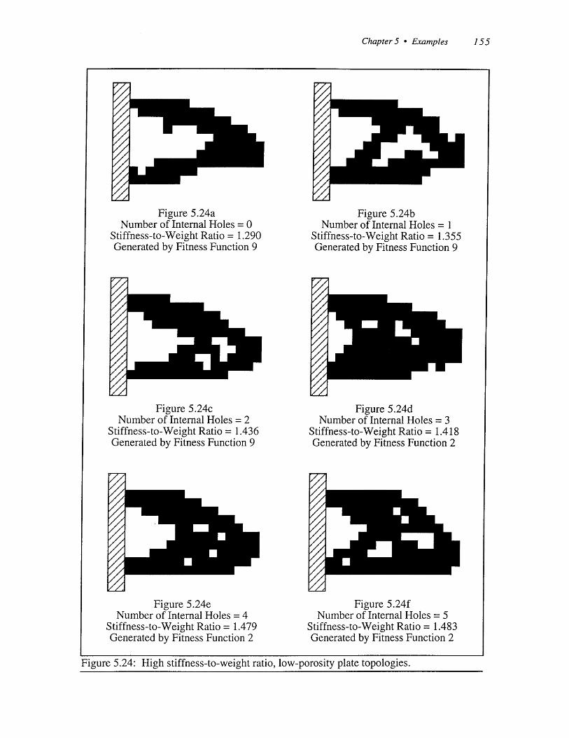
Chapter 5 - Examples 155
Figure 5.24aNumber of Internal Holes = 0
Stiffness-to-Weight Ratio = 1.290Generated by Fitness Function 9
Figure 5.24cNumber of Internal Holes = 2
Stiffness-to-Weight Ratio = 1.436Generated by Fitness Function 9
Figure 5.24eNumber of Internal Holes = 4
Stiffness-to-Weight Ratio = 1.479Generated by Fitness Function 2
Figure 5.24bNumber of Internal Holes = 1
Stiffness-to-Weight Ratio = 1.355Generated by Fitness Function 9
Figure 5.24dNumber of Internal Holes = 3
Stiffness-to-Weight Ratio = 1.418Generated by Fitness Function 2
Figure 5.24fNumber of Internal Holes = 5
Stiffness-to-Weight Ratio = 1.483Generated by Fitness Function 2
Figure 5.24: High stiffness-to-weight ratio, low-porosity plate topologies.

156 Chapter 5 - Examples
# of optimizations Mean Bonferroni GroupingFitness Stiffness-to-Weight
Function terormedfunin Ratio of optimal Means with the same letter arethis fitness function topologies not significantly different
1 10 1.44445 A2 70 1.38307 A3 10 1.25356 A9 300 1.21846 A B7 60 1.18592 A B6 10 0.95431 C B8 60 0.84680 C4 10 0.78166 C D5 10 0.57193 D
Table 5.3: Ranking of candidate fitness functions according to Stiffness-to-Weight Ratio.
J # of optimizations Mean number of Bonferroni GroupingFitness performed using internal holes in M
Function this fitness function optimal topologies Means with the same letter are__________ j j not significantly different5 10 0.000 A6 10 0.200 A4 10 0.800 A9 300 2.290 A B3 10 2.700 A B8 60 4.350 C B7 60 6.100 C2 70 7.043 C1 10 12.000 D
Table 5.4: Ranking of candidate fitness functions according to number of internal holes.
statistically-equivalent numbers of internal holes). Hence, fitness functions 3 and 9 obtain
topologies combining highest stiffness-to-weight ratio with lowest porosity. This result is
also demonstrated graphically in Figure 5.25, which plots the mean stiffness-to-weight
ratio against the mean number of holes for each of the nine candidate fitness functions.
Note that in Figure 5.25, fitness functions 3 and 9 are located in the area representing plate
topologies combining high stiffness-to-weight ratio with low porosity.
Casual examination of this example's experimental data, provided in Figure 5.26
(which plots stiffness-to-weight ratio vs. number of internal holes data from all 540
optimization runs), suggests that a plate's stiffness-to-weight ratio may increase as its
porosity increases. This relationship is also suggested by Bendsoe et al. (1993), who,
using a homogenization-based technique (see Section 3.2.1 for details of the technique),
find that plate topologies containing large areas of intermediate-density (i.e., highly-
porous) material (obtained using a Rank-2 microstructure model) are slightly stiffer than

Chapter 5 - Examples 157
Figure 5.25: Mean stiffness-to-weight ratio vs. mean number of internal holes.
Figure 5.26: Stiffness-to-weight ratio vs. number of internal holes. Note that this graphcontains data from all 540 optimization runs.
Mean Stiffness-to-Weight Ratio vs. MeanNumber of Internal Holes
1.60-
1.20 9 3 m 7
0.80 -- m 4 8
A50.40--
0.000.00 5.00 10.00 15.00
Mean Number of Internal Holes
Stiffness-to-Weight Ratio vs. Number ofInternal Holes
2
0.5
0
0 5 10 15 20 25
Number of Internal Holes
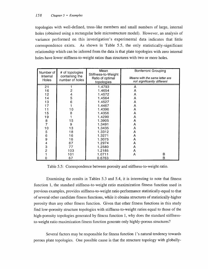
158 Chapter 5 - Examples
topologies with well-defined, truss-like members and small numbers of large, internal
holes (obtained using a rectangular hole microstructure model). However, an analysis of
variance performed on this investigation's experimental data indicates that little
correspondence exists. As shown in Table 5.5, the only statistically-significant
relationship which can be inferred from the data is that plate topologies with zero internal
holes have lower stiffness-to-weight ratios than structures with two or more holes.
Number of # of topologies Mean Bonferroni GroupingInternal containing the Stiffness-to-WeightHoles number of holes Ratio of optimal Means with the same letter are
topologies not significantly different
21 1 1.4793 A16 2 1.4654 A12 4 1.4572 A14 5 1.4564 A13 6 1.4527 A17 1 1.4467 A11 10 1.4396 A15 8 1.4356 A19 1 1.4290 A8 15 1.3905 A7 9 1.3491 A10 13 1.3435 A5 18 1.3312 A6 16 1.3271 A9 16 1.3075 A4 67 1.2974 A3 77 1.2580 A2 103 1.2185 A1 101 1.0711 A B0 67 0.6763 B
Table 5.5: Correspondence between porosity and stiffness-to-weight ratio.
Examining the results in Tables 5.3 and 5.4, it is interesting to note that fitness
function 1, the standard stiffness-to-weight ratio maximization fitness function used in
previous examples, provides stiffness-to-weight ratio performance statistically-equal to that
of several other candidate fitness functions, while it obtains structures of statistically-higher
porosity than any other fitness function. Given that other fitness functions in this study
find low-porosity structure topologies with stiffness-to-weight ratios equal to those of the
high-porosity topologies generated by fitness function 1, why does the standard stiffness-
to-weight ratio maximization fitness function generate only highly-porous structures?
Several factors may be responsible for fitness function l's natural tendency towards
porous plate topologies. One possible cause is that the structure topology with globally-

Chapter 5 - Examples 159
optimal stiffness-to-weight ratio is indeed highly-porous, but optimizations using fitness
function 1 have not been allowed to evolve long enough (i.e., for a sufficient number of
generations) to converge to the globally-optimal structure topology (and have instead
generated highly-porous structure topologies which exhibit stiffness-to-weight ratios no
better than those of low-porosity structures obtained by other fitness functions). Another
possibility is that fitness function 1 does consistently generate plate topologies with higher
stiffness-to-weight ratios than other fitness functions, but additional experiment replications
are required to establish statistically-significant differences. Finally, the exceptionally large
search space resulting from this example's finely-discretized design domain may be
responsible for the natural tendency towards porous structures-while fitness function 1
found plate topologies with high stiffness-to-weight ratio and low porosity when using
relatively small search spaces in Examples 2 and 3, it may be unable to efficiently search
larger search spaces for high stiffness-to-weight ratio, low-porosity plate topologies. Note
that simply increasing the genetic algorithm population size and the number of generations
performed during search would likely improve the genetic algorithm's abilities in finding
high stiffness-to-weight ratio, low-porosity plate topologies.
When examining the results and conclusions provided by this example, it is
important to note that unlike homogenization-based techniques, which are based on
deterministic principles, the genetic algorithm is based on probabilistic principles. Hence,it is impossible to determine whether a structure generated by the genetic algorithm is
indeed locally- or globally-optimal, and it is also impossible to predict, using either
mathematical techniques or results from a single genetic algorithm optimization run, the
nature of the optimal structure topology. Consequently, this example's conclusions that
fitness functions 3 and 9 generate structures combining highest stiffness-to-weight ratio
with lowest porosity, and that little relationship exists between a structure's porosity and its
stiffness-to-weight ratio, have little rigorous mathematical basis and are based entirely on
the experimental results of the 540 optimization runs. However, statistical analyses of this
example's experimental results do, with a high level of confidence, substantiate these
conclusions.
Note also that the results of this study, as well as the conclusions which this
example makes based on the results, could possibly change if different genetic algorithm
population sizes, varied crossover and mutation probabilities, new fitness functions,
coarser or finer design domain discretizations, or different design domains and boundary
conditions were used. In fact, this example clearly demonstrates that the fitness function
160 Chapter 5 - Examples
used has a great effect on the type of structure obtained. However, additional experiment
replications would, given the genetic algorithm's probabilistic nature, produce slightly
different experimental results even if all of the above parameters were held constant.
So, the genetic algorithm's probabilistic nature prevents the development of
mathematically-rigorous convergence criteria or error bounds (and investigators must
therefore use statistical analysis to model the genetic algorithm's behavior and capabilities),
and the particular parameter values (i.e., population size, probabilities of crossover and
mutation, fitness function formulation, design representation, etc.) used in a genetic
algorithm search have a great effect on the optimization's outcome. However, while this
example's findings could indeed change if other parameter values were used, statistical
analysis nonetheless shows with a high level of confidence that, given the set of parameter
values used in this experiment, little correspondence exists between porosity and stiffness-
to-weight ratio. Consequently, this study presents a strong counterexample to the notion
that porosity and structural performance (here stiffness-to-weight ratio) are related.
However, it is not this example's intent to make general conclusions regarding the
nature of optimal structure topologies. Instead, this example simply attempts to provide
insight into the behavior exhibited by the genetic algorithm in Examples 4 and 5.
Specifically, given the:
- design domain representation, geometry, and discretization
- boundary conditions
- genetic algorithm parameters
used in Examples 4 and 5 (which generated highly-porous optimal structure topologies),
this example attempts to determine:
- if the genetic algorithm can generate structure topologies combining highstiffness-to-weight ratio with low porosity.
- if highly-porous structures indeed have higher stiffness-to-weight ratios thanlow-porosity structures (i.e., what, if any, relationship exists between stiffness-to-weight ratio and porosity).
- why the genetic algorithm was unable to generate low-porosity, high-stiffness-to-weight-ratio structures in Examples 4 and 5.
Chapter 5 - Examples 161
This example was also investigated with the hope that it might demonstrate both the
varied, probabilistic behavior of the genetic algorithm as well as the ad hoc nature ofgenetic algorithm fitness function design. This example also hoped to demonstrate thatvastly different fitness functions can be used in an attempt to achieve a given objective (inthis case, maximize stiffness-to-weight ratio while minimizing porosity), and that these
different fitness functions typically provide varying levels of optimization performance.
5.9 Example 8: Comparison with Homogenization-Based Techniques.5.9.1 Introduction. Previous examples in this investigation used the genetic
algorithm to optimize the topologies of cantilevered plates with design domain geometries
and discretizations, as well as boundary and loading conditions, similar to those examined
using homogenization-based techniques (Papalambros and Chirehdast (1990), Suzuki and
Kikuchi (1990)). Unfortunately, no quantitative comparisons could be made between the
two methods because this investigation's genetic algorithm-based technique maximizes a
plate's stiffness-to-weight ratio while homogenization-based techniques typically minimize
a structure's mean compliance subject to a maximum volume constraint.
This example, by using the genetic algorithm to minimize a plate's mean compliance
subject to a maximum volume constraint, provides a quantitative comparison between this
investigation's genetic algorithm-based approach and homogenization-based methods.
Specifically, this example evaluates the optimization abilities of the genetic algorithm, a
global search technique which typically avoids local optima, in relation to those of the
optimality criteria methods used in homogenization-based methods, which can be expected
to converge to local extrema (Bendsoe et al., 1993).
Hence, as in Examples 4, 5, 6, and 7, this example optimizes the topology of a
rectangular, cantilevered plate subject to a downward vertical load. No symmetry
constraints are imposed on the topology, and the constant meshing technique and
hierarchical subdivision are used to facilitate the efficient generation of finely-discretized
plate topologies. However, unlike previous examples which attempted to maximize a
plate's stiffness-to-weight ratio, this example minimizes a plate's mean compliance subject
to a maximum volume constraint.
5.9.2 Design Domain. The cantilevered plate is modeled using a rectangular
design domain 10 units tall by 16 units wide (Figure 5.27), and no symmetry constraints
are imposed on the plate's topology. The design domain is initially discretized into a
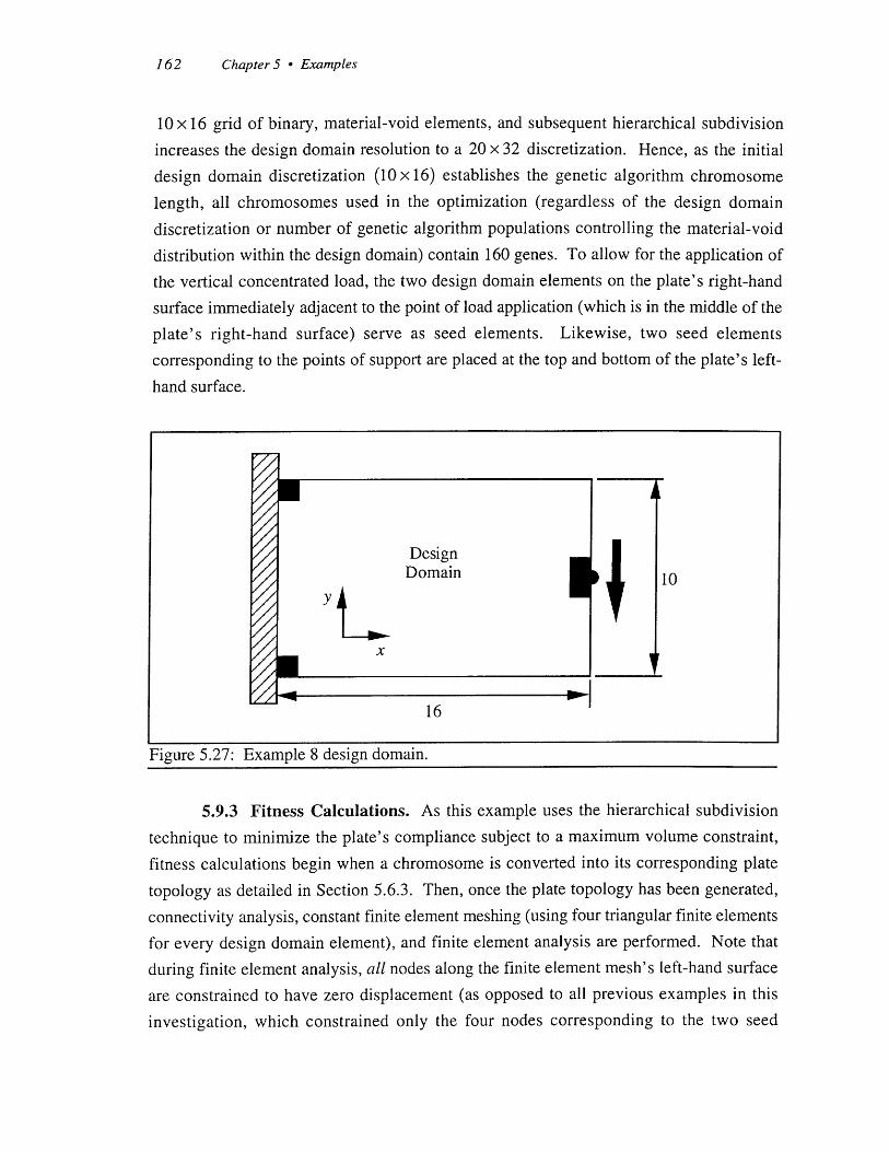
162 Chapter 5 - Examples
10 x 16 grid of binary, material-void elements, and subsequent hierarchical subdivision
increases the design domain resolution to a 20 x 32 discretization. Hence, as the initial
design domain discretization (10 x 16) establishes the genetic algorithm chromosome
length, all chromosomes used in the optimization (regardless of the design domain
discretization or number of genetic algorithm populations controlling the material-void
distribution within the design domain) contain 160 genes. To allow for the application of
the vertical concentrated load, the two design domain elements on the plate's right-hand
surface immediately adjacent to the point of load application (which is in the middle of the
plate's right-hand surface) serve as seed elements. Likewise, two seed elements
corresponding to the points of support are placed at the top and bottom of the plate's left-
hand surface.
DesignDomain 10
16
Figure 5.27: Example 8 design domain.
5.9.3 Fitness Calculations. As this example uses the hierarchical subdivision
technique to minimize the plate's compliance subject to a maximum volume constraint,
fitness calculations begin when a chromosome is converted into its corresponding plate
topology as detailed in Section 5.6.3. Then, once the plate topology has been generated,
connectivity analysis, constant finite element meshing (using four triangular finite elements
for every design domain element), and finite element analysis are performed. Note that
during finite element analysis, all nodes along the finite element mesh's left-hand surface
are constrained to have zero displacement (as opposed to all previous examples in this
investigation, which constrained only the four nodes corresponding to the two seed

Chapter 5 - Examples 163
elements), while the concentrated load is applied to the middle node along the finite elementmesh's right-hand surface. Finally, fitness calculations are performed as detailed inSection 4.4.6. Again, chromosomes corresponding to plate topologies which exhibitminimum mean compliance and satisfy the maximum volume constraint are assigned highfitness, while chromosomes corresponding to plate topologies which exhibit large meancompliance and/or violate the maximum volume constraint are assigned low fitness.Hence, the fitness of a plate topology (and therefore the fitness, to be maximized, of thechromosome corresponding to the plate topology) which satisfies the maximum volumeconstraint is given by:
Fitness = n m n (4.9)In fCompliance)'
where Compliance represents the mean compliance of the plate topology. As detailed inSection 4.4.6, a plate's mean compliance is equal to the applied load vector (FAPPLJEDmultiplied by the plate's displacement at the point of load application (UT):
Compliance = uT -F APPLUED (4.6)
where
u T =[u, uY (4.7)
and
~FYF APPLIED * ;] (4.8)
Again, Fx and F, represent the magnitude, in the x- and y-directions, of the single
concentrated load acting on the plate while u, and u, represent the displacement, in the x-
and y- directions, of the finite element node where the concentrated load is applied.
Then, if the plate topology violates the maximum volume constraint (as detailed in
Section 4.4.6, these fitness calculations use the area of connected material in a plate
topology as a qualitative measure of the plate's volume, and the maximum volume
constraint is therefore actually a maximum area constraint), the above fitness function is
penalized by 6% for every 10% volume constraint violation. Note that this fitness penalty

164 Chapter 5 - Examples
is linearly attenuated according to the current generation number, with no penalty at
generation 0 and full (6%) penalty at generation 175. Hence, prior to generation 175, the
fitness of a chromosome corresponding to a structure topology violating the maximum
volume constraint is given by:
geeato 0.06 VM -V nfl 1Fitness = 1. 0 - ,eeain0 6 , (4.10)
175 0.10 Vmax ln(Compliance)'
where generation represents the current generation of genetic algorithm evolution, V
represents the volume (i.e., the area of connected material elements) of the current plate
topology, and VMAx represents the maximum allowable volume of the plate. After
generation 175, the fitness of a chromosome corresponding to a plate topology violating the
maximum volume constraint is given by:
f [0.06 (V-VA 1)1Fitness = 1. 0 - 0^. .6 ( V - m (.1
0.10 V x J ln(Compliance)
Again, chromosomes corresponding to plate topologies which do not violate the
maximum volume constraint are assigned the fitness value given by Equation 4.9.
During fitness calculations, a maximum volume constraint of 25 percent is used.
Again, because these fitness calculations use the area of connected material in a plate
topology as a qualitative measure of the plate's volume, the maximum volume constraint is
actually a maximum area constraint. Hence, because the design domain has an area of 160
units 2, the maximum volume constraint stipulates that the maximum allowable area of
connected material elements in a plate topology is 40 units2 .
5.9.4 Hierarchical Subdivision Parameters. Optimization begins with a
single genetic algorithm population optimizing the plate topology using the coarse, 10 x 16
design domain discretization. Note that this population contains 30 160-gene
chromosomes. After performing 225 generations of evolution at this initial discretization,
hierarchical subdivision (with a nuking probability of 0.3) is performed to quadruple the
resolution of the design domain. Hence, following hierarchical subdivision, four genetic
algorithm populations optimize the plate's topology using a 20 x 32 design domain
discretization. At this discretization, each design domain element has I the area of the
Chapter 5 - Examples 165
original, coarse design domain elements, and each of the four populations contains 30 160-gene chromosomes. Optimization then concludes after 150 cycles (i.e., 150 generations ofevolution in each design domain quadrant) have been performed at this 20 x 32 designdomain discretization.
Best optimization results were obtained when the maximum volume constraint isrelaxed during early stages of the search. Specifically, when using the coarse designdomain discretization, the maximum allowable volume fraction is set to 1.5 times thedesired 25 percent, or 37.5 percent. Then, after performing hierarchical subdivision andswitching to the finely-discretized design domain, the maximum allowable volume fractionis returned to the desired 25 percent.
Hence, as the maximum volume constraint is actually a maximum area constraint,the initial 37.5 percent maximum volume constraint corresponds to a maximum allowableplate area of 60 units2 (.375 -160 = 60). Because this initial area constraint is used with thecoarse design domain discretization, where the 10 unit tall by 16 unit wide design domainis discretized into a 10 x 16 grid of elements and each element therefore has an area of 1unit 2, the maximum allowable plate area of 60 units 2 corresponds to a maximum of 60design domain elements containing material. Then, when hierarchical subdivision isperformed and the maximum allowable volume fraction is returned to its desired value of25 percent, the maximum allowable plate area becomes 40 units2 (0.25 -160 = 40). Notethat this maximum area constraint of 40 units 2 corresponds to a maximum of 160 designdomain elements containing material, for the 10 unit tall by 16 unit wide design domain isdiscretized into a 20 x 32 grid of elements, where each element has an area of - units2.
5.9.5 Results. The result of the genetic algorithm-based topologicaloptimization is shown in Figure 5.28, while the homogenization-based solution to theproblem is shown in Figure 5.29 (Rodrigues, 1993). 6,750 structural analyses wererequired to generate an optimal coarse, 10 x 16 plate topology:
225 Generations -30 Chromosomes= 6,750 Chromosomes, (5.19)Generation
while an additional 18,000 structural analyses were performed to obtain the final, 20 x 32plate topology:

Chapter 5 * Examples
Generations Chromosomes150 Cycles -4 -30 =18,000 Chromosomes.
Cycle Generation(5.20)
Hence, generating the final, 20 x 32 plate topology required a total of 24,750 finite
element analyses.
Figure 5.28: Genetic algorithm-based optimal plate topology.
Figure 5.29: Homogenization-based optimal plate topology. (Rodrigues, 1993).
9
1 66
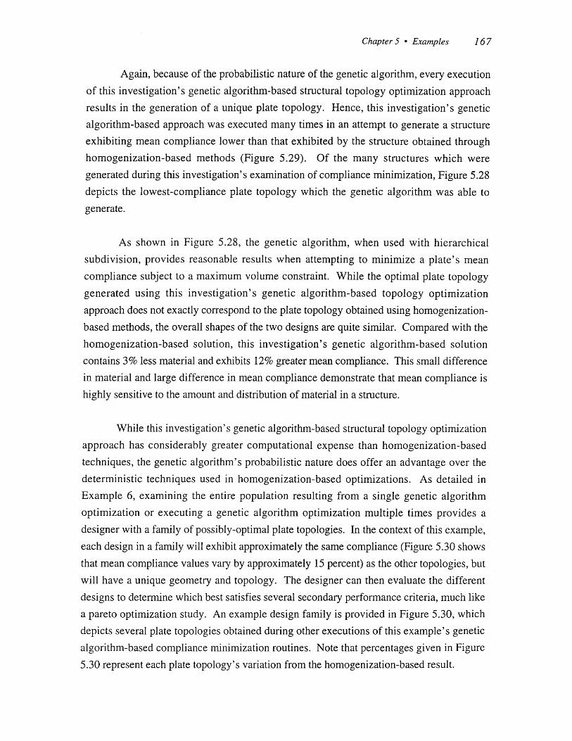
Chapter 5 Examples 167
Again, because of the probabilistic nature of the genetic algorithm, every execution
of this investigation's genetic algorithm-based structural topology optimization approach
results in the generation of a unique plate topology. Hence, this investigation's genetic
algorithm-based approach was executed many times in an attempt to generate a structure
exhibiting mean compliance lower than that exhibited by the structure obtained through
homogenization-based methods (Figure 5.29). Of the many structures which were
generated during this investigation's examination of compliance minimization, Figure 5.28
depicts the lowest-compliance plate topology which the genetic algorithm was able to
generate.
As shown in Figure 5.28, the genetic algorithm, when used with hierarchical
subdivision, provides reasonable results when attempting to minimize a plate's mean
compliance subject to a maximum volume constraint. While the optimal plate topology
generated using this investigation's genetic algorithm-based topology optimization
approach does not exactly correspond to the plate topology obtained using homogenization-
based methods, the overall shapes of the two designs are quite similar. Compared with the
homogenization-based solution, this investigation's genetic algorithm-based solution
contains 3% less material and exhibits 12% greater mean compliance. This small difference
in material and large difference in mean compliance demonstrate that mean compliance is
highly sensitive to the amount and distribution of material in a structure.
While this investigation's genetic algorithm-based structural topology optimization
approach has considerably greater computational expense than homogenization-based
techniques, the genetic algorithm's probabilistic nature does offer an advantage over the
deterministic techniques used in homogenization-based optimizations. As detailed in
Example 6, examining the entire population resulting from a single genetic algorithm
optimization or executing a genetic algorithm optimization multiple times provides a
designer with a family of possibly-optimal plate topologies. In the context of this example,each design in a family will exhibit approximately the same compliance (Figure 5.30 shows
that mean compliance values vary by approximately 15 percent) as the other topologies, but
will have a unique geometry and topology. The designer can then evaluate the different
designs to determine which best satisfies several secondary performance criteria, much like
a pareto optimization study. An example design family is provided in Figure 5.30, which
depicts several plate topologies obtained during other executions of this example's genetic
algorithm-based compliance minimization routines. Note that percentages given in Figure
5.30 represent each plate topology's variation from the homogenization-based result.
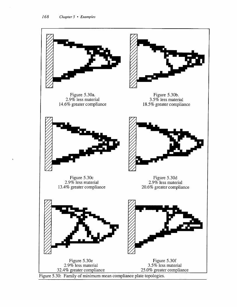
168 Chapter 5 - Examples
Figure 5.30a. Figure 5.30b.2.9% less material 3.5% less material
14.6% greater compliance 18.5% greater compliance
Figure 5.30c Figure 5.30d2.9% less material 2.9% less material
13.4% greater compliance 20.6% greater compliance
Figure 5.30e2.9% less material
32.4% greater compliance
Figure 5.30f3.5% less material
25.0% greater complianceFigure 5.30: Family of minimum mean compliance plate topologies.

Chapter 6 - Conclusions 169
Conclusions
6.1 Overview
This chapter first overviews the contributions of this investigation, and thenprovides conclusions regarding the abilities and limitations of the genetic algorithm-based
structural topology optimization technique developed in this investigation. Finally,potential areas of future work are offered.
6.2 Contributions of This Investigation
This investigation applied the genetic algorithm, a search and optimization techniquebased on the theory of natural selection, to the structural topology optimization of
continuum structures, where the optimal distribution of material within a discretized design
domain was found. Significantly extending previous work in this area, this investigation
focused on, and examined in great detail, the genetic algorithm-based structural topology
optimization of cantilevered plates using a binary, material-void design domain
representation. The technique developed in this investigation was utilized to generate the
optimal topologies of a variety of cantilevered plates, which were optimized based upon
stiffness, mean compliance, weight, and manufacturability considerations.
As a preliminary verification of the abilities of this investigation's technique, the
unconstrained topological optimization of a beam cross-section was examined. After many
generations of search, the genetic algorithm generated a cross-section topology with
material concentrated in locations furthest away from the neutral axis. This was the
expected result. Then, to establish the technique's constrained optimization abilities, the
beam cross-section optimization was re-examined using a maximum stress constraint.

170 Chapter 6 - Conclusions
With the constraint, the genetic algorithm generated optimal cross-section topologies
containing additional material in the flanges, which again is the expected result.
The genetic algorithm was then used in conjunction with finite element analysis to
optimize the topology of a small cantilevered plate in tension. This also yielded the
predicted results.
As the adaptive finite element meshing technique used in the small cantilevered plate
optimization proved to be computationally expensive, a constant finite element meshing
technique was investigated. When used with connectivity analysis, the constant meshing
technique was shown to generate, with less computational expense, plate topologies
exhibiting structural performance equal to that of structures obtained using the adaptive
finite element meshing technique.
The topological optimization of a finely-discretized, cantilevered plate was then
examined to determine if this investigation's genetic algorithm-based structural topology
optimization technique could perform optimization using design domain discretizations
approaching those used by homogenization-based methods. Satisfactory results were
obtained.
In an attempt to enhance the genetic algorithm's optimization abilities and efficiency
when using finely-discretized design domains, a hierarchical subdivision technique was
introduced. Compared to previous examples which used a constant design domain
discretization, hierarchical subdivision was able to produce highly-fit plate topologies of
equal discretization while requiring fewer structural analyses. The hierarchical subdivision
technique also enabled the genetic algorithm to generate plate topologies of much higher
discretization than that possible with a constant design domain discretization.
The genetic algorithm's ability to obtain, during a single optimization, a family of
plate topologies which a designer can evaluate using alternate, secondary criteria (e.g.,
manufacturability, weight, displacement, etc.) was then demonstrated. To obtain families
of designs when using traditional optimization methods such as mathematical programnming
or optimality criteria techniques, optimization must be performed multiple times using a
variety of initial conditions, with the hope that the search will converge to different plate
topologies.

Chapter 6 - Conclusions 1 71
As many of the plate topologies generated in these examples contained largenumbers of internal holes, which are undesireable from a manufacturing standpoint, anexperiment was then conducted to determine if the genetic algorithm could generate platetopologies with high stiffness-to-weight ratio and low porosity. A group of high-stiffness-to-weight ratio, low-porosity structures was obtained. Results of the experiment were thenused to establish that little statistically-significant correspondence exists between astructure's porosity and its stiffness. Possible reasons as to why previous examples onlygenerated highly-porous plate topologies were also discussed.
To provide a quantitative comparison between the optimization capabilities of thisinvestigation's genetic algorithm-based approach and those of homogenization-basedmethods, the genetic algorithm was used to minimize a plate's mean compliance subject to amaximum volume constraint. While the optimal plate topology generated using thisinvestigation's approach did not exactly correspond to the homogenization-based solution,the overall shapes of the two designs were quite similar. Compared with thehomogenization-based solution, this investigation's genetic algorithm-based solutioncontained less material but exhibited greater mean compliance.
These examples significantly focused and extended the previous work of Jensenand associated researchers (Section 3.3.4). Whereas Jensen's research examines thegenetic algorithm-based topological optimization of a variety of structure types using avariety of design domain representations, this investigation emphasized the topologicaloptimization of cantilevered plates using a binary, material-void design domainrepresentation. Specifically, this investigation extended Jensen's work by examining thefollowing:
Design domain discretizations much finer than those used by Jensen, as well ashierarchical subdivision and constant finite element meshing techniques which
improved the genetic algorithm's optimization abilities and efficiency when
using finely-discretized design domains. While Jensen used a meshing
technique similar to that used in this investigation, this investigation's
introduction of hierarchical subdivision was a significant extension and
enhancement of Jensen's constant design domain discretizations.
- A connectivity analysis technique which deterministically removed disconnected
material elements from cantilevered plate topologies. This connectivity analysis
1 72 Chapter 6 - Conclusions
provided a guarantee of structural stability-no "chain-link" type structures
(which are unable to withstand any torque or compressive load) were allowed
by the analysis.
- Fitness functions for unconstrained optimization problems which were based on
a structure's strength-to-weight or stiffness-to-weight ratio. Unlike the fitness
functions used by Jensen, which involve a combination of weight minimization
and constraint violation terms, the fitness functions introduced in this
investigation do not require carefully-chosen penalty terms and therefore attempt
to directly influence the structure's topology above all else. These fitness
functions also provided adequate performance when used in constrained
optimization problems.
- The genetic algorithm's ability to generate, in a single optimization run, a family
of highly-fit cantilevered plate topologies which can then be compared using
alternate, secondary criteria. Jensen examines only those chromosomes which
maximize a given fitness function.
- Methods for driving the genetic algorithm search towards plate topologies
combining high stiffness-to-weight ratio with high manufacturability. In his
examples, Jensen considers only weight, stress, and displacement.
- A direct, quantitative comparison between the genetic algorithm's structural
topology optimization abilities and those of homogenization-based methods,which are currently the most widely-used approach to structural topology
optimization. Jensen provides no such comparison.
6.3 Conclusions
This investigation's genetic algorithm-based structural topology optimization
approach was able to generate structure topologies of relatively high quality and
discretization. When examining the "optimal" structures generated using this
investigation's approach, it is evident that many of the structures would require
modification before they could be considered optimal or manufacturable. For example,
many structures are unsymmetric when they should be symmetric, and other structures
contain a great number of "stray" material elements which, while connected to the structure,
do little to support the applied load. Hence, the performance of these structures would
Chapter 6 - Conclusions 173
likely improve if they were symmetric or did not contain stray material elements (or thestray material was moved to other locations within the structure). Unfortunately, becausegenetic algorithm search is probabilistic rather than deterministic in nature and does notutilize sensitivity information (such as function gradients), the genetic algorithm cannot
determine whether an optimum has been reached and therefore cannot "fine-tune" a
structure in an attempt to generate an exact optimum. Hence, genetic algorithm search
typically produces a "pseudo-optimum," which is similar, but not exactly equal, to the
truly-optimal structure topology. Conversely, the optimality criteria optimization methods
used in homogenization-based techniques use sensitivity information to determine if an
exact optimum has been generated, and search is not concluded until a true optimum is
found. Hence, the structures obtained using homogenization-based techniques are
symmetric when they should be, and they typically do not contain stray material elements.
Note, however, that while the genetic algorithm's probabilistic nature typically prevents the
generation of exact optima, it does allow the genetic algorithm to search in discrete,discontinuous, multi-modal search spaces which would be troublesome to mathematical
programming and optimality criteria techniques.
Additionally, most of the structures generated using this investigation's genetic
algorithm-based structural topology optimization technique were of lower discretization
than structures typically obtained using homogenization-based methods. This is a directresult of the genetic algorithm's extreme computational expense. Specifically, because the
genetic algorithm must evaluate the fitness of every chromosome in every generation of asearch, structural topology optimizations in this investigation required thousands of finite
element analyses. Hence, as increases in design domain discretization result in an increase
in the computational expense of each finite element analysis, using design domain
discretizations approaching those used by homogenization-based methods would make an
already-computationally-expensive optimization prohibitively expensive. Consequently,structures subject to genetic algorithm-based structural topology optimization must
currently be of limited size and complexity. Because the optimality criteria methods used in
homogenization-based structural topology optimization approaches require many fewer
analyses and provide good performance independent of the number of design variables,
homogenization-based techniques can be applied to structures of exceptionally high
discretization. Note that while the genetic algorithm's populations of chromosomes and
probabilistic nature do result in great computational expense, they enable the genetic
algorithm to search in discrete, discontinuous, multi-modal search spaces (which again
would be troublesome to optimality criteria methods) and they allow the genetic algorithm

1 74 Chapter 6 - Conclusions
to automatically generate families of structures which the designer can evaluate using
secondary criteria.
Finally, many of the plate topologies generated during this investigation contained alarge number of internal holes, which could lead to difficulties when parameterizing thetopology for sizing and shape analysis. However, as demonstrated in this investigation,simple modifications to the fitness function can eliminate many of these internal holes.Note that most topologies found using homogenization-based techniques will also lead to
interpretation difficulties, as they generally contain material of intermediate density. Hence,when parameterizing topologies obtained with homogenization-based techniques
(particularly those topologies obtained using Rank-2 microstructure models), the designer
must select a density threshold. The density threshold chosen likely has a great effect on
the resultant topology. While the topologies obtained using this investigation's approachare generally porous, they contain only material and void-no density threshold is neededduring parameterization.
Indeed, the motivation for using the genetic algorithm to perform structural
topology optimization is not an enhanced ability to find exact optima or an increase incomputational speed, but an increase in simplicity and generality. Unlike most other
optimization algorithms, the genetic algorithm can be applied to a wide variety of (possiblyill-behaved) problem domains simply by changing the chromosome-to-design-variable
mappings and fitness function procedures. In this investigation, the genetic algorithm waseasily applied to the domain of structural topology optimization and was able to performadmirably.
6.4 Future Work
Future investigations of genetic algorithm-based structural topology optimization
must focus on decreasing the computational expense of this approach. For example, whileincreasing the genetic algorithm population size or the number of generations performed in
a search would likely allow the genetic algorithm to generate structure topologies of higher
quality than those found in this investigation, either of these changes would increase the
number of structural analyses required by the genetic algorithm and would therefore make
the genetic algorithm search prohibitively expensive computationally. Whereas the
computational expense of the actual genetic algorithm routines is relatively low and would
be difficult to reduce, structural analysis is the major source of this approach's
computational expense. Possible enhancements include a parallel implementation of this

Chapter 6 Conclusions 175
genetic algorithm-based structural topology optimization approach, where multiple
processors would perform finite element analysis on the population of structure topologies.
Approximate fitness calculations could also be used in an attempt to reduce this approach's
computational complexity.
While this investigation used one-dimensional, binary-string genetic algorithm
chromosomes to represent structure topologies, several other chromosome representations
might provide better chromosome-to-design-domain correspondence. For example, when
using a constant design domain discretization, two-dimensional chromosomes (i.e., arrays
of binary digits) would provide an intuitive 2D-chromosome-to-2D-design-domain
correspondence. Likewise, when using hierarchical subdivision, where each element in an
initial, coarse design domain is periodically subdivided into smaller and smaller elements, a
quadtree chromosome structure would allow the genetic algorithm to adaptively increase
design domain discretization in those regions of the domain requiring fine discretization,while regions of the domain which do not require fine discretization would remain at the
original, coarse discretization.
Finally, this investigation demonstrated the great effect which fitness calculations
have on the results of a genetic algorithm search-slight modifications in penalty parameter
value or fitness formulation can drive the genetic algorithm to vastly different "optimal"
structure topologies. To eliminate this great dependency on the fitness function designer's
intuition, an implicit fitness function could be used. Instead of the technique used in this
investigation, where the fitness function is defined a priori and the genetic algorithm
chromosomes are then evaluated using the time-invariant fitness function, an implicit
fitness function would itself evolve during optimization until both an optimal fitness
function and structure topology are found. This would minimize the ad hoc nature of the
fitness function development process and would likely enhance the genetic algorithm's
abilities in finding highly-fit structure topologies.

1 76 Chapter 6 - Conclusions
Chapter 7 - References 177
Re erences
Aarts, E., van Laarhoven, P., 1987, "Simulated Annealing: A Pedestrian Review of theTheory and Some Applications," Pattern Recognition Theory and Applications,Devijver, P., Kittler, J., eds., Springer-Verlag, Berlin, pps. 179-192.
Allaire, G., Francfort, G., 1993, "A Numerical Algorithm for Topology and ShapeOptimization," Topology Design of Structures, Bendsoe, M., Soares, C., eds.,Kluwer Academic Publishers, Dordrecht, The Netherlands, pps. 239-248.
Allaire, G., Kohn, R., 1993, "Topology Optimization and Optimal Shape Design usingHomogenization," Topology Design of Structures, Bendsoe, M., Soares, C., eds.,Kluwer Academic Publishers, Dordrecht, The Netherlands, pps. 207-218.
Anagnostou, G., Ronquist, E., Patera, A., 1992, "A Computational Procedure for PartDesign," Computer Methods in Applied Mechanics and Engineering, Volume 97,Number 1, pps. 33-48.
Arora, J., 1989, Introduction to Optimum Design, McGraw-Hill Book Company, NewYork.
Back, T., Hoffmeister, F., 1991, "Extended Selection Mechanisms in GeneticAlgorithms," Proceedings of the Fourth International Conference on GeneticAlgorithms, Belew, R., Booker, L., eds., University of California, San Diego, pps.92-99.
Baker, J., 1989, Analysis of the Effects of Selection in Genetic Algorithms, DoctoralDissertation, Department of Computer Science, Vanderbilt University.
Baker, J., 1987, "Reducing Bias and Inefficiency in the Selection Algorithm," GeneticAlgorithms and their Applications: Proceedings of the Second International Conference

178 Chapter 7 - References
on Genetic Algorithms, Grefenstette, J., ed., Massachusetts Institute of Technology,pps. 14-21.
Baker, J., 1985, "Adaptive Selection Methods for Genetic Algorithms," Proceedings of theFirst International Conference on Genetic Algorithms and their Applications,Grefenstette, J., ed., Carnegie-Mellon University, pps. 101-111.
Banerjee, P., Butterfield, R., 1981, Boundary Element Methods in Engineering Science,McGraw-Hill Book Company, London.
Bathe, K., 1982, Finite Element Procedures in Engineering Analysis, Prentice-Hall,Englewood Cliffs, New Jersey.
Bendsoe, M., Diaz, A., Kikuchi, N., 1993, "Topology and Generalized LayoutOptimization of Elastic Structures," Topology Design of Structures, Bendsoe, M.,Soares, C., eds., Kluwer Academic Publishers, Dordrecht, The Netherlands, pps.159-205.
Bendsoe, M., Kikuchi, N., 1988, "Generating Optimal Topologies in Structural Designusing a Homogenization Method," Computer Methods in Applied Mechanics andEngineering, Volume 71, Number 2, pps. 197-224.
Bendsoe, M., Rasmussen, J., Rodrigues, H., 1991, "Topology and Boundary ShapeOptimization as an Integrated Tool for Computer Aided Design," EngineeringOptimization in Design Processes, Eschenauer, H., Mattheck, C., Olhoff, N., eds.,Springer-Verlag, Berlin, pps. 27-34.
Bendsoe, M., Soares, C., eds., 1993, Topology Design of Structures, Kluwer AcademicPublishers, Dordrecht, The Netherlands.
Braibant, V., Fleury, C., 1984, "Shape Optimal Design Using B-Splines," ComputerMethods in Applied Mechanics and Engineering, Volume 44, Number 3, pps. 247-267.
Brebbia, C., 1978, The Boundary Element Methodfor Engineers, John Wiley & Sons,New York.
Cartwright, H., Harris, S., 1993, "The Application of the Genetic Algorithm to Two-Dimensional Strings: The Source Apportionment Problem," Proceedings of the FifthInternational Conference on Genetic Algorithms, Forrest, S., ed., University of Illinoisat Urbana-Champaign, pg. 631.

Chapter 7 - References 179
Chapman, C., Jakiela, M., 1994, "Genetic Algorithm-Based Structural Topology Designwith Compliance and Manufacturability Considerations," accepted for presentation(included in proceedings) at the 1994 ASME Design Automation Conference,Minneapolis, Minnesota.
Chapman, C., Saitou, K., Jakiela, M., 1993a, "Genetic Algorithms as an Approach toConfiguration and Topology Design," ASME Journal of Mechanical Design, to appear.
Chapman, C., Saitou, K., Jakiela, M., 1993b, "Genetic Algorithms as an Approach toConfiguration and Topology Design," Proceedings of the 1993 Design AutomationConference, Gilmore, B., Hoeltzel, D., Azarm, S., Eschenauer, H., eds., DE-Vol. 65-1, Published by the American Society of Mechanical Engineers, Albuquerque, NewMexico, pps. 485-498.
Chirehdast, M., Gea, H., Kikuchi, N., Papalambros, P., 1992, "Structural ConfigurationExamples of an Integrated Optimal Design Process," Proceedings of the 1992 DesignAutomation Conference, Hoeltzel, D., ed., DE-Volume 44-1, Published by theAmerican Society of Mechanical Engineers, Scottsdale, Arizona, pps. 11-20.
Cox, H., 1965, The Design of Structures of Least Weight, Pergamon Press, Oxford.
De Jong, K., 1975, An Analysis of the Behavior of a Class of Genetic Adaptive Systems,Doctoral Dissertation, Department of Computer and Communication Sciences, TheUniversity of Michigan.
de la Maza, M., Tidor, B., 1993, "An Analysis of Selection Procedures with ParticularAttention Paid to Proportional and Boltzmann Selection," Proceedings of the FifthInternational Conference on Genetic Algorithms, Forrest, S., ed., University of Illinoisat Urbana-Champaign, pps. 124-13 1.
Delyon, B., 1988, Convergence of the Simulated Annealing Algorithm, Center forIntelligent Control Systems Report #CICS-P-78, Massachusetts Institute ofTechnology.
Devore, J., 1987, Probability and Statistics for Engineering and the Sciences, Brooks/ColePublishing Company, Monterey, California.
Dfaz, A., Belding, B., 1993, "On Optimum Truss Layout by a Homogenization Method,"ASME Journal of Mechanical Design, Volume 115, Number 3, pps. 367-373.
Eschenauer, H., Mattheck, C., Olhoff, N., eds., 1991, Engineering Optimization inDesign Processes, Springer-Verlag, Berlin.
180 Chapter 7 - References
Eshelman, L., Caruana, R., Schaffer, J., 1989, "Biases in the Crossover Landscape,"Proceedings of the Third International Conference on Genetic Algorithms, Schaffer, J.,ed., George Mason University, pps. 10-19.
Farin, G., 1993, Curves and Surfacesfor Computer Aided Geometric Design, AcademicPress, San Diego.
Fleury, C., Geradin, M., 1978, "Optimality Criteria and Mathematical Programming inStructural Weight Optimization," Computers and Structures, Volume 8, Number 1,pps. 7-17.
Fukushima, J., Suzuki, K., Kikuchi, N., 1993, "Applications to Car Bodies: GeneralizedLayout Design of Three-Dimensional Shells," Optimization of Large StructuralSystems, Rozvany, G., ed., Volume I, Kluwer Academic Publishers, Dordrecht, TheNetherlands, pps. 177-191.
Ghaddar, C., Maday, Y., Patera, A., 1993, "Analysis of a Part Design Procedure,"Submitted to Numer. Math.
Goldberg, D., 1989a, Genetic Algorithms in Search, Optimization, and Machine Learning,Addison-Wesley, Reading, Massachusetts.
Goldberg, D., 1989b, "Sizing Populations for Serial and Parallel Genetic Algorithms,"Proceedings of the Third International Conference on Genetic Algorithms, Schaffer, J.,ed., George Mason University, pps. 70-79.
Goldberg, D., Deb, K., 1991, "A Comparative Analysis of Selection Schemes used inGenetic Algorithms," Foundations of Genetic Algorithms, Rawlins, G., ed., MorganKaufmann Publishers, pps. 69-93.
Goldberg, D., Deb, K., Clark, J., 1992, "Genetic Algorithms, Noise, and the Sizing ofPopulations," Complex Systems, Volume 6, pps. 333-362.
Goldberg, D., Lingle, R., 1985, "Alleles, Loci, and the Traveling Salesman Problem,"Proceedings of the First International Conference on Genetic Algorithms and theirApplications, Grefenstette, J., ed., Carnegie-Mellon University, pps. 154-159.
Goldberg, D., Samtani, M., 1986, "Engineering Optimization via Genetic Algorithm,"Electronic Computation-Proceedings of the Ninth Conference on ElectronicComputation, Will, K., ed., Published by the American Society of Civil Engineers,University of Alabama at Birmingham, pps. 471-482.

Chapter 7 References 181
Grefenstette, J., 1986, "Optimization of Control Parameters for Genetic Algorithms,"IEEE Transactions on Systems, Man, and Cybernetics, Volume SMC-16, Number 1,pps. 122-128.
Grefenstette, J., Baker, J., 1989, "How Genetic Algorithms Work: A Critical Look atImplicit Parallelism," Proceedings of the Third International Conference on GeneticAlgorithms, Schaffer, J., ed., George Mason University, pps. 20-27.
Grierson, D., Pak, W., 1993, "Discrete Optimal Design using a Genetic Algorithm,"Topology Design of Structures, Bendsoe, M., Soares, C., eds., Kluwer AcademicPublishers, Dordrecht, The Netherlands, pps. 89-102.
Haftka, R., Grandhi, R., 1986, "Structural Shape Optimization-A Survey," ComputerMethods in Applied Mechanics and Engineering, Volume 57, Number 1, pps. 91-106.
Haftka, R., Gtirdal, Z., 1992, Elements of Structural Optimization, Kluwer AcademicPublishers, Dordrecht, The Netherlands.
Hajela, P., 1992, "Genetic Algorithms in Automated Structural Synthesis," Optimizationand Artificial Intelligence in Civil and Structural Engineering, Topping, B., ed.,Volume I, Kluwer Academic Publishers, Dordrecht, The Netherlands, pps. 639-653.
Hajela, P., 1990, "Genetic Search-An Approach to the Nonconvex OptimizationProblem," AIAA Journal, Volume 28, Number 7, pps. 1205-12 10.
Hajela, P., Lee, E., Lin, C., 1993, "Genetic Algorithms in Structural TopologyOptimization," Topology Design of Structures, Bendsoe, M., Soares, C., eds.,Kluwer Academic Publishers, Dordrecht, The Netherlands, pps. 117-133.
Hemp, W., 1973, Optimum Structures, Oxford University Press, London.
Holland, J., 1975, Adaptation in Natural and Artificial Systems, The University ofMichigan Press, Ann Arbor, Michigan.
Jenkins, W., 1992, "Plane Frame Optimum Design Environment Based on GeneticAlgorithm," Journal of Structural Engineering, Volume 118, Number 11, pps. 3103-3112.
Jenkins, W., 199 1a, "Structural Optimisation with the Genetic Algorithm," The StructuralEngineer, Volume 69, Number 24, pps. 418-422.

182 Chapter 7 - References
Jenkins, W., 1991b, "Towards Structural Optimization via the Genetic Algorithm,"Computers & Structures, Volume 40, Number 5, pps. 1321-1327.
Jensen, E., 1992, Topological Structural Design Using Genetic Algorithms, Doctor ofPhilosophy Thesis, Department of Mechanical Engineering, Purdue University.
Jog, C., Haber, R., Bendsoe, M., 1993, "A Displacement-Based Topology DesignMethod with Self-Adaptive Layered Materials," Topology Design of Structures,Bendsoe, M., Soares, C., eds., Kluwer Academic Publishers, Dordrecht, TheNetherlands, pps. 219-238.
Kirkpatrick, S., Gelatt, C., Vecchi, M., 1983, "Optimization by Simulated Annealing,"Science, Volume 220, pps. 671-680.
Kirsch, U., 1993, Structural Optimization-Fundamentals and Applications, Springer-Verlag, Berlin.
Kirsch, U., 1981, Optimum Structural Design, McGraw-Hill Book Company, New York.
Kohn, R., 1993, "The Relaxed Approach to Structural Optimization," Smart Structuresand Materials 1993: Mathematics in Smart Structures, Banks, H., ed., SPIE Volume1919, Published by the International Society for Optical Engineering, Albuquerque,New Mexico, pps. 325-327.
Kohn, R., Strang, G., 1986, "Optimal Design and Relaxation of Variational Problems, I,II, III," Communications on Pure and Applied Mathematics, Volume 39, pps. 113-137, 139-182, 353-377.
Kreinovich, V., Quintana, C., Fuentes, 0., 1993, "Genetic Algorithms: What FitnessScaling is Optimal?," Cybernetics and Systems, Volume 24, Number 1, pps. 9-26.
Kumar, A., 1993, Shape and Topology Synthesis of Structures using a SequentialOptimization Algorithm, Doctor of Philosophy in Mechanical Engineering Thesis,Massachusetts Institute of Technology, September.
Levy, S., 1992, Artificial Life-The Questfor a New Creation, Pantheon Books, NewYork.
Lin, C., Hajela, P., 1993, "Genetic Search Strategies in Large Scale Optimization," AIAAPaper #93-1585.

Chapter 7 - References 183
Mitchell, A., 1904, "The Limits of Economy of Material in Frame Structures,"Philosophical Magazine, Series 6, Volume 8, pps. 589-597.
Mortenson, M., 1985, Geometric Modeling, John Wiley & Sons, New York.
Nilsson, N., 1971, Problem-Solving Methods in Artificial Intelligence, McGraw-HillBook Company, New York.
Olhoff, N., Bendsoe, M., Rasmussen, J., 1991, "On CAD-Integrated Structural Topologyand Design Optimization," Computer Methods in Applied Mechanics and Engineering,Volume 89, pps. 259-279.
Papalambros, P., Chirehdast, M., 1990, "An Integrated Environment for StructuralConfiguration Design," Journal of Engineering Design, Volume 1, Number 1, pps. 73-96.
Popov, E., 1978, Mechanics of Materials, Prentice-Hall, Englewood Cliffs, New Jersey.
Rajeev, S., Krishnamoorthy, C., 1992, "Discrete Optimization of Structures UsingGenetic Algorithms," Journal of Structural Engineering, Volume 118, Number 5, pps.1233-1250.
Richards, R., Sheppard, S., 1992, "Learning Classifier Systems in Design Optimization,"Proceedings of the 1992 Design Theory and Methodology Conference, Taylor, D.,Stauffer, L., eds., DE-Volume 42, Published by the American Society of MechanicalEngineers, Scottsdale, Arizona, pps. 179-186.
Rodrigues, H., 1993, Personal Communication.
Rozvany, G., ed., 1993, Optimization of Large Structural Systems, Volume I, KluwerAcademic Publishers, Dordrecht, The Netherlands.
Rozvany, G., 1989, Structural Design via Optimality Criteria, Kluwer AcademicPublishers, Dordrecht, The Netherlands.
Rozvany, G., Zhou, M., 1991a, "The COC algorithm, Part I: Cross-section optimizationor sizing," Computer Methods in Applied Mechanics and Engineering, Volume 89,pps. 281-308.
Rozvany, G., Zhou, M., 199 1b, "Applications of the COC Algorithm in LayoutOptimization," Engineering Optimization in Design Processes, Eschenauer, H.,Mattheck, C., Olhoff, N., eds., Springer-Verlag, Berlin, pps. 59-70.
184 Chapter 7 - References
Rozvany, G., Zhou, M., Birker, T., Sigmund, 0., 1993, "Topology Optimization usingIterative Continuum-Type Optimality Criteria (COC) Methods for DiscretizedSystems," Topology Design of Structures, Bendsse, M., Soares, C., eds., KluwerAcademic Publishers, Dordrecht, The Netherlands, pps. 273-286.
Sakamoto, J., Oda, J., 1993, "A Technique of Optimal Layout Design for Truss Structuresusing Genetic Algorithm," AIAA Paper #93-1582.
Sandgren, E., Jensen, E., 1992, "Automotive Structural Design Employing a GeneticOptimization Algorithm," SAE Technical Paper #920772, Proceedings of the 1992SAE International Congress and Exposition, Detroit, Michigan.
Sandgren, E., Jensen, E., Welton, J., 1990, "Topological Design of StructuralComponents using Genetic Optimization Methods," Sensitivity Analysis andOptimization with Numerical Methods, Saigal, S., Mukherjee, S., eds., AMD-Volume115, Proceedings of the Winter Annual Meeting of the American Society of MechanicalEngineers, Dallas, Texas, pps. 31-43.
Sandgren, E., Wu, S., 1988, "Shape Optimization Using the Boundary Element Methodwith Substructuring," International Journal for Numerical Methods in Engineering,Volume 26, Number 9, pps. 1913-1924.
Schaffer, J., Caruana, R., Eshelman, L., Das, R., 1989, "A Study of Control ParametersAffecting Online Performance of Genetic Algorithms for Function Optimization,"Proceedings of the Third International Conference on Genetic Algorithms, Schaffer, J.,ed., George Mason University, pps. 51-60.
Schaffer, J., Morishima, A., 1987, "An Adaptive Crossover Distribution Mechanism forGenetic Algorithms," Genetic Algorithms and their Applications: Proceedings of theSecond International Conference on Genetic Algorithms, Grefenstette, J., ed.,Massachusetts Institute of Technology, pps. 36-40.
Schmit, L., 1981, "Structural Synthesis-Its Genesis and Development," AIAA Journal,Volume 19, Number 10, pps. 1249-1263.
Shankar, N., Hajela, P., 1991, "Heuristics Driven Strategies for Near-Optimal StructuralTopology Development," Artificial Intelligence and Structural Engineering, Topping,B., ed., Civil-Comp Press, Edinburgh, pps. 219-226.
Shigley, J., Mischke, C., 1989, Mechanical Engineering Design, McGraw-Hill BookCompany, New York.

Chapter 7 - References 185
Spears, W., De Jong, K., 1991, "On the Virtues of Parameterized Uniform Crossover,"Proceedings of the Fourth International Conference on Genetic Algorithms, Belew, R.,Booker, L., eds., University of California, San Diego, pps. 230-236.
Strang, G., Kohn, R., 1986, "Optimal Design in Elasticity and Plasticity," InternationalJournalfor Numerical Methods in Engineering, Volume 22, Number 1, pps. 183-188.
Suzuki, K., Kikuchi, N., 1993, "Layout Optimization using the HomogenizationMethod," Optimization of Large Structural Systems, Rozvany, G., ed., Volume I,Kluwer Academic Publishers, Dordrecht, The Netherlands, pps. 157-175.
Suzuki, K., Kikuchi, N., 1991, "A Homogenization Method for Shape and TopologyOptimization," Computer Methods in Applied Mechanics and Engineering, Volume 93,Number 2, pps. 291-318.
Suzuki, K., Kikuchi, N., 1990, "Shape and Topology Optimization by a HomogenizationMethod," Sensitivity Analysis and Optimization with Numerical Methods, Saigal, S.,Mukherjee, S., eds., AMD-Volume 115, Proceedings of the Winter Annual Meeting ofthe American Society of Mechanical Engineers, Dallas, Texas, pps. 15-30.
Syswerda, G., 1989, "Uniform Crossover in Genetic Algorithms," Proceedings of theThird International Conference on Genetic Algorithms, Schaffer, J., ed., GeorgeMason University, pps. 2-9.
van Laarhoven, P., 1988, Theoretical and Computational Aspects of Simulated Annealing,Stichting Mathematisch Centrum, Amsterdam, The Netherlands.
van Laarhoven, P., Aarts, E., 1987, Simulated Annealing: Theory and Applications, D.Reidel Publishing Company, Dordrecht, The Netherlands.
Vanderplaats, G., 1993, "Thirty Years of Modern Structural Optimization," Advances inEngineering Software, Volume 16, Number 2, pps. 81-88.
Vanderplaats, G., 1992a, "An Assessment of Current Non-Linear ProgrammingAlgorithms for Structural Design, Part I: Basic Algorithms," Optimization andArtificial Intelligence in Civil and Structural Engineering, Topping, B., ed., Volume I,Kluwer Academic Publishers, Dordrecht, The Netherlands, pps. 107-125.
Vanderplaats, G., 1992b, "An Assessment of Current Non-Linear ProgrammingAlgorithms for Structural Design, Part II: Some Recent Approximation Methods,"Optimization and Artificial Intelligence in Civil and Structural Engineering, Topping,B., ed., Volume I, Kluwer Academic Publishers, Dordrecht, The Netherlands, pps.127-141.

186 Chapter 7 - References
Vanderplaats, G., 1982, "Structural Optimization-Past, Present, and Future," AIAAJournal, Volume 20, Number 7, pps. 992-1000.
Wang, S., Cheng, X., Zhou, J., Yu, J., 1993, "An Efficient Genetic Algorithm for LargeScale Built-Up Structural Optimization," Proceedings of the 1993 Design AutomationConference, Gilmore, B., Hoeltzel, D., Azarm, S., Eschenauer, H., eds., DE-Volume65-1, Published by the American Society of Mechanical Engineers, Albuquerque, NewMexico, pps. 505-5 10.
Watabe, H., Okino, N., 1993, "A Study on Genetic Shape Design," Proceedings of theFifth International Conference on Genetic Algorithms, Forrest, S., ed., University ofIllinois at Urbana-Champaign, pps. 445-450.
Zhou, M., Rozvany, G., 1991, "The COC algorithm, Part II: Topological, geometricaland generalized shape optimization," Computer Methods in Applied Mechanics andEngineering, Volume 89, pps. 309-336.
Zienkiewicz, 0., 1989, The Finite Element Method, McGraw-Hill Book Company, NewYork.

Chapter 8 - Index 187
Index
Aarts, E. 37, 177, 185Allaire, G. 65, 177Anagnostou, G. 67, 68, 93, 177ANOVA 154Arora, J. 27, 32, 33, 177Bdck, T. 57, 177Baker, J. 51, 52, 57, 177, 178, 181Banerjee, P. 39, 178Bathe, K. 39, 178Belding, B. 64, 179Bendsoe, M. 64, 65, 67, 101, 156, 178, 182,183Birker, T. 34, 184Bonferroni procedure 154Boundary element method 39Braibant, V. 41, 178Brebbia, C. 39, 178Butterfield, R. 39, 178Cartwright, H. 87, 178Caruana, R. 57, 180, 184Chapman, C. 83, 179Cheng, X. 73, 186Chirehdast, M. 67, 131, 161, 179, 183Clark, J. 57, 180Constraints 96
design 28in genetic algorithm search 58, 89, 90, 104,111, 116, 153, 163performance 25side 29
Cox, H. 26, 179Curves 74
B-Spline 41B6zier 41
Das, R. 57, 184De Jong, K. 57, 179, 185de la Maza, M. 57, 179Deb, K. 57, 180Delyon, B. 37, 179Design
conceptual design 19
configuration design 42cost 28criteria 22, 26domain 21, 42, 43, 64, 66, 68, 78, 85, 91,159, 171feasibility 28optimization 25representation 42, 72, 78, 85, 86, 91, 159,171specifications 25stages 19utility 25variables 27, 30, 34, 38, 39, 40, 42, 44, 45,48, 59, 64, 66, 68, 70, 72, 74, 90, 91
Devore, J. 154, 179Dfaz, A. 64, 65, 67, 156, 178, 179Eschenauer, H. 64, 179Eshelman, L. 57, 180, 184Farin, G. 41, 180Finite element mesh 38, 39Finite element method 39Fleury, C. 35, 41, 178, 180Francfort, G. 65, 177Fuentes, 0. 57, 182Fukushima, J. 64, 180Functional requirements 25Gea, H. 67, 179Gelatt, C. 35, 182Genetic algorithm 21, 28, 37, 43, 90, 159
allele 44, 52, 54applied to conceptual design 20applied to shape optimization 70, 73, 76applied to sizing optimization 70, 73, 76applied to structural optimization 70applied to topology optimization 70, 75, 85,86, 93, 169character string 44child chromosomes 48, 51, 52, 53, 54, 58chromosome 44, 48, 56, 70, 72, 79, 90chromosome structure 45, 90
- - . - MW111- I -Z- ,

188 Chapter 8 - Index
chromosome-to-design-variable decoding 47,174classifier system 74computational expense 60, 167, 173, 174crossover 53, 56, 57, 58, 70design variables 45, 59, 70, 72, 74, 90determining when a search should end 60differences with other techniques 58, 114,148, 170, 171, 172, 174elitist selection algorithm 57, 58fitness evaluation 48, 49, 70, 90, 175fitness function 49, 58, 90, 159, 161, 174,175fitness scaling 50fitness scaling coefficient 56, 57gene 44, 52, 54mutation 48, 54, 58, 70, 90organism 44parameter 45, 47, 70, 72parent chromosomes 48, 50, 52, 53, 58parent selection 48, 50, 70, 90population 44, 70, 79population size 56, 57, 80, 159probability of crossover 54, 56, 57, 58, 159probability of mutation 55, 56, 57, 58, 80,159reproduction 48, 52, 54, 70, 90roulette wheel selection 52schema theorem 52, 88search from a population of points 59search space size 47selection algorithm 52, 53, 56, 57, 58single point crossover 53, 54, 57solution families 59uniform crossover 54
Geradin, M. 35, 180Ghaddar, C. 67, 68, 69, 93, 180Goldberg, D. 20, 50, 52, 53, 57, 58, 61, 70, 71,72, 74, 180Grandhi, R. 63, 181Graph search 117Grefenstette, J. 57, 181Grierson, D. 76, 181Gurdal, Z. 32, 34, 35, 181Haber, R. 65, 182Haftka, R. 32, 34, 35, 63, 181Hajela, P. 71, 72, 73, 76, 77, 142, 181, 182,184Harris, S. 87, 178Hemp, W. 26, 181Hoffmeister, F. 57, 177Holland, J. 43, 52, 181Homogenization method 64, 68, 78, 121, 129,132, 156, 159, 161, 167, 170, 171, 172, 173,174
artificial composite microstructure 65, 66design domain 64, 66design variables 64, 66
microstructure models 64optimality criteria optimization method 64,67, 161, 173Rank-2 microstructure 65, 66, 156, 174rectangular hole microstructure 65, 66, 158topology boundary definition 67
Jakiela, M. 83, 179Jenkins, W. 73, 74, 75, 181, 182Jensen, E. 78, 79, 80, 81, 82, 83, 86, 87, 88,89, 90, 96, 101, 131, 132, 136, 171, 172, 182,184Jog, C. 65, 182Kikuchi, N. 64, 65, 66, 67, 101, 156, 161, 178,179, 180, 185Kirkpatrick, S. 35, 182Kirsch, U. 19, 20, 26, 32, 34, 35, 182Kohn, R. 64, 65, 67, 93, 177, 182, 185Kreinovich, V. 57, 182Krishnamoorthy, C. 72, 183Kumar, A. 25, 182Lee, E. 76, 77, 181Levy, S. 61, 182Lin, C. 72, 73, 76, 77, 142, 181, 182Lingle, R. 57, 180Maday, Y. 67, 68, 69, 93, 180Mathematical programming 28, 31, 34, 37, 58,148, 170, 173Mattheck, C. 64, 179Mischke, C. 19, 184Mitchell, A. 26, 183Modeler 30, 38
geometric model 38Morishima, A. 57, 184Mortenson, M. 38, 183Nilsson, N. 117, 183Objective function 27, 30, 45, 50, 58, 90Oda, J. 77, 78, 184Okino, N. 74, 75, 186Olhoff, N. 64, 67, 179, 183Optimality criteria 28, 32, 37, 58, 148, 161,170, 173
applied to sizing optimization 77applied to topology optimization 64, 67,173
Optimization algorithm 28, 30Optimization problem formulation 29Pak, W. 76, 77, 181Papalambros, P. 67, 131, 161, 183Patera, A. 67, 68, 69, 93, 177, 180Popov, E. 111, 183Quintana, C. 57, 182Rajeev, S. 72, 183Rasmussen, J. 64, 67, 178, 183Richards, R. 74, 183Rodrigues, H. 64, 178, 183Ronquist, E. 67, 68, 93, 177Rozvany, G. 34, 35, 64, 183, 184, 186Saitou, K. 83, 179

Chapter 8 - Index 189
Sakamoto, J. 77, 78, 184Samtani, M. 70, 71, 72, 180Sandgren, E. 39, 78, 79, 80, 83, 184Schaffer, J. 57, 180, 184Schmit, L. 63, 184Shankar, N. 76, 184Shape optimization 39, 40, 42, 63, 73, 76Sheppard, S. 74, 183Shigley, J. 19, 184Sigmund, 0. 34, 184Simulated annealing 28, 35
applied to topology optimization 68, 78, 93Sizing optimization 39, 40, 42, 63, 70, 73, 76,96Soares, C. 64, 178Spears, W. 57, 185Strang, G. 64, 67, 93, 182, 185Structural analysis 30, 39, 174Structural optimization 25, 39, 70
analytical 26numerical 26
Suzuki, K. 64, 66, 161, 180, 185Syswerda, G. 54, 57, 185This investigation
adaptive finite element meshing 98, 116,118, 120, 121, 122, 123, 125, 170analytical structural analysis 97, 101, 109,111, 115areas of application 20, 86buckling 96chromosome allele 92, 93, 95, 96chromosome gene 92, 93, 96, 133, 135chromosome structure 87, 88, 91, 92, 94,175chromosome-to-topology conversion 91, 92,93, 94chromosomes 85, 87, 88, 92, 93, 94, 96,97, 101, 133, 135conclusions 172connected and disconnected topologies 117,118, 120, 121, 122, 132connectivity analysis 82, 94, 97, 114, 120,122, 125, 126, 132, 136, 170, 171constant finite element meshing 98, 100,120, 121, 122, 124, 125, 131, 136, 170,171constraints 90, 104, 111, 116, 153, 163,169contributions 169crossover 57, 86, 88design domain 85, 86, 91, 93, 143design families 143, 167, 170, 172, 174design representation 85, 86, 91design variables 91finite element analysis 97, 98, 101, 115,136, 170finite element mesh 97, 98, 100, 101, 120,121, 124, 136
fitness evaluation 86, 87, 89, 91, 97, 101,122, 136, 175fitness function 89, 91, 93, 172, 175fitness scaling coefficient 57genetic algorithm population 85genetic algorithm-based optimization 86hierarchical subdivision 132, 164, 170, 171,175motivation 19mutation 86, 97, 136objectives 20parent selection 86, 136population size 57probability of crossover 57probability of mutation 57problem statement 21reproduction 86, 88, 97, 136selection algorithm 57structural analysis 91, 95, 97, 174topology boundary 93
Tidor, B. 57, 179Topology optimization 39, 42, 63, 64, 67, 75,85van Laarhoven, P. 37, 177, 185Vanderplaats, G. 32, 63, 185, 186Vecchi, M. 35, 182Wang, S. 73, 186Watabe, H. 74, 75, 186Welton, J. 78, 79, 83, 184Wu, S. 39, 184Yu, J. 73, 186Zhou, J. 73, 186Zhou, M. 34, 183, 184, 186Zienkiewicz, 0. 39, 186

190
/
Copyright © 2022 FDOKUMEN