This article was downloaded by: [University of Sydney]On: 11 March 2014, At: 20:44Publisher: Taylor & FrancisInforma Ltd Registered in England and Wales Registered Number: 1072954 Registeredoffice: Mortimer House, 37-41 Mortimer Street, London W1T 3JH, UK

Engineering OptimizationPublication details, including instructions for authors andsubscription information:http://www.tandfonline.com/loi/geno20

Topology optimization of continuumstructures with bi-modulus materialsKun Caia, Zhaoliang Gaob & Jiao Shiaa College of Water Resources and Architectural Engineering,Northwest A&F University, Yangling, PR Chinab Institute of Soil and Water Conservation, Northwest A&FUniversity, Yangling, PR ChinaPublished online: 29 Apr 2013.

To cite this article: Kun Cai, Zhaoliang Gao & Jiao Shi (2014) Topology optimization ofcontinuum structures with bi-modulus materials, Engineering Optimization, 46:2, 244-260, DOI:10.1080/0305215X.2013.765001

To link to this article: http://dx.doi.org/10.1080/0305215X.2013.765001

PLEASE SCROLL DOWN FOR ARTICLE

Taylor & Francis makes every effort to ensure the accuracy of all the information (the“Content”) contained in the publications on our platform. However, Taylor & Francis,our agents, and our licensors make no representations or warranties whatsoever as tothe accuracy, completeness, or suitability for any purpose of the Content. Any opinionsand views expressed in this publication are the opinions and views of the authors,and are not the views of or endorsed by Taylor & Francis. The accuracy of the Contentshould not be relied upon and should be independently verified with primary sourcesof information. Taylor and Francis shall not be liable for any losses, actions, claims,proceedings, demands, costs, expenses, damages, and other liabilities whatsoever orhowsoever caused arising directly or indirectly in connection with, in relation to or arisingout of the use of the Content.

This article may be used for research, teaching, and private study purposes. Anysubstantial or systematic reproduction, redistribution, reselling, loan, sub-licensing,systematic supply, or distribution in any form to anyone is expressly forbidden. Terms &Conditions of access and use can be found at http://www.tandfonline.com/page/terms-and-conditions

Engineering Optimization, 2014Vol. 46, No. 2, 244–260, http://dx.doi.org/10.1080/0305215X.2013.765001

Topology optimization of continuum structures withbi-modulus materials

Kun Caia*, Zhaoliang Gaob∗ and Jiao Shia

aCollege of Water Resources and Architectural Engineering, Northwest A&F University, Yangling, PRChina; bInstitute of Soil and Water Conservation, Northwest A&F University, Yangling, PR China

(Received 25 June 2012; final version received 3 December 2012)

Since the elasticity of bi-modulus materials is stress dependent, it is difficult to apply most conventionaltopology optimization methods to such bi-modulus structures owing to great computational expense.Therefore, this study employs the material-replacement method to improve the computational efficiency fortopology optimization of bi-modulus structures. In this method, first, the bi-modulus material is replacedby two isotropic materials which have the same tensile or compressive modulus. Secondly, the isotropicmaterials for finite elements are determined by the local stress/strain states. The local elemental stiffnesscan be modified according to the current modulus and stress state of the element. Thirdly, the relativedensities of elements, acting as the design variables, are updated using the optimality criterion method.Finally, the distributions of elemental densities and moduli are obtained for further applications. Severaltypical numerical examples are used to demonstrate the effectiveness of the proposed method.

Keywords: topology optimization; continuum structures; bi-modulus; material replacement

1. Introduction

Structural optimization of topology (Bendsøe and Sigmund 2003) has undergone considerabledevelopment, with a range of engineering applications, including design problems of aerospacestructures (Luo, Yang, and Chen 2006), fluidics (Andreasen, Gersborg, and Sigmund 2009),acoustics (Dühring, Jensen, and Sigmund 2008), laminated composites (Swan and Arora 1997;Kang and Tong 2008; Paulino, Silva, and Le 2009; Kato, Lipka, and Ramm 2009; Luo et al.2011), microelectromechanical systems (MEMS) (Maute and Frangopol 2003; Luo, Tong, andMa 2009; Du et al. 2009) and heat conduction (Zhuang, Xiong, and Ding 2007, 2010). With thedevelopment of modern computational methods, topology optimization is becoming a preferredindustrial design tool in the process of product designs. Topology optimization is essentiallya numerical iterative procedure to redistribute a given amount of material in the extended ref-erence domain, subjecting it to supports and loads to determine the best material layout, byoptimizing a prescribed objective function under specific constraint(s). The design optimizationof structures can be generally categorized as the detailed designs, including size and shape opti-mization, and conceptual designs, including topography and topological optimization. Size andshape optimizations are used to modify the size and shape of structural geometry while keeping the

*Corresponding authors. Email: cai_kun@sohu.com; coopcg@163.com. These two authors are equal first authors forthis article.

© 2013 Taylor & Francis

Dow

nloa

ded

by [

Uni

vers

ity o

f Sy

dney

] at

20:

44 1

1 M

arch

201

4

Engineering Optimization 245

topology of structure unchanged. Topology optimization can determine the best material layoutby changing structural topology in the stage of conceptual design, to optimize the performancesfor bearing loads.

So far, several methods have been developed for topology optimization, such as the homoge-nization method (Bendsøe and Kikuchi 1988), solid isotropic microstructures with penalization(SIMP) method (Zhou and Rozvany 1991; Bendsøe and Sigmund 1999), evolutionary structuraloptimization (ESO) approach (Xie and Steven 1993) and level set-based method (Wang, Wang,and Guo 2003; Allaire, Jouve, and Toader 2004). However, topology optimization is actually afamily of integer programming problems with (0, 1) discrete design variables, to which manygradient-based optimization algorithms cannot be directly applied. To this end, the original opti-mization needs to be relaxed to allow for the design variables taking intermediate densities. SIMP,as an extension of the homogenization method, has experienced great popularity in recent yearsowing to its conceptual simplicity and ease of implementation. In SIMP, to guarantee a meaningfulsolution close to the original 0 and 1 binary design, a ‘power-law’ scheme (Bendsøe and Sigmund1999) is usually included to penalize the intermediate densities, and some additional numericaltechnologies (Sigmund 2001) are incorporated to eliminate numerical instabilities (Sigmund andPetersson 1998).

From the above studies it can be seen that most topology optimization problems are basedon isotropic material models, which are applicable in most cases for a wide range of practicaldesigns. However, there exists a family of materials in engineering areas, namely bi-modulusmaterials, which show different behaviour in tension and compression. Such materials (e.g.concrete, plastic, synthetic rubber and cast iron) are popular in many engineering designs.Therefore, the optimal layout of bi-modulus material in a continuum structure is essential inthe related design fields, e.g. steel-strengthened concrete structures. Clearly, in the layout ofthe bi-modulus material in the structure according to the traditional optimal results (e.g. opti-mal isotropic material topologies), the mechanical behaviour of structures should be differentand even far from the ideal. For bi-modulus material structures, most conventional topologyoptimization methods may not be computationally effective. Furthermore, the mechanical prop-erties of bi-modulus structures are required to be considered as nonlinear (Ambarstumyan 1970;Medri 1982; Jung and Gea 2004), which will lead to structural analysis being repeated manytimes of to find the accurate displacement solutions, before updating the design variables atevery loop.

So far, only a few research papers have been concerned with topology optimization of bi-modulus structures. For instance, Chang, Zheng, and Gea (2007) proposed an approximateapproach for the optimization of structures with tension-only or compression-only material. Anonlinear but derivable function was used to approximate the stress–strain curve of bi-modulusmaterials. Cai and Shi (2008) prescribed a bionics method to solve topology optimization prob-lems based on a bone remodelling methodology, in which different updating rules were appliedto enable the change of materials subject to tension and compression according to local stress–strain states. However, the final material distribution does not suit manufacturing processes well,owing to the existence of a large amount of mid-density elements in the final structure. Querin,Victoria, and Marti (2010) proposed a solution for topology optimization of truss-like structureswith different material properties in tension and compression, in which the original bi-modulusmaterial was replaced by two isotropic materials (pure tension or compression) and several dif-ferent orthotropic material models were also discussed in terms of local stress states. Usingbi-modulus material to form Michell-type truss structures has also been discussed in the worksof Dewhurst (2005) and Dewhurst, Fang, and Srithongchai (2009). Cai (2011) discussed tension-only or compression-only topological design using a material replacement scheme, by which thetension-only or compression-only material can be replaced with one isotropic material. To con-sider the difference between two materials (the original material and the new isotropic material),

Dow

nloa

ded

by [

Uni

vers

ity o

f Sy

dney

] at

20:

44 1

1 M

arch

201

4

246 K. Cai et al.

local stiffness was then modified according to the local stress state. Liu and Qiao (2011) proposeda design method for bi-modulus materials, which described the original modulus curve via amodified Heaviside function.

This research proposes a topology optimization method for structures with bi-modulus materi-als. The computationally expensive structural reanalysis, due to the nonlinearity of material, willbe addressed, and the update scheme of local stiffness will be discussed based on local stressstates. Using two isotropic materials to approximate the original of piecewise linear bi-modulusmaterial is more promising in generating a reasonable solution to the problem. Compared withprevious works (e.g. Chang, Zheng, and Gea 2007; Liu and Qiao, 2011), the present method iseasy to implement and the computational cost is much lower because no inner structural reanalysisis required to determine accurate deformation. Compared with these previous studies, the presentmethod is a semi-heuristic method. This article is organized as follows: Section 2 introduces thebasic properties of bi-modulus materials, Section 3 focuses on the optimization model, Section 4demonstrates the effectiveness of this method via numerical examples, and Section 5 presentssome conclusions.

2. Materials

2.1. Bi-modulus material

When the tension modulus (ET = tan α) and compression (EC = tan β) modulus of a materialalong the same direction are different (α �= β), the material is called bi-modulus material. Forexample, the elastic stress–strain (σ − ε) curve can be expressed as in Figure 1. For two specialcases, the material shows compression-only behaviour when α = 0 or tension-only behaviourwhen β = 0.

Clearly, the material is isotropic with a modulus of ET when under pure tension, i.e. the stresstensor is positive and definite. If the bi-modulus material is under pure compression, i.e. allthe principal stresses are negative, the bi-modulus material is isotropic and the modulus is EC .Only under complicated stress states, i.e. if the stress tensor is neither positive nor negativeand definite, is the bi-modulus transversely isotropic. This is the major reason for selecting twoisotropic materials (with moduli of ET and EC , respectively) to replace the original bi-modulusmaterial in iteration.

Figure 1. Stress–strain (σ − ε) curve of bi-modulus materials.

Dow

nloa

ded

by [

Uni

vers

ity o

f Sy

dney

] at

20:

44 1

1 M

arch

201

4

Engineering Optimization 247

2.2. Material model description

Traditionally, topology optimization is formulated as a material distribution problem, in whichsolid and void phases are indicated by discrete density values 1 and 0, respectively. As alreadymentioned, the discrete density field is usually relaxed, to make material properties continuouslydependent on the local amount of material. The SIMP model (Zhou and Rozvany 1991; Bendsøeand Sigmund 1999) has been widely utilized for this purpose in synthesizing optimal topologyof structures in a variety of independent disciplines, owing to its conceptual simplicity, ease ofimplementation and computational efficiency. The key motivation of SIMP is to regularize theoriginal ill-posed optimization problem with 0 and 1 discrete design variables into a relaxed onewhich enables the design variables to continuously change from 0 to 1. In doing so, many moreeffective gradient-based optimization algorithms can be employed to solve topology optimizationproblems of continuum structures. A density–stiffness interpolation scheme is used to denotethe nonlinear dependency between elemental material properties and densities. To recovery theoriginal 0 and 1 binary material distribution, a power-law exponential relationship (Bendsøe andSigmund 1999) is applied to penalize the intermediate densities towards its discrete bounds (0/1).

So, with the concept of SIMP, the stiffness tensor at any point in the design domain � is givenas follows:

Dm,ijkl = ρpmD0,ijkl (1)

where m represents a material point in the design domain, and 0 < ρmin ≤ ρm ≤ 1 is the relativedensity of the mth material point. ρmin is a small positive constant (e.g. 0.001) in order to avoidnumerical singularity in finite element (FE) implementation. The power p is the penalizationfactor, and p = 3 is used (Bendsøe and Sigmund 1999) in this study. Dm, ijkl is the stiffness tensorof the mth material point or element, and D0, ijkl is the stiffness tensor of the solid material (ρm = 1,not limited to be isotropic material).

When the solid material is isotropic, D0,ijkl in Equation (1) can be expressed as:

D0,ijkl = λδijδkl + μ(δikδjl + δilδjk) (2)

where δij is the Kronecker delta (Simmonds 1991). λ and μ are two Lame constants of the solidphase.

In the traditional SIMP method, the modulus of the solid phase of material in an element isfixed. As the material shows bi-modulus, the SIMP method cannot be used directly as the originalmaterial is replaced with two isotropic materials. Therefore, the modulus of material in elementsshould also be updated in iteration. This is shown in detail in Section 3.3.

3. Methods

3.1. Basic equations for linear elasticity problem

For linear elastic structures, the basic equations and boundary conditions, respectively, aregiven as:

σij = Dijkl · εkl

εij = 1

2(vi,j + vj,i) (3)

σij,i + fj = 0

Dow

nloa

ded

by [

Uni

vers

ity o

f Sy

dney

] at

20:

44 1

1 M

arch

201

4

248 K. Cai et al.

σ : σij · nj = F∗i

v : vi = v∗i

(4)

where boundaries σ ∪ v = ∂�. σij is the stress tensor, εij the strain tensor, vi the displacementvector of a point, fi the body force vector, F∗

i the boundary force on the boundary σ of the designdomain �, with the normal direction nj, and v∗

i the assigned displacement on the boundary v of�. The finite element method (FEM) is employed to solve the partial differential equations withthe specified boundary conditions.

3.2. Optimization model

The topology optimization formulation for structural mean compliance design can be expressed as:

Find: {ρm|m ∈ �}

min: c({ρm}) = UT K̄U =Ne∑

m=1

(ρm)puTmk̄mum

s.t.:1

V0

N∑m=1

ρmvm = fv

KU = P

0 < ρmin ≤ ρm ≤ 1.0, m = 1, 2, . . . , Ne

(5)

where m = 1, . . . , Ne is the number of finite elements, {ρm} is the relative density set in domain�, U and P are the global displacement and force vectors, respectively, k̄m is the modified matrixof the mth element stiffness matrix km, K is the global stiffness matrix of structure with newisotropic materials, K̄ is the modified stiffness matrix assembled with {k̄m}, um is the currentnodal displacement vector of the mth element, vm is the element volume, V0 is the total materialvolume of solid material phase, and fv is the volume ratio of allowable material usage in the designdomain.

3.3. Choice of elastic modulus of an element

A structure with bi-modulus material is complicated for numerical analysis using the FEM (Jungand Gea 2004; Chang, Zheng, and Gea 2007; Liu and Qiao 2011). The reason is that the materialproperty is piece-wise linear, which is different from the traditional differentiable nonlinear.Therefore, the stress–strain curve is first approximated with differentiable curves, and furtherNewton–Raphson iterations are carried out to determine the accurate deformation of the structure.To simplify the FEM analysis, the original material in the design domain is replaced by two typesof isotropic materials. Their moduli are equal to the tension modulus, i.e. ET , and the compressionmodulus, i.e. EC , respectively. Here, a factor,

RTCE = ET

EC(6)

is defined, which is used to indicate the difference between the tension modulus and compressionmodulus for bi-modulus materials.

For any finite element inside the design domain, only one modulus is needed and the localstress state is used to determine which modulus should be used. Here, three cases are under

Dow

nloa

ded

by [

Uni

vers

ity o

f Sy

dney

] at

20:

44 1

1 M

arch

201

4

Engineering Optimization 249

consideration. First, the isotropic material with tension modulus will be used if all of the principalstresses of the material point are not negative. Secondly, the isotropic material with compressionmodulus will be adopted when all of the principal stresses are not positive. Finally, if the firstprincipal stress is positive and the third is negative, i.e. under a complex stress state, the modulusof new isotropic material is determined by the comparison between the strain energies causedby positive principal stress(es) and negative principal stress(es). Although the actual elasticity ofthe bi-modulus material is orthotropic, structural reanalysis may need to be repeated many timesin conventional methods. In the work of Cai (2011), only one isotropic material is required toreplace the original single-directional material (tension/compression-only material). Therefore,it is unnecessary to consider the selection of moduli. This is the major difference between theproposed work and the previous work (Cai 2011).

Base on the above discussion, the elastic modulus of an element can be simply determined by:

Em =

⎧⎪⎨⎪⎩

ET , if σ3 ≥ 0 or SEDT > SEDC

EC , if σ1 ≤ 0 or SEDT < SEDC

max(ET , EC), Others

(7)

where Em is the elastic modulus of the mth element, and σ1 and σ3 are the first and third principalstresses of the element, respectively. Equation (7) implies that the current local elastic modulus ofthe element is determined by the comparison between previous strain energy densities (SEDs) bypositive stress(es) and negative stress(es). It is not determined by the values of principal stresses.The third case in Equation (7) rarely happens. SEDT and SEDC are the strain energy densi-ties generated by the positive principal stress/tensile stress(es) and negative principal stress(es),respectively. They can be expressed as follows:

SEDT =NG∑

G=1

3∑i=1

(1

4NG(|σi| + σi) · εi

)G

SEDC =NG∑

G=1

3∑i=1

( −1

4NG(|σi| − σi) · εi

)G

(8)

In this work, the Gaussian quadratic method is used in FE analysis. NG is the number of Gaussianintegral points for the mth element. From Equation (8), it can be found that the difference betweenSEDT and SEDC is not the same as that between the first and third principal stresses, whichconsiders the effects of the second principal stress.

As the stress state is complex, only the approximate strain and stress field of the original structurecan be found in each loop of structural analysis. It is well known that most of the material in thefinal optimal structure actually distributes in a simple manner. So the approximated stress fieldtends to be identical to the actual one during iterations. At the same time, it is unnecessary toevaluate the accurate stress field (the stress field of the structure with the original bi-modulusmaterial) for the update of the design variables in iteration in the present method. To reflect theerror between the current stress field (the stress field of structure with isotropic material) and theaccurate one, the local effective SED is defined and calculated from the approximate stress stateboth for the modification of local stiffness and for the update of design variables.

3.4. Local effective strain energy density

For the mth element/material point under complex stress state at the kth iteration, the SED andthe local effective SED (the effective SED of the mth element), respectively, can be expressed

Dow

nloa

ded

by [

Uni

vers

ity o

f Sy

dney

] at

20:

44 1

1 M

arch

201

4

250 K. Cai et al.

as follows:

SEDk,m =NG∑

G=1

3∑i=1

(1

2NGσi · εi

)G

(9)

SEDeffectivek,m =

NG∑G=1

3∑i=1

(1

2NGsign(σi) · σi · εi

)G

(10)

Equation (9) gives the calculation of total SED of the element, i.e. the summation of the SEDs ofGaussian integrating points in the element. Equation (10) is the effective SED of the element. It isknown that the original bi-modulus material is replaced with isotropic material; therefore, underthe same stress state, the SED of the original material may be different from that of the currentisotropic material.

If the current modulus of the element is ET , Equation (11) is used to obtain the value of sign(·)in Equation (10):

sign(σi) ={

1 if σi ≥ 0

RTCE if σi < 0(11)

Equation (11) shows the calculation of the modification factor for the ith principal. If the modulusis ET , tension stress for either the original or the current isotropic material will lead to the samedeformation along its direction. But, under the compression state, the current isotropic materialhas different deformation compared with that of the original bi-modulus material. Therefore, themodification factor is set as RTCE .

On the other hand, if the current modulus of element is EC , Equation (12) is used:

sign(σi) ={

1 if σi ≤ 0

R−1TCE if σi > 0

(12)

where σi and εi (i = 1, 2, 3) are the principal stresses and principal strains of the mth ele-ment/material point. In particular, RTCE = 1 means that the material is isotropic. If 0 < RTCE <<

1.0, the material can be approximately considered as compression-only material. The materialwill be considered as tension-only material when RTCE >> 1.0. Clearly, the effective SED of amaterial point is absolutely equal to the actual SED of the point under a pure tension or pure com-pression stress state. But under a complex stress state, the effective SED is not equal to the actualSED. To show the different effects between the tension modulus and compressive modulus of theoriginal material, local stiffness needs to be modified to obtain the final material distribution.

3.5. Modification of local stiffness

The purpose of the modification of local stiffness is to keep the local stiffness distribution close tothe original structural stiffness in numerical iterations. Simultaneously, the mechanical behaviourof the structure with the new isotropic materials is required to be identical to the original one.

The stiffness matrix of the mth element with the new isotropic material can be expressed as:

km =∫

vm

BTmDmBmdv (13)

where Bm is the strain–displacement operator of the mth element, and Dm is the elasticity matrixof the porous isotropic material with a relative density of ρm.

Dow

nloa

ded

by [

Uni

vers

ity o

f Sy

dney

] at

20:

44 1

1 M

arch

201

4

Engineering Optimization 251

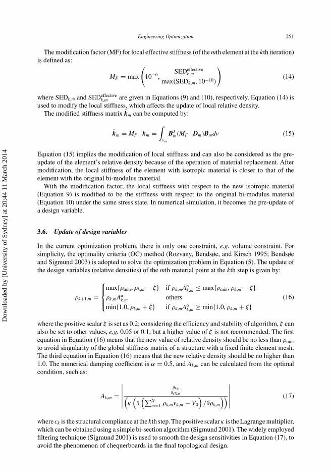
The modification factor (MF) for local effective stiffness (of the mth element at the kth iteration)is defined as:

MF = max

(10−6,

SEDeffectivek,m

max(SEDk,m, 10−10)

)(14)

where SEDk,m and SEDeffectivek,m are given in Equations (9) and (10), respectively. Equation (14) is

used to modify the local stiffness, which affects the update of local relative density.The modified stiffness matrix k̄m can be computed by:

k̄m = MF · km =∫

vm

BTm(MF · Dm)Bmdv (15)

Equation (15) implies the modification of local stiffness and can also be considered as the pre-update of the element’s relative density because of the operation of material replacement. Aftermodification, the local stiffness of the element with isotropic material is closer to that of theelement with the original bi-modulus material.

With the modification factor, the local stiffness with respect to the new isotropic material(Equation 9) is modified to be the stiffness with respect to the original bi-modulus material(Equation 10) under the same stress state. In numerical simulation, it becomes the pre-update ofa design variable.

3.6. Update of design variables

In the current optimization problem, there is only one constraint, e.g. volume constraint. Forsimplicity, the optimality criteria (OC) method (Rozvany, Bendsøe, and Kirsch 1995; Bendsøeand Sigmund 2003) is adopted to solve the optimization problem in Equation (5). The update ofthe design variables (relative densities) of the mth material point at the kth step is given by:

ρk+1,m =

⎧⎪⎨⎪⎩

max{ρmin, ρk,m − ξ} if ρk,mAαk,m ≤ max{ρmin, ρk,m − ξ}

ρk,mAαk,m others

min{1.0, ρk,m + ξ} if ρk,mAαk,m ≥ min{1.0, ρk,m + ξ}

(16)

where the positive scalar ξ is set as 0.2; considering the efficiency and stability of algorithm, ξ canalso be set to other values, e.g. 0.05 or 0.1, but a higher value of ξ is not recommended. The firstequation in Equation (16) means that the new value of relative density should be no less than ρmin

to avoid singularity of the global stiffness matrix of a structure with a fixed finite element mesh.The third equation in Equation (16) means that the new relative density should be no higher than1.0. The numerical damping coefficient is α = 0.5, and Ak,m can be calculated from the optimalcondition, such as:

Ak,m =∣∣∣∣∣∣

∂ck∂ρk,m(

κ(∂

(∑Nm=1 ρk,mvk,m − V0

)/∂ρk,m

))∣∣∣∣∣∣ (17)

where ck is the structural compliance at the kth step.The positive scalarκ is the Lagrange multiplier,which can be obtained using a simple bi-section algorithm (Sigmund 2001). The widely employedfiltering technique (Sigmund 2001) is used to smooth the design sensitivities in Equation (17), toavoid the phenomenon of chequerboards in the final topological design.

Dow

nloa

ded

by [

Uni

vers

ity o

f Sy

dney

] at

20:

44 1

1 M

arch

201

4

252 K. Cai et al.

3.7. Optimization procedure

(1) Create a FE model for structural optimization, and initiate the elastic modulus of elementsand design variables/relative density of elements.

(2) Perform the finite element analysis.(3) Calculate principal stresses and principal strains for each element.(4) Select the elastic modulus for each element, to be employed in the next step according to

Equation (7).(5) Calculate the local effective SED of each element, to obtain MF according to Equation (14).(6) Calculate the objective and constraint functions and their sensitivities; update the design

variables according to Equation (16).(7) Check the convergence of the algorithm: if Equation (18) is not satisfied, return to (2), else

go to 8).(8) Stop.

In this work, the initial elastic moduli of elements are the same as the tension modulus of theoriginal bi-modulus material. All the initial relative densities are considered to be identical. Theconvergent criterion is defined as below, according to the compliance of the structure:∣∣∣∣ cj

ck− 1.0

∣∣∣∣ ≤ η, j = k − 1, k − 2, . . . , k − 5 > 0 (18)

where the tolerance η = 0.001 is adopted. j = k − 1, k − 2, . . . , k − 5, is used to judge the con-vergence of algorithm, i.e. the relative errors between the structural compliances in the previousfive steps and the current the kth one should be no higher than the tolerance.

4. Numerical examples and discussions

The commercial software ANSYS (version 12.0; Ansys 2010) is employed for structural analysisin the following examples. In each example, a uniform finite element mesh is used to describethe structural geometry and mechanical response in the design domain. The same computer(Intel Pentium dual-core processor, CPU 2.66 GHz, 2 GB memory) with the same settings ofcomputational ability is used in the following examples.

4.1. Example 1: Analytical example

Figure 2(a) shows the design domain filled with bi-modulus material, which is a 1 m × 3.2 msquare plate with thickness of 0.01 m. The left side of the plate is fixed, and a concentrated forceP = 1.0 kN is applied at the centre of the right side of the plate. The tension modulus of thematerial is 210 GPa, and the Poisson’s ratios of the new isotropic materials are set to 0.2. Thestructure is discretized with 2700 four-nodal plane stress elements. In the optimization problem,the objective is to minimize the structural mean compliance and the constraint is that the finalstructural volume ratio (the ratio between the current volume and that of the full-solid structure)is less than 10%. To find the difference between the tension modulus and compression moduluson the topological designs, this example considers two numerical cases, namely (a) RTCE = 2 and(b) RTCE = 3.

Compared to the optimal topologies in Figure 2, their analytical solution following optimizationis discussed. The structure shown in Figure 3 is composed of two bars, AC and BC. The moduli ofthe two different bars E1 for AC and E2 for BC. The bars have the same area of cross-section, i.e.

Dow

nloa

ded

by [

Uni

vers

ity o

f Sy

dney

] at

20:

44 1

1 M

arch

201

4

Engineering Optimization 253

(a) (b) (c) (d)

Figure 2. Initial design domain and the final material distributions for different cases. For each case, the left figureshows density distribution, and the right one material modulus [pink (dark grey) = EC ; orange (light grey) = ET ]. (a)Initial design; (b) RTCE = 1; (c) RTCE = 2; (d) RTCE = 3.

Figure 3. Two-bar structure.

Abar. The distance between the joint C and the fixed line is a constant, i.e. h = 1. The deformationof the linear structure under the load of P is small. Supposing the total amount of material of thetwo-bar structure is fixed, e.g. V0, the purpose of this case is to determine the optimal values of α

and β to minimize the structural compliance. The problem can be expressed as Equation (19):

Find {α, β}

min : c = P · UT =(

N21

E1Abar+ N2

2

E2Abar

)

s.t.

(hAbar

sin α+ hAbar

sin β

)= V0

α, β ∈ (0, 90◦)

(19)

where U is the displacement vector of point C, and N1 and N2 are the axial forces of the two bars.

Dow

nloa

ded

by [

Uni

vers

ity o

f Sy

dney

] at

20:

44 1

1 M

arch

201

4

254 K. Cai et al.

The optimal design is simple and direct, because the two bars are orthogonally laid out,which implies that the relation between α and β (α + β = 90◦) and the existing mutual rela-tion E1 sin α = E2 cos α leads to the optimal design. Since bar AC is under tension and BC isunder compression, E1 = RTCEE2 will lead to cos α = RTCE sin α. For example, RTCE = 1 denotesα = 45◦, RTCE = 2 is for α ≈ 40.1◦ and RTCE = 3 is for α ≈ 37.3◦.

Now to focus on the original problem. Figure 2(b) shows the traditional resulting structure withisotropic material. The two bars in the structure are vertical and have the same length. Figure 2(c)gives the optimal topology of the structure with bi-modulus material under the condition ofRTCE = 2. It can be seen that the bars have different lengths. Analytically, the angle betweenthe fixed boundary and the bar under tension should approach α ≈ 40.1◦. At the same time, thecross-sectional areas of the two bars are identical. This is proved by the current result. Figure 2(d)demonstrates the final material distribution of the structure with material RTCE = 3. It givesthe same result as the analytical one. It can also be shown that the two bars have the samecross-sectional areas, but with different moduli.

4.2. Example 2: Sensitivity of material distribution to RTCE

A rectangle design domain of size 4 m × 1 m is given in Figure 4; the thickness is 0.01 m. Aconcentrated force P = 2000 N is applied vertically at the centre of its top surface, and the twovertical sides are fixed. The whole structure is discretized with 120 × 30 plane stress elements.The material in the structure is specified with different bi-modulus materials, to determine thedifferent effects of the moduli on the final material distribution. The Poisson’s ratios for the twonew isotropic materials are set as 0.2. For all the cases discussed below, the objective is to findthe optimal material distribution of the structure with 20% volume ratio to maximize the stiffnessof structure.

For the convenience of comparison, the traditional design, i.e. the structure with isotropicmaterial or RTCE = 1, is given in Figure 5(a). In this case, a very small amount of materialis under tension. Figure 5(b) gives the optimal topology of the structure with the bi-modulusmaterial when RTCE ≤ 0.25. It shows that the topology remains unchanged if RTCE is less than0.25. It is obvious that all the material in the final structure is under compression. Figure 5(c)shows the material optimal distribution in the structure when RTCE = 1.2. In the structure, therealso exists a small amount of material under tension, which is different from the traditional design.If the value of RTCE closes to 1.5, there is a larger portion of material under tension comparedwith the material under compression. The optimal material distribution is given in Figure 5(d),which shows that the topology of the structure changes again compared with the previous cases.Figure 5(e) gives the final material distribution in the structure when RTCE = 3. Both the topologyplot and the material ratio under compression have been changed, in contrast to the case withRTCE = 1.5.

When the tension modulus is much higher than the compression modulus, the topology of thefinal design is relatively simple, such as the topology of the structure with RTCE = 10 (Figure 5f).

Figure 4. Initial design domain of structure.

Dow

nloa

ded

by [

Uni

vers

ity o

f Sy

dney

] at

20:

44 1

1 M

arch

201

4

Engineering Optimization 255

Figure 5. Optimal material distributions for different RTCE: the upper is of relative density distribution; the lower is ofdistribution of moduli of materials [pink (dark grey) = EC ; orange (light grey) = ET ]. (a) Traditional design/RTCE = 1;(b) RTCE ≤ 0.25; (c) RTCE = 1.2; (d) RTCE = 1.5; (e) RTCE = 3; (f) RTCE = 10.

It can also be found that the hole in the middle region of the structure will disappear if the value ofRTCE is sufficiently high. However, the amount of material under compression will not decreaseand instead will increase to a higher level to decrease the displacement of the loading point. It canbe easily figured out that the number of elements under complex stress states (e.g. the ‘islands’in each figure) is very small. Although the distribution of element moduli looks complicated, thepaths formed by the solid elements (with unity relative densities) are very clear, which is beneficialto the manufacturing stage.

Figure 6 gives the iterations of structural compliances for different cases. The results show thatthe structural compliance decreases with the increase in RTCE. This is because the tension modulusof material is identical in all of the cases. Therefore, the compression modulus will decrease whenRTCE undergoes a larger change. It is easy to understand that the softer material will lead to ahigher compliance of the structure.

Table 1 gives the CPU times for each case. The results show that the difference between theiteration number for traditional design (RTCE = 1) by the SIMP method and those for bi-modulusdesigns by the present method are not obvious. At the same time, the differences between theaverage CPU times for those cases are also not obvious. The lowest efficiency is 41.89 secondsper iteration for the case of RTCE = 10, which is 9.5% higher than that for the case of RTCE = 1.It should also be mentioned that a detailed analysis of local stress states in modifications oflocal stiffness of elements is not required as the material shows isotropic material, i.e. RTCE = 1.

Dow

nloa

ded

by [

Uni

vers

ity o

f Sy

dney

] at

20:

44 1

1 M

arch

201

4

256 K. Cai et al.

Figure 6. Iteration histories of structural compliance for different cases.

Table 1. Computational cost for different cases.

Cases RTCE = 1a RTCE ≤ 0.25 RTCE = 1.2 RTCE = 1.5 RTCE = 3 RTCE = 10

Iterations 48 38 45 46 47 38Total CPU-T 1836 1567 1690 1768 1810 1592Average CPU-T 38.25 41.24 37.56 38.43 38.51 41.89

Note: aUsing the SIMP method; CPU time (seconds).

In other words, the computational cost of a structural topology optimization with bi-modulusmaterial solved by the present method is slightly different from that of the same structure withisotropic material solved by the SIMP method. Therefore, the efficiency of the present methodfor solving bi-modulus stiffness design is practically reasonable.

4.3. Example 3: Three-dimensional example

A block of size 1 m × 1 m × 0.75 m is shown in Figure 7. A concentrated force P of 1.0 kN isapplied vertically to the centre of its top surface. Four lines are fixed parallel to the top surfaceand with the same distances of 0.25 m. Considering its symmetry, only a quarter of the structure

Figure 7. Initial design of a block structure.

Dow

nloa

ded

by [

Uni

vers

ity o

f Sy

dney

] at

20:

44 1

1 M

arch

201

4

Engineering Optimization 257

is included in the simulation. The whole structure is discretized with 30 × 30 × 45 eight-nodebrick elements. Supposing the structure is filled with a bi-modulus material in which the tensionmodulus and Poisson’s ratio are 100 GPa and 0.2, respectively. The tension modulus is three timesthe compression modulus, i.e. RTCE = 3. The objective of structural optimization is to minimizethe structural compliance, and the allowable material usage ratio is 1.5%.

The right column in Table 2 gives the optimal isotropic material distribution of the structure,in which the modulus of material is 100 GPa. It is obvious that there are four supports in thestructure, all of which are only under compression. There is no material remaining below the‘fixed lines’ in Figure 7. The right column in Table 2 shows the final topology design of thestructure with bi-modulus material when RTCE = 3.0. It can be seen that the topology is differentfrom the traditional design (left column in Table 2). Obviously, part of the material in the structureis under tension. The major reason is that the tension modulus is much higher than the compressionmodulus. To improve the stiffness of the structure, more material under tension should be used.

Table 2. Comparison between material distributions of isotropic and bi-modulus materials.

Isotropic material/RTCE = 1.0 Bi-modulus material/RTCE = 3.0

Top view

Side view

Oblique view

Dow

nloa

ded

by [

Uni

vers

ity o

f Sy

dney

] at

20:

44 1

1 M

arch

201

4

258 K. Cai et al.

–3

–2

–1

0

1

2

0 10 20 30 40 50Iteration Number

Log

(Com

plia

nce/

(N.m

), 1

0)

RTCE=3

RTCE=1

Figure 8. Iteration histories of objective function for different cases.

Figure 8 demonstrates the iteration histories of the objective function for different cases, i.e.the structure with different types of materials. In both cases, the objectives fluctuate from step5 to step 13. The reason is that the initial relative densities of elements are set to be 1.0. So,solutions of the first nine steps are not feasible for the case of RTCE = 1.0, and the first 11 stepsfor RTCE = 3.0. After 43 iterations, the optimization objective with isotropic material reaches itsminimum, i.e. 0.00892 Nm. For the structure with bi-modulus material, 48 iterations are required toreach the optimum, with the objective value 0.0234 Nm. The objective value for the bi-modulusmaterial is about 2.62 times that of the isotropic material. The reason is that nearly half ofthe material remaining in the structure is under compression with a modulus of one-third of100 GPa.

5. Conclusions

Bi-modulus materials, e.g. concrete, iron and rubber, are very popular in practical engineering.Intuitively, the traditional solution, in which the bi-modulus material is considered as an isotropicmaterial, may be far from the real ‘optimal’ design considering the characteristics of the piece-wise linear constitutive curve of the bi-modulus material. In consideration of such problems, in themethod presented here, the bi-modulus material in the design domain is replaced by two isotropicmaterials. Both the relative densities of elements and their elastic moduli need to be updated initerations to bring the local stiffness close to the real values. Numerical results have shown thevalidity of the material-replacement method for topology optimization of continuum structureswith bi-modulus materials. In detail:

(1) The example of the two-bar structure shows that analytical results can be obtained by thepresent method.

(2) The optimal topologies of some structures are very sensitive to the ratio between the tensionmodulus and compression modulus. This shows that the optimal design, under the assumptionthat there is no difference between the compression and extension properties, may lead to atopology design that is not really expected in the manufacturing stage.

(3) With the present method, the computational cost of solving bi-modulus material layoutoptimization problems is approximately equal to that of solving topology optimization prob-lems with isotropic material, which is beneficial in reducing the computational cost forthree-dimensional bi-modulus layout optimization designs.

Dow

nloa

ded

by [

Uni

vers

ity o

f Sy

dney

] at

20:

44 1

1 M

arch

201

4

Engineering Optimization 259

Acknowledgements

This study is partially supported by the National Natural Science Foundation of China (50908190, 51279171), the YouthTalents Foundation of Shanxi Province (2011KJXX02), Research Foundation of NorthwestA&F University (QN2011125),and Research Foundation (GZ1205) of State Key Laboratory of Structural Analysis for Industrial Equipment, DalianUniversity of Technology, Dalian, PR China. This support is gratefully acknowledged.

References

Allaire, G., F. Jouve, and A. M. Toader. 2004. “Structural Optimization Using Sensitivity Analysis and a Level-SetMethod.” Journal of Computational Physics 194: 363–393.

Ambarstumyan, S. A. 1970. “Equations of the Theory of Thermal Stresses in Double-Modulus Materials.” In Proceedingsof the IUTAM Symposium, June 25–28. East Kilbride. Vienna: Springer.

Andreasen, C. S., A. R. Gersborg, and O. Sigmund. 2009. “Topology Optimization of Microfluidic Mixers.” InternationalJournal for Numerical Methods in Fluids 61: 498–513.

Ansys. 2010. ANSYS. http://www.ansys.comBendsøe, M. P., and N. Kikuchi. 1988. “Generating Optimal Topology in Structural Design Using a Homogenization

Method.” Computer Methods in Applied Mechanics and Engineering 71: 197–224.Bendsøe, M. P., and O. Sigmund. 1999. “Material Interpolation Schemes in Topology Optimization.” Archive of Applied

Mechanics 69: 635–654.Bendsøe, M. P., and O. Sigmund. 2003. Topology Optimization: Theory, Methods, and Applications. Berlin: Springer.Cai, K. 2011. “A Simple Approach to Find Optimal Topology of a Continuum with Tension-only or Compression-Only

Material.” Structural and Multidisciplinary Optimization 43: 827–835.Cai, K., and J. Shi. 2008. “A Heuristic Approach to Solve Stiffness Design of Continuum Structures with Tension/

Compression-Only Materials.” In Proceedings of the 4th International Conference on Natural Computation, October18–20, Jinan, China, Los Alamitos, CA: IEEE Computer Society, 1, 131–135.

Chang, C. J., B. Zheng, and H. C. Gea. 2007. “Topology Optimization for Tension/Compression only Design.” In Pro-ceedings of the 7th World Congress on Structural and Multidisciplinary Optimization, May 21–25, COEX Seoul,South Korea. Seoul: WCSMO-7 Official Agency, 1, 2488–2495.

Dewhurst, P. 2005. “A General Optimality Criterion for Combined Strength and Stiffness of Dual-Material-PropertyStructures.” International Journal of Mechanical Sciences 47: 293–302.

Dewhurst, P., N. Fang, and S. Srithongchai. 2009. “A General Boundary Approach to the Construction of Michell TrussStructures.” Structural and Multidisciplinary Optimization 39: 373–384.

Du, Y., Z. Luo, Q. Tian, and L. Chen. 2009. “Topology Optimization for Thermo-Mechanical Compliant Actuators UsingMesh-Free Methods.” Engineering Optimization 41: 753–772.

Dühring, M. B., J. S. Jensen, and O. Sigmund. 2008. “Acoustic Design by Topology Optimization.” Journal of Sound andVibration 317: 557–575.

Jung, D., and H. C. Gea. 2004. “Topology Optimization of Nonlinear Structures.” Finite Element Analysis and Design40: 1417–1427.

Kang, Z., and L. Y. Tong. 2008. “Integrated Optimization of Material Layout and Control Voltage for PiezoelectricLaminated Plates.” Journal of Intelligent Material Systems and Structures 19: 889–904.

Kato, J., A. Lipka, and E. Ramm. 2009. “Multiphase Material Optimization for Fiber Reinforced Composites with StrainSoftening.” Structural and Multidisciplinary Optimization 39: 63–81.

Liu, S. T. and H. T. Qiao. 2011. “Topology Optimization of Continuum Structures with Different Tensile and CompressiveProperties in Bridge Layout Design.” Structural and Multidisciplinary Optimization 43: 369–380.

Luo, Z., Q. Luo, L. Tong, W. Gao, and C. Song. 2011. “Shape Morphing of Laminated Composite Structures withPhotostrictive Actuators via Topology Optimization Methods.” Composite Structures 93: 406–418.

Luo, Z., L. Tong, and H. Ma. 2009. “Shape and Topology Optimization for Electrothermomechanical Microactuatorsusing Level Set Methods.” Journal of Computational Physics 228: 3173–3181.

Luo, Z., J.Yang, and L. Chen. 2006. “A New Procedure for Aerodynamic Missile Designs Using Topological OptimizationApproach of Continuum Structures.” Aerospace Science and Technology 10: 364–373.

Maute, K., and D. M. Frangopol. 2003. “Reliability-Based Design of MEMS Mechanisms by Topology Optimization.”Computers & Structures 81: 813–824.

Medri, G. 1982. “A Nonlinear Elastic Model for Isotropic Materials with Different Behavior in Tension and Compression.”Journal of Engineering Materials and Technology 104: 26–28.

Paulino, G. H., E. C. N. Silva, and C. H. Le. 2009. “Optimal Design of Periodic Functionally Graded Composites withPrescribed Properties.” Structural and Multidisciplinary Optimization 38: 469–489.

Querin, O. M., M. Victoria, and P. Marti. 2010. “Topology Optimization of Truss-Like Continua with Different MaterialProperties in Tension and Compression.” Structural and Multidisciplinary Optimization 42: 25–32.

Rozvany, G. I. N., M. P. Bendsøe, and U. Kirsch. 1995. “Layout Optimization of Structures.” Applied Mechanics Review48: 1579–1605.

Sigmund, O. 2001. “A 99 Line Topology Optimization Code Written in MATLAB.” Structural and MultidisciplinaryOptimization 31: 419–429.

Dow

nloa

ded

by [

Uni

vers

ity o

f Sy

dney

] at

20:

44 1

1 M

arch

201

4

260 K. Cai et al.

Sigmund, O. and J. Petersson. 1998. “Numerical Instabilities in Topology Optimization: A Survey on Procedures Dealingwith Checkerboards, Mesh-Dependencies and Local Minima.” Structural and Multidisciplinary Optimization 16:68–75.

Simmonds, J. G. 1991. A Brief on Tensor Analysis. 2nd ed. New York: Springer.Swan, C. C., and J. S. Arora. 1997. “Topology Design of Material Layout in Structured Composites of High Stiffness and

Strength.” Structural and Multidisciplinary Optimization 13: 45–59.Wang, M. Y., X. M. Wang, and D. M. Guo. 2003. “A Level Set Method for Structural Topology Optimization.” Computer

Methods in Applied Mechanics and Engineering 192: 227–246.Xie, Y. M., and G. P. Steven. 1993. “A Simple Evolutionary Procedure for Structural Optimization.” Computers &

Structures 49: 885–896.Zhou, M., and G. I. N. Rozvany. 1991. “The COC Algorithm, Part II: Topological, Geometry and Generalized Shape

Optimization.” Computer Methods in Applied Mechanics and Engineering 89: 197–224.Zhuang, C. G., Z. H. Xiong, and H. Ding. 2007. “A Level Set Method for Topology Optimization of Heat Conduction

Problem Under Multiple Load Cases.” Computer Methods in Applied Mechanics and Engineering 106: 1074–1084.Zhuang, C. G., Z. H. Xiong, and H. Ding. 2010. “Topology Optimization of Multi-Material for the Heat Conduction

Problem Based on the Level Set Method.” Engineering Optimization 42: 811–831.

Dow

nloa

ded

by [

Uni

vers

ity o

f Sy

dney

] at

20:

44 1

1 M

arch

201

4