Quantum simulation of non-trivial topology

Octavi BoadaPhysics of Information Group, Instituto de Telecomunicacoes, P-1049-001 Lisbon, Portugal

Alessio Celi and Maciej LewensteinICFO-Institut de Ciencies Fotoniques, Barcelona, Spain

Javier Rodrıguez-LagunaIFT-Instituto de Fısica Teorica, UAM-CSIC, Madrid, Spain and

ICFO-Institut de Ciencies Fotoniques, Barcelona, Spain

Jose I. LatorreDept. ECM, Universitat de Barcelona, Spain

We propose several designs to simulate quantum many-body systems in manifolds with a non-trivial topology. The key idea is to create a synthetic lattice combining real-space and internaldegrees of freedom via a suitable use of induced hoppings. The simplest example is the conversionof an open spin-ladder into a closed spin-chain with arbitrary boundary conditions. Further ex-ploitation of the idea leads to the conversion of open chains with internal degrees of freedom intoartificial tori and Mobius strips of different kinds. We show that in synthetic lattices the Hubbardmodel on sharp and scalable manifolds with non-Euclidean topologies may be realized. We providea few examples of the effect that a change of topology can have on quantum systems amenable tosimulation, both at the single-particle and at the many-body level.

I. INTRODUCTION

The research field of quantum simulation explores,among other goals, the possibility of using well-controlledquantum systems to simulate the behavior of other quan-tum systems whose dynamics escapes standard theoret-ical or experimental approaches. As a relevant exam-ple, quantum simulators have been used to successfullyanalyse condensed matter phenomena [1]. Through syn-thetic gauge fields [2], more ambitious and multidisci-plinary problems can be addressed, such as the determi-nation of the phase diagram of (lattice) gauge theories[3–8]. This theoretical progress is supported by vigor-ous experimental developments with a growing numberof platforms available for quantum simulation like coldneutral atoms and molecules [9], trapped ions [10], pho-tonic crystals [11], NV-centers [12], and superconductingqubits [13].

On a different line of research, topological models haveattracted great interest as well. Topology is a key featureto understand many physical phenomena, such as thequantum Hall and quantum spin-Hall effects [14], quan-tization of Dirac monopole charge [15], charge fractional-ization and non-perturbative properties of vacua of Yang-Mills theories [16–19], etc. Topology also plays an essen-tial role in engineering novel states of ultracold matter,such as topological insulators [20]. Notably, topologicalprotection has been considered as a resource for quan-tum computation [21]. Nonetheless, non-trivial topol-ogy is not easy to implement in practical systems. Forinstance, there is no obvious way to manipulate a 2Dcondensed matter system to be topologically connectedas on a higher genus Riemann surface. Experimental

limitations are thus an obstacle to analyse the effects ofnon-trivial topologies on quantum systems.

The reunion of these two topics, namely quantum sim-ulation and topology, is a natural and tantalizing evolu-tion for both sets of ideas. So far, the focus in quantumsimulation has been on topological properties emergingin infinite systems due to their dynamics, e.g., in thetoric code [22–24] or in periodically driven systems [25–27], and in synthetic quantum Hall [28–31] and quantumspin-Hall [32–36] systems that exhibit edge states whensubjected to open boundary conditions. The search foredge states includes also theoretical and experimental ef-forts in understanding Majorana fermions, since they areproduced at the boundaries of some quantum systems[37–39]. But, so far, the simulation of systems with non-trivial boundary conditions, with the exception of cir-cle/torus geometry (cf. theory [40–42], and experiments[43–49], and references therein), has been very scantilyexplored (see also [50, 51], which appeared while thiswork was in progress).

Geometry and topology have already made their ap-pearance in quantum simulators, specifically in opticallattices with ultracold atoms. Recently, there have beenproposals to simulate quantum many-body physics in cer-tain types of curved background spacetimes [52], tailor-ing the hopping amplitudes of the optical lattice. More-over, in [53] a protocol was introduced to use the differentatomic states as an artificial extra dimension. This latterproposal plays a key role in our approach to the simula-tion of quantum matter in different topologies. In effect,by managing the internal interactions between the inter-nal states, we will show how to turn an open 1D opticallattice into a system with periodic boundary conditions,a cylinder, a torus or a Mobius strip. Our proposal can

arX

iv:1

409.

4770

v1 [

cond

-mat

.qua

nt-g

as]

16

Sep

2014

2

be engineered also using other platforms and/or may becombined with other techniques such as the ones allowingfor well-established toroidal compactifications [54–69], orthe speckle potentials allowing to simulate in a controlledway disorder [70, 71].

The paper is organized as follows. Section II presentsthe general strategy to simulate non-trivial topology on aquantum system, while the experimental aspects are dis-cussed in section III. Section IV is devoted to an analysisof signatures of non-trivial topological effects, which canbe observed in systems amenable to experimental realiza-tion. We end up, in section V presenting the conclusionsand a discussion of the possibilities for future work.

II. ARTIFICIAL TOPOLOGY

The general aim of our work is to build quantum sim-ulators for dynamics in different topologies out of an op-tical lattice, which naturally have open boundary condi-tions. In order to illustrate our strategy let us start withthe simplest paradigmatic example: simulating quantumdynamics on a ring i.e., a 1D system with periodic bound-ary conditions (PBC). In principle, this can be achievedby embedding it into a plane, bending it into a circum-ference and creating an effective interaction between thetwo extremes which is identical to the one in the bulk.Thus, an extra dimension is required, as well as the possi-bility of bending the system without altering its dynam-ical properties. Both requirements are difficult to meet.Therefore, we shall explore a different possibility, whichamounts to engineering an artificial extra dimension.

For definiteness, let us discuss a bosonic 1D hoppingmodel with L sites whose Hamiltonian is merely kinetic.

Let a†i create a boson at site i. The PBC are obtainedby connecting the end points with an extra term.

Hc = −

(J

L−1∑i=1

a†iai+1 + Jca†1aL

)+H.c., (1)

where Jc, the closing hopping, should be taken as Jc = J .The problem of simulating an S1 topology is tanta-mount to generating this closing term which connectsboth boundaries of the system. There are several genericstrategies to create that term:

• Embed the system in a plane and bend it until bothboundaries touch, thus reducing the boundary termto an ordinary bulk term.

• Induce a long-range hopping through a medium oran intermediate state.

• Use a synthetic dimension.

This work focuses on the last solution. The introduc-tion of an extra dimension through internal degrees offreedom was proposed in [53]. Indeed, an open 1D line

FIG. 1. Idea of a synthetic lattice: a 1D chain of length Lsites with M species is equivalent to a L×M synthetic lattice,once the chain is dressed with appropriate couplings betweenspecies.

of L sites, each endowed with M internal states, can beregarded as an L ×M synthetic 2D lattice, see Fig. 1.In geometric terms, we can think of the internal statesas a fiber opening at each real-space site. The resultingsynthetic lattice would be, therefore, a discrete analogueof a fibre bundle. A generic hopping Hamiltonian for thissystem can be written as

H = −

∑σ,σ′

L−1∑i=1

Jvi,σ,σ′b†(σ)i b

(σ′)i + Jhi,σ,σ′b

†(σ)i b

(σ′)i+1

+H.c.,

(2)where Jv and Jh are sets of vertical and horizontal hop-pings, in the synthetic lattice view. The vertical termallows us to connect any pair of internal states in thesame physical site, while the horizontal term allows us toconnect any two internal states in physically neighboringsites.

Figure 2 illustrates the process by which we can con-vert an open spin chain with M = 2 states per site into asystem with PBC. In Eq. (2), simply set Jhi,σ,σ′ = J δσ,σ′

and Jvi,σ,σ′ to be zero in the bulk, but not in the ex-tremes, i = 1 or i = L, in which case we have a con-necting term between the two species: Jvi,1,2 = J . If we

introduce 2L virtual particle creation operators, aj = b(1)j

and a2L+1−j = b(2)j , j = 1, . . . , L, the Hamiltonian reads

exactly as a 1D-PBC hopping Hamiltonian.Let us summarize the idea. By inducing appropriate

hoppings on the internal degrees of freedom —whetherwe call them species, spin values, etc.— we can attaineffectively higher-dimensional dynamics, giving them ageometric meaning [53]. This higher dimension can bebent and sewn in different ways, as shown in the previousexample. The simplest application consists on turningan open chain with two species into a closed one witha single species. It only needs localized control of thetransformations between the species at the boundaries ofthe open system.

As an additional feature, our synthetic approach al-lows to control the phases of the induced hoppings. This

3

FIG. 2. Engineering a circumference of 2L lattice sites from aL synthetic lattice that carries M = 2 species. The blue solidlinks indicate the hopping along the chain, e.g., the free hop-ping in a cold-atom implementation, while the two dashed redlinks are induced local interactions between the two species,e.g., a Raman coupling between hyperfine levels of atoms.The vertical black ellipses represent the physical sites in thereal 1D-chain occupied by the two species.

is equivalent to inducing a magnetic field piercing thechain and, via a gauge transformation, to create bound-ary conditions which interpolate continuously betweenperiodic and anti-periodic ones. In critical 1D spin mod-els a non-trivial magnetic flux can be regarded as a defectin the associated conformal field theory (CFT) [72, 73].

The 1D-PBC lattice described above is the basic build-ing block for more interesting 2D models. In the nextsections we will discuss more exotic boundary conditions,such as Mobius strips.

A. Assembling cylinder and torus

A cylinder can be understood as a fiber bundle of seg-ments emerging from each point of a circumference. Letus describe how to create cylindricalal synthetic lattice(i.e., a ladder with PBC) of size 2Lx×Ly from a 1D openchain of Lx real sites, with M = 2Ly internal states per

site. Let a†i,j create a particle at site (i, j) of the cylin-der. Its correspondent in the synthetic lattice will be

b†(2j−1)i if i ≤ Lx and b

†(2j)2Lx+1−i otherwise. An example

with Ly = 2 is shown in figure 3.

The Hamiltonian of a free bosonic system on a cylindercan be written as

H =− J

2Lx∑i=1

Ly∑j=1

a†i,j(ai+1,j + ai,j+1)

+

Ly∑j=1

a†2Lx,ja1,j

+H.c. (3)

which can be mapped to the form (2). If i 6= 1 and i 6= L,we have

Jhi,σ,σ′ = J δσ,σ′

Jvi,σ,σ′ = J Bσ,σ′(4)

FIG. 3. Engineering a cylinder of basis Lx and height Lylattice sites from a L ×M synthetic lattice with L = Lx/2and M = 2Ly. (a) Ly = 2 synthetic cylinder. In a coldatom implementation, the blue solid links indicate the freehopping while the dashed ones are laser or radio-frequencyinduced. The dashed red links are the “sewing” hoppingsCσσ′ closing each circle of the cylinder, while the dashed greenones are the hoppings Bσσ′ along its height, connecting thedifferent circles. (b) and (c) Spectroscopical arrangement ofthe four internal degrees of freedom in the one-manifold andtwo-manifold scheme, respectively. The former can be realizedby using the groundstate of atoms F ≥ 3

2like Li, K, Yb, Sr,

Er, etc, and requires quadratic Zeeman splitting in order tohave J ′-coupling (in red) only between odd-even mF -states.The latter requires earth-alkali like atoms with F ≥ 1

2as

171Yb, 173Yb, and 87Sr and in this case the linear splittingis sufficient in order to make the spin accessible by Ramanlasers or radio-frequency pulses.

where Bσ,σ′ is a 2Ly × 2Ly bulk Hermitian matrix ofinternal hoppings implementing motion in the transversedirection of the cylinder

Bσ,σ′ = δσ,σ′±2, (5)

i.e., it is always possible to jump between internal statesdiffering by two units. On the extremes, for i = 1 ori = L, we have to add a new term

Jvi,σ,σ′ = J Bσ,σ′ + J Cσ,σ′ (6)

where Cσ,σ′ is a closing Hermitian matrix which is re-sponsible for sewing the open edges of the cylinder. Sinceit corresponds to a pile of circumferences, the non-zeroentries of those matrix are of the form C2j−1,2j andC2j,2j−1. The geometrical meaning of that closing ma-trix is that each horizontal line bends on itself, withoutmixing.

The synthetic cylinder we just described can be easilyturned into a torus by changing matrix Bσ,σ′ , with the in-troduction of new non-zero terms B1,2Ly−1 = B2Ly−1,1 =B2,2Ly

= B2Ly,2 = 1 which sew together the upper andlower ends of each fiber, see Fig. 4. This constructionmakes sense for Ly ≥ 3. In other terms, each fiber be-comes a circumference instead of an open segment. How-ever, while the number of layers, Ly, of the cylinder are

4

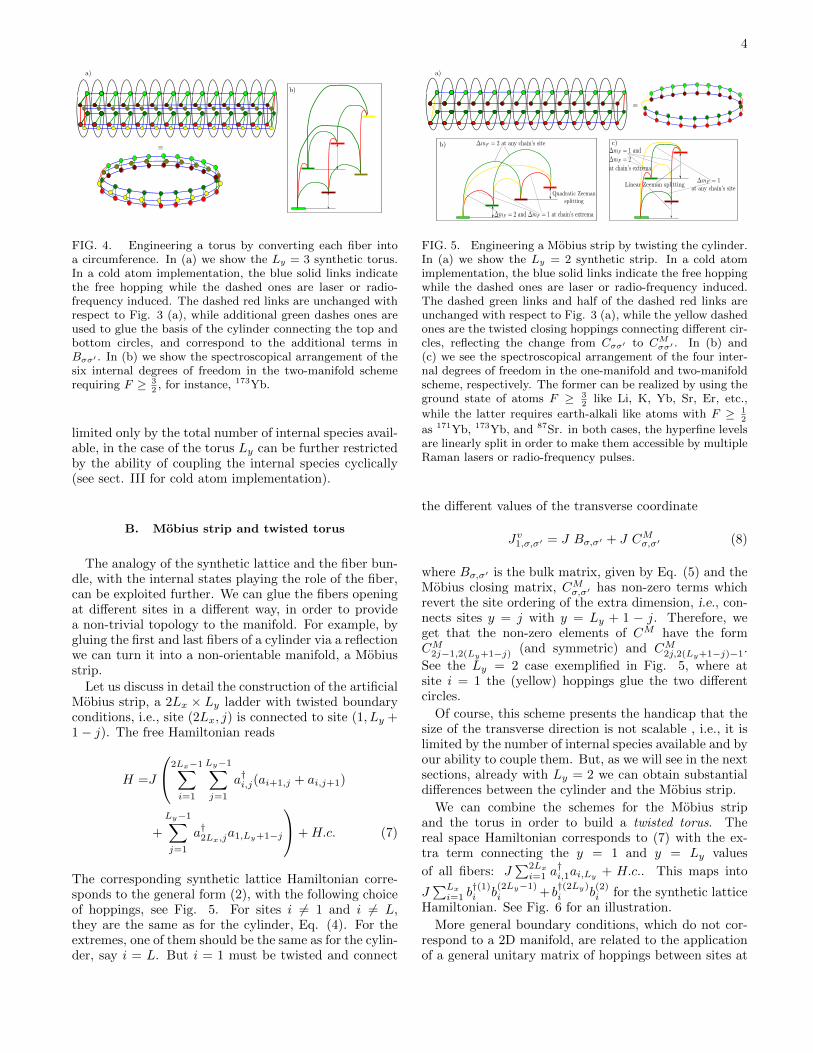
FIG. 4. Engineering a torus by converting each fiber intoa circumference. In (a) we show the Ly = 3 synthetic torus.In a cold atom implementation, the blue solid links indicatethe free hopping while the dashed ones are laser or radio-frequency induced. The dashed red links are unchanged withrespect to Fig. 3 (a), while additional green dashes ones areused to glue the basis of the cylinder connecting the top andbottom circles, and correspond to the additional terms inBσσ′ . In (b) we show the spectroscopical arrangement of thesix internal degrees of freedom in the two-manifold schemerequiring F ≥ 3

2, for instance, 173Yb.

limited only by the total number of internal species avail-able, in the case of the torus Ly can be further restrictedby the ability of coupling the internal species cyclically(see sect. III for cold atom implementation).

B. Mobius strip and twisted torus

The analogy of the synthetic lattice and the fiber bun-dle, with the internal states playing the role of the fiber,can be exploited further. We can glue the fibers openingat different sites in a different way, in order to providea non-trivial topology to the manifold. For example, bygluing the first and last fibers of a cylinder via a reflectionwe can turn it into a non-orientable manifold, a Mobiusstrip.

Let us discuss in detail the construction of the artificialMobius strip, a 2Lx × Ly ladder with twisted boundaryconditions, i.e., site (2Lx, j) is connected to site (1, Ly +1− j). The free Hamiltonian reads

H =J

2Lx−1∑i=1

Ly−1∑j=1

a†i,j(ai+1,j + ai,j+1)

+

Ly−1∑j=1

a†2Lx,ja1,Ly+1−j

+H.c. (7)

The corresponding synthetic lattice Hamiltonian corre-sponds to the general form (2), with the following choiceof hoppings, see Fig. 5. For sites i 6= 1 and i 6= L,they are the same as for the cylinder, Eq. (4). For theextremes, one of them should be the same as for the cylin-der, say i = L. But i = 1 must be twisted and connect

FIG. 5. Engineering a Mobius strip by twisting the cylinder.In (a) we show the Ly = 2 synthetic strip. In a cold atomimplementation, the blue solid links indicate the free hoppingwhile the dashed ones are laser or radio-frequency induced.The dashed green links and half of the dashed red links areunchanged with respect to Fig. 3 (a), while the yellow dashedones are the twisted closing hoppings connecting different cir-cles, reflecting the change from Cσσ′ to CMσσ′ . In (b) and(c) we see the spectroscopical arrangement of the four inter-nal degrees of freedom in the one-manifold and two-manifoldscheme, respectively. The former can be realized by using theground state of atoms F ≥ 3

2like Li, K, Yb, Sr, Er, etc.,

while the latter requires earth-alkali like atoms with F ≥ 12

as 171Yb, 173Yb, and 87Sr. in both cases, the hyperfine levelsare linearly split in order to make them accessible by multipleRaman lasers or radio-frequency pulses.

the different values of the transverse coordinate

Jv1,σ,σ′ = J Bσ,σ′ + J CMσ,σ′ (8)

where Bσ,σ′ is the bulk matrix, given by Eq. (5) and theMobius closing matrix, CMσ,σ′ has non-zero terms whichrevert the site ordering of the extra dimension, i.e., con-nects sites y = j with y = Ly + 1 − j. Therefore, weget that the non-zero elements of CM have the formCM2j−1,2(Ly+1−j) (and symmetric) and CM2j,2(Ly+1−j)−1.

See the Ly = 2 case exemplified in Fig. 5, where atsite i = 1 the (yellow) hoppings glue the two differentcircles.

Of course, this scheme presents the handicap that thesize of the transverse direction is not scalable , i.e., it islimited by the number of internal species available and byour ability to couple them. But, as we will see in the nextsections, already with Ly = 2 we can obtain substantialdifferences between the cylinder and the Mobius strip.

We can combine the schemes for the Mobius stripand the torus in order to build a twisted torus. Thereal space Hamiltonian corresponds to (7) with the ex-tra term connecting the y = 1 and y = Ly values

of all fibers: J∑2Lx

i=1 a†i,1ai,Ly

+ H.c.. This maps into

J∑Lx

i=1 b†(1)i b

(2Ly−1)i + b

†(2Ly)i b

(2)i for the synthetic lattice

Hamiltonian. See Fig. 6 for an illustration.

More general boundary conditions, which do not cor-respond to a 2D manifold, are related to the applicationof a general unitary matrix of hoppings between sites at

5

FIG. 6. Engineering a twisted torus by wrapping the Mobiusstrip. Equivalently, a twisted torus can be visualized as atorus cut and glued with a twist. In (a) we see the Ly = 3synthetic twisted torus. In a cold atom implementation, theblue solid links indicate the free hopping while the dashedones are laser or radio-frequency induced. The dashed redlinks are unchanged with respect to Fig. 5 (a), while thegreen dashed ones are used to glue the borders of the Mobiusstrip. In (b) we show the spectroscopical arrangement of thesix internal degrees of freedom in the two-manifold scheme,which requires F ≥ 3

2as, for instance, in 173Yb.

i = 2Lx and i = 1, which can be parametrized as

Ly∑j,j′=1

Uj,j′a†2Lx,j

a1,j′ +H.c. (9)

where U ∈ U(Ly). If U is the identity matrix, we obtainthe cylinder. Let us now consider the case Ly = 2. TheMobius strip corresponds to the U = σx case, which hasdeterminant −1. Therefore, can not be connected con-tinuously to the identity matrix. On the other hand, onecan reach a pseudo-Mobius strip using a rotation of π,U1,2 = −U2,1 = 1.

III. COLD ATOM IMPLEMENTATION

In this section, we show how the artificial topologiesdescribed previously can be made concrete, for instance,in a cold atom set-up. The basic features that allow torealize the abstract construction of sect. II in a cold atomsystem are the following:

• the synthetic lattice is obtained by loading in a 1D(spin-independent) optical lattice the atoms, whosehyperfine states, belonging to a unique or few hy-perfine manifolds, provide internal species whichform the synthetic dimension;

• the hopping term Jhi,σ,σ′ of (2) is the free hoppingof atoms in the 1D optical lattice and is naturallyspin-independent, Jhi,σ,σ′ = J δσ,σ′ , as assumed in

the construction of Hamiltonians (3) and (7) andtheir periodic completions;

• the hopping term Jvi,σ,σ′ is induced and tailored bylaser and radiofrequency couplings which are local

in the real-space picture, i.e., are acting on a singlesite of the 1D chain.

A similar dictionary can be obtained for other platforms.For instance, in the spirit of [53], a synthetic dimensioncan be achieved also in photonic crystals as in [74, 75],by changing the connectivity of the lattice.

It is worth to notice that, while the real spatial dimen-sion is virtually “unlimited” (or better scaled up to order102 lattices sites), the synthetic dimension is limited al-ways by the number of atomic internal states available,which is up to 10 for standard atoms like 40K or 87Sr [76],but can be up to 20 in 167Er [77], if just one hyperfinemanifold is taken into account. However, by consider-ing more than one hyperfine manifold simultaneously orultracold molecules, see e.g., [78], this number can befurther increased. A limited synthetic dimension trans-lates into a limited transverse dimension of the artificialtopology.

Let us start by discussing how to implement the build-ing block of our construction, a (spinless) periodic chainfrom a (spinful) open one. In cold atoms, model (2) ap-plied to create PBC can be realized for instance by load-ing atoms with at least two hyperfine (almost degenerate)ground states (F ≥ 1

2 ) in a spin-independent quasi-1Doptical lattice of L sites. The free tunneling provides theterms in Jh, while the terms in Jv can be created usingRabi oscillations between the hyperfine states, inducedby Raman lasers focused on sites 1 and L, respectively.Thus, the synthetic approach we are proposing is essen-tially local, since the different species are physically atthe same site. Notice the scalability of the procedure:we can build PBC 1D systems of any size 2L, if we canbuild an associated open system with L sites and M = 2internal states.

A. Cylinder and Torus

Let us extend the above construction to the simulationof a cylinder by layering many circles together as ex-plained in sect. II A. It is easy to realize that the Hamil-tonian of (3) can be implemented with up to two-photontransitions. Indeed, the most direct arrangement of theinternal degrees of freedom σ is in terms of hyperfine

states within a unique hyperfine manifold F ≥ Ly−12 , e.g.,

|σ〉 = b(σ)†|0〉 = |F,mF = m+ σ〉. For this ordering ofthe spins, the synthetic sewing coupling Cσσ′ applied atreal-space sites i = 1 and i = L requires ∆mF = 1, whilethe synthetic transverse coupling Bσσ′ requires ∆mF = 2for any Ly. Thus, the only limitation in Ly is given bythe number of available internal states. It is worth to no-tice that the coupling Cσσ′ applies only alternatively, i.e.,it connects only odd and even spin values. This impliesthat the hyperfine states have to be spectroscopically dis-tinguishable, for instance, through a quadratic Zeemansplitting.

The spin arrangement considered above is not the only

6

possible one. Furthermore, two or more (meta)stable hy-permanifolds can be considered. Such a construction isparticularly favorable in earth-alkali like atoms like Yb(see e.g., [79–82]) where the optically connected 1S0 andthe 3P0 may be used. In this case, a convenient arrange-ment is to place odd (even) σ’s in the first (second)manifold, i.e., |2σ〉 = b(2σ)†|0〉 = |I, F,mF = m+ σ〉,(|2σ + 1〉 = b(2σ+1)†|0〉 = |II, F,mF = m+ σ〉). Thus,the Hamiltonian (3) involves in this scheme just ∆mF =1 transitions. As further discussed below (cf. sect. III C),the two-manifold construction allows for a richer interac-tion pattern than single-manifold one. Both schemes aredepicted in Fig. 3.

Let us now turn to the implementation of a torus ge-ometry. As described in sect. II A, further couplings areneeded, which connect the top and the bottom circles. Inthe synthetic-lattice basis, this is equivalent to connect-ing the last of the odd (even) spins with the first odd(even) one, for any real-space site. Such a constructionmakes sense when Ly is at least 3, the case whose im-plementation is detailed in Fig. 4. For simplicity, let usfocus on the two-manifold construction. Here, the addi-tional coupling requires just ∆mF = 2 and, similarly tothe periodic boundary conditions engineered in [30], canbe achieved for instance via a 3-photon transition. Forgeneric Ly, the needed transition has ∆mf = Ly − 1.

B. Mobius and Twisted Torus

Let us now discuss the cold atom implementation ofa Mobius strip. As explained in sect. II B, we can geta Mobius from the cylinder by replacing the syntheticcoupling Cσσ′ , at (e.g.) real-space site i = 1 with thecoupling CMσσ′ . This is equivalent to connecting the in-ternal states |σ = 2l〉 with |2(Ly + 1− l)〉, and the states|σ = 2l − 1〉 with |2(Ly − l) + 1〉, for l = 1, . . . , Ly. Itis immediate to realize that for any arrangement of theinternal states as hyperfine states (both in the one- andtwo-manifold scenarios) this implies that the maximum∆mf needed to engineer CMσσ′ scales with Ly. For in-stance, in the two-manifold scheme with the arrangementfor the σ’s described above, the maximal ∆mF is exactlyLy, see Fig. 5 c). Thus, the feasible transverse dimensionof the strip is technically limited, let us say to Ly = 4,value which requires at least four-photon transitions.

The step to the implementation of a twisted torus isquite easy and requires the addition of a coupling with∆mF = Ly − 1, as described above.

C. Interactions

The constructions we have presented produced the ki-netic terms of the Hamiltonians, which are indeed therelevant part for the connectivity of the model (includ-ing boundary conditions) and, thus, for the hoppings.Cold atom implementation provides a natural way of in-

cluding interactions. In the synthetic-lattice picture, or-dinary on-site interactions due to collisions of atoms withdifferent spins appear as long-ranged.

The pattern of such long-range interactions can be par-tially controlled. For instance, it is potentially very dif-ferent for in the (i) one-manifold and in the (ii) two-manifold schemes. Interactions between hyperfine statesof the same manifold may change a lot from atom toatom, but the non-spin-changing ones are in general all ofthe same order of magnitude and, for earth-alkali atoms,they are equal. The spin-changing ones are naturally sup-pressed (p-wave) and can be enhanced without inducingtoo high three-body losses by using optical Feshbach res-onances [83–85]. An alternative route is given by Raman-induced interactions near s-wave Feshbach resonance [86–88]. Collisions between atoms in different manifolds arenot affected by such constraint but are in general lossy.

Let us start discussing in details the case (i) withthe assumption of SU(2F + 1)-symmetric interactions

HI = U2

∑j nj(nj − 1), where nj =

∑σ=1,2L′ b

(σ)†j b

(σ)j

is the total occupation on site j of the physical 1D-chain. As the interaction is invariant under reorder-ing of the spins, the final Hubbard model on the syn-thetic cylinder and the Mobius strip looks the same forany of the arrangements chosen to represent the σ interms of mF . Indeed, supposing that we selectively fillonly the spin-states needed i.e., 2Ly, the local occu-pation at site j of the chain becomes the sum of lo-cal occupations at sites r = j and r′ = 2Lx + 1 − j

of the synthetic lattice, nj =∑Ly

l=1(a†r,lar,l + a†r′,lar′,l).Thus, the interactions will be full range in the trans-verse direction at fixed r and for pairs (r, 2Ly + 1 −r), HI = U

2

∑2Lx

r=1

(Nr(Nr − 1) + NrN2Lx+1−r

), where

Nr ≡∑Ly

l=1 a†r,lar,l.

The situation is quite different in scenario (ii), even un-der the assumption that the interactions are SU(2F +1)-invariant in each hyperfine manifold. To be definite letus consider earth-alkali like atoms and assume that in-teractions are negligible in each hyperfine manifold withrespect to the inter-manifold ones, which we model to bejust density-density. The final HI -term in the syntheticlattice is strongly dependent on the chosen spin arrange-ment. For instance, we can engineer a model where onlythe term U

2

∑r NrN2Lx+1−r appears.

IV. TOPOLOGY SIGNATURES

Let us discuss possible experimental signatures of thetopology of the underlying manifold showing up in quan-tum many-body dynamics which are amenable to exper-imental observation in our synthetic lattices.

We start by discussing the simplest paradigmatic ex-ample of a line with two species which can be designed tomimic a single species Hamiltonian on a circumference,as described in Sect. II. In order to illustrate this ideain a simple way, let us consider the following Hamilto-

7

- 1.0 - 0.5 0.5 1.0J

0.1

0.2

0.3

0.4

0.5

X Σ x , 1H 1L Σ x , 4

H 2L \

FIG. 7. Two four-spin Ising chains can be turned into asingle chain of eight spins by tuning the boundary couplings,as shown in Eq. 11. The plot shows the correlation of spins ofeach species at the different boundaries, B, as a function of thecoupling JL ∈ [−1, 1], for J1 = λ = 1. Note the cancellation ofcorrelations in the case of an artificially frustrated boundary.

nian for a double spin chain of length L, with tunableconnecting terms at the boundaries:

H =

L−1∑i=1

σxi,1σxi+1,1 + λ

L∑i=1

σzi,1

+

L−1∑i=1

σxi,2σxi+1,2 + λ

L∑i=1

σzi,2

+J1σx1,1σ

x1,2 + JLσ

xL,1σ

xL,2. (10)

where σki,m denotes the k-th component of the spin on sitei, rung m. The two closing interactions J1 and JL areresponsible for turning the two open chains into a singleone on a circumference. As a consequence, boundary con-ditions are dictated by these coefficients. A signature ofthe artificial boundary conditions can be measured by thecorrelation between spins on different chains at a bound-ary, namely:

B ≡ 〈σx1,1σxL,2〉 − 〈σx1,1〉〈σxL,2〉 . (11)

Observable B should be zero for disconnected chains. Itsvalue for fixed J1 = 1 and J ≡ JL ∈ [−1, 1] is shownin Fig. 7 for L = 4 and λ = 1. Notice that J = 1corresponds to the PBC case, which maximally entanglesboth chains and gives the highest correlator. For J = 0,we obtain a single open BC chain. More interestingly,for J = −1, the twist in the boundary condition inducesa perfect cancellation in the correlator. This effect is,indeed, a signature of the non-triviality of the topologicaleffects.

Nonetheless, realistic simulations should model the un-derlying geometry by tuning the hoppings of fermions orbosons. We shall now address such cases, looking forboth single-particle and interacting signatures.

A. Single-Particle signatures

A natural single-particle playground where we can ob-serve the effect of the topology is to consider syntheticmagnetic fluxes, which boils down to hoppings with non-trivial phases. In our synthetic lattice it is very easy tocontrol such phases, in particular to make them linearlydependent with the position on the chain if the syntheticlinks are induced through Raman lasers.

Let us start with a 1D Hamiltonian with PBC, as inEq. (1), either for spinless fermions or bosons, with anarbitrary closing phase Jc = eiφ, representing a mag-netic flux. Its single-particle spectrum, as a function ofφ ∈ [0, 2π] is shown in Fig. 8. Thus, the left and right ex-tremes are periodic boundary conditions, while the centercorresponds to anti-periodic ones. Notice that the gap ofa fermionic system at half-filling will evolve continuously,presenting a maximum at φ = π.

The more involved case of a 2-rung ladder is shown inFig. 8 (b) and (c). In those cases we have again a freeHamiltonian either for spinless fermions or bosons, suchas Eq. (3) with Ly = 2. The closing link between the twoextremes can be chosen to be a generic unitary matrix,as shown in Eq. (9). In both cases, we have selecteda one-parameter family of unitary matrices with specialproperties. In 8 (b) it is a rotation of angle φ:

U+1(φ) =

(cosφ − sinφsinφ cosφ

)(12)

where the +1 stands for the value of the determinant.Thus, for φ = 0 we have the identity matrix, which meanscylindrical boundary conditions. Meanwhile, for (c) wehave used a different one-parameter family:

U−1(φ) =

(cosφ sinφsinφ − cosφ

)(13)

Although those transformations are unitary, they havedeterminant −1, and thus can not be connected contin-uously with the identity matrix. For φ = π we obtaina Mobius strip. Notice that the single-particle spectrumis different in both cases, and thus the energy gap athalf-filling constitute a topological signature.

The magnetic single-particle behavior is sensitive tothe orientability of the underlying lattice. If the latticeis topologically equivalent to a cylinder and orientable,a constant magnetic field piercing the surface inducessteady counter-propagating currents on each edge, whichare called edge states. Their topological nature reflectson their robustness under local perturbations. If the lat-tice is not orientable, intuition dictates that the currentcannot form as there is no notion of normal to the lattice,i.e., of sign of the magnetic flux and thus of chirality ofthe currents. We can check our intuition by consideringthe synthetic cylinder and Mobius strip as examples oforientable and no-orientable surface with sharp bound-ary, respectively. Our synthetic construction allows to

8

FIG. 8. Hofstadter-like single-particle spectra of severalquasi-1D systems under a continuous change of boundary con-ditions. In all cases the X-axis is labeled by φ ∈ [0, 2π], andcolor corresponds to eigenvalue index. In (a) we present thespectrum for a PBC system such as that in Eq. (1) withL = 40, pierced with a flux Jc = eiφ with φ ∈ [0, 2π]. In (b)and (c) we show the single-body spectrum of a ladder of size40 × 2, such as Eq. (3) in which the opposite extremes arejoined with a unitary matrix of different types: cylindricalin (b) and Mobius-like in (c), as specified in the boundaryconditions given in equations (12) and (13).

FIG. 9. Single-particle spectrum of the 40× 2 ladder Hamil-tonian represented in Eq. (3) undergoing a smooth transitionbetween a cylinder and a Mobius strip, with boundary condi-tions specified in Eq. (14).

smoothly interpolate between the two by considering aU matrix of the form

U+1→−1(φ) =

(cosφ − sinφeiφ

sinφ cosφeiφ

)(14)

this hopping matrix is also unitary, but its determinantis eiφ. For φ = 0 it is +1, and we have the cylinder,while for φ = π it gets −1, and we obtain the Mobiusstrip. The single-particle spectrum of this Lx × 2 ladderwith different boundary conditions is shown in Fig. 9.

B. Interacting signatures

Quantum simulators are not restricted to the study offree systems. Interactions can typically be tailored to acertain extent. Our generic Hamiltonian can be writtenas

H = HK + U∑〈i,j〉

ninj −∑i

µini , (15)

where HK is the kinetic Hamiltonian described in Eq.(2), and U is the strength of the nearest-neighbor in-teraction, µi is a local chemical potential and ni is thelocal particle number. The sum in the second term isover nearest neighbors of a certain adjacency structure,which need not be the same as the one employed for the

9

FIG. 10. Ground state particle-number fluctuations for theBose-Hubbard model of Eq. 15 at half filling, defined on a 2Dlattice with periodic boundary conditions in both directions –a torus– and on a 2D lattice with the boundary conditions of aKlein bottle, computed via exact diagonalization. The resultsare for a 4x4 lattice. Similarly to the results for the Mobiusband, the ground state in twisted boundary conditions seemsto favor larger particle-number fluctuations at intermediatevalues of J/U . The computation has been done with smalldisorder in µ to remove the degeneracy at J = 0, as thetwo complementary checkerboard coverings of the lattice areground states.

kinetic term. We take µi to be slightly random, in or-der to remove exact degeneracy in the ground state. Thetopology of the underlying lattice are totally encoded inthe kinetic Hamiltonian HK , which is affected by a globalhopping constant J .

Let us start by considering a bosonic system withHamiltonian (15) and focus on the local particle-numberfluctuations in the ground state, σ2 =

∑i(⟨n2i⟩−

〈ni〉2)/N , where N is the total particle number. It can beemployed to distinguish the different phases. Mean-fieldcalculations cannot distinguish between different topolo-gies, since they are local in character so, a fortiori, it willgive the same estimate for σ2 for all boundary conditions.Using exact diagonalization, on the other hand, differenttopologies can be told apart by inspecting the behavior ofσ2 as a function of J/U . For a large J/U the bosons arein a superfluid state with large particle-number fluctua-tions, since each particle is delocalized over the whole lat-tice. For small J/U the bosons are localized in a checker-board pattern and the particle-number fluctuations aresmall.

We consider different boundary conditions for compactlattices (torus and Klein bottle) and open lattices (cylin-

● ● ● ● ● ●●

●

●

●

●

●

●

●

●●

● ● ● ● ● ● ● ● ● ● ● ● ● ● ●

■

■

■

■

■

■■

■ ■ ■ ■ ■ ■ ■ ■ ■ ■ ■ ■ ■ ■ ■ ■ ■ ■ ■ ■ ■ ■ ■ ■

◆ ◆ ◆ ◆ ◆ ◆ ◆ ◆ ◆ ◆◆

◆◆

◆

◆

◆

◆

◆

◆

◆◆

◆◆ ◆ ◆ ◆ ◆ ◆ ◆ ◆ ◆

▲

▲

▲

▲

▲

▲

▲▲

▲ ▲ ▲ ▲ ▲ ▲ ▲ ▲ ▲ ▲ ▲ ▲ ▲ ▲ ▲ ▲ ▲ ▲ ▲ ▲ ▲ ▲ ▲

▼ ▼ ▼ ▼ ▼ ▼ ▼ ▼ ▼ ▼▼

▼▼

▼

▼

▼

▼

▼

▼▼

▼ ▼ ▼ ▼ ▼ ▼ ▼ ▼ ▼ ▼ ▼

○

○

○

○

○

○

○

○

○

○

○

○

○○

○○

○ ○ ○ ○ ○ ○ ○ ○ ○ ○ ○ ○ ○ ○ ○

● Normal 2 x 4

■ Moebius 2 x 4

◆ Normal 2 x 6

▲ Moebius 2 x 6

▼ Normal 2 x 8

○ Moebius 2 x 8

��� ��� ��� ��� ��� ������

���

���

���

���

�/�

σ�

FIG. 11. Particle-number fluctuations in the ground state ofthe Bose-Hubbard model of Eq. (15) at half filling defined ona strip with periodic and Mobius boundary conditions com-puted with exact diagonalization. The results are for strips4, 6 and 8 sites long. For large interactions compared to thehopping parameter the ground state presents larger particle-number fluctuations for twisted boundary conditions than forregular ones. This behavior does not disappear as the systemsize increases, for the range of sizes analyzed. The computa-tion has been done with small disorder in µ to remove spuriousdegeneracy.

der and Mobius strip) for different sizes. In Fig. 11 weplot σ2 as a function of J/U for the normal strip andthe Mobius strip for different strip lengths. As expected,in the limits J/U → 0 and J/U → 1 the ground statehas the same boson number fluctuations, which is ex-plained by the fact that in both limits the ground stateis a product state in the site basis [89]. In the latter limitthis is not exactly the case due to finite size effects. Thedata shows that for intermediate values of J/U , wherethe ground state is entangled, σ2 is sensitive to the dif-ferent boundary conditions. In Fig. 10 we plot σ2 for theground state of the Bose-Hubbard model on a torus andon a Klein bottle. The data shows that σ2 can tell thedifferent boundary conditions apart in this case as wellfor intermediate values of J/U .

Let us now consider a fermionic system with twospecies per site and a slightly different dynamics. Let(15) still be the Hamiltonian, but we make the repulsionterm work only along vertical lines, i.e., only betweenparticles in the same real-space site. In terms of the syn-thetic lattice we can write

H = HK + U

Lx∑i=1

n(1)i n

(2)i +H.c. (16)

For an even Lx we have studied the ground state andfirst excited state of Hamiltonian (16) on a cylinder andMobius strip. The first is characterized by the indepen-dent motion of each species. The second by a crossing atthe end, where the species transmute.

Some results are shown in Fig. 12, for U=J. From topto bottom we see panels (a) and (b), which depict the

10

FIG. 12. Representation of the ground state and first excitedstate of the fermionic Hubbard model (16) on a cylinder anda Mobius strip of size Lx = 6 and Ly = 2. The repulsiononly takes place along the same rung. The color of each noderepresents the expected value of 〈ni〉. The color of the bentline represents the correlator 〈ninj〉 − 〈ni〉 〈nj〉. The dashed

lines are the correlators⟨a†iaj

⟩.

ground state and first excited state for the cylinder, andpanels (c) and (d) which show the corresponding Mobiusstates. The color of the circles represent the density,〈ni〉, while the colored arcs represent the density-densitycorrelator: 〈ninj〉−〈ni〉 〈nj〉. The dashed lines represent

the hopping correlator,⟨a†iaj

⟩, red being positive and

blue negative in all cases.

The ground state of the cylinder, panel (a) of 12 is char-acterized by a homogeneous density and density-densitycorrelators. The first excited state, shown in figure (b) isdoubly degenerate, and it is obtained by adding one moreparticle at the upper species. Particles never move be-tween species, as shown in the null vertical hopping corre-lators. The physical picture can be described as follows.The particles move along their lines in counter-phase, i.e.,with highly negative density-density correlator betweenthe two lines. This does not lead to frustration becauseLx is even and the lanes never cross.

Panels (c) and (d) show the situation for the Mobiustopology. The ground state is degenerate, and bothstates are depicted there. The local density now showsa checkered pattern, and also the density-density cor-relators. The vertical hopping correlators show also aninteresting pattern, alternating positive and negative val-ues. The physical picture is as follows. The lane crossing

induced by topology makes impossible the previous con-figuration due to frustration. The two lanes have becomeone, and the only possibility to reduce vertical repulsionis to freeze the system into a charge-density wave. Par-ticles can not move as fast as they would like to reducetheir kinetic energy, which is an analogue of a traffic jam.That is the reason for the lane changing correlators.

Combining the information of Fig. 12 we see that theMott transition takes place at different values of the J/Uparameter, independently of the system size. This effectis related in a non-trivial way to frustration.

V. CONCLUSIONS

We have shown that non-trivial topologies can be sim-ulated by a combination of two techniques, namely theuse of several species at every spatial degrees of freedomand the generation of couplings among these species onlyat the boundaries of the system. In other words, specieswork as an extra dimension that allows for the genera-tion of topological transformations from localized inter-actions.

In particular we have presented explicit proposals forthe realization of the following geometries:

• a circle

• a cylinder

• a torus

• a Mobius strip

• a twisted torus

We have discussed different possibilities of experimen-tal realization of the proposed schemes, extending signif-icantly the ideas of Ref. [53]. Finally, we have presentedseveral signatures of the underlying lattice topology bothon free and interacting systems. These examples involvesynthetic gauge fields and synthetic dimension, including:

• A two-species open Ising chain with localized inter-actions among them can be converted in a double-length single-species chain with a synthetic mag-netic field.

• Hofstadter-like spectra can be obtained for a circle,a cylinder and a Mobius strip.

• Hubbard systems of moderate size can be engi-neered on a torus, a Klein bottle, a cylinder anda Mobius strip.

Our findings open paths to further investigations ofboth free and weakly interacting, as well as strongly cor-related systems in optical lattices with non-trivial topol-ogy. Combining such lattice geometries with syntheticgauge fields leads to various spectacular effects that arewithin the reach of current experiments.

11

ACKNOWLEDGMENTS

We acknowledge useful discussions with S. Iblis-dir, P. Massignan and L. Tagliacozzo, and financialsupport from FIS2013-41757-P, FIS2012-33642, ERCAdG OSYRIS, EU IP SIQS, EU STREP EQuaM,and Fundacio CELLEX. O.B. acknowledges support

from Fundacao para a Ciencia e a Tecnologia (Por-tugal), namely through programmes PTDC/POPHand projects PEst-OE/EGE/UI0491/2013, PEst-OE/EEI/LA0008/2013, IT/QuSim and CRUP-CPU/CQVibes, partially funded by EU FEDER,and from the EU FP7 projects LANDAUER (GA318287) and PAPETS (GA 323901).

[1] M. Lewenstein, A. Sanpera, and V. Ahufinger, UltracoldAtoms in Optical Lattices: Simulating quantum many-body systems (Oxford University Press, 2012).

[2] J. Dalibard, F. Gerbier, G. Juzeliunas, and P. Ohberg,Rev. Mod. Phys. 83, 1523 (2011).

[3] E. Zohar, J. I. Cirac, and B. Reznik, Phys. Rev. Lett.109, 125302 (2012).

[4] D. Banerjee, M. Dalmonte, M. Muller, E. Rico, P. Ste-bler, U.-J. Wiese, and P. Zoller, Phys. Rev. Lett. 109,175302 (2012).

[5] L. Tagliacozzo, A. Celi, A. Zamora, and M. Lewenstein,Ann. Phys. 330, 160 (2013).

[6] E. Zohar, J. I. Cirac, and B. Reznik, Phys. Rev. Lett.110, 125304 (2013).

[7] D. Banerjee, M. Bogli, M. Dalmonte, E. Rico, P. Stebler,U.-J. Wiese, and P. Zoller, Phys. Rev. Lett. 110, 125303(2013).

[8] L. Tagliacozzo, A. Celi, P. Orland, M. W. Mitchell, andM. Lewenstein, Nature Comm. 4 (2013).

[9] I. Bloch, J. Dalibard, and S. Nascimbene, Nature Phys.8, 267 (2012).

[10] R. Blatt and C. Roos, Nature Phys. 8, 277 (2012).[11] A. Aspuru-Guzik and P. Walther, Nature Phys. 8, 285

(2012).[12] J. Cai, A. Retzker, F. Jelezko, and M. B. Plenio, Nature

Phys. 9, 168 (2013).[13] A. A. Houck, H. E. Tureci, and J. Koch, Nature Phys.

8, 292 (2012).[14] F. Haldane and M. Duncan, Phys. Rev. Lett. 61, 2015

(1988).[15] J. J. Sakurai and J. Napolitano, Modern quantum me-

chanics (Addison-Wesley, 2011).[16] W. Su, J. R. Schrieffer, and A. J. Heeger, Phys. Rev.

Lett. 42, 1698 (1979).[17] R. Jackiw and C. Rebbi, Phys. Rev. D 13, 3398 (1976).[18] E. Witten, Nuclear Physics B 156, 269 (1979).[19] G. Veneziano, Nuclear Physics B 159, 213 (1979).[20] M. Z. Hasan and C. L. Kane, Rev. Mod. Phys. 82, 3045

(2010).[21] C. Nayak, S. H. Simon, A. Stern, M. Freedman, and

S. D. Sarma, Rev. Mod. Phys. 80, 1083 (2008).[22] A. Y. Kitaev, Ann. Phys. 303, 2 (2003).[23] H. Weimer, M. Muller, I. Lesanovsky, P. Zoller, and H. P.

Buchler, Nature Phys. 6, 382 (2010).[24] J. T. Barreiro, M. Muller, P. Schindler, D. Nigg, T. Monz,

M. Chwalla, M. Hennrich, C. F. Roos, P. Zoller, andR. Blatt, Nature 470, 486 (2011).

[25] T. Kitagawa, E. Berg, M. Rudner, and E. Demler, Phys.Rev. B 82, 235114 (2010).

[26] T. Kitagawa, M. A. Broome, A. Fedrizzi, M. S. Rudner,E. Berg, I. Kassal, A. Aspuru-Guzik, E. Demler, andA. G. White, Nature Comm. 3, 882 (2012).

[27] J. K. Asboth and H. Obuse, Phys. Rev. B 88, 121406(2013).

[28] N. Goldman, J. Beugnon, and F. Gerbier, Phys. Rev.Lett. 108, 255303 (2012).

[29] D. Hugel and B. Paredes, Phys. Rev. A 89, 023619(2014).

[30] A. Celi, P. Massignan, J. Ruseckas, N. Goldman, I. B.Spielman, G. Juzeliunas, and M. Lewenstein, Phys. Rev.Lett. 112, 043001 (2014).

[31] M. Atala, M. Aidelsburger, M. Lohse, J. T. Barreiro,B. Paredes, and I. Bloch, Nature Physics 10, 588 (2014).

[32] N. Goldman, I. Satija, P. Nikolic, A. Bermudez,M. Martin-Delgado, M. Lewenstein, and I. Spielman,Phys. Rev. Lett. 105, 255302 (2010).

[33] P. Hauke, O. Tieleman, A. Celi, C. Olschlager, J. Si-monet, J. Struck, M. Weinberg, P. Windpassinger,K. Sengstock, M. Lewenstein, et al., Phys. Rev. Lett.109, 145301 (2012).

[34] M. Beeler, R. Williams, K. Jimenez-Garcia, L. LeBlanc,A. Perry, and I. Spielman, Nature 498, 201 (2013).

[35] G. Jotzu, M. Messer, R. Desbuquois, M. Lebrat,T. Uehlinger, D. Greif, and T. Esslinger, arXiv preprintarXiv:1406.7874 (2014).

[36] J. Struck, J. Simonet, and K. Sengstock, arXiv preprintarXiv:1407.1953 (2014).

[37] L. Fu and C. L. Kane, Phys. Rev. Lett. 100, 096407(2008).

[38] V. Mourik, K. Zuo, S. Frolov, S. Plissard, E. Bakkers,and L. Kouwenhoven, Science 336, 1003 (2012).

[39] L. Jiang, T. Kitagawa, J. Alicea, A. Akhmerov,D. Pekker, G. Refael, J. I. Cirac, E. Demler, M. D. Lukin,and P. Zoller, Phys. Rev. Lett. 106, 220402 (2011).

[40] R. Kanamoto, L. D. Carr, and M. Ueda, Phys. Rev. A79, 063616 (2009).

[41] L. D. Carr, C. W. Clark, and W. P. Reinhardt, Phys.Rev. A 62, 063610 (2000).

[42] L. D. Carr, C. W. Clark, and W. P. Reinhardt, Phys.Rev. A 62, 063611 (2000).

[43] A. Ramanathan, K. C. Wright, S. R. Muniz, M. Ze-lan, W. T. Hill III, C. J. Lobb, K. Helmerson, W. D.Phillips, and G. K. Campbell, Phys. Rev. Lett. 106,130401 (2011).

[44] S. Eckel, F. Jendrzejewski, A. Kumar, C. Lobb, andG. Campbell, arXiv preprint arXiv:1406.1095 (2014).

[45] F. Jendrzejewski, S. Eckel, N. Murray, C. Lanier, M. Ed-wards, C. J. Lobb, and G. K. Campbell, Phys. Rev. Lett.113, 045305 (2014).

[46] K. C. Wright, R. B. Blakestad, C. J. Lobb, W. D.Phillips, and G. K. Campbell, Phys. Rev. A 88, 063633(2013).

[47] N. Murray, M. Krygier, M. Edwards, K. C. Wright, G. K.Campbell, and C. W. Clark, Phys. Rev. A 88, 053615

12

(2013).[48] K. C. Wright, R. B. Blakestad, C. J. Lobb, W. D.

Phillips, and G. K. Campbell, Phys. Rev. Lett. 110,025302 (2013).

[49] A. Ramanathan, K. C. Wright, S. R. Muniz, M. Ze-lan, W. T. Hill, C. J. Lobb, K. Helmerson, W. D.Phillips, and G. K. Campbell, Phys. Rev. Lett. 106,130401 (2011).

[50] W. Beugeling, A. Quelle, and C. M. Smith, Phys. Rev.B 89, 235112 (2014).

[51] A. Quelle, W. Beugeling, and C. M. Smith,arXiv:1408.3087.

[52] O. Boada, A. Celi, J. I. Latorre, and M. Lewenstein,New J. Phys. 13, 035002 (2011).

[53] O. Boada, A. Celi, J. I. Latorre, and M. Lewenstein,Phys. Rev. Lett. 108, 133001 (2012).

[54] C. Ryu, M. F. Andersen, P. Clade, V. Natarajan,K. Helmerson, and W. D. Phillips, Phys. Rev. Lett. 99,260401 (2007).

[55] J. Brand and W. P. Reinhardt, Journal of Physics B:Atomic, Molecular and Optical Physics 34, L113 (2001).

[56] M. Abad, A. Sartori, S. Finazzi, and A. Recati, Phys.Rev. A 89, 053602 (2014).

[57] S. Baharian and G. Baym, Phys. Rev. A 87, 013619(2013).

[58] L. A. Toikka and K.-A. Suominen, Phys. Rev. A 87,043601 (2013).

[59] M. Abad, M. Guilleumas, R. Mayol, M. Pi, and D. M.Jezek, Phys. Rev. A 81, 043619 (2010).

[60] P. Mason and N. G. Berloff, Phys. Rev. A 79, 043620(2009).

[61] M. Ogren and G. Kavoulakis, Journal of Low Tempera-ture Physics 154, 30 (2009).

[62] A. D. Jackson and G. M. Kavoulakis, Phys. Rev. A 74,065601 (2006).

[63] T. Fernholz, R. Gerritsma, P. Kruger, and R. J. C.Spreeuw, Phys. Rev. A 75, 063406 (2007).

[64] A. Parola, L. Salasnich, R. Rota, and L. Reatto, Phys.Rev. A 72, 063612 (2005).

[65] A. B. Bhattacherjee, E. Courtade, and E. Arimondo,Journal of Physics B: Atomic, Molecular and OpticalPhysics 37, 4397 (2004).

[66] T. Schulte, L. Santos, A. Sanpera, and M. Lewenstein,Phys. Rev. A 66, 033602 (2002).

[67] E. M. Wright, J. Arlt, and K. Dholakia, Phys. Rev. A63, 013608 (2000).

[68] L. Salasnich, A. Parola, and L. Reatto, Phys. Rev. A

59, 2990 (1999).[69] M. Benakli, S. Raghavan, A. Smerzi, S. Fantoni, and

S. R. Shenoy, EPL (Europhysics Letters) 46, 275 (1999).[70] W. S. Bakr, J. I. Gillen, A. Peng, S. Folling, and

M. Greiner, Nature 462, 74 (2009).[71] J. F. Sherson, C. Weitenberg, M. Endres, M. Cheneau,

I. Bloch, and S. Kuhr, Nature 467, 68 (2010).[72] F. C. Alcaraz, M. N. Barber, and M. T. Batchelor, Phys.

Rev. Lett. 58, 771 (1987).[73] F. C. Alcaraz, M. N. Barber, and M. T. Batchelor, Ann.

Phys. 182, 280 (1988).[74] D. Jukic and H. Buljan, Phys. Rev. A 87, 013814 (2013).[75] J. M. Edge, J. Tworzyd lo, and C. W. J. Beenakker, Phys.

Rev. Lett. 109, 135701 (2012).[76] S. Stellmer, R. Grimm, and F. Schreck, Phys. Rev. A

87, 013611 (2013).[77] K. Aikawa, A. Frisch, M. Mark, S. Baier, R. Grimm, and

F. Ferlaino, Phys. Rev. Lett. 112, 010404 (2014).[78] M. Wall, K. Maeda, and L. Carr, arXiv:1402.0465.[79] G. Pagano, M. Mancini, G. Cappellini, P. Lombardi,

F. Schafer, H. Hu, X.-J. Liu, J. Catani, C. Sias, M. In-guscio, et al., Nature Phys. (2014).

[80] G. Cappellini, M. Mancini, G. Pagano, P. Lombardi,L. Livi, M. S. de Cumis, P. Cancio, M. Pizzocaro,D. Calonico, F. Levi, et al., arXiv:1406.6642.

[81] F. Scazza, C. Hofrichter, M. Hofer, P. De Groot, I. Bloch,and S. Folling, arXiv:1403.4761.

[82] M. Lahrz, M. Lemeshko, K. Sengstock, C. Becker, andL. Mathey, Phys. Rev. A 89, 043616 (2014).

[83] P. O. Fedichev, Y. Kagan, G. V. Shlyapnikov, andJ. Walraven, Phys. Rev. Lett. 77, 2913 (1996).

[84] M. Theis, G. Thalhammer, K. Winkler, M. Hellwig,G. Ruff, R. Grimm, and J. H. Denschlag, Phys. Rev.Lett. 93, 123001 (2004).

[85] K. Goyal, I. Reichenbach, and I. Deutsch, Phys. Rev. A82, 062704 (2010).

[86] R. A. Williams, L. J. LeBlanc, K. Jimenez-Garcia, M. C.Beeler, A. R. Perry, W. D. Phillips, and I. B. Spielman,Science 335, 314 (2012).

[87] P. Wang, Z.-Q. Yu, Z. Fu, J. Miao, L. Huang, S. Chai,H. Zhai, and J. Zhang, Phys. Rev. Lett. 109, 095301(2012).

[88] R. A. Williams, M. C. Beeler, L. J. LeBlanc, K. Jimenez-Garcıa, and I. Spielman, Phys. Rev. Lett. 111, 095301(2013).

[89] I. Bloch, J. Dalibard, and W. Zwerger, Rev. Mod. Phys.80, 885 (2008).