Robustness of the quantum Hall e ect, sample size versus sample topology, and quality control...

arX

iv:c

ond-

mat

/980

5313

25

May

199

8

Robustness of the quantum Hall effect,

sample size versus sample topology,

and quality control management of

III-V molecular beam epitaxy

Ralf D. Tscheuschner∗, Sascha Hoch, Eva Leschinsky,

Cedrik Meier, Sabine Theis, and Andreas D. Wieck

Angewandte Festkorperphysik

Ruhr-Universitat Bochum

Universitatsstraße 150

D-44780 Bochum

Federal Republic of Germany

May 21, 2002

Abstract

We measure the IQHE on macroscopic (1.5 cm× 1.5 cm) “quick and dirty” pre-

pared III-V heterostucture samples with van der Pauw and modified Corbino ge-

ometries at 1.3 K. We compare our results with (i) data taken on smaller specimens,

among them samples with a standard Hall bar geometry, (ii) results of our numerical

analysis taking inhomogenities of the 2DEG into account. Our main finding is a

confirmation of the expected robustness of the IQHE which favours the development

of wide plateaux for small filling factors and very large samples sizes (here with areas

10 000 times larger than in standard arrangements).

∗permanent e-mail address: [email protected]

1

2

Contents

1 Introduction and theoretical perspective 3

2 Computer simulations 10

3 Experiments with topological trivial samples 12

4 Measurements on topological non-trivial samples 14

5 Conclusion 15

6 Acknowledgements 16

7 References 17

8 Figures: Numerical simulations 22

9 Figures: Sample geometry and topology 32

10 Figures: Experimental results 38

11 Tables 49

3

1 Introduction and theoretical perspective

A remarkable fact is that the inverse von Klitzing constant [1]

1

RvK=e2

h=

e

h/e(1)

is nothing but a ratio between an elementary electric and an elementary magnetic quantity,

namely the elementary electronic charge and the London magnetic flux quantum.1 This

is not unlike the expression for the vacuum impedance

Z0 =

√µ0

ε0, (2)

the fundamental quantity of r.f. technology. In fact, the fundamental constant of quantum

electrodynamics, the Sommerfeld fine structure constant, is given by the ratio (in MKSA

units)

α =Z0

2RvK=

√µ0/ε0

2h/e2=

e2

4πε0 hc=e2µ0c

4πh. (3)

More strikingly, the ratio g/e between the charge of a hypothetical Dirac magnetic

monopole [2] and an electron charge is supposed to be

g

e=Z0

2α= RvK , (4)

since the Dirac quantization condition for a configuration consisting of an elementary

electric charge e and an elementary magnetic charge g reads (in MKSA)

1

hc· g√

4πµ0· e√

4πε0=

1

2. (5)

Notice, in terms of Gaußian quantities we have to write instead

α =e2

hc,

g

e=

1

2α,

g · ehc

=1

2. (6)

“The von Klitzing resistance is an universal ratio between a magnetic and an electric

quantity.” This statement suggests that the quantum Hall effect is a truly fundamental

1“London magnetic flux quantum h/e” as opposed to the “BCS magnetic flux quantum h/2e” reflecting

the fact that the electrons, from which the superconducting ground state is built, are paired.

4

phenomenon of quantum electrodynamics contrary to the popular belief prevalent in semi-

conductor physics [3, 4, 5, 6, 7].2 In particular, it implies that the transversal conductivity

plateaus appearing at integer (resp. odd rational) multiples of e2/h reflect a macroscopic

quantum state exhibiting a certain range of rigidity against a variation of external param-

eters such as the strength of the magnetic field or the density of charge carriers. However,

unlike BCS superconductivity (including high-TC superconductivity), here we do not en-

counter a Bose-like condensate made up from paired electric charges, i.e. the electrons (or

holes), but, obviously, a Bose-like condensate made up from flux-charge composites3 [9, 10,

11, 12]. Let us briefly recall the essence of the argument.

The state characterized by a filling factor ν = 1 may be regarded as an assembly of

bound states, each made up from a point-like electric charge e and an infinite thin magnetic

solenoid carrying a flux quantum h/e. The cumulative Aharonov-Bohm-Aharonov-

Casher (ABAC) [13, 14] phase for adiabatically looping one bound state around another

is equal to

q.m. phase shift (charge around vortex) · q.m. phase shift (vortex around charge)

= exp{i

he (h/e)

}· exp

{i

h(h/e) e

}= exp

{i

h2 e (h/e)

}= exp i4π = 1, (7)

where, as usual, we have set h = h/2π.

A simple exchange of two bound states, interpreted as an exchange of indistinguishable

particles in the sense of quantum mechanics, is topologically equivalent to one half of the

2For example, Haldane and Chen strongly argue against this view [8]. They consider the material

independence of the QHE a strong evidence against electrodynamics effects. They state that then in

a physical realistic situation the effect would depend on a material dependent “effective fine structure

constant” α′ = (µ/ε)1/2/2RvK. However, quantum physical quantization rules always manifest themselves

in terms of bare (microscopic) quantities. One prominent example is the quantization of circulation in

neutral superfluids which only depend on the bare mass (of the helium atoms for example) in spite of the

strong renormalization effects. (Thanks one extended to Professor Nils Schopohl for reminding us of

this point.)3This interpretation is based on the composite boson model by Zhang, Hanson, and Kivelson for

the fractional effect, but it works for the integer one as well. (For a theoretical framework providing a

unified description of the integer and fractional quantum Hall effects the reader is refered to Jains work

[9].)

5

above operation, such that the statistics parameter becomes

exp iθ = exp{i

he (h/e)

}= exp i2π = 1, (8)

where we assumed that the constituents, the electric as well as the magnetic ones, are all

bosons. It follows immediately that the composites are bosons at least in a long-distance

limit.

However, if we try to incorporate these objects into an action principle, i.e. into a

Lagrangian framework, things change dramatically: The composites become fermions, or,

if they are built from fermionic electric charges (as electrons are) and bosonic flux lines,

they transmute to bosonic charge-flux composites. Let us explain how this happens. The

Lagrangian function for an assembly of electrically charged point-like particle in an external

electromagnetic potential is given by

L = Lkin − V (xα) +∑

α

xα ·A(xα) = Lkin −∑

α

dxαµdt

Aµ, (9)

with xµ and Aµ being the space-time coordinate and the electromagnetic 4-potential, re-

spectively. The attachment of a flux line Φ to an electric charge may Q be viewed as an

additional constraint, say

Q ∝ Φ, (10)

such that for the elementary quanta the relation

e =1

Rvk· he. (11)

is fulfilled. In an oversimplified language of mathematical physics, where we set h = h/2π =

1 as well as e = 1, the celebrated von Klitzing resistance is simply 2π, and the constraint

has to be rewritten as

Q =1

2π· Φ. (12)

This is a poor man’s form4 of the Chern-Simons relation [10, 11, 12]. Expressed in terms

of the associated densities, e.g. for one pointlike composite at the origin,

%2D(x, y) = δ(x)δ(y) (13)

Bz(x, y) = 2πδ(x)δ(y) (14)4freespoken after a joke by P.W. Anderson on the renormalization group analysis of the Kondo

problem.

6

we have

∫%2D d

2x =1

2π

∫Bzd

2x

=1

2π

∫rot A d2x =

1

2π

∮Adl. (15)

Using a relativistic notation, which is of course the natural choice in a context of a problem

involving classical electrodynamics, we rewrite this as

j0 =1

2πF 12

=1

2π(∂1A2 − ∂2A1)

=1

4πε012 (∂1A2 − ∂2A1), (16)

which, taking Lorentz invariance into account, may be generalized to

j% =1

4πε%στ (∂σAτ − ∂τAσ). (17)

Inserting this constraint into the Lagrangian we finally get

L = L0 −∑

α

dxαµdt

Aµ +1

4π

∫d2x εµν%Aµ∂νA%

=: L0 −∫d2x jµA

µ +1

4π

∫d2x εµν%Aµ∂νA%

=: L0 −( ∫

d2x jparticlesµ − 1

4π

∫d2x εµν%∂νA%

)Aµ

=: L0 −∫d2x (jparticlesµ − jfieldµ )Aµ

=: L0 −∫d2x jtotalµ Aµ. (18)

What now seems to come as a suprise is that the quantum mechanical statistics parameter

θ is exactly the fourth part of the denominator of the topological constraint term, i.e.

π. This can be verified with help of functional integral techniques: Integrating out the

electromagnetic vector potential Aµ we get an effective non-local action bilinear in the

currents jparticlesµ . Calculations show that a two-particle-exchange trajectory gives rise to

the correct phase factor. The naive picture is consolidated if we redefine the true electric

charge of the charge-flux composite as

Qtrue =∫d2x jtotal0 =

∫d2x

(jparticles0 − 1

4πε0νλF

νλ)

=1

2Q, (19)

7

yielding the correct statistics phase factor even in the ABAC inspired picture.5 Thus,

if the picture is true, a prerequesite for building the macroscopic Bose-condensed QHE

state, is the validity of the Chern-Simons dynamics, a fact emphasized by Frohlich,

Balachandran, and others [16, 17, 18]. Recently, Ghabhoussi claimed the fundamen-

tal validity of the Chern-Simons Lagrangian for the integral quantum Hall effect [18].

However, the latter is a postulate, at best comparable to the London theory of supercon-

ductivity. The fundamental problem is to find a microscopic justification of this.

As early as 1984 Levine, Libby, and Pruisken [19] as well as Pruisken himself [20]

decribed the integral quantum Hall effect in the language of a σ model with a topological

term, in which the longitudinal and transversal components of the conductivity tensor,

σxx and σxy, respectively, play the role of coupling constants. In an appropriate quan-

tum field theoretical treatment, these are subject to renormalization expressed in terms

of a two-parameter scaling analysis as shown in the pioneering work by Khmel’nitzkii

[21]. Hall conductivity plateaus correspond to vanishing Callan-Symanzik β-functions,

those points, at which the quantized σ model exhibits its conformal invariance.6 In spite of

its sophistication and beauty, we think that even this model, as well as many other related

approaches, are build on presuppositions, which already contain the expected result. Up

to now, we have no microscopic theory of the IQHE in which the exact quantization ap-

pears as a result, not as a hidden assumption. Moreover, the debate whether the integral

quantum Hall effect is a direct consequence of the fundamental laws of a dimensionally

reduced quantum electrodynamics or genuinely tied to certain subtleties of semiconductor

physics still seems to be open.

A theory of the quantum Hall effect should not only explain the exact quantization

5This point is missed in most popular treatments on two-dimensional statistics (e.g. anyons). The

readers are often confused about the very origin of statistics transmutation. As shown, the flux-line

pierced electron picture has to be supplemented by a renormalization of the effective electric charge of the

composite [15].6The foliated phase structure of quantum field theories with topological terms has been known for

some time in the high-energy physics community, see e.g. [22, 23]. In particular, Figs. 1 and 2 of Ref. 23

anticipate the phase structure of the full quantum Hall problem ten years before it became clear [12].

One of us (R.D.T.) is indebted to R.L. Stuller for this remark.

8

of the transversal conductivity but also describe the exact shape of the curves, which are

only step and delta functions in the limit of zero temperature. Clearly, Landau levels are

broadened by impurity scattering, but this effect alone does not explain the shape of the

longitudinal and transversal resistivity curves. For the many different approaches to the

problem the reader is refered to [3,4,5,6,7].

Some time ago Chang and Tsui [24] observed that the derivative of the finite-tempe-

rature quantum Hall resistance %yx with respect to the two-dimensional carrier density

n2D exhibits a remarkable similarity to the longitudinal resistivity %xx to the extent that

one is almost directly proportional to the other, i.e.

d%yxdn2D

≈ −a · %xx. (20)

Two significant deviations of this behaviour should be mentioned: Firstly, the relation does

no longer hold in the classical regime B → 0 and, secondly, the spikes appearing in the

derivative of the transversal resistivity are smeared out in the longitudinal one.

What is the reason for this apparently fundamental relation between the two quan-

tities? Chang and Tsui speculate about a Kramers-Kronig type relation based on

causality [25]. The presence of a natural frequency scale ωc, the cyclotron frequency, and

the suggestive association of the longitudinal and transversal resistivities as parts of a gen-

eralized complex resistivity describing a general type of a dielectric response phenomenon

in the sense of Keldysh et al. [26] should give rise to this kind of dispersion relation.

We cannot expect, however, that the standard Kubo formula treatment does provide a

background for this speculation as claimed by Chang and Tsui in their 1985 paper [24]

since it certainly does not contain all the information necessary for a thorough treatment

of the electromagnetic response problem defined by the quantum Hall setup [27].

The relation discovered by Chang and Tsui can only directly verified in gated sys-

tems where we can continuously control the two-dimensional charge carrier density n2D.

Therefore, in the context of this paper, it is interesting to reexpress the derivative relation

in terms of the resistivities and the magnetic field alone. If one assumes that the filling

factor

ν =n2Dh

eB(21)

9

is the relevant variable, we may write

d%yxdn

=d%yxdν

dν

dn2D=d%yxdB

dB

dν

dν

dn2D= − 1

n2D

d%yxdB· B. (22)

Combining both equations we obtain

d%yxdB≈ a · n2D

B· %xx. (23)

Within a simple scaling model Vagner and Pepper discuss some generalizations of this

formula [28]. Assumptions on the nature of the impurity scattering, on the spatial vari-

ations of the transversal resistivities, on the strength of the applied magnetic field etc.

restrict the possible values of the exponents of the general, still phenomenological, formula

d%yxdB≈ a · n2D · Bs · %txx. (24)

In the cases accessible in our experiments we have t = 1 with s being a small positive

or negative number of order 10−2 for a negative or positive slope of %xx(B) at B = 0,

respectively.

We will use these phenomenological formulas as a basis of numerical simulations where

we average over a finite number of replicas with a certain distribution of values simulating

inhomogenities of the two-dimensional charge carrier density n2D and external magnetic

field B.

Our stategy is to push quantum Hall experiments to the extremes - in a truly literal

sense! If this effect is really a macroscopic quantum effect, then it should be as robust as

superconductivity, where it is possible to create situations where the macroscopic quantum

state is extended over a region of many kilometers. Furthermore such a state should exhibit

a robustness which allows a “quick ’n’ dirty” preparation. Nevertheless it still should

exhibit features uniquely associated with the topology of boundary conditions. This paper

is intended to be a first step toward a realization of this strategy, following a (more or less)

crazy suggestion by one of us (A.D.W.) to Professor von Klitzing some time ago, namely

to investigate the quantized Hall effects on huge samples [29].

To summarize, there are three main reasons to do so:

1. To study the general limits of macroscopic quantum coherence attributed to the

quantum Hall phenomenon.

10

2. To study the scaling laws in the infrared (using the terminology of quantum field

theory), i.e. in the large scale regime.

3. To study the influence of inhomogenities of the charge carrier density, the mobility,

and the external magnetic field on the “spectral smearing” of the QHE signal.

The latter topic seems to be of great importance in quality control management of III-V

(GaAs) molecular beam epitaxy (MBE); for a review on this topic see [30]. If it is possible

to interpret a huge sample quantum Hall curve in an appropriate way we will have a

technique to measure the quality, say electrical homogenity, of a full wafer in a purely

electronic, non-destructible way.

The remaining part of the paper is organized as follows: In the next section we present

some computer simulations based on a simple phenomenological model. This enables us

to get a feeling about the influence of inhomogenities on the shape of the quantum Hall

curve. In what follows we briefly describe the experimental set-up including the preparation

of the samples. Finally, we review the experimental results, try to interpret them, and make

some suggestions towards future research.

2 Computer simulations

The classical formula for the Hall resistance in case of a Hall bar geometry is given by

RclH =

B

en2D=

h(hn2D

eB

)e2

. (25)

The quantum analog reads

RquH =

h

νe2. (26)

Consequently, an idealized quantum Hall curve, in which the Hall resistance RidealH (B)

is understood as a function depending on the external magnetic field B is given by the

assignment

ν 7−→ ν(B) =

int

(hn2D

eB+

1

2

)if

hn2D

eB>

1

2hn2D

eBelse

(27)

11

The “else” condition guarantees that below ν = 1 the curve is classical as will be expected

if the fractional effect is absent. The case including spin degeneracy is modelled in an

analogous way (Figures 1-4).

Averaging may be done additively (arithmetic mean), multiplicatively (geometric

mean), or reciprocal additively (harmonic mean) by scattering the parameters for the two-

dimensional charge carrier density and the external magnetic field around selected fixed

values. In case of a different geometry than the Hall bar one an additional multiplicative

factor γ has to be included

RclH =

γB

en2D

=h(

hn2D

eγB

)e2

(28)

in such a way that the quantization (which must not depend on geometry) stays intact:

RquH =

h

νe2. (29)

Geometry factors may vary as well and can be absorbed in a redefinition of the two-

dimensional carrier density and magnetic field, respectively, introducing new effective quan-

tities neff2D and Beff . This may be useful in comparing totally different kinds of specimens.

The mathematically inequivalent averaging methods correspond to different quantum

Hall-sample-network models such as arrangements in series, parallel, or combinations

thereof. However, in cases of a sufficiently narrow distribution of values (≤ 6 %) it does

not matter which method we prefer since then the results of all averaging methods nearly

coincide.

Including in this algorithm the proposal by Vagner and Pepper [28] we get a fairly

good simulation of realistic Hall curves which explicitely show up the smoothing of the

steps and exhibit an extremely realistic behaviour of the logitudinal resistance. This can be

seen in Figures 5-10. Clearly, our averaging model does not include microscopic mechanisms

such as quantum interference. However, our diagrams can be used as a reference in the

study of experimental curves to get knowledge about the large scale behaviour.

12

3 Experiments with topological trivial samples

We grow a GaAs/Al0.33Ga0.67As modulation doped heterostructure by molecular beam

epitaxy on a semi-insulating GaAs (100) substrate. It consists of a 2 µm nominally doped

GaAs buffer layer and a 23 nm undoped Al0.33Ga0.67As spacer layer, followed by 50 nm

of Si doped Al0.33Ga0.67As and a 10 nm GaAs cap. The two-dimensional electron gas is

localized in a sheet within the GaAs buffer right at the interface to the spacer.

The measured values for the electron sheet density and the electron mobility are

• at room temperature 3.36× 1011 cm−2 and 6 477 cm2 V−1s−1

• at T=77 K in the dark 3.33× 1011 cm−2 and 84 600 cm2 V−1s−1

• at T=5 K in the dark 3.1× 1011 cm−2 and 336 000 cm2 V−1s−1

After the growth process the wafer (#7235) is cut into parts. One sample is mesa-

etched into a standard Hall-bar geometry with a width of 150 µm and a distance of 200

µm between ohmic contacts which were made with an AuGe/Ni alloy. Thus in this type

of specimen (called “micro”) we have an electric active area of some 0.1 mm2 depending

on the patching. The other ones are square-shaped vander Pauw-type [31] specimens

of 3× 3 mm2 = 9 mm2 (called “milli”) of 1.5 cm× 1.5 cm = 625 mm2 (called “centi”),

respectively. Roughly speaking, this collection of samples enables us to study real-space

scaling experimentally over four orders of magnitude, which is a lot! (The next two orders

of magnitude would require specimens of about 100 000 mm2 corresponding to full 300 mm

wafers, which are not available yet.) The larger specimens were contacted “quick ’n’ dirty”

by alloying-in some indium at the corners and the inner edges, respectively. This was done

under an nitrogen-hydrogen atmosphere. The samples are mounted on a chip carrier and

the measurement was done in a standard way using a home-made7 metal cryostat used in

experimental lab courses. The arrangements of the contacts and the sample geometry are

shown in Figures 11-16.

Experimental results are shown in Figures 17-27 and Tables 1-3. We observed an inter-

esting aging effect, a drop of the signal for the longitudinal resistivity which disappeared

7by one of us (A.D.W.)

13

after an experimental rest (Figures 17-22). The effect could be reproduced and was prob-

ably attributed to the thermodynamics of the set-up, which eventually caused one sample

to break (see Figure 14).

As a main result of our investigations, the scaling behaviour can be read off from Figures

23-25 and, finally, from Figure 26 and Table 1.

In the literature, scaling mostly is discussed not by considering the renormalization

of the sample size in real space but, rather, in terms of its low temperature behaviour.

Essentially, the dependence of conductance on temperature is equivalent to its dependence

on the sample size. In a very interesting experiment H.-P. Wei et al. performed such

a scaling analysis for the quantum Hall problem [33, 34]. Essentially, they observed

the behaviour of the derivative of the transversal Hall resistance with respect to the

temperature, which diverges algebraically with T → 0. For the critical exponent which

characterizes this divergence they obtain from measurements between 4.2 and 0.1 K a

universal value of 0.42.

In any finite-temperature experiment an effective sample size is determined by the

Thouless length which is a measure of the mean free path for inelastic scattering. But

the temperature-size analogy rests on certain assumptions which may be questioned in

the very large scale limit, such that, of course, it makes sense to perform a real-space

experiment in the laboratory. By rescaling the magnetic field the curves in Figure 26 are

normalized in such a way that they can be compared directly. In Table 1 we list some

characteristic properties of the curves, from which the reader may find an appropriate

phenomenological formula. In terms of our numerical simulations the samples corresponds

to a family of replica of an idealized reference sample with a variation of parameters (i.e.

the plateau width) within a few percent range showing again the robustness of the effect.

Two qualitative observations should be underlined: Firstly, whereas the higher plateaux

(ν > 4) are smeared out, the lower seems to become more pronounced and stable for very

large samples, secondly, the lifting of the spin degenacy is worse for huge specimens. That

is probably due to the fact that polarized domains have an characteristic maximum size.

Of course, our samples are not ideal. But, in general, it is very difficult to distin-

guish between genuine effects and effects attributed to additional imperfections introduced

14

by the specific production process which may be afflicted with one or another shortcom-

ing in the MBE growth. According to common wisdom the quantum Hall effect is a

localization-delocalization phenomenon due to a mild form of disorder and therefore it is

almost impossible to define an idealized reference sample. Nevertheless it would be useful

to do this empirically by repeating these experiments again and again and logging them.

4 Measurements on topological non-trivial samples

Like the setup proposed by vander Pauw [31] the technique utilizing a Corbino disk

(i.e. a ring shaped sample) can be used to measure Hall mobilities in different types

of semiconductors, see e.g. [35], or the low-temperature parameters of a two-dimensional

electron gas [36].

In the study of the quantized Hall effect the Corbino technique enables us to study

situations in which the samples are contactless (with respect to the injected current) and

hence the currents are edgeless. This is interesting since it provides us with information

on the physics in the bulk. The connection between 2+1 dimensional Chern-Simons

quantum field theory and 1+1 dimensional conformal field theory indicate, from first prin-

ciples of quantum physics and gauge theory alone, that the edge and the bulk pictures

should not be seen as concurrent but rather as complementary and, hence, compatible

approaches, e.g. [37, 38]. Thus the analysis of the Corbino topology definitely completes

our understanding of a two-dimensional quantum-electrodynamical response phenomenon.

In the edgeless case current is induced inductively either by modulating the external

magnetic field with an a.c. driven solenoid [39, 40, 41] or by a capacitive coupling [42, 43].

The independent injection of different currents into the different connected components of

the topologically disconnected boundary in a ring geometry was also studied [44]. Wolf et

al. produced window-shaped quantum Hall effect samples with contacts both on the inner

and on the outer edges. This allowed them to study potentials appearing on contacts inside

a sample but still lying on an edge and hence not decoupling from the two-dimensional

electron gas [45]. Their experimental results indicate that under quantum Hall effect

conditions there is no electron transfer between the inner and the outer edge.

15

In our experiments we performed conventional quantum Hall measurements on a very

large vander Pauw-Corbino hybrid geometry/topology. The sample is a square shaped

device of 1.5 cm2 × 1.5 cm2 with a centered hole of 7 mm diameter. The latter was milled

out by putting the varnished specimen in a spinner and applying a pen-like rod of wood

with sandpaper glued on its bottom. (As a rather unconventional method it is without any

respect.) Contacts were soldered in exact the same way as in the case of the samples with

trivial topology. Experimental results are shown in Figure 27 and commented in Table 3.

Whereas it is interesting in itself that even in the topological non-trivial case everything

works fine with this “quick ’n’ dirty” preparation we should point the reader onto two

interesting additional observations: Firstly, the behavior of the slopes in the longitudinal

resistivity depending on the fact whether it is measured inside or outside (curves γ and

δ) and, secondly, the onset of a second-derivative content if the current is injected on

the different boundary than on which the voltage is measured (curve ζ). However, these

structures are not always as pronounced and vary.

5 Conclusion

From the viewpoint of a professional technician our experiments may look a little bit

sportive if not amateurish. However, from the viewpoint of a theoretician who is interested

in first principles our investigations definitely have the flavour of realized gedankenexper-

iments intimately touching the first principles underlying our field of interest, namely the

mesoscopic realization of a dimensionally reduced 2+1 dimensional quantum electrody-

namics.

The main result of our work is: Yes, the integral quantum Hall effect is indeed a

macroscopic, extremely robust, quantum phenomenon.

How far can we go? Clearly, one should repeat all measurements on still larger samples

(up to 300 mm wafers, if they are available, placed in high-energy accelerator detector

magnets), at lower temperatures (down to mK range) and on samples of higher genera

in the language of analytic function theory (i.e. with more holes). Of course, it would

be useful to study the scaling laws in more detail experimentally although the essence is

16

already captured in Figure 26 and Table 1.

If we add techniques like focused ion beam lithography, in particular in-plane gated

set-ups [46, 47] we probably could observe the topological transition from a Corbino disk

to a Hall bar or from a Corbino to a van der Pauw geometry. In other words, we could

perform experiments within a unique topology changing scenario in mesoscopic physics, as

it was recently done with help of different preparation methods [48]. Last but not least

we should mention the famous fountain pressure experiments by Klass et al. which could

give us additional relevant information about the physics in these huge samples [49].

6 Acknowledgements

The authors would like to thank all the members of Angewandte Festkorperphysik for

experimental support. Eva Leschinksy (Witten) gratefully acknowledges the kind hos-

pitality of the Bochum group. One of us (R.D.T.) is indebted to Sabine Gargosch and

Martin Versen (Bochum), Farhad Ghaboussi (Konstanz), Professor Nils Scho-

pohl (Bochum/Tubingen), Hermann Heßling and Larry Stuller (both at DESY

Hamburg) for inspring discussions.

17

7 References

[1] K. vonKlitzing, G. Dorda, and M. Pepper, New method for high-accuracy

determination of the fine-structure constant based on quantized Hall resistance, Phys.

Rev. Lett. 45, 494-497 (1980)

[2] P.A.M. Dirac, Quantized singularities in the electromagnetic field , Proc. Roy. Soc.

A133, 60-72 (1931)

[3] R.E. Prange and S.M. Girvin, The Quantum Hall Effect , Springer-Verlag, Berlin

1987

[4] M. Stone ed., Quantum Hall Effect , World Scientific, Singapore 1992

[5] M. Janssen, O. Viehweger, U. Fastenrath, and J. Hajdu, Introduction to the

Theory of the Integer Quantum Hall Effect , Verlag Chemie, Weinheim 1994

[6] T. Chakraborty and P. Pietilainen, The Quantum Hall Effects, Springer-

Verlag, Berlin 1995

[7] K. Efetov, Supersymmetry in Disorder and Chaos, Cambridge University Press

1997

[8] F.D.M. Haldane and L. Chen, Magnetic flux of “vortices” on the two-dimensional

Hall surface, Phys. Rev. Lett. 53, 2591 (1984)

[9] J.K. Jain, Theory of the fractional quantum Hall effect , Phys. Rev. B41, 7653-7665

(1990)

[10] S.-C. Zhang, T.H. Hanson, and S. Kivelson, Effective-field-theory model for the

fractional quantum Hall effect , Phys. Rev. Lett. 62, 82-85 (1989)

[11] S.-C. Zhang, The Chern-Simons-Landau-Ginzburg theory of the fractional quantum

Hall effect , Int. J. Mod. Phys. B6, 25-58 (1992)

[12] S. Kivelson, D.-H. Lee, and S.-C. Zhang, Global phase diagramm in the quantum

Hall effect , Phys. Rev. B46, 2223-2238 (1992)

18

[13] Y. Aharonov and D. Bohm, Significance of electromagnetic potentials in the quan-

tum theory , Phys. Rev. 115, 485-491 (1959)

[14] Y. Aharonov and A. Casher, Topological quantum effects for neutral particles,

Phys. Rev. Lett. 53, 319-321 (1984)

[15] X.G. Wen and A. Zee, On the possibility of a statistics-changing phase transition,

J. Phys. France 50, 1623-1629 (1989)

[16] J. Frohlich and A. Zee, Large scale physics of the quantum Hall fluid , Nucl. Phys.

B364, 517-540 (1991)

[17] A.P. Balachandran, Chern-Simons dynamics and the quantum Hall effect , Pre-

print Syracuse SU-4228-492 (1991). Published in a volume in honor of Professor R.

Vijayaraghavan.

[18] F. Ghaboussi, Quantum theory of the Hall effect , Int. J. Theor. Phys. 36, 923-934

(1997)

[19] H. Levine, S.B. Libby, and A.M.M. Pruisken, Theory of the quantized Hall

effect I , Nucl. Phys. B240 (FS12), 30-48 (1984); II , Nucl. Phys. B240 (FS12), 49-70

(1984); III , Nucl. Phys. B240 (FS12), 71-90 (1984)

[20] A.M.M. Pruisken, On localization in the theory of the quantized Hall effect: a

two dimensional realization of the theta vacuum , Nucl. Phys. B235 (FS11), 277-298

(1984)

[21] D.E. Khmel’nitzkii, Quantization of Hall conductivity , JETP Lett. 38, 552-556

(1983)

[22] J.L. Cardy and E. Rabinovici, Phase structure of Z(P) models in the presence of

a theta parameter , Nucl. Phys. B205 (FS5) 1-16 (1982)

[23] J.L. Cardy and E. Rabinovici, Duality and the theta parameter in abelian lattice

models, Nucl. Phys. B205 (FS5) 17-26 (1982)

19

[24] A.M. Chang and D.C. Tsui, Experimental observation of a striking similarity

between quantum Hall transport coefficients, Solid State Comm. 56, 153-154 (1985)

[25] G.D. Mahan, Many-Particle Physics, Plenum Press, New York 1986

[26] L.V. Keldysh, D.A. Kirzhnitz, and A.A. Maraduduin, The dielectric function

of condensed systems, North-Holland, Amsterdam 1989

[27] N. Schopohl, private communication.

[28] I.D. Vagner and M. Pepper, Similarity between quantum Hall transport coeffi-

cients, Phys. Rev. 37, 7147-7148 (1988)

[29] K. von Klitzing, private communication.

[30] M.A. Hermann and H. Sitter, Molecular Beam Epitaxy , Springer-Verlag, Berlin

(1989)

[31] L.J. vander Pauw, A method of measuring specific resistivity and Hall effects of

discs of arbitrary shape, Philips Research Reports 13, 1-9 (1958)

[32] M.A. Hermann and H. Sitter, Molecular Beam Epitaxy , Springer-Verlag, Berlin

(1989)

[33] H.P. Wei, D.C. Tsui, M.A. Paalanen, and A.M.M. Pruisken, Experiments on

delocalization and universality in the integral quantum Hall effect , Phys. Rev. Lett.

61, 1294-1296 (1988)

[34] H.P. Wei, S.Y. Lin, D.C. Tsui, and A.M.M. Pruisken, Effect of long-range

potential fluctuations on scaling in the integer quantum Hall effect , Phys. Rev. 45,

3926-3928 (1992)

[35] G.P. Carver, A Corbino disk apparatus to measure Hall mobilities in amorphous

semiconductors, Rev. Scient. Instr. 43, 1257-1263 (1972)

[36] I.M. Templeton, A simple contactless method for evaluating the low-temperature

parameters of a two-dimensional electron gas, J. Appl. Phys. 62, 4005-4007 (1987)

20

[37] A.P. Balachandran, L. Chandar, and B. Sathiapalan, Duality and the frac-

tional quantum Hall effect , Nucl. Phys. B443, 465-500 (1995)

[38] A.P. Balachandran, L. Chandar, and B. Sathiapalan, Chern-Simons duality

and the fractional quantum Hall effect , Int. J. Mod. Phys. A11, 3587-3608 (1996)

[39] P.F. Fontein, J.M. Lagemaat, J. Wolter, and J.P. Andre, Magnetic field

modulation - a method for measuring the Hall conductance with a Corbino disc,

Semiconductor Science and Technology 3, 915-918 (1988)

[40] B. Jeanneret, B.D. Hall, H.-J. Buhlmann, R. Houdre, M. Ilegems, B.

Jeckelmann, and U. Feller, Observation of the integer quantum Hall effect by

magnetic coupling to a Corbino ring, Phys. Rev. B51, 9752-9756 (1995)

[41] B. Jeanneret, B.D. Hall, B. Jeckelmann, U. Feller, H.-J. Buhlmann,

and M. Ilegems, AC measurements of edgeless currents in a Corbino ring in the

quantum Hall regime, Solid State Comm. 102, 287-290 (1997)

[42] C.L. Petersen and O.P. Hansen, Two-dimensional electron gases in the quantum

Hall regime: analysis of the circulating current in contactless Corbino geometry , Solid

State Comm. 98, 947-950 (1996)

[43] C.L. Petersen and O.P. Hansen, The diagonal and off-diagonal AC conductivity

of two-dimensional electron gases with contactless Corbino geometry in the quantum

Hall regime, J. Appl. Phys. 80, 4479-4483 (1996)

[44] R.G. Mani, Steady-state bulk current at high magnetic fields in Corbino-type

GaAs/AlGaAs heterostructure devices, Europhys. Lett. 36, 203-208 (1996)

[45] H. Wolf, G. Hein, L. Bliek, G. Weimann, and W. Schlapp, Quantum Hall

effect in devices with an inner boundary , Semiconductor Science and Technology 5,

1046-50 (1990)

[46] R.J. Haug, A.D. Wieck, and K. von Klitzing, Magnetotransport properties of

Hall-bar with focused-ion-beam written in-plane-gate, Physica B184, 192-196 (1993)

21

[47] R.D. Tscheuschner and A.D. Wieck, Quantum ballistic transport in in-plane-

gate transistors showing onset of a novel ferromagnetic phase transition, Superlattices

and Microstructures 20, 616-622 (1996)

[48] A.S. Sachrajda, Y. Feng, R.P. Taylor, R. Newbury, P.T. Coleridge,

J.P. McCaffrey, The topological transition from a Corbino to Hall bar geometry ,

Superlattices and Microstructures 20, 651-656 (1996)

[49] U. Klass, W. Dietsche, K. von Klitzing, and K. Ploog, Fountain-pressure

imaging of the dissipation in quantum-Hall experiments, Physica B169, 363-367

(1991)

22

8 Figures: Numerical simulations

0 5 10 15 20

0

10000

20000

30000

40000

50000

60000

70000

Ryx

[O

hm

]

B [Tesla]

Figure 1: Nearly ideal transversal quantized Hall resistance (without spin degeneracy)

down to filling factor ν = 1. (Computer simulation based on a phenomenological formula

averaging over N > 50 replicas within a charge carrier density variance σ < 0.1 % around

n2D ≈ 2.0 · 1015/m2.)

23

0 5 10 15 20

0

20000

40000

60000

80000

100000

Rxx

[O

hm

]

B [Tesla]

Figure 2: Nearly ideal longitudinal quantized Hall resistance (without spin degeneracy)



n2D ≈ 2.0 · 1015/m2.)

24

0 5 10 15 20

0

10000

20000

30000

40000

50000

60000

70000

Ryx

[O

hm

]

B [Tesla]

Figure 3: Nearly ideal transversal quantized Hall resistance including spin degeneracy



n2D ≈ 2.0 · 1015/m2.)

25

0 5 10 15 20-20000

0

20000

40000

60000

80000

100000

120000

140000

Rxx

[O

hm

]

B [Tesla]

Figure 4: Nearly ideal longitudinal quantized Hall resistance including spin degeneracy



n2D ≈ 2.0 · 1015/m2.)

26

0 1 2 3 4 5 6

0

5000

10000

15000

20000

Ryx

[O

hm

]

B [Tesla]

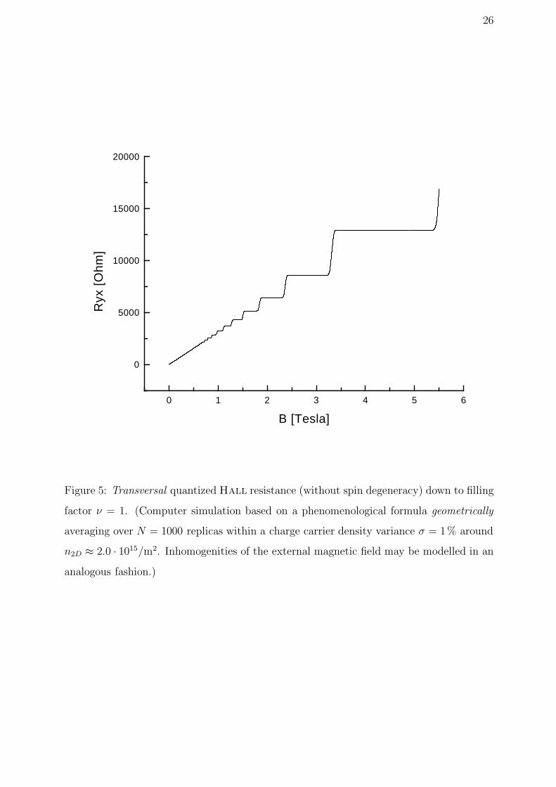
Figure 5: Transversal quantized Hall resistance (without spin degeneracy) down to filling

factor ν = 1. (Computer simulation based on a phenomenological formula geometrically

averaging over N = 1000 replicas within a charge carrier density variance σ = 1 % around

n2D ≈ 2.0 · 1015/m2. Inhomogenities of the external magnetic field may be modelled in an

analogous fashion.)

27

0 1 2 3 4 5 6

0

10000

20000

30000

40000

50000

60000

Rxx

[O

hm

]

B [Tesla]

Figure 6: Longitudinal quantized Hall resistance (without spin degeneracy) down to filling




analogous fashion.)

28

0 1 2 3 4 5 6

0

5000

10000

15000

20000

Ryx

[O

hm

]

B [Tesla]





analogous fashion.)

29

0 1 2 3 4 5 6

0

5000

10000

15000

20000

25000

30000

Rxx

[O

hm

]

B [Tesla]

Figure 8: Longitudinal quantized Hall resistance (without spin degeneracy) down to filling




analogous fashion.)

30

0 1 2 3 4 5 6

0

5000

10000

15000

20000

Ryx

[O

hm

]

B [Tesla]





analogous fashion.)

31

0 1 2 3 4 5 6

0

5000

10000

15000

20000

Rxx

[O

hm

]

B [Tesla]

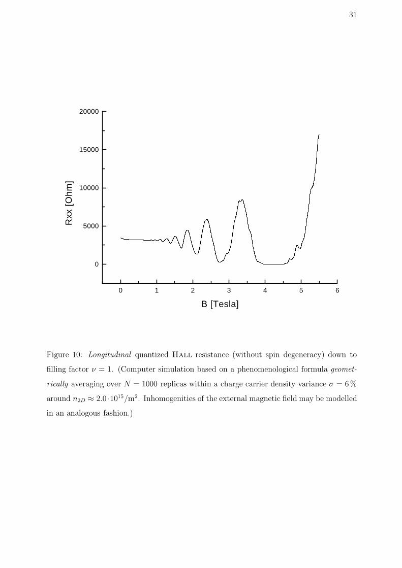
Figure 10: Longitudinal quantized Hall resistance (without spin degeneracy) down to

filling factor ν = 1. (Computer simulation based on a phenomenological formula geomet-

rically averaging over N = 1000 replicas within a charge carrier density variance σ = 6 %

around n2D ≈ 2.0·1015/m2. Inhomogenities of the external magnetic field may be modelled

in an analogous fashion.)

32

9 Figures: Sample geometry and topology

Figure 11: Hall-bar layout

33

Figure 12: Photograph of the Hall-bar

34

Figure 13: van der Pauw-type sample layout

35

Figure 14: Photograph of the (broken) vander Pauw-type “centi” sample

36

Figure 15: van der Pauw-Corbino-hybrid sample layout

37

Figure 16: Photograph of the vander Pauw-Corbino-hybrid sample

38

10 Figures: Experimental results

Figure 17: Measurement 1 on the vander Pauw-type “centi” sample

39


40


41


42


43


44

Figure 23: Measurement on a Hall-bar-type “micro” sample

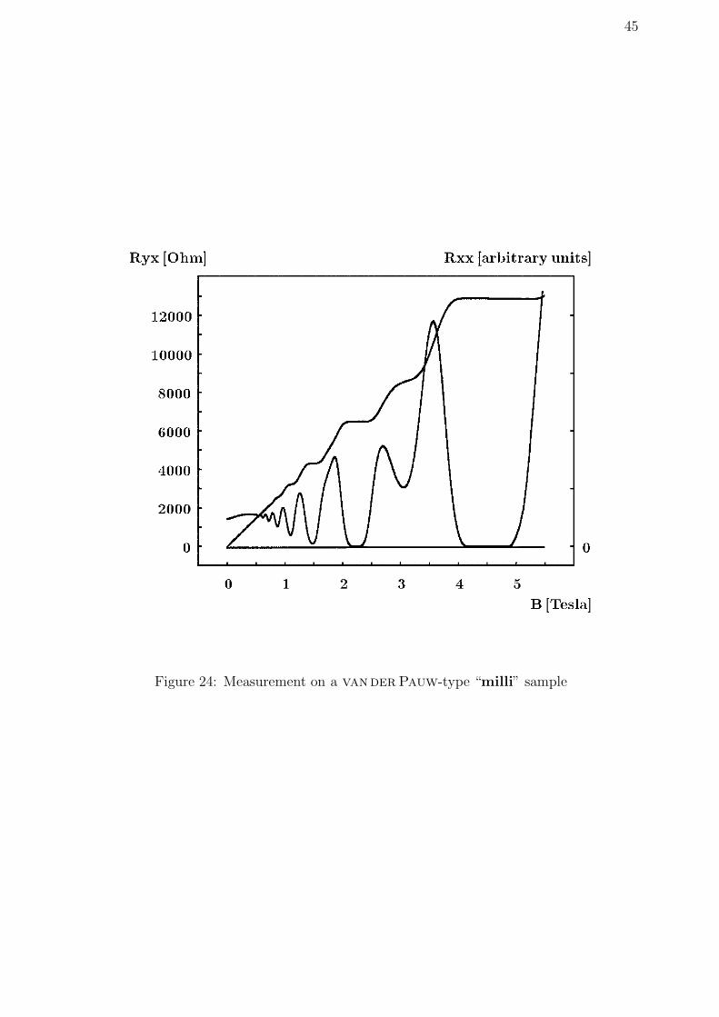
45

Figure 24: Measurement on a vander Pauw-type “milli” sample

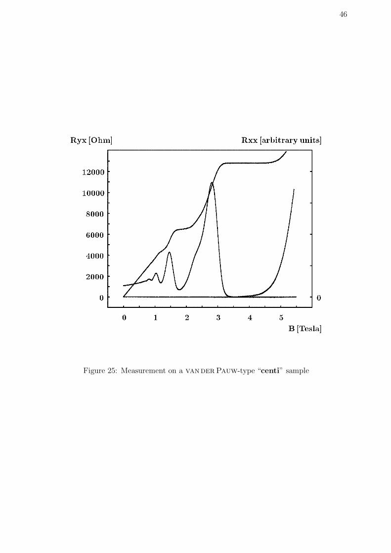
46

Figure 25: Measurement on a vander Pauw-type “centi” sample

47

Figure 26: Scaling in real space: Comparison of different sample sizes

48

Figure 27: Measurement on a vander Pauw-Corbino-hybrid sample

49

11 Tables

ν “micro” “milli” “centi”

2 100 % 121 % 179 %

3 100 % 150 % 50 %

4 100 % 117 % 150 %

6 100 % 117 % 100 %

8 100 % 117 % 50 %

10 100 % 100 % 0 %

12 100 % 100 % 0 %

Table 1: Relative plateau width in Fig. 26

50

meas. no. time Iin Uout Uout range

1 00:00 AC BD 3 mV

AB CD 0.3 mV

2 00:20 BD CA 3 mV

BC AD 0.3 mV

3 00:37 CA DB 3 mV

CD AB 0.3 mV

4 00:45 DB AC 3 mV

DA BC 0.3 mV

5 00:60 AC BD 3 mV

AB CD 0.3 mV

6 01:31 AC BD 3 mV

AB CD 0.3 mV

Table 2: Measurements depicted in Fig. 17 - Fig. 22

51

curve Iin Uout Uout range zero line overall characteristics

α AC DB 3 mV low standard transversal curve

β ac db 3 mV low standard transversal curve

γ AB CD 0.3 mV low longitudinal curve with neg. slope

δ ab cd 0.3 mV low longitudinal curve with pos. slope

ε AD bd 3 mV mid longitudinal curve with pos. slope

ζ AC bd 0.3 mV mid curve with second derivative content

η AB bd 3 mV mid longitudinal curve with neg. slope

ϑ AC bB 3 mV low hybrid curve

Table 3: Evaluation of Fig. 27

Robustness of the quantum Hall e ect, sample size versus sample topology, and quality control...

Documents

Transcript of Robustness of the quantum Hall e ect, sample size versus sample topology, and quality control...