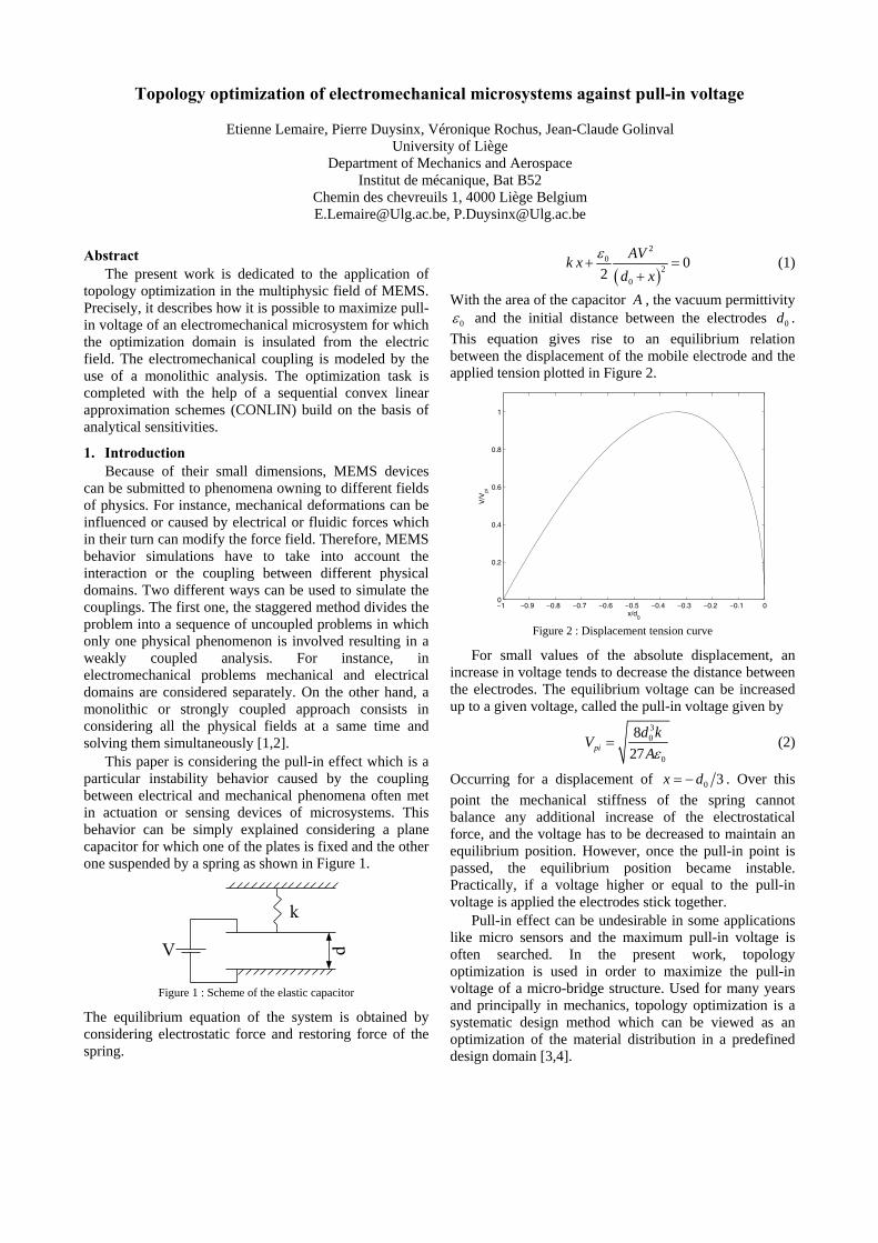
Topology optimization of electromechanical microsystems against pull-in voltage

Etienne Lemaire, Pierre Duysinx, Véronique Rochus, Jean-Claude Golinval University of Liège

Department of Mechanics and Aerospace Institut de mécanique, Bat B52

Chemin des chevreuils 1, 4000 Liège Belgium E.Lemaire@Ulg.ac.be, P.Duysinx@Ulg.ac.be

Abstract The present work is dedicated to the application of

topology optimization in the multiphysic field of MEMS. Precisely, it describes how it is possible to maximize pull-in voltage of an electromechanical microsystem for which the optimization domain is insulated from the electric field. The electromechanical coupling is modeled by the use of a monolithic analysis. The optimization task is completed with the help of a sequential convex linear approximation schemes (CONLIN) build on the basis of analytical sensitivities.

1. Introduction Because of their small dimensions, MEMS devices

can be submitted to phenomena owning to different fields of physics. For instance, mechanical deformations can be influenced or caused by electrical or fluidic forces which in their turn can modify the force field. Therefore, MEMS behavior simulations have to take into account the interaction or the coupling between different physical domains. Two different ways can be used to simulate the couplings. The first one, the staggered method divides the problem into a sequence of uncoupled problems in which only one physical phenomenon is involved resulting in a weakly coupled analysis. For instance, in electromechanical problems mechanical and electrical domains are considered separately. On the other hand, a monolithic or strongly coupled approach consists in considering all the physical fields at a same time and solving them simultaneously [1,2].

This paper is considering the pull-in effect which is a particular instability behavior caused by the coupling between electrical and mechanical phenomena often met in actuation or sensing devices of microsystems. This behavior can be simply explained considering a plane capacitor for which one of the plates is fixed and the other one suspended by a spring as shown in Figure 1.

Figure 1 : Scheme of the elastic capacitor

The equilibrium equation of the system is obtained by considering electrostatic force and restoring force of the spring.

( )

20

20

02

AVk xd x

ε+ =

+ (1)

With the area of the capacitor A , the vacuum permittivity 0ε and the initial distance between the electrodes 0d .

This equation gives rise to an equilibrium relation between the displacement of the mobile electrode and the applied tension plotted in Figure 2.

−1 −0.9 −0.8 −0.7 −0.6 −0.5 −0.4 −0.3 −0.2 −0.1 00

0.2

0.4

0.6

0.8

1

x/d0

V/V

pi

Figure 2 : Displacement tension curve

For small values of the absolute displacement, an increase in voltage tends to decrease the distance between the electrodes. The equilibrium voltage can be increased up to a given voltage, called the pull-in voltage given by

30

0

827pi

d kVAε

= (2)

Occurring for a displacement of 0 3x d= − . Over this point the mechanical stiffness of the spring cannot balance any additional increase of the electrostatical force, and the voltage has to be decreased to maintain an equilibrium position. However, once the pull-in point is passed, the equilibrium position became instable. Practically, if a voltage higher or equal to the pull-in voltage is applied the electrodes stick together.

Pull-in effect can be undesirable in some applications like micro sensors and the maximum pull-in voltage is often searched. In the present work, topology optimization is used in order to maximize the pull-in voltage of a micro-bridge structure. Used for many years and principally in mechanics, topology optimization is a systematic design method which can be viewed as an optimization of the material distribution in a predefined design domain [3,4].

2. Electromechanical coupled simulation The modeling method used here is based on the finite

element discretization described in [1,2]. In this approach one considers finite elements owning both mechanical (nodal displacements) and electrical (nodal potentials) degrees of freedom resulting in a monolithic formulation of the electomechanical problem. The monolithic formulation allows performing a strongly coupled analysis. The monolithic formulation has the advantage to allow the computation of the complete voltage-displacement curve even in the instable region, namely after pull-in. This ability to follow the whole curve is very useful for the search of the pull-in point.

The monolithic model lead to a system of equations that can be written under matrix form, as follow ( ) [ ], ,TV with⋅ = =K q f q q u φ (3) where u stands for the mechanical displacements and φ the nodal electric potentials, q are the generalized displacements, f the generalized internal forces and V the applied electric voltage. The system of equations is non-linear since, for instance, the mechanical forces depend on the electrical charges and vice versa. In most solution schemes of non linear problems, a linearization of the equation system is involved. Prior linearizing the system, a vector ( )r q is introduced and expressed by,

( ) ( )= ⋅ −r q K q f q (4) This vector vanishes at equilibrium. Then the first order approximation of r is taken around a position 0q , which gives,

( ) ( ) ( )0

0 0 2O∂+ Δ = − Δ + Δ

∂ q

rr q q r q q qq

(5)

The jacobian matrix ∂ ∂r q is called the tangent stiffness matrix of the system and is denoted by tK in the following. Using (5) and starting from a position 0q , the goal of most solution methods to non linear problems is to find a Δq sequence leading to a new position q for which ( ) =r q 0 . The tangent stiffness matrix has in consequence a great importance. To compute this matrix in the context of an electromechanical strongly coupled formulation, a general energetic approach is described in [1]. This approach is based on the Gibbs energy density given by

1 12 2

T TG = −S T D E (6)

Two contributions can be identified in the Gibbs density energy. First the mechanical contribution depends on the strain tensor S and the stress tensor T . Secondly, the electric part is computed as the product between electric displacement vector D and electric field vector E . The Gibbs energy density is integrated over the domain volume and a variational principle is applied to obtain a discretized expression of the equilibrium equation. The

proposed method leads to a tangent stiffness symmetric matrix of the form,

uu ut

u

φ

φ φφ

⎡ ⎤= ⎢ ⎥⎣ ⎦

K KK

K K (7)

The terms uφK and uφK introduce a coupling between the electric potential field and the displacement field. These two bloc matrices stem from the introduction into

tK of the electrical forces included in f . Moreover, the matrix uuK possesses two components. The first contribution to this matrix is of course the structural stiffness. The second one proceeds from the influence of the displacements upon the electrical forces.

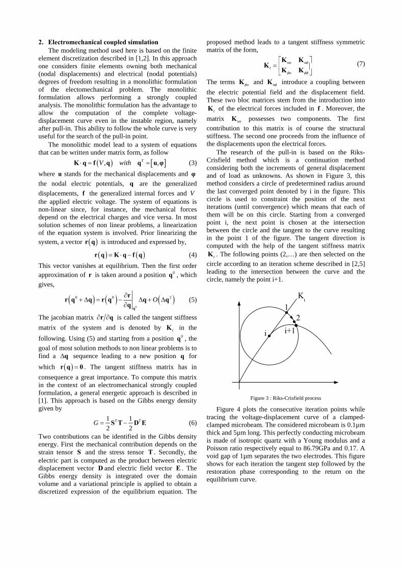
The research of the pull-in is based on the Riks-Crisfield method which is a continuation method considering both the increments of general displacement and of load as unknowns. As shown in Figure 3, this method considers a circle of predetermined radius around the last converged point denoted by i in the figure. This circle is used to constraint the position of the next iterations (until convergence) which means that each of them will be on this circle. Starting from a converged point i, the next point is chosen at the intersection between the circle and the tangent to the curve resulting in the point 1 of the figure. The tangent direction is computed with the help of the tangent stiffness matrix

tK . The following points (2,…) are then selected on the circle according to an iteration scheme described in [2,5] leading to the intersection between the curve and the circle, namely the point i+1.

Figure 3 : Riks-Crisfield process

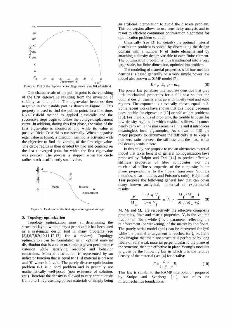
Figure 4 plots the consecutive iteration points while tracing the voltage-displacement curve of a clamped-clamped microbeam. The considered microbeam is 0.1µm thick and 5µm long. This perfectly conducting microbeam is made of isotropic quartz with a Young modulus and a Poisson ratio respectively equal to 86.79GPa and 0.17. A void gap of 1µm separates the two electrodes. This figure shows for each iteration the tangent step followed by the restoration phase corresponding to the return on the equilibrium curve.

−8 −7 −6 −5 −4 −3 −2 −1 0

x 10−7

50

100

150

200

250

300

350

400

450

Displacement (m)

Vol

tage

(V

)

Figure 4 : Plot of the displacement-voltage curve using Riks-Crisfield

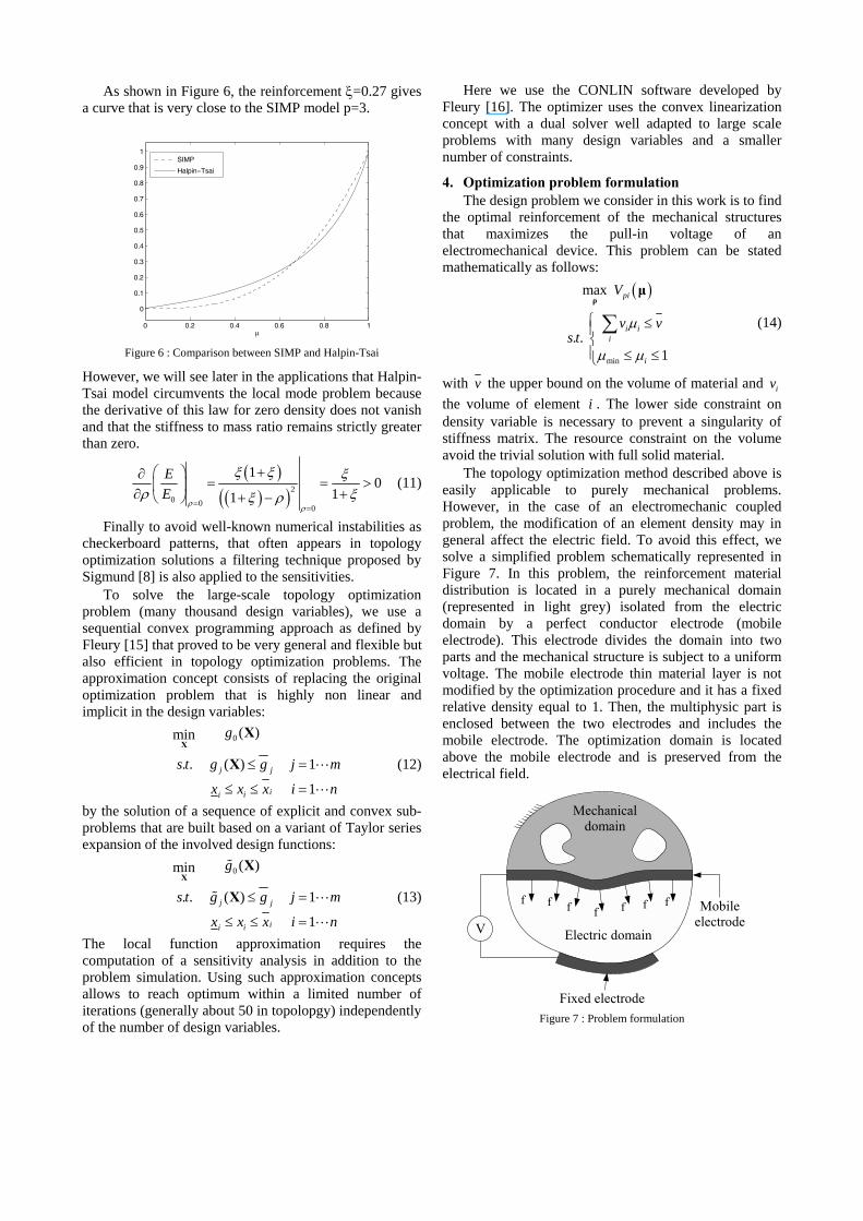
One characteristic of the pull-in point is the vanishing of the first eigenvalue resulting from the inversion of stability at this point. The eigenvalue becomes then negative in the instable part as shown in Figure 5. This property is used to find the pull-in point. In a first time, Riks-Crisfield method is applied classically and the successive steps begin to follow the voltage-displacement curve. In addition, during this first phase, the value of the first eigenvalue is monitored and while its value is positive Ricks-Crisfield is run normally. When a negative eigenvalue is found, a bisection method is activated with the objective to find the zeroing of the first eigenvalue. The circle radius is then divided by two and centered on the last converged point for which the first eigenvalue was positive. The process is stopped when the circle radius reach a sufficiently small value.

Figure 5 : Evolution of the first eigenvalue against voltage

3. Topology optimization Topology optimization aims at determining the

structural layout without any a priori and it has been used as a systematic design tool in many problems (see [3,4,6,7,8,9,10,11,12,13] for a review). Topology optimization can be formulated as an optimal material distribution that is able to maximize a given performance criterion while satisfying resource and behavior constraints. Material distribution is represented by an indicator function that is equal to ‘1’ if material is present and ‘0’ where it is void. The purely discrete optimization problem 0-1 is a hard problem and is generally not mathematically well-posed (non existence of solution, etc.) Therefore the density is allowed to vary continuously from 0 to 1, representing porous materials or simply being

an artificial interpolation to avoid the discrete problem. This conversion allows to use sensitivity analysis and to resort to efficient continuous optimization algorithms for optimization problem solution.

Classically (see [3] for details) the optimal material distribution problem is solved by discretizing the design domain with a number N of finite elements and by attaching a density design variable to each finite element. The optimization problem is thus transformed into a very large scale, but finite dimension, optimization problem.

The modeling of material properties with intermediate densities is based generally on a very simple power law model also known as SIMP model [7]: 0 0

pE µ E µρ ρ= = (8) The power law penalizes intermediate densities that give little mechanical properties for a full cost so that the optimal design usually ends up with mostly void and solid regions. The exponent is classically chosen equal to 3. Some recent works have shown that this model becomes questionable for eigenvalue [12] or self-weight problems [13]. For these kinds of problems, the trouble happens for low density regions in which residual stiffness becomes nearly zero while the mass remains finite and it introduces meaningless local eigenmodes. As shown in [13] the major property to circumvent the difficulty is to keep a non-zero ratio between the stiffness and the mass when the density tends to zero.

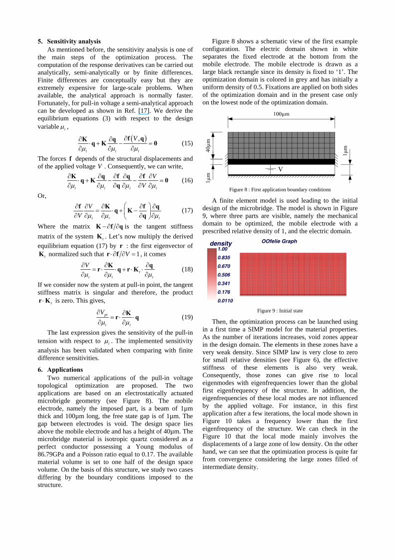
In this study, we propose to use an alternative material model that takes benefit of general homogenization laws proposed by Halpin and Tsai [14] to predict effective stiffness properties of fiber composites. For the mechanical stiffness properties of the composite in the plane perpendicular to the fibers (transverse Young’s modulus, shear modulus and Poisson’s ratio), Halpin and Tsai propose the following general law that can cover many known analytical, numerical or experimental results:

1 / 1

1 /

V M MM f f mwithM V M Mm f f m

ξ ηη

η ξ

+ −= =

− + (9)

M, Mf and Mm are respectively the effective composite properties, fiber and matrix properties, Vf is the volume fraction of fibers while ξ is a parameter reflecting the reinforcement (or weakening) of the matrix by the fibers. The purely serial model (p=1) can be recovered for ξ=0 while the parallel arrangement is reached for ξ=∞. Let’s now imagine that the plane structure is perforated by long fibers of very weak material perpendicular to the plane of the structure, then the effective in plane Young’s modulus is given by the following law in which µ is the relative density of the material (see [4] for details):

01µE E

µξξ

=+ −

(10)

This law is similar to the RAMP interpolation proposed by Stolpe and Svanberg [11], but relies on micromechanics foundations.

As shown in Figure 6, the reinforcement ξ=0.27 gives a curve that is very close to the SIMP model p=3.

0 0.2 0.4 0.6 0.8 1

0

0.1

0.2

0.3

0.4

0.5

0.6

0.7

0.8

0.9

1

μ

SIMP

Halpin−Tsai

Figure 6 : Comparison between SIMP and Halpin-Tsai

However, we will see later in the applications that Halpin-Tsai model circumvents the local mode problem because the derivative of this law for zero density does not vanish and that the stiffness to mass ratio remains strictly greater than zero.

( )( )( )2

0 0 0

10

11

EE

ρ ρ

ξ ξ ξρ ξξ ρ=

=

+⎛ ⎞∂= = >⎜ ⎟∂ ++ −⎝ ⎠

(11)

Finally to avoid well-known numerical instabilities as checkerboard patterns, that often appears in topology optimization solutions a filtering technique proposed by Sigmund [8] is also applied to the sensitivities.

To solve the large-scale topology optimization problem (many thousand design variables), we use a sequential convex programming approach as defined by Fleury [15] that proved to be very general and flexible but also efficient in topology optimization problems. The approximation concept consists of replacing the original optimization problem that is highly non linear and implicit in the design variables:

0 ( )min

. . ( ) 1

1j j

iii

g

s t g g j m

x x x i n

≤ =

≤ ≤ =

XX

X (12)

by the solution of a sequence of explicit and convex sub-problems that are built based on a variant of Taylor series expansion of the involved design functions:

0 ( )min

. . ( ) 1

1j j

iii

g

s t g g j m

x x x i n

≤ =

≤ ≤ =

XX

X (13)

The local function approximation requires the computation of a sensitivity analysis in addition to the problem simulation. Using such approximation concepts allows to reach optimum within a limited number of iterations (generally about 50 in topolopgy) independently of the number of design variables.

Here we use the CONLIN software developed by Fleury [16]. The optimizer uses the convex linearization concept with a dual solver well adapted to large scale problems with many design variables and a smaller number of constraints.

4. Optimization problem formulation The design problem we consider in this work is to find

the optimal reinforcement of the mechanical structures that maximizes the pull-in voltage of an electromechanical device. This problem can be stated mathematically as follows:

( )

min

max

. .1

pi

i ii

i

V

v vs t

μ

μ μ

⎧ ≤⎪⎨⎪ ≤ ≤⎩

∑ρ

μ

(14)

with v the upper bound on the volume of material and iv the volume of element i . The lower side constraint on density variable is necessary to prevent a singularity of stiffness matrix. The resource constraint on the volume avoid the trivial solution with full solid material.

The topology optimization method described above is easily applicable to purely mechanical problems. However, in the case of an electromechanic coupled problem, the modification of an element density may in general affect the electric field. To avoid this effect, we solve a simplified problem schematically represented in Figure 7. In this problem, the reinforcement material distribution is located in a purely mechanical domain (represented in light grey) isolated from the electric domain by a perfect conductor electrode (mobile electrode). This electrode divides the domain into two parts and the mechanical structure is subject to a uniform voltage. The mobile electrode thin material layer is not modified by the optimization procedure and it has a fixed relative density equal to 1. Then, the multiphysic part is enclosed between the two electrodes and includes the mobile electrode. The optimization domain is located above the mobile electrode and is preserved from the electrical field.

Figure 7 : Problem formulation

5. Sensitivity analysis As mentioned before, the sensitivity analysis is one of

the main steps of the optimization process. The computation of the response derivatives can be carried out analytically, semi-analytically or by finite differences. Finite differences are conceptually easy but they are extremely expensive for large-scale problems. When available, the analytical approach is normally faster. Fortunately, for pull-in voltage a semi-analytical approach can be developed as shown in Ref. [17]. We derive the equilibrium equations (3) with respect to the design variable iμ ,

( ),

i i i

Vμ μ μ

∂∂ ∂⋅ + − =

∂ ∂ ∂f qK qq K 0 (15)

The forces f depends of the structural displacements and of the applied voltage V . Consequently, we can write,

i i i i

VVμ μ μ μ

∂ ∂ ∂ ∂ ∂ ∂⋅ + − − =

∂ ∂ ∂ ∂ ∂ ∂K q f q fq K 0

q (16)

Or,

i i i

VV μ μ μ

⎛ ⎞∂ ∂ ∂ ∂ ∂= ⋅ + −⎜ ⎟∂ ∂ ∂ ∂ ∂⎝ ⎠

f K f qq Kq

(17)

Where the matrix − ∂ ∂K f q is the tangent stiffness matrix of the system tK . Let’s now multiply the derived equilibrium equation (17) by r : the first eigenvector of

tK normalized such that 1V⋅ ∂ ∂ =r f , it comes

ti i i

Vμ μ μ∂ ∂ ∂

= ⋅ ⋅ + ⋅ ⋅∂ ∂ ∂

K qr q r K (18)

If we consider now the system at pull-in point, the tangent stiffness matrix is singular and therefore, the product

t⋅r K is zero. This gives,

pi

i i

Vμ μ

∂ ∂= ⋅ ⋅

∂ ∂Kr q (19)

The last expression gives the sensitivity of the pull-in tension with respect to iμ . The implemented sensitivity analysis has been validated when comparing with finite difference sensitivities.

6. Applications Two numerical applications of the pull-in voltage

topological optimization are proposed. The two applications are based on an electrostatically actuated microbrigde geometry (see Figure 8). The mobile electrode, namely the imposed part, is a beam of 1µm thick and 100µm long, the free state gap is of 1µm. The gap between electrodes is void. The design space lies above the mobile electrode and has a height of 40µm. The microbridge material is isotropic quartz considered as a perfect conductor possessing a Young modulus of 86.79GPa and a Poisson ratio equal to 0.17. The available material volume is set to one half of the design space volume. On the basis of this structure, we study two cases differing by the boundary conditions imposed to the structure.

Figure 8 shows a schematic view of the first example configuration. The electric domain shown in white separates the fixed electrode at the bottom from the mobile electrode. The mobile electrode is drawn as a large black rectangle since its density is fixed to ‘1’. The optimization domain is colored in grey and has initially a uniform density of 0.5. Fixations are applied on both sides of the optimization domain and in the present case only on the lowest node of the optimization domain.

Figure 8 : First application boundary conditions

A finite element model is used leading to the initial design of the microbridge. The model is shown in Figure 9, where three parts are visible, namely the mechanical domain to be optimized, the mobile electrode with a prescribed relative density of 1, and the electric domain.

OOfelie GraphOOfelie Graphdensitydensity

0.01100.0110

0.176 0.176

0.341 0.341

0.506 0.506

0.670 0.670

0.835 0.835

1.00 1.00

Figure 9 : Initial state

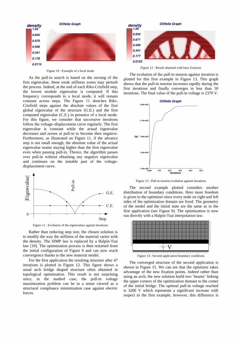
Then, the optimization process can be launched using in a first time a SIMP model for the material properties. As the number of iterations increases, void zones appear in the design domain. The elements in these zones have a very weak density. Since SIMP law is very close to zero for small relative densities (see Figure 6), the effective stiffness of these elements is also very weak. Consequently, those zones can give rise to local eigenmodes with eigenfrequencies lower than the global first eigenfrequency of the structure. In addition, the eigenfrequencies of these local modes are not influenced by the applied voltage. For instance, in this first application after a few iterations, the local mode shown in Figure 10 takes a frequency lower than the first eigenfrequency of the structure. We can check in the Figure 10 that the local mode mainly involves the displacements of a large zone of low density. On the other hand, we can see that the optimization process is quite far from convergence considering the large zones filled of intermediate density.

OOfelie GraphOOfelie Graphdensitydensity

0.01150.0115

0.176 0.176

0.341 0.341

0.506 0.506

0.670 0.670

0.835 0.835

1.00 1.00

Figure 10 : Example of a local mode

As the pull-in search is based on the zeroing of the first eigenvalue, these weak stiffness zones may perturb the process. Indeed, at the end of each Riks-Crisfield step, the lowest module eigenvalue is computed. If this frequency corresponds to a local mode, it will remain constant across steps. The Figure 11 sketches Riks-Crisfield steps against the absolute values of the first global eigenvalue of the structure (G.E.) and the first computed eigenvalue (C.E.) in presence of a local mode. For this figure, we consider that successive iterations follow the voltage–displacement curve regularly. The first eigenvalue is constant while the actual eigenvalue decreases and zeroes at pull-in to become then negative. Furthermore, as illustrated on Figure 11, if the advance step is not small enough, the absolute value of the actual eigenvalue seams staying higher than the first eigenvalue even when passing pull-in. Thence, the algorithm passes over pull-in without obtaining any negative eigenvalue and continues on the instable part of the voltage-displacement curve.

Figure 11 : Evolution of the eigenvalues against iterations

Rather than reducing step size, the chosen solution is to modify the way the stiffness of the material varies with the density. The SIMP law is replaced by a Halpin-Tsai law [10]. The optimization process is then restarted from the initial configuration of Figure 9 and can now reach convergence thanks to the new material model.

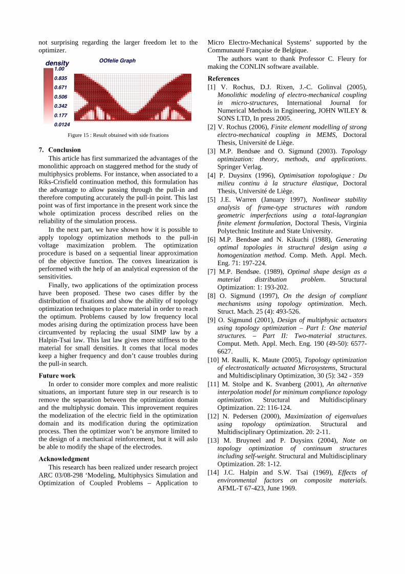
For the first application the resulting structure after 47 iterations is plotted in Figure 12. This figure shows a usual arch bridge shaped structure often obtained in topological optimization. This result is not surprising since, in the studied case, the pull-in voltage maximization problem can be in a sense viewed as a structural compliance minimization case against electric forces.

OOfelie GraphOOfelie Graphdensitydensity

0.01220.0122

0.177 0.177

0.341 0.341

0.506 0.506

0.671 0.671

0.835 0.835

1.00 1.00

Figure 12 : Result obtained with base fixations

The evolution of the pull-in tension against iteration is plotted for this first example in Figure 13. This graph shows that the pull-in tension increases rapidly during the first iterations and finally converges in less than 50 iterations. The final value of the pull-in voltage is 2370 V.

OOfelie GraphOOfelie Graph

iterationsiterations0.000 0.000 10.0 10.0 20.0 20.0 30.0 30.0 40.0 40.0 50.0 50.0

VpiVpi

2.40e+0032.40e+003

2.10e+0032.10e+003

1.80e+0031.80e+003

1.50e+0031.50e+003

1.20e+0031.20e+003

Figure 13 : Pull-in tension evolution against iterations

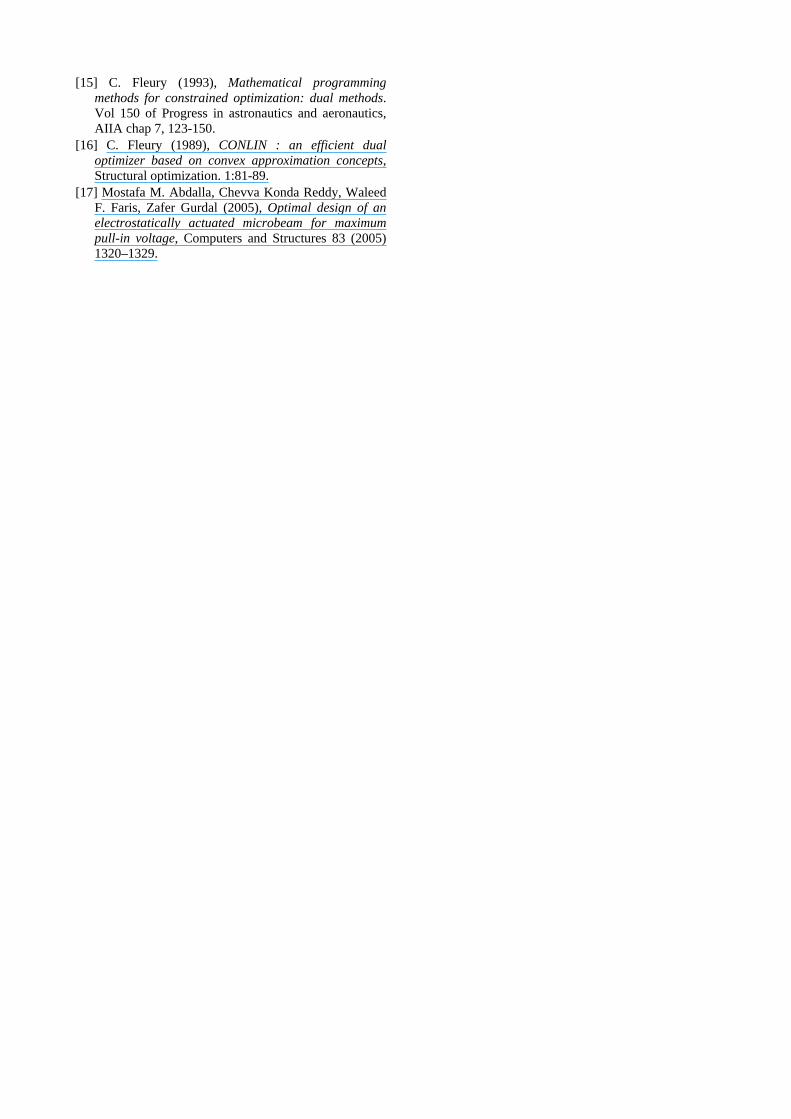
The second example plotted considers another distribution of boundary conditions. Here more freedom is given to the optimizer since every node on right and left sides of the optimization domain are fixed. The geometry of the model and the initial state are the same as in the first application (see Figure 9). The optimization is now run directly with a Halpin-Tsai interpolation law.

Figure 14 : Second application boundary conditions

The converged structure of the second application is shown in Figure 15. We can see that the optimizer takes advantage of the new fixation points. Indeed rather than using an arch, the new solution build two ‘beams’ linking the upper corners of the optimization domain to the center of the initial bridge. The optimal pull-in voltage reached is 3206 V which represents a significant increase with respect to the first example, however, this difference is

not surprising regarding the larger freedom let to the optimizer.

OOfelie GraphOOfelie Graphdensitydensity

0.01240.0124

0.177 0.177

0.342 0.342

0.506 0.506

0.671 0.671

0.835 0.835

1.00 1.00

Figure 15 : Result obtained with side fixations

7. Conclusion This article has first summarized the advantages of the

monolithic approach on staggered method for the study of multiphysics problems. For instance, when associated to a Riks-Crisfield continuation method, this formulation has the advantage to allow passing through the pull-in and therefore computing accurately the pull-in point. This last point was of first importance in the present work since the whole optimization process described relies on the reliability of the simulation process.

In the next part, we have shown how it is possible to apply topology optimization methods to the pull-in voltage maximization problem. The optimization procedure is based on a sequential linear approximation of the objective function. The convex linearization is performed with the help of an analytical expression of the sensitivities.

Finally, two applications of the optimization process have been proposed. These two cases differ by the distribution of fixations and show the ability of topology optimization techniques to place material in order to reach the optimum. Problems caused by low frequency local modes arising during the optimization process have been circumvented by replacing the usual SIMP law by a Halpin-Tsai law. This last law gives more stiffness to the material for small densities. It comes that local modes keep a higher frequency and don’t cause troubles during the pull-in search.

Future work In order to consider more complex and more realistic

situations, an important future step in our research is to remove the separation between the optimization domain and the multiphysic domain. This improvement requires the modelization of the electric field in the optimization domain and its modification during the optimization process. Then the optimizer won’t be anymore limited to the design of a mechanical reinforcement, but it will aslo be able to modify the shape of the electrodes.

Acknowledgment This research has been realized under research project

ARC 03/08-298 ‘Modeling, Multiphysics Simulation and Optimization of Coupled Problems – Application to

Micro Electro-Mechanical Systems’ supported by the Communauté Française de Belgique.

The authors want to thank Professor C. Fleury for making the CONLIN software available.

References [1] V. Rochus, D.J. Rixen, J.-C. Golinval (2005),

Monolithic modeling of electro-mechanical coupling in micro-structures, International Journal for Numerical Methods in Engineering, JOHN WILEY & SONS LTD, In press 2005.

[2] V. Rochus (2006), Finite element modelling of strong electro-mechanical coupling in MEMS, Doctoral Thesis, Université de Liège.

[3] M.P. Bendsøe and O. Sigmund (2003). Topology optimization: theory, methods, and applications. Springer Verlag.

[4] P. Duysinx (1996), Optimisation topologique : Du milieu continu à la structure élastique, Doctoral Thesis, Université de Liège.

[5] J.E. Warren (January 1997), Nonlinear stability analysis of frame-type structures with random geometric imperfections using a total-lagrangian finite element formulation, Doctoral Thesis, Virginia Polytechnic Institute and State University.

[6] M.P. Bendsøe and N. Kikuchi (1988), Generating optimal topologies in structural design using a homogenization method. Comp. Meth. Appl. Mech. Eng. 71: 197-224.

[7] M.P. Bendsøe. (1989), Optimal shape design as a material distribution problem. Structural Optimization: 1: 193-202.

[8] O. Sigmund (1997), On the design of compliant mechanisms using topology optimization. Mech. Struct. Mach. 25 (4): 493-526.

[9] O. Sigmund (2001), Design of multiphysic actuators using topology optimization – Part I: One material structures. – Part II: Two-material structures. Comput. Meth. Appl. Mech. Eng. 190 (49-50): 6577-6627.

[10] M. Raulli, K. Maute (2005), Topology optimization of electrostatically actuated Microsystems, Structural and Multidisciplinary Optimization, 30 (5): 342 - 359

[11] M. Stolpe and K. Svanberg (2001), An alternative interpolation model for minimum compliance topology optimization. Structural and Multidisciplinary Optimization. 22: 116-124.

[12] N. Pedersen (2000), Maximization of eigenvalues using topology optimization. Structural and Multidisciplinary Optimization. 20: 2-11.

[13] M. Bruyneel and P. Duysinx (2004), Note on topology optimization of continuum structures including self-weight. Structural and Multidisciplinary Optimization. 28: 1-12.

[14] J.C. Halpin and S.W. Tsai (1969), Effects of environmental factors on composite materials. AFML-T 67-423, June 1969.

[15] C. Fleury (1993), Mathematical programming methods for constrained optimization: dual methods. Vol 150 of Progress in astronautics and aeronautics, AIIA chap 7, 123-150.

[16] C. Fleury (1989), CONLIN : an efficient dual optimizer based on convex approximation concepts, Structural optimization. 1:81-89.

[17] Mostafa M. Abdalla, Chevva Konda Reddy, Waleed F. Faris, Zafer Gurdal (2005), Optimal design of an electrostatically actuated microbeam for maximum pull-in voltage, Computers and Structures 83 (2005) 1320–1329.