-1-

A -Model Solution for the Inverse Position Problem of Calibrated Robots Using Virtual Elementary Motions.

Ibrahim A. Sultan School of Engineering University of Ballarat PO Box 663 Ballarat VIC 3350 Australia John G. Wager Department of Mechanical and Materials Engineering The University of Western Australia Nedlands WA 6907 Australia

Keywords: Robots – Kinematic Modelling – Position Analysis – Transformation. Abstract:

It is central to the control of manipulators to calculate the set/sets of joint-displacements

which correspond to a given spatial pose (position and orientation) of the end-effector.

This problem, which is referred to as the inverse position problem, represents one of the

most difficult mathematical challenges in the field of robotics, particularly when

performed for calibrated robots (or robots with general structures). In such cases, closed

form solutions are too impractical to implement and iterative solutions suffer from

numerical singularities.

-2-

In the present work a procedure is introduced to obtain multiple inverse position

solutions for serial robotic structures. For calibrated robots, the procedure involves a

simple iterative technique designed to ensure fast convergence and eliminate the

occurrence of singularity. However, inverse position solutions for spherical-wrist

manipulators will be obtained in a straight-forward non-iterative fashion. A published

kinematic notation, referred to as the -model, was used to develop the system equations.

1. Introduction and Problem Statement:

The main function of a robot manipulator in industrial applications is to place an object

(tool or end-effector) at a given spatial pose (position and orientation). Since any

unconstrained such pose is defined by six independent parameters, three for position and

three for orientation, the robot may have to possess at least six degrees of freedom to be

dextrous enough for flexible automation and other applications. Therefore robots are

often provided with six single-degree-of-freedom joints of a rotary or sliding type. These

particular kinematic pairs are used due to the ease they provide for powering and control.

Position (or kinematic) analysis of robotic manipulators is often performed by attaching a

set of Cartesian frames to the successive links on the structure and constructing a

corresponding set of 4x4 matrices (Homogeneous Transformation matrices) to perform

transformation between these frames. Usually the Z-axes of the link frames coincide

with the axes of the manipulator joints. The Homogeneous Transformation matrix, iTi+1,

uses a set of geometric parameters to express the spatial particulars of Cartesian frame

number i+1 with respect to frame number i. These parameters (4 or 5 depending on the

-3-

model used) may be divided into link parameters and joint parameters. While the link

parameters reflect on the geometric features of the manipulator link (length, twist, …etc),

a joint parameter indicates the amount of displacement (angular or linear) performed by

the joint connecting the two successive frames. The spatial particulars of frame number n

(which is always attached to the tool) with respect to the base frame, number 0, can be

obtained by a matrix chain product as follows;

nn

nn

n TTTTTT 11

23

22

11

00

(1)

If the set of joint displacements are known, i.e. all the matrices 1iiT are given, equation

(1) may be used to calculate the matrix, nT0 . Such straightforward procedure is always

referred to as the direct position analysis. On the other hand, the inverse position

analysis is performed to calculate the set (or sets) of joint displacements which

correspond to a known spatial particulars of the end-effector frame, i.e. nT0 is given and

all the transformation matrices, 1iiT should be worked out. This problem represents a

special difficulty in the field of robot control and a good deal of literature was published

to deal with it. Examples of the published literature are reviewed in the next section.

2. Literature Survey:

Published literature reveals that the homogeneous transformation matrix which was

developed by Denavit and Hartenberg (1955) has extensively been employed for the

analysis of robot manipulators. The matrix involves the use of four parameters, usually

referred to as the DH-parameters, intended to perform transformation between two spatial

Cartesian coordinate systems. Sultan and Wager (1999) reflect on the aspects of the

-4-

models used to describe the kinematic behaviour of manipulators. They then propose a

zero-initial position notation (referred to as the -model) which has been designed to be

complete and non-singular. This is particularly important if the model is going to be

implemented for robot calibration purposes. Pennock and Yang (1985), Gu and Luh

(1987) and Pardeep et al (1989) reported techniques which utilise the theory of dual-

number algebra as presented to the field of kinematics by Yang and Freudenstein (1964).

In addition to these approaches, which are based on matrices, vector methods were also

employed in the field of kinematic analysis of robots by Duffy (1980) and Lee and Liang

(1988A & 1988B.)

Many industrial robots possess parallel and intersecting joint-axes and their direct-

position models can be inverted analytically such that closed-form solutions may be

obtained for the joint-displacements. Examples of such approaches have been published

by Gupta (1984), Pennock and Yang (1985), Pardeep et al (1989), Wang and Bjorke

(1989) and other researchers.

Spherical-wrist manipulators have their last three joint-axes intersecting at a common

point. For these manipulators the position of the end-effector in space is determined only

by the displacements performed about the first three joint-axes. This concept is often

referred to as the position-orientation decoupling and was first utilised by Pieper and

Roth (1969) to produce a closed form solution, for the inverse position problem of simple

structure robots, efficient enough to be implemented for computer control. Sultan and

Trevelyan (1992) also utilise the decoupling theory but their approach does not require

-5-

any particular spatial relations (e.g. parallelism or perpendicularity) between the arm

joint-axes. However all approaches which utilise particular geometric features (such as

the spherical-wrist property) of the manipulator structures are likely to produce

positioning errors since the actual structures always deviate from their intended

geometry.

Iterative techniques have been employed by researchers for the inverse position analysis

of general robot manipulators. Many of these techniques involve the computation of a

Jacobian matrix which has to be calculated and inverted at every iteration. The solution

in this case may be obtained by a Newton-Raphson technique as reported by Hayati and

Reston (1986) or a Kalman filter approach in a manner similar to that described by

Coelho and Nunes (1986). The inversion of the system Jacobian may not be possible

near singular configurations (where the motion performed about one joint-axis produces

exactly the same effect, at the end-effector, as the motion performed about another axis,

hence resulting in loss of one or more degrees of freedom). Therefore, Chiaverini et al

(1994) report a singularity avoidance approach where the technique of damped least-

squares is used for the analysis. However, this technique seems to be rather sluggish near

singular points and extra computational procedure may have to be involved.

Optimisation techniques are also employed to solve the inverse-position problem of

manipulators as reported by Goldenberg et al (1985) who implemented a six-element

error vector for the analysis. The vector combines the current spatial information

(position and orientation) of the robot hand and compares it to the desired pose to

-6-

produce error values. Fast-converging numerical procedure is then proposed and

implemented to calculate the set of joint-displacements that minimises the error

quantities. The procedure can be used for both redundant and non-redundant

manipulators and is able to account for the physical displacement limits of the various

joints. The work also offers valuable insights into such issues as step size control and the

formulation of the Jacobian matrix. It was found that the convergence would improve

considerably if the Jacobian was analytically determined. Other optimisation techniques

have been published by Mahalingam and Sharan (1987) and Wang and Chen (1991) who

employed a technique by which the robot is moved about one joint at a time to close an

error gap. Techniques developed about this idea were also reported by Sultan et al

(1987) and Poon and Lawrence (1988).

Manseur and Doty (1992A & 1992B) and (1996) described the kinematic behaviour of

robots in terms of simplified polynomials that can be solved iteratively. A similar

approach was adopted by Tsai and Morgan (1985) who described the kinematic

behaviour of robots in terms of eight polynomials which were then solved numerically to

obtain different possible solutions to the inverse position problem. They arrived at the

conclusion that the maximum number of meaningful solutions to the inverse position

problem of a general robotic structure is 16 not 32 as was suggested by Duffy and Crane

(1980). However Manseur and Doty (1989) point out that a manipulator with 16

different real inverse position solutions can seldom be found in real life. In reality most

manipulators are designed to possess up to 8 solutions of which only one or two can be

physically attained.

-7-

Lee and Liang (1988A & 1988B) express the inverse position problem of robots in terms

of a 16 degree polynomial in the tan-half-angle of a joint-displacement. A similar

polynomial was developed by Raghavan and Roth (1989). However Smith and Lipkin

(1990) argue that the coefficients of such polynomials are likely to contain too many

terms which may render them impractical to use. Also, these polynomials are obtained

by evaluating the eliminants of hyper-intricate determinants which may be impossible to

handle symbolically in the first place. This may have motivated Manocha and Canny

(1992) and Kohli and Osvatic (1993) to reformulate the solutions in form of elegant

eigenvalue models in order to simplify the analysis and avoid numerical complications.

The procedure proposed here for the inverse position analysis of robot manipulators is

described in the rest of this paper.

3. Kinematic Notation:

The work presented in this paper has been developed using a published kinematic

notation referred to as the -model, Sultan and Wager (1999). The notation possesses the

property of zero-initial-position. By virtue of this property the robot can be set at any

desired home position where all the joint-displacements are conveniently assigned the

value of zero. This section is not intended to offer a full discussion on the characteristics

of the notation, since this may be sought in the publication indicated above, but rather to

briefly review the portion of its mathematical framework which is relevant to the content

of this paper.

-8-

The kinematic aspects of the -model notation are shown in Figure (1). The model is

established by introducing an intermediate Cartesian system between the joint-frames

number (i) and (i+1). The Z-axis of the new frame, which is referred to as the i-frame,

lies in a plane parallel to the XiYi-plane and at a distance, di, equal to the linear joint-

displacement from it. In case of a rotary joint, di may be set equal to zero. This Z-axis,

which may be referred to as Zi, is initially set by the user at a constant angle, i, from

Zi

//Xi

//Yi

Zi+1

Xi+1

//Xi+1

//Zi

Zi

Xii

i

ai

bi

i

i

Xi

Yi

di

i

i+i

Figure (1): The Kinematic Notation of the -Model.

-9-

the Xi-axis. i, which is measured in a right-handed sense about Zi, is selected to ensure

that Zi may not be parallel to Zi+1. The Xi-axis of the i-frame is then established in a

plane perpendicular to both Zi and Zi. The i-frame is then used to establish a Cartesian

system, Xi+1Yi+1Zi+1, about the Zi+1-axis in a DH-fashion. The i-frame and the (i+1)-

frame are on the same rigid link and perform the same displacement (di or i) along or

about the Zi respectively.

The transformation, iTi+1, relating the (i+1)-frame to the i-frame may now be expressed

as follows,

iTi+1 =

iTi iT

i+1 (2)

where iTi and iT

i+1 represent the transformation relating the i-frame to the i-frame

and the (i+1)-frame to the i-frame respectively. These matrices may be expressed as

follows,

i

i i i

i i i i

i

i

dT

sin( ) cos( )

cos( ) sin( )i 0 0

0 0

0 1 0

0 0 0 1

and (3)

ii i i i i i i

i i i i i i i

i i ii

10

0 0 0 1

T

cos( ) sin( )cos( ) sin( )sin( ) b cos( )

sin( ) cos( )cos( ) cos( )sin( ) b sin( )

sin( ) cos( ) a

-10-

where ai, bi, i and i are the DH-parameters which relate the (i+1)-frame to the i-frame

as shown in Figure (1). As the above expression for iTi indicates, the angle between the

Xi- and the Zi-axes is initially i. However with the onset of the rotational motion, this

angle would vary by the value of the motor displacement, i. The expression also reveals

that the i-frame may slide along the Zi-axis a distance di if the joint was of the sliding

type; in such a case i may be set equal to zero.

To render the model complete such that arbitrarily-located frames (e.g. the tool frame,

which may be predetermined by the requirements of some manufacturing set-up rather

than assigned systematically according to the rules of the -model, or any other model for

this matter) can be described, a rotation, i, and a translation, hi, may be performed about

and along the Zi+1-axis. The new (i+1)-frame can now be related to the i-frame by the

following equation,

iTi+1 = Trans(0, 0, ai) Rot(z, i) Trans(bi, 0, 0) Rot(x, i) Rot(z, i) Trans(0, 0, hi)

(4)

In a more expanded form equation (4) can be re-expressed as follow;

1000

100

00)sin()sin(

00)sin()cos(

1000

a)cos()sin(0

)sin(b)sin()cos()cos()cos()sin(

)cos(b)sin()sin()cos()sin()cos(

1

ih

ii

ii

iii

iiiiiii

iiiiiii

ii

T

(5)

-11-

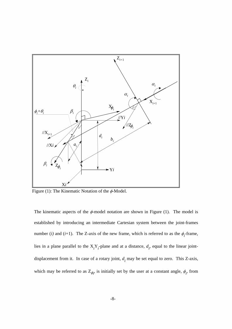
4. Model Reduction:

The inverse-position model of any 6-degree-of-freedom serial-manipulator can be

reduced to a 5-degree-of-freedom-model where the position of the last joint may be dealt

with separately. This reduction will result in a simpler model where the manipulator may

be regarded as a 5-degree-of-freedom serial mechanism attempting to locate the axis of

the sixth joint at a desired pose (location and direction) in space.

Usually the end-effector frame, XeYeZe, is related to a Cartesian frame attached to joint-

axis number 6, X6Y

6Z

6, by a homogeneous transformation matrix, T

e. This matrix may

be expressed in terms of any convenient kinematic representation. If the -model was

used for that purpose, the matrix Te may be calculated as follows,

Te= T

T

e (6)

where the matrix T is established as detailed in section (3) and T

e is constructed, as

described in equation (5), to define the arbitrary location of the tool frame with respect to

the coordinate system of the sixth joint, X6Y

6Z

6.

Typically, the Z-axis of the X6Y

6Z

6-frame is directed along the axis of the sixth joint and

the spatial particulars of the tool frame with respect to the base coordinate system are

given in form of a known homogeneous transformation matrix, Te. The sixth joint frame

may be evaluated with respect to the base frame, T6, as follows,

T6= T

e (Te)1 (7)

-12-

where the elements of the third and fourth columns of the matrix (Te)1 do not include

any reference to the variable joint-displacement, 6. This may be attributed to the fact

that the elements of these third and fourth columns respectively represent the unit vector

of the sixth joint-axis and the position vector of the origin of the sixth joint-frame with

respect to the tool frame. Both vectors are not affected by rotations performed about the

sixth joint-axis and are respectively given as follows,

sin( ) cos( ) cos( ) cos( ) sin( )

sin( ) sin( ) cos( ) cos( ) cos( )

cos( ) sin( )

6 6 6 6 6

6 6 6 6 6

6 6

0

and

b a

a b

h a

6 6 6 6 6

6 6 6 6 6

6 6 6

1

cos( ) sin( ) sin( )

cos( ) sin( ) sin( )

cos( )

where all parameters are as introduced in section (3).

Since these two columns will , after performing the matrix multiplication as per equation

(7), produce the direction and position respectively of the sixth joint-axis with respect to

the base frame, it may be concluded that the final pose of the sixth joint-axis is always

fully defined in space at the outset of the inverse-position analysis. Since this axis is

positioned in space solely by virtue of the motions performed by the first five joints on

the manipulator structure next to the stationary base, the inverse position problem is

reduced to finding the sets of five joint-displacements which correspond to a given

spatial particulars of the sixth joint-axis on the manipulator.

In the following sections the models proposed for the solution of the inverse-position

problem for robots are presented. In producing these models the 5R-manipulator has

been regarded as consisting of two groups of joints where each group is assigned a

-13-

distinctive positioning task. The first group, which is referred to as the arm, consists of

the first three joints on the manipulator structure next to the base. In the current context,

the arm is assigned the task of positioning a given point on the sixth-joint axis at a

required location in space.

The second joint group, which is referred to as the wrist, consists of the fourth and fifth

joints on the manipulator structure. This group is assigned the task of aligning the sixth

joint-axis with a given spatial orientation.

In calibrated robots where the property of spherical wrist is no longer realised,

positioning tasks may not be distinctively distinguished but the two joint groups will

collaborate to position the sixth joint-axis in the required pose. This characteristic has

been utilised below to produce an approach for inverse position analysis of calibrated

robots.

5. Positioning of the Arm:

A schematic diagram of an arm-group is shown in Figure (2). The arm, as depicted in

this figure, consists of three rotary joints whose axes , Z, Z and Z3 are fully-defined in

space with respect to a base coordinate system XYZ. The initial location of the point,

pi , is given with respect to the base coordinates in terms of the position vector, p0i . This

point is required to be displaced to a new location, pn , defined by the position vector p0n

which is also given in terms of the base frame.

-14-

Z1

Z0

Z2

Z3

1

pi

Z6

iY0

X0

.pn

Figure (2): The Arm Positioning Group.

The location of point pi with respect to a frame established about the axis Z3 may be

expressed in terms of the position vector, p3 which is independent of the joint-

displacements or arm configuration. This position vector can be calculated as follows,

pT

p

3

30 0

1 1

i

(8)

where 30T is the matrix which performs transformation relating the base frame to

Z3frame at zero initial position of the manipulator. This matrix may be calculated as

follows,

30

33 1

23

1

22 1

12

1

11 1

01

1

00 1

T T T T T T T T

(9)

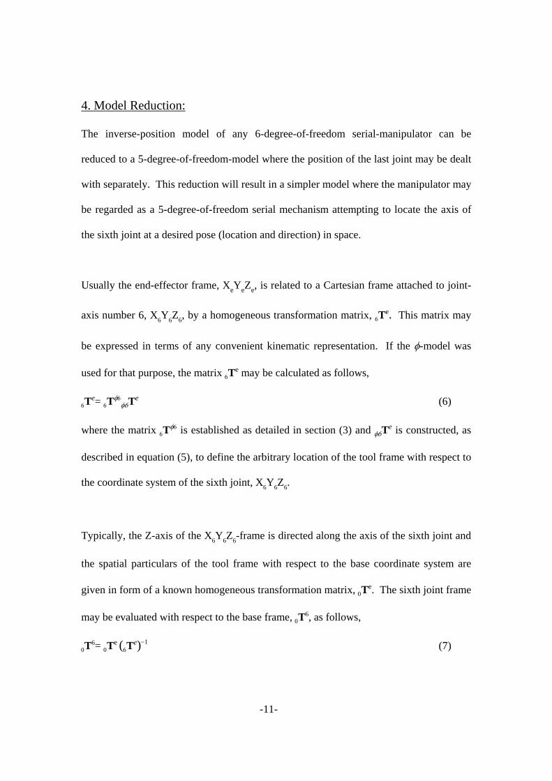
-15-

where all matrices are established as pointed out in section (3).

Since the matrix 30T is worked out at zero initial position, all joint-displacements in

equation (9) will be assigned the value of zero.

The configuration of the arm will then change in a sense that causes point pi to coincide

with the required position pn . The joint-displacements, 1,

2 and

3, which correspond

to the new arm configurations are required. At the new configuration, the known

position vector p0n can be related to p3 as follows,

11 1

01

1

00 1

12

22

23

33 3

T T Tp

T T T Tp

0n

1 1 (10)

where the matrices, 11T , 2

2T and 33T ,contain reference to their corresponding joint-

displacements as described in section (3).

The resulting vector quantities on the right- and left-hand sides of the equation (10) will

be referred to below as p R and p L respectively. The following set of equations may

then be written,

p pLx Rx (11)

p pLz Rz (12)

p pLy Ry (13)

and

p p p pL L R R (14)

-16-

where (p Lx , p Ly and p Lz ) and (p Rx , p Ry and p Rz ) are the components of p L and p R

respectively in the direction of the corresponding axes of the X1Y1

Z1-frame.

Generally, the above four equations contain linear combinations of S1 and C

1 on their left-

hand sides and non-linear combinations of S2, C

2, S

3 and C

3 on their right-hand sides,

where Si refers to sin(

i) and C

i designates cos(

i). However the last two equations, (13)

and (14), do not contain S1 and C

1 by virtue of the kinematic aspects of rotation. When

solved together these two equations will produce the following,

Sf S C

f S C31 2 2

2 2 2

( )

( )

,

,

and (15)

Cf S C

f S C33 2 2

2 2 2

( )

( )

,

,

where f S C1 2 2( ), , f S C2 2 2( ), and f S C3 2 2( ), designate linear functions of S2 and C

2.

Equations (15) may be combined with the well-known trigonometric identity

( S C32

32 1 ) to produce the following expression,

f S C f S C f S C12

2 2 32

2 2 22

2 2( ) ( ) ( ), , , (16)

where equation (16) is a second degree polynomial of S2 and C

2.

Both S2 and C

2 may be substituted for in equation (16) by the following trigonometric

identities,

-17-

St

t2 2

2

1

and (17)

Ct

t2

2

2

1

1

where t refers to tan( )1

2 2 .

After due substitution equation (16) becomes a fourth-degree polynomial of t taking the

following form,

P tjj

j

0

4

0 (18)

where the values of the coefficient Pj depend on the arm dimensions and the initial and

final locations of the positioned point. In the present work, a computer algebra package

has been used to evaluate symbolic expressions for these coefficients.

It may be concluded from equation (18) that the inverse position problem of the arm

possesses four possible solutions, where each solution corresponds to a distinctive

configuration. For every solution, the corresponding root of t can be substituted in

equations (17) to obtain unique values for S2 and C

2. These values will be subsequently

substituted in equations (15) such that both S3 and C

3 may be uniquely calculated.

The analysis will be completed when the obtained values for S2, C

2, S

3 and C

3 are

eventually substituted in equations (11) and (12) to evaluate corresponding values for S1

-18-

and C1. Once all the sine- and cosine-terms have been found out, the atan2 function is

then implemented to calculate the corresponding angles.

The model proposed for the wrist joint group is presented in the next section.

6. Positioning of the Wrist:

The wrist consists of the fourth and fifth joints of the manipulator structure. In the

present analysis, the joints of this group are assumed to stay locked until the arm joints

have positioned a point defined on the sixth axis at a required location in space as

described in section (5). Naturally, this will also displace the wrist joint-axes together

with the sixth joint-axis to new spatial poses. At these poses the wrist joints are required

to perform displacements in such a fashion that will align the sixth joint-axis with a

desired spatial direction.

-19-

A schematic diagram of the wrist joint-axes, Z

4 and Z

5, is shown in Figure (3). As

depicted in this figure the direction of the axis Z6i is given with respect to the base-frame

by the unit vector z6i . This axis is required to be aligned with the axis Z6

n whose

direction, z6n , is also given with respect to the same frame and the corresponding joint-

displacements, 4 and

5, are to be obtained.

The direction of the axis Z6i may be expressed with respect to X5

Y5Z5

-frame in terms

of the constant unit vector v5 as follows,

Z4

Z0

Z5

Z6

i

Y0

X0

Z6

n

Figure (3): The Wrist Positioning Group.

-20-

v T T T T T z

5 55 1

45

1

44 1

04

1

00 1

6 i (19)

where all T-matrices are established as described in section (3).

In equation (19), all joint-displacements may be assigned the value of zero because the

directional vector, v5 , is a constant that depends neither on the values of joint-

displacements nor on the instantaneous configuration of the wrist.

The wrist joints may now perform displacements in a manner that would cause z6i to take

a direction parallel to that of z6n . At this new configuration v5 may be related to z6

n as

follows,

44 1

04

1

00 1

6 45

55

5T T T z T T v

n (20)

where the matrices, 44T and 5

5T , contain reference to their corresponding joint-

displacements as described in section (3).

The vector quantities resulting on the right- and left-hand sides of the equation (20) will

be referred to below as zR and zL respectively. The following set of equations may then

be written,

z zLx Rx (21)

z zLz Rz (22)

and

z zLy Ry (23)

-21-

where ( zLx , zLy and zLz ) and ( zRx , zRy and zRz ) are the components of zL and zR

respectively in the direction of the corresponding axes of the X4Y4

Z4-frame.

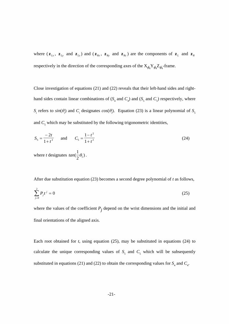
Close investigation of equations (21) and (22) reveals that their left-hand sides and right-

hand sides contain linear combinations of (S4 and C

4) and (S

5 and C

5) respectively, where

Si refers to sin(

i) and C

i designates cos(

i). Equation (23) is a linear polynomial of S

5

and C5 which may be substituted by the following trigonometric identities,

St

t5 2

2

1

and Ct

t5

2

2

1

1

(24)

where t designates tan( )1

2 5 .

After due substitution equation (23) becomes a second degree polynomial of t as follows,

P tjj

j

0

2

0 (25)

where the values of the coefficient Pj depend on the wrist dimensions and the initial and

final orientations of the aligned axis.

Each root obtained for t, using equation (25), may be substituted in equations (24) to

calculate the unique corresponding values of S5 and C

5 which will be subsequently

substituted in equations (21) and (22) to obtain the corresponding values for S4 and C

4.

-22-

As revealed by equation (25), the inverse position analysis of the wrist group produces

two distinctive solutions. In other words, this group possesses two configurations for

each required orientation of the aligned axis.

7. The Inverse Solution Procedure:

Figure (4) depicts a flow chart that has been designed to explain the procedure proposed

here for inverse position analysis of manipulators. As shown in the figure, the procedure

features a simple iterative approach which does not involve any Jacobian matrix

computations. Moreover, it produces multiple solutions to the problem which is a

considerable advantage over other iterative methods. By virtue of the concepts

presented, the various solutions may be calculated simultaneously if parallel computing

facilities are available.

In the present approach, the arm is assigned the task of positioning any point on the sixth

joint-axis at its required spatial location. The closest point on the sixth-joint axis to the

fifth joint-axis may be conveniently selected for this purpose. This point will be referred

to in the following discussion as p0i . The four joint-displacement solutions which

-23-

Read and Write Data

Perform Inverse Position Analysis (IPA) of the Arm to Get 4 Solutions

IPA of Wrist IPA of Wrist IPA of WristIPA of Wrist

m=1

IPA of arm to save the solution withminimum norm.

IPA of wrist to savethe solution withminimum norm.

m m-1 new

0

jk

Compare with therequired position andwork out the error e.

e

Get pjk

Compare to therequired position andwork out the error e.

e m=m+1

Get p=1

=2 =4=3=1

=2k k

j j jj

=1k=1k=2k =2k=2k

Yes

No

No

Yes

m

Stop

Calculate 6

Figure (4): Inverse Position Analysis of Robots Using Elementary Motions.

-24-

correspond to this positioning task are therefore obtained using the models presented

above and saved in four 3D-vectors, vj, where j=1,2,3 and 4.

At arm configuration number j, the wrist joints align the sixth joint-axis with its required

final orientation, as described in section (5), and the two corresponding solutions are

accordingly obtained and saved in a pair of 2D- vectors, wjk, where k may assume the

values of 1 or 2. To this end, a set of eight joint-displacement solutions have been

obtained. If the robot was of the spherical-wrist type these solutions should accurately

represent the required joint-displacements and no iterations would be required.

Calibrated robots, however, are not likely to have their last three joint-axes intersecting at

a common point (i.e. the spherical-wrist property was lost), the motions performed by the

wrist joints will displace the point which was previously positioned by the arm to eight

new locations, p0jk , corresponding to the wrist solutions obtained.

At location number jk, the instantaneous position vector, p0jk , of the displaced point may

be calculated, using a suitable direct kinematic procedure, and compared to the required

position vector p0n where the net radial error, e

jk, is calculated as follows,

e njk 0

jk p p0 (26)

If the calculated value for ejk does not fall within an allowable error zone (e.g. 0. 01mm)

the calculations proceed such that at iteration number m, the arm sets out from the most

-25-

updated configuration number jk(m-1) to position point pm-1jk in the required location.

The four solutions obtained may be stored in four 3D-vectors whose norms are

subsequently calculated and compared. Only the vector which corresponds to minimum

norm, v jkm , may be saved in the memory and the other solutions would be discarded.

This vector is referred to here as the arm elementary-motions vector because it contains

fractional quantities of elementary joint-displacements.

The two corresponding wrist solutions may then be obtained and stored in a pair of 2D-

vectors whose norms will also be calculated and compared. The vector with minimum

norm, w jkm , is subsequently saved while the other vector may be disposed of. In the

current context, w jkm is designated as the wrist elementary-motions vector because it

contains small values of joint-displacements.

The new displaced location of the positioned point may then be calculated and compared

with the required location as per equation (26). When the radial error is small enough,

the final joint-displacement vector, v jkn , of the arm group which corresponds to solution

number jk may be calculated as follows,

v v vjkn

j jkm

m

M

1

(27)

where M is the corresponding number of iterations.

-26-

The vector, w jkn , which corresponds to the jk-solution of the wrist group may be

expressed as follows,

w w wjkn

jk jkm

m 1

M

(28)

Once the jk-solution for the first five joint-displacement has been obtained, the

corresponding displacement of the last joint may simply be calculated.

The iterative technique proposed here utilises the physical kinematic behaviour of

manipulator joints and therefore fast and singularity-proof convergence may be assured.

The procedure is also suitable for use with parallel-computing facilities where each joint-

displacement solution may be conveniently assigned to a different processor. The

technique does not require any user-defined initial guesses introduced into the model.

8. Full-pose Alignment :

The work described in the previous sections is intended to locate the Z-axis of the sixth

joint at its desired spatial position, pn , and align it with the desired directional vector,

z6n . It is worth noting here that the tool (or end-effector) is pivoted to the sixth joint-axis

and can only rotate about it. As such, once this axis is located in its desired position and

direction in space, the tool needs to perform a single rotation about it to take its desired

final pose. To calculate the required displacement, 6, of the sixth joint, the intermediate

-27-

directional vector, intex , of the tool X-axis (after having performed 5 rotations about the

first 5 joint-axes) may be evaluated as follows,

00

ie

66

55

44

33

22

11

0

inte x

TTTTTTTx e (29)

where 6, in the above equation (29) is set equal to zero and i

ex is given as, T001 .

The transformation matrices, 1iiT , are calculated as indicated in section (3); also the 3x3

rotational matrices can be used for this purpose.

The angular displacement, 6, can now be calculated by rotating int

ex about z6n to coincide

with the desired final direction of the X-axis of the tool, nex . This may be achieved by

using the following equation,

nee

neenn

ee xx

xxzxxsign

int

int

16

int6 tan)( (30)

This final analysis is performed for every possible robot configuration and should ensure

that a full-pose identification has now been performed for the end-effector.

9. Experimental Results :

The models described in the present paper have been implemented in an integrated

approach developed for accurate kinematic control of robot manipulators. The ASEA

IRB/L6 robot which is shown in Figure (5) was used for experimental verification of the

results. At the selected zero-initial position, the -model parameters for both the

calibrated and nominal robots are given in Table (1).

-28-

Table (1): -Model Parameters of the ASEA IRB/L6 Robot at the Zero-Initial-Position. Nominal Manipulator Actual Manipulator

frame i ai (m) bi (m) i (deg) i (deg) ai (m) bi (m) i (deg) i (deg)

1 90 0.0000 0.0000 90.0 -90.0 0.00232 0.0 90.0 -90.378

2 0.0 -0.6900 0.0000 90.0 -180.0 -0.6931 0.00487 89.828 -179.54

3 0.0 -0.6700 0.0000 90.0 -180.0 -0.6727 0.00162 90.4213 -179.99

4 0.0 0.0000 0.0000 90.0 -90.0 -0.0007 0.00297 89.8033 -89.921

5 0.0 0.0000 -0.2325 90.0 -90.0 -0.0039 -0.2331 89.4829 -90.137

The frame of the first joint-axis was taken as the base frame and the end-effector shared

its Z-axis and origin with the sixth joint frame. This eliminates the need to include an

arbitrarily-located frame in the model and therefore and h do not appear in the Table.

Position commands were then issued to the robot controller via the models described

above and the end-effector position was measured, using theodoliltes, to evaluate the

robot accuracy. The average value of this accuracy improved more than 33 fold (from 47

mm to 1.4 mm) since many sources of error (transducer deviations, gear train errors,

geometric errors, …etc) were taken into account during the calibration procedure. The

details of the calibration procedure may be sought in the work by Sultan and Wager

(2001).

-29-

Figure (5): Schematic Diagram of the Robot Used for Experimental Verification.

One of the commanded positions was given, with respect to the Cartesian base

coordinates, by the Ten matrix as follows,

1000

0.85297168.02092306.0235371.0

1.636214198.034253757.0914758.0

7.19709976.093926805.0328356.0

6n0T

where all lengths are in mm.

The initial hand pose, as measured by theodolites, is given as follows,

1000

0.690999946.0005383.0008803.0

32.9030087983.0000181.0999961.0

49.100538.0999985.0000764.0

6iact0T

The results of the inverse position analysis which was performed on the robot are

displayed in Table (2). The number of iterations which correspond to the physically-

Z1Z6

-Ze

Z0

Z4

Z5

Z3

Z2

Y0

X0Xe

Ye

12

3 4

6

5

-30-

attainable solution is equal to 6 and the allowable radial error (as per equation 26) used in

the analysis was 0.007 mm. It should be noted here that the procedure produces no error

in the orientation of the end-effector axis by the virtue of the iterative technique used as

described in section 7. As such no convergence criterion is needed for orientation.

Table (2) Inverse Position Analysis Results for a Calibrated ASEA IRB/L6 Robot. Sol. No. j k 1

jk deg 2jk deg. 3

jk deg. 4jk deg. 5

jk deg. 6jk deg.

1 1 17.35 18.13 -4.60 -3.70 -9.50 36.59 1 2 16.65 -23.57 46.43 167.39 -172.07 -144.37 2 1 16.53 -74.92 -174.82 -100.261 -8.30 35.48 2 2 16.02 -66.67 134.06 122.97 -172.73 -144.97 3 1 -162.06 74.183 -4.34 100.0 169.91 37.08 3 2 -162.72 65.70 47.161 -123.43 8.86 -143.84 4 1 -160.76 -18.572 -175.15 3.60 169.70 37.28 4 2 -162.27 23.28 -133.36 -167.22 8.77 -143.92

10. Conclusion:

An approach is proposed to obtain multiple inverse-position solutions for robotic

structures. The procedure involved, which is suitable for both conventional and parallel

computer applications, regards the manipulator as consisting of two open-ended

mechanisms co-operating to place the end-effector at a desired spatial pose.

For calibrated robots, the procedure proposed adopts a simple iterative technique that

does not require user-defined initial guesses and does not involve the use of the

differential Jacobian-based models to eliminate the occurrence of singularity. Moreover,

for spherical-wrist robots, the technique produces straight forward non-iterative solutions

to the inverse position problem.

-31-

References:

1) Chiaverini, S., Siciliano, B. and Egeland, O., Review of the Damped Least-Squares

Inverse kinematics with Experiments on an Industrial Robot Manipulator, IEEE

Trans. Control Systems Technology, Vol. 2, No. 2, June 1994. pp. 123-134.

2) Coelho, P. H. G. and Nunes, L. F. A., Application of Kalman Filtering to Robot

Manipulators, Recent Trends in Robotics: Modelling, Control and Education. Edited

by Jamshidi, M., Luh, L. Y. S. and Shahinpoor, M. Elsevier Science Publishing Co.,

Inc., 1986, pp. 35-40.

3) Craig, John J., Introduction to Robotics, Addison-Wesley Publishing Company, 1986

4) Denavit, J. and Hartenberg, R. S., A Kinematic Notation for Low Pair Mechanisms

Based on Matrices, ASME J. Appl. Mechanics, Vol. 22, June 1955, pp. 215-221.

5) Duffy, J. and Crane C., A Displacement Analysis of the General Spatial 7-Link, 7R

Mechanism, Mech. Mach. Theory, Vol. 15, No. 3-A, 1980, pp. 153-169.

6) Goldenberg, A. A., Benhabib, B. and Fenton, R. G., A Complete Generalised

Solution to the Inverse Kinematics of Robots, IEEE. Trans. on Robotics and

Automation, Vol. RA-1, No. 1, March 1985, pp. 14-20.

7) Grudic, G. Z. and Lawrence, P. D., Iterative Inverse Kinematics with Manipulator

Configuration Control, IEEE. Trans. on Robotics and Automation, Vol. 9, No. 4,

August 1993, pp. 476-483.

-32-

8) Gu, Y.-L. and Luh, J. Y. S., Dual-Number Transformation and Its Application to

Robotics, IEEE J Robotics and Automation, Vol. RA-3, No. 6, Dec. 1987, pp. 615-

623.

9) Gupta, K., A Note on Position Analysis of Manipulators, Mech. Mach. Theory, Vol.

19, No. 1, 1984, pp. 5-8.

10) Hayati, S. and Roston, G., Inverse Kinematic Solution for Near-Simple Robots and

Its Application to Robot Calibration, Recent Trends in Robotics: Modelling, Control

and Education. Edited by, Jamshidi, M., Luh, L. Y. S. and Shahinpoor, M. Elsevier

Science Publishing Co., Inc, 1986, 41-50.

11) Kohli, D. and Osvatic, M., Inverse Kinematics of General 6R and 5R,P Spatial

Manipulators, ASME J. Mechanical Design, Vol. 115, Dec. 1993, pp. 922-930.

12) Lee, H.-Y. and Liang, C. G., A New Vector Theory for the Analysis of Spatial

Mechanisms, Mech. Mach. Theory, Vol. 23, No. 13, 1988A, pp. 209-217.

13) Lee, H.-Y. and Liang, C. G., Displacement Analysis of the General Spatial 7-Link 7R

Mechanism, Mech. Mach. Theory, Vol. 23, No. 13, 1988B, pp. 219-226.

14) Lee, H.-Y., Reinholtz, C. F., Inverse Kinematics of Serial-Chain Manipulators,

ASME J. Mechanical Design, Vol. 118, Sept. 1996, pp. 396-404.

15) Mahalingam, S. and Sharan, A., The Nonlinear Displacement Analysis of Robotic

Manipulators Using the Complex Optimisation Method, Mech. Mach. Theory, Vol.

22, No. 1, 1987, pp. 89-95.

-33-

16) Manocha, D. and Canny, J. F., Real Time Inverse Kinematics for General 6R

Manipulators, Proc. IEEE Conf. on Robotics and Automation, Nice-France, May

1992, pp. 383-389.

17) Manseur, R. and Doty, K., A Complete Kinematic Analysis of Four-Revolute-Axis

Robot Manipulators, Mech. Mach. Theory, Vol. 27, No. 5, 1992A, pp. 575-586.

18) Manseur, R. and Doty, K., A Robot Manipulator with 16 Real Inverse Kinematic

Solution Sets, The Int. J. Robotics Research, Vol. 8, No. 5, October 1989, pp. 75-79.

19) Manseur, R. and Doty, K., Fast Algorithm for Inverse Kinematic Analysis of Robot

Manipulators, The Int. J. Robotics Research, Vol. 7, No. 3, June 1988, pp. 52-63.

20) Manseur, R. and Doty, K., Fast Inverse Kinematics of Five-Revolute-Axis Robot

Manipulators, Mech. Mach. Theory, Vol. 27, No. 5, 1992B, pp. 587-597.

21) Manseur, R. and Doty, K., Structural Kinematics of 6-Revolute-Axis Robot

Manipulators, Mech. Mach. Theory, Vol. 31, No. 5, 1996, pp. 647-657.

22) Mooring, B. W., Roth, Z. S. and Driels, M. R., Fundamentals of Manipulator

Calibration, John Wiley & Sons, New York, 1991.

23) Paul, R., Robot Manipulators Mathematics, Programming and Control, MIT Press,

Cambridge, MA, 1981.

24) Phol, E. D. and Lipkin, H., Complex Robotic Inverse Kinematic Solutions, ASME J.

Mechanical Design, Vol. 115, Sept. 1993, pp. 509-514.

-34-

25) Pieper, D. L. and Roth, B., The Kinematics of Manipulators Under Computer

Control, Proc. 2nd Int. Congress on the Theory of Machines and Mechanisms, Vol. 2,

Zakopane, Poland, 1969, pp. 159–168.

26) Poon, J. K. and Lawrence, P. D., Manipulator Inverse Kinematics Based on Joint

Functions, Proc. IEEE Conf. on Robotics and Automation, Philadelphia, April 1988,

pp. 669-674.

27) Pradeep, A. K., Yoder, P. J. and Mukundan, R., On the Use of Dual-Matrix

Exponentials in Robotic Kinematic, The Int. J. Robotics Research, Vol. 8, No. 54,

October 1989, pp. 57-66.

28) Raghavan, M. and Roth, B., Kinematic Analysis of the 6R Manipulator of General

Geometry, Proceedings of the 5th Int. Symposium on Robotics Research, Tokyo, Aug.

28-31, 1989. pp. 263-269.

29) Smith, D. R. and Lipkin, H., Analysis of Fourth Order Manipulator Kinematics Using

Conic Sections, Proc. IEEE Conf. on Robotics and Automation, Cincinnati 1990, pp.

274-278.

30) Sultan, I. A. and Trevelyan, J. P., Inverse Kinematic Analysis of Bent Robots,

Proceedings of the Second International Conference On Automation, Robotics and

Computer Vision, Singapore, Sept. 15-18, 1992.

31) Sultan. I. A. An Integrated Approach for Accurate Kinematic Control of Robot

Manipulators, A PhD Thesis, The University of Western Australia, 1997.

-35-

32) Sultan, I. A. and Wager, J. G., User-Controlled Kinematic Modelling, Int. J.

Advanced Robotics, Vol. 12, No. 6, pp 663-677, 1999.

33) Sultan, I. A. and Wager, J. G., A Technique for the Independent-axis Calibration of

Robot Manipulators with Experimental Verification, Int. J. of Computer Integrated

Manufacturing, Vol. 14, No. 5, 2001.

34) Tsai, L.-W. and Morgan, A. P., Solving the Kinematics of the Most General Six- and

Five-Degree-of-Freedom Manipulators by Continuation Methods, ASME J.

Mechanisms, Transmissions and Automation in Design, June 1985, Vol. 107, pp.

189-199.

35) Wang, K. and Bjorke, O., An Efficient Inverse Kinematic Solution with a Closed

Form for Five-Degree-of-Freedom Robot Manipulators with a Non-Spherical Wrist,

Annals of CIRP, Vol. 38, 1989, pp. 365-368.

36) Wang., L. T. and Chen, C. C., A Combined Optimisation Method for Solving the

Inverse Kinematics Problem of Mechanical Manipulators, IEEE. Trans. on Robotics

and Automation, Vol. 7, No. 4, August 1991, pp. 489-499.

37) Yang, A. T. and Freudenstein, F., Application of Dual-Numbers Quaternion Algebra

to the Analysis of Spatial Mechanisms, ASME J. of Appl. Mechanics, June 1964, pp.

300-308.