arX

iv:n

ucl-

th/9

8040

43v2

30

Jul 1

998

SNUTP-98-022KOBE-FHD-98-1nucl-th/9804043

Photoproduction of φ mesons from the proton:

Polarization observables and strangeness in the nucleon

Alexander I. Titov a∗, Yongseok Oh b†, Shin Nan Yang c‡, and Tosiyuki Morii d§a Bogoliubov Laboratory of Theoretical Physics, JINR, 141980 Dubna, Russia

b Research Institute for Basic Sciences and Department of Physics, Seoul National University,

Seoul 151-742, Koreac Department of Physics, National Taiwan University, Taipei, Taiwan 10617, Republic of Chinad Faculty of Human Development, Kobe University, 3-11 Tsurukabuto, Nada, Kobe 675, Japan

Abstract

The polarization observables in φ meson photoproduction is studied to probe

the strangeness content of the nucleon. In addition to the dominant diffrac-

tive production and the one-pion-exchange process, we take into account the

direct knockout mechanism that arises from the possible hidden strangeness

content of the nucleon. We find that some double polarization observables are

very sensitive to the strangeness content of the proton because of the differ-

ent spin structures of the amplitudes associated with different mechanisms.

This suggests that such measurements could be very useful in probing the

strangeness content in the proton. The orbitally excited quark-cluster config-

urations in the proton are included in the calculation and found to have little

effect.

PACS number(s): 13.88.+e, 24.70.+s, 25.20.Lj, 13.60.Le

Typeset using REVTEX

∗E-mail address : atitov@thsun1.jinr.ru

†E-mail address : yoh@phya.snu.ac.kr

‡E-mail address : snyang@phys.ntu.edu.tw

§E-mail address : morii@kobe-u.ac.jp

1

I. INTRODUCTION

The possible existence of hidden strangeness in the nucleon has recently become one of themost controversial problems in nuclear/hadron physics. Some analyses of the pion-nucleonsigma term [1,2], polarized deep-inelastic lepton-proton scattering [3–5], and low energyelastic neutrino-proton scattering [6,7] indicate a significant role of strange sea quarks in thenucleon structure [8]. However, it has also been argued that such experimental results couldbe understood with little or null strangeness in the nucleon [9,10].

It will be interesting, therefore, to study other processes that might be related directly tothe strangeness content of the nucleon [11–16]. One of them is φ meson production from theproton. Since the φ meson is a nearly pure ss state because of ideal mixing with the ω meson,its coupling to the proton is suppressed through the OZI rule. Then the idea is that we couldextract information about the hidden strangeness of the nucleon by studying the strangesea quark contribution through the OZI evasion processes. One example is φ production inproton–anti-proton annihilation. Recent experiments on vector meson production throughpp annihilation at rest [17–19] report a strong violation of the OZI rule. It can be accountedfor by the presence of an intrinsic ss component in the nucleon wave function [8,20], whichcontributes to the process through the rearrangement and shake-out diagrams [21–24]. Onthe other hand, it was also claimed that this OZI violation could be explained throughmodified meson exchange models [25,26] without any strangeness content of the nucleon.

Another possibility is φ photo- and electro-production from proton targets [13]. In thisprocess, in addition to the vector-meson dominance model (VDM), the contribution from thehidden strangeness of the proton arises through the direct knockout process. In Refs. [27,28],Henley et al. calculated the contribution from knockout process to φ electroproduction crosssection and found it comparable to that of VDM with an assumption of a 10–20% strangesea quark admixture in the proton wave function. To arrive at this conclusion, they usednonrelativistic quark model wave functions for the hadrons. However, since the kinematicalregion of φ meson production is beyond the applicability of the nonrelativistic quark model,the relativistic corrections are expected to be important. In Refs. [29,30] we improved thecalculations of Refs. [27,28] with the use of a relativistic harmonic oscillator quark model(RHOQM). We found that the cross section of the direct knockout mechanism for the elec-troproduction is comparable to that of VDM at moderately large electron four-momentumtransfer with less than 5% admixture of strange sea quarks in the proton. However, it is noteasy to disentangle the two mechanisms from the cross section measurement because theirrespective contributions have similar dependence on momentum transfer [30].

To distinguish between the knockout and VDM processes, it was suggested the differencein the spin structures of various amplitudes be exploited [27,31–34]. In Ref. [33], we showedthat some double polarization observables are indeed very sensitive to the hidden strangenesscontent of the proton. We found that, with the use of RHOQM, the direct knockout processgives a very distinct contribution to some of the double polarization observables in φ pho-toproducton as compared to those of diffractive production and one-pion-exchange (OPE)process. A similar conclusion was drawn from the pp→ ΛΛ process to distinguish betweencontributions from the hidden strangeness of the nucleon and the effects from meson ex-change processes [35]. (See also Ref. [36].) The one-pion-exchange process arises from theφ-π-ρ(γ) coupling. Similar ω-π-ρ(γ) coupling gives non-negligible effects in the ω-meson

2

production case [37].In this paper, we extend our previous work to discuss other spin observables in φ photo-

production and give the details which were left out in Ref. [33]. We also improve the VDMamplitude to take into account the gauge invariance requirement within a quark-Pomeroninteraction picture. We further include, besides the lowest one, other configurations in the5-quark cluster model of the nucleon, which may give non-negligible contribution to thenucleon spin [20].

In Sec. II, we define the kinematical variables and briefly review the definitions of generalspin observables in terms of helicity amplitudes. Section III is devoted to our model for φphotoproduction. We include the diffractive and OPE production processes as well as thedirect knockout processes that arise from the hidden strangeness of the nucleon. The gaugeinvariance of VDM amplitude is discussed as well. Our results for the spin observables arepresented in Sec. IV along with their dependence on the hidden strangeness content of theproton. In Sec. V we discuss the role of orbitally excited quark-cluster configurations inthe nucleon wave function in φ photoproduction. We find that their effect is not important.Section VI contains summary and conclusion. Some detailed discussions and expressions forthe physical parameters are given in Appendixes.

II. SPIN OBSERVABLES AND THE HELICITY AMPLITUDES

We first define the kinematical variables for φ photoproduction from the proton, γ+p→φ + p, as shown in Fig. 1. The four-momenta of the incoming photon, outgoing φ, initial(target) proton, and final (recoil) proton are k, q, p, and p′, respectively. In the laboratoryframe, we write k = (EL

γ ,kL), q = (ELφ ,qL), p = (EL

p ,pL), and p′ = (ELp′,p

′L). The variables

in the c.m. system are written as k = (ν,k), q = (Eφ,q), p = (Ep,−k), and p′ = (Ep′,−q),respectively, as in Fig. 2. We also define t = (p − p′)2 and W 2 = (p + k)2 with MN thenucleon mass, Mπ the pion mass, and Mφ the φ mass. The differential cross section is givenby

dσ

dΩ= ρ0|Tfi|2, (2.1)

where ρ0 = (M2N |q|)/(16π2W 2|k|).

The general formalism for the spin observables of γ + p → φ + p has been discussedextensively in the literature. For completeness, we briefly review here the density matrixformalism and refer the interested readers to Refs. [38–42] for details.

To study the spin observables, it is useful to work with the helicity amplitudes in thec.m. frame. For polarized φ meson photoproduction, ~γ + ~p→ ~φ+ ~p, the helicity amplitudetakes the form,

Hλφ,λf ;λγ ,λi≡ 〈q;λφ, λf | T |k;λγ, λi〉, (2.2)

where the variables and the coordinate systems are shown in Fig. 2 with λγ (= ±1),λφ (= 0,±1), and λi,f (= ±1/2) denoting the helicities of the photon, φ meson, targetproton, and recoil proton, respectively. We follow the Jacob-Wick phase convention [39,43]

3

throughout this paper. In principle, there are 2 × 2 × 3 × 2 = 24 complex amplitudes.However, by virtue of parity invariance relation,

〈q;λφ, λf | T |k;λγ, λi〉 = (−1)Λf−Λi〈q;−λφ,−λf | T |k;−λγ,−λi〉, (2.3)

with Λf = λφ − λf and Λi = λγ − λi, only 12 complex helicity amplitudes are independent.We label them as [41]

H1,λφ≡ 〈λφ, λf = +1

2| T | λγ = 1, λi = −1

2〉,

H2,λφ≡ 〈λφ, λf = +1

2| T | λγ = 1, λi = +1

2〉,

H3,λφ≡ 〈λφ, λf = −1

2| T | λγ = 1, λi = −1

2〉,

H4,λφ≡ 〈λφ, λf = −1

2| T | λγ = 1, λi = +1

2〉. (2.4)

The φ-meson photoproduction amplitude can then be represented by a 6 × 4 matrix F inhelicity space;

F ≡

H2,1 H1,1 H3,−1 −H4,−1

H4,1 H3,1 −H1,−1 H2,−1

H2,0 H1,0 −H3,0 H4,0

H4,0 H3,0 H1,0 −H2,0

H2,−1 H1,−1 H3,1 −H4,1

H4,−1 H3,−1 −H1,1 H2,1

. (2.5)

In actual calculations, sometimes it is easier to evaluate the matrix elements in thenucleon spin space. They are related to the helicity amplitude discussed above, in thereference frame of Fig. 2, by

Hλφ,λf ;λγ ,λi= (−1)1−λi−λf

∑

mi,mf

d(1/2)mi,−λi

(0)d(1/2)mf ,−λf

(θ)〈λφ, mf | T | λγ, mi〉. (2.6)

This expression reduces to that of Ref. [44] for the pseudoscalar meson photoproductionprocess.

The differential cross section is given by the classical ensemble average as

dσ

dΩ= ρ0 Tr (ρF ). (2.7)

The final state density matrix is

ρF = FρIF †, (2.8)

where ρI is the initial state density matrix,

ρI = ργρN . (2.9)

The photon and proton density matrices, ργ and ρN , are defined in Appendix A. For example,in the unpolarized case where ργ = ρN = 1

2, we get

4

dσ

dΩ

(U)

=ρ0

4Tr (FF †) ≡ ρ0I(θ), (2.10)

which defines the cross section intensity I(θ).In general, any spin observable Ω can be written as

Ω =Tr [FAγANF †BVBN ′]

Tr (FF †), (2.11)

where AN denotes (12,σN), which are elements of the nucleon density matrix. The explicitforms of Aγ , BN ′, and BV can be obtained from the density matrices given in AppendixA. Note that the dimensions of the matrices are F(6 × 4), AγAN(4 × 4), F †(4 × 6), andBVBN ′(6 × 6).

A. Single polarization observables

When only the incoming photon beam is polarized, we can define the polarized beamasymmetry (analyzing power) Σx as

Σx =Tr [Fσx

γF †]

Tr (FF †). (2.12)

If we define σ(B,T ;R,V ) for the cross section dσ/dΩ where the superscripts (B, T ;R, V ) denotethe polarizations of (photon beam, target proton; recoil proton, produced vector-meson),then the physical meaning of Σx becomes clear through the relation,

Σx =σ(‖,U ;U,U) − σ(⊥,U ;U,U)

σ(‖,U ;U,U) + σ(⊥,U ;U,U), (2.13)

where the superscript U refers to an unpolarized particle and ‖ (⊥) corresponds to a photonlinearly polarized along the x (y) axis.

Similarly, we can define the polarized target asymmetry T , recoil polarization asymmetryP , and the vector-meson polarization asymmetry V as

Ty =Tr (Fσy

NF †)

TrFF †),

Py′ =Tr (FF †σy′

N ′)

Tr (FF †),

Vj =Tr (FF †ΩV

j )

Tr (FF †), (2.14)

where ΩVj ’s are given in Appendix A. The explicit expressions for the single polarization

observables can be found in Appendix B.

5

B. Double polarization observables

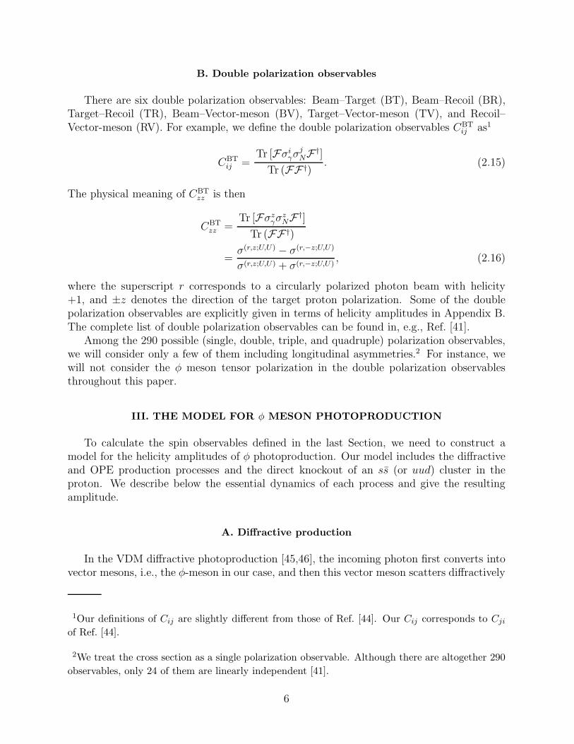
There are six double polarization observables: Beam–Target (BT), Beam–Recoil (BR),Target–Recoil (TR), Beam–Vector-meson (BV), Target–Vector-meson (TV), and Recoil–Vector-meson (RV). For example, we define the double polarization observables CBT

ij as1

CBTij =

Tr [Fσiγσ

jNF †]

Tr (FF †). (2.15)

The physical meaning of CBTzz is then

CBTzz =

Tr [Fσzγσ

zNF †]

Tr (FF †)

=σ(r,z;U,U) − σ(r,−z;U,U)

σ(r,z;U,U) + σ(r,−z;U,U), (2.16)

where the superscript r corresponds to a circularly polarized photon beam with helicity+1, and ±z denotes the direction of the target proton polarization. Some of the doublepolarization observables are explicitly given in terms of helicity amplitudes in Appendix B.The complete list of double polarization observables can be found in, e.g., Ref. [41].

Among the 290 possible (single, double, triple, and quadruple) polarization observables,we will consider only a few of them including longitudinal asymmetries.2 For instance, wewill not consider the φ meson tensor polarization in the double polarization observablesthroughout this paper.

III. THE MODEL FOR φ MESON PHOTOPRODUCTION

To calculate the spin observables defined in the last Section, we need to construct amodel for the helicity amplitudes of φ photoproduction. Our model includes the diffractiveand OPE production processes and the direct knockout of an ss (or uud) cluster in theproton. We describe below the essential dynamics of each process and give the resultingamplitude.

A. Diffractive production

In the VDM diffractive photoproduction [45,46], the incoming photon first converts intovector mesons, i.e., the φ-meson in our case, and then this vector meson scatters diffractively

1Our definitions of Cij are slightly different from those of Ref. [44]. Our Cij corresponds to Cji

of Ref. [44].

2We treat the cross section as a single polarization observable. Although there are altogether 290

observables, only 24 of them are linearly independent [41].

6

from the nucleon through Pomeron exchange, as shown in Fig. 3. Experimental observationsfor vector-meson production, small-|t| elastic scattering, and diffractive dissociation indicatethat Pomeron behaves rather like a C = +1 isoscalar photon [47,48]. A microscopic model forvector-meson photo- and electro-production at high energy based on the Pomeron–photonanalogy has been proposed by Donnachie and Landshoff [49], and the Pomeron could besuccessfully described in terms of a non-perturbative two-gluon exchange model [31,50–54].

In our previous calculation [33], we used the vector-meson dominance model withPomeron-photon analogy within the hadron-Pomeron interaction picture, which is expectedto be valid in the low energy region. In this paper, we employ a microscopic model for theVDM. In this approach, the incoming photon first converts into a quark and antiquark pair,which then exchanges a Pomeron3 with one of the quarks in the proton before recombininginto an outgoing φ meson, as depicted in Fig. 4. (See, e.g., Ref. [48].) In terms of φ (pho-ton) polarization vector εφ (εγ), the invariant amplitude of the diffractive production canbe written as

TVDMfi = iT0ε

∗φµMµνεγν , (3.1)

with

Mµν = FαΓα,µν , (3.2)

where Fα describes the Pomeron-nucleon vertex and Γα,µν is associated with the Pomeron–vector-meson coupling which is related to the γ → qq vertex Γν and the qq → φ vertex Vµ,as shown in Fig. 4. The dynamics of the Pomeron-hadron interactions is contained in T0.

To determine the explicit forms of the vertices, we have to rely on some model assump-tions. Based on the Pomeron-photon analogy, the quark-quark-Pomeron vertex, i.e., q2q3Pvertex in Fig. 4, is assumed to be γµ. Accordingly, we also have

Fα = u(p′)γαu(p), (3.3)

where u(p) is the Dirac spinor of the proton with momentum p. The factor Nq of the numberof quarks in the proton can be absorbed into T0.

With the assumptions used in Ref. [48], namely, (i) quarks q1 and q2 which recombineinto a φ-meson are almost on-shell and share equally the 4-momentum of the outgoing φ,i.e., the nonrelativistic wave function assumption, (ii) quark q3, which is between photonand Pomeron, is far off-shell, and (iii) Γν ∝ γν and Vµ ∝ γµ, the loop integral in Fig. 4 canbe easily carried out to give

Γα,µν ∝ 2 Tr γµ( 6p1 +Ms)γν( 6p1+ 6k +Ms)γ

α( 6p1+ 6q +Ms) , (3.4)

where Ms is the s quark mass and p1 is the 4-momentum of the quark q1. Explicit calculationleads to

3We do not consider two-gluon-exchange model for the Pomeron in this work.

7

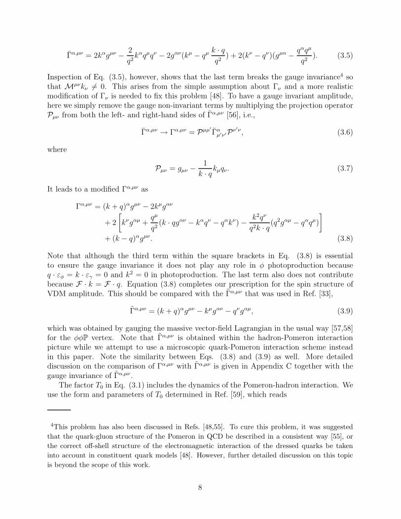
Γα,µν = 2kαgµν − 2

q2kαqµqν − 2gαν(kµ − qµ k · q

q2) + 2(kν − qν)(gµα − qαqµ

q2). (3.5)

Inspection of Eq. (3.5), however, shows that the last term breaks the gauge invariance4 sothat Mµνkν 6= 0. This arises from the simple assumption about Γν and a more realisticmodification of Γν is needed to fix this problem [48]. To have a gauge invariant amplitude,here we simply remove the gauge non-invariant terms by multiplying the projection operatorPµν from both the left- and right-hand sides of Γα,µν [56], i.e.,

Γα,µν → Γα,µν = Pµµ′

Γαµ′ν′Pν′ν , (3.6)

where

Pµν = gµν −1

k · qkµqν . (3.7)

It leads to a modified Γα,µν as

Γα,µν = (k + q)αgµν − 2kµgαν

+ 2

[

kνgαµ +qµ

q2(k · qgαν − kαqν − qαkν) − k2qν

q2k · q (q2gαµ − qαqµ)

]

+ (k − q)αgµν . (3.8)

Note that although the third term within the square brackets in Eq. (3.8) is essentialto ensure the gauge invariance it does not play any role in φ photoproduction becauseq · εφ = k · εγ = 0 and k2 = 0 in photoproduction. The last term also does not contributebecause F · k = F · q. Equation (3.8) completes our prescription for the spin structure ofVDM amplitude. This should be compared with the Γα,µν that was used in Ref. [33],

Γα,µν = (k + q)αgµν − kµgαν − qνgαµ, (3.9)

which was obtained by gauging the massive vector-field Lagrangian in the usual way [57,58]for the φφP vertex. Note that Γα,µν is obtained within the hadron-Pomeron interactionpicture while we attempt to use a microscopic quark-Pomeron interaction scheme insteadin this paper. Note the similarity between Eqs. (3.8) and (3.9) as well. More detaileddiscussion on the comparison of Γα,µν with Γα,µν is given in Appendix C together with thegauge invariance of Γα,µν .

The factor T0 in Eq. (3.1) includes the dynamics of the Pomeron-hadron interaction. Weuse the form and parameters of T0 determined in Ref. [59], which reads

4This problem has also been discussed in Refs. [48,55]. To cure this problem, it was suggested

that the quark-gluon structure of the Pomeron in QCD be described in a consistent way [55], or

the correct off-shell structure of the electromagnetic interaction of the dressed quarks be taken

into account in constituent quark models [48]. However, further detailed discussion on this topic

is beyond the scope of this work.

8

(

dσ

dt

)

VDM

= σγ(W )bφ exp(−bφ|t− tmax|), (3.10)

with bφ = 4.01 GeV−2 and σγ(W ) = 0.2 µb around W = 2 ∼ 3 GeV.5 This normalizes theamplitude T0 and explicitly we have

T0 =W 2 −M2

N

MNN√

4πσγ(W )bφ exp(−12bφ|t− tmax|), (3.11)

where

tmax = |t|min = 2M2N − 2EpEp′ + 2|k||q|, (3.12)

and the normalization constant N reads

N 2 =2

M2NM

2φ

k · p[

k · pM2φ + (k · q)2

]

+ 2k · p k · q[p · q − 2M2φ]

− (k · q)2[p · q +M2N ]. (3.13)

It is now straightforward to obtain the VDM helicity amplitude as

HVDMλφ,λf ;λγ ,λi

=∑

mi,mf

d(1/2)mf ,λf

(π + θ)d(1/2)mi,λi

(π)TVDMλφ,mf ;λγ ,mi

(3.14)

where

TVDMλφ,mf ;λγ ,mi

= iCT0

[

(1 + αα′ cos θ) (V0 −W0)

− az(Vz −Wz) + axWx − 2mi bx ImWy

]

δmi mf

+ 2mi

[

αα′ sin θ(V0 −W0)

− bx(Vz −Wz) − bzWx +1

2mi

bz ImWy]

δmi −mf

, (3.15)

with C =√

(γp + 1)(γ′p + 1)/2 and θ is the c.m. scattering angle. Definitions for the other

variables and their detailed derivation are given in Appendix D. Close inspection of thisamplitude shows that at small |t| (or θ → 0), the dominant part, namely the (k + q)αgµν

term in Γα,µν , has the spin/helicity conserving form as known in the conventional VDMamplitude,

TVDMλφ,mf ;λγ ,mi

≃ −2i|k|CT0(1 + αα′) δλφ λγ≡ −iMVDM

0 δλφ λγδmi mf

, (3.16)

while the spin-flip part is suppressed. Note also that TVDM is purely imaginary.

5 There are two comments concerning the parameters. First, these parameters may be dependent

on the energy scale. However, for our present qualitative study we will assume constant values

for them at W = 2 ∼ 3 GeV throughout this paper. Second, the parameters are determined by

fitting the formula (3.10) to the experimental data, so the contributions from the knockout and

OPE processes are neglected. However, as we will see, these mechanisms of the φ photoproduction

are suppressed compared with that of the VDM and the use of this parameter set is justified.

9

B. One-pion-exchange in φ photoproduction

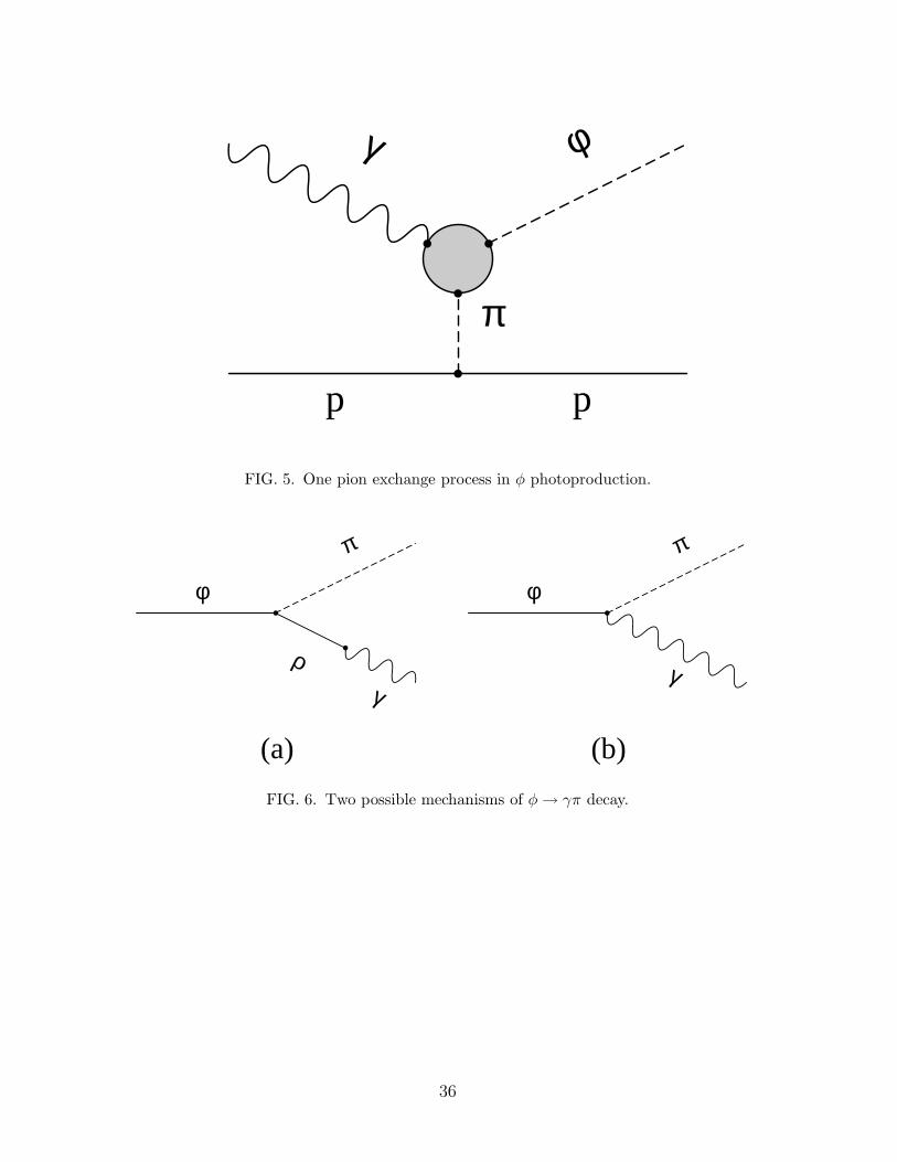
At low photon energy, one-pion-exchange diagram (Fig. 5) gives non-negligible contri-bution. This may be regarded as a correction to the VDM process [37].

The effective Lagrangian for the φγπ interaction has the form,

Lφγπ = gφγπǫµναβ∂µφν∂αAβπ

0, (3.17)

where Aβ is the photon field. The effective coupling constant gφγπ can be estimated throughthe decay width of φ→ γπ, which reads

Γ(φ→ γπ) =1

96π

(M2φ −M2

π)3

M3φ

g2φγπ. (3.18)

From the empirical value of Γ(φ→ γπ0) = 5.8 × 10−6 GeV, we get gφγπ = 0.042 GeV−1. Aremark is needed here concerning this estimate. The blob in Fig. 5 contains two processesas shown in Fig. 6. In addition to the VDM-like process of Fig. 6(a), there is anotherGell-Mann–Sharp–Wagner type diagram shown in Fig. 6(b). In the pure VDM, the decayprocess is completely dominated by Fig. 6(a) and there is no contact term. However, thispure VDM diagram gives

Γ(φ→ γπ)VDM =αe

24

g2φρπ(M2

φ −M2π)3

M3φf

2ρ

= 1.65 × 10−5 GeV, (3.19)

with the ρ-meson decay constant fρ (= 5.04), αe = e2/4π, and gφρπ = 1.19 GeV−1. Thusthe pure VDM overestimates the decay width by a factor of 3 and we have to allow forthe contact term of Fig. 6(b) to fit the experimental decay width. However, since the twotransition amplitudes of Fig. 6 have the same structure, we combine the two processes intoone term as in Eq. (3.17) with an effective coupling constant gφγπ.

For the NNπ interaction, one can use either pseudoscalar or pseudovector coupling whichare equivalent at the tree level. For definiteness we use the pseudoscalar coupling of the form

LPS = −igπNN Nγ5τ · πN, (3.20)

with g2πNN/4π = 14.3.

To include the off-shell effects, each vertex in Fig. 5 has to be modified with a formfactor. We follow Ref. [37] and use the Benecke-Durr form factors [60] in which the πNNform factor FN and the φγπ form factor Fφ are parameterized as

FN =1 + (2.9)2Q2

N

1 + (2.9)2Q2NT

, Fφ =U(2.3QF )

U(2.3QT )

(

QT

QF

)2

, (3.21)

where QN (QNT ) is the on-shell (off-shell) π-N c.m. momentum and QT (QF ) is the mo-mentum of the on-shell (off-shell) pion in the φ rest frame [61], respectively,

Q2N =

M2π(M2

π − 4M2N)

4M2N

, Q2NT =

t(t− 4M2N)

4M2N

,

QT =1

2Mφ(M2

φ −M2π), QF =

1

2Mφ(M2

φ − t). (3.22)

10

And U(x) is given as

U(x) =1

2x2

[

2x2 + 1

4x2log(4x2 + 1) − 1

]

. (3.23)

Before using these form factors, one should be careful with the use of factor 2.3 in Fφ of Eq.(3.21) since this factor is determined for the ωγπ coupling [37]. However, since we do nothave enough data for the φ meson case, we will use this value in our qualitative study on φphotoproduction.

The T matrix element of the OPE process then reads

TOPEfi =

i

t−M2π

gNNπgφγπWFmf ,mi

WBλφ,λγ

, (3.24)

where the coupling constants contain the Benecke-Durr form factors and

W Fmf ,mi

= u(p′)γ5u(p), WBλφ,λγ

= ǫµναβqµkαεφνεγβ. (3.25)

Direct calculation of W F and WB gives

W Fmf ,mi

= C[

2mf (α′ cos θ − α)δmf mi

− α′ sin θδmf −mi

]

,

WBλφ,λγ

= iEγ

[

λγ(Eφ − |q| cos θ)εφ · εγ +|q| sin θ√

2Mφ

(|q| − |q|Eφ cos θ)δλφ 0

− λφ|q| sin2 θ

2

]

, (3.26)

where

εφ · εγ = [1 + (Eφ

Mφ− 1)δλφ 0]d

(1)λγ ,λφ(θ), (3.27)

and α and α′ are given in Appendix D. Note also that the OPE amplitude is purely real.This implies that it does not interfere with the knockout amplitudes in the differential crosssection as we shall see below.

One may also consider the t-channel η-meson exchange instead of pion. In fact, the decaywidth of φ→ γη is about 5.58 × 10−5 GeV, which is larger than Γ(φ→ γπ) by an order ofmagnitude. This gives us the large φγη coupling constant gφγη = 0.218 GeV−1 as comparedto gφγπ = 0.042 GeV−1. However, we should also consider the ηNN coupling. By assumingSU(3) flavor symmetry, one obtains gηNN/gπ0NN = 1√

3· (D−3F )/(D+F ) ≃ −0.19 ∼ −0.35

using F/D = 0.5 ∼ 2/3, and we find that the product of the coupling constants in η-exchange diagram is of the same order of magnitude as that of OPE. Nevertheless, becauseof its heavier mass, the η-meson exchange amplitude is expected to be smaller than thatof OPE at least in the forward scattering region. There can also be cancellation betweenthe two because gηNN/gπ0NN < 0. In this work, therefore, we will not consider the η-mesonexchange diagram in φ photoproduction.6

6Furthermore, since this one boson exchange amplitude is purely real, its contribution to the

double polarization observables is expected to be negligible. See Eq. (4.10).

11

C. Direct knockout production

When the incoming photon interacts with the 5-quark component of the proton, wehave an additional process called direct knockout as shown in Fig. 7. This process can beclassified, according to the struck quark-cluster, into ss- and uud-knockout. In order to in-vestigate the effects from the hidden strangeness content of the proton in φ photoproduction,we parameterize the proton wave function in Fock space as

| p〉 = A0| uud〉+∑

X

AX | uudX〉+∑

X

BX | uudssX〉, (3.28)

where X denotes any combination of gluons and light quark pairs of u and d quarks. Our aimis to estimate |BX |2 by isolating the OZI evasion processes. Ellis et al. [22] estimated it tobe 1–19% from an analysis of pp annihilation. From the φ electroproduction process, Henleyet al. [27] claimed that its theoretical upper-bound would be 10–20%. We improved theirprediction by employing a relativistic quark model [29,30], and showed that the upper-boundcould be lowered to 3–5%.

For simplicity and for our qualitative study, we approximate the proton wave function(3.28) as

| p〉 = A| uud〉+B| uudss〉. (3.29)

This parameterization of the nucleon wave function can be justified in our case of φ pro-duction as argued in Refs. [27–30]. To compensate for the negative parity of the ss cluster,only the odd orbital excitations in the wave function of relative motion between uud andss clusters are allowed. In principle, there are two more configurations when we considerthe first orbital excitation of the quark clusters: either ss-cluster or uud-cluster is orbitallyexcited. In this Section, we consider only the ss clusters with jP

ss = 0− and 1−, where jPss

stands for the spin of an ss cluster of parity P , and leave the study of the other quark-clusterconfigurations to Sec. V. The proton wave function can then be expressed as

|p〉 = A|[uud]1/2〉 +∑

jss=0,1; jc

bjss|[

[[uud]1/2 ⊗ [L]]jc ⊗ [ss]jss]1/2〉, (3.30)

where the superscripts 1/2 and jss denote the spin of each cluster and (b0, b1) correspond tothe amplitudes of the ss cluster with spin 0 and 1, respectively. The strangeness admixtureof the proton, B2, is then defined to be

∑ |bjss|2, which is constrained to A2 +B2 = 1 by the

normalization of the wave function. The symbol ⊗ represents vector addition of the clusterspins and the orbital angular momentum L. We choose the lowest negative-parity excitationwith ℓ = 1. For jss = 1, jc (Jc = Suud + L) can either be 1/2 or 3/2 because suud = 1/2and ℓ = 1, As in Ref. [30], we assume that the two possible states have the same amplitude.We also limit our consideration to color-singlet cluster configurations, assuming that hiddencolor configurations do not contribute to the single (one-step) knockout processes [27,30].Our analyses show that the different ss configurations play different role in the knockoutproduction.

When the incoming photon strikes the ss cluster, we have the ss-knockout process asshown in Fig. 7(a), and Fig. 7(b) corresponds to the uud-knockout. In the ss-knockout

12

process, symmetry property of the spatial wave functions in the initial proton state onlyallows for magnetic transition to contribute, while electric (spin-independent) transition isforbidden. Then the transition amplitude is proportional to the matrix element

〈Sφ = 1|σs − σs|jss = 0, 1〉 · (q × εγ) , (3.31)

so that only the antisymmetric initial state with jss = 0 contributes. This leads to T ssfi ∝ b0.

In the case of uud knockout, the ss-cluster is a spectator, and only jss = 1 state can matchthe physical outgoing φ meson. Here, both the electric and magnetic transitions contributeand T uud

fi ∝ b1.The detailed description of the knockout process with the relativistic harmonic oscillator

quark model and its electromagnetic current can be found in Refs. [29,30]. In this paper wejust quote the relevant results. The knockout amplitudes are most easily evaluated in thelaboratory frame as given in Ref. [30]. After transforming into the c.m. frame, they read

T ssmφ,mf ;λγ ,mi

= iT ss0 Sss

mφ,mf ;λγ ,mi,

T uudmφ,mf ;λγ ,mi

= iT uud0 Suud

mφ,mf ;λγ ,mi. (3.32)

Here T ss0 and T uud

0 include the dependence of the amplitudes on the energy and momentumtransfer, and Sss and Suud contain their spin structure. Explicitly they take the form,

T ss0 =

(

8παeELφE

Lp′

MN

)1/2

A∗b0Fss(γLφ , qss)Fuud(γ

Lp′, 0)Vss(p

′L)µsE

Lγ

3MN,

T uud0 =

(

8παeELφE

Lp′

MN

)1/2

A∗b1Fss(γLφ , 0)Fuud(γ

Lp′, quud)Vuud(qL)

µELγ

2MN

, (3.33)

and

Sssfi =

√3∑

〈12mf 1 | 1

2mi〉ξss

λγε∗φ(mφ) · εγ(λγ),

Suudfi = −

√3∑

,jc,mc

〈12mf − λγ 1 |jcmc〉 〈jcmc 1mφ|12 mi〉 ξuud

, (3.34)

where

ξss±1 = ± 1√

2sin θp′ , ξuud

±1 = ∓ 1√2

sin θq,

ξss0 = cos θp′ , ξuud

0 = cos θq, (3.35)

with θα being the production angle in the laboratory frame. In addition, we use µs =MN/Ms, and µ = MN/Mq, with s quark mass Ms (= 500 MeV) and u,d quark mass Mq

(= 330 MeV). The functions Fβ’s (β = ss, uud) are the Fourier transforms of the overlapof the spatial wave functions of the struck cluster β in the entrance and exit channels [30],which read

13

Fss(γLφ , qss) = (γL

φ )−1 exp(−r2ssq

2ss/6) = (γL

φ )−1 exp−q2ss/(8Ωρ),

Fuud(γLp′, quud) = (γL

p′)−2 exp(−r2

uudq2uud/6) = (γL

p′)−2 exp−q2

uud/(6Ωξ), (3.36)

with

γLp′ =

ELp′

MN, q2

uud = 2(ELγ )2 − EL

γ

ELp′

[(ELγ )2 + p′2

L − q2L],

γLφ =

ELφ

Mφ, q2

ss = 2(ELγ )2 − EL

γ

ELp′

[(ELγ )2 − p′2

L + q2L], (3.37)

where ruud and rss are the rms radii of the proton and φ meson, respectively, and Ωρ,ξ

are the harmonic oscillator parameters. We use the parameters determined in Ref. [30] as√

Ωξ = 1.89 fm−1 and√

Ωρ = 3.02 fm−1.The momentum distribution function Vβ(p) of cluster β is given by

1

(2π)3Vβ(p) =

vβ(p)∫

dp vβ(p),

vβ(p) = p2 exp

− 5

3Ωχ

(

p2 − xβMNEβ

)

, (3.38)

where xss = 3/5, Ess = ELp′ and xuud = 2/5, Euud = EL

φ . The parameter Ωχ is again related

to the hadron rms radii and taken to be√

Ωχ = 2.63 fm−1 [30].Note that all knockout amplitudes are purely imaginary, which indicates the absorption

of incoming photon by the 5-quark component of the proton. Therefore, they do not in-terfere with the OPE amplitude in the differential cross section. However, we do expect astrong interference between the dominant imaginary part of the VDM photoproduction andknockout amplitudes.

IV. RESULTS

It is straightforward, with the help of Eq. (2.6), to obtain the helicity amplitudes of theknockout and OPE processes. The total photoproduction helicity amplitude H is given by

H = HVDM +Hss +Huud +HOPE. (4.1)

We can then proceed to calculate various spin observables with the formulas developed inSec. II and Appendix B. Among those presented in Appendix B, we focus on those whichare found to be strongly dependent on the strangeness content of the proton.

A. Unpolarized cross section

Before studying the spin observables, let us discuss the parameters of our model. Inaddition to the parameters of the VDM and RHOQM fixed in Sec. III, we have to determinethe amplitudes b0,1 of the proton wave function (3.30). As we will see, the prediction on the

14

spin observables is sensitive to the combination A∗bjss≡ ηjss

|A∗bjss|, where ηjss

(= ±1) is therelative phase between the strange and non-strange amplitudes. In principle, the purpose ofthis study is to determine these values by comparing the predictions with the experimentaldata. However, because of the lack of experimental data, we will make an assumption aboutthese values and compare our results with the pure VDM and OPE predictions that areassociated with the B2 = 0 case. For simplicity, we assume b20 = b21 = B2/2.

The result of our numerical calculation on the unpolarized φ photoproduction withinthe RHOQM is shown in Fig. 8. In Ref. [30], we have argued that a theoretical upper-bound of B2 would be around 3–5%. In Fig. 8, we carry out the calculation with thestrangeness probability B2 = 0.01. We find that the VDM process dominates the knockoutand OPE mechanisms except in the backward scattering region. However, our results atlarge scattering angles should not be taken seriously because, in this region the applicabilityof the VDM is questionable and the contributions from the intermediate excited hadronicstates are expected to be important. Therefore, the VDM gives the dominant contributionto the cross section in the kinematical region at small scattering angles in which we areinterested in.

B. Polarization observables

We show our predictions for the single polarization asymmetries, Σx, Vx′x′y′y′, Vz′z′, andVz′x′, in Fig. 9. It turns out that the single polarization asymmetries are not sensitive to thestrange quark admixture of the proton. However, the story is totally different for the doublepolarization asymmetries, namely, some of them are very sensitive to the strange admixturein the proton. Before presenting our numerical results for double polarization observables,we first discuss qualitatively why they are important.

Let us consider the most interesting region of t, i.e., |t| → |t|min (or θ → 0), wherethe differential cross section is maximal. Here we can neglect the uud-knockout mechanismbecause the uud-knockout cross section is suppressed in the forward scattering region. Asshown in Eq. (3.16), the diffractive photoproduction amplitude has the following helicityconserving form in this region

HVDMλφ,λf ;λγ ,λi

≃ −iMVDM0 δλf λi

δλφ λγ, (4.2)

where MVDM0 denotes the corresponding amplitude at |t| ∼ |t|min.

For the ss-knockout amplitude we use p′ν ≃ δν 0 at |t| ≃ |t|min and 〈12λi 1 0|1

2λi 〉 = 2λi/

√3

to obtain

Hssλφ,λf ;λγ ,λi

≃ −iMss0 (2λiλγ) δλf λi

δλφ λγ. (4.3)

Comparison of the helicity dependence of Eqs. (4.2) and (4.3) shows that the ss-knockouthelicity conserving amplitude has an additional important phase factor (2λiλγ). Here, theλγ factor comes from the magnetic structure of the electromagnetic interaction while 2λi

results from the coupling of Suud with L in the initial proton. The OPE amplitude in thisregion reads

HOPEλφ,λf ;λγ ,λi

≃ −MOPE0 (2λiλγ) δλf λi

δλφ λγ. (4.4)

15

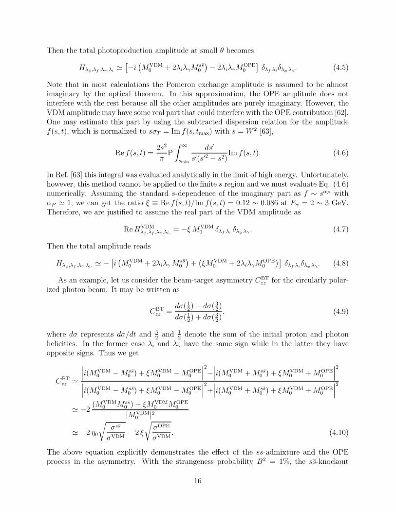
Then the total photoproduction amplitude at small θ becomes

Hλφ,λf ;λγ ,λi≃[

−i(

MVDM0 + 2λiλγM

ss0

)

− 2λiλγMOPE0

]

δλf λiδλφ λγ

. (4.5)

Note that in most calculations the Pomeron exchange amplitude is assumed to be almostimaginary by the optical theorem. In this approximation, the OPE amplitude does notinterfere with the rest because all the other amplitudes are purely imaginary. However, theVDM amplitude may have some real part that could interfere with the OPE contribution [62].One may estimate this part by using the subtracted dispersion relation for the amplitudef(s, t), which is normalized to sσT = Im f(s, tmax) with s = W 2 [63],

Re f(s, t) =2s2

πP

∫ ∞

smin

ds′

s′(s′2 − s2)Im f(s, t). (4.6)

In Ref. [63] this integral was evaluated analytically in the limit of high energy. Unfortunately,however, this method cannot be applied to the finite s region and we must evaluate Eq. (4.6)numerically. Assuming the standard s-dependence of the imaginary part as f ∼ sαP withαP ≃ 1, we can get the ratio ξ ≡ Re f(s, t)/Im f(s, t) = 0.12 ∼ 0.086 at Eγ = 2 ∼ 3 GeV.Therefore, we are justified to assume the real part of the VDM amplitude as

ReHVDMλφ,λf ,λγ ,λi,

= −ξ MVDM0 δλf λi

δλφ λγ. (4.7)

Then the total amplitude reads

Hλφ,λf ,λγ ,λi, ≃ −[

i(

MVDM0 + 2λiλγ M

ss0

)

+(

ξMVDM0 + 2λiλγM

OPE0

)]

δλf λiδλφ λγ

. (4.8)

As an example, let us consider the beam-target asymmetry CBTzz for the circularly polar-

ized photon beam. It may be written as

CBTzz =

dσ(12) − dσ(3

2)

dσ(12) + dσ(3

2), (4.9)

where dσ represents dσ/dt and 32

and 12

denote the sum of the initial proton and photonhelicities. In the former case λi and λγ have the same sign while in the latter they haveopposite signs. Thus we get

CBTzz ≃

∣

∣

∣i(MVDM

0 −Mss0 ) + ξMVDM

0 −MOPE0

∣

∣

∣

2

−∣

∣

∣i(MVDM

0 +Mss0 ) + ξMVDM

0 +MOPE0

∣

∣

∣

2

∣

∣

∣i(MVDM

0 −Mss0 ) + ξMVDM

0 −MOPE0

∣

∣

∣

2

+∣

∣

∣i(MVDM

0 +Mss0 ) + ξMVDM

0 +MOPE0

∣

∣

∣

2

≃ −2(MVDM

0 Mss0 ) + ξMVDM

0 MOPE0

|MVDM0 |2

≃ −2 η0

√

σss

σVDM− 2 ξ

√

σOPE

σVDM. (4.10)

The above equation explicitly demonstrates the effect of the ss-admixture and the OPEprocess in the asymmetry. With the strangeness probability B2 = 1%, the ss-knockout

16

contribution to the total unpolarized cross section is only at the level of 5%. But in theasymmetry CBT

zz , its contribution may be seen at the level of 0.45 since it is proportionalto the square root of the hidden strangeness contribution to the cross section. This shouldbe compared with the prediction of VDM plus OPE, which gives CBT

zz ≈ 0 when the VDMamplitude is purely imaginary. The OPE contribution to the unpolarized cross sectionhas the same order of magnitude as that of the ss knockout, and its contribution to CBT

zz

comes only from the interference with the real part of the VDM amplitude. However, thiscontribution is suppressed by the additional factor ξ ∼ 0.1 and, as a result, it is at the levelof 0.05 which is much smaller than the effect of hidden strangeness in the proton. Thus, inthe results presented below we do not take into account the real part of the VDM amplitude.

C. Numerical results

Our results for the Beam–Target double asymmetry7, CBTij , are shown in Fig. 10.

Here the solid line corresponds to the VDM plus OPE prediction, and the dashed andthe dot-dashed lines are the predictions when we include the knockout contributions withB2 = 0.25% and 1%, respectively. Since we have no a priori information about the phasesη0,1, we give results for all the four different choices of relative phases. Our numerical cal-culation confirms the previous qualitative considerations. One can see that CBT

zz in Fig.10(a) depends strongly on the hidden strangeness content of the proton even in the forward

scattering region. This difference is caused by the different spin structures of the VDMand the knockout amplitudes. Therefore, this observable can be used to extract the hiddenstrangeness of the proton even for B2 ≤ 1%. The results for CBT

zx in Fig. 10(b) lead to thesame conclusion although it is not as sensitive as in CBT

zz . Note that the results at small θare nearly independent of η1. This is because the uud-knockout process is suppressed com-pared with other mechanisms in this region. Similarly, the results are nearly independentof the phase η0 at large θ. From the energy dependence of the polarization observables,we observe that the knockout contribution is suppressed at higher energies because of thestrong suppression due to the form factors in the knockout amplitudes. This leads to theconclusion that the optimal range of the initial photon energy needed to measure the sscomponent of the proton would be around 2–3 GeV. Furthermore, we find that the forwardscattering region of θ ≤ 30 offers a better opportunity to measure the hidden strangenesscontribution. This conclusion holds for the other spin observables as will be seen below.

In Fig. 11, we give our results for the Beam–Recoil asymmetries, CBRzx′ and CBR

zz′ . Thisshows that these observables can be useful in probing the strangeness of the nucleon.

The Target–Recoil double asymmetries CTRxz′ and CTR

zz′ are shown in Fig. 12. In this case,however, the knockout mechanism gives a very similar behavior of VDM except at largeangles. Thus the observables CTR

xz′ and CTRzz′ are not so useful for the purpose of extracting

the knockout process. The same conclusion applies to the Beam–Vector-meson asymmetriesCBV

ij . As an example, we give our results in Fig. 13, which shows that CBVzx′ and CBV

zz′ are

7Note that our CBTzz corresponds to the minus of LBT of Ref. [33].

17

nearly independent of the hidden strangeness content of the proton.8

Figure 14 shows our results for CTV. We also present the predictions for CRV in Fig. 15.We see that all of them show strong sensitivity to the strangeness content of the proton.

V. OTHER CONFIGURATIONS OF NUCLEON WAVE FUNCTION

In the last Section, we assume that both the ss and uud clusters are in their lowest orbitalconfiguration, namely, S-state. We label this configuration as “Configuration (I).” In thisSection, we discuss the role of the orbitally excited cluster configurations in the 5-quarkcluster model for the nucleon in φ photoproduction. We consider the orbital excitationof the ss cluster, called “Configuration (II)” and the orbitally excited uud-cluster, called“Configuration (III).” In these cases, the ss- and uud-clusters form a positive parity physicalproton with ℓ = 0. Then we can generalize the proton wave function as

|p〉 = A|[uud]1/2〉 +∑

n=I,II,IIIjss=0,1

b(n)jss

|[[uud]jn ⊗ [ss]jss ⊗ [L]]1/2〉, (5.1)

where the superscripts jn and jss denote the spin of each cluster and |b(n)0 |2 and |b(n)

1 |2correspond to the spin-0 and spin-1 amplitudes of the ss cluster of “Configuration (n),”

respectively. B2, the strangeness admixture of the proton, is then∑

(b(n)jss

)2. The amplitudes

are constrained to be A2+B2 = A2+∑

(b(n)jss

)2 = 1 by the normalization of the wave function.The symmetry properties of the wave functions in the initial and final states lead to the

selection rules for different ss configurations as summarized in Table I. We find that fromsix possible terms of the proton wave function (5.1), only four can contribute to the directknockout process: two in ss-knockout and two in uud-knockout. The other two amplitudesdo not contribute to the direct knockout process, although they can give a contribution tothe total hidden strangeness probability.

By analyzing the amplitudes one can find that the electric transition is suppressed bythe magnetic as in the case of Configuration (I) [30]. For example, the suppression factorfor Configuration (II) reads

f(II) =|p′

L| sin θp′

ELγ

, (5.2)

which can be expressed in the invariant form as

f 2(II) = −2M2

N

W 2t2 +[

W 2(

W 2 − 2M2N −M2

φ

)

+M2N

(

M2N −M2

φ

)

t]

+M4φM

2N

(W 2 −M2N )

4 . (5.3)

Numerical estimation shows that with W ∼ 2.1 GeV the suppression factor f 2(II) reaches

its maximum value around 0.02 at t ∼ −0.8 GeV2 and it becomes negligibly small as

8Note that the quantities CBVij , CTV

ij , and CRVij with (j = x′, y′, z′) are defined to vary between

±√

3/2 [38].

18

|t| → |t|max or |t| → |t|min. A similar suppression factor appears in the electric transitionof uud-knockout in Configuration (III). Thus in the region of t of interest to us, wherethe knockout mechanism would be important, the contribution of the electric transitions isnegligible and we will consider the magnetic transitions only.

The amplitudes for Configurations (II) and (III) can be calculated in a straightforwardway using the method of Refs. [29,30]. The corresponding amplitudes have the form as givenin Eq. (3.32) by replacing T0 and S by

Tss(II)0 =

(

8παeELφE

Lp′

MN

)1/2

A∗b(II)0 F

(II)ss (γL

φ , qss)F(I)uud(γ

Lp′, 0)Vss(p

′L)µsE

Lγ

3MN, (5.4)

Sss(II)fi = −λγ

√3∑

jc=0,1

〈1ms 1 0|jcms〉〈12mf jc ms|12mi〉〈1ms 1 λi|1mφ〉, (5.5)

for “Configuration (II)” and

Tuud(III)0 =

(

8παeELφE

Lp′

MN

)1/2

A∗b(III)1 F

(I)ss (γL

φ , 0)F(III)uud (γL

p′, quud)Vuud(qL)µEL

γ

2MN, (5.6)

Suud(III)fi = −

√

3

2

∑

jc=1/2,3/2

〈jc mf − λγ 1mφ|12 mi〉〈12mf − λγ 1 0|jcmf − λγ〉, (5.7)

for “Configuration (III).” The functions F(II),(III)β with β = (ss, uud) are related to the

correspondent F(I)β of Eq. (3.36) as

F(II)ss (γL

φ , qss) =EL

γ

√

r2ss(1 − Vq‖)

3F

(I)ss (γL

φ , qss),

F(III)uud (γL

p′, quud) =EL

γ

√

r2uud(1 − Vp′‖)

3F

(I)uud(γ

Lp′, quud), (5.8)

where Vp ‖ = |p| cos θp/ELp . The momentum distribution function Vβ(p) of cluster β is given

by

1

(2π)3Vβ(p) =

vβ(p)∫

dp v(0)β (p)

,

vβ(p) = exp

− 5

3Ωχ

(

p2 − xβMNEβ

)

. (5.9)

Note that the difference with vβ of Eq. (3.38) lies in the absence of the factor p2. Thecalculation of T ss(II) is rather similar to that of T ss(I) which is given in Ref. [30] and AppendixE contains the derivation of T ss(III) in some detail.

Analyses of the relative contribution from different cluster configurations show that thecontribution of Configurations (II) and (III) are much smaller (by an order of magnitude)

than that of Configuration (I) even if we assume the same values for b(n)0,1 . This can be

19

seen from Fig. 16 where we present our results for the differential cross sections from eachconfiguration.

For clarity, let us consider the ss-knockout for Configurations (I) and (II). The ratio ofthe spatial matrix elements for Configurations (I) and (II) read

Rss =EL

γ (1 − Vq ‖)√

r2ss

|p′L|

NII

3NI

, (5.10)

where NI,II are the normalization factors of the radial wave functions of Configurations (I)and (II), respectively. Since

N−2α ∼

∫

dpvα(p), (5.11)

we can obtain

NII

NI

≃√

3Ωχ

2. (5.12)

Using the numerical value of the dimensional parameters rss = 0.29 fm and√

Ωχ = 2.63fm−1 [30], we obtain

Rss ≃ 0.31EL

γ (1 − Vq ‖)

|p′L|

. (5.13)

Since at θ ≃ 0 we have cos θp′ ≃ cos θφ ≃ 1, ELφ = EL

γ + t/2MN ≃ ELγ , and

|p′L| = |kL| − |qL| ≃ EL

γ

(

1 − |qL|EL

φ

)

= ELγ (1 − Vq ‖), (5.14)

we then obtain R2ss ≃ 0.1, which agrees with the numerical calculation of Fig. 16. A similar

conclusion can be drawn for the uud-knockout from Configurations (I) and (III).The above analysis shows that the cross section of the knockout process is dominated by

Configuration (I) and we can safely neglect the other cluster configurations in the protonwave function. Now let us consider the polarization observables. For simplicity, we againconsider the case of Configuration (II). From the amplitude (5.5), one can find

Hss(II)λf ,λφ;λγ ,λi

∝ δλf λiδλφ λγ

. (5.15)

This has the same structure as the VDM helicity amplitude (4.2). Since its amplitude issuppressed by the dominant VDM amplitude, however, it cannot be extracted from thebackground VDM contribution. We could verify this analysis by numerical calculation evenwith the assumption of the same values for b

(n)jss

. Furthermore, because of their heavy mass,the coefficients b0,1 of Configurations (II) and (III) are expected to be much smaller thanthose of Configuration (I). As a conclusion, therefore, the contributions from the orbitallyexcited cluster configurations can be neglected in the polarization observables as well.

20

VI. SUMMARY AND CONCLUSION

We have studied the possibility of using the spin observables of the φ meson photopro-duction process in probing the hidden strangeness content of the proton. We consider thedirect knockout mechanism in addition to the VDM and OPE processes by assuming anss component in the proton wave function. Unlike the differential cross section, we findthat the spin observables could be useful in disentangling the knockout process from theVDM and OPE processes. We find that single polarization observables are not sensitiveto the strangeness content of the proton. However, some double polarization observables,notably, CBT

zx,zz, CBRzx′,zz′, C

TVzx′,zz′, and CRV

xx′,zz′, are very sensitive to the hidden strangeness con-tent of the proton in the forward scattering region, whereas most of the Target–Recoil andBeam–Vector-meson double asymmetries are not. It indicates that measurements of thesedouble polarization observables could be very useful in probing the strangeness content ofthe proton.

We also find that the contribution of the knockout mechanism is suppressed with in-creasing initial photon energy because of the strong suppression due to the form factors inthe knockout amplitudes. Therefore, we expect that the optimal range of the initial pho-ton energy needed to measure the ss component of the proton would be around 2–3 GeV.However, it should be mentioned that at extremely low energy just near the threshold onehas to take into account the OZI evading re-scattering process and it would be interestingto study its effect on the polarization observables.

The orbitally excited quark cluster configurations in the proton wave function was alsoinvestigated in connection with φ photoproduction. We find that their role is not importantin the cross section and polarization observables and, therefore, these configurations can beneglected in the study of φ photoproduction.

The purpose of this study is to determine the strangeness content of the proton by investi-gating the polarization observables. Unfortunately, because of the scarcity of presently avail-able experimental data [64,65], we can not give any definite predictions for the strangenesscontent of the proton based on our analyses. Thus, new experiments are strongly called forat the current electron facilities which, hopefully, will help to shed light on our understandingof the proton structure.

Finally, we point out that, since the ss knockout process dominates the uud knockout atthe forward scattering angle, one can estimate the value of b0 in the proton wave function(3.30) by analyzing polarization observables. However, it is not easy to get estimate for b1because its contribution can be seen only at large θ where corrections to our model are ex-pected to be important. To get information for b1, therefore, it would be interesting to applyour analyses to η(η′) photoproduction as a complementary process to φ photoproduction,since the ss knockout process in this case is associated with b1.

ACKNOWLEDGMENTS

We gratefully acknowledge the useful discussions with M. Fujiwara, S. B. Gerasimov, S.V. Goloskokov, C. R. Ji, T. Kinashi, and M. Namiki. Y.O. is also grateful to D.-P. Min forencouragement and wish to thank the Physics Department and the Center for Theoretical

21

Sciences of the National Taiwan University for the warm hospitality. A.I.T. appreciates thewarm hospitality of the Faculty of Human Development of Kobe University where part ofthis work was carried out. This work was supported in part by the Russian Foundation forBasic Research under grant No. 96-15-96423, the Korea Science and Engineering Foundationthrough the Center for Theoretical Physics of Seoul National University, the National ScienceCouncil of ROC under grant No. NSC87-2112-M-002, and Monbusho’s Special Program forPromoting Advanced Study (1996, Japan). Lastly we thank A. Jackson of Kobe ShoinWomen’s College for careful reading of the manuscript.

APPENDIX A: DENSITY MATRICES

In this Appendix, we discuss the density matrices of the photon, target and recoil proton,and the vector meson. In general, the density matrix of the photon can be written as

ργ =1

2(12 + σγ · PS), (A1)

in photon helicity space, where 12 is the 2×2 unit matrix and PS is the Stokes vector whichdefines the direction and degree of polarization of the photon beam. The presence of σγ isdue to the fact that a real photon has only two spin degrees of freedom. The Stokes vectorscorresponding to some special cases of photon polarization can be found, for example, inRef. [44].

The proton density matrix is in the spin 12

space and is therefore a 2 × 2 Hermitianmatrix. So we have

ρN =1

2(12 + σN · PN), (A2)

for the target proton and

ρN ′ =1

2(12 + σN ′ · PN ′), (A3)

for the recoil proton.For the vector meson, because of its spin-1 structure, the density matrix cannot be

described by vector polarizations only. To describe the vector meson polarization completely,we have to take into account the tensor polarizations. The tensor polarization operator isdefined as [39,40]

Sjk =3

2(SjSk + SkSj) − 2δj k13, (A4)

where 13 is the 3 × 3 unit matrix with

Sx =1√2

0 1 01 0 10 1 0

, Sy =1√2

0 −i 0i 0 −i0 i 0

, Sz =

1 0 00 0 00 0 −1

. (A5)

Only five of them are independent since Sxx + Syy + Szz = 0. Therefore, we are led to thefinal form of the density matrix of vector meson as

22

ρV =1

3(13 +

∑

j

P Vj ΩV

j ), (A6)

where

ΩVj =

√

3

2(Sx, Sy, Sz),

1√6(Sxx − Syy),

1√2Szz,

√

2

3(Sxy, Syz, Szx), (A7)

which are normalized as Tr ΩVj ΩV

k = 3δj k.The explicit forms of the matrices appearing in Eq. (2.11) are (12,σγ) for Aγ , (12,σN(N ′))

for AN (BN ′), and (13,ΩVj ) for BV .9

APPENDIX B: SINGLE AND DOUBLE POLARIZATION OBSERVABLES IN

HELICITY AMPLITUDES

In this Appendix, we give the explicit expressions for the spin observables in terms ofhelicity amplitudes.

The cross section intensity I(θ) is defined as

I(θ) =1

4Tr (FF †), (B1)

which leads to

I(θ) =1

2

4∑

i=1

∑

a=±1,0

|Hi,a|2. (B2)

The explicit expressions for non-vanishing single polarization observables are as follows.

Σx · I(θ) = −Re

H∗4,1H1,−1 −H∗

4,0H1,0 +H∗4,−1H1,1

−H∗3,1H2,−1 +H∗

3,0H2,0 −H∗3,−1H2,1

. (B3a)

Ty · I(θ) = −Im

H∗4,−1H3,−1 +H∗

4,0H3,0 +H∗4,1H3,1

+H∗2,−1H1,−1 +H∗

2,0H1,0 +H∗2,1H1,1

. (B3b)

Py′ · I(θ) = −Im

H∗4,−1H2,−1 +H∗

4,0H2,0 +H∗4,1H2,1

+H∗3,−1H1,−1 +H∗

3,0H1,0 +H∗3,1H1,1

. (B3c)

Vy′ · I(θ) = −√

3

2Im

H∗4,0(H4,1 −H4,−1) +H∗

3,0(H3,1 −H3,−1)

+H∗2,0(H2,1 −H2,−1) +H∗

1,0(H1,1 −H1,−1)

. (B3d)

Vx′x′y′y′ · I(θ) =

√

3

2Re

H∗4,−1H4,1 +H∗

3,−1H3,1 +H∗2,−1H2,1 +H∗

1,−1H1,1

. (B3e)

9One has to use −σx and −σz for the initial and final protons instead of σx and σz in order to

have the correct helicity states in the c.m. system [44].

23

Vz′z′ · I(θ) =1

2√

2

|H4,−1|2 − 2|H4,0|2 + |H4,1|2 + |H3,−1|2 − 2|H3,0|2 + |H3,1|2

+ |H2,−1|2 − 2|H2,0|2 + |H2,1|2 + |H1,−1|2 − 2|H1,0|2 + |H1,1|2

. (B3f)

Vz′x′ · I(θ) =

√3

2Re

H∗4,0(H4,1 −H4,−1) +H∗

3,0(H3,1 −H3,−1)

+H∗2,0(H2,1 −H2,−1) +H∗

1,0(H1,1 −H1,−1)

. (B3g)

The explicit expressions for some double polarization observables are given below.• Beam–Target

CBTyx · I(θ) = Im

H∗4,−1H2,1 −H∗

4,0H2,0 +H∗4,1H2,−1

−H∗3,−1H1,1 +H∗

3,0H1,0 −H∗3,1H1,−1

, (B4a)

CBTyz · I(θ) = −Im

H∗4,−1H1,1 −H∗

4,0H1,0 +H∗4,1H1,−1

+H∗3,−1H2,1 −H∗

3,0H2,0 +H∗3,1H2,−1

, (B4b)

CBTzx · I(θ) = −Re

H∗4,−1H3,−1 +H∗

4,0H3,0 +H∗4,1H3,1

+H∗2,−1H1,−1 +H∗

2,0H1,0 +H∗2,1H1,1

, (B4c)

CBTzz · I(θ) = −1

2

|H4,−1|2 + |H4,0|2 + |H4,1|2 − |H3,−1|2 − |H3,0|2 − |H3,1|2

+ |H2,−1|2 + |H2,0|2 + |H2,1|2 − |H1,−1|2 − |H1,0|2 − |H1,1|2

. (B4d)

• Beam–Recoil

CBRyx′ · I(θ) = Im

H∗4,−1H3,1 −H∗

4,0H3,0 +H∗4,1H3,−1

−H∗2,−1H1,1 +H∗

2,0H1,0 −H∗2,1H1,−1

, (B5a)

CBRyz′ · I(θ) = Im

H∗4,−1H1,1 −H∗

4,0H1,0 +H∗4,1H1,−1

−H∗3,−1H2,1 +H∗

3,0H2,0 −H∗3,1H2,−1

, (B5b)

CBRzx′ · I(θ) = −Re

H∗4,−1H2,−1 +H∗

4,0H2,0 +H∗4,1H2,1

+H∗3,−1H1,−1 +H∗

3,0H1,0 +H∗3,1H1,1

, (B5c)

CBRzz′ · I(θ) =

1

2

|H4,−1|2 + |H4,0|2 + |H4,1|2 + |H3,−1|2 + |H3,0|2 + |H3,1|2

− |H2,−1|2 − |H2,0|2 − |H2,1|2 − |H1,−1|2 − |H1,0|2 − |H1,1|2

. (B5d)

• Target–Recoil

CTRxx′ · I(θ) = Re

H∗4,−1H1,−1 +H∗

4,0H1,0 +H∗4,1H1,1

+H∗3,−1H2,−1 +H∗

3,0H2,0 +H∗3,1H2,1

, (B6a)

CTRxz′ · I(θ) = −Re

H∗4,−1H3,−1 +H∗

4,0H3,0 +H∗4,1H3,1

−H∗2,−1H1,−1 −H∗

2,0H1,0 −H∗2,1H1,1

, (B6b)

CTRzx′ · I(θ) = Re

H∗4,−1H2,−1 +H∗

4,0H2,0 +H∗4,1H2,1

−H∗3,−1H1,−1 −H∗

3,0H1,0 −H∗3,1H1,1

, (B6c)

CTRzz′ · I(θ) = −1

2

|H4,−1|2 + |H4,0|2 + |H4,1|2 − |H3,−1|2 − |H3,0|2 − |H3,1|2

− |H2,−1|2 − |H2,0|2 − |H2,1|2 + |H1,−1|2 + |H1,0|2 + |H1,1|2

. (B6d)

24

• Beam–Vector-meson

CBVyx′ · I(θ) = −

√3

2Im

H∗4,−1H1,0 −H∗

4,0(H1,−1 +H1,1) +H∗4,1H1,0

−H∗3,−1H2,0 +H∗

3,0(H2,−1 +H2,1) −H∗3,1H2,0

, (B7a)

CBVyz′ · I(θ) = −

√

3

2Im

H∗4,−1H1,1 −H∗

4,1H1,−1 −H∗3,−1H2,1 +H∗

3,1H2,−1

, (B7b)

CBVzx′ · I(θ) =

√3

2Re

H∗4,0(H4,−1 +H4,1) +H∗

3,0(H3,−1 +H3,1)

+H∗2,0(H2,−1 +H2,1) +H∗

1,0(H1,−1 +H1,1)

, (B7c)

CBVzz′ · I(θ) = −1

2

√

3

2

|H4,−1|2 − |H4,1|2 + |H3,−1|2 − |H3,1|2

+ |H2,−1|2 − |H2,1|2 + |H1,−1|2 − |H1,1|2

. (B7d)

• Target–Vector-meson

CTVxx′ · I(θ) = −

√3

2Re

H∗4,0(H3,−1 +H3,1) +H∗

3,0(H4,−1 +H4,1)

+H∗2,0(H1,−1 +H1,1) +H∗

1,0(H2,−1 +H2,1)

, (B8a)

CTVxz′ · I(θ) =

√

3

2Re

H∗4,−1H3,−1 −H∗

4,1H3,1 +H∗2,−1H1,−1 −H∗

2,1H1,1

, (B8b)

CTVzx′ · I(θ) = −

√3

2Re

H∗4,0(H4,−1 +H4,1) −H∗

3,0(H3,−1 +H3,1)

+H∗2,0(H2,−1 +H2,1) −H∗

1,0(H1,−1 +H1,1)

, (B8c)

CTVzz′ · I(θ) =

1

2

√

3

2

|H4,−1|2 − |H4,1|2 − |H3,−1|2 + |H3,1|2

+ |H2,−1|2 − |H2,1|2 − |H1,−1|2 + |H1,1|2

. (B8d)

• Recoil–Vector-meson

CRVx′x′ · I(θ) = −

√3

2Re

H∗4,0(H2,−1 +H2,1) +H∗

3,0(H1,−1 +H1,1)

+H∗2,0(H4,−1 +H4,1) +H∗

1,0(H3,−1 +H3,1)

, (B9a)

CRVx′z′ · I(θ) =

√

3

2Re

H∗4,−1H2,−1 −H∗

4,1H2,1 +H∗3,−1H1,−1 −H∗

3,1H1,1

, (B9b)

CRVz′x′ · I(θ) =

√3

2Re

H∗4,0(H4,−1 +H4,1) +H∗

3,0(H3,−1 +H3,1)

−H∗2,0(H2,−1 +H2,1) −H∗

1,0(H1,−1 +H1,1)

, (B9c)

CRVz′z′ · I(θ) = −1

2

√

3

2

|H4,−1|2 − |H4,1|2 + |H3,−1|2 − |H3,1|2

− |H2,−1|2 + |H2,1|2 − |H1,−1|2 + |H1,1|2

. (B9d)

25

APPENDIX C: MODELS ON THE VDM AMPLITUDE

In Sec. III.A, we write the invariant amplitude of the diffractive production as

TVDMfi = iT0ε

∗φµMµνεγν , (C1)

with Mµν = FαΓα,µν , where Fα and Γα,µν correspond to the Pomeron-nucleon vertex andPomeron–photon–vector-meson vertex, respectively.

In Ref. [33], we used

Γα,µν = (k + q)αgµν − kµ gαν − qν gαµ, (C2)

instead of the Γα,µν of Eq. (3.8). This expression comes from gauging the massive-vector fieldLagrangian for the φφP interaction which is assumed to have the same spin structure as theφφγ vertex. However, it does not satisfy the gauge invariance condition qµMµν = Mµνkν =0. One way to get a gauge invariant amplitude is to multiply Γα,µν by the projection operatorPµν as in Sec. III,

Γα,µν → Γα,µν1 = Pµµ′

Γαµ′ν′Pν′ν

= (k + q)αgµν − (k + q)α

k · q kµqν . (C3)

Another way to project the gauge non-invariant part out of Γα,µν is to multiply Pµν(l) and

Pµν(r) as

Γα,µν → Γα,µν2 = Pµµ′

(l) Γαµ′ν′Pν′ν

(r) , (C4)

where

Pµν(l) = gµν − 1

q2qµqν ,

Pµν(r) = gµν − 1

k2kµkν . (C5)

This gives us

Γα,µν2 = (k + q)αgµν − kµgαν − qνgαµ

− 1

q2qµ(kαqν − k · q gαν) − 1

k2kν(qαkµ − k · q gαµ), (C6)

which retains all the terms of Γα,µν . In fact, since the qµ and kν terms do not contributeafter being multiplied with the boson polarization vectors, Γα,µν

2 gives results identical tothat of Γα,µν in the calculation.

When we consider the Pomeron exchange model of Sec. III, we obtained the gaugeinvariant amplitude (3.8) by applying the projection operator Pµν to the Γα,µν of Eq. (3.5).One may, however, use the projection operators Pµν

(l) and Pµν(r) to get

26

Γα,µν → Γα,µν2 = Pµµ′

(l) Γαµ′ν′Pν′ν

(r)

= (k + q)αgµν − 2kµgαν − 2qνgαµ

− k · qk2q2

(k + q)αqµkν − qµ

q2kαqν − qαqν − 2k · q gαν

− kν

k2qαkµ − kαkµ − 2k · q gαµ, (C7)

where the last three terms vanish after being multiplied with the boson polarization vectorsalthough they are required to ensure gauge invariance. Note the close similarity betweenthe amplitudes Γα,µν ’s.

Different choice of the gauge invariant Γα,µν ’s as given in Eqs. (3.8), (C3), (C6), and(C7) will necessitate the use of different form for T0 [56]. However, these different formsof T0’s will be related to each other as they are required to describe the unpolarized crosssection. As it turns out, because of the incompleteness of our model, the Γα,µν ’s of Eqs. (C6)and (C7) have a singularity problem in the case of electroproduction as k2 → 0. In orderto have a model for VDM amplitude which can be applied to electroproduction, we use theΓα,µν of Eq. (3.8) with the T0 of Eq. (3.11) in our calculation. To see the model dependenceof our results, we carry out the calculations for the Γα,µν of Eq. (C2) as well10. Our resultsfor CBT

zz in these two models are shown in Fig. 17. One can see the close similarity of thetwo model predictions at small θ. This is true for the other spin observables as well, namely,they give nearly the same results in the kinematical region of our interest, say θ ≤ 30. Thisis because the dominant contribution in this region comes from the (k+ q)αgµν term, whichis present in both models for VDM amplitude. As a conclusion, the model of this work givesthe same predictions with those of Ref. [33] in the kinematical range of interest in this study.

APPENDIX D: HELICITY AMPLITUDE IN VDM

In this Appendix, we give the details of the derivation for the helicity amplitude (3.15)of the VDM. We first define

γp =EL

p

MN

and γ′p =EL

p′

MN

, (D1)

which leads to

α ≡ |p|EL

p +MN

=

√

γp − 1

γp + 1,

α′ ≡ |p′|EL

p′ +MN

=

√

γ′p − 1

γ′p + 1. (D2)

Let n = p/|p| and n′ = p′/|p′|, we can then write

10This is the model adopted in Ref. [33].

27

um(p) =

√

γp + 1

2

(

1ασ · n

)

χm, (D3)

for the Dirac spinor of the proton with spin projection m, and a similar expression for um′(p′)for the outgoing proton.

Let us define Uα as

Uα = ε∗φµΓα,µνεγν . (D4)

It is then straightforward to obtain

umf(p′)γµumi

(p)Uµ = C

[

(1 + αα′n′ · n)U0 − a · U]

δmf mi

+ i[

αα′(n′ × n)U0 − (b × U)]

· 〈mf |σ|mi〉

, (D5)

where we have used a ≡ α′n′ + αn, b ≡ α′n′ − αn, and C =√

(γp + 1)(γ′p + 1)/2.

With Γα,µν of Eq. (3.8), Uα can be decomposed into

Uα = 2(Vα −Wα), (D6)

with

Vα = kα(ε∗φ · εγ), Wα = (ε∗φ · k)εαγ , (D7)

where the identity u(p′)γµu(p)(p − p′)µ = 0 has been used in order to simplify the form ofVα. Then the Wigner–Eckart theorem enables us to write the VDM amplitude as the sumof the spin-conserving part and the spin-flip part as in Eq. (3.15).

Using explicit forms of boson polarization vectors in the c.m. frame, we further have

Vµ = −kµd(1)λγ ,λφ

(θ)[1 + (γφ − 1)δλφ 0], (D8)

and

Wµ =

(0, 12|k| sin θ,± i

2|k| sin θ, 0) λφ = ±1, λγ = ±1,

(0,−12|k| sin θ,± i

2|k| sin θ, 0) λφ = ±1, λγ = ∓1,

(0,∓1√2Mφ

|k|(|q| − q0 cos θ),−i√2Mφ

|k|(|q| − q0 cos θ), 0) λφ = 0, λγ = ±1,

(D9)

where γφ ≡ ELφ /Mφ, which is close to 1 in the kinematical range considered in this paper.

APPENDIX E: KNOCKOUT AMPLITUDE FOR CONFIGURATION (III)

In this case the knockout amplitude is proportional to the matrix element

28

Tuud (III)fi ∝ iA∗b

(III)1

∑

i=1,2,3

〈q[ss]1mφ|〈p′[uud]1/2

mf|j(i)

µ εµγ |[

ψJc⊗ [ss]1

]1/2

mi〉. (E1)

For simplicity we consider only the uud-quark configuration with the orbital excitation(ℓ = 1) of the [28, 70] multiplet with suud = 1

2. Thus, we do not consider the configuration of

[48, 70] with suud = 32

because the corresponding electromagnetic transitions are suppressedby the Moorhouse selection rule. The relevant uud-cluster wave function reads

ψjmc= 〈1

2m 1 ν|jcmc〉

1

2

[

ψMSℓ,ν

(

φMSχMS − φMAχMA)

+ ψMAℓ,ν

(

φMSχMA + φMAχMS)]

, (E2)

where ψgℓ,ν is the radial wave function, and φg and χg are the flavor and spin wave functions

respectively. The superscript g (= MS, MA) specifies the symmetric property of the statewith respect to the permutation 1 ↔ 2. Using the Jacobian coordinates of Ref. [66], i.e.,ξ2 ∼ x1 − x2 and ξ2 ∼ (x1 + x2)/2 − x3, each part of Eq. (E2) reads:

ψMS1 = ψ1(ξ1)ψ0(ξ2), ψMA

1 = ψ0(ξ1)ψ1(ξ2),

φMS =1√6(udu+ duu− 2uud), φMA =

1√2(udu− duu),

χMS1

2

=1√6(↑↓↑ + ↓↑↑ −2 ↑↑↓), χMA

1

2

=1√2(↑↓↑ − ↓↑↑). (E3)

The 3-quark proton wave function in this convention has the form

ψ 1

2,mp

=1√2

[

ψSℓ=0

(

φMSχMS + φMAχMA)]

. (E4)

Then it is straightforward to show that the magnetic transition matrix element betweenthe two uud states is

M.E. = 〈ψ 1

2,mf

|∑

j=1,2,3

ejσj

2Mue−ik·xj |ψjc,mc

〉 · (k × εγ)

=1

2Mu〈ψ 1

2,mf

|e3σ3e−ik·x3|ψjc,mc

〉 · (k × εγ), (E5)

which leads to

M.E. = −i 3ELγ

2Mu

λγ

√3

2√

2

∑

〈12m 1 ν|jcmc〉 〈1

2m 1 λi|12 mf〉 〈ψS

ℓ=0|e−ik·x3|ψMSℓ=1,ν〉

× 〈φMSχMS + φMAχMA|e3σz3 |φMSχMS − φMAχMA〉. (E6)

Then the spin-flavor part of the matrix element can be evaluated to be 2e/3. The spatialmatrix element can be calculated using the standard techniques of the RHOQM, e.g., as inRef. [30].

29

REFERENCES

[1] J. F. Donoghue and C. R. Nappi, Phys. Lett. B 168, 105 (1986).[2] J. Gasser, H. Leutwyler, and M. E. Sainio, Phys. Lett. B 253, 252 (1991).[3] EM Collaboration, J. Ashman et al., Nucl. Phys. B 328, 1 (1989).[4] SM Collaboration, D. Adams et al., Phys. Lett. B 329, 399 (1994).[5] E143 Collaboration, K. Abe et al., Phys. Rev. Lett. 74, 346 (1995).[6] L. A. Ahrens, et al., Phys. Rev. D 35, 785 (1987).[7] E. J. Beise and R. D. McKeown, Commn. Nucl. Part. Phys. 20, 105 (1991).[8] J. Ellis, E. Gabathuler, and M. Karliner, Phys. Lett. B 217, 173 (1989).[9] M. Anselmino and M. D. Scadron, Phys. Lett. B 229, 117 (1989).

[10] H. J. Lipkin, Phys. Lett. B 256, 284 (1991).[11] D. B. Kaplan and A. Manohar, Nucl. Phys. B310, 527 (1988).[12] R. D. McKeown, Phys. Lett. B 219, 140 (1989).[13] E. M. Henley, G. Krein, S. J. Pollock, and A. G. Williams, Phys. Lett. B 269, 31 (1991).[14] D. B. Kaplan, Phys. Lett. B 275, 137 (1992).[15] M. J. Musolf, T. W. Donnelly, J. Dubach, S. J. Pollock, S. Kowalski, and E. J. Beise,

Phys. Rep. 239, 1 (1994).[16] T. Morii, A. I. Titov, and T. Yamanishi, Phys. Lett. B 375, 343 (1996); (E) 389, 767

(1996).[17] ASTERIX Collaboration, J. Reifenrother et al., Phys. Lett. B 267, 299 (1991).[18] Crystal Barrel Collaboration, C. Amsler et al., Phys. Lett. B 346, 363 (1995).[19] OBELIX Collaboration, A. Bertin et al., Phys. Lett. B 388, 450 (1996).[20] S. B. Gerasimov, Phys. Lett. B 357, 666 (1995); Chin. J. Phys. (Taipei) 34, 848 (1996).[21] C. B. Dover and P. M. Fishbane, Phys. Rev. Lett. 62, 2917 (1989).[22] J. Ellis, M. Karliner, D. E. Kharzeev, and M. G. Sapozhnikov, Phys. Lett. B 353, 319

(1995).[23] J. Ellis and M. Karliner, CERN Report No. CERN-TH/95-334, 1996, Invited lectures at

the International School of Nucleon Spin Structure, Erice, Aug. 1995, hep-ph/9601280.[24] T. Gutsche, A. Faessler, G. D. Yen, and S. N. Yang, Nucl. Phys. B (Proc. Suppl.) 56A,

311 (1997).[25] Y. Lu, B. S. Zou, and M. P. Locher, Z. Phys. A 345, 207 (1993); H. J. Lipkin and B.-S.

Zou, Phys. Rev. D 53, 6693 (1996); V. E. Markushin, Nucl. Phys. B (Proc. Suppl.)56A, 303 (1997).

[26] D. Buzatu and F. M. Lev, Phys. Lett. B 329, 143 (1994).[27] E. M. Henley, G. Krein, and A. G. Williams, Phys. Lett. B 281, 178 (1992).[28] E. M. Henley, T. Frederico, S. J. Pollock, S. Ying, G. Krein, and A. G. Williams,

Few-Body Syst. (Suppl) 6, 66 (1992).[29] A. I. Titov, Y. Oh, and S. N. Yang, Chin. J. Phys. (Taipei) 32, 1351 (1994).[30] A. I. Titov, S. N. Yang, and Y. Oh, Nucl. Phys. A618, 259 (1997).[31] J. M. Laget, J. Korean Phys. Soc. 26, S244 (1993).[32] A. I. Titov, S. N. Yang, and Y. Oh, JINR-Communication E2-95-226 (1995).[33] A. I. Titov, Y. Oh, and S. N. Yang, Phys. Rev. Lett. 79, 1634 (1997).[34] R. A. Williams, Phys. Rev. C 57, 223 (1998).

30

[35] M. Alberg, J. Ellis, and D. Kharzeev, Phys. Lett. B 356, 113 (1995); M. Alberg, Prog.Part. Nucl. Phys. 36, 217 (1996).

[36] N. K. Pak and M. P. Rekalo, Eur. Phys. J. A 1, 201 (1998).[37] P. Joos, et. al, Nucl. Phys. B122, 365 (1977).[38] G. G. Ohlsen, Rep. Prog. Phys. 35, 717 (1972).[39] C. Bourrely, E. Leader, and J. Soffer, Phys. Rep. 59, 95 (1980).[40] H. E. Conzett, Rep. Prog. Phys. 57, 1 (1994).[41] F. Tabakin, Nucl. Phys. A570, 311c (1994); M. Pichowsky, C. Savkli, and F. Tabakin,

Phys. Rev. C 53, 593 (1996).[42] C. Savklı, F. Tabakin, and S. N. Yang, Phys. Rev. C 53, 1132 (1996).[43] M. Jacob and G. C. Wick, Ann. Phys. (N.Y.) 7, 404 (1959).[44] C. G. Fasano, F. Tabakin, and B. Saghai, Phys. Rev. C 46, 2430 (1992).[45] D. G. Cassel et al., Phys. Rev. D 24, 2787 (1981).[46] D. W. G. S. Leith, in Electromagnetic Interactions of Hadrons, Vol. 1, edited by A.

Donnachie and G. Shaw, (Plenum Press, New York, 1978), p. 345.[47] A. Donnachie and P. V. Landshoff, Nucl. Phys. B244, 322 (1984); ibid. B267, 690

(1986).[48] M. A. Pichowsky and T.-S. H. Lee, Phys. Lett. B 379, 1 (1996); Phys. Rev. D 56, 1644

(1997).[49] A. Donnachie and P. V. Landshoff, Phys. Lett. B 185, 403 (1987).[50] P. V. Landshoff and O. Nachtmann, Z. Phys. C 35, 405 (1987).[51] A. Donnachie and P. V. Landshoff, Nucl. Phys. B311, 509 (1988/1989); Phys. Lett. B

296, 227 (1992).[52] J. R. Cudell, Nucl. Phys. B336, 1 (1990).[53] S. V. Goloskokov, Phys. Lett. B 315, 459 (1993).[54] J.-M. Laget and R. Mendez-Galain, Nucl. Phys. A581, 397 (1995).[55] J. R. Cudell and I. Royen, Phys. Lett. B 397, 317 (1997); A. Hebecker and P. V.

Landshoff, ibid. B 419, 393 (1998); M. Diehl, DAPNIA/SPhN, CEA/Saclay ReportNo. DAPNIA/SPhN-98-16, hep-ph/9803296.

[56] H. Fraas and D. Schildknecht, Nucl. Phys. B14, 543 (1969).[57] J. D. Bjorken and S. D. Drell, Relativistic Quantum Mechanics , (McGraw-Hill, New

York, 1964).[58] T. D. Lee and C. N. Yang, Phys. Rev. 128, 885 (1962).[59] H. J. Besch, G. Hartmann, R. Kose, F. Krautschneider, W. Paul, and U. Trinks, Nucl.

Phys. B70, 257 (1974).[60] J. Benecke and H. P. Durr, Nuovo Cim. 56A, 269 (1968).[61] G. Wolf, Phys. Rev. 182, 1538 (1969).[62] A. I. Titov and Y. Oh, Phys. Lett. B 422, 33 (1998).[63] J. B. Bronzan, G. L. Kane, and U. P. Sukhatme Phys. Lett. B 49, 272 (1974).[64] G. McClellan, N. Mistry, B. Sandler, J. Swartz, R. Talman, P. Walstrom, and G.

Diambrini-Palazzi, Phys. Rev. Lett. 26, 1597 (1971); H.-J. Halpern, R. Prepost, D.H. Tompkins, R. L. Anderson, B. Gottschalk, D. Gustavson, D. Ritson, G. Weitsch,and B. Wiik, ibid. 29, 1425 (1972); J. Ballam et al., Phys. Rev. D 7, 3150 (1973);Omega Photon Collaboration, M. Atkinson et al., Z. Phys. C 27, 233 (1985).

[65] M. M. Lowry, BNL Report No. BNL-64156, 1997 (unpublished); T. Nakano et al.,

31

Invited talk at 1997 Autumn Conference of the Korean Phys. Soc., Oct. 24–25, 1997,Kyonggi Univ., Korea, Bull. Korean Phys. Soc. 15, No. 2 & 3, 23 (1997); H. Gao(spokesperson), Jlab proposal.

[66] F. E. Close, An Introduction to Quarks and Partons, (Academic Press, London, 1979).

32

TABLES

Configuration I II III

Sss 0 1 0 1 0 1

ss-knockout M — — E,M — —

uud-knockout — E,M — — — E,M

TABLE I. Selection rules of knockout processes for each quark configuration of the nucleon.

The electric and magnetic transitions are represented by E and M, respectively.

33

FIGURES

γ (k) φ (q)

p (p) p (p′)FIG. 1. Kinematics for φ meson photoproduction from the proton, γ p → φp.

zy

x

z′

y′

x′

γ (k, λγ)

p (−k, λi)

φ (q, λ φ)

p (−q, λ f)

θ

FIG. 2. The coordinate system and kinematical variables for φ meson photoproduction in the

c.m. frame. θ is the scattering angle.

34

γ φ

p p

PI

φ

FIG. 3. Diffractive φ meson production within the vector-meson-dominance model through

Pomeron exchange.

γ φ

p p

PI

Γν Vµ

Fα

q1 (p1)

q2q3(p1+q)(p1+k)

FIG. 4. Quark picture for the Pomeron exchange model of φ photoproduction. The

four-momenta of the quarks q1,2,3 are given in parentheses.

35

γ φ

p p

π

FIG. 5. One pion exchange process in φ photoproduction.

φ

π

ργ

(a)

φ

π

γ

(b)

FIG. 6. Two possible mechanisms of φ → γπ decay.

36

p

p

φγ

uud

ss

(a)

pp

φ

γ

uud

ss

(b)

FIG. 7. (a) ss-knockout and (b) uud-knockout contributions to φ meson photoproduction.

0 45 90 135 180θ (degree)

10−12

10−10

10−8

10−6

10−4

dσ/d

t (

barn

/GeV

2 )

FIG. 8. The unpolarized photoproduction cross section dσ/dt(θ) at W = 2.155 GeV

(ELγ = 2.0 GeV). The solid, dotted, dashed, and dot-dashed lines give the cross section of VDM,

OPE, ss-knockout, and uud-knockout, respectively, with strangeness admixture B2 = 1% and

|b0| = |b1| = B2/√

2. The experimental data are from Ref. [59].

37

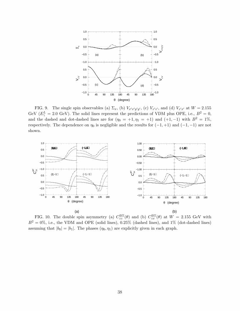
0 45 90 135 180−1.0

−0.5

0.0

0.5

Vz’

z’

−1.0

−0.5

0.0

0.5

1.0

Σ x

45 90 135 180−1.0

−0.5

0.0

0.5

Vz’

x’

−1.0

−0.5

0.0

0.5

1.0

Vx’

x’y’

y’

θ (degree)

(a) (b)

(c) (d)

FIG. 9. The single spin observables (a) Σx, (b) Vx′x′y′y′ , (c) Vz′z′ , and (d) Vz′x′ at W = 2.155

GeV (ELγ = 2.0 GeV). The solid lines represent the predictions of VDM plus OPE, i.e., B2 = 0,

and the dashed and dot-dashed lines are for (η0 = +1, η1 = +1) and (+1,−1) with B2 = 1%,

respectively. The dependence on η0 is negligible and the results for (−1,+1) and (−1,−1) are not

shown.

0 45 90 135 180−1.0

−0.5

0.0

0.5

−1.0

−0.5

0.0

0.5

1.0

45 90 135 180

(a)

(+1,+1) (−1,+1)

(−1,−1)

(+1,+1) (−1,+1)(+1,+1) (−1,+1)(+1,+1) (−1,+1)(+1,+1)

(+1,−1)

(−1,+1)

θ (degree)

CB

T

zz

0 45 90 135 180−1.0

−0.5

0.0

0.5

−1.00

−0.50

0.00

0.50

1.00

45 90 135 180

θ (degree)

(+1,+1)

(+1,−1)

(−1,+1)

(−1,−1)

(b)

(+1,+1) (−1,+1)(+1,+1) (−1,+1)(+1,+1) (−1,+1)(+1,+1) (−1,+1)

CB

T

zx

FIG. 10. The double spin asymmetry (a) CBTzz (θ) and (b) CBT

zx (θ) at W = 2.155 GeV with

B2 = 0%, i.e., the VDM and OPE (solid lines), 0.25% (dashed lines), and 1% (dot-dashed lines)

assuming that |b0| = |b1|. The phases (η0, η1) are explicitly given in each graph.

38

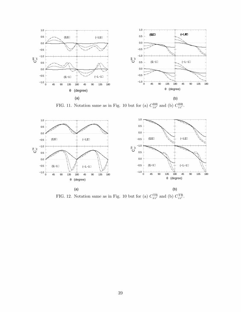
0 45 90 135 180−1.0

−0.5

0.0

0.5

−1.0

−0.5

0.0

0.5

1.0

45 90 135 180

CB

R zx’

θ (degree)

(+1,+1) (−1,+1)

(+1,−1) (−1,−1)

(a)

0 45 90 135 180−1.0

−0.5

0.0

0.5

−1.0

−0.5

0.0

0.5

1.0

45 90 135 180

θ (degree)

(+1,+1)

(+1,−1)

(−1,+1)

(b)

(+1,+1) (−1,+1)(+1,+1) (−1,+1)

(−1,−1)

(+1,+1) (−1,+1)(+1,+1) (−1,+1)

CB

R zz’

FIG. 11. Notation same as in Fig. 10 but for (a) CBRzx′ and (b) CBR

zz′ .

0 45 90 135 180−1.0

−0.5

0.0

0.5

−1.0

−0.5

0.0

0.5

1.0

45 90 135 180

θ (degree)

(+1,+1)

(+1,−1)

(−1,+1)

(−1,−1)

(a)

CT

R xz’

0 45 90 135 180−1.0

−0.5

0.0

0.5

−1.0

−0.5

0.0

0.5

1.0

45 90 135 180

θ (degree)

(+1,+1)

(+1,−1)

(−1,+1)

(−1,−1)

(b)

CT

R zz’

FIG. 12. Notation same as in Fig. 10 but for (a) CTRxz′ and (b) CTR

zz′ .

39

0 45 90 135 180−1.25

−0.75

−0.25

0.25

0.75

−1.25

−0.75

−0.25

0.25

0.75

1.25

45 90 135 180

(+1,+1)

(+1,−1)

(−1,+1)

(−1,−1)

(a)

θ (degree)

CB

V zx’

0 45 90 135 180−1.25

−0.75

−0.25

0.25

0.75

−1.25

−0.75

−0.25

0.25

0.75

1.25

45 90 135 180

θ (degree)

(+1,+1)

(+1,−1)

(−1,+1)

(−1,−1)

(b)

CB

V zz’

FIG. 13. Notation same as in Fig. 10 but for (a) CBVzx′ and (b) CBV

zz′ .

0 45 90 135 180−1.25

−0.75

−0.25

0.25

0.75

−1.25

−0.75

−0.25

0.25

0.75

1.25

45 90 135 180

θ (degree)

(a)

(+1,+1)

(+1,−1)

(−1,+1)

(−1,−1)CT

V zx’

0 45 90 135 180−1.25

−0.75

−0.25

0.25

0.75

−1.25

−0.75

−0.25

0.25

0.75

1.25

45 90 135 180

θ (degree)

(b)

(−1,−1)

(+1,+1)

(+1,−1)

(−1,+1)

CT

V zz’

FIG. 14. Notation same as in Fig. 10 but for (a) CTVzx′ and (b) CTV

zz′ .

40

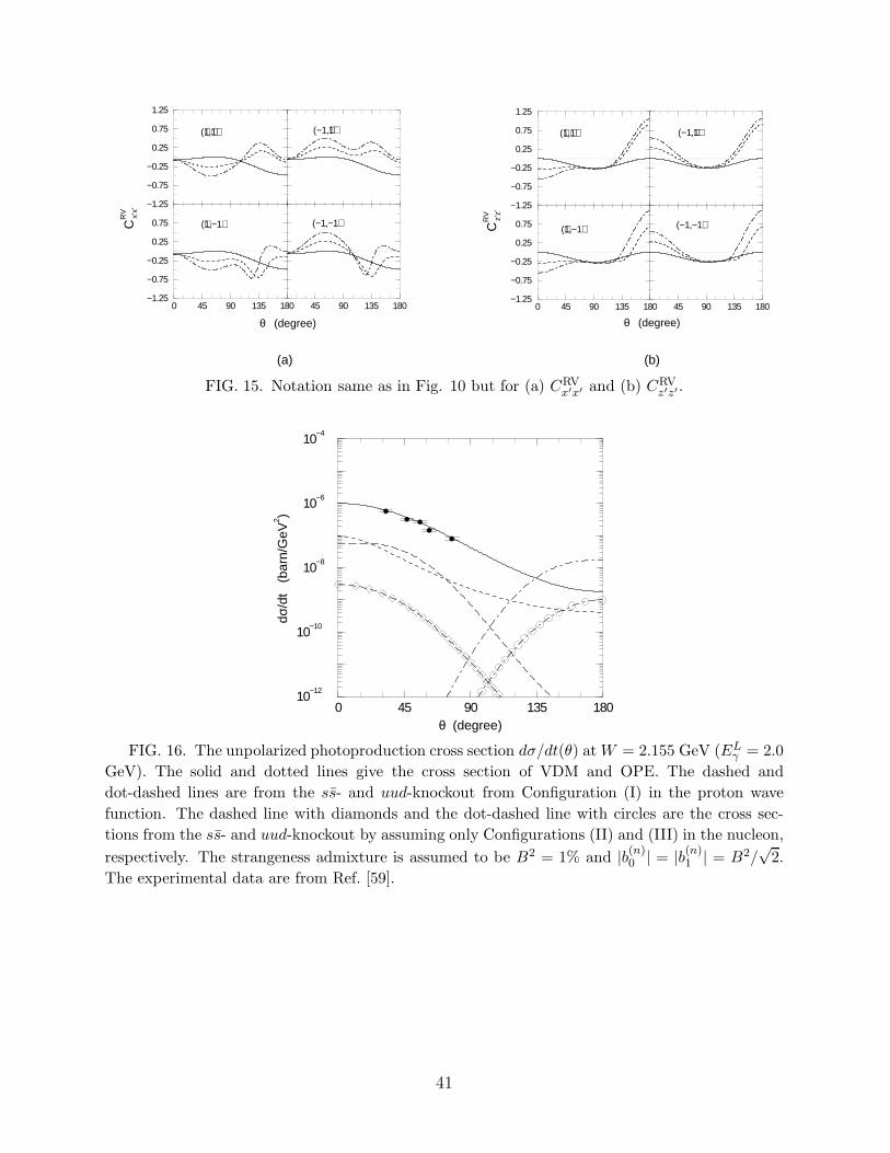
0 45 90 135 180−1.25

−0.75

−0.25

0.25

0.75

−1.25

−0.75

−0.25

0.25

0.75

1.25

45 90 135 180

(a)

(+1,+1)

(−1,−1)

(−1,+1)

(+1,−1)

θ (degree)

CR

V x’x’

0 45 90 135 180−1.25

−0.75

−0.25

0.25

0.75

−1.25

−0.75

−0.25

0.25

0.75

1.25

45 90 135 180

θ (degree)

(b)

(−1,+1)(+1,+1)

(+1,−1) (−1,−1)CR

V z’z’

FIG. 15. Notation same as in Fig. 10 but for (a) CRVx′x′ and (b) CRV

z′z′ .

0 45 90 135 180θ (degree)

10−12

10−10

10−8

10−6

10−4

dσ/d

t (

barn

/GeV

2 )

FIG. 16. The unpolarized photoproduction cross section dσ/dt(θ) at W = 2.155 GeV (ELγ = 2.0

GeV). The solid and dotted lines give the cross section of VDM and OPE. The dashed and

dot-dashed lines are from the ss- and uud-knockout from Configuration (I) in the proton wave

function. The dashed line with diamonds and the dot-dashed line with circles are the cross sec-

tions from the ss- and uud-knockout by assuming only Configurations (II) and (III) in the nucleon,

respectively. The strangeness admixture is assumed to be B2 = 1% and |b(n)0 | = |b(n)

1 | = B2/√

2.

The experimental data are from Ref. [59].

41

0 45 90 135 180θ (degree)

−1.0

−0.5

0.0

0.5

1.0

CB

T

zz

45 90 135 180θ (degree)

−1.0

−0.5

0.0

0.5

1.0

CB

R zz’

(b)(a)

B2=0%

B2=1%

B2=0%

B2=1%

FIG. 17. Double polarization asymmetries (a) CBTzz and (b) CBR

zz′ for two models of Γα,µν with

B2 = 0 and 1%. The solid lines are obtained with Γα,µν of (3.8) and the dashed lines with Γα,µν

of (C2). For simplicity, we take the phases (η0, η1) = (+,+).

42