arX

iv:n

ucl-

th/9

6120

59v1

22

Dec

199

6

nucl-th/9612059

Electroproduction of φ meson from proton

and the strangeness in the nucleon

Alexander I. Titov∗, Shin Nan Yang and Yongseok Oh†

Department of Physics, National Taiwan University, Taipei, Taiwan 10617, Republic of China

Abstract

We analyze the process e p → e p φ near the threshold within uud-ss cluster

model as a probe of the strangeness content of proton. Our consideration

is based on the relativistic harmonic oscillator quark model which takes into

account the Lorentz-contraction effect of the hadron wavefunctions. We find

that the knockout mechanisms are comparable to the diffractive production of

vector-meson-dominance model when only (3–5)% strange quark admixture

is assumed, which should be compared with (10–20)% of the nonrelativistic

quark model prediction. The cross sections of the uud- and ss-knockout pro-

cesses have qualitatively different dependence on the four-momentum trans-

fer squared to the proton and may be distinguished experimentally. We also

briefly discuss a way to determine the strangeness content of proton in 5-quark

cluster model.

Typeset using REVTEX

∗Permanent address: Bogoliubov Theoretical Laboratory, Joint Institute for Nuclear Research,

141980 Dubna, Russia.

†Present address: Institut fur Theoretische Physik, Physik Department, Technische Universitat

Munchen, James–Franck–Straße, D-85747 Garching, Germany.

1

I. INTRODUCTION

Conventional phenomenological quark models widely used for describing low-energy prop-erties of baryons treat nucleon as consisting of only up and down quarks; intrinsically, thereis no strange quark in the nucleon. Considering the success of the constituent quark models[1], it may come as a surprise when some recent measurements and theoretical analysesindicate a possible existence of a significant strange quark content in the nucleon.

For example, analyses of the sigma term [2] in pion-nucleon scattering suggest that aboutone third of the rest mass of the proton comes from ss pairs inside the proton. The EMCmeasurement of the proton spin structure functions in deep-inelastic muon scattering [3,4]has been interpreted as an indication of the strange quark sea ss strongly polarized oppositeto the nucleon spin, leading to the conclusion that the total quark spin contributes little tothe total spin of the proton. A similar conclusion1 has been drawn from the BNL elasticneutrino-proton scattering [5,6]. This has stimulated a set of new experimental proposals[8] to measure the neutral weak form factors of the nucleon which might be sensitive to thestrange quarks of the nucleon.

One of the intriguing idea associated with a direct probe of the strangeness content ofproton is to use φ meson production from proton [9–12]. Since φ meson is nearly 100%ss-state because of the ω-φ ideal mixing, its coupling to the proton is suppressed by theOZI rule. The main idea of this proposal, called OZI “evasion” process, is to determine theamount of the ss-admixture of nucleon, if any, by isolating its contribution in φ productionprocesses. For example, ss admixture in the proton wavefunction allows contributions from“shakeout” and “rearrangement” diagrams in φ production from pp and pp collisions [12].Another idea is to use φ-meson lepto- and electroproduction from proton target as advocatedby Henley et al. [9,10]. In this case, in addition to the diffractive production mechanism of thevector-meson–dominance model (VDM) we have contributions from the direct “knockout”mechanism.

If we consider ss admixture of proton, we can parameterize the Fock-space decompositionof the proton wavefunction as

|p〉 = A0|uud〉+∑

X

AX |uudX〉+∑

X

BX |uudssX〉, (1.1)

where X denotes any combination of gluons and light quark pairs of u and d quarks. Anal-yses of the φ production experiments can give estimates on BX . For instance, investigationof pp annihilation by connected quark line diagrams estimates that the ss sea quark con-tribution to the proton wavefunction is between 1% and 19% [13]. In Ref. [10], by usingthe φ electroproduction its upper bound is estimated to be about 10-20%. To obtain thisestimation, the authors used nonrelativistic quark model (NRQM) and calculated the crosssection of the ss-knockout process. Because of the paucity of experimental data [14,15], it

1For other interpretations of these experiments, see, for instance, Ref. [7].

2

was compared with the VDM predictions2. However, as was pointed out by our previouspublication [17] where a preliminary result was reported, the knockout contributions areclosely related to the hadron form factors and in the considered kinematical region of φproduction, the minimum value of q2 is about 3.6 GeV2, where q is the three-momentumtransferred to the hadron system. So it is clear that the value of the momentum transfer inthis process is too large to use the NRQM because its predictions on hadron form factorsare in poor agreement with experiment at q2 ≥ 0.3 GeV2.

In this paper, we improve the work of Ref. [10] by including relativistic effects basedon the relativistic harmonic oscillator model (RHOM) [18–24] which describes successfullythe proton form factors in a wide range of q2. We also carry out the calculations for theuud-knockout and its interference with the ss-knockout which were argued to be suppressedand left out in Ref. [10] as well as for the ss-knockout. The calculations are done both inNRQM and in RHOM for a comparison. As in Ref. [10], we will compare the cross sectionsof the knockout processes with the VDM predictions. However, this does not mean thatthe knockout mechanism should replace the VDM mechanism. The latter is present as abackground of the knockout mechanism and our purpose is to determine a theoretical upperbound of B2

X using φ electroproduction process.This paper is organized as follows. In the next section, we briefly review the general

structure of the knockout and VDM differential cross sections and introduce the kinematicalvariables for φ meson electroproduction. Then in Sect. III we discuss the proton wave-function of 5-quark cluster model. Section IV is devoted to the evaluation of the knockoutprocess matrix elements within the non-relativistic harmonic oscillator quark model. InSect. V we perform the calculations based on the RHOM which provides an explanationof the dipole-like Q2 dependence of the elastic nucleon form factor. This model, thoughprobably it has not underlying physical significance, has the pleasant feature that basicallyall quantities of interest can be worked out analytically, and, in many cases, it allows un-derstanding of the qualitative picture of the reaction. The nontrivial role of the relativisticLorentz-contraction effect is also discussed. In Sec. VI we briefly discuss a way to extractout the strangeness content of proton in an extended quark model. Section VII contains asummary and some details in the calculation are given in Appendix.

II. KINEMATICS AND CROSS SECTIONS

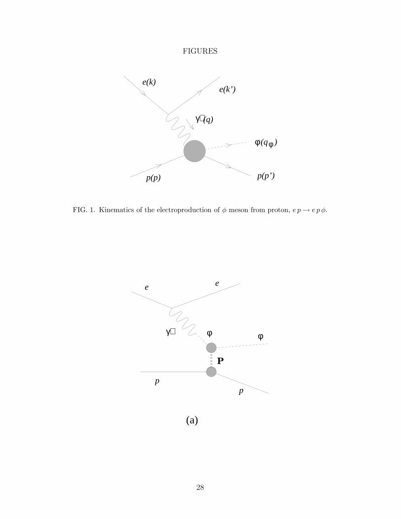
The one-photon exchange diagram for φ electroproduction is shown in Fig. 1. The fourmomenta of the initial electron and proton, final electron and proton, the produced φ meson,and the virtual photon are denoted by k, p, k′, p′, qφ, and q, respectively. In the laboratoryframe, we write k ≡ (Ee,k), k′ ≡ (E ′

e,k′), p ≡ (Ep,p) = (MN , 0), where MN is the nucleon

mass, p′ ≡ (E ′p,p

′), qφ ≡ (ωφ, qφ), and q ≡ (ν, q), respectively. The electron scattering angleθ is defined by cos θ = k · k′/ |k| |k′|. We also denote the electron mass and φ mass by Me

and Mφ, respectively. The other invariant kinematical variables are ν ≡ p ·q/MN = Ee−E ′e,

2 The recent ZEUS experiment [16] was done at very high energy, and is beyond the applicability

of this work.

3

the minus of photon mass squared Q2 ≡ −q2, the four-momentum transfer squared to theproton t ≡ (p − p′)2, the proton–virtual-photon center-of-mass energy W 2 = (p + q)2, andthe total energy squared in the CM system s = (p+k)2. We also use dimensionless invariantvariables η, y and z defined as

η =Q2

4M2N

, y =−t

4M2N

, z =W 2 −M2

N

4M2N

. (2.1)

So, in the laboratory frame we have

q2 = 4M2N [(η + z)2 + η], ν = 2MN (η + z),

E ′p = MN + 2MNy, ωφ = ν − 2MNy, s ≃MN (2Ee +MN). (2.2)

In terms of the conventional T -matrix elements Tfi, the differential cross section is givenas

dσfi = (2π)4δ(p+ q − p′ − qφ)2EpEe

√

λ(s,M2e ,M

2N)

|Tfi|2dk′

(2π)3

dp′

(2π)3

dqφ

(2π)3, (2.3a)

and

|Tfi|2 =1

4

∑

mi,mf ,mφ,

me,me′

|Tfi|2, (2.3b)

where mi,f (me,e′) and mφ are the spin projections of the incoming and outgoing proton(electron) and outgoing φ meson, respectively, and

λ(x, y, z) = x2 + y2 + z2 − 2(xy + yz + zx). (2.4)

Upon integrating Eq. (2.3) over non-fixed kinematical variables we find the triple-differentialcross section of the φ electroproduction in the laboratory frame in the form of

d3σ

dWdQ2dt=WE ′

eE′pωφ

4M2N |k||q|

1

(2π)3|Tfi|2, (2.5a)

where

|Tfi|2 =∫

|Tfi|2dϕp′

2π

dϕq

2π, (2.5b)

and ϕp′,q are the corresponding azimuthal angles, respectively.The tree diagrams that could contribute to φ electroproduction are illustrated in Fig. 2.

In Fig. 2(a), the virtual photon turns into the φ meson and then scatters diffractivelywith the proton through the exchange of a Pomeron. This VDM of diffractive productionhas been widely used to describe vector-meson photo- and electro-productions. It generallyreproduces well the Q2 dependence of the cross sections for fixed W , but is not successful toaccount for the experimentally observed rapid decrease in the cross sections with increasingW . The double differential cross section predicted by the VDM is [15]

4

d2σdif

dWdQ2= (2π)ΓW (Q2,W )σdif(Q

2,W ), (2.6)

where

ΓW (Q2,W ) =e2

32π3

W

MNE2e

W 2 −M2N

MNQ2

1

1 − ǫ, (2.7)

which is related to the flux of transverse virtual photons in the laboratory frame(2π)ΓT (θ, E ′

e) (for fixed θ and E ′e) by ΓW = JΓT , with J being the Jacobian

J(cos θ, E ′e;Q

2,W ) = W/(2MNEeE′e). Here, ǫ is the virtual-photon polarization parame-

ter

ǫ =1

1 + 2[(Q2 + ν2)/Q2] tan2(θ/2) . (2.8)

As in Refs. [10,15], we will work with the cross section σ(Q2,W ), which is predicted byVDM as [15]

σdif(Q2,W ) =

σφ(0,W )

(1 +Q2/M2φ)2

p∗γ(0)

p∗γ(Q2)

(1 + ǫRφ) exp(−bφ|tmax(Q2) − tmax(0)|), (2.9)

where σφ(0,W ) is the photoproduction cross section. The range of t (tmin < t < tmax) canbe obtained from cos θqp′ = (p′2 +q2−q2

φ)/(2|p′||q|) = ±1. The first part of (2.9) representsthe photoproduction cross section extrapolated to Q2 by the square of the φ propagator.The second represents a correction to the virtual photon flux where p∗γ is the virtual photonmomentum in γ∗p CM frame. Explicitly it is written as [26]

p∗γ(0)

p∗γ(Q2)

=

√

√

√

√

(W −MN)2(W +MN )2

[(W −MN)2 +Q2][(W +MN)2 +Q2], (2.10)

which can be approximated to unity in the large W limit. This term is a measure of theambiguity in the model predictions [15,26], and comes from a choice made in the definition ofthe transverse photon flux. The (1+ǫRφ) term corrects the cross section for the longitudinalcomponent which is missing at Q2 = 0, and the exponential factor corrects for the fact thatfor a given W the physical range of t is smaller when Q2 > 0 than its range at Q2 = 0. Wefix the parameters following Refs. [14,15] as bφ = 3.46 GeV2, Rφ = ξ2Q2/M2

φ with ξ2 = 0.33,and σφ(0,W ) = 0.22 µb, which is fitted for W = 2.1 GeV.

The t-dependence of the cross section can be obtained by assuming exp(bφt) dependence.This gives

σdif(Q2,W, t) = σdif(Q

2,W ) bφ ebφ[t−tmax(Q2)], (2.11)

provided that exp(bφtmin) is negligible [10].Figure 2(b) corresponds to the process where an ss pair is directly knocked out by the

photon and Fig. 2(c) to the direct uud-knockout. It is also possible that the system wouldhave some hadronic intermediate states likeN andN∗ before and after the φmeson is emittedas shown in Fig. 3. These diagrams represent some of the rescattering effects and deserves

5

to be studied. However, we will focus only on the direct knockout mechanism of Fig. 2(b,c)in this paper and leave the other for future study. Instead of triple and double differentialelectroproduction cross sections d3σ/dWdQ2dt and d2σ/dWdQ2 for the knockout process,respectively, we will work with the cross sections σ(Q2,W ) and σ(Q2,W, t) defined as

σ(Q2,W, t) =1

2πΓW (Q2,W )

d3σ

dWdQ2dt,

σ(Q2,W ) =1

2πΓW (Q2,W )

d2σ

dWdQ2. (2.12)

The knockout amplitude Tfi in the one-photon exchange approximation may be writtenin the most general form as

− i(2π)4δ4(p+ q − p′ − qφ)Tfi =⟨

hf |Jhµ |hi

⟩ gµν

q2

⟨

k′|Jeν |k⟩

, (2.13)

where⟨

f |Jh,eν |i

⟩

are the hadron and electron electromagnetic (e.m.) current matrix elements,respectively. The electron matrix element is given by

⟨

k′|Jeν |k⟩

≡√

√

√

√

M2e

EeE ′e

jeν =

√

√

√

√

M2e

EeE ′e

ume′(k′)eγνume

(k), (2.14)

where ume(k) is the plane wave electron Dirac spinor (me denotes the spin projection)

normalized as uu = 1. The hadron e.m. current matrix element depends on the model fordescription of the initial and final hadron states |hi,f〉 and the form of the e.m. current

operator Jhµ . The additivity of the e.m. current in the quark model enables one to write the

amplitude Tfi as

Tfi = T ssfi + T uud

fi , (2.15)

where the first term describes the interaction of the e.m. field with the s and s quarks, i.e.,the ss-cluster knockout, while the second one corresponds to the uud-knockout.

Then the squared amplitude consists of three terms which are the contributions of thess- and uud-cluster knockout and the interference:

|Tfi|2 = |T ssfi |2 + |T uud

fi |2 + |T intfi |2. (2.16)

III. PROTON WAVEFUNCTION

For simplicity and for our qualitative study, we approximate the proton wavefunction(1.1) as

|p〉 = A|uud〉+B|uudss〉, (3.1)

by absorbing the contributions from AX terms into the coefficient A and keeping the leadingorder term in BX types. The AX-type terms must be present in the proton wavefunction.

6

However, as we shall see, the cross sections of the knockout mechanism for φ electroproduc-tion depends on (AB)2, so that such an approximation may be justifiable in this process.We can further decompose the wavefunction as

|p〉 = A|[uud]1/2〉 +B

a0|[[uud]1/2 ⊗ [ss]0]1/2〉 + a1|[[uud]1/2 ⊗ [ss]1]1/2〉

, (3.2)

where the superscripts denote the spin of each cluster. Then B2 is the strangeness admixtureof the proton and a2

0 and a21 correspond to the spin-0 and spin-1 fractions of ss cluster,

respectively. They are constrained to A2 + B2 = a20 + a2

1 = 1 by the normalization of thewavefunction. The symbol ⊗ represents a possible orbital angular momentum between thetwo clusters. In the simplest picture, the s and s quarks are in a relative 1s state withrespect to each other with negative intrinsic parity. The uud cluster is also in a relative1s state with respective to the CM of the cluster. We also neglect a possible hidden colorcomponents, which was shown to be negligible in SU(2) 5-quark model [25]. Therefore, theconfiguration (3.2) corresponds to ηs and φ meson “in the air” in proton wavefunction, whereηs (=ss) is the mixture of η and η′.

Then to describe positive parity proton, the ss cluster should be in a relative P -waveabout the CM with the uud cluster that is the “bare” proton. More complicated configu-rations are possible by allowing complex combinations. But we expect that the above twocomponents give major contribution to the φ electroproduction. Also excluded is the higherspin states of uud cluster. For example, we may include spin 3/2 uud cluster. However,since the isospin of φ is zero, the uud cluster should have isospin 1/2. Experimentally ob-

served states with i = 1/2, j = 3/2 are N∗(32

−) and N∗(3

2

+) at 1520 MeV and 1720 MeV,

respectively. Because of their heavier mass, their role is expected to be small and excludedin our study as in Ref. [10].

The spin-orbital wavefunction can be obtained by noting that the total spin J (withj = 1/2) is

J = J c + J ss = Juud + L + J ss, (3.3)

where Juud is the spin of the uud cluster (juud = 1/2), J ss of the ss cluster (jss =0,1),and L the relative orbital angular momentum (ℓ = 1). Therefore, we can write the spinwavefunction as

|j = 12, mi〉 =

∑

m’s

〈12m′ 1mλ|jcmc〉〈jcmc jss mss|12 mi〉|12 m′〉uud|jssmss〉ss|1mλ〉ℓ. (3.4)

For jss = 0, we have jc = 12

and

|12, mi; jss = 0〉 =

∑

m’s

〈12m′ 1mλ|12 mi〉|12 mi〉uud|0 0〉ss|1mλ〉ℓ. (3.5)

And for jss = 1, since jc can be either 1/2 or 3/2, we have

|12, mi; jss = 1〉 =

∑

jc

b2jc

∑

m’s

〈12m′ 1mλ|jcmc〉〈jc mc 1mss|12 mi〉|12 m′〉uud|1mss〉ss|1mλ〉ℓ,

(3.6)

7

with b21 + b23 = 1. Finally, the spin-orbital wavefunction reads

|12, mi〉 = A|1

2, mi〉〉 +Ba0|12 , mi; jss = 0〉 + a1|12 , mi; jss = 1〉, (3.7)

where |12, mi〉〉 denotes the bare proton wavefunction. When combined with the flavor, spatial

and color wavefunctions, this completes our proton wavefunction.

IV. NON-RELATIVISTIC QUARK MODEL

A. The model

For the spatial wavefunctions of hadrons, we use the nonrelativistic harmonic oscillatorquark potential model in this Section. If we consider the proton wavefunction in 5 quarkconfigurations, the spatial wavefunction is obtained from the Hamiltonian

H(5) =5∑

i=1

(

− ∇2i

2Mi

)

+ k3∑

i6=j=1

(xi − xj)2 + ks(x4 − x5)

2 + k′∑

i=1,2,3j=4,5

(xi − xj)2, (4.1)

where the labels i = 1, 2, 3 refer to the particles in the uud-cluster and i = 4, 5 to thess-cluster, and Mi is the mass of i-th quark. In this work, we use Mq ≡ Mu = Md = 330MeV and Ms = 500 MeV. This Hamiltonian can be diagonalized by introducing Jacobiancoordinates as

ξ1 =1√6(x2 + x3 − 2x1), ξ2 =

√

1

2(x3 − x2), ρ =

√3(x5 − x4),

χ =1

3(x1 + x2 + x3) −

1

2(x4 + x5), R = (

∑

i

Mixi)/M5, (4.2)

where M5 =∑

iMi = 3Mq + 2Ms.Then the spatial wavefunction ΨSP

P ,λ(r1, r2, r3, r4, r5) with momentum P and the pro-jection λ of the orbital angular momentum ℓ(=1), has the form

ΨSPP ,λ(r1, r2, r3, r4, r5) = eiP ·Rψuud(ξ1, ξ2)ψ

ss(ρ)ψλ(χ) = eiP ·Rψ(ξ1)ψ(ξ2)ψ(ρ)ψλ(χ),

(4.3a)

where the normalized radial wavefunctions are

ψ(ui) =(

Ωi

π

)3/4

e−1

2Ωiu

2i ,

ψλ(χ) =√

2Ωχ

(

Ωχ

π

)3/4

χλe− 1

2Ωχχ2

, (4.3b)

where ui = ξ1, ξ2,ρ and Ωi represents Ωui. They are normalized as

∫

d3ui |ψ(ui)|2 =∫

d3χ|ψλ(χ)|2 = 1, and χ0 = χz, χ±1 = ∓(χx ± iχy)/√

2. The dimensional parameters are

Ω2ξ1

= Ω2ξ2≡ Ω2

ξ = 2(3k + 2k′)Mq, Ω2ρ = (ks + 3

2k′)Ms, Ωχ = 12Mχk

′, (4.3c)

8

with Mχ = (6MqMs)/M5. The spatial wavefunctions of the bare proton and φ meson havethe similar structure.

We fix the dimensional parameters as in Ref. [10] by using the fact that they are relatedto the hadron rms radii. The wavefunctions (4.3) give

〈r2uud〉 =

1

Ωξ, 〈r2

ss〉 =3

8

1

Ωρ, 〈χ2〉 =

5

2

1

Ωχ, (4.4)

and we assume that Ω0ξ of the bare proton and Ω0

ρ of the φ are equal to Ωξ and Ωρ, respectively.

By making use of the empirical values of√

〈r2p〉 (= 0.83 fm) and

√

〈r2φ〉 (= 0.45 fm) and by

introducing scaling factor c (=1.5) [10], we get

√

Ωξ = 1.81 fm−1,√

Ωρ = 2.04 fm−1,√

Ωχ = 2.43 fm−1. (4.5)

To obtain Ωχ we assumed that the spring constant of χ coordinate is the same as that of φmeson.

We also use the additive form of the NRQM e.m. current;

Jh0 =

5∑

k=1

Jhk,0, J

h=

5∑

k=1

Jh

k , (4.6)

where

〈p′k|Jhk,0|pk〉 = ekδ

3(p′k − pk)

〈p′k|Jh

k|pk〉 =ek

2Mk

p′k + pk + iσk × (p′

k − pk) , (4.7)

in momentum space, where ek and Mk are the charge and mass of the k-th quark and p′k

(pk) is its final (initial) momentum.

B. ss-knockout

The ss-knockout process is depicted in Fig. 2(b). Because of the symmetric propertyof the spatial wavefunction and the current, it is manifest that only the jss = 0 part of theproton wavefunction (3.2) and the magnetic part of the e.m. current (4.7) can contribute.Then the T -matrix is obtained as

T(NR)ss = −2

3A∗Ba0

(

eµs

2MN

)

∑

λ

Issλ 〈1

2mf 1 λ|1

2mi〉(−1)mφ(q × A)−mφ

, (4.8)

where µs = MN/Ms and Aµ is a four-vector defined as

Aµ =1

Q2

√

√

√

√

M2e

EeE ′e

ume′(k′)eγµume

(k). (4.9)

The spatial overlap integral Issλ in NRQM is defined as

9

Issλ = γssβss(q)ψ

(NR)λ (p′), (4.10a)

where

γss =∫

dξ1dξ2 ψuudf (ξ1, ξ2)ψ

uudi (ξ1, ξ2), (4.10b)

βss(q) =∫

dρ eiq·ρ/2ψssf (ρ)ψss

i (ρ), (4.10c)

ψ(NR)λ (p′) =

∫

dχ e−ip′·χψλ(χ). (4.10d)

By making use of

∑

me,me′

AµA∗ν =

e2

q4

1

EeE ′e

[kµk′ν + k′µkν − gµν(k · k′ −M2

e )], (4.11)

for unpolarized case, we can obtain

|T (NR)ss |2 =

4

9(ABa0)

2 e4

Q4ΓssFss(q)Vss(p

′) cos2 θ2

(

f ss1 + f ss

2 tan2 θ2

)

, (4.12)

where

f ss1 = µ2

sη, f ss2 = 2µ2

s[η + (η + z)2]. (4.13)

The spatial integrals are calculated using (4.3) as

Γss = γ2ss = 1,

Fss(q) = [βss(q)]2 = exp[

−q2/(8Ωρ)]

,

Vss(p′) =

1

3

∑

λ

|ψλ(p′)|2 =

2(2π)3

3

(

1

πΩχ

)3/2p′2

Ωχe−p′2/Ωχ . (4.14)

This is the result derived in Ref. [10] for the ss knockout process. Since it depends on t onlythrough p′2 of Vss, one can see that the cross section is maximum near tmax by noting thatp′2 increases as decreasing t.

C. uud-knockout

As depicted in Fig. 2(c), the ss cluster is a spectator in this process. So only the jss = 1part contribute contrary to the ss knockout. The relevant amplitude reads

T(NR)uud = iA∗Ba1

∑

jc,m′,mc,λ

b2jc〈1

2m′ 1 λ|jcmc〉〈jcmc 1mφ|12 mi〉〈1

2mf |F uud

µ |12m′〉Iuud

λ Aµ,

(4.15)

where

10

F uud0 = e, F uud =

e

2MN

(2p′ − q + iµσ × q), (4.16)

with µ = MN/Mq. The overlap integral Iuudλ reads

Iuudλ = γuudβuud(q)ψ

(NR)λ (−qφ), (4.17a)

where

γuud =∫

dρψssf (ρ)ψss

i (ρ), (4.17b)

βuud(q) =∫

dξ1dξ2 e−i√

2

3q·ξ1ψuud

f (ξ1, ξ2)ψuudi (ξ1, ξ2), (4.17c)

ψ(NR)λ (−qφ) =

∫

dχ eiqφ·χψλ(χ). (4.17d)

Then we have the squared amplitude as

|T (NR)uud |2 = (ABa1)

2 e4

Q4ΓuudFuud(q)Vuud(qφ) cos2 θ

2

(

fuud1 + fuud

2 sin2 θ2

)

, (4.18)

where

fuud1 = ηµ2

1 +1

ηµ2

(

1 − νν

q2

)2

+c

µ2

,

fuud2 = 2(µ2 + c)[η + (z + η)2], (4.19)

with

ν =1

2MN

(2p′ · q − q2), c = − 1

2q4λ(q2, q2

φ,p′2), (4.20)

where λ(x, y, z) is defined in Eq. (2.4). The radial wavefunctions of NRQM give

Γuud = γ2uud = 1,

Fuud(q) = [βuud(q)]2 = exp[

−q2/(3Ωξ)]

,

Vuud(qφ) =1

3

∑

λ

|ψλ(−qφ)|2 =2(2π)3

3

(

1

πΩχ

)3/2q2

φ

Ωχe−q2

φ/Ωχ . (4.21)

Then the cross section depends on t only through q2φ of Vuud. This shows that in contrary

to the ss-knockout, the uud-knockout process gives its main contribution near tmin.

D. gauge invariance

The electron e.m. current in (2.14) satisfies the conservation condition qµjeµ = 0. The

gauge invariance implies the same condition for the hadronic current:

qµJhµ = 0. (4.22)

11

In general, however, this condition is not satisfied in inelastic scattering [27]. In our case,this condition is satisfied only in the ss knockout process since only the magnetic part ofthe e.m. current contributes. In uud knockout process, however, the convection currenttakes part in the process and the relation (4.22) is not obeyed. The breakdown of the gaugeinvariance is crucial at small Q2 because the matrix elements of qµJ

hµ are proportional to

(ν − ν)2/Q2 as Q2 → 0.The most commonly used technique of enforcing gauge invariance [19,27] in photopro-

duction is to project out the gauge non-invariant part as

Fµ → F ′µ = (gµν −

qµqνq2

)F ν. (4.23)

This modification, however, is not adequate for the electroproduction, where the electrone.m. current cancels the subtracted part.

A possible way for restoring the gauge invariance is to modify the longitudinal componentof the current. Decomposition of the spatial component of the current (4.16) gives thelongitudinal part as

F ‖ =eν

q2q, (4.24)

and we modify it as

F ‖ → F ′‖ =

eν

q2q. (4.25)

This ansatz restores the gauge invariance of the hadronic e.m. current.The modification (4.25) causes a change of fuud

1 in the squared T matrix as

fuud1 → fuud

1 = ηµ2

(

1 +1

µ2

η

[η + (η + z)2]2+

c

µ2,

)

, (4.26)

with others unchanged. This is equivalent to replace ν by ν in Eq. (4.19). Close inspectionshows that the second and the third terms are negligible in the considered kinematical region.This leads to the conclusion that the main contribution to the uud knockout process comesalso from the magnetic part of the e.m. current.3

E. interference

From the T matrices of ss knockout (4.8) and of uud knockout (4.15), we can obtain theinterference between the two processes;

|T (NR)int |2 = cint(AB)2a0a1

e4

Q4ΓintFint(q)Vint(p

′, qφ) cos2 θ2

(

f int1 + f int

2 tan2 θ2

)

, (4.27)

3 One may modify the time component of the current to restore the gauge invariance. But it does

not change this conclusion.

12

where

cint =4

9√

3(b1 + 2

√2b3),

f int1 = µµsη,

f int2 = 2µµs[η + (η + z)2], (4.28)

and

Γint = γssγuud = 1,

Fint(q) = βss(q)βuud(q) = exp(−8Ωρ + 3Ωχ

48ΩρΩχq2),

Vint(p′, qφ) =

1

3

∑

λ

ψ(NR)λ (p′)[ψ

(NR)λ (−qφ)]

∗ = −8

3

(

π

Ωχ

)3/2p′ · qφ

Ωχ

e−(p′2+q2φ)/2Ωχ . (4.29)

Therefore, if we assume cint > 0, the interference between the two knockout processes isconstructive when a0a1 < 0 and destructive when a0a1 > 0.

F. results

For numerical calculations, we fix the incident electron energy Ee as 11.5 GeV andW = 2.1 GeV throughout this paper. We also use the parameters of VDM and NRQMas determined before. The purpose of this study is to determine the coefficients of theproton wavefunction (3.2), especially B2, by comparing the cross sections of the knockoutprocess with the VDM predictions. For our qualitative study, we set a2

0 = a21 = 1/2 and

b1 = b3 = 1/√

2. Since the interference depends on the sign of a0a1, we give only itsmagnitude.

Given in Fig. 4 is σ(Q2,W ) with (a) B2 = 10% and (b) B2 = 20%. The solid line is theVDM prediction and the dotted, dashed, and dot-dashed lines are the contributions from ssknockout, uud knockout, and the interference, respectively. This shows that the knockoutprocess is comparable to the VDM with B2 = 10–20% at small Q2, say, Q2 < 1.5 GeV2 [10].It is also manifest that over the entire region of Q2 the contribution of the uud knockoutand the interference are suppressed with respect to that of the ss knockout process. Thisis because of the strong suppression of the form factor Fuud compared with Fss, where theformer involves 〈r2

uud〉 and the latter involves 〈r2ss〉. In general, the knockout cross section in

NRQM falls rapidly with Q2 than that of VDM. This is mainly due to the strong suppressionof Fss,uud of NRQM.

The t dependences of the cross section σ(Q2,W, t) at Q2 = 0.02 GeV2 and 0.5 GeV2

are given in Figs. 5 and 6, respectively. As discussed earlier, the ss knockout cross sectionincreases with increasing t, whereas the uud knockout cross section decreases. One can findthat at small Q2 and t ∼ tmin, the three knockout cross sections have the same order ofmagnitude. However, except this limited region, the ss knockout process dominates theothers.

13

V. RELATIVISTIC HARMONIC OSCILLATOR QUARK MODEL

A. The model

The RHOM first considered in Ref. [19] enables one to take into account the Lorentz-contraction effect of the composite particle wavefunction. This effect, which is essentiallyrelativistic, becomes important at large Q2 and provides an explanation of the dipole-likeQ2 dependence of the elastic nucleon form factor. Due to this advantage, RHOM has beenwidely used for description of the hadron properties at large momentum transfers [19–24],in spite of some theoretical difficulties which are inherent in the model [20,28].

In RHOM, the spatial motion of a 5-quark system is described by

5∑

i=1

2i −5∑

i6=j=1

κij (xi − xj)2 + V0

Ψ = 0, (5.1)

where κij and V0 are the usual harmonic oscillator model parameters, and x2 = x2t −x2 with

2 = ∂2t −∇2. This equation can be diagonalized using the relativistic Jacobian coordinates,

ξ1 = 1√6(x2 + x3 − 2x1), ξ2 = 1√

2(x3 − x2), ρ = 1√

2(x5 − x4),

χ =√

215

(x1 + x2 + x3) −√

310

(x4 + x5), X = 1√5

5∑

i=1

xi. (5.2)

In the rest frame, P = (M0, 0), the ground state spatial wavefunction is written as [19]

ΨSPP,λ = e−iM0Xt/

√5ψuud(ξ1, ξ2)ψ

ss(ρ)ψλ(χ) = e−iM0Xt/√

5ψ(ξ1)ψ(ξ2)ψ(ρ)ψλ(χ), (5.3)

and

ψ(υ) =(

Ωυ

π

)

exp[−12Ωυ(υ

2t + υ2)],

ψλ(χ) =√

2Ωχ

(

Ωχ

π

)

χλ exp[−12ωχ(χ2

t + χ2)], (5.4)

where υ = ξ1,ξ2,ρ and χ0 = χz with χ±1 = ∓ 1√2(χx ± iχy). They are normalized as

∫

d4υ|ψ(υ)|2 =∫

d4χ|ψλ(χ)|2 = 1. The wavefunction with arbitrary momentum P can beobtained by replacing −(υ2

t + υ2) with

υ2 − 2(

P · υM0

)2

. (5.5)

Note that in the covariant wavefunction of a state with momentum P , the argument of theHermite polynomials contains the component of the space-like four vector υµ−(P ·υ/M2

0 )Pµ.The wavefunctions of the three-quark proton and the φ meson in the final state have thesimilar structure.

In RHOM, the quarks are treated as spinless particles, so we have to introduce a modelfor the interaction of the quark spin with the external electromagnetic field. One of the

14

commonly used methods is to use the nonrelativistic electromagnetic current [18,29]. Thenext order corrections can be included by Foldy-Wouthuysen transformation, if needed. An-other method is to develop relativistic generalizations [19–21] by assuming additional quarkspinor structures of the intrinsic wavefunction and by keeping the additivity of the quarkcurrent. The models based on this approach, therefore, contains some specific assumptionswhich are not proved yet. Furthermore, we have to modify the current to satisfy the gaugeinvariance condition as in the previous Section. In this work, therefore, by rememberingthat the main relativistic effects come from the Lorentz contraction of the hadron intrinsicwavefunction [19], we use the following ansatz for the relativistic electromagnetic current,

Jhµ = Jh

min,µ + Jhmag,µ, (5.6a)

with keeping the additivity of the quark current. Here Jhmin,µ is obtained by the minimal

substitution and written as

Jhmin,µ = C

5∑

k=1

ek

(

p′k,µ + pk,µ

)

, (5.6b)

in momentum space, where p′k,µ and pk,µ are the final and initial 4-momentum of the k-th quark, respectively. The normalization constant C is determined by the condition thatJh

0 = e when p′k = pk, which gives C = 5/(2MN) in our case. Jhmag,µ takes part in the

interactions of the quark spins with the external electromagnetic field and has the sameform as in NRQM,

Jhmag,0 = 0, J

h

mag =5∑

k=1

iekµk

2MN

σk × (p′k − pk), (5.6c)

where the magnetic moment µk is defined as µu,d ≡ µ = MN/Mq and µs = MN/Ms as inNRQM.

To determine the model parameters Ωi, we note that they are related to the hadron rmsradii as

〈r2uud〉 =

1

Ωξ, 〈r2

ss〉 =3

4

1

Ωρ. (5.7)

We fix Ωξ so as to reproduce the empirical proton magnetic form factor. Since this modelpredicts the proton magnetic form factor as

GpM(Q2) = µ(1 +

Q2

2M2N

)−2 exp[−16Ω−2

ξ Q2(1 +Q2

2M2N

)−1], (5.8)

we can find that√

Ωξ = 1.89 fm−1 fits the empirical dipole formula up to Q2 ≈ 20 GeV.

This gives the relativistic scale factor c(RL) = 1.57. It is interesting to note that this value isvery similar to the nonrelativistic scale factor c = 1.5 [10] used in Sec. IV. We fix Ωρ withc(RL) as in NRQM calculation. All this process yields

√

Ωξ = 1.89 fm−1,√

Ωρ = 3.02 fm−1. (5.9)

The parameter Ωχ will be discussed in the next subsection.

15

B. ss-knockout

Because of the structure of the current (5.6), the ss knockout amplitude has the sameform as in NRQM,

T(RL)ss = −2

3A∗Ba0

(

eµs

2MN

)

∑

λ

Issλ 〈1

2mf 1 λ|1

2mi〉(−1)mφ(q × A)−mφ

. (5.10)

The only difference lies in the spatial overlap integrals, Issλ , defined by

Issλ = γssβssψ

(RL)λ , (5.11a)

where

γss =∫

d4ξ1d4ξ2 ψ

uudf (p′; ξ1, ξ2)ψ

uudi (p; ξ1, ξ2), (5.11b)

βss =∫

d4ρ ei√2q·ρψss

f (qφ; ρ)ψssi (p; ρ), (5.11c)

ψ(RL)ss,λ (p′) =

∫

d4χ eiχ·(√

5/6 p′−√

3/10 p)ψλ(p;χ). (5.11d)

In the relativistic case, the overlap integral βss depends not only on q2(Q2,W ) but also ont since the intrinsic wavefunction depends on qφ. The integral γss is also dependent of tthrough p′ dependence of the intrinsic wavefunction of the final state.

Then the spin-averaged amplitude squared is

|T (RL)ss |2 =

4

9(ABa0)

2 e4

Q4ΓssFssVss(p

′) cos2 θ2

(

gss1 + gss

2 tan2 θ2

)

, (5.12)

where

gss1 = µ2

sη, gss2 = 2µ2

s[η + (η + z)2], (5.13)

which are the same as f ss1,2 of the NRQM. The overlap integrals can be calculated as described

in Appendix. From Eq. (5.11), we have

Γss = (γss)2 = (1 − t

2M2N

)−4,

Fss = (βss)2 =

(

Mφ

ωφ

)2

exp[−q21/(4Ωρ)],

Vss(p′) =

1

3

∑

λ

|ψ(RL)ssλ (p′)|2, (5.14)

where

q21 = q2 t

2MNωφ+ ν2

(

1 − q2φ − p′2

ωφν

)

. (5.15)

16

The momentum distribution Vss(p′) is related to the outgoing proton momentum as in

NRQM, but the normalization is different from Vss(p′) of NRQM because of the normal-

ization condition of the intrinsic wavefunction and an additional integration over the timecomponent of χ. In NRQM, we have the usual physical normalization, i.e., one baryonnumber per unit volume. We keep this condition in the relativistic case by renormalizingVss(p

′) as

∫

dp′

(2π)3Vss(p

′) = 1, (5.16)

which gives the final form of Vss(p′) as

1

(2π)3Vss(p

′) =vss(p

′)∫

dp′vss(p′), (5.17)

with

vss(p′) = p′2 exp−5

3Ω−1

χ (p′2 − 35MNE

′p). (5.18)

We fix the parameter Ωχ so that vss(p′) approaches to the NRQM result with p′2 ≪ M2

N .This gives Ωχ = 7

6Ω(NR)

χ by comparing with the expression given in (4.14). With the valuedetermined in Sec. IV, we get

√

Ωχ = 2.63 fm−1. (5.19)

C. uud-knockout

By the same way, we can obtain the amplitude of the uud knockout process as

T(RL)uud = iA∗Ba1

∑

jc,m′,mc,λ

b2jc〈1

2m′ 1 λ|jcmc〉〈jcmc 1mφ|12 mi〉〈1

2mf |F uud

µ |12m′〉Iuud

λ Aµ. (5.20)

With the current (5.6), F uudµ becomes

F uud0 = ef0, F

uud= efmin +

iµe

2MN

σ × q, (5.21)

where

f0 =5

6

(

1 +E ′

p − ωφ

MN+

2q · p′

E ′pMN

)

,

fmin =5

6MN

(

q − 2qφ +2ν

E ′p

p′)

. (5.22)

As in NRQM, this amplitude does not satisfy the gauge invariance. So we modify thepart of fmin which is parallel to q to satisfy qµF uud

µ = 0. This gives

17

fmin → f ′min =

5e

6MN

−2qφ + 2q · qφq

q2+

2q0E ′

p

(

p′ − q · p′ q

q2

)

+ f0q0q

q2. (5.23)

The overlap integral Iuudλ is defined as

Iuudλ = γuudβuudψ

(RL)uud,λ(qφ), (5.24a)

where

γuud =∫

d4ρψssf (qφ; ρ)ψ

ssi (p; ρ), (5.24b)

βuud =∫

d4ξ1d4ξ2 ei

√2

3q·ξ1ψuud

f (p′; ξ1, ξ2)ψuudi (p; ξ1, ξ2), (5.24c)

ψ(RL)uud,λ(qφ) =

∫

d4χ eiχ·(√

5/12 p−√

5/6 qφ)ψλ(p;χ). (5.24d)

The squared matrix element is, therefore,

|T (RL)uud |2 = (ABa1)

2 e4

Q4ΓuudFuud(q)Vuud(qφ) cos2 θ

2

(

guud1 + guud

2 sin2 θ2

)

, (5.25)

where

guud1 = ηµ2

1 +f 2

0

µ2

η

[η + (η + z)2]2+

25

9

c

µ2

(

1 +2(η + z)

1 + 2y

)

,

guud2 = 2µ2[η + (η + z)2]

1 +25

9

c

µ2

(

1 +2(η + z)

1 + 2y

)

, (5.26)

with c defined in (4.20). By analyzing the numerical values of guud1,2 we can find that guud

1,2 ≈fuud

1,2 . This means that the magnetic part of the e.m. current gives the main contribution asin NRQM.

By making use of the formulas given in Appendix, the overlap integrals can be calculatedas

Γuud = (γuud)2 =

(

Mφ

ωφ

)2

,

Fuud = (βuud)2 = (1 − t

2M2N

)−4 exp[−q22/(3Ωξ)], (5.27)

where

q22 = q2

(

1 − ν

E ′p

)

+ ν2

(

1 − p′2 − q2φ

νE ′p

)

. (5.28)

As in the ss knockout case, they depend on t as well as on Q2 and W . In Eq. (5.25),

Vuud(qφ) is defined as 13

∑

λ |ψ(RL)uud,λ|2 and is normalized as in Vss(p

′), i.e.,

1

(2π)3Vuud(qφ) =

vuud(qφ)∫

dqφvuud(qφ), (5.29)

with

vuud(qφ) = q2φ exp−5

3Ω−1

χ (q2φ − 2

5MNωφ). (5.30)

Note that it contains factor 25

while vss has 35.

18

D. interference

The interference between the two knockout processes are obtained as

|T (RL)int |2 = cint(AB)2a0a1

e4

Q4ΓintFintVint(p

′, qφ) cos2 θ2

(

gint1 + gint

2 tan2 θ2

)

, (5.31)

where

cint =4

9√

3(b1 + 2

√2b3),

gint1 = µµsη = f int

1 ,

gint2 = 2µµs[η + (η + z)2] = f int

2 , (5.32)

and

Γint = γssγuud =Mφ

ωφ

(1 − t

2M2N

)−2,

Fint = βssβuud = Γint exp

(

− 1

8Ωρ

q21 −

1

6Ωξ

q22

)

,

Vint(p′, qφ) = −Np′ · qφ exp

[

− 5

6Ωχ

(

p′2 + q2φ − 3

5E ′

pMN − 2

5ωφMN

)

, (5.33)

where N is the normalization constant which can be derived from the normalization condi-tions of Vss and Vuud. As in NRQM, Vint has overall (−) sign.

E. results

The main difference between the NRQM and the RHOM lies in the overlap integrals dueto the similar structure of the electromagnetic currents. In RHOM, the overlap integrals,Γss, Γuud are smaller than 1 (= Γss, uud) over the whole area of t. This effect is stronger inΓss than in Γuud and becomes larger at small (large) t for Γss (Γuud). This holds also for Vss

and Vuud. In this case, however, the suppression is stronger in Vuud than in Vss. These bringsome suppressions of the RHOM amplitudes.

However, such suppressions are of order of 10 at most and they are compensated anddominated by strong enhancement of Fss, uud that contain the wavefunctions of the struckquarks. The Q2 dependence of the amplitudes is mainly determined by Fss, uud. In RHOM,they depend on the effective momentum transfers, q2

1 and q22 , as defined in (5.15) and (5.28).

Figure 7 shows the t-dependence of q21,2 at Q2 = 0.5 GeV2. One can find that q2

1,2 are alwayssmaller than q2 and the suppression becomes larger at large (small) t for q2

1 (q22). This results

in enhancement of Fss and Fuud, which is strong enough to dominate over the suppressionof the other overlap integrals. As a result, the RHOM amplitudes are enhanced as a whole.

Displayed in Fig. 8 is the RHOM predictions of σ(Q2,W ) with B2 = 3 and 5%. Wefind that the RHOM prediction exceeds the NRQM ones and the difference reaches severalorders of magnitude. This is mainly because of the new functional dependence of Fss, uud

19

in RHOM. This relativistic modification of form factors is more crucial for Fuud due to thefact that the rms radius of uud cluster is larger than that of ss cluster. Only at small Q2

the RHOM result is close to NRQM one. As in NRQM, we can find that the ss knockoutprocess is the dominant one. The uud knockout and the interference are small. As a result,we can find that because of the strong enhancement of the form factors the cross section ofthe knockout process is comparable to that of VDM only with B2 = 3 ∼ 5%.

In Figs. 9–11 we present the t-dependence of the cross section σ(Q2,W, t) at Q2 = 0.02GeV2, 0.5 GeV2, and 1.0 GeV2, respectively. The RHOM gives strong enhancement of theuud knockout cross sections. Because of the suppressions of form factors at small t, thess knockout cross section is smaller than the NRQM one at small t and Q2, where theenhancement of Fss is small. However as Q2 increases, we can see that the ss knockout crosssection is comparable to VDM one at large t. At small t, the uud knockout is the dominantone and exceeds even the VDM prediction near tmin. The effect of the interference is smalland is suppressed as Q2 increases.

Note that our result is based mainly on the Lorentz contraction effect of the wavefunctionand is not sensitive to the models of hadron electromagnetic current in the relativistic model.For instance, if we compare σ(Q2,W ) of the ss knockout with that of Ref. [30] which isobtained with relativistic hadron electromagnetic current of Ref. [19], the main differencebetween the two comes from an additional kinematical factor of the amplitude. However,the two predictions are close to each other within the accuracy of the model.

VI. STRANGENESS COEFFICIENTS OF THE PROTON IN QUARK MODEL

We have seen that the φ electroproduction cross sections are very sensitive to thestrangeness coefficients B, a0, and a1 of the proton wavefunction (3.2). The coefficientBa0 is directly related to the ss-knockout process and Ba1 to the uud-knockout. The pur-pose of this study is to determine theoretical upper bounds of these coefficients by comparingthe cross sections of the knockout process for the φ electroproduction with the experimentaldata. Because of the shortage of the data, however, it will be interesting to estimate them inother phenomenologically successful models at the present stage. In this Section, we brieflydiscuss a way to extract the strangeness coefficients of the proton wavefunction, i.e., B2,from an extended quark model using some results of the cloudy bag model.

When we take into account (3q)(qq) admixture in the proton wavefunction as well as theconventional 3q-structure, we can write the physical proton wavefunction as

| Ψp〉 = A0 | ψp0〉 +

∑

B,M

ABM

A | ψBψ

Mϕ

BM〉, (6.1)

where ψp0is the conventional 3-quark proton wavefunction, ψ

Band ψ

Mare the baryonic core

and mesonic cloud wavefunctions, respectively, with ϕBM

describing their relative motion.A is the antisymmetrizer which guarantees the symmetry property of Ψp under interchangeof quark labels. Then the quantities of our interests can be obtained as

Ba0 = 〈p0ηsϕp0ηs| Ψp〉, Ba1 = 〈p0φsϕp0φs

| Ψp〉. (6.2)

20

Hereafter, we use ηs and φs for [ss]0 and [ss]1 of (3.2), respectively. Although the coreand cloud wavefunctions, ψ

Band ψ

Min (6.1), can be any of the usual color-singlet baryon

and meson or their resonances [31], we expect that the main contribution comes from thecombinations of the ground states [32] on energetic grounds. In addition, there can behidden color combinations between them; i.e., ψ

Bcan be a wavefunction of a non-color-

singlet particle which form a totally color-singlet proton state with a non-color-singlet mesoncloud. However, in the nonrelativistic quark model [25], it was shown that the hidden colorcombinations contribute little to the physical proton wavefunction. Therefore, we neglectthese combinations in our simple calculation. A0, ABM , and ϕBM may be found fromphenomenological models, e.g., by diagonalizing the nonrelativistic quark model Hamiltonian[25] or from the chiral bag model. In our simple calculation, we will use the cloudy bag model[33], which has an advantage that the probabilities of the meson clouds can be read easily.

As in most versions of the cloudy bag model, we will consider only the pseudoscalar octetmeson clouds. To this end, we extend the work of Ref. [34] by including the η meson cloudas well. The probabilities of meson clouds are given in Fig. 12 as a function of the bag radiusRB. We can verify that the meson cloud effects are important at small bag radius and theroles of the K and η clouds are much smaller than that of the π cloud; The probability ofK cloud is less than 4% and that of η cloud is less than 0.5% in the region of RB ≥ 0.7 fm.

Our method to estimate the strangeness coefficients is very similar to the determinationof the 6-q configuration of the deuteron wavefunction [24,35]. As a specific example, let usconsider the ΛK+ combination of the proton wavefunction, which can be written as

ψ5q(ΛK) =1

N(1 −

∑

i=1,2,3j=4,5

Pij)ψΛψK+ϕΛK+, (6.3)

where N is the normalization constant and Pij is the permutation operator exchanging

the color, spin-flavor, and spatial coordinates of quarks in the core and the cloud; Pij =

PCij P

SFij PX

ij . So the probability of (B′M ′) configuration in ψ5q(ΛK) of (6.3) is

P(B′M ′) =| 〈B′M ′ϕB′M ′ | ψ5q(ΛK)〉 |2

∑

B,M | 〈BMϕBM | ψ5q(ΛK)〉 |2

=| δB′ΛδM ′K+ − 6〈B′M ′ϕB′M ′ | P34 | ΛK+ϕΛK+〉 |2

∑

B,M| δBΛδMK+ − 6〈BMϕBM | P34 | ΛK+ϕΛK+〉 |2. (6.4)

Here we shall consider the case that (B,M)=(ΛK+),(p0, ηs),(p0, φ); the contributions of theother clusters are found to be negligible.

Then it is straightforward to calculate the color exchange term as

〈PC34〉 = 1

6, (6.5)

for all configurations. From the spin-flavor wavefunction of the clusters [1], we obtained

〈ΛK+ | P SF34 | ΛK+〉 = 1

12, (6.6a)

〈p0ηs | P SF34 | ΛK+〉 = 1

4√

6, (6.6b)

21

after some exercises. For the p0φ configuration, we have two types of them because φ is avector meson. When we write J c = JB + L which forms the total spin J (j = 1

2) with the

meson spin JM , then jc can be either 12

or 32. We distinguish the two by representing φ1

s andφ3

s for [ss]1 cluster with jc = 12

and jc = 32, respectively, which leads us to

〈p0φ1s | P SF

34 | ΛK+〉 = 14√

2, (6.6c)

〈p0φ3s | P SF

34 | ΛK+〉 = 0. (6.6d)

Note that the recoupling coefficient between the p0φ3s and ΛK+ is zero because of the struc-

ture of the spin-flavor wavefunctions.For internal wavefunctions of the clusters, we use those of the harmonic oscillator poten-

tial model:

ψBint =

(

ΩB

π

)3/2

exp[−12ΩB(ξ2

1 + ξ22)], ψM

int =(

ΩM

π

)3/4

exp(−12ΩMρ2), (6.7)

in terms of the Jacobian coordinates defined in (4.2). For simplicity, we assume thatMu=Md=Ms and the same ΩB (ΩM) for baryon (meson) clusters. After performing PX

34 , theJacobian coordinates transform as

ξ1 → ξ′1 = 1

3ξ1 + 2√

6χ − 1√

6ρ,

ξ2 → ξ2 = ξ2,

ρ → ρ′ = χ −√

23ξ1 + 1

2ρ,

χ → χ′ = 16χ + 5

12ρ + 5

6

√

23ξ1. (6.8)

Then we have

〈B′M ′ϕB′M ′ | PX34 | ΛK+ϕΛK+〉 =

∫

dχdχ′ϕB′M ′(χ)K(χ,χ′)ϕΛK+(χ′), (6.9)

where

K(χ,χ′) =(

12

5

)3(

3ΩM

(3 + 8g)π

)3/2

exp[−h1(χ2 + χ′2) + h2χ · χ′], (6.10)

with g = ΩM/ΩB and

h1 =6(12g2 + 25g + 3)

25(3 + 8g)ΩB,

h2 =36(4g2 + 1)

25(3 + 8g)ΩM . (6.11)

Finally, using the above informations, we get

| 〈ΛK+ | ψ5q(ΛK)〉 |2 =10

N2| 1 − 1

12

∫

dχdχ′ ϕΛK+(χ)K(χ,χ′)ϕΛK+(χ′) |2, (6.12a)

| 〈p0ηs | ψ5q(ΛK)〉 |2 =10

N2| 1

4√

6

∫

dχdχ′ ϕp0ηs(χ)K(χ,χ′)ϕΛK+(χ′) |2, (6.12b)

| 〈p0φ1s | ψ5q(ΛK)〉 |2 =

10

N2| 1

4√

2

∫

dχdχ′ ϕp0φs(χ)K(χ,χ′)ϕΛK+(χ′) |2, (6.12c)

| 〈p0φ3s | ψ5q(ΛK)〉 |2 = 0. (6.12d)

22

For numerical calculations, we use the ϕBM(r) of the cloudy bag model, which read

ϕBM(r) =

CA

mMr

cosh(mMr) −sinh(mMr)

mMr

r ≤ RB,

CB

mMr

(

1 +1

mMr

)

e−mM r r ≥ RB,

(6.13)

where mM is the meson mass and the constants CA,CB are fixed by the relations [36],

CB

CA=

1

2

(

b− 1

b+ 1e2b + 1

)

,

CA = − bβ

mM

(

sinh b+CB

CA

e−b)−1

, (6.14)

with b = mMRB and

β =N 2

fM

j0(Ω)j1(Ω). (6.15)

Here, N is the normalization constant of the bag, fM the meson decay constant, and Ω theeigenfrequency of the bag with spherical Bessel functions j0 and j1.

Using the radial wavefunction of (6.13), we can obtain the numerical results for theintegrals of Eq. (6.12), which leads to the probabilities of each cluster in ψ5q(ΛK) of (6.3)as

P(ΛK+) ≈ 1.0,

P(p0ηs) ≈ 2.7 × 10−7,

P(p0φ1s) ≈ 8.0 × 10−7,

P(p0φ3s) = 0.0. (6.16)

We also carried out the calculations for other configurations: ΣK, p0η, Σ∗K, and ∆η,and obtained similar results of Eq. (6.16); i.e., the recoupling effects are very small. Espe-cially, the probability of p0φ

3s is zero in ψ5q(ΛK) and in ψ5q(ΣK) because of the spin-flavor

structure. By the same reason we have P(p0φ1,3s ) = 0 in ψ5q(pη), P(p0ηs) = P(p0φ

1s) = 0

in ψ5q(Σ∗K), and P(p0ηs) = P(p0φ

1,3s ) = 0 in ψ5q(∆η). All these results imply that (i) the

strangeness coefficient Ba0 is approximately equal to the amplitude Ap0η of (6.1), of whichsquare is estimated as ≤ 0.5% in the cloudy bag model; (ii) the coefficient Ba1 is nearly zerowhen we consider only the pseudoscalar meson cloud. Therefore, to get more accurate valuefor Ba1, it is necessary to know the probabilities and radial wavefunctions of the vectormeson cloud. Inclusion of vector meson degrees of freedom in chiral bag, however, is stillincomplete [37].

VII. SUMMARY

As a summary, we re-estimated the φ meson electroproduction from a proton target inuud-ss cluster model. Our calculation is based on the RHOM which takes into account the

23

main relativistic effect, namely, the Lorentz contraction of the composite particle wavefunc-tion.

First, we confirmed the results of Ref. [10] for the ss knockout process in NRQM. For theknockout cross section to be comparable to the VDM one, we have to assume B2 = 10 ∼ 20%,which is regarded as an upper bound of the strange quark content of the nucleon. Then weextended the calculation to the study of the uud knockout and their interference. We foundthat the uud knockout and the interference effect are dominated by the ss knockout and themagnetic part of the hadron e.m. current gives the main contribution.

Next, we improved the model predictions by taking the RHOM which is successful indescribing nucleon form factors in a wide range of q2. This successful description comes fromthe different functional dependence of the overlap integrals, which can explain the empiricaldipole-type formula of the form factors. In this model we found that assuming only 3–5%admixture of the strange quarks in the nucleon can give a similar size of the cross sections forthe ss-knockout and diffractive contributions. The cross sections of the RHOM are enhancedcompared with the NRQM ones by an order of magnitude. As in NRQM, we could find thatthe main contribution of the amplitudes is from the magnetic part of the current. We alsofound that the t-dependence of the cross section of uud knockout is different from those ofss knockout and VDM. This strong difference may be useful in determining the ratio a0/a1

of Eq. (3.2) and can be checked in future experiments at CEBAF.Finally, we examined the strangeness coefficients of the proton wavefunction in quark

model using the cloudy bag model predictions on the meson clouds. We found that theamplitude Ba0 is nearly equal to the amplitude of the η meson cloud in the proton wave-function, which is predicted as less than 0.5% in the cloudy bag model. We can not inferthe amplitude Ba1 unless we include vector meson clouds in the model. Nonetheless, thissmaller value of B2 may imply an important role of the VMD diffractive process of theφ electroproduction. Therefore, to distinguish the knockout and the diffractive contribu-tions, it will be useful to study other physically measurable quantities, such as polarizationmeasurements [10,38].

ACKNOWLEDGMENTS

We are grateful to Profs. T.-S. H. Lee, M. Namiki and F. Tabakin for helpful discussions.One of us (A.I.T.) acknowledges the support from the National Science Council of theRepublic of China as well as the warm hospitality of the Physics Department at NationalTaiwan University. This work was supported in part by the National Science Council ofROC under Grant No. NSC82-0212-M002-170Y and in part by the ISF Grant No. MP80000.

APPENDIX:

In this Appendix, we calculate the overlap integrals in RHOM. Let us consider an overlapintegral of the form

I =∫

d4x eiq·xψf (Pf ; x)ψi(Pi; x), (A1)

24

where ψi,f(Pi,f ; x) are the RHOM intrinsic wavefunctions of the composite two-particle sys-tems with 4-momentum Pi,f ,

ψi,f(Pi,f , x) =Ωi,f

πexp

Ωi,f

2

[

x2 − 2(Pi,f · xMi,f

)2]

. (A2)

For our purpose we take Ωi = Ωf = Ω and qµ is an arbitrary 4-momentum. In the laboratoryframe, Pi,µ = (Mi, 0) and Pf,µ = (Ef ,P f). This integral can be easily evaluated in the “k-frame,” where

P ′f = −Mf

MiP ′

i =k

2, (A3a)

with

k2 = 2M2f

(

Ef

Mf

− 1

)

. (A3b)

Then in the k-frame the integration can be carried out straightforwardly and the overlapintegral becomes

I = (1 +k2

2Mf

)−1 exp− 1

4Ω[q′2

⊥ + (q′20 + q′2

‖)(1 +k2

2Mf

)−1], (A4)

where q′

⊥ and q′

‖ are the components of q′ in the k-frame, which are perpendicular andparallel to k, respectively. Transformation to the laboratory frame gives

I =Mf

Efexp(− 1

4Ωq2eff), (A5)

where

q2eff = q2 + q2

0 − 2q0Ef

q · P f . (A6)

Extending this result to an n-particle system leads us to

In =

(

Mf

Ef

)n−1

exp(− 1

4Ωq2eff), (A7)

which is used to calculate the overlap integrals in Sec. V. In the elastic scattering limit,where Mi = Mf = M , qµ = A(Pf − Pi)µ with a constant A, then Ef/M = 1 + Q2/(2M2)and Eq. (A7) is reduced to the well-known result [19]

In = (1 +Q2

2M2)1−n exp(− 1

4Ωq2eff), q2

eff = A2Q2(1 +Q2

2M2)−1, (A8)

with Q2 = −(Pf − Pi)2.

25

REFERENCES

[1] See, for example, F. E. Close, An Introduction to Quarks and Partons (Academic Press,London, 1979).

[2] T. P. Cheng and R. F. Dashen, Phys. Rev. Lett. 26 (1971) 594; T. P. Cheng, Phys. Rev.D 13 (1976) 2161; J. F. Donoghue and C. R. Nappi, Phys. Lett. B 168 (1986) 105; J.Gasser, H. Leutwyler and M. E. Sainio, Phys. Lett. B 253 (1991) 252.

[3] EM Collaboration, J. Ashman et al., Phys. Lett. B 206 (1988) 364; Nucl. Phys. B 328(1989) 1.

[4] For more recent measurements, see e.g., SM Collaboration, D. Adams et al., Phys. Lett.B 329 (1994) 399.

[5] L. A. Ahrens et al., Phys. Rev. D 35 (1987) 785; G. T. Garvey, W. C. Louis and D. H.White, Phys. Rev. C 48 (1993) 761.

[6] See, for instance, E. J. Beise and R. D. McKeown, Comments Nucl. Part. Phys. 20(1991) 105.

[7] M. Anselmino and M. D. Scadron, Phys. Lett. B 229 (1989) 117; H. J. Lipkin, Phys.Lett. B 256 (1991) 284; R. L. Jaffe and H. J. Lipkin, Phys. Lett. B 266 (1991) 458.

[8] D. B. Kaplan and A. Manohar, Nucl. Phys. B 310 (1988) 527; D. H. Beck, Phys. Rev.D 39 (1989) 3248; R. D. McKeown, Phys. Lett. B 219 (1989) 140; D. B. Kaplan, Phys.Lett. B 275 (1992) 137.

[9] E. M. Henley, G. Krein, S. J. Pollock and A. G. Williams, Phys. Lett. B 269 (1991) 31.[10] E. M. Henley, G. Krein and A. G. Williams, Phys. Lett. B 281 (1992) 178.[11] J. Ellis, E. Gabathuler and M. Karliner, Phys. Lett. B 217 (1989) 173.[12] J. Ellis and M. Kaliner, Invited lectures at the International School of Nucleon Spin

Structure, Erice, 1995, CERN Report No. CERN-TH/95-334, (1995), hep-ph/9601280,and references therein.

[13] J. Ellis, M. Karliner, D. E. Kharzeev and M. G. Sapozhnikov, Phys. Lett. B 353 (1995)319; For a recent experiment, see, OBELIX Collaboration, A. Bertin et al., Phys. Lett.B 388 (1996) 450.

[14] For old experiments on φ electroproduction, see, for instance, R. Dixon et al., Phys.Rev. Lett. 39 (1977) 516; R. Dixon et al., Phys. Rev. D 19 (1979) 3185;

[15] D. G. Cassel et al., Phys. Rev. D 24 (1981) 2787 and references therein.[16] ZEUS Collaboration, M. Derrick et al., Phys. Lett. B 380 (1996) 220.[17] A. I. Titov, Y. Oh and S. N. Yang, Chin. J. Phys. (Taipei) 32 (1994) 1351.[18] H. Yukawa, Phys. Rev. 91 (1953) 416; M. A. Markov, Hyperons and K Mesons (Fiz-

matgiz, Moscow, 1958).[19] K. Fujimura, T. Kobayashi and M. Namiki, Prog. Theor. Phys. 44 (1970) 193; Prog.

Theor. Phys. 43 (1970) 73.[20] R. P. Feynman, M. Kisslinger and F. Ravndal, Phys. Rev. D 3 (1971) 2706.[21] R. G. Lipes, Phys. Rev. D 5 (1972) 2849.[22] Y. S. Kim and M. E. Noz, Phys. Rev. D 12 (1975) 129.[23] Y. Kizukuri, M. Namiki and K. Okano, Prog. Theor. Phys. 61 (1979) 559.[24] V. V. Burov, S. M. Dorkin, V. K. Lukyanov and A. I. Titov, Z. Phys. A 306 (1982) 149.[25] Y. Fujiwara and K. T. Hecht, Nucl. Phys. A 444 (1985) 541; R. Muller and H. M.

Hofmann, Phys. Rev. Lett. 65 (1990) 3245.

26

[26] H. Fraas and D. Schildknecht, Nucl. Phys. B 14 (1969) 543; P. Joos et al., Nucl. Phys.B 113 (1976) 577.

[27] R. H. Dalitz and D. R. Yennie, Phys. Rev. 105 (1957) 1598; C. W. Akerlof et al., Phys.Rev. 163 (1967) 1482; T. Abdullah and F. E. Close, Phys. Rev. D 5 (1972) 2332; M.Warns, H. Schroder, W. Pfeil and H. Rollnik, Z. Phys. C 45 (1990) 613.

[28] R. P. Feynman, Photon-Hadron Interactions (W.A. Benjamin, Reading, 1972).[29] S. J. Brodsky and J. R. Primack, Ann. Phys. (N.Y.) 52 (1969) 315; F. E. Close and Z.

Li, Phys. Rev. D 42 (1990) 2194.[30] A. I. Titov and S. N. Yang, in Proceedings of the 13th International Conference on

Particle and Nuclei, Perugia, Italy, 1993 , edited by A. Pascolini (World Scientific,Singapore, 1994), p. 625.

[31] Jaffe and Lipkin in Ref. [7].[32] J. Keppler and H. M. Hofmann, Phys. Rev. D 51 (1995) 3936.[33] S. Theberge, A. W. Thomas and G. A. Miller, Phys. Rev. D 22 (1980) 2838; A. W.

Thomas, S. Theberge and G. A. Miller, Phys. Rev. D 24 (1981) 216.[34] P. Zenczykowski, Phys. Rev. D 29 (1984) 577; E. A. Veit, B. K. Jennings, A. W. Thomas

and R. C. Barrett, Phys. Rev. D 31 (1985) 1033.[35] V. A. Matveev and P. Sorba, Lett. Nuovo Cimento 20 (1977) 435; S. M. Dorkin, V. K.

Lukyanov and A. I. Titov, Z. Phys. A 316 (1984) 331.[36] F. Myhrer, in Quarks and Nuclei , International Review of Nuclear Physics, Vol. 1,

edited by W. Weise (World Scientific, Singapore, 1984).[37] D. Klabucar and G. E. Brown, Nucl. Phys. A 454 (1986) 589; A. Hosaka, H. Toki and

W. Weise, Nucl. Phys. A 506 (1990) 501; A. Hosaka, Nucl. Phys. A 546 (1992) 493.[38] A. I. Titov, S. N. Yang and Y. Oh, in preparation.

27

FIGURES

φ

p(p’)

e(k)

p(p)

φ(q )

e(k’)

(q)γ∗

FIG. 1. Kinematics of the electroproduction of φ meson from proton, e p → e p φ.

φ

(a)

e e

pp

γ∗

P

φ

28

(b)

uud

ss_

φ

p

p

ee

γ∗

(c)

uud

ss_

p

ee

γ∗

p

φ

FIG. 2. (a) Diffractive φ meson production within the vector-meson-dominance model by

means of Pomeron exchange; (b) ss-knockout and (c) uud-knockout contributions to φ meson

electroproduction.

p p

(a)

ee

φ

N*

γ∗

p p

(b)

ee

φγ∗

N*

FIG. 3. φ meson production with some intermediate hadronic exited states.

29

0.0 1.0 2.0 3.0 4.0 5.010

-10

10-8

10-6

10-4

10-2

100

(a)

Q (GeV )

(Q ,

W)

( b

)σ

µ2

2 2

0.0 1.0 2.0 3.0 4.0 5.010

-10

10-8

10-6

10-4

10-2

100

(b)

Q (GeV )

(Q ,

W)

( b

)σ

µ2

2 2

FIG. 4. The Q2-dependence of the cross section σ(Q2,W ) at W=2.1 GeV and Ee = 11.5 GeV

in NRQM with (a) B2 = 10 % and (b) B2 = 20%. The diffractive cross section is given by the

solid line, the ss- and uud-knockout cross sections are by the dotted and dashed lines, respectively,

and the interference term is by the dash-dotted line.

-1.5 -1.0 -0.5 0.010

-6

10-4

10-2

100

t (GeV )

(a)

( b

/GeV

)(Q

,W

,t)σ

22

µ

2

-1.5 -1.0 -0.5 0.010

-6

10-4

10-2

100

t (GeV )

(b)

( b

/GeV

)(Q

,W

,t)σ

22

µ

2

FIG. 5. The t-dependence of the cross section σ(Q2,W, t) at W=2.1 GeV, Ee = 11.5 GeV,

and Q2 = 0.02 GeV2 with (a) B2 = 10 % and (b) B2 = 20%. Notations are the same as in Fig. 4.

30

-2.0 -1.5 -1.0 -0.5 0.010

-6

10-4

10-2

100

t (GeV )

(a)

( b

/GeV

)(Q

,W

,t)σ

22

µ

2

-2.0 -1.5 -1.0 -0.5 0.010

-6

10-4

10-2

100

t (GeV )

(b)

( b

/GeV

)(Q

,W

,t)σ

22

µ

2

FIG. 6. The t-dependence of the cross section σ(Q2,W, t) at W=2.1 GeV, Ee = 11.5 GeV,

and Q2 = 0.5 GeV2 with (a) B2 = 10 % and (b) B2 = 20%. Notations are the same as in Fig. 4.

-2.0 -1.5 -1.0 -0.5 0.01.0

2.0

3.0

4.0

5.0

6.0

t (GeV )

q

(G

eV )

2

22

eff

FIG. 7. The t dependence of q21 and q2

2 in the RHOM overlap integrals at Q2 = 0.5 GeV2.

The solid line is the value of q2, and the dotted and dot-dashed lines are q21 and q2

2, respectively.

31

0.0 1.0 2.0 3.0 4.0 5.010

-10

10-8

10-6

10-4

10-2

100

(a)

Q (GeV )

(Q ,

W)

( b

)σ

µ2

2 2

0.0 1.0 2.0 3.0 4.0 5.010

-10

10-8

10-6

10-4

10-2

100

(b)

Q (GeV )

(Q ,

W)

( b

)σ

µ2

2 2

FIG. 8. The Q2-dependence of the cross section σ(Q2,W ) at W=2.1 GeV and Ee = 11.5 GeV

in RHOM with (a) B2 = 3 % and (b) B2 = 5%. Notations are the same as in Fig. 4.

-1.5 -1.0 -0.5 0.010

-6

10-4

10-2

100

t (GeV )

(a)

( b

/GeV

)(Q

,W

,t)σ

22

µ

2

-1.5 -1.0 -0.5 0.010

-6

10-4

10-2

100

t (GeV )

(b)(

b/G

eV )

(Q ,

W,t)

σ2

2µ

2

FIG. 9. The t-dependence of the cross section σ(Q2,W, t) at W=2.1 GeV, Ee = 11.5 GeV,

and Q2 = 0.02 GeV2 with (a) B2 = 3 % and (b) B2 = 5%. Notations are the same as in Fig. 4.

32

-2.0 -1.5 -1.0 -0.5 0.010

-6

10-4

10-2

100

t (GeV )

(a)

( b

/GeV

)(Q

,W

,t)σ

22

µ

2

-2.0 -1.5 -1.0 -0.5 0.010

-6

10-4

10-2

100

t (GeV )

(b)

( b

/GeV

)(Q

,W

,t)σ

22

µ

2

FIG. 10. The t-dependence of the cross section σ(Q2,W, t) at W=2.1 GeV, Ee = 11.5 GeV,

and Q2 = 0.5 GeV2 with (a) B2 = 3 % and (b) B2 = 5%. Notations are the same as in Fig. 4.

-2.5 -2.0 -1.5 -1.0 -0.5 0.010

-6

10-4

10-2

100

t (GeV )

(a)

( b

/GeV

)(Q

,W

,t)σ

22

µ

2

-2.5 -2.0 -1.5 -1.0 -0.5 0.010

-6

10-4

10-2

100

t (GeV )

(b)(

b/G

eV )

(Q ,

W,t)

σ2

2µ

2

FIG. 11. The t-dependence of the cross section σ(Q2,W, t) at W=2.1 GeV, Ee = 11.5 GeV,

and Q2 = 1.0 GeV2 with (a) B2 = 3 % and (b) B2 = 5%. Notations are the same as in Fig. 4.

33

0.7 0.9 1.1 1.3 1.50.0

0.2

0.4

0.6

0.8

1.0

R (fm)B

FIG. 12. Prediction of the cloudy bag model on the probabilities of meson clouds in proton as

a function of bag radius RB (in fm). The solid line represents the probability of the bare proton, the

dotted line the π cloud, the dashed (dot-dashed) line the K (η) cloud. The dashed and dot-dashed

lines are exaggerated by 5 and 10 times, respectively.

34