Electroproduction of φ(1020) Mesons at High Q2 with CLAS

Joseph P. Santoro

Dissertation submitted to the Physics Department of Virginia Polytechnic Institute

and State University in partial fulfillment of the requirements for the degree

Doctor of Philosophy

in

Physics

Elton Smith, Co-Chair

John Ficenec, Co-Chair

Mark Pitt

Tetsuro Mizutani

Uwe Tauber

August 5, 2004

Blacksburg, Virginia

Keywords: Vector Meson, Electroproduction, Nucleon, GPDs, quark

c©2004, Joseph Santoro

Electroproduction of φ(1020) Mesons at High Q2 with CLAS

Joseph P. Santoro

ABSTRACT

This analysis studies the reaction ep → e′p′φ in the kinematical range 1.6 ≤ Q2 ≤ 3.8

GeV2 and 2.0 ≤ W ≤ 3.0GeV at CLAS. After successful signal identification, total

and differential cross sections are measured and compared to the world data set.

Comparisons are made to the predictions of the Jean-Marc Laget(JML) model based

on Pomeron plus 2-gluon exchange. The overall scaling of the total cross section was

determined to be 1/Q4.6±1.7 which is compatible within errors to the Vector Meson

Dominance prediction of 1/Q4 as well as to the expected behavior of a quark and gluon

exchange-dominated model described by Generalized Parton Distributions of 1/Q6.

The differential cross section dσdΦ

was used to determine that the s-channel helicity

conservation (SCHC) assumption is valid within the precision of the current data.

SCHC leads to a simple expression for the decay angular distribution from which R,

the ratio of the longitudinal to the transverse cross section, can be extracted. Under

the assumption of SCHC, we determine R = 1.33±0.18 at an average Q2 of 2.21GeV2

which leads to a determination of the longitudinal cross section σL = 5.3± 1.3 nb for

exclusive φ production.

Contents

1 Theoretical Background and Motivation 1

1.1 φ(1020) Electroproduction Overview . . . . . . . . . . . . . . . . . . 1

1.1.1 Notation . . . . . . . . . . . . . . . . . . . . . . . . . . . . . . 2

1.2 The Vector Meson Dominance (VMD) Model . . . . . . . . . . . . . 6

1.3 Particle Exchange Mechanisms, Regge Theory and the JML Model . 8

1.3.1 Particle Exchange Mechanisms . . . . . . . . . . . . . . . . . 8

1.3.2 Regge Theory . . . . . . . . . . . . . . . . . . . . . . . . . . . 9

1.3.3 JML Model . . . . . . . . . . . . . . . . . . . . . . . . . . . . 10

1.3.4 Extension of JML to electroproduction . . . . . . . . . . . . . 13

1.4 Generalized Parton Distributions . . . . . . . . . . . . . . . . . . . . 14

1.4.1 Functional Form of the GPDs and Factorization . . . . . . . . 16

1.4.2 Consequences and Results of GPDs . . . . . . . . . . . . . . . 19

1.5 Summary of Previous Data and Measurements . . . . . . . . . . . . . 20

1.6 Goals and hopes of the present analysis . . . . . . . . . . . . . . . . . 21

2 Experimental Apparatus and CLAS Overview 24

2.1 Continuous Electron Beam Accelerator Facility . . . . . . . . . . . . 24

2.2 CEBAF Large Acceptance Spectrometer, An Overview . . . . . . . . 26

2.2.1 Torus Magnet . . . . . . . . . . . . . . . . . . . . . . . . . . . 27

2.2.2 Cryogenic Target . . . . . . . . . . . . . . . . . . . . . . . . . 29

2.2.3 Drift Chambers . . . . . . . . . . . . . . . . . . . . . . . . . . 30

2.2.4 Cerenkov Counters . . . . . . . . . . . . . . . . . . . . . . . . 32

2.2.5 Time of Flight . . . . . . . . . . . . . . . . . . . . . . . . . . . 33

2.2.6 Electromagnetic Calorimeter . . . . . . . . . . . . . . . . . . . 33

iii

2.3 CLAS Electronics and Data Acquisition . . . . . . . . . . . . . . . . 34

2.3.1 Overview . . . . . . . . . . . . . . . . . . . . . . . . . . . . . 34

2.3.2 Detector and Trigger Electronics . . . . . . . . . . . . . . . . 34

2.3.3 Data Acquisition . . . . . . . . . . . . . . . . . . . . . . . . . 36

2.3.4 CEBAF Online Data Acquisition . . . . . . . . . . . . . . . . 37

3 Time of Flight Detector 41

3.1 Overview . . . . . . . . . . . . . . . . . . . . . . . . . . . . . . . . . . 41

3.1.1 TOF Counters . . . . . . . . . . . . . . . . . . . . . . . . . . 42

3.2 TOF Electronics . . . . . . . . . . . . . . . . . . . . . . . . . . . . . 43

3.2.1 Discriminators . . . . . . . . . . . . . . . . . . . . . . . . . . . 43

3.2.2 Time to Digital Converter . . . . . . . . . . . . . . . . . . . . 44

3.2.3 Analog to Digital Converter . . . . . . . . . . . . . . . . . . . 45

3.2.4 Pretrigger . . . . . . . . . . . . . . . . . . . . . . . . . . . . . 45

3.3 CEBAF RF Structure . . . . . . . . . . . . . . . . . . . . . . . . . . 47

3.4 Hardware Adjustments: Gain Matching . . . . . . . . . . . . . . . . . 47

3.5 TOF Calibration . . . . . . . . . . . . . . . . . . . . . . . . . . . . . 49

3.5.1 Pedestal Calibration . . . . . . . . . . . . . . . . . . . . . . . 51

3.5.2 TDC Calibration . . . . . . . . . . . . . . . . . . . . . . . . . 51

3.5.3 Time-Walk Corrections . . . . . . . . . . . . . . . . . . . . . . 52

3.5.4 Paired Counters . . . . . . . . . . . . . . . . . . . . . . . . . . 53

3.5.5 Attenuation Length and Effective Velocity . . . . . . . . . . . 54

3.5.6 Time-Delay Calibration (Paddle to Paddle Delay) . . . . . . . 54

3.5.7 Alignment of TOF to RF Signal and RF Correction . . . . . . 55

3.5.8 Overall TOF Performance and Summary . . . . . . . . . . . . 57

4 Calibration and Data Reduction 60

4.1 Data Reduction . . . . . . . . . . . . . . . . . . . . . . . . . . . . . . 60

4.2 Detector Calibration Procedure . . . . . . . . . . . . . . . . . . . . . 62

4.2.1 Drift Chamber Calibration . . . . . . . . . . . . . . . . . . . 63

4.2.2 EC Energy Calibration . . . . . . . . . . . . . . . . . . . . . 66

4.2.3 Electromagnetic Calorimeter Timing Calibration . . . . . . . 67

4.2.4 Time of Flight Calibration . . . . . . . . . . . . . . . . . . . 67

iv

4.2.5 Cerenkov Counter Calibration . . . . . . . . . . . . . . . . . 68

4.3 Further Data Reduction . . . . . . . . . . . . . . . . . . . . . . . . . 69

4.4 The epK+K− Final State . . . . . . . . . . . . . . . . . . . . . . . . 71

5 Reconstruction and Analysis 73

5.1 Scattered Electron Identification . . . . . . . . . . . . . . . . . . . . 73

5.1.1 Good Track Selection . . . . . . . . . . . . . . . . . . . . . . 74

5.1.2 Cuts to eliminate detector inefficiencies . . . . . . . . . . . . 75

5.1.3 Cuts to eliminate π− background . . . . . . . . . . . . . . . . 76

5.2 Hadron Cuts and ID . . . . . . . . . . . . . . . . . . . . . . . . . . . 78

5.2.1 Proton ID . . . . . . . . . . . . . . . . . . . . . . . . . . . . . 79

5.2.2 K+ ID . . . . . . . . . . . . . . . . . . . . . . . . . . . . . . 79

5.2.3 K− ID . . . . . . . . . . . . . . . . . . . . . . . . . . . . . . . 80

5.2.4 Other Cuts to Eliminate Background . . . . . . . . . . . . . . 81

5.2.5 Electron Momentum Corrections . . . . . . . . . . . . . . . . 82

5.2.6 Hadron Energy-Loss Corrections . . . . . . . . . . . . . . . . 83

5.2.7 Hadron Momentum Corrections . . . . . . . . . . . . . . . . . 84

5.3 φ Event Identification . . . . . . . . . . . . . . . . . . . . . . . . . . 85

5.3.1 Physics Background . . . . . . . . . . . . . . . . . . . . . . . 87

5.4 Acceptance Correction . . . . . . . . . . . . . . . . . . . . . . . . . . 89

5.4.1 Event Generator . . . . . . . . . . . . . . . . . . . . . . . . . 89

5.4.2 GSIM . . . . . . . . . . . . . . . . . . . . . . . . . . . . . . . 91

5.4.3 GPP . . . . . . . . . . . . . . . . . . . . . . . . . . . . . . . 91

5.4.4 Generated Track Reconstruction . . . . . . . . . . . . . . . . 93

5.4.5 Extraction of the Acceptance . . . . . . . . . . . . . . . . . . 93

5.5 Cherenkov Efficiency . . . . . . . . . . . . . . . . . . . . . . . . . . . 95

5.6 Radiative Corrections . . . . . . . . . . . . . . . . . . . . . . . . . . 97

5.7 Accumulated Charge Normalization . . . . . . . . . . . . . . . . . . 100

6 Cross Sections 101

6.1 Extraction of φ meson σ and dσdt

as a function of Q2 . . . . . . . . . . 101

6.1.1 σ(Q2,W ) . . . . . . . . . . . . . . . . . . . . . . . . . . . . . 101

6.1.2 Differential Cross Section in t′, dσdt′ . . . . . . . . . . . . . . . . 103

v

6.1.3 Differential Cross Section in t, dσdt

. . . . . . . . . . . . . . . . 104

6.2 Bin Centering Correction . . . . . . . . . . . . . . . . . . . . . . . . . 107

6.3 tmin(Q2,W ) Correction . . . . . . . . . . . . . . . . . . . . . . . . . . 108

6.4 Systematic Error Estimates . . . . . . . . . . . . . . . . . . . . . . . 111

7 Angular Distributions 113

7.1 Background . . . . . . . . . . . . . . . . . . . . . . . . . . . . . . . . 113

7.2 Acceptance Correction for the Angular Distribution . . . . . . . . . . 115

7.3 Extraction of rαij parameters . . . . . . . . . . . . . . . . . . . . . . . 117

7.3.1 Differential Cross Section dσdΦ

and test of SCHC . . . . . . . . 117

7.3.2 Polar Angular distribution projection . . . . . . . . . . . . . . 119

7.3.3 Angular distribution projection in ψ . . . . . . . . . . . . . . 120

8 Conclusions 122

8.1 Comparison to Previous Data . . . . . . . . . . . . . . . . . . . . . . 122

8.2 Comparison to VMD Model . . . . . . . . . . . . . . . . . . . . . . . 122

8.3 Comparison to JML Predictions . . . . . . . . . . . . . . . . . . . . . 125

8.3.1 Q2 dependence of the total cross section . . . . . . . . . . . . 126

8.4 SCHC and the Extraction of σL . . . . . . . . . . . . . . . . . . . . . 127

8.5 Discussion and Conclusions . . . . . . . . . . . . . . . . . . . . . . . 128

A Acceptance and Efficiency Tables 134

vi

List of Figures

1.1 Graphical representation of φ meson electroproduction. Shown from left to

right then above are the electron scattering plane, the hadron production

plane and helicity rest frame of the φ respectively. Φ is the relative angle

between the electron scattering and hadron production planes. θH and φH

are the polar and azimuthal angles of the K+ defined in the helicity frame

basis of the φ meson as defined in reference [1] . . . . . . . . . . . . . . . 5

1.2 φ electroproduction through diffractive scattering off the nucleon. The re-

gion enclosed in the dotted box represents the VMD assumption of the

fluctuation of the virtual photon into a vector meson. . . . . . . . . . . 7

1.3 The electromagnetic interaction mediated by a virtual photon. . . . . 8

1.4 Channel-dependent exchange mechanisms for γ∗P → P ′X . . . . . . 9

1.5 Dominant exchange diagrams for ρ, ω, and φ electroproduction in the

JML model. The φ channel is shown highlighted in yellow . . . . . . 11

1.6 Plot shows W dependence of ρ(black), ω(red), and φ(blue) photopro-

duction cross sections. The dashed curves are the JML model predic-

tions for just Pomeron exchange. The dotted curves are Pomeron+f2

exchange, and the solid curves are the full JML model predictions.

Both the JML predictions and cross section data are integrated over

angles. . . . . . . . . . . . . . . . . . . . . . . . . . . . . . . . . . . . 13

1.7 Top plot shows dσdt

data from ZEUS at high W superposed with JML

model predictions. Bottom plot shows various φ photoproduction data

measuring dσdt

as well as JML model predictions for pure Pomeron ex-

change, pure 2-gluon exchange, u-channel (baryon) exchange as well as

the full model (Correlations). . . . . . . . . . . . . . . . . . . . . . . 14

vii

1.8 Exchange diagrams for meson electroproduction. The top two dia-

grams are the quark exchange GPDs (blue blobs) and the bottom two

are the gluon GPDS. . . . . . . . . . . . . . . . . . . . . . . . . . . . 15

1.9 Handbag diagram representation of the electroproduction of the vector

mesons ρ0, ω, and φ. The lines highlighted in dark blue represent

the perturbative “hard” part of the scattering amplitude. The entire

non-perturbative part of is represented by the light blue oval. The

formation of the vector meson, described by the meson distribution

amplitude, is represented by the light green blob. This diagram is the

handbag diagram for quark GPDs F q. A diagram like the bottom two

in Figure 1.8 can be drawn for the gluon GPDs F g. . . . . . . . . . . 17

1.10 Figure shows some of the existing φ electroproduction data along with

the Pomeron exchange predictions at high W (solid) and low W (dotted

line). Also shown are data from two photoproduction measurements

(Q2 = 0). . . . . . . . . . . . . . . . . . . . . . . . . . . . . . . . . . 22

2.1 Schematic layout of the CEBAF accelerator. . . . . . . . . . . . . . . . . 25

2.2 The CLAS Detector in Hall B. . . . . . . . . . . . . . . . . . . . . . . . 27

2.3 The Superconducting Torus. . . . . . . . . . . . . . . . . . . . . . . . . 28

2.4 Horizontal Cross Section of e1-6 Target . . . . . . . . . . . . . . . . . . 29

2.5 Vertical cut through the drift chambers transverse to the beam line at the

target location. . . . . . . . . . . . . . . . . . . . . . . . . . . . . . . . 30

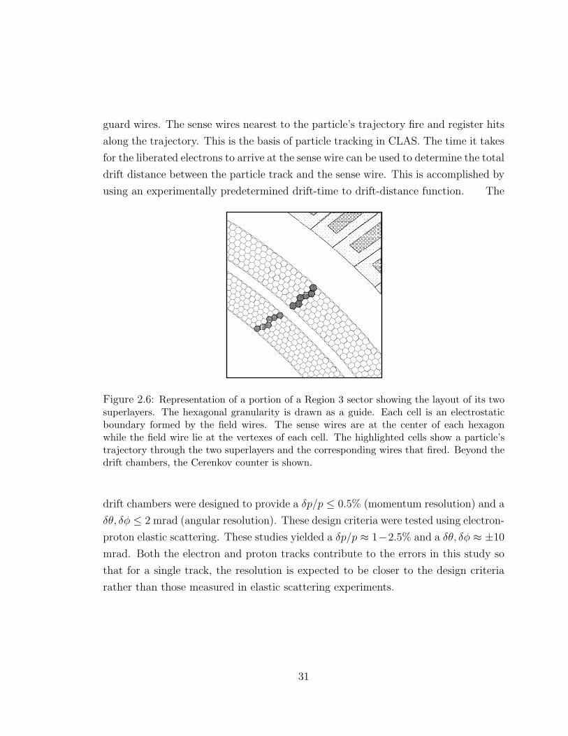
2.6 Representation of a portion of a Region 3 sector showing the layout of its

two superlayers. The hexagonal granularity is drawn as a guide. Each cell

is an electrostatic boundary formed by the field wires. The sense wires

are at the center of each hexagon while the field wire lie at the vertexes

of each cell. The highlighted cells show a particle’s trajectory through the

two superlayers and the corresponding wires that fired. Beyond the drift

chambers, the Cerenkov counter is shown. . . . . . . . . . . . . . . . . . 31

2.7 Schematic representation of Cerenkov segment. An electron track is shown

along with the path of the reflected Cerenkov light. . . . . . . . . . . . . 32

2.8 Exploded view of one of the six CLAS electromagnetic calorimeter modules. 33

viii

2.9 The arrangement of scintillator wedges in each sector. View is shown with

the beam direction into the page. Also shown is the event reconstruction.

The ovals depict the calorimeter-reconstructed location of the passage of a

showering particle. The size of the ovals denote the transverse energy spread

in the shower. . . . . . . . . . . . . . . . . . . . . . . . . . . . . . . . 35

2.10 Diagram showing the flow of data from its collection points at the various

detector subsystems to its collection and storage. . . . . . . . . . . . . . 39

2.11 A schematic diagram showing the CLAS data flow from the EB → ET →ER Also shown are the ancillary ET systems (E2 & E3) used for monitoring. 40

3.1 View of the TOF counters in one sector showing the panel grouping . . . 42

3.2 Schematic diagram of the high-voltage divider for the TOF PMTs. . . . . 44

3.3 Overall schematic of the TOF electronics. . . . . . . . . . . . . . . . . . 45

3.4 Logic diagram for the pretrigger circuit. . . . . . . . . . . . . . . . . . . 46

3.5 Typical pulse-height spectrum of all hits in a TOF counter. The energy

is estimated by evaluating the geometric mean of right and left PMTs. 48

3.6 Figure shows a cosmic ray incident on a scintillator bar. An accumulation of

events uniformly illuminating the scintillator bar produces the distribution

shown in the bottom right of the diagram. This distribution is centered

around zero if the two phototubes are properly gain-matched. . . . . . . . 50

3.7 Example of the time dependence of a TOF TDC on pulse height. The solid

line represents the calibration fit. . . . . . . . . . . . . . . . . . . . . . 53

3.8 Plot of corrected modulus of (T0−TRF ) vs TRF for selected runs of the e1-6

data. . . . . . . . . . . . . . . . . . . . . . . . . . . . . . . . . . . . . 56

3.9 Overall timing resolution for electrons achieved for the e1-6 experimental run. 57

3.10 A plot of ∆TK+ vs momentum of the kaon and proton sample shows suitable

timing separation of kaons and protons up to ∼ 1.8 GeV. The data plotted

include timing selection cuts on both the kaon and the proton. . . . . . . 58

4.1 An example 3-pronged reconstructed epK+ event as reconstructed by REC-

SIS.This particular event shows time-based as well as hit-based tracks re-

constructed in a Monte-Carlo event. . . . . . . . . . . . . . . . . . . . . 61

ix

4.2 Scatter plot of DOCA versus the corrected drift time for a) R3 axial wires

and b) R2 axial wires along with a sample fit of the time-to-distance correlation 65

4.3 Fitted ADC values for one Cerenkov channel. This is an example of a pmt

with very little noise. . . . . . . . . . . . . . . . . . . . . . . . . . . . . 68

4.4 Kinematic distribution of epK+ event sample . . . . . . . . . . . . . . . 70

5.1 3σEP

cuts on E vs. P. Horizontal line is the straight cut on the EC energy

at 0.64 GeV. The curved lines are the 3σEP

E/p vs. P cuts. . . . . . . . . 74

5.2 Electron sample after fiducial cuts imposed. Figure shows sector 1. . . . . 74

5.3 Vertex position of electron tracks in cm. The mean shows the z-position of

the target. The slant of the distribution is due to acceptance effects in the

scattered electron angle. . . . . . . . . . . . . . . . . . . . . . . . . . . 75

5.4 Figure shows number of photoelectrons distributions. The pion peak is

clearly seen at zero. The red dashed line shows the cut to eliminate this

pion contamination. . . . . . . . . . . . . . . . . . . . . . . . . . . . . 77

5.5 Plot of TOF Mass2 vs momentum for identified protons. The 5σ cuts are

clearly visible. . . . . . . . . . . . . . . . . . . . . . . . . . . . . . . . 80

5.6 Plot of TOF Mass2 vs momentum for identified K+s. The 4σ cuts are clearly

visible. Also clearly visible is the π+ contamination at higher momenta. . 80

5.7 Scatter plot of φ vs. θ for the K+ sample before fiducial volume cut is applied. 81

5.8 Scatter plot of φ vs. θ for the K+ sample after fiducial volume cut is applied. 81

5.9 Plot of epK+X missing mass. Shown is the Gaussian+2nd-order polynomial

fit to the K− peak. . . . . . . . . . . . . . . . . . . . . . . . . . . . . 82

5.10 Plot of epK+X missing mass vs. the K+K− invariant mass. ±2σ cuts are

applied to the epK+X missing mass in order to select K−s. . . . . . . . . 82

5.11 Scatter plot of epK+ missing mass with modified K+ mass versus the regular

epK+ missing mass. The cuts on these two variables are shown. . . . . . 83

5.12 eK+ missing mass before cut (unfilled) and after cut (green-hatched) illus-

trated in Figure 5.11. The ground-state Λ(1115) is shown as well as the

Σ(1189) directly right of the Λ. . . . . . . . . . . . . . . . . . . . . . . 83

x

5.13 Plot shows the ratio of the corrected electron momentum to uncorrected

electron momentum versus the uncorrected momentum. The electron mo-

mentum correction has a less than 1% effect for all applicable momenta. . 84

5.14 K+K− invariant mass including all data cuts and fit to φ peak with Eq. 5.10. 86

5.15 Feynman diagram for excited Λ(1520) hyperon production. This is the

primary background for φ(1020) production. . . . . . . . . . . . . . . . 87

5.16 Plot of pK− invariant mass. The Λ∗(1520) removed by the cut (white) is

clearly visible as well as the data kept (green shaded region). . . . . . . . 88

5.17 Scatter plot of IMKK versus IMpK . The well-defined vertical strip at

IMpK = 1.52 GeV is the Λ(1520) band. The horizontal strip at IMKK =

1.02 GeV is the φ band. The lines show the range cut applied to remove the

Λ background. Also discernible are the φ events located below the low-end

cut that would be thrown away with a single-valued cut above IMpK = 1.53. 90

5.18 Generated, weighted Q2 versus ν histogram used to obtain correlated Q2

and ν values. . . . . . . . . . . . . . . . . . . . . . . . . . . . . . . . . 92

5.19 Generated ψ versus cos ΘH histogram weighted with W (cosΘH , ψ) used to

obtain correlated ψ and cos ΘH values. . . . . . . . . . . . . . . . . . . . 92

5.20 23,000 reconstructed Monte Carlo events (histogram) overlayed with same

amount of reconstructed data (blue error points). . . . . . . . . . . . . . 93

5.21 2-dimensional representation of CLAS acceptance in Q2 and t. Each “lego”

represents a 0.2 GeV × 0.2 GeV 2-d bin. The z-axis is the efficiency for

each bin. . . . . . . . . . . . . . . . . . . . . . . . . . . . . . . . . . . 95

5.22 2-dimensional representation of CLAS acceptance in Q2 and t′. Each “lego”

represents a 0.2 GeV × 0.2 GeV 2-d bin. The z-axis is the efficiency for

each bin. . . . . . . . . . . . . . . . . . . . . . . . . . . . . . . . . . . 96

5.23 Plot shows Nphe x 10 distribution for scattered electrons after all electron

selection cuts are made. The solid line shows a fit to the generalized Poisson

distribution from 40 to 200 while the dashed line shows the extrapolation

of the function to 0. . . . . . . . . . . . . . . . . . . . . . . . . . . . . 97

xi

5.24 Contributing graphs of the radiative correction calculation Bremsstrahlung

radiation (a), (b) self-absorption of radiated photon (c) and the inter-

nal loop of e+/e− pair production/annihilation (d). The born process

(no radiated photon) is not shown. . . . . . . . . . . . . . . . . . . . 98

5.25 Plot of radiative correction Frad as a function of ΦCM = Φ for assorted

values of W from 2.0 to 3.0 GeV. The correction for each W value was

computed at a < Q2 >= 2.47 GeV2 and cos θCM = 0.345. . . . . . . . 99

6.1 Fitted φ yields in given Q2 bins given by a fit to Equation 5.10. . . . . . . 103

6.2 Plot shows σ(Q2) for all t and W values for a previous JLab data set [2]

(blue points) and the from present analysis (green points). . . . . . . . . 104

6.3 Fitted dσdt′ yields in t′ bins given by a fit to Equation 5.10. . . . . . . . . . 106

6.4 dσdt′ vs t′ for all Q2. . . . . . . . . . . . . . . . . . . . . . . . . . . . . . 107

6.5 dσdt vs -t integrated over the entire Q2 range. . . . . . . . . . . . . . . . . 108

6.6 dσdt vs -t for the entire Q2 range and the JML predictions at 5 Q2 points. . 110

6.7 dσdt vs -t for the Q2 bin 1.6 ≤ Q2 ≤ 2.6 and the JML predictions. . . . . . 110

6.8 Plot of tmin(Q2, W ) surface for e1-6 kinematics. . . . . . . . . . . . . . . 111

6.9 Plot illustrates the essence of the tmin(Q2,W ) correction. The blue points

represent the observed differential cross section as a function of t while the

green dotted curve represents where these points should fall in the absence

of tmin effects i.e. if one plotted the differential cross section as a function of

t′= t− tmin(Q2,W ). It is important to note that the green curve represents

the t-dependence of the cross section assuming some model and can assume

various forms. . . . . . . . . . . . . . . . . . . . . . . . . . . . . . . . 112

7.1 Helicity states of the virtual photon and φ. The blue arrows indicate the

spin directions corresponding to each helicity state. . . . . . . . . . . . . 114

7.2 2-dimensional representation of CLAS acceptance in ψ and cos θH . Each

bin represents a 18.0 Degree × 0.1 units of cos θH 2-d bin. The z-axis is the

efficiency for each bin. . . . . . . . . . . . . . . . . . . . . . . . . . . . 116

7.3 Fits to K+K− invariant mass in 9 bins in ΦCM . . . . . . . . . . . . . . 117

7.4 dσdΦ vs Φ. Green line shows a fit to equation 7.5 along with extracted fit

parameters σTT and σLT . . . . . . . . . . . . . . . . . . . . . . . . . . 118

xii

7.5 K+K− invariant mass in cos θH bins plus a fit to equation 5.10 (red line). 119

7.6 dNd cos θH

extracted for all Q2 values plus a fit to equation 7.6. Also shown is

the extracted r0400 parameter. . . . . . . . . . . . . . . . . . . . . . . . . 120

7.7 dNdψ extracted for all Q2 values plus a fit to equation 7.7. . . . . . . . . . 121

8.1 Total cross sections as a function of Q2 for our data (green points), previous

JLab data (blue points)[2], Cornell data (triangles) [3], HERMES data for

W between 4 and 6 GeV2, and HERA data at high W (W=75 GeV2). . . 123

8.2 Plot shows dσdt′ along with a fit to equation 8.1 over the full range of the data.124

8.3 Plot shows dσdt′ along with a fit to equation 8.1 from 0.0 to 1.4 GeV2 which

corresponds to the range of the first diffractive minima. . . . . . . . . . . 124

8.4 Spacetime picture of the interaction between the virtual φ meson (radius rφ)

and the proton (radius rh). The diagram shows the characteristic fluctuation

distance c∆τ compared to the overall size of the proton. This is not drawn

to scale. . . . . . . . . . . . . . . . . . . . . . . . . . . . . . . . . . . 125

8.5 Figure shows our data (green points) well as the previous CLAS analysis

(blue points) plotted with the JML prediction for the total cross section at

three different W values: W=2.0,2.45, and 2.90 GeV. . . . . . . . . . . . 126

8.6 Plot shows R = σL/σT vs. Q2 for our data (green dot), previous CLAS

results (blue dot), HERMES results (yellow triangles) and Cornell data (red

stars). . . . . . . . . . . . . . . . . . . . . . . . . . . . . . . . . . . . 128

xiii

List of Tables

1.1 Summary of φ electroproduction data . . . . . . . . . . . . . . . . . . . 21

3.1 The order and requirements for the TOF calibration. . . . . . . . . . . . 51

4.1 Calibration cooking steps performed on the three separate run ranges and

the meaning of each version. . . . . . . . . . . . . . . . . . . . . . . . . 62

4.2 Parameter Values for Ep

Pevs Pe cut . . . . . . . . . . . . . . . . . . . . 70

4.3 Summary of Cuts in epK+ Skim . . . . . . . . . . . . . . . . . . . . . . 71

4.4 Summary of additional cuts in final Phi++ skim. . . . . . . . . . . . . . 72

5.1 Summary of Cuts used for electron selection. The percentages shown indi-

cate the effect of each cut on the “epK skimmed” data sample. Each cut

was applied one at a time to the data so the effectiveness of each cut could

be considered separately. . . . . . . . . . . . . . . . . . . . . . . . . . . 78

5.2 Values show the fitted mean and σ of the K− peak for each sector before and

after momentum corrections are applied to the proton and kaon samples.

The last row shows the variances ∆ of each column. . . . . . . . . . . . . 85

5.3 Summary of investigated IMpK cuts along with their respective signal to

background ratios and φ yield. . . . . . . . . . . . . . . . . . . . . . . . 89

5.4 List of kinematic and VMD input parameters for the event generator phi gen. 91

5.5 Summary of GPP input parameters . . . . . . . . . . . . . . . . . . . . 94

6.1 Binning for the extraction of the cross sections in Q2, t, and t′ and the

number of acceptance bins in each respective cross section bin. t′ has the

same binning and number of cross section bins as t so it is omitted in this

table for brevity. . . . . . . . . . . . . . . . . . . . . . . . . . . . . . . 102

xiv

6.2 Total cross section σ(Q2) and kinematics of each data point. < Q2 > is the

bin center, and < ε > is the average ε in each bin. . . . . . . . . . . . . 105

6.3 Differential cross section dσdt′ and kinematics of each data point. < t′ > is

the bin center, and < ε > is the average ε in each bin. . . . . . . . . . . 105

6.4 Differential cross section dσdt and kinematics of each data point. < −t > is

the bin center, and < ε > is the average ε in each bin. . . . . . . . . . . 109

6.5 tmin(Q2,W ) Correction values for each t bin in which the cross section is

extracted. . . . . . . . . . . . . . . . . . . . . . . . . . . . . . . . . . . 112

7.1 Acceptance table values for the extraction of the angular distribution. . . 117

8.1 The value of the impact parameter b for a fit to the full t′ range for this

analysis and the previous CLAS analysis. . . . . . . . . . . . . . . . . . 125

8.2 Summary of parameters extracted as a consequence of SCHC . . . . . . . 127

8.3 Extraction of σL . . . . . . . . . . . . . . . . . . . . . . . . . . . . . . 127

A.1 Acceptance table for all Q2 and t bins. The values are quoted in percent.

Bins with a value “-” are those with an acceptance value below 0.2%. . . . 134

A.2 Cherenkov Efficiency table. . . . . . . . . . . . . . . . . . . . . . . . . . 135

A.3 Radiative corrections table. Φ is in degrees and W is in GeV. . . . . . . . 135

xv

For my grandfathers Louis and Nicola

xvi

Acknowledgments

There are many people whose constant support and encouragement resulted in the

successful completion of my PhD. First I would like to thank my on site co-advisor

Elton Smith who provided the constant guiding voice for the duration of this project.

Without Elton’s constant support and advice, this work would have never come to

fruition. I would also like to thank my other co-advisor John Ficenec, based at

Virginia Tech, who was directly responsible for the opportunity to complete my re-

search at Jefferson Lab. Both co-advisors exhibited unwaivering patience and support

throughout the entirety of this project.

I would also like to thank the rest of my committee who spent the time reading and

critiquing my thesis and providing the much needed feedback facilitating its success-

ful completion. They, along with all the professors I had at Virginia Tech have been

an integral part of my physics education, both in the classroom and out.

Special thanks goes out the Virginia Tech Physics department secretary Christa

Thomas who was a pillar of support and great friend throughout my tenure as a

graduate student.

I would especially like to thank Dr. Jean-Marc Laget for his invaluable discussions of

the theoretical framework of this thesis topic as well as for providing a phenomeno-

logical model and calculation to which to compare my results.

The success and quality of the e1-6 experiment was a result of the hard work and

dedication of the entire CLAS collaboration, especially those intimately involved in

the calibration of the detector as well as the processing of the data for the e1-6 run.

Besides the collaboration members, there is an invaluable staff of Hall B technicians,

engineers and staff who were responsible for the smooth operation of the detector and

accelerator during the e1-6 run. I extend a special thanks to Tom Carstens, Denny

Insley, and Jill Gram for allowing me to tag along during the detector maintenance

periods during which I accrued very useful hardware knowledge and experience.

Throughout the duration of this project, I have been blessed to have the unyielding

support and encouragement of a group of close friends. To all of you in New York,

Newport News, and elsewhere, I’d like to express my heartfelt and never-ending grat-

itude. You all make this accomplishment all the more sweeter.

xvii

I want to thank my entire family for their love, guidance and support throughout

my entire life leading up to this achievement, especially my brother who provided a

calming voice and open ear whenever it was needed.

Last but definitely not least, I want to thank my parents who through a lifetime of

sacrifice, hard work, and unabated love provided me every opportunity possible to

make the most of life. They are the primary reason I am the person I am today.

It has been a long and winding road ending miles and years from where it began.

xviii

Chapter 1

Theoretical Background and

Motivation

1.1 φ(1020) Electroproduction Overview

Vector meson electroproduction has opened a unique window into the substruc-

ture of the nucleon as well as the hadronic structure of the photon [4]. Historically,

vector meson electroproduction has been described in terms of the hadronization of

the virtual photon at low Q2 (low virtuality of the photon), where the virtual pho-

ton fluctuates into a virtual meson and subsequently scatters diffractively off of the

nucleon. This occurs in a time ∆τ , consistent with the uncertainty principle, and

completely characterizes the temporal and spatial extent (c∆τ) of the fluctuation. In

this regime, the exchange mechanisms are dominated by hadronic degrees of freedom.

At higher Q2 the wavelength of the virtual photon, given by λ = h√Q2

, decreases mak-

ing the virtual photon probe more sensitive to increasingly smaller distance scales.

This corresponds to a transition from hadronic to quark and gluon (partonic) degrees

of freedom. In this domain, deeply inelastic production of vector mesons is described

by generalized parton distributions(GPDs). Primarily, GPDs are a set of four func-

tions of quark/gluon momentum (transverse, longitudinal and orbital) and spin which

describe the behavior of these partons in the target nucleon. The Q2 domain where

the vector meson exchange→GPD transition occurs is still a matter of debate. The

1

systematic study of φ electroproduction as well as ρ, and ω electroproduction has the

potential to shed some light on this question as well as other relevant quandaries of

hadronic physics.

The pure ss content of the φ makes it an ideal candidate to study the pure gluon

exchange mechanisms in each regime; the Pomeron in the low Q2 region and gluon

exchange graphs in the high Q2 region. The φ meson is 99% (ss) and has no quark

flavors in common with the nucleon (uud,udd) and thus any diagrams containing

disconnected quark lines are suppressed relative to connected ones. The suppression

of these disconnected quark graphs is known as OZI suppression [5]. Any ss content

in the nucleon will be reflected in the cross section as well as the spin properties of

the decay products.

Through the study of the Q2 scaling of the total cross section and the scaling of

the differential cross section dσdt

, φ electroproduction can be effective in probing the

validity of the two Q2 regimes.

1.1.1 Notation

Assuming the one photon exchange (OPE) approximation, vector meson electro-

production can be written as

γ∗ + N → P + φ (1.1)

where γ∗ is the virtual photon 4-momentum, N is the target nucleon 4-momentum,

P is the scattered nucleon 4-momentum, and φ is the electroproduced vector meson

4-momentum (in this case the φ). If V is a generalized 4-vector, it can be expressed

as an energy part and a 3-momentum part: V = (E, ~V ). The 4-vectors then assume

the following forms in the laboratory:

γ∗ = (ν, ~q), N = (MP , 0), P = (EP , ~PP ), Pφ = (Eφ, ~Pφ)

The virtual photon 4-momentum can be written in terms of the incident electron

4-momentum e and the scattered electron 4-momentum e′ as

γ∗ = e− e′ (1.2)

2

where e = (Ee, ~Pe) and e′ = (Ee′ , ~Pe′)

Key kinematic variables can now be defined that describe the aforementioned re-

action:

• The negative of the 4-momentum squared of the virtual photon,

Q2 = −q2 = −(γ∗)2 = −(e− e′)2(1.3)

which can be interpreted as the negative mass squared of the virtual photon.

• The γ∗p center of mass energy or the γ∗p invariant mass

W =√

s =√

(γ∗ + P )2 (1.4)

where s is one of three Mandelstam invariant variables, the next two to be defined

forthwith.

• Virtual photon energy

ν = Ee − Ee′ (1.5)

• The 4-momentum transfer squared between the virtual photon and the vector meson

(or between the target and scattered nucleon):

t = (γ∗ − Pφ)2 = (N − P )2 (1.6)

which is the second Mandelstam variable, and the third

u = (γ∗ − P )2 = (Pφ −N)2 (1.7)

which is the 4-momentum transfer squared between the virtual photon and scattered

nucleon or between the target nucleon and the vector meson.

• The minimum 4-momentum transfer squared tmin is given by

tmin = (Eγ∗cm − Eφ

cm)2 − (|~pγ∗cm| − |~pφ

cm|)2 (1.8)

where Eγ∗cm(~pγ∗

cm) is the energy(momentum) of the virtual photon in the γ∗p center of

3

mass frame and Eφcm(~pφ

cm) is the energy(momentum) of the vector meson (in this case

the φ) in the same reference frame.

• One can define [6]

t′ =∣∣∣t− tmin

∣∣∣ (1.9)

• Q2, ν, and W can be related via the following relation

W 2 = M2p + 2Mpν −Q2 (1.10)

• The Bjorken scaling variable xB, which is the fraction of nucleon 4-momentum

carried by the parton impacted upon by the virtual photon is

xB =Q2

2Mpν=

Q2

W 2 + Q2 −Mp2 (1.11)

• The angle Φ between the electron scattering plane and the hadron production plane

(see Figure 1.1)

The electroproduction reaction can then be described by the following set of 4 inde-

pendent variables:

(Q2, t, Φ, [W or ν or xB]) (1.12)

The reduced cross section σ(Q2,W ) integrated in Φ and t is given by

σγ∗+N→P+φ(Q2,W ) = σT (Q2,W ) + εσL(Q2,W ) (1.13)

where ε is the virtual photon polarization parameter given by

ε =1

[1 + 2(Q2 + ν2)/(4Ee(Ee − ν)−Q2)](1.14)

ε is expressible in terms of the ratio of two elements L11 and L12 of the spin density ma-

trix of the photon Lµν evaluated in the Breit-Wigner reference frame [1]. σT (Q2,W )

is the cross section due to transversely polarized virtual photons and σL(Q2,W ) is

the cross section due to the longitudinally polarized virtual photons. The reduced

cross section is related to the measured cross section through the virtual photon flux

4

e

*γ’eTarget

P

φ

CMZ

LABZ

Φ CMY

CMX

+KHELY

HELZ

Electron Scattering Plane (Lab)

Hadron Production Plane (CM)

φ

HELX

Hφ

Hθ

Decay Plane (Helicity Frame)

P

Figure 1.1: Graphical representation of φ meson electroproduction. Shown from left toright then above are the electron scattering plane, the hadron production plane and helicityrest frame of the φ respectively. Φ is the relative angle between the electron scattering andhadron production planes. θH and φH are the polar and azimuthal angles of the K+ definedin the helicity frame basis of the φ meson as defined in reference [1]

factor Γ(Q2,W )

d2σ

dQ2dWdφe′= Γ(Q2,W )[σT (Q2,W ) + εσL(Q2,W )] (1.15)

and after integrating over the azimuthal angle of the scattered electron in the lab,

the measured cross section becomes

d2σ

dQ2dW= 2πΓ(Q2,W )[σT (Q2,W ) + εσL(Q2,W )] (1.16)

5

where Γ(Q2, W ) is given by

Γ(Q2,W ) =α

8π2

W

MpE2e

W 2 −Mp2

MpQ2

1

1− ε(1.17)

and α is the fine structure constant. Γ(Q2,W )can be interpreted as the probability

per GeV3 of producing a virtual photon at a given Q2 and W . The definition of the

virtual photon flux is ambiguous and there are varying conventions employed. Each

convention requires the virtual photon flux to equal the real photon flux as Q2 → 0

[5]. The convention used here is that from [7].

1.2 The Vector Meson Dominance (VMD) Model

The analysis of photoproduced vector mesons has historically been described

within the framework of the Vector-Meson Dominance (VMD) model. The main

tenet of the VMD model is the assumption that vector meson production is domi-

nated by interactions between the nucleon and the vector meson intermediate states

of the incoming photon [3]. In other words, if the photon is given by the state vector

|γ〉, it can be expressed as a linear combination of a “bare” photon state |γB〉 which

accounts for a negligible part of the interaction and a hadronic component |h〉.

|γ〉 ∼=√

Z3|γB〉+√

α|h〉 (1.18)

Z3 is introduced to ensure proper normalization of |γ〉 [8]. Due to invariance

considerations, |h〉 must have the same quantum numbers as the photon namely

JPC = 1−−. Experimental observations of real and virtual photoproduction demon-

strate that ρ0, ω, and φ are produced copiously and therefore are the main contribu-

tions to |h〉. The main hypothesis of VMD is that these three mesons are the sole

hadronic constituents of the photon |γ〉 and that the bare photon state |γB〉 does

not interact with the target hadron or photoproduced hadron. The assumption that

|h〉 is composed of more than just the three aforementioned mesons is referred to as

generalized vector dominance (GVD) [8]. The VMD cross section can be expressed

6

e e’

Target p

φ

+K

-K

φ

VMD Assumption

Figure 1.2: φ electroproduction through diffractive scattering off the nucleon. The regionenclosed in the dotted box represents the VMD assumption of the fluctuation of the virtualphoton into a vector meson.

asd2σ

dQ2dW= 2πΓ(Q2,W )ζσt(1 + εR)WD(cos θH , ψ) (1.19)

where within the VMD framework

R = ξ2 Q2

Mφ

(1.20)

is the ratio of the longitudinal to transverse cross sections. ξ2 is the VMD scaling

parameter and takes on a typical value of 0.33. The other components of equation

1.18 are given by:

σt =Aφ

bφ

exp(−bφt′) (1.21)

ζ =W 2 −Mp

2

2Mp2√

ν2 + Q2

1

(1 + Q2

Mφ)2

(1.22)

WD(cos θH , ψ) is the angular decay distribution. Within the framework of VMD and

7

assuming s-channel helicity conservation (SCHC) the angular decay distribution is

WD(cos θH , ψ) =3

8π

1

(1 + εR)[sin2 θH(1 + ε cos 2ψ)

+ 2εR cos2 θH −√

2ε(1 + ε)R cos δ sin 2θH cos ψ] (1.23)

where the angle ψ is defined as ψ = Φ − ΦH and θH is defined in Figure 1.1. δ

is a relative phase factor between the two independent helicity amplitudes. For a

discussion and definition of helicity amplitudes see chapter 7 section 1 or reference

[1]. The factor ζ allows the extrapolation away from Q2 = 0, a.k.a into the virtual

photoproduction regime. This term includes a propagator term as well as a correction

to the virtual photon flux [3].

1.3 Particle Exchange Mechanisms, Regge The-

ory and the JML Model

1.3.1 Particle Exchange Mechanisms

The present analysis is concerned with the generalized reaction γ∗N → PX.

When describing the interaction of the electron and the proton, the virtual photon γ∗

arises as the exchange particle of the electromagnetic force between the two, Figure

1.3. A similar quantum field theoretic exchange particle mechanism can be used

e

’e

*γp

Figure 1.3: The electromagnetic interaction mediated by a virtual photon.

when describing the interaction of the virtual photon γ∗ with the proton P at low

8

energies. The nature of this interaction is illustrated in Figure 1.4. The species of

the exchange particle is multi-fold for each reaction considered and is determined by

which exchange channel one is considering. The exchange channels are named for

the three Mandelstam variables s, t, and u described in section 1.1.1 and denote the

three possible directions of momentum flow in γ∗P scattering. For the t-channel, the

exchange particle is a meson, and is a baryon for the s and u channels (see Figure 1.4).

The amplitude A of each of the diagrams can be constructed from factors associated

*γ *γ*γ

p p

X

X’p

’p

p

X

’p

Meson Nucleon Baryon

t u

s

Figure 1.4: Channel-dependent exchange mechanisms for γ∗P → P ′X

with each line within the diagram. These are known as the Feynman rules of the

diagram [9]. For the diagrams above the amplitude is proportional to the following

product of the Feynman propagator PF , the coupling constants at each of the two

vertices g and g′ and the spin-dependent vertex functions V and V ′ which depend on

which three particles are joined at the vertex [10].

A ∝ gVPF g′V ′ (1.24)

1.3.2 Regge Theory

The process 1+2 → 1′+2′ (γ∗+p → p′+X) is historically described with S-matrix

theory. S-matrix theory characterizes the aforementioned scattering process from the

initial state vector |1, 2〉 into a final state vector |1′, 2′〉 by way of the scattering matrix

9

S where S is unitary matrix [9]. The purpose of S-matrix theory is to calculate the

matrix element

A =< 1′, 2′|S|1, 2 > (1.25)

where the matrixA represents the amplitude of the scattering process. The amplitude

A can be expressed as partial-wave expansion

A(s, t) =∞∑

l=0

(2l + 1)Al(t)Pl(cos θCM) (1.26)

where l is the total angular momentum, Al(t) are the coefficients of the Legendre

polynomials Pl(cos θCM). This t-channel partial wave amplitude can be cast into

integral form using the Sommerfeld-Watson transform. This step is where angular

momentum becomes a complex number and is the foundation of Regge theory [11, 12].

In relativistic field theory, the mapping of non-negative integer angular momentum

values l to complex values [13] is not unique. This requires the introduction of two

amplitudes corresponding to odd (-) and even (+) real parts of l. This is known as

the signature. Incorporating these requirements, the amplitude can be expressed as

A±(s, t) = 8πi∫

Cdl(2l + 1)

sin(πl)A±(l, t)[Pl(− cos θCM)± Pl(cos θCM)] (1.27)

It was shown that the singularities of A±(l, t) in the complex l-plane are poles whose

locations vary with t:

l = α(t) (1.28)

These poles are known as Regge poles or Reggeons and as t varies, they trace out paths

parameterized by α(t) in the complex l-plane that are known as Regge trajectories

[12].

1.3.3 JML Model

Regge theory makes its connection to scattering theory through the fact that

each of these trajectories α(t) corresponds to the exchange of a different family of

particles. The model of Jean-Marc Laget et. al., denoted as the JML model from

10

this point on, has at its foundation the exchange of Regge trajectories in the t-

channel [10]. Therefore, the predictive power of the JML model will be in describing

the t-behavior of the cross section as well as the scaling of the total cross section

with cm energy squared: σ ∼ ( ss0

)(2α(0)−1). The photoproduction of each meson is

described by a channel-appropriate sum of exchanges of the four main t-channel Regge

trajectories π0, σ, f2, and P(Pomeron). These are diagrammatically shown in Figure

1.5. Each of the π0, σ, f2, and P exchanges has a corresponding Regge trajectory:

γ ρ

P ’P

σ +:ρ

:ω

:φ

γ ρ

P ’P

2f+

γ ρ

P ’P

Pomeron

γ ω

P ’P

0π +

γ ω

P ’P

2f +

γ ω

P ’P

Pomeron

γ φ

P ’P

Pomeron

Figure 1.5: Dominant exchange diagrams for ρ, ω, and φ electroproduction in theJML model. The φ channel is shown highlighted in yellow

The Pomeron trajectory is αP(t) = 1.08 + 0.25t, the f2 is αf2(t) = 0.55 + 0.7t, the π0

is απ(t) = 0.7(t−mπ2) and finally the σ is ασ(t) = −0.175+0.7t [10, 14]. From these

trajectories, the Regge propagators PRegge which are the analogues of the Feynman

propagator in the aforementioned amplitude A can be calculated. For φ production

11

we are concerned with the Pomeron propagator:

PRegge =(

s

s0

)αP(t)−1

e−12iπαP(t) (1.29)

s0 = 1.0 GeV2 is a mass scale variable. In contrast to the π0, σ, f2 Reggeon family,

which is composed of two-quark ordinary meson exchanges, the Pomeron, a reggeon

with the quantum numbers of the vacuum (0++), corresponds to the exchange of a

glueball. Glueballs can be thought of as complicated color-neutral structures com-

posed entirely of gluons. In the regime Q2,−t > 1 GeV2 [14], the Pomeron exchange

reduces to a simple 2-gluon exchange. The transition from the Pomeron to the non-

perturbative 2-gluon regime occurs when the formation process of the Pomeron has

no time to develop [14]. The 2-gluon propagator is given by:

P2g =β0√πλ0

exp(

l2

λ02

)(1.30)

l here denotes the total transverse momentum of the exchange gluons and the range

parameter λ02 = 2.7 GeV2 characterizes the spatial scale of the interaction. The

coupling of the Pomeron to the quark, or more generally the effective coupling of the

gluon to the quark β0 is set by high energy nucleon-nucleon scattering and assumes

the value β0 ∼ 4.0 GeV2.

The JML model predictions for photoproduction data of vector mesons reproduces

the magnitude of the cross sections up to W∼100 GeV, however, in the range W∼10 GeV, the pure Pomeron exchange mechanism is an underestimate of the data.

The superposition of the JML predictions over various photoproduction data plotted

against W is shown in Figure 1.6. The data shown are from various photoproduc-

tion experiments conducted at JLAB, SLAC, CERN, HERA, and Fermi Lab. It is

clear from Figure 1.5 that the φ channel provides a convenient way of isolating the

gluon exchange mechanism, in the cast of Pomeron exchange, from quark exchange

mechanisms. This is due to the OZI suppression of quark exchange mechanisms in φ

production [5]. The data at two different W values corresponding to the HERA en-

ergy range (top plot) and the JLAB energy range (bottom plot), are shown in Figure

1.7. As for other vector meson channels, the JML model reproduces the data well up

12

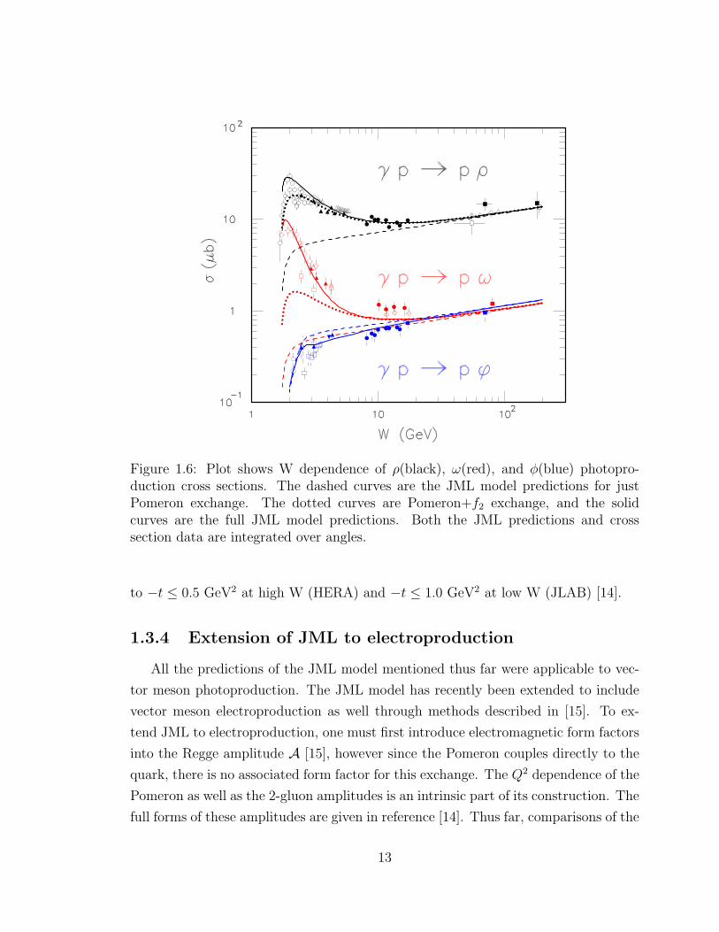
Figure 1.6: Plot shows W dependence of ρ(black), ω(red), and φ(blue) photopro-duction cross sections. The dashed curves are the JML model predictions for justPomeron exchange. The dotted curves are Pomeron+f2 exchange, and the solidcurves are the full JML model predictions. Both the JML predictions and crosssection data are integrated over angles.

to −t ≤ 0.5 GeV2 at high W (HERA) and −t ≤ 1.0 GeV2 at low W (JLAB) [14].

1.3.4 Extension of JML to electroproduction

All the predictions of the JML model mentioned thus far were applicable to vec-

tor meson photoproduction. The JML model has recently been extended to include

vector meson electroproduction as well through methods described in [15]. To ex-

tend JML to electroproduction, one must first introduce electromagnetic form factors

into the Regge amplitude A [15], however since the Pomeron couples directly to the

quark, there is no associated form factor for this exchange. The Q2 dependence of the

Pomeron as well as the 2-gluon amplitudes is an intrinsic part of its construction. The

full forms of these amplitudes are given in reference [14]. Thus far, comparisons of the

13

Figure 1.7: Top plot shows dσdt

data from ZEUS at high W superposed with JMLmodel predictions. Bottom plot shows various φ photoproduction data measuring dσ

dt

as well as JML model predictions for pure Pomeron exchange, pure 2-gluon exchange,u-channel (baryon) exchange as well as the full model (Correlations).

JML model for electroproduction have been made with ω[10], and ρ [16] electropro-

duction data from JLAB, and ρ electroproduction data from HERMES [17, 10, 16].

JML seems to overestimate the W dependence of σL, however σT is satisfactorily

described.

1.4 Generalized Parton Distributions

As Q2 increases, the resolution of the inelastic probe γ∗ is improved in the γ∗N →PX reaction. In this higher Q2 domain, γ∗ becomes sensitive to the internal struc-

ture of the nucleon, composed of quarks and gluons. A generalized description of the

14

momentum and spatial distribution of the partons in the nucleon is encoded in func-

tions called Generalized Parton Distributions(GPDs) [18]. A formalism which unifies

exclusive reactions at large Q2 is by no means a new concept, however through the

recent work of Ji, Radyushkin, and Collins, GPDs have acquired a new predictive

richness and descriptive form [19]. To first order, GPDs can be classified into two

*γ

N P

)ω,ρV(

Quark

*γ

N P

,ω,ρV(

Gluon

φ )*γ

N P

,ω,ρV(

Gluon

φ )

*γ

N P

)ω,ρV(

Quark

Figure 1.8: Exchange diagrams for meson electroproduction. The top two diagramsare the quark exchange GPDs (blue blobs) and the bottom two are the gluon GPDS.

groups corresponding to quark-exchange GPDs and gluon-exchange GPDs, whose re-

spective graphs are shown in Figure 1.8. This figure also illustrates the particular

species of vector meson production to which each of these graphs contributes. It is

seen from this figure that for ρ and ω production, both quark and gluon graphs con-

tribute and do in fact contribute almost equally. For φ production however, only the

gluon graphs contribute due to the OZI suppression of the quark exchange graphs. φ

meson electroproduction becomes a useful filter for isolating and studying these glu-

15

onic GPDs. As a result of this, any quark exchange in φ production occurs through

the ss content of the proton wave function, and thus such exchanges are a direct

probe of the physics associated with the dynamics of strange sea quarks in the proton

[19]. This is the GPD description of the familiar ss knockout mechanism described

in [20].

1.4.1 Functional Form of the GPDs and Factorization

GPDs describe the soft part of the exclusive meson electroproduction amplitude

in the so-called handbag diagrams. These handbag diagrams contain a hard, pertur-

bative part which is exactly calculable within regular perturbation theory as well as a

soft, non-perturbative part describing the strong interaction with the partons in the

target nucleon. The predictive power of GPDs arises when factorization [21] of the

perturbative and non-perturbative parts is valid. To the extent that the virtual pho-

ton γ∗ is longitudinally polarized and |t| ¿ Q2 the amplitude AL can be factorized

into a perturbative and non-perturbative part (GPD) part. AL is the amplitude of σL

so the experimental access to GPDs will be accomplished through the measurement

of the longitudinal cross section σL. Assuming SCHC, R can be extracted from the

decay angular distribution. Before introducing the explicit form of the amplitudes

and associated GPDs, it is appropriate to introduce light-cone coordinates:

v± =1√2(v0 ± v3), v = (v1, v2) (1.31)

where v is any arbitrary 4-vector with components vi, i = 0, 1, 2, 3.

Following the form used in [19, 22], AL can be decomposed into a quark GPD

part Aq and a gluon GPD part Ag. Aq is given by:

Aq = e16παs

9

1

Q

∫ 1

0dz

∑q

eqΦq(z)

z

∫ 1

−1dx F q(x, ξ, t)

[1

ξ − x− iε− 1

ξ + x− iε

](1.32)

Ag is given by:

Ag = eπαs

3

1

Q

∫ 1

0dz

∑q

eqΦq(z)

z

∫ 1

−1dx

F g(x, ξ, t)

x

[1

ξ − x− iε− 1

ξ + x− iε

](1.33)

16

The factorization theorem and its associated variables is elucidated in Figure 1.9.

where

e

’e

L*γ

N P

, ω, ρX=q

(z)Φz

,t)ξ(x,qF

ξx+ξx-

φ

2∆t=

Figure 1.9: Handbag diagram representation of the electroproduction of the vectormesons ρ0, ω, and φ. The lines highlighted in dark blue represent the perturbative“hard” part of the scattering amplitude. The entire non-perturbative part of is rep-resented by the light blue oval. The formation of the vector meson, described by themeson distribution amplitude, is represented by the light green blob. This diagram isthe handbag diagram for quark GPDs F q. A diagram like the bottom two in Figure1.8 can be drawn for the gluon GPDs F g.

• αs is the strong coupling constant and eq is the quark charge

• Φq(z) is the distribution amplitude of the electroproduced meson which is a function

of the 4-momentum fraction z [19]

• The index q describes the quark flavor composition of the electroproduced meson

in the amplitude Aq

• ξ is the symmetrized momentum transfer fraction ξ = N+−P−N++P− (N±, P± are the

light-cone 4-vectors of N and P )

• x is the light-cone momentum fraction carried by the exchange quarks

• F q/g(x, ξ, t) is the non-perturbative part of the amplitude which is a function of the

17

GPDs E, E,H, H. E,H are for vector mesons and E, H are for psuedoscalar mesons.

The amplitude Aq is associated with the top two diagrams of Figure 1.8 while Ag is

represents the bottom two diagrams. For φ production, the amplitude Aq is strongly

suppressed so the main contribution comes from Ag. The function F q/g(x, ξ, t) are

the GPDs describing the nucleon structure. For vector meson electroproduction, it is

defined according to [23]

F q/g(x, ξ, t) = Hq/g(x, ξ, t)N(P )γ+N(N) + Eq/g(x, ξ, t)N(P )iσ+κ ∆κ+

2MN

N(N)

(1.34)

where

• N(P ), and N(N) are the nucleon spinors (explicitly written in appendix B of ref-

erence [19]

• γ+ and γ5 are the Dirac matrices

• σ+κ is Pauli matrix. κ is the spinor index.

• ∆+ = −2ξP+ is related to the t-channel momentum transfer (∆2 = t) expressed as

lightcone 4-vectors

There is a similar expression for Hq/g(x, ξ, t) and Eq/g(x, ξ, t) which are applicable to

psuedoscalar mesons but will not be discussed here. The study of ρ0, ω, and φ electro-

production channels act as a filter for isolating the Hq/g(x, ξ, t) and Eq/g(x, ξ, t) GPDs.

The φ channel has the capability of further isolating the gluonic GPDs Hg(x, ξ, t) and

Eg(x, ξ, t).

The amplitude for φ electroproduction can be written as the sum of the gluon

GPD contribution and a strange quark GPD contribution:

Aφ ∝ F g(x, ξ, t) + F s(x, ξ, t) (1.35)

The strange quark GPD contribution to this amplitude, F s(x, ξ, t), is strongly OZI

suppressed so the main contribution to φ production comes from the gluon contri-

bution. Any strange quark component of the nucleon wave function will however

manifest itself through the contribution from F s(x, ξ, t).

18

1.4.2 Consequences and Results of GPDs

Given that σL can be successfully extracted and the requirements of factorization

are met, GPDs can yield a tremendous wealth of information concerning the structure

of the nucleon as well as the behavior of its constituents. Some predictive aspects

of GPD formalism have already been touched upon and some of the more salient

predictions will now be discussed [19].

3-D spatial distributions of partons in the nucleon

• Given that the momentum transfer t can have a small component transverse to

the nucleon direction, one can obtain information about the transverse structure of

the nucleon. When expressed in the impact parameter representation of the GPDs

(where the spatial distribution of quarks and gluons in the plane transverse to the

momentum of the hadron is given as opposed to the momentum representation of

GPDs already introduced), a 3-D picture of the partonic stucture of the nucleon can

be constructed.

Spin structure of the nucleon

• A long-standing mystery of nucleon structure is how the total nucleon spin is

constructed from its partonic constituents. Reference [24] shows how the nucleon

spin can be decomposed into a quark intrinsic (helicity) spin , a quark orbital, and a

gluon contribution. Furthermore, it is shown how this total quark spin contribution

to the nucleon can be accessed through deeply virtual Compton scattering (DVCS).

The total nucleon spin can be decomposed as

(Sq + Lq)︸ ︷︷ ︸Jq

+Jg =1

2(1.36)

The contribution Sq is known from inclusive measurements on polarized targets, so

using the DVCS reaction will yield Lq and thus the quark contribution to the nucleon

spin. Such a measurement is accessible through measurements of ρ0 electroproduction

19

by exploiting the relation:

Jq = limt→0

1

2

∫dx x

[H(x, ξ, t) + E(x, ξ, t)

](1.37)

at fixed ξ.

Cross section ratio predictions: σρ0 : σω : σφ

If one assumes the regular qq content of the neutral vector mesons,

ρ0 : 1√2(|uu > −|dd >)

ω : 1√2(|uu > +|dd >)

φ : |ss >

then the ratio of their production amplitudes can be written as [19]:

Aρ0 : Aω : Aφ =∫ 1

−1

dx

ξ − x− iε

(2F u(x, ξ, t) + F d(x, ξ, t)√

2+

9

8√

2

F g(x, ξ, t)

x

)

:∫ 1

−1

dx

ξ − x− iε

(2F u(x, ξ, t)− F d(x, ξ, t)√

2+

3

8√

2

F g(x, ξ, t)

x

)

:∫ 1

−1

dx

ξ − x− iε

(−F s(x, ξ, t) +

3

8

F g(x, ξ, t)

x

)(1.38)

This relation leads to predictions about the cross section ratios:

σρ0 : σω : σφ = 9 : 1 : 2 in the region at very small xB where gluon exchange dominates.

Otherwise, in the quark-exchange-dominated region, the expected cross section ratio

between the ρ0 and the ω meson is expected to become σρ0 : σω = 25 : 9 as quark

exchange becomes more important. The expected ratio to the φ cross section does

not change as a result of the suppression of quark exchange diagrams in φ production.

1.5 Summary of Previous Data and Measurements

One of the leading motivations for completing the present analysis is the sparse

amount of existing φ electroproduction data. Aside from the previous data in refer-

ences [2, 25, 3] most of the measurements are at high W (W > 10 GeV). A summary

of the world data along with kinematical regime of each contributions can be found in

20

Table 1.1. The data is plotted in Figure 1.10 along with additional photoproduction

Table 1.1: Summary of φ electroproduction data

Data Author/Location Q2 W YearLukashin/CLAS 0.70 to 2.20 GeV2 2.0 to 2.6 GeV2 2001Airapetian/HERMES 0.70 to 5.00 GeV2 4.0 to 6.0 GeV2 2003Cassel/Cornell 0.80 to 4.00 GeV2 W= 2.7 GeV2 1981Dixon/Cornell 0.23 to 0.97 GeV2 1977Adloff/H1 1.00 to 15.0 GeV2 40.0 to 130.0 GeV2 2000Adloff/H1 Q2 > 7.0 GeV2 W= 75.0 GeV2 1997Breitwig/H1 3.00 to 20.0 GeV2 4.0 to 120.0 GeV2 2000Derrick/H1 7.00 to 25.0 GeV2 42.0 to 134.0 GeV2 1996

data (Q2=0 GeV2).

1.6 Goals and hopes of the present analysis

The objectives of the following analysis are multi-fold and are summarized as fol-

lows:

• Extraction of the total cross section σ(Q2)

The predictions of the VMD model predict a 1Q4 scaling of the total cross section. A

different behavior of σ(Q2) would indicate the contribution of other exchange mech-

anisms.

• Extraction of the differential cross section dσdt

and dσdt′

The comparison of the measured differential cross section with multiple models re-

quires the extraction of both dσdt

and dσdt′ . The comparison of the data to VMD pre-

dictions amounts to the extraction of the t-slope parameter b from dσdt′ vs t′. VMD

predicts the t-dependent part of the cross section to behave as:

σt′ ∝ Aφ exp(−bt′) (1.39)

21

( Q 2 + Mφ 2 ) ( GeV 2 )

σ(Q

2 ,W)

( µb

)

- CLAS Lukashin, W ≈ 2.3 GeV - H1 Adloff, W ≈ 75 GeV - ZEUS Derrick, W ≈ 70, 94, 99 GeV - CORNELL Cassel, W ≈ 2.7 GeV - BONN Besch, W ≈ 2.2 GeV (Q2 = 0)◊ - SLAC Ballam, W ≈ 2.5, 4.3 GeV (Q2 = 0)

10-3

10-2

10-1

1

1 10

Figure 1.10: Figure shows some of the existing φ electroproduction data along withthe Pomeron exchange predictions at high W (solid) and low W (dotted line). Alsoshown are data from two photoproduction measurements (Q2 = 0).

The slope parameter is expected to decrease with increasing Q2.

The JML model predicts a certain behavior of dσdt

depending upon whether Reggeon

(Pomeron) exchange or 2-gluon exchange is the dominant production mechanism. The

extraction of dσdt

is complicated by the tmin effect (see section 6.3), which must be cor-

rected for before dσdt

vs. t can be plotted. Again, due to poor statistics, the extraction

of dσdt

will be extracted in two Q2 bins for comparison to the JML model predictions

at two < Q2 > values.

• Extraction of R and σL from the angular distributions

The φ(1020) meson is a spin 1 particle which decays into two spin-0 particles:

φ → K+K−. The decay angular distribution WD(cos θH , ψ) of the K+ (or K−),

22

provides a complete description of the φ polarization [20]. SCHC. will first be tested

via the extraction of dσdΦ

. Assuming SCHC, the VMD parameters R and ξ2 can be

extracted with a fit to the assumed angular distribution (Eq. 1.23). The consistency

of these parameters can then be gaged relative to previous measurements.

Secondly, assuming SCHC and the successful extraction of R, σL (the cross section

due to longitudinally polarized photons) can be extracted from σ.

σL =R

1 + εRσ (1.40)

It is still unclear whether the kinematic regime of the present analysis is compatible

with the region of validity of GPDs. The GPD formalism makes predictions about

the behavior of σL, namely its scaling as a function of Q2 and t. The extraction of

σL is tantamount to making a meaningful comparison to the model. It is the hope

that at the very least we have entered a transition region where hadronic degrees of

freedom give way to quark, and more appropriately gluonic degrees of freedom.

23

Chapter 2

Experimental Apparatus and

CLAS Overview

2.1 Continuous Electron Beam Accelerator Facil-

ity

Thomas Jefferson National Accelerator Facility or TJNAF in Newport News,

Virginia is home to a recirculating linear electron accelerator capable of delivering

beam to three experimental halls simultaneously. The accelerator along with some

of its components is shown schematically in Figure 2.1. At its heart is a series of

superconducting Niobium cavities, five per cryomodule which produce a minimum

energy gradient of 5 MeV per meter. A beam of 45 MeV electrons is injected into

one of the linacs which are connected on one end by five recirculation arcs and four

on the extraction side. Each successive pass through the linacs boost the electron

energy by a typical value ∆E where ∆E is about 0.4 GeV per line-ac. With the

recent accelerator upgrade, the available beam energies range from 1.140 GeV to 5.70

GeV in multiples of 1.140 GeV.

The electron beam is extracted at the recirculation arcs which allow the three Halls

to operate at 3 different but correlated energies simultaneously. As a result of the

RF signal structure operating at 1.497 GHz, each beam bunch is separated by about

two-thirds of a nanosecond. In other words, the electron beam can be delivered to

24

each hall at a frequency of 499 MHz with currents ranging from ∼ 100pA to ∼ 100µA.

Each of the end stations contain spectrometers which support complimentary ex-

perimental physics programs. Two High Resolution Spectrometers (HRS’s) with a

momentum resolution of ∆pp≤ 10−4, and a maximum momentum of 4 GeV/c make

their home in Hall A. Hall C contains two medium resolution magnetic spectrome-

ters, each with a ∆pp≤ 10−4 but each with a different maximum momentum. The

Short Orbit Spectrometer (SOS) has a maximum momentum of 1.8 GeV/c while the

High Momentum Spectrometer (HMS) has a maximum momentum of 7 GeV/c. Ex-

perimental Hall B is home to CLAS or SELF Large Acceptance Spectrometer. The

CLAS detector is dedicated to the measurement of multi particle final states and will

be discussed in great detail in the following section.

AB

CEnd

Stations

45-MeV Injector (2 1/4 Cryomodules)

0.4-GeV Linac

Helium Refrigerator

Extraction Elements

0.4-GeV Linac

Recirculation Arcs

(20 Cryomodules)

(20 Cryomodules)

Figure 2.1: Schematic layout of the CEBAF accelerator.

25

2.2 CEBAF Large Acceptance Spectrometer, An

Overview

The CEBAF Large Acceptance Spectrometer or CLAS detector, as shown in Fig-

ure 2.2 in experimental Hall B, is nearly a 4π acceptance detector. Its design is based

on a toroidal magnetic field generated by six (6) superconducting kidney-shaped coils.

The detector’s primary requirements include the ability to measure charged particles

with good momentum resolution while also providing geometrical coverage of charged

particles to large laboratory angles. CLAS is separate into six (6) sectors which effec-

tively act as six independent magnetic spectrometers with a common target, trigger

and data acquisition system or DAQ [26].

The detector consists of a set of drift chambers to measure particle trajectories and

momenta, gas Cerenkov counters for electron identification, scintillators that measure

the time of flight of particles and electromagnetic calorimeters that measure energy

deposition of showering particles (e′s and γ′s) and neutrons.

The CLAS detector can operate in a mode with either a pure electron beam or

a pure photon beam. During operation in electron mode, a normal-conducting mini-

torus surrounds the target to sweep away low-momentum Moller electrons produced

in the target. While operating in photon mode, the mini-torus is replaced by a

scintillator-based start counter which provides fast input to the trigger and the correct

start time for the time of flight (TOF) counters.

The trigger in CLAS is multi tiered, making use of multiple levels of information

in the detector at once. The Level 1 trigger utilizes fast information from the TOF,

the Cerenkov, and the electromagnetic calorimeters. In addition to this, the Level 2

trigger uses hit patterns in the drift chambers to create rudimentary particle tracks.

Once the data is digitized, the data acquisition collects and stores it for subsequent

offline analysis.

Each subsystem will be discussed in further detail in the sections to follow.

26

Figure 2.2: The CLAS Detector in Hall B.

2.2.1 Torus Magnet

As previously mentioned, the magnetic field in CLAS is produced by six supercon-

ducting coils arranged to produce a toroidal magnetic field around the electron beam.

This arrangement, as illustrated in Figure 2.3, produces a magnetic field directed

mainly in the φ or azimuthal direction.

There are deviations from a pure φ field close to the coils, however, deviations

on the particle trajectories in these regions is minimized by the circular inner shape

of the coil. This is due to the fact that particle trajectories coming from the target

will be perpendicular to the inner coil face. The maximum design current of the

27

Figure 2.3: The Superconducting Torus.

coils is 3860 Amperes. At this current, the magnetic field integral in the forward

direction reaches 2.5 Tesla-meters while at a scattering angle of 90 degrees, the field

drops to 0.6 Tesla-meters. To avoid out-of-limit mechanical stresses on the coils and

its support structure, operation of the torus has been limited to 87% of maximum

current or 3375 A. Each of the six coils consists of 4 layers and 54 turns of aluminum-

stabilized NbTi/Cu conductor. They are cooled to 4.5 K by forcing super-critical

helium through cooling tubes. This supercooling is maintained by a intermediate

liquid-nitrogen-cooled heat shield and super insulation.

28

x

z

CL

AS

Cen

ter-

line

materials inbeam-line

z position (cm)

thickness (µm)

Al H2 Al Super ins. Al

-6.5

-4.0

-1.5 0.5 23

.4

155 (

cm)

15 71.5 71

!" # $&% '( ! ) * +& ,#-. ,# /10 2 !1 # $&% $&+#3 ,#, $'45 6 7 - +5 8&9:" $;, . $< 2 2 ! /=0 $& += =% >" + ?@ ) ,# 7 . +" 6 #% 2A/

Figure 2.4: Horizontal Cross Section of e1-6 Target

2.2.2 Cryogenic Target

The target used in the e1-6 experiment was a cryogenic liquid hydrogen target.

A diagram of its horizontal cross section is illustrated in Figure 2.4 [27]. The target

cell is 5.0 cm long with a radius of 1.5cm. The cell walls were constructed of 128

µm Kapton. The two target windows had radii of 5 cm and were made of 15 µm

thick Aluminum. During the course of the experiment, empty target runs were taken

to measure container contributions to the H2 cross section. The target pressure and

temperature were continuously monitored while data were accumulated and their

values recorded in an on line database.

29

2.2.3 Drift Chambers

Particle tracking and momentum information is made possible by the CLAS Drift

Chambers. The drift chamber system consists of three (3) chambers placed in increas-

ing radial positions in each of the six sectors to give a total of 18 separate chambers.

The radial locations are referred to as “Regions” where Region 1 is located closest to

the target in an area of low magnetic field, Region 2 is situated between the coils in

a region of high magnetic field and finally Region 3 is located radially the furthest

from the target and outside the coils. This is illustrated in Figure 2.5. Each region

R3

R2

R1

1 m

Torus Coils

Figure 2.5: Vertical cut through the drift chambers transverse to the beam line at thetarget location.

is divided into two superlayers consisting of six layers of hexagonally arranged field

wires to produce a total of 35,148 individually instrumented hexagonal drift cells.

The field wires consist of a 140 µm gold-plated aluminum kept at high voltage. At

the center of each of these hexagonal field wire cells is a 20µm diameter gold-plated

tungsten sense wire. The wires in one superlayer in each region are arranged axially

with respect to the magnetic field (the axial layer) while the wires in the second

superlayer are oriented at a 6 stereo angle with respect to the radial direction.

The chambers were filled with a gas mixture of 90% Ar, 10% CO2. As a charged

particle passes through the gas, it ionizes and the liberated electrons are guided to the

sense wire(s) via the total electric field produced by the field wires, sense wires, and

30

guard wires. The sense wires nearest to the particle’s trajectory fire and register hits

along the trajectory. This is the basis of particle tracking in CLAS. The time it takes

for the liberated electrons to arrive at the sense wire can be used to determine the total

drift distance between the particle track and the sense wire. This is accomplished by

using an experimentally predetermined drift-time to drift-distance function. The

Figure 2.6: Representation of a portion of a Region 3 sector showing the layout of its twosuperlayers. The hexagonal granularity is drawn as a guide. Each cell is an electrostaticboundary formed by the field wires. The sense wires are at the center of each hexagonwhile the field wire lie at the vertexes of each cell. The highlighted cells show a particle’strajectory through the two superlayers and the corresponding wires that fired. Beyond thedrift chambers, the Cerenkov counter is shown.

drift chambers were designed to provide a δp/p ≤ 0.5% (momentum resolution) and a

δθ, δφ ≤ 2 mrad (angular resolution). These design criteria were tested using electron-

proton elastic scattering. These studies yielded a δp/p ≈ 1−2.5% and a δθ, δφ ≈ ±10

mrad. Both the electron and proton tracks contribute to the errors in this study so

that for a single track, the resolution is expected to be closer to the design criteria

rather than those measured in elastic scattering experiments.

31

PMT

Magnetic ShieldSector Centerline

RadiationCerenkov

Elliptical Mirror Light CollectionCone

Hyperbolic Mirror

ConeLight Collection

PMT

Hyperbolic Mirror

Elliptical Mirror

CylindricalMirror

CylindricalMirror

Electron Track

Magnetic Shield

Window

Figure 2.7: Schematic representation of Cerenkov segment. An electron track is shownalong with the path of the reflected Cerenkov light.

2.2.4 Cerenkov Counters

The Cerenkov counters are used primarily for electron identification, separating

pions from electrons, and as a means of triggering on electrons. It is comprised of

six identical threshold counters allocated one per sector. Each of these six counters

provides a polar angle (θ) coverage from 8 to 45 along with nearly full coverage

in φ. The counter is constructed of two side walls in the same plane as the magnet

coils, a cylindrical section near the beamline and in the vicinity of the vertex, and a

“45-degree wall” made of a highly durable and lightweight material called GreySeal.

The entrance window to each counter is made from a sandwich’s of 10µm Mylar

surrounded by 2µm Teldar [28].

The radiator material used is Perflorobutan (C4F10) maintained at 0.2% above the

ambient atmospheric pressure. Perflorobutan’s attributes as a heavy (10x that of air),

non-flammable, and ultra-violet transparent gas qualify it as a very effective radiator.

As a charged particle passes through the gas (n = 1.00153), it emits Cerenkov light if

its velocity exceeds the threshold value (c/n). This light is collected by the elliptical,

hyperbolic, and cylindrical mirrors. This ordering reflects the sequence in which the

Cerenkov light hits them. The arrangement of the mirrors optimizes light collection

by the PMTs.

32

Figure 2.8: Exploded view of one of the six CLAS electromagnetic calorimeter modules.

2.2.5 Time of Flight

The purpose of the Time of Flight (TOF) system is to measure the flight time

elapsed from the event start time to the time when the particle arrives at the TOF

counter. The TOF system contains 288 “logical” counters amounting to 48 per sector

as well as read-out electronics and a laser calibration system. The TOF system will

be elaborated upon further in chapter 3 because its maintenance and calibration were

a substantial part of the author’s work here at Jefferson Lab.

2.2.6 Electromagnetic Calorimeter

The forward electromagnetic calorimeter serves several purposes including the

detection of and the triggering on electrons of energy greater than 0.5 GeV, the

detection of photons of energy above 0.2 GeV and the detection of neutrons.

Each sector of CLAS contains a wedged-shaped section of the EC consisting of

39 lead-scintillator layers equaling 16 radiation lengths of material and providing a θ

coverage between 8 and 45 (Figure 2.9). Each layer contains 10-mm thick scintillator

divided into 36 scintillator paddles followed by a 2.2-mm antimony-doped lead sheet.

The EC utilizes a “pointing” geometry with each wedge pointing to the nominal target

33

position. With this configuration, the area of each successive layer increases linearly

with distance. Each successive layer is rotated by 120 relative to the previous, which

provides 3 orientations or views denoted by U,V, and W (Figure 2.8). This gives 13

layers of each orientation where the first five of these layers are denoted as the “inner”

stack and the remaining eight comprise the “outer” stack. The 36 paddles per layer

are read out using one 1296 XP2262 PMT in one of the 3 views. The average energy

resolution of the EC is comparable to its design value of

σ(E)E

= 10√(E)

%

In the e1-6 experiment, the deposited energy was used in the trigger in coincidence

with an above-threshold signal in the Cerenkov in the same sector. The relation

between the EC hardware threshold, which was used for triggering, and the corre-

sponding electron energy (Egyian CLAS NOTE) is given by:

ECThr(MeV ) = 214 + 2.47× ECThr(mV ) (2.1)

2.3 CLAS Electronics and Data Acquisition

2.3.1 Overview

The gathering of data in CLAS occurs in two stages and thus is comprised of two

main components. The first is the large array of hardware including discriminators,

amplifiers, ADC’s (Analog to Digital Converter), TDC’s (Time to Digital Converter),

multiplexers (fan outs, fan-ins) and miles of cabling responsible for digitizing, stream-

ing and filtering the data. The data is then streamed to the second component, the

software and computer hardware that comprise the Data Acquisition system or DAQ,

responsible for collection, monitoring, and storage of the data.

2.3.2 Detector and Trigger Electronics

For compatibility’s sake, most of the subsystem readout electronics in CLAS are

the same type. Most analog signals are digitized using commercial FASTBUS mod-

34

ced[stepanya] Sun Mar 18 18:18:59 2001 Run_23160_Event_141.ps

1

2 3

4

56

31 4

6

2

5

Figure 2.9: The arrangement of scintillator wedges in each sector. View is shown with thebeam direction into the page. Also shown is the event reconstruction. The ovals depict thecalorimeter-reconstructed location of the passage of a showering particle. The size of theovals denote the transverse energy spread in the shower.

ules, although recently there has been a gradual integration of VME modules into

some of the newer detector components as they have become available. These VME

crates are used for the scaler readouts of the various detector subsystems as well as

for the polarimeter readout.

The signals from the drift chambers are read out using LeCroy 1877 pipeline

TDCs. The timing information of two wires is multiplexed into one thereby reducing

the total number of modules required by a factor of two. The signal times from the

PMT-based detectors are digitized using LeCroy FASTBUS 1872A TDCs while the

signal amplitude is digitized via LeCroy 1881M ADCs. The high-resolution TDCs are

needed to achieve the desired timing resolution for TOF measurements. The ADC

information is used to determine the amount of energy deposited in each detector and

to perform the Time-Walk correction. This will be further elaborated upon in the

section of this paper dealing solely with the TOF detector.

CLAS uses a multilevel, hierarchical trigger system divided into two levels: Level

1 and Level 2. The Level 1 trigger is designed to select candidate events using any

35

or all prompt information from the PMT channels within a 90 ns period. This infor-

mation includes signals in the Cerenkov detector used for electron identification, the

general location of hits in the TOF detector and energy deposition in the calorime-

ter. The signals are processed in the trigger supervisor (TS) module through which

they are responsible for providing the common start signal for the PMT TDCs, the

integrating gate signal for the PMT ADCs and the common stop for the drift cham-

ber TDCs. In order to facilitate the fast response of the Level 1 trigger system, bit

patterns from these detector subsystems are compared to pre-loaded bit patterns in

memory tables.

Events lacking a matching particle trajectory in the drift chambers, such as cosmic-

rays can satisfy the Level 1 trigger. In order to minimize these occurrences, the

more sophisticated Level 2 trigger system was developed to find “likely tracks” in

the drift chamber system. This process is initiated by finding track segments in five

superlayers in each sector, excluding the region 1 stereo superlayer. Drift chamber hits

are compared with nine templates designed to catch all tracks traversing a superlayer

up to an angle of 60. In its present form the Level 2 trigger identifies a “likely track”

in a given sector when track segments are found in at least three of the five used

superlayers.

The next step in the CLAS electronics chain is the Trigger Supervisor (TS) board,

a custom-designed electronics board that takes the Level 1 and Level 2 trigger signals

as input and produces all common signals, busy gates, and resets required by the

detector electronics. The TS has a total of twelve inputs, the first eight of which are

used for the Level 1 triggers. The remaining four are used for assorted calibration

triggers. In addition to these twelve inputs, there exists an input for the Level 2

trigger confirmation. The TS can operate in two modes, CLASS1 which requires only

a Level 1 trigger input or CLASS2 which requires both a Level 1 input and a Level

2 trigger confirmation.

2.3.3 Data Acquisition

The CLAS data acquisition system or DAQ was commissioned in 1997 and orig-

inally designed for an event rate of 2kHz. The gradual development and dedicated

36

improvement of the DAQ has allowed it to accommodate event rates between 3 and

4kHz for the 2000/2001 run period. As was previously mentioned, the DAQ is the

second and final component of the CLAS data accumulation process. Data from the

assorted subsystem electronics is digitized in 24 VME or FASTBUS crates and these

signals are gathered by the 24 VME Readout Controllers (ROC1 to ROC24). This

digitized data is then translated into tables in which the up-to-16-bit data values are

associated with a unique number tagging and describing the active subsystem in the

detector. These “event fragments” are buffered and transfered to a the CLAS Online

acquisition computer (CLON10) where they are processed in three primary stages.

First the Event Builder (EB) takes these event fragments and builds complete events.

The individual data tables are prefixed by headers to form “banks” with alphanu-

meric names, and tagged with an event and run number contained in a header bank

(HEAD). In this form, the data is ready for offline analysis. The EB system passes

the data to the Event Transfer system (ET) which manages shared memory on the

CLON system, allowing for the data to be utilized by several simultaneously active

event producer and consumer processes. The data stream is transferred to remote

ET systems (ET2 & ET3) which check the raw data, display hits and perform some

rudimentary track reconstruction (online RECSIS). The final link in the data col-

lection daisy-chain is the Event Recorder (ER) system which collects all events for

permanent storage on magnetic tape. The data is stored on local RAID disks before

being transferred to the computer center’s tape silo, a kilometer away, on a dedicated

fiber connection. This entire process is represented schematically in Figure 2.11.

2.3.4 CEBAF Online Data Acquisition

The successful flow of data in CLAS from detector to tape is contingent upon the

seamless communication of some 100 processes running on a system of processors in

the Hall and linked to two Symmetric Multi-Processor (SMP) computers and assorted

workstations in the control room. The organizational framework which makes this

communication possible is the CEBAF Online Data Acquisition (CODA) system.

Accessed through a front-end RUN CONTROL GUI, the CODA system is responsible

for the configuration and execution of data runs. This includes the downloading of all

37

crucial values and executable software to the VME crates as well as the initialization

of such processes as the EB, ET, and ER components among many others.

38

Electromagnetic Calorimeter

Time of Flight Counter

Cerenkov Detector

Drift Chamber

FASTBUS Crate 1

FASTBUS Crate 2

FASTBUS Crate 1

FASTBUS Crate 1

FASTBUS crate

FASTBUS crate FASTBUS

Crate 11

Level1 Trigger

Level2 Trigger

Trigger Supperviser

Event Builder

Event Recorder

Large-Angle Calorimeter

Photon Tagger

FASTBUS Crate 1

FASTBUS Crate 1

VME Scaler Crate

VME Scaler Crate

VME Scaler Crate

VME Scaler Crate

ET1

Local Disk SILO

Event Distributor

Event Distributor

Slow Control

Event Receiver

Event Monitor

RECSIS

STADIS

CED

Scaler Server

Event Receiver

TRLIB PRLIB

Online Reconstru

ction

ET2 ET3

Async. Input

L1 trigger L2 start

L2 pass

L2 fail

Gate/Start

Fast Clear

Stop Gate/Start

Fast Clear

Readout Branch Readout Branch

Readout Branch Readout Branch

Data Network

Data

Data

Data

Network

Network

Network

Trigger Inputs Track Segment Finder Signals

(Event Transport System)

CLAS DAQ Block Diagram

Vardan Gyurjyan 11.1.2002

Fast Clear

Gate/Start

F a

s t

c l e

a r

Copies of the Selected Datasets

Empty Buffers Fast Clear

FASTBUS Trigger Crate

VME Polarimeter

R e

a d o

u t

B r a

n c h

R e a

d o u

t B

r a n

c h

Readout Branch

G a

t e / S

t o p

F a

s t

C l e

a r

Figure 2.10: Diagram showing the flow of data from its collection points at the variousdetector subsystems to its collection and storage.

39

***

ROC1

ROC2

ROC3

ROC4

ROC 5

bufferFE VME

memory

ROC24

EB ER SILO

Computer

Center

FASTBUS/VME

Fiber Connection

< 25MByte/s

Network

Networ

k

serverScaler

STADIS

CED

RECSIS

Monitor

2 CPU’s 400MHz

CLON04 CLON006 CPU’s 400MHz

PRLIB

TRLIB

Analyse

Rem

ote

ET

Remote ET

500H

z

2KHz

ET 3ET 2

ET 1

6KHz

CLON10

6 CPU’s 400MHz

8 x 60GByte

RAID

controlinfo

Figure 2.11: A schematic diagram showing the CLAS data flow from the EB → ET → ERAlso shown are the ancillary ET systems (E2 & E3) used for monitoring.

40

Chapter 3

Time of Flight Detector

3.1 Overview

The design of the TOF system is based on rectangular scintillator bars with a

photomultiplier tube (PMT) at each end. The TOF system consists of 57 scintillator

bars per sector providing angular coverage in the lab from 8 to 142 in θ and almost

a full coverage in the azimuthal direction, φ. The TOF system is located between the

Cerenkov counter and in front of the electromagnetic calorimeter as viewed from the

center of CLAS. The PMTs and light guides are positioned in a way such that they

occupy the inactive regions behind each of the superconducting magnet coils. The

counters are mounted on four flat panels spanning each of the six sectors. Scintillators

1-23 are mounted on the Panel 1 and are commonly referred to as the “Forward-Angle”

counters because they detect particles at scattering angles of less than 45. Panels

2,3, and 4 support the “Large-Angle” counters. In order for the counters to yield a

large signal from minimally-ionizing particles compared to background, the thickness

of the counters is a uniform 2 in (5.08 cm) throughout. This 2 in thickness also

matches the 2-in PMTs chosen for the forward-angle counters. The scintillators are

all arranged perpendicular to the beam direction in a manner such that the width

of each counter subtends ∼ 2.0 of scattering angle. The counters are parallel to the

axial drift chamber wires while spanning nearly the entire φ range in each sector.

41

Figure 3.1: View of the TOF counters in one sector showing the panel grouping

3.1.1 TOF Counters

Each counter employs an organic polymer scintillator, Bicron BC-408, and two

Thorn EMI 9954 PMTS for the forward counters or two Phillips 4112B/D2 PMTs for

the large-angle counters. Due to the length of the longer, large-angle scintillator bars

(≥ 300 cm), a material with low light attenuation was needed. In order to achieve

the desired timing resolution, the chosen scintillator material also had to have a fast

time response. Bicron was chosen as the scintillator material because it satisfied both

of these requirements as well as being cost-effective. Good particle identification was

one of the main original design goals of the TOF system. The reconstructed time of

each scintillator is given by

t =(tL + tR)

2(3.1)

where tR and tL are the times from the right and left phototubes respectively. Hence,

the readout of both counters reduces the timing uncertainty of each scintillator bar

by a factor of 1√2, thus improving the kaon-pion separation for instance. Further

improvement to the TOF resolution can be made in software, for example by using

the RF time to specify the event start time. This is described in more detail later

when the multistage calibration procedure is discussed.

42

3.2 TOF Electronics

The TOF system slow controls are responsible for providing the high-voltage power

for the PMTs and the TOF system electronics are responsible for the collection and

processing of the PMT signals. The high-voltage for the PMTs (∼ 2000 Volts each)

are provided by 5 LeCroy 1458 mainframes which can be remotely controlled using

the Experimental Physics Industrial Control System (EPICS) in the Counting House

(the nerve-center for the detector). The light signal emanated from the scintillator

is guided to the PMT via a light guide, and the signal of the PMT is collected by a

custom-designed voltage divider. The schematic for the 2-in tube is shown in Figure

3.2 (The divider used for the 3-in tube is very similar). The gain of each PMT is

stabilized by four Field-Effect Transistors (FET) which protects the circuit in the

event of a current spike. The output of the TOF counters are prompt signals used

for input into the Level 1 trigger as well as signals for pulse-height (Energy) and

timing analysis. The anode signal is split into two signals using a splitter. One goes

to a LeCroy 1881M ADC for energy deposition analysis while the other is the input

to the LeCroy 2313 discriminator. The time of the event is recorded by a LeCroy

1872A FASTBUS TDC. The inverted dynode signal goes to a pretrigger circuit which

produces two signals. One is for the Level 1 trigger and the other is used as a gate

pulse for the discriminator preceding the TDC. The flow of a signals from the PMT

anode and dynode are shown in Figure 3.3.

3.2.1 Discriminators

The discriminators chosen for the TOF system are leading-edge rather than con-

stant fraction discriminators. Although the timing of constant fraction discriminators

is initially superior to their leading edge counterparts, offline timewalk corrections can

be performed that give comparable results and at a substantially reduced cost. The

LeCroy 2313 leading-edge discriminator was chosen because of the system’s need for

a many-channel discriminator with low cross-talk.

43

-SHV

4700150 V150 V180 V

75Ω

8 MΩ

10 MΩ

150 Ω

10 kΩ

µF

µF

µF

F

Fp

FpµF

p

µF

A

500

500

0.001

0.001µF

1:1 inverting toroid

Shielded Dynode Signal

Shielded Anode Signal

0.0033

0.01

0.01

K

G1

D1

D2

D3

D4

D5

D6

D7

D8

D9

D10

D11

D12

to µ - metal shield

150 Ω

50 Ω BNC

150 Ω

13.6 MΩ

9.4 MΩ

6.8 MΩ

5.6 MΩ

4.7 MΩ

240 kΩ

270 kΩ

150 Ω

75 Ω

51 Ω

51 Ω

240 kΩ

240 kΩ

240 kΩ

240 kΩ

470 kΩ

470 kΩ

0.01

Figure 3.2: Schematic diagram of the high-voltage divider for the TOF PMTs.

3.2.2 Time to Digital Converter

The LeCroy 1872A Mod 100 time-to-digital converter was chosen as the TOF

TDC module. This unit is a 12-bit, 64-channel, single-width FASTBUS module.

This original version of this hardware was modified from its original form to fulfill

certain requirements of CLAS, for instance the dependence of any time measurement

on the activity in other (adjacent) channels was required to be less than one count.The

module was required to have a conversion time of less than 5µs. The 1872A Modules

have a conversion time of 10 plus 2.7µs per hit channel.

44

ScintillatorAnode Anode

Dynode Dynode

TOF Pretrigger Board

Level 1 Trigger

ADC LeCroy 1881M

Disc LeCroy

2313

TDC LeCroy 1872A

Delay

Single-ended 50-Ω Ribbon

Passive Splitter

Enable Start

Gate

(16 counters) Counters 17-48 "Triples"

"Doubles"Flat Ribbon

Flat Ribbon

Counters 1-16Passive patches

Ribbon Coax16

8

Figure 3.3: Overall schematic of the TOF electronics.

3.2.3 Analog to Digital Converter

The LeCroy 1881M Analog-to-digital converter FASTBUS module was chosen as

the TOF ADC module, responsible for measuring and recording the integrated charge

of the PMTs. The 1881M is a 13-bit, 64-channel module with a fixed conversion time

of 12 µs.

3.2.4 Pretrigger

A custom-designed circuit called the pretrigger board, which sums the PMT dyn-

ode signals from both ends of a counter is one of the main components of an efficient

trigger. Since particles traveling in curved trajectories can deposit energy in adjacent

counters as well, the pretrigger board must also sum the signals of adjacent counters

to obtain an amplitude proportional to the total energy deposited. This circuit is

shown schematically in Figure 3.4 . The signals from counters 1-16 are the OR of two

45

adjacent counters and are called the “doubles”. Fine granularity is not required in

the large angles, so to reduce the total number of input lines to the Level 1 trigger,

the “doubles” are combined for channels 17-48 to produce “triples”. This can be done

with little worry of including accidentals due to the decreased rate in the large-angle

counters. The pretrigger discriminator has two outputs. The first is scaled and used

as input to the Level 1 trigger. The second output is used as an enable to the fast

(low-level) discriminator preceding the TDC.

Threshold

"Doubles"To board for

adjacent channels

From board for adjacent channels

"Triples"

Outputs to trigger

DiscD1RD1L

D2RD2L

D3RD3L

D4RD4L

D15RD15L

D16RD16L

OR1+2

3+4

3+4

14+15

15+16

15+16

16+17

4+5

1+22+3

2+3

OR

OR

OR

OR

OR

One shot

One shot

One shot

One shot

One shot

One shot

Disc

Disc

Disc

Disc

Disc

Enable to discriminatorDelay

Delay

Delay

Delay

Delay

Delay

Width

ΣΣΣΣΣΣ

Figure 3.4: Logic diagram for the pretrigger circuit.

46

3.3 CEBAF RF Structure

As previously mentioned, the CEBAF accelerator is based on superconducting

accelerating cavities operated at a highly stabilized frequency of 1.497 × 109 sec−1.

Electrons ride on the crest of the RF field wave with a bunch length of a few picosec-

onds. Every third bunch is directed to one of the experimental halls creating a train

of electrons equally spaced by 2.004 ns.

3.4 Hardware Adjustments: Gain Matching

In order to normalize the response of the TOF paddles, a gain-matching calibration

is required. This calibration ensures that each counter contributes equally to the

trigger for a common-threshold discriminator level. This is accomplished by adjusting

PMT voltages such that the energy deposited by a normally-incident MIP (Minimally

Ionizing Particle) produces a peak at ADC channel 600 after pedestal subtraction.

The measured pulse height in each counter subtracted by the pedestals is given by

AL = kELe−y/λ

AR = kERe+y/λ (3.2)

where AL/R is the pedestal-subtracted ADC value, k is an conversion factor between

energy and ADC Channels ref[29]), EL/R is the energy deposited in the counter as

measured by the left/right PMT, λ is the attenuation constant for the counter, and

y is the position of the hit along the counter whose zero is at the center of each

scintillator. First the position-independent pulse height distribution E =√

EL · ER

is obtained for each scintillator bar via a fit. The log of the ratio of the right ADC

to left ADC ln AL

ARis then used to separate the contributions from each PMT to this

overall pulse height distribution. If one parameterizes the gain of the phototube G as

G ∝ V sα (3.3)

where s is the number of dynodes stages of the PMT (s=12 for the phototubes in the

CLAS TOF system), α is the gain constant for the PMT (for the phototubes in the

47

Geometric Mean

0

100

200

300

400

500

600

0 200 400 600 800 1000 1200 1400 1600

(ADC channels )

Counter 4

Sector 1

Figure 3.5: Typical pulse-height spectrum of all hits in a TOF counter. The energyis estimated by evaluating the geometric mean of right and left PMTs.

CLAS TOF system sα ∼ 7.2), and V is the voltage drop between the cathode and

anode one can then obtain an expression that governs the gain change if one changes

the voltage:

ln G = sα ln V → dG

G=

sαdV

V(3.4)

The for relatively small changes in voltage this expression becomes

∆V = Vi∆G′

G′sα(3.5)

where Vi is the old voltage of the PMT, G′ is the pulse height of the PMT propor-

tionate to the gain measured in ADC channels, ∆G′ = 600−G′ is the desired pulse

height change and sα = 7.2.

The first step in this calibration is taking a cosmic-ray data run. There are two

48

separate data acquisition configurations used, one for the large-angle counters and

one for the forward counters. The trigger for the large-angle configuration requires

cosmic tracks traversing sectors offset by 120 instead of a simple opposite-sector

trigger. This overcomes the horizontal track requirement for sectors 1 and 4 required

by a pure opposite-sector trigger. The nature of incoming cosmic radiation requires

a separate configuration for the forward counters. Since incident cosmic rays are

predominantly vertical, a software trigger was developed, which utilizes the EC, to

construct tracks that approximately point back to the target. Such a situation would

require multiple day-long data-taking sessions to accumulate sufficient statistics in

these sectors.

Until recently, the gain-matching procedure for each counter was conducted man-

ually. There now exists a software package managed by Concurrent Versions System,

hv code which automates this procedure. This software operates on three different

file sources as input: fitted gains peaks for each counter (from the software package

gains), text files containing the voltages of each PMT when the cosmic data was

taken and fits of the ln AL

ARdistributions (from the software package log stuff) used

to separate the left PMTs’ contribution to the gain from the right. During the a

cosmic ray run, each scintillator is assumed to be uniformly illuminated as shown in

Figure 3.6. This uniform illumination of each scintillator produces the distributions

such as the ln AL

ARdistributions that are later fitted. The fitted parameters from these

distributions are the input to the hv code. The output of hv code are four files con-

taining the new voltages for the PMTs separated by carriage, north, south, space, and

forward, as well as diagnostic histograms. Usually this procedure requires multiple

iterations to converge upon suitably-balanced gains for each tube.

3.5 TOF Calibration

To obtain meaningful information from the TOF system, the ADCs, TDCs, dis-

criminators and delay in the cables must all first be calibrated. To accomplish this,

a software package managed by Concurrent Versions System (CVS) exists for each

aspect of the calibration procedure. More specifically, the calibration procedure in-

cludes the determination of the ADC pedestals, PMT gain-matching, determination

49

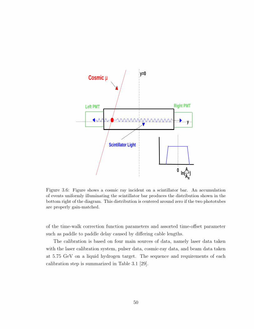
µCosmic

y

y=0

Scintillator Light

Left PMT Right PMT

)RALA

ln(0

Figure 3.6: Figure shows a cosmic ray incident on a scintillator bar. An accumulationof events uniformly illuminating the scintillator bar produces the distribution shown in thebottom right of the diagram. This distribution is centered around zero if the two phototubesare properly gain-matched.

of the time-walk correction function parameters and assorted time-offset parameter

such as paddle to paddle delay caused by differing cable lengths.

The calibration is based on four main sources of data, namely laser data taken

with the laser calibration system, pulser data, cosmic-ray data, and beam data taken

at 5.75 GeV on a liquid hydrogen target. The sequence and requirements of each

calibration step is summarized in Table 3.1 [29].

50

Calibration step Main requirementsStatus Raw Beam DataPedestals Pulser dataTDC calibration Pulser dataTime-walk correction Laser dataLeft-right Adjustment Raw Beam DataEnergy loss Cosmic Ray Data, left-right time alignment at SC levelAttenuation length Cosmic Ray Data, left-right time alignment at SC levelEffective velocity Reconstructed-Track Data and all constants aboveRF parameters Reconstructed-Track Data and all constants aboveCounter-to-counter delays Reconstructed-Track Data and all constants aboveRF offsets Reconstructed-Track Data and all constants aboveGeometric constants survey data

Table 3.1: The order and requirements for the TOF calibration.

3.5.1 Pedestal Calibration

The ADC pedestal values are obtained using dedicated 100Hz pulser data com-

pleted before taking production data. The data is analyzed at the counting house

using the PEDMAN utility, a ROOT-based, online software package that enables the

user to analyze the pedestal values for each counter in each subsystem, and then set

them.

3.5.2 TDC Calibration

The TDC calibration serves to determine the constants in the quadratic equation

used to convert raw TDC channels T to time t in nanoseconds.

t = c0 + c1T + c2T2 (3.6)

Typical values for these constants are c0 ∼ 1ns, c1 ∼ 0.05ns/channel, and c2 ∼5 × 10−8ns/ch2. A pulser run is taken and then analyzed offline with the software

package TDC calib. In order to reduce correlations between adjacent channels, every

fourth channel is pulsed sequentially.

51

3.5.3 Time-Walk Corrections

The Time-Walk is an instrumental shift in the measured time from a leading-edge

discriminator due to the finite rise time of the analog pulse. The purpose of the

Time-Walk correction is to measure and correct for the dependence of the LeCroy

2313 leading-edge discriminator output pulse time on the input pulse height. Bursts

of laser light of differing intensities using a neutral density filter are delivered to the

center of each counter via optical fibers. The pulse-time measurement tells us the

time a PMT pulse crosses a fixed (leading-edge) voltage threshold. The time-walk

corrections are performed in software using an empirically-determined function

tw = t− fw

(A− P

Th

)+ fw

(600

Th

)(3.7)

where A is the ADC channel, P is the pedestal value, Th is the ADC channel corre-

sponding to the leading-edge discriminator threshold of 20mV, and fw is the time-walk

correction function

fw(x) =w2

xw3if x < w0

fw(x) =w2

w0w3

(1 + w3)− w2w3

w0w3+1

x if x > w0 (3.8)

The time vs. ADC distribution is fit using equations 3.9 and 3.10 with two ad-

justable fit parameters w2 and w3. These parameters are determined for each counter

and are then recorded in the calibration database. Ref[30].

52

Pedestal-subtracted ADC (channels)

Cou

nter

tim

e -

diod

e ti

me

(ns)

Sector 6 Counter 21 Left

26

28

30

32

34

36

38

40

0 1000 2000 3000 4000 5000 6000 7000 8000

Figure 3.7: Example of the time dependence of a TOF TDC on pulse height. The solidline represents the calibration fit.

3.5.4 Paired Counters

As was mentioned in section 3.1, there are 57 counters per sector giving a grand

total of 342 physical counters. In order to simplify the electronics, the last 18 counters

in each sector were paired into nine effective counters, giving us a total of 288 logical

counters. The pulses from each of the four PMTs are matched in time during the

coupled-paddle calibration step and the ADC peaks are matched during the gain-

matching calibration step.

53

3.5.5 Attenuation Length and Effective Velocity

The attenuation of light collection in the scintillator material is accounted for

during the attenuation length calibration. Beam data is used to obtain the effec-

tive attenuation constants for each paddle which depend upon the dimensions of the

scintillator paddle. For each paddle, ln AL

ARvs hit position is plotted. The hit posi-

tion is the position y along the scintillator (taken to be 0 at the center) where the

charged track crosses, as determined by CLAS tracking. The fitted slope of this plot

is recorded as the attenuation constant of that paddle.

The effective velocity of light in each scintillator, which is the propagation velocity

in the scintillator material, must also be calibrated. This quantity becomes quite

important in the situation where there is only one working PMT for a counter. For

instance, in this case where only the left PMT is functioning, the time of the hit is

given by

T = TL − y

Veff

(3.9)

where TL is the time given by the working left TDC, y is the position of the hit,

and Veff is the effective velocity of light to the right PMT. Although the left/right

effective velocity values can be different, they are usually the same in practice. A

quality effective velocity calibration is then essential for obtaining meaningful timing

information from such a counter. For each paddle, the SC time vs hit position is

plotted. The fitted slope of this plot is the effective velocity of the paddle.

3.5.6 Time-Delay Calibration (Paddle to Paddle Delay)

Events of the topology ep → epπX are used to fine-tune the calibration of the

relative time delays between the 288 counters. This is accomplished by comparing

the TOF time of an event with the beam RF time. The TOF time is given by

TOF time = TOF− d

βc(3.10)

54

where TOF is the time to reach the TOF counter, d is the distance from the event

vertex to TOF counter (length of the track), β is given as

β =p√

p2 + M2(3.11)

p is the momentum of the track as measured by the drift chambers and M is the

assumed mass of the particle producing the track. The RF period is the time between

successive, picosecond electron bunches. The RF signal from the accelerator has a

2.004 ns period which can be resolved by the TOF counter via scattered electrons.

The calibration is divided into four steps. First the difference between the TOF

vertex time and the RF time is calculated for pions or electrons. This time is divided

by 2.004 and the remainder is taken as the offset correction to the TOF time. There

is a 2.004 ns ambiguity introduced by not knowing which beam bunch was associ-

ated with the event. To correct for this, electron-pion coincident events were used.

The calibration constants are determined modulo 2.004 ns by requiring that the two

reconstructed tracks (e− and π) have a common vertex time. Secondly, due to their

abundance in the forward direction, electrons are detected in the first 10 counters of

each sector which are calibrated to an arbitrary but fixed counter using coincident

pions within each sector. Third, using pion events, the first 10 counters of sector

1 are calibrated to the first 10 counters of the remaining five sectors using electron

events. In the fourth and final step, paddles 11-48 for all the sectors are calibrated

against the offset of the first 10 paddles in each sector using pion events. A plot of

TOF vertex time compared to RF time for all the counters shows the result of the

calibration. Ref[29].

3.5.7 Alignment of TOF to RF Signal and RF Correction

Along with the timing information from the TOF counters, a sub multiple of

the RF signal time is also recorded. One can then synchronize the event start time

to the correct beam bunch and use the RF time as the correct event start time.

Since the knowledge of the RF time is much more accurate, this should improve the

overall timing resolution by a factor of√

2 by eliminating any of the uncertainty

associated with the electron timing. The paddle-to-paddle delays were already fixed

55

Corrected RF Structure

-2.5

-2

-1.5

-1

-0.5

0

0.5

1

1.5

2

2.5

0 10 20 30 40 50 60 70 80 90 100

Figure 3.8: Plot of corrected modulus of (T0 − TRF ) vs TRF for selected runs of the e1-6data.

with respect to the RF signal, so the purpose of the RF correction calibration is to

fix the RF time to zero relative to the entire TOF system on an event-by-event basis.

This adjustment corrects for shifts in the RF signal introduced by changes in the

accelerator run conditions as a function of time. The difference between event start

time and the RF time RFcorr is given by:

RFcorr = TRF −

Event Start Time︷ ︸︸ ︷(T TOF

e − Le

βe

)+

Vertex Correction︷ ︸︸ ︷Zvert

βe

(3.12)

where TRF is the time of the RF signal, T TOFe is the measured electron time in the TOF

counters, Le is the measured length of the electron track, Zvert is the z-coordinate

of the event vertex position and βe is the electron velocity. The vertex correction

term is added to compensate for the effect of the target length. The purpose of

the RF calibration is to fix the mean value of RFcorr to zero and to eliminate any

56

dependence of RFcorr on RF time. Proper calibration of the RF ensures an accurate

determination of the TOF resolution which will be described later in this paper. The

fitting algorithm uses four independent third-order polynomials that are fit to four

regions of the raw RF time. Outside the range of these regions, the correction is set

to zero. See Figure 3.8. There is also one overall offset constant, that is applied to

all four regions at once, and shifts the RF correction up or down.

RF correction (ns)

22.04 / 14Constant 0.1986E+05Mean 0.2077E-01Sigma 0.1607

0

2500

5000

7500

10000

12500

15000

17500

20000

-1.5 -1 -0.5 0 0.5 1 1.5

Figure 3.9: Overall timing resolution for electrons achieved for the e1-6 experimental run.

3.5.8 Overall TOF Performance and Summary

The resolution achieved during the calibrations for this run has been the best so

far in the detector’s history. The resolution of the each paddle is going to depend

upon several factors including the length of the scintillator in question. A scintillator

100 cm in length (corresponding to a scattering angle of 18) has an average resolu-

tion of ∼ 150 ps. As the scintillator length increases so does the scattering angle1,

1Refer to Figure 3.1 The forward direction is in the direction of the beam and the scintillatorbars here are the shortest.

57

and resolution degrades as expected. There have been significant improvements made

in the TOF calibration procedure for the e1-6 run compared to previous runs. An

example of this is the newly-automated gain-matching procedure which contributed

significantly to the overall quality of the TOF data. The overall resolution for elec-

trons in the e1-6 run is shown in Figure 3.9. A fitted value of 160 ps was attained. A

good determination of the quality achieved of the TOF resolution is the measurement

of the timing separation of pions and kaons or the separation of kaons and protons.

∆TK+ (ns) vs P (GeV/c)

-10

-8

-6

-4

-2

0

2

4

6

8

10

0 0.5 1 1.5 2 2.5 3 3.5 4

Figure 3.10: A plot of ∆TK+ vs momentum of the kaon and proton sample shows suitabletiming separation of kaons and protons up to ∼ 1.8 GeV. The data plotted include timingselection cuts on both the kaon and the proton.

The timing separation is characterized by ∆T which is the difference between the

measured TOF time and a calculated time if a particle mass is assumed. The particle

mass can either be the proton mass if protons are being identified or the kaon mass

if K+’s are being identified. A plot of ∆T vs particle momentum is shown for K+

identification in Figure 3.10. The straight horizontal band is the kaon band with a

∆T centered around zero. The curved band are protons with a clear time separation

58

up to a momentum of ∼ 1.8 GeV. ∆T is discussed further in section 5.2.

59

Chapter 4

Calibration and Data Reduction

The data was taken during the e1-61 electron beam run period between October

2001 and January 2002. With an electron beam of 5.75 GeV incident on a Hydrogen

target, a total of 22.439 mC of total, useful charge was accumulated. The luminosity

was maintained at ∼ 1034cm−2 ·s−1, which was limited by the background population

in the CLAS drift chambers. During the entire span of the experiment, the torus

current was set at its full value of 3375 Amperes. The Level 1 trigger for the e1-6 run

required a coincidence between the Cerenkov counter and the forward electromagnetic

calorimeter. The e1-6 run period was separated into three distinct periods demarcated

by machine shutdown and maintenance, during which certain run parameters, such

as the RF constants, could and did change.

4.1 Data Reduction

The sample of files (∼ 2% of the total data) used to complete the Pass0 calibra-

tion cooking2 fairly democratically represented all three data-taking periods. The

cooking software used was the production version 3-5 of RECSIS, which was the

track-reconstruction software package used. Its output included BOS files, which in-

clude the track-reconstructed data banks as well as raw banks, but also monitoring

1Denotes an electron run at 6 Gev, designated E-99-105.2“Cooking” refers to the process of reconstructing charged particle tracks in the detector from

raw data banks.

60

histograms. After the calibration stage was completed, the software was tagged, the

ced[santoro] Wed Mar 31 09:49:52 2004 Run_1_Event_126.eps

Figure 4.1: An example 3-pronged reconstructed epK+ event as reconstructed by REC-SIS.This particular event shows time-based as well as hit-based tracks reconstructed in aMonte-Carlo event.

calibration constants were copied to the MySQL calibration database3 to the main

run index table of that database and pass1 cooking was begun.

For the purpose of calibrating the detector, we selected a sample of data to be

processed that was uniformly distributed across the entire run. This step was dubbed

calibration cooking and the files were used for the calibration of the detector com-

ponents, as well as to improve the event reconstruction software. The calibration

cooking was completed in 3 steps or versions for data in periods 2 and 3 and only in

one step for data in period 1. The data in period 1 was cooked last, with calibration

constants refined from cooking the other run periods because of the lack of RF in-

formation in period 1. The significance of each cooking step is summarized in Table

3The calibration database is a centrally-managed database responsible for the management andimplementation of the calibration constants of all detector subsystems. It supersedes the old mapfile

61

Pass 0 Cooking SummaryPeriod Version Meaning

Cooking with constants as of 03/19/02 6pmPeriod 1 V3 (includes DC alignment and best paddle2paddle

10/31/01 -11/21/01 constants from run 30921)

Cooking with constantsV1 as of 02/07/02

Period 2 Cooking with Yoffset calibration,11/28/01 -12/21/01 V2 new time-walk constants and

RF offset position adjustmentCooking with DC alignment constants

V3 and new paddle2paddle constants

Cooking with constantsV1 as of 02/07/02

Period 3 Cooking with Yoffset calibration,01/05/02 -01/30/02 V2 new time-walk constants and

RF offset position adjustmentCooking with DC alignment constants

V3 and new paddle2paddle constants

Table 4.1: Calibration cooking steps performed on the three separate run ranges and themeaning of each version.

4.1.

4.2 Detector Calibration Procedure

In order for the data collected to be analyzable, the detector components must be

calibrated. The three major calibration procedures are mentioned below.

scheme.

62

4.2.1 Drift Chamber Calibration

Before the drift chamber calibration procedure can be described, some background

information related to the track reconstruction in CLAS must be presented.

Track Reconstruction Overview

Charged particle track reconstruction is completed in four steps. The first three

steps are required before proceeding with hit-based (HBT) track fitting, followed by

time-based (TBT) track fitting.

1. cluster finding: The first step is to find a contiguous group of hits (called a

cluster) in each of the superlayers. Each cluster may contain several track

segments.

2. track segment finding: A lookup table is used to find groups of hits or segments

within one cluster that are consistent with a track traversing a superlayer.

3. segment linking: Segments from individual superlayers are identified with seg-

ments in other superlayers, again using a look-up table. If the look-up table

address corresponds to a possible track, it also contains an estimate of the

track’s initial parameters.

4. track fitting: Using the linked segments, a preliminary angle and momentum

are assigned and a trial track is propagated through the CLAS magnetic field.

At each layer we calculate the distance-of-closest-approach (DOCA) of the track

to the hit wire (HBT), or to the position derived from the drift times (TBT).

As described below, track parameters are then adjusted to provide the best fit

of the track to the measured positions.

The fitting procedure minimizes the following quantity

χ2 =∑

i

[dmeas,i − di(~q)]2

σ2i

, (4.1)

where di(~q) is a reference trajectory whose parameter vector ~q is composed of inverse

momentum, the polar and azimuthal angles (w.r.t. the beam), and the interaction

63

vertex transverse to and parallel to the beam direction. The uncertainty for HBT is

given by σi ∼ cell size 2√

12, and for TBT by a distance-dependent resolution which

varies between 200 and 800 µ.

Alignment

Each of the 18 drift chambers was surveyed upon installation. This served as

reasonable starting point for the drift chamber alignment and positions, to be refined

using straight-track (no magnetic field) data.

Time-Delay Calibration

The fixed time delays for each wire must be determined before the drift times

can be known. These delays are mainly a result of different cable lengths, and are

determined using a pulser that generates two pulses with constant time separation.

One pulse goes to the Amplifier/Discriminator (DAB) crates while the other goes

acts as a common stop for the TDCs. This provides a relative t0 for each signal wire.

Time-to-distance Calibration

In order to have confidence in the track fitting procedure, the measured drift

time from the sense wire and the distance-of-closest-approach (DOCA) to the sense

wire must be calibrated. DOCA is a reconstructed quantity, obtained from a fit to

a time-based track. These two quantities are used to determine the drift-velocity

function of the drift cells. The measured drift time, along with other parameters is

used to calculate the predicted distance from the sense wire DIST. The difference of

the absolute values of these quantities is called the time residual:

Res = |DOCA| − |DIST | (4.2)

The residual is used to measure the resolution of the drift chambers.

64

0

0.5

1

1.5

2

0 400 800 1200

0

0.4

0.8

1.2

0 200 400 600

R3

R2

Drift Time (ns)

Dis

tanc

e of

Clo

sest

App

roac

h (

cm)

α : 20° - 25°

α : 5° - 10°

B : 0.45 - 0.55 T

B : 0.75 - 0.85 T

(a)

(b)

Figure 4.2: Scatter plot of DOCA versus the corrected drift time for a) R3 axial wires andb) R2 axial wires along with a sample fit of the time-to-distance correlation

Function Parameterization

The ultimate purpose of the drift chamber calibrations is to obtain the drift-

velocity function mentioned above for each superlayer in every sector. The drift-

velocity function relates the quantity DIST of a particle track to the drift time, which

is the time it takes for the electrons, created by the ionization of the gas in the drift

chamber, to arrive at the sense wire. The determination of this function depends on

the drift chamber operating conditions and geometry. As an added complication, the

hexagonal shape of the drift cells adds entrance angle dependence to this function.

65

The parameterized drift time to drift distance function has the form:

x(t) = v0t + η(

t

tmax

)p

+ κ(

t

tmax

)q

, (4.3)

where v0 is the the saturated drift velocity at or near t = 0, and the coefficients η and

κ, and the exponents p and q are obtained from a fit to the time-to-distance correlation

in Figure 4.2. Ions emanating from tracks close to the edge of a cell follow the electric-

field line from the field wire to the sense wire, regardless of the entrance angle α. The

drift time of these ions is denoted by tmax, and is used to define a normalized drift

time t = t/tmax. This quantity is used in the time-to-distance function which defines

the cell boundary constraint:

x(t = 1, α) = C · cos(30 − α). (4.4)

where C characterizes the linear cell size. The time-to-distance function can be written

in terms of a correction function f(t):

x(t, α) = x0(t, α0) + C (cos (30 − α)− cos (30 − α0)) f(t). (4.5)

where x0 is expected drift distance for a normalized drift time with an assumed

entrance angle α0. The function f(t) is used to correct the extracted drift distance

corresponding to the actual entrance angle of the track. The R2 drift chambers are

located between the torus cryostats, a region of high and inhomogeneous magnetic

field, which affects the drift velocity. These effects are modeled by a modification to

α and also by an increase in tmax. Further discussion of these effects can be found in

reference [31].

4.2.2 EC Energy Calibration

In order to obtain meaningful energy information from the electromagnetic calorime-

ter, the gains of the phototubes must be calibrated. This is done in a similar fashion

to the gain matching procedure for the TOF (section 3.4). In fact, the same cosmic

ray data is used for the EC energy calibration as is used for the TOF forward carriage

66

counters. Due to the large number of triggers required, raw data files are not stored

during cosmic runs. Instead events are filtered in real time with a ET client called

level3 to select muon tracks which activate a single pixel in the EC. A pixel is defined

as an intersection between scintillators in the U, V, and W planes [32]. The pixel ID

is calculated and six sets of pixel histograms (one for each U,V,W and inner/outer

view) are weighted with the measured ADC for the PMT in that view. These pixel

histograms are later analyzed with a PAW kumac to estimate the PMT gains and

scintillator attenuation lengths [33]. The high voltage of the PMTs are adjusted to

equalize the gains of all the channels.

4.2.3 Electromagnetic Calorimeter Timing Calibration

The CLAS Electromagnetic Calorimeter is an essential component of the CLAS

detector. It serves as the primary electron trigger for CLAS and thus the successful

calibration of the Electromagnetic Calorimeter is essential in obtaining quality data.

The Electromagnetic Calorimeter serves three main functions:

• Detection and triggering of electrons at energies above 0.5 GeV. The total en-

ergy deposited in the EC is available at the trigger level to reject minimum ionizing

particles or to select a particular range of scattered electron energy. This is directly

related to the EC energy calibration.

• Detection of photons at energies above 0.2 GeV, allowing πo and η reconstruction

from the measurement of their 2γ decays.

• Detection of neutrons, with discrimination between photons and neutrons using

time-of-flight measurements.

The EC timing calibration is crucial to the DECS analysis within this data set

but are not directly relevant to this analysis.

4.2.4 Time of Flight Calibration

The calibration of the TOF system is discussed in detail in chapter 3, section 3 of

this paper.

67

4.2.5 Cerenkov Counter Calibration

The Cerenkov counters perform the dual function of triggering on electrons as

well as providing electron-pion separation. The single-photoelectron response of the

photomultiplier tubes is used to perform the gain-matching calibration of the detector

as well as to calibrate the response of the detector in terms of the number of pho-

toelectrons. A value of 4-5 photoelectrons per in-bending electron track is typical.

Figure 4.3: Fitted ADC values for one Cerenkov channel. This is an example of a pmtwith very little noise.

TDC and Pedestal Calibrations

Ultimately, the pedestals, TDCs, and single photoelectron position must be cal-

ibrated. To accomplish this, pulser runs are used to calibrate the CC TDCs after a

pedestal calibration has been completed. More specifically the constant T1, which is

used to convert raw TDC channels to nanoseconds. Secondly, in order to obtain mean-

ingful ADC information, the pedestal values for each channel must be determined.

68

This is accomplished as part of an online calibration procedure that determines the

pedestal values for each detector subsystem. The Single Photoelectron (SPE) ampli-

tude calibration is unique to the Cerenkov counter, whose purpose is to determine

the position of the SPE and the noise function for each PMT. The calibration is

accomplished using cosmic ray data. Once sufficient data has been accumulated, the

ADC distribution for every PMT is fit with a Gaussian function. This determines

the SPE position. An example of this fit is shown in Figure 4.3.

4.3 Further Data Reduction

During the e1-6 run period, over 5 billion triggers were recorded. For a trigger to

qualify as an event, there must be at least one hit-based, negative, reconstructed track

in the drift chambers. More precise tracking is achieved by also requiring time-based

tracking to be present. The fraction of triggers containing at least one negative hit-

based track is ∼ 33%. For this sample of events, full event reconstruction, monitoring,

and filtering were performed.

In order to reduce the multi-terabyte data set to a manageable size for analysis, the

data set was filtered with an epK+ (electron-proton-kaon) skim program. This skim

uses multiple levels of cuts to “skim” events from the full data set containing exactly

one electron, one proton, and one K+ candidate plus possible additional negative

tracks. The skim program identifies and selects electrons using the PID definition

with additional cuts on the EC energy and particle momentum as measured by the

drift chambers. The EC cut is a polynomial cut of Ee

Pevs Pe in the variable Ee

Pe. This

ratio is parameterized as

f(Pe) = A + BPe − CPe2 + DPe

3 (4.6)

and

σEePe

= a− bPe + cPe2 − dPe

3 (4.7)

The cut is defined as f(Pe)− 3σEePe

≤ Ee

Pe≤ f(Pe)+ 3σEe

Pe

. These cuts are summarized

in Table 4.3. In order to recoup high-momentum proton and kaon candidate events

that would be lost by cutting on the TOF mass, cuts on the particle time-of-flight

69

Table 4.2: Parameter Values for Ep

Pevs Pe cut

A B C D0.26662 0.20317e-01 0.26262e-02 0.18451e-04

a b c d0.42904e-01 0.21558e-01 0.73153e-02 0.91419e-03

are employed to make proton and kaon selection. To identify and select a Kaon or

Proton candidate, a positive particle is selected and its TOF time TTOF is recorded.

A second time Tcalculated is then computed from measured momentum of the particle,

which is the time-of-flight of the particle if it is assumed to have the K+ or proton

mass. The difference TTOF − Tcalculated is computed and the all events within ±1.05

ns are kept. This timing cut is discussed in further detail in the section 5.2 Hadron

Cuts and ID. The filtering process isolated about 5.6 million such events (∼ 31 GB)

for further analysis. The filtering process greatly reduces the size of analyzable data,

considering the size of the original data set was over 2 Terabytes.

0

1

2

3

4

5

6

1 1.5 2 2.5 3 3.5 4

Figure 4.4: Kinematic distribution of epK+ event sample

70

Table 4.3: Summary of Cuts in epK+ Skim

Cut Purpose ValueElectron PID Identify good Electrons -EC Energy Eliminate false triggers E = 0.64GeVE/p vs p Avoid e−/π− misidentifica-

tion3σE

P

Proton Timing Loose cut to identify Pro-tons

±1.05 ns

K+ Timing Loose cut to identify K+’s ±1.05 ns

4.4 The epK+K− Final State

The desire to further reduce the data size prompted the completion of one more

filtering step. The average time taken to cycle through all the epK+ skim files (≈20 minutes) greatly increased the turn-around time whenever new plots had to be

produced. Therefore the data was filtered once through the C++ analysis code phi++

with a set of relaxed cuts summarized in Table 4.4. The cuts included here are many

of the same cuts used in the final analysis but with slightly relaxed values in the

case of the proton and K+ timing cuts. The magnetic field configuration for the

e1-6 run was such that all negative tracks were “in-bending” relative to the beam.

These conditions equate to a very small acceptance for the K−. Thus the K− was

reconstructed via the epK+(X) missing mass. 4

4see Nphe definition on page 60

71

Cut Purpose ValueElectron Fiducial Cuts Use trustworthy detector

volume to identify electrons-

Vertex Cut Eliminate contributionsfrom the target windows

−8.0cm ≤ z ≤ −0.8cm

Number of Photoelectrons Cut Further reduce e−/π−

misidentificationNphe ≤ 2.5

Hadron Fiducial Cuts Use trustworthy detectorvolume to identify hadrons

-

Proton Timing Cuts - ±0.90 nsK+ Timing Cuts - ±0.90 ns3 or 4 Tracks per Event Eliminate additional pion

background-

Table 4.4: Summary of additional cuts in final Phi++ skim.

72

Chapter 5

Reconstruction and Analysis

The φ decays into a K+ and a K− with a branching ratio of 49.1%. To select

events of the topology ep → epK+(K−), the K+ is detected in CLAS, along with

the scattered electron and scattered proton, while the K− is reconstructed using the

missing mass technique. The following describes the further reduction and subsequent

analysis of the e1-6 data set. The procedure employed for electron and hadron ID,

along with all relevant cuts are discussed. The acceptance-corrected total yield and

cross sections as a function of Q2,W, t, Φ and helicity angular distribution in cosθH

are discussed, evaluated and presented. The successful extraction of R = σL/σT will

allow the separation of the longitudinal cross section σL from the total cross section,

which will enable direct comparison with GPD model predictions.

5.1 Scattered Electron Identification

The cuts used during the analysis ensure only the purest events survive to be

included in the final event sample. The following sequence shows the procedure used

to identify good epK+K− events. An initial round of particle id is completed during

cooking but these selections can be and will be improved upon.

73

E vs. P0

0.5

1

1.5

2

2.5

3

3.5

4

4.5

0 0.5 1 1.5 2 2.5 3 3.5 4 4.5 5

Figure 5.1: 3σEP

cuts on E vs. P. Hori-zontal line is the straight cut on the ECenergy at 0.64 GeV. The curved lines arethe 3σE

PE/p vs. P cuts.

φe vs Θe (Degrees)

-30

-20

-10

0

10

20

30

10 15 20 25 30 35 40 45 50 55 60

Figure 5.2: Electron sample after fiducialcuts imposed. Figure shows sector 1.

5.1.1 Good Track Selection

Part ID=3

Good electron selection is the essential first step in the reconstruction of the

epK+K− final state [34]. The first requirement is that the track have a PID number

3 in the PART bank. This requirement encompasses all the general attributes of an

electron such as the track being negative as well as loose cuts on the energy deposited

in the Electromagnetic Calorimeter.

Vertex Corrections and Z vertex cut

In addition, a cut on the vertex position of the electron track was made to confine

the event sample to those emanating from within the target. Electrons that come

from the target window, located 2cm downstream from the target are eliminated by a

cut on the z component of the vertex position. The cut made is -8.0 cm ≤ Zvtx ≤ -0.8

74

Z-Vertex

0

5000

10000

15000

20000

25000

30000

35000

40000

-10 -8 -6 -4 -2 0 2

Figure 5.3: Vertex position of electron tracks in cm. The mean shows the z-position of thetarget. The slant of the distribution is due to acceptance effects in the scattered electronangle.

cm. The distribution of electron vertex positions after this cut was made is shown in

Figure 5.3.

5.1.2 Cuts to eliminate detector inefficiencies

Cherenkov fiducial cut

In order to ensure that the events chosen came from a trustworthy volume of

the detector, fiducial volume cuts were imposed. The efficiency of the Cherenkov

counters are compromised as the light path approaches the edge of the mirrors. This

is equivalent to saying the Cherenkov efficiency decreases as the particle (electron)

track approaches the geometrical edge of each sector. Cuts are applied to eliminate

these inefficient volumes that are a function of electron momentum pe, polar angle

of the scattered electron θe, and the azimuthal angle of the scattered electron φe. A

75

standard CLAS parametrization of the cuts are

θ ≥ θcut, θcut = C1 +C2

(p + pshift)

|φs| ≤ C4 sin(θ − θcut)C3pα

(5.1)

Where |φs| is the azimuthal angle defined relative to the center of each sector and the

parameters C1 − C4, pshift, and α are parameters that were determined for the e1-6

run in reference [35, 36]. The effect of these cuts are shown in Figure 5.2.

Electromagnetic calorimeter fiducial cut

When an electron enters the EC too close to the edge, the resulting particle shower

is not completely contained by the detector volume, which means that the measured

deposited energy is no longer related to the particle energy. This distance is typically

∼ 10 cm from the edge. Therefore a cut is applied in the local coordinate system of

the EC (UEC ,VEC , and WEC), which are calculated from the global coordinate XEC

and YEC . The cuts applied are the same used for the e1-6 ω analysis [10]; UEC ≥ 40,

VEC ≤ 360, WEC ≤ 390.

EC/DC Energy/Momentum cut

A cut on the electron energy, as determined by the EC can be estimated from the

trigger threshold value ECthreshold = 175 mV for e1-6. The cut value is calculated via:

EEC(MeV ) = 214 + 2.47× ECthreshold(mV ) (5.2)

This was determined by an in-depth study documented in reference [37]. Due to

fluctuations in the trigger signal, a cut, EEC ≥ 700 MeV was applied.

5.1.3 Cuts to eliminate π− background

At the cooking stage, there are a number of π−’s that are misidentified as electrons.

76

E/p vs. p cut

To avoid e−/π− misidentification, the expected ratio of the electron energy as

determined by the EC to its momentum as determined by the DC was exploited in

the form of cuts on E/P vs P, and were imposed at the epK+ skim level. Due to

the sampling ratio of the EC, the expected value of E/p for electrons is ∼ 0.29. The

details of this cut are discussed in section 4.3 and are shown in Figure 5.1.

Ein Cut

Minimum-ionizing pions are expected to deposit ∼ 25 MeV of energy in the inner

part of the calorimeter as well as ∼ 40 MeV in the outer part of the calorimeter. If

one applies a cut on the energy deposited in the inner calorimeter Ein ≥ 60 MeV,

this eliminates most of this pion background. [10]

Nphe x 100 20 40 60 80 100 120 140 160 180 200

0

2000

4000

6000

8000

10000

Figure 5.4: Figure shows number of photoelectrons distributions. The pion peak is clearlyseen at zero. The red dashed line shows the cut to eliminate this pion contamination.

77

Number of photoelectrons cut

Upon inspection of the number of photoelectrons distribution (Nphe) in the Cherenkov

counter, one observes the electron signal, distributed according to the Poisson distri-

bution, centered at around Nphe = 9 or 10. In addition to this, there exists a very

distinct peak centered at Nphe ∼ 1 which is due to pion contamination.

Table 5.1: Summary of Cuts used for electron selection. The percentages shown indicatethe effect of each cut on the “epK skimmed” data sample. Each cut was applied one at atime to the data so the effectiveness of each cut could be considered separately.

Electron Id Cut Accepted (%)

PART ID = 3 100Z-Vertex 96

EC Energy/DC momentum 89CC Fiducial Cuts 77EC Fiducial Cuts 70

Ein 98ETOT /p 99Nphe 64

5.2 Hadron Cuts and ID

To complete the construction of the epK+K− final state, a clean sample of protons

and K+ must be successfully identified. The beam energy for this data sample was

5.754 GeV, which was significantly higher than previous runs. Due to this, cuts

on the TOF mass would lead to inefficiencies at high momenta. This is due to the

spreading or smearing of the measured TOF mass as β → 1. To counteract this effect,

we employed cuts on particle times, which are closely related to the experimental

resolution. These cuts were described in section 4.3. The time as measured by the

TOF is denoted by Tmeasured. The quantity Tcalc is the calculated flight time of the

78

respective track with a specific mass assignment. First, assuming either the Mp for

case of proton selection or MK+ for the case of K+ selection, the quantity βcalc is

computed:

βcalc =p2

√p2 + M2

P/K+

, (5.3)

where p is the particle momentum as measured by the drift chambers. Tcalc is then

given by:

Tcalc =dtrk

βcalc · c, (5.4)

where dtrk is the measured track length from the target to the detection plane. The

quantity ∆T is then given by ∆T = Tmeasured − Tcalc.

∆T (p/K+) = Tmeasured(p/K+)− Tcalc(p/K

+) (5.5)

This is the quantity used to make proton and K+ selections.

5.2.1 Proton ID

The proton was selected using a timing cut, ∆T (p) < 0.75ns. The proton selec-

tion included tracks which satisfied only the proton cuts as well as high momentum

particles which satisfied both the proton and K+ timing cuts but were identified as

protons because a kaon was unambiguously associated with the other positive track.

In addition, fiducial volume cuts were also applied to final proton sample in order to

cut out tracks in inefficient and unreliable parts of the detector. The fiducial cuts

take the following functional form f(θ)upper = A(1.0 − e−B(θ−C)) for the upper cut

and f(θ)lower = a(1.0 − e−b(θ−c)) for the lower cut. A(a), B(b), and C(c) are sector

dependent fit parameters adjusted to give a liberal cut in the kaon lab angles θ and

φ.

5.2.2 K+ ID

The K+ was selected using a timing cut, ∆T (K+) < 0.60ns. The Kaon selection

included tracks which satisfied only the Kaon cuts as well as high momentum particles

79

0

0.2

0.4

0.6

0.8

1

1.2

1.4

1.6

1.8

2

0 0.5 1 1.5 2 2.5 3 3.5 4

Figure 5.5: Plot of TOF Mass2 vs mo-mentum for identified protons. The 5σcuts are clearly visible.

Recon. Kaon Mass Sq. vs. Mom. ePK

0

0.2

0.4

0.6

0.8

1

1.2

1.4

1.6

1.8

2

0 0.5 1 1.5 2 2.5 3 3.5 4

Figure 5.6: Plot of TOF Mass2 vs mo-mentum for identified K+s. The 4σ cutsare clearly visible. Also clearly visible isthe π+ contamination at higher momenta.

which satisfied both the proton and K+ timing cuts but were identified as Kaons

because a proton was unambiguously associated with the other positive track. In

addition, fiducial volume cuts were also applied to final K+ sample in order to cut

out tracks in inefficient and unreliable parts of the detector. These are shown in

Figures 5.7 and 5.8. The same functional form of the fiducial cuts are used for the

K+ as was used for the proton, however the parameters differed slightly.

5.2.3 K− ID

Due to the e1-6 magnetic field configuration, all negative particles were in-bending.

This amounts to a very small acceptance of K−’s, therefore K− identification was

accomplished via the missing mass technique. The epK+ missing mass is shown in

Figure 5.9. A 2σ cut was applied to the epK+X sample to select K−s. The epK+

missing mass vs K+K− invariant mass is shown in Figure 5.10 along with the 2σ cuts

on the epK+ missing mass. The invariant mass is defined as

IMK+K− =√

(K+ + K−) · (K+ + K−) (5.6)

80

φK+ vs ΘK+ sec1

-30

-20

-10

0

10

20

30

0 10 20 30 40 50 60

Figure 5.7: Scatter plot of φ vs. θ for theK+ sample before fiducial volume cut isapplied.

φK+ vs ΘK+ sec1

-30

-20

-10

0

10

20

30

0 10 20 30 40 50 60

Figure 5.8: Scatter plot of φ vs. θ forthe K+ sample after fiducial volume cutis applied.

where K+ and K− are the kaon 4-vectors with the rest mass replaced with the particle

data group value and the K− momentum is the measured missing momentum.

5.2.4 Other Cuts to Eliminate Background

Additional cuts can be useful in order to obtain the cleanest sample of events in

the epK+K− final state. If one plots the epK+ missing mass versus the same variable

redefined with the K+ mass replaced by the pion mass, one can separate the real K−

sample from the misidentified pion background. This pion background is mainly the

decay product of ρ, ω and the ground-state hyperons Λ and Σ+/−. This background

would eventually have been removed during the K− selection process, however by

applying the cut shown in Figure 5.11, one obtains a much cleaner K+ sample at the

K+ id stage. The effectiveness of this cut in eliminating the Λ and Σ+/− background

is illustrated in Figure 5.12.

81

523.2 / 144P1 -779.4P2 6836.P3 -7258.P4 1347.P5 0.4930P6 0.1352E-01

0

500

1000

1500

2000

2500

0.3 0.35 0.4 0.45 0.5 0.55 0.6 0.65 0.7

Figure 5.9: Plot of epK+X missing mass.Shown is the Gaussian+2nd-order polyno-mial fit to the K− peak.

0.3

0.35

0.4

0.45

0.5

0.55

0.6

0.65

0.7

0.80.850.90.95 1 1.051.11.151.21.251.3

Figure 5.10: Plot of epK+X missingmass vs. the K+K− invariant mass. ±2σcuts are applied to the epK+X missingmass in order to select K−s.

5.2.5 Electron Momentum Corrections

Our knowledge of the CLAS geometry and magnetic field distribution is incom-

plete. This causes errors in the track momentum and position reconstruction, which

affect the determination of physics quantities such as energy (invariant mass of the

φ) and missing mass. To correct for these effects, empirically-determined momentum

and angle corrections were imposed on the electron. The electron angle is corrected

first, which accounts for uncertainties in the torus field and angles defined by the

DC geometry. These corrected angles were then used to determine the corrected

momentum.

Pecorr = Pemeasured × g(θe, φe, sector) (5.7)

The correction function g(θe, φe, sector) is treated as a sector-dependent scale factor

which is also a function of the polar angle of the scattered electron θe and the scattered

82

M.M. epk+X with PION MASS vs M.M.epk+X

0

0.2

0.4

0.6

0.8

1

1.2

1.4

0 0.2 0.4 0.6 0.8 1 1.2 1.4

Figure 5.11: Scatter plot of epK+ miss-ing mass with modified K+ mass versusthe regular epK+ missing mass. The cutson these two variables are shown.

M.M. ek+X

0

2500

5000

7500

10000

12500

15000

17500

20000

0.6 0.8 1 1.2 1.4 1.6 1.8 2

Figure 5.12: eK+ missing mass be-fore cut (unfilled) and after cut (green-hatched) illustrated in Figure 5.11. Theground-state Λ(1115) is shown as well asthe Σ(1189) directly right of the Λ.

electron azimuthal angle φe.

g(θe, φe, sector) = δpe = pecorr/pemeasured (5.8)

5.2.6 Hadron Energy-Loss Corrections

In order to correct for the energy loss suffered by the proton in the target and

to a lesser extent, in the drift chamber regions of CLAS, an empirical proton energy

correction is applied to the proton sample. The correction function is defined as a

function of the detected proton momentum preconstructed and scattering angle θp.

pcorr = preconstructed × F (preconstructed, θp) (5.9)

83

pcorr/puncorr vs. puncorr (GeV/c)

0.95

0.96

0.97

0.98

0.99

1

1.01

1.02

1.03

1.04

1.05

0 1 2 3 4 5 6

Figure 5.13: Plot shows the ratio of the corrected electron momentum to uncorrectedelectron momentum versus the uncorrected momentum. The electron momentum correctionhas a less than 1% effect for all applicable momenta.

The range of validity in these variables is ∼ 0.2 GeV/c ≤ preconstructed ≤∼ 6.0 GeV/c

and ∼ 7 ≤ θp ≤ 120. The parameters of the correction function were determined

by running a GSIM simulation of only protons with momenta and scattering angles

in the range specified above. The data was binned in θp and the parameters were

obtained by a fit of pgenerated/preconstructed vs preconstructed for each θp slice. Since the

data is in the K+ minimally-ionizing region, the above-mentioned energy correction

was not applied to the K+ sample [38].

5.2.7 Hadron Momentum Corrections

As is the case with the electron, the limitations of our knowledge of the CLAS

magnetic field and geometry force the implementation of momentum corrections for

hadron tracks. A set of momentum corrections based on kinematical fits using the

84

reactions ep → eπ+(n) and ep → ep(γ) were developed as a function of momentum,

and azimuthal and polar angles. These corrections were applied to both the proton

and K+ sample, and although the corrections from this to the e1-6 data were small

(∼ 0.1 − 0.7%), they did have a overall “tightening” effect on the epK+ missing

mass peak width on a sector-by-sector basis [39]. As is illustrated in Table 5.2,

Before Correction After CorrectionSectorMK− σK− MK− σK−

1 0.4934 0.0136 0.4919 0.01372 0.4924 0.0126 0.4912 0.01243 0.4915 0.0127 0.4902 0.01254 0.4938 0.0124 0.4919 0.01255 0.4926 0.0135 0.4912 0.01366 0.4935 0.0139 0.4921 0.0138

∆ 0.0059 0.0033 0.0042 0.0038

Table 5.2: Values show the fitted mean and σ of the K− peak for each sector before andafter momentum corrections are applied to the proton and kaon samples. The last rowshows the variances ∆ of each column.

the momentum corrections decrease the variance of the means by ∼ 30% effectively

reducing sector-by-sector variations.

5.3 φ Event Identification

The purpose of the all the cuts mentioned above is to identify candidate φ events

with the epK+(K−) topology. After applying the data filtering techniques and cuts

mentioned above, 23, 282 such events were identified. The sample contains all phys-

ical processes that contribute to this final state as well as real φ’s and accidental

background from pions. Contamination from high mass hyperons such as the Λ∗ will

be removed with a cut on the PK− invariant mass.

Figure 5.14 shows the K+K− invariant mass with a highly-pronounced φ meson

peak. This distribution is simultaneously fit to a Gaussian (whose integral is shown in

85

/ ndf 2χ 31.05 / 16

p0 76.0± 1840 p1 152.1± -1939 p2 24.2± 317.8 p3 0.001± 1.019 p4 0.00081± 0.00809

0.96 0.98 1 1.02 1.04 1.06 1.08 1.1 1.12 1.140

100

200

300

400

500

600

700

/ ndf 2χ 31.05 / 16

p0 76.0± 1840 p1 152.1± -1939 p2 24.2± 317.8 p3 0.001± 1.019 p4 0.00081± 0.00809

UNWEIGHTEDφ kkIM

101± = 805 φN

0.001 GeV± = 1.019 φM

0.8 MeV± = 8.1 φσ

Figure 5.14: K+K− invariant mass including all data cuts and fit to φ peak with Eq. 5.10.

the green shaded region) plus an empirical phase space function for the background,

FIT = gaussian + background

gaussian = A exp

[−(IMkk − µ)2

2σ

]

background = B1

√IMkk

2 −M2th + B2

(IMkk

2 −M2th

)

(5.10)

where Mth is the threshold for φ production (Mth=1.96 GeV), and A,B1, and B2 are

extracted parameters of the fit. The mean µ and the width σ of the gaussian have

been fixed at their average values for most of the fits to extract the φ yields. The

total φ yield is extracted via:

Nφ =

√2π

∆bin

Aσ (5.11)

where A is the height of the Gaussian, σ is its width, and ∆bin is the bin size of the

histogram. This fit yields Nφ = 805 and a mean Mφ = 1.019 GeV and a width of 8.1

86

MeV. The statistical error σNφis given as

σNφ= Nφ

√σA

2

A2+

σσ2

σ2(5.12)

5.3.1 Physics Background

There are competing channels which lead to a epK+K− final state. In order

to successfully extract the φ signal, the contribution from these channels must be

well-understood. The majority of this background comes from the production and

subsequent decay of high-mass hyperons decaying via ep → e′Λ∗(Σ∗) such as the

Λ∗(1520) as seen in Figure 5.15. In fact, the main contributor to the background is

the Λ∗(1520) whose cross section is similar to the φ. There are additional contributions

from the Λ∗(1600), Λ∗(1800), Λ∗(1820), Σ∗(1660), and Σ∗(1750). A cut on the pK−

vγ

Target p

-K+K

+K

)*Σ(*Λ

Figure 5.15: Feynman diagram for excited Λ(1520) hyperon production. This is the pri-mary background for φ(1020) production.

invariant mass is employed to cut out the Λ∗(1520) contribution to the φ peak. This

cut is illustrated in Figure 5.16. Instead of a single high-end cut on IMpK , a “range”

cut that removes the Λ peak and retains data below IMpK = 1.5 GeV is employed.

This procedure serves the two-fold purpose of retaining essentially all the φ statistics

while increasing the signal-to-background ratio. The low end of the range cut is

87

IMpK = 1.49 GeV and the high end is at IMpK = 1.55 GeV, which equates to a 2σ

cut. This is illustrated in Figure ??. The criteria to select the best cut to eliminate

the Λ∗(1520) background was two-fold. The best cut would maximize the signal-

to-background ratio as well as the φ yield. A summary of the various cut values

investigated as well as their respective signal to background ratios and φ yields is

shown in Table 5.3.

IMpk

0

200

400

600

800

1000

1200

1400

1600

1800

1.4 1.5 1.6 1.7 1.8 1.9 2

Figure 5.16: Plot of pK− invariant mass. The Λ∗(1520) removed by the cut (white) isclearly visible as well as the data kept (green shaded region).

The single-valued cuts, ranging between IMpK = 1.53 GeV and IMpK = 1.57 GeV

result in a 23-27% loss in statistics and a ∼ 20% decrease in the signal to background

ratio. In sharp contrast, the range cut preserves essentially all the φ statistics as well

as increasing the signal to background ratio by ∼ 13%. The reason for this becomes

obvious if one investigates a plot of the IMKK versus IMpK , Figure 5.17. A sizable

sample of φ’s are located in the IMpK phase space below 1.5 GeV which would be

eliminated with a single-valued cut at IMpK = 1.53 or above.

88

IMpK Cut Signal to Background Ratio Nφ

No Cut 0.5664 972

IMpK = 1.53 0.4535 754IMpK = 1.54 0.4698 762IMpK = 1.55 0.4662 760IMpK = 1.56 0.4759 748IMpK = 1.57 0.4913 716

Range Cut 0.6413 963

Table 5.3: Summary of investigated IMpK cuts along with their respective signal to back-ground ratios and φ yield.

5.4 Acceptance Correction

Before cross sections can be extracted, the φ yields must first be corrected for

the detector acceptance. The acceptance is actually a combination of the geometrical

acceptance of CLAS, the detector efficiencies of the SC and DC, the track reconstruc-

tion efficiency, and the event selection efficiency. It is calculated using a full GEANT-

based simulation for CLAS called GSIM. Since the electromagnetic calorimeter and

Cerenkov detectors aren’t well modeled in GSIM, their efficiencies will be determined

using the data. The acceptance correction proceeds in four main steps as follows:

EVENT GENERATOR ⇒ GSIM ⇒ GPP ⇒ RECONSTRUCTION

5.4.1 Event Generator

During the event generator step, events with the topology ep → epφ are generated

according to a specific physics model whose parameters are adjusted to closely repli-

cate the data. In the case of this analysis, the event generator phi gen was written

by the author specifically for the purpose of generating φ events according to the Vec-

tor Meson Dominance (VMD) model. The C++ based code takes as input various

kinematical and model-based parameters summarized in Table 5.4 and generates φ

events according to the following cross section:

σφV MD(Q2,W ) = σφ(0,W )

p∗γ(Q2 = 0)

p∗γ(Q2)

1 + ε

(1 + Q2/Λ)3exp(−b | t− tmin(Q2) |) (5.13)

89

IMkk vs IMpk

0.96

0.98

1

1.02

1.04

1.06

1.08

1.1

1.12

1.14

1.4 1.5 1.6 1.7 1.8 1.9 2

Figure 5.17: Scatter plot of IMKK versus IMpK . The well-defined vertical strip at IMpK =1.52 GeV is the Λ(1520) band. The horizontal strip at IMKK = 1.02 GeV is the φ band.The lines show the range cut applied to remove the Λ background. Also discernible are theφ events located below the low-end cut that would be thrown away with a single-valued cutabove IMpK = 1.53.

where σφ(0,W ) is the photoproduction cross section,p∗γ(Q2=0)

p∗γ(Q2)is a phase-space cor-

rection factor defined as W 2−Mp2√

(W 2−Mp2−Q2)2+4W 2Q2)

, ε is the polarization parameter (see

chapter 1 section 1.1.1), R = σL

σT, and Λ is a scaling parameter. The cross section

includes a factor exp(−b | t− tmin(Q2) |) which describes the t behavior. The prop-

agator is actually a modified from its normal 1Q4 dependence to a 1

Q6 dependence to

more closely resemble the data. A weighted 2-Dimensional histogram in Q2 and ν is

generated according to equation 5.13. This histogram is randomly sampled to produce

all the kinematic distributions and quantities. In the VMD model, the decay process

φ → K+K− proceeds according to the angular decay distribution W (cos θH , ψ), (see

equation 7.4) and is included in the simulation. This is accomplished by creating a

2-Dimensional histogram in cos θH and ψ weighted by W (cos θH , ψ). The decay frame

90

Parameter Value Description

Beam Energy 5.754 GeV e1-6 Beam EnergyQ2 Range 1.0 to 5.0 GeV2 Low and high range of Q2

ν Range 2.5 to 4.3 GeV Low and high range of νt Range 0.0 to -6.0 GeV2 Low and high range of tLint 1.0× 1040cm−2 integrated Luminosity

b 1.05 Impact parameterξ2 0.33 VMD scaling parameter

cosδ 0.70 L/T phase factorΛ 1.039 Propagator scaling factor

Table 5.4: List of kinematic and VMD input parameters for the event generator phi gen.

angles are then randomly sampled from this histogram.

For the present acceptance study, approximately 10 million events were generated.

5.4.2 GSIM

The generated events from phi gen are then processed with a tagged version,

release 4-5 of GSIM. GSIM is a GEANT based simulation of the CLAS detector which

models the propagation of particle tracks through the CLAS detector components.

As was previously mentioned, the GSIM modeling of the CC and to a lesser extent the

EC, are unreliable so the efficiency of those subsystems will be calculated separately

from the e1-6 data. The 4-5 release of GSIM was modified to include the GEANT

implementation of the e1-6 target (Figure 2.4). The simulation of each ep → epφ

event took approximately 0.875 seconds to complete on the JLAB batch farms. All

10 million generated events were propagated through GSIM which was completed in

about 2 days.

5.4.3 GPP

In order to obtain realistic spacial and timing resolution as well as for the purpose

of removing dead or inefficient DC and SC channels, the GSIM data is processed

with the GSIM Post Processing (GPP) program. In order to deal with dead SC

91

(GeV)ν1 1.5 2 2.5 3 3.5 4 4.5 5 5.5 6

)2

(G

eV

2Q

0

1

2

3

4

5

6

7

8

h7Entries 100370Mean x 4.037Mean y 1.798RMS x 0.8387RMS y 0.8272

h7Entries 100370Mean x 4.037Mean y 1.798RMS x 0.8387RMS y 0.8272

Q2 vs nu

Figure 5.18: Generated, weighted Q2 ver-sus ν histogram used to obtain correlatedQ2 and ν values.

Hθcos-1 -0.8 -0.6 -0.4 -0.2 -0 0.2 0.4 0.6 0.8 1

(R

ad

)ψ

-3

-2

-1

0

1

2

3

hdecay2Entries 100370Mean x -0.0001815Mean y -0.001973RMS x 0.5357RMS y 1.85

hdecay2Entries 100370Mean x -0.0001815Mean y -0.001973RMS x 0.5357RMS y 1.85

PSI (rad) vs COS(thetaH) After GetRandom

Figure 5.19: Generated ψ versus cos ΘH

histogram weighted with W (cosΘH , ψ)used to obtain correlated ψ and cos ΘH

values.

counters, GPP simply references the SC status entries in the calibration database

and removes them. GPP also accepts an SC smearing factor f at the command line

which was optimized to match the timing resolution of the data. GPP also accepts

3 DOCA smearing factors a, b, and c which are responsible for smearing the drift

chamber resolution for regions 1, 2, and 3 respectively. This smearing was matched to

the data through the timing-independent epK+ missing mass. The DOCA smearing

factors were chosen to reproduce the resolution of K− missing mass. The values of

these parameters used in this study are summarized in Table 5.5. In addition to

the smearing of the drift chambers, GPP also takes into account the individual wire

efficiency through an efficiency lookup table constructed from the actual e1-6 data

[40].

92

2Q1 1.5 2 2.5 3 3.5 4 4.5 5

0

500

1000

1500

2000

2500

3000

rec2Q

Figure 5.20: 23,000 reconstructed Monte Carlo events (histogram) overlayed with sameamount of reconstructed data (blue error points).

5.4.4 Generated Track Reconstruction

After the previous steps are completed, the generated data, which is identical

to the raw beam data, must be processed with RECSIS (see Section 4.1) the track

reconstruction software. The generated data was processed with the same version,

release 3-5 of RECSIS as was used to process the e1-6 data. This reconstructed data

was then processed with the same cuts as the data except for the EC cuts. The

energy loss correction was applied but not the momentum corrections since there are

no ambiguities in the GSIM magnetic field or drift chamber positions.

5.4.5 Extraction of the Acceptance

The efficiency or acceptance is defined as the ratio of accepted events Nacc to

generated events Ngen in a discrete phase space element Γ.

Acc(Γ) =Nacc(Γ)

Ngen(Γ)(5.14)

93

Parameter Value

f 1.30a 2.25b 2.25c 2.25

Table 5.5: Summary of GPP input parameters

For this analysis, the acceptance will be calculated in 2-dimensional phase space

elements of dΓ = dQ2dt. Ideally these phase space elements should be as small as

possible to eliminate any dependence of the acceptance calculation on the model used

to generate the events. This is not especially important in this case since the event

generator used is expected to reproduce the real data [10]. The event generator used

very accurately represents the real data as is demonstrated in Figure 5.20 where the

Q2 histogram of reconstructed Monte Carlo events is overlayed with the Q2 data with

errors. The binning as well as the values for the acceptance calculation in Q2 and

t is shown in Table A.1. The binning for the Q2,t′ acceptance table is the same as

the Q2,t table. The extraction of the cross section in these variables is completed in

coarser bins than the acceptance correction. For each 2-dimensional bin (Q2,−t), the

acceptance or efficiency is defined as:

Acc(Q2,−t) =Nacc(Q

2,−t)

Ngen(Q2,−t)(5.15)

where Ngen(Q2,−t) is the number of generated events in this bin and Nacc(Q2,−t) is

the number of accepted events in this bin. It is desirable to extract the differential

cross section in t′ as well, so another acceptance table in Q2 and t′ is generated for

this purpose. The binning is the same as for the table in Q2 and t and is shown in

Figure 5.22.

94

t -3.5 -3 -2.5 -2 -1.5 -1 -0.5 0

2 Q

11.5

22.5

33.50

0.005

0.01

0.015

0.02

0.025

0.03

,t)2ACC(Q

Figure 5.21: 2-dimensional representation of CLAS acceptance in Q2 and t. Each “lego”represents a 0.2 GeV × 0.2 GeV 2-d bin. The z-axis is the efficiency for each bin.

5.5 Cherenkov Efficiency

The Cherenkov counters are not properly modeled in GSIM therefore a separate

efficiency study had to be conducted. One can describe the electron signal from the

CC by a generalized Poisson distribution

y(

x

C3

)=

C1C2

xC3 e−C2

Γ( xC3

+ 1)(5.16)

95

t’

00.5

1 1.52 2.5

33.5

2 Q

11.5

22.5

33.5

0

0.005

0.01

0.015

0.02

0.025

)’,t2ACC(Q

Figure 5.22: 2-dimensional representation of CLAS acceptance in Q2 and t′. Each “lego”represents a 0.2 GeV × 0.2 GeV 2-d bin. The z-axis is the efficiency for each bin.

where C1, C2, and C3 are adjustable fit parameters. C1 is an overall amplitude, C2

is the mean of the Poisson distribution and C3 is a scaling parameter. The function

was used to fit the Nphe x 10 distribution between 40 and 200 after all other electron

selection cuts were made. These fit parameters were used to extrapolate the function

to 0. The detection efficiency is then defined as

CCeff (Q2, xB) =

∫∞25 y(Nphe x 10)∫∞0 y(Nphe x 10)

(5.17)

96

[10] The Cherenkov efficiency depends on Q2 and xB therefore this correction was

calculated in Q2 and xB bins. One such example is shown in Figure 5.23 for

0.3≤ xB ≤0.4 and 1.8≤ Q2 ≤2.0.

/ ndf 2χ 63.17 / 77p0 22.7± 1187 p1 0.092± 3.246 p2 0.63± 26.69

0 20 40 60 80 100 120 140 160 180 2000

50

100

150

200

250

300 / ndf 2χ 63.17 / 77p0 22.7± 1187 p1 0.092± 3.246 p2 0.63± 26.69

Figure 5.23: Plot shows Nphe x 10 distribution for scattered electrons after all electronselection cuts are made. The solid line shows a fit to the generalized Poisson distributionfrom 40 to 200 while the dashed line shows the extrapolation of the function to 0.

5.6 Radiative Corrections

Radiative effects must be taken into account when determining cross section val-

ues. In this analysis, the radiative effects are calculated in two distinct steps. The

external radiative process, which is the finite probability that the incoming or scat-

tered electron will radiate a hard photon in the presence of a nucleon in the target

other than the one associated with the event are taken into account during the ac-

ceptance calculation at the GSIM step. There is also the possibility of the incoming

electron (beam) to radiate external to the event. This effect is not modeled and will

97

e e’

*γ

Target p

φ

Bremstrahlung Bremstrahlung

Vertex Vacuum Polarization

a) b)

c) d)

Figure 5.24: Contributing graphs of the radiative correction calculationBremsstrahlung radiation (a), (b) self-absorption of radiated photon (c) and the in-ternal loop of e+/e− pair production/annihilation (d). The born process (no radiatedphoton) is not shown.

be included in the systematic error of the correction, however such effects are partially

taken into account in the intrinsic energy spread of the beam. The internal radiative

corrections include the Bremsstrahlung process for the incoming or scattered electron

in the presence of the nucleon associated with the event as well as diagrams such as

vacuum polarization, which are not accounted for during the acceptance calculation,

are shown in Figure 5.24. These internal corrections are calculated in a radiative

correction factor Frad using the radiative correction code exclurad, with vcut = 0.02

98

GeV2 [41]. Frad1 is calculated in each W and Φ bin as

Frad =σrad

σnorad

(5.18)

where σnorad is the cross section calculated without any radiative effects (a.k.a. the

Born cross section) and σrad is the cross section calculated with radiative effects

included (diagrams 5.24 a-d). The correction factor for various W bins is shown as a

function of Φ in Figure 5.25. The correction was made in W and Φ bins at average

values of Q2 and cos θCM because the correction was found not to vary significantly

in Q2 and cos θCM .

0 50 100 150 200 250 300 350

0.74

0.75

0.76

0.77

0.78

0.79

0.8

Graph

W=2.0

W=2.1

W=2.2

W=2.3

W=2.8

W=2.9

W=2.7

W=2.4W=2.5

W=2.6

=2.472

)=0.345, QcmθCOS(

φ

Co

rr

Figure 5.25: Plot of radiative correction Frad as a function of ΦCM = Φ for assortedvalues of W from 2.0 to 3.0 GeV. The correction for each W value was computed ata < Q2 >= 2.47 GeV2 and cos θCM = 0.345.

1Frad is δ as defined in Equation 75 of Reference [41].

99

5.7 Accumulated Charge Normalization

In order to properly normalize the cross section measurements, the total accumu-

lated charge for the data analyzed must be known. This is accomplished by reading

the information recorded in scalar events which retain a record of accumulated charge

Q as measured by the Faraday cup. For the data set analyzed, the quantity FCG,

which is the live time-gated reading from the Faraday cup, is read from these scalar

events. There exists a slight ambiguity in measuring the accumulated charge using

this method due to the scalar readout not being synchronized with the start of each

run. In other words, there is a fraction of charge at the beginning and end of each run

that is not accounted for. This uncertainty is estimated to be less than a 1% effect.

For the data contained in this analysis, Q = 22420× 10−6 Coulombs. Once the total

charge Q is known, the integrated luminosity can be calculated as

Lint =lt ·Dt · N

MH

· Q

qe

(5.19)

where

• lt is the length of the target (5.0 cm)

• Dt is the density of the target (0.0708 g/cm3)

• N is Avagadro’s number (6.022× 1023)

• MH is the molar density of Hydrogen (1.0 g/mol)

• qe is the electron charge (1.6× 10−19 C)

The integrated luminosity is then

Lint = 2.98× 1040 cm−2 (5.20)

100

Chapter 6

Cross Sections

6.1 Extraction of φ meson σ and dσdt as a function

of Q2

6.1.1 σ(Q2,W )

The total φ electroproduction cross section is given by

σ(Q2,W,Ebeam) =1

Γ(Q2,W,Ee)

dσφ

dQ2dW(6.1)

where Γ(Q2,W,Ee) is given by equation 1.16 and Ee enters through the polarization

parameter ε given by equation 1.13. We can extract the φ cross section from the data

viadσ

dQ2dW=

1

BRφ→K+K−

nW

Lint∆Q2∆W(6.2)

where

• BRφ→K+K− = 0.491± 0.009 is the branching ratio of the decay φ → K+K−

• nW is the acceptance-weighted, CC efficiency-weighted and radiative-correction

weighted yield in each kinematic bin

nW =Nφ

ACC(Γ) · Frad · CCeff

(6.3)

101

where Nφ is defined in Equation 5.11.

• Lint is the integrated luminosity

• ∆Q2 is the size of the Q2 bin in GeV 2

• ∆W is the size of the W bin in GeV .

The binning in Q2 and −t for the extraction of the cross section in those variables are

shown in Table 6.1. The binning in t′ is the same as that used for t. In this analysis,

Variable Bin (GeV2) Bin Size (GeV2) Number of Acceptance Bins

1.6 - 1.8 0.2 11.8 - 2.0 0.2 1

Q2 2.0 - 2.2 0.2 12.2 - 2.6 0.4 22.6 - 3.0 0.4 23.0 - 3.8 0.8 40.0 - 0.4 0.4 20.4 - 0.8 0.4 20.8 - 1.2 0.4 2

−t 1.2 - 1.6 0.4 21.6 - 2.0 0.4 22.0 - 2.4 0.4 22.4 - 2.8 0.4 22.8 - 3.6 0.8 4

Table 6.1: Binning for the extraction of the cross sections in Q2, t, and t′ and the numberof acceptance bins in each respective cross section bin. t′ has the same binning and numberof cross section bins as t so it is omitted in this table for brevity.

σ was integrated over the entire W range of 2.0 ≤ W ≤ 3.0. This is allowable because

the cross section varies only slightly with W. This permits one to express σ(Q2,W )

as σ(Q2). To obtain the σ(Q2), each event is weighted for acceptance, radiative

effects, the CC efficiency as well as the virtual photon flux factor. The invariant

mass distribution (IMKK) of weighted events in each Q2 bin is then fit to equation

5.10. This is shown in Figure 6.1. The cross section for each of the bins is calculated

102

hIMkkq2Entries 2165Mean 1.074RMS 0.04703

/ ndf 2χ 20.69 / 18

p0 637.2± 4060

p1 1329.1± -3338

p2 255.1± 1065 p3 0.00± 1.02 p4 0.00000± 0.00631

0.96 0.98 1 1.02 1.04 1.06 1.08 1.1 1.12 1.140

200

400

600

800

1000

1200

1400

1600

1800

2000

2200

2400

hIMkkq2Entries 2165Mean 1.074RMS 0.04703

/ ndf 2χ 20.69 / 18

p0 637.2± 4060

p1 1329.1± -3338

p2 255.1± 1065 p3 0.00± 1.02 p4 0.00000± 0.00631

< 1.82 1.6 < QkkIMhIMkkq3

Entries 3156Mean 1.073RMS 0.04552

/ ndf 2χ 22.47 / 18p0 480.2± 4677

p1 993.9± -4386 p2 188.7± 802.8 p3 0.000± 1.026

p4 0.00000± 0.00631

0.96 0.98 1 1.02 1.04 1.06 1.08 1.1 1.12 1.140

200

400

600

800

1000

1200

1400

1600

1800

2000

hIMkkq3Entries 3156Mean 1.073RMS 0.04552

/ ndf 2χ 22.47 / 18p0 480.2± 4677

p1 993.9± -4386 p2 188.7± 802.8 p3 0.000± 1.026

p4 0.00000± 0.00631

< 2.02 1.8 < QkkIM

hIMkkq4Entries 3146

Mean 1.075RMS 0.04482

/ ndf 2χ 10.11 / 18

p0 430.6± 4091

p1 895.6± -3187

p2 170.9± 825.2

p3 0.00± 1.02

p4 0.00000± 0.00631

0.96 0.98 1 1.02 1.04 1.06 1.08 1.1 1.12 1.140

200

400

600

800

1000

1200

1400

1600

1800

hIMkkq4Entries 3146

Mean 1.075RMS 0.04482

/ ndf 2χ 10.11 / 18

p0 430.6± 4091

p1 895.6± -3187

p2 170.9± 825.2

p3 0.00± 1.02

p4 0.00000± 0.00631

< 2.22 2.0 < QkkIMhIMkkq5

Entries 5227Mean 1.072RMS 0.04566

/ ndf 2χ 19.92 / 18p0 808± 1.059e+04 p1 1668± -1.105e+04

p2 310.5± 1493

p3 0.000± 1.017

p4 0.00000± 0.00631

0.96 0.98 1 1.02 1.04 1.06 1.08 1.1 1.12 1.140

500

1000

1500

2000

2500

3000

3500

hIMkkq5Entries 5227Mean 1.072RMS 0.04566

/ ndf 2χ 19.92 / 18p0 808± 1.059e+04 p1 1668± -1.105e+04

p2 310.5± 1493

p3 0.000± 1.017

p4 0.00000± 0.00631

< 2.62 2.2 < QkkIM

hIMkkq6Entries 3632Mean 1.071

RMS 0.04512

/ ndf 2χ 18.42 / 18

p0 656.6± 8796

p1 1348.8± -9876

p2 270.4± 1023

p3 0.000± 1.018

p4 0.00000± 0.00631

0.96 0.98 1 1.02 1.04 1.06 1.08 1.1 1.12 1.140

500

1000

1500

2000

2500

hIMkkq6Entries 3632Mean 1.071

RMS 0.04512

/ ndf 2χ 18.42 / 18

p0 656.6± 8796

p1 1348.8± -9876

p2 270.4± 1023

p3 0.000± 1.018

p4 0.00000± 0.00631

< 3.02 2.6 < QkkIMhIMkkq7

Entries 3534

Mean 1.072

RMS 0.04372

/ ndf 2χ 22.07 / 18

p0 984± 1.4e+04

p1 2000± -1.582e+04

p2 414.0± 1287

p3 0.000± 1.019

p4 0.00000± 0.00631

0.96 0.98 1 1.02 1.04 1.06 1.08 1.1 1.12 1.140

500

1000

1500

2000

2500

3000

3500

4000

4500

hIMkkq7Entries 3534

Mean 1.072

RMS 0.04372

/ ndf 2χ 22.07 / 18

p0 984± 1.4e+04

p1 2000± -1.582e+04

p2 414.0± 1287

p3 0.000± 1.019

p4 0.00000± 0.00631

< 3.82 3.0 < QkkIM

Figure 6.1: Fitted φ yields in given Q2 bins given by a fit to Equation 5.10.

according to equations 6.1 and 6.2 and is shown along with previous JLab results, in

Figure 6.2. The values for the cross section in each Q2 bin as well as the relevant

kinematics is shown in Table 6.2.

The total cross section was fit to determine the scaling behavior. For this data we

determined the scaling to be 1/Q4.6±1.7 for 1.6 ≤ Q2 ≤ 3.8.

6.1.2 Differential Cross Section in t′, dσdt′

The differential cross section in t′ was extracted in 8 bins in t′. The fitted data

is shown in Figure 6.3. The differential cross section plotted for each t′ is shown in

103

)2

(GeV2Q0 0.5 1 1.5 2 2.5 3 3.5 4 4.5 5

) nb

2(Qσ

10

CLAS/Santoro W=2.5 GeV

CLAS/Lukashin W=2.5 GeV

)2(Qσ

Figure 6.2: Plot shows σ(Q2) for all t and W values for a previous JLab data set [2] (bluepoints) and the from present analysis (green points).

Figure 6.4. The values for the cross section in each t′ bin as well as the relevant

kinematics is shown in Table 6.3.

6.1.3 Differential Cross Section in t, dσdt

The differential cross section is easiest to compare with theory if it is computed

in terms of the Mandelstam variable t. Experientially, dσdt′ is often plotted, as in

the previous section, in order to avoid corrections due to kinematic effects of the

minimum 4-momentum transfer tmin. The differential cross section as a function of

104

Bin < Q2 > (GeV2) < ε > σ (nb)

1 1.7 0.430 16.3 ± 3.92 1.9 0.475 10.5 ± 2.53 2.1 0.479 11.1 ± 2.34 2.4 0.459 10.3 ± 2.15 2.8 0.433 7.8 ± 2.06 3.4 0.387 5.2 ± 1.7

Table 6.2: Total cross section σ(Q2) and kinematics of each data point. < Q2 > is the bincenter, and < ε > is the average ε in each bin.

Bin < t′ > (GeV2) < ε > dσ/dt′ (nb/GeV 2)1 0.19 0.453 7.2 ± 1.22 0.59 0.441 2.4 ± 0.83 0.99 0.435 2.3 ± 0.64 1.39 0.429 0.4 ± 0.45 1.79 0.430 1.2 ± 0.46 2.19 0.435 1.2 ± 0.37 2.59 0.426 0.5 ± 0.28 3.17 0.392 0.3 ± 0.1

Table 6.3: Differential cross section dσdt′ and kinematics of each data point. < t′ > is the

bin center, and < ε > is the average ε in each bin.

t was extracted first for all values of Q2, then for a Q2 bin 1.6 ≤ Q2 ≤ 2.6 The

differential cross section in t is given as

dσ

dt=

σ

∆t(6.4)

where ∆t is the bin size in GeV 2 in which the cross section is extracted. A correction

for tmin(Q2,W ) is applied to relevant bins and is described in section 6.3. Such a

correction is usually avoided by extracting and plotting the data as a function of t′

but in order to compare to predictions of the JML model, the extraction versus t was

necessary. dσdt

for all Q2 is shown in Figure 6.5. The values for the cross section in

each t bin as well as the relevant kinematics is shown in Table 6.4.

The data show very similar trends as previous data [2] namely they are consistent

105

0.960.98 1 1.021.04 1.061.08 1.1 1.121.140

1000

2000

3000

4000

5000

6000

0.0<= -t’ < 0.4kkIM

0.960.98 1 1.021.04 1.061.08 1.1 1.121.140

500

1000

1500

2000

2500

3000

3500

4000

0.4 < -t’ < 0.8kkIM

0.960.98 1 1.021.04 1.061.08 1.1 1.121.140

200

400

600

800

1000

1200

1400

1600

1800

2000

2200

0.8 < -t’ < 1.2kkIM

0.960.98 1 1.021.04 1.061.08 1.1 1.121.140

200

400

600

800

1000

1200

1400

1.2 < -t’ < 1.6kkIM

0.960.98 1 1.021.04 1.061.08 1.1 1.121.140

200

400

600

800

1000

1.6 < -t’ < 2.0kkIM

0.960.98 1 1.021.04 1.061.08 1.1 1.121.14

0

100

200

300

400

500

600

700

800

900 2.0 < -t’ < 2.4kkIM

0.960.98 1 1.021.04 1.061.08 1.1 1.121.140

50

100

150

200

250

300

350

400

450

2.4 < -t’ < 2.8kkIM

0.960.98 1 1.021.04 1.061.08 1.1 1.121.140

100

200

300

400

500

600

2.8 < -t’ < 3.6kkIM

Figure 6.3: Fitted dσdt′ yields in t′ bins given by a fit to Equation 5.10.

with diffractive production (e−b|t|) below a |t| of ≈ 1.5 GeV2. dσdt

was extracted in two

bins in Q2 for comparison to the JML model. For our total Q2 range, 1.6 ≤ Q2 ≤ 4.0

the data is shown in Figure 6.6 along with the JML predictions calculated in 2 Q2

bins. The data in our truncated Q2 bin, 1.6 ≤ Q2 ≤ 2.6 is shown in Figure 6.7 as

well as the JML predictions calculated in one Q2 bin.

106

)2t’ (GeV0 0.5 1 1.5 2 2.5 3

)2/d

t’ (n

b/G

eVσd

1

/dt’σd

Figure 6.4: dσdt′ vs t′ for all Q2.

6.2 Bin Centering Correction

The distribution of data in each kinematical bin is not flat. As a result, the average

value of the data in a bin doesn’t coincide with the center but is offset depending upon

the data distribution so any measurement made from data within that bin cannot be

naively quoted at the center but rather where the real average of the data occurs. For

this, a bin centering correction has to be made. An analytic form for the correction

can be obtained if one makes an assumption of the functional form of the data. In

this analysis, the bin centering correction was made for the t and t′ distributions,

which are assumed to have an exponential shape. This greatly simplifies the form of

the correction:

x = x0 − 1

bln

sinh(p)

p(6.5)

where x0 is the center of the bin, b is the impact parameter measured from the fitted

distribution, and p = b∆2

where ∆ is the bin width. It should be noted that one may

107

)2-t (GeV0 0.5 1 1.5 2 2.5 3

)2/d

t (nb

/GeV

σd

1

10

/dtσd

Figure 6.5: dσdt vs -t integrated over the entire Q2 range.

alternatively quote a modified value of the differential cross section dσ/dt, dσ/dt′ at

the center of each bin.

6.3 tmin(Q2,W ) Correction

In this section we correct for this kinematic effect assuming a simple form for the

differential cross section. The differential cross section dσdt

contains contributions from

all kinematically accessible Q2 values

dσ

dt=

Q2max∫

Q2min

dσ

dt(Q2)dQ2 (6.6)

108

Bin < −t > (GeV2) < ε > dσ/dt (nb/GeV 2)1 0.19 0.361 67.5 ± 17.32 0.59 0.419 25.0 ± 4.93 0.99 0.445 4.6 ± 1.44 1.39 0.449 2.5 ± 0.95 1.79 0.447 1.2 ± 0.56 2.19 0.452 0.7 ± 0.37 2.59 0.450 0.9 ± 0.38 3.17 0.430 0.4 ± 0.2

Table 6.4: Differential cross section dσdt and kinematics of each data point. < −t > is the

bin center, and < ε > is the average ε in each bin.

however experimentally, the Q2 range accessible in each t bin is limited by tmin where

tmin(Q2,W ) =[Q2 + M2

φ

2W

]2

−[[(

W 2 −Q2 + Mφ2

2W

)2

+Q2] 1

2−[(

W 2 + Mφ2 −Mp

2

2W

)2

−Mφ2] 1

2

]2

(6.7)

tmin(Q2,W ) is the momentum transfer t when the center-of-mass scattering angle

θCM , the angle between the γ∗ and φ is 0. tmin(Q2,W ) is plotted in Figure 6.8. This

translates into a truncation of the allowable Q2 values contributing to dσdt

. The range

of Q2 can be obtained by an inversion of tmin(Q2,W ) and evaluated at a given t

value corresponding to the center of a given t bin. Consequently, what is observed

experimentally is(

dσ

dt

)

exp

=

tmin−1(Q2,W )∫

Q2min

dσ

dt(Q2)dQ2 (6.8)

dσdt

is whatever function is used to model the t-dependence of the cross section. In the

simplest case, there is no Q2 dependence

σ(t) = Aφexp(−bφt) (6.9)

109

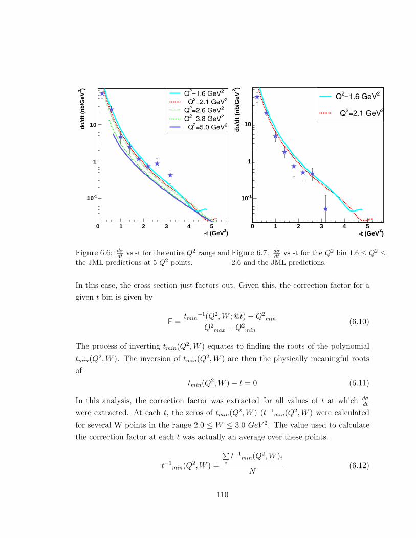
)2-t (GeV0 1 2 3 4 5

)2/d

t (nb

/GeV

σd

-110

1

10

2=1.6 GeV2 Q2=2.1 GeV2 Q

2=2.6 GeV2 Q2=3.8 GeV2 Q

2=5.0 GeV2 Q

JML Model

Figure 6.6: dσdt vs -t for the entire Q2 range and

the JML predictions at 5 Q2 points.

)2

-t (GeV0 1 2 3 4 5

)2/d

t (n

b/G

eVσd

-110

1

10

2=1.6 GeV2 Q

2=2.1 GeV2 Q

JML Model

Figure 6.7: dσdt vs -t for the Q2 bin 1.6 ≤ Q2 ≤

2.6 and the JML predictions.

In this case, the cross section just factors out. Given this, the correction factor for a

given t bin is given by

F =tmin

−1(Q2,W ; @t)−Q2min

Q2max −Q2

min

(6.10)

The process of inverting tmin(Q2,W ) equates to finding the roots of the polynomial

tmin(Q2,W ). The inversion of tmin(Q2,W ) are then the physically meaningful roots

of

tmin(Q2,W )− t = 0 (6.11)

In this analysis, the correction factor was extracted for all values of t at which dσdt

were extracted. At each t, the zeros of tmin(Q2,W ) (t−1min(Q2,W ) were calculated

for several W points in the range 2.0 ≤ W ≤ 3.0 GeV 2. The value used to calculate

the correction factor at each t was actually an average over these points.

t−1min(Q2,W ) =

∑i

t−1min(Q2,W )i

N(6.12)

110

2Q

1 1.5 2 2.5 3 3.54 4.5 5

W

22.2

2.42.6

2.83

3.2

-2

-1.5

-1

-0.5

0

,W)2(Qmint

,W)2(Qmint

Figure 6.8: Plot of tmin(Q2,W ) surface for e1-6 kinematics.

This correction is pictorially represented in Figure 6.9. A table of this correction

factor for each t is given in Table 6.5, with the observed dσdt

is divided by this factor

to obtain the corrected or true dσdt

.

6.4 Systematic Error Estimates

The relatively low number of measured φ events leads to statistical domination of

the errors. There were sources of systematic errors in this experiment and they can

be summarized as follows:

• Fitting Procedure

• Acceptance Correction

• tmin Correction (applicable only to the extraction of dσ/dt).

111

exp(-bt)

/dt)σln(d

t

Measured/dtσd

t t∆t+

Figure 6.9: Plot illustrates the essence of the tmin(Q2,W ) correction. The blue pointsrepresent the observed differential cross section as a function of t while the green dottedcurve represents where these points should fall in the absence of tmin effects i.e. if oneplotted the differential cross section as a function of t

′= t− tmin(Q2,W ). It is important to

note that the green curve represents the t-dependence of the cross section assuming somemodel and can assume various forms.

< −t >(GeV2) t−1min(Q2,W )(GeV2) Low Q2 F all Q2 F

0.2 1.48 0.12 0.030.6 1.85 0.65 0.191.0 2.35 1.0 0.401.4 2.87 1.0 0.621.8 3.37 1.0 0.842.2 3.88 1.0 1.02.6 4.37 1.0 1.03.2 5.09 1.0 1.0

Table 6.5: tmin(Q2,W ) Correction values for each t bin in which the cross section isextracted.

112

Chapter 7

Angular Distributions

7.1 Background

The angular decay distribution of the K+(K−) in the φ rest frame describes the

polarization properties of the φ meson. The scattering amplitude M for vector meson

electroproduction γ∗ + N → P + V can be expressed in terms of helicity amplitudes

TλV λP λγ∗λNwhere λ is the helicity of each particle. The vector meson spin density

matrix is derived from these helicity amplitudes by exploiting the Von Neumann

formula

ρ(V ) =1

2Tρ(γ∗)T † (7.1)

where ρ(γ∗) is the spin-density matrix of the virtual photon. The details of this

derivation can be found in reference [1, 42]. The decomposition of ρ(V ) can be

accomplished on a basis of nine 3 x 3 hermetian matrices ραij. The index α ranges

from 0 to 8 and corresponds to the particular decomposition. This index can also be

related to the virtual photon polarization α = 0 − 2 for purely transverse photons,

α = 4 for purely longitudinal photons while other values correspond to Longitudinal-

Transverse interference terms. The indices ij correspond to the helicity state of the

vector meson; for instance ρ000 is proportional to the probability that a transversely

polarized virtual photon will produce a longitudinally polarized (λ = 0) vector meson

while ρ001 is an interference term between a meson of helicity 0 and a meson of helicity

1 produced by a transversely polarized virtual photon [10]. In the case that there is

113

-1 +1

0

φ and *γHelicity states of

*γTransverse Transverse

Longitudinal

φ

+1-10

*γP

φP

Figure 7.1: Helicity states of the virtual photon and φ. The blue arrows indicate the spindirections corresponding to each helicity state.

no σL/σT separation, ραij can be parameterized as follows

r04ij =

ρ0ij + εRρ4

ij

1 + εR; α = 4

rαij =

ραij

1 + εR; α = 0− 3

rαij =

√R

ραij

1 + εR; α = 5− 8

(7.2)

where R and ε retain their earlier definitions.

In terms of these parameters, the full angular decay distribution assumes the normal-

ized form

W(

cos θH , φH , Φ)

=3

4π

[1

2(1− r04

00) +1

2(3r04

00 − 1) cos2 θH

114

−√

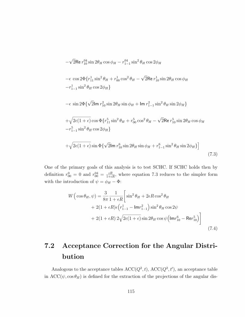
2Re r0410 sin 2θH cos φH − r04

1−1 sin2 θH cos 2φH

−ε cos 2Φr111 sin2 θH + r1

00 cos2 θH −√

2Re r110 sin 2θH cos φH

−r11−1 sin2 θH cos 2φH

−ε sin 2Φ√

2Im r210 sin 2θH sin φH + Im r2

1−1 sin2 θH sin 2φH

+√

2ε(1 + ε) cos Φr511 sin2 θH + r5

00 cos2 θH −√

2Re r510 sin 2θH cos φH

−r51−1 sin2 θH cos 2φH

+√

2ε(1 + ε) sin Φ√

2Im r610 sin 2θH sin φH + r6

1−1 sin2 θH sin 2φH]

(7.3)

One of the primary goals of this analysis is to test SCHC. If SCHC holds then by

definition r000 = 0 and r04

00 = εR1+εR

, where equation 7.3 reduces to the simpler form

with the introduction of ψ = φH − Φ:

W(

cos θH , ψ) =3

8π

1

1 + εR

[sin2 θH + 2εR cos2 θH

+ 2(1 + εR)ε(r11−1 − Imr2

1−1

)sin2 θH cos 2ψ

+ 2(1 + εR) 2√

2ε(1 + ε) sin 2θH cos ψ(Imr6

10 − Rer510

)]

(7.4)

7.2 Acceptance Correction for the Angular Distri-

bution

Analogous to the acceptance tables ACC(Q2, t), ACC(Q2, t′), an acceptance table

in ACC(ψ, cos θH) is defined for the extraction of the projections of the angular dis-

115

tributions dNdψ

and dNd cos θH

. Ten million Monte Carlo events were generated with the

phi++ generator assuming the SCHC form of the angular distribution (see Figure

5.19). The bin size for each variable is shown in Table 7.1. The correction is shown

graphically in Figure 7.2. The events that were used to generate this acceptance table

Hθ cos-1 -0.8 -0.6 -0.4 -0.2 -0 0.2 0.4 0.6 0.8 1 ψ

050

100150

200250

300350

0

0.002

0.004

0.006

0.008

0.01

)Hθ, cosψACC(

Figure 7.2: 2-dimensional representation of CLAS acceptance in ψ and cos θH . Each binrepresents a 18.0 Degree × 0.1 units of cos θH 2-d bin. The z-axis is the efficiency for eachbin.

were the same as those used for the previous acceptance tables. In a similar fashion

to the previous acceptance table, the weight of events was limited to be less than 400.

116

Variable Range Number of Bins Bin Size

ψ (Degrees) 0 to 360 20 18

cos θH -1 to 1 20 0.1

Table 7.1: Acceptance table values for the extraction of the angular distribution.

7.3 Extraction of rαij parameters

7.3.1 Differential Cross Section dσdΦ and test of SCHC

The differential cross section in Φ were extracted in the same manner as the other

differential cross sections. Due to the limited statistics of this experiment, dσdΦ

was

extracted for integrated Q2 and t′ so a one dimensional acceptance correction in 20 Φ

bins was used. dσdΦ

was extracted in 9 bins whose respective fits are shown in Figure

7.3. The expected Φ dependence arises from integrating equation 7.3 in cos θH ,and

hIMkkphi1Entries 3010

Mean 1.074

RMS 0.04502

/ ndf 2χ 11.61 / 18

p0 3048± 2.635e+04

p1 6216± -2.646e+04

p2 1152.4± 2195

p3 0.000± 1.019

p4 0.00000± 0.00631

0.96 0.98 1 1.02 1.04 1.06 1.08 1.1 1.12 1.140

1000

2000

3000

4000

5000

6000

7000

8000

9000

hIMkkphi1Entries 3010

Mean 1.074

RMS 0.04502

/ ndf 2χ 11.61 / 18

p0 3048± 2.635e+04

p1 6216± -2.646e+04

p2 1152.4± 2195

p3 0.000± 1.019

p4 0.00000± 0.00631

= 20.CM

Φ kkIM hIMkkphi2Entries 2773

Mean 1.069

RMS 0.04456

/ ndf 2χ 17.92 / 18

p0 1853± 1.87e+04

p1 3774± -2.145e+04

p2 789.7± 3008

p3 0.000± 1.019

p4 0.00000± 0.00631

0.96 0.98 1 1.02 1.04 1.06 1.08 1.1 1.12 1.140

1000

2000

3000

4000

5000

6000

7000

8000

hIMkkphi2Entries 2773

Mean 1.069

RMS 0.04456

/ ndf 2χ 17.92 / 18

p0 1853± 1.87e+04

p1 3774± -2.145e+04

p2 789.7± 3008

p3 0.000± 1.019

p4 0.00000± 0.00631

= 60.CM

Φ kkIM hIMkkphi3Entries 3138

Mean 1.068

RMS 0.04538

/ ndf 2χ 19.9 / 18

p0 1560± 1.666e+04

p1 3175± -1.854e+04

p2 671.8± 4130

p3 0.000± 1.019

p4 0.00000± 0.00631

0.96 0.98 1 1.02 1.04 1.06 1.08 1.1 1.12 1.140

1000

2000

3000

4000

5000

6000

7000

hIMkkphi3Entries 3138

Mean 1.068

RMS 0.04538

/ ndf 2χ 19.9 / 18

p0 1560± 1.666e+04

p1 3175± -1.854e+04

p2 671.8± 4130

p3 0.000± 1.019

p4 0.00000± 0.00631

= 100.CM

Φ kkIM

hIMkkphi4Entries 1982

Mean 1.066

RMS 0.0451

/ ndf 2χ 12.55 / 18

p0 1542± 1.422e+04

p1 3112± -1.613e+04

p2 759.0± 4612

p3 0.000± 1.019

p4 0.00000± 0.00631

0.96 0.98 1 1.02 1.04 1.06 1.08 1.1 1.12 1.140

1000

2000

3000

4000

5000

6000

7000

8000

hIMkkphi4Entries 1982

Mean 1.066

RMS 0.0451

/ ndf 2χ 12.55 / 18

p0 1542± 1.422e+04

p1 3112± -1.613e+04

p2 759.0± 4612

p3 0.000± 1.019

p4 0.00000± 0.00631

= 140.CM

Φ kkIM hIMkkphi5Entries 562

Mean 1.058

RMS 0.04285

/ ndf 2χ 15.7 / 18

p0 1719± 1.078e+04

p1 3433± -1.444e+04

p2 961.8± 4764

p3 0.000± 1.019

p4 0.00000± 0.00631

0.96 0.98 1 1.02 1.04 1.06 1.08 1.1 1.12 1.140

1000

2000

3000

4000

5000

6000

7000

hIMkkphi5Entries 562

Mean 1.058

RMS 0.04285

/ ndf 2χ 15.7 / 18

p0 1719± 1.078e+04

p1 3433± -1.444e+04

p2 961.8± 4764

p3 0.000± 1.019

p4 0.00000± 0.00631

= 180.CM

Φ kkIM hIMkkphi6Entries 2063

Mean 1.068

RMS 0.04413

/ ndf 2χ 12.54 / 18

p0 1510± 1.599e+04

p1 3060± -1.979e+04

p2 653.6± 2089

p3 0.000± 1.019

p4 0.00000± 0.00631

0.96 0.98 1 1.02 1.04 1.06 1.08 1.1 1.12 1.140

1000

2000

3000

4000

5000

6000

hIMkkphi6Entries 2063

Mean 1.068

RMS 0.04413

/ ndf 2χ 12.54 / 18

p0 1510± 1.599e+04

p1 3060± -1.979e+04

p2 653.6± 2089

p3 0.000± 1.019

p4 0.00000± 0.00631

= 220.CM

Φ kkIM

hIMkkphi7Entries 3118

Mean 1.067

RMS 0.04453

/ ndf 2χ 14.23 / 18

p0 1552± 1.841e+04

p1 3112± -2.296e+04

p2 642.8± 2916

p3 0.000± 1.019

p4 0.00000± 0.00631

0.96 0.98 1 1.02 1.04 1.06 1.08 1.1 1.12 1.140

1000

2000

3000

4000

5000

6000

hIMkkphi7Entries 3118

Mean 1.067

RMS 0.04453

/ ndf 2χ 14.23 / 18

p0 1552± 1.841e+04

p1 3112± -2.296e+04

p2 642.8± 2916

p3 0.000± 1.019

p4 0.00000± 0.00631

= 260.CM

Φ kkIM hIMkkphi8Entries 2775

Mean 1.069

RMS 0.04474

/ ndf 2χ 20.84 / 18

p0 1910± 2.028e+04

p1 3854± -2.491e+04

p2 693.2± 1875

p3 0.000± 1.019

p4 0.00000± 0.00631

0.96 0.98 1 1.02 1.04 1.06 1.08 1.1 1.12 1.140

1000

2000

3000

4000

5000

6000

7000

hIMkkphi8Entries 2775

Mean 1.069

RMS 0.04474

/ ndf 2χ 20.84 / 18

p0 1910± 2.028e+04

p1 3854± -2.491e+04

p2 693.2± 1875

p3 0.000± 1.019

p4 0.00000± 0.00631

= 300.CM

Φ kkIM hIMkkphi9Entries 2937

Mean 1.075

RMS 0.04482

/ ndf 2χ 28.01 / 18

p0 2409± 1.639e+04

p1 5008.5± -6629

p2 1113.4± 5587

p3 0.000± 1.019

p4 0.00000± 0.00631

0.96 0.98 1 1.02 1.04 1.06 1.08 1.1 1.12 1.140

2000

4000

6000

8000

10000

12000

hIMkkphi9Entries 2937

Mean 1.075

RMS 0.04482

/ ndf 2χ 28.01 / 18

p0 2409± 1.639e+04

p1 5008.5± -6629

p2 1113.4± 5587

p3 0.000± 1.019

p4 0.00000± 0.00631

= 340.CM

Φ kkIM

Figure 7.3: Fits to K+K− invariant mass in 9 bins in ΦCM

117

φH to obtain:

dσ

dΦ=

1

2π

(σ + ε cos 2ΦσTT +

√2ε(1 + ε) cos ΦσLT

)(7.5)

where σLT and σTT are the interference terms of the longitudinal and transverse parts

of the cross section. The cross section along with a fit to equation 7.5 is shown in

(degrees)CMΦ0 50 100 150 200 250 300 350

(nb/

40 d

egre

es)

CM

Φ/dσd

0

0.5

1

1.5

2

2.5

3

3.5

4

4.5

/ ndf 2χ 13.78 / 6p0 0.2077± 2.108 p1 0.3316± 0.2833 p2 0.1089± -0.066

/ ndf 2χ 13.78 / 6p0 0.2077± 2.108 p1 0.3316± 0.2833 p2 0.1089± -0.066

CMΦ/dσd

0.33± = 0.28 TTσ 0.11± = -0.06 LTσ

/D.F. = 2.32χ

Figure 7.4: dσdΦ vs Φ. Green line shows a fit to equation 7.5 along with extracted fit

parameters σTT and σLT .

Figure 7.4. If SCHC is a valid assumption then these interference terms must vanish

[10]. It can be concluded from Figure 7.4 that these terms are compatible with zero.

The errors quoted are purely statistical so the inclusion of systematic errors associated

with the acceptance calculation, etc would only strengthen our conclusion. A fit of

the dσ/dΦ distribution to a constant yields χ2/D.F. = 1.9 (χ2 = 15.2) as opposed to

a χ2/D.F. = 2.3 (χ2 = 13.8) from a fit to Equation 7.5 indicates compatibility with

zero. In order to extract the rαij parameters from the measured angular distribution,

one has the option of taking two 1-dimensional projections of equation 7.3.

118

7.3.2 Polar Angular distribution projection

To obtain the polar angular distribution, an integration in Φ and φH (or ψ) yields

W (cos θH) =3

2

[1

2

(1− r04

00

)+

1

2

(3r04

00 − 1)

cos2 θH

](7.6)

In order to obtain this projection from the data, the acceptance-efficiency-radiative

correction-weighted distribution K+K− invariant mass is extracted in 10 bins in

cos θH (0.20 units of cos θH each). The same fit to a Gaussian plus a polynomial

background was made to extract the weighted yields in each of these bins as shown

in Figure 7.5.

0.960.98 1 1.02 1.041.061.08 1.1 1.12 1.140

2000

4000

6000

8000

10000

12000

14000

) <= -0.80Hθ -1.00<= cos(kkIM

0.96 0.98 1 1.021.041.06 1.08 1.1 1.121.140

2000

4000

6000

8000

10000

12000

14000

16000 ) <= -0.60Hθ -0.80 < cos(kkIM

0.960.98 1 1.02 1.041.061.08 1.1 1.12 1.140

2000

4000

6000

8000

10000

12000

14000

16000

) <= -0.40Hθ -0.60 < cos(kkIM

0.96 0.98 1 1.021.041.06 1.08 1.1 1.121.140

2000

4000

6000

8000

10000

12000

14000

16000 ) <= -0.20Hθ -0.40 < cos(kkIM

0.960.98 1 1.02 1.041.061.08 1.1 1.12 1.140

2000

4000

6000

8000

10000

12000

14000

) <= 0.00Hθ -0.20 < cos(kkIM

0.96 0.98 1 1.021.041.06 1.08 1.1 1.121.140

2000

4000

6000

8000

10000

12000

14000

16000) <= 0.20Hθ 0.00 < cos(kkIM

0.960.98 1 1.02 1.041.061.08 1.1 1.12 1.140

2000

4000

6000

8000

10000

12000

14000

16000

18000

) <= 0.40Hθ 0.20 < cos(kkIM

0.96 0.98 1 1.021.041.06 1.08 1.1 1.121.140

2000

4000

6000

8000

10000

12000

14000

16000

18000

20000) <= 0.60Hθ 0.40 < cos(kkIM

0.960.98 1 1.02 1.041.061.08 1.1 1.12 1.140

2000

4000

6000

8000

10000

12000

14000

16000

18000

) <= 0.80Hθ 0.60 < cos(kkIM

0.96 0.98 1 1.021.041.06 1.08 1.1 1.121.14

0

2000

4000

6000

8000

10000

12000

14000

16000

18000

) <= 1.00Hθ 0.80 < cos(kkIM

Figure 7.5: K+K− invariant mass in cos θH bins plus a fit to equation 5.10 (red line).

119

)Hθcos(-1 -0.5 0 0.5 1

0

5000

10000

15000

20000

/ ndf 2χ 1.92 / 8p0 1554± 2.362e+04 p1 0.05015± 0.3765

/ ndf 2χ 1.92 / 8p0 1554± 2.362e+04 p1 0.05015± 0.3765

)HθdN/dcos(

0.05± = 0.37 0400r

/D.F. = 0.242χ

Figure 7.6: dNd cos θH

extracted for all Q2 values plus a fit to equation 7.6. Also shown is theextracted r04

00 parameter.

7.3.3 Angular distribution projection in ψ

After an integration in cos θH , a substitution of φH = ψ + Φ, an integration in Φ,

and some algebra, the projected angular distribution in ψ is given as

W (ψ) =1

2π

[1 + ε

(r11−1 − Imr2

1−1

)cos 2ψ

](7.7)

The factor of 12π

is a normalization factor. A fit of dNdψ

to Eq. 7.7 shown in Figure

7.7 determines the difference r11−1 − Imr2

1−1. If the SCHC assumption is valid then

r11−1 = −Imr2

1−1, where the fit yields r11−1 − Imr2

1−1 = 0.09 ± 0.08 . An alternative

method of determining r11−1 or Imr2

1−1 can be made using the method of moments.

120

ψ0 50 100 150 200 250 300 350

0

5000

10000

15000

20000

/ ndf 2χ 8.9 / 8p0 1016± 1.449e+04 p1 0.08309± 0.09115

/ ndf 2χ 8.9 / 8p0 1016± 1.449e+04 p1 0.08309± 0.09115 ψdN/d

0.08± = 0.09 21-1 - Imr1

1-1r

/D.F. = 1.12χ

Figure 7.7: dNdψ extracted for all Q2 values plus a fit to equation 7.7.

121

Chapter 8

Conclusions

8.1 Comparison to Previous Data

The measurements of σ(Q2) from the present analysis along with the previous

CLAS measurement [2] was shown in Figure 6.2. The one overlap point at Q2 = 1.7

is in good agreement with the previous CLAS data. The data at low W [2, 25, 3, 43]

is the most relevant for comparison to our data. The total cross sections are plotted

in Figure 8.1 along with assorted data sets tabulated in Table 1.1. The data shows a

similar trend to [2] and is good agreement with the overlapping data point as well as

with the overlap point of the data from [25]. There is no overlap between our data

and the DESY or H1 data because of the different [3, 25] ranges in W, but these data

do demonstrate a common behavior. There are errors on the DESY points however

they are relatively small compared to the other data sets.

8.2 Comparison to VMD Model

The VMD model predicts an exponential form for the t′ behavior of the cross

sectiondσ

dt′= Aφe

−bφt′ (8.1)

122

)2

(GeV2Q0 0.5 1 1.5 2 2.5 3 3.5 4 4.5 5

) nb

2(Qσ

10

210

310

CLAS/Santoro W=2.5 GeV

CLAS/Lukashin W=2.5 GeV

Cornell/Cassel

H1/Adloff W=75 GeV

HERMES/Borissov W=4-6 GeV

)2

(Qσ

Figure 8.1: Total cross sections as a function of Q2 for our data (green points), previousJLab data (blue points)[2], Cornell data (triangles) [3], HERMES data for W between 4and 6 GeV2, and HERA data at high W (W=75 GeV2).

If the interaction is assumed to proceed diffractively, bφ can be related to the radius

of interaction Rint between the virtual φ and the target proton. 1

bφ =R2

int

4(8.2)

and is thusly referred to as the impact parameter. The measurement of dσdt′ permits the

extraction of bφ through a fit of equation 8.1. Figure 8.2 shows a fit of the measured

differential cross section to equation 8.1 yielding a bφ = 0.99 GeV−2 (Rint = 0.39 fm)

for the full range of the data. This corresponds to about one quarter the diameter

of the nucleon (proton). The presence of a diffractive minima at t′ = 1.4 GeV2 is

quite apparent in Figures 8.2 and 8.3 so the fit above was repeated for the region

1Rint in diffractive φ production is analogous to the classical light-scattering aperture of radiusR[20].

123

)2t’ (GeV0 0.5 1 1.5 2 2.5 3

)2

/dt’

(n

b/G

eV

σd

1

/ ndf 2χ 14.87 / 6Constant 0.2234± 1.764 Slope 0.1707± -0.9953

/ ndf 2χ 14.87 / 6Constant 0.2234± 1.764 Slope 0.1707± -0.9953

/dt’σd

0.17±b = 0.99 /D.F. = 2.52χ

Figure 8.2: Plot shows dσdt′ along with a

fit to equation 8.1 over the full range ofthe data.

)2t’ (GeV0 0.5 1 1.5 2 2.5 3

)2

/dt’

(n

b/G

eV

σd

1

/ ndf 2χ 3.109 / 2Constant 0.2331± 2.314 Slope 0.4229± -2

/ ndf 2χ 3.109 / 2Constant 0.2331± 2.314 Slope 0.4229± -2

/dt’σd

0.4±b = 2.0 /D.F. = 1.52χ

Figure 8.3: Plot shows dσdt′ along with a

fit to equation 8.1 from 0.0 to 1.4 GeV2

which corresponds to the range of the firstdiffractive minima.

in t′ between 0.0 and 1.4, corresponding to the first “diffractive fringe”, yielding

bφ = 2.00 GeV−2. The variable c∆τ characterizes the spatial or temporal extent of

the fluctuation of the virtual meson. It is obtained through uncertainty principle

arguments to be

∆τ =2ν

(Q2 + M2φ)

(8.3)

The nature of the interaction becomes more point-like as Q2 increases and the fluctu-

ation time and the spatial extent of the fluctuation decreases. This transition should

be observed as a decrease in the measured b parameter. This is illustrated in Figure

8.4. Since the differential cross section in t′ was extracted for all Q2, the value for b

will be quoted at an average c∆τ calculated at an average Q2 = 2.21 GeV2 and the

average value of ν = 4.23 GeV for the data. These values along with those of the

124

p

γV

φ

2rφ

2rh

c∆τ

Figure 8.4: Spacetime picture of the interaction between the virtual φ meson (radius rφ)and the proton (radius rh). The diagram shows the characteristic fluctuation distance c∆τcompared to the overall size of the proton. This is not drawn to scale.

previous CLAS analysis are quoted in table 8.1. The results are consistent with the

expected decrease in b.

Data b c∆τ (fm) Q2 (GeV2)CLAS/Santoro 0.99± 0.17 0.46 2.21CLAS/Lukashin 1.61± 0.31 0.60 1.02

Table 8.1: The value of the impact parameter b for a fit to the full t′ range for this analysisand the previous CLAS analysis.

8.3 Comparison to JML Predictions

The differential cross section in t was extracted for comparison to the JML model.

The data for 1.6 ≤ Q2 ≤ 4.0 GeV2 plus the JML model prediction [44] is shown in

125

6.6. The hybrid model, assuming a Pomeron plus 2 gluon exchange [45], represented

the data in this bin quite well. Deviations at high -t suggest that we have not yet

reached the region where 2 gluon exchange is completely dominant. The data for all

Q2 plus the JML prediction is shown in 6.6.

8.3.1 Q2 dependence of the total cross section

The total cross sections as a function of Q2 and the JLM predictions for the total

cross section at three different center of mass energies is shown in figure 8.5. The

)2 (GeV2Q0 0.5 1 1.5 2 2.5 3 3.5 4 4.5 5

) nb

2(Qσ

1

10

210

J.M Laget W=2.00 GeV

J.M Laget W=2.45 GeV

J.M Laget W=2.90 GeV

)2

(Qσ

Figure 8.5: Figure shows our data (green points) well as the previous CLAS analysis (bluepoints) plotted with the JML prediction for the total cross section at three different Wvalues: W=2.0,2.45, and 2.90 GeV.

JML cross section predictions were calculated at the average ε = 0.44 of our data.

The model brackets the data at the W values used for calculation and also shows the

same common trend as the data.

126

8.4 SCHC and the Extraction of σL

There are multiple handles on testing the validity of SCHC. The method employed

in this analysis is to fit the dσdΦ

distribution to equation 7.5. If SCHC holds, both σTT

and σLT should vanish. In Figure 7.4, the fit parameters σTT and σLT are shown to

be compatible with 0. For this analysis, we can conclude that SCHC is valid. This

allows a simple expression for the ratio R = σL

σT

R =1

ε

r0400

1− r0400

(8.4)

The value of r0400 = 0.37 was obtained through a fit to the polar angle decay distribution

W (cos θH) for the entire Q2 range. The ratio R can now be computed for an average

Q2 utilizing equation 8.4. The values are tabulated in 8.2. Ideally, one would like

r0400 0.37 ± 0.05

< ε > 0.44R 1.33 ± 0.18

Table 8.2: Summary of parameters extracted as a consequence of SCHC

to extract a value of r0400 and R for each Q2 bin and a corresponding σL. As was

previously mentioned, the statistics of this channel are limited, so instead an r0400

for a weighted-average Q2 was extracted and a corresponding R. The value of the

longitudinal cross section for the weighted-averaged Q2 and average < ε > can be

computed as:

σL =σavg

R(1+ < ε >)(8.5)

For this data, the value used and the results are in Table 8.3. The measurement from

σavg σL

10.2± 2.4 5.3± 1.3

Table 8.3: Extraction of σL

this analysis is plotted along with the previous CLAS result, HERMES measurements

127

)2

(GeV2Q0 0.5 1 1.5 2 2.5 3 3.5

R

-210

-110

1

10

CLAS/SantoroCLAS/LukashinHERMESCornell/Dixon

Graph

Figure 8.6: Plot shows R = σL/σT vs. Q2 for our data (green dot), previous CLAS results(blue dot), HERMES results (yellow triangles) and Cornell data (red stars).

and electroproduction from Cornell in Figure 8.6. The data shows a slow rise in R

as expected relative to the Cornell and HERMES data. Our data point is consistent

with the previous CLAS data point at Q2 = 1.0 GeV2.

8.5 Discussion and Conclusions

φ meson electroproduction was examined in the kinematical regime: 1.6 ≤ Q2 ≤3.8, 0.0 ≤ t′ ≤ 3.6, and 2.0 ≤ W ≤ 3.0. This analysis accrued approximately

four times the statistics as the previous φ electroproduction analysis [2]. From the

measurement of the impact parameter bφ = 0.99 GeV−2 (Rint = 0.39 fm compared

to the proton radius of 1.0 fm), it can be concluded that we have entered a regime

where the partonic structure of the proton is being probed (See Figure 8.4). The

behavior of the impact parameter is consistent with the predictions of VMD as well

as withprevious measurements. Comparisons of the differential cross section dσ/dt

128

to the JML model predictions show very good agreement with the data up to high

values of −t ∼ 3.0 GeV2. The JML model predictions at various values of W bracket

the total cross section σ(Q2) measurements but are systematically high. The scaling

behavior of the total cross section 1/Q4.6±1.7 is compatable within errors to the 1/Q4

VMD prediction as well as the 1/Q6 GPD scaling prediction. The data suggest that

we are straddling an intermediate region between the applicability of the two models.

It was shown from the differential cross section dσ/dΦ that SCHC is valid at the

13% level. The decay distribution parameter r0400 was then measured from a fit of the

1-dimensional projection W (cos θH) to the dN/d cos θH distribution.

In their range of validity, GPDs make certain predictions about the cross section,

namely that the longitudinal part of the cross section σL becomes dominant as Q2

increases. In other words, we expect R to increase as a function of Q2. SCHC

permitted us to determine an average value of R from the determination of r0400 and

subsequently an average value of σL. The R value measured for this analysis was

larger compared to previous measurements at lower Q2 and is consistent with the

prediction that σL increases with Q2. However, it does not yet dominate the cross

sections, suggesting that we have not yet reached a kinematic domain where reliable

calculations can be made within the framework of GPDs.

129

Bibliography

[1] K. Schilling and G. Wolfe. Nucl. Phys., B61:381, 1973.

[2] K. Lukashin et al. Exlcusive electroproduction of φ(1020) mesons at 4.2 GeV.

Phys. Rev. C, 64:059901(E), 2001.

[3] D.G. Cassel et al. Exclusive ρ0, ω and φ electroproduction. Phys. Rev. D,

24(11):2787, 1981.

[4] E.S. Smith, H. Funsten, and P. Rubin. Measurement of the polarization of the

φ(1020) in electroproduction. Proposal to PAC6, Jefferson Lab Hall B, 5 April

1993.

[5] E. Leader and E. Predazzi. An Introduction to Gauge Theories and the New

Physics. Cambridge University Press, 1982.

[6] J. Bartels, D. Haidt, and A. Zichichi. Review of particle physics. Eur. Phys. J.

C, 15(1-4), 2000.

[7] L.N. Hand. Experimental investigation of pion electroproduction. Phys. Rev.,

129(4):1834, 1962.

[8] T.H. Bauer and R.D. Spital. The hadronic properties of the photon in high-

energy interactions. Rev. of Modern Physics, 50(2):261, 1978.

[9] T.D. Lee. Particle Physics and Introduction to Field Theory. Harwood Academic

Publishers, 1981.

[10] L. Morand. Deeply Virtual Production of the Omega Meson. PhD thesis, CEA-

Saclay, 2004.

130

[11] T. Regge. Introduction to complex orbital momenta. Nuovo Cimento, XIV(5),

1959.

[12] S. Donnachie, Guenter Dosch, Peter Landshoff, and Otto Nachtman. Pomeron

Physics and QCD. Cambridge University Press, 2002.

[13] T. Regge. Bound state, shadow states and mandelstam representation. Nuovo

Cimento, XVIII(5), 1960.

[14] J.-M. Laget and R. Mendez-Galain. Exclusive photo- and electroproduction of

vector mesons at large momentum transfer. Nuclear Physics, A581:397–428,

1995.

[15] F. Cano and J.-M. Laget. Real and virtual compton scattering in a regge ap-

proach. Phys. Letters B., 551:317–323, 2003.

[16] C. Hadjidakis et al. Deeply virtual production of ρ0 mesons. CLAS-ANALYSIS

2004-108, Jefferson Lab Hall B, IPN Orsay, DAPNIA/SPhN, CEA-Saclay, 2004.

[17] A. Airapetian. Exclusive leptoproduction of ρ0 mesons from hydrogen at inter-

mediate virtual photon energies. Eur. Phys. Journal C., 17:389–398.

[18] M. Guidal et al. Deeply virtual electroproduction of vector mesons. JLab pro-

posal e-99-105, Hall B, 1999.

[19] M. Diehl. Generalized parton distributions. Physics Reports, 388:41–277, 2003.

[20] K. Lukashin. Electroproduction of the φ(1020) Vector Meson at 4.2 GeV. PhD

thesis, Virginia Polytechnic Institute and State University, 2000.

[21] J. Collins et al. Factorization for hard exclusive electroproduction of meson in

QCD. Phys. Rev. D., 56(5), 1997.

[22] M. Vanderhaeghen, P.A.M. Guichon, and M. Guidal. Deeply virtual electropro-

duction of photons and mesons on the nucleon: Leading order amplitudes and

power corrections. Phys. Rev. D, 60:094017, 1999.

131

[23] M. Vanderhaeghen, P.A.M. Guichon, and M. Guidal. Hard electroproduction of

photons and mesons on the nucleon. Phys. Rev. Letters, 80(23):5064, 1998.

[24] X. Ji. Gauge-invariant decomposition of nucleon spin. Phys. Rev. Letters,

78(4):610, 1997.

[25] R. Dixon et al. Electroproduction of φ mesons. Phys. Rev. Letters, 39(9):516,

1977.

[26] B.A. Mecking et al. The CEBAF large acceptance spectrometer. Nuclear Instru-

ments and Methods in Physics Research A, 503:513–553, 2003.

[27] S. Morrow et al. Target cell and vacuum chamber in GSIM for e1-6a. Technical

report, SPhN-Saclay, 19 Dec. 2002.

[28] G. Adams et al. The CLAS cherenkov detector. Nuclear Instruments and Methods

in Physics Research A, 465:414–427, 2001.

[29] E.S. Smith et al. Calibration of the CLAS TOF system. CLAS-NOTE 2001-011,

Jefferson Lab Hall B, 2001.

[30] E.S. Smith and R. Nasseripour. Systematic study of time-walk corrections for

the tof counters. CLAS-NOTE 2002-007, Jefferson Lab Hall B, 2002.

[31] M.D. Mestayer et al. The CLAS drift chamber system. Nuclear Instruments and

Methods in Physics Research A, 449:81–111, 2000.

[32] M. Amarian et al. The CLAS forward electromagnetic calorimeter. Nuclear

Instruments and Methods in Physics Research A, 460:239, 2001.

[33] L.C. Smith. Private Communications.

[34] L. Elouadrhiri et al. Charged particle identification in CLAS. CLAS-NOTE

1998-004, Jefferson Lab Hall B, 1998.

[35] Kijun Park. Electron fiducial cuts. webpage: http://www.jlab.org/Hall-

B/secure/e1-6/parkkj/public html/e1-6/e1-6-meeting/first talk.html.

132

[36] Kijun Park et al. Kinematical corrections for CLAS. CLAS-NOTE 2003-012,

Jefferson Lab Hall B, 2003.

[37] K.S. Egyian. Determination of electron energy cut due to the CLAS EC thresh-

old. CLAS-NOTE 1999-007, Jefferson Lab Hall B, 1999.

[38] S. Morrow et al. Proton energy loss correction for e1-6a. Technical report,

SPhN-Saclay, 20 Nov. 2003.

[39] F. Sabatie et al. Momentum corrections for e1-6 using kinematical fits. CLAS-

NOTE 2003-010, Jefferon Lab Hall B, 2003.

[40] M. Ungaro and J. Li. Procedure for drift chamber inefficiencies. CLAS-NOTE

2003-006, Jefferson Lab Hall B, 2003.

[41] A. Afanasev and I. Akushevich. QED radiative corrections in processes of exclu-

sive pion production. Phys. Rev. D, 66:074004, 2002.

[42] K. Schilling, P. Seyboth, and G. Wolf. On the analysis of vector-meson produc-

tion by polarized photons. Nucl. Phys., B15:397–412, 1970.

[43] A. Borissov. Meson 2000 workshop. In Cross Sections of Vector Meson Produc-

tion at intermediate virtual photon energies, Cracow, Poland, 2000.

[44] J.-M. Laget. Private Communications.

[45] J.-M. Laget. Photoproduction of vector mesons at large momentum transfer.

Phys. Letters B., 489:313–318, 2000.

133

Appendix A

Acceptance and Efficiency Tables

< Q2 > (GeV2) 1.7 1.9 2.1 2.3 2.5 2.7 2.9 3.1 3.3 3.5 3.7

0.1 0.2 - - - - - - - - - -0.3 0.5 0.9 1.0 0.9 1.1 0.9 0.7 0.5 0.2 - -0.5 0.6 1.1 1.6 1.8 1.8 1.8 1.5 1.6 0.8 0.4 0.20.7 0.6 1.1 1.6 1.8 1.9 2.0 2.1 1.9 1.8 1.7 1.00.9 0.6 1.2 1.6 1.9 2.2 2.2 2.4 2.2 2.2 2.2 1.71.1 0.6 1.2 1.6 1.9 2.2 2.2 2.2 2.3 2.4 2.1 2.11.3 0.6 1.2 1.7 2.2 2.1 2.4 2.3 2.5 2.4 2.2 2.01.5 0.7 1.1 1.7 2.1 2.3 2.5 2.3 2.4 2.5 2.2 2.01.7 0.6 1.4 1.5 2.0 2.4 2.5 2.7 2.5 2.5 2.5 2.21.9 0.7 1.2 1.8 1.9 2.4 2.5 2.6 2.6 2.3 2.6 1.9

< −t > 2.1 0.6 1.1 1.7 1.7 2.3 2.6 2.3 2.1 2.4 2.3 2.2(GeV2) 2.3 0.7 1.4 1.7 2.0 2.3 2.3 2.2 2.3 2.5 2.7 2.1

2.5 0.7 1.1 1.5 1.6 1.9 2.0 2.3 2.6 2.5 2.6 2.22.7 0.8 1.3 1.7 1.9 2.0 2.5 2.5 2.5 2.6 2.0 1.72.9 0.6 1.0 1.6 1.8 1.9 2.0 2.3 2.2 2.2 2.5 2.23.1 0.8 1.1 1.3 1.6 1.8 1.8 2.2 2.4 1.5 2.4 2.33.3 0.8 1.1 1.2 1.6 2.1 2.3 2.2 2.3 1.6 2.0 1.93.5 0.6 1.1 1.1 0.9 1.5 1.6 1.9 2.3 2.6 2.2 2.03.7 0.5 0.9 1.0 1.5 1.6 1.9 2.4 1.2 1.9 2.4 1.6

Table A.1: Acceptance table for all Q2 and t bins. The values are quoted in percent. Binswith a value “-” are those with an acceptance value below 0.2%.

134

Q2 1.7 1.9 2.1 2.3 2.5 2.7 2.9 3.1 3.3 3.5 3.7(GeV2)

0.05 90.5 96.4 96.4 96.4 96.4 96.4 96.4 96.4 96.4 96.4 96.40.15 91.7 93.6 95.1 96.1 96.3 96.4 96.4 96.4 96.4 96.4 96.40.25 91.9 93.3 94.5 95.3 96.3 97.2 97.0 96.2 96.0 96.0 96.0

xB 0.35 96.0 88.9 93.1 94.2 96.0 97.0 97.2 97.0 96.8 96.7 96.50.45 96.8 91.3 92.3 93.1 94.3 96.2 97.7 97.7 97.3 97.1 97.00.55 96.8 96.8 96.8 96.8 96.8 96.8 97.5 97.5 98.0 98.5 97.20.65 97.6 97.6 97.6 97.6 97.6 97.6 97.6 97.6 97.6 97.6 97.6

Table A.2: Cherenkov Efficiency table.

ΦW 18 54 90 126 162 198 244 280 316 352

2.0 0.750 0.746 0.740 0.735 0.733 0.733 0.735 0.740 0.746 0.7502.1 0.767 0.760 0.749 0.741 0.736 0.736 0.741 0.749 0.760 0.7672.2 0.776 0.767 0.753 0.742 0.737 0.737 0.742 0.753 0.767 0.7762.3 0.783 0.772 0.756 0.744 0.739 0.739 0.744 0.756 0.772 0.7832.4 0.789 0.776 0.759 0.746 0.741 0.741 0.746 0.759 0.776 0.7892.5 0.793 0.780 0.762 0.749 0.743 0.743 0.749 0.762 0.780 0.7932.6 0.796 0.783 0.765 0.752 0.746 0.746 0.752 0.752 0.752 0.7522.7 0.797 0.785 0.768 0.756 0.750 0.750 0.756 0.768 0.785 0.7972.8 0.797 0.787 0.772 0.760 0.755 0.755 0.760 0.772 0.787 0.7972.9 0.794 0.787 0.775 0.766 0.762 0.762 0.766 0.775 0.787 0.794

Table A.3: Radiative corrections table. Φ is in degrees and W is in GeV.

135