Numerical Study of Heavy Mesons Spectra Using Matrix Numerov's Method

A. M. Yasser1,*

, G. S. Hassan2, T. A. Nahool

1,+

1 Physics Department, Faculty of Science at Qena, South Valley University, Egypt

2 Physics Department, Faculty of Science, Assiut University, Egypt

* Yasser.mostafa@sci.svu.edu.eg

+ tareknahool@yahoo.com

ABSTRACT

The Numerov's method for solving Schrödinger's equation is reintroduced by

transforming it into a matrix form. The method gives high accuracy results

which are in a good agreement with other methods and with recently published

experimental data.

KEYWORDS: Numerov's method, Schrödinger equation, eigenvalues,

eigenvectors, bottomonium spectra.

1. INTRODUCTION

About eighty years after the birth of quantum mechanics, the Schrödinger's

equation still a subject for various studies, aim to extend its field of applications

and to develop more efficient analytic and approximation methods for obtaining

its solutions. Approximation methods for solutions, such as variation [1],

Wentzel– Kramers– Brillouin (WKB) [2], and perturbation [1], have been used

extensively but their application range is almost restricted for practical

problems. To overcome these restriction, numerical methods of solution by

shooting [3] or matching wave functions obtained by Numerov's method [4,5]

have been developed for atomic structure calculations early. Additional method

of solution is the discretized matrix eigenvalue problem. The main aim of the

paper is to introduce a highly accurate method to solve Schrödinger equation by

using the simplest possible method. Here we will first discuss solution of the

time-independent 1-D Schrödinger equation which is a problem almost identical

to solve the radial wave in three dimensions. We will derive and use Numerov's

method, which is a specialized integration formula for numerically integrating

differential equations to transform it into a new representation of matrix form on

a discrete lattice depends only on the displacement of grid d and the number of

grid N by studying the stability of N and 𝑟𝑚𝑎𝑥 fm, where 𝑑 =𝑟𝑚𝑎𝑥

𝑁.

2. THEORETICAL BASIS

2.1 Solving the Schrödinger Equation with Matrix Numerov’s Method:

Numerov’s Method is a specialized integration formula for numerical

integration of the differential equation:

𝜓′′ 𝑥 = 𝑓 𝑥 𝜓(𝑥) (1)

For the time-independent 1D Schrödinger equation, we have:

𝑓 𝑥 = −2𝑚 𝐸 − 𝑉 𝑥 ħ2 (2)

By using a lattice of 𝑥𝑖 points spaced by a distance d, the integration formula

is

𝜓𝑖+1 =𝜓 𝑖−1 12−𝑑2𝑓𝑖−1 −2𝜓 𝑖 (5𝑑2𝑓𝑖 +12)

𝑑2𝑓𝑖+1 −12 (3)

Substitute from Eq. (2 & 3) in Eq. (1) we have,

−2𝑚𝑑2 ħ2 𝐸𝜓𝑖−1 –𝑉𝑖−1 𝜓𝑖−1 + 10𝐸𝜓𝑖 − 10𝑉𝑖 𝜓𝑖 + 𝐸𝜓𝑖+1 –𝑉𝑖+1 𝜓𝑖+1 =

12𝜓𝑖−1 − 2𝜓𝑖 + 𝜓𝑖+1 (4)

where 𝜓𝑖 = 𝜓(𝑥𝑖). By re-arranging the above equation, then:

−ħ2

2𝑚

(𝜓 𝑖−1 −2𝜓 𝑖+𝜓 𝑖+1 )

𝑑2+

(𝑉𝑖−1 𝜓 𝑖−1 +10𝑉𝑖 𝜓 𝑖 +𝑉𝑖+1 𝜓 𝑖+1 )

12= 𝐸

(𝜓 𝑖+1 +10𝜓 𝑖 + 𝜓 𝑖_1 )

12 (5)

Now we will transform the well-known Numerov’s method into a

representation of matrix form on a discrete lattice depending only on the grid

number d and the matrix size N. To do that, will be represented by a

column vector (… .𝜓𝑖−1 ,𝜓𝑖 ,𝜓𝑖+1 … . ) , where i runs from 1 to N and define

matrices

𝐴𝑁,𝑁 = 𝐼−1 − 2𝐼0 + 𝐼1

𝑑2, 𝐵𝑁,𝑁 =

𝐼−1 + 10𝐼0 + 𝐼1

12,

𝑉𝑁 = 𝑑𝑖𝑎𝑔(… . ,𝑉𝑖−1 ,𝑉𝑖 ,𝑉𝑖+1 )

where 𝐼−1 , 𝐼0 and 𝐼1 represent sub-, main-, and up- diagonal unit matrices

respectively. Hence, Eq. (5) could be transformed into a matrix form as follows −ħ𝟐

2𝑚𝐴𝑁,𝑁ψ𝑖 + 𝐵𝑁,𝑁 𝑉𝑁ψ𝑖 = 𝐸𝑖𝐵𝑁,𝑁𝜓𝑖 (6)

Multiplying by BN,N−1 we get

−ħ𝟐

2𝑚𝐴𝑁,𝑁 BN,N

−1 ψ𝑖 + 𝑉𝑁ψ𝑖 = 𝐸𝑖ψ𝑖 (7)

For the 3D radial Schrödinger equation, Eq. (2) reads

𝑓 𝑟 = −2µ ħ2 𝐸𝑖 − 𝑉𝑁 𝑟 −𝑙(𝑙+1)

𝑟2 (8)

Then, Eq. (7) could be written as:

−ħ𝟐

2𝑚𝐴𝑁,𝑁 BN,N

−1 ψ𝑖 + [𝑉𝑁 𝑟 +𝑙(𝑙+1)

𝑟2]ψ𝑖 = 𝐸𝑖ψ𝑖 (9)

By considering the natural units ħ =1 then,

−𝟏

2𝑚𝐴𝑁,𝑁 BN,N

−1 ψ𝑖 + [𝑉𝑁 𝑟 +𝑙(𝑙+1)

𝑟2]ψ𝑖 = 𝐸𝑖ψ𝑖 (10)

The first term is the Numerov’s representation of the kinetic energy operator and

the second is the Numerov’s representation of the potential energy operator.

2.2 The Potential Model of Bottomonium Mesons:

The potential model used in solving Eq. (10) is [6, 7]:

𝑉𝑁 𝑟 =𝑙(𝑙+1)

2µ𝑟2−

4𝛼𝑠

3+ 𝑏𝑟 +

32𝜋𝛼𝑠

9𝑚𝑏2𝛿 𝑟 𝑆𝑏𝑆𝑏 +

1

𝑚𝑏2

[ 2𝛼𝑠

𝑟3−

𝑏

2𝑟 𝐿. 𝑆 +

4𝛼𝑠

𝑟3𝑇] (11)

where b b

s(s +1) 3S .S = -

2 4 , μ is the reduced mass of the quark and anti-quark,

bm is the mass of the bottom quark, and S is the total spin quantum number of

the meson. For the bb mesons, the parameterss

, b, σ, and b

m are taken to be

0.4036, 0.1624 GeV2, 2.4948GeV and 4.8097 GeV respectively [8]. T is the

tensor operator and the spin-orbit operator is [9] diagonal in a |J, L, S> basis,

with the matrix elements. J(J +1) - (L(L +1) -S(S+1))

L.S =2

3. NUMERICAL RESULTS AND DISCUSSION

A non relativistic potential model is used to study heavy meson spectra by using

the Numerov’s Method. To check out the Numerov’s method, we have firstly

started by checking the stability by changing the value of N. Then, the

theoretical spectra of 1S, 2S, 3S, 4S bottomonium states are extracted we set the

order of the matrix N at 𝑟𝑚𝑎𝑥 = 20 fm, it is obvious that the results are stable

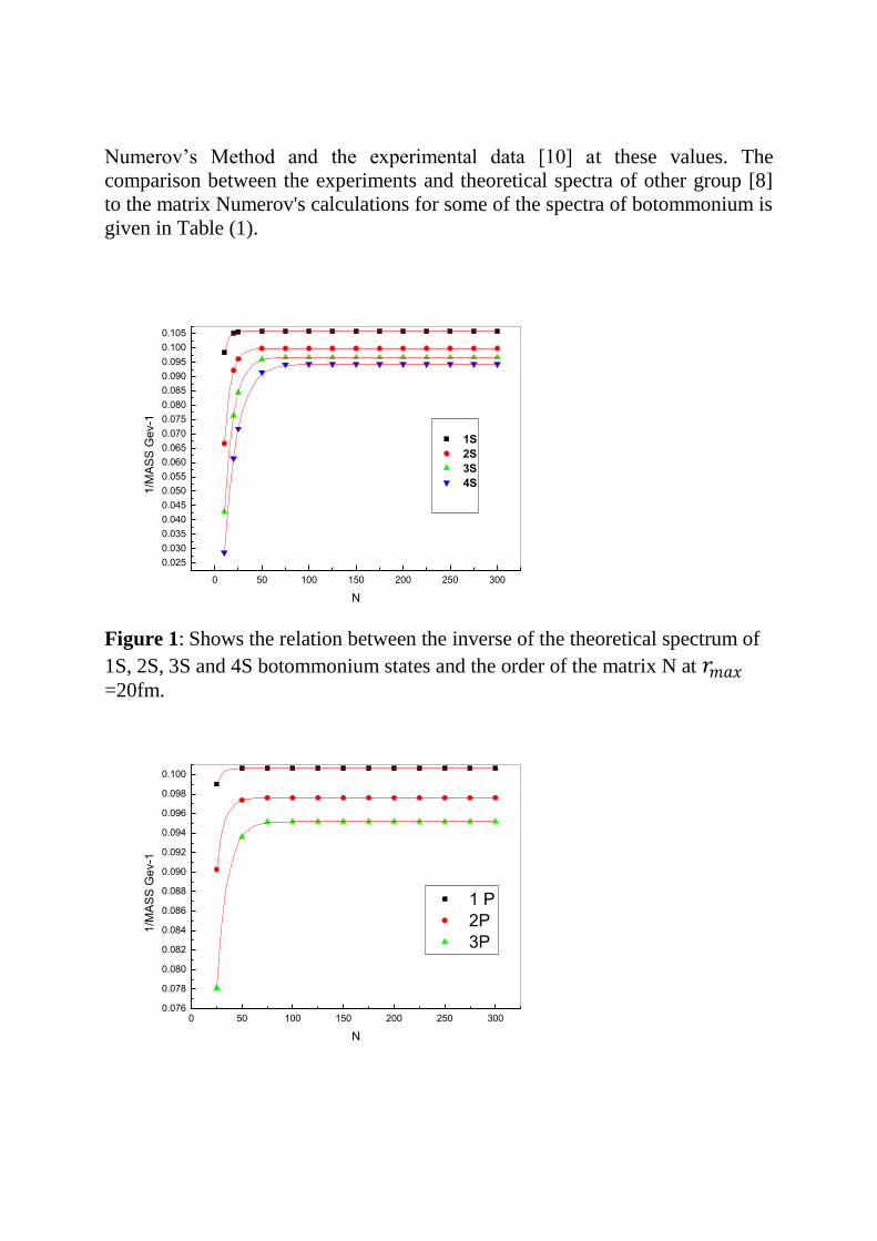
when N ≥ 98 as shown in Fig (1). Moreover, the theoretical spectrum of 1P, 2P,

3P bottomonium states are calculated and at 𝑟𝑚𝑎𝑥 = 20 fm, it is obvious that the

results are stable when N ≥ 71. These results are shown in Fig (2). Secondly, the

stability of the method is checked out by using different values of 𝑟𝑚𝑎𝑥 fm. The

calculation of the theoretical spectrum of 1S, 2S, 3S and 4S bottomonium states

and the distance between the quark- anti quark 𝑟𝑚𝑎𝑥 at N = 100, it is obvious

that the results are stable when 𝑟𝑚𝑎𝑥 ≥ 9 fm as shown In Fig (3). The same

procedure is used to calculate the theoretical spectra of 1P, 2P, 3P bottomonium

states, Fig. (4) shows that the results are stable when 𝑟𝑚𝑎𝑥 ≥ 9 fm. According to

the figures, the value of N ≅ 200 and the value of 𝑟𝑚𝑎𝑥 ≅ 20 fm could be used

to give the spectra of bottominium that consist with the experimental data. This

is obvious from the agreement between the theoretical results obtained by using

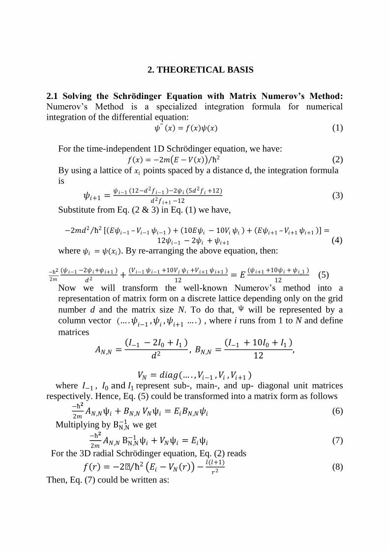
Numerov’s Method and the experimental data [10] at these values. The

comparison between the experiments and theoretical spectra of other group [8]

to the matrix Numerov's calculations for some of the spectra of botommonium is

given in Table (1).

0 50 100 150 200 250 300

0.025

0.030

0.035

0.040

0.045

0.050

0.055

0.060

0.065

0.070

0.075

0.080

0.085

0.090

0.095

0.100

0.105

1/M

AS

S G

ev-1

N

1S

2S

3S

4S

Figure 1: Shows the relation between the inverse of the theoretical spectrum of

1S, 2S, 3S and 4S botommonium states and the order of the matrix N at 𝑟𝑚𝑎𝑥

=20fm.

0 50 100 150 200 250 3000.076

0.078

0.080

0.082

0.084

0.086

0.088

0.090

0.092

0.094

0.096

0.098

0.100

1 P

2P

3P

1/M

AS

S G

ev-1

N

Figure 2: Shows the relation between the inverse of the theoretical spectrum of

1P, 2P and 3P bottomonium states and the order of the matrix N at 𝑟𝑚𝑎𝑥 = 20

fm.

0 2 4 6 8 10 12 14 16 18 200.00

0.01

0.02

0.03

0.04

0.05

0.06

0.07

0.08

0.09

0.10

0.11

1/M

AS

S G

ev-1

r_max fm

1S

2S

3S

4S

Figure 3: The theoretical spectrum of 1S, 2S, 3S and 4S bottomonium states

versus the distance between the quark- anti quark 𝑟𝑚𝑎𝑥 at N = 100.

0 5 10 15 20

0.030

0.035

0.040

0.045

0.050

0.055

0.060

0.065

0.070

0.075

0.080

0.085

0.090

0.095

0.100

0.105

1P1

2P1

3P1

1/M

AS

S G

ev-1

r_max fm

Figure 4: The theoretical spectrum of 1P, 2P and 3P botommonium states versus

the distance between the quark- anti-quark 𝑟𝑚𝑎𝑥 at N = 100.

Table1: The obtained theoretical spectra of bottomonium 𝑏𝑏 compared to other

groups

Experimental masses [10] A. Aly[8] Theoretical

Spectra Name

State

9,390.9±2.8 9.389 9.393 ηb (1S) 11S0

9.994 9.996 ηb (2S) 21S0

10.328 10.33 31S0

10.593 10.596 41S0

9,460.30±0.26 9.459 9.458 Υ (1S) 1

3S1

10,023.26±0.31 10.015 10.017 Υ (2S) 2

3S1

10,355.2±0.5 10.354 10.345 Υ (3S) 3

3S1

10,579.4±1.2 10.738 10.607 Υ (4S) 4

3S1

9,912.21±0.40 9.935 9.936 𝜒𝑏2 (1P) 1

3P2

10,268.65±0.55 10.27 10.272 𝜒𝑏2 (2P) 2

3P2

9,892.76±0.40 9.912 9.904 𝜒𝑏1 (1P) 1

3P1

10,255.46±0.55 10.251 10.244 𝜒𝑏1 (2P) 2

3P1

9,859.44±0.52 9.879 9.884 𝜒𝑏0 (1P) 1

3P0

10,232.5±0.6 10.228 10.234 𝜒𝑏0 (2P) 2

3P0

9.92 9.92 hb(1P) 11P1

10.258 10.258 hb(2P) 21P1

4. CONCLUSION

As a remarkable result, we can point out that it is recommended to use the

Numerov's matrix method to solve 3D radial Schrödinger equation, for the

following reasons:

1- It is easier to use compared to other methods.

2- Saving time, both in implementation and extraction results.

3- Its accuracy in the theoretical calculations, it indicates a good agreement with

the published experimental ones.

5. REFERENCES

[1] J. J. Sakurai, Modern Quantum Mechanics .Tuan, San Fu, ed. (Revised ed.).

Addison–Wesley. (1994).

[2] Liboff, Richard L. Introductory Quantum Mechanics (4th ed.). Addison-

Wesley (2003).

[3] D. Y. Sung, S hooting method for numerical solutions, International Journal

of Numerical Analysis and Modeling (2007).

[4] L. Aceto , P. Ghelardoni, C. Magherini, Boundary Value Methods as an

extension of Numerov’s method. Applied Numerical Mathematics 59 (2009).

[5] Mohandas Pillai, Joshua Goglio, and Thad G. Walker Am. J. Phys (2012).

[6] D. H. Perkins, Introduction to High Energy Physics, Addison-Wesley

(1987).

[7] Olga .Lakhina, Study of Meson Properties in Quark Models, arXi v: hep-

ph/0612160v1 13 Dec 2006.

[8] A. A. Aly," Heavy Meson Spectra in The Non-Relativistic Quark model",

M.SC Thesis, South Valley University, (2012)

[9] T.Barnes, S.Godfreyand, E.S.Swanson, Higher Charmonia, arXiv:hep-

ph/0505002 v2 27 May 2005.

[10] J. Beringer et al. (Particle Data Group, partial updating 2013 for the 2014

edition), Phys. Rev. D86, 010001 (2012).