Improving frequency resolution of discrete spectra

AGH University of Science and Technology, Kraków, Poland

Faculty of Electrical Engineering, Automatics,

Computer Science and Electronics

Marek GĄSIOR

Improving Frequency Resolution

of Discrete Spectra

A doctoral dissertation done under guidance of

Professor Mariusz ZIÓŁKO

Kraków 2006

Marek Gąsior, Improving frequency resolution of discrete spectra - II -

Marek Gąsior, Improving frequency resolution of discrete spectra - III -

Akademia Górniczo-Hutnicza w Krakowie

Wydział Elektrotechniki, Automatyki, Informatyki

i Elektroniki

Marek GĄSIOR

Poprawa rozdzielczości

częstotliwościowej

widm dyskretnych

Rozprawa doktorska wykonana pod kierunkiem

prof. dra hab. inż. Mariusza ZIÓŁKO

Kraków 2006

Marek Gąsior, Improving frequency resolution of discrete spectra - IV -

Marek Gąsior, Improving frequency resolution of discrete spectra - V -

To my Parents

Moim Rodzicom

Acknowledgements

I would like to thank all those who influenced this work. They were in particular the Promotor, Professor Mariusz Ziółko, who also triggered my interest in digital signal processing already during mastership studies; my CERN colleagues, especially Jeroen Belleman and José Luis González, from whose experience I profited so much. I am also indebted to Jean Pierre Potier, Uli Raich and Rhodri Jones for supporting these studies.

Separately I would like to thank my wife Agata for her patience, understanding and sacrifice without which this work would never have been done, as well as my parents, Krystyna and Jan, for my education. To them I dedicate this doctoral dissertation.

Podziękowania

Pragnę podziękować wszystkim, którzy mieli wpływ na kształt niniejszej pracy. W szczególności byli to Promotor, Pan profesor Mariusz Ziółko, który także zaszczepił u mnie zainteresowanie cyfrowym przetwarzaniem sygnałów jeszcze w czasie studiów magisterskich; moi koledzy z CERNu, przede wszystkim Jeroen Belleman i José Luis González, z których doświadczenia skorzystałem tak wiele. Panowie Jean-Pierre Potier, Uli Raich oraz Rhodri Jones wspierali niniejszą pracę, za co jestem im bardzo wdzięczny. Osobne podziękowania składam mojej żonie Agacie – za cierpliwość, wyrozumiałość i poświęcenie, bez których ta praca nigdy by nie powstała, oraz moim Rodzicom, Krystynie i Janowi, za wykształcenie. Im dedykuję tę rozprawę doktorską.

Marek Gąsior, Improving frequency resolution of discrete spectra - VI -

Marek Gąsior, Improving frequency resolution of discrete spectra - VII -

Everything should be made as simple as possible, but not simpler. Albert Einstein

Wszystko powinno być robione najprościej jak można, ale nie prościej.

Abstract

Discrete spectra can be used to measure frequencies of signal components. Such a measurement consists in digitizing the input signal, performing windowing of the signal samples and computing their discrete Fourier spectrum, usually by means of the Fast Fourier Transform algorithm. Frequencies of individual components can be evaluated from their locations in the discrete spectrum magnitude with resolution depending on the number of processed samples, which is usually limited by the time required for computing the spectrum. The subject of this dissertation is interpolation algorithms of discrete Fourier spectra allowing to increase the frequency resolution of such measurements by a few orders of magnitude, depending first of all on the interpolation method, window used and noise present in the spectrum. The author focuses on three methods. All of them consist in fitting an interpolating curve upon the three largest consecutive spectrum bins corresponding to the measured component of the input signal. The abscissa of the curve maximum determines the component frequency with improved resolution. The interpolation methods consist in fitting a parabola, a Gaussian curve and (so-called in the dissertation) an exponential parabola and, for commonly used windows, allow resolution improvement, typically by one, two and four orders of magnitude, respectively. It is assumed that the measured frequency is constant during the signal sampling and that the corresponding spectral peak can be found in the discrete spectrum. The paper includes a description of the dependence of the algorithm efficiency on the used windowing function, noise present in the spectrum, interference from undesirable large components and an exponential decay of the input signal. A direct application of the interpolation algorithms are systems measuring frequency of betatron oscillations of high energy particle beams. They are used presently in such systems in the European Organization for Particle Physics (CERN), Geneva, Switzerland. It seems that the algorithms presented in this dissertation may be also used in laboratory and industrial systems for frequency measurement of signals of limited periodicity, everywhere where real time, high resolution measurements, based on small sample sets are required.

Streszczenie

Widma dyskretne mogą służyć do pomiaru częstotliwości składowych sygnałów. Pomiar taki polega na zamianie sygnału wejściowego na postać cyfrową, poddaniu próbek sygnału procesowi okienkowania oraz wyznaczeniu ich fourierowskiego widma dyskretnego, najczęściej za pomocą algorytmu szybkiej transformacji Fouriera. Częstotliwości poszczególnych składowych sygnału mogą być określone z ich lokalizacji w module widma z rozdzielczością zależną od liczby próbek wziętych do jego wyznaczenia, która często jest ograniczona czasem potrzebnym na obliczenie widma. Tematem niniejszej rozprawy są algorytmy interpolacji fourierowskich widm dyskretnych umożliwiające poprawę rozdzielczości częstotliwościowej takich pomiarów o kilka rzędów wielkości, zależnie przede wszystkim od użytej metody interpolacji, okienkowania oraz od szumu zawartego w interpolowanym widmie. Autor skupia się na trzech metodach. Wszystkie polegają na dopasowaniu krzywej interpolacyjnej na podstawie trzech węzłów wyznaczonych przez trzy kolejne największe prążki widmowe odpowiadające mierzonemu składnikowi sygnału wejściowego. Odcięta maksimum tej krzywej określa częstotliwość danej składowej sygnału z poprawioną rozdzielczością. Algorytmy interpolacyjne polegają na dopasowaniu paraboli, krzywej gaussowskiej oraz (tak zwanej w pracy) potęgowanej paraboli i dla powszechnie używanych okien umożliwiają poprawę rozdzielczości odpowiednio, o około rząd, dwa i cztery rzędy wielkości. Zakłada się, że mierzona częstotliwość jest stała podczas próbkowania sygnału oraz że odpowiadający jej prążek może być znaleziony w widmie dyskretnym. Praca zawiera opis zależności efektywności algorytmów od użytego okna, szumu obecnego w widmie, interferencji od niepożądanych silnych składowych sygnału wejściowego oraz wykładniczego tłumienia tego sygnału. Bezpośrednim zastosowaniem opisywanych algorytmów są systemy do pomiaru częstotliwości oscylacji betatronowych wiązek cząstek elementarnych wielkich energii. Obecnie są one używane w takich systemach w Europejskiej Organizacji Badań Jądrowych (CERN) w Genewie. Wydaje się, że opisane w rozprawie algorytmy mogą znaleźć także zastosowanie w systemach oraz technikach do laboratoryjnego i przemysłowego pomiaru częstotliwości sygnałów o ograniczonej okresowości, wszędzie tam, gdzie wymaga się pomiarów w czasie rzeczywistym, o dużej rozdzielczości i na podstawie niewielkiej ilości próbek.

Marek Gąsior, Improving frequency resolution of discrete spectra - VIII -

Marek Gąsior, Improving frequency resolution of discrete spectra - IX -

Table of contents

List of the most important symbols and abbreviations .................................................................... XI

1. Introduction, theses, assumptions ............................................................................................... 1

2. From an analogue signal to its discrete spectrum.................................................................... 15

2.1. Analogue to digital conversion ............................................................................................ 15

2.2. Fourier and Discrete Fourier Transforms ............................................................................ 18

2.3. Sample windowing .............................................................................................................. 22

3. Three node interpolations of discrete spectra .......................................................................... 33

3.1. Main lobe shapes of window spectra ................................................................................... 33

3.2. Parabolic interpolation (PI) .................................................................................................. 36

3.3. Gaussian interpolation (GI) ................................................................................................. 40

3.4. Exponential parabolic interpolation (EPI) ........................................................................... 44

4. The interpolations on perturbed spectra .................................................................................. 49

4.1. Influence of noise on the interpolation methods .................................................................. 49

4.2. The interpolations on a peak distorted by a nearby interference ......................................... 65

4.3. The interpolations on spectra of exponentially decaying signals......................................... 71

5. Application examples ................................................................................................................. 75

5.1. Measuring the betatron tune of an accelerator ..................................................................... 75

5.2. A measurement on the SPS accelerator ............................................................................... 78

5.3. A measurement on the LEIR accelerator ............................................................................. 82

6. Conclusions ................................................................................................................................. 91

References ............................................................................................................................................ 93

Marek Gąsior, Improving frequency resolution of discrete spectra - X -

Version of 15/05/21

Changes with respect to the original, submitted thesis:

- quite a few typo corrections (e.g. “widow” → “window”); - some language improvements; - no changes whatsoever in math and figures.

All corrections did not change original page numbering.

Marek Gąsior, Improving frequency resolution of discrete spectra - XI -

List of the most important symbols and abbreviations

t – time f – frequency – normalized frequency – phase s(t) – continuous signal S(f), S() – continuous magnitude spectrum of a signal s(t) Ŝ(f), Ŝ() – complex-valued continuous spectrum of a signal s(t) w(t) – continuous window function W(f), W() – window magnitude spectrum Ŵ(f), Ŵ() – complex-valued window spectrum s[n] – sequence of samples S[k] – discrete magnitude spectrum of a sequence s[n] Ŝ[k] – complex-valued discrete spectrum of a sequence s[n] w[n] – discrete window function

^. – complex valued quantity

. – mean value {.}rms – root-mean-square value {.}std – standard deviation |.| – absolute value arg(.) – argument of a complex number max(.), {.}max – maximum value round(.) – rounded value {.} – energy ln(.) – natural logarithm lg(.) – decimal logarithm 1(.) – Heaviside's unit step function [a;b] – interval with boundaries a and b, closed on both sides a;b – interval with boundaries a and b, open on both sides [a;b – interval with boundaries a and b, right side open – proportionality sign X{.}, {.}X – operator X FT{.} – Fourier transform IFT{.} – inverse Fourier transform DFT{.} – discrete Fourier transform IDFT{.} – inverse discrete Fourier transform fin – input frequency to be measured fm – measured frequency (result of discrete spectrum interpolation) km – index of the largest spectrum bin corresponding to fm fs – sampling frequency fNq – Nyquist frequency Ts – sampling period

Marek Gąsior, Improving frequency resolution of discrete spectra - XII -

N – number of samples, number of discrete spectrum bins L – window length, length of the analyzed signal interval f – discrete spectrum bin spacing (frequency domain) m – interpolation correction G – interpolation gain – resolution of a discrete spectrum E – frequency measurement absolute error Emax – frequency measurement maximum error e – frequency measurement relative error Es – systematic frequency error of an interpolation method En – noise (random) frequency error of an interpolation method Rc – resolution in bits of an analogue to digital converter Re – effective resolution in bits of an analogue to digital converter vLSB – voltage corresponding to one ADC LSB vn – noise voltage vnq – quantization noise voltage – noise error crest factor (maximum to the RMS value ratio) n – spectral energy noise density – signal relative decay factor SNR – signal to noise ratio (please note: SNR – a symbol, SNR – an abbreviation) SNR – signal to noise ratio in the normalized frequency domain ENBW – equivalent noise bandwidth Abbreviations PI – Parabolic Interpolation GI – Gaussian Interpolation EPI – Exponential Parabolic Interpolation SNR – Signal to Noise Ratio (please note: SNR – an abbreviation, SNR – a symbol) ADC – Analogue to Digital Converter FFT – Fast Fourier Transform LSB – Least Significant Bit ppm – part per million RMS – Root Mean Square ENBW – Equivalent Noise BandWidth

Chapter 1

Marek Gąsior, Improving frequency resolution of discrete spectra - 1 -

1. Introduction, theses, assumptions

Frequency can be measured with resolution directly proportional to the metrologist patience, expressed in time spent on waiting for the result. This rule refers to a typical frequency measurement method, based on counting periods of the measured signal within a reference time interval. Illustrating the method, to measure frequency of a signal of 100 kHz with resolution of one part per million (ppm), it is needed to count 106 signal periods, awaiting the result for 10 s. The resolution can be increased by extending the measurement time to count more periods.

A metrologist who cannot wait so long may evaluate the signal frequency by measuring the duration of one signal period. The time can be measured by counting within its periods of a reference frequency. In this case the measurement resolution depends on the number of reference frequency periods occurring within the measured interval, so it depends on the reference to the input frequency ratio. Assuming conditions as above, to measure the 10 s period of a 100 kHz input signal with resolution of 1 ppm it would be needed a fantastic reference frequency of 100 GHz.

The impatient metrologist can rationalize the reference frequency accepting an intermediate method, where one counts reference frequency periods within a number of measured signal periods. If one decides to count reference frequency periods within a thousand of periods of the input signal, i.e. 10 ms, it is enough to use the frequency of 100 MHz to achieve the assumed resolution of 1 ppm.

From the above examples it can be concluded that the effectiveness of each mentioned method depends on the value of the measured signal frequency. Also, for two mentioned methods, the input signal is assumed to be of constant frequency for a million or thousands of periods. If this condition is not fulfilled, measurements yield a sort of averaged frequency. Thus, counting can be used only for signals of constant frequency, otherwise the mean frequency value is measured.

All the methods assume the measured signal to contain one dominant component and only its frequency is to be measured. If this is not the case, prior to the measurement, the interesting component has to be filtered out. Theoretically it can be done by using an appropriate analogue filter, but often it may be inefficient, uneconomical or just unfeasible solution. In particular, it can be so if the interesting component constitutes only a small fraction of the signal and/or in its spectral vicinity other undesirable strong components are located. Such difficult cases can be resolved by discrete spectrum frequency measurement, consisting in converting the measured signal into digital samples and to calculate their discrete Fourier spectrum. This operation, being in fact a digital filtering (i.e. one filter channel per discrete spectrum bin), yields a spectral image of the signal content, which can be examined to find the component of interest. Frequency of the component is then evaluated from its position in the spectrum with the resolution set by the number of discrete spectrum bins, being equal to the sample total taken for the spectrum calculation. Since the calculation time depends on this number, for many applications the affordable value is limited to at most a few thousands, resulting in the spectrum frequency resolution a couple of orders of magnitude smaller than 1 ppm, being a standard for the counting methods. It is the case in tune measurements systems for circular accelerators of high energy particle beams, where frequency of beam betatron oscillations has to be measured in real time with resolution between, typically, 0.1 % and 0.01 %, depending on the machine and conditions of its operation. Such measurements, which are of paramount importance for running an accelerator, have to be usually based on some thousand samples, due to the limited time for spectrum calculation.

The goal of this dissertation is to provide, study and evaluate the efficiency of means to improve frequency resolution of discrete spectra. The computing cost should be as small as possible to allow applications in real time systems. Consequently, such methods should be simple. This work was inspired by a method of parabolic interpolation (PI) of discrete Fourier spectra, already known and used in tune measurement systems for particle accelerators [Chapman-Hatchett, Chohan, d’Amico 1999] (1), also by the author [Gasior, González 1999b]. Despite its popularity, to the author's knowledge, it was only himself together with J.L. González

(1) [Asséo 1985], [Bartolini 1995], [Bartolini 1996], [González, Johnston, Schulte 1994] describe a less general method.


- 2 -

who evaluated the method interpolation gain [Gasior, González 2004a, 2004b]. In the same papers the authors proposed the Gaussian interpolation (GI) algorithm (1), advancing the potential interpolation gain to two orders of magnitude, as compared to one order of magnitude for the parabolic method. Here, after recapitulation of both algorithms, their behavior is analytically studied when interpolated discrete spectra are perturbed by noise, interference from strong components and an exponential decay of the analyzed signal.

The main contribution of this dissertation is the exponential parabolic interpolation (EPI) method, which allows improving the frequency resolution of discrete spectra by some five orders of magnitude. As for the previous two algorithms, the dependence of the frequency resolution improvement of the EPI method upon the spectrum perturbations is analytically investigated.

In the literature one can find quite a few methods based on interpolating local maxima of discrete Fourier spectra. However, these methods are either limited to the use of the rectangular window [Asséo 1985], [Bartolini et al. 1995, 1996], [Bibl 2005], [Donghai Li et al. 2001], [González, Johnston, Schulte 1994], [Grandke 1983], [Hikawa, Jain 1990], [Jain, Collins, Davis 1990], Hamming window [Goto 2000], [Scheppach 2002], or are more complicated than the methods proposed in this dissertation [Althoff, Keiler, Zölzer 1999], [Andria, Savino, Trotta 1989], [Chun-Kit Chan, Lian-Kuan Chen 1996], [Fusheng Zhang, Zhongxing Geng, Wei Yuan 2001], [Keiler, Marchand 2002], [Keiler, Zölzer 2001], [Offelli, Petri 1990], [Pan Wen, Qian Yu Shou, Zhou E. 1994], [Schoukens, Pintelon, Hamme 1992]. There are also methods not based on interpolations [Bonacci, Mailhes, Djuric 2003], [Borkowski 2000], [Jianguo Huang, Kay 1989], [Kay 1984, 1988], [Rothacker, Mammone, Davidovici 1986]. The algorithms studied in this dissertation in comparison with methods described in the abovementioned publications are very simple, can be used with any windowing except the rectangular one and can compete in terms of frequency resolution and robustness for distortions of discrete spectra.

The subject and the goals of this work can be outlined by the following examples, introducing intuitively dissertation basic ideas, quantities and denotations. The theory in the examples is intentionally limited to the most important issues, fully developed in the further chapters. The aim of the rest of this chapter is to familiarize the Reader with ideas of the dissertation and to give a view of its content.

Beginning an example, it is given a hypothetical signal

)π2sin()π2sin()()()( tfAtfAtststs bgbgininbgin (1-1)

of unitary amplitude, containing two sinusoidal (2) components: of interest sin(t) and an undesirable sbg(t), considered as a background reduced to one component. The component sin(t) is of frequency fin

of 100.25 kHz and frequency fbg of the background is 110 kHz (3). Amplitudes Ain and Abg of the components are 0.25 and 0.75 respectively (4). Waveforms of the signal and its components are plotted in Fig. 1-1.

In the example it is assumed that the component of interest sin(t), also referred to as the input component, is to be separated from its larger background and its frequency fin, referred to as the input frequency, is imagined as unknown and is to be measured. Exact value of fin is used only to evaluate measurement errors.

A very powerful way to separate the input component from its background is to digitize the considered signal by means of an Analogue to Digital Converter (ADC) and to perform a spectral analysis of the signal samples. In Fig. 1-2 the signal s(t) is shown, along with dots marking N = 1024 full scale signal samples of resolution Rc =12 bits, imagined to be taken with the rate of the sampling frequency fs of 1.024 MHz.

(1) Keiler and Marchand (2002) described a similar method, but they called it “parabolic”. This reference was found by the author already after publishing the papers [Gasior, González 2004a, 2004b]. In the later publications the systematic interpolation error was derived, to the author’s knowledge, for the very first time. (2) Term sinusoidal component is supposed to mean in this work a signal described by a sine function with an arbitrary phase. Hence, a cosine waveform is considered here also as a sinusoidal component. (3) Numbers for the examples were arbitrarily chosen to reveal as many important issues of this work as possible. (4) In the example the amplitude ratio is 3 to ensure readable plots, but in real cases the ratio can be orders of magnitude larger.


- 3 -

0 25 50 75 100 125 150 175 200Time [ s]

-1

-0.5

0

0.5

1

Am

plitu

de

100.25 kHz110.0 kHzsum

Fig. 1-1. Signal s(t) (black solid line) of unitary amplitude contains two sinusoidal components: the component of interest, sin(t) (red dashed line), whose frequency is to be measured, and an undesirable component, sbg(t) (blue dashed line), considered as a simplified background. Component frequencies are fin = 100.25 kHz and fbg = 110.0 kHz, their amplitudes Ain = 0.25 and Abg = 0.75.

The left vertical axis of Fig. 1-2 is scaled in numbers corresponding to the digital output of the ADC and the right vertical axis has the usual (analogue) scale. The samples can be represented as a sequence s[n] (1) of integer numbers, linked with the sampled continuous signal s(t) as

1,2,...,1,0,2

)()(2round][

NNn

A

TnsRns sc (1-2)

where round(x) (2) means the rounded value of x, Rc is the converter resolution in bits, Ts is the sampling period Ts = fs

–1 and A is the amplitude of s(t). The above equation describes the ideal signal sampling and the conversion to integer numbers

with the quantization noise taken into account. The noise is caused by the signal sample rounding and it is a function of the ADC resolution Rc (3).

Discrete spectrum magnitude S[k] (4) of signal sample sequence s[n] can be obtained by means of the Discrete Fourier Transform (DFT), and

1

0

π2jexp][][

N

n N

knnskS (1-3)

The magnitude spectrum of the sample sequence of Fig. 1-2 is presented in Fig. 1-3 up to bin

N/2 = 512 (the other half is mirror symmetric to the part shown). In the spectrum of Fig. 1-3 one does not see two narrow peaks related to the two sinusoidal

components of s(t) due to the spectral leakage. The phenomenon is a consequence of the fact that the transform in (1-3) assumes the input signal s(t) to be a periodic function of period equal to L = N Ts, the length of the transform input. If this function is built from periods that do not fit on the boundaries, i.e. for t = 0 and t = L the signal and its time derivatives are much different, the corresponding spectrum is distorted by components related to the abrupt boundary irregularities. It is the case for the discussed example, but only for the component sin(t), while sbg(0) = sbg(L), since fbg

–1 is an integer multiple of Ts. The leakage effect reveals in the signal spectrum of Fig. 1-3 as the pedestal of the peak corresponding to sin(t), biasing also sbg(t) peak, which is narrow as not directly affected by the leakage.

A remedy for the spectral leakage is a technique called windowing, in which a smooth function or its corresponding sequence in the case of sampled signals is used to attenuate the input signal sequence s[n] close to its boundaries to make them fit each other. In such a windowing process each signal sample is multiplied by the corresponding window value, resulting in the windowed sample sequence

(1) Square brackets [ ] are used to enclose an independent variable for sequences while round brackets ( ) are used for continuous variable functions. (2) See Section 2.1 (Analogue to digital conversion) for details. (3) See Section 2.1 (Analogue to digital conversion) for details. (4) Since in this dissertation almost always magnitude spectra are used, the usual absolute value brackets | | are systematically omitted to simplify the notation. Complex valued quantities are marked by the caret sign ^.


- 4 -

1,2,...,1,0],[][][ NNnnwnsnsw (1-4)

After windowing, the discrete spectrum is calculated in the usual way.

0 200 400 600 800 1000Time [ s]

-1

-0.5

0

0.5

1

Ana

logu

e am

plitu

de

0 256 512 768 1024Sample number

-2048

-1536

-1024

-512

0

512

1024

1536

2048

Dig

ital a

mpl

itude

0 50 100 150 200 250 300 350 400 450 500Bin number

5

235

235

235

235

235

23

1E-1

1E+0

1E+1

1E+2

1E+3

1E+4

Ma

gnitu

de s

pect

rum

0 50 100 150 200 250 300 350 400 450 500

Frequency [kHz]

-100

-80

-60

-40

-20

0

Nor

mal

ized

ma

gnitu

de s

pect

rum

[dB

]

Fig. 1-2. Digitization of the example input signal. The dots mark the samples taken with the converter resolution Rc = 12 bits and the sampling rate fs = 1.024 MHz. About hundred periods of the signal input component are acquired. The signal envelope results from beating of the input and thebackground components.

Fig. 1-3. The magnitude spectrum of N = 1024 samples of the example signal shown in Fig. 1-2. The smaller spectral peak corresponds to the input component and the bigger to the background one. The input component peak is biased by the spectral leakage effect, while the background peak is narrow and biased only by the spectral leakage of the input component. The right vertical axis is scaled in dB with respect to the highest peak.

In this chapter a four-term window with continuous first derivative is used exclusively, referred to as the 4T1 (1) window [Nuttall 1981]. The window is defined as (2):

1,2,...,1,0,π6

cosπ4

cosπ2

cos][ 3210

NNii

Nci

Nci

Ncciw (1-5)

with coefficients c0 = 0.355768, c1 = 0.487396, c2 = 0.144232, c3 = 0.012604 and N being the number of windowed samples; N = 1024 for all examples of this chapter.

The windowed sequence sw[n] of the discussed example is shown in Fig. 1-4, together with the 4T1 window shape. The sequence boundaries fit each other smoothly, since their values decay gradually to zero, attenuated by the window.

The magnitude spectrum Sw[k] of the windowed sequence sw[n] is presented in Fig. 1-5 up to bin N/2 = 512. It looks completely different than the spectrum in Fig. 1-3 of the non-windowed samples (note the same right dB scales). It can be seen even the floor of the quantization noise originating from the conversion of the input signal samples into digital numbers. Also the spectrum peaks corresponding to both components have very similar shapes. It means that the shapes do not depend any more on the relationship between the sampling boundaries, component frequencies and phases, as it was the case without windowing.

The spacing of spectral bins corresponds to the frequency increment

LTNN

fΔ

s

sf

11 (1-6)

(1) 4T1 stands for 4-term with continuous 1st derivative. (2) See Section 2-3 (Sample windowing) for details. Other windows are also described there.


- 5 -

where L is the length of the transform input. For the discussed example fs and N were chosen to have f exactly of 1 kHz.

0 200 400 600 800 1000

Time [ s]

-1

-0.5

0

0.5

1

Ana

log

ue a

mpl

itude

0 256 512 768 1024Sample number

-2048

-1536

-1024

-512

0

512

1024

1536

2048

Dig

ital a

mpl

itude

0 50 100 150 200 250 300 350 400 450 500Bin number

235

235

235

235

235

235

1E-1

1E+0

1E+1

1E+2

1E+3

1E+4

Mag

nitu

de

spec

trum

0 50 100 150 200 250 300 350 400 450 500

Frequency [kHz]

-100

-80

-60

-40

-20

0

Nor

mal

ize

d m

agni

tud

e sp

ectr

um [

dB]

Fig. 1-4. Digitization and windowing of the example input signal. The dots mark N = 1024 windowed samples taken with resolution Rc = 12 bits. The red bell-shaped curve is the 4T1 window (1-5).

Fig. 1-5. The magnitude spectrum of the windowed samples of Fig. 1-4. The smaller spectral peak corresponds to the input component and the second to the background. With windowing, the shapes of both components are similar and they are not biased by the spectral leakage. It is seen the noise floor, previously completely drowned out by the leakage. The right vertical dB axis has the same scale as Fig. 1-3 with the spectrum of the non-windowed data.

Assuming that the spectrum peak corresponding to the input frequency fin constitutes a local maximum within a given range, here referred to as the working range, the peak of the maximum and, in consequence, its index km can be found and the value of fin can be evaluated from the position of the maximum in the discrete magnitude spectrum as (1)

mfmin kΔff (1-7)

with the largest error

LTNN

fΔff

s

sfinm 2

1

2

1

22

1max (1-8)

for the input frequency lying exactly between two spectrum bins. The maximum error (1-8) is considered as the frequency resolution of discrete spectra and it is referred to as the DFT frequency resolution.

For the magnitude spectrum shown in Fig. 1-5 the index km is 100, resulting in fm of 100 kHz with the absolute error

inm ffE (1-9)

of 0.25 kHz and the relative error

in

inm

f

ffe

(1-10)

of 0.25 %.

(1) Subscripts m refer to the words measured and maximum.


- 6 -

According to (1-8), frequency resolution of a discrete spectrum, and therefore, of a frequency measurement based on it, depends on the length of the input signal taken into account. This observation is related to a more general rule, called the uncertainty theorem. Before the author starts explaining in detail how one can improve frequency resolution of discrete spectra, he would like to try to convince the Reader that this is not against this theorem.

Note that the theorem deals with the signal bandwidth and, therefore, is related rather to the fact that if a signal record is too short, then signal components with similar frequencies cannot be distinguished in the frequency domain, since the corresponding spectral peaks overlap. Methods proposed in this dissertation assume that the signal components can be distinguished in the frequency domain and only the component frequencies, therefore the abscissae of the corresponding spectral peaks, can be known with resolution orders of magnitude better than the discrete spectrum frequency resolution (1-8).

As it will be explained, discrete spectra can be considered as samples of their continuous equivalents. The goal of the interpolation methods proposed in this dissertation is to find frequencies of signal components, when the corresponding peaks in the magnitude spectrum have centers located between the discrete bins.

Notice that if frequency of a sinusoidal component is such that it is located on the discrete spectrum bin, the corresponding peak in the magnitude spectrum occupies only this bin, even if the spectrum was calculated on only few signal samples (see the larger peak in Fig. 1-3). This observation, looking as disproving the uncertainty theorem, can be explained by the periodic nature of the DFT. The transform implies that the sampled signal is periodic with the period of the DFT length (1), so it is as the analyzed sample set (i.e. the observation period) was infinitely large, resulting in the infinitesimal component bandwidth. Unfortunately, the sampled fraction of the analyzed component contains not necessarily an integer number of periods and, as a consequence, the signal as seen by the DFT can contain abrupt parts, making the component not sinusoidal anymore. This side effect can be minimized by performing windowing, attenuating the samples close to the sampling interval boundaries to make them fit each other. After windowing, the infinitely long signal sample set is smooth, as seen by the DFT. This is done at the expense of making the component bandwidth larger, since windowing can be considered as an amplitude modulation. Furthermore, as it will be explained in detail, this modulation is necessary to make the spectral peak wide enough to sample it by at least three discrete spectrum bins. Without explicit windowing the peak is too narrow, making it impossible to evaluate its center from three discrete spectrum samples.

The presented examples and discussion illustrate the following Thesis 1 of this dissertation:

T1 Frequency fin of a sinusoidal component sin(t) of a compound signal s(t) can be obtained from the discrete magnitude spectrum S[k] of the signal samples s[n] of s(t) with resolution improved by making an interpolation on appropriate bins of the spectrum and taking the interpolation maximum abscissa fm as a better approximation of the input frequency fin. This is possible under the following conditions: a) The signal s(t) was properly sampled, i.e. with the sampling theorem

respected and the samples s[n] having sufficient signal to noise ratio. b) The signal samples are properly windowed. c) The signal component sin(t) has in the discrete magnitude spectrum S[k] a

corresponding observable peak constituting a spectrum local maximum at a bin of index km and the peak is spread at least on three consecutive spectrum bins of indexes km – 1, km and km + 1.

Please note that the condition T1.c) implies the discrete spectrum to have the bin spacing (number of bins) sufficient to resolve the peak of interest from all potential interferences. This is equivalent to

(1) See Section 2.2 (Fourier and Discrete Fourier Transforms) for details.


- 7 -

having sufficient resolution of the spectrum. This resolution is something different than the frequency resolution meant before and can be considered as the ability to resolve close spectral peaks. This is the resolution to which the uncertainty theorem refers. In the dissertation the term spectrum frequency resolution is understood as the largest error with which one can measure frequency of a signal component, in contrast to the term spectrum resolution, considered as a spectrum ability to resolve individual components. According to these definitions, it can be said that the frequency resolution of a spectrum can be improved if the spectrum itself has sufficient resolution.

Thesis T1 and its conditions are illustrated by the following frequency measurement examples, all in similar conditions to those already presented. More formal analyses are elaborated in the next chapters.

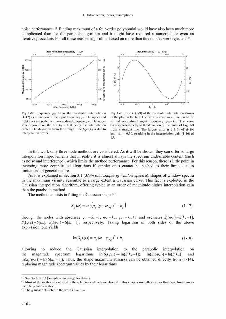
Spectral peak shapes corresponding to components of a signal are described by the Fourier transform of the window function applied to the signal prior to calculating the spectrum. In general, such peak shapes can be expressed in the maximum vicinity as frequency polynomials of even orders. The simplest polynomial which can be efficiently used is the second order one. In this case, the frequency measurement error can be reduced by using a parabola fit on the highest three bins of the working range, namely km –1, km and km +1, as shown in Fig. 1-6, and taking the parabola maximum abscissa fmp as a better approximation of fin.

The parabola form is (1)

pmppp hffafS 2)()( (1-11)

and the fit is done through the three nodes with abscissae fn– = (km –1)f, fn0 = km f, fn+ = (km +1)f and ordinates Sp(fn–) = S[km –1], Sp(fn0) = S[km], Sp(fn+) = S[km +1], respectively. Solving appropriate equations (2) results in the parabola maximum abscissa

])1[]1[][2(2

]1[]1[

mmm

mmmfmp kSkSkS

kSkSkΔf (1-12)

Taking the magnitude spectrum of windowed samples shown in Fig. 1-5 and applying (1-12) for

the bins of indexes 99, 100 and 101, results in the parabola maximum at fmp = 100.2180. The fitting is illustrated in Fig. 1-6. The frequency fin is approximated by fmp with the error E of 32 Hz, so the result has been improved by a factor of 7.8 with respect to the simple estimate f km (1-7).

99 100 101Bin number

1500

2000

2500

3000

Am

plitu

de

fin

E

99 99.5 100 100.5 101Frequency [kHz]

fmp

Fig. 1-6. Parabolic interpolation (1-12) on the bins 99, 100 and 101 of the magnitude spectrum of Fig. 1-5. Theinterpolation error E is 32 Hz, i.e. 3.2 % of f, and therelative error e amounts to 0.07 %. The parabolic interpolation decreased the error of 250 Hz of the simple estimate f km by a factor of 7.8. The coefficients of parabola (1-11) are fmp = 100.2180, ap = 865.3 and hp = 2888.5.

(1) The p subscripts refer to the word parabolic. (2) See Section 3.2 (Parabolic interpolation) for details.


- 8 -

The idea of the discrete spectra interpolation can be further investigated to evaluate the interpolation error dependence on input frequency changes. An example is shown in Fig. 1-7, where the bins concerned are presented, along with interpolating parabolas for four input frequencies, namely fin1 = 100.0 kHz, fin2 = 100.1 kHz, fin3 = 100.5 kHz and fin4 = 100.6 kHz. Other conditions, such as the presence of the background component, the signal amplitudes and windowing are the same as for the previous examples.

99 99.5 100 100.5 101Frequency [kHz]

1000

1500

2000

2500

3000

Am

plitu

de

fmp1 fmp2

99 99.5 100 100.5 101Normalized frequency

fmp3 fmp4

1: 100.0 kHz

2: 100.1 kHz

3: 100.5 kHz

4: 100.6 kHz

Input frequency

Fig. 1-7. Parabolic interpolation (1-12) for fin1 = 100.0 kHz, fin2 = 100.1 kHz, fin3 = 100.5 kHz and fin4 = 100.6 kHz. For fin1 lying exactly on bin 100, bins 99 and 101 have equalheights, so the corresponding interpolation result fmp1 is located on bin 100. When the input frequency increases, bin 99 gets smaller and 101 higher, so the abscissa of the parabola maximum shifts in the positive direction, as for fin2. Bin 100 remains the largest until the input frequency is located exactly between bins 100 and 101, as for fin3 when they have the same heights. If the input frequency is increased further, bin 101 becomes the interpolation center as the highest one, like in the case of fin4. For a decreasing input frequency the analysis is similar, resulting in symmetrical cases. Interpolation results and the corresponding errors are listed in Table 1-1.

For the input frequency fin1 =100 kHz lying exactly on the bin of index 100, the spectrum bins 99 and 101 have equal heights, so the parabola maximum lies precisely on the top of bin 100 and the interpolation gives no error. When the frequency increases, bin 99 gets smaller and bin 101 higher, so the abscissa of the parabola maximum shifts in the positive direction, as for fin2 =100.1 kHz in the figure. Bin 100 remains the largest until the frequency reaches fin3 = 100.5 kHz, i.e. is located exactly between bins 100 and 101. In this case the bins have equal heights, so the parabola maximum is exactly between the bins and the interpolation works again with no error, despite the fact that the simplest frequency estimate f km gives at such points the biggest error of f /2. When the measured frequency is increased further, bin 101 becomes the interpolation center as the highest one, like for fin4 =100.6 kHz in the figure. For the input frequency decreasing, the analysis could be similar, resulting in symmetrical cases. Numbers related to the parabolic interpolation presented in Fig. 1-7 are listed in Table 1-1. Table 1-1. Interpolation results, errors and parabola coefficients for the parabolic interpolation example shown in Fig. 1-7.

input frequency fin [kHz], in

interpolation result fmp [kHz], m

absolute error E [% of f ], [kHz]

Parabola coefficients

ap hp

100.0 100.0000 0.000 -918.049 2914.79

100.1 100.0842 -0.016 -909.521 2910.14

100.5 100.5000 0.000 -716.338 2833.45

100.6 100.6264 0.026 -786.175 2855.42

The upper horizontal axis of the plot of Fig. 1-7 is scaled in units named normalized frequency. This continuous quantity, denominated in the paper as , has the meaning of ordinary frequency, but adjusted to the scale of indexes of discrete spectrum bins

fLfTNf

fN

Δ

fs

sf

(1-13)


- 9 -

Normalized frequency is a dimensionless equivalent of ordinary frequency in units of f, i.e. integer values of correspond exactly to bin indexes. The quantity links the discrete and continuous spectra, making it possible to replace expressions like “the frequency is located halfway between bins 100 and 101” simply by =100.5. It can help even more in the case of, for example, =123.456.

Two first columns of Table 1-1 could have been used to produce a plot of fmp as a function of fin, if it had only included more rows. Such a function is plotted in Fig. 1-8, for the input frequency changing from 99.5 kHz to 100.5 kHz. In the ideal case the interpolation result should follow the input frequency and fmp = fin. The presented curve has a deviation from a straight line, resulting from interpolation errors, seen already before in the presented examples.

The interpolating parabola shape depends only on the relative position of the input frequency with respect to the interpolation center km, thus interpolating shapes, and in consequence, errors are the same around each bin. This can be derived by scaling equation (1-12) into domain to make it independent of f

mpmininin

ininm

f

mpmp Δk

kSkSkS

kSkSk

Δ

f

])1[]1[][2(2

]1[]1[ (1-14)

The maximum abscissa mp is a sum of the maximum bin index and a correction

])1[]1[][2(2

]1[]1[

ininin

ininmp kSkSkS

kSkSΔ (1-15)

with values ranging from –1/2 for S[km ] = S[km –1] to 1/2 for S[km ] = S[km +1]. Since the measured normalized frequency in = fin/f can be at most 1/2 apart from the interpolation center km, to investigate systematic errors of the interpolation for all frequencies it is enough to sweep the shifted frequency in – km from –1/2 to 1/2 around freely chosen bin km and look on the shifted interpolation result mp – km. This was done to produce Fig. 1-8 with km = 100 and in changing from 99.5 to 100.5. The shifted coordinates are used to scale the right and upper axes of the plot.

The interpolation error E (1-9), corresponding to simulations of Fig. 1-8, is plotted in Fig. 1-9. The error is given as a function of the shifted measured frequency in – km and expressed in units of f. In this way the presented shape characterizes the interpolation for all frequencies, all sampling rates and it does not depend on the sample number N. The absolute error for all possible combinations of these three parameters can be calculated if the shape is known. This is the usual way of presenting interpolation errors in this dissertation.

The halves of the error curve of Fig. 1-9 are anti-symmetric with module of extremes Emax = 3.3 % of f for |in – km| = 0.30. The error Emax can be considered as the maximum interpolation systematic error of the method. Thus, the parabolic interpolation method increases the DFT resolution (1-8) of f /2 by a factor

][2

1

maxmax fΔEEG

(1-16)

which is referred to as the interpolation gain. If the error Emax is expressed in units of f, then the gain is just a half of the error reciprocal. For the parabolic interpolation method with the 4T1 windowing the gain calculated in this way amounts to 15.

A higher interpolation gain can be achieved if the shape of the continuous spectrum is better reproduced from the corresponding discrete spectrum samples. A more accurate polynomial fit would have been of fourth order, requiring using five discrete spectrum bins as the interpolation nodes. This would have required spectrum peaks at least six bins wide, and, as a consequence, windowing giving so wide peaks. Such windowing would have decreased the spectral resolvability and deteriorated the


- 10 -

noise performance (1). Finding maximum of a four-order polynomial would have also been much more complicated than for the parabola algorithm and it might have required a numerical or even an iterative procedure. For all these reasons algorithms based on more than three nodes were rejected (2).

99.50 99.75 100.00 100.25 100.50Input frequency [kHz]

99.50

99.75

100.00

100.25

100.50

Me

asur

ed

fre

quen

cy

[kH

z]

-0.5 -0.25 0 0.25 0.5

Input normalized frequency - 100

-0.5

-0.25

0

0.25

0.5

Mea

sure

d no

rmal

ized

freq

uenc

y -

100

-0.5 -0.25 0 0.25 0.5-

-4

-2

0

2

4

[

% o

f

]

-0.5 -0.25 0 0.25 0.5

Input frequency - 100 [kHz]

-40

-20

0

20

40

[

Hz]

km

E

E

in

f

Fig. 1-8. Frequency fmp from the parabolic interpolation (1-12) as a function of the input frequency fin. The upper and right exes are scaled with normalized frequency . The upper axis origin is on the bin km = 100 being the interpolation center. The deviation from the straight line fmp = fin is due tointerpolation errors.

Fig. 1-9. Error E (1-9) of the parabolic interpolation shown in the plot on the left. The error is given as a function of the shifted normalized input frequency in – km. The error corresponds directly to the deviation of the curve of Fig. 1-8from a straight line. The largest error is 3.3 % of f for|in – km| = 0.30, resulting in the interpolation gain (1-16) of 15.

In this work only three node methods are considered. As it will be shown, they can offer so large interpolation improvements that in reality it is almost always the spectrum undesirable content (such as noise and interference), which limits the method performance. For this reason, there is little point in inventing more complicated algorithms if simpler ones cannot be pushed to their limits due to limitations of general nature.

As it is explained in Section 3.1 (Main lobe shapes of window spectra), shapes of window spectra in the maximum vicinity resemble to a large extent a Gaussian curve. This fact is exploited in the Gaussian interpolation algorithm, offering typically an order of magnitude higher interpolation gain than the parabolic method.

The method consists in fitting the Gaussian shape (3)

gmggg haS 2)(exp)( (1-17)

through the nodes with abscissae n– = km –1, n0 = km, n+ = km +1 and ordinates Sg(n–) = S[km –1], Sg(n0) = S[km], Sg(n+) = S[km +1], respectively. Taking logarithm of both sides of the above expression, one yields

gmggg haS 2)())(ln( (1-18)

allowing to reduce the Gaussian interpolation to the parabolic interpolation on the magnitude spectrum logarithms ln(Sg(n–)) = ln(S[km –1]), ln(Sg(n0)) = ln(S[km]) and ln(Sg(n+)) = ln(S[km +1]). Thus, the shape maximum abscissa can be obtained directly from (1-14), replacing magnitude spectrum values by their logarithms

(1) See Section 2.3 (Sample windowing) for details. (2) Most of the methods described in the references already mentioned in this chapter use either two or three spectrum bins as the interpolation nodes. (3) The g subscripts refer to the word Gaussian.


- 11 -

])1[ln(])1[ln(])[ln(22

])1[ln(])1[ln(

mmm

mmmmg kSkSkS

kSkSk (1-19)

An example of using the Gaussian interpolation is shown in Fig. 1-10. Its conditions correspond to

the parabolic interpolation case of Fig. 1-6; note the different axis scales for the two figures. The input frequency of 100.25 kHz gives the Gaussian shape peak at 100.2531 kHz, resulting in the interpolation error of 3.1 Hz, i.e. 31 ppm, that is 10.4 times less than the parabolic interpolation method and 81 times less than the simplest estimate f km (1-7).

The way used to visualize the interpolation errors of the parabolic method shown in Fig. 1-9 was repeated for the Gaussian interpolation. The resulting interpolation error E, expressed in units of f, is shown in Fig. 1-11 as a function of the shifted input frequency in – km. The error is smaller than that of the parabolic interpolation, so the figure scales had to be expanded. In consequence, the error curve is slightly influenced by noise, originating in the quantization noise present in the spectrum. That noise affects the amplitudes of the bins concerned and in the interpolation process the amplitude noise is converted into a frequency jitter, visible in the figure. The error curve is also anti-symmetric, exact to the noise contribution. The maximum error Emax is 0.33 % of f for in – km = 0.30. The Gaussian interpolation gain G (1-16) calculated with the worst-case error is 150 for the used 4T1 windowing.

100 100.1 100.2 100.3Normalized frequency

2850

2900

Am

plitu

de

fmgfin

E

100 100.1 100.2 100.3

Frequency [kHz]

-0.5 -0.25 0 0.25 0.5-

-0.4

-0.2

0

0.2

0.4

[

% o

f

]

-0.5 -0.25 0 0.25 0.5


-4

-2

0

2

4

[H

z]

km

E

E

in

f

Fig. 1-10. The Gaussian interpolation (1-19) on bins 99, 100 and 101 of the magnitude spectrum of Fig. 1-5. The interpolation error E is 3.1 Hz, i.e. 0.31 % of f, and the relative error e amounts to 31 ppm. The Gaussian interpolation decreased the error of 250 Hz of the simplest estimate f km by a factor of 81. The Gaussian shape (1-17) coefficients are mg = 100.2531, ag = 0.3807 and hg = 7.978.

Fig. 1-11. The error (1-9) of the Gaussian interpolation (1-19) as a function of the shifted input frequency in – km. The largest error is 0.33 % of f for in – km = 0.30, resulting in the interpolation gain (1-16) of 150. The noise seen contributes to the interpolation error, decreasing the gain. With no noise, the theoretical gain of the Gaussian interpolation method with the 4T1 windowing is 159, so for this example the influence of the noise seen in the figure is not very important.

As seen in Figures 1-9 and 1-11, the interpolation errors for the parabolic and Gaussian methods are of opposite signs. This was a hint for the author that an intermediate method should have existed, giving a smaller interpolation error than either algorithm. As such a method, referred to as the exponential parabolic interpolation (EPI), the author proposes to use a parabolic shape raised to a real number power. The EPI function is (1)

pemeee haS

1

2)()( (1-20)

(1) The e subscripts refer to the word exponential.


- 12 -

going through nodes with abscissae n– = km –1, n0 = km, n+ = km +1 and ordinates Se(n–) = S[km –1], Se(n0) = S[km], Se(n+) = S[km +1], respectively. The exponent p is chosen such as to minimize the interpolation error and, since the error depends on the windowing method used, it is specific for each window function. Rising both sides of (1-20) to the power of p gives

emeep

e haS 2)()( (1-21)

allowing to reduce the EPI method to the parabolic interpolation on the magnitude spectrum exponents Se(n-) p

= S[km –1] p, Se(n0) p = S[km] p and Se(n+) p

= S[km +1] p. Thus, the shape maximum abscissa can be obtained directly from (1-14), replacing magnitude spectrum values by theirs exponents

pm

pm

pm

pm

pm

mmekSkSkS

kSkSk

]1[]1[][22

]1[]1[

(1-22)

An example of using the EPI algorithm is shown in Fig. 1-12. Its conditions correspond to the

parabolic interpolation case of Fig. 1-6 and the Gaussian interpolation presented in Fig. 1-10. Notice the different scales of the figures. For the 4T1 windowing used in the example the exponent p is 0.085685011 (1).

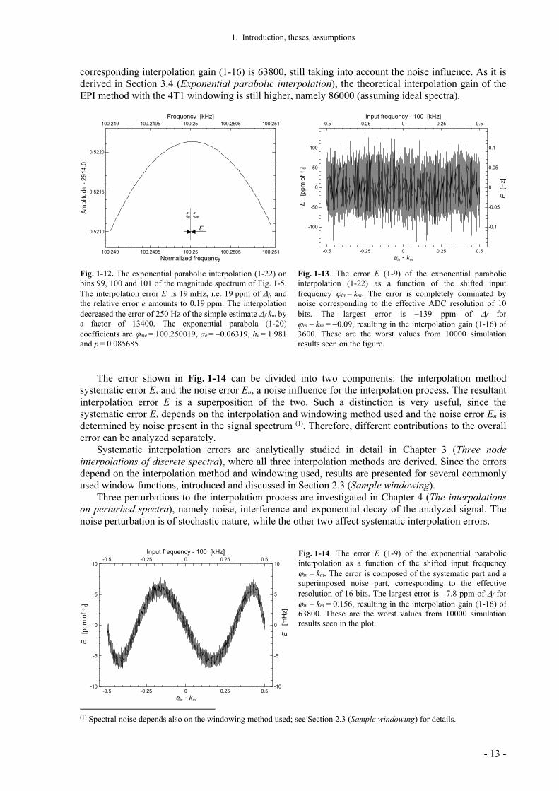
The input frequency of 100.25 kHz gives the EPI shape peak at 100.250019 kHz, resulting in the interpolation error E of 19 mHz, i.e. relative error e of 0.19 ppm, so 165 times less than the Gaussian interpolation method, 1700 times less than the parabolic interpolation method and 13400 times less than the DFT simple estimate f km (1-7).

The EPI algorithm allowed obtaining the frequency resolution comparable to the counting frequency measurement methods described in the beginning of this chapter. There was mentioned a good method of measuring the frequency of 100 kHz of a signal component consisted in counting the reference frequency periods of 100 MHz within a thousand of periods of the input signal, requiring 10 ms to achieve the resolution of 1 ppm. The example of Fig. 1-12 requires acquisition of 1024 samples, i.e. some 100 signal periods lasting 1 ms. With assumed another millisecond to perform necessary computations (2), the time of the frequency measurement by the spectral analysis and the EPI interpolation can be shorter and the resolution higher than these of the conventional counting methods, with the advantage that it can be used to measure frequencies of components of compound signals.

The interpolation error E of the EPI method with the 4T1 windowing, corresponding to Fig. 1-9 and Fig. 1-11 with PI and GI respectively, is shown in Fig. 1-13 as a function of in – km. In this case the error is completely determined by noise, related to the ADC resolution assumed in the example. The maximum error Emax is 139 ppm of f for in – km = 0.09. The EPI interpolation gain calculated with the worst-case error is 3600. It is less than achieved in the former example of Fig. 1-12, since Fig. 1-13 contains 10000 simulation results (Fig. 1-12 only one), so the probability of getting bigger errors is correspondingly increased.

It can be concluded that the ADC resolution Rc of 12 bits used for the presented example is not sufficient to get the most from the EPI method. Note also that the component of interest constitutes only 25 % of the total signal amplitude, so the effective digitization resolution Re is only 10 bits, and the remaining two bits are used to separate the component from its background.

The example of Fig. 1-13 is repeated with the converter resolution Rc increased to 18 bits, i.e. effective resolution Re of 16 bits for the component of interest. The results are shown in Fig. 1-14. With the resolution increased, it can be seen also the interpolation systematic error with still some noise superimposed. The maximum error is Emax = 7.8 ppm of f for in – km = 0.156. As it is shown on the right vertical axis of the plot, the maximum error corresponds to 7.8 mHz, assuring measurement of the input frequency of 125.25 kHz with the relative resolution of 0.06 ppm. The

(1) Section 3.4 (Exponential parabolic interpolation) contains related derivations and exponent values for other windowing methods. (2) It has to be performed: windowing of the samples, FFT, spectrum module calculation, search of the peak, and finally, the interpolation itself. To compute all the steps a fraction of a millisecond is a conservative estimate even for already quite old hardware.


- 13 -

corresponding interpolation gain (1-16) is 63800, still taking into account the noise influence. As it is derived in Section 3.4 (Exponential parabolic interpolation), the theoretical interpolation gain of the EPI method with the 4T1 windowing is still higher, namely 86000 (assuming ideal spectra).

100.249 100.2495 100.25 100.2505 100.251Normalized frequency

0.5210

0.5215

0.5220

Am

plitu

de -

291

4.0

fmefin

E

100.249 100.2495 100.25 100.2505 100.251

Frequency [kHz]

-0.5 -0.25 0 0.25 0.5-

-100

-50

0

50

100

[pp

m o

f ]

-0.5 -0.25 0 0.25 0.5


-0.1

-0.05

0

0.05

0.1

[

Hz]

km

E

E

in

f

Fig. 1-12. The exponential parabolic interpolation (1-22) on bins 99, 100 and 101 of the magnitude spectrum of Fig. 1-5. The interpolation error E is 19 mHz, i.e. 19 ppm of f, and the relative error e amounts to 0.19 ppm. The interpolation decreased the error of 250 Hz of the simple estimate f km by a factor of 13400. The exponential parabola (1-20) coefficients are me = 100.250019, ae = 0.06319, he = 1.981 and p = 0.085685.

Fig. 1-13. The error E (1-9) of the exponential parabolic interpolation (1-22) as a function of the shifted input frequency in – km. The error is completely dominated by noise corresponding to the effective ADC resolution of 10 bits. The largest error is 139 ppm of f for in – km = 0.09, resulting in the interpolation gain (1-16) of 3600. These are the worst values from 10000 simulationresults seen on the figure.

The error shown in Fig. 1-14 can be divided into two components: the interpolation method systematic error Es and the noise error En, a noise influence for the interpolation process. The resultant interpolation error E is a superposition of the two. Such a distinction is very useful, since the systematic error Es depends on the interpolation and windowing method used and the noise error En is determined by noise present in the signal spectrum (1). Therefore, different contributions to the overall error can be analyzed separately.

Systematic interpolation errors are analytically studied in detail in Chapter 3 (Three node interpolations of discrete spectra), where all three interpolation methods are derived. Since the errors depend on the interpolation method and windowing used, results are presented for several commonly used window functions, introduced and discussed in Section 2.3 (Sample windowing).

Three perturbations to the interpolation process are investigated in Chapter 4 (The interpolations on perturbed spectra), namely noise, interference and exponential decay of the analyzed signal. The noise perturbation is of stochastic nature, while the other two affect systematic interpolation errors.

-0.5 -0.25 0 0.25 0.5-

-10

-5

0

5

10

[pp

m o

f ]

-0.5 -0.25 0 0.25 0.5


-10

-5

0

5

10

[m

Hz]

km

E

E

in

f

Fig. 1-14. The error E (1-9) of the exponential parabolic interpolation as a function of the shifted input frequency in – km. The error is composed of the systematic part and a superimposed noise part, corresponding to the effective resolution of 16 bits. The largest error is 7.8 ppm of f for in – km = 0.156, resulting in the interpolation gain (1-16) of 63800. These are the worst values from 10000 simulation results seen in the plot.

(1) Spectral noise depends also on the windowing method used; see Section 2.3 (Sample windowing) for details.


- 14 -

The goal of the previous examples was to illustrate the following Thesis 2 of this dissertation:

T2 If the conditions of thesis T1 are satisfied, then the frequency fin of a sinusoidal component sin(t) of a compound signal s(t) can be estimated from the discrete magnitude spectrum S[k] of the signal sample sequence s[n] with resolution improved by performing an interpolation on the spectrum bins of indexes km – 1, km and km + 1, where km is the index of the largest bin corresponding to the component sin(t). The abscissa of the interpolating curve maximum is the improved estimate of the input frequency fin. In the dissertation three methods are studied and characterized by the following expressions for the component frequency estimate: Parabolic interpolation (PI)

]1[]1[][22

]1[]1[

mmm

mmmfmp kSkSkS

kSkSkΔf

Gaussian interpolation (GI)

])1[ln(])1[ln(])[ln(22

])1[ln(])1[ln(

mmm

mmmfmg kSkSkS

kSkSkΔf

Exponential parabolic interpolation (EPI)

p

mp

mp

m

pm

pm

mfmekSkSkS

kSkSkΔf

]1[]1[][22

]1[]1[

where power p is specific for each windowing method. The interpolation gain for each method depends on windowing used and the spectral level of component sin(t) with respect to noise and interference biasing the concerned bins. For commonly used window functions the potential gains are in the order of ten, one hundred and more than ten thousand for PI, GI and EPI methods, respectively.

Chapter 2


2. From an analogue signal to its discrete spectrum

In this chapter there are briefly described all important operations necessary to obtain the discrete Fourier spectrum of an analogue signal, which is suitable for interpolation algorithms outlined in the Introduction and developed further in the next chapter. Sampling and digitization processes are sketched, then the Fourier and discrete Fourier transforms, and finally windowing. All these operations are well known, and the main task of this chapter is to express this common knowledge with notation specific to this dissertation, in particular with using the normalized frequency instead of the natural frequency f. By this convention the author introduces a link between the continuous and discrete spectra, which in turn simplifies and makes more coherent the derivations elaborated in the further chapters.

2.1. Analogue to digital conversion

The analogue to digital conversion consists of two operations: signal sampling and digitization. In practice both operations are done by a hardware block, an Analogue to Digital Converter (ADC), which is usually realized as an integrated circuit.

In the sampling process a continuous signal s(t) is converted into a sequence s[n], where n is an integer number. In this work only the uniform ideal sampling is considered, linking s(t) and s[n] as

)(][ sTnsns (2.1-1)

In this dissertation time interval Ts is called the sampling period and its reciprocal fs = Ts-1 – the

sampling frequency. In the digitization process sample values are converted into integer numbers, so each sample has

amplitude being a multiple of a value characterizing the ADC resolution. If the ADC has resolution of Rc bits and a signal of amplitude A fills entirely its input dynamic range, the sequence of digitized samples can be described as

][

2

)(2round][ ns

A

vRns LSB

c

D (2.1-2)

where round(x) (1) means the rounded value of x and vLSB is the amplitude corresponding to the least significant bit (LSB) of the ADC. The digital amplitude corresponding to analogue vLSB is 1. Whenever necessary, the digital unitary amplitude will be denoted by LSB for better clarity.

During the digitization process signal samples with the amplitudes being real numbers are approximated by integer values. This makes the analogue and digitized samples different and the difference can be interpreted as noise, called the quantization noise. As the phenomenon is widely discussed in the literature, here there are provided only a few basic formulae in order to make coherent further derivations, especially these of section 4.1 (Influence of noise on the interpolation methods).

The quantization noise of a signal sequence has the amplitude evenly distributed between 0.5 LSB, providing that the amplitude of the sampled signal is much larger than vLSB. The root-mean-square (RMS) amplitude of the quantization noise is

LSB12

1}{ rmsnqv (2.1-3)

(1) round(5.49) = 5, round(5.50) = 5, round(5.51) = 6.

2.1. Analogue to digital conversion

- 16 -

In the frequency domain this noise is in practice uniformly distributed over the full available bandwidth, i.e. between 0 (DC) and half of the sampling frequency (the Nyquist frequency). If a sinusoidal signal fills fully the input dynamic range of an ideal ADC of resolution of Rc bits, i.e. the whole converter noise is caused by the quantization noise vnq, then the signal to noise ratio (SNR) of the digitized signal is

c

c

R

R

rmsnq

rmss

v

vSNR 2

2

6

LSB12

122

LSB2

}{

}{ (2.1-4)

In the literature the above expression is often given in decibels and then

76.102.62

6lg20)2lg(202

2

6lg20]dB[

cc

R RRSNR c (2.1-5)

If the input signal itself contains some “intrinsic” noise of amplitude {vni}rms, or such noise is introduced by the (real world) ADC converter in addition to the usual quantization noise, then the SNR of the digitized signal is

1

}{12

22

6

12

1}{

22

2

}{}{

}{2222

LSB

rmsni

R

LSB

rmsni

R

rmsnqrmsni

rmss

v

v

v

vvv

vSNR

c

c

(2.1-6)

For a given SNR of the digitized signal one can calculate the corresponding resolution of a hypothetical ADC, which would yield the observed SNR, with assumed noiseless input signal. This hypothetical resolution can be calculated by rearranging (2.1-4). In the dissertation the quantity is referred to as the effective resolution (1) Re and is defined as

SNRRe 3

6log2 [bits] (2.1-7)

The effective resolution is a convenient measure of SNR. By inserting (2.1-6) into (2.1-7) one can calculate Re when some input signal noise vni is also involved, and

1

}{12log

2

1

1}{

12

2log

2

222LSB

rmsnic

LSB

rmsni

R

e v

vR

v

vR

c

(2.1-8)

Solving for {vni}rms / vLSB gives

(1) In the literature a similar quantity, called equivalent number of bits (ENOB), is used. It is reserved to characterize only an ADC. In the dissertation the term effective resolution takes into account both, the ADC and input signal noise.


- 17 -

3

12

2

1}{ )(2

ec RR

LSB

rmsni

v

v (2.1-9)

From this one can calculate that the effective resolution of the digitized signal degrades by one bit (i.e. Rc – Re = 1) when the RMS of the input signal noise is half of vLSB (i.e. {vni}rms = vLSB/2). This information is used in Section 4.1 (Influence of noise on the interpolation methods).

If the ADC input signal noise is greater than vLSB, then the unity in (2.1-8) can be neglected and

79.1}{

log12log2

1}{log 222

LSB

rmsnic

LSB

rmsnice v

vR

v

vRR (2.1-10)

2.2. Fourier and Discrete Fourier Transforms

- 18 -


In this work the Fourier Transform (FT) Ŝ(f) (1) of a continuous-time signal s(t) is defined with the notation used in this paper as

dttftstsFTfS )π2jexp()()()(ˆ (2.2-1)

Similarly, the Discrete Fourier Transform (DFT) is defined as

1

0

π2jexp][][ˆ

N

n N

nknskS (2.2-2)

For this dissertation it is very important that an N-point DFT can be thought of as a result of the

uniform sampling of the FT at frequencies being integer multiples of f

1

0

1

0

π2jexp][)π2jexp(][)(ˆ][ˆ

N

n

N

nfsf N

nknsnkTnskSkS (2.2-3)

where the DFT input data are samples of the continuous signal of duration Nf, taken as the input for the FT [Zieliński 2005]. The quantity

LTNN

fΔ

s

sf

11 (2.2-4)

is the discrete spectrum bin spacing (2), setting its frequency resolution.

Note that, since in practice one has to deal with signals of finite extend, a window function is always involved in this DFT-FT relationship. In the simplest case, the function is the “natural” rectangular window, which cuts out the part of the continuous input signal taken for the FT and of the sample set for the DFT. The aim of using other, more sophisticated windows is to minimize side effects of the periodic nature of the DFT, i.e. to cope with the fact that the DFT period (i.e. the length of the transform input) in general does not fit to the input signal periodicity. If (2.2-2) is considered as a transform of infinitely long signal sample sequence s[n]

n N

nknskS

π2jexp][][ˆ (2.2-5)

then the infinite summation can be divided into an infinite number of summations, each of length N, as

(1) Complex valued spectra are denoted with dashes Ŝ(f) (or Ŝ() in the case of normalized frequency) and the symbol S(f) (as well as S()) is reserved for magnitude spectra, much more often used in the dissertation. (2) The author uses systematically the term bin spacing, originating in the fact that, as discussed in this section, discrete spectra can be thought of as samples of their corresponding continuous spectra, and therefore, discrete spectrum bins have no with. However, in the literature often discrete spectrum bins are considered as “rectangles” of with f, (most likely) originating in understanding discrete spectra as banks of filters, i.e. each bin corresponds to a filter. The term “discrete spectrum bin” could have been replaced by “discrete spectrum line” to better correspond to the author’s picture of discrete spectra. It was not done so to stay compatible with the literature.


- 19 -

a

NaN

aNn

N

Nn

N

n

Nnn

N

nkns

N

nkns

N

nkns

N

nkns

N

nknskS

1

121

0

1

π2jexp][

π2jexp][

π2jexp][

π2jexp][

π2jexp][][ˆ

(2.2-6)

If the inner summation index is shifted by –a N and the summation order is interchanged, one gets

1

0

π2jexp][][ˆ

N

n a N

nkaNnskS (2.2-7)

which is the DFT of N samples of infinitely long sequence

a

aNnsns ][][' (2.2-8)

This infinitely long sequence is periodic with the period of N demonstrating that the DFT “considers” the input sample sequence to be periodically replicated to the infinite extent with the period of the length of the transform input. This is compatible with the fact that the finite length transform (2.2-2) can be considered as a transform of one period of length N of an infinitely long input sequence (2.2-8). This conclusion explains the necessity of windowing, described in the next section, which helps to make a smooth fit between the adjacent periods of the hypothetical infinite length input sequence. In this dissertation one deals with interpolations of discrete magnitude spectra, obtained through the DFT. To investigate interpolation efficiencies it is necessary to know spectra values between its bins, so to know continuous spectra. As it was already mentioned in this section, the DFT can be thought of as a sampled version of the FT of a signal sample sequence, so often in this work efficiency of a DFT spectra interpolation is investigated on equivalent FT spectra. Since the DFT and FT have different abscissae, i.e. the DFT argument is an index going from 0 to N–1, and the FT argument is just ordinary frequency, it is convenient to scale the argument of one transform to be compatible with the other. It was decided to scale the usual frequency f of the FT by replacing it by a real-valued quantity, denoted by and referred to as the normalized frequency (1)

LffNTf

fN

fs

sf

(2.2-9)

Substituting f = /L into (2.2-1) one gets

dt

L

ttsS π2jexp)()(ˆ (2.2-10)

Therefore, FT of variable is the ordinary FT but with normalized (condensed) time scale by a factor of L – the observation interval of the input signal and the length of the signal taken for the transform calculation.

Using (2.2-9), an analogue signal of frequency fin

(1) Often in the literature the term normalized frequency is used for the quotient f/fs [Zieliński 2005] and is usually denoted by F. The normalized frequency as used in this dissertation is, therefore, N times larger, = N f/fs = N F.


- 20 -

)π2sin()( tfAts inin (2.2-11)

can be written as

)π2sin()π2sin()( L

tAtfAts ininin (2.2-12)

confirming the above conclusion for the time domain.

If the signal (2.2-11) is uniformly sampled at the rate of frequency fs=Ts-1 and N samples are taken,

then the end of the signal sample sequence sin[n] is

insinsinin ANTfATNsNs π2sinπ2sin)(][ (2.2-13)

where in /N was substituted for fin

Ts, according to (2.2-9). As seen in (2.2-13), normalized frequency in can be considered as the number of periods of signal sin(t) (or in general, of a sinusoidal component of a compound signal) falling into the sampling interval L = N Ts, i.e. instead of taking second as the unit period, one takes L. The in integer part is the number of whole fin periods falling into L and this is the index kin of the corresponding discrete spectrum bin. The goal of the interpolation methods studied in this dissertation is to evaluate the in fractional part, the difference in – kin, corresponding to the fin period fractional part, completing the time Ts kin to the whole sampling interval L. This information is neglected when using discrete spectra for “classical” frequency measurements, with no interpolation.

Since s(t) in (2.2-10) is taken for the transform only within the time interval [0,L, this relation can be rewritten as

L

dtL

ttsS

0

π2jexp)()(ˆ (2.2-14)

so s(t) is considered to be a periodic replication of its fraction within the interval [0,L. Taking index k as the integer truncation of real quantity as well as substituting L = N Ts and t = Ts n into (2.2-14) yields

1

0

1

00

π2jexp][

π2jexp][)(

π2jexp)(ˆ

N

n

NTN

ss

ss

N

nkns

ndN

nknsnTd

TN

nTknTskS

s

(2.2-15)

From this one can conclude that the DFT (2.2-2) can be thought of as the continuous spectrum (2.2-14) of variable , which is sampled at integer values. This is the main reason for introducing quantity as the common variable for continuous and discrete spectra. If the DFT is calculated according to (2.2-2), then the computing cost is in the order of N2 complex multiplications and N2 complex additions. In practice the DFT is almost always calculated according to a version of the Fast Fourier Transform (FFT) algorithm, reducing the computation effort to the order of

NN

2log2

cost computing FFT (2.2-16)

complex multiplications and N log2N complex additions in the case of the Decimation in Time (DIT) radix-2 version of the FFT algorithm.


- 21 -

Relation (2.2-16) is an estimation only, as the actual computational complexity depends on the version of the FFT algorithm, its implementation and whether the transform input is a complex or a real sequence [Zieliński 2005]. For simplicity, in this dissertation FFT computing costs will be estimated using formula (2.2-16).

2.3. Sample windowing

- 22 -


In the previous section it was shown that the DFT “considers” the input samples to be periodic with the period equal to the length of the transform input. This is equivalent to have as the transform input a hypothetical periodic sequence constructed from the analyzed sample sequence replicated along the whole time axis. Almost always the boundaries of the period of this hypothetical sequence do not enclose an integer number of analyzed component periods. In consequence, the boundaries of the replicated period do not fit each other and in the hypothetical sequence appear abrupt irregularities. In the frequency domain such artifacts appear as so-called spectral leakage [Bach, Meigen 1999], [Harris 1978]. The effect can be seen in Fig. 1-3 (Chapter 1, page 3), where the smaller spectral peak corresponding to a sinusoidal component is unusually wide while the bigger peak is nicely narrow. The explanations can be found in Fig. 1-2, showing N = 1024 samples of the corresponding signal. The signal contains two sinusoidal components of frequencies fin = 100.25 kHz (smaller amplitude) and fbg = 110.0 kHz (larger amplitude) sampled at the rate of fs = 1.024 MHz. The sampling window has duration L = 1 ms, therefore, the component of frequency fbg has exactly 110 periods within the sampling window and as such is not distorted. The component of frequency fin has 100 periods and one quarter as seen on the envelope being the beating product of frequency fbg – fin. This is why the spectral peak corresponding to the smaller component is affected by the spectral leakage. In the frequency domain it is as the energy from the component bin was leaking to adjacent bins – this is the origin of the phenomenon name. Another example of the spectral leakage effect and the influence of windowing is demonstrated below. N = 1024 full scale 12-bit samples of a signal containing two components of normalized frequencies 1 = 10.5 and 1 = 20.5, having much disparate amplitudes

1023 1022, ..., 1, 0,,π2sin001.0π2sin999.0][][][ 212112

n

N

n

N

nnsnsns (2.3-1)

are shown in Fig. 2-1, together with the sequence s12[n] replicated as seen by the DFT. The larger component has 10 and a half periods, so it is seen that the sequence boundaries do not fit each other resulting in abrupt irregularities between adjacent replicas. These irregularities appear as a strong spectral leakage in the corresponding magnitude spectrum shown in Fig. 2-2. The smaller component is not seen at all, drowned by the leakage from the stronger component.

0 256 512 768 1024Sample number

-2048

-1536

-1024

-512

0

512

1024

1536

2048

Am

plitu

de

0 50 100 150 200 250 300 350 400 450 500Bin number

-120

-100

-80

-60

-40

-20

0

Nor

mal

ized

mag

nitu

de

spec

trum

[dB

]

Fig. 2-1. Sample sequence (2.3-1) (black dots and magenta line) and its replicas (dashed line, green) as seen by the DFT.

Fig. 2-2. Magnitude spectrum of the time domain sequence shown in the plot on the left. It is seen a strong spectral leakage due to the fact that the replicas of the time domain sequence do not fit on the boundaries, resulting in abrupt irregularities.


- 23 -

In Fig. 2-3 sequence s12[n] is shown, but now windowed using 4T1 window (1-5). The window

attenuates the sequence gradually to zero at the boundaries so that they fit each other, resulting in a smooth curve built from replicas of windowed s12[n]. The spectrum magnitude of the windowed sequence shown in Fig. 2-4 contains two peaks corresponding to components 1 and 2 present in the input sequence. The smaller peak is nicely visible despite the fact that it is 60 dB (i.e. thousand times) smaller than the bigger one.

0 256 512 768 1024Sample number

-2048

-1536

-1024

-512

0

512

1024

1536

2048

Am

plitu

de

0 50 100 150 200 250 300 350 400 450 500Bin number

-120

-100

-80

-60

-40

-20

0

Nor

mal

ized

mag

nitu

de

spec

trum

[dB

]

Fig. 2-3. Sample sequence (2.3-1) (black dots and magenta line) windowed with the 4T1 window (red line) and their replicas (green line for the sequence and dashed red line for the window).

Fig. 2-4. Magnitude spectrum of the time domain sequence shown in the plot on the left. Windowing removed the spectral leakage effect seen in the corresponding plot of Fig. 2-2; please note same scales. It is seen the smaller component of the input sequence as well as noise originating in the quantization of the input samples.

Windows and their properties are a vast subject, which cannot and should not be elaborated in this work [Geckinli, Yavuz 1978], [Kulkarni 2000, 2001], [Kulkarni, Lahiri 1999], [Malocha, Bishop 1987], [Zieliński 2005]. An exhaustive description of this topic was given by Harris [1978] and Nuttal [1981]. In this dissertation some of the windows described therein are used. For all of them the author calculated the corresponding spectra and other parameters, utilized in further analysis. In this section some basic explanation is also given, necessary for clarity of this work. For the sake of simplicity analyses in this section are done on continuous time and frequency, but all results are also valid for their corresponding discrete equivalents. If a cosine normalized signal

2

))π2(jexp())π2(jexp()2cos()(

tftftfts inin

in (2.3-2)

is windowed by a window w(t – t0), then the spectrum of the windowed signal is.

)(ˆ2

)))(π2(jexp()(ˆ

2

)))(π2(jexp(

)π2jexp()()()}()({)(ˆ

00

00

inin

inin

w

ffWfft

ffWfft

dttftsttwtsttwFTfS

(2.3-3)

If the two spectral peaks of (2.3-3) do not influence each other, i.e. they are sufficiently apart to let their sidelobes decay, one can consider the module of one peak and then


- 24 -

)(2

1)(ˆ

2

)))(π2(jexp()( 0

1 ininin

w ffWffWfft

fS

(2.3-4)

The magnitude spectrum of a windowed sinusoidal component has therefore shape of the

magnitude spectrum of the window shifted to the frequency of the component. For this reason, the spectral shapes of the windows are crucial for spectral interpolation and define its properties, in particular the interpolation efficiency. Shapes of magnitude spectrum peaks do not depend on the window time position, so the position can be freely chosen to simplify calculations. Also the magnitude spectrum of a windowed sinusoidal component is independent of the component phase.

The 1/2 coefficient in (2.3-4) is the consequence of the fact that the window energy is shared in the frequency domain by two peaks. The coefficient can be also explained employing the modulation theorem for a cosine signal s(t), considered as the carrier, and a window w(t), considered as the modulation function.

Halves of the 12 windows used in this dissertation are plotted in Fig. 2-5. All parameters of the interpolation methods were calculated for each window except the rectangular one, which is included in this chapter only for comparison purposes. The proposed interpolation methods based on three nodes do not work well with this window. This is not considered as a large problem, as this window has very large, slowly decaying sidelobes, and therefore, is not appropriate for applications for which the interpolation methods are targeted. For the rectangular windowing other interpolation algorithms may be useful, e.g. those based on the use of two discrete spectrum bins [Asséo 1985], [Bartolini et al. 1995, 1996], [Donghai Li et al. 2001], [Grandke 1983], [Hikawa, Jain 1990], [Jain, Collins, Davis 1990].

0 0.1 0.2 0.3 0.4 0.5| Normalized time | [ ]

0

0.2

0.4

0.6

0.8

1

No

rma

lize

d a

mp

litu

de

[1/

]

L

L

rectangular

triangular

Gaussian r = 6

Gaussian r = 7

Gaussian r = 8

Hanning

Blackman

3T1

3T3

4T1

4T3

4T5

Fig. 2-5. Windows considered in this dissertation. They are symmetric, so only their halves are plotted to better reveal differences between the windows. The further paragraphs include window descriptions and the following figures – their corresponding magnitude spectra.

Since parameters of the interpolation algorithms are specific for a given windowing function, each window included in the dissertation required laborious recalculations of all parameters derived here.


- 25 -

For this reason it was necessary to make an arbitrary choice of windows to be used in this dissertation. Finally there were included a few “textbook” windows, serving as references, and the windows which are used in practice with the studied interpolation methods. However, equations derived in this work may be used to calculate parameters of the interpolation methods for any window.

Window spectral and noise properties are described in the following paragraphs and listed in Table 2-1. To simplify window comparisons, most of the columns of the table are visualized in the bar plots of Figures 2-6 and 2-7. Expressions for window functions and their spectra are provided in this section with the notation specific to the dissertation, using the normalized frequency .

The rectangular window is mentioned here only as a reference. The triangular window is reported for the fact that it is probably the simplest window for which the three-node interpolation algorithms are efficient as well as for comparison purposes. Gaussian windows for their slow sidelobe decay have more a theoretical than a practical meaning in this dissertation. They are included here for comparisons and for the fact that the GI method has the largest frequency resolution gains with these windows.

The windows which are considered by the author as the most appropriate for spectral analysis in tune measurement systems of particle accelerators are the weighted cosine ones. The windows are used in this dissertation for their very good spectral properties and the fact that they are described by simple functions, which can be easily generated in practical systems. Weighted cosine windows offer a wide choice of trade-offs between the most important window parameters: the spectrum main lobe width, the highest sidelobe and the sidelobe decay. One window from this family, namely 4T1, is systematically used in examples.

In practice the author uses either Hanning, 3T1 or 4T1 window, depending on the level of the undesirable background and its distance to the analyzed spectrum band. However, there is not the best window in all aspects and the choice of the optimal window should be done according to the requirements of the particular application. Often results are not that sensitive upon the window selection, relaxing the importance of the window choice. Rectangular window

The rectangular window, plotted in Fig. 2-5 together with other windows, is defined in this dissertation as

22

1)(

Lt

Lt

Ltwrtg 11 (2.3-5)

where 1(t) is the Heaviside's unit step function. The window magnitude spectrum, shown in Fig. 2-8, is

sin

)(rtgW (2.3-6)

The window amplitude is normalized to L in order to keep the window energy unitary. In this case the windowed signal energy is independent of the window length. This convention is used for all windows considered in this dissertation. For the spectral analysis in real systems the input signal is always of finite extent. The operation of cutting out an input signal interval can be modeled as applying the rectangular window function. This is why the rectangular window can be considered as being always present in all windowing methods. As seen in Fig. 2-8, the rectangular window spectrum (2.3-6) has large sidelobes, which in addition decay very slowly, only 6 dB/octave since Wrtg() -1. This means that a large spectral leakage is associated with the rectangular windowing, in fact the largest from all windows. If the frequency of a sinusoidal component is


- 26 -

2

11i

Lfin (2.3-7)

where L is the time interval of the spectrum analysis and i is an integer, then the component exhibits the strongest leakage and in this case its spectrum has the envelope described by (2.3-6). The spectrum magnitude of the rectangular window has the main lobe of width of two bins and, as it is explained in the next chapter, cannot be used for three node spectral interpolations. Rectangular windowing is considered in the paper only for comparison purposes. Its parameters are listed in Table 2-1, together with properties of other windows used in this dissertation. Triangular window

The triangular window, shown in Fig. 2-5, is defined in this paper as

L

ttwtw rtgtrg 21)()( (2.3-8)

where wrtg(t) is the rectangular window (2.3-5). The triangular window magnitude spectrum is

2

2

12

1sin

2

1)(

trgW (2.3-9)

and is plotted in Fig. 2-9. Its main lobe has width of four bins and as such is suitable for three node interpolations. This is probably the simplest window for which the presented interpolation methods work efficiently. As summarized in Table 2-1, the triangular window does not have very good spectral properties. Nevertheless, it is considered here for comparison purposes. Also, for its simplicity, it may be preferred in some systems, in particular those based on integer arithmetic. Gaussian windows (1)

Gaussian windows in this work are defined as

2

22

2

2

2exp)(

2exp)()(

L

rttw

ttwtw rtgrtggau

(2.3-10)

where the usual standard deviation is expressed as = L/r. Therefore, r is the window length in units of the standard deviation . In Fig. 2-5 three Gaussian windows are plotted, of length 6 (r = 6, i.e. Gaussian shape (2.3-10) is truncated at 3), 7 and 8. The magnitude spectrum of a Gaussian window the author calculated to be

r

r

r

r

rrWgau

22

j4erf

22

j4erf2exp

1)(

222 (2.3-11)

(1) In the literature these windows are also called truncated Gaussian windows.


- 27 -

where erf() is the error function generalized for a complex argument. The magnitude spectrum is plotted in Figures 2-10, 2-11 and 2-12 for the windows of r of 6, 7 and 8, respectively. The main lobes of the spectra are quite large and the sidelobes do not decay rapidly, only 6 dB/octave. This is why in this dissertation the Gaussian windows have more a theoretical than a practical meaning. They are considered here also for comparison purposes. Table 2-1 lists properties of the Gaussian windows of r of 6, 7 and 8. Weighted cosine windows The weighted cosine windows are considered here as the most appropriate for practical applications in tune measurement systems based on analyzing discrete spectra. These windows are simple and offer a wide choice of trade-offs between the most important window parameters. In the dissertation there are used weighted cosine windows described by Nuttall [1981] and having fast sidelobe asymptotic fall-off at least of 18 dB/octave. The windows have the form of

3

0

2cos)()(

iirtgwcs t

L

ictwtw

(2.3-12)

with two, three or four terms. Their magnitude spectra the author calculated to be

3

022

)1()sin()(

i

i

i

wcs i

cW

(2.3-13)

The names and coefficients of the windows used in this dissertation are listed in Table 2-2, their

shapes are shown in Fig. 2-5 and spectra depicted in Figures 2-13 to 2-19. For the windows derived by Nuttal [1981] the author uses a three-character naming convention. The first digit corresponds to the number of nonzero terms in (2.3-13), which is followed by “T” standing for “term”, and the last digit is the number of window continuous derivatives. From a window name in this convention one can deduce immediately general window properties, such as main lobe width and the slope of the asymptotic sidelobe decay.

All the windows with continuous first derivative have the sidelobe asymptotic fall-off of 18 dB/octave, those with continuous third derivative have sidelobes decaying asymptotically as rapidly as 30 dB/octave, and the window with continuous fifth derivative has the fall-off of 42 dB/octave. It is seen that the main lobe gets wider and sidelobes smaller with increasing number of terms. Windows with faster asymptotic fall-off have larger first sidelobes than those with slower decay. Therefore, rapidly decaying windows are good for applications with large interferences located further from the band of interest. Similarly, windows with small sidelobes are preferred for applications with interferences located closer. Note that in Table 2-1 maxima of the largest sidelobes are given after = 8 and =16. At these distances from the main lobe center the sidelobes in most cases do not reach yet the asymptotic decay, so the difference between these two numbers is an estimate of the sidelobe decay there. Numbers form 6 columns of Table 2-1 are visualized on bar plots in Figures 2-6 and 2-7, helping in comparing parameters of the windows. Window noise properties As window functions get steeper, the main lobes of the corresponding spectra increase their width and, in consequence, noise power collected by the lobes increases. This explains the fact that each explicit windowing (that is except the rectangular one) deteriorates the frequency domain signal to noise ratio as compared to the rectangular windowing. A convenient measure of the noise performance


- 28 -

degradation by a window is so-called equivalent noise bandwidth (ENBW). Since the parameter is used in the dissertation, Table 2-1 lists its value for all described windows. The ENBW is defined as the spectral width in bins of a hypothetical rectangle filter with coherent gain equal to the gain of the window, which would introduce the same amount of noise

gaincoherent window

windowby the gatheredpower noiseENBW (2.3-14)

As the ENBW for the rectangular window is 1, the quantity can be thought of as the “noise deterioration factor” with respect to the rectangular window.

Employing the Parseval's theorem, the noise energy collected by a window is

tdtwL

L

n

2/

2/

2)( windowby the gatheredenergy noise (2.3-15)

where n is the noise energy density, here considered as a constant.

The window coherent gain can be expressed as

22/

2/

2

)()(gaincoherent window

tdtwtdtwL

L

(2.3-16)

so the ENBW normalized to the noise energy per unit bandwidth (i.e. discrete spectrum bin) is

22/

2/

2/

2/

2 )()(

tdtwdttwENBW

L

L

L

L

(2.3-17)

As listed in Table 2-1, the ENBW varies from 1.0 to 2.3 for the widest window 4T5, so the noise

properties can be deteriorated significantly. This is the price for improving the spectral leakage, which is done by, in fact, attenuating the signal.


- 29 -

Table 2-1. Most important properties of the window functions used in this dissertation. Numbers from 6 columns are visualized on bar plots in Figures 2-6 and 2-7, helping in comparing parameters of the windows.

Window W

(0)

(coh

eren

t gai

n)

Hig

hest

sid

elob

e [d

B]

Asy

mpt

otic

fal

l-of

f [d

B/o

ctav

e]

Side

lobe

af

ter

= 8

[d

B]

Side

lobe

af

ter

= 1

6 [d

B]

3 dB

Ban

dwid

th

[bin

s]

6 dB

Ban

dwid

th

[bin

s]

Equ

ival

ent n

oise

ba

ndw

idth

(E

NB

W)

[bin

s]

Rectangular 1.000 -13.3 6 -28.5 -34.3 0.89 1.21 1.000

Triangular 0.500 -26.5 12 -46.0 -57.1 1.28 1.77 1.333

Gaussian r = 6 0.417 -56.1 6 -60.5 -65.9 1.60 2.26 1.702

Gaussian r = 7 0.358 -71.0 6 -73.7 -78.8 1.86 2.62 1.977

Gaussian r = 8 0.313 -87.6 6 -89.3 -94.1 2.12 3.00 2.257

Hanning 0.500 -31.5 18 -65.5 -82.9 1.44 2.00 1.500

Blackman 0.420 -58.1 18 -73.6 -90.5 1.64 2.30 1.727

3T1 0.409 -64.2 18 -76.2 -92.8 1.69 2.36 1.772

3T3 0.375 -46.7 30 -90.1 -119.4 1.85 2.59 1.944

4T1 0.356 -93.3 18 -94.4 -107.6 1.92 2.69 2.021

4T3 0.339 -82.6 30 -98.2 -126.4 2.02 2.83 2.125

4T5 0.313 -60.9 42 -106.8 -148.7 2.19 3.07 2.310

Table 2-2. Coefficients of the weighted cosine windows used in this dissertation.

Window c0 c1 c2 c3 Comments

Hanning 1/2 1/2 0 0 2-term, continuous 1st derivative

Blackman 0.42 0.50 0.08 0 3-term, continuous 1st derivative

3T1 0.40897 0.5 0.09103 0 3-term, continuous 1st derivative

3T3 3/8 1/2 1/8 0 3-term, continuous 3rd derivative

4T1 0.355768 0.487396 0.144232 0.012604 4-term, continuous 1st derivative

4T3 0.338946 0.481973 0.161054 0.018027 4-term, continuous 3rd derivative

4T5 10/32 15/32 6/32 1/32 4-term, continuous 5th derivative


- 30 -

-160

-140

-120

-100

-80

-60

-40

-20

0

Re

cta

ng

ula

r

Tri

an

gu

lar

Ga

uss

ian

r =

6

Ga

uss

ian

r =

7

Ga

uss

ian

r =

8

Ha

nn

ing

Bla

ckm

an

3T

1

3T

3

4T

1

4T

3

4T

5

Highest sidelobe [dB]

Sidelobe after 8th bin [dB]

Sidelobe after 16th bin [dB]

Fig. 2-6. Window spectral properties on a bar plot. The bars are made from three columns of Table 2-1. Differences between bars in each triplet describe the window sidelobe fall-off.

0

0.5

1

1.5

2

2.5

3

3.5

Re

cta

ng

ula

r

Tri

an

gu

lar

Ga

uss

ian

r =

6

Ga

uss

ian

r =

7

Ga

uss

ian

r =

8

Ha

nn

ing

Bla

ckm

an

3T

1

3T

3

4T

1

4T

3

4T

5

3 dB BW [bins]

6 dB BW [bins]

ENBW [bins]

Fig. 2-7. Window properties on a bar plot. The bars are made from three columns of Table 2-1. Note that the equivalent noise bandwidth ENBW and the 3 dB main lobe width are similar for each window.


- 31 -

0 4 8 12 16 20Normalized frequency

-100

-80

-60

-40

-20

0

Nor

mal

ized

mag

nitu

de s

pect

rum

[dB

]

Rectangular

0 4 8 12 16 20

Normalized frequency

-100

-80

-60

-40

-20

0

Nor

mal

ized

mag

nitu

de s

pect

rum

[dB

]

Triangular

Fig. 2-8. Magnitude spectrum of the rectangular window.

Fig. 2-9. Magnitude spectrum of the triangular window.


-100

-80

-60

-40

-20

0

Nor

mal

ized

mag

nitu

de s

pect

rum

[dB

]

Gaussian= 6r

0 4 8 12 16 20


-100

-80

-60

-40

-20

0N

orm

aliz

ed m

agni

tude

spe

ctru

m [

dB]

Gaussian= 7r

Fig. 2-10. Magnitude spectrum of the Gaussian window of length 6 (i.e. truncated at 3).

Fig. 2-11. Magnitude spectrum of the Gaussian window of length 7 (i.e. truncated at 3.5).


-100

-80

-60

-40

-20

0

Nor

mal

ized

mag

nitu

de s

pect

rum

[dB

]

Gaussian= 8r

0 4 8 12 16 20


-100

-80

-60

-40

-20

0

Nor

mal

ized

mag

nitu

de s

pect

rum

[dB

]

Hanning

Fig. 2-12. Magnitude spectrum of the Gaussian window of length 8 (i.e. truncated at 4).

Fig. 2-13. Magnitude spectrum of the Hanning window.


- 32 -


-100

-80

-60

-40

-20

0

Nor

mal

ized

mag

nitu

de s

pect

rum

[dB

]

Blackman

0 4 8 12 16 20


-100

-80

-60

-40

-20

0

Nor

mal

ized

mag

nitu

de s

pect

rum

[dB

]

3T1

3-term, cont. 1st derivative

Fig. 2-14. Magnitude spectrum of the Blackman window.

Fig. 2-15. Magnitude spectrum of the weighted cosine window with 3 terms and continuous 1st derivative (3T1).


-140

-120

-100

-80

-60

-40

-20

0

Nor

mal

ized

mag

nitu

de s

pect

rum

[dB

]

3T33-term, cont. 3rd derivative

0 4 8 12 16 20


-140

-120

-100

-80

-60

-40

-20

0

Nor

mal

ized

mag

nitu

de s

pect

rum

[dB

]

4T14-term, cont. 1st derivative

Fig. 2-16. Magnitude spectrum of the weighted cosine window with 3 terms and continuous 3rd derivative (3T3).

Fig. 2-17. Magnitude spectrum of the weighted cosine window with 4 terms and continuous 1st derivative (4T1)


-140

-120

-100

-80

-60

-40

-20

0

Nor

mal

ized

mag

nitu

de s

pect

rum

[dB

]

4T34-term, cont. 3rd derivative

0 4 8 12 16 20


-160

-140

-120

-100

-80

-60

-40

-20

0

Nor

mal

ized

mag

nitu

de s

pect

rum

[dB

]

4T54-term, cont. 5th derivative

Fig. 2-18. Magnitude spectrum of the weighted cosine window with 4 terms and continuous 3rd derivative (4T3)

Fig. 2-19. Magnitude spectrum of the weighted cosine window with 4 terms and continuous 5th derivative (4T5)

Chapter 3


3. Three node interpolations of discrete spectra

This chapter contains a detailed description of the methods of improving frequency resolution of discrete Fourier spectra. First section deals with shapes of window spectrum main lobes, on which the interpolation process takes place. The following three sections describe the parabolic, Gaussian and exponential parabolic interpolation methods. For all three algorithms interpolation systematic errors and corresponding gains are calculated. In this chapter perfect spectra are assumed, i.e. not affected by noise, interference or other defects and their shapes depend only on the window applied prior to spectra calculation. Influence of spectrum perturbations on interpolation efficiency is studied in the next chapter.

As already sketched in the Introduction, the interpolation methods studied in this dissertation can improve frequency resolution of discrete spectra by a few orders of magnitude. It may seem that this is not compatible with the uncertainty theorem, since such high-resolution results can be obtained when observing analyzed signals for relatively short time intervals. In theory, for infinitely precise frequency measurements it is needed to know the full signal history. However, the full knowledge of the signal history is something different than observing the signal for infinitely long time. In particular, for a sinusoidal signal with the constant frequency and amplitude, even a finite duration observation can yield information about the signal full history, as the signal is assumed to never change. Therefore, in such a case the signal exact frequency can be evaluated without breaking the uncertainty theorem. In other words, for the interpolation methods studied in this dissertation it is assumed a model, i.e. analyzed components are sinusoidal, and the methods evaluate the parameter of this model, i.e. frequency. Summarizing, large frequency resolution improvements offered by the studied interpolation methods concern only sinusoidal signal components, whose frequency can be considered as constant during the acquisition (1).

The discussed algorithms are based on the use of discrete Fourier spectra and it is assumed that each interpolated peak is resolved in the analyzed spectrum. There are other powerful methods of estimating signal spectra, such as maximum likelihood, parametric and subspace methods [Bonacci, Mailhes, Djuric 2003], [Choi 1997], [Gu 1993], [Kay, Marple 1981], [Kay, Shaw 1988], [Morishima 1986], [Rife, Boorstyn 1974], [Villalba, Walker 1989], [Zieliński 2005]. These methods can offer better frequency resolution, spectral resolution (understood as the ability to resolve close components) and better performance in presence of noise than the classical Fourier analysis. However, for many practical applications these methods are too complex and require too much computing. In such cases the Fourier analysis, in most cases done through the very efficient FFT algorithm, followed by the simple interpolation algorithms studied in this dissertation can be used.

3.1. Main lobe shapes of window spectra

As it was described in Section 2.3 (Sample windowing), windowing applied to a signal containing a sinusoidal component can be thought of as a modulation, which shapes the spectral peak corresponding to the component to the shape of the window spectrum, located at the component frequency. When using discrete spectra for frequency measurement it is necessary to evaluate the peak maximum abscissa from a few shape samples. Furthermore, in practice the number of samples is limited by the fact that the further the sample from the maximum, the smaller the bin amplitude and the smaller signal to noise ratio. For this reason, in this dissertation only methods taking into account three bins are considered. As it will be shown, the systematic error related to the interpolation methods is small enough to improve discrete spectra resolution by up to some five orders of magnitude. In practice the noise and other spectra perturbations are much larger that this systematic error and they

(1) As far as the author can see, this assumption has to be valid for each frequency measurement method yielding one number as the result. Otherwise, what it is measured is a sort of an average over the acquisition period.

3.1. Main lobe shapes of window spectra

- 34 -

limit the interpolation gain achievable in practice. Hence, there is little point in decreasing further the systematic error at the expense of complicating necessary calculations. When using only three discrete spectrum bins to find the abscissa of the peak of the corresponding continuous spectrum, this peak has to have width of at least three bins, i.e. 3 f. This is required to resolve the case with the measured frequency located exactly between two discrete spectrum bins. In such situation, depicted in the Introduction in Fig. 1-7 (blue line for the fmp3 case), the corresponding continuous peak has three discrete (spectrum) samples with one located 1.5 f from the peak maximum abscissa. Since the peak is symmetric, this puts the lower bound of the peak width on exactly 3 f. This is why, apart of reasons explained in Section 2.3 (Sample windowing), the rectangular window, having main lobe of width of 2 f, should not be used for discrete spectra frequency measurements and will not be considered in this chapter. The goal of the interpolations is to evaluate the abscissa of the spectral peak maximum corresponding to the signal component whose frequency is to be evaluated and to do so only from three peak samples. The spectral peak shape corresponds to the spectrum of the window function applied to the signal samples, so the interpolation process efficiency depends on how close one can substitute the peak shape by the interpolating curve. As already stated, spectral peaks are interpolated on three spectral bins and only within this band their shapes are important, as long as all spectrum imperfections are not taken into account. Special cases of perturbed spectra are considered in the individual sections of the next chapter. Shapes of the main lobes of the windows considered in this dissertation are plotted in Fig. 3-1 and coefficients of their Maclaurin power series expansions are listed in Table 3-1, with the coefficients normalized to the one upon 2. The shapes are even functions of the normalized frequency .

0 0.25 0.5 0.75 1 1.25 1.5| Normalized frequency |

0

0.2

0.4

0.6

0.8

1

Win

do

w n

orm

aliz

ed

ma

gni

tud

e sp

ect

rum

Hanning

Blackman

3T1

3T3

4T1

4T3

4T5

triangular

Gaussian r = 6

Gaussian r = 7

Gaussian r = 8

Fig. 3-1. Main lobes of window magnitude spectra, shown up to | | = 1.5, the part which is important for the interpolation methods studied in this dissertation.

Note that the wider the peak, the smaller content of higher order components in the expansions. The interpolation algorithms take into account a limited number of power series components, so it can be expected that the windows giving wider peaks are better to achieve small interpolation errors.


- 35 -

Furthermore, as it will be shown, interpolation efficiency can be improved by widening the spectral peaks using nonlinear transformations. This results in decreasing the higher order component content in the spectrum peaks and allows better reconstructions of the peak shapes using only their three samples. Table 3-1. Coefficients of Maclaurin power series expansions of the magnitude spectra main lobes of the windows considered in this dissertation; the coefficients are normalized to a2.

Window a0 a2 a4 a6 a8 a10

Triangular -1.215854 1.000000 -0.328987 0.057982 -0.006358 0.000475

Gaussian r = 6 -1.873741 1.000000 -0.251625 0.038578 -0.003982 0.000293

Gaussian r = 7 -2.497634 1.000000 -0.196363 0.024704 -0.002195 0.000145

Gaussian r = 8 -3.245753 1.000000 -0.153331 0.015474 -0.001142 0.000065

Hanning -1.550546 1.000000 -0.258644 0.037125 -0.003418 0.000220

Blackman -1.991727 1.000000 -0.219865 0.028319 -0.002420 0.000148

3T1 -2.092066 1.000000 -0.211045 0.026317 -0.002193 0.000131

3T3 -2.532068 1.000000 -0.172370 0.017534 -0.001198 0.000059

4T1 -2.685519 1.000000 -0.170628 0.017805 -0.001280 0.000068

4T3 -2.977616 1.000000 -0.152759 0.014190 -0.000905 0.000042

4T5 -3.523323 1.000000 -0.128739 0.010094 -0.000546 0.000022

3.2. Parabolic interpolation (PI)

- 36 -


Magnitude spectrum W() of a window w(t) is an even function and can be expanded into a Maclaurin power series. The expansion is done around = 0, so it concerns the spectrum main lobe. A few coefficients of such an expansion

...)( 1010

88

66

44

20 aaaaaW (3.2-1)

normalized to the one upon 2, are listed in Table 3-1 for windows used in the dissertation. The normalization can help to quantifying to what extent one can consider the shapes to be parabolas. The magnitude of the coefficient a4 can be used as a measure of this resemblance: the smaller the value, the closer the window shape to a second order curve. The fact that a4 is about three to eight times smaller than a2 indicates a possibility to approximate spectrum peaks by parabolas. This approach is developed throughout this section. It is assumed that a spectral peak of shape W( – in), centered at in, can be approximated by a second order function

pmppp caS 2)()( (3.2-2)

where the approximation peak maximum has coordinates (mp; cp) and abscissa mp is being looked for as an approximation of in. If discrete spectrum S[k] corresponds to continuous spectrum S(), i.e. S[k] = S(k), then the approximation can be based on three discrete spectrum nodes of coordinates (km – 1, S[km – 1]), (km, S[km]) and (km + 1, S[km + 1]), where km is the index of the largest discrete spectrum bin corresponding to the input signal component of frequency in. The curve (3.2-2) goes through the nodes for

])1[]1[][2(8

]1[]1[][

])1[]1[][2(2

1

])1[]1[][2(2

]1[]1[

2

mmm

mmmp

mmmp

mmm

mmmmp

kSkSkS

kSkSkSc

kSkSkSa

kSkSkS

kSkSk

(3.2-3a)

(3.2-3b)

(3.2-3c)

and has a maximum if

][2]1[]1[ mmm kSkSkS (3.2-4)

The maximum abscissa (3.2-3a) can be rewritten as

mpmmp Δk (3.2-5)

where the quantity

])1[]1[][2(2

]1[]1[

mmm

mmmp kSkSkS

kSkSΔ (3.2-6)

is the correction linking abscissa mp of the approximated continuous spectrum peak and the index of the largest bin in the corresponding discrete spectrum peak.


- 37 -

The discrete spectrum bin of index km constitutes a local maximum until S[km] = S[km – 1] or S[km] = S[km + 1]. In these cases, due to symmetry, the approximation curve maximum lies exactly between two discrete spectrum bins, so mp is –1/2 or 1/2, respectively.

For real-time calculation, the correction (3.2-6) can be simplified to gain one division by 2 or multiplication by 1/2 (1):

]1[]1[][2

]1[][

2

1

mmm

mmmp kSkSkS

kSkSΔ (3.2-7)

or in the symmetrical way:

2

1

]1[]1[][2

]1[][

mmm

mmmp kSkSkS

kSkSΔ (3.2-8)

The results contain only additions, subtractions and one division if the term 2S[km] is calculated as

S[km] + S[km]. Please note that for extreme cases S[km] = S[km – 1] and S[km] = S[km + 1], (3.2-7) and (3.2-8) give the expected values –1/2 and 1/2.

In practice, frequency fmp corresponding to the approximated abscissa mp of the discrete magnitude spectrum peak can be calculated from (3.2-7) or (3.2-8) as

2

1

]1[]1[][][

]1[][

mmmm

mmm

smp kSkSkSkS

kSkSk

N

ff (3.2-9a)

2

1

]1[]1[][][

]1[][

mmmm

mmm

smp kSkSkSkS

kSkSk

N

ff (3.2-9b)

The above formulae can be combined for shorted notation as

2

1

]1[]1[][][

]1[][

mmmm

mmm

smp kSkSkSkS

kSkSk

N

ff (3.2-9c)

Due to its symmetry, the expression (3.2-6) is used for studies in this dissertation. The slightly more computationally efficient expressions are used only for final results which are supposed to be computed in real systems.

An example of the parabolic interpolation is presented in Fig. 3-1. The solid curve corresponds to the continuous normalized magnitude spectrum S() of a signal containing a sinusoidal component of normalized frequency in, referred to as the input component. The signal was windowed using a window w(t), having spectrum magnitude W(). The spectral peak corresponding to the input component has therefore the shape of the window spectrum, with the maximum abscissa at in. The blue vertical lines represent three bins of discrete magnitude spectrum S[k], considered here as the samples of the continuous spectrum S() and S[k] = S(k). Bin of index km is the largest one, which corresponds to the input component; this bin constitutes a local maximum in S[k]. The red dashed curve is the interpolation (3.2-2) through the nodes (km – 1, S[km – 1]), (km , S[km]) and (km + 1, S[km + 1]). The abscissa mp of the interpolating parabola maximum is calculated using (3.2-5) and d = in – km is the displacement of the input frequency in from the fitting center km.

(1) To gain calculation time, a common programming practice is to replace a division by a constant factor with a multiplication by its reciprocal.


- 38 -

k +m 1

S( )S k[ ]Sp( )

k -m 1 km

, k

mp

d

in

mp

Fig. 3-1. An example of the parabolic interpolation.

S() – continuous magnitude spectrum, solid black curve; S[k] – discrete spectrum bins, blue lines; Sp() – interpolating parabola, dashed line in red; d – parabola maximum displacement from km; mp – correction from the parabola fit; mp – parabola maximum abscissa, the interpolation result.

In the ideal case, the normalized frequency mp obtained by the interpolation should be equal to in, the actual frequency of the signal component of interest. The PI systematic error observed in measurements is therefore

dmpinmpminmpdsp ΔΔkE )( (3.2-10)

As seen in Fig. 3-1, the spectrum amplitude S[km – 1] can be expressed as

)1()1(]1[ ddm WWkS (3.2-11a)

since the spectral peak has the shape of the main lobe of magnitude spectrum W() and it is an even function. Similarly

)1(]1[

)(][

dm

dm

WkS

WkS

(3.2-11b)

(3.2-11c)

Inserting mp (3.2-6) as well as equations (3.2-11a), (3.2-11b) and (3.2-11c) into (3.2-10) yields

dddd

dddsp WWW

WWE

)1()1()(22

)1()1()( (3.2-12)

This formula allows calculating the interpolation systematic error. For unperturbed spectra (i.e. with no interference, no noise, no distortion), the error is a function of d and only the windowing method used, since the spectrum peak shapes depend only on the windowing.

Note that equation (3.2-12) is given in the “measurement coordinate system”, in which the biggest bin of index km (the interpolation center) constitutes the system origin. The continuous spectrum peak shape is given in the coordinate system with the peak maximum abscissa in in the origin. This is the reason for negative signs in (3.2-12). For unperturbed spectra, error (3.2-12) is the same around each discrete spectrum bin, i.e. is periodic with the period of f. As an example, the systematic PI error Esp(d) is shown in Fig. 3-2 for 4T1 windowing, calculated by inserting (2.3-13) into (3.2-12). Its maximum value is 3.3 % of f for |d| = 0.3. The corresponding interpolation gain (1-16) is 15. Interpolation errors for other windows have similar shapes and can be characterized by the error maximum Emax = max(|Esp(d)|) and its abscissa, as listed in Table 3-2. The corresponding interpolation gains are about one order of magnitude. Laboratory measurements of the PI systematic errors, confirming conclusions of this section, can be found in [Gasior, González 2004a, 2004b].


- 39 -

-0.5 -0.25 0 0.25 0.5

-

-4

-2

0

2

4

[% o

f ]

km

E

in

f

sp

Emax

Emax

Fig. 3-2. The systematic error of the parabolic interpolation for 4T1 windowing. Its maximum value is 3.3 % of f for |d| = 0.3; the corresponding interpolation gain is 15. The errors for other windows have similar shapes and can be characterized by the error maximum Emax = max(|Esp(d)|) and its abscissae. They are listed in Table 3-2.

Table 3-2. Maxima of parabolic interpolation systematic errors, corresponding interpolation gains and abscissae of the error maxima.

Window Emax = max(|Esp(d)|)

[% of f] G |in - km| for Emax

Triangular 6.92 7.2 0.312 Gaussian r = 6 4.95 10.1 0.305 Gaussian r = 7 3.80 13.2 0.301 Gaussian r = 8 2.95 17.0 0.298 Hanning 5.28 9.5 0.307 Blackman 4.38 11.4 0.303 3T1 4.18 11.9 0.303 3T3 3.40 14.7 0.300 4T1 3.34 15.0 0.300 4T3 2.99 16.7 0.299 4T5 2.51 19.9 0.297

It is to be pointed out that (3.2-3c) expressing the amplitude of the fitted parabola maximum can be used as an estimate of the true amplitude of the analyzed spectrum peak.

3.3. Gaussian interpolation (GI)

- 40 -


Magnitude spectra of the window functions already shown in Fig. 3-1, are expanded up to | | = 4 in Fig. 3-3. It is seen that their main lobes are smooth bell-shaped curves. Since the FT of a Gaussian shape is also a Gaussian, the magnitude spectra of Gaussian windows resemble Gaussian shapes. Note that the main lobes of other window spectra are not much different from the Gaussian window spectra. For this reason the author verified a hypothesis that all window spectra main lobes are similar to Gaussian shapes. It was found that, as shown in this section, this assumption is true to a large extent.

0 0.5 1 1.5 2 2.5 3 3.5 4| Normalized frequency |

0

0.2

0.4

0.6

0.8

1

Win

do

w n

orm

aliz

ed

ma

gn

itud

e sp

ect

rum

Hanning

Blackman

3T1

3T3

4T1

4T3

4T5

triangular

Gaussian r = 6

Gaussian r = 7

Gaussian r = 8

Fig. 3-3. Window magnitude spectra, shown up to | | = 4. Note that all window spectra main lobes are smooth, bell shaped curves, resembling the Gaussian shape.

It is assumed that a spectral peak of shape W( – in), centered at in, can be approximated by a Gaussian curve

gmggg caS 2)(exp)( (3.3-1)

where the approximation peak maximum has coordinates (mg; exp(cg)) and abscissa mg is being looked for as an approximation of in. If discrete spectrum S[k] corresponds to continuous spectrum S(), i.e. S[k] = S(k), then the approximation can be based on three discrete spectrum nodes of coordinates (km – 1, S[km – 1]), (km , S[km]) and (km +1, S[km + 1]), where km is the index of the largest discrete spectrum bin corresponding to the input signal component of frequency in.

Taking logarithms of both sides of (3.3-1) yields

gmggg caS 2)()(ln (3.3-2)


- 41 -

reducing the Gaussian curve (3.3-1) to a parabola in the logarithmic scale. By doing so, the Gaussian interpolation reduces to the parabolic interpolation as in (3.2-5)

mgmmg Δk (3.3-3)

where the correction (3.2-6) has magnitude spectra replaced by their logarithms

])1[ln]1[ln][ln2(2

]1[ln]1[ln

mmm

mmmg kSkSkS

kSkSΔ (3.3-4)

The Gaussian interpolation systematic error can be obtained in a similar way from (3.2-12)

dddd

dddsg WWW

WWE

)1(ln)1(ln)(ln22

)1(ln)1(ln)( (3.3-5)

As an example, the systematic GI error Esg(d) is shown in Fig. 3-4 for 4T1 windowing, calculated

by inserting (2.3-13) into (3.3-5). The error maximum value is 0.31 % of f for |d| = 0.29. The corresponding interpolation gain (1-16) is 159 – an order of magnitude larger than for the PI. The interpolation errors for other windows have similar shapes and can be characterized by the error maximum Emax = max(|Esg(d)|) and its abscissa, which are listed in Table 3-3. The interpolation gains are about two orders of magnitude, except Gaussian windows having much larger gains. This can be explained by the fact that increasing window steepness causes the windows to be less distorted by the truncations, which occur at smaller residual amplitudes, resulting in spectral peaks with shapes closer to the Gaussian one.

Laboratory measurements of the GI systematic errors, confirming conclusions of this section, can be found in [Gasior, González 2004a, 2004b].

-0.5 -0.25 0 0.25 0.5-

-0.4

-0.2

0

0.2

0.4

[%

of

]

km

E

in

f

sg

Fig. 3-4. The systematic error of the Gaussian interpolation for 4T1 windowing. Its maximum value is 0.31 % of f for |d| = 0.29; the corresponding interpolation gain is 159. The errors for other windows have similar shapes and can be characterized by the error maximum Emax = max(|Esg(d)|) and its abscissae. They are listed in Table 3-3.

As seen in Table 3-3, the Gaussian windows give excellent gains of the GI method, but as it was shown in Section 2.3 (Sample windowing), they have rather poor spectral properties, especially a slow sidelobe decay. For this reason, the interpolation works very well only if the analyzed spectral peak is free from distortions caused by nearby interference. This issue is discussed in detail Section 4.2 (The interpolations on a peak distorted by a nearby interference).

The logarithms in (3.3-4) allowing to calculate the correction for the GI can be also considered as a nonlinear transformation applied to magnitude spectrum peaks to make them more similar to second order curves. Indeed, expanding ln(W()) into a Maclaurin power series expansion with coefficients normalized to the one upon 2


- 42 -

...)(ln 1010

88

66

44

20 aaaaaW (3.3-6)

results in coefficients listed in Table 3-4. Note that coefficients a4 (and the others) are much smaller than these in Table 3-1, indicating that ln(W()) can be better approximated by a parabola than W().

In practice, frequency fmg corresponding to the approximated abscissa mg of the discrete magnitude spectrum peak can be calculated as

2

1

]1[]1[

][ln

]1[

][ln

2

mm

m

m

m

ms

mg

kSkS

kS

kS

kS

kN

ff (3.3-7)

This is the Gaussian interpolation formula corresponding to the parabolic interpolation formula (3.2-9c), with grouped logarithms of (3.3-4).

Please note that the natural logarithm functions in (3.3-7) can be replaced by the logarithm of any other base, since

y

x

y

x

b

b

a

a

log

log

log

log (3.3-8)

This feature can be used for optimizing the time of calculation of the interpolation formula (3.3-7). Table 3-3. Maxima of Gaussian interpolation systematic errors, corresponding interpolation gains and abscissae of the error maxima.

Window Emax = max(|Esg(d)|)

[% of f] G |in - km| for Emax

Triangular 2.08 24.1 0.290 Gaussian r = 6 0.24 208.3 0.281 Gaussian r = 7 0.052 969.8 0.279 Gaussian r = 8 0.0087 5756.5 0.278 Hanning 1.60 31.2 0.291 Blackman 0.66 75.3 0.289 3T1 0.59 84.7 0.289 3T3 0.53 93.7 0.289 4T1 0.31 159.0 0.289 4T3 0.31 162.9 0.289 4T5 0.27 187.3 0.289

The GI method, similarly to the PI algorithm, may be used to estimate the true amplitude of the analyzed spectrum peak. It can be done so by adapting the “PI amplitude formula” (3.2-3c) to the GI method, resulting in


- 43 -

]1[]1[

][ln4

]]1[

]]1[ln

][lnexp)(2

mm

m

m

m

mmgg

kSkS

kS

kS

kS

kSS (3.3-9)

Table 3-4. Coefficients of Maclaurin power series expansion (3.3-6). The coefficients are normalized to a2.


Triangular 0.000000 1.000000 0.082247 0.012885 0.002384 0.000475

Gaussian r = 6 0.000000 1.000000 0.015220 -0.000771 -0.000165 -0.000015

Gaussian r = 7 0.000000 1.000000 0.003827 -0.000481 -0.000017 0.000001

Gaussian r = 8 0.000000 1.000000 0.000716 -0.000126 0.000004 0.000000

Hanning 0.000000 1.000000 0.063823 0.008964 0.001581 0.000308

Blackman 0.000000 1.000000 0.031173 0.001957 0.000151 0.000013

3T1 0.000000 1.000000 0.027953 0.001598 0.000114 0.000009

3T3 0.000000 1.000000 0.025097 0.001450 0.000108 0.000009

4T1 0.000000 1.000000 0.015556 0.000488 0.000019 0.000001

4T3 0.000000 1.000000 0.015161 0.000483 0.000019 0.000001

4T5 0.000000 1.000000 0.013173 0.000407 0.000016 0.000001

3.4. Exponential parabolic interpolation (EPI)

- 44 -


Note that the systematic interpolation errors of the PI and GI algorithms seen in Figures 3.2 and 3.4 are of opposite signs for the same 4T1 windowing. This was a hint for the author that a better interpolation method should have existed, giving errors smaller than either of the PI or GI algorithms. As such a method, referred to as the exponential parabolic interpolation (EPI), the author proposes using a parabolic shape raised to a real number power. The EPI function is

pemeee haS

1

2)()( (3.4-1)

where the exponent p is a real number.

If discrete spectrum S[k] corresponds to continuous spectrum S(), i.e. S[k] = S(k), then the approximation can be based on three discrete spectrum nodes of coordinates (km – 1, S[km – 1]), (km , S[km]) and (km +1, S[km + 1]), where km is the index of the largest discrete spectrum bin corresponding to the input signal component of frequency in.

By rising both sides of the above equation to the power of p

emeep

e haS 2)()( (3.4-2)

one reduces the EPI function (3.4-1) to a parabola in the “p-exponential scale” (1). By doing so, the exponential interpolation reduces to the parabolic interpolation as in (3.2-5)

memme Δk (3.4-3)

with the correction (3.2-6) and magnitude spectra replaced by their exponents

)]1[]1[][2(2

]1[]1[p

mp

mp

m

pm

pm

mekSkSkS

kSkSΔ

(3.4-4)

The EPI systematic error can be obtained in a similar way from (3.2-12)

dp

dp

dp

d

pd

pd

dseWWW

WWE

)1()1()(22

)1()1()(

(3.4-5)

The parameter p, specific for each windowing method, is chosen to minimize the interpolation

systematic error Ese(d) (3.4-5). As an example, the error is shown in Fig. 3-5 for the 4T1 windowing, calculated by inserting (2.3-13) into (3.4-5). Its maximum value is 5.8 ppm of f for |d| = 0.16 and 0.43. The corresponding interpolation gain (1-16) is very large – about 86 thousand. The interpolation errors for other windows have similar shapes and can be characterized by the error maximum Emax = max(|Ese(d)|) and its abscissae. They are listed in Table 3-5. The interpolation gains are from three to more than five orders of magnitude.

The exponent p was found for each windowing method by minimizing with respect to p the maximum values of |Ese(d)| (3.4-5) with respect to . This can be reduced to minimizing max| (, p)|, where function (, p) is

(1) This is supposed to be a justification of the method name.


- 45 -

-0.5 -0.25 0 0.25 0.5

-

-6

-4

-2

0

2

4

6

[

ppm

of

]

km

E

in

f

se

Fig. 3-5. The systematic error of the exponential parabolic interpolation for 4T1 windowing. Its maximum value is 5.8 ppm of f for |d| = 0.16 and 0.43; the corresponding interpolation gain is 85800. The errors for other windows have similar shapes and can be characterized by the error maximum Emax = max(|Esg(d)|) and its abscissae. They are listed in Table 3-5, together with optimal exponents p for each windowing method.

Table 3-5. Optimal exponents for the interpolation correction (3.4-4) as well as maxima of the interpolation systematic error (3.4-5), corresponding interpolation gains and abscissae of the error maxima. Note that the gains are given in thousands.

Window p Es

[ppm of f] G

103 |in - km| for Emx1

|in - km| for Emx2

Triangular 0.2266445042 243.5 2.1 0.167 0.429 Gaussian r = 6 0.04551046677 54.6 9.2 0.164 0.427 Gaussian r = 7 0.01320205730 16.1 31.0 0.162 0.425 Gaussian r = 8 0.002897564565 3.2 158.4 0.162 0.425 Hanning 0.2308787020 245.2 2.0 0.168 0.430 Blackman 0.1308166563 27.0 18.5 0.164 0.426 3T1 0.1228194643 22.6 22.1 0.164 0.426 3T3 0.1349868356 25.4 19.7 0.164 0.427 4T1 0.08568501118 5.8 85.8 0.163 0.426 4T3 0.09282650760 6.3 79.9 0.163 0.426 4T5 0.09582337426 6.3 79.7 0.163 0.426

ppp

pp

WWW

WWpΞ

)1()1)()(22

)1()1(),( (3.4-6)

Since (, p) includes window spectra, which can be as complex as (2.3-11) with erf() (1) function

of a complex argument in the case of the Gaussian windows, optimal values of p could not be found algebraically. Instead, the following iterative procedure was carried out: p0, a0 and b0 were found by iterating its values in small steps, such that they fulfilled the following

conditions:

(1) on.distributiGaussian theof integral theis exp

π

2)(erf function error The

0

2 x

xx


- 46 -

0),( and 0),(

or

0),( and 0),(

5.0;0[

5.0;0[

0000

0000

00

0

0

pΞpΞ

pΞpΞ

ba

ba

ba

b

a

(3.4-7a)

(3.4-7b)

(3.4-7c)

(3.4-7d)

(3.4-7e)

that is the function (, p) (3.4-6) was changing sign within the range 0; 0.5. p1 was found by solving numerically the equation

20

20 ),(),( pΞpΞ ba (3.4-8)

in an attempt to make the extremes of the function (, p) equal, which is equivalent to minimizing max| (, p)|.

New values of a1 and b1 were calculated for new p1 as the abscissae of max| (a0, p1)| and max| (b0, p1)|, respectively.

Equation (3.4-8) was again solved to get a new value of p (i.e. p2 for the second iteration), giving a smaller value of max| (, p)|.

The procedure was carried out until X-th iteration, when pX, aX and bX were found, such that equation (3.4-8) was fulfilled with an accuracy at least in the order of 10-9, that is the maxima and minima of (, p) were equal. This is equivalent to finding p, resulting in the minimal value of max| (b0, p1)|. For each windowing method the necessary number of iteration steps was smaller than 10.

The exponent in (3.4-2) allowing calculation of the correction for the EPI can be also considered as a nonlinear transformation applied to magnitude spectrum peaks to make them more similar to second order curves. Indeed, expanding W()p into a Maclaurin power series expansion with coefficients normalized to the one upon 2

...)( 1010

88

66

44

20 aaaaaW p (3.4-9)

results in coefficients listed in Table 3-6. Note that coefficients a4 (and the others) are much smaller than these in Table 3-4 for the GI method. In addition the coefficients a4 and a6 of Table 3-6 are always of opposite signs.

In practice, frequency fme corresponding to the approximated abscissa me of the discrete magnitude spectrum peak can be calculated as

2

1

]1[]1[][2

]1[][p

mp

mp

m

pm

pm

ms

me kSkSkS

kSkSk

N

ff (3.4-10)

The above formula is the exponential parabolic interpolation equivalent to (3.2-9c) for the parabolic interpolation.

The exponents of the type xy in (3.4-10) are usually in practice computed as exp(y ln x). This formula was a suggestion for the author that rising to a power may result in a spectral peak transformation giving interpolation errors between these of the PI and GI methods.


- 47 -

Table 3-6. Coefficients of Maclaurin power series expansion (3.4-9). The coefficients are normalized to a2.


Triangular -5.364587 1.000000 -0.010957 0.003345 0.000511 0.000096

Gaussian r = 6 -41.171650 1.000000 0.003076 -0.001042 -0.000145 -0.000011

Gaussian r = 7 -189.185180 1.000000 0.001184 -0.000497 -0.000014 0.000001

Gaussian r = 8 -1120.1659 1.000000 0.000270 -0.000126 0.000004 0.000000

Hanning -6.715847 1.000000 -0.010628 0.003156 0.000513 0.000101

Blackman -15.225329 1.000000 -0.001667 0.000629 0.000046 0.000004

3T1 -17.033668 1.000000 -0.001401 0.000531 0.000037 0.000003

3T3 -18.757890 1.000000 -0.001559 0.000586 0.000044 0.000004

4T1 -31.341755 1.000000 -0.000397 0.000161 0.000006 0.000000

4T3 -32.077220 1.000000 -0.000427 0.000173 0.000007 0.000000

4T5 -36.768933 1.000000 -0.000426 0.000172 0.000007 0.000000

The EPI method, similarly to the PI and GI algorithms, may be used to estimate the true amplitude of the analyzed spectrum peak. It can be done so by adapting the “PI amplitude formula” (3.2-3c) to the EPI method, resulting in

p

pm

pm

pm

pm

pmp

mmeekSkSkS

kSkSkSS

1

)]1[]1[][2(8

]1[]1[][)(

(3.4-11)


- 48 -

Chapter 4


4. The interpolations on perturbed spectra

Systematic errors of the PI, GI and EPI methods were derived in the previous chapter assuming ideal spectra, not perturbed by any distortion. This allowed to find ultimate limits of each method for the frequency resolution improvement. However, in real world systems this improvement depends on the level of perturbation of the interpolated spectra and this dependence is studied in the chapter. The most important spectrum perturbation is noise. Some noise is always present in real world spectra. Even if the analyzed input signal and the ADC are assumed to be perfect, the corresponding discrete spectrum is not noiseless, due to the quantization noise of the ideal ADC. In reality the input signal is affected by noise and the ADC has also some additional noise, related to the reference voltage, amplifiers, sampling circuitry and phase jitter of the sampling clock source. In Section 4.1 the influence of spectral noise on behavior of the interpolation methods is investigated. It is assumed that all time domain noise contributions are independent (not correlated), giving resultant white noise and as such yield white noise in the frequency domain. This allows to deal with spectral noise without distinguishing its sources. In this case the only parameter which matters is the resultant noise power density (or its equivalents) of the analyzed spectrum. The most general (and beautiful) outcome of noise influence analyses is the rule of thumb (3.4-20), stating that the interpolation gain limit due to noise can be estimated as the reciprocal of the SNR in the frequency domain. If a signal contains more than one sinusoidal component (spectral methods of frequency measurement are dedicated for such cases), then in the signal spectrum appear corresponding peaks. Due to finite efficiency of windowing, each peak has sidelobes interfering with other peaks. This interference biases the analyzed peak and causes the interpolation methods to have an additional systematic error. Such errors are studied in Section 4.2. As shown there, by using an appropriate window one can minimize effects of interference for the interpolation process. The primary application of the interpolation methods studied in this dissertation is tune measurement systems, where measured signals often exhibit fast decay. The decay can be assumed to be exponential and the influence of such a perturbation on the interpolation efficiency is investigated in Section 4.3.

4.1. Influence of noise on the interpolation methods

An example of noise influence on the interpolation error is shown in Fig. 4-1 for the EPI method with 4T1 windowing and 14-bit effective resolution of the samples of the component of interest. The frequency of the component was swept in a simulation in 10 000 steps to move its corresponding spectral peak around bin 100 of the 1024-point magnitude spectrum.

The simulated error can be divided into two parts: the interpolation method systematic error Es and the noise error En, a noise influence for the interpolation process. The two contributions are plotted in Figures 4-2 and 4-3. The noise part was successfully separated from the simulation results by subtracting the theoretical error of the EPI method, derived in Section 3.4 (Exponential parabolic interpolation).

The interpolation systematic error Es can be characterized by its maximum value {|Es|}max of 5.8 ppm of f, setting the limit of 86000 for the interpolation gain of the EPI method with 4T1 windowing. The noise error En superimposed on Es can be characterized by its maximum value {|En|}max = 8.5, mean En = 7 10-3, standard deviation {En}std = 2, all given as ppm of f, and visualized in Fig. 4-4 as a histogram; note that the error histogram resembles the Gaussian distribution. Such a noise error contribution to the interpolation error is studied in this section. It can be quantified only on statistical bases and is expressed either by its RMS or maximum values. The maximum is derived from the RMS


- 50 -

value, assuming the Gaussian distribution of the error and a certain ratio to the RMS value (usually 3.0), corresponding to a given confidence level (usually 99.7 %) that the error is not larger (1).

-0.5 -0.25 0 0.25 0.5-

-10

-5

0

5

10

[pp

m o

f ]

-0.5 -0.25 0 0.25 0.5


-10

-5

0

5

10

[m

Hz]

km

E

E

in

f

-0.5 -0.25 0 0.25 0.5-

-10

-5

0

5

10

[pp

m o

f ]

-0.5 -0.25 0 0.25 0.5


-10

-5

0

5

10

[

mH

z]

km

E

E

in

f

s

Fig. 4-1. Simulation results of the interpolation error of the EPI method as a function of the shifted DFT input frequency in – km. The error is composed of the systematic part Es and superimposed noise part En, corresponding to the effective resolution of 14 bits. The systematic and noise error contributions are shown separately in Figures 4-2 and 4-3respectively. The three figures have same scales.

Fig. 4-2. The systematic part Es of the EPI error E of Fig. 4-1. The largest error is 5.8 ppm of f for |in – km| = 0.16 and |in – km| = 0.43, corresponding to the interpolation gain of 86000.

-0.5 -0.25 0 0.25 0.5-

-10

-5

0

5

10

[pp

m o

f ]

-0.5 -0.25 0 0.25 0.5


-10

-5

0

5

10

[

mH

z]

km

E

E

in

f

n

- 7.5 - 5 - 2.5 0 2.5 5 7.5

0

100

200

300

400

Occ

urre

nce

num

ber

En [ppm of ]f

Fig. 4-3. The noise part En of the EPI error E of Fig. 4-1. The largest error is 8.5 ppm of f for in km = 0.08, as theworst-case from 10000 simulations seen on the figures. The noise error is an important contribution to the total noise seen in Fig. 4-1.

Fig. 4-4. Histogram of the amplitude distribution of the interpolation noise error En of Fig. 4-3. The horizontal axis is symmetrical with respect to 0 with the error maximum value of 8.5 ppm as the extremes. The vertical axis is scaled in occurrence numbers for 10000 total cases. Mean and standard deviation values are 7 10-3 and 2 ppm of f, respectively.

Let {vn}rms be the RMS voltage of white noise sn(t) present in a signal s(t) containing also a sinusoidal component sin(t) of frequency fin and of RMS voltage {vin}rms

)()π2sin()()()( tstfAtststs nininnin (4.1-1)

(1) In this section RMS values of noise-related quantities are often used as “engineering” equivalents to corresponding standard deviations, as the mean of noise is zero. RMS values are considered as more universal, since they can be used to quantify both, deterministic and random signals and in this chapter the two signal types appear in single equations.


- 51 -

The signal s(t) is imagined to be digitized into N samples with an ideal ADC with sampling frequency fs = Ts

–1 and quantization step voltage vLSB; L is the length of the analyzed signal part and L = N Ts. The input fin and sampling fs frequencies satisfy the sampling theorem, i.e. fs 2 fin. Spectrum Ŝ(f) of s(t) contains noise related to sn(t) and the noise is evenly distributed between the 0 (DC) and Nyquist frequencies and augmented by the ADC quantization noise of the RMS amplitude

LSBrmsq vv12

1}{ (4.1-2)

Exchanging the ordinary frequency variable f for the normalized frequency = L f in the Parseval's relation

dffSdtts22 )(ˆ)( (4.1-3)

and taking into account the assumptions, one gets

NL

dSL

dtts0

2

0

2 )(ˆ1)( (4.1-4)

The above relation can be rewritten for the DFT replacing the integrals by sums, the continuous quantities by their corresponding sequences and L by N Ts, considering Ts as unity

1

0

21

0

2 ][ˆ1

][N

k

N

n

kSN

ns (4.1-5)

Relation (4.1-5) can be used to link the whole time domain noise, i.e. the noise present in the input signal and the quantization noise, to the frequency domain noise

nLSBrmsn NN

vvN 1

12

1}{ 22

(4.1-6)

The frequency domain noise energy is expressed as Nn, where n is the spectral noise energy density per bin (and normalized frequency unit). Therefore

22

12

1}{ LSBrmsnn vvN (4.1-7)

Employing (4.1-5) for the input sinusoidal component results in

)}(ˆ{1

}{ 2 inrmsin SN

vN (4.1-8)

where {Ŝin()} is the energy of the input component spectrum Ŝin() in the normalized frequency domain. From the above one gets

22 }{)}(ˆ{ rmsinin vNS (4.1-9)


- 52 -

When prior to calculating the DFT the ADC samples are windowed using a window w(t) of spectrum Ŵ(), then in the frequency domain there are two symmetrical peaks of the window spectrum shape, corresponding to the input signal sinusoidal component sin(t). Both spectral peaks contribute to energy {Ŝin()}as

)}(ˆ{2

1

)(ˆ2

1)(ˆ)(ˆ

2

11)}(ˆ{

0

2

0

2

W

dWN

dNWWN

S in

N

ininin

(4.1-10)

where it was assumed that the window spectrum sidelobes do not cross Nyquist normalized frequency N/2 (i.e. there is no aliasing as the sampling theorem is respected) and do not interfere between each other. {Ŵ()} is the spectrum energy of the normalized spectrum peak, i.e. the peak has a unitary amplitude. The coefficient 1/2 in (4.1-10) results from this convention and the fact that there are two symmetrical spectral peaks (1). Noise amplitude is also referred to the unitary peak.

By combining (4.1-9) and (4.1-10) one gets

rmsinvNW }{2)}(ˆ{ (4.1-11)

As described in Section 2.3 (Sample windowing), the spectral noise on each bin is increased by the

equivalent noise bandwidth, ENBW, of the window. Therefore, the bin signal to noise ratio SNR in the (normalized) frequency domain is

nENBW

WSNR

)}(ˆ{

(4.1-12)

Substituting (4.1-7) and (4.1-11) into (4.1-12) yields

ENBW

SNRN

vv

v

ENBW

N

vvNENBW

vN

ENBW

WSNR

LSBrmsn

rmsin

LSBrmsn

rmsin

n

2

12

1}{

)(2

12

1}{

)(2)}(ˆ{

2222

(4.1-13)

where 22

12

1}{}{ LSBrmsnrmsin vvvSNR is the time domain signal to noise ratio with the

quantization noise taken into account.

Note that the signal to noise ratio in the frequency domain SNR increases as N with respect to the signal to noise ratio SNR in the time domain. This improvement is often called in the literature the processing gain (2).

The reciprocal of SNR can be considered as a relative amplitude noise n with respect to the spectral content related to the sinusoidal component, when the corresponding spectral peak is located exactly on bin km. When the peak is not centered on the bin, the noise relative amplitude on the bin changes correspondingly to the peak shape, and

(1) A similar conclusion can be drawn from (2.3-4). (2) The term appears in the literature also as the FFT processing gain.


- 53 -

SNR

kWΨ min

n)(

)(

(4.1-14)

If in order to get a better input frequency estimate a spectrum interpolation method is used, then

during the interpolation process the amplitude noise (4.1-14) is converted into a frequency jitter. When a correction function () is used to improve the spectrum resolution, then the frequency jitter resulting in the interpolation noise error En() can be calculated as

)()(

)( nn Ψ

d

ΔdE (4.1-15)

since the conversion of the amplitude noise to the frequency noise is set by the () derivative module.

Substituting (4.1-14) into (4.1-15) yields

)(1

)()(1

)()(

)( minnminnn kSNR

kWd

Δd

SNRΨ

d

ΔdE

(4.1-16)

where

)()(

)( minminn kWd

Δdk

(4.1-17)

Quantity n(inkm ) describes the exchange of the spectral amplitude noise to the interpolation noise error En() as a function of the spectral peak position between bins. As an example, the quantity is plotted in Fig. 4-5 for PI, GI and EPI interpolation methods when used with Hanning, 3T1 and 4T1 windows. For other windows the function shapes are similar and can be characterized by their values for in km = 0 and in km = 0.5, as listed in Table 4-1. Coefficient n is also tabulated, which is the RMS value of n(in km) calculated around any spectrum bin within the interval [1/2 ; 1/2]

5.0

5.0

2)(m

m

k

k

inminnn dkΓ (4.1-18)

n is a convenient one-number measure of noise influence for a given combination of the interpolation and windowing methods.

The RMS value of the noise error can be calculated by integrating (4.1-16). This gives

SNR

Γdk

SNRE n

k

k

inminnrmsn

m

m

5.0

5.0

2

)(1

)( (4.1-19)

Please note that n, listed in Table 4-1, is within the range [1.037;1.186] for all considered windows for PI method, within the range [1.024;1.068] for GI method and within the range [1.000;1.007] for EPI method. Since n is so close to 1 for EPI and GI method and fairly close for PI method, for simplicity n can be considered to be 1 in general. In this case (4.1-19) simplifies to a very basic and general expression

SNR

E rmsn1

)( (4.1-20)


- 54 -

Relation (4.1-20) states that the RMS value of the interpolation noise error measured as a part of

the bin spacing f can be approximated by the reciprocal of the signal to noise ratio in the frequency domain. This ratio should be understood as the magnitude of the spectrum bin related to the analyzed signal divided by the RMS value of the whole noise contributing to this bin, as defined in (4.1-12). Indeed, this relation can be used as a rule of thumb whenever it is necessary to quickly estimate the RMS of the interpolation noise error from known spectral signal to noise ratio or to assess the necessary signal to noise ratio in the frequency domain ensuring desired interpolation error or the corresponding interpolation gain.

-0.5 -0.25 0 0.25 0.5

-

0.8

1.0

1.2

1.4

kmin

PI

Hanning

3T1

4T1

n

-0.5 -0.25 0 0.25 0.5

-

0.7

0.8

0.9

1.0

1.1

kmin

GI

Hanning

3T1

4T1

n

a) b)

-0.5 -0.25 0 0.25 0.5-

0.85

0.90

0.95

1.00

kmin

EPI

Hanning

3T1

4T1

n

Fig. 4-5. Quantity n(inkm) (4.1-17) describing spectral amplitude noise exchange to frequency jitter resulting in the interpolation noise error En(). As an example, it is plotted for PI, GI and EPI interpolation methods with Hanning, 3T1 and 4T1 windows in figures a), b) and c). For other windows n can be characterized by its values for inkm of 0 and 0.5 as well as by its RMS value n. All these quantities are listed in Table 4-1.

c)

Substituting (4.1-13) into (4.1-16) yields

)()(

2)(

)(1)( minminn kW

d

Δd

SNRN

ENBWkW

d

Δd

SNRE

(4.1-21)

which is the most general expression for En().

Since the derivation of En() (4.1-21) was not trivial for the author, its correctness was verified with simulations, whose results are presented in Fig. 4-6 for a few combinations of the interpolation method, windowing and spectra bin number. The simulation results are summarized in Table 4-2. Each figure shows noise errors from 100 thousand simulations with the interpolation method and windowing specified on the plot, and in – km changing in equal steps within the interval [–1/2 ; 1/2] around bin N128

17 , i.e. around normalized frequency )2/(112817 NNin . This frequency was

chosen to:


- 55 -

Avoid strong correlation between the quantization noise and the sampling frequency, resulting in a spectral noise distribution, which is not flat (1). This may happen if the input and clock frequency are a ratio of small integers.

Be close to N81 , which may be considered as the middle of the working range if one chooses the

range end at half of the Nyquist frequency fNq using the band from fNq /2 to fNq to develop the stop-band of the antialiasing filter.

In addition, to avoid correlation between quantization noise and the sampling frequency, the sample resolution was one bit higher than indicated in the Table 4-2. The value from the table was achieved by adding to the input signal an additional white noise having Gaussian amplitude distribution of the RMS of vLSB/2, calculated from (2.1-9). This additional noise lowers the sample effective resolution by one bit. The initial phase of simulated input signals was also random, with flat distribution between 0 and 2. The noise error was separated by subtracting the (calculated in the previous chapter) theoretical interpolation systematic error, from the total error obtained from simulations. Table 4-1. Coefficients related to the interpolation noise errors. The highlighted rows correspond to the curves shown in Fig. 4-5.

Window PI GI EPI

n (0) n (0.5) n n (0) n (0.5) n n (0) n (0.5) n

Triangular 0.681 2.383 1.186 1.107 0.964 1.068 0.998 1.046 1.007

Gaussian r = 6 0.763 1.842 1.098 1.013 1.117 1.046 1.001 1.005 1.000

Gaussian r = 7 0.815 1.602 1.063 1.003 1.100 1.035 1.000 1.001 1.000

Gaussian r = 8 0.854 1.446 1.043 1.000 1.079 1.027 1.000 1.000 1.000

Hanning 0.750 1.963 1.120 1.082 0.976 1.054 0.998 1.023 1.004

Blackman 0.789 1.739 1.085 1.034 1.056 1.042 1.000 1.009 1.001

3T1 0.798 1.698 1.079 1.031 1.059 1.040 1.000 1.007 1.001

3T3 0.833 1.546 1.058 1.027 1.043 1.033 1.000 1.005 1.001

4T1 0.836 1.527 1.055 1.016 1.062 1.032 1.000 1.003 1.000

4T3 0.852 1.464 1.047 1.016 1.053 1.028 1.000 1.003 1.000

4T5 0.875 1.381 1.037 1.014 1.044 1.024 1.000 1.002 1.000

Each blue point on the plots in Fig. 4-6 corresponds to the result of a simulation. The red curve is a 1000-point moving average on the simulation results, revealing the trends. The black curve is the theoretical prediction of the noise error calculated according to (4.1-21). It is seen that the theoretical calculations fit remarkably well to averaged simulation results. Quantitative comparisons are summarized in Table 4-2. Note that the RMS noise errors from calculations and simulations do not differ by more than 2 %. For many practical applications it may be useful to know the maximum error which may occur with given probability, allowing to estimate the corresponding minimal interpolation gain. This can be calculated from the RMS noise error, assuming certain error distribution. As seen in the result histograms, simulations yielded errors with amplitudes having distributions close to the Gaussian one. For each figure the quotient of the maximum and the RMS noise error was calculated, referred to as the noise crest factor (2)

(1) Such cases may occur in simulations with perfect input signals. In real systems the analyzed signal contains always a small amount of noise, randomizing sufficiently the sampling process to result in the flat distribution of noise in the frequency domain. (2) Another name for the quantity used in the literature is noise-loading factor.


- 56 -

rmsn

maxn

E

E

)(

|)(|

(4.1-22)

Its values for simulation results are listed in Table 4-2. Table 4-2. Account of simulation results presented in plots of Fig. 4-6.

Plo

t of

Fig

. 4-6

Inte

rpol

atio

n m

etho

d

Win

dow

ing

Bin

num

ber

N

Tim

e do

mai

n

SNR

[dB

]

Eff

ectiv

e re

solu

tion

Re

[bit]

Freq

uenc

y do

mai

n SN

R

[dB

]

{En}

rms s

imul

atio

n [p

pm o

f

f]

{En}

rms c

alcu

latio

n [p

pm o

f

f]

{En}

rms d

iffe

renc

e fr

om

sim

. and

cal

c. [

%]

{En}

max

sim

ulat

ion

[ppm

of

f]

Cre

st f

acto

r (4

.1-2

2)

=

{E

n}m

ax /

{En}

rms

d

iffe

renc

e fr

om th

e va

lue

assu

min

g G

auss

ian

dist

ribu

tion

[%

]

a PI Han 512 31.9 5.0 58.4 1120 1140 -1.8 6610 5.90 33.5

b GI 3T1 1024 43.9 7.0 72.0 237 241 -1.7 1120 4.73 6.9

c GI 4T1 2048 43.9 7.0 73.9 193 196 -1.5 864 4.48 1.3

d EPI Han 512 68.0 11.0 94.6 17.8 17.7 0.6 760 4.27 -3.4

e EPI 3T1 1024 68.0 11.0 96.1 14.7 15.0 -2.0 682 4.64 5.0

f EPI 4T1 2048 68.0 11.0 98.0 12.0 12.2 -1.6 535 4.46 0.9

Assuming that the probability density function of the noise error amplitude n is Gaussian

2

2

)(2exp

)(2

1)(

rmsn

n

rmsnn

EEPDF

(4.1-23)

then the corresponding cumulative distribution function is

rmsn

nn

ECDF

)(2erf

2

1

2

1)(

(4.1-24)

Probability that the ratio (4.1-22) is larger than 0 is then

2erf

2

1

2

12)( 0

0p (4.1-25)

where coefficient 2 stands for the fact that one is interested in the maximum of an absolute value. Therefore, can be either larger than 0 or smaller than –0. The probability p(>0) is listed in Table 4-3 for a few integer values of 0. Often in this dissertation 0 of 3 is used for quantitative estimates, corresponding to the confidence level of 0.997, i.e. larger than 3 happens with probability about 0.3 %.

The largest occurring during N measurements can be calculated by solving the equation similar to (4.1-25)

2erf1

1 0N

(4.1-26)


- 57 -

- 0.6 - 0.4 - 0.2 0 0.2 0.4 0.6En [% of ]f

0

1000

2000

3000

4000

Nu

mberof

occu

renc

ies

outof

1000

00

a1) PI method, Hanning windowing, 512-points, effective resolution 5.0 bits. {En}rms from the simulation and calculation [% of f]: 0.112 and 0.114, error -1.7 %.

a2) Histogram of noise error En of the plot to the left. {En}max = 0.661 [% of f], {En}max /{En}rms = 5.89

En [% of ]f

- 0.1 - 0.05 0 0.05 0.1

0

500

1000

1500

2000

2500

3000

Nu

mberof

occu

renc

ies

outof

100000

b1) GI method, 3T1 windowing, 1024-points, effective resolution 7.0 bits. {En}rms from the simulation and calculation [% of f]: 0.0237 and 0.0241, error -1.7 %.

b2) Histogram of noise error En of the plot to the left. {En}max = 0.112 [% of f], {En}max /{En}rms = 4.74

En [% of ]f

- 0.075 - 0.05 - 0.025 0 0.025 0.05 0.075

0

1000

2000

3000

4000

Nu

mberof

occu

renc

ies

outof

100000

c1) GI method, 4T1 windowing, 2048-points, effective resolution 7.0 bits. {En}rms from the simulation and calculation [% of f]: 0.0193 and 0.0196, error -1.5 %.

c2) Histogram of noise error En of the plot to the left. {En}max = 0.0864 [% of f], {En}max /{En}rms = 4.48

Fig. 4-6. Interpolation noise errors from simulations for the interpolation method and windowing specified on the plots.On each figure in the left column blue dots mark noise errors from 100000 simulations. The red curve is a 1000-point moving average on the simulation results and the black curve is the theoretical prediction calculated according to (4.1-21). The histograms show the corresponding noise error distributions.


- 58 -

En [ppm of ]f

- 60 - 40 - 20 0 20 40 60

0

500

1000

1500

2000

Num

be

rof

occu

rencie

sou

tof

100000

d1) EPI method, Hanning windowing, 512-points, effective resolution 11.0 bits. {En}rms from the simulation and calculation [ppm of f]: 17.8 and 17.7, error 0.6 %.

d2) Histogram of noise error En of the plot to the left. {En}max = 76.0 [ppm of f], {En}max /{En}rms = 4.27

En [ppm of ]f

- 60 - 40 - 20 0 20 40 60

0

500

1000

1500

2000

2500N

um

be

rof

occu

rencie

sou

tof

100000

e1) EPI method, 3T1 windowing, 1024-points, effective resolution 11.0 bits. {En}rms from the simulation and calculation [ppm of f]: 14.7 and 15.0, error -2.0 %.

e2) Histogram of noise error En of the plot to the left. {En}max = 68.2 [ppm of f], {En}max /{En}rms = 4.65

En [ppm of ]f

- 40 - 20 0 20 40

0

500

1000

1500

2000

2500

3000

Num

be

rof

occu

rencie

sou

tof

100000

f1) EPI method, 4T1 windowing, 2048-points, effective

resolution 11.0 bits. {En}rms from the simulation and calculation [ppm of f]: 12.0 and 12.2, error -1.7 %.

f2) Histogram of noise error En of the plot to the left. {En}max = 53.5 [ppm of f], {En}max /{En}rms = 4.44

Fig. 4-6 (continued). Interpolation noise errors from simulations for the interpolation method and windowing specified on the plots. On each figure in the left column blue dots mark noise errors from 100000 simulations. The red curve is a 1000-point moving average on the simulation results and the black curve is the theoretical prediction calculated according to (4.1-21). The histograms show the corresponding noise error distributions.


- 59 -

since one measurement per N is required that has larger than 0 (probability p(>0)). Doing so numerically, one gets the values listed in Table 4-4. For 105 measurements, as it is the case for the simulations of Fig. 4-6, the theoretical value for 0 is 4.42. This value was used to calculate the differences in the most right column of Table 4-2. Note that all differences are smaller than 7%, except the first row, corresponding to the PI method with 4T1 windowing. The explanation of this can be seen in Fig. 4-6a1. The noise error for |in – kin| closer to 0.5 gets significantly larger (1), resulting in the noise error distribution with unusually long tails, as shown in the histogram of Fig. 4-6a2. Table 4-3. Tabularized arguments and result values of equation (4.1-25).

Table 4-4. Tabularized arguments and result values of equation (4.1-26).

0 p(>0) N, (1/p(>0)) 0

1 32 % 10 1.64

2 4.6 % 102 2.58

3 0.27 % 103 3.29

4 63 ppm 104 3.89

5 0.57 ppm 105 4.42

6 2.010-9 106 4.89

The maximal noise error {En()}max can be calculated by combining (4.1-20) and (4.1-22)

SNR

EE rmsnmaxn )()( (4.1-27)

Taking into account also the maximum systematic interpolation error {Es}max, the total maximum error observed can be approximated as

maxnmaxstot EEE )(}{ (4.1-28)

Note that this is the worst-case estimate, since one assumes that the largest interpolation error due to noise occurs for the measurement with the largest systematic error. This conclusion can be illustrated by the interpolation error example of Fig. 4-1.

Substituting (4.1-28) into (1-16), one gets

max

max

maxnmax

max

maxnmax

maxnmaxstotmin

GSNR

G

EG

G

EG

EEEG

21

)(21)(21

1

)(2}{2

1

2

1

(4.1-29)

where Gmax, calculated according to (1-16), is the interpolation method maximal gain, corresponding to the maximum of the systematic interpolation error {Es}max.

maxsmax E

G}{2

1 (4.1-30)

(1) This can be characterized by the quotient of n(0) and n(0.5), listed in Table 4-1; n(0.5)/n(0) = 2.62 for the PI method with the 4T1 window.


- 60 -

Inserting (4.1-13) yields the final expression for the minimal interpolation gain

max

max

max

maxmin

GSNRN

ENBW

G

GSNR

GG

21

21

(4.1-31)

This important relation is visualized on a few plots, displayed in Figures 4-7 to 4-16. Each plot

shows a few curves visualizing the minimal interpolation gain Gmin (4.1-31) as a function of the time domain signal to noise ratio SNR and each curve corresponds to one value of a parameter. The parameters used are the windowing method, the number of spectral bins N and the noise crest factor (4.1-22). The equivalent noise bandwidth ENBW (2.3-14) is a parameter set by the windowing method used and the maximal gain Gmax (4.1-30) depends on both, the interpolation method and windowing. Each plot shows curves for one parameter changing at the time, while the remaining parameters have “standard values”. The standard window function is 4T1, the number of samples N is 1024 and the noise crest factor is 3. Behavior of Gmin for other parameter combinations can be approximated by setting the plots against the others.

How Gmin of the EPI method changes with SNR is shown in Fig. 4-7 for the windows considered in this dissertation. Note that the upper horizontal axis is scaled with effective resolution in bits, calculated according to (2.1-7). The curves have two regions: the slope, which is defined by the noise error (4.1-21) and the flat-top, determined by the interpolation systematic error (expressed by Gmax in (4.1-31)). It is seen that until SNR is about 40 dB, there is little difference in the interpolation gain offered by the considered windows, since Gmin is limited by noise. Small differences result from different ENBW values for each window (steeper windows are worse, as seen also on the plot). As SNR increases, the noise contribution becomes smaller than systematic interpolation error, and the gain does not increase anymore, even that noise gets smaller.

Note that the curves corresponding to the weighted cosine windows with the same number of terms are located close each other on the plot. Hanning and triangular windows give similar performance, as they have similar main lobe widths. Generalizing, since systematic errors and noise performance corresponding to a window are determined by its main lobe width, the position of a window curve on the plot depends on its main lobe width. This rule explains also positions of the curves corresponding to the three Gaussian windows.

Curves for windows offering the smallest systematic interpolation errors bend only in the vicinity of the SNR in the order of 100 dB (effective resolution of 16 bits). Below this range it is noise which limits the interpolation gain. In practice signal to noise ratio in the time domain is usually much smaller. In such cases the EPI method with steep windows causes the interpolation gain to be limited by noise, not by the method (very small) systematic error. Corresponding plots for GI and PI methods are shown in Figures 4-8 and 4-9, respectively. Since interpolation errors for these methods are smaller, the curves have flat-tops for correspondingly lower signal to noise ratios. A comparison between the EPI, GI and PI methods is shown in Fig. 4-10. For the conditions of the plot (i.e. 4T1 window, N = 1024 and = 3) a significant difference in the interpolation gain for the PI and GI methods is already at the time domain SNR of 10 dB (i.e. of about 3). Therefore, for SNRs already in this range the slightly larger computational cost of the GI method pays off. The difference between GI and EPI methods starts becoming important for SNRs in the order of 30 dB (i.e. about 30). From SNRs of 40 dB onwards (i.e. 100) the EPI method should be used to minimize the interpolation errors. Influence of the number of samples on the interpolation gain of the EPI method is visualized in Fig. 4-11. As expected, quadrupling N doubles the gain. This is a consequence of the DFT processing

gain changing like N , as discussed earlier in this section. The rule is valid only on the curve slopes, when the gain is determined by the noise error. Corresponding plots for the GI and PI methods are shown in Figures 4-12 and 4-13. Due to smaller method gains differences between curves are better seen.

Figures 4-14, 4-15 and 4-16 show dependence of Gmin on the time domain signal to noise ratio of the analyzed signal component with the noise crest factor as the parameter. Note that on the slopes


- 61 -

the difference between interpolation gains for of 1 and 5 is a factor 5, but the probability of having interpolation gains smaller than shown by the corresponding curves changes by some 6 orders of magnitude, as specified in Table 4-3.

0 20 40 60 80 100 120Time domain SNR of the analyzed component [dB]

5

23

5

23

5

23

5

23

5

2

1E+1

1E+2

1E+3

1E+4

1E+5

Inte

rpol

atio

n ga

in

Hanning

Blackman

3T1

3T3

4T1

4T3

4T5

triangular

Gaussian r = 6

Gaussian r = 7

Gaussian r = 8

0 4 8 12 16 20Effective resolution of the analyzed component [bit]

= 3EPI N = 1024

Fig. 4-7. Interpolation gain of the EPI method as a function of the time domain SNR of the analyzed component for the windows considered in this dissertation, assuming 1024-point discrete spectra and the noise crest factor (4.1-22) of 3.

0 20 40 60 80Time domain SNR of the analyzed component [dB]

2

3

5

2

3

5

2

3

5

2

3

5

1E+0

1E+1

1E+2

1E+3

Inte

rpol

atio

n ga

in

Hanning

Blackman

3T1

3T3

4T1

4T3

4T5

triangular

Gaussian r = 6

Gaussian r = 7

Gaussian r = 8

-2 0 2 4 6 8 10 12Effective resolution of the analyzed component [bit]

GI = 3

N = 1024

Fig. 4-8. Interpolation gain of the GI method as a function of the time domain SNR of the analyzed component for the windows considered in this dissertation, assuming 1024-point discrete spectra and the noise crest factor of 3.

Figures 4-7 to 4-16 can be also explained by simplifying (4.1-31) to

SNR

SNRG

Gc

maxmin

1

(4.1-32)

where

N

GENBWSNR max

c 2 (4.1-33)


- 62 -

-10 0 10 20 30 40Time domain SNR of the analyzed component [dB]

2

3

5

2

3

1E+0

1E+1

Inte

rpol

atio

n ga

in

Hanning

Blackman

3T1

3T3

4T1

4T3

4T5

triangular

Gaussian r = 6

Gaussian r = 7

Gaussian r = 8

-2 0 2 4 6Effective resolution of the analyzed component [bit]

PI = 3

N = 1024

Fig. 4-9. Interpolation gain of the PI method as a function of the time domain SNR of the analyzed component for the windows considered in this dissertation, assuming 1024-point discrete spectra and the noise crest factor of 3.


5

23

5

23

5

23

5

23

5

1E+1

1E+2

1E+3

1E+4

1E+5

Inte

rpol

atio

n ga

in

N


= 1024

4T1

Method

EPI

GI

PI

= 3

Fig. 4-10. A comparison of the interpolation gain of the three interpolation methods as a function of the time domain SNR of the analyzed component for the 4T1 windowing, 1024-point discrete spectra and the noise crest factor of 3.

is a SNR, referred to as the characteristic SNR, at which Gmin = Gmax/2 (1). Then for SNR << SNRc one in the denominator of (4.1-32) can be ignored and

SNRSNR

GG

c

maxmin (4.1-34)

Therefore, in this regime, Gmin is a linear function of the time domain SNR, as seen in Figures 4-7 to 4-16.

(1) Note that (4.1-32) is different than a classical “high pass function”

1

j1

x

xf(x) c

as (4.1-32) is not a complex-valued function, and therefore, at the “characteristic” or “cut-off” value it has half, instead of 2/2 , of its maximum value.


- 63 -


5

23

5

23

5

23

5

23

5

1E+1

1E+2

1E+3

1E+4

1E+5In

terp

olat

ion

gain


= 3

EPI4T1

N

256

512

1024

2048

4096

0 20 40 60

Time domain SNR of the analyzed component [dB]

2

3

5

2

3

5

2

1E+0

1E+1

1E+2

Inte

rpol

atio

n ga

in

-2 0 2 4 6 8Effective resolution of the analyzed component [bit]

= 3

GI4T1

N

256

512

1024

2048

4096

Fig. 4-11. The interpolation gain of the EPI method as afunction of the discrete spectrum bin number N, assuming the 4T1 windowing and the noise crest factor (4.1-22) of 3.

Fig. 4-12. The interpolation gain of the GI method as a function of the discrete spectrum bin number N, assuming the 4T1 windowing and the noise crest factor of 3.

-10 0 10 20 30 40Time domain SNR of the analyzed component [dB]

2

3

5

2

1E+0

1E+1

Inte

rpol

atio

n ga

in

-2 0 2 4 6Effective resolution of the analyzed component [bit]

= 3

PI4T1

N

256

512

1024

2048

4096

0 20 40 60 80 100 120


5

23

5

23

5

23

5

23

5

1E+1

1E+2

1E+3

1E+4

1E+5

Inte

rpol

atio

n ga

in

N


= 1024

EPI4T1

1

2

3

4

5

Fig. 4-13. The interpolation gain of the PI method as a function of the discrete spectrum bin number N, assuming the 4T1 windowing and the noise crest factor of 3.

Fig. 4-14. The interpolation gain of the EPI method as a function of the noise crest factor of 3, assuming 4T1 windowing and 1024-point spectra.

0 20 40 60Time domain SNR of the analyzed component [dB]

2

3

5

2

3

5

2

1E+0

1E+1

1E+2

Inte

rpol

atio

n ga

in

N


= 1024

GI4T1

1

2

3

4

5

-10 0 10 20 30 40


2

3

5

2

1E+0

1E+1

Inte

rpol

atio

n ga

in

N


= 1024

PI4T1

1

2

3

4

5

Fig. 4-15. The interpolation gain of the GI method as a function of the noise crest factor of 3, assuming 4T1 windowing and 1024-point spectra.

Fig. 4-16. The interpolation gain of the PI method as a function of the noise crest factor of 3, assuming 4T1 windowing and 1024-point spectra.


- 64 -

By inserting (4.1-33) into (4.1-34) one gets

SNRENBW

NSNR

SNR

GG

c

maxmin 2

(4.1-35)

which is independent of Gmax. Note that the proportionality factor between Gmin and SNR is just the ratio Gmax /SNRc. This important quantity sets the slopes of the straight parts of the characteristics in Figures 4-7 to 4-16.

As a numerical example, Gmax /SNRc is listed in Table 4-5 for all windows considered in this work for the usual N = 1024 and = 3; please note that Gmax /SNRc is independent of the interpolation method. The quantity is listed alongside with Gmax, SNRc and ENBW, all expressed in dB. Since all quantities in Table 4-5 are expressed in dB, Gmin can be quickly obtained from (4.1-34) expressed in “the engineering form”

]dB[]dB[]dB[]dB[ SNRSNRGG cmaxmin (4.1-36)

Table 4-5. Noise parameters expressed in decibels, allowing a quick calculation of the minimal interpolation gain Gmin (4.1-34) and (4.1-35) for N = 1024 and = 3.

Window ENBW

[dB]

Gmax [dB] SNRc [dB] Gmax / SNRc [dB]

PI GI EPI PI GI EPI PI GI EPI

Triangular 2.5 17 28 66 2.1 13 51 15.1 Gaussian r = 6 4.6 20 46 79 7.2 33 66 12.9 Gaussian r = 7 5.9 22 60 90 10.8 48 78 11.6 Gaussian r = 8 7.1 25 75 104 14.1 65 94 10.5 Hanning 3.5 20 30 66 5.5 16 52 14.0 Blackman 4.7 21 38 85 8.4 25 73 12.8 3T1 5.0 22 39 87 9.0 26 74 12.6 3T3 5.8 23 39 86 11.6 28 74 11.8 4T1 6.1 24 44 99 12.1 33 87 11.4 4T3 6.5 24 44 98 13.5 33 87 11.0 4T5 7.3 26 45 98 15.7 35 88 10.3

Note that Table 4-5 summarizes noise performance of the interpolation methods for all windows. The numbers are given for N = 1024 and = 3, but Gmin can be easily calculated for their another values. In particular, according to (4.1-35) Gmin increases by 3 dB for each doubling of N. Similar correction can be done for different than 3.

As seen in the table, SNRc for the PI method is from 2 to 16 dB for all windows considered. Therefore, in the vicinity of these values the Gmin curves start saturating, as depicted in Fig. 4-9. This explains again why the PI algorithm should be used only for these special applications, where the computing cost of the more powerful methods is very important.

SNRc for the GI and EPI methods is from 13 to 65 dB and from 51 to 94 dB, respectively. In general, SNRc is smaller from Gmax by values specified in the Gmax /SNRc column. This is between some 10 and 15 dB, which sets a rule of thumb for assessing the SNRc from Gmax.


- 65 -

4.2. The interpolations on a peak distorted by a nearby interference

When an interpolation method is used to improve resolution of frequency measurements based on analyzing digital spectra in presence of some strong interference, then the sidelobes related to the interference spectral peak may influence the peak on which the interpolation takes place. This biases the interpolated peak, resulting in an additional systematic interpolation error. The perturbation level depends on the distance to the interference and the interference strength. The perturbation to the interpolated peak is proportional to the interference level. In this section the level is assumed to be normalized (equal) to the interpolated peak amplitude. It is assumed also a simple sinusoidal interference, shifted from the analyzed peak by a “displacement frequency”, which is treated here as a variable.

As given by (3.2-12), the systematic error of the parabolic interpolation is

dddd

dddsp WWW

WWE

)1()1()(22

)1()1()( (4.2-1)

where d = in – km, in is the normalized frequency of the component of interest and km is the index of the largest spectrum bin corresponding to the component. Now it is assumed that in the analyzed discrete magnitude spectrum there is another peak of equal amplitude, related to an interference sinusoidal component of frequency i. What is important for the perturbation strength, is the spectral distance between frequencies in and i, denoted by

iindi (4.2-2)

In the presence of the interference, the systematic interpolation error depends also on di and error (4.2-1) can be rewritten as

ddidbdidbdidb

didbdidbdidspi WWW

WWE

),1(),1(),(22

),1(),1(),( (4.2-3)

where the shape Wb(d, di) of the biased magnitude spectrum peak is

)(ˆ)(ˆ),( didddidb WWW (4.2-4)

Note that Espi(d, di) and Wb(d, di) are functions of two variables: d – the distance to the bin km, and di – the distance to the interference of frequency i. The addition in (4.2-4) is done on complex spectra, prior to calculating the magnitude. An example explaining the above reasoning is shown in Fig. 4-17. It is seen the peak related to the component of interest with 4T1 windowing, perturbed by a single tone interference. Both peaks are of equal amplitude. The interpolated peak is shown in Fig. 4-18 within boundaries important for the interpolation. It is seen that for 4T1 windowing the peak perturbation is noticeable “by eye” until the interference is located some 4.5 bins from the interpolated peak. The interference-induced systematic error (4.2-3) of the parabolic interpolation and 4T1 windowing is shown on the 3D plot in Fig. 4-19. There is presented the error absolute value for better readability. Note that the error dependence on the distance to the interference di finishes around bin 4. Therefore, if the interference is not closer than this distance to the interpolated peak, it has no influence on the interpolation error. The error depends then only on the location of the frequency of the component of interest between the bins of the discrete magnitude spectrum, as it was already explained in Chapter 3 (Three node interpolations of discrete spectra) for unperturbed spectra.


- 66 -

Interpolation errors due to a nearby interference for GI and EPI methods can be derived by inserting the shape (4.2-4) of the perturbed peak to (3.3-5) and (3.4-5), describing interpolation errors for unperturbed spectra. The errors for the GI and EPI algorithms are

ddidbdidbdidb

didbdidbdidsgi WWW

WWE

),1(ln),1(ln),(ln22

),1(ln),1(ln),( (4.2-5)

and

dpdidb

pdidb

pdidb

pdidb

pdidb

didseiWWW

WWE

),1(),1(),(22

),1(),1(),( (4.2-6)

A 3D plot of the GI method error and 4T1 windowing is shown in Fig. 4-20. Due to the larger

interpolation gain the GI method remains slightly longer affected by the interference than the PI algorithm. The effect is by far more pronounced in Fig. 4-21, showing the EPI error (4.2-6) for the 4T1 windowing. In this case the enormous interpolation gain of the method makes the interpolation process very sensitive even for small peak shape perturbations. It is seen that the interference has influence for the interpolation gain even if it is located a dozen of bins from the interpolated peak. Note that the vertical scale had to be logarithmic to accommodate the whole necessary range.

-12 -8 -4 0 4 8 12-

-120

-100

-80

-60

-40

-20

0

Nor

mal

ized

mag

nitu

de s

pect

rum

[dB

]

km

interpolated peak

interference

superposition di

di = 4.5

4T1

i

in

-1.5 -1 -0.5 0 0.5 1 1.5-

0.4

0.6

0.8

1

Nor

mal

ize

d m

agni

tude

sp

ectr

um

km

4T1 windowing

di = 4.5

unperturbed peak

di

di = 3.0

= 4.0

Fig. 4-17. The left spectral peak (of the “superposition spectrum” in black), supposed to be interpolated according to one of the methods studied in this dissertation, is perturbed by a nearby interference, simulated here as a sinusoidal component, giving the right peak. The peaks have equal amplitudes, as the interference is normalized to the amplitude of the component of interest.

Fig. 4-18. Shapes of the interference-perturbed spectral peak for 4T1 windowing. In the plot three interference locations are considered: 3, 4 and 4.5 bins from the frequency of the component of interest. The shape of the unperturbed peak is given for a comparison (solid black curve).

The fact that the interference influence on the interpolation systematic errors depends on two variables is not very convenient for its clear quantification. What counts in practice, at least in this section, is in fact the maximum error introduced by the interference. The dependence on the analyzed component frequency location between discrete spectrum bins of the surfaces in plots of Figures 4-19, 4-20 and 4-21 can be removed by taking the error maximum with respect to that location. This method is used in the dissertation.

The maximum systematic interpolation error due to interference located at di can be defined as


- 67 -

Fig. 4-19. The interpolation systematic error of the PI method with the 4T1 window as a function of the distance to the interference di (of the same amplitude as the analyzed component) and the position between two spectrum bins d = in – kin.

Fig. 4-20. The interpolation systematic error of the GI method with the 4T1 window as a function of the distance to the interference di (of the same amplitude as the analyzed component) and the position between two spectrum bins d = in – kin.

Fig. 4-21. The interpolation systematic error of the EPI method with the 4T1 window as a function of the distance to the interference di (of the same amplitude as the analyzed component) and the position between two spectrum bins d = in – kin.Note that the interpolation error magnitude is shown on the (decimal) logarithmic scale.


- 68 -

2

1

2

1for),(),(

such that iswhere),()( xmax

ddidspidimaxdspi

dmadimaxdspidispi

EE

EE

(4.2-7a)

(4.2-7b)

for the PI method. For the GI and EPI algorithms the Espi error (4.2-3) is replaced by the errors Esgi (4.2-5) and Esei (4.2-6), respectively. The maximal error for the PI method is shown in Fig. 4-22 for windows considered in this dissertation. It is seen that for the interference located three bins from the analyzed peak (i.e. plot beginning) the interpolation error is already almost minimal for widest windows, giving narrowest spectral peaks (the triangular and Hanning windows). On the other hand, for the steepest windows, having widest spectral peaks, the interpolation does not work almost at all, as the interpolation errors are close to 100% of f. For these windows the interpolation error maximum approaches its “steady state” value for the interference four, five bins away from the analyzed peak.

4 6 8 10

2

4

6

8

2

4

6

8

10

|

|

(%

of

)

Hanning

Blackman

3T1

3T3

4T1

4T3

4T5

PI

di

triangular

Gaussian r = 6

Gaussian r = 7

Gaussian r = 8

f

Esp

i m

ax

4 6 8 10

5

23

5

23

5

23

5

23

5

1E-2

1E-1

1E+0

1E+1

1E+2|

|

(

% o

f )

GI

di

triangular

Gaussian r = 6

Gaussian r = 7

Gaussian r = 8

Hanning

Blackman

3T1

3T3

4T1

4T3

4T5

Esg

i m

ax

f

Fig. 4-22. The maximum interpolation systematic error of the PI method for the windows considered in the dissertation as a function of the distance di to the interference of the same amplitude as the analyzed component.

Fig. 4-23. The maximum interpolation systematic error of the GI method for the windows considered in the dissertation as a function of the distance di to the interference of the same amplitude as the analyzed component.

10 20 30 40 50

3

5

23

5

23

5

23

5

2

1E+1

1E+2

1E+3

1E+4

|

|

(pp

m o

f ) EPI

di

triangular

Gaussian r = 6

Gaussian r = 7

Gaussian r = 8

4T1

Ese

i m

ax

f

10 20 30 40 50

3

5

23

5

23

5

23

5

2

1E+1

1E+2

1E+3

1E+4

|

|

(pp

m o

f ) EPI

di

Hanning

Blackman

3T1

3T3

4T1

4T3

4T5

Ese

i m

ax

f

Fig. 4-24a. The maximum interpolation systematic error of the EPI method for the windows with a slow sidelobe fall-off as a function of the distance di to the interference of the same amplitude as the analyzed component. The case of the 4T1 window, having a fast sidelobe decay, is shown as a reference and a link to the plot on the right, displaying the error for the windows with a fast sidelobe fall-off. The two plots have same scales.

Fig. 4-24b. The maximum interpolation systematic error of the EPI method for the windows with a fast sidelobe fall-off as a function of the distance di to the interference of the same amplitude as the analyzed component.


- 69 -

The maximal systematic error due to a nearby interference for the GI method is plotted in Fig. 4-23. In this case the errors without perturbation are smaller than for the PI method, so a nearby interference can influence the GI method from longer (spectral) distance. Furthermore, for windows giving slowly decaying sidelobes the error is not constant, but undulates according to the sidelobe pattern. In this case the “steady state” error is achieved only for faraway interferences. This is why the author considers windows with slow sidelobe decay as inferior to windows having steep sidelobe fall-off, at least for the applications for which the studied interpolation methods were originally developed.

The sidelobe decay is even more important for the EPI method, as shown in Figures 4-24a and 4-24b, due to its very small interpolation errors. For a better readability the windows with slow sidelobe decays are presented in Fig. 4-24a, with 4T1 window as a reference. It is seen that the sidelobes are important even for interference located 50 bins (the plot boundary) from the interpolated peak. Much better results are given by windows with fast sidelobe fall-off, shown in Fig. 4-24b. For applications where one can expect large interference signals only such windows should be used. As it was already stated in Section 2.3 (Sample windowing), for such applications the triangular and Gaussian windows are not adequate. These windows are considered in the dissertation only for comparison purposes. The interpolation errors due to a nearby interference shown in Figures 4-22, 4-23, 4-24a and 4-24b can be translated into corresponding interpolation gains, according to (1-16). The results are shown in Figures 4-25, 4-26, 4-27a and 4-27b.

4 6 8 10

6

8

2

4

6

8

2

1

10

G Hanning

Blackman

3T1

3T3

4T1

4T3

4T5

PI

di

triangular

Gaussian r = 6

Gaussian r = 7

Gaussian r = 8

min

Fig. 4-25. The minimum interpolation gain of the PI method for the windows considered in the dissertation as a function of the distance di to the interference of the same amplitude as the analyzed component.

4 6 8 10

5

235

235

235

235

1E+0

1E+1

1E+2

1E+3

1E+4

G

GI

di

triangular

Gaussian r = 6

Gaussian r = 7

Gaussian r = 8

Hanning

Blackman

3T1

3T3

4T1

4T3

4T5

min

Fig. 4-26. The minimum interpolation gain of the GI method for the windows considered in the dissertation as a function of the distance di to the interference of the same amplitude as the analyzed component.


- 70 -

10 20 30 40 50

5

235

235

235

235

235

1E+0

1E+1

1E+2

1E+3

1E+4

1E+5

G

EPI

di

triangular

Gaussian r = 6

Gaussian r = 7

Gaussian r = 8

4T1

min

Fig. 4-27a. The minimum interpolation gain of the EPI method for the windows with a slow sidelobe fall-off as a function of the distance di to the interference of the same amplitude as the analyzed component. The case of the 4T1 window, having a fast sidelobe decay, is shown as a reference and a link to the plot below, displaying the gain for the windows with a fast sidelobe fall-off. The two plots have same scales.

10 20 30 40 50

5

235

235

235

235

235

1E+0

1E+1

1E+2

1E+3

1E+4

1E+5

G EPI

di

Hanning

Blackman

3T1

3T3

4T1

4T3

4T5

min

Fig. 4-27b. The minimum interpolation gain of the EPI method for the windows with a fast sidelobe fall-off as a function of the distance di to the interference of the same amplitude as the analyzed component.


- 71 -

4.3. The interpolations on spectra of exponentially decaying signals

The primary application of the interpolation methods studied in this dissertation is tune measurement systems of high energy particle accelerators. In such systems the particle beam is excited by means of a kicker, causing the beam to oscillate in the transverse plane. Such oscillations are observed on a beam position monitor, whose signals are used by a tune measurement system. The goal of such a system is to measure the frequency of these oscillations and its variations in time. Due to physics of a circular accelerator, the oscillations as seen by the position monitor decay. In this section it is investigated how such decay influences the systematic error of frequency measurements when the methods of interpolating discrete Fourier spectra are used. It is assumed that the decay is exponential, which is a good approximation of real machines with no betatron coupling. The principle of tune measurement systems is described in more detail in the next chapter, where also two measurement examples are presented. Please note that an exponential decay of a signal, which is subject to discrete spectral analysis and the use of one of the interpolation methods studied in this dissertation, can be treated as a modification of the window function used to cut out the analyzed signal. As discussed in Section 2.3 (Sample windowing), the fact that in real systems the input signal is always of finite extent causes the rectangular window to be always present in all windowing methods. Therefore, an exponential decay of a signal can be modeled by modifying the rectangular window function (2.3-5) as

2exp

22

1

2exp)()(

Lt

L

Lt

Lt

L

Lt

Ltwtw rtgdcy

11 (4.3-1)

where is the decay factor referred to the window length L. In this way for = 0 there is no decay at all, for = 1 wdcy(t) = e–1 at the end of the window; in general wdcy(t) = e– at the window end. The decay function (4.3-1) is plotted in Fig. 4-28 for a few values of . The exponential function is shifted by L/2 to start at the beginning of the rectangular window, which is symmetric with respect to t = 0. In this way the damping effect is maximized and such conditions can be considered as the worst case. As an example, the effect of combining the decay function with 4T1 window is shown in Fig. 4-29 for a few values of . The curves are calculated by replacing wrtg(t) in (2.3-12) by wdcy(t) (4.3-1). Normalized versions of the curves are plotted in Fig. 4-30. Please note that the decaying window functions become asymmetric for larger . To calculate the effect of the exponential decay on the systematic errors of the interpolation methods one can repeat procedures described in Section 3.2 (Parabolic interpolation), 3.3 (Gaussian interpolation) and 3.4 (Exponential parabolic interpolation) for the PI, GI and EPI methods, respectively, with the window functions modified by the exponential decay defined by (4.3-1). Such results are shown in Figures 4-31, 4-32 and 4-33 for the PI, GI and EPI algorithms, respectively, all with 4T1 windowing. There are shown interpolation error curves, normalized to the case with no decay. It can be seen that the exponential decay has almost no influence for the PI method. The interpolation systematic error is slightly smaller for = 5. Similar effect is seen for the GI method, but the error decreases more significantly for = 5. Since the EPI method offers much larger interpolation gains, it is also more sensitive to the window shape, especially that for this algorithm the exponent p in (3.4-4) is specific for each windowing function. For = 5 the interpolation systematic error increases by some two orders of magnitude. Figures 4-31, 4-32 and 4-33 show in detail the effects of the exponential decay on the interpolation methods for the 4T1 window. For other window functions pictures would be quite similar. To simplify comparisons between the windows only maximal systematic interpolation errors as functions of the decay factor were calculated. Next, from these errors there were evaluated the corresponding (minimal) interpolation gains referred to the gains with no decay. Such results are shown in Figures 4-34, 4-35 and 4-36 for the PI, GI and EPI algorithms, respectively. Note that the 4T1 window is also considered on the plots as the reference.


- 72 -

-0.5 -0.25 0 0.25 0.5Normalized time [ ]

0

0.2

0.4

0.6

0.8

1

Am

plitu

de

L

Decay factor

00.10.20.5125

-0.5 -0.25 0 0.25 0.5

Normalized time [ ]

0

0.2

0.4

0.6

0.8

1

Am

plitu

de

L

4T1Decay factor

00.10.20.5125

Fig. 4-28. Shapes superimposed on the window functions to simulate exponential decay of the analyzed signal.

Fig. 4-29. 4T1 window with exponentially decaying functions of Fig. 4-28 superimposed.

-0.5 -0.25 0 0.25 0.5Normalized time [ ]

0

0.2

0.4

0.6

0.8

1

Nor

mal

ize

d am

plit

ude

L

4T1Decay factor

00.10.20.5125

-0.5 -0.25 0 0.25 0.5

-

-1

-0.5

0

0.5

1

Rel

ativ

e in

terp

olat

ion

erro

r

kmin

PI4T1

Decay factor

00.10.20.5125

Fig. 4-30. Modified 4T1 window shapes of Fig. 4-29, but normalized to compare the window shapes. As seen, the shapes become asymmetric.

Fig. 4-31. Systematic interpolation error of the PI method with 4T1 window for a few decay factor values.

-0.5 -0.25 0 0.25 0.5-

-1

-0.5

0

0.5

1

Rel

ativ

e in

terp

olat

ion

erro

r

kmin

GI4T1

Decay factor

00.10.20.5125

-0.5 -0.25 0 0.25 0.5

-

-10

-5

0

5

10

Rel

ativ

e in

terp

olat

ion

erro

r

kmin

EPI4T1

-100

-50

0

50

100

25

Decay factor

00.10.20.51

Decay factor

Fig. 4-32. Systematic interpolation error of the GI method with 4T1 window for a few decay factor values.

Fig. 4-33. Systematic interpolation error of the EPI method with 4T1 window for a few decay factor values. The curves for the decay factor of 0, 0.1, 0.5 and 1 are referred to the left vertical axis and the two remaining, namely 2 (green) and 5 (blue), to the right vertical axis.


- 73 -

It is seen in Fig. 4-34 that the interpolation gains of the PI method do not change significantly with the decay factor . The gains become even slightly bigger for larger .

As it has been already shown on the example of the 4T1 window, the GI algorithm is more sensitive for the exponential decay, since it offers larger frequency resolution improvements. It is seen in Fig. 4-35 that for most of the windows, namely Blackman, 3T1, 3T3, 4T1, 4T3, 4T5, the interpolation gains behave as those for the PI method, that is they get slightly bigger when is increasing. For the triangular and Hanning windows the gains increase by a lot until certain value of and then they decrease. The Gaussian windows are exceptions, as for these the interpolation gains get smaller for increasing .

As presented in Fig. 4-36, the interpolation gains of the EPI method decrease significantly for all windows. It is some one order of magnitude for = 2 and close to two orders of magnitude for = 5. An exponential decay of the analyzed signal, apart of influencing the systematic interpolation errors, also decreases the signal amplitude. Since noise present in the windowed signal also changes, the signal to noise ratio is modified by the decay. This phenomenon can be quantified similarly to the influence of windowing for the SNR, described in Section 2.3 (Sample windowing), by the equivalent noise bandwidth, ENBW, defined in (2.3-14). Now the ENBW has to be calculated for functions modified by the exponential decay (4.3-1).

To calculate the ENBW of a window w(t) modified by an exponential decay of factor , (2.3-17) can be re-written as

22/

2/

2/

2/

2

2exp)(

2exp)(

tdL

tL

tw

dtL

tL

tw

ENBWL

L

L

L

(4.3-2)

In this case ENBW is a function of the decay factor . It is plotted in Fig. 4-37 for all windows considered in this dissertation. The normalized ENBW can be defined as

0

Normalized

ENBW

ENBWENBW (4.3-3)

and is plotted in Fig. 4-38. It is seen that the ENBW is influenced the most by the decay for simple windows, namely triangular and Hanning ones, which have best noise properties (smallest ENBWs). For other windows ENBW changes less than 10 % for between 0 and 5. The change is particularly small for Gaussian windows.


- 74 -

0 1 2 3 4 5Decay factor

5

10

15

20

Inte

rpol

atio

n ga

in

PI

TriangularGau. r=6Gau. r=7Gau. r=8HanningBlackman3T13T34T14T34T5

0 1 2 3 4 5

Decay factor

2

3

5

2

3

5

2

3

5

1E+2

1E+3

1E+4

Inte

rpol

atio

n ga

in GI


Fig. 4-34. Minimal interpolation gain of the PI method as a function of the decay factor.

Fig. 4-35. Minimal interpolation gain of the GI method as a function of the decay factor.


2

3

5

2

3

5

2

3

5

2

3

5

2

1E+2

1E+3

1E+4

1E+5

Inte

rpol

atio

n ga

in

EPITriangularGau. r=6Gau. r=7Gau. r=8HanningBlackman3T13T34T14T34T5

0 1 2 3 4 5

Decay factor

1.2

1.6

2.0

2.4E

NB

W (

equi

vale

nt n

oise

ban

dwid

th) Triangular

Gau. r=6Gau. r=7Gau. r=8HanningBlackman3T13T34T14T34T5

Fig. 4-36. Minimal interpolation gain of the EPI method as a function of the decay factor.

Fig. 4-37. The ENBW of particular windows as a function of the decay factor.


1.00

1.10

1.20

No

rmal

ized

E

NB

W


Fig. 4-38. The normalized ENBW of particular windows as a function of the decay factor.

Chapter 5


5. Application examples

The primary application of the methods of interpolating discrete Fourier spectra studied in this dissertation is tune measurement systems of high energy particle accelerators. As it is explained in more detail in this chapter, such systems should measure the frequency of beam betatron oscillations with large resolution in real time, therefore, cost of tune computing is an important issue. Techniques elaborated in this work make it possible to improve frequency resolution of such measurements by a few orders of magnitude at negligible computing effort. Two examples of using the interpolation methods are presented in this chapter. They are based on analyzing real signals, acquired with the tune measurement systems on the CERN Super Proton Synchrotron (SPS) and Low Energy Ion Ring (LEIR) accelerators; the systems were designed and built by the author. In both examples the betatron frequencies are derived from discrete spectra with the frequency resolution increased by the interpolation methods. In order to estimate interpolation errors, the SPS results are compared to the frequencies obtained from high resolution discrete spectra, calculated from corresponding zero-padded signals. For the LEIR measurement there are calculated a few frequencies corresponding to several betatron peaks present in the signal spectrum and the corresponding statistical parameters are presented.

5.1. Measuring the betatron tune of an accelerator

A particle beam is guided in a circular accelerator machine by a magnetic field, defined by a magnet lattice. The most important components of the lattice are dipole magnets, bending the beam to go around the machine, and quadrupoles, alternately focusing and defocusing the beam to control its transverse size around the machine circumference. The quadruples cause the particle beam to oscillate in the transverse plane around an ideal trajectory (so-called closed orbit). The number of periods of these oscillations per machine revolution is called the betatron tune or operating point and is usually denoted by Q, i.e. Q is the betatron wavenumber. Its fractional part, the fractional betatron tune q, is one of the most important accelerator parameters upon which relays the beam stability [Wilson 2001]. If q is a quotient of small integers, then every a few turns the betatron oscillations have the same phase in a given machine point. In such conditions betatron oscillations can build up until their amplitude is too large to fit into the beam vacuum pipe and the beam is lost.

An example of such a case is sketched in Fig. 5-1, for q of 0.25. After four turns the betatron oscillations would superimpose on themselves in phase and the oscillation amplitude would grow. For example, if q is increased to 0.251, then the betatron oscillation phase is the same in a given machine location only after 251 turns (since 251 is a prime number). In such conditions a build-up is more difficult to maintain, as betatron oscillations have the same phase only after many turns and therefore the build-up rate is correspondingly smaller. Due to machine physics there are a few phenomena introducing a natural damping of betatron oscillations [Wilson 2001]. If the damping rate is faster than the build-up, the beam can be controlled and kept in the beam vacuum pipe.

The sketch of Fig. 5-1 is very simplistic, as in real machines betatron oscillations are not of equal amplitude around the machine circumference, but change, often according to a complicated function, defined by the magnet lattice. Betatron oscillations have different frequencies in both, horizontal and vertical machine planes and the oscillations may be coupled.

Due to its crucial role for beam stability, the betatron tune must be measured with a large accuracy. Its values are measured in both, horizontal and vertical machine planes and often the coupling factor between the two planes. Betatron tune vales can be also used to determine other important parameters of accelerators or their components [Gasior et al. 2005c, 2005d]. Quality of such parameters is often determined by the frequency resolution of tune measurements. Usually tune measurements have to be done in real time and in such cases the computing cost of the tune evaluation must be minimized. This is why the author, who is responsible for tune measurement systems of a few

5.1. Measuring the betatron tune of an accelerator

- 76 -

CERN accelerators, has started studying methods for improving frequency resolution of discrete spectra.

turn n turn +1n

Q = 11.25q = 0.25

closed orbitt a e t rr j c o y

Fig. 5-1. The concept of the betatron tune of an accelerator and betatron resonance. The tune value Qis the number of betatron oscillation periods per machine revolution and q is its fractional part. If q is a quotient of small integers, then every a few turns the betatron oscillations have the same phase in a given machine point and in such conditions they can build up until the beam is lost. On the sketch q = 0.25, i.e. every four turns the betatron oscillations superimpose on themselves and the oscillation amplitude may grow.

To avoid beam resonances the tune values must be kept within tight limits around the design values. In general, the design tune is not just a constant, but a function of the machine acceleration cycle time. A tune value different from the design value by more than allowable margin may cause a beam resonance during which the whole beam can be lost. Often the tune value must be controlled with accuracy better than 10-3 and measured with an order of magnitude higher resolution. Even better frequency resolutions may be needed for large machines.

The task of keeping the tunes close to the desired values is often accomplished by complicated feedback systems [Gasior et al. 2005a, 2006a]. In such cases tune measurement readings are used to steer the magnet system in order to keep the accelerator tunes at the design value (or the design function). For these applications the tune measurement system must be very reliable.

To analyze beam resonances often special techniques are used, such as the frequency map analysis [Nadolski, Laskar 2003], [Papaphilippou 1999], [Papaphilippou et al. 2004], [Steier et al. 2000] [Tan, Boland, LeBlanc 2005]. It seems that the interpolation algorithms developed in this dissertation may be used to simplify such techniques, as they can give precise tune readings based on classical discrete Fourier spectra. A simplified block diagram of a typical tune measurement system is shown in Fig. 5-2 for one machine plane. The particle beam is excited by a so-called kicker, to perform coherent betatron oscillations. The oscillations are then observed on a beam position monitor, so-called pick-up. The position signal from the pick-up is then usually digitized and its discrete magnitude spectrum is calculated. In this spectrum the peak corresponding to the betatron frequency is then located. To make such measurements independent of the revolution frequency that changes during particle acceleration, the sampling frequency is usually a multiple of the revolution frequency, derived from the accelerator radio-frequency system. In this way the position of the betatron frequency peak in the discrete spectrum is referred to the revolution frequency [Gasior, González 1999a, 1999b].

Since the pick-up observes the beam only at one location, only the fractional part of the tune value is measured. Due to limited time for calculating discrete magnitude spectra, records of length from 512 to 2048 samples are typically taken for real-time tune calculations. Usually the natural frequency resolution of 512- to 2048-point discrete spectra is not sufficient for reliable machine operation. Even


- 77 -

more resolution may be required for special measurements. For such cases the interpolation methods presented in this dissertation are used.

–+

turnsturns

kickerpick-up

excitation beam response

closed orbit

0 0 2 4

6 8 10

1

Fig. 5-2. A (simplified) block diagram of a tune measurement system for one accelerator plane. The particle beam is excited by the kicker to perform coherent betatron oscillations. The oscillations are then observed on the position pick-up. The system measures the frequency of betatron oscillations and refers it to the machine revolution frequency to yield the tune value. Due to various damping mechanisms, the oscillations last typically for a period in the order of one hundred turns.

5.2. A measurement on the SPS accelerator

- 78 -


The measurement to be discussed was performed by the author on the CERN Super Proton Synchrotron (SPS) machine [Benedikt et al. 2004] on 24 September 2004 around 13h50. The beam (of protons for a fixed target experiment) was excited in the vertical plane by a kick around 0.7 s after the beam injection. The beam was still at the injection flat-top with the momentum of 14 GeV/c.

The measurement was done with the prototype Base-Band Tune (BBQ) Measurement system, designed and built by the author [Gasior, Jones 2005a, 2005b]. The signal yielded by the BBQ system was digitized at the constant rate of 96 kS/s with the resolution of 16 bits. 128 samples of the acquired signal are shown in Fig. 5-3. They represent small beam oscillations (the peak amplitude is a fraction of a mm) in the machine vertical plane. The measurement was chosen from many others for the fact that the oscillations due to machine parameters lasted only a few tens of turns (1), yielding betatron oscillations decaying with the time constant in the order of ten betatron periods. Such a case is particularly difficult to measure with large resolution and small data set and this is why it was chosen for the example. It should be stressed that the signal is of fine quality with a good signal to noise ratio. In addition, due to a new technique developed by the author [Gasior, Jones 2005a, 2005b], the signal has no revolution frequency content, simplifying extraction of the tune value from its discrete spectrum. As it will be shown in the second example, without this feature the undesirable revolution content may waste most of the ADC dynamic range, leaving few bits for efficient betatron signal digitization.

In Fig. 5-3 two window functions are also shown, namely the Hanning and 4T1 ones, which were used to window the beam signal. The two resulting signals are plotted in Fig. 5-4 and their discrete magnitude spectra in Fig. 5-5, up to the Nyquist frequency. The peaks corresponding to the betatron frequency have maxima on 26th bin, corresponding to the absolute frequency of 19500 Hz (2). However, it can be seen from the distribution of the amplitudes of the adjacent bins that the true betatron frequency is smaller.

To estimate the true betatron frequency, the windowed signals of Fig. 5-4 were zero-padded to get data sets 128000 long, resulting in a thousand-fold increase of the original data set length and therefore, the frequency resolution of the corresponding discrete spectra. The zero-padding technique is widely used to increase the frequency resolution of discrete spectra, but this is done at the expense of a large increase of the spectrum calculation time. In this section the zero-padding technique is compared to the interpolation methods studied in this dissertation. However, please note that the interpolation computing cost is completely negligible as compared to zero-padding.

The discrete magnitude spectra calculated from the zero-padded signals are shown in Fig. 5-6. From the abscissae of the peaks the betatron frequencies were calculated and are listed in Table 5-1 (3). As seen in the table, the error of calculating the frequencies from the 128-point discrete spectrum is around 250 Hz, i.e. around 30 % of the discrete spectrum bin spacing (750 Hz).

Results of interpolating the 128-point spectra according to the PI, GI and EPI methods with the Hanning and 4T1 windows are listed in Table 5-1. They are compared to the frequencies obtained from the (zero-padding) 128000-point discrete spectra, which are considered here as the true values. As seen in the table, the interpolation methods reduce the errors of the results with no interpolations by a large factor. The error reduction is from one order of magnitude for the PI method and up to three orders of magnitude for the EPI method with 4T1 windowing.

Please note that the conditions of the example measurement were quite unfavorable, as the true betatron frequency was located in the 128-point spectrum some 30 % from the highest bin, where PI and GI methods have maxima of the systematic interpolation errors, as calculated in Sections 3.2 (Parabolic interpolation) and 3.3 (Gaussian interpolation). Furthermore, the signal decays rapidly with respect to the record length, which introduces an additional error, as explained in Section 4.3

(1) The SPS revolution frequency and period are 43.4 kHz and 23 s, respectively. (2) 19500 Hz is calculated as 26 / 128 96 kHz. (3) The frequencies for both window functions are slightly different and this can be explained by the fact that the frequency of the betatron oscillations is not exactly constant during the whole record, which in turn can be explained by the physics of the machine. Since the two windows cut out the original signal slightly in a different way, the measured frequencies, which are a sort of a window-weighted average over the whole record, are slightly different.


- 79 -

(The interpolations on spectra of exponentially decaying signals). The decay factor of the betatron signal in the 128-sample record can be estimated for approximately 2. Despite these unfavorable constrains, the interpolation methods worked very well.

The EPI method with 4T1 window when used for 128-point spectrum yielded the frequency resolution to a large extent equivalent to the 128000-point spectrum, calculated from the zero-padded signal. As calculated from (2.2-16), the factor of thousand between the spectra lengths means a factor of 5000 (1) in the time of calculation of the discrete spectra with the FFT algorithm. Table 5-1. Summary of betatron frequency calculations from high resolution spectra and when using interpolation methods on the corresponding low-resolution spectra. The quantities are explained in the legend below.

Quantity Hanning windowing 4T1 windowing

PI GI EPI PI GI EPI

fDFT with no interpolation [Hz] 19500 19500

f0 (from zero-padding) [Hz] 19254.6 19234.5

error EDFT = fDFT – f0 245.4 265.5

EDFT / frev (frev 43.4 kHz) 5.710-3 6.110-3

interpolation correction m -0.312370 -0.332655 -0.328002 -0.341373 -0.355486 -0.35429

normalized frequency m = km + m 25.6876 25.6673 25.6720 25.6586 25.6445 25.6457

frequency fm = m fs [Hz] 19265.7 19250.5 19254.0 19244.0 19233.4 19234.3

error Ei = fm – f0 [Hz] 11.1 -4.09 -0.601 9.47 -1.11 -0.217

Ei / frev (frev 43.4 kHz) 2.610-4 -9.410-5 -1.410-5 2.210-4 -2.610-5 -5.010-6

ratio EDFT /Ei, i.e. interpolation yield 22.0 60.0 408 28.0 238 1221

Legend:

fDFT betatron frequency obtained from the “original” 128-point discrete spectrum

f0 betatron frequency obtained from the zero-padded 128000-point spectrum, considered as the “true” frequency and used as the reference

EDFT = fDFT – f0 absolute frequency error given by the 128-point discrete spectrum with respect to the reference frequency yielded by the zero-padding 128000-point spectrum

EDFT / frev the above error referred to the machine revolution frequency; this is a figure-of-merit of a tune measurement system

m the correction given by the corresponding interpolation method, expressed in units of bin spacing f

m = km + m the normalized frequency of the (betatron) peak maximum given by the corresponding interpolation method

fm = m fs the above normalized frequency translated to the “natural” frequency in Hz

Ei = fm – f0 the absolute interpolation error with respect to the value yielded by the zero-padding 128000-point spectrum

Ei / frev the above error referred to the machine revolution frequency

EDFT /Ei the frequency measurement error given by the 128-point discrete spectrum referred to the error resulting from interpolation; the ratio quantifies by how much a given interpolation method decreased the initial error

(1) 0.51000log2(1000) 5000


- 80 -

0 32 64 96 128Sample number

-0.5

-0.25

0

0.25

0.5S

igna

l nor

mal

ized

am

plit

ude

0

0.2

0.4

0.6

0.8

1

Win

dow

am

plitu

de

0 0.2 0.4 0.6 0.8 1 1.2Time [ms]

signal

Hanning win.4T1 window

Fig. 5-3. The record of small beam betatron oscillations in the vertical plane of the SPS machine, measured with the BBQ system. The 16-bit samples were taken at the rate of 96 kS/s. The two windows used in the example are also plotted.


-0.5

-0.25

0

0.25

0.5

Sig

nal n

orm

aliz

ed a

mpl

itude

0 0.2 0.4 0.6 0.8 1 1.2Time [ms]

Hanning wind. signal

4T1 wind. signal

Fig. 5-4. The samples of Fig. 5-3 windowed according to the Hanning and 4T1 functions.


- 81 -

0 16 32 48 64Bin number

0

0.25

0.5

0.75

1

Nor

mal

ized

mag

nitu

de s

pect

rum

0 10 20 30 40Frequency [kHz]

Hanning windowing

4T1 windowing

Fig. 5-5. The magnitude spectra of the windowed samples shown in Fig. 5-4.

0 16000 32000 48000 64000Bin number

0

0.25

0.5

0.75

1

Nor

mal

ized

mag

nitu

de s

pect

rum

0 10 20 30 40Frequency [kHz]

Hanning windowing

4T1 windowing

Fig. 5-6. Magnitude spectra of the zero-padded signals, created by extending the 128 sample records of Fig. 5-4 to the length of 128 thousand samples. The spectra are high resolution versions of the spectra of Fig. 5-5 and they are used to estimate the exact values of the betatron frequencies to determine the efficiency of the interpolation methods applied to the low resolution 128-point spectra.

5.3. A measurement on the LEIR accelerator

- 82 -


The measurement to be discussed was performed by the author on the CERN Low Energy Ion Ring (LEIR) machine [Benedikt et al. 2004] on 27 March 2006 around 17h10. The beam of lead ions Pb54+ was excited in the vertical plane by a fraction of a mm kick around 1.8 s after beam injection.

The measurement was performed with the Base-Band Tune (BBQ) measurement system, designed and built by the author [Gasior et al. 2005b, 2006b]. The beam signal processed by the BBQ system was digitized at the rate of 8th harmonic of the machine revolution frequency with 12-bit resolution. In this way the bin spacing of discrete spectra calculated upon acquired samples is related to the machine revolution frequency, in the LEIR case changing by some two octaves during beam acceleration (1). This technique is very often used in tune measurement systems for hadron accelerators, allowing direct calculation of the machine tune from the beam signal spectra [Gasior, González 1999a].

1024 samples of the acquired signal, being the subject of discussion in this example, are shown in Fig. 5-7. The large periodic signal corresponds to the revolution frequency of the machine and its betatron modulation can be seen as a modulation of its zero-crossings.

As it has been already mentioned, the LEIR revolution frequency varies during the acceleration cycle by a factor of four, therefore, the revolution frequency content cannot be filtered by a fixed frequency steep filter, as it was the case for the previous example with the SPS tune measurement system (2). For the LEIR system some 40 dB (i.e. two orders of magnitude) of revolution frequency attenuation is given by the used measurement technique, introduced by the author [Gasior, Jones 2005a]. As it is shown in this example, the remainder of the revolution frequency content, which can be still very large with respect to the measured betatron signal, has to be resolved by spectral analysis at the expense of the ADC dynamic range.

In Fig. 5-7 two window functions are also shown, namely the Hanning and 4T1 ones, which were used to window the discussed beam signal. The two resulting signals are plotted in Fig. 5-8 and their discrete magnitude spectra in Fig. 5-9, up to the Nyquist frequency. As seen, the spectra are dominated by revolution frequency harmonics and peaks corresponding to the betatron frequency are only hardly seen as small ripples. However, they can be clearly seen in Fig. 5-10, where the magnitude spectra are shown in the logarithmic scale.

Since the beam signal was digitized synchronously to the 8th harmonic of the machine revolution frequency, four revolution lines are seen up to the Nyquist frequency. The betatron signal, corresponding to the amplitude modulation of the revolution content, appears as the sidebands of the revolution lines. The betatron peak denoted as 1 in Fig. 5-10 is a sideband of the DC value (i.e. “zeroth” revolution harmonic), which was removed by beam signal processing in the analogue front-end. Similarly, peaks 2 and 3 are sidebands of the first revolution harmonic, peaks 4 and 5 – of the second revolution harmonic, and peaks 6 and 7 – of the third revolution harmonic. The fourth harmonic, present at the Nyquist frequency, was (surprisingly well) attenuated in the processing chain, together with its sidebands (however, the upper sideband would have been aliased to the betatron peak 1). The amplitudes of the revolution harmonics are defined by the shape of the revolution frequency signal, which is a function of the frequency characteristic of the BBQ analogue front-end, signal amplitude and clamping thresholds at each stage of the front-end. The shape is shown in Fig. 5-11, which is a zoomed part of Fig. 5-7.

The fact that the betatron peaks are sidebands of the revolution frequency harmonics and that the signal was digitized synchronously to the beam causes all betatron peaks to be equidistant from their corresponding revolution lines, which are positioned exactly on discrete spectrum bins. This can be employed to evaluate errors of the interpolation methods when they are used to measure frequencies of the betatron peaks.

The betatron peaks seen in Fig. 5-10 are spaced by 38 bins from the corresponding revolution lines, but they do not lie exactly on discrete spectrum bins. Their relative frequencies to the revolution

(1) LEIR revolution frequency changes from some 360 kHz to 1.4 MHz for Pb54+ ions. (2) The SPS BBQ analogue front-end suppresses the revolution frequency content by some 160 dB (i.e. eight orders of magnitude) [Gasior, Jones 2005a].


- 83 -

frequency can be obtained with increased resolution by using the interpolation methods studied in this dissertation. The frequency corrections (in units of the discrete spectrum bin spacing, f), evaluated according to the PI, GI and EPI methods with Hanning and 4T1 windows, are listed in Table 5-2 for the first 5 betatron peaks marked on the spectrum of Fig. 5-10. Peaks 6 and 7 are not taken into consideration as having much smaller SNR (by about a factor of 2), which would have dominated the overall measurement error. Table 5-2. Corrections from the interpolation methods applied to the first five betatron peaks of the vertical plane spectra in Fig. 5-10, their mean and (unbiased) standard deviation (1).


PI GI EPI PI GI EPI

correction m for betatron peak #1 [f] -0.0905 -0.1270 -0.1178 -0.1022 -0.1231 -0.1212

correction m for betatron peak #2 [f] 0.0912 0.1274 0.1183 0.1029 0.1235 0.1216


correction m for betatron peak #4 [f] 0.0828 0.1166 0.1082 0.0918 0.1110 0.1093


mean of |m| [f] 0.0876 0.1229 0.1140 0.0973 0.1172 0.1154

standard deviation of |m| [f] 0.0035 0.0045 0.0043 0.0051 0.0058 0.0058

From these five frequency corrections yielded by the interpolations the mean and standard deviation were calculated, which are listed in Table 5-2 (1). The standard deviation can be used as an estimate of the overall frequency measurement error for a given combination of the interpolation and windowing methods. As seen in the table, this value varies from about 0.35 % of the discrete spectrum bin spacing f for the PI method and Hanning window, to some 0.6 % of f for the GI and EPI methods and 4T1 window. Hanning windowing gives smaller interpolation errors than the 4T1 one, as the error is dominated by noise and Hanning window has better noise properties.

Differences between the mean values in Table 5-2 for each interpolation method are related to the systematic errors. Given the fact that the peaks on which the interpolations take place are some 45 dB above the frequency domain noise floor, the systematic interpolation errors of the PI method are much larger than the noise errors discussed above. The systematic errors for the GI method are comparable to the noise errors. For such a SNR only the EPI method gives systematic errors significantly smaller than the noise errors and therefore, only this method is adequate for the discussed measurement. Note that the corrections yielded by the methods are in the order of 0.1f. For such a value the PI and GI methods have systematic errors some 3 times smaller than the maximum ones, while the EPI method gives almost the largest systematic errors (2).

The standard deviations in Table 5-2 were obtained from the interpolations done on discrete spectra peaks having amplitudes some 45 dB (i.e. about 180 times) above the noise floor. These results roughly confirm the rule of thumb expressed by (4.1-20), stating that the noise error is close to the reciprocal of the signal to noise ratio in the frequency domain (1/180 0.6 %). In this example the rule can be checked only to some extent due to the fact that a precise estimation of the noise floor of the presented spectra is difficult, because in the beam signal there are other coherent components in addition to the analyzed revolution and betatron signals. Yet another coherent component which can be identified in the presented spectra is the betatron content from the second, i.e. horizontal, machine plane. This is seen as a few small peaks, standing out by a few dB above the “noise floor”.

(1) The mean and standard deviation were calculated for the absolute values of the corrections, as the corrections have opposite signs for both sides of the revolution line. (2) See Fig. 3-2, Fig. 3-4 and Fig. 3-5 for PI, GI and EPI systematic errors, respectively.


- 84 -

0 256 512 768 1024Sample number

-0.5

-0.25

0

0.25

0.5S

igna

l nor

mal

ized

am

plitu

de

0

0.2

0.4

0.6

0.8

1

Win

dow

am

plitu

de

0 32 64 96 128Turns

signal


Fig. 5-7. The beam signal from the LEIR BBQ system after a small beam kick, vertical machine plane. The 12-bit samples were taken at the rate of 8th harmonic of the revolution frequency, so there are 8 samples per machine turn. The large signal is the revolution frequency content and the betatron signal, seen as modulation of the signal zero-crossings, is much smaller. The two windows used in the example are also plotted.

0 256 512 768 1024Sample number

-0.5

-0.25

0

0.25

0.5

Sig

nal n

orm

aliz

ed a

mpl

itude

0 32 64 96 128Turns

Hanning4T1



- 85 -

0 128 256 384 512Bin number

0

0.25

0.5

0.75

1

Nor

mal

ized

mag

nitu

de s

pect

rum

0 1 2 3 4Frequency / revolution frequency

Hanning windowing

4T1 windowing

Fig. 5-9. The magnitude spectra of the windowed samples shown in Fig. 5-8. Peaks corresponding to the revolution frequency harmonics are clearly seen and these related to the betatron signal are very small.

0 128 256 384 512Bin number

-100

-80

-60

-40

-20

0

Nor

mal

ized

mag

nitu

de s

pect

rum

[dB

]


Hanning windowing

4T1 windowing

12 3 4

65

7

Fig. 5-10. The spectra of the signal of the above Fig. 5-9 in the logarithmic scale. Now the betatron peaks, marked with numbers, are clearly visible. Their amplitudes are some 40 dB (a factor of 100) smaller that the revolution frequency lines and also some 45 dB (a factor of about 180) above the noise floor.


- 86 -

32 64 96 128Sample number

-0.5

-0.25

0

0.25

0.5

Sig

nal n

orm

aliz

ed a

mp

litud

e

4 8 12 16Turns

Fig. 5-11. Zoomed samples of Fig. 5-7, revealing the shape of the revolution signal. The shape defines the amplitudes of the revolution harmonic lines seen in Fig. 5-9 and 5-10. The kick was applied to the beam around the middle of the shown record.

The revolution frequency content can be removed from the analyzed samples (shown in Fig. 5-7) by averaging each eight consecutive samples and taking this average as a sample of the “decimated” signal, due to the fact that there are exactly eight samples per one revolution period. The effect of such a procedure is shown in Fig. 5-12, again with Hanning and 4T1 window functions, used to window the beam signal samples. The resulting signals are shown in Fig. 5-13. Spectra of the windowed signals are presented in Fig. 5-14 in the linear scale and in Fig. 5-15 in the logarithmic scale. In the spectra one sees clearly the peak related to vertical betatron oscillations, and, around bin 23, a small peak corresponding to horizontal betatron oscillations. A still smaller peak around bin 54 is of unknown origin. This is not that surprising, giving the fact that the discussed measurement was done during early commissioning of the LEIR radiofrequency accelerating system with lead Pb54+ ions and not all beam parameters were well optimized. Results of using the interpolation methods to evaluate the (vertical) machine tune are listed in Table 5-3. As expected, the corrections are very close to the mean of the values obtained from the original 1024-point spectra. Table 5-3. Summary of vertical plane betatron frequency calculations from the 128-point spectra shown in Figures 5-14 and 5-15, computed from the vertical plane BBQ signal.


PI GI EPI PI GI EPI

correction m from 128-point spectrum [f] -0.0847 -0.1190 -0.1105 -0.0963 -0.1159 -0.1142

betatron normalized frequency 37.9153 37.8809 37.8895 37.9037 37.8841 37.8858

betatron tune 0.296213 0.295945 0.296012 0.296123 0.295969 0.295983

In the operational real-time LEIR tune measurement system the (horizontal and vertical plane) signals from the BBQ front-end are also digitized at 8th harmonic of the revolution frequency and each eight consecutive samples are replaced by their average already in the VME digitizer module, so only 1024 samples are stored, economizing memory and necessary processing time. This procedure makes also the resulting signals more readable for the machine operators, as the revolution frequency is suppressed. In addition, by averaging one improves the betatron SNR, as noise on consecutive samples is not coherent and the betatron signal is. For the presented example there was no clear SNR improvement, as the original 1024-sample record was replaced by the “decimated” 128-sample one and in both signals the betatron to noise energy was similar. In the operational system one can store 8 times longer betatron signals when the “decimation” technique is used, as the further spectral analysis is performed on fixed length 1024-sample data sets.


- 87 -

0 32 64 96 128

Sample number

-0.01

0

0.01S

igna

l nor

mal

ized

am

plitu

de

0

0.2

0.4

0.6

0.8

1

Win

dow

am

plitu

de

0 32 64 96 128Turns

signalHanning win.4T1 window

0 32 64 96 128

Sample number

-0.01

0

0.01

Sig

nal

nor

mal

ize

d am

plitu

de

0 32 64 96 128Turns

Hanning windowing4T1 windowing

Fig. 5-12. The beam signal of Fig. 5-7 with each eight consecutive samples replaced by their mean. This procedure averages out the revolution frequency content.


0 16 32 48 64Bin number

0

0.25

0.5

0.75

1

Nor

mal

ized

mag

nitu

de

spec

trum

0 0.125 0.25 0.375 0.5Frequency / revolution frequency

Hanning windowing

4T1 windowing

0 16 32 48 64Bin number

-60

-40

-20

0N

orm

aliz

ed

ma

gnitu

de

spe

ctru

m


Hanning windowing

4T1 windowing

Fig. 5-14. The magnitude spectra of the windowed samples shown in Fig. 5-13. The large peak corresponds to the vertical plane betatron frequency.

Fig. 5-15. The magnitude spectra of Fig. 5-14 in the logarithmic scale.

Yet another interpolation error estimation can be done by comparing the presented vertical plane results to the corresponding values calculated from the horizontal plane spectra.

In Fig. 5-16 there are shown 1024 samples of the signal yielded by the horizontal plane channel of the BBQ system, and in Fig. 5-17 – the corresponding spectra calculated when using Hanning and 4T1 window. Note that both, the horizontal and vertical plane signals, were processed in the same way and acquired “in parallel” on two identical ADC channels. The difference in revolution line amplitudes for spectra of each plane is related to a difference in signal amplitudes, and therefore, revolution signal shape, as large revolution signals from each plane were clamped in a different way in the analogue front-end.

In the horizontal plane spectra of Fig. 5-17 one can see peaks related to beam betatron oscillations in both, horizontal and vertical planes, due to the fact that the tune measurement pick-up and kicker were located on the machine circumference in places favoring betatron oscillations in the vertical plane. For this reason, in the spectra of the horizontal machine plane one can clearly see betatron peaks related to both machine planes, while in the vertical plane spectra horizontal peaks are hardly visible.

The spectra of Fig. 5-17, containing large revolution line harmonics and peaks related to betatron oscillations in both, horizontal and vertical machine planes, are typical for tune measurement systems


- 88 -

0 256 512 768 1024Sample number

-0.5

-0.25

0

0.25

0.5

Sig

nal n

orm

aliz

ed a

mpl

itude

0

0.2

0.4

0.6

0.8

1

Win

dow

am

plitu

de

0 32 64 96 128Turns

signal


Fig. 5-16. The beam signal from the LEIR BBQ system after a small beam kick, horizontal machine plane. The 12-bit samples were taken at the rate of 8th harmonic of the revolution frequency, so there are 8 samples per machine turn. The large signal is the revolution frequency content and the betatron signal, seen as modulation of the signal zero-crossings, is much smaller. The two windows used in the example are also plotted.

0 128 256 384 512Bin number

-100

-80

-60

-40

-20

0

Nor

mal

ized

mag

nitu

de s

pec

trum

[dB

]


Hanning windowing

4T1 windowing

v1v2 v3

v4v6

v5v7

v8h1

h2 h3

h4 h5

h6 h7

h8

Fig. 5-17. The magnitude spectra of the signal of the above Fig. 5-16, with Hanning and 4T1 windows applied prior to the spectra calculation. Betatron peaks marked with “h” correspond to betatron oscillations in the horizontal machine plane, and these marked with “v” – to the vertical machine plane. This is how looks like a typical spectrum yielded by a tune measurement system of a hadron machine with an important revolution frequency swing.


- 89 -


-0.01

0

0.01S

igna

l nor

ma

lized

am

plit

ude

0

0.2

0.4

0.6

0.8

1

Win

dow

am

plitu

de

0 32 64 96 128Turns

signal


0 16 32 48 64

Bin number

-60

-40

-20

0

Nor

mal

ized

mag

nitu

de s

pect

rum


Hanning windowing

4T1 windowing

Fig. 5-18. The beam signal of Fig. 5-16 with each eight consecutive samples replaced by their mean. This procedure averages out the revolution frequency content, allowing to observe the betatron signal in the time domain.

Fig. 5-19. The magnitude spectra of the windowed signal of Fig. 5-18. The left (larger) peak corresponds to the betatron oscillations in the horizontal plane, and the right (smaller) one – to the oscillations in the vertical plane.

of hadron machines with an important revolution frequency swing. They are presented here to give ideas of what one has to deal with when measuring accelerator tunes.

Due to the fact that most of the peaks in the horizontal plane spectra of Fig. 5-17 have much different SNRs, the author does not repeat the procedure of evaluating interpolation errors, used for the vertical plane spectra of Fig. 5-10. Instead, author profits from the horizontal plane spectra shown in Fig. 5-19, corresponding to Hanning and 4T1 windowed signal shown in Fig. 5-18, produced by replacing each eight consecutive samples of the horizontal plane signal seen in Fig. 5-18 by their average.

In Table 5-4 there are listed results of evaluating the vertical tune from the horizontal plane spectra of Fig. 5-19. Since the vertical tune peaks in the vertical spectra have much better SNR than in the horizontal spectra, the frequency correction yielded by the interpolation algorithms from the horizontal plane spectra can be compared to the corresponding previous results obtained from the vertical plane spectra, considered as more precise and therefore used as the reference. The difference between the frequency corrections, considered as the measurement errors on the poorer horizontal spectra, are listed in Table 5-4. The errors are from about 0.08 f for the PI method and Hanning windowing, to 0.13 f for GI method and 4T1 windowing. Given the fact that the frequency domain SNR of the vertical tune peak is in the order of 20 dB (a factor of 10), this again confirms the rule of thumb for the relation between the interpolation noise error and the interpolated peak SNR. Table 5-4. Summary of vertical plane betatron frequency calculations from the 128-point spectra shown in Fig. 5-19, obtained from the horizontal plane BBQ signal. The interpolation error listed in the last row is calculated as the difference between the correction in the first row and the corresponding (mean of |m|) values in Table 5-3 with results from the vertical plane spectra.


PI GI EPI PI GI EPI

correction m from 128-point spectrum [f] -0.007 -0.010 -0.010 0.012 0.014 0.014

betatron normalized frequency 37.993 37.990 37.990 38.012 38.014 38.014

betatron tune 0.29682 0.29679 0.29680 0.29697 0.29699 0.29699

m error with respect to the vert. plane values 0.078 0.109 0.101 0.108 0.130 0.128


- 90 -

As seen in Fig. 5-19, the vertical tune peak has on its right an “interference” component (of unknown origin), which makes interpolations even more difficult. For the 4T1 windowing the two peaks even start merging, which may have introduced an additional systematic error.

Note that the systematic interpolation errors should be the same in the presented examples, and as such, they do not influence the noise errors estimated in this section.

Chapter 6


6. Conclusions

In this doctoral dissertation interpolation methods of improving frequency resolution of discrete Fourier spectra were studied, allowing a large frequency resolution increase with small computing cost. Three methods were considered, namely parabolic interpolation (PI), Gaussian interpolation (GI) and exponential parabolic interpolation (EPI). All the methods are based on fitting an interpolating curve through the largest three consecutive discrete spectrum bins corresponding to the measured component of the analyzed signal. The abscissa of the curve maximum determines the component frequency with improved resolution. The interpolation methods require discrete spectra to have enough bins to resolve all components of interest.

The frequency resolution increase yielded by the interpolation methods depends on the method used, the window function applied to the signal samples prior to calculating the discrete magnitude spectrum and the level of perturbation of the bins taken as the interpolation nodes. All these factors were analytically studied in detail in the dissertation. The parabolic interpolation consists of calculating the frequency of a signal component according to the simple formula

2

1

]1[]1[][2

]1[][

mmm

mmm

smp kSkSkS

kSkSk

N

ff (6-1)

where:

– fs is the frequency of sampling of the analyzed signal; – N is the number of samples taken for the discrete spectrum calculation and the number of its bins; – km is the index of the largest spectrum bin corresponding to the component whose frequency is to

be evaluated with improved resolution; – S[km] is the magnitude of the bin km and S[km – 1], S[km + 1] are the magnitudes of the adjacent

bins. The PI method is the simplest studied in this work and should be used when the required interpolation gain is not larger than one order of magnitude and a logarithm function cannot be calculated, preventing from the use of the more powerful GI method.

The Gaussian interpolation formula

2

1

]1[]1[

][log

]1[

][log

2

mm

mb

m

mb

ms

mg

kSkS

kS

kS

kS

kN

ff (6-2)

requires calculating two logarithm functions of any base. The GI algorithm offers interpolation gains of two orders of magnitude for many windows with very good spectral properties and yet larger gains for Gaussian windows. The GI method should be used whenever calculating logarithms is affordable and the method interpolation gain is sufficient. If the required interpolation gains are more than two orders of magnitude, then the EPI method should be used. The GI method with a Gaussian window may be preferred for some applications where the calculation time of the interpolation formula is important and more than two orders of magnitude of the interpolation gain is required. The most powerful algorithm proposed in this dissertation is the exponential parabolic interpolation, given by the formula

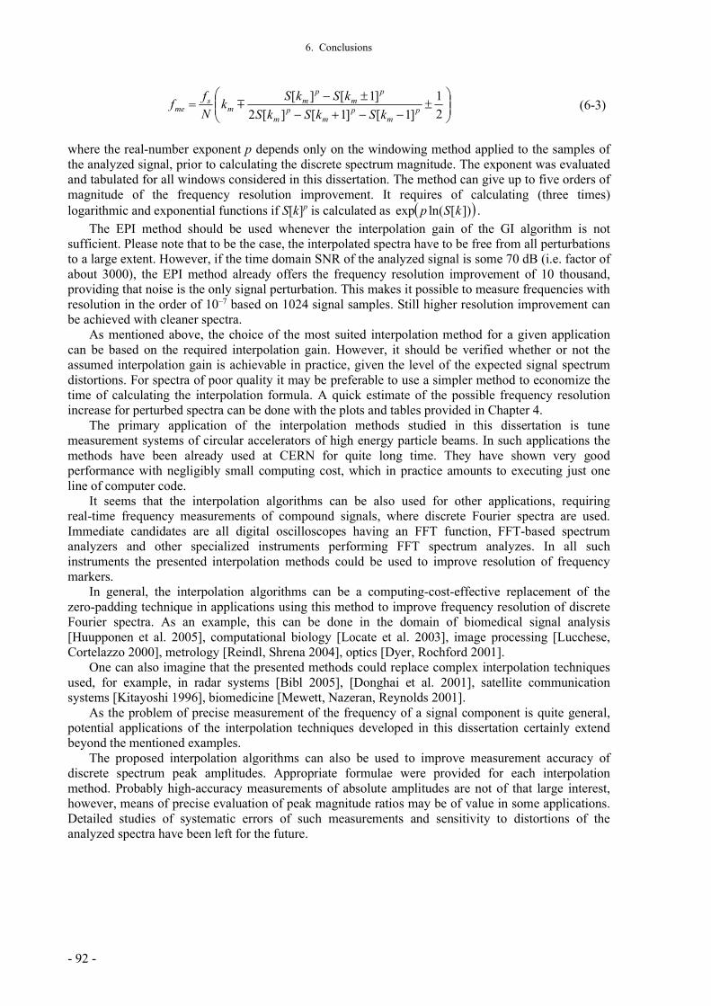
6. Conclusions

- 92 -

2

1

]1[]1[][2

]1[][p

mp

mp

m

pm

pm

ms

me kSkSkS

kSkSk

N

ff (6-3)

where the real-number exponent p depends only on the windowing method applied to the samples of the analyzed signal, prior to calculating the discrete spectrum magnitude. The exponent was evaluated and tabulated for all windows considered in this dissertation. The method can give up to five orders of magnitude of the frequency resolution improvement. It requires of calculating (three times) logarithmic and exponential functions if S[k]p is calculated as ])[ln(exp kSp .

The EPI method should be used whenever the interpolation gain of the GI algorithm is not sufficient. Please note that to be the case, the interpolated spectra have to be free from all perturbations to a large extent. However, if the time domain SNR of the analyzed signal is some 70 dB (i.e. factor of about 3000), the EPI method already offers the frequency resolution improvement of 10 thousand, providing that noise is the only signal perturbation. This makes it possible to measure frequencies with resolution in the order of 10–7 based on 1024 signal samples. Still higher resolution improvement can be achieved with cleaner spectra.

As mentioned above, the choice of the most suited interpolation method for a given application can be based on the required interpolation gain. However, it should be verified whether or not the assumed interpolation gain is achievable in practice, given the level of the expected signal spectrum distortions. For spectra of poor quality it may be preferable to use a simpler method to economize the time of calculating the interpolation formula. A quick estimate of the possible frequency resolution increase for perturbed spectra can be done with the plots and tables provided in Chapter 4. The primary application of the interpolation methods studied in this dissertation is tune measurement systems of circular accelerators of high energy particle beams. In such applications the methods have been already used at CERN for quite long time. They have shown very good performance with negligibly small computing cost, which in practice amounts to executing just one line of computer code.

It seems that the interpolation algorithms can be also used for other applications, requiring real-time frequency measurements of compound signals, where discrete Fourier spectra are used. Immediate candidates are all digital oscilloscopes having an FFT function, FFT-based spectrum analyzers and other specialized instruments performing FFT spectrum analyzes. In all such instruments the presented interpolation methods could be used to improve resolution of frequency markers.

In general, the interpolation algorithms can be a computing-cost-effective replacement of the zero-padding technique in applications using this method to improve frequency resolution of discrete Fourier spectra. As an example, this can be done in the domain of biomedical signal analysis [Huupponen et al. 2005], computational biology [Locate et al. 2003], image processing [Lucchese, Cortelazzo 2000], metrology [Reindl, Shrena 2004], optics [Dyer, Rochford 2001].

One can also imagine that the presented methods could replace complex interpolation techniques used, for example, in radar systems [Bibl 2005], [Donghai et al. 2001], satellite communication systems [Kitayoshi 1996], biomedicine [Mewett, Nazeran, Reynolds 2001].

As the problem of precise measurement of the frequency of a signal component is quite general, potential applications of the interpolation techniques developed in this dissertation certainly extend beyond the mentioned examples. The proposed interpolation algorithms can also be used to improve measurement accuracy of discrete spectrum peak amplitudes. Appropriate formulae were provided for each interpolation method. Probably high-accuracy measurements of absolute amplitudes are not of that large interest, however, means of precise evaluation of peak magnitude ratios may be of value in some applications. Detailed studies of systematic errors of such measurements and sensitivity to distortions of the analyzed spectra have been left for the future.

References


References

Andria G., Savino M., Trotta A. (1989), Windows and interpolation algorithms to improve electrical measurement accuracy. IEEE Transactions on Instrumentation and Measurement, vol. 38, pp. 856-863.

Asséo E. (1985), Causes et corrections des erreurs dans la mesure des caractéristiques des oscillations bétatroniques obtenues à partir d'une Transformation de Fourier, CERN PS 85-9 (LEA), December.

Althoff R., Keiler F., Zölzer U. (1999), Extracting Sinusoids from Harmonic Signals. Proceedings of DAFx-99 – Workshop on Digital Audio Effects, pp. 97-100.

Bach M., Meigen T. (1999), Do's and don'ts in Fourier analysis of steady-state potentials. Documenta Ophthalmologica, vol. 99, pp. 69-82.

Bartolini R. et al. (1995), Tune evaluation in simulations and experiments. CERN/SL 95-84 (AP).

Bartolini R. et al. (1996), Algorithms for a precise determination of the betatron tune. CERN/SL 96-48 (AP). Proceedings of EPAC 1996 - European Particle Accelerator Conference, Sitges, Spain, vol. II, pp. 1329-1331.

Benedikt M. et al. (2004), LHC Design Report vol.3: the LHC Injector Chain. CERN-2004-003-V-3.

Bibl K. (2005), Iterative precision spectrum analysis. United States Patent 6850552.

Bonacci D., Mailhes C., Djuric P.M., (2003), Improving frequency resolution for correlation-based spectral estimation methods using subband decomposition. IEEE International Conference on Acoustics, Speech, and Signal Processing ICASSP '03, vol. 6, pp 329-32.

Borkowski J. (2000), LIDFT-the DFT linear interpolation method. IEEE Transactions on Instrumentation and Measurement, vol. 49, pp. 741-745.

Chapman-Hatchett A., Chohan V., d’Amico E. T. (1999), Tune measurement for the CERN Proton Synchrotron Booster rings using DSP in VME. Proceedings of PAC 1999 – Particle Accelerator Conference, New York, USA, pp. 2202-204.

Choi A. (1997), Real-Time Fundamental Frequency Estimation by Least-Square Fitting. IEEE Transactions on Speech and Audio Processing, vol. 5, pp. 201-205.

Chun-Kit Chan, Lian-Kuan Chen (1996), A correction scheme for measurement accuracy improvement in multichannel CATV systems. IEEE Transactions on Broadcasting, vol. 42, pp. 122-129.

Donghai Li et al. (2001), High-precision measurement of radar carrier frequency. Proceedings of the 2001 CIE International Conference on Radar, pp. 241-243.

Dyer S. D., Rochford K. B. (2001), Low-Coherence Interferometric Measurements of the Dispersion of Multiple Fiber Bragg Gratings. IEEE Photonics Technology Letters, vol. 13, pp. 230-232.

Fusheng Zhang, Zhongxing Geng, Wei Yuan (2001), The algorithm of interpolating windowed FFT for harmonic analysis of electric power system. IEEE Transactions on Power Delivery, vol. 16, pp. 160-164.

Gasior M., González J. L. (1999a), New Hardware of the Tune Measurement System for the Proton Synchrotron Booster Accelerator. CERN/PS/BD Note 99-10.

References

- 94 -

Gasior M., González J. L. (1999b), DSP Software of the Tune Measurement System for the Proton Synchrotron Booster Accelerator. CERN/PS/BD Note 99-11.

Gasior M., González J. L. (2004a), Improving FFT Frequency Measurement Resolution by Parabolic and Gaussian Interpolation. AB-Note-2004-021 BDI.

Gasior M., González J. L. (2004b), Improving FFT Frequency Measurement Resolution by Parabolic and Gaussian Spectrum Interpolation. BIW 2004 - Beam Instrumentation Workshop, Knoxwille, Tennesee, USA. American Institute of Physics Conference Proceedings, vol. 732, pp. 276-285.

Gasior M., Jones R. (2005a), The Principle and First Results of Betatron Tune Measurement by Direct Diode Detection. LHC-Project-Report-853.

Gasior M., Jones R. (2005b), High Sensitivity Tune Measurement by Direct Diode Detection. Proceedings of DIPAC 2005 - European Workshop on Beam Diagnostics and Instrumentation for Particle Accelerators, Lyon, France, pp. 312-314.

Gasior M. et al. (2005a), Advances Towards the Measurement and Control of LHC Tune and Chromaticity. Proceedings of DIPAC 2005 - European Workshop on Beam Diagnostics and Instrumentation for Particle Accelerators, Lyon, France, pp. 27-29.

Gasior M. et al. (2005b), LEIR Beam Instrumentation. Proceedings of DIPAC 2005 - European Workshop on Beam Diagnostics and Instrumentation for Particle Accelerators, Lyon, France, pp. 258-260.

Gasior M. et al. (2005c), LHC Collimation: Design and Results from Prototyping and Beam Tests. Proceedings of PAC 2005 - Particle Accelerator Conference, Knoxville, TN, USA, pp. 1078-1080.

Gasior M. et al. (2005d), Measurements of the LHC Collimator Impedance with Beam in the SPS. Proceedings of PAC 2005 - Particle Accelerator Conference, Knoxville, TN, USA, pp. 1132-1134.

Gasior M. et al. (2006a), Tune and Coupling Feedback during RHIC Run 6. BIW 2006 - Beam Instrumentation Workshop, Fermilab, Batavia, Illinois, USA.

Gasior M. et al. (2006b), Commissioning the beam diagnostic systems for the CERN Low Energy Ion Ring. BIW 2006 - Beam Instrumentation Workshop, Fermilab, Batavia, Illinois, USA.

Geckinli N., Yavuz D. (1978), Some novel windows and a concise tutorial comparison of window families. IEEE Transactions on Acoustics, Speech, and Signal Processing, vol. 26, pp. 501-507.

González, J., Johnston S., Schulte E. (1994), Fast Q-measurement for the PS by FFT analysis. CERN/PS 94-1 (BD). Proceedings of EPAC 1994 - European Particle Accelerator Conference, London, UK.

Grandke T. (1983), Interpolation algorithms for discrete Fourier transforms of weighted signals. IEEE Transactions on Instrumentation and Measurement, vol. 32, pp. 350-355.

Goto Y. (2000), Interpolation of Hamming-Apodized DFT Spectra. Electronics and Communications in Japan, vol. 83, pp. 107-113.

Gu H., (1993), Frequency Resolution and Estimation of AR Spectral Analysis. IEEE Transactions on Signal Processing, vol. 41, 432-436.

Harris F. J. (1978), On the Use of Windows for Harmonic Analysis with the Discrete Fourier Transform, Proceedings of the IEEE, vol. 66, No. 1, January, pp. 51-83.

Hikawa H., Jain V.K., (1990), Jamming canceler using interpolated FFT. Conference Record of SUPERCOMM/ICC '90 - IEEE International Conference on Communications, vol. 4, pp. 1275-1279.

References

- 95 -

Huupponen E. J. et al. (2005), Determination of EEG Sleep Spindle Frequency with DFT and Matching Persuit Approaches. Proceedings of BioMED 2005 - The IASTED Conference on Biomedical Engineering, Innsbruck, Austria, pp. 458-010.

Jain V., Collins W., Davis D. (1990), DFT Interpolation for estimation of tone amplitudes and phases. IEEE International Conference on Acoustics, Speech, and Signal Processing ICASSP '80, vol. 5, pp 662-665.

Jianguo Huang, Kay S. (1989), Frequency estimation using a dynamic programming-type algorithm. Proceedings of ICASSP-89 - International Conference on Acoustics, Speech, and Signal Processing, vol. 4, 2282-2285.

Kay S. (1984), Accurate frequency estimation at low signal-to-noise ratio. IEEE Transactions on Acoustics, Speech, and Signal Processing, vol. 32, pp. 540-547.

Kay S. (1988), Statistically/computationally efficient frequency estimation. Proceedings of ICASSP-88 - International Conference on Acoustics, Speech, and Signal Processing, vol. 4, pp. 2292-2295.

Kay S., Marple L. M. (1981), Spectrum analysis – A modern perspective. Proceedings of the IEEE, vol. 69, pp. 1380-1419.

Kay S., Shaw A. K. (1988), Frequency estimation by principal component AR spectral estimation method without eigendecomposition. IEEE Transactions on Acoustics, Speech, and Signal Processing, vol. 36, pp. 95-101.

Keiler F., Marchand S. (2002), Survey on extraction of sinusoids in stationary sounds. Proceedings of DAFx-02 − International Conference on Digital Audio Effects, University Federal Armed Forces, Hamburg, Germany, pp. 51-58.

Keiler F., Zölzer U. (2001), Extracting Sinusoids from Harmonic Signals. Journal of New Music Research. Special Issue: "Musical Applications of Digital Signal Processing", vol. 30.

Kitayoshi H. (1996), Doppler shift compensation apparatus. United States Patent 5519402.

Kulkarni R. G. (2000), Asymptotic Behavior of Cosine Windows. Microwave Journal, October, pp. 96-104.

Kulkarni R. G. (2001), Sidelobe cancellation technique for achieving high rejection in SAW filters. IEEE Transactions on Ultrasonics, Ferroelectrics and Frequency Control, vol. 48, pp. 1283-1288.

Kulkarni R. G., Lahiri S. K. (1999), Improved sidelobe performance of cosine series functions. IEEE Transactions on Ultrasonics, Ferroelectrics and Frequency Control, vol. 46, pp. 464-466.

Locate S. et al. (2003), Fourier Spectral Analysis of Protein Functional Families. Proceedings of ECCB 2003 - European Conference on Computational Biology, Paris, France.

Lucchese L., Cortelazzo G. M. (2000), A Noise-Robust Frequency Domain Technique for Estimating Planar Roto-Translations. IEEE Transactions on Signal Processing, vol. 48, pp. 1769-1786.

Malocha D. C., Bishop C. D. (1987), The classical truncated cosine series functions with applications to SAW filters. IEEE Transactions on Ultrasonics, Ferroelectrics and Frequency Control, vol. 34, pp. 75-85.

Mewett D.T., Nazeran H., Reynolds K.J. (2001), Removing power line noise from recorded EMG. Proceedings of Annual International Conference of the IEEE Engineering in Medicine and Biology Society, vol. 3, pp. 2190-2193.

Morishima N. (1986), On the frequency resolution of conventional and autoregressive spectral estimates of stationary reactor noise. Annals of Nuclear Energy, vol. 13, pp. 125-130.

References

- 96 -

Nadolski L., Laskar J. (2003), Review of single particle dynamics for third generation light sources through frequency map analysis. Physical Review Special Topics - Accelerators and Beams, Vol. 6, 114801.

Nuttall A. H. (1981), Some Windows with Very Good Sidelobe Behavior. IEEE Transactions on Acoustics, Speech, and Signal Processing, vol. ASSP-29, No. 1, February, pp. 84-91.

Offelli C., Petri D., (1990), Interpolation techniques for real-time multifrequency waveform analysis. IEEE Transactions on Instrumentation and Measurement, vol. 39, pp. 106 – 111.

Pan Wen, Qian Yu Shou, Zhou E., (1994), An improved interpolated FFT algorithm and its application in power harmonics measurement. Proceedings of the 1994 IEEE International Conference on Industrial Technology, pp. 273-277.

Papaphilippou Y. (1999), Frequency Maps of LHC Models. PAC 1999 - Particle Accelerator Conference, New York, USA, pp. 1554-1556.

Reindl L. M., Shrena I. M. (2004), Wireless Measurement of Temperature Using Surface Acoustic Waves Sensors. IEEE Transactions on Ultrasonics, Ferroelectrics, and Frequency Control, vol. 51, pp. 1457-1463.

Rife D., Boorstyn R. (1974), Single-tone Parameter Estimation from discrete-time observation. IEEE Transactions on Information Theory, vol. IT-20, pp 591-598.

Rothacker R., Mammone R., Davidovici S., (1986), Spectrum enhancement using linear programming. IEEE International Conference on Acoustics, Speech, and Signal Processing ICASSP '86, vol. 11, pp. 2351-2354.

Scheppach F. (2002), Method for estimating the frequency of a time signal. European software patent EP1049937. Equivalents WO9938018, US6484112, DE19802193.

Schoukens J., Pintelon R., Hamme H.V. (1992), The interpolated fast Fourier transform: A comparative study. IEEE Transactions on Instrumentation and Measurement, vol. 41, pp. 226-232.

Steier C. et al. (2000), Lattice Model Calibration and Frequency Map Measurements at the ALS. Proceedings of EPAC 2000 - European Particle Accelerator Conference, Vienna, Austria, pp. 1077-1079.

Tan Y.-R. E., Boland M. J., LeBlanc G. (2005), Applying Frequency Map Analysis to the Australian Synchrotron Storage Ring. Proceedings of PAC 2005 - Particle Accelerator Conference, Knoxville, TN, USA, pp. 1269-1271.

Villalba M.J., Walker B.K., (1989), Spectrum manipulation for improved resolution. IEEE Transactions on Acoustics, Speech, and Signal Processing, vol. 37, pp. 820 – 831.

Wilson E. J. N (2001), An Introduction to Particle Accelerators. Oxford University Press.

Zieliński T. P. (2005), Cyfrowe przetwarzanie sygnałów. Od teorii do zastosowań. WKŁ.

Improving frequency resolution of discrete spectra

Documents

Transcript of Improving frequency resolution of discrete spectra