Response Spectra Bedrock Motion Ground Motions

Response Spectra

Magnitude (M), Distance (R)

Rock Outcropping Motion

Attenuation Relationship (PGA – Sa, target)
SHAKE
Shear Stress/Strain Time History

Ground Motions

Site

Bedrock Motion

SHAKE2000 Tutorial – Page No. 2

SHAKE2000 Quick Tutorial This tutorial is intended to guide you through most of the functions in SHAKE2000. Additional information can be obtained by using the Help command button on each form. Please note that this tutorial is not intended as a teaching tool for 1-D dynamic analysis, i.e. it is assumed that the user is familiar with the theoretical background of the analytical tools included with SHAKE2000. The tutorial uses English units for convenience. SHAKE is a computer program which employs an equivalent linear total stress analysis to compute the response of a horizontally layered visco-elastic system subjected to vertically propagating shear waves. As such, the program was intended to model level ground by using a one-dimensional (i.e. 1-D) representation of the soil profile, herein known as a SHAKE Column. However, several researches and practitioners have demonstrated that SHAKE can be also used for the approximate analysis of 2-D structures such as dams. In this tutorial, we will use SHAKE2000 to perform the seismic analysis of the slope shown below. First, we will use Column No. 1 to conduct the analysis of the level ground using SHAKE2000. We will then use Column No. 3 to determine permanent slope displacements due to earthquake shaking, using the Newmark Method. As part of these two analyses, we will try to cover as many of the features of SHAKE2000 as possible.

12

3

Data for Column No. 1 (Layer No. 1 at Top of Embankment)

Layer Thickness (ft)

γT (pcf)

Soil Type

1 5.5 130.0 1 2 3.3 130.0 1 3 3.3 130.0 1 4 3.3 130.0 1


5 3.3 130.0 1 6 3.3 130.0 1 7 3.3 130.0 2 8 3.3 130.0 2 9 3.3 130.0 2

10 3.3 130.0 2 11 3.3 130.0 2 12 3.3 130.0 2 13 3.3 130.0 2 14 3.3 130.0 2 15 3.3 130.0 3 16 3.3 130.0 3 17 3.3 130.0 3 18 3.3 130.0 3 19 3.3 130.0 3 20 3.3 130.0 3 21 Half Space 150.0 4

The soil type, thickness, and unit weight for each layer in Soil Column No. 1 are given in the table above. The data for column number 3 and other data that will be used in this tutorial are saved in the sample_1.edt file created in the sample directory during installation. Two time histories for the object motion are saved as sample1.eq and sample2.eq in the sample directory. In this example, we will compute maximum accelerations, stresses and strains in the soil column, and response spectra for the surface and the half space layers. The modulus reduction and the damping ratio curves are given below for material number 1. Three other materials will be used, but the properties for these will be retrieved from the database of material properties provided with SHAKE2000. Material No. 1: Sand S1 G/Gmax - S1 (SAND CP<1.0 KSC) 3/11 1988 Sand Avg. Damping for SAND, Average (Seed & Idriss 1970)

Strain G/Gmax Strain Damping 0.0001 1.000 0.0001 0.50 0.0003 0.978 0.0003 0.80 0.0010 0.934 0.0010 1.70 0.0032 0.838 0.0030 3.45 0.0100 0.672 0.0100 6.50 0.0316 0.463 0.0300 10.70 0.1000 0.253 0.1000 16.50 0.3160 0.140 0.3000 21.90 1.000 0.057 1.000 25.70

It will be assumed that the depth to the groundwater table is 5.5 feet for the liquefaction analysis section of this tutorial. SPT values for the soil column are presented later in this tutorial. The failure surface depicted in the figure will be used in the displacement analysis section of the tutorial. For this latter analysis, a static factor of safety of 1.54 will be used, and the acceleration time histories at the top of layers 4 for column No. 1 (or just below the failure surface), layer 8 for column No. 2, and layer 3 for column No. 3 will be obtained for use in the Newmark Method. Other data or information used in this example is provided in the appropriate sections of this tutorial.


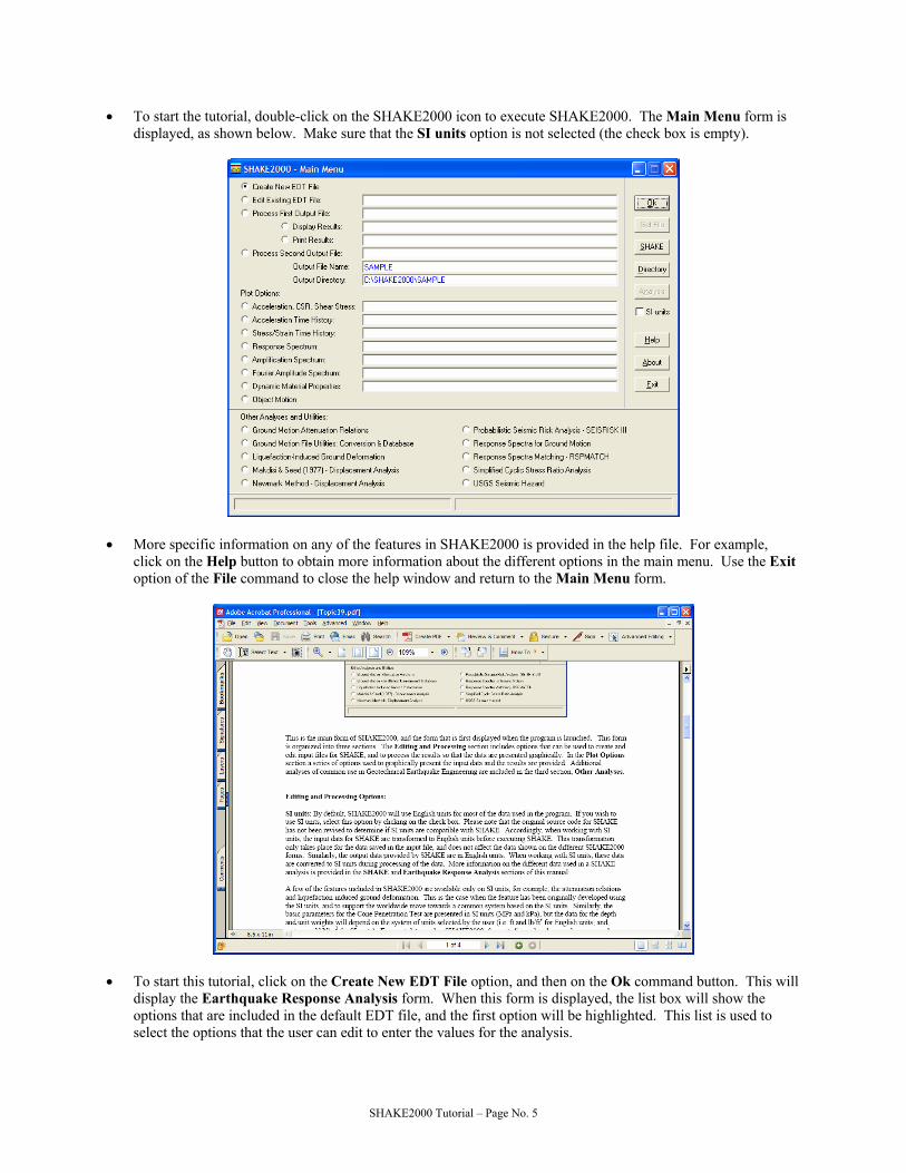
• To start the tutorial, double-click on the SHAKE2000 icon to execute SHAKE2000. The Main Menu form is displayed, as shown below. Make sure that the SI units option is not selected (the check box is empty).

• More specific information on any of the features in SHAKE2000 is provided in the help file. For example,

click on the Help button to obtain more information about the different options in the main menu. Use the Exit option of the File command to close the help window and return to the Main Menu form.

• To start this tutorial, click on the Create New EDT File option, and then on the Ok command button. This will display the Earthquake Response Analysis form. When this form is displayed, the list box will show the options that are included in the default EDT file, and the first option will be highlighted. This list is used to select the options that the user can edit to enter the values for the analysis.


• Option 1, dynamic soil properties, is highlighted. Use this option to enter the data for the modulus reduction and the damping ratio curves for each soil type.

• Click on the Edit command button to display the Option 1 Editor: Dynamic Material Properties form.

• In this form, you will enter the dynamic material properties for Material No. 1. • Place the cursor on the Material Name text box. Type in the following: Sand S1 • Place the cursor on the Identification for this Set of Modulus Reduction Values text box. Type in the

following: G/Gmax - S1 (Sand CP < 1 ksc) 3/11/88 • Use the Tab key to place the cursor on the first data cell for the strain values. Type in 0.0001. Use the Tab key

to move to the next cells, and type in the following data:

Strain: 0.000316 0.001 0.00316 0.01 0.0316 0.1 0.316 1.00 • Notice that after entering a strain value, a default value for G/Gmax is automatically entered in the appropriate

cell. You still need to modify the moduli values. • Place the cursor on the first cell of the Values of Modulus Reduction (G/Gmax), and enter the following data:


Moduli: 1.00 0.978 0.934 0.838 0.672 0.463 0.253 0.14 0.057 • Click on the Damping button to display the damping data cells. Use the above procedure to enter the following

data: Material Name: Sand Avg. ID: Damping for Sand, Average (Seed & Idriss 1970) Strain: 0.0001 0.0003 0.001 0.003 0.01 0.03 0.1 0.3 1.00 Damping: 0.5 0.8 1.7 3.45 6.5 10.7 16.5 21.9 25.7

• To add materials No. 2, 3, and 4, we will retrieve the information from the database of material properties

included with SHAKE2000. First, click on the Moduli command button to display the G/Gmax data. • Click on the New command button. This will clear the information from the form (your data for material

number 1 are still in the computer's memory). • Click on the MAT command button to open the G/Gmax Curves Database form. This form lists a series of

materials whose information is saved in the shakey2k.mat file.

• To select a material, highlight it and then click on the Choose command button. For this tutorial, first click on

the material described as Sand S2 G/Gmax - S2 (Sand CP=1-3 KSC) 3/11 1988 to highlight it and then click on the Choose button. You will be asked if you would like to update the current set of Option 1. Click on Yes.

• The G/Gmax values are shown in the form. To add the damping curve for this material, click on the Damping command button to switch to the form used to enter this type of data.

• Click on the MAT command button to open the Damping Ratio Curves Database form. • Click on the Sand Damping for Sand, February 1971 curve to highlight it, and then click on the Choose

command button. You will be asked if you would like to update the current set of Option 1. Click on Yes. • Now that you have both the G/Gmax and damping ratio curves for material number 2, click on the Save

command button to add this material to your Option 1. Note that the number of materials has been increased to 2 as shown in the text box below the No. Materials label.

• Follow the same procedure to add data for materials number 3 (i.e. Sand S3 G/Gmax - S3 (SAND CP>3.0 KSC) 3/11 1988 and Sand Damping for SAND, February 1971) and for material number 4 (i.e. Rock G/Gmax - ROCK (Schnabel 1973) and Rock Damping for Rock (Schnabel 1973)).


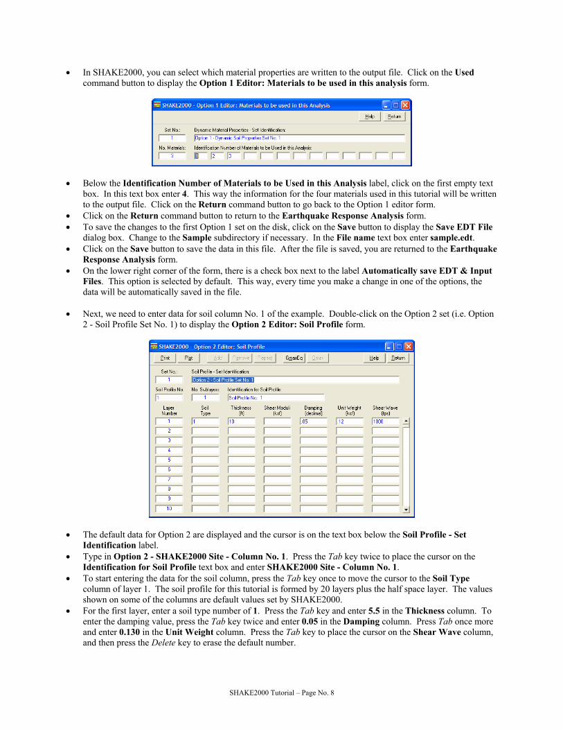
• In SHAKE2000, you can select which material properties are written to the output file. Click on the Used command button to display the Option 1 Editor: Materials to be used in this analysis form.

• Below the Identification Number of Materials to be Used in this Analysis label, click on the first empty text

box. In this text box enter 4. This way the information for the four materials used in this tutorial will be written to the output file. Click on the Return command button to go back to the Option 1 editor form.

• Click on the Return command button to return to the Earthquake Response Analysis form. • To save the changes to the first Option 1 set on the disk, click on the Save button to display the Save EDT File

dialog box. Change to the Sample subdirectory if necessary. In the File name text box enter sample.edt. • Click on the Save button to save the data in this file. After the file is saved, you are returned to the Earthquake

Response Analysis form. • On the lower right corner of the form, there is a check box next to the label Automatically save EDT & Input

Files. This option is selected by default. This way, every time you make a change in one of the options, the data will be automatically saved in the file.

• Next, we need to enter data for soil column No. 1 of the example. Double-click on the Option 2 set (i.e. Option

2 - Soil Profile Set No. 1) to display the Option 2 Editor: Soil Profile form.

• The default data for Option 2 are displayed and the cursor is on the text box below the Soil Profile - Set Identification label.

• Type in Option 2 - SHAKE2000 Site - Column No. 1. Press the Tab key twice to place the cursor on the Identification for Soil Profile text box and enter SHAKE2000 Site - Column No. 1.

• To start entering the data for the soil column, press the Tab key once to move the cursor to the Soil Type column of layer 1. The soil profile for this tutorial is formed by 20 layers plus the half space layer. The values shown on some of the columns are default values set by SHAKE2000.

• For the first layer, enter a soil type number of 1. Press the Tab key and enter 5.5 in the Thickness column. To enter the damping value, press the Tab key twice and enter 0.05 in the Damping column. Press Tab once more and enter 0.130 in the Unit Weight column. Press the Tab key to place the cursor on the Shear Wave column, and then press the Delete key to erase the default number.


• Follow the same procedure and enter the following data for the other layers:

Layer No. Soil Type Thickness Damping Unit Weight 2 1 3.3 0.05 0.130 3 1 3.3 0.05 0.130 4 1 3.3 0.05 0.130 5 1 3.3 0.05 0.130 6 1 3.3 0.05 0.130 7 2 3.3 0.05 0.130 8 2 3.3 0.05 0.130 9 2 3.3 0.05 0.130 10 2 3.3 0.05 0.130 11 2 3.3 0.05 0.130 12 2 3.3 0.05 0.130 13 2 3.3 0.05 0.130 14 2 3.3 0.05 0.130 15 3 3.3 0.05 0.130 16 3 3.3 0.05 0.130 17 3 3.3 0.05 0.130 18 3 3.3 0.05 0.130 19 3 3.3 0.05 0.130 20 3 3.3 0.05 0.130 21 4 ----- 0.05 0.150

• For layer 21, place the cursor on the Shear Wave column and enter 2500.0.

• For a quick example on how to edit the data in this form, click on the Soil Type column of layer 18. The Layer

and Remove buttons are enabled. Click on the Remove button. The data for layer 18 are deleted, and the other layers are scrolled upward one position. To add data for a new layer, place the cursor on any column where the new layer will be located, and then click the Layer button. For this example, the cursor is still on layer 18, therefore, just click on the Layer button. By default, the new layer is given the same data as the layer where the cursor is placed. In this example, the new layer has the same values as those of layer 19.

• There are a number of equations that can be used to estimate the maximum shear modulus (Gmax) value. We

will explain how to enter the variables for one of these equations next. • Click on the GmaxEq command button to display the Shear Moduli Equations form. More information on

these equations is provided in the Shear Moduli Equations section of this manual.


• For this example, we will use equation number 6 for layers 1 through 20. As explained in the Shear Moduli

Equations section, the variables for equation 6 are N1,60, Ko, and σ'v.

• Click on the Layers button to switch to the form used to enter the variables for the equations used for specific layers.

• Using the Tab key or the mouse pointer, place the cursor on the Eq. No. column for layer No. 1. Type in a 6. Use the Tab key to move to the Ko column. Enter 0.40, and move the cursor to the N column using the Tab key. Type in 17.

• Use the Tab key or the mouse cursor to place the cursor on the Eq. No. column of layer 2. Enter the following data for the other layers. Use the Next command button to scroll down the layers in groups of 5.

Layer Eq. # Ko N 1,60 2 6 0.4 8 3 6 0.4 5 4 6 0.4 5 5 6 0.4 7 6 6 0.4 12 7 6 0.4 15 8 6 0.4 14 9 6 0.4 15 10 6 0.4 10 11 6 0.4 23 12 6 0.4 12 13 6 0.4 10 14 6 0.4 10 15 6 0.4 21 16 6 0.4 22 17 6 0.4 4 18 6 0.4 5 19 6 0.4 3 20 6 0.4 29 • Click on the Enter depth to water table check box, and then place the cursor on the text box next to it. Enter

5.5 for water depth.


• Click on the Save button. If necessary, double-click on the Sample subdirectory to select it. On the File name text box type sample.gmx, and then click on the Save button. The data for the equations are saved in this file. The File button is used to retrieve the coefficients from the file for later use.

• Once you have entered all the information for the equations, click on the Return command button to return to

the Option 2 form. • The Gmax command button is enabled. Click on it to estimate the maximum shear moduli. You will be asked

if you wish to continue with the calculation of Gmax. Click on Yes. After a few seconds, the modulus values will be displayed in the Shear Moduli column.

• Click on the Return button to return to the Earthquake Response Analysis form. • Once you have entered the data for the material properties and the soil column, the next step is to enter the

information for the ground motion record that will be used in the analysis. The basic function of this option is to read the acceleration values from the file.

• Click on Option 3 - Input (Object) Motion Set No. 1 to highlight it, and then click on the Edit command button to display the Option 3 Editor: Input (Object) Motion form.

• Some default information is shown on the text boxes. The cursor is on the text box below the Input (Object)

Motion - Set Identification label. For this tutorial, type in Option 3 - Input motion: SAMPLE1.EQ and press the Tab key once to move the cursor to the text box below the Acceleration Values label.

• The object motion saved in the sample1.eq file is formed by 3800 acceleration values, with a time step of 0.01 seconds, with 1 header line and saved with a format of (8F9.6).

• Enter 3800 and press the Tab key once to move the cursor to the text box below the No. Fourier Values label. A value of 8192 is automatically set for the number of Fourier values.


• Place the cursor on the text box below the Time Interval label. Enter 0.01 and press the Tab key once to move the cursor to the text box below the Format of Object Motion File label. Enter (8F9.6) and press the Tab key once to move the cursor to the text box below the Name and Path of Object Motion File label. This format means that the acceleration data in the file are to be read in 8 columns per row, each column formed by 9 figures and of the 9 figures the left most 6 should be used for the decimal portion of the number.

• When SHAKE2000 was installed, the sample1.eq file was created in the Sample subdirectory. If the root directory for SHAKE2000 is c:\shake2000, enter in this text box c:\shake2000\sample\sample1.eq and press the Tab key once to move the cursor to the text box below the Multiplication Factor label.

• We will not scale the motion to a different value of peak acceleration, thus enter 1.0 and press the Tab key twice to move the cursor to the text box below the Maximum Frequency label.

• The default values for maximum frequency, number of header lines and acceleration values per line are the ones that we want to use for this file.

• Click on the Return button to return to the Earthquake Response Analysis form. • As noted in Section 4.2, the ground motion file used as input in SHAKE is usually formed by a series of

acceleration values in g’s saved in a formatted way (e.g. 8F9.6) that is compatible with the Format statement used in the FORTRAN programming language. Today, the user can obtain ground motion records from a wide variety of sources, e.g. the Internet. However, these files are not likely to be uniform in their formatting or processing. Thus, SHAKE2000 includes a feature to extract the acceleration data from the file, convert them to g’s and save them to a formatted text file that can be used by SHAKE.

• We will create a second set of Option 3 using a ground motion record downloaded from the Pacific Earthquake Engineering Research Center (PEER) Strong Motion Database (http://peer.berkeley.edu/smcat/search.html). This file is named ALS-E_AT2.TXT and is saved in the Sample folder.

• Files downloaded from the PEER web site are usually formed by 4 header lines that provide information about the earthquake for which the motion is a record of, the person/institution that processed the record, and values for the number of points and time interval. The acceleration data are next, saved in rows of five columns each, in g’s. As is, the file cannot be used in SHAKE because the acceleration data are saved in 5 columns. SHAKE requires that the acceleration data be saved in rows of even number of columns.

• To continue with the tutorial, we will create the second set of Option 3. To do this, click on the New command

button. This will display the Option List form.


• Click on the Option 3 – Input (Object) Motion label to highlight it, and then click on the Choose command button. You will return to the Earthquake Response Analysis form. Note that a second set for Option 3 has been added to the EDT list box. This new set has the label Option 3 – Input (Object) Motion Set No. 2.

• Click on this new set to highlight it, and then on the Edit command button to display the Option 3 Editor form. • Click on the Convert command button to display the Conversion of Ground Motion File form.

• Conversion of a ground motion file involves the following steps: 1) opening the original or source ground motion file; 2) defining the way the data in the source file are to be read; and, 3) defining the way the data will be written to the new converted ground motion file.

• For the first step, click on the Open command button to display the Open Source Ground Motion File dialog form. Switch to the Sample folder if necessary.

• Select the ALS-E_AT2.TXT file and then click on the Open command button. After a few seconds, the first

few lines of the file (up to 90 lines) will be displayed on the top list box of the form.


• The first few characters displayed in red are the numbers of each row of data in the file followed by a “|”. These characters are not part of the source file and are only shown to number the rows. After the row-numbers, the alphanumeric characters that constitute the information saved in the file for each row are shown. Note that the characters are displayed as blue on a white background, and that every tenth character is displayed in red. However, if the tenth character is a “blank space” then the character is not shown. This is done to guide the user when defining the order of the data in the file.

• By default, the converted record will be saved in the same folder as the source file. If you would like to save the converted file to a different directory, you would use the Save command button to display the Save Converted Ground Motion File dialog form. For our tutorial, the converted file will be saved as c:\shake2000\sample\ALS-E_AT2.eq.

• During the second step, you need to define the way the data in the source file are to be read. First, place the

cursor in the text box below the No. Values label. From the information on the fourth line of the file, we know that there are 11800 acceleration values in the file, separated at a time interval of 0.005 seconds.

• Enter 11800, and press the Tab key to place the cursor on the Time Step text box. Enter a value of 0.005 for the time interval.

• Place the cursor in the No. Header Lines text box and enter 4. • Press the Tab key or use the mouse pointer to place the cursor in the Values per Line text box. As noted

before, there are 5 acceleration values per row of data. Enter a 5. • Place the cursor in the No. Digits text box. We need to count the number of characters in (including blank

spaces), or the length of each column. For example, for the first column, start immediately after the “|” and end at the last character before the first blank space. Each column is formed by 15 characters, or digits. Enter a 15 in this text box.

• In the third step, you will define how the data will be written to the converted file. First, define the format, i.e.

the way the data are written to the file, of the acceleration values. The format string tells SHAKE2000 and SHAKE how to read the ground motion values from the file. This string is based on the syntax used in the Format statement of the FORTRAN computer language. For this tutorial we will accept the default value of (6F15.8).

• Next, place the cursor on the text box below the Option 3 Set ID – Line label. Here you need to enter a value that represents the number of the line from the header section that will be used to identify the converted file in the set identification of Option 3. For example, for the above record, you could use the second line to be included in the database; thus, enter a 2.


• We will include the 4 header lines in the output file. Thus, place the cursor in the first text box below the Lines from Source File header to be included in header of Converted Ground Motion File label, and enter 1-4.

• To convert the file, click on the Convert command button. After a few seconds, the first lines of the converted

file will be displayed in the bottom list box of the form.

• To verify that the conversion was successful, plot the motion to visually verify that it looks normal. Click on

the Plot command button to display the Plot Object Motion form.

• Click on the Plot command button to plot the acceleration, velocity and displacement time histories for the converted motion.


• Click on the Close command button to return to the Plot Object Motion form, and then click on Close again to

return to the conversion file form. • The procedure to convert PEER files has been automated in SHAKE2000. In other words, the conversion of the

file following the previous procedure can be performed by choosing the PEER option of the Source File Type menu list. For learning purposes in this tutorial, we followed the manual method by using the Other option. More information on conversion of files is included in the Conversion of Ground Motion File section of this manual.

• Click on the Close command button to return to the Option 3 form. • The information for the converted ground motion file will be displayed on the form.

• Click on the Return button to return to the Earthquake Response Analysis form. • The object motion defined with Option 3 needs to be assigned to a specific sublayer in the soil deposit. This is

done with Option 4. Click on Option 4 - Assignment of Object Motion to a Specific Sublayer Set No. 1 to highlight it, and then click on the Edit command button to display the Option 4 Editor form.


• The cursor is on the text box below the set identification label. Type in Option 4 - Sublayer for input motion

is No. 21 and then press the Tab key to move the cursor to the text box below the No. of Sublayer label. For column number 1, the object motion will be assigned to layer 21, the half-space.

• Type in 21 and press the Tab key to move the cursor to the text box below the Outcrop or Within Profile label. For this tutorial, the motion is felt to represent an outcrop rock motion. Thus, use a code of 0. Enter 0.

• Click on the Return button to return to the list of options form. • SHAKE goes through an iterative process to obtain values for modulus and damping compatible with the

effective strains in each layer. Option 5 is then used to define the maximum number of iterations and the ratio between effective strain and maximum strain.

• Click on Option 5 - Number of Iterations & Strain Ratio Set No. 1 to highlight it, and then on the Edit command button to display the Option 5 Editor form.

• For this set identification, enter Option 5 - No. iterations 10, strain ratio 0.65 and press the Tab key twice to

move the cursor to the text box below the Number of Iterations label. Enter 10 and press the Tab key once to move the cursor to the text box below the Strain Ratio label. A value of 0.65 is shown as default. This value is adequate for our tutorial.

• Click on the Return button to return to the list of options form. • With options 1 through 5 you have basically entered most of the input data required for the analysis. The

following options, i.e. 6 through 11, are used to obtain the results. • Option 6 is used to obtain acceleration time histories at the top of specified sublayers and the peak acceleration

for each sublayer. • Click on Option 6 - Computation of Acceleration at Specified Sublayers Set No. 1 to highlight it, and then

on the Edit command button to display the Option 6 Editor form.


• Note that a maximum of fifteen sublayers can be specified at a time. If accelerations for more than 15 sublayers are desired, then Option 6 can be repeated as many times as needed. Because column number 1 is formed by 21 layers, we will need to use two sets of Option 6.

• The cursor is in the set identification text box. Enter Option 6 - Acceleration time history for layers 1-15 of Column No. 1 and press the Tab key twice to move the cursor to the second text box below the Sublayers for which acceleration time histories are computed label. Enter 2 and press the Tab key once to move the cursor to the next text box. Note that default values have been set for the type of sublayer (second row of text boxes) and for the output mode (bottom row of boxes). Repeat this procedure to enter 3, 4, 5, and so on until you enter 15 in the last box.

• You can obtain peak acceleration only, or peak acceleration and acceleration time history for each sublayer. For our tutorial, we will compute the displacement of an imaginary failure surface (as shown in the figure in the introduction section of this tutorial) using the Newmark Method, thus we will need the acceleration time histories at top of layers 4 and 8. Place the cursor on the fourth text box from left to right (i.e. for layer 4) below the Output mode for computed accelerations… label and enter a 1. Repeat the same procedure for layer 8.

• Click on the Return button to return to the list of options form. • As noted before, we need to create a second set of Option 6 to compute acceleration values for layers 16

through 21. • To create a new set, click on the New command button. This will display the Option List form.

• Click on the Option 6 - Computation of Acceleration at Specified Sublayers label to highlight it, and then

click on the Choose command button. You will return to the Earthquake Response Analysis form. Note that a second set for Option 6 has been added to the EDT list box. This new set has the label Option 6 - Computation of Acceleration at Specified Sublayers Set No. 2.

• Click on this new set to highlight it, and then on the Edit command button to display the Option 6 Editor form. • For the identification of this set enter Option 6 - Acceleration time history for layers 16-21 of Column No. 1.

Press the Tab key once to move the cursor to the first text box of the top row. As we did before, enter 16 through 21. Repeat 21 twice, one will have a within (1) code and the other an outcrop (0) code.

• As before, default values are shown for type of sublayer and output mode. We need to change a couple of these values. First, place the cursor in the first text box of the middle row (i.e. the type of sublayer for layer 16). There is a zero in this box, which means that layer 16 would be defined as an outcrop (i.e. top of the soil column). However, layer 16 is near the bottom of the soil column, so it should be defined as “within”. Enter a 1. Next, we do not need the acceleration time history for layer 16, thus change the value in the output mode box


for layer 16 from 1 to 0. Finally, we would like to get the acceleration time history for the half-space layer, i.e. layer 21. Thus, enter a 1 in the output mode boxes of layer 21.

• Click on the Return button to return to the list of options form. • To compute the shear stress or strain time history at top of specified sublayers use Option 7. For this tutorial,

we will compute these histories for layers 4 and 8. • Click on Option 7 - Computation of Shear Stress or Strain Time History Set No. 1 to highlight it, and then

on Edit to display the Option 7 Editor form.

• In the identification text box enter Option 7 - Shear stress & strain time histories at Layer 4 - Column No.

1. In the first row, we will compute the strain time history for layer 4. First, place the cursor in the text box below the Sublayer No. label and enter 4. A code of zero (1) is used to compute the stress time history, thus we will accept the default value for Stress/Strain. Also, the default values for Save History and No. Values are adequate, thus, press the Tab key three times to move the cursor to the text box below the Identification label. Enter SHAKE2000 Site - Column No. 1 and press Tab once to move the cursor to the first text box of the bottom row. In this second sublayer, we will get the strain time history for layer 4. Accordingly, enter a 4 for sublayer number and SHAKE2000 Site - Column No. 1 for identification.

• Click on the Return button to return to the Earthquake Response Analysis form. • Create a new set of Option 7, and follow the previous procedure to compute the shear strain and shear stress

time histories for layer 8. • The following step in the analysis is the computation of the response spectra at the top of a specified sublayer. • Click on Option 9 - Response Spectrum Set No. 1 to highlight it, and then on Edit to display the Option 9

Editor form.


• In the identification text box enter Option 9 - Response spectrum at surface - Damping 1, 2.5, 5, 10, 15, 20%

and press the Tab key once to move the cursor to the text box below the Sublayer No. label. The surface layer is sublayer number 1, thus we will accept the default value. In addition, the surface is considered an outcrop (i.e. code zero) so we will also accept the default value for the Outcrop/Within data. The number of damping values is automatically updated every time you enter or delete a damping value, so this value cannot be modified by the user. Next, the value for Null is always zero and cannot be changed. This is an old SHAKE input datum that is included in SHAKE2000 to support old data files. We are working with English units thus a value of 32.2 for Gravity is appropriate for this tutorial.

• Place the cursor in the first text box below the Damping Ratios (in decimal) label, i.e. the one with a .05 value in it. We will compute spectra for damping values of 1%, 2.5%, 5%, 10%, 15% and 20%. Enter 0.01 and press the Tab key once to move the cursor to the following text box (i.e. the one with a .1 in it). Enter 0.025 and repeat the same procedure to enter the other damping ratios in decimal form.

• Click on the Return button to return to the Earthquake Response Analysis form. • The next option in SHAKE is option 10 that is used to compute the amplification spectrum between any two

layers. For this tutorial, we will compute the spectrum between layers 21 and 1. • Click on Option 10 - Amplification Spectrum Set No. 1 to highlight it, and then on Edit to display the Option

10 Editor form.

• The cursor is in the identification text box. Type in Option 10 - Amplification spectrum between layers 21 & 1 - Column No. 1 and press the Tab key once to move the cursor to the text box below the First Layer label. The amplification factors are computed from the first sublayer to the second. Thus, enter 21. The value of 1 for outcrop/within is adequate for this layer, so press the Tab key twice to move the cursor to the Second Layer text box. Enter 1, and press the Tab key once. This layer is an outcrop, so enter a 0 (zero) in this text box. The


value of 0.125 is adequate for the frequency step. Place the cursor in the Amplification Spectrum Identification text box and enter Surface/half-space. This label will be displayed when you plot the graph.

• Click on the Return button to return to the Earthquake Response Analysis form. • The last option of SHAKE is Option 11, used to obtain the Fourier spectrum of the computed motions at the top

of the specified sublayers. • On the list of options, click on Option 11 - Fourier Spectrum Set No. 1 to highlight it and then on the Edit

command button to display the Option 11 Editor form.

• The cursor is in the identification text box. Enter Option 11 - Fourier spectrum for layers 1 & 21 - Column No. 1 and press the Tab key once to move the cursor to the first text box below the Sublayer Number label.

• The value of 1 is adequate, so press the Tab key once more to move the cursor to the Outcrop Within text box. This is the surface layer, so enter a value of 0 (zero). The code for Save to File is not necessary but is still supported by SHAKE2000 to maintain compatibility with old input files. A value of 3 for the No. Times to Smooth is adequate. Then, place the cursor on the No. Values to Save text box and enter 2048.

• Follow the same procedure to enter values of 21 for the sublayer number; 1 for outcrop/within; and 2048 for number of values to save.

• Click on the Return button to return to the Earthquake Response Analysis form. • For the second part of this tutorial, we will use an EDT file that was created in the sample subdirectory when

you installed SHAKE2000. This other file, sample_1.edt, has the same options that you created in this section, and some more options that we will use in the following sections of the tutorial.

• Click on the Return button to return to the SHAKE2000 - Main Menu form. You will be asked if you would like to save the data to the disk. Click on Yes. This will display the file dialog form. Click on Save and then on Yes to save the data to the disk.

• Click on the Edit Existing EDT File option, and then on the Get File button to display the Open Existing EDT File dialog box. If necessary, change to the drive where the SHAKE2000 directory was created. Then, click on the SHAKE2000 and Sample directories to display the available *.EDT files.


• Click on the Sample_1.edt file to select it, and then click on the Open button to return to the Main Menu form. You can also double-click on the file name to select it and return to the main menu.

• The Ok button on the Main Menu form will be highlighted (i.e. is shown in black characters instead of grayed out).

• Click on the Ok button to display the Earthquake Response Analysis form. This form displays the different

SHAKE options available on the Sample_1.edt file.

• The next step in the tutorial is to create an input file for SHAKE. The top list box shows the options available

in the *.EDT file. The bottom list box will show the options to be included in the input file. We will now conduct the analysis for Column No. 1.

• To choose the options you want to include in the input file, just click once to highlight it and then click the Add

button. This will add the option to the input-file-options list. • Click on Option 1 to highlight it, and then click on the Add button. The option is shown on the bottom list box.

Now, highlight the second set of Option 2 (i.e. the data for Column No. 1) and then click on Add. The option should also be shown on the input-file-options list, i.e. bottom list box.

• Select the following options: first set of Option 3; second set of Option 4 (i.e. Sublayer for input motion is No. 21); Option 5; first and second sets of Option 6; first and second sets of Option 7; first, second, third and fifth sets of Option 9; and, first sets of Options 10 and 11.


• For a quick example on how to modify the order of the options in the input file list, first click on Option 3 on

the input-file-options list (i.e. bottom-list-box). The Remove, Clear and Order buttons are enabled. Click on the Remove button to delete this option from the input-file-options list. (Note: the Clear button would delete all of the options from the list).

• Select the first set of Option 3 from the edit-file-options list (i.e. top-list-box), and click the Add button. This option will be placed at the end of the input file options list (i.e. order 15). You need to place this option after Option 2 in position 3. Use the scroll bar to scroll down the list, and click on Option 3 on the input-file-options list (i.e. bottom list box) to highlight it, and then click on the Order button to display the Input File Order form.

• Enter 3, and then click the Ok button. The option has been placed after Option 2, in position 3, and the list has

been updated to reflect the change. • You have now returned to the Earthquake Response Analysis form. • To create the input file click on the Save button to display the Save Input File form. Change to the Sample

subdirectory if necessary. • Place the cursor on the File name text box, and enter sample.in. Click on the Save button to save the file. • The Save EDT File dialog form will also be displayed. Click on Save and then on Yes to save the *.EDT file

also. • All the plot files will have the same name, but different extensions. This name is set by entering it on the Name

of Plot Files text box. For our example, we will accept the default name of Sample. • You also need to enter the name of the two SHAKE output files at the text boxes located in the upper right

corner of the form. Place the cursor on the text box next to the Output File No. 1 label and type in the name of the first output file, i.e. sample10.out. Now, place the cursor in the text box next to the Output File No. 2 label and enter the name of the second output file, i.e. sample20.out.


• By default, when processing the output files created above, SHAKE2000 will assume that the two output files will be written to the subdirectory shown in the Directory of Output Files text box and the files will have the name entered in the Output File No. 1 and Output File No. 2 text boxes.

• Now that you have created the input file and provided the name for the output files, the next step is to perform the earthquake response analysis using SHAKE.

• Click on the SHAKE button to open the SHAKE DOS window.

• Introductory information about SHAKE is displayed on the DOS window, followed by the name and path of the input and the two output files that will be created by SHAKE to save the results. The various options are then executed in the order they were saved in the input file.

• After SHAKE terminates execution, you will return to the Earthquake Response Analysis form. • The two output files created by SHAKE need to be processed by SHAKE2000 to obtain the most significant

input data and results, and to create other files that will be used to graphically present the results. • The different files created will be saved to the directory shown on the text box next to the Directory of Output

Files label at the bottom of the form. For this tutorial, we will save the files to the sample subdirectory. • To change to this directory, click on the command button next to the text box (i.e. the button with the open

folder icon) to open the Choose Output Directory form.

• Double click on the SHAKE2000 directory first, and then double click on the Sample subdirectory to select it. The new path is shown on the text box next to the Output Directory label. Click on the Ok button. Upon returning to the Earthquake Response Analysis form, the path will be shown on the text box at the bottom of the form.

• To process the output files, click on the Process command button. After a few seconds, a message indicating

that processing of the first and second output files has been completed is displayed. Further, the plot and display options will be enabled (i.e. they are not grayed out).


• The main results are stored in the sample.grf file. To display these results, click on the Display Results of

First Output File option to select it, and then click on the Display button to display the main data.

• Click on the Print button to display the Print Menu form that is used to print a copy of the table of results.


• Click on the Zoom command-arrow and select the 100% magnification factor.

• The table will be zoomed so it is easier to read. You can also double-click with the left mouse button on the

window to magnify the image a little bit at a time. Double clicking with the right mouse button will zoom out the image.

• The appearance of the table information can be changed through the Options button. Click on it to display the

Options for Table of Results form.


• To change the attributes of an item, first, place the cursor on its respective text box. Click on the check box

next to any of the font attributes (i.e., bold, italic, etc.) to select or deselect them. You can also change the alignment of the item by clicking on the Alignment options. You can also edit the item, i.e., you can change the title of the table, or add a header or footer.

• After you change the appearance of the table data, click on the Ok button to return to the Print Menu form; or, click on the Cancel button to return to the results window without modifying the default settings.

• On the Print Menu form, click on the Close button to return to the Summary of Results of First Output File form, and then click on the Return command button to return to the Earthquake Response Analysis form.

• Click on the Display SHAKE Analyses Summary option to select it and then on the Display command button

display a summary of the different options and results saved in the first and second output files.

• To return to the Earthquake Response Analysis form, click the Close command button. • After viewing the different data files with the two previous options, you can use the plot options to graph the

results. • Click on the Peak Acceleration, CSR, Shear Stress option.


• Click on the Plot button to display the graphics window that displays the plots of the calculated parameters from the first output file.

• By default, the Peak Acceleration vs. Depth curve is shown when executing this option. • The sample.grf file contains other data that can be plotted. Click on the Graph button to display the

Calculated Results Plot Menu form.

• Click on the Maximum Shear Strain option to select it and then click on the Ok button to display the graph.


• You can view the coordinates for any point on the graph. Click on any point on the graph (i.e. the symbol), and the X and Y coordinate values will be displayed on the respective cells.

• The graphics routine includes a number of property pages that can be used for customization of the graph. For

example, you could add a 3-D look to the graph, or change the colors. The property pages are accessed through the icons on the toolbar. Some of these icons are not enabled (i.e. they will appear grayed-out).

• For example, click on the Background icon, the seventh icon from the right to display the Background property page of the Graph Control.

• Click on the Ok or Cancel button to close the options form.


• You can display the different soil layers to define the soil profile on the graph. To do this, click the Profile button. The soil layers are displayed as dashed lines.

• Click on the Profile button again to delete the soil layers. • To print a graph, click on the Print button to display the print menu form.

• To change the size of the graph, enter the X and Y coordinates of the top left corner of the graph, and then the

width or height. For this example enter X = 1, Y = 1, and width = 6. • To send a copy of the graph to the default printer, click on the Print button. • If you want to change the printer or any other printer option, click on the Printer command button to display

the dialog form that displays the printers available.


• For better presentation of your results, you can print a form on the same sheet of paper. To create the form, first click on the Report command button to display the Company & Project Information form.

• A standard form has been included with this tutorial. You will complete this form by adding a few lines and

some other information for your project. • Next, click on the Form command button to display the Report Form Development form.

• Click on the Open command button to display the Open Report Form File dialog box. If necessary, change to

the Sample subdirectory. • Select the sample.frm file, and then click on the Open command button. • You will be asked if you would like to overwrite the current information. Click on Yes. A series of lines that

are used to draw a form will be displayed on the form. • To complete this form, you need to add two lines at the bottom right corner of the form, where you will type in

some information about the project in the next section of this tutorial. • To draw a line, you need to enter the X and Y coordinates for its left and right end-points. The left end-point of

the first line that you will add has coordinates of X = 5 and Y= 10.1 (These are in inches because we are working with a standard 8½” by 11” sheet of paper.); and, the end right point has coordinates of (8, 10.1).

• Place the cursor on the X left column for row No. 9 and type in 5. Press the Tab key once to move the cursor to the Y left column and enter 10.1. Move the cursor to the X right column and enter 8; then, in the Y right column type in 10.1.


• By default, a thickness of 25 is assigned to each line drawn. To change the thickness of the line, click on the down-arrow several times until 15 is shown on the Thickness column.

• Repeat the same procedure for the next line with left coordinates of (5, 10.3) and right coordinates of (8, 10.3).

• Click on the Save command button to save the new information to the sample.frm file. • Click on the Ok command button to return to the Company & Project Information form. • In this form, you can type in some information, such as your company's name, that will be printed with the form

and the graph. • For this tutorial, we will first use the standard information included with SHAKE2000. To do this, first click on

the Open command button to display the Open Report File dialog form. If necessary, change to the Sample subdirectory. Then, select the sample.rpt file and click on the Open command button. You will be asked if you would like to overwrite the current information. Click on Yes.

• Now, to enter more information, place the cursor on the Label column for row No. 5, and enter Initials: • Press the Tab key once to move the cursor to the Information column, and type in ABC • Move the cursor to the X left column and enter 5.05. Then on the Y left column enter 10.37. • Press the Tab key once to move the cursor to the Label column for row No. 6. Enter SHAKE2000 Software in

this column; and, type in 0.75 and 9.85 in the X left and Y left columns respectively.


• Then click on the Font command button to display the Font dialog form. In the Font list, select Times New Roman. Click on the Bold Italic option from the Font style list, and then on the 20 for the Size. Click on the Ok command button to return to project information form.

• Click on the Save command button to save the new information to the sample.rpt file. • Click on the Ok command button to return to the Graphics Print Menu form. • In this form, click on the check box for the Print report form option to select it. This will redraw the graph

and the form.

• If you would like to print the graph, click on the Print command button. • Click on the Close command button to return to the graphics window. • To close the graphics window and return to the Earthquake Response Analysis form, click on the Close

command button. • To display the acceleration time history for the layers selected with Option 6, click on the Acceleration Time

History option, and then on the Plot button to display the graph.


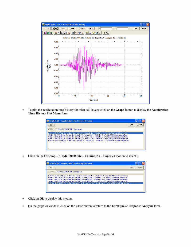
• To plot the acceleration time history for other soil layers, click on the Graph button to display the Acceleration Time History Plot Menu form.

• Click on the Outcrop – SHAKE2000 Site – Column No – Layer 21 motion to select it.

• Click on Ok to display this motion. • On the graphics window, click on the Close button to return to the Earthquake Response Analysis form.


• To display the shear stress or strain time histories from Option 7, click on the Shear Stress/Strain Time History option, and then on the Plot button to display the graph.

• The Graph button, when clicked on, will display the menu that lists the shear stress/strain time histories

available.

• Click on the SHAKE2000 Site – Column No. 1 – Layer No. 8 ….. Stress History history to select it.

• Click on Ok to plot this time history. • On the graphics window, click on the Close button to return to the Earthquake Response Analysis form.


• To plot the response spectra defined in Option 9, click on the Response Spectrum option to select it. • Click on the Plot button to display the Relative Displacement Response Spectrum.

• Click on the Graph button to display the Response Spectrum Plot Menu form.

• To select a type of spectrum (Relative Displacement, Relative Velocity, Pseudo-Relative Velocity, Absolute

Acceleration or Pseudo-Absolute Acceleration) click on the check box next to it. Then, select a damping ratio by clicking on the check box adjacent to it.

• For this tutorial, click on the Pseudo-Absolute Acceleration check box and on the Response spectrum for 5% damping box.

• The Ok button is not enabled until you have selected both a damping ratio and a type of response spectrum. The AASHTO, Attenuate, IBC, NEHRP, Target and UBC buttons are enabled only when you select an acceleration spectrum option and 5% damping. The EuroCode button is enabled for any damping value.

• Click on the Ok button to plot the graph.


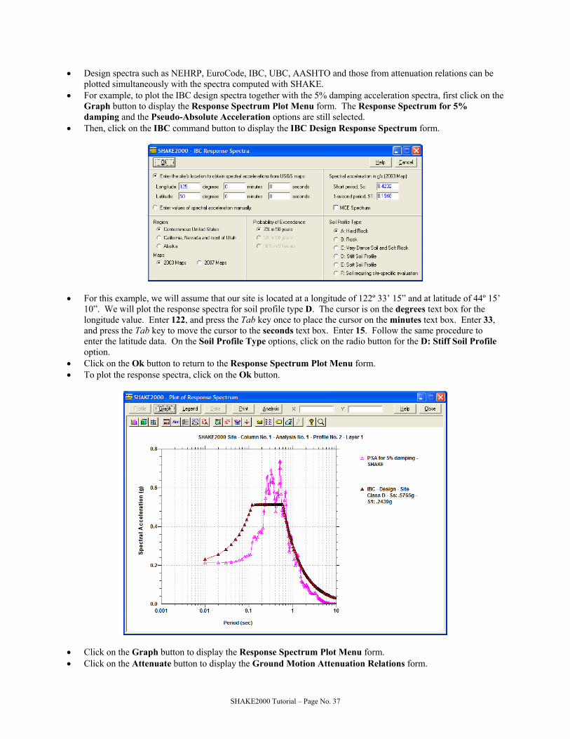
• Design spectra such as NEHRP, EuroCode, IBC, UBC, AASHTO and those from attenuation relations can be plotted simultaneously with the spectra computed with SHAKE.

• For example, to plot the IBC design spectra together with the 5% damping acceleration spectra, first click on the Graph button to display the Response Spectrum Plot Menu form. The Response Spectrum for 5% damping and the Pseudo-Absolute Acceleration options are still selected.

• Then, click on the IBC command button to display the IBC Design Response Spectrum form.

• For this example, we will assume that our site is located at a longitude of 122º 33’ 15” and at latitude of 44º 15’

10”. We will plot the response spectra for soil profile type D. The cursor is on the degrees text box for the longitude value. Enter 122, and press the Tab key once to place the cursor on the minutes text box. Enter 33, and press the Tab key to move the cursor to the seconds text box. Enter 15. Follow the same procedure to enter the latitude data. On the Soil Profile Type options, click on the radio button for the D: Stiff Soil Profile option.

• Click on the Ok button to return to the Response Spectrum Plot Menu form. • To plot the response spectra, click on the Ok button.

• Click on the Graph button to display the Response Spectrum Plot Menu form. • Click on the Attenuate button to display the Ground Motion Attenuation Relations form.


• Click on the check box next to the Abrahamson & Silva (1997) option. Use the mouse pointer to place the cursor on the text box next to the Distance (km) label, and enter 20.

• Click on the M ±SD (i.e. median plus/minus standard deviation) option to select it. • Click on the Plot button to return to the spectra menu form. • Click on the Ok button to plot the response spectra.


• Click on the Close button to return to the Earthquake Response Analysis form. • Click on the Amplification Spectrum option, and then on the Plot button to display the Amplification Ratio vs.

Frequency graph. The Graph button will display a list of the different amplification spectra available.

• Click on the Close button to return to the Earthquake Response Analysis form. • Click on the Fourier Amplitude Spectrum option, and then on the Plot button to display the Fourier

Amplitude vs. Frequency graph.


• To improve the appearance of the graph, we can change the type of axis and reduce the number of points plotted. First, to plot the graph using linear instead of logarithmic scales, click on the Style icon of the graph toolbar (i.e. the third icon from the left). This will display the Style tab of the graph control. On the Log Data section of the form, click on both the Y axis and X axis check boxes to deselect them. Now, click on the Ok command button to redraw the graph.

• To change the number of points shown on the graph, click on the Data button to display the Number of Points

on a Graph form.

• This form is used to enter the number of points to plot. For this example, the graph has 2048 points. However,

as the graph shows, most of the points have a y-coordinate value of zero. Thus, we can show the most significant part of the graph by plotting only the leftmost portion.

• The Reset button will restore the number of points to the original value. In this example, it will be 2048. • For our example, enter 512 on the data cell. Click on the Ok button. • The graph will be plotted again, this time with less data.

• Click on the Close button to return to the Earthquake Response Analysis form. • The Dynamic Material Properties option is used to plot the dynamic material properties (i.e. modulus

reduction (G/Gmax) vs. strain and damping ratio vs. strain) curves saved in the EDT file. • Click on this option and then on the Plot command button to display the graph.


• Click on the Graph button to display the Plot Dynamic Material Properties menu form that shows the other property curves available in the data file.

• Select up to 5 curves by clicking on their check boxes, and then click on the Plot button to plot them.

• On the graphics window, click on the Close button to return to the Earthquake Response Analysis form. • The Object Motion option can be used to create a graph of the input object motion used in the SHAKE

analysis. • Click on the Object Motion option, and then on the Plot button to display the Plot Object Motion form. Some

basic information for sample1.eq and ALS-E_AT2.eq will be displayed next to the option showing the object motion file name. These are the earthquake files used by Options 3 stored in the sample_1.edt file. By default, SHAKE2000 will display the information for the Options 3 stored in this file.


• Click on the second option button to select \SHAKE2000\SAMPLE\ALS-E_AT2.EQ. The Plot button is

enabled after you select an option. • Click the Plot button to display the object motion plot.

• Click the Close button to return to the Plot Object Motion form. • To plot the acceleration, displacement and velocity time histories for this ground motion, click on the All three

option to select it, and then click on the Plot command button.


• Click the Close button to return to the Plot Object Motion form. • An individual plot of the velocity or displacement time histories can also be created. For example, click on the

Velocity option to select it. Now, click on the Plot command button.

• Click the Close button to return to the Plot Object Motion form.


• A feature of SHAKE2000 allows the user to obtain various parameters used to characterize a ground motion, e.g. Arias Intensity, Root-Mean-Square, etc., which can then be used to select a representative time history for site-specific response analyses. To do this, click on the GMP command button to display the Ground Motion Parameters form.

• On the bottom section of the form, there are a number of plotting options. The Husid Plot option will display a

graph of the Normalized Husid Plot. If you select the Plot Ground Motion option, then the acceleration time history will be plotted on the same graph with the Husid Plot. In the plot, the section of the Husid Plot for the Trifunac & Brady duration is shown as a red curve.

• Click on the check box for the Plot Ground Motion to select it, and then click on the Plot command button.

• Click the Close button to return to the Ground Motion Parameters form. • Click the Close button to return to the Plot Object Motion form. • An alternative way of plotting the object motion is to select a file with information not included in the input file

for SHAKE2000. For example, to plot the object motion saved in the sample1.eq file, use the Other command button to display the open file dialog form. Double click on the Sample directory, select the All Files (*.*)


option of the Files of type list, and then select the sample1.eq file by double clicking on it. You will return to the Plot Object Motion form, and the path to the file will be shown on the bottom section of the form.

• Click on the Earthquake File option. This will enable you to enter the information for the object motion on the data cells below the option. Use the Tab key, or the mouse pointer, to move to the text box below the No. Values label.

• This file is formed by 3800 acceleration points; arranged in rows with 8 values each, formed by 9 digits, has a time step of 0.01 seconds, and contains 1 header line. Enter 3800 in the No. Values cell, and then move to the corresponding cells and enter the above information. Click on the Acceleration option to select it, and then click Plot to display the acceleration time history. Click the Close button to return to the Plot Object Motion form, and then click Close to return to the Earthquake Response Analysis form.

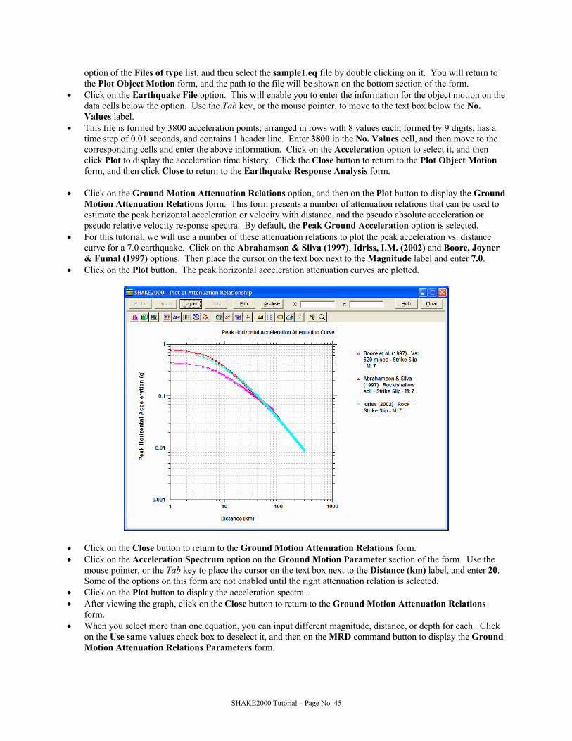
• Click on the Ground Motion Attenuation Relations option, and then on the Plot button to display the Ground

Motion Attenuation Relations form. This form presents a number of attenuation relations that can be used to estimate the peak horizontal acceleration or velocity with distance, and the pseudo absolute acceleration or pseudo relative velocity response spectra. By default, the Peak Ground Acceleration option is selected.

• For this tutorial, we will use a number of these attenuation relations to plot the peak acceleration vs. distance curve for a 7.0 earthquake. Click on the Abrahamson & Silva (1997), Idriss, I.M. (2002) and Boore, Joyner & Fumal (1997) options. Then place the cursor on the text box next to the Magnitude label and enter 7.0.

• Click on the Plot button. The peak horizontal acceleration attenuation curves are plotted.

• Click on the Close button to return to the Ground Motion Attenuation Relations form. • Click on the Acceleration Spectrum option on the Ground Motion Parameter section of the form. Use the

mouse pointer, or the Tab key to place the cursor on the text box next to the Distance (km) label, and enter 20. Some of the options on this form are not enabled until the right attenuation relation is selected.

• Click on the Plot button to display the acceleration spectra. • After viewing the graph, click on the Close button to return to the Ground Motion Attenuation Relations

form. • When you select more than one equation, you can input different magnitude, distance, or depth for each. Click

on the Use same values check box to deselect it, and then on the MRD command button to display the Ground Motion Attenuation Relations Parameters form.


• For the Idriss, I.M. (2002) equation, enter a magnitude of 7.0 and a distance of 20 km. For the Abrahamson

& Silva (1997) equation, enter a distance of 12 km and a magnitude of 7.25; and, for the Boore, Joyner & Fumal (1997) equation enter a distance of 15 km and a magnitude of 6.75. Click on the Ok button to close the form, and return to the Ground Motion Attenuation Relations form. Click on the Plot button to display the response spectra.

• Click on the Close button and then on the Return button to return to the Earthquake Response Analysis form.


• For the second part of this tutorial, we will modify the sample.in file so that it contains three different analyses. First, we will use the same input data as before, and then we will analyze the same profile using a different input motion (i.e. ALS-E_AT2.EQ).

• Next, we will obtain the acceleration time history at the top of layer 3 of column No. 3 using the sample1.eq ground motion. We will use this time history in the Newmark Displacement Analysis section of this tutorial.

• To continue with the tutorial, add the following options to the input file:

Position Option 16 Option 2 - SHAKE2000 Site – Column No. 1 17 Option 3 - Input Mtion: CHI CHI 09/20/99, ALS, E (CWB) 18 Option 4 - Sublayer for input motion is No. 21 19 Option 5 - No. iterations 10, strain ratio 0.65 20 Option 6 - Acceleration time history for layers 1-15 of Column No. 1 21 Option 6 - Acceleration time history for layers 16-21 of Column No. 1 22 Option 7 - Shear stress & strain time histories at Layer 4 - Column No. 1 23 Option 7 - Shear stress & strain time histories at Layer 8 - Column No. 1 24 Option 9 - Response spectrum at surface – Damping 1, 2.5, 5, 10, 15, 20% 25 Option 9 - Response spectrum layer 4 – Damping 1, 2.5, 5, 10, 15, 20% 26 Option 9 - Response spectrum layer 8 – Damping 1, 2.5, 5, 10, 15, 20% 27 Option 9 - Response spectrum layer 21 – Damping 1, 2.5, 5, 10, 15, 20% 28 Option 10 - Amplification spectrum between layers 21& 1 – Column No. 1 29 Option 11 - Fourier spectrum between layers 1 & 21 – Column No. 1 30 Option 2 - SHAKE2000 Site – Column No. 3 31 Option 3 - Input motion: SAMPLE1.EQ 32 Option 4 - Sublayer for input motion is No. 13 33 Option 5 - No. iterations 10, strain ratio 0.65 34 Option 6 - Acceleration time history for layers 1-13 of Column No. 3 35 Option 7 - Shear stress & strain time histories at Layer 3 - Column No. 3 36 Option 9 - Response spectrum at surface – Damping 1, 2.5, 5, 10, 15, 20% 37 Option 9 - Response spectrum layer 13 – Damping 1, 2.5, 5, 10, 15, 20% 38 Option 10 - Amplification spectrum between layers 13 & 1 – Column No. 3 39 Option 11 - Fourier spectrum between layers 1 & 13 – Column No. 3


• Save the input and EDT files using the Save command button. • We will use the same name for the output files, i.e. sample10.out and sample20.out; and, the same name for

the data files as before, i.e. sample. • Run SHAKE and then process the output files. • After the files are processed, click on the Display Results of First Output File option and then on the Display

button to display the Summary of Results of First Output File form. • Click on the Next button once to display the results for the second analysis, i.e. the analysis for Column No. 1

using the ALS-E_AT2.EQ ground motion file.

• Use the scroll bars to display the results for the other soil layers. • To see the results for the analysis for Column No. 3 using the sample1.eq object motion record, click on the

Next button once.

• Click on the Return button to return to the Earthquake Response Analysis form. • Click on the Peak Acceleration, CSR, Shear Stress option, and then on the Plot button. • Click on the Graph button to display the plot menu, and then click on the Next button to display the plot menu

for the analysis of Column No. 1 using the ALS-E_AT2.EQ object motion. • Click on the Peak Acceleration option, and then on the Ok button to return to the graphics window.


• Because we have analyzed the same soil profile with two different object motions, it is possible to obtain an

average result. • For this example, we will get the average peak acceleration vs. depth curve. • To do this, click on the Graph button to display the plot menu. The Peak Acceleration option is still selected.

Click on the Mean button to display the Average Calculated Results Menu form.

• Select the two analyses by clicking on the check boxes, then select the Plot average curve plus above selected

curves option by clicking on it. If you would like to plot the average curve only, select the Plot average curve only option. To plot the computed curves without showing the average curve, select the Plot above selected curves only option.

• Click on the Ok button to display the peak acceleration curves.


• Click on the Close button to return to the Earthquake Response Analysis form. • The average response spectrum can also be computed. For this example, we will obtain the average pseudo-

absolute acceleration response spectrum for layer No. 1 (i.e. the surface layer) from the spectra computed using the two object motions. To do this, click on the Response Spectrum option, and then on the Plot button.

• Click on the Graph button. The plot menu for the first analysis is shown. • Select Response spectrum for 5% damping and the Pseudo-Absolute Acceleration response spectrum

options, and then click on the Mean command button to display the Average Response Spectrum form.

• Select Analysis No. 1 and Analysis No. 2 by clicking on the first two check boxes, and then select the Plot

average curve plus above selected curves option by clicking on it. • Click on the Ok button to display the average spectrum and the spectra computed with each object motion.


• Another useful feature of SHAKE2000 is the ability to simultaneously plot response spectra for different layers of the same soil profile. For this example, we will obtain a plot that shows the pseudo-absolute acceleration spectrum for 5% damping, for layers 1 (surface), 4, 8 and 21 (half-space) of Column No. 1, computed with the ALS-E_AT2.eq motion.

• To do this, first click on the Graph button. The plot menu for the first analysis is shown. • Click on the Next button four times to move to the second analysis (Analysis No. 2 – Profile No. 2 is shown on

the text box next to the Profile label). • Select the 5% damping value and the Pseudo-Absolute Acceleration response spectrum option, and then click

on the Site command button to display the Response Spectra – Site Effects Menu form.

• Select all of the layers by clicking on the check boxes. • Click on the Ok button to display the curves.


• You can change the legends for a curve using the Legend command button. • Click on the Legend button to display the Legend Text form.

• Move the cursor to the legend you would like to change and enter the new information. The Reset button will

change the legends back to their default setting. Once completed, click the Ok button to redraw the graph. • Click on the Close button to return to the Earthquake Response Analysis form. • To demonstrate the liquefaction analysis feature of SHAKE2000, click on the Peak Acceleration, CSR, Shear

Stress option and then on the Plot button to display the peak acceleration vs. depth graph. • Click on the Graph button to display the Calculated Results Plot Menu form. • Click on the Cyclic Stress Ratio option. The SPT-BPT, CPT, Vs and CSR command buttons along with the

Water Depth for CSR & CRR Analyses (ft) text box are enabled. • For this part of the tutorial, we will do the liquefaction analysis using SPT data. • First, place the cursor on the Water Depth for CSR & CRR Analyses (ft) text box and enter a value of 5.5 for

the depth to water table. • Click on the SPT-BPT button to display the Cyclic Resistance Ratio using SPT form. The cursor is located

on the Earthquake Magnitude text box.


• Enter a value of 7.1 for the earthquake magnitude. Press on the Tab key twice to move the cursor to the Cn Water Table Depth (ft) text box. A value of 1.15 is displayed on the Magnitude Scaling Factor text box. Assume that the water table during drilling was at a depth of 7.5 feet (different from the water table depth entered before). Enter 7.5 for the Cn water table.

• The combo box below the Cn Water Table Depth is used to select an energy ratio for the analysis. Click on the down arrow to show a list of options, and select the Automatic-Trip Hammer option. Then press the Tab key once to move the cursor to the text box. An average value of 1.1 is shown on the text box. Press the Tab key once to move the cursor to the first row on the Depth column.

• Enter a value of 4.0 for the first depth value. Press the Tab key once to move the cursor to the N (field) column.


• A series of values are automatically displayed: 1.1 for Energy, 1 for Rod, 1 for Sampler, 520 for Total Stress (psf), 1.7 for CN, 0 for % Fines, and 1 for Ksigma. The value of CN is computed using the Liao & Whitman option, which is the default option.

• Enter a value of 7 for the measured SPT value and press the Tab key. A value of 13 is displayed on the N1,60,cs column, and “- - -” on the CRR and Safety Factor columns. Because this SPT is above the water table, there is not a value for CRR.

• Use the Tab key or the mouse pointer to place the cursor on the second row of the Depth (ft) column. Enter the

following data for depth and SPTs. When you need to scroll down the list, use the scroll-down bar on the right side of the input data section. The scroll-down bar is inactive when you are entering data on a text box. To activate it, you need to move to a different text box by either using the Tab key or the mouse buttons.

SPT No. Depth N 2 7 4 3 10 3 4 14 3 5 17 5 6 20 9 7 24 12 8 27 12 9 30 14 10 33 9 11 37 23 12 40 13 13 43 11 14 47 11 15 50 24 16 53 27 17 57 5 18 60 6 19 63 4 20 66 38


• Try using the other options. For example, to use a different equation for the magnitude scaling factor click the respective option shown on the MSF options. Click on the I.M. Idriss (1999) option. The magnitude scaling factor changes to 1.111, as shown on the Magnitude Scaling Factor text box; and, the cyclic resistance ratios using this new value are recalculated and displayed.

• Click on the down arrow on the Rod Length list, on the bottom right corner of the form. A list of factors is

shown to correct for different drill rod lengths. Click on the Seed‘s 0.75 for <= 10’ option and press the Tab key once to move the cursor off this list. Again, the cyclic resistance ratios for the SPT values at the top of the soil column are recalculated using the new correction factor for drill rod length.

• Click on the Save button to display the Save CRR Data dialog form. Switch to the Sample subdirectory. • On the File name text box, enter sample.crr, and click on the Save button. The results of the cyclic ratio

analysis will be saved in this file. These results can be retrieved later with the Open command button.

• To plot the curves, click on the Plot button. You will return to the plot menu form. Click on Ok.

• Click on the FSL button to plot the Factor of Safety against Liquefaction curve.


• We will estimate the settlement in the soil column due to earthquake shaking. Click on the Graph command button to display the Calculated Results Plot Menu form, and then click on the Settlement command button to display the Settlement Analysis form.

• By default, SHAKE2000 will estimate the thickness of the layers based on the position of the SPTs. A layer

interface will be set at the midpoint between two SPTs. Another layer interface will also be set at the depth of the ground water table. The thickness for these layers will be different from the ones read from Option 2 from the first SHAKE output file. A total settlement of approximately 20 inches is calculated.

• Click on the Ishihara & Yoshimine (1992) option. The settlement is recalculated using this method. An approximate settlement of 25 inches is calculated.


• Click on the Close command button to return to the plot menu. You will be asked if you would like to save the

data to a file. Click No for the time being. • Click on Ok or Cancel to return to the graphics window. • Click on the Close button to return to the Earthquake Response Analysis form. Then, click on the Return

command button to return to the Main Menu form. • We will now use the acceleration time histories computed to determine permanent slope displacements due to

earthquake shaking using the Newmark Method. • Click the Newmark Method - Displacement Analysis option to select it, and then on the Ok button to display

the form used to enter the data for the displacement analysis.

• We will use this mehtod to estimate the displacements due to shaking on the failure surface shown in the figure

on the first page of this tutorial. The acceleration time history for points immediately below the shear zone was computed with Option 6 (the points are assumed to be at the top of layers 4 & 8 for Column No. 1 and at the top of layer 3 for Column No. 3), and saved as l4a1d2-2.ahl, l8a1d2-3.ahl and l3a3d1-20.ahl in the Sample subdirectory. These files were created when the second output file was processed.


• For this example, we will use a constant yield acceleration value of 0.07 g. • Place the cursor on the text box next to the Constant Acceleration label, and enter 0.07. • Click the File command button for the Acceleration Time History (g's) option. This will open the Newmark

Displacement Ground Motion File form.

• We will use a weighted-average approach to compute an average acceleration file from a series of n files.

Further information on the method used is provided in the Newmark Displacement section of this manual. You can also click on the Help command button to display a help window that provides the same information.

• The cursor is on the text box next to the Weighted motion description label. Type in SHAKE2000 Site – Newmark Displacement Analysis.

• To select the first file, click on the first (Click Choose to select a file) check box to select it and then on the Choose command button to display the Open Acceleration Time History file dialog form. If necessary, change to the Sample subdirectory by double clicking on it.

• A series of files that start with the letter “l” are displayed in the file dialog window. These files have the *.AHL

extension, and were created when the second output file was processed. The “l” stands for layer, and the number following the “l” is the layer number. The “a” stands for analysis, followed by the analysis number; the “d” stands for soil deposit, followed by the soil deposit number; and, the number after the dash is the position of this time history on the second output file. Select the file l4a1d2-2.ahl. Click the Open button to return to the displacement ground motion file form. The file name will be shown next to the first check box.

• To select the second file, l8a1d2-3.ahl, first click on the second check box and then on the Choose command button to display the file dialog form. Select the file and click on Open.


• Now, click on the third check box to select it, and on the Choose command button. Select the l3a3d1-20.ahl file and click on Open. The file names and paths, and some basic information will be shown on the form.

• The average accelerogram will be saved in the file named sample.nmk. Click on the Save command button to display the Save Accelerogram File form, and enter sample.nmk on the File name box. Click on Save to return to the Newmark Displacement Ground Motion Files form. To create the average file, click on the Motion command button.

• Now click on the Ok button to return to the Newmark Displacement form. The average file name and path are

shown in the box next to the Acceleration Time History (g’s) label. The peak acceleration for this record is shown in the text box next to the Maximum Acceleration Value (g) label.

• The computed displacements will appear in the Maximum, Average, and Minimum data cells at the bottom of the form.

• To plot the results, click on the Plot command button.



• Click on the Print command button to display the Graphics Print Menu form.

• Use the Copy command button to copy the graph to the clipboard. You can then use the Paste or Paste Special

commands on other Windows applications (e.g. Microsoft Word), to insert the graph into other documents, e.g. see graph on following page.

• Click the Close button to return to the graphics form, and then click on Close to return to the Newmark

Analysis form. • Click the Close button to return to the Main Menu form.

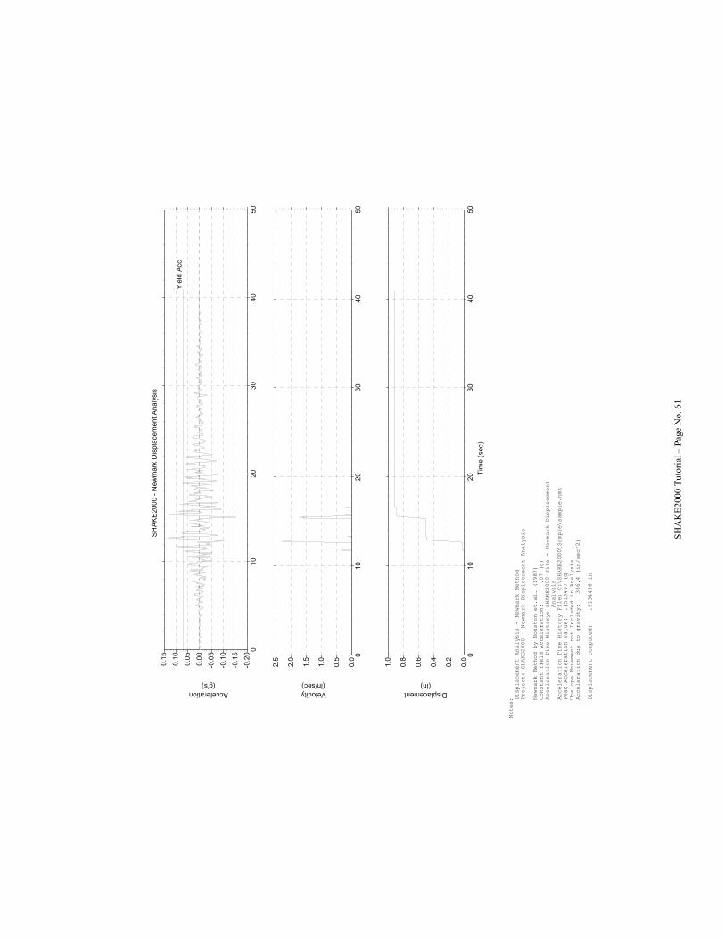
SHA

KE2

000

Tuto

rial –

Pag

e N

o. 6

1

SHAK

E20

00 -

New

mar

k D

ispl

acem

ent A

naly

sis

Acceleration(g's)

-0.0

5

-0.1

0

-0.1

5

-0.2

0

0.00

0.05

0.10

0.15

010

2030

4050

Yiel

d Ac

c.

Velocity(in/sec)

0.0

0.5

1.0

1.5

2.0

2.5 0

1020

3040

50

Tim

e (s

ec)

Displacement(in)

0.0

0.2

0.4

0.6

0.8

1.0 0

1020

3040

50

Notes: Displacement A

Project: SHAKE

Newmark Method

Constant Yield

Acceleration T

Acceleration T

Peak Accelerat

Upslope Moveme

Acceleration d

Displacement c

nalysis - Newmark Method

2000 - Newmark Displacement Analysis

by Houston et.al. (1987)

Acceleration: .07 (g)

ime History: SHAKE2000 Site - Newmark Displacement

Analysis

ime History File: C:\SHAKE2000\Sample\sample.nmk

ion Value: .1513497 (g)

nt not Included in Analysis

ue to gravity: 386.4 (in/sec^2)

omputed: .9134436 in

• Another option to estimate the displacement due to ground motion applicable to embankments is the simplified approach proposed by Makdisi & Seed. For this tutorial, assume that the cross section shown on the introduction to the tutorial is the downstream slope of an earth embankment.

• Click on the Makdisi & Seed (1977) – Displacement Analysis option to select it, and then on Ok to display the Makdisi & Seed (1977) Simplified Displacement Analysis form.

• The cursor is in the text box next to the Project Information label. Type in SHAKE2000 Dam –

Displacement Analysis as description for this analysis. Press the Tab key once to move the cursor to the text box next to the Earthquake Magnitude label, and enter 7.1 for magnitude. Use the mouse to place the cursor on the text box next to the Peak acceleration (g) label and enter 0.14. Enter the following data for the embankment: 35 feet for height, 130 pcf for unit weight, 557 ksf for Gmax, 0.07 g for yield acceleration, and 1.0 for depth ratio.

• Now, to select the G/Gmax and Damping Ratio curves for the embankment material first click on the Get command button next to the box for the G/Gmax Curve label. This will display the G/Gmax Curves Database form. This is a database of G/Gmax curves saved in the shakey2k.mat file.

• Select the Sand S2 G/Gmax – S2 (Sand CP = 1-3 KSC) 3/11/1988 curve by clicking on it to highlight it.

• Click on the Choose command button. The curve identification will be shown on the label box. • To select a damping ratio curve, click on the Get command button next to the text box for the Damping Ratio

Curve label. This will display the Damping Ratio Curves Database form. • Select the Sand Damping for SAND, February 1971 curve by clicking on it to highlight it. Then, click on the

Choose command button. The curve identification will be shown on the text box next to the Damping Ratio Curve label.


• Press the Tab key, or use the mouse, to place the cursor on the text box next to the Assume average shear strain (%) label. Enter an estimate of the average shear strain level in the embankment. For this example, enter 0.06 and then press the Tab key once to move the cursor off the text box.

• Some values are calculated for G/Gmax, G, Damping, Vs, and modal periods (i.e. T1, T2, and T3). • To compute the spectral accelerations (i.e. Sa1, Sa2, and Sa3) corresponding to the calculated damping ratio of

12.8 and the three modal periods, we need to compute the response spectra for different values of damping for the sample1.eq ground motion. To do this, click on the Sa command button to display the Response Spectra for Ground Motion form.


• Use the Other button to display the Open Ground Motion File dialog form. Change to the Sample subdirectory and then select the sample1.eq file by double clicking on it. The path to the file will be shown on the text box next to the Other Ground Motion File label.

• Click on the check box for the Other Ground Motion File to select it. This way the program will use the information in this file to compute the response spectra. Use the Tab key, or the mouse pointer, to move to the No. Values cell.

• This file is formed by 3800 acceleration points, arranged in rows with 8 values each, formed by 9 digits, has a

time step of 0.01 seconds, and contains 1 header line. Enter 3800 in the No. Values cell, and then move to the corresponding cells and enter the above information.

• Use the mouse to place the cursor on the first text box of the Damping Ratios (in decimal) data cells. We will compute the spectra for damping values of 0.025, 0.05, 0.1, 0.125, 0.15, and 0.20. Enter 0.025 and press the Tab key once to move to the following data cell and enter 0.05. On the other data cells enter 0.1, 0.125, 0.15, and 0.20.

• Use the Save command button to save the response spectra to the sample.spc file in the Sample folder. The file information will be shown on the text box next to the File for Response Spectra Data label.

• Click on the Spectra button to compute the response spectra for the ground motion. After the spectra are

computed, click on Ok to return to the Makdisi & Seed form. Note that the spectral accelerations are displayed in their respective boxes (e.g. Sa1 = 0.315).

• Values for the maximum crest acceleration, average shear strain, Kmax/Umax, Kmax, Ky/Kmax are also computed. Further, the displacement values are obtained from the charts provided by Makdisi & Seed, and shown on the bottom section of the form.

• This procedure is iterative and based on convergence of the average shear strain. Thus, if the average

equivalent shear strain computed in Step 5 (shown on the data box next to the Average equivalent shear strain (%) label) is not similar, or close, to the assumed value entered in Step 1, then you need to repeat the process using this time the computed value.


• Enter a value of 0.074 for the Assumed average shear strain in Step 1. Press the Tab key once to move the

cursor off the text box. New values are computed. The average shear strain is now 0.067. • To continue with the iterative process, enter a value of 0.038 for the Assumed average shear strain in Step 1.

Press the Tab key once to move the cursor off the text box. New values are computed. The average shear strain converges at 0.07. A permanent displacement range between 0.84 inches and 6.65 inches is computed.

• If you would like to save the results, click on the Save command button. • Click on Close to return to the Main Menu form.


• Another analysis feature of SHAKE2000 is the estimation of liquefaction induced ground deformation with any of the Multiple Linear Regression models developed by Bartlett & Youd, Bardet, Mace & Tobita and Zhang et al..

• In the Main Menu form, click on the Liquefaction-Induced Ground Deformation option to select it, and then click on the Ok command button to display the form used to enter the input data.

• The cursor is on the Project Information text box. For this tutorial, type in SHAKE2000 Site - Liquefaction

induced ground deformation analysis. Press the Tab key once to move the cursor to the text box next to the Earthquake moment magnitude (Mw) label and enter 7.1. For the other input data enter: 50 for closest distance to source; 1000 for distance to free face; 10 for height of free face; 2 for ground slope; 5 for thickness of soils with (N1)60 < 15; 16 for average fines content in T15 layer; and, 0.1 for average mean grain size in T15 layer. Press the Tab key to move the cursor off the text box. By default, the Bartlet & Youd Ground slope MLR model is selected, and after you entered the last data, the values for ground deformation are automatically calculated and shown in the text boxes below the Ground Deformation label.

• To use a different model for the analysis, click on the respective option button. The values for ground

deformation will be recalculated and shown on the text boxes. • Click on the Print command button to obtain a printed copy of the input data and results. This will display the

Print Menu form. Click on the down arrow for the Zoom list and select 100.


• Click on the Close command button to return to the liquefaction-induced deformation form. • Click on the Close command button to return to the Main Menu form. • SHAKE2000 includes a pre & postprocessor for SEISRISK III, a computer program for seismic hazard

estimation developed by the USGS. • On the Main Menu form click on the Probabilistic Seismic Risk Analysis - SEISRISK III option, and then

on Ok to display the Probabilistic Seismic Risk Analysis with SEISRISK III form. This form is used to create input files for, and to process output files created with SEISRISK III.

• We will use the sample data provided in the SEISRISK III User’s Manual for this tutorial. The sample file is

shown in the following page. The numbers before the “|” symbol are used only as line reference.


1| SEISRISK III Sample Problem 2| 0 20. 3| .90 3 10 50 250 4| 1. 0 .5 0 5| 123.0 38.0 120.0 38.0 6| 123.00 39.00 120.00 37.00 .100 7| 12 17 3 8 8| 1 9| 3 10| 123. 39. 123. 38 11| 6 12 12| 'watashh79' 8.5 7.6 6.6 5.6 5.2 4.2 13| 3.22 .74 .73 .67 .45 .195 .072 14| 6.43 .64 .62 .53 .36 .135 .047 15| 16.09 .49 .43 .32 .19 .052 .02 16| 32.18 .36 .28 .17 .09 .02 .0052 17| 64.3 .21 .14 .06 .035 .0051 .0013 18| 96.5 .12 .07 .03 .0138 .0023 .00042 19| 160.9 .045 .025 .015 .005 .00083 .0001 20| 321.8 .013 .0076 .0026 .0012 .00021 .00003 21| 643.0 .0034 .0019 .00065 .0003 .00005 .00001 22| 1288.0 .00085 .00047 .00016 .00007 .00001 .00001 23| 2570.0 .00021 .00012 .00004 .00002 .00001 .00001 24| 5140.0 .0001 .00006 .00002 .00001 .00001 .00001 25| 00 100. 2 zn01 26| 3 1 1 27| 122.20 37.22 122.00 37.32 28| 123.85 38.97 123.68 39.05 29| 124.12 39.32 123.89 39.40 30| .106 .281 .74 1.97 31| 6.100 5.500 4.900 4.300 32| 00 65.2 2 zn02 33| 2 1 1 34| 120.05 34.09 119.26 34.20 35| 120.40 33.50 119.77 33.39 36| .031 .073 .172 .405 .955 2.248 37| 7.300 6.700 6.100 5.500 4.900 4.300 38| 98 1.0 2 zn03 20. 39| 7 1 2 40| 120.40 34.68 120.00 34.78 41| 120.56 34.93 120.28 35.00 42| 120.78 35.20 120.38 35.39 43| 121.00 35.48 121.00 36.00 44| 121.51 36.00 121.47 36.50 45| 121.82 36.45 121.80 36.80 46| 122.00 36.73 122.21 37.11 47| 2 2 2 48| 121.80 36.80 121.77 36.88 49| 122.21 37.11 122.20 37.22 50| .0198 .0641 .2074 .6712 51| 6.100 5.500 4.900 4.300 52| 99 1.0 2 ft01-1.085 .389 .50 53| 12 1 1 54| 117.37 34.17 118.09 34.59 118.67 34.79 119.03 34.85 55| 119.26 34.90 119.54 35.06 121.27 36.66 121.69 36.94 56| 122.10 37.27 123.77 39.01 124.01 39.36 124.16 39.93 57| .0021 .0057 .015 .040 58| 8.500 7.900 7.300 6.700 59| 00 10. 2 ft02-1.085 .389 .50 60| 4 1 4 61| 122.40 38.10 122.90 38.66 123.38 39.10 123.94 39.79 62| 3 2 4 63| 122.60 38.68 123.10 39.20 123.74 39.95 64| 5 3 4 65| 122.16 38.16 122.46 38.80 122.75 38.98 123.18 39.56 66| 123.40 39.98 67| 3 4 4 68| 122.50 39.10 122.80 39.25 122.95 39.43 69| .0072 .0200 .057 70| 7.900 7.300 6.700 71| 99


• Similarly to SHAKE, SHAKE2000 separates the data used in SEISRISK into “options”. Using the data from the previous page, the following “options” are defined: 1) one set of Option 1 is formed by the information about the probabilities and the area of study, i.e. between the title line and before the attenuation data (lines 1 thru 10); 2) one set of Option 2 is formed by lines 11 thru 24 (i.e. the attenuation data); 3) there are 3 sets of Option 3, one for each seismic source zone, i.e. between lines 25-31, 32-37 and 38-51 respectively; and, 4) there are two sets of Option 4, one for each fault, i.e. between lines 52-58 and 59-70 respectively. The value of 99 on line 71 only indicates that this is the end of the data. This value will be automatically entered by SHAKE2000 when the input file is created.

• To enter the data, first click on the New command button to display the SEISRISK III Option List form. This form is used to create a new set for an option.

• The data for “Option 1”, Default Probability & Study Area Data, is highlighted. • Click on the Choose command button to select this option and return to the SEISRISK III form. The option

will be shown in the top list box, which will display the different options that make up the SRK file, or the file that will save the different sets for each option.

• Click on this option to select it, and then on the Edit command button to display the SEISRISK III Probability

& Study Area form.

• The cursor is on the Identification text box. For this option enter SEISRISK III User’s Manual Sample Problem, and press the Tab key to move the cursor to the Title text box.

• In the Title text box enter SEISRISK III Sample Problem.


• Use the same procedure and enter the following information in the respective text boxes.

isw sigmax 0 20.0 prob ntims jtim(1) jtim(2) jtim(3) 0.90 3 10 50 250 scale dw sd inos 1.0 0 0.5 0 x1 y1 x2 y2 123.0 38.0 120.0 38.0 fl1 ph1 fl2 ph2 phinc 123.00 39.00 120.00 37.00 0.100 irow1 icol1 irow2 icol2 12 17 3 8 indv 1 nvs 3 xe1 ye1 xe2 ye2 123.0 39.0 123.0 38.0

• Click on Ok to return to the SEISRISK III form. • Use the New command button to create a second set of Option 1, i.e. Default Probability & Study Area Data. • Highlight the second set for Option 1 and then click on the Edit command button to display the SEISRISK III

Probability & Study Area form. • For this second set, we will use most of the same data as for the first set entered above. The only difference will

be on the value of the isw variable. In this set, we will use a value of 1 for isw to indicate that the analysis will continue from a previous run.

• In the identification text box enter SEISRISK III User’s Manual Sample Problem – Restart and press the Tab key to move the cursor to the isw text box.

• Use the same procedure to enter the following information in their respective text boxes.


isw sigmax 1 20.0 prob ntims jtim(1) jtim(2) jtim(3) 0.90 3 10 50 250 scale dw sd inos 1.0 0 0.5 0 x1 y1 x2 y2 123.0 38.0 120.0 38.0 fl1 ph1 fl2 ph2 phinc 123.00 39.00 120.00 37.00 0.100 irow1 icol1 irow2 icol2 12 17 3 8 indv 1 nvs 3 xe1 ye1 xe2 ye2 123.0 39.0 123.0 38.0

• Click on Ok to return to the SEISRISK III form. • Use the New command button to create a set of Option 2, i.e. attenuation function. • Highlight the set for the attenuation data and then click on the Edit command button to display the SEISRISK

III Attenuation Function form. • In the identification text box enter Attenuation data from WATASHH79 and press the Tab key to move the

cursor to the jent text box. • Use the same procedure to enter the following information in their respective text boxes.

jent mdis 6 12 nam tm(1) tm(2) tm(3) tm(4) tm(5) tm(6) watashh79 8.5 7.6 6.6 5.6 5.2 4.2


rtab atab(1) atab(2) atab(3) atab(4) atab(5) atab(6) 3.22 .74 .73 .67 .45 .195 .072 6.43 .64 .62 .53 .36 .135 .047 16.09 .49 .43 .32 .19 .052 .02 32.18 .36 .28 .17 .09 .02 .0052 64.3 .21 .14 .06 .035 .0051 .0013 96.5 .12 .07 .03 .0138 .0023 .00042 160.9 .045 .025 .015 .005 .00083 .0001 321.8 .013 .0076 .0026 .0012 .00021 .00003 643.0 .0034 .0019 .00065 .0003 .00005 .00001 1288.0 .00085 .00047 .00016 .00007 .00001 .00001 2570.0 .00021 .00012 .00004 .00002 .00001 .00001 5140.0 .0001 .00006 .00002 .00001 .00001 .00001

• Click on Ok to return to the SEISRISK III form. • Use the New command button to create a set of Option 3, i.e. seismic source zone data. • Highlight the set for the seismic source zone data and then click on the Edit command button to display the

SEISRISK III Seismic Source Zone Data form. • In the identification text box enter ZN01 Seismic Source Zone and press the Tab key to move the cursor to the

num text box. • Use the same procedure to enter the following information in their respective text boxes. Note that for some of

the text boxes there is no information to be entered.

num yrnoc iprint totl dumid als bls sigls 00 100.0 2 zn01

• After entering the data for dumid, place the cursor on the itot text box. Enter a 1. The jseg text box will be

enabled and a default value of 2 will be shown. Place the cursor in the jseg text box and enter a 3. • Use the mouse or the Tab key and place the cursor in the first row of the xl column, and continue entering the

following data.

xl yl xr yr 122.20 37.22 122.00 37.32 123.85 38.97 123.68 39.05 124.12 39.32 123.89 39.40


noc(1) fm(l) 0.106 6.100 0.281 5.500 0.74 4.900 1.97 4.300

• Click on Ok to return to the SEISRISK III form. • Use the New command button to create a second set of Option 3, i.e. seismic source zone data. • Highlight the second set for the seismic source zone data and then click on the Edit command button to display

the SEISRISK III Seismic Source Zone Data form. • In the identification text box enter ZN02 Seismic Source Zone and press the Tab key to move the cursor to the



num yrnoc iprint totl dumid als bls sigls 00 65.2 2 zn02 jseg ifr itot 2 1 1 xl yl xr yr 120.05 34.09 119.26 34.20 120.40 33.50 119.77 33.39 noc(1) fm(l) 0.31 7.30 0.73 6.7 0.172 6.1 0.405 5.5 0.955 4.9 2.248 4.3

• Click on Ok to return to the SEISRISK III form. • Use the New command button to create a third set of Option 3, i.e. seismic source zone data. • Highlight the third set for the seismic source zone data and then click on the Edit command button to display

the SEISRISK III Seismic Source Zone Data form. • In the identification text box enter ZN03 Seismic Source Zone and press the Tab key to move the cursor to the




num yrnoc iprint totl dumid als bls sigls 98 1.0 2 zn03 20.0

• After entering the data for dumid, place the cursor on the itot text box. Enter a 2. The jseg text box will be

enabled and a default value of 2 will be shown. Place the cursor in the jseg text box and enter a 7. • Use the mouse or the Tab key and place the cursor in the first row of the xl column, and continue entering the

following data.

xl yl xr yr 120.40 34.68 120.00 34.78 120.56 34.93 120.28 35.00 120.78 35.20 120.38 35.39 121.00 35.48 121.00 36.00 121.51 36.00 121.47 36.50 121.82 36.45 121.80 36.80 122.00 36.73 122.21 37.11

• After entering the data for the seventh value of yr, use the mouse to click on the down-arrow for the ifr list, and

select 2, or the second set of quadrilateral endpoint lines. The jseg text box will be enabled and a default value of 2 will be shown.

• Use the mouse or the Tab key and place the cursor in the first row of the xl column, and continue entering the following data.

xl yl xr yr 121.80 36.80 121.77 36.88 122.21 37.11 122.20 37.22 noc(1) fm(l) 0.0198 6.10 0.0641 5.50 0.2074 4.90 0.6712 4.30

• Click on Ok to return to the SEISRISK III form. • Use the New command button to create a set of Option 4, i.e. fault input data. • Highlight the first set for the fault input data and then click on the Edit command button to display the

SEISRISK III Fault Data form. • In the identification text box enter FT01 Fault Data and press the Tab key to move the cursor to the num text

box.


• Use the same procedure to enter the following information in their respective text boxes. Note that for some of the text boxes there is no information to be entered.

num yrnoc iprint totl dumid als bls sigls 99 1.0 2 0 ft01 -1.085 0.389 0.50 jseg ifr itot 12 1 1 xl yl 117.37 34.17 118.09 34.59 118.67 34.79 119.03 34.85 119.26 34.90 119.54 35.06 121.27 36.66 121.69 36.94 122.10 37.27 123.77 39.01 124.01 39.36 124.16 39.93 noc(1) fm(l) .0021 8.50 .0057 7.90 .015 7.30 .040 6.70

• Click on Ok to return to the SEISRISK III form. • Use the New command button to create a second set of Option 4, i.e. fault input data. • Highlight the second set for the fault input data and then click on the Edit command button to display the

SEISRISK III Fault Data form. • In the identification text box enter FT02 Fault Data and press the Tab key to move the cursor to the num text

box. • Use the same procedure to enter the following information in their respective text boxes. Note that for some of

the text boxes there is no information to be entered. Also, for our tutorial we will change the value of the num variable from 00 (i.e. the value used in the SEISRISK III User’s Manual) to 99 in order to conduct an individual analysis for this fault.

num yrnoc iprint totl dumid als bls sigls 99 10. 2 0 ft02 -1.085 0.389 0.50


jseg ifr itot 4 1 4 xl yl 122.40 38.10 122.90 38.66 123.38 39.10 123.94 39.79 jseg ifr itot 3 2 4 xl yl 122.60 38.68 123.10 39.20 123.74 39.95 jseg ifr itot 5 3 4 xl yl 122.16 38.16 122.46 38.80 122.75 38.98 123.18 39.56 123.40 39.98 jseg ifr itot 3 4 4 xl yl 122.50 39.10 122.80 39.25 122.95 39.43 noc(1) fm(l) .0072 7.90 .0200 7.30 .057 6.70

• Click on Ok to return to the SEISRISK III form.


• If you have different seismic sources or faults, you can perform an individual analysis and create an output file for each source or fault. You can also perform successive runs, accumulating the results for each source or fault, and then save the final results in the last output file created. This option will allow you to combine both output files, the individuals and the total, so that you can view the influence of each source on the total result. We will follow this procedure in this tutorial. Accordingly, we will create individual input files for each zone and fault to conduct individual analyses.

• First, create the input file for the ZN01 seismic source zone. Click on the first set of Option 1, SEISRISK III

User’s Manual Problem and click on the Add command button to add this option to the list of options to be included in the input file.

• On the SRK options list, click on the set of attenuation data, i.e. Attenuation data using WATASHH79 and click on the Add button.

• Click on the first set of zone data, i.e. ZN01 Seismic Source Zone to highlight it and then on the Add button. • To create the input file, click on the Save command button to display the Save SEISRISK III Input File dialog

form. Switch to the Sample folder if necessary. Name the file ZONE01.IN by entering this name in the File name text box and click on the Save button.

• The Save SEISRISK III SRK File dialog form will be displayed. This file will contain all of the different options created, i.e. the options listed in the top list box. Switch to the Sample folder if necessary. Enter SAMPLE.SRK in the File name text box and click on the Save command button.

• In the Output File Name text box enter the name of the output file that we will use for this run. Type in ZONE01.OUT.

• Further, the input and output files will be saved in the Sample folder. To direct the program to look for output files in this folder, click on the icon next to the Directory of Output Files text box to display the Choose Output Directory form. In this form, switch to the Sample folder and then click on Ok. The c:\shake2000\sample path will be shown on the text box.


• We are now ready to run the SEISRISK analysis using the zone01 data. • Click on the SEISRISK button to open the SEISRISK III DOS window. If necessary, change to the

SHAKE2000 main directory (e.g. you will type cd c:\shake2000 and press Enter at the DOS prompt). • Type seisrisk to execute the program. • You will be requested to enter the name of the input, output, auxiliary 02 and auxiliary 03 file names. Use the

following, and press the Enter key after typing each file name:

Enter input file name sample\zone01.in Enter output file name sample\zone01.out Enter auxiliary file name 02 sample\zone01.02 Enter auxiliary file name 03 sample\total.03

• Note that the auxiliary file 03 does not use the same name as the other files. We will use this file in the

following part of the tutorial when the cumulative contribution from each zone and fault to the total is accounted for.

• After a few seconds, execution of SEISRISK will terminate.

• Type exit at the DOS prompt and press Enter to close the window and return to SHAKE2000. • Before continuing with the hazard analyses using the other input files, we will plot some of the information

included in the output file. • Click on the Process command button.


• Click on the Plot Site's Location option. • Click on Plot to display the grid of points and the seismic sources used in the hazard analysis.

• Click on Close to return to the SEISRISK menu form. • Click on the Plot Seismic Hazard Curves after Source option. To select a point on the grid, click on the

down arrow for the at site list (i.e. the list showing the Lat. and Long.). Scroll down to the end of the list and select the point at Long. 123W Lat. 38N. Click on Plot to display the curve.


• Click on Close to return to the SEISRISK menu form. • Click on the Plot Extreme Probability after Source option. Click on the down arrow for the years list, and

select 250. Then, click on Plot to plot the 2-D contour graph.

• Click on Close to return to the SEISRISK menu form. • To plot a 3-D surface view of the above contour plot, click on the Surface (3D) option to select it, and then

click on Plot to display the graph.

• Click on Close to return to the SEISRISK menu form.


• Now, we will continue with the tutorial by conducting the hazard analyses for the other zones and faults individually and then cumulatively.

• Create an input file for seismic source zone 02 using the following options: SEISRISK III User’s Manual Problem Attenuation data using WATASHH79 ZN02 Seismic Source Zone

• To do this, first click on the ZN01 Seismic Source Zone option on the input list box, and then on the Remove command button. Click on Yes to remove this option from the list of input options.

• Click on the ZN02 Seismic Source Zone option on the SRK options list box, and then on the Add command button. This will add the option at the end of the input list box.

• Save the input file as ZONE02.IN in the Sample folder, and run the seisrisk analysis using the following file names:

Enter input file name sample\zone02.in Enter output file name sample\zone02.out Enter auxiliary file name 02 sample\zone02.02 Enter auxiliary file name 03 sample\zone02.03

• Type exit at the DOS prompt and press Enter to close the window and return to SHAKE2000. • Create an input file for seismic source zone 03 using the following options:

SEISRISK III User’s Manual Problem Attenuation data using WATASHH79 ZN03 Seismic Source Zone

• Save the input file as ZONE03.IN in the Sample folder, and run the seisrisk analysis using the following file names:

Enter input file name sample\zone03.in Enter output file name sample\zone03.out Enter auxiliary file name 02 sample\zone03.02 Enter auxiliary file name 03 sample\zone03.03

• Type exit at the DOS prompt and press Enter to close the window and return to SHAKE2000. • Create an input file for fault 01 using the following options:

SEISRISK III User’s Manual Problem Attenuation data using WATASHH79 FT01 Fault Data

• Save the input file as FAULT01.IN in the Sample folder, and run the seisrisk analysis using the following file names:

Enter input file name sample\fault01.in Enter output file name sample\ fault01.out Enter auxiliary file name 02 sample\ fault01.02 Enter auxiliary file name 03 sample\ fault01.03


SEISRISK III User’s Manual Problem Attenuation data using WATASHH79 FT02 Fault Data

• Save the input file as FAULT02.IN in the Sample folder, and run the seisrisk analysis using the following file names:

Enter input file name sample\fault02.in Enter output file name sample\ fault02.out Enter auxiliary file name 02 sample\ fault02.02 Enter auxiliary file name 03 sample\ fault02.03

• Type exit at the DOS prompt and press Enter to close the window and return to SHAKE2000.


• For the second part of the SEISRISK tutorial, we will conduct the cumulative part of the analysis by creating similar input files for zones 02 and 03 and for faults 01 and 02. The only difference is that for each file we will use the second set of Option 1, the set where the value for the isw variable was set to 1, i.e. the analyses continues from the previous run. Because there are no analyses conducted prior to zone 01, there is not need to conduct the analysis for zone 01 again.

• Create an input file for seismic source zone 02 using the following options:

SEISRISK III User’s Manual Problem - Restart Attenuation data using WATASHH79 ZN02 Seismic Source Zone

• To avoid confusion, save the input file using a slightly different name, i.e. ZONE02C.IN in the Sample folder; and, use also different names for the other files used by SEISRISK. Please note that when restarting the analysis using the data from a previous run, it is necessary to use the same auxiliary file 03 created by the previous run. Hence, we need to use the auxiliary file 03 created when we ran the analysis for seismic source zone 01 before. Run the seisrisk analysis using the following file names:

Enter input file name sample\zone02c.in Enter output file name sample\zone02c.out Enter auxiliary file name 02 sample\zone02c.02 Enter auxiliary file name 03 sample\total.03

• Type exit at the DOS prompt and press Enter to close the window and return to SHAKE2000. • Create an input file for seismic source zone 03 using the following options:

SEISRISK III User’s Manual Problem - Restart Attenuation data using WATASHH79 ZN03 Seismic Source Zone

• Save the input file as ZONE03C.IN in the Sample folder, and run the seisrisk analysis using the following file names:

Enter input file name sample\zone03c.in Enter output file name sample\zone03c.out Enter auxiliary file name 02 sample\zone03c.02 Enter auxiliary file name 03 sample\total.03


SEISRISK III User’s Manual Problem - Restart Attenuation data using WATASHH79 FT01 Fault Data

• Save the input file as FAULT01C.IN in the Sample folder, and run the seisrisk analysis using the following file names:

Enter input file name sample\fault01c.in Enter output file name sample\ fault01c.out Enter auxiliary file name 02 sample\ fault01c.02 Enter auxiliary file name 03 sample\ total.03


SEISRISK III User’s Manual Problem - Restart Attenuation data using WATASHH79 FT02 Fault Data

• Save the input file as FAULT02C.IN in the Sample folder. For this last run, we will use a different name for the output file. Run the seisrisk analysis using the following file names:

Enter input file name sample\fault02c.in Enter output file name sample\ total.out Enter auxiliary file name 02 sample\ fault02c.02 Enter auxiliary file name 03 sample\ total.03


• Type exit at the DOS prompt and press Enter to close the window and return to SHAKE2000. • As noted before, when you perform successive, cumulative runs of SEISRISK III using different input files, you

can process the different output files and display the results at the same time. • To do this, first click on the Process a Series of Output Files check box to select it. If necessary, change to the

Sample folder by clicking on the folder icon of the Directory of Output Files text box. Select the directory where the output files are saved (in this example, select the Sample subdirectory), and click Ok. The directory will be shown next to the option's label. Click the Series command button to display the SEISRISK III Output Files form used to select the different output files.

• To select a file, click on the file first and then on the Add button. Select the files in the following order:

zone01.out, zone02.out, zone03.out, fault01.out, fault02.out, and Total.out. The files will be added to the bottom list.

• After adding the files to the bottom list, click on Return to close the form and return to the SEISRISK menu

form. After a few seconds, the SEISRISK menu form will be displayed. • Click on the Plot Site's Location option. This option displays the grid of points and the seismic sources used

for the SEISRISK analysis. • Click on Plot to display the grid of points and the seismic sources used for the SEISRISK analysis.


• Click on Close to return to the SEISRISK form. • Click on the Plot Seismic Hazard Curves after Source option. You can select the hazard curve after each

source has been analyzed, or display the individual and cumulative curves after all of the sources have been considered. We will do the later.

• Click on the down arrow for the source list, and select Total. Scroll down the at site list and select the point at Long. 122.338W Lat. 37.406N. Click on the Surface (3D) check box to deselect it, and then click on Plot to display the curves.


• Click on Close to return to the SEISRISK menu form. • Click on the Plot Extreme Probability after Source option. Click on the down arrow for the source list, and

select Total. Click on the down arrow for the years list, and select 250. Then, click on Plot to plot the 2-D contour graph that shows the total contribution from all of the sources.

• Click on the Close button to return to the SEISRISK menu form, and then click on the Close button to return to the Main Menu form.

• The next option of the Other Analyses and Utilities feature in SHAKE2000 is the Simplified Cyclic Stress

Ratio Analysis. • Click on the Simplified Cyclic Stress Ratio Analysis option and then on Ok.


• We will use the same data that we used in previous sections of this tutorial, but this time we will use the simplified equation for CSR.

• The cursor is on the Project text box. Enter a description for this example, e.g. SHAKE2000 Tutorial. Press the Tab key once to place the cursor on the Profile text box and enter SHAKE2000 Site. In the Project Number text box enter SHAKE2000 10/06, and then press the Tab key to move the cursor to the Earthquake text box and enter Mw 7.1.

• Place the cursor on the Depth to Groundwater (ft) text box. For the first CSR analysis, we used a depth to

water table of 5.5 feet. Enter 5.5, and then press the Tab key twice to move the cursor to the Peak Ground Acceleration (g’s) text box.

• From the first analysis we conducted, we obtained a peak ground acceleration of 0.21 g at the top of the first layer. Enter 0.21 in the text box. Use the mouse to place the cursor on the first cell of the Thickness column.

• In the first section of this tutorial, we entered a thickness of 5.5 feet for the first layer, and 3.3 for layers 2

through 20; and, a total unit weight of 130 pcf for all of the layers. Thus, enter 5.5 and then press the Tab key to move the cursor to the Unit Weight column and enter 130.0. Values for Depth, Stress Ratio, rd, and CSR are calculated and displayed.

• Press the Tab key to move the cursor to the second cell of the Thickness column and enter 3.3. Enter the thickness and unit weight data for the other layers.

• Note that the scroll bar is not enabled when you are entering data on a data cell. After you enter a value, the

cursor needs to be moved out of the data cell in order to activate the scroll bar. For example, after entering the unit weight for layer 10, press the Tab key to move the cursor out of the Unit Weight data cell. The scroll bar is activated.

• Use the scroll bar to display more blank cells to enter the data for layers 11 through 20.

• Click on the Save command button to display the Save CSR Data dialog form. Double-click on the Sample subdirectory to select it, and then type sample.csr in the File name text box. Click on the Save button to save the data in this file.

• Upon returning to the CSR form, click on the SPT - BPT option to select it, and then on the CRR button to display the Cyclic Resistance Ratio using SPT form.


• We already entered the SPT data in the first part of this tutorial; therefore, you will only need to retrieve the data from the saved file.

• Click on the Open command button to display the Open CRR File dialog form. Change to the shake2000\sample directory if necessary, and then select the sample.crr file. Click on the Open button. You will be asked if you want to use the data in the file. Click Yes.

• Click on the Plot command button to return to the CSR form, and then click on the Plot button to plot the curves.


• Click on the Close button to return to the CSR form. • We will estimate the settlement in the soil column due to earthquake shaking. Click on the Settlement

command button to display the Settlement Analysis form.

• A total settlement of approximately 20 inches is calculated. • Click on the Plot command button to display the total settlement curve, and then on the Profile button to

display the soil layers.

• Click on the Close command button to return to the Settlement Analysis form, and then on Close to return to

the Simplified Cyclic Stress Ratio Analysis form.


• You can display a series of graphs that summarize the SPT input data and the results of the liquefaction analysis. You can also display a graph of the soil column with soil type information. To do this, click on the CRR command button to display the Cyclic Resistance Ratio using SPT form and then click on the Report command button. This will display the Plot SPT Data form.

• The first graph is a representation of the soil column, and the dotted lines represent the soil layers. You can modify this graph to present more detailed information like soil description, etc. To do this, click on the Profile command button to display the SPT Profile Information form.

• Let us assume that the first soil layer in the field has a thickness of 10 feet. Then, for layer No.1, enter 10 in the

text box below the Depth to Layer Bottom label. Press the Tab key once to move the cursor to the Soil Type column. For the soil description, enter Silty Sand with Gravel. Move the cursor to the Soil Description column and enter a more detailed description of this soil layer: Brown, fine to coarse gravel, loose to medium dense.

• Enter the following information to create the other soil layers:

Depth Soil Type Soil Description 25 Sand with Gravel Brown, medium to coarse sand, loose to medium dense


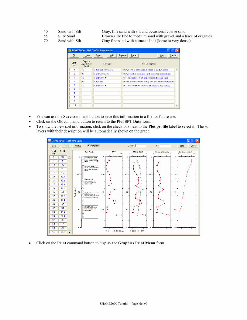
40 Sand with Silt Gray, fine sand with silt and occasional coarse sand 55 Silty Sand Brown silty fine to medium sand with gravel and a trace of organics 70 Sand with Silt Gray fine sand with a trace of silt (loose to very dense)

• You can use the Save command button to save this information in a file for future use. • Click on the Ok command button to return to the Plot SPT Data form. • To show the new soil information, click on the check box next to the Plot profile label to select it. The soil

layers with their description will be automatically shown on the graph.

• Click on the Print command button to display the Graphics Print Menu form.


• To change the position of any of the graphs on the paper, first click on the option button for the graph to select it

(e.g. Factor of Safety against Liquefaction). Then, enter the new coordinates on the coordinate’s text boxes, or use the up-down arrows to change the coordinates. If you do not want the graph to be printed, click on the appropriate check box of the Print column to deselect it (i.e. the x is not shown on the box). Selecting or deselecting a graph does not modify the position of the other graphs.

• On the Graphics Print Menu form click on the Close button to return to the Plot SPT Data form. Now, click on the Close button to return to the CRR using SPT form. Then click on Cancel to return to the Simplified CSR Analysis form.

• A liquefaction analysis can also be conducted using Cone Penetration Test or Shear Wave Velocity data. In this tutorial, we will use data recorded during a CPT sounding and saved in the Sample subdirectory.

• Click on the Cone Penetration Test option to select it, and then on the CRR command button to display the Cyclic Resistance Ratio using CPT form.


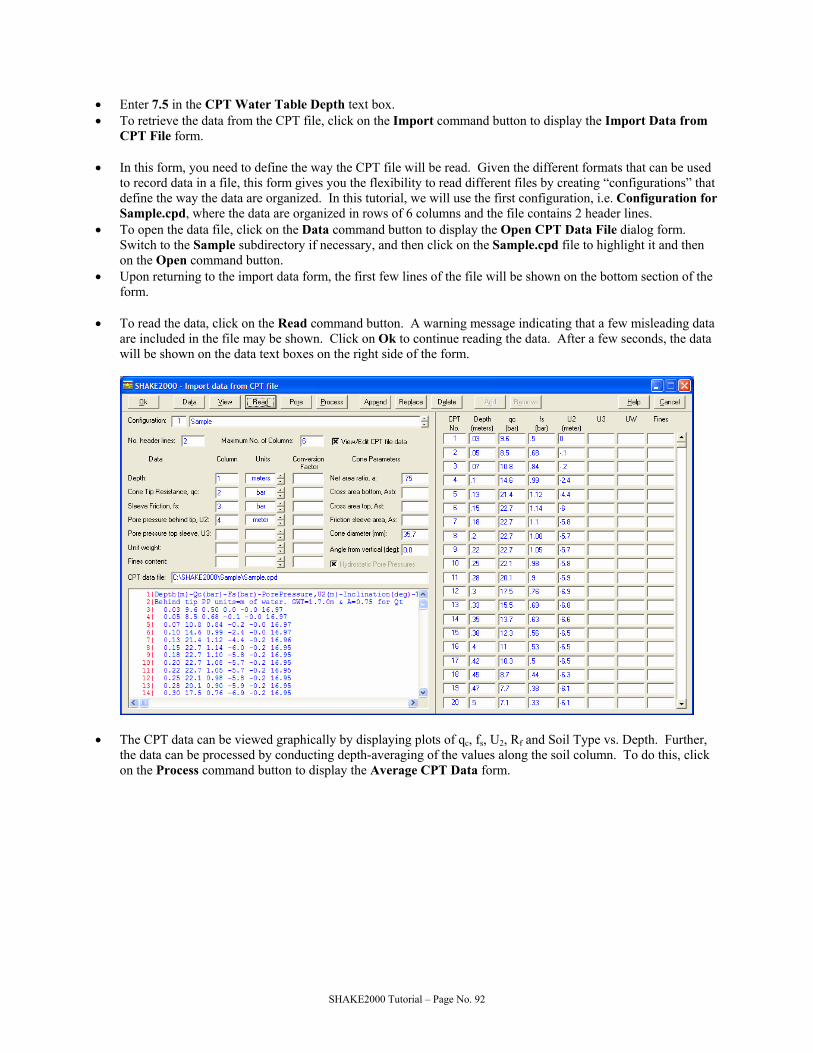
• Enter 7.5 in the CPT Water Table Depth text box. • To retrieve the data from the CPT file, click on the Import command button to display the Import Data from

CPT File form.

• In this form, you need to define the way the CPT file will be read. Given the different formats that can be used to record data in a file, this form gives you the flexibility to read different files by creating “configurations” that define the way the data are organized. In this tutorial, we will use the first configuration, i.e. Configuration for Sample.cpd, where the data are organized in rows of 6 columns and the file contains 2 header lines.

• To open the data file, click on the Data command button to display the Open CPT Data File dialog form. Switch to the Sample subdirectory if necessary, and then click on the Sample.cpd file to highlight it and then on the Open command button.

• Upon returning to the import data form, the first few lines of the file will be shown on the bottom section of the form.

• To read the data, click on the Read command button. A warning message indicating that a few misleading data

are included in the file may be shown. Click on Ok to continue reading the data. After a few seconds, the data will be shown on the data text boxes on the right side of the form.

• The CPT data can be viewed graphically by displaying plots of qc, fs, U2, Rf and Soil Type vs. Depth. Further,

the data can be processed by conducting depth-averaging of the values along the soil column. To do this, click on the Process command button to display the Average CPT Data form.


• If you wish to conduct depth-averaging of the data, it is convenient to first determine the main soil stratification. To do this, click on the Cum. Rf check box to select it. This will plot the cumulative curve of the friction ratio, IR(z) on the right most graph, i.e. the Soil type chart. According to Harder and Van Gloh (1988), the changes in slope along the IR(z) curve delineate the boundaries for the main soil layers.

• Note that the curve changes slope at depths of approximately 5 and 49 feet. To define soil boundaries at these

depths, we will use the Layer Top and Layer Bot. options. After that, you will enter an interval for depth averaging within these major soil zones.

• For the very first CPT value, the one at a depth of 0.098 feet, click on the check box below the Layer Top label. This indicates that an upper boundary for a soil layer is set at this depth.

• Next, use the scroll bar to scroll down to the CPT data at a depth of 5.019 feet. At this point, click on the check box for the Layer Top column and for the Layer Bot. column. This means that at this point we set the bottom elevation for the uppermost layer and the top elevation for the layer below.

• Similarly, click on both check boxes to select them for the point at elevation 49.047 feet. • To define the bottom of the soil column, you need to select the point that marks the bottom of this layer. Scroll

down to the end of the soil column data, i.e. the point at elevation 82.02 feet and click on the Layer Bot. check box to select it.

• Now that you have defined the main soil layers, you will average the values within a depth range. • For this tutorial, we will use a depth interval of 1 foot. • To select a depth interval, click on the up-arrow button next to the Weighted average every label until a 1

appears in the text box. • Next, click on the check box for the Weighted average every label to select it. Now, click on the Process

command button. After a few seconds, the different layers of 1 foot thickness will be shown as red lines overlying the original curves. These lines represent average values for qc, fs and U2, and computed value for Rf and new soil types based on the average values.


• Once you have processed the CPT data, click on the Ok command button to return to the Import Data from CPT File form. The processed data will be shown on the data text boxes.

• Then click on Ok to return to the Cyclic Resistance Ratio using CPT form. You may get a warning message telling you that the depth of the CSR column is smaller than the depth of the CPT column. Click on Ok for the time being. The averaged CPT data and other information will be displayed in the appropriate text boxes.

• You need to change a few of the options on this form to use the same input parameters as used for the CRR

analysis with SPT data.


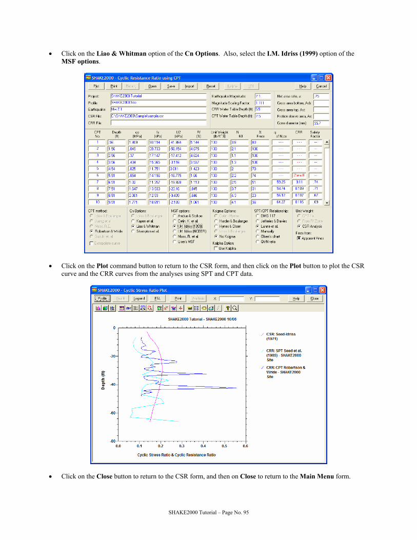
• Click on the Liao & Whitman option of the Cn Options. Also, select the I.M. Idriss (1999) option of the MSF options.

• Click on the Plot command button to return to the CSR form, and then click on the Plot button to plot the CSR

curve and the CRR curves from the analyses using SPT and CPT data.

• Click on the Close button to return to the CSR form, and then on Close to return to the Main Menu form.


• The last utility option on SHAKE2000 is the USGS Seismic Hazard. This option allows you to retrieve the Peak Ground Acceleration from the gridded points used to make the 1996 USGS National Seismic Hazard Maps, and for the 2002 and 2003 updates; and also, to plot the results of the seismic hazard deaggregation for a site in the Conterminous United States.

• After selecting this option, click on the Ok command button to display the USGS Seismic Hazard Maps form.

• Assume that the SHAKE2000 Site used in this tutorial is located at the following coordinates: Longitude 122°

51′ West and Latitude 47° North. • The cursor is on the degrees data cell of the Longitude. Enter 122, and then press the Tab key once to move

the cursor to the minutes text box. Enter 51. • Press the Tab key twice to move the cursor to the degrees data box of the Latitude. Enter 47. • Press the Tab key once to move the cursor to the minutes text box. The PGA with 2% probability of

exceedance in 50 years value will be retrieved from the data files and shown on the text box.

• From the interactive deaggregation web page at the USGS website you can download a text file that contains

the deaggregation information. The results in this file can be used to obtain a plot of the deaggregated distance, magnitude and ground-motion uncertainty for the specified parameters.

• For this tutorial, the information for the above site was used at the USGS Interactive Deaggregations 2002 web site (http://eqint.cr.usgs.gov/eq/html/deaggint2002.html) to obtain the hazard matrix.

• The file is saved in the Sample folder as USGShzrd.txt. To retrieve the hazard information, click on the icon next to the Hazard Matrix text box at the bottom of the form to open the USGS Hazard Matrix dialog box.


Switch to the Sample folder if necessary, and select the USGShzrd.txt file. Then click on the Open command button.

• Some basic information is shown on the text boxes. • To plot the seismic hazard deaggregation for this site, click on the Plot command button.

• Click on the Close command button to return to the USGS form. • Click on the Close command button to return to the Main Menu form. • The following section of the tutorial will cover the use of the Random Generation of EDT Options and the

Ratio of Response Spectra features of SHAKE2000. • The Random Generation of EDT Options feature of SHAKE2000 is used to randomly generate data for layer

thickness, Gmax, shear wave velocity, peak acceleration, or modulus reduction and damping vs. strain curves. Please note that this should not be considered a formal, scientifically based approach (e.g. Monte Carlo Simulation) to account for the uncertainty on any of these data. It should be considered more like a “crude


Soil Profile SHAKE Column Thickness Gmax

Peat

Sand

Gravel

Bedrock

12.5 ft ± 2.5 ft 700 ksf ± 200 ksf

34.75 ft ± 1.75 ft 1000 ksf ± 100 ksf

14 ft ± 3.75 ft 1200 ksf ± 50 ksf

Layer 1

Layer 2

Layer 3

Layer 4

Layer 5

Layer 6

Layer 7

Layer 8

Layer 9

Layer 11

Layer 10

5000 ksf ± 500 ksf

Soil Profile and SHAKE Column for RRS Analysis Tutorial

sensitivity analysis” conducted to evaluate the effect of the variability of these data on the site response. For this part of the tutorial, we will use the following soil profile and data.

• For example, for the Peat stratum shown on the above drawing, the user would first choose to generate a

number of different thicknesses for this stratum ranging between 10.0 (i.e., 12.5 – 2.5) feet to 15.0 (i.e., 12.5 + 2.5) feet. For each random thickness, this stratum will then be divided into two layers of equal thickness.

• The RRS feature is used to input the data necessary to conduct a ratio of response spectra analysis of the ground surface motions to the input outcropping rock motions. The results of the analysis can then be used to obtain a surface response spectrum by multiplying either the mean or the median curve of the resultant RRS curves by a rock response spectrum.

• In order not to repeat procedures that have been covered in other sections of the tutorial, it is assumed that the

user has followed the tutorial step by step. In addition, some of the data used in this section of the tutorial have been saved in the Sample_RRS.edt file created in the RRS Sample folder during installation of the program.

• To use the tutorial file, click on the Edit Existing EDT File option to select it and then on the Get File command button to display the Open Existing EDT File dialog form. Switch to the RRS Sample folder if necessary and select the Sample_RRS.edt file and click Open.

• Click on Ok to display the Earthquake Response Analysis form. • First, we need to create a profile formed by the different strata shown on the figure above. To do this, double

click on the Option 2 – Soil Profile Set No. 1 option to display the Option 2 Editor: Soil Profile form. • To randomly generate the soil profiles, we will enter the average values for thickness and Gmax as shown above.

Although we are using Option 2, this soil profile should not be considered a SHAKE column. The options that we are going to create in this section of the tutorial are “seed options” formed by the average values that will be used to randomly generate the different SHAKE columns for the analyses.

• Enter Option 2 – SHAKE 2000 Site – RRS Analysis in the Soil Profile – Set Identification text box. • In the Identification for Soil Profile text box enter SHAKE2000 Site - RRS. • Enter the following data for each soil stratum:

Stratum Soil Thickness Shear Damping Unit Number Type Moduli Weight 1 1 12.5 700 0.05 0.100 2 2 34.75 1000 0.05 0.130 3 3 14 1200 0.05 0.120 4 4 5000 0.05 0.150


• Click on Return to close the form and return to the Earthquake Response Analysis form. • The next step is to generate a series of SHAKE columns using the average values entered in the above options. • Click on the Random command button to display the Random Generation of EDT Options form.

• For this tutorial we’ll use a simple random generation process that consists of dividing the range of data into

intervals, and then randomly picking a value from each interval. For example, for the first stratum, the thickness can range between 10 feet to 15 feet. In SHAKE2000, this range is first divided into a lower bound range, i.e. 10 feet to 12.5 feet; and, into an upper bound range, i.e. 12.5 feet to 15 feet. For both the lower and upper bound ranges, the user will further subdivide them in intervals. For example, the lower bound range will be divided in 2 intervals, i.e. from 10 feet to 11.25 feet and from 11.25 feet to 12.50 feet. Similarly, the upper bound range could be subdivided also into two intervals; i.e. one from 12.5 feet to 13.75 feet and the other from 13.75 feet to 15 feet. The number of intervals to use is entered in the No. Lower Samples and No. Upper Samples text boxes. These intervals will be used for every soil stratum in the soil profile. SHAKE2000 will then randomly pick a value from each interval and create a total of lower + upper interval SHAKE columns, i.e. Options 2. In this tutorial, two hundred SHAKE columns will be created. These intervals will also be applied for the random generation of Gmax and/or Shear Wave Velocity values, peak acceleration and dynamic material properties.


• To generate the 200 columns, we’ll use the Stratified/Random Field option. With this option, 200 sets of Option 1 and 2, and 200 sets for each set of Option 3 will be generated, and then randomly ordered to create the input file. In total, 400 different analyses will be conducted.

• Click on the Stratified/Random Field option to select it. • After the thickness of the stratum has been randomly selected, the stratum will be divided in layers of equal

thickness using the value entered in the Number of Layers text box; i.e., the randomly picked thickness of the stratum would be divided by the number of layers to obtain the thickness for each layer.

• The SHAKE column would be formed by a total number of layers equal to the sum of individual number of layers for each stratum, plus 1 for the half-space layer.

• To continue with the tutorial, enter 100 in the No. Lower Samples and 100 in the No. Upper Samples text boxes.

• Place the cursor on the Lower Bound text box for stratum number 1. Enter 10 and press the Tab key to move the cursor to the Upper Bound text box and enter 15. Place the cursor in the No. Layers text box and enter 2.

• For stratum number 2 enter 33 and 36.5 for the lower and upper intervals respectively, and 6 for the number of layers.

• For stratum number 3 enter 10.25 and 17.75 for the lower and upper intervals respectively, and 2 for the number of layers. The fourth stratum is the half-space layer, which will not be subdivided.

• The total depth variation of the soil column will be constrained to fit within the half-space depth variation. For this tutorial, the depth to the half-space varies between 60 to 64 feet. To enable this option, click on the Thickness option of the Obtain Random Sampling for options first. This will enable the Half-Space Depth option. Place the cursor on the text box below the Min. Depth to Half-Space label and enter 60. Press the Tab key once, and enter 64 on the text box below the Max. Depth to Half-Space label. Click on the check box for the Half-Space Depth option to select it. When this option is selected, the program will check that the depth of each column generated is within the limits set for the depth to the half-space layer.

• Click on the Shear Modulus Option to switch to the form used to enter the data range of Gmax values used in

the analysis. • Enter the following information for each stratum:

Stratum Gmax Gmax No. Lower Bound Upper Bound 1 500 900 2 900 1100 3 1150 1250 4 4500 5500


• Click on the Peak Acceleration option of the Obtain Random Sampling for options to switch to the form used to enter the range of peak acceleration values used for the analysis.

• For each motion, the minimum value of peak acceleration expected is 0.10 g and the maximum value is 0.23 g. Enter these values in the Lower Bound and Upper Bound text boxes respectively for each motion.

• To randomly generate the SHAKE columns, click on the check boxes for Shear Modulus and Peak

Acceleration of the Obtain Random Sampling for options to select them. This way, random data will be generated for these parameters. Also, click on the Stratified/Random Field option to select it.


• To randomly generate the SHAKE columns using the range of data entered above, click on the Random

command button. The mouse icon will change to the hour glass icon for a few seconds. The iteration number will be shown on the text box next to the Stratified/Random Filed option.

• Click on Ok to return to the Earthquake Response Analysis form. • Upon returning to the Earthquake Response Analysis form, the options listed on the bottom of the form will

be used as a guideline to create the input file. • For example, the first SHAKE column saved in the file is shown on the following page. However, note that

because of the random generation routine, the values generated in your computer will more than likely be different from the ones shown on the following page.

• As shown on the following page, the first SHAKE column is formed by one set each of options 1, 2, 3, 4, 5, 6 and 9.

• For the RRS analysis, the response spectrum at the surface is computed using the acceleration time history at

the ground surface obtained from Option 6. The response spectrum for the outcropping motion is computed using the ground motion files from Option 3, i.e. it is assumed that the records used in option 3 are representative of rock outcrop motions.

• The information about the ground motion files, i.e. outcropping motions and associated surface ground motions, can be automatically collected during the processing of the two output files created by SHAKE. Alternatively, the surface and the outcropping ground motion files can be manually selected when using the Ratio of Response Spectra form. For this part of the tutorial we will let SHAKE2000 collect the information. Click on the Save Ground Motion Data for RRS Analysis option to select it. When this option is selected before executing SHAKE, the Option 4 data will be checked to determine if the input ground motion for the SHAKE analysis was set as an outcrop motion. Alternatively, if the option is selected after executing SHAKE, then the information about the ground motion files will be gathered by the program and it will be assumed that the input motions in Option 3 were defined as outcrop motions in Option 4.

• Before executing SHAKE, select the output folder where all of the output files will be stored. Click on the

folder icon next to the text box for the Directory of Output Files to open the Choose Output Directory file dialog form. Select the RRS Sample folder to store the output files and then click on Ok to return to the Earthquake Response Analysis form.

• To conduct the 400 site response analyses, click on the SHAKE command button. This will open the SHAKE DOS window and the different analyses will be conducted.

• After a few minutes, execution of SHAKE is completed.


Option 1 - Dynamic Soil Properties - SHAKE2000 Site - Random No. 1 1 4 11 Peat G/Gmax for Fibrous Peaty Organic Soil (Mean for 12 kPa - Wehling, JGGE 129,10) .0001 .0003 .001 .003 .01 .03 .1 .3 1 3 10 1 .99 .9696 .9189 .8282 .7278 .5975 .4671 .2978 .1589 .0696 11 Peat Damping for Fibrous Peaty Organic Soil (Mean for 12 kPa - Wehling, JGGE 129,10) .0001 .0003 .001 .003 .01 .03 .1 .3 1 3 10 4.983 4.983 5.083 5.179 5.476 6.172 7.759 10.339 14.515 18.798 22.585 9 Sand Avg. G/Gmax - SAND, Average (Seed & Idriss 1970) .0001 .0003 .001 .003 .01 .03 .1 .3 1 1 .9827 .941 .8631 .6875 .4775 .2609 .1265 .051 9 Sand Avg. Damping for SAND, Average (Seed & Idriss 1970) .0001 .0003 .001 .003 .01 .03 .1 .3 1 .411 .623 1.259 2.547 4.827 8.19 13.55 19.082 23.498 20 Gravel mean G/Gmax - Gravel (Mean) - Rollins et al. JGGE, V. 124, No. 5, 5/98 .0001 .0002 .0005 .0008 .001 .002 .003 .004 .007 .01 .02 .07 .1 .2 .3 .4 .5 .6 .8 1 1 .9998 .9994 .9991 .9988 .9785 .9583 .9382 .8973 .852 .7367 .4918 .422 .3068 .2373 .1974 .1677 .1479 .1088 .0888 20 Gravel Mean Damping for Gravel (Mean) - Rollins et al. JGGE, V. 124, No. 5, 5/98 .0001 .0003 .0006 .001 .002 .003 .004 .006 .008 .01 .02 .03 .05 .1 .2 .3 .4 .6 .8 1 1.386 1.781 2.078 2.473 3.068 3.66 4.058 4.947 5.543 6.04 8.126 9.714 11.608 14.4 16.509 17.71 18.412 19.118 19.521 19.822 8 Rock G/Gmax - ROCK (Schnabel 1973) .0001 .0003 .001 .003 .01 .03 .1 1 1 1 .99 .95 .9 .81 .725 .55 5 Rock Damping for ROCK (Schnabel 1973) .0001 .001 .01 .1 1 .4 .8 1.5 3 4.6 4 1 2 3 4 Option 2 - SHAKE2000 Site - RRS Analysis - Random No. 1 2 1 11 SHAKE2000 Site - RRS - Rndm 1 1 1 5.956 527.2 .05 .1 2 1 5.956 527.2 .05 .1 3 2 5.865 913.23 .05 .12 4 2 5.865 913.23 .05 .12 5 2 5.865 913.23 .05 .12 6 2 5.865 913.23 .05 .12 7 2 5.865 913.23 .05 .12 8 2 5.865 913.23 .05 .12 9 3 7.446 1156.56 .05 .13 10 3 7.446 1156.56 .05 .13 11 4 4568.09 .05 .15 Option 3 - SHAKE2000 Site - Outcropping Input Motion No. 1 - Random No. 1 3 798616384 .005 (6E15.7) C:\SHAKE2000\RRS Sample\rrs000.eq .1221 15 2 6 Option 4 - Assignment of Object Motion to Layer 11 4 11 0 Option 5 - Number of Iterations 10 - Strain Ratio 0.65 5 10 .65 Option 6 - Computation of Acceleration at Layers 1 through 11 6 1 2 3 4 5 6 7 8 9 10 11 11 0 1 1 1 1 1 1 1 1 1 1 0 1 0 0 0 0 0 0 0 0 0 0 0 Option 9 - Response Spectrum at Surface 9 1 0 3 0 32.2 .05 .1 .2


• Next, the two output files created by SHAKE need to be processed to obtain the information about the surface and outcropping ground motions that will be used for the RRS analysis; and also, to obtain the mean and median values for the peak acceleration, strain, etc.; and, for the response spectrum at the surface.

• Click on the Process command button. Depending on the number of analyses conducted, it may take a few minutes to complete the processing of the files. The mouse icon will change to the sand-clock icon to indicate that processing of the data is being done. Messages indicating the processing status may be displayed on the bottom of the form.

• A message will be shown once processing of the two files has been completed. Click on Ok to close the message window.

• Click on the Peak Acceleration, CSR, Shear Stress option to select it and then on the Ok command button.

• The Median and Median + Standard Deviation for the 400 analyses will be shown on the graphics window.

You can click on the other options to plot the Mean, the Data Range and the Data curves.

• Click on the Close command button to return to the Earthquake Response Analysis form.

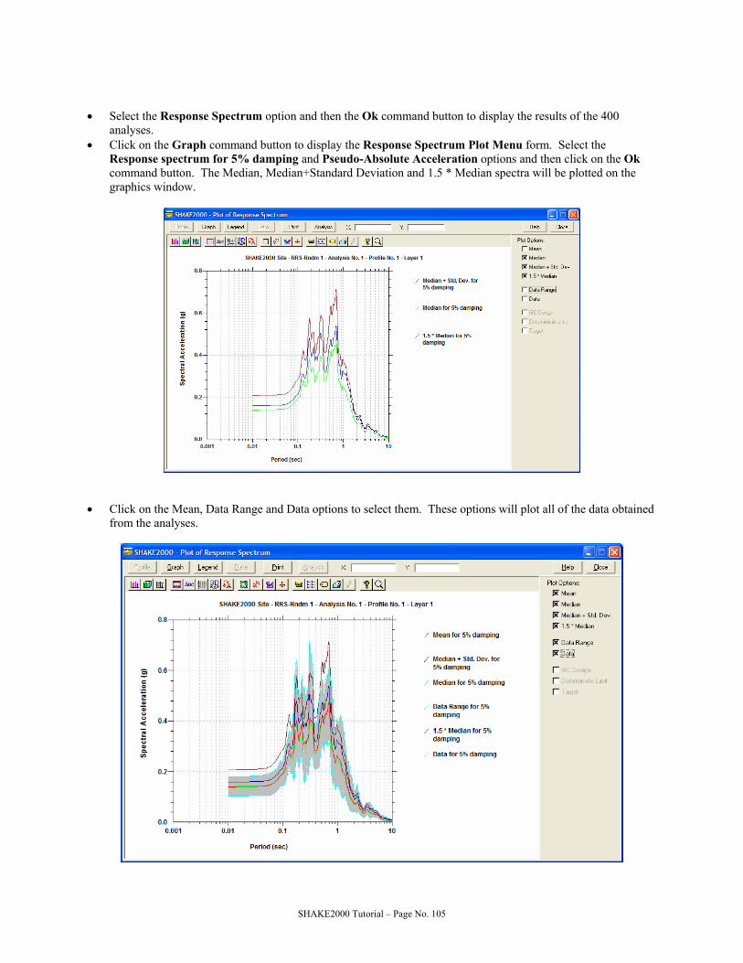
• Select the Response Spectrum option and then the Ok command button to display the results of the 400

analyses. • Click on the Graph command button to display the Response Spectrum Plot Menu form. Select the

Response spectrum for 5% damping and Pseudo-Absolute Acceleration options and then click on the Ok command button. The Median, Median+Standard Deviation and 1.5 * Median spectra will be plotted on the graphics window.

• Click on the Mean, Data Range and Data options to select them. These options will plot all of the data obtained

from the analyses.


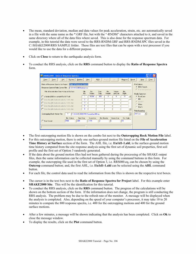
• The mean, standard deviation, median and data values for peak acceleration, strain, etc. are automatically saved

in a file with the same name as the *.GRF file, but with the “-RNDM” characters attached to it, and saved in the same directory where all of the data files where saved. This is also done for the response spectrum data. For example, in this tutorial the data were saved to the RRS-RNDM.GRF and RRS-RNDM.SPC files saved in the C:\SHAKE2000\RRS SAMPLE folder. These files are text files that can be open with a text processor if you would like to use the data for a different purpose.

• Click on Close to return to the earthquake analysis form. • To conduct the RRS analysis, click on the RRS command button to display the Ratio of Response Spectra

form.

• The first outcropping motion file is shown on the combo list next to the Outcropping Rock Motion File label. • For this outcropping motion, there is only one surface-ground motion file listed on the File of Acceleration

Time History at Surface section of the form. The AHL file, i.e. l1a1d1-1.ahl, is the surface-ground motion time history computed from the site response analysis using the first set of dynamic soil properties, first soil profile and the first set of Option 3 randomly generated.

• If the data about the ground motion files had not been gathered during the processing of the SHAKE output files, then the same information can be collected manually by using the command buttons in this form. For example, the outcropping file used in the first set of Option 3, i.e. RRS000.eq, can be chosen by using the Outcrop command button; and, the first AHL, i.e. l1a1d1-1.ahl can be selected using the AHL command button.

• For each file, the control data used to read the information from the files is shown on the respective text boxes. • The cursor is in the text box next to the Ratio of Response Spectra for Project label. For this example enter

SHAKE2000 Site. This will be the identification for this tutorial. • To conduct the RRS analysis, click on the RRS command button. The progress of the calculations will be

shown on the bottom section of the form. If the information does not change, the program is still conducting the RRS analysis. The problem may be due to the refresh rate of the monitor. A message will be displayed when the analysis is completed. Also, depending on the speed of your computer’s processor, it may take 10 to 20 minutes to compute the 800 response spectra, i.e. 400 for the outcropping motions and 400 for the ground surface motions.

• After a few minutes, a message will be shown indicating that the analysis has been completed. Click on Ok to

close the message window. • To display the results, click on the Plot command button.


• By default, all of the computed curves are plotted. To plot the mean curve and the mean ± standard deviation

curves only, click on the Median, Data Range and Data options to deselect them.

• Click on Close to return to the RRS form.


• To create a surface, e.g. soil, response spectrum using the results of the RRS analysis, first select one of the

Modify Spectrum options to obtain a rock response spectrum, e.g. using the IBC or NEHRP MCE rock response spectrum. For this tutorial, click on the IBC option, and then on the Modify command button to display the IBC Response Spectra form.

• The tutorial site is located at a longitude of 122° 43’ and a latitude of 37° 11’. Enter these coordinates in the Longitude and Latitude text boxes. Next, select the B: Rock option of the Soil Profile Type options.

• Click on the MCE Spectrum option to select it.

• Click on Ok to return to the RRS form. • To plot the source spectrum, i.e. IBC Soil Profile Type B: Rock spectrum, and the modified spectrum, i.e. soil

spectrum at the ground surface, click on the Modified Spectrum option to select it, and then click on the Plot command button.

• Click on Close to return to the RRS form.


• To save the results of the analysis, click on the Save command button to open the Save Ratio of Response

Spectra File dialog form. Select a folder, and enter the name of the file in the File name text box. Then click on Save. The input data and the results will be saved in this file. The data can be retrieved for further use with the Open command button. This file is an ASCII text file, thus, the file can be open with other software for further analysis by the user.

• Click on Close to return to the Earthquake Response Analysis form. • Click on Return to close this form and return to the Main Menu form. • To complete this tutorial, click on Exit to finish execution of the program.


Response Spectra Bedrock Motion Ground Motions

Documents

Transcript of Response Spectra Bedrock Motion Ground Motions