Expansive motions and the polytope of pointed pseudo-triangulations
38
Expansive Motions and the Polytope of Pointed Pseudo-Triangulations G¨ unter Rote Francisco Santos Ileana Streinu Abstract We introduce the polytope of pointed pseudo-triangulations of a point set in the plane, defined as the polytope of infinitesimal expansive motions of the points subject to certain constraints on the increase of their distances. Its 1-skeleton is the graph whose vertices are the pointed pseudo-triangulations of the point set and whose edges are flips of interior pseudo-triangulation edges. For points in convex position we obtain a new realization of the associahe- dron, i.e., a geometric representation of the set of triangulations of an n-gon, or of the set of binary trees on n vertices, or of many other combinatorial objects that are counted by the Catalan numbers. By considering the 1-dimensional version of the polytope of constrained expansive motions we obtain a second distinct realization of the associahedron as a perturbation of the positive cell in a Coxeter arrangement. Our methods produce as a by-product a new proof that every simple polygon or polygonal arc in the plane has expansive motions, a key step in the proofs of the Carpenter’s Rule Theorem by Connelly, Demaine and Rote (2000) and by Streinu (2000). 1 Introduction Polytopes for combinatorial objects. Describing all instances of a com- binatorial structure (e.g. trees or triangulations) as vertices of a polytope is often a step towards giving efficient optimization algorithms on those struc- tures. It also leads to quick prototypes of enumeration algorithms using known vertex enumeration techniques and existing code [2,9]. One particularly nice example is the associahedron, (see Figure 4 for an example): the vertices of this polytope correspond to Catalan structures. The Catalan structures refer to any of a great number of combinatorial ob- jects which are counted by the Catalan numbers (see the extensive list in Stanley [24, ex. 6.19, p. 219]). Some of the most notable ones are the trian- gulations of a convex polygon, binary trees, the ways of evaluating a product of n factors when multiplication is not associative (hence the name associa-
-
Upload
independent -
Category
Documents
-
view
0 -
download
0
Transcript of Expansive motions and the polytope of pointed pseudo-triangulations

Expansive Motions and the Polytopeof Pointed Pseudo-Triangulations
Gunter RoteFrancisco SantosIleana Streinu
Abstract
We introduce the polytope of pointed pseudo-triangulations of a point set in theplane, defined as the polytope of infinitesimal expansive motions of the pointssubject to certain constraints on the increase of their distances. Its 1-skeletonis the graph whose vertices are the pointed pseudo-triangulations of the pointset and whose edges are flips of interior pseudo-triangulation edges.
For points in convex position we obtain a new realization of the associahe-dron, i.e., a geometric representation of the set of triangulations of an n-gon, orof the set of binary trees on n vertices, or of many other combinatorial objectsthat are counted by the Catalan numbers. By considering the 1-dimensionalversion of the polytope of constrained expansive motions we obtain a seconddistinct realization of the associahedron as a perturbation of the positive cellin a Coxeter arrangement.
Our methods produce as a by-product a new proof that every simple polygonor polygonal arc in the plane has expansive motions, a key step in the proofs ofthe Carpenter’s Rule Theorem by Connelly, Demaine and Rote (2000) and byStreinu (2000).
1 Introduction
Polytopes for combinatorial objects. Describing all instances of a com-binatorial structure (e.g. trees or triangulations) as vertices of a polytope isoften a step towards giving efficient optimization algorithms on those struc-tures. It also leads to quick prototypes of enumeration algorithms usingknown vertex enumeration techniques and existing code [2, 9].
One particularly nice example is the associahedron, (see Figure 4 for anexample): the vertices of this polytope correspond to Catalan structures.The Catalan structures refer to any of a great number of combinatorial ob-jects which are counted by the Catalan numbers (see the extensive list inStanley [24, ex. 6.19, p. 219]). Some of the most notable ones are the trian-gulations of a convex polygon, binary trees, the ways of evaluating a productof n factors when multiplication is not associative (hence the name associa-

700 G. Rote, F. Santos, and I. Streinu
hedron), and monotone lattice paths that go from one corner of a square tothe opposite corner without crossing the diagonal.
In this paper we describe a new polyhedron whose vertices correspond topointed pseudo-triangulations.
Pseudo-triangulations. Pseudo-triangulations, as well as the closely re-lated geodesic triangulations of simple polygons, have been used in Compu-tational Geometry in applications such as visibility [18–20, 23], ray shoot-ing [12], and kinetic data structures [1,14]. The minimum or pointed pseudo-triangulations introduced in Streinu [25] have applications to non-collidingmotion planning of planar robot arms. They also have very nice combinato-rial and rigidity theoretic properties. The polytope we define in this paperadds to the former, and is constructed exploiting the latter.
Expansive motions. An expansive motion on a set of points P is an in-finitesimal motion of the points such that no distance between them decreases.
Expansive motions were instrumental in the first proof of the Carpenter’sRule Theorem by Connelly, Demaine and Rote [6]: Every simple polygonor polygonal arc in the plane can be unfolded into convex position with-out collisions. Streinu [25] built on this work, realizing the importance ofpseudo-triangulations in connection with expansive motions and studyingtheir rigidity properties. This paper provides a systematic study of expan-sive motions in one and two dimensions. The expansive motions of a setof n points in the plane form a polyhedral cone of dimension 2n − 3 (theexpansion cone). As by-products of our approach we get a new proof ofthe existence of expansive motions for non-convex polygons and polygonalarcs (Theorem 4.3) and a characterization of the extreme rays of the expan-sion cone of a planar point set in general position, as equivalence classes ofpointed pseudo-triangulations with one convex hull edge removed, modulorigid subcomponents (Proposition 2.8).
Our tool is the introduction of constrained expansions as expansive mo-tions with a special lower bound on the edge length increase. They form apolyhedron obtained by translation of the facets of the expansion cone. Ourmain result is the following (see a more precise statement as Theorem 3.1):
Theorem. Let P be a set of n points in general position in the plane, b ofthem in the boundary of the convex hull. Then, there is a choice of constraintswhich produces as constrained expansions of P a simple polyhedron of dimen-sion 2n−3 with a unique maximal bounded face of dimension 2n−b−3 whosevertices correspond to pointed pseudo-triangulations and edges correspond toflips between them.
The flips mentioned in the statement are a certain neighborhood structureamong pointed pseudo-triangulations (flips of interior edges). See the detailsin Section 2.

Expansive Motions and the Pseudo-Triangulation Polytope 701
Two appearances of the associahedron. For points in convex position,pseudo-triangulations coincide with triangulations. We prove (Corollary 5.5)that, in this case, our construction gives a polytope affinely equivalent to thestandard (n−3)-dimensional associahedron obtained as a secondary polytopeof the point set [28, Section 9.2]. Perhaps surprisingly, this shows that thesecondary polytope of n points in convex position in the plane (which lives inRn) can naturally be embedded as a face in a (2n−3)-dimensional unbounded
polyhedron.The associahedron appears again as the analog of our construction for
points in one dimension (Section 5.3).
Rigidity. The connection of these results with rigidity theory is also worthmentioning. Pointed pseudo-triangulations are special instances of infinitesi-mally minimally rigid frameworks in dimension 2, whose combinatorial struc-ture is well understood (see [13]). One-dimensional minimally rigid frame-works are trees, another well understood combinatorial structure. Adding theconstraint of expansiveness is what leads to pointed pseudo-triangulations in2d, and to the special non-crossing and alternating trees which appear inSection 5.3.
Future perspectives. It is our hope that the insight into one- and two-dimensional motions may eventually lead to generalizations to higher dimen-sions. There is no satisfactory definition of an analog of pseudo-triangulationsin 3 dimensions. The 3-dimensional version of the robot arm motion plan-ning problem, with potential applications to computational biology (proteinfolding), is much more challenging.
Overview. In Section 2 we give the preliminary definitions and results.Section 3 contains the main result, the construction of the polytope of pointedpseudo-triangulations (ppt-polytope). Section 4 applies the main result to geta new proof for the existence of expansive motions for non-convex polygonsand polygonal arcs in the plane. In Section 5 we present an alternative con-struction of the ppt-polytope and two special cases leading to the associahe-dron: points in convex position and the polytope of constrained expansionsin dimension 1. Section 6 attempts to put the results in 1 and 2 dimensionsinto a broader perspective, with the aim of extending the results to higherdimensions and to point sets which are not in general position. We concludewith some final comments in Section 7.
2 Preliminaries
Abbreviations and conventions. Throughout this paper we will assumegeneral position for our point sets, i.e. we assume that no d + 1 points inRd lie in the same hyperplane (unless otherwise specified). We abbreviate

702 G. Rote, F. Santos, and I. Streinu
“polytope of pointed pseudo-triangulations” as ppt-polytope, “one-degree-of-freedom mechanism” as 1DOF mechanism and “pseudo-triangulation expan-sive mechanism” as pte-mechanism.
For an ordered sequence of d + 1 points q0, . . . , qd ∈ Rd, det(q0, . . . , qd)denotes the determinant of the (d+1)×(d+1)matrix with columns (q0, 1), . . . ,(qd, 1). Equivalently, det(q0, . . . , qd) equals d! times the Euclidean volume ofthe simplex with those d+1 vertices, with a sign depending on the orientation.
Pseudo-triangulations. A pseudo-triangle is a simple polygon with onlythree convex vertices (called corners) joined by three inward convex polygonalchains, see Figure 1a. In particular, every triangle is a pseudo-triangle. Apseudo-triangulation is a partitioning of the convex hull of a point set P ={p1, . . . , pn} into pseudo-triangles using P as vertex set.
Pseudo-triangulations are graphs embedded on P , i.e. graphs drawn inthe plane on the vertex set P and with straight-line segments as edges. Wewill work with other graphs embedded in the plane. If edges intersect onlyat their end-points, as is the case for pseudo-triangulations, the graphs willbe called non-crossing or plane graphs. A graph is pointed at a vertex v ifthere is (locally) an angle at v strictly larger than π and containing no edges.Under our general position assumption, convex-hull vertices are pointed forany embedded graph, as are vertices of degree at most two. A graph is calledpointed if it is pointed at every vertex. Parts (b) and (c) of Figure 1 (includingthe broken edges) show two pointed pseudo-triangulations of a certain pointset.
(a) (b) (c) (d) (e)
p
Fig. 1. (a) A pseudo-triangle. (b) A minimum, or pointed, pseudo-triangulation.(c) The broken edge in (b) is flipped, and gives another pointed pseudo-triangulation. (d) A schematic drawing of the flip operation. (e) The two edgesinvolved in a flip may share a common vertex p.
The following properties of pseudo-triangulations were initially proved forthe slightly different situation of pseudo-triangulations of convex objects byPocchiola and Vegter [18, 19]. For completeness, we sketch the easy proofs(see also [3]).
Lemma 2.1. (Streinu [25]) Let P be a set of n points in general positionin the plane. Let G be a pointed and non-crossing graph on P .
(a) G has at most 2n− 3 edges, with equality if and only if it is a pseudo-triangulation.

Expansive Motions and the Pseudo-Triangulation Polytope 703
(b) If G is not a pseudo-triangulation, then edges can be added to it keepingit non-crossing and pointed.
Proof. (a) If the graph G is not connected, we can analyze the componentsseparately. So let us assume that it is connected. Let e and f be the numbersof edges and bounded faces in G. Let a+ and a− denote the number of angleswhich are > π and < π, respectively. (By our general position assumption,there are no angles equal to π.) Clearly, a+ + a− = 2e. Pointedness meansa+ = n and, since any bounded face has at least three convex vertices,a− ≥ 3f with equality if and only ifG is a pseudo-triangulation. The equation2e ≥ n+ 3f , together with Euler’s formula e = n+ f − 1, implies e ≤ 2n− 3(and f ≤ n− 2).
(b) The basic idea is that the addition of geodesic paths (i.e., paths whichhave shortest length among those sufficiently close to them) between convexvertices of a polygon keeps the graph pointed and non-crossing and, unlessthe polygon is a pseudo-triangle, there is always some of these geodesic pathsgoing through its interior.
Streinu [25] proved the following additional properties of pointed pseudo-triangulations, which we do not need for our results but which may interestthe reader:
• Every pseudo-triangulation on n points has at least 2n − 3 edges,with equality if and only if it is pointed. Hence, pointed pseudo-triangulations are the pseudo-triangulations with the minimum numberof edges. For this reason they are calledminimum pseudo-triangulationsin [25]. In contrast with part (b) of Lemma 2.1, not every pseudo-triangulation contains a pointed one. An example of this is a regularpentagon with its central point, triangulated as a wheel. Hence, a min-imal pseudo-triangulation is not always pointed.
• The graph of any pointed pseudo-triangulation has the Laman property:it has 2n− 3 edges and the subgraph induced on any k vertices has atmost 2k − 3 edges. This property characterizes generically minimallyrigid graphs in the plane ( [15], see also [13]); that is, graphs which areminimally rigid in almost all their embeddings in the plane.
• All pointed pseudo-triangulations can be obtained starting with a tri-angle and adding vertices one by one and adding or adjusting edges, inmuch the same way as the Henneberg construction of generically mini-mally rigid graphs (cf. [13, page 113]), suitably modified to give pointedpseudo-triangulations in intermediate steps (see the details in [25]).
The other crucial properties of pointed pseudo-triangulations that we useare that all interior edges can be flipped in a natural way (part (a) of thefollowing statement) and that the graph of flips between pointed pseudo-triangulations of any point set is connected. Both results were known to

704 G. Rote, F. Santos, and I. Streinu
Pocchiola and Vegter for pseudo-triangulations of convex objects (see [18,19]). Parts (b) and (c) of Figure 1 show a flip between pointed pseudo-triangulations. An O(n2) bound on the diameter of the flip graph is provedin [3].
Lemma 2.2. (Flips between pointed pseudo-triangulations) Let P bea point set in general position in the plane.
(a) (Definition of Flips) When an interior edge (not on the convex hull)is removed from a pointed pseudo-triangulation of P , there is a uniqueway to put back another edge to obtain a different pointed pseudo-triangulation.
(b) (Connectivity of the flip graph) The graph whose vertices are pointedpseudo-triangulations and whose edges correspond to flips of interioredges is connected.
Proof. [3, 25] (a) When we remove an interior edge from a pointed pseudo-triangulation we get a planar and pointed graph with 2n−4 edges. The samearguments of the proof of Lemma 2.1 imply now that a− = 3f + 1. Hence,the new face created by the removal must be a pseudo-quadrilateral (that is,a simple polygon with exactly four convex vertices).
In any pseudo-quadrilateral there are exactly two ways of inserting aninterior edge to divide it into pseudo-triangles, which can be obtained by theshortest paths between opposite convex vertices of the pseudo-quadrilateral(see the details in Lemma 2.1 of [26], and a schematic drawing in Figure 1d).One of these two is the edge we have removed, so only the other one remains.Note that the two interior edges of a pseudo-quadrilateral may be incidentto the same vertex, see Figure 1e. This can only happen when the interiorangle at this vertex is bigger than π.
(b) Let p be a convex hull vertex in P . Pointed pseudo-triangulationsin which p is not incident to any interior edge are just pointed pseudo-triangulations of P \ {p} together with the two tangent edges from p to theconvex hull of the rest. By induction, we assume all those pointed pseudo-triangulations to be connected to each other. To show that all others arealso connected to those, just observe that if a pointed pseudo-triangulationhas an interior edge incident to p, then a flip on that edge inserts an edgenot incident to p. (The case of Figure 1e cannot happen for a hull vertex p.)Hence the number of interior edges incident to p decreases.
Infinitesimal rigidity. In this paper we work mostly with points in di-mensions d = 2 and d = 1. Occasionally we will use superscripts to denotethe components of the vectors pi = (p1
i , . . . , pdi ).
An infinitesimal motion on a point set P = {p1, . . . , pn} ∈ Rd is an assign-ment of a velocity vector vi = (v1
i , . . . , vdi ) to each point pi, i = 1, . . . , n. The
trivial infinitesimal motions are those which come from (infinitesimal) rigid

Expansive Motions and the Pseudo-Triangulation Polytope 705
transformations of the whole ambient space. In R2 these are the translations(for which all the vi’s are equal vectors) and rotations with a certain centerp0 (for which each vi is perpendicular and proportional to the segment p0pi).Trivial motions form a linear subspace of dimension
(d+1
2
)in the linear space
(Rd)n of all infinitesimal motions. Two infinitesimal motions whose differenceis a trivial motion will be considered equivalent, leading to a reduced spaceof non-trivial infinitesimal motions of dimension dn −
(d+1
2
). In particular,
this is n− 1 for d = 1 and 2n− 3 for d = 2. Rather than performing a formalquotient of vector spaces we will “tie the framework down” by fixing
(d+1
2
)variables. E.g., for d = 1 we can choose:
v1 = 0 (1)
and for d = 2 (assuming w.l.o.g. that p22 = p2
1):
v11 = v2
1 = v12 = 0 (2)
Here, p1 and p2 can be any two vertices. A different choice of normalizingconditions only amounts to a linear transformation in the space of infinitesi-mal motions.
In rigidity theory, a graph G = (P,E) embedded on P is customarilycalled a framework and denoted by G(P ). We will use the term frameworkwhen we want to emphasize its rigidity-theoretic properties (stresses, mo-tions), but we will use the term graph when speaking about graph-theoreticproperties, even if graph is embedded on a set P . For a given frameworkG = (P,E), an infinitesimal motion such that 〈pi − pj, vi − vj〉 = 0 for everyedge ij ∈ E is called a flex of G. This condition states that the length ofthe edge ij remains unchanged, to first order. The trivial motions are theflexes of the complete graph, provided that the vertices span the whole spaceRd. A framework is infinitesimally rigid if it has no non-trivial flexes. It is
infinitesimally flexible or an infinitesimal mechanism otherwise.Infinitesimal motions are to be distinguished from global motions, which
describe paths for each point throughout some time interval. In this paperwe are not concerned with global motions, nor their associated concept ofrigidity, weaker than infinitesimal rigidity ( [7, Theorem 4.3.1] or [13, page6]). Let us also insist that we distinguish between infinitesimal motions (ofthe point set) and flexes (of the framework or embedded graph), while theterms flex and infinitesimal motion are sometimes equivalent in the rigiditytheory literature.
The (infinitesimal) rigidity map MG(P ) : (Rd)n → RE(G) is a linear map
associated with an embedded framework G(P ), P ⊂ Rd. It sends each in-finitesimal motion (v1, . . . , vn) ∈ (Rd)n to the vector of infinitesimal edgeincreases (〈pi − pj, vi − vj〉)ij∈E . When no confusion arises, it will be simplydenoted as M . The number 〈pi − pj , vi − vj〉 is called the strain on the edgeij in the engineering literature. As usual, the image of M is denoted byImM = { f | f = Mv }. The matrix of M is called the rigidity matrix. In

706 G. Rote, F. Santos, and I. Streinu
this matrix, the row indexed by the edge ij ∈ E has 0 entries everywhereexcept in the i-th and j-th group of d columns, where the entries are pi − pjand pj − pi, respectively.
The kernel of M (after reducing Rdn to Rdn−(d+1
2 ) by forgetting trivialmotions) is the space of flexes of G(P ). In particular, a framework is in-finitesimally rigid if and only if the kernel of its associated rigidity map Mis the subspace of trivial motions. In general, the dimension of the (reduced)space of flexes is the degree of freedom (DOF) of the framework. A 1DOFmechanism is a mechanism with one degree of freedom.
Finally, expansive (infinitesimal) motions v1, . . . , vn are those which si-multaneously increase (perhaps not strictly) all distances: 〈pi−pj , vi−vj〉 ≥ 0for every pair i, j of vertices. A mechanism is expansive if it has non-trivialexpansive flexes.
The following results of Streinu [25] can be obtained as a corollary of ourmain result (see the proof after the statement of Theorem 3.1).
Proposition 2.3. (Rigidity of pointed pseudo-triangulations [25])
(a) Pointed pseudo-triangulations are minimally infinitesimally rigid (andtherefore rigid).
(b) The removal of a convex hull edge from a pointed pseudo-triangulationyields a 1DOF expansive mechanism (called a pseudo-triangulation ex-pansive mechanism or shortly a pte-mechanism).
Part (a) is in accordance with the fact that the graph of any pointedpseudo-triangulation has the Laman property, and hence is generically rigidin the plane. It is a trivial consequence of (a) that the removal of an edgecreates a (not necessarily expansive) 1DOF mechanism. The expansivenessof pte-mechanisms (part (b)) was proved in [25] using the Maxwell-Cremonacorrespondence between self-stresses and 3-d liftings of planar frameworks, atechnique that was introduced in [6].
Self-stresses. A self-stress (or an equilibrium stress) on a framework G(P )(see [27] or [6, Section 3.1]) is an assignment of scalars ωij to edges suchthat ∀i ∈ P ,
∑ij∈E ωij(pi − pj) = 0. That is, the self-stresses are the row
dependences of the rigidity matrix M . The proof of the following lemma isthen straightforward.
Lemma 2.4. Self-stresses form the orthogonal complement of the linear sub-space ImM ⊂ R
(d2). In other words, (ωij)ij∈E is a self-stress if and onlyif for every infinitesimal motion (v1, . . . , vn) ∈ (Rd)n the following identityholds: ∑
ij∈Eωij〈pi − pj, vi − vj〉 = 0
As an example, the following result gives explicitly a stress for the com-plete graph on any affinely dependent point set:
Expansive Motions and the Pseudo-Triangulation Polytope 707
Lemma 2.5. Let∑n
i=1 αipi = 0,∑
αi = 0, be an affine dependence ona point set P = {p1, . . . , pn}. Then, ωij = αiαj for every i, j defines aself-stress of the complete graph G on P .
Proof. For any pi ∈ P we have:
∑ij∈G
ωij(pi − pj) =n∑j=1
αiαj(pi − pj) = αipi
n∑j=1
αj − αi
n∑j=1
αjpj = 0.
Let us analyze here the case of d+2 points P = {p1, . . . , pd+2} in generalposition in Rd (this is the first non-trivial case, because no self-stress canarise between affinely independent points). It can be easily checked that,under these assumptions, removing any single edge from the complete graphon P leaves a minimally infinitesimally rigid graph. This implies that thecomplete graph has a unique self-stress (up to a scalar factor). This self-stress is the one given in Lemma 2.5 for the unique affine dependence on P .The coefficients of this dependence can be written as:
αi = (−1)i det([p1, . . . , pd+2]\{pi}).
(Recall that det(q0, . . . , qd) is d! times the signed volume of the simplexspanned by the d+ 1 points q0, . . . , qd ∈ Rd.)
The special case d = 2, n = 4 will be extremely relevant to our purposes,and it will be convenient to renormalize the unique self-stress as follows:
Lemma 2.6. The following gives a self-stresses for any four points p1, . . . , p4
in general position in the plane:
ωij :=1
det(pi, pj , pk) det(pi, pj , pl)(3)
where k and l are the two indices other than i and j.
Proof. Set αi = (−1)i det([p1, . . . , p4]\{pi}) in Lemma 2.5 and divide all theωij ’s of the resulting self-stress by the non-zero constant
− det(p1, p2, p3) det(p1, p2, p4) det(p1, p3, p4) det(p2, p3, p4).
The direct application of Lemma 2.5 would give as ωij a product of twodeterminants, rather than the inverse of such a product. The reason why weprefer the self-stress of Lemma 2.6 is because of the signs it produces. Thereader can easily check, considering the two cases of four points in convexposition and one point inside the triangle formed by the other three, thatwith the choice of Lemma 2.6 boundary edges always receive positive stressand interior edges negative stress. This uniformity is good for us becausein both cases pointed pseudo-triangulations are the graphs obtained deletingfrom the complete graph any single interior edge.

708 G. Rote, F. Santos, and I. Streinu
The expansion cone. We are given a set of n points P = (p1, . . . , pn)in Rd that are to move with (unknown) velocities vi ∈ Rd, i = 1, . . . , n. Anexpansive motion is a motion in which no inter-point distance decreases. Thisis described by the system of homogeneous linear inequalities:
〈pi − pj , vj − vi〉 ≥ 0, ∀ 1 ≤ i < j ≤ n (4)
and hence defines a polyhedral cone.The only motions in the intersection of all facets of the cone are the trivial
motions. Thus, when we add normalizing equations like (1) or (2), we get apointed polyhedral cone containing the origin as a vertex. We call it the coneof expansive motions or simply the expansion cone of P .
An extreme ray of the expansion cone is given by a maximal set of in-equalities satisfied with equality by non-trivial motions. Each inequality cor-responds to an edge of the point set, so that the ray corresponds to a graphembedded in our point set. The cardinality of this set of edges is at least thedimension of the cone minus 1, but may be much larger. Let’s analyze thelow dimensional cases.
For d = 1 the expansion cone is not very interesting. Let’s assume thatthe points pi ∈ R are labeled in increasing order p1 < p2 < · · · < pn. Then:
Proposition 2.7. The expansion cone in one dimension has n− 1 extremerays corresponding to the motions where p1, . . . , pi remain stationary and thepoints pi+1, . . . , pn move away from them at uniform speed :
0 = v1 = v2 = · · · = vi < vi+1 = · · · = vn (5)
Proof. Note that the actual values of pi are immaterial in this case. Theexpansion cone is given by the linear system vj ≥ vi, 1 ≤ i ≤ j ≤ n plusthe extra condition v1 = 0, and any maximal set of inequalities satisfied withequality and yet not trivial is obviously given by (5).
The 2d case is more complex and requires additional terminology. 1DOFmechanisms may contain rigid subcomponents (r-components, cf. [13]): max-imal sets of some k vertices spanning a Laman subgraph on 2k − 3 edges.The r-components of pte-mechanisms are themselves pseudo-triangulationsspanning convex subpolygons including all points in their interior. Addingedges to complete each r-component to a complete subgraph yields a collapsedpte-mechanism (see Figures 2 and 3).
Proposition 2.8. In dimension 2, the extreme rays of the expansion conecorrespond to the collapsed pte-mechanisms.
The proof will be given in Section 4.1, after we have determined theextreme rays of a perturbed version of the polytope.

Expansive Motions and the Pseudo-Triangulation Polytope 709
Fig. 2. A pte-mechanism with rigid sub-components (convex subpolygons) drawnshaded, the corresponding collapsed pte-mechanism, and another pte-mechanismthat yields the same expansive motion.
Fig. 3. The collapsed pte-mechanisms corresponding to the 20 extreme rays ofthe expansion cone for a planar point set of 5 points. The rigid sub-components(complete subgraphs) are shaded.
The polytope of constrained expansions. The construction we will givein section 3 can roughly be interpreted as separating the pseudo-triangulationscontained in the same collapsed pte-mechanisms, to obtain a polyhedronwhose vertices correspond to distinct pseudo-triangulations. The originalexpansion cone is highly degenerate: its extreme rays contain informationabout all the bars whose length is unchanged by a motion of a 1DOF expan-sive mechanism. We would like to perturb the constraints (4) to eliminatethese degeneracies and recover pure pseudo-triangulations. We do so by giv-ing up homogeneity, i.e., by translating the facets of the expansion cone. Oursystem will become:
〈vj − vi, pi − pj〉 ≥ fij , ∀1 ≤ i < j ≤ n (6)
for some numbers fij . In some cases we will change these inequalities toequations for the edges on the convex hull of the given point set.
〈vj − vi, pi − pj〉 = fij , for the convex hull edges ij. (7)

710 G. Rote, F. Santos, and I. Streinu
Section 3 proves our main result, Theorem 3.1: For any point set in generalposition in the plane and for some appropriate choices of the parameters fij ,(6) defines a polyhedron whose vertices are in bijection with pointed pseudo-triangulations and all lie in a unique maximal bounded face given by (7).We call this face the “polytope of pointed pseudo-triangulations” or ppt-polytope.
A similar thing in 1d is done in Section 5.3, with the surprising outcomethat the (unique) maximal bounded face of the polyhedron turns out tobe an associahedron with vertices corresponding to non-crossing alternatingtrees (which are Catalan structures, as shown in [10]). The next paragraphprepares the ground for this result.
The associahedron. The associahedron is a polytope which has a vertexfor every triangulation of a convex n-gon, and in which two vertices areconnected by an edge of the polytope if the two triangulations are connectedby an edge flip. Equivalently, various types of Catalan structures are reflectedin the associahedron. Fig. 4 shows an example.
9
11
13
15
46
810
12
13
5
7
v4
v2
v3
Fig. 4. The three-dimensional associahedron. The vertices represent all triangula-tions of a convex hexagon or all possible ways to insert parentheses into the producta∗b∗c∗d∗e. Left: a symmetric representation, the secondary polytope of a regularhexagon. Right: our representation, from Section 5.3. Both pictures are orthogonalprojections.
There is an easy geometric realization of this polytope associated witheach set P of n points in convex position in the plane, as a special caseof a secondary polytope (Gel′fand, Zelevinskiı, and Kapranov [11], see alsoZiegler [28, Section 9.2]). Every triangulation is represented by a vector(a1, . . . , an) of n component with the entry ai being simply the sum of theareas of all triangles of the triangulation that are incident to the i-th vertex.We will refer to this realization as the classical realization of the associahe-dron. It depends on the location of the vertices of the convex n-gon, but all
Expansive Motions and the Pseudo-Triangulation Polytope 711
polytopes that one gets in this way are combinatorially equivalent. Their facelattice is the poset of polygonal subdivisions of the n-gon or, in the terminol-ogy of the previous paragraphs, non-crossing and pointed graphs embeddedin P and containing the n convex hull edges. But observe that the word“pointed” is superfluous for a graph with vertices in convex position. Theorder structure in this poset is just inclusion of edge sets (in reverse ordersince maximal graphs represent vertices).
Dantzig, Hoffman, and Hu [8, Section 2], and independently de Loera etal. [17] in a more general setting, have given other representations of the setof triangulations as the vertices of a 0-1-polytope in
(n3
)variables correspond-
ing to the possible triangles of a triangulation (the universal polytope), or in(n2
)variables corresponding to the possible edges of a triangulation. These
realizations are in a sense most natural, but they have higher dimensions andhave more adjacencies between vertices than the associahedron. Every clas-sical associahedron, however, arises as a projection of the universal polytope.The first published realization of an associahedron is due to Lee [16], but itis not fully explicit. A few earlier and more complicated ad-hoc realizationsthat were never published are mentioned in Ziegler [28, Section 0.10].
In this paper the associahedron appears in two forms. First, we willshow that for n points in convex position our polytope of pointed pseudo-triangulations is affinely equivalent to the secondary polytope of the configu-ration, which is a classical associahedron (Section 5.2). Second, as mentionedbefore, our construction adapted to a one-dimensional point configurationproduces in a natural way an associahedron (Section 5.3). Notice that indimension 1 the coordinates pi can be eliminated from the constraints (6).Only the order of points along the line matters. One can also look at thewhole arrangement of hyperplanes of the form
vj − vi = gij .
This arrangement, for various special values of g, has been the object ofextensive combinatorial studies. For g ≡ 0 it is the classical Coxeter orreflection arrangement of type An. The case g ≡ 1 has been studied byPostnikov and Stanley [22]. The expansion cone of a 1d point set is thepositive cell in the arrangement An, and our associahedron is a bounded faceof the polyhedron obtained by translating the facets of this cell.
A different realization of the associahedron based in the root system oftype An has recently appeared in [5]. It is interesting that these two new as-sociahedra are not affinely equivalent to any classical associahedron obtainedas a secondary polytope, or to one another. Also, that we are trying to geta simple polyhedron, in contrast to the above-mentioned choices of g whichlead to highly degenerate arrangements.
712 G. Rote, F. Santos, and I. Streinu
3 The Main Result: the Polytope of Pointed Pseudo-Triangulations
In this section we prove our main result.
Theorem 3.1. For every set P = {p1, . . . , pn} of n ≥ 3 planar points ingeneral position, there is a choice of fij’s for which equations (6) together withthe normalizing equations (2) define a simple polyhedron Xf(P ) of dimension2n− 3 with the following properties :
1. The face poset of the polyhedron equals the opposite of the poset ofpointed and non-crossing graphs on P , by the map sending each faceto the set of edges whose corresponding equations (6) are satisfied withequality over that face. In particular:
(a) Vertices of the polyhedron are in 1-to-1 correspondence with pointedpseudo-triangulations of P .
(b) Bounded edges correspond to flips of interior edges in pseudo-triangulations, i.e., to pseudo-triangulations with one interior edgeremoved.
(c) Extreme rays correspond to pseudo-triangulations with one convexhull edge removed.
2. The face Xf (P ) obtained by changing to equalities (7) those inequalitiesfrom (6) which correspond to convex hull edges of P is bounded (hencea polytope) and contains all vertices. In other words, it is the uniquemaximal bounded face, and its 1-skeleton is the graph of flips amongpointed pseudo-triangulations.
The proof is a consequence of lemmas proved throughout this section.Theorem 3.9 states that the choice fij := det(a, pi, pj) det(b, pi, pj) producesthe desired object, where a and b are any fixed points in the plane. In Section5.1 we will derive a more canonical description of the polyhedron (and thepolytope) in question.
It turns out that the polyhedron Xf (P ) is the most convenient object forthe proof. The properties of the polytope Xf (P ) (part 2 of the theorem) andthe extreme ray description of the expansion cone (Proposition 2.8), whichmay be more interesting by themselves, are then easily derived.
Before going on, let us see that Theorem 3.1 implies Proposition 2.3.Observe that a framework is minimally infinitesimally rigid if and only ifthe hyperplanes 〈pi − pj , vi − vj〉 = 0 corresponding to its edges ij meettransversally and at a single point, in the (2n − 3)-dimensional space givenby equations (2). Part 1.a of our theorem says that this happens for the2n − 3 translated hyperplanes 〈pi − pj , vi − vj〉 = fij corresponding to anypointed pseudo-triangulation, hence giving part (a) of Proposition 2.3. An(infinitesimally) expansive 1DOF mechanism is one whose corresponding hy-perplanes intersect in a line contained in the expansion cone. Part 1.c of the

Expansive Motions and the Pseudo-Triangulation Polytope 713
theorem says that this happens for a pointed pseudo-triangulation with onehull edge removed, giving part (b) of Proposition 2.3.
The polyhedron and the polytope of constrained expansions. Thesolution set v ∈ (R2)n of the system of inequalities (6) together with the nor-malizing equations (2) will be called the polyhedron of constrained expansionsXf (P ) for the set of points P and perturbation parameters (constraints) f .We will frequently omit the point set P when it is clear from the context.A solution v may satisfy some of the inequalities in (6) with equality: thecorresponding edges E(v) of G are said to be tight for that solution. In thesame way, for a face K of Xf we call tight edges of K and denote E(K) theedges whose equations are satisfied with equality over K (equivalently, overa relative interior point of K). This is the correspondence that Theorem 3.1refers to: the edges E(K) of a face K form the pointed and non-crossinggraph corresponding to that face.
When f ≡ 0, we just get the expansion cone X0 itself (in this sense, ournotations X0 and Xf are consistent.) This cone equals the recession cone ofXf , for any choice of f . (The recession cone of a polyhedron is the cone ofvectors parallel to infinite rays contained in the polyhedron.) We will firstestablish a few properties of the expansion cone.
Lemma 3.2. (a) The expansion cone X0 is a pointed polyhedral cone offull dimension 2n−3 in the subspace defined by the three equations (2).(In this context, “pointed” means that the origin is a vertex of the cone.)
(b) Consider the set E(v) of tight edges for any feasible point v ∈ X0. IfE(v) contains
(i) two crossing edges,
(ii) a set of edges incident to a common vertex with no angle largerthan π (witnessing that E(v) is not pointed at this vertex ), or
(iii) a convex subpolygon,
then E(v) must contain the complete graph between the endpoints of allinvolved edges. In case (iii), this complete graph also includes all pointsinside the convex subpolygon.
Proof. (a) The dilation (scaling motion) vi := pi satisfies all inequalities (4)strictly. By adding a suitable rigid motion, the three equations (2) can besatisfied, too, without changing the status of the inequalities (4), and so weget a relative interior point in the (2n− 3)-dimensional subspace (2).
If the cone were not pointed, it would contain two opposite vectors v and−v. From this we would conclude that 〈vj − vi, pj − pi〉 = 0 for all i, j, andhence v would be a flex of the complete graph on P . By the normalizingequations (2), v must then be 0.
714 G. Rote, F. Santos, and I. Streinu
(b) We first consider (iii), which is the most involved case. Let v be anexpansive motion which preserves all edge lengths of some convex polygon.First we see that v preserves all distances between polygon vertices: indeed,if it preserves lengths of polygon edges but is not a trivial motion of thepolygon then the angle at some polygon vertex pi infinitesimally decreases,because the sum of angles remains constant. But decreasing the angle atpi while preserving the lengths of the two incident edges implies that thedistance between the two vertices adjacent to pi in the polygon decreases.This is a contradiction.
By choosing p1 and p2 in (2) to be polygon vertices, the above impliesthat the polygon remains stationary under v. Now no interior point pi canmove with respect to the polygon, without decreasing the distance to somepolygon vertex: If vi = 0, there is at least one hull vertex pj in the half-plane〈pi − pj , vi〉 < 0. The edge ij will then violate condition (4).
Case (ii) is similar: If the edges incident to a vertex pi do not move rigidly,at least one angle between two neighboring edges must decrease, and, thisangle being less than π, this implies that the distance between the endpointsof these edges decreases, a contradiction.
For case (i), we apply Lemma 2.4 to our given four-point set in convexposition, with the self-stress of Lemma 2.6, which is positive for the four hulledges and negative for the two diagonals. This implies that this four-pointset can have no non-trivial expansive motion which is not strictly expansiveon at least one of the two diagonals.
As an immediate consequence of Lemma 3.2(a), we get:
Corollary 3.3. Xf (P ) is a (2n−3)-dimensional unbounded polyhedron withat least one vertex, for any choice of parameters f .
It is easy to derive part 2 of Theorem 3.1 from part 1. For every vertexor bounded edge of Xf (P ), the set E(v) contains all convex hull edges of P .On the contrary, for any unbounded edge (ray) of Xf(P ), the set E(v) missessome convex hull edge of P . Hence, by setting to equalities the inequalitiescorresponding to convex hull edges we get a face Xf (P ) of Xf (P ) whichcontains all vertices and bounded edges of Xf (P ), but no unbounded edge.
In order to prove part 1, we first need to check that indeedXf is a boundedface, and hence a polytope which we call the polytope of constrained expan-sions or pce-polytope for the set of points P and perturbation parameters f .
Lemma 3.4. For any choice of f , Xf (P ) is a bounded set.
Proof. Suppose that v0+tv is in Xf for all t ≥ 0. Then we must have v ∈ X0.Hence, it suffices to show that X0 = 0, i.e. that the framework consisting ofall convex hull edges has no non-trivial expansive flexes. This is an immediateconsequence of Lemma 3.2b(iii).
Expansive Motions and the Pseudo-Triangulation Polytope 715
Reducing the problem to four points. We call a choice of the constantsf = (fij) ∈ R(
n2) valid if the corresponding polyhedron Xf of constrained
expansions has the combinatorial structure claimed in Theorem 3.1.
Lemma 3.5. A choice of f ∈ R(n2) is valid if and only if the graph E(v) of
tight edges corresponding to any feasible point v ∈ Xf (P ) is non-crossing andpointed.
Proof. Necessity is trivial, by definition of being valid. To see sufficiency notethat, by Corollary 3.3, Xf has dimension 2n− 3. Thus, any vertex v of thepolyhedron is incident to at least 2n−3 faces E(v). If E(v) is non-crossing andpointed, Lemma 2.1 implies that E(v) has exactly 2n− 3 incident faces andis a pointed pseudo-triangulation. In particular, the polyhedron is simple.Also, since the tight edges of faces incident to v are different subgraphs ofE(v), the poset of faces incident to the vertex v is the poset of all subgraphsof the pointed pseudo-triangulation E(v).
It remains only to show that every pointed pseudo-triangulation actuallyappears as a vertex, for which we use a somewhat indirect argument, basedon the fact that the flip graph is connected. This type of argument has alsobeen used by Carl Lee for the case of the associahedron in [16], where it isattributed to Gil Kalai and Micha Perles.
Since the polytope is simple, every vertex v is incident to 2n− 3 edges ofXf . The sets of tight edges corresponding to them are the 2n−3 subgraphs ofE(v) obtained removing a single edge. We denote by Kij the polyhedral edgecorresponding to the removal of ij. By Lemma 3.4, if ij is interior then Kij isbounded. Hence, it is incident to another vertex, which must correspond to apointed pseudo-triangulation that completes E(v)−{ij}. By Lemma 2.2(a),this can only be the one obtained from E(v) by a flip at ij. Together withthe fact that the flip graph is connected (Lemma 2.2(b)) and that Xf has atleast one vertex, this implies that all pointed pseudo-triangulations appearas vertices of Xf , and hence that all pointed and non-crossing graphs appearas well.
Also, the extreme rays have the structure predicted in Theorem 3.1. Fora convex hull edge ij, Kij must be an unbounded edge because there is noother pointed pseudo-triangulation that contains E(v)− {ij}.
We now conclude that valid perturbation vectors f ∈ R(n2) can be recog-
nized by looking at 4-point subsets only.
Lemma 3.6. A choice of f ∈ R(n2) is valid if and only if it is valid when
restricted to every four points of P .
Proof. By the previous Lemma, if f is not valid for P then there is a pointv of Xf for which the graph E(v) is either non-pointed or crossing. In eithercase, there is a subset of four points P ′ ⊆ P on which the induced subgraphis non-pointed or crossing. Let v′ and f ′ denote v and f restricted to P ′.
716 G. Rote, F. Santos, and I. Streinu
Then, v′ is in Xf ′(P ′) and the graph E(v′) is crossing or not pointed, hencef ′ is not valid on P ′. Contradiction.
The case of four points.
Theorem 3.7. A choice of perturbation parameters f ∈ R(42) on four points
P = (p1, p2, p3, p4) forms a valid choice if and only if∑
1≤i<j≤4
ωijfij > 0, (8)
where the ωij’s are the unique self-stress on the four points, with signs chosenas in Lemma 2.6.
For a set of four points P = (p1, p2, p3, p4), we denote by Gij the graph onP whose only missing edge is ij. Recall that the choice of self-stress on fourpoints has the property that Gij is pointed and non-crossing (equivalently,ij is interior) if and only if ωij is negative.
Since Xf (P ) is five-dimensional, for every vertex v the set E(v) containsat least five edges. Therefore E(v) is either the complete graph or one ofthe graphs Gij . Theorem 3.7 is then a consequence of Lemma 3.5 and thefollowing statement.
Lemma 3.8. Let R :=∑
1≤i<j≤4 ωijfij. For every edge kl, the followingproperties are equivalent:
1. The graph Gkl appears as a vertex of Xf(P ).
2. R and ωkl have opposite signs.
Proof. The graph Gkl appears as a face if and only if the (unique, since Gklis rigid) motion with edge length increase fij for every edge ij other than klhas edge length increase on kl greater than fkl. In this case, by rigidity ofGkl, the face is actually a vertex. But, for this motion:
0 =∑
1≤i<j≤4
ωij〈pj − pi, vj − vi〉 =∑
1≤i<j≤4
ωijfij + ωkl(〈pk − pl, vk − vl〉 − fkl)
= R+ ωkl(〈pk − pl, vk − vl〉 − fkl).
Hence, 〈pk − pl, vk − vl〉 > fkl is equivalent to R and ωkl having oppositesign.
Observe that the previous lemma implicitly includes the statement thatthe complete graph appears as a vertex if and only if R = 0. The only ifpart of this is actually an easy consequence of Lemma 2.4. In this case Xf
degenerates to a single point.To complete the proof of Theorem 3.1 we still need to show that valid
choices of perturbation parameters exist:

Expansive Motions and the Pseudo-Triangulation Polytope 717
Theorem 3.9. Let a and b be any two points in the plane. For any pointset P = {p1, . . . , pn} in general position in the plane, the following choice ofparameters f is valid:
fij = det(a, pi, pj) det(b, pi, pj) (9)
Proof. This follows from the following Lemma, taking into account Lemma 3.6and Theorem 3.7.
Lemma 3.10. For any two points a and b and for any four points p1, . . . , p4
in general position in the plane, we have∑
1≤i<j≤4
ωijfij = 1,
where fij is given by (9) and ωij are the self-stress of Lemma 2.6.
Proof. Let us consider the four points pi as fixed and regard R =∑
ωijfijas a function of a and b.
R(a, b) =∑
1≤i<j≤4
det(a, pi, pj) det(b, pi, pj)ωij .
For fixed b, R(a, b) is clearly an affine function of a. We claim thatR(pi, b) = 1for each of the four points p1, . . . , p4, which implies that R(a, b) is constantlyequal to 1. To prove the claim, without loss of generality we take a = p1.Now, R(p1, b) is an affine function of b. By a similar argument as before,it suffices to show R(p1, b) = 1 for the three affinely independent pointsb = p2, p3, p4. Without loss of generality we look only at R(p1, p2). Then,fij = 0 for every i, j except f34 = det(p1, p3, p4) det(p2, p3, p4). Hence,
R(p1, p2) = ω34f34 =det(p1, p3, p4) det(p2, p3, p4)det(p3, p4, p1) det(p3, p4, p2)
= 1.
This proof is quite easy, but it does not provide much intuition whythis choice of f works. The first valid choice that we found by heuristicconsiderations was the function
f ′ij =12 ·(|pi|2 + |pj |2 + 〈pi, pj〉
)· |pi − pj |2. (10)
The intuition behind this is as follows. Looking back to Lemma 3.6, thereare two cases of four points: in convex position and as a triangle with a pointin the middle. In both cases we want to avoid the situation that all interioredges (inside the convex hull) are tight, while the hull edges expand at leastat their prescribed rate fij . Thus, we want fij to be big for the “peripheral”edges and small for the “central” edges. (This goal is in accordance withTheorem 3.7, as our choice of ωij is positive on boundary edges and negativeon interior ones.)
718 G. Rote, F. Santos, and I. Streinu
A function which has this property of being on average bigger on theborder of a region than in the middle is the convex function |x|2. When weintegrate |x|2 over the edge pipj and multiply the result by the edge length(because fij is expressed in terms of the derivative of the squared edge length),we get (10), up to a multiplicative constant.
The parameters f ′ij are valid. Indeed, it can be checked that∑
ωijf′ij = 1
holds for all 4-tuples of points: setting a = b = 0 in the definition (9) of f ,the difference
f ′ij − fij =: gij =[|pi|2|pi|2 + |pj |2|pj |2 − (|pi|2 + |pj |2)〈pi, pj〉
]/2
satisfies∑i,j ωijgij = 0, which follows from Lemma 2.4 with vi = |pi|2pi/2.
Of course, the equation∑
ωijf′ij = 1 can be trivially checked by expand-
ing the values of ωij and f ′ij with the help of a computer algebra package.Attempts to find a more classical proof have lead to the function fij of (9).
4 Applications of the Main Result
4.1 The Expansion Cone
As mentioned in the previous section, the expansion cone is the recessioncone X0 of the pce-polyhedron Xf , whose structure we know. The extremerays of X0 are precisely the extreme rays of Xf , shifted to start at 0, butparallel rays of Xf give rise to only one ray of X0, of course.
Studying when this happens will allow us to give now a rather easy proofof the characterization of the extreme rays of X0 (Proposition 2.8): We con-clude from Theorem 3.1 that the extreme rays correspond to pointed pseudo-triangulations with one hull edge removed, i.e., pte-mechanisms. Any convexsubpolygon in a pte-mechanism must be rigid in the mechanism, according toLemma 3.2b(iii). This corresponds to the fact that every convex subpolygonof a pointed pseudo-triangulation contains a pointed pseudo-triangulation ofthat polygon and the enclosed points, and is therefore rigid. We still have toshow that these r-components are the only subcomponents that move rigidlyin the (unique) flex v on a pte-mechanism G(P ).
Lemma 4.1. Let P ′ ⊂ P be a maximal subset that moves (infinitesimally)rigidly by the unique flex v of the pte-mechanism G(P ).
(a) Then P ′ contains all points of P within its convex hull,
(b) G contains no edge which either crosses the boundary of the convex hullof P ′ or gives a non-pointed graph together with the boundary of P ′, and
(c) G contains all boundary edges of the convex hull of P ′.
Proof. (a) A subset P ′ ⊂ P moves rigidly if and only if E(v), considered inX0, contains the complete subgraph spanned by P ′. Then part (a) followsfrom Lemma 3.2b(iii).
Expansive Motions and the Pseudo-Triangulation Polytope 719
(b) An edge ij ∈ G ⊆ E(v) in either of those two situations would, byLemma 3.2b(i) or (ii), imply that the complete graph on P ′ ∪ ij is part ofE(v). and hence i and j are rigidly connected to P ′. On the other hand,either of the two conditions implies that one of i or j is not in P ′, violatingmaximality of P ′ as a subset which moves rigidly.
(c) Assume that a hull edge ij of P ′ is missing in G. Let G′ be thegraph obtained adding ij to G. Since P ′ moves rigidly, G′ is still a 1DOFmechanism. On the other hand, part (b) implies that G′ is still a pointedand non-crossing graph. Since G had 2n − 4 edges, G′ has 2n − 3 edgesand, by Lemma 2.1, it is a pointed pseudo-triangulation. This is a contradic-tion, because pointed pseudo-triangulations are infinitesimally rigid (Propo-sition 2.3).
If follows from the last statement that the rigidly moving componentsare precisely the convex subpolygons of the pte-mechanism, and two pte-mechanisms yield the same motion (extreme ray) if and only if they lead to thesame collapsed pte-mechanism, thus concluding the proof of Proposition 2.8.
4.2 Strictly Expansive Motions and Unfoldings of Polygons
Lemma 4.2. Let G(P ) be a non-crossing and pointed framework in the plane.Then, G(P ) has a non-trivial expansive flex if and only if it does not containall the convex hull edges. In this case, there is an expansive motion that isstrictly expansive on all the convex hull edges not in G.
Proof. If all the convex hull edges are in G, then Lemma 3.4 implies thestatement: the face of Xf corresponding to G is bounded and, hence, it de-generates to the origin in X0. If a certain convex hull edge ij is not in G,then we extend G to a pointed pseudo-triangulation, according to Lemma 2.1.Removing ij yields a pte-mechanism, whose expansive motion is strictly ex-pansive on ij. Adding all such motions for the different missing hull edgesgives the stated motion.
This immediately gives the following theorem.
Theorem 4.3. Let G(P ) be a non-crossing non-convex plane polygon or aplane polygonal arc that does not lie on a straight line. Then there is anexpansive motion that is strictly expansive on at least one edge.
This statement has been crucial to show that every simple polygon inthe plane can be unfolded by a global motion into convex position and ev-ery polygonal arc can be straightened, without collisions [6, 25]. The proofgiven in those papers is based on several reduction steps between infinitesi-mal motions, self-stresses, and polyhedral terrains. The above new proof iscompletely independent, although not less indirect.

720 G. Rote, F. Santos, and I. Streinu
Actually, one can work a little harder in the proof of Lemma 4.2 and showthat any edge ij /∈ G that is not contained inside a convex subpolygon of Gcan be chosen to be strictly expansive. (The proof constructs an appropri-ate pte-mechanism by a flipping argument, applied to the minimal convexsubpolygon enclosing the chosen edge.) By adding several motions of G(P )one can obtain an expansive motion that is strictly expansive on all eligibleedges, and hence, in Theorem 4.3, there is a motion that is strictly expansiveon all edges ij /∈ G. This is actually the statement that was proved in [6], ina more general setting.
5 Other Constructions
In this section we present three related results: a different representation forthe ppt-polytope that is less dependent on some seemingly arbitrary choiceof parameters f , and the two constructions leading to the associahedron:2-dimensional points in convex position and the one-dimensional expansionpolytope.
5.1 A redefinition of the ppt-polyhedron
Let P = {p1, . . . , pn} be a fixed point configuration in general position. Asbefore, with each possible choice of parameters f = (fij) ∈ R(
n2) we associate
the polyhedron Xf defined by the constraints (2) and (6), and the polytopeXf obtained setting to equalities the inequalities corresponding to convexhull edges. The case f ≡ 0 produces the expansion cone, with the polytopedegenerating to a point. The choice fij = det(0, pi, pj)2, among others, pro-duces our polytope of pointed pseudo-triangulations, according to Theorem3.9. But the results of Section 3 imply that actually any other choice of fij ’swould provide (combinatorially) the same polyhedron and polytope as longas it satisfies inequality (8) for every four points pi1 , pi2 , pi3 and pi4 , wherethe ωij ’s are the self-stress on the four points with sign chosen as in Lemma2.6.
In this section we give a new construction for this polyhedron, with theadvantage that it does not depend on any choice of parameters. It has thedisadvantage, however, that it involves more variables: one for each of the(n2
)possible edges among the n points.The basic idea is to study the image of the previously defined ppt-polytope
under the rigidity map M : R2n → R(n2) for the complete graph on P , using
the variables δij := 〈pi − pj, vi − vj〉. The following lemma is a strongerversion of Lemma 2.4.
Lemma 5.1. (Equivalence of parameters) Let δ = (δij) be a vector inR(n2). Then, the following properties are equivalent :
(a) δ ∈ ImM

Expansive Motions and the Pseudo-Triangulation Polytope 721
(b) For any four points pi1 , pi2 , pi3 and pi4 in P one has∑
i<j∈{i1,i2,i3,i4}ωijδij = 0
where the ωij’s are a nonzero self-stress of the complete graph on thosefour points.
Proof. The implication (a)⇒(b) follows directly from one direction of Lemma2.4. Lemma 2.4 also gives (b)⇒(a) for each quadruple: if (a) holds, then foreach four points there is an infinitesimal motion (ai1 , ai2 , ai3 , ai4) whose imageby the rigidity map of the four points are the six relevant entries of δ. Themotion for a quadruple is not unique, but any two choices differ only by atrivial motion of the quadruple.
To define a global motion (a1, . . . , an) of the whole configuration, let usstart by setting a1 = (0, 0) and a2 = (0, b), where b must be the unique num-ber satisfying 〈p1 − p2, (0, b)〉 = δ12. (We assume without loss of generalitythat p1 and p2 do not have the same y-coordinate.) The condition δ = M(a)on the edges 1i and 2i then uniquely defines ai for every i = 1, 2, becausethese two equations are linearly independent, the directions pi−p1 and pi−p2
being not parallel. To see that this global motion satisfies δ =M(a) also forany other edge ij (i = 1, 2, j = 1, 2), it is sufficient to consider the quadru-ple (p1, p2, pi, pj). By construction, the motion (a1, a2, ai, aj) satisfies thecondition δ = M(a) for five of the six edges in the quadruple. Assump-tion (b) says that
∑k,l∈{1,2,i,j} ωklδij = 0 which, by Lemma 2.4, implies that
δ restricted to (p1, p2, pi, pj) is the set of edge increases produced by somemotion v = (v1, v2, vi, vj). This motion can be normalized to v1 = (0, 0) andv2 = (0, b) and then it must coincide with a by our uniqueness argumentabove.
This, together that the observation that the kernel of M consists only oftrivial motions immediately gives the following lemma.
Lemma 5.2. For any f ∈ R(n2), the polyhedron Xf is linearly isomorphic to
the one defined in(n2
)variables δij = δji by the following
(n4
)equations and(
n2
)inequalities.
∑i<j∈{i1,i2,i3,i4} ωijδij = 0, ∀ i1, i2, i3, i4 ∈ {1, . . . , n},
δij ≥ fij , ∀ i, j ∈ {1, . . . , n}.
Moreover, setting to equalities the inequalities corresponding to convex hulledges produces a polytope linearly isomorphic to Xf .
By making the change of variables dij = fij − δij and taking into accountthat
∑ωijfij = 1 for any four points, for the valid choices f of Theorem 3.9,
we conclude:
722 G. Rote, F. Santos, and I. Streinu
Theorem 5.3. For any given point set P = {p1, . . . , pn} in the plane ingeneral position, the following
(n4
)equations and
(n2
)inequalities define a
simple polyhedron in R(n2) linearly isomorphic to the polyhedron Xf (P ) of
Theorem 3.1, with fij chosen as in Theorem 3.9.
•∑
ωijdij = 1 for every quadruple, where the ωij’s of each equation arethe self-stress on the corresponding quadruple stated in Lemma 2.6.
• dij ≤ 0 for every variable.
The maximal bounded face in the polyhedron is obtained setting to equalitiesthe inequalities corresponding to convex hull edges.
The(n4
)equations are highly redundant. It follows from the proof of
Lemma 5.1 that the(n−2
2
)quadruples involving two fixed vertices are suf-
ficient. Subtracting this number from the number(n2
)of variables actually
gives the right dimension 2n− 3 of the polyhedron.
5.2 Convex position and the associahedron
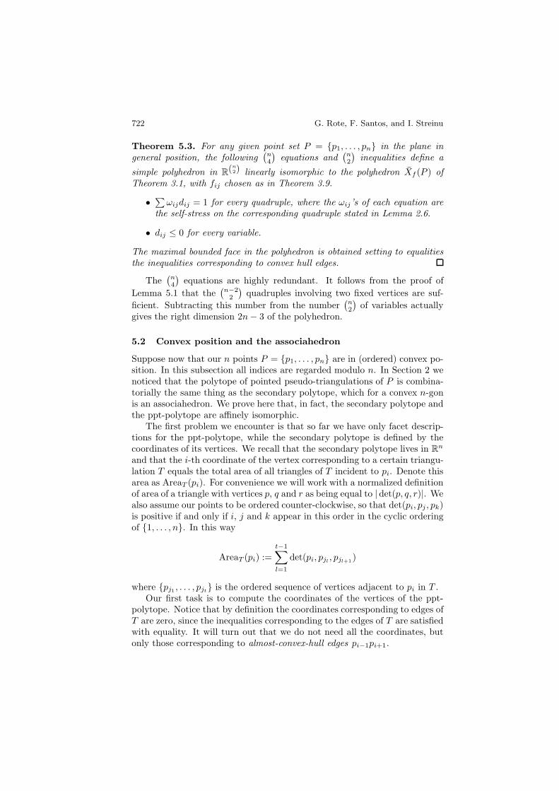
Suppose now that our n points P = {p1, . . . , pn} are in (ordered) convex po-sition. In this subsection all indices are regarded modulo n. In Section 2 wenoticed that the polytope of pointed pseudo-triangulations of P is combina-torially the same thing as the secondary polytope, which for a convex n-gonis an associahedron. We prove here that, in fact, the secondary polytope andthe ppt-polytope are affinely isomorphic.
The first problem we encounter is that so far we have only facet descrip-tions for the ppt-polytope, while the secondary polytope is defined by thecoordinates of its vertices. We recall that the secondary polytope lives in Rn
and that the i-th coordinate of the vertex corresponding to a certain triangu-lation T equals the total area of all triangles of T incident to pi. Denote thisarea as AreaT (pi). For convenience we will work with a normalized definitionof area of a triangle with vertices p, q and r as being equal to | det(p, q, r)|. Wealso assume our points to be ordered counter-clockwise, so that det(pi, pj , pk)is positive if and only if i, j and k appear in this order in the cyclic orderingof {1, . . . , n}. In this way
AreaT (pi) :=t−1∑l=1
det(pi, pjl , pjl+1)
where {pj1 , . . . , pjt} is the ordered sequence of vertices adjacent to pi in T .Our first task is to compute the coordinates of the vertices of the ppt-
polytope. Notice that by definition the coordinates corresponding to edges ofT are zero, since the inequalities corresponding to the edges of T are satisfiedwith equality. It will turn out that we do not need all the coordinates, butonly those corresponding to almost-convex-hull edges pi−1pi+1.

Expansive Motions and the Pseudo-Triangulation Polytope 723
Lemma 5.4. Let T be a triangulation of P . Then, in the ppt-polytope ofTheorem 5.3, the coordinate di−1,i+1 corresponding to an almost-convex-hulledge equals
di−1,i+1 = − det(pi−1, pi, pi+1) (AreaT (pi)− det(pi−1, pi, pi+1)) .
Proof. Let pj1 , . . . , pjt be the ordered sequence of vertices adjacent to pi inT , with pj1 = pi+1 and pjt = pi−1. We will prove by induction on k = 2, . . . , tthat the coordinate dj1jk of the ppt-polytope vertex corresponding to T equals
dj1jk = − det(pi, pj1 , pjk)Area(pj1 , . . . , pjk)
where Area(pj1 , . . . , pjk) denotes the area of the polygon with vertices pj1 , . . . ,pjk , in that order. This reduces to the formula in the statement for k = t.
The base case k = 2 is trivial: since j1j2 is an edge in the triangulation,we have dj1j2 = 0. To compute dj1jk for k > 2 we consider the quadruplepi, pj1 , pjk−1 , pjk . The only non-zero d’s on this quadruple are dj1jk−1 anddj1jk . (For k = 3, dj1jk−1 is also zero.) Hence, the equation
∑ωαβdαβ = 1
for this quadruple reduces to
dj1jkωj1jk + dj1jk−1ωj1jk−1 = 1.
From this we infer the stated value for dj1jk from the known values of theother quantities:
ωj1jk =1
det(pi, pj1 , pjk) det(pj1 , pjk−1 , pjk),
ωj1jk−1 =−1
det(pi, pj1 , pjk−1) det(pj1 , pjk−1 , pjk), and
dj1jk−1 = − det(pi, pj1 , pjk−1)Area(pj1 , . . . , pjk−1).
(The last equation is the inductive hypothesis.)
This Lemma immediately implies the following:
Corollary 5.5. (a) The affine map
ai = −di−1,i+1
det(pi−1, pi, pi+1)+ det(pi−1, pi, pi+1)
gives the coordinates (a1, . . . , an) of a triangulation in the secondarypolytope in terms of its coordinates (dij)ij∈(n2) in the ppt-polytope ofTheorem 5.3.
(b) The substitution dij = fij −〈pi− pj, vi− vj〉 in the above formula givesan affine map R2n → R
n sending the ppt-polytope of Theorem 3.1 tothe secondary polytope, whenever the fij’s are a valid choice satisfying
∑1≤i<j≤4
ωijfij = 1
for every quadruple, such as the choices in Theorem 3.9.

724 G. Rote, F. Santos, and I. Streinu
Observe that Corollary 5.5 implies that, for points in convex position, wecan consider the ppt-polytope of Theorem 5.3 as lying in the n-dimensionalspace given by the coordinates di−1,i+1. For the polyhedron, we additionallyneed the coordinates di,i+1. (These are zero on the polytope, but not on thepolyhedron.)
5.3 The 1-Dimensional Case: the Associahedron Again
By considering 1-dimensional expansive motions, in this section we will re-cover the associahedron via a different route. The analogy of this constructionto the 2-dimensional case will become even more apparent in Section 6.
The polytope of constrained expansions in dimension 1. In the 1-dimensional case we will rewrite constraints (6) in the form
vj − vi ≥ gij , ∀i < j. (11)
One set of inequalities is equivalent to the other under the change of constantsgij(pj − pi) = fij , for any i < j. This reformulation explicitly shows thatthe solution set does not depend on the point set P = {p1, . . . , pn} thatwe choose. We denote this solution set Xg, to mimic the notation of the2-dimensional case.
It is easy to see that the polyhedron Xg is full-dimensional and it containsno lines if we add the normalization equation v1 = 0. Hence, after normaliza-tion, it has dimension n−1 and contains some vertex. For any vertex v or forany feasible point v ∈ Xg, we may look at the set E(v) of tight inequalitiesat v:
E(v) := { ij | 1 ≤ i < j ≤ n, vj − vi = gij }We regard E(v) as the set of edges of a graph on the vertices {1, . . . , n}.
One may get various polyhedra by choosing different numbers gij in (11).We choose them with the following properties.
gil + gjk > gik + gjl, ∀1 ≤ i < j ≤ k < l ≤ n. (12)
For j = k we use this with the interpretation gjj = 0, so we require
gil > gik + gkl, ∀1 ≤ i < k < l ≤ n. (13)
One way to satisfy these conditions is to select
gij := h(tj − ti), ∀i < j (14)
for an arbitrary strictly convex function h with h(0) = 0 and arbitrary realnumbers t1 < · · · < tn. The simplest choice is h(t) = t2 and ti = i, yieldinggij = (i− j)2.
Two edges ij and jk with i < j < k are called transitive edges, and edgesik and jl with i < j < k < l are called crossing edges.

Expansive Motions and the Pseudo-Triangulation Polytope 725
Lemma 5.6. If g satisfies (12–13) and v ∈ Xg, then E(v) cannot containtransitive or crossing edges.
Proof. If we have two transitive edges ij, jk ∈ E(v) this means that vj−vi =gij and vk − vj = gjk. This gives vk − vi = gij + gjk < gik, by (13), andthus v cannot be in Xg because it violates (6). The other statement followssimilarly.
Non-crossing alternating trees. A graph without transitive edges iscalled an alternating or intransitive graph: every path in an alternating graphchanges continually between up and down.
Lemma 5.7. A graph on the vertex set {1, . . . , n} without transitive or cross-ing edges cannot contain a cycle.
Proof. Assume that C is a cycle without transitive edges. Let i andm be thelowest and the highest-numbered vertex of a cycle C, and let ik be an edgeof C incident to i, but different from im. The next vertex on the cycle afterk must be between i and k; continuing the cycle, we must eventually reachm, so there must be an edge jl which jumps over k, and we have a pair ik,jl of crossing edges.
Since the polyhedron is (n − 1)-dimensional, the set E(v) of a vertex vmust contain at least n − 1 edges. We have just seen that it is acyclic, andhence it must be a tree and contain exactly n− 1 edges. So we get:
Proposition 5.8. Xg is a simple polyhedron. The tight inequalities for eachvertex correspond to non-crossing alternating trees.
We will see below that Xg contains in fact all non-crossing alternatingtrees as vertices.
A new realization of the associahedron. Let’s look at the combinato-rial properties of these trees. Alternating trees have been studied in com-binatorics in several papers, see for example [21, 22] or [24, Exercise 5.41,pp. 90–92] and the references given there. Non-crossing alternating trees werestudied only by Gelfand, Graev, and Postnikov, under the name of “standardtrees”. They proved the following fact [10, Theorem 6.4].
Proposition 5.9. The non-crossing alternating trees non n + 1 points arein one-to-one correspondence with the binary trees on n vertices, and hencetheir number is the n-th Catalan number
(2nn
)/(n+ 1).
The bijection given in [10] to prove this fact is that the vertices of thebinary tree correspond to the edges of the alternating tree. It is easy to seethat every non-crossing alternating tree must contain the edge 1n. Removingthis edge splits the tree into two parts; they correspond to the two subtreesof the root in the binary tree. The two parts are handled recursively. Even
726 G. Rote, F. Santos, and I. Streinu
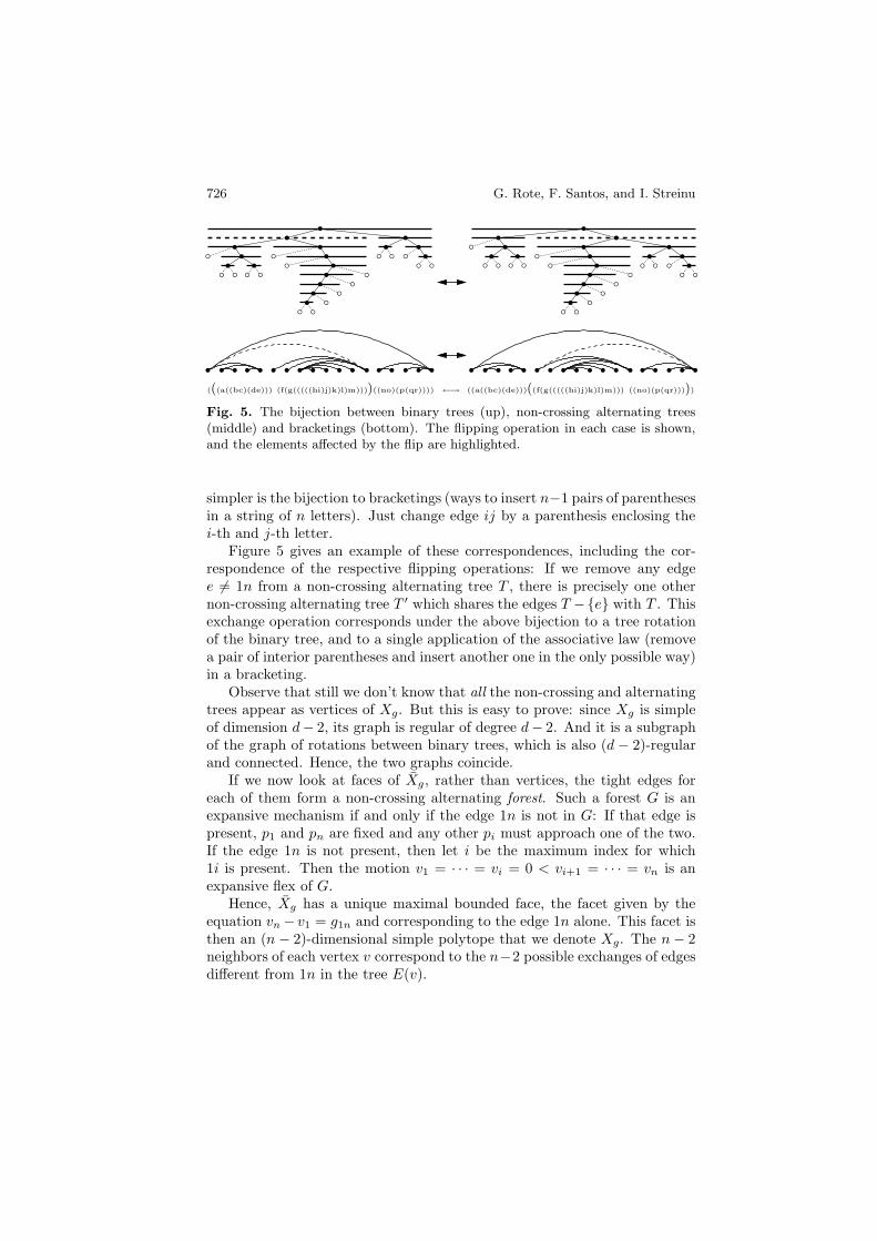
(((a((bc)(de))) (f(g(((((hi)j)k)l)m))))((no)(p(qr)))) ←→ ((a((bc)(de)))((f(g(((((hi)j)k)l)m))) ((no)(p(qr)))))
Fig. 5. The bijection between binary trees (up), non-crossing alternating trees(middle) and bracketings (bottom). The flipping operation in each case is shown,and the elements affected by the flip are highlighted.
simpler is the bijection to bracketings (ways to insert n−1 pairs of parenthesesin a string of n letters). Just change edge ij by a parenthesis enclosing thei-th and j-th letter.
Figure 5 gives an example of these correspondences, including the cor-respondence of the respective flipping operations: If we remove any edgee = 1n from a non-crossing alternating tree T , there is precisely one othernon-crossing alternating tree T ′ which shares the edges T −{e} with T . Thisexchange operation corresponds under the above bijection to a tree rotationof the binary tree, and to a single application of the associative law (removea pair of interior parentheses and insert another one in the only possible way)in a bracketing.
Observe that still we don’t know that all the non-crossing and alternatingtrees appear as vertices of Xg. But this is easy to prove: since Xg is simpleof dimension d− 2, its graph is regular of degree d− 2. And it is a subgraphof the graph of rotations between binary trees, which is also (d − 2)-regularand connected. Hence, the two graphs coincide.
If we now look at faces of Xg, rather than vertices, the tight edges foreach of them form a non-crossing alternating forest. Such a forest G is anexpansive mechanism if and only if the edge 1n is not in G: If that edge ispresent, p1 and pn are fixed and any other pi must approach one of the two.If the edge 1n is not present, then let i be the maximum index for which1i is present. Then the motion v1 = · · · = vi = 0 < vi+1 = · · · = vn is anexpansive flex of G.
Hence, Xg has a unique maximal bounded face, the facet given by theequation vn− v1 = g1n and corresponding to the edge 1n alone. This facet isthen an (n − 2)-dimensional simple polytope that we denote Xg. The n− 2neighbors of each vertex v correspond to the n−2 possible exchanges of edgesdifferent from 1n in the tree E(v).

Expansive Motions and the Pseudo-Triangulation Polytope 727
Theorem 5.10. Xg is a simple (n−2)-dimensional polytope whose face posetis that of the associahedron. Vertices are in one-to-one correspondence withthe non-crossing alternating trees on n vertices. Two vertices are adjacent ifand only if the two non-crossing alternating trees differ in a single edge.
Xg is an unbounded polyhedron with the same vertex set as Xg. Theextreme rays correspond to the non-crossing alternating trees with the edge1n removed.
Proof. Only the statement regarding the face poset remains to be proved.This can be proved in two ways: On the one hand, we already know thatthe graphs of Xg and of the (d− 2)-associahedron coincide (the latter beingthe graph of rotations between binary trees). And simple polytopes withthe same graph have also the same face poset. (This is a result of Blindand Mani; see [28, Section 3.4]). As a second proof, the correspondencebetween non-crossing alternating trees and bracketings trivially extends to acorrespondence between non-crossing alternating forests containing 1n and“partial bracketings” in a string of n letters which include the parenthesesenclosing the whole string. The poset of such things is the face poset of theassociahedron (see [24], Proposition 6.2.1 and Exercise 6.33). In particular,the face-poset of Xg is a subposet of the face-poset of the associahedron, andtwo polytopes of the same dimension cannot have their face posets properlycontained in one another. This is true in general by topological reasons, butspecially obvious in our case since we know our polytopes to be simple andtheir vertices to correspond one to one. Each vertex is incident to exactly(d−2i
)faces of dimension i in both polytopes, and two subsets of cardinality(
d−2i
)cannot be properly contained in one another.
A result which is related to Theorem 5.10 was proved by Gelfand, Graev,and Postnikov [10, Theorem 6.3], in a setting dual to ours: there a triangula-tion of a certain polytope was constructed. The non-crossing alternating treescorrespond to the simplices of the triangulation. It is shown explicitly thatthe simplices form a partition of the polytope. Certain numbers gij are thenassociated with the vertices of the polytope to show that the triangulation isa projection of the boundary of a higher-dimensional polytope. Incidentally,the numbers that were suggested for this purpose are (i−j)2, which coincideswith the simple proposal given above after (14), but the calculations are notgiven in the paper [10].
One easily sees that the conditions (12–13) on g are also necessary for thetheorem to hold: If any of these conditions would hold as an equality or as aninequality in the opposite direction, the argument of Lemma 5.6 would workin the opposite direction, and certain non-crossing alternating trees wouldbe excluded. Thus, (12–13) are a complete characterization of the “valid”parameter values gij .

728 G. Rote, F. Santos, and I. Streinu
Further Remarks. The result we presented in this section is surprisingin two ways: first, that it produces such a well studied object as the associ-ahedron; second, that it requires additional types of linear constraints thatare not needed in dimension 2. Indeed, inequalities (13) in the 1-dimensionalcase are the exact analog of inequalities (8) in the 2-dimensional case, as wewill see in Section 6. But the constraints (12) have no analog. This secondaspect makes the task of producing 3d generalization of the constructions ofthis paper more challenging, as there does not seem to be a straightforwardpattern for producing the linear constraints whose instantiations in 1d and2d give the polytopes of expansive motions.
The conditions (12–13) leave a lot of freedom for the choice of the vari-ables gij . We have an
(n2
)-dimensional parameter space. This is in contrast
to the classical representation, which has 2n parameters (the coordinates ofn points in the plane). If we select the parameters to be integral, we obtainan associahedron which is an integral polytope (this is also true for the clas-sical associahedron for a polygon with integer vertices.) But observe that, infact, the associahedra obtained here are in a sense much more special thanthe classical associahedra obtained as secondary polytopes. They have n− 2pairs of parallel facets, given by the equations vi = v1 + g1i and vi = vn− gin(i.e., corresponding to the pairs of edges 1i and in). See the right picture ofFigure 4, where n = 5. This is no surprise, since we have constructed ourpolytope by perturbing (a region of) a Coxeter arrangement, whose hyper-planes are in extremely non-general position.
One can check that classical associahedra have no parallel facets. Hence,are associahedra are not affinely equivalent to the classical ones. Recently,Chapoton, Fomin and Zelevinsky [5] have shown another construction of theassociahedron having as facet normals the root system of type An (moregenerally, they show a similar construction for all root systems). Still, ourassociahedra are not affinely equivalent to theirs: Comparing the right partof our Figure 4 with their Figure 2 we see that both are 3-dimensional asso-ciahedra with three pairs of parallel facets but in their realization the threeremaining facets share a vertex while in ours they do not. It is howeverconceivable that they are related by projective transformations.
(a) (b)
Fig. 6. (a) The non-crossing alternating trees appear as a face of a ppt-polytope.(b) Another associahedron in the same ppt-polytope.

Expansive Motions and the Pseudo-Triangulation Polytope 729
The non-crossing alternating trees also appear directly as a face of the ppt-polytope. Consider the configuration of points shown in Figure 6, consistingof a convex chain {p1, . . . , pn} and an additional point p0. The pseudotrian-gulations containing all the edges from p0 to the other points (Figure 6a),correspond to the non-crossing alternating trees on p1, . . . , pn, forming an as-sociahedron of dimension n− 2. Another associahedron (of dimension n− 3)appears as a different face of this ppt-polytope: the face corresponding tothe edges of the convex chain (Figure 6b). These two faces are disjoint.
Relations to optimization and the Monge matrices. Constraints ofthe form (11) are commonly found in project planning and critical path anal-ysis. The variables vi represent unknown start times of tasks, and the con-straints (11) specify waiting conditions between different tasks. For example,the minimization of vn − v1 is a longest path problem in an acyclic network.The different vertices of Xg correspond to the different optimal solutionswhen we apply various linear objective functions.
Matrices G = (gij) with the property (12) are said to have the Mongeproperty, if we set gii = 0 and gij = ∞ for i > j. The Monge propertyhas received a great deal of attention in optimization because it arises oftenin applications and it characterizes special classes of optimization problemsthat can be solved efficiently, see [4] for a survey.
The dual linear program of the linear programming problem (11) (witha suitable objective function) is a minimum-cost flow problem on an acyclicnetwork with edges ij for 1 ≤ i < j ≤ n, and cost coefficients −gij . Net-work flow is actually one of the oldest areas in optimization in which theMonge property has been applied, and where it has been shown that optimalsolutions can be obtained by a greedy algorithm in certain cases. The non-crossing alternating trees are just the different possible subgraphs of thoseedges which carry flow in an optimal solution.
6 Towards a General Framework, in Arbitrary Dimen-sion
To make more explicit the analogy between our 1d and 2d constructions we’llrewrite the 1d construction back in terms of inequalities (6) instead of (11).As we mentioned at the beginning of Section 5.3, the way to do this is tosubstitute gi,j = fi,j/(pj−pi) everywhere. In particular, the constraints (13)become
fikpi − pk
+fkl
pk − pl+
filpl − pi
> 0.
But ωik = 1pi−pk , ωkl =
1pk−pl and ωil = 1
pl−pi define a self-stress on any1-dimensional point set {pi, pk, pl}. Hence, inequalities (13) are the exactanalog of inequalities (8) of the 2d case. The difference is that in 2d these in-equalities are necessary and sufficient for a choice of parameters to be “valid”,

730 G. Rote, F. Santos, and I. Streinu
while in 1d we need the additional constraints (12), which do not follow from(13) as the following example shows:
g12 = g23 = g34 = 1, g13 = g24 = 2.2, g14 = 3.3.
Let’s see what would be a generalization of the 1d and 2d cases to ar-bitrary dimension. For any finite point set P = {p1, . . . , pn} spanning Rd
(in general position or not) there is a well-defined cone of expansive motionsX0 of dimension nd−
(d+1
2
), which is the positive region in the arrangement
of hyperplanes defined by the constraints (4). Every choice of perturba-tion parameters (fij)i,j∈{1,...,n}, via inequalities (6), produces a polyhedronof constrained expansions Xf , whose faces are in correspondence with somegraphs embedded on P . If the fij ’s are sufficiently generic, this polyhedronis simple and:
• The face poset of Xf is isomorphic to a subposet of the graphs embed-ded on P , ordered by reverse inclusion.
• The maximal graphs in this subposet are some of the infinitesimallyminimally rigid frameworks on P .
• Adjacent vertices on the polyhedron correspond to graphs differing onlyby one edge.
The main question is whether there is a clever choice of the fij ’s or a sensi-ble choice of a special family of minimally rigid frameworks to be the verticesof the polyhedron which admits a nice and simple geometric characterization,as non-crossing alternating trees in 1d or pointed pseudo-triangulations in 2ddo. In particular, what should be the analog of pointed pseudo-triangulationson a point set in general position in 3d? One difficulty is that the combina-torics of minimally rigid graphs in dimension three is not fully understood.Perhaps a good case to start with would be points in convex and general posi-tion in dimension 3, for which the convex hull edges provide a very canonicalminimally rigid framework to start with.
Another observation is that both in the 1d and 2d cases that we havetreated here, the resulting polytope Xf has a unique maximal bounded face.This is related to the graph of flips between the special minimally rigid frame-works considered being connected and regular, which is an extra desirableproperty.
It would even be interesting to have a good generalization of the 2d caseto point sets which are not in general position. If we use the 2d definition off from equations (9) with many points on a common line, there are solutionsin which all the inequalities are tight. In this way we get essentially the one-dimensional expansion cone of Proposition 2.7, when we project all vectorsvi on the direction of that line. (This is the same situation as when allrelations (13) are satisfied as equations.) One way to get rid of this degeneracyis to “perturb the perturbations” by adding an infinitesimal component of

Expansive Motions and the Pseudo-Triangulation Polytope 731
the one-dimensional expansion parameters of Section 5.3: instead of f we usef
(2)ij + εf
(1)ij , where f (2) is valid for two-dimensional point sets, f (1)
ij satisfythe restrictions required for the 1d perturbation parameters, and ε > 0 issufficiently small. The situation would be like in Figure 6a when the points onthe convex chain converge to being collinear. We have not further investigatedthis idea.
Another consideration which may help to treat degenerate point sets andarbitrary-dimensional ones is that the ideas in Section 5.1 generalize with notmuch difficulty under very weak general position assumptions. Let us first tryto generalize Lemma 5.1. We need to decide what is the right analog of thestatement in part (b). We propose the following. Remember that a circuitof a point set P = {p1, . . . , pn} ⊂ Rd is a minimal affinely dependent subset.If P is in general position, its set of circuits C(P ) is
(Pd+2
). In general, any
set of d+ 2 points spanning d dimensions contains a unique circuit, but thiscircuit can have less than d+2 elements. In any case, the complete graph ona circuit C has (up to a constant factor) a unique self stress (ωij)i,j∈C withno vanishing ωij , which is the one given by Lemma 2.5.
Let us consider the following linear maps:
M : Rdn −→ R
(n2)
(v1, . . . , vn) �−→ 〈vi − vj , pi − pj〉,
∆: R(n2) −→ R
C(P )
{fij}ij∈(n2) �−→{ ∑ij∈C
ωijfij
}C∈C(P )
.
M is just the rigidity map of the complete graph on P . The equivalence of(b) and (c) in Lemma 5.1 can be rephrased as
ker∆ = ImM, for every planar point set in general position.
But in fact the same is true in arbitrary dimension and under much weakerassumptions than general position:
Proposition 6.1. For any point set P ⊂ Rd, ImM ⊆ ker∆. If P has
d affinely independent points whose spanned hyperplane contains no otherpoint of P , then the reversed inclusion also holds.
Proof. That ImM ⊂ ker∆ (i.e., ∆ ◦M = 0) is one direction of Lemma 2.4.To prove ker∆ ⊂ ImM , let f ∈ R(
n2) be such that
∑ij∈C ωijfij = 0 for every
circuit C. We want to find a motion a = (a1, . . . , an) for which M(a) = f .Without loss of generality assume that p1, . . . , pd are the claimed affinelyindependent points. Let us fix a motion (a1, . . . , ad) for the first d pointssatisfying the
(d2
)equations of the system Ma = f concerning these points.
This motion exists and is unique up to an arbitrary translational and rota-tional component, because the complete graph on any affinely independentpoint set is minimally infinitesimally rigid.

732 G. Rote, F. Santos, and I. Streinu
By assumption, {p1, . . . , pd, pi} is an affine basis for every i > d, and hencethe complete graph on it is again minimally infinitesimally rigid. Thus, thereis a motion (a′1, . . . , a
′d, ai) satisfying the
(d+1
2
)corresponding equations of the
system Ma = f . Adding translations and rotations we can assume a′j = aj ,j = 1, . . . , d. So we have constructed a motion (a1, . . . , an) which restricts tothe one chosen for the d first points and which satisfies all the equations forpairs of points that include one of the first d.
It remains to show that the equations are also satisfied for the edgeskl with k, l > d. We follow the same idea as in the proof of Lemma 5.1.Our assumption on the point set implies that the unique circuit C containedin {p1, . . . , pd, pk, pl} uses both pk and pl. To simplify notation, assumethat this circuit is {p1, . . . , pi, pk, pl}. By Lemma 2.4, there is a feasiblemotion (a′1, . . . , a
′i, a′k, a′l). By translations and rotations we assume aj =
a′j for j = 1, . . . , i. Observe now the value of 〈v − u, pj1 − pj2〉, for anyof the points in the circuit and for any vectors v and u, depends only onthe projection of v and u to the affine subspace spanned by C. Since thecomplete graphs on {p1, . . . , pi}, on {p1, . . . , pi, pk} and on {p1, . . . , pi, pl} areminimally infinitesimally rigid when motions are restricted to that subspace,we conclude that the projections of ak and al to that affine subspace coincidewith the projections of a′k and a′l. In particular, 〈al − ak, pl − pk〉 = 〈a′l −a′k, pl − pk〉 = fkl.
Hence, Lemma 5.1 and its corollary, Lemma 5.2, hold in this generalizedsetting, with one equation per circuit instead of one equation per 4-tuple.The weakened general position assumption for d of the points holds for everyplanar point set, since, by Sylvester’s theorem, any finite set of points in theplane, not all on a single line, has a line passing through only two of thepoints.
In dimension 3, however, the same is not true, and actually there arepoint sets for which ImM = ker∆. Consider the case of six points, threeof them in one line and three in another, with the two lines being skew (notparallel and not crossing). These two sets of three points are the only twocircuits in the point set. In particular, ker∆ has at most codimension 2 inR
15, i.e., it has dimension at least 13. On the other hand, ImM has at mostthe dimension of the reduced space of motions, 18− 6 = 12.
7 Final Comments
We describe some open questions and ideas for further research. The mainquestions related to this work are how to extend the constructions from di-mensions 1 and 2 to 3 and higher, and how to treat subsets in special posi-tion in 2d. The expectation is that this would give a coherent definition for“pseudo-triangulations” in higher dimensions. Some ideas in this directionhave been mentioned in Section 6.
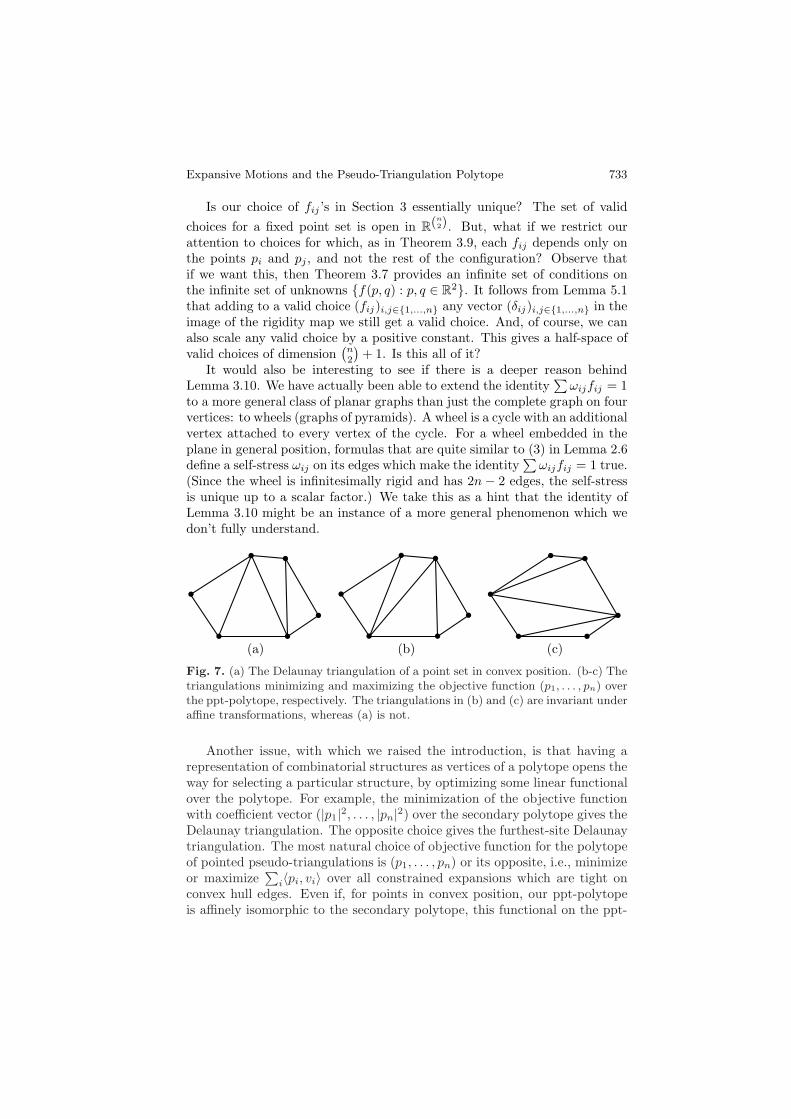
Expansive Motions and the Pseudo-Triangulation Polytope 733
Is our choice of fij ’s in Section 3 essentially unique? The set of validchoices for a fixed point set is open in R(
n2). But, what if we restrict our
attention to choices for which, as in Theorem 3.9, each fij depends only onthe points pi and pj , and not the rest of the configuration? Observe thatif we want this, then Theorem 3.7 provides an infinite set of conditions onthe infinite set of unknowns {f(p, q) : p, q ∈ R2}. It follows from Lemma 5.1that adding to a valid choice (fij)i,j∈{1,...,n} any vector (δij)i,j∈{1,...,n} in theimage of the rigidity map we still get a valid choice. And, of course, we canalso scale any valid choice by a positive constant. This gives a half-space ofvalid choices of dimension
(n2
)+ 1. Is this all of it?
It would also be interesting to see if there is a deeper reason behindLemma 3.10. We have actually been able to extend the identity
∑ωijfij = 1
to a more general class of planar graphs than just the complete graph on fourvertices: to wheels (graphs of pyramids). A wheel is a cycle with an additionalvertex attached to every vertex of the cycle. For a wheel embedded in theplane in general position, formulas that are quite similar to (3) in Lemma 2.6define a self-stress ωij on its edges which make the identity
∑ωijfij = 1 true.
(Since the wheel is infinitesimally rigid and has 2n− 2 edges, the self-stressis unique up to a scalar factor.) We take this as a hint that the identity ofLemma 3.10 might be an instance of a more general phenomenon which wedon’t fully understand.
(a) (b) (c)
Fig. 7. (a) The Delaunay triangulation of a point set in convex position. (b-c) Thetriangulations minimizing and maximizing the objective function (p1, . . . , pn) overthe ppt-polytope, respectively. The triangulations in (b) and (c) are invariant underaffine transformations, whereas (a) is not.
Another issue, with which we raised the introduction, is that having arepresentation of combinatorial structures as vertices of a polytope opens theway for selecting a particular structure, by optimizing some linear functionalover the polytope. For example, the minimization of the objective functionwith coefficient vector (|p1|2, . . . , |pn|2) over the secondary polytope gives theDelaunay triangulation. The opposite choice gives the furthest-site Delaunaytriangulation. The most natural choice of objective function for the polytopeof pointed pseudo-triangulations is (p1, . . . , pn) or its opposite, i.e., minimizeor maximize
∑i〈pi, vi〉 over all constrained expansions which are tight on
convex hull edges. Even if, for points in convex position, our ppt-polytopeis affinely isomorphic to the secondary polytope, this functional on the ppt-

734 G. Rote, F. Santos, and I. Streinu
polytope does not, in general, give the Delaunay triangulation of those points,see Figure 7. In fact, the result on the ppt-polytope is invariant under affinetransformations of the point set, while the Delaunay triangulation is not.The properties of the pointed pseudo-triangulations that are defined in thisway await further studies.
Added in proof. The second author, together with David Orden, hasextended the main construction of this paper to a simple polyhedron of di-mension 3n− 3 with a unique maximal bounded face whose vertices are allthe pseudo-triangulations of the point set. Bounded edges correspond to ei-ther classical edge-flips or to the creation or destruction of pointedness at avertex by the deletion or inclusion of a single edge. The face poset of thispolyhedron is (essentially) the poset of all non-crossing graphs on the pointset.
References
[1] Pankaj Agarwal, Julien Basch, Leonidas Guibas, John Hershberger, andLi Zhang, Deformable free space tilings for kinetic collision detection. inBruce Randall Donald, Kevin Lynch and Daniela Rus (eds.), Algorithmic andComputational Robotics: New Directions, 4th Int. Workshop on Alg. Found.Robotics (WAFR), A K Peters, 2000, pp. 83–96.
[2] David Avis and Komei Fukuda, Reverse search for enumeration. DiscreteAppl. Math. 65 (1996), 21–46.
[3] Herve Bronnimann, Lutz Kettner, Michel Pocchiola, and Jack Snoeyink.Counting and enumerating pseudo-triangulations with the greedy flip algo-rithm. Manuscript, submitted for publication, 2001.
[4] Rainer E. Burkard, Bettina Klinz, and Rudiger Rudolf, Perspectives of Mongeproperties in optimization. Discrete Appl. Math. 70 (1996), 95–161.
[5] Frederic Chapoton, Sergey Fomin, and Andrei Zelevinsky, Polytopal realiza-tions of generalized associahedra, preprint math.CO/0202004, 25 pages, Febru-ary 2002.
[6] Robert Connelly, Erik D. Demaine, and Gunter Rote, Straightening polygo-nal arcs and convexifying polygonal cycles. Discrete & Computational Geom-etry, to appear. Preliminary version in Proc. 41st Ann. Symp. on Found. ofComputer Science (FOCS 2000), Redondo Beach, California; IEEE ComputerSociety Press, Washington, D.C., 2000, pp. 432–442; an extended version isavailable as technical report B 02-02, Freie Universitat Berlin, Institut furInformatik, 2002.
[7] Robert Connelly and Walter Whiteley, Second-order rigidity and prestresstensegrity frameworks. SIAM Journal on Discrete Mathematics 9 (1996), 453–491.
[8] George B. Dantzig, Alan J. Hoffman, T. C. Hu, Triangulations (tilings) andcertain block triangular matrices. Math. Programming 31 (1985), 1–14.

Expansive Motions and the Pseudo-Triangulation Polytope 735
[9] Komei Fukuda, cdd code.http://www.ifor.math.ethz.ch/staff/fukuda/fukuda.html
[10] Israel M. Gelfand, M. I. Graev, and Alexander Postnikov, Combinatorics ofhypergeometric functions associated with positive roots. In: Arnold, V. I. et al.(ed.), The Arnold-Gelfand Mathematical Seminars: Geometry and SingularityTheory. Boston, Birkhauser. pp. 205–221 (1997)
[11] Israel M. Gel′fand, Andrei V. Zelevinskiı, and M. M. Kapranov, Discrimi-nants of polynomials in several variables and triangulations of Newton poly-hedra. Leningrad. Math. J. 2 (1991), 449–505, translation from Algebra Anal.2 (1990), No. 3, 1–62.
[12] Michael Goodrich and Roberto Tamassia, Dynamic ray shooting and shortestpaths in planar subdivisions via balanced geodesic triangulations. J. Algo-rithms 23 (1997), 51–73.
[13] Jack Graver, Brigitte Servatius, and Hermann Servatius, Combinatorial Rigid-ity. AMS Graduate Studies in Mathematics vol. 2, 1993.
[14] David Kirkpatrick, Jack Snoeyink, and Bettina Speckmann, Kinetic collisiondetection for simple polygons. International Journal of Computational Geom-etry and Applications 12 (2002), 3–27. Extended abstract in Proc. 16th Ann.Symposium on Computational Geometry, pp. 322–330, 2000.
[15] G. Laman, On graphs and rigidity of plane skeletal structures. J. EngineeringMath. 4 (1970), 331–340.
[16] Carl Lee, The associahedron and triangulations of the n-gon. European J.Combinatorics 10 (1989), 551–560.
[17] Jesus A. de Loera, Serkan Hosten, Francisco Santos, and Bernd Sturmfels,The polytope of all triangulations of a point configuration. Documenta Math-ematica, J. DMV 1 (1996), 103–119.
[18] Michel Pocchiola and Gert Vegter, Topologically sweeping visibility complexesvia pseudo-triangulations. Discr. & Comput. Geometry 16 (1996), 419–453.
[19] Michel Pocchiola and Gert Vegter, The visibility complex. Int. J. Comput.Geom. Appl. 6 (1996), 279–308.
[20] Michel Pocchiola and Gert Vegter, Pseudo-triangulations: Theory and appli-cations. In Proc. 12th Ann. ACM Sympos. Comput. Geom., ACM Press, May1996, pp. 291–300.
[21] Alexander Postnikov, Intransitive trees. J. Combin. Theory, Ser. A 79 (1997),360–366.
[22] Alexander Postnikov and Richard P. Stanley, Deformations of Coxeter hyper-plane arrangements. J. Combin. Theory, Ser. A 91 (2000), 544–597.
[23] B. Speckmann and C. D. Toth, Vertex π-guards in simple polygons. In Ab-stracts of the 18th European Workshop on Computational Geometry (Eu-roCG), April 10–12, 2002, Warszawa, Poland, pp. 12–15. Full version submit-ted for publication.
[24] Richard Stanley, Enumerative Combinatorics. Vol. 2, Cambridge UniversityPress, 1999.

736 G. Rote, F. Santos, and I. Streinu
[25] Ileana Streinu, A combinatorial approach to planar non-colliding robot armmotion planning, In Proc. 41st Ann. Symp. on Found. of Computer Science(FOCS 2000), Redondo Beach, California, November 2000, pp. 443–453.
[26] Ileana Streinu, A combinatorial approach to planar non-colliding robot armmotion planning, preprint, 2002.
[27] Walter Whiteley, Rigidity and Scene Analysis, in: Jacob E. Goodman andJoseph O’Rourke (eds.) Handbook of Discrete and Computational Geometry,CRC Press, 1997, pp. 893–916.
[28] Gunter Ziegler, Lectures on Polytopes (2nd ed.), Springer-Verlag, 1999.
About the Authors
Gunter Rote is at the Institut fur Informatik, Freie Universitat Berlin, Taku-straße 9, D-14195 Berlin, Germany, [email protected].
Francisco Santos is at the Departamento de Matematicas, Estadıstica y Com-putacion, Universidad de Cantabria, E-39005 Santander, Spain,[email protected].
Ileana Streinu is at the Department of Computer Science, Smith College,Northampton, MA 01063, USA, [email protected].
Acknowledgments
We thank Ciprian Borcea for pointing out some relevant references in themathematical literature. This work started at the Workshop on Pseudo-triangulations held at the McGill University Bellairs Institute in Barbados,January 2001, partially funded by NSF grant CCR-0104370, and contin-ued during a visit of the third author to the Graduiertenkolleg Combina-torics, Probability and Computing at Freie Universitat Berlin, supportedby Deutsche Forschungsgemeinschaft, grant GRK 588/1. Work by IleanaStreinu was partially supported by NSF RUI Grants CCR-9731804 and CCR-0105507. Work by Francisco Santos was partially supported by grants PB97–0358 and BMF2001-1153 of the Spanish Direccion General de EnsenanzaSuperior.