arX

iv:0

808.

3055

v1 [

stat

.ME

] 2

2 A

ug 2

008

Minimal average degree aberration and the

state polytope for experimental designs

Yael Berstein∗, Hugo Maruri-Aguilar†, Shmuel Onn∗,Eva Riccomagno‡, Henry Wynn†

August 22, 2008

Abstract

For a particular experimental design, there is interest in finding

which polynomial models can be identified in the usual regression set

up. The algebraic methods based on Grobner bases provide a sys-

tematic way of doing this. The algebraic method does not in general

produce all estimable models but it can be shown that it yields mod-

els which have minimal average degree in a well-defined sense and in

both a weighted and unweighted version. This provides an alterna-

tive measure to that based on “aberration” and moreover is applicable

to any experimental design. A simple algorithm is given and bounds

are derived for the criteria, which may be used to give asymptotic

Nyquist-like estimability rates as model and sample sizes increase.

1 Introduction

It is of considerable value to represent an experimental design as the solutionof a set of polynomial equations. In the terminology of algebraic geometry adesign is a zero dimensional variety and the corresponding ideal comprisingall polynomials which are zero on every design point is called an “ideal ofpoints”. Pistone & Wynn (1996) first used explicit methods from algebraic

∗Technion, Israel Institute of Technology, Haifa 32000, Israel†Department of Statistics, London School of Economics, London WC2A 2AE, UK‡Dipartimento di Matematica, Universita di Genova, Genova 16146, Italy

1

geometry and in particular introduced Grobner bases into designs. Issues todo with identifiability of polynomial regression models, or interpolators, canbe translated into problems about such varieties and ideals, see Pistone et al.(2001).

The purpose of this paper is to introduce the notion of linear aberration ofa polynomial model. Linear aberration is defined only for polynomial models,which are used routinely in statistical literature. A polynomial model withlow order terms has low aberration, thus engaging low aberration with thestandard practice of preferring polynomial models with low order terms. Thepreference for models with low order terms has been acknowledged in recentpapers, see Li et al. (2003) and Balakrishnan and Yang (2006), although theydo not refer to linear aberration.

Let α = (α1, . . . , αd) be a nonnegative d-dimensional integer multi-index.A monomial in the indeterminates x1, . . . , xd is the power product xα =xα1

1 · · ·xαd

1 . A model basis is a collection of distinct monomials {xα, α ∈ L},where L is a finite set of multi-indices. By combining linearly monomials inL we form polynomials:

ηL(x) =∑

α∈L

θαxα,

where θα are real coefficients. The polynomial ηL(x) is a candidate for inter-polation or statistical modelling.

This paper is concerned with the following concepts.

Definition 1 Let L be a model basis and let w = (w1, . . . , wd) be a collectionof non-negative weights with

∑di=1 wi = 1. We define the weighted linear

aberration of L as

A(w, L) =1

n

∑

(α1,...,αd)∈L

d∑

i=1

wiαi,

where n is the number of elements in L.

We are interested in studying aberration for models identifiable by anexperimental design and along this paper we compare models and designs ofthe same size n.

Definition 2 An experimental design D, of sample size n = |D|, is a set ofpoints in R

d.

2

We say that a model basis L with cardinality |L| = n is identifiable by Dif the design model matrix X = [xα]x∈D,α∈L is invertible.

The term aberration is used to acknowledge the work on “minimumaberration” for regular fractional factorial designs of Wu and others, seeFries and Hunter (1980) and Wu and Wu (2002). For fractional factorialdesigns, the notion of estimation capacity is related to the ability of a de-sign to identify models of low degree, see Cheng and Mukerjee (1998) andChen and Cheng (2004). We do not make a direct mathematical comparisonwith that work but simply point to a common motivation.

In Section 2 we review the basic ideas on algebraic identifiability. Thesearch for identifiable models is driven by a divisibility condition, whichmakes the search problem tractable. We then introduce the state polytope,whose vertices correspond to the models identified using the algebra. InSection 3 we study aberration. The basic ideas on aberration are closelylinked with the algebraic work on corner cut models and state polytopes inOnn and Sturmfels (1999). We are specially interested in obtaining minimalvalues for aberration for which we establish upper and lower bounds. Anapproximate approach to minimal aberration is discussed. In Section 4 wediscuss various examples. In Section 5 we discuss possible extensions of thetheory and, by example, a connection with the notion of aberration by Wuand others is discussed.

2 The G-basis method and the state polytope

The aberation A(w, L) has remarkable connections with the algebraic methodin experimental design introduced by Pistone and Wynn Pistone and Wynn(1996) and developed in the monograph Pistone et al. (2001) and the jointwork of Onn and Sturmfels Onn and Sturmfels (1999). In this section wepresent the basic ideas on identifiability using algebraic techniques.

Let the set of all monomials in d indeterminates be T d = {xα, α ∈ Zd≥0},

where Z≥0 is the set of non-negative integers and Zd≥0 is the set of all vectors

in d dimensions and with entries in Z≥0. A polynomial is a finite linear com-bination of monomials in T d with real coefficients. The set of all polynomialsis denoted as R[x1, . . . , xd]. It has the structure of a ring with the usualoperations of sum and product of polynomials.

A term ordering ≻ on R[x1, . . . , xd] is a total ordering on T d such that i)xα ≻ 1 for all xα ∈ T d, α 6= (0, . . . , 0) and ii) for all xα, xβ, xγ ∈ T d if xα ≻ xβ

3

then xαxγ ≻ xβxγ . The leading term of a polynomial is the largest term withnon-zero coefficient with respect to ≻. For a polynomial f ∈ R[x1, . . . , xd],we write its leading term as LT≻(f).

A partial order on T d is defined by a vector w ∈ Rd≥0 as xα �w xβ if

wTα ≥ wTβ, where xα, xβ ∈ T d and wT is the transposed vector of w. Undersome conditions on w (see Babson et al. (2003); Cox et al. (1997)) this definesa term order. Given a term order ≻, there are w such that xα ≻ xβ if andonly if xα �w xβ.

A design D, considered as a zero-dimensional variety gives rise to a de-sign ideal, I(D), which is the set of all polynomials which have zeros atall the points of D. We have that I(D) ⊂ R[x1, . . . , xd]. The polyno-mial ideal I is generated by the set of polynomials G = {g1, . . . , gs} ifI = {∑s

i=1 figi : fi ∈ R[x1, . . . , xd]} and we write I = 〈g1, . . . , gs〉.An important set of generators for the design ideal is the Grobner basis.

Grobner bases were introduced by Buchberger in Buchberger (1966) and theyhave become a powerful computational tool in many fields Cox et al. (1997,2005). A Grobner basis of I(D) with respect to a term order ≻ is a finitesubset G≻(D) ⊂ I(D) such that 〈LT≻(g) : g ∈ G≻(D)〉 = 〈LT≻(f) : f ∈I(D)〉. The computation of Grobner bases is implemented in standard com-puter programs such as CoCoA, Singular or Maple, see CoCoATeam (2007);Greuel et al. (2005); Monagan et al. (2005).

Two polynomials f and g in R[x1, . . . , xd] are equivalent with respect toI(D) if the following conditions hold:

i) f − g ∈ I(D)

ii) f(d) = g(d) for all d ∈ D

Given a term ordering ≻, the quotient ring R[x1, . . . , xd]/I(D) has a uniqueR-vector space basis given by the monomials in T d that cannot be dividedby the leading terms of the polynomials in G≻(D) for I(D). The monomialbasis so obtained, or equivalently, the set of its exponents L = L(D,≻),has a staircase (also echelon, order ideal) property: for α ∈ L, if β ≤ αcomponentwise, then β ∈ L. Equivalently we say that for any xα ∈ L, ifxβ divides xα then xβ ∈ L. We call bases which have a staircase structurestaircase models. The dimension of R[x1, . . . , xd]/I(D) as R-vector spaceis n, see Pistone and Wynn (1996), i.e. the number of points in D and ofmulti-indices in L is n.

4

For a given basis of the quotient ring with exponents in L and a set ofreal values (data) Yx, x ∈ D, there exists a unique interpolator ηL(x) suchthat Yx = ηL(x), x ∈ D. Other non-saturated statistical sub-models can beconstructed from subsets of L, see Holliday et al. (1999) and Peixoto (1987).

Definition 3 The algebraic fan of D is La(D) = {L(D,≻), where ≻ is aterm ordering in R[x1, . . . , xd]}. This is the collection of staircases L(D,≻)arising from a fixed design D by varying all monomial orderings.

The algebraic fan of a design was proposed by Caboara et al. Caboara et al.(1997), constructing upon the algebraic fan of an ideal of Mora and RobbianoMora and Robbiano (1988). Babson et al. Babson et al. (2003) proposed apolynomial time algorithm to compute La(D). They compute an efficientset of weight vectors and perform a change of basis which stems from theso-called FGLM algorithm, see Faugere et al. (1993). In Section 3.1 an al-gorithm is presented to identify a model in the algebraic fan using a weightvector.

It is important to note that not all staircase models identified by D arein La(D). We denote the set of all identifiable staircase models for a designD as Ls(D). In fact the algebraic fan is small relative to Ls(D), that isLa(D) ⊆ Ls(D), see Chapter 6 in the unpublished Ph.D. thesis by Maruri-Aguilar (2007) and Section 4 in Pistone et al. (2006).

We now establish the link between the algebraic fan of a design and thestate polytope of the design ideal. For a model basis L = {α1, . . . , αn}, αi ∈Z

d≥0 define

αL =∑

αi∈L

αi.

This vector appears in the definition of A(w, L) and we can write A(w, L) =(wTαL)/n. The set all such vectors over La(D) gives the state polytope.

Definition 4 The state polytope S(D) of a design D, or equivalently of thedesign ideal I(D) is the convex hull

S(D) := conv ({αL : L is a staircase in La(D)}) .

The following theorem (Sturmfels, 1996, Ch. 2) summarizes the connec-tion between the state polytope and the set of models La(D), i.e. the relationbetween a design and its algebraic fan.

5

Theorem 1 Let D be a design and let S(D) be its state polytope. Then theset of vertices of the state polytope of D is in one to one correspondence withthe algebraic fan of D.

The state polytope does not only contain information concerning modelsin the algebraic fan of a design, but it also provides information about theterm ordering vectors needed to construct it. We recall that a d-dimensionalpolytope is a bounded subset of R

d, which corresponds to the solutions of asystem of linear inequalities. The normal cone of a face of a polytope is therelatively open cone of those vectors in R

d uniquely minimised over the faceof the polytope. The normal fan of a polytope is the collection of all thenormal cones of the polytope.

Two ordering vectors w and w′ are said to be equivalent (modulo I(D))if L(D,≻w) = L(D,≻w′). The normal fan of the state polytope partitionsR

d≥0 into equivalence classes of ordering vectors, see Babson et al. (2003);

Fukuda et al. (2007); Sturmfels (1996). Indeed every vertex of S(D) corre-sponds to a model in La(D). Moreover, the interior of the normal cone ofa vertex in S(D) contains those vectors w which correspond to the sameequivalence class.

We motivate Theorem 2 below with a simple example. The black dotsin Figure 1 give a 5 point design in 2 dimensions, D. They also give theset of exponents L obtained for any term ordering, indeed the size of thealgebraic fan of D is one. The crosses represent the exponents of the leadingterms of the Grobner basis: (2, 0), (1, 2), (0, 3). The line separates the modelexponents, L, from these leading terms. This is an example of a corner cutmodel. Note that equivalently the line separates L from its complement inZ

2≥0.

Definition 5 A model L, of size |L| = n, is said to be a corner cut model ifthere is a (d − 1) dimensional hyperplane separating L from its complementZ

d≥0 \ L.

Not all staircases are corner cuts, for example L = {(0, 0), (1, 0), (0, 1), (1, 1)}is a staircase that cannot be separated by a hyperplane from its complementin Z

2≥0.

The set of exponents of a corner cut model is referred to as a corner cutstaircase or simply, as a corner cut. Corner cuts were introduced by Onn andSturmfels Onn and Sturmfels (1999). A generating function for the number

6

×

××

1 2

1

2

3

0

Figure 1: Corner cut and separating hyperplane.

of bidimensional corner cuts is given in Corteel et al. (1999), while the orderof the cardinality of the set of corner cuts is proven bounded by (n log n)d−1

in Wagner (2002). A special class of designs is composed with those designsthat identify all corner cut models of a given size.

Definition 6 A design D ⊂ Rd comprised of n distinct points is said to be

generic if all corner cut models of size n = |D| are identifiable.

A special polytope is constructed with the exponents for corner cut mod-els. It will be used to compute the algebraic fan of generic designs.

Definition 7 The corner cut polytope is CC(n, d) := conv({αL : L is acorner cut staircase in d dimensions and of size n}).

For a discussion on the properties of bidimensional corner cut polytopessee the paper by Muller Muller (2003). The algebraic fan of generic de-signs corresponds to the set of corner cut models, as stated in the followingtheorem.

Theorem 2 (Onn and Sturmfels, 1999) Let D ⊂ Rd be a generic design

with n points. Then

i) S(D) = CC(n, d) and

ii) the algebraic fan of D is the set of corner cut models in d dimensionsand with n elements.

We remark that the corner cut polytope is an invariant object for theclass of all the ideals generated by generic designs with the same samplesize n and number of factors d and all generic designs have the same statepolytope.

7

3 Minimal linear aberration

An important feature of the state polytope is that its vertices are automat-ically “lower” vertices in the sense of convexity. State polytopes relate di-rectly to models with minimal linear aberration. In Section 3.1 an algorithmto compute a models of minimal aberration is presented.

Theorem 3 Given a design D ⊂ Rd with n distinct points and a weight

vector w ∈ Rd>0, there is a least one vertex α∗ ∈ S(D) which minimises

A(w, L) over all identifiable staircase models Ls(D), that is

1

n(wTα∗) = A(w, L∗) = min

L∈Ls(D)A(w, L)

for all L∗ such that αL∗ = α∗. Moreover, given a vertex of S(D), there is atleast one w∗ ∈ R

d>0 such that this vertex (model) minimizes A(w, L), that is,

A(w∗, L) = minw∈R

d>0

A(w, L)

for L such that αL = αL.

Proof. First, for given w we minimise wT αL for L ∈ La(D), which is a finiteset, see Mora and Robbiano (1988). The αL for L ∈ La(D) are vertices ofS(D) by definition. Furthermore, because we restrict L to the algebraic fanof D there cannot be three aligned αL in S(D), see Sturmfels (1996). For thesecond claim, it is sufficient to take a vector wL in the interior of a normalcone for αL. By definition, A(w, L) is minimised for vectors on the interiorof the normal cone.

Theorem 4 follows directly from Theorem 3.

Theorem 4 For every weight vector w there is a design D ⊂ Rd which

minimizes A(w, L), among all designs with sample size n and identifiablestaircases.

This is stated compactly as:

A∗(w, n) = minD:|D|=n

minL∈La(D)

A(w, L)

is achieved for a generic design. That is, if a design is generic then automat-ically its algebraic fan contains models of minimal aberration.

8

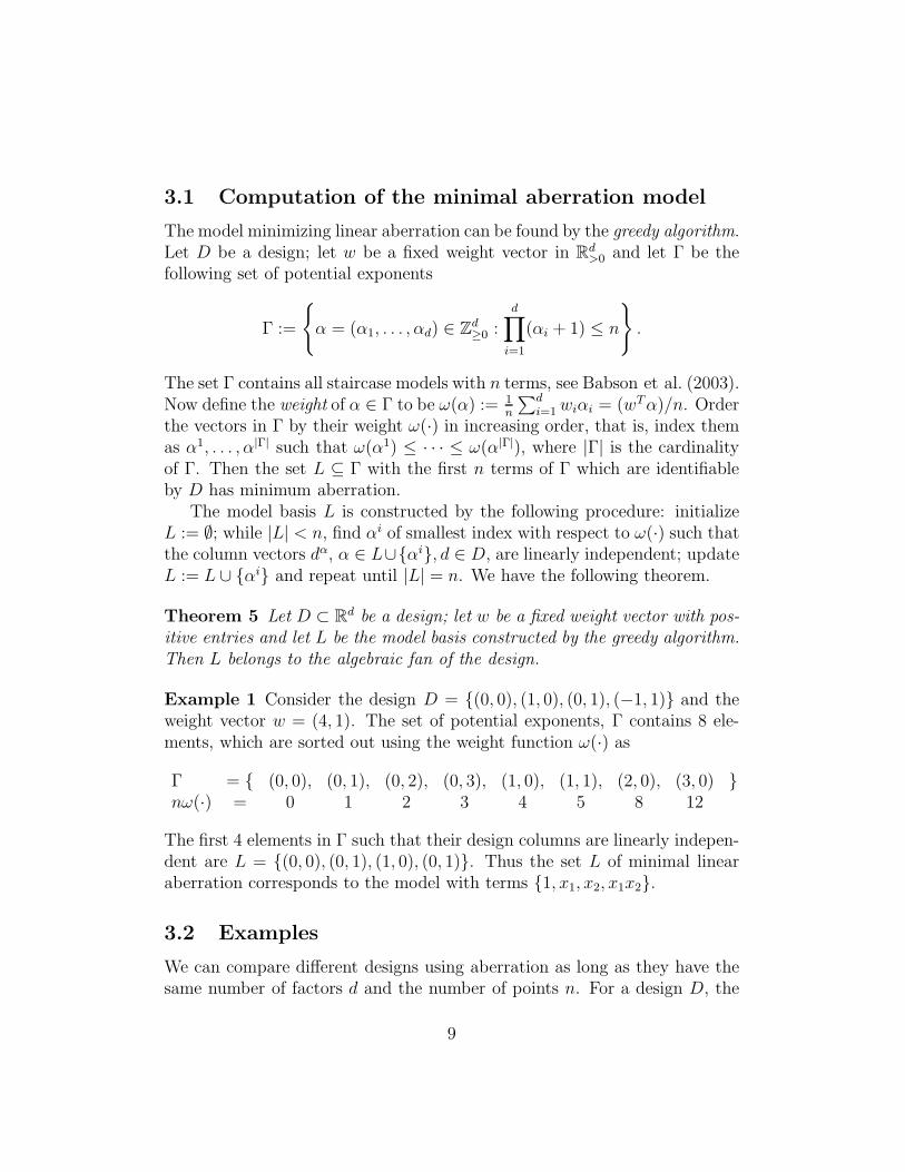
3.1 Computation of the minimal aberration model

The model minimizing linear aberration can be found by the greedy algorithm.Let D be a design; let w be a fixed weight vector in R

d>0 and let Γ be the

following set of potential exponents

Γ :=

{

α = (α1, . . . , αd) ∈ Zd≥0 :

d∏

i=1

(αi + 1) ≤ n

}

.

The set Γ contains all staircase models with n terms, see Babson et al. (2003).Now define the weight of α ∈ Γ to be ω(α) := 1

n

∑di=1 wiαi = (wTα)/n. Order

the vectors in Γ by their weight ω(·) in increasing order, that is, index themas α1, . . . , α|Γ| such that ω(α1) ≤ · · · ≤ ω(α|Γ|), where |Γ| is the cardinalityof Γ. Then the set L ⊆ Γ with the first n terms of Γ which are identifiableby D has minimum aberration.

The model basis L is constructed by the following procedure: initializeL := ∅; while |L| < n, find αi of smallest index with respect to ω(·) such thatthe column vectors dα, α ∈ L∪{αi}, d ∈ D, are linearly independent; updateL := L ∪ {αi} and repeat until |L| = n. We have the following theorem.

Theorem 5 Let D ⊂ Rd be a design; let w be a fixed weight vector with pos-

itive entries and let L be the model basis constructed by the greedy algorithm.Then L belongs to the algebraic fan of the design.

Example 1 Consider the design D = {(0, 0), (1, 0), (0, 1), (−1, 1)} and theweight vector w = (4, 1). The set of potential exponents, Γ contains 8 ele-ments, which are sorted out using the weight function ω(·) as

Γ = { (0, 0), (0, 1), (0, 2), (0, 3), (1, 0), (1, 1), (2, 0), (3, 0) }nω(·) = 0 1 2 3 4 5 8 12

The first 4 elements in Γ such that their design columns are linearly indepen-dent are L = {(0, 0), (0, 1), (1, 0), (0, 1)}. Thus the set L of minimal linearaberration corresponds to the model with terms {1, x1, x2, x1x2}.

3.2 Examples

We can compare different designs using aberration as long as they have thesame number of factors d and the number of points n. For a design D, the

9

state polyhedron of D is obtained by (Minkowski) addition of Rd≥0 to the

state polytope S(D), see Babson et al. (2003). The state polyhedron yieldsthe same information as the state polytope. Indeed the normal fan of the(negative) state polyhedron yields automatically the first orthant, see Fukudaet al. Fukuda et al. (2007).

10 20 30

10

20

30

0

b

b

State polyhedron

S(D)

10 20 30

10

20

30

0bc

bcbc

bc

bc

bc

bc

bc

bc

bc

bc

bc

b

b

u

GenericCCD

Factorial 32

Figure 2: The left graph depicts S(D) and the state polyhedron for the CCDof Example 2. The right graph shows state polyhedra for the three designs ofExample 2. The empty dots correspond to vertexes/models identified by thegeneric design only, while the triangle is for the sole model in the algebraicfan of the 32 design.

Example 2 Consider a central composite design (CCD by Box and WilsonBox and Wilson (1951)) with two factors, one observation at the origin andaxial distance α =

√2. The CCD has 9 runs and its algebraic fan contains

exactly two models, namely

{1, x1, x21, x

31, x

41, x2, x1x2, x

21x2, x

22} (1)

together with the model obtained by permuting the roles of x1 and x2. LetL1 be the set of exponents of the model support in Equation (1). Clearly,αL1

= (13, 5) and the state polytope for the design ideal of the CCD isconv ({(13, 5), (5, 13)}), see left graph of Figure 2. Now consider a genericdesign with the same number of runs as the CCD. In Corteel et al. (1999)and Onn and Sturmfels (1999) it is shown that there are 12 corner cut modelsfor d = 2 and n = 9. By Theorem 2, the algebraic fan of the generic designcontains all the 12 corner cut models, including those in the algebraic fanof the CCD. We consider also a full factorial design 32, which identifies only

10

the model with support {1, x1, x21} ⊗ {1, x2, x

22}, where ⊗ is the Kronecker

product. Its state polytope is the point (9, 9). In the right graph of Figure 2we depict the state polyhedra for the three designs and in Figure 3 we plotminL∈La(D) A(w, L) for w = (w1, w2) ∈ [0, 1]2 and w1 + w2 = 1. For the CCDthis is

{ (

(w1, 1 − w1)(13, 5)T)

/9 = (8w1 + 5)/9 if w1 ≤ 1/2(

(w1, 1 − w1)(5, 13)T)

/9 = (−8w1 + 13)/9 if w1 > 1/2

For the generic design the aberration curve is a piecewise linear functionwith 12 segments. Finally, the aberration for the design 32 is constant for allweights. As expected, the aberration takes its minimum value for the genericdesign, over all possible weights.

0.5 1w1

0

0.5

1 32

CCD

Generic

Figure 3: Minimal aberration for three designs in two factors and nine runs,see Example 2.

Example 3 Consider the design D = {(0, 0), (1, 1), (2, 2), (3, 4), (5, 7), (11, 13),(α, β)}, where (α, β) ≈ (1.82997, 1.82448) is the only real solution of a sys-tem of polynomial equations, see (Onn and Sturmfels, 1999, Page 47). Thealgebraic fan of the above design has ten models and its state polytope is

conv ({(21, 0), (15, 1), (11, 2), (9, 3), (6, 5), (5, 6), (3, 9), (2, 11), (1, 15), (0, 21)}) .

Now consider a generic design G with the same number of runs and factors.The algebraic fan of G is the set of corner cut models which for 7 points in 2

11

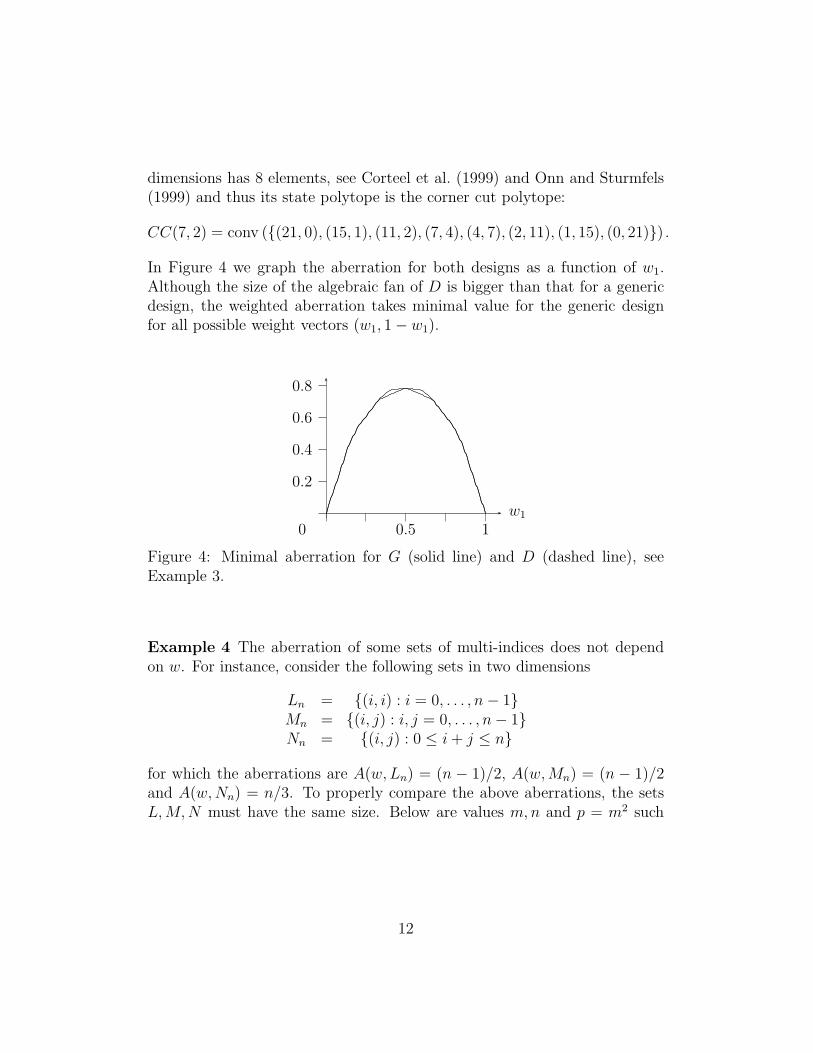
dimensions has 8 elements, see Corteel et al. (1999) and Onn and Sturmfels(1999) and thus its state polytope is the corner cut polytope:

CC(7, 2) = conv ({(21, 0), (15, 1), (11, 2), (7, 4), (4, 7), (2, 11), (1, 15), (0, 21)}) .

In Figure 4 we graph the aberration for both designs as a function of w1.Although the size of the algebraic fan of D is bigger than that for a genericdesign, the weighted aberration takes minimal value for the generic designfor all possible weight vectors (w1, 1 − w1).

0.5 1w1

0

0.2

0.4

0.6

0.8

Figure 4: Minimal aberration for G (solid line) and D (dashed line), seeExample 3.

Example 4 The aberration of some sets of multi-indices does not dependon w. For instance, consider the following sets in two dimensions

Ln = {(i, i) : i = 0, . . . , n − 1}Mn = {(i, j) : i, j = 0, . . . , n − 1}Nn = {(i, j) : 0 ≤ i + j ≤ n}

for which the aberrations are A(w, Ln) = (n − 1)/2, A(w, Mn) = (n − 1)/2and A(w, Nn) = n/3. To properly compare the above aberrations, the setsL, M, N must have the same size. Below are values m, n and p = m2 such

12

that #Lp = #Mm = #Nn for m up to 8000.

m n A(w, Lp) A(w, Mm) A(w, Nn)1 0 0 0 06 8 17.5 2.5 2.6

35 49 612.0 17.0 16.3204 288 20807.5 101.5 96.0

1189 1981 7.0 × 105 594.0 560.36930 9800 2.4 × 107 3464.5 3266.6

40391 57121 8.1 × 108 20195.0 19040.3

As sample size grows, the aberration of the triangular set Nn remains smallerthan for the square set Mm.

3.3 Bounds for the aberration

Although the minimal value of the aberration A∗(w, n), depends on theweight vector w = (w1, . . . , wd), we can carry out a special normalisationwhich leads to bounds for the minimal aberration. These bounds dependonly on a simple function of the weights, surprisingly the geometric mean.Our construction is based upon the expected value of auxiliary random vari-ables which are suitably constructed.

For the rest of this Section let D ⊂ Rd be a generic design with n points.

Let w be a fixed weight vector with positive elements and let L be the cornercut model identified by w. We recall that |L| = n.

For an integer multindex α define its upper cell as the unit cube withlower vertex at α

c(α) = {v ∈ Rd : αi ≤ vi ≤ αi + 1}

and similarly the lower cell of α is

c(α) = {v ∈ Rd : αi − 1 ≤ vi ≤ αi}

Define:Q = ∪α∈L c(α), Q = ∪α∈L c(α).

See Figure 5 for a depiction of lower and upper cells with L a corner cut.Clearly, the volume of Q and of Q equals n, that is the cardinality of L.

We now create a simplex S(w) ⊂ Rd which is directed by the vector w and

13

1 2

1

2

3

0

w

S(w)

v1

v2

1 2

1

2

3

0

w

S(w)

v1

v2

Figure 5: Bidimensional corner cut together with upper (left diagram) andlower cells (right diagram) Q and Q. In both diagrams the vector w, aseparating hyperplane and equivalent simplexes S(w) and S(w) were added.

has volume n. We call this simplex and the subset of the first orthant below it

the equivalent simplex, which is formally S(w) ={

v ∈ Rd≥0 :

∑di=1 viwi ≤ c

}

.

The volume of S(w) is determined up to the constant c > 0. We find thevalue of this constant by setting the total volume of the equivalent simplexequal to n:

n =cd

d!∏d

i=1 wi

,

giving

c = (nd!)1d g(w), (2)

where

g(w) =

(

d∏

i=1

wi

)

1d

is the geometric mean of the components of the weight vector w. We callH(w) the hyperplane which limits the equivalent simplex, that is H(w) ={

v ∈ Rd≥0 :

∑di=1 viwi = c

}

.

The expected value of a random variable with uniform support over S(w)will be used now to compute bounds for aberration. We can compute a no-tional value of A, the linear aberration for a distribution D as the expectation

14

A(w, S(w)) = E(∑

wiXi) for the random vector (X1, . . . , Xd) with uniformdistribution over S(w). Thus for the equivalent simplex we have that

A(w, S(w)) =1

n

d

(d + 1)!

cd+1

∏di=1 wi

= (nd!)1d

d

d + 1g(w), (3)

after substituting Equation (2) in A(w, S(w))We observe that the region Q is obtained from Q by a negative shift

(−1, . . . ,−1). As before, we consider a random vector with joint uniformdistribution over Q. We then use the expected value of

∑

wiXi as the aber-

ration A(w, Q). Analogously we define A(w, Q) and we have

A(w, Q) = A(w, Q) − 1

Similarly we can create a region S(w) by the same downward shift, and wehave

A(w, S(w)) = A(w, S(w))− 1.

As D is generic and thus L is a corner cut there exist cutting hyperplanesseparating L from its complement in Z

d≥0. Moreover if w is in the interior

of the normal cone of the corner cut polytope, then we can select a cut-ting hyperplane H which is orthogonal to w and thus parallel to H(w), seeOnn and Sturmfels (1999).

Example 5 Consider a generic design with d = 2, n = 3 and L = {(0, 0),(1, 0),(2, 0)}. The weight vector w = (1, 2) is not in the interior of a normalcone of the corner cut polytope CC(2, 3). Indeed the weight vector is onthe boundary of the normal cone separating L from the corner cut model{(0, 0), (1, 0), (0, 1)}. The hyperplanes perpendicular to w are 2x1 − x2 = cand none of them is a cutting hyperplane for L.

By a simple argument the simplex SH with faces xi = 0, (i = 1, . . . , d)and H lies wholly within the upper quadrant region Q because otherwise,the cutting hyperplane hypothesis for H would be violated and thus SH hasvolume less than n. Recall that the equivalent simplex S(w) has volume n.

There is one additional argument that leads to our first inequality. Sincethe region Q and the equivalent simplex S(w) have the same volume n, itmust be that Q protrudes beyond S(w). Equivalently we may move mass

15

from Q, that is, beyond H(w), inside S(w). As this mass occurs orthogonallyto w, we claim that this movement diminishes the aberration, thus

A(w, S(w)) ≤ A(w, Q).

This property is also inherited by the downward shifted version, and we haveA(w, S(w)) ≤ A(w, Q). The same orthogonality argument shows the middleinequality in the following sequence:

A(w, S(w)) ≤ A(w, Q) ≤ A(w, S(w)) ≤ A(w, Q).

By Theorem 4, as the design is generic and L is the model identified by w,clearly we have

A(w, Q) ≤ A∗(w, n) ≤ A(w, Q).

Analogous argument and construction as above shows that A(w, Q) ≤ A(w, S(w))+1.

Theorem 6 Let D ⊂ Rd be a generic design with n points; let w ∈ R

d bea vector of positive weights. Then the minimal aberration A∗(w, n) satisfiesthe bounds

A(w, S(w))− 1 ≤ A∗(w, n) ≤ A(w, S(w)) + 1, (4)

where A(w, S(w)) is computed in Equation (3).

There are various kinds of asymptotic that this formula leads to. Fromthe inequality between geometric and arithmetic mean we have g(w) ≤ 1

d.

This suggests the condition limd7→∞ g(w) = c/d for some constant 0 ≤ c ≤ 1.Now for wi = (1 + δi)/d, with

∑

δi = 0, and assuming convergence of∑

δ2i

and n = kd, we use use Stirling’s approximation to obtain

limd7→∞

A∗(w, n) =kc

e.

Such limits may be considered as asymptotic identifiability rates, analogousto the more familiar Nyquist rates in Fourier analysis.

Example 6 For small d and n the bounds of Equation (4) are rather coarse.Figure 6 shows the bounds A(w, S(w)) ± 1 of Theorem 6 together with theminimal aberration A∗(w, n), plotted as function of w1 for d = 2 and n = 4.

16

Notice that, as function of w, the minimal aberration A∗(w, n) is a piece-wise linear graph (this is a general fact, consequence of Definition 1), eachsegment corresponding to a different vertex (different corner cut) of the cornercut polytope. Figures 7 and 8 give the bounds and minimal aberration forn = 20 and n = 100. In Figures 6, 7 and 8 we also added a curve for theapproximate aberration which is presented in Theorem 7 below.

0.5 1

w1

−1

−0.5

0

0.5

1

2

1.5

Figure 6: Minimal aberration A∗(w, n) (solid line) for a generic design withd = 2, n = 4; bounds A(w, S(w)) and A(w, S(w))± 1 of Theorem 6 (dashedlines). We also show approximate aberration A using Theorem 7 (thin dashedline).

3.4 Approximated state polytope for generic designs

Note that as w changes the hyperplanes H(w) are tangent to the surfacedefined by

d∏

i=1

xi = cd = nd!

(

1

d

)d

and the (normalised) centroids of the equivalent simplices lie on the surfacedefined by

d∏

i=1

xi = b+ = n

(

1

d + 1

)d

d! (5)

17

0.5 1

w1

−1

0

1

2

3

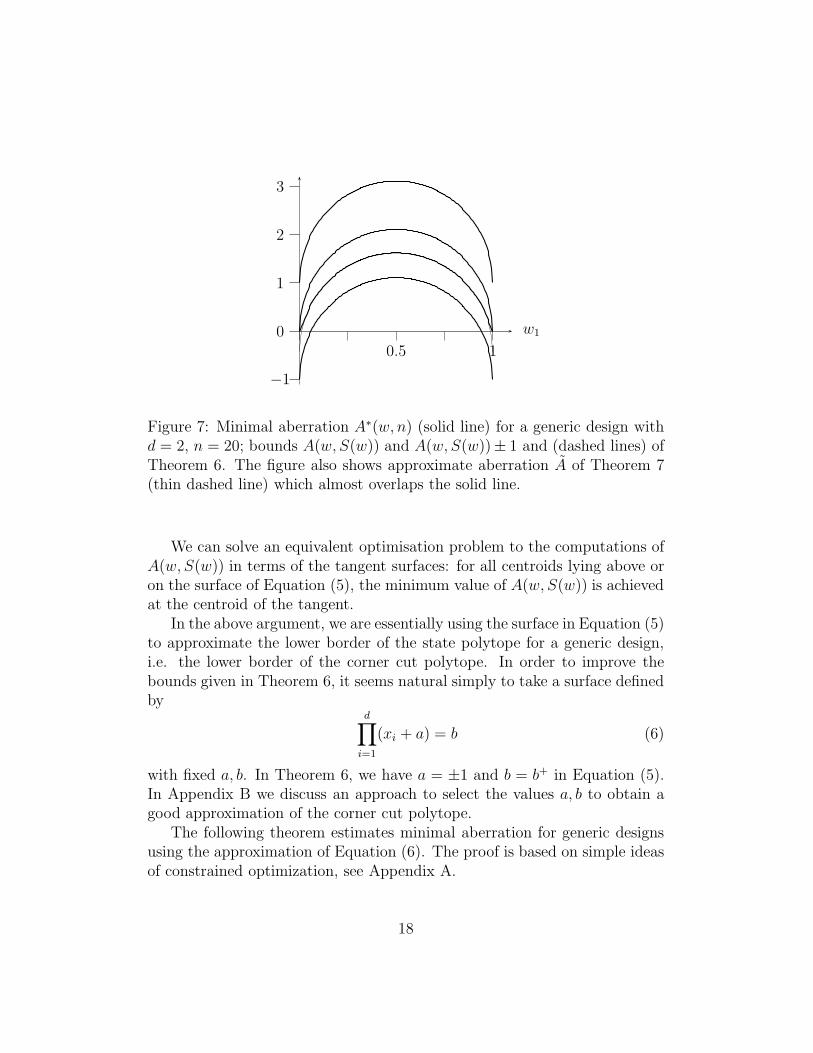
Figure 7: Minimal aberration A∗(w, n) (solid line) for a generic design withd = 2, n = 20; bounds A(w, S(w)) and A(w, S(w))± 1 and (dashed lines) ofTheorem 6. The figure also shows approximate aberration A of Theorem 7(thin dashed line) which almost overlaps the solid line.

We can solve an equivalent optimisation problem to the computations ofA(w, S(w)) in terms of the tangent surfaces: for all centroids lying above oron the surface of Equation (5), the minimum value of A(w, S(w)) is achievedat the centroid of the tangent.

In the above argument, we are essentially using the surface in Equation (5)to approximate the lower border of the state polytope for a generic design,i.e. the lower border of the corner cut polytope. In order to improve thebounds given in Theorem 6, it seems natural simply to take a surface definedby

d∏

i=1

(xi + a) = b (6)

with fixed a, b. In Theorem 6, we have a = ±1 and b = b+ in Equation (5).In Appendix B we discuss an approach to select the values a, b to obtain agood approximation of the corner cut polytope.

The following theorem estimates minimal aberration for generic designsusing the approximation of Equation (6). The proof is based on simple ideasof constrained optimization, see Appendix A.

18

0.5 1

w1

−1

0

1

2

3

4

5

6

Figure 8: Minimal aberration A∗(w, n) (solid line) for a generic design withd = 2, n = 100; bounds A(w, S(w)) and A(w, S(s)) ± 1 (dashed lines). Theapproximate aberration A of Equation (7) (thin dashed line) is also plotted,but is undistinguishable from the minimal aberration.

Theorem 7 Let w = (w1, . . . , wd) be a fixed positive weight vector; let D ⊂R

d be a generic design with n points. Let the state polytope of I(D) beapproximated by Equation (6). Then the value

A(w) = db1/dg(w) − a

d∑

i=1

wi (7)

is an approximation of A∗(w, n).

We recall that g(w) is the geometrical mean of the components in w. Figures6, 7 and 8 give examples (d = 2 factors, n = 4, 20, 100) of the minimalaberration A(w) in Theorem 7. The values a, b for each case were selectedusing the technique in Appendix B.

4 Examples

In this section we discuss through extended examples other possible usesof the ideas on generic designs and aberration. In Section 4.1 we exploreand conjecture the existence of generic designs over Latin hypercubes forall factors and sample sizes. In Section 4.2 we compare fractional factorialdesigns through their state polytopes.

19

4.1 Latin hypercube design

Latin hypercube designs (LH) were first proposed by McKay et al. McKay et al.(1979) in the context of computer experiments. Latin hypercubes are designswith reasonable space filling properties and good projections in lower dimen-sions.

Theorem 4 relates minimal aberration to generic designs, i.e. if the designis generic, then it identifies models of lower weighted degree (and minimalaberration) for any weight vector w. In what follows we study LH usingDefinition 6 of generic designs.

The construction of a Latin hypercube design can be summarised as fol-lows.

1. Divide the range of each factor into n equal segments.

2. Select a value in each segment using a random uniform distribution, orany other continuous distribution.

3. Randomly permute the list for each factor.

By Theorem 30 in Pistone et al. (2001), a Latin hypercube design con-structed as above is generic with probability one.

We now consider a special type of LH designs. This type is constructedby selecting a fixed value in every segment in Step 2. For instance, we couldselect the minimum, maximum or the midpoint value for every segment.

There are a few obvious cases of LH designs which are not generic, forexample when the points of the design lie on a line. We have performedexhaustive search for a few cases of LH in two dimensions. Our search pointsout to the existence of generic LH for different values of d, n. In fact forthe values we tried the proportion of generic LH tends clearly to one. SeeFigures 9 and 10 for a depiction of the results, where we additionally plot theproportion of maximal fan designs among LH, i.e. LH designs that identifyall possible staircase models for given d, n. We have the following conjecturefor the existence of generic LHS for any value of d, n.

Conjecture 8 For every d ≥ 2 and n ≥ 2 there exists at least one genericLH design, constructed by setting a fixed value for every one of the n segmentsin the above procedure.

20

100%

75%

50%

95%

n

2 3 4 5 6 7 8 9 10 11 12 13 14 15

Generic

Maximal fan

Figure 9: Percentage of generic LHS designs for d = 2 and n ≤ 15.

3 5 10 15n

10−1

10−2

10−3

10−4

10−5

Generic

Maximal fan

Figure 10: Minus logarithm of the percentage of non generic LHS designsfor d = 2 and n ≤ 15.

21

Figure 11: LH on [0, 1]2 for d = 2, n = 10 which are not generic and identifyL.

Experimentally we observed that when the sample size is n =(

k+1d

)

fork ≥ 1, the genericity of a LH design is closely linked to the identification ofa model of total degree k − 1. For example for k = 4, d = 2, n = 10 there are10! LH of which 99% are generic. Of the remaining 1% which are not genericonly 6 designs (up to reflection and rotation), which are given in Figure 11,identify the cubic model with exponent set

L = {(0, 0), (1, 0), (0, 1), (2, 0), (1, 1), (0, 2), (3, 0), (2, 1), (1, 2), (0, 3)}.

4.2 Orthogonal fractions

In this Section we consider some of the techniques of this paper for theclass of fractional factorial designs with two levels. We first explore therelation between state polyhedron and then later propose a tool to comparethe identification capability of designs.

In Examples 2 and 3 we observed that in general, nesting of state poly-hedra for two designs does not imply any easy relation between the algebraicfan of the designs. If instead we restrict to the family of designs with twolevels then there is a clear relation between such nesting and algebraic fans.We have the following Lemma from Chapter 6 in the Ph.D. thesis by Maruri-Aguilar (2007).

22

Lemma 9 Let F1 and F2 be two fractional factorial designs with two lev-els and let S1 and S2 be their corresponding state polyhedra of I(F1), I(F2).Then the nesting of state polyhedra S1 ⊂ S2 implies nesting of algebraic fansLa(F1) ⊂ La(F2).

The following example is based upon Lemma 9 and presents an interestingrelation between resolution and identifiability. That is, bigger resolutionpoints to more models in the algebraic fan.

Example 7 Let F1 and F2 be the 24−1IV and 24−1

III fractional fractional designswith eight runs in four factors and respective generators x1x2x3x4 − 1 = 0and x1x2x3 − 1 = 0. The subindices III, IV refer to the resolution of thefraction, see Box and Hunter (1961a,b). Their corresponding state polyhedraare nested, i.e. S(F2) ⊂ S(F1) and by direct computation we confirm thatthe algebraic fans are also nested. The algebraic fan La(F2) has four models,while La(F1) includes 12 elements.

For fractional factorial designs, the estimation of interactions in a designwas related to the resolution of the design through the property termedhidden projection, see Evangelaras and Koukouvinos (2006); Wang and Wu(1995). We conjecture the nesting of algebraic fans of two designs 2k−p withdifferent resolution. However, exploiting this nesting property of fans tocompare designs using aberration might need additional considerations.

Example 8 Let F1, F2 be the fractions 27−2IV given by generators x6−x1x2x3 =

0, x7−x2x3x4 = 0 and x6−x1x2x3x4 = 0, x7−x1x2x3x5 = 0 respectively. Al-though both fractions have the same resolution, the fraction F2 correspondsto a minimum aberration design using the definition of Fries and Hunter(1980). The state polyhedron S(F1) has 133 vertices while S(F2) has 1708.There is no nesting of the state polyhedra and La(F1) ∩ La(F2) 6= ∅.

A proposal to compare two designs D1, D2 of the same size through theirstate polytopes is to map the vertices of the state polytopes S(D1), S(D2)with a function f : R

d → R. In this way the state polytopes of D1 and D2

are compared by the univariate projections of their vertices. We propose aweighted sum of the vertex coordinates

f(v1, . . . , vd) =

d∑

i=1

wivi, (8)

23

with positive weights wi > 0. We use wi = 1 for i = 1, . . . , d and thusEquation (8) allows for direct comparison of designs based on the distributionof total degrees for models in the algebraic fan.

Example 9 (Continuation of Example 8) We transform the vertices of thestate polytopes for F1 and F2 using Equation (8). In Table 1 in Appendix Bwe summarize the results for each fraction as the distribution of absolute andrelative frequencies. Clearly, the fraction F2 with minimum aberration forgenerators identifies models with a smaller total degree than that for F1 andin that sense it has smaller linear aberration. See Figure 12 for a histogramof the relative frequencies for F1 and F2.

F2

F1

F3

60 70 80

10%

20%

30%

40%

50%

Figure 12: Histograms of relative frequencies for fractions F1 and F2, seeExample 9. We added F3 of Example 10.

5 Discussion

5.1 Generalised concave aberration

This paper is partly concerned with a problem of linear programming, i.e.optimising a linear function f : R

d → R over a convex polytope. We nowdiscuss extensions of our work using other types of aberration. When weconsider concave aberration criteria, some of our results still hold.

Consider any concave function f : Rd → R. Now, given a model L, define

its aberration by

A(f, L) := f

(

∑

α∈L

α1, . . . ,∑

α∈L

αd

)

.

24

The linear aberration of Definition 1 is the special case where f is the fol-lowing linear (hence concave) function,

f : Rd −→ R

x = (x1, . . . , xd) 7→ 1

n

d∑

i=1

wixi.

Since we only appealed to convexity, Theorem 3 is valid when we replaceA(w, L) by the more general form A(f, L). That is to say, the set of lowervertices of the state polytope (corresponding to models in the algebraic fan)contains the solution to minimising any concave aberration function. Thiscan be understood as minimisation over a matroid, which was studied furtherin Berstein et al. (2008). A further development is to consider aberrationA(w, S(w)) with respect to other distributions rather than the uniform.

5.2 Connection with aberration of Wu and others

In the statistical literature, the word aberration has been used to refer toproperties of the generators for fractional factorial designs, see Chen and Hedayat(1998); Fries and Hunter (1980); Wu and Wu (2002). A topic of future re-search is to link minimal aberration of Definition 1 with the traditional mea-sure based on generators for a fractional factorial design.

We conjecture that among the class of orthogonal fractions of 2d designsthere is some kind of correspondence between the minimal linear aberrationof this paper and minimum generator aberration of Wu and others. If weselect non-orthogonal fractions, the situation is more complex, as the nextexample shows.

Example 10 Let F3 be the non-orthogonal fraction with size n = 32 of a 27

design given in Table 2 of Appendix B. We also consider the designs F1 andF2 of Examples 8 and 9. The three designs have the same size, but the designF3 cannot be compared with F1 or F2 in traditional terms as it is not evenorthogonal. However, we can compare the designs based in the distributionof degrees in their algebraic fans.

An interpolation as presented in Appendix B suggests that the mini-mum degree of models identified by a generic design with n = 32, d = 7 is53.5 ≈ 54. This number is a lower bound for the total degree of modelsidentified by designs F1, F2 and F3. In other words, the set of total degrees

25

for models in algebraic fan of F1, F2 and F3 is lower bounded by 54, e.g.54 ≤ min({∑d

i=1 αL : L ∈ La(Fi)}) for i = 1, 2, 3.Initial results show that

i) the size of La(F3) is much longer (it has around 6 × 105 models) thanthat for designs F1 and F2, see Table 1 in Appendix B;

ii) the algebraic fans of F1 and F2 are not contained in the algebraic fanof F3, and

iii) the design F3 identifies model of lower degree than F1 or F2 (indeed oftotal degree 58), and the bound 54 is verified.

It is clear that F3 has smaller minimal linear aberration than F1 and F2, seeFigure 12. We also note that the histogram for F3 presents more symmetrythan that for F1 and F2.

Acknowledgments

The research of Shmuel Onn and Henry Wynn was partially supported bythe Joan and Reginald Coleman-Cohen Exchange Program during a stay ofHenry Wynn at the Technion-Israel Institute of Technology. Yael Bersteinwas supported by an Irwin and Joan Jacobs Scholarship and by a schol-arship from the Graduate School of the Technion. Shmuel Onn was alsosupported by the ISF: Israel Science Foundation. Henry Wynn and HugoMaruri-Aguilar were also supported by the Research Councils UK (RCUK)Basic Technology grant “Managing Uncertainty in Complex Models”.

Appendix A: Proof of Theorem 7

Proof. The proof is basically the minimisation over the first orthant of∑d

i=1 wixi subject to the constraint∏d

i=1(xi + a) = b. The problem is solvedby a change of coordinates to x′

i = xi + a for i = 1, . . . , d. We minimise∑d

i=1 wix′i subject to

∏di=1 x′

i − b = 0 . Using standard optimization tools,we form the Lagrange multiplier

L(x′, λ) =

d∑

i=1

wix′i − λ

(

d∏

i=1

x′i − b

)

26

and then solve the system of equations ∇L(x′, λ) = 0, ∂L(x,λ)∂λ

= 0. The

solution vector is x∗′ = (x∗′

1 , . . . , x∗′

d ) where

x∗′

i = b1/d

∏di=1 w

1/di

wi

.

The convexity of the functions∑d

i=1 wixi and∏d

i=1 xi = b over the firstorthant guarantees that x∗′ is indeed the minimum. The aberration for thisminimal point is

d∑

i=1

wix∗i = db1/dg(w).

Finally we note that x∗i = x∗′

i − a and compute the aberration using x∗i ,

achieving the approximate aberration A of Equation (7).We remark that for a fixed w, x∗

i serves as an approximation to the cen-troid of the corresponding corner cut model and therefore A is an approxima-tion to A∗(w, n). Although the approximate aberration A does not depend onthe actual corner cut identified by L, the minimal aberration A∗(w, n) doesdepend on it. If L is the corner cut directed by w, the practical validity ofthe approximate aberration A relies on x∗

i being close enough to 1n

∑

α∈L αi.This closeness depends ultimately on a, b. See Appendix 5.2 for a proposalto compute a, b.

Appendix B: Computing values a, b for the ap-

proximate corner cut polytope

In Section 3.4 we proposed the continuous function of Equation (6) to ap-proximate the corner cut polytope (which is piecewise linear surface). In thissection we discuss on the selection of the values a, b so that the approxima-tion is good enough. In general, the values a, b will depend on the numberof dimensions d and number of points in the design n. However, for fixed d,the approximation will be coarse for small values of n.

For our approximation we use the following properties of the corner cutpolytope, which have been studied as well in Muller (2003) and Onn and Sturmfels(1999).

Lemma 10 The corner cut polytope satisfies the following properties.

27

i) The intersection of the corner cut polytope with the axes occurs at thepoint

(

n2

)

.

ii) When for k ≥ 1, the sample size n satisfies

n =

(

k + d − 1

d

)

(9)

then the corner cut polytope is pointed.

Proof.

i) The intersection is the the sum of exponents for any marginal modelof the form {1, xi, x

2i , . . . , x

n−1i }. Therefore the intersection must occur

at∑n−1

i=0 i =(

n2

)

.

ii) The corner cut polytope is pointed when the sample size is the sameas the size of a model of total degree k − 1, that is, there are

(

d+1−jj

)

terms of degree j in the model where j = 0, . . . , k − 1. Therefore thesample size must be n =

∑k−1j=0

(

d+1−jj

)

=(

k+d−1d

)

.

Remark 11 When Equation (9) is satisfied, the tip of the pointed cornercut polytope has coordinates αL =

((

k+d−1d+1

)

, . . . ,(

k+d−1d+1

))

.

We propose to force Equation (6) to satisfy the condition of Item 1 inLemma 10 and pass through the tip point αL for the model of total degreek − 1. To summarize, when sample size satisfies Equation (9) then a, b mustsatisfy the following equations:

b = ad−1

(

n − 1

2+ a

)

and b = (c + a)d,

where c = 1n

(

k+d−1d+1

)

is the scaled tip of the corner cut poytope. When design

size, n, is not of the form n =(

k+d−1d

)

for some k ≥ 1, we propose tointerpolate the value for c, the scaled tip of the polytope, that is to solveEquation (9) for k and interpolate the corresponding tip with 1

n

(

k+d−1d+1

)

.For two dimensions (d = 2) by interpolation and solving the two condi-

tions above we obtain the following formulæ for a, b in terms of n:

a =5 − 3

√1 + 8n + 4n

3(3 − 2√

1 + 8n + 3n), b = a

(

n − 1

2+ a

)

.

28

See Figure 13 for a depiction of the corner cut polytope and the approximatecurve for d = 2, n = 7. This interpolation is difficult for d > 2 and we haveto rely on approximations. The following formulæ are rough approximationsfor a, b obtained by truncation of the binomial expansions

a ≈(

2d!n

(d + 1)d(n − 1)

)1

d−1

, b = ad−1

(

n − 1

2+ a

)

≈ d!n

(d + 1)d.

b

b

b

b

b

b

b

b

w

0 321

3

2

1

Figure 13: Minimal aberration using the corner cut polytope. The corner cutpolytope is the piecewise linear solid curve, while the approximation is thedashed curve. The minimal aberration is the projection over the direction ofw of the vertex (using dotted line), and an approximate value uses Equation(6) (dashed line).

29

Totaldegree

AF F1 AF F2 AF F3 RF F1 RF F2 RF F3

58 - - 2290 - - 0.8459 - - 5437 - - 1.9960 - - 15036 - - 5.5161 - 8 34574 - 0.47 12.6662 - 52 55025 - 3.04 20.1563 - 108 57848 - 6.32 21.1864 - 124 47851 - 7.26 17.5265 - 220 28511 - 12.88 10.4466 - 268 13928 - 15.7 5.167 - 204 6837 - 11.94 2.568 72 340 3378 54.14 19.91 1.2469 - 60 1596 - 3.51 0.5870 - 136 567 - 7.96 0.2171 - 8 140 - 0.47 0.0572 48 144 33 36.09 8.43 0.0173 - - 12 - - 0.0074 - 20 5 - 1.17 0.0080 12 16 - 9.02 0.94 0.0083 - - 1 - - 0.0085 - - 1 - - 0.00

119 1 - - 0.75 - -

Total 133 1708 273071 100.00 100.00 100.00

Table 1: Absolute (AF) and relative (RF) frequencies of total degrees formodels identified by fractions F1 and F2 of Example 9 and F3 of Example10. The symbol - represents zero.

References

Babson, E., Onn, S., and Thomas, R. (2003). The Hilbert zonotope and apolynomial time algorithm for universal Grobner bases. Adv. Appl. Math.,30(3):529–544.

Balakrishnan, N. and Yang, P. (2006). Connections between the resolutionsof general two-level factorial designs. AISM, 58:595–608.

Berstein, Y., Lee, J., Maruri-Aguilar, H., Onn, S., Riccomagno, E., Weis-mantel, R., and Wynn, H. (2008). Nonlinear matroid optimization andexperimental design. SIAM J. Discrete Math., 22(3):901–919.

Box, G. and Hunter, J. (1961a). The 2k−p fractional factorial designs. I.Technometrics, 3:311–351.

Box, G. and Hunter, J. (1961b). The 2k−p fractional factorial designs. II.Technometrics, 3:449–458.

Box, G. and Wilson, K. (1951). On the experimental attainment of optimumconditions. J. Roy. Statist. Soc. Ser. B, 13(1):1–45.

30

x1 x2 x3 x4 x5 x6 x7

+ + + + - - ++ - + - - + ++ - + + - + -+ + + - + + -+ + - - - - ++ - + + - - ++ - - - + + ++ - - + - - +- + + - + - -+ - - + - + -+ - + - + - -- + + + - - +- + + + + - -+ - - + + + -- - - - - - -+ - - - + - -- + + + + - +- - + + - + -+ - - - - + -- - - - + + +- - + - - + ++ - + - + + -- + + - + + -- + - - - + +- - - + + - ++ + - - + + ++ + + + - + +- - - - - - +- - + - + - ++ + - - + - +- - - - - + ++ + - - - - -

Table 2: Design F3 of Example 10. The signs + and − correspond to +1 and−1.

Buchberger, B. (1966). On finding a vector space basis of the residue classring modulo a zero dimensional polynomial ideal (in German). Ph.D. the-sis, Department of Mathematics, University of Innsbruck.

Caboara, M., Pistone, G., Riccomagno, E., and Wynn, H. (1997). Thefan of an experimental design. SCU Research Report 33, Department ofStatistics, University of Warwick.

Chen, H. and Hedayat, A. S. (1998). Some recent advances in minimumaberration designs. In New developments and applications in experimentaldesign (Seattle, WA, 1997), volume 34 of IMS Lecture Notes Monogr. Ser.,pages 186–198. Inst. Math. Statist., Hayward, CA.

Chen, H. H. and Cheng, C.-S. (2004). Aberration, estimation capacity andestimation index. Statist. Sinica, 14(1):203–215.

Cheng, C.-S. and Mukerjee, R. (1998). Regular fractional factorial de-signs with minimum aberration and maximum estimation capacity. Ann.Statist., 26(6):2289–2300.

31

CoCoATeam (2007). CoCoA: a system for doing Computations in Commu-tative Algebra. Available at http://cocoa.dima.unige.it.

Corteel, S., Remond, G., Schaeffer, G., and Thomas, H. (1999). The numberof plane corner cuts. Adv. Appl. Math., 23(1):49–53.

Cox, D., Little, J., and O’Shea, D. (1997). Ideals, Varieties, and Algorithms.Springer-Verlag, New York. Second Edition.

Cox, D., Little, J., and O’Shea, D. (2005). Using algebraic geometry, volume185 of Graduate Texts in Mathematics. Springer, New York, second edition.

Evangelaras, H. and Koukouvinos, C. (2006). A comparison between theGrobner bases approach and hidden projection properties in factorial de-signs. Comput. Statist. Data Anal., 50(1):77–88.

Faugere, J., Gianni, P., Lazard, D., and Mora, T. (1993). Efficient compu-tation of zero-dimensional Grobner bases by change of ordering. J. Symb.Comp., 16(4):329–344.

Fries, A. and Hunter, W. (1980). Minimum aberration 2k−p designs. Tech-nometrics, 22(4):601–608.

Fukuda, K., Jensen, A. N., and Thomas, R. R. (2007). Computing Grobnerfans. Math. Comp., 76(260):2189–2212 (electronic).

Greuel, G., Pfister, G., and Schonemann, H. (2005). Singular 3.0. A Com-puter Algebra System for Polynomial Computations, Centre for ComputerAlgebra, University of Kaiserslautern. http://www.singular.uni-kl.de.

Holliday, T., Pistone, G., Riccomagno, E., and Wynn, H. (1999). The ap-plication of computational algebraic geometry to the analysis of designedexperiments: a case study. Comput. Statist., 14(2):213–231.

Li, W., Lin, D. K. J., and Ye, K. Q. (2003). Optimal foldover plans fortwo-level nonregular orthogonal designs. Technometrics, 45(4):347–351.

McKay, M. D., Beckman, R. J., and Conover, W. J. (1979). A comparisonof three methods for selecting values of input variables in the analysis ofoutput from a computer code. Technometrics, 21(2):239–245.

32

Monagan, M. B., Geddes, K. O., Heal, K. M., Labahn, G., Vorkoetter, S. M.,McCarron, J., and DeMarco, P. (2005). Maple 10 Programming Guide.Maplesoft, Waterloo ON, Canada.

Mora, T. and Robbiano, L. (1988). The Grobner fan of an ideal. J. Symb.Comp., 6(2-3):183–208. Computational aspects of commutative algebra.

Muller, I. (2003). Corner cuts and their polytopes. Beitrage Algebra Geom.,44(2):323–333.

Onn, S. and Sturmfels, B. (1999). Cutting corners. Adv. Appl. Math.,23(1):29–48.

Peixoto, J. (1987). Hierarchical variable selection in polynomial regressionmodels. Am. Stat., 41(4):311–313.

Pistone, G., Riccomagno, E., and Rogantin, M. (2006). Algebraic statisticsmethods in DOE (with a contribution by Maruri-Aguilar, H.). (Forthcom-ing).

Pistone, G., Riccomagno, E., and Wynn, H. P. (2001). Algebraic Statistics,volume 89 of Monographs on Statistics and Applied Probability. Chapman& Hall/CRC, Boca Raton.

Pistone, G. and Wynn, H. (1996). Generalised confounding with Grobnerbases. Biometrika, 83(3):653–666.

Sturmfels, B. (1996). Grobner bases and convex polytopes, volume 8 of Uni-versity Lecture Series. American Mathematical Society, Providence, RI.

Wagner, U. (2002). On the number of corner cuts. Adv. Appl. Math.,29(2):152–161.

Wang, J. C. and Wu, C.-F. J. (1995). A hidden projection property ofPlackett-Burman and related designs. Statist. Sinica, 5(1):235–250.

Wu, H. and Wu, C. F. J. (2002). Clear two-factor interactions and minimumaberration. Ann. Statist., 30(5):1496–1511.

33