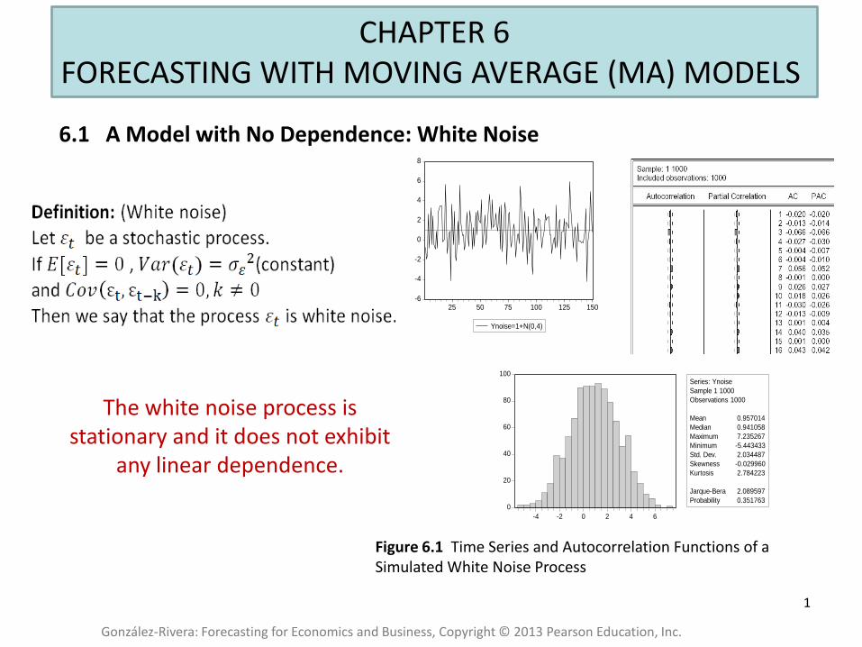
1

CHAPTER 6 FORECASTING WITH MOVING AVERAGE (MA) MODELS

González-Rivera: Forecasting for Economics and Business, Copyright © 2013 Pearson Education, Inc.

Figure 6.1 Time Series and Autocorrelation Functions of a Simulated White Noise Process

6.1 A Model with No Dependence: White Noise

-6

-4

-2

0

2

4

6

8

25 50 75 100 125 150

Ynoise=1+N(0,4)

0

20

40

60

80

100

-4 -2 0 2 4 6

Series: Ynoise

Sample 1 1000

Observations 1000

Mean 0.957014

Median 0.941058

Maximum 7.235267

Minimum -5.443433

Std. Dev. 2.034487

Skewness -0.029960

Kurtosis 2.784223

Jarque-Bera 2.089597

Probability 0.351763

The white noise process is stationary and it does not exhibit

any linear dependence.

2

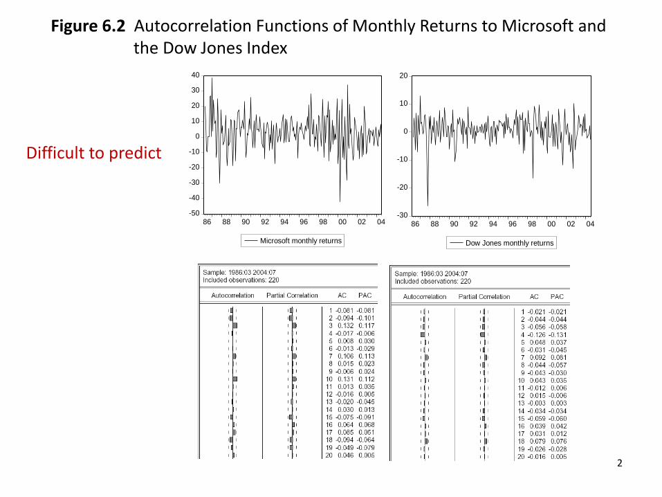
Figure 6.2 Autocorrelation Functions of Monthly Returns to Microsoft and the Dow Jones Index

-50

-40

-30

-20

-10

0

10

20

30

40

86 88 90 92 94 96 98 00 02 04

Microsoft monthly returns

-30

-20

-10

0

10

20

86 88 90 92 94 96 98 00 02 04

Dow Jones monthly returns

Difficult to predict

3

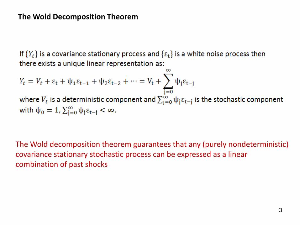
The Wold Decomposition Theorem

The Wold decomposition theorem guarantees that any (purely nondeterministic) covariance stationary stochastic process can be expressed as a linear combination of past shocks

4

Finite Representation of the Wold Decomposition Theorem

The infinite polynomial can be appproximated by the ratio of two finite polynominals :

and the Wold decomposition can be approximated (or written) as:

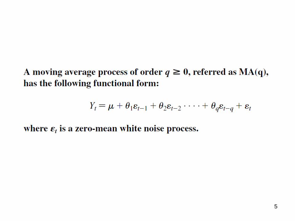
5

6

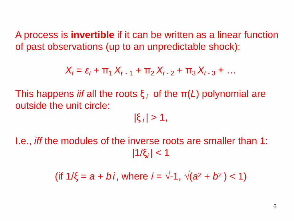
A process is invertible if it can be written as a linear function

of past observations (up to an unpredictable shock):

Xt = εt + π1 Xt - 1 + π2 Xt - 2 + π3 Xt - 3 + …

This happens iif all the roots ξ i of the π(L) polynomial are

outside the unit circle:

|ξ i | > 1,

I.e., iff the modules of the inverse roots are smaller than 1:

|1/ξi | < 1

(if 1/ξ = a + b i , where i = √-1, √(a2 + b2 ) < 1)

7

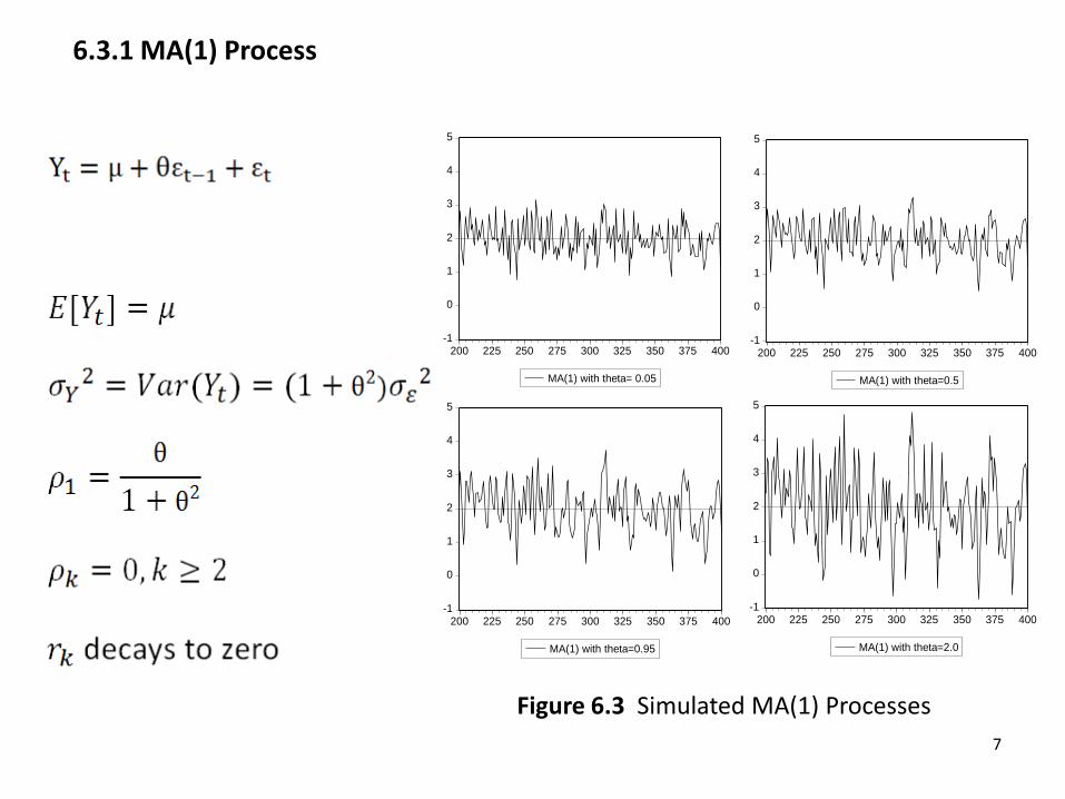
Figure 6.3 Simulated MA(1) Processes

6.3.1 MA(1) Process

-1

0

1

2

3

4

5

200 225 250 275 300 325 350 375 400

MA(1) with theta=0.5

-1

0

1

2

3

4

5

200 225 250 275 300 325 350 375 400

MA(1) with theta= 0.05

-1

0

1

2

3

4

5

200 225 250 275 300 325 350 375 400

MA(1) with theta=2.0

-1

0

1

2

3

4

5

200 225 250 275 300 325 350 375 400

MA(1) with theta=0.95

8

Figure 6.4 Autocorrelation Functions of Simulated MA(1) Processes

12

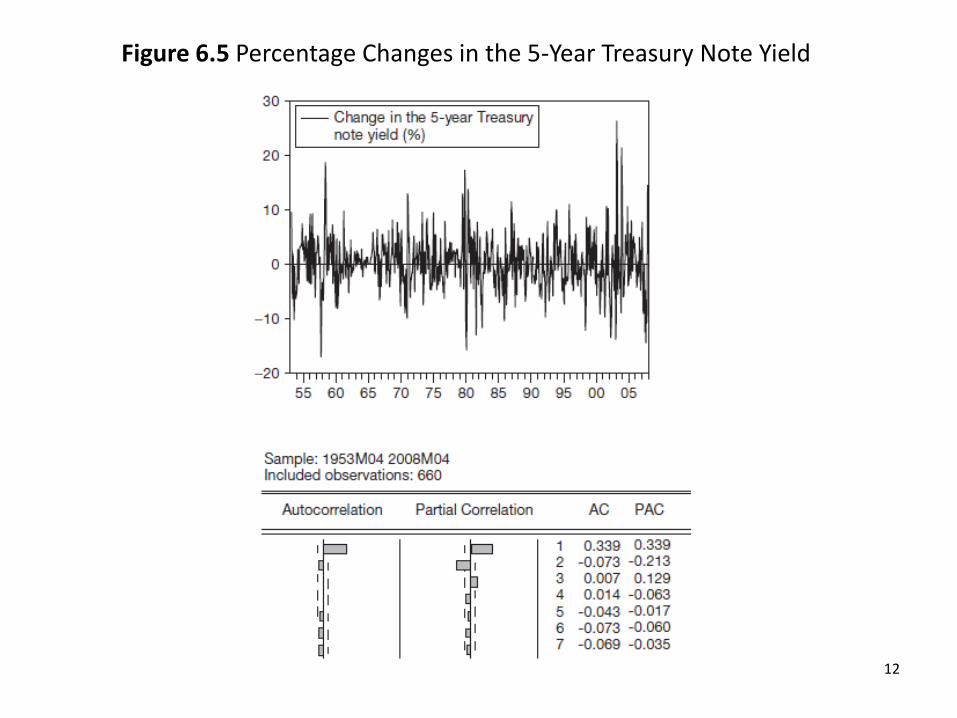
Figure 6.5 Percentage Changes in the 5-Year Treasury Note Yield

-20

-10

0

10

20

30

55 60 65 70 75 80 85 90 95 00 05

Change in the 5-year Treasury-Note Yield (%)

13

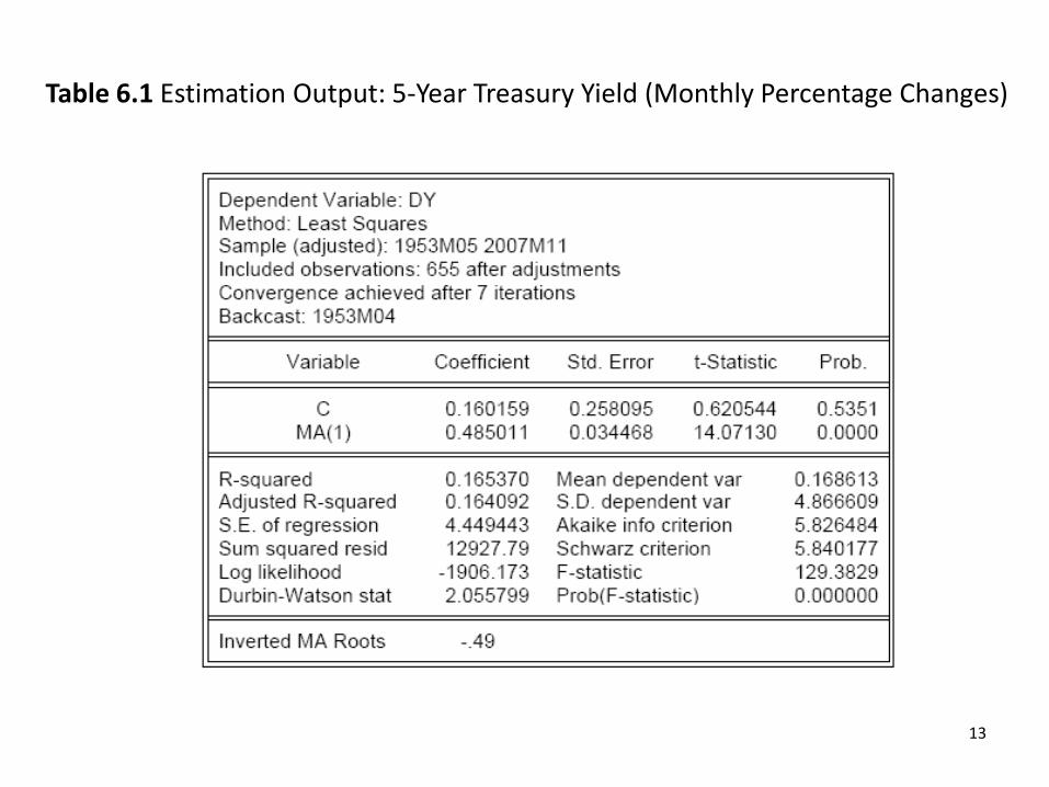
Table 6.1 Estimation Output: 5-Year Treasury Yield (Monthly Percentage Changes)

14

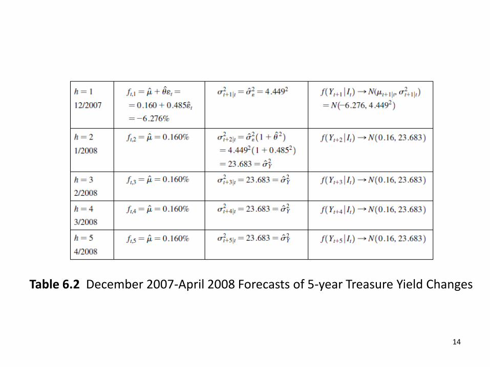
Table 6.2 December 2007-April 2008 Forecasts of 5-year Treasure Yield Changes

15

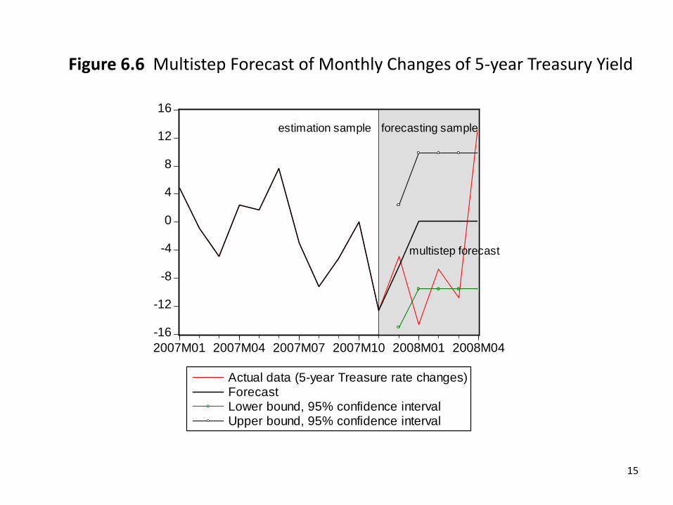
Figure 6.6 Multistep Forecast of Monthly Changes of 5-year Treasury Yield

-16

-12

-8

-4

0

4

8

12

16

2007M01 2007M04 2007M07 2007M10 2008M01 2008M04

Actual data (5-year Treasure rate changes)ForecastLower bound, 95% confidence intervalUpper bound, 95% confidence interval

estimation sample forecasting sample

multistep forecast

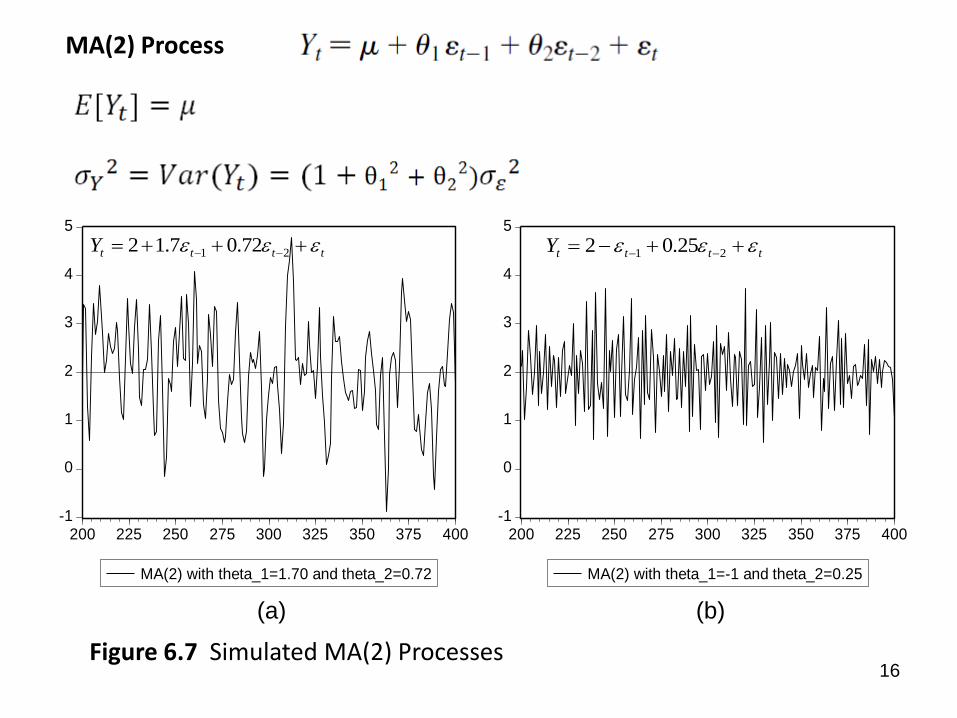
16 Figure 6.7 Simulated MA(2) Processes

MA(2) Process

-1

0

1

2

3

4

5

200 225 250 275 300 325 350 375 400

MA(2) with theta_1=1.70 and theta_2=0.72

-1

0

1

2

3

4

5

200 225 250 275 300 325 350 375 400

MA(2) with theta_1=-1 and theta_2=0.25

ttttY 21 25.02ttttY 21 72.07.12

(a) (b)

17

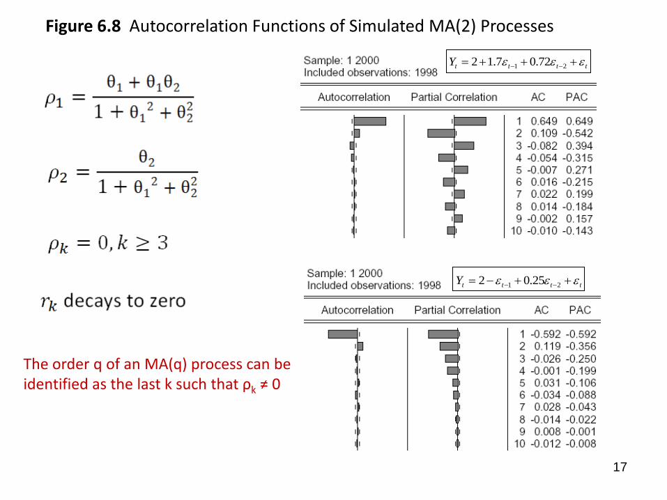
Figure 6.8 Autocorrelation Functions of Simulated MA(2) Processes

ttttY 21 25.02

ttttY 21 72.07.12

The order q of an MA(q) process can be identified as the last k such that ρk ≠ 0

18

Figure 6.9 Autocorrelation Functions of MA Process ttttY 21 442

The MA(2) process is invertible if the roots of the characteristic equation are, in absolute value, greater than one.