DELINEATING THE AVERAGE RATE OF CHANGE AND

CONSEQUENCES OF FITTING AN INCORRECT GROWTH MODEL

A Thesis

Submitted to the Graduate School

of the University of Notre Dame

in Partial Fulfillment of the Requirements

for the Degree of

Master of Arts

by

Kenneth Kelley III, B.A.

Scott E. Maxwell, Director

Graduate Program in Psychology

Notre Dame, Indiana

April 2003

DELINEATING THE AVERAGE RATE OF CHANGE AND

CONSEQUENCES OF FITTING AN INCORRECT GROWTH MODEL

Abstract

by

Kenneth Kelley III

The average rate of change is a key concept in longitudinal analyses that examine

change over time. However, this concept has been misunderstood both implicitly

and explicitly in the literature. The present work attempts to clarify the concept

and show unequivocally the mathematical definition and meaning of the average rate

of change. Oftentimes the slope from the straight-line growth model is interpreted

as though it were the average rate of change. It is shown, however, that this is

generally not the case and holds true in only a limited number of situations. General

equations are presented for the bias and discrepancy factor when the slope from the

straight-line growth model is used to estimate the average rate of change. The

importance of fitting an appropriate individual growth model is discussed, as are

the benefits provided by nonlinear models for longitudinal data.

CONTENTS

FIGURES. . . . . . . . . . . . . . . . . . . . . . . . . . . . . . . . . . . . . . . . . . iv

TABLES. . . . . . . . . . . . . . . . . . . . . . . . . . . . . . . . . . . . . . . . . . . v

ACKNOWLEDGMENTS. . . . . . . . . . . . . . . . . . . . . . . . . . . . . . . . . vi

INTRODUCTION. . . . . . . . . . . . . . . . . . . . . . . . . . . . . . . . . . . . . 1

DERIVATION OF THE AVERAGE RATE OF CHANGE . . . . . . . . . . . . 8The Mathematical Definition of the Average Rate of Change. . . . . . . . . 11

STATISTICAL MODELS OF INDIVIDUAL GROWTH. . . . . . . . . . . . . . 15Polynomial Models for the Analysis of Change. . . . . . . . . . . . . . . . . . 16Nonlinear Growth Models for the Analysis of Change. . . . . . . . . . . . . . 17

The Asymptotic Regression Growth Curve. . . . . . . . . . . . . . . . . . . 18The Gompertz Growth Curve. . . . . . . . . . . . . . . . . . . . . . . . . . . 21The Logistic Growth Curve. . . . . . . . . . . . . . . . . . . . . . . . . . . . 23

Nonlinear Models in the Behavioral Sciences. . . . . . . . . . . . . . . . . . . 25

RELATIONSHIP BETWEEN STRAIGHT LINE GROWTHMODELS AND THE AVERAGE RATE OF CHANGE. . . . . . . . . . . . . . 30

The Regression Coe!cient from the Straight-LineGrowth Model and the Average Rate of Change. . . . . . . . . . . . . . . . . 34Fitting a Quadratic Growth Model ToEstimate the Average Rate of Change. . . . . . . . . . . . . . . . . . . . . . . 38

THE DISCREPANCY BETWEEN THE REGRESSIONCOEFFICIENT FROM THE STRAIGHT-LINE GROWTHMODEL AND THE AVERAGE RATE OF CHANGE. . . . . . . . . . . . . . . 40

Examining the Bias in the Average Rate of Change:The Limiting Case when Time Is Continuous. . . . . . . . . . . . . . . . . . . 42

When Y Can Be Written As a Linear Function of Time. . . . . . . . . . 44When Y Conforms to Certain Nonlinear Functions of Time. . . . . . . . 47

ii

1

Examining the Bias in the Average Rate of Change:The Case when Time Is Discrete. . . . . . . . . . . . . . . . . . . . . . . . . . 54

EMPIRICAL INVESTIGATION OF THEDISTRIBUTION OF INSTANTANEOUS RATES OF CHANGE. . . . . . . . 65

PRELIMINARY SUGGESTIONS AND CAUTIONSWHEN ESTIMATING THE AVERAGE RATE OF CHANGE. . . . . . . . . . 70

The Relationship Between the Di!erenceScore and the Average Rate of Change. . . . . . . . . . . . . . . . . . . . . . . 70Other Suggestions for Estimating the Average Rate of Change. . . . . . . . 76

DISCUSSION. . . . . . . . . . . . . . . . . . . . . . . . . . . . . . . . . . . . . . . . 84

APPENDIX A. . . . . . . . . . . . . . . . . . . . . . . . . . . . . . . . . . . . . . . 90

APPENDIX B. . . . . . . . . . . . . . . . . . . . . . . . . . . . . . . . . . . . . . . 92Maple Syntax. . . . . . . . . . . . . . . . . . . . . . . . . . . . . . . . . . . . . . 92

APPENDIX C. . . . . . . . . . . . . . . . . . . . . . . . . . . . . . . . . . . . . . . 95Derivations for the Asymptotic Regression Growth Model:Making Use of the Maple Syntax From Appendix B. . . . . . . . . . . . . . . 95Derivations for the Gompertz Growth Model:Making Use of the Maple Syntax From Appendix B. . . . . . . . . . . . . . . 96Derivations for the Logistic Growth Model:Making Use of the Maple Syntax From Appendix B. . . . . . . . . . . . . . . 97

APPENDIX D. . . . . . . . . . . . . . . . . . . . . . . . . . . . . . . . . . . . . . . 99

REFERENCES. . . . . . . . . . . . . . . . . . . . . . . . . . . . . . . . . . . . . . 101

iii

2

FIGURES

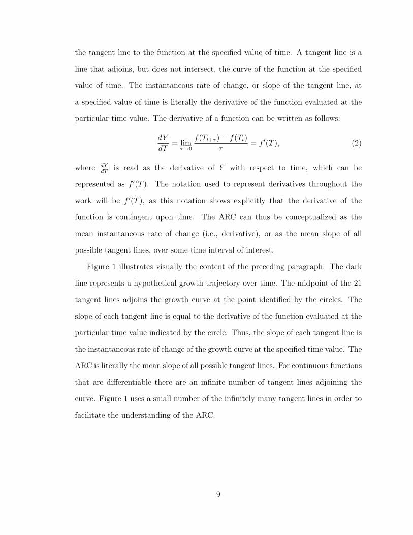
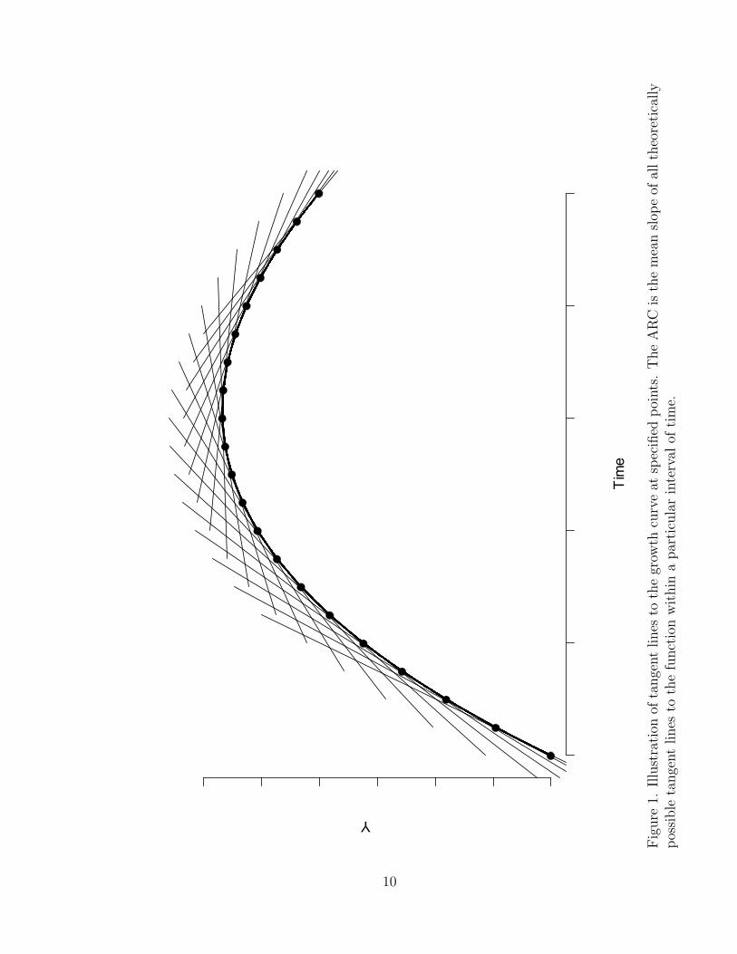
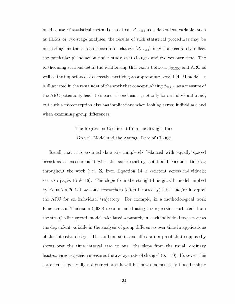
1 Illustration of tangent lines to the growth curve at specified points.The ARC is the mean slope of all theoretically possible tangent linesto the function within a particular interval of time. . . . . . . . . . . 10

2 Illustration of a typical asymptotic regression model where themeaningfulness and direct interpretation of the parameters is illustrated 20

3 Illustration of a typical Gompertz growth model where themeaningfulness and interpretation of the parameters is illustrated . . 22

4 Illustration of a typical logistic growth model where themeaningfulness and interpretation of the parameters is illustrated . . 24

5 Illustration of the straight-line growth model fit to a variety ofasymptotic growth curves along with B and !, given the parametersthat are specified. . . . . . . . . . . . . . . . . . . . . . . . . . . . . . 51

6 Illustration of the straight-line growth model fit to a variety ofGompertz growth curves along with B and !, given the parametersthat are specified. . . . . . . . . . . . . . . . . . . . . . . . . . . . . . 52

7 Illustration of the straight-line growth model fit to a variety of logisticgrowth curves along with B and ! given, given the parameters thatare specified. . . . . . . . . . . . . . . . . . . . . . . . . . . . . . . . . 53

8 Ratio of the precision of !ARC to "!SLGM for two to 25 equally spacedoccasions of measurement when the assumption of straight-linegrowth is correct . . . . . . . . . . . . . . . . . . . . . . . . . . . . . 81

iv

TABLES

1 GENERAL EQUATIONS FOR B AND ! FOR TWO TO 12EQUALLY SPACED TIMEPOINTS WITH ARBITRARY INITIALAND END POINTS . . . . . . . . . . . . . . . . . . . . . . . . . . . 56

2 B AND ! VALUES FOR FOUR TO 12 TIMEPOINTS FORSELECTED LINEAR AND NONLINEAR MODELS . . . . . . . . . 60

3 B AND ! VALUES FOR FOUR TO 12 TIMEPOINTS WHENGROWTH FOLLOWS AN ASYMPTOTIC REGRESSIONGROWTH CURVE WITH " = 5, AND COMBINATIONSOF ! (3, 4, & 5) AND # (4, 6, 8, 10, & 12) VALUES, T ! [0, 1] . . 62

4 B AND ! VALUES FOR FOUR TO 12 TIMEPOINTS WHENGROWTH FOLLOWS A GOMPERTZ GROWTH CURVE WITH" = 5, AND COMBINATIONS OF ! (3, 4, & 5) AND # (4, 6, 8,10, & 12) VALUES, T ! [0, 1] . . . . . . . . . . . . . . . . . . . . . . 63

5 B AND ! VALUES FOR FOUR TO 12 TIMEPOINTS WHENGROWTH FOLLOWS A LOGISTIC GROWTH CURVE WITH" = 5, AND COMBINATIONS OF ! (3, 4, & 5) AND # (4, 6,8, 10, & 12) VALUES, T ! [0, 1] . . . . . . . . . . . . . . . . . . . . 64

6 DESCRIPTIVE VALUES OF THE DISTRIBUTION OFINSTANTANEOUS RATES OF CHANGE FOR THE SELECTEDFUNCTIONAL FORMS OF GROWTH . . . . . . . . . . . . . . . . 67

v

ACKNOWLEDGMENTS

I would like to thank Dr. Scott E. Maxwell for his academic guidance over the last

three years and for his invaluable help necessary for the completion of this thesis. I

would also like to acknowledge Dr. Richard S. Melton and Dr. Donald A. Schumsky,

who introduced me to statistical methods, experimental design, and methodology in

general, while I was an undergraduate at the University of Cincinnati. In addition

to these fine mentors, I would also like to thank Dr. Steven M. Boker, Dr. David

A. Smith, and Joseph R. Rausch, each of whom provided valuable insight and

challenged me with poignant questions, leading to a more general and stronger

thesis.

vi

INTRODUCTION

The goal of data analytic techniques and procedures applied within the context

of longitudinal data analysis should be to help researchers systematically and

quantitatively document what is changing (The attribute(s) should be operationally

defined.), who is changing (What type of individual changes?), how they change

(What sort of trend describes transition over time?), when they change (Does

change occur only after a specified time or after a certain event?), with the ultimate

goal of understanding why the attribute of interest is in a state of transition. The

what, who, how, when, and why of longitudinal research is important for developing

predictions and explanations of the changing phenomena in order for the research

community to make sense of, and potentially using, the findings and conclusions

educed from longitudinal investigations.

The study of change has long been a central topic in the sciences. A philosophical

account of the process of change was given more than 100 years ago by Davies (1900).

Davies realized even then that “change is by no means a simple a"air” (1900, p.

506). Davies identified the mind as being “in no sense Eleatic,” but rather that

such “perpetual change” is what “di"erentiates and constitutes the unique problem

of psychology” when compared to other disciplines (p. 508). Rather than being a

“problem” with psychology per se, it seems that such “perpetual change” is what

leads to such a dynamic field of study. In fact, studying such non-static relationships

in the behavioral sciences dates back at least to the early part of the twentieth

century, where Billings and Shepard (1910) attempted to measure change in heart

1

rate as a function of attention level. Of course the study of change is much older

in the physical and mathematical sciences, where Newton (1643-1727) and Leibniz

(1646-1716) laid the foundation for modern calculus, the branch of mathematics

concerned with the study of change, in the late seventeenth century.

In the behavioral sciences the analysis of change is generally studied over time

by way of longitudinal research designs. The general requirement for longitudinal

research is that one or more variables are repeatedly measured over time on the

same unit of analysis. It is through longitudinal research that inferences regarding

intraindividual change, inter individual change, and group change can be examined.

A formal set of rationales for longitudinal research has been given by Baltes and

Nesselroade (1979, pp. 23 – 27):

1. direct identification of intraindividual change;

2. direct identification of interindividual di"erences (similarity)in intraindividual change;

3. analysis of interrelationships in behavioral change;

4. analysis of causes (determinants) of intraindividual change;

5. analysis of causes (determinants) of interindividual di"erencesin intraindividual change.

While understanding various descriptions of change (Rationale 1 & 2) is

important before attempting to understand correlates (Rationale 3) and causes

(Rationale 4 & 5) of change, measuring change has proved to be no less than

a daunting task. The methodological literature in the behavioral sciences has

long attempted to address problems associated with the conceptualization and

measurement of change. Since the design, analysis, and the interpretation of

longitudinal research is the driving force behind many areas of inquiry, it is

important when utilizing current methods or developing novel ones that they lead

2

to accurate and meaningful descriptions of the transition over time exhibited by the

phenomena of interest.

From the 1950s until the 1980s, di"erent conceptualizations of change, its

measurement, and the design of studies examining change led to serious questions in

the methodological literature of the behavioral sciences about the appropriateness

of the analysis of change. An extreme view on the measurement of change by

Cronbach and Furby (1970) questioned if the measurement and analysis of change

should even be attempted. Their assessment of the “problems” of measuring and

analyzing change, particularly with di"erence scores, along with similar “problems”

documented by others (e.g., the works contained in Harris, 1963; Lord, 1956 & 1958;

Linn & Slinde, 1977), left those who worked within the longitudinal framework in

a disconcerted position regarding the measurement and analysis of change. The

publication of these works suggested that researchers who were interested in the

examination of change “frame their questions in other ways” (Cronbach & Furby,

1970, p. 80). Because a major goal in the behavioral sciences is to understand

transition over time, framing such questions in “other ways” detours and potentially

wreaks havoc on the scientific goals and inferences of the investigator.1

However, hope was not lost for the analysis of change. In recent times it has

been realized that there were both implicit and explicit problems in the vintage

arguments against the analysis of change. The major problem with the works

that criticized the analysis of change is that the focus of such critiques examined

cases where emphasis was placed on distinguishing interindividual di"erences in

change between measurement occasions rather than distinguishing intraindividual

di"erences in change among individuals over time. This misconception in the

1Sometimes interest is not in transition over time, but rather in the lack of transition. This lackof transition is known as stability. Stability is thus a special case of change, specifically implyingthe lack of change (i.e., constancy).

3

measurement of change is detrimental to the conceptualization and analysis of

change (Bryk & Raudenbush, 1992, pp. 130-131). In general, methods and strategies

for distinguishing interindividual di"erences at a particular time are ill equipped for

the analysis of intraindividual change over time (Collins, 1996).

More recently, however, the analysis of change has been reconceptualized

where “individual time paths are the proper focus for the analysis of change”

(Rogosa, Brandt, & Zimowski, 1982, p. 744; see also the methodological works

of Raudenbush, 2001; Mehta & West, 2000; Rogosa & Willett, 1985; Collins, 1996;

Bryk & Raudenbush, 1987; Willett, 1988; with applications of these strategies in

Francis, Fletcher, Stuebing, Davidson, & Thompson, 1991; Francis, Schatschneider,

& Carlson, 2000; Karney & Bradbury, 1995). By focusing on individuals over time,

rather than at a specific time, researchers can develop and test precise hypotheses

regarding change using reliable and sophisticated models. From these models a

better understanding of the phenomenon of interest as it exists, changes, and evolves

over time can be realized. Generally speaking, most behavioral phenomena seem

to change in a continuous fashion over time rather than at discrete steps or stages.

The process of this continuous change is important and can be quite informative

in understanding the underlying system(s) responsible for transition. An extension

of examining how individuals change is to examine whether there are di"erences in

rates of change for the overall trends among individuals or groups. However, the first

step in understanding interindividual di"erences in change is, by logical necessity,

the precise and valid measurement of intraindividual change (Collins, 1996, p. 38),

and the foundation of intraindividual change is a statistical model for individual

time paths (Rogosa et al., 1982, p. 726).

In large part the analysis of change has been facilitated over the last 20 years by

the realization that longitudinal data are hierarchical in nature, where observations

4

over time are nested within the entity under study (e.g., the individual), which in

turn may be nested within an organizational structure (e.g., a group) at a higher

level (Shadish, 2002). Given this realization, new methods for the analysis of change

have been developed that explicitly model the hierarchical structure of longitudinal

data in a class of statistical models known as hierarchical linear models (HLM) and

hierarchical nonlinear models (HNLM; Laird & Ware, 1982; Bryk & Raudenbush,

1987; Bryk & Raudenbush, 1992; Davidian & Giltinan, 1995; Goldstein, 1995;

chapters 6 & 8 of Vonesh & Chinchilli, 1997).2 Given the new conceptualization,

measurement, and design of studies involving issues of change, some of the long

held beliefs about “problems” measuring change have been dispelled, as many of

the previous criticisms of the analysis of change were misguided and based on

inappropriate assumptions (See Rogosa et al., 1982, Rogosa, 1995, and Willett,

1988, for their critiques of works that criticized and questioned the measurement

and analysis of change.).

The concept of intraindividual change should be the starting point for

longitudinal research. It is by first focusing on the individual that broad

generalizations over individuals can (or cannot) be made. The description of

intraindividual change can be given in numerous ways, and is limited only by the

research design and the researcher’s creativity in forming and testing models. For

example, by focusing on one individual trajectory, the unknown functional form

of growth can be described as any combination of linear, quadratic, exponential,

or even as a dampened or undampened sinusoidal function. The adequacy of the

particular model chosen, however, depends in large part on the true functional form

of growth and the number of timepoints that measurements are obtained. Given

2Because of the simultaneous interdisciplinary development of HLMs and HNLMs, such modelsare also termed multilevel, mixed-e!ects, random-e!ects, covariance components, and randomcoe"cient models.

5

that such a vast array of possibilities exists for describing intraindividual change, a

measure of change that can describe all possible functional forms of growth by way

of a single descriptive statistic would have great practical value for the numerical

description that it could provide. A measure known as the average rate of change

is such a value.

The major purpose of the present work is to delineate the meaning and

interpretation of the average rate of change (ARC), as well as what the ARC is not, in

order for this measure of overall change to be better used by researchers attempting

to understand the what, who, how, when and why of longitudinal research as well

as the rationales laid out by Baltes and Nesselroade (1979, pp. 23–27), such that

the potentially complicated and problematic process(es) of intraindividual change

can be better understood. The delineation of the ARC begins at an intuitive level

and progresses to a mathematical description. Most of the emphasis throughout

the present work is concerned foremost with a single trajectory, as the individual

trajectory is the appropriate starting point for understanding change.

Implicitly or explicitly the ARC is often a central focus for many longitudinal

research projects. Attempts are often made to succinctly describe the average or

typical amount of change that occurs within some time interval of interest. Rather

than describing change in several dimensions simultaneously (e.g., linear, quadratic,

and cubic), researchers often wish to describe change parsimoniously. The regression

coe#cient from the straight-line growth model has often been the medium in which a

succinct description of change over time has been attempted. Apparently a widely

held belief is that the regression coe#cient from the straight-line growth model

provides a measure of the typical, or average, amount of change occurring within

an interval of time for an individual trend. The idea of using a single value as a

descriptor of a potentially complicated process of change has great intuitive appeal.

6

However, as the remainder of the work shows, the regression coe#cient from the

straight-line growth model is generally not equal to the mean rate of change over

time for a given trajectory. A major purpose of this work is to illustrate that making

use of the regression coe#cient from the straight-line growth model as if it was the

ARC can yield biased estimates, potentially leading to incorrect conclusions about

the underlying process of change. This work contends that the ARC should be used

more often in applied research, not to supplant other analyses, but to supplement

the information gained from modeling and examining growth over time.

Because the ARC provides the average or typical rate of change, not only a

single dimension of change (such as the linear, quadratic, or exponential growth

component does), it is a parsimonious measure that describes the overall trend of a

growth trajectory, regardless of the functional form of growth. The ARC is itself a

mean and thus the well-known and generally desirable properties of the mean are

also properties of the ARC. Although the concept of the ARC is appealing and seems

to be straightforward, the technical underpinnings have not received much formal

attention. The attention that the ARC has received, however, is often misguided

and surrounded by confusion and misinterpretation. It is believed that the ARC will

help researchers and the research community in general in the quest of understanding

the dynamic and static relationships among a set of variables as they exist over time.

7

DERIVATION OF THE AVERAGE RATE OF CHANGE

The present section details the precise mathematical definition of the ARC by a

set of mathematical derivations. The derivations presented define the ARC without

ambiguity and illustrate in a longitudinal data analytic context a well-known fact of

the mathematical sciences. It will be shown that regardless of whether the functional

form of growth is known or unknown, and regardless of whether time is measured

continuously or at discrete occasions, the same definition of the ARC holds. To ease

the transition between the mathematical statements given in this section and their

application to growth models in future sections, the symbolic representations within

this section will make use of the corresponding analysis of change notation.

The rate of change of a nonvertical line that passes through two sets of points,

(Tt, Yt) and (Tt+! , Yt+! ), is the slope of the line, where T represents time, t the

measurement occasion (t = 1, . . . , F ), $ is some arbitrary, yet constant once defined,

length of time between measurement occasions, and Yt is the dependent variable at

the tth measurement occasion. The slope of the line connecting two points is the

change in Y divided by the change in time, and can be represented by the following

expression:

Slope =f(Tt+! )" f(Tt)

Tt+! " Tt=

Yt+! " Yt

Tt+! " Tt=

$Y

$T, (1)

where f(T ) is the dependent variable Y , which is some function of time, and $x is

the change in the variable x (where x represents some random variable).

Equation 1 is closely related to the derivative. In the limit as $ approaches zero,

Equation 1 yields the instantaneous rate of change when evaluated at a specific time

value. The instantaneous rate of change can also be conceptualized as the slope of

8

the tangent line to the function at the specified value of time. A tangent line is a

line that adjoins, but does not intersect, the curve of the function at the specified

value of time. The instantaneous rate of change, or slope of the tangent line, at

a specified value of time is literally the derivative of the function evaluated at the

particular time value. The derivative of a function can be written as follows:

dY

dT= lim

!!0

f(Tt+! )" f(Tt)

$= f "(T ), (2)

where dYdT is read as the derivative of Y with respect to time, which can be

represented as f "(T ). The notation used to represent derivatives throughout the

work will be f "(T ), as this notation shows explicitly that the derivative of the

function is contingent upon time. The ARC can thus be conceptualized as the

mean instantaneous rate of change (i.e., derivative), or as the mean slope of all

possible tangent lines, over some time interval of interest.

Figure 1 illustrates visually the content of the preceding paragraph. The dark

line represents a hypothetical growth trajectory over time. The midpoint of the 21

tangent lines adjoins the growth curve at the point identified by the circles. The

slope of each tangent line is equal to the derivative of the function evaluated at the

particular time value indicated by the circle. Thus, the slope of each tangent line is

the instantaneous rate of change of the growth curve at the specified time value. The

ARC is literally the mean slope of all possible tangent lines. For continuous functions

that are di"erentiable there are an infinite number of tangent lines adjoining the

curve. Figure 1 uses a small number of the infinitely many tangent lines in order to

facilitate the understanding of the ARC.

9

Time

Y

Fig

ure

1.Illu

stra

tion

ofta

nge

ntlines

toth

egr

owth

curv

eat

spec

ified

poi

nts.

The

AR

Cis

the

mea

nsl

ope

ofal

lth

eore

tica

lly

pos

sible

tange

ntlines

toth

efu

nct

ion

wit

hin

apar

ticu

lar

inte

rval

ofti

me.

10

Since the derivative evaluated at a specific timepoint is the instantaneous rate

of change at that timepoint, and interest lies in finding the mean of the set of

derivatives, accomplishing such a task seems to require evaluating Equation 2 at

each of the values of time and then dividing the sum of each of the derivatives by F .

However, there are at least two seemingly unavoidable problems with attempting

to calculate the ARC in such a manner. The first problem is that derivatives are

defined only for continuous functions that are di"erentiable, that is, where $ # 0

and F # $ (F approaches infinity). The second problem is that in practice the

functional form of growth is generally unknown. Because the derivative itself is based

on the functional form, the derivative is also unknown. Although these complications

seem unavoidable, the following section illustrates that they are overcome with what

turns out to be a simple algebraic solution.

The Mathematical Definition of the Average Rate of Change

Because the true functional form of growth is generally assumed to exist continuously

over time, deriving the mean of an infinite number of derivatives requires integral

calculus. The integral of a continuous function is a limit of summations. After

finding the infinite sum of derivatives for some function, obtained by integrating

the derivative of the functional form of growth, the infinite sum must be divided by

the width of the time interval in order to obtain the mean of the derivatives. The

rationale for such a procedure is due to the Mean Value Theorem for Integrals (See

section 4.5 of Finney, Weir, & Giordano, 2001 or section 6.5 of Stewart, 1998, for a

thorough treatment of the Mean Value Theorem for Integrals.).

The Mean Value Theorem for Integrals states that over a closed interval

a continuous function assumes its average (i.e., the mean) value at least once

within the interval. The particular mean value for a continuous function that is

11

di"erentiable over the interval Tt to Tt+! is given by an application of the Mean

Value Theorem for Integrals:

fc =1

Tt+! " Tt

Tt+!#

Tt

f(T )dT, (3)

where x represents the mean of x, in this case a continuous function that is

di"erentiable, andTt+!$

Tt

f(T )dT is read as the integral of f(T ) with respect to time

from Tt to Tt+! (Finney et al., 2001, p. 352; Stewart, 1998, p. 470). Thus, after

the function has been integrated, the value of the integral is divided by the length

of the time interval in order to obtain the mean value of the function.3 Since

Equation 3 yields the mean of a continuous di"erentiable function, and Equation 2

is a special case of a continuous function, combining the two equations will yield

the mean instantaneous rate of change (i.e., mean mean derivative or mean slope of

all possible tangent lines) of the function from Tt to Tt+! . Thus, when Equations 2

and 3 are combined, the resultant value is the ARC.

However, to integrate a function is to find its antiderivative. Finding the

derivative of a function (as in Equation 2) and then integrating the function (to

find its antiderivative) yields the original function itself and is a corollary of the

fundamental theorem of calculus (Kline, 1977, p. 258). An example of an integral

of a derivative is given as,

#f "(T )dT = f(T ) + C, (4)

3In the present situation the Mean Value Theorem for Integrals guarantees that for integrablefunctions there is at least one value of time where the instantaneous rate of change equals the meanof the instantaneous rates of change within the time interval of interest. Furthermore, Equation 3follows the same formulation as the expected value of a uniform probability distribution. In fact,a uniform probability distribution can be thought of as a special case of a continuous function,where all values on the abscissa have the same corresponding value of the ordinate (i.e., occur withthe same probability).

12

where C is the constant of integration and the resultant value is the function itself.4

Therefore, when Equations 2 and 3 are combined, the mean of the derivatives,

which is literally the ARC, can be written as the following:

f "(T ) =1

Tt+! " Tt

Tt+!#

Tt

f "(T )dT (5a)

=f(Tt+! )" f(Tt)

Tt+! " Tt(5b)

=$Y

$T. (5c)

As can be seen in Equation 5c, the ARC is simply the change in Y divided by

the change in time. The resultant formulation of Equation 5c is a well-known

mathematical fact of analytic calculus (e.g., Stewart, 1998, pp. 146-147 and p. 208;

Finney et al., 2001, pp. 86-88), where it is known that regardless of the function,

the mean of all of the derivatives evaluated over a specified interval must equal !Y!T .

While the definition of the ARC may at first seem simplistic, it is important to

understand why this is the mathematical definition. The Total Change Theorem

states that “the integral of a rate of change is the total change” (Stewart, 1998, p.

377). Thus, when the integral of the derivative is evaluated in Equation 5a, it leads

to the numerator of Equation 5c, which is (Yt+! " Yt), the total change. This total

change is then divided by the length of the time interval, as specified by Equation 3,

in order to obtain the mean. Thus, the mean of the infinitely many instantaneous

rates of change (i.e., the ARC) is the change in the dependent variable divided by the

change in time. Notice that the true functional form of growth was never specified.

Equation 5c holds regardless of whether the functional form is known or unknown,

as only the initial and final pairs of points are required. Although the ARC was

4Finding the integral (antiderivative) of a function actually defines a family of functions thatdi!er by at most a constant value (Finney et al., 2001, p. 314). Further, Equation 4 is technicallyan indefinite integral because it yields another equation, not a numeric value. An integral withreal valued limits that yields a numeric value (not another equation) is a definite integral.

13

defined in the case where time was continuous, the same formulation holds true in

the more typical case where the occasions of measurement are discrete, regardless

of whether the occasions of measurement are equally spaced.

Although Equation 5c is a well-known fact of analytic calculus, in the context of

longitudinal data analysis the mathematics underlying the ARC have not been well

delineated. Because of the lack of attention to the ARC, but yet its intuitive appeal

as the mean instantaneous rate of change, the ARC has often been misunderstood in

practice. A major purpose of this work is to clarify misconceptions that persist both

implicitly and explicitly throughout the methodological and applied longitudinal

literature regarding the ARC.

14

STATISTICAL MODELS OF INDIVIDUAL GROWTH

Before further delineation of the ARC in the context of longitudinal data analysis,

a necessary digression provides an overview of statistical models useful for describing

individual growth curves. This digression provides a broad context for the ARC as

well as elucidating a variety of growth models not often discussed or considered in

applications of longitudinal data analyses within the behavioral sciences.

Statistical models that examine growth or change explicitly as a function

of time are known as growth curve models. In addition to one or more

time-varying covariates, growth curve models may or may not include fixed

covariates. Throughout the remainder of the work the only time-varying covariate

explicitly included in the growth model will be time itself (However, the discussion

is equally applicable to other time-varying covariates, such as age, grade-level, etc.).

A variety of methods can be used for modeling growth over time, with an important

common theme among them being that the individual is explicitly incorporated into

the model. In the following two sections, two classes of intraindividual growth will

be described. The first class of growth models are those commonly employed in

the behavioral sciences, where the growth models are linear in their parameters and

consist of a limited set of polynomial trends. The second class of growth models

illustrates three nonlinear models that are likely a better approximation to reality

in some situations than a limited set of polynomial trends, as these models allow

asymptotic values to be explicitly included in the model.

Throughout the work, Yit is the dependent variable for the ith individual

(i = 1, ..., N) at the tth timepoint (t = 1, ..., F ). Unless otherwise specified, it is

15

assumed that the observed data are completely balanced and that the occasions of

measurement are equally spaced with the same starting point and constant time-lag

($) within and across individuals. Such a data set implies that all N individuals have

the same starting value, no missing data, F measurement occasions, and constant $

both within and across individuals. Thus, all of the N individuals have a common

set (i.e., vector) of time values.

Polynomial Models for the Analysis of Change

Polynomial growth models are the most common and straightforward statistical

models for fitting growth curves to data. Growth models in the polynomial family

can be conceptualized as a function of a systematic growth trajectory and random

error. An example of a polynomial growth curve of degree K is given as,

Yit = %0i + %1iTit + %2iT2it + · · · + %KiT

Kit + &it, (6)

where %ki is the kth growth rate parameter (k = 0, ..., K) for individual i, and &it is

the individual’s random error, generally assumed normally distributed about zero

with a constant variance across time.

While Equation 6 illustrates the intraindividual model of growth, each of the

K polynomial growth parameters can themselves be modeled in an interindividual

(between individual) fashion. That is, each of the parameters in Equation 6, known

as the Level 1 model, are the dependent variables in the interindividual Level 2

model. For example, a growth parameter in Equation 6 can be modeled as,

%ki = !k0 + !k1Xk1i + !k2Xk2i + · · · + !kP XkP i + uki, (7)

where there is one constant, !k0 (when p = 0), with p (p = 0, ..., P ) representing

the particular X variable, !kp being the overall e"ect of Xkp on the kth growth

16

parameter, and uki is the unique e"ect for the ith individual’s kth trend, generally

assumed normally distributed about zero (Bryk & Raudenbush, 1987).

Equation 6 is a special case of a linear model. A linear model is one that is linear

in its parameters, not necessarily in the predictors (“predictors” can be thought of as

covariates or independent variables). The %s in Equation 6 and the !s in Equation 7

are the parameters (each of which is raised only to the first power in linear models)

while Tit, T 2it, · · · , TK

it and Xk1i, Xk2i, · · · , XKPi represent the predictors. Notice that

there are various powers of time included in the model. When nonzero weights

are given to powers of time other than one, the predicted growth curve will not

be a straight-line. Thus, a linear model and a linear trend (straight-line) are not

synonymous. In theory, a linear model of growth can be of any shape as long as

there are enough additive e"ects of powers of time included in the model. The next

section extends linear models in order to allow non-additive e"ect parameters to be

included in the growth model.

Nonlinear Growth Models for the Analysis of Change

Statistical models that are linear in their parameters are generally

straightforward to fit given a set of observed data. As the phenomenon under study

grows increasingly more complex, the order of the polynomial growth model can

be increased accordingly until the predicted scores reasonably correspond with the

observed scores. Nonlinear models of the same complex phenomenon can oftentimes

be more interpretable, parsimonious, and are generally more valid beyond the

observed range of data when compared to linear models (Pinheiro & Bates, 2000,

p. 273). Furthermore, it is often the case that the parameters in nonlinear models

can be easily interpreted, while once a polynomial model is beyond quadratic, the

meaning of the set of polynomial trends typically o"ers little physical or behavioral

17

interpretation. An example of such a di"erence between nonlinear and linear models

relates to asymptotes.

In polynomial growth models, limiting asymptotic values cannot generally be

modeled in order for the asymptotic value to hold beyond the range of the observed

data. Thus, researchers who make use of polynomial trends must accept the fact

that their model will likely fail beyond the range of the data actually collected.5 This

is not to say that researchers who use nonlinear models can haphazardly extrapolate

beyond their data, however, if the phenomenon truly asymptotes linear models will

generally fail to take this into consideration outside the range of observed values.

Such scenarios can potentially lead to inadequate models where impossible values

occur (e.g., probabilities larger than 1 or smaller than 0, negative reaction times,

predicted scores higher than the admissible range, unlimited growth or decay, etc.).

In order to demonstrate problems that arise when data truly follow nonlinear

trends but yet are modeled by straight-line growth models, three nonlinear growth

models will be illustrated. The selected nonlinear models are the asymptotic

regression growth curve, the Gompertz growth curve, and the logistic growth

curve. Although a wide variety of nonlinear models exist, the asymptotic regression,

Gompertz, and logistic growth curves were chosen because they seemed most useful

for behavioral science research. A brief introduction to each of these models is

given followed by some potential applications of nonlinear models in the behavioral

sciences.

The Asymptotic Regression Growth Curve

The general asymptotic regression growth curve (often referred to as exponential

growth or decay) describes a family of potential regression models where the

5However, the point at which the polynomial growth model eventually fails may be beyond therange of theoretical interest. In such situations there may be a less compelling argument in favorof nonlinear models because of the benefits they provide regarding asymptotic values.

18

dependent variable asymptotes to some limiting value as time increases. A general

asymptotic regression equation for a single trajectory is given by Stevens (1951) as:

Yt = " + !'Tt + &t, (8)

where " is the asymptotic value approached as T #$, ! is the change in Yt from

T = 0 to T # $ (i.e., ! represents total change in Y ), and ' (0 < ' < 1) is a

scaler that defines the factor by which the deviation between Yt and " is reduced

for each unit change of time, thus reflecting the rate at which Yt # ".6 Equation 8

can be equivalently rewritten, such that it is explicitly expressed as an exponential

equation:

Yt = " + ! exp("#Tt) + &t, (9)

where # = " log(') (0 < # < $) and can be thought of as a scaling parameter

(Stevens, 1951).

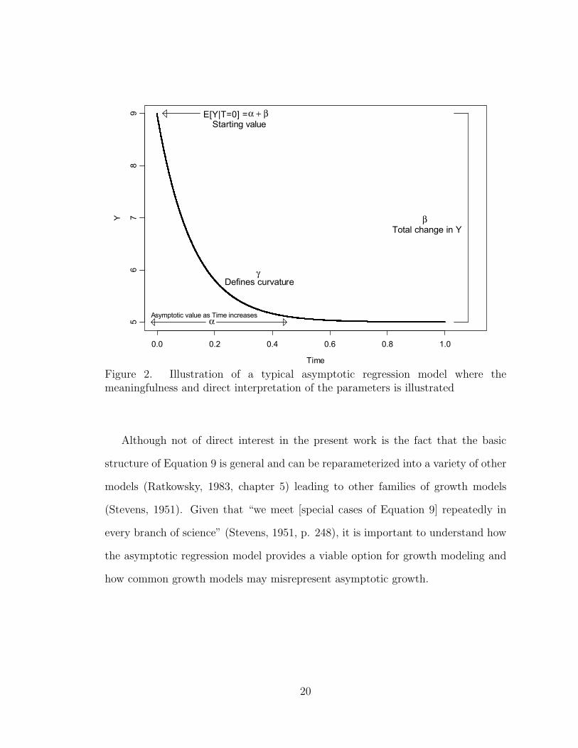
In order to facilitate the discussion of the asymptotic regression model, a

graphical depiction of a “typical” asymptotic regression curve is presented in

Figure 2. The graphical depiction is said to be typical, even though there are

an infinite number of asymptotic growth curves, because the overall shape of the

curve presented in Figure 2 shows the general characteristic of asymptotic growth.7

The dark line represents the asymptotic growth function over the time interval zero

to one (T ! [0, 1]) with parameter values " = 5, ! = 4, and # = 8.

6The deviation between Yt and ! can be expressed as "#Tt . When time changes in unit steps,# is literally the factor by which the deviation is reduced from one step of time to the next step.

7Note that the particular asymptotic regression model plotted in Figure 2 illustrates asymptoticdecay. Holding everything else constant, changing the sign of the " in Figure 2 to negative wouldillustrate asymptotic growth.

19

Time

Y

0.0 0.2 0.4 0.6 0.8 1.0

56

78

9

βTotal change in Y

αAsymptotic value as Time increases

E[Y|T=0] = α + βStarting value

γDefines curvature

Figure 2. Illustration of a typical asymptotic regression model where themeaningfulness and direct interpretation of the parameters is illustrated

Although not of direct interest in the present work is the fact that the basic

structure of Equation 9 is general and can be reparameterized into a variety of other

models (Ratkowsky, 1983, chapter 5) leading to other families of growth models

(Stevens, 1951). Given that “we meet [special cases of Equation 9] repeatedly in

every branch of science” (Stevens, 1951, p. 248), it is important to understand how

the asymptotic regression model provides a viable option for growth modeling and

how common growth models may misrepresent asymptotic growth.

20

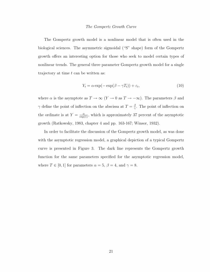
The Gompertz Growth Curve

The Gompertz growth model is a nonlinear model that is often used in the

biological sciences. The asymmetric sigmoidal (“S” shape) form of the Gompertz

growth o"ers an interesting option for those who seek to model certain types of

nonlinear trends. The general three parameter Gompertz growth model for a single

trajectory at time t can be written as:

Yt = " exp(" exp(! " #Tt)) + &t, (10)

where " is the asymptote as T #$ (Y # 0 as T # "$). The parameters ! and

# define the point of inflection on the abscissa at T = "# . The point of inflection on

the ordinate is at Y = $exp(1) , which is approximately 37 percent of the asymptotic

growth (Ratkowsky, 1983, chapter 4 and pp. 163-167; Winsor, 1932).

In order to facilitate the discussion of the Gompertz growth model, as was done

with the asymptotic regression model, a graphical depiction of a typical Gompertz

curve is presented in Figure 3. The dark line represents the Gompertz growth

function for the same parameters specified for the asymptotic regression model,

where T ! [0, 1] for parameters " = 5, ! = 4, and # = 8.

21

Time

Y

0.0 0.2 0.4 0.6 0.8 1.0

01

23

45

Point of InflectionT= β/γ , Y= α/ exp(1)

Approx. 37% of asymptotic growth

αAsymptotic value as Time increases

Figure 3. Illustration of a typical Gompertz growth model where the meaningfulnessand interpretation of the parameters is illustrated

Although not of interest for the present work, Equation 10 can be transformed

such that the transformed dependent variable can be expressed as a linear equation:

log

%" log

%Yt

"

&&= ! " #Tt + &t. (11)

The parameters ! and # can then be conceptualized as the intercept and the slope

of the transformed dependent variable respectively. Even though the Gompertz

growth model can be transformed to a simple linear model, doing so generally does

not lead to any meaningful interpretation. The reason transformations such as that

given in Equation 11 should not be used in place of an appropriate nonlinear model

is because the dependent variable (i.e., log'" log

'Yt$

(() generally does not represent

any real-word phenomenon. Thus, obtaining an estimate of the slope and intercept

22

is oftentimes of little or no interest. It is interesting to note, however, that by taking

the exponential of Equation 8, the resultant model is a form of Gompertz growth

(Stevens, 1951, p. 249).

The Logistic Growth Curve

The logistic growth model is another nonlinear sigmoidal model that shows

promise for modeling growth over time in the behavioral sciences. The general three

parameter logistic growth model for a single trajectory at time t can be written as:

Yt ="

1 + exp(! " #Tt)+ &t, (12)

where " is the asymptote as T #$ (Y # 0 as T # "$). The parameters ! and

# define the point of inflection on the abscissa at T = "# . The point of inflection on

the ordinate is at Y = $2 , 50 percent of the asymptotic growth (chapter 4 and pp.

167-169 of Ratkowsky, 1983 and Winsor, 1932).

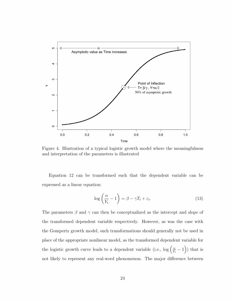
In order to facilitate the discussion of the logistic growth model, as was done with

the asymptotic regression and Gompertz growth models, a graphical depiction of a

typical logistic curve is presented in Figure 4. The dark line represents the logistic

growth function for the same parameters specified for the asymptotic regression and

Gompertz growth models, where the T ! [0, 1] for parameters " = 5, ! = 4, and

# = 8.

23

Time

Y

0.0 0.2 0.4 0.6 0.8 1.0

01

23

45

Point of InflectionT= β/γ , Y=α/2

50% of asymptotic growth

αAsymptotic value as Time increases

Figure 4. Illustration of a typical logistic growth model where the meaningfulnessand interpretation of the parameters is illustrated

Equation 12 can be transformed such that the dependent variable can be

expressed as a linear equation:

log

%"

Yt" 1

&= ! " #Tt + &t. (13)

The parameters ! and # can then be conceptualized as the intercept and slope of

the transformed dependent variable respectively. However, as was the case with

the Gompertz growth model, such transformations should generally not be used in

place of the appropriate nonlinear model, as the transformed dependent variable for

the logistic growth curve leads to a dependent variable (i.e., log)

$Yt" 1

*) that is

not likely to represent any real-word phenomenon. The major di"erence between

24

the Gompertz and the logistic growth curves is that the logistic is symmetric about

its point of inflection (50% of the asymptotic value) whereas the Gompertz is not

(approximately 37% of the asymptotic value). It is interesting to note that by taking

the inverse of Equation 8, the resultant model is a form of logistic growth (Stevens,

1951, p. 249).

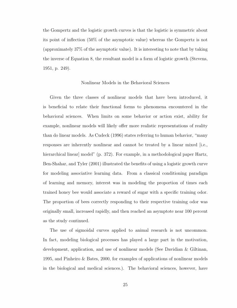
Nonlinear Models in the Behavioral Sciences

Given the three classes of nonlinear models that have been introduced, it

is beneficial to relate their functional forms to phenomena encountered in the

behavioral sciences. When limits on some behavior or action exist, ability for

example, nonlinear models will likely o"er more realistic representations of reality

than do linear models. As Cudeck (1996) states referring to human behavior, “many

responses are inherently nonlinear and cannot be treated by a linear mixed [i.e.,

hierarchical linear] model” (p. 372). For example, in a methodological paper Hartz,

Ben-Shahar, and Tyler (2001) illustrated the benefits of using a logistic growth curve

for modeling associative learning data. From a classical conditioning paradigm

of learning and memory, interest was in modeling the proportion of times each

trained honey bee would associate a reward of sugar with a specific training odor.

The proportion of bees correctly responding to their respective training odor was

originally small, increased rapidly, and then reached an asymptote near 100 percent

as the study continued.

The use of sigmoidal curves applied to animal research is not uncommon.

In fact, modeling biological processes has played a large part in the motivation,

development, application, and use of nonlinear models (See Davidian & Giltinan,

1995, and Pinheiro & Bates, 2000, for examples of applications of nonlinear models

in the biological and medical sciences.). The behavioral sciences, however, have

25

been slower to make the transition from various extensions of the general linear

model to models that are explicitly nonlinear in their parameters. With the recent

emphasis some psychologists have placed on prescribing medication, particularly in

New Mexico where a law was recently passed (New Mexico House Bill 170 took

e"ect in July of 2002) allowing qualified psychologists to prescribe medication for

certain mental illnesses, dose response curves will likely be a new area of interest and

research activity for psychologists. Because such dose response curves are generally

sigmoidal in nature, it seems likely that psychologists will soon make better use

of sigmoidal models in both practice and research, as such sigmoidal relationships

cannot generally be satisfactorily modeled by linear models.

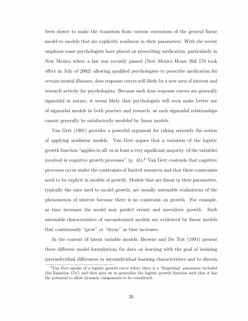
Van Gert (1991) provides a powerful argument for taking seriously the notion

of applying nonlinear models. Van Gert argues that a variation of the logistic

growth function “applies to all–or at least a very significant majority–of the variables

involved in cognitive growth processes” (p. 45).8 Van Gert contends that cognitive

processes occur under the constraints of limited resources and that these constraints

need to be explicit in models of growth. Models that are linear in their parameters,

typically the ones used to model growth, are usually untenable realizations of the

phenomenon of interest because there is no constraint on growth. For example,

as time increases the model may predict erratic and unrealistic growth. Such

untenable characteristics of unconstrained models are evidenced by linear models

that continuously “grow” or “decay” as time increases.

In the context of latent variable models, Browne and Du Toit (1991) present

three di"erent model formulations for data on learning with the goal of isolating

interindividual di"erences in intraindividual learning characteristics and to discern

8Van Gert speaks of a logistic growth curve where there is a “forgetting” parameter included(his Equation 17a!) and then goes on to generalize the logistic growth function such that it hasthe potential to allow dynamic components to be considered.

26

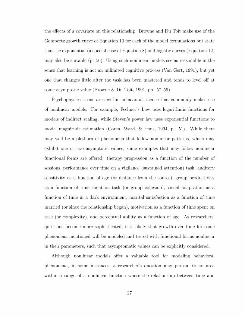
the e"ects of a covariate on this relationship. Browne and Du Toit make use of the

Gompertz growth curve of Equation 10 for each of the model formulations but state

that the exponential (a special case of Equation 8) and logistic curves (Equation 12)

may also be suitable (p. 56). Using such nonlinear models seems reasonable in the

sense that learning is not an unlimited cognitive process (Van Gert, 1991), but yet

one that changes little after the task has been mastered and tends to level o" at

some asymptotic value (Browne & Du Toit, 1991, pp. 57–59).

Psychophysics is one area within behavioral science that commonly makes use

of nonlinear models. For example, Fechner’s Law uses logarithmic functions for

models of indirect scaling, while Steven’s power law uses exponential functions to

model magnitude estimation (Coren, Ward, & Enns, 1994, p. 51). While there

may well be a plethora of phenomena that follow nonlinear patterns, which may

exhibit one or two asymptotic values, some examples that may follow nonlinear

functional forms are o"ered: therapy progression as a function of the number of

sessions, performance over time on a vigilance (sustained attention) task, auditory

sensitivity as a function of age (or distance from the source), group productivity

as a function of time spent on task (or group cohesion), visual adaptation as a

function of time in a dark environment, marital satisfaction as a function of time

married (or since the relationship began), motivation as a function of time spent on

task (or complexity), and perceptual ability as a function of age. As researchers’

questions become more sophisticated, it is likely that growth over time for some

phenomena mentioned will be modeled and tested with functional forms nonlinear

in their parameters, such that asymptomatic values can be explicitly considered.

Although nonlinear models o"er a valuable tool for modeling behavioral

phenomena, in some instances, a researcher’s question may pertain to an area

within a range of a nonlinear function where the relationship between time and

27

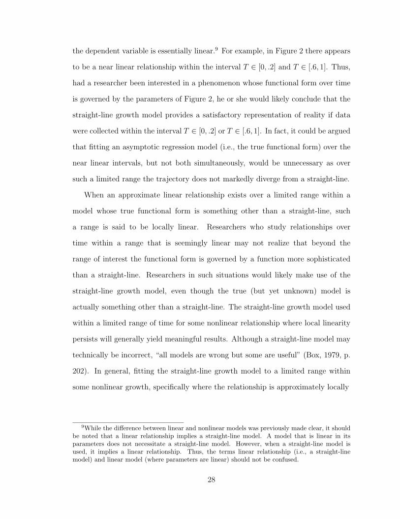
the dependent variable is essentially linear.9 For example, in Figure 2 there appears

to be a near linear relationship within the interval T ! [0, .2] and T ! [.6, 1]. Thus,

had a researcher been interested in a phenomenon whose functional form over time

is governed by the parameters of Figure 2, he or she would likely conclude that the

straight-line growth model provides a satisfactory representation of reality if data

were collected within the interval T ! [0, .2] or T ! [.6, 1]. In fact, it could be argued

that fitting an asymptotic regression model (i.e., the true functional form) over the

near linear intervals, but not both simultaneously, would be unnecessary as over

such a limited range the trajectory does not markedly diverge from a straight-line.

When an approximate linear relationship exists over a limited range within a

model whose true functional form is something other than a straight-line, such

a range is said to be locally linear. Researchers who study relationships over

time within a range that is seemingly linear may not realize that beyond the

range of interest the functional form is governed by a function more sophisticated

than a straight-line. Researchers in such situations would likely make use of the

straight-line growth model, even though the true (but yet unknown) model is

actually something other than a straight-line. The straight-line growth model used

within a limited range of time for some nonlinear relationship where local linearity

persists will generally yield meaningful results. Although a straight-line model may

technically be incorrect, “all models are wrong but some are useful” (Box, 1979, p.

202). In general, fitting the straight-line growth model to a limited range within

some nonlinear growth, specifically where the relationship is approximately locally

9While the di!erence between linear and nonlinear models was previously made clear, it shouldbe noted that a linear relationship implies a straight-line model. A model that is linear in itsparameters does not necessitate a straight-line model. However, when a straight-line model isused, it implies a linear relationship. Thus, the terms linear relationship (i.e., a straight-linemodel) and linear model (where parameters are linear) should not be confused.

28

linear, likely provides “useful” information about the phenomenon under study.10

Local linearity is a topic that nicely illustrates potential problems that can arise

when extrapolation beyond the range of data is carried out. While the relationship

between time and the dependent variable may be locally linear, values of the

dependent variable may diverge sharply from such an apparent linear relationship

just beyond the range of collected data. In situations where local linearity persists,

provided the entire time interval of interest exhibits local linearity, the need for

nonlinear models may be less pressing.11

Although there may be numerous behavioral phenomena that follow nonlinear

functional forms, the straight-line growth model seems to be used more than any

other growth model. One reason the straight-line growth model is so often used is

because researchers would like to describe growth in a parsimonious way, often by

talking about the “average” rate or amount of change. The “average” descriptor is

often the regression coe#cient from the straight line growth model. For this reason

the next section explores the relationship between the straight-line growth model

and the ARC.

10However, such a statement rests on the assumption that there truly is a near linear relationshipbetween time and Y . To the extent that this is not true, making use of the straight-line growthmodel may provide misleading information about change.

11The concept of local linearity can be extended to local quadrature. In such a case, therelationship between time and the dependent variable may be nonlinear, but the relationshipbetween time and the dependent variable may be essentially quadratic. Of course local quadraturecan be extended to local cubature. However, once a relationship is beyond quadratic, theinterpretation of such a polynomial growth model is di"cult. Thus, rather than thinking of arelationship as locally cubic, for example, a nonlinear model should be considered.

29

RELATIONSHIP BETWEEN STRAIGHT-LINE GROWTH

MODELS AND THE AVERAGE RATE OF CHANGE

Due to the hierarchical structure of longitudinal data (scores over time nested

within person, who in turn may be nested within group), special statistical models

are required that take into consideration the nonindependence of the hierarchically

structured data. HLMs and HNLMs explicitly model the hierarchical structure

of nested data and allow for nonconstant time-lags within and across individuals,

and some types of missing data (i.e., the design need not be completely balanced

nor occasions of measurement equally spaced within or across individuals; See

Raudenbush & Bryk, 2002, Davidian & Giltinan, 1995, or Goldstein, 1995, for a

thorough treatment of these issues.).

The most common method of analyzing an individual’s trajectory is through the

generalization of the polynomial growth model (illustrated in Equation 6) into a

HLM. Growth models linear in their parameters allow various polynomial trends to

be specified and then tested against other competing models. Given an observed

set of data, provided a su#cient number of polynomial trends are specified, (at

the expense of degrees of freedom) the growth model can be made to accurately

represent the data. This desirable property, combined with the relative ease of

calculation, has made the HLM of polynomial growth essentially the model of choice

for analyzing individual change over time in the behavioral sciences. However, a

caution is warranted because by adding additional polynomial trends to a growth

model, the sum of squared deviations between the predicted scores and the observed

scores will necessarily decrease (or at the very least stay the same). In fact, as the

30

number of polynomial trends approaches the number of timepoints, the sum of

squared deviations between predicted and observed scores approaches zero. One

wants to avoid overparameterization in growth models, otherwise the model will

account for measurement error in addition to the true relationship (Box, 1984).

The general HLM for the ith individual’s set of scores can be given as,

Yi = Xi! + ZiUi + "i, (14)

where ! is the vector of unknown population parameters linked to the vector Yi

by the design matrix Xi, Ui is a matrix of unknown unique individual e"ects

linked to Yi by the design matrix Zi, and "i is a vector of errors generally

assumed to be normally distributed about a mean of zero with a constant variance

across time (Laird & Ware, 1982). This general HLM formulation allows for the

desired polynomial function(s) of time to be included in the model, as well as

other time-varying and fixed covariates. Furthermore, models having the form of

Equation 14 o"er great flexibility in terms of model testing and model comparisons.

A straight-line HLM of growth for individual i, a special case of Equations 6 and

14, can be represented by the following growth model:

Yit = %0i + %1iTit + &it. (15)

As illustrated in Equation 7, the parameters of Equation 15 are themselves modeled

as dependent variables in the following manner:

%0i = !00 + u0i, (16a)

%1i = !10 + u1i, (16b)

where !00 is the mean of the individual intercepts (i.e., E[Y |T = 0]), !10 is the mean

of the individual slopes (rate of change) across the N individuals, and u0i and u1i

31

represent the unique e"ects associated with the ith individual’s intercept and slope

parameter respectively.12 By combining Equations 15, 16a, and 16b, the full HLM

model for the ith individual’s straight-line growth model can be rewritten as follows:

Yit = !00 + u0i + (!10 + u1i)Tit + &it. (17)

While the fixed e"ect parameters (!00 & !10) of Equation 17 define the overall

growth model, the unique e"ects (u0i & u1i) lead directly to the population

covariance matrix of the unique components and the reliability of the sample

estimates. In the special case of zero variance for the unique e"ects of a particular

fixed e"ect parameter (equivalent to a set of parameter estimates with zero

reliability), the parameter is said to be constant across individuals and a unique term

need not be included in the model. For example, if the variance of u0i in Equation 16a

was zero, the implication is that all N individuals have the same intercept (and thus

are indistinguishable from one another, which is why the reliability would be zero

in the case of zero variance for a random component).

In the context of growth models where each of the N individuals share a common

design matrix for the unique e"ects (Zi from Equation 14 equals Z for all N

individuals), the mean of the ordinary least squares (OLS) regression coe#cients

are equivalent to the fixed e"ects of the HLM model (see Laird & Ware, 1982,

p. 966, for technical details). In the context of the straight-line growth model of

Equation 15, a common design matrix of the unique e"ects implies a common set

(i.e., vector) of time values across each of the N individuals. When the previously

stated assumptions of the work are satisfied (i.e., those outlined on pages 15 & 16),

each of the N individuals will share a common vector for the time values. Thus,

the !s in Equation 17 will be equivalent to the mean of the OLS estimates across

12Equation 15 is an unconditonal model. An unconditional model implies that there are no Level2 predictors, and thus the dependent variable is not conditioned upon any Level 2 predictors.

32

individuals. That is, if OLS regression analyses were performed for each of the N

individuals, the mean of the estimated intercepts and slopes would correspond to

the estimated fixed e"ects calculated via the HLM growth model. Thus, the mean

of the N intercepts and the mean of the N slopes would estimate !00 and !10 in

Equation 17. Because the estimated fixed e"ects of the HLM model are equal to the

mean OLS estimates in the present context, in order to make the discussion more

comprehensible and generalizable, the remainder of the work focuses specifically on

the OLS estimates of a single trajectory. The HLM regression model of straight-line

growth for a specific individual thus simplifies to the following OLS formulation:

Yt = !0 + !1Tt + &t, (18)

where the intercept is

!0 = µY " !1µT (19)

and the slope from the straight-line growth model is

!1 =

F+t=1

(Yt " µY )(Tt " µT )

F+t=1

(Tt " µT )2

= !SLGM, (20)

where µY and µT represent the population means of the dependent variable (Y ) and

time (T ) respectively, and !SLGM is the regression coe#cient for the straight-line

growth model. Notice that no i subscripts are needed in Equation 18 (and thus

Equations 19 and 20) because N = 1.

When straight-line growth models are used in the context of the analysis of

change, an implicit assumption for descriptive and inferential purposes is that

Equation 20 provides a meaningful measure of change. If the relationship between

time and the dependent variable of interest is something other than linear, making

use of !SLGM for individual trajectories may lead to incorrect conclusions. When

33

making use of statistical methods that treat !SLGM as a dependent variable, such

as HLMs or two-stage analyses, the results of such statistical procedures may be

misleading, as the chosen measure of change (!SLGM) may not accurately reflect

the particular phenomenon under study as it changes and evolves over time. The

forthcoming sections detail the relationship that exists between !SLGM and ARC as

well as the importance of correctly specifying an appropriate Level 1 HLM model. It

is illustrated in the remainder of the work that conceptualizing !SLGM as a measure of

the ARC potentially leads to incorrect conclusions, not only for an individual trend,

but such a misconception also has implications when looking across individuals and

when examining group di"erences.

The Regression Coe#cient from the Straight-Line

Growth Model and the Average Rate of Change

Recall that it is assumed data are completely balanced with equally spaced

occasions of measurement with the same starting point and constant time-lag

throughout the work (i.e., Zi from Equation 14 is constant across individuals;

see also pages 15 & 16). The slope from the straight-line growth model implied

by Equation 20 is how some researchers (often incorrectly) label and/or interpret

the ARC for an individual trajectory. For example, in a methodological work

Kraemer and Thiemann (1989) recommended using the regression coe#cient from

the straight-line growth model calculated separately on each individual trajectory as

the dependent variable in the analysis of group di"erences over time in applications

of the intensive design. The authors state and illustrate a proof that supposedly

shows over the time interval zero to one “the slope from the usual, ordinary

least-squares regression measures the average rate of change” (p. 150). However, this

statement is generally not correct, and it will be shown momentarily that the slope

34

from the straight-line growth model and the ARC are equivalent only in a limited

number of circumstances. The fact that Kraemer and Thiemann define the slope

as the ARC and then go on to state that “no assumption of linearity [straight-line

growth] is made” when using the slope from OLS regression as a measure of the ARC

(p. 150) is unfortunate. Such statements are troublesome because they potentially

lead researchers to believe they are examining the ARC (or the mean of the ARC

across individuals) when in fact they are examining an OLS regression coe#cient

(or the mean OLS regression coe#cient), a measure designed to minimize the sum

of squared deviations between the predicted and observed scores, not to measure

the ARC over some time interval.13

An example that shows how the regression coe#cient from the straight-line

growth model can be incorrectly conceptualized in applied applications of

longitudinal data analysis is taken from Svartberg (1999). Svartberg states that

it is a “fact” that the “linear component provides a good estimate of average

change even when the growth pattern is complicated” (p. 1315). Svartberg goes

on to state that “even when the underlying trajectory is curved, the straight-line

model is a reasonable option since the linear rate of change is equal to the average

rate of change of the curved function” (p. 1318).14 Svartberg is not alone

13Kraemer and Thiemann go on to state that the regression coe"cient from the straight-linegrowth model is the “average rate of change over all pairs of time points” (p. 150). This is alsomisleading as the reader is first told that the slope is the ARC regardless of the true functionand then the reader is told that it is actually the ARC over all pairs of time points. In fact, theregression coe"cient is not the average over pairs of timepoints, but a weighted average over allpairs of timepoints, where the weights are defined as (Tt " Tt!)2/

+t"=t!

(Tt " Tt!)2, and are simply

the OLS regression weights obtained by rewriting Equation 20.14Svartberg (1999) cites Willett (1989) after he claims “the linear rate of change is equal to

the average rate of change of the curved function” (p. 1918). However, Willett states that “evenwhen the underlying trajectory is quadratic, the use of the straight-line model is equal to theaverage slope of the quadratic function over the same time interval” (p. 590). Thus, Svartberg hasovergeneralized Willett’s summary of Seigel (1975). Furthermore, it should be noted that Willett’sstatement is only true when the occasions of measurement are equally spaced, which he failed toacknowledge.

35

in his use of the straight-line growth model for seemingly complicated growth

functions, as it supposedly provides an “overall average” for potentially complicated

functional forms of growth. However, he is very explicit about why he made

use of the straight-line growth model, potentially leading other researchers astray

when analyzing and attempting to understand their own potentially complicated

longitudinal data. Since Svartberg’s clear exposition on the rationale for making

use of the straight-line growth model is, like some of Kraemer and Thiemann’s

statements, flawed, the works have the potential to: (a) encourage others to ignore

searching for the true functional form of growth, (b) “fall-back” on the straight-line

growth model, and (c) lead to interpretations based on biased estimates of the mean

ARC across individuals.

A commonly used but potentially confusing statement regarding the ARC occurs

when the “average rate of change” is presented and interpreted in HLMs. This

“average rate of change,” however, is generally not the ARC examined in the present

work. When fitting the straight-line growth model in the context of HLM, each

individual is typically allowed a unique value for their slope over time, as well as

a unique intercept. As previously stated, the expected value (i.e., mean) of each

parameter across all individuals are known as fixed e"ects. Recall the fixed e"ect for

the slope is represented in Equation 17 by !10 (see p. 32). In straight-line growth

models this parameter is often referred to as the “average rate of change” (examples

in methodological works include Laird and Wang, 1990, p. 405, and Raudenbush

and Xiao-Feng, 2001, p. 387) because it is literally the mean of all individual slope

(i.e., rate of change) estimates. Authors who use the term “average rate of change”

when referring to the fixed e"ect are not literally wrong, provided the “average rate

of change” is not interpreted as the grand mean (mean of the individual means) of

the instantaneous rate of change for the individual trajectories over time, but as the

36

mean of the individual slopes. However, using the term “average rate of change”

to describe the fixed e"ect value provides a poor description of its meaning, as it

gives the impression that it measures the ARC across a set of individuals. As is will

be shown momentarily, in general !10 %= ARC and !SLGM %= ARC. In summary, the

value of the fixed e"ect for the slope is the average of the individual rates of change

across individuals (i.e., the average of the individual slopes), whereas the ARC is

literally the average rate of change for an individual. Although the phrases may be

subtly di"erent, the two convey very di"erent concepts. When individuals’ average

rates of change are biased, by conceptualizing them as if they were the slope from the

straight-line growth model for example, the mean of the biased estimates is itself a

biased estimate of the group ARC. Confusion surrounding the use and interpretation

of the ARC persists, in part, because of the labels commonly employed for the fixed

e"ect parameter estimates in the context of HLMs.

In summary, !10 (Equation 17) is the mean slope across all individuals in

some population, however, !10 generally does not represent the mean ARC across

individuals, nor does !SLGM (Equation 20) generally represent the ARC for an

individual. The belief that the slope from the straight-line growth model is always

equal to the ARC is explicit in some work and implicit in the interpretations of many

others. The overall group e"ect for the rate of change, although it is an averaged

value, is not generally a measure of the overall ARC across individuals. Although

it is a measure of the average of the individual slopes, the individuals’ slopes do

not generally measure the average rate of change. As it will be shown, the slope

from the straight-line growth model is equal to the ARC in a limited number of

situations. A major goal of this work is to examine the potential bias that develops

when interpreting the ARC as if it was the slope from the straight-line growth model.

37

Fitting a Quadratic Growth Model To Estimate the Average Rate of Change

When curvature is, or at least seems to be, present in longitudinal data, it is

often suggested that the straight-line growth model be extended to a quadratic

growth model. The Level 1 (intraindividual) model for a quadratic growth model

is extended by incorporating the square of the time-varying covariate as another

predictor variable in addition to the intercept and the time-varying covariate itself.

The Level 1 quadratic growth model for a single individual can be represented as,

Yt = !0 + !1Tt + !2T2t + &t, (21)

where !2 represents the quadratic component of the growth curve. Note that

all three parameter estimates (!0, !1, and !2) can be modeled via a Level 2

(interindividual) model. Furthermore, because the parameter estimates are solved

for simultaneously, !0 and !1 of Equation 18 are generally not equal to !0 and !1 of

Equation 21, as adding one term generally changes all terms.

Making the assumption that a particular phenomenon is a function of linear

and quadratic components over time, a question arises as to how the ARC may be

estimated given the parameter estimates from a quadratic growth model. Assuming

that the true underlying model follows a second degree polynomial, Seigel (1975)

shows that the ARC can be estimated by evaluating the derivative of Equation 21

(with respect to T ) at the mean value of T . Thus, for a quadratic growth model

where growth is truly governed by a second order polynomial equation, the ARC is

equal to the following:

ARCQGM = !1 + 2!2µT . (22)

However, Seigel shows that Equation 22 reduces to Equation 20. Thus, the first

derivative (with respect to time) of a quadratic growth model evaluated at the mean

value of time is equivalent to the slope from the straight-line growth model. Thus,

38

in an attempt to obtain a “better estimate” of the ARC when curvature is present,

Equation 22 yields exactly the same value as the slope from the straight-line growth

model when there is equal spacing between measurement occasions. In this respect,

conceptualizing the ARC via the parameter estimates from a quadratic growth

model is equivalent to conceptualizing it as the ARC using the regression coe#cient

from the straight-line growth model. Thus, in this narrow sense, using a more

elaborate model provides no better estimate of the ARC than does the slope from

the straight-line growth model, regardless of the true functional form of growth. As

Seigel points out (and which will be proved momentarily) if the true functional form

of growth is a first or second degree polynomial, the ARC is equal to Equation 22

or Equation 20. However, as the next section shows, when the true functional form

of growth is something other than a first or second degree polynomial, the slope

from the straight-line growth model (or Equation 22) is generally a biased estimate

of the ARC.

39

THE DISCREPANCY BETWEEN THE REGRESSION

COEFFICIENT FROM THE STRAIGHT-LINE GROWTH

MODEL AND THE AVERAGE RATE OF CHANGE

The potential discrepancy between the regression coe#cient and the ARC is

described by two parameters. For fixed values of time the first parameter that

describes the discrepancy is the bias and is operationally defined as,

B = E[!SLGM|f(T )]" E[(YF " Y1)|f(T )]

TF " T1= !SLGM " ARC, (23)

where Y is conditional on the true functional form of growth and E[x] represents

the expectation value of the random variable x. For fixed values of time the

second parameter that describes the discrepancy is the discrepancy factor and is

operationally defined as,

! =E[!SLGM|f(T )]E[(YF#Y1)|f(T )]

TF#T1

=!SLGM

ARC, (24)

where again Y is conditional on the true functional form of growth. When B

equals zero ! must equal one; the converse is also true. In this special case !SLGM

is exactly equal to the ARC. Thus, in situations where B=0 (!=1) interpreting

!SLGM as the ARC yields no inconsistency in research conclusions or interpretation.

However, when B %= 0 (by implication ! %= 1), conceptualizing !SLGM as the ARC

is problematic and can potentially lead to misinformed conclusions regarding

40

intraindividual change, interindividual change, as well as group di"erences in

change.15

Before examining B and !, it is first helpful to realize that any functional

form can generally be represented by a power series, such that the sum of squared

deviations between values of the true function and the values approximated by the

power series can be made to be infinitesimally small by adding enough polynomial

powers and coe#cients (Stewart, 1998, section 8.6; Finney et al., 2001, chapter 8).

A power series in the longitudinal context is a limiting sum of coe#cients multiplied

by integer powers of time. Such a power series is given as,

f(T ) = limM!$

M,

m=0

((mTm) , (25)

where (m is the coe#cient ("$ < (m <$) for the mth power (m = 0, ...,M).

Although a power series is infinite by definition, known functional forms can

be represented by finite sums. In general, the following finite sum can be used

to impose or approximate some known or unknown functional form of growth and

is more general than the power series, as the powers of time are not limited to

nonnegative integers, but can take on any real values,

f(T ) =K,

k=1

'(kT

"k(, (26)

where %k ("$ < % < $) represents the kth (k = 1, ..., K; 1 & K < $) power

constant.16 General results emerge for B and ! by realizing that functional forms of15It should be noted that # can be reformulated into another measure of discrepancy, such that

it represents the proportion of bias relative to the ARC. The proportion of bias is thus given as:!SLGM#ARC

ARC = !SLGMARC " ARC

ARC = # " 1. Because the proportion of bias and # provide the sameinformation, only one needs to be used as a supplement for B. The second discrepancy measurethat will be used throughout the remainder of the work is #.

16The intercept of a particular growth curve is the sum of the $ks whose $k is zero. In the specialcase where T ! [0, TF ] the intercept is the

+$k0!k , which strictly speaking is an indeterminate

form when $k = 0. However, due to l’Hopital’s Rule which uses derivatives to evaluate theconverging limit of a function that would otherwise be indeterminate under standard algebraicrules, the quantity 00 ' 1 by standard conventions (Stewart, 1998, section 4.5; Finney et al., 2001,section 7.6). When evaluating the equations given in this section by computer, care should betaken to ensure the particular program defines 00 as 1 (rather than returning an error message).

41

growth can generally be represented by Equation 26.17 The following section makes

use of this fact when examining B and ! when time is continuous for any linear

model as well as the nonlinear models presented in the Nonlinear Growth Models

for the Analysis of Change section.

Examining the Bias in the Average Rate of Change:

The Limiting Case when Time Is Continuous

Often times in statistics, and mathematically based disciplines in general,

limiting cases are of most interest and utility. It is in this spirit that the examination

of B and ! will first proceed. For the limiting case where time is continuous [F #$

as (Tt+1 " Tt)# 0], deriving B and ! will provide insight into problems associated

with using !SLGM as a measure of the ARC.

Regardless of the functional form of growth, B and ! can both be obtained

by making use of the equations for !SLGM and ARC. The equation for the slope

presented in Equation 20 is for a finite number of timepoints. In the case of

continuous data, Equation 20 generalizes (by integrating rather than summating)

to the following:

!SLGMC =

TF$

T1

(Tt " µT )(Yt " µY )dT

TF$

T1

(Tt " µT )2dT

, (27)

where !SLGMC is the regression coe#cient for the straight-line growth model when

time is continuous.17If the functional form of growth is a known linear equation, the values of $k and $k can

be specified and written via Equation 26. If the functional form is known but yet follows somenonlinear equation, an exact linearized analog to a nonlinear function can be derived by specifyinga sequence of $s from zero to F (if F is large or even infinite, the function can be approximatedby specifying a large number of $s) by one and solving for the $s via multiple regression. Thenonlinear equation can then be written as Equation 26 with the specified $ and $ values such thatthe nonlinear function is represented as a linear equation.

42

Equation 27 can be rewritten as the integral of a sum after expanding the

numerator and denominator,

!SLGMC =

TF$

T1

(YtTt " YtµT " TtµY + µT µY )dT

TF$

T1

(T 2t " 2TtµT + µ2

T )dT

. (28)

Because the integral of a sum is the sum of the integrals, Equation 28 can be

rewritten as the following:

!SLGMC =

TF$

T1

(YtTt)dT " µT

TF$

T1

(Yt)dT " µY

TF$

T1

(Tt)dT + µT µY (TF " T1)

TF$

T1

(T 2t )dT " 2µT

TF$

T1

(Tt)dT + µ2T (TF " T1)

. (29)

Realizing that µT = (TF + T1)/2 and that µY

$ TF

T1(Tt)dT equals µY (T 2

F " T 21 )/2,

the last two components in the numerator of Equation 29 are equal and of opposite

sign, leading to a reduction of the numerator because the two components cancel.

Alternatively, a second perspective to understand why the two components cancel

in the numerator of Equation 29 can be seen by rewriting the last two components

as µY

TF$

T1

(Tt " µT )dT . BecauseTF$

T1

(Tt " µT )dT is the first moment about the mean,

this quantity must always equal zero (Stuart and Ord, 1994, chapter 3). In the

following sections where time is continuous, the reduced form of Equation 29,

!SLGMC =

TF$

T1

(YtTt)dT " µT

TF$

T1

(Yt)dT

TF$

T1

(T 2t )dT " 2µT

TF$

T1

(Tt)dT + µ2T (TF " T1)

, (30)

will be applied to linear and then to nonlinear models.

43

When Y Can Be Written As a Linear Function of Time

Recall from Equations 25 and 26 that Y can be written as a sum of coe#cients

multiplied by powers of time. This sum can be in the form of a limiting sum

(Equation 25) of some unknown functional form of growth or in the form of a finite

sum (Equation 26) of a known functional form of growth written as a linear equation.

In the remainder of this section, Y will be represented by Equation 26, in order for

general results to be derived for B and !.

Replacing Y in Equation 30 with the finite sum of Equation 26 yields:

!SLGMC =

TF$

T1

%K+

k=1(kT

!k+1

t

&dT " µT

TF$

T1

%K+

k=1(kT

!k

t

&dT

TF$

T1

(T 2t ) dT " 2µT

TF$

T1

(Tt) dT + µ2T (TF " T1)

. (31)

Carrying out the integration and replacing µT by its definition [µT = (TF + T1)/2]

yields:

!SLGMC =

K+k=1

%k

!T

!k+2

F #T!k+2

1

"

"k+2 " TF +T1

2

K+k=1

%k

!T

!k+1

F #T!k+1

1

"

"k+1

T 3F#T 3

1

3 " (TF +T1)(T 2F#T 2

1 )

2 + (TF +T1)2(TF#T1)4

. (32)

After simplifying both the numerator and the denominator, details of which are

given in Appendix A, the general equation for the regression coe#cient from the

straight-line growth model when Y can be written in the form of Equation 26 and

when time is continuous is given as follows:

"SLGMC =6

(TF # T1)3

K#

k=1

$

%%k

&"k

!T

!k+2

F # T!k+21 + TF T

!k+11 # T1T

!k+1

F

"+ 2

!TF T

!k+11 # T1T!k+1

F

"'

("k + 2) ("k + 1)

(

) .

(33)

It is useful to note that Equation 33 does not constrain the values of T1 or TF , the

number of components defining Y (i.e., K), or the values of % and (.18

18Implicit in the derivations presented is the fact that the equations are only valid for legitimatesets of parameter values. As with any mathematic model, evaluating the model for indeterminateforms will not result in meaningful solutions. Thus, care must be taken to ensure that a chosenset of parameters provides a mathematically meaningful set of parameters.

44

The ARC when Y is defined as a sum of K coe#cients multiplied by powers of

time can be written as the following:

ARC =

K+k=1

(k(T!k

F " T!k

1 )

TF " T1. (34)

Because the slope (Equation 33) and the ARC (Equation 34) have been defined

when Y is expressed as a special case of Equation 26, general equations emerge for

B and !.

The general bias for the present situation is given as,

B =6

(TF ! T1)3

K!

k=1

"

#$"k

%!k

&T

!k+2F ! T

!k+21 + TF T

!k+11 ! T1T

!k+1F

'+ 2

&TF T

!k+11 ! T1T

!k+1F

'(

(!k + 2) (!k + 1)

)

*+!

K,k=1

"k(T!kF ! T

!k1 )

TF ! T1,

(35)

which is Equation 34 subtracted from Equation 33, as specified by the definition of

B given in Equation 23. The general discrepancy factor is then given as

" =6

(TF ! T1)2K,

k=1"k(T

!kF

! T!k1 )

K!

k=1

"

#$"k

%!k

&T

!k+2F ! T

!k+21 + TF T

!k+11 ! T1T

!k+1F

'+ 2

&TF T

!k+11 ! T1T

!k+1F

'(

(!k + 2) (!k + 1)

)

*+

(36)

which is Equation 33 divided by Equation 34, as specified by the definition of !

given in Equation 24.

Oftentimes in behavioral research the initial value of time is represented as zero

(T1 = 0). This is especially true in experimental studies when Y1 represents a

baseline measure of some attribute (pretest) before treatment begins. Another

reason why T1 often equals zero is because time is often scaled such that the intercept

represents the initial (starting) value. In the special case where T1 is replaced by

zero, Equations 35 and 36 can be simplified. The simplified slope when the initial

value of time (or scaled time) is zero can be written as the following:

!SLGMC = 6K,

k=1

-(kT

!k!1

F %k

(%k + 2)(%k + 1)

.. (37)

45

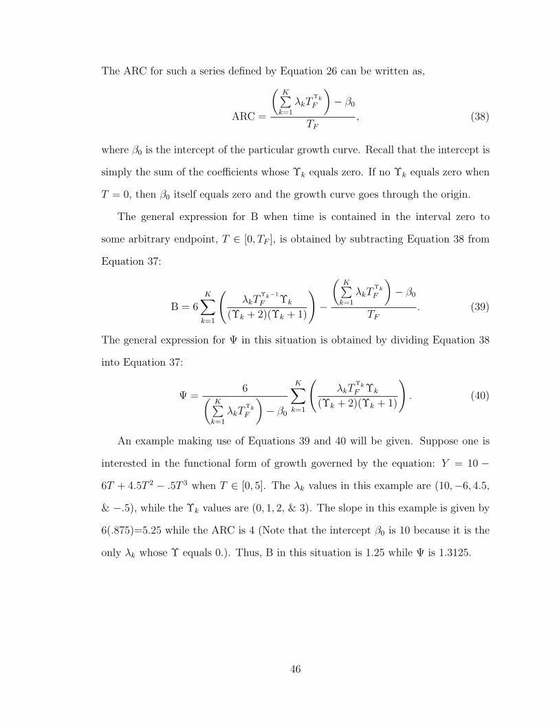
The ARC for such a series defined by Equation 26 can be written as,

ARC =

%K+

k=1(kT

!k

F

&" !0

TF, (38)

where !0 is the intercept of the particular growth curve. Recall that the intercept is

simply the sum of the coe#cients whose %k equals zero. If no %k equals zero when

T = 0, then !0 itself equals zero and the growth curve goes through the origin.

The general expression for B when time is contained in the interval zero to

some arbitrary endpoint, T ! [0, TF ], is obtained by subtracting Equation 38 from

Equation 37:

B = 6K,

k=1

-(kT

!k!1

F %k

(%k + 2)(%k + 1)

."

%K+

k=1(kT

!k

F

&" !0

TF. (39)

The general expression for ! in this situation is obtained by dividing Equation 38

into Equation 37:

! =6%

K+k=1

(kT!k

F

&" !0

K,

k=1

-(kT

!k

F %k

(%k + 2)(%k + 1)

.. (40)

An example making use of Equations 39 and 40 will be given. Suppose one is

interested in the functional form of growth governed by the equation: Y = 10 "

6T + 4.5T 2 " .5T 3 when T ! [0, 5]. The (k values in this example are (10,"6, 4.5,

& ".5), while the %k values are (0, 1, 2, & 3). The slope in this example is given by

6(.875)=5.25 while the ARC is 4 (Note that the intercept !0 is 10 because it is the

only (k whose % equals 0.). Thus, B in this situation is 1.25 while ! is 1.3125.

46

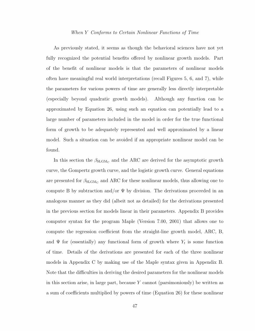
When Y Conforms to Certain Nonlinear Functions of Time

As previously stated, it seems as though the behavioral sciences have not yet

fully recognized the potential benefits o"ered by nonlinear growth models. Part

of the benefit of nonlinear models is that the parameters of nonlinear models

often have meaningful real world interpretations (recall Figures 5, 6, and 7), while

the parameters for various powers of time are generally less directly interpretable

(especially beyond quadratic growth models). Although any function can be

approximated by Equation 26, using such an equation can potentially lead to a

large number of parameters included in the model in order for the true functional

form of growth to be adequately represented and well approximated by a linear

model. Such a situation can be avoided if an appropriate nonlinear model can be

found.

In this section the !SLGMC and the ARC are derived for the asymptotic growth

curve, the Gompertz growth curve, and the logistic growth curve. General equations

are presented for !SLGMC and ARC for these nonlinear models, thus allowing one to

compute B by subtraction and/or ! by division. The derivations proceeded in an

analogous manner as they did (albeit not as detailed) for the derivations presented

in the previous section for models linear in their parameters. Appendix B provides

computer syntax for the program Maple (Version 7.00, 2001) that allows one to

compute the regression coe#cient from the straight-line growth model, ARC, B,

and ! for (essentially) any functional form of growth where Yt is some function

of time. Details of the derivations are presented for each of the three nonlinear

models in Appendix C by making use of the Maple syntax given in Appendix B.

Note that the di#culties in deriving the desired parameters for the nonlinear models

in this section arise, in large part, because Y cannot (parsimoniously) be written as

a sum of coe#cients multiplied by powers of time (Equation 26) for these nonlinear

47

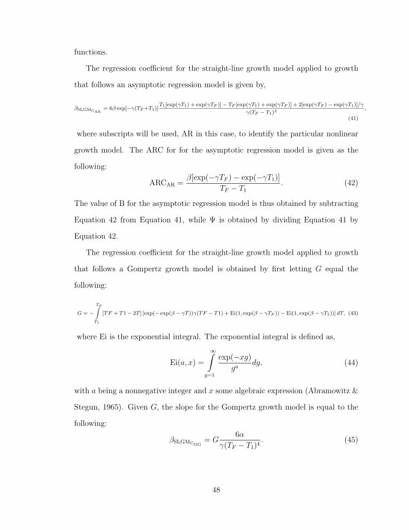
functions.

The regression coe#cient for the straight-line growth model applied to growth

that follows an asymptotic regression model is given by,

"SLGMCAR= 6" exp[##(TF +T1)]

T1[exp(#T1) + exp(#TF )]# TF [exp(#T1) + exp(#TF )] + 2[exp(#TF )# exp(#T1)]/#

#(TF # T1)3,

(41)

where subscripts will be used, AR in this case, to identify the particular nonlinear

growth model. The ARC for for the asymptotic regression model is given as the

following:

ARCAR =![exp("#TF )" exp("#T1)]

TF " T1. (42)

The value of B for the asymptotic regression model is thus obtained by subtracting

Equation 42 from Equation 41, while ! is obtained by dividing Equation 41 by

Equation 42.

The regression coe#cient for the straight-line growth model applied to growth

that follows a Gompertz growth model is obtained by first letting G equal the

following:

G = #TF*

T1

[TF + T1# 2T ] [exp(# exp(" # #T ))#(TF # T1) + Ei(1, exp(" # #TF ))# Ei(1, exp(" # #T1))] dT, (43)

where Ei is the exponential integral. The exponential integral is defined as,

Ei(a, x) =

$#

g=1

exp("xg)

gadg, (44)

with a being a nonnegative integer and x some algebraic expression (Abramowitz &

Stegun, 1965). Given G, the slope for the Gompertz growth model is equal to the

following:

!SLGMCGG= G

6"

#(TF " T1)4. (45)

48

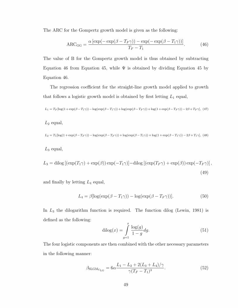
The ARC for the Gompertz growth model is given as the following:

ARCGG =" [exp(" exp(! " TF #))" exp(" exp(! " T1#))]

TF " T1. (46)

The value of B for the Gompertz growth model is thus obtained by subtracting

Equation 46 from Equation 45, while ! is obtained by dividing Equation 45 by

Equation 46.

The regression coe#cient for the straight-line growth model applied to growth

that follows a logistic growth model is obtained by first letting L1 equal,

L1 = TF [log(1+exp("#T1#))# log(exp("#T1#))+ log(exp("#TF #))+ log(1+exp("#TF #))#2" +TF #], (47)

L2 equal,

L2 = T1[log(1+ exp("#TF #))# log(exp("#TF #)) + log(exp("#T1#)) + log(1+ exp("#T1#))# 2" + T1#], (48)

L3 equal,

L3 = dilog [(exp(T1#) + exp(!)) exp("T1#)]"dilog [(exp(TF #) + exp(!)) exp("TF #)] ,

(49)

and finally by letting L4 equal,

L4 = ![log(exp(! " T1#))" log(exp(! " TF #))]. (50)

In L3 the dilogarithm function is required. The function dilog (Lewin, 1981) is

defined as the following:

dilog(x) =

x#

g=1

log(g)

1" gdg. (51)

The four logistic components are then combined with the other necessary parameters

in the following manner:

!SLGMCLG= 6"

L1 " L2 + 2(L3 + L4)/#

#(TF " T1)3. (52)

49

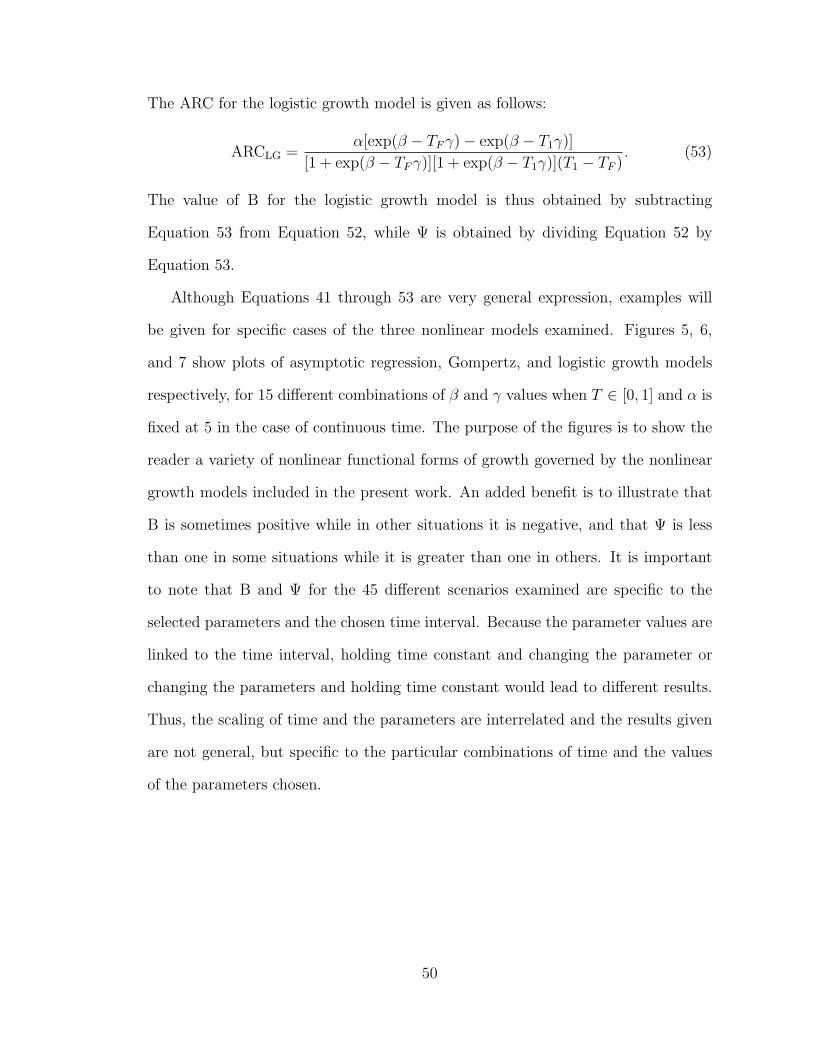
The ARC for the logistic growth model is given as follows:

ARCLG ="[exp(! " TF #)" exp(! " T1#)]

[1 + exp(! " TF #)][1 + exp(! " T1#)](T1 " TF ). (53)

The value of B for the logistic growth model is thus obtained by subtracting

Equation 53 from Equation 52, while ! is obtained by dividing Equation 52 by

Equation 53.

Although Equations 41 through 53 are very general expression, examples will

be given for specific cases of the three nonlinear models examined. Figures 5, 6,

and 7 show plots of asymptotic regression, Gompertz, and logistic growth models

respectively, for 15 di"erent combinations of ! and # values when T ! [0, 1] and " is

fixed at 5 in the case of continuous time. The purpose of the figures is to show the

reader a variety of nonlinear functional forms of growth governed by the nonlinear

growth models included in the present work. An added benefit is to illustrate that

B is sometimes positive while in other situations it is negative, and that ! is less

than one in some situations while it is greater than one in others. It is important

to note that B and ! for the 45 di"erent scenarios examined are specific to the

selected parameters and the chosen time interval. Because the parameter values are

linked to the time interval, holding time constant and changing the parameter or

changing the parameters and holding time constant would lead to di"erent results.

Thus, the scaling of time and the parameters are interrelated and the results given

are not general, but specific to the particular combinations of time and the values

of the parameters chosen.

50

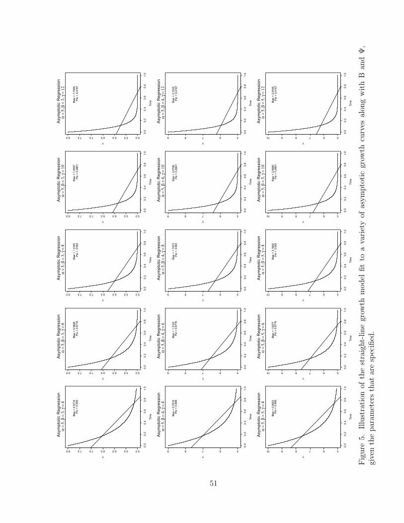
Tim

e

Y

0.0

0.2

0.4

0.6

0.8

1.0

5.05.56.06.57.07.58.0

Asy

mpt

otic

Reg

ress

ion

α =

5, β

= 3

, γ =

4

Bias

= 0

.571

4 P

si =

0.8

06

Tim

e

Y0.

00.

20.

40.

60.

81.

0

5.05.56.06.57.07.58.0

Asy

mpt

otic

Reg

ress

ion

α =

5, β

= 3

, γ =

6

Bias

= 0

.982

6 P

si =

0.6

716

Tim

e

Y

0.0

0.2

0.4

0.6

0.8

1.0

5.05.56.06.57.07.58.0

Asy

mpt

otic

Reg

ress

ion

α =

5, β

= 3

, γ =

8

Bias

= 1

.310

5 P

si =

0.5

63

Tim

e

Y

0.0

0.2

0.4

0.6

0.8

1.0

5.05.56.06.57.07.58.0

Asy

mpt

otic

Reg

ress

ion

α =

5, β

= 3

, γ =

10

Bias

= 1

.559

7 P

si =

0.4

801

Tim

e

Y

0.0

0.2

0.4

0.6

0.8

1.0

5.05.56.06.57.07.58.0

Asy

mpt

otic

Reg

ress

ion

α =

5, β

= 3

, γ =

12

Bias

= 1

.749

9 P

si =

0.4

167

Tim

e

Y

0.0

0.2

0.4

0.6

0.8

1.0

56789

Asy

mpt

otic

Reg

ress

ion

α =

5, β

= 4

, γ =

4

Bias

= 0

.761

9 P

si =

0.8

06

Tim

e

Y

0.0

0.2

0.4

0.6

0.8

1.0

56789

Asy

mpt

otic

Reg

ress

ion

α =

5, β

= 4

, γ =

6

Bias

= 1

.310

2 P

si =

0.6

716

Tim

e

Y

0.0

0.2

0.4

0.6

0.8

1.0

56789

Asy

mpt

otic

Reg

ress

ion

α =

5, β

= 4

, γ =

8

Bias

= 1

.747

3 P

si =

0.5

63

Tim

e

Y

0.0

0.2

0.4

0.6

0.8

1.0

56789

Asy

mpt

otic

Reg

ress

ion

α =

5, β

= 4

, γ =

10

Bias

= 2

.079

6 P

si =

0.4

801

Tim

e

Y

0.0

0.2

0.4

0.6

0.8

1.0

56789

Asy

mpt

otic

Reg

ress

ion

α =

5, β

= 4

, γ =

12

Bias

= 2

.333

2 P

si =

0.4

167

Tim

e

Y

0.0

0.2

0.4

0.6

0.8

1.0

5678910

Asy

mpt

otic

Reg

ress

ion

α =

5, β

= 5

, γ =

4

Bias

= 0

.952

3 P

si =

0.8

06

Tim

e

Y

0.0

0.2

0.4

0.6

0.8

1.0

5678910

Asy

mpt

otic

Reg

ress

ion

α =

5, β

= 5

, γ =

6

Bias

= 1

.637

7 P

si =

0.6

716

Tim

e

Y

0.0

0.2

0.4

0.6

0.8

1.0

5678910

Asy

mpt

otic

Reg

ress

ion

α =

5, β

= 5

, γ =

8

Bias

= 2

.184

2 P

si =

0.5

63

Tim

e

Y

0.0

0.2

0.4

0.6

0.8

1.0

5678910

Asy

mpt

otic

Reg

ress

ion

α =

5, β

= 5

, γ =

10

Bias

= 2

.599

5 P

si =

0.4

801

Tim

e

Y

0.0

0.2

0.4

0.6

0.8

1.0

5678910

Asy

mpt

otic

Reg

ress

ion

α =

5, β

= 5

, γ =

12

Bias

= 2

.916

5 P

si =

0.4

167

Fig

ure

5.Illu

stra

tion

ofth

est

raig

ht-lin

egr

owth

mod

elfit

toa

vari

ety

ofas

ympto

tic

grow

thcu

rves

alon

gw

ith

Ban

d!

,gi

ven

the

par

amet

ers

that

are

spec

ified

.

51

Tim

e

Y

0.0

0.2

0.4

0.6

0.8

1.0

0123

Gom

pertz

Gro

wth

α =

5, β

= 3

, γ =

4

Bias

= 0

.134

6 P

si =

1.03

89

Tim

e

Y0.

00.

20.

40.

60.

81.

0

01234

Gom

pertz

Gro

wth

α =

5, β

= 3

, γ =

6

Bias

= 1

.422

7 P

si =

1.2

991

Tim

e

Y

0.0

0.2

0.4

0.6

0.8

1.0

012345

Gom

pertz

Gro

wth

α =

5, β

= 3

, γ =

8

Bias

= 1

.710

2

Psi =

1.3

444

Tim

e

Y

0.0

0.2

0.4

0.6

0.8

1.0

012345

Gom

pertz

Gro

wth

α =

5, β

= 3

, γ =

10

Bias

= 1

.407

Psi

= 1.

2817

Tim

e

Y

0.0

0.2

0.4

0.6

0.8

1.0

012345

Gom

pertz

Gro

wth

α =

5, β

= 3

, γ =

12

Bias

= 0

.935

4 P

si =

1.1

871

Tim

e

Y

0.0

0.2

0.4

0.6

0.8

1.0

0.00.51.01.5

Gom

pertz

Gro

wth

α =

5, β

= 4

, γ =

4

Bias

= -0

.560

9 P

si =

0.69

51

Tim

e

Y

0.0

0.2

0.4

0.6

0.8

1.0

01234

Gom

pertz

Gro

wth

α =

5, β

= 4

, γ =

6

Bias

= 0

.565

4 P

si =

1.1

295

Tim

e

Y

0.0

0.2

0.4

0.6

0.8

1.0

012345

Gom

pertz

Gro

wth

α =

5, β

= 4

, γ =

8

Bias

= 1

.749

Ps

i = 1

.356

3

Tim

e

Y

0.0

0.2

0.4

0.6

0.8

1.0

012345

Gom

pertz

Gro

wth

α =

5, β

= 4

, γ =

10

Bias

= 1

.974

1 P

si =

1.39

58

Tim

e

Y

0.0

0.2

0.4

0.6

0.8

1.0

012345

Gom

pertz

Gro

wth

α =

5, β

= 4

, γ =

12

Bias

= 1

.738

2 P

si =

1.3

478

Tim

e

Y

0.0

0.2

0.4

0.6

0.8

1.0

0.00.10.20.3

Gom

pertz

Gro

wth

α =

5, β

= 5

, γ =

4

Bias

= -0

.206

1 P

si =

0.37

55

Tim

e

Y

0.0

0.2

0.4

0.6

0.8

1.0

0123

Gom

pertz

Gro

wth

α =

5, β

= 5

, γ =

6

Bias

= -0

.597

2 P

si =

0.8

274

Tim

e

Y

0.0

0.2

0.4

0.6

0.8

1.0

01234

Gom

pertz

Gro

wth

α =

5, β

= 5

, γ =

8

Bias

= 1

.036

5

Psi =

1.2

179

Tim

e

Y

0.0

0.2

0.4

0.6

0.8

1.0

012345

Gom

pertz

Gro

wth

α =

5, β

= 5

, γ =

10

Bias

= 1

.964

3 P

si =

1.39

55

Tim

e

Y

0.0

0.2

0.4

0.6

0.8

1.0

012345

Gom

pertz

Gro

wth

α =

5, β

= 5

, γ =

12

Bias

= 2

.127

2 P

si =

1.4

258

Fig

ure

6.Illu

stra

tion

ofth

est

raig

ht-lin

egr

owth

mod

elfit

toa

vari

ety

ofG

omper

tzgr

owth

curv

esal

ong

wit

hB

and

!,gi

ven

the

par

amet

ers

that

are

spec

ified

.

52

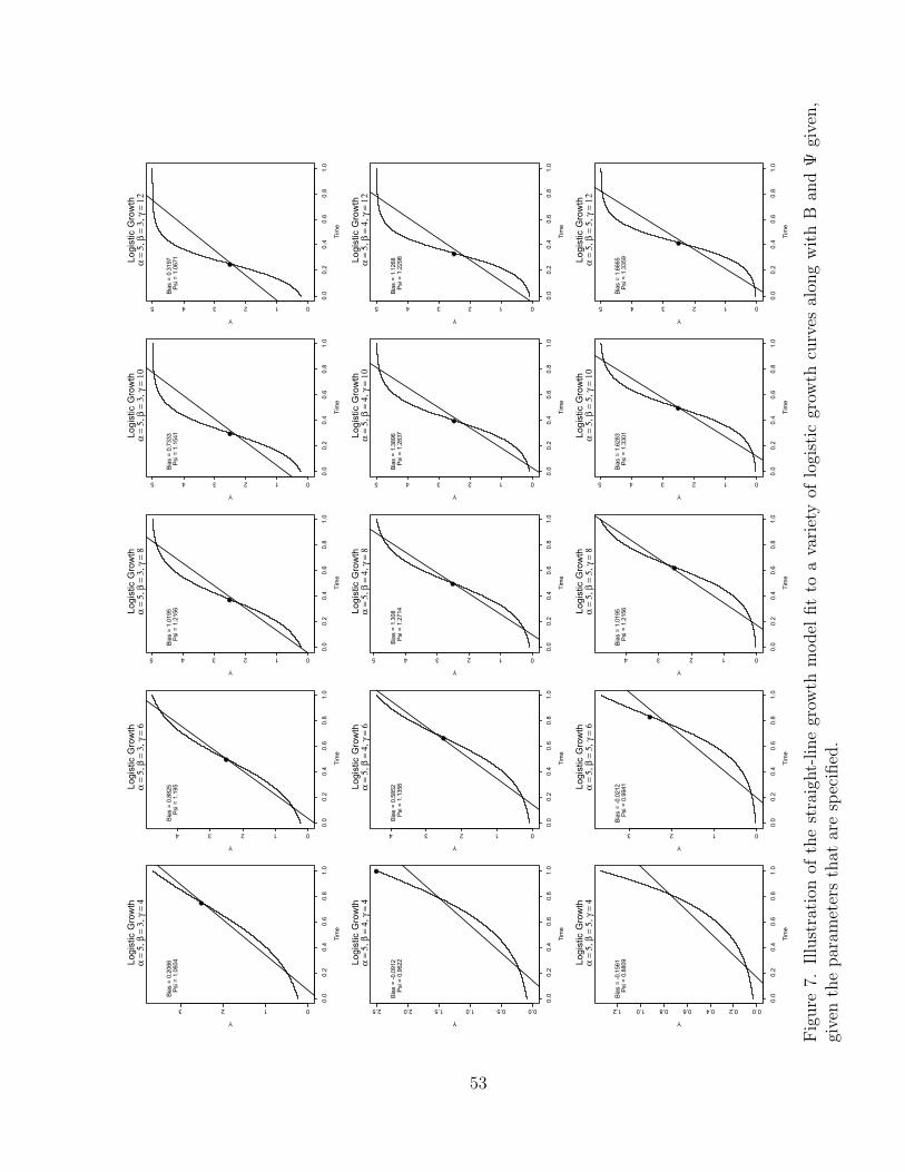
Tim

e

Y

0.0

0.2

0.4

0.6

0.8

1.0

0123

Logi

stic

Gro

wth

α =

5, β

= 3

, γ =

4

Bias

= 0

.206

6 P

si =

1.0

604

Tim

e

Y0.

00.

20.

40.

60.

81.

0

01234

Logi

stic

Gro

wth

α =

5, β

= 3

, γ =

6

Bias

= 0

.882

5 P

si =

1.1

95

Tim

e

Y

0.0

0.2

0.4

0.6

0.8

1.0

012345

Logi

stic

Gro

wth

α =

5, β

= 3

, γ =

8

Bias

= 1

.019

5 P

si =

1.2

156

Tim

e

Y

0.0

0.2

0.4

0.6

0.8

1.0

012345

Logi

stic

Gro

wth

α =

5, β

= 3

, γ =

10

Bias

= 0

.733

3 P

si =

1.1

541

Tim

e

Y

0.0

0.2

0.4

0.6

0.8

1.0

012345

Logi

stic

Gro

wth

α =

5, β

= 3

, γ =

12

Bias

= 0

.319

7 P

si =

1.0

671

Tim

e

Y

0.0

0.2

0.4

0.6

0.8

1.0

0.00.51.01.52.02.5

Logi

stic

Gro

wth

α =

5, β

= 4

, γ =

4

Bias

= -0

.091

2 P

si =

0.9

622

Tim

e

Y

0.0

0.2

0.4

0.6

0.8

1.0

01234

Logi

stic

Gro

wth

α =

5, β

= 4

, γ =

6

Bias

= 0

.585

2 P

si =

1.1

356

Tim

e

Y

0.0

0.2

0.4

0.6

0.8

1.0

012345

Logi

stic

Gro

wth

α =

5, β

= 4

, γ =

8

Bias

= 1

.308

Psi

= 1

.271

4

Tim

e

Y

0.0

0.2

0.4

0.6

0.8

1.0

012345

Logi

stic

Gro

wth

α =

5, β

= 4

, γ =

10

Bias

= 1

.389

6 P

si =

1.2

837

Tim

e

Y

0.0

0.2

0.4

0.6

0.8

1.0

012345

Logi

stic

Gro

wth

α =

5, β

= 4

, γ =

12

Bias

= 1

.126

8 P

si =

1.2

296

Tim

e

Y

0.0

0.2

0.4

0.6

0.8

1.0

0.00.20.40.60.81.01.2

Logi

stic

Gro

wth

α =

5, β

= 5

, γ =

4

Bias

= -0

.156

1 P

si =

0.8

809

Tim

e

Y

0.0

0.2

0.4

0.6

0.8

1.0

0123

Logi

stic

Gro

wth

α =

5, β

= 5

, γ =

6

Bias

= -0

.021

2 P

si =

0.9

941

Tim

e

Y

0.0

0.2

0.4

0.6

0.8

1.0

01234

Logi

stic

Gro

wth

α =

5, β

= 5

, γ =

8

Bias

= 1

.019

5 P

si =

1.2

156

Tim

e

Y

0.0

0.2

0.4

0.6

0.8

1.0

012345

Logi

stic

Gro

wth

α =

5, β

= 5

, γ =

10

Bias

= 1

.628

3 P

si =

1.3

301

Tim

e

Y

0.0

0.2

0.4

0.6

0.8

1.0

012345

Logi

stic

Gro

wth

α =

5, β

= 5

, γ =

12

Bias

= 1

.666

5 P

si =

1.3

359

Fig

ure

7.Illu

stra

tion

ofth

est

raig

ht-lin

egr

owth

mod

elfit

toa

vari

ety

oflo

gist

icgr

owth

curv

esal

ong

wit

hB

and

!gi

ven,

give

nth

epar

amet

ers

that

are

spec

ified

.

53

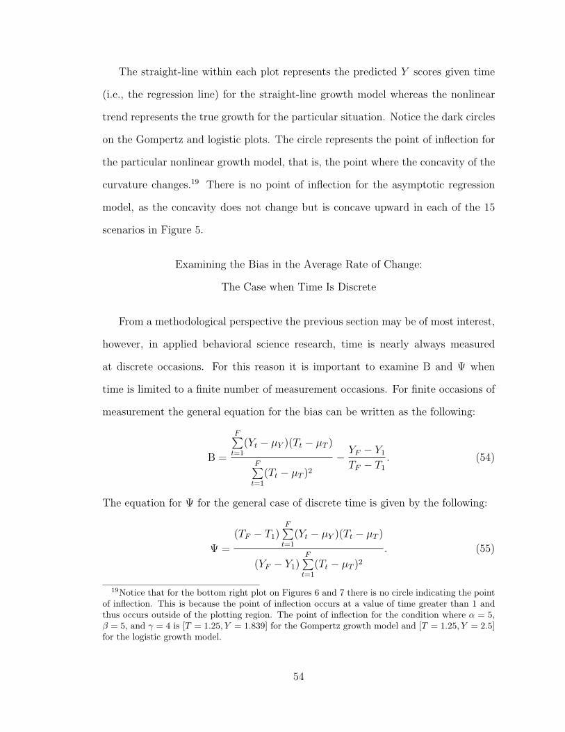
The straight-line within each plot represents the predicted Y scores given time

(i.e., the regression line) for the straight-line growth model whereas the nonlinear

trend represents the true growth for the particular situation. Notice the dark circles

on the Gompertz and logistic plots. The circle represents the point of inflection for

the particular nonlinear growth model, that is, the point where the concavity of the

curvature changes.19 There is no point of inflection for the asymptotic regression

model, as the concavity does not change but is concave upward in each of the 15

scenarios in Figure 5.

Examining the Bias in the Average Rate of Change:

The Case when Time Is Discrete

From a methodological perspective the previous section may be of most interest,

however, in applied behavioral science research, time is nearly always measured

at discrete occasions. For this reason it is important to examine B and ! when

time is limited to a finite number of measurement occasions. For finite occasions of

measurement the general equation for the bias can be written as the following:

B =

F+t=1

(Yt " µY )(Tt " µT )

F+t=1

(Tt " µT )2

" YF " Y1

TF " T1. (54)

The equation for ! for the general case of discrete time is given by the following:

! =

(TF " T1)F+

t=1(Yt " µY )(Tt " µT )

(YF " Y1)F+

t=1(Tt " µT )2

. (55)

19Notice that for the bottom right plot on Figures 6 and 7 there is no circle indicating the pointof inflection. This is because the point of inflection occurs at a value of time greater than 1 andthus occurs outside of the plotting region. The point of inflection for the condition where ! = 5," = 5, and % = 4 is [T = 1.25, Y = 1.839] for the Gompertz growth model and [T = 1.25, Y = 2.5]for the logistic growth model.

54

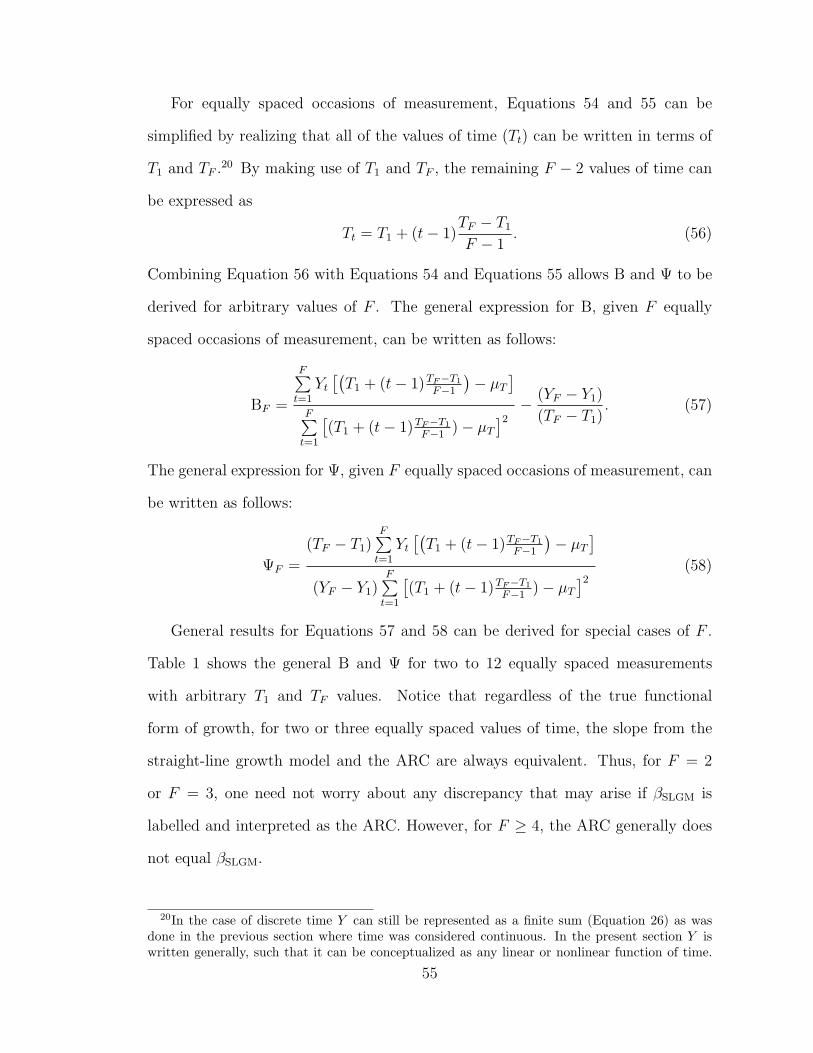
For equally spaced occasions of measurement, Equations 54 and 55 can be

simplified by realizing that all of the values of time (Tt) can be written in terms of

T1 and TF .20 By making use of T1 and TF , the remaining F " 2 values of time can

be expressed as

Tt = T1 + (t" 1)TF " T1

F " 1. (56)

Combining Equation 56 with Equations 54 and Equations 55 allows B and ! to be

derived for arbitrary values of F . The general expression for B, given F equally

spaced occasions of measurement, can be written as follows:

BF =

F+t=1

Yt

/'T1 + (t" 1)TF#T1

F#1

(" µT

0

F+t=1

/(T1 + (t" 1)TF#T1

F#1 )" µT

02" (YF " Y1)

(TF " T1). (57)

The general expression for !, given F equally spaced occasions of measurement, can

be written as follows:

!F =

(TF " T1)F+

t=1Yt

/'T1 + (t" 1)TF#T1

F#1

(" µT

0

(YF " Y1)F+

t=1

/(T1 + (t" 1)TF#T1

F#1 )" µT

02(58)

General results for Equations 57 and 58 can be derived for special cases of F .

Table 1 shows the general B and ! for two to 12 equally spaced measurements

with arbitrary T1 and TF values. Notice that regardless of the true functional

form of growth, for two or three equally spaced values of time, the slope from the

straight-line growth model and the ARC are always equivalent. Thus, for F = 2

or F = 3, one need not worry about any discrepancy that may arise if !SLGM is

labelled and interpreted as the ARC. However, for F ( 4, the ARC generally does

not equal !SLGM.

20In the case of discrete time Y can still be represented as a finite sum (Equation 26) as wasdone in the previous section where time was considered continuous. In the present section Y iswritten generally, such that it can be conceptualized as any linear or nonlinear function of time.

55

Tab

le1.

GEN

ER

AL

EQ

UATIO

NS

FO

RB

AN

D!

FO

RTW

OTO

12EQ

UA

LLY

SPA

CED

TIM

EPO

INTS

WIT

HA

RBIT

RA

RY

INIT

IAL

AN

DEN

DPO

INTS

FB

ias

!

20

13

01

4(Y

1#

Y4)+

3(Y3#

Y2)

10(T

4#

T1)

3 103(

Y1#

Y4)+

(Y2#

Y3)

(Y1#

Y4)

5(Y

1#

Y5)+

2(Y4#

Y2)

5(T5#

T1)

2 52(

Y5#

Y1)+

(Y4#

Y2)

(Y5#

Y1)

62(

Y1#

Y6)+

3(Y5#

Y2)+

(Y4#

Y3)

7(T6#

T1)

5(Y6#

Y1)+

3(Y5#

Y2)+

(Y4#

Y3)

7(Y6#

Y1)

75(

Y1#

Y7)+

6(Y6#

Y2)+

3(Y5#

Y3)

14(T

7#

T1)

3 143(

Y7#

Y1)+

2(Y

6#

Y2)+

(Y5#

Y3)

(Y7#

Y1)

85(

Y1#

Y8+

Y7#

Y2)+

3(Y6#

Y3)+

(Y5#

Y4)

12(T

8#

T1)

7(Y8#

Y1)+

5(Y7#

Y2)+

3(Y6#

Y3)+

(Y5#

Y4)

12(Y

8#

Y1)

97(Y

1#

Y9)+

6(Y

8#

Y2)+

4(Y

7#

Y3)+

2(Y

6#

Y4)

15(T

9#

T1)

2 154(

Y9#

Y1)+

3(Y8#

Y2)+

2(Y7#

Y3)+

(Y6#

Y4)

(Y9#

Y1)

1028(Y

1#

Y10)+

21(Y

9#

Y2)

+15

(Y8#

Y3)+

9(Y

7#

Y4)+

3(Y

6#

Y5)

55(T

10#

T1)

3 559(

Y10#

Y1)+

7(Y

9#

Y2)+

5(Y8#

Y3)+

3(Y7#

Y4)+

(Y6#

Y5)

(Y10#

Y1)

116(

Y1#

Y11)+

4(Y10#

Y2)+

3(Y9#

Y3)+

2(Y8#

Y4)+

(Y7#

Y5)

11(T

11#

T1)

5(Y11#

Y1)+

4(Y

10#

Y2)+

3(Y9#

Y3)+

2(Y8#

Y4)+

(Y7#

Y5)

11(Y

11#

Y1)

1215

(Y1#

Y12)+

9(Y

11#

Y2)+

7(Y10#

Y3)+

5(Y9#

Y4)+

3(Y8#

Y5)+

(Y7#

Y6)

26(T

12#

T1)

11(Y

12#

Y1)+

9(Y11#

Y2)+

7(Y10#

Y3)+

5(Y9#

Y4)+

3(Y8#

Y5)+

(Y7#

Y6)

26(Y

12#

Y1)

56

Table 1 can be used in at least two ways. Suppose that some functional form of

growth, the initial value of time, and F are known for equally spaced values of time.

The value of B and ! can then be determined by making use of the expressions given

in Table 1 (2 & F & 12). For any case where B does not equal zero (implying ! %= 1),

the extent of the discrepancy will be known for the functional form of interest. In the

event that the true functional form of growth is known exactly, the expected value

for !SLGM could be “corrected” by scaling the expected !SLGM in order for B to equal

zero (equivalently making ! = 1), such that the scaled regression coe#cient could

be used as an unbiased estimate of the ARC.21 Furthermore, for a given F , B could

be set to zero (or ! set to one) in order to discern under what circumstances the

expected !SLGM will equal ARC. For example, when F = 4, !SLGM = ARC whenever

Y1 " Y4 = 3(Y2 " Y3). Thus, there is zero bias whenever "Y1 + 3Y2 " 3Y3 + Y4 = 0.

Note that the coe#cients in the bias equation when F = 4 (-1, 3, -3, and 1

for Y1 through Y4 respectively) have an interpretation beyond that of the present

context. In fact, the coe#cients (or the coe#cients scaled by a constant) correspond

to orthogonal polynomial coe#cients in the context of trend analysis. Specifically for

four levels of a quantitative factor in an analysis of variance context, the coe#cients

in the bias equation for F = 4 correspond to the coe#cients for the test of the

cubic trend (Tables of orthogonal polynomial can be found in Pearson & Hartley,

1970, specifically Table 47). When F = 4, fitting a third degree polynomial growth

model ensures a perfect fit and fitting a fourth degree polynomial equation cannot

be carried out as the degrees of freedom become negative. In order for the expected

value of !SLGM to be equal to the ARC when F = 4, there must be no evidence

By writing Y generally, B and # can themselves be expressed in the most general general form fordiscrete data.

21Of course, this second potential use for Table 1 would imply that the true functional form ofgrowth was known exactly. If this were true, it would make more sense to fit the correct functionalform of growth to begin with rather than fitting the straight-line growth model for “interpretationalease.”

57

of a cubic trend. That is, the coe#cients for the bias from Table 1 multiplied by

the appropriate expected dependent variables must equal zero. Because any strictly

linear trend or a combination of linear and/or quadratic trends (when measurement

occasions are equally spaced) yields an unbiased estimate of the ARC as measured

from !SLGM, the sum of the coe#cients multiplied by the appropriate Yt will equal

zero. In cases where F = 4 (and indeed when F > 4) and there is evidence of a

cubic trend, !SLGM will not be an unbiased estimate of the ARC.

A similar interpretation for values of F > 4 also exists, namely that when a

strictly linear trend exists, when occasions of measurement are equally spaced and

a quadratic trend exists, or when occasions of measurement are equally spaced and

a combination of linear and quadratic trends exists, the sum of the orthogonal

polynomials multiplied by the appropriate Yt will be zero for all trends greater

than quadratic. Thus, when measurement occasions are equally spaced, the sum

of the orthogonal polynomials multiplied by the appropriate Yt is zero for trends

greater than quadratic, implying that only a linear and/or a quadratic trend exists,

!SLGM will exactly equal ARC. The point is that when a strictly linear trend exists,

when measurement occasions are equally spaced and a strictly quadratic trend

exists, or some combination or linear and quadratic trends exists for equally spaced

measurement occasions, the bias in Table 1 will be zero. When there are trends

greater than quadratic, the equations in Table 1 will not be zero implying that

!SLGM will di"er from the ARC.

Rather than examining Table 1 for general cases of discrete time (for two to

12 timepoints), it is also helpful to examine B and ! for specific functional forms

of growth. Tables 2, 3, 4, and 5 illustrate B and ! for a variety of scenarios (9

conditions within each of 57 conditions = 513 total scenarios). Specifically Table 2

examines various linear models when T ! [0, 1], as well as additional linear models

58

(and two logarithmic) when T ! [1, 5].22 Tables 3, 4, and 5 give the value of B and

! for four to 12 timepoints for the asymptotic regression, Gompertz, and logistic

growth models previously illustrated in Figures 5, 6, and 7 respectively.

22Note that the ARC=1 in each condition where T ! [0, 1]. Further note that the intervalT ! [0, 5] was used for the linear models not defined when T = 0].

59

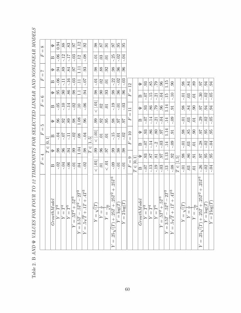
Tab

le2.

BA

ND

!VA

LU

ES

FO

RFO

UR

TO

12TIM

EPO

INTS

FO

RSELECTED

LIN

EA

RA

ND

NO

NLIN

EA

RM

OD

ELS

F=

4F

=5

F=

6F

=7

F=

8T!

[0,1

]G

row

thM

odel

B#

B#

B#

B#

B#

Y=

T3

-.02

.98

-.04

.96

-.05

.95

-.06

.94

-.06

0.94

Y=

T4

-.04

.96

-.07

.92

-.10

.90

-.11

.89

-.12

.88

Y=

T5

-.06

.94

-.11

.89

-.14

.86

-.16

.84

-.17

.83

Y=

.5T

2+

.5T

3-.0

1.9

9-.0

2.9

8-.0

2.9

8-.0

3.9

7-.0

3.9

7Y

=3.

5T"

.5T

2"

2T3

.04

1.04

.08

1.08

.10

1.1

.11

1.11

.12

1.12

Y=

.5)

T+

.1T

+.4

T3

-.02

.98

-.04

.96

-.06

.94

-.07

.93

-.08

.92

T!

[1,5

]Y

=1

(T)

<|.0

1|.9

9<

|.01|

.99

<|.0

1|.9

8-.0

1.9

8-.0

1.9

8Y

=1 T

.01

.96

.01

.92

.02

.90

.02

.88

.03

.87

Y=

1 %T

<.0

1.9

7.0

1.9

5.0

1.9

3.0

1.9

2.0

1.9

1Y

=.2

51(T

)+.2

5T+

.25T

2+

.25T

3-.0

9.9

9-.1

5.9

8-.1

9.9

8-.2

2.9

8-.2

5.9

7Y

=lo

g(T

)-.0

1.9

8-.0

1.9

7-.0

1.9

6-.0

2.9

6-.0

2.9

5Y

=2

log(

T)

-.01

.98

-.02

.97

-.03

.96

-.03

.96

-.04

.95

F=

9F

=10

F=

11F

=12

T!

[0,1

]G

row

thM

odel

B#

B#

B#

B#

Y=

T3

-.07

.93

-.07

.93

-.07

.93

-.07

.93

Y=

T4

-.13

.87

-.14

.86

-.14

.86

-.15

.85

Y=

T5

-.19

.81

-.2.8

0-.2

1.7

9-.2

1.7

9Y

=.5

T2+

.5T

3-.0

3.9

7-.0

3.9

7-.0

4.9

6-.0

4.9

6Y

=3.

5T"

.5T

2"

2T3

.13

1.13

.14

1.14

.14

1.14

.15

1.15

Y=

.5)

T+

.1T

+.4

T3

-.08

.92

-.09

.91

-.09

.91

-.10

.90

T!

[1,5

]Y

=1

(T)

-.01

.98

-.01

.98

-.01

.98

-.01

.98

Y=

1 T.0

3.8

6.0

3.8

5.0

3.8

4.0

3.8

4Y

=1 %T

.01

.91

.01

.90

.01

.90

.01

.89

Y=

.251

(T)+

.25T

+.2

5T2+

.25T

3-.2

6.9

7-.2

8.9

7-.2

9.9

7-.3

0.9

7Y

=lo

g(T

)-.0

2.9

5-.0

2.9

5-.0

2.9

4-.0

2.9

4Y

=2

log(

T)

-.04

.95

-.04

.95

-.05

.94

-.05

.94

60

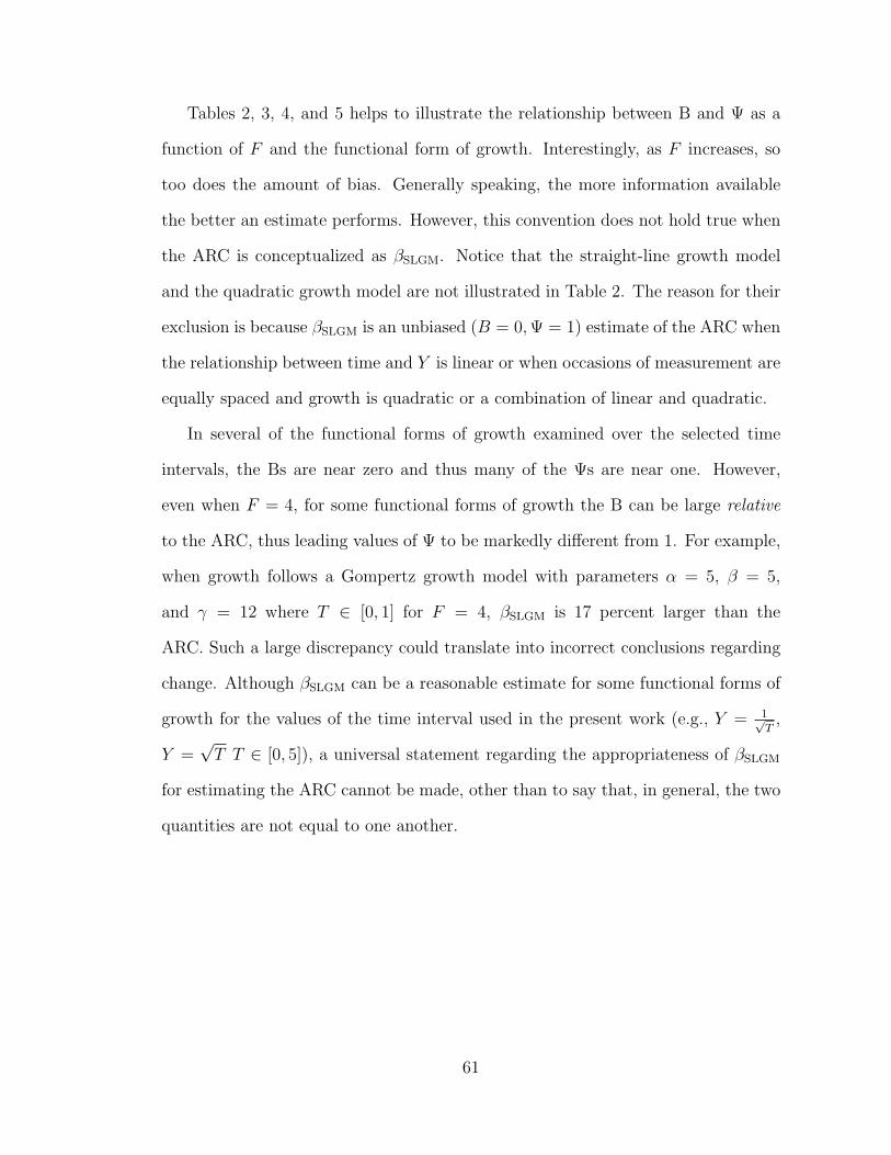
Tables 2, 3, 4, and 5 helps to illustrate the relationship between B and ! as a

function of F and the functional form of growth. Interestingly, as F increases, so

too does the amount of bias. Generally speaking, the more information available

the better an estimate performs. However, this convention does not hold true when

the ARC is conceptualized as !SLGM. Notice that the straight-line growth model

and the quadratic growth model are not illustrated in Table 2. The reason for their

exclusion is because !SLGM is an unbiased (B = 0, ! = 1) estimate of the ARC when

the relationship between time and Y is linear or when occasions of measurement are

equally spaced and growth is quadratic or a combination of linear and quadratic.

In several of the functional forms of growth examined over the selected time

intervals, the Bs are near zero and thus many of the !s are near one. However,

even when F = 4, for some functional forms of growth the B can be large relative

to the ARC, thus leading values of ! to be markedly di"erent from 1. For example,

when growth follows a Gompertz growth model with parameters " = 5, ! = 5,

and # = 12 where T ! [0, 1] for F = 4, !SLGM is 17 percent larger than the

ARC. Such a large discrepancy could translate into incorrect conclusions regarding

change. Although !SLGM can be a reasonable estimate for some functional forms of

growth for the values of the time interval used in the present work (e.g., Y = 1%T,

Y =)

T T ! [0, 5]), a universal statement regarding the appropriateness of !SLGM

for estimating the ARC cannot be made, other than to say that, in general, the two

quantities are not equal to one another.

61

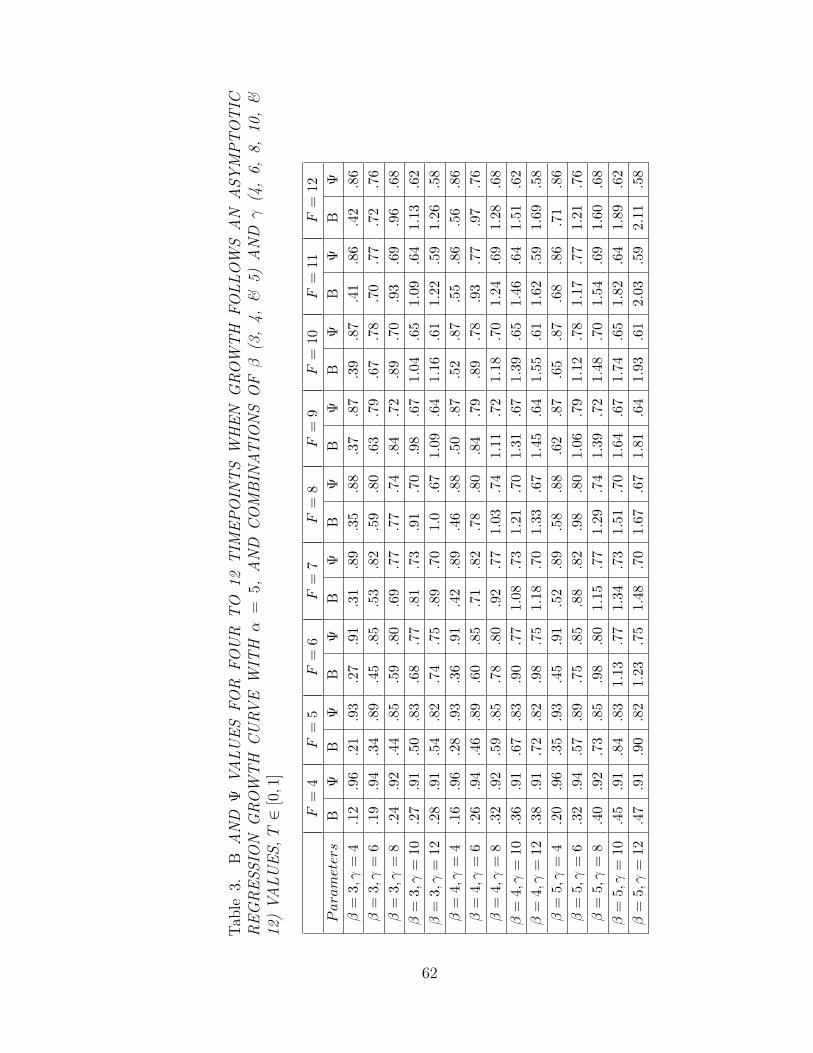
Tab

le3.

BA

ND

!VA

LU

ES

FO

RFO

UR

TO

12T

IMEPO

INTS

WH

EN

GRO

WTH

FO

LLO

WS

AN

ASY

MPTO

TIC

REG

RESSIO

NG

RO

WTH

CU

RV

EW

ITH

"=

5,A

ND

CO

MBIN

ATIO

NS

OF

!(3

,4,

&5)

AN

D#

(4,

6,8,

10,

&12

)VA

LU

ES,T!

[0,1

]

F=

4F

=5

F=

6F

=7

F=

8F

=9

F=

10F

=11

F=

12P

aram

eter

sB

#B

#B

#B

#B

#B

#B

#B

#B

#"

=3,

%=

4.1

2.9

6.2

1.9

3.2

7.9

1.3

1.8

9.3

5.8

8.3

7.8

7.3

9.8

7.4

1.8

6.4

2.8

6"

=3,

%=

6.1

9.9

4.3

4.8

9.4

5.8

5.5

3.8

2.5

9.8

0.6

3.7

9.6

7.7

8.7

0.7

7.7

2.7

6"

=3,

%=

8.2

4.9

2.4

4.8

5.5

9.8

0.6

9.7

7.7

7.7

4.8

4.7

2.8

9.7

0.9

3.6

9.9

6.6

8"

=3,

%=

10.2

7.9

1.5

0.8

3.6

8.7

7.8

1.7

3.9

1.7

0.9

8.6

71.

04.6

51.

09.6

41.

13.6

2"

=3,

%=

12.2

8.9

1.5

4.8

2.7

4.7

5.8

9.7

01.

0.6

71.

09.6

41.

16.6

11.

22.5

91.

26.5

8"

=4,

%=

4.1

6.9

6.2

8.9

3.3

6.9

1.4

2.8

9.4

6.8

8.5

0.8

7.5

2.8

7.5

5.8

6.5

6.8

6"

=4,

%=

6.2

6.9

4.4

6.8

9.6

0.8

5.7

1.8

2.7

8.8

0.8

4.7

9.8

9.7

8.9

3.7

7.9

7.7

6"

=4,

%=

8.3

2.9

2.5

9.8

5.7

8.8

0.9

2.7

71.

03.7

41.

11.7

21.

18.7

01.

24.6

91.

28.6

8"

=4,

%=

10.3

6.9

1.6

7.8

3.9

0.7

71.

08.7

31.

21.7

01.

31.6

71.

39.6

51.

46.6

41.

51.6

2"

=4,

%=

12.3

8.9

1.7

2.8

2.9

8.7

51.

18.7

01.

33.6

71.

45.6

41.

55.6

11.

62.5

91.

69.5

8"

=5,

%=

4.2

0.9

6.3

5.9

3.4

5.9

1.5

2.8

9.5

8.8

8.6

2.8

7.6

5.8

7.6

8.8

6.7

1.8

6"

=5,

%=

6.3

2.9

4.5

7.8

9.7

5.8

5.8

8.8

2.9

8.8

01.

06.7

91.

12.7

81.

17.7

71.

21.7

6"

=5,

%=

8.4

0.9

2.7

3.8

5.9

8.8

01.

15.7

71.

29.7

41.

39.7

21.

48.7

01.

54.6

91.

60.6

8"

=5,

%=

10.4

5.9

1.8

4.8

31.

13.7

71.

34.7

31.

51.7

01.

64.6

71.

74.6

51.

82.6

41.

89.6

2"

=5,

%=

12.4

7.9

1.9

0.8

21.

23.7

51.

48.7

01.

67.6

71.

81.6

41.

93.6

12.

03.5

92.

11.5

8

62

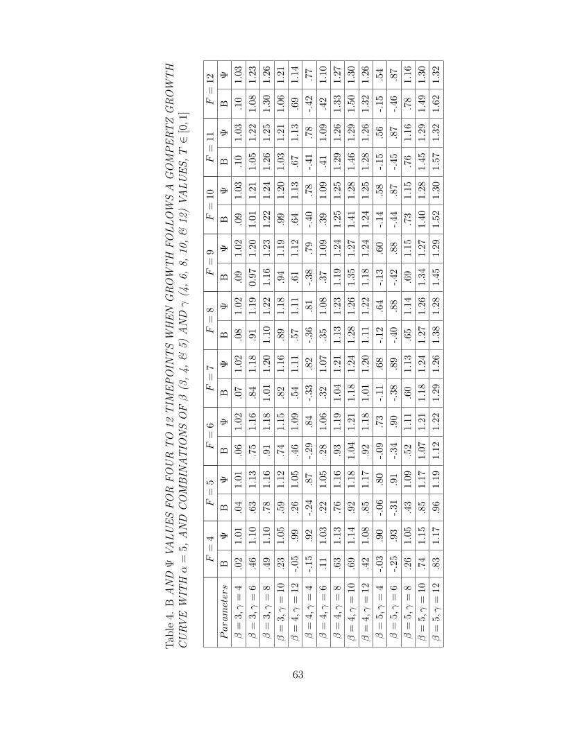
Tab

le4.

BA

ND

!VA

LU

ES

FO

RFO

UR

TO

12TIM

EPO

INTS

WH

EN

GRO

WTH

FO

LLO

WS

AG

OM

PERTZ

GRO

WTH

CU

RV

EW

ITH

"=

5,A

ND

CO

MBIN

ATIO

NS

OF

!(3

,4,

&5)

AN

D#

(4,6,

8,10

,&

12)

VA

LU

ES,T!

[0,1

]

F=

4F

=5

F=

6F

=7

F=

8F

=9

F=

10F

=11

F=

12P

aram

eter

sB

#B

#B

#B

#B

#B

#B

#B

#B

#"

=3,

%=

4.0

21.

01.0

41.

01.0

61.

02.0

71.

02.0

81.

02.0

91.

02.0

91.

03.1

01.

03.1

01.

03"

=3,

%=

6.4

61.

10.6

31.

13.7

51.

16.8

41.

18.9

11.

190.

971.

201.

011.

211.

051.

221.

081.

23"

=3,

%=

8.4

91.

10.7

81.

16.9

11.

181.

011.

201.

101.

221.

161.

231.

221.

241.

261.

251.

301.

26"

=3,

%=

10.2

31.

05.5

91.

12.7

41.

15.8

21.

16.8

91.

18.9

41.

19.9

91.

201.

031.

211.

061.

21"

=4,

%=

12-.0

5.9

9.2

61.

05.4

61.

09.5

41.

11.5

71.

11.6

11.

12.6

41.

13.6

71.

13.6

91.

14"

=4,

%=

4-.1

5.9

2-.2

4.8

7-.2

9.8

4-.3

3.8

2-.3

6.8

1-.3

8.7

9-.4

0.7

8-.4

1.7

8-.4

2.7

7"

=4,

%=

6.1

11.

03.2

21.

05.2

81.

06.3

21.

07.3

51.

08.3

71.

09.3

91.

09.4

11.

09.4

21.

10"

=4,

%=

8.6

31.

13.7

61.

16.9

31.

191.

041.

211.

131.

231.

191.

241.

251.

251.

291.

261.

331.

27"

=4,

%=

10.6

91.

14.9

21.

181.

041.

211.

181.

241.

281.

261.

351.

271.

411.

281.

461.

291.

501.

30"

=4,

%=

12.4

21.

08.8

51.

17.9

21.

181.

011.

201.

111.

221.

181.

241.

241.

251.

281.

261.

321.

26"

=5,

%=

4-.0

3.9

0-.0

6.8

0-.0

9.7

3-.1

1.6

8-.1

2.6

4-.1

3.6

0-.1

4.5

8-.1

5.5

6-.1

5.5

4"

=5,

%=

6-.2

5.9

3-.3

1.9

1-.3

4.9

0-.3

8.8

9-.4

0.8

8-.4

2.8

8-.4

4.8

7-.4

5.8

7-.4

6.8

7"

=5,

%=

8.2

61.

05.4

31.

09.5

21.

11.6

01.

13.6

51.

14.6

91.

15.7

31.

15.7

61.

16.7

81.

16"

=5,

%=

10.7

41.

15.8

51.

171.

071.

211.

181.

241.

271.

261.

341.

271.

401.

281.

451.

291.

491.

30"

=5,

%=

12.8

31.

17.9

61.

191.

121.

221.

291.

261.

381.

281.

451.

291.

521.

301.

571.

321.

621.

32

63

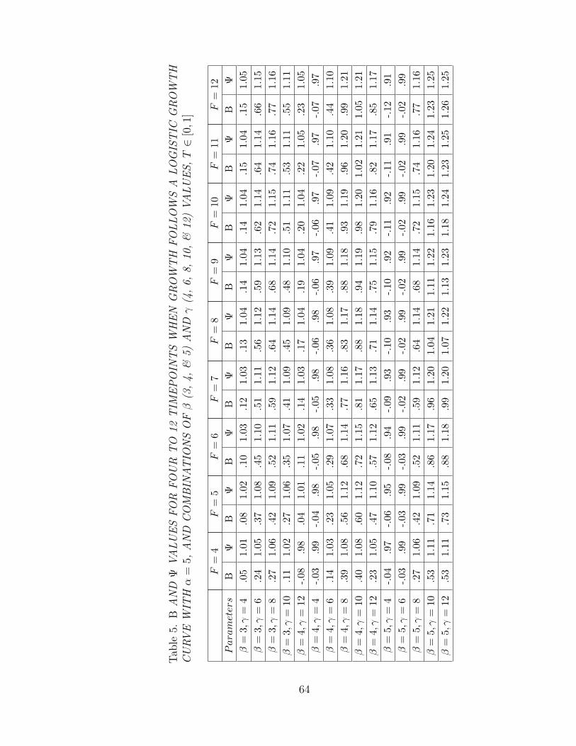
Tab

le5.

BA

ND

!VA

LU

ES

FO

RFO

UR

TO

12TIM

EPO

INTS

WH

EN

GRO

WTH

FO

LLO

WS

ALO

GIS

TIC

GRO

WTH

CU

RV

EW

ITH

"=

5,A

ND

CO

MBIN

ATIO

NS

OF

!(3

,4,

&5)

AN

D#

(4,6,

8,10

,&

12)

VA

LU

ES,T!

[0,1

]

F=

4F

=5

F=

6F

=7

F=

8F

=9

F=

10F

=11

F=

12P

aram

eter

sB

#B

#B

#B

#B

#B

#B

#B

#B

#"

=3,

%=

4.0

51.

01.0

81.

02.1

01.

03.1

21.

03.1

31.

04.1

41.

04.1

41.

04.1

51.

04.1

51.

05"

=3,

%=

6.2

41.

05.3

71.

08.4

51.

10.5

11.

11.5

61.

12.5

91.

13.6

21.

14.6

41.

14.6

61.

15"

=3,

%=

8.2

71.

06.4

21.

09.5

21.

11.5

91.

12.6

41.

14.6

81.

14.7

21.

15.7

41.

16.7

71.

16"

=3,

%=

10.1

11.

02.2

71.

06.3

51.

07.4

11.

09.4

51.

09.4

81.

10.5

11.

11.5

31.

11.5

51.

11"

=4,

%=

12-.0

8.9

8.0

41.

01.1

11.

02.1

41.

03.1

71.

04.1

91.

04.2

01.

04.2

21.

05.2

31.

05"

=4,

%=

4-.0

3.9

9-.0

4.9

8-.0

5.9

8-.0

5.9

8-.0

6.9

8-.0

6.9

7-.0

6.9

7-.0

7.9

7-.0

7.9

7"

=4,

%=

6.1

41.

03.2

31.

05.2

91.

07.3

31.

08.3

61.

08.3

91.

09.4

11.

09.4

21.

10.4

41.

10"

=4,

%=

8.3

91.

08.5

61.

12.6

81.

14.7

71.

16.8

31.

17.8

81.

18.9

31.

19.9

61.

20.9

91.

21"

=4,

%=

10.4

01.

08.6

01.

12.7

21.

15.8

11.

17.8

81.

18.9

41.

19.9

81.

201.

021.

211.

051.

21"

=4,

%=

12.2

31.

05.4

71.

10.5

71.

12.6

51.

13.7

11.

14.7

51.

15.7

91.

16.8

21.

17.8

51.

17"

=5,

%=

4-.0

4.9

7-.0

6.9

5-.0

8.9

4-.0

9.9

3-.1

0.9

3-.1

0.9

2-.1

1.9

2-.1

1.9

1-.1

2.9

1"

=5,

%=

6-.0

3.9

9-.0

3.9

9-.0

3.9

9-.0

2.9

9-.0

2.9

9-.0

2.9

9-.0

2.9

9-.0

2.9

9-.0

2.9

9"

=5,

%=

8.2

71.

06.4

21.

09.5

21.

11.5

91.

12.6

41.

14.6

81.

14.7

21.

15.7

41.

16.7

71.

16"

=5,

%=

10.5

31.

11.7

11.

14.8

61.

17.9

61.

201.

041.

211.

111.

221.

161.

231.

201.

241.

231.

25"

=5,

%=

12.5

31.

11.7

31.

15.8

81.

18.9

91.

201.

071.

221.

131.

231.

181.

241.

231.

251.

261.

25

64

EMPIRICAL INVESTIGATION OF THE DISTRIBUTION

OF INSTANTANEOUS RATES OF CHANGE

Recall the discussion of Figure 1. The value selected to describe the 21

instantaneous rates of change was the mean. Recall that for illustrative purposes

only 21 of the infinitely many rates of change were used for the presumed case of

continuous time. At the present time it is not clear that the mean alone is su#cient

to fully and adequately represent the set of instantaneous rates of change. Thus,

a question that remains is how the change for an individual trajectory from T1 to

TF should be described. One possibility that emerges is examining the distribution

of instantaneous rates of change in order to discern characteristic properties of the

instantaneous rates of change.

Apparently the distribution of instantaneous rates of change from an individual

trajectory has not previously received much attention. Thus, the shape of such

a distribution, its median, and its standard deviation are not well-known. The

majority of the present work has been centered around describing growth via a single

summary value, namely the mean of all possible instantaneous rates of change for

an individual trajectory. Unacknowledged until the present section has been the

implicit assumption that the mean of all possible rates of change, rather than some

other measure, is the statistic of choice for describing and helping to understand

growth for an individual trajectory. Although the mean rate of change is perhaps the

most intuitive value for describing a collection of rates of change, questions remain

as to whether the mean alone is the optimal value in the context of longitudinal

data. Further questions remain regarding the shape and spread of the distribution

65

of instantaneous rates of change from an individual trajectory. This section explores

other descriptive statistics that have the potential to be useful for describing the

instantaneous rate of change over time for an individual trajectory.

For 23 functional forms of growth a distribution of instantaneous rates of change

was produced by evaluating the derivative of the function at a large number of points

(The number of timepoints, $ = 10#6, was 1,000,001 for the first 18 conditions

(T ! [0, 1]) and 4,000,001 for the remaining 5 conditions (T ! [1, 5]), thus time

was nearly continuous.). This collection of instantaneous rates of change was

used to calculate descriptive statistics in order to document selected distributional

properties of the instantaneous rates of change for individual trajectories for a

variety of functional forms of growth. The mean, median, standard deviation, skew,

kurtosis, and selected percentiles (2.5, 5, 95, 97.5) of the instantaneous rates of

change were calculated.23 The particular functional forms of growth examined and

the accompanying descriptive statistics of the distribution of instantaneous rates of

change are given in Table 6.

23Measures of skew and kurtosis were calculated in accord with the recommendations of Stuart

and Ord (1994, p. 109). Specifically, skew was defined asn"1

n,i=1

x3i

-n"1

n,i=1

x2i

.1.5 whereas kurtosis was

defined asn"1

n,i=1

x4i

-n"1

n,i=1

x2i

.2 " 3, where xi is (Xi " X) and n is the number of Xi values.

66

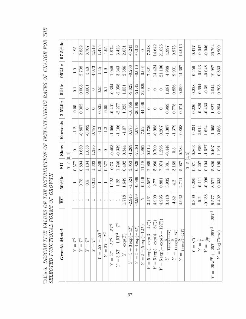
Tab

le6.

DESCR

IPTIV

EVA

LU

ES

OF

TH

ED

ISTR

IBU

TIO

NO

FIN

STA

NTA

NEO

US

RATES

OF

CH

AN

GE

FO

RTH

ESELECTED

FU

NCTIO

NA

LFO

RM

SO

FG

RO

WTH

Gro

wth

Mod

elR

C50

%ile

SD

Ske

wK

urt

osis

2.5%

ile

5%ile

95%

ile

97.5

%ile

T!

[0,1

]Y

=T

21

10.

577

0-1

.20.

050.

11.

91.

95Y

=T

31

0.75

0.89

40.

639

-0.8

570.

002

0.00

82.

708

2.85

2Y

=T

41

0.5

1.13

41.

058

-0.0

920

0.00

13.

433.

707

Y=

T5

10.

313

1.33

31.

385

0.78

70

04.

073

4.51

8Y

=.5

T+

.5T

21

10.

289

0-1

.20.

525

0.55

1.45

1.47

5Y

=2T"

T2

11

0.57

70

-1.2

0.05

0.1

1.9

1.95

Y=

2T"

.5T

2"

.5T

31

1.12

50.

73-0

.403

-1.0

66-0

.401

-0.3

041.

946

1.97

4Y

=3.

5T"

1.5T

2"

T3

11.

251.

746

-0.3

39-1

.106

-2.2

77-2

.058

3.34

33.

423

Y=

exp(

T)

1.71

81.

649

0.49

20.

344

-1.0

71.

025

1.05

12.

586

2.65

1Y

=5

+3

exp("

4T)

-2.9

45-1

.624

3.05

3-1

.269

0.57

3-1

0.85

8-9

.825

-0.2

68-0

.243

Y=

5+

4ex

p("

8T)

-3.9

99-0

.586

6.92

9-2

.181

4.07

3-2

6.19

9-2

1.45

-0.0

16-0

.013

Y=

5+

5ex

p("

12T

)-5

-0.1

4911

.18

-2.8

627.

92-4

4.44

9-3

2.92

9-0

.001

0Y

=5

exp("

exp(

3"

4T))

3.46

13.

587

2.96

90.

012

-1.7

390

07.

321

7.34

8Y

=5

exp("

exp(

4"

8T))

4.90

92.

775.

086

0.70

9-0

.988

00

14.4

2414

.642

Y=

5ex

p("

exp(

5"

12T

))4.

995

0.88

17.

074

1.29

60.

207

00

21.1

0621

.826

Y=

51+

exp(3#

4T

)3.

418

3.93

21.

381

-0.4

48-1

.307

0.98

91.

081

4.98

84.

997

Y=

51+

exp(4#

8T

)4.

824.

23.

168

0.3

-1.3

790.

778

0.85

69.

901

9.97

5Y

=5

1+ex

p(5#

12T

)4.

962

2.71

15.

037

0.78

4-0

.868

0.07

40.

099

14.6

6714

.916

T!

[1,5

]Y

=)

T0.

309

0.28

90.

071

0.86

3-0

.234

0.22

60.

228

0.45

60.

477

Y=

1 T-0

.2-0

.111

0.20

7-1

.859

2.91

4-0

.826

-0.6

94-0

.043

-0.0

42Y

=1 %T

-0.1

38-0

.096

0.10

4-1

.527

1.62

4-0

.433

-0.3

8-0

.048

-0.0

46Y

=.2

5)T

+.2

5T+

.25T

2+

.25T

39.

577

8.57

25.

826

0.40

7-1

.065

1.82

72.

044

19.9

8720

.764

Y=

log(

Tim

e)0.

402

0.33

30.

195

1.19

10.

566

0.20

40.

208

0.83

30.

909

67

In each of the 23 conditions the obtained mean rate of change'RC

(of the

distribution of instantaneous rates of change was equal to the known ARC, as must

be the case given the previous discussion of the ARC. It is interesting to compare the

RC with the 50%ile (median) to see under what conditions the mean and the median

are equal. As shown in Table 6, the mean and the median are generally not equal

to one another, illustrating that the shape of the distribution of instantaneous rates

of change is not often symmetric. In fact, examining the skew of the distributions

(skew equals zero when a distribution is symmetric) shows that there are cases

where the distribution was positively skewed (12 instances), negatively skewed (8

instances), and few cases where the distribution was symmetric (3 instances).

The three distributions that were not skewed corresponded exactly to a uniform

distribution. A distribution where skew = 0 and kurtosis = -1.2 is a uniform (i.e.,

rectangular) distribution (DeCarlo, 1997, p. 293). These three distributions are

cases where !SLGM for the functional form of growth and the ARC are equivalent

across time and cases where growth is represented by a quadratic trend or by a

combination of linear and quadratic trend. Notice that absent from Table 6 is

the functional form for straight-line growth. Information about the distribution of

instantaneous rates of change for this particular growth model is not needed, as it

is known a priori. The mean instantaneous rates of change is the slope itself over

the range of time. Thus, the mean, median and percentiles are equal to the slope,

while the standard deviation, skew, and kurtosis are zero.

Table 6 illustrates that understanding a particular trajectory over time, let alone

a collection of trajectories, is a potentially daunting task. Because no consistent

distributional form emerged for the instantaneous rates of change for the selected

functional forms of growth, researchers should be aware that understanding growth

trajectories over time potentially involves more than a single descriptive value to

68

adequately describe the distribution of instantaneous rates of change. Although the

ARC is a useful summary value, the same shortcomings of the mean as a descriptive

and inferential value, which have been well documented in the literature, also apply

to the ARC in the present context. Nevertheless, regardless of the distributional

form of the instantaneous rates of change, the ARC describes the mean of all

theoretically possible instantaneous rates of change, a value of potential interest

to researchers who study change over time. Presumably such a statistic will help

researchers describe and potentially better understand the typical rate at which a

trajectory is, or is not, changing over time.24

24Although gaining a better understanding of the distribution of the instantaneous rates ofchange or even the ARC itself may well be helpful for describing and understand the processof change, the importance of estimating and interpreting the parameters of growth should not beneglected. Not only does the ARC provide potentially useful information, so too do the parametersof growth (perhaps even more so by estimating asymptotic values, scaling factors, and linearand/or quadratic components, etc.) and should also be of utmost concern. As previously stated,the proposed usage for the ARC is to supplement not supplant other measures of change. Thus,estimation of the growth parameters should not be neglected because interest is in the ARC.

69

PRELIMINARY SUGGESTIONS AND CAUTIONS WHEN

ESTIMATING THE AVERAGE RATE OF CHANGE

Conspicuously absent from the work thus far have been suggestions and

procedures for estimating the ARC. To thoroughly delineate such a topic would

require a lengthy work in itself. However, the present section allows for the discussion

of potentially useful methods when interest lies in estimating the ARC for a single

individual as well as the mean ARC across individuals. This section also provides

an opportunity to voice concerns about intuitively appealing, but perhaps not

statistically optimal, methods of estimating the ARC.

The Relationship Between the Di"erence Score and the Average Rate of Change

The observed di"erence score (also called change score or gain/loss score

depending on its sign) for a single individual over the time period Tt to Tt+! is

defined as

Dt+!,t = Yt+! " Yt, (59)

which is an estimate of the numerator of the true ARC given in Equation 5c. In

the spirit of classical test theory (e.g., Lord & Novick, 1968), an observed score is a

composite of a true score and error. An observed Yt is thus equal to

Yt = )t + &t, (60)

where )t is the true score and &t is the error at the tth timepoint. Because the

expected value of &t is zero, the expected value of Yt is )t. This equality extends

70

to the di"erence score, where it is shown that the expected value of the observed

di"erence score is equal to the expected value of the true score di"erence:

E[Dt+!,t] = E[Yt+! " Yt] (61a)

= E[Yt+! ]" E[Yt] (61b)

= )t+! " )t (61c)

= $t+!,t, (61d)

where $t+!,t is the true di"erence score over the time period Tt to Tt+! . Thus, the

observed di"erence score is an unbiased estimate of the population di"erence score,

regardless of the amount of measurement error in the observed scores (Rogosa et al.,

1982, p. 730).

Even though the di"erence score is an unbiased estimate, the di"erence score has

been subjected to harsh criticisms (See, for instance, the works contained in Harris,

1963, Lord, 1956 & 1958, Cronbach & Furby, 1970, and Linn & Slinde, 1977, but also

Rogosa et al., 1982, Zimmerman & Williams, 1982, and Willett, 1988, who show that

many of the previous criticisms of the di"erence score are unwarranted.). The vast

majority of criticisms regarding the di"erence score have to do with its reliability,

and to a lesser extent, the appearance that the true initial status and the true

di"erence score are negatively correlated, when in fact the observed correlation is a

poor estimate of the true correlation (Rogosa et al., 1982, pp. 734-735; Blomqvist,

1977).25 However, as Willett (1988) argues, “recent methodological research has

25The reason for the “appearance” that true initial status and true change are negativelycorrelated is because the sample correlation coe"cient between the observed initial status andobserved change is negatively biased for estimating the population correlation of the true initialstatus and the true change. The spuriousness of the observed correlation coe"cient, however, is“in no way . . . a fundamental problem with the use of the di!erence score as a measure ofindividual change” (Rogosa et al., 1982, p. 734). This is actually a long known fact (see Thomson,1924) that the relationship between true initial status and true change is attenuated because ofthe errors in the observed scores (Lord, 1958). Because interest lies in the correlation between thetrue scores, not the observed, the negatively biased correlation between the observed initial statusand observed change is not a valid criticism of the analysis of change.

71

revealed that these deficiencies are perceived rather than actual, imaginary rather

than real” (p. 367). Modern research on the analysis of change overshadows many of

the well-known critiques of yesteryear. Statements such as “the di"erence between

two fallible measures is frequently much more fallible than either” measure (Lord,

1963, p. 32) has been refuted, because it has been realized the reliability of a

di"erence can, in realistic situations, be more reliable than either of the fallible

measures.

The definition of reliability in the context of di"erence scores can be given as

'(D) =*2

&t+!#&t

*2&t+!#&t

+ *2't+!#'t

, (62)

where '(·) represents the population reliability of the quantity in parentheses and

*2 is the variance of the e"ect noted in the subscript and can be defined only over

a group or population (i.e., not for a single di"erence; Rogosa et al., 1982, p. 730).

When &t and &t+! are independent within and across individuals, Equation 62 can

be rewritten as

'(D) =*Yt'(Yt) + *Yt+! '(Yt+! )" 2*Yt*Yt+! '&t&t+!

*2Yt

+ *2Yt+!

" 2*Yt*Yt+! '&t&t+!

, (63)

where ' represents the population zero-order correlation coe#cient of the two

subscripted random variables (Rogosa et al., 1982, pp. 730–731).

Conceptually, the reliability of the di"erence score represents the accuracy in

which individuals can be distinguished from one another on the basis of their

di"erence score. If the variance of the di"erence scores across a group or population

is small, meaning the di"erence scores are very similar, individuals will not be well

di"erentiated on the basis of their di"erence score and thus '(D) will be low. In such

circumstances, even when the error variance (*2't+!#'t

) is small, the reliability can

still be low. In order for the reliability of the di"erence score to be large, individual

72

di"erence in growth must persist, such that individuals can be di"erentiated from

one another on the basis of their di"erence score. However, as Rogosa et al. (1982)

point out, “low reliability does not necessarily imply lack of precision” and in fact

“the absence of such [individual] di"erences does not preclude meaningful assessment

of individual change” (p. 731).

One of the main reasons why the di"erence score has so often been criticized

is because authors commonly make use of restrictive special cases of Equation 62,

which oftentimes may be unrealistic in the context of longitudinal data analysis.

As Rogosa and Willett (1983) point out, authors who disparage the di"erence score

usually do so in a context where *&t = *&t+! , '(Yt) = '(Yt+! ), and for large positive

values of '&t&t+! (p. 336). Thus, low reliability of the di"erence score comes at

no surprise, because when '&t&t+! is large in the presence of constant reliabilities

and variances, di"erentiating among individual di"erence scores is di#cult. Rogosa

and Willett (1983) summarize the dubious pre-1980s literature on di"erence scores

by saying that the “di"erence score cannot detect individual di"erences in change

that do not exist, but it will show good reliability when individual di"erences in

true change are appreciable” (p. 341). Furthermore, the “di"erence score can be

an accurate and useful measure of individual change even in situations where the

reliability is low” (Rogosa et al., 1982, p. 730).26

Because an obvious method of estimating the ARC is to divide the di"erence

score by the time interval of interest,

!ARCt+!,t =Dt+!,t

Tt+! " Tt, (64)

where "x represents an estimate of the parameter x, the preceding remarks concerning

26In addition to low reliability not markedly a!ecting the usefulness of the di!erence score,Overall and Woodward (1975) showed that as the di!erence score reliability decreases, the power ofparametric statistical tests to detect group di!erences increases. This “paradox” helps to illustratethe fact that highly unreliable di!erences can be highly informative.

73

the di"erence score were necessary in order to develop the most natural method

of estimating the ARC. Specifically, the reliability of the ARC when the ARC

is calculated via Equation 64 is closely related to the reliability of the di"erence

score. In fact, for fixed values of time, the reliability of the ARC (calculated via

Equation 64) is equivalent to the reliability of the di"erence score.27 The reason

such an equivalency holds is because when the time interval of interest is fixed

(i.e., constant), the divisor of the ARC simply scales both *&t+!#&t and *'t+!#'t

(Equation 62) by Tt+! " Tt. Thus, the constant scaling cancels in the equation for

the reliability of the ARC and equals the reliability of the di"erence score. This

relationship is best illustrated by the definitional formula given in Equation 62

applied to the ARC:

(( +ARCt+!,t) =

#2!t+""!t

(Tt+"!Tt)2

#2!t+""!t

(Tt+"!Tt)2+

#2#t+""#t

(Tt+"!Tt)2

=

#2!t+""!t

(Tt+"!Tt)2

#2!t+""!t

+#2#t+""#t

(Tt+"!Tt)2

=()2

$t+"!$t)(Tt+! # Tt)2

(Tt+! # Tt)2()2$t+"!$t

+ )2%t+"!%t

)= ((D).

(65)

It is important to remember that Equation 65 holds only for fixed values of

time. If the time interval of interest is random across replications of the ARC, it

is not clear to what extent the reliability of !ARCt+!,t may change. The reason for

such uncertainty is because when the time interval is random across replications, the

variance of the true scores and the variance of the errors are themselves divided by a

random quantity. Khuri and Casella (2002) provide a discussion on the di#culties in

determining E(1/x), where x is some nonnegative continuously distributed random

variable, and the su#cient conditions for such an expectation to exist for continuous

distributions. Apparently no exact analog of the continuous case exists for E(1/x)

27In order to derive the reliability of the ARC, the variance of the ARC must be established.Appendix D shows the derivation of the variance of an individual’s di!erence score as well as thevariance of !ARCt+",t.

74

when x is discrete.28 Furthermore, when time is fixed and !ARCt+!,t is used to

estimate the ARC, !ARCt+!,t is an unbiased estimate of the true ARC. This can be

seen in an analogous manner as the reliability of the ARC:

E)

!ARCt+!,t

*= E

2Yt+! " Yt

Tt+! " Tt

3=

1

Tt+! " TtE[Yt+! " Yt] =

)t+! " )t

Tt+! " Tt. (66)

Thus, because the expected value is exactly equal to the true ARCt+!,t, it is an

unbiased estimate of the true ARC. Like the reliability of the ARC, it is not clear

if the ARC remains unbiased when (Tt+! " Tt) is a random quantity.

Although Equation 64 yields an unbiased estimate of the true ARC, in cases

where F > 2 such a method literally ignores all data between T1 and TF . Ignoring

data is not generally considered advisable. However, as Overall and Tonidandel

(2002) show, when the dependent variable follows an order one autoregressive

correlational structure with monotonically increasing growth over time, the ordinary

di"erence score is more powerful for detecting group di"erences than using !SLGM

and is essentially as powerful as the generalized least squares approach where

the autoregressive correlational structure is explicit in the model. Overall and

Tonidandel show this in the context of two stage (i.e., intensive design) growth

models (see page 115 and the power comparisons in Table 1 of Overall and

Tonidandel, 2002). Thus, if the order one autoregressive correlational structure

holds, a potentially complicated generalized least squares analysis can e"ectively

reduce to an analysis of di"erence scores. The next section illustrates two di"erent

methods of estimating the ARC.

28Mood, Graybill, and Boes give an approximation to E4

x1x2

5, where x1 and x2 are random

variables (1974, p. 181). Such an approximation would allow for the expected value of Equation 64to be a estimated when the time interval of interest was not considered fixed, as is the case in thepresent context, but when the time interval is random across the individuals.

75

Other Suggestions for Estimating the Average Rate of Change

Suppose that one makes the strong, and potentially untenable, assumption

that the growth model selected to represent the true functional form of growth

is literally the correct model. This supposition, however, is not trivial and the

method described under this assumption relies heavily on the model being correct.

Nevertheless, if the growth model selected by the researcher is correct, the approach

taken for producing the distributions of instantaneous rates of change for the results

contained in Table 1 may provide interesting and potentially useful information.

The empirical estimation of the instantaneous rates of change could proceed by

first assuming all individuals are governed by the same functional form of growth.29

After the model has been fit and the estimates of the fixed e"ects obtained, the

derivative of the assumed functional form of growth should be computed. The

derivative can be for a set of individuals or generalized such that di"erent groups

each have their own derivative. Once the derivative (derivatives for multiple group

designs) has been computed, the derivative should then be evaluated over a nearly

continuous time period in a computer program. The values of time can be thought

of as a vector from T1 to TF with $ being some small (e.g., 10#4) value. This vector

of nearly continuous time values can then be used for evaluating the derivative, such

that a large number of instantaneous rates of change are obtained.29This assumption, while not explicit in applications of HLM type analyses, is generally implicit

in the interpretation of results. When individuals (or groups) change following a di!erent functionalform of growth, modeling them as though they follow the same functional form leads to potentiallymisleading results. What does it mean for a significant linear trend to be found across a set ofindividuals when the individuals’ change follows di!erent functional forms of growth? For example,some individuals may follow exponential growth, some Gompertz growth, and still others quadraticgrowth. Obtaining statistical significance for a particular trend (e.g., linear and/or quadratic) whenthe individual trajectories follow di!erent forms of growth is not likely to shed much light on theunderlying question(s) of interest. The same problems arise when making group comparisons.For example, finding a significant di!erence for the slope between two groups means little if thefunctional form of growth is di!erent in the groups (let alone if individuals within the groups havedi!erent functional forms of growth). Discussions of this sort do not seem to manifest themselvesoften in methodological HLM works or in the context of longitudinal data analysis in general. Insituations where individuals follow di!erent functional forms of growth, the ARC may be an idealmeasure, because even when individuals have di!erent functional forms of growth, their ARC stillprovides meaningful information about the mean rate of change across time.

76

Once the set (i.e., vector) of instantaneous rates of change is computed, the mean,

median, standard deviation, confidence intervals, et cetera, can be computed as was

done in Table 6. Of course, because the obtained fixed e"ects are literally estimates

of the population values they represent, the computed statistics will not literally be

equal to their corresponding parameters. At the present time it is not clear how

well the confidence interval obtained by finding the value of the instantaneous rate

of change for selected lower and upper percentiles corresponds to the percentiles of

the population distribution of the instantaneous rate of change.

A possibility for yielding what could probabilistically be thought of as a “worst”

and/or “best” case scenario is to calculate the derivative not given the obtained

point estimates, but rather calculating the derivative using the lower and/or upper

confidence limits of the e"ect. Again, at the present time it is not clear how well

such a method may work. However, the basis for such a suggestion is that if the

lower and/or upper bound are treated as point estimates when the derivatives are

calculated, loosely speaking, those values represent, with the selected probability,

likely limits for the population parameter(s). Thus, if the population value(s)

are no smaller or no larger (probabilistically speaking) than the bounds of the

confidence interval, then the procedure o"ered here yields bounding distribution(s)

for the population instantaneous rates of change. Descriptive statistics can then

be calculated for these bounding distributions such that the estimates represent

one or both extremes of the probabilistic worst and best case scenarios for the

distribution of instantaneous rates of change. As the width of the confidence interval

around the population value approaches zero, the upper and/or lower bound(s) of

the confidence interval approach the obtained point estimate. Thus, the bounding

distributions of the instantaneous rates of change approach the distribution when

the point estimate itself is used. Thus, the more precise the obtained point estimate,

77

the more consistent the statistics from the bounding distributions will be with the

distribution of instantaneous rates of change based on the obtained estimate. As a

reminder, performing an analysis of this type requires the researcher to make strong

assumptions regarding the nature of the underlying growth curve, namely that the

selected growth curve is equal to the true growth curve.

Another method of estimating the ARC is based on the strong assumption of

straight-line growth. Recall that if the selected growth curve is the straight-line

growth model, the instantaneous rate of change is constant across the range of

time. Thus, the mean, median, and all percentiles will equal !SLGM. For such

straight-line growth models each individual !SLGM provides an estimate of the

individuals’ ARC. In fact, each of the N !SLGMs represent what can be thought

of as estimates for each individual’s latent di"erence score that has been scaled by

a factor of Tt+! " Tt (Rausch & Maxwell, 2003). Such a scaling of the di"erence

score yields what can be thought of as a latent ARC. An individual’s latent ARC

estimate can also be estimated by making use of the unique slopes calculated via a

HLM analysis. Such slopes are empirical Bayes estimates that combine information

across individuals in order to have a better estimate of each individual’s slopes

(See Bryk & Raudenbush, 1987, for empirical Bayes applied within the analysis of

change framework and Morris, 1983, for more technical information regarding the

general theory of empirical Bayes estimation procedures.). Also of interest in the

context of latent estimates of the ARC is the fact that when there is equal spacing

between timepoints, growth that follows a quadratic or a combination of linear and

quadratic growth fit with the straight-line growth model yields unbiased estimates

of each individual’s ARC (This fact can be verified via Equations 35 and 36 when

time is continuous or via Equations 57 and 58 when time is discrete and equally

spaced measurements are obtained.).

78

One may wonder why a discussion of estimation procedures for the ARC is

necessary, given the fact that the ARC calculated via Equation 64 yields an unbiased

estimate of the true ARC when time is fixed. While unbiasedness is a desirable

property in the context of parameter estimation, the precision of the estimate is

also important. For example, when &t and &t+! are independent, which is typically

assumed in psychometric contexts, the population variance of the ARC for an

individual calculated via Equation 64 is,

*2+ARCt+!,t

=*2

't+ *2

't+!

(Tt+! " Tt)2, (67)

and equals,

*2+ARCt+!,t

=2*2

'

(Tt+! " Tt)2, (68)

when there is homogeneity of error variance (Recall that the details leading to the

derivation of Equations 67 and 68 are given in Appendix D). The variance for the

estimated regression coe#cient for an individual when the errors are uncorrelated

and have constant variance across time can be written as

*2,"SLGM

=*2

'F+

t=1(Tt " µT )2

. (69)

Note that in the special case of two or three equally spaced timepoints, Equation 69

reduces to

*2,"SLGM

=*2

'

(Tt+! " Tt)2/2=

2*2'

(Tt+! " Tt)2, (70)

which is equal to the variance of !ARCt+!,t (Equation 68).30

The population precision of !ARCt+!,t can be directly compared to the population

precision of "!SLGM . The comparison proceeds in the form of the ratio of variances.

30Note that the estimation of &2# necessarily involves more than one individual for the variance

of !ARCt+",t and ""SLGM when F = 2. As Rogosa et al. (1982, p. 730) have pointed out, withinformation from only two waves of data, &2

# cannot be estimated. However, when F ( 3, &2# can

be estimated for ""SLGM by "&2Y (1" "#2

Y T ).

79

Specifically the variance of !ARCt+!,t will be compared to the variance of "!SLGM

when T ! [Tt, TF ]. The ratio of precisions is given as,

*2+ARCF,1

*2,"SLGM

=

2)2%

(TF#T1)2

)2%

F-t=1

(Tt#µT )2

=

2F+

t=1(Tt " µT )2

(TF " T1)2, (71)

and depends only on F . Although Equation 71 may initially appear as though

it depends on the particular scaling of time, further investigation reveals that

Equation 71 is independent of the scaling of time (i.e., the ratio is invariant to

the scaling of time). The irrelevance of the scaling of time can be seen by realizing

time can be scaled by a factor of A. In such a case (TF " T1)2 in Equation 67

becomes (ATF " AT1)2, which reduces to A2(TF " T1)2. Likewise,F+

t=1(Tt " µT )2 in

Equation 69 becomesF+

t=1(ATt "AµT )2, which reduces to A2

F+t=1

(Tt " µT )2. Thus, in

the ratio of precisions, the A2s cancel making the scaling of time irrelevant when

comparing the precision of !ARCt+!,t to !SLGM. Note that this is guaranteed to hold

only in situations where time is equally spaced (constant $).

Figure 8 illustrates the ratio of precisions of Equation 71 for three to 25 occasions

of measurement. Initial inspection may appear to suggest that there is some constant

of proportionality between F and the ratio of precisions. Further investigation

by examining the regression line reveals that there is indeed a small amount of

curvilinearity. Nevertheless, it is easy to see that the precision of *2,"SLGM

quickly

outperforms the precision of *2+ARCF,1

. When F = 2 or 3, the ratio is 1 and thus the

precisions are the same. However, when F = 5, *2+ARCF,1

has a variance 1.25 times

larger than *2,"SLGM

. When F = 10 the ratio of * +ARC2F,1

to *2,"SLGM

is slightly larger

than 2. When F = 20 the ratio is 3.68.

80

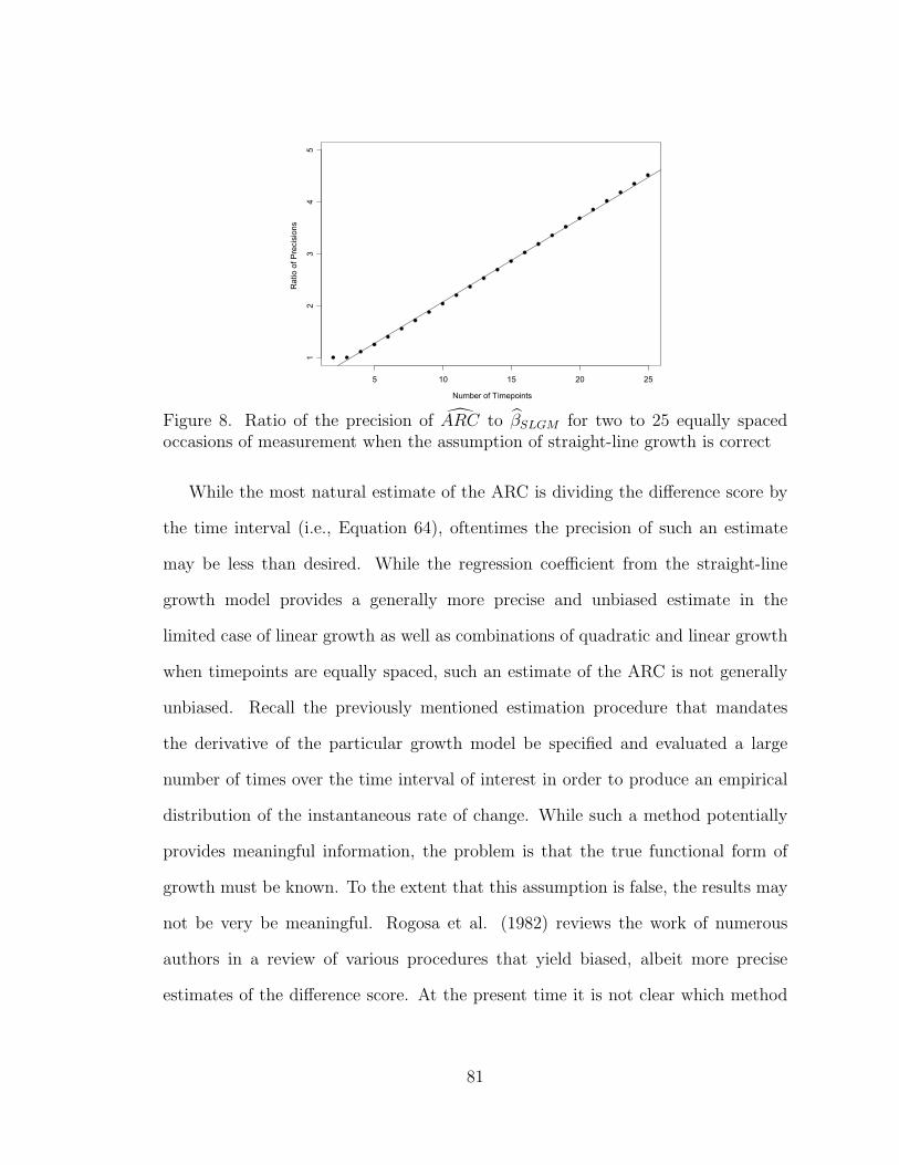
Number of Timepoints

Rat

io o

f Pre

cisi

ons

5 10 15 20 25

12

34

5

Figure 8. Ratio of the precision of !ARC to "!SLGM for two to 25 equally spacedoccasions of measurement when the assumption of straight-line growth is correct

While the most natural estimate of the ARC is dividing the di"erence score by

the time interval (i.e., Equation 64), oftentimes the precision of such an estimate

may be less than desired. While the regression coe#cient from the straight-line

growth model provides a generally more precise and unbiased estimate in the

limited case of linear growth as well as combinations of quadratic and linear growth

when timepoints are equally spaced, such an estimate of the ARC is not generally

unbiased. Recall the previously mentioned estimation procedure that mandates

the derivative of the particular growth model be specified and evaluated a large

number of times over the time interval of interest in order to produce an empirical

distribution of the instantaneous rate of change. While such a method potentially

provides meaningful information, the problem is that the true functional form of

growth must be known. To the extent that this assumption is false, the results may

not be very be meaningful. Rogosa et al. (1982) reviews the work of numerous

authors in a review of various procedures that yield biased, albeit more precise

estimates of the di"erence score. At the present time it is not clear which method

81

provides the best overall estimate of the ARC.

Although "!SLGM is typically more precise than !ARCF,1, it is also a generally

biased estimate of the ARC. However, precision alone does not necessarily lead to

an optimal parameter estimate. Bias is also an important property when evaluating

parameter estimates. Arguably the most important property of a parameter

estimate is accuracy. Conceptually, accuracy is a measure of the discrepancy

between an estimate and the true value it represents. Formally the square root of

the mean square error is a measure of accuracy (Rozeboom, 1966, p. 500; Hellmann

& Fowler, 1999). The accuracy of a measure is a function of the precision and bias

and can be expressed as follows:

RMSE =6

E[(+ " +)2] =6

E[(+ " E[+])2] + (E[+ " +])2, (72)

where RMSE is the square root of the mean square error, + is an estimate of +, the

true value of the parameter of interest. The first component under the second radical

represents the precision while the second component represents the bias. Ideally

unbiased estimates are preferred, however, if accuracy can be improved (reducing the

RMSE) by adding bias and obtaining a more precise estimate, such a bias-accuracy

tradeo" should be considered in order to obtain the estimates that are overall most

accurate.

In the context of estimating the ARC, the bias-accuracy tradeo" surfaces in the

context of at least two potential estimation techniques. The first situation involves

literally using "!SLGM as an estimate of the ARC. As can be seen from Equation 71

and Figure 8, in many circumstances the precision of "!SLGM is much better than

the precision of !ARCF,1. The bias, however, can be great for some functional forms

of growth when !SLGM is used as an estimate of the ARC. Thus, the potential gain

in precision is potentially negated by an increase in bias. Further research could

82

illustrate situations where the overall accuracy is improved by making use of the

!SLGM rather than Equation 64. Of course, when F = 2 or F = 3 equally spaced

timepoints, both methods yield the same estimate and are equally precise. Another

context where the bias-accuracy tradeo" surfaces is making use of biased, albeit

more accurate, estimates for the true di"erence score (for instance, those reviewed

in Rogosa et al., 1982). Obtaining better estimates of the di"erence score translates

into better estimates of the ARC if these estimates are used in the numerator of

Equation 64.

83

DISCUSSION

Statistical methods applied within the longitudinal setting should help

researchers, and the research community in general, better understand and explain

the what, who, how, when and why of longitudinal research. Research questions

involving change over time, either for an individual or for a group, are inherently

longitudinal in nature. In the context of experimental design, longitudinal studies

are unique, as such designs allow individual trajectories (Rationale 1) to be modeled

before identifying di"erences across individuals (Rationale 2) and correlates of

change (Rationale 3). Understanding transitions over time for the individual is

a precursor to learning what causes influence individual trajectories over time

(Rationale 4). Learning what influences individual trajectories is a precursor to

understanding what influences di"erences among individual trajectories over time

(Rationale 5). Implicit in research questions involving change is the individual.

Thus, intraindividual change should be the starting point for longitudinal research.

While understanding change for individual trajectories is an important goal for

longitudinal data analysis, understanding such a potentially complicated processes

is not often straightforward. This is especially true when several polynomial terms

are included in the Level 1 growth model. For models more complicated than a

single polynomial term, individual parameters cannot be explained without regard

to the other parameters in the model, as each parameter a"ects the trajectory

simultaneously. However, it is often the case that complicated polynomial growth

models can be avoided by making use of an appropriate nonlinear model. Because

nonlinear models generally have parameters whose meaning has a substantive

84

interpretation, researchers who make use of nonlinear growth models will likely

make greater strides in understanding and explaining the process of change over

time. It seems likely that as the general research community begins to recognize the

value of nonlinear models, more nonlinear models will be employed and exciting

questions, both novel and longstanding, will likely be better answered than if

polynomial models continue to dominate the landscape of applied growth modeling

in the behavioral sciences.

Although the present work contends nonlinear models are underutilized in

applied applications of growth models in the behavioral sciences, the overarching

theme is that the researchers carefully consider the Level 1 model of individual

growth. Making use of a nonlinear model when the true functional form of growth is

linear does not help clarify the underlying process of change. Likewise, making use of

the straight-line growth model when the true functional form of growth is nonlinear

also does not help to clarify the underlying process of change. The importance of

the Level 1 model of individual growth (essentially) cannot be overemphasized.

Rather than “always” assuming the straight-line growth is appropriate,

researchers should carefully consider other Level 1 models. Although it may seem

simpler to consider only an intercept and a slope (i.e., the parameters of the

straight-line growth model) than it is to consider the parameters from higher degree

polynomial growth models or nonlinear models, such reasoning ignores the accuracy

of the growth model itself. The point is that the making use of an incorrect model

because the parameters are “straightforward” to interpret, may not shed much light

on the underlying process of change. Ideally researchers should carefully consider the

appropriateness of the Level 1 model for the study, analysis, and understanding of

change. Perhaps the straight-line growth model is deemed the appropriate growth

model after carefully considering other alternatives. In such scenarios the use of

85

the straight-line growth model was not based on a default mind-set, but rather on

seriously considered alternatives to the straight-line growth model.31

In addition to understanding the importance of the correct Level 1 model,

another dimension of the present work was to delineate the meaning and

interpretation of the average rate of change (ARC). The ARC is a single value that

describes the mean rate at which an individual trend changes over time. The ARC

is literally the mean of all theoretically possible instantaneous rates of change across

the time interval of interest. The present work contends that the ARC is a measure

that can be used by researchers in order for potentially complicated processes of

change to be better described and understood, not necessarily the specifics within

an interval of time but over the whole interval. The suggested use of the ARC

is to supplement, not supplant, descriptors of change that are currently in use.

Presumably the ARC will be appreciated by applied researchers who seek to model,

understand, and describe overall change parsimoniously.

Unfortunately the ARC has been, both implicitly and explicitly, conceptualized

as the regression coe#cient from the straight-line growth model in the

methodological literature as well as in applications of straight-line growth models

in substantive research. However, as Equations 35, 36, 57, and 58 demonstrate, the

31Model checking and model diagnostics are important to ensure that the selected model (e.g.,the straight-line growth model) is a reasonable choice given the obtained data. Although modelchecking and diagnostics are beyond the scope of the present work, they should be considered whenworking within the context of unknown Level 1 growth models. Model checking and diagnostics areespecially important when making use of the procedures outlined in the Empirical Investigationof the Distribution of Instantaneous Rates of Change section, where the strong assumption ismade that the true functional form of growth used in the estimation of the distribution ofthe instantaneous rates of change is correct. Although model checking and diagnostics areundeniably important, they are more appropriate in the context of exploratory analyses ratherthan confirmatory ones. For example, if no model is specified a priori and one attempts severalmodels for one that fits the obtained data best, the probability values associated with the statisticalsignificance tests are not accurate, as fitting multiple growth models to find one that “fits better”capitalizes on chance. For confirmatory analyses a model is specified and then fit given the obtaineddata. Such a confirmatory analysis results in probability values that, provided the assumptions ofthe statistical procedure are met, do not capitalize on chance.

86

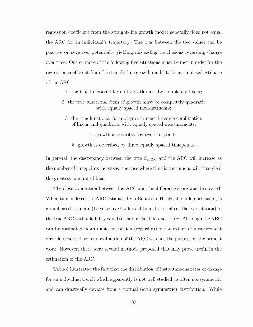
regression coe#cient from the straight-line growth model generally does not equal

the ARC for an individual’s trajectory. The bias between the two values can be

positive or negative, potentially yielding misleading conclusions regarding change

over time. One or more of the following five situations must be met in order for the

regression coe#cient from the straight-line growth model to be an unbiased estimate

of the ARC:

1. the true functional form of growth must be completely linear;

2. the true functional form of growth must be completely quadraticwith equally spaced measurements;

3. the true functional form of growth must be some combinationof linear and quadratic with equally spaced measurements;

4. growth is described by two timepoints;

5. growth is described by three equally spaced timepoints.

In general, the discrepancy between the true !SLGM and the ARC will increase as

the number of timepoints increases; the case where time is continuous will thus yield

the greatest amount of bias.

The close connection between the ARC and the di"erence score was delineated.

When time is fixed the ARC estimated via Equation 64, like the di"erence score, is

an unbiased estimate (because fixed values of time do not a"ect the expectation) of

the true ARC with reliability equal to that of the di"erence score. Although the ARC

can be estimated in an unbiased fashion (regardless of the extent of measurement

error in observed scores), estimation of the ARC was not the purpose of the present

work. However, there were several methods proposed that may prove useful in the

estimation of the ARC.

Table 6 illustrated the fact that the distribution of instantaneous rates of change

for an individual trend, which apparently is not well studied, is often nonsymmetric

and can drastically deviate from a normal (even symmetric) distribution. While

87

it is believed the mean instantaneous rate of change is a useful and important

measure for describing and attempting to understand individual trajectories, other

measures that describe the distribution of instantaneous rates of change may also

provide meaningful information. It would be beneficial to conduct more research on

the estimation of the distribution of instantaneous rates of change, in order for the

ARC to be supplemented by other measures of the instantaneous rate of change (e.g.,

various percentiles and measures of dispersion). Estimating derivatives is an area

currently receiving attention in the context of dynamical systems (systems where the

current state of the system depends, at least in part, on previous states of the system;

Boker & Nesselroade, 2002). Perhaps some of the estimation procedures developed

within the dynamic systems context will be useful for estimating properties of the

distribution of instantaneous rates of change for individual trajectories.

Absent from the present work was the e"ect of misidentified growth models

for individual trends as they relate to group comparisons. Group comparisons of

longitudinal data are often carried out in the context of HLMs and HNLMs. The

implications that a misspecified Level 1 model can have on group comparisons

is potentially troublesome. By misspecifying individual trajectories, group

comparisons are e"ectively comparing sets of erroneous models with other sets

of erroneous models. There is no reason to believe the specification errors for

individuals will cancel across individuals and then groups. Thus researchers may

well be led astray when attempting to make meaningful group comparisons when

incorrect models are fit, even in randomized designs.

An example of a misspecification of individual trajectories and its a"ect on group

comparisons is when there is di"erential attrition across groups. For example,

suppose that the null hypothesis is true and the experimental and control group

literally do not di"er in their mean trajectory over time. Further assume that the

88

individual trends follow an asymptotic regression growth model. If little or no data

are missing, say in the experimental group, but yet the probability of missing data

increases over time for the control group, the straight-line growth model would give

the impression that the typical trend is a steeper negative slope for those in the

control group. Such a “result” would likely be interpreted as the control group’s

scores were decreasing quicker when compared to the experimental group. However,

because the null hypothesis was true, the discrepant slopes are a function of two

events: (a) fitting the wrong model and (b) di"erential attrition. If the groups

had no attrition or even the same type and likelihood of missingness, the model

would have been misspecified but, there would have likely been a failure to reject

the null hypothesis (i.e., a correct decision would have likely been made). However,

because the control group had more participants earlier in the study, the regression

slope would have been weighted heavier for the early scores and later scores would

have a"ected the estimated slope less. Such a problem would not have existed if

the correct model would have been fit. When the correct model is fit and data

are missing at random (or more stringently completely at random), HLMs and

HNLMs still yield maximum likelihood estimates of the population parameters (see

Raudenbush & Bryk, 2002 but also Dempster, Laird, & Rubin, 1977 for seminal

work on the topic).

While there is no doubt that longitudinal data analysis will continue to develop

and improve upon existing techniques, it is believed that the present work adds

to the rich analysis of change literature by clarifying and extending the current

understanding of the ARC. While it is not suggested that the ARC supplant

currently used descriptors of change, it is suggested that the ARC supplement them.

It is believed that the ARC will help researchers and the research community in the

ongoing quest for a better understanding of the dynamic and static relationship that

89

exist among sets of variables over time.

90

APPENDIX A

The numerator of Equation 32 can be simplified by realizing the whole quantity

can be multiplied by (k and then summed over rather than doing the same operations

for both components separately:

NE32 =K,

k=1

-$k

7(T!k+2

F " T!k+2

1 )$k + 2

" TF + T1

2

K,

k=1

(T!k+1

F " T!k+1

1 )$k + 1

8., (A1)

where NE32 is the numerator of Equation 32.

A common denominator for the two components is obtained by multiplying the

first component by 2(%k + 1) and the second component by (%k + 2):

NE32 =K,

k=1

-$k

72($k + 1)(T!k+2

F " T!k+2

1 )" ($k + 2)(TF + T1)(T!k+1

F " T!k+1

1 )2($k + 1)($k + 2)

8..

(A2)

After multiplying the appropriate quantities in the numerator of Equation A2,

simplifying like-terms, and placing the 2 in the denominator outside of the

summation (because it is a constant), the reduced numerator of Equation 32 can be

written as:

NE32 =12

K,

k=1

9

:$k

4$k

)T

!k+2

F " T!k+2

1 + TF T!k+1

1 " T1T!k+1

F

*+ 2

)TF T

!k+1

1 " T1T"k+1F

*5

($k + 2) ($k + 1)

;

< .

(A3)

The three components of the denominator of Equation 32 can be multiplied by

4, 6, and 3 respectively, such that a common denominator of 12 allows like terms to

91

be combined across the three:

DE32 =4(T 3

F # T 31 )# 6(TF + T1)(T 2

F # T 21 ) + 3(TF + T1)2(TF # T1)

12, (A4)

where DE32 is the denominator of Equation 32.

After multiplying out the quantities of Equation A4 and then simplifying, the

resultant value is:

DE32 =(TF " T1)3

12. (A5)

Equation 33 in the text results from combining Equations A3 as the numerator and

Equation A5 as the denominator.

92

APPENDIX B

The following Maple (Version 7.00, 2001) syntax allows one to symbolically derive

the regression coe#cient from the straight-line growth model, ARC, B, and ! for

(essentially) any functional form of growth when time is considered continuous and

Y can be written as a function of time. By setting ‘Y’ equal to some functional form

of growth (by replacing ‘f(Time)’ with the functional form of interest), defining

the time interval (or leaving it general as is done here), the syntax allows for

potentially complicated derivations to be carried out in a straightforward manner.

Note that ‘Y’ can be set equal to ‘Asymptotic Regression,’ ‘Gompertz Growth,’ or

‘Logistic Growth’ directly because these functions are defined at the beginning of

the syntax.

Maple Syntax

Asymptotic_Regression := beta*exp(-gamma*Time) + alpha;

Gompertz_Growth := alpha*exp(-exp(beta - gamma*Time));

Logistic_Growth := alpha/(1 + exp(beta - gamma*Time));

> Y := f(Time);# Defines ‘Y’ as any functional form of growth, where ‘Time’ is the# independent variable. Note that ‘Y’ can be any function, a linear# or nonlinear model for example, with an arbitrary number of# parameters. For example, ‘Y’ can be defined as some linear model,# the ‘Asymptotic_Regression’ model, ‘Gompertz_Growth’ model,# ‘Logistic_Growth’ model, or some other nonlinear model. There# are (virtually) no restrictions on the complexity of the model.

> Low_Limit := TI;# Defines the initial value of ‘Time’. ‘Low_Limit’ can be a numerical

93

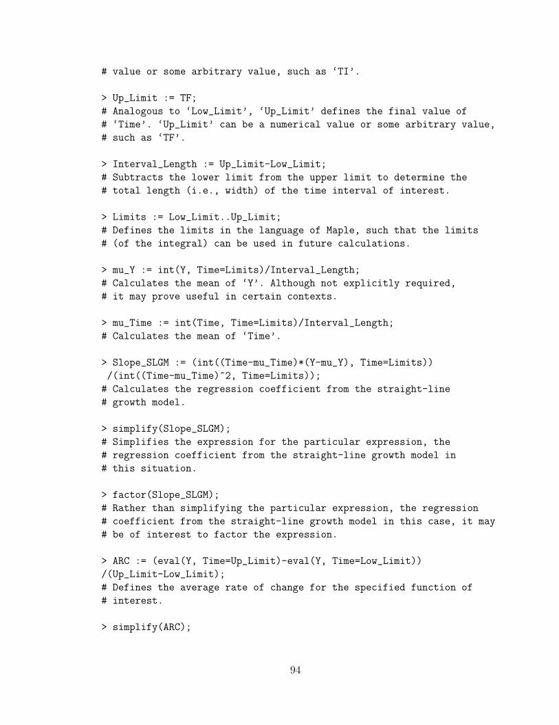
# value or some arbitrary value, such as ‘TI’.

> Up_Limit := TF;# Analogous to ‘Low_Limit’, ‘Up_Limit’ defines the final value of# ‘Time’. ‘Up_Limit’ can be a numerical value or some arbitrary value,# such as ‘TF’.

> Interval_Length := Up_Limit-Low_Limit;# Subtracts the lower limit from the upper limit to determine the# total length (i.e., width) of the time interval of interest.

> Limits := Low_Limit..Up_Limit;# Defines the limits in the language of Maple, such that the limits# (of the integral) can be used in future calculations.

> mu_Y := int(Y, Time=Limits)/Interval_Length;# Calculates the mean of ‘Y’. Although not explicitly required,# it may prove useful in certain contexts.

> mu_Time := int(Time, Time=Limits)/Interval_Length;# Calculates the mean of ‘Time’.

> Slope_SLGM := (int((Time-mu_Time)*(Y-mu_Y), Time=Limits))/(int((Time-mu_Time)^2, Time=Limits));# Calculates the regression coefficient from the straight-line# growth model.

> simplify(Slope_SLGM);# Simplifies the expression for the particular expression, the# regression coefficient from the straight-line growth model in# this situation.

> factor(Slope_SLGM);# Rather than simplifying the particular expression, the regression# coefficient from the straight-line growth model in this case, it may# be of interest to factor the expression.

> ARC := (eval(Y, Time=Up_Limit)-eval(Y, Time=Low_Limit))/(Up_Limit-Low_Limit);# Defines the average rate of change for the specified function of# interest.

> simplify(ARC);

94

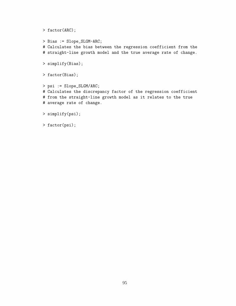
> factor(ARC);

> Bias := Slope_SLGM-ARC;# Calculates the bias between the regression coefficient from the# straight-line growth model and the true average rate of change.

> simplify(Bias);

> factor(Bias);

> psi := Slope_SLGM/ARC;# Calculates the discrepancy factor of the regression coefficient# from the straight-line growth model as it relates to the true# average rate of change.

> simplify(psi);

> factor(psi);

95

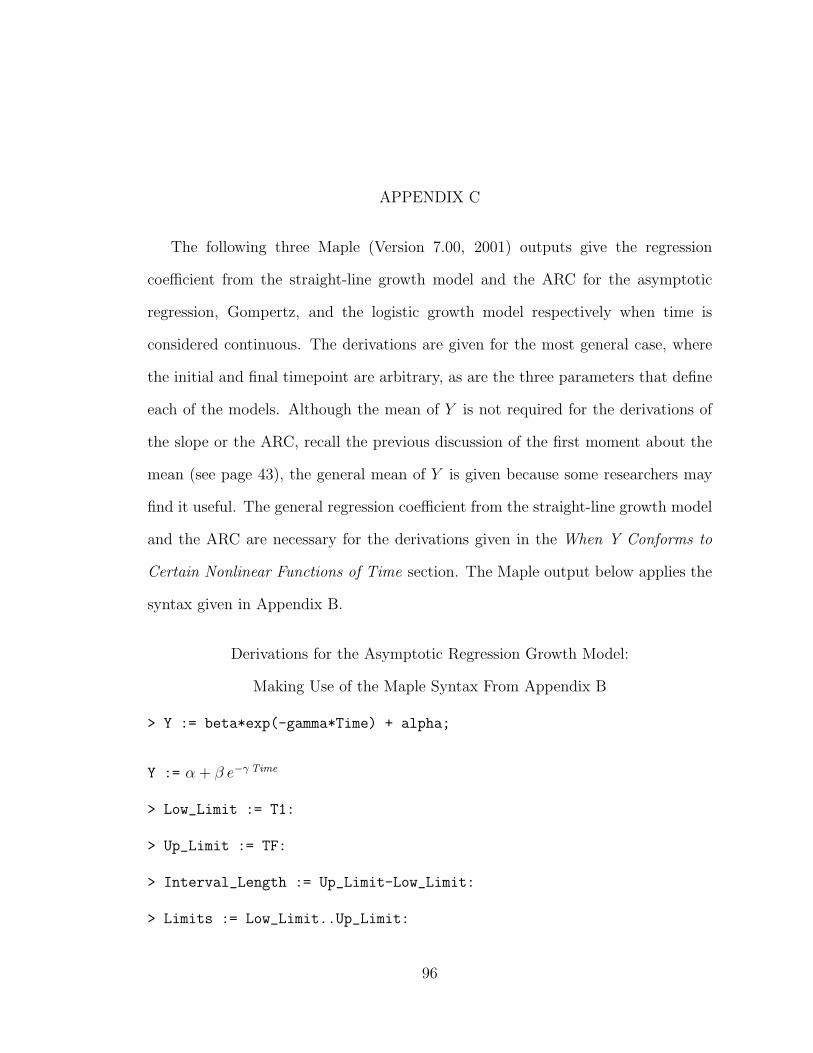
APPENDIX C

The following three Maple (Version 7.00, 2001) outputs give the regression

coe#cient from the straight-line growth model and the ARC for the asymptotic

regression, Gompertz, and the logistic growth model respectively when time is

considered continuous. The derivations are given for the most general case, where

the initial and final timepoint are arbitrary, as are the three parameters that define

each of the models. Although the mean of Y is not required for the derivations of

the slope or the ARC, recall the previous discussion of the first moment about the

mean (see page 43), the general mean of Y is given because some researchers may

find it useful. The general regression coe#cient from the straight-line growth model

and the ARC are necessary for the derivations given in the When Y Conforms to

Certain Nonlinear Functions of Time section. The Maple output below applies the

syntax given in Appendix B.

Derivations for the Asymptotic Regression Growth Model:

Making Use of the Maple Syntax From Appendix B

> Y := beta*exp(-gamma*Time) + alpha;

Y := " + ! e## Time

> Low_Limit := T1:

> Up_Limit := TF:

> Interval_Length := Up_Limit-Low_Limit:

> Limits := Low_Limit..Up_Limit:

96

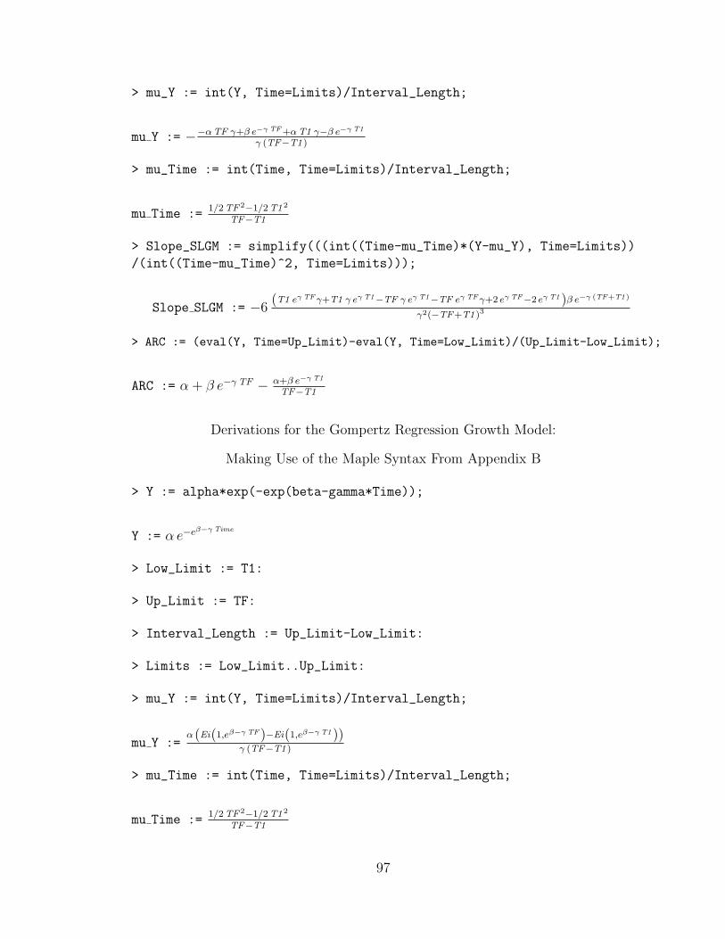
> mu_Y := int(Y, Time=Limits)/Interval_Length;

mu Y := "#$TF #+" e!& TF+$T1 ##" e!& T1

# (TF#T1 )

> mu_Time := int(Time, Time=Limits)/Interval_Length;

mu Time := 1/2TF2#1/2T12

TF#T1

> Slope_SLGM := simplify(((int((Time-mu_Time)*(Y-mu_Y), Time=Limits))/(int((Time-mu_Time)^2, Time=Limits)));

Slope SLGM := "6(T1 e& TF#+T1 # e& T1#TF # e& T1#TF e& TF#+2 e& TF#2 e& T1)" e!& (TF+T1)

#2(#TF+T1 )3

> ARC := (eval(Y, Time=Up_Limit)-eval(Y, Time=Low_Limit)/(Up_Limit-Low_Limit);

ARC := " + ! e## TF " $+" e!& T1

TF#T1

Derivations for the Gompertz Regression Growth Model:

Making Use of the Maple Syntax From Appendix B

> Y := alpha*exp(-exp(beta-gamma*Time));

Y := " e#e'!& Time

> Low_Limit := T1:

> Up_Limit := TF:

> Interval_Length := Up_Limit-Low_Limit:

> Limits := Low_Limit..Up_Limit:

> mu_Y := int(Y, Time=Limits)/Interval_Length;

mu Y :=$ (Ei(1,e'!& TF)#Ei(1,e'!& T1))

# (TF#T1 )

> mu_Time := int(Time, Time=Limits)/Interval_Length;

mu Time := 1/2TF2#1/2T12

TF#T1

97

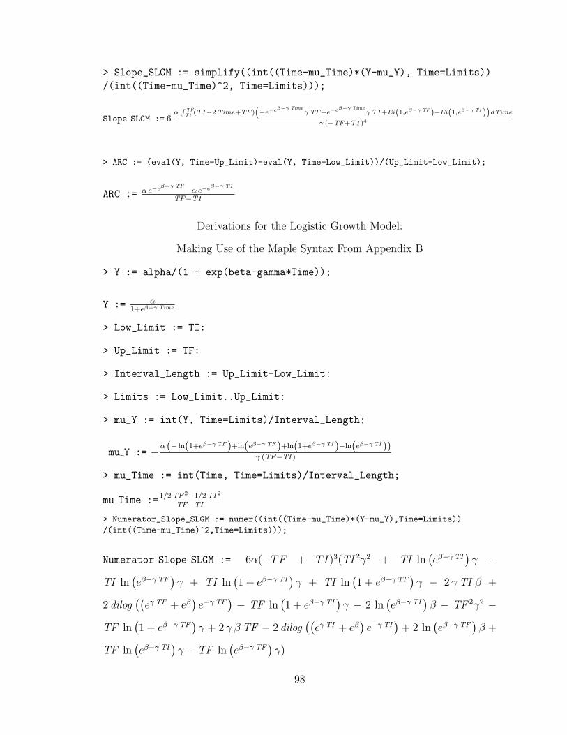
> Slope_SLGM := simplify((int((Time-mu_Time)*(Y-mu_Y), Time=Limits))/(int((Time-mu_Time)^2, Time=Limits)));

Slope SLGM := 6$

/ TFT1 (T1#2Time+TF)

&#e"e$"% Time

% TF+e"e$"% Time% T1+Ei(1,e$"% TF)#Ei(1,e$"% T1)

'dTime

% (#TF+T1)4

> ARC := (eval(Y, Time=Up_Limit)-eval(Y, Time=Low_Limit))/(Up_Limit-Low_Limit);

ARC := $ e!e'!& TF#$ e!e'!& T1

TF#T1

Derivations for the Logistic Growth Model:

Making Use of the Maple Syntax From Appendix B

> Y := alpha/(1 + exp(beta-gamma*Time));

Y := $1+e'!& Time

> Low_Limit := TI:

> Up_Limit := TF:

> Interval_Length := Up_Limit-Low_Limit:

> Limits := Low_Limit..Up_Limit:

> mu_Y := int(Y, Time=Limits)/Interval_Length;

mu Y := "$ (# ln(1+e'!& TF)+ln(e'!& TF)+ln(1+e'!& TI )#ln(e'!& TI ))# (TF#TI )

> mu_Time := int(Time, Time=Limits)/Interval_Length;

mu Time :=1/2TF2#1/2TI 2

TF#TI

> Numerator_Slope_SLGM := numer((int((Time-mu_Time)*(Y-mu_Y),Time=Limits))/(int((Time-mu_Time)^2,Time=Limits)));

Numerator Slope SLGM := 6"("TF + TI)3(TI 2#2 + TI ln'e"## TI

(# "

TI ln'e"## TF

(# + TI ln

'1 + e"## TI

(# + TI ln

'1 + e"## TF

(# " 2 # TI ! +

2 dilog''

e# TF + e"(e## TF

(" TF ln

'1 + e"## TI

(# " 2 ln

'e"## TI

(! " TF 2#2 "

TF ln'1 + e"## TF

(# + 2 # ! TF " 2 dilog

''e# TI + e"

(e## TI

(+ 2 ln

'e"## TF

(! +

TF ln'e"## TI

(# " TF ln

'e"## TF

(#)

98

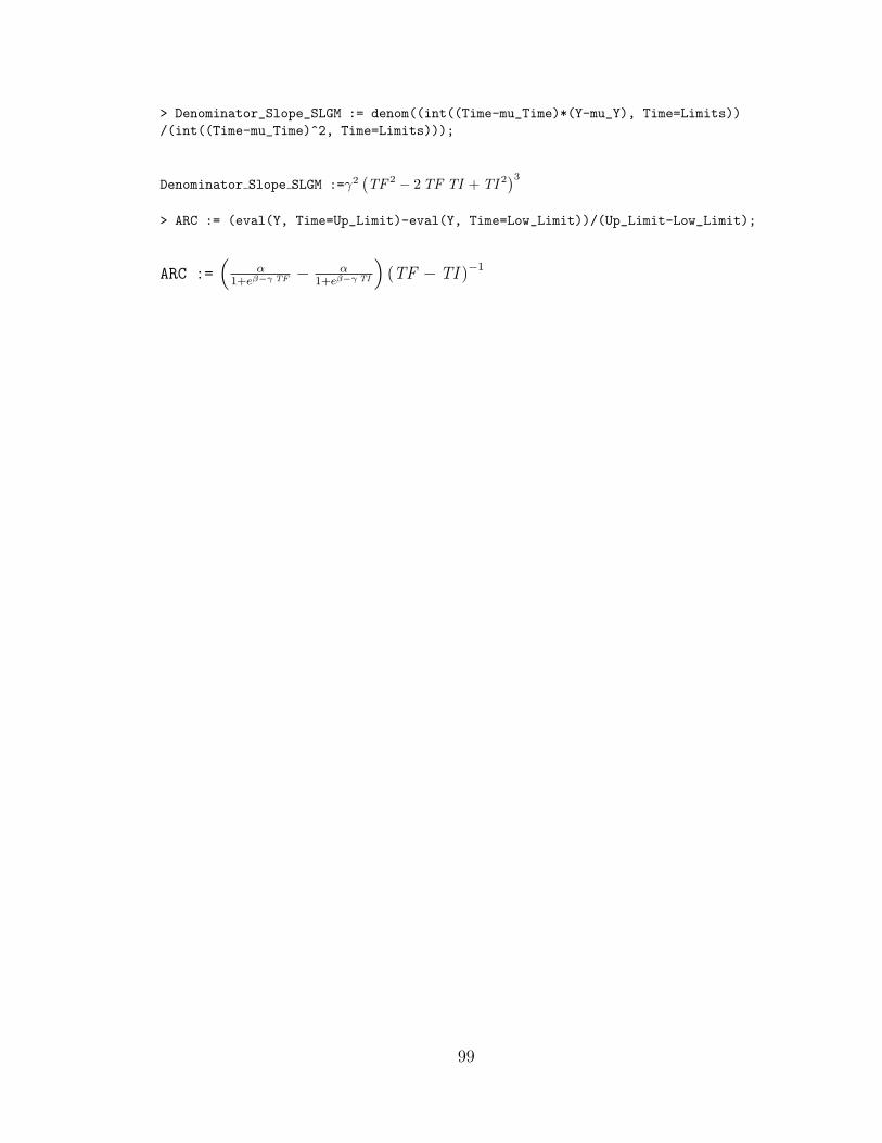
> Denominator_Slope_SLGM := denom((int((Time-mu_Time)*(Y-mu_Y), Time=Limits))/(int((Time-mu_Time)^2, Time=Limits)));

Denominator Slope SLGM :=%2'TF 2 " 2TF TI + TI 2

(3

> ARC := (eval(Y, Time=Up_Limit)-eval(Y, Time=Low_Limit))/(Up_Limit-Low_Limit);

ARC :=)

$1+e'!& TF " $

1+e'!& TI

*(TF " TI )#1

99

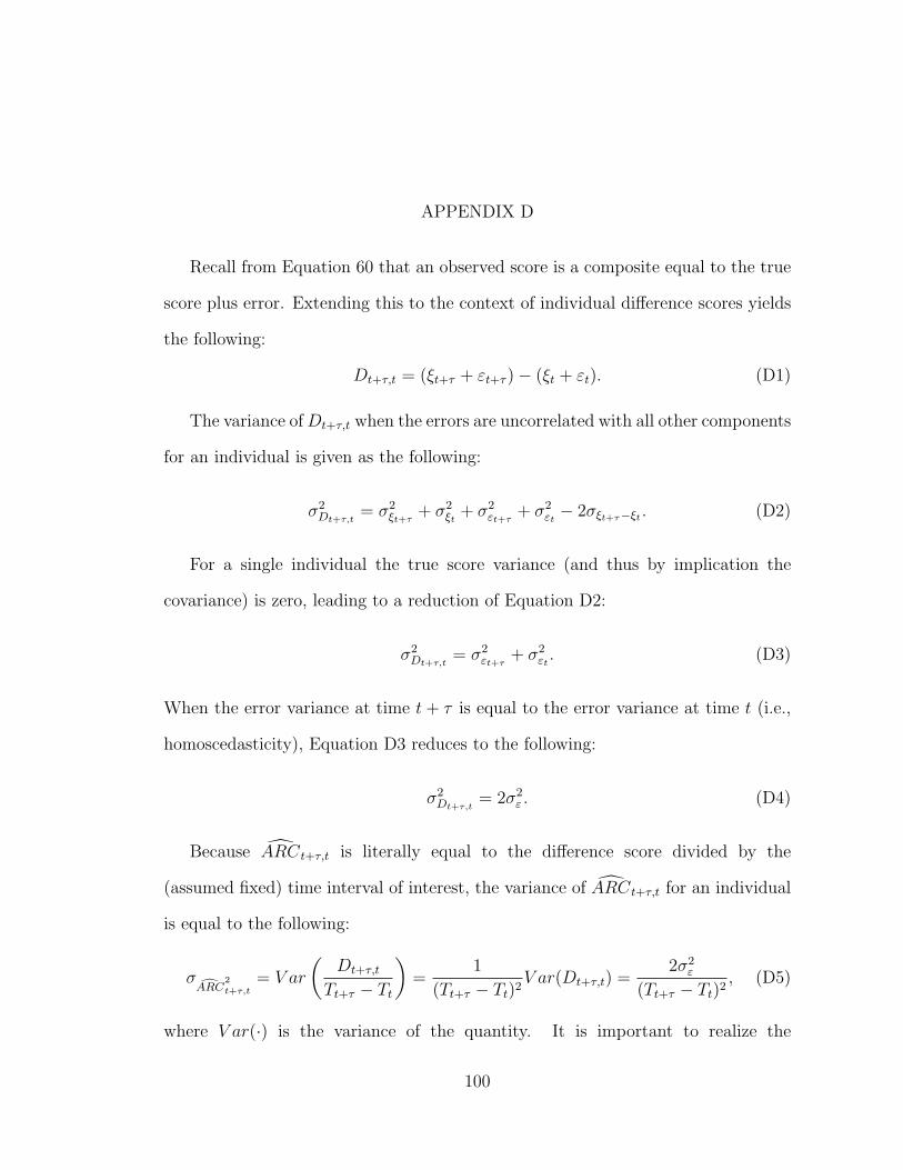
APPENDIX D

Recall from Equation 60 that an observed score is a composite equal to the true

score plus error. Extending this to the context of individual di"erence scores yields

the following:

Dt+!,t = ()t+! + &t+! )" ()t + &t). (D1)

The variance of Dt+!,t when the errors are uncorrelated with all other components

for an individual is given as the following:

*2Dt+!,t

= *2&t+!

+ *2&t

+ *2't+!

+ *2't" 2*&t+!#&t . (D2)

For a single individual the true score variance (and thus by implication the

covariance) is zero, leading to a reduction of Equation D2:

*2Dt+!,t

= *2't+!

+ *2't. (D3)

When the error variance at time t + $ is equal to the error variance at time t (i.e.,

homoscedasticity), Equation D3 reduces to the following:

*2Dt+!,t

= 2*2' . (D4)

Because !ARCt+!,t is literally equal to the di"erence score divided by the

(assumed fixed) time interval of interest, the variance of !ARCt+!,t for an individual

is equal to the following:

* +ARC2t+!,t

= V ar

%Dt+!,t

Tt+! " Tt

&=

1

(Tt+! " Tt)2V ar(Dt+!,t) =

2*2'

(Tt+! " Tt)2, (D5)

where V ar(·) is the variance of the quantity. It is important to realize the

100

assumptions both implicit and explicit in Equation D5. These assumptions are that

the variance pertains to one individual, errors at time Tt and Tt+! are uncorrelated

with one another and each true score, and that the error variance is equal for the

two occasions of measurement.

101

REFERENCES

Abramowitz, M., & Stegun, I. (1965). Handbook of mathematical functions. NewYork, NY: Dover Publications.

Baltes, P. B., & Nesselroade, J. R. (1979). History and rationale of longitudinalresearch. In J. R. Nesselroade & P. B. Baltes (Eds.), Longitudinal research inthe study of behavior and development (pp. 1–39). New York, NY: AcademicPress.

Billings, L., & Shepard, J. (1910). The change of heart rate with attention.Psychological Review, 17 (3), 217–228.

Blomqvist, N. (1977). On the relation between change and initial value. Journal ofthe American Statistical Association, 72 (360), 746–749.

Boker, S. M., & Nesselroade, J. R. (2002). A method for modeling theintrinsic dynamics of intraindividual variability: Recovering the parametersof simulated oscillators in multi-wave panel data. Multivariate BehavioralResearch, 37 (1), 127–160.

Box, G. (1979). Robustness in the strategy of scientific model building. In R. L.Launder & G. N. Williamson (Eds.), Robustness in statistics (pp. 201–236).New York, NY: Academic Press.

Box, G. (1984). Science and statistics. Journal of the American StatisticalAssociation, 71 (356), 791–799.

Browne, M., & Du Toit, S. (1991). Models for learning data. In L. M.Collins & J. L. Horn (Eds.), Best methods for the analysis of change: Recentadvances, unanswered questions, future directions. Washington, DC: AmericanPsychological Association.

Bryk, A. S., & Raudenbush, S. W. (1987). Application of hierarchical linear modelsto assessing change. Psychological Bulletin, 101 (1), 147-158.

Bryk, A. S., & Raudenbush, S. W. (1992). Hierarchical linear models: Applicationsand data analysis methods. Newbury Park, CA: Sage Publications.

Collins, L. M. (1996). Measurement of change in research on aging: Old and newissues from an individual growth perspective. In J. E. Birren & K. Schaie(Eds.), Handbook of the psychology of the aging (4th ed., pp. 38–58). SanDiego, CA: Academic Press.

102

Coren, S., Ward, L. M., & Enns, J. T. (1994). Sensation and perception (4th ed.).New York, NY: Harcourt Brace & Company.

Cronbach, L. J., & Furby, L. (1970). How we should measure “change”: Or shouldwe? Psychological Bulletin, 74, 68–80.

Cudeck, R. (1996). Mixed-e"ects models in the study of individual di"erences withrepeated measures data. Multivariate Behavioral Research, 31 (3), 371–403.

Davidian, M., & Giltinan, D. M. (1995). Nonlinear models for repeated measurementdata. New York, NY: Chapman & Hall.

Davies, A. E. (1900). The concept of change. The Philosophical Review, 9 (5),502–517.

DeCarlo, L. (1997). On the meaning and use of kurtosis. Psychological Methods,2 (3), 292–307.

Dempster, A., Laird, N., & Rubin, D. (1977). Maximum likelihood from incompletedata via the EM algorithm. Journal of the Royal Statistical Society, Series B,39, 1–8.

Finney, R. L., Weir, M. D., & Giordano, F. R. (2001). Thomas’ calculus (10th ed.).New York, NY: Addison Wesley.

Francis, D. J., Fletcher, J. M., Stuebing, K. K., Davidson, K. C., & Thompson,N. M. (1991). Analysis of change: Modeling individual growth. Journal ofConsulting and Clinical Psychology, 59 (1), 27–37.

Francis, J., David, Schatschneider, C., & Carlson, C. D. (2000). Introduction toindividual growth curve analysis. In D. Drotar (Ed.), Handbook of research inpediatric and clinical child psychology: Practical strategies and methods (pp.51–73). New York, NY: Kluwer Academic/Plenum Publishers.

Goldstein, H. (1995). Multilevel statistical models (Vol. 3, 2nd ed.). New York, NY:Halsted Press.

Harris, C. W. (Ed.). (1963). Problems in measuring change. Madison, WI: Universityof Wisconsin Press.

Hartz, S., Ben-Shahar, Y., & Tyler, M. (2001). Logistic growth curve analysis inassociative learning data. Animal Cognition, 4, 185–189.

Hellmann, J. J., & Fowler, G. W. (1999). Bias, precision, and accuracy of fourmeasures of species richness. Ecological Applications, 9 (3), 824–834.

Karney, B. R., & Bradbury, T. N. (1995). Assessing longitudinal change in marriage:An introduction to the analysis of growth curves. Journal of Marriage andthe Family, 57, 1091–1108.

Khuri, A., & Casella, G. (2002). The existence of the first negative moment revisited.The American Statistician, 56 (1), 44–47.

103

Kline, M. (1977). Calculus: An intuitive and physical approach. New York, NY:John Wiley and Sons.

Kraemer, H. C., & Thiemann, S. (1989). A strategy to use soft data e"ectivelyin randomized controlled clinical trials. Journal of Consulting and ClinicalPsychology, 57 (1), 148–154.

Laird, N. M., & Wang, F. (1990). Estimating rates of change in randomized clinicaltrials. Controlled Clinical Trials, 11, 405–419.

Laird, N. M., & Ware, H. (1982). Random-e"ects models for longitudinal data.Biometrics, 38, 963–974.

Lewin, L. (1981). Polylogarithms and associated functions. New York, NY:North-Holland.

Linn, R. L., & Slinde, J. A. (1977). The determination of the significance of changebetween pre- and posttesting periods. Review of Educational Research, 47 (1),121–150.

Lord, F. M. (1956). The measurement of growth. Educational and PsychologicalMeasurement, 16, 421–437.

Lord, F. M. (1958). Further problems in the measurement of growth. Educationaland Psychological Measurement, 18 (3), 437–451.

Lord, F. M. (1963). Elementary models for measuring change. In C. W. Harris(Ed.), Problems in measuring change (pp. 21–38). Madison, WI: Universityof Wisconsin Press.

Lord, F. M., & Novick, M. R. (1968). Statistical theories of mental test scores.Reading, MA: Addison-Wesley.

Maple (Version 7.00). (2001). [Computer software] Waterloo Maple Inc.

Mehta, P. D., & West, S. G. (2000). Putting the individual back into individualgrowth curves. Psychological Methods, 5 (1), 23–43.

Mood, A. M., Graybill, F. A., & Boes, D. C. (1974). Introduction to the theory ofstatistics (3rd ed.). New York, NY: McGraw-Hill.

Morris, H. (1983). Parametric empirical Bayes inference: Theory and applications.Journal of the American Statistical Association, 78, 47–65.

Overall, J. E., & Tonidandel, S. (2002). Measuring change in controlled longitudinalstudies. British Journal of Mathematical and Statistical Psychology, 55,109–124.

Overall, J. E., & Woodward, J. A. (1975). Unreliability of di"erence scores: Aparadox for measurement of change. Psychological Bulletin, 82 (1), 85–86.

Pearson, E., & Hartley, H. (Eds.). (1970). Biometrika tables for statisticians (Vol. 1,3rd ed.). New York, NY: Cambridge University Press.

104

Pinheiro, J., & Bates, D. (2000). Mixed-e!ects models in S and S-Plus. New York,NY: Springer.

Ratkowsky, D. A. (1983). Nonlinear regression modeling: A unified practicalapproach. New York, NY: Marcel Dekker, Inc.

Raudenbush, S., & Xiao-Feng, L. (2001). E"ects of study duration, frequencyof observation, and sample size on power in studies of group di"erences inpolynomial change. Psychological Methods, 6 (4), 387–401.

Raudenbush, S. W. (2001). Comparing personal trajectories and drawing causalinferences from longitudinal data. Annual Review of Psychology, 52, 501–525.

Raudenbush, S. W., & Bryk, A. S. (2002). Hierarchical linear models: Applicationsand data analysis methods (2nd ed.). Thousand Oaks, CA: Sage.

Rausch, J. R., & Maxwell, S. E. (2003). Longitudinal designs in randomized groupcomparisons: Optimizing power when the latent individual growth trajectoriesfollow straight-lines. Unpublished Manuscript.

Rogosa, D. (1995). Myths and methods: “Myths about Longitudinal Research”plus supplemental questions. In J. M. Gottman (Ed.), The analysis of change(pp. 3–66). Nahwah, NJ: Lawrence Earlbaum Associates.

Rogosa, D., Brandt, D., & Zimowski, M. (1982). A growth curve approach to themeasurement of change. Psychological Bulletin, 92 (3), 726–748.

Rogosa, D., & Willett, J. B. (1985). Understanding correlates of change by modelingindividual di"erences in growth. Psychometrika, 50 (2), 203–228.

Rogosa, D. R., & Willett, J. B. (1983). Demonstrating the reliability of the di"erencescore in the measurement of change. Journal of Educational Measurement,20 (4), 335–343.

Rozeboom, W. W. (1966). Foundations of the theory of prediction. Homewood, IL:The Dorsey Press.

Seigel, D. G. (1975). Several approaches for measuring average rates of change fora second degree polynomial. The American Statistician, 29 (1), 36–37.

Shadish, W. R. (2002). Revisiting field experimentation: Field notes for the future.Psychological Methods, 7 (1), 3–18.

Stevens, W. (1951). Asymptotic regression. Biometrics, 7 (3), 247–267.

Stewart, J. (1998). Calculus: Concepts and contexts. Cincinnati, OH: Brooks/ColePublishing Company.

Stuart, A., & Ord, J. K. (1994). Kendall’s advanced theory of statistics: Distributiontheory (Vol. 1, 6th ed.). New York, NY: John Wiley & Sons.

Svartberg, M. (1999). Therapist competence: Its temporal course, temporalstability, and determinants in short-term anxiety-provoking psychotherapy.Journal of Clinical Psychology, 55 (10), 1313–1319.

105

Thomson, G. H. (1924). A formula to correct for the e"ect of errors of measurementon the correlation of initial values with gains. Journal of ExperimentalPsychology, 7, 321–324.

Van Gert, P. (1991). A dynamic systems model of cognitive and language growth.Psychological Review, 98 (1), 3–52.

Vonesh, E. F., & Chinchilli, V. M. (1997). Linear and nonlinear models for theanalysis of repeated measurements. New York, NY: Marcel Dekker.

Willett, J. B. (1988). Questions and answers in the measurement of change. InE. Z. Rothkopf (Ed.), Review of research in education (Vol. 15, pp. 345–422).Washington, DC: American Educational Research Association.

Willett, J. B. (1989). Some results on the reliability for the longitudinalmeasurement of change: Implications for the design of studies of individualchange. Educational and Psychological Measurement, 49, 587–601.

Winsor, C. P. (1932). The Gompertz curve as a growth curve. The Proceedingsof the National Academy of Sciences of the United States of America, 18 (1),1–8.

Zimmerman, D., & Williams, R. (1982). Gain scores in research can be highlyreliable. Journal of Educational Measurement, 19, 149–154.

106