Minimizing Average Flow-time : Upper and Lower Bounds

Naveen Gargnaveen@cse.iitd.ac.in

Amit Kumaramitk@cse.iitd.ac.in

Indian Institute of Technology Delhi, India

Abstract

We consider the problem of minimizing average flow timeon multiple machines when each job can be assigned onlyto a specified subset of the machines. This is a special caseof scheduling on unrelated machines and we show that noonline algorithm can have a bounded competitive ratio. Weprovide an O(logP )-approximation algorithm by modify-ing the single-source unsplittable flow algorithm of Dinitzet.al. Here P is the ratio of the maximum to the minimumprocessing times.

We establish an Ω(logP )-integrality gap for our LP-relaxation and use this to show an Ω(logP/ log logP )lower bound on the approximability of the problem. Wethen extend the hardness results to the problem of mini-mizing flow time on parallel machines and establish thefirst non-trivial lower bounds on the approximability; weshow that the problem cannot be approximated to withinΩ(√

logP/ log logP ).

1. Introduction

We consider the problem of scheduling jobs that arriveover time in multiprocessor environments. This is a funda-mental scheduling problem and has many applications, e.g.,servicing requests in web servers. The goal of a schedulingalgorithm is to process jobs on the machines so that somemeasure of performance is optimized. A natural measure isthe average flow time of the jobs. Flow-time of a job is de-fined as the difference between its completion time and itsrelease time, i.e., the time it spends in the system.

The special case of this problem when all machines areidentical has received considerable attention in the recentpast [1, 2, 12]. There has been recent progress on the prob-lem where machines can have different speeds [7, 6]. How-ever very little is known about the problem when a job cango only on a subset of machines. Often in an heteroge-neous environment, e.g., grid computing, a job can only beprocessed by a subset of machines. This can happen dueto various reasons – geographical proximity, capabilities

of machines, security reasons. In this paper, we considerscheduling in such heterogeneous environments.

We give new results on approximating the average flow-time of jobs on multiple machines. We consider the follow-ing setting : we have several machines of the same speed.Further each job may specify a subset of machines on whichit can be processed. We use the following nomenclature : ifeach job can be processed on any machine, we call it theParallel Scheduling problem. If we add the constraintsthat each job can only be processed on a subset of machines,then we call it the Parallel Scheduling with Subset Con-straints problem.

We consider both the on-line and the off-line settings.We allow jobs to be preempted. Indeed, the problem turnsout to be intractable if we do not allow preemption. Kellereret. al. [10] showed that the problem of minimizing averageflow time without preemption has no online algorithm witho(n) competitive ratio even on a single machine. They alsoshowed that it is hard to get a polynomial time O(n1/2−ε)-approximation algorithm for this problem. So preemptionis a standard, and much needed assumption when minimiz-ing flow time. It is desirable that our algorithms give non-migratory schedules, i.e., a job gets processed on only onemachine. Our scheduling algorithm has this property andthe approximation ratio holds even if we compare with mi-gratory schedules. Our lower bound results apply to migra-tory schedules as well.

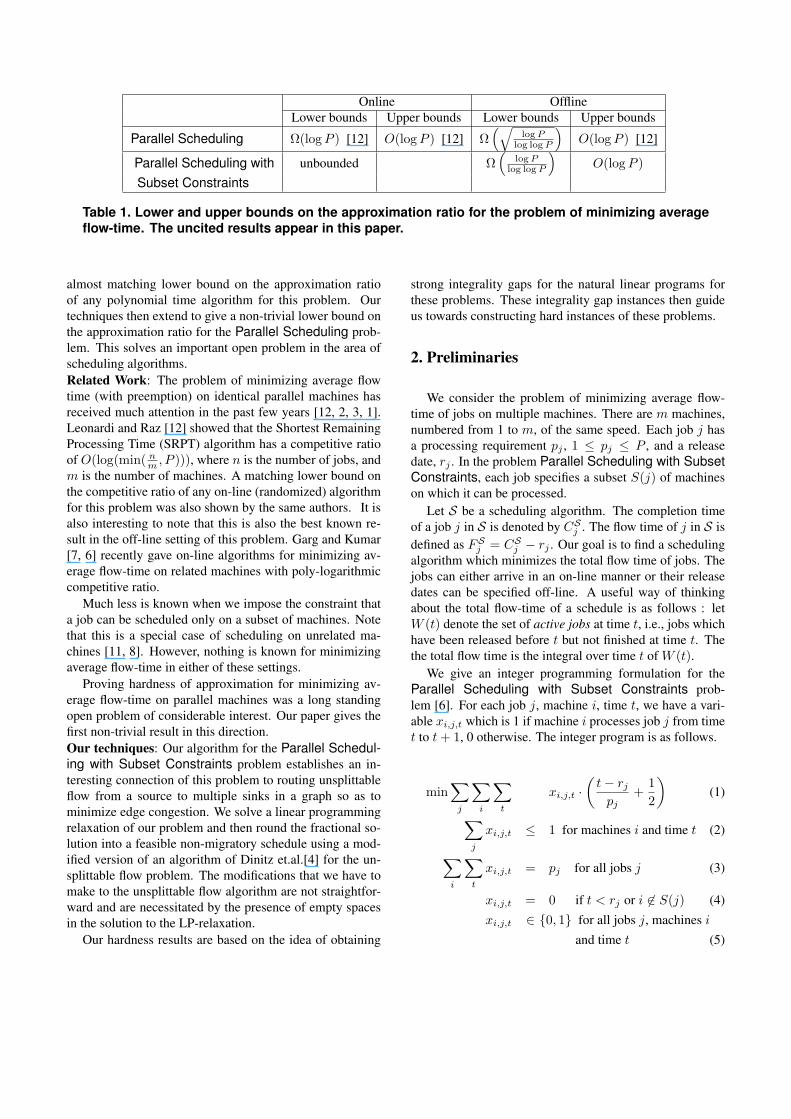
Table 1 summarizes our results and the previous resultsknown for the problem of minimizing average flow-time.Here P refers to the ratio of the highest processing require-ment to the smallest processing requirement of a job.

Our first result a strong lower bound on the competitiveratio of any on-line algorithm for the Parallel Schedulingwith Subset Constraints problem. One might think thatthis is because of the fact that the set of subsets of machinesspecified of the jobs is a complex set system. However weshow that our lower bounds hold even if this set system islaminar.

In the offline setting, we give a polynomial time loga-rithmic approximation algorithm for the Parallel Schedul-ing with Subset Constraints problem. We also show an

Online OfflineLower bounds Upper bounds Lower bounds Upper bounds

Parallel Scheduling Ω(logP ) [12] O(logP ) [12] Ω(√

log Plog log P

)O(logP ) [12]

Parallel Scheduling with unbounded Ω(

log Plog log P

)O(logP )

Subset Constraints

Table 1. Lower and upper bounds on the approximation ratio for the problem of minimizing averageflow-time. The uncited results appear in this paper.

almost matching lower bound on the approximation ratioof any polynomial time algorithm for this problem. Ourtechniques then extend to give a non-trivial lower bound onthe approximation ratio for the Parallel Scheduling prob-lem. This solves an important open problem in the area ofscheduling algorithms.Related Work: The problem of minimizing average flowtime (with preemption) on identical parallel machines hasreceived much attention in the past few years [12, 2, 3, 1].Leonardi and Raz [12] showed that the Shortest RemainingProcessing Time (SRPT) algorithm has a competitive ratioof O(log(min( n

m , P ))), where n is the number of jobs, andm is the number of machines. A matching lower bound onthe competitive ratio of any on-line (randomized) algorithmfor this problem was also shown by the same authors. It isalso interesting to note that this is also the best known re-sult in the off-line setting of this problem. Garg and Kumar[7, 6] recently gave on-line algorithms for minimizing av-erage flow-time on related machines with poly-logarithmiccompetitive ratio.

Much less is known when we impose the constraint thata job can be scheduled only on a subset of machines. Notethat this is a special case of scheduling on unrelated ma-chines [11, 8]. However, nothing is known for minimizingaverage flow-time in either of these settings.

Proving hardness of approximation for minimizing av-erage flow-time on parallel machines was a long standingopen problem of considerable interest. Our paper gives thefirst non-trivial result in this direction.Our techniques: Our algorithm for the Parallel Schedul-ing with Subset Constraints problem establishes an in-teresting connection of this problem to routing unsplittableflow from a source to multiple sinks in a graph so as tominimize edge congestion. We solve a linear programmingrelaxation of our problem and then round the fractional so-lution into a feasible non-migratory schedule using a mod-ified version of an algorithm of Dinitz et.al.[4] for the un-splittable flow problem. The modifications that we have tomake to the unsplittable flow algorithm are not straightfor-ward and are necessitated by the presence of empty spacesin the solution to the LP-relaxation.

Our hardness results are based on the idea of obtaining

strong integrality gaps for the natural linear programs forthese problems. These integrality gap instances then guideus towards constructing hard instances of these problems.

2. Preliminaries

We consider the problem of minimizing average flow-time of jobs on multiple machines. There are m machines,numbered from 1 to m, of the same speed. Each job j hasa processing requirement pj , 1 ≤ pj ≤ P , and a releasedate, rj . In the problem Parallel Scheduling with SubsetConstraints, each job specifies a subset S(j) of machineson which it can be processed.

Let S be a scheduling algorithm. The completion timeof a job j in S is denoted by CSj . The flow time of j in S isdefined as FSj = CSj − rj . Our goal is to find a schedulingalgorithm which minimizes the total flow time of jobs. Thejobs can either arrive in an on-line manner or their releasedates can be specified off-line. A useful way of thinkingabout the total flow-time of a schedule is as follows : letW (t) denote the set of active jobs at time t, i.e., jobs whichhave been released before t but not finished at time t. Thethe total flow time is the integral over time t of W (t).

We give an integer programming formulation for theParallel Scheduling with Subset Constraints prob-lem [6]. For each job j, machine i, time t, we have a vari-able xi,j,t which is 1 if machine i processes job j from timet to t+ 1, 0 otherwise. The integer program is as follows.

min∑

j

∑i

∑t

xi,j,t ·(t− rjpj

+12

)(1)

∑j

xi,j,t ≤ 1 for machines i and time t (2)

∑i

∑t

xi,j,t = pj for all jobs j (3)

xi,j,t = 0 if t < rj or i 6∈ S(j) (4)xi,j,t ∈ 0, 1 for all jobs j, machines i

and time t (5)

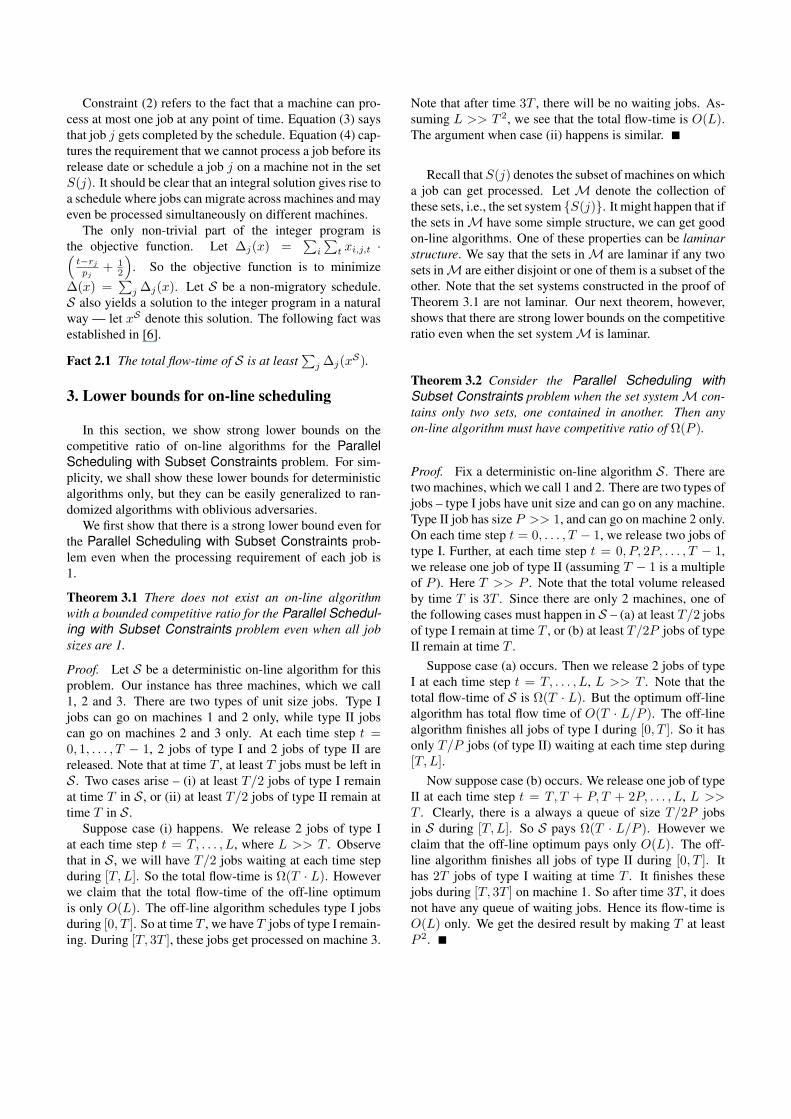
Constraint (2) refers to the fact that a machine can pro-cess at most one job at any point of time. Equation (3) saysthat job j gets completed by the schedule. Equation (4) cap-tures the requirement that we cannot process a job before itsrelease date or schedule a job j on a machine not in the setS(j). It should be clear that an integral solution gives rise toa schedule where jobs can migrate across machines and mayeven be processed simultaneously on different machines.

The only non-trivial part of the integer program isthe objective function. Let ∆j(x) =

∑i

∑t xi,j,t ·(

t−rj

pj+ 1

2

). So the objective function is to minimize

∆(x) =∑

j ∆j(x). Let S be a non-migratory schedule.S also yields a solution to the integer program in a naturalway — let xS denote this solution. The following fact wasestablished in [6].

Fact 2.1 The total flow-time of S is at least∑

j ∆j(xS).

3. Lower bounds for on-line scheduling

In this section, we show strong lower bounds on thecompetitive ratio of on-line algorithms for the ParallelScheduling with Subset Constraints problem. For sim-plicity, we shall show these lower bounds for deterministicalgorithms only, but they can be easily generalized to ran-domized algorithms with oblivious adversaries.

We first show that there is a strong lower bound even forthe Parallel Scheduling with Subset Constraints prob-lem even when the processing requirement of each job is1.

Theorem 3.1 There does not exist an on-line algorithmwith a bounded competitive ratio for the Parallel Schedul-ing with Subset Constraints problem even when all jobsizes are 1.

Proof. Let S be a deterministic on-line algorithm for thisproblem. Our instance has three machines, which we call1, 2 and 3. There are two types of unit size jobs. Type Ijobs can go on machines 1 and 2 only, while type II jobscan go on machines 2 and 3 only. At each time step t =0, 1, . . . , T − 1, 2 jobs of type I and 2 jobs of type II arereleased. Note that at time T , at least T jobs must be left inS. Two cases arise – (i) at least T/2 jobs of type I remainat time T in S , or (ii) at least T/2 jobs of type II remain attime T in S.

Suppose case (i) happens. We release 2 jobs of type Iat each time step t = T, . . . , L, where L >> T . Observethat in S, we will have T/2 jobs waiting at each time stepduring [T, L]. So the total flow-time is Ω(T · L). Howeverwe claim that the total flow-time of the off-line optimumis only O(L). The off-line algorithm schedules type I jobsduring [0, T ]. So at time T , we have T jobs of type I remain-ing. During [T, 3T ], these jobs get processed on machine 3.

Note that after time 3T , there will be no waiting jobs. As-suming L >> T 2, we see that the total flow-time is O(L).The argument when case (ii) happens is similar.

Recall that S(j) denotes the subset of machines on whicha job can get processed. Let M denote the collection ofthese sets, i.e., the set system S(j). It might happen that ifthe sets inM have some simple structure, we can get goodon-line algorithms. One of these properties can be laminarstructure. We say that the sets inM are laminar if any twosets inM are either disjoint or one of them is a subset of theother. Note that the set systems constructed in the proof ofTheorem 3.1 are not laminar. Our next theorem, however,shows that there are strong lower bounds on the competitiveratio even when the set systemM is laminar.

Theorem 3.2 Consider the Parallel Scheduling withSubset Constraints problem when the set systemM con-tains only two sets, one contained in another. Then anyon-line algorithm must have competitive ratio of Ω(P ).

Proof. Fix a deterministic on-line algorithm S. There aretwo machines, which we call 1 and 2. There are two types ofjobs – type I jobs have unit size and can go on any machine.Type II job has size P >> 1, and can go on machine 2 only.On each time step t = 0, . . . , T − 1, we release two jobs oftype I. Further, at each time step t = 0, P, 2P, . . . , T − 1,we release one job of type II (assuming T − 1 is a multipleof P ). Here T >> P . Note that the total volume releasedby time T is 3T . Since there are only 2 machines, one ofthe following cases must happen in S – (a) at least T/2 jobsof type I remain at time T , or (b) at least T/2P jobs of typeII remain at time T .

Suppose case (a) occurs. Then we release 2 jobs of typeI at each time step t = T, . . . , L, L >> T . Note that thetotal flow-time of S is Ω(T · L). But the optimum off-linealgorithm has total flow time of O(T · L/P ). The off-linealgorithm finishes all jobs of type I during [0, T ]. So it hasonly T/P jobs (of type II) waiting at each time step during[T, L].

Now suppose case (b) occurs. We release one job of typeII at each time step t = T, T + P, T + 2P, . . . , L, L >>T . Clearly, there is a always a queue of size T/2P jobsin S during [T, L]. So S pays Ω(T · L/P ). However weclaim that the off-line optimum pays only O(L). The off-line algorithm finishes all jobs of type II during [0, T ]. Ithas 2T jobs of type I waiting at time T . It finishes thesejobs during [T, 3T ] on machine 1. So after time 3T , it doesnot have any queue of waiting jobs. Hence its flow-time isO(L) only. We get the desired result by making T at leastP 2.

4. Algorithm for Parallel Scheduling with Sub-set Constraints

We say that a job is of class k if 2k−1 ≤ pj < 2k. LetJk denote the jobs of class k and let C be the number ofclasses. Consider the integer program (1). For the pur-pose of subsequent discussion, we modify the integer pro-gram slightly by replacing the objective function

∑j ∆j(x)

by∑

j ∆′j(x), where ∆′j(x) =∑

i

∑t xi,j,t

(t−rj

dpje+ 1

2

).

Here dpje equals pj rounded up to the nearest power of2. Note that dpje is the same for all jobs j of the sameclass. Thus the terms in this new objective function can begrouped together in a convenient manner. It is easy to seethat this modification does not increase the cost of a solu-tion x and reduces it by at most a factor 2 so that Fact 2.1still holds. We now relax the integer program by replacingthe constraints (5) by 0 ≤ xi,j,t ≤ 1. Let x∗ be an optimalfractional solution to this linear program (LP).

By the slot (i, t) we mean the time slot (t, t+ 1) on ma-chine i.

4.1. The Structure of the Algorithm

We begin with a description of the overall structure ofthe algorithm. The algorithm proceeds in C iterations. Inthe kth iteration the algorithm starts with a feasible solutionto the LP, xk−1 (x0 is the same as x∗).

Consider a slot (i, t) and define the available spacein this slot as the total volume of this slot that is eitherempty or is occupied by jobs of class k in the solutionxk−1. In this iteration the algorithm rearranges the jobsof class k in the total available space, so that each jobj ∈ Jk is completely scheduled on one machine in S(j).We denote this new solution to the LP by xk and arguethat

∑j∈Jk

∆′j(xk) ≤∑

j∈Jk∆′j(xk−1) + U where U =∑

j pj is the total processing time of all jobs. Since in iter-ation k we only move jobs of class k, the above implies that∆′(xk) ≤ ∆′(xk−1)+U . Thus after C iterations we wouldhave ensured that every job j is scheduled completely onone machine in S(j). Further, ∆′(xC) ≤ ∆′(x∗) + C · U .

The solution xC defines a preemptive, non-migratoryschedule, S. If some slot in S is partly empty and a job jcan be brought forward to this slot then we do that. Let Sf

be the schedule so obtained and xf be the LP solution cor-responding to this schedule. Note that ∆′(xf ) ≤ ∆′(xC).Further, as in [6], we can bound the flow time of Sf by∆′(xf ) + C · U . Putting everything together we get thatthe flow time of schedule Sf is at most ∆′(x∗) + 2C · U .Since both U and ∆′(x∗) are lower bounds on the optimumflow time we obtain a schedule whose flow time is atmost1 + 2 logP times the optimum.

4.2. The kth iteration

We construct a graph Gk for iteration k.

1. Gk has one vertex v(i, t), for each choice of machine iand time t. Besides these, there is one vertex, v(j) foreach job j of class k and a vertex u(t) for each time t.The source is a vertex s.

2. There is an edge from v(i, rj) to v(j) iff i ∈ Sj . Thisedge has flow

∑t x

k−1i,j,t . If this flow is zero we remove

the edge. There are no other edges incident at vertexv(j). Note that for each job j the LP has a constraint∑

i

∑t xi,j,t = pj . This implies that the total flow

reaching vertex v(j) is exactly pj and this is the de-mand of vertex v(j).

3. For every i, t there is an edge from v(i, t) to u(t). Theflow on this edge is the extent to which the time slot ton machine i is empty, ie 1 −

∑j x

k−1i,j,t . We refer to

such edges as ”null-edges” and to the vertex u(t) as anull-vertex. The flow reaching vertex u(t) equals thetotal empty space in the slots at time t. This is also thedemand of vertex u(t).

4. There is an edge from v(i, t−1) to v(i, t) and the flowon these edges is given by conservation constraints.The vertex v(i, 0) is the same as the vertex s.

From the construction of the graph it follows that eachedge has a unique predecessor edge.

Let f ′ be the initial flow as described above. We willcompute a flow, f∗, in which all demand from the sources to sink v(j) is routed on a single path. The flow from sto the sink u(t) could use multiple paths. Besides this, wehave the following additional requirement on the flow f∗:

1. Let e be a null-edge and e′ its predecessor. If f∗(e) >0 then f∗(e′) ≤ f ′(e′).

2. For any edge, e, f∗(e) should not exceed f ′(e) bymore than 2k − 1.

The unsplittable flow f∗ in graph Gk, assigns each jobto a unique machine by virtue of the fact that the flow froms to v(j) is routed on a single path. Thus if the edge(v(i, rj), v(j)) has non-zero flow in f∗ then we schedulejob j, which is of class k, on machine i. Further, a flowof p units on the null-edge from v(i, t) to u(t) is viewed asscheduling a null-job, having release time t and processingtime p (same as p empty slots) on machine i. These jobsare scheduled in the available space for this iteration. Todo the actual assignment of jobs to slots on machine i, weorder slots by decreasing time and the jobs by decreasingrelease time; If a job j and a null-job have the same releasetime then the null-job appears before j in the ordering. The

jobs and slots are considered in this order and each job isassigned to slots with total available space equal to the pro-cessing time of the job. Note that we might not be able toassign all jobs to slots since we might run out of availablespace. It might also happen that only a part of a job can beassigned.

Let x′ be a (possibly infeasible) solution to the LP thatcaptures the above reassignment of class k jobs. Note thatx′ is identical to xk−1 for jobs of all classes other than k.

Lemma 4.1∑

j∈Jk∆′j(x′) ≤

∑j∈Jk

∆′j(xk−1).

Proof. Since we have only assigned class k jobs to the avail-able space for this iteration, the difference in cost can beviewed as arising from the placement of empty spaces. Wenow argue that in x′, the empty spaces only occur later thanin the xk−1. Suppose the total empty space at time t in thesolution xk−1 is p. In the graph Gk, vertex u(t) would havea demand p. This demand p is perhaps routed on multiplepaths and leads to the creation of multiple null-jobs eachwith a release time t. Consider the null-job so created onmachine i. The flow f∗ we compute has the property thatf∗(e) ≤ f ′(e) where e is the edge from v(i, t−1) to v(i, t).This implies that the total processing time of all jobs (nulland of class k) with release time t or more that are sched-uled on machine i is at most the total available space at andafter time t on machine i in this iteration. Hence the null-jobin consideration would be assigned slots on machine i aftertime t. Since this is true for each null-job created for theempty space at time t, we have established that the emptyspaces in xk−1 only move ahead in time in the solution x′

This proves the lemma.

However, the solution x′ is not feasible. There are twosources of infeasibility stemming from the fact that in theunsplittable flow we exceed the original flow value on theedges.

Note that on some machine i we might not be able toassign all jobs given by the unsplittable flow in the avail-able space. This is because the flow on the edge (s, v(i, 1))exceeds the initial flow. Note that the sum

∑j∈Jk

∆′j(x′)does not include the contribution of jobs which do not getassigned. However, the total volume of jobs which are tobe scheduled on machine i but cannot be assigned to theavailable space is at most 2k − 1.

The second source of infeasibility could be that a job isscheduled before its release date.

Claim 4.2 On any machine i, at most 2k − 1 units of avail-able space before time t are assigned to jobs released at orafter t.

Proof. The flow through the edge (v(i, t − 1), v(i, t)) inf∗ exceeds the original flow through this edge by at most

2k−1. Since the total available space after t equals the orig-inal flow through this edge, the amount of available spaceneeded, before t, to schedule jobs released at or after t, is atmost 2k − 1.

The above two infeasibilities can therefore be easily han-dled if we create 2k − 1 new slots on each machine at theend of the schedule and shift the class k jobs and the emptyspaces in the solution x′ to the right by 2k−1 units of avail-able space. Let xk be a feasible solution to the LP whichcorresponds to this modification.

Claim 4.3∑

j∈Jk∆′j(xk) ≤

∑j∈Jk

∆′j(x′) + U .

Proof. We begin by assuming that all empty spaces in x′ arealso occupied by jobs of class k. For a machine i considera time t. As a result of the above shift, the total volumeof class k jobs scheduled on i after time t would increaseby exactly 2k − 1. This implies that the contribution of theclass k jobs increases by the processing time of all jobs (andany empty spaces) on machine i. Now note that every unitof empty space, which we treated as occupied by class kjobs, would move at least 2k − 1 units to the right. Hence,removing the contribution of these empty spaces would leadto a net increase which is at most the total processing timeon machine i. Since this is true for all machines the claimfollows.

This completes our description of the kth iteration andalso establishes that the solution to the LP, xk, obtained atthe end of this iteration satisfies, ∆′(xk) ≤ ∆′(xk−1) + U .We now discuss how to compute the an unsplittable flowmeeting the two requirements.

4.3. Computing the Unsplittable Flow

We will modify the unsplittable flow algorithm of Dinitzet.al.(DGG algorithm) to get a flow which satisfies theabove requirements.

We begin with a brief review of the DGG algorithm. Thealgorithm starts with a fractional flow from the source tothe sinks. Each sink gets flow equal to its demand whichcould be routed along multiple paths. The algorithm makesthe flow unsplittable by redistributing it along ”alternatingcycles”. An alternating cycle is composed of alternate ”for-ward” and ”backward” paths; flow is increased along thebackward paths and decreased along the forward paths. Abackward path is formed by starting at a sink and follow-ing incoming edges till we reach a vertex which has morethan one outgoing edge. We take the outgoing edge not onthe backward path to start a forward path. The forward pathcontinues by taking outgoing edges till we reach a sink atwhich point we start building a backward path by taking anincoming edge other than the one on the forward path. At

any point in the algorithm, if a vertex has a terminal andan incoming edge with flow exceeding the demand of thisterminal , then we move the terminal across this edge andreduce the flow on the edge by the demand. Once an edgehas zero flow it is removed from the graph. This implies thatevery sink has atleast two incoming edges. We can similarlyensure that the source has at least two outgoing edges andthese two facts together imply that we can always build analternating cycle.

The extent of augmentation along an alternating cycle isdetermined by the minimum of two quantities — the flowon an edge on the forward paths and the increase in flowon a backward edge that would cause a terminal to move.An edge (u, v) is singular if v has at most one outgoingedge. Note that all edges on backward paths are singularand hence flow is increased only on singular edges. Sincewe do not add any edges to the graph, a singular edge re-mains singular till it is deleted. Key to the analysis of the al-gorithm is the fact that we move at most one terminal alonga singular edge. This implies that the total unsplittable flowrouted along an edge exceeds the initial flow on the edge bythe maximum demand.

Our first modification to the DGG algorithm is:

We call a null-edge carrying zero flow an emptyedge. An empty edge, say from v(i, t) to u(t) isremoved iff the edge from v(i, t) to v(i, t + 1) ison a backward path.

Note that the flow on an edge is increased only when itis on the backward path of an alternating cycle. The abovemodification preserves the property that all such edges aresingular. Hence, as in the DGG algorithm we can argue thatfor any edge, e, f∗(e) exceeds f ′(e) by at most the maxi-mum demand sent through e after e is on a backward path.Our second modification will ensure that the maximum de-mand we send through an edge after it is part of a backwardpath is 2k−1. This would then imply that our second re-quirement on f∗ is met.

Since the flow corresponding to the null vertex u(t) doesnot have to be routed unsplittably, we do not have to waittill one of the edges incident to u(t) has flow equal to thedemand of u(t). We can route a part of this demand earlier.This gives us our second modification to the DGG algo-rithm:

The terminals u(t) are never moved. However, ifthe flow on a null-edge e, incident to u(t), equalsthe flow on the preceding edge e′, we route thisamount of flow from the source to u(t) along theunique path terminating in edge e.

Note that after we route the flow as above, edges e, e′ areremoved from the graph. The above modification allows usto prove the following useful claim.

Claim 4.4 Let e be a null-edge carrying non-zero flow.None of the edges on the unique path from s to e was everon a backward path.

Proof. Let e′ be the immediate predecessor of e. If e′ wasever on a backward path then e would also be on this path.At that point the flow on e and e′ was the same and hence wewould have routed part of the demand of terminal u(t) fromthe source thereby removing edges e and e′. This impliesthat e′ was never on a backward path and hence none of theedges preceding it could have been on a backward path.

This claim lets us prove that flow f∗ meets the two re-quirements.

1. If we route non-zero flow along a null-edge e in theflow f∗ then by the above claim, the edge preceding e,say e′ was not part of a backward path till the point intime that the flow from s to the null-vertex was routed.At this point the edge e′ was removed. Hence, wenever increased flow through edge e′ and so the finalflow through e′ does not exceed the initial flow and thefirst requirement on the flow f∗ is met.

2. If we route non-zero flow along a null-edge e in theflow f∗ then none of edges preceding e on the pathfrom s to e had been part of a backward path beforethis point. This implies that once an edge is part of abackward path, it can only carry flow for the terminalsv(j). Since the maximum demand for these terminalsis 2k − 1 and since only one such terminal can travelacross this edge (as in the DGG algorithm) we route atmost 2k − 1 units of flow through the edge after it ispart of a backward path. This implies that the final flowthrough any edge exceeds the initial flow by atmost2k − 1 and establishes our second requirement on f∗.

Since we might not move terminal u(t) even when oneof the edges incident to it carries flow equal to its demand,we might now have a situation where a null-vertex has onlyone edge entering it. Hence if we reach this vertex on aforward path, we will not be able to leave it and so will notbe able to build an alternating cycle.

The structure of the problem allows us to get around thislast remaining difficulty.

Lemma 4.5 The modified algorithm is able to find an al-ternating cycle at each step.

Proof. Consider all null-vertices which have only one in-coming edge and let u(t) be the one with maximum t. Let(v(i, t), u(t)) be the only edge entering u(t). Since thisedge has non-zero flow none of the edges preceding it wouldhave been part of a backward path. This implies that everynull-vertex u(t′), t′ ≤ t has an edge from v(i, t′).

We start our alternating path from vertex u(t), take theedge (v(i, t), u(t)) to form a backward path and then con-tinue with a forward path. As we continue this process, sup-pose, we get stuck at a null-vertex u(t′), t′ < t. We musthave reached u(t′) from vertex v(i, t′) as we were buildinga forward path. An alternate way of continuing the forwardpath would have been to take the path from v(i, t′) to v(i, t)and this would have formed an alternating cycle.

5. Integrality Gap for Parallel machines

In this section, we show that the integrality gap of thelinear program in Section 2 is large. In fact this large gapholds even when we restrict to the special case of the Paral-lel Scheduling problem. This integrality gap instance willform the basis of our lower bound reductions. Our instancewill have m machines and the ratio of the largest job size tothe smallest job size will be m as well. The number of jobsn can be much larger than m (in fact has no dependence onm). We pick two parameters C, ` such that C` = m. Weshall make both of these Ω

(log m

log log m

). We shall say that a

job is of type k if its size is Ck.Jobs arrive in ` phases, each phase being of length ex-

actly T (T is an arbitrary parameter, it can as big as wewish). Let us describe phase 0 : at each integral time stept, 0 ≤ t < T , one job of type ` arrives. Phase i ≥ 0can be described similarly : at each integral time step t,i · T ≤ t < (i+ 1) · T , Ci jobs of type `− i arrive.

Let us first see what the fractional solution does. In phasei, consider the jobs that arrive at time t. The total volume ofthese jobs isCi·C`−i = C` = m. So themmachines finishthese jobs by time t+ 1 (note that in the fractional solutionthe jobs can be done concurrently on several machines). Soevery job spends just 1 unit of time in the system. Nownote the total processing time of the jobs in our instance ism · T · `. Therefore, the value of the fractional solution isalso O(m · T · `).

We now show that any integral solution will have to payabout logm/ log logm times this value. The intuition is asfollows : consider phase 0. The integral solution cannotfinish all jobs in this phase by time T . Indeed, only onemachine can be busy at time 0, only two machines can bebusy at time 2 and so. So we will need to shift about m ·C`/2 volume of jobs of type ` after time T . The key thingto observe is that this number is a factor of C larger thanthe amount of shift needed in phase 1 and so on. So thisshifted volume cannot fit in the gaps created by shifting jobsin subsequent phases. This volume will have to go to thevery end of the schedule. We now prove the result formally.

Lemma 5.1 Consider an integral schedule S. For any i,0 ≤ i < `, S must process at leastmC`−i/2 volume of jobs

of type `− i after time (i+1) ·T , which is the time at whichphase i ends.

Proof. Consider phase i. Call a machine at time t good ifit is processing a job of type ` − i at time t. We claim thatat time i · T + x, there are at most x · Ci good machines.Indeed, at each unit of time between i · T and i · T + x,Ci jobs of type ` − i are released. So there are at mostx · Ci jobs of type ` − i at time i · T + x in this schedule.Since a job can be processed by at most one machine atany point of time, the number of good machines at this timemust also be at at most x · Ci. Let I denote the interval[i · T, i · T + C`−i]. In this interval, at most

∑C`−i

x=0 x · Ci

volume of processing of jobs of type ` − i is done. Thisquantity is at most m · C`−i/2 (because m = C`). Butthe total volume of jobs that can be processed during I ism ·C`−i. So there is at least m ·C`−i/2 volume of time inthis interval I during which S does not process a job of type` − i. Since the total volume of jobs of type ` − i releasedduring phase i is exactly m · T , at least m ·C`−i/2 volumeof such jobs must be processed after this phase ends.

We are now ready to prove the main theorem.

Theorem 5.2 Any integral schedule S for this instancemust have total flow-time at least Ω(min(C, `) ·m · ` · T ).

Proof. Consider a schedule S. Fix an i ≤ `/4. Let Ti

denote the time at which phase i ends, i.e., Ti = (i+ 1) ·T .Lemma 5.1 says that at least mC`−i/2 volume of jobs oftype ` − i must be processed after time Ti. Let T ′ denotethe time at which phase `/2 begins, i.e., ` · T/2. Now oneof these two cases must happen in S : either (i) at leastmC`−i/4 volume of jobs of type `− i is processed betweentime Ti and T ′, or (ii) at least mC`−i/4 volume of jobs oftype `− i is processed after time T ′.

Suppose case (i) happens. Fix a time t ∈ [T ′, ` ·T ] (` ·Tis the time at which the last phase ends). During [Ti, t],exactly (t− Ti) ·m volume of jobs of type `− i− 1 or lessare released. Since at leastmC`−i/4 volume of jobs of type` − i are processed between time Ti and T ′, it follows thatat least this much volume of jobs of type ` − i − 1 or lessmust be waiting at time t in the schedule S. Since each suchjobs has processing time at most C`−i−1, it follows that atleast mC/4 jobs must be waiting at time t. Since this holdsfor any time t lying in the interval [T ′, ` · T ], the total flowtime of S is at least mC/4 · (` · T − T ′) = Ω(m ·C · ` · T ),and so we are done.

Therefore we can assume that case (ii) holds for everyi ≤ `/4. Fix such an i. Since mC`−i/4 volume of jobs oftype ` − i translates to at least m/4 jobs, at least m/4 jobsof type ` − i finish processing after time T ′. So the totalflow time of such jobs is at least m/4 · (T ′− i ·T ), which isΩ(m ·` ·T ) because i ≤ `/4. But this holds for all values of

i between 0 and `/4. So the total flow time is Ω(m · `2 · T ).This proves the theorem.

Thus we have shown that the integrality gap of this LPin case of parallel machines is Ω

(log m

log log m

).

6. Hardness Results

We now prove lower bounds on the approximation ratioof poly-time algorithms for the Parallel Scheduling andParallel Scheduling with Subset Constraints problems.Let us first describe the main idea used in these proofs. Re-call the integrality gap instance in the previous section. Thekey reason it worked was as follows : identical jobs arereleased in a time slot of length T so that the fractionalsolution could process these jobs in this time slot and fillthe entire time slot on each machine. However any inte-gral solution would need to process a large volume of suchjobs after the slot ends. We achieved this by allowing thefractional solution to process the same job concurrently onmultiple machines.

We use a similar idea for constructing lower boundproofs. We show that it is possible to release almost iden-tical jobs in a time slot of length T so that no polynomialtime algorithm can distinguish between these two cases :(i) all jobs can be completed in the time slot and hence fillthis entire time slot on all machines, or (ii) a significant vol-ume of jobs need to be processed after time T . We use thehardness of the 3-Dimensional Matching problem and the3-partition problem to prove such results.

6.1. Parallel machine scheduling with subset con-straints

Our hardness result will use the 3-Dimensional Match-ing problem. Recall the definition of the 3-DimensionalMatching problem : we are given three sets X,Y and Zeach of size n. We are also given a subset E of X ×Y ×Z.We shall call an element of E a triplet or a hyperedge. Thegoal is to find a subset E′ of E of size n such that each ele-ment inX∪Y ∪Z appears in (exactly) one of these triplets.Such a set of edges is called a perfect matching. The prob-lem of deciding whether an instance of the 3-DimensionalMatching problem has perfect matching is NP-complete[5].

In fact, we shall deal with a special case of the3-Dimensional Matching problem, which we call theBounded 3-Dimensional Matching problem. In thisproblem, the total number of triplets in the set E is at mostδ times the size of the set X , where δ is a constant. It turnsout that the Bounded 3-Dimensional Matching problemis NP-complete as well [9]. In fact one can prove the fol-lowing stronger theorem.

Theorem 6.1 [9] There exists a constant γ > 0 such thatit is NP-hard to distinguish between the following instancesof the Bounded 3-Dimensional Matching problem : (i)the instance has a perfect matching, or (ii) any matching inthe instance has at most γ · n edges.

Theorem 6.2 There exist constants α, β > 0 such that thefollowing statement is true. Let K and T be arbitrary pa-rameters, where T is a multiple of 3K (typically T >> K).There is a poly-time reduction f from the Bounded 3-Dimensional Matching problem to the Parallel Schedul-ing with Subset Constraints problem which has the fol-lowing properties :

• Given an instance I of the Bounded 3-DimensionalMatching problem, f(I) has job sizes in the range[K, 3K]. Let m denote the number of machines inf(I). Then the total volume of jobs in f(I) is exactlym · T .

• Suppose there is a perfect matching in I. Then all jobsin f(I) can be scheduled in a manner so that they fin-ish processing by time T . Further the total flow-timeof these jobs is at most α ·m · T .

• Suppose there is no matching in I which has more thanγ · n hyperedges. Then any scheduling of jobs in f(I)must leave at least β ·m ·K volume of jobs unfinishedat time T .

Proof. We use the reduction of Lenstra et. al. [11]. Let Ibe an instance of the Bounded 3-Dimensional Matchingproblem. Let E denote the set of triplets, which is a subsetof X × Y × Z. Recall that the sets X,Y, Z have size neach and E has at most δ · n hyperedges. Let m denote thesize of E. We now construct an instance I ′ of the ParallelScheduling with Subset Constraints problem. I ′ willnot be the instance f(I), but will form the basic buildingblock in the construction of f(I).

In I ′ all jobs are released at time 0. There are two kindsof jobs : for each element v ∈ X ∪ Y ∪Z, we have one jobv of size K (although we are using the same notation for anelement ofX∪Y ∪Z and the corresponding job, this shouldnot cause any confusion). There are m − n dummy jobs ofsize 3K. It is easy to see that the total volume of jobs is3mK. There are m machines, one machine for each triplete ∈ E. A job v can be processed by a machine e if and onlyif v is in the triplet e. Dummy jobs can be processed on anymachine.

Let us see the key properties of I ′. Suppose I has a per-fect matching E′ ⊂ E. Then on the machines correspond-ing to E′, we can schedule the jobs in these triplets. Theremaining m − n dummy jobs go in each of the machinescorresponding to E −E′. Thus, all jobs in I ′ finish by 3K.

Also the total flow-time of the jobs is at most 3K ·(m+2n)(because there are m+ 2n jobs) which is at most 9mK.

Now suppose I does not have a matching of size morethan γn. We want to claim that in any scheduling of the jobsin I ′, lot of jobs will remain unfinished at time 3K. Let ussee why. Consider a scheduling S of jobs in I ′. We calla machine e corresponding to the triplet (ex, ey, ez) goodif S schedules ex, ey, ez on e. Clearly there are at mostγ · n good machines. Let Jg be the set of jobs from X ∪Y ∪ Z which are scheduled on good machines. Recall thatthere are a total of 3n jobs corresponding to X ∪ Y ∪ Zand at most 3γn of these are scheduled on good machines.Let Jb denote the remaining jobs from X ∪ Y ∪ Z. So|Jb| ≥ 3n(1− γ). Call a machine bad if a job from Jb getsscheduled on it. So the total number of bad machines is atleast |Jb|/2 (because at most 2 jobs from Jb can go on sucha machine). Consider a bad machine e corresponding to thetriplet (ex, ey, ez). During [0, 3K] either 1 or 2 jobs fromJb get scheduled on it. So one of the following cases musthappen : (i) At least K units of time is idle during [0, 3K],or (ii) A dummy job is scheduled on this machine. Note thatin case (ii) the machine processes at leastK units of volumeafter time 3K (because each dummy job is of size 3K andwe have at least one job from Jb on this machine). Let M1

be the bad machines which satisfy (i), and M2 be the madmachines which satisfy (ii).

If |M1| > |M2|, then we see that the schedule S hasat least |M1|K ≥ |Jb| · K/4 volume of idle time during[0, 3K]. Since the total volume of jobs in the instanceI ′fits exactly on m machines during [0, 3K] it follows that Sprocesses at least |Jb| ·K/4 volume of jobs after time 3K.

If |M1| ≤ |M2|, then S processes at least K · |M2| ≥|Jb| · K/4 units of volume after time 3K. Thus in eithercase, S processes Ω(K · n) volume of job after time 3K.Since m = O(n), we have shown the theorem when T =3K.

In order to extend it to larger values of T , we simplytake T

3K copies of I ′ and schedule them one after another.More formally, we construct f(I) as follows. We take T

3Kcopies of I ′. The jobs in the ith copy get released at time(i−1) ·3K. This completes the description of f(I). Let usnow prove that each of the three statements in the theoremare satisfied.

The first statement is true simply by the properties ofI ′. Let us prove the second statement. Suppose I has aperfect matching. Then the jobs in the ith copy can be pro-cessed during [(i − 1) · 3K, i · 3K]. So all jobs finish bytime T . Since the flow-time of jobs in any copy is at most9mK, the total flow-time is O(m · T ). Let us now provethe third statement. Suppose any matching in I has at mostγn hyperedges. Consider the last copy of I ′ in f(I), i.e.,the copy which starts at time T − 3K. By properties of I ′above, Ω(mK) volume of jobs in this copy must be pro-

cessed after time T by any schedule. Thus the theorem isproved.

We are now ready to give the reduction from Bounded3-Dimensional Matching to Parallel Scheduling withSubset Constraints. The reduction closely follows theconstruction of the integrality gap example in Section 5.Let I be an instance of the Bounded 3-DimensionalMatching problem. We shall invoke Theorem 6.2 sev-eral times. The parameter T will remain fixed, but K willvary on different calls to this theorem. So let f(I,K) de-note the instance of the Parallel Scheduling with SubsetConstraints problem returned by Theorem 6.2 when giventhe instance I of the Bounded 3-Dimensional Matchingproblem and the parameter K.

We now show how to obtain an instance g(I) of the Par-allel Scheduling with Subset Constraints problem whichwill complete the hardness proof. The construction has `phases, each phase having length T . Let us describe phasei. We get the instance f(I, C`−i). All jobs in this instancereleasing at time t get released at time (t+i·T ) in g(I), i.e.,we just shift the release dates by i · T units of time. Here Cis a parameter we shall fix later.

Having described g(I) let us see the properties of thisreduction. Suppose I has a perfect matching. Then jobs inphase i can be scheduled during [i · T, (i + 1) · T ]. So thetotal flow-time is O(m · T · `).

Now suppose I does not have a matching of size morethan γ · n. Consider phase i. Theorem 6.2 implies thatat least Ω(mC`−i) volume of jobs of size C`−i must bewaiting at time (i + 1) · T in any scheduling of the jobs ing(I). But this is analogous to Lemma 5.1. Therefore we canuse the same arguments as in Theorem 5.2 to show that anyschedule must have flow-time at least Ω(min(C, `)·m·`·T ).

Thus we have shown it NP-hard to get a poly-timeO(min(C, `))-approximation algorithm for minimizing thetotal flow-time for the Parallel Scheduling with SubsetConstraints problem. Now as in Section 5, set C = ` suchthat C` = m. So we get Ω(logm/ log logm) hardness re-sult for this problem.

6.2. Parallel Scheduling

We use the 3-partition problem to prove the hardness ofthe Parallel Scheduling problem. Recall the 3-partitionproblem. We are given a set X of 3m elements and a boundB. Each element x ∈ M has size sx which is an inte-ger. We would like to partition the set X into m sets suchthat the total size of elements in any such set is exactly B.Such a partition is said to be valid partition. We can assumewithout loss of generality that the sum of the sizes of theelements in X is exactly m ·B. It is NP-complete to decideif such a valid partition exists or not [5].

In fact, we can say more about this problem. If we lookat the NP-completeness proof of the 3-partition problem(see for example [5]) we can add two more constraints onthe problem instance : (i) For every element x, sx lies be-tween B/4 and B/2. Hence if there is a valid partition,then every set in this partition must contain exactly three el-ements of X , and (ii) The bound B is a polynomial in m,i.e., there is a universal constant c such that B is at most mc

(for all instances on 3m elements). The problem remainsNP-complete even in this setting. So when we talk aboutthe 3-partition problem in this section, we shall assume thatwe are talking about this special case.

The following theorem is the analogue of Theorem 6.2 :

Theorem 6.3 Given an instance I of the 3-partition prob-lem, parameters T and K, there is a poly-time computablefunction f , which gives an instance f(I) of the ParallelScheduling problem. Here T is a multiple of K · B (B isthe bound appearing in I). This reduction has the followingproperties :

• There are m machines in f(I), and the job sizes lie inthe range (KB/4,KB/2). The total volume of jobs inf(I) is T ·m.

• If I has a valid partition, then all jobs in f(I) can befinished during [0, T ]. Further the flow-time of thesejobs is O(m · T ).

• If I does not have a valid partition, then any schedul-ing of jobs in f(I) must leave at least K units of un-finished volume of jobs at time T .

Remark : The result in this theorem is much weaker thanthat in Theorem 6.2. Indeed consider the case when I doesnot have a valid partition. The amount of volume remainingat time T in the theorem above is much smaller than the sizeof even a single job.Proof. Fix an instance I of the 3-partition problem andthe parameters K and T . Let X denote the set of items inI and sx denote the size of x. Let |X| = 3m. Recall thatall sizes are integers. Let B be the bound specified in I.We first construct an instance I ′ of Parallel Scheduling.There are 3m jobs in I ′, one job for each element inX . Thejob corresponding to x has release date 0 and processingrequirement K · sx. There are m machines.

Let us see the properties of I ′. Clearly job sizes are in therange (KB/4,KB/2). Suppose I has a valid partitioning.Let I(j) be the set of 3 items assigned to set j in such apartition. Then schedule the jobs corresponding to I(j) onthe machine j. Clearly, on each machine we assign a totalof KB volume of job. So all jobs finish by time K · B.Since there are only three jobs per machine, it is easy to seethat the flow-time is also O(K ·B ·m).

Suppose I does not have a valid partitioning. We claimthat any scheduling in I ′ must leave at least K units of un-finished volume at time K ·B. Suppose this is not true. LetS be a schedule which contradicts this claim. Let I(j) bethe jobs scheduled on machine j by S. If we scale downthe sizes of the jobs in I(j) by a factor of K to their actualsizes in I, we see that the set corresponding to j containselements which have total size less than B + 1. But sinceall quantities are integers, it must be the case that the sumof the sizes sx of the jobs x ∈ I(j) is at most B. Since thisholds for all machines, and the sum of the sizes of all jobsis m · B, we see that the sets I(j) form a valid partitioningof I, a contradiction. This proves the theorem for the caseT = K · B. For a larger value of T (while maintaining theconstraint that T is a multiple of K · B), we just take T

KBcopies of I ′ and argue as in the proof of Theorem 6.2.

The rest of the plan is similar to that in Section 6.1. How-ever, since Theorem 6.3 is much weaker than Theorem 6.2,we get a weaker lower bound. There are ` phases. Eachphase shall invoke Theorem 6.3. The parameter T in thetheorem will remain unchanged, but K will vary. So again,we shall denote by f(I,K) the instance returned by thetheorem above when the inputs to f are I, T and K. Theparameter ` will be m2.

Let us describe phase i. In phase i we get the instanceI ′i = f(I,m2(`−i)c). Recall that c is such that the bound Bis at most mc for any instance of the 3-partition problem.As before we shift the release dates of the jobs in I ′i by i ·Tunits. Let us call this instance of Parallel Scheduling asg(I).

Suppose I has a valid partitioning. Then it is easy thatjobs in phase i of g(I) can be processed during [iT, (i +1)T ]. So all jobs finish by time ` · T and the total flow-time is O(m · T · `). Now suppose I does not have a validpartitioning. We would like to argue that for any schedulingof the jobs in g(I), the total flow-time is much larger thanO(m · T · `).

The following fact is clear from the proof of Theo-rem 6.3.

Fact 6.4 For each i, 1 ≤ i ≤ `, at least m2(`−i)c volume ofjobs from I ′i are scheduled in S after time (i + 1) · T , i.e.,the time at which phase i ends.

The proof of the following theorem proceeds along thesame lines as Theorem 5.2.

Theorem 6.5 If I does not has a valid partitioning, thenany scheduling of the jobs in g(I) must incur Ω(m2 · l · T )flow-time.

Proof. Fix a scheduling S of g(I). Consider an i < `/4.Let Ti be the time at which phase i ends, i.e., (i + 1) · T .Let T ′ be the time at which phase `/2 begins, i.e., ` · T/2.

Fact 6.4 implies that at least m2(`−i)c volume of jobs fromthe instance I ′i are scheduled after Ti. Now two cases arise: (i) at least m2(`−i)c/2 volume of these jobs is processedafter T ′ in S, or (ii) at leastm2(`−i)c/2 volume of jobs fromI ′i is processed between Ti and T ′ in S.

Consider case (ii) first. Consider a time t between T ′ and` ·T (` ·T is the time at which the last phase ends). Let I ′′i+1

denote I ′i+1 ∪ · · · ∪ I ′`.

Claim 6.6 At least m2(`−i)c/2 volume of jobs from I ′′i+1

must be waiting at time t.

Proof. Suppose t lies in phase j, i.e., between j · T and(j+1) ·T . Recall the construction of I ′j in Theorem 6.3. InI ′j , jobs get released at T

KB time instances, namely, j ·T, j ·T +KB, j ·T +2KB, . . .. Further, the total volume of jobsreleased during [j ·T + rKB, j ·T + (r+ 1)KB] is exactlym · KB. Now suppose t lies between j · T + rKB andj ·T +(r+1)KB. Let t′ denote the time j ·T +(r+1)KB.From j ·T to t′, exactly (t′− j ·T ) ·m volume of jobs fromI ′j get released. Further between Ti and j · T , we releaseexactly (j · T − Ti) volume of jobs from I ′i+1 ∪ · · · ∪ I ′j−1.Thus we see that exactly (t′ − Ti) ·m volume of jobs fromI ′′i+1 are released between Ti and t′.

Now, if we schedule m2(`−i)c/2 volume of jobs from I ′ibetween Ti and t′ (note that t′ is larger than T ′), then thismuch volume of jobs from I ′′i+1 must be waiting at time t′.Since no jobs get released between t and t′, the jobs waitingat t′ must also be waiting at t. This proves the claim.

Now each job in I ′i+1 has processing time at most B ·m2(`−i−1)c ≤ m2(`−i−1)c+c ≤ m2(`−i)c/m2 (assuming cis at least 2). So at least m2 jobs must be waiting at time t.The time t was chosen arbitrarily between T · `/2 and T · `.So the total flow time is at least Ω(m2 · ` · T ). This provesthe theorem.

So it must be the case that (i) happens. Thus for eachvalue of i between 1 and `/2, at least one job from I ′i iswaiting at time T ′. So the total flow-time is at least Ω(`2 ·T )which proves the theorem because ` = m2.

So we have shown that it is NP-hard to get a poly-timeO(m) approximation algorithm for this problem. Let usexpress this in terms of P . Note that P = B ·m2·`·c. Now` = m2. So we get P ≤ m2·m2·c+c. This implies that m is

Ω(√

log Plog log P

).

7. Open Problems

We leave open the problem of minimizing average flow-time on unrelated machines. We believe there is a poly-logarithmic approximation algorithm for this problem. Infact, one can write a linear program for this problem sim-ilar to what we have in this paper. We conjecture that

the integrality gap of this natural linear program is poly-logarithmic.

8. Acknowledgements

Part of this work was done when both authors were vis-itng the Max-Planck-Institut fuer Informatik, Saarbruecken.The research of the first author is partly supported bythe ”Approximation Algorithms” partner group of MPI-Informatik, Germany.

References

[1] N. Avrahami and Y. Azar. Minimizing total flow time andtotal completion time with immediate dispatching. In Proc.15th ACM Symp. on Parallel Algorithms and Architectures(SPAA), pages 11–18, 2003.

[2] B. Awerbuch, Y. Azar, S. Leonardi, and O. Regev. Minimiz-ing the flow time without migration. In ACM Symposium onTheory of Computing, pages 198–205, 1999.

[3] C. Chekuri, S. Khanna, and A. Zhu. Algorithms forweighted flow time. In ACM Symposium on Theory of Com-puting, pages 84–93, 2001.

[4] Y. Dinitz, N. Garg, and M. X. Goemans. On the single-source unsplittable flow problem. In IEEE Symposium onFoundations of Computer Science, pages 290–299, 1998.

[5] M. Garey and D. Johson. Computers and intractability - aguide to NP-completeness. W.H. Freeman and Company,1979.

[6] N. Garg and A. Kumar. Better algorithms for minimizingaverage flow-time on related machines. In ICALP, pages181–190, 2006.

[7] N. Garg and A. Kumar. Minimizing average flow-time onrelated machines. In ACM Symposium on Theory of Com-puting, pages 730–738, 2006.

[8] K. Jansen and L. Porkolab. Improved approximationschemes for scheduling unrelated parallel machines. In ACMSymposium on Theory of Computing, pages 408–417, 1999.

[9] V. Kann. Maximum bounded 3-dimensional matching ismax snp-complete. Information Processing Letters, 37:27–35, 1991.

[10] H. Kellerer, T. Tautenhahn, and G. J. Woeginger. Approx-imability and nonapproximability results for minimizing to-tal flow time on a single machine. In ACM Symposium onTheory of Computing, pages 418–426, 1996.

[11] J. K. Lenstra, D. Shmoys, and E. Tardos. Approximation al-gorithms for scheduling unrelated parallel machine. Mathe-matical Programming, 46(3):259–271, 1990.

[12] S. Leonardi and D. Raz. Approximating total flow time onparallel machines. In ACM Symposium on Theory of Com-puting, pages 110–119, 1997.