New lower bounds for Hopcroft's problem

Discrete Comput Geom 16:389-418 (1996) Discrete & Computational Geometry ~) 1996 Springer-Verlag New York Inc.

New Lower Bounds for Hopcroft's Problem*

J. Er ickson

Computer Science Division, University of California, Berkeley, CA 94720, USA [email protected] and Fachbereich 14 - Informatik, Universitat des Saarlandes, D-66123 SaarbrUcken, Germany

Abstract. We establish new lower bounds on the complexity of the following basic geometric problem, attributed to John Hopcroft: Given a set of n points and m hyperplanes in R d, is any point contained in any hyperplane? We define a general class of partitioning algorithms, and show that in the worst case, for all m and n, any such algorithm requires time f2 (n log m d-n 2/3m2/3 + m log n) in two dimensions, or f2 (n log m + nS/6m U2 + nl /2m 5/6 +

m log n) in three or more dimensions. We obtain slightly higher bounds for the counting version of Hopcrofl's problem in four or more dimensions. Our planar lower bound is within a factor of 2 ~176 of the best known upper bound, due to Matou~ek. Previously, the best known lower bound, in any dimension, was f2 (n log m + m log n). We develop our lower bounds in two stages. First we define a combinatorial representation of the relative order type of a set of points and hyperplanes, called a monochromatic cover, and derive lower bounds on its size in the worst case. We then show that the running time of any partitioning algorithm is bounded below by the size of some monochromatic cover. As a related result, using a straightforward adversary argument, we derive a quadratic lower bound on the complexity of Hopcroft's problem in a surprisingly powerful decision tree model of computation.

* This research was partially supported by NSF Grant CCR-9058440. An earlier version of this paper was published as Technical Report A/04/94, Fachbereich Informatik, Universit~it des Saarlandes, Saarbriicken, Germany, November 1994.

390 J. Erickson

1. Introduction

In the early 1980s John Hopcrofl posed the following problem to several members of the computer science community:

Given a set of n points and n lines in the plane, does any point lie on a line?

Hopcroft's problem arises as a special case of many other geometric problems, including collision detection, ray shooting, and range searching.

The earliest subquadratic algorithm for Hopcroft's problem, due to Chazelle [7], runs in time O(n1"695). (Actually, this algorithm counts intersections among a set of n line segments in the plane, but it can easily be modified to count point-line incidences instead.) A very simple algorithm, attributed to Hopcroft and Seidel [16], described on p. 350 of [17], runs in time O(n 3/2 log 1/2 n). Cole et al. [16] combined these two algorithms, achieving a running time of O(n1"412). Edelsbrunner et al. [20] developed a randomized algorithm with expected running time O (na/3+e); 1 see also [19]. A somewhat simpler algorithm with the same running time was developed by Chazelle et al. [13]. Further research replaced the n ~ term in this upper bound with a succession of smaller and smaller polylogarithmic factors. The running time was im- proved by Edelsbrunner et al. [18] to O(n 4/3 log 4 n) (expected), then by Agarwal [1] to O (n 4/3 log L78 n), then by Chazelle [9] to O (ll 4/3 log 1/3 n), and most recently by Ma- tougek [30] to n4/32 O(l~ n).2 This is currently the fastest algorithm known. Matougek's algorithm can be tuned to detect incidences among n points and m lines in the plane in time O(n logm + n2/3m2/32 O(l~ q- m logn) [5], or more generally among n points and m hyperplanes in IR d in time

O(n log m + nd/(d+l)md/(d+l)20(l~ q- m log n).

The lower bound history is much shorter. The only previously known lower bound is f2 (n log m + m log n), in the algebraic decision tree and algebraic computation tree models, by reduction from the problem of detecting an intersection between two sets of real numbers [34], [3].

In this paper we establish new lower bounds on the complexity of Hopcroft's problem. We formally define a general class of partitioning algorithms, which includes most (if not all) of the algorithms mentioned above, and prove that any partitioning algorithm can be forced to take time f2 (n log m + n2/3m 2/3 -t- m log n) in two dimensions, or f2 (n log m-FnS/6m 1/2_Fn l/2m5/6-Fm log n) in three or more dimensions. We improve this lower bound slightly in dimensions four and higher for the counting version of Hopcroft's problem, where we want to know the number of incident point-hyperplane pairs.

Informally, a partitioning algorithm covers space with a constant number of (not necessarily disjoint) connected regions, determines which points and hyperplanes intersect each region, and recursively solves each of the resulting subproblems. The algorithm

1 In time bounds of this form, e refers to an arbitrary positive constant. For any fixed value of e, the algorithm can be tuned to run within the stated time bound. However, the multiplicative constants hidden in the big-Oh notation depend on e, and typically tend to infinity as e approaches zero.

2 The iterated logarithm log* n is defined to be 1 for all n _< 2 and 1 + log* (lg n) for all n > 2.

New Lower Bounds for Hopcroft's Problem 391

may apply projective duality 3 to reverse the roles of the points and hyperplanes, that is, to partition the input according to which dual hyperplanes and dual points intersect each region. The algorithm is also allowed to merge subproblems arbitrarily before partitioning. For purposes of proving lower bounds, we assume that partitioning the points and hyperplanes requires only linear time, regardless of the complexity of the regions or how they depend on the input. We give a more formal definition of partitioning algorithms in Section 4.

To develop lower bounds in this model, we first define a combinatorial representation of the relative order type of a set of points and hyperplanes, called a monochromatic cover, and derive lower bounds on its worst-case complexity. A monochromatic cover is a partition of the sign matrix induced by the relative orientations of the points and hyperplanes into (not necessarily disjoint) minors, such that all entries in each minor are equal. The size of a cover is the total number of rows and columns in the minors. Our main result (Theorem 4.2) is that the running time of any partitioning algorithm is bounded below by the size of some monochromatic cover of its input.

Some related results deserve to be mentioned here. Erdrs constructed a set of n points and n lines in the plane with f2 (n 4/3) incident point-line pairs [17, p. 112]. It follows immediately that any algorithm that reports all incident pairs requires time f2 (n 4/3) in the worst case. Of course, we cannot apply this argument to either the decision version or the counting version of Hopcroft's problem, since the output size for these problems is constant. Our planar lower bounds are ultimately based on the Erdrs configuration.

Chazelle [8], [10] has established lower bounds for the closely related simplex range counting problem: Given a set of points and a set of simplices, how many points are in each simplex? For example, any data structure of size s that supports triangular range queries among n points in the plane requires f2 (n/~Cd) time per query [8]. It follows that answering n queries over n points requires S2 (n 4/3) time in the worst case. For the offline version of the same problem, where all the triangles are known in advance, Chazelle establishes a slightly weaker bound of f2 (na/3/log 4/3 n) [10], although an f2 (n 4/3) lower bound follows immediately from the Erdrs construction using Chazelle's methods. In higher dimensions Chazelle's results imply lower bounds of f2 (n2d/~d+l~/log d/td+l~ n) and f2 (nZd/~d+l~/log 5/2-r n) in the online and offline cases, respectively, where y > 0 is a small constant that depends on d. For related results, see also [6] and [12].

These lower bounds hold in the Fredman/Yao semigroup arithmetic model [25]. In this model, points are given arbitrary weights from an additive semigroup, and the complexity of the algorithm is given by the number of additions required to calculate the total weight of the points in each range. Unfortunately, the semigroup model is inappropriate for studying Hopcroft's problem, or any similar decision problem. If there are no incidences, then we perform no additions; conversely, if we perform a single addition, there must be an incidence.

Lower bounds in the semigroup model are based on the existence of configurations of points and ranges, such as the planar Erdrs configuration, whose incidence graphs have no large complete bipartite subgraphs. Our lower bounds have a similar basis. In Section 3 we develop point-hyperplane configurations of this type, naturally generalizing

3 We assume the reader is familiar with point-hyperplane duality. Otherwise, see [17] or [35].

392 J. Erickson

the Erdrs configuration to arbitrary dimensions. These configurations also allow us to extend Chazelle's offline lower bounds to a counting version of Hopcroft's problem.

The paper is organized as follows. In Section 2 we derive a quadratic lower bound for Hopcroft's problem in two decision tree models of computation. In Section 3 we derive lower bounds on the worst-case complexity of monochromatic covers, using the Erdrs configuration and its generalizations to higher dimensions. In Section 4 we formally define the class of partitioning algorithms and prove our main results. In Section 5 we discuss a number of related geometric problems for which our techniques yield new lower bounds. Finally, in Section 6, we offer our conclusions and suggest directions for further research.

2. Quadratic Lower Bounds

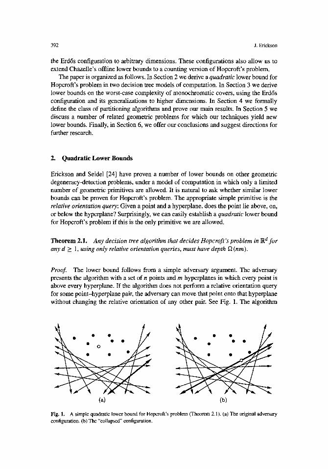
Erickson and Seidel [24] have proven a number of lower bounds on other geometric degeneracy-detection problems, under a model of computation in which only a limited number of geometric primitives are allowed. It is natural to ask whether similar lower bounds can be proven for Hopcroft's problem. The appropriate simple primitive is the relative orientation query: Given a point and a hyperplane, does the point lie above, on, or below the hyperplane? Surprisingly, we can easily establish a quadratic lower bound for Hopcroft's problem if this is the only primitive we are allowed.

Theorem 2.1. Any decision tree algorithm that decides Hopcroft's problem in R d for any d > 1, using only relative orientation queries, must have depth f2 (nm).

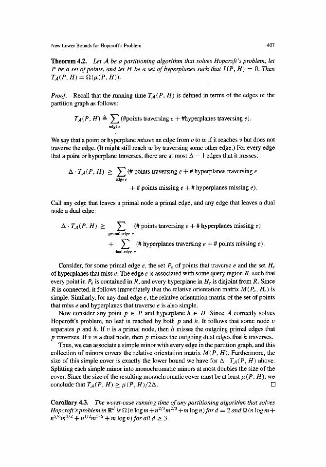
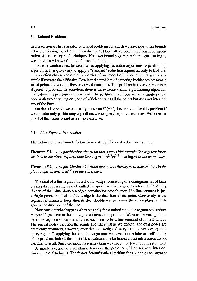
Proof. The lower bound follows from a simple adversary argument. The adversary presents the algorithm with a set of n points and m hyperplanes in which every point is above every hyperplane. If the algorithm does not perform a relative orientation query for some point-hyperplane pair, the adversary can move that point onto that hyperplane without changing the relative orientation of any other pair. See Fig. 1. The algorithm

�9 �9

O

Fig. 1. A simple quadratic lower bound for Hopcroft's problem (Theorem 2.1). (a) The original adversary configuration. (b) The "collapsed" configuration.


cannot tell the two configurations apart, even though one has an incidence and the other does not. Thus, in order to be correct, the algorithm must perform a relative orientation query for every pair. []

In dimensions higher than one, we can considerably strengthen the model of computation in which this quadratic lower bound holds. We explicitly describe only the two-dimensional case; generalization to higher dimensions is straightforward. Our new model of computation is a decision tree with three types of primitives: relative orientation queries, point queries, and line queries. A point query is any decision that is based exclusively on the coordinates the input points. Line queries are defined analogously, We emphasize that point queries can combine information from any number of points, and line queries from any number of lines. We call a point query algebraic if the result is given by the sign of a multivariate polynomial evaluated at the point coordinates.

Theorem 2.2. Any decision tree algorithm that solves Hopcroft' s problem in the plane, using only relative orientation queries, algebraic point queries, and (arbitrary) line queries, must make f2 (nm) relative orientation queries in the worst case.

Proof. For any real number x0, let P (x0) denote the set of n points

{(Xo, x~), (xo + 1, (Xo + 1) 2) . . . . . (Xo q'- n - 1, (xo d-- n - 1)2)},

and let L(xo) denote the set ofm lines tangent to the unit parabola y = x 2 at the points

{(Xo + n, (Xo + n)2), (Xo 4- 2n, (xo + 2n) 2) . . . . . (Xo + mn, (Xo + ran)2)}.

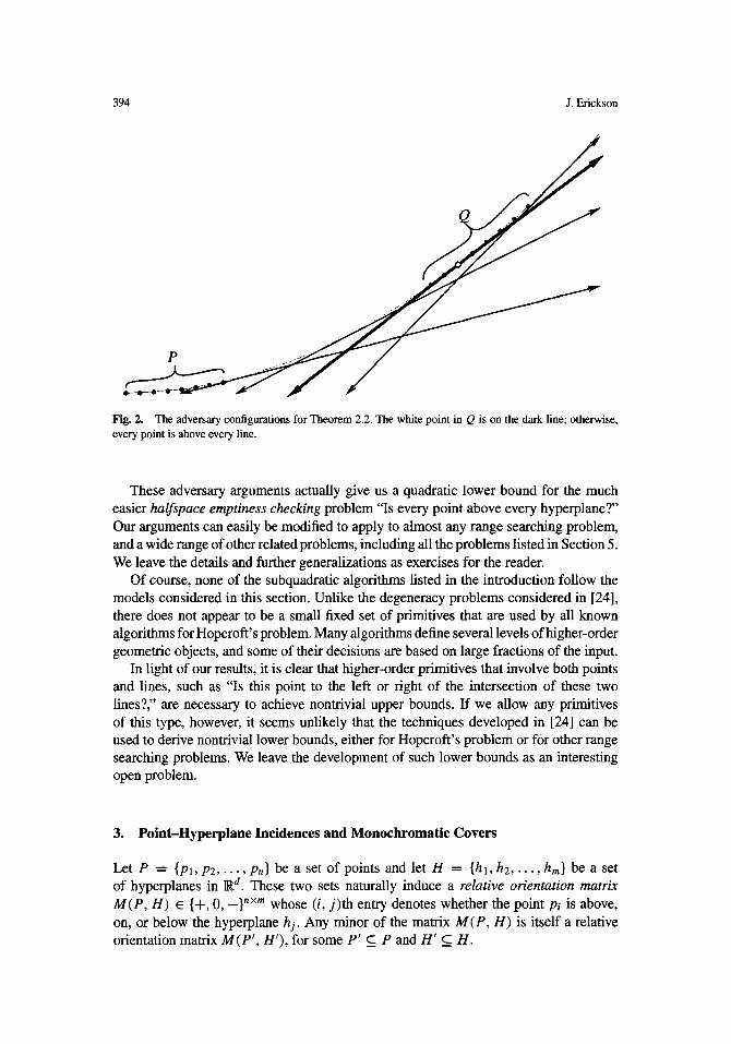
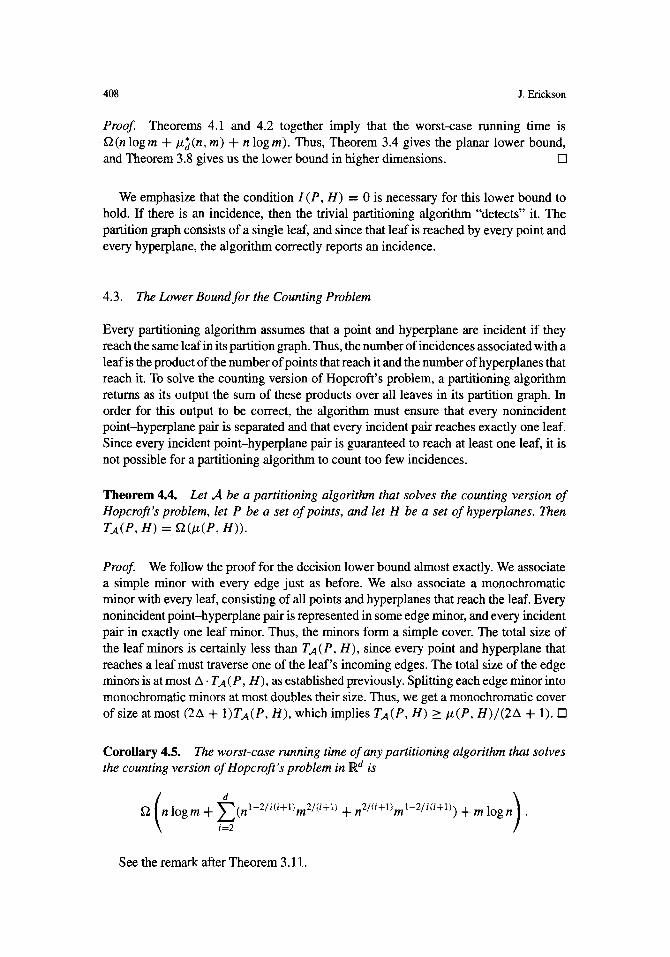
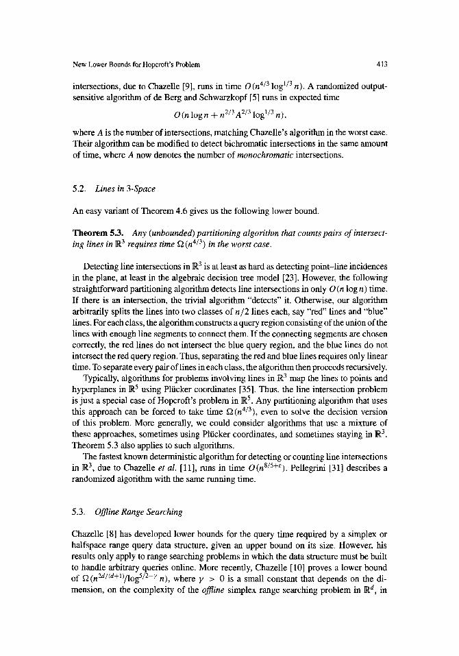
As before, our lower bound follows from an adversary argument. The adversary initially presents the points P = P(xo) and the lines L = L(xo), for some real value x0 to be specified later. If the algorithm does not perform a relative orientation query for the ith point and the j th line, then the adversary replaces the points with the new set Q = P(xo + in - j + 1). We easily verify that in the new configuration, the ith point and the j th line are incident, but otherwise, every point is above every line. See Fig. 2.

Since the adversary does not change the lines, no line query can distinguish between �9 the two configurations. It remains only to consider the point queries. The result of any

algebraic point query in P(x) is given by the sign of a polynomial in x. Let rmax be the largest root of all the point-query polynomials used by the algorithm, ignoring those that are identically zero. If Xl and x2 are both larger than rmax, then every point-query polynomial has the same sign at both P(xl) and P(x2). Thus, if the adversary fixes x0 > rmax, then the algorithm cannot distinguish between the original point set P and any of the collapsed point sets Q.

It follows that the algorithm cannot be correct unless it performs a relative orientation query for every pair. []

Note that our restriction to algebraic point queries is stronger than the result requires. If we rephrase this argument in the dual space, we get a quadratic lower bound in a model that allows arbitrary point queries but requires line queries to be algebraic.

394 J. Efickson

Fig. 2. The adversary configurations for Theorem 2.2. The white point in Q is on the dark line; otherwise, every point is above every line.

These adversary arguments actually give us a quadratic lower bound for the much easier halfspace emptiness checking problem "Is every point above every hyperplane?" Our arguments can easily be modified to apply to almost any range searching problem, and a wide range of other related problems, including all the problems listed in Section 5. We leave the details and further generalizations as exercises for the reader.

Of course, none of the subquadratic algorithms listed in the introduction follow the models considered in this section. Unlike the degeneracy problems considered in [24], there does not appear to be a small fixed set of primitives that are used by all known algorithms for Hopcroft's problem. Many algorithms define several levels of higher-order geometric objects, and some of their decisions are based on large fractions of the input.

In light of our results, it is clear that higher-order primitives that involve both points and lines, such as "Is this point to the left or right of the intersection of these two lines?," are necessary to achieve nontrivial upper bounds. If we allow any primitives of this type, however, it seems unlikely that the techniques developed in [24] can be used to derive nontrivial lower bounds, either for Hopcroft's problem or for other range searching problems. We leave the development of such lower bounds as an interesting open problem.

3. Point-Hyperplane Incidences and Monochromatic Covers

Let P = {Pl, P2 . . . . . Pn} be a set of points and let H = {hi, h2 . . . . . h,n} be a set of hyperplanes in ~d. These two sets naturally induce a relative orientation matrix M(P, H) ~ {+, 0, _},• whose (i, j ) th entry denotes whether the point Pi is above, on, or below the hyperplane h:. Any minor of the matrix M(P, H) is itself a relative orientation matrix M(P', H~), for some P ' C P and H' __. H.


We call a sign matrix monochromatic if all its entries are equal. A minor cover of a matrix is a set of minors whose union is the entire matrix. If every minor in the cover is monochromatic, we call it a monochromatic cover. The size of a minor is the number of rows plus the number of columns, and the size of a minor cover is the sum of the sizes of the minors in the cover. Given a set of points and hyperplanes, a monochromatic cover of its relative orientation matrix provides a succinct combinatorial representation of the relative order type of the set.

We similarly define a succinct representation for the incidence structure of a set of points and hyperplanes. A zero cover of P and H is a collection of monochromatic minors that covers all (and only) the zeros in the relative orientation matrix M(P, H). A zero cover can also be interpreted as a partition of the incidence graph induced by P and H into (not necessarily disjoint) complete bipartite subgraphs.

Monochromatic covers for 0-1 matrices have been previously used to prove lower bounds for communication complexity problems [28]. Typically, however, these results make use of the number of minors in the cover, not the size of the cover as we define it here. 4 Covers of bipartite graphs by complete subgraphs were introduced by Tar j~ [37] in the context of switching theory. Tuza [38], and independently Chung et al. [14], showed that every n x m bipartite graph has such a cover of size O (nm/log(max(m, n))) and that this bound is tight in the worst case, up to constant factors. These results apply immediately to monochromatic covers of arbitrary sign matrices. See also [2] for a geometric application of bipartite clique covers.

Relative orientation matrices are defined in terms of a fixed (projective) coordinate system, which determines what it means for a point to be "above" or "below" a hyperplane. This coordinate system determines which minors of the relative orientation matrix are monochromatic, and therefore determine the minimum monochromatic cover size. However, we easily observe that the minimum monochromatic cover size is independent of any choice of coordinate system, up to a factor of.two, as follows. Call a relative orientation matrix simple if it can be changed into a monochromatic matrix by inverting some subset of the rows and columns. Projective transformations preserve simple minors. See Fig. 3. Every monochromatic minor is simple, and every simple minor can be par- titioned into four monochromatic minors, whose total size is twice that of the original minor.

We use the following notation throughout the rest of the paper. Given a set P of points and H of hyperplanes, let I (P, H) denote the number of point-hyperplane incidences, ~(P, H) the minimum size of their smallest zero cover, and /z (P , H) the size of their smallest monochromatic cover. Let la (n, m) denote the maximum of I (P, H) over all sets P of n points and all sets H of m hyperplanes in R a, and define fro(n, m) and /za (n, m) similarly. Finally, let #~ (n, m) denote the maximum of/z (P, H) over all sets of n points and m hyperplanes in I~ a with no incidences. In the remainder of this section we develop asymptotic lower bounds for #~(n, m) and fa(n, m), which in turn imply lower bounds for #a(n, m).

4 Since any row or column can be split into three or fewer monochromatic minors, any sign matrix can be covered by 3 min(m, n) such minors. Furthermore, there are sets of n points and m lines in the plane whose relative orientation matrices require 3 min(m, n) monochromatic minors to cover them.

396 J. Efickson

i ~

< /

O 0

§

Fig. 3. Three collections of points and lines with simple relative orientation matrices.

3.1. One Dimension

In one dimension, points and hyperplanes are both just real numbers. We can always permute the rows and columns of the relative orientation matrix of two sets of numbers, by sorting the sets, so that the number of + (resp. - ) entries in successive rows or columns is nonincreasing (resp. nondecreasing). The matrix can then be split into two "staircase" matrices, one positive and one negative, and a collection of zero minors of total size at most n + m. We immediately observe that ~1 (n, m) = n + m.

Theorem 3.1.

[| if n > m, lz~(m,n) = | | if n =m,

I| if n < m.

Proof. Without loss of generality, we assume n and m are both powers of two. It suffices to bound the cover size of a monochromatic staircase with n rows and m columns.

First consider the simplest case, n = m. To prove the upper bound, we construct a cover of an arbitrary n x n staircase matrix by partitioning the staircase into an n/2 x k monochromatic minor and two smaller staircases, where k is the number of entries in the (n/2)th row of the original matrix. The total size C(n, n) of this cover is bounded by the recurrence

(n (n ,k ~ c ( n ) ) 3n (2 2) C(n,n)< max - + k + C + - k < + 2 C -o<J,<_, 2 \2 ] ~,n _ - ~ , ,

whose solution is clearly C(n, n) = O(n logn). To prove the matching lower bound, it suffices to consider a triangular matrix, where,

for all i, the ith row has i entries. We claim that any cover for this matrix must have size at least (n /2 ) lgn . Fix a cover. Partition the staircase into an n/2 x n/2 rectangle and two n/2 x n/2 staircases. If a minor in the cover intersects the lower triangle, call it a lower minor; otherwise, call it an upper minor. The upper (resp. lower) minors induce a


cover of the upper (resp. lower) triangle, of size at least (n/4) lg(n/2), by induction. It remains to bound the contribution of the rectangle to the total cover size.

If some row in the rectangle is completely contained in lower minors, then those lower minors have (altogether) n/2 more columns than we accounted for in the induction step. Otherwise, every row contains an element of an upper minor, and those upper minors have (altogether) n/2 more rows than we accounted for in the induction step. Thus, the rectangle contributes at least n/2 to the total cover size. This completes the proof for the case n --- m.

Now suppose n > m. An explicit recursive construction gives us a cover of size 0 (n logn/m m) for any n x m staircase. An inductive counting argument implies that any cover of the n x m triangular matrix, whose ith row has [irn/n] entries, must have size at least (n/2) logn/m m. In both arguments we start by dividing the n rows of the matrix into n/m slabs of m rows each, and cutting each slab into a maximal rectangle and a smaller staircase.

The final case n < m is handled symmetrically. []

This bound simplifies to O(n + m) when either n = O(m k) or m = O(n ~) for any constant k < 1, and to | (n log n) when n = | (m). In the special case n = m, our upper- bound proof is nothing more than an application of quicksort. The connection between the size of the monochromatic cover and the running time of the divide-and-conquer algorithm is readily apparent in this case. In Section 4 we generalize this connection to higher dimensions.

3.2. Two Dimensions

To derive lower bounds for #~(n, m) and (2(n, m), we use the following combinatorial result of Erd6s. (See [25] or p. 112 of [17] for proofs.)

�9 L e m m a 3.2 (Erd6s). For all n and m, there is a set ofn points and m lines in the plane with f2(n q- n2/3m 2/3 q- m) incident pairs. Thus, 12(n, m) ----- f2(n -t- n2/3m 2/3 d- m).

Fredman [25] uses Erd6s' construction to prove lower bounds for dynamic range- query data structures in the plane. 5 This lower bound is asymptotically tight. The corresponding upper bound was first proven by Szemer6di and Trotter [36]. A simpler proof, with better constants, was later given by Clarkson et al. [15].

Theorem 3.3. (2(n, m) = f2(n + n2/3m 2/3 -k- m).

Proof. It is not possible for two distinct points both to be adjacent to two distinct lines; any mutually incident set of points and lines has either exactly one point or exactly one line. It follows that, for any set P of points and H of lines in the plane, ( ( P , H) > 1 (P, H). The theorem now follows from Lemma 3.2. []

5 Perhaps it is more interesting that Chazelle's static lower bounds [8], [10] do not use this construction.

398 J. Erickson

Theorem 3.4. /z~(n, m) = f2(n + n2/3m 2/3 + m).

Proof. Consider any configuration of n points and m/2 lines with f2 (n + n2/3m 2/3 q- m) point-line incidences, as given by Lemma 3.2. Replace each line s in this configuration with a pair of lines, parallel to g and at distance e on either side, where e is chosen sufficiently small that all point-line distances in the new configuration are at least e. The resulting configuration of n points and m lines clearly has no point-line incidences. We call a point-line pair in this configuration close if the distance between the point and the line is e. There are f2 (n + n2/3m 2/3 q- m) such pairs.

Now consider a single monochromatic minor in the relative orientation matrix of these points and lines. Let P' denote the set of points and H ' the set of lines represented in this minor. We claim that the number of close pairs between P ' and H ' is small.

Without loss of generality, we can assume that all the points are above all the lines. If a point is close to a line, the point must be on the convex hull of P', and the line must support the upper envelope of H ~. Thus, we can assume that both P ' and H p are in convex position. In particular, we can order both the points and lines from left to right.

Either the leftmost point is close to at most one line, or the leftmost line is close to at most one point. It follows inductively that the number of close pairs is at most I P'[ + [H'I, which is exactly the size of the minor. The theorem follows immediately. []

3.31 Three Dimensions

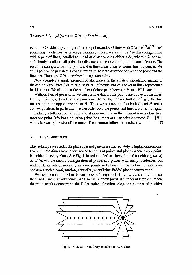
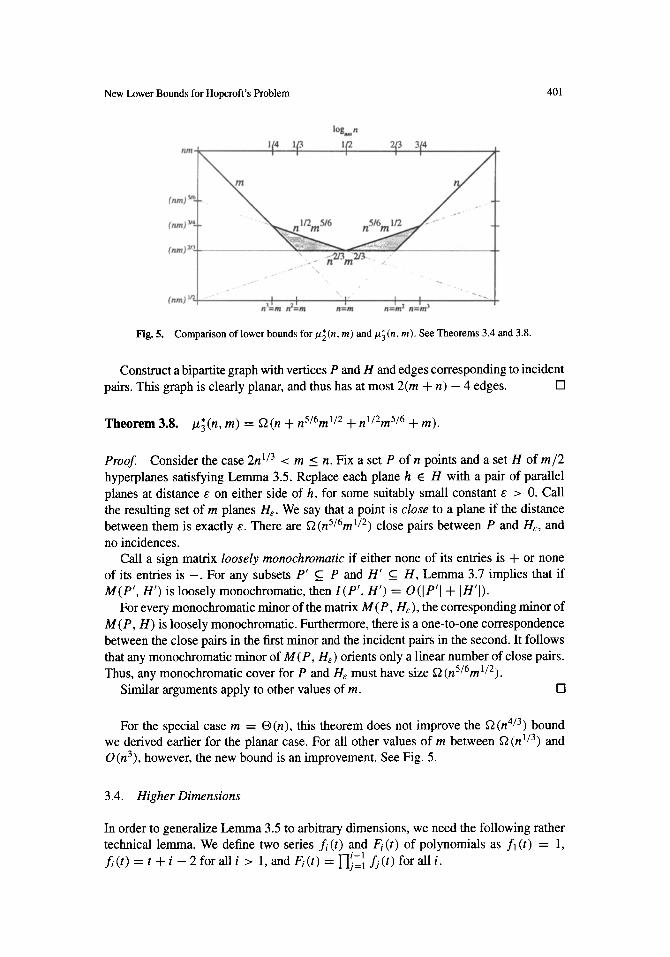
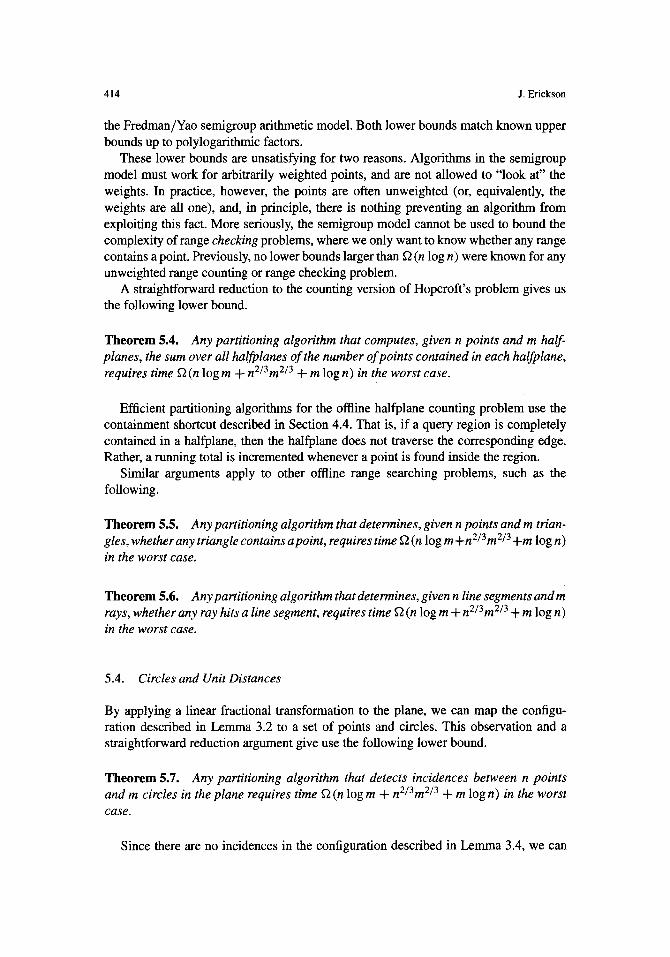
The technique we used in the plane does not generalize immediately to higher dimensions. Even in three dimensions, there are collections of points and planes where every points is incident to every plane. See Fig. 4. In order to derive a lower bound for either (3 (m, n) or/z~(n, m), we need a configuration of points and planes with many incidences, but without large sets of mutually incident points and planes. In the following lemma we construct such a configuration, naturally generalizing Erd6s' planar construction.

We use the notation [n] to denote the set of integers {1, 2 . . . . . n}, and i _1_ j to mean that i and j are relatively prime. We also use (without proof) a number of simple number- theoretic results concerning the Euler totient function ~o(n), the number of positive

Fig. 4. 13(n, m) = ran. Every point lies on every plane.

New Lower Bounds for Hopcrof t ' s Problem 399

integers less than or equal to n that are relatively prime to n. We refer the reader to [26] for relevant background.

L e m m a 3.5. For all n and m such that Lnl/3j < m, there exists a set P o f n points and a set H o f m planes, such that I (P, H) = ~ (nS/6m 1/2) and any three planes in H intersect in at most one point.

Proof Fix sufficiently large n and m such that Lnl/3J < m. Let h(a, b, c; i, j ) denote the plane passing through the points (a, b, c), (a + i, b + j , c), and (a + i, b, c + i - j ) . Let p = [nl/3J and q = [ot(m/p)l/4J for some suitable constant ot > 0. (Note that with n sufficiently large and m in the indicated range, p and q are both positive integers.)

Now consider the points P = [p]3 = {(x, y, z) I x, y, z E [p]} and the hyperplanes

H= {h(a,b,c;i,,)li~tqJ, j~[i],i • j, a ~ t/a, b ~ [j~,c ~ [ [ - ~ J ] }

The number of planes in H is

q 2 i j = _ o ( p q 4) = O ( m ) .

i=1 j=l i=1 )zi

By choosing the constant ot appropriately and possibly adding in o(m) extra planes, we can ensure that H contains exactly m planes. We claim that this collection of points and planes satisfies the lemma.

Consider a single plane h = h(a, b, c; i, j ) E H. Since i, j , and i - j are palrwise relatively prime, h intersects exactly one point (x, y, z) such that x r [i] and y 6 [j] , namely, the point (a, b, c). Thus, for each fixed i and j we use, the planes h (a, b, c; i, j ) H are distinct. Since planes with different "slopes" are clearly different, it follows that the planes in H are distinct.

For all k ~ [ [p/2iJ ], the intersection o fh (a, b, c; i, j ) 6 H with the plane x = a + ki contains at least k points of P. It follows that

Lp l2i J

I e n h ( a , b , c ; i , j ) l > _ _ y ~ k k = l

Thus, the total number of incidences between P and

I (P, H) q i

>-- i=1 j=l

~.l_j

1 p 2

>sL J H can be calculated as follows.

j p 2

>

i=1 j ~ l i&j

i = l 4

= ~(p3q2)

= ~2(nS/6ml/a).

400 J. Efickson

Finally, If H contains three planes that intersect in a line, the intersection of those planes with the plane x = 0 must consist of three concurrent lines. It suffices to consider only the planes passing through the point (1, 1, 1), since for any other triple of planes in H there is a parallel triple passing through that point. The intersection of h (1, 1, 1; i, j ) with the plane x = 0 is the line through (0, 1 - j / i , 1) and (0, 1, j / i ) . Since i _1_ j , each such plane determines a unique line. Furthermore, since all these lines are tangent to a parabola, no three of them are concurrent. It follows that the intersection of any three planes in H consists of at most one point. []

Edelsbrunner et al. [19] prove an upper bound of O(n logm + n4/5+2em 3/5-e q- m) on the maximum number of incidences between n points and m planes, where no three planes contain a common line. Using the probabilistic counting techniques of Clarkson et al. [15], we can improve this upper bound to O(n + na/5m 3/5 q- m).

Theorem3.6. (3(n,m) = f2(n-bn5/6ml/2q-nl/2mS/6q-m).

Proof. Consider the case n 1/3 < m < n. Fix a set P of n points and a set H of m hyperplanes satisfying Lemma 3.5. Any mutually incident subsets of P and H contain either at most one point or at most two planes. Thus, the number of entries in any zero minor of M(P, H) is at most twice the size of the minor. It follows that any zero cover of M(P, H) must have size f2(I (P, H)) = f2(nS/6ml/2). The dual construction gives us a lower bound of f2 (nl/2mS/6) for all m in the range n < m < n 3, and the trivial lower bound f2 (n + m) applies for other values of m. []

Lemma 3.7. Let P be a set of n points and let H be a set of m planes in ll~ 3, such that every point in P is either on or above every plane in H, and any three planes in H intersect in at most one point. Then I (P, H) < 2(m + n).

Proof. Call any point (resp. plane) lonely if it is incident to less than three planes (resp. points). Without loss of generality, we can assume that none of the points in P or planes in H is lonely, since each lonely point and plane contributes at most two incidences.

No point in the interior of the convex hull of P can be incident to a plane in H. Any point in the interior of a facet of the convex hull can be on at most one plane in H. Consider any point p 6 P in the interior of an edge of the convex hull. Any plane containing p also contains the two endpoints of the edge. There cannot be more than two such planes in H, so p must be lonely. It follows that every point in P is a vertex Of the convex hull of P.

No plane can contain a point unless it touches the upper envelope of H. Any plane that only contains a vertex of the upper envelope must be lonely. For any plane h that contains only an edge of the envelope, two other planes also contain that edge, and any points on h must also be on the other two planes. Then h must be lonely, since any three planes in H intersect in at most one point. It follows that every plane in H spans a facet of the upper envelope of H. Furthermore, every point in P is a vertex of this upper envelope.


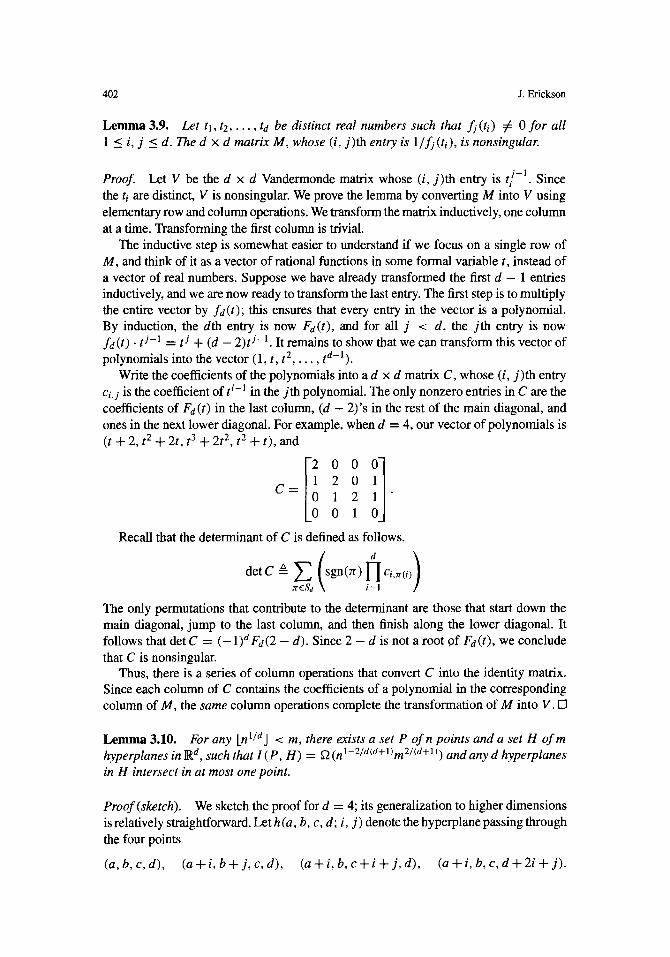
Iogmn

\ / ._- i

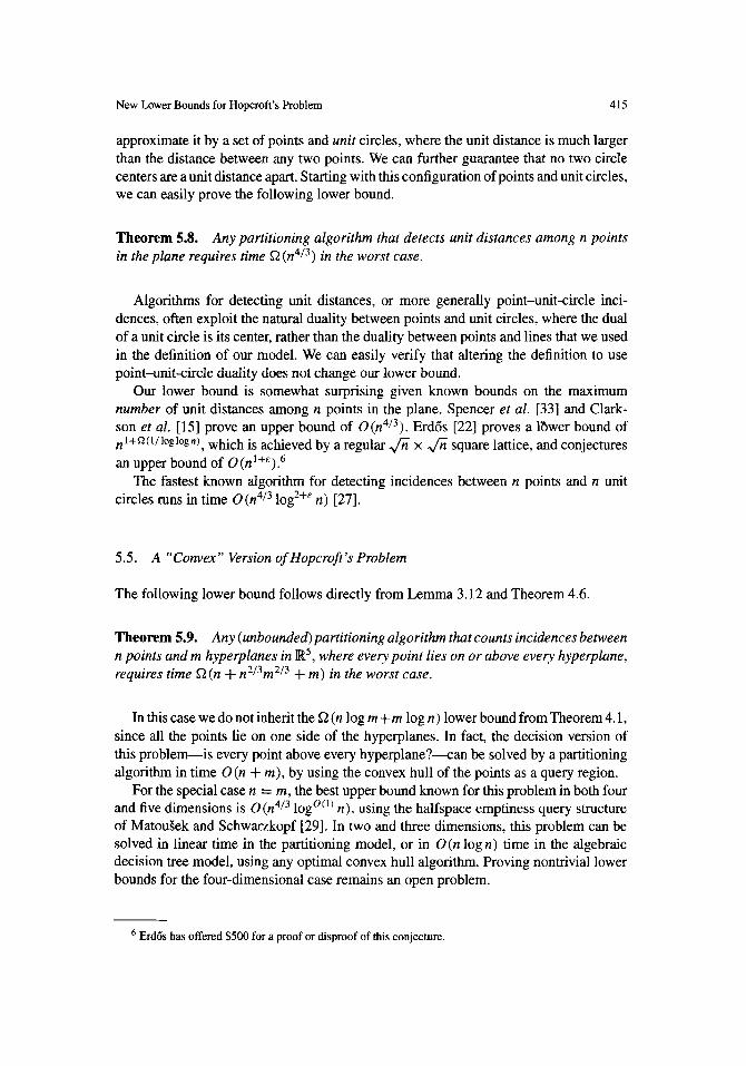
Fig. 5. Comparison of lower bounds for/~(n, m) and/z~(n, m). See Theorems 3.4 and 3.8.

Construct a bipartite graph with vertices P and H and edges corresponding to incident pairs. This graph is clearly planar, and thus has at most 2(m + n) - 4 edges. []

Theorem 3.8. # ] (n , m) = f2(n + nS/6m 1/2 + nl/2m 5/6 + m).

Proof. Consider the case 2n 1/3 < m < n. Fix a set P of n points and a set H of m/2 hyperplanes satisfying Lemma 3.5. Replace each plane h e H with a pair of parallel planes at distance e on either side of h, for some suitably small constant e > 0. Call the resulting set of m planes He. We say that a point is close to a plane if the distance between them is exactly e. There are ~(nS/6m 1/2) close pairs between P and He, and no incidences.

Call a sign matrix loosely monochromatic if either none of its entries is + or none of its entries is - . For any subsets P ' __. P and H ' ___ H , Lemma 3.7 implies that if M(P', H') is loosely monochromatic, then I(P', H ' ) = O(IP ' I + In ' l ) .

For every monochromatic minor of the matrix M(P, He), the corresponding minor of M(P, H) is loosely monochromatic. Furthermore, there is a one-to-one correspondence between the close pairs in the first minor and the incident pairs in the second. It follows that any monochromatic minor of M (P, He) orients only a linear number of close pairs. Thus, any monochromatic cover for P and He must have size f2 (n5/6ml/2).

Similar arguments apply to other values of m. lq

For the special case m = | this theorem does not improve the ~2(n 4/3) bound we derived earlier for the planar case. For all other values of m between ~ ( n 1/3) and O(n3), however, the new bound is an improvement. See Fig. 5.

3.4. Higher Dimensions

In order to generalize Lemma 3.5 to arbitrary dimensions, we need the following rather technical lemma. We define two series fi (t) and Fi (t) of polynomials as f l (t) = 1, ~ ( t ) = t + i - 2 for all i > 1, and Fi(t) = ]-Ij-ll f j ( t ) for all i.

402 J. Erickson

Lemma 3.9. Let tl, t2 . . . . . ta be distinct real numbers such that f j (ti) ~ 0 for all 1 < i, j < d. The d x d matrix M, whose (i, j ) th entry is 1/ f j ( t i ) , is nonsingular.

j - 1 Proof Let V be the d • d Vandermonde matrix whose (i, j ) th entry is t i . Since the ti are distinct, V is nonsingular. We prove the lemma by converting M into V using elementary row and column operations. We transform the matrix inductively, one column at a time. Transforming the first column is trivial.

The inductive step is somewhat easier to understand if we focus on a single row of M, and think of it as a vector of rational functions in some formal variable t, instead of a vector of real numbers. Suppose we have already transformed the first d - 1 entries inductively, and we are now ready to transform the last entry. The first step is to multiply the entire vector by fa(t); this ensures that every entry in the vector is a polynomial. By induction, the dth entry is now Fa(t), and for all j < d, the j th entry is now f d ( t ) �9 t j - 1 -~ t j -I- ( d - - 2 ) t j - 1 . It remains to show that we can transform this vector of polynomials into the vector (1, t, t 2 . . . . . ta-1).

Write the coefficients of the polynomials into a d • d matrix C, whose (i, j ) th entry ci, j is the coefficient o f t i-1 in the j th polynomial. The only nonzero entries in C are the coefficients of Fa(t) in the last column, (d - 2)'s in the rest of the main diagonal, and ones in the next lower diagonal. For example, when d = 4, our vector of polynomials is (t + 2, t 2 + 2t, t 3 + 2t 2, t 2 + t), and

C =

E 002 0 1 2 0 1

Recall that the determinant of C is defined as follows.

det C -~ ~ Jr c Sd

The only permutations that contribute to the determinant are those that start down the main diagonal, jump to the last column, and then finish along the lower diagonal. It follows that detC = (--1)dFd(2 -- d). Since 2 - d is not a root .of Fd(t), we conclude that C is nonsingular.

Thus, there is a series of column operations that convert C into the identity matrix. Since each column of C contains the coefficients of a polynomial in the corresponding column of M, the same column operations complete the transformation of M into V. []

Lemma 3.10. For any Lnl/aJ < m, there exists a set P o fn points and a set H o f m hyperplanes in 1~ a, such that I ( P, H) = f2 (nl-2/ala+l~m 2/~a+1 i) and any d hyperplanes in H intersect in at most one point.

Proof (sketch). We sketch the proof for d = 4; its generalization to higher dimensions is relatively straightforward. Let h (a, b, c, d; i, j ) denote the hyperplane passing through the four points

( a , b , c , d ) , ( a + i , b + j , c , d ) , ( a + i , b , c + i + j , d ) , ( a + i , b , c , d + 2 i + j ) .


Let p = [nl/4j and q = Lot(m/p)l/sj for some suitable constant a > 0. Then P = [p]4 and H is the set of hyperplanes h(a, b, c, d; i, j ) satisfying the following set of conditions:

i �9 [q], j �9 [i], j is odd, i .L j ,

a � 9 b � 9 c � 9 d E 11~-11. L L Z - I J

Note that j is odd and relatively prime with i if and only if i, j , i + j , and 2i + j are pairwise relatively prime. This condition is necessary to establish that the hyperplanes in H are distinct. It follows from relatively straightforward algebraic manipulation that [HI = O(pq 5) = O(m) and I (P, H ) = f2(p4q 2) = f2(n9/l~

To establish that no four hyperplanes in H intersect in a common line, we examine the intersection of each hyperplane h(1, 1, 1, 1; i, j ) �9 H with the hyperplane xl = 0. This intersection is the plane

1 x2-- 1 x3-- 1 x 4 - - 1

7+ + + - - j ~ 2 i + j - - 0 .

It follows from Lemma 3.9, by setting tk = jk/ik, that no four of these planes are concurrent. []

Note that the lower bound for dimension d only improves the bound for dimension d - 1 when n = f2 (m(d-1)/2). Again, using probabilistic counting techniques [15], we can prove an upper bound of I (P, H) = O(n + n(2d-2)/(2d-a)m d/~ + m) if any d hyperplanes in H intersect in at most one point.

The previous lemma immediately gives us the following lower bound for (d(n, m).

Theo rem 3.11. (d(n, m) = ~ '2(~ id l (nl-2/i(i+llm 2/(i+1) -}- n2/t i+l)ml-2/i(i+l)) ).

Since our d-dimensional lower bound only improves our (d - 1)-dimensional lower bound for certain values of n and m, we have combined the lower bounds from all dimensions 1 < i < d into a single expression. If the relative growth rates of n and m are fixed, the entire sum can be reduced to a single tenn.

Unfortunately, we are unable to generalize Lemma 3.7 even into four dimensions. Consequently, the best lower bound we can derive for #~(n, m) for any d > 3 derives trivially from Theorem 3.8. The best upper bound we can prove for the number of incidences between n points and m hyperplanes in I~ 4, where every point is above or on every hyperplane and no four hyperplanes contain a line, is O(n + n2/3m 2/3 + m). (See [21] for the derivation of a similar upper bound.) No superlinear lower bounds are known in any dimension, so there is some hope for a linear upper bound.

However, we can achieve a superlinear number of incidences in five dimensions, under a weaker combinatorial general position requirement. Thus, unlike in lower dimensions, some sort of geometric general position requirement is necessary to keep the number of incidences small.

L e m m a 3.12. For all n and m, there exists a set P of n points and a set H of m hyperplanes in 1~5, such that every point is on or above every hyperplane, no two

404 J. Erickson

hyperplanes in H contain more than one point of P in their intersection, and I (P, H) = ~2(n q- n2/3m 2/3 q- m).

Proof Define the function tr :R 3 ~ ~6 as follows:

tr(x, y, z) = (x 2, y2, Z 2, ~ x y , ,r yz, V~xz ) .

For any v, w 6 ]I~ 3, we have (tr(v), a(w)) = (v, 10) 2, where (., .) denotes the usual inner product of vectors. In a more geometric setting, cr maps points and lines in the plane, represented in homogeneous coordinates, to points and hyperplanes in R 5, also represented in homogeneous coordinates [35]. For any point p and line s in the plane, the point cr (p) is incident to the hyperplane tr (s if and only if p is incident to g; otherwise, cr (p) lies above tr (s Thus, we can take P and H to be the images under tr of any sets of n points and m lines with ~2 (n + nZ/3m 2/3 d- m) incidences, as given by Lemma 3.2. []

3.5. A Lower Bound in the Semigroup Model

Our results immediately imply a lower bound for a variant of the counting version of Hopcroft's problem, in the Fredman/Yao semigroup arithmetic model. The lower bound follows from the following result of Chazelle [10, Lemma 3.3]. (Chazelle's lemma only deals with the case n = m, but his proof generalizes immediately to the more general case.)

Lemma 3.13. If A is an n x m incidence matrix with I ones and no p x q minor of ones, then the complexity of computing Ax over a semigroup is f2(I /pq - n/p).

Theorem 3.14. Given n weighted points and m hyperplanes in ~d,

I ) ~2 Z(nl -2/ i f i+l)m 2/(i+1) -.[- n2/(i+l)m 1-2/i(i+l)) \ i = 1

semigroup operations are required to determine the sum of the weights of the points on each hyperplane, in the worst case.

Proof The lower bound follows immediately from Lemma 3.10. []

As in Theorem 3.11, we have combined the best lower bounds from several dimensions into a single expression. When m ----- | (n), this bound simplifies to f2 (n4/3), which already follows immediately from Chazelle's lemma and the Erd6s construction. For all other values of m between ~2 (n 1/d) and 0 (ha), however, the new bound is an improvement over any previously known lower bounds for this problem. The best known upper bound is given by Matou~ek's algorithm [30].


4. Partitioning Algorithms

A partition graph is a directed acyclic graph, with one source, called the root, and several sinks, or leaves. Associated with each nonleaf node v is a set ~ of query regions, satisfying three conditions:

1. The cardinality of ~ is at most some constant A > 2. 2. Each region in Ro is connected. 3. The union of the regions in Ro is •d.

(We do not require the query regions to be disjoint, convex, simply connected, semial- gebraic, or of constant combinatorial complexity.) In addition, every nonleaf note v is either a primal node or a dual node, depending on whether its query regions ~ should be interpreted as a partition of primal or dual space. Each query region in 7~ corresponds to an outgoing edge of o. Thus, the out-degree of the graph is at most A.

Given sets P of points and H of hyperplanes as input, a partitioning algorithm constructs a partition graph, which can depend arbitrarily on the input, and uses it to drive the following divide-and-conquer process. The algorithm starts at the root and proceeds through the graph in topological order. At every node except the root, points and hyperplanes are passed in along incoming edges from preceding nodes. For each node v, let Po c p denote the points and Hv ~ H the hyperplanes that reach v; at the root, we have Proot= P and/-/root = H. At every nonleaf node v, the algorithm partitions the sets Po and Ho into (not necessarily disjoint) subsets by the query regions ~ and sends these subsets out along outgoing edges to succeeding nodes. If v is a primal node, then, for every query region R ~ ~ , the points in P~ that are contained in R and the hyperplanes in Hv that intersect R traverse the outgoing edge corresponding to R. If v is a dual node, then, for every query region R e ~v, the points p ~ Pv whose dual hyperplanes p* intersect R and the hyperplanes h ~ Hv whose dual points h* are contained in R traverse the corresponding outgoing edge. Note that a single point or hyperplane may enter or leave a node along several different edges.

For the purpose of proving lower bounds, the entire running time of the algorithm is given by charging unit time whenever a point or hyperplane traverses an edge. In particular, we do not charge for the construction of the partition graph or its query regions, nor for the time that would be required in practice to decide if a point or hyperplane intersects a query region. As a result, partitioning algorithms are effectively nondeterministic. In principle, the algorithm has "time" to compute the optimal partition graph for its input, and even very similar inputs might result in radically different partition graphs.

To solve Hopcroft's problem, the algorithm reports an incidence if and only if some leaf in the partition graph is reached by both a point and a hyperplane. It is easy to see that if some point and hyperplane are incident, then there is at least one leaf in every partition graph that is reached by both the point and the hyperplane. Thus, for any set P of points and set H of hyperplanes, a partition graph in which no leaf is reached by both a point and a hyperplane provides a proof that there are no incidences between P and H.

In this section we derive lower bounds for the worst-case running time of partitioning algorithms that solve Hopcrofl's problem. With the exception of the basic lower bound

406 J. Erickson

of f2 (n log m + m log n), which in light of Theorem 3.1 we must prove directly, our lower bounds are derived from the cover size bounds in Section 3. At the end of the section we describe how existing algorithms for Hopcroft's problem fit into our computational framework.

4.1. The Basic Lower Bound

Theorem 4.1. Any partitioning algorithm that solves Hopcrofi's problem in any dimension must take time f2 (n log m + m log n) in the worst case.

Proof It suffices to consider the following configuration, where n is a multiple of m. P consists of n points on some vertical line in I~ d, say the xd-ards, and H consists of m hyperplanes normal to that line, placed so that n/m points lie between each hyperplane and the next higher hyperplane, or above the top hyperplane. (We implicitly used a one- dimensional version of this configuration to prove the lower bound in Theorem 3.1.) For each point, call the hyperplane below it its partner. Each hyperplane is a partner of n/m points.

Let G be the partition graph generated by some partitioning algorithm. Recall that the out-degree of every node in G is at most A. The level of any node in G is the length of the shortest path from the root to that node. There are at most A ~ nodes at level k. We say that a node v separates a point-hyperplane pair if both the point and the hyperplane reach v, and none of the outgoing edges of v is traversed by both the point and the hyperplane. In order for the algorithm to be correct, every point-hyperplane pair must be separated. Finally, we say that a hyperplane h is active at level k if none of the nodes in the first k levels separates h from any of its partners.

Suppose v is a primal node. For each hyperplane h that v separates from one of its partner points p, mark some query region in 7~v that contains p but misses h. The marked region lies completely above h, but not completely above any hyperplane higher than h. It follows that the same region cannot be marked more than once. Since there are at most A regions, at most A hyperplanes become inactive. By similar arguments, if v is a dual node, then v separates at most A points from their partners.

Thus, the number of hyperplanes that are inactive at level k is less than A k+2. In particular, at level [log a mJ - 3, at least m(1 - l / A ) hyperplanes are still active. It follows that at least n(1 - I / A ) points each traverse at least [log a mJ - 3 edges. We conclude that the total running time of the algorithm is at least

n ( 1 - 1 ) (Lloga mJ - 3) = ~(nlogm).

Similar arguments establish a lower bound of if2 (m log n) when n < m. []

4.2. The Lower Bound for the Decision Problem

Let T.a (P, H) denote the running time of an algorithm ,4 that solves Hopcroft's problem in •d for some d, given points P and hyperplanes H as input.


Theorem 4.2. Let .A be a partitioning algorithm that solves Hopcroft's problem, let P be a set ofpoints, and let H be a set ofhyperplanes such that I (P , H) = O. Then TA(P, H) = f2(it(P, H)).

Proof. Recall that the running time T.a(P, H) is defined in terms of the edges of the partition graph as follows:

T.a(P, H) & E (#points traversing e -t- #hyperplanes traversing e). edge e

We say that a point or hyperplane misses an edge from v to w if it reaches v but does not traverse the edge. (It might still reach w by traversing some other edge.) For every edge that a point or hyperplane traverses, there are at most/x - 1 edges that it misses:

A �9 T.a(P, H) > E (# points traversing e + # hyperplanes traversing e edgee

+ # points missing e + # hyperplanes missing e).

Call any edge that leaves a primal node a primal edge, and any edge that leaves a dual node a dual edge:

�9 T/t(P, H) > E (# points traversing e A + # hyperplanes missing e)

primal edge e

+ E (# hyperplanes traversing e + # points missing e ) .

dual edge e

Consider, for some primal edge e, the set Pe of points that traverse e and the set He of hyperplanes that miss e. The edge e is associated with some query region R, such that every point in Pe is contained in R, and every hyperplane in He is disjoint from R. Since R is connected, it follows immediately that the relative orientation matrix M (Pe, He) is simple. Similarly, for any dual edge e, the relative orientation matrix of the set of points that miss e and hyperplanes that traverse e is also simple.

Now consider any point p 6 P and hyperplane h 6 H. Since ,,4 correctly solves Hopcroft's problem, no leaf is reached by both p and h. It follows that some node v separates p and h. ff v is a primal node, then h misses the outgoing primal edges that p traverses. If v is a dual node, then p misses the outgoing dual edges that h traverses.

Thus, we can associate a simple minor with every edge in the partition graph, and this collection of minors covers the relative orientation matrix M(P, H). Furthermore, the size of this simple cover is exactly the lower bound we have for A �9 T.a(P, H) above. Splitting each simple minor into monochromatic minors at most doubles the size of the cover. Since the size of the resulting monochromatic cover must be at least It (P, H), we conclude that T.a(P, H) > It(P, H)/2A. []

Corollary 4.3. The worst-case running time of any partitioning algorithm that solves , d Hop croft s problem in • is f2 (n log m + nZ/3m2/3 -k-m log n)for d = 2 and f2 (n log m +

nS/6m 1/2 + nl/Zm 5/6 + m log n) for all d > 3.

408 J. Erickson

Proof. Theorems 4.1 and 4.2 together imply that the worst-case running time is f2(n logm +/z~(n, m) + n logm). Thus, Theorem 3.4 gives the planar lower bound, and Theorem 3.8 gives us the lower bound in higher dimensions. []

We emphasize that the condition I(P, H) = 0 is necessary for this lower bound to hold. If there is an incidence, then the trivial partitioning algorithm "detects" it. The partition graph consists of a single leaf, and since that leaf is reached by every point and every hyperplane, the algorithm correctly reports an incidence.

4.3. The Lower Bound for the Counting Problem

Every partitioning algorithm assumes that a point and hyperplane are incident if they reach the same leaf in its partition graph. Thus, the number of incidences associated with a leaf is the product of the number of points that reach it and the number of hyperplanes that reach it. To solve the counting version of Hopcroft's problem, a partitioning algorithm returns as its output the sum of these products over all leaves in its partition graph. In order for this output to be correct, the algorithm must ensure that every nonincident point-hyperplane pair is separated and that every incident pair reaches exactly one leaf. Since every incident point-hyperplane pair is guaranteed to reach at least one leaf, it is not possible for a partitioning algorithm to count too few incidences.

Theorem 4,4. Let .4 be a partitioning algorithm that solves the counting version of Hopcrofi's problem, let P be a set of points, and let H be a set of hyperplanes. Then TA(P, H) = f2(#(e, H)).

Proof. We follow the proof for the decision lower bound almost exactly. We associate a simple minor with every edge just as before. We also associate a monochromatic minor with every leaf, consisting of all points and hyperplanes that reach the leaf. Every nonincident point-hyperplane pair is represented in some edge minor, and every incident pair in exactly one leaf minor. Thus, the minors form a simple cover. The total size of the leaf minors is certainly less than T.a(P, H), since every point and hyperplane that reaches a leaf must traverse one of the leaf's incoming edges. The total size of the edge minors is at most A. T.a (P, H), as established previously. Splitting each edge minor into monochromatic minors at most doubles their size. Thus, we get a monochromatic cover of size at most (2& + 1)T.a(P, H), which implies TA(P, H) > #(P, H)/ (2A + 1). []

Corollary 4.5. The worst-case running time of any partitioning algorithm that solves the counting version of Hopcroft's problem in •a is

g2 n log m + E(nl-2/i(i+l)m 2/(i+1) q- n2/(i+l)m 1-2~ill+l)) --}- m log n .

i=2

See the remark after Theorem 3.11.


We can prove the following stronger lower bound by only paying attention to the minors induced at the leaves. We define an unbounded partition graph to be just like a partition graph except that we place no restrictions on the number of query regions associated with each node. Call the resulting class of algorithms unbounded partitioning algorithms. Note that such an algorithm can solve the decision version of Hopcroft's problem in linear time.

Theorem 4.6. Let ,A be an unbounded partitioning algorithm that solves the counting version of Hopcroft' s problem, let P be a set of points, and let H be a set of hyperplanes. Then T.a(P, H) = f2(((P, H)).

Proof. We associate a zero minor with every leaf, and these minors form a zero cover. The total size of the leaf minors is less than T,a(P, H), since every point and hyperplane that reaches a leaf must traverse one of the leaf's incoming edges. []

The following corollary is now immediate.

Corollary 4.7. The worst-case running time of any unbounded partitioning algorithm that solves the counting version of Hopcrofi's problem in I~ d is

I ) ~'2 Z ( n l - 2 / i ( i + l ) m 2/(i+1) + n2/(i+l)m l-2/ifi+l)) .

\ i = 1

4.4. Aside: Containment Shortcuts Don't Help

We might consider adding the following containment shortcut to our model. Suppose that while partitioning points and hyperplanes at a primal node, the algorithm discovers that a query region R is completely contained in some hyperplane h. Then we know immediately that any point contained in R is incident to h. Rather than sending h down the edge corresponding to R, the algorithm could increment a running counter for each point in R. We can apply a symmetric shortcut at each dual node, potentially reducing the number of points traversing each dual edge. In addition to charging for edge traversals, we now also charge unit time whenever an algorithm discovers that a hyperplane (either primal or dual) contains a query region.

Clearly, adding this shortcut can only decrease the running time of any partitioning algorithm. However, for any algorithm that uses this shortcut, we can derive an equivalent algorithm without shortcuts that is slower by only a small constant factor, as follows.

Ifa hyperplane h contains a query region R, then it must also contain aft(R), the affine hull of R. We can reverse the containment relation by applying a duality transformation-- the dual point h* is contained in the dual flat (aft(R))*. Similarly, i fa point p is contained in R, then (aft(R))* e p*.

For each node v in the partition graph of the shortcut algorithm, and each query region R e T~o, we modify the graph as follows. Let e(R) be the edge of the partition graph corresponding to R, and let w be the destination of this edge. We introduce two new

410 J. Erickson

~176176

/ - - ~ -....

Fig. 6. Eliminating containment shortcuts.

nodes, a "test" node t (R) and a leaf s (R). If v is a primal node, then t (R) is a dual node, and vice versa. The query subdivision ~ t (R~ consists of exactly two regions: (aft(R))* and Rd\(aff(R)) *, whose corresponding edges point to e(R) and w, respectively. Finally, we redirect e(R) so that it points to t(R). See Fig. 6. The new algorithm ,,4' uses this modified partition graph, without explicitly checking for containments.

The new node t(R) strictly separates the hyperplanes that contain R from the hyperplanes that merely intersect it. Any point contained in R reaches both w and s Thus, the new algorithm reports or counts exactly the same incidences as the original shortcut algorithm. We easily verify that the running time of the new algorithm is at most three times the running time of the shortcut algorithm.

4.5. Existing Algorithms

Existing algorithms for Hopcroft's problem all employ roughly the same divide-and- conquer strategy. Each algorithm divides space into a number of regions, determines which points and hyperplanes intersect each region, and recursively solves the resulting subproblems. In some cases [7], [20], [13] the number of regions used at each level of recursion is a constant, and these algorithms fit naturally into the partitioning algorithm framework.

For most algorithms, however, the number of regions is a small polynomial function of the input size, and not a constant as required by the definition of the partitioning model�9 However, we can still model most, if not all, of these algorithms by partitioning algorithms.

In order to determine which points lie in which regions, each of these algorithms constructs a (possibly trivial) point location data structure. Each node in this data structure partitions space into a constant number of simple regions, and, for each region, there is a pointer to another node in the data structure. Each leaf in the data structure corresponds to one of the high-level query regions. Composing all the point location data structures used by the algorithm in all recursive subproblems gives us the algorithm's partition graph. Many of these algorithms alternate between primal and dual spaces at various levels of recursion [9], [30]. The data structures used in primal space give us the primal nodes in the partition graph, and the data structures used in dual space give us the dual nodes.


What about the hyperplanes? Many algorithms also use the point location data structures to determine the regions hit by each hyperplane. Algorithms of this type fit into our model perfectly. In particular, Matou~ek's algorithm [30], which is based on Chazelle's hierarchical cuttings [9] and is the fastest algorithm known, can be model- ed this way. Matou~ek's algorithm and Theorem 4.4 immediately give us the following theorem.

Theorem 4.8. lzd(n, m) = O(m logn + nd/~d+l)md/(d+l)20(l~ -'}- n logm).

However, other algorithms do not use the point-location data structure to locate hyperplanes, at least not at all levels of recursion. In these algorithms [ 18], [ 1 ] the query regions form a decomposition of space into ceils of constant complexity, typically simplices or trapezoids. The algorithms determine which cells a given hyperplane hits by iteratively "walking" through the cells. At each cell that the hyperplane intersects, the algorithm can determine in constant time which of the neighboring cells are also intersected, by checking each of the boundary facets.

In many cases, modifying such an algorithm to use the point-location data structure directly instead of the iterative procedure increases the running time by only a constant factor. If the current point location data structure locates the hyperplanes too slowly, we may be able to replace it with a different data structure that supports fast hyperplane location, again without increasing the asymptotic running time. We could use, for example, the randomized incremental construction of Seidel [32] in the plane, or the hierarchical cuttings data structure of Chazelle [9] in higher dimensions. The modified algorithm can then be described as a partitioning algorithm.

Other algorithms construct a point location data structure for the arrangement of the entire set of hyperplanes [16], [20], [9]. Usually, this is done only when the number of hyperplanes is much smaller than the number of points. In this case the algorithm does not need to locate the hyperplanes at all! Again, however, we can modify the algorithm so that it uses a point location data structure that allows efficient hyperplane location as well, and artificially locates the hyperplanes. If we use an appropriate data structure, the running time will only increase by a constant factor.

These arguments are admittedly ad hoc. Modifying the partitioning model to include naturally algorithms that use different strategies for point and hyperplane location, or strengthening our lower bounds to a similar model that does not require constant-degree partitioning, is an interesting open problem,

Finally, a few algorithms partition the points or the hyperplanes arbitrarily into subsets, without using geometric information of any kind [ 17, p. 350], [ 16]. In this case every hyperplane becomes part of every subproblem. In order to take algorithms of this kind into account, we must strengthen our model of computation by adding a new type of node that partitions either the points or the hyperplanes (but not both!) into arbitrary subsets at no cost. Lemmas 4.2 and 4.4 still hold in this stronger model, since the new nodes cannot separate any point from any hyperplane. However, Lemma 4.1 does not hold in this model; for example, we can solve Hopcroft's problem in ~d in time O(n + m d+l) by "arbitrarily" partitioning the points so that each subset is contained in a single cell of the hyperplane arrangement.

412 J. Erickson

5. Related Problems

In this section we list a number of related problems for which we have new lower bounds in the partitioning model, either by reduction to Hopcroft's problem, or from direct application of our earlier proof techniques. No lower bound bigger than f2 (n log m + m log n) was previously known for any of these problems.

Extreme caution must be taken when applying reduction arguments to partitioning algorithms. It is quite easy to apply a "standard" reduction argument, only to find that the reduction changes essential properties of our model of computation. A simple example illustrates the difficulty. Consider the problem of detecting incidences between a set of points and a set of lines in three dimensions. This problem is clearly harder than Hopcroft's problem; nevertheless, there is an extremely simple partitioning algorithm that solves this problem in linear time. The partition graph consists of a single primal node with two query regions, one of which contains all the points but does not intersect any of the lines.

On the other hand, we can easily derive an f2 (n 4/3) lower bound for this problem if we consider only partitioning algorithms whose query regions are convex. We leave the proof of this lower bound as a simple exercise.

5.1. Line-Segment Intersection

The following lower bounds follow from a straightforward reduction argument.

Theorem 5.1. Any partitioning algorithm that detects bichromatic line segment intersections in the plane requires time f2(n logm -t- n2/3m 2/3 + m logn) in the worst case.

Theorem 5.2. Any partitioning algorithm that counts line segment intersections in the plane requires time f2 (n 4/3) in the worst case.

The dual of a line segment is a double wedge, consisting of a contiguous set of lines passing through a single point, called the apex. Two line segments intersect if and only if each of their dual double wedges contains the other's apex. If a line segment is just a single point, the dual double wedge is the dual line of the point. Conversely, if the segment is infinitely long, then its dual double wedge covers the entire plane, and its apex is the dual point of the line.

Now consider what happens when we apply the standard reduction argument to reduce Hopcroft's problem to the line segment intersection problem. We consider each point to be a line segment of zero length, and each line to be a line segment of infinite length. The primal nodes partition the points and lines just as we expect. The dual nodes are practically worthless, however, since the dual wedge of every line intersects every dual query region. In applying the reduction argument, we have lost the inherent self-duality of the problem. Indeed, the most efficient algorithms for line-segment intersection do not use duality at all. Since the model is weaker than we expect, the lower bounds still hold.

A simple sweep-line algorithm determines the presence of line segment intersections in time O (n log n). The fastest deterministic algorithm for counting line segment


intersections, due to Chazelle [9], runs in time O(n 4/3 log 1/3 n). A randomized output- sensitive algorithm of de Berg and Schwarzkopf [5] runs in expected time

O(n logn + n2/3A 2/3 log t/3 n),

where A is the number of intersections, matching Chazelle's algorithm in the worst case. Their algorithm can be modified to detect bichromatic intersections in the same amount of time, where A now denotes the number of monochromatic intersections.

5.2. Lines in 3-Space

An easy variant of Theorem 4.6 gives us the following lower bound.

Theorem 5.3. Any (unbounded)partitioning algorithm that counts pairs of intersect- ing lines in l~ 3 requires time f2 (n 4/3) in the worst case.

Detecting line intersections in R3 is at least as hard as detecting point-line incidences in the plane, at least in the algebraic decision tree model [23]. However, the following straightforward partitioning algorithm detects line intersections in only O (n log n) time. If there is an intersection, the trivial algorithm "detects" it. Otherwise, our algorithm arbitrarily splits the lines into two classes of n/2 lines each, say "red" lines and "blue" lines. For each class, the algorithm constructs a query region consisting of the union of the lines with enough line segments to connect them. If the connecting segments are chosen correctly, the red lines do not intersect the blue query region, and the blue lines do not intersect the red query region. Thus, separating the red and blue lines requires only linear time. To separate every pair of lines in each class, the algorithm then proceeds recursively.

Typically, algorithms for problems involving lines in R3 map the lines to points and hyperplanes in ~5 using Pliicker coordinates [35]. Thus, the line intersection problem is just a special case of Hopcrofl's problem in I~ 5. Any partitioning algorithm that uses this approach can be forced to take time f2 (n4/3), even to solve the decision version of this problem. More generally, we could consider algorithms that use a mixture of these approaches, sometimes using Pliicker coordinates, and sometimes staying in ~3. Theorem 5.3 also applies to such algorithms.

The fastest known deterministic algorithm for detecting or counting line intersections in R3, due to Chazelle et al. [11], runs in time O(n8/5+E). Pellegrinl [31] describes a randomized algorithm with the same running time.

5.3. Offline Range Searching

Chazelle [8] has developed lower bounds for the query time required by a simplex or halfspace range query data structure, given an upper bound on its size. However, his results only apply to range searching problems in which the data structure must be built to handle arbitrary queries online. More recently, Chazelle [10] proves a lower bound of ff2(n~/(d+ll/log 5/2-y n), where Y > 0 is a small constant that depends on the dimension, on the complexity of the offline simplex range searching problem in I~ d, in

414 J. Erickson

the Fredman/Yao semigroup arithmetic model. Both lower bounds match known upper bounds up to polylogarithmic factors.

These lower bounds are unsatisfying for two reasons. Algorithms in the semigroup model must work for arbitrarily weighted points, and are not allowed to "look at" the weights. In practice, however, the points are often unweighted (or, equivalently, the weights are all one), and, in principle, there is nothing preventing an algorithm from exploiting this fact. More seriously, the semigroup model cannot be used to bound the complexity of range checking problems, where we only want to know whether any range contains a point. Previously, no lower bounds larger than f2 (n log n) were known for any unweighted range counting or range checking problem.

A straightforward reduction to the counting version of Hopcroft's problem gives us the following lower bound.

Theorem 5.4. Any partitioning algorithm that computes, given n points and m halfplanes, the sum over all halfplanes of the number of points contained in each halfplane, requires time f2 (n log m + n2/3 m 2/3 + m log n) in the worst case.

Efficient partitioning algorithms for the offline halfplane counting problem use the containment shortcut described in Section 4.4. That is, if a query region is completely contained in a halfplane, then the halfplane does not traverse the corresponding edge. Rather, a running total is incremented whenever a point is found inside the region.

Similar arguments apply to other offline range searching problems, such as the following.

Theorem 5.5. Any partitioning algorithm that determines, given n points and m triangles, whether any triangle contains a point, requires time f2 (n log m +n2/3m 2/3 +m log n) in the worst case.

Theorem 5.6. Any partitioning algorithm that determines, given n line segments and m rays, whether any ray hits a line segment, requires time f2 (n log m + n2/3m 2/3 + m log n) in the worst case.

5.4. Circles and Unit Distances

By applying a linear fractional transformation to the plane, we can map the configuration described in Lemma 3.2 to a set of points and circles. This observation and a straightforward reduction argument give use the following lower bound.

Theorem 5.7. Any partitioning algorithm that detects incidences between n points and m circles in the plane requires time f2 (n log m q- n2/3m 2/3 + m log n) in the worst

case.

Since there are no incidences in the configuration described in Lemma 3.4, we can


approximate it by a set of points and unit circles, where the unit distance is much larger than the distance between any two points. We can further guarantee that no two circle centers are a unit distance apart. Starting with this configuration of points and unit circles, we can easily prove the following lower bound.

Theorem 5.8. Any partitioning algorithm that detects unit distances among n points in the plane requires time if2 (n 4/3) in the worst case.

Algorithms for detecting unit distances, or more generally point-unit-circle incidences, often exploit the natural duality between points and unit circles, where the dual of a unit circle is its center, rather than the duality between points and lines that we used in the definition of our model. We can easily verify that altering the definition to use point-unit-circle duality does not change our lower bound.

Our lower bound is somewhat surprising given known bounds on the maximum number of unit distances among n points in the plane. Spencer et al. [33] and Clark- son et al. [15] prove an upper bound of O(n4/3). Erdts [22] proves a llSwer bound of n l+~Cl/]~176 which is achieved by a regular ~ x 4rff square lattice, and conjectures an upper bound of O (nl+E). 6

The fastest known algorithm for detecting incidences between n points and n unit circles runs in time O (n 4/3 log 2+e n) [27].

5.5. A "Convex" Version of Hopcroft's Problem

The following lower bound follows directly from Lemma 3.12 and Theorem 4.6.

Theorem 5.9. Any(unbounded)partitioningalgorithmthatcountsincidencesbetween n points and m hyperplanes in I~ 5, where everypoint lies on or above every hyperplane, requires time f2 (n + n2/3m2/3 q- m) in the worst case.

In this case we do not inherit the ~2 (n log m + m log n) lower bound from Theorem 4.1, since all the points lie on one side of the hyperplanes. In fact, the decision version of this problem--is every point above every hyperplane?----van be solved by a partitioning algorithm in time O (n + m), by using the convex hull of the points as a query region.

For the special case n = m, the best upper bound known for this problem in both four and five dimensions is O(n 4/3 log ~ n), using the halfspace emptiness query structure of Matou~ek and Schwarzkopf [29]. In two and three dimensions, this problem can be solved in linear time in the partitioning model, or in O(n log n) time in the algebraic decision tree model, using any optimal convex hull algorithm. Proving nontrivial lower bounds for the four-dimensional case remains an open problem.

6 Erd6s has offered $500 for a proof or disproof of this conjecture.

416 J. Erickson

6. Conclusions and Open Problems

We have proven new lower bounds on the complexity of Hopcroft's problem that apply to a broad class of geometric divide-and-conquer algorithms. Our lower bounds were developed in two stages. First, we derived lower bounds on the minimum size of a monochromatic cover in the worst case. Second, we showed that the running time of any partitioning algorithm is bounded below by the size of some monochromatic cover of its input.

A number of open problems remains to be solved. The most obvious is to improve the lower bounds, in particular for the case n = m. The true complexity almost certainly increases with the dimension, but the best lower bound we can achieve in higher dimensions comes trivially from the two-dimensional case. Is there a configuration of n points and n planes in ~3 whose minimum monochromatic cover size is f2 (n3/2)?

One possible approach is to consider restrictions of the partitioning model. Can we achieve better bounds if we only consider algorithms whose query regions are convex? What if the query regions at every node are distinct? What if the running time depends on the complexity of the query regions?

The class of'partitioning algorithms is general enough to include directly many, but not all, existing algorithms for solving Hopcroft's problem. The model requires that a single data structure be used to determine which points and hyperplanes intersect each query region, but many algorithms use a tree-like structure to locate the points and an iterative procedure to locate the hyperplanes. We can usually modify such algorithms so that they do fit our model, at the cost of only a constant factor in their running time, but this is a rather ad hoc solution. Any extension of our lower bounds to a more general model, which would explicitly allow different strategies for locating points and hyperplanes, would be interesting.

The partitioning algorithm model is specifically tailored to detect intersections or con- taluments between pairs of objects. There are a number of similar geometric problems for which the partitioning algorithm model simply does not apply. We mention one spe- cific example, the cyclic overlap problem. Given a set of nonintersecting line segments in ll~ 3, does any subset form a cycle with respect to the "above" relation? The fastest known algorithm for this problem, due to de Berg et al. [4], runs in time 0(n4/3+~), using a divide-and-conquer strategy very similar to algorithms for Hopcroft's problem. In the algebraic decision tree model the cyclic overlap problem is at least as hard as Hopcroft's problem [23]. Apparently, however, this problem cannot even be solved by a partitioning algorithm, since the answer might depend on arbitrarily large tuples of segments, arbitrarily far apart. Extending our lower bounds into more traditional models of computation remains an important and very difficult open problem.

Acknowledgments

I am grateful to the anonymous referees for their helpful suggestions, one of which led to the tight bounds in Theorem 3.1. I would also like to thank Kurt Mehlhorn and the Max-Planck-Institut fiir Informatik in Saarbriicken for their generous hospitality, and my adviser Raimund Seidel for his continuing support, encouragement, suggestions, and patience.


References

1. P. K. Agarwal. Partitioning arrangements of lines: II. Applications. Discrete Comput. Geom., 5:533-573, 1990.

2. E K. Agarwal, N. Alon, B. Aronov, and S. Suri. Can visibility graphs be represented compactly? Proc. 9th Ann. ACM Symp. on Computational Geometry, pages 338-347, 1993.

3. M. Ben-Or. Lower bounds for algebraic computation trees. Proc. 15th Ann. ACM Symp. on Theory of Computing, pages 80-86, 1983.

4. M. de Berg, M. Overmars, and O. Schwarzkopf. Computing and verifying depth orders. Proc. 8th Ann. ACM Syrup. on Computational Geometry, pages 138-145, 1992.

5. M. de Berg and O. Schwarzkopf. Cuttings and applications. Internat. J. Comput. Geom. Appl., 5:343-355, 1995.

6. H. Br6nnimann, B. Chazelle, and J. Pach. How hard is half-space range searching? Discrete Comput. Geom., 10:143-155, 1993.

7. B. Chazelle. Reporting and counting segment intersections. J. Comput. System Sci., 32:156-182, 1986. 8. B. Chazelle. Lower bounds on the complexity of polytope range searching. J. Amer. Math. Soc., 2:6374566,

1989. 9. B. Chazelle. Cutting hyperplanes for divide-and-conquer. Discrete Comput. Geom., 9:145-158, 1993.

l 0. B. Chazelle. Lower bounds for off-line range searching. Proc. 27th Ann. ACM Syrup. Theory of Computing, pages 733-740, 1995.

11. B. Chazelle, H. Edelsbrunner, L. Guibas, and M. Sharir. Diameter, width, closest line pair, and parametric searching. Discrete Comput. Geom., 10:183-196, 1993.

12. B. Chazelle and B. Rosenberg. Simplex range reporting on a pointer machine. Comput. Geom. Theory Appl., 5:237-247, 1996.

13. B. Chazelle, M. Sharir, and E. Welzl. Quasi-optimal upper bounds for simplex range searching and new zone theorems. Algorithmica, 8:407-429, 1992.

14. E R. K. Chang, E Erd6s, and J. Spencer. On the decomposition of graphs into complete bipartite subgraphs. In E Erd6s, editor, Studies in Pure Mathematics, pages 95-101. Birkh~iuser, Borel, 1983.

15. K. Clarkson, H. Edelsbranner, L. Guibas, M. Sharir, and E. Welzl. Combinatorial complexity bounds for arrangements of curves and spheres. Discrete Comput. Geom., 5:99-160, 1990.

16. R. Cole, M. Sharir, and C. K. Yap. On k-hulls and related problems. SIAM J. Comput., 16:61-77, 1987. 17. H. Edelsbrunner. Algorithms in Combinatorial Geometry. EATCS Monographs on Theoretical Computer

Science, volume 10. Springer-Verlag, New York, 1987. 18. H. Edelsbrunner, L. Guibas, J. Hershberger, R. Seidel, M. Sharir, J. Snoeyink, and E. Welzl. Implicitly

representing arrangements of lines or segments. Discrete Comput. Geom., 4:433-466, 1989. 19. H. Edelsbrunner, L. Guibas, and M. Sharir. The complexity of many cells in arrangements of planes and

related problems. Discrete Comput. Geom., 5:197-216, 1990. 20. H. Edelsbrunner, L. J. Guibas, and M. Sharir. The complexity and construction of many faces in arrange-

merits of lines and of segments. Discrete Comput. Geom., 5:161 - 196, 1990. 21. H. Edelsbrunner and M. Sharir. A hyperplane incidence problem with applications to counting distances.

In E Gritzman and B. Sturmfels, editors, Applied Geometry and Discrete Mathematics: The Victor Klee Festschrift, pages 253-263. DIMACS Series in Discrete Mathematics and Theoretical Computer Science, volume 4. American Mathematical Society, Providence, RI, 1991.

22. E Erd6s. On a set of distances o fn points. Amer. Math. Monthly, 53:248-250, 1946. 23. J. Erickson. On the relative complexities of some geometric problems. Proc. 7th Canad. Conf. on Compu-

tational Geometry, pages 85-90, 1995. 24. J. Erickson and R. Seidel. Better lower bounds on detecting affine and spherical degeneracies. Proc. 34th

Ann. IEEE Symp. on Foundations of Computer Science (FOCS 93), pages 528-536, 1993. 25. M. L. Fredman. Lower bounds on the complexity of some optimal data structures. SIAM J. Comput.,

10:1-10, 1981. 26. G. Hardy and E. Wright. The Theory of Numbers, 4th edition. Oxford University Press, London, 1965. 27. M. J. Katz and M. Sharir. An expander-based approach to geometric optimization. Proc. 9th Ann. ACM

Symp. on Computational Geometry, pages 198 207, 1993. 28. L. Lov~z. Communication complexity: A survey. In Paths, Flows, and VLSI Layout, pages 235-265.

Algorithms and Combinatorics, volume 9. Springer-Verlag, New York, 1990.

418 J. Erickson

29. J. Matou~ek and O. Schwarzkopf. On ray shooting in convex polytopes. Discrete Comput. Geom., 10:215- 232, 1993.

30. J. Matou~ek. Range searching with efficient hierarchical cuttings. Discrete Comput. Geom., 10:157-182, 1993.

31. M. Pellegrini. Incidence and nearest-neighbor problems for lines in 3-space. Proc. 8th Ann. ACM Symp. on Computational Geometry, pages 130-137, 1992.

32. R. Seidel. A simple and fast incremental randomized algorithm for computing trapezoidal decompositions and for triangulating polygons. Comput. Geom. Theory Appl., 1:51-64, 1991.

33. J. Spencer, E. Szemer6di, and W. T. Trotter, Jr. Unit distances in the Euclidean plane. In B. Bollob~is, editor, Graph Theory and Combinatorics: Proceedings of the Cambridge Combinatorial Conference in Honor of Paul Erdds, pages 293-303. Academic Press, London, 1984.

34. J. M. Steele and A. C. Yao. Lower bounds for algebraic decision trees. J. Algorithms, 3: I-8, 1982. 35. J. Stolfi. Oriented Projective Geometry: A Framework for Geometric Computations. Academic Press, New

York, 1991. 36. E. Szemer6di and W. T. Trotter, Jr. Extremal problems in discrete geometry. Combinatorica, 3:381-392,

1983. 37. T. G. Tarj~n. Complexity of lattice-configurations. Stadia Sci. Math. Hungar., 10:203-211, 1975. 38. Zs.Tuza.Coveringofgraphsbycompletebipartite subgraphs;complexityof0-1 matrices. Combinatorica,

4:111-116, 1984.

Received April 12, 1995, and in revised form January 23, 1996.

New lower bounds for Hopcroft's problem

Documents

Transcript of New lower bounds for Hopcroft's problem