arX

iv:q

uant

-ph/

0206

181v

1 2

6 Ju

n 20

02

Bounds and enhancements for the Hartman effect

J. G. Muga,1 I. L. Egusquiza,2 J. A. Damborenea,2, 1 and F. Delgado1, 2

1Departamento de Quımica-Fısica, Universidad del Paıs Vasco, Apdo. 644, Bilbao, Spain2Fisika Teorikoaren Saila, Euskal Herriko Unibertsitatea, 644 P.K., 48080 Bilbao, Spain

(Dated: June 26, 2002)

The time of passage of the transmitted wave packet in a tunneling collision of a quantum parti-cle with a square potential barrier becomes independent of the barrier width in a range of barrierthickness. This is the Hartman effect, which has been frequently associated with “superluminality”.A fundamental limitation on the effect is set by non-relativistic “causality conditions”. We demon-strate first that the causality conditions impose more restrictive bounds on the negative time delays(time advancements) when no bound states are present. These restrictive bounds are in agreementwith a naive, and generally false, causality argument based on the positivity of the “extrapolatedphase time”, one of the quantities proposed to characterize the duration of the barrier’s traversal.Nevertheless, square wells may in fact lead to much larger advancements than square barriers. Wepoint out that close to thresholds of new bound states the time advancement increases consider-ably, while, at the same time, the transmission probability is large, which facilitates the possibleobservation of the enhanced time advancement.

PACS numbers: PACS: 03.65.-w

I. INTRODUCTION

The Hartman effect occurs when the time of passagetd of the transmitted wave packet in a tunneling collisionof a quantum particle with an opaque square barrier be-comes essentially independent of the barrier width d [1, 2](td could be defined as the time of passage of the peak,or by means of some average of arrival or detection timesas in Eq. (6) below). Since the velocity, when definedby comparing the instants of the incoming and outgoingpeaks, may exceed arbitrarily large numbers, and there isa related effect for photons or electromagnetic waves, this“fast tunneling” has been frequently interpreted as, or re-lated to, a “superluminal effect”, see e.g. [3, 4, 5, 6, 7],even though, of course, the velocity of light c plays norole in the non-relativistic Schrodinger equation [58].

Buttiker, Landauer, and other authors have stressedhowever that there is no physical law that turns peaksinto peaks, namely, there is no necessary “causal” link be-tween the peak (or any other wave packet feature) at theleft barrier edge and the one at the right edge [8, 9, 10].In fact, even a well chosen statistical ensemble of classi-cal particles could show a similar “superluminal effect”for certain barrier shapes. The ensembles can be actu-ally prepared, both in the classical and quantum cases,so that the transmitted peak appears to the right evenbefore the incident peak is formed to the left [11].

A related and controversial discussion is that of defin-ing a “tunneling time”. Some of the definitions proposedlead in tunneling conditions to very short times, whichcan even become negative in some cases. This may seemto contradict simple concepts of causality. The classicalcausality principle states that the particle cannot exit aregion before entering it. Thus the traversal time mustbe positive. When trying to extend this principle tothe quantum case, one encounters the difficulty that thetraversal time concept does not have a straightforward

and unique translation in quantum theory. In fact forsome of the definitions proposed, in particular for the socalled “extrapolated phase time” [12], the naive exten-sion of the classical causality principle does not applyfor an arbitrary potential, even though it does work inthe absence of bound states, as we shall justify below.Indeed, when bound states are present, e.g., for squarewells, the advancements may be much more important(even though also bounded by a causal principle) at lowenergies than those characteristic of the Hartman effectfor square barriers. Thus, it seems appropriate to renamethe time advancement due to the bound states as an “ul-tra Hartman effect”. We will also point out that thisenhanced effect may be readily observable since the lowenergy time advancement is accompanied by high trans-mission probabilities close to the onset of a new boundstate.

The Hartman effect and related superluminal effectshave triggered quite a number of works, both theoreti-cal and experimental, workshops, and even the attentionof the mass media. Many of these works have discussedthe relativistic or “Einstein causality” principle, i.e., thelimiting role of the velocity of light in the transmissionof signals [13, 14, 15, 16, 17, 18, 19], which must beapplicable to relativistic wave equations; the influenceof the different wavepacket regions (rear, front) in thetransmitted signal, also in the non-relativistic case [20];the attainability of a sensible signal to noise ratio in su-perluminal experiments with a small number of photons[21, 22, 23]; or the role of the frequency band limitationof the signals [24, 25, 26, 27, 28]. Much less attentionhas been paid to the consequences of the more primitiveand general causality principle stating that “the effectcannot precede the cause”. In the context of scatteringby spherical potentials this basic causality principle im-plies analytical properties of the S matrix elements whichimpose certain limitations on the possible time advance-

2

ment of the outgoing wave packet [29].The aim of this work is to describe bounds and en-

hancements for the Hartman effect derived from thecausality principle. This principle has been barely dis-cussed in the context of one dimensional collisions, withthe exception of [30, 31, 32]. We follow the track of theseresults by translating to the 1D case some previous classi-cal work by van Kampen [33], Nussenzveig and others forthree dimensional collisions of spherical potentials [29].

Another type of limitation on the Hartman effect isthat, for large enough barriers, the above-the-barriercomponents with momentum p > pb = (2mV0)

1/2, V0

being the barrier energy, start to dominate, so that thetime of passage becomes “classical” and depends againon the barrier width d. This has been discussed by var-ious authors [15, 34], first of all by Hartman himself [1],but we shall present a brief review for completeness inthe following section, which also introduces the Hartmaneffect itself from a quantitative point of view [59]. Sec-tion III presents the known causality bounds and intro-duces the concepts and notation to establish the boundfor the absence of bound states in Section IV. Section Vprovides some examples and shows the enhancement ofthe advancement that can be achieved with square wells.The article ends with a discussion and some technicalappendices.

II. THE HARTMAN EFFECT AND ITSLARGE-BARRIER-WIDTH LIMITATION

We shall first review, briefly, the main features ofthe Hartman effect and its large-d limitation. For aminimum-uncertainty wave packet, the critical width dc

separating the Hartman and classical regimes may be es-timated by the formula [34, 35]

dc ≈ h

4∆2p

(

(pb − p0)3

pb + p0

)1/2

, (1)

where p0 is the central momentum of the incident wavepacket, and ∆p its standard deviation in the momen-tum representation. This limiting width can be obtainedby equating the contributions to the total transmittanceabove and below the barrier [35].

A simple derivation of the Hartman effect is based onthe stationary phase approximation. Let us write the

transmitted wave function as

ψT (x, t) =1√h

∫

∞

0

dp eixp/h−iEpt/h+iΦT φin(p, 0)|T (p)|,(2)

where φin is the incident wave function (assumed tohave only components of positive momenta), and Tthe complex transmission probability amplitude, T =|T | exp(iΦT ).

If the initial state is narrowly peaked around p0, theintegral will be appreciably different from zero only ifthe phase of the exponential function is stationary nearp = p0. This implies a “spatial delay” with respect tothe free-motion wave packet,

∆x = hdΦT

dp

∣

∣

∣

∣

p=p0

, (3)

and a corresponding “time delay”

∆t(p0) =hm

p0

dΦT

dp

∣

∣

∣

∣

p=p0

. (4)

Taking into account the explicit expression of the trans-mission amplitude T for the square barrier, the total “ex-trapolated phase time” (defined as the free motion termfor crossing the barrier width, md/p0, plus the time de-lay) is easily shown to tend to a constant for large d,

τPh = md/p0 + ∆t(p0) ∼ 2mh/(pbp0), d→ ∞. (5)

Of course this simple argument alone does not providethe whole picture: it fails to predict the transition tothe classical regime described by Eq. (1). Technically,the stationary phase approximation leading to Eq. (4) isinadequate for large enough barriers because of the dom-inance of a different critical point, namely, the “barriermomentum” pb.

An alternative, more detailed approach is based onevaluating the average passage instant in terms of theflux. Throughout the paper we shall assume that thebarrier is located between −a and a, the barrier widthbeing thus d = 2a. The average passage time at a maybe defined as follows [34],

〈t〉outa =

1

PT

∫

∞

−∞

JT (a, t)t dt =m

PT

∫

∞

0

dp

p|φin(p, 0)|2 |T (p)|2 [a− x0 + hΦ′

T (p)] , (6)

where

x0 = x0(p) ≡ −h Im

(

dφin(p, 0)/dp

φin(p, 0)

)

, (7)

3

(for a Gaussian wave function x0 becomes a constant, the center of the packet at t = 0), JT is the flux calculatedwith ψT , and PT is the total (final) transmission probability for the wave packet.

This result does not require the assumption of a narrowpacket in the momentum representation. A physical in-terpretation of 〈t〉out

a as an average detection time is notstraightforward, since the flux JT is not a positive defi-nite quantity, even for wave packets composed entirely bypositive momenta [36]. One can show however that these“averages” do coincide with the ones calculated with thepositive definite “ideal” time-of-arrival distribution of Ki-jowski [37, 38]. They are also in essential agreement withaverages computed with localized detectors modeled bycomplex potentials [39, 40].

Formally, the integral represents an average, weightedby |φin(p, 0)|2|T (p)|2/PT , of the time tPh(x0, a) = m[a−x0 + hΦ′

T ]/p associated with each momentum. If we sub-tract from this quantity the time required for a classicalparticle (or a freely moving wave packet) to travel fromx0 to the left barrier edge −a, one obtains again the “ex-trapolated phase time” of Eq. (5). The simple asymp-totic behavior of Eq. (5) as d → ∞ does not howevertranslate necessarily to 〈t〉out

a , since for sufficiently larged the transmission factor |T |2 is so strongly suppressed atp0 that the integral cannot be dominated by p0; instead,it becomes dominated by the region around pb. More-over, the explicit integration shows other interesting de-viations from the simple “constant-with-d” behaviour ofthe monochromatic limit: 〈t〉out

a in fact decreases slowlyas d increases due to the filtering effect of the barrier [11].The total decrease may actually attain a point where thedifference between 〈t〉out

a and a hypothetical free motionentrance instant tin = |x0 + a|/p0 becomes negative [11].

The “extrapolated phase times” for traversal shouldnot be over-interpreted as actual traversal times [12, 41].Not only because the quantization of the classical traver-sal time does not lead to a unique quantity [34], but alsobecause a wave packet peaked around p0 is very broadin coordinate representation, so it is severely deformedbefore the reference instant tin, and at x = −a thereis an important interference effect between incident andreflected components [60].

III. NEGATIVE DELAYS

In partial wave analyses of three dimensional colli-sions with spherical potentials, the time delay has beenused mainly as a way to characterize resonance scatter-ing. One of the standard definitions of a resonance isa jump by π in the eigenphaseshifts δj of the S ma-trix. In one dimensional collisions the time delay hasalso been used frequently to characterize non-resonanttunnelling, where it may become negative. In fact thedifferent delay signs associated with the two types of ef-fects, resonances and tunnelling, are not independent. In3D it was soon understood by Wigner [42] that the in-

0 5 10 15p (a.u.)

-5

0

5

10

FIG. 1: ΦT (lower curves) and 10 × |T |2 (upper curves)versus momentum for a square barrier of “height” V0 = 5 andfor two different widths, d = 1 (dashed lines), and 3 (solidlines). m = 1. All quantities in atomic units

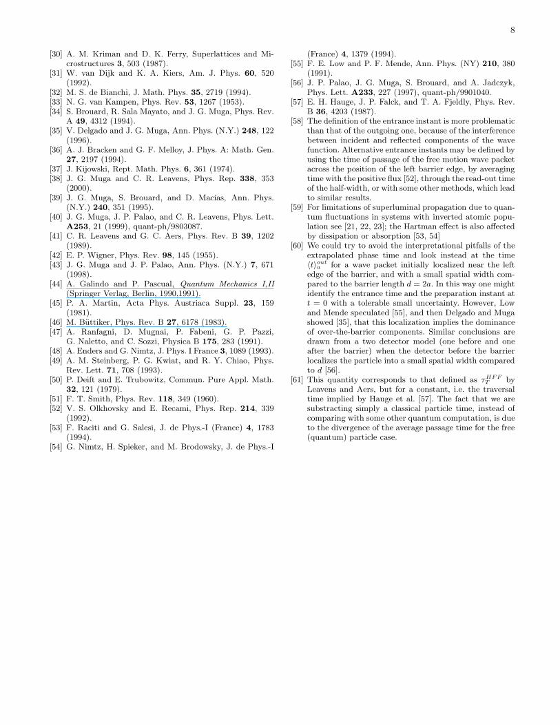
creases and decreases of the phase should balance eachother. Since Levinson’s theorem imposes a fixed phasedifference from p = 0 to ∞, there must be intervals ofnegative delay to compensate for the phase increases as-sociated with the resonances. A similar analysis appliesin 1D to the transmission amplitude. In Figure 1, thephase of the transmission amplitude for a square bar-rier is shown versus p for two different values of the bar-rier width d. As d increases, the scattering resonances“above the barrier” p > p0 = (2mV0)

1/2 become moredense, and the π−jumps are better defined, because ofthe approach of the resonance poles in the fourth quad-rant to the real axis. The corresponding increases of thephase are compensated by a more negative delay in thetunneling region.

Negative delays also arise if a pole of T (p) crosses thereal axis upwards, when varying the interaction strength,to become a loosely bound state in the positive imaginaryaxis. Levinson’s theorem [32],

ΦT (0) =

{

π(nb − 1/2) if T (p = 0) = 0πnb, if T (p = 0) 6= 0

(8)

(the convention being that ΦT (∞) = 0, with nb denot-ing the number of bound states), imposes then a suddenjump in the phase ΦT (0) that must be compensated by astrong negative slope. This effect is more important nearthreshold, i.e., when the pole is very close to the real axis[31]. Similar effects have been described for non-boundstate poles in complex potential scattering [43].

Note that the effects mentioned so far (due to reso-nances and bound states) apply to arbitrary barriers.Universal bounds on the allowed negative delays may

4

also be found. Whereas positive delays can be arbitrarilylarge, negative delays are restricted by “causality condi-tions” [29]. Some back-of-the-envelope causality argu-ments may however be misleading. For example, if thetotal time τPh

T (−a, a) is to be positive, the delay cannotbe more negative than the reference free time,

∆t > −mdp, (9)

cf. [44]. In fact this bound may be violated, in particularat low energy in the proximity of a loosely bound state.This should not surprise the reader after our warningagainst an over-interpretation of the extrapolated timeτPhT (−a, a). The flaw in the argument is the assump-

tion of positivity of τPhT (−a, a) because of an inadequate

translation from the classical trajectory case. Neverthe-less, rigorous bounds have been established by Wignerhimself and various authors in 3D collisions, see [29, 45]for review. In 1D collisions the following bounds holdfor even potentials with finite support between −a and a[31, 32] (k = p/h):

∆t ≥ m

hk

{

−d− 1

2k[sin(2ka+ 2δ0) − sin(2ka+ 2δ1)]

}

≥ m

p

(

−d− 1

k

)

. (10)

which follow from the bounds for the derivatives of thephase shifts,

δ0′ > −a− 1

2ksin[2(ka+ δ0)] > −a− 1

2k, (11)

δ1′ > −a+

1

2ksin[2(ka+ δ1)] > −a− 1

2k, (12)

where the prime indicates derivative with respect to k.Sometimes Eqs. (10,11,12) -or their 3D analogs- are pic-torially or intuitively described as the result of the classi-cal causality condition (“the traversal time must be pos-itive”) corrected by a term of the order of a wavelength,that takes into account the wave nature of matter, seee.g. [29, 30, 42]. In fact the proof, summarized in theappendix, is based on the positivity of the norm insidethe barrier region,

∫ a

−adxψj(x)

2 > 0 (ψj(x) are the even

and odd real -improper- eigenstates of the Hamiltonian).Alternatively, it may be obtained from the positivity ofthe dwell time [29, 32, 45], which is in this case the true“causality principle” behind the bound. The dwell timein the case at hand is defined [46] as

τD(−a, a) ≡ m

hk

∫ a

−a

dx|ψj(x)|2. (13)

Note that, unlike the extrapolated phase time, this quan-tity does not distinguish between transmitted and re-flected particles, and its positivity is directly implied byits definition.

In Eqs. (10), (11) and (12), δj , j = 1, 2, are the phaseshifts of the eigenvalues, Sj = exp(2iδj), of the S-matrix,

S(p) ≡(

T (p) R(p)R(p) T (p)

)

, (14)

where R is the reflection amplitude. Since we are dealingwith parity invariant potentials,

S0 = T +R,

S1 = T −R. (15)

According to the bound in Eq. (10) the negative delaymay be arbitrarily large for small enough momenta andmay diverge at p = 0, as it occurs when a bound state ap-pears when making the potential more attractive [31]. Inthe absence of bound states, however, the time advance-ment is actually bound by Eq. (9), instead of Eq. (10).Thus, whereas the experiments looking for large traversalvelocities have been frequently based on evanescent con-ditions in square barriers (tunneling) [47, 48, 49], squarewells may lead to much larger advancement effects forbarrier depths near the thresholds.

In the next section we will show the validity of Eq.(9) in the absence of bound states for a generic class ofpotentials and for all real k. Sassoli de Bianchi, usingLevinson’s theorem, had previously pointed out the va-lidity of Eq. (9) in the absence of bound states, but onlyin the limit k → 0 [32].

Later we will insist on the further time advancementsdue to bound states in the specific setting of square wells.

IV. BOUND WITHOUT BOUND STATES

The bound for the time advancement without boundstates follows from the “canonical product expansion” ofthe Sj . Note first that for cut-off potentials T and R,and thus both S0 and S1, are meromorphic functions ofk in the entire complex plane [50]. In the absence ofbound states, Sj may only have simple poles in the lowerhalf plane, and the corresponding zeros in the upper halfplane,

Sj = ±e−2ika∏

n

(k − k∗j,n)(k + kj,n)

(k − kj,n)(k + k∗j,n). (16)

Even more, each pole kj,n in the fourth quadrant goeshand in hand with a twin pole at −k∗j,n. This is the mostgeneral form compatible with the following properties ofthe Sj :

Sj(k)S∗

j (k∗) = 1, (17)

S∗

j (k) = Sj(−k∗), (18)

|Sa,j| ≤ 1 (Imk ≥ 0), (19)

where

Sa,j = e2ikaSj . (20)

5

The first two are the the “unitarity” and “symmetry”relations that follow from the reality of the potential,whereas the last one follows (in the absence of boundstates) from van Kampen’s causality condition [29, 33],namely from the fact that the total probability of findingthe particle outside any sphere of radius r ≥ a cannotbe greater than one. An equivalent formulation is thatthe outgoing probability current, integrated from −∞ tot, cannot exceed the integrated ingoing current by morethan the absolute value of the integral of the interference(ingoing-outgoing) term. Van Kampen arrived at thiscausality condition noticing that the causality conditionfor the scattering of the Maxwell field, which implies amaximum velocity c, does not apply to the Schrodingerequation; moreover, no wave packets could be built whichpropagate with a sharp front for any finite interval oftime. The mathematical arguments leading to Eq. (19)are lengthy but admit a direct translation to the twopartial waves of the one dimensional case. That Eq. (19)is fulfilled may be checked in any case in the examplesconsidered below.

Taking the logarithmic derivative on both sides of Eq.(16) one obtains,

dδj/dk = −a−∑

n

(

1

|k − kj,n|2+

1

|k + kj,n|2)

Im kj,n,

(21)assuming that k is real. Since all the poles lie in the lowerhalf-plane the second term is positive. In the absence ofbound states, δ′j ≥ −a and, since ΦT = δ0 + δ1, thetransmission time delay does indeed satisfy the bound ofEq. (9).

A bound state of energy −(hKb)2/(2m) for the

j-partial wave implies for Sj an extra factor (k +iKb)/(iKb − k), with Kb > 0, which spoils the lowerlimit −a for δ′j . The contribution of these bound-stateterms will however be negligible for large k. If there isjust one bound state corresponding to a pole at k = iKb,one obtains, similarly to the 3D case [29],

∆t ≥ −mp

(

d+1

Kb

)

, (22)

which may be interpreted in terms of an increased size ofthe scatterer due to the broad range of the loosely boundstate.

V. EXAMPLES

The above properties of the Sj can be easily exem-plified with the aid of analytically solvable models. Wehave in particular checked the validity of Eq. (9) for thesquare barrier,

Vsb(x) = V0 χ(−a, a), (23)

for V0 > 0, where χ(−a, a) is the characteristic func-tion for the barrier region. The eigenphaseshifts δj and

-2 -1,5 -1 -0,5 0 0,5 1V

0 (a.u.)

-60

-40

-20

0

20

40

60

Del

ay ti

me

(a. u

.)

FIG. 2: Time delay versus barrier height/depth for a squarepotential. The incident momentum is k = 0.1, mass m = 1,and barrier width d = 2 (all magnitudes in atomic units).The exact expression for the time delay is depicted with acontinuous line. The dotted line corresponds to the top boundof (10), whereas the dashed line is the constant quantity ofthe failed bound (9)

their derivatives are easily computed as explicit func-tions; however, those expressions are not very enlighten-ing for current purposes, so they are not displayed here.By making V0 < 0 and allowing for the presence of boundstates the bound (9) is not satisfied any more, but Eq.(10) does hold.

In order to make this explicit, we have plotted in Fig.2 the delay time as a function of the well depth for a setvalue of momentum, and, so as to compare, both con-stant bound (9), and the more adequate Eq. (10). Theline depicting the constant value −md

p is seen to cut the

computed line at points close to those that correspond tothe onset of a new bound state. On the other hand, theoscillatory bound of Eq. (11) keeps track of the injectionof new bound states. This effect takes place for each newbound state that comes into play; in the figure only thefirst two thresholds for new bound states appear, but thesame structure repeats itself. Note that, as we are stress-ing throughout, the simple bound (9) does indeed holdfor barriers (V0 > 0).

The analysis of the bound has pertained to stationarywaves, or, alternatively, to wavepackets highly centeredin a particular momentum component. It now behoovesus to check whether the enhancement of time delays canbe carried over to wavefunctions more extended in mo-mentum space (and therefore more localized in space),with some chance of being detected. For this purpose wewill reexamine Eq. (6) for the case of a square well. Insuch a situation |T (k)| ∼ O(k) as k tends to zero, exceptwhen the depth of the well corresponds to the thresh-old of a new bound state, that is to say, except whenV0 = −(h2n2π2)/(8ma2). In other words, there is no sta-tionary state with zero energy in the presence of the well,but for the exceptional threshold cases, when such a sta-

6

-6 -4 -2 0V

0 (a.u.)

-5

0

5A

v. s

ubst

ract

ed d

elay

(a.

u.)

Tra

nsm

issi

on P

roba

bilit

y

FIG. 3: Transmission probability (dashed line) and averagedsubstracted passage time (continuous line) versus potentialfor a truncated gaussian wavefuncion with central momentumk0 = π/8 and dispersion 1.0, whose center is located at x0 =−41 at time t = 0. The mass of the particle is m = 1 and thewidth of the square well/barrier is d = 2. All magnitudes inatomic units.

tionary state does indeed exist, as it does for the free par-ticle case. Therefore, except for the exceptional thresh-old case, the integral presents no singularity. On theother hand, for those exceptional situations |T (k)| → 1as k tends to zero; since the time delay does not tendto zero in that limit either, the integral will be divergentif the asymptotic initial state in momentum representa-tion does not go zero fast enough. This should be nosurprise: exactly the same divergence would take placefor free motion, and for exactly the same reason, namely,the presence of k = 0 stationary components, for whichno phase time can make sense. We depict in Figure 3 thetransition probability as a function of the height/depthof a square barrier/well for an asymptotic wavepacketwhich is gaussian in momenta, truncating out the nega-tive momentum part, and is centered at x0 = −41a atthe instant t = 0. For the same wavepacket we also de-pict the “averaged substracted passage time”, that is, theresult of integral (6), minus the time that a classical par-ticle whose momentum is the central momentum of thewavepacket would take to reach the right-hand side ofthe potential well, from an initial position at x0 = −41a(the classical particle would be moving in the potentialwell, for adequate comparison) [61]. The applicability ofEq. (6) is ensured by the large initial distance. Negativesubstracted passage times are apparent for zones of thepotential strength for which a new state has just beeninjected into the bound sector. These negative passagetimes would be enhanced if the gaussian were closer tok = 0 in momentum space, be it because the center ofthe wavepacket in momentum space moved towards theorigin, or because the width of the packet increased. Animportant aspect, apparent from the figure, is that thetransmission probability is big in some zones of negative

average passage times. This is due to the fact that themodule of the transmission amplitude, |T (k)|, has a max-imum very close to k = 0 if the gap from the highest lyingbound state to the continuum spectrum is small. There-fore, we can have at the same time high transmissionprobability, and strongly enhanced negative time delays;the idea of using parameters of the potentials very closeto those introducing a new bound state in order to mea-sure negative delays immediately springs to mind.

VI. DISCUSSION

We have shown that the time advancement of thetransmitted wave packet of a particle colliding with apotential barrier without bound states is bounded, dueto the causality condition of van Kampen, by the simpleprediction based on assuming the positivity of the ex-trapolated phase time. This positivity does not hold inthe presence of bound states, in which case a differentbound allows for large advancements al low incident en-ergy near depth thresholds where a bound state appears(“ultra Hartman effect”). We have also argued, and pro-vided explicit examples, that these large advancementsare indeed observable, since the transmission probabilityis large at low energies near the thresholds.

The present approach is formally limited by the as-sumption of a cut-off in the potential and one may won-der about its relevance for arbitrary potentials, but it isclear that the difference between the actual (non-cut-off)potential and a potential truncated at an arbitrarily largedistance from the center cannot be physically significant.Thus, even though the canonical form assumed for theSj in the complex plane may fail for the non-cut-off po-tential, all observable features associated with real andpositive values of the wave number will be essentially un-changed, in particular the delay times and their bounds.

APPENDIX A: PROOF OF BOUNDS (11) AND(12)

Eq. (10) may be proven by using the even and oddeigenfunctions ψj(x) of the Hamiltonian, for which theboundary conditions are

limx→−∞

ψ0(x) =

(

2

h

)1/2

cos(−px/h+ δ0),

limx→∞

ψ0(x) =

(

2

h

)1/2

cos(px/h+ δ0),

limx→−∞

ψ1(x) =

(

2

h

)1/2

sin(px/h− δ1),

limx→∞

ψ1(x) =

(

2

h

)1/2

sin(px/h+ δ1). (A1)

In particular we shall use the fact that∫ a

−adxψ2

j > 0. We

start by calculating the logarithmic derivative of ψ0(x)

7

at x = a from the known expression for the outer region,see (A1),

La ≡ ψ′

0(x)

ψ0(x)

∣

∣

∣

∣

x=a

= − p

htan(pa/h+δ0) = −k tan(ka+δ0),

(A2)where ψ′(x) = dψ0(x)/dx, and henceforward the primesdenote derivative wih respect to x. Taking the derivativeof La with respect to k,

dδ0dk

= −1

k

dLa

dkcos2(ka+ δ0) − a− 1

2ksin[2(ka+ δ0)].

(A3)The first term on the right hand side may also be writtenas

− cos2(ka+ δ0)

k

dLa

dk= − h

2kψ2

0(a)

[

ψ′

0(x)

ψ0(x)

]

k

∣

∣

∣

∣

x=a

=

= − h

2kψ0(a)∂

↔

kψ′

0(a) =

= − h3

8π2mψ0(a)∂

↔

Eψ′

0(a) .

(A4)

Here and in what follows, the subscript k and E are short-hand notation for the derivatives with respect to k andE, respectively, whereas the derivative with respect to x

is denoted by primes, and the symbol g(x)∂↔

yf(x) indi-cates g(x)∂yf(x) − (∂yg(x))f(x) . Repeating the sameoperations for x = −a one finds that

[ψ0,E(−a)ψ′

0(−a) − ψ0(−a)ψ′

0,E(−a)]

= −[ψ0,E(a)ψ′

0(a) − ψ0(a)ψ′

0,E(a)]. (A5)

We shall now prove that this is a positive quantity. Tak-ing the derivative of the stationary Schrodinger equationwith respect to energy one obtains for real eigenfunctionsof H the identity [51]

ψ(x)2 = − h2

2m

∂

∂x

(

ψ(x)ψ′

,E(x) − ψ,E(x)ψ′(x))

, (A6)

so that, using (A5),

∫ a

−a

dxψ0(x)2 =

h2

m

(

ψ0,E(a)ψ′

0(a) − ψ0(a)ψ′

0,E(a))

,

(A7)whence the positivity of − 1

kdLa

dk cos2(ka+δ0) follows, andthus bound (11) is seen to hold.

Carrying out similar manipulations for the odd wavefunction ψ1(x), and using ΦT = δ0 + δ1, (10) is found asa consequence of the positivity of the probability to findthe particle in the barrier region.

ACKNOWLEDGMENTS

This work is supported by Ministerio de Ciencia y Tec-nologıa, The University of the Basque Country, and theBasque Government. J.A.D. acknowledges financial sup-port by the Basque Government. F.D. acknowledges fi-nancial support by Ministerio de Educacion y Cultura.

[1] T. E. Hartman, J. Appl. Phys. 33, 3427 (1962).[2] J. R. Fletcher, J. Phys. C:Solid State Phys. 18, 3427

(1985).[3] A. Enders and G. Nimtz, Phys. Rev. E 48, 632 (1993).[4] D. Mugnai, A. Ranfagni, R. Ruggeri, A. Agresti, and

E. Recami, Phys. Lett. A 209, 227 (1995).[5] J. Jakiel, V. S. Olkhovsky, and E. Recami, Phys. Lett. A

248, 156 (1998).[6] R. Y. Chiao (1998), quant-ph/9811019.[7] G. Nimtz, Ann. Phys. (Leipzig) 7, 618 (1998).[8] M. Buttiker and R. Landauer, Phys. Rev. Lett. 49, 1739

(1982).[9] R. Landauer and T. Martin, Rev. Mod. Phys. 66, 217

(1994).[10] M. Y. Azbel, Solid State Comm. 91, 439 (1994).[11] V. Delgado, S. Brouard, and J. G. Muga, Solid State

Commun. 94, 979 (1995).[12] E. H. Hauge and J. A. Støvneng, Rev. Mod. Phys. 61,

917 (1989).[13] J. M. Deutch and F. E. Low, Ann. Phys. 228, 184 (1993).[14] A. M. Steinberg, P. G. Kwiat, and R. Y. Chiao, Found.

Phys. Lett. 7, 223 (1994).[15] K. Hass and P. Busch, Phys. Lett. A 185, 9 (1994).[16] G. Diener, Phys. Lett. A 223, 327 (1996).[17] P. Kochanski and K. Wodkiewicz, Phys. Rev. A 60, 2689

(1999), quant-ph/9902044.[18] E. Recami, F. Fontana, and R. Garavaglia, Int. J. Mod.

Phys. A 15, 2793 (2000).[19] G. C. Hegerfeldt, in Extensions of Quantum Theory,

edited by A. Horzela and E. Kapuscik (Apeiron, Mon-treal, 2001), pp. 9–16.

[20] R. Sala, S. Brouard, and J. G. Muga, J. Phys. A 28, 6233(1995).

[21] Y. Aharonov, B. Reznik, and A. Stern, Phys. Rev. Lett.81, 2190 (1998).

[22] B. Segev, P. W. Milonni, J. F. Babb, and R. Y. Chiao,Phys. Rev. A 62, 022114 (2000), quant-ph/0004047.

[23] A. Kuzmich, A. Dogariu, L. J. Wang, P. W. Milonni, andR. Y. Chiao, Phys. Rev. Lett. 86, 3925 (2001).

[24] W. Heitmann and G. Nimtz, Phys. Lett. A 196, 154(1994).

[25] G. Nimtz, Eur. Phys. J. B 7, 523 (1999).[26] M. Buttiker and H. Thomas, Superlattices and Mi-

crostructures 23, 781 (1998).[27] A. Ranfagni and D. Mugnai, Phys. Rev. E 52, 11288

(1995).[28] J. G. Muga and M. Buttiker, Phys. Rev. A 62, 023808

(2000), quant-ph/0001039.[29] H. M. Nussenzveig, Causality and Dispersion Relations

(Academic Press, New York, 1972).

8

[30] A. M. Kriman and D. K. Ferry, Superlattices and Mi-crostructures 3, 503 (1987).

[31] W. van Dijk and K. A. Kiers, Am. J. Phys. 60, 520(1992).

[32] M. S. de Bianchi, J. Math. Phys. 35, 2719 (1994).[33] N. G. van Kampen, Phys. Rev. 53, 1267 (1953).[34] S. Brouard, R. Sala Mayato, and J. G. Muga, Phys. Rev.

A 49, 4312 (1994).[35] V. Delgado and J. G. Muga, Ann. Phys. (N.Y.) 248, 122

(1996).[36] A. J. Bracken and G. F. Melloy, J. Phys. A: Math. Gen.

27, 2197 (1994).[37] J. Kijowski, Rept. Math. Phys. 6, 361 (1974).[38] J. G. Muga and C. R. Leavens, Phys. Rep. 338, 353

(2000).[39] J. G. Muga, S. Brouard, and D. Macıas, Ann. Phys.

(N.Y.) 240, 351 (1995).[40] J. G. Muga, J. P. Palao, and C. R. Leavens, Phys. Lett.

A253, 21 (1999), quant-ph/9803087.[41] C. R. Leavens and G. C. Aers, Phys. Rev. B 39, 1202

(1989).[42] E. P. Wigner, Phys. Rev. 98, 145 (1955).[43] J. G. Muga and J. P. Palao, Ann. Phys. (N.Y.) 7, 671

(1998).[44] A. Galindo and P. Pascual, Quantum Mechanics I,II

(Springer Verlag, Berlin, 1990,1991).[45] P. A. Martin, Acta Phys. Austriaca Suppl. 23, 159

(1981).[46] M. Buttiker, Phys. Rev. B 27, 6178 (1983).[47] A. Ranfagni, D. Mugnai, P. Fabeni, G. P. Pazzi,

G. Naletto, and C. Sozzi, Physica B 175, 283 (1991).[48] A. Enders and G. Nimtz, J. Phys. I France 3, 1089 (1993).[49] A. M. Steinberg, P. G. Kwiat, and R. Y. Chiao, Phys.

Rev. Lett. 71, 708 (1993).[50] P. Deift and E. Trubowitz, Commun. Pure Appl. Math.

32, 121 (1979).[51] F. T. Smith, Phys. Rev. 118, 349 (1960).[52] V. S. Olkhovsky and E. Recami, Phys. Rep. 214, 339

(1992).[53] F. Raciti and G. Salesi, J. de Phys.-I (France) 4, 1783

(1994).[54] G. Nimtz, H. Spieker, and M. Brodowsky, J. de Phys.-I

(France) 4, 1379 (1994).[55] F. E. Low and P. F. Mende, Ann. Phys. (NY) 210, 380

(1991).[56] J. P. Palao, J. G. Muga, S. Brouard, and A. Jadczyk,

Phys. Lett. A233, 227 (1997), quant-ph/9901040.[57] E. H. Hauge, J. P. Falck, and T. A. Fjeldly, Phys. Rev.

B 36, 4203 (1987).[58] The definition of the entrance instant is more problematic

than that of the outgoing one, because of the interferencebetween incident and reflected components of the wavefunction. Alternative entrance instants may be defined byusing the time of passage of the free motion wave packetacross the position of the left barrier edge, by averagingtime with the positive flux [52], through the read-out timeof the half-width, or with some other methods, which leadto similar results.

[59] For limitations of superluminal propagation due to quan-tum fluctuations in systems with inverted atomic popu-lation see [21, 22, 23]; the Hartman effect is also affectedby dissipation or absorption [53, 54]

[60] We could try to avoid the interpretational pitfalls of theextrapolated phase time and look instead at the time〈t〉out

a for a wave packet initially localized near the leftedge of the barrier, and with a small spatial width com-pared to the barrier length d = 2a. In this way one mightidentify the entrance time and the preparation instant att = 0 with a tolerable small uncertainty. However, Lowand Mende speculated [55], and then Delgado and Mugashowed [35], that this localization implies the dominanceof over-the-barrier components. Similar conclusions aredrawn from a two detector model (one before and oneafter the barrier) when the detector before the barrierlocalizes the particle into a small spatial width comparedto d [56].

[61] This quantity corresponds to that defined as τHF F

T byLeavens and Aers, but for a constant, i.e. the traversaltime implied by Hauge et al. [57]. The fact that we aresubstracting simply a classical particle time, instead ofcomparing with some other quantum computation, is dueto the divergence of the average passage time for the free(quantum) particle case.