THE SOCIAL COSTS OF AIR TRAFFIC DELAYS

Part One: A Survey

Etienne Billette de Villemeur

University of Toulouse (IDEI - GREMAQ)

Marc Ivaldi University of Toulouse (IDEI), EHESS and CEPR)

Emile Quinet Ecole National des Ponts et Chaussées

Miguel Urdánoz University of Toulouse (GREMAQ)

April 2005

Interim report

INSTITUT D’ECONOMIE INDUSTRIELLE Université Toulouse 1 – Sciences Sociales

21, Allée de Brienne 31000 - Toulouse

2

CONTENT

Executive Summary ...................................................................................................................................4

1. Introduction.......................................................................................................................................5

2. Applied Studies on Cost of Delays ...................................................................................................7 2.1. Evaluation of Congestion Costs at Madrid Airport.................................................................10 2.2. Costs of Air Transport Delay in Europe....................................................................................9 2.3. Evaluating the True Cost of Delays for Airlines .....................................................................13 2.4. Summary on Applied Studies ...................................................................................................15

3. Theoretical Analysis on Congestion ..............................................................................................17 3.1. The conceptual models and the value of time..........................................................................17 3.2. The values of time....................................................................................................................20

3.2.1. The value of travel time......................................................................................................21 3.2.2. The value of waiting time ...................................................................................................24 3.2.3. The value of time for early and late arrival.........................................................................25 3.2.4. Value of reliability..............................................................................................................26

3.3. Theoretical Models of Congestion...........................................................................................29

4. Towards an Objective Definition of Delays ..................................................................................34

References .................................................................................................................................................36

List of Acronyms ......................................................................................................................................39

Appendix 1: A Model of Congestion Costs.............................................................................................40

Appendix 2: A theoretical decomposition of time value........................................................................42

Appendix 3: Perception of Passengers Delays: An explanatory study.................................................46

Appendix 4: A Model on Network Benefits and Flight Delays.............................................................47

3

LIST OF TABLES

Table 1: Total and Average Passenger Congestion Costs .............................................. 11 Table 2: Airlines' Congestion Costs (monthly costs, million euros) .............................. 11 Table 3: Marginal Congestion Costs Generated by a Flight (euros) .............................. 12 Table 4: Summary on Studies of Costs of Air Traffic Delays ....................................... 15 Table 5: Value of time for France in 1990 ..................................................................... 22 Table 6: Time values in Inter-city travels (1998) per passenger .................................... 23 Table 7: Values of time .................................................................................................. 23 Table 8: Values of time in Euro/hour ............................................................................. 24 Table 9: Values for different waiting times.................................................................... 25 Table 10: Value of time for early and late arrival .......................................................... 25 Table 11: Value of time schedule expressed as a proportion of value of travel time..... 25 Table 12: Comparison of selected model results............................................................ 26 Table 13: Comparison of Alternative Empirical Estimates of Travel Time Variability 27 Table 14: Estimated time values..................................................................................... 30

LIST OF FIGURES

Figure 1: Percentage of delayed flights in the U.S. ............... Erreur ! Signet non défini. Figure 2: Percentage of delayed flights in Europe ................ Erreur ! Signet non défini. Figure 3: Commercial flights and delays at the 15 biggest airports in France ................. 6 Figure 4: Minimum, Scheduled and Actual Travel Times ............................................... 8 Figure 5: Cost of delay per minute distribution.............................................................. 16

4

Executive Summary In this report we do a thorough review of theoretical and empirical studies on the

estimation of costs of air traffic delays and on the literature about value of time. In

general empirical estimations do not address the issues discussed by the theoretical

models. The latter mainly focuses on the modeling of queues at congested airports while

the former are based on previous studies of the value of time and the question of a

proper definition of delays.

Besides methodological problems, empirical analysis provides very different

estimates of delays and costs of delays. On the other side, theoretical models provide

some insights although they are difficult to test and apply in practice. Nevertheless they

show the crucial role of a right definition of delays.

The relevant delay must take into account the fact that airlines add some extra time

to their schedules in addition to what it is technically required to avoid partial

congestion. This is the so-called buffer delay. Airlines obtain different benefits from

this practice. For instance it helps them building their reputation in terms of reliability,

i.e., in their capacity to avoid cascading delays. The buffer delay is defined as the

number of minutes the airlines should add to the schedule so that marginal cost of this

buffer is equaled to the expected benefit. Similarly, for the society as a whole, minutes

of congestion should be added up to the point where benefits equal costs. Therefore,

when we study delay costs, we should not consider the whole delay. We should be able

to distinguish what it is the optimal delay, in the total amount of delays. Only the

difference between observed and optimal delays could be harmful for the consumers of

air traffic and airport services.

5

1. Introduction

“Placing users at the heart of the transport policy” is one of the key actions proposed by

the White Paper of the Commission of the European Community. Particularly, “Specific

new measures are needed on user's rights in all modes of transport so that, regardless of

the mode of transport used, users can both know their rights and enforce them.” (See

European Commission, 2001.) “The Commission's aim over the next ten years is to

develop and define the rights of users”. In the short term, the Commission intended to:

• Increase air passengers existing rights through new proposals concerning in

particular, denied boarding due to overbooking, delays and flight cancellations.

• Put forward a regulation concerning requirements to air transport contracts.

In fact, new regulation about passenger rights has entered into force in February

2005. The EU acted in 1991 to strengthen passenger's rights, particularly for the cases

of overbooking. The new law has extended these rights to all kind of flights from and/or

with destination the EU. It also has increased the monetary compensations in case of

denied boarding; it includes compensations for some type of cancellations and cover

also long delays.1 However, no economic explanation has been presented to defend

these new measures and airlines argue that it will immediately suppose an increase in

cost that will be translated to prices.

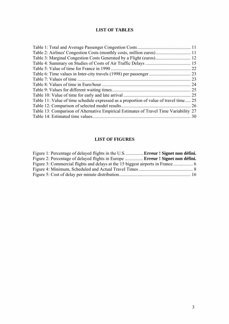
For France, congestion and delays have become a common operational

characteristic. According to l’observatoire des retards aeriens, the proportion of flights

delayed more than 15 minutes was 25% with an average delay of 43 minutes. The

delays in Europe were affected by the attacks of 2001 as well as they were disturbed by

the war during 1999 in Yugoslavia. The most remarkable feature is the decline produced

in the 2001 due to the terrorist attack of September 11th which undermined the

confidence on passengers.

France presents quite high average delays however we have to take into account that

this can be increased due to the central geographic position of France in Europe (more

than one of each four flights in Europe cross the French airspace).

1 See European Commission (2005).

6

Figure 1: Commercial flights and delays at the 15 biggest airports in France

730000

750000

770000

790000

810000

830000

850000

1998 1999 2000 2001 2002 2003 200415%

20%

25%

30%

35%

40%

45%

Number of commercialflights at departure

% of flights delayed atleast 15 minutes

Source: L’observatoire des retards du transport aerien

Even if airlines through Europe have signed voluntary agreements (not binding) to

deliver defined standards of service to air travelers (such as the 2002 undertaking by the

major players in the sector), in the absence of Community legislation, passengers are

confronted with an increasing level of delays and with a set of national rules to protect

them which are largely ineffective.

These figures raise several questions. First of all, one may question their relevance

as the measures of delays could be based on imperfect or even incorrect definitions.

Second, one may wonder whether the impact of delays on social welfare is significant.

In order to provide a set of objective replies, the Direction General de l'Aviation

Civile (DGAC) of the French Ministry of Transport has commanded to the Institut

D’Economie Industrielle (IDEI) a study of costs that passengers in French airports incur

due to delays.

This interim report is aimed at providing a review of the state of literature on this

topic. It accounts for with applied studies as well as theoretical and methodological

considerations.

In a second section, we review the few applied studies that reckon costs of delays.

The three main studies mainly deal with the cost for operators, and to a much smaller

extent with the cost for users. They use a rough methodological framework based on a

unique value of time, just taking into account the travel time spent and reckoning the

gaps between the scheduled and the real times.

These studies contrast with the complexity and sophistication of theoretical models,

which are discussed in the third section. Here we mainly focus on the question of a

proper modeling of the congestion phenomenon. Theoretical models take into account

7

different dimensions of time delay like the gap between desired and actual arrival time,

different values of time or the existence of buffer delay. To our knowledge however,

none of these approaches has been used to reckon the cost of delays or even to set up a

definition of delays and how to implement measures of delays according to these

definitions.

The last section summarizes these results and draws some directions for future

research or study.

2. Applied Studies on Cost of Delays

Three applied studies are reviewed:

• The ITA study “Costs of Air Transport Delay in Europe” (2000).

• The study “Evaluation of Congestion Costs for Madrid Airport” made in the

framework of the UNITE research program by Nombela, de Rus and Betancor

(2002).

• The report by the University of Westminster (2004).

These three studies deal with the cost of delays for the operator; the cost of delays for

the users is just considered by the first two ones.

It must be mentioned that these studies use a crude definition of delays: the

discrepancy between the scheduled arrival time and the real arrival time. However the

Westminster study makes a distinction between arrival delays and departure delays.

For airlines, an important point noted in several studies is the difference between

scheduled and what could be considered an optimal or minimum time for a trip. Due to

the high cost that delays can represent for airlines, it is quite common to schedule a

longer time for the trip than what could be gained without any kind of congestion. This

difference is know as “buffer”, and is specially used by hub-airlines, which want to

ensure the connections for all their passengers, and by low-cost companies that wants to

build a reputation of on-time flights. Airlines use buffers to recover from delay by

“padding” the schedule so that they can improve the predictability of rotations and also

improve their punctuality performance with respect to published schedules. This

distinction between schedule and buffer is mentioned in the ITA study, but no

reckoning is made (it is clear that the optimal travel time and the buffer time are not

published, we know just their sum which is the scheduled time).

8

A few studies attempted to estimate this buffer time, or at least to approximate it

since even the airlines only know an average estimate. (See, for instance, Morrison,

Winston, Bailey and Khan, 1989.) They have been unsuccessful so that the most usual

approach to estimate buffer time is to just compare the schedule time with the minimum

travel time for each route that was obtained on the studied period. However this

measure is imprecise as it could be affected by very favorable weather conditions. In

that case it would be more adequate to consider some percentile of the distribution of

buffer times. However nobody has even proposed such a measure.

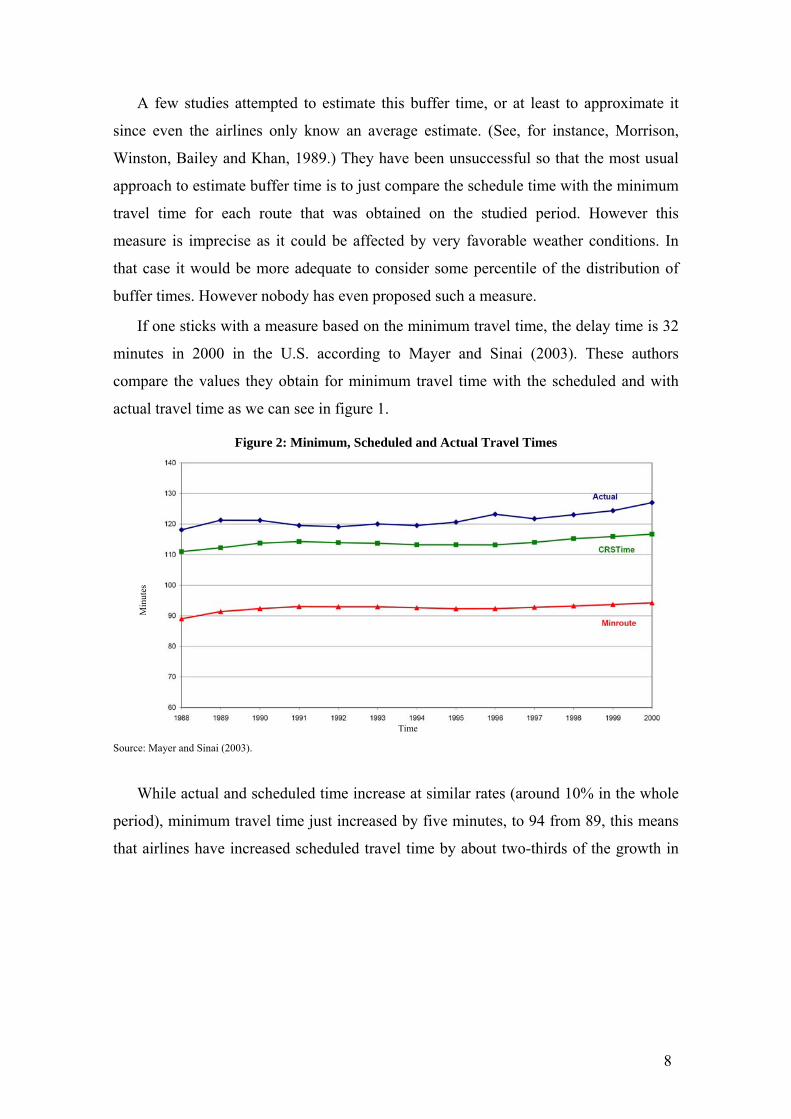
If one sticks with a measure based on the minimum travel time, the delay time is 32

minutes in 2000 in the U.S. according to Mayer and Sinai (2003). These authors

compare the values they obtain for minimum travel time with the scheduled and with

actual travel time as we can see in figure 1.

Figure 2: Minimum, Scheduled and Actual Travel Times

Time

Source: Mayer and Sinai (2003).

While actual and scheduled time increase at similar rates (around 10% in the whole

period), minimum travel time just increased by five minutes, to 94 from 89, this means

that airlines have increased scheduled travel time by about two-thirds of the growth in

Min

utes

9

average travel time.2 A similar evolution can be expected in Europe due to the new

regulation of the Commission for passenger rights.3

2.1. Costs of Air Transport Delay in Europe The Institut du Transport Aérien (2000) estimates the delay costs for airlines and

passengers in Europe. It provides an estimation of costs of delays based on the cost for

passengers and airlines drawn from previous studies about the value of time. Note that

they consider two concepts of delay that they denote as “operated flights versus

schedule” and “schedule versus optimum” that we are going to denote as schedule

delays and buffer delays respectively.

As we have previously explained buffer delays make reference to the extra time that

airlines add to the schedule of a city pair, with respect to what is technically needed

while schedule delays refer to the observed difference between announced

arrival/departure time and the real one.

For the latter, the authors just add the different estimations of costs. They use data

coming from IATA and ATA completed with data from EUROCONTROL in order to

differentiate between primary and reactionary delays. They study just the delays due to

Air Traffic Flow Management (ATFM). 4,5

The number of passengers affected by ATFM delays is calculated from an estimated

number of delayed flights, and an average aircraft capacity and load factor. Passengers

are distinguished between business, personal convenience and tourism travelers. Two

scenarios for the value of time of the different categories, high and low, are considered.

The values of time comes just from “a conservative range” that moves between 34 and

44 euros taken from values of time offered by previous studies.

2 These figures have been obtained from a sample that includes 66.4 million flights at the top 27 US airports. The data set covers all airlines with at least one percent of all domestic traffic and only routes where flights are observed in each month of the entire sample period. 3 In fact, there is already evidence for the scheduled buffers. According to Eurocontrol, 13 percent of flights in 2004 departed before scheduled time and 34 percent of flights arrived before their scheduled time. 4 According to ITA, the study of IATA produces a very rough evaluation of the direct operating costs; the study of ATA covers only the U.S. and provides a valuation of 34.1$ per minute without providing information on the procedure followed to obtain this value. 5 ATFM delay is defined as "duration between the last take-off time requested by the aircraft operator and the take-off slot given by the central flow management unit".

10

For buffer delay costs, the same values assumed for schedule delay are used for the

passengers and a value of €45 per minute is assumed for airlines. The authors do not

estimate what is the “optimum” time, but just consider two scenarios, increased flight

time of either 5 or 10%.

They get a final estimation of 1.6 to 2.3 billion of euros for schedule delays costs for

airlines in 1999, which rises to a ranging between 3 and 5.1 billion of euros if we

consider also non-optimal scheduling. Costs of scheduled delays for passengers would

be between 2.13 and 2.74 billion of euros and between 1.42 and 2.85 billion of euros for

buffer delays (total costs range between 3.55 and 5.59 billions of euros).

The estimations offered by this study are quite rough as the authors recognize it for

two reasons. First, the authors use a vague estimation of the cost per minute for both

airlines and passengers for the two kinds of delays considered. The same value of time

is applied for buffer and schedule delays. For airlines, as we will see in the study by the

University of Westminster, these values are different; in particular, their approximation

for the value of buffer time is on average 70% smaller than for the cost of schedule

delay while here, the average cost for buffer is even a bit bigger than the cost for

schedule delay, which makes unreasonable the existence of buffers. For passengers, is

difficult to justify such a high cost for buffer time since passengers probably does not

take the buffer time into their expectations, but rather look to the scheduled time.

Second, the ATFM delays do not include reactionary delays and does not take into

account possible differences between the slot take-off time and the actual departure time

caused by airport operations or aircraft operator operations.

2.2. Evaluation of Congestion Costs at Madrid Airport Nombela, de Rus and Betancor (2002) study the congestion costs for Madrid airport in

the period 1997-2000. They consider both airlines and passengers delay costs. The

authors define the delay as the schedule delay, i.e., the difference between scheduled

and actual arrival (and departure) times. They discuss how studies must be cautious

when studying a network to avoid double-counting effect of delays, and the difficulty

that presents the system to determine who causes the delays. In their case, as they want

to study the congestion costs at Madrid airport regardless of who has caused the

congestion, they just add up all experimented schedule delays.

11

The main contribution of their study is a small step they are performing toward the

use of economic theory to define delay costs. Nonetheless, as for the Westminster

report, their cost estimations are based on an accounting approach.

The authors develop a simple model to identify what are the basic variables that

should be included to study congestion costs and explain why total congestion costs can

be evaluated by adding the cost borne by passengers and by airlines separately.6

As in the preceding study, the final cost estimation is based on previous estimations

of the value of time for the passengers and previous studies of the direct and indirect

cost of delays for airlines. Values for passengers are estimated based on assuming

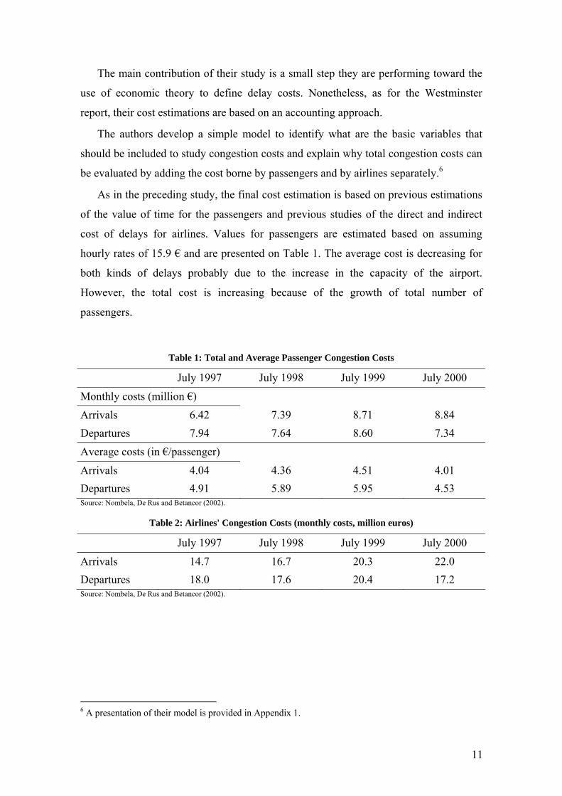
hourly rates of 15.9 € and are presented on Table 1. The average cost is decreasing for

both kinds of delays probably due to the increase in the capacity of the airport.

However, the total cost is increasing because of the growth of total number of

passengers.

Table 1: Total and Average Passenger Congestion Costs

July 1997 July 1998 July 1999 July 2000

Monthly costs (million €) Arrivals 6.42 7.39 8.71 8.84 Departures 7.94 7.64 8.60 7.34 Average costs (in €/passenger)

Arrivals 4.04 4.36 4.51 4.01 Departures 4.91 5.89 5.95 4.53 Source: Nombela, De Rus and Betancor (2002).

Table 2: Airlines' Congestion Costs (monthly costs, million euros)

July 1997 July 1998 July 1999 July 2000 Arrivals 14.7 16.7 20.3 22.0 Departures 18.0 17.6 20.4 17.2 Source: Nombela, De Rus and Betancor (2002).

6 A presentation of their model is provided in Appendix 1.

12

Table 2 presents the results for airlines, which are obtained from an hourly cost of

5,000 €. Costs have increased for arrival delays while the evolution is not so clear for

departures.

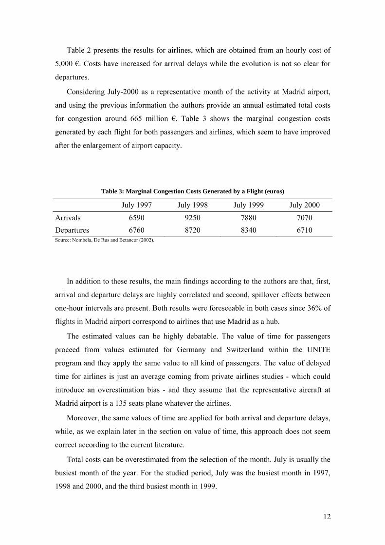
Considering July-2000 as a representative month of the activity at Madrid airport,

and using the previous information the authors provide an annual estimated total costs

for congestion around 665 million €. Table 3 shows the marginal congestion costs

generated by each flight for both passengers and airlines, which seem to have improved

after the enlargement of airport capacity.

Table 3: Marginal Congestion Costs Generated by a Flight (euros)

July 1997 July 1998 July 1999 July 2000 Arrivals 6590 9250 7880 7070 Departures 6760 8720 8340 6710 Source: Nombela, De Rus and Betancor (2002).

In addition to these results, the main findings according to the authors are that, first,

arrival and departure delays are highly correlated and second, spillover effects between

one-hour intervals are present. Both results were foreseeable in both cases since 36% of

flights in Madrid airport correspond to airlines that use Madrid as a hub.

The estimated values can be highly debatable. The value of time for passengers

proceed from values estimated for Germany and Switzerland within the UNITE

program and they apply the same value to all kind of passengers. The value of delayed

time for airlines is just an average coming from private airlines studies - which could

introduce an overestimation bias - and they assume that the representative aircraft at

Madrid airport is a 135 seats plane whatever the airlines.

Moreover, the same values of time are applied for both arrival and departure delays,

while, as we explain later in the section on value of time, this approach does not seem

correct according to the current literature.

Total costs can be overestimated from the selection of the month. July is usually the

busiest month of the year. For the studied period, July was the busiest month in 1997,

1998 and 2000, and the third busiest month in 1999.

13

Part of this bias could be corrected because the authors do not take into account the

utilization of buffers, which could underestimate total costs. Nonetheless, we believe

that the cost of delays is overestimated since the authors ignore the fact that some

congestion is present at the optimal equilibrium that is explained in the next section.

2.3. Evaluating the True Cost of Delays for Airlines

On behalf of the Performance Review Commission, the University of Westminster

prepared one of the latest studies about air congestion. The study focuses on the costs of

delays due to air traffic management and born by air traffic carriers. It does not study

the delay cost for passengers.

Two types of delays for airlines that we have previously discussed are considered

here: buffer delays and schedule delays. Schedule delays are defined as the off-block/on

block time of an aircraft relative to the operator's published schedule. Buffers refer in

general to the extra time that airlines add to the schedule of a city pair, with respect to

what is technically needed.7

Schedule delays

The study presents a thorough analysis of all possible costs that an airline face during a

delay at the different phases of a flight (in airborne, on the ground, at the gate, during

taxiing). It provides estimates for the cost that an airline faces for 15 and 65 minutes

delays, typifying ‘short’ and ‘long’ delays. For each delay's duration they estimated a

‘low’, ‘base’ and ‘high’ cost scenarios.8

The study reports airborne and ground costs starting from each cost elements; i.e.,

crew costs, handling costs, fuel, maintenance costs, airport charges, passengers

compensations for each kind of plane – the study considers twelve models of planes –

and destination. The data are obtained through interviews conducted with airlines,

handling agents, aircraft operating lessors and other parties.

7 For example, if an airline observed that a particular flight is usually late, it can set the return of the airplane at a later time in order to accommodate this regular delay. This is called by the authors “turnaround buffers.” The airline can also add extra time to the scheduled time of the original flight. This is called “scheduled buffers.” 8 For example, ‘high’ cost scenarios include a higher probability of missing connections, the highest load factor, the highest weight payload factor and so on.

14

The study includes a detailed description about depreciation, financing, valuation of

the planes, accounting practices. It includes also the cost of reactionary delays thanks to

a ‘scale up’ of the gate-to-gate costs. Since a delay at a given moment of time can

produce cascading delays, the authors of the report scale up the cost of a delay by a

factor that comes from a previous study on American Airlines by Beatty, Hsu, Berry

and Rome (1998). This scale up varies on different categories of costs.

Buffer delay

The authors estimate the cost of incorporating one minute of buffer into the schedule in

three cases: When airlines do not use it; when airlines use it exactly; when airlines use it

plus some extra time. They follow the same analysis, studying element by element the

possible cost for each kind of scenario, aircrafts, routes and the like. So finally they

have estimations for airborne buffer costs, “at gate” buffer costs and taxi buffer costs.

In theory, minutes of strategic buffer should be added to the airline schedule up to

the point at which the cost of doing this equals the expected cost of the delays they are

designed to absorb, possibly with some extra margin for uncertainty. The costs can

come from a decrease in the rotations of the plane on a day or from the increase in costs

that suppose to register higher gate-to-gate times on the computers reservation system.

However, it is not possible to know the phase of a flight to which the extra-buffer

should be associated because even the airlines do not know it. This problem forces the

report’s authors not to include this cost into the global estimations, but to consider the

hypothetical benefits of the reduction of buffers.9

The final estimation for the total cost of delays falls in the range of 800-1200 million

euros, which represents an average cost of around 72 euros per minute of delay.

One of the main problems of their analysis is that the Westminster report estimates

the cost just for two measures of delay, 15 and 65 minutes of delay, typifying ‘short’

and ‘long’ delay. The authors attribute the cost of the long delay to all the delays longer

than 15 minutes. This produces an overestimation of the costs.10 In fact, approximately

99.9 percent of the total estimated cost comes from delays over 15 minutes. Average

cost per delay minute is around 1 euro for delays up to 15 minutes and around 84 euros

for delays over 15 minutes. 9 Through a “rudimentary estimation” they obtain a benefit between 5 and 40 euros per minute. 10 In 2004, almost 70% of flights delayed by more than 15 minutes were delayed by less than 30 minutes. For 2002, this number is around 65 percent. See Eurocontrol, 2003 and 2005.

15

Also, the cost of passenger delays for airlines comes from studies done by two

airlines, Austrian Airlines and another carrier that wants to keep the confidentiality of

its research. The problem is that for these private firms, the loss of a passenger

represents a large cost because it represents a decrease of its market size while, when

considering the whole air sector, it is expected that the passenger that quits an airline

will move to another airline, and not just disappear. Hence the report probably

overestimates the delay costs.

Finally, and most important, as we expect to show in our theoretical model (Part

Two), we believe that their cost value is overestimated because the Westminster report

captures too much congestion which differs from the optimal level of congestion.

As the report mentions, minutes of strategic buffer should be added to the airline

schedule up to the point at which the cost of doing this equals the expected benefit.

Similarly, for the society as a whole, minutes of congestion should be added up to the

point where benefits equal costs. Therefore, when we study delay costs, we should not

consider the whole delay, but just the difference with respect to what could be

considered an optimal delay, for both airlines and passengers.

This critic is also relevant in the other studies we discuss above. In this sense both

would be biased and present too high values for their estimation of delay costs.

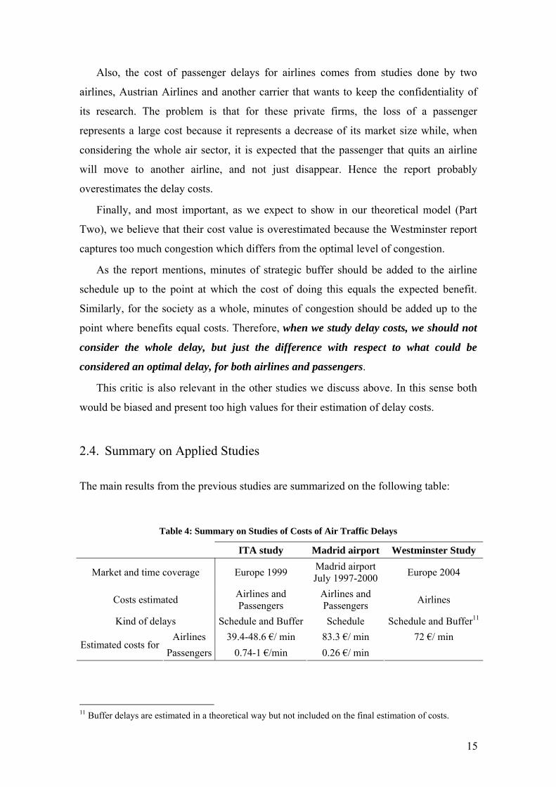
2.4. Summary on Applied Studies

The main results from the previous studies are summarized on the following table:

Table 4: Summary on Studies of Costs of Air Traffic Delays

ITA study Madrid airport Westminster Study

Market and time coverage Europe 1999 Madrid airport July 1997-2000 Europe 2004

Costs estimated Airlines and Passengers

Airlines and Passengers Airlines

Kind of delays Schedule and Buffer Schedule Schedule and Buffer11

Airlines 39.4-48.6 €/ min 83.3 €/ min 72 €/ min Estimated costs for

Passengers 0.74-1 €/min 0.26 €/ min

11 Buffer delays are estimated in a theoretical way but not included on the final estimation of costs.

16

As we can see, the estimated values for both airlines and passengers costs, are

relatively heterogeneous. The low value presented by the ITA study for airlines is

especially noticeable, even if it is the only study that is taking into account buffer

delays, which, in principle, should drive the estimates towards higher values. Probably

this low value comes from the controversial definition they use for the delays and from

a low estimation for the cost of a minute of delay.

Even if they do not apply it into their analysis, Nombela, De Rus and Betancor

(2002) suggests that the impact of the delay depend on the duration of delay of a

specific delay, on the nature of the airline and also on the interaction of delays for many

flights (specially if hubbing is important).

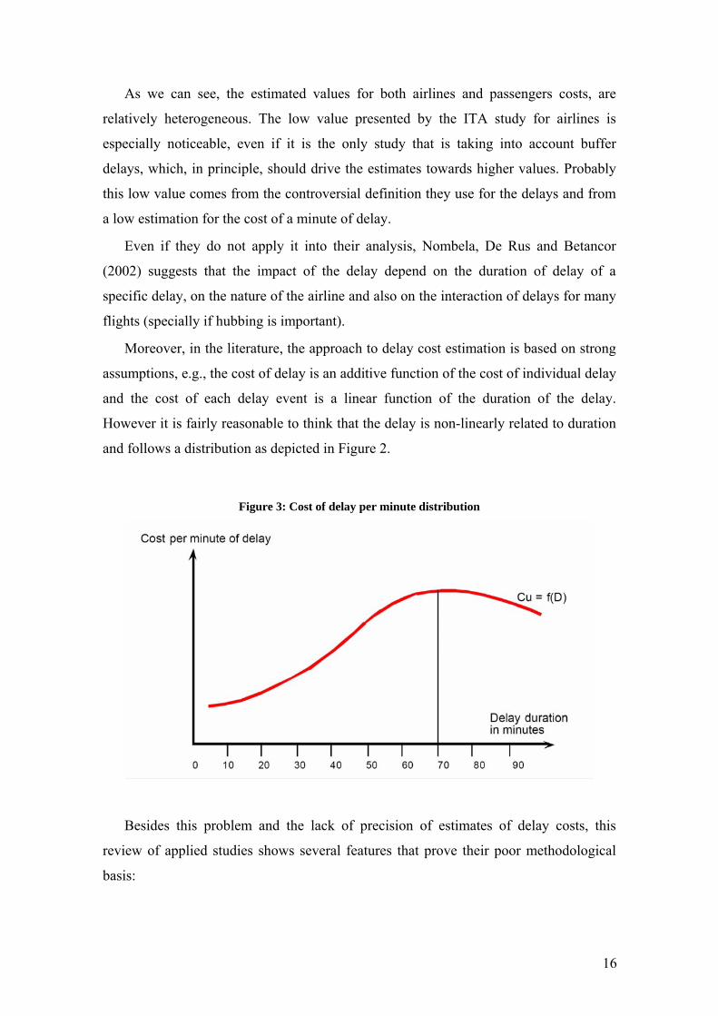
Moreover, in the literature, the approach to delay cost estimation is based on strong

assumptions, e.g., the cost of delay is an additive function of the cost of individual delay

and the cost of each delay event is a linear function of the duration of the delay.

However it is fairly reasonable to think that the delay is non-linearly related to duration

and follows a distribution as depicted in Figure 2.

Figure 3: Cost of delay per minute distribution

Besides this problem and the lack of precision of estimates of delay costs, this

review of applied studies shows several features that prove their poor methodological

basis:

17

• A rough definition of delays, despite the fact that the policy of airlines shows

that delays are not so simple to define. Indeed airlines include buffer times in the

scheduled travel time in order to cope with delays. Some hints of these policies

tend to the fact, which we will address more extensively in the forthcoming

report (Part Two), that the optimal management of the time-tables implies some

delays.

• A tough appraisal of values of time: A unique value of time is usually

applied, while many research studies in the field of air transport as well as in the

field of other modes show that there is a variety of values of time.

• No use of reliability per se: The fact that reliability, not just the travel time, is

valued is not taken into account.

• No consideration of the fact that the users have more or less information on

the probability of delays.

• A poor consideration of the situation of delays at connecting airports.

3. Theoretical Analysis on Congestion

The literature about delays and air traffic congestion can be classified into different

categories:

• First, we find conceptual models that aim to explain the passengers’ behavior,

and result essentially in the definition and estimation of the values of time.

• Second, models that are more connected with reality that attempt to model

congestion.

3.1. The conceptual models and the value of time

The oldest conception of costs related to travel time includes the trip time only,

distinguishing if necessary the durations of different elements of the complete transport

chain: Time spent on the way to the public transport systems or to the parking lots;

possible waiting time in the case of public transport; trip time, differentiated according

18

to the transport mode (each mode presents disadvantages and advantages like comfort);

then, again terminal time.12

A more complex and realistic element has been added when one introduces the

concepts of desired arrival time and mismatch with respect to this desired arrival time.

Usually this idea is formulated by considering the so-called disutility of transport (or the

cost related to the transport), U(th.). Following Small (1992), this function is written as

Lh DSDLSDETtU θγβα +++=)( .

It is a function of the departure time, th. It also involves:

• T which represents the trip time, and α, the value of this trip time;

• SDE or schedule delay-early, which is the gap of early arrival, and β the

cost that represents to the traveler arriving before the preferred arrival time, that

from now on we denote as PAT;

• SDL or schedule delay-late, is the gap of late arrival or delay, and γ the cost

that arriving late stand for the passenger;

• DL is a dummy equal to 1 in the case of late arrival, and θ the fix cost

associated.

The introduction of uncertainty is an additional level of complexity. Usually

uncertainty is introduced through the expected utility of a risk-averse agent, which is

equal to the expected total time T , increased by a component proportional to the

variance of the travel time σ , specifically:

σα rvTEU +=* .

This functional form is usually chosen to econometrically estimate the coefficients α

and vr based on a behavioral analysis of trips with random duration. Note that vr is

considered as the unit value of reliability.

If we restrict ourselves to the original model, the literature considers that the value

of the reliability vr is perfectly measured by the costs of early and late arrival, β and γ,

12 This introduction is based on Bates, Polack, Jones and Cook (2001) and by Noland and Polack (2002).

19

which can be estimated through studies of declared or revealed preferences even

without the presence of uncertainty on the travel time (see Arnott, de Palma and

Lindsey, 1993), and therefore without the need to observe the behavior of agents in case

of uncertainty. The model by Small has the advantage of introducing an asymmetry

between the early and late schedule delay, which was not considered in the traditional

model that includes only two parameters of the distribution function of trip times,

namely the mean and the standard deviation.

Nevertheless this assimilation can present some problems. In fact, within the models

that follow the idea of Small like the one of Arnott, de Palma and Lindsey, the agent

knows perfectly the traffic situation, the late or early arrival that he will face. Therefore

he can perfectly plan his agenda; for example, he can carry a book if he knows he will

be in advance or announce his delay to a meeting if he knows he will be late. In the case

of uncertainty, the agent cannot do it. From this point of view, if we assume to simplify

the same value of time for the value of delay, β, and the value of early arrival, γ, a

known delay of one hour is not equivalent to a situation where you have one hour of

delay with a 50 percent probability or an early arrival of one hour with the same

probability, in opposition to what is assumed by the model of Small. The difference

between the two comes from the information that the agent has on the first case (the

decisions are taken after receiving the information) and has not on the second case

(decision of the utilization of time under uncertainty). This could be interpreted as an

option value that would decrease the cost of mismatch in the schedule in the case of

uncertainty over the arrival time. This difference is not taken into account by the

literature; Specific surveys, probably based on declared preferences, allow us to

measure the importance of this phenomenon. It can be particularly important in public

transport, in which two types of schedule cost coexist: An expected schedule cost, based

on the discreteness of timetables of transport services; and a random schedule cost that

depends on unexpected early or late arrivals.

The case of public transport includes some other specific aspects that accentuate the

considerations that we have presented above. This is extended in the Appendix 2, and

show how the models, initially developed for the case of roads, where the departing

time is chosen within a continuum set, could be applied to the case of public transport-

in particular the case of air transport- where the departing times are discrete. In this

case, most of the authors introduce new elements to the model like the fulfillment of the

20

departure time and the difference of the departure time with respect to the announced

departure time; however there is almost no measure of the value associated to these

elements.

3.2. The values of time

From the previous analysis we can conclude that it is required to consider several values

for time:

• The value of trip time, which could be differentiated according to the degree of

comfort;

• The value for the waiting time;

• The value of the time for the cases of early or late arrival;

• The value of the reliability, that it is linked to the value of early or late arrival in

models that follow the idea of Small.

• Finally, in some models, the value of respecting schedules, for the case of public

transport.

Several studies have been devoted to the value of travel time, mainly for surface

transportation, i.e., road, rail, cars and bus. The studies on the value of travel time are

not so common for the case of air transport. With respect to the studies addressing the

value of the other components of trip duration, they are much less numerous and mainly

focused on other means of transport; there is almost nothing for air transport.

The estimation methods of these values start from simple principles, based on the

fact that all these values operate as parameters that explain the behavior of travelers

facing the choice between different transport means or between itineraries characterized

by different costs and by different trip durations.

We can estimate these parameters:

• Either by methods of revealed preferences, through traffic models that

attempt to explain the choice and therefore the value of time is one of the

parameters,

• Either by methods of declared preferences, by questionnaires where we

propose to the agent to choose among several hypothetical choices between different

21

transport modes, different routes characterized by longer or shorter time and

between larger or smaller prices.

3.2.1. The value of travel time Several studies provide values of travel time. A non exhaustive list comprises: Étude

MVA Consultancy (1987), Merlin (1991), Hague Consulting Group (1994), EURET

(1996), Hague Consulting Group (1996), SNRA (1996), Hensher (1997), Morellet

(1997), Small (1997), Wardman (1998), Boiteux (2000), Lam and Small (2001) and

finally Quinet and Vickerman (2004).

The general results from these studies bear on the determinants of the change in the

value of time:

• According to the trip motives. The value of travel time for business

purposes is around (and usually under) the labor cost; it is higher than the value

of travel time for commuting reasons, which itself is higher than the value of

leisure time;

• According to the transport modes (keeping in mind that the modal choice

results from income effect and the purpose of the trip): The value of time with

air transportation is higher than the mean value of first class passengers in train,

which is itself higher than the mean value of time for second class passengers in

train, that is higher than the value of time by car;

• The value of time increases with income, although at a slower rate

(elasticity from 0.5 to 1);

• The value of time for urban trips is smaller then the value of time for inter-

city travels;

• The value of time increase with the duration of the travel.

Several studies are devoted to urban transport, less numerous for inter-city travels,

and really few for the air transport.13 Wardman (1998), in his review about estimated

values of time for the United Kingdom, finds values for air transport that are almost

double than the value of travel time by cars in inter-city travels, and are around 40 euros

per hour.

13 In fact some studies have been done by airlines. They are not published due for confidentiality reasons.

22

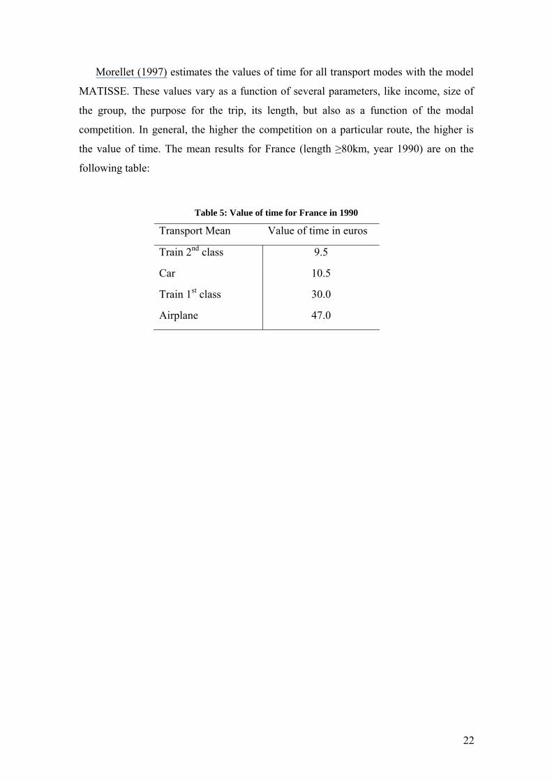
Morellet (1997) estimates the values of time for all transport modes with the model

MATISSE. These values vary as a function of several parameters, like income, size of

the group, the purpose for the trip, its length, but also as a function of the modal

competition. In general, the higher the competition on a particular route, the higher is

the value of time. The mean results for France (length ≥80km, year 1990) are on the

following table:

Table 5: Value of time for France in 1990

Transport Mean Value of time in euros

Train 2nd class 9.5

Car 10.5

Train 1st class 30.0

Airplane 47.0

23

Table 6: Time values in Inter-city travels (1998) per passenger

For distances smaller than Mean

50 km 150 km

For the distances d included between 50 km or 150 km and 400 km

Stabilization for the distances superiors to

400 km Road 8,4 € - 50 km < d VDT= (d/10+50).1/6,56 13,7 €

Train 2° Cl. - 10,7 € 150 km < dVDT=1/7(3d/10+445) .1/6,56 12,3 €

Train 1° Cl. - 27,4 € 150 km < dVDT=1/7(9d/10+1125) .1/6,56 32,3 €

Airplane - - 45,7 € 45,7 € Source: Rapport Boiteux (2000)

Table 7: Values of time

Relevant VOT studies HCG 1994

HCG 1998

HCG 1998

SNRA 1997

EUNET 1998

UNITE Values

Transport Segment Euro 1998 Euro 1998 Inflation to 1998 Normal Transfer to Euro travel Passenger transport – VOT per person-hour Car / motorcycle 6.70 9.31

Business 21.23 21.00 11.95 21.00 Commuting / private 5.53 6.37 3.91 6.00 Leisure / holiday 3.79 5.08 3.10 4.00

Coach (Inter-urban) Business 21.23 21.00 Commuting / private 5.95 5.40 6.00 Leisure / holiday 3.08 4.37 4.00

Urban bus / tramway Business 21.23 21.00 Commuting / private 5.95 4.94 6.00 Leisure / holiday 3.08 3.22 4.00

Inter-urban rail 4.97 8.50 Business 18.43 11.95 21.00 Commuting / private 6.48 6.21 6.40 Leisure / holiday 4.41 4.94 4.70

Air traffic 40.60 Business 16.20 28.50 Commuting / private 10.11 10.00 Leisure / holiday 10.11 10.00

Freight VOT Road Transport

LGV 39.68 30.75 40.76 40.00 HGV 39.68 30.75 43.47 43.00

Rail Transport Full trainload 645.37 725.45 725.00 Wagon load 26.16 28.98 30.00 Average per tone 0.76 0.76

Inland Navigation Full ship load 178.55 201.06 200.00 Average per tone 0.18 0.18

Maritime shipping Full ship load 178.55 201.06 200.00 Average per tone 0.18 0.18

Air transport Average per tone 4.00

Source: Quinet and Vickerman, 2004.

24

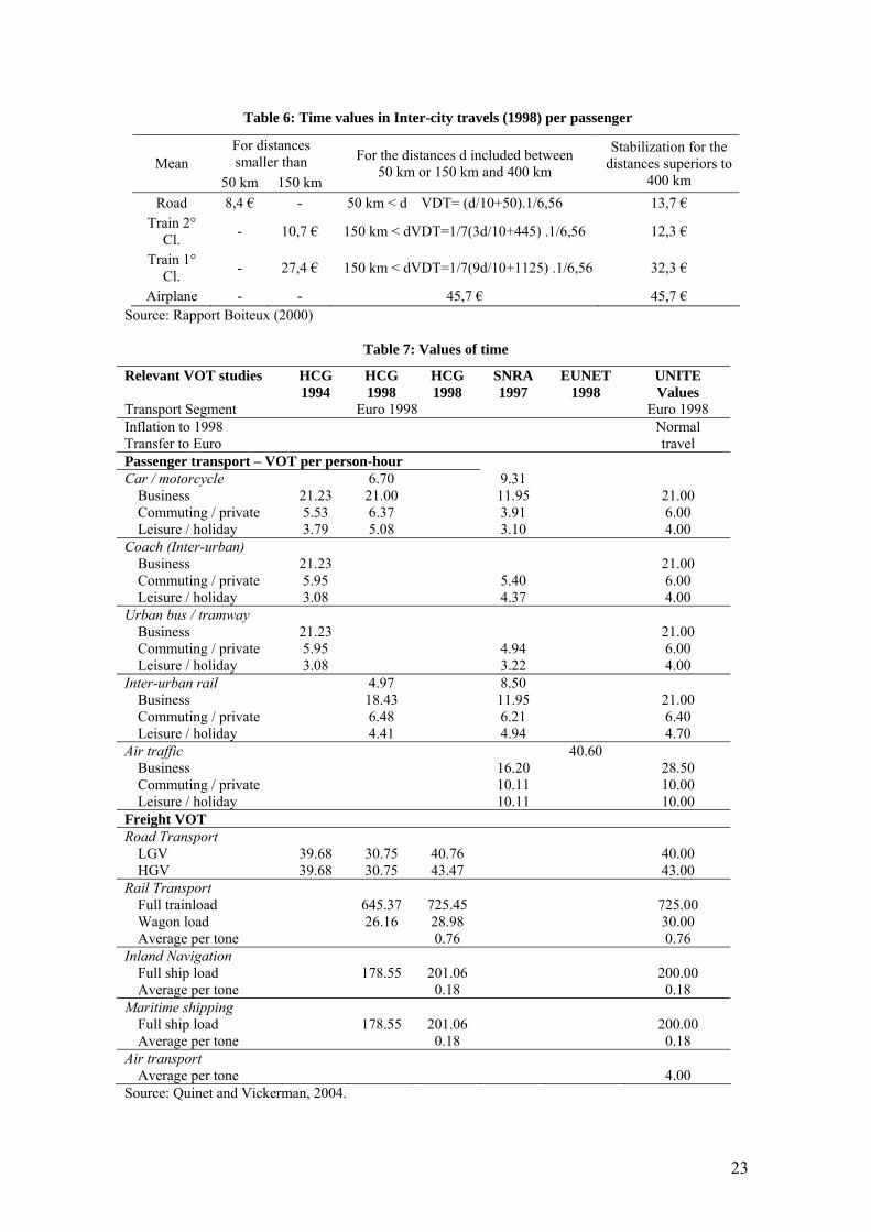
Boiteux (2000), in a report for the French Government about the values of time to

be used in investment economic appraisal, recommends the values of time for intercity

travels presented in Table 6. These values are based on a critical review of the

previously quoted studies.

Quinet and Vickerman (2004) collects the following values from the report UNITE

in Table 7.

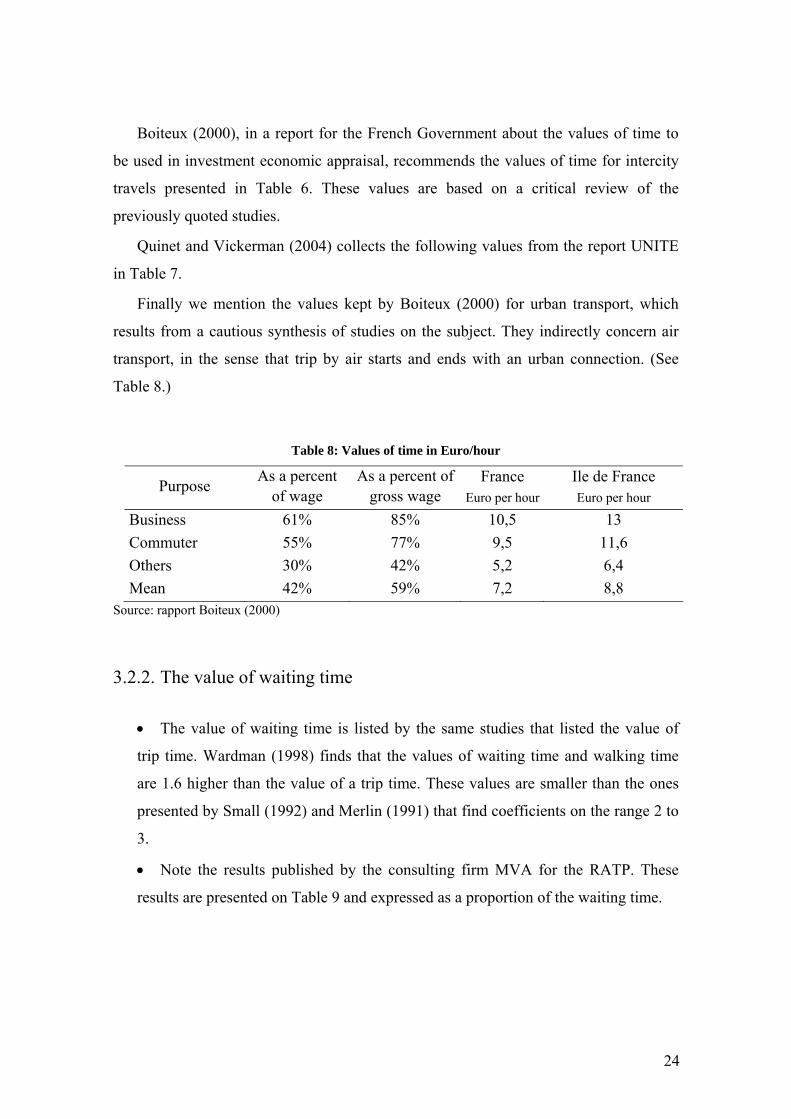
Finally we mention the values kept by Boiteux (2000) for urban transport, which

results from a cautious synthesis of studies on the subject. They indirectly concern air

transport, in the sense that trip by air starts and ends with an urban connection. (See

Table 8.)

Table 8: Values of time in Euro/hour

Purpose As a percent of wage

As a percent of gross wage

France Euro per hour

Ile de France Euro per hour

Business 61% 85% 10,5 13 Commuter 55% 77% 9,5 11,6 Others 30% 42% 5,2 6,4 Mean 42% 59% 7,2 8,8

Source: rapport Boiteux (2000)

3.2.2. The value of waiting time

• The value of waiting time is listed by the same studies that listed the value of

trip time. Wardman (1998) finds that the values of waiting time and walking time

are 1.6 higher than the value of a trip time. These values are smaller than the ones

presented by Small (1992) and Merlin (1991) that find coefficients on the range 2 to

3.

• Note the results published by the consulting firm MVA for the RATP. These

results are presented on Table 9 and expressed as a proportion of the waiting time.

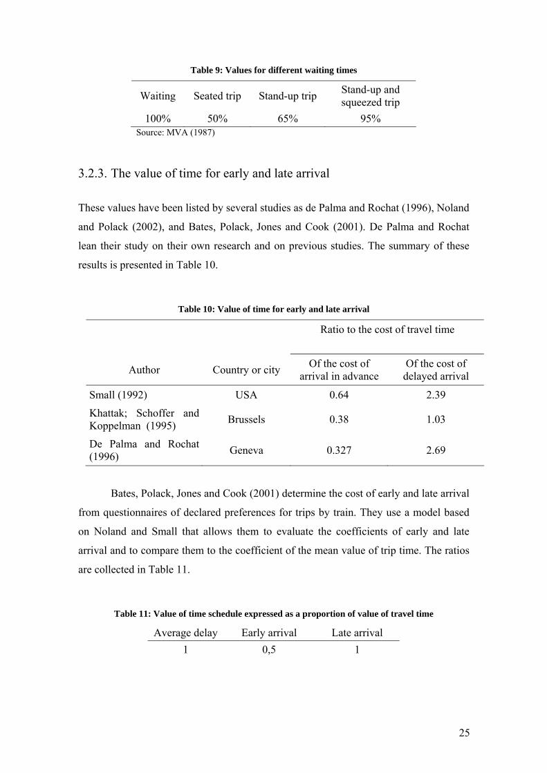
25

Table 9: Values for different waiting times

Waiting Seated trip Stand-up trip Stand-up and squeezed trip

100% 50% 65% 95% Source: MVA (1987)

3.2.3. The value of time for early and late arrival

These values have been listed by several studies as de Palma and Rochat (1996), Noland

and Polack (2002), and Bates, Polack, Jones and Cook (2001). De Palma and Rochat

lean their study on their own research and on previous studies. The summary of these

results is presented in Table 10.

Table 10: Value of time for early and late arrival

Ratio to the cost of travel time

Author Country or city Of the cost of arrival in advance

Of the cost of delayed arrival

Small (1992) USA 0.64 2.39

Khattak; Schoffer and Koppelman (1995) Brussels 0.38 1.03

De Palma and Rochat (1996) Geneva 0.327 2.69

Bates, Polack, Jones and Cook (2001) determine the cost of early and late arrival

from questionnaires of declared preferences for trips by train. They use a model based

on Noland and Small that allows them to evaluate the coefficients of early and late

arrival and to compare them to the coefficient of the mean value of trip time. The ratios

are collected in Table 11.

Table 11: Value of time schedule expressed as a proportion of value of travel time

Average delay Early arrival Late arrival 1 0,5 1

26

3.2.4. Value of reliability

Within the framework of the Small’s model, the valuation of reliability comes directly

from the estimation of the value of time of early and late arrival. We have already

discussed some elements of the value of reliability

However more direct estimations have been made. They attempts to resolve a

previous problem: How do you measure reliability physically? The literature on the

topic presents two measures: The standard deviation of the trip time and the interval

between the quantile 50% and the quantile 90% of the travel time distribution. The use

of this last measure is justified by the dissymmetry of consequences of the delays and

by the dissymmetry of the distribution of travel times that spreads out for the delays.

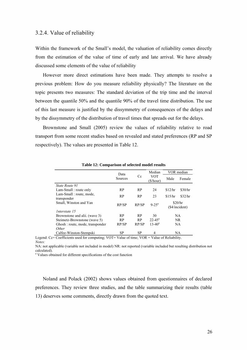
Brownstone and Small (2005) review the values of reliability relative to road

transport from some recent studies based on revealed and stated preferences (RP and SP

respectively). The values are presented in Table 12.

Table 12: Comparison of selected model results

VOR median

Data Sources Cc

Median VOT

($/hour) Male Female

State Route 91 Lam-Small : route only RP RP 24 $12/hr $30/hr Lam-Small : route, mode, transponder RP RP 23 $15/hr $32/hr

Small, Winston and Yan RP/SP RP/SP 9-25a $20/hr ($4/incident)

1nterstate 15 Brownstone and alii. (wave 3) RP RP 30 NA Steimetz-Brownstone (wave 5) RP RP 22-45a NR Ghosh : route, mode, transponder RP/SP RP/SP 13-40a NA Other Calfee-Winston-Stempski SP SP 4 NA

Legend: Cc= Coefficients used for computing; VOT= Value of time; VOR = Value of Reliability. Notes: NA: not applicable (variable not included in model) NR: not reported (variable included but resulting distribution not calculated). a Values obtained for different specifications of the cost function

Noland and Polack (2002) shows values obtained from questionnaires of declared

preferences. They review three studies, and the table summarizing their results (table

13) deserves some comments, directly drawn from the quoted text.

27

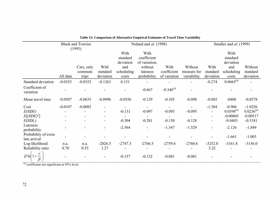
Table 13: Comparison of Alternative Empirical Estimates of Travel Time Variability

Black and Towriss (1993)

Noland and al. (1998) Smaller and al. (1999)

All data

Cars, only commute

trips

With standard deviation

With standard deviation

and scheduling

costs

With coefficient

of variation, without lateness

probability

With coefficient of variation

Without measure for variability

With standard deviation

With standard deviation

and scheduling

costs

Without standard deviation

Standard deviation -0.0353 -0.0352 -0.1263 0.151 - - - -0.274 0.0665(a) - Coefficient of variation - - - - -0.667 -0.346(a) - - - -

Mean travel time -0.0507 -0.0635 -0.0996 -0.0556 -0.129 -0.105 -0.098 -0.085 -0480 -0.0578

Cost -0.0107 -0.0082 - - - - - -1.304 -0.906 -1.0256 E(SDE) - - - -0.131 -0.097 -0.093 -0.095 - 0.0398(a) 0.0236(a) E[(SDE)2] - - - - - - - - -0.00605 -0.00517 E(SDL) - - - -0.304 -0.281 -0.130 -0.128 - -0.0403 -0.3181 Lateness probability - - - -2.564 - -1.347 -1.529 - -2.126 -1.849

Probability of extra late arrival - - - - - - - - -1.661 -1.003

Log-likelihood n.a. n.a. -2826.5 -2747.3 -2766.5 -2759.6 -2760.6 -3252.0 -3161.8 -3156.0 Reliability ratio 0.70 0.55 1.27 - - - - 3.22 - -

⎟⎟⎠

⎞⎜⎜⎝

⎛+βγβ 1ln - - - -0.157 -0.132 -0.081 -0.081 - - -

(a) coefficient not significant at 95% level.

28

Black and Towris (1993) reckon a reliability coefficient, defined as the ratio

between the coefficient of the standard deviation and the coefficient of the mean travel

time.

Noland et al. (1998) and Small et al. (1999) made statistical estimations according

both to the “standard deviation/mean” model (in that case Noland uses not the standard

deviation, but the coefficient of variation which is the ratio between dispersion and

mean) and to the Small (1992) model. In some models they include a probability of late

arrival and also a probability of extra-late arrival, taking into account the flexibility of

arrival at work. Small and alii introduce a quadratic term for the late arrival, taking into

account the non-linearity of reactions of the users to the late arrival delay.

The MVA study already quoted and relative to the RATP gives as well estimations

of the reliability for the case of urban public transport; the ratio between the value of the

standard deviation and the value of travel time is 0.2, much smaller than the previous

results; on the other hand the reliability of waiting times is higher: the correspondent

ratio becomes equal to 0.5.

Bates et al. study the reliability of train services based on the results of the review of

revealed preferences for the determination of the value of early and late arrival times.

They use these values to model the departure time choice of a user as a function of the

distribution of the travel time. The choice of the service depends not only on the mean

delay but also on its dispersion, and the disutility linked to the non-reliability is weak

when the dispersion of delays is small, and increases rapidly with this dispersion.

This example shows that the effect of delays depends on the knowledge that the

users have. Bates et al. shows how an erroneous perception of the distribution of

probabilities of delays could involve a loss for the user due to the wrong decision with

respect to his departing time.

As we can see from this short review of the estimations for reliability, there are

really few statistical results of the value of reliability in collective transport; this fact is

similar to what happens for the value of travel time. In particular, we have not found

any evaluation of the value of reliability in the area of air transport. As previously

noted, it’s probable that the air carriers have their own studies, but they are not

published due to their confidentiality.

29

Besides, the studies present widespread results. Nevertheless the results are

sufficiently significant to consider that reliability is an important element in the cost of

transport, too often neglected.

However little attention is paid to the fact that the cost of reliability -essentially the

delays with respect to the desired schedule- is or is not known in advance by the user.

However the users seem to be sensible to the information level as shows the study done

by inquiry to the users by Eurocontrol, and explained in the Appendix 3.

3.3. Theoretical Models of Congestion

Most of theoretical models on congestion that we present here focus on modeling the

queues that the congestion can create, rather than on the reasons that create congestion.

In general, congestion is assumed to be generated by some random process and the

authors focus their attention on how, once congestion appears, it changes over time. It

seems quite logical that, as congestion is present on a daily basis at most airports in the

world, airlines can anticipate congestion and adapt their behavior accordingly.

As we have previously explained, this is captured by the buffer delays that airlines

introduce into their schedule to control a part of the randomness of day-to-day

operations.

The important question that we consider is why airlines do not account for a larger

percentage of delays. In other words, what is the optimal level of average delays for

airlines? Is there an optimal social average delay different from zero? We believe that

the answer to these questions is positive. In the literature, only one paper addresses in

part this issue.

We now summarize the models of congested transportation systems, which,

according to Daniel (1995), can fall into three categories.

Econometric models

Econometric models estimate time-varying demand and delay functions and calculate

equilibrium congestion fees. They use nonstructural specifications of delay functions

and ignore intertemporal traffic adjustment in response to congestion fees. In this

category we find for example Carlin and Park (1970), Park (1971) and Morrison and

Winston (1989). Carlin and Park attempt to estimate the effects of using marginal cost

30

pricing at the Airport of LaGuardia with a simple model. They do not try to estimate

total time and costs of delays, but to estimate the marginal delay cost that an additional

operation can create; for this, they just assume different values of one minute of delay

for passengers and airlines.

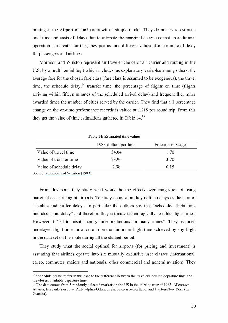
Morrison and Winston represent air traveler choice of air carrier and routing in the

U.S. by a multinomial logit which includes, as explanatory variables among others, the

average fare for the chosen fare class (fare class is assumed to be exogenous), the travel

time, the schedule delay,14 transfer time, the percentage of flights on time (flights

arriving within fifteen minutes of the scheduled arrival delay) and frequent flier miles

awarded times the number of cities served by the carrier. They find that a 1 percentage

change on the on-time performance records is valued at 1.21$ per round trip. From this

they get the value of time estimations gathered in Table 14.15

Table 14: Estimated time values

1983 dollars per hour Fraction of wage Value of travel time 34.04 1.70 Value of transfer time 73.96 3.70 Value of schedule delay 2.98 0.15

Source: Morrison and Winston (1989)

From this point they study what would be the effects over congestion of using

marginal cost pricing at airports. To study congestion they define delays as the sum of

schedule and buffer delays, in particular the authors say that “scheduled flight time

includes some delay” and therefore they estimate technologically feasible flight times.

However it “led to unsatisfactory time predictions for many routes”. They assumed

undelayed flight time for a route to be the minimum flight time achieved by any flight

in the data set on the route during all the studied period.

They study what the social optimal for airports (for pricing and investment) is

assuming that airlines operate into six mutually exclusive user classes (international,

cargo, commuter, majors and nationals, other commercial and general aviation). They

14 "Schedule delay" refers in this case to the difference between the traveler's desired departure time and the closest available departure time. 15 The data comes from 5 randomly selected markets in the US in the third quarter of 1983: Allentown-Atlanta, Burbank-San Jose, Philadelphia-Orlando, San Francisco-Portland, and Dayton-New York (La Guardia).

31

get the expected result that optimal and arrival departures tolls should equal the extra

cost that operation imposes on other users and on the airport authority. They also

estimate the optimal capacity that is reached when the savings in delay costs from

adding runway capacity equal the extra cost of that capacity.

According to their model, the increase in tolls that should be applied to improve the

situation would make some users to be “tolled off” the airports. However the

improvement in the financial health of these airports, plus the decrease on delays would

more than offset these losses.

Also the study is conservative in this aspect since it is not considering possible

substitutions. For example it assumes that the demand for using the airport in a given

hour is a function of the price for that hour only. So the model does not capture “peak

spreading”.

Also they study the effects of the deregulation of 1978 over air safety and the effects

of mergers; in particular they study the case of the six mergers that took place on 1986-

87.

By means of a simple model, Park (1971) studies the theoretical effects of imposing

a congestion toll to the airlines or to the passengers in a context of flexible or fixed

ticket price (perfect competition or competition just in schedules). This model is

difficult to be applied in practice since for example delays are expressed just as an

unknown increasing function on the number of flights and the total value of

transportation is also an unknown function which increases with the number of

passengers and decreases with delays. The model uses quite simplifying assumptions. It

assumes for example that there exists only one destination and that traffic is

homogeneous. It focuses its attention on the passenger loads which according to the

model should be increased to achieve efficiency.

Bottleneck models

Bottleneck models generate equilibrium fees with intertemporal traffic adjustment, but

generally employ simple deterministic queuing processes (see e.g., Vickrey (1969),

Arnott, de Palma, and Lindsey (1990b, 1993) and Lindsey and Verhoef (2000)). They

are focused on road transportation, which presents important differences with respect to

air transport. For example, airport’s infrastructure is used by a relatively small number

of agents whose decision of entry is not random but scheduled. They end up proposing

32

similar solutions as for roads: (1) enlarge capacity; (2) manage demand by peak-load

pricing.

Queuing-theoretic models

Queuing-theoretic models capture the effects of stochastic arrivals on the evolution of

queues, but assume exogenous arrival rates and do not calculate equilibrium congestion

fees (see, e.g. Koopman (1972) and Menhdiratta and Kiefer (2000) and Janic and

Stough (2003)). Most of this kind of models assumes a constant arrival rate. Such

systems have steady-state solutions and do not adequately model airport queues

resulting from rapid fluctuations of traffic rates

The model by Daniel (1995) is in between: it develops a stochastic queuing model

implanted into a bottleneck model. His model is especially applicable to hubs, which

experience rapid fluctuations and severe peaking of traffic rates and queue lengths.

Hub-and-spoke networks enable airlines to reduce their aircraft-operating cost and

passenger schedule-delay (defined as the time between the most preferred travel time of

a passenger and the closest available flight) by achieving higher load factors on larger

aircraft with greater service frequency. To minimize costs, hub and spoke networks

schedule arrivals and departures at hubs in “banks” of flights.

The model study arrival and departure queues and layover costs (time aircraft spend

at hubs after exiting arrival queues and before entering departure queues) and

interchange-encroachment costs (costs from the risk of passengers missing connections

flights due to inadequate layover times). The model accounts for the effects of

overlapping traffic and residual delays from one arrival or departure bank to the next.

With respect to his definition of delay, Daniel takes into account the buffers.

According to his model the social planner can implement the optimal arrival schedule

by imposing a congestion fee equal to the increase in costs imposed by the nth aircraft

on all other aircraft. Because the airport authority cannot observe directly schedule

times, aircraft operators would have incentives to misrepresent their schedule times if

these were the basis of the toll assessments so the fee should be contingent on the actual

arrival time.

He estimates the equilibrium of the model for five cases: no congestion fee and

competition in the market, no-fee with a Nash dominant firm, no-fee with a Stackelberg

33

dominant firm, no-fee with joint-cost-minimizing airlines and the case of congestion fee

and perfect competition.

Using Data from the Minneapolis-St. Paul Airport during a week of May of 1990,

and according to his model, the atomistic model fits better the actual traffic patterns.

Therefore it studies the theoretical effects that congestion pricing would have over this

equilibrium.

The part of his model most open to criticism is that he assumes that there are two

independent queuing systems at the airport, one for landings and one for takeoffs. Also,

arrival and departure distribution is Poisson with time dependent rates and service times

are deterministic and occur at equally spaced intervals. The study does not compute

congestion costs.

Any of the studies we have discussed so far has studied why congestion appears and

if congestion should disappear totally or if there is congestion on the social optimum.

The model developed by Mayer and Sinai (2003) explains that delays appear largely

due to network benefits from hubbing and to congestion externalities.

As the authors mention in general, it is believed that congestion is an externality,

and agents do not take into account the externality that they create for others. This can

explain why airports without a single dominant carrier should have high delays.

However it is not valid to explain the persistence of congestion at airports with a

dominant large carrier.

Brueckner (2002) follows this argument and shows that, when a monopolist

dominates an airport, congestion is fully internalized. Under a Cournot oligopoly,

however, carriers are shown to internalize only the congestion they impose on

themselves. In this case a toll should be equal to the congestion cost from an extra flight

times one minus the carrier's flight share.

There are two problems with this idea: First, even if overall the data presented by

the author about congestion in US airports presents evidence against his theory, it is true

that some of the airports with high levels of delays present a high degree of

concentration on the airline market. Second, it is difficulty to link congestion fees and

market power, given the actual difficulty for new airlines to enter into most of the big

European airports.

Mayer and Sinai (2003) suggest that air traffic congestion exists at some level due to

the network benefits associated with the hub and spoke system. The authors construct a

34

measure of delay that is unaffected by airline scheduling, actual travel time minus

minimum feasible travel time. According to their model, longer delays at hub airports

are the efficient equilibrium outcome of a hub airline equating high marginal benefits

from hubbing (one new round-trip flight from a hub connected to n cities will create 2n

additional connecting routes) with the marginal costs of delay.16

The authors test their model with data from the US Department of Transportation

with covers all airlines with at least one percent of all domestic traffic and 27 top U.S.

airports from 1988 to 2000.

In this direction, according to the Logistics Management Institute, between April

1993 and April 1997scheduled block time for flights among the 29 hub airports in the

U.S. increased by 1.25 minutes over this four year period. This increases to 1.61 if the

spacious new airport of Denver is excluded. Looking to individual airports the average

increase ups to 3.28 minutes at Atlanta and to 4.71 minutes at Dallas-Ft. Worth (DFW).

These number seems to be small but, just looking at DFW, that had around 450.000

scheduled departures in 1997 and assuming a cost of 40$/block minute implies a cost

increase of about $85 million over the four years in direct costs for airlines alone.17

Also, following the idea of social gains coming from congestion, we could cite the

paper of Betancor and Nombela (2002) explaining how an increase in the frequency of a

service can increase the welfare of all travelers. So not only new destinations, but also

increases in the frequency of old ones can present benefits for the society even if

congestion is already present.

4. Towards an Objective Definition of Delays As we have seen, the proper definition of delays is a complex problem. Most of the

literature considers only the observed delays to study the cost of these delays. However

several authors have observed that companies include buffer times in the scheduled

travel time in order to cope with delays. This comes from the fact that delays produce

also profits and not only costs and it can produce profits for both airlines and

passengers. In hubs, the creation of a new route represents a big increase on the

16 A more detailed description of the model can be found on Appendix 4. 17 Source, Air Traffic Services Performance Focus Group: Airline metric concepts for evaluating air traffic service performance.

35

possibilities of combinations for all the users of the route and for other airports the

passengers can benefit from an increase on the frequency of flights on a given route

which would represent a diminution of the difference between their departing times and

their desired departing time. These benefits must be confronted with the cost that the

introduction of this new flight can represent over congestion.

These facts lead us to believe that to compute the cost of delays, we should

measured not the observed delays but the difference between these and what we define

as optimal delays, that are the delays that we will try to identify in Part Two of the

report, and that result from equaling the cost and benefit of congestion.

Even if this is the most important problem of the literature, is not the only one.

Specially, the effect of uncertainty over the cost that transport can represent for

passengers has been obviated and the fact that passengers can adapt their behavior to the

extent they know the existence of these delays has been understated.

The next part of the report will have as objective to model these phenomena to

deduct a coherent economic definition of the delays for the user, and a formula that

allows to calculate them. The model will therefore modelize the optimal decision for

airlines and society in order to compare it to the actual situation.

36

References

AEA (2005), Yearbook 2004, www.aea.be Air Traffic Services Performance Focus Group (Feb. 1999); “Airline Metric Concepts

for Evaluating Air Traffic Service Performance”. Arnott, R., De Palma, A. and L. Robin (1993); “A structural model of Peak-Period

Congestion: A Traffic Bottleneck with Elastic Demand,” American Economic Review, vol. 83, No. 1, pp. 161-179.

Bates, J., Polack, J., Jones, P. and A. Cook, (2001): “The valuation of reliability for personal travel”, Transportation Research Part E, vol. 37, pp. 191-229.

Beatty, R., Hsu, R., Berry, L.and J. Rome (1998): “Preliminary Evaluation of Flight Delay Propagation through an Airline Schedule” 2nd USA/Europe Air Traffic Management R&D Seminar, Orlando, 1st - 4th December 1998.

Betancor, O. and G. Nombela (2002): “Mohring Effects for Air Transport”, Competitive And Sustainable Growth Programme, UNITE.

Boiteux M. (2000) “Choix des investissements and prise en compte des nuisances”, Paris, la documentation française.

Brownstone R. and K. Small (2005) “Expériences de tarification routière en Californie, enseignements pour l'évaluation du temps and de la fiabilité” in “La tarification des transports, problèmes and enjeux”, de Palma A. and E. Quinet.

Brownstone, D., Gosh, A., Golob, T. F., Kazimi, C. and D. Van Amelsfort (2003) “Drivers’ willingness-to-pay to reduce travel time: evidence from the San Diego I-15 Congestion Pricing Project” Transportation Research A vol. 37, pp. 373-387.

Brueckner, J. K. (2002); “Internalization of airport congestion,” Journal of Air Transport Management, vol. 8, pp. 141-147.

Calfee, J., Winston, C. and R. Stempski (2001) “Econometric issues in estimating consumer preferences from stated preference data: a case study of the value of automobile travel time” Review of Economics and Statistics vol. 83, pp. 699-707.

Carlin, A., and Park, R. (1970); “Marginal Cost Pricing of Airport Runway Capacity”, The American Economic Review, vol. 60, pp. 310-319.

Daniel, J. I. (1995), “Congestion Pricing and Capacity of Large Hub Airports: A Bottleneck Model with Stochastic Queues”, Econometrica, vol. 63, No. 2, 327-370.

EURET (1996), Transport Research Concerted Action 1.1, Commission Européenne, DG Transport.

Eurocontrol Experimental Centre (2002): “Analysis of passengers delays: An exploratory case study” EEC Note No.10/02.

Eurocontrol, Ecoda (2005); "Delays to Air Transport in Europe Annual Report 2004" Brussels.

European Commission (2001), “White paper: European Transport policy for 2010: time to decide”, COM 370, Brussels.

European Commission, (2005) “Strengthening passenger rights within the European Union”, COM 46, Brussels.

Hague Consulting Group (1994); “UK Value of Time Study”. Hague Consulting Group (1996 ); “The 1985-1996 Dutch VOT Studies” PTRC

Seminar on the Value of Time, Wokingham, UK.

37

Henscher D. (1997); “Behavioral Value of Travel Time Savings in Personal and Commercial Automobile Travel”, in Greene, Jones and Delucchi “The full Costs and Benefits of Transportation”.

Institut du Transport Aerien (2000), “Costs of Air Transport delay in Europe”. Janic, M. and R. Stough (2003); “Congestion charging at airports: dealing with an

inherent complexity”, ERSA-STELLA. Khattak A., Schofer J., and F. Koppelman (1995), “Effect of traffic reports on

commuters' route and departure time changes.” Journal of Advanced Transportation, Vol. 29, No. 2, pp. 193-212.

Koopman, B. O. (1972); “Air-Terminal Queues under Time-Dependent Conditions”, Operations Research, vol. 20, No. 6, pp. 1089-1114.

Lam T.C. and Small K. A. (2001); “The value of Time and Reliability: measurement from a Value Pricing Experiment” Transportation Research E, vol. 37, pp. 231-251.

Lindsey, R. and Verhoef, E. (2000); “Congestion Modeling”, Handbook of Transport Modeling, Elsevier Science Ltd.

Mayer, C. and T. Sinai (2003); “Network Effects, Congestion externalities, and air traffic delays: or why all delays are not evil” The American Economic Review, 93(4).

Mehndiratta, S. R. and M. Kiefer (2003); “Impact of slot controls with a market-based allocation mechanism at San Francisco International Airport”, Transportation Research Part A, vol. 37, pp. 555-578.

Merlin P. (1991); “Géographie, Economie and Planification des Transports”, Paris, PUF.

Morellet O. (1997); “Modèle MATISSE. Test de la version du 14/05/1997” Inrets. Morrison, S., Winston, C., Bailey, E., and A. Khan (1989); “Enhancing the

Performance of the Deregulated Air Transportation System”, Brooking Papers on Economic Activity, Microeconomics, vol. 1989, pp. 61-123.

MVA Consultancy (1987); “Value of Travel Time Savings”. Nombela, G., de Rus, G. and O. Betancor (2002); “Evaluation of Congestion Costs for

Madrid Airport”, UNITE. Noland R. and J. Polack (2002); “Travel Time Variability: a review of theoretical and

Empirical Studies” Transport Reviews, vol. 22, n°1, pp. 39-54. Observatoire des retards du transport Aerien (2004), “Bilan intermediare 1er semestre

2004”, Conseil National des Clients aériens. de Palma A. and D. Rochat (1996); “Urban congestion and commuters behaviour: the

departure time context” Revue d'Economie Régionale and Urbaine, vol. 3, pp. 467-488.

Park, E. (1971); “Congestion Tolls for Commercial Airports”, Econometrica, Vol. 39, No. 5, pp. 683-694.

Quinet, E., Schwartz , D. and J. P. Taroux, (2003): “Pilot Accounts - Results for France”, Competitive And Sustainable Growth Programme, UNITE.

Quinet E. and R. Vickerman (2004); “Principles of Transport Economics” Edward Elgar.

Small K. (1992); “Urban Transportation Economic”, Vol. 51 of Fundamental of Pure and Applied Economic series, Harwood Academic Publishers.

38

Small K., Winston, C. and J. Yan (2002) “Uncovering the distribution of motorists’ preferences for travel time and reliability: implications for road pricing, working paper #546, University of California Transportation Center.

Suzuki, Y. (2000); “The relationship between on-time performance and airline market share: a new approach”, Transportation Research Part E, vol. 36, pp. 139-154.

Suzuki, Y., Tyworth, J. E. and R. A. Novack (2001); “Airline market share and customer service quality: a reference dependent model”, Transportation Research Part A, vol. 35, pp. 773-778.

Swedish National Road and Transport Research Institute (SNRA) (1996); “Swedish National Value of Time Study”.

University of Westminster (2004), “Evaluating the true cost of one minute of airborne or ground delay”, Performance Review Commission, Eurocontrol.

Vickrey, W. (1969); “Congestion Theory and Transport Investment”, The American Economic Review, Vol. 59, No.2, Papers and Proceedings of the Eighty-first Annual Meeting of the American Economic Association, 251-260.

Wardman M. (1998 ); “The Value of Travel Time : a Review of British Evidence” Journal of Transport Economics and Policy, 32-3, pp. 285-316

39

List of Acronyms

Abbreviations Full term AEA Association of European Airlines ATA US Air Transport Association ATFM Air Traffic Flow Management DGAC Direction General de l’Aviation Civile eCODA Enhanced Central Office for Delays Analysis EUNET EUropean NETwork EURET European Research Programme for Transport IDEI Institut D’Economie Industrielle ITA Institut du Transport Aerien IATA International Air Traffic Association PAT Preferred Arrival Time RATP Régie Autonome des Transports Parisiens RP Revealed Preferences SDE Schedule Delay-Early SDL Schedule Delay-Late SNRA Swedish National Road Administration SP Stated Preferences UNITE Unification of accounts and marginal costs for Transport Efficiency VOR Value of Reliability VOT Value of Time

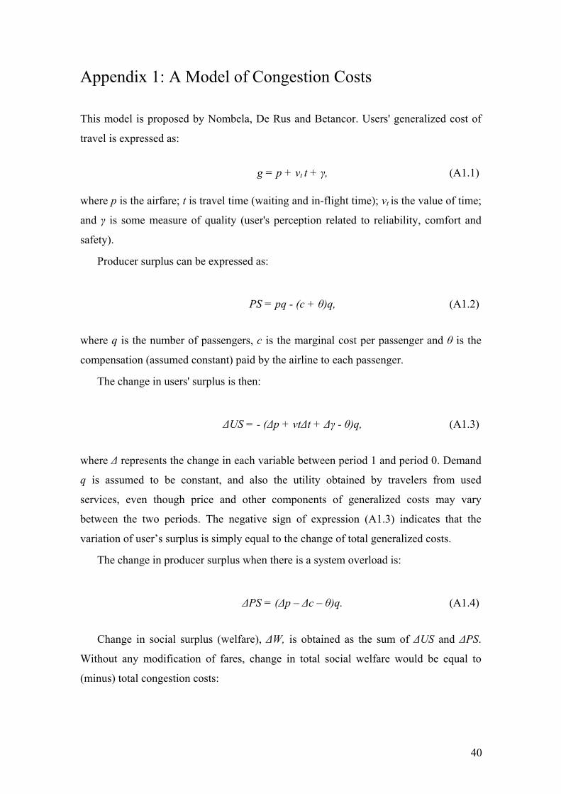
40

Appendix 1: A Model of Congestion Costs This model is proposed by Nombela, De Rus and Betancor. Users' generalized cost of

travel is expressed as:

g = p + vt t + γ, (A1.1) where p is the airfare; t is travel time (waiting and in-flight time); vt is the value of time;

and γ is some measure of quality (user's perception related to reliability, comfort and

safety).

Producer surplus can be expressed as:

PS = pq - (c + θ)q, (A1.2)

where q is the number of passengers, c is the marginal cost per passenger and θ is the

compensation (assumed constant) paid by the airline to each passenger.

The change in users' surplus is then:

ΔUS = - (Δp + vtΔt + Δγ - θ)q, (A1.3)

where Δ represents the change in each variable between period 1 and period 0. Demand

q is assumed to be constant, and also the utility obtained by travelers from used

services, even though price and other components of generalized costs may vary

between the two periods. The negative sign of expression (A1.3) indicates that the

variation of user’s surplus is simply equal to the change of total generalized costs.

The change in producer surplus when there is a system overload is:

ΔPS = (Δp – Δc – θ)q. (A1.4)

Change in social surplus (welfare), ΔW, is obtained as the sum of ΔUS and ΔPS.

Without any modification of fares, change in total social welfare would be equal to

(minus) total congestion costs:

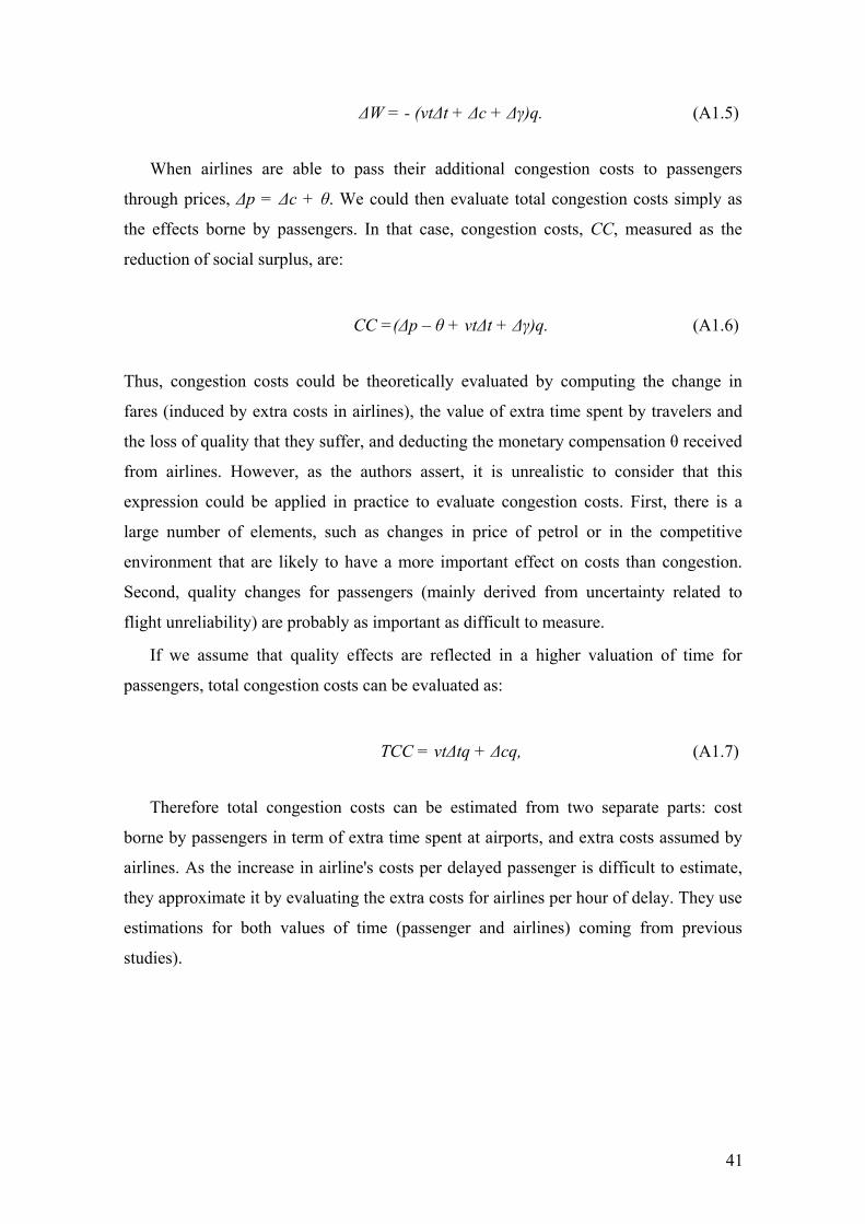
41

ΔW = - (vtΔt + Δc + Δγ)q. (A1.5)

When airlines are able to pass their additional congestion costs to passengers

through prices, Δp = Δc + θ. We could then evaluate total congestion costs simply as

the effects borne by passengers. In that case, congestion costs, CC, measured as the

reduction of social surplus, are:

CC =(Δp – θ + vtΔt + Δγ)q. (A1.6)

Thus, congestion costs could be theoretically evaluated by computing the change in

fares (induced by extra costs in airlines), the value of extra time spent by travelers and

the loss of quality that they suffer, and deducting the monetary compensation θ received

from airlines. However, as the authors assert, it is unrealistic to consider that this

expression could be applied in practice to evaluate congestion costs. First, there is a

large number of elements, such as changes in price of petrol or in the competitive

environment that are likely to have a more important effect on costs than congestion.

Second, quality changes for passengers (mainly derived from uncertainty related to

flight unreliability) are probably as important as difficult to measure.

If we assume that quality effects are reflected in a higher valuation of time for

passengers, total congestion costs can be evaluated as:

TCC = vtΔtq + Δcq, (A1.7)

Therefore total congestion costs can be estimated from two separate parts: cost

borne by passengers in term of extra time spent at airports, and extra costs assumed by

airlines. As the increase in airline's costs per delayed passenger is difficult to estimate,

they approximate it by evaluating the extra costs for airlines per hour of delay. They use

estimations for both values of time (passenger and airlines) coming from previous

studies).

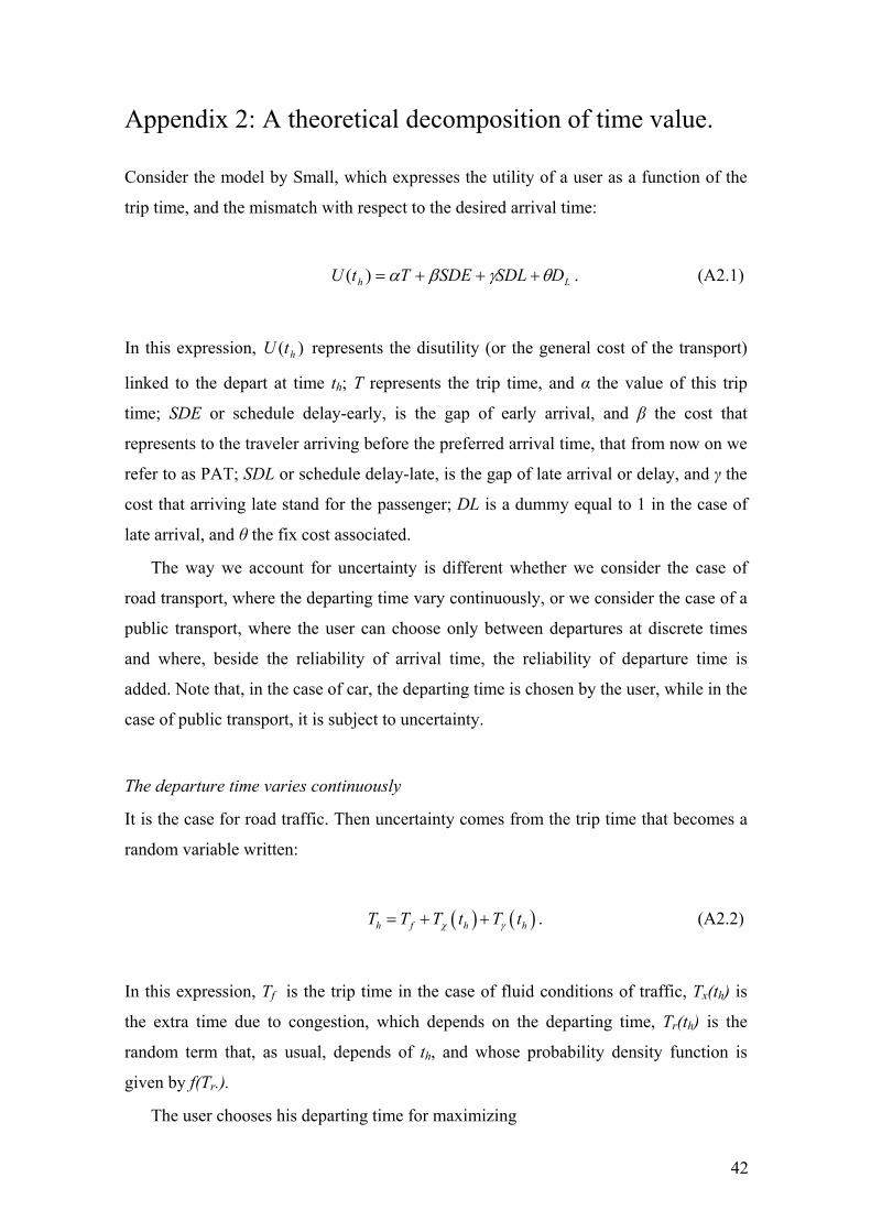
42

Appendix 2: A theoretical decomposition of time value.

Consider the model by Small, which expresses the utility of a user as a function of the

trip time, and the mismatch with respect to the desired arrival time:

Lh DSDLSDETtU θγβα +++=)( . (A2.1)

In this expression, )( htU represents the disutility (or the general cost of the transport)

linked to the depart at time th; T represents the trip time, and α the value of this trip

time; SDE or schedule delay-early, is the gap of early arrival, and β the cost that

represents to the traveler arriving before the preferred arrival time, that from now on we

refer to as PAT; SDL or schedule delay-late, is the gap of late arrival or delay, and γ the

cost that arriving late stand for the passenger; DL is a dummy equal to 1 in the case of

late arrival, and θ the fix cost associated.

The way we account for uncertainty is different whether we consider the case of

road transport, where the departing time vary continuously, or we consider the case of a

public transport, where the user can choose only between departures at discrete times

and where, beside the reliability of arrival time, the reliability of departure time is

added. Note that, in the case of car, the departing time is chosen by the user, while in the

case of public transport, it is subject to uncertainty.

The departure time varies continuously

It is the case for road traffic. Then uncertainty comes from the trip time that becomes a

random variable written:

( ) ( )h f h hT T T t T tχ γ= + + . (A2.2)

In this expression, Tf is the trip time in the case of fluid conditions of traffic, Tx(th) is

the extra time due to congestion, which depends on the departing time, Tr(th) is the

random term that, as usual, depends of th, and whose probability density function is

given by f(Tr.).

The user chooses his departing time for maximizing

43

( )[ ] ( ) ( )∫= rrhh dTTftUtUE (A2.3)

With the previously defined utility function, this expression can be written as:

( )[ ] ( ) ( )[ ] ( )[ ] ( )hLhhhh tptSDLEtSDEETEtUE θγβα +++= (A2.4)

Choosing the distribution of the random variable Tr we can calculate the expression for

E[U(th)] and determine the value of th that minimizes it. The mathematic expression can

be simplified for some specific density functions. With an exponential distribution

(defined by f(u)=(1/b)exp(-u/b), and where the average and the standard deviation are

equal to b, the expression becomes:

( ) ( )( )

( )( )

** lnf x L

b bEU T T b p b

b bθ β γ β α

α θ β αβ α θ β γ

⎧ ⎫⎡ ⎤+ + − Δ⎪ ⎪= + + + + − − Δ⎨ ⎬⎢ ⎥− Δ + +⎪ ⎪⎣ ⎦⎩ ⎭ (A2.5)

where

( )( )γβθαθβθ++

−=

bpL

* (A2.6)

and : ( )xx TT ´´ 1/ ′+′−=Δ .

The optimal departing time is given by:

( )( ) ⎥⎦

⎤⎢⎣

⎡Δ−++

−−−=αβ

γβθb

bbTTPATt xfh ln* (A2.7)

The previous expression can be rewritten as:

( ) ( )Δ++++= ,,,,* * bbHpbTTEU Lxf γβαθα (A2.8)

With some additional hypothesis, θ=Δ=0, and in the case of a logarithmic

distribution of risks, it becomes:

44

( ) ( )βγβα /1* ++++= bbTTEU xf (A2.9)

We find therefore the actual expression for the expected value of a risk averse agent,

equal to the expected total times plus a term that is proportional to the variance of trip

time:

σα rvTEU +=* (A2.10)

This is the functional form usually employed in econometrics works, which try to

estimate the two coefficients α and vr from the analysis of the behavior in cases of

aleatory trip time, and where vr is considered the unit value of the reliability.

If we restrict ourselves to the original model, the literature considers that the value

of the reliability vr is perfectly measured by the costs of early and late arrival, β and γ,

which can be estimated through studies of declared or revealed preferences even

without the presence of uncertainty on the travel time (see the work by Arnott, de Palma

and Lindsey), and therefore without the need to observe the behavior of the agents in

case of uncertainty.

Discrete choice of the departing time

This is the case for the collective transports, in particular the case of air transport. The

analysis is therefore quite more complex and is difficult to get general conclusions as

we where able to do in the continuum case, because the choice of the user is not done

within a continuum set but within discrete values , the departing times of the services.

Besides, in the collective transport, several factors can be introduced in the formulation

for the utility of the user for better explaining his choice:

- the waiting time (that is valued differently from the trip time, and that includes

a security margin depending on the uncertainty over the schedule),

- the eventual correspondances,

- the fulfillment of the schedule (we can assume that the users attach a

significative importance to the fulfillment of the timetable), as well at the

depart than at the arrival,

45

- finally the information of the users about the probabilities. These probabilities

are more numerous since, apart from the uncertainty about the trip time, there

is also uncertainty about the arrival times.

But with the modeling of Small for the utility of the users, is remarkable that the

assessment of the reliability will pass exclusively by the early and late arrival costs,

besides the transport time costs.

Surely the final results in terms of cost of reliability combine this valuations with

the probability laws of the different times (trip, arrival), but the diversity of cases and

the discrete character of the choices prevent from succeeding on simple analytical

formalizations like is the case for the road traffic.

The road modeling remains however an estimate of the isolated case of the services,

all the more suitable as the intervals between services are reduced.

Bates et. al (2001) have simulated situations relative to the choice of passengers

faced to railroad services. They first determine the optimal choice without uncertainty

over the schedule and trip times. Then they look at the consequences of uncertainty over

these schedules and trip times over the optimal decision, and the economic loss that

results with respect to the situation without uncertainty. The results depend heavily on

the particular situation studied. Although they can appear to be unexpected, they are

very logical: The economic loss does not depend on the mean delay but also on its

dispersion. On the one hand, a constant average delay would not imply any economic

loss, but would drive to changes in the users’ choices; on the other hand the dispersion

of delays would drive to high economic losses. These results are obviously linked to the

structure of the information of the users. Here the authors have assumed that the user

knows perfectly the density functions over the transport offer.

46

Appendix 3: Perception of Passengers Delays: An explanatory study

The study run by Eurocontrol (2002) analyzes the differences between aircraft or flight-

based performance indicators and actual passengers perception. It was elaborated

through interviews to passengers during a three week summer period in 2001 at the

airport of Barcelona. The most striking result is that, on a scale of 10, perception on

delays averages 7.7; it is increased to 8.6 if the passenger already knows that she/he is

delayed. Also when a passenger arrives on a delayed flight, he/she demands a thirty five

percent faster airport processing time than when he/she arrives on time.

Other important findings from the study are:

• Arrival delays are quoted to be twenty percent more important to the passenger

than departure delays;

• Passengers' expectations are independent of the trip chain organization.

Passengers do not care about the sources of delays or how production takes

place.;

• Expectations seem to be established rationally and formed in relation to

passenger needs. For example, passengers flying through a hub airport and

passengers with non domestic destinations are more concerned about arrival

delays than passengers on a one-leg trip and passengers on a domestic flight

respectively.;

• Eurocontrol data on delays provide a non accurate estimation of overall delays

perceived by passengers while aircraft-based delay indicators are sufficient and

not biased to capture them;

• Passengers do not seem to have full information of the trip chain events.

Passengers are quite demanding on airport processes.

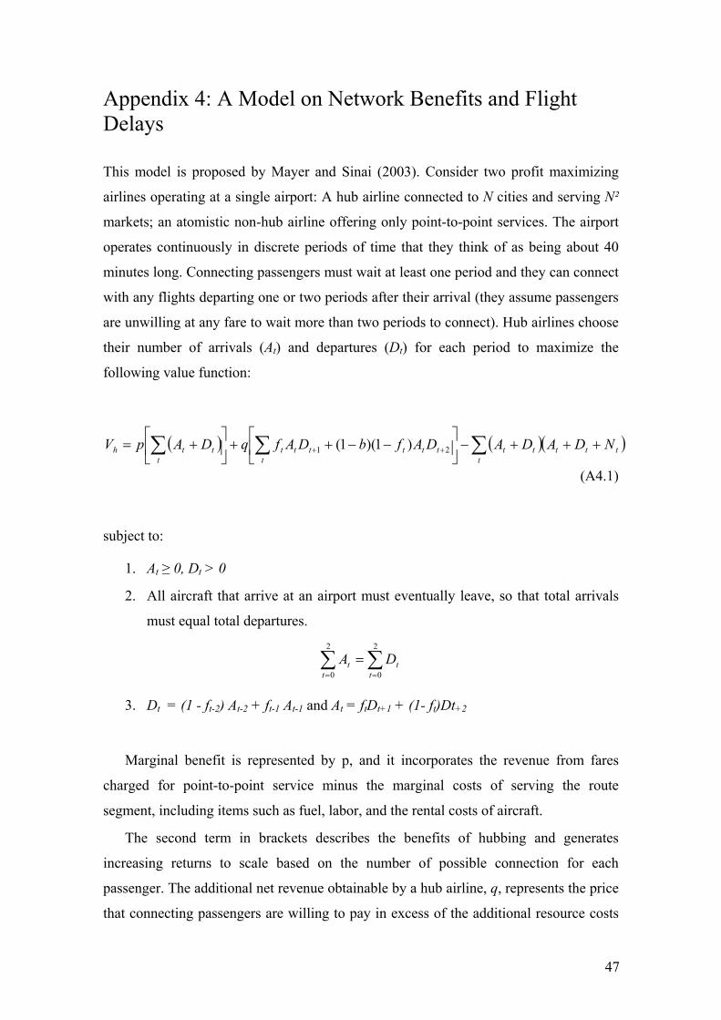
47

Appendix 4: A Model on Network Benefits and Flight Delays

This model is proposed by Mayer and Sinai (2003). Consider two profit maximizing

airlines operating at a single airport: A hub airline connected to N cities and serving N²

markets; an atomistic non-hub airline offering only point-to-point services. The airport

operates continuously in discrete periods of time that they think of as being about 40

minutes long. Connecting passengers must wait at least one period and they can connect

with any flights departing one or two periods after their arrival (they assume passengers

are unwilling at any fare to wait more than two periods to connect). Hub airlines choose

their number of arrivals (At) and departures (Dt) for each period to maximize the

following value function:

( ) ( )( )tttt

ttt

ttttttt

tth NDADADAfbDAfqDApV +++−⎥⎦

⎤⎢⎣

⎡−−++⎥

⎦

⎤⎢⎣

⎡+= ∑∑∑ ++ 21 )1)(1(

(A4.1)

subject to:

1. At ≥ 0, Dt > 0

2. All aircraft that arrive at an airport must eventually leave, so that total arrivals

must equal total departures.

∑ ∑= =

=2

0

2

0t ttt DA

3. Dt = (1 - ft-2) At-2 + ft-1 At-1 and At = ftDt+1 + (1- ft)Dt+2

Marginal benefit is represented by p, and it incorporates the revenue from fares

charged for point-to-point service minus the marginal costs of serving the route

segment, including items such as fuel, labor, and the rental costs of aircraft.

The second term in brackets describes the benefits of hubbing and generates

increasing returns to scale based on the number of possible connection for each

passenger. The additional net revenue obtainable by a hub airline, q, represents the price

that connecting passengers are willing to pay in excess of the additional resource costs

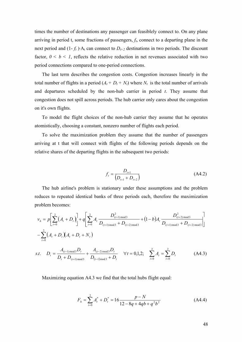
48

times the number of destinations any passenger can feasiblely connect to. On any plane

arriving in period t, some fractions of passengers, ft, connect to a departing plane in the

next period and (1- ft )·At can connect to Dt+2 destinations in two periods. The discount

factor, 0 < b < 1, reflects the relative reduction in net revenues associated with two

period connections compared to one-period connections.

The last term describes the congestion costs. Congestion increases linearly in the

total number of flights in a period (At + Dt + Nt) where Nt is the total number of arrivals

and departures scheduled by the non-hub carrier in period t. They assume that

congestion does not spill across periods. The hub carrier only cares about the congestion

on it's own flights.

To model the flight choices of the non-hub carrier they assume that he operates

atomistically, choosing a constant, nonzero number of flights each period.

To solve the maximization problem they assume that the number of passengers

arriving at t that will connect with flights of the following periods depends on the

relative shares of the departing flights in the subsequent two periods:

( )21

1

++

+

+=

tt

tt DD

Df (A4.2)

The hub airline's problem is stationary under these assumptions and the problem

reduces to repeated identical banks of three periods each, therefore the maximization

problem becomes:

( ) ( )

( )( )∑

∑∑

=

++

+

= ++

+

=

+++−

⎥⎥⎦

⎤

⎢⎢⎣

⎡

+−+

++⎥

⎦

⎤⎢⎣

⎡+=

2

0

3mod)2(3mod)1(

23mod)2(

2

0 3mod)2(3mod)1(

23mod)1(

2

01

tttttt

tt

tt

t tt

tt

ttth

NDADA

DDD

AbDD

DAqDApv

( )∑ ∑= =−

−

+

− ==∀+

++

=2

0

2

03mod1

3mod)2(

3mod)1(

3mod)1( ;2,1,0..t t

tttt

tt

tt

ttt DAt

DDDA

DDDA

Dts (A4.3)

Maximizing equation A4.3 we find that the total hubs flight equal:

∑= ++−

−=+=

2

022

**

481216

ttth bqqbq

NpDAF (A4.4)

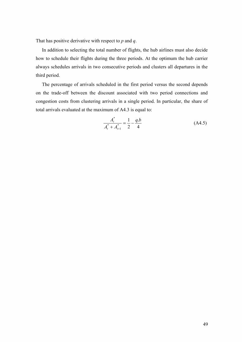
49

That has positive derivative with respect to p and q.

In addition to selecting the total number of flights, the hub airlines must also decide

how to schedule their flights during the three periods. At the optimum the hub carrier

always schedules arrivals in two consecutive periods and clusters all departures in the

third period.

The percentage of arrivals scheduled in the first period versus the second depends

on the trade-off between the discount associated with two period connections and

congestion costs from clustering arrivals in a single period. In particular, the share of

total arrivals evaluated at the maximum of A4.3 is equal to:

4.

21

*1

*

* bqAA

A

tt

t −=+ +

(A4.5)