Imprinting Costs Total Variable Costs Revenues Variable Costs Contribution Margin Setups Product...

Chapter 3

Copyright © 2013 Pearson Canada Inc. 3-57

CHAPTER 3

COST‐VOLUME‐PROFIT ANALYSIS

SHORT‐ANSWER QUESTIONS

3‐1 The assumptions underlying CVP analysis are:

1. Changes in the sales volume and production volume are identical. The ending

balances of inventories are zero.

2. All costs are classified as fixed or variable with no mixed costs.

3. All cost behavior is linear within the relevant volume range.

4. The unit selling price, unit variable costs, fixed costs and sales volume are known.

5. Either the product sold or the product mix remains constant although the volume

changes.

6. All revenues and costs can be added and compared without taking into account

the time value of money.

3‐2 Operating income is total revenues from operations for the accounting period

minus total costs from operations:

Operating income = Total revenues from operations – Total costs from operations

Net income is operating income plus non‐operating revenues (such as interest

revenue) minus non‐operating costs (such as interest cost) minus income taxes.

3‐3 CVP certainly is simple, with its assumption of a single revenue driver, a single

cost driver, and linear revenue and cost relationships. Whether these assumptions make it

simplistic depends on the decision context. In some cases, these assumptions may be

sufficiently accurate for CVP to provide useful insights.

3‐4 An increase in the income tax rate does not affect the breakeven point. Operating

income at the breakeven point is zero and thus no income taxes will be paid at this point.

3‐5 Sensitivity analysis is a “what‐if” technique that examines how a result will

change if the original predicted data are not achieved or if an underlying assumption

changes. The advent of spreadsheet software has greatly increased the ability to explore

the effect of alternative assumptions at minimal cost. CVP is one of the most widely used

software applications in the management accounting area.

Instructor’s Solutions Manual for Cost Accounting, 6Ce

3-58 Copyright © 2013 Pearson Canada Inc.

3‐6 Examples include:

• Manufacturing—substituting a robotic machine for hourly wage workers.

• Marketing—changing a sales force compensation plan from a percentage of

sales dollars to a fixed salary.

• Customer service—hiring a subcontractor to do customer repair visits on an

annual retainer basis rather than a per visit basis.

3‐7 Examples include:

• Manufacturing—subcontracting a component to a supplier on a per unit basis

to avoid purchasing a machine with a high fixed amortization cost.

• Marketing—changing a sales compensation plan from a fixed salary to a

percentage of sales dollars basis.

• Customer service—hiring a subcontractor to do customer service on a per visit

basis rather than an annual retainer basis.

3‐8 Operating leverage describes the effects that fixed costs have on changes in

operating income as changes occur in units sold and hence in contribution margin.

Knowing the degree of operating leverage at a given level of sales helps managers

calculate the effect of fluctuations in sales on operating incomes.

3‐9 A company with multiple products can compute a breakeven point by assuming

there is a constant mix of products at different levels of total revenue.

EXERCISES

3‐10 (10 min.) Terminology

1. capital intensive

2. Cost‐volume‐profit analysis

3. breakeven point

4. Operating leverage

5. Risk‐loving

6. contribution margin

7. contribution margin percentage

8. gross margin

9. sales mix

10. Risk aversion

11. margin of safety

Chapter 3


3‐11 (15 min.) CVP analysis computations.

Case Revenues

Variable

Costs

Fixed

Costs

Total

Costs OI CM (S) CM%

a $3,000 $2,290 $250 $2,540 $460 $710 23.67%

b

18,500 7,400 1,300 8,700 9,800 11,100 60.00%

c $10,600 7,420 3,200 10,620 (20) 3,180 30.00%

d

9,450 5,670 2,500 8,170 1,280 3,780 40.00%

Case a: Revenues ‐ Total Costs = Operating Income

$3,000 ‐ Total Costs = $460, Total Costs = $2,540

Total Costs = $2,540 = Variable Costs + Fixed Costs

$2,540 = $250 + Variable Costs, Variable Costs = $2,290

CM = Revenues – Variable Costs = $3,000 ‐ $2,290 = $710

CM % = CM/Revenues = $710 ÷ $3,000 = 23.67%

Case b: Total Costs = Variable Costs + Fixed Costs

$8,700 = $7,400 + Fixed Costs, Fixed Costs = $1,300

Revenue ‐ Total Costs = OI

Revenue ‐ $8,700 = $9,800, Revenue = $18,500

CM = Revenues ‐ Variable Costs = $18,500 ‐ $7,400 = $11,100

CM % = CM/Revenues = $11,100 ÷ $18,500= 60.00%

Case c: CM % = CM/Revenues

30% = CM/$10,600, CM = $3,180

CM = Revenues ‐ Variable Costs

$3,180 = $10,600 ‐ Variable Costs, Variable Costs = $7,420

Total Costs = Variable Costs + Fixed Costs

Total Costs = $7,420 + $3,200 = $10,620

OI = Revenues ‐ Total Costs = $10,600 ‐ $10,620 = ($20)

Case d: Total Costs = Variable Costs + Fixed Costs

$8,170 = Variable Costs + $2,500, Variable Costs = $5,670

OI = Revenues ‐ Total Costs = $9,450 ‐ $8,170 = $1,280

CM = Revenues ‐ Variable Costs = $9,450 ‐ $5,670 = $3,780

CM % = CM/Revenues = $3,780 ÷ $9,450= 40.00%



3‐12 (15 min.) CVP analysis computations.

Case

Unit Selling

Price

Unit

VC

Units

Sold TCM Fixed Costs OI

A $70 $25

20,000 $900,000 $700,000 $200,000

B

87 62 15,000 375,000 250,000 125,000

C 250 100

30,000 4,500,000 3,600,000 900,000

D 150 78

24,000 1,728,000 1,500,000 228,000

a. TCM = Q (USP ‐ UVC)

$900,000 = Q ($70 ‐ $25)

Q = 20,000

TFC = TCM ‐ OI

= $900,000 ‐ $200,000 = $700,000

b. OI = TCM ‐ TFC

$125,000 = TCM ‐ $250,000

TCM = $375,000

TCM = Q (USP ‐ UVC)

$375,000 = 15,000 (USP ‐ $62)

$25 = (USP ‐ $62)

USP = $87

c. OI = TCM ‐ TFC

$900,000 = $4,500,000 ‐ TFC

TFC = $3,600,000


$4,500,000 = 30,000 ($250 ‐ UVC)

$150 = $250 ‐ UVC

UVC = $100

Chapter 3


3‐12 (cont’d)

d. OI = TCM ‐ TFC

OI = $1,728,000 ‐ $1,500,000

OI = $228,000


$1,728,000 = 24,000 ($150 ‐ UVC)

$72 = $150 ‐ UVC

UVC = $78

3‐13 (10 min.) CVP computations.

1a. Sales ($30 per unit × 200,000 units) $6,000,000

Variable costs ($25 per unit × 200,000 units) 5,000,000

Contribution margin $1,000,000

1b. Contribution margin (from above) $1,000,000

Fixed costs 800,000

Operating income $ 200,000

2a. Sales (from above) $6,000,000

Variable costs ($16 per unit × 200,000 units) 3,200,000

Contribution margin $2,800,000

2b. Contribution margin $2,800,000

Fixed costs 2,400,000


3. Operating income is expected to increase by $200,000 if Ms. Schoenen’s proposal

is accepted.

The management would consider other factors before making the final decision.

It is likely that product quality would improve as a result of using state of the art

equipment. Due to increased automation, probably many workers will have to be laid

off. Patel’s management will have to consider the impact of such an action on employee

morale. In addition, the proposal increases the company’s fixed costs dramatically. This

will increase the company’s operating leverage and risk.



3‐14 (10 min.) CVP analysis, income taxes.

1. Monthly fixed costs = $60,000 + $70,000 + $10,000 = $140,000

Contribution margin per unit = $26,000 ‐ $22,000 ‐ $500 = $3,500

Breakeven units per month = Monthly fixed costs

Contribution margin per unit =

$140,000

$3,500 per car = 40 cars

2. Tax rate = 40%

Target net income = $63,000

Target operating income =Target net income $63,000 $63,000

1 - tax rate (1 0.40) 0.60

$105,000

Quantity of output unitsrequired to be sold =

Fixed costs + Target operating income $140,000 $105,000

Contribution margin per unit $3,500

70 cars

3‐15 (10 min.) CVP analysis, income taxes

1. Monthly fixed costs = $28,000 + $45,000 + $5,600 + $1,200 = $79,800

CM per unit = $16,000 ‐ $12,200 = $3,800

Breakeven = Monthly Fixed Costs ÷ UCM

= $79,800 ÷ $3,800 = 21 mowers

2. OI = Target Net Income ÷ [1 ‐ tax rate]

OI = $42,750 ÷ [1 ‐ 0.25]

OI = $57,000

Q = Fixed Costs + Target OI

Unit CM

Q = [$79,800 + $57,000] ÷ $3,800

= 36 mowers

Chapter 3


3‐16 (20 min.) CVP analysis, income taxes.

1. Variable cost percentage is $3.20 $8.00 = 40%

Let R = Revenues needed to obtain target net income

R ‐ 0.40R ‐ $450,000 = 30.01

000,105$

0.60R = $450,000 + $150,000

R = $600,000 0.60 R = $1,000,000

Proof: Revenues $1,000,000

Variable costs (at 40%) 400,000

Contribution margin 600,000

Fixed costs 450,000

Operating income 150,000

Income taxes (at 30%) 45,000

Net income $ 105,000

2.a. Customers needed to earn net income of $105,000:

Total revenues Sales check per customer: $1,000,000 $8 = 125,000 customers

b. Customers needed to break even:

Contribution margin per customer = $8.00 ‐ $3.20 = $4.80

Breakeven number of customers = Fixed costs Contribution margin per customer

= $450,000 $4.80 per customer

= 93,750 customers

3. Using the shortcut approach:

Change in net income =

Change in

number of customers

Unit

contribution

margin (1 ‐ Tax rate)

= (150,000 ‐ 125,000) $4.80 (1 ‐ 0.30) = $120,000 0.7 = $84,000 New net income = $84,000 + $105,000 = $189,000



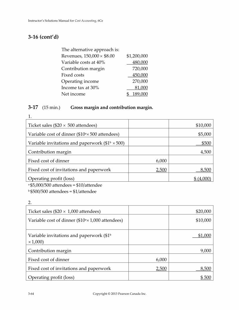
3‐16 (cont’d)

The alternative approach is:

Revenues, 150,000 $8.00 $1,200,000

Variable costs at 40% 480,000


Fixed costs 450,000


Income tax at 30% 81,000

Net income $ 189,000

3‐17 (15 min.) Gross margin and contribution margin.

1.

Ticket sales ($20 500 attendees) $10,000

Variable cost of dinner ($10a500 attendees) $5,000

Variable invitations and paperwork ($1b 500) $500


Fixed cost of dinner 6,000

Fixed cost of invitations and paperwork 2,500 8,500

Operating profit (loss) $ (4,000)a $5,000/500 attendees = $10/attendee b $500/500 attendees = $1/attendee

2.

Ticket sales ($20 1,000 attendees) $20,000

Variable cost of dinner ($10a1,000 attendees)

$10,000

Variable invitations and paperwork ($1b

1,000) $1,000


Fixed cost of dinner 6,000

Fixed cost of invitations and paperwork 2,500 8,500

Operating profit (loss) $ 500

Chapter 3


3‐18 (20 min.) Scholarships, CVP analysis.

1. Full course load = 30 credits

Tuition fees for full course load = 30 credits x $400 = $12,000

Let the number of scholarships be denoted by Q.

Then, $600,000 + $12,000Q = $4,500,000

$12,000Q = $4,500,000 ‐ $600,000

$12,000Q = $3,900,000

Q = 325 scholarships

2. Total budget for next year = $4,500,000 (1 ‐ 0.20) = $4,500,000 x 0.80

= $3,600,000

Then, 600,000 + $12,000Q = $3,600,000

$12,000Q = $3,600,000 ‐ $600,000

Q = $3,000,000 ÷ $12,000 = 250 scholarships

3. Let the scholarship award per student per year be denoted by V.

Then, $600,000 + 325V = $3,600,000

325V = $3,600,000 ‐ $600,000

V = $3,000,000 ÷ 325 = $9,230.77

3‐19 (35–40 min.) CVP analysis, changing revenues and costs.

1a. SP = 8% × $1,000 = $80 per ticket

UVC = $35 per ticket

UCM = $80 ‐ $35 = $45 per ticket

FC = $22,000 a month

Q = UCM

FC =

per ticket $45

$22,000= 489 tickets (rounded up)

1b. Q = UCM

TOI FC =

per ticket $45

$10,000 $22,000 =

per ticket $45




3‐19 (cont’d)

2a. SP = $80 per ticket

VCU = $29 per ticket

UCM = $80 ‐ $29 = $51 per ticket


Q = UCM

FC =

per ticket $51


2b. Q = UCM

TOI FC =

per ticket $51

$10,000 $22,000 =

per ticket $51


3a. SP = $48 per ticket


CMU = $48 ‐ $29 = $19 per ticket


Q = UCM

FC =

per ticket $19

$22,000= 1,158 tickets (rounded up)

3b. Q = UCM

TOI FC =

per ticket $19

$10,000 $22,000 =

per ticket $19


4a. The $5 delivery fee can be treated as either an extra source of revenue (as done

below) or as a cost offset. Either approach increases CMU $5:

SP = $53 ($48 + $5) per ticket


CMU = $53 ‐ $29 = $24 per ticket


Q = CMU

FC =

per ticket $24


4b. Q = CMU

TOI FC =

per ticket $24

$10,000 $22,000 =

per ticket $24


The $5 delivery fee results in a higher contribution margin, which reduces both

the breakeven point and the tickets sold to attain operating income of $10,000.

Chapter 3


3‐20 (20 min.) Contribution margin, gross margin and margin of safety.

1.

Mirabel Cosmetics

Operating Income Statement, June 2012

Units sold 10,000

Revenues $100,000

Variable costs

Variable manufacturing costs $ 55,000

Variable marketing costs 5,000

Total variable costs 60,000


Fixed costs

Fixed manufacturing costs $ 20,000

Fixed marketing & administration costs 10,000

Total fixed costs 30,000


2. Contribution margin per unit = $40,000

$4 per unit10,000 units

Breakeven quantity = Fixed costs $30,000

7,500 unitsContribution margin per unit $4 per unit

Selling price = Revenues $100,000

$10 per unitUnits sold 10,000 units

Breakeven revenues = 7,500 units $10 per unit = $75,000

Alternatively,

Contribution margin percentage = Contribution margin $40,000

40%Revenues $100,000

Breakeven revenues = Fixed costs $30,000

$75,000Contribution margin percentage 0.40

3. Margin of safety = 10,000 units ‐ 7,500 units = 2,500 units



3‐20 (cont’d)

4. Units sold 8,000

Revenues (Units sold Selling price = 8,000 $10) $80,000

Contribution margin (Revenues CM percentage = $80,000 40%) $32,000

Fixed costs 30,000


Taxes (30% $2,000) 600

Net income $ 1,400

3‐21 CVP computations.

1. (a) 5,000,000 ($0.60 ‐ $0.36) ‐ $1,080,000 = $120,000

(a) 1,080,000 ÷ [($0.60 ‐ $0.36) ÷ $0.60] = $2,700,000

2. 5,000,000 ($0.60 ‐ $0.408) ‐ $1,080,000 = $(120,000)

3. [5,000,000 (1.1) ($0.60 ‐ $0.36)] ‐ [$1,080,000 (1.1)] = $132,000

4. [5,000,000 (1.4) ($0.48 ‐ $0.324)] ‐ [$1,080,000 (0.8)] = $228,000

5. $1,080,000 (1.1) ÷ ($0.60 ‐ $0.36) = 4,950,000 units

6. ($1,080,000 + $24,000) ÷ ($0.66 ‐ $0.36) = 3,680,000 units

3‐22 (15 min.) CVP exercises.

1. Total CM = $3,240,000 48% = $1,555,200 CM = Revenues ‐ Variable Costs

$1,555,200 = $3,240,000 ‐ Variable Costs, VC = $1,684,800

Units Sold = $3,240,000 ÷ $36 = 90,000

Per Unit Dollars %

Revenues @ $36/unit (given) $36.00 $3,240,000 100%

Variable Costs $18.72 $1,684,800 52%

Contribution Margin $17.28 $1,555,200 48%

Fixed Costs (given) $730,000

Budgeted Operating Income $825,200

Chapter 3


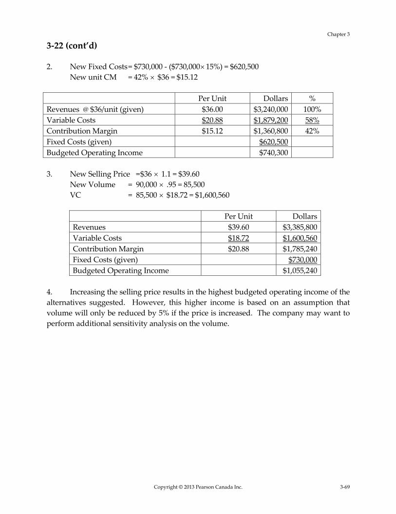
3‐22 (cont’d)

2. New Fixed Costs = $730,000 ‐ ($730,00015%) = $620,500

New unit CM = 42% $36 = $15.12

Per Unit Dollars %

Revenues @ $36/unit (given) $36.00 $3,240,000 100%

Variable Costs $20.88 $1,879,200 58%

Contribution Margin $15.12 $1,360,800 42%


Budgeted Operating Income $740,300

3. New Selling Price = $36 1.1 = $39.60 New Volume = 90,000 .95 = 85,500 VC = 85,500 $18.72 = $1,600,560

Per Unit Dollars

Revenues $39.60 $3,385,800

Variable Costs $18.72 $1,600,560

Contribution Margin $20.88 $1,785,240


Budgeted Operating Income $1,055,240

4. Increasing the selling price results in the highest budgeted operating income of the

alternatives suggested. However, this higher income is based on an assumption that

volume will only be reduced by 5% if the price is increased. The company may want to

perform additional sensitivity analysis on the volume.



3‐23 (25 min.) Operating leverage.

1. Let Q denote the quantity of bracelets sold

a. Breakeven point under Option 1

$125Q ‐ $80Q = ($435 3) $45Q = $1,305

Q = 29 bracelets

b. Breakeven point under Option 2

$125Q ‐ $80Q ‐ (0.12 $125Q) = 0 $30Q = 0

Q = 0

All costs are variable and therefore can be avoided.

2. Operating income under Option 1 = $45Q ‐ $1,305

Operating income under Option 2 = $30Q

Find Q such that $45Q ‐ $1,305 = $30Q

$15Q = $1,305

Q = 87

87 is the mathematical point of indifference.

Option 1: $125(87) ‐ $80(87) ‐ ($435 3) = $2,610 Option 2: $125(87) ‐ $80(87) ‐ $15(87) = $2,610

3. a. For Q > 87, say, 88,

Option 1 gives operating income = $45 88 ‐ $1,305 = $2,655 better Option 2 gives operating income = $30 88 = $2,640 Rothman will prefer Option 1.

3. b. For Q < 87, say, 86,

Option 1 gives operating income = $45 86 ‐ $1,305 = $2,565 Option 2 gives operating income = $30 86 = $2,580 better Rothman will prefer Option 2.

Chapter 3


3‐23 (cont’d)

4. Degree of operating leverage = CM ÷ Operating Income

Under Option 1, the total CM = $45 150 units = $6,750

Operating Income = $6,750 ‐ $1,305 = $5,445

The Degree of Operating Leverage (Opt 1) = $6,750 ÷ $5,445 = 1.24

Under Option 2, the total CM = OI = $30 150 = $4,500 The Degree of Operating Leverage (Opt 2) = $4,500 ÷ $4,500 = 1.00

5. The calculations in requirement 4 indicate that, when sales are 150 units, a

percentage change in sales and contribution margin will result in 1.24 times that

percentage change in operating income for Option 1, but the same percentage change in

operating income for Option 2. The degree of operating leverage at a given level of sales

helps managers calculate the effect of fluctuations in sales on operating incomes.

3‐24 (15 min.) Gross margin and contribution margin, making decisions.

1. Revenues $800,000

Deduct variable costs:

Cost of goods sold $384,000

Sales commissions 96,000

Other operating costs 32,000 512,000

Contribution margin $288,000

2. Contribution margin percentage = %00.36000,800$

000,288$

3. Incremental revenue (25% $800,000) $200,000

Incremental contribution margin (36% $200,000) 72,000

Incremental fixed costs (advertising) 24,300

Incremental operating income $47,700

If Mr. Saunders increases his advertising, the operating income will increase by

$47,700 converting an operating loss of $44,700 to an operating income of $3,000.



3‐24 (cont’d)

Proof (Optional):

Variable Other Operating Costs = $32,000 ÷ $800,000 = 4% of sales

Revenues (125% $800,000) $1,000,000

Cost of goods sold (48% of sales) 480,000

Gross margin 520,000

Operating costs:

Store rent $61,200

Salaries and wages 212,000

Sales commissions (12% of sales) 120,000

Amortization of equipment and fixtures 19,200

Other operating costs:

Variable (4% of sales) 40,000

Fixed 64,600 517,000


3‐25 (20 min.) CVP, revenue mix.

1.

Men’s Dominator Ladies Luxury

Selling Price $750 $640

Variable Cost $475 $390

Sales Commission $25 $21

Unit CM $250 $229

2. Weighted Average CM = (70% $250) + (30% $229) = $175 + $68.70 = $243.70

3. Units required = Fixed Costs + Target OI

Weighted Average CM

= ($180,000 + $115,000) ÷ $243.70

= 1,210.5 or 1,211 total units

Men’s Dominator = 70% 1,211 = 848 units (rounded up) Ladies Luxury = 30% 1,211 = 363 units (rounded down)

Chapter 3


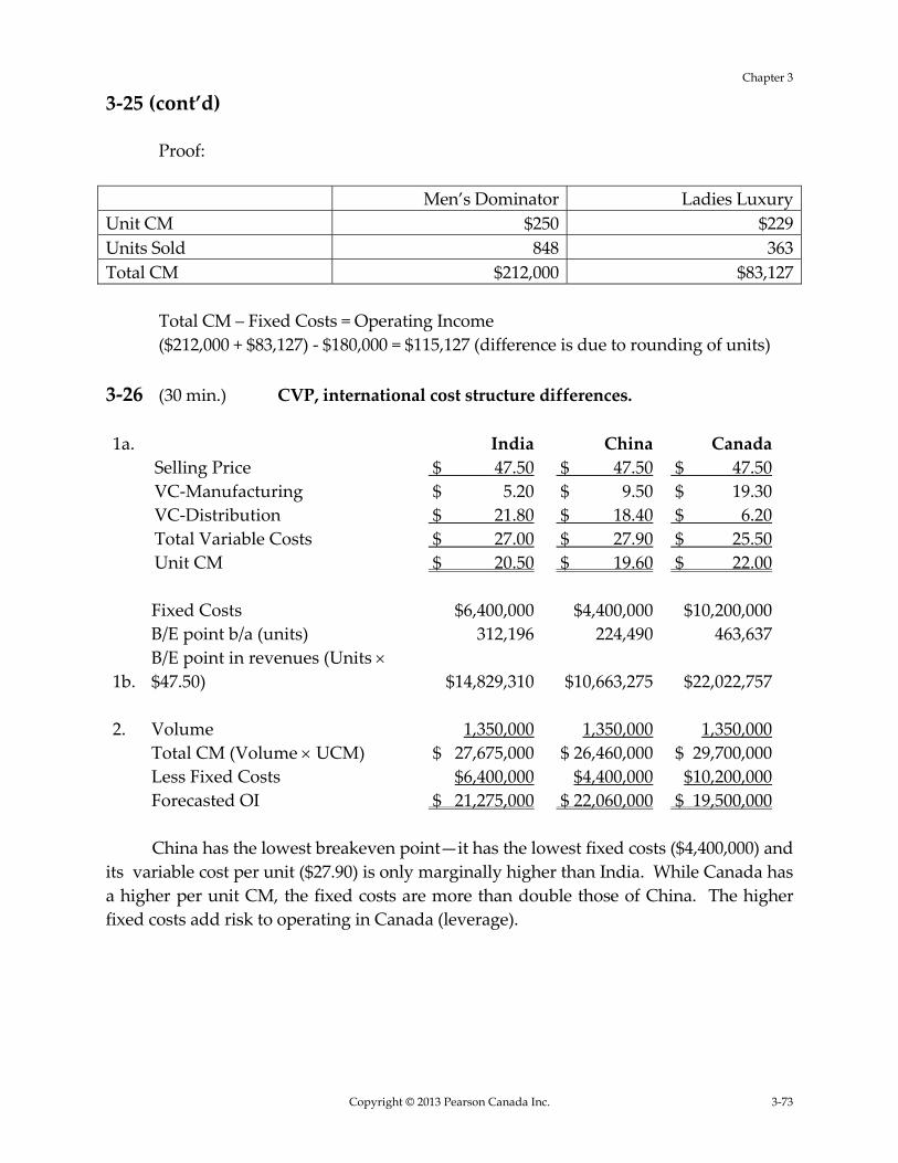
3‐25 (cont’d)

Proof:

Men’s Dominator Ladies Luxury

Unit CM $250 $229

Units Sold 848 363

Total CM $212,000 $83,127

Total CM – Fixed Costs = Operating Income

($212,000 + $83,127) ‐ $180,000 = $115,127 (difference is due to rounding of units)

3‐26 (30 min.) CVP, international cost structure differences.

1a. India China Canada

Selling Price $ 47.50 $ 47.50 $ 47.50

VC‐Manufacturing $ 5.20 $ 9.50 $ 19.30

VC‐Distribution $ 21.80 $ 18.40 $ 6.20

Total Variable Costs $ 27.00 $ 27.90 $ 25.50

Unit CM $ 20.50 $ 19.60 $ 22.00

Fixed Costs $6,400,000 $4,400,000 $10,200,000

B/E point b/a (units) 312,196 224,490 463,637

1b.

B/E point in revenues (Units $47.50) $14,829,310 $10,663,275 $22,022,757

2. Volume 1,350,000 1,350,000 1,350,000

Total CM (Volume UCM) $ 27,675,000 $ 26,460,000 $ 29,700,000

Less Fixed Costs $6,400,000 $4,400,000 $10,200,000

Forecasted OI $ 21,275,000 $ 22,060,000 $ 19,500,000

China has the lowest breakeven point—it has the lowest fixed costs ($4,400,000) and

its variable cost per unit ($27.90) is only marginally higher than India. While Canada has

a higher per unit CM, the fixed costs are more than double those of China. The higher

fixed costs add risk to operating in Canada (leverage).



3‐26 (cont’d)

3. China’s OI = $19.60 per unit less Fixed Costs of $4,400,000

Canada’s OI = $22.00 per unit less Fixed Costs of $10,200,000

$19.60X ‐ $4,400,000 = $22.00X ‐ $10,200,000

$5,800,000 = $2.40X

X = 2,416,666.667 (or 2,416,667)

Proof and India’s Operating Income at same sales volume

India China Canada

Unit CM $ 20.50 $ 19.60 $ 22.00

Volume 2,416,666.667 2,416,666.667 2,416,666.667

Total CM (Volume UCM) $49,541,667 $ 47,366,667 $ 53,166,667

Less Fixed Costs $6,400,000 $4,400,000 $10,200,000

Forecasted OI $43,141,667 $ 42,966,667 $ 42,966,667

(Note: India’s forecasted OI is slightly higher at this volume)

3‐27 (25 min.) CVP, Not for profit

1. Contributions $19,000,000


Cash available to purchase land $18,000,000

Divided by cost per hectare to purchase land ÷3,000

Hectares of land SG can purchase 6,000 hectares

2. Contributions ($19,000,000 ‐ $5,000,000) $14,000,000


Cash available to purchase land $13,000,000

Divided by cost per hectare ($3,000 ‐ $1,000) ÷2,000

Hectares of land SG can purchase 6,500 hectares

On financial considerations alone, SG should take the subsidy because it can

purchase 500 more hectares (6,500 ‐ 6,000).

Chapter 3


3‐27 (cont’d)

3. Let the decrease in contributions be$x . Cash available to purchase land = $19,000,000 ‐ $x ‐ $1,000,000

Cost to purchase land = $3,000 ‐ $1,000 = $2,000

To purchase 6,000 hectares, we solve the following equation for x .

19,000,000 1,000,0006,000

2,000

18,000,000 6,000 2,000

18,000,000 12,000,000$6,000,000

x

x

xx

SG will be indifferent between taking the government subsidy or not if

contributions decrease by $6,000,000.

3‐28 (30 min.) CVP, revenue mix

Zyrcon

1. Alien Predators

Vegas

Pokermatch

Revenue $89 $59

Variable Manufacturing Costs 18 12

Variable Marketing Costs 27 16

Total Variable Costs 45 28

Unit CM $44 $31

Sales Mix 40% 60%

Weighted CM $17.60 $18.60

Weighted CM = $17.60 + $18.60 = $36.20

Breakeven in total units = Fixed Costs ÷ Weighted CM

= $18,750,000 ÷ $36.20

= 517,956 units

40% of 517,596 = 207,183 units of Alien Predators

60% of 517,596 = 310,773 units of Vegas Pokermatch



3‐28 (cont’d)

Proof:

OI = Total CM ‐ Fixed Costs

OI = ($44 207,183) + ($31 310,773) ‐ $18,750,000 OI = $9,116,052 + $9,633,963 ‐ $18,750,000

OI = $15 (difference due to rounding of units)

2. Alien Predators Vegas Pokermatch

Revenue $89 $59

Variable Manufacturing Costs 18 12

Variable Marketing Costs 27 16

Total Variable Costs 45 28

Unit CM $44 $31

Sales Mix 25% 75%


Weighted CM = $11.00 + $23.25 = $34.25

Breakeven in total units = Fixed Costs ÷ Weighted CM

= $18,750,000 ÷ $34.25

= 547,446 units

25% of 547,446 = 136,862 units of Alien Predators

75% o‐f 547,446 = 410,584 units of Vegas Pokermatch

Proof:

OI = Total CM ‐ Fixed Costs

OI = ($44 136,862) + ($31 410,584) ‐ $18,750,000 OI = $6,021,928 + $12,728,104 ‐ $18,750,000

OI = $32 (difference due to rounding of units)

3. 40%/60% Mix 25%/75% Mix


Unit Sales 750,000 750,000

Total CM $27,150,000 $25,687,500

Fixed Costs 18,750,000 18,750,000

OI $8,400,000 $6,937,500

Chapter 3


3‐29 (40 min.) Alternative cost structures, uncertainty, and sensitivity analysis.

1. Contribution margin assuming fixed rental arrangement = $50 ‐ $30 = $20 per

bouquet

Fixed costs = $5,000

Breakeven point = $5,000 ÷ $20 per bouquet = 250 bouquets

Contribution margin assuming $10 per arrangement rental agreement

= $50 ‐ $30 ‐ $10 = $10 per bouquet

Fixed costs = $0

Breakeven point = $0 ÷ $10 per bouquet = 0

2. Let x denote the number of bouquets EB must sell for it to be indifferent

between the fixed rent and royalty agreement.

To calculate x we solve the following equation.

$50 x ‐ $30 x ‐ $5,000 = $50 x ‐ $40 x $20 x ‐ $5,000 = $10 x $10 x = $5,000 x = $5,000 ÷ $10 = 500 bouquets

For sales between 0 to 500 bouquets, EB prefers the royalty agreement because in

this range, $10 x > $20 x ‐ $5,000. For sales greater than 500 bouquets, EB prefers the fixed rent agreement because in this range, $20 x ‐ $5,000 > $10 x .

3. If we assume the $5 savings in variable costs applies to both options, we solve

the following equation for x .

$50 x ‐ $25 x ‐ $5,000 = $50 x ‐ $35 x $25 x ‐ $5,000 = $15 x $10 x = $5,000 x = $5,000 ÷ $10 per bouquet = 500 bouquets

The answer is the same as in Requirement 2, that is, for sales between 0 to 500

bouquets, EB prefers the royalty agreement because in this range, $15 x > $25 x ‐ $5,000. For sales greater than 500 bouquets, EB prefers the fixed rent agreement because in this

range, $25 x ‐ $5,000 > $15 x .



3‐29 (cont’d)

4. Fixed rent agreement:

Bouquets

Sold

(1)

Revenue

(2)

Fixed

Costs

(3)

Variable

Costs

(4)

Operating

Income

(Loss)

(5)=(2)–(3)–(4) Probability

(6)

Expected

Operating

Income

(7)=(5) (6)200 200$50=$10,000 $5,000 200$30=$ 6,000 $ (1,000) 0.20 $ ( 200)

400 400$50=$20,000 $5,000 400$30=$12,000 $ 3,000 0.20 600

600 600$50=$30,000 $5,000 600$30=$18,000 $ 7,000 0.20 1,400

800 800$50=$40,000 $5,000 800$30=$24,000 $11,000 0.20 2,200

1,000 1,000$50=$50,000 $5,000 1,000$30=$30,000 $15,000 0.20 3,000

Expected value of rent agreement $7,000

Royalty agreement:

Bouquets

Sold

(1)

Revenue

(2)

Variable

Costs

(3)

Operating

Income

(4)=(2)–(3)

Probability

(5)

Expected Operating

Income

(6)=(4) (5) 200 200$50=$10,000 200$40=$ 8,000 $2,000 0.20 $ 400

400 400$50=$20,000 400$40=$16,000 $4,000 0.20 800

600 600$50=$30,000 600$40=$24,000 $6,000 0.20 1,200

800 800$50=$40,000 800$40=$32,000 $8,000 0.20 1,600

1,000 1,000$50=$50,000 1,000$40=$40,000 $10,000 0.20 2,000

Expected value of royalty agreement $6,000

EB should choose the fixed rent agreement because the expected value is higher

than the royalty agreement. EB will lose money under the fixed rent agreement if EB

sells only 200 bouquets but this loss is more than made up for by high operating

incomes when sales are high.

Chapter 3


3‐30 (20 min.) CVP analysis, multiple cost drivers.

1. 350,000 pens sold, order size 100

2. 350,000 pens sold, order size 250

Per 100 Each Pen

Costs to buy pens $ 95.00 $ 0.95

Imprinting Costs $ 35.00 $ 0.35

Total Variable Costs $130.00 $ 1.30

Revenues 350,000 $4.50 $1,575,000

Variable Costs 350,000 $1.30 $455,000

Contribution

Margin $1,120,000

Setups (350,000/100) $120 $420,000

Product Margin $700,000

Fixed Costs $275,000

OI $425,000

Revenues 350,000 $4.50 $1,575,000

Variable Costs 350,000 $1.30 $455,000

Contribution

Margin $1,120,000

Setups (350,000/250) $120 $168,000

Product Margin $952,000


OI $677,000



3‐30 (cont’d)

3. Unit Margins, Breakevens & Setups at various order sizes

Order Size 50 units/order 100 units/order 250 units/order 500 units/order

Setup Costs $120.00 $120.00 $120.00 $120.00

Setup/unit $2.40 $1.20 $0.48 $0.24

VC/Unit $1.30 $1.30 $1.30 $1.30

Subtotal $3.70 $2.50 $1.78 $1.54

Revenues $4.50 $4.50 $4.50 $4.50

Unit Margin $0.80 $2.00 $2.72 $2.96

Fixed Costs $275,000 $275,000 $275,000 $275,000

Breakeven

FC/Unit Marg

343,750 units 137,500 units 101,103 units 92,906 units

Number of setups

at breakeven point

6,875 setups 1,375 setups 404 setups 186 setups

The breakeven point is not unique because there are two cost drivers—quantity of

pens and number of setups. Various combinations of the two cost drivers can yield zero

operating income.

3‐31 (15‐20 min.) Uncertainty, CVP.

1. King pays Couture $3.2 million plus $6.75 (25% of $27.00) for every home

purchasing the pay‐per‐view. The expected value of the variable component is:

Demand Payment Probability Expected payment

(1) (2) = (1) $6.75 (3) (4) = (2) (3) 250,000 $ 1,687,500 0.05 $ 84,375

300,000 2,025,000 0.10 202,500

350,000 2,362,500 0.20 472,500

400,000 2,700,000 0.40 1,080,000

500,000 3,375,000 0.15 506,250

1,000,000 6,750,000 0.10 675,000

$3,020,625

The expected value of King’s payment is $6,220,625 ($3,200,000 fixed fee +

$3,020,625).

Chapter 3


3‐31 (cont’d)

2. USP = $27.00

UVC = $9.00 ($6.75 payment to Couture + $2.25 variable cost)

UCM = $18.00

FC = $3,200,000 + $1,300,000 = $4,500,000

Q = FC

UCM = $4,500,000 ÷ $18 = 250,000

If 250,000 homes purchase the pay‐per‐view, King will break even.



PROBLEMS

3‐32 (20‐30 min.) Effects on operating income, pricing decision.

1. Analysis of special order:

Sales, 5,000 units $98 $490,000

Variable costs:

Direct materials, 5,000 units $48 $240,000

Direct manufacturing labour, 5,000 units $16 80,000

Variable manufacturing overhead, 5,000 units $8 40,000

Other variable costs, 5,000 units $7 35,000

Sales commission, flat rate 9,500


Contribution margin $ 85,500

Note that the variable costs, except for commissions, are affected by production

volume, not sales dollars.

If the order is accepted, operating income increases by $85,500.

4. Whether the general manager is making a correct decision depends on many

factors. He is incorrect if the capacity would otherwise be idle and if his objective is to

increase operating income in the short run. If the offer is rejected, Teguchi, in effect, is

willing to invest $85,500 in immediate gains forgone (an opportunity cost) to preserve the

long‐run selling‐price structure. He is correct if he thinks future competition or future

price concessions to customers will hurt Teguchi’s operating income by more than

$85,500.

There is also the possibility that Andrews could become a long‐term customer. In

this case, is a price that covers only short‐run variable costs adequate? Would the sales

representative be willing to accept the lower flat sales commission (as distinguished from

the regular $58,800 = 12% $490,000) on a long term basis?

Chapter 3


3‐33 (20‐30 min.) CVP, executive teaching compensation.

1. (a) Advertising in magazines $5,200

Mailing of brochures 2,500

Administrative labour at UKBS 3,700

Charge for UKBS lecture auditorium 1,800

Airfare and accommodation 3,800

Lecture fee 2,750

Total fixed costs $19,750

Meals and drinks $38

Binders and photocopying 37

Unit variable cost $75

Unit contribution margin = Unit revenues – Unit variable costs

= $350 ‐ $75

= $275

Breakeven point = Fixed costs

Unit contribution margin

= $19,750 ÷ $275

= 71.82 or 72 attendees

(b) Advertising in magazines $5,200

Mailing of brochures 2,500

Administrative labour at UKBS 3,700

Charge for UKBS lecture auditorium 1,800

Total fixed costs $13,200

Unit contribution margin = $275



= $13,200 ÷ $275

= 48 attendees



3‐33 (cont’d)

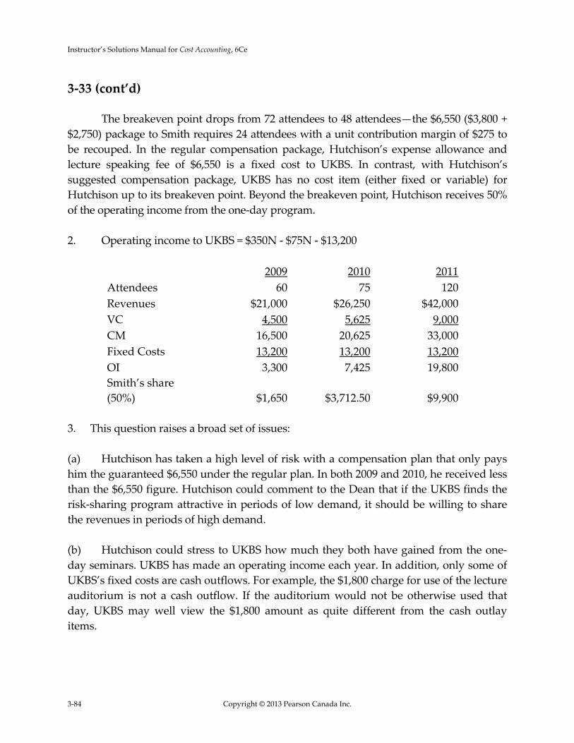
The breakeven point drops from 72 attendees to 48 attendees—the $6,550 ($3,800 +

$2,750) package to Smith requires 24 attendees with a unit contribution margin of $275 to

be recouped. In the regular compensation package, Hutchison’s expense allowance and

lecture speaking fee of $6,550 is a fixed cost to UKBS. In contrast, with Hutchison’s

suggested compensation package, UKBS has no cost item (either fixed or variable) for

Hutchison up to its breakeven point. Beyond the breakeven point, Hutchison receives 50%

of the operating income from the one‐day program.

2. Operating income to UKBS = $350N ‐ $75N ‐ $13,200

2009 2010 2011

Attendees 60 75 120

Revenues $21,000 $26,250 $42,000

VC 4,500 5,625 9,000

CM 16,500 20,625 33,000

Fixed Costs 13,200 13,200 13,200

OI 3,300 7,425 19,800

Smith’s share

(50%) $1,650 $3,712.50 $9,900

3. This question raises a broad set of issues:

(a) Hutchison has taken a high level of risk with a compensation plan that only pays

him the guaranteed $6,550 under the regular plan. In both 2009 and 2010, he received less

than the $6,550 figure. Hutchison could comment to the Dean that if the UKBS finds the

risk‐sharing program attractive in periods of low demand, it should be willing to share

the revenues in periods of high demand.

(b) Hutchison could stress to UKBS how much they both have gained from the one‐

day seminars. UKBS has made an operating income each year. In addition, only some of

UKBS’s fixed costs are cash outflows. For example, the $1,800 charge for use of the lecture

auditorium is not a cash outflow. If the auditorium would not be otherwise used that

day, UKBS may well view the $1,800 amount as quite different from the cash outlay

items.

Chapter 3


3‐33 (cont’d)

(c) Hutchison could respond to the Dean that the agreement is not really a 50%/50%

profit‐sharing plan. It considers only the UKBS costs. Assume Hutchison pays $3,300 for

airfare/accommodation. Then, in 2009 he actually lost $1,650 ($1,650 ‐ $3,300) for giving

the seminar, while in 2010 he received only $412.50 ($3,712.50 ‐ $3,300).

(d) If Hutchison views the Dean as adamant in wanting to change the formula, he

could consider negotiating with another university or organization to handle the

planning and marketing of the seminar.

3‐34 (20 Min.) CVP computations with sensitivity analysis

1. USP = $36.00 � (1 ‐ 0.30 margin to bookstore)

= $36.00 � 0.70 = $25.20

UVC = $4.80 variable production and marketing cost

3.78 variable author royalty cost (0.15 � $36.00 � 0.70)

$8.58

UCM = $25.20 ‐ $8.58 = $16.62

FC = $600,000 fixed production and marketing cost

3,600,000 up‐front payment to Washington

$4,200,000

(a) Breakeven number in units = $4,200,000 ÷ $16.62 = 252,708 copies sold

(rounded)

(b) Target OI = ($4,200,000 + $2,400,000) ÷ $16.62 = 397,112 copies sold (rounded)



3‐34 (cont’d)

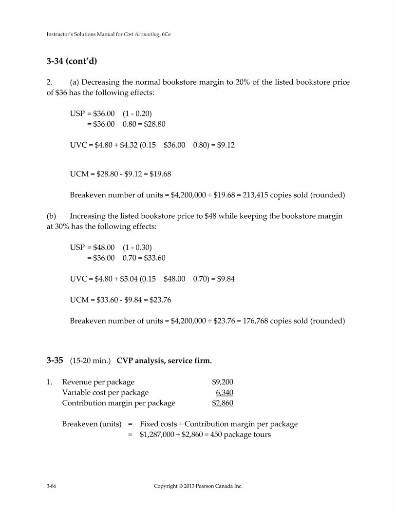
2. (a) Decreasing the normal bookstore margin to 20% of the listed bookstore price

of $36 has the following effects:

USP = $36.00 � (1 ‐ 0.20)

= $36.00 � 0.80 = $28.80

UVC = $4.80 + $4.32 (0.15 � $36.00 � 0.80) = $9.12

UCM = $28.80 ‐ $9.12 = $19.68

Breakeven number of units = $4,200,000 ÷ $19.68 = 213,415 copies sold (rounded)

(b) Increasing the listed bookstore price to $48 while keeping the bookstore margin

at 30% has the following effects:

USP = $48.00 � (1 ‐ 0.30)

= $36.00 � 0.70 = $33.60

UVC = $4.80 + $5.04 (0.15 � $48.00 � 0.70) = $9.84

UCM = $33.60 ‐ $9.84 = $23.76

Breakeven number of units = $4,200,000 ÷ $23.76 = 176,768 copies sold (rounded)

3‐35 (15‐20 min.) CVP analysis, service firm.

1. Revenue per package $9,200

Variable cost per package 6,340

Contribution margin per package $2,860

Breakeven (units) = Fixed costs ÷ Contribution margin per package

= $1,287,000 ÷ $2,860 = 450 package tours

Chapter 3


3‐35 (cont’d)

2. Contribution margin ratio = Contribution margin per package

Selling price = $2,860 ÷ $9,200

=31.09%

Units needed to achieve target income = (Fixed costs + target OI) ÷ UCM

= ($1,287,000 + $214,500) ÷ $2,860 = 525 packages

Revenues to earn $214,500 OI = 525 tour packages $9,200= $4,830,000

or

Revenue to achieve target income = (Fixed costs + target OI) ÷ CM ratio

= ($1,287,000 + $214,500) ÷ .3109

= $4,829,527 (rounding difference)

3. Fixed costs = $1,287,000 + $40,500 = $1,327,500

Breakeven (units) = Fixed costs

Contribution margin per unit

Contribution margin per unit = $1,327,500 ÷ 450

= $2,950 per tour package

Desired variable cost per tour package = $9,200 – $2,950 = $6,250

Because the current variable cost per unit is $6,340 the unit variable cost will need to

be reduced by $90 to achieve the breakeven point calculated in requirement 1.

Alternate Method: If fixed cost increases by $40,500 then total variable costs must be

reduced by $40,500 or $40,500/450 or $90 per package tour.



3‐36 (30 min.) CVP, target operating income and net income

1. Selling price to break even

(USP ‐ UVC) Q ‐ Fixed Costs = $0

(USP ‐ $24.75) 80,000 ‐ $800,000 = $0

(USP ‐ $24.75) = $800,000 ÷ 80,000

USP ‐ $24.75 = $10

USP = $34.75

2.

[USP ‐ $24.75] 60,000 = (0.20USP 60,000) + Fixed Costs 60,000USP ‐ $1,485,000 = 12,000USP + $800,000

48, 000USP = $2,285,000

USP = $47.61

3. Offer should be rejected. The proposed variable cost to purchase of $28 exceeds

the variable manufacturing costs of $24.75. The company would lose $3.25 ($28.00 ‐

$24.75) per unit.

Cost Item Total Cost Unit Cost

Total Variable Costs:

Direct Material $600,000 $7.50

Direct Labour 400,000 5.00

Variable Overhead 720,000 9.00

Variable Selling 260,000 3.25

Total Variable Costs $1,980,000 $24.75

Total Fixed Costs

Fixed Overhead $400,000

Fixed Selling 250,000

Fixed Administration 150,000 $800,000

Chapter 3


3‐36 (cont’d)

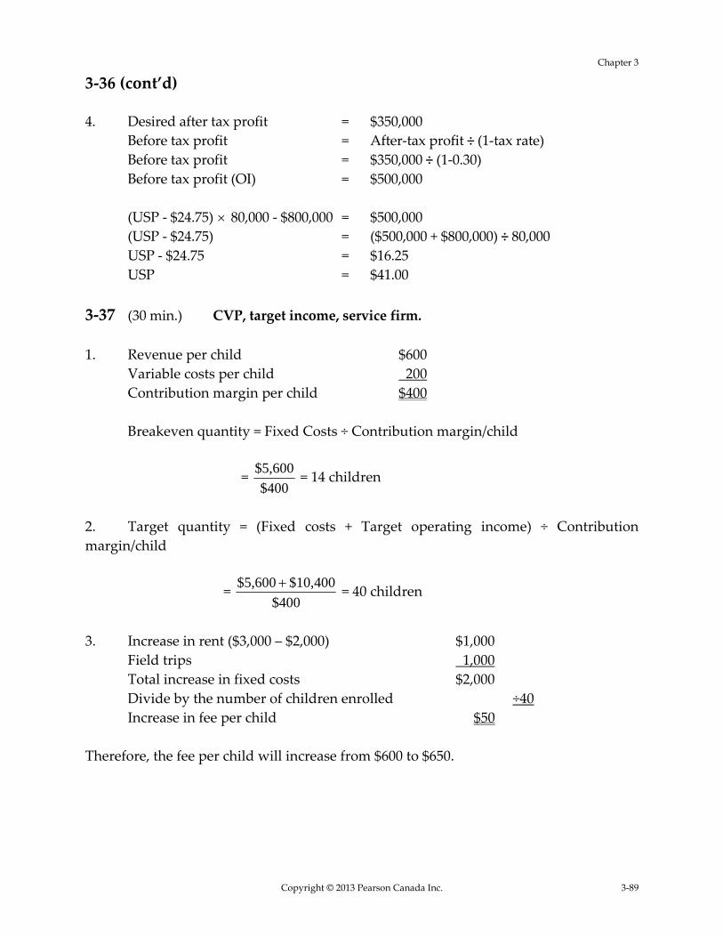
4. Desired after tax profit = $350,000

Before tax profit = After‐tax profit ÷ (1‐tax rate)

Before tax profit = $350,000 ÷ (1‐0.30)

Before tax profit (OI) = $500,000

(USP ‐ $24.75) 80,000 ‐ $800,000 = $500,000

(USP ‐ $24.75) = ($500,000 + $800,000) ÷ 80,000

USP ‐ $24.75 = $16.25

USP = $41.00

3‐37 (30 min.) CVP, target income, service firm.

1. Revenue per child $600

Variable costs per child 200

Contribution margin per child $400

Breakeven quantity = Fixed Costs ÷ Contribution margin/child

= $400

$5,600 = 14 children

2. Target quantity = (Fixed costs + Target operating income) ÷ Contribution

margin/child

= $400

10,400$ $5,600 = 40 children

3. Increase in rent ($3,000 – $2,000) $1,000

Field trips 1,000

Total increase in fixed costs $2,000

Divide by the number of children enrolled ÷40

Increase in fee per child $50

Therefore, the fee per child will increase from $600 to $650.



3‐37 (cont’d)

Alternatively,

New contribution margin per child = 40

10,400$000,2$ $5,600 = $450

New fee per child = Variable costs per child + New contribution margin per child

= $200 + $450 = $650

3‐38 (20 min.) CVP and income taxes.

1. Revenues – Variable costs ‐ Fixed costs = Target net income ÷ (1 ‐ tax rate)

Let X = Net income for 2012

20,000($30.00) ‐ 20,000($16.50) ‐ $162,000 = X ÷ (1‐0.40)

$600,000 ‐ $330,000 ‐ $162,000 = X ÷ 0.60

X = $64,800

2. Let Q = Number of unit to break even $30.00Q ‐ $16.50Q ‐ $162,000 = 0 Q = $162,000 ÷ $ 13.50 = 12,000 units

3. Let X = Net income for 2013

22,000($30.00) ‐ 22,000($16.50) ‐ ($162,000 + $13,500) = X ÷ (1‐0.40)

$297,000 ‐ $175,500 = X ÷ 0.60

X = $72,900

4. Let Q = Number of units to break even with new fixed costs of $175,500

$30.00Q ‐ $16.50Q ‐ $175,500 = 0

Q = $175,500 ÷ $ 13.50 = 13,000 units

Revenues = 13,000($30.00) = $390,000

Alternatively, the computation could be $175,500 divided by the contribution margin percentage of 45% to obtain $390,000.

Chapter 3


3‐38 (cont’d)

5. Let S = Required sales units to equal 2012 net income

$30.00S ‐ $16.50S ‐ $175,500 = $64,800 ÷ 0.60

$13.50S = $283,500

S = 21,000 units

Revenues = 21,000 units � $30.00 = $630,000

6. Let A = Amount spent for advertising in 2013

$660,000 ‐ $363,000 ‐ ($162,000 + A) = $72,000 ÷ 0.6

$297,000 ‐ $162,000 ‐ A = $120,000

A = $15,000

3‐39 (20‐25 min.) CVP income taxes, manufacturing decisions.

1.

Total Per Unit

Sales $1,350,000 $54.00

Variable Costs $742,500 $29.70

CM $607,500 $24.30


Operating Income $232,500

Income Taxes (40%) $93,000

Net Income $139,500

Breakeven point = Fixed Costs ÷ Unit CM = $375,000 ÷ $24.30

= 15,433 units (rounded)

Breakeven point ($) = 15,433 $54 = $833,382

or Alternate calculation:

CM Percentage = $24.30 ÷ $54.00 = 45%

Breakeven point ($) = Fixed Costs ÷ CM% = $375,000 ÷ 0.45

= $833,333

Margin of Safety = Sales ‐ Breakeven Sales

= $1,350,000 ‐ $833,333 = $516,667

or = $1,350,000 ‐ $833,382 = $516,618



3‐39 (cont’d)

2.

Operating Income = After Tax Income ÷ (1‐tax rate)

= $225,000 ÷ (1‐0.40)

= $375,000

Units needed = (Fixed Costs + Target OI) ÷ Unit CM

= ($375,000 + $375,000) ÷ $24.30


3.

Change in CM = $9.80 ‐ $7.50 = $2.30 decrease in unit CM

New CM = $24.30 ‐ $2.30 = $22.00

Change In Annual Fixed Costs = Increased Amortization Charges

= ($25,000 ‐ $0) ÷ 5 = $5,000

New Fixed Costs = $375,000 + $5,000 = $380,000

New Breakeven Point = New Fixed Costs ÷ New Unit CM

= $380,000 ÷ $22 = 17,273 units (rounded)

Units Needed for Target OI = (New Fixed Costs + Target OI) ÷ New Unit CM

= ($380,000 + $232,500) ÷ $22.00


4. Variable Costs of New Product = $29.70 1.6 = $47.52

Old Product New Product Total

Units 30,000 20,000 50,000

Sales $1,620,000 $1,900,000 $3,520,000

VC ($891,000) ($950,400) ($1,841,400)

CM $729,000 $949,600 $1,678,600

CM% 45% 49.98% 47.6875%

Chapter 3


3‐39 (cont’d)

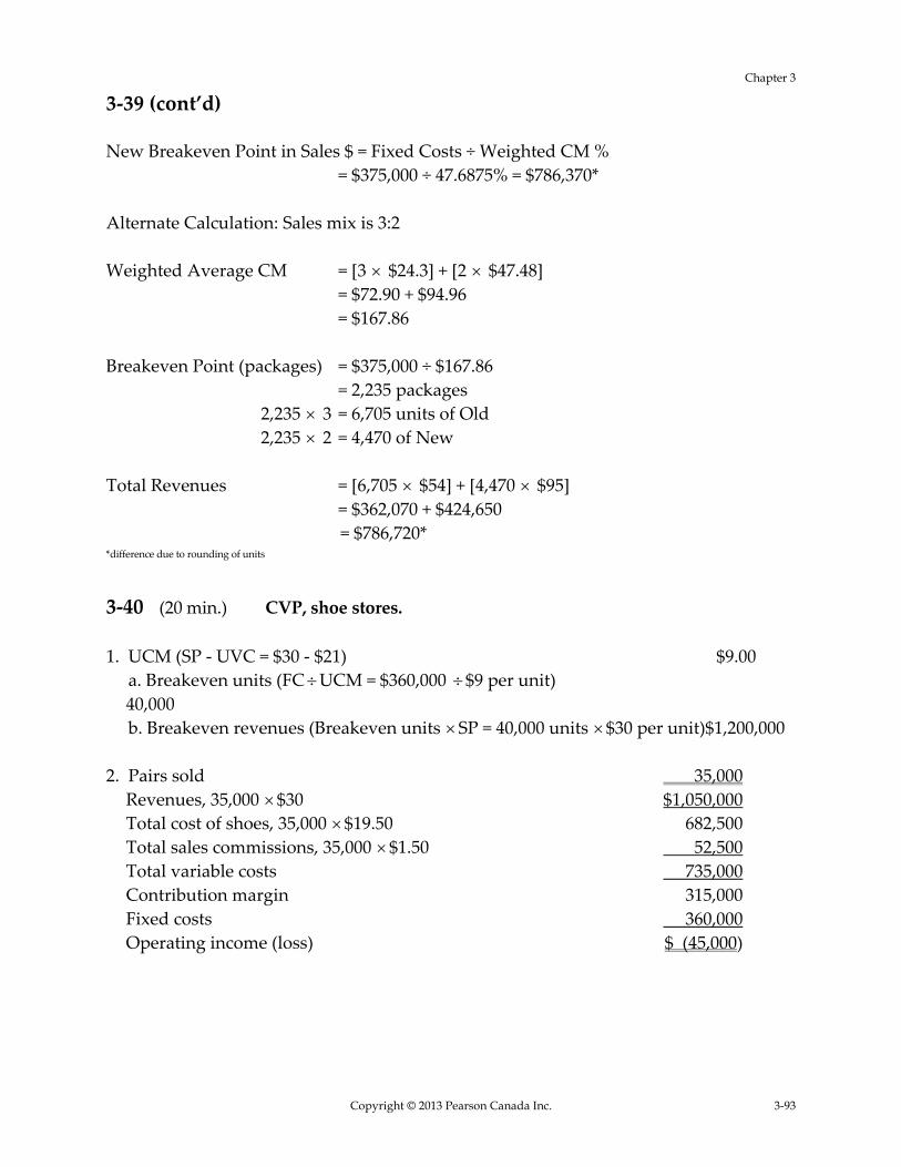
New Breakeven Point in Sales $ = Fixed Costs ÷ Weighted CM %

= $375,000 ÷ 47.6875% = $786,370*

Alternate Calculation: Sales mix is 3:2

Weighted Average CM = [3 $24.3] + [2 $47.48]

= $72.90 + $94.96

= $167.86

Breakeven Point (packages) = $375,000 ÷ $167.86

= 2,235 packages

2,235 3 = 6,705 units of Old 2,235 2 = 4,470 of New

Total Revenues = [6,705 $54] + [4,470 $95] = $362,070 + $424,650

= $786,720* *difference due to rounding of units

3‐40 (20 min.) CVP, shoe stores.

1. UCM (SP ‐ UVC = $30 ‐ $21) $9.00

a. Breakeven units (FCUCM = $360,000 $9 per unit) 40,000

b. Breakeven revenues (Breakeven units SP = 40,000 units $30 per unit)$1,200,000

2. Pairs sold 35,000

Revenues, 35,000 $30 $1,050,000

Total cost of shoes, 35,000 $19.50 682,500

Total sales commissions, 35,000 $1.50 52,500



Fixed costs 360,000

Operating income (loss) $ (45,000)



3‐40 (cont’d)

3. Unit variable data (per pair of shoes)

Selling price $ 30.00

Cost of shoes 19.50

Sales commissions 0

Variable cost per unit $ 19.50

Annual fixed costs

Rent $ 60,000

Salaries, $200,000 + $81,000 281,000

Advertising 80,000

Other fixed costs 20,000

Total fixed costs $ 441,000

UCM, $30 ‐ $19.50 $ 10.50

a. Breakeven units, $441,000$10.50 per unit 42,000

b. Breakeven revenues, 42,000 units $30 per unit $1,260,000

4. Unit variable data (per pair of shoes)

Selling price $ 30.00

Cost of shoes 19.50

Sales commissions 1.80

Variable cost per unit $ 21.30

Total fixed costs $ 360,000

UCM, $30 ‐ $21.30 $ 8.70

a. Break even units = $360,000$8.70 per unit 41,380 (rounded up)

b. Break even revenues = 41,380 units $30 per unit $1,241,400

Chapter 3


3‐40 (cont’d)

5. Pairs sold 50,000

Revenues (50,000 pairs $30 per pair) $1,500,000

Total cost of shoes (50,000 pairs $19.50 per pair) $ 975,000

Sales commissions on first 40,000 pairs (40,000 pairs $1.50 per pair) 60,000

Sales commissions on additional 10,000 pairs:

[10,000 pairs ($1.50 + $0.30 per pair)] 18,000

Total variable costs $1,053,000

Contribution margin $ 447,000

Fixed costs 360,000


Alternative approach:

Breakeven point in units = 40,000 pairs

Store manager receives commission of $0.30 on 10,000 (50,000 ‐ 40,000) pairs.

Contribution margin per pair beyond breakeven point of 10,000 pairs = $8.70 ($30 ‐ $21 ‐ $0.30) per

pair.

Operating income = 10,000 pairs $8.70 contribution margin per pair = $87,000.



3‐41 (30 min.) CVP, shoe stores (continuation of 3‐40).

Salaries + Commission Plan Higher Fixed Salaries Only

No. of

units sold

CM

per Unit CM

Fixed

Costs

Operating

Income

CM

per Unit CM

Fixed

Costs

Operating

Income

Difference in

favour of higher‐

fixed‐salary‐only

(1) (2) (3)=(1) (2) (4) (5)=(3)–(4) (6) (7)=(1) (6) (8) (9)=(7)–(8) (10)=(9)–(5)

40,000 $9.00 $360,000 $360,000 0 $10.50 $420,000 $441,000 $ (21,000) $(21,000)

42,000 9.00 378,000 360,000 18,000 10.50 441,000 441,000 0 (18,000)

44,000 9.00 396,000 360,000 36,000 10.50 462,000 441,000 21,000 (15,000)

46,000 9.00 414,000 360,000 54,000 10.50 483,000 441,000 42,000 (12,000)

48,000 9.00 432,000 360,000 72,000 10.50 504,000 441,000 63,000 (9,000)

50,000 9.00 450,000 360,000 90,000 10.50 525,000 441,000 84,000 (6,000)

52,000 9.00 468,000 360,000 108,000 10.50 546,000 441,000 105,000 (3,000)

54,000 9.00 486,000 360,000 126,000 10.50 567,000 441,000 126,000 0

56,000 9.00 504,000 360,000 144,000 10.50 588,000 441,000 147,000 3,000

58,000 9.00 522,000 360,000 162,000 10.50 609,000 441,000 168,000 6,000

60,000 9.00 540,000 360,000 180,000 10.50 630,000 441,000 189,000 9,000

62,000 9.00 558,000 360,000 198,000 10.50 651,000 441,000 210,000 12,000

64,000 9.00 576,000 360,000 216,000 10.50 672,000 441,000 231,000 15,000

66,000 9.00 594,000 360,000 234,000 10.50 693,000 441,000 252,000 18,000

Chapter 3


3‐41 (cont’d)

1. See preceding table. The new store will have the same operating income under

either compensation plan when the volume of sales is 54,000 pairs of shoes. This can

also be calculated as the unit sales level at which both compensation plans result in the

same total costs:

Let Q = unit sales level at which total costs are same for both plans:

$19.50Q + $360,000 + $81,000 = $21Q + $360,000

$1.50 Q = $81,000

Q = 54,000 pairs

2. When sales volume is above 54,000 pairs, the higher‐fixed‐salaries plan results in

lower costs and higher operating incomes than the salary‐plus‐commission plan. So, for

an expected volume of 55,000 pairs, the owner would be inclined to choose the higher‐

fixed‐salaries‐only plan. But it is likely that sales volume itself is determined by the

nature of the compensation plan. The salary‐plus‐commission plan provides a greater

motivation to the salespeople, and it may well be that for the same amount of money paid

to salespeople, the salary‐plus‐commission plan generates a higher volume of sales than

the fixed‐salary plan.

3. Let TQ = Target number of units

For the salary‐only plan:

$30.00TQ ‐ $19.50TQ ‐ $441,000 = $168,000

$10.50TQ = $609,000

TQ = $609,000 ÷ $10.50

TQ = 58,000 units

For the salary‐plus‐commission plan:

$30.00TQ ‐ $21.00TQ ‐ $360,000 = $168,000

$9.00TQ = $528,000

TQ = $528,000 ÷ $9.00

TQ = 58,667 units (rounded up)

The decision regarding the salary plan depends heavily on predictions of

demand. For instance, the salary plan offers the same operating income at 58,000 units

as the commission plan offers at 58,667 units.



3‐41 (cont’d)

4.

WalkRite Shoe Company

Operating Income Statement, 2008

Revenues (48,000 pairs $30) + (2,000 pairs $18) $1,476,000

Cost of shoes, 50,000 pairs $19.50 975,000

Commissions = Revenues 5% = $1,476,000 0.05 73,800


Fixed costs 360,000


3‐42 (30 min.) Uncertainty and expected costs.

1. Monthly Number of

Orders Cost of Current System

300,000 $1,000,000 + $40(300,000) = $13,000,000

400,000 $1,000,000 + $40(400,000) = $17,000,000

500,000 $1,000,000 + $40(500,000) = $21,000,000

600,000 $1,000,000 + $40(600,000) = $25,000,000

700,000 $1,000,000 + $40(700,000) = $29,000,000

Monthly Number of

Orders Cost of Partially Automated System

300,000 $5,000,000 + $30(300,000) = $14,000,000

400,000 $5,000,000 + $30(400,000) = $17,000,000

500,000 $5,000,000 + $30(500,000) = $20,000,000

600,000 $5,000,000 + $30(600,000) = $23,000,000

700,000 $5,000,000 + $30(700,000) = $26,000,000

Monthly Number of

Orders Cost of Fully Automated System

300,000 $10,000,000 + $20(300,000) = $16,000,000

400,000 $10,000,000 + $20(400,000) = $18,000,000

500,000 $10,000,000 + $20(500,000) = $20,000,000

600,000 $10,000,000 + $20(600,000) = $22,000,000

700,000 $10,000,000 + $20(700,000) = $24,000,000

Chapter 3


3‐42 (cont’d)

2. Current System Expected Cost:

$13,000,000 × 0.1 = $ 1,300,000

17,000,000 × 0.25 = 4,250,000

21,000,000 × 0.40 = 8,400,000

25,000,000 × 0.15 = 3,750,000

29,000,000 × 0.10 = 2,900,000

$ 20,600,000

Partially Automated System Expected Cost:

$14,000,000 × 0.1 = $ 1 ,400,000

17,000,000 × 0.25 = 4,250,000

20,000,000 × 0.40 = 8,000,000

23,000,000 × 0.15 = 3,450,000

26,000,000 × 0.10 = 2,600,000

$19,700,000

Fully Automated System Expected Cost:

$16,000,000 × 0.1 = $ 1,600,000

18,000,000 × 0.25 = 4,500,000

20,000,000 × 0.40 = 8,000,000

22,000,000 × 0.15 = 3,300,000

24,000,000 × 0.10 = 2,400,000

$19,800,000

3. Dawmart should consider the impact of the different systems on its relationship

with suppliers. The interface with Dawmart’s system may require that suppliers also

update their systems. This could cause some suppliers to raise the cost of their

merchandise. It could force other suppliers to drop out of Dawmart’s supply chain

because the cost of the system change would be prohibitive. Dawmart may also want to

consider other factors such as the reliability of different systems and the effect on

employee morale if employees have to be laid off as it automates its systems.



3‐43 (25 min.) CVP analysis, decision making.

1. Unit selling price $148

Variable manufacturing costs per unit 63

Variable marketing and distribution costs per unit 15

Contribution margin per unit $ 70

Fixed manufacturing costs $ 1,012,000

Fixed marketing and distribution costs 780,000

Total fixed costs $1,792 ,000

Breakeven point in units = Total fixed costs

Contribution margin per unit

= $1,792,000 ÷ $70

= 25,600 units

Breakeven point in revenues = 25,600 units $148 per unit = $3,788,800

2. Tocchet’s current operating income is as follows:

Revenues, $148 60,000 $8,880,000

Variable costs, $78 60,000 4,680,000

Contribution margin 4,200,000


Operating income $ 2,408,000

Let the fixed costs be $F. We calculate $F when operating income = $2,408,000 and

the selling price is $140.

($140 70,000) ‐ ($78 70,000) – $F = $2,408,000 $9,800,000 ‐ $5,460,000 – $F = $2,408,000

$F = $1,932,000

Hence the maximum increase in fixed costs for which Tocchet will prefer to reduce the

selling price is $140,000 ($1,932,000 ‐ $1,792,000).

Chapter 3


3‐43 (cont’d)

3. Let the selling price be P.

We calculate P for which, after increasing fixed manufacturing costs by $150,000 to

$1,942,000 and variable manufacturing cost per unit by $3.20 to $66.20, operating income

= $2,408,000

60,000P ‐ ($66.20 60,000) ‐ ($15 60,000) ‐ $1,942,000 = $2,408,000 60,000P ‐ $3,972,000 ‐ $900,000 ‐ $1,942,000 = $2,408,000

60,000P = $9,222,000

P = $153.70

Tocchet will consider adding the new features provided the selling price is at least

$153.70 per unit.

Proof: New CM = $153.70 ‐ $66.20 ‐ $15 = $72.50

OI = (60,000 $72.50) ‐ $1,942,000 = $2,408,000

3‐44 (20–25 min.) Sales mix, two products.

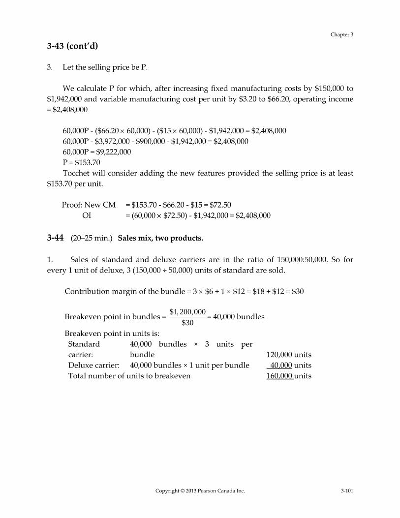
1. Sales of standard and deluxe carriers are in the ratio of 150,000:50,000. So for

every 1 unit of deluxe, 3 (150,000 ÷ 50,000) units of standard are sold.

Contribution margin of the bundle = 3 $6 + 1 $12 = $18 + $12 = $30

Breakeven point in bundles = $1,200,000

$30= 40,000 bundles

Breakeven point in units is:

Standard

carrier:

40,000 bundles × 3 units per

bundle 120,000 units

Deluxe carrier: 40,000 bundles × 1 unit per bundle 40,000 units

Total number of units to breakeven 160,000 units



3‐44 (cont’d)

Alternatively,

Let Q = Number of units of Deluxe carrier to break even

3Q = Number of units of Standard carrier to break even

Revenues – Variable costs – Fixed costs = Zero operating income

$20(3Q) + $30Q ‐ $14(3Q) ‐ $18Q ‐ $1,200,000 = 0

$60Q + $30Q ‐ $42Q ‐ $18Q = $1,200,000

$30Q = $1,200,000

Q = 40,000 units of Deluxe

3Q = 120,000 units of Standard

The breakeven point is 120,000 Standard units plus 40,000 Deluxe units, a total of

160,000 units.

2a. Unit contribution margins are: Standard: $20 ‐ $14 = $6; Deluxe: $30 ‐ $18 = $12

If only Standard carriers were sold, the breakeven point would be:

$1,200,000 $6 = 200,000 units.

2b. If only Deluxe carriers were sold, the breakeven point would be:

$1,200,000 $12 = 100,000 units 3. Operating income = Contribution margin of Standard + Contribution margin of Deluxe - Fixed costs

= 180,000($6) + 20,000($12) ‐ $1,200,000

= $1,080,000 + $240,000 ‐ $1,200,000

= $120,000

Sales of standard and deluxe carriers are in the ratio of 180,000: 20,000. So for

every 1 unit of deluxe, 9 (180,000 ÷ 20,000) units of standard are sold.

Contribution margin of the bundle = 9 $6 + 1 $12 = $54 + $12 = $66

Breakeven point in bundles = $1,200,000

$66= 18,182 bundles (rounded up)

Chapter 3


3‐44 (cont’d)

Breakeven point in units is:

Standard

carrier:

18,182 bundles × 9 units per

bundle 163,638 units

Deluxe carrier: 18,182 bundles × 1 unit per bundle 18,182 units

Total number of units to breakeven 181,820 units

Alternatively,

Let Q = Number of units of Deluxe product to break even

9Q = Number of units of Standard product to break even

$20(9Q) + $30Q ‐ $14(9Q) ‐ $18Q ‐ $1,200,000 = 0

$180Q + $30Q ‐ $126Q ‐ $18Q = $1,200,000

$66Q = $1,200,000

Q = 18,182 units of Deluxe (rounded up)

9Q = 163,638 units of Standard

The breakeven point is 163,638 Standard + 18,182 Deluxe, a total of 181,820 units.

The major lesson of this problem is that changes in the sales mix change

breakeven points and operating incomes. In this example, the budgeted and actual total

sales in number of units were identical, but the proportion of the product having the

higher contribution margin declined. Operating income suffered, falling from $300,000

to $120,000. Moreover, the breakeven point rose from 160,000 to 181,820 units.

3‐45 (15 min.) CVP, movie production.

1. Fixed costs = $22,000,000 (production cost)

Unit variable cost = (4% +4% + 8% + 8% + 12%) = 36% of revenues

Unit contribution margin = 100% ‐ 36% = 64% of revenues or $0.64 per $1

(a) Breakeven point in revenues = Fixed costs

Unit contribu tion margin per $1 revenue

= $22,000,000/$0.64

= $34,375,000

(b) Panther receives 65% of box‐office receipts.

Required box‐office receipts = $34,375,000 ÷ 0.65 = $52,884,616 (rounded)



3‐45 (cont’d)

2. Revenues, 0.65 $320,000,000 $208,000,000

Variable costs, 0.36 $208,000,000 74,880,000



Operating income $111,120,000

3‐46 (20 min.) CVP, cost structure differences, movie production (continuation of 3‐

45).

1. Contract A

Fixed costs for Contract A:

Production costs $32,000,000

Fixed salary 50,000,000

Total fixed costs $82,000,000

Unit variable cost = 8% + 8% + 18% = 34% or $0.34 per $1 revenue marketing fee

Unit contribution margin = $0.66 per $1 revenue

(a) Breakeven point in revenues =

Fixed costs

Unit contribu tion margin per $1 revenue

= $82,000,000 ÷ $0.66

= $124,242,425 (rounded)

Breakeven point in box office sales = $124,242,425 ÷ 0.65

= $191,142,192 (rounded)

Chapter 3


3‐46 (cont’d)

Contract B

Fixed costs for Contract B:

Production costs $32,000,000

Fixed salary 8,000,000

Total fixed costs $40,000,000

Unit variable cost = $0.18 per $1 revenue fee to Parimont Productions

[3%+3%+8%+8%] $0.22 per $1 revenue residual to directors/actors

$0.40 per $1 revenue

Unit contribution margin = $0.60 per $1 revenue

Breakeven point in revenues = $40,000,000/$0.60 = $66,666,667 (rounded)

Breakeven point in box office sales = $66,666,667/0.65

= $102,564,103 (rounded)

Difference in Breakeven Points

Contract A has a higher fixed cost and a lower variable cost per sales dollar. In

contrast, Contract B has a lower fixed cost and a higher variable cost per sales dollar. In

Contract B, there is more risk‐sharing between Panther and the actors that lowers the

breakeven point, but results in Panther receiving less operating income if the film is a

mega‐success.

2.

Contract A:

Revenues, 0.65 $280,000,000 $182,000,000

Variable costs, 0.34 $182,000,000 61,880,000




Contract B:

Revenues, 0.65 $280,000,000 $182,000,000

Variable costs, 0.4 $182,000,000 72,800,000






3‐46 (cont’d)

Contract A has a higher breakeven point than Contract B, because it has a higher

level of fixed costs and a lower unit contribution margin. This means after breakeven is

reached, under Contract A, $0.66 of every additional revenue dollar will contribute to OI,

but under Contract B only $0.60 of every additional revenue dollar will contribute to OI.

However, the fixed costs for Contract A are significantly higher than for Contract B.

At the predicted level of box office receipts, Contract B is the more lucrative contract.

The point of indifference (in terms of revenue to Panther) (not required in question)

($1.00R ‐ $0.34R) ‐ $82,000,000 = ($1.00R ‐ $0.40R) ‐ $40,000,000

$0.66R ‐ $0.60R = $42,000,000

R = $700,000,000

It seems highly unlikely the film will gross enough box office receipts to generate

$700 million of revenue to Panther. Panther should select Contract B.

3‐47 (30 min.) Multi‐product breakeven, decision making.

1. Unit CM = USP ‐ UVC = $600 ‐ $210 ‐ $60 = $330

Breakeven point in 2011 (units) = Fixed Costs ÷ Unit CM

= $2,574,000 ÷ $330

= 7,800 units

Breakeven point in 2011 (in revenues) = 7,800 units $600 = $4,680,000 in sales revenues or CM % = UCM ÷ USP = $330 ÷ $600 = 55%

Breakeven point in 2011 in revenues = $2,574,000 ÷ 55% = $4,680,000

Chapter 3


3‐47 (cont’d)

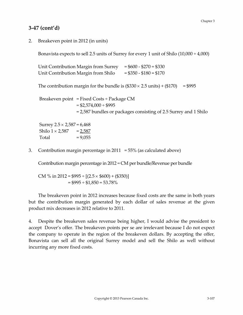
2. Breakeven point in 2012 (in units)

Bonavista expects to sell 2.5 units of Surrey for every 1 unit of Shilo (10,000 ÷ 4,000)

Unit Contribution Margin from Surrey = $600 ‐ $270 = $330

Unit Contribution Margin from Shilo = $350 ‐ $180 = $170

The contribution margin for the bundle is ($330 2.5 units) + ($170) = $995

Breakeven point = Fixed Costs ÷ Package CM

= $2,574,000 ÷ $995

= 2,587 bundles or packages consisting of 2.5 Surrey and 1 Shilo

Surrey 2.5 2,587 = 6,468 Shilo 1 2,587 = 2,587

Total = 9,055

3. Contribution margin percentage in 2011 = 55% (as calculated above)

Contribution margin percentage in 2012 = CM per bundle/Revenue per bundle

CM % in 2012 = $995 ÷ [(2.5 $600) + ($350)] = $995 ÷ $1,850 = 53.78%

The breakeven point in 2012 increases because fixed costs are the same in both years

but the contribution margin generated by each dollar of sales revenue at the given

product mix decreases in 2012 relative to 2011.

4. Despite the breakeven sales revenue being higher, I would advise the president to

accept Dover’s offer. The breakeven points per se are irrelevant because I do not expect

the company to operate in the region of the breakeven dollars. By accepting the offer,

Bonavista can sell all the original Surrey model and sell the Shilo as well without

incurring any more fixed costs.



3‐47 (cont’d)

Profits in 2012 with and without Shilo are expected to be as follows:

Surrey Shilo Total

Selling Price $600 $350

Units 10,000

4,000 14,000

Total Sales $6,000,000 $1,400,000 $7,400,000

Variable

Costs $2,700,000 $720,000 $3,420,000

CM $3,300,000 $680,000 $3,980,000

Fixed Costs $ 2,574,000 $ – $2,574,000

OI $ 726,000 $ 680,000 $ 1,406,000

Chapter 3


3‐48 (30 min.) Choosing between compensation plans, operating leverage.

1. We can recast Marston’s income statement to emphasize contribution margin,

and then use it to compute the required CVP parameters.

Marston Corporation

Income Statement

For the Year Ended December 31, 2011

Using Sales Agents Using Own Sales Force

Revenues $26,000,000 $26,000,000

Variable Costs

Cost of goods sold—variable $11,700,000 $11,700,000

Marketing commissions 4,680,000 16,380,000 2,600,000 14,300,000

Contribution margin $9,620,000 $11,700,000

Fixed Costs

Cost of goods sold—fixed 2,870,000 2,870,000

Marketing—fixed 3,420,000 6,290,000 5,500,000 8,370,000

Operating income $3,330,000 $ 3,330,000

Contribution margin

percentage

($9,620,00026,000,000; $11,700,000$26,000,000)

37% 45%

Breakeven revenues

($6,290,0000.37; $8,370,0000.45) $17,000,000 $18,600,000

Degree of operating leverage

($9,620,000$3,330,000; $11,700,000$3,330,000)

2.89

3.51



3‐48 (cont’d)

2. The calculations indicate that at sales of $26,000,000, a percentage change in sales

and contribution margin will result in 2.89 times that percentage change in operating

income if Marston continues to use sales agents and 3.51 times that percentage change

in operating income if Marston employs its own sales staff. The higher contribution

margin per dollar of sales and higher fixed costs gives Marston more operating

leverage, that is, greater benefits (increases in operating income) if revenues increase

but greater risks (decreases in operating income) if revenues decrease. Marston also

needs to consider the skill levels and incentives under the two alternatives. Sales agents

have more incentive compensation and hence may be more motivated to increase sales.

On the other hand, Marston’s own sales force may be more knowledgeable and skilled

in selling the company’s products. That is, the sales volume itself will be affected by

who sells and by the nature of the compensation plan.

3. Variable costs of marketing = 15% of Revenues

Fixed marketing costs = $5,500,000

Operating income = Revenues costs manuf.Variable costs manuf.

Fixed costs

marketingVariable

costs

marketingFixed

Denote the revenues required to earn $3,330,000 of operating income by R, then:

R ‐ 0.45R ‐ $2,870,000 ‐ 0.15R ‐ $5,500,000 = $3,330,000

R ‐ 0.45R ‐ 0.15R = $3,330,000 + $2,870,000 + $5,500,0

0.40R = $11,700,000

R = $11,700,000 0.40 = $29,250,000

Chapter 3


3‐49 (20‐25 min.) Special‐order decision.

1. Time spent on manufacturing bottles = 750,000 bottles ÷ 100 bottles per hour = 7,500

hours

So 10,000 ‐ 7,500 = 2,500 hours available for toys.

Moulded plastic toy requires: 100,000 units ÷ 40 units per hour = 2,500 hours, so

MPC has enough capacity to accept the toys order. Additional income from accepting the

order is:

Revenue $3.40 100,000 $340,000

Variable costs 2.70 100,000 270,000


Fixed costs 24,000

Additional income $ 46,000

So MPC should accept the order since it has enough excess capacity to make the

100,000 toys.

2. Time spent on manufacturing bottles = 850,000 ÷ 100= 8,500 hours


From requirement 1, the moulded plastic toy requires 2,500 hours and generates

$46,000 in operating income.

So if the toy offer is accepted, 1,000 hours (2,500 hours required ‐ 1,500 hours

available) of bottle making will be forgone, equal to 100,000 bottles (100 bottles/hr. 1,000 hrs.):

Operating income from accepting $46,000

Forgone contribution margin (100,000 bottles $0.30)* 30,000

Increase in operating income $16,000

So MPC should accept the special order.

*CM = $0.55 ‐ $0.25 = $0.30



3‐49 (cont’d)

Without considering the fixed costs for the toy mould, the contribution per

machine‐hour of the constrained resource for bottles and the special toy are as follows:

Bottles Toys

Contribution margin per unit $0.30 $0.70

Multiplied by units made in 1 machine‐hour 100 40

Contribution margin per machine‐hour $30 $ 28

This suggests that MPC should make as many bottles as it can rather than the

special toys, because bottles generate a higher contribution margin per machine‐hour.

So if MPC used the 1,500 hours available to it for making toys after using the 8,500

hours to make bottles, it would be able to make 1,500 40 = 60,000 toys and earn operating income of:

Contribution margin 60,000 $0.70 $42,000

Fixed mould costs 24,000

Increase in operating income $18,000

The contribution margin earned covers the fixed costs of the mould, so MPC should

make 850,000 bottles and 60,000 toys.

3. Time spent on manufacturing bottles = 900,000 ÷ 100 = 9,000 hours


So if the toy offer is accepted, then 1,500 hours (2,500 hours required ‐ 1,000 hours

available) of bottle capacity will be forgone = 150,000 bottles

Contribution from accepting toy offer $ 46,000

Forgone profits on bottles 150,000 $0.30 (45,000)

Increase (decrease) in operating income $ 1,000

So accept the special order.

Chapter 3


3‐50 (25 min.) CVP, sensitivity analysis.

Contribution margin per corkscrew = $4 ‐ 3 = $1

Fixed costs = $6,000

Units sold = Total sales ÷ Selling price = $40,000 ÷ $4 per corkscrew = 10,000 corkscrews

1. Sales increase 10%

Sales revenues 10,000 1.10 $4.00 $44,000

Variable costs 10,000 1.10 $3.00 33,000


Fixed costs 6,000


2. Increase fixed costs $2,000; Increase sales 50%

Sales revenues 10,000 1.50 $4.00 $60,000

Variable costs 10,000 1.50 $3.00 45,000


Fixed costs ($6,000 + $2,000) 8,000


3. Increase selling price to $5.00; Sales decrease 20%

Sales revenues 10,000 0.80 $5.00 $40,000

Variable costs 10,000 0.80 $3.00 24,000


Fixed costs 6,000

Operating income $10,000

4. Increase selling price to $6.00; Variable costs increase $1 per corkscrew

Sales revenues 10,000 $6.00 $60,000

Variable costs 10,000 $4.00 40,000


Fixed costs 6,000

Operating income $14,000

Alternative 4 yields the highest operating income. If TOP is confident that unit sales

will not decrease despite increasing the selling price, it should choose alternative 4.



3‐51 (15‐25 min.) Nonprofit institution.

1. Let Q = Number of visits

Revenues ‐ Variable costs ‐ Fixed costs = 0

$850,000 ‐ $16Q ‐ $500,000 = 0

$16Q = $350,000

Q = 21,875 visits

Revenues ‐ Variable costs ‐ Fixed costs = 0

$765,000 ‐ $16Q ‐ $500,000 = 0

$16Q = $265,000

Q = 16,562 visits

The reduction in service is more than the 10% reduction in the budget. Without

restructuring operations, the quantity of service units must be reduced by 24.29% [(21,875

‐ 16,562) ÷ 21,875] to stay within the budget.

3. Let V = Variable cost per visit

$765,000 ‐ 21,875V ‐ $500,000 = 0

21,875V = $265,000

V = $12.11 ($12.114285)*

Percentage drop: ($16 ‐ $12.114285*) ÷ $16 = 24.29%

Regarding requirements 2 and 3, note that the decrease in service can be measured by a

formula:

% reduction in service = (% budget change) ÷ (% variable cost)

The variable cost percentage is ($16 21,875) ÷ $850,000 = $350,000 ÷ $850,000 = 41.1765%*

% reduction in service = 10% ÷ 41.1765% = 24.29%

*The extra decimal places are used to minimize the rounding difference. Most will

round to two decimals for the money and to 24%.

Chapter 3


3‐52 (30 min.) CVP, nonprofit event planning.

1. Computation of fixed costs.

Hotel University

Rental cost of venue $2,700 $ 7,000

Permits 0 500

Chamber administration/marketing 5,000 5,000

Entertainment 4,000 4,000

$11,700 $16,500

Computation of contribution margin per person:

Hotel University

Selling (ticket) price per person $175 $175

Catering cost per person 110 75

Contribution margin per person $65 $100



Breakeven point for Hotel venue = $11,700 ÷ $65 = 180 tickets

Breakeven point for University venue = $16,500 ÷ $100 = 165 tickets

2. Operating Income Projections with 100 attendees and 250 attendees

Hotel

Attendees 100 250

Ticket Price $175 $175

Total Revenues $17,500 $43,750

VC @ $110 11,000 27,500

CM 6,500 16,250

Fixed Costs 11,700 11,700

Operating Income $(5,200) $4,550

University

Attendees 100 250

Ticket Price $175 $175

Total Revenues $17,500 $43,750

VC @ $75 7,500 18,750

CM 10,000 25,000


Operating Income $(6,500) $8,500



3‐52 (cont’d)

The Hotel venue has higher variable costs per person and lower fixed costs. In

contrast, the University venue has lower variable costs per person and higher fixed costs.

3. Requirement 2 gives the operating income equation for each venue. Setting these

two equations equal and solving for Q gives the level of ticket sales at which the

operating incomes for the two venues are equal:

$175Q ‐ $110Q ‐ $11,700 = $175Q ‐ $75Q ‐ $16,500

$100Q ‐ $65Q = $16,500 ‐ $11,700

$35Q = $4,800

Q = 137 (rounded)

Proof:

Hotel University

Attendees 137.14286 137.14286

Ticket Price 175 175

Total Revenues 24,000 24,000

VC @ $110; $75 15,086 10,286

CM 8,914 13,714


Operating Income (2,786) (2,786)

Above 137, the University venue will yield higher operating income (or a lower

operating loss) than the hotel venue.

Chapter 3


3‐53 (20‐30 min.) CVP under uncertainty.

1. (a) At a selling price of $120, the unit contribution margin is ($120 ‐ $60) = $60, and

it will require the sale of ($240,000 ÷ $60) = 4,000 units to break even. The sales in dollars

are $480,000 and there is a 2/3 probability of equaling or exceeding this sales level—that

is, that 2/3 of the area under the graph exists between $480,000 and $720,000.

(b) At a selling price of $84, the unit contribution margin is ($84 ‐ $60) = $24, and it

will require the sale of ($240,000 ÷ $24) = 10,000 units to break even. At the lower price,

the sales in dollars are $840,000 and there is a 2/3 probability of equaling or exceeding this

sales volume.

Therefore, if you seek to maximize the probability of showing an operating income,

you are indifferent between the two strategies.

2.

Expected ExpectedSelling Variable Fixedoperating sales price per unit cost per unit costsincome level

At a selling price of $120:

Expected revenues = $540,000 ($120 4,500) Expected operating income = [($120 ‐ $60) 4,500] ‐ $240,000

= $30,000

At a selling price of $84:

Expected revenues = $900,000 ($84 10,715) Expected operating income = [($84 ‐ $60) 10,715] ‐ $240,000 = $17,160

A selling price of $120 will maximize the expected operating income.



3‐54 (30 min.) Governance, CVP analysis.

1. Contribution margin percentage = Revenues – Variable costs

Revenues

= ($8,000,000 ‐ $4,320,000) ÷ $8,000,000

= $3,680,000 ÷ $8,000,000

= 46%

Breakeven revenues = Fixed Costs/CM Percentage

= $3,900,000 ÷ .46 = $8,478,261 (rounded)

2. If variable costs are 48% of revenues, CM percentage equals 52% (100% ‐ 48%).

Breakeven revenues = Fixed costs

Contribu tion margin percentage

= $3,900,000 ÷ .52 = $7,500,000

3. Revenues $8,000,000

Variable costs (0.48 $8,000,000) 3,840,000



4. Incorrect reporting of environmental costs with the goal of continuing operations is

unethical.

The management accountant could consider the following issues:

Competence

Clear reports using relevant and reliable information should be prepared. Preparing

reports on the basis of incorrect environmental costs in order to make the company’s

performance look better than it is violates competence standards. It is unethical for

Walton not to report environmental costs in order to make the plant’s performance look

good.

Integrity

The management accountant has a responsibility to avoid actual or apparent

conflicts of interest and advise all appropriate parties of any potential conflict. Walton

may be tempted to report lower environmental costs to please Bell and Klein and save

the jobs of her colleagues. This action, however, violates the responsibility for integrity.

Chapter 3


3‐54 (cont’d)

Objectivity

The management accountant should require that information should be fairly and

objectively communicated and that all relevant information should be disclosed. From a

management accountant’s standpoint, underreporting environmental costs to make

performance look good would violate the standard of objectivity.

Walton should indicate to Bell that estimates of environmental costs and liabilities

should be included in the analysis. If Bell still insists on modifying the numbers and

reporting lower environmental costs, Walton should raise the matter with one of Bell’s

superiors. If, after taking all these steps, there is continued pressure to understate

environmental costs, Walton should consider resigning from the company and not

engage in unethical behaviour.

Walton can also argue the sustainability issue, that is, companies should act with a

view to sustainable operations, from all perspectives, environmental, social responsibility,

and economic.

3‐55 (20‐25 min.) Governance, CVP, cost analysis.

1. (a) USP = $68

UVC = $28.50 ($19.25 + $9.25)

UCM = $39.50

FC = $25,000,000

Q = FC ÷ UCM

= $25,000,000 ÷ $39.50

= 632,912 monthly treatments (rounded up)

(b) USP = $68

UVC = $19.25

UCM = $48.75

FC = $25,000,000

Q = FC ÷ UCM

= $25,000,000 ÷ $48.75

= 512,821 monthly treatments (rounded up)



3‐55 (cont’d)

2. Diba believes that the $9.25 per monthly visit should be included in the variable

costs per visit. His argument is that a product like “Vital Hair” has a positive probability

of attracting product litigation. By excluding any allowance for the possible event, the

assumption is that it will be zero.

Diba faces an integrity issue. His report to the Executive Committee will understate

his expected cost estimates when he takes Kelly’s advice.

One possibility Diba should have explored is reporting the $19.25 per treatment

variable cost in the breakeven computations as well as including qualifications in the

report about possible product litigation costs.

3. Diba likely has been placed in a compromised situation. He may feel Kelly

deliberately set him up to avoid the $9.25 amount being reported to the Executive

Committee. At a minimum, he should directly confront Kelly with his concerns. If she is

unresponsive, he faces a very tough dilemma. His options are:

(a) Stay in his current position and be more determined next time to have his concerns

registered.

(b) Report his concerns to Kelly’s immediate superior.

(c) Resign.

If he selects (a), it would be useful to show Kelly the Code of Professional Ethics and

stress how her behaviour has put him in a difficult ethical situation.

Chapter 3


3‐56 (35 min.) Deciding where to produce.

Peona Modine

Selling price $150.00 $150.00

Variable cost per unit

Manufacturing $72.00 $88.00

Marketing and distribution 14.00 86.00 14.00 102.00

Contribution margin per unit (CMU) 64.00 48.00

Fixed costs per unit

Manufacturing 30.00 15.00

Marketing and distribution 19.00 49.00 14.50 29.50

Operating income per unit $ 15.00 $ 18.50

CMU of normal production $64 $48

CMU of overtime production

($64 – $3; $48 – $8) 61 40

1.

Annual fixed costs:

P ‐ ($49.00 400 units 240 days) M ‐ ($29.50 320 units 240 days) $4,704,000 $2,265,600

Breakeven volume:

P ‐ ($4,704,000 $64) M ‐ ($2,265,600 $48)

73,500 units

47,200 Units

2.

Units produced and sold 96,000 96,000

Normal annual volume (units)

(400 × 240; 320 × 240) 96,000 76,800

Units over normal volume (overtime) 0 19,200

CM from normal production units

(normal annual volume CMU normal

production)

(96,000 × $64; 76,800 × $48) $6,144,000 $3,686,400

CM from overtime production units

(0; 19,200 $40) 0 768,000

Total contribution margin 6,144,000 4,454,400

Total fixed costs 4,704,000 2,265,600

Operating income $1,440,000 $2,188,800

Total operating income $3,628,800



3‐56 (cont’d)

3. The optimal production plan is to produce 120,000 units at the Peona plant and

72,000 units at the Modine plant. The full capacity of the Peona plant, 120,000 units (400

units × 300 days), should be used because the contribution from these units is higher at

all levels of production than is the contribution from units produced at the Modine

plant.

Contribution margin per plant:

Peona, 96,000 × $64 $ 6,144,000

Peona 24,000 × ($64 ‐ $3) 1,464,000

Modine, 72,000 × $48 3,456,000

Total contribution margin 11,064,000

Deduct total fixed costs 6,969,600

Operating income $ 4,094,400

The contribution margin is higher when 120,000 units are produced at the Peona

plant and 72,000 units at the Modine plant. As a result, operating income will also be

higher in this case since total fixed costs for the division remain unchanged regardless

of the quantity produced at each plant.

COLLABORATIVE LEARNING PROBLEM

3‐57 (25 Min.) (CVP analysis and revenue mix)

1. Let A = Number of units of A to break even

5A = Number of units of B to break even

4A = Number of units of C to break even

$3.60A + $2.40(5A) + $1.20(4A) ‐ $306,000 = 0

A = 15,000 units of A

5A = 75,000 units of B

4A = 60,000 units of C

Total = 150,000 units

Chapter 3


3‐57 (cont’d)

2. Contribution margin:

A: 20,000 � $3.60 = $72,000

B: 100,000 � $2.40 = $240,000

C: 80,000 � $1.20 = $96,000

$408,000


3. Contribution margin:

A: 20,000 � $3.60 = $72,000

B: 80,000 � $2.40 = $192,000

C: 100,000 � $1.20 = $120,000

$384,000


Let A = Number of units of A to break even

4A = Number of units of B to break even

5A = Number of units of C to break even

$3.60A + $2.40(4A) + $1.20(5A) ‐ $306,000 = 0

A = 15,938 units of A

5A = 63,752 units of B

4A = 79,690 units of C

Total = 159,380 units

Imprinting Costs Total Variable Costs Revenues Variable Costs Contribution Margin Setups Product...

Documents

Transcript of Imprinting Costs Total Variable Costs Revenues Variable Costs Contribution Margin Setups Product...