applied sciences

Article

Comparison of Traffic Flow Models with Real Traffic DataBased on a Quantitative Assessment

Aleksandra Romanowska * and Kazimierz Jamroz

Citation: Romanowska, A.; Jamroz,

K. Comparison of Traffic Flow Models

with Real Traffic Data Based on a

Quantitative Assessment. Appl. Sci.

2021, 11, 9914. https://doi.org/

10.3390/app11219914

Academic Editor: Sehyun Tak

Received: 23 September 2021

Accepted: 20 October 2021

Published: 23 October 2021

Publisher’s Note: MDPI stays neutral

with regard to jurisdictional claims in

published maps and institutional affil-

iations.

Copyright: © 2021 by the authors.

Licensee MDPI, Basel, Switzerland.

This article is an open access article

distributed under the terms and

conditions of the Creative Commons

Attribution (CC BY) license (https://

creativecommons.org/licenses/by/

4.0/).

Faculty of Civil and Environmental Engineering, Gdansk University of Technology, 11/12 Narutowicza Str.,80-233 Gdansk, Poland; kjamroz@pg.edu.pl* Correspondence: aleksandra.romanowska@pg.edu.pl

Abstract: The fundamental relationship of traffic flow and bivariate relations between speed andflow, speed and density, and flow and density are of great importance in transportation engineering.Fundamental relationship models may be applied to assess and forecast traffic conditions at uninter-rupted traffic flow facilities. The objective of the article was to analyze and compare existing modelsof the fundamental relationship. To that end, we proposed a universal and quantitative method forassessing models of the fundamental relationship based on real traffic data from a Polish expressway.The proposed methodology seeks to address the problem of finding the best deterministic modelto describe the empirical relationship between fundamental traffic flow parameters: average speed,flow, and density based on simple and transparent criteria. Both single and multi-regime modelswere considered: a total of 17 models. For the given data, the results helped to identify the bestperforming models that meet the boundary conditions and ensure simplicity, empirical accuracy, andgood estimation of traffic flow parameters.

Keywords: traffic flow models; fundamental relationship of traffic flow; uninterrupted traffic flow;traffic conditions analysis; single-regime models; multi-regime models

1. Introduction

Traffic flow models describe vehicle flows using three basic parameters: average speed(v), density (k), and flow (q). When traffic flow is considered a stationary phenomenon,the parameters are linked with one another using a relationship (1), which is known as thefundamental relationship.

q = kv (1)

The relationship (1) and bivariate relations between speed and flow, speed and density,and flow and density are of great importance in transportation engineering. They are usedin planning, design and redesign, operation, and control of transportation facilities; theyhelp to determine the actual capacity of an existing road, assess its traffic conditions orselect the cross-section for a new road depending on forecasted traffic volumes.

The relations between speed, flow, and density have been proved empirically in manystudies over the last nine decades, starting from Greenshields in the 1930s [1]. Since then,researchers have been exploring ways to offer the best possible mathematical descriptionof the relations. Historically, these were established either empirically by looking formathematical models that fit the observed data or derived from microscopic traffic flowcharacteristics or from the analogy to the movement of fluid. The models proposed in theliterature are predominantly deterministic and describe the average behavior of a trafficstream. The output of the model is fully determined by the initial conditions and theparameters. Since they are simple to use, interpret, and determine traffic characteristics,the models have a wide variety of applications, including methods for forecasting andassessing traffic conditions.

In 1995, Castillo and Benitez [2] concluded that while the literature includes a numberof proposed solutions, a mathematical deterministic model still has not been found to

Appl. Sci. 2021, 11, 9914. https://doi.org/10.3390/app11219914 https://www.mdpi.com/journal/applsci

Appl. Sci. 2021, 11, 9914 2 of 19

give a sufficiently good description of the fundamental relationship for all facility typesand ranges of traffic density. Later literature studies also suggest that the problem is stillopen [3,4]. Similarly, it is not clear from the literature, which of the existing models can beperceived as the best and what the criteria would be. The latter are not commonly agreed,and even if used, the assessment or benchmarking of the models is often a subjectivematter.

The problem of selecting traffic flow model has practical implications. The modelsrepresenting the relationship between speed, flow, and density serve as a basis for trafficconditions forecasts and assessments such as in the case of United States’ HCM [5] orGermany’s HBS [6]. Thus, it was also one of the problems to be solved in the context ofthe recent development of a new Polish method for highway capacity analyses. How tochoose the right model for this purpose? What expectations should be given? How toassess whether the model performs well or not? These questions motivated us to the workpresented in the paper.

The main objective of the article is to review and compare existing models of thefundamental relationship using empirical data from Polish roads. In particular, the articleaims to: (1) Identify the criteria to be met by a good model of the fundamental relationship;(2) Develop a transparent and quantitative method for assessing fundamental relationshipmodels based on identified criteria; (3) Assess, compare, and rank the existing models ofthe fundamental relationship.

The paper is organized as follows: Section 2 gives an overview of deterministic math-ematical models of the fundamental relationship and criteria and methods for assessingthem. Section 3 discusses the proposed methodology for assessing models of the funda-mental relationship. Section 4 presents an application of the methodology for field data.The results are discussed in Section 5.

2. Theoretical Background2.1. Modeling Equilibrium Traffic Flow Relationships

Fundamental relationship models are divided into single-regime and multi-regimemodels, depending on how traffic conditions are described. Single-regime models describethe relationship using a single mathematical function for an entire range of traffic conditions.Multi-regime models use two or more mathematical functions for this purpose, eachrepresenting different conditions of traffic.

An important feature of speed–flow–density relationships is the presence of character-istic, boundary values of the particular relations (boundary points, extremes, and points ofinflection):

• Boundary points: free flow speed (vsw) occurs theoretically when volume and densityapproach zero (k→ 0 , q→ 0); maximal density (kmax) occurs when flow and speedapproach zero (q→ 0 , v→ 0);

• Extremes and points of inflection of the function: maximal flow (qmax) and the corre-sponding optimal speed (vopt) and optimal density (kopt).

The values of these parameters define the particular traffic regimes: free-flow con-ditions when density increases, flow rises from zero until the maximal value is reached(q→ qmax ), and speed decreases from the maximal value (vsw) until the optimal value isreached (v→ vopt ); congested conditions when density keeps increasing until it reachesthe maximal value (k→ kmax ), causing speed and flow to decrease to zero (v→ 0 , q→ 0).The characteristics helps to identify the boundary values of the fundamental relationship(further referred to as BC1 and BC2): (a) at zero density, the speed is equal to the freeflow speed, (b) at maximum density (jam density), the speed is zero. These conditions arereferred to as static properties of traffic flow [2].

Appl. Sci. 2021, 11, 9914 3 of 19

2.1.1. Single-Regime Traffic Flow Models

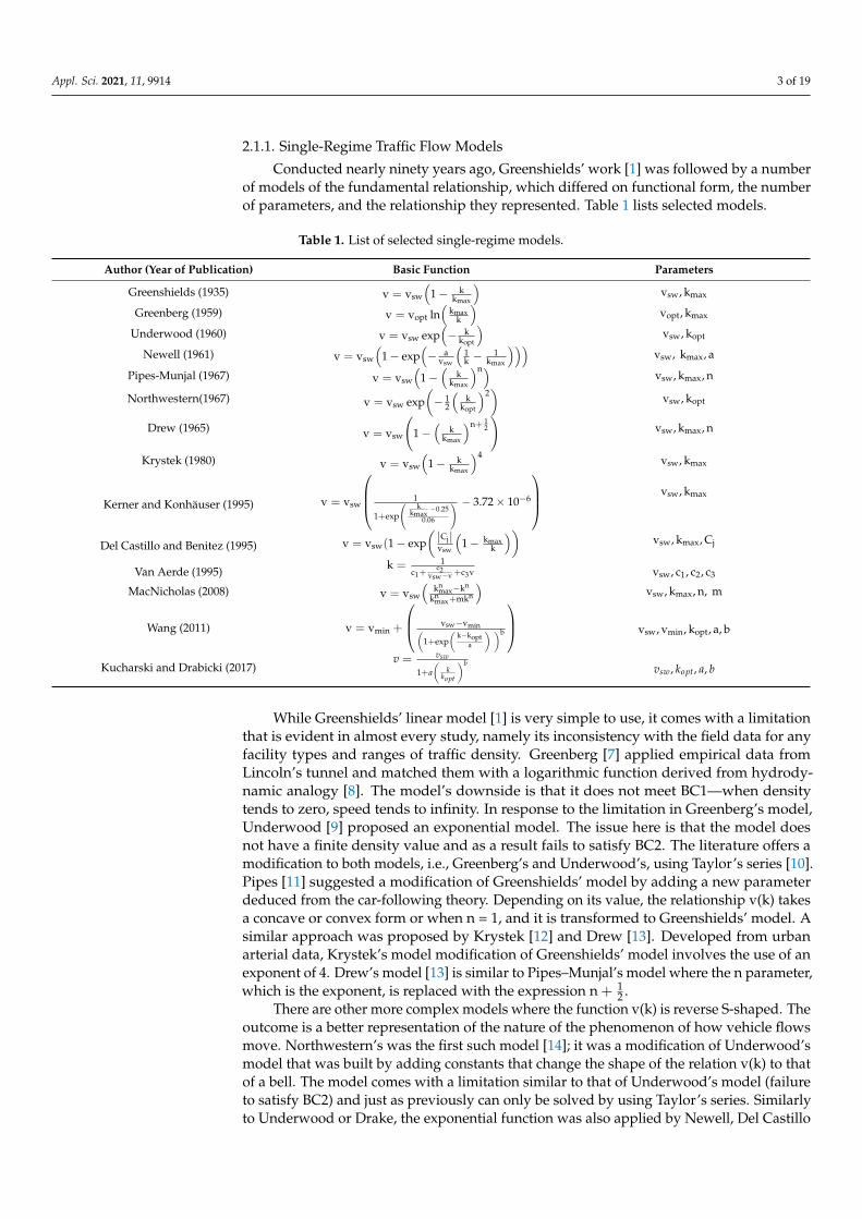
Conducted nearly ninety years ago, Greenshields’ work [1] was followed by a numberof models of the fundamental relationship, which differed on functional form, the numberof parameters, and the relationship they represented. Table 1 lists selected models.

Table 1. List of selected single-regime models.

Author (Year of Publication) Basic Function Parameters

Greenshields (1935) v = vsw

(1− k

kmax

)vsw, kmax

Greenberg (1959) v = vopt ln(

kmaxk

)vopt, kmax

Underwood (1960) v = vsw exp(− k

kopt

)vsw, kopt

Newell (1961) v = vsw

(1− exp

(− a

vsw

(1k −

1kmax

)))vsw, kmax, a

Pipes-Munjal (1967) v = vsw

(1−

(k

kmax

)n)vsw, kmax, n

Northwestern(1967) v = vsw exp(− 1

2

(k

kopt

)2)

vsw, kopt

Drew (1965) v = vsw

(1−

(k

kmax

)n+ 12

)vsw, kmax, n

Krystek (1980) v = vsw

(1− k

kmax

)4 vsw, kmax

Kerner and Konhäuser (1995) v = vsw

1

1+exp

( kkmax

−0.250.06

) − 3.72× 10−6

vsw, kmax

Del Castillo and Benitez (1995) v = vsw(1− exp(|Cj|vsw

(1− kmax

k

))vsw, kmax, Cj

Van Aerde (1995) k = 1c1+

c2vsw−v +c3v vsw, c1, c2, c3

MacNicholas (2008) v = vsw

(kn

max−kn

knmax+mkn

)vsw, kmax, n, m

Wang (2011) v = vmin +

vsw−vmin(1+exp

(k−kopt

a

) )b

vsw, vmin, kopt, a, b

Kucharski and Drabicki (2017)v = vsw

1+a(

kkopt

)bvsw, kopt, a, b

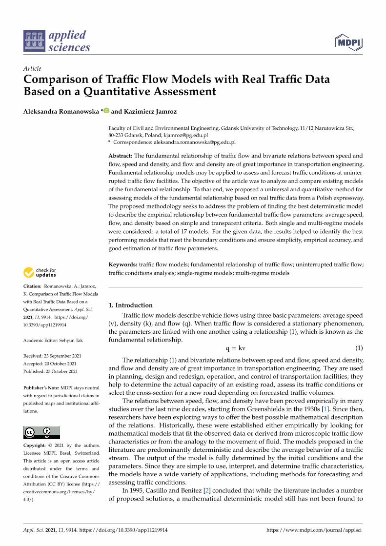
While Greenshields’ linear model [1] is very simple to use, it comes with a limitationthat is evident in almost every study, namely its inconsistency with the field data for anyfacility types and ranges of traffic density. Greenberg [7] applied empirical data fromLincoln’s tunnel and matched them with a logarithmic function derived from hydrody-namic analogy [8]. The model’s downside is that it does not meet BC1—when densitytends to zero, speed tends to infinity. In response to the limitation in Greenberg’s model,Underwood [9] proposed an exponential model. The issue here is that the model doesnot have a finite density value and as a result fails to satisfy BC2. The literature offers amodification to both models, i.e., Greenberg’s and Underwood’s, using Taylor’s series [10].Pipes [11] suggested a modification of Greenshields’ model by adding a new parameterdeduced from the car-following theory. Depending on its value, the relationship v(k) takesa concave or convex form or when n = 1, and it is transformed to Greenshields’ model. Asimilar approach was proposed by Krystek [12] and Drew [13]. Developed from urbanarterial data, Krystek’s model modification of Greenshields’ model involves the use of anexponent of 4. Drew’s model [13] is similar to Pipes–Munjal’s model where the n parameter,which is the exponent, is replaced with the expression n + 1

2 .There are other more complex models where the function v(k) is reverse S-shaped. The

outcome is a better representation of the nature of the phenomenon of how vehicle flowsmove. Northwestern’s was the first such model [14]; it was a modification of Underwood’smodel that was built by adding constants that change the shape of the relation v(k) to thatof a bell. The model comes with a limitation similar to that of Underwood’s model (failureto satisfy BC2) and just as previously can only be solved by using Taylor’s series. Similarlyto Underwood or Drake, the exponential function was also applied by Newell, Del Castillo

Appl. Sci. 2021, 11, 9914 4 of 19

and Benitez [2], and Kerner and Konhäuser [15]. Newell’s exponential model, similarlyto Pipes’ model, was deduced from the car-following theory. The model satisfies bothBC1 and BC2. Speed in the model falls rapidly as density increases, which is considered alimitation [4]. Del Castillo and Benitez [2] assumed that vehicle flow is strongly affected bythe parameter of kinematic wave speed at jam density Cj—the parameter was includedin the model. Kerner and Konhäuser [15] proposed a model based on two parametersextended by three constant numerical values that cannot be interpreted in terms of physicalparameters and may be seen as a downside. Van Aerde’s model [16] was derived from amicroscopic model of following the leader and combines Pipes’ and Greenshields’ modelinto a single-regime model [17]. The advantage of the model is that it ensures a goodmatch to data for a wide variety of facility types and for entire ranges of densities. Itsdisadvantage is that it is computationally complex (c1, c2, c3 are parameters that mustbe determined), and variable k is used as a dependent variable, which makes the modelinconvenient to use [18]. MacNicholas [18] offered a simpler alternative to Van Aerde’smodel. His own model reported comparable empirical accuracy to Van Aerde’s model.Wang [4] proposed using the logistic function to describe the relationship v = f(k). Heassumed that even when traffic is very dense, vehicles move at a finite minimal speed vmin.In the model, a, b are shape parameters. The outcome of modeling is a sigmoid curvev(k) with a very good match to empirical data [4]. On the downside, speed never reacheszero in the model and density never reaches a finite value, which is inconsistent with BC2.One of the recent models is the four-parameter v = f(k) model proposed by Kucharski andDrabicki [19] built based on a BPR speed–flow equation [20] and overcoming its limitationto represent only a free-flow traffic regime. The downside is that the model fails to satisfyBC2.

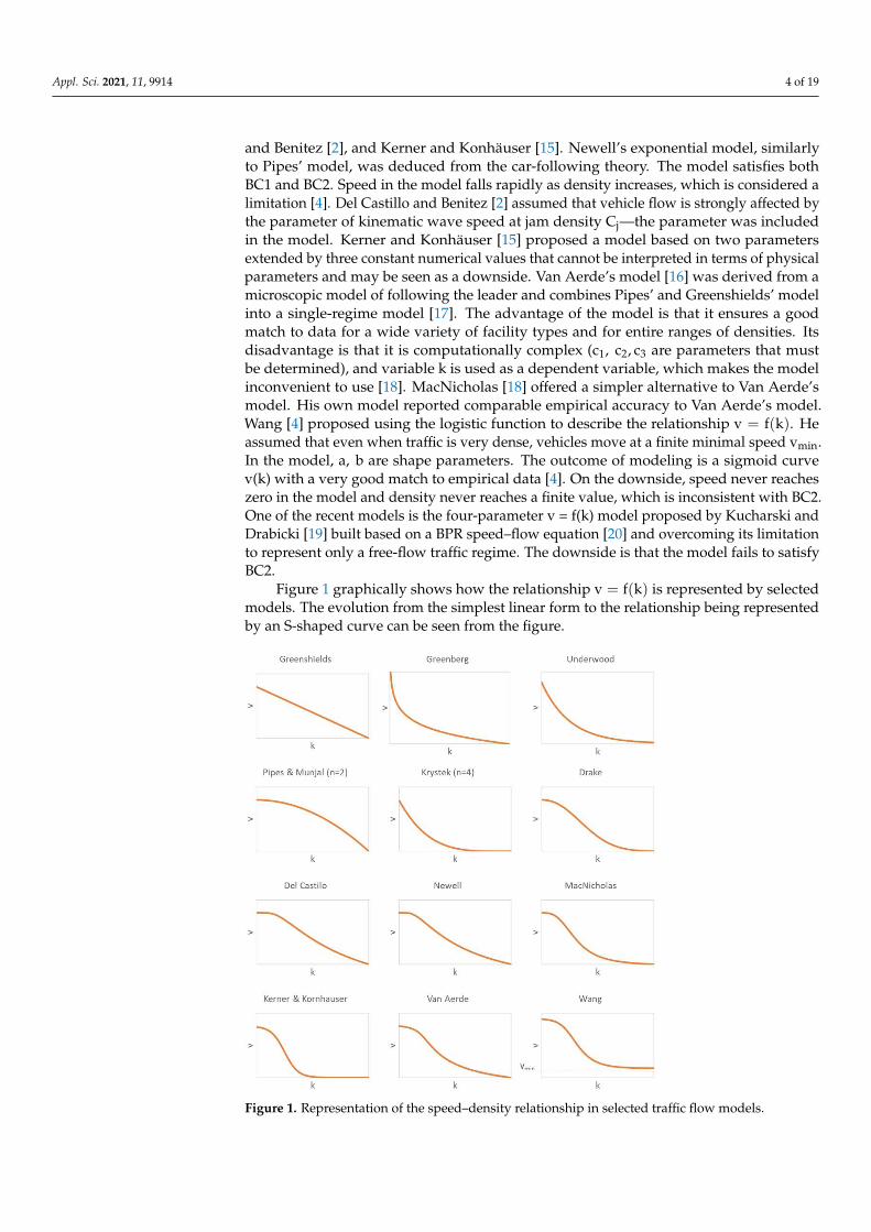
Figure 1 graphically shows how the relationship v = f(k) is represented by selectedmodels. The evolution from the simplest linear form to the relationship being representedby an S-shaped curve can be seen from the figure.

Appl. Sci. 2021, 11, x FOR PEER REVIEW 5 of 20

Figure 1. Representation of the speed–density relationship in selected traffic flow models.

There is also a group of models (with v = f(q) BPR function [20] as an example) that

represent the speed–flow–density relationship for a free-flow regime only and do not con-

sider traffic flow characteristics after the maximum flow and corresponding optimum

density are reached. It is not a limitation if the purpose is to analyze traffic under free-

flow conditions; however, to estimate values of traffic flow parameters at the maximum

flow (qmax, kopt, vopt), some initial assumptions regarding the boundary of the free-flow

regime need to be made. As a result of these reasons, these kinds of models are not in-

cluded in Table 1.

2.1.2. Multi-Regime Traffic Flow Models

Researchers proposed multi-regime models primarily for their empirical accuracy.

However, this can only be obtained at the cost of a more complicated functional form and

much more complicated calibration with field data. The main problem with multi-regime

models is determining the boundaries of the particular traffic conditions described by sep-

arate functions and determining the points of transition from one state to another. Table

2 lists selected two-regime models.

Table 2. List of selected multi-regime models.

Author (Year of Publi-

cation) Basic Function Parameters

Edie (1961) v =

vswexp(−k

kopt)k < k1

voptln (kmaxk) k ≥ k1

vsw, kopt,

vopt, kmax,

k1

Smulders (1989) v = vsw − αkk ≤ k1

d (1

k−

1

kmax) k > k1

, where d =vsw−αkopt1

kopt−

1

kmax

vsw, α, kopt,

kmax,k1

Figure 1. Representation of the speed–density relationship in selected traffic flow models.

Appl. Sci. 2021, 11, 9914 5 of 19

There is also a group of models (with v = f(q) BPR function [20] as an example) thatrepresent the speed–flow–density relationship for a free-flow regime only and do notconsider traffic flow characteristics after the maximum flow and corresponding optimumdensity are reached. It is not a limitation if the purpose is to analyze traffic under free-flowconditions; however, to estimate values of traffic flow parameters at the maximum flow(qmax, kopt, vopt), some initial assumptions regarding the boundary of the free-flow regimeneed to be made. As a result of these reasons, these kinds of models are not included inTable 1.

2.1.2. Multi-Regime Traffic Flow Models

Researchers proposed multi-regime models primarily for their empirical accuracy.However, this can only be obtained at the cost of a more complicated functional form andmuch more complicated calibration with field data. The main problem with multi-regimemodels is determining the boundaries of the particular traffic conditions described byseparate functions and determining the points of transition from one state to another.Table 2 lists selected two-regime models.

Table 2. List of selected multi-regime models.

Author (Year of Publication) Basic Function Parameters

Edie (1961) v =

vsw exp(− k

kopt

)k < k1

vopt ln(

kmaxk

)k ≥ k1

vsw, kopt,

vopt, kmax,

k1

Smulders (1989) v =

vsw − αk k ≤ k1

d(

1k −

1kmax

)k > k1

, where d =

vsw−αkopt1

kopt− 1

kmax

vsw,α, kopt,

kmax,k1

Triangular q =

vswk k < k1

qmax −k−kopt

kmax−koptqmax k ≥ k1

vsw,qmax,

kopt, kmax,k1

Daganzo (1997) q =

vswk k < k1

vswk1 k1 < k < k2

qmax − k−k2kmax−k2

qmax k ≥ k2

Wu (2002) q =

k(1−(

kk1

)l−1vsw +

(kk1

)l−1vopt v > vopt

voptk1 − k−k1kmax−k1

vswk1 k ≥ k1

vsw, vopt,

kmax, l, k1

where: k1, k2—boundary values of density at which there is a transition between traffic flow regimes.

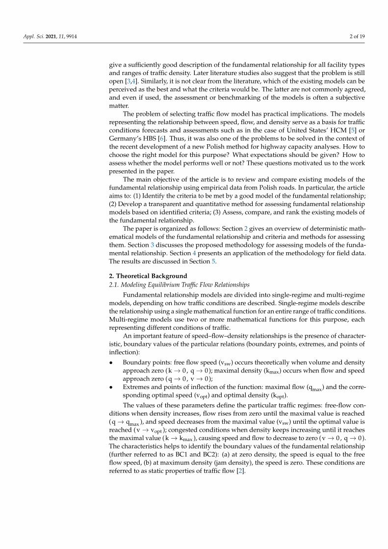
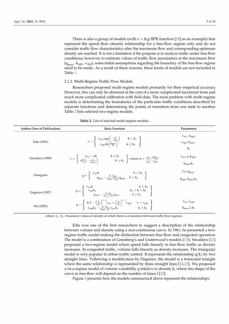
Edie was one of the first researchers to suggest a description of the relationshipbetween volume and density using a non-continuous curve. In 1961, he presented a two-regime traffic model making the distinction between free-flow and congested operation.The model is a combination of Greenberg’s and Underwood’s models [7,9]. Smulders [21]proposed a two-regime model where speed falls linearly in free-flow traffic as densityincreases. In congested traffic, volume falls linearly as density increases. The triangularmodel is very popular in urban traffic control. It represents the relationship q(k) by twostraight lines. Following a modification by Daganzo, the model is a truncated trianglewhere the same relationship is represented by three straight lines [22,23]. Wu proposeda two-regime model of volume variability q relative to density k, where the shape of thecurve in free-flow will depend on the number of lanes l [23].

Figure 2 presents how the models summarized above represent the relationships.

Appl. Sci. 2021, 11, 9914 6 of 19

Appl. Sci. 2021, 11, x FOR PEER REVIEW 6 of 20

Triangular q =

vswkk < k1

qmax −k − kopt

kmax − koptqmaxk ≥ k1

vsw,qmax,

kopt,kmax,k1

Daganzo (1997) q =

vswkk < k1vswk1k1 < k < k2

𝑞𝑚𝑎𝑥 −𝑘 − 𝑘2

𝑘𝑚𝑎𝑥 − 𝑘2𝑞𝑚𝑎𝑥 𝑘 ≥ 𝑘2

Wu (2002) q =

k(1 − (

k

k1)l−1

vsw + (k

k1)l−1

voptv > vopt

voptk1 −k − k1

kmax − k1vswk1k ≥ k1

vsw, vopt,

kmax, l, k1

where: 𝑘1, 𝑘2—boundary values of density at which there is a transition between traffic flow regimes

Edie was one of the first researchers to suggest a description of the relationship be-

tween volume and density using a non-continuous curve. In 1961, he presented a two-

regime traffic model making the distinction between free-flow and congested operation.

The model is a combination of Greenberg’s and Underwood’s models [7,9]. Smulders [21]

proposed a two-regime model where speed falls linearly in free-flow traffic as density

increases. In congested traffic, volume falls linearly as density increases. The triangular

model is very popular in urban traffic control. It represents the relationship q(k) by two

straight lines. Following a modification by Daganzo, the model is a truncated triangle

where the same relationship is represented by three straight lines [22,23]. Wu proposed a

two-regime model of volume variability q relative to density k, where the shape of the

curve in free-flow will depend on the number of lanes l [23].

Figure 2 presents how the models summarized above represent the relationships.

Figure 2. Relationships v(k), v(q), and q(k) in selected multi-regime models (assuming model con-

tinuity).

Figure 2. Relationships v(k), v(q), and q(k) in selected multi-regime models (assuming modelcontinuity).

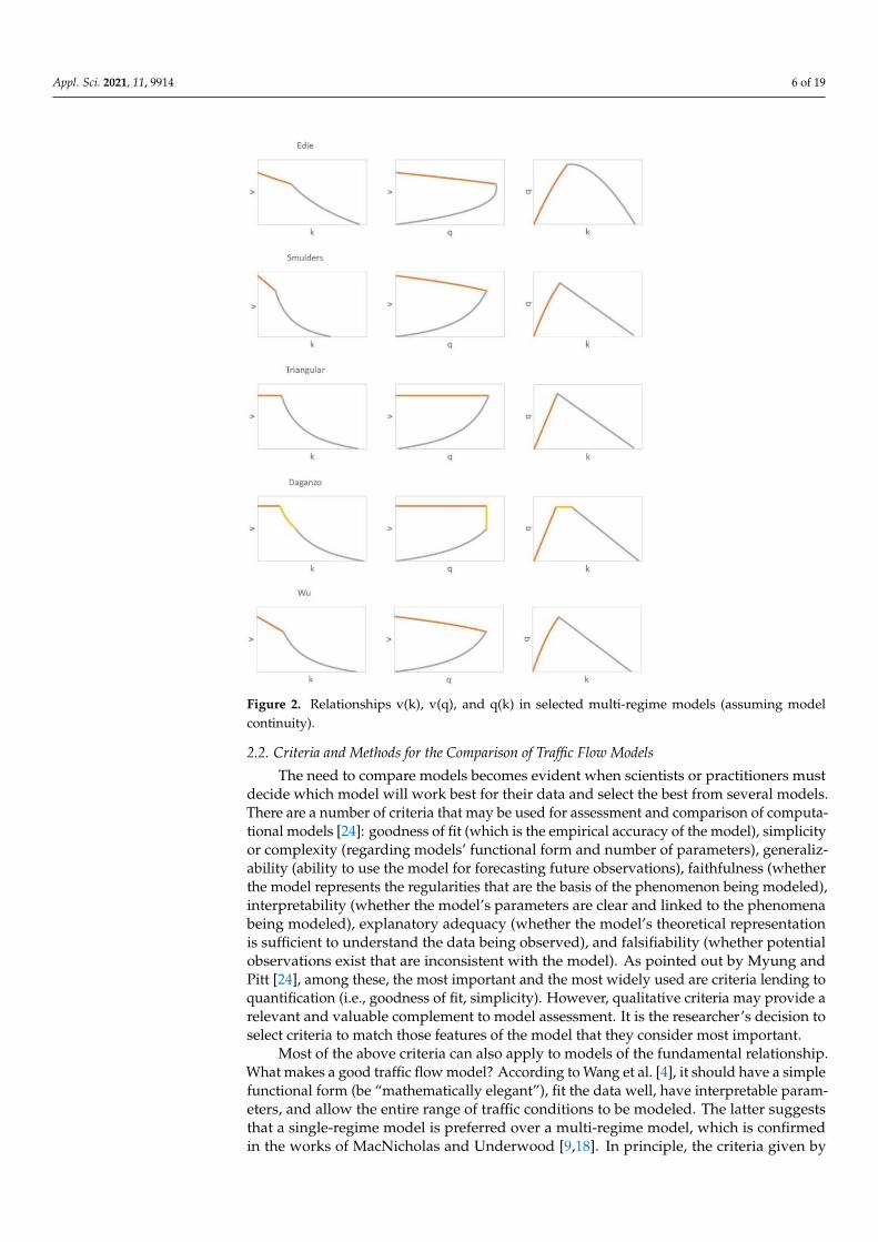
2.2. Criteria and Methods for the Comparison of Traffic Flow Models

The need to compare models becomes evident when scientists or practitioners mustdecide which model will work best for their data and select the best from several models.There are a number of criteria that may be used for assessment and comparison of computa-tional models [24]: goodness of fit (which is the empirical accuracy of the model), simplicityor complexity (regarding models’ functional form and number of parameters), generaliz-ability (ability to use the model for forecasting future observations), faithfulness (whetherthe model represents the regularities that are the basis of the phenomenon being modeled),interpretability (whether the model’s parameters are clear and linked to the phenomenabeing modeled), explanatory adequacy (whether the model’s theoretical representationis sufficient to understand the data being observed), and falsifiability (whether potentialobservations exist that are inconsistent with the model). As pointed out by Myung andPitt [24], among these, the most important and the most widely used are criteria lending toquantification (i.e., goodness of fit, simplicity). However, qualitative criteria may provide arelevant and valuable complement to model assessment. It is the researcher’s decision toselect criteria to match those features of the model that they consider most important.

Most of the above criteria can also apply to models of the fundamental relationship.What makes a good traffic flow model? According to Wang et al. [4], it should have a simplefunctional form (be “mathematically elegant”), fit the data well, have interpretable param-eters, and allow the entire range of traffic conditions to be modeled. The latter suggeststhat a single-regime model is preferred over a multi-regime model, which is confirmedin the works of MacNicholas and Underwood [9,18]. In principle, the criteria given by

Appl. Sci. 2021, 11, 9914 7 of 19

MacNicholas and Underwood are consistent with those identified by Wang. MacNicholasmentions an additional aspect of having to meet boundary conditions. Underwood, on theother hand, points out that the model should easily lend itself to mathematical analysisand that its limitations should be known in advance.

A review of the above works suggests that researchers are in agreement as to whatcriteria should be met by the fundamental relationship model. As a result, the criteria theyidentified may be used to assess and compare models of the fundamental relationship.This type of comparison in the literature usually has an expert basis rather than concretecriteria and measures to assess the criteria. The criteria researchers refer to most ofteninclude goodness of fit, which is a quantitative measure. In addition, faithfulness of themodel is often assessed by checking how the model fits in with the empirical data and howthe phenomena are represented on the fundamental diagram. An example is the work ofGaddam and Rao [25], who assess models matching data from two sections of an urbanarterial in Delhi with goodness of fit, using root mean square error, average relative error,and cumulative residual plots for the assessment. To complement the criterion assessment,expert judgement on the properties of the models on the speed–density diagrams is applied.To assess existing models for a 55 mph motorway section, May [26] used two quantitativemeasures: goodness of fit, measured by mean deviation, and parameter value, which isassessed by checking if they are consistent with the ranges established from empiricaldata. It is not clear from the publication how these ranges were identified. The samecriterion was used by Rakha [27] for the same data and the same ranges of parametersas May [26], comparing known single and multi-regime models with Van Aerde’s model.Cheng et al. [28] compared 10 single-regime models using goodness of fit and testedthe models’ stability by comparing how the same model parameters change on differentsections of the same road. In many other studies, models are compared with a qualitativeassessment only, e.g., a visual check is made of the match between the models and empiricaldata, limitations are identified, and model properties are assessed [4,17,29].

The conclusion from the review of the literature is that while researchers are inagreement about the criteria of a good model of the fundamental relationship, there isno agreement as to how traffic flow models should be assessed or compared. Thereare no commonly agreed criteria that would apply to the assessment, comparison, orbenchmarking of traffic flow models. Similarly, ways to assess particular criteria are notagreed, and it is usually up to the individual interpretation of the researcher.

3. Materials and Methods3.1. Data

To develop and apply the methodology, the data were sourced from a section of the S6express road located in Gdansk, Poland (5425′ N, 1829′ E). The section is part of a dualcarriageway with four lanes running within the conurbation. The speed limit for passengercars is 120 km/h and 80 km/h for heavy goods vehicles. The share of trucks in overalltraffic is 9% on average. Annual average daily traffic is 74,000 vehicles per day. Duringpeaks of traffic (summer holidays), volumes are observed to exceed 100,000 vehicles perday.

The data [30] come from a continuous traffic measurement station which is operatedby a double induction loop. Vehicles crossing the station are automatically detected bydevices installed on each lane, which register the time a vehicle is detected, ascertain itsspot speed, and identify the type of vehicle and lane it is using.

The data cover a period of 36 months between 2014 and 2017 on the southboundcarriageway. A total of 37.5 million vehicles were recorded over that period.

Structured Query Language (SQL) was used for data processing and initial analysis.The data processing was divided into the following stages:

1. Raw traffic data that were provided by the national road authority (General Directorfor National Roads and Motorways, GDDKiA) in the text file format were importedto the database on the installed SQL server.

Appl. Sci. 2021, 11, 9914 8 of 19

2. The data were verified in terms of empty rows, zero values, vehicle speeds beyond theexpected range, and unusual vehicle lengths. The problem of zeros or unusual valuesconcerned approximately 2% of registered vehicles and had marginal impact on thenumber of registered vehicles—the records were excluded from further processing.

3. Individual vehicle headways were calculated for each record.4. The data were aggregated into 5 min intervals generating information about traffic

volume, space-mean speed, share of heavy goods vehicles, or average headways.The traffic volume was calculated into flow rate using passenger car equivalents [5].Traffic density was determined from the relation (1).

The database was extended with weather information (condition and intensity ofprecipitation, condition of road surface, horizontal visibility), conditions of natural lighting(dusk, day, dawn, night), and presence of road events (road works, collisions, accidents,stationary vehicles, etc.). Precipitation, wet or snow-covered/icy road surface, lack ofnatural lighting, and visibility below 200 m were proved to have a significant impact onspace-mean speed [31]. Thus, periods of road events and adverse weather and lightingconditions were excluded from further analyses.

3.2. Method

Empirical data are shown in the fundamental diagram (Figure 3). They are repre-sented by the scattered cloud of empirical data for the entire range of traffic conditions. Thephenomena are reported by many studies and explained by e.g., heterogeneity of drivers,non-stationary dynamical features of traffic flow, randomness in individual driving be-haviors, and errors in measurement methods or data processing [32–35]. The existence ofthe scatter raises some questions: What should be the functional form of the deterministicmodel to ensure the highest empirical accuracy? Should it be represented by a single ormulti-regime model? How to estimate boundary parameters and what should be theirvalues?

Appl. Sci. 2021, 11, x FOR PEER REVIEW 9 of 20

Figure 3. Empirical relations between speed, density, and flow.

To answer the questions, work was divided into the following stages: (stage I) data

preparation and determination of expected values of boundary parameters, (stage II) se-

lection of criteria for model assessment and adoption of detailed principles for criteria

assessment and criteria acceptance levels, (stage III) model calibration, (stage IV) model

assessment and comparison.

3.2.1. Preparation of the Data and Determination of Expected Parameter Values

The scatter on the empirical fundamental diagram may make model assessment and

the identification of real boundary traffic parameters more difficult. The classical defini-

tion of the fundamental relationship assumes that traffic is stationary and homogeneous,

which means that vehicles behave the same way in similar traffic circumstances [22]. This

suggests that for the same traffic density, vehicles in a stream will move with the same

speed. Building on this, an averaged representation of traffic conditions was determined

from the data. This helps to significantly reduce the number of points in the diagram,

making a visual assessment easier. It will be possible to state whether the actual traffic

conditions are correctly represented in the model. In the proposed approach, observed

densities are divided into narrow ranges e.g., 0.1 pc/km wide. The empirical mean of the

other parameters, i.e., speed and flow rate, are computed. A similar approach can be

found in the works of Rakha and Arafeh and Zheng et al. [36,37]. Figure 4 presents the

data averaged against density. As we can see, the scatter has been significantly reduced

with only the congested traffic still represented by a cloud of points. This may be partly

due to a much smaller sample of observed congested traffic—from nearly 110,000 of ana-

lyzed time intervals, only 3,000 represented densities above 20 pc/h/lane (as a result for

high traffic densities, the parameters are averaged on the basis of just a few time intervals).

Figure 4. Curves v(q) and v(k) that determine the averaged representation of traffic conditions.

Figure 3. Empirical relations between speed, density, and flow.

To answer the questions, work was divided into the following stages: (stage I) datapreparation and determination of expected values of boundary parameters, (stage II)selection of criteria for model assessment and adoption of detailed principles for criteriaassessment and criteria acceptance levels, (stage III) model calibration, (stage IV) modelassessment and comparison.

3.2.1. Preparation of the Data and Determination of Expected Parameter Values

The scatter on the empirical fundamental diagram may make model assessment andthe identification of real boundary traffic parameters more difficult. The classical definitionof the fundamental relationship assumes that traffic is stationary and homogeneous, which

Appl. Sci. 2021, 11, 9914 9 of 19

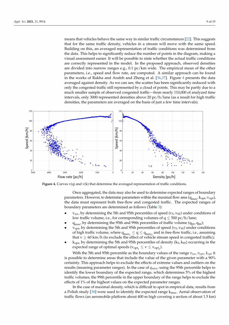
means that vehicles behave the same way in similar traffic circumstances [22]. This suggeststhat for the same traffic density, vehicles in a stream will move with the same speed.Building on this, an averaged representation of traffic conditions was determined fromthe data. This helps to significantly reduce the number of points in the diagram, making avisual assessment easier. It will be possible to state whether the actual traffic conditionsare correctly represented in the model. In the proposed approach, observed densitiesare divided into narrow ranges e.g., 0.1 pc/km wide. The empirical mean of the otherparameters, i.e., speed and flow rate, are computed. A similar approach can be foundin the works of Rakha and Arafeh and Zheng et al. [36,37]. Figure 4 presents the dataaveraged against density. As we can see, the scatter has been significantly reduced withonly the congested traffic still represented by a cloud of points. This may be partly due to amuch smaller sample of observed congested traffic—from nearly 110,000 of analyzed timeintervals, only 3000 represented densities above 20 pc/h/lane (as a result for high trafficdensities, the parameters are averaged on the basis of just a few time intervals).

Appl. Sci. 2021, 11, x FOR PEER REVIEW 9 of 20

Figure 3. Empirical relations between speed, density, and flow.

To answer the questions, work was divided into the following stages: (stage I) data

preparation and determination of expected values of boundary parameters, (stage II) se-

lection of criteria for model assessment and adoption of detailed principles for criteria

assessment and criteria acceptance levels, (stage III) model calibration, (stage IV) model

assessment and comparison.

3.2.1. Preparation of the Data and Determination of Expected Parameter Values

The scatter on the empirical fundamental diagram may make model assessment and

the identification of real boundary traffic parameters more difficult. The classical defini-

tion of the fundamental relationship assumes that traffic is stationary and homogeneous,

which means that vehicles behave the same way in similar traffic circumstances [22]. This

suggests that for the same traffic density, vehicles in a stream will move with the same

speed. Building on this, an averaged representation of traffic conditions was determined

from the data. This helps to significantly reduce the number of points in the diagram,

making a visual assessment easier. It will be possible to state whether the actual traffic

conditions are correctly represented in the model. In the proposed approach, observed

densities are divided into narrow ranges e.g., 0.1 pc/km wide. The empirical mean of the

other parameters, i.e., speed and flow rate, are computed. A similar approach can be

found in the works of Rakha and Arafeh and Zheng et al. [36,37]. Figure 4 presents the

data averaged against density. As we can see, the scatter has been significantly reduced

with only the congested traffic still represented by a cloud of points. This may be partly

due to a much smaller sample of observed congested traffic—from nearly 110,000 of ana-

lyzed time intervals, only 3,000 represented densities above 20 pc/h/lane (as a result for

high traffic densities, the parameters are averaged on the basis of just a few time intervals).

Figure 4. Curves v(q) and v(k) that determine the averaged representation of traffic conditions. Figure 4. Curves v(q) and v(k) that determine the averaged representation of traffic conditions.

Once aggregated, the data may also be used to determine expected ranges of boundaryparameters. However, to determine parameters within the maximal flow area (qmax, kopt, vopt),the data must represent both free-flow and congested traffic. The expected ranges ofboundary parameters are determined as follows (Table 3):

• vsw, by determining the 5th and 95th percentiles of speed (v5, v95) under conditions oflow traffic volume, i.e., for corresponding volumes of q ≤ 500 pc/h/lane;

• qmax, by determining the 95th and 99th percentiles of traffic volume (q95, q99);• vopt, by determining the 5th and 95th percentiles of speed (v5, v95) under conditions

of high traffic volume, where qmax1≤ q ≤ qmax2

and in free-flow traffic, i.e., assumingthat v ≥ 60 km/h (to exclude the effect of vehicle stream speed in congested traffic);

• kopt, by determining the 5th and 95th percentiles of density (k5, k95) occurring in theexpected range of optimal speeds (vopt1

≤ v ≤ vopt2).

With the 5th and 95th percentile as the boundary values of the range vsw, vopt, kopt itis possible to determine areas that include the value of the given parameter with a 90%certainty. This approach helps to exclude the effects of extreme values and outliers on theresults (meaning parameter ranges). In the case of qmax, using the 95th percentile helps toidentify the lower boundary of the expected range, which determines 5% of the highesttraffic volumes; the 99th percentile in the upper boundary of the range helps to exclude theeffects of 1% of the highest values on the expected parameter ranges.

In the case of maximal density, which is difficult to spot in empirical data, results froma Polish study [38] were used to identify the expected range kmax. Aerial observation oftraffic flows (an aeromobile platform about 400 m high covering a section of about 1.5 km)

Appl. Sci. 2021, 11, 9914 10 of 19

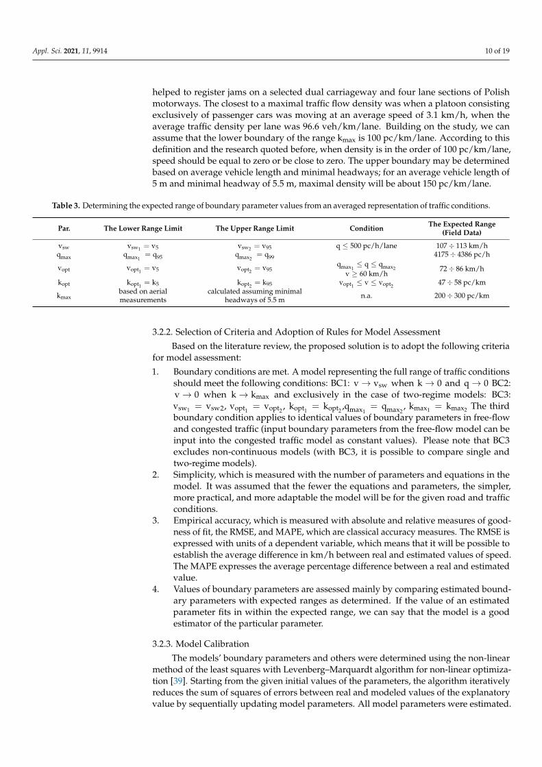
helped to register jams on a selected dual carriageway and four lane sections of Polishmotorways. The closest to a maximal traffic flow density was when a platoon consistingexclusively of passenger cars was moving at an average speed of 3.1 km/h, when theaverage traffic density per lane was 96.6 veh/km/lane. Building on the study, we canassume that the lower boundary of the range kmax is 100 pc/km/lane. According to thisdefinition and the research quoted before, when density is in the order of 100 pc/km/lane,speed should be equal to zero or be close to zero. The upper boundary may be determinedbased on average vehicle length and minimal headways; for an average vehicle length of5 m and minimal headway of 5.5 m, maximal density will be about 150 pc/km/lane.

Table 3. Determining the expected range of boundary parameter values from an averaged representation of traffic conditions.

Par. The Lower Range Limit The Upper Range Limit Condition The Expected Range(Field Data)

vsw vsw1 = v5 vsw2 = v95 q ≤ 500 pc/h/lane 107÷ 113 km/hqmax qmax1

= q95 qmax2= q99 4175÷ 4386 pc/h

vopt vopt1= v5 vopt2

= v95qmax1

≤ q ≤ qmax2 72÷ 86 km/hv ≥ 60 km/h

kopt kopt1= k5 kopt2

= k95 vopt1≤ v ≤ vopt2

47÷ 58 pc/km

kmaxbased on aerialmeasurements

calculated assuming minimalheadways of 5.5 m n.a. 200÷ 300 pc/km

3.2.2. Selection of Criteria and Adoption of Rules for Model Assessment

Based on the literature review, the proposed solution is to adopt the following criteriafor model assessment:

1. Boundary conditions are met. A model representing the full range of traffic conditionsshould meet the following conditions: BC1: v→ vsw when k→ 0 and q→ 0 BC2:v→ 0 when k→ kmax and exclusively in the case of two-regime models: BC3:vsw1 = vsw2, vopt1

= vopt2, kopt1

= kopt2,qmax1

= qmax2, kmax1 = kmax2 The third

boundary condition applies to identical values of boundary parameters in free-flowand congested traffic (input boundary parameters from the free-flow model can beinput into the congested traffic model as constant values). Please note that BC3excludes non-continuous models (with BC3, it is possible to compare single andtwo-regime models).

2. Simplicity, which is measured with the number of parameters and equations in themodel. It was assumed that the fewer the equations and parameters, the simpler,more practical, and more adaptable the model will be for the given road and trafficconditions.

3. Empirical accuracy, which is measured with absolute and relative measures of good-ness of fit, the RMSE, and MAPE, which are classical accuracy measures. The RMSE isexpressed with units of a dependent variable, which means that it will be possible toestablish the average difference in km/h between real and estimated values of speed.The MAPE expresses the average percentage difference between a real and estimatedvalue.

4. Values of boundary parameters are assessed mainly by comparing estimated bound-ary parameters with expected ranges as determined. If the value of an estimatedparameter fits in within the expected range, we can say that the model is a goodestimator of the particular parameter.

3.2.3. Model Calibration

The models’ boundary parameters and others were determined using the non-linearmethod of the least squares with Levenberg–Marquardt algorithm for non-linear optimiza-tion [39]. Starting from the given initial values of the parameters, the algorithm iterativelyreduces the sum of squares of errors between real and modeled values of the explanatoryvalue by sequentially updating model parameters. All model parameters were estimated.

Appl. Sci. 2021, 11, 9914 11 of 19

The initial values of boundary parameters were treated as the centers of the expectedranges of values that were determined during data preparation. The boundary densityfor traffic conditions in two-regime models was set as the middle value from the range ofexpected kopt values.

3.2.4. Model Assessment and Comparison

Given the criteria that were used, we must ensure that the models under comparisonare related to the same dependent variable. The assessment was conducted for generalmodels (2) or models transformed to a general form (2), where speed is a function ofdensity, of parameters related to the traffic flow (boundary parameters), and of othernon-dimensional parameters.

v = f(k, boundary parameters, non-dimensional parameters) (2)

From the models listed in Tables 1 and 2, all but Van Aerde’s model meet the require-ment. Unless the condition is met, the model cannot be transformed directly to (2). As aresult, the model cannot be analyzed further.

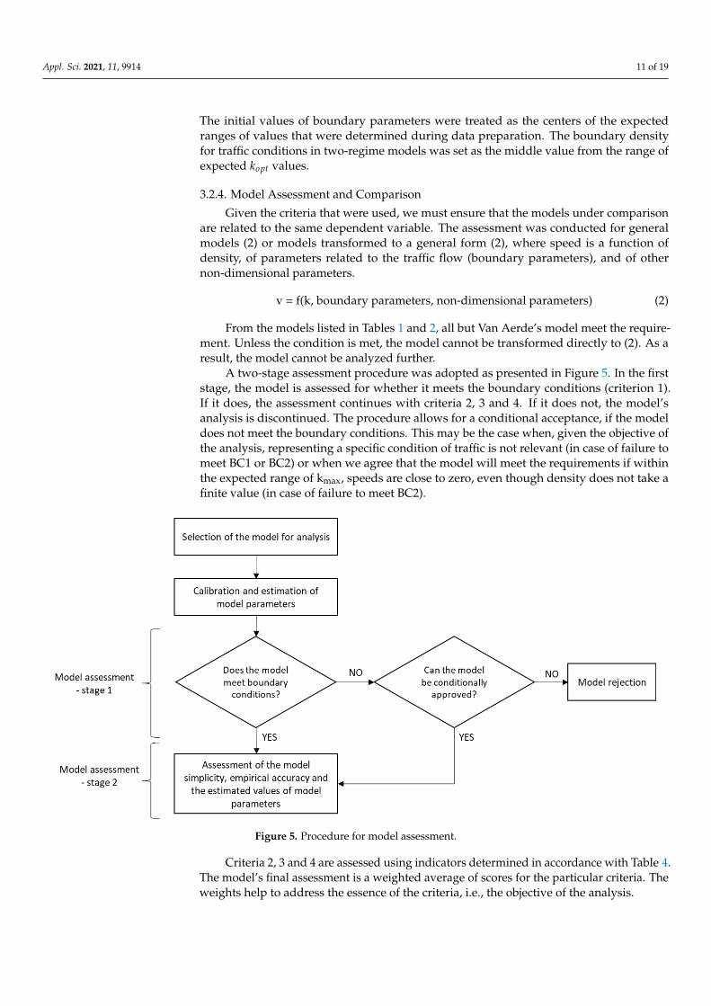
A two-stage assessment procedure was adopted as presented in Figure 5. In the firststage, the model is assessed for whether it meets the boundary conditions (criterion 1).If it does, the assessment continues with criteria 2, 3 and 4. If it does not, the model’sanalysis is discontinued. The procedure allows for a conditional acceptance, if the modeldoes not meet the boundary conditions. This may be the case when, given the objective ofthe analysis, representing a specific condition of traffic is not relevant (in case of failure tomeet BC1 or BC2) or when we agree that the model will meet the requirements if withinthe expected range of kmax, speeds are close to zero, even though density does not take afinite value (in case of failure to meet BC2).

Appl. Sci. 2021, 11, x FOR PEER REVIEW 12 of 20

meet the boundary conditions. This may be the case when, given the objective of the anal-

ysis, representing a specific condition of traffic is not relevant (in case of failure to meet

BC1 or BC2) or when we agree that the model will meet the requirements if within the

expected range of kmax, speeds are close to zero, even though density does not take a finite

value (in case of failure to meet BC2).

Figure 5. Procedure for model assessment.

Criteria 2, 3 and 4 are assessed using indicators determined in accordance with Table

4. The model’s final assessment is a weighted average of scores for the particular criteria.

The weights help to address the essence of the criteria, i.e., the objective of the analysis.

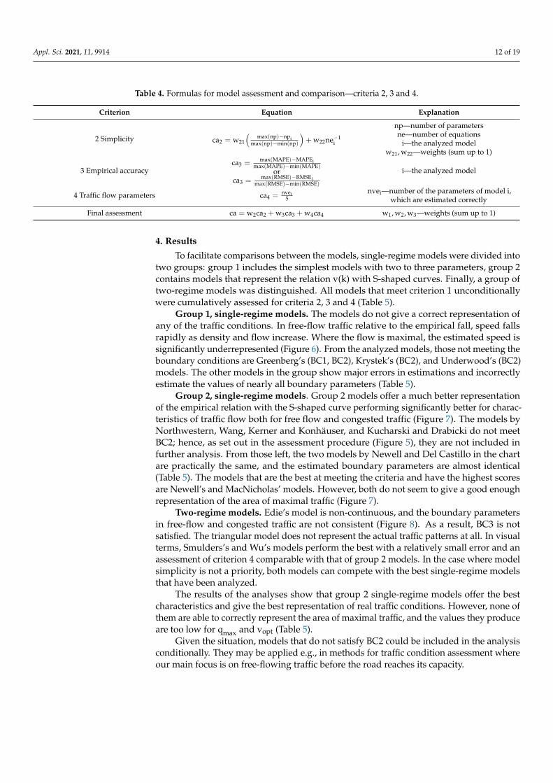
Table 4. Formulas for model assessment and comparison—criteria 2, 3 and 4.

Criterion Equation Explanation

2 Simplicity ca2 = w21 (max(np) − npi

max(np) − min(np)) + w22nei

−1

np—number of parameters

ne—number of equations

i—the analyzed model

w21, w22—weights (sum up to 1)

3 Empirical accuracy

ca3 =max(MAPE) − MAPEi

max(MAPE) − min(MAPE)

or

ca3 =max(RMSE) − RMSEi

max(RMSE) − min(RMSE)

i—the analyzed model

4 Traffic flow parameters ca4 =nvei5

nvei—number of the parameters of

model i, which are estimated cor-

rectly

Final assessment ca = w2ca2 + w3ca3 +w4ca4 w1, w2, w3—weights (sum up to 1)

4. Results

To facilitate comparisons between the models, single-regime models were divided

into two groups: group 1 includes the simplest models with two to three parameters,

group 2 contains models that represent the relation v(k) with S-shaped curves. Finally, a

Figure 5. Procedure for model assessment.

Criteria 2, 3 and 4 are assessed using indicators determined in accordance with Table 4.The model’s final assessment is a weighted average of scores for the particular criteria. Theweights help to address the essence of the criteria, i.e., the objective of the analysis.

Appl. Sci. 2021, 11, 9914 12 of 19

Table 4. Formulas for model assessment and comparison—criteria 2, 3 and 4.

Criterion Equation Explanation

2 Simplicity ca2 = w21

(max(np)−npi

max(np)−min(np)

)+ w22ne−1

i

np—number of parametersne—number of equations

i—the analyzed modelw21, w22—weights (sum up to 1)

3 Empirical accuracyca3 = max(MAPE)−MAPEi

max(MAPE)−min(MAPE)or

ca3 = max(RMSE)−RMSEimax(RMSE)−min(RMSE)

i—the analyzed model

4 Traffic flow parameters ca4 = nvei5

nvei—number of the parameters of model i,which are estimated correctly

Final assessment ca = w2ca2 + w3ca3 + w4ca4 w1, w2, w3—weights (sum up to 1)

4. Results

To facilitate comparisons between the models, single-regime models were divided intotwo groups: group 1 includes the simplest models with two to three parameters, group 2contains models that represent the relation v(k) with S-shaped curves. Finally, a group oftwo-regime models was distinguished. All models that meet criterion 1 unconditionallywere cumulatively assessed for criteria 2, 3 and 4 (Table 5).

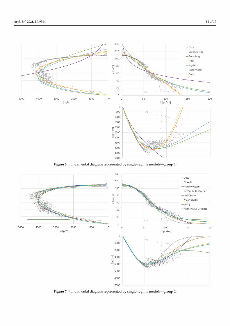
Group 1, single-regime models. The models do not give a correct representation ofany of the traffic conditions. In free-flow traffic relative to the empirical fall, speed fallsrapidly as density and flow increase. Where the flow is maximal, the estimated speed issignificantly underrepresented (Figure 6). From the analyzed models, those not meeting theboundary conditions are Greenberg’s (BC1, BC2), Krystek’s (BC2), and Underwood’s (BC2)models. The other models in the group show major errors in estimations and incorrectlyestimate the values of nearly all boundary parameters (Table 5).

Group 2, single-regime models. Group 2 models offer a much better representationof the empirical relation with the S-shaped curve performing significantly better for charac-teristics of traffic flow both for free flow and congested traffic (Figure 7). The models byNorthwestern, Wang, Kerner and Konhäuser, and Kucharski and Drabicki do not meetBC2; hence, as set out in the assessment procedure (Figure 5), they are not included infurther analysis. From those left, the two models by Newell and Del Castillo in the chartare practically the same, and the estimated boundary parameters are almost identical(Table 5). The models that are the best at meeting the criteria and have the highest scoresare Newell’s and MacNicholas’ models. However, both do not seem to give a good enoughrepresentation of the area of maximal traffic (Figure 7).

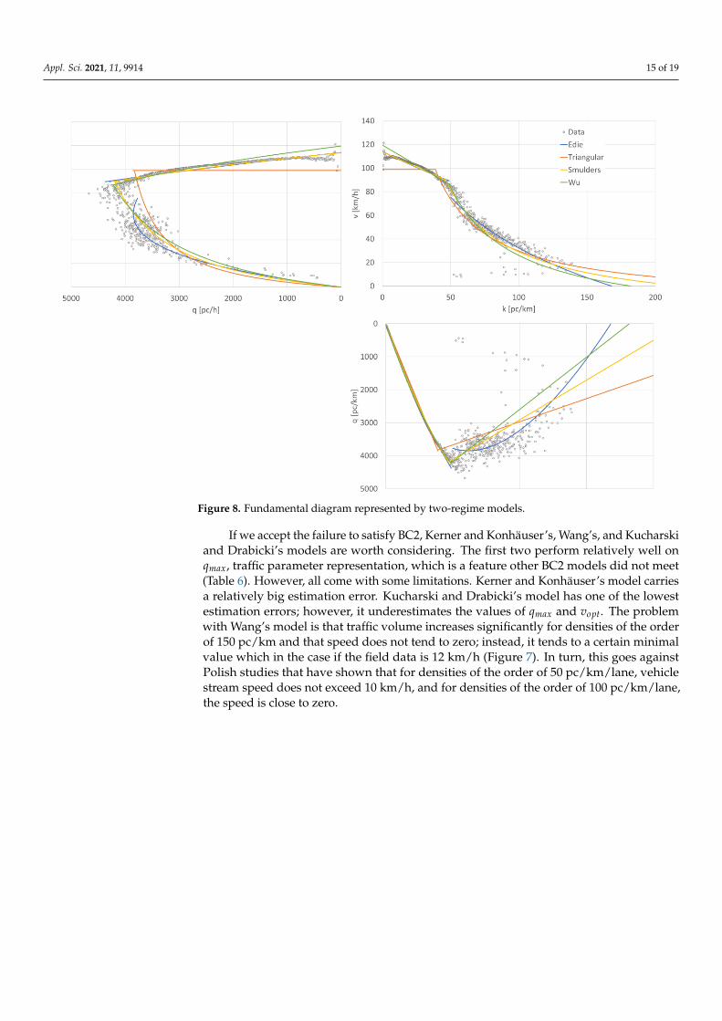
Two-regime models. Edie’s model is non-continuous, and the boundary parametersin free-flow and congested traffic are not consistent (Figure 8). As a result, BC3 is notsatisfied. The triangular model does not represent the actual traffic patterns at all. In visualterms, Smulders’s and Wu’s models perform the best with a relatively small error and anassessment of criterion 4 comparable with that of group 2 models. In the case where modelsimplicity is not a priority, both models can compete with the best single-regime modelsthat have been analyzed.

The results of the analyses show that group 2 single-regime models offer the bestcharacteristics and give the best representation of real traffic conditions. However, none ofthem are able to correctly represent the area of maximal traffic, and the values they produceare too low for qmax and vopt (Table 5).

Given the situation, models that do not satisfy BC2 could be included in the analysisconditionally. They may be applied e.g., in methods for traffic condition assessment whereour main focus is on free-flowing traffic before the road reaches its capacity.

Appl. Sci. 2021, 11, 9914 13 of 19

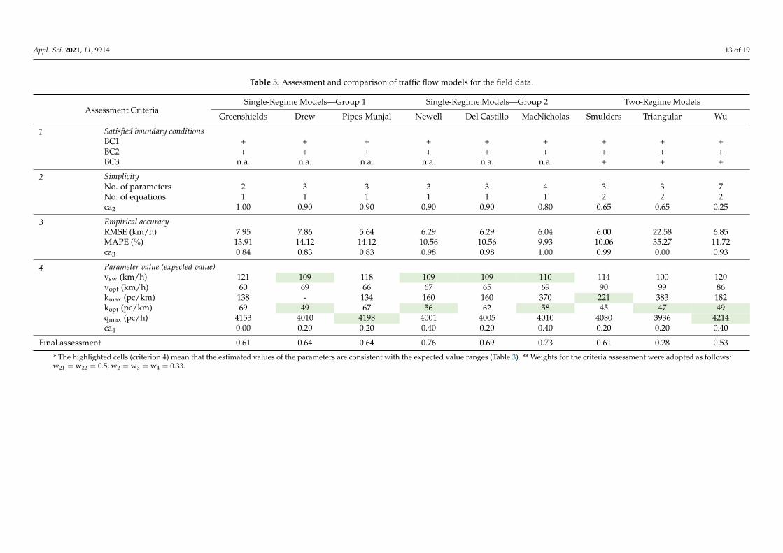
Table 5. Assessment and comparison of traffic flow models for the field data.

Assessment CriteriaSingle-Regime Models—Group 1 Single-Regime Models—Group 2 Two-Regime Models

Greenshields Drew Pipes-Munjal Newell Del Castillo MacNicholas Smulders Triangular Wu

1 Satisfied boundary conditionsBC1 + + + + + + + + +BC2 + + + + + + + + +BC3 n.a. n.a. n.a. n.a. n.a. n.a. + + +

2 SimplicityNo. of parameters 2 3 3 3 3 4 3 3 7No. of equations 1 1 1 1 1 1 2 2 2ca2 1.00 0.90 0.90 0.90 0.90 0.80 0.65 0.65 0.25

3 Empirical accuracyRMSE (km/h) 7.95 7.86 5.64 6.29 6.29 6.04 6.00 22.58 6.85MAPE (%) 13.91 14.12 14.12 10.56 10.56 9.93 10.06 35.27 11.72ca3 0.84 0.83 0.83 0.98 0.98 1.00 0.99 0.00 0.93

4 Parameter value (expected value)vsw (km/h) 121 109 118 109 109 110 114 100 120vopt (km/h) 60 69 66 67 65 69 90 99 86kmax (pc/km) 138 - 134 160 160 370 221 383 182kopt (pc/km) 69 49 67 56 62 58 45 47 49qmax (pc/h) 4153 4010 4198 4001 4005 4010 4080 3936 4214ca4 0.00 0.20 0.20 0.40 0.20 0.40 0.20 0.20 0.40

Final assessment 0.61 0.64 0.64 0.76 0.69 0.73 0.61 0.28 0.53

* The highlighted cells (criterion 4) mean that the estimated values of the parameters are consistent with the expected value ranges (Table 3). ** Weights for the criteria assessment were adopted as follows:w21 = w22 = 0.5, w2 = w3 = w4 = 0.33.

Appl. Sci. 2021, 11, 9914 14 of 19

Appl. Sci. 2021, 11, x FOR PEER REVIEW 13 of 20

group of two-regime models was distinguished. All models that meet criterion 1 uncon-

ditionally were cumulatively assessed for criteria 2, 3 and 4 (Table 5).

Group 1, single-regime models. The models do not give a correct representation of

any of the traffic conditions. In free-flow traffic relative to the empirical fall, speed falls

rapidly as density and flow increase. Where the flow is maximal, the estimated speed is

significantly underrepresented (Figure 6). From the analyzed models, those not meeting

the boundary conditions are Greenberg’s (BC1, BC2), Krystek’s (BC2), and Underwood’s

(BC2) models. The other models in the group show major errors in estimations and incor-

rectly estimate the values of nearly all boundary parameters (Table 5).

Figure 6. Fundamental diagram represented by single-regime models—group 1.

Table 5. Assessment and comparison of traffic flow models for the field data.

Assessment criteria

Single-regime models -

group 1

Single-regime models - group

2

Two-regime models

Greenshiel

ds Drew

Pipes-

Munjal Newell

Del

Castill

o

MacNichol

as

Smulder

s

Triangul

ar Wu

1 Satisfied boundary conditions

BC1 + + + + + + + + +

BC2 + + + + + + + + +

BC3 n.a. n.a. n.a. n.a. n.a. n.a. + + +

2 Simplicity

No. of parameters 2 3 3 3 3 4 3 3 7

No. of equations 1 1 1 1 1 1 2 2 2

ca2 1.00 0.90 0.90 0.90 0.90 0.80 0.65 0.65 0.25

3 Empirical accuracy

RMSE (km/h) 7.95 7.86 5.64 6.29 6.29 6.04 6.00 22.58 6.85

Figure 6. Fundamental diagram represented by single-regime models—group 1.

Appl. Sci. 2021, 11, x FOR PEER REVIEW 14 of 20

MAPE (%) 13.91 14.12 14.12 10.56 10.56 9.93 10.06 35.27 11.72

ca3 0.84 0.83 0.83 0.98 0.98 1.00 0.99 0.00 0.93

4 Parameter value (expected value)

vsw (km/h) 121 109 118 109 109 110 114 100 120

vopt (km/h) 60 69 66 67 65 69 90 99 86

kmax (pc/km) 138 - 134 160 160 370 221 383 182

kopt (pc/km) 69 49 67 56 62 58 45 47 49

qmax (pc/h) 4153 4010 4198 4001 4005 4010 4080 3936 4214

ca4 0.00 0.20 0.20 0.40 0.20 0.40 0.20 0.20 0.40

Final assessment 0.61 0.64 0.64 0.76 0.69 0.73 0.61 0.28 0.53 * The highlighted cells (criterion 4) mean that the estimated values of the parameters are consistent with the expected value

ranges (table 3). ** Weights for the criteria assessment were adopted as follows: w21 = w22 = 0.5, w2 = w3 = w4 = 0.33.

Group 2, single-regime models. Group 2 models offer a much better representation

of the empirical relation with the S-shaped curve performing significantly better for char-

acteristics of traffic flow both for free flow and congested traffic (Figure 7). The models by

Northwestern, Wang, Kerner and Konhäuser, and Kucharski and Drabicki do not meet

BC2; hence, as set out in the assessment procedure (Figure 5), they are not included in

further analysis. From those left, the two models by Newell and Del Castillo in the chart

are practically the same, and the estimated boundary parameters are almost identical (Ta-

ble 5). The models that are the best at meeting the criteria and have the highest scores are

Newell’s and MacNicholas’ models. However, both do not seem to give a good enough

representation of the area of maximal traffic (Figure 7).

Figure 7. Fundamental diagram represented by single-regime models—group 2. Figure 7. Fundamental diagram represented by single-regime models—group 2.

Appl. Sci. 2021, 11, 9914 15 of 19

Appl. Sci. 2021, 11, x FOR PEER REVIEW 15 of 20

Two-regime models. Edie’s model is non-continuous, and the boundary parameters

in free-flow and congested traffic are not consistent (Figure 8). As a result, BC3 is not sat-

isfied. The triangular model does not represent the actual traffic patterns at all. In visual

terms, Smulders’s and Wu’s models perform the best with a relatively small error and an

assessment of criterion 4 comparable with that of group 2 models. In the case where model

simplicity is not a priority, both models can compete with the best single-regime models

that have been analyzed.

Figure 8. Fundamental diagram represented by two-regime models.

The results of the analyses show that group 2 single-regime models offer the best

characteristics and give the best representation of real traffic conditions. However, none

of them are able to correctly represent the area of maximal traffic, and the values they

produce are too low for qmax and vopt (Table 5).

Given the situation, models that do not satisfy BC2 could be included in the analysis

conditionally. They may be applied e.g., in methods for traffic condition assessment where

our main focus is on free-flowing traffic before the road reaches its capacity.

If we accept the failure to satisfy BC2, Kerner and Konhäuser’s, Wang’s, and Ku-

charski and Drabicki’s models are worth considering. The first two perform relatively well

on 𝑞𝑚𝑎𝑥 , traffic parameter representation, which is a feature other BC2 models did not

meet (Table 6). However, all come with some limitations. Kerner and Konhäuser’s model

carries a relatively big estimation error. Kucharski and Drabicki’s model has one of the

lowest estimation errors; however, it underestimates the values of 𝑞𝑚𝑎𝑥 and 𝑣𝑜𝑝𝑡. The

problem with Wang’s model is that traffic volume increases significantly for densities of

the order of 150 pc/km and that speed does not tend to zero; instead, it tends to a certain

minimal value which in the case if the field data is 12 km/h (Figure 7). In turn, this goes

against Polish studies that have shown that for densities of the order of 50 pc/km/lane,

vehicle stream speed does not exceed 10 km/h, and for densities of the order of 100

pc/km/lane, the speed is close to zero.

Figure 8. Fundamental diagram represented by two-regime models.

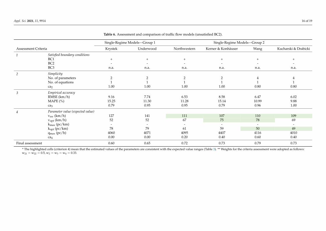
If we accept the failure to satisfy BC2, Kerner and Konhäuser’s, Wang’s, and Kucharskiand Drabicki’s models are worth considering. The first two perform relatively well onqmax, traffic parameter representation, which is a feature other BC2 models did not meet(Table 6). However, all come with some limitations. Kerner and Konhäuser’s model carriesa relatively big estimation error. Kucharski and Drabicki’s model has one of the lowestestimation errors; however, it underestimates the values of qmax and vopt. The problemwith Wang’s model is that traffic volume increases significantly for densities of the orderof 150 pc/km and that speed does not tend to zero; instead, it tends to a certain minimalvalue which in the case if the field data is 12 km/h (Figure 7). In turn, this goes againstPolish studies that have shown that for densities of the order of 50 pc/km/lane, vehiclestream speed does not exceed 10 km/h, and for densities of the order of 100 pc/km/lane,the speed is close to zero.

Appl. Sci. 2021, 11, 9914 16 of 19

Table 6. Assessment and comparison of traffic flow models (unsatisfied BC2).

Single-Regime Models—Group 1 Single-Regime Models—Group 2

Assessment Criteria Krystek Underwood Northwestern Kerner & Konhäuser Wang Kucharski & Drabicki

1 Satisfied boundary conditionsBC1 + + + + + +BC2 - - - - - -BC3 n.a. n.a. n.a. n.a. n.a. n.a.

2 SimplicityNo. of parameters 2 2 2 2 4 4No. of equations 1 1 1 1 1 1ca2 1.00 1.00 1.00 1.00 0.80 0.80

3 Empirical accuracyRMSE (km/h) 9.16 7.74 6.53 8.58 6.47 6.02MAPE (%) 15.25 11.30 11.28 15.14 10.99 9.88ca3 0.79 0.95 0.95 0.79 0.96 1.00

4 Parameter value (expected value)vsw (km/h) 127 141 111 107 110 109vopt (km/h) 52 52 67 75 78 69kmax (pc/km) - - - - - -kopt (pc/km) 78 79 61 59 50 49qmax (pc/h) 4060 4071 4095 4407 4116 4010ca4 0.00 0.00 0.20 0.40 0.60 0.40

Final assessment 0.60 0.65 0.72 0.73 0.79 0.73

* The highlighted cells (criterion 4) mean that the estimated values of the parameters are consistent with the expected value ranges (Table 3). ** Weights for the criteria assessment were adopted as follows:w21 = w22 = 0.5, w2 = w3 = w4 = 0.33.

Appl. Sci. 2021, 11, 9914 17 of 19

5. Discussion

Considering the need to prepare the Polish Highway Capacity Manual, the objectiveof the article was to analyze existing models of the fundamental relationship, comparethem, and select the best performing ones that could be used as a basis for the Polishmethod.

The problem that we encountered when reviewing the literature was that there isno agreement of researchers on how to assess and compare traffic flow models. Manycomparisons have an expert basis rather than a quantitative approach [4,17,29]. The mostwidely used in quantitative assessment is the model fitness to empirical data [25–28]. Themodels’ simplicity, compatibility with boundary conditions, and parameter values validityare rarely considered. On the other side, visual assessment of the models is hampered bythe existence of the scatter in the real data explained by stochastic characteristics of trafficin real world [32–35], which is revealed by many speed values corresponding to the samedensity. Taking these issues into account, we proposed a universal and quantitative methodfor assessing models of the fundamental relationship. Based on the literature [4,9,18,24],we adopted four criteria for traffic flow models assessment and comparison: simplicity,empirical accuracy, correct estimation of model parameters, and meeting the boundaryconditions; the criteria were quantified and assessed in a two-stage procedure. The finalassessment is a weighted average of criteria assessment.

A detailed analysis using the method confirms the conclusions from the literature re-view, which is that no model fully meets the requirements the researchers [4,9,18] expectedof the fundamental relationship models. This suggests and comes as a confirmation of DelCastillo and Benitez’s conclusion [2] that the problem of finding the best model remainsopen. This is the most important conclusion from the study that encourages a search for anew model that could be applied to represent the empirical relations of traffic flow.

Analysis results show that the simplest two and three-parameter models do notrepresent traffic flow characteristics well. While two-regime models offer a much betterempirical accuracy, they do so at the cost of model simplicity. The best representation ofempirical relations with a relatively simple mathematical function is offered by modelsthat represent the relation v = f(k) with an S-shaped curve. This observation was pickedby Wang [4], who proposed a model that uses a sigmoidal curve to represent the relation.Similarly, Drake et al. [14] proposed a model based on a bell-shaped curve. Thanks to theshape, it is possible to include the empirical data pattern where in the initial phase speed,it falls slowly until maximal flow is reached and starts falling much faster afterwards. Thepace of the fall slows for low speeds. It also helps to take account of the break point wherek = kopt. However, most of these models fail to represent the area of maximum flow, andthis is probably caused by the inevitable scatter in data that occurs at the highest flows andin congested traffic regime.

We observed that some of the models (with the S-shaped curve representing therelation v = f(k)) that fail to meet boundary conditions (Wang et al., Kerner and Konhäuser)seem to give a good representation of traffic flow, even in the intractable area of maximumflow. This raises some questions: Does the BC2 boundary condition have to be absolutelysatisfied? Is failure to meet BC2 conditionally acceptable, and if so, under what condition?If our interest is solely in a free-flow regime before the maximum flow is reached (e.g., inmethods for traffic condition assessment), is it crucial to meet BC in the congested regime?There are no obvious answers to these questions, and a lot will depend on the purpose ofmodeling. The results of a Polish study of maximal density [38] suggest that a conditionalacceptance of a model that does not satisfy BC2 may be possible if within the expectedrange of maximal density (app. 100÷ 150 pc/km/lane), speed is close to zero (≤ 5 km/h)and diminishes as density continues to increase. This possibility is included in the proposedmethodology (Figure 5).

The research comes with some limitations that we are aware of. The proposed method-ology was tested on one site (permanent traffic counting station) and, thus, requires furtherinvestigation and validation with data from other sites. Another limitation is that the

Appl. Sci. 2021, 11, 9914 18 of 19

models cannot be assessed if they have a different form and are not transformed to (2).One example is Van Aerde’s four-parameter model [16], which is well received in theliterature [17,40] and used as the basis for Germany’s method for motorway traffic assess-ment [6]. This leads to the question: Would this model provide a better representation ofthe empirical relation compared with the analyzed models? Another limitation is that theassessment of a model’s simplicity does not address its functional form. As a consequence,Greenshields’ linear model and Greenberg’s logarithmic model are given equal scores.How to include this issue in the assessment of model simplicity? All these issues should beconsidered in further work.

Author Contributions: Conceptualization, A.R. and K.J.; methodology, A.R.; validation, A.R. andK.J.; formal analysis, A.R.; investigation, A.R.; resources, A.R.; data curation, A.R.; writing—originaldraft preparation, A.R.; writing—review and editing, K.J.; visualization, A.R.; supervision, K.J. Allauthors have read and agreed to the published version of the manuscript.

Funding: This research received no external funding.

Institutional Review Board Statement: Not applicable.

Informed Consent Statement: Not applicable.

Data Availability Statement: The data presented in this study are openly available in MostWiedzyrepository at https://doi.org/10.34808/8xkq-7714 (accessed on 18 October 2021), reference num-ber [30].

Acknowledgments: The study is part of a doctoral thesis [31] and was delivered under the RID2B project which is designed to develop methods for estimating capacity and assessing trafficconditions on Poland’s dual carriageways. The outcome of the project is the Polish Highway CapacityManual, with procedures for assessing traffic conditions and identifying the capacity of rural andagglomeration roads [38].

Conflicts of Interest: The authors declare no conflict of interest.

References1. Greenshields, B.D. A study of traffic capacity. In Proceedings of the Fourteenth Annual Meeting of the Highway Research Board,

Washington, DC, USA, 6–7 December 1934; Highway Research Board: Washington, DC, USA, 1935; pp. 448–477. Available online:http://pubsindex.trb.org/view.aspx?id=120649 (accessed on 6 September 2021).

2. Castillo, J.M.D.; Benítez, F.G. On the functional form of the speed-density relationship—I: General theory. Transp. Res. Part BMethodol. 1995, 29, 373–389. [CrossRef]

3. Wang, H.; Li, J.; Chen, Q.-Y.; Ni, D. Speed-Density Relationship: From Deterministic to Stochastic. In Proceedings of the 88thTransportation Research Board Annual Meeting, Washington, DC, USA, 11–15 January 2009.

4. Wang, H.; Li, J.; Chen, Q.-Y.; Ni, D. Logistic modeling of the equilibrium speed-density relationship. Transp. Res. Part A 2011, 45,554–566. [CrossRef]

5. Transportation Research Board. Highway Capacity Manual 6th Edition: A Guide for Multimodal Mobility Analysis; TransportationResearch Board of the National Academies: Washington, DC, USA, 2016.

6. Baier, M.M.; Brilon, W.; Hartkopf, G.; Lemke, K.; Maier, R.; Schmotz, M. HBS2015 Handbuch für die Bemessung von Straßen-verkehrsanlagen. Teil A - Autobahnen; Forschungsgesellschaft für Straßen- und Verkehrswesen (FGSV), Kommission Bemessungvon Straßenverkehrsanlagen: Köln, Germany, 2015.

7. Greenberg, H. An analysis of traffic flow. Oper. Res. 1958, 7, 79–85. Available online: http://links.jstor.org/sici?sici=0030-364X%28195901%2F02%297%3A1%3C79%3AAAOTF%3E2.0.CO%3B2-7 (accessed on 6 September 2021). [CrossRef]

8. Lighthill, M.J.; Whitham, G.B. On kinematic waves. II. A theory of traffic flow on long crowded roads. Proc. R. Soc. A Math. Phys.Eng. Sci. 1955, 229, 317–345. [CrossRef]

9. Underwood, R.T. Speed, volume and density relationships. In Quality and Theory of traffic Flow; Bureau of Highway Traffic, YaleUniversity: New Haven, CT, USA, 1960; pp. 141–188. Available online: http://tft.eng.usf.edu/greenshields/docs/Greenshields_Quality_and_Theory_of_Traffic_Flow_1961.pdf (accessed on 14 August 2018).

10. Ardekani, S.A.; Ghandehari, M.; Nepal, S.M. Macroscopic speed-flow models for characterization of freeway and managed lanes.Bul. Institutului Politeh. Din Iasi 2011, 57, 149. Available online: http://www.bipcons.ce.tuiasi.ro/Archive/222.pdf (accessed on13 August 2018).

11. Pipes, L.A. Car following models and the fundamental diagram of road traffic. Transp. Res. 1967, 1, 21–29. [CrossRef]12. Krystek, R. Syntetyczny Wskaznik Jakosci Ruchu Ulicznego; Politechnika Gdanska: Gdansk, Poland, 1980.

Appl. Sci. 2021, 11, 9914 19 of 19

13. Drew, D.R. Deterministic Aspects of Freeway Operations and Control; Research Report Number 24-4; Texas Transportation Institute:College Station, TX, USA, 1965. Available online: https://static.tti.tamu.edu/tti.tamu.edu/documents/24-4.pdf (accessed on9 August 2017).

14. Drake, J.S.; Schofer, J.L.; May, A.D. A statistical analysis of speed density hypotheses. Highw. Res. Rec. 1966, 154, pp. 53–87.Available online: http://onlinepubs.trb.org/Onlinepubs/hrr/1967/154/154-004.pdf (accessed on 27 December 2017).

15. Kerner, B.S.; Konhäuser, P.; Schilke, M. Deterministic spontaneous appearance of traffic jams in slightly inhomogeneous trafficflow. Phys. Rev. E 1995, 51, 6243–6246. [CrossRef] [PubMed]

16. Van Aerde, M. A single regime speed-flow-density relationship for freeways and arterials. In Proceedings of the 74th Transporta-tion Research Board Annual Meeting, Washington, DC, USA, 22–28 January 1995.

17. Rakha, H.; Crowther, B. Comparison of Greenshields, Pipes and Van Aerde car-following and traffic stream models. Transp. Res.Rec. J. Transp. Res. Board 2002, 1802, 248–262. [CrossRef]

18. MacNicholas, M.J. A simple and pragmatic representation of traffic flow. In 75 Years of the Fundamental Diagram for Traffic FlowTheory; Greenshields Symposium; Transport Research Board: Woods Hole, MA, USA, 2011.

19. Kucharski, R.; Drabicki, A. Estimating macroscopic volume delay functions with the traffic density derived from measuredspeeds and flows. J. Adv. Transp. 2017, 2017, 4629792. [CrossRef]

20. Bureau of Public Roads. Traffic Assignment Manual for Application with a Large, High Speed Computer; Bureau of Public Roads:Washington, DC, USA, 1964.

21. Smulders, S.A. Control of Freeway Traffic Flow; Stichting Mathematisch Centrum: Amsterdam, The Netherlands, 1989.22. Daganzo, C.F. Fundamentals of Transportation and Traffic Operations; Emerald: Bingley, UK, 1997.23. Knoop, V.L. Introduction to Traffic Flow Theory: An Introduction with Exercises; Delft University of Technology: Delft, The Netherlands,

2017. Available online: http://www.victorknoop.eu/research/book/Knoop_Intro_traffic_flow_theory_edition1.pdf (accessed on27 December 2017).

24. Myung, J.I.; Pitt, M.A. Model Comparison Methods. Methods Enzymol. 2004, 383, 351–366. [CrossRef] [PubMed]25. Gaddam, H.K.; Rao, K.R. Speed–density functional relationship for heterogeneous traffic data: A statistical and theoretical

investigation. J. Mod. Transp. 2019, 27, 61–74. [CrossRef]26. May, A.D. Traffic Flow Fundamentals; Prentice-Hall, Inc.: Englewood Cliffs, NJ, USA, 1990; p. 464. Available online: http:

//books.google.com/books?id=JYJPAAAAMAAJ&pgis=1 (accessed on 11 September 2021).27. Rakha, H. Validation of Van Aerde’s simplified steadystate car-following and traffic stream model. Transp. Lett. 2009, 1, 227–244.

[CrossRef]28. Cheng, X.U. Analysis of Traffic Flow Speed-density Relation Model Characteristics. J. Highw. Transp. Res. Dev. 2014, 8, 104–110.29. Ni, D.; Zheng, C.; Wang, H. A Unified Perspective on Traffic Flow Theory, Part III: Validation and Benchmarking. In Proceedings

of the 11th International Conference of Chinese Transportation Professionals (ICCTP), Nanjing, China, 14–17 August 2011.[CrossRef]

30. Romanowska, A.; Kustra, W. Permanent Traffic Counting Stations—Expressway S6 in Gdansk (Dataset Containing 5-min Aggre-gated Traffic Data and Weather Information), 2021. Available online: https://mostwiedzy.pl/en/open-research-data/permanent-traffic-counting-stations-expressway-s6-in-gdansk-dataset-containing-5-min-aggregated-traf,923120743943369-0 (accessed on 11September 2021).

31. Romanowska, A. Macroscopic traffic Flow Models for basic Motorways and Express Roads Sections. Ph.D. Thesis, GdanskUniversity of Technology, Gdansk, Poland, 2019.

32. Coifman, B. Advancing Traffic Flow Theory Using Empirical Microscopic Data; NEXTRANS Project, No. 174OSUY2.2; The Ohio StateUniversity: Columbus, OH, USA, 2015.

33. Wang, H.; Ni, D.; Chen, Q.-Y.; Li, J. Stochastic modeling of the equilibrium speed-density relationship. J. Adv. Transp. 2013, 47,126–150. [CrossRef]

34. van Wageningen-Kessels, F.; van Lint, H.; Vuik, K.; Hoogendoorn, S. Genealogy of traffic flow models. EURO J. Transp. Logist.2014, 4, 445–473. [CrossRef]

35. Jabari, S.E.; Zheng, J.; Liu, H.X. A probabilistic stationary speed-density relation based on Newell’s simplified car-followingmodel. Transp. Res. Part B Methodol. 2014, 68, 205–223. [CrossRef]

36. Zheng, L.; He, Z.; He, T. A flexible traffic stream model and its three representations of traffic flow. Transp. Res. Part C Emerg.Technol. 2017, 75, 136–167. [CrossRef]

37. Rakha, H.; Arafeh, M. Calibrating steady-state traffic stream and car-following models using loop detector data. Transp. Sci. 2010,44, 151–168. [CrossRef]

38. Olszewski, P.; Dybicz, T.; Kustra, W.; Romanowska, A.; Jamroz, K.; Ostrowski, K. Development of the New Polish Method forCapacity Analysis of Motorways and Expressways. Arch. Civ. Eng. 2020, 66, 453–470. [CrossRef]

39. Gavin, H.P. The Levenberg-Marquardt Algorithm for nonlinear Least Squares Curve-Fitting Problems. 2019. Available online:http://people.duke.edu/~hpgavin/ce281/lm.pdf (accessed on 24 May 2019).

40. Van Aerde, M.; Rakha, H. Multivariate calibration of single regime speed-flow-density relationships. In Proceedings of the 6thInternational VNIS Conference, Seattle, WA, USA, 30 July–2 August 1995; IEEE: New York, NY, USA, 1995; pp. 334–341.