Computational Queuing Analysis: An Application to Traffic Flow Analysis of the NAS

American Institute of Aeronautics and Astronautics 1

Computational Queuing Analysis: An Application to Traffic Flow Analysis of the NAS

Prasenjit Sengupta*, Monish D. Tandale*, and P. K. Menon†

Optimal Synthesis Inc., Los Altos, CA 94022-2777

The application of Queuing Theory to quantify the relationships between trajectory uncertainties due to aviation operations, precision of navigation and control, and traffic flow efficiency in the National Airspace System is discussed. This work builds on a previous research effort on Markovian queuing network models of the NAS. While the Markovian network model provides closed-form analytical solutions, it does not model arrival and service distributions with high fidelity. On the other hand, Phase-Type distributions such as the Coxian can model any distribution with arbitrary accuracy, however analytical solutions for such queuing networks are not available. This paper develops a numerical solution methodology for analysis of queuing networks with Coxian arrivals and service time distributions. This approach is based on state enumeration and propagation of Chapman Kolmogorov equations. This paper develops novel numerical methods to obtain exact solutions to the departure process from a queue as well as aggregation and disaggregation of flows with arbitrary inter-arrival distributions. Sample results for a Center Level model of the U.S. National Airspace System are presented.

I. Introduction nderstanding the relationships between trajectory uncertainties due to aviation operations, precision of navigation and control, and the traffic flow efficiency is central to the design of Next Generation Air

Transportation Systems (NextGen). In all that follows, the traffic flow efficiency is defined as the degree to which the aircraft is delayed due to congestion effects as compared to an unimpeded flight along the same route. Congestion arises when the demand exceeds capacity in a region of the airspace, which requires that the upstream aircraft entering the airspace must be delayed until the capacity becomes available.

The analysis of the National Airspace System (NAS) using Markovian network models at Airspace-level, Center-level, Sector-level and latitude/longitude-level spatial resolutions were discussed in Refs. 1 and 2. The assumption of exponential inter-arrival time and service distributions was central for deriving the results in that paper.

However, observations from FACET simulations with real traffic data reveal that at certain spatial resolutions, the service time distributions are poorly represented by exponential probability density functions. For instance, it may be observed from Refs. 1 and 2, that the service time distribution is not necessarily exponentially distributed. Consequently, accurate computation of the flow metrics such as the probability distribution of the number of elements in service, expected queue length and waiting time require the consideration of realistic arrival and service distributions in the queuing network.

One approach for deriving queuing results using more general inter-arrival and service time distributions is to approximate these processes by Erlang or Coxian distributions3. This produces a semi-Markovian queue, which can be numerically solved using the state-enumeration approach4. Queuing networks with semi-Markovian nodes require additional computations at node junctions. These computations can also be formulated using the state-enumeration process. While networks with few nodes can be directly approached in this manner, more realistic networks may involve extremely large number of states, requiring solutions based on decomposition. The following sections will

* Research Scientist, 95 First Street Suite 240, Senior Member AIAA. † Chief Scientist and President, 95 First Street Suite 240, Fellow AIAA.

U

10th AIAA Aviation Technology, Integration, and Operations (ATIO) Conference 13 - 15 September 2010, Fort Worth, Texas

AIAA 2010-9137

Copyright © 2010 by Optimal Synthesis Inc. Published by the American Institute of Aeronautics and Astronautics, Inc., with permission.


discuss the approach adopted for formulation and solution of the Center-level queuing network model incorporating Coxian inter-arrival and service time distributions.

II. Center-Level Coxian Model Unlike the Jackson model of the NAS discussed in Ref. 1, the service time distributions and inter-arrival

distributions into the network are given by multi-phase Coxian distributions. Coxian distributions are fitted to the service time and inter-arrival times obtained from FACET using a non-linear least squares curve fit. The resulting distributions are used in the network solution for Coxian nodes, described in the next section.

A. Node Capacity The capacity of Centers translates into the number of parallel servers employed by the Center node. As

discussed in Ref. 5, the Center capacity tends to be large. Due to the large number of parallel servers resulting from this assumption, the solution for the network using state-enumeration techniques will turn out to be computationally intractable. Therefore, the items in the network are quantized into groups of aircraft. The network solution is obtained by treating a group of aircraft as a single item, with the number of parallel servers in the Center being factored by the group size. These concepts are explained in detail in the following sections.

B. Introduction of NAS Uncertainties in the Coxian Network Model The service rates, arrival rates and Center capacity are obtained from FACET simulations, and are used to

model the NAS as a network of queuing nodes. Since it is possible to run FACET simulations using as-filed flight data, the network of queues representing the NAS under these circumstances can be assumed to simulate the NAS under ideal conditions. Models representing different sources of uncertainty discussed in Refs. 5 and 6 can then be incorporated into the solution framework. These uncertainty models modify the service rates and Center capacity, and their effect on the network parameters can then be examined. Methods for incorporating the uncertainties into the network model are discussed in Refs. 5 and 6.

III. Solution Methods for the Coxian Networks This section presents techniques for solving a network composed of nodes with �� queuing discipline as

shown in Figure 1. It is assumed at the outset that the network is stable in the sense that in steady state, the network capacity exceeds the inflow. It is also assumed that the general inter-arrival and service time distributions can be represented by an �-phase Coxian, and �-phase Coxian distribution, respectively. It is known that the Coxian distribution is dense in the field of all positive-valued distribution, that is, a Coxian distribution of suitable order and parameters can be used to approximate any given probability density function. Consequently, an equivalent problem is to solve a network of �� nodes. Each node in the network is composed of up to five operations: 1) Arrival into network: depicted by a green arrow, indicating that an item has entered the network from the

external environment. 2) Aggregation: depicted by a red circle, this represents the combined input into a queuing system, from external

arrivals, as well as arrivals from the other nodes in the network. 3) Queuing system: this represents the service performed with a service time defined by a �-phase Coxian

distribution on items arriving with an �-phase Coxian distribution of inter-arrival times, with � servers in parallel. The result of the queuing system is a distribution of inter-departure times of the items.

4) Disaggregation: depicted by a red circle, this represents the branching of items departing from a node to the other nodes of the network.

5) Departure from network: also depicted by a green arrow, this indicates that an item has left the network. The flow prior to the disaggregation point, and the disaggregated flows, including departure from network, must conserve flow balance. It should be noted that it is not necessary for each node to contain all of the five operations listed in the

foregoing.


Figure 1. Network of G/G/s Nodes

A. Prior Work and Preliminary Developments There is a considerable amount of literature available on the solution of queues with different classes of arrival

and service time distributions. The simplest queuing discipline is the �� queue, where the arrival and service processes are assumed to be exponential, with arrival flow rate �, and service rate . Analytical solutions for this type of queue, as well as the multiple server variety (��) are well-known, and available in standard texts on queuing theory4. An analytical solution for a queuing service with the �� discipline using the method of generating functions is given in Refs. 7 and 8. In particular, the latter work compared results with numerical techniques9 and derived an exact algorithm to calculate the number of items in the system at steady state, and queuing analysis parameters such as the waiting time.

Several works in the literature also analyze the steady-state probabilities of networks that are composed of Markovian and semi-Markovian queuing nodes. The simplest of these is the Jackson network10, which is a network composed of nodes with exponentially-distributed service times and Poisson arrivals.

An essential aspect of the analysis of queuing networks is the characterization of the departure process of a queue, since this process will serve as the input to the remaining nodes in the network. A survey of historical results in the analysis of the departure process has been presented in Ref. 11. Later work12,13 approximates the departure process of a queue, as well as disaggregation, using the first two moments.

A method for the approximate analysis of a network of single-server nodes with arbitrary distributions has been developed14, which uses approximate formulae to calculate the first two moments of the inter-departure time distribution. Reference 15 develops a queuing model of the National Airspace System using Erlang distributions to model the service time distribution, and exponential distributions to model the arrival processes. The Queuing Network Analyzer algorithm16 also uses approximate formulae to solve for the first two moments of aggregated, disaggregated, and departing flows through nodes in a queuing network. This algorithm has been used to analyze traffic flow in the NAS, in Ref. 2.

Reference 17 has developed approximations for the departure process of a single-server node with phase-type service, and a superposition of phase-type arrivals. Approximations for the departure process have also been developed18.

The research in this paper develops a convergent algorithm for solving a network of nodes with Coxian service, with Coxian external arrivals. The component processes of aggregation, disaggregation, and queuing service are solved individually using semi-analytical techniques for matrix exponential calculations. Recent research in the analysis of matrix exponentials19 has resulted in the development of extremely efficient algorithms for the evaluation


of repeated products of matrix exponentials and vectors. More recently20, techniques have been developed for the evaluation of the exponentials of sparse matrices. These techniques allow for the fast solutions to the state-enumeration problem in systems with very large number of states. A method is developed to obtain the inter-departure time distribution of the component processes to a given accuracy.

B. Queuing Service In this section, the state-enumeration procedure is developed for the analysis of the departure process of a

queue with Coxian service time distribution and multiple servers, with an arrival process that can also be represented by a Coxian distribution. It is assumed that the arrival process into the node can be represented by an �-phase Coxian distribution (a “generator" node), with parameters �, and transition probabilities ��. Service is rendered by a �-phase Coxian service node, with parameters �, and transition probabilities ��. This node has � identical servers with identical parameters. A schematic of this queuing system is given by Figure 2.

Figure 2. Queuing Service

The characterization of the state space in a �� queuing service presented here has been derived in Ref. 8. The state of the system is uniquely defined by three quantities: 1) the phase of the generator node, 2) the number of items in service in the service node, and 3) the number of servers in the same phase, for every phase of the service node. Since each server is identical, the number of servers in each phase of the service node is sufficient to uniquely identify each state. The state of the system is represented by the sequence �� where � is the phase of the generator node, � is the number of items in service, and �� denote the number of servers currently in phases �� , respectively. It should be noted that

� ��

�� ! " � " ��

�� # � (1)

If the maximum number of items in the system is denoted by $, then ! " � " $. The forward Chapman-Kolmogorov equations21 for the node can be written by assuming that at each instant,

the state transitions occur as birth-death processes. Consequently, the states evolve according to the following linear equation:

%& � '% (2)

where %� is the probability of the system being in the (th state. The variable '�) is the �(� *�th entry of the matrix ', and denotes the rate of transition from the *th state to the (th state. The transitions from a given state


�� can be classified as a phase change in the generator or service node, arrival into the service node (equivalently, departure from the generator node), and departure from the service node.

C. Total Number of States Let +,-.-/, be the total number of states of the system, which is also the length of the state vector in Eq. (2).

Since the complexity of the solution procedure is dependent on +,-.-/,, its value needs to be obtained at the outset. This value is given by:

+,-.-/, � 0 � 1$ 2 �� 3 � ! " $ " �� 4�$ 5 �� 2 � 2 �� 6 7� 2 � 5 �� 5 � 8 � $ # � (3)

State-enumeration for a queue with multiple servers with identical characteristics can result in a large number of states. Let : be the increase in the number of phases or servers, for a system with a single-phase generator node. Let +� and +� be defined as follows: +� � ;�$ 2 :� 2 �� <

+� � ;$ 2 �� 2 :�� 2 :� < (4)

In Eq. (4), +� and +� denote the number of states when the number of items and number of phases are respectively increased by :. Using Eq. (4) it can be shown that:

+� � �$ 2 � 2 :�=�� 2 :�= $= � �$ 2 ��$ 2 �� > �$ 2 :�� 2 �� 2 �� > �� 2 :� +� (5)

In most cases, $ # �, and therefore

+� # 7$ 2 :� 2 :8? +� (6)

The foregoing expression indicates that an increase in the number of server node phases results in larger dimensional state space than an increase in the maximum number of items in the queuing system.

D. Steady State Distribution The steady state probability distribution for the system denoted by %@, can obtained by solving '%@ � !, with the

constraint A%@A� � �. Whereas an analytical formulation to obtain a solution to the above equations is given in Ref. 8, matrix exponential methods that take advantage of the sparse structure can also be used efficiently to propagate any initial condition to steady state. In other words,

%@ � BCD-EF GHI�'J� %K � L BCDMEFNGHI�':J�OMP %K (7)

where %K is an arbitrary initial vector. Without loss of generality, this vector can be defined as %K � Q� +,-.-/,R � +,-.-/,R > � +,-.-/,R ST. Highly efficient techniques19 are available to compute the products of matrix exponentials with vectors. The matrix exponential method is also chosen because it is useful in obtaining the departure process of a queue as a function of time, as will be shown in the next section.

E. Departure Process of a Queue The departure process of a queuing system can also be obtained using state enumeration. The output process

for Poisson arrivals and service with multiple servers is derived in Ref. 22. This method is extended to Coxian arrival and service rate distributions in the following. The transition rate matrix ' can be written as:

' � 'UV.,/W 2 'UV.,/X 2 '.YY�Z.[ 2 '\/U.Y-]Y/ 2 '\�.^ (8)


where each of the first four component matrices in the above equation correspond to the four types of transitions detailed in the end of Section III.B. The matrix '\�.^ is a diagonal matrix that denotes the transition rate from each state into itself, and whose entries can be obtained from the negative row sum of the first four component matrices.

Let the matrix _ denote the following:

_ � ' 5 '\/U.Y-]Y/ � 'UV.,/W 2 'UV.,/X 2 '.YY�Z.[ 2 '\�.^ (9)

Given the steady state distribution %@, let K̀ denote the following:

K̀ � '\/U.Y-]Y/%@:Ja'\/U.Y-]Y/%@:Ja� � 5 _%@A_%@A� (10)

The vector K̀ is the probability (suitably normalized) associated with the system states after departure of an item. Let `�J� denote a vector, whose (th component �̀�J� denotes the probability that the system is in state ( after an inter-departure time segment. As noted in Ref. 22, the complementary cumulative distribution function, also known as the survival function, and denoted herein by c.c.d.f., can be obtained by the following equation:

bbc \̀/U.Y-]Y/ �J� � � �̀�J�F��K (11)

For a stable linear system representing the Chapman-Kolmogorov equations for queuing, with sufficiently large maximum number of items, the above relation can be approximated as follows:

� �̀�J�F��K d � �̀�J�e

��K (12)

Consider the dynamical system &̀ � _`, with `�!� � K̀ given by Eq. (10). This system of linear differential equations governs the evolution of the states with no departures from the system. The cumulative distribution function (c.d.f.) of the departure process, at steady state, is thus given by:

bc \̀/U.Y-]Y/ �J� � � 5 � �̀�J�e��K (13)

The probability density function (p.d.f.), can be obtained by differentiating the c.d.f. with respect to time:

fc \̀/U.Y-]Y/ �J� � 5 � &̀��J�e��K � 5 � � _�) )̀�J�e

)�Ke

��K (14)

F. Disaggregation The process of disaggregation shown in Figure 3, occurs after the queuing service has been rendered. In

disaggregation, an arrival process with given �-phase Coxian distribution parameters � �� , and �� g�� !�, is split into h flows, with flow fraction i� through i[, such that i� 2 i� 2 > 2 i[ � �. A flow that leaves the network can also be modeled as one of the branches of the disaggregation process. The Jackson network approximation shows that the flow rates after a disaggregation point, multiplied by their flow fractions, sum to the flow rate before the disaggregation point. However, this only enables one to calculate the mean inter-departure time of the disaggregated distributions. Reference 14 used approximate analytical formulae to obtain the second moment of the disaggregated flow. Reference 23 used an iterative decomposition algorithm to obtain approximate solutions for a fork / joint queuing system. In this section, an exact analysis of the disaggregation process is presented using the enumeration of states.


Figure 3. Disaggregation

Of interest is the departure process from the (th branch, where ( � �� h. The flow prior to the disaggregation point is assumed to emerge from a generator node similar to the one described in Section III.B. The states of the system are thus composed of phase changes in the generator node, and departures from the generator node, whereupon the generator returns to the first phase. The states are indexed such that the first �� 5 �� states correspond to phase changes, and the next h states correspond to departures along each branch, with the system returning to the first phase of the generator node. Let the state vector for departure through the (th branch be denoted by �̀, and let this vector’s *th component be denoted by �̀) . The initial condition for the c.c.d.f. of the departure process is then given by �̀��jg��!� � �, and �̀�)�!� � !, k* l ( 2 � 5 �. The forward Chapman-Kolmogorov equations for the c.c.d.f., for states ! through � 5 � can be written as follows: &̀��K � 5 �̀�K 2 g��g� �̀��&̀�� 5 g� �̀�� 2 g��g� �̀��m&̀��g�� 5 � �̀��g�� 2 �� ̀��g�� 2 �̀�� 2 �̀��j�� 2 > 2 �̀��j[g��

(15)

For the remaining state equations, it is convenient to define the vector in, whose components in) are given by in) � i), k* l (, and in) � ! when * � (. Furthermore, define �o� � � 5 ��. The remaining state equations can then be written as follows: &̀��g�� in�p �o �̀�K 2 g��og� �̀�� 2 > 2 ��o� �̀��g��q2 �p5r� 5 �o�in�s �̀��g�� 2 �o�in� �̀�� 2 �o�in� �̀��j�� 2 >2 �o�in� �̀��j[g��q&̀�� in�p �o �̀�K 2 g��og� �̀�� 2 > 2 ��o� �̀��g��q2 �p�o�in� �̀��g�� 5 r� 5 �o�in�s �̀�� 2 �o�in� �̀��j�� 2 >2 �o�in� �̀��j[g��q&̀��j�� intp �o �̀�K 2 g��og� �̀�� 2 > 2 ��o� �̀��g��q2 �p�o�int �̀��g�� 2 �o�int �̀�� 5 r� 5 �o�ints �̀��j�� 2 >2 �o�int �̀��j[g��q m&̀��j[g�� in[p �o �̀�K 2 g��og� �̀�� 2 > 2 ��o� �̀��g��q2 �p �o�in[ �̀��g�� 2 �o�in[ �̀�� 2 �o�in[ �̀��j�� 2 >5 r� 5 �o�in[s �̀��j[g��q

(16)

Equations (15) and (16) can be conveniently rewritten as the linear system &̀� � _� �̀ , and propagated in time to obtain the departure time distribution at the (th branch.


G. Aggregation The aggregation of flows occurs before entry into the queuing system. As shown in Figure 4, the process of

aggregation combines h Coxian arrival processes with the number of phases given by �� [, and with the parameters of the (th input denoted by � �� and r�� g�� !s. Arrivals from sources external to the network can also be modeled and included at the point of aggregation, using this technique. As was observed in the previous section, the flow rate at aggregation is the sum of the flow rates prior to aggregation. Several approximate methods for flow aggregation have been compared in Ref. 24. In this section, a method based on state-enumeration is presented for the aggregation of flows.

Figure 4. Aggregation of Flows

Much of the required background has already been covered in the section on the analysis of departures from queues. It may be noted that the aggregation process can be represented by h generator nodes, and the states of the system can be uniquely identified by the phase of each generator. Consequently, the total number of states in the system is given by u ��[�� , and the state of the system is identified by the h-tuple �(�� (�� ([�, where � " (� " ��, � " (� " ��,etc. The index for a given state follows from the following formula:

v � �(� 5 �� w �)[

)�� 2 �(� 5 �� w �)[

)�� 2 > 2 �([g� 5 ��[g��[ 2 �([g� 5 ��[ 2 ([ 5 � (17)

The only transitions possible for this system are phase changes in any of the generators, and a departure from any of the generators. Therefore, the transition rate matrix for aggregations, denoted by '., may be constructed in a manner similar to the construction of the transition rate matrix of the queuing service, shown in Section III.B. The steady-state distribution corresponding to the transition matrix '. is denoted by %@., and can be found using techniques discussed in Section III.D. The system of equations for the c.c.d.f. is given by:

&̀. � _. .̀� .̀�!� � 5 _.%@.A_.%@.A� (18)

The off-diagonal elements of _. are the same as those of '. 5 '.xyz{|}~|y . The diagonal elements denote the transitional probability of remaining in the same state due to all possible departures or phase transitions. In any generator node, a departure from any phase always transitions to a state with that generator node in the first phase. This is different from a departure from a service node: a departure from a service node may not necessarily be accompanied by another element arriving in its first phase. Consequently, the diagonal elements of the matrix _. are given by _.�� 2 �� 2 > 2 [�� , where v is obtained from Eq. (17).

H. Solution of the Network The network can now be solved in an iterative manner, using the component processes described in the

previous sections. The number of nodes in the system is +. Each node has an associated Coxian service time


distribution. Each node may also have an external arrival process associated with it, where each arrival process can also be modeled by a Coxian distribution. The vector denotes the mean arrival rates at the nodes, which can be obtained from the reciprocal of the expected values of the Coxian distributions that represent the arrival.

Associated with the network is a connectivity matrix �, whose �(� *�th entry denotes the flow fraction from the (th node of the network to the *th node of the network. It is understood that the diagonal entries of � denote the fraction of the flow that leaves the network at that node, and that furthermore, � ��)e)�� , k(.

Let �� denote the matrix composed of the off-diagonal entries of �. The departure flow rate vector � can be obtained from the flow balance equations for the Jackson network10, for given external arrival flow rate vector �, as shown below:

� � r� 5 ��sg�� (19)

In this equation, � is used to denoted the identity matrix of dimension + � +. Although the flow balance equation can be used regardless of the queuing discipline at each node, Eq. (19) is

not particularly useful, since the formulae for network metrics available in the literature are only valid for special cases of the queuing disciplines. Therefore, the network is solved iteratively, using exponential arrivals with rates �as initial guesses at each node. The output of the queuing service is obtained using the methods developed in the previous sections, and disaggregated. These are fed back to each node based on the connectivity matrix, and the procedure is repeated until the change in the expected rate at output reduces to below a desired value.

An essential procedure at every step of the network solution is to fit an appropriate Coxian distribution to the output of the aggregation, queuing service, and disaggregation processes. Since the p.d.f. at any stage can be obtained at any desired resolution, very accurate fits are possible using gradient-based methods.

I. Solving a Network with Large Node Capacities Using Quantization The number of states required to solve a node with Coxian arrivals and service can be very large when the

number of servers very high. For a Center-level model, the number of aircraft that can be served in parallel is of the order of hundreds. However, if a group of predetermined size is treated as one item in the queuing service, the number of servers required to model the queuing system can be reduced by a factor of the size of the group. For example, a queuing system with expected arrival flow rate �, expected service rate , and � parallel servers, is considered equivalent to one with expected service rate and �� parallel servers, where � is the size of the group of aircraft, such that �� . For this system, the arrival p.d.f. is modified to ensure that flow balance equations and utilization factor � � �� remain unchanged. As a result, the arrival process for the new system is �-phase Erlang, with parameter �. This is equivalent to the arrival of a group of incoming items, whose inter-arrival time distribution is measured starting from the entry of the first item, and ending at the entry of the �th item.

Although a rigorous mathematical basis for the quantized formulation is still under development, it has been observed that the expected numbers of items in the system with and without quantization are equal, and the expected departure flow rate from the node using quantization is �� times the expected departure flow rate of the system without quantization. The process of quantization is depicted in Figure 5.

Figure 5. Queuing Service with Quantization of Arriving Items


IV. Queuing Network Validation The results for a Center-level Coxian queuing network is compared with the Markovian queuing network and

FACET traffic simulation data in this section. The external inter-arrival time distributions from airports in the Center, service time distribution for each Center, and the flow fraction of aircraft traffic from one Center to another are derived from FACET simulations as in Refs. 1,2, and 5. In order to keep the computations within manageable limits, the aircraft count in the Center is quantized in terms of 20 aircraft.

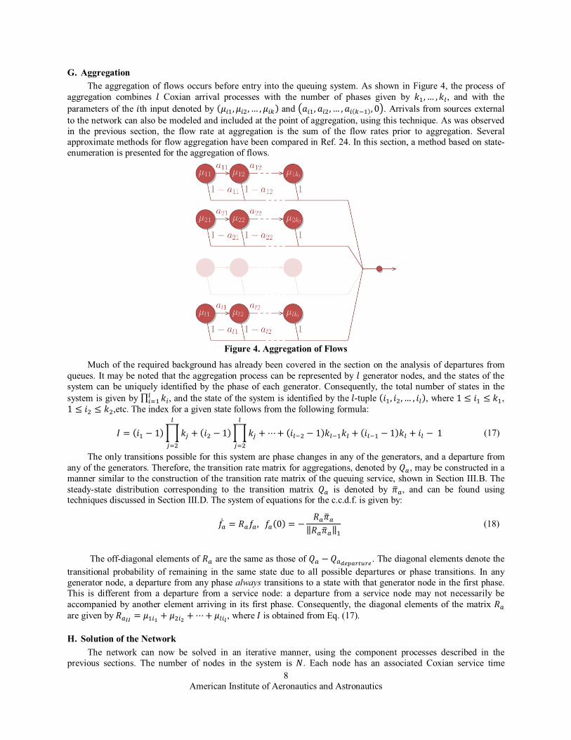
Results are provided in this section for traffic flow between Los Angeles and New York Centers, respectively. The aircraft in this flow stream traverse the Los Angeles, Denver, Minneapolis, Chicago, Cleveland, and New York Centers. The comparison between the departure rates obtained from FACET simulation, Coxian queuing network and the Markovian queuing network are shown in Figure 6.

Care should be exercised in interpreting the results presented in Figure 6 because the FACET results consist of traffic data for just one day, and may not be statistically representative of the actual situation.

Figure 6. Departure Rates from FACET and Network Simulation

It may be observed that the results from the Coxian queuing network compare very well with the FACET data. In most cases, the Coxian network appears to provide a better match between the queuing network and FACET data, perhaps due to the fact that the Coxian distributions more accurately represent the service time at each node. However, in the case of the Minneapolis Center, the Markovian model seems to better represent the traffic flow than the Coxian network. The causes for this difference are currently under investigation.

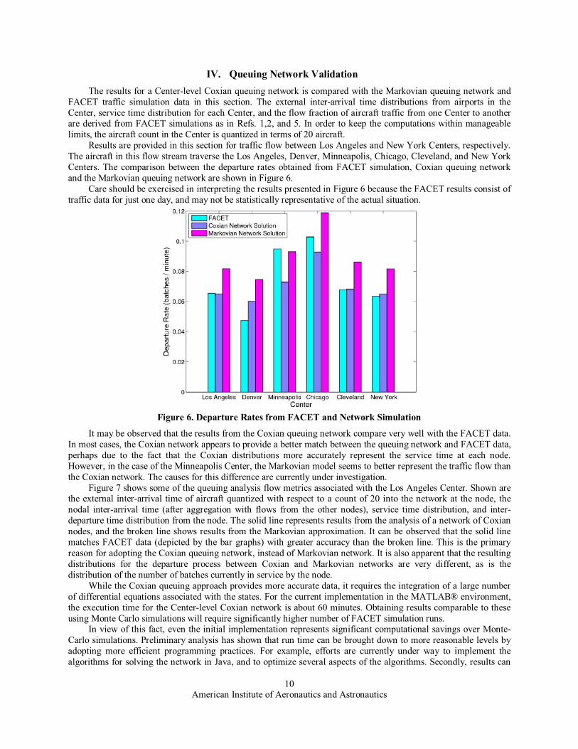
Figure 7 shows some of the queuing analysis flow metrics associated with the Los Angeles Center. Shown are the external inter-arrival time of aircraft quantized with respect to a count of 20 into the network at the node, the nodal inter-arrival time (after aggregation with flows from the other nodes), service time distribution, and inter-departure time distribution from the node. The solid line represents results from the analysis of a network of Coxian nodes, and the broken line shows results from the Markovian approximation. It can be observed that the solid line matches FACET data (depicted by the bar graphs) with greater accuracy than the broken line. This is the primary reason for adopting the Coxian queuing network, instead of Markovian network. It is also apparent that the resulting distributions for the departure process between Coxian and Markovian networks are very different, as is the distribution of the number of batches currently in service by the node.

While the Coxian queuing approach provides more accurate data, it requires the integration of a large number of differential equations associated with the states. For the current implementation in the MATLAB® environment, the execution time for the Center-level Coxian network is about 60 minutes. Obtaining results comparable to these using Monte Carlo simulations will require significantly higher number of FACET simulation runs.

In view of this fact, even the initial implementation represents significant computational savings over Monte-Carlo simulations. Preliminary analysis has shown that run time can be brought down to more reasonable levels by adopting more efficient programming practices. For example, efforts are currently under way to implement the algorithms for solving the network in Java, and to optimize several aspects of the algorithms. Secondly, results can


be obtained several times faster if the convergence criteria are relaxed at minimal loss of accuracy. These elements of the algorithm are currently under analysis.

Figure 7. Flow Properties at the Los Angeles Center

V. Airspace-Level, Sector-Level and Latitude-Longitude Coxian Models Although a Coxian network solution at the Airspace-level, Sector-level and latitude-longitude-level spatial

resolutions has not been implemented, the procedure for solving such networks is essentially the same as that outlined in the foregoing. In each case, the service time distributions and arrival time distributions can be obtained from FACET simulations. However, a fundamental difference between them is the scale of the problem. For instance, at Center-level resolution, the network is composed of 20 nodes representing the airspace over the continental United States, whereas the number of nodes is more than 1000 at the Sector level. Latitude-longitude spatial discretization can create far more nodes. This increases the complexity of the network solution for Coxian nodes, and the development of a suitable numerical technique to handle such large-scale network was not pursued in the present research. Techniques to incorporate higher moments are currently under investigation.

VI. Conclusions The primary goal of this research was the development of high-fidelity queuing models for a network

representation of the NAS, which also include the effects of higher moments in the service time or inter-arrival time distributions at the nodes. While current techniques in the literature utilize some form of approximation for the propagation of moment information of aggregated and disaggregated flows in a network, this paper develops a convergent algorithm that preserves complete moment information of the p.d.f.s associated with the departure processes, with accuracy equal to that of the Coxian distributions used to fit historical data for the network service and arrival processes.

This paper formulated a Center-level queuing network model, which modeled the NAS as 20 nodes with service time distributions obtained by sampling time of flight across the 20 Centers over the continental US. Efforts are underway to perform similar studies for finer resolutions of the NAS, for example Sector-level or Latitude/Longitude grid level, as well as to validate results for the departure process from FACET-based simulations.


Acknowledgments This research was supported under NASA Contract No. NNA07BC55C, with Mr. Michael Bloem serving as

the Technical Point-of-Contact. Ms. Rebecca M. Grus and Mr. Robert Lockyer served as the COTRs.

References 1Tandale, M. D., Sengupta, P., Menon, P. K., Cheng, V. H. L., Rosenberger, J., and Subbarao, K., “Queuing Network

Models of the National Airspace System,” 8th AIAA Aviation Technology, Integration, and Operations Conference, Paper AIAA 2008-8942, Anchorage, AK, September 2008.

2Sengupta, P., Tandale, M. D., Kim, J., and Menon, P. K., “Queuing Models for Analyzing the Impact of Trajectory Uncertainties on the NAS Flow Efficiency,” 9th AIAA Aviation Technology, Integration, and Operations Conference, Paper AIAA 2009-6913, Hilton Head, SC, September 2009.

3Perros, H. G., Queueing Networks with Blocking, Oxford University Press, New York, NY, 1994, pp. 15-30. 4Saaty, T. L., Elements of Queuing Theory with Applications, Dover Publications, Inc., New York, NY, 1983. 5Menon, P. K., Tandale, M. D., Kim, J., Sengupta, P., Kwan, J. S., Cheng, V. H. L., Subbarao, K., and Rosenberger, J., Multi-

Resolution Queuing Models for Analyzing the Impact of Trajectory Uncertainty and Precision on NGATS Flow Efficiency, Contractor Report No. NNA07BC55C, NASA Ames Research Center, Moffett Field, January 2010.

6Kim, J., Tandale, M. D., and Menon, P. K., “Air Traffic Uncertainty Models for Queuing Analysis,” 9th AIAA Aviation Technology, Integration, and Operations Conference, Paper AIAA 2009-7053, Hilton Head, SC, September 2009.

7Bertsimas, D., “An Exact FCFS Waiting Time Analysis for a General Class of G/G/s Queuing Systems,” Queuing Systems, Vol. 3, No. 4, December 1988, pp. 305–320.

8Bertsimas, D., “An Analytic Approach to a General Class of G/G/s Queuing Systems,” Operations Research, Vol. 38, No. 1, January-February 1990, pp. 139–155.

9Takahashi, Y. and Takami, Y., “A Numerical Method for the Steady-State Probabilities of a G1/G/c Queuing System in a General Class,” Journal of the Operations Research Society of Japan, Vol. 19, No. 2, June 1976, pp. 147–157.

10Jackson, J. R., “Networks of Waiting Lines,” Operations Research, Vol. 5, No. 4, August 1957, pp. 518–521. 11Daley, D. J., “Queuing Output Processes,” Advances in Applied Probability, Vol. 8, No. 2, June 1976, pp. 395–415. 12Bitran, G. R. and Dasu, S., “A Review of Open Queuing Network Models of Manufacturing Systems,” Queuing Systems,

Vol. 12, No. 1-2, March 1992, pp. 95–133. 13Whitt, W., “Approximations for Departure Processes and Queues in Series,” Naval Research Logistics Quarterly, Vol. 31,

No. 4, December 1984, pp. 499–521. 14Kuehn, P. J., “Approximate Analysis of General Queuing Networks by Decomposition,” IEEE Transactions on

Communications, Vol. 27, No. 1, January 1979, pp. 113–126. 15 Long, D., Lee, D., Johnson, J., Gaier, E., and Kostiuk, P., “Modeling Air Traffic Management Technologies with a

Queuing Network Model of the National Airspace System,” NASA Contractor Report No. NASA-CR-1999-208988, NASA Langley Research Center, Hampton, VA, January 1999.

16 Whitt, W., “The Queuing Network Analyzer,” The Bell System Technical Journal, Vol. 62, Issue No. 9, November 1983, pp. 2779-2815.

17Bitran, G. R. and Dasu, S., “Analysis of the G/G/1 Queue,” Operations Research, Vol. 41, No. 1, January-February 1994, pp. 158–174.

18Albin, S. L. and Kai, S.-R., “Approximation of the Departure Process of a Queue in a Network,” Naval Research Logistics Quarterly, Vol. 33, No. 1, February 1986, pp. 129–143.

19Sidje, R. B., “EXPOKIT: A Software Package for Computing Matrix Exponentials,” ACM Transactions on Mathematical Software, Vol. 24, No. 1, March 1998, pp. 130–156.

20Moler, C. and van Loan, C., “Nineteen Dubious Ways to Compute the Exponential of a Matrix, Twenty-Five Years Later,” SIAM Review, Vol. 45, No. 1, February 2003, pp. 3–49.

21Medhi, J., Stochastic Models in Queueing Theory, 2nd Edition, Academic Press, November 12, 2002. 22Burke, P. J., “The Output of a Queuing System,” Operations Research, Vol. 4, No. 6, December 1956, pp. 699–704. 23Liu, Y. C. and Perros, H. G., “A Decomposition Procedure for the Analysis of a Closed Fork/Join Queuing System,” IEEE

Transactions on Computers, Vol. 40, No. 3, March 1991, pp. 365–370. 24Albin, S. L., “Delays for Customers from Different Arrival Streams to a Queue,” Management Science, Vol. 32, No. 3,

March 1986, pp. 329–340.

Computational Queuing Analysis: An Application to Traffic Flow Analysis of the NAS

Documents

Transcript of Computational Queuing Analysis: An Application to Traffic Flow Analysis of the NAS