Speed Advisory System Using Real-Time Actuated Traffic ...

This work has been submitted to the IEEE for possible publication. Copyright may be transferred without notice, after which this version may no longer be accessible. 1

Speed Advisory System Using Real-Time ActuatedTraffic Light Phase Length Prediction

Mikhail Burov, Murat Arcak and Alexander Kurzhanskiy

Abstract—Speed advisory systems for connected vehicles relyon the estimation of green (or red) light duration at signalizedintersections. A particular challenge is to predict the signalphases of semi- and fully-actuated traffic lights. In this paper,we introduce an algorithm that processes traffic measurementdata collected from advanced detectors on road links andassigns “PASS”/“WAIT” labels to connected vehicles accordingto their predicted ability to go through the upcoming signalizedintersection within the current phase. Additional computationsprovide an estimate for the duration of the current green phasethat can be used by the Speed Advisory System to minimize fuelconsumption. Simulation results show 95% prediction accuracy,which yields up to 30% reduction in fuel consumption whenused in a driver-assistance system. Traffic progression qualityalso benefits from our algorithm demonstrating an improvementof 20% at peak for medium traffic demand, reducing delays andidling at intersections.

Index Terms—Speed Advisory System, connected vehicles,actuated traffic light, phase prediction, real-time algorithm

I. INTRODUCTION

VEHICLES equipped with the Speed Advisory System(SAS) [1] use traffic light information and traffic data to

obtain the near-optimal speed trajectories to reduce fuel con-sumption. These trajectories also benefit progression quality byminimizing idling at intersections. One of the key parametersrequired by the SAS is the estimated remaining time until theend of the current traffic light (TL) phase. In the case of statictraffic light (constant phase length) this information can beeasily obtained directly from the traffic light via Signal Phaseand Timing (SPaT) messages or any other signaling system.However, if an intersection is equipped with an actuatedTL, the phase length depends on the traffic demand (vehicleflow) and, therefore, may vary from “minimum duration”to “maximum duration” - specific variables characterizing aparticular traffic light. Since the exact phase length valueis unavailable, a prediction algorithm is required to providean estimation to be used in near-optimal speed trajectoryderivation.

The software presented in [2] encourages drivers to usesmartphone cameras to identify the traffic light color at theupcoming intersection and estimate the remaining time withinthe current phase. The study reports error rates from 7.8% to

Manuscript received ...M. Burov and M. Arcak are with the Department of Electrical Engineering

and Computer Sciences, University of California, Berkeley, CA, 94704 USA(e-mails: [email protected]; [email protected]).

A. Kurzhanskiy is with PATH, Berkeley, CA, 94720, USA (e-mail:[email protected]).

This project was sponsored by the NSF CPS grant CNS-1545116 - TrafficOperating System for Smart Cities.

12.4%. The phase length estimation, based on the five previousgreen-red/red-green transitions is also inefficient: according tothe algorithm, the best prediction is just slightly better thanestimating the current phase length to be the same as theprevious phase length.

A follow-on study [3] addresses the problem of findingoptimal speed trajectories to minimize fuel consumption. How-ever, the work considers only pre-timed signals, leaving behindissues with adaptive phase duration. The studies [4] and [5]also focus on pre-timed traffic lights.

References [2] and [6] use noisy measurements of a signalphase to process SPaT estimation. The study analyzes a largenumber of GPS position and speed samples from 4300 buseswithin a period of one month to estimate phase duration, cyclelength and cycle start time. However, a large percentage of therecorded data was not suitable for the analysis, which limitedthe accuracy of the algorithm (6s error for 36s phase duration).The later study [7] estimates the waiting time spent by busesin queues and presents significantly better results for the SPaTestimate.

All of the noisy measurement-based algorithms are imple-mented only for pre-timed traffic lights. In addition, collectingand processing noisy measurements may be computationallyinefficient, since most of the signal data are available fromtransportation authorities.

The study [8] makes probabilistic SPaT predictions basedon the intersection traffic data. At the beginning of each cycle,the empirical frequency distribution is computed. Furthermore,for every second within the cycle, the algorithm tries to predictwhether a certain phase is G(green), R(red) or M(uncertain)with some level of confidence. Further estimation of the phaseresidual time requires the knowledge of within-cycle time,which even if available does not guarantee the accuracy ofthe prediction. In addition to the fact that “80% confidence”predictions may be incorrect, the algorithm does not providefirm guarantees and uncertainty may grow with the increaseof confidence level.

An algorithm presented in [9] relies on the historical datafrom several intersections in Munich and uses a Kalman Filterto predict future probability distributions of phase durations.Although a high level of accuracy was achieved (95%), thepractical applicability is limited since the availability level isonly 71% on average.

Another study [10] suggests using both the historical phasemeasurements and the real-time information that locates thecurrent time within the current phase to predict all future phasetransitions. Two approaches are considered: “conditional ex-pectation based prediction” and “confidence based prediction”.

arX

iv:2

107.

1037

2v1

[ee

ss.S

Y]

21

Jul 2

021


These methods greatly improve the prediction of the residualtime for the current phase as well as for the subsequent phase;however, as stated in the paper, the proposed algorithms “posea challenge to the design of speed profiles that reduce fuelconsumption”. Since both algorithms update their predictionsevery second, SAS-equipped vehicles are forced to reevaluatethe speed trajectories every second as well, causing jerkymotion and fuel consumption increase. Several other papersstudy vehicle flow estimation at arterial roads using adaptivesignal control predictions [11], [12], [13].

Most of the algorithms discussed above try to estimateor predict the phase length/residual time of the phase usinghistorical data and statistical methods. In contrast, our primaryobjective is to determine whether or not a vehicle can passthe upcoming intersection during the current green phase.Using real-time traffic data from advanced detectors and theupcoming actuated TL, the algorithm analyzes downstreamtraffic, estimates the time vehicles can reach the TL andassigns labels (“PASS”/ “WAIT”) depending on the vehicle’spassing capability. According to the obtained labels, the algo-rithm derives an estimated phase residual time for near-optimalspeed trajectory computation for every participating vehicle.

II. THE ALGORITHM

We consider traffic lights with fixed cycle length and oneactuated axis (later in the paper “green / red / yellow phase”refers to the phase of the actuated axis). Therefore, knowingthe time within the cycle allows us to compute the preciseremaining time until the next cycle (i.e. next green phase,assuming that every cycle starts with the green phase). In otherwords, for a non-green phase the remaining time until the nextgreen is known and no predictions are required. However, ifthe current phase is green, the algorithm is used to estimatethe phase length.

All the computations and simulations were conducted in anopen source simulator SUMO (Simulation of Urban Mobility).

A. Simple and Complex Network Architecture

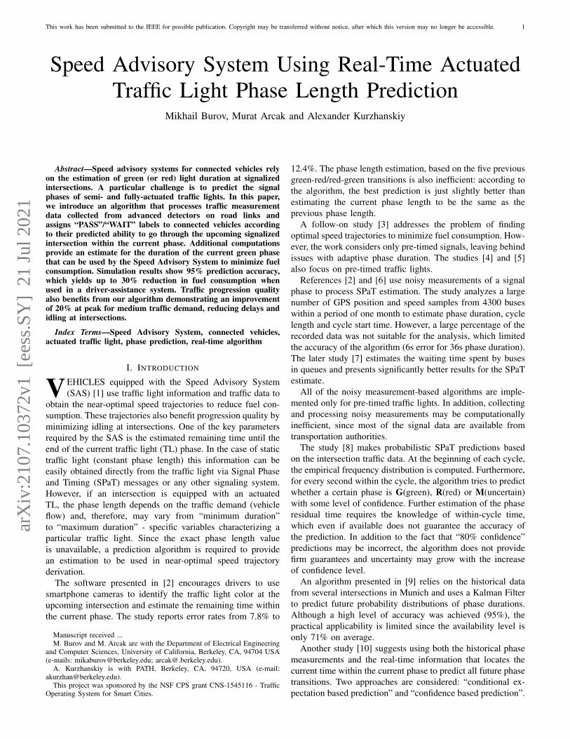
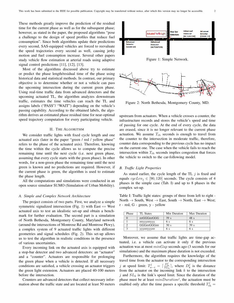
The project consists of two parts. First, we analyze a simplesymmetric signalized intersection (Fig. 1) with East ↔ Westactuated axis to test an idealistic set-up and obtain a bench-mark for further evaluation. The second part is a simulationof North Bethesda, Montgomery County, Maryland network(around the intersections of Montrose Rd and Montrose Pkwy),a complex system of 9 actuated traffic lights with differentgeometries and signal schedules (Fig. 2). This set-up allowsus to test the algorithm in realistic conditions in the presenceof various uncertainties.

Every incoming link on the actuated axis is equipped witha stop-bar detector and two advanced detectors: an “actuator”and a “counter”. Actuators are responsible for prolongingthe green phase when a vehicle is detected. If all necessaryconditions are satisfied, a vehicle crossing an actuator triggersthe green light extension. Actuators are placed 40-100 metersbefore the intersection.

Counters are advanced detectors that collect necessary infor-mation about the traffic state and are located at least 50 meters

Figure 1: Simple Network.

Figure 2: North Bethesda, Montgomery County, MD.

upstream from actuators. When a vehicle crosses a counter, theinfrastructure records and stores the vehicle’s speed and timeof passing for one cycle. At the end of every cycle, the dataare erased, since it is no longer relevant to the current phaseactuation. We assume Tth seconds is enough to travel fromthe counter to the intersection in moderate traffic, therefore,counter data corresponding to the previous cycle has no impacton the current one. The case when the vehicle fails to reach theintersection within Tth seconds implies congestion that forcesthe vehicle to switch to the car-following model.

B. Traffic Light Properties

As stated earlier, the cycle length of the TL j is fixed andequals cycLenj ∈ [90, 120] seconds. The cycle consists of 4phases in the simple case (Tab. I) and up to 8 phases in thecomplex set-up.

Table I: Traffic light states: groups of three from left to right -North → South, West → East, South → North, East → West;r - red, G - green, y - yellow

Phase TL States Min Duration Max Duration0 rrrGGGrrrGGG 39 s 48 s1 rrryyyrrryyy 6 s 6 s2 GGGrrrGGGrrr 30 s 39 s3 yyyrrryyyrrr 6 s 6 s

Moreover, we assume that traffic lights are time-gap ac-tuated, i.e. a vehicle can activate it only if the previousactuation was at most minGap seconds ago (3 seconds for oursimulations) and the maximum phase duration is not exceeded.

Furthermore, the algorithm requires the knowledge of thetravel time from the actuator to the corresponding intersectionj at speed limit: T j

a−i = d Djk

SLke, where Dj

k is the distancefrom the actuator on the incoming link k to the intersectionj and SLk is the link’s speed limit. Since the duration of thephase must be at least minDurationj , the actuation must beenabled only after the time passes a specific threshold T j

th =


minDurationj − T ja−i. The first vehicle must arrive within

minGap after the threshold to prolong the phase. If such avehicle exists, the next car has minGap seconds to trigger theTL again. The process terminates when either no such vehicleis found or the maxDurationj is reached.

C. Speed Advisory System Modification

Since we augment our prediction algorithm with a simplifiedversion of SAS proposed in [1], we briefly summarize themain points of this system. The optimal (in terms of fuelconsumption) speed trajectory consists of bang-singular-bangsegments: (1) accelerate with maximal acceleration / deceleratewith engine off - (2) keep the constant speed - (3) deceleratewith engine off / accelerate with maximal acceleration. Thesingular segment is present only at very low speeds, so mostof the time the optimal trajectory is bang-bang shaped. Thisis both hard to implement in real life and uncomfortable fordrivers, so [1] suggests a near-optimal speed trajectory: bang-singular ((1) accelerate with maximal acceleration / deceleratewith engine off or with minimal deceleration - (2) keep theconstant speed).

We further assume the acceleration and deceleration to beconstant. According to the original dynamics, for speeds under30m/s the engine-off deceleration ranges from 0.1460m/s2

to 0.1480m/s2. The difference is insignificantly small and,therefore, rounding the deceleration up to 0.15m/s2 would notmake any noticeable impact on the system compared to otheruncertainties and assumptions. The acceleration also followsan almost linear pattern, so it was decided to set it to a constantvalue amax (2.5m/s2 in our model). In addition, it simplifiedthe simulation implementation, since the model presented inSUMO uses constant acceleration.

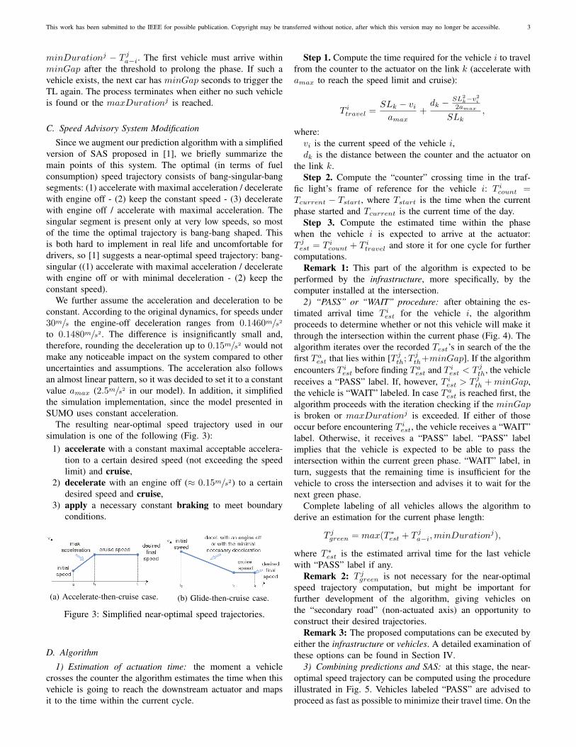
The resulting near-optimal speed trajectory used in oursimulation is one of the following (Fig. 3):

1) accelerate with a constant maximal acceptable accelera-tion to a certain desired speed (not exceeding the speedlimit) and cruise,

2) decelerate with an engine off (≈ 0.15m/s2) to a certaindesired speed and cruise,

3) apply a necessary constant braking to meet boundaryconditions.

(a) Accelerate-then-cruise case. (b) Glide-then-cruise case.

Figure 3: Simplified near-optimal speed trajectories.

D. Algorithm

1) Estimation of actuation time: the moment a vehiclecrosses the counter the algorithm estimates the time when thisvehicle is going to reach the downstream actuator and mapsit to the time within the current cycle.

Step 1. Compute the time required for the vehicle i to travelfrom the counter to the actuator on the link k (accelerate withamax to reach the speed limit and cruise):

T itravel =

SLk − viamax

+dk − SL2

k−v2i

2amax

SLk,

where:vi is the current speed of the vehicle i,dk is the distance between the counter and the actuator on

the link k.Step 2. Compute the “counter” crossing time in the traf-

fic light’s frame of reference for the vehicle i: T icount =

Tcurrent − Tstart, where Tstart is the time when the currentphase started and Tcurrent is the current time of the day.

Step 3. Compute the estimated time within the phasewhen the vehicle i is expected to arrive at the actuator:T jest = T i

count + T itravel and store it for one cycle for further

computations.Remark 1: This part of the algorithm is expected to be

performed by the infrastructure, more specifically, by thecomputer installed at the intersection.

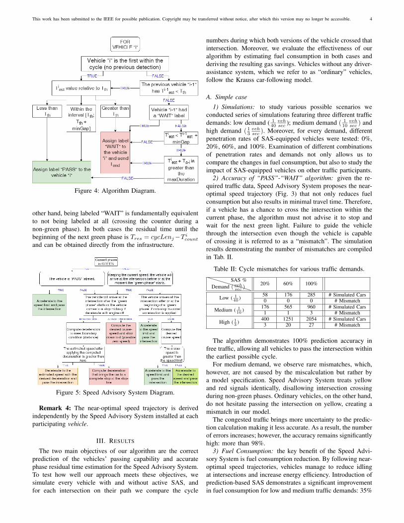
2) “PASS” or “WAIT” procedure: after obtaining the es-timated arrival time T i

est for the vehicle i, the algorithmproceeds to determine whether or not this vehicle will make itthrough the intersection within the current phase (Fig. 4). Thealgorithm iterates over the recorded Test’s in search of the thefirst T a

est that lies within [T jth;T

jth+minGap]. If the algorithm

encounters T iest before finding T a

est and T iest < T j

th, the vehiclereceives a “PASS” label. If, however, T i

est > T jth +minGap,

the vehicle is “WAIT” labeled. In case T aest is reached first, the

algorithm proceeds with the iteration checking if the minGapis broken or maxDurationj is exceeded. If either of thoseoccur before encountering T i

est, the vehicle receives a “WAIT”label. Otherwise, it receives a “PASS” label. “PASS” labelimplies that the vehicle is expected to be able to pass theintersection within the current green phase. “WAIT” label, inturn, suggests that the remaining time is insufficient for thevehicle to cross the intersection and advises it to wait for thenext green phase.

Complete labeling of all vehicles allows the algorithm toderive an estimation for the current phase length:

T jgreen = max(T ∗

est + T ja−i,minDuration

j),

where T ∗est is the estimated arrival time for the last vehicle

with “PASS” label if any.Remark 2: T j

green is not necessary for the near-optimalspeed trajectory computation, but might be important forfurther development of the algorithm, giving vehicles onthe “secondary road” (non-actuated axis) an opportunity toconstruct their desired trajectories.

Remark 3: The proposed computations can be executed byeither the infrastructure or vehicles. A detailed examination ofthese options can be found in Section IV.

3) Combining predictions and SAS: at this stage, the near-optimal speed trajectory can be computed using the procedureillustrated in Fig. 5. Vehicles labeled “PASS” are advised toproceed as fast as possible to minimize their travel time. On the


Figure 4: Algorithm Diagram.

other hand, being labeled “WAIT” is fundamentally equivalentto not being labeled at all (crossing the counter during anon-green phase). In both cases the residual time until thebeginning of the next green phase is Tres = cycLenj−T i

count

and can be obtained directly from the infrastructure.

Figure 5: Speed Advisory System Diagram.

Remark 4: The near-optimal speed trajectory is derivedindependently by the Speed Advisory System installed at eachparticipating vehicle.

III. RESULTS

The two main objectives of our algorithm are the correctprediction of the vehicles’ passing capability and accuratephase residual time estimation for the Speed Advisory System.To test how well our approach meets these objectives, wesimulate every vehicle with and without active SAS, andfor each intersection on their path we compare the cycle

numbers during which both versions of the vehicle crossed thatintersection. Moreover, we evaluate the effectiveness of ouralgorithm by estimating fuel consumption in both cases andderiving the resulting gas savings. Vehicles without any driver-assistance system, which we refer to as “ordinary” vehicles,follow the Krauss car-following model.

A. Simple case

1) Simulations: to study various possible scenarios weconducted series of simulations featuring three different trafficdemands: low demand ( 1

40vehsec ); medium demand ( 1

10vehsec ) and

high demand ( 13vehsec ). Moreover, for every demand, different

penetration rates of SAS-equipped vehicles were tested: 0%,20%, 60%, and 100%. Examination of different combinationsof penetration rates and demands not only allows us tocompare the changes in fuel consumption, but also to study theimpact of SAS-equipped vehicles on other traffic participants.

2) Accuracy of “PASS”-“WAIT” algorithm: given the re-quired traffic data, Speed Advisory System proposes the near-optimal speed trajectory (Fig. 3) that not only reduces fuelconsumption but also results in minimal travel time. Therefore,if a vehicle has a chance to cross the intersection within thecurrent phase, the algorithm must not advise it to stop andwait for the next green light. Failure to guide the vehiclethrough the intersection even though the vehicle is capableof crossing it is referred to as a “mismatch”. The simulationresults demonstrating the number of mismatches are compiledin Tab. II.

Table II: Cycle mismatches for various traffic demands.

Demand ( vehsec

)

SAS %20% 60% 100%

Low ( 140

) 58 176 285 # Simulated Cars0 0 0 # Mismatch

Medium ( 110


High ( 13


The algorithm demonstrates 100% prediction accuracy infree traffic, allowing all vehicles to pass the intersection withinthe earliest possible cycle.

For medium demand, we observe rare mismatches, which,however, are not caused by the miscalculation but rather bya model specification. Speed Advisory System treats yellowand red signals identically, disallowing intersection crossingduring non-green phases. Ordinary vehicles, on the other hand,do not hesitate passing the intersection on yellow, creating amismatch in our model.

The congested traffic brings more uncertainty to the predic-tion calculation making it less accurate. As a result, the numberof errors increases; however, the accuracy remains significantlyhigh: more than 98%.

3) Fuel Consumption: the key benefit of the Speed Advi-sory System is fuel consumption reduction. By following near-optimal speed trajectories, vehicles manage to reduce idlingat intersections and increase energy efficiency. Introduction ofprediction-based SAS demonstrates a significant improvementin fuel consumption for low and medium traffic demands: 35%


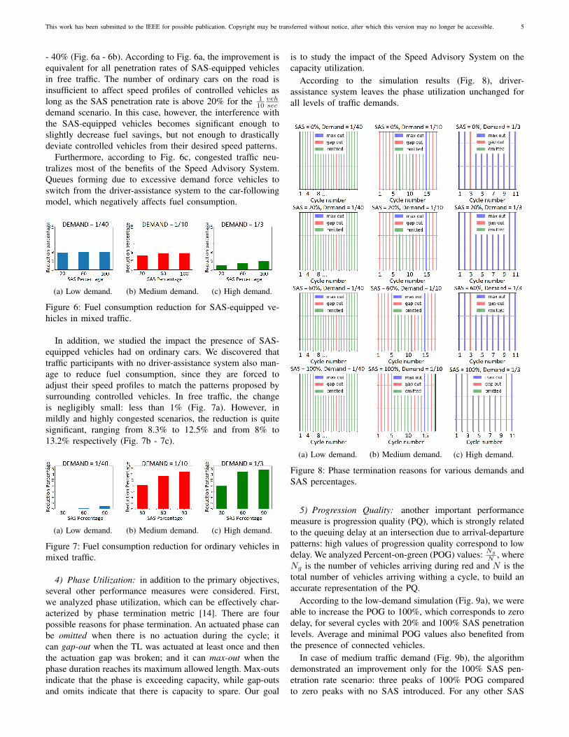
- 40% (Fig. 6a - 6b). According to Fig. 6a, the improvement isequivalent for all penetration rates of SAS-equipped vehiclesin free traffic. The number of ordinary cars on the road isinsufficient to affect speed profiles of controlled vehicles aslong as the SAS penetration rate is above 20% for the 1

10vehsec

demand scenario. In this case, however, the interference withthe SAS-equipped vehicles becomes significant enough toslightly decrease fuel savings, but not enough to drasticallydeviate controlled vehicles from their desired speed patterns.

Furthermore, according to Fig. 6c, congested traffic neu-tralizes most of the benefits of the Speed Advisory System.Queues forming due to excessive demand force vehicles toswitch from the driver-assistance system to the car-followingmodel, which negatively affects fuel consumption.

(a) Low demand. (b) Medium demand. (c) High demand.

Figure 6: Fuel consumption reduction for SAS-equipped ve-hicles in mixed traffic.

In addition, we studied the impact the presence of SAS-equipped vehicles had on ordinary cars. We discovered thattraffic participants with no driver-assistance system also man-age to reduce fuel consumption, since they are forced toadjust their speed profiles to match the patterns proposed bysurrounding controlled vehicles. In free traffic, the changeis negligibly small: less than 1% (Fig. 7a). However, inmildly and highly congested scenarios, the reduction is quitesignificant, ranging from 8.3% to 12.5% and from 8% to13.2% respectively (Fig. 7b - 7c).


Figure 7: Fuel consumption reduction for ordinary vehicles inmixed traffic.

4) Phase Utilization: in addition to the primary objectives,several other performance measures were considered. First,we analyzed phase utilization, which can be effectively char-acterized by phase termination metric [14]. There are fourpossible reasons for phase termination. An actuated phase canbe omitted when there is no actuation during the cycle; itcan gap-out when the TL was actuated at least once and thenthe actuation gap was broken; and it can max-out when thephase duration reaches its maximum allowed length. Max-outsindicate that the phase is exceeding capacity, while gap-outsand omits indicate that there is capacity to spare. Our goal

is to study the impact of the Speed Advisory System on thecapacity utilization.

According to the simulation results (Fig. 8), driver-assistance system leaves the phase utilization unchanged forall levels of traffic demands.


Figure 8: Phase termination reasons for various demands andSAS percentages.

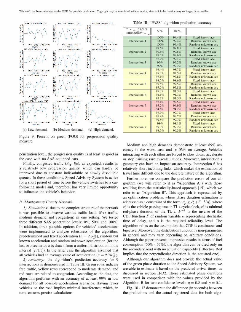
5) Progression Quality: another important performancemeasure is progression quality (PQ), which is strongly relatedto the queuing delay at an intersection due to arrival-departurepatterns: high values of progression quality correspond to lowdelay. We analyzed Percent-on-green (POG) values: Ng

N , whereNg is the number of vehicles arriving during red and N is thetotal number of vehicles arriving withing a cycle, to build anaccurate representation of the PQ.

According to the low-demand simulation (Fig. 9a), we wereable to increase the POG to 100%, which corresponds to zerodelay, for several cycles with 20% and 100% SAS penetrationlevels. Average and minimal POG values also benefited fromthe presence of connected vehicles.

In case of medium traffic demand (Fig. 9b), the algorithmdemonstrated an improvement only for the 100% SAS pen-etration rate scenario: three peaks of 100% POG comparedto zero peaks with no SAS introduced. For any other SAS



Figure 9: Percent on green (POG) for progression qualitymeasure.

penetration level, the progression quality is at least as good asthe case with no SAS-equipped cars.

Finally, congested traffic (Fig. 9c), as expected, results ina relatively low progression quality, which can hardly beimproved due to constant indissoluble or slowly dissolublequeues. In these conditions, Speed Advisory System is activefor a short period of time before the vehicle switches to a car-following model and, therefore, has very limited opportunityto influence the vehicle’s behavior.

B. Montgomery County Network

1) Simulations: due to the complex structure of the networkit was possible to observe various traffic loads (free traffic,medium demand and congestion) in one setting. We testedthree different SAS penetration levels: 0%, 50% and 100%.In addition, three possible options for vehicles’ accelerationswere implemented to analyze robustness of the algorithm:predetermined and fixed acceleration (a = 2.5m

s2 ), random butknown acceleration and random unknown acceleration (for thelast two scenarios a is drawn from a uniform distribution in theinterval [2, 3.5]). In the latter case the algorithm assumed thatall vehicles had an average value of acceleration (a = 2.75m

s2 ).2) Accuracy: the algorithm’s prediction accuracy for 9

intersections is demonstrated in Table III. Green rows indicatefree traffic, yellow rows correspond to moderate demand, andred rows are related to congestion. According to the data, thealgorithm performs with an accuracy of at least 99% in lowdemand for all possible acceleration scenarios. Having fewervehicles on the road implies minimal interference, which, inturn, ensures precise calculations.

Table III: “PASS” algorithm prediction accuracy

IntersectionSAS % 50% 100%

100% 99.4% Fixed known acc100% 99.4% Random known accIntersection 1100% 99.4% Random unknown acc99.6% 99.8% Fixed known acc99.6% 99.5% Random known accIntersection 299.3% 99.6% Random unknown acc98.7% 99.1% Fixed known acc99% 99.2% Random known accIntersection 399% 99.2% Random unknown acc

96.4% 98.7% Fixed known acc98.3% 97.5% Random known accIntersection 498.1% 97.8% Random unknown acc98.5% 98.6% Fixed known acc97.5% 97.5% Random known accIntersection 597.7% 97.8% Random unknown acc89.3% 91.3% Fixed known acc91.1% 91.3% Random known accIntersection 691.2% 91.3% Random unknown acc93.4% 92.5% Fixed known acc93.2% 94.9% Random known accIntersection 794.6% 94.2% Random unknown acc97.9% 99.7% Fixed known acc99.4% 99.7% Random known accIntersection 899.5% 99.7% Random unknown acc98% 98.1% Fixed known acc

99.3% 99.2% Random known accIntersection 998.5% 99.3% Random unknown acc

Medium and high demands demonstrate at least 89% ac-curacy in the worst case and ≈ 95% on average. Vehiclesinteracting with each other are forced to slow down, accelerateor stop causing rare miscalculations. Moreover, intersection’sgeometry can have an impact on accuracy. Intersection 6 hasrelatively short incoming links, which makes the estimation oftravel time difficult due to the discrete nature of the algorithm.

Furthermore, we compare the prediction errors of our al-gorithm (we will refer to it as “Algorithm A”) with thoseresulting from the statistically-based approach [15], which werefer to as “Algorithm B”. This approach is represented byan optimization problem, where phase duration estimation isaddressed as a constraint of the form: cip ≥ cir+F−1(η), wherecip is the vehicle passing time in TL i cycle clock, cir is minimalred-phase duration of the TL i, F−1 is the inverse of theCDF function F of random variable α representing stochastictime of delay, and η is the required reliability level. Thealgorithm relies on the assumption that CDF is continuous andbijective. Moreover, the distribution function is non-parametricin general and may vary depending on arbitrary conditions.Although the paper presents impressive results in terms of fuelconsumption (50% - 57%), the algorithm can be used only onthe secondary road with no actuation capability (Effective Redimplies that the perpendicular direction is the actuated one).

Although our algorithm does not provide the actual valueof the green phase duration to the Speed Advisory System, weare able to estimate it based on the predicted arrival times, asdiscussed in section II-D2. These estimated phase durationswere used in comparison with the values provided by theAlgorithm B for two confidence levels: η = 0.8 and η = 0.1.

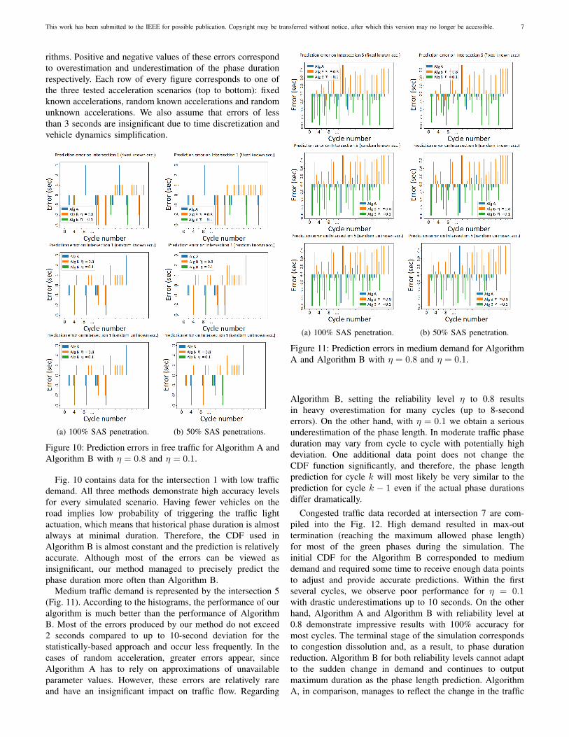
Fig. 10 - 12 demonstrate the difference (in seconds) betweenthe predictions and the actual registered data for both algo-


rithms. Positive and negative values of these errors correspondto overestimation and underestimation of the phase durationrespectively. Each row of every figure corresponds to one ofthe three tested acceleration scenarios (top to bottom): fixedknown accelerations, random known accelerations and randomunknown accelerations. We also assume that errors of lessthan 3 seconds are insignificant due to time discretization andvehicle dynamics simplification.

(a) 100% SAS penetration. (b) 50% SAS penetrations.

Figure 10: Prediction errors in free traffic for Algorithm A andAlgorithm B with η = 0.8 and η = 0.1.

Fig. 10 contains data for the intersection 1 with low trafficdemand. All three methods demonstrate high accuracy levelsfor every simulated scenario. Having fewer vehicles on theroad implies low probability of triggering the traffic lightactuation, which means that historical phase duration is almostalways at minimal duration. Therefore, the CDF used inAlgorithm B is almost constant and the prediction is relativelyaccurate. Although most of the errors can be viewed asinsignificant, our method managed to precisely predict thephase duration more often than Algorithm B.

Medium traffic demand is represented by the intersection 5(Fig. 11). According to the histograms, the performance of ouralgorithm is much better than the performance of AlgorithmB. Most of the errors produced by our method do not exceed2 seconds compared to up to 10-second deviation for thestatistically-based approach and occur less frequently. In thecases of random acceleration, greater errors appear, sinceAlgorithm A has to rely on approximations of unavailableparameter values. However, these errors are relatively rareand have an insignificant impact on traffic flow. Regarding

(a) 100% SAS penetration. (b) 50% SAS penetration.

Figure 11: Prediction errors in medium demand for AlgorithmA and Algorithm B with η = 0.8 and η = 0.1.

Algorithm B, setting the reliability level η to 0.8 resultsin heavy overestimation for many cycles (up to 8-seconderrors). On the other hand, with η = 0.1 we obtain a seriousunderestimation of the phase length. In moderate traffic phaseduration may vary from cycle to cycle with potentially highdeviation. One additional data point does not change theCDF function significantly, and therefore, the phase lengthprediction for cycle k will most likely be very similar to theprediction for cycle k − 1 even if the actual phase durationsdiffer dramatically.

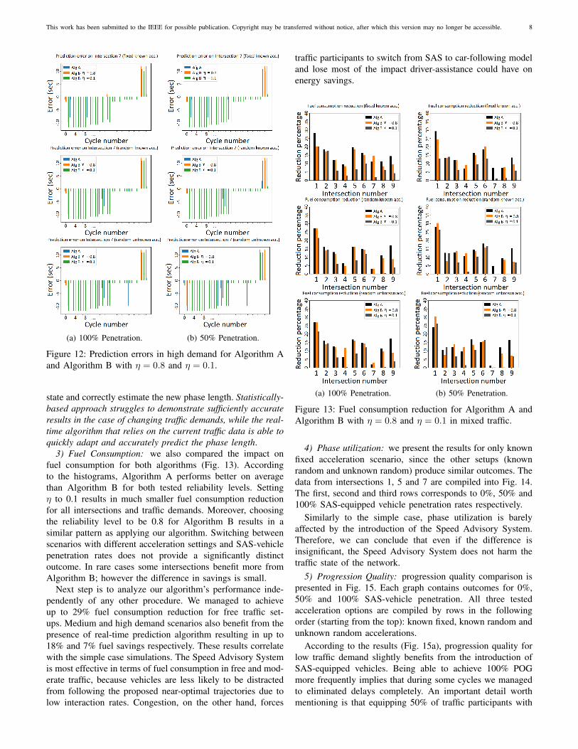
Congested traffic data recorded at intersection 7 are com-piled into the Fig. 12. High demand resulted in max-outtermination (reaching the maximum allowed phase length)for most of the green phases during the simulation. Theinitial CDF for the Algorithm B corresponded to mediumdemand and required some time to receive enough data pointsto adjust and provide accurate predictions. Within the firstseveral cycles, we observe poor performance for η = 0.1with drastic underestimations up to 10 seconds. On the otherhand, Algorithm A and Algorithm B with reliability level at0.8 demonstrate impressive results with 100% accuracy formost cycles. The terminal stage of the simulation correspondsto congestion dissolution and, as a result, to phase durationreduction. Algorithm B for both reliability levels cannot adaptto the sudden change in demand and continues to outputmaximum duration as the phase length prediction. AlgorithmA, in comparison, manages to reflect the change in the traffic


(a) 100% Penetration. (b) 50% Penetration.

Figure 12: Prediction errors in high demand for Algorithm Aand Algorithm B with η = 0.8 and η = 0.1.

state and correctly estimate the new phase length. Statistically-based approach struggles to demonstrate sufficiently accurateresults in the case of changing traffic demands, while the real-time algorithm that relies on the current traffic data is able toquickly adapt and accurately predict the phase length.

3) Fuel Consumption: we also compared the impact onfuel consumption for both algorithms (Fig. 13). Accordingto the histograms, Algorithm A performs better on averagethan Algorithm B for both tested reliability levels. Settingη to 0.1 results in much smaller fuel consumption reductionfor all intersections and traffic demands. Moreover, choosingthe reliability level to be 0.8 for Algorithm B results in asimilar pattern as applying our algorithm. Switching betweenscenarios with different acceleration settings and SAS-vehiclepenetration rates does not provide a significantly distinctoutcome. In rare cases some intersections benefit more fromAlgorithm B; however the difference in savings is small.

Next step is to analyze our algorithm’s performance inde-pendently of any other procedure. We managed to achieveup to 29% fuel consumption reduction for free traffic set-ups. Medium and high demand scenarios also benefit from thepresence of real-time prediction algorithm resulting in up to18% and 7% fuel savings respectively. These results correlatewith the simple case simulations. The Speed Advisory Systemis most effective in terms of fuel consumption in free and mod-erate traffic, because vehicles are less likely to be distractedfrom following the proposed near-optimal trajectories due tolow interaction rates. Congestion, on the other hand, forces

traffic participants to switch from SAS to car-following modeland lose most of the impact driver-assistance could have onenergy savings.

(a) 100% Penetration. (b) 50% Penetration.

Figure 13: Fuel consumption reduction for Algorithm A andAlgorithm B with η = 0.8 and η = 0.1 in mixed traffic.

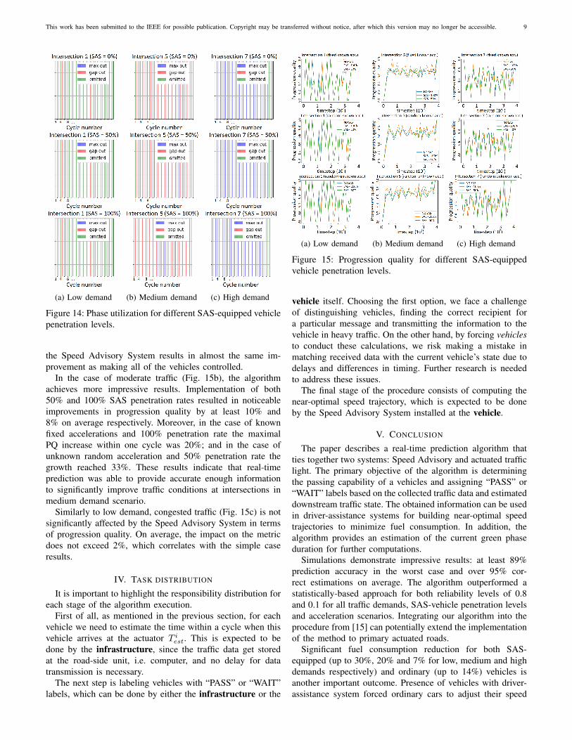
4) Phase utilization: we present the results for only knownfixed acceleration scenario, since the other setups (knownrandom and unknown random) produce similar outcomes. Thedata from intersections 1, 5 and 7 are compiled into Fig. 14.The first, second and third rows corresponds to 0%, 50% and100% SAS-equipped vehicle penetration rates respectively.

Similarly to the simple case, phase utilization is barelyaffected by the introduction of the Speed Advisory System.Therefore, we can conclude that even if the difference isinsignificant, the Speed Advisory System does not harm thetraffic state of the network.

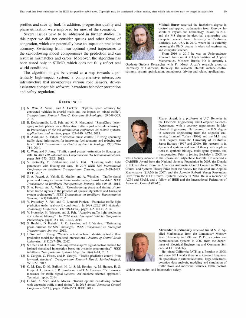
5) Progression Quality: progression quality comparison ispresented in Fig. 15. Each graph contains outcomes for 0%,50% and 100% SAS-vehicle penetration. All three testedacceleration options are compiled by rows in the followingorder (starting from the top): known fixed, known random andunknown random accelerations.

According to the results (Fig. 15a), progression quality forlow traffic demand slightly benefits from the introduction ofSAS-equipped vehicles. Being able to achieve 100% POGmore frequently implies that during some cycles we managedto eliminated delays completely. An important detail worthmentioning is that equipping 50% of traffic participants with


(a) Low demand (b) Medium demand (c) High demand

Figure 14: Phase utilization for different SAS-equipped vehiclepenetration levels.

the Speed Advisory System results in almost the same im-provement as making all of the vehicles controlled.

In the case of moderate traffic (Fig. 15b), the algorithmachieves more impressive results. Implementation of both50% and 100% SAS penetration rates resulted in noticeableimprovements in progression quality by at least 10% and8% on average respectively. Moreover, in the case of knownfixed accelerations and 100% penetration rate the maximalPQ increase within one cycle was 20%; and in the case ofunknown random acceleration and 50% penetration rate thegrowth reached 33%. These results indicate that real-timeprediction was able to provide accurate enough informationto significantly improve traffic conditions at intersections inmedium demand scenario.

Similarly to low demand, congested traffic (Fig. 15c) is notsignificantly affected by the Speed Advisory System in termsof progression quality. On average, the impact on the metricdoes not exceed 2%, which correlates with the simple caseresults.

IV. TASK DISTRIBUTION

It is important to highlight the responsibility distribution foreach stage of the algorithm execution.

First of all, as mentioned in the previous section, for eachvehicle we need to estimate the time within a cycle when thisvehicle arrives at the actuator T i

est. This is expected to bedone by the infrastructure, since the traffic data get storedat the road-side unit, i.e. computer, and no delay for datatransmission is necessary.

The next step is labeling vehicles with “PASS” or “WAIT”labels, which can be done by either the infrastructure or the

(a) Low demand (b) Medium demand (c) High demand

Figure 15: Progression quality for different SAS-equippedvehicle penetration levels.

vehicle itself. Choosing the first option, we face a challengeof distinguishing vehicles, finding the correct recipient fora particular message and transmitting the information to thevehicle in heavy traffic. On the other hand, by forcing vehiclesto conduct these calculations, we risk making a mistake inmatching received data with the current vehicle’s state due todelays and differences in timing. Further research is neededto address these issues.

The final stage of the procedure consists of computing thenear-optimal speed trajectory, which is expected to be doneby the Speed Advisory System installed at the vehicle.

V. CONCLUSION

The paper describes a real-time prediction algorithm thatties together two systems: Speed Advisory and actuated trafficlight. The primary objective of the algorithm is determiningthe passing capability of a vehicles and assigning “PASS” or“WAIT” labels based on the collected traffic data and estimateddownstream traffic state. The obtained information can be usedin driver-assistance systems for building near-optimal speedtrajectories to minimize fuel consumption. In addition, thealgorithm provides an estimation of the current green phaseduration for further computations.

Simulations demonstrate impressive results: at least 89%prediction accuracy in the worst case and over 95% cor-rect estimations on average. The algorithm outperformed astatistically-based approach for both reliability levels of 0.8and 0.1 for all traffic demands, SAS-vehicle penetration levelsand acceleration scenarios. Integrating our algorithm into theprocedure from [15] can potentially extend the implementationof the method to primary actuated roads.

Significant fuel consumption reduction for both SAS-equipped (up to 30%, 20% and 7% for low, medium and highdemands respectively) and ordinary (up to 14%) vehicles isanother important outcome. Presence of vehicles with driver-assistance system forced ordinary cars to adjust their speed


profiles and save up fuel. In addition, progression quality andphase utilization were improved for most of the scenarios.

Several issues have to be addressed in further studies. Inthis paper we did not consider queues and other forms ofcongestion, which can potentially have an impact on predictionaccuracy. Switching from near-optimal speed trajectories tothe car-following model compromises the prediction and canresult in mismatches and errors. Moreover, the algorithm hasbeen tested only in SUMO, which does not fully reflect realworld conditions.

The algorithm might be viewed as a step towards a po-tentially high-impact system: a comprehensive intersectioninfrastructure that incorporates various road sensors, driver-assistance compatible software, hazardous behavior preventionand safety regulation.

REFERENCES

[1] N. Wan, A. Vahidi, and A. Luckow. “Optimal speed advisory forconnected vehicles in arterial roads and the impact on mixed traffic”.Transportation Research Part C: Emerging Technologies, 69:548–563,2016.

[2] E. Koukoumidis, L.-S. Peh, and M. R. Martonosi. “SignalGuru: lever-aging mobile phones for collaborative traffic signal schedule advisory”.In Proceedings of the 9th international conference on Mobile systems,applications, and services, pages 127–140. ACM, 2011.

[3] B. Asadi and A. Vahidi. “Predictive cruise control: Utilizing upcomingtraffic signal information for improving fuel economy and reducing triptime”. IEEE Transactions on Control Systems Technology, 19(3):707–714, 2010.

[4] C. Wang and S. Jiang. “Traffic signal phases’ estimation by floating cardata. In 2012 12th International Conference on ITS Telecommunications,pages 568–573. IEEE, 2012.

[5] V. Protschky, C. Ruhhammer, and S. Feit. “Learning traffic lightparameters with floating car data. In 2015 IEEE 18th InternationalConference on Intelligent Transportation Systems, pages 2438–2443.IEEE, 2015.

[6] S. A. Fayazi, A. Vahidi, G. Mahler, and A. Winckler. “Traffic signalphase and timing estimation from low-frequency transit bus data”. IEEETransactions on Intelligent Transportation Systems, 16(1):19–28, 2014.

[7] S. A. Fayazi and A. Vahidi. “Crowdsourcing phase and timing of pre-timed traffic signals in the presence of queues: algorithms and back-endsystem architecture”. IEEE Transactions on Intelligent TransportationSystems, 17(3):870–881, 2015.

[8] V. Protschky, S. Feit, and C. Linnhoff-Popien. “Extensive traffic lightprediction under real-world conditions”. In 2014 IEEE 80th VehicularTechnology Conference (VTC2014-Fall), pages 1–5. IEEE, 2014.

[9] V. Protschky, K. Wiesner, and S. Feit. “Adaptive traffic light predictionvia Kalman filtering”. In 2014 IEEE Intelligent Vehicles SymposiumProceedings, pages 151–157. IEEE, 2014.

[10] S. Ibrahim, D. Kalathil, R. O. Sanchez, and P. Varaiya. “Estimatingphase duration for SPaT messages. IEEE Transactions on IntelligentTransportation Systems, 2018.

[11] J. Sun and L. Zhang. “Vehicle actuation based short-term traffic flowprediction model for signalized intersections”. Journal of Central SouthUniversity, 19(1):287–298, 2012.

[12] S. Chen and D. J. Sun. “An improved adaptive signal control method forisolated signalized intersection based on dynamic programming”. IEEEIntelligent Transportation Systems Magazine, 8(4):4–14, 2016.

[13] S. Coogan, C. Flores, and P. Varaiya. “Traffic predictive control fromlow-rank structure”. Transportation Research Part B: Methodological,97:1–22, 2017.

[14] C. M. Day, D. M. Bullock, H. Li, S. M. Remias, A. M. Hainen, R. S.Freije, A. L. Stevens, J. R. Sturdevant, and T. M. Brennan. “Performancemeasures for traffic signal systems: An outcome-oriented approach”.Technical report, 2014.

[15] C. Sun, X. Shen, and S. Moura. “Robust optimal eco-driving controlwith uncertain traffic signal timing”. In 2018 Annual American ControlConference (ACC), pages 5548–5553. IEEE, 2018.

Mikhail Burov received the Bachelor’s degree incontrol and applied mathematics from Moscow In-stitute of Physics and Technology, Russia, in 2017and the MS degree in electrical engineering andcomputer science from University of California,Berkeley, CA, USA in 2019, where he is currentlypursuing the Ph.D. degree in electrical engineeringand computer science.

From 2016 to 2017 he was an UndergraduateResearch Assistant at Keldysh Institute of AppliedMathematics, Moscow, Russia. He is currently a

Graduate Student Researcher with Pr. Murat Arcak’s research group atUniversity of California, Berkeley. His research interests include controlsystems, system optimization, autonomous driving and related applications.

Murat Arcak is a professor at U.C. Berkeley inthe Electrical Engineering and Computer SciencesDepartment, with a courtesy appointment in Me-chanical Engineering. He received the B.S. degreein Electrical Engineering from the Bogazici Uni-versity, Istanbul, Turkey (1996) and the M.S. andPh.D. degrees from the University of California,Santa Barbara (1997 and 2000). His research is indynamical systems and control theory with applica-tions to synthetic biology, multi-agent systems, andtransportation. Prior to joining Berkeley in 2008, he

was a faculty member at the Rensselaer Polytechnic Institute. He received aCAREER Award from the National Science Foundation in 2003, the DonaldP. Eckman Award from the American Automatic Control Council in 2006, theControl and Systems Theory Prize from the Society for Industrial and AppliedMathematics (SIAM) in 2007, and the Antonio Ruberti Young ResearcherPrize from the IEEE Control Systems Society in 2014. He is a member ofACM and SIAM, and a fellow of IEEE and the International Federation ofAutomatic Control (IFAC).

Alexander Kurzhanskiy received his M.S. in Ap-plied Mathematics from the Lomonosov MoscowState University in 1998 and Ph.D. in control andcommunication systems in 2007 from the depart-ment of Electrical Engineering and Computer Sci-ence at UC Berkeley.

He joined California PATH as a Postdoc in 2008,and since 2011 works there as a Research Engineer.He specializes in automatic control, large scale trans-portation data analysis, modeling and simulation oftraffic flows and individual vehicles, traffic control,

vehicle automation and intersection safety.

Speed Advisory System Using Real-Time Actuated Traffic ...

Documents

Transcript of Speed Advisory System Using Real-Time Actuated Traffic ...