University of Tennessee, Knoxville University of Tennessee, Knoxville

TRACE: Tennessee Research and Creative TRACE: Tennessee Research and Creative

Exchange Exchange

Doctoral Dissertations Graduate School

8-2015

A Magnetic Actuated Fully Insertable Robotic Camera System for A Magnetic Actuated Fully Insertable Robotic Camera System for

Single Incision Laparoscopic Surgery Single Incision Laparoscopic Surgery

Xiaolong Liu University of Tennessee - Knoxville, xliu57@vols.utk.edu

Follow this and additional works at: https://trace.tennessee.edu/utk_graddiss

Part of the Biomedical Commons, Biomedical Devices and Instrumentation Commons, Electrical and

Electronics Commons, Hardware Systems Commons, and the Robotics Commons

Recommended Citation Recommended Citation Liu, Xiaolong, "A Magnetic Actuated Fully Insertable Robotic Camera System for Single Incision Laparoscopic Surgery. " PhD diss., University of Tennessee, 2015. https://trace.tennessee.edu/utk_graddiss/3507

This Dissertation is brought to you for free and open access by the Graduate School at TRACE: Tennessee Research and Creative Exchange. It has been accepted for inclusion in Doctoral Dissertations by an authorized administrator of TRACE: Tennessee Research and Creative Exchange. For more information, please contact trace@utk.edu.

To the Graduate Council:

I am submitting herewith a dissertation written by Xiaolong Liu entitled "A Magnetic Actuated

Fully Insertable Robotic Camera System for Single Incision Laparoscopic Surgery." I have

examined the final electronic copy of this dissertation for form and content and recommend

that it be accepted in partial fulfillment of the requirements for the degree of Doctor of

Philosophy, with a major in Biomedical Engineering.

Jindong Tan, Major Professor

We have read this dissertation and recommend its acceptance:

William R. Hamel, Andy Sarles, Nicole McFarlane

Accepted for the Council:

Carolyn R. Hodges

Vice Provost and Dean of the Graduate School

(Original signatures are on file with official student records.)

A Magnetic Actuated Fully

Insertable Robotic Camera System

for Single Incision Laparoscopic

Surgery

A Dissertation Presented for the

Doctor of Philosophy

Degree

The University of Tennessee, Knoxville

Xiaolong Liu

August 2015

c© by Xiaolong Liu, 2015

All Rights Reserved.

ii

This dissertation is dedicated to my parents Ying Ma, and Qing Liu.

iii

Acknowledgements

I would like to thank my advisor Dr. Jindong Tan for his support and guidance

during the past five years. I appreciate his patience and tolerance that helped me to

overcome difficulties in my research and my life.

I would like to thank Dr. William R. Hamel, Dr. Andy Sarles and Dr. Nicole

McFarlane, who served as my committee members of dissertation defense.

I would like to thank all my labmates at Michigan Technological University, from

2010 to 2012: Dr. Shaolin Wang, Dr. Fanyu Kong, Dr. Shuo Huang, Dr. Sheng

Hu, Dr. Lufeng Shi, Dr. Xinying Zheng, Dr. Ya Tian, Kuan Xing, and Jian Lu. I

appreciate their help on my research.

I would like to thank my labmates at the University of Tennessee, Knoxville.

Thanks for their support on my works and dissertation writing after I transferred

from Michigan Technological University from 2012 to 2015: Dr. Jie Zhang, Dr.

Binrui Wang, Dr. Heng Zhang, Dr. Hongsheng He, Dr. Zhenzhou Shao, Dr. Xi

Chen, Ning Li, Yan Li, Reza Yazdanpanah, and Xiaodong Yang. Thanks also to

Qin Zou, Dr. Yujia Bai, Kai Kang, Ran Huang, Gefei Kou, and Ran Duan for their

encouragement and friendship.

Finally, I would like to specially thank to my family members for their support

and love all the time.

iv

Abstract

Minimally Invasive Surgery (MIS) is a common surgical procedure which makes

tiny incisions in the patients anatomy, inserting surgical instruments and using

laparoscopic cameras to guide the procedure. Compared with traditional open

surgery, MIS allows surgeons to perform complex surgeries with reduced trauma to

the muscles and soft tissues, less intraoperative hemorrhaging and postoperative pain,

and faster recovery time. Surgeons rely heavily on laparoscopic cameras for hand-

eye coordination and control during a procedure. However, the use of a standard

laparoscopic camera, achieved by pushing long sticks into a dedicated small opening,

involves multiple incisions for the surgical instruments. Recently, single incision

laparoscopic surgery (SILS) and natural orifice translumenal endoscopic surgery

(NOTES) have been introduced to reduce or even eliminate the number of incisions.

However, the shared use of a single incision or a natural orifice for both surgical

instruments and laparoscopic cameras further reduces dexterity in manipulating

instruments and laparoscopic cameras with low efficient visual feedback.

In this dissertation, an innovative actuation mechanism design is proposed for

laparoscopic cameras that can be navigated, anchored and orientated wirelessly with

a single rigid body to improve surgical procedures, especially for SILS. This design

eliminates the need for an articulated design and the integrated motors to significantly

reduce the size of the camera. The design features a unified mechanism for anchoring,

navigating, and rotating a fully insertable camera by externally generated rotational

magnetic field. The key component and innovation of the robotic camera is the

v

magnetic driving unit, which is referred to as a rotor, driven externally by a specially

designed magnetic stator. The rotor, with permanent magnets (PMs) embedded in a

capsulated camera, can be magnetically coupled to a stator placed externally against

or close to a dermal surface. The external stator, which consists of PMs and coils,

generates 3D rotational magnetic field that thereby produces torque to rotate the

rotor for desired camera orientation, and force to serve as an anchoring system that

keeps the camera steady during a surgical procedure. Experimental assessments have

been implemented to evaluate the performance of the camera system.

vi

Table of Contents

1 Introduction 1

1.1 Minimally Invasive Surgery . . . . . . . . . . . . . . . . . . . . . . . . 1

1.2 Miniature Surgical Robots . . . . . . . . . . . . . . . . . . . . . . . . 2

1.2.1 Laparoscopic surgical camera robots . . . . . . . . . . . . . . 3

1.2.2 Endoscopic capsule robots . . . . . . . . . . . . . . . . . . . . 4

1.3 Research Goals . . . . . . . . . . . . . . . . . . . . . . . . . . . . . . 7

1.4 Research Challenges . . . . . . . . . . . . . . . . . . . . . . . . . . . 9

1.5 Contributions . . . . . . . . . . . . . . . . . . . . . . . . . . . . . . . 10

1.6 Dissertation Outline . . . . . . . . . . . . . . . . . . . . . . . . . . . 11

2 Semi-spherical Rotor/Stator Driving Unit Design 13

2.1 Abstract . . . . . . . . . . . . . . . . . . . . . . . . . . . . . . . . . . 14

2.2 Conceptual Design . . . . . . . . . . . . . . . . . . . . . . . . . . . . 15

2.3 Stator Designs . . . . . . . . . . . . . . . . . . . . . . . . . . . . . . . 17

2.4 Rotor Designs . . . . . . . . . . . . . . . . . . . . . . . . . . . . . . . 18

2.5 Design Parameters . . . . . . . . . . . . . . . . . . . . . . . . . . . . 19

2.6 Modeling of Actuation Mechanism . . . . . . . . . . . . . . . . . . . . 20

2.6.1 Stator’s Magnetic Flux Density B . . . . . . . . . . . . . . . . 21

2.6.2 Rotor’s Magnetic Moment M . . . . . . . . . . . . . . . . . . 22

2.6.3 Force and Torque Calculation . . . . . . . . . . . . . . . . . . 23

2.7 Experiment Validation . . . . . . . . . . . . . . . . . . . . . . . . . . 25

vii

2.7.1 Simulation Results . . . . . . . . . . . . . . . . . . . . . . . . 25

2.7.2 Camera System Fabrication . . . . . . . . . . . . . . . . . . . 30

2.7.3 Force and Torque Measurement Experiments . . . . . . . . . . 31

2.8 Summary . . . . . . . . . . . . . . . . . . . . . . . . . . . . . . . . . 33

3 Line-arranged Rotor Driving Unit Design 34

3.1 Abstract . . . . . . . . . . . . . . . . . . . . . . . . . . . . . . . . . . 35

3.2 Design Consideration of Line-arranged Rotor Driven Unit . . . . . . . 36

3.3 Configurations of Rotor and Stator . . . . . . . . . . . . . . . . . . . 39

3.4 Modeling of Actuation Mechanism . . . . . . . . . . . . . . . . . . . . 39

3.4.1 Stator’s Magnetic Flux Density B . . . . . . . . . . . . . . . . 40

3.4.2 Rotor’s Magnetic Moment M . . . . . . . . . . . . . . . . . . 41

3.4.3 Force and Torque Modeling . . . . . . . . . . . . . . . . . . . 42

3.4.4 Pan Motion Analytical Model . . . . . . . . . . . . . . . . . . 43

3.4.5 Tilt Motion Analytical Model . . . . . . . . . . . . . . . . . . 47

3.5 Simulation Assessment . . . . . . . . . . . . . . . . . . . . . . . . . . 48

3.5.1 Verification of Extended Assumption . . . . . . . . . . . . . . 48

3.5.2 Evaluation of the Superimposed Magnetic Fields . . . . . . . . 49

3.5.3 Evaluation of Force and Torque Model . . . . . . . . . . . . . 50

3.5.4 Pan Motion Evaluation . . . . . . . . . . . . . . . . . . . . . . 52

3.5.5 Tilt Motion Evaluation . . . . . . . . . . . . . . . . . . . . . . 53

3.6 Summary . . . . . . . . . . . . . . . . . . . . . . . . . . . . . . . . . 55

4 Improved Hybrid Stator Design with Line-arranged Driving Unit 56

4.1 Abstract . . . . . . . . . . . . . . . . . . . . . . . . . . . . . . . . . . 57

4.2 Line-arranged Rotor Actuation Strategy with Hybrid Stator . . . . . 58

4.2.1 Configurations of Hybrid Stator and Rotor Design . . . . . . . 58

4.2.2 System Overview . . . . . . . . . . . . . . . . . . . . . . . . . 60

4.3 Hybrid Stator Design and Rotor Design . . . . . . . . . . . . . . . . . 60

4.3.1 Rotor Design . . . . . . . . . . . . . . . . . . . . . . . . . . . 61

viii

4.3.2 Stator Design . . . . . . . . . . . . . . . . . . . . . . . . . . . 62

4.4 Control Model of Robot Tilt Motion . . . . . . . . . . . . . . . . . . 69

4.4.1 Magnetic Field Analysis of the Stator . . . . . . . . . . . . . . 70

4.4.2 Control with Electromagnetic Coils . . . . . . . . . . . . . . . 74

4.5 Prototype Fabrication and Experimental Validation . . . . . . . . . . 76

4.5.1 Prototype Fabrication and Experiment Platform Setup . . . . 76

4.5.2 Model Evaluation . . . . . . . . . . . . . . . . . . . . . . . . . 78

4.5.3 Open-loop Control of Tilt motion . . . . . . . . . . . . . . . . 82

4.5.4 Decoupled Pan and Tilt Motion . . . . . . . . . . . . . . . . . 84

4.6 Summary . . . . . . . . . . . . . . . . . . . . . . . . . . . . . . . . . 85

5 Closed-loop Control of the Robotic Camera System 86

5.1 Abstract . . . . . . . . . . . . . . . . . . . . . . . . . . . . . . . . . . 87

5.2 Problem Description of Camera Orientation Control . . . . . . . . . . 88

5.3 Control Method of Magnetic Actuation Mechanism . . . . . . . . . . 89

5.3.1 Optimal Vertical Displacement of cEPM . . . . . . . . . . . . 90

5.3.2 Abdominal Wall Thickness Estimation . . . . . . . . . . . . . 93

5.3.3 cEPM Adjusting Mechanism . . . . . . . . . . . . . . . . . . . 96

5.3.4 Tilt Motion Control . . . . . . . . . . . . . . . . . . . . . . . 98

5.3.5 Pan Motion Mechanism . . . . . . . . . . . . . . . . . . . . . 100

5.4 Prototype Development and Experimental Investigation . . . . . . . . 101

5.4.1 Stator Fabrication . . . . . . . . . . . . . . . . . . . . . . . . 101

5.4.2 Rotor Fabrication . . . . . . . . . . . . . . . . . . . . . . . . . 105

5.4.3 Calibration of Magnetic Field Models . . . . . . . . . . . . . . 106

5.4.4 Control of cEPM Displacements . . . . . . . . . . . . . . . . . 107

5.4.5 Evaluation of Abdominal Wall Thickness Sensing Method . . . 108

5.4.6 Experimental Platform . . . . . . . . . . . . . . . . . . . . . . 109

5.4.7 Camera Motion Control . . . . . . . . . . . . . . . . . . . . . 110

5.5 Summary . . . . . . . . . . . . . . . . . . . . . . . . . . . . . . . . . 113

ix

6 Conclusion and Future Work 117

6.1 Conclusion . . . . . . . . . . . . . . . . . . . . . . . . . . . . . . . . . 117

6.2 Future Work . . . . . . . . . . . . . . . . . . . . . . . . . . . . . . . . 119

Bibliography 121

Vita 129

x

List of Tables

2.1 3 Coil Stator Models Evaluation Based on Rotor 1 Configuration . . . 28

2.2 4 Coil Stator Models Evaluation Based on Rotor 1 Configuration . . . 28

2.3 5 Coil Stator Models Evaluation Based on Rotor 1 Configuration . . . 28

2.4 Rotor Models Evaluation under 3 Coils Stator with R=20 mm, Iron

Core. . . . . . . . . . . . . . . . . . . . . . . . . . . . . . . . . . . . . 28

3.1 Stator and Rotor Design, Unit: [mm] . . . . . . . . . . . . . . . . . . 38

3.2 Input Currents For Evaluating Tilt Mode 1 and Mode 2, Unit [A] . . 54

4.1 The Central Axis Magnetic Field Boundary |Bepm| for 50 mm ∼

100 mm Robot Length . . . . . . . . . . . . . . . . . . . . . . . . . . 68

4.2 Specifications of The Rotor and Stator Prototype Designs . . . . . . . 69

4.3 Magnetic Torque Between tIPMs and cIPM Tipm . . . . . . . . . . . . 79

4.4 Stator/Rotor Attractive Magnetic Force . . . . . . . . . . . . . . . . 81

5.1 Specifications of The Rotor and Stator Prototype Designs . . . . . . . 107

5.2 Calibrated parameters of the sEPMs, the cEPM and the coils. The

units of m and L are ampere meter square [Am2] and meter [m]

respectively. . . . . . . . . . . . . . . . . . . . . . . . . . . . . . . . . 109

5.3 Mean Absolute Error (MAE) and Standard Deviation (SD) of The

Sensed Distances . . . . . . . . . . . . . . . . . . . . . . . . . . . . . 112

xi

List of Figures

1.1 Multiple-port and single-port minimally invasive surgeries. . . . . . . 2

1.2 Laparoscopic cameras robots. (a) Hu et al. (2009); (b) Platt et al.

(2009); (c) Castro et al. (2013); (d) Simi et al. (2013); (e) Simi et al.

(2011). . . . . . . . . . . . . . . . . . . . . . . . . . . . . . . . . . . . 3

1.3 Endoscopy surgical robots. (a) Valdastri et al. (2009); (b) Glass et al.

(2008); (c-d) Kim et al. (2005a,b); (e) Tortora et al. (2009); (f) Zabulis

et al. (2008); (g) Yim and Sitti (2012); (h-i) Carpi and Pappone (2009),

Ciuti et al. (2010); (j) Sendoh et al. (2003); (k) Uehara and Hoshina.

(2003). . . . . . . . . . . . . . . . . . . . . . . . . . . . . . . . . . . . 5

1.4 The research goals and the structure of this dissertation. . . . . . . . 8

2.1 Concept of the capsule-shaped laparoscopic camera system. . . . . . . 15

2.2 The working principle of the spherical motor inspired locomotion

mechanism. . . . . . . . . . . . . . . . . . . . . . . . . . . . . . . . . 16

2.3 Three stator designs. . . . . . . . . . . . . . . . . . . . . . . . . . . . 18

2.4 Four rotor designs. . . . . . . . . . . . . . . . . . . . . . . . . . . . . 19

2.5 Bx component magnetic flux density. . . . . . . . . . . . . . . . . . . 26

2.6 Bz component magnetic flux density . . . . . . . . . . . . . . . . . . 27

2.7 Stator design comparisons. . . . . . . . . . . . . . . . . . . . . . . . . 29

2.8 The fabricated rotors and stator. . . . . . . . . . . . . . . . . . . . . 30

2.9 The force and torque measurement setups. . . . . . . . . . . . . . . . 31

xii

2.10 Force and torque comparison results between measurements and

simulations. . . . . . . . . . . . . . . . . . . . . . . . . . . . . . . . . 32

3.1 The conceptual illustration of the our proposed locomotion mechanism

design. . . . . . . . . . . . . . . . . . . . . . . . . . . . . . . . . . . . 36

3.2 Application scenario of the laparoscopic camera system. . . . . . . . . 37

3.3 Rotor and stator design. . . . . . . . . . . . . . . . . . . . . . . . . . 38

3.4 Pan and tilt motion working modes. (a) illustrates a single phase of

pan motion; (b) shows tilt mode 1; and (c) shows tilt mode 2. . . . . 44

3.5 Analysis of the camera system dynamics. . . . . . . . . . . . . . . . . 47

3.6 (a) and (b) illustrate the working space for verifying the extended

assumption in Section 3.5.1, and the evaluation space of the analytical

magnetic field in Section 3.5.2. (c) shows the configuration for

evaluating the analytical model of force and torque in Section 3.5.3. . 49

3.7 Verifications on the assumption of superimposing magnetic fields. . . 50

3.8 The analytical model of magnetic field evaluation. . . . . . . . . . . . 51

3.9 Analytical force and torque models evaluation on two different sizes of

cylindrical magnets. . . . . . . . . . . . . . . . . . . . . . . . . . . . . 52

3.10 Evaluation of pan motion. (a)-(c) validate the necessary conditions in

equations (3.21), (3.22), (3.24) for generating a pan motion. (d)-(h)

show the activated coils and input current values. . . . . . . . . . . . 53

3.11 Evaluations of tilt motion. (a)-(c) analyze tilt mode 1, and (d)-(f)

analyze tilt mode 2. . . . . . . . . . . . . . . . . . . . . . . . . . . . . 54

xiii

4.1 Conceptual illustration of the magnetic actuated camera robot. (A1)

The process of inserting the camera robot into the patient’s abdominal

cavity through a trocar. (A2) The initialized position after the camera

inserted inside. (A3) The stator. (B) The visual information is

transmitted through wireless communication from the camera to the

display terminal (C) and current control system (E). (D) A surgeon can

control the current input of the stator through current control system

(E) for a desired robot pose. . . . . . . . . . . . . . . . . . . . . . . . 58

4.2 The conceptual design of the proposed camera robot system. . . . . . 59

4.3 Rotor design and its disassembled parts. . . . . . . . . . . . . . . . . 60

4.4 Fixation forces are investigated by using four pairs of candidate sEPMs

and a pair of tIPMs. The evaluation is conducted under 25 mm ∼

50 mm rotor-to-stator distances and a 80 mm distance between the

sEPMs. . . . . . . . . . . . . . . . . . . . . . . . . . . . . . . . . . . 61

4.5 Translational force and pan motion torque investigation. (a) The

comparison result of translational force Fx between a stator and a rotor

in X direction, and frictional force Ff in -X direction with the stator

offset distance ranging from 0 mm to 10 mm. (b) The comparison result

of the pan motion torque Tz and the frictional torque Tf against the

pan motion. . . . . . . . . . . . . . . . . . . . . . . . . . . . . . . . . 63

4.6 Configurations of electromagnetic coils in the stator. (a) The setup

for testing the coils δ angle to generate optimal magnetic field in the

robot working space. Bmin and Bmax represent the minimum and

the maximum magnetic field strength in a rotational magnetic field

generated by the coils. (b) The relationship between the coils tilt

angle δ and Bmin. . . . . . . . . . . . . . . . . . . . . . . . . . . . . . 65

4.7 Design of the central axis field of the stator. (a) The configuration of

the cEPM and the EPMs magnetic field in the working space of the

cIPM. (b) The analysis of the central axis field Bepm. . . . . . . . . . 66

xiv

4.8 EPM magnetic field modeling. . . . . . . . . . . . . . . . . . . . . . . 70

4.9 Stator magnetic field modeling and evaluations. (a) The configuration

for testing the composed magnetic field of the EPMs. (b)-(c) The

magnetic fields of the EPMs in the testing region of (a) calculated

by the magnetic field model and a FEM model separately. (d) The

configuration for testing the magnetic field of the coils. In this setting,

only the right coil is activated with a unit-current input. (e)-(f) The

magnetic fields of the coil in the testing region of (d). (e) is generated

by the magnetic field model, and (f) is developed by a FEM model.

The black dots in (b), (c), (e), (f) represent the sampled data for

quantitatively comparing the results from the magnetic field model

and the FEM model. . . . . . . . . . . . . . . . . . . . . . . . . . . . 71

4.10 Experimental environment and the fabricated capsule robot system:

(a) experiment setups for evaluating the robot locomotion capabilities;

(b) the simulated abdominal wall tissue made by a viscoelastic

material; (c) the stator design; (d) the rotor design. . . . . . . . . . . 76

4.11 Stator magnetic field experimental evaluation. . . . . . . . . . . . . . 78

4.12 Experiment configurations for evaluating the model of Ts in (a),

estimating the polynomial coefficients of Tipm in (b) and Fattr in (c).

1©: stator lifting mechanism; 2©: the stator; 3©: the stator supporting

board made by aluminum; 4©: six axis force/torque sensor; 5©: camera

housing with the cIPM inside, and without the tIPMs at the tail-

ends; 6©: shaft; 7©: camera housing with the cIPM inside, and with

the tIPMs at the tail-ends; 8©: tilt angle indicator; 9©: caliper for

measuring the stator-to-rotor distance. . . . . . . . . . . . . . . . . . 79

4.13 Experimental evaluation of magnetic torque on the cIPM. . . . . . . . 80

4.14 Experimental setup for open-loop control of the camera tilt motion. . 82

4.15 Experimental results of the open-loop control of tilt motion. (a)

Desired tilt angle θd = 20; (b) θd = 50; (c) θd = 80. . . . . . . . . . 83

xv

4.16 Demonstration of decoupled pan and tilt motion. . . . . . . . . . . . 84

5.1 Robotic camera system orientation control architecture. . . . . . . . . 90

5.2 Rotor poses for the pre-built magnetic field map. . . . . . . . . . . . 93

5.3 Magnetic field sensor configuration at the bottom surface of the stator.

The simulation result is generated by COMSOL Multiphysics 5.0. . . 94

5.4 cEPM displacement adjusting mechanism in the stator . . . . . . . . 96

5.5 (a) Conceptual illustration of the rotor design. (b) Rotor tilt motion

control with the coils. . . . . . . . . . . . . . . . . . . . . . . . . . . . 97

5.6 Block diagram of the camera tilt motion control. . . . . . . . . . . . . 100

5.7 Pan motion mechanism. . . . . . . . . . . . . . . . . . . . . . . . . . 101

5.8 Fabrication of the cEPM adjusting mechanism. . . . . . . . . . . . . 103

5.9 Fabrication of abdominal wall thickness sensing system,. . . . . . . . 104

5.10 The disassembled dummy camera parts and the assembled dummy

camera. . . . . . . . . . . . . . . . . . . . . . . . . . . . . . . . . . . 106

5.11 Experimental setup to calibration the magnetic field models of the stator.108

5.12 Control of cEPM displacement . . . . . . . . . . . . . . . . . . . . . . 110

5.13 Abdominal wall thickness estimation result. . . . . . . . . . . . . . . 111

5.14 Experiment platform. . . . . . . . . . . . . . . . . . . . . . . . . . . . 113

5.15 Tilt motion control experiment. . . . . . . . . . . . . . . . . . . . . . 114

5.16 Tilt motion control trajectories. . . . . . . . . . . . . . . . . . . . . . 115

5.17 Pan motion control experiment. . . . . . . . . . . . . . . . . . . . . . 115

5.18 Pan and tilt motion control experiment. . . . . . . . . . . . . . . . . 116

xvi

Chapter 1

Introduction

1.1 Minimally Invasive Surgery

Minimally Invasive Surgery (MIS) involves making small incisions in the patients

anatomy, inserting surgical instruments and laparoscopic cameras through the

incisions, and using laparoscopic visual feedback to guide the procedure. It allows

surgeons to perform complex surgeries with a few small incisions that reduce

scarring, hospital stay duration, hemorrhaging, postoperative pain, recovery time

and unnecessary muscle cuts Cleary and Peters (2010). Surgeons rely heavily on

laparoscopic cameras for hand-eye coordination and control during a procedure.

However, the use of a standard trocar endoscope camera, achieved by pushing long

sticks into small openings, involves multiple incisions for the endoscope ports and

surgical instruments, as illustrated in the left figure∗ of Fig. 1.1. Robotic systems

such as the Intuitive Surgicals da Vinci system for laparoscopic procedures has

been extremely successful in manifesting the flexibility of the surgical instruments

yet still requires the multiple incisions of traditional laparoscopy. Recently, single

incision laparoscopic surgery (SILS) and natural orifice translumenal endoscopic

surgery (NOTES) have been introduced to reduce the number of, or even eliminate,

∗http://www.endosurgery.org/technique.html

1

Multiple-port MIS Single-port MIS

Figure 1.1: Multiple-port and single-port minimally invasive surgeries.

incisions Navarra et al. (2010), Saidy et al. (2012b), as shown in the right figure† of

Fig. 1.1. The benefits of SILS or NOTES include less bleeding, less post-operative

pain, faster incision recovery, and better cosmetic results compared with multiple-

port surgeries Desai et al. (2009), Saidy et al. (2012a), Tracy et al. (2008). However,

the shared use of a single incision or a natural orifice for both surgical instruments

and laparoscopic cameras further reduces dexterity in manipulating instruments and

laparoscopic cameras for better view angles.

1.2 Miniature Surgical Robots

Due to the limited surgical spaces inside human bodies, miniature laparoscopy and

endoscopy surgical robots with various functions were developed to inspect abdominal

cavities, and travel along GI tracts Moglia et al. (2009), Toennies et al. (2010), or be

manipulated in fluid-filled lumens and/or soft tissues Nelson et al. (2010).

†http://www.gynaedurban.co.za/48-2/

2

(a) (b)

(c) (d) (e)

Figure 1.2: Laparoscopic cameras robots. (a) Hu et al. (2009); (b) Platt et al.(2009); (c) Castro et al. (2013); (d) Simi et al. (2013); (e) Simi et al. (2011).

1.2.1 Laparoscopic surgical camera robots

Insertable imaging robots with magnetic fixation and positioning for laparoscopic

procedures have been reported in Cadeddu et al. (2009), Fakhry et al. (2009),

Silvestri et al. (2013), Swain et al. (2010). In these solutions, the purposes of

the on-board magnetic elements are intended for fixation, and manipulation of the

device for positioning and orientation adjustments is normally achieved by manually

maneuvering an external permanent magnet. To achieve greater accuracy and

controllability of the imaging robots, researches have been done to manipulate the

external permanent magnets with precisely controlled robot manipulators to overcome

the exponential variability of magnetic fields. Research has also been done to

integrate magnetic or electrical driven mechanism into the camera to manipulate

the camera components Platt et al. (2009), Simi et al. (2011, 2013), as shown in

Fig. 1.2(b), (d), and (e). The existing internal driven mechanisms usually consist

of two articulated components, one providing fixation with the abdominal wall, and

the other enabling manipulation of the camera module Castro et al. (2013), Hu et al.

3

(2009). Tethered multi-link robotic laparoscopic cameras as shown in Fig. 1.2(a) were

proposed by Hu et al. (2009) which adopt on-board motors and peripheral mechanisms

to actuate pan/tilt motion with camera bodies sutured against an abdominal wall

for fixation.The camera design proposed in Castro et al. (2013) applied a wirelessly

controlled motor-driven mechanism for pan/tilt motion with an on-board needle

pierced through an abdominal wall for the camera fixation and electronics powering,

as shown in Fig. 1.2(c). This articulated structure inevitably increases the size and

complexity of the modules.

1.2.2 Endoscopic capsule robots

Researches have been intensively studied on swallowable medical robots, especially

endoscopic robots to obtain visual feedbacks from GI tracts for disease inspects and

diagnoses. Possible modules in a miniature surgical robot include vision, locomotion,

localization, telemetry, and additional diagnostics, etc. One of the major research

challenges to design such a robot is the development of its locomotion and localization

modules, which actuate the robot to a desired surgical inspection target. To provide

the surgical robots controllable motion, various solutions have been proposed which

can be categorized into (1) internal locomotion; and (2) external locomotion.

The robot designs in Fig. 1.3(a)-(f) apply internal locomotion mechanisms that

require on-board motors for actuation. A bidirectional legged locomotion mechanism

with 12 legs was presented by Valdastri et al. (2009), as shown in Fig. 1.3(a). This

design can uniformly distend tissue by using six-leg contacts, and is capable of

traveling a colon in a time similar to conventional colonoscopy. To improve adhesion

to an oesophageal wall, a similar design that applies bio-inspired feet was proposed

by Glass et al. (2008), as shown in Fig. 1.3(b). Another locomotion mechanism

that inspired by biology for a capsule robot was developed by Kim et al. (2005a,b)

with two different prototypes shown in Fig. 1.3(c) and (d). The earthworm-like

design propels itself by using extension/compression of Shape Memory Alloy (SMA)

4

(a)

(c)

(d)

(e) (f) (g)

(h) (i)(j)

(k)

(b)

Figure 1.3: Endoscopy surgical robots. (a) Valdastri et al. (2009); (b) Glass et al.(2008); (c-d) Kim et al. (2005a,b); (e) Tortora et al. (2009); (f) Zabulis et al. (2008);(g) Yim and Sitti (2012); (h-i) Carpi and Pappone (2009), Ciuti et al. (2010); (j)Sendoh et al. (2003); (k) Uehara and Hoshina. (2003).

actuators. Micro needles were designed at both ends for anchoring to a surface. A

propeller propulsion mechanism was developed by Tortora et al. (2009), as shown in

Fig. 1.3(e) for actuating a capsule robot in GI environment filled with liquid. The

submarine-like design can be actuated for various directions, speeds by its propellers

that are controlled by a human interface. Zabulis et al. (2008) proposed a vibratory

actuation mechanism shown in Fig. 1.3(f) , which consists of a micromotor and an

assymetric mass, for a capsule robot to assist its traveling in GI tracts by decreasing

friction with its surroundings.

5

The designs that applied external locomotion mechanisms are illustrated in

Fig. 1.3(g)-(k). A drug-release robot shown in Fig. 1.3(g) was reported by Yim and

Sitti (2012), in which the drug-release and locomotion mechanisms were designed by

adopting a rolling cylinder EPM placed externally and a pair of axially magnetized

IPMs inside the robot. The capsule robots with a magnetic shell and four internal

permanent magnets (IPMs) shown in Fig. 1.3(h) and (i) were proposed by Carpi

and Pappone (2009), Ciuti et al. (2010), which utilized a single cylindrical external

permanent magnets (EPMs) mounted on a six-DOF robot arm to guide the robot to

inspect GI tracts. Because of the low controllability by using EPMs, electromagnetic

coils were applied to achieve flexible control of endoscopic robots. A three axis

Helmholtz coils system was proposed to create rolling/rotating motions for a drug-

release robot by Kim and Ishiyama (2014). An actuation mechanism of a capsule

robot shown in Fig. 1.3(k) was achieved by wirelessly powering on-board motors and

electronics with a coil vest by Uehara and Hoshina. (2003). A spiral structure warped

capsule robot shown in Fig. 1.3(j) was proposed by Sendoh et al. (2003), which applied

an externally rotational magnetic field to actuate the robot with an IPM on-board.

A microrobot, which was made of permanent magnets for delicate retinal surgery,

was designed to be actuated by eight electromagnetic coils for pose and force/torque

control Kummer et al. (2010).

A major difference of the actuation requirements between a laparoscopic camera

robot and an endoscopic camera robot is that the fixation function is trivial for an

endoscopic camera robot. However, for a laparoscopic camera robot, the fixation

and rotation functions have to work simultaneously to keep the camera being stably

fixed in position when a rotational motion is actuated. Therefore, the locomotion

mechanisms for endoscopic camera robots are limited to apply in a laparoscopic robot.

6

1.3 Research Goals

The two challenges in state-of-the-art systems are anchoring and manipulating

(translational and rotational motion) the laparoscopic camera systems. Research

efforts so far have addressed separate mechanisms for locomotion in the body cavity

and pan/tilt of a laparoscopic camera, which results in bulky articulated systems

and only limited degrees of freedom for locomotion and camera control. Therefore,

there is a need to develop a unified fixation, translation, and rotation mechanism

for autonomously controlling the locomotion of a fully insertable laparoscopic camera

robot with high control accuracy.

The demands for multi-degrees of freedom (DOF) actuators or motors in robotics

have motivated researchers to explore various mechanical design and actuation

methods to enhance the system dynamic response and avoid singularities. Spherical

induction motors were introduced in early in mid-1950s and ignite the interests of

many researchers Chirikjian and Stein (1999), Liang et al. (2006), Lim et al. (2004),

Rossini et al. (2011). Various forms of structural design have been conceived for

multi-degrees of freedom and some have been prototyped. However, spherical motors

have not been widely used in practical applications due to their constraints in the

3D workspace design of the stators and rotors and complexity of electromechanical

analysis. Therefore, the implementation and control of spherical motors are usually

confined to spherical step motors Chirikjian and Stein (1999), Liang et al. (2006), Lim

et al. (2004), which affect their full potential as an isotropic real time control in 3D

space. Additionally, the use of a spherical structure as a motor requires sophisticated

bearing design for robotic systems. However, the application of such a concept to a

wirelessly controlled laparoscopic camera system is an innovative design that could

eventually break the barrier towards real applications of magnetically driven capsule

cameras in minimally invasive surgery.

Motivated by various spherical motor concepts Chirikjian and Stein (1999), Liang

et al. (2006), Lim et al. (2004), Rossini et al. (2011) and magnetic link designs for

7

Rotor design Stator designExperiment

investigation

Improved design

Simulation

investigation

Camera

motion control

Modeling of actuation

mechanism

Development of control

system

Final design

(a) Design of Rotor/Stator Mechanism

(b) Control of the Actuation Mechanism

Figure 1.4: The research goals and the structure of this dissertation.

magnetically anchoring systems of endoscopic cameras Platt et al. (2009), Simi et al.

(2011, 2013), Valdastri et al. (2010), the objective of this research is to develop

an innovative actuation mechanism for wireless laparoscopic cameras that can be

navigated, anchored and orientated wirelessly with a single rigid body to enhance

and improve surgical procedures. The key component and innovation of the robotic

camera is the magnetic driving unit, which is referred to as a rotor, driven externally

by a specially designed magnetic stator. The rotor, consisting of magnets placed in

the dome, can be magnetically coupled to a stator placed ex vivo against or close

to the dermal surface. The ex vivo coils generate a 3D rotational magnetic field,

thereby generating both torque to rotate the in vivo rotor in all three dimensions,

and force to serve as an anchoring system that keeps the camera steady during a

surgical procedure. The integration of the camera on-board electronics, such as an

illumination and vision system, an inertial sensing system, a battery and battery

management system, and a wireless communication system, is beyond the scope of

this work.

8

Specifically, there are two main research goals achieved in this dissertation: first,

the development of a reliable rotor/stator actuation mechanism for providing sufficient

magnetic force and torque to anchor, translate, and rotate the camera; and second,

the autonomous control of the developed actuation mechanism for the robotic camera

with high accuracy.

The first goal can be achieved by following the design pipeline as shown in

Fig. 1.4(a) and discussed in Chapters 2, 3, 4. Starting from a semi-spherical

rotor/stator conceptual design, the locomotion capabilities are evaluated by simu-

lation and experimental studies. Based on the design investigation results, improved

designs of the rotor and the stator are proposed to enhance the camera locomotion

capabilities.

The second goal can be achieved by developing the control model and control

system of the final design, as shown in Fig. 1.4(b) and discussed in Chapters 5.

1.4 Research Challenges

The research challenges to develop the unified locomotion mechanism for a wireless

laparoscopic camera robot are (1) design and analysis of the rotor and stator; and (2)

the camera motion control by using the designed locomotion mechanism.

Design and analysis of the rotor and stator

To provide reliable manipulation of the camera by the external rotation magnetic

field from the stator, the magnetic coupling between the rotor and stator should

be capable of generating sufficient force and torque for the translation and rotation

of the camera. Compared with a spherical actuator, the air gap between the rotor

and the stator is much larger in the surgical situation due to a patient’s abdominal

wall thickness, which normally ranges is 20 mm ∼ 40 mm Song et al. (2006). The

magnetic force and torque will rapidly reduce while the distance from the rotor to the

stator increases. Therefore, the design and analysis of the magnetic driving unit and

9

the externally positioned stator will be thoroughly studied in this work for reliable

actuation of the camera.

Motion control of the robotic camera

Once the laparoscopic camera is inserted into the body cavity, the camera is first

manipulated to focus on the operative area. At this stage, we assume that the

attractive force between the rotor and the stator is strong enough such that the rotor

is pushed against the abdominal wall. The camera system can also be controlled

such that the camera is floating in the gas filled body cavity, which requires accurate

compensation of gravity by the external magnetic field and estimation of the camera

locations. It becomes difficult for the camera system with limited sensing capability.

In this work, a contact based control model will be adopted.

The tissue pressure on the rotor is a result of the balanced gravity and magnetic

attractive forces to the rotor. The membrane forces are determined by a viscoelastic

model consisting of the tissue stiffness and the viscous damping. Considering

the variation in the thickness of the abdominal wall, the external magnetic forces

should balance the camera gravity but cause little undesired internal pressure to the

surrounding tissue. The membrane force is associated with deflection of the tissue,

which is an exponential function of the depth of the deflection. With the design of

the rotor, the membrane force can be integrated over the depth of the deflection.

In this work, the control model of the camera will be developed according to the

force and torque analysis between the camera body and an abdominal wall tissue, in

order to realize automatic motion control of the camera.

1.5 Contributions

The major contributions of my research presented in this dissertation are listed as

follows.

10

1. An innovative magnetic actuated insertable robotic camera system was devel-

oped for SILS with a line-arranged rotor and a hybrid stator as the final design.

The successful final design was invented based on two generation prototypes

which are a semi-spherical driving unit and a line-arranged driving unit with

pure coil stators. The final design features a reliable unified fixation, translation

and rotation control of the capsulated dummy laparoscopic camera.

2. An closed-loop control system was designed and implemented which can

automatically actuate the orientation of the camera with less than 1 control

accuracy under an abdominal wall with a normal range thickness.

3. A novel abdominal wall thickness sensing system was proposed and implemented

inside the hybrid stator. The sensing system, which consists of four-group

tri-axis hall effect sensors, can provide sub-millimeter sensing accuracy in real

time. With sensed abdominal wall thicknesses, the stator can thus generate

appropriate rotational magnetic field for the camera motion control.

1.6 Dissertation Outline

This dissertation consists of four main chapters that are organized as follows:

Chapter 2 introduces a semi-spherical magnetic driving unit head for the camera

locomotion. The proposed camera has two semi-spherical domes, one for housing

the illumination and the camera module; the other for housing the small cylindrical

magnets which serve as the driving unit in the camera system. The stator consists

of multiple coils which are distributed around a virtual dome to simulate part of a

stator of a spherical motor. The adjustable currents in the coils provide attracting

force and rotating torque to fixate and manipulate the camera.

11

Chapter 3 introduces an improve line-arranged driving unit design based on the

design in Chapter 2. A locomotion mechanism was proposed which consists of a flat-

arranged stator with 17 iron-core coils and a line-arranged rotor with 3 cylindrical

permanent magnets inside the camera. The motor-free design unifies the camera’s

fixation and manipulation by adjusting input currents in the stator which generates

3D rotational magnetic fields, and decouples the camera’s locomotion into pan motion

and tilt motion.

Chapter 4 introduces an improved hybrid stator design to enhance the locomotion

capabilities of the mechanism developed in Chapter 3. This design features a unified

mechanism for anchoring, navigating, and rotating a fully insertable camera by

externally generated rotational magnetic field. The insertable camera body, which

has no active locomotion mechanism on-board, is capsulated in a one-piece housing

with two ring-shaped tail-end magnets and one cylindrical central magnet embedded

on-board as a rotor. The stator positioned outside an abdominal cavity consists of

both permanent magnets and electromagnetic coils for generating reliable rotational

magnetic field. The prototype investigation was also demonstrated in this chapter.

Chapter 5 demonstrates a two-degree-of-freedom (2-DOF) orientation control of

a magnetic actuated robotic surgical camera system for single incision laparoscopic

surgery. The development of the control system is based on the successful design

in Chapter 4. A closed-loop control system was developed to enable automatic fine

orientation control (tilt motion and pan motion) of the camera. The experimental

investigations were conducted to assess the control accuracy in tilt and pan motions

respectively of the camera system. The combined orientation control in three-

dimensional space was also evaluated by experiments.

At last, Chapter 6 concludes the dissertation and discusses the future work.

12

Chapter 2

Semi-spherical Rotor/Stator

Driving Unit Design

13

2.1 Abstract

This chapter introduces an initial prototype of a unified active locomotion mechanism

for a capsule-shaped laparoscopic surgical camera system. The proposed design

integrates the camera’s fixation and manipulation together by adjusting a 3D

rotational magnetic field from a stator outside a patient’s body. The stator generates

both torque to rotate the inside rotor dome in all three dimensions, and force to serve

as an anchoring system that keeps the camera steady during a surgical procedure.

This design eliminates the need for an articulated design and therefore the integrated

motors to significantly reduce the size of the camera. A set of stator and rotor designs

are developed and evaluated by simulations and experiments.

14

Figure 2.1: Concept of the capsule-shaped laparoscopic camera system.

2.2 Conceptual Design

A novel motor-free unified active locomotion mechanism is proposed for a laparoscopic

camera, as shown in Fig. 2.1. Similar to a rotor in a spherical actuator, a set of

magnets arranged at the semi-spherical dome can be magnetically coupled to a stator

placed outside patient’s body against or close to the dermal surface. The coils generate

a 3D rotational magnetic field, thereby generating both torque to rotate the inside

rotor dome in all three dimensions, and force to serve as an anchoring system that

keeps the camera steady during a surgical procedure. This design eliminates the need

for an articulated design and therefore the integrated motors to significantly reduce

the size of the camera. This design enables the unified translational and rotation

controls with the external device.

However, different from a spherical actuator, the distance from the camera’s rotor

to a stator is much longer in the surgical situation due to the thickness of patient’s

15

Figure 2.2: The working principle of the spherical motor inspired locomotionmechanism.

abdominal wall. The magnetic force and torque will rapidly reduce while the distance

from a rotor to a stator increases. Only improving the input currents cannot solve

this problem because of the limited power supply and coils’s overheating. In order to

address the problems mentioned above, a set of rotor and stator designs are proposed

and evaluated in this paper for achieving a reliable laparoscopic camera system.

The laparoscopic camera system consists of two parts: a rotor embedded capsule-

shaped camera and a coil winding stator. The camera consists of five main

components, as shown in Fig. 2.1: a semi-spherical magnetic head for locomotion,

an illumination and a camera module for visualization, a battery and a battery

management module for power supply, a wireless communication module for data

transmission, and an inertial sensing module for controlling. Our proposed camera has

two semi-spherical domes, one for housing the illumination and the camera module;

the other for housing the small cylindrical magnets which serve as the driving unit

in the camera system. The stator consists of multiple coils which are distributed

around a virtual dome to simulate part of a stator in a spherical motor. The

adjustable currents in the coils provide attracting force and rotating torque to fixate

and manipulate the camera.

16

The working principle of the proposed design can be illustrated in Fig. 2.2. The

system is designed to enable two types of motions for the camera system, translational

control and orientation control, in addition to the compensation of the gravity of the

camera. The singularityless orientation control requires torque along three axes of

camera system, and the translation control requires forces along three axes, with the

force along z axis providing the fixation of the camera against an abdominal wall.

By varying the input currents of all coils which coordinate at Σj = Xj, Yj, Zj,

any desirable rotation can be achieved by the generated rotational magnetic field.

The translational control is provided by moving the passive fixture along the dermal

surface with attractive forces between the permanent magnets and coils. To simplify

the analysis of our proposed designs, Σr and Σj are all referred to a common reference

frame Σ = X, Y, Z by assuming Σ ’s origin O locates at Or.

2.3 Stator Designs

The number of the coils in a stator should be at least four because of the camera’s

three degrees of freedom orientation mobility (1 for camera fixation in Z direction, 3

for camera orientation). But in fact, the rotation around capsule’s long axis is not as

important as the other two rotations due to the camera’s symmetry structure along

its long axis. Therefore, the coil’s number of a stator can be extended to 3.

Considering a proper size of the stator, the designs consist of 3, 4, and 5 coils

respectively as shown in Fig. 2.3 (a), (c), (d). To simplify the stator designs, all the

coils share the same dimension: an outer radius R, an inner radius r, a height h and

a tilt angle ψ. Taking the 3 coil stator as an example, the initial setting assumes

all the coils are tangent to each other in the XY plane with ψ = 0, as shown in

Fig. 2.3(a). The ψ rotating axises are fixed at the bottoms of the coils. To calculate

ψ, the coil to rotor distance d has to be determined. According to the reference

Song et al. (2006), the average thickness of the abdominal wall is about 30 mm. For

compensating a tilted depth of the stator, d is set as 40 mm. As illustrated in Fig. 2.3

17

Figure 2.3: Three stator designs.

(b) where OA = d, AB = L, ψ can be calculated by arcsin (L/d). Considering the

weak magnetic flux density generated by air-core coils, soft iron rods are inserted in

the coils for producing stronger magnetic field. Similar calculations are applied to 4

and 5 coils stators in Fig. 2.3(c) and (d). In the 5 coil stator design, there is no tilt

angle on the central coil.

2.4 Rotor Designs

For designing the rotor, a set of axially magnetized cylinder magnets are embedded in

the semi-spherical dome of the camera. In this paper, four rotor designs are proposed

as shown in Fig. 2.4. The red magnets represent the north poles pointing outside or

upside while the blue ones point to the opposite ways. The rotor designs 1 and 4 in

Fig. 2.4(a), (d) both include a disc magnet. It is worth noting that a disc magnet and

a cylinder magnet can both be considered as a magnetic dipole in the far field. This

fact will be used for developing the analytical model of the locomotion mechanism in

Section 2.6. The rotor 1 in Fig. 2.4(a) consists of 12 small cylinder magnets that are

18

Figure 2.4: Four rotor designs.

mounted along the equator at the longitude of every 60, along the latitude of 60 at

the longitude of every 60. The rotor 2 in Fig. 2.4(b) consists of 13 small cylinder

magnets which are mounted along the equator at the longitude of every 45, along

the latitude of 45 at the longitude of every 90, and one on the north pole. The rotor

3 shown in Fig. 2.4(c) is similar to model 2 with the only difference that the magnets

are mounted along the latitude of 45 at the longitude of every 45. The rotor 4 adds

a disc magnet based on the rotor 3.

2.5 Design Parameters

The purpose of proposing different designs aims at seeking reasonable designs

and parameters for a reliable camera locomotion mechanism. Therefore, a set of

parameters of the stator and the rotor have to be specified. The outer radius R of

the coils ranges from 8 mm to 30 mm, the inner radius and coil height are fixed at

5 mm and 30 mm respectively. The reason for fixing the inner radius and coil height

is because changing the two parameters will not significantly affect the generated

19

force and torque compared with the outer radius R according to our preliminary

experiments. Considering the dimension of the camera whose dome has a 8 mm

inner radius and commercially available cylinder magnets. The radius and height

of a cylinder magnet are selected as 1.27 mm and 2.54 mm separately with residual

magnetization as 1.32 Tesla. The disc magnet is chosen as 1.59 mm height and 8 mm

radius with its residual magnetization as 1.43 Tesla.

The current density in the coils has a major impact on the generated force and

torque. The maximum current carrying capacity of a coil is determined by a copper

wire’s cross sectional area. In this paper, we select copper wire’s with a cross sectional

area as 1 mm2. In terms of experiential data, a 1 mm2 copper wire can carry less than

8 A for long-time duty and less than 16 A for short-time duty. The current carrying

capacity also depends on insulation materials and cooling conditions. For testing our

designs, we safely assume the maximum current carrying capacity |Imax| is 5 A.

2.6 Modeling of Actuation Mechanism

The objective of building the analytical model of the camera system’s locomotion

mechanism is twofold: to realize real-time dynamic control of the laparoscopic camera;

and to analyze the control capabilities of the rotor and stator designs. In this paper,

we focus on evaluating the control capabilities of our proposed designs based on

the analytical model. The major problem of developing the analytical model is the

calculation of the force and torque generated on the rotor. The techniques applied

to spherical motors for deriving their dynamic analytical model are all based on

Lorentz law due to the air-core coils Rossini et al. (2013), Wang et al. (2003), Liang

et al. (2006). However, in our application the thickness of the abdominal wall is

much greater than the air gap in the spherical motors. Compared with air-core

coils, iron-core coils can provide stronger magnetic field because of the high magnetic

permeability of soft iron. In this paper, both air-core and iron-core coils will be

20

considered. The Lorentz force law can not develop the analytical model for iron-core

coils. Considering the shapes of the cylinder/disc magnets in the semi-spherical dome

of the camera, the magnetic moment of each magnet can be described as M. The force

and torque applied on a magnet with its magnetic moment M can be represented by

T = M×B, (2.1)

F = (M · ∇)B, (2.2)

where B is the magnetic flux density at the location of M Jackson (1999). To analyze

the generated force and torque, the rotor’s magnetic moment M and the stator’s

magnetic flux density B have to be calculated.

2.6.1 Stator’s Magnetic Flux Density B

For modeling the stator’s magnetic flux density, a set of local coordinate systems of the

coils are set as Σ1 = X1, Y1, Z1, Σ2 = X2, Y2, Z2, ..., ΣN = XN , YN , ZN where

N is the number of the coils. M and B in (2.1) and (2.2) share the same coordinate

system. A coordinate frame Σ = X, Y, Z is adopted for establishing the relationship

between the stator’s coordinates and rotor’s coordinates. The transformation from

local coil coordinates Σj = Xj, Yj, Zj to the reference coordinates Σ = X, Y, Z

can be expressed as

Pj = RjP + Tj, (2.3)

where P = (x, y, z)T and Pj = (xj, yj, zj)T are the same point in different coordinates

Σ and Σj, and j = 1, ..., N . Rj ∈ R3×3 and Tj ∈ R3×1 are the rotational matrix and

translational vector from Σj to Σ respectively.

The magnetic flux density at a point in space can be superimposed from each coil

in Σ

B(x, y, z) =N∑j=1

RTj Bj(xj, yj, zj), (2.4)

21

where Bj is the coil’s magnetic flux density in its local coordinates. Considering

we have an air-core and an iron-core for the coils, it is preferred to have a common

representation of the coil’s magnetic flux density. Finite Element Method (FEM)

is able to obtain accurate solutions of the coil’s magnetic flux density by building

extra fine meshes. However, the expensive computational time of FEM fails itself to

serve in a real time application. A magnetic dipole model fitting method proposed in

Kummer et al. (2010), which adopts the coil’s axial magnetic flux density simulation

results from Finite Element Method as the fitting data, is applied for estimating the

parameter p and l in

Bj(Pj) =µ0

4π

(− M

|Pj|3+

3(M ·Pj)Pj

|Pj|5

), (2.5)

where M = pl is the coil’s equivalent magnetic moment. It has been verified in

Kummer et al. (2010) the magnetic flux density Bj has a linear relationship with

input current Ij. Thus, (3.3) can be reformulated as

B(x, y, z) =N∑j=1

RTj Bu

j (xj, yj, zj)Ij, (2.6)

Buj is the unit magnetic flux density of coil j.

2.6.2 Rotor’s Magnetic Moment M

The complex structures of the rotor designs make it difficult to express the rotor’s

magnetic moment in one piece. Because the forces and torques applied on each

individual magnet can be superimposed in a linear way, a strategy for expressing

the rotor’s magnetic moment is to establish the relationship between each magnet’s

magnetic moment and the magnetic flux density generated from each coil.

In the rotor’s local coordinates Σr = Xr, Yr, Zr, the cylindrical magnets are

distributed around the semi-spherical dome, as shown in Fig. 2.2. The orientations

22

and positions of the magnets in Σr are denoted as Rmi and Tm

i , i = 1, ..., n, n is the

number of the cylindrical magnets. The magnetic moment of the ith magnet in Σr is

expressed as

Mri = mi · di, (2.7)

where the value of the magnetic moment mi can be calculated by

mi =1

4M0πD

2iLi, (2.8)

M0 is the residual magnetization of the cylinder magnet; Di and Li are the

diameter and height of the ith cylinder Wang and Meng (2006). di is the magnet’s

orientation which is calculated by di = Rmi (0, 0, 1)T . Due to the rotor’s rotational

motion characterized by a rotational matrix R in the reference coordinates Σ, the

transformation from Σr to Σ is represented by

Pr = RP + T, (2.9)

where Pr denotes a point in Σr. R ∈ R3×3 and T ∈ R3×1 are the rotation matrix

and the translation vector from Σr to Σ. With (2.9) and (2.3), the transformation is

established between the rotor and stator by

Pj = (RjRT )(Pr −T) + Tj, (2.10)

which is used to represent M and B in a common coordinates in order to calculate

the force and torque in (2.1) and (2.2).

2.6.3 Force and Torque Calculation

Because magnetic forces contribute part of magnetic torques, shifting the magnet’s

rotational centers to the semi-spherical rotor’s center is necessary for superimposing

23

the force-contributed torques generated on different magnets. According to what we

have discussed in Section 2.6.1, 2.6.2 and (2.1)-(2.2), the force and torque generated

on the rotor from a single unit-current coil j are formulated as

Fuj =

n∑i=1

(Mji · ∇)Bu

j , (2.11)

Tuj =

n∑i=1

[Mji ×Bu

j + Li × (Mji · ∇)Bu

j ]. (2.12)

where Li is the ith magnet’s lever arm; Mji is the ith magnetic moment represented

in Σj and calculated by

Mji = (RjR

T ) ·Mri . (2.13)

To develop the complete force and torque models, Fuj and Tu

j have to be

transformed in Σ. Denoting the input current as I = (I1, I2, ..., IN)T , the final

expression of electromagnetic force and torque in Σ can thus be formulated as

F =N∑j=1

RTj Fu

j Ij, (2.14)

T =N∑j=1

RTj Tu

j Ij. (2.15)

Considering the force analysis of the laparoscopic camera inside a patient’s abdominal

cavity, the forces applied on the camera can be categorized as the electromagnetic

force F, the membrane force fm from the squeezed abdominal cavity wall tissue,

the liquid friction force fl while the camera is transitioning and rotating, and the

camera’s gravity force mg. The electromagnetic force F will balance all the other

forces. Assume p is the camera’s location in Σ. According to Newton’s law, the

dynamic model of the camera can thus be expressed as

mp = F− fl − fm −mg. (2.16)

24

It is important to note that in (2.16) the Z component of the electromagnetic force fz

will lead to the tissue deformation and subsequently changes fl and fm. To maximally

eliminate the torques generated from fl and fm when the camera is steering, one

control strategy to deal with this problem is that before manipulating the camera,

reduce fz for alleviating the effects of fl and fm on the camera. After actuating,

increase fz for applying the torques generated from fl and fm to balance the torque

from the camera’s gravity.

2.7 Experiment Validation

In this section, the prototype designs of our proposed laparoscopic camera system are

fabricated and evaluated based on the developed analytical model of the locomotion

mechanism. To analyze the analytical model of stator’s magnetic flux density, the

data from a FEM software is adopted as benchmarks. The maximum output forces

and torques of different designs are compared in accordance with analytical solutions.

At last, the generated forces and torques of the fabricated stator and rotor are tested

by real force/torque sensors.

2.7.1 Simulation Results

Stator’s Magnetic Flux Density Evaluation

For evaluating the analytical model of the iron-core stator’s magnetic flux density

developed in Section 2.6.1, a set of simulation data obtained from COMSOL

Multiphysics 4.3a (COMSOL Inc., Sweden) are used to compare with our analytical

results. As shown in Fig. 2.5 and 2.6, the analytical magnetic flux density of the

stator is estimated by FEM. The parameters p and l for the magnetic dipole model

in (2.5) are calculated as p = 2.98 Am2 and l = 0.44 m. The origin of the stator

coordinates Σs = Xs, Ys, Zs is located at the geometric center of the three origins

of coil coordinates. The direction Zs is determined by summing the vectors Z1, Z2,

25

Figure 2.5: Bx component magnetic flux density.

and Z3 in Σ. Fig. 2.5 and 2.6 show the comparison results of Bx and Bz in the working

region which is along negative Zs direction ranging from 0.03 m to 0.05 m with two

sets of x-y coordinates xs = 0.01 m, ys = −0.01 m and xs = −0.01 m, ys = 0.01 m.

Due to the stator’s symmetric structure, By can be referred to Bx. As illustrated in

Fig. 2.6, Bz has a major contribution to the generated force and torque because of

being much greater than Bx.

Stator’s Design Evaluation

Table 2.1, 2.2 and 2.3 show the three stator models’ evaluation results based on

the rotor 1. The maximum force and torque components in x, y, z directions are

evaluated under the input current −5 A ∼ 5 A. With a fixed rotor to coil distance as

d = 40 mm, we test the coil radius 10 mm, 20 mm, 30 mm on the 3 coil stator, 10 mm,

20 mm, 25 mm on the 4 coil stator, and 8 mm, 10 mm, 15 mm on the 5 coil stator.

The reason for not applying the same set of radius on all the stator models is because

a large radius R for 4 and 5 coil stator will lead ψ to approach to 90. It is shown in

Table 2.1, 2.2 and 2.3 that an iron-core stator can generate much greater force and

torque than an air-core stator under the same set of design parameters. To clarify

the evaluation results, the iron-core experimental results are visualized as shown in

26

Figure 2.6: Bz component magnetic flux density

Fig. 2.7. The maximum force and torque in x and y directions increases as the outer

radius R and tilt angle ψ increases. But the force component in z direction decreases

after the tilt angle ψ is over 45. The 5 coil stator is a special case which shows

that ψ = 48.6 still keeps a growing trend of Fzmax value due to the effect of central

coil. The torque values Tz along the camera’s axis have a e−18 scale which means the

camera cannot be rotated around its Zr axis. This fact is actually reasonable because

in a real application the camera will not be required to rotate around its own Zr axis.

Comparing the three models in Table 2.1, 2.2 and 2.3, the 3 coils iron-core stator

with R = 20 mm and the 4 coils iron-core stator with R = 20 mm, 25 mm provide

reasonable forces and torques in all x, y, and z directions. In a real surgery situation,

a small tilt angle ψ design is preferred because a larger ψ leads to a greater distance

from the rotor to the stator. Therefore, the 3 coil stator with R = 20 mm is selected as

the candidate design and used in the rotor models evaluation due to its good balance

of coil tilt angle ψ and generated forces and torques.

Rotor’s Design Evaluation

Table 2.4 shows the evaluation results of four rotor designs based on the 3 coil iron-

core stator with R = 20 mm. The rotor 1 and 4 generate greater forces and torques

27

Table 2.1: 3 Coil Stator Models Evaluation Based on Rotor 1 Configuration

Core Type R (mm) ψ () Fxmax (N) Fymax (N) Fzmax (N) Txmax (Nm) Tymax (Nm) Tzmax (Nm)

Air Core10 16.8 0.0023 0.0020 0.0073 4.08e-5 4.71e-5 2.03e-2020 35.3 0.0374 0.0324 0.0395 7.79e-4 8.99e-4 1.38e-1930 60 0.0991 0.0858 0.0286 3.40e-3 3.90e-3 2.72e-15

Iron Core10 16.8 0.0318 0.0275 0.1004 5.65e-4 6.52e-4 2.68e-1920 35.3 0.1983 0.1718 0.2099 4.10e-3 4.80e-3 8.40e-1930 60 0.3441 0.2980 0.0993 1.17e-2 1.35e-2 3.71e-18

Table 2.2: 4 Coil Stator Models Evaluation Based on Rotor 1 Configuration

Core Type R (mm) ψ () Fxmax (N) Fymax (N) Fzmax (N) Txmax (Nm) Tymax (Nm) Tzmax (Nm)

Air Core10 20.7 0.0027 0.0027 0.0090 5.76e-5 5.76e-5 9.13e-2020 45 0.0396 0.0396 0.0264 1.10e-4 1.10e-4 2.86e-2025 61.9 0.0438 0.0438 0.0235 1.80e-3 1.80e-3 9,85e-20

Iron Core10 20.7 0.038 0.038 0.1244 7.97e-4 7.97e-4 1.36e-1920 45 0.2103 0.2103 0.1402 5.80e-3 5.80e-3 9.40e-1925 61.9 0.2405 0.2405 0.1291 1.00e-2 1.00e-2 2.62e-19

Table 2.3: 5 Coil Stator Models Evaluation Based on Rotor 1 Configuration

Core Type R (mm) ψ () Fxmax (N) Fymax (N) Fzmax (N) Txmax (Nm) Tymax (Nm) Tzmax (Nm)

Air Core8 23.6 0.0013 0.0013 0.0048 2.80e-5 2.80e-5 1.19e-2110 30 0.0036 0.0036 0.0097 8.15e-5 8.15e-5 4.49e-2115 48.6 0.0164 0.0164 0.0179 4.88e-4 4.88e-4 3.18e-20

Iron Core8 23.6 0.0237 0.0237 0.0871 5.09e-4 5.09e-4 2.17e-2010 30 0.0497 0.0497 0.1340 1.10e-3 1.10e-3 1.05e-1915 48.6 0.1274 0.1274 0.1391 3.80e-3 3.80e-3 2.88e-19

Table 2.4: Rotor Models Evaluation under 3 Coils Stator with R=20 mm, Iron Core.

Rotor models Fxmax (N) Fymax (N) Fzmax (N) Txmax (Nm) Tymax (Nm) Tzmax (Nm)Model 1 0.1983 0.1718 0.2099 4.10e-3 4.80e-3 8.40e-19Model 2 0.0091 0.0079 0.0097 2.89e-4 3.34e-4 2.54e-19Model 3 0.0153 0.0132 0.0162 4.89e-4 5.65e-4 2.37e-19Model 4 0.2136 0.1850 0.2261 4.60e-3 5.30e-3 2.42e-18

28

Figure 2.7: Stator design comparisons.

than those generated in the rotor 2 and 3 due to the disc magnet. Rotor 3 has

a better performance than rotor model 2. To analyze if the design of our active

locomotion system works well, the camera dynamics and abdominal wall tissue model

have to be involved. Being evaluated by the Solidworks software, the camera weights

approximately 15 grams, and the distance from the gravity center to rotor’s center is

about 10 mm. The threshold force and torque to actuate the camera are 0.147 N and

0.001 47 Nm which indicates the rotor 1 and 4 are capable of providing enough force

and torque for the locomotion mechanism.

29

Figure 2.8: The fabricated rotors and stator.

2.7.2 Camera System Fabrication

Rotor Fabrication

According to the analytical evaluations of the rotors in Table 2.4, the rotor 4 is

selected due to the best force and torque performance among all four rotor designs.

The sizes of the small cylinder magnets and the disc magnet are 1/10′′× 1/10′′ (K&J

Magnetics, NdFeB N42) and 5/8′′ × 1/16′′ (K&J Magnetics, NdFeB N52) with their

residual magnetizations as 1.32 Tesla and 1.43 Tesla respectively. Based on the size

of the magnets, the size of the capsule-shaped camera is designed as 0.75′′× 1.18′′. A

3D printer is used to fabricate the prototype, as shown in Fig. 2.8.

Stator Fabrication

According to the analytical evaluation in Table 2.1, 2.2, 2.3, the 3 coils iron-core

stator with 20 mm outer radius shows the best balance of reasonable dimension and

sufficient force and torque for manipulating the camera. Therefore, in this paper we

30

rXrY

rZ

215L mm

Figure 2.9: The force and torque measurement setups.

fabricate this stator design for experimental test, as shown in Fig. 2.8. The coils are

wound by 600 turns copper ware with 1 mm2 cross sectional area. The height, outer

radius and inner radius of each of the coils are 40 mm, 20 mm, and 5 mm respectively.

The resistance of each coil is about 1.3 Ω. The soft iron rods applied in the coils are

9.5 mm in diameter and 60 mm in height with their maximum magnetic permeability

2000 H/m. In order to provide controllable independent current inputs for each of

the coils, three DC power supplies (Mastech HY5020E) with a maximum output

voltage 50 V and maximum current output 20 A are adopted for driving the camera’s

transitional and rotational motions.

2.7.3 Force and Torque Measurement Experiments

For validating the analytical model and the maximum generated forces/torques,

experiments were set up based on our fabricated rotor and stator. The magnetic force

and torque were measured by Barrett WAM arm’s Six-Axis Force/Torque sensor with

50 mN force sensing resolution and 1.5 mNm torque sensing resolution. In both of the

force and torque measurements, the z axis of the rotor Zr was configured to coincide

31

Figure 2.10: Force and torque comparison results between measurements andsimulations.

with the symmetry axis of the stator. And the distance from the coils to the center

of the rotor was set as 40 mm. For measuring the magnetic force and torque, the

locomotion mechanism was placed upside down, as shown in Fig. 2.9. An “L” shaped

lever arm connected the rotor model 4 on one side, and was attached to the F/T

sensor on the other side.

The forces along Zr axises were measured under various current input limits

from 0 to 5 A. And the torques were measured around Xr axis. Due to the torque

sensing resolution, the F/T sensor was not capable of recording the generated torque

according to the simulation results in Table 2.1–2.4. Therefore, the lever arm was

used to amplify torque measurements for compensating the limits of the sensor.

Figure. 2.10 compares the measurements and simulation results of the generated force

and torque. For measuring Fz, all the coils were applied the same current value and

direction ranging from 0 to 5 A. In order to measure Fy and Tx, the current of the

coil on YrZr plane ranges 0 ∼ −5 A with the other coils keeping a constant current

input at 5 A. The preliminary comparison results indicate that the simulation results

32

from our developed analytical model agrees with the measurement results from the

F/T sensor.

2.8 Summary

In this chapter, we proposed an innovative active locomotion mechanism for a

wireless laparoscopic camera. The locomotion mechanism enables a unified control

of transition and orientation for the camera by varying the input current of stator’s

coils. This design eliminates the need for an articulated design and therefore the

integrated motors to significantly reduce the size of the camera. Three stator designs

and four rotor designs are developed and evaluated by simulations and experiments

for testing manipulation capability of different designs. According to the simulation

and experimental results, the proposed designs are able to provide reasonable force

and torque to translate and rotate a laparoscopic camera inside patient’s abdominal

cavities.

Although this design benefits from its small size, simple fabrication, and unified

actuation, for stable motion control the stator needed at least 5 A current inputs,

which resulted in coil overheating. To resolve this problem, a line-arranged driving

unit is proposed and investigated in the next chapter.

33

Chapter 3

Line-arranged Rotor Driving Unit

Design

34

3.1 Abstract

This chapter introduces a line-arranged rotor driving unit design for a wireless

laparoscopic surgical camera based on the experimental investigations of the previous

semi-spherical rotor design. The mechanism consists of a flat-arranged stator with

17 iron-core coils and a line-arranged rotor with 3 cylindrical permanent magnets

inside the camera. This design unifies the camera’s fixation and manipulation by

adjusting input currents in the stator which generates 3D rotational magnetic fields,

and decouples the camera’s locomotion into pan motion and tilt motion. In the

simulation studies, the proposed design can conservatively achieve 360 pan motion

with a 22.5 resolution, and 127 ∼ 164 maximum tilting range for tilt motion which

depends on tilt motion working modes and the distance between the rotor and the

stator.

35

3mZ

3mX 3mY

1mZ

1mX1mY

CXcY

1oZ

1oX1oY

2oZ

2oX

2oY

5oZ

5oX

5oY

6oZ

6oX

6oY

IiZ

IiX

IiY

1M

3M2M

1OC

2OC

5OC

6OC

C

Pan Axis

Tilt Axis

2mZ

2mX

2mY

3OC4OC

7OC

8OC CZ

1IC2IC 3IC

4IC

5IC6IC

7IC

8IC

1mΣ3mΣ

2mΣ

2OΣ

6OΣ

Σ

1OΣ

CΣ

5OΣ

IiΣ

Z

YX

Rotor

Stator

Ab

do

min

al

Wa

ll

Figure 3.1: The conceptual illustration of the our proposed locomotion mechanismdesign.

3.2 Design Consideration of Line-arranged Rotor

Driven Unit

The locomotion mechanism of laparoscopic camera system consists of a magnetic rotor

and a coil winding stator. In this paper, we concentrate on developing the locomotion

mechanism and leave out the other components in the camera for future work. The

camera design has three housings connected by two rigid bars, as shown in Fig. 3.1.

Each of the housing can freely rotate around the axis of the bar. For each tail-end

housing, a diametrically magnetized cylindrical magnet is embedded with a free axial

rotation relative to its housing. One diametrically magnetized cylindrical magnet is

fixed with the central housing. All the other main components of the camera, such

as a camera module, batteries, internal sensors, wireless modules, are sealed in the

central housing. The stator consists of multiple coils to generate a rotating magnetic

field for pan and tilt motions of the camera.

36

Figure 3.2: Application scenario of the laparoscopic camera system.

Fig. 3.2 shows the application scenario of our proposed laparoscopic camera

system. To insert the laparoscopic camera (A) into the patient’s abdominal cavity,

a trocar has to be applied first. After the camera reaches to (B) position, the stator

(C) is activated for attracting the camera against the abdominal wall at position (D).

The process of posing camera from (B) to (D) can be assisted by using laparoscopic

clamp forceps. A surgeon controls the current inputs to adjust a desired camera visual

direction.

The working principle of our proposed camera system is illustrated in Fig. 3.1.

The system is designed to enable two types of motions: orientation and translation.

The orientation control is decoupled into a pan motion control and a tilt motion

control that are capable to function separately based on our design. To initialize the

pose of the camera, CO1, CO5, C are activated to align magnets M1, M2, M3 with

the coils respectively.

For the pan motion of the camera, outer coils and tail-end magnets M1, M2 are

mainly involved. Due to the symmetric design of the stator and rotor, the motion,

that magnet M1 rotates from aligning with CO1 to aligning with CO2 while magnet

M2 rotates from CO5 to CO6, is the whole process we need to discuss. In order to

keep the camera rotating around pan-axis during the pan motion, the current values

in CO5 and CO6 have to separately synchronized with CO1 and CO2. After the camera

37

1

23

1D 2DR

2l

1l 1L

2L

hs

2m

hc

c 3D1m

Figure 3.3: Rotor and stator design.

reaches the desired pan angle, the outer coils will replace the function of central coil

C to provide the fixation of the camera against the abdominal wall.

The tilt motion is activated by the remaining coils to generate a torque along Xm3

axis on the central magnet M3. The eletromagnetic torque applied on M3 generate a

rotational motion on the central housing around tilt axis due to the fixed attachment

of M3 and its housing. The purpose of translational control is to reposition the

camera to a desired location. It can be achieved by the initialized coil setting and

moving the stator manually. The magnets follow the repositioning of the stator to a

new location.

Table 3.1: Stator and Rotor Design, Unit: [mm]

Stator Rotorφ1 32 R 23 φhs 12 l1 12.7φ2 17 D1 122 φhc 13 l2 25.4φ3 24 D2 90 φm1 6.35 L1 14φc 10 D3 102 φm2 6.35 L2 40

38

3.3 Configurations of Rotor and Stator

According to the working principle introduced in Section 3.2, it is desired to have

the stator design with symmetric structure which arranges coils circularly around one

central coil. To make the stator have sufficient control capability, it is designed with 8

outer coils, 8 inner coils, and 1 central coil by considering the compromise between coil

sizes and the number of coils, as shown in Fig. 3.3. The specifications of the rotor and

stator design are shown in Table 3.1. All the coils in the stator are 50 mm in height

and wound by AWG23 copper wires which can tolerate 2.5 A maximum current. The

windings of an outer coil, an inner coil and the central coil are 2000, 600, and 1000

turns respectively. For generating stronger magnetic field compared with air-core

stators, iron cores with diameter 9 mm, height of 50 mm are applied to all the coils.

Three diametrically magnetized cylindrical magnets are in three separate housings

of the camera. Two identical tail-end magnets are with the residual magnetization

1.32 T, and the central magnet is with the residual magnetization 1.43 T.

3.4 Modeling of Actuation Mechanism

The objective of building an analytical model for the camera system’s locomotion

mechanism is twofold: to analyze the locomotion capabilities of the proposed design;

and to control of the laparoscopic camera in real time. In this paper, we focus on

the first objective based on the analytical model. The central problem of developing

the model is how to calculate forces and torques generated on the magnets. The

analytical models of spherical motors are based on Lorentz law due to their air-core

stators Rossini et al. (2013), Wang et al. (2003), Liang et al. (2006). In our application

the thickness of the abdominal wall is much greater than the air gap in the spherical

motors. Iron-core coils are thus considered because the high magnetic permeability

of soft iron can significantly enhance the coil’s magnetic field. However, the Lorentz

law can not handle the force and torque analysis with iron-core coils.

39

An alternative way to formulate magnetic force and torque is to consider a magnet

as a magnetic moment M. The equations can be represented as

T = M×B, F = (M · ∇)B, (3.1)

where B is the magnetic flux density at the location of M Jackson (1999). If the size

of the magnet is small enough, it can be assumed that the magnetic field applied over

the magnet is uniform. Under this assumption, the computation of (3.1) is greatly

simplified. However, considering the thickness of an abdominal wall and the sizes of

magnets in our camera, it is not appropriate to use the assumption for deriving our

analytical model. Therefore, two main problems have to be addressed first: how to

represent the magnetic field of the iron-core stator; and how to calculate the magnetic

force and torque without the simplified assumption. Then analytical models of the

pan and tilt motions are developed.

3.4.1 Stator’s Magnetic Flux Density B

For modeling the stator’s magnetic flux density, a set of coordinates have to be set

first. As shown in Fig. 3.1, ΣOi, ΣIi, ΣC are the local frame of outer coils, inner

coils and central coil respectively, where i = 1, ..., 8. It is important to note that for

the purpose of clear illustration, we draw the coil’s local coordinates on the top of

them. But in all the following model developments, we set the origins of the local

coordinates at the coil’s bottoms. The representations of M and B in (3.1) have to

share the same coordinates. Therefore, the central coil local frame ΣC is adopted

as a reference frame Σ = X, Y, Z for establishing the relationship of coordinates

between the stator and rotor. The transformation from local coil frame Σj to the

reference frame Σ is expressed as

P = RjPj + Tj, (3.2)

40

where P = (x, y, z) and Pj = (xj, yj, zj) are the same point in Σ and Σj, and

j = Oi, Ii, C. Rj and Tj are a rotational matrix and a translational vector.

It has been claimed in Kummer et al. (2010) that an iron-core coil’s magnetic flux

density has linear relationships with its input current, and all the individual fields

can be superimposed linearly. This assumption has been verified at the coinciding

point of the axes of the coils. According to our stator design, the working space is

not under the verified region. We extend the assumption that it still holds when the

working space has an offset to the coil axes. This extended assumption is verified in

Section 3.5.1. The superimposed magnetic flux density in Σ is represented as

B(x, y, z) =N∑j=1

RjBuj (xj, yj, zj)Ij, (3.3)

where Buj is the unit current magnetic flux density of coil j in its local frame; N is

the number of coils. Finite Element Method (FEM) can yield accurate solutions of

a coil’s magnetic flux density by building extra fine meshes. However, the expensive

computational time of FEM fails this method to serve in a real time application.

A magnetic dipole model fitting method proposed in Kummer et al. (2010), which

adopts the coil’s axial magnetic flux density from FEM as the fitting data, is applied

for estimating the parameter p and l in

Buj (Pj) =

µ0

4π

(− M

|Pj|3+

3(M ·Pj)Pj

|Pj|5

), (3.4)

where M = pl is the coil’s equivalent magnetic moment.

3.4.2 Rotor’s Magnetic Moment M

To calculate (3.1), the magnetic moments M have to be determined. The rotor of

the camera consists of three diametrically magnetized cylinder magnets: one central

magnet fixed with its housing, two tail-end magnets rotationally free around the tilt

axis with respect to their housings. Body fixed frames of the magnets are set as Σm1,

41

Σm2 and Σm3. The magnetic moment of the kth magnet in Σmk is expressed as

Mk = M0V · [0, 0, 1]T , (3.5)

where k = 1, 2, 3; M0 is the residual magnetization of the magnet; V = π(ak/2)2lk is

the volume of the magnet k; ak and lk are the diameter and length of the kth magnet;

The transformation from Σmk to Σ is represented by

P = RmkPmk + Tmk, (3.6)

where Pmk denotes a point in Σmk. Rmk and Tmk are a rotational matrix and a

translational vector.

3.4.3 Force and Torque Modeling

The locomotion of the camera depends on forces and torques applied on all the

three magnets. A strategy to solve this problem is to calculate the force and torque

separately on each magnet and superimpose them. For deriving the magnetic force

and torque on magnet Mk, B has to be integrated over the magnet’s volume V . Due

to the complexity of B, it is cumbersome to use its exact representation in (3.3).

Instead, expending the magnetic field at the origin point of Σmk by using Taylor

series expansion is an effective way to simplify B Groom (1997). Equation (3.1) is

reformulated as

Tk =

∫V

(Mk × ˜B) + [r× (Mk · ∇) ˜B] dv, (3.7)

Fk =

∫V

(Mk · ∇) ˜B dv, (3.8)

where ’-’ represents a vector in Σmk, r is the position of an element of the magnet

in Σmk;˜B and B are Taylor series expansions of B in Σmk and Σ respectively; and

42

˜B = RmkB|(P=RmkPmk+Tmk). Equations (3.7) and (3.8) are solved by ignoring high

order gradient terms, i.e.

Tkx = −mkV (λk2Bx + ηk2By + ζk2Bz), (3.9)

Tky = mkV (λk1Bx + ηk1By + ζk1Bz), (3.10)

Tkz =(1/12)mkV l2k(λ

k2Bxzx + ηk2Byzx + ζk2Bzzx)−

(1/4)mka2kV (λk1Bxzy + ηk1Byzy + ζk1Bzzy),

(3.11)

Fkx = mkV (λk1Bxz + ηk1Byz + ζk1Bzz), (3.12)

Fky = mkV (λk2Bxz + ηk2Byz + ζk2Bzz), (3.13)

Fkz = mkV (λk3Bxz + ηk3Byz + ζk3Bzz), (3.14)

where Bi is ith component of B in Σ; Bij is the first order gradient of Bi on variable

j; Bijr is the second order gradient of Bij on variable r. In (3.9), (3.10), j = x, y, z is

a coordinate in Σ. In (3.11)-(3.14), j, r = x, y, z are coordinates in Σmk. λkn, η

kn, ζ

kn, ρ

kn

are the components of Rmk = (λk,ηk, ζk)3×3 and Tmk = (ρk1, ρk2, ρ

k3)T , n = 1, 2, 3.

Because the number of coils is 17, (3.7) and (3.8) are decomposed as a 3 × 17

force matrix Fuk , a 3× 17 torque matrix T

uk and a 17× 1 input current vector I. T

uk

and Fuk are derived from unit current inputs. Since all the forces and torques should

be analyzed in a common frame, Tk and Fk have to be represented in the reference

frame by using Rmk,

Tk = RmkTukI, Fk = RmkF

ukI. (3.15)

With (3.15), different groups of coils can be activated to achieve desired motions.

3.4.4 Pan Motion Analytical Model

The idea of the locomotion mechanism of our proposed camera system is to separately

activate its pan and tilt motion. The coil activation of pan motion is shown in

43

1OC

2OC

3OC

4OC

5OC6OC

7OC

8OC1IC

2IC

3IC

4IC5IC

6IC

7IC8IC

C

(b) (c)

2IC

3IC 6IC

7IC

1OC

5OC

2IC

3IC

4IC6IC

7IC8IC

1OC

2OC

5OC6OC

(a)

12

3

12Positive rotational

direction

3OC

4OC

7OC

8OC

3OC7OC

γ

Figure 3.4: Pan and tilt motion working modes. (a) illustrates a single phase ofpan motion; (b) shows tilt mode 1; and (c) shows tilt mode 2.

Fig. 3.4(a) where the highlighted circles are the coils to be activated. A full 360

pan motion consists of 8 identical phases. Fig 3.4(a) shows a single phase of coils

activation. The camera is centered at C and rotated from 1 to 3 by adjusting the

current inputs in CO1,2,5,6. During the pan motion, the currents in CO5 and CO6 is

simultaneous with CO1 and CO2 respectively while coil C provides attractive force for

the camera fixation. Theoretically, the camera can stop at any pan angle between

1 and 3 by adjusting the input currents. But in practical applications, a 22.5

resolution is sufficient because field of views (FOV) of commercially available camera

modules are much larger than 22.5, e.g. PillCam SB2 (Given Imaging Inc.) with

FOV 156, MicroCam (IntroMedic Inc.) with FOV 150 Moglia et al. (2009).

Due to the symmetrical structure of the camera system, only M1 is analyzed

under coil CO1 and CO2. To calculate the force and torque, M1’s direction has to be

determined according to (3.5) and (3.6). Considering M1 aligns with the magnetic

field generated by CO1,2, the currents are designed with the rotational feedback angle

γ around Z axis, as shown in Fig. 3.4(a). For the pan motion from position 1 to 2 ,

the currents are designed as

IO1 =

ξImax + (1− ξ)Imax(1−∣∣∣γ−γg1γg1

∣∣∣), γ < γg1

Imax, γ ≥ γg1(3.16)

44

IO2 =

Imax, γ < γg1,

ξImax + (1− ξ)Imax(1−∣∣∣γ−γg1γg1

∣∣∣), γ ≥ γg1(3.17)

where ξ ∈ [0, 1] is a coefficient, which initially reduces IO1 for the starting of the

rotation; |Imax| ≤ 2.5 A; γg1 = 22.5. To rotate the camera from 2 to 3 , CO1,2 are

activated by setting IO1 = 0,

IO2 = ξImax + (1− ξ)Imax |(γ − γg2)/γg2| , (3.18)

where γg2 = 45. The direction of magnetic field generated by CO1,2 at the center of

M1 in Σm1 is represented as

d1 = RTm1

RO1BuO1IO1 + RO2B

uO2IO2

|RO1BuO1IO1 + RO2B

uO2IO2|

. (3.19)

Therefore, the forces applied on M1,2,3 are derived according to (3.15)

Fk = RmkFukIactk , (3.20)

Iactk is the current vector of activated coils, k = 1, 2, 3.

Fig. 3.5 illustrates the dynamics of the camera system which is analyzed in Σo.

Xo is along the camera’s long axis, Zo is with the same direction of Z in Σ, and Yo

is perpendicular to Xo and Zo. F x,y,z1 and F x,y,z

2 are derived by using F1, F2 and

the camera’s pan angle with respect to Σ. The magnetic torques Tm1 and Tm2 rotate

the tail-end magnets to align with the magnetic field. Due to the lubricated friction

between the tail-end magnet and its housing, we only need to confirm that Tm1 and

Tm2 can overcome Tm1f and Tm2

f when the tail-end housings are moving.

Tmi ≥ Tmif = µlub|Fyi + Fz

i |rmag, (3.21)

45

where Tmif is the frictional torque between the magnet and its housing; µlub is the

lubricated friction coefficient; rmag is the radius of the magnet; and F zi is the magnetic

force in Zo direction, i = 1, 2. (3.21) will be validated in Section 3.5.4.

The pan motion is actuated by F y1 and F y

2 . By considering the tissue-housing

sliding friction coefficient µtis as 0.1 Loring et al. (2005), the lubricated friction

coefficient µlub between metal and plastic can be made smaller than µtis. The tail-end

housings roll against the tissue if (3.22) is satisfied

Tpan=rcam(F y1 + F y

2 − F r1 − F r

2 )− T panf ≥ 0, (3.22)

where rcam = D2/2; F r1,2 are the rolling resistances between the housings and the

tissue; T panf is the central housing’s spinning frictional torque which is modeled by

T panf = µtis(Fz1 + F z

2 + F z3 −G)ravg, (3.23)

where ravg = L2/4 is the average distance from the rotational center to friction applied

point on the central housing; G is the whole gravity of the camera. To fix the camera

against the abdominal wall,

F z = F z1 + F z

2 + F z3 −G > 0, (3.24)

has to be always satisfied. The rolling resistance F r1,2 are modeled by following

Hunter’s work Hunter (1961), which is under some assumptions: the tissue is a

viscoelastic half space by comparing thickness of abdominal wall (30 ∼ 50 mm) and

tail-end housing indention (maximum indention is φhs/2 = 6 mm) and the tail-end

housing rotates at constant velocity V which neglects the acceleration term in order

to simplify the preliminary analysis.

F ri =

2FNφhs

(b− V τ

1 + f+ Γ

a0

a), (3.25)

46

1

mT

1m

fT

1

zF

1

yF

1

rF

pan

fT

3

mT

3

zF

tilt

fT

G

2

yF2

zF

2

rF

1

xF

2

xF

2

mT

2m

fT

oZ

oX

oY

Figure 3.5: Analysis of the camera system dynamics.

where FN is the load per unit length of a cylindrical tail-end housing; τ and f are

parameters which specify the model of the viscoelastic tissue; a0 denotes semicontact

width of the housing when V = 0. The unknown variables a,Γ, b are solved by a set

of boundary conditions.

3.4.5 Tilt Motion Analytical Model

In tilt motion modes, the central coil C is set off and replaced by the outer coils to

provide attractive force for pulling the camera against the abdominal wall. As shown

in Fig. 3.4(b) and 3.4(c), the dash lines represent the two tilt modes. In Fig. 3.4(b),

coil CO1,5 are activated for balancing the weight of the camera, and coil CI2,3,6,7, CO3,7

are activated for generating tilt motions on the central magnet. Fig. 3.4(c) is similar

to Fig. 3.4(b), but with coils CO1,2,5,6 activated for camera weight balancing and with

coils CI2,3,4,6,7,8, CO3,4,7,8 activated for generating tilt motion. The torque generated

by the activated coils are represented by

T3 = Rm3Tu3Itilt, (3.26)

where Itilt is the current vector of the activated coils. Fig. 3.4 shows Tm3 is the

eletromagnetic rotational torque around the central housing’s long axis, and is derived

47

from T3 by using Rm3. The tilt motion of the central housing requires Tm3 can

overcome the frictional torque T tiltf and the torque Tg from central housing ’s gravity

Gc. Therefore,

Ttilt = Tm3 − T tiltf − Tg > 0, (3.27)

has to be satisfied, where T tiltf is calculated by

T tiltf = µtis(Fz1 + F z

2 + F z3 −G)rmag. (3.28)

The necessary conditions for enabling pan and tilt motions in (3.21), (3.22), (3.24),

(3.27) are validated in Section 3.5.5.

3.5 Simulation Assessment

In this section, the locomotion mechanism of our proposed design is evaluated by

simulations. The extended assumption on superimposing magnetic field is firstly

verified. The analytical model of magnetic field and electromagnetic force and torque

are evaluated by using a benchmark software. And the locomotion capabilities of pan

and tilt motions are investigated separately in the last part of this chapter.

3.5.1 Verification of Extended Assumption

To verify the extended assumption for developing (3.3), two points in the working

space are selected. The evaluation point of pan motion is set on the intersection line

of two planes which are a tangent plane to separate the coils CO1 and CO2, and a

cut-through plane which is determined by the two coils’ axes, as shown in Fig. 3.6(a)

point A. The distance from A to the two coils’ bottom is set as 30 mm. The tilt

motion evaluation point B shown in Fig. 3.6(b) is set on the axis of the central coil

with a distance of 30 mm to the coil’s bottom. The coils CI2 and CI4 are selected for

verifying the tilt case. Fig. 3.7(a) and Fig. 3.7(b) show the verification results by using

48

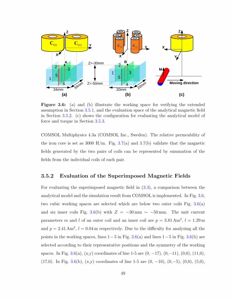
23

4

Y

Z

34mm 34mm

X

Y

Z

X

1

2

3

420mm 20m

m

5

Z=-30mm

Z=-50mm

(a) (b)

5

X

Y

Z

M

Moving direction

(c)

1OC2OC

2IC 4IC

1

A B

Figure 3.6: (a) and (b) illustrate the working space for verifying the extendedassumption in Section 3.5.1, and the evaluation space of the analytical magnetic fieldin Section 3.5.2. (c) shows the configuration for evaluating the analytical model offorce and torque in Section 3.5.3.

COMSOL Multiphysics 4.3a (COMSOL Inc., Sweden). The relative permeability of

the iron core is set as 3000 H/m. Fig. 3.7(a) and 3.7(b) validate that the magnetic

fields generated by the two pairs of coils can be represented by summation of the

fields from the individual coils of each pair.

3.5.2 Evaluation of the Superimposed Magnetic Fields

For evaluating the superimposed magnetic field in (3.3), a comparison between the

analytical model and the simulation result from COMSOL is implemented. In Fig. 3.6,

two cubic working spaces are selected which are below two outer coils Fig. 3.6(a)

and six inner coils Fig. 3.6(b) with Z = −30 mm ∼ −50 mm. The unit current

parameters m and l of an outer coil and an inner coil are p = 3.81 Am2, l = 1.29 m

and p = 2.41 Am2, l = 0.04 m respectively. Due to the difficulty for analyzing all the

points in the working spaces, lines 1−5 in Fig. 3.6(a) and lines 1−5 in Fig. 3.6(b) are

selected according to their representative positions and the symmetry of the working

spaces. In Fig. 3.6(a), (x,y) coordinates of line 1-5 are (0, −17), (0,−11), (0,0), (11,0),

(17,0). In Fig. 3.6(b), (x,y) coordinates of line 1-5 are (0, −10), (0,−5), (0,0), (5,0),

49

(a) Verification on point A. (b) Verification on point B.

Figure 3.7: Verifications on the assumption of superimposing magnetic fields.

(10,0), unit [mm]. The magnetic flux density B in (3.3) is expressed by the norm

of magnetic field strength H because of its concise and comprehensive expression of

magnetic field. Fig. 3.8(a) and 3.8(b) show the comparison between the COMSOL

results and our analytical model results for the two working spaces. The average

differences are 8.97% (the case in Fig. 3.6(a)) and 11.86%(the case in Fig. 3.6(b)).

3.5.3 Evaluation of Force and Torque Model

This evaluation aims at proving the validation of the analytical model of force and

torque developed in (3.15). The evaluation is implemented by using diametrically

magnetized cylindrical magnets with the two different sizes which have been explained

50

(a) Evaluation of superimposed magnetic

field of outer coils.(b) Evaluation of superimposed magnetic

field of inner coils.

Figure 3.8: The analytical model of magnetic field evaluation.

in Section 3.3. The long axis of the magnet is perpendicular to XZ plane and centered

at X=−20 ∼ 20 mm, Z=−30 mm, as shown in Fig. 3.6(c). The magnetized direction

of the magnet is always kept in Z direction. The magnetic field is generated by a

single coil which has the configuration of outer coils in Section 3.3 with a maximum

2.5 A current input. A comparison model is built by COMSOL with 879, 160 mesh

elements and 1 mm maximum element size of the selected mesh. Fig. 3.9 shows the

comparison results of the force and torque agree well for the magnet with the length

of 12.7 mm. For the magnet with the length of 25.4 mm, the agreement of results

are worse than the shorter magnet’s. This is due to the high order terms in (3.9)-

(3.14) are ignored in order to simplify the calculation. Although the accuracy of the

model can be further improved, it still can provide us a reasonable assessment for

the locomotion performance of our proposed design. The following pan/tilt motion

analyses will base on this analytical model.

51

Figure 3.9: Analytical force and torque models evaluation on two different sizes ofcylindrical magnets.

3.5.4 Pan Motion Evaluation

In this paper, we conduct quasi-static evaluations to quantize the locomotion

capability of the camera system. For the pan motion, (3.22) and (3.24) are to

be validated by orientating the camera from 1 to 3 as shown in Fig. 3.4(a).

The viscoelastic tissue is modeled as Standard Linear Solid (SLS) model which

is characterized by spring module E1 = 4.28 × 103 N/m2, spring-dashpot series

E2 = 1.61 × 104 N/m2, η = 8.05 × 103 N-s/m2, Poisson ratio ν = 0.5 Wang et al.

(2013). The friction coefficients are set as µtis = 0.1, µlub = 0.05. According to

Hunter (1961), we maximize F ri in (3.25) by setting V = a0/τ .

The pan motion consists of two phases 0 ∼ 22.5 and 22.5 ∼ 45. CO1,2,5,6 and C

are activated in Fig. 3.10d-3.10h. During the period 0 ∼ 22.5, the currents are set

as IO1 = IO5 (refer to (3.16)), IO2 = IO6 = Imax, IC = 0.2 A with ξ = 0, Imax = 2 A;

during the period 22.5 ∼ 45, the currents are set as IO1 = IO5 = 0, IO2 = IO6 (refer

to (3.18)), IC = 0.2 A with ξ = 0.3, Imax = 2 A. Fig. 3.10a shows under the distance

from the camera to the stator Z = −35 ∼ −50 mm, Tpan is validated until γ reaches

to 0.74 rad. The unreached angles can be achieved by the next set coils. Fig. 3.10b

validates (3.24) that the eletromagnetic force in Z direction can always balance the

52

0.74

Z=-50mm

Z=-35mm

(a) Tpan

00.2

0.40.6

0.8

−0.05

−0.045

−0.04

−0.0350

0.5

1

1.5

2

γ [rad]Z in Σ [m]

Fz [N

]

(b) F z

0 0.2 0.4 0.6 0.8−0.05

−0.04−0.03

0

1

2

3

x 10−4

γ [rad]Z in Σ [m]

Tor

que

[Nm

]

Tmi

Tmif

(c) Tmi and Tmi

f comparison

0 0.2 0.4 0.6 0.8−0.05

−0.04

−0.030

0.5

1

1.5

2

γ [rad]Z in Σ [m]

Io1

[A]

(d) IO1

0 0.2 0.4 0.6 0.8

−0.05

−0.045

−0.04

−0.0350.5

1

1.5

2

γ [rad]

Z in Σ [m]

Io2

[A]

(e) IO2

0 0.2 0.4 0.6 0.8−0.05

−0.04

−0.030

0.5

1

1.5

2

γ [rad]Z in Σ [m]

Io5

[A]

(f) IO5

0 0.2 0.4 0.6 0.8−0.05

−0.045

−0.04

−0.0350.5

1

1.5

2

γ [rad]

Z in Σ [m]

Io6

[A]

(g) IO6

0 0.2 0.4 0.6 0.8

−0.05

−0.045

−0.04

−0.0350

0.1

0.2

0.3

0.4

Ic [A

]

γ [rad]Z in Σ [m]

(h) IC

Figure 3.10: Evaluation of pan motion. (a)-(c) validate the necessary conditionsin equations (3.21), (3.22), (3.24) for generating a pan motion. (d)-(h) show theactivated coils and input current values.

weight of the camera (assume G = 30 grams). Fig. 3.10c validates (3.21) which shows

magnetic torque Tmi on tail-end magnet can overcome the lubricated frictional torque

Tmif between the magnet and its housing.

3.5.5 Tilt Motion Evaluation

The objective of evaluating tilt motion is to analyze the available tilting range

constrained by (3.27) and (3.24). The tilt motion has two modes as shown in

Fig. 3.4(b) and (c). The central housing is positioned from α = 0 (the magnet

is in Z direction in Σ) to α = 90 (the central housing counterclockwise rotating

around the camera shaft). Each mode is investigated by Z = −35 ∼−50 mm. The

current setting for this evaluation is shown in Table 3.2. Fig.3.11a and 3.11d illustrate

when Z = −35 mm, 1.37 rad (78.5) tilt motion for mode 1 and 1.43 rad (82) tilt

motion for mode 2 are available; and when Z = −50 mm, 1.14 rad (65.3) tilt motion

for mode 1 and 1.11 rad (63.6) for mode 2 are available. The full ranges of tilt

motion of mode 1 and mode 2 thus vary from 130.6 to 157 and from 127.2 to 164

53

1.14 1.37

Z=-50mm

Z=-35mm

α

(a) Ttilt in mode 1

00.5

11.5

−0.05

−0.045

−0.04

−0.0350

0.5

1

1.5

2

α [rad]Z in Σ [m]

Fz

[N]

(b) Fz in mode 1

0 0.5 1 1.5 2−0.05

−0.04−0.03

0

0.05

0.1

0.15

0.2

α [rad]Z in Σ [m]

Fy

[N]

Fmy

Ffy

(c) Fy in mode 1

1.11 1.43

Z=-50mm

Z=-35mm

α

(d) Ttilt in mode 2

0 0.5 1 1.5 2

−0.05

−0.04

−0.030.2

0.4

0.6

0.8

1

α [rad]Z in Σ [m]

Fz

[N]

(e) Fz in mode 2

00.5

11.5

2

−0.05

−0.04

−0.030.02

0.04

0.06

0.08

0.1

α [rad]Z in Σ [m]

Fy

[N]

Fmy

Ffy

(f) Fy in mode 2

Figure 3.11: Evaluations of tilt motion. (a)-(c) analyze tilt mode 1, and (d)-(f)analyze tilt mode 2.

Table 3.2: Input Currents For Evaluating Tilt Mode 1 and Mode 2, Unit [A]

IO1 IO2 IO3 IO4 IO5 IO6 IO7 IO8 II1 II2 II3 II4 II5 II6 II7 II8 ICMode 1 1 0 −1 0 1 0 1 0 −2.5 −2.5 −2.5 −2.5 2.5 2.5 2.5 2.5 0Mode 2 1 1 −1 −1 1 1 1 1 0 −2.5 −2.5 −2.5 0 2.5 2.5 2.5 0

respectively. Fig. 3.11b and 3.11e validate (3.24) with a minimum 0.2 N remaining

force after balancing the weight of the camera.

The electromagnetic forces for generating tilt motions cause the tail-end magnets

a Y0 direction (as shown in Fig. 3.5) motion trend by F yf . Therefore, it is necessary to

compare F yf and the sliding friction F y

m between the camera housings and abdominal

wall. Fig. 3.11c and 3.11f show F yf is capable to balance F y

m for keeping the camera

in position.

54

3.6 Summary

This chapter presented a line-arranged rotor driving unit design for a wireless

laparoscopic camera. The design applied 17 flatly arranged coils as a stator and three

diametrically magnetized cylindrical magnets as a stator. This design features the

camera’s fixation and manipulation, and enables a decoupled pan and tilt activation of

the camera by varying the input current of stator’s coils. According to our simulation

results, the laparoscopic camera conservatively has the capability to achieve 360

pan motion with a 22.5 resolution, and the range of 127 ∼ 164 tilt motion which

depends on tilt motion working modes and the distance between the rotor and the

stator.

However, the experimental testings of the fabricated design showed that the

current control of the 17 coils required a complex algorithm, which caused poor

control reliability. To enhance the performance of the actuation system, a hybrid

stator which consists of both permanent magnets and coils is introduced in the next

chapter.

55

Chapter 4

Improved Hybrid Stator Design

with Line-arranged Driving Unit

56

4.1 Abstract

This chapter presents an improved hybrid stator design to drive a line-arranged

rotor capasulated in laparoscopic cameras. This design features a unified mechanism

for anchoring, navigating, and rotating a fully insertable camera by externally

generated rotational magnetic field. The insertable camera body, which has no

active locomotion mechanism on-board, is capsulated in a one-piece housing with

two ring-shaped tail-end magnets and one cylindrical central magnet embedded on-

board as a rotor. The stator positioned outside an abdominal cavity consists of

both permanent magnets and electromagnetic coils for generating reliable rotational

magnetic field. The prototype results in a compact insertable camera robot with a

12.7 mm diameter and a 68 mm length. The design concepts are analyzed theoretically

and verified experimentally. The experiments validate that the proposed camera robot

design provides reliable camera fixation and locomotion capabilities under various

testing conditions. According to the great performance demonstrated in experimental

studies, the hybrid stator and the line-arranged rotor are served as the final actuation

mechanism design.

57

D

E

B

C

Wireless

communicationA1A2

A3

Current control

system

Abdominal

cavity

Figure 4.1: Conceptual illustration of the magnetic actuated camera robot. (A1)The process of inserting the camera robot into the patient’s abdominal cavity througha trocar. (A2) The initialized position after the camera inserted inside. (A3) Thestator. (B) The visual information is transmitted through wireless communicationfrom the camera to the display terminal (C) and current control system (E). (D) Asurgeon can control the current input of the stator through current control system(E) for a desired robot pose.

4.2 Line-arranged Rotor Actuation Strategy with

Hybrid Stator

4.2.1 Configurations of Hybrid Stator and Rotor Design

The objective of this chapter is to design a unified active locomotion mechanism

for a fully insertable wireless laparoscopic camera robot with no on-board motors.

As conceptually illustrated in Fig.4.2, the locomotion mechanism consists of (1)

a rotor with two tail-end IPMs (tIPMs) and one central IPM (cIPM), and (2) a

stator with two coils, two side EPMs (sEPMs), and one central EPM (cEPM). In the

stator that placed externally against an abdominal wall, the EPMs and the coils are

orthogonally arranged. In the rotor that pushed against an abdominal wall internally,

the robot body can rotate freely related to the ring-shaped tIPMs that have unchanged

orientations with respect to the stator, and the diametrically magnetized cylindrical

cIPM is fixed with the robot body.

58

Figure 4.2: The conceptual design of the proposed camera robot system.

The stator-rotor mechanism is designed to enable orientation (rotational control),

navigation (translational control), in addition to the compensation of the gravity of

the camera (fixation control). The robot orientation consists of pan motion and tilt

motion. The pan motion requires torque along ZI axis of the robot, and the tilt

motion control requires torque along XI axis. The robot navigation requires forces

along XI , YI , ZI axes, with the force along ZI axis providing fixation of the robot

against the abdominal wall. The robot navigation control is provided by moving the

stator along the dermal surface with the attractive forces between the sEPMs and the

tIPMs. A spinning motion of the stator along ZS can actuate the robot pan motion

by coupling the magnetic field of the sEPMs and the tIPMs. Due to the dominated

magnetic field from the sEPMs at the location of the cIPM, the cEPM with its north

pole pointing downside is used to eliminate the influence from the sEPMs on the cIPM

by adjusting the cEPM displacement along ZS. In this way, the robot tilt motion can

be effectively actuated by the magnetic coupling between the coils and the cIPM.

59

Space for

onboard

electronics

Opening

for camera

Camera

housing cap

Tail-end shaft

Tail-end IPM

Central IPM

Figure 4.3: Rotor design and its disassembled parts.

The open-ended research problem of chapter is twofold: (1) the effective design

of the stator-rotor locomotion mechanism for the camera robot; and (2) the control

model of the robot tilt motion. The detailed discussions are presented in Section 4.3

and 4.4.

4.2.2 System Overview

Fig. 4.1 illustrates an application scenario of the proposed laparoscopic camera robot.

To insert the camera robot (A1) into the patient’s abdominal cavity, a trocar is firstly

applied. The robot is introduced into the abdominal cavity with surgical forceps, and

fixed against the abdominal wall at an initial position (A2) by a stator (A3). A

surgeon (D) sends signals of desired robot poses to the current control system (E) by

using a user interface. The camera robot at (A2) sends imaging information to the

display terminal (C) through the wireless communication module (B).

4.3 Hybrid Stator Design and Rotor Design

The working environments of the laparoscopic camera robot are insufflated abdominal

cavities and abdominal walls. To insert the robot into an abdominal cavity, the

60

N

S

N

S

80 mm

d [mm]

Att

ract

ive

forc

e [N

]

d

Figure 4.4: Fixation forces are investigated by using four pairs of candidate sEPMsand a pair of tIPMs. The evaluation is conducted under 25 mm ∼ 50 mm rotor-to-stator distances and a 80 mm distance between the sEPMs.

diameter of the robot should adapt to the 12 mm ∼ 15 mm diameter of a standard

trocar. Considering the normal thickness of an abdominal wall that ranges from

20 mm to 40 mm Song et al. (2006), the actuation mechanism design should be able

to provide sufficient actuation capabilities under this working range.

4.3.1 Rotor Design

Robot Housing

The robot housing is designed to host on-board electronics and a cIPM by using a

12.7 mm outer diameter (OD), 10 mm inner diameter (ID) tube, as shown in Fig. 4.3.

A small cylindrical housing is built in the middle of the tube to fix the cIPM. Two

shafts connected with the robot housing caps are designed to support the tIPMs.

This design enables the robot housing and the tIPMs to be separate pieces when

they rotate along the robot axis. The robot length is an important parameter to be

determined, because it affects the torque on the cIPM from the tIPMs. To reserve

sufficient space for on-board electronics and avoid overly lengthy device, the candidate

61

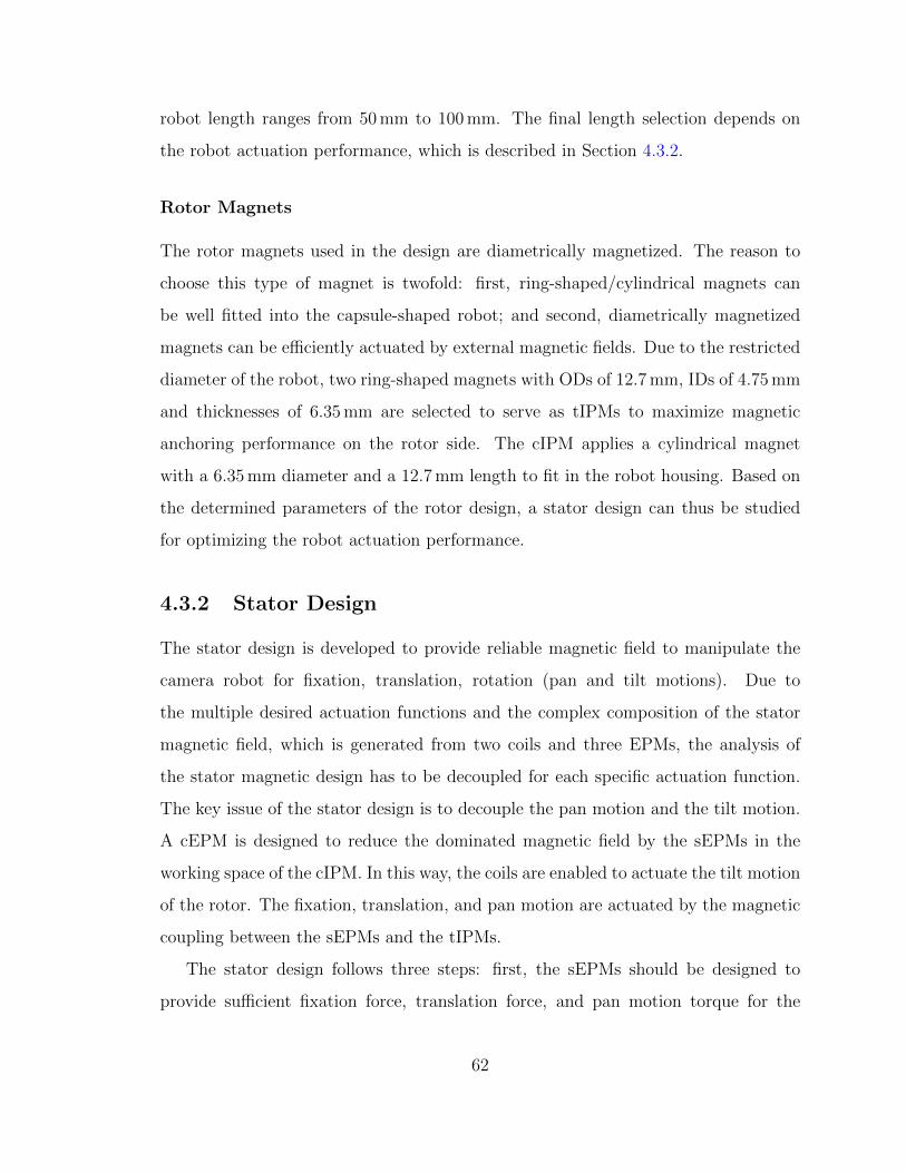
robot length ranges from 50 mm to 100 mm. The final length selection depends on

the robot actuation performance, which is described in Section 4.3.2.

Rotor Magnets

The rotor magnets used in the design are diametrically magnetized. The reason to

choose this type of magnet is twofold: first, ring-shaped/cylindrical magnets can

be well fitted into the capsule-shaped robot; and second, diametrically magnetized

magnets can be efficiently actuated by external magnetic fields. Due to the restricted

diameter of the robot, two ring-shaped magnets with ODs of 12.7 mm, IDs of 4.75 mm

and thicknesses of 6.35 mm are selected to serve as tIPMs to maximize magnetic

anchoring performance on the rotor side. The cIPM applies a cylindrical magnet

with a 6.35 mm diameter and a 12.7 mm length to fit in the robot housing. Based on

the determined parameters of the rotor design, a stator design can thus be studied

for optimizing the robot actuation performance.

4.3.2 Stator Design

The stator design is developed to provide reliable magnetic field to manipulate the

camera robot for fixation, translation, rotation (pan and tilt motions). Due to

the multiple desired actuation functions and the complex composition of the stator

magnetic field, which is generated from two coils and three EPMs, the analysis of

the stator magnetic design has to be decoupled for each specific actuation function.

The key issue of the stator design is to decouple the pan motion and the tilt motion.

A cEPM is designed to reduce the dominated magnetic field by the sEPMs in the

working space of the cIPM. In this way, the coils are enabled to actuate the tilt motion

of the rotor. The fixation, translation, and pan motion are actuated by the magnetic

coupling between the sEPMs and the tIPMs.

The stator design follows three steps: first, the sEPMs should be designed to

provide sufficient fixation force, translation force, and pan motion torque for the

62

4.3 1.64

(a) (b)Pan angle γ [deg]Offset [mm]

Tra

nsl

ati

on

al

forc

e [N

]

Pa

n m

oti

on

to

rqu

e [N

m]

Tz

Tf

Fx

Ff

N

S

d=50mm

80 mm

N

S

Offset

X

Z

N

S N

S

Z

X

γ

d=30mm

80mm

Figure 4.5: Translational force and pan motion torque investigation. (a) Thecomparison result of translational force Fx between a stator and a rotor in X direction,and frictional force Ff in -X direction with the stator offset distance ranging from0 mm to 10 mm. (b) The comparison result of the pan motion torque Tz and thefrictional torque Tf against the pan motion.

camera robot; second, parameters and configurations of the coils have to be optimized

to balance the coil volumes and magnetic field strength; and third, the central axis

field of the stator has to be designed by using a cEPM to decouple the pan motion

and the tilt motion of the camera robot. The design analysis of the stator in this

section is conducted by COMSOL Multiphysics 5.0 (COMSOL Inc., Sweden).

sEPMs of the Stator

According to our preliminary experimental study, a set of axially magnetized

cylindrical magnets serve as sEPM candidates. The dimensions and materials of

the magnets are illustrated in the legend of Fig. 4.4. To investigate the attractive

force between the sEPMs and the tIPMs, the robot length is temporary determined

at 80 mm which is approximately the middle point of the desired length range

50 ∼ 100 mm. Since the normal range of an abdominal wall thickness is 20 mm ∼

63

40 mm, the range of the rotor-to-stator distance d, which is the distance between

the bottom surface of the stator and the symmetric axis of the rotor, is estimated

as 30 mm ∼ 50 mm. Fig. 4.4 shows the simulation results of the attractive forces

between different sets of the sEPMs and the tIPMs under the rotor-to-stator distance

ranging from 30 mm to 50 mm. With the estimated the total robot weight that is

under 30 g, the magnet with the dimension φ25.4 mm ×H25.4 mm, which generates

more than 4 N force at 30 mm and 1 N at 50 mm, can provide reliable fixation force

with maximum contact compression about 0.5 psi against an abdominal wall. This

pressure is much smaller than the safe threshold 3.45 psi for preventing undesired

histological damages Best et al. (2011).

Based on the selected sEPMs, the translation and pan motion of the rotor are

investigated in Fig. 4.5. Fig. 4.5(a) shows the simulation results of the translational

motion with offsets ranging from 0 to 10 mm between the sEPMs and the tIPMs

under 50 mm rotor-to-stator distance. The result shows the translational force Fx

in X direction can overcome the frictional force Ff in -X direction after the offset

distance reaches 4.3 mm. Fig. 4.5(b) shows the sEPMs can provide sufficient pan

motion torque Tz along the central axis of the stator to overcome frictional torque Tf

after a relative rotational angle γ = 1.64 is reached.

Coils of the Stator

The coil dimension design is based on the intensive experimental studies in our

prior work Liu et al. (2014a,b) to determine a compact size of the coils, which

should compromise with providing sufficient magnetic field strength. The experiments

indicate a coil with 50 mm height, 50 mm OD, 10 mm ID, and an iron core with 60 mm

height is optimal. The winding wire used in the coils is AWG23 copper wire with

2, 000 turns. For the safety consideration, the input current of the coils is limited to

1.5 A for preventing coil overheating.

To optimize the utilization of the coil magnetic field in the robot working space,

as illustrated in the yellow area of Fig. 4.6(a), the configurations that include the

64

30

mm

Reserved

space for

cEPM

30 mm

65mm

Ic1 =

-1A~1A

N

S

N

SIc2 = -1A~1A

Bc2

Bmin

(a) (b)

h= 30mmh= 50mm

Robot

working space

-Bc1

-Bc2

BmaxPA

PB

YS

Coil 1 Coil 2

50

mm

ZS

Bc1

|Bm

in| [T

]

δ [deg]

Figure 4.6: Configurations of electromagnetic coils in the stator. (a) The setup fortesting the coils δ angle to generate optimal magnetic field in the robot working space.Bmin and Bmax represent the minimum and the maximum magnetic field strength ina rotational magnetic field generated by the coils. (b) The relationship between thecoils tilt angle δ and Bmin.

distance between the coils, and the tilt angle δ need to be studied. The minimal

distance between the two coils is determined by the volume of a cEPM. According

to the dimensions of the sEPMs (25.4 mm diameter, 25.4 mm height), a cylindrical

space with 30 mm in diameter, as shown in the blue region of Fig. 4.6(a), is reserved

for a central EPM to balance the central axis field of the stator. The tilt angle δ of

the coils is used to adjust the magnetic field performance. Due to the desire of having

a compact stator design, the coil pivot points used to achieve tilt angles are set at

±65 mm on the YS axis by considering the 50 mm diameters of the coils.

To determine the optimal δ angle, Bmin, which is a minimum composed magnetic

field by the coils, is used to quantify a δ angle performance. As illustrated in

Fig. 4.6(a), Bc1 and Bc2 are the magnetic fields generated by the coil 1 and the coil

2 respectively. The rhombus demonstrates the region of possible composed magnetic

field by setting −1 A ∼ 1 A current input in each coil.

Fig. 4.6(b) shows the |Bmin| values at the working space boundary points PA and

PB, which represent the rotor-to-stator distance 30 mm and 50 mm respectively. The

65

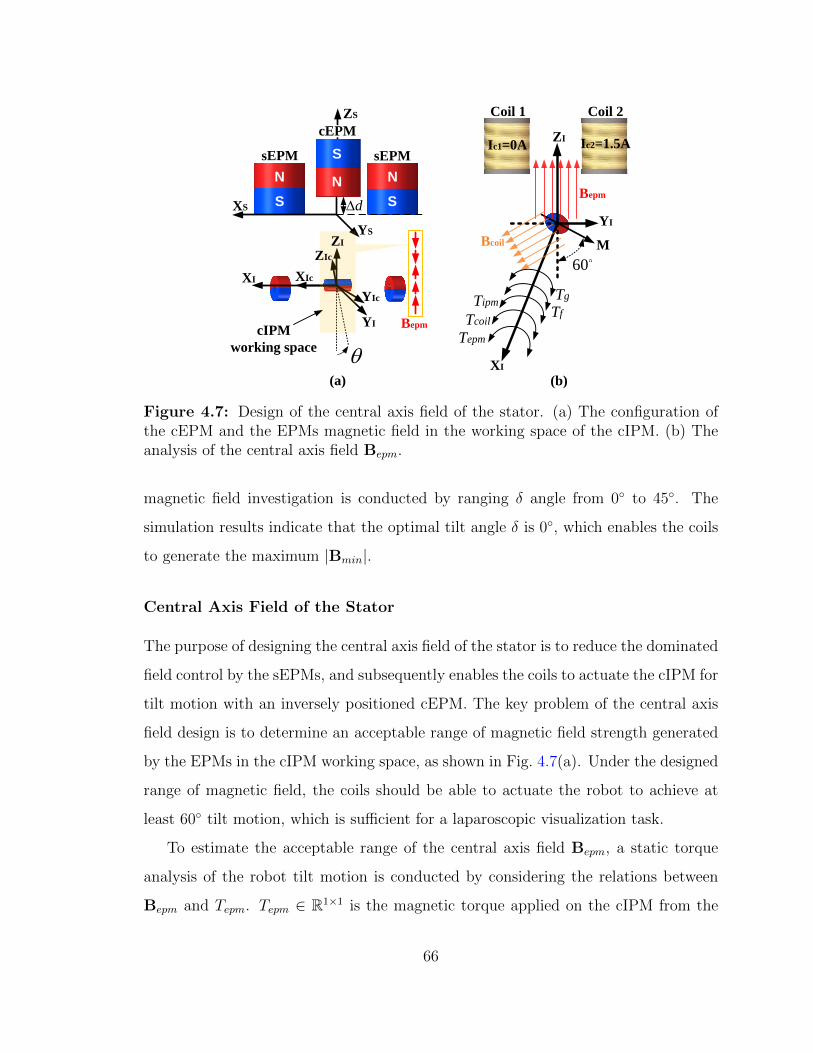
XS

YS

YI

60

XI

YI

ZI

Bepm

Bcoil

(a) (b)

Bepm

Ic2=1.5AIc1=0A

M

d

N

S

NN

S S

N

TipmTg

TcoilTf

TepmcIPM

working space

sEPM sEPM

cEPM

ZS Coil 1 Coil 2

XI

ZI

ZIc

XIc

YIc

Figure 4.7: Design of the central axis field of the stator. (a) The configuration ofthe cEPM and the EPMs magnetic field in the working space of the cIPM. (b) Theanalysis of the central axis field Bepm.

magnetic field investigation is conducted by ranging δ angle from 0 to 45. The

simulation results indicate that the optimal tilt angle δ is 0, which enables the coils

to generate the maximum |Bmin|.

Central Axis Field of the Stator

The purpose of designing the central axis field of the stator is to reduce the dominated

field control by the sEPMs, and subsequently enables the coils to actuate the cIPM for

tilt motion with an inversely positioned cEPM. The key problem of the central axis

field design is to determine an acceptable range of magnetic field strength generated

by the EPMs in the cIPM working space, as shown in Fig. 4.7(a). Under the designed

range of magnetic field, the coils should be able to actuate the robot to achieve at

least 60 tilt motion, which is sufficient for a laparoscopic visualization task.

To estimate the acceptable range of the central axis field Bepm, a static torque

analysis of the robot tilt motion is conducted by considering the relations between

Bepm and Tepm. Tepm ∈ R1×1 is the magnetic torque applied on the cIPM from the

66

EPMs along XI axis. We assume the cIPM is described by a body-attached magnetic

moment M ∈ R3×1 with a constant magnitude in ampere square meter. The torque

and force on the cIPM generated from the stator, in newton meters and newtons

respectively, can be expressed as

T = M×B, F = (M · ∇)B, (4.1)

where B ∈ R3×1 represents the magnetic field of the stator Jackson (1999). In

accordance with (4.1), Tepm can be calculated by

Tepm = |Bepm| · |M| · sin(Bepm,M). (4.2)

To guarantee the robot can achieve at least 60 tilt angle, the boundary condition

of Tepm is expressed by

Tepm + Tf ≤ Tcoil + Tipm + Tg, (4.3)

where Tf is a frictional torque generated between the abdominal wall and the robot;

Tcoil is the torque on the cIPM with 60 tilt angle by giving input current of the

coil 2 as 1.5 A; Tipm is the torque on the cIPM with 60 tilt angle from the tIPMs;

Tg is the gravity torque of the robot. The reason to put Tf on the left side of

(4.3) is to develop a strict boundary to Tepm. The boundary condition (4.3) should

be valid under 30 mm ∼ 50 mm rotor-to-stator distances. The robot length, which

determines the distance between the sEPMs, has a major impact on Tipm and is

evaluated in the range of 50 mm ∼ 100 mm. Except Tepm, all the other torques in

(4.3) are calculated by modeling the rotor and the stator in COMSOL. The boundary

values of the central axis field Bepm are calculated according to the boundary values

of Tepm and (4.2), as illustrated in Table 4.1. The minimum boundary value of |Bepm|

is 0.0138 T under the condition of the rotor-to-stator distance 50 mm, and the robot

67

Table 4.1: The Central Axis Magnetic Field Boundary |Bepm| for 50 mm ∼ 100 mmRobot Length

Distance (mm) 50 60 70 80 90 10030 0.0416 T 0.0371 T 0.0361 T 0.0334 T 0.0329 T 0.0328 T50 0.0219 T 0.0179 T 0.0168 T 0.0143 T 0.0139 T 0.0138 T

length 100 mm. Therefore, the central axis magnetic field of the stator can be bounded

as |Bepm| < 0.0138 T.

Under the guideline of the central axis field boundary developed above, the cEPM

can be designed. As illustrated in Fig. 4.7(a), the central axis field Bepm changes its

direction as the rotor-to-stator distance increases. To control the tilt motion of the

robot, Bepm with +ZI direction is desired in the cIPM working space as illustrated

in Fig. 4.7(b), because the magnetic field with this direction can help the coils to

actuate the cIPM for achieving a larger tilt angle. To reserve sufficient space for

on-board electronics, the distance between the centers of the tIPMs is determined as

60 mm. The distance between the sEPMs is subsequently determined. By using trial

and error method, the cEPM is designed as an axially magnetized cylindrical magnet

with 22.22 mm in diameter, 28.57 mm in height, and an offset distance ∆d = 5 mm ∼

10 mm in +ZS direction. The range of the central axis field with the designed central

EPM is evaluated by COMSOL under rotor-to-stator distance 30 mm ∼ 50 mm. The

simulation results in |Bepm| ∈ [0.0014 T, 0.004 97 T], which has a uni-directional field

point in +ZS direction, and is within the acceptable central axis field boundary

|Bepm| < 0.0138 T.

Table 4.2 shows the summarized specifications of the rotor and the stator designs.

The whole length of the robot is designed as 68 mm in accordance with the determined

distance of the tIPMs. The distance of the sEPMs and the distance of the coils, which

are 60 mm and 80 mm respectively, are measured between their axial axes.

68

Table 4.2: Specifications of The Rotor and Stator Prototype Designs

Part Name DimensionCentral housing OD 12.7 mm, ID 10 mmRobot whole length 68 mmcIPM: Diametrically magnetized

Size Diameter 6.35 mm, Length 12.7 mmMaterial NdFeB Grade N42

tIPM: Diametrically magnetizedSize OD 12.7 mm, ID 4.75 mm

Thickness 6.35 mmMaterial NdFeB Grade N42

Dummy robot weight 16.6 gElectromagnetic coils:

Dimensions Height 50 mm, OD 50 mm, ID 10 mmAxial distance 80 mmWire type AWG23Turns 2,000Iron-core dimensions Diameter 9 mm, Length 60 mmIron-core permeability 100,000

sEPMs: Axially magnetizedSize Diameter 25.4 mm, Height 25.4 mmMaterial NdFeB Grade N52Axial distance 60 mm

cEPM: Axially magnetizedSize Diameter 22.22 mm, Height 28.57 mmMaterial NdFeB Grade N52Offset ∆d 5 mm∼ 10 mm

4.4 Control Model of Robot Tilt Motion

This section aims at developing a control model for the robot tilt motion activated

by the coils. The objective can be achieved by (1) analyzing the stator magnetic

field, and (2) modeling the robot dynamics with the magnetic force/torque between

the rotor and the stator, and the frictional force/torque between the robot and an

abdominal wall.

69

Z

X

Y

OL

P

aX

Ya

…

...a

(a) (b)

… ...

… ..

.

Pmij-

Pmij+

Qij-

Qij+

Figure 4.8: EPM magnetic field modeling.

To clarify the relationship between the stator and the rotor, coordinate systems

are defined in Fig. 4.2, and explained as follows:

• ΣEiXEi, YEi, ZEi represent the coordinate systems of the EPMs, i = 1, 2, 3.

• ΣCiXCj, YCj, ZCj represent the coordinate systems of the coils, j = 1, 2.

• ΣSXS, YS, ZS and ΣIXI , YI , ZI represent the internal coordinates of the

stator and the rotor respectively.

• ΣIcXIc, YIc, ZIc represents the body attached coordinate systems of the cIPM.

4.4.1 Magnetic Field Analysis of the Stator

Due to the fixed relative positions of the EPMs and the coils, the stator magnetic

field can be calculated by superimposing the magnetic fields from the EPMs and the

coils Liu et al. (2014b).

EPM Magnetic Field

Inspired by Kok-Meng and Hungsun (2007), the EPMs can be represented by a

magnetic dipole array, as shown in Fig. 4.8(a). The magnetized direction is along +Z

axis, and the diameter and length of the magnet are a and L respectively. The positive

70

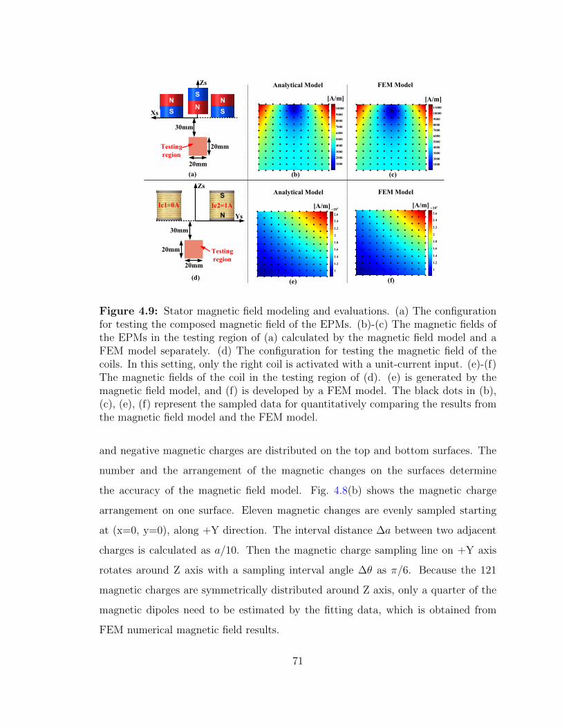
(a)

(d)

XsN

S

NN

S S

N

Zs

30mm

20mm

20mm

Testing region

Ic2=1AIc1=0A

N

S

Zs

Ys

30mm

20mm

20mm

Testing region

[A/m] [A/m]

[A/m] [A/m]

10000

9000

8000

7000

6000

5000

4000

3000

2000

1000

10000

9000

8000

7000

6000

5000

4000

3000

2000

1000

11000

2.6

2.4

2.2

2

1.8

1.6

1.4

1.2

1

2.6

2.4

2.2

2

1.8

1.6

1.4

1.2

1

410 410

(b)

(e)

(c)

(f)

Analytical Model FEM Model

Analytical Model FEM Model

Figure 4.9: Stator magnetic field modeling and evaluations. (a) The configurationfor testing the composed magnetic field of the EPMs. (b)-(c) The magnetic fields ofthe EPMs in the testing region of (a) calculated by the magnetic field model and aFEM model separately. (d) The configuration for testing the magnetic field of thecoils. In this setting, only the right coil is activated with a unit-current input. (e)-(f)The magnetic fields of the coil in the testing region of (d). (e) is generated by themagnetic field model, and (f) is developed by a FEM model. The black dots in (b),(c), (e), (f) represent the sampled data for quantitatively comparing the results fromthe magnetic field model and the FEM model.

and negative magnetic charges are distributed on the top and bottom surfaces. The

number and the arrangement of the magnetic changes on the surfaces determine

the accuracy of the magnetic field model. Fig. 4.8(b) shows the magnetic charge

arrangement on one surface. Eleven magnetic changes are evenly sampled starting

at (x=0, y=0), along +Y direction. The interval distance ∆a between two adjacent

charges is calculated as a/10. Then the magnetic charge sampling line on +Y axis

rotates around Z axis with a sampling interval angle ∆θ as π/6. Because the 121

magnetic charges are symmetrically distributed around Z axis, only a quarter of the

magnetic dipoles need to be estimated by the fitting data, which is obtained from

FEM numerical magnetic field results.

71

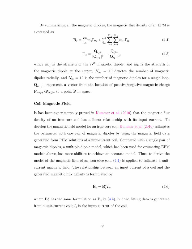
By summarizing all the magnetic dipoles, the magnetic flux density of an EPM is

expressed as

Be =µ0

4πm0Γ00 +

µ0

4π

Km∑i=1

Nm∑j=1

mijΓij, (4.4)

Γij =Qij+

|Qij+|3−

Qij−

|Qij−|3, (4.5)

where mij is the strength of the ijth magnetic dipole, and m0 is the strength of

the magnetic dipole at the center; Km = 10 denotes the number of magnetic

dipoles radially, and Nm = 12 is the number of magnetic dipoles for a single loop;

Qij+/− represents a vector from the location of positive/negative magnetic charge

Pmij+/Pmij− to a point P in space.

Coil Magnetic Field

It has been experimentally proved in Kummer et al. (2010) that the magnetic flux

density of an iron-core coil has a linear relationship with its input current. To

develop the magnetic field model for an iron-core coil, Kummer et al. (2010) estimates

the parameter with one pair of magnetic dipoles by using the magnetic field data

generated from FEM solutions of a unit-current coil. Compared with a single pair of

magnetic dipoles, a multiple-dipole model, which has been used for estimating EPM

models above, has more abilities to achieve an accurate model. Thus, to derive the

model of the magnetic field of an iron-core coil, (4.4) is applied to estimate a unit-

current magnetic field. The relationship between an input current of a coil and the

generated magnetic flux density is formulated by

Bc = Buc Ic, (4.6)

where Buc has the same formulation as Be in (4.4), but the fitting data is generated

from a unit-current coil; Ic is the input current of the coil.

72

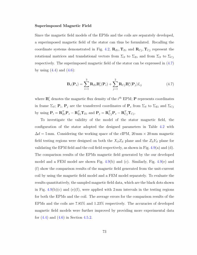
Superimposed Magnetic Field

Since the magnetic field models of the EPMs and the coils are separately developed,

a superimposed magnetic field of the stator can thus be formulated. Recalling the

coordinate systems demonstrated in Fig. 4.2, REi,TEi and RCj,TCj represent the

rotational matrices and translational vectors from ΣS to ΣEi and from ΣS to ΣCj

respectively. The superimposed magnetic field of the stator can be expressed in (4.7)

by using (4.4) and (4.6):

Bs(Ps) =3∑i=1

REiBie(Pi) +

2∑j=1

RCjBuc (Pj)Icj (4.7)

where Bie denotes the magnetic flux density of the ith EPM; P represents coordinates

in frame ΣS; Pi, Pj are the transferred coordinates of Ps from ΣS to ΣEi and ΣCj

by using Pi = RTEiPs −RT

EiTEi and Pj = RTCjPs −RT

CjTCj.

To investigate the validity of the model of the stator magnetic field, the

configuration of the stator adopted the designed parameters in Table 4.2 with

∆d = 5 mm. Considering the working space of the cIPM, 20 mm × 20 mm magnetic

field testing regions were designed on both the XSZS plane and the ZSYS plane for

validating the EPM field and the coil field respectively, as shown in Fig. 4.9(a) and (d).

The comparison results of the EPMs magnetic field generated by the our developed

model and a FEM model are shown Fig. 4.9(b) and (c). Similarly, Fig. 4.9(e) and

(f) show the comparison results of the magnetic field generated from the unit-current

coil by using the magnetic field model and a FEM model separately. To evaluate the

results quantitatively, the sampled magnetic field data, which are the black dots shown

in Fig. 4.9(b)(c) and (e)(f), were applied with 2 mm intervals in the testing regions

for both the EPMs and the coil. The average errors for the comparison results of the

EPMs and the coils are 7.85% and 1.23% respectively. The accuracies of developed

magnetic field models were further improved by providing more experimental data

for (4.4) and (4.6) in Section 4.5.2.

73

4.4.2 Control with Electromagnetic Coils

The robot tilt motion is activated by the magnetic coupling between the coils and

the cIPM. Ic1 and Ic2 are represented as the current inputs of the coils, and θ is

represented as the rotational angle of the robot tilt motion. The robot dynamics

need to be studied for developing the relationship between the control inputs Ic1, Ic2

and the output θ.

Fig. 4.7(b) shows the dynamic analysis of the robot tilt motion. The torques that

affect the tilt motion along XI include (1) Ts which is the combination of Tepm and

Tcoil on the cIPM from the EPMs and the coils of the stator; (2) Tipm which is the

magnetic torque on the cIPM from the tIPMs along XI ; (3) Tf and Tg which are

the frictional torque of the robot-tissue interaction and the torque due to the robot

gravity along XI . The bold fonts Ts,Tipm,Tf , and Tg are used to represent the

torque vectors with the components along XI , YI , ZI .

Combining (4.1) and (4.7), the torque on the cIPM generated from the stator, in

newton meters, can be expressed as

Ts = M× (∑

REiBie)︸ ︷︷ ︸

E

+ (M×RC1Buc )︸ ︷︷ ︸

C1

Ic1 + (M×RC2Buc )︸ ︷︷ ︸

C2

Ic2, (4.8)

where E ∈ R3×1 denotes the torque from the EPMs, i=1,2,3; C1 ∈ R3×1 and C2 ∈

R3×1 denote the unit current torques from the coils. Benefiting from the magnetic

field model in (4.4), E, C1, and C2 can be computed in real time.

The non-zero components in Tf and Tipm are the x-components represented by

Tf and Tipm. Tf is determined by Fattr which is the attractive force between the

stator and the rotor. Due to the reduced magnetic field of the EPMs in the cIPM

working space, the magnetic coupling between the stator and the central IPM has a

minor contribution which is less than 7% of the total attractive force according to our

simulation. To reduce the complexity of the system control, this trivial contribution

of the attractive force Fattr is neglected. As Fattr = f1(h) and Tipm = f2(θ) are

74

functions of an abdominal wall thickness h and the robot tilt angle θ respectively, f1

and f2 can be modeled by polynomial approximation

f1(h) =n+1∑k=1

ηkhn−k+1, f2(θ) =

m+1∑k=1

ξkθm−k+1, (4.9)

where ηk and ξk are the polynomial coefficients to be determined by experimental

data; n and m denote the degrees of f1 and f2.

By representing ω = [θ, 0, 0]T as the angular velocity of the robot tilt motion, the

dynamic model can be formulated in ΣI as

Ts + Tipm + Tf + Tg = I′ω + ω × I′ω, (4.10)

where I ∈ R3×3 is the moment of inertia in the body attached frame ΣIc ; RIcI ∈ R3×3

is the rotational matrix from ΣI to ΣIc ; I′ = RIcI · I · (R

IcI )T is the moment of inertia

of the rigid body in ΣI .

Since the tilt motion is actuated along the XI axis, only the x components need

to be considered in (4.10). By substituting (4.8) and (4.9) in (4.10), the dynamic

equation is reformulated as

Ex + C1xIc1 + C2xIc2 + Tipm + µ(Fattr −mg)rf +mgrg sin θ = a11θ, (4.11)

where Ex, C1x, C2x are the x components in E,C1, and C2 respectively; µ is the

frictional coefficient between the robot and an abdominal wall; mg represents the

gravity of the robot; rf and rg denote the lever arms of the friction force and the

gravity force to generate Tf and Tg; a11 denotes the element of 1th row, 1th column in

I;

To generate a desired tilt angle for the robot, the coil current inputs Ic1 and Ic2

can be found by applying pseudoinverse to

CxIc = G, (4.12)

75

where Cx = [C1x, C2x] ∈ R1×2; Ic = [Ic1, Ic2]T ∈ R2×1; G represents the summation

of the remaining terms in (4.11). Because Cx has a full row rank, the solution of the

current input vector Ic can be calculated by using

Ic = CTx (CxC

Tx )−1G. (4.13)

4.5 Prototype Fabrication and Experimental Val-

idation

4.5.1 Prototype Fabrication and Experiment Platform Setup

CoilCoil

cEPMsEPM

sEPM

cIPMtIPM

tIPM

(a)

(b)

(c)

(d)

Figure 4.10: Experimental environment and the fabricated capsule robot system:(a) experiment setups for evaluating the robot locomotion capabilities; (b) thesimulated abdominal wall tissue made by a viscoelastic material; (c) the stator design;(d) the rotor design.

Experiment platform setup

Fig. 4.10(a) shows the overview of the experimental environment. The robot system

was fabricated by a 3D prototyping machine (Fortus 400mc, Stratasys Inc.). To

76

simulate the viscoelastic properties of a real insufflated abdominal wall (average

Young’s modulus 32.5 kPa) Song et al. (2006), a viscoelastic material Durometer 40

with (Young’s modulus 27.57 kPa at 15% deflection, Sorbothane, Inc.) was applied

as illustrated in Fig. 4.7(b). The initial abdominal wall thickness was 26 mm (tissue

layer 15 mm, support layer 11 mm), which can be adjusted by increasing the distance

between the stator and the support layer. The vertical displacement ∆d of the cEPM

can be manually adjusted at this stage. A silicone oil lubricated rotor-tissue contact

layer was added to the bottom of the viscoelastic material for mimicking an internal

abdominal wall surface.

Rotor and stator fabrication

Fig. 4.10(c) and (d) show the prototype of the camera robot and the stator. The

specifications of the stator and rotor designs are illustrated in Table 4.2. The

permanent magnets applied in the prototype are all from K&J Magnetics. The

AWG23 cooper wires adopted in the coils are from TEMCo. And the iron-cores

of the coils are made by EFI Alloy 50 from Ed Fagan. The space above the EPMs in

the stator is reserved for the on-board electronics and the tetherless power supply of

the stator.

Current control system

A tethered current control system was developed by the PWM technique. The

system consists of a micro-controller (STM32F4Discovery, STMicroelectronics Inc.)

to generate PWM signals, two PWM amplifiers (L6205 DMOS Full Bridge Driver,

STMicroelectronics Inc.) to amplify the signals, a power supply for powering up the

amplifiers, and a PC computer to send control command to the micro-controller via

a serial communication.

77

(a)

(b)

(c)

(e)

(d)

Coil central line

Sensor

central

line

Figure 4.11: Stator magnetic field experimental evaluation.

4.5.2 Model Evaluation

Stator magnetic field

The models of the stator magnetic field developed in Section 4.4.1 were validated by

using hall effect sensors (CYL8405, ChenYang Technologies GmbH) with measuring

range 0 ∼ 64 mT and sensitivity about 50 mV/mT. The measured analog magnetic

field signals were converted to digital signals with sensing resolution 0.01 mT by using

a 16bit ADC (ADS1115, Texas Instruments Inc.). Due to the imperfection of the

coil wrapping, the iron cores, and the permanent magnets, model calibration was

performed by using experimental data. Fig. 4.11(a) shows the experiment platform

for magnetic field validation which consists of a vertical moving track with a position

indicator (Fig. 4.11(b)), three hall effect sensors for 3-axis sensing (Fig. 4.11(c)), and

a transparent support board for placing the coils or the EPMs at desired locations.

Fig. 4.11(d) and (e) show the magnetic flux density norm comparison results of the

experimental data and the magnetic field models along the sensor central line for a

single coil with unit current input and the three EPMs with the vertical displacement

of the cEPM as ∆d = 1 mm. According to the configuration of the stator, the distance

from the coil central line to the sensor central line was set as 40 mm for validating

78

(a)

(b) (c)

Fattr

Tipm 4

1

Ts

2

5

7

8

6

9

Ic1

Ic23

Figure 4.12: Experiment configurations for evaluating the model of Ts in (a),estimating the polynomial coefficients of Tipm in (b) and Fattr in (c). 1©: stator liftingmechanism; 2©: the stator; 3©: the stator supporting board made by aluminum; 4©:six axis force/torque sensor; 5©: camera housing with the cIPM inside, and withoutthe tIPMs at the tail-ends; 6©: shaft; 7©: camera housing with the cIPM inside, andwith the tIPMs at the tail-ends; 8©: tilt angle indicator; 9©: caliper for measuringthe stator-to-rotor distance.

the coil magnetic field. For the EPMs, the sensor central line was set to coincide

with the central line of the cEPM. The average errors of the magnetic field models

demonstrated in Fig.4.11(d) and (e) were 0.001% and 0.02% respectively.

Table 4.3: Magnetic Torque Between tIPMs and cIPM Tipm

θ (deg) 0 15 30 45 60 75 90Tipm (mNm) 0 -0.76 -1.23 -1.53 -1.68 -1.85 -1.96

79

h=20mm

h=30mm

h=40mm

Figure 4.13: Experimental evaluation of magnetic torque on the cIPM.

Magnetic torque on the cIPM

Fig. 4.12(a) shows the experimental setup for evaluating Ts in (4.8). Due to the

tilt motion generated along the camera axis, Ts which is the x component of Ts

was measured by changing the current inputs of the coils Ic1 and Ic2. A six axis

force/torque(F/T) sensor (HEX-58-RB-2000N, OptoForce Inc.), as illustrated in

Fig. 4.12(a)- 4© with torque resolution 5× 10−4 Nm along the shaft was applied. A

cIPM was embedded in the camera housing (Fig. 4.12(a)- 5©) which was connected to

the F/T sensor with a shaft (Fig. 4.12(a)- 6©). The tilt angle of the camera housing

was fixed at 0. The distance h between the stator and the camera was adjusted

by a lifting mechanism (Fig. 4.12(a)- 1©), and measured by a caliper (Fig. 4.12(c)-

9©). An aluminum board was used at the bottom surface of the lifting mechanism

((Fig. 4.12(a)- 3©) with relative magnetic permeability about 1. The input current Ic1

was fixed at −1.5 A, while Ic2 was linearly changed from −1.5 A to 1.5 A. Fig. 4.13

shows the comparison results of experiment data and the model in (4.8) under

stator-to-rotor distances 20 mm, 30 mm, and 40 mm. The average error of the model

demonstrated in Fig. 4.13 was 0.0035%.

80

Table 4.4: Stator/Rotor Attractive Magnetic Force

h (mm) ∆d (mm) Fattr(N) ∆F (N)

20 11 3.978 ±0.034

25 8 2.590 ±0.034

30 4 1.626 ±0.034

35 2 0.916 ±0.034

40 1 0.544 ±0.034

45 0 0.442 ±0.034

50 0 0.340 ±0.034

Polynomial coefficients estimation

Fig. 4.12(b) shows the experimental setup for measuring the magnetic torque Tipm to

estimate the polynomial coefficients in (4.9). Compared with the configuration of the

camera housing in Fig. 4.12(a)- 5©, the configuration in Fig. 4.12(b)- 7© applied two

tIPMs with fixed orientations at both ends of the camera housing. The tilt angle of

the cIPM was indicated by an angle indicator as illustrated in Fig. 4.12(b)- 8©. After

a tilt angle was set, the shaft at the sensor side was fastened by the screws to hold

the angle.

Table 4.3 shows the Tipm experiment data by changing the tilt angle from 0 to

90 with 15 interval. The estimated polynomial coefficients for Tipm are ξ1 = 0.0247,

ξ2 = −0.1176, ξ3 = 0.2298, ξ4 = −0.4801, ξ5 = −1.5159 with a fitting error 0.76% at

the fourth degree polynomial (m = 4 in (4.9)).

Fig. 4.12(c) demonstrates the experimental setup for measuring the magnetic

attractive force Fattr to estimate the polynomial coefficients in (4.9). Table 4.4 shows

81

the attractive force Fattr between the stator and the rotor with respect to stator-to-

rotor distance h sampled from 20 mm to 50 mm. The values in the column of ∆d show

the optimal displacements of the cEPM that enable minimal magnetic field from the

EPMs on the cIPM. ∆F represents the maximum influence on the attractive force by

activating the coils in the stator. The experiment data validates that the magnetic

force contribution from the coils is minor compared with the magnetic force from

the EPMs. A fourth degree polynomial curving fitting (n = 4 in (4.9)) was applied

for Fattr to achieve a curve fitting error 1.66% with the coefficients η1 = −0.0498,

η2 = −0.1143, η3 = 0.7364, η4 = −1.0856, η5 = 0.9237.

Angle pointer

IC1

Protractor

IC2

Tissue layer

Support layer

Adjustable

layer

Figure 4.14: Experimental setup for open-loop control of the camera tilt motion.

4.5.3 Open-loop Control of Tilt motion

Fig. 4.14 shows the experimental setups for the camera robot tilt motion control by

using (4.11). The simulated abdominal wall consisted of three types of layers: (1) the

tissue layer lubricated with silicone oil; (2) support layer; and (3) adjustable layer

which was used for changing the total thickness of the abdominal wall. To indicate

the tilt angles, a protractor and an angle pointer were applied.

82

(a) (b) (c)

Figure 4.15: Experimental results of the open-loop control of tilt motion. (a)Desired tilt angle θd = 20; (b) θd = 50; (c) θd = 80.

Considering the candidate on-board electronics to be integrated in the camera

robot, the moment of inertia matrix I of the robot was estimated by modeling it in

SolidWorks2013 (Dassault Systemes SolidWorks Corp.) as

I =

0.174 0 −0.003

0 3.473 0

0 0 3.469

, (4.14)

where the unit of each element in I is kg mm2. The other parameters used in (4.11)

were estimated or measured as µ = 0.1, rf = 4 mm, and rg = 1.5 mm. Extra weights

were filled in the camera housing to simulate the full load of on-board electronics with

the total weight of the camera robot as mg = 0.26 N.

To control the tilt motion with (4.11), 5th-order desired trajectories, which are

smooth at the angular acceleration level, were generated by initializing the robot tilt

angles as 0 and setting the desired tilt angles θd. The control current inputs Ic1 and

Ic2 were computed by (4.13) in real time.

83

(a) (b)

(c) (d)

Figure 4.16: Demonstration of decoupled pan and tilt motion.

Fig. 4.15 shows the experimental results of open-loop control of the camera tilt

motion by setting the desired tilt angles as 20, 50, and 80 which are illustrated

by the green lines in Fig. 4.15(a), (b), and (c) respectively. This experiment was

grouped by 30 mm, 40 mm, and 50 mm abdominal wall thicknesses. For each group

and each desired tilt angle, the control process was implemented by 30 trials. The

box-and-whisker plots indicate that the tilt angle errors fell in ±7. The tilt angle

control for θd = 50 in Fig. 4.15(b) was better behaved than in (a) and (c) with

no single sample considered as extremes. Fig. 4.15(c) demonstrates that camera tilt

angle can be successfully controlled up to 80 which is sufficient for visualization tasks

of abdominal cavities.

4.5.4 Decoupled Pan and Tilt Motion

Fig. 4.16 shows the decoupled the robot pan and tilt motion by setting a fixed 60

tilt angle, while generating the pan motion. Fig. 4.16(a) illustrates the rotational

84

axis of the stator for pan motion. To demonstrate the fixed tilt angle, orange makers

were attached on the robot. Fig. 4.16(b)-(d) show the sampled pan angles with a 30

sampling interval from 0 to 60, while the pan motion is continuously generated.

4.6 Summary

In this chapter, an innovative hybrid stator was developed for generating reliable

rotational magnetic field to actuate a a fully insertable laparoscopic camera robot,

which consists of an improved line-arranged rotor design. Fixation, translation and

rotation functions are unified into a capsule design of insertable body, which is

controlled by adjusting rotational magnetic field from the stator. The experiment

investigations showed that the system provide reliable anchoring, translation, 360

continuous pan motion control, and fine tilt motion control up to 80 under the

conditions of 30 mm ∼ 50 mm simulated abdominal wall thicknesses. Pan and tilt

motion can be simultaneously controlled in a decoupled way, which enables a flexible

motion control of the camera robot to illuminate and visualize a target surgical area.

85

Chapter 5

Closed-loop Control of the Robotic

Camera System

86

5.1 Abstract

This chapter demonstrates a magnetic actuated robotic surgical camera system with

two-degree-of-freedom (2-DOF) orientation control for single incision laparoscopic

surgery. The design of the camera system that consists of a stator and a rotor

features a unified mechanism for anchoring, navigating, and rotating the insertable

camera (rotor) by externally generated rotational magnetic field from the stator. The

insertable camera that has no on-board active locomotion mechanism is capsulated

in a one-piece housing with two ring-shaped tail-end magnets and one cylindrical

central magnet as the rotor. The stator positioned outside an abdominal cavity

consists of both permanent magnets and electromagnetic coils to generate rotational

magnetic field. A closed-loop control system was developed to enable autonomous

fine orientation control (tilt motion and pan motion) of the camera. The experimental

investigations indicated that the camera can achieve 0.67 and 0.49 control accuracies

in tilt and pan motions respectively. The combined orientation control in three-

dimensional space demonstrated less than 1 control accuracy.

87

5.2 Problem Description of Camera Orientation

Control

As illustrated in Fig. 4.2, the magnetic actuation mechanism of the camera robot

consists of (1) a rotor with two tail-end IPMs (tIPMs) and one central IPM (cIPM),

and (2) a stator with two coils, two side EPMs (sEPMs), and one central EPM

(cEPM). In the stator that placed externally against an abdominal wall, the EPMs

and the coils are orthogonally arranged. In the rotor that pushed against an

abdominal wall internally, the robot body can rotate freely related to the ring-shaped

tIPMs , and the diametrically magnetized cylindrical cIPM is fixed with the robot

body.

The stator-rotor mechanism is designed to enable orientation (rotational control),

navigation (translational control), in addition to the compensation of the gravity of

the camera (fixation control). The robot orientation consists of pan motion and tilt

motion. The pan motion requires torque along ZI axis of the robot, and the tilt

motion control requires torque along XI axis. The robot navigation requires forces

along XI , YI , ZI axes, with the force along ZI axis providing fixation of the robot

against an abdominal wall. The robot navigation control is provided by moving the

stator along the dermal surface with the attractive forces between the sEPMs and the

tIPMs. A spinning motion of the stator along ZS can actuate the robot pan motion

by coupling the magnetic field of the sEPMs and the tIPMs. Due to the dominant

magnetic field from the sEPMs at the location of the cIPM, the cEPM with its north

pole pointing downside is used to eliminate the influence from the sEPMs on the

cIPM by adjusting the cEPM displacement along ZS. The cEPM displacement is

adjusted according to an abdominal wall thickness for minimizing the magnetic field

from the EPMs on the cIPM. In this way, the camera tilt motion can be actuated by

the magnetic coupling between the coils and the cIPM.

The research objective of this work is to enable automatic control of the

camera robot’s tilt motion and pan motion. To control the tilt motion, the cEPM

88

displacement ∆d has to be firstly adjusted in accordance with the thickness of an

abdominal wall h at the current stator location. In our prior work Liu et al. (2015),

the optimal displacements of the cEPM ∆d with respect to different abdominal wall

thicknesses h were formulated in ∆d = f(h), which is a function represented by a

lookup table with h as a variable. The first research task of this paper is to

develop an abdominal wall thickness estimation method with an automatic cEPM

displacement mechanism. Based on this step, our second research task is to

developed a closed-loop tilt motion control scheme for the camera robot by controlling

the current inputs of the coils with an on-board tilt angle feedback sensing module.

To control the pan motion of the camera robot, the stator has to be rotated externally

to generate rotational magnetic coupling with the tIPMs in the camera robot. This

function was achieved manually in our previous prototype. In this work, the third

research task is to design a pan motion mechanism in the stator for achieving

automatic pan motion control of the camera robot.

5.3 Control Method of Magnetic Actuation Mech-

anism

Fig. 5.1 illustrates the orientation control architecture of the camera robot. The

system initialization is firstly executed by estimating the abdominal wall thickness

and adjusting the displacement of the cEPM according to the rotor-to-stator distance

when the stator is repositioned to new locations on an abdominal wall. The input

parameters of the control system are the desired tilt angles θd and pan angles φd. For

tilt motion, the output angle θ is controlled by the calculated input currents Ic1 and

Ic2 of the coils. A tri-axis accelerometer embedded in the camera robot is applied for

providing the tilt angle feedback. The details of the tilt motion control are illustrated

in Fig. 5.6. The pan motion output angle φ is controlled by an actuation mechanism

design presented in Section 5.3.5 with a pan motion feedback system.

89

Abdominal wall

thickness estimation

cEPM displacement

adjusting Δd=f(h)h

-

d

Pan motion mechanismd

Camera

orientation

Stator

reposition

System initialization

Orientation closed-loop control

Pan angle sensing

+

Tilt motion control

Figure 5.1: Robotic camera system orientation control architecture.

To clarify the relationship between the stator and the rotor, coordinate systems

are defined in Fig. 4.2, and explained as follows:

• ΣEiXEi, YEi, ZEi represent the coordinate systems of the EPMs, i = 1, 2, 3.

• ΣCiXCj, YCj, ZCj represent the coordinate systems of the coils, j = 1, 2.

• ΣSXS, YS, ZS and ΣIXI , YI , ZI represent the internal coordinates of the

stator and the rotor respectively.

• ΣIcXIc, YIc, ZIc represents the body attached coordinate systems of the cIPM.

5.3.1 Optimal Vertical Displacement of cEPM

The criteria of the optimal vertical displacement ∆d of the cEPM is to minimize the

magnetic field generated by the three EPMs at the location of the cIPM. Since the

location of the cIPM with respect to the stator is determined by an abdominal wall

thickness h, the objective is to develop a function for ∆d with h as the variable.

90

Magnetic Field Analysis of the Stator

Due to the fixed relative positions of the EPMs and the coils, the stator magnetic field

can be calculated by superimposing the magnetic fields from the EPMs and the coils

Liu et al. (2014b). The whole stator magnetic field Bs ∈ R3×1 in ΣS is formulated as

Bs(Ps) =3∑i=1

REiBie +

2∑j=1

RCjBuc Icj, (5.1)

where Bie ∈ R3×1 denotes the magnetic flux density of the ith EPM in ΣEi; Bu

c ∈ R3×1

represents the magnetic flux density of an iron-core coil with unit current in ΣCj;

Icj are the coil current inputs; Ps represents a spacial point in ΣS; REi ∈ R3×3 and

RCj ∈ R3×3 represent the rotational matrices from ΣS to ΣEi and from ΣS to ΣCj

respectively.

Assume that Ps = (0, 0,−h)T is the location of the cIPM in ΣS and the coils are

deactivated with Icj = 0. According to (5.1), the objective function that characterizes

the optimal vertical displacement ∆d can be represented as

Bs(0, 0,−h) =2∑i=1

REiBie + RE3B

3e(P3) = 0, (5.2)

where P3 = RTC3(0, 0,−h − ∆d)T is the point Ps represented in ΣE3; B3

e represents

the magnetic flux density of the cEPM.

Unified Analytical Model of Bie and Bu

c

The representation of the stator magnetic field in (5.1) and the identification of

the relationship between ∆d and h in (5.2) both require analytical models of the

EPMs and the coils. Inspired by Kok-Meng and Hungsun (2007), Bie and Bu

c can be

represented in a unified multi-pair magnetic dipole model due to the cylinder shape of

the EPMs and the coils. Compared with a single-pair magnetic dipole model applied

91

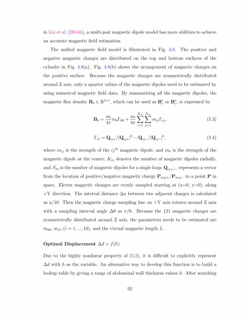
in Liu et al. (2014b), a multi-pair magnetic dipole model has more abilities to achieve

an accurate magnetic field estimation.

The unified magnetic field model is illustrated in Fig. 4.8. The positive and

negative magnetic charges are distributed on the top and bottom surfaces of the

cylinder in Fig. 4.8(a). Fig. 4.8(b) shows the arrangement of magnetic charges on

the positive surface. Because the magnetic charges are symmetrically distributed

around Z axis, only a quarter values of the magnetic dipoles need to be estimated by

using numerical magnetic field data. By summarizing all the magnetic dipoles, the

magnetic flux density B0 ∈ R3×1, which can be used as Bie or Bu

c , is expressed by

B0 =µ0

4πm0Γ00 +

µ0

4π

Km∑i=1

Nm∑j=1

mijΓij, (5.3)

Γij = Qij+/|Qij+|3 −Qij−/|Qij−|3, (5.4)

where mij is the strength of the ijth magnetic dipole, and m0 is the strength of the

magnetic dipole at the center; Km denotes the number of magnetic dipoles radially,

and Nm is the number of magnetic dipoles for a single loop; Qij+/− represents a vector

from the location of positive/negative magnetic charge Pmij+/Pmij− to a point P in

space. Eleven magnetic changes are evenly sampled starting at (x=0, y=0), along

+Y direction. The interval distance ∆a between two adjacent charges is calculated

as a/10. Then the magnetic charge sampling line on +Y axis rotates around Z axis

with a sampling interval angle ∆θ as π/6. Because the 121 magnetic charges are

symmetrically distributed around Z axis, the parameters needs to be estimated are

m00, mi1, (i = 1, ..., 10), and the virtual magnetic length L.

Optimal Displacement ∆d = f(h)

Due to the highly nonlinear property of (5.2), it is difficult to explicitly represent

∆d with h as the variable. An alternative way to develop this function is to build a

lookup table by giving a range of abdominal wall thickness values h. After searching

92

(a) Rotor initial pose 1 (b) Rotor initial pose 2

Figure 5.2: Rotor poses for the pre-built magnetic field map.

for ∆d that satisfy (5.2), the optimized ∆d values are stored in the lookup table. To

this end, the optimal vertical displacement of cEPM ∆d can be identified in real time

for different abdominal wall thicknesses h.

5.3.2 Abdominal Wall Thickness Estimation

Due to both the rotor (camera robot) and the stator contacting an insufflated

abdominal wall internally and externally respectively, the abdominal wall thickness

can be estimated by the rotor-to-stator distance. The rotor creates a static magnetic

field when its orientation is not actuated by the stator. Benefiting from this fact, the

magnetic field of the rotor measured at the stator side varies only according to the

rotor-to-stator distance. The main idea of estimating an abdominal wall thickness is

to sense the magnetic field from the rotor by using a pre-built rotor magnetic field

map which is with respect to the rotor-to-stator distances.

There are three problems to address for estimating an abdominal wall thickness:

1) the rotor orientation which is used for building the magnetic field map; 2) the

configuration of the magnetic field sensors in the stator; and 3) the rotor-to-stator

distance estimation method by using the sensed magnetic field from the rotor. The

sensor configuration should avoid making the sensors inundated by the magnetic field

93

0.015

0.02

0.025

0.03

0.035

0.040.045

0.05

Magnetic flux density norm (T)

Coil CoilcEPM

sEPM

sEPM

S1 S2

S3S4

S1S2

S3

S4

h

B1

B2

B3B4

(a) (b)

Stator botto

m

surfa

ce

Inundation

region

h4=

f4(B

4)

h3=

f3(B

3)

h1=

f1(B

1)

h2=

f2(B

2)

XY

Z

Figure 5.3: Magnetic field sensor configuration at the bottom surface of the stator.The simulation result is generated by COMSOL Multiphysics 5.0.

from the EPMs, and keep the distances between the rotor and the sensors as close as

possible, which can make the rotor magnetic field be well recognized by the sensors.

The method used to estimate the rotor-to-stator distance should be robust, can be

computed in real time, and is capable of providing accurate results.

Rotor pose

The rotor pose determines the magnetic field distribution, which impacts on the

difficulty of building up the magnetic field map and the performance of an abdominal

wall thickness estimation. Fig. 5.2 shows two desired rotor poses that can generate

symmetric magnetic field maps. The two rotor poses can be actuated by deactivating

the stator coils and adjusting the cEPM to its minimum and maximum displacements

for (a) and (b) respectively. Under the minimum cEPM displacement, the cIPM

is dominated by the magnetic field from the cEPM, and aligned with the cEPM

94

orientation. Under the maximum cEPM displacement, the cIPM is dominated by

the magnetic field from the sEPMs, and aligned with the sEPMs orientation. The

arrows in Fig. 5.2 (a) and (b) illustrates the magnetic field strength (proportional to

the arrow lengths) and magnetic field direction (the arrow directions) in the space

between the rotor and the stator. It is obvious that the rotor pose in (b) can generate

more recognizable magnetic field than that in (a) to be sensed in the stator. Therefore,

the rotor pose in (b) is used to build the magnetic field map and estimate the rotor-

to-stator distances.

Sensor configuration

To estimate the rotor-to-stator distance by sensing the symmetric magnetic field

from the rotor, four sets of tri-axis hall effect sensors are applied at the bottom the

stator. It is important to select appropriate locations for the sensors to prevent being

inundated by the magnetic field from the EPMs. Fig. 5.3(a) shows the magnetic flux

density norm distribution at the bottom surface of the stator. The inundation region

in dark red is determined by the measuring ranges of the applied hall effect sensors

(CYL8405, Chenyang-Technologies GmbH& Co. KG, measuring range 64 mT). The

symmetrically distributed black squares S1, S2, S3, S4 represent the sensor installing

locations which are out of the inundation region and closest to the rotor aligned with

the EPMs. The distances from S1 to S2 and S4 are both 60 mm.

Rotor-to-stator distance estimation

As illustrated in Fig. 5.3(b), the tri-axis hall effect sensors Si(i = 1, 2, 3, 4) detect

magnetic field Bi from the rotor under the rotor-to-stator distance h. Due to the

magnetic coupling of the EPMs and the IPMs, the positions between the sensors

and the rotor are relatively fixed in X and Y directions. The magnetic field maps fi

represent the relationship between the rotor magnetic field Bi as inputs and the rotor-

to-stator distances hi as outputs. The mapping functions fi represented in lookup

95

Side View Top View

Moving

Track

Worm

Gear

Motor

sEPMsEPM

cEPM

Coupler

Figure 5.4: cEPM displacement adjusting mechanism in the stator

tables are developed by recording the magnetic fields with the sensors while adjusting

the rotor-to-stator distance h.

With the mapping functions fi and the magnetic fields Bi sensed by Si, an

abdominal wall thickness can be estimated by

h =1

N

N∑i=1

fi(Bi), (5.5)

where N = 4 represents the total group number of the hall effect sensors.

5.3.3 cEPM Adjusting Mechanism

According to the estimated abdominal wall thickness h by using (5.5), the optimal

displacements of the cEPM ∆d = f(h) developed in Section 5.3.1 needs to be applied

on the cEPM. To enable autonomous control of this process, a displacement adjusting

mechanism for the cEPM is required in the stator. Considering the strong magnetic

96

1 – Shell cap

2 – tIPM

3 – Camera housing

4 – cIPM

tIPM

5 – Transparent shell

6 – tIPM shaft

7 – Ceramic bearing

Shell cap

YI

ZI

Ic2Ic1

TtIPM

Tg

Coil 1 Coil 2

Bd

(a) (b)

Figure 5.5: (a) Conceptual illustration of the rotor design. (b) Rotor tilt motioncontrol with the coils.

coupling between the cEPM and the sEPMs, the design objective of the adjusting

mechanism should be capable of providing sufficient lifting force for the cEPM, and

keep the whole stator as compact as possible.

Fig. 5.4 shows the conceptual illustration of the mechanism design which is

basically a screw jack driven by a motor. The reason to use such a mechanism is

twofold: 1) the lifting force for the cEPM can be efficiently provided by the motor

torque through the worm and gear mechanism; 2) the self-locking function of the

design enables the cEPM to keep still when the motor is not actuated. The bolt

that connects with the cEPM by using a coupler is actuated by the gear rotation.

The moving track restricts the bolt rotation, keeps the bolt and the cEPM moving

vertically.

97

5.3.4 Tilt Motion Control

Camera protection shell

According to our original rotor design in Liu et al. (2015), the camera lens can

easily get blurred by peritoneal fluid due to the direct contact with an abdominal

wall. To address this issue, a transparent shell is applied to prevent the camera

lens from contacting with tissue and also to maintain imaging quality, as illustrated

in Fig. 5.5(a)-5. Two ceramic bearings (Fig. 5.5(a)-7) and two tIPM shafts, which

are fixed in the shell caps (Fig. 5.5(a)-1), are used for hanging the camera housing

(Fig. 5.5(a)-3) inside the transparent shell with no contact. This design provides

the camera smooth rotation inside the shell when rotational torque is exerted on

the cIPM (Fig. 5.5(a)-4). Another benefit of this design is to make the laparoscopic

camera reusable by depositing the shell after use, and subsequently reduces a surgery

cost.

Control with electromagnetic coils

The robot tilt motion is activated by the magnetic coupling between the coils and

the cIPM. Ic1 and Ic2 are represented as the current inputs of the coils, and θ is

represented as the rotational angle of the robot tilt motion.

The factors that impact on the camera tilt motion need to be considered before

developing a tilt motion control method. The camera protection shell insulates the

rotor from contacting with an abdominal wall. It makes the camera free of frictional

torque from an abdominal wall during tilt motion. After estimating an abdominal

wall thickness and adjusting the displacement of the cEPM that were developed in

Section 5.3.2 and 5.3.3, the EPMs have ignorable impact on the tilt motion of the

cIPM. Beside the control inputs Ic1 and Ic2, the tilt motion of the cIPM is also affected

by Tg and TtIPM which are the torque due to the robot gravity along XI and the

magnetic torque on the cIPM from the tIPMs along XI respectively. As illustrated in

Fig. 5.5(b), Tg and TtIPM are always in opposite directions that are canceled by each

98

other according to our preliminary experimental investigation. Therefore, the camera

tilt angle aligns with the direction of the magnetic field generated by the coils. The

objective to control the camera tilt motion is to determine Ic1 and Ic2 for generating

a magnetic field with the direction θ at Ps in ΣS that is the location of the cIPM.

The relationship between the current inputs Ic1, Ic2 and a desired magnetic field

direction θ at Ps can be formulated by (5.6) in ΣS as follows

(RC1Buc )︸ ︷︷ ︸

BSc1

Ic1 + (RC2Buc )︸ ︷︷ ︸

BSc2

Ic2 = RSI RIx(θ)B

−z︸ ︷︷ ︸Bd

, (5.6)

where RSI ∈ R3×3 represents a rotational matrix from ΣI to ΣS. According to the

setting of ΣS and ΣI in Fig. 4.2(b), RSI is an identity matrix. RIx(θ) ∈ R3×3 represents

the rotational matrix along XI with θ as the variable. B−z ∈ R3×1 denotes a unit

vector pointing in −ZI . BSc1,B

Sc2 ∈ R3×1 denote the unit current magnetic field of the

coils at Ps in ΣS. Bd ∈ R3×1 denotes the desired magnetic field direction as shown

in Fig. 5.5(b). Benefiting from the analytical magnetic field model in (5.3), BSc1, BS

c2

can be computed in real time.

Considering the x components in BSc1, BS

c2, and Bd are zeros, (5.6) is reformulated

as

Byzd = BSyz

c Ic, (5.7)

where BSyzc = [B

Syz

c1 ,BSyz

c2 ] ∈ R2×2, Byzd ∈ R2×2, Ic = [Ic1, Ic2]T ∈ R2×1. Because BSyz

c

has a full row rank, the current input vector Ic can be found in (5.8) by applying

pseudoinverse to (5.7)

Ic = (BSyzc )T (BSyz

c (BSyzc )T )−1Byz

d . (5.8)

To achieve high accuracy tilt motion control, a closed-loop control scheme is

developed as illustrated in Fig. 5.6. Given a desired tilt angle θd, the current control

vector is calculated by Ic = f(Ps, θ) which is a representation of (5.8). Because

99

Figure 5.6: Block diagram of the camera tilt motion control.

the solution of (5.8) only provides the ratio of Ic1 and Ic2, the input current vector is

amplified by using the limit value of current inputs Imax for maximizing the generated

magnetic field. A current input trajectory Imaxc (t) can thus be developed within a

given time ∆T , and applied to the camera. The arrived tilt angle θ at the end of

Imaxc (t) is sensed by a tilt angle sensor for feedback. If |θd− θ| is smaller than a given

threshold δ, the tilt angle control process is complete. Otherwise, an adjusted tilt

angle θ = θd ±∆θ, where ∆θ is a small angle, is served as an input to calculate Ic.

5.3.5 Pan Motion Mechanism

The pan motion of the camera robot is actuated by the rotation of the stator due to

the magnetic coupling between the EPMs and the tIPMs as conceptually illustrated in

Fig. 4.2. To control the pan motion automatically, it is desired to design an actuation

mechanism that can generate rotational motion of the stator.

Fig. 5.7 shows the pan motion mechanism in the stator. The design objective is

to control the rotation of the stator core which is sitting inside the stator shell. The

motor driven spur gear is fixed on the stator core, while an internal gear is attached

on the internal surface of the stator shell. The stator core can thus be actuated by

the relative motion of the spur gear and the internal gear. To keep smooth relative

rotation between the stator core and the stator shell, a thrust bearing is applied at

their contact surfaces.

100

Drive pinion

Internal gear

Stator core

Thrust bearing

Stator shell

Figure 5.7: Pan motion mechanism.

5.4 Prototype Development and Experimental In-

vestigation

5.4.1 Stator Fabrication

cEPM adjusting mechanism

The function of the cEPM adjusting mechanism that proposed in section 5.3.3 is

to position the cEPM to the vertical displacement ∆d according to the estimated

abdominal wall thickness in (5.5). To make the mechanism function, two issues have

to be concerned: (1) the mechanism has to provide sufficient lifting force to overcome

the magnetic force between the cEPM and the sEPMs; (2) the cEPM has to be

accurately controlled to the desired displacement ∆d.

Fig. 5.8 shows the fabrication of the cEPM adjusting mechanism. The worm

in Fig. 5.8(a) is with pitch diameter 12.19 mm, outside diameter 15 mm, number of

101

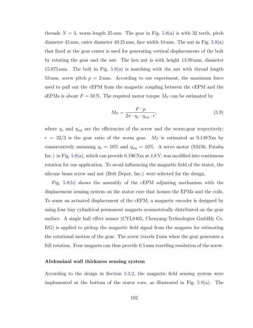
threads N = 3, worm length 25 mm. The gear in Fig. 5.8(a) is with 32 teeth, pitch

diameter 45 mm, outer diameter 49.25 mm, face width 10 mm. The nut in Fig. 5.8(a)

that fixed at the gear center is used for generating vertical displacements of the bolt

by rotating the gear and the nut. The hex nut is with height 13.89 mm, diameter

15.875 mm. The bolt in Fig. 5.8(a) is matching with the nut with thread length

53 mm, screw pitch p = 2 mm. According to our experiment, the maximum force

used to pull out the cEPM from the magnetic coupling between the cEPM and the

sEPMs is about F = 50 N. The required motor torque MT can be estimated by

MT =F · p

2π · ηs · ηwg · r, (5.9)

where ηs and ηwg are the efficiencies of the screw and the worm-gear respectively;

r = 32/3 is the gear ratio of the worm gear. MT is estimated as 0.149 Nm by

conservatively assuming ηs = 10% and ηwg = 10%. A servo motor (S3156, Futaba

Inc.) in Fig. 5.8(a), which can provide 0.196 Nm at 4.8 V, was modified into continuous

rotation for our application. To avoid influencing the magnetic field of the stator, the

silicone brass screw and nut (Bolt Depot, Inc.) were selected for the design.

Fig. 5.8(b) shows the assembly of the cEPM adjusting mechanism with the

displacement sensing system on the stator core that houses the EPMs and the coils.

To sense an actuated displacement of the cEPM, a magnetic encoder is designed by

using four tiny cylindrical permanent magnets symmetrically distributed on the gear

surface. A single hall effect sensor (CYL8405, Chenyang-Technologies GmbH& Co.

KG) is applied to pickup the magnetic field signal from the magnets for estimating

the rotational motion of the gear. The screw travels 2 mm when the gear generates a

full rotation. Four magnets can thus provide 0.5 mm traveling resolution of the screw.

Abdominal wall thickness sensing system

According to the design in Section 5.3.2, the magnetic field sensing system were

implemented at the bottom of the stator core, as illustrated in Fig. 5.9(a). The

102

Sensor

Magnet

Gear

Bolt

Worm

Coupler

Track

(a) (b)

Stator

coreHex nut

Motor

Figure 5.8: Fabrication of the cEPM adjusting mechanism.

bottom of the stator core is carved around the EPMs and the coils with 5 mm depth

for installing magnetic field sensors. Four sets of tri-axis hall effect sensors with

measuring ranges 0 ∼ 64 mT and sensitivities about 50 mV/mT were symmetrically

fixed in the carved bottom. To enable the sensing system to well recognize the tiny

change of the magnetic field from the rotor, the measured signals were converted

to digital signals with sensing resolution 0.01 mT by using a 16bit ADC (ADS1115,

Texas Instruments Inc.).

The estimation function developed in (5.5) was implemented by the data acquired

from Fig. 5.9(b). The configuration of the hall effect sensors in Fig. 5.9(b) is the same

as the sensor configuration in Fig. 5.9(a). A rotor with the pose in Fig. 5.2(b) was

fixed on a vertical positioning stage for adjusting the distance between the rotor and

the sensors Si. Fig. 5.9(c) shows the mapping functions fi, (i = 1, 2, 3, 4), which record

the norms of the magnetic flux densities |Bi| and the vertical distances hi between

the rotor and the sensors Si. During the process of an abdominal wall thickness

103

60mm

h1=f1(|B1|)

h2=f2(|B2|)

h3=f3(|B3|)

h4=f4(|B4|)

h1

h2

h3

h4

4

1

1

4i

i

h h

(a)

(b) (c)

Hall effect sensors

Rotor

Sensor

board

60mm

S1 S2

S3S4

Figure 5.9: Fabrication of abdominal wall thickness sensing system,.

estimation, fi return the distances hi by using the detected Bi in Si. An average

value of hi was used as the final estimated abdominal wall thickness h for improving

the robustness of this method.

Stator core

According to the design in Liu et al. (2015), the stator core consists of two coils, two

identical sEPMs and one cEPM. The detailed dimensions and materials are shown in

Table 4.2.

Pan motion mechanism

The fabricated parts of the pan motion mechanism is demonstrated in Fig. 5.14(c).

The internal gear has 52 teeth with a pitch diameter 132 mm, a major diameter

139.4 mm, and a minor diameter 128 mm. The drive pinion has 12 teeth with a pitch

104

diameter 30.48 mm, a major diameter 36.56 mm, and a minor diameter 25.13 mm.

The face widths of the internal gear and the drive pinion are both 10 mm. The stator

shell is with an external diameter 164 mm and a height 109 mm. The thrust bearing

with an inner diameter 133.6 mm and an outer diameter 154.6 mm sits inside the

stator shell with 30 mm distance to the shell bottom. A modified digital servo motor,

which is identical to the motor applied on the cEPM adjusting mechanism, is fixed on

the stator core and connected with the drive pinion. To protect the stator core when

the stator contacts with an abdominal wall and avoid impacting on the magnetic field

interaction between the rotor and the stator, a brass board with diameter 164 mm

and thickness 1.64 mm was applied at the bottom of the stator shell.

Coil current control system

A tethered current control system was developed by the PWM technique. The

system consists of a micro-controller (STM32F4Discovery, STMicroelectronics Inc.)

to generate PWM signals, two PWM amplifiers (L6205 DMOS Full Bridge Driver,

STMicroelectronics Inc.) to amplify the signals, a power supply for powering up the

amplifiers, and a PC computer to send control command to the micro-controller via

a serial communication.

5.4.2 Rotor Fabrication

Fig. 5.10 shows the fabrication of the dummy camera with the disassembled parts.

The specifications of the camera is illustrated in Table 5.1. The outer diameter of

the transparent shell (MOCAP, Inc.) determines the diameter of the camera which

is 14.52 mm. Considering that the diameter of a standard trocar is in the range

of 12 mm ∼ 15 mm, our camera design can be inserted into an abdominal cavity

through a standard trocar. The miniature ceramic ball bearings (NationSkander

California Corp.), which have 5 mm inner diameter and 9 mm outer diameter with

105

tIPM

Transparent

shell

Camera

housing

Shell caps

tIPM shafts cIPM

Ceramic

bearings

Camera housing caps

Assembled

dummy camera

Figure 5.10: The disassembled dummy camera parts and the assembled dummycamera.

3 mm thickness, enable smooth rotation of the camera housing inside the transparent

shell.

5.4.3 Calibration of Magnetic Field Models

The models of the stator magnetic field developed in Section 5.3.1 were represented

by (5.3) with parameters m00, mi1, (i = 1, ..., 10), and the magnetic length L . Due

to the imperfection of the coil wrapping, the iron cores, and the permanent magnets,

the model calibration was performed by using experimental data. Fig. 5.11(a) shows

the experiment platform for magnetic field calibration which consists of a transparent

board to support the EPMs or the coils, a X-Z position stage, and three hall effect

sensors for 3-axis sensing. Fig. 5.11(b) and (c) show the magnetic flux density norm

comparison results of the experimental data and the magnetic field models.

Fig. 5.11(b) illustrates the calibrated coil magnetic field model (the blue line) with

a unit current input based on the experiment data (the blue circles). The red line

106

Table 5.1: Specifications of The Rotor and Stator Prototype Designs

Part Name DimensionCamera total length 79 mmTransparent shell OD 14.52 mm, ID 13.92 mmCamera housing OD 12.7 mm, ID 10 mmcIPM: Diametrically magnetized

Size Diameter 6.35 mm, Length 12.7 mmMaterial NdFeB Grade N42

tIPM: Diametrically magnetizedSize OD 12.7 mm, ID 4.75 mm

Thickness 6.35 mmMaterial NdFeB Grade N42

Dummy camera weight 21.38 g

and the red circles illustrates the magnetic field comparison result between the coil

magnetic field with I = 0.5 A and the experiment data. This result validates the linear

relationship between the coil input current and the generated magnetic field strength.

Fig. 5.11(c) shows the magnetic field comparison result of the EPMs magnetic field

model with the vertical displacements of the cEPM as ∆d = 1 mm, 3 mm, 5 mm, 7 mm,

and the experiment data. The coincidences of the model data and the experiment

data at Bnorm = 0 with different ∆d validate the optimal displacement function

∆d = f(h) developed in Section 5.3.1. The average errors of the magnetic field

models demonstrated in Fig.5.11(b) and (c) were 1.32% and 1.57% respectively.The

calibrated parameters of the EPMs and the coils are illustrated in Table 5.2.

5.4.4 Control of cEPM Displacements

Fig. 5.12 shows the investigation of the control accuracy for the cEPM adjusting

mechanism developed in Section 5.4.1. The target cEPM displacements were set

from 2 mm to 10 mm with 2 mm intervals. For each test, the cEPM displacement

were set at ∆d = 0 initially. The results show that the average errors of all the

tests were all within 0.35 mm which provides sufficient control accuracy for the our

107

Δd=1mm

Δd=3mm

Δd=5mm

Δd=7mm

Coil positionCoil position

EPM positions

Hall effect

sensors

X-Z position

stage

(a)

(b)

(c)

I=1A

I=0.5A

h (mm)

h (mm)

(m)

(m)

Figure 5.11: Experimental setup to calibration the magnetic field models of thestator.

system. As the cEPM displacements traveled from 2 mm to 10 mm, the errors were

accumulated. The accumulated error can be limited within 0.35 mm by reseting the

displacement counter when the minimum or the maximum displacements are reached.

5.4.5 Evaluation of Abdominal Wall Thickness Sensing Method

Fig. 5.13 shows the experimental setup (a) and experimental results (b) for evaluating

the abdominal wall thickness sensing method developed in Section 5.3.2. To evaluate

the sensing accuracy of the proposed method, the experiment was divided into two

groups, which were 1) sensing under the impact of the EPMs; and 2) sensing without

108

Table 5.2: Calibrated parameters of the sEPMs, the cEPM and the coils. The unitsof m and L are ampere meter square [Am2] and meter [m] respectively.

m00 m11 m21 m31 m41 m51 m61 m71 m81 m91 m10,1 L

sEPM 2.479 2.676 2.516 2.294 2.063 1.894 1.759 1.536 1.225 1.136 1.252 0.055

cEPM 2.493 2.456 2.436 2.393 2.349 2.305 2.264 2.233 2.209 2.193 2.185 0.038

Coil 2.494 2.401 2.394 2.398 2.394 2.403 2.395 2.398 2.398 2.393 2.401 0.016

the impact of the EPMs. The first group experiment was investigated by using the

experimental setup in Fig. 5.13(a). The second group experiment was conducted

by using the experimental setup in Fig. 5.9(b), which was used for developing the

estimation function (5.5). In both groups, the rotor with the pose demonstrated in

Fig. 5.2(b) was positioned under the sensors. To test the reliability and robustness of

this method, the stator core in Fig. 5.13(a) and the sensor board in Fig. 5.9(b) were

rotated within the range of ±20 during each sensing process. Fig. 5.13(b) shows the

errors in detecting the rotor-to-stator distances for 25 mm, 30 mm, 35 mm, 40 mm,

45 mm, and 50 mm. The mean absolute errors and the standard deviations of the

two groups under different testing distances are shown in Table 5.3. The data show

the distance sensing system can provide less than 1 mm accuracy in average. To

investigate the differences of the sensing errors between the two experiment groups,

two-sample t-tests were applied to compare the MAEs and the SDs. The P values for

the MAEs and the SDs were 0.6693 and 0.4210 respectively, which indicate that the

differences were considered to be not statistically significant.

5.4.6 Experimental Platform

Fig. 5.14(a) shows the overview of the experimental environment. The robot system

was fabricated by a 3D prototyping machine (Fortus 400mc, Stratasys Inc.). To

simulate the viscoelastic properties of a real insufflated abdominal wall (average

109

0

0.05

0.1

0.15

0.2

0.25

0.3

0.35

0.4

2mm 4mm 6mm 8mm 10mm

cEP

M d

ispl

acem

ent

erro

rs (

mm

)

Figure 5.12: Control of cEPM displacement

Young’s modulus 32.5 kPa) Song et al. (2006), a viscoelastic material Durometer

40 (Young’s modulus 27.57 kPa at 15% deflection, Sorbothane, Inc.) was applied as

illustrated in Fig. 5.14(b). The initial abdominal wall thickness was 26 mm (tissue

layer 15 mm, support layer 11 mm). To increase the abdominal wall thickness for

experimental studies, a vertical stator positioning mechanism in Fig. 5.14(a) was

applied. A silicone oil lubricated rotor-tissue contact layer was added to the bottom

of the viscoelastic material for mimicking an internal abdominal wall surface.

5.4.7 Camera Motion Control

The closed-loop control of the camera motion requires sensing systems for tilt

angle and pan angle. Due to the lack of on-board internal sensing system at the

current stage, separate motion feedback systems were designed for pan and tilt

motion. The tilt motion sensing system applied a tri-axis accelerometer (LIS331HH,

STMicroelectronics Inc.) inside the camera housing with wires for power supply and

data transmission. To minimize the impact on the camera tilt motion from the wires,

110

(a)(b)

+20°

-20°

rotate

Figure 5.13: Abdominal wall thickness estimation result.

42 AWG enameled copper wires with diameter 0.066 mm were applied, as shown in

Fig. 5.14(d). The pan motion sensing system applied a webcam (Logitech Pro 9000)

under the rotor to track the positions of two color markers on the transparent shell

of the rotor. The simulated abdominal wall thickness was adjusted to 35 mm which

is about the average value of an normal abdominal wall thickness Song et al. (2006).

The current inputs of the two coils are limited at |Imax| = 1.5 A to prevent coil

overheating.

Control of tilt motion

Fig. 5.15 shows the tilt motion control experiment by setting the desired tilt angles

(red arrows) from 75 to −75 with 15 intervals. The green arrows shows the

controlled tilt angles by using the control model developed in Section 5.3.4. Fig. 5.16

shows the tilt motion control trajectories for the desired tilt angles 15, 45, and 75

which cost 0.93 s, 1.74 s, and 1.99 s to reach to steady states. The average steady-state

error of the controlled tilt angles in Fig. 5.15 and Fig. 5.16 was 0.67.

111

Table 5.3: Mean Absolute Error (MAE) and Standard Deviation (SD) of The SensedDistances

With EPMs Without EPMs

Dist. (mm) MAE (mm) SD (mm) MAE (mm) SD (mm)

25 0.2672 0.3531 0.2368 0.5506

30 0.6118 0.3025 0.1771 0.2989

35 0.5256 0.3431 0.7216 0.3678

40 0.0116 0.3856 0.6910 0.3807

45 0.2 0.2857 0.1684 0.3832

50 0.5682 0.2424 0.5729 0.1943

Control of pan motion

Fig. 5.17 shows the pan motion control experiment which set the desired pan angles

from 0 to 315 with 45 intervals. The drive pinion demonstrated in Fig. 5.7 was

activated to rotate the stator core clockwise or counterclockwise accordingly for

generating pan motion of the rotor, while the pan motion sensing sytem was detecting

the current pan angle for feedback. The red and green arrows represent the desired

pan angles and controlled pan angles respectively. The average control error was

0.49.

Control of combined pan and tilt motion

Fig. 5.18 shows the combined control experiment of pan and tilt motion to

demonstrate the control capability of our proposed system. By giving some desired

orientations (red arrows) of the camera which covered the whole three dimensional

space in an abdominal cavity, the orientations of the camera were controlled

112

(a)

(b)

(c)

(d)

Color markersSoft wires

Tracking camera

Internal gear

Drive pinion

Stator

Stator positioning

mechanism

Support layer

Figure 5.14: Experiment platform.

accordingly as illustrated by the green arrows. In the control tests, the experimental

results indicate that the control system can provide the camera with less than 1

control accuracy for all the orientations investigated in the experiment.

5.5 Summary

In this chapter, a closed-loop control system of a novel insertable laparoscopic camera

has been presented to enable autonomous fine orientation control of the camera. The

experimental results indicate that the camera can achieve 0.67 and 0.49 control

accuracies in tilt and pan motions respectively. The combined orientation control in

three-dimensional space demonstrated less than 1 control accuracy. In our future

work, the camera on-board electronics will be integrated especially an inertial sensor

which is used to provide the camera orientation feedback wirelessly. the dimensions

113

Desired tilt angle

Controlled tilt angle

Z

Y

Tilt angle

Camera

shellRotor

0°15°

30°

45°

60°

75°

-15°

-30°

-45°

-60°

-75°

Figure 5.15: Tilt motion control experiment.

and the weight of the stator will be further decreased. The stator cables will be

removed by integrating a wireless module, coil drivers, and batteries inside the stator.

The camera system will be tested in vivo by using a porcine abdominal cavity.

114

75° desired

tilt angle

75° controlled

trajectory

45° desired

tilt angle45° controlled

trajectory

15° desired

tilt angle

15° controlled

trajectory

0.93s

1.74s

1.99s

Figure 5.16: Tilt motion control trajectories.

Desired pan angle

Controlled pan angle

X

Y

Rotor 0°

45°

90°

135°

180°

225°

270°

315°

Figure 5.17: Pan motion control experiment.

115

Tilt 45°

Tilt 60°

Tilt 75°

Pan 0° Pan 22.5° Pan 45° Pan 90°

Pan 180°

Desired

orientation

Controlled

orientation

X

Y

ZPan motionTilt motion

Camera orientation

Figure 5.18: Pan and tilt motion control experiment.

116

Chapter 6

Conclusion and Future Work

This research aims at developing a magnetic actuated fully insertable robotic camera

system to enhance procedures of single incision laparoscopic surgery. The design

objective is to feature unified fixation, translation, and rotation functions for the

camera actuation mechanism by controlling a externally generated magnetic field

from a stator. Inspired by a spherical motor concept, a semi-spherical and a line-

arranged driving units with pure coil stators were firstly developed and experimentally

evaluated. Due to the coil heating problem and the requiring of unreliably complex

control algorithm, a hybrid stator with the line-arranged driving unit was proposed

as the final design based on the previous two generation prototypes. A closed-

loop control system was developed on the final actuation mechanism design for

achieving automatic orientation control of the camera. The actuation capabilities

of the proposed design were thoroughly evaluated by experiments.

6.1 Conclusion

In the original prototype, a semi-spherical rotor/stator driving system for a wireless

laparoscopic camera was proposed. To study reasonable stator and rotor patterns for

providing sufficient actuation capabilities, three stator designs that consist of 3, 4, and

5 coils and four rotor designs were proposed. Experimental investigations indicate

117

that the 3 coils iron-core stator with 20 mm outer radius and the Rotor 1 show the

best balance of reasonable dimension and sufficient force and torque for manipulating

the camera. However, one major issue of this design is the usage of maximum 5 A

current inputs for stable actuation, which results in coil overheating.

In the second prototype, a line-arranged rotor driving unit design was developed to

address the problem arose from the original semi-spherical rotor/stator design. This

second generation prototype applied a 17 flatly arranged coils as a stator to control the

line-arranged rotor with three diametrically magnetized cylindrical magnets. Besides

holding the functions of fixation and translation for the camera, the design enables

a decoupled pan and tilt activation by controlling the input current of stator’s coils.

A simulation study was conducted that indicate under the current limit of 2.5 A, the

system conservatively has the capability to achieve 360 pan motion with a 22.5

resolution, and the range of 127 ∼ 164 tilt motion which depends on tilt motion

working modes and the distance between the rotor and the stator. However, a

drawback of the second design is that according to the experimental study of the

prototype, the current control of the 17 coils needs a complex algorithm, which

resulted in unreliable camera motion control.

To design a practical actuation mechanism based on the second prototype, a

hybrid stator that consists of three permanent magnets and two coils was developed

for reliable camera motion control with a simple control algorithm. Experiment

investigations indicated that the hybrid stator with the line-arranged rotor design

can provide reliable anchoring, translation, 360 pan motion control, and up to 80

tilt motion control. The pan and tilt motions can be simultaneously controlled in

a decoupled way. Therefore, this successful prototype was considered as the final

design.

Grounded on the final design of the actuation mechanism, a closed-loop control

system was developed for automatic control of the camera. The main components

of the control system include the pan motion mechanism in the stator, the central

EPM adjusting mechanism, the abdominal wall thickness sensing system, and

118

pan/tilt motion sensing system. The experimental results indicate that The camera

orientation control can achieve 360 continuous pan motion with 0.49 control

accuracy, and at least 75 tilt motion with 0.67 control accuracy. The combined

orientation control in three-dimensional space demonstrated less than 1 control

accuracy.

6.2 Future Work

This dissertation presents a promising magnetic actuated fully insertable surgical

camera to help surgeons for improving procedures in single incision laparoscopic

surgery. The innovative design features a unified and automatic actuation mechanism

which can anchor, navigate, and rotate a laparoscopic camera wirelessly with a

capsulated body. The experiment investigations demonstrate reliable, practical, and

accurate control of the camera robot. To move a further step towards a real surgical

instrument that can be commercialized, the future work includes:

1. Integration of on-board electronics in the dummy camera. There are four

main components to be designed for the camera on-board electronics, which

are a miniature camera and its illumination system, a battery and the battery

management system, an inertial sensing system, and a wireless module. An

auto-focus lens will be developed for the miniature imaging device to optimize

surgical visualization. The inertial sensing system will provide camera motion

feedback for the closed-loop motion control. The wireless module will be in

charge of transmitting imaging data and motion feedback.

2. Dimension reduction and electronics integration of the stator. For a clinical

application, a light and small size stator for the camera control is preferred. So

in the future work, the stator dimension and weight will be further optimized.

In the current stage, control commands to the stator for generating rotational

magnetic field is transmitted through wires. In our future design, the stator

119

cables will be removed by integrating a wireless module, coil drivers, and

batteries inside the stator.

3. Development of the camera delivery system. To insert the camera into an

abdominal cavity and position the camera under the magnetic couping of the

stator, a miniature flexible continuum manipulator that can be fitted in a

standard trocar will be developed.

4. Development of autonomous surgical device tracking algorithm. During a

surgical procedure, a laparoscopic camera has to be continuously adjusted by

surgeons in order to achieve high quality visual feedback. In the future work,

besides controlling the camera system by a user interface, a surgical device

tracking algorithm will be developed that enables our robotic camera system to

autonomously adjust the camera orientation and center the surgical instruments

in the imaging feedback.

5. Ex vivo and in vivo tests. In the current stage, the camera system has been

tested by simulated abdominal wall environments. To further investigate the

actuation capabilities in real application scenarios, ex vivo and in vivo tests will

be conducted by using porcine abdominal cavities.

120

Bibliography

121

Best, S., Kabbani, W., Scott, D., Bergs, R., Beardsley, H., Fernandez, R.,

Mashaud, L., and Cadeddu, J. (2011). Magnetic anchoring and guidance

system instrumentation for laparo-endoscopic single-site surgery/natural orifice

transluminal endoscopic surgery: lack of histologic damage after prolonged

magnetic coupling across the abdominal wall. Urology, 77(1):243–7. 64

Cadeddu, J., Fernandez, R., Desai, M., Bergs, R., Tracy, C., Tang, S., Rao, P.,

Desai, M., and Scott, D. (2009). Novel magnetically guided intra-abdominal camera

to facilitate laparoendoscopic single-site surgery: initial human experience. Surg

Endosc., 23(8):1894–9. 3

Carpi, F. and Pappone, C. (2009). Magnetic maneuvering of endoscopic capsules by

means of a robotic navigation system. Biomedical Engineering, IEEE Transactions

on, 56(5):1482–1490. xii, 5, 6

Castro, C., Smith, S., Alqassis, A., ketterl, T., Yu, S., Ross, S., Rosemurgy, A.,

Savage, P., and Gitlin, R. (2013). A wireless robot for networked laparoscopy.

Biomedical Engineering, IEEE Transactions on, 60(4):930–936. xii, 3, 4

Chirikjian, G. and Stein, D. (1999). Kinematic design and commutation of a spherical

stepper motor. Mechatronics, IEEE/ASME Transactions on, 4(4):342–353. 7

Ciuti, G., Valdastr, P., Menciassi, A., and Dario, P. (2010). Robotic magnetic steering

and locomotion of capsule endoscope for diagnostic and surgical endoluminal

procedures. Robotica, 28(2):199–207. xii, 5, 6

Cleary, K. and Peters, T. M. (2010). Image-guided interventions: technology review

and clinical applications. Annual Review of Biomedical Engineering, 12:11942. 1

Desai, M., Berger, A., Brandina, R., Aron, M., Irwin, B., Canes, D., Desai, M., Rao,

P., Sotelo, R., Stein, R., and Gill, I. (2009). Laparoendoscopic single-site surgery:

Initial hundred patients. Urology, 74(4):805 – 812. 2

122

Fakhry, M., Gallagher, B., Bello, F., and Hanna, G. (2009). Visual exposure using

single-handed magnet-driven intra-abdominal wireless camera in minimal access

surgery: is better than 30 degrees endoscope. Surg Endosc., 23(3):539–543. 3

Glass, P., Cheung, E., and Sitti, M. (2008). A legged anchoring mechanism for

capsule endoscopes using micropatterned adhesives. Biomedical Engineering, IEEE

Transactions on, 55(12):2759–2767. xii, 4, 5

Groom, N. (1997). Expanded equations for torque and force on a cylindrical

permanent magnet core in a large-gap magnetic suspension system. 42

Hu, T., Allen, K., Hogle, J., and Fowler, L. (2009). Insertable surgical imaging device

with pan, tilt, zoom, and lighting. The International Journal of Robotics Research,

28(10):1373–1386. xii, 3, 4

Hunter, S. (1961). The rolling contact of a rigid cylinder with a viscoelastic half

space. Journal of Applied Mechanics, 28(4):611–617. 46, 52

Jackson, J. D. (1999). Classical electrodynamics. Wiley, New York, NY. 21, 40, 67

Kim, B., Lee, S., Park, J. H., and Park, J.-O. (2005a). Design and fabrication of

a locomotive mechanism for capsule-type endoscopes using shape memory alloys

(smas). Mechatronics, IEEE/ASME Transactions on, 10(1):77–86. xii, 4, 5

Kim, B., Park, S., Jee, C. Y., and Yoon, S.-J. (2005b). An earthworm-like locomotive

mechanism for capsule endoscopes. In Intelligent Robots and Systems, 2005. (IROS

2005). 2005 IEEE/RSJ International Conference on, pages 2997–3002. xii, 4, 5

Kim, S. H. and Ishiyama, K. (2014). Magnetic robot and manipulation for active-

locomotion with targeted drug release. Mechatronics, IEEE/ASME Transactions

on, 19(5):1651–1659. 6

123

Kok-Meng, L. and Hungsun, S. (2007). Distributed multipole model for design

of permanent-magnet-based actuators. Magnetics, IEEE Transactions on,

43(10):3904–3913. 70, 91

Kummer, M., Abbott, J., Kratochvil, B., Borer, R., Sengul, A., and Nelson, B. J.

(2010). Octomag: An electromagnetic system for 5-dof wireless micromanipulation.

Robotics, IEEE Transactions on, 26(6):1006–1017. 6, 22, 41, 72

Liang, Y., I-Ming, C., Guilin, Y., and Kok-Meng, L. (2006). Analytical and

experimental investigation on the magnetic field and torque of a permanent magnet

spherical actuator. Mechatronics, IEEE/ASME Transactions on, 11(4):409–419. 7,

20, 39

Lim, C. K., Yan, L., Chen, I.-M., Yang, G., and Lin, W. (2004). Mechanical

design numerical electromagnetic analysis of a dc spherical actuator. In Robotics,

Automation and Mechatronics, 2004 IEEE Conference on, volume 1, pages 536–541

vol.1. 7

Liu, X., Mancini, G., and Tan, J. (2014a). Design of a unified active locomotion

mechanism for a capsule-shaped laparoscopic camera system. In Robotics and

Automation (ICRA), 2014 IEEE International Conference on, pages 2449–2456.

64

Liu, X., Mancini, G. J., and Tan, J. (2014b). Design of a unified active locomotion

mechanism for a wireless laparoscopic camera system. In Intelligent Robots and

Systems (IROS), 2014 IEEE/RSJ International Conference on, pages 1294–1301.

64, 70, 91, 92

Liu, X., Mancini, G. J., and Tan, J. (2015). Design and analysis of a magnetic actuated

capsule camera robot for single incision laparoscopic surgery. In Intelligent Robots

and Systems (IROS), 2015 IEEE/RSJ International Conference on. 89, 98, 104

124

Loring, S., Brown, R., Gouldstone, A., and Butler, J. (2005). Lubrication regimes in

mesothelial sliding. Journal of Biomechanics, 38(12):2390–6. 46

Moglia, A., Menciassi, A., Dario, P., and Cuschieri, A. (2009). Capsule endoscopy:

progress update and challenges ahead. Nat. Rev. Gastroenterol. Hepatol., 6(1):353–

362. 2, 44

Navarra, G., Malfa, G. L., Lazzara, S., Ullo, G., and Curro, G. (2010). Sils and notes

cholecystectomy: a tailored approach. Journal of Laparoendoscopic and Advanced

Surgical Techniques, 20:511514. 2

Nelson, B. J., Kaliakatsos, I., and Abbott, J. (2010). Microrobots for minimally

invasive medicine. Annu Rev Biomed Eng., 12:55–85. 2

Platt, S., Hawks, J., and Rentschler, M. (2009). Vision and task assistance

using modular wireless in vivo surgical robots. Biomedical Engineering, IEEE

Transactions on, 56(6):1700 –1710. xii, 3, 8

Rossini, L., Chetelat, O., Onillon, E., and Perriard, Y. (2011). Analytical and

experimental investigation on the force and torque of a reaction sphere for satellite

attitude control. In Advanced Intelligent Mechatronics (AIM), 2011 IEEE/ASME

International Conference on, pages 487–492. 7

Rossini, L., Chetelat, O., Onillon, E., and Perriard, Y. (2013). Force and torque

analytical models of a reaction sphere actuator based on spherical harmonic rotation

and decomposition. Mechatronics, IEEE/ASME Transactions on, 18(3):1006–1018.

20, 39

Saidy, M., Tessier, M., and Tessier, D. (2012a). Single-incision laparoscopic surger–

hype or reality: A historical control study. Perm J., 16(1):47–50. 2

Saidy, M. N., Tessier, M., and Tessier., D. (2012b). Single-incision laparoscopic

surgery hype or reality: A historical control study. The Permanente Journal,

16:4750. 2

125

Sendoh, M., Ishiyama, K., and Arai, K.-I. (2003). Fabrication of magnetic actuator

for use in a capsule endoscope. Magnetics, IEEE Transactions on, 39(5):3232–3234.

xii, 5, 6

Silvestri, M., Ranzani, T., Argiolas, A., Vatteroni, M., and Menciassi, A. (2013). A

multi-point of view 3d camera system for minimally invasive surgery. Sensors and

Actuators A: Physical, 202(0):204 – 210. 3

Simi, M., Sardi, G., Valdastri, P., Menciassi, A., and Dario, P. (2011). Magnetic

levitation camera robot for endoscopic surgery. In Robotics and Automation

(ICRA), 2011 IEEE International Conference on, pages 5279–5284. xii, 3, 8

Simi, M., Silvestri, M., Cavallotti, C., Vatteroni, M., Valdastri, P., Menciassi,

A., and Dario, P. (2013). Magnetically activated stereoscopic vision system for

laparoendoscopic single-site surgery. Mechatronics, IEEE/ASME Transactions on,

18(3):1140–1151. xii, 3, 8

Song, C., Alijani, A., Frank, T., Hanna, G., and Cuschieri, A. (2006). Mechanical

properties of the human abdominal wall measured in vivo during insufflation for

laparoscopic surgery. Surgical Endoscopy And Other Interventional Techniques,

20(6):987–990. 9, 17, 61, 77, 110, 111

Swain, P., Austin, R., Bally, K., and Trusty, R. (2010). Development and testing of

a tethered, independent camera for notes and single-site laparoscopic procedures.

Surg Endosc., 24(8):2013–21. 3

Toennies, J., Simi, M., Valdastri, P., and Webster, R. (2010). Swallowable medical

devices for diagnosis and surgery: The state of the art. J. Mech. Eng. Sci,

224(7):1397–1414. 2

Tortora, G., Valdastri, P., Susilo, E., Menciassi, A., Dario, P., Rieber, F., and Schurr,

M. (2009). Propeller-based wireless device for active capsular endoscopy in the

gastric district. Minim. Invasive Therapy Allied Technol., 18:280290. xii, 5

126

Tracy, C., Raman, J., Cadeddu, J. A., and Rane, A. (2008). Laparoendoscopic single-

site surgery in urology: where have we been and where are we heading? Nat Clin

Pract Urol., 5(10):561–568. 2

Uehara, A. and Hoshina., K. (2003). Capsule endoscope norika system. Minim

Invasive Ther Allied Technol., 12(5):227–34. xii, 5, 6

Valdastri, P., Quaglia, C., Buselli, E., Arezzo, A., Lorenzo, N. D., Morino, M.,

Menciassi, A., and Dario, P. (2010). A magnetic internal mechanism for precise

orientation of the camera in wireless endoluminal applications. Endoscopy,

42(6):481–6. 8

Valdastri, P., Webster, R., Quaglia, C., Quirini, M., Menciassi, A., and Dario, P.

(2009). A new mechanism for mesoscale legged locomotion in compliant tubular

environments. Robotics, IEEE Transactions on, 25(5):1047–1057. xii, 4, 5

Wang, W., Wang, J., Jewell, G., and Howe, D. (2003). Design and control of a novel

spherical permanent magnet actuator with three degrees of freedom. Mechatronics,

IEEE/ASME Transactions on, 8(4):457–468. 20, 39

Wang, X. and Meng, M. (2006). Dipole modeling of magnetic marker for capsule

endoscope localization. In The 6th World Congress on Intelligent Control and

Automation, volume 2, pages 5382–5386. 23

Wang, X., Sliker, L., Qi, H., and Rentschler, M. (2013). A quasi-static model of

wheel–tissue interaction for surgical robotics. Medical Engineering and Physics,

35(9):1368 – 1376. 52

Yim, S. and Sitti, M. (2012). Design and rolling locomotion of a magnetically actuated

soft capsule endoscope. Robotics, IEEE Transactions on, 28(1):183–194. xii, 5, 6

Zabulis, X., Sfakiotakis, M., and Tsakiris, D. (2008). Effects of vibratory actuation on

endoscopic capsule vision. In Engineering in Medicine and Biology Society, 2008.

127

EMBS 2008. 30th Annual International Conference of the IEEE, pages 5901–5904.

xii, 5

128

Vita

Xiaolong Liu was born in Shenyang, Liaoning, China in 1985. He received a Bachelor’s

degree in Electrical Engineering and a Master’s degree in Computer Engineering from

Northeastern University in Shenyang, China in 2008 and 2010 respectively. In the

year 2010, he was admitted in a PhD program advised by Prof. Jindong Tan in

Michigan Technological University in Houghton, MI, USA. He worked as a graduate

teaching assistant in the Department of Electrical and Computer Engineering from

2010 to 2012. He transferred to the University of Tennessee, Knoxville in September

2012 and continued his research with Prof. Tan. He graduated with a Doctor of

Philosophy degree in Biomedical Engineering in August 2015.

129